Biodiversidade e distribuição das diatomáceas em represas do...
165
STÉFANO ZORZAL DE ALMEIDA Biodiversidade e distribuição das diatomáceas em represas do Estado de São Paulo com ênfase na bacia do rio Piracicaba e do Sistema Cantareira Tese apresentada ao Instituto de Botânica da Secretaria do Meio Ambiente, como parte dos requisitos exigidos para a obtenção do título de DOUTOR em BIODIVERSIDADE VEGETAL E MEIO AMBIENTE, na Área de Concentração de Plantas Avasculares e Fungos em Análises Ambientais. SÃO PAULO 2016
Transcript of Biodiversidade e distribuição das diatomáceas em represas do...

STÉFANO ZORZAL DE ALMEIDA
Biodiversidade e distribuição das diatomáceas
em represas do Estado de São Paulo com ênfase
na bacia do rio Piracicaba e do Sistema
Cantareira
Tese apresentada ao Instituto de Botânica da
Secretaria do Meio Ambiente, como parte dos
requisitos exigidos para a obtenção do título de
DOUTOR em BIODIVERSIDADE VEGETAL E
MEIO AMBIENTE, na Área de Concentração de
Plantas Avasculares e Fungos em Análises
Ambientais.
SÃO PAULO
2016

i
STÉFANO ZORZAL DE ALMEIDA
Biodiversidade e distribuição das diatomáceas
em represas do Estado de São Paulo com ênfase
na bacia do rio Piracicaba e do Sistema
Cantareira
Tese apresentada ao Instituto de Botânica da
Secretaria do Meio Ambiente, como parte dos
requisitos exigidos para a obtenção do título de
DOUTOR em BIODIVERSIDADE VEGETAL E
MEIO AMBIENTE, na Área de Concentração de
Plantas Avasculares e Fungos em Análises
Ambientais.
ORIENTADORA: DRª DENISE DE CAMPOS BICUDO
CO-ORIENTADOR: DR. LUIS MAURICIO BINI (UFG)


i
A mente que se abre para uma nova ideia, jamais voltará ao seu tamanho original.”
Albert Einstein
“If you wanna make the world a better place, take a look at yourself and then make a change.”
Michael Jackson
“A persistência é o caminho do êxito.”
Charles Chaplin
“Impossível é apenas uma palavra usada pelos fracos que acham mais fácil viver no mundo que lhes
foi determinado do que explorar o poder que possuem para mudá-lo. O impossível não é um fato
consumado. É uma opinião. Impossível não é uma afirmação. É um desafio. O impossível é algo
potencial. O impossível é algo temporário. Nada é impossível.”
Muhammad Ali

ii
À minha mãe, Maria de Lourdes,
Ao meu pai, Aristides (in memorian),
À minha irmã, Soraya,
À minha companheira e namorada, Layla,
Por todo amor, carinho e compreensão,
Dedico.

iii
AGRADECIMENTOS
À minha orientadora Drª Denise de Campos Bicudo, pelas oportunidades, ensinamentos e apoio
(acadêmico e pessoal) durante esses quatro anos que me aventurei por São Paulo. Sinto que
termino essa jornada com outros olhos e uma cabeça mais aberta, e muito disso devo a você.
Ao meu co-orientador Dr. Luis Mauricio Bini, da Universidade Federal de Goiás, por me guiar pelos
caminhos árduos da ecologia e análise numérica, e sempre disposto a responder a todas minhas
dúvidas.
Ao Dr. Janne Soininen, por receber um estranho perdido num país distante (eu), sempre solícito e
presente durante o estágio.
Ao Dr. Carlos E. M. Bicudo, por toda vasta experiência compartilhada, conversas e brincadeiras. Sei
que lá no fundinho o senhor gosta um pouco, mas bem pouquinho de mim.
À Drª Carla Ferragut, por toda sua atenção, dedicação, experiência compartilhada e sempre disposta a
ajudar nas dúvidas de quem está começando a carreira.
Aos Dr. Donato S. Abe e Drª Corina S. Galli, do Instituto Internacional de Ecologia, pela ajuda e,
principalmente, pelas experiências compartilhadas durante as campanhas de campo.
À SABESP, pelo enorme suporte com informações e pronta disponibilidade para a ajuda logística nas
coletas, em especial à Lina, Valesca, Di Tullio, Teixeira, Cláudio e Humberto.
À Hidrelétrica Salto do Lobo, pela ajuda com suporte tático, informações e acesso à Represa do Tatu,
em especial aos senhores Oswaldo S. Giacomo Filho e Hélio Lima.
Ao Barco Escola da represa Salto Grande, pela ajuda logística nas coletas desta represa, em especial
aos senhores Zé Roberto, Adilson e Denis Marto.
Aos colegas desta árdua jornada: Simone Wengrat, Krysna Morais, Elton Lehmkuhl, Ângela Maria,
Diego Tavares, Richard Lambrecht, Jennifer Paola, Gisele Marquardt, Elaine Bartozek, Simone

iv
“Nega Preta de Mãe” Oliveira, Lucineide Santana, Samantha Faustino, Thiago “Batráquio” dos
Santos, Carolina Destito, Gabrielle Araújo, Maria “Dorinha” Auxiliadora Pinto, Amariles,
Marli, Mayara Casartelli, Pryscilla Almeida, Angélica Riguetti, Barbara Pellegrini, Jennifer
Pereira, Karine Rivelino, Yukio Hayashi, Larissa Stevanato, Ana Margarita, Stefania Biolo,
Luciane Fontana, Mariane de Souza e Majoi Nascimento (Sorteei a ordem dos nomes no R para
ninguém ficar com ciúmes). Ainda, a todo pessoal do Núcleo de Pesquisas em Ecologia pelas
boas conversas e risadas.
Ao Luiz Evangelista, do Instituto de Pesca, pelo auxílio nas coletas, puxando muito testemunhador,
carregando muita caixa, sempre com bom humor. E lembrando aquela música: “Começar um
novo dia, com essa alegria, antes do café...”.
Ao Prof. William de Queiróz, do Laboratório de Geoprocessamento da Universidade de Guarulhos,
pela ilustração da área de estudo.
À Ma. Aline Salim e ao Dr Marcio R. M. Andrade pela cooperação e trabalho com o uso do solo.
À CAPES (Coordenação de Aperfeiçoamento de Pessoal de Nível Superior) pelo apoio financeiro
através de bolsa de doutoramento, concedida inicialmente. À FAPESP (Fundação de Amparo à
Pesquisa do Estado de São Paulo) pelo apoio financeiro através da continuação da bolsa de
doutoramento (Processo nº 2013/23703-7) e pelo apoio recebido através do projeto temático
AcquaSed (Processo 2009/53898-9) ao qual esta tese está vinculada.
A todos aqueles tantos outros amigos e familiares que estiveram por perto, ajudando e dando todo
suporte necessário para que essa missão fosse um sucesso. Como diz aquela frase: “Sozinhos
vamos mais rápido, porém juntos vamos mais longe”.

v
SUMÁRIO
RESUMO.......................................................................................................................................... 1
ABSTRACT..................................................................................................................................... 2
INTRODUÇÃO GERAL................................................................................................................. 3
OBJETIVOS .................................................................................................................................... 9
MÉTODOS GERAIS ...................................................................................................................... 10
REFERÊNCIAS .............................................................................................................................. 31
CAPÍTULO 1 - Land use and ecological quality of tropical reservoirs in southeastern Brazil:
relationships at local and watershed scales
Abstract ............................................................................................................................................ 44
Introduction ...................................................................................................................................... 45
Material and Methods ..................................................................................................................... 46
Results .............................................................................................................................................. 51
Discussion ........................................................................................................................................ 61
Conclusion........................................................................................................................................ 64
References......................................................................................................................................... 65
CAPÍTULO 2 - Unravelling the key drivers of diatom species and trait variation in tropical
reservoirs
Summary........................................................................................................................................... 73
Introduction....................................................................................................................................... 74
Methods............................................................................................................................................. 76
Results............................................................................................................................................... 83
Discussion ........................................................................................................................................ 89
References ........................................................................................................................................ 93
Supporting Information .................................................................................................................... 101
CAPÍTULO 3 - Beta diversity of diatoms is driven by environmental heterogeneity, spatial
extent and productivity
Abstract............................................................................................................................................. 109
Introduction....................................................................................................................................... 110
Materials and Methods .................................................................................................................... 112
Results............................................................................................................................................... 116
Discussion......................................................................................................................................... 120
Reference.......................................................................................................................................... 123
Supplementary Information ........................................................................................................... 130
CONCLUSÕES GERAIS ................................................................................................................ 133
ANEXOS.......................................................................................................................................... 136

1
RESUMO
Ecossistemas aquáticos continentais são importantes hot spots da biodiversidade mundial,
suportando uma grande quantidade de espécies em uma área relativamente pequena. As
diatomáceas são importantes componentes desses ecossistemas, sendo a base de diversas
cadeias tróficas e contando com um grande número de espécies. A presente tese teve como
principal objetivo avaliar os principais fatores que controlam a biodiversidade e distribuição
das diatomáceas em represas tropicais. Sete represas foram amostradas na bacia do rio
Piracicaba e Sistema Cantareira (31 estações amostrais), localizadas no nordeste do Estado de
São Paulo. Amostras de água (verão e inverno) e de sedimento superficial (inverno) foram
coletadas para análise das características ambientais das represas e da comunidade de
diatomáceas. Além disso, foi utilizado o banco de dados (abióticos e de diatomáceas) do
projeto temático AcquaSed para a análise da diversidade beta. Análises de ordenação e
correlações foram utilizadas na determinação das relações uso do solo com as características
limnológicas e das relações diatomáceas-ambiente, nas sete represas da bacia do rio
Piracicaba e Sistema Cantareira. Modelos de mínimos quadrados generalizados foram
utilizados para a avaliação da relação da diversidade beta com as características morfo-
limnéticas em 23 represas do Estado de São Paulo. Os resultados mostraram que as
características da água e do sedimento superficial das represas são dependentes do uso do
solo, respondendo de forma similar quando este é avaliado na escala de entorno da represa e
na de bacia hidrográfica. A conectividade entre as estações amostrais também é um fator
importante da determinação das características dos reservatórios. De fato, os efeitos do uso do
solo são muito provavelmente espacialmente estruturados pela conectividade. Da mesma
forma, a distribuição da comunidade de diatomáceas (plâncton e sedimento superficial) é
direcionada pela conectividade. Contudo, as diatomáceas respondem primariamente às
características locais do ambiente (gradiente trófico e disponibilidade de luz). Ainda, a
diferença entre as comunidades de diatomáceas (diversidade beta) em uma mesma represa é
dependente da sua heterogeneidade ambiental, produtividade e extensão espacial. Conhecer os
processos direcionadores da organização das comunidades aquáticas, incluindo diatomáceas, é
requisito básico para ações para a proteção da biodiversidade aquática e processos de manejo
dos mananciais.
Palavras-chaves: beta diversidade; conectividade; plâncton; represas; sedimento superficial;
uso do solo.

2
ABSTRACT
Freshwater ecosystems are important hot spots of global biodiversity, supporting a large
number of species in a relatively small area. Diatoms are important components of these
ecosystems, being the basis for many food webs, with a large number of species. This thesis
aimed to evaluate the key factors that control biodiversity and distribution of diatoms in
tropical reservoirs. Seven reservoirs were sampled in Piracicaba river basin and Cantareira
System (31 sampling sites), located in the northeast of São Paulo State. Water samples
(summer and winter) and surface sediment (winter) were collected for analysis of the
reservoir‟s environmental characteristics and the diatom community. In addition, we used
database (abiotic and diatomaceous) from the thematic project AcquaSed for the analysis of
beta diversity. Ordination analysis and correlations were used to determine land use
relationships with limnological characteristics and between diatom and environment, in the
seven reservoirs of the Piracicaba river basin and Cantareira System. Generalized least
squares models were used to assess the relationship of beta diversity with the morpho-
limnetic features of 23 reservoir in São Paulo State. Results showed that water and surface
sediment characteristics are dependent of the land use, responding similarly when it is
evaluated in buffer zone and watershed scales. Connectivity between sampling stations is also
an important factor in determining the characteristics of the reservoirs. In fact, the effects of
land use are probably spatially-structured by connectivity. Similarly, the distribution of
diatom community (plankton and sediment surface) is driven by connectivity. However,
diatoms respond primarily to local environmental characteristics (trophic gradient and light
availability). Furthermore, differences among diatom communities within reservoirs (beta
diversity) are dependent of heterogeneous environment, productivity and spatial extent.
Knowing the processes that drive aquatic communities, including diatoms, is a basic
requirement to improve actions towards protection of aquatic biodiversity and management of
water sources.
Keywords: beta diversity; connectivity; plankton; reservoirs; surface sediment; land use.

3
INTRODUÇÃO
Ao longo de toda a história natural, diversos processos levaram a significativas
reduções no número de espécies, denominadas extinções em massa, todas elas relacionadas
com eventos extremos de nível global, como grandes erupções vulcânicas e queda de
meteoros. Devido à excepcionalmente alta taxa de extinção nos últimos séculos, tem-se
sugerido que outra extinção em massa no planeta esteja se iniciando, a sexta, causada não por
um evento catastrófico de nível global, mas por uma única espécie: Homo sapiens (Ceballos
et al. 2015). De forma geral, as ações humanas levam à homogeneização da biota pela
transferência de espécies para áreas onde elas não existiam, devido à superexploração dos
recursos bióticos e à alteração dos ecossistemas pela grande capacidade de manipulação dos
ambientes naturais (Williams et al. 2015), aumentando assim a taxa de extinção.
Os ecossistemas aquáticos de água doce são uns dos mais afetados por essas ações
antrópicas. A alteração de fluxo de água, a degradação de habitat, a poluição das águas, a
superexploração e a invasão de espécies figuram entre as maiores ameaças à biota desses
ecossistemas (Dudgeon et al. 2006), tornando-os cada vez mais vulneráveis com o crescente
desenvolvimento humano. Este quadro se agrava, uma vez que esses ecossistemas possuem
maior razão espécies-área, assim como maior número de espécies ameaçadas de extinção por
unidade de área, quando comparados a ecossistemas marinhos e terrestres (Strayer &
Dudgeon 2010). Assim, a degradação dos ecossistemas de água doce pode acelerar ainda mais
a taxa de extinção das espécies. Ainda, há uma subestimativa da diversidade real, uma vez
que os microrganismos ainda são bastante negligenciados. Isto pode estar relacionado ao fato
de que, até recentemente, os microrganismos serem considerados em sua generalidade como
ubíquos, ou seja, podendo ser encontrados em qualquer local devido a sua alta capacidade de
dispersão (Finlay 2002). Contudo, diversos estudos vão contra esta afirmação, e mostram que
a distribuição das comunidades do zooplâncton (e.g. Beisner et al. 2006) e microalgas (e.g.
Chust et al. 2013) podem ser dependentes de fatores espaciais relacionados com a dispersão,
assim como o grupo das diatomáceas (Heino et al. 2010), o qual possui comunidades que
podem ser discriminadas de acordo com a sua região geográfica (Soininen et al. 2016). Dessa
forma, torna-se de grande importância a compreensão dos padrões de distribuição e dos
principais fatores controladores das diferentes comunidades de microrganismo para
conservação da sua diversidade.
O grupo de microalgas eucariontes mais bem-sucedido do ponto de vista de riqueza,
com estimativas que ultrapassam 200.000 espécies, é o das diatomáceas (Mann & Dropp

4
1996), um dos grupos de organismos mais representativos na biodiversidade dos ecossistemas
aquáticos. As diatomáceas, distribuídas em cerca de 250 gêneros (Round et al. 1990)
caracterizam-se pela parede celular impregnada de sílica, e são encontradas nos mais diversos
ambientes, de aquáticos a subaéreos, existindo em uma grande variedade de formas e
tamanhos (Mann 1999). Além do elevado número de espécies, as diatomáceas têm importante
papel ecológico tanto na ciclagem mundial de nutrientes, principalmente de carbono e sílica
(Mann 1999), quanto como base de cadeias tróficas, uma vez que são abundantes produtores
primários nos ecossistemas aquáticos. A grande amplitude ecológica e geográfica desses
microrganismos, ciclo de vida curto e resposta rápida às alterações ambientais, além da
presença de parede celular silificada, faz com que as diatomáceas sejam um importante grupo
alvo em estudos de monitoramento ambiental de qualidade da água ou paleolimnológicos
(Lobo et al. 2002, Smol 2008, Bennion & Simpson 2011). Todavia, há controvérsias sobre os
principais fatores que direcionam os padrões de distribuição das diatomáceas. Apesar da
característica do ambiente local ser considerado o principal direcionador (Soininen, 2007;
Bottin et al., 2014), o componente espacial também representa uma importante fração na
variação desses padrões, principalmente relacionados com a dispersão das espécies (Wetzel et
al. 2012; Vilar et al. 2014). Neste aspecto, a distribuição das diatomáceas pode ser estudada
dentro do contexto de metacomunidades. De fato, estudos recentes têm demonstrado que as
comunidades de diatomáceas funcionam de acordo com os modelos teóricos de
metacomunidade (Wetzel et al. 2012; Göthe et al. 2013), inclusive em escala global
(Verleyen et al. 2009).
Metacomunidade é definida como um conjunto de comunidades locais que interagem
entre si por meio da dispersão de espécies (Leibold et al., 2004). Estes mesmos autores
sugerem que os trabalhos teóricos e empíricos tratam descrevem o funcionamento das
metacomunidades por meio de quatro modelos teóricos: triagem de espécies (species sorting),
dinâmica de manchas (patch dynamics), efeitos de massa (mass effects) e neutro (neutral). O
primeiro modelo, triagem de espécies, considera que os gradientes ambientais causam
mudanças relevantes na demografia e nas interações das espécies, e que a qualidade do
ambiente e a dispersão afetam, conjuntamente, a composição da comunidade local. O modelo
denominado dinâmica de manchas assume que todos os ambientes são iguais e a diversidade
local é limitada pela dispersão e capacidade de colonização. O modelo de efeito de massa
considera que as espécies, mesmo em condições desfavoráveis, são capazes de se manter
devido à alta taxa de imigração proveniente de locais favoráveis ao seu desenvolvimento. Por
último, o modelo neutro supõe que todas as espécies possuem as mesmas habilidades

5
competitivas e que a diversidade local é regida por processos de perda (extinção e emigração)
e ganho de espécies (especiação e imigração). A triagem de espécies e a dispersão têm sido
reportadas como os principais fatores que determinam os padrões das metacomunidades nos
mais diferentes ambientes, de marinhos a água doce, para diversas comunidades dos
diferentes níveis tróficos, como apresentado na meta-análise de Heino et al. (2015).
Em meio a diversas fragmentações de habitats, como a construção de barragens, o
estudo de metacomunidades tem relevante importância para a conservação da biodiversidade
aquática (Strayer & Dudgeon 2010). Contudo, alguns trabalhos têm encontrado uma relação
nula entre microalgas e padrões espaciais em represas (e.g. Santos et al. 2016). Entretanto,
esses trabalhos têm levado em consideração apenas a distância geográfica linear,
relacionando-a com a limitação por dispersão. Uma vez que esses organismos possuem
dispersão passiva, essa abordagem “através da terra” (overland) pode subestimar a relação das
comunidades com o componente espacial. Assim, abordagens que consideram a conectividade
entre os locais de estudos e a direção do fluxo da corrente, principalmente no caso de rios, são
cruciais para o melhor entendimento dos padrões espaciais de distribuição da microbiota (Liu
et al. 2013).
Outros eventos em escala regional, como barreiras biogeográficas (como os limites
entre bacias hidrográficas) e uso do solo (Mangadze, Bere & Mwedzi 2015), podem afetar a
distribuição das diatomáceas, sendo que a influência do último é indireta por meio da variação
na química e física da água (Pan et al. 2004). Por exemplo, o aumento na atividade agrícola
em uma bacia hidrográfica pode aumentar a taxa de escoamento superficial, provocando
alterações das condições locais como aumento da turbidez e aporte de nutrientes nos corpos
d‟água, o que pode afetar a organização da comunidade de diatomáceas (Cooper, 1995;
Zampella, Laidig & Lowe, 2007). Ainda, o aumento de nutrientes devido às fontes antrópicas
pontuais (e.g. esgoto doméstico e industrial) e não pontuais (e.g. áreas agrícolas) é um dos
grandes problemas atuais dos ecossistemas aquáticos. O enriquecimento acelerado,
principalmente por fósforo e nitrogênio, proveniente dessas fontes leva ao aumento da
produtividade e da biomassa fitoplactônica (eutrofização artificial), causando diversos efeitos
negativos nos ecossistemas aquáticos como, por exemplo, a degradação dos ecossistemas,
simplificação estrutural das comunidades com efeito nas redes tróficas, e floração de
cianobactérias potencialmente tóxicas (Jeppesen et al. 2000, Davidson & Jeppensen 2013).
Ainda, o aumento abrupto de produtividade causado por esse enriquecimento acelerado, como
é o caso do enriquecimento devido às ações antrópicas, acarreta condições não favoráveis à
sobrevivência de diversas espécies, podendo causar a homogeneização das comunidades

6
(Donohue et al. 2009). A eutrofização artificial é um problema antigo, de âmbito global, e
atinge os mais variados ecossistemas aquáticos (e.g. Qin et al. 2006, Heinsalu et al. 2007,
Bicudo et al. 2007, Schindler et al. 2008, Hung et al. 2013). E, mais recentemente, tem sido
considerada como um dos principais fatores controladores da importância relativa dos fatores
que controlam a diversidade de diatomáceas (Vilar et al. 2014).
Os estudos sobre a ecologia das diatomáceas, incluindo os fatores controladores da sua
distribuição, vêm sendo amplamente realizados em regiões temperadas, como por exemplo
em lagos e rios de países como a Alemanha (Adler & Hübener 2007), Canadá (Rühland et al.
2003, Pla et al. 2005), China (Chen et al. 2012, Rioual et al. 2013), Estônia (Puusepp &
Punning 2011), Finlândia (Soininen & Weckström 2009, Virtanen & Soininen 2012) e
diversas regiões da Europa Ocidental (Blanco et al. 2014), entre outros. Comparativamente,
tais estudos em ambientes tropicais são mais escassos, podendo-se citar os realizados em rios
e lagos da Costa Rica (Michels 1998), Indonésia (Bramburger et al. 2014), Malásia (Khan
1991), México (Ardiles et al. 2012, Caballero et al. 2013, Bojorge-Garcia et al. 2014) e
Zimbábue (Bere et al. 2013, Mangadze et al. 2015). Particularmente para o Brasil, podemos
citar dois trabalhos que avaliaram a distribuição e abundância de diatomáceas, um em
planícies de inundação (Raupp et al. 2009) e outro sobre a mudança da comunidade em
relação à distância geográfica em um rio (Wetzel et al. 2012), ambos da região Amazônica.
Contudo, o conhecimento sobre a ecologia das diatomáceas no Brasil está mais concentrado
na região sul, sendo os estudos iniciados na década de 70 (e.g. Torgan & Aguiar 1974).
Destacam-se os trabalhos que abordam o uso das diatomáceas como bioindicadoras da
qualidade da água, como Lobo et al. (2004, 2006), Salomoni et al. (2005), Hermany et al.
(2006) e Düpont et al. (2007). Para o Estado de São Paulo, o conhecimento ecológico das
diatomáceas é bem mais recente e, consequentemente, escasso. Os primeiros estudos
abordaram a associação da comunidade de diatomáceas com as condições do rio Monjolinho e
seus tributários (Souza 2002, Bere & Tundisi 2011a, 2011b, 2012). A partir de 2008, foram
iniciados os estudos em represas vinculados a um projeto maior (AcquaSed), e que abrange a
distribuição das comunidades de diatomáceas em sedimentos superficiais, perifíton e
fitoplâncton (Silva 2008, Ferrari 2010, Wengrat 2011, Fontana & Bicudo 2012, Nascimento
2012, Silva 2012, Rocha 2012, Fontana & Bicudo 2014 e Faustino et al. 2016). Também
vinculado ao projeto maior, iniciaram-se os estudos paleolimnológicos no Brasil utilizando as
diatomáceas para reconstrução da eutrofização, os quais foram realizados em represas na
Bacia do Alto Tietê e bacias vizinhas (Costa-Böddeker et al. 2012, Fontana et al. 2014 e
Wengrat 2016). Mais particularmente sobre a bacia do rio Piracicaba, existe apenas a

7
dissertação de mestrado de Nascimento (2012), que trabalhou com a distribuição das
diatomáceas de sedimento superficial e fitoplâncton nas represas Jaguari-Jacareí do Sistema
Cantareira. A maioria desses estudos citados para o Estado de São Paulo concentra-se em
represas. Esses ecossistemas representam um recurso estratégico para o abastecimento público
e geração de energia do estado, uma vez que a vazão natural dos ecossistemas aquáticos do
estado não suporta a alta densidade populacional, principalmente da Região Metropolitana da
Grande São Paulo. Contraditoriamente, a maior ameaça desses ecossistemas é a eutrofização
artificial gerada pelo adensamento populacional desprovido de saneamento adequado no
entorno desses ambientes ou dos rios que os alimentam.
Represas são ecossistemas artificiais, intermediários entre rios e lagos, com a
organização vertical de um lago e horizontal de um rio, tornando-as diferentes de outros
ecossistemas aquáticos (Margalef 1983; Thornton et al. 1990; Tundisi & Matsumara-Tundisi
2008). A dinâmica desses sistemas resulta de um conjunto de respostas complexas, dos mais
variados graus, direcionado por forças externas, naturais ou artificiais, como precipitações ou
gerenciamento da barragem (Tundisi & Matsumara-Tundisi 2008). Foram concebidas, a
priori, para atender a crescente demanda energética durante as últimas décadas. Porém, outros
usos têm sido atribuídos a esses ecossistemas, mesmo que de forma incipiente e não
planejada, como abastecimento de água, controle de vazão, recreação (esportes náuticos,
pesca esportiva e praias artificiais), destinação de efluentes urbanos, pesca profissional,
aquicultura e irrigação (Julio Jr. et al. 2005). Essas ações, quando não gerenciadas
adequadamente, possuem grande potencial de degradação do ecossistema, podendo,
consequentemente, causar a perda de diversidade de espécies. Além das atividades
particulares que variam entre as represas, essas também podem ser afetadas pela acumulação
dos efeitos antrópicos que ocorrem em sua bacia hidrográfica (Tundisi 1999). Imersas dentro
desta rede interativa de componentes estruturais, físicos e químicos, as comunidades bióticas
(incluindo as diatomáceas) respondem diretamente às variações ambientais e espaciais
(Santos et al. 2016). Assim, a conectividade entre os locais pode ser avaliada como um fator
espacial tanto para a variação das comunidades de diatomáceas quanto para a variação das
características da água e do sedimento superficial, uma vez que as represas estão inseridas
dentro da malha fluvial e estão interligadas por túneis em alguns casos.
No contexto acima, o objetivo central deste trabalho é avaliar a biodiversidade e a
distribuição das diatomáceas planctônicas e de sedimento superficial em represas conectadas
de diferentes estados tróficos. Considerando que os ecossistemas de regiões tropicais possuem
metabolismo mais acelerado do que aqueles de regiões temperadas, principalmente pela maior

8
temperatura, espera-se encontrar diferenças nas relações da comunidade de diatomáceas com
o ambiente local e o espaço. Assim, a presente tese visa responder às seguintes questões: “As
atividades antrópicas, medidas pelo uso do solo, influenciam de forma diferente a qualidade
da água quando são avaliadas em contexto regional (bacia hidrográfica) e local (entorno da
represa)?” (capítulo 1), “Quais são os principais componentes que determinam a distribuição
das comunidades de diatomáceas em represas de região tropical?” (capítulo 2) e “Quais são os
principais fatores que levam ao aumento da diversidade de diatomáceas em represas de região
tropical?” (capítulo 3). A presente tese foi divida em três capítulos, cada qual referente a um
artigo científico. Ainda, informações complementares sobre a distribuição das espécies com
abundância ≥ 2%, assim como suas medidas e ilustrações, são apresentadas no Anexo da tese.
De acordo com a literatura avaliada, a presente tese contribui com informações inéditas para o
conhecimento da ecologia de diatomáceas. Em nível mundial é o primeiro trabalho a abordar
a beta diversidade de diatomáceas em represas tropicais. Em nível de Brasil, traz contribuição
pioneira para avaliação da análise conjunta dos efeitos do ambiente local, da conectividade e
do uso do solo na distribuição de diatomáceas em represas.

9
OBJETIVOS
Geral
Avaliar os principais fatores (ambientais e espaciais) que controlam a biodiversidade e a
distribuição das diatomáceas planctônicas e de sedimento superficial em represas conectadas
de diferentes estados tróficos, com ênfase na bacia do rio Piracicaba e Sistema Canteira.
Específicos
Caracterizar as represas da bacia do rio Piracicaba e Sistema Cantareira a partir de
variáveis limnológicas da água e geoquímicas do sedimento;
Avaliar a influência do uso do solo e da conectividade em diferentes escalas espaciais
(entorno da represa e bacia hidrográfica) nas características da água e do sedimento
superficial de represas;
Avaliar como as diatomáceas do plâncton e do sedimento superficial de represas
respondem às variáveis ambientais locais, à conectividade e ao uso do solo, e se as
respostas são similares nos dois compartimentos.
Avaliar o uso de traços ecológicos na determinação das relações diatomácea-ambiente.
Determinar qual a força e direção das relações da diversidade de diatomáceas
(diversidade β) com a heterogeneidade ambiental, produtividade e extensão espacial
das represas no Estado de São Paulo.

10
MÉTODOS GERAIS
ÁREA DE ESTUDO
A área de estudo do presente estudo variou entre os capítulos. Os dois primeiros
capítulos foram desenvolvidos utilizando dados coletados das represas da Bacia do rio
Piracicaba e Sistema Cantareira. Além dessas represas, outras foram incluídas no
desenvolvimento do Capítulo 3, utilizando-se o banco de dados do projeto AcquaSed. Dessa
forma, o total de vinte quatro represas do Estado de São Paulo, distribuídas em quatro bacias
hidrográficas (Piracicaba, Capiravi e Jundiaí; Alto Tietê; Médio Tietê/ Alto Sorocaba; Ribeira
de Iguape/Litoral Sul), foram avaliadas no presente estudo (Figura 1). A descrição detalhada
da área de estudo dos capítulos 1 e 2 é apresentada a seguir, uma vez que esta é o foco do
presente estudo. Detalhes de outras represas, quando pertinentes à interpretação dos
resultados, são apresentados no Capítulo 3.
Figura 1. Localização das 24 represas do Estado de São Paulo avaliadas no presente.
As Bacias dos rios Piracicaba, Capiravi e Jundiaí (PCJ; Figura 2) localiza-se entre as
coordenadas 22°00‟ e 23°20‟ de latitude sul e 45°50‟ e 48°30‟ de longitude oeste, abrangendo
72 municípios paulistas e cinco municípios mineiros, cobrindo área de 15.303,67 km2. A

11
maior delas, a Bacia do Rio Piracicaba, possui área de 12.568,72 km2
e faz parte da Bacia do
rio Tietê em sua porção média, inserindo-se na região leste/nordeste do Estado de São Paulo
(SHS 2006).
A ausência de um planejamento integrado de infraestrutura de saneamento ambiental e
do uso e ocupação do solo na Bacia do rio Piracicaba (pertencente à bacia do PCJ) torna-se
um agravante da problemática da disponibilidade de recursos hídricos, onde já existem
diversos conflitos quanto ao aspecto quantitativo da água (SHS 2006). A maior problemática
dos recursos hídricos da Bacia do rio Piracicaba é a poluição por esgoto doméstico, que
diminui a qualidade das águas das bacias prejudicando, por exemplo, atividades nas represas
de abastecimento público ou geração de energia. Para os capítulos que focam a Bacia do rio
Piracicaba e Sistema Cantareira (Capítulos 1 e 2), foram selecionadas sete represas (Figura 2;
Tabela 1), sendo seis represas na Bacia do rio Piracicaba (represas Jaguari, Jacareí, Cachoeira,
Atibainha, Salto Grande e do Tatu) e uma represa na Bacia do Alto Tietê (Paiva Castro). Esta
represa, apesar de pertencer à Bacia do Alto Tietê, foi contemplada por fazer parte do Sistema
Produtor Cantareira.
Figura 2. Localização das represas da Bacia do rio Piracicaba e do Sistema Produtor
Cantareira. As estações amostrais selecionadas são indicadas pelos pontos e a área cinza
indica a sub-bacia de cada represa.

12
MÉTODOS GERAIS
ÁREA DE ESTUDO
A área de estudo do presente estudo variou entre os capítulos. Os dois primeiros
capítulos foram desenvolvidos utilizando dados coletados das represas da Bacia do rio
Piracicaba e Sistema Cantareira. Além dessas represas, outras foram incluídas no
desenvolvimento do Capítulo 3, utilizando-se o banco de dados do projeto AcquaSed. Dessa
forma, o total de vinte quatro represas do Estado de São Paulo, distribuídas em quatro bacias
hidrográficas (Piracicaba, Capiravi e Jundiaí; Alto Tietê; Médio Tietê/ Alto Sorocaba; Ribeira
de Iguape/Litoral Sul), foram avaliadas no presente estudo (Figura 1). A descrição detalhada
da área de estudo dos capítulos 1 e 2 é apresentada a seguir, uma vez que esta é o foco do
presente estudo. Detalhes de outras represas, quando pertinentes à interpretação dos
resultados, são apresentados no Capítulo 3.
Figura 1. Localização das 24 represas do Estado de São Paulo avaliadas no presente.
As Bacias dos rios Piracicaba, Capiravi e Jundiaí (PCJ; Figura 2) localiza-se entre as
coordenadas 22°00‟ e 23°20‟ de latitude sul e 45°50‟ e 48°30‟ de longitude oeste, abrangendo
72 municípios paulistas e cinco municípios mineiros, cobrindo área de 15.303,67 km2. A

13
maior delas, a Bacia do Rio Piracicaba, possui área de 12.568,72 km2
e faz parte da Bacia do
rio Tietê em sua porção média, inserindo-se na região leste/nordeste do Estado de São Paulo
(SHS 2006).
A ausência de um planejamento integrado de infraestrutura de saneamento ambiental e
do uso e ocupação do solo na Bacia do rio Piracicaba (pertencente à bacia do PCJ) torna-se
um agravante da problemática da disponibilidade de recursos hídricos, onde já existem
diversos conflitos quanto ao aspecto quantitativo da água (SHS 2006). A maior problemática
dos recursos hídricos da Bacia do rio Piracicaba é a poluição por esgoto doméstico, que
diminui a qualidade das águas das bacias prejudicando, por exemplo, atividades nas represas
de abastecimento público ou geração de energia. Para os capítulos que focam a Bacia do rio
Piracicaba e Sistema Cantareira (Capítulos 1 e 2), foram selecionadas sete represas (Figura 2;
Tabela 1), sendo seis represas na Bacia do rio Piracicaba (represas Jaguari, Jacareí, Cachoeira,
Atibainha, Salto Grande e do Tatu) e uma represa na Bacia do Alto Tietê (Paiva Castro). Esta
represa, apesar de pertencer à Bacia do Alto Tietê, foi contemplada por fazer parte do Sistema
Produtor Cantareira.
Figura 2. Localização das represas da Bacia do rio Piracicaba e do Sistema Produtor
Cantareira. As estações amostrais selecionadas são indicadas pelos pontos e a área cinza
indica a sub-bacia de cada represa.

14
Tabela 1. Resumo das principais características dos reservatórios. ET = Estado Trófico. Zmáx
= profundidade máxima, tres = tempo de residência, e Vmáx = Volume máximo.
Jaguari-
Jacareí Cachoeira Atibainha
Paiva
Castro
Represa do
Tatu
Salto
Grande
ET Oligo(1)
Oligo(1)
Oligo(1)
Oligo-
meso(1)
Meso-eu
(3) Eu-hiper
(2)
Zmáx (m) 46,0(5)
23,0(5)
24,7(5)
12,4(5)
7,0(3)
19,8(2)
tres (dias) 384,2(4)
36,3(4)
99,6(4)
10,3(4)
12,5(3)
30(2)
Área (km²) 42,4(4)
6,99(4)
20,17(4)
4,22(4)
0,46(3)
13,25(2)
Vmáx (106 m³) 1082,5
(4) 113,9
(4) 303,2
(4) 32,7
(4) 1
(3) 106
(2)
Construção 1982 (1)
1974(1)
1975(1)
1973(1)
1924(3)
1949(2)
Coordenadas 22º53‟20”S
46°24‟49”O
23°01‟27”S
46°17‟11”O
23°10‟45”S
46°22‟36”O
23°20'03”S
46°39'36”O
22°39'17''S
47°15'58''O
22°43'00''S
47°15'52''O
Município
Piracaia/
Joanópolis/
Vargem/
Bragança
Paulista
Piracaia Nazaré
Paulista
Franco da
Rocha Limeira Americana
Abastecimento RMSP RMSP RMSP RMSP - -
Monitoramento Sabesp Sabesp Sabesp Sabesp Cetesb Cetesb (1)Whatley & Cunha (2007); (2)Leite et al. (2000); (3)Mansor (2005); (4)ANA (2013). (5)Sabesp - comunicação pessoal.
Sistema Cantareira: Considerado um dos maiores sistemas produtores de água do
mundo, abastecia até 2014, antes da severa estiagem, 46% da população da Região
Metropolitana de São Paulo (RMSP). O Sistema Cantareira produzia 33 mil litros de água por
segundo, sendo 31 mil litros provenientes da bacia do rio Piracicaba e dois mil litros da Bacia
do Alto Tietê. O Sistema Cantareira está inserido no Parque Estadual da Cantareira, um dos
maiores parques urbanos do mundo (7.482 ha), e sua área de drenagem possui área total de
aproximadamente 228 mil hectares, abrangendo oito municípios no Município de São Paulo
(55,2% da área total) e quatro deles em Minas Gerais (44,8% da área). As águas produzidas
são, em sua grande maioria, provenientes da bacia hidrográfica do rio Piracicaba e transpostas
para a bacia hidrográfica do Alto Tiete (Whately & Cunha 2007). O Sistema Cantareira sofreu
uma drástica redução de seu volume devido à forte estiagem no ano de 2014, chegando a
esgotar toda a capacidade útil do sistema, operando apenas com o chamado volume morto
(Coutinho et al. 2015).
O Sistema Cantareira é formado por cinco represas de regularização de vazão,
interligadas por túneis e canais na seguinte sequência: Jaguari, Jacareí, Cachoeira, Atibainha e
Paiva Castro (Figura 3). As águas retiradas do Paiva Castro são bombeadas para o
reservatório Águas Claras e então enviadas para a Estação de Tratamento de Água do Guaraú,
onde passam pelo processo de tratamento e são distribuídas.

15
Figura 3. Esquema representativo do Sistema Cantareira inserido no contexto das bacias do
PCJ (Piracicaba, Capivari e Jundiaí) (quadro superior) e do Alto Tietê (quadro inferior).
Fonte: adaptado de SHS (2006).
Represas Jaguari e Jacareí: são as duas primeiras represas do Sistema Produtor da
Cantareira, consideradas algumas vezes na literatura como uma represa, conectadas em seu
corpo central por um canal de interligação de aproximadamente 670 m de extensão. Somadas,
tornam-se a maior de todas as represas do Sistema Cantareira, com área inundada nos
municípios de Vargem, Bragança Paulista, Joanópolis e Piracaia. Produz grande parte da água
do Sistema Cantareira (22 mil litros por segundo), com maior contribuição da sub-bacia do rio
Jaguari. Esta sub-bacia, dentro do Sistema Cantareira, possui área de drenagem de 103.243,4
hectares que abrange municípios do Estado de São Paulo (15 municípios) e do Estado de
Minas Gerais (quatro municípios), sendo então considerada Federal. A sub-bacia do rio
Jacareí, dentro do Sistema Cantareira, possui área de drenagem de 20.290,7 hectares, que
abrange os municípios de Vargem, Bragança Paulista, Piracaia e Joanópolis, onde, neste
último, possui a maior parte das suas nascentes. A represa Jaguari-Jacareí está conectada à
represa Cachoeira através do túnel 7, com 5.885 m de extensão (Whately & Cunha 2007). No
presente trabalho, elas serão consideradas como duas represas, uma vez que são alimentadas
por diferentes tributários e apresentam duas barragens distintas.

16
Represa Cachoeira: é a terceira represa da sequência do Sistema Cantareira, ocupando
uma posição intermediária entre as represas Jaguari-Jacareí e Atibainha. É formada pela
barragem do rio Cachoeira e entrou em operação em novembro de 1974, como parte das obras
da 1ª etapa do Sistema Cantareira. A bacia hidrográfica do rio Cachoeira, com área de
39.167,3 hectares, abrange parcialmente os municípios de Camanducaia, Joanópolis e
Piracaia. A área inundada do reservatório contribui com cinco mil litros por segundo para o
sistema produtor, e está localizada no Município de Piracaia. Está interligado à represa
Atibainha pelo túnel 6, com 4.700 metros de extensão, e por um canal de cerca de 1.200
metros (Whately & Cunha 2007).
Represa Atibainha: é a quarta represa da sequência, ocupando posição intermediária
entre os reservatórios Cachoeira e Paiva Castro. É formada pelo represamento do rio
Atibainha, cuja área de drenagem abrange 31.476,9 hectares, compreendendo parcialmente os
municípios de Piracaia e Nazaré Paulista, e contribuindo com a formação da bacia
hidrográfica do rio Piracicaba. Entrou em operação em fevereiro de 1975, durante a 1ª etapa
de implantação do Sistema Cantareira. Sua área inundada, localizada inteiramente no
Município de Nazaré Paulista, contribui com quatro mil litros de água por segundo para o
Sistema Cantareira. Está interligada ao reservatório Paiva Castro pelo túnel 5, com 9.840
metros de extensão, e por um canal à jusante do rio Juquery-mirim (Whately & Cunha 2007,
Ditt et al. 2008).
Represa Paiva Castro: é a receptora final do Sistema Produtor Cantareira. É formada
pela barragem do rio Juquery, que conta com uma bacia hidrográfica de 33.771 hectares,
sendo a única do sistema que não faz parte da bacia do PCJ, integrando a bacia hidrográfica
do Alto Tietê. A bacia, localizada parcialmente nos municípios de Caieiras, Franco da Rocha,
Mairiporã e Nazaré Paulista, apresenta intensa urbanização, apesar de estar parcialmente
inserida nos limites da Área de Proteção dos Mananciais. Situada no Município de Mairiporã,
a represa entrou em operação em maio de 1971 e contribui com dois mil litros de água por
segundo. Está situada entre a crista da Serra da Cantareira e a da Serra do Juqueri, tornando-se
passível da recepção das cargas poluidoras, principalmente, de origem doméstica proveniente
do Município de Mairiporã (Giatti 2000, Whately & Cunha 2007).
O uso do solo no Sistema Cantareira é caracterizado por usos não urbanos,
principalmente devido às atividades econômicas que se desenvolveram ali, como o café e a
agropecuária. Mais da metade da área do sistema é ocupada por áreas de campos antrópicos

17
que, somando-se as áreas de agriculturas, mineração e outros usos antrópicos, atingem 70%
de alteração do território. De forma contrastante, a bacia do rio Jaguari abriga tanto grande
parte dos usos antrópicos do Sistema Cantareira (47%) quanto a maioria das áreas de
vegetação natural (38,2%). O uso urbano ocupa 3% da área total do sistema, concentrando-se
nas bacias do Juquery (42,2%) e do Jaguari (33,5%). Em um contexto geral, todas as bacias
formadoras do Sistema Cantareira possuem pelo menos metade do seu território alterado por
atividades humanas (Whately & Cunha 2007).
Além das represas formadoras do Sistema Cantareira, outras duas represas foram
incorporadas ao presente estudo, aumentando assim a malha espacial dentro da Bacia do PCJ:
represa Salto Grande e Represa do Tatu.
Represa Salto Grande: pertencente à sub-bacia hidrográfica do rio Piracicaba, é
formada pela barragem do rio Atibaia, que por sua vez é formado pela união dos rios
Cachoeira e Atibainha, que fazem parte do Sistema Cantareira. A bacia do rio Atibaia, na qual
estão inseridas as bacias hidrográficas do rio Cachoeira e do rio Atibainha, tem área de
281.640 hectares e abrange, total ou parcialmente, 16 municípios do Estado de São Paulo e
um município do Estado de Minas Gerais (Laurentis et al. 2009). Localizado no Município de
Americana (SP), o reservatório Salto Grande localiza-se em um dos maiores centros de
desenvolvimento econômico e concentração populacional do Estado de São Paulo, a Região
Metropolitana de Campinas (Caporusso et al. 2009).
Represa do Tatu: está localizada na parte jusante da bacia do Ribeirão do Pinhal,
sendo este o seu principal tributário. Localizada no Município de Limeira (SP), a bacia
hidrográfica do Ribeirão do Pinhal compreende uma área de 301,4 km², principalmente
utilizada na citricultura e monocultura de cana (Mansor 2005). A represa tem como principal
uso a geração de energia elétrica (desde 2003, PCH Ribeirão do Pinhal) e foi construída em
1924 (PCH Salto do Lobo - comunicação pessoal). O entorno da represa é em grande parte
utilizado em atividades agrícolas, com exceção de uma estreita faixa nas margens da represa,
onde foi feito o reflorestamento da mata ciliar.
DELINEAMENTO AMOSTRAL
As estações amostrais foram escolhidas após visita prévia de modo a abranger as
principais entradas (túneis e afluentes) e saídas (túneis e barragem) de água das represas, a
região mais profunda, onde há maior acumulação de informações no sedimento, além de levar

18
em considerações informações de monitoramento da Sabesp, Cetesb (CETESB 2012) e dados
de literatura (e.g. Espíndola et al. 2004; Mansor, 2005; Whately & Cunha 2007). Desta forma,
para as represas da bacia do rio Piracicaba e Sistema Cantareira foram selecionadas 31
estações amostrais (Tabela 2).
As amostragens da coluna d‟água para análises das variáveis físicas e químicas da água
e das diatomáceas planctônicas foram realizadas em duas épocas do ano (verão e inverno de
2010 - Jaguari and Jacareí – e de 2013 – Cachoeira, Atibainha, Paiva Castro, Salto Grande
and Tatu), com auxílio de garrafa tipo van Dorn, na sub-superfície, profundidade média da
coluna d‟água e a 1 m do fundo da coluna d‟água. A média da coluna d‟água para as variáveis
ambientais foi calculada a fim de compor apenas uma leitura geral da estação amostral. Para
as diatomáceas, as amostras das diferentes profundidades coletadas foram integradas, visando
compor uma única amostra.
Os sedimentos superficiais para análise geoquímica e de diatomáceas foram
amostrados apenas no inverno por integrarem uma escala de tempo maior. Para tanto, foi
utilizado testemunhador de gravidade UWITEC (Mondsee, Áustria), aproveitando-se os dois
primeiros centímetros superficiais, os quais usualmente integram de um a dois anos de
informação (Smol 2008). Para compor a heterogeneidade do sedimento superficial, foram
integradas três amostras (n = 3) em cada estação de amostragem.
Tabela 2. Código, coordenadas, estado trófico, profundidade máxima e uso do solo
predominante das estações amostrais (US = Uso Solo: A = agricultura, C = campos, M = mata
e U = urbanização; Z = profundidade).
Represa Estação Coordenadas Estado Trófico Z (m) US(5)
Jaguari JA1 22º54‟17”S 46º24‟03”O Mesotrófico
(1) 9,9
(1) C/M
JA2 22º55‟52”S 46º25‟47”O Oligotrófico(1)
42,5(1)
C/M
Jacareí
JC1 22º57‟08”S 46º26‟33”O Ultraoligotrófico(1)
39,5(1)
C/M
JC2 22º58‟54”S 46º25‟07”O Ultraoligotrófico(1)
29,0(1)
C/M
JC3 22º59‟11”S 46º24‟86”O Ultraoligotrófico(1)
37,8(1)
C/U
JC4 22º58‟15”S 46º23‟03”O Ultraoligotrófico(1)
32,5(1)
C
JC5 22º57‟43”S 46º21‟44”O Ultraoligotrófico(1)
29,2(1)
C
JC6 22º58‟62”S 46º20‟42”O Ultraoligotrófico(1)
22,7(1)
C
JC7 22º56‟94”S 46º18‟49”O Mesotrófico(1)
8,0(1)
C/U
Cachoeira
CA1 23°00'06" S 46°16'05" O Oligotrófico(2)
11,5(2)
C
CA2 23°00'37" S 46°17'11" O n.d. n.d. C
CA3 23°01'56" S 46°17'20" O Oligotrófico(2)
23,1(2)
C
CA4 23°03'00" S 46°19'07" O Oligotrófico(2)
17,3(2)
C
CA5 23°04'11" S 46°18'41" O Oligotrófico(2)
13,9(2)
C
Atibainha
AT1 23°08‟50” S 46°18‟50” O n.d. 11,2(2)
M
AT2 23°09‟42” S 46°21‟44” O Oligotrófico(2)
21,1(2)
M
AT3 23°11‟11” S 46°22‟51” O n.d. 24,4(2)
M/C

19
AT4 23°10‟31” S 46°23‟29” O Oligotrófico(2)
22,7(2)
C/U
AT5 23°12‟46” S 46°22‟54”O n.d. 16,5(2)
M/C
AT6 23°10‟46” S 46°21‟25” O n.d. n.d. M/C
Paiva Castro
PC1 23°19'30" S 46°36'03" O n.d. n.d. U/M
PC2 23°19'44" S 46°38'12" O Oligotrófico(2)
8,9(2)
M/U
PC3 23°20'08" S 46°39'39" O Mesotrófico(2)
12,4(2)
M/C
PC4 23°19'55" S 46°40'35" O Oligotrófico(2)
8,5(2)
M/C
Salto Grande
SG1 22°43'43" S 47°13'56" O Hipereutrófico(3)
7,0(3)
A/U
SG2 22°42'59" S 47°14'26" O Hipereutrófico(3)
4,0(3)
A
SG3 22°43'05" S 47°16'02" O Hipereutrófico(3)
10,0(3)
A/U
SG4 22°42'04" S 47°16'51" O Supereutrófico(3)
12,0(3)
A/U
Represa do
Tatu
TU1 22°38'45" S 47°17'09" O Eutrófico(4)
4,0(4)
A
TU2 22°39'17" S 47°17'01" O Mesotrófico(4)
5,0(4)
A
TU3 22°39'36" S 47°16'45" O Eutrófico(4)
4,0(4)
A
(1)Nascimento (2012);
(2)Sabesp (comunicação pessoal, 2012);
(3)Espíndola et al. (2004);
(4)Mansor (2005);
(5)Google Earth (2013); n.d. = dados não disponíveis.
VARIÁVEIS AMBIENTAIS FÍSICAS E QUÍMICAS
Uso do solo
Para a determinação e quantificação do uso do solo foram utilizados (1) mapeamentos
a partir da interpretação de imagens SPOT 2007-2009, desenvolvido pela Coordenadoria de
Planejamento Ambiental, Instituto Geológico - Secretaria do Meio Ambiente do Estado de
São Paulo, escala 1:25.000, para o entorno das represas (exceto Paiva Castro) e para as sub-
bacias (exceto Paiva Castro e Jaguari) (São Paulo 2013), (2) mapeamentos a partir da
interpretação de imagens IKONOS 2002, escala 1:25.000, desenvolvido pela Emplasa, para o
entorno e sub-bacia da represa Paiva Castro (São Paulo 2015), e (3) mapeamentos a partir das
informações do IBGE 2010, escala: 1:5.000.000, para a sub-bacia da represa Jaguari (IBGE,
2015). O uso do solo foi classificado em áreas naturais (florestas, área de reflorestamento,
áreas ripárias e cursos d‟água), pastagens, agricultura (culturas permanentes e
semipermanentes) e em áreas urbanas (áreas edificáveis e solo exposto).
O percentual de cobertura de cada uma das classes de uso do solo foi determinado em
duas escalas: entorno - referente à área circundante à represa até a distância de 1 km a partir
da sua margem (Figura 4A) - e bacia - referente à sub-bacia à montante de cada uma das
represas (Figura 4B). Contudo, para representar o efeito do uso do solo nas características da
água e do sedimento superficial e na comunidade de diatomáceas, para cada uma das estações

20
amostrais foi necessário ponderar o valor do uso do solo de acordo com a magnitude do efeito
na estação amostral. Para a ponderação do efeito do uso do solo no entorno foi considerado
que somente a área do uso do solo à montante da estação amostral possuiria uma relação com
as variáveis medidas da água e do sedimento. Assim, o fator de ponderação foi calculado
baseado na razão da distância da estação amostral para o rio principal formador da represa (di)
com a distância da estação amostral mais distante em relação ao rio principal (D), dadas essas
distâncias em metros (Figura 4C). Esta razão, quando multiplicada pelos valores de percentual
de cobertura das classes do uso do solo do entorno (Eq. 1), resultará em valores menores de
cobertura do uso do solo quanto mais próximo a estação amostral estiver do rio principal. Para
a ponderação do uso do solo na escala de bacia, foi levado em consideração que todos os
acontecimentos da área da sub-bacia da represa devem ter maior efeito nas características da
água e do sedimento superficial da estação amostral mais próxima ao rio principal e que esse
efeito seria diluído ao longo da represa, sendo, assim, menor na estação amostral mais
distante. O fator de ponderação neste caso seria o inverso da distância da estação amostral
para o rio principal (1/di), que deve ser multiplicado pelo percentual de cobertura das classes
de uso do solo da sub-bacia da represa (Figura 4D; Eq. 2). Desta forma, quanto mais próxima
for a estação amostral do rio principal, maior serão os valores de cobertura do uso do solo
referentes àquela estação amostral.
(
) [Eq. 1]
(
) [Eq. 2]
Onde,
USEi = uso do solo na estação amostral;
USentorno = uso do solo do entorno da represa;
USbacia = uso do solo da sub-bacia da represa;
di = distância da estação amostral para o rio principal formador da represa;
D = distância da estação amostral mais distante para o rio principal.

21
Figura 4. Esquema da delimitação da área avaliada para a determinação do uso do solo no
entorno (A) e na bacia (B) da represa. Para a ponderação do efeito do uso do solo foram
determinadas as distâncias de cada uma das estações amostrais em relação ao rio principal (d)
e a distância máxima, representada pela distância da estação amostral mais distante em
relação ao rio principal (D; Figura 4C e 4D). O triângulo branco representa a represa, os
círculos pretos as estações amostrais e a área cinza a região onde foi determinada a cobertura
do uso do solo.
Variáveis limnológicas abióticas e biomassa fitoplanctônica
Na coluna d´água, foram medidos, in situ, a temperatura, pH, condutividade elétrica
utilizando sonda multiparâmetro Horiba U-53. A transparência da água foi determinada a
partir do desaparecimento do disco de Secchi. As amostras de água foram transportadas em
caixa térmica, sob refrigeração, até o laboratório, sendo processadas no dia de amostragem.
As variáveis limnológicas abióticas analisadas foram: alcalinidade (Golterman & Clymo
1969), espécies de carbono inorgânico, nitrato e nitrito (Mackreth et al. 1978), nitrogênio
amoniacal (Solorzano 1969), fósforo solúvel reativo e fósforo total dissolvido (Strickland &
Parsons 1960), nitrogênio total e fósforo total (Valderrama 1981), sílica solúvel reativa
(Golterman et al. 1978) e oxigênio dissolvido, pelo método de Winkler. As amostras para
análise da fração dissolvida dos nutrientes foram filtradas em filtro Whatman GF/F, sob baixa

22
pressão (< 0,50 atm). A clorofila-a (corrigida da feofitina pela acidificação) foi determinada
pelo método de extração em etanol 90% aquecido por 5 minutos, sem maceração (Sartory &
Grobellar 1984) e os cálculos baseados em Golterman et al. (1978). A fração total de
nitrogênio e fósforo, bem como as análises de clorofila-a foram processadas em, no máximo,
30 dias após a amostragem.
Variáveis geoquímicas do sedimento
O sedimento superficial foi caracterizado a partir dos marcadores geoquímicos: fósforo
total (Andersen 1976; Valderrama 1981), carbono orgânico total, nitrogênio total, seus
isótopos estáveis (13
C e 15
N) e granulometria. A geoquímica orgânica (C, N, C/N) e a
isotópica (δ13
C e δ15
N) vêm sendo empregadas para caracterizar as fontes de matéria orgânica
(Meyer 1994), bem como na avaliação dos impactos causados pelo uso e ocupação do entorno
e as consequentes alterações na acumulação de matéria orgânica nos sedimentos, pois
permitem distinguir a matéria orgânica oriunda de plantas terrestres, macrófitas aquáticas,
algas e bactérias (Augustinus et al. 2006; Das et al. 2007). Tais análises (exceto fósforo total)
foram realizadas em laboratório acreditado internacionalmente (UC Davis Stable Isotope
Facility, University of California) a partir de analisador elementar PDZ Europa ANCA_GSL
acoplado a espectrômetro de massa PDZ Europa 20-20. O tamanho das partículas para análise
da granulometria foi avaliado a partir do espalhamento de feixe laser, por meio de analisador
automático de marca CILAS, modelo 1064L, no Laboratório de Sedimentologia da UFF e os
resultados da granulometria foram calculados a partir do programa estatístico Gradistat 8.0
(Blott & Pye 2001).
VARIÁVEIS BIÓTICAS
A estrutura da comunidade de diatomáceas foi avaliada a partir de análise taxonômica
e quantitativa das amostras planctônicas e de sedimentos superficiais. O material foi oxidado
segundo Battarbee et al. (2001), utilizando peróxido de hidrogênio (H2O2 35%) e ácido
clorídrico (HCl 10%). As lâminas permanentes foram montadas utilizando Naphrax® (IR =
1,73) como meio de inclusão.
Análise qualitativa
O exame taxonômico foi baseado em análise populacional (n = 20 por unidade
amostral), registrando a variabilidade morfológica dos táxons. A análise foi realizada por
meio de microscópio óptico binocular Zeiss, Axioskop2 plus, equipado com contraste-de-fase

23
e sistema de captura de imagem. Os táxons foram, sempre que possível, identificados em
nível específico e infraespecífico, com auxílio de obras clássicas (e.g. van Heurck 1899,
Hustedt 1930, Simonsen 1987, Round et al. 1990) e recentes (e.g. Metzeltin et al. 2005,
Metzeltin & Lange-Bertalot 2007, Taylor et al. 2007; Cremer & Koolmes 2010), bem como
do banco de dados do projeto AcquaSed. A padronização dos nomes botânicos foi feita
mediante consulta ao catálogo de gêneros e espécies de diatomáceas disponibilizado pela
Academia de Ciências da Filadélfia (Academia de Ciências da Filadélfia 2013). As amostras
foram incorporadas ao acervo do Herbário Científico do Estado “Maria Eneyda P. Kauffmann
Fidalgo” (SP) do Instituto de Botânica da Secretaria do Meio Ambiente do Estado de São
Paulo e as lâminas permanentes armazenadas no laminário de diatomáceas no Núcleo de
Pesquisa de Ecologia desta instituição.
Análise quantitativa
A análise quantitativa foi realizada conforme Battarbee et al. (2001). A contagem de
indivíduos foi feita em transeções longitudinais nas lâminas permanentes, utilizando
microscópio óptico binocular Zeiss, Axioscop2 Plus, equipado com contraste de fase e
sistema de captura de imagem, em aumento de 1000x. A unidade básica de contagem foi a
valva, onde fragmentos foram incluídos desde que passíveis de identificação por meio da área
central ou das extremidades (no caso de algumas espécies arrafídeas) e os quais se visualizem,
pelo menos, 50% da valva (Barttabee et al. 2001). O limite de contagem foi determinado por
dois critérios: mínimo de 400 valvas no total (Battarbee et al. 2001) e eficiência de contagem
mínima de 90%, de acordo com Pappas & Stoermer (1996).
Traços ecológicos
As espécies de diatomáceas com abundância ≥2% na análise quantitativa foram
organizadas em três diferentes grupos de traços ecológicos: (1) morfologia de crescimento, (2)
tamanho da célula e (3) preferência trófica.
A matriz de morfologia de crescimento (grupo 1) foi dividida em espécies
planctônicas, espécies de baixo perfil, espécies de alto perfil e espécies móveis, descritas
primeiramente por Passy (2007) e aprimoradas por Rimet & Bouchez (2012). Para tanto,
foram consideradas (a) espécies plactônicas, as que apresentam adaptações a ambientes
lênticos com atributos morfológicos que dificultam a sua sedimentação, como a formação de
filamentos em Aulacoseira; (b) espécies de baixo perfil, as que apresentam características de
resistência à alta velocidade de corrente e a baixos teores de nutrientes, como Achnanthidium,

24
e (c) espécies de alto perfil as que apresentam adaptações à baixa velocidade de corrente e a
altos teores de nutrientes, como Gomphonema. A última classe de morfologia de crescimento,
composto pelas espécies móveis, são aquelas de rápido movimento, como Navicula.
A matriz de tamanho da célula (grupo 2) tomou como base o maior comprimento da
valva, seja o eixo apical da face valvar, como em Brachysira, ou seja pelo comprimento do
manto, com em Aulacoseira. As categorias de tamanho basearam-se nas classes de tamanho
do fitoplâncton, segundo adaptações das classes propostas por Reynolds (1997): nano (2-20
µm), micro (20-200 µm) e macro (>200 µm). Devido ao fato das espécies de diatomáceas
possuírem grande variação de tamanho intrapopulacional, também foram incluídas categorias
de tamanho mais amplas: nano-micro e micro-macro.
A matriz de preferências tróficas (grupo 3) baseou-se na classificação das espécies
pela preferência a ambientes oligotróficos, mesotróficos ou eutróficos. As espécies foram,
ainda, classificadas em categorias mais amplas (oligo-mesotróficas, mesoeutróficas, e oligo-
eutróficas), uma vez que a ampla tolerância ecológica de algumas espécies pode ultrapassar as
categorias estabelecidas. Para a determinação das preferências tróficas, foi realizada revisão
bibliográfica sobre a ecologia dos táxons encontrados (e.g. Lowe 1974, Denys 1991, van Dam
et al. 1994, Moro & Fürstenberg 1997), além de busca em endereços eletrônicos específicos
de diatomáceas e uso do programa OMNIDIA,versão 5.3 (Lecointe, Coste & Prygiel 1993),
que oferece um banco de dados completo sobre a ecologia de ~14.000 táxons.
VARIÁVEIS ESPACIAIS
O espaço foi representado por dois conjuntos de variáveis espaciais. O primeiro
considera apenas a distância linear geográfica entre as estações amostrais e o segundo, a
conectividade das estações amostrais, bem como o sentido do efeito dessa conexão.
O primeiro conjunto foi gerado utilizando Mapas de Autovetores de Moran (Moran’s
Eigenvectors Maps – MEM; Dray et al. 2006), que utiliza apenas das coordenadas
geográficas, e foi calculado pela Coordenadas Principais de Matrizes Vizinhas (Principal
Coordinates of Neighbour Matrices – PCNM), utilizando o pacote PCNM (Legendre et al.
2009) no programa R versão 3.1.3 (R Core Team, 2015).
O segundo conjunto de dados gerados foi construído utilizando Mapas de Autovetores
Assimétricos (Asymetric Eigenvalues Maps – AEM; Blanchet et al. 2008, 2009). A criação
das variáveis (os autovetores) pelo AEM levou em consideração, além das coordenadas
geográficas, uma matriz de conectividade entre as estações amostrais (baseada na Figura 5).
Para a seleção dos autovetores que seriam utilizados em cada um dos conjuntos de dados

25
espaciais, foi calculada a dependência espacial de cada um dos autovetores por meio do I de
Moran (Blanchet et al. 2011, Bertolo et al. 2012), onde foram aproveitados aqueles
autovetores que apresentaram autocorrelação espacial positiva e significativa (P ≤ 0,05) com a
distribuição espacial das estações amostrais. A criação das variáveis pelos AEM, assim como
a análise da dependência espacial pelo I de Moran, foi realizada utilizando o pacote AEM
(Blanchet 2009) no programa R.
Figura 5. Diagrama de conexão entre as estações amostrais das represas estudadas da bacia do
rio Piracicaba e Sistema Cantareira. Setas indicam a conexão e a direção do fluxo de água,
caixas em cinza representam as represas e as caixas brancas representam as estações
amostrais. O comprimento das setas não representa a real distância entre as estações
amostrais.
INFORMAÇÕES DO BANCO DE DADOS DO PROJETO ACQUASED
Os dados abióticos e bióticos da represa Jaguari-Jacareí foram obtidos do banco de
dados do projeto AcquaSed (referido projeto maior). Deste mesmo banco de dados, foram
obtidos dados de abundância relativa das espécies de diatomáceas do sedimento superficial e
alguns dados abióticos para a utilização no Capítulo 3. Todos os dados que foram utilizados
do banco do AcquaSed seguiram o mesmo delineamento amostral e métodos de análises
supracitados.

26
ANÁLISES NUMÉRICAS
Índice de uso do solo (Land Use Index – LUI)
Para avaliar o potencial de degradação dos recursos hídricos pelo uso do solo, foi
utilizado o Índice de Uso do Solo (LUI), desenvolvido por Ometto et al. (2000) e baseado em
dados da região da bacia do rio Piracicaba. Este índice é mensurado por um único valor,
calculado pela soma da porcentagem das classes de uso do solo ponderadas por valores de
impacto, de forma que menores valores são atribuídos às ocupações menos degradantes aos
sistemas hídricos, como áreas de florestas, e maiores valores são atribuídos às áreas urbanas.
Para adaptação às classes de uso do solo utilizadas nesta tese, as classes originais sugeridas
por Ometto et al. (2000) foram realocadas (Tabela 3).
Tabela 3: Valores de ponderação (w) das classes de uso do solo para o cálculo do Índice de
Uso do Solo (LUI).
Uso do solo Peso (w)
Áreas Naturais 0,0
Pastagens 0,2
Agricultura 0,5
Áreas Urbanas 5,0
Análises de ordenação
A Análise de Componentes Principais (Principal Components Analysis – PCA) foi
utilizada na análise exploratória das represas para diminuir a dimensionalidade dos dados.
Duas matrizes abióticas foram utilizadas, variáveis da água e do sedimento superficial, as
quais foram previamente transformadas (log [x+1] e z-scores, respectivamente).
Para avaliar a relação dos traços ecológicos com as variáveis da água e uso do solo,
levando em consideração a abundância das espécies, foi realizada a Análise RLQ (Dolédec et
al. 1996), utilizando uma matriz ambiental R (variáveis da água e uso do solo x estações
amostrais), uma matrix de espécies L (espécies x estações amostrais) e uma matriz de traços
ecológicos Q (traços ecológicos x espécies). Nesta análise, as matrizes devem ser ordenadas a
priori para caracterizar os principais gradientes ambientais (matriz R), descrever os principais
padrões de composição de espécies (matriz L) e identificar os traços síndromes (matriz Q).
Dray et al. (2014) sugerem algumas análises de ordenação de acordo com o tipo de matriz
utilizada. As matrizes utilizadas nesta tese foram ordenadas utilizando a Análise de
Componentes Principais (matriz ambiental R), Análise de Correspondência (matriz de

27
espécies L) e Análise de Correspondência Múltipla (matriz de traços ecológicos Q). Em
seguida, a Análise RLQ foi utilizada para encontrar as principais relações entre as variáveis
ambientais, traços ecológicos e espécies. Esta análise foi realizada com o pacote ade4 (Dray,
Dufour & Thioulouse 2015).
Análises de correlação
A correlação de Spearman foi utilizada para explorar as relações par a par entre as
variáveis da água e do sedimento superficial com as classes do uso do solo e com o LUI. Para
a avaliação da similaridade entre as matrizes de espécies de diatomáceas do sedimento
superficial e do plâncton (verão e inverno) foi utilizado o coeficiente RV (Robert & Escoufier
1976), calculado utilizando o pacote FactoMineR (Husson et al. 2016).
Análises de Redundância Parcial
A quantificação da importância relativa do conjunto de variáveis preditoras na variação
de uma matriz resposta foi realizada utilizando a Análise de Redundância Parcial (partial
Redundancy Analysis – pRDA; Bocard, Legendre & Drapeau 1992), seguindo as
recomendações de Peres-Neto et al. (2006) para estimar os coeficientes de determinação
ajustado. Nesta análise, o total da variação explicada da matriz resposta é particionada entre
contribuições compartilhadas e puras (i.e. relativas somente à um preditor sem efeito dos
demais) das matrizes preditoras. A pRDA foi utilizada para (a) avaliar a importância relativa
do uso do solo e das variáveis espaciais (MEM e AEM) na variação das características da
água e do sedimento superficial e (b) para avaliar a importância relativa das variáveis da água,
conectividade (AEM) e do uso do solo na variação da comunidade de diatomáceas do
sedimento superficial e plâncton. Os resultados da pRDA podem ser apresentados em forma
de tabela, ou representados na forma de diagrama de Venn. Neste caso, cada círculo,
parcialmente sobreposto a um ou mais círculos, corresponde à importância relativa total de
um conjunto de variáveis preditoras. Ainda, a fração não sobreposta indica a fração pura desse
componente preditor e a fração sobreposta com outro círculo indica a fração compartilha entre
os dois conjuntos de dados (Figura 6). Finalmente, a fração não explicada por nenhuma dos
componentes preditores é indicada pelo valor dos resíduos.

28
Figura 6. Diagrama de Venn na apresentação da Análise de Redundância Parcial com dois
componentes preditores.
Diversidade beta e preditores
A diversidade beta das diatomáceas foi calculada utilizando dados da comunidade de
diatomáceas do sedimento superficial de 23 represas, incluindo seis represas daquelas
descritas anteriormente (exceto Jaguari). Os dados das demais represas foram obtidos no
banco de dados do Projeto Acquased. A diversidade beta foi então determinada pela distância
média das estações amostrais, o centroide do grupo em uma mesma represa (Anderson et al.
2006, Anderson 2006), onde quanto maior o valor da distância média, mais dissimilares
seriam as comunidades de diatomáceas. Esta medida de diversidade beta leva em
consideração tanto as mudanças na abundância quanto na composição de espécies e, para este
caso, foi utilizada uma matriz de distância calculada pelo método de Bray-Curtis. Dessa
forma, foi determinado um valor de diversidade beta por represa.
Os preditores utilizados na modelagem da variação da diversidade beta foram
produtividade, extensão espacial, estabilidade da represa e heterogeneidade ambiental, sendo
que este último foi subdividido em heterogeneidade abiótica, morfologia do reservatório e
heterogeneidade de hábitat, compondo um total de seis componentes preditores. A
produtividade foi representada por dois indicadores, o fósforo total e a clorofila-a. Para
tanto, foram determinados os valores médios por represa de cada uma dessas variáveis. A
extensão espacial foi representada pelo valor da maior distância entre as estações amostrais
encontrada na represa. A estabilidade da represa também representada por uma única
variável e foi quantificada pelo tempo de residência da água, considerando que quanto maior
for o tempo de residência, mais estável será a represa. A heterogeneidade abiótica da represa
foi representada por dois indicadores: a soma dos coeficientes de variação, e a distância média
para o grupo centroide utilizando a distância euclidiana (Anderson et al. 2006, Anderson
2006). Em ambos os casos foram utilizadas profundidade, condutividade, transparência da
água, nitrogênio e fósforo total das estações amostrais em uma mesma represa. A morfologia

29
do reservatório foi determinada pelo índice de desenvolvimento de margem da represa (Kalff
2001), e pela dimensão fractal das linhas de costas circundantes da represa, a qual foi
calculada pelo método box-counting utilizando 2, 4, 6, 8, 12, 16, 32, 64, 128 e 256 para as
dimensões das caixas (Sugihara & May 1990, Halley et al. 2004). Por fim, a heterogeneidade
de habitat foi determinada pela presença/ausência de banco de macrófitas na represa,
assumindo que um número maior de nichos esteja disponível na presença de macrófitas do
que em sua ausência. As análises utilizaram os programas ImageJ 1.47 (Rasband 2008) e R
versão 3.1.3 (R Core Team, 2015) e o pacote vegan (Oksanen et al. 2013).
Modelando a diversidade beta
A variação da diversidade em função dos seis componentes preditores descritos acima
(produtividade, extensão espacial, estabilidade da represa, heterogeneidade ambiental
abiótica, morfologia da represa e heterogeneidade de hábitat) foi modelada utilizando os
Mínimos Quadrados Generalizados (Generalized Least Squared – GLS). Como alguns
componentes preditores possuíam mais de um indicador (e.g. fósforo total e clorofila-a para
produtividade), foram construídos modelos com todas as combinações possíveis, sempre em
função dos seis componentes, e utilizando apenas um dos indicadores para cada componente
(Tabela 4).

30
Tabela 4. Combinação dos indicadores dos seis componentes preditores para modelagem da
diversidade beta. PT = fósforo total; Dist. máx = distância máxima entre as estações
amostrais; TR = tempo de residência da água; Soma CV = soma dos coeficientes de variação;
Dist. cent = Distância média para o centroide; IDM = índice de desenvolvimento de margem;
DF = dimensão fractal; Macro = presença/ausência de macrófitas.
Modelo Produtividade Extensão
espacial
Estabilidade
represa
Heterog.
abiótica
Morfologia
represa
Heterog.
habitat
mod1 PT Dist. máx TR Soma CV IDM Macro
mod2 PT Dist. máx TR Soma CV DF Macro
mod3 PT Dist. máx TR Dist. cent IDM Macro
mod4 PT Dist. máx TR Dist. cent DF Macro
mod5 Clorofila-a Dist. máx TR Soma CV IDM Macro
mod6 Clorofila-a Dist. máx TR Soma CV DF Macro
mod7 Clorofila-a Dist. máx TR Dist. cent IDM Macro
mod8 Clorofila-a Dist. máx TR Dist. cent DF Macro
Cada um dos modelos gerados foi ainda avaliado em busca de autocorrelações
espaciais em seis diferentes estruturas: nenhum, exponencial, gaussiana, linear, racional
quadrada e esférica (Zuur et al. 2009). Desta forma, um total de 48 modelos foi avaliado. A
seleção do melhor modelo de diversidade beta foi realizada por meio da comparação dos
valores do Critério de Akaike de segunda ordem (AICc), o qual foi calculado para cada um
dos modelos concorrentes. O modelo com menor valor de AICc foi considerado o melhor
modelo. Contudo, a simples comparação desses valores não é suficiente para concluir sobre o
melhor modelo, uma vez que eles podem refletir o tamanho amostral. Dessa forma, foi
também utilizado a diferença entre os AICc dos modelos (Δi), onde modelos com Δi < 2 têm
substancial nível de suporte empírico (i.e. provavelmente são similares), Δi = 4 -7 têm suporte
empírico consideravelmente menor, e modelos com Δi > 10 não possuem suporte (Burnham &
Anderson 2002).

31
REFERENCIAS
Academia de Ciências da Filadélfia - Diatom Collection. 2013.
http://research.calacademy.org/izg/research/diatom (acesso em 25.10.2013).
Adler, S. & Hübener, T. 2007. Spatial variability of diatom assemblages in surface lake
sediments and its implications for transfer functions. Journal of Palaeolimnology 37: 573-
590.
ANA – Agência Nacional das Águas. 2013. Série hidrológica 2004-2012 do Sistema
Cantareira. http://www2.ana.gov.br/. (acesso em 26.10.2013).
Andersen, J.M. 1976. An ignition method for determination of total phosphorus in lake
sediments. Water Research 10: 329-331.
Ardiles, V., Alcocer, J., Vilaclara, G., Oseguera, L.A. & Velasco, L. 2012. Diatom fluxes
in a tropical, oligotrophic lake dominated by large-sized phytoplankton. Hydrobiologia
679: 77-90.
Augustinus, P., Reid, M., Andersson, S., Deng, Y. & Horrocks, M. 2006. Biological and
geochemical record of anthropogenic impacts in recent sediments from Lake Pupuke,
Auckland City, New Zeland. Journal of Paleolimnology 35: 789-805.
Battarbee, R.W., Jones, V., Flower, R.J., Cameron, N., Bennion, H., Carvalho, L. &
Juggins, S. 2001. Diatoms. In: Tracking Environmental Change Using Lake Sediments
(Eds J.P. Smol, H.J.B. Birks & W.M. Last), pp. 155-203. Vol. 3. Kluwer Academic
Publishers, London.
Beisner, B.E., Peres-nEto, P.R., Lindström, E.S., Barnett, A. & Longhi, M.L. 2006. The
role of environmental and spatial processes in structuring lake communities from bactéria
to fish. Ecology 87: 2985-2991.
Bennion, H. & Simpson, G.L. 2011. The use of diatom records to establish reference
conditions for UK lakes subject to eutrophication. Journal of Paleolimnology 45: 469-
488.
Bere, T. & Tundisi, J.G. 2011a. Applicability of borrowed diatom-based water quality
assessment indices in streams around São Carlos-SP, Brazil. Hydrobiologia 673: 179-
192.
Bere, T. & Tundisi, J.G. 2011b. The effects of substrate typeon diatom-based multivariate
wáter quality assessment in a tropical river (Monjolinho), São Carlos, SP, Brazil. Water,
Air & Soil Pollution 216: 391-409.
Bere, T. & Tundisi, J.G. 2012. Applicability of the Pampean Diatom Index (PDI) to streams
around São Carlos-SP, Brazil. Ecological Indicators 13: 342-346.

32
Bere, T., Phiri, C., Kadye, W.T. & Utete, B. 2013. Benthic diatom assemblages in mountain
streams: community structure in relation to environmental and human pressures. African
Journal of Ecology 51: 625-634.
Bicudo, D.C., Fonseca, B.M., Bini, L.M., Crossetti, L.O., Bicudo, C.E.M. & Araújo-
Jesus, T. 2007. Undesirable side-effects of water hyacinth control in a shallow tropical
reservoir. Freshwater Biology 52:1120-1133.
Blanco, S., Cejudo-Figueiras, C., Álvarez-Blanco, I., van Donk, E., Gross, E.M.,
Hansson, L., Irvine, K., Jeppesen, E., Kairesalo, T., Moss, B., Nöges, T. & Bécares,
E. 2014. Epiphytic diatoms along environmental gradientes in Western European
shallow lakes . Clean – Soil, Air, Water 42: 229-235.
Blott, S.J. & Pye, K. 2001. GRADISTAT: a grain size distribution and statistic package for
the analysis of inconsolidated sediments. Earth Surface Processes and Landforms 26:
1237-1248.
Bojorge-Garcia, M., Carmona, J. & Ramírez, R. 2014. Species richness and diversity of
benthic diatom communities in tropical mountain streams of Mexico. Inland Waters 4:
279-292.
Bottin, M., Soininen, J., Ferrol, M. & Tison-Rosebery, J. 2014. Do spatial patterns of
benthic diatom assemblages vary across regions and years? Freshwater Science 33: 402-
416.
Bramburger, A., Hamilton, P.B. & Haffner, G.D. 2014. Effects of a simulated upwelling
event on the littoral epilithic diatom community of an ancient tropical lake (Lake Matano,
Sulawesi Island, Indonesia). Hydrobiologia 739: 133-143.
Caballero, M., Rodríguez, A., Vilaclara, G., Ortega, B., Roy, P. & Lozano, S. 2013.
Hydrochemistry, ostracods and diatoms in a deep, tropical, crater lake in Western
Mexico. Journal of Limnology 72: 512-523.
Caporusso, D., Matias, L.F., Cruz, J.R. & Carvalho J.C.B. 2009. Avaliação de imagens
sintéticas do satélite CBERS-2B (CCD/HRC) para mapeamento do uso da terra: estudo
de caso do entorno da Represa de Salto Grande no município de Americana (SP). Anais
XIV Simpósio Brasileiro de Sensoriamento Remoto, pp. 1959-1966.
Ceballos, G., Ehrlich, P.R., Barnosky, A.D., García, A., Princle, R.M. & Palmer, T.M.
2015. Accelerated modern human-induced species losses: entering the sixth mass
extinction. Science Advances 1: e1400253.
CETESB. 2012. Companhia de Tecnologia de Saneamento Ambiental. Relatório de
Qualidade das Águas Interiores do Estado de São Paulo. 370p.

33
Chen, X., Yang, X., Dong, X. & Liu, E. 2012. Inlfuence of environmental and spatial factors
on the distribution of surface sediment diatoms in CHaohu Lake, Southeast China. Acta
Botanica Croatica 71: 299-310.
Chust, G., Irigoinen, X., Chave, J. & Harris, R.P. 2013. Latitudinal phytoplankton
distribution and the neutral theory of biodiversity. Global Ecology and Biogeography 22:
531–543
Cooper S.R. 1995. Chesapeake Bay Watershed historical land use: impact on water quality
and diatom communities. Ecological Applications 5: 703 – 723.
Costa-Böddeker, S., Bennion, H., Jesus, T.A., Albuquerque, A.L.S., Figueira, R.C.L. &
Bicudo, D.C. 2012. Paleolimnologically inferred eutrophication of a shallow tropical
urban reservpir, southeast Brazil. Journal of Paleolimnology, 48: 751-766.
Coutinho, R.M., Kraenkel, R.A., Prado, P.I. 2015. Catastrophic Regime Shift in Water
Reservoirs and São Paulo Water Supply Crisis. PLoS ONE 10(9): e0138278.
Cremer, H. & Koolmees, H. 2010. Common diatoms (Centrales and Fragilariaceae,
Bacillariophyta) of modern and fossil freshwater environments in the Netherlands. Nova
Hedwigia 90: 343 – 381.
Das, S., Lyla, P.S. & Khan, S.A. 2007. Biogeochemical processes in the continental slope of
Bay of Bengal: 1. Bacterial solubilization of inorganic phosphate. Revista de Biologia
Tropical 55: 1-9.
Davidson, T. & Jeppesen, E. 2013. The role of palaeolimnology in assessing eutrophication
and its impact on lakes. Journal of Palaeolimnology 49: 391-410.
Denys L. 1991. A check-list of the diatoms in the Holocene deposits of the western Belgian
coastal plain with a survey of their apparent ecological requirements, I: introduction,
ecological code and complete list. Service Geologique de Belgique, Professional Paper
246, 1-41.
Ditt, E.H., Knight, J.D., Mourato, S., Padua, C.V., Martins, R.R. & Ghazoul, J. 2008.
Defying legal protection of Atlantic Forest in the transforming landscape around the
Atibainha reservoir, south-eastern Brazil. Landscape and Urban Planning 86: 276-283.
Donohue, I., Jackson, A.L., Pusch, M.T. & Irvine, K. 2009. Nutrient enrichment
homogenizes lake benthic assemblages at local and regional scales. Ecology 90: 3470-
3477.
Dudgeon, D., Arthington, A.H., Gessner, M.O., Kawabata, Z., Knowler, D.J., Lévêque,
C., Naiman, R.J., Pieur-Richard, A., Soto, D., Stiassny, M.L.J. & Sullivan, C.A.

34
2006. Freshwater biodiversity: importance, threats, status and conservation challenges.
Biology Reviews 81: 163-182.
Düpont, A., Lobo, E.A., Costa, A.B. & Schuch, M. 2007. Avaliação da qualidade da água
do Arroio do Couto, Santa Cruz do Sul, RS, Brasil. Caderno de Pesquisa. Série Biologia
(UNISC) 9: 20-31.
Espindola, E.L.G., Leite, M.A. & Dornfeld, C.B. 2004. Reservatório de Salto Grande:
caracterização, impactos e propostas de manejo. RiMa, São Carlos.
Faria, M.F., Guimarães, A.T.B. & Ludwig, T.A.V. 2013. Responses of periphytic diatoms
to mechanical removal of Pistia stratiotes L. in a hypereutrophic subtropical reservoir:
dynamics and tolerance. Brazilian Journal of Biology 73: 681-689.
Ferrari, F. 2010. Estrutura e dinâmica da comunidade de algas planctônicas (com ênfase nas
diatomáceas) em reservatório oligotróficos e hipertrófico (Parque Estadual das Fontes do
Ipiranga, São Paulo). Tese de Doutorado, Universidade Estadual Paulista, Rio Claro.
Finlay, B.J. 2002. Global dispersal of Free-living microbial eukaryote species. Science
296:1061-1063
Fontana, L. & Bicudo, D.C. 2012. Biodiversidade e distribuição das diatomáceas
(Bacillariophyceae) de sedimentos superficiais dos reservatórios em cascata do rio
Paranapanema (SP/PR, Brasil). Hoehnea 39: 587-612.
Fontana, L., Albuquerque, A.L.S., Brenner, M., Bonotto, D.M., Sabaris, T.P.P., Pires,
M.A.F., Cotrim, M.E.B. & Bicudo, D.C. 2014. The eutrophication history of a tropical
water supply reservoir in Brazil. Journal of Paleolimnology 51: 29–43.
Giatti, L.L. 2000. Reservatório Paiva Castro – Mairiporã – SP, avaliação da qualidade da
água sobre alguns parâmetros físicos, químicos e biológicos (1987/1998). Dissertação de
mestrado, Universidade de São Paulo, São Paulo.
Golterman, H.L. & Clymo, R.S. 1969. Methods for chemical analysis of freshwaters.
Blackwell Scientific Publications, Oxford and Edinburg.
Golterman, H.L., Clymo, R.S. & Ohnstad, M.A.M. 1978. Methods for physical and
chemical analisys of fresh waters. 2a ed. Blackwell Scientific Publications, Oxford.
GoogleEarth. 2013. Google Earth software versão 7.1.1.1888.
Göthe, E., Angeler, D.G., Gottschalk, S., Löfgren, S. & Sandlin, L. 2013. The influence of
environmental, biotic and spatial factors on diatom metacommunity structure in Swedish
headwater streams. PLoS ONE 8: e72237.

35
Heino, J., Bini, L.M., Karjalainen, S.M., Mykrä, H., Soininen, J., Vieira, L.C.G. &
Diniz-Filho, J.A.F. 2010. Geographical patterns of micro-organismal community
structure: are diatoms ubiquitously distributed across boreal streams? Oikos 119:129-137.
Heino, J., Melo, A.S., Siqueira, T., Soininen, J., Valanko, S. & Bini, L.M. 2015.
Metacommunity organisation, spatial extent and dispersal in aquatic systems: patterns,
processes and prospects. Freshwater Biology 60: 845-869.
Heinsalu, A., Alliksaar, T., Leeben, A. & Nõges, T. 2007. Sediment diatom assemblages
and composition of pore-water dissolved organic matter reflect recent eutrophication
history of Lake Peipsi (Estonia/Russia). Hydrobiologia 584: 133-143.
Hermany, G., Lobo, E.,A., Schwarzbold, A. & Oliveira, M. A. 2006. Ecology of the
epilithic diatom community in a low-order stream system of the Guaíba hidrographical
region: subsidies to the enviromental monitoring of southern brazilian aquatic system.
Acta Limnologica Brasiliensia 18: 9-27.
Hung, J.J., Huang, W.C. & Yu, C.S. 2013. Environmental and biogeochemical changes
following a decade‟s reclamation in the Dapeng (Tapong) Bay, southweatern Taiwan.
Estuarine, Coastal and Shelf Science 130: 9-20.
Hustedt, F. 1930. Die Susswasser – Flora Mitteleuropas. Otto Koeltz Science Publishers,
Germany.
IBGE – Instituto Brasileiro de Geografia e Estatística. 2015. Mapa da Utilização e do Uso da
Terra no Brasil. http://www.ibge.gov.br (acesso 20.05.2015).
Jeppesen, E., Jensen, J.P., Søndergaard, M., Lauridsen, T. & Landkildehus, F.
2000.Trophic structure, species richness and biodiversity in Danish lakes: changes along
a phosphorous gradient. Freshwater Biology 45: 201-218.
Julio Jr., H.F., Thomaz, S.M., Agostinho, A.A. & Latini, J.D. 2005. Distribuição e
caracterização dos reservatórios. In: Rodrigues, L., Thomaz, S.M., Agostinho, A.A. &
Gomes, L.C. Biocenoses em reservatórios: padrões espaciais e temporais. RiMa, São
Carlos.
Khan, N. 1991. Effect of urban and industrial wastes in species diversity of the diatom
community in a tropical river, Malaysia. Hydrobiologia 224: 175-184.
Laurentis, G.L., Demanboro, A.C., Conforti, T.B., Adami, S.F. & Bettine, S.C. 2009.
Diagnóstico ambiental da bacia hidrográfica do Rio Atibaia, SP, utilizando ferramentas
de geoprocessamento. Anais II Seminário de Recursos Hídricos da Bacia Hidrográfica do
Paraíba do Sul: Recuperação de Áreas Degradadas, Serviços Ambientais e
Sustentabilidade. pp. 89-96

36
Lecointe, C., Coste, M. & Prygiel, J. 1993. „„Omnidia‟‟: software for taxonomy, calculation
of diatom indices and inventories management. Hydrobiologia 209: 509–513.
Leibold, M.A., Holyoak, M., Mouquet, N., Amarasekare, P., Chase, J.M., Hoopes, M.F..
Holt, R.D., Shurin, J.B., Law, R., Tilman, D., Loreau, M. & Gonzalez, A. 2004. The
metacommunity concept: a framework for multi-scale community ecology. Ecological
Letters 7: 601-613.
Leite M.A., Espíndola E.L.G. & Calijuri M.C. 2000. Tripton sedimentation rates in the
Salto Grande reservoir (Americana, SP, Brazil): a methodological evaluation. Acta
Limnologica Brasiliensia 12: 63-68.
Liu, J., Soininen, J., Han, B. & Declerck, S.J.A. 2013. Effects of connectivity, dispersal
directionality and functional traits on the metacommunity structure of river benthic
diatoms. Journal of Biogeography 40: 2238–2248
Lobo, E.A., Callegaro, V.L.M. & Bender, E.P. 2002. Utilização das algas diatomáceas
epilíticas como indicadoras da qualidade da água em rios e arroios da Região
Hidrográfica de Guaíba, RS, Brasil. 1 ed. Santa Cruz do Sul: Edunisc. 127 p.
Lobo, E.A., Callegaro, V.L.M., Hermany, G., Bes, D., Wetzel, C.E. & Oliveira, M.A.
2004. Use of epilithic diatoms as bioindicators from lotic system in southern Brazil. With
special emphasis on eutrophication. Acta Limnologica Brasiliensis 16: 25-40.
Lobo, E.A., Salomoni, S., Rocha, O. & Callegaro, V. L. 2006. Epilithic diatoms as
indicatores of water quality in the Gravataí river, Rio Grande do Sul, Brazil.
Hydrobiologia (The Hague), Hague 559: 233-246.
Lowe, R.L. 1974. Environmental Requirements and Pollution Tolerance of Freshwater
Diatoms. National Environmental Research Center, Cincinati, Ohio.
Mackereth, F.J.H., Heron, J. & Talling, J.F. 1978. Water analysis: some revised methods
for limnologists. Freshwater Biological Association Scientific Publications 36: 117.
Mangadze T., Bere T. & Mwedzi T. 2015. Epilithic diatom flora in contrasting land-use
settings in tropical streams, Manyame Catchment, Zimbabwe. Hydrobiologia 753: 163-
173.
Mangadze, T., Bere, T. & Mwedzi, T. 2015. Epilithic diatom flora in contrasting land-use
settings in tropical streams, Manyame Catchment, Zimbabwe. Hydrobiologia 753: 163-
173.
Mann, D.G. & Drop, S.J.M. 1996. Biodiversity, Biogeography and conservation of diatoms.
Hydrobiologia 336: 19-32.

37
Mann, D.G. 1999. The species concept in diatoms. Phycologia 38: 437-495.
Mansor, M.T.C. 2005. Potencial de poluição de águas superficiais por fontes não pontuais de
fósforo na Bacia Hidrográfica do Ribeirão do Pinhal, Limiera-SP. Tese de Doutorado,
Universidade Estadual de Campinas, Campinas.
Margalef, R. 1983. Limnologia. Editora Omega, Barcelona.
Medlin, L.K. & Kaczamarska, I. 2004. Evolution of the diatoms V. morphological and
cytological support for the major clades and taxonomic revision. Phycologia 43: 245-270.
Metzeltin, D. & Lange-Bertalot, H. 2007. Tropical Diatoms of South America. Iconografia
Diatomologica 18. Koeltz Scientific Books, Stuttgart.
Metzeltin, D., Lange-Bertalot, H. & Garcia-Rodriguez, F. 2005. Diatoms of Uruguay.
Iconografia Diatomologica 15. Koeltz Scientific Books, Stuttgart.
Meyers, P.A. 1994. Preservation of source identification of sedimentary organic matter
during and after deposition. Chemical Geology 144: 289–302.
Michels, A. 1998. Effects of sewage water on diatoms (bacillariophyceae) and water quality
in two tropical streams in Costa Rica. Revista de Biologia Tropical 46: 153-175.
Moro R.S. & Fürstenbeger C.B. 1997. Catálogo dos principais parâmetros ecológicos de
diatomáceas não-marinhas. Editora da Universidade Estadual de Ponta Grossa, Ponta
Grossa.
Nascimento, M.N. 2012. Biodiversidade e distribuição das diatomáceas planctônicas e de
sedimento superficial em represa profunda oligotrófica (Sistema Cantareira, represa
Jaguari-Jacareí). Dissertação de mestrado, Instituto de Botânica da Secretaria do Meio
Ambiente, São Paulo.
Pan Y., Herlihy A., Kaufmann P., Wigington J., van Sickle J. & Moser T. 2004. Linkages
among land-use, water quality, physical habitat conditions and lotic diatom assemblages:
A multi-spatial scale assessment. Hydrobiologia 515: 59-73.
Pappas J.L. & Stoermer E.F. 1996. Quantitative method for determining a representative
algal sample count. Journal of Phycology 32: 393-696.
Pla, S., Paterson, A.M., Smol, J.P., Clark, B.J. & Ingram, R. 2005. Spatial variability in
water quality and surface sediment diatom assemblages in a complex lake basin: Lake of
the Woods, Ontario, Canada. Journal of Great Lakes Research 31: 253-266.
Puusepp, L. & Punning, J. 2011. Spatio-temporal variability of diatom assemblages in
surface sediments of Lake Peipsi. Journal of Great Lakes Research 37: 33-40.
Qin, B., Yang, L., Chen, F., Zhu, G., Zhang, L., & Chen, Y. 2006. Mechanism and control
of lake eutrophication. Chinese Science Bulletin 51: 2401-2412.

38
R Core Team. 2015. R: A language and environment for statistical computing. R Foundation
for Statistical Computing, Vienna, Austria.
Rasband, W. 2008. ImageJ. U.S. National Institutes of Health, Bethesda, Maryland.
http://rsb.info.nih.gov/ij/.
Raupp, S.V., Torgan, L. & Melo, S. 2009. Planktonic diatom composition and abundance in
the Amazonian floodplain Cutiuaú Lake are driven by the flood pulse. Acta Limnologica
Brasiliensia 21:227-234.
Rioual, P., Lu, Y., Yang, H., Scuderi, L., Chu, G., Holmes, J., Zhu, B. & Yang, X. 2013.
Diatom-environment relationships and a transfer function for conductivity in lakes of the
Badain JAran Desert, Inner Mongolia, China. Journal of Palaeolimnology 50:207-229.
Rocha, A.C.R. 2012. Influência do habitat e do estado trófico na biodiversidade e
distribuição das diatomáceas (Baccilariophyta) em reservatórios da sub-bacia doAlto-
Tietê, São Paulo. Tese de doutorado, Instituto de Biociências Universidade Estadual
Paulista, Rio Claro.
Round, F.E., Crawford, R.M. & Mann, D.G. 1990. The diatoms.Biology & morphology of
the genera. Cambridge University Press, New York.
Round, F.E., Crawford, R.M. & Mann, D.G. 1990. The diatoms: biology and morphology
of the genera. Cambridge: Cambridge University Press. 747p.
Rühland, K.M., Smol, J.P. & Pienitz, R. 2003. Ecology and spatial distribution of surface-
sediment diatoms from 77 lakes in the subartic Canadian treeline region. Canadian
Journal of Botany 81: 57-73.
Salomoni, S.E., Rocha, O., Callegaro, V.L.M. & Lobo, E.A. 2005. Epilithic diatoms as
indicators of water quality in the Gravataí river, Rio Grande do Sul, Brazil.
Hydrobiologia: 1-14.
Santos, J.B.O., Silva, L.H.S., Branco, C.W.C. & Huszar, V.L.M. 2016. The roles of
environmental conditions and geographical distances on the species turnover of the whole
phytoplankton and zooplankton communities and their subsets in tropical reservoirs.
Hydrobiologia 764: 171-186.
São Paulo. 2013. Mapeamento do Uso e Cobertura do Solo da UGRHI 5 (PCJ) - Escala
1:25.000. Coordenadoria de Planejamento Ambiental, Instituto Geológico, Secretaria do
Meio Ambiente do Estado de São Paulo. http://www.ambiente.sp.gov.br/cpla/mapa-de-
uso-e-ocupacao-da-terra-ugrhi-5-pcj/.

39
São Paulo. 2015. Uso e Ocupação do Solo da Região Metropolitana de São Paulo e Bacia
Hidrográfica do Alto Tietê - Escala 1:25.000. Empresa Paulista de Planejamento
Metropolitano AS (EMPLASA).
Sartory D.P. & Grobbelaar J.E. 1984. Extraction of chlorophyll a from freshwater
phytoplankton for spectrophotometric analysis. Hydrobiologia 114: 177-187.
Schindler, D.W., Hecky, R.E., Findlay, D.L., Stainton, M.P., Parker, B.R., Paterson,
M.J., Beaty, K.G., Lyng, M. & Kasian, S.E.M. 2008. Eutrophication of lakes cannot be
controlled by reducing nitrogen input: results of a 37-year whole-ecosystem experiment.
Proceedings of the National Academy of Sciences 105: 11254-11258.
SHS – Consultoria e Projetos de Engenharia S/S Ltda. (2006) Plano de bacias hidrográficas
2004-2007 dos rios Piracicaba, Capivari e Judiaí: síntese do relatório final. Suprema
Gráfica e Editora, São Carlos.
Silva, L.F. 2008. Distribuição longitudinal da comunidade de diatomáceas de sedimentos
superficiais nos reservatórios em cascata do Rio Paranapanema. Dissertação de mestrado,
Instituto de Botânica, São Paulo.
Silva, P.D.A. 2012. Biodiversidade e distribuição das diatomáceas planctônicas e de
sedimento superficial nas represas de abastecimento do Sistema Alto Cotia (SP).
Dissertação de mestrado, Instituto de Botânica da Secretaria de Meio Ambiente, São
Paulo.
Simonsen, R. 1987. Atlas and Catalogue of the diatoms types of Friedrich Hustedt.J. Cramer,
Berlin.
Smol, J.P. 2008. Pollution of lakes and rivers: a paleoenvironmental perspective. 2 ed.
Blackwell Publishing, Oxford.
Soininen J. 2007. Environmental and spatial control of freshwater diatoms – a review.
Diatom Research 22: 473-490.
Soininen, J. & Weckström, J. 2009. Diatom community structure along environmental and
spatial gradients in lakes and streams. Fundamental and Applied Limnology 174: 205-
213.
Soininen, J., Jamoneau, A., Rosebery, J. & Passy, S.I. 2016. Global patterns and drivers of
species and trait composition in diatoms. Global Ecology and Biogeography 25: 940-950.
Solorzano, L. 1969. Determination of ammonia in natural waters by the phenolhypochlorite
method. Limnology and Oceanography 14: 799-801.

40
Souza, M.G.M. 2002. Variação da comunidade de diatomáceas epilíticas ao longo de um rio
impactado no município de São Carlos – SP e sua relação com variáveis físicas e
químicas. Tese de Doutorado, Universidade de São Carlos, São Carlos.
Strayer, D.L. & Dudgeon, D. 2010. Freshwater biodiversity conservation: recent progress
and future challenges. Journal of the North American Benthological Society 29: 344-358.
Strickland, J.D. & Parsons, T.R. 1960.A manual of sea water analysis. Bulletin of the
Fisheries Research Board of Canada 125.
Taylor, J.C., Harding, W.R. & Archibald, G.M. 2007. An Illustrated Guide to Some
Common Diatom Species from South Africa. WRC Report TT 282/07. pp. 1-224.
Thornton, K.W., Kimmel, B.L. & Payne F.E. 1990. Perspectives on reservoir limnology.
In: Thorton, K.W., Kimmel, B.L. & Payne, F.E. (Eds.) Reservoir Limnology. Wiley
Interscience Publication, New York. pp. 1-14.
Torgan, L.C. & Aguiar, L.W. 1974. Nota preliminar sobre a flora diatomológica do Guaíba
- RS. In: XXV Congresso Nacional de Botânica, Mossoró, Rio Grande do Norte. Anais
da Sociedade Botânica do Brasil.
Tundisi, J.G. & Matsumara-Tundisi, T.M. 2008. Limnologia. Oficina de texto, São Paulo.
Tundisi, J.G. 1999. Reservatórios como sistemas complexos: teoria, aplicações e
perspectivas para usos múltiplos. In: Henry, R. (Ed.). Ecologia de reservatórios: estrutura,
função e aspectos sociais. Fundibio/Fapesp, São Paulo. p. 19-38.
Valderrama, G.C. 1981. The simultaneous analysis of total nitrogen and total phosphorus in
natural waters. Marine Chemistry 10: 109-122.
van Dam, H., Mertens, A. & Sinkeldam, J. 1994. A coded checklist and ecological
indicator values of freshwater diatoms from the Netherlands. Netherlands Journal of
Aquatic Ecology 28: 117-133.
van Heurck, H. 1899. Traité dês Diatomées. EditéauxFrais de L‟Auteur, pp. 1-572.
Verleyen, E., Vyverman, W., Sterken, M., Hodgson, D.A., De Wever, A., Juggins S., van
de Vijver, B., Jones, V.J., Vanormelingen, P., Roberts, D., Flower, Kilroy, C.,
Soufreau, C. & Sabbe, K. 2009. The importance of dispersal related and local factors in
shaping the taxonomic structure of diatom metacommunities. Oikos 118: 1239-1249.
Vilar, A.G., van Dam, H., van Loon, E.E., Vonk, J.A., van Der Geest, H.G. & Admiraal,
W. 2014. Eutrophication decrease distance decay of similarity in diatom communities.
Freshwater Biology 559: 1522-1531.

41
Vilar, A.G., vanDam, H., van Loon, E.E., Vonk, J.A., van Der Geest, H.G. & Admiraal,
W. 2014. Eutrophication decrease distance decay of similarity in diatom communities.
Freshwater Biology 559: 1522-1531.
Virtanen , L. & Soininen, J. 2012. The roles of environment and space in shaping stream
diatom communities. European Journal of Phycology,47: 160-168.
Wengrat, S. 2011. Biodiversidade e distribuição das diatomáceas no Complexo Billings, São
Paulo: influência da compartimentalização espacial e do estado trófico. Dissertação de
mestrado, Instituto de Botânica da Secretaria de Meio Ambiente, São Paulo.
Wengrat, S. 2016. Avaliação das alterações da biodiversidade de diatomáceas recentes e
pretéritas e, reservatórios com diferentes estados tróficos (áreas de mananciais da RMSP
e arredores, SP). Tese de doutorado, Instituto de Botânica, São Paulo.
Wetzel C.E., Bicudo D.C., Ector L., Lobo E.A., Soininen J., Landeiro V.L., Bini, L.M.
2012. Distance decay of similarity in neotropical diatom communities. PLOS One 7: 1-8.
Whately, M. & Cunha, P. 2007. Cantareira 2006: um olhar sobre o maior manancial de água
da Região Metropolitana de São Paulo. Instituto Socioambiental, São Paulo.
Williams, M., Zalasiewicz, J., Haff, P.K., Schwägerl, C., Barnosly, A.D. & Ellis, E.C.
2015. The Anthopocene biosphere. The Anthropocene Review 1-24.
Zampella R.A., Laidig K.J. & Lowe R.L. 2007. Distribution of diatoms in relation to land
use and pH in Blackwater Coastal Plain Streams. Environmental Management 39: 369 –
384.

42
CAPÍTULO 1
Land use and ecological quality of tropical reservoirs in
southeastern Brazil: relationships at local and watershed
scales

43
Title: Land use and ecological quality of tropical reservoirs in southeastern Brazil:
relationships at local and watershed scales
Authors: Stéfano ZORZAL-ALMEIDAa,*
, Aline SALIMb, Márcio Roberto Magalhães
ANDRADEc, Majoi Novaes NASCIMENTO
d, Luis Mauricio BINI
e, Denise Campos
BICUDOa.
aInstituto de Botânica, Department of Ecology, Av. Miguel Stéfano, 3687, São Paulo, SP, Brazil. CEP
04301-012.
b Coordenadoria de Planejamento Ambiental, SMA. Av. Professor Frederico Hermann Júnior, 345, São
Paulo, SP, Brazil. CEP 05459-900.
cCentro Nacional de Monitoramento e Alertas de Desastres Naturais, MCTI. Estrada Altino Bondesan,
500, São José dos Campos, SP, Brazil. CEP 12247-016.
dFlorida Institute of Technology, Department of Biological Sciences, Paleo Ecology Laboratory, 150 W
University Blvd, Melbourne, FL 32901, United States.
eUniversidade Federal de Goiás, Instituto de Ciências Biológicas, Departamento de Ecologia, Goiânia,
GO, Brazil. Avenida Esperança, s/n, Goiânia, GO, Brazil. CEP 74690-900.
*Corresponding author at: Instituto de Botânica, Department of Ecology, Av. Miguel Stéfano, 3687, São
Paulo, SP, Brazil. CEP 04301-012
E-mail address: [email protected] (S. Zorzal-Almeida), [email protected] (A. Salim),
[email protected] (M.R.M. Andrade), [email protected] (M.N. Nascimento),
[email protected] (L.M. Bini), [email protected] (D.C. Bicudo).

44
Abstract
Land use and connectivity, both important as co-drivers of water quality, can be scale
dependent. We aimed to evaluate the relationships among land use at buffer and
watershed scales with water and surface sediment, taking into account the connectivity
among reservoirs. We sampled water and surface sediment in seven reservoirs (totaling
31 sampling sites) in Piracicaba River basin and Cantareira System, during austral
summer and winter. We used 15 water variables and seven surface sediment variables in
analyses. We determined land use at buffer zone and watershed scales, and we classified
land use in natural areas, pasture, agriculture and urban areas. Moran‟s Eigenvectors
Maps and Asymmetric Eigenvector Maps (connectivity) were calculated to represent the
spatial variables. We evaluated the relationship among land use and water-surface
sediment variables using Spearman correlation and partial Redundancy Analysis, and its
correlation with Land Use Index (LUI). We found a similar association between water
and land use in buffer zone and watershed. Surface sediment was an important tool to
understand the interaction between land use and quality of water resources, responding
better than water variables. Our results show that the relationship between land use and
water-sediment quality are independent of spatial scales, whereas connectivity plays an
important role.
Key words: land use, water quality, surface sediment, Land Use Index, spatial variables.

45
1. Introduction
Changes in watershed land use may occur due to the interaction among natural,
economic, technological, demographic, institutional and cultural factors (Lambin et al.,
2003). Type and proportion of land use in a watershed have a key role in the
characteristics of water resources (Legesse et al., 2003; Stendra & Johnson, 2006;
López-Moreno et al., 2014; El-Khoury et al., 2015). For example, increasing
agricultural areas leads to higher surface runoff, which leads to greater stream flows
variability (Lin et al., 2015). Land use also influences water quality. Urban areas, for
example, often result in increase of nutrients levels in rivers (Bu et al., 2014). Thus,
export of nutrients to water bodies by anthropogenic activities is one of the factors
accelerating eutrophication (Taranu & Gregory-Eaves, 2008), and thereby reducing the
water ecosystems services (Zedler & Kercher, 2005). In this context, it is important to
understand the interaction between watershed and aquatic ecosystems, since agricultural
areas and urban density have presented accelerated growth in recent decades and are
among the main causes of the water quality decline (Keatley et al., 2011).
Pure effects of land use are difficult to detect because they are mixed with other
anthropogenic impacts (Stendra & Johnson, 2006) or even natural factors. Lake
landscape-context (LLC) framework (Soranno et al., 2009) recognizes three sets of
landscape features that interact to determine chemical, physical and biological lake
characteristics at multiple spatial scales: human activity, terrestrial features and aquatic
connection. Land use is one of the human activities variables in LLC framework and the
analyses of its relationship with the quality of water and sediment often include other
LLC variables such as lake morphometry (Liu et al., 2011), precipitation (Yu et al.,
2016), and climate change (El-Khoury et al., 2015). However, to the best of our
knowledge, stream network in aquatic connection-LLC features has been neglected in

46
all studies. Connectivity should be part of all analyses of land use-water relationship,
especially when reservoirs are the object of study. These artificial ecosystems are inside
the stream network (since they were originally river before damming) and can integrate
and accumulate pollutants from watershed (Shivoga et al., 2007; Burford et al., 2012).
Besides this complex network, effects of land use in water-sediment characteristics may
be scale dependent (Wagner et al., 2011). However, it is not clear if the effects are
stronger at local or watershed scales (Sliva & Williams, 2001).
In this context, this study aims to evaluate the influence of land use on water and
surface sediment characteristics at two spatial scales (buffer zone and watershed,
defined in methods) taking into account the connectivity among reservoirs. We expect
that (1) land use, at buffer scale, has higher influence in water quality of reservoirs in
summer, when runoff increases, (2) a higher surface sediment response to land use than
water response due to its capacity to accumulate information along time and space, (3)
connectivity play an important role in the relationship of land use and water-sediment
quality, since reservoirs are in the context of river network. In addition, we evaluated
the relationship between Land-Use Index (LUI) and water-surface sediment variables.
2. Materials and methods
2.1. Study area
Piracicaba River basin has area of 12,568.72 km2 (SHS, 2006) and is part of the
Medium Tiete River basin, in east/northeast of the State of São Paulo, Brazil (Figure 1).
Mean monthly precipitation range between 31 and 233 mm. Cantareira System (CS) is
located in this basin and has five flow regulation reservoirs, connected by tunnels or
waterways: Jaguari, Jacareí, Cachoeira, Atibainha and Paiva Castro. The system can
produce 33 m3 of water per second: 31 m
3 from Piracicaba River basin and 2 m
3 from

47
Upper Tietê River basin (Paiva Castro basin), supplying more than 9 million people in
the Metropolitan Region of São Paulo (Whately & Cunha, 2007). Salto Grande and Tatu
are used to private power generation by small hydropower systems and recreation. The
five reservoirs differ in management strategies and morphometric features, such as
maximum depth, retention time and maximum volume (Table 1).
Figure 1. Location of the studied reservoirs in the Piracicaba River basin and Upper
Tietê River basin (Paiva Castro).

48
Table 1. Main characteristics of the studied reservoirs. Zmax = maximum depth, tret =
retention time, and Vmax = maximum volume. Jaguari-Jacareí Cachoeira Atibainha Paiva Castro Tatu Salto Grande
Zmáx (m) 46.0(5)
23.0(5)
24.7(5)
12.4(5)
7.0(3)
19.8(2)
tret (days) 384.2(4)
36.3(4)
99.6(4)
10.3(4)
12.5(3)
30(2)
Area (km²) 42.4(4)
6.99(4)
20.17(4)
4.22(4)
0.46(3)
13.25(2)
Vmax (106 m³) 1082.5
(4) 113.9
(4) 303.2
(4) 32.7
(4) 1
(3) 106
(2)
Catchment
area (km²)
1032.4 (Jaguari) (1)
202.9 (Jacareí) (1)
391.7
(1) 314.8
(1) 337.7
(1) 2816.4(3) 301.4(2)
Construction 1982 (1)
1974(1)
1975(1)
1973(1)
1924(3)
1949(2)
Coordinates 22º53‟20”S
46°24‟49”W
23°01‟27”S
46°17‟11”W
23°10‟45”S
46°22‟36”W
23°20'03”S
46°39'36”W
22°39'17''S
47°15'58''W
22°43'00''S
47°15'52''W
Main use Public supply Public
supply Public supply Public supply
Power
generation
Power
generation
Sampling
station
2 (Jaguari)
7 (Jacareí) 5 6 4 3 4
(1)Whately & Cunha (2007); (2)Leite et al. (2000); (3)Mansor (2005); (4)ANA (2013). (5)Sabesp – personal
communication.
2.2. Sampling design
Samples were carried out during the austral summer and winter of 2010 (Jaguari and
Jacareí reservoirs) and 2013 (Cachoeira, Atibainha, Paiva Castro, Salto Grande and Tatu
reservoirs). Sampling sites were selected considering the influence of the main
tributaries and outflows, as well as the deepest region of the reservoir. Number of
sampling sites per reservoir varied between two and seven (Table 1).
Water was collected with van Dorn sampling bottle in sub-surface, middle depth, and
one meter above bottom (water column mean values were used in all data analysis).
Surface sediments were sampled only during winter because they integrate a large
temporal scale, usually one or two years (Smol, 2008). UWITEC gravity corer was used
to collect the first two centimeters of the sediment core.
2.3. Land Use
Percentage of land use categories were determined and quantified using three data
sources: (1) SPOT images 2007-2009 interpretation maps (1:25000 – São Paulo, 2013),
(2) IKONOS images 2002 interpretation maps (1:25000 – São Paulo, 2015), and (3)
IBGE information maps (1:5000000 – IBGE, 2010). Land use was classified into four

49
categories: natural areas (forests, reforestation, riparian areas, and water courses),
pasture (pasture and fields), agriculture (permanent and semi-permanent crops), and
urban areas (urban area and exposed ground). Percentage cover data were generated by
ArcGIS 10.2 at two scales: (1) buffer zone (1 km from reservoir boundary), and (2)
watershed (entire area of the basin upstream the reservoir). At buffer zone scale, land
use was weighted for each site by their relative distance to the maximum distance from
the main tributary in the reservoir. At watershed scale, land use was weighted dividing
by site distance from the main tributary, taking into account that closest locations
receive greater influence than more distant sites.
2.4. Characterization of water and surface sediment
Temperature, pH and electrical conductivity were measured in situ using Horiba U-53
Multiparameter. Water transparency was determined by Secchi disk. Other water
variables measured were dissolved oxygen, alkalinity, inorganic carbon species, nitrate,
nitrite, ammonium, reactive soluble phosphorus, total dissolved phosphorus, total
nitrogen and total phosphorus, soluble reactive silica, following APHA (2005). Samples
for analysis of dissolved nutrients were filtered in Whatman GF/F filter, under low
pressure (<0.50 atm). Chlorophyll-a (corrected for pheophytin by acidification) was
determined after extraction with 90% ethanol (Sartory & Grobellar, 1984), using the
methods described by Golterman et al. (1978).
Surface sediment was characterized by grain size and five geochemical variables: total
phosphorus (TP – Andersen, 1976; Valderrama, 1981), total organic carbon (TOC),
total nitrogen (TN), stable isotopes (δ13
C e δ15
N) and carbon/nitrogen atomic ratio.
Grain sizes were determined using a CILAS Automatic Analyzer and the GRADSTAT
software (Blott and Pye, 2001). Total organic carbon, total nitrogen and their stable

50
isotopes were determined using an ANCA-GSL elemental analyzer interfaced to a PDZ
Europa 20–20 isotope ratio mass spectrometer (Sercon Ltd., Cheshire, UK) at the
University of California, Davis, Stable Isotope Facility. We express the values for stable
isotope data based in international standards V-PDB (Vienna PeeDee Belemnite) for
carbon and in concentration in the air for nitrogen.
2.5. Numerical analyses
Principal Component Analysis (PCA) was used to reduce the dimensionality of the data.
The following variables were used in this analysis: temperature (Temp), transparency
(Trans), carbon dioxide (CO2), dissolved oxygen (DO), conductivity (Cond),
ammonium (NH4), nitrate (NO3), total nitrogen (TN), reactive soluble phosphorus
(PO4), total phosphorus (TP), soluble reactive silica (SRSi) and chlorophyll-a (Chlo-a) -
for water during summer and winter; and total organic carbon (TOC), total phosphorus
(TP), atomic ratio C/N and stable isotopes δ13
C and δ15
N – for surface sediment.
Spearman correlation were performed to evaluated the relationship between water
variables during summer and winter (Trans, Cond, TN, TP, SRSi, and pH) and surface
sediments (TOC, C/N, δ13C, δ15N, TN and TP) with land use classes in different scales.
Using the same variables, except TN in surface sediment, partial Redundancy Analysis
(pRDA) quantified the relative importance of land use (at buffer zone and watershed
scales) and spatial variables in water and sediment quality (Borcard et al., 1992; Peres-
Neto et al., 2006) and results were given in terms of adjusted fractions and significance
tests were based on 1000 randomizations. Two sets of spatial variables with distinct
approaches were generated: Moran‟s Eigenvectors Maps (MEM – Dray et al., 2006)
that takes into account the geographic position of sampling sites (calculated using
PCNM – Borcard & Legendre, 2002), and Asymmetric Eigenvector Maps (AEM –

51
Blanchet et al., 2008, 2009) that takes into account the connectivity and directional
processes, as water currents in rivers. Water variables were log transformed (log [x+1]),
sediment variables were standardized (z-scores), and land use data were arcsine
transformed.
Land-Use Index (LUI) is a metric that determines the level of degraded lands in
catchment, measured by the sum of land use percentage weighted by impact values
(Ometto et al., 2000): natural areas – 0; pasture – 0.2; agriculture – 0.5; and urban areas
- 5. Relationship between LUI and water (Trans., CO2, DO, Cond., pH, NH4, NO3, TN,
PO4, TP, SRSi, and chlor-a) and sediment variables (TOC, TN, TP, C/N, δ13
C, and
δ15
N) were explored from Pearson correlation.
For all the statistical analysis we used R program version 3.1.3 (R Core Team, 2015)
using packages „AEM‟ (Blanchet, 2009), „PCNM‟ (Legendre et al., 2009) and 'vegan'
(Oksanen et al., 2013).
3. Results
3.1. Land Use
Land use varied substantially among reservoirs and between scales (Figure 2 and Figure
3A). Watershed and buffer land use in Atibainha and Paiva Castro reservoirs were the
most preserved (with higher coverage of natural areas) in both scales. Pasture
dominated the area of others reservoirs in the CS (Jaguari, Jacareí and Cahoeira),
followed by natural areas. The basin of Jaguari Reservoir is the only covered by an
expressive agricultural area in the CS. The buffer zone of Salto Grande Reservoir was
mainly covered by urban area, and the buffer zone (and watershed) of Tatu Reservoir
was covered almost entirely by agricultural areas.

52
Figure 2. Land use in watershed (black lines) and 1 km buffer zones (in squared).

53
Figure 3. Land use (A) and Land Use Index LUI (B) in buffer zone and watershed of
reservoirs. JA – Jaguari; JC – Jacareí; CA – Cachoeira; AT – Atibainha; PC – Paiva
Castro; SG – Salto Grande; TU – Tatu.
3.2. Characterization of water and surface sediment
Overall, we observed low values for conductivity, chlorophyll-a, and nutrients and high
values for water transparency in reservoirs from the CS, in summer and winter (Table 2
and 3). Tatu Reservoir presented similar characteristics except for total nitrogen (higher)
and water transparency (lower). Salto Grande Reservoir showed higher conductivity and
nutrients values than CS reservoirs.

54
Table 2. Mean and standard deviation of limnological characteristics of the sampling station in each reservoir during summer.
Jaguari Jacareí Cachoeira Atibainha Paiva Castro Salto Grande Tatu
Temperature (ºC) 22.0 ± 2.6 22.0 ± 1.4 23.3 ± 1.4 22.4 ± 1.0 23.6 ± 0.9 27.5 ± 0.4 21.8 ± 1.1
Transparency (m) 2.1 ± 0.8 3.0 ± 0.5 1.9 ± 0.6 2.6 ± 0.7 0.7 ± 0.3 0.9 ± 0.6 0.6 ± 0.1
Alkalinity (mEq L-1
) 0.316 ± 0.008 0.311 ± 0.018 0.313 ± 0.022 0.297 ± 0.020 0.407 ± 0.032 0.757 ± 0.023 0.340 ± 0.008
Conductivity (µS cm-1
) 39 ± 2 36 ± 5 41 ± 5 28 ± 4 29 ± 6 212 ± 15 63 ± 2
pH 7.1 ± 0.3 7.2 ± 0.2 6.1 ± 0.2 5.9 ± 0.3 5.9 ± 0.1 7.2 ± 0.4 5.8 ± 0.4
CO2 (mg L-1
) 4.2 ± 1.9 2.5 ± 1.0 86.4 ± 45.6 79.6 ± 45.1 64.3 ± 19.0 25.1 ± 5.0 108.3 ± 71.6
HCO3 (mg L-1
) 20.9 ± 1.8 18.9 ± 1.1 19.1 ± 1.3 18.1 ± 1.2 24.9 ± 1.9 44.4 ± 3.1 20.7 ± 0.5
CO3 (mg L-1
) 0.023 ± 0.018 0.022 ± 0.009 0.003 ± 0.001 0.001 ± 0.001 0.001 ± 0.000 0.698 ± 0.885 0.001 ± 0.001
DO (mg L-1
) 5.4 ± 0.2 4.8 ± 1.0 4.4 ± 1.0 3.6 ± 0.9 4.8 ± 1.0 5.2 ± 0.9 5.9 ± 0.3
N-NH4 (µg L-1
) 157.8 ± 39.4 46.3 ± 70.5 120.0 ± 83.3 122.9 ± 59.8 102.8 ± 142.4 242.5 ± 135.1 49.1 ± 10.8
N-NO2 (µg L-1
) 11.9 ± 7 5.9 ± 2.3 5.2 ± 0.3 5.0 ± 0.0 5.0 ± 0.0 127.7 ± 38.6 8.0 ± 0.4
N-NO3 (µg L-1
) 133.3 ± 12.3 59.7 ± 51.3 112.3 ± 25.2 33.1 ± 40.9 51.5 ± 18.9 937.9 ± 452.1 107.7 ± 16.3
NT (µg L-1
) 279.4 ± 81.0 164.3 ± 70.1 451.7 ± 115.9 284 ± 34.6 259.9 ± 187.1 2723.8 ± 951.2 527.9 ± 171.4
P-PO4 (µg L-1
) 9.2 ± 7.3 4.0 ± 0.0 5.4 ± 0.6 7.0 ± 0.8 4.2 ± 0.2 19.9 ± 9.6 10.2 ± 1.6
TDP (µg L-1
) 16.1 ± 1.8 4.3 ± 0.9 9.6 ± 0.9 8.7 ± 1.1 12.2 ± 1.5 42.6 ± 14.3 12.7 ± 1.4
TP (µg L-1
) 32.5 ± 27.2 9.6 ± 6.2 17.3 ± 5.8 9.9 ± 2.1 14.2 ± 3.3 65.4 ± 28.0 24.2 ± 2.6
SRSi (mg L-1
) 4.5 ± 0.1 3.1 ± 0.4 3.8 ± 0.3 3.6 ± 0.3 4.0 ± 0.1 4.1 ± 0.1 4.2 ± 0.2
Chlorophyll a (µg L-1
) 3.0 ± 1.0 2.4 ± 2.0 2.2 ± 1.2 3.0 ± 1.4 2.0 ± 0.9 55.2 ± 64.9 1.7 ± 1.0

55
Table 3. Mean and standard deviation of limnological characteristics of the sampling station in each reservoir during winter.
Jaguari Jacareí Cachoeira Atibainha Paiva Castro Salto Grande Tatu
Temperature (ºC) 16.9 ± 1.3 19.1 ± 0.1 14.2 ± 0.5 14.2 ± 0.4 16.6 ± 0.6 21.6 ± 0.2 19 ± 1.1
Transparency (m) 2.7 ± 0.4 4.0 ± 0.7 2.0 ± 0.2 2.1 ± 0.7 2.2 ± 0.5 1.0 ± 0.4 0.9 ± 0.2
Alkalinity (mEq L-1
) 0.290 ± 0.002 0.316 ± 0.01 0.305 ± 0.008 0.296 ± 0.017 0.307 ± 0.003 0.974 ± 0.034 0.351 ± 0.002
Conductivity (µS cm-1
) 34 ± 0 34 ± 1 39 ± 2 40 ± 1 59 ± 5 388 ± 21 49 ± 3
pH 6.5 ± 0.1 6.6 ± 0.1 6.6 ± 0.3 6.4 ± 0.2 6.2 ± 0.1 7.1 ± 0.2 6.3 ± 0.1
CO2 (mg L-1
) 9.7 ± 1.8 8.2 ± 0.9 10.8 ± 5.9 15.8 ± 3.9 25.3 ± 3.3 34.4 ± 8.4 19.2 ± 2.6
HCO3 (mg L-1
) 17.8 ± 0.3 19.2 ± 0.6 18.6 ± 0.5 18.1 ± 1.0 18.7 ± 0.1 57.8 ± 4.0 21.4 ± 0.1
CO3 (mg L-1
) 0.002± 0.001 0.004 ± 0.001 0.003 ± 0.002 0.002 ± 0.001 0.001 ± 0.000 0.685 ± 0.909 0.002 ± 0.000
DO (mg L-1
) 6.5 ± 0.8 5.2 ± 0.9 7.5 ± 2.1 6.4 ± 1.1 7.0 ± 0.3 4.5 ± 0.7 6.8 ± 0.3
N-NH4 (µg L-1
) 39.7 ± 7.1 78 ± 23.4 49.1 ± 21.9 161.1 ± 88.8 123.2 ± 27.5 946.5 ± 273.7 37.1 ± 11.7
N-NO2 (µg L-1
) 5.0 ± 0.1 5.0 ± 0.0 5.. ± 0.0 5.4 ± 1.0 5.0 ± 0.1 98.0 ± 28.4 5.8 ± 0.4
N-NO3 (µg L-1
) 140.2 ± 19.7 47.7 ± 17.7 55.8 ± 20.7 44.6 ± 17.3 134.7 ± 7.4 906.2 ± 283.7 139.8 ± 67.1
NT (µg L-1
) 424.2 ± 85.3 276.4 ± 35 217.3 ± 81.2 544.1 ± 135.4 278.7 ± 67 2453 ± 388.5 543.8 ± 35.3
P-PO4 (µg L-1
) 8.6 ± 4.9 4.5 ± 1.4 4.0 ± 0.1 4.0 ± 0.0 4.0 ± 0.0 50.7 ± 15.8 7.1 ± 0.6
TDP (µg L-1
) 14.0 ± 1.6 5.4 ± 3.8 4.2 ± 0.5 4.0 ± 0.0 4.0 ± 0.0 71.9 ± 11.8 10.8 ± 0.6
TP (µg L-1
) 19.1 ± 0.5 12.9 ± 3.2 12.8 ± 5.2 8.9 ± 2.1 11.3 ± 1.0 158.8 ± 54.2 18.3 ± 1.2
SRSi (mg L-1
) 6.0 ± 0.1 4.3 ± 0.9 5.0 ± 0.3 4.2 ± 0.2 4.3 ± 0.0 5.5 ± 0.1 5.2 ± 0.1
Chlorophyll a (µg L-1
) 2.0 ± 0.4 4.4 ± 3.2 1.9 ± 0.5 1.9 ± 0.6 1.1 ± 1.0 87.2 ± 66.6 1.8 ± 1.1

56
The principal components analysis explained 60.8% of data variation in its first axis and
17.7% in its second axis. The reservoirs were ordered by phytoplanktonic biomass
(chlorophyll-a), nutrient availability and conductivity (Figure 4A). Only Salto Grande
was associated to higher values of these variables. A group was formed by the other
reservoirs during winter, indicating that there was less limnological variability during
this period. Other two groups formed by summer sampling were located in opposite
sides of axis two, mainly associated to carbon dioxide.
Figura 4. Principal components analysis of water variables (white points – summer;
black points – winter) and surface sediment. A: water variables; B: sediment variables.
(Cond – conductivity; DO – dissolved oxygen; Trans – water transparency; Temp –
temperature; TN – total nitrogen; TP – total phosphorus; SRSi – soluble reactive silica;
Chlo a – chlorophyll-a; TOC – total organic carbon; C:N – carbon nitrogen ratio; d15
N –
nitrogen stable isotopes; d13
C – carbon stable isotopes).
Regarding sediments, stable isotopes (δ13
C e δ15
N) and total phosphorus were the
variables that most distinguished the environments from each other, especially Salto
Grande (Table 4). Considering grain sized, Jacareí presented mostly larger grains (> 16
µm), whilst Tatu smaller grains (<16 µm – Figure 5). A higher relative quantity of clay

57
occurred in reservoirs located in the Middle Piracicaba River Basin (Salto Grande and
Tatu).
Figure 5. Grain size analysis of surface sediments.
Principal components analysis for surface sediment resumed 47.5% of total data
variability in its first axis and 29.5% in the second (Figure 4B). Salto Grande was
associated with higher values of TP and δ15
N, and Tatu with higher δ13
C and lower
TOC.

58
Table 4. Mean and standard deviation of surface sediment characteristics of the sampling station in each reservoir (TOC – total organic carbon;
TN – total nitrogen; TP – total phosphorus; C:N – carbon nitrogen ratio; d13
C – carbon stable isotopes; d15
N – nitrogen stable isotopes;). Jaguari Jacareí Cachoeira Atibainha Paiva Castro Salto Grande Tatu
TOC (%) 3.3 ± 0.4 3.6 ± 0.7
2.8 ± 0.3
3.9 ± 0.8
2.5 ± 0.5
4.3 ± 1.4
2.4 ± 0.1
TN (%) 0.3 ± 0.0
0.4 ± 0.1
0.3 ± 0.04
0.4 ± 0.1
0.3 ± 0.1
0.5 ± 0.2 0.2 ± 0.01
TP (mgP kgMS-1
) 361.4 ± 62.3 301.5 ± 137.8 987.6 ± 246.9 936.5 ± 145.9 1491.2 ± 40.5 5496.3 ± 1134.8 993.1 ± 65.7
C/N 10.2 ± 1.3
8.4 ± 0.3
10.4 ± 0.4
9.7 ± 0.3
10 ± 1.2
8.6 ± 0.4
10.2 ± 0.1
δ13
C (‰) -23.9 ± 0.7
-24.8 ± 1.0
-24.4 ± 0.7
-27.1 ± 0.7
-26.2 ± 0.6
-23.6 ± 0.2
-22.5 ± 0.2
δ15
N (‰) 5.1 ± 0.1
5.5 ± 0.5
7.1 ± 0.8
6.1 ± 0.3
5.5 ± 0.3
12.3 ± 1.8
7.2 ± 0.3

59
3.3. Land use and reservoir quality relationship
All results for pure land uses effects in water and surface sediment characteristics were
significant, with higher values for surface sediment in both spatial variables data set (Table 5).
Space variables were the most important component in the variance of the water and surface
sediment characteristics, except for surface sediment at buffer zone scale. The effect of pure
spatial variables was higher when we considered the AEM variables, as well as the residuals
were lower. Moreover, shared component (land use + spatial variables) were relatively high,
except for surface sediment at watershed scale, indicating that the land use effects can be
spatially-structured.
Table 5. Partial Redundancy Analyses (pRDA) of land use (LU) and spatial data set (Moran‟s
Eigenvectors Maps - MEM - and Asymmetric Eigenvectors Maps - AEM) contribution to the
water and surface sediment characteristic variance.
Water - summer Water - winter Surface sediment
Buffer zone Watershed Buffer zone Watershed Buffer zone Watershed
MEM
LU 0.13** 0.15** 0.24** 0.23** 0.25** 0.29**
LU + Space 0.25 0.26 0.27 0.19 0.21 -0.01
Space 0.27** 0.26** 0.28** 0.37** 0.04* 0.27**
Residuals 0.34 0.33 0.20 0.21 0.49 0.46
AEM
LU 0.08** 0.10** 0.03** 0.04** 0.15** 0.12**
LU + Space 0.30 0.32 0.49 0.39 0.31 0.15
Space 0.42** 0.40** 0.41** 0.52** 0.28** 0.44**
Residuals 0.20 0.18 0.07 0.05 0.26 0.29
* p < 0.05; ** p < 0.01.
Watershed showed higher numbers of significant correlation when compared with buffer
zone, especially with water variables in summer (Figure 6). At watershed scale, agriculture
and urban areas were positively related with water TP. At buffer zone scale, natural areas
were related with lower values of conductivity, nutrients (TP and TN), and pH in water during
summer, and also related with TP and pH in winter. High values of stable isotopes of carbon
were mainly related to natural areas (negatively at buffer zone scale) and agriculture

60
(positively at watershed scale). Moreover, C:N values were negatively related with agriculture
and urban areas at buffer zone, and positively related with natural areas at watershed scale.
Figure 6. Spearman correlation of water (summer and winter) and surface sediment variables
with land use (Trans – water transparency; Cond – conductivity; TN – total nitrogen; TP –
total phosphorus; SRSi – soluble reactive silica; TOC – total organic carbon; C:N – carbon
nitrogen ratio; d15
N – nitrogen stable isotopes; d13
C – carbon stable isotopes).
3.4. LUI and environmental variables relationship
We observe higher LUI values in Salto Grande and Paiva Castro buffer zones, and in
watershed of Tatu and Salto Grande (Figure 3B). Significant correlations between LUI and
water variables are observed especially in winter at buffer zone scale (Table 6). Nutrients
(phosphorus and nitrogen) are positively correlated with LUI, as well as conductivity, CO2,
and chlorophyll-a. All surface sediment variables at buffer zone, except δ13
C, are significantly
correlated with LUI.

61
Table 6. Correlation between Land Use Index (LUI) and environmental variables at buffer
zone and watershed scales.
Water
Summer Winter
LUI
Buffer
LUI
Watershed
LUI
Buffer
LUI
Watershed
Transp. -0.21 -0.39** -0.27 -0.16
CO2 -0.10 0.00 0.64** 0.02
DO 0.07 0.22 -0.30 0.67**
Cond. 0.50** -0.03 0.57** -0.04
pH 0.17 -0.09 0.31 -0.11
NH4 0.35 -0.04 0.43** -0.05
NO3 0.27 0.07 0.44** 0.01
TN 0.36** 0.02 0.52** -0.09
PO4 0.19 0.04 0.39** -0.01
TP 0.27 0.15 0.69** -0.06
SRSi 0.22 0.25 0.17 0.16
Chloro-a 0.41** -0.05 0.77** -0.12
Surface Sediment
LUI
Buffer
LUI
Watershed
TOC 0.50** -0.35
TN 0.55** -0.40**
TP 0.70** -0.04
C/N -0.42** 0.43**
δ13
C -0.08 0.37
δ15
N 0.60** 0.05
* p < 0.05.
4. Discussion
We found that land use plays a similar role in water and surface sediment characteristics of
tropical reservoir at both buffer zone and watershed scales. Despite several studies show close
relationship between water and surface sediment quality and land use (e.g. Maberly et al.,
2003; Wagner et al., 2011; El-Khoury et al., 2015), spatial effects have been neglected.
Furthermore, our results show significant influence of connectivity among reservoirs in water
and surface sediment characteristics when effects of land use are removed.
Contrary to our expectations, the importance of land use in water-sediment characteristics is
quite similar in both spatial scales. There is no consensus in the literature about what is the

62
best scale to use in land use studies, since some works suggest that land use in buffer zone is
more important to water characteristics (e.g. Su et al., 2015), while others consider the
watershed scale more important (e.g. Sliva & Williams, 2001). Ding et al. (2016) found that
land use in watershed scale is better than riparian and local scales to explain water
characteristics variation. They suggest that these contrasting results are likely due to the
method used to determine the buffer zone, besides the differences in regional settings and
water quality parameters of interest. In addition, we suppose that each land use classes per se
have its own pattern of relationship with the water and surface sediment variables, revealing
differences between spatial scales.
Our results suggest that classes of land use in watershed scale have more important effects in
water variables than in buffer zone. Effects of agriculture and urban areas are stronger in
summer, likely due to runoff increases, which ultimately lead to decrease in water
transparency and increase in variables related to eutrophication (conductivity and nutrients).
Global meta-analysis, about the relationship between agriculture, depth and TP, shows that
agriculture explains a significant proportion of TP variation in lakes (28%), as well as the
increased summer TP concentration in temperate lakes (Taranu & Gregory-Eaves, 2008). Our
results show that this relationship may also occurs in tropical reservoirs, both in summer and
winter, but mostly at watershed scale. Moreover, water TN has a positive correlation with
agriculture in summer (rainy season). Surplus nutrients (TN and TP) applied in crops are
inputted in water bodies by runoff, which is higher in summer, and could lead to
eutrophication (Carpenter et al., 1998; Kalkhoff et al., 2016). Positive correlation with soluble
reactive silica in summer reinforces our assumption that the increase of the effects of land use
in water variables at watershed scale is likely due to runoff increasing, such as also observed
by Davis (1964). However, despite runoff in summer play an important role in the land use
effects in water characteristics, similar correlations of the water variables (mainly TP) with

63
urban areas in summer and winter indicate that point sources, such as sewage and industrial
discharges, are probably the main cause of the nutrient increase (Carpenter et al., 1998).
As we expected, the effects of land use are higher in surface sediment but without substantial
difference between buffer zone and watershed scales. These results indicate that surface
sediment can retain a greater quantity of information about land use than water. Carbon stable
isotope (d13
C) in surface sediment was positively related to anthropic activities at watershed,
especially agriculture. At buffer zone, agriculture was negatively correlated with C:N ratio.
Our results suggest that agriculture areas are an important source of organic matter in tropical
reservoirs. High values of d13
C can indicate sites with elevated organic matter growth rates
and productivity (Wu et al., 2006), but we suppose that higher values of d13
C in reservoirs are
related with some crops, such as sugar cane, likely due to plant C4 sources (Meyers, 1994).
Sediments can provide a large range of information about environmental changes in
paleolimnological approaches (Smol, 2008), and is very useful in studies about land use
changes and eutrophication (Keatley et al., 2011; Fontana et al., 2014).
Exceeding our expectations, connectivity among reservoirs shows a huge importance in these
processes, mainly when we consider connectivity (AEM variables). For this spatial data set,
pure spatial component have a higher contribution in variance of water-sediment quality.
Spatial patterns are more often investigated by ecologists to understand the mechanisms
controlling community distribution (Legendre & Legendre, 2012; Padial et al., 2014;
Soininen, 2015), however is often an overlooked issue when applied to land use and water
quality. We understand that spatial patterns are important factors that also need to be
considered in land use and water-sediment quality relationship studies, particularly when
sampling sites are connected, like in reservoirs.
Indexes that summarize many variables in a single number or classification are a useful tool
for decision-makers in watershed management, such as Carlson‟s trophic state index for lakes
(Carlson, 1977). Land-Use Index (LUI) was proposed to summarize in a single number the

64
power of land use to impact the aquatic ecosystems. Our results show that the relationships
between LUI and water-sediment variables are more significant at buffer zone and,
surprisingly, more in winter than in summer. We suppose that the effects of land use, measure
by LUI, are more pronounced in winter when the noises of the analysis due to rainfall are
negligible. Besides, urban area has a higher weight in LUI and its main pollution source is
punctual and independent of runoff (Carpenter et al., 1998).
5. Conclusion
We concluded that there are no relevant differences between the land use and water-sediment
relationships at buffer zone and watershed scales, highlighting that is crucial to develop
strategies in both local level (especially in terms of dam operation) and watershed scale
(López-Moreno et al., 2014). This becomes clear when we plan management strategies for a
specific land use, for example agriculture, which is mainly related to a watershed scale. On
the other hand, urban areas, which have is a potential point pollution source, should be mainly
observed at local scale (buffer zone). Surface sediment is a useful tool to monitoring land use
effects in reservoirs, as our results suggest, gathering information from buffer zone and
watershed in the same way. Moreover, connectivity, representing by AEM spatial variables, is
an important factor in water-sediment quality since rivers are the path of the land use effects
in watersheds (Martínez-Carreras et al., 2015), and we strongly recommend that it should be
considered in future land use analysis. Furthermore, our findings provide one of the last
limnological characterization of CS reservoirs before the catastrophic drought that drastically
reduced the reservoirs volume between 2013 and 2014 (Coutinho et al., 2015), thereby
bringing a reference for this important water supply system. Strategies executed without the
knowledge of land use changes may lead to inappropriate management actions to mitigate
impacts in the basin (El-Khoury et al., 2015).

65
Acknowledgments
This study was carried out within the framework of the AcquaSed project supported by funds
from FAPESP (Fundação de Amparo à Pesquisa do Estado de São Paulo, AcquaSed Project,
nº 2009/53898–9) and was undertaken as part of SZA‟s Ph.D. thesis (FAPESP doctoral
fellowship nº 2013/23703-7 to SZA) at the Institute of Botany (São Paulo, Brazil). Funds
were also provided by CNPq (Conselho Nacional de Desenvolvimento Científico e
Tecnológico, grant 310940/2013–3 and 304314/2014-5 to DCB and LMB, respectively). We
deeply appreciate the valuable assistance of personnel from the agency in charge of the public
water supply in São Paulo - SABESP (Companhia de Saneamento do Estado de São Paulo),
Barco Escola da Natureza Association and Companhia Energética Salto do Lobo for their
valuable logistical support during the fieldwork.
References
ANA (Agência Nacional das Águas), 2013. Série hidrológica 2004-2012 do Sistema
Cantareira. Available from URL: http://www2.ana.gov.br/. Acessed 26 Octuber 2013.
Andersen, J.M., 1976. An ignition method for determination of total phosphorus in lake
sediments. Water Res. 10, 329-331. DOI: 10.1016/0043-1354(76)90175-5
APHA, 2005. Standard Methods for Examination of Water and. Wastewater. 21st ed.
American Public Health Association WWA, Washington, D.C.
Blanchet F.G., 2009. AEM: Tools to construct asymmetric eigenvector maps (AEM) spatial
variables. R Package Version 0.2–5. Available at: http://r-forge.rproject.org/R/?group_id =
195.
Blanchet, F.G., Legendre, P., Borcard, D., 2008. Modelling directional spatial processes in
ecological data. Ecol. Model. 215, 325-336. DOI: 10.1016/j.ecolmodel.2008.04.001
Blanchet, F.G., Legendre, P., Borcard, D., 2009. Erratum to “Modelling directional spatial
processes in ecological data” [Ecol. Modell. 215 (2008) 325–336]. Ecol. Model. 220, 82-83.
DOI: 10.1016/j.ecolmodel.2008.08.018

66
Blott, S.J., Pye, K., 2001. GRADISTAT: a grain size distribution and statistic package for the
analysis of inconsolidated sediments. Earth Surf. Proc. Land. 26,1237-1248. DOI:
10.1002/esp.261
Borcard, D., Legendre, P., 2002. All-scale spatial analysis of ecological data by means of
principal coordinates of neighbor matrices. Ecol. Model. 153, 51-68. DOI: 10.1016/S0304-
3800(01)00501-4
Borcard, D., Legendre, P., Drapeau, P., 1992. Partialling out the spatial component of
ecological variation. Ecology. 73, 1045-1055. DOI: 10.2307/1940179
Bu, H., Meng, W., Zhang, Y., Wan, J., 2014. Relationships between land use patterns and
water quality in the Taizi River basin, China. Ecol. Indic. 41,187–197. DOI: Relationships
between land use patterns and water quality in the Taizi River basin, China
Burford, M.A., Green, S.A., Cook, A.J., Jonhson, S.A., Kerr, J.G., O‟Brien, K.R., 2012.
Sources and fate of nutrients in a subtropical reservoir. Aquat. Sci. 74, 179-190. DOI
10.1007/s00027-011-0209-4
Carlson, R.E., 1977. A trophic State Index of lakes. Limnol. Oceanogr. 22, 361-369. DOI:
10.4319/lo.1977.22.2.0361
Carpenter, S.R., Caraco, N.F., Correl, D.L., Howarth, R.W., Sharpley, A.N., Smith, V.H.,
1998. Nonpoint pollution of surface waters with phosphorous and nitrogen. Ecol. Appl. 8,
559-568. DOI: 10.1890/1051-0761(1998)008[0559:NPOSWW]2.0.CO;2
Coutinho, R.M., Kraenkel, R.A., Prado, P.I., 2015. Catastrophic regime shift in water
reservoirs and São Paulo water supply crisis. PLoS ONE 10, e0138278. DOi:
10.1371/journal.pone.0138278
Davis, S.N., 1964. Silica in streams and ground water. Am. J. Sci. 262, 870-891.
Ding, J., Jiang, Y., Liu, Q., Hou, Z., Liao, J., Fu, L., Peng, Q., 2016. Influences of the land
use pattern on water quality in low-order streams of the Dongjiang River basin, China: A
multi-scale analysis. Sci. Total Environ. 551-552, 205-216. DOI:
10.1016/j.scitotenv.2016.01.162
Dray, S., Legendre, P., Peres-Neto, P.R., 2006. Spatial modelling: a comprehensive
framework for principal coordinate analysis of neighbour matrices (PCNM). Ecol. Model.
196, 483-493. DOI: 10.1016/j.ecolmodel.2006.02.015
El-Khoury, A., Seidou, O., Lapen, D.R., Que, Z., Mohammadian, M., Sunohara, M., Bahram,
D., 2015. Combined impacts of future climate and land use changes on discharge, nitrogen

67
and phosphorous loads for a Canadian river basin. J. Environ. Manage. 151, 76-86. DOI:
10.1016/j.jenvman.2014.12.012
Fontana, L., Albuquerque, A.L.S., Brenner, M., Bonotto, D.M., Sabaris, T.P.P., Pires, M.A.F.,
Cotrim, M.E.B., Bicudo, D.C., 2014. The eutrophication history of a tropical water supply
reservoir in Brazil. J. Paleolimnol. 51, 29–43. DOI 10.1007/s10933-013-9753-3
Golterman, H.L., Clymo, R.S., Ohnstad, M.A.M., 1978. Methods for physical and chemical
analisys of fresh waters. second ed. Blackwell Scientific Publications, Oxford.
IBGE (Instituto Brasileiro de Geografia e Estatística), 2015. Mapa da Utilização e do Uso da
Terra no Brasil. Available from URL: http://www.ibge.gov.br/. Accessed 20 May 2015.
Kalkhoff, S.J., Hubbard, L.E., Tomer, M.D., James, D.E., 2016. Effect of variable annual
precipitation and nutrient input on nitrogen and phosphorus transport from two Midwestern
agricultural watersheds. Sci. Total Environ. 559, 53-62. DOI: 10.1016/j.scitotenv.2016.03.127
Keatley, B.E., Bennett, E.M., MacDonald, G.K., Taranu, Z.E., Gregory-Eaves, I., 2011. Land-
use legacies are important determinants of lake eutrophication in the anthropocene. PLoS
ONE. 6, e15913. DOI:10.1371/journal.pone.0015913
Lambin, E.F., Geist, H.J., Lepers, E., 2003. Dynamics of land-use and land-cover change in
tropical regions. Annu. Rev. Environ. Resour. 28, 205-241. DOI:
10.1146/annurev.energy.28.050302.105459
Legendre, P., Borcard, D., Blanchet, F.G., De Caceres, M., Dray, S., 2009. MEM spatial
eigenfunction and principal coordinate analyses. R Package Version 2.1-4. Available at:
http://R-Forge.R-project.org
Legendre, P., Legendre L., 2012. Numerical Ecology. third ed. Elsevier Science Publication,
London.
Legesse, D., Vallet-Coulomb, C., Gasse, F., 2003. Hydrological response of a catchment to
climate and land use changes in Tropical Africa: case study South Central Ethiopia. J. Hydrol.
275, 67-85. DOI: 10.1016/S0022-1694(03)00019-2
Leite, M.A., Espíndola, E.L.G., Calijuri, M.C., 2000. Tripton sedimentation rates in the Salto
Grande reservoir (Americana, SP, Brazil): a methodological evaluation. Acta Limnol. Bras.
12, 63-68.
Lin, Z., Anar, M.J., Zheng, H., 2015. Hydrologic and water-quality impacts of agricultural
land use changes incurred from bioenergy policies. J. Hydrol. 525, 429–440. DOI:
10.1016/j.jhydrol.2015.04.001

68
Liu, W., Zhang, Q., Liu, G., 2011. Effects of watershed land use and lake morphometry on the
trophic state of Chinese lakes: implications for eutrophication control. Clean – Soil, Air,
Water, 39, 35–42. DOI: 10.1002/clen.201000052
López-Moreno, J.I., Zabalza, J., Vicente-Serrano, S.M., Revuelto, J., Gilaberte, M., Azorin-
Molina, C., Morán-Tejeda, E., García-Ruiz, J.M., Tague, C., 2014. Impact of climate and land
use change on water availability and reservoir management: scenarios in the upper Aragón
River, Spanish Pyrenees. Sci. Total Environ. 493, 1222-1231. DOI:
10.1016/j.scitotenv.2013.09.031
Maberly, S.C., King, L., Gibson, C.E., May, L., Jones, R.I., Dent, M.M., Jordan, C., 2003.
Linking nutrient limitation and water chemistry in upland lakes to catchment characteristics.
Hydrobiologia 506-509, 83-91.
Mansor, M.T.C., 2005. Potencial de poluição de águas superficiais por fontes não pontuais de
fósforo na Bacia Hidrográfica do Ribeirão do Pinhal, Limiera-SP. Doctoral thesis of State
University of Campinas, Campinas. 189 p.
Martínez-Carreras, N., Wetzel, C.E., Frentress, J., Ector, L., McDonnell, J.J., Hoffmann, L.,
Pfister, L., 2015. Hydrological connectivity inferred from diatom transport through the
riparian-stream system. Hydrol. Earth Syst. Sc. 19, 3133-3151. DOI: 10.5194/hess-19-3133-
2015
Meyers, P.A., 1994. Preservation of source identification of sedimentary organic matter
during and after deposition. Chem. Geol. 144, 289–302.
Oksanen, J., Blanchet, F.G., Kindt, R., Legendre, P., Minchin, P.R., O'Hara, R.B., Simpson,
G.L., Solymos, P., Stevens, M.H.H., Wagner, H., 2013. Vegan: Community Ecology
Package. R package version 2.0–9. Available from URL:
http://CRAN.Rproject.org/package=vegan
Ometto, J.P.H.B., Martinelli, L.A., Ballester, M.V., Gessner, A., Krusche, A.V., Victoria,
R.L., Williams, M., 2000. Effects of land use on water chemistry and macroinvertebrates in
two streams of the Piracibaca river basin, south-east Brazil. Freshwater Biol. 44, 327-337.
DOI: 10.1046/j.1365-2427.2000.00557.x
Padial, A.A., Ceschin, F., Declerck, S.A.J., De Meester, L., Bonecker, C.C., Lansac-Tôha,
F.A., Rodrigues, L., Rodrigues, L.C., Train, S., Velho, L.F.M., Bini, L.M., 2014. Dispersal
Ability Determines the Role of Environmental, Spatial and Temporal Drivers of
Metacommunity Structure. PLoS ONE. 9, e111227. DOI: 10.1371/journal.pone.0111227

69
Peres-Neto, P.R., Legendre, P., Dray, S., Borcard, D., 2006. Variation partitioning of species
data matrices: estimation and comparison of fractions. Ecology 87, 2614–2625. DOI:
10.1890/0012-9658(2006)87[2614:VPOSDM]2.0.CO;2
R Core Team., 2015. R: A language and environment for statistical computing. R Foundation
for Statistical Computing, Vienna, Austria.
São Paulo, 2013. Mapeamento do Uso e Cobertura do Solo da UGRHI 5 (PCJ) - Escala
1:25.000. Coordenadoria de Planejamento Ambiental, Instituto Geológico, Secretaria do
Meio Ambiente do Estado de São Paulo. Available at:
http://www.ambiente.sp.gov.br/cpla/mapa-de-uso-e-ocupacao-da-terra-ugrhi-5-pcj/.
São Paulo, 2015. Uso e Ocupação do Solo da Região Metropolitana de São Paulo e Bacia
Hidrográfica do Alto Tietê - Escala 1:25.000. Empresa Paulista de Planejamento
Metropolitano AS (EMPLASA).
Sartory, D.P., Grobbelaar, J.E., 1984. Extraction of chlorophyll a from freshwater
phytoplankton for spectrophotometric analysis. Hydrobiologia 114, 177-187.
Shivoga, W.A., Muchiri, M., Kibichi, S., Odanga, J., Miller, S.N., Baldyga, T.J., Enanga,
E.M., Gichaba, M.C., 2007. Influences of land use/cover on water quality in the upper and
middle reaches of River Njoro, Kenya. Lake Reserv. Manage. 12, 97-105. DOI:
10.1111/j.1440-1770.2007.00325.x
SHS (Consultoria e Projetos de Engenharia S/S Ltda.), 2006. Plano de bacias hidrográficas
2004-2007 dos rios Piracicaba, Capivari e Judiaí: síntese do relatório final. Suprema Gráfica e
Editora, São Carlos.
Sliva, L., Williams, D.D., 2001. Buffer zone versus whole catchment approaches to studying
land use impact on river water quality. Water Res. 35, 3462-3472. DOI: 10.1016/S0043-
1354(01)00062-8
Smol, J.P., 2008. Pollution of lakes and rivers: a paleoenvironmental perspective. second ed.
Blackwell Publishing, Oxford.
Soininen, J., 2015, Spatial structure in ecological communities – a quantitative analysis. Oikos
125, 160-166. doi: 10.1111/oik.02241
Soranno, P.A., Webster, K.E., Cheruvelil, K.S., Bremigan, M.T., 2009. The lake landscape-
context framework: linking aquatic connections, terrestrial features and human effects at
multiple spatial scales. Verh. Internat. Verein. Limnol. 30, 695-700.

70
Stendra, S., Johnson, R.K., 2006. Multiscale drivers of water chemistry of boreal lakes and
streams. Environ. Manage. 38, 760-770. DOI: 10.1007/s00267-005-0180-8
Su, Z.H., Lin, C., Ma, R.H., Luo, J.H., Liang, Q.O., 2015. Effect of land use change on lake
water quality in different buffer zones. Appl. Ecol. Env. Res. 13, 639-653. DOI:
10.15666/aeer/1303_639653
Taranu, Z.E., Gregory-Eaves, I., 2008. Quantifying Relationships Among Phosphorus,
Agriculture, and Lake Depth at an Inter-Regional Scale. Ecosystems 11, 715–725. DOI:
10.1007/s10021-008-9153-0
Valderrama, G.C., 1981. The simultaneous analysis of total nitrogen and total phosphorus in
natural waters. Mar. Chem. 10, 109-122. DOI: 10.1016/0304-4203(81)90027-X
Wagner, T., Soranno, P.A., Webster, K.E., Cheruvelil, K.S., 2011. Landscape drivers of
regional variation in the relationship between total phosphorus and chlorophyll in lakes.
Freshwater Biol. 56, 1811-1824. DOI: 10.1111/j.1365-2427.2011.02621.x
Whately, M., Cunha, P., 2007. Cantareira 2006: um olhar sobre o maior manancial de água da
Região Metropolitana de São Paulo. Instituto Socioambiental, São Paulo.
Wu, J., Lin, L., Gagan, M.K., Schleser, G.H., Wang, S., 2006. Organic matter stable isotope
(d13C, d15N) response to historical eutrophication of Lake Taihu, China. Hydrobiologia 563,
19-29. DOI: 10.1007/s10750-005-9133-8
Yu, S., Xu, Z., Wu, W., Zuo, S., 2016. Effects of land use types on stream water quality under
seasonal variation and topographic characteristics in the Wei River basin, China. Ecol. Indic.
60, 202–212. DOI: 10.1016/j.ecolind.2015.06.029
Zedler, J.B., Kercher, S., 2005. Wetland resources: status, trends, ecosystem services, and
restorability. Annu. Rev. Env. Resour. 30, 39-74. DOI:
10.1146/annurev.energy.30.050504.144248

71
CAPÍTULO 2
Unravelling the key drivers of diatom species and trait
variation in tropical reservoirs

72
Title: Unravelling the key drivers of diatom species and trait variation in tropical
reservoirs
STÉFANO ZORZAL-ALMEIDA1, JANNE SOININEN², LUIS MAURICIO BINI
3
AND DENISE CAMPOS BICUDO1.
1Instituto de Botânica, Department of Ecology. Av. Miguel Stéfano, 3687, São Paulo,
SP, Brazil. CEP 04301-012. [email protected]
²Department of Geosciences and Geography, University of Helsinki, Helsinki, Finland
3Universidade Federal de Goiás, Instituto de Ciências Biológicas, Departamento de
Ecologia, Goiânia, GO, Brazil.
Abbreviated title: Diatom communities in tropical reservoirs
Keywords: connectivity; environmental gradients; land use; phytoplankton; surface
sediment.

73
SUMMARY
1. A metacommunity is defined as a set of local communities that are connected by
species dispersal and are controlled by historical and environmental drivers operating at
different spatial and temporal scales. Several organisms have been reported to comply
with metacommunity processes, such as diatoms. There is an extensive literature about
diatom ecology in temperate and lotic ecosystems, but the knowledge about tropical
lentic systems is scarce.
2. We aimed to evaluate how diatom communities, including trait-based communities,
were structured by environmental, spatial and land-use variables in tropical reservoirs,
and to test whether planktonic and surface sediment diatoms respond similarly to these
drivers.
3. Diatoms were sampled in seven reservoirs (31 sites in total) in southeast Brazil from
the surface sediment and plankton in summer and winter.
4. Diatom communities responded primarily to a trophic gradient and, secondarily, to a
light-availability gradient. Connectivity was also a strong driver, especially in winter,
whereas land use had a weaker influence on community variation. Our results suggested
that surface sediment and planktonic diatoms were similarly related to the explanatory
variables. Growth morphology and trophic preference traits also responded to
environmental and spatial factors.
5. We conclude that (i) trophic gradient, light availability and connectivity are the main
drivers of the diatoms in tropical reservoirs resulting in spatially structured
communities; (ii) patterns for surface sediment diatoms resemble both summer and
winter diatom communities in plankton; and (iii) the importance of the drivers varies
among the different traits used in the analyses. We highlight that studies in tropical
reservoirs should take into account spatially structured environmental variation due to
likely connectivity.

74
Introduction
A metacommunity is defined as a set of local communities that interact by species
dispersal (Leibold et al., 2004). Dispersal may involve active and passive processes,
such as flying in adult insects and dispersal by water or air in algae. Dispersal mode and
intensity are important factors in metacommunities and they hypothetically influence
the relationship between the community structure and environmental filtering (Cottenie,
2005). Actively dispersing species (e.g. adult insects, birds) are efficient dispersers and
thus track environmental heterogeneity (Grönroos et al., 2013), while passively
dispersed taxa (e.g. algae, plants) may be strongly influenced by spatial processes (Liu
et al., 2013). Furthermore, the relative roles of environmental filtering and spatial
processes depend on the spatial extent of the study, i.e. with increasing scale, spatial
structuring of communities is expected to be stronger (Soininen, 2007). In addition to
spatial extent, connectivity may affect the degree of spatial structure in communities
(Rouquette et al., 2013). For example, in freshwater diatoms, connectivity between
environments (e.g. connected streams) is likely to facilitate species dispersal between
sites (Verleyen et al., 2009).
Regional-scale processes, such as biogeographic barriers and land use, also affect
diatom communities (Mangadze, Bere & Mwedzi, 2015). For instance, land use may
affect diatoms by influencing water chemistry in lakes or streams (Pan et al., 2004). An
increase in agricultural activity is related to increasing runoff rates, turbidity and diffuse
nutrient loading, which may be detrimental to diatom communities (Cooper, 1995;
Zampella, Laidig & Lowe, 2007).
Tropical diatom distribution patterns have received relatively little attention, and
most of the studies have focused on lotic systems (Townsend & Gell, 2005; Wetzel et
al., 2012; Mangadze et al., 2015) and, in particular, on the use of periphytic diatoms for

75
river biomonitoring (Wu & Kow, 2002; Bere, Mangadze & Mwedzi, 2014). Some
studies have also evaluated how the environment influences tropical diatom
communities in plankton. For example, Raupp, Torgan & Melo (2009) found that flood
pulses drive the planktonic diatoms in a lake in the Amazonian floodplain. They found
that during the low-water-level period, diatom richness was higher due to the
contribution of both benthic and periphytic species to the plankton. Furthermore,
paleolimnological approaches using surface sediment samples have been used to assess
patterns in diatom distribution in tropical ecosystems on contemporary time scales
(Faustino et al., 2016). Despite the increasing number of studies about planktonic and
surface sediment diatoms in tropical lentic ecosystems, our understanding about the
factors that drive these communities is still limited. In an applied context, our limited
knowledge of the factors underlying diatom distributions in lentic tropical ecosystems
hinders our ability to use these organisms in biomonitoring. From a conceptual
viewpoint, this also limits our capacity of generalisation (considering the type of
ecosystem and climate) of the main processes that structure biological communities.
Species identities have so far been the main tool to understand the relationship
between diatom communities and environmental variation (e.g. Townsend & Gell,
2005). However, functional traits can provide an interesting complementary approach
(Bayona et al., 2014). Traits have been successfully used in marine (Terseleer et al.,
2014) and freshwater environments (Gottschalk & Kahlert, 2012) to study diatom
community structures. This approach is useful because functional traits provide a quick
way to assess ecological patterns and improves the predictive power in
community/environment relationships (McGill et al., 2006). Passy (2007) described
three ecological guilds based on the diatom growth morphologies, their potential to use
nutrients and their resistance to physical disturbances: low-profile, high-profile and

76
motile guilds. Passy‟s classification has recently been modified by the inclusion of a
planktonic species guild and the rearrangement of the species among the guilds (Rimet
& Bouchez, 2012). In addition to the growth form, cell size and attachment-ability have
also been used in some diatom studies (e.g. Wetzel et al., 2012; Liu et al., 2013).
Moreover, diatom guilds with different trophic status requirements have been used in
paleoenvironmental reconstructions (e.g. Fontana et al., 2014). In short, despite its
simplicity, the functional trait-based approach seems to be a strong tool for investigating
patterns of diatom community (Stenger-Kovács et al., 2013).
Here, we aim to (i) test how diatom communities in tropical reservoirs respond to
local environmental variables, connectivity and land use; (ii) test whether surface
sediment and plankton diatoms respond similarly to these drivers. Moreover, we also
investigate how the results from these analyses change when traits (growth morphology,
cell size and trophic preference) are used to organise the response matrices (instead of
species identities). We expected that the patterns for surface sediment diatoms would
resemble both summer and winter diatom communities in plankton as they have the
same key drivers. Our prediction was based on the idea that surface sediment
communities reflect the conditions at a longer timescale and thus integrate the patterns
from both seasons (Smol, 2008). We also expected that the traits would show a similar
response to local environmental variables, connectivity and land use.
Methods
Study area and sampling
The Piracicaba River basin, where this study was conducted, is located in a tropical
zone and covers 12,569 km² of the Medium Tietê River basin, São Paulo State, Brazil
(SHS, 2006). Total annual precipitation ranges from 1200 to 1800 mm (CBH PCJ,

77
2012). In this basin, there is one of the greatest water supply systems in the world, the
Cantareira System, which consists of five reservoirs connected via tunnels in the
following sequence: Jaguari, Jacareí, Cachoeira, Atibainha and Paiva Castro (Fig. 1;
Table 1). The Cantareira System can produce 33 m3/s of water of which 31 m
3/s comes
from the Piracicaba River basin and 2 m3/s comes from the High Tietê River basin. A
tunnel that links Atibainha and Paiva Castro reservoirs connects Piracicaba River and
the High Tietê River basins. The Salto Grande and Tatu reservoirs (Fig. 1; Table 1) are
hydroelectric power plants and only the first is connected with the other reservoir of
Cantareira System by the Atibaia River.
Table 1. Main characteristics of the studied reservoirs. Zmax = maximum depth, tret =
water residence time, and Vmax = maximum volume. Jaguari-Jacareí Cachoeira Atibainha Paiva Castro Tatu Salto Grande
Zmáx (m) 46.0(5)
23.0(5)
24.7(5)
12.4(5)
7.0(3)
19.8(2)
tret (days) 384.2(4)
36.3(4)
99.6(4)
10.3(4)
12.5(3)
30(2)
Area (km²) 42.4(4)
6.99(4)
20.17(4)
4.22(4)
0.46(3)
13.25(2)
Vmáx (106 m³) 1082.5
(4) 113.9
(4) 303.2
(4) 32.7
(4) 1
(3) 106
(2)
Catchment
area (km²)
1032.4 (Jaguari) (1)
202.9 (Jacareí) (1)
391.7
(1) 314.8
(1) 337.7
(1) 2816.4(3) 301.4(2)
Main use Public supply Public
supply Public supply Public supply
Power
generation
Power
generation
Sampling
stations
2 (Jaguari)
7 (Jacareí) 5 6 4 3 4
(1)Whately & Cunha (2007); (2)Leite, Espíndola & Calijuri (2000); (3)Mansor (2005); (4)ANA (2013). (5)Sabesp –
personal communication.

78
Fig. 1. Location of the reservoirs in the Piracicaba River basin. Light grey areas
represent the watersheds of the reservoirs.
Sampling campaigns were carried out in 2010 (Jaguari and Jacareí) and 2013
(Cachoeira, Atibainha, Paiva Castro, Salto Grande and Tatu) in austral summer and
winter. Sampling sites in each reservoir (total n = 31 sites) were selected according to
the main water inputs (main rivers and tunnels), main water outputs (dams and tunnels),
and in the deepest region to consider its entire area. The water column was sampled
with a van Dorn bottle at the subsurface, the middle and 1 m above the bottom of the
water column in summer and winter (for limnological variables and diatoms). Diatoms
in the surface sediments (the top 2 cm sections) were collected using a UWITEC gravity
corer in winter.

79
Diatom analysis and ecological traits
Plankton and surface sediment material for diatom analyses were cleaned by oxidation
using concentrated hydrogen peroxide (37%) and hydrochloric acid (Battarbee et al.,
2001). Oxidised subsamples were rinsed with deionized water and permanent slides
were prepared using NaphraxTM
mounting medium. Quantitative analyses were
performed using an optical microscope (Zeiss, Axioscop2 Plus) at 1000× magnification
with an oil immersion objective. At least 400 valves were counted per slide (Battarbee
et al., 2001) and until reaching 90% counting efficiency, according to Pappas &
Stoermer (1996). Species abundances were calculated as the percentage of the total
counts. Only taxa with relative abundance equal to or higher than 2% were used in
further analyses (Winegardner et al. 2015). Codes for the diatoms names are in
accordance with the OMNIDIA software (Lecointe, Coste & Prygiel 1993).
Three groups of traits were used: growth morphology, cell size and trophic
preference. For growth morphology, species were classified as planktonic or benthic,
and the latter was subdivided into low-profile species (species of short stature, including
prostrate, adnate, erect, and solitary centrics, and slow-moving species), high-profile
species (species of tall stature, including erect, filamentous, branched, chain-forming,
tube-forming, stalked, and colonial centrics), and motile species (species that are able to
move; see Passy, 2007; Rimet & Bouchez, 2012). Size categories were based on
phytoplankton size classes, following an adaptation of the classes proposed by Reynolds
(1997): nano (2-20 µm), micro (20–200 µm) and macro (>200 µm). Additionally,
intermediate categories (nano-micro, and micro-macro size) were necessary because of
the broad size variation. Diatom maximum length was used to classify the species into
size categories and was measured for at least 20 specimens per species. Lastly, diatom
species were classified according to their trophic preferences into oligotrophic,

80
mesotrophic and eutrophic groups. As for size category, intermediate categories (oligo-
mesotrophic, meso-eutrophic and oligo-eutrophic) were included because some species
have broad trophic tolerance. Ecological information about trophic diatom preferences
was taken from different sources, mainly Denys (1991), Hofmann (1994), van Dam,
Mertens & Sinkeldam (1994), Moro & Fürstenberger (1997), and the AquaSed project
dataset (a local project that is identifying the ecological preferences of the tropical
diatom species).
Predictors of the diatom community
Water physicochemical variables (representing local factors) in each site comprised
water transparency, nutrient concentrations (total nitrogen and total phosphorus), water
acidity (pH), ionic content (conductivity) and total algal biomass (chlorophyll-a).
Conductivity, pH (U-53 Multiparameter) and water transparency (Secchi disk) were
measured in the field, while total nitrogen, total phosphorus (Valderrama, 1981) and
chlorophyll-a corrected for phaeophytin (Sartory & Grobellar, 1984) were analysed in
the laboratory. Except for water transparency, mean values of the variables in the water
column were used in the analyses described below.
Asymmetric Eigenvector Maps (AEM; Blanchet, Legendre & Borcard, 2008;
2009) were used to model the spatial variation in the diatom community. AEM takes
into account directional water flows, which could hypothetically explain the spatial
structuring of the diatom communities (Liu et al., 2013). To compute the AEM, we
applied a vector of weights (inverse of squared distance) to the edges of the
hydrological network (see Fig. S1 in Supporting Information), which represents the
level of connectivity between sites (Legendre & Legendre, 2012). Moran‟s I
coefficients were used for the AEMs and those with a positive and significant (P ≤ 0.05)

81
spatial autocorrelation were used in the analyses described below (see Fig. S2; Blanchet
et al., 2011; Bertolo et al., 2012).
Land use in the catchment of each reservoir was used as a landscape-level
component (or a regional factor) in our analyses and was divided into four categories:
natural areas (forests, reforested areas, riparian areas and water courses), pasture
(pasture and fields), agriculture (permanent and semi-permanent crops) and urban areas
(urban area and bare ground). The relative area covered by each category was
determined by (1) SPOT images interpretation (1:25,000; São Paulo, 2013), (2)
IKONOS images interpretation (1:25,000; São Paulo, 2015), and (3) IBGE (Instituto
Brasileiro de Geografia e Estatística) information maps (1:5,000,000; IBGE, 2015)
using ArcGIS 10.2. Thereafter, the land use associated with each site was determined by
dividing the entire watershed land use by the distance (in kilometres) of the sites to the
fluvial region of the reservoir (Fig. 2, Fig. S3). By doing so, we considered that sites
located closer to the fluvial region of reservoirs are more likely to be affected by land
use than the more distant sites.

82
Fig. 2. Diagram of land-use calculations for each sampling site based on the distance
from the main river (d), where di is the geographic distance of the site si from the main
river. Land use (LU) was calculated for each land-use class separately.
Data analysis
Before analyses, species abundances, local physicochemical variables (except pH) and
land-use data were Hellinger- (Legendre & Gallagher, 2001), log-, and arcsine-
transformed, respectively.
We tested the relationships between environmental gradients and traits using an
RLQ analysis (Dolédec et al., 1996). In this analysis, R is the environmental matrix
(local physicochemical variables and land use), L is the species abundance matrix
(species data from the surface sediment and plankton in summer or winter), and Q is a
species-by-traits matrix. Following Dray et al. (2014), we used a principal component
analysis, a correspondence analysis, and a multiple correspondence analysis to
characterise the main environmental gradients (using matrix R), to describe patterns of

83
species composition (using matrix L) and to identify trait syndromes (using matrix Q),
respectively. After that, the RLQ analysis was used to find the main relationships
between traits and environmental variables, weighted by species abundances.
We also quantified the relative importance of local environmental variables,
spatial eigenvectors and land use on diatom species and trait abundances by partial
redundancy analysis (pRDA; Borcard, Legendre & Drapeau, 1992), following the
recommendations by Peres-Neto et al. (2006) to estimate the adjusted coefficients of
determination. In this analysis, the total variation explained is partitioned into the shared
and pure contributions of the three explanatory variables (local environment,
connectivity, and land use). For trait-based analyses, abundances of traits for each site
were calculated by the sum of the species abundances belonging to the same trait group
(a flow diagram of the analysis is shown in Fig. S4).
Finally, the RV coefficient (Robert & Escoufier, 1976) was used to evaluate the
similarity between diatom communities in the surface sediment and the plankton in
summer and winter. All analyses were performed using R (version 3.1.3; R Core Team,
2015) packages „ade4‟ (Dray, Dufour & Thioulouse, 2015), „AEM‟ (Blanchet, 2009),
„FactoMineR‟ (Husson et al., 2016), „labdsv‟ (Roberts, 2016), and „vegan‟ (Oksanen et
al., 2013).
Results
The reservoirs showed similar values for water physicochemical variables, except for
Salto Grande Reservoir, which showed high ionic, total nitrogen (TN), total phosphorus
(TP) and chlorophyll-a concentrations (Table 2). Differences between reservoirs were
more evident in winter, especially for transparency, TN, TP and chlorophyll-a. Despite
these similarities, land-use coverage differed substantially between reservoirs (Table 3).

84
For example, the Jaguari and Tatu reservoirs had a high amount of agriculture in their
watersheds while the Atibainha and Paiva Castro reservoirs had more natural
watersheds.
Table 2. Mean and standard deviation of physicochemical variables in each reservoir in
summer and winter. TN = total nitrogen; TP = total phosphorous.
Transparency Conductivity pH TN TP Chlorophyll-a (m) (µS cm-1) (µg L-1) (µg L-1) (µg L-1)
Summer
Jaguari 2.1 ± 0.8 39 ± 2 7.1 ± 0.3 279.4 ± 81.0 32.5 ± 27.2 3.0 ± 1.0
Jacareí 3.0 ± 0.5 36 ± 5 7.2 ± 0.2 164.3 ± 70.1 9.6 ± 6.2 2.4 ± 2.0
Cachoeira 1.9 ± 0.6 41 ± 5 6.1 ± 0.2 451.7 ± 115.9 17.3 ± 5.8 2.2 ± 1.2
Atibainha 2.6 ± 0.7 28 ± 4 5.9 ± 0.3 284 ± 34.6 9.9 ± 2.1 3.0 ± 1.4
Paiva Castro 0.7 ± 0.3 29 ± 6 5.9 ± 0.1 259.9 ± 187.1 14.2 ± 3.3 2.0 ± 0.9
Salto Grande 0.9 ± 0.6 212 ± 15 7.2 ± 0.4 2723.8 ± 951.2 65.4 ± 28.0 55.2 ± 64.9
Tatu 0.6 ± 0.1 63 ± 2 5.8 ± 0.4 527.9 ± 171.4 24.2 ± 2.6 1.7 ± 1.0
Winter
Jaguari 2.7 ± 0.4 34 ± 0 6.5 ± 0.1 424.2 ± 85.3 19.1 ± 0.5 2.0 ± 0.4
Jacareí 4.0 ± 0.7 34 ± 1 6.6 ± 0.1 276.4 ± 35 12.9 ± 3.2 4.4 ± 3.2
Cachoeira 2.0 ± 0.2 39 ± 2 6.6 ± 0.3 217.3 ± 81.2 12.8 ± 5.2 1.9 ± 0.5
Atibainha 2.1 ± 0.7 40 ± 1 6.4 ± 0.2 544.1 ± 135.4 8.9 ± 2.1 1.9 ± 0.6
Paiva Castro 2.2 ± 0.5 59 ± 5 6.2 ± 0.1 278.7 ± 67 11.3 ± 1.0 1.1 ± 1.0
Salto Grande 1.0 ± 0.4 388 ± 21 7.1 ± 0.2 2453 ± 388.5 158.8 ± 54.2 87.2 ± 66.6
Tatu 0.9 ± 0.2 49 ± 3 6.3 ± 0.1 543.8 ± 35.3 18.3 ± 1.2 1.8 ± 1.1
Table 3. Percentages of land-use coverage in the watersheds of the reservoirs.
Pasture Agriculture Natural areas Urban areas
Jaguari 9.16 25.10 53.66 12.08
Jacareí 55.26 0.87 35.5 8.37
Cachoeira 40.42 0.48 55.85 3.25
Atibainha 25.11 0.04 68.49 6.36
Paiva Castro 9.38 0.24 74.55 15.83
Salto Grande 37.24 6.94 30.43 25.39
Tatu 11.48 52.6 9.06 26.86
We found 63 diatom taxa with abundances of ≥2% in the surface sediment and
plankton samples (Table S1). In the surface sediment samples, we identified 41 taxa, of
which 13 occurred exclusively in the sediment, and 50 taxa in the plankton, of which 22

85
occurred only in the plankton. Discostella stelligera was the only species that was
present in all samples.
In the RLQ analysis, surface sediment and planktonic diatoms in summer and
winter showed similar ordination patterns (Fig. 3). The first axis for the surface
sediment and planktonic diatoms in the summer ordination reflected the distribution of
the sites along a trophic gradient (conductivity, pH, TN, TP and chlorophyll-a), while
the second axis ordinate shows the sites along a light-availability gradient. However, for
planktonic diatoms in winter, the sites were ordinated along a light-availability gradient
along the first axis. Similar species groups were associated with these main gradients for
the three ordinations. For example, Aulacoseira granulata var. granulata (AUGR), A.
granulata var. angustissima (AUGA), A. ambigua (AAMB) and Cyclotella
meneghiniana (CMEN) were associated with higher concentrations of nutrients and
chlorophyll-a, and with high values of conductivity, pH, and proportion of urban area.
In contrast, A. tenella and Eunotia sp. occurred mainly in oligotrophic, slightly acidic
and transparent waters.

86
Fig. 3 Ordination plots of the RLQ analyses of the species/trait/environmental
relationship in surface sediment (A), plankton in summer (B), and plankton in winter
(C). Chlor = chlorophyll-a; Cond = conductivity; TN = total nitrogen; TP = total
phosphorous; Trans = water transparency; Agri = agriculture; Natu = natural areas; Past
= pasture areas; Urba = urban areas; LowP = low profile species; HighP = high profile

87
species; Moti = motile species; Plank = planktonic species; Nano = nano size species;
NanoMi; nano-micro size species; Micr = micro size species; MiMacr = micro-macro
species; Oli = oligotrophic species; OliMes = oligo-mesotrophic species; Meso =
mesotrophic species; MesoEu = meso-eutrophic species; Eu = eutrophic species; OliEu
= oligo-eutrophic species. Species codes are showed in Supplementary Table 1.
The results of the variation partitioning clearly indicated that most of the variation
in our data, independently of how they were organised (i.e. either using a species data
table or data tables organised according to traits), was accounted for by the spatially
structured environmental component, encompassing the local environmental variables
and the spatial variables (Fig. 4). It is also worth noting that the changes in the adjusted
coefficients of determination depended on how the response matrices were organised.
For example, the variations explained by the spatially structured local variables were
32%, 21%, 42% and 37% for the dataset organised taxonomically, morphologically, in
terms of size, and trophic preference, respectively (considering surface sediment
samples; Fig. 4).
The RV coefficient showed a strong concordance between diatom communities
from the surface sediment and plankton samples, both in summer (RV = 0.69, P < 0.01)
and winter (RV = 0.77, P < 0.01).

88
Fig. 4. Variation partitioning of the diatom communities between environmental ([E]), connectivity ([C]) and land-use ([L]) variables for species
and trait abundance. Significant components are represented by bold numbers (P < 0.05).

89
Discussion
Our results highlight three main aspects. First, diatom communities in the set of tropical
reservoirs were mainly controlled by the spatially structured environmental component.
Second, the result was consistent for both the surface sediment and planktonic diatom
communities. Third, the variance attributable to local variables, connectivity and land
use varied greatly depending on how the community data were organised.
The role of local environment
Our results suggest that nutrients, conductivity, pH and chlorophyll-a are important
environmental variables that drive the diatom community. Nutrients, especially nitrogen
and phosphorus, have been documented as the main environmental factors that structure
the diatom community in temperate lakes (Blanco et al., 2014) and in tropical streams
(Mangadze et al., 2015; Liu et al., 2016). Besides trophic conditions, our results suggest
that light availability also represents an important environmental gradient that structures
diatoms, especially in winter. High light availability, which is associated with oligo-
mesotrophic conditions, favoured some diatom species (e.g. Aulacoseira tenella and
Eunotia sp.), which is in line with previous studies on phytoplankton and diatom
communities (Domingues et al., 2015). Virtanen & Soininen (2012) similarly suggested
that water transparency is an important factor for stream diatoms. In general, several
studies have shown that benthic diatoms are strongly influenced by local environmental
factors (e.g. Soininen, 2007; Bottin et al., 2014). Therefore, salient similarities between
reservoirs (this study) and lakes and streams (previous studies; e.g. Soininen &
Weckström, 2009; Kahlert & Gottschalk, 2014) with regard to the main drivers of the
diatom community structure can be pointed out. This is an interesting finding given the

90
conspicuous differences between these types of ecosystems (e.g. in terms of
morphology, hydrology, and level of anthropic influence), and our results suggest that
some level of generalisation can be achieved. Our results also highlight previous
assertions about the suitability of diatoms as ecological indicators (e.g. Bennett et al.,
2010).
The role of connectivity
In general, and particularly in South America, reservoirs are strongly connected by
hydrology and form reservoir cascades (Tundisi & Matsumara-Tundisi, 2008). Thus, the
water output of an upstream reservoir is the water input of a downstream reservoir. In
theory, the passive dispersal between hydrologically connected reservoirs would tend to
homogenise local communities, masking the effect of environmental structuring.
However, even with this homogenising force, we found a highly spatially structured
environmental component. Thus, if we assume that such a large component can be
attributable to the role of species-sorting mechanisms (Smith & Lundholm, 2010), our
results echo those found by Cottenie et al. (2003). Specifically, they found a strong
relationship between local environmental variables and the zooplankton community
structure in a set of highly connected ponds.
Land use
Our results revealed that diatoms are secondarily driven by light availability, probably
due to the expansion of agricultural areas and the associated increase in turbidity (Hill
1998). Recently, it has been suggested that diatom communities differ among forested,
urbanised and cultivated catchments mostly by indirect effects through the water
chemistry (Teittinen et al., 2015). Similarly, Bere & Tundisi (2010) found that diatom

91
communities of tropical streams are affected by urbanisation. However, they found that
Aulacoseria granulata and A. ambigua were related to less-polluted streams, while our
results and those of other studies (e.g. Fontana et al. 2014) show that these species
typically occur in eutrophic reservoirs. Such different results reflect the fact that
diatom/land-use relationships may be strongly context-dependent. In general, despite
the growing number of studies evaluating the effects of land use on the structure of
aquatic communities (Lenat & Crawford, 1994; Carneiro et al., 2014; Mantyka-Pringle
et al., 2014), our results suggest a higher predictive power of local environmental
variables. For example, the adjusted coefficients of determination pertaining to the
shared fractions between local and spatial variables were equal to 32%, 20% and 23%,
for surface sediment, and planktonic samples in summer and winter, respectively (for
species data, see Fig 4). These figures were equal to 6%, 5% and 6% when the shared
fractions between land-use and spatial variables were considered.
Surface sediment vs. planktonic diatoms
The main drivers of diatoms were consistent for the sediment and planktonic
communities. Furthermore, similar species abundances and drivers of the communities
suggest that most surface sediment diatoms originated from the plankton environment in
reservoirs. As far as we know, only Winegardner et al. (2015) explicitly evaluated if the
same drivers act on the plankton and surface sediment communities and found that both
communities had similar relationships with environmental and spatial predictors.
Studies showing similarities between the plankton and surface sediment communities
and species/environment relationships are encouraging, especially for paleolimnological
studies examining surface sediment communities.

92
Traits
Although trait-based groups of diatoms were also mainly controlled by the spatially
structured environmental component, the pure effects of local variables, land use and
connectivity also seem to be important drivers. However, our results suggest that the
degree of variance explained purely by each of these three components depends on
which traits were used in the analyses. Traits based on growth morphologies indicated
significant pure effects of local environment in all diatom communities and pure land-
use effects in planktonic diatom communities. On the other hand, cell size group did not
show any relationship with the pure fractions. Size variation has been recognised as an
important feature in diatom distribution (Passy 2012). High fractions of the variance
controlled by the spatially structured environmental component in our study suggest that
cell size is also important in tropical reservoirs. Finally, even in the same trait group, the
importance of the components can be different, such as in the trophic preference group,
where the main driver is probably dependent on seasonality.
Conclusions
We conclude that (i) trophic gradient, light availability (most likely associated with
land-use variation and associated runoff of inorganic material) and connectivity are the
main drivers of the diatom community in reservoirs, resulting in a spatially structured
environmental component; (ii) the patterns for surface sediment diatoms resemble both
summer and winter planktonic diatom communities because plankton and sediment
diatoms have the same key drivers and the community composition is relatively similar;
(iii) the studied traits show potential to be used for understanding the diatom
distribution in reservoirs, but patterns depend on how the species are grouped. Our
results reveal that the main drivers of the diatom communities (local environment and

93
connectivity) are the same for the communities in plankton and in the surface sediment,
and – based on earlier literature – for lakes and rivers. However, our results also
highlight that the patterns in the diatom community should be carefully evaluated by
considering that the local environment can be spatially structured in tropical reservoirs
due to likely connectivity.
Acknowledgments
This study was carried out within the framework of the AcquaSed project supported by
funds from FAPESP (Fundação de Amparo à Pesquisa do Estado de São Paulo,
AcquaSed Project, nº 2009/53898–9) and was undertaken as part of SZA‟s Ph.D. thesis
(FAPESP doctoral fellowship nº 2013/23703-7 to SZA) at the Institute of Botany (São
Paulo, Brazil). Funds were also provided by CNPq (Conselho Nacional de
Desenvolvimento Científico e Tecnológico, grant 310940/2013–3 and 304314/2014-5 to
DCB and LMB, respectively). We deeply appreciate the valuable assistance of
personnel from the agency in charge of the public water supply in São Paulo - SABESP
(Companhia de Saneamento do Estado de São Paulo), Barco Escola da Natureza
Association and Companhia Energética Salto do Lobo for their valuable logistical
support during the fieldwork and MSc. William de Queiroz for the study area map.
References
ANA – Agência Nacional das Águas (2013) Série hidrológica 2004-2012 do Sistema
Cantareira. Available from URL: http://www2.ana.gov.br/. Acessed 26 Octuber 2013.
Battarbee R.W., Jones V., Flower R.J., Cameron N., Bennion H., Carvalho L. et al.
(2001) Diatoms. In: Tracking Environmental Change Using Lake Sediments (Eds J.P.
Smol, H.J.B. Birks & W.M. Last), p. 155-203. Vol. 3. Kluwer Academic Publishers,
London.

94
Bayona Y., Roucaute M., Cailleaud K., Lagadic L., Bassères A. & Caquet T. (2014)
Structural and biological trait responses of diatom assemblages to organic chemical in
outdoor flow-through mesocosms. Environmental Pollution, 192, 186-195.
Bennett J.R., Cumming B.F., Ginn B.K. & Smol J.P. (2010) Broad-scale environmental
response and niche conservatism in lacustrine diatom communities. Global Ecology
and Biogeography, 19, 724-732.
Bere T. & Tundisi J.G. (2010) Episamic diatoms in streams influenced by urban
pollution, São Carlos, SP, Brazil. Brazilian Journal of Biology, 70, 921-930.
Bere T., Mangadze T. & Mwedzi T. (2014) The application and testing of diatom-based
indices of stream water quality in Chinhoyi Town, Zimbabwe. Water SA, 40, 503-512.
Bertolo A., Blanchet F.G., Magnan P., Brodeur P., Mingelbier M., & Legendre P.
(2012) Inferring processes from spatial patterns: the role of directional and non–
directional forces in shaping fish larvae distribution in a freshwater lake system. PloS
one, 7, e50239.
Blanchet F.G. (2009) AEM: Tools to construct asymmetric eigenvector maps (AEM)
spatial variables. R Package Version 0.2–5. Available at: http://r-
forge.rproject.org/R/?group_id = 195.
Blanchet F.G., Legendre P. & Borcard D. (2008) Modelling directional spatial processes
in ecological data. Ecological Modelling. 215, 325-336.
Blanchet F.G., Legendre P. & Borcard D. (2009) Erratum to “Modelling directional
spatial processes in ecological data” [Ecological Modelling 215 (2008): 325-336].
Ecological Modelling. 220, 82-83.
Blanchet F.G., Legendre P., Maranger R., Monti D. & Pepin P. (2011) Modelling the
effect of directional spatial ecological processes at different scales. Oecologia, 166,
357-368.
Blanco S., Cejudo-Figueiras C., Álvarez-Blanco I., van Donk E., Gross E.M., Hansson
L. et al. (2014) Epiphytic diatoms along environmental gradients in Western European
shallow lakes. Clean – Soil, Air, Water, 42, 229-235.
Borcard D., Legendre P. & Drapeau P. (1992) Partialling out the spatial component of
ecological variation. Ecology, 73, 1045-1055.
Bottin M., Soininen J., Ferrol M. & Tison-Rosebery J. (2014). Do spatial patterns of
benthic diatom assemblages vary across regions and years? Freshwater Science, 33,
402-416.

95
Carneiro F.M., Nabout J.C., Vieira L.C.G., Roland F. & Bini L.M. (2014) Determinants
of chlorophyll-a concentration in tropical reservoirs. Hydrobiologia, 740, 89 – 99.
CBH PCJ - Comitê das Bacias Hidrográficas dos Rios Piracicaba, Capivari e Jundiaí;
IRRIGART, IRRIGART - Engenharia e Consultoria em Recursos Hídricos e Meio
Ambiente Ltda. (2012) Relatório Síntese do Relatório de Situação dos Recursos
Hídricos das Bacias dos Rios Piracicaba, Capivarí e Jundiaí 2008/2011. Available at:
http://www.comitepcj.sp.gov.br/.
Cooper S.R. (1995) Chesapeake Bay Watershed historical land use: impact on water
quality and diatom communities. Ecological Applications, 5, 703 – 723.
Cottenie K (2005) Integrating environmental and spatial processes in ecological
community dynamics. Ecology Letters, 8, 1175 – 1182.
Cottenie K., Michels E., Nuytten N. & De Meester L. (2003) Zooplankton
metacommunity structure: regional vs. local processes in highly interconnected ponds.
Ecology, 84, 991-1000.
Denys L. (1991) A check-list of the diatoms in the Holocene deposits of the western
Belgian coastal plain with a survey of their apparent ecological requirements, I:
introduction, ecological code and complete list. Service Geologique de Belgique,
Professional Paper, 246, 1-41.
Dolédec S., Chessel D., ter Braak C.J.F. & Champely S. (1996) Matching species traits
to environmental variables: a new three-table ordination method. Environmental and
Ecological Statistics, 3, 143-166.
Domingues R.B., Guerra C.C., Barbosa A.B. & Galvão H.M. (2015) Are nutrients and
light limiting summer phytoplankton in a temperate coastal lagoon? Aquatic Ecology,
49, 127-146.
Dray S., Choler P., Dolédec S., Peres-Neto P.R., Thuiller W., Pavoine, S. et al. 2014.
Combining the fouth-corner and the RLQ methods for assessing trait responses to
environmental variation. Ecology, 95, 14-21.
Dray S., Dufour A. & Thioulouse J. (2015) Analysis of Ecological Data: Exploratory
and Euclidean Methods in Environmental Sciences. R package version 1.7-3.
Available at: http://pbil.univ-lyon1.fr/ADE-4.
Faustino S.B., Fontana L., Bartozek E.C.R., Bicudo C.E.M. & Bicudo D.C. (2016)
Composição e distribuição das diatomáceas de perfil sedimentar e sedimentos
superficiais em reservatório de abastecimento no Sudeste do Brasil. Biota Neotropica,
16, e20150129.

96
Fontana L., Albuquerque A.L.S., Brenner M., Bonotto D.M., Sabaris T.P.P., Pires
M.A.F. et al. (2014) The eutrophication history of a tropical water supply reservoir in
Brazil. Journal of Paleolimnology, 51, 29-43.
Gottschalk S. & Kahlert M. (2012) Shifts in taxonomical and guild composition of
litoral diatom assemblages along environmental gradientes. Hydrobiologia, 694, 41-
56.
Grönroos M., Heino J., Siqueira T., Landeiro V.L., Kotanen J. & Bini L.M. (2013)
Metacommunity structuring in stream networks: roles of dispersal mode, distance type,
and regional environmental context. Ecology and Evolution, 3, 4473–4487.
Hill B.T. (1998) Oregon Watersheds: Many Activities Contribute to Increased Turbidity
During Large Storms. DIANE Publishing, Darby.
Hofmann G. (1994) Aufwuchs-Diatomeen in Seen and ihre Eignung als Indikatoren der
Trophie. Bibliotheca Diatomologica, 30, 1–241.
Husson F., Josse J., Le S. & Mazet J. (2016) FactoMineR: Multivariate Exploratory
Data Analysis and Data Mining. R package version 1.32. Available at:
http://factominer.free.fr
IBGE (2015) Mapa da Utilização e do Uso da Terra no Brasil. Available at:
http://www.ibge.gov.br/.
Kahlert M. & Gottschalk S. (2014) Differences in benthic diatom assemblages between
streams and lakes in Sweden and implications for ecological assessment. Freshwater
Science, 33, 655-669.
Lecointe C., Coste M. & Prygiel J. (1993) „„Omnidia‟‟: software for taxonomy,
calculation of diatom indices and inventories management. Hydrobiologia, 209, 509–
513.
Legendre P. & Gallagher E.D. (2001) Ecologically meaningful transformations for
ordination of species data. Oecologia, 129, 271-280.
Legendre P. & Legendre L. (2012) Numerical Ecology. Elsevier Science Publication,
London.
Leibold M.A., Holyoak M., Mouquet N., Amarasekare P., Chase J.M., Hoopes M.F. et
al. 2004. The metacommunity concept: a framework for multi-scale community
ecology. Ecological Letters, 7, 601-613.
Leite M.A., Espíndola E.L.G. & Calijuri M.C. (2000) Tripton sedimentation rates in the
Salto Grande reservoir (Americana, SP, Brazil): a methodological evaluation. Acta
Limnologica Brasiliensia. 12, 63-68.

97
Lenat D.R. & Crawford J.K. (1994) Effects of land use on water quality and quatic biota
of three North Carolina Piedmont streams. Hydrobiologia, 294, 185 – 199.
Liu J., Soininen J., Han B. & Declerck S.J.A. (2013) Effects of connectivity, dispersal
directionality and functional traits on the metacommunity structure of river benthic
diatoms. Journal of Biogeography, 40, 2238–2248.
Liu S., Xie G., Wang L., Cottenie K., Liu D. & Wang B. (2016) Different roles of
environmental variables and spatial factors in structuring stream benthic diatom and
macroinvertebrate in Yangtze River Delta, China. Ecological Indicators, 61, 602-611.
Mangadze T., Bere T. & Mwedzi T. (2015) Epilithic diatom flora in contrasting land-
use settings in tropical streams, Manyame Catchment, Zimbabwe. Hydrobiologia, 753,
163-173.
Mansor M.T.C. (2005) Potencial de poluição de águas superficiais por fontes não
pontuais de fósforo na Bacia Hidrográfica do Ribeirão do Pinhal, Limiera-SP. PhD
Thesis, University of Campinas, Campinas.
Mantyka-Pringle C.S., Martin T.G., Moffatt D.B., Linke S. & Rhodes J.R. (2014)
Understanding and predicting the combined effects of climate change and land-use
change on freshwater macroinvertebrates and fish. Journal of Applied Ecology, 51, 572
– 581.
McGill B.J., Enquist B.J., Weiher E. & Westoby M. (2006) Rebuilding community
ecology from functional traits. TRENDS in Ecology and Evolution, 21, 178-185.
Moro R.S. & Fürstenbeger C.B. (1997) Catálogo dos principais parâmetros ecológicos
de diatomáceas não-marinhas. Editora da Universidade Estadual de Ponta Grossa,
Ponta Grossa.
Oksanen J., Blanchet F.G., Kindt R., Legendre P., Minchin P.R., O'Hara R.B. et al.
(2013) vegan: Community Ecology Package. R package version 2.0–9. Available at:
http://CRAN.Rproject.org/package=vegan.
Pan Y., Herlihy A., Kaufmann P., Wigington J., van Sickle J. & Moser T. (2004)
Linkages among land-use, water quality, physical habitat conditions and lotic diatom
assemblages: A multi-spatial scale assessment. Hydrobiologia, 515, 59-73.
Pappas J.L. & Stoermer E.F. (1996) Quantitative method for determining a
representative algal sample count. Journal of Phycology, 32, 393-696.
Passy S.I. (2007) Diatom ecological guilds display distinct and predictable behavior
along nutrient and disturbance gradients in running waters. Aquatic Botany, 86, 171-
178.

98
Passy S.I. (2012) A hierarchical theory of macroecology. Ecology Letters, 15, 923-934.
Peres-Neto P.R., Legendre P., Dray S. & Borcard D. (2006) Variation partitioning of
species data matrices: estimation and comparison of fractions. Ecology, 87, 2614-2625.
R Development Core Team (2012) R: A Language and Environment for Statistical
Computing. R Foundation for Statistical Computing, Vienna, Austria. ISBN 3-900051-
07-0. Available at: http://www.R-project.org/.
Raupp S.V., Torgan L. & Melo S. (2009) Planktonic diatom composition and
abundance in the Amazonian floodplain Cutiuaú Lake are driven by the flood pulse.
Acta Limnologica Brasiliensia, 21, 227-234.
Reynolds C.S. (1997) Excellence in Ecology – Vegetation Processes in the Pelagic: A
Model for Ecosystem Theory. Ecology Institute, Germany.
Rimet F. & Bouchez A. (2012) Life-forms, cell-sizes and ecological guilds of diatoms
in European rivers. Knowledge and Management of Aquatic Ecosystems, 406, 01.
Robert P. & Escoufier Y. (1976) A unifying tool for linear multivariate statistical
methods: the RV-coefficient. Applied statistics, 25, 257-265.
Roberts D.W. (2016) Ordination and Multivariate Analysis for Ecology. R package
version 1.8-0. Available at: http://ecology.msu.montana.edu/labdsv/R.
Rouquette J.R., Dallimer M., Armsworth P.R., Gaston K.J., Maltby L. & Warren P.H.
(2013) Species turnover and geographic distance in an urban river network. Diversity
and Distribution, 19, 1429-1439.
São Paulo (2013) Mapeamento do Uso e Cobertura do Solo da UGRHI 5 (PCJ) -
Escala 1:25.000. Coordenadoria de Planejamento Ambiental, Instituto Geológico,
Secretaria do Meio Ambiente do Estado de São Paulo. Available at:
http://www.ambiente.sp.gov.br/cpla/mapa-de-uso-e-ocupacao-da-terra-ugrhi-5-pcj/.
São Paulo (2015) Uso e Ocupação do Solo da Região Metropolitana de São Paulo e
Bacia Hidrográfica do Alto Tietê - Escala 1:25.000. Empresa Paulista de Planejamento
Metropolitano AS (EMPLASA).
Sartory D.P. & Grobbelaar J.E. (1984) Extraction of chlorophyll a from freshwater
phytoplankton for spectrophotometric analysis. Hydrobiologia, 114, 177-187.
SHS – Consultoria e Projetos de Engenharia S/S Ltda. (2006) Plano de bacias
hidrográficas 2004-2007 dos rios Piracicaba, Capivari e Judiaí: síntese do relatório
final. Suprema Gráfica e Editora, São Carlos.
Smith, T.W., & Lundholm, J.T. (2010) Variation partitioning as a tool to distinguish
between niche and neutral processes. Ecography, 33, 648-655.

99
Smol J.P. (2008) Pollution of lakes and rivers: a paleoenvironmental perspective.
Blackwell Publishing, Oxford.
Soininen J. & Weckström J. (2009) Diatom community structure along environmental
and spatial gradients in lakes and streams. Fundamental and Applied Limnology, 174,
205-2013.
Soininen J. (2007) Environmental and spatial control of freshwater diatoms – a review.
Diatom Research, 22, 473-490
Stenger-Kovács C., Lengyel E., Crossetti L.O., Üveges V., Padisák J. (2013) Diatom
ecological guilds as indicators of temporally changing stressors and disturbances in the
small Torna-stream, Hungary. Ecological Indicators, 24, 138-147.
Teittinen A., Taka M., Ruth O. & Soininen J. (2015) Variation in stream diatom
communities in relation to water quality and catchment variables in a boreal, urbanized
region. Science of the Total Environment, 530-531, 279-289.
Terseleer N., Bruggeman J., Lancelot C. & Gypens N. (2014) Trait-based representation
of diatom functional diversity in a plankton functional type model of the eutrophied
southern North Sea. Limnology and Oceanography, 59, 1958-1972.
Townsend S.A. & Gell P.A. (2005) The role of substrate type on benthic diatom
assemblages in the Daly and Roper Rivers of the Australian wet/dry tropics.
Hydrobiologia, 548, 101-115.
Tundisi, J. G.; Matsumara-Tundisi, T. M. 2008. Limnologia. Oficina de texto, São
Paulo.
Valderrama G.C. (1981) The simultaneous analysis of total nitrogen and total
phosphorus in natural waters. Marine Chemistry, 10, 109-122.
van Dam H., Mertens A. & Sinkeldam J. (1994) A coded checklist and ecological
indicator values of freshwater diatoms from the Netherlands. Netherlands Journal of
Aquatic Ecology, 28, 117-133.
Verleyen E., Vyverman W., Sterken M., Hodgson D.A., De Wever A., Juggins S. et al.
(2009) The importance of dispersal related and local factors in shaping the taxonomic
structure of diatom metacommunities. Oikos, 118, 1239-1249.
Virtanen L. & Soininen J. (2012) The roles of environment and space in shaping stream
diatom communities. European Journal of Phycology, 47, 160-168.
Wetzel C.E., Bicudo D.C., Ector L., Lobo E.A., Soininen J., Landeiro V.L. et al. (2012)
Distance decay of similarity in neotropical diatom communities. PLOS One, 7, 1-8.

100
Whately M. & Cunha P. (2007) Cantareira 2006: um olhar sobre o maior manancial de
água da Região Metropolitana de São Paulo. Instituto Socioambiental, São Paulo.
Winegardner A.K., Beisner B.E., Legendre P. & Gregory-Eaves I. (2015) Are the
landscape-level drivers of water column and surface sediment diatoms different?
Freshwater Biology, 60, 267-281.
Wu J. & Kow L. (2002) Applicability of a generic index for diatom assemblages to
monitor pollution in the tropical River Tsanwun, Taiwan. Jounal of Applied
Phycology, 14, 63-69.
Zampella R.A., Laidig K.J. & Lowe R.L. (2007) Distribution of diatoms in relation to
land use and pH in Blackwater Coastal Plain Streams. Environmental Management.
39, 369 – 384.

101
SUPPORTING INFORMATION
Table S1. Species codes, frequency of occurrence (f, %), and minimum (min) and maximum (max) relative abundance (%) of the species with a
relative abundance of ≥2% in the 31 sampling sites. Diatom names were coded according to the OMNIDIA software.
Species
code
Surface sediment Plankton - Summer Plankton - Winter
f min max f min max f min max
Achnanthidium catenatum (Bily & Marvan) Lange-Bertalot ADCT 80.6 0.0 18.4 67.7 0.0 46.4 58.1 0.0 13.6
Achnanthidium exiguum (Grunow) D.B.Czarnecki ADEG 0.0 0.0 0.0 67.7 0.0 26.8 48.4 0.0 25.6
Achnanthidium jackie Rabenhorst ADJK 51.6 0.0 5.7 71.0 0.0 24.7 48.4 0.0 10.0
Achnanthidium lineare W.Smith ACLI 6.5 0.0 6.5
Achnanthidium macrocephalum (Hustedt) Round & Bukhtiyarova ADMA 45.2 0.0 2.6 41.9 0.0 17.1
Achnanthidium minutissimum (Kützing) Czarnecki ADMI 45.2 0.0 13.2 45.2 0.0 10.1 41.9 0.0 17.3
Asterionella formosa Hassall AFOR 6.5 0.0 2.0
Aulacoseira ambigua (Grunow) Simonsen AAMB 96.8 0.0 47.6 96.8 0.0 26.9 96.8 0.0 25.8
Aulacoseira granulata var. angustissima (O. Müller) Simonsen AUGA 96.8 0.0 63.7 96.8 0.0 33.9 74.2 0.0 8.5
Aulacoseira granulata var. granulata (Ehrenberg) Simonsen AUGR 87.1 0.0 13.8 90.3 0.0 24.9 83.9 0.0 20.4
Aulacoseira herzogii (Lemmermann) Simonsen AUHE 0.0 0.0 0.0 25.8 0.0 0.9 32.3 0.0 3.5
Aulacoseira tenella (Nygaard) Simonsen AUTL 90.3 0.0 54.7 96.8 0.0 38.4 100.0 2.2 84.0
Brachysira microcephala (Grunow) Compère BMIC 90.3 0.0 3.8 77.4 0.0 3.3
Brachysira sp. BRSP1 32.3 0.0 5.3
Cyclotella meneghiniana Kützing CMEN 51.6 0.0 16.4 67.7 0.0 20.7 54.8 0.0 25.4
Diadesmis confervacea Kützing DCOF 19.4 0.0 3.2 16.1 0.0 8.5
Diploneis ovalis (Hilse) Cleve DOVA 12.9 0.0 0.7 12.9 0.0 2.9
Discostella pseudostelligera (Hustedt) Houk & Klee DPST 9.7 0.0 8.3 6.5 0.0 0.4
Discostella stelligera (Cleve & Grunow) Houk & Klee DSTE 100.0 1.1 49.9 100.0 1.5 40.0 100.0 0.7 65.9
Encyonema silesiacum (Bleisch) D.G.Mann ESLE 61.3 0.0 9.6 67.7 0.0 2.4 41.9 0.0 3.7

102
Table S1. Cont.
Species
code
Surface sediment Plankton - Summer Plankton - Winter
f min max f min max f min max
Encyonema sp. ENSP1 29.0 0.0 2.2 12.9 0.0 2.5 6.5 0.0 1.1
Eolimna minima (Grunow in Van Heurck) H. Lange-Bertalot EOMI 6.5 0.0 2.5
Eunotia camelus Ehrenberg ECAM 12.9 0.0 2.5 12.9 0.0 18.8 16.1 0.0 3.7
Eunotia intricans H. Lange-Bertalot & D. Metzeltin EITC 32.3 0.0 4.4 19.4 0.0 1.5 19.4 0.0 3.3
Eunotia meridiana Metzeltin & Lange-Bertalot EMER 12.9 0.0 2.3 12.9 0.0 0.5
Eunotia sp. EUSP1 45.2 0.0 3.5 38.7 0.0 1.5 29.0 0.0 5.7
Fragilaria crotonensis Kitton FCRO 64.5 0.0 2.8 35.5 0.0 23.8
Fragilaria gracilis Østrup FGRA 16.1 0.0 2.7 9.7 0.0 4.5
Fragilaria longifusiformis (Hains & Sebring) Siver et al. FLFU 9.7 0.0 3.8 9.7 0.0 9.0
Fragilaria pararumpens Lange-Bertalot, G. Hofmann & Werum FPRU 6.5 0.0 0.5 16.1 0.0 2.4
Fragilaria parva (Grunow) A.Tuji & D.M.Williams FPAV 22.6 0.0 9.0
Fragilaria pectinales (O.F. Muller) Lyngbye FPEC 19.4 0.0 1.2 29.0 0.0 3.2
Fragilaria sp. FRSP1 3.2 0.0 5.0 29.0 0.0 18.4 25.8 0.0 17.3
Fragilaria tenera var. nanana (Lange-Bertalot) Lange-Bertalot & S.Ulrich FTNA 19.4 0.0 5.8 3.2 0.0 0.3
Fragilaria tenuissima Lange-Bertalot & S.Ulrich FTNU 35.5 0.0 7.3 19.4 0.0 1.0
Fragilaria vaucheriae (Kutzing) Petersen FVAU 9.7 0.0 1.3 22.6 0.0 2.9
Frustulia crassinervia (Brébisson) Lange-Bertalot & Krammer in Lange-Bertalot &
Metzeltin FCRS 19.4 0.0 0.5 22.6 0.0 2.1
Geissleira punctifera (Hustedt) Metzeltin, Lange-Bertalot and García-Rodríguez GPTF 6.5 0.0 1.2 16.1 0.0 3.0
Geissleria lateropunctata (Wallace) Potapova and Winter GELA 35.5 0.0 3.3 32.3 0.0 1.9 22.6 0.0 7.7
Gomphonema hawaiiense E.Reichardt GHAW 45.2 0.0 1.3 35.5 0.0 2.0
Gomphonema lagenula Kützing GLGN 54.8 0.0 2.2 54.8 0.0 3.2 35.5 0.0 1.3
Gomphonema naviculoides W. Smith GNAVC 9.7 0.0 2.9 12.9 0.0 2.3 9.7 0.0 0.7
Gomphonema parvulum (Kützing) Kützing GPAR 38.7 0.0 7.2 0.0 0.0 0.0
Hantzschia amphioxys (Ehrenberg) Grunow in Cleve & Grunow HAMP 12.9 0.0 3.5 0.0 0.0 0.0

103
Table S1. Cont.
Species
code
Surface sediment Plankton - Summer Plankton - Winter
f min max f min max f min max
Humidophila contenta (Grunow) Lowe, Kociolek, J.R.Johansen, Van de Vijver, Lange-
Bertalot & Kopalová HUCO 58.1 0.0 7.9 64.5 0.0 8.4 64.5 0.0 3.3
Luticola intermedia (Hustedt) Levkov, Metzeltin & Pavlov in Levkov et al. LINT 12.9 0.0 6.7
Navicula cryptocephala Kützing NCRY 35.5 0.0 8.1
Navicula neomundana (Lange-Bertalot & Rumrich) Lange-Bertalot, Jarlman & van de
Vijver in van de Vijver & Lange-Bertalot NNMU 29.0 0.0 7.0 29.0 0.0 1.8 22.6 0.0 3.0
Navicula notha Wallace NNOT 51.6 0.0 13.1 96.8 0.0 19.7 96.8 0.0 7.1
Navicula symmetrica Patrick NSYM 6.5 0.0 2.0
Naviculadicta sassiana Metzeltin & Lange-Bertalot NDSA 35.5 0.0 3.6 35.5 0.0 9.5 9.7 0.0 0.3
Nitzschia amphibia Grunow NAMP 12.9 0.0 2.2 12.9 0.0 2.7
Nitzschia amphibioides Hustedt NAMH 74.2 0.0 4.4 80.6 0.0 5.0 71.0 0.0 4.5
Nitzschia palea (Kützing) W. Smith NPAL 3.2 0.0 3.2 45.2 0.0 3.0 48.4 0.0 0.9
Nitzschia palea var. debilis (Kützing) Grunow in Cleve and Grunow NPAD 48.4 0.0 2.3 6.5 0.0 0.3
Nitzschia perminuta (Grunow) M.Peragallo NIPM 12.9 0.0 2.0
Nitzschia sp. NISP1 9.7 0.0 20.2 9.7 0.0 3.3
Pseudostaurosira brevistriata Williams and Round PSBR 29.0 0.0 2.3
Rimoneis sp. RISP1 9.7 0.0 2.6
Sellaphora rostrata (Hustedt) J.R.Johansen in J.R.Johansen et al. SRTR 16.1 0.0 5.4 9.7 0.0 0.2 19.4 0.0 2.7
Sellaphora sp. SESP1 3.2 0.0 0.7 3.2 0.0 2.0
Spicaticribra rudis (P.I.Tremarin, T.A.V.Ludwig, V.Becker & L.C.Torgan) A.Tuji,
P.Leelahakriengkrai & Y. Peerapornpisal SPRU 80.6 0.0 67.2 93.5 0.0 43.3 90.3 0.0 6.4
Ulnaria acus (Kützing) Aboal in Aboal, Alvarez Cobelas, Cambra & Ector UACU 32.3 0.0 2.7 25.8 0.0 2.0

104
Fig. S1. Diagram of the links between the sampling sites in the study area. Red arrows
indicate the link and the direction of the water flow, blue boxes represent the reservoirs
and white boxes represent the sampling sites. The arrow lengths do not represent the
geographic distances.

105
Fig. S2. Moran‟s I for 30 asymmetric eigenvectors maps (AEM). Black points above the
red line represent the eigenvectors that have a positive spatial correlation that were used
as the spatial variables in variation partitioning analyses.

106
Fig. S3. Map of the land-use coverage in the watershed of the seven reservoirs studied.

107
Fig. S4. Flow diagram of the partial Redundancy Analysis (partial RDA; A) and the
RLQ analysis.

108
CAPÍTULO 3
Beta diversity of diatoms is driven by environmental
heterogeneity, spatial extent and productivity

109
Title: Beta diversity of diatoms is driven by environmental heterogeneity, spatial extent and
productivity
Authors: STÉFANO ZORZAL-ALMEIDA*, LUIS MAURICIO BINI and DENISE
CAMPOS BICUDO.
*Address:
Instituto de Botânica, Department of Ecology. Av. Miguel Stéfano, 3687, São
Paulo, SP, Brazil. CEP 04301-012. [email protected]
Summary
1. Simultaneous effects of productivity, environmental heterogeneity (EH) and spatial
extent on beta diversity of microbial communities have seldom been investigated. Here, we
evaluated how these components are related to diatom beta diversity in tropical reservoirs. We
hypothesised positive relationships between beta diversity and EH, productivity and spatial
extent.
2. Our results suggest a strong relationship between beta diversity and EH, productivity
and spatial extent. However, contrary to our hypothesis, productivity was negatively related to
beta diversity.
3. We speculate that artificial eutrophication can lead to decreased beta diversity (biotic
homogenisation). In conclusion, EH and dispersal limitation were the main factors that
determined diatom beta diversity in tropical reservoirs.
4. Synthesis. Our study shows that beta diversity is ruled both by environment and spatial
components, but its relationships are dependent of the approach used to determine the
predictors.
Key-words: artificial eutrophication, biotic-abiotic interaction, determinants of plant
community diversity and structure, dispersal limitation, , generalized least squares, tropical
reservoirs, surface sediment.

110
Introduction
Beta diversity can be defined as “the extent of species replacement or biotic change along
environmental gradient” (Whittaker 1972), and the search for correlates of beta diversity, a
subject that has attracted much attention in the past years (Anderson et. al 2011), is of
paramount importance in community ecology, both in theoretical and applied ways (Chase
2010; Socolar et al. 2016). However, despite the ever increasing number of studies, we still
lack a general consensus on the relative roles of deterministic and stochastic processes
underlying beta diversity variation (Powell et al. 2015).
Productivity has been described as one of the most important drivers of beta diversity. Higher
values of beta diversity have been associated with productive environments, both in terrestrial
(Harrison et al. 2006) and aquatic environments (Langenheder et al. 2012; Bini et al. 2014),
and for producers and animals (Chase 2010). According to Chase & Leibold (2002a), if
productivity is positively related to environmental heterogeneity, with the temporal variation
of species composition and the tendency of local communities to exhibit multiple stable
states, then, a positive relationship between beta diversity and productivity might arise.
However, rapid nutrient enrichment in ecosystems may be related to biotic homogenisation,
leading to a decrease in beta diversity (Donohue et al. 2009; Vilar et al. 2014). Furthermore,
the strength of the relationship between beta diversity and geographic distance (Vilar et al.
2014) and the importance of the stochastic processes (Chase 2010) vary as a function of
primary productivity.
Environmental heterogeneity (sensu Stein & Kreft 2014) is another correlate driver of beta
diversity that has been tested in recent years. A positive relationship between environmental
heterogeneity and beta diversity has been found for different biological groups, including
aquatic macroinvertebrates (Heino et al. 2013), phytoplankton (Santos et al. 2016),
macrophytes (Thomaz, Souza & Bini 2003), terrestrial insects (Kadowaki & Inouye 2015)

111
and vertebrates (López-Gonzáles et al. 2014; Martin & Ferrer 2015). In the light of species
sorting and a niche-based framework, the high variability of environmental factors within an
area leads to the formation of niches with different resources, which are colonised by species
with different requirements, increasing beta diversity (Chase & Leibold 2002b; Leibold et al.
2004).
In addition to productivity, environmental heterogeneity and other niche-based mechanisms,
stochastic processes, particularly dispersion limitation, have also been invoked to explain beta
diversity variation (Dong et al. 2015). Geographic distance per se, after accounting for all
relevant environmental factors and assuming that biotic interactions are negligible (Vellend et
al. 2014), may explain variation in beta diversity due to the reduced rate of species exchange
with increasing distance between sampling units. This “separation by distance effect” has
been inferred even for microorganisms, which. until recently. were regarded as free from
spatial constraints (“the everything is everywhere” part of the Baas-Becking‟s statement;
Green & Bohannan 2006; Martiny et al. 2006). An increase in beta diversity (dissimilarity
measure) with increasing geographic distance without increasing of environmental distance,
although not sufficient, is a necessary evidence for inferring dispersal limitation. In general,
examples of spatial structuring in microbial communities are ever increasing (Wetzel et al.
2012; Rouquette et al. 2013; Wang et al. 2016).
Little is known about the simultaneous effects of productivity, environmental heterogeneity
and dispersal limitation on microbial beta diversity variation. Furthermore, different
components of environmental heterogeneity (e.g. abiotic and biotic environmental
heterogeneity and morphological complexity of the system; see Stein, Gerstner & Kreft 2014)
and stability have rarely been included in the same study. Here, we test the hypothesis that
diatom beta diversity in reservoirs is positively correlated with productivity and different
components of environmental heterogeneity (Fig. 1). We also expected that the higher the

112
stability of reservoirs (as proxied by water residence time) and the spatial extent of the
samples within reservoirs, the higher beta diversity.
Figure 1. Schematic model of the components that control beta diversity. Inner boxes
represent the proxies used for each component to model beta diversity.
Materials and methods
Study area and sampling design
The study area is located in south-eastern Brazil within four watersheds, covering about
50,000 km² (Fig. 2). Apart from forested and agricultural areas, the region is highly populated
and contains, besides other metropolitan regions, the Metropolitan Region of São Paulo (ca.
19 million people), one of the largest in the world. A total of 23 reservoirs, from oligotrophic

113
to hypereutrophic, were sampled between 2009 and 2014. Sampling sites in each reservoir
(ranging from 3 to 14; total = 104; see Table S1 in Supporting Information) were chosen near
the main tributaries, outflows (e.g., dam) and at maximum depth, covering the entire
extension of the reservoir. Water samples (for abiotic analyses) were collected in summer and
winter, integrating three layers in the water column (sub-surface, middle and one meter above
bottom). Surface sediment samples (for diatom analyses) were collected in winter.
Figure 2. Location of the 23 reservoirs evaluated in the study. Black lines are the boundaries
of the watersheds.
Diatom analysis
The first two centimetres of surface sediment were collected using a gravity core sampler. The
material for diatom analyses was cleaned by oxidation, using hydrogen peroxide and

114
hydrochloric acid (Battarbee et al. 2001). Slides were mounted with Naphrax, and quantitative
analyses were performed at 1000x magnification, using valves as counting units. Counting
limit was determined by two criteria: at least 400 valves per slide in total count (Battarbee et
al. 2001) and at least 90% in counting efficiency (Pappas & Stoermer 1996).
Diatom beta diversity was measured as the average distance from sample site to the group
centroid within each reservoir (Anderson 2006; Anderson, Ellingsen & McArdle 2006). This
measure of beta diversity considers that both changes in abundance and in species
composition have the same order-of-magnitude. The distance matrix (Bray-Curtis method)
used in the beta diversity measurement was calculated using a standardised matrix of relative
abundance of diatoms (Hellinger-transformed; Legendre & Gallagher 2001).
Predictors of Beta Diversity
Environmental heterogeneity was represented by three components: abiotic environmental
heterogeneity, reservoir morphology and habitat heterogeneity (see Stein and Kreft 2014).
Two proxies were used to measure abiotic environmental heterogeneity based on water
characteristics and depth of the sampling sites: (a) sum of the coefficients of variation (CV) of
the variables and (b) average distance to group centroid using standardised Euclidian distance
(Anderson 2006), where high values of these quantities represent high environmental
heterogeneity. The following variables were used for the calculations: conductivity (U-53
Multiparameter), water transparency (Secchi disc), total nitrogen and total phosphorus
concentrations (which were determined according to methods described in APHA 2005).
Reservoir morphology was determined by two proxies: (a) the shoreline development factor
(Kalff 2001) and (b) fractal dimension of the shorelines surrounding the reservoirs, calculated
by the box-counting method (Sugihara & May 1990; Halley et al. 2004), using 2, 4, 6, 8, 12,
16, 32, 64, 128 and 256 for the boxes dimension. Habitat heterogeneity was determined by the

115
presence/absence of macrophytes, assuming that a higher number of different niches were
available in the presence of macrophytes than in their absence (Kovalenko, Thomaz & Warfe
2012; Tokeshi & Arakaki 2012). Spatial extent was represented by the maximum distance, in
meters, between the outermost sampling sites within the reservoirs. Reservoir stability was
given by the water residence time (WRT; Kalff 2001). Two surrogates of productivity were
used: (a) total phosphorus (main limiting nutrient for algal growth) and (b) chlorophyll a
(algal biomass) concentrations, which were determined by standard methods (Golterman,
Clymo & Ohnstad 1978; Sartory & Grobbelaar 1984). We used the averaged values of these
variables (per reservoir). All the components (Fig. 1) were measured for each reservoir.
Data Analysis
Generalized least squares (GLS) was used to model beta diversity as a function of our
explanatory variables (i.e., different measures of abiotic environmental heterogeneity,
productivity, reservoir morphology, spatial extent, habitat heterogeneity). We tested 48
models, which varied according to explanatory variables entering the models and according to
the spatial autocorrelation structures (none, exponential, Gaussian, linear, rational quadratic
and spherical; Zuur et al. 2009). For example, for each model, we used only one variable
representing abiotic environmental heterogeneity (i.e., CV or distance to centroid based on
environmental variables), reservoir morphology (fractal dimension or shoreline development
factor) and productivity (total phosphorus or chlorophyll-a). Presence/absence of macrophytes
(habitat heterogeneity), spatial extent and water residence time (reservoir stability) were
entered in all 48 models.
Second-order Akaike information criterion (AICc) was calculated for each candidate model,
and they were ordered from smallest to largest. Thus, the model with smallest AICc (AICc min)
was considered the best model. However, just the absolute sizes of the AIC values are not

116
sufficient to conclude about the best model because they can reflect sample size and some
constants. Therefore, AICc differences (Δi = AICc,i- AICc min; where AICc,i is the AICc value of
the i-th model) were calculated because they are easy to interpret and allow a quick
comparison and ranking of candidate models. Models with Δi > 2 have substantial level of
empirical support (i.e., probably they are similar), models with Δi = 4 – 7 have considerably
less empirical support and models with Δi > 10 have essentially no support (see Burnham &
Anderson 2002 for detailed description of the procedures in this paragraph).
Fractal dimension analyses were performed using the software ImageJ 1.47 (Rasband 2008)
and the other analyses with the R program version 3.1.3 (R Core Team 2015), using packages
AICcmodavg (Mazerolle 2016), ncf (Bjornstad 2016), nlme (Pinheiro et al. 2016) and vegan
(Oksanen et al. 2013).
Results
Trophic states of the reservoirs ranged from oligotrophic to hypereutrophic (see Table S1).
We found high concentrations of total phosphorus (TP), total nitrogen (TN) and ions
(conductivity) in Barra Bonita Reservoir; low values were found in the Ribeirão do Campo
Reservoir (TP and conductivity) and Tanque Grande Reservoir (TN). Water transparency was
highest in Serraria Reservoir and lowest in Tatu Reservoir. The highest concentrations of
chlorophyll-a occurred in Salto Grande Reservoir and the lowest in Ribeirão do Campo
Reservoir. We also found a wide variation in maximum distance among the sites (0.3-23.3
kilometres), residence time (3-3,400 days), shoreline development (1.9-13.9) and fractal
dimension (1.132-1.506). We observed the presence of aquatic macrophytes in 13 reservoirs.
Total species richness ranged from 16 to 139 diatom species per reservoir and mean species
richness from 8 (Barra Bonita Reservoir) to 68 (Salto do Iporanga Reservoir - see Table S1).

117
The centric diatom Discostella stelligera was the species more frequent as the most abundant
species (six reservoirs), while Punctastriata cf. lancetula was the species with higher relative
abundance (81.8%).
Based in AICc (absolute values, delta AICc and Akaike weights), two models without spatial
autocorrelation structures were selected as the best ones. The difference between these models
was due to the variables representing productivity, which was total phosphorus in the model
with the smallest AICc (-10.84) and chlorophyll-a for the second best model (-9.35). Thus,
the best models for beta diversity included the following explanatory variables: total
phosphorus (or chlorophyll-a), distance to centroid, maximum distance, fractal dimension,
water residence time and presence of macrophytes (Fig. 3; see Table S2 in Supporting
Information for details about multicollinearity). The model with total phosphorous as
productivity proxy accounted for a substantial proportion of the variance in beta diversity (r²
adjusted = 0.60; p < 0.001). We calculated r² adjusted using a linear model, since the chosen
model did not show any spatial autocorrelation (see Fig. S1 in Supporting Information).

118
Figure 3. Spatial variation of beta diversity and the explanatory variables (proxies of the
chosen model) across the four watersheds. Circle size represents the absolute value of the
factor, except for habitat heterogeneity that shows presence (gray points) and absence of
macrophytes (black point).
GLS regression coefficients indicated that abiotic environmental heterogeneity (distance to
centroid) and spatial extent were significantly and positively related to beta diversity. On the
other hand, beta diversity declined significantly with productivity and reservoir morphology,
whereas it was unrelated to reservoir stability (water residence time) and habitat heterogeneity
(presence/absence of aquatic macrophytes; Table 1; Fig. 4).

119
Table 1. Coefficients and statistical significance of the controlling factors in beta diversity
model.
Explanatory variables Estimate Std. Error t value Pr(>|t|)
Intercept 0.600 0.235 2.552 0.021
Productivity -0.036 0.016 -2.191 0.044
Reservoir stability -0.001 0.011 -0.061 0.952
Spatial extent 0.082 0.022 3.812 0.002
Abiotic environmental heterogeneity 0.207 0.049 4.263 0.001
Reservoir morphology -0.810 0.244 -3.320 0.004
Habitat heterogeneity -0.017 0.031 -0.562 0.582
Figure 4. Partial regression plot showing the individual effect of the controlling factors in
beta diversity. Points represent the reservoirs used to model beta diversity.

120
Discussion
Our results suggest that environmental heterogeneity (EH) was the main correlate of diatom
beta diversity within reservoirs. Species sorting (i.e., change in species composition due to
changes in environmental change) is believed to be the underlying reason for a positive
relationship between beta diversity and EH (Veech & Crist 2007). An increase in EH within a
unit of analysis (reservoir, in our case) provides an increase in niche opportunities, increasing
variation in species composition between sampling sites.
How often has EH successfully predicted beta diversity variation? Considering studies with
designs similar to ours, the evidences are mixed. For example, studies in freshwater and
marine systems have found a positive relationship between beta diversity and EH (Ellingsen
& Gray 2002; Anderson, Ellingsen & McArdle 2006; Astorga et al. 2014). Other studies,
however, failed to demonstrate that EH drives beta diversity (Heino et al. 2013; Bini et al.
2014; Heino, Melo & Bini 2015). These contrasting results point to the need of a meta-
analysis to evaluate the generality of the beta diversity-environmental heterogeneity
relationship and, mainly, to disentangle the factors influencing the strength of this relationship
(e.g., methodological choices and spatial scales; Heino et al. 2015). To exemplify the
potential of this suggestion, we can consider the results of a meta-analysis conducted by Stein,
Gerstner & Kreft 2014. Their results indicated that EH was a consistent predictor of species
richness. In addition, they showed that the strength of the relationship depended on, for
instance, spatial scale (grain and extent) and on how EH was measured. To some extent, our
results also indicate that the predictive power of EH depends on how it is measured. For
example, we did not find a significant relationship between beta diversity and our measure of
“biotic EH” (following Stein, Gerstner & Kreft 2014), as proxied by the presence/absence of
aquatic macrophytes. Studies on fishes and aquatic macrophytes have suggested that shoreline
complexity (represented here as reservoir morphology) may be an important biodiversity

121
correlate (Olden 2003; Hansson et al. 2005) because more dendritic aquatic systems are
supposed to have higher diversity of habitats and flow variation, which in turn control a
number of key variables (e.g., nutrient concentrations) related to aquatic biodiversity.
However, surprisingly, and contrary to abiotic EH, reservoir morphology was negatively
related to diatom beta diversity. This result, along with those described above, suggests that
the role of reservoir morphology on biodiversity patterns may be assemblage-dependent.
Until recently, compositional variation of microorganisms was believed to be spatially
independent owing to their high dispersal capabilities and abundance (Finlay 2002). However,
we found that spatial extent was also positively correlated with diatom beta diversity. The
interpretation of this positive relationship is, nevertheless, far from being trivial, because EH
is also likely to increase with spatial extent. If EH is accurately proxied by spatial extent, then
one can, as above, invoke the role of niche-based, deterministic processes to explain a positive
relationship between beta diversity and spatial extent. As we accounted for different variables
related to environmental heterogeneity, a likely explanation has to do with the role of limited
exchange of diatom species between sites situated farthest from each other. This is a
remarkable result in the context of microorganisms, given the debate surrounding the idea that
“everything is everywhere” (de Wit & Bouvier 2006; Martiny et al. 2006; Telford, Vandvik &
Birks 2006; O‟Malley 2007; Heino et al. 2010; Martiny et al. 2011).
Our results should be put in the context of reservoirs. Within these systems, owing to the
unidirectional flow (from riverine to lacustrine areas), it is expected that high-flow dwelling
species from the riverine areas of reservoirs are likely to reach the lacustrine zone (due to
passive dispersal). However, the opposite (i.e., low-flow dwelling species from the lacustrine
are reaching the riverine areas of the reservoirs) may be less frequent.
Our prediction that beta diversity increases with increasing productivity was not supported.
Instead, we detected a negative relationship. This is surprising, as previous studies have

122
shown the opposite for different biological groups and ecosystem types, including terrestrial
plants (Harrison et al. 2006), animal and producers in experimental ponds (Chase 2010),
bacteria in rock pools (Langenheder et al. 2012) and stream invertebrates (Bini et al. 2014).
However, non-significant (Lopes et al. 2014; Johnson & Angeler 2014 for macrophytes and
benthic diatoms) and negative relationships (Johnson & Angeler 2014 for fish and
invertebrates) have also been reported. This variety of results indicates that it is premature to
draw generalised conclusions about how productivity generates and maintains beta diversity.
Although contrary to our prediction, the negative relationship between productivity and beta
diversity is not insubstantial. Natural and gradual enrichment can increase beta diversity, but
rapid increases in productivity, such as anthropogenic enrichment, can lead to unfavourable
conditions and, consequently, to a decrease in beta diversity (Donohue et al. 2009). In view of
this finding, we speculate that an increase in productivity due to cultural eutrophication (a
major water quality problem in the reservoirs of São Paulo State) and the increase in the
dominance/distribution of eutrophic-tolerant species (e.g. Aulacoseira granulata – Bicudo et
al., in press) may actually lead to a decrease in beta diversity (see McGoff et al. 2013 and
Vilar et al. 2014). Therefore, cultural eutrophication may be one of the processes underlining
global trends of biotic homogenisation (Dornelas et al. 2014).
Our results suggest that the way in which HE (sensu Stein & Kreft 2014) and productivity
drive beta diversity is dependent of the approach used to determine the environmental
variability (e.g. see the contrasting relationships between beta diversity and our metrics of
environmental heterogeneity). Furthermore, some components (e.g., reservoir stability) could
be more important at temporal scales. Temporal variation in stability, which can be
determined by natural (e.g., precipitation) or anthropogenic factors (e.g., water residence time
regulation in reservoirs) should be examined in future studies. Furthermore, we highlight that
the components evaluated have independent effects on beta diversity. Our findings strongly

123
suggest that abiotic environmental heterogeneity and spatial extent were the two main
components modelling beta diversity. Understanding what are the main factors and how they
act in diversity is essential for aquatic ecosystem conservation actions and management.
Acknowledgements
This study was carried out within the framework of the AcquaSed project supported by funds
from FAPESP (Fundação de Amparo à Pesquisa do Estado de São Paulo, AcquaSed Project,
nº 2009/53898–9) and was undertaken as part of S.Z.‟s Ph.D. thesis (FAPESP doctoral
fellowship nº 2013/23703-7 to S.Z.) at the Institute of Botany (São Paulo, Brazil). Funds were
also provided by CNPq (Conselho Nacional de Desenvolvimento Científico e Tecnológico,
grant 310940/2013–3 and 304314/2014-5 to D.C.B. and L.M.B., respectively). We deeply
appreciate the valuable assistance of personnel from the agency in charge of the public water
supply in São Paulo - SABESP (Companhia de Saneamento do Estado de São Paulo) and
MSc. William de Queiroz for the study area map.
References
Anderson, M.J. (2006) Distance-based tests for homogeneity of multivariate dispersions.
Biometrics, 62, 245–253.
Anderson, M.J., Crist, T.O., Chase, J.M., Vellend, M., Inouye, B.D., Freestone, A.L. et al.
(2011) Navigating the multiple meanings of b diversity: a roadmap for the practicing
ecologist. Ecology Letters, 14, 19–28.
Anderson, M.J., Ellingsen, K.E. & McArdle, B.H. (2006) Multivariate dispersion as a
measure of beta diversity. Ecology Letters, 9, 683-693.
APHA (2005) Standard Methods for Examination of Water and Wastewater. American Public
Health Association WWA, Washington, D.C.

124
Astorga, A., Death, R., Death, F., Paavola, R., Chakraborty, M. & Muotka, T. (2014) Habitat
heterogeneity drives the geographical distribution of beta diversity: the case of New Zealand
stream invertebrates. Ecology and Evolution, 4, 2693–2702.
Battarbee, R.W., Jones, V., Flower, R.J., Cameron, N., Bennion, H., Carvalho, L. et al. (2001)
Diatoms. Tracking Environmental Change Using Lake Sediments (eds J.P. Smol, H.J.B. Birks
& W.M. Last), pp. 155-203. London: Kluwer Academic Publishers, London.
Bini, L.M., Landeiro, V.L., Padial, A.A., Siqueira, T. & Heino, J. (2014) Nutrient enrichment
is related to two facets of beta diversity from stream invertebrates across the United States.
Ecology, 95, 1569-1578.
Bjornstad, O.N. (2016) Spatial nonparametric covariance functions. R package version 1.1-7.
Available from URL: http://ento.psu.edu/directory/onb1
Burnham, K.P. & Anderson, D.R. (2002) Model Selection and Multi-model Inference: A
Practical Information – Theoretic Approach. Springer, New York.
Chase, J.M. & Leibold, M.A. (2002a) Spatial scale dictates the productivity-biodiversity
relationship. Nature, 416, 427-430.
Chase, J.M. & Leibold, M.A. (2002b) Ecological niches: linking classical and contemporary
approaches. The University of Chicago Press, Chicago.
Chase, J.M. (2010) Stochastic community assembly causes higher biodiversity in more
productive environments. Science, 328, 1388-1391.
de Wit, R. & Bouvier, T. (2006) „Everithing is everywhere, but, the environment selects‟;
what did Bass Becking and Beijerinck really say? Environmental Microbiology, 8, 755-758.
Dong, X., Muneepeerakul, R., Olden, J.D. & Lytle, D.A. (2015) The effects of spatial
configuration of habitat capacity on β diversity. Ecosphere, 6, 1-11.
Donohue, I., Jackson, A.L., Pusch, M.T. & Irvine, K. (2009) Nutrient enrichment
homogenizes lake benthic assemblages at local and regional scales. Ecology, 90, 3470-3477.
Dornelas, M., Gotelli, N.J., McGill, B., Shimadzu, H., Moyes, F. Sievers, C. et al. (2014)
Assemblage time series reveal biodiversity change but not systematic loss. Science, 344, 296-
299.
Ellingsen, K. & Gray, J.S. (2002) Spatial patterns of benthic diversity: is there a latitudinal
gradient along the Norwegian continental shelf? Journal of Animal Ecology, 71, 373-389.

125
Finlay, B.J. (2002) Global dispersal of Free-living microbial eukaryote species. Science, 296,
1061-1063
Golterman, H.L., Clymo, R.S. & Ohnstad, M.A.M. (1978) Methods for physical and chemical
analisys of fresh waters. Blackwell Scientific Publications, Oxford.
Green, J. & Bohannan, B.J.M. (2006) Spatial scaling of microbial biodiversity. Trends in
Ecology and Evolution, 21, 501-507.
Halley, J. M., Hartley, S., Kallimanis, A.S., Kunin, W.E., Lennon, J.J. & Sgardelis S.P.
(2004) Uses and abuses of fractal methodology in ecology. Ecology Letters, 7, 254-271.
Hansson, L., Brönmark, C., Nilsson, P.A. & Abjörnsson, K. (2005) Conflicting demands on
wetlands ecosystem services: nutrient retention, biodiversity or both? Freshwater Biology, 50,
705-714.
Harrison, S., Davies, K.F., Safford, H.D., Viers, J.H. (2006) Beta diversity and the scale-
dependence of the productivity-diversity relationship: a test in the Californian serpentine
flora. Journal of Ecology, 94, 110-117.
Heino, J., Bini, L.M., Karjalainen, S.M., Mykrä, H., Soininen, J. Vieira, L.C.G. et al. (2010)
Geographical patterns of micro-organismal community structure: are diatoms ubiquitously
distributed across boreal streams? Oikos, 119, 129-137.
Heino, J., Grönroos, M., Ilmonen, J., Karhu, T., Niva, M. & Paasivirta, L. (2013)
Environmental heterogeneity and β diversity of stream macroinvertebrate communities at
intermediate spatial scales. Freshwater Science, 32, 142-154.
Heino, J., Melo, A.S. & Bini, L.M. (2015) Reconceptualising beta diversity-environmental
heterogeneity relationship in running water systems. Freshwater Biology, 60, 223-235.
Heino, J., Melo, A.S., Bini, L.M., Altermatt, F., Al-Shami, S.A., Angeler, D.G. et al. (2015).
A comparative analysis reveals weak relationships between ecological factors and beta
diversity of stream insect metacommunities at two spatial levels. Ecology and Evolution, 5,
1235–1248.
Johnson, R.K. & Angeler, G.A. (2014) Effects of agricultural land use on stream
assemblages: Taxon-specific responses of alpha and beta diversity. Ecological Indicators, 45,
386-393.

126
Kadowaki, K. & Inouye, B.D. (2015) Habitat configuration affects spatial pattern of β
diversity of insect communities breeding in oyster mushrooooms. Ecosphere, 6, 1-12.
Kalff, J. (2001) Limnology: inland water ecosystems. Prentice-Hall, Upper Saddle River.
Kovalenko, K.E., Thomaz, S.M & Warfe, D.M. (2012) Habitat complexity: approaches and
future directions. Hydrobiologia, 658, 1-17.
Langenheder, S., Berga, M., Östman, O. & Székely, A.J. (2012) Temporal variation of b-
diversity and assembly mechanisms in a bacterial metacommunity. The ISME Journal, 6,
1107–1114.
Legendre, P. & Gallagher, E.D. (2001) Ecologically meaningful transformations for
ordination of species data. Oecologia, 129, 271–280.
Leibold M.A., Holyoak M., Mouquet N., Amarasekare P., Chase J.M., Hoopes M.F. et al.
(2004) The metacommunity concept: a framework for multi-scale community ecology.
Ecological Letters, 7, 601-613.
Lopes, P.M., Bini, L.M., Declerck, S.A.J., Farjalla, V.F., Vieira, L.C.G., Bonecker, C.C. et al.
(2014) Correlates of Zooplankton Beta Diversity in Tropical Lake Systems. PLoS ONE, 9,
e109581.
López-Gonzáles, C., Presley, S.J., Lozano, A., Stevens, R.D. & Higgins, C.L. (2014)
Ecological biogeography of Mexican bats: the relative contributions of habitat heterogeneity,
beta diversity, and environmental gradients to species richness and composition patterns.
Ecography, 37, 1-12.
Martin, B. & Ferrer, M. (2015) Temporally variable environments maintain more beta-
diversity in Mediterranean landscapes. Acta Oecologica, 68, 1-10.
Martiny, J.B.H., Bohannan, B.J.M., Brown, J.H., Colwell, R.K., Fuhrman, J.A., Green, J.L. et
al. (2006) Microbial biogeography: putting microorganisms on the map. Nature Reviews
Microbiology, 4, 102-112.
Martiny, J.B.H., Eisen, J.A., Penn, K., Allison, S.D. & Horner-Devine, M.C. (2011) Drivers
of bacterial β-diversity depend on spatial scale. PNAS, 108, 7850-7854.
Mazerolle, M.J. (2016) Model selection and multimodel inference based on (Q)AIC(c). R
package version 2.0–4. Available from URL:
http://CRAN.Rproject.org/package=AICcmodavg

127
McGoff, E., Solimini, A.G., Pusch, M.T., Jurca, T. & Sandin, L. (2013) Does lake habitat
alteration and land-use pressure homogenize European littoral macroinvertebrate
communities? Journal of Applied Ecology, 50, 1010-1018.
O‟Malley, M.A. 2007. The nineteenth century roots of „everything is everywhere‟. Nature
Reviews Microbiology, 5, 647-651.
Oksanen, J., Blanchet, F.G., Kindt, R., Legendre, P., Minchin, P.R., O'Hara, R.B. et al. (2013)
Vegan: Community Ecology Package. R package version 2.0–9. Available from URL:
http://CRAN.Rproject.org/package=vegan
Olden, J.D. (2003) A species specific approach to modeling biological communities and its
potential for conservation. Conservation Biology, 17, 854-863.
Pappas, J.L. & Stoermer, E.F. (1996) Quantitative method for determining a representative
algal sample count. Journal of Phycology, 32, 393-696.
Pinheiro, J., Bates, D., DebRoy, S., Sarkar, D., Heisterkamp, S. & van Willigen, B. (2016)
Linear and nonlinear mixed effects models. R package version 3.1-127. Available from URL:
s http://bugs.r-project.org
Powell, J.R., Karunaratne, S., Campbell, C.D., Yao, H., Robinson, L. & Singh, B.K. (2015)
Deterministic processes vary during community assembly for ecologically dissimilar taxa.
Nature Communications, 6, 8444.
R Core Team. (2015) R: A language and environment for statistical computing. R Foundation
for Statistical Computing, Vienna, Austria.
Rasband, W. (2008) ImageJ. U.S. National Institutes of Health, Bethesda, Maryland.
http://rsb.info.nih.gov/ij/.
Rouquette, J.R., Dallimer, M., Armsworth, P.R., Gaston, K.J., Maltby, L. & Warren, P.H.
(2013) Species turnover and geographic distance in an urban river network. Diversity and
Distribution, 19, 1429-1439.
Santos, J.B.O, Silva, L.H.S., Branco, C.W.C. & Huszar, V.L.M. (2016) The roles of
environmental conditions and geographical distances on the species turnover of the whole
phytoplankton and zooplankton communities and their subsets in tropical reservoirs.
Hydrobiologia, 764, 171-186.

128
Sartory, D.P. & Grobbelaar, J.E. (1984) Extraction of chlorophyll a from freshwater
phytoplankton for spectrophotometric analysis. Hydrobiologia, 114, 177-187.
Socolar, J.B., Gilroy, J.J., Kunin, W.E. & Edwards, D.P. (2016) How Should Beta-Diversity
Inform Biodiversity Conservation? Trends in ecology & evolution, 31, 67-80.
Stein, A. & Kreft, H. (2014) Terminology and quantification of environemntal heterogeneity
in species-richness research. Biological Reviews, 90, 815-836.
Stein, A., Gerstner, K. & Kreft, H. (2014) Environmental heterogeneity as a universal driver
of species richness across taxa, biomes and spatial scales. Ecology Letters, 17, 866-880.
Sugihara, G. & May, R. (1990) Application of fractals in ecology. Trends in Ecology &
Evolution, 5, 79-86.
Telford, R.J., Vandvik, V. & Birks, H.J.B. (2006) Dispersal Limitation Matter for Microbial
Morphospecies. Science, 312, 1015.
Thomaz, S.M., Souza, D.C. & Bini, L.M. (2003) Species richness and beta diversity of
aquatic macrophytes in a large subtropical reservoir (Itaipu Reservoir, Brazil): the influence
of limnology and morphometry. Hydrobiologia, 505, 119–128
Tokeshi, M. & Arakaki, S. (2012) Habitat complexity in aquatic systems: fractals and beyond.
Hydrobiologia, 685, 27-47.
Veech, J.A. & Crist, T.O. (2007) Habitat and climate heterogeneity maintain beta-diversity of
birds among landscapes within ecoregions. Global Ecology and Biogeography, 16, 650-656.
Vellend, M., Srivastava, D.S., Anderson, K.M., Brown, C.D., Jankowski, J.E., Kleynhans,
E.J., et al. (2014) Assessing the relative importance of neutral stochasticity in ecological
communities. Oikos, 123, 1420–1430.
Vilar, A.G., van Dam, H., van Loon, E.E., Vonk, J.A., van Der Geest, H.G. & Admiraal, W.
(2014) Eutrophication decrease distance decay of similarity in diatom communities.
Freshwater Biology, 559, 1522-1531.
Wang, X., Li, H., Bezemer, T.M. & Hao, Z. (2016) Drivers of bacterial beta diversity in two
temperate forests. Ecological Research, 31, 57-64.
Wetzel, C.E., Bicudo, D.C., Ector, L., Lobo, E.A., Soininen, J., Landeiro, V. et al. (2012)
Distance decay of similarity in neotropical diatom communities. Plos ONE, 7, 1-8.

129
Whittaker, R.H. (1972) Evolution and Measurement of Species Diversity. Taxon, 21, 213-
251.
Zuur, A., Ieno, E.N., Walker, N., Saveliev, A.A. & Smith, G.M. (2009) Mixed effects models
and extensions in ecology with R. Springer-Verlag, New York.

130
Supplementary information
Table S1. Description of diatom structure and environmental characteristics of the 23 reservoir studied.
Reservoirs
Nº of
sampling
sites
Most abundant species TP TN Conductivity Transparency Maximum
depth Chlorophyll a
Relative abundance µg L-1 µg L-1 µS cm-1 m m µg L-1
Atibainha 5 Spicaticribra rudis (67.2%) 8.5 (0.8) 334.3 (48.4) 33.6 (2.0) 2.4 (0.4) 18.6 (4.7) 2.6 (0.6)
Barra Bonita 5 Aulacoseira granulata (51.6%) 283.5 (149.5) 5334.5 (2451.3) 354.2 (34) 1.1 (0.2) 15.3 (2.0) 82.9 (31.4)
Billings 8 Aulacoseira ambigua (47.9%) 46.4 (32.8) 1683.9 (1476.0) 131.2 (61.4) 1.1 (0.2) 7.8 (3.9) 37.8 (12.8)
Cabuçu 3 Aulacoseira tenella (68.9%) 14.3 (1.2) 265.9 (61.9) 37.3 (1.0) 2.4 (0.2) 7.3 (2.9) 5.9 (1.3)
Cachoeira 5 Discostella stelligera (49.9%) 13.1 (2.6) 286.6 (82.7) 39.0 (1.9) 2.0 (0.4) 14.2 (5.4) 2.4 (0.5)
Cachoeira da Fumaça 3 Discostella stelligera (57.5%) 6.5 (1.7) 195.1 (29.1) 26.2 (0.3) 2.5 (0.3) 28.1 (8.3) 2.8 (1.0)
Cachoeira do França 4 Discostella stelligera (72.8%) 7.3 (1.9) 213.6 (54.9) 24.1 (0.5) 1.8 (0.1) 27.4 (4.7) 13.1 (9.7)
Guarapiranga 14 Aulacoseira ambigua (37.1%) 57.1 (43.0) 1231.3 (472.5) 97.4 (30.2) 1.3 (0.2) 6.6 (2.7) 27.3 (13.0)
Itupararanga 5 Aulacoseira ambigua (63.6%) 26.2 (12.1) 765.5 (107.4) 98.3 (7.0) 1.0 (0.3) 9.6 (3.5) 18.2 (14.7)
Jacareí 7 Aulacoseira tenella (52.6%) 10.0 (3.7) 202.8 (63.0) 35.1 (1.2) 3.5 (0.6) 28.4 (10.6) 2.5 (2.3)
Jundiaí 3 Aulacoseira ambigua (48.8%) 33.6 (0.8) 432.4 (34.8) 40.0 (0.2) 1.5 (0.1) 8.0 (2.6) 18.7 (2.8)
Jurupará 4 Discostella stelligera (76.5%) 15.7 (2.9) 425.8 (51.1) 23.8 (0.3) 1.9 (0.3) 12.1 (3.0) 10.1 (4.7)
Paiva Castro 4 Aulacoseira tenella (34.2%) 13.0 (1.6) 216.6 (54.9) 42.0 (3.4) 1.5 (0.4) 10.6 (4.1) 2.1 (1.1)
Pedro Beicht 5 Aulacoseira tenella (18.2%) 14.4 (1.8) 194.1 (48.4) 14.1 (0.1) 1.3 (0.3) 4.1 (3.2) 10.9 (6.1)
Ponte Nova 3 Aulacoseira tenella (66.9%) 7.2 (0.7) 510.2 (34.6) 14.4 (0.5) 2.6 (0.4) 15.5 (4.5) 3.7 (1.2)
Ribeirão do Campo 3 Kobayasiella cf. pseudosubtilissima (17.8%) 4.4 (0.7) 361.0 (60.3) 10.5 (0.2) 1.5 (0.9) 7.7 (6.7) 1.8 (0.4)
Rio Grande 4 Achnanthidium catenatum (42.9%) 38.9 (34.2) 844.8 (655.8) 121.5 (18.0) 1.7 (0.5) 8.0 (3.7) 20.8 (8.0)
Salto do Iporanga 3 Discostella stelligera (56.5%) 26.9 (4.7) 345.4 (61.3) 45.5 (3.9) 1.7 (0.2) 23.1 (9.5) 30.3 (11.2)
Salto Grande 4 Aulacoseira granulata var.angustissima
(63.7%) 189.8 (81.8) 2337.7 (723.1) 313.1 (23.2) 0.9 (0.1) 11.0 (3.4) 180.1 (130.3)
Santa Helena 3 Punctastriata cf. lancettula (81.8%) 13.9 (1.3) 544.5 (66.2) 100.0 (4.0) 1.4 (0.1) 7.1 (2.7) 4.5 (2.9)
Serraria 3 Discostella stelligera (44.6%) 8.2 (0.3) 190.4 (22.4) 24.8 (3.8) 4.0 (0.2) 28.5 (6.0) 4.6 (2.9)
Tanque Grande 3 Staurosira construens (66.9%) 12.9 (2.9) 180.7 (31.4) 57.0 (0.9) 1.3 (0.1) 2.6 (0.5) 4.8 (0.7)
Tatu 3 Nitzschia sp. (20.2%) 22.1 (1.1) 596.6 (158.6) 56.8 (2.0) 0.8 (0.1) 4.5 (1.0) 2.5 (1.6)

131
Table S2. Variance inflation factor (VIF) and correlation of the variables used in the selected model.
VIF
Correlation
Productivity
Reservoir
stability
Spatial
extent
Environmental
heterogeneity
Morphological
complexity
Habitat
heterogeneity
Productivity 1.98 1.00
Reservoir stability 2.42 0.07 1.00
Spatial extent 3.85 0.38 0.63 1.00
Environmental heterogeneity 1.53 0.27 0.48 0.49 1.00
Morphological complexity 4.72 -0.09 0.66 0.72 0.44 1.00
Habitat heterogeneity 1.91 0.45 0.05 -0.03 0.12 -0.40 1.00

132
Figure S1. Spatial correlogram of the residuals of the chosen beta diversity model

133
CONCLUSÕES E CONSIDERAÇÕES FINAIS
O presente estudo, dividido em três capítulos, onde foram apresentadas evidências sobre
os efeitos do uso do solo na qualidade da água (Capítulo 1) e de diversos fatores
estruturadores da comunidade de diatomáceas em represas tropicais, como
conectividade (Capítulo 2), além daqueles relacionados com a alteração da
biodiversidade, como heterogeneidade ambiental e produtividade (Capítulo 3). As
principais conclusões de cada capítulo serão tratadas separadamente, seguido das
conclusões finais da tese como um todo.
No Capítulo 1, que trata das relações do uso do solo com as características da água e
sedimento superficial, foi possível observar em uma avaliação conjunta das variáveis
que não existem diferenças relevantes entre as relações do uso do solo com as
características da água e sedimento superficial avaliadas em escala do entorno e de
bacia. Contudo, uma análise individual das relações das classes do uso do solo com as
variáveis da água e do sedimento superficial indica diferenças entre as escalas avaliadas,
mostrando a correlação positiva de atividades potencialmente degradadoras dos corpos
d‟água (agricultura e áreas urbanas) com variáveis indicadoras dessa degradação (e.g.
fósforo total). Esses resultados sugerem a necessidade de abordagens em diferentes
escalas de acordo com o uso do solo em questão (e.g. uma abordagem mais focada em
escala de bacia para agricultura). Destaca-se neste capítulo a importância da
conectividade nas relações do uso do solo. Muitas vezes negligenciada, a conectividade
deveria ser uma variável recorrente no gerenciamento de represas e de suas bacias
hidrográficas, uma vez que esses ecossistemas estão inseridos dentro de uma malha
fluvial interconectada. Ainda, o estudo faz um dos últimos registros das características
ambientais do Sistema Cantareira antes de uma seca catastrófica que reduziu o nível das
represas para o volume morto entre 2013 e 2014.
No Capítulo 2, que trata dos fatores direcionadores da comunidade de diatomáceas do
plâncton e do sedimento superficial das represas da bacia do Rio Piracicaba e do
Sistema Cantareira, foi possível concluir que o gradiente trófico, a disponibilidade de
luz (provavelmente relacionado com a variação do uso do solo e com o escoamento
superficial de material particulado inorgânico) e a conectividade são os principais
estruturadores da comunidade de diatomáceas, resultando em um componente ambiental
espacialmente estruturado. Essa relação dos direcionadores avaliados foi similar para o

134
plâncton (verão e inverno) e para o sedimento superficial, sugerindo que há uma
congruência na estrutura e resposta da comunidade de diatomáceas nesses
compartimentos. Esses resultados reafirmam o uso potencial das diatomáceas do
sedimento superficial nas reconstruções paleolimnológicas e em estudos de
biomonitoramento. Contudo, os resultados do uso de traços ecológicos na determinação
das relações diatomácea-ambiente sugerem que estes devem ser avaliados com mais
cautela, uma vez que foi observado incongruências na importância dos fatores
direcionadores na comunidade de diatomáceas, dependendo da forma como esta foi
organizada.
No Capítulo 3, que trata dos efeitos dos direcionadores da diversidade beta de
diatomáceas em represa, observou-se que a diferença entre comunidade de diatomáceas
de diferentes locais em uma mesma represa está relacionada positivamente com a
diferença das características ambientais locais (heterogeneidade abiótica) e com a
distância geográfica das estações amostrais (extensão espacial). Contrariando as
expectativas, a produtividade primária apresentou um efeito negativo na diversidade
beta da represa. Este fato pode estar relacionado com a eutrofização cultural, que ocorre
nas represas com produtividade mais alta, e que pode levar a uma homogeneização das
espécies presentes na represa e, consequentemente, a uma diminuição e simplificação da
diversidade de diatomáceas. Ainda, foi possível concluir que a heterogeneidade
ambiental, que possui um conceito amplo e engloba uma série de componentes
(heterogeneidade abiótica, complexidade da morfologia da represa e heterogeneidade de
hábitat), apresenta diferentes respostas de acordo com o componente preditor avaliado.
Assim, os resultados sugerem que não é possível generalizar a relação da diversidade
beta com a heterogeneidade ambiental. De forma geral, pode-se concluir que a
heterogeneidade abiótica das estações amostrais, extensão espacial da represa, assim
como sua produtividade, foram os principais preditores da diversidade beta.
O presente trabalho destacou de forma pioneira a importância de se incluir a
conectividade tanto em abordagens de relação uso do solo-qualidade da água, quanto
em estudos da relação das diatomáceas em represas tropicais com as características
ambientais, uma vez que, além da probabilidade de dispersão entre os ambientes, há
também a probabilidade de homogeneização de certas características ambientais, como
concentração de nutrientes, o que influencia a organização da comunidade. Os
resultados dessa interrelação entre o uso do solo, conectividade, qualidade da água e

135
diatomáceas são de extrema importância para a tomada de decisões dos gestores de
modo a conciliar os múltiplos usos para os quais as represas foram construídas e a
manutenção da biodiversidade aquática desses ecossistemas. Estudos com essa
abordagem exploratória tornam-se cada vez mais importantes dentro do cenário mundial
de constantes e rápidas alterações antrópicas dos ecossistemas, dos quais o
funcionamento muitas vezes é desconhecido, dificultando assim ações de recuperação,
preservação e conservação.

136
ANEXOS
Ilustração, medidas e distribuição das espécies de
diatomáceas com abundância ≥ 2% no fitoplâncton e
sedimento superficial das represas da bacia do rio
Piracicaba e do Sistema Produtor Cantareira.

137
Prancha 1 Escala: 10 µm
Figuras 1-5. Aulacoseira ambigua (Grunow) Simonsen
Figura 6-9. Aulacoseira granulata var. angustissima (Otto Müller) Simonsen
Figura 10-11. Aulacoseira herzogii (Lemmermann) Simonsen
Figura 12-16. Aulacoseira granulata var. granulata (Ehrenberg) Simonsen
Figuras 17-21. Aulacoseira tenella (Nygaard) Simonsen
Figuras 22-24. Discostella pseudostelligera (Hustedt) Houk & Klee
Figuras 25-28. Discostella stelligera (Cleve & Grunow) Houk & Klee
Figuras 29-31. Cyclotella meneghiniana Kützing
Figuras 32-33. Spicaticribra rudis (P.I.Tremarin, T.A.V.Ludwig, V.Becker & L.C.Torgan)
A.Tuji, P.Leelahakriengkrai & Y. Peerapornpisal
Figuras 1-2. Forma japonica, exemplares do sedimento superficial da represa Salto Grande (SG3).
Figuras 3-5. Exemplares do sedimento superficial da represa Atibainha (AT2).
Figura 6. Exemplar com espinho do sedimento superficial da represa Salto Grande (SG2).
Figuras 7-9. Exemplares do sedimento superficial da represa Cachoeira (CA4).
Figuras 10-11. Exemplares do sedimento superficial da represa Salto Grande (SG3).
Figuras 12-14. Exemplares do sedimento superficial da represa Salto Grande (SG1).
Figuras 15-16. Exemplares do sedimento superficial da represa Atibainha (AT1).
Figuras 17-19. Exemplares na vista conectival do sedimento superficial da represa Cachoeira (CA3).
Figuras 20-21. Exemplares na vista valvar do sedimento superficial da represa Cachoeira (CA3).
Figuras 22-24. Exemplares do fitoplâncton (verão) da represa Atibainha (AT6).
Figuras 25-28. Exemplares do sedimento superficial da represa Cachoeira (CA2).
Figuras 29-31. Exemplares do sedimento superficial da represa Salto Grande (SG1).
Figuras 32-33. Exemplares do sedimento superficial da represa Atibainha (AT2).

138

139
Prancha 2 Escala: 10 µm
Figura 1. Asterionella formosa Hassall
Figuras 2-4. Fragilaria crotonensis Kitton
Figuras 5-7. Fragilaria gracilis Østrup
Figura 8. Fragilaria longifusiformis (Hains & Sebring) Siver, Morales, Van de Vijver, Smits,
Hamilton, Lange-Bertalot & Hains
Figuras 9-10. Fragilaria pararupens Lange-Bertalot, Hofmann & Werum in Hofmann & et
al.
Figuras 11-13. Fragilaria parva (Grunow) A.Tuji & D.M.Williams
Figuras 14-15. Ulnaria acus (Kützing) Aboal
Figuras 16-18. Fragilaria tenuissima Lange-Bertalot & S.Ulrich
Figuras 19-20. Fragilaria pectinales (O. F. Müller) Gray
Figuras 21-24. Fragilaria sp.
Figura 25. Fragilaria tenera var. nanana (Lange-Bertalot) Lange-Bertalot & S.Ulrich
Figuras 26-29. Pseudostaurosira brevistriata (Grunow) Williams and Round
Figuras 30-34. Rimoneis sp.
Figura 1. Não foram encontrados exemplares completos. Exemplar do sedimento superficial da represa Salto
Grande (SG3).
Figuras 2-4. Exemplares do sedimento superficial da represa Paiva Castro (PC3).
Figuras 5-7. Exemplares do fitoplâncton no verão da represa do Tatu (TU2).
Figura 8. Não foram encontrados exemplares completos. Exemplar do sedimento superficial da represa Paiva
Castro (PC4).
Figuras 9-10. Exemplares do fitoplâncton no inverno da represa Salto Grande (SG1).
Figuras 11-13. Exemplares do fitoplâncton no verão da represa do Tatu (TU3).
Figuras 14-15. Exemplares do sedimento superficial da represa Salto Grande (SG1).
Figuras 16-18. Exemplares do sedimento superficial da represa Atibainha (AT5).
Figuras 19-20. Exemplares do fitoplâncton no inverno da represa Jaguari (JA1).
Figuras 21-24. Exemplares do sedimento superficial da represa do Tatu (TU3).
Figura 25. Exemplar do fitoplâncton no verão da represa Paiva Castro (PC3).
Figuras 26-29. Exemplares do sedimento superficial da represa Paiva Castro (PC4).
Figuras 30-34. Exemplares do sedimento superficial da represa Paiva Castro (PC4).

140
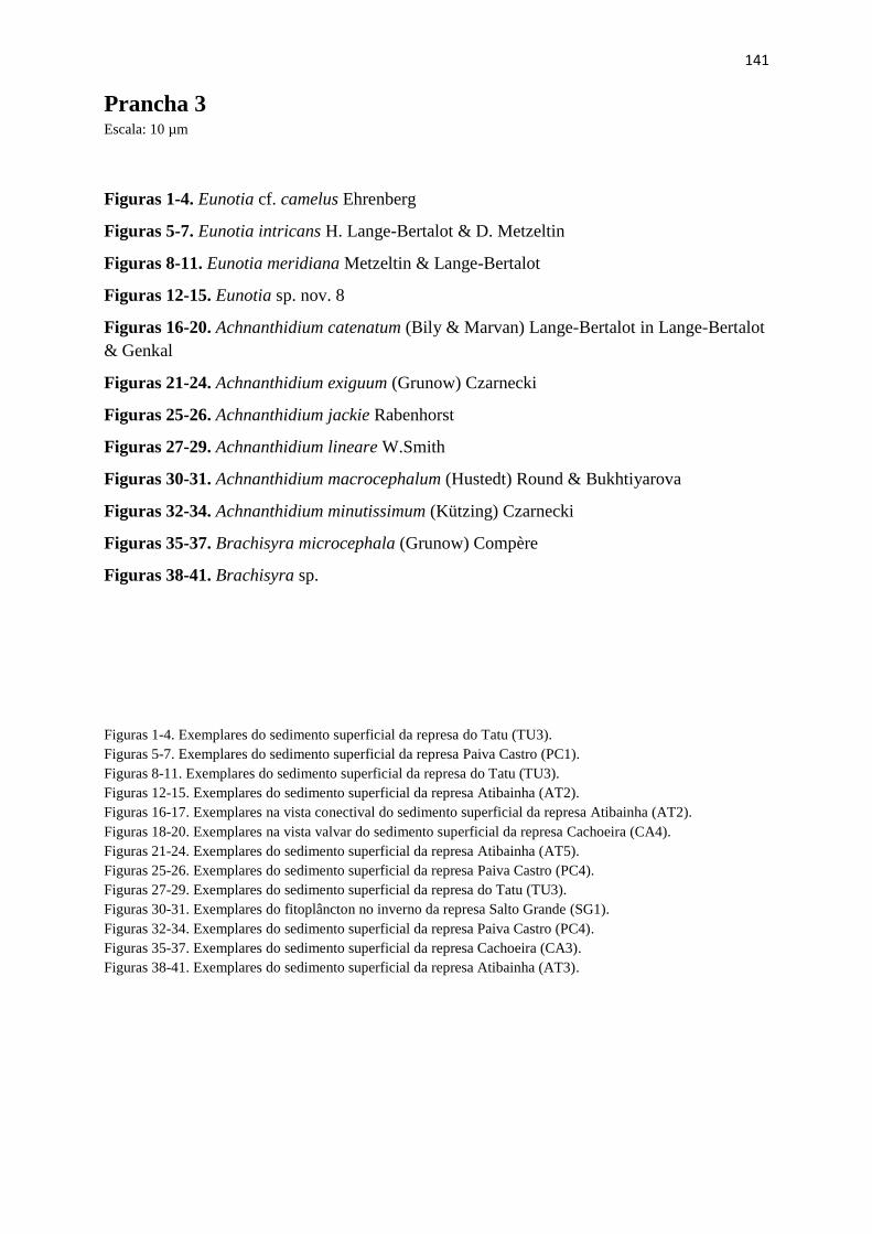
141
Prancha 3 Escala: 10 µm
Figuras 1-4. Eunotia cf. camelus Ehrenberg
Figuras 5-7. Eunotia intricans H. Lange-Bertalot & D. Metzeltin
Figuras 8-11. Eunotia meridiana Metzeltin & Lange-Bertalot
Figuras 12-15. Eunotia sp. nov. 8
Figuras 16-20. Achnanthidium catenatum (Bily & Marvan) Lange-Bertalot in Lange-Bertalot
& Genkal
Figuras 21-24. Achnanthidium exiguum (Grunow) Czarnecki
Figuras 25-26. Achnanthidium jackie Rabenhorst
Figuras 27-29. Achnanthidium lineare W.Smith
Figuras 30-31. Achnanthidium macrocephalum (Hustedt) Round & Bukhtiyarova
Figuras 32-34. Achnanthidium minutissimum (Kützing) Czarnecki
Figuras 35-37. Brachisyra microcephala (Grunow) Compère
Figuras 38-41. Brachisyra sp.
Figuras 1-4. Exemplares do sedimento superficial da represa do Tatu (TU3).
Figuras 5-7. Exemplares do sedimento superficial da represa Paiva Castro (PC1).
Figuras 8-11. Exemplares do sedimento superficial da represa do Tatu (TU3).
Figuras 12-15. Exemplares do sedimento superficial da represa Atibainha (AT2).
Figuras 16-17. Exemplares na vista conectival do sedimento superficial da represa Atibainha (AT2).
Figuras 18-20. Exemplares na vista valvar do sedimento superficial da represa Cachoeira (CA4).
Figuras 21-24. Exemplares do sedimento superficial da represa Atibainha (AT5).
Figuras 25-26. Exemplares do sedimento superficial da represa Paiva Castro (PC4).
Figuras 27-29. Exemplares do sedimento superficial da represa do Tatu (TU3).
Figuras 30-31. Exemplares do fitoplâncton no inverno da represa Salto Grande (SG1).
Figuras 32-34. Exemplares do sedimento superficial da represa Paiva Castro (PC4).
Figuras 35-37. Exemplares do sedimento superficial da represa Cachoeira (CA3).
Figuras 38-41. Exemplares do sedimento superficial da represa Atibainha (AT3).

142

143
Prancha 4 Escala: 10 µm
Figuras 1-2. Frustulia crassinervia (Brébisson ex W.Smith) Lange-Bertalot & Krammer in
Lange-Bertalot & Metzeltin
Figuras 3-4. Diadesmis confervacea Kützing
Figuras 5-6. Diploneis ovalis (Hilse) Cleve
Figuras 7-10. Eolimna minima (Grunow) Lange-Bertalot & W.Schiller in W.Schiller &
Lange-Bertalot
Figuras 11-12. Humidophila contenta (Grunow) Lowe, Kociolek, J.R.Johansen, Van de
Vijver, Lange-Bertalot & Kopalová
Figuras 13-14. Geissleria punctifera (Hustedt) Metzeltin, Lange-Bertalot &García-Rodríguez
Figuras 15-16. Geissleria lateropunctata (Wallace) Potapova & Winter
Figuras 17-19. Luticola intermedia (Hustedt) Levkov, Metzeltin & Pavlov in Levkov et al.
Figuras 20-21. Navicula cryptocephala Kützing
Figuras 22-23. Navicula neomundana (Lange-Bertalot & Rumrich) Lange-Bertalot, Jarlman
& van de Vijver in van de Vijver & Lange-Bertalot
Figuras 24-27. Navicula notha J.H.Wallace
Figuras 28-29. Navicula symmetrica R.M.Patrick
Figuras 1-2. Exemplares do sedimento superficial da represa Atibainha (AT6).
Figuras 3-4. Exemplares do sedimento superficial da represa Salto Grande (SG2).
Figuras 5-6. Exemplares do sedimento superficial da represa Atibainha (AT3).
Figuras 7-10. Exemplares do sedimento superficial da represa Paiva Castro (PC4).
Figuras 11-12. Exemplares do sedimento superficial da represa do Tatu (TU3).
Figuras 13-14. Exemplares do fitoplâncton no verão da represa Paiva Castro (PC1).
Figuras 15-16. Exemplares do sedimento da represa Paiva Castro (PC4).
Figuras 17-19. Exemplares do sedimento da represa Jaguari (JA1).
Figuras 20-21. Exemplares do sedimento da represa Salto Grande (SG2).
Figuras 22-23. Exemplares do sedimento da represa Paiva Castro (PC4).
Figuras 24-27. Exemplares do sedimento da represa Cachoeira (CA3).
Figuras 28-29. Exemplares do sedimento da represa do Tatu (TU1).

144

145
Prancha 5 Escala: 10 µm
Figuras 1-3. Naviculadicta sassiana Metzeltin & Lange-Bertalot
Figuras 4-5. Sellaphora rostrata (Hustedt) J.R.Johansen in J.R.Johansen et al.
Figura 6. Sellaphora sp.
Figuras 7-9. Encyonema silesiacum (Bleisch) D.G.Mann in Round, R.M.Crawford &
D.G.Mann
Figuras 10-11. Encyonema sp.
Figuras 12-13. Gomphonema hawaiiense E.Reichardt
Figuras 14-16. Gomphonema lagenula Kützing
Figuras 17-19. Gomphonema naviculoides Skabitschevsky [Skabichevskii, Skabichevskij]
Figuras 20-22. Gomphonema parvulum (Kützing) Kützing
Figuras 1-3. Exemplares do sedimento superficial da represa Atibainha (AT2).
Figuras 4-5. Exemplares do sedimento superficial da represa do Tatu (TU2).
Figura 6. Exemplar do fitoplâncton no verão da represa do Tatu (TU2).
Figuras 7-9. Exemplares do sedimento superficial da represa Atibainha (AT3).
Figuras 10-11. Exemplares do sedimento superficial da represa Paiva Castro (PC3).
Figuras 12-13. Exemplares do sedimento superficial da represa Atibainha (AT1).
Figuras 14-16. Exemplares do sedimento superficial da represa Cachoeira (CA1).
Figuras 17-19. Exemplares do sedimento superficial da represa Atibainha (AT6).
Figuras 20-22. Exemplares do sedimento superficial da represa Cachoeira (CA1).

146

147
Prancha 6 Escala: 10 µm
Figuras 1-3. Hantzschia amphioxys (Ehrenberg) Grunow in Cleve & Grunow
Figuras 4-7. Nitzschia amphibia Grunow
Figuras 8-13. Nitzschia amphibioides Hustedt
Figura 14. Nitzschia palea var. palea (Kützing) W.Smith
Figura 15. Nitzschia palea var. debilis (Kützing) Grunow in Cleve & Grunow
Figuras 16-18. Nitzschia perminuta (Grunow) M.Peragallo
Figuras 19-21. Nitzschia sp.
Figuras 1-3. Exemplares do sedimento superficial da represa do Tatu (TU1).
Figuras 4-7. Exemplares do sedimento superficial da represa Salto Grande (SG3).
Figuras 8-13. Exemplares do sedimento superficial da represa Cachoeira (CA4).
Figura 14. Exemplar do sedimento superficial da represa Atibainha (AT3).
Figura 15. Exemplar do fitoplâncton no verão da represa Atibainha (AT4).
Figuras 16-18. Exemplares do sedimento superficial da represa Paiva Castro (PC4).
Figuras 19-21. Exemplares do sedimento superficial da represa do Tatu (TU2).

148

149
Tabela A1. Medidas dos táxons de diatomáceas do sedimento superficial e fitoplâncton (com abundância relativa ≥2%) encontrados nas represas
da Bacia do rio Piracicaba e do Sistema Cantareira.
Táxon Código do
OMNIDIA
Comprimento/
Altura manto
Largura/
Diâmetro Estrias Auréolas Fíbulas Espinhos
µm µm nº/10µm nº/10µm nº/10µm µm
Achnanthidium catenatum ADCT 9-19 2,1-3,2 - - - -
Achnanthidium exiguum ADEG 11,5-16 6-8 21-23 - - -
Achnanthidium jackie ADJK 8-15 2-3,5 - - - -
Achnanthidium macrocephalum ADMA 9-14 2-3 - - - -
Achnanthidium minutissimum ADMI 11,5-19 2-3,5 - - - -
Achnanthidium lineare ACLI 11,5-12 2-2,8 12-12 - - -
Asterionella formosa AFOR 2- - - - - -
Aulacoseira ambigua AAMB 5-13,5 4,5-8,5 14-21 14-24 - -
Aulacoseira granulata var. angustissima AUGA 10-20,5 2,5-5,2 12-18 12-18 - 12,5-16
Aulacoseira granulata var. granulata AUGR 14-24 6-18 8-12 8-10 - 13-19
Aulacoseira herzogii AUHE 12-18 4,5-5 - - - 9
Aulacoseira tenella AUTL 1,3-2 4,5-6 12-18 2-3 - -
Brachysira microcephala BMIC 12-24 4-5 - - - -
Brachysira sp. BRSP1 13,5-27 3,2-5 32-35 - - -
Cyclotella meneghiniana CMEN - 8-29 7-9 - - -
Diadesmis converfacea DCOF 16-20 6-8 19-20 - - -
Diploneis ovalis DOVA 17,5-28,5 11-14 11-13 - - -
Discostella pseudostelligera DPST - 6-8,5 - - - -
Discostella stelligera DSTE - 6-18,2 10-15 - - -
Encyonema sp. ENSP1 11-22,2 4-5,8 10-13 - - -
Encyonema silesiacum ESLE 24-48 6-11,5 9-12 16-20 - -
Eunotia cf. camelus ECAM 13-63 4-8 9-13 24-30 - -
Eunotia intricans EITC 18-40,5 3-5 9-14 - - -
Eunotia meridiana EMER 21-35 4-5 14-15 - - -

150
Tabela A1. Continuação.
Táxon Código do
OMNIDIA
Comprimento/
Altura manto
Largura/
Diâmetro Estrias Auréolas Fíbulas Espinhos
µm µm nº/10µm nº/10µm nº/10µm µm
Eunotia sp. nov. 8 EUSP1 10,7-20 2,5-3,5 13-21 - - -
Fragilaria tenuissima FTNU 68,5-141 2-2,5 15-16 - - -
Fragilaria longifusiformis FLFU 52 3 - - - -
Fragilaria pectinales FPEC 17-25 2-2,5 16-17 - - -
Fragilaria crotonensis FCRO 50-63 1-1,5 - - - -
Fragilaria tenera var. nanana FTNA 71-96 1-1,5 - - - -
Fragilaria pararupens FPRU 25-52,5 3-4 14-15 - - -
Fragilaria parva FPAV 29,5-65,5 2-3,2 14-17 - - -
Fragilaria sp. FRSP1 27-59 2-4 14-16 - - -
Fragilaria gracilis FGRA 18-36 2-3 20 - - -
Frustulia crassinervia FCRS 38-59 8-12,5 - - - -
Geissleira puctifera GPTF 21-26 6-7,5 16-17 - - -
Geissleria lateropunctata GELA 18,5-25 7-8,8 17-19 - - -
Gomphonema naviculoides GNAVC 22-55 5-8,2 10-15 - - -
Gomphonema hawaiiense GHAW 29-45 6,5-8 16-17 - - -
Gomphonema lagenula GLGN 13-24,3 4,2-8 12-17 - - -
Gomphonema parvulum GPAR 11-22,5 4-6 13-17 - - -
Hantzschia amphoxys HAMP 14,5-44 3,5-6,8 24-30 - - -
Humidophila contenta HUCO 7,8-11 2-3,7 - - - -
Luticola intermedia LINT 12-30 6-7 21-24 - - -
Navicula cryptocephala NCRY 24,5-31 5,5-6,5 15-17 - - -
Navicula neomundana NNMU 53-75 9,5-11,5 9-9 24-27 - -
Navicula notha NNOT 21-31,7 4-5,5 15-18 - - -
Navicula symmetrica NSYM 33,5-40 6-7 14-16 - - -
Naviculadicta sassiana NDSA 12,8-15,5 4-4,8 21-27 - - -

151
Tabela A1. Continuação.
Táxon Código do
OMNIDIA
Comprimento/
Altura manto
Largura/
Diâmetro Estrias Auréolas Fíbulas Espinhos
µm µm nº/10µm nº/10µm nº/10µm µm
Nitzschia palea var. debilis NPAD 39,5-46 3,5-4 - - 13-14 -
Nitzschia amphibia NAMP 10-31 4,5-5 17-18 - 7-9 -
Nitzschia amphibioides NAMH 8-29 3,5-4,5 16-17 - 7-8 -
Nitzschia palea NPAL 25,5-30,5 3,3-4,3 23-25 - 10-12 -
Nitzschia sp. NISP1 19-20,5 3,5-4,5 23-26 - 10-13 -
Nitzschia perminuta NIPM 17-26 2,1-4 25-26 - 10-17 -
Eolimna minima EOMI 6-11,5 2,5-4,5 12-24 - - -
Pseudostaurosira brevistriata PSBR 8,8-19,8 3-4 16-18 - - -
Rimoneis sp. RISP1 9,2-15,5 1,5-3 - - - -
Sellaphora sp. SESP1 22-25 6,5-7 22-23 - - -
Sellaphora rostrata SRTR 19-29 6,5-8 19-24 - - -
Spicaticribra rudis SPRU - 8,7-20,5 - - - -
Ulnaria acus UACU 153-267 5-6,5 10-11 - - -

152
Tabela A2. Ocorrência dos táxons de diatomáceas no fitoplâncton com abundância ≥ 2%, no período de inverno. Represas: AT = Atibainha; CA
= Cachoeira; PC = Paiva Castro; SG = Salto Grande; TU = Represa do Tatu; JA = Jaguari; JC = Jacareí. Os números abaixo do código das
represas são referentes às estações amostrais.
Táxons AT CA PC SG TU JA JC
1 2 3 4 5 6 1 2 3 4 5 1 2 3 4 1 2 3 4 1 2 3 1 2 1 2 3 4 5 6 7
Achnanthidium catenatum X
X X X X
X X X X
X X X X X X X X X
Achnanthidium exiguum X
X X
X X X X X X X X
X
X X X
Achnanthidium jackie X X
X X
X
X X
X X X X X X X X
Achnanthidium
macrocephalum X
X X X
X X
X X X X X X X
Achnanthidium
minutissimum X X
X X
X X X X X
X
X X X
Aulacoseira ambigua X X X X
X X X X X X X X X X X X X X X X X X X X X X X X X X
Aulacoseira granulata var.
angustissima X X
X
X X X
X
X X X X X X
X X X X X X X X X X
Aulacoseira granulata var.
granulata X
X X X X X X X X X
X X X X X X
X X X X X X X X X X
Aulacoseira herzogii
X X X X X X X X X X
Aulacoseira tenella X X X X X X X X X X X X X X X X X X X X X X X X X X X X X X X
Brachysira microcephala X X X X X
X X X X
X
X X X X X X X X X X X X
X X
Cyclotella meneghiniana
X X
X
X X X X
X X X X X X X X X X
Diadesmis converfacea
X X
X X
X
Diploneis ovalis
X X
X
X
Discostella pseudostelligera
X X
Discostella stelligera X X X X X X X X X X X X X X X X X X X X X X X X X X X X X X X
Encyonema sp.10
X
X
Encyonema silesiacum X
X
X
X X X X X X X
X X
X
Eunotia cf. camelus
X
X
X X X
Eunotia intricans X
X X X
X
X
Eunotia meridiana
X X
X X
Eunotia sp. nov. 8 X
X
X
X X
X
X X X
Fragilaria tenuissima
X
X
X X
X X

153
Tabela A2. Continuação.
Táxons AT CA PC SG TU JA JC
1 2 3 4 5 6 1 2 3 4 5 1 2 3 4 1 2 3 4 1 2 3 1 2 1 2 3 4 5 6 7
Fragilaria pectinales
X X X X X X X X X
Fragilaria crotonensis X
X
X
X X X X X
X X X
Fragilaria tenera var.
nanana X
Fragilaria pararupens
X
X
X X X
Fragilaria sp.
X X X X X X
Fragilaria gracilis
X X X
Fragilaria vauchaeriae
X X
X X X X X
Frustulia crassinervia
X
X X X
X X X
Geissleira puctifera
X
X X X X
Geissleria lateropunctata
X X X
X X X
X
Gomphonema naviculoides
X
X
X
Gomphonema hawaiiense
X
X
X X
X
X
X X X
X
X
Gomphonema lagenula
X X
X
X
X X
X X
X
X X
Humidophila contenta
X
X X X
X X X X X X
X
X X X X X X X X X
Navicula neomundana X X
X
X X X
X
Navicula notha X X X X X X X X X X X X X X X X X X X X X X X
X X X X X X X
Naviculadicta sassiana
X
X
X
Nitzschia palea var. debilis
X
X
Nitzschia amphibia
X X X X
Nitzschia amphibioides X X
X
X X
X X X X X X
X X
X X X X X X X X X
Nitzschia palea X X
X X X
X X
X
X X
X
X
X
X X
Nitzschia sp.
X X X
Sellaphora sp.
X
Sellaphora rostrata
X
X
X
X X X
Spicaticribra rudis X X
X
X X X X X X X X
X X X X X X X X X X X X X X X X X
Ulnaria acus
X
X
X X X X X
X

154
Tabela A3. Ocorrência dos táxons de diatomáceas no fitoplâncton com abundância ≥ 2%, no período de verão. Represas: AT = Atibainha; CA =
Cachoeira; PC = Paiva Castro; SG = Salto Grande; TU = Represa do Tatu; JA = Jaguari; JC = Jacareí. Os números abaixo do código das represas
são referentes às estações amostrais.
Táxons AT CA PC SG TU JA JC
1 2 3 4 5 6 1 2 3 4 5 1 2 3 4 1 2 3 4 1 2 3 1 2 1 2 3 4 5 6 7
Achnanthidium catenatum X X X X X X X X X X X X X X X X X X X X X
Achnanthidium exiguum X X X X X X X X X X X X X X X X X X X X X
Achnanthidium jackie X X X X X X X X X X X X X X X X X X X X X X
Achnanthidium
macrocephalum X X X X X X X X X X X X X X
Achnanthidium
minutissimum X X X X X X X X X X X X X X
Aulacoseira ambigua X X X X X X X X X X X X X X X X X X X X X X X X X X X X X X
Aulacoseira granulata var.
angustissima X X X X X X X X X X X X X X X X X X X X X X X X X X X X X X
Aulacoseira granulata var.
granulata X X X X X X X X X X X X X X X X X X X X X X X X X X X X
Aulacoseira herzogii X X X X X X X X
Aulacoseira tenella X X X X X X X X X X X X X X X X X X X X X X X X X X X X X X
Brachysira microcephala X X X X X X X X X X X X X X X X X X X X X X X X X X X X
Cyclotella meneghiniana X X X X X X X X X X X X X X X X X X X X X
Diadesmis converfacea X X X X X X
Diploneis ovalis X X X X
Discostella pseudostelligera X X X
Discostella stelligera X X X X X X X X X X X X X X X X X X X X X X X X X X X X X X X
Encyonema sp. X X X X
Encyonema silesiacum X X X X X X X X X X X X X X X X X X X X X
Eunotia camelus X X X X
Eunotia intricans X X X X X X
Eunotia meridiana X X X X
Eunotia sp. nov. 8 X X X X X X X X X X X X
Fragilaria tenuissima X X X X X X X X X X X

155
Tabela A3. Continuação.
Táxons AT CA PC SG TU JA JC
1 2 3 4 5 6 1 2 3 4 5 1 2 3 4 1 2 3 4 1 2 3 1 2 1 2 3 4 5 6 7
Fragilaria longifusiformis X X X
Fragilaria pectinales X X X X X X
Fragilaria crotonensis X X X X X X X X X X X X X X X X X X X X
Fragilaria tenera var.
nanana X X X X X X
Fragilaria pararupens X X
Fragilaria sp. X X X X X X X X X X X
Fragilaria gracilis X X X X X
Fragilaria vauchaeriae X X X
Frustulia crassinervia X X X X X X
Geissleira puctifera X X
Geissleria lateropunctata X X X X X X X X X X
Gomphonema naviculoides X X X X
Gomphonema hawaiiense X X X X X X X X X X X X X X
Gomphonema lagenula X X X X X X X X X X X X X X X X X
Humidophila contenta X X X X X X X X X X X X X X X X X X X X
Navicula neomundana X X X X X X X X X
Navicula notha X X X X X X X X X X X X X X X X X X X X X X X X X X X X X X
Naviculadicta sassiana X X X X X X X X X X X
Nitzschia palea var. debilis X X X X X X X X X X X X X X X
Nitzschia amphibia X X X X
Nitzschia amphibioides X X X X X X X X X X X X X X X X X X X X X X X X X
Nitzschia palea X X X X X X X X X X X X X X
Sellaphora sp. X
Sellaphora rostrata X X X
Spicaticribra rudis X X X X X X X X X X X X X X X X X X X X X X X X X X X X X
Ulnaria acus X X X X X X X X X X

156
Tabela A4. Ocorrência dos táxons de diatomáceas no sedimento superficial com abundância ≥ 2%. Represas: AT = Atibainha; CA = Cachoeira;
PC = Paiva Castro; SG = Salto Grande; TU = Represa do Tatu; JA = Jaguari; JC = Jacareí. Os números abaixo do código das represas são
referentes às estações amostrais.
Táxons AT CA PC SG TU JA JC
1 2 3 4 5 6 1 2 3 4 5 1 2 3 4 1 2 3 4 1 2 3 1 2 1 2 3 4 5 6 7
Achnanthidium catenatum X X X X X X X X X X X X X X X X X X X X X X X X X
Achnanthidium jackie X X X X X X X X X X X X X X X X
Achnanthidium
minutissimum X X X X X X X X X X X X X X
Achnanthidium lineare X X
Asterionella formosa X X
Aulacoseira ambigua X X X X X X X X X X X X X X X X X X X X X X X X X X X X X X
Aulacoseira granulata var.
angustissima X X X X X X X X X X X X X X X X X X X X X X X X X X X X X X
Aulacoseira granulata var.
granulata X X X X X X X X X X X X X X X X X X X X X X X X X X X
Aulacoseira tenella X X X X X X X X X X X X X X X X X X X X X X X X X X X X
Brachysira sp. X X X X X X X X X X
Cyclotella meneghiniana X X X X X X X X X X X X X X X X
Discostella stelligera X X X X X X X X X X X X X X X X X X X X X X X X X X X X X X X
Encyonema sp. X X X X X X X X X
Encyonema silesiacum X X X X X X X X X X X X X X X X X X X
Eunotia cf. camelus X X X X
Eunotia intricans X X X X X X X X X X
Eunotia sp. nov. 8 X X X X X X X X X X X X X X
Fragilaria longifusiformis X X X
Fragilaria parva X X X X X X X
Fragilaria sp. X
Geissleria lateropunctata X X X X X X X X X X X
Gomphonema naviculoides X X X
Gomphonema lagenula X X X X X X X X X X X X X X X X X

157
Tabela A4. Continuação.
Táxons AT CA PC SG TU JA JC
1 2 3 4 5 6 1 2 3 4 5 1 2 3 4 1 2 3 4 1 2 3 1 2 1 2 3 4 5 6 7
Gomphonema parvulum X X X X X X X X X X X X
Hantzschia amphoxys X X X X
Humidophila contenta X X X X X X X X X X X X X X X X X X
Luticola intermedia X X X X
Navicula cryptocephala X X X X X X X X X X X
Navicula neomundana X X X X X X X X X
Navicula notha X X X X X X X X X X X X X X X X
Navicula symmetrica X X
Naviculadicta sassiana X X X X X X X X X X X
Nitzschia amphibioides X X X X X X X X X X X X X X X X X X X X X X X
Nitzschia palea X
Nitzschia sp. X X X
Nitzschia perminuta X X X X
Eolimna minima X X
Pseudostaurosira
brevistriata X X X X X X X X X
Rimoneis sp. X X X
Sellaphora rostrata X X X X X
Spicaticribra rudis X X X X X X X X X X X X X X X X X X X X X X X X X