
Bolsas Universidade de Lisboa / Fundação Amadeu...
21
Bolsas Universidade de Lisboa / Fundação Amadeu Dias Edição 2010/2011 Relatório de Projecto Identificação da origem dos principais focos de poluição através do mapeamento espacial de isótopos de enxofre na área industrial de Sines Bolseira: Ceres Barros Faculdade de Ciências Curso: Licenciatura em Biologia Ano: 3.º Tutora: Prof.ª Dra. Cristina Branquinho
Transcript of Bolsas Universidade de Lisboa / Fundação Amadeu...
Bolsas Universidade de Lisboa / Fundação Amadeu Dias
Edição 2010/2011
Relatório de Projecto
Identificação da origem dos principais focos de poluição através do mapeamento espacial de isótopos de enxofre na
área industrial de Sines
Bolseira: Ceres Barros
Faculdade de Ciências Curso: Licenciatura em Biologia
Ano: 3.º
Tutora: Prof.ª Dra. Cristina Branquinho
Bolsas Universidade de Lisboa / Fundação Amadeu Dias Relatório de Projecto
2
Preâmbulo
O trabalho proposto em Julho para a bolsa de investigação Universidade de Lisboa / Fundação
Amadeu Dias com o título Identificação da origem dos principais focos de poluição através do
mapeamento espacial de isótopos de enxofre na área industrial de Sines decorreu de Setembro
desse mesmo ano a Julho de 2011. Todo o processo decorreu dentro dos limites previstos e todos
os objectivos propostos inicialmente foram cumpridos, até mesmo ultrapassados. Durante o
trabalho a bolseira foi envolvida em todos os procedimentos de um projecto de investigação desde
a elaboração de hipóteses ao tratamento e análise estatística e interpretação de resultados. Neste
sentido, era também um dos objectivos que a bolseira encarasse com seriedade o projecto
elaborado de tal forma a que o seu produto final fosse a elaboração de um relatório no formato de
um artigo científico, de modo a que pudesse compreender o modo como são publicados os estudos
em Ciência e qual o exercício de raciocínio necessário para tal. Assim, este relatório foi elaborado
respeitando o formato de um artigo científico no que toca à estruturação do texto e à exposição e
discussão dos resultados, mantendo-se, no entanto, os capítulos definidos pelo Regulamento das
Bolsas Universidade de Lisboa / Fundação Amadeu Dias 2010/2011.
Agradecimentos
Gostaria de deixar um agradecimento especial à Sofia pela paciência que demonstrou ao longo
deste ano e pelas gargalhadas durante o trabalho de campo; ao Pedro sempre pronto a ajudar e
também aos seus conhecimentos de SIG, sem eles metade deste estudo teria sido praticamente
impossível; à Cristina Antunes, à Silvana e ao Paulo Beliche pela ajuda prestada nas colheitas de
campo; ao Rodrigo Maia do SIAAF pela sua enorme simpatia e disponibilidade; à Professora
Cristina Máguas pela sua frontalidade e espírito crítico; a todos os restantes sempre presentes na
salinha dos doutorandos, pela companhia e por tantos lanchinhos e celebrações; e por último, mas
mais especial ainda, à Dra. Cristina Branquinho, por ter arranjado tempo no meio das suas milhares
de tarefas, para mais um projecto e para guiar uma jovem e inexperiente recém-bióloga nos seus
primeiros passos na investigação, por me ter sempre estimulado a fazer mais e melhor e pela sua
incansável paciência para a minha falta de ‘know-how’.
Resumo
A monitorização do enxofre (S) é extremamente importante nos dias de hoje, mesmo tendo em
conta a implementação e legislação de medidas de redução das emissões de compostos
sulfurosos, já que é necessário averiguar a eficácia destas mesmas medidas e o modo como os
valores de S nos ecossistemas têm vindo a evoluir. Esta monitorização pode ser feita com recurso
a biomonitores, como é o caso dos líquenes. Dadas as características fisiológicas destes
organismos, os líquenes retêm em si os elementos que absorvem da atmosfera e portanto a sua
análise é representativa da mesma. No entanto, o S pode ser emitido a partir tanto de fontes
naturais, como vulcânicas, marinhas, ou de processos de decomposição, como de fontes
Bolsas Universidade de Lisboa / Fundação Amadeu Dias Relatório de Projecto
3
antropogénicas, dificultando a identificação da sua origem. Para responder a este problema é feita
a análise isotópica do S retido pelos líquenes, cuja assinatura é fiel àquela que interceptaram do
ambiente e, por sua vez, nos dá a indicação da fonte emissora de onde o S proveio. Através da
amostragem do líquen Parmotrema hypoleucinum na área industrial de Sines e envolventes, e sua
análise em concentração de S e seus valores isotópicos, este estudo demonstrou que na área de
estudo existem duas fontes principais de S: antropogénica e marinha. A influência marinha,
traduzida por valores isotópicos superiores, estende-se até cerca de 4000m de distância ao mar,
mas mesmo nesta faixa foi possível distinguir as fontes antropogénicas de S (ETAR e Central
Termoeléctrica de Sines). Através da comparação dos resultados obtidos com resultados de
estudos anteriores na mesma área de estudo, concluiu-se também que as emissões de S têm
vindo a reduzir, o que significará que as medidas de mitigação implementadas pelas indústrias
emissoras de S serão eficazes.
Framework
Lichens have been used as biomonitors for atmospheric pollution for more than 30 years, and
several scientific articles and reviews have been published regarding this subject (Pirintsos, et al.,
2003; Vingiani, et al., 2004). Lichens retain essential characteristics that make them excellent
biomonitors: their morphology doesn’t change with seasons, allowing accumulation to occur all year-
round (Szczepaniak, et al., 2003); they have significant longevity (Sloof, 1993), therefore in-situ
lichens can integrate the pollution for long-term or used to study the evolution of atmospheric
conditions when collected over different periods of time (Garty, 2001; Wadleigh, 2003; Rosamilia, et
al., 2004); because lichens lack a root apparatus, protective cuticle and stomata, they mostly
depend on atmospheric inputs and accumulate mineral elements, such as heavy metals, far beyond
their metabolic needs (Backor, et al., 2009), thus reflecting wet and dry atmospheric deposition
(Vingiani, et al., 2004); lichens respond to changes in the environment within a few months (Cuny,
et al., 2001; Wadleigh, 2003; Backor, et al., 2009) and they tend to reach concentration and isotopic
equilibrium with the atmosphere within that time (Wiseman, et al., 2002; Wadleigh, 2003). Lichens
use highly effective but unselective mechanisms to absorb and accumulate low concentration
minerals present in air and moisture (Batts, et al., 2004), some species also being rather tolerant
even to some high levels of trace elements (Garty, 2001; Häffner, et al., 2001; Van Dobben, et al.,
2001), which allows their use to estimate trace element concentrations in the environment (Van
Dobben, et al., 2001). These characteristics combined with their vast geographical dispersion and
low costs of sample collection and treatment (Martin, et al., 1982) make them some of the best
biological communities’ biomonitors of air pollution (Garty, 2001).
From several air pollutants, sulphur dioxide (SO2) seems to be the one which affects lichen survival
and biodiversity the most (James, 1973), thus the mapping of lichen diversity has become a routine
process in many countries (Sigal, 1988; Nimis, 1999) to easily assess the biological impact of air
pollution due to SO2. Hawksworth, et al. (1970) established and later revised (Hawksworth, et al.,
Bolsas Universidade de Lisboa / Fundação Amadeu Dias Relatório de Projecto
4
1976) a semi quantitative scale that correlates zones of mean SO2 concentrations with the
occurrence of certain lichen species.
However, despite that the decline in lichen biodiversity may indicate a prolonged exposure to air
pollutants (James, 1973; Ferry, et al., 1973; Doll, et al.; Guderian, et al., 1985; Sigal, et al., 1983), it
is crucial to correctly identify pollution sources, firstly because many of the anthropogenic pollutants
such as SO2 also have natural sources such as, sea spray, volcanoes emissions or decomposition
processes (McArdle, et al., 1995; Chin, et al., 1996; Beričnik-Vrbovšek, et al., 2002; Hissler, et al.,
2008), and secondly to apply adequate strategies to improve air quality. For that some researchers
have been using the concentration of sulphur (S) measured in epiphytic lichens (Evans, 1996;
Blake, 1998; Wadleigh, et al., 1999; Wiseman, et al., 2002; Wadleigh, 2003; Vingiani, et al., 2004)
as an estimate of the amount of S that suffers deposition from the atmosphere. This is possible
since changes in S concentration in transplant lichens have shown to be mainly attributable to
changes in the inorganic S fraction and not in the organic S-fraction (Krouse, 1977; Takala, et al.,
1985; Häffner, et al., 2001) and because epiphytic lichens depend mainly on atmospheric
absorption. As already has been shown for several case studies, S concentrations seem to increase
with decreasing distance from an anthropogenic source of S (Wadleigh, et al., 1999; Novák, et al.,
2001; Vingiani, et al., 2004). Yet the S concentrations in lichens do not provide us the S source,
because it is not possible to distinguish natural sources from anthropogenic sources exclusively
through concentration measurements. However, it is possible to distinguish them when these are
combined with their stable isotopic signatures (Wiseman, et al., 2002; Wadleigh, 2003; Hissler, et
al., 2008).
Although much effort and great deals of money have been put into reducing the anthropogenic
emissions of S in western countries, resulting in a decrease of its atmospheric concentration (Smith,
et al., 2001; Aherne, et al., 2008; Hamed, et al., 2010), the monitoring of atmospheric S is still very
important, not only because SO2 induces great damage in the ecosystems, such as forest decline
due to soil and water acidification (Ulrich, et al., 1980; Reuss, et al., 1987; Zhao, et al., 1998), but
also because it is crucial to evaluate the effectiveness of the mitigation measures adopted. Sulphur
isotopes 32S and 34S (the most abundant) are frequently used to study pathways through the
ecosystems (Winner, et al., 1978). Their atmospheric values have been determined in many places
given that they may hold source-specific information that can help identify S sources and assess
their relative impact (McArdle, et al., 1995; Ohizumi, et al., 1997; Novák, et al., 2001; Xiao, et al.,
2002; Pruett, et al., 2004). The natural abundances of the two isotopes are fairly constant (Beričnik-
Vrbovšek, et al., 2002), but chemical, physical and biological processes lead to the enrichment, or
depletion, of one isotope relatively to another (Lindberg, et al., 1986; Wadleigh, 2003; Batts, et al.,
2004) leading to significant differences between different samples (Griffith, 2004). These variations,
or fractionation, are expressed in terms of a ‘delta’ (δ) and, although small, they are characteristic of
a certain emission (Lindberg, et al., 1986). Measuring absolute abundances of a certain isotope is

Bolsas Universidade de Lisboa / Fundação Amadeu Dias Relatório de Projecto
5
extremely unpractical, except for heavy metals, therefore it is easier to compare and analyse the
isotopic ratios of samples, relatively to a known standard material (Beričnik-Vrbovšek, et al., 2002).
In respect to S, the δ34S values of major contributors to the atmosphere can be divided into marine
sources, usually with higher values, and continental sources, usually with lower values (McArdle, et
al., 1995; Wadleigh, et al., 1999; Wiseman, et al., 2002). As for anthropogenic emissions, the δ34S
values can show a wide range, depending on the source (Wiseman, et al., 2002; Xiao, et al., 2010).
Lichens are extremely useful for identifying S pollution sources and Conti, et al. (2001) recognised
that as biomonitors, lichens respond better to SO2 than to other pollutants. Little or no fractionation
occurs to δ34S after it has been assimilated by this organism (Mektiyeva, et al., 1976; Trust, et al.,
1992; Batts, et al., 2004; Backor, et al., 2009), except when the lichen is exposed to excessive
atmospheric SO2, where the selective emission of reduced S compounds causes an increase of
δ34S within the lichen (Batts, et al., 2004). Therefore, lichens retain the isotopic signature of the
surrounding atmosphere (Krouse, 1977; Evans, 1996; Wadleigh, et al., 1999), integrating it for long
term periods.
In contrary to the mapping of lichen diversity to infer pollution impacts, or its correlation to measured
atmospheric pollution, the mapping of isotopic values in lichens, be it S or any other element, is not
of common practise. Except for Jeran, et al. (1996), who mapped the concentration of trace
elements measured in lichens and Wadleigh and Blake (1999), who mapped the δ34S found in
epiphytic lichens. Those were the only two studies that simultaneously mapped S isotopes and
elemental concentrations. Moreover, Wadleigh and Blake (1999) could not relate the isotopic values
with the S concentrations in lichens, and therefore they did not integrate the geographical analysis
of S isotopes with the geographical analysis of its concentration, which greatly increases the
chances of understanding S sources.
Nevertheless several authors have verified that coastal lichens may reveal two different marine-
derived isotopic signatures: sea spray with +21‰, derived from the well-mixed reservoir of ocean
sulphate (SO4) (Rees, et al., 1978); and +15,6‰ ± 3,1‰ from dimethyl sulphide (DMS) (Calhoun, et
al., 1991) a form of biogenic sulphur that is a major secondary metabolite in some marine algae.
DMS can also be produced by bacterial transformation of dimethyl sulfoxide (DMSO), usually
present in sewers where it can cause odour problems (Glindemann, et al., 2006). Although isotopic
signatures from anthropogenic emissions vary greatly depending on the nature of the source
(Wadleigh, 2003) values between ≈5‰ (pulp and paper mills) and ≈7‰ (thermal power plant) were
obtained by Beričnik-Vrbovšek, et al. (2002) and Wadleigh, et al.(1999), respectively, from lichens
near anthropogenic sources. Novák, et al. (2001) obtained a δ34S value of 3,4‰ on forest floor
samples (ecological sulphur pools) in Czech Republic, which only differed from the Czech
Republican coal (main pollution source) by 1,4‰. Lichens, unlike forest floor, do not supply nutrients
to other organisms; therefore they will probably be more faithful to the original atmospheric source
of isotopic signature. The extent of the impact of the marine-derived isotopes was not previously

Bolsas Universidade de Lisboa / Fundação Amadeu Dias Relatório de Projecto
6
investigated and that is important to understand what the level of interference of those isotopes is
when using S isotopes as environmental tracers.
Thus, when we have simultaneously natural and anthropogenic sources that change over space, as
in the case of industrialized coastal areas, it is very important to distinguish between natural and
anthropogenic S sources and evaluate the amount of atmospheric deposition due to S emissions.
Since the 80’s that European legislation has been imposing strong emission reductions to the
industry and it is important to evaluate whether those reductions have been reflected at the
ecosystem level.
Objectives
This study aims to apply the great utility of lichens as biomonitors to spatially trace S pollution
sources, integrating S concentration and isotopic analysis in order to distinguish between natural
and anthropogenic sources of S in a Portuguese coastal and industrial area. We also aim to
compare the level of S that was intercepted by lichens in this study with the one obtained in
previous studies in the region in order to evaluate the impact of the reduction in atmospheric
emissions.
Applied Methodology
Study area
The study area, with approximately 1500km2 (50x30km), is located in the SW the coast of Portugal,
having the Atlantic ocean on its western side. It comprises two small mountain ranges (Serra de
Grândola, 383m; and Serra do Cercal, 378m) with N-S orientation, parallel to the coast (Fig. 1a).
The annual average temperature is 16 to 17,5°C, the average annual precipitation is 600 to
1000mm and the average annual insolation is 3000h (averages from 1931 to 1960; source
APA,2004). The dominant winds come from the N-NW direction.
Figure 1b shows the land use cover in the study area. Four municipalities are included in the area of
study: Grândola (population 14.901); Santiago do Cacém (population 31.105), Odemira (population
26.106) and Sines (population 13.577) (INE, 2001). The area comprises a number of important
industries established since the late 1970’s: a coal-fired power station, an oil refinery, a petro-
chemical plant, an industrial sewage treatment plant and, more recently, an industrial landfill, and
many other smaller industries. There is also the sea harbour of Sines, which is the main door for
energetic supplies (coal, oil and derivatives, gas, and other chemicals) of the country, and an
important harbour for general and container cargoes, with potential international importance. There
are also two main motorways, which respond to the high vehicle traffic which is growing in
importance over time, and a railway. Urban development of littoral towns has recently (last 30 years)
expanded, but agro-forest activities (mainly cork-oak woodlands – Quercus suber L.) rule the inland
landscapes. The natural reserve area Parque Natural do Sudoeste Alentejano e Costa Vicentina
(PNSACV) is located in the SW.
Bolsas Universidade de Lisboa / Fundação Amadeu Dias Relatório de Projecto
7
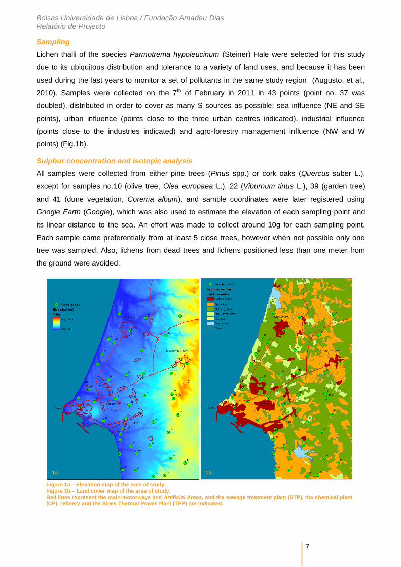
Sampling
Lichen thalli of the species Parmotrema hypoleucinum (Steiner) Hale were selected for this study
due to its ubiquitous distribution and tolerance to a variety of land uses, and because it has been
used during the last years to monitor a set of pollutants in the same study region (Augusto, et al.,
2010). Samples were collected on the 7th of February in 2011 in 43 points (point no. 37 was
doubled), distributed in order to cover as many S sources as possible: sea influence (NE and SE
points), urban influence (points close to the three urban centres indicated), industrial influence
(points close to the industries indicated) and agro-forestry management influence (NW and W
points) (Fig.1b).
Sulphur concentration and isotopic analysis
All samples were collected from either pine trees (Pinus spp.) or cork oaks (Quercus suber L.),
except for samples no.10 (olive tree, Olea europaea L.), 22 (Viburnum tinus L.), 39 (garden tree)
and 41 (dune vegetation, Corema album), and sample coordinates were later registered using
Google Earth (Google), which was also used to estimate the elevation of each sampling point and
its linear distance to the sea. An effort was made to collect around 10g for each sampling point.
Each sample came preferentially from at least 5 close trees, however when not possible only one
tree was sampled. Also, lichens from dead trees and lichens positioned less than one meter from
the ground were avoided.
Figure 1a – Elevation map of the area of study. Figure 1b – Land cover map of the area of study. Red lines represent the main motorways and Artificial Areas, and the sewage treatment plant (STP), the chemical plant (CP), refinery and the Sines Thermal Power Plant (TPP) are indicated.
1b 1a
Bolsas Universidade de Lisboa / Fundação Amadeu Dias Relatório de Projecto
8
Samples were cleaned from tree bark fragments and dried at room temperature, to be later
powdered and homogenized in a Reitsch MM2000 ball-mill (in FCUL, laboratory 2,5.39). From the
total 10g collected, the samples were homogenised and 3mg were weighted for S concentration and
isotopic analysis. These were analysed for all samples (n=43) using continuous flow isotope mass
spectrometry (CF-IRMS) (Preston, et al., 1983) on a Isoprime (GV, UK) stable isotope ratio mass
spectrometer, coupled to an EuroEA (EuroVector Italy) elemental analyser for online sample
preparation by Dumas-combustion which is located in FCUL in the SIAF Lab (2.1.16). Regarding
δ34S, the standards used were IAEA-S1 and IAEA-NBS127 and results were referred to Viena
Canyon Diablo Triolite.
Not all samples were replicated due to analytical costs. However at every 9 samples, one sample
was replicated three times in order to guarantee measurement accuracy, and the maximum
percentage of variance between each of those four repeated samples was 1,9% for %S and 4,4‰
for δ34S, the minimum was 0,9% for %S and 1,4‰ for δ34S, and the mean percentage of variance
was 1,6% for %S, and 2,6‰ for δ34S .Values from 9 replicates of laboratory standard material
interspersed among samples in every batch analysis were used to calculate the precision of the
isotope ratio analysis, which resulted in 0.35‰.
Statistical analysis and sulphur mapping
All data from the elemental and isotopical analysis was organized using Microsoft Excel (Microsoft),
combined with the sample coordinates and integrated with land use data with ArcMap v9.3 (ESRI
Inc.). To produce S concentration and isotopic signature maps both %S and δ34S values obtained
were mapped and interpolated with Inverse Distance Weighted (IDW) interpolation, using ArcMap
v9.3.
However, given that different S sources lead to differences in its dispersion length, buffers of 100,
200, 300, 500, 1000, 2000, 3000 and 5000m were drawn around each sample point and intersected
with the CORINE Land Cover 2006 map of Continental Portugal. The different land use areas inside
each buffer were calculated using ArcMap v.9.3 and exported to Excel for data organization: land
use areas that referred to artificial areas, such as urban and industrial areas and roads, were
aggregated as Artificial Areas; any agricultural, silvicultural and pasture systems were aggregated
as Agriculture; natural forests and any other naturally vegetated areas were aggregated as Natural
Vegetation Areas (Nat. Veg. Areas); burnt forest areas, rocky areas, degraded or recently
cut/planted vegetation and areas with sparse vegetation were aggregated as Natural Barren Areas
(Nat. Barren Areas); wetlands and intertidal zones were aggregated as Interface; freshwater bodies
were aggregated as Freshwater; the ocean and beaches were aggregated as Ocean.
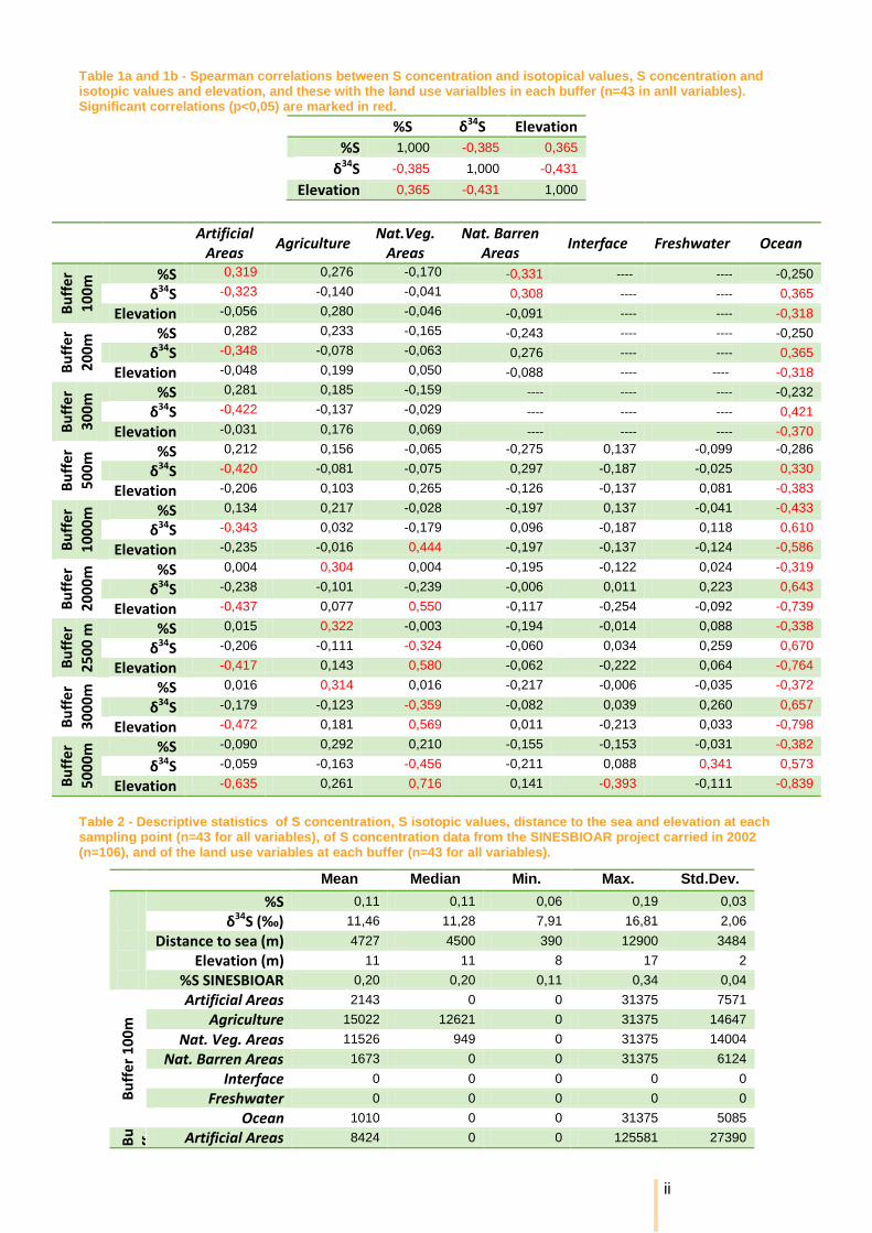
Normality of all data was analysed using the Shapiro-Wilk (W) normality test available in Statistica.
Correlations and linear and multiple regressions between %S, δ34S, and land use were also
calculated for each buffer using Statistica. Since most variables didn’t show a normal distribution,
Spearman correlations (ρ) were used (Table 1a and 1b in annexes). The best correlation values
Bolsas Universidade de Lisboa / Fundação Amadeu Dias Relatório de Projecto
9
between the different land use types and buffers, and both %S and δ34S defined which variables
would be later included in a Principal Components Analysis (PCA). A logarithmic regression
between δ34S and distance to sea was also calculated to establish the maximum distance of
influence (MDI) of the sea on δ34S values, which was observed graphically as the point from which
δ34S values remained constant.
A Principal Components Analysis (PCA) was used to observe the relationship between the different
types of land use and both %S and δ34S. As already mentioned, the land use variables were
correlated to %S and δ34S, considering each separate buffer. Those included firstly in the PCA were
those which presented the best Spearman correlation values with either %S or δ34S (see Table 1a
and 1b in annexes). These were: Artificial Areas with the 300m buffer, Nat. Veg. Areas with the
100m buffer, Nat. Barren Areas with the 100m buffer and Ocean with the 2500m buffer. Agriculture
was also included but the buffer selected did not correspond to the one with higher correlations (see
Table 1a and 1b in annexes), because it was considered that this high correlation did not reflect the
true effect of agricultural areas of %S, or δ34S, which is usually felt in a smaller radius. Elevation
was also included as a variable since it showed significant correlations between both %S and δ34S.
However, in a second instance redundant variables were removed from the final PCA. The removed
variables were Artificial Areas, Agriculture, Nat. Veg. Areas and Nat. Barren Areas, leaving Ocean
and Elevation, together with %S and δ34S. The factor scores of the component which better
explained the variance of the variables were exported to Excel where the highest absolute value
was summed to the rest in order to transform values into positive. These transformed factor scores
were then exported to ArcMap v9.3 and interpolated with an IDW interpolation, in order to obtain a
land use influence map.
Given that the effect of Artificial Areas did not appear as a relevant component due to the strong
influence of the sea on these parameters another strategy was implemented. An ocean influence
model was estimated through a linear regression between the δ34S values and their distance to the
sea up to 4000m from the coast (MDI) since this was shown to be under maritime influence. Once
the most important trend was obtained we registered the residuals from this model as were
reflecting the deviations from the general model trend, being that negative residual values were
probably resultant from anthropogenic influences, and positive residual values were probably
resultant from a higher ocean influence than the predicted by the model. These residuals were then
interpolated in ArcMap v9.3 with an IDW interpolation, so that the deviation from the ocean influence
model could be obtained.
Results
Sulphur concentrations in lichens over time
The mean, median, minimum, maximum and standard deviation values for S concentrations
(expressed in %) and isotopic S values (expressed in ‰) measured from 43 lichen samples are

Bolsas Universidade de Lisboa / Fundação Amadeu Dias Relatório de Projecto
10
presented in Table 2 (in annexes). Sulphur concentrations varied from 0,06% to 0,19%, with a mean
value of 0,11.
Lichen transplant studies to the polluted city of Naples showed an increase of S concentration
values to 0,261% for the species Phagnum capillifolium (Ehrh.) and 0,225% for the species
Pseudevernia furfuracea (L.) Zopf (Vingiani, et al., 2004). Much lower S concentration values were
obtained in the island of Newfoundland,
Canada, for the lichen Alectoria
sarmentosa (Ach.) Ach. (0,026% in interior
locations away from industrial S sources, to
0,115% in S point sources). However, the
lower S concentration values obtained by
Wadleigh, et al. (1999) may be due to the
fact the lichen A. sarmentosa tends to have
lower S concentrations relatively to other
lichens (Evans, 1996; Blake, 1998;
Wadleigh, et al., 1999), or that it occurs in
very pristine areas.
Only few studies published in international
journals used P. hypoleucinum to measure
pollutants concentrations (Pinho, et al.,
2008; Augusto, et al., 2010) and none of
these showed to have measured
specifically to measure S concentrations
and, or, isotopic values. However, some
reports from studies developed in the same region during the SINESBIOAR project, led by the
Commission for Regional Coordination and Development of the Alentejo (CCDR- Alentejo) and
financed by the European Union through the LIFE Environment programme, have shown to
measure %S in the same lichen species. In fact, when we compared the values obtained for S in the
present study with the ones reported in 2002 we found that for the same area of study the values
decrease approximately by 50% in this study (see Table 2 in annexes). This is very interesting since
that new legislation implemented between 2002 and 2011 lead the local industries to reduce
considerably the SO2 emissions as a result of large investments in technological solutions to reduce
this pollutant. To confirm that the concentration of S in lichens reduced due to the reductions in air
quality in the region we plotted the SO2 concentrations measured in the 3 air quality monitoring
stations from 2002 to 2009, which that are located in the studied region (source APA, 2010). In fact
we observe a considerable decrease in the levels of SO2 for all the air quality monitoring stations
(Fig. 2a and b) especially in the one located in the direction of the prevailing winds south from the
industrial region (Sonega). The decrease in SO2 in air was more than 50%, and was reflected in the
Figure 2a – Annual mean limit values of S measured from 2002 to 2009 in three air quality stations in the area of study (data source APA, 2010). Figure 2b – Annual mean hourly values of S measured from 2002 to 2009 in three air quality stations in the area of study (data source APA, 2010). The same legend of Figure 2a applies to Figure 2b.
2a
2b
Bolsas Universidade de Lisboa / Fundação Amadeu Dias Relatório de Projecto
11
decrease observed in lichens. This could be interesting to explore since the effects in ecosystems
do not take the same time to respond as the atmospheric levels of SO2, showing that lichens might
reflect some kind of memory of the highest emissions that occurred in the region. Revisiting some of
these sampling sites in the future, would be interesting to track the pattern of decrease of S
concentration in lichens over time.
The range of δ34S in the studied area
As for the δ34S values a wide range according to S source type was found in this study: δ34S varied
from 7,91‰ to 16,81‰, with a mean value of 11,46‰. These values are in accord with those from
Wadleigh, et al. (1999) and by Novák, et al. (2001), who obtained a maximum of ≈ 16‰ for δ34S
values obtained in coastal areas and concluded that these were related to the ocean influence. In
the same study, Wadleigh, et al. (1999) obtained minimums of ≈ 5‰ from sampling points near pulp
and paper mills, values which they related to S industrial emissions.
Beričnik-Vrbovšek, et al. (2002) also studied the S isotopic signatures near SO2 anthropogenic
sources and obtained δ34S values around 7‰ in samples of Hypogymnia physodes (L.) Nyl.
exposed to SO2 originating from a nearby power plant.
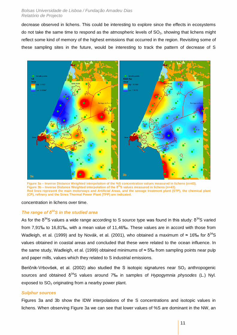
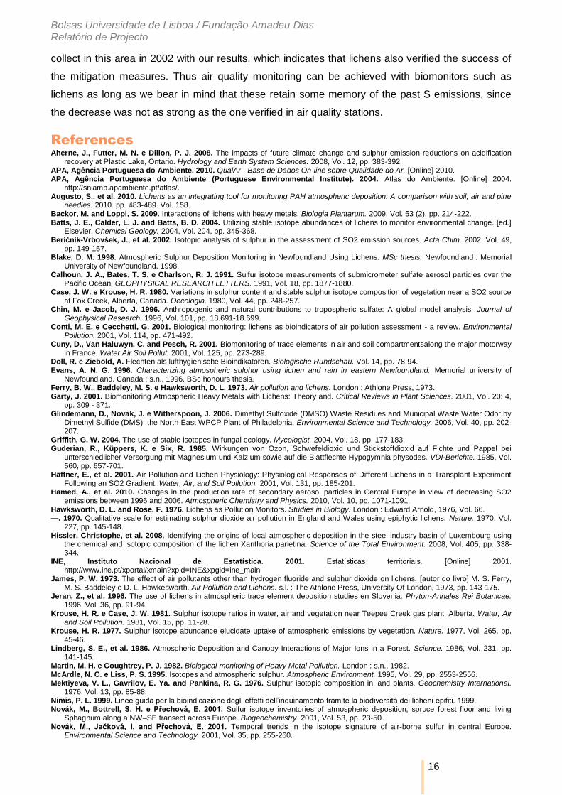
Sulphur sources
Figures 3a and 3b show the IDW interpolations of the S concentrations and isotopic values in
lichens. When observing Figure 3a we can see that lower values of %S are dominant in the NW, an
Figure 3a – Inverse Distance Weighted interpolation of the %S concentration values measured in lichens (n=43). Figure 3b – Inverse Distance Weighted interpolation of the δ
34S values measured in lichens (n=43).
Red lines represent the main motorways and Artificial Areas, and the sewage treatment plant (STP), the chemical plant (CP), refinery and the Sines Thermal Power Plant (TPP) are indicated.
3a 3b

Bolsas Universidade de Lisboa / Fundação Amadeu Dias Relatório de Projecto
12
area more exposed to the sea, and increase towards the SE direction. Values in SW are not as low
and this area is not as exposed either, receiving the NW winds from the Artificial Areas in red, which
present higher values of %S. The higher %S values shown in red in points 04, 06 and 34 maybe
due to several causes: 04 is very near to the main motorway that connects Sines, first to Santiago
do Cacém, and then to the freeway to Lisbon; 06 is between the motorway just mentioned and the
one that connects Sines to Santo André; 34 is probably receiving the S emitted by the Sines
Thermal Power Plant, which has one of the tallest chimneys in Europe (234m) and therefore, the S
emitted may not be recorded between point 34 and the points which are closest to it.
As for Figure 3b, δ34S shows a clearer pattern than %S. The highest values (near 16‰) were
measured in the coast line (NW and SW) and are a result of strong ocean influence (discussed
further). Lowest values fall near the Artificial Areas: Santiago do Cacém urban area and the
industrial area of Sines, the last with three low peaks one above the Sines Thermal Power Plant (09,
01), another to south (22 and 26), and the third near the sewage treatment plant (05) that deals with
sewage from the petrol industry. The urban areas of Sines and Santo André show neither
characteristically sea isotopic signatures, nor characteristically anthropogenic ones, probably
resulting in the mixture of these two.
In Figure 4 we can see that the effect of the sea on δ34S is observed up to 4.000m from the sea.
After this distance the values decrease more slowly with increasing distance from the sea. Thus, it
appears that the maximum distance of influence (MDI) of the sea on δ34S values is around 4.000m
(Fig. 4). This an important result, since if we want to use δ34S as a tracer for environment studies up
to 4km from the coast we need to be careful when interpreting data due to the interference of the
ocean signature.
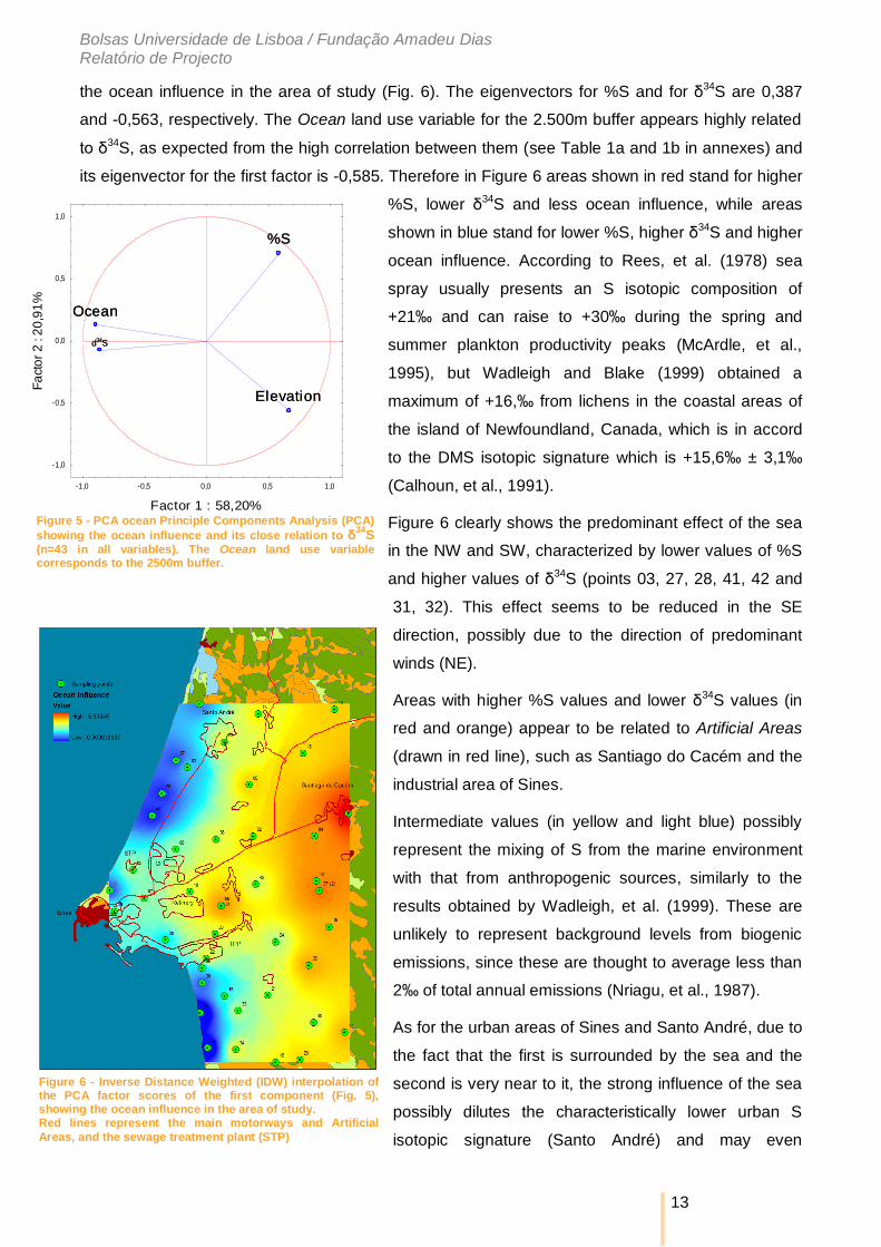
As already mentioned, %S and δ34S and selected variables of land use were confronted using a
PCA (Fig. 5). The land use variable which has shown better correlation with either %S or δ34S and
the less redundancy in the PCA was Ocean considering the 2.500m buffer, which means that the
maximum ocean influence is at a distance of 2.500, although its influence reaches the 4.000m
(MDI). Elevation was also included not only because it showed a significant correlation with δ34S
(ρ=-0,431; p<0,05), but because it may
explain the δ34S gradient in the study
area (see Fig. 6), which is traversed N-S
by the Serra de Grândola and Serra do
Cercal (see Fig. 1), two mountain
ranges parallel to the coast.
In Figure 5 %S appears in opposite of
both δ34S and Ocean regarding the first
factor (58,20% total variance), whose
factor scores were used to interpolate Figure 4 - Scatterplot showing the δ
34S values and their correspondent
distance to the sea (n=43). The distance from which δ34
S stabilizes (4000m) was considered to be the maximum distance of influence (MDI) of the sea on δ
34S values in lichens.
Bolsas Universidade de Lisboa / Fundação Amadeu Dias Relatório de Projecto
13
the ocean influence in the area of study (Fig. 6). The eigenvectors for %S and for δ34S are 0,387
and -0,563, respectively. The Ocean land use variable for the 2.500m buffer appears highly related
to δ34S, as expected from the high correlation between them (see Table 1a and 1b in annexes) and
its eigenvector for the first factor is -0,585. Therefore in Figure 6 areas shown in red stand for higher
%S, lower δ34S and less ocean influence, while areas
shown in blue stand for lower %S, higher δ34S and higher
ocean influence. According to Rees, et al. (1978) sea
spray usually presents an S isotopic composition of
+21‰ and can raise to +30‰ during the spring and
summer plankton productivity peaks (McArdle, et al.,
1995), but Wadleigh and Blake (1999) obtained a
maximum of +16,‰ from lichens in the coastal areas of
the island of Newfoundland, Canada, which is in accord
to the DMS isotopic signature which is +15,6‰ ± 3,1‰
(Calhoun, et al., 1991).
Figure 6 clearly shows the predominant effect of the sea
in the NW and SW, characterized by lower values of %S
and higher values of δ34S (points 03, 27, 28, 41, 42 and
31, 32). This effect seems to be reduced in the SE
direction, possibly due to the direction of predominant
winds (NE).
Areas with higher %S values and lower δ34S values (in
red and orange) appear to be related to Artificial Areas
(drawn in red line), such as Santiago do Cacém and the
industrial area of Sines.
Intermediate values (in yellow and light blue) possibly
represent the mixing of S from the marine environment
with that from anthropogenic sources, similarly to the
results obtained by Wadleigh, et al. (1999). These are
unlikely to represent background levels from biogenic
emissions, since these are thought to average less than
2‰ of total annual emissions (Nriagu, et al., 1987).
As for the urban areas of Sines and Santo André, due to
the fact that the first is surrounded by the sea and the
second is very near to it, the strong influence of the sea
possibly dilutes the characteristically lower urban S
isotopic signature (Santo André) and may even
Ocean
%S
d34S
Elevation
-1,0 -0,5 0,0 0,5 1,0
Factor 1 : 58,20%
-1,0
-0,5
0,0
0,5
1,0
Fa
cto
r 2
: 2
0,9
1%
Ocean
%S
d34S
Elevation
Figure 5 - PCA ocean Principle Components Analysis (PCA)
showing the ocean influence and its close relation to δ34
S (n=43 in all variables). The Ocean land use variable corresponds to the 2500m buffer.
Figure 6 - Inverse Distance Weighted (IDW) interpolation of the PCA factor scores of the first component (Fig. 5), showing the ocean influence in the area of study. Red lines represent the main motorways and Artificial
Areas, and the sewage treatment plant (STP)
Bolsas Universidade de Lisboa / Fundação Amadeu Dias Relatório de Projecto
14
predominate over the last (Sines).
Our results point to the same conclusions as those from Wadleigh, et al. (1999) and Beričnik-
Vrbovšek, et al. (2002): higher δ34S values (and lower values of %S) are a result of the ocean
influence which is reduced in direction to the interior and seems to be not so preponderant when
other possible sources are present. The same δ34S pattern has also been verified by air samples by
McArdle, et al. (1995) who obtained δ34S values of +5‰ and +6‰ for anthropogenic S sources and
+22‰ values for marine S sources.
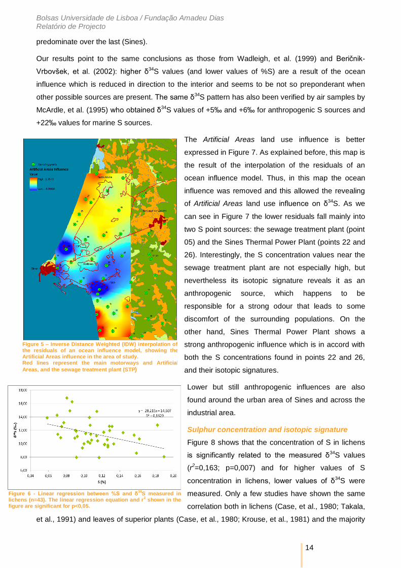
The Artificial Areas land use influence is better
expressed in Figure 7. As explained before, this map is
the result of the interpolation of the residuals of an
ocean influence model. Thus, in this map the ocean
influence was removed and this allowed the revealing
of Artificial Areas land use influence on δ34S. As we
can see in Figure 7 the lower residuals fall mainly into
two S point sources: the sewage treatment plant (point
05) and the Sines Thermal Power Plant (points 22 and
26). Interestingly, the S concentration values near the
sewage treatment plant are not especially high, but
nevertheless its isotopic signature reveals it as an
anthropogenic source, which happens to be
responsible for a strong odour that leads to some
discomfort of the surrounding populations. On the
other hand, Sines Thermal Power Plant shows a
strong anthropogenic influence which is in accord with
both the S concentrations found in points 22 and 26,
and their isotopic signatures.
Lower but still anthropogenic influences are also
found around the urban area of Sines and across the
industrial area.
Sulphur concentration and isotopic signature
Figure 8 shows that the concentration of S in lichens
is significantly related to the measured δ34S values
(r2=0,163; p=0,007) and for higher values of S
concentration in lichens, lower values of δ34S were
measured. Only a few studies have shown the same
correlation both in lichens (Case, et al., 1980; Takala,
et al., 1991) and leaves of superior plants (Case, et al., 1980; Krouse, et al., 1981) and the majority
Figure 5 – Inverse Distance Weighted (IDW) interpolation of the residuals of an ocean influence model, showing the Artificial Areas influence in the area of study. Red lines represent the main motorways and Artificial
Areas, and the sewage treatment plant (STP)
Figure 6 - Linear regression between %S and δ34
S measured in lichens (n=43). The linear regression equation and r
2 shown in the
figure are significant for p<0,05.
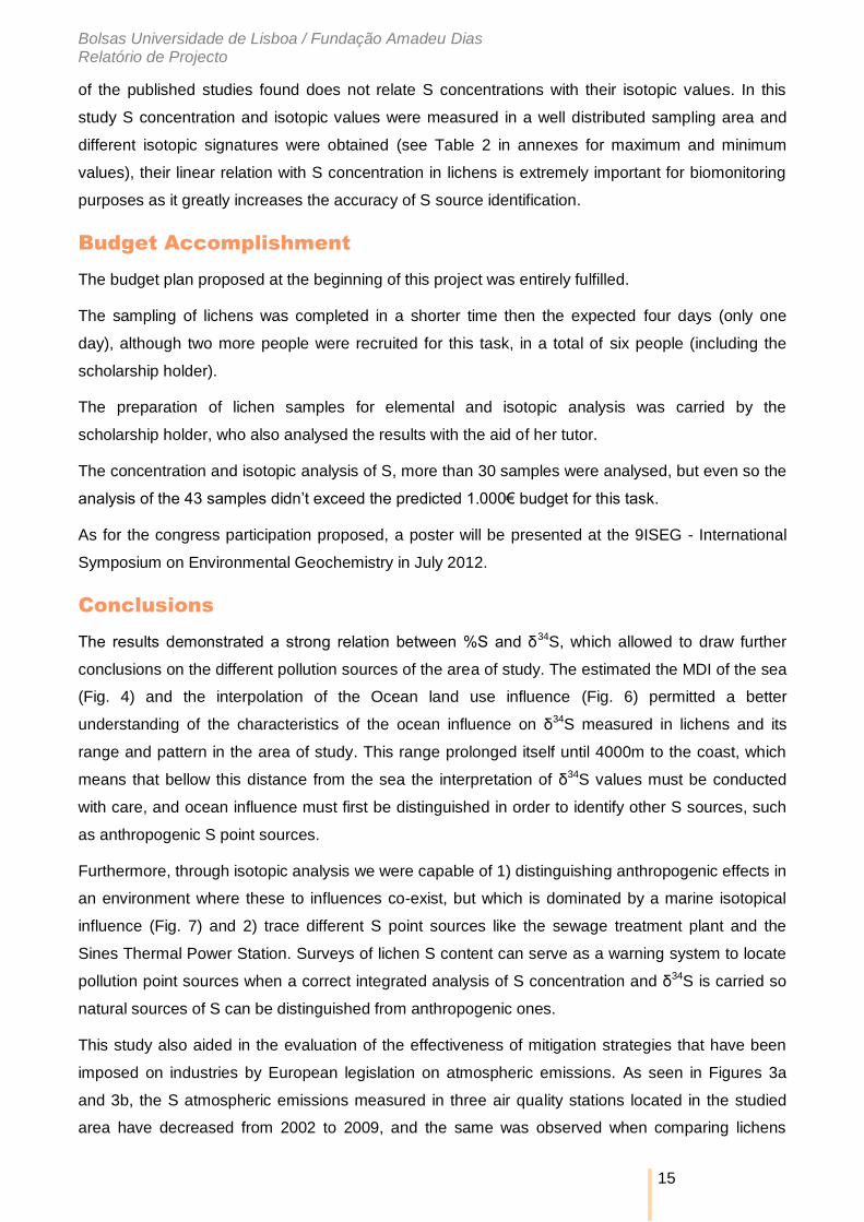
Bolsas Universidade de Lisboa / Fundação Amadeu Dias Relatório de Projecto
15
of the published studies found does not relate S concentrations with their isotopic values. In this
study S concentration and isotopic values were measured in a well distributed sampling area and
different isotopic signatures were obtained (see Table 2 in annexes for maximum and minimum
values), their linear relation with S concentration in lichens is extremely important for biomonitoring
purposes as it greatly increases the accuracy of S source identification.
Budget Accomplishment
The budget plan proposed at the beginning of this project was entirely fulfilled.
The sampling of lichens was completed in a shorter time then the expected four days (only one
day), although two more people were recruited for this task, in a total of six people (including the
scholarship holder).
The preparation of lichen samples for elemental and isotopic analysis was carried by the
scholarship holder, who also analysed the results with the aid of her tutor.
The concentration and isotopic analysis of S, more than 30 samples were analysed, but even so the
analysis of the 43 samples didn’t exceed the predicted 1.000€ budget for this task.
As for the congress participation proposed, a poster will be presented at the 9ISEG - International
Symposium on Environmental Geochemistry in July 2012.
Conclusions
The results demonstrated a strong relation between %S and δ34S, which allowed to draw further
conclusions on the different pollution sources of the area of study. The estimated the MDI of the sea
(Fig. 4) and the interpolation of the Ocean land use influence (Fig. 6) permitted a better
understanding of the characteristics of the ocean influence on δ34S measured in lichens and its
range and pattern in the area of study. This range prolonged itself until 4000m to the coast, which
means that bellow this distance from the sea the interpretation of δ34S values must be conducted
with care, and ocean influence must first be distinguished in order to identify other S sources, such
as anthropogenic S point sources.
Furthermore, through isotopic analysis we were capable of 1) distinguishing anthropogenic effects in
an environment where these to influences co-exist, but which is dominated by a marine isotopical
influence (Fig. 7) and 2) trace different S point sources like the sewage treatment plant and the
Sines Thermal Power Station. Surveys of lichen S content can serve as a warning system to locate
pollution point sources when a correct integrated analysis of S concentration and δ34S is carried so
natural sources of S can be distinguished from anthropogenic ones.
This study also aided in the evaluation of the effectiveness of mitigation strategies that have been
imposed on industries by European legislation on atmospheric emissions. As seen in Figures 3a
and 3b, the S atmospheric emissions measured in three air quality stations located in the studied
area have decreased from 2002 to 2009, and the same was observed when comparing lichens
Bolsas Universidade de Lisboa / Fundação Amadeu Dias Relatório de Projecto
16
collect in this area in 2002 with our results, which indicates that lichens also verified the success of
the mitigation measures. Thus air quality monitoring can be achieved with biomonitors such as
lichens as long as we bear in mind that these retain some memory of the past S emissions, since
the decrease was not as strong as the one verified in air quality stations.
References
Aherne, J., Futter, M. N. e Dillon, P. J. 2008. The impacts of future climate change and sulphur emission reductions on acidification recovery at Plastic Lake, Ontario. Hydrology and Earth System Sciences. 2008, Vol. 12, pp. 383-392.
APA, Agência Portuguesa do Ambiente. 2010. QualAr - Base de Dados On-line sobre Qualidade do Ar. [Online] 2010. APA, Agência Portuguesa do Ambiente (Portuguese Environmental Institute). 2004. Atlas do Ambiente. [Online] 2004.
http://sniamb.apambiente.pt/atlas/. Augusto, S., et al. 2010. Lichens as an integrating tool for monitoring PAH atmospheric deposition: A comparison with soil, air and pine
needles. 2010. pp. 483-489. Vol. 158. Backor, M. and Loppi, S. 2009. Interactions of lichens with heavy metals. Biologia Plantarum. 2009, Vol. 53 (2), pp. 214-222. Batts, J. E., Calder, L. J. and Batts, B. D. 2004. Utilizing stable isotope abundances of lichens to monitor environmental change. [ed.]
Elsevier. Chemical Geology. 2004, Vol. 204, pp. 345-368. Beričnik-Vrbovšek, J., et al. 2002. Isotopic analysis of sulphur in the assessment of SO2 emission sources. Acta Chim. 2002, Vol. 49,
pp. 149-157. Blake, D. M. 1998. Atmospheric Sulphur Deposition Monitoring in Newfoundland Using Lichens. MSc thesis. Newfoundland : Memorial
University of Newfoundland, 1998. Calhoun, J. A., Bates, T. S. e Charlson, R. J. 1991. Sulfur isotope measurements of submicrometer sulfate aerosol particles over the
Pacific Ocean. GEOPHYSICAL RESEARCH LETTERS. 1991, Vol. 18, pp. 1877-1880. Case, J. W. e Krouse, H. R. 1980. Variations in sulphur content and stable sulphur isotope composition of vegetation near a SO2 source
at Fox Creek, Alberta, Canada. Oecologia. 1980, Vol. 44, pp. 248-257. Chin, M. e Jacob, D. J. 1996. Anthropogenic and natural contributions to tropospheric sulfate: A global model analysis. Journal of
Geophysical Research. 1996, Vol. 101, pp. 18.691-18.699. Conti, M. E. e Cecchetti, G. 2001. Biological monitoring: lichens as bioindicators of air pollution assessment - a review. Environmental
Pollution. 2001, Vol. 114, pp. 471-492. Cuny, D., Van Haluwyn, C. and Pesch, R. 2001. Biomonitoring of trace elements in air and soil compartmentsalong the major motorway
in France. Water Air Soil Pollut. 2001, Vol. 125, pp. 273-289. Doll, R. e Ziebold, A. Flechten als lufthygienische Bioindikatoren. Biologische Rundschau. Vol. 14, pp. 78-94. Evans, A. N. G. 1996. Characterizing atmospheric sulphur using lichen and rain in eastern Newfoundland. Memorial university of
Newfoundland. Canada : s.n., 1996. BSc honours thesis. Ferry, B. W., Baddeley, M. S. e Hawksworth, D. L. 1973. Air pollution and lichens. London : Athlone Press, 1973. Garty, J. 2001. Biomonitoring Atmospheric Heavy Metals with Lichens: Theory and. Critical Reviews in Plant Sciences. 2001, Vol. 20: 4,
pp. 309 - 371. Glindemann, D., Novak, J. e Witherspoon, J. 2006. Dimethyl Sulfoxide (DMSO) Waste Residues and Municipal Waste Water Odor by
Dimethyl Sulfide (DMS): the North-East WPCP Plant of Philadelphia. Environmental Science and Technology. 2006, Vol. 40, pp. 202-207.
Griffith, G. W. 2004. The use of stable isotopes in fungal ecology. Mycologist. 2004, Vol. 18, pp. 177-183. Guderian, R., Küppers, K. e Six, R. 1985. Wirkungen von Ozon, Schwefeldioxid und Stickstoffdioxid auf Fichte und Pappel bei
unterschiedlicher Versorgung mit Magnesium und Kalzium sowie auf die Blattflechte Hypogymnia physodes. VDI-Berichte. 1985, Vol. 560, pp. 657-701.
Häffner, E., et al. 2001. Air Pollution and Lichen Physiology: Physiological Responses of Different Lichens in a Transplant Experiment Following an SO2 Gradient. Water, Air, and Soil Pollution. 2001, Vol. 131, pp. 185-201.
Hamed, A., et al. 2010. Changes in the production rate of secondary aerosol particles in Central Europe in view of decreasing SO2 emissions between 1996 and 2006. Atmospheric Chemistry and Physics. 2010, Vol. 10, pp. 1071-1091.
Hawksworth, D. L. and Rose, F. 1976. Lichens as Pollution Monitors. Studies in Biology. London : Edward Arnold, 1976, Vol. 66. —. 1970. Qualitative scale for estimating sulphur dioxide air pollution in England and Wales using epiphytic lichens. Nature. 1970, Vol.
227, pp. 145-148. Hissler, Christophe, et al. 2008. Identifying the origins of local atmospheric deposition in the steel industry basin of Luxembourg using
the chemical and isotopic composition of the lichen Xanthoria parietina. Science of the Total Environment. 2008, Vol. 405, pp. 338-344.
INE, Instituto Nacional de Estatística. 2001. Estatísticas territoriais. [Online] 2001. http://www.ine.pt/xportal/xmain?xpid=INE&xpgid=ine_main.
James, P. W. 1973. The effect of air pollutants other than hydrogen fluoride and sulphur dioxide on lichens. [autor do livro] M. S. Ferry, M. S. Baddeley e D. L. Hawkesworth. Air Pollution and Lichens. s.l. : The Athlone Press, University Of London, 1973, pp. 143-175.
Jeran, Z., et al. 1996. The use of lichens in atmospheric trace element deposition studies en Slovenia. Phyton-Annales Rei Botanicae. 1996, Vol. 36, pp. 91-94.
Krouse, H. R. e Case, J. W. 1981. Sulphur isotope ratios in water, air and vegetation near Teepee Creek gas plant, Alberta. Water, Air and Soil Pollution. 1981, Vol. 15, pp. 11-28.
Krouse, H. R. 1977. Sulphur isotope abundance elucidate uptake of atmospheric emissions by vegetation. Nature. 1977, Vol. 265, pp. 45-46.
Lindberg, S. E., et al. 1986. Atmospheric Deposition and Canopy Interactions of Major Ions in a Forest. Science. 1986, Vol. 231, pp. 141-145.
Martin, M. H. e Coughtrey, P. J. 1982. Biological monitoring of Heavy Metal Pollution. London : s.n., 1982. McArdle, N. C. e Liss, P. S. 1995. Isotopes and atmospheric sulphur. Atmospheric Environment. 1995, Vol. 29, pp. 2553-2556. Mektiyeva, V. L., Gavrilov, E. Ya. and Pankina, R. G. 1976. Sulphur isotopic composition in land plants. Geochemistry International.
1976, Vol. 13, pp. 85-88. Nimis, P. L. 1999. Linee guida per la bioindicazione degli effetti dell’inquinamento tramite la biodiversità dei licheni epifiti. 1999. Novák, M., Bottrell, S. H. e Přechová, E. 2001. Sulfur isotope inventories of atmospheric deposition, spruce forest floor and living
Sphagnum along a NW–SE transect across Europe. Biogeochemistry. 2001, Vol. 53, pp. 23-50. Novák, M., Jačková, I. and Přechová, E. 2001. Temporal trends in the isotope signature of air-borne sulfur in central Europe.
Environmental Science and Technology. 2001, Vol. 35, pp. 255-260.
Bolsas Universidade de Lisboa / Fundação Amadeu Dias Relatório de Projecto
17
Nriagu, J. O., Holdway, D. A. e Coker, R. D. 1987. Biogenic sulphur and the cidity of rainfal in remote areas of Canada. Science. 1987, Vol. 237, pp. 1189-1192.
Ohizumi, T., Fukuzaki, N. and Kusakabh, M. 1997. Sulphur isotopic view on the sources of sulphur in atmospheric fallout along the coast of the sea of Japan. Atmospheric Environment. 1997, Vol. 31, pp. 1339-1348.
Pinho, P., et al. 2008. Causes of change in nitrophytic and oligotrophic lichen species in a Mediterranean climate: Impact of land cover and atmospheric pollutants. Environmental Pollution. 2008, Vol. 154, pp. 380-389.
Pirintsos, S. A. and Loppi, S. 2003. Lichens as bioindicators of environmental quality in dry Mediterranean areas: A case study from northern Greece. Israel Journal of Plant Sciences. 2003, Vol. 51, pp. 143-151.
Preston, Thomas and Owens, Nicholas J. P. 1983. Interfacing an automatic elemental analyser with an isotope ratio mass sepectrometer: the potential for fully automated total nitrogen and nitrogen-15 analysis. Analyst. 1983, Vol. 108, pp. 971-977.
Pruett, L. E., et al. 2004. Assessment of sulfate sources in high-elevation Asian precipitation using stable sulfur isotopes. Environmental Science and Technology. 2004, Vol. 38, pp. 4728–4733.
Rees, C. E., Jenkins, W. J. e Monster, J. 1978. The sulphur isotopic composition of ocean water sulphate. Geochim. Cosmochim. Acta. 1978, Vol. 42, pp. 377-381.
Reuss, J. O., Cosby, B. J. e Wright, T. F. 1987. Chemical processes governing soil and water acidification. Nature. 1987, Vol. 329, pp. 27-32.
Rosamilia, S., et al. 2004. Uranium Isotopes, Metals and Other Elements in Lichens and Tree Barks Collected in Bosnia–Herzegovina. Journal of Atmospheric Chemistry. 2004, Vol. 49, pp. 447-460.
Sigal, L. L. e Nash, T. H. 1983. Lichen Communities on Conifers in Southern California Mountains: An Ecological Survey Relative to Oxidant Air Pollution. Ecology. 1983, Vol. 64, pp. 1343-1354.
Sigal, L. L. 1988. The relationship of lichen and bryophyte research to regulatory decisions in the United States. Bibliotheca Lichenologica. 1988, Vol. 30, pp. 269-287.
Sloof, J. E. 1993. Environmental Lichenology: Biomonitoring Trace-Element Air Pollution. Interfaculty Reactor Institute, Delft University of Technology. Delft : s.n., 1993. p. 191, Doctor's Thesis.
Smith, S. J., itcher, H. e Wigley, T.M. L. 2001. Global and regional anthropogenic sulfur dioxide emissions. Global and Planetary Change. 2001, Vol. 29, pp. 99-119.
Szczepaniak, K. and Biziuk, M. 2003. Aspects of the biomonitoring studies using mosses and lichens as indicators of metal pollution. Environmental Research. 2003, Vol. 93, pp. 221-230.
Takala, K., et al. 1985. Total sulphur contents of epiphytic and terricolous lichens in Finland. Annales Botanici Fennici. 1985, Vol. 22, pp. 91-100.
Takala, K., Olkkonen, H. e Krouse, H. R. 1991. Sulphur isotope composition of epiphytic and terricolous lichens and pine bark in Finland. Environmental Pollution. 1991, Vol. 69, pp. 337-348.
Trust, B. A. and Fry, B. 1992. Stable sulphur isotopes in plants: a review. Plant, Cell and Environment. 1992, Vol. 15, pp. 1105-1110. Ulrich, B., Mayer, R. e Khanna, R. K. 1980. Chemical changes due to acid precipitation in A loess-derived soil in Central Europe. Soil
Science. 1980, Vol. 130, p. 193. Van Dobben, H. F., et al. 2001. Relationship between epiphytic lichens, trace elements and gaseous atmospheric pollutants. Environ.
Pollut. 2001, Vol. 112, pp. 163-169. Vingiani, S., Adamo, P. and Giordano, S. 2004. Sulphur, nitrogen and carbon content of Sphagnum capillifolium and Pseudevernia
furfuracea exposed in bags in the Naples urban area. Environmental Pollution. 2004, Vol. 129, pp. 145-158. Wadleigh, M. A. and Blake, D. M. 1999. Tracing sources of atmospheric sulphur using epiphytic lichens. Environmental Pollution. 1999,
Vol. 106, pp. 265-271. Wadleigh, Moire A. 2003. Lichens and atmospheric sulphur: what stable isotopes reveal. Environmental Pollution. 2003, pp. 345-351. Winner, W. E., et al. 1978. Stable sulfur isotope analysis of SO2 pollution impact on vegetation. Oecologia. 1978, Vol. 36, 3, pp. 351-361. Wiseman, R. D. and Wadleigh, M. A. 2002. Lichen response to changes in atmospheric sulphur: isotopic evidence. Environmental
Pollution. 2002, 116, pp. 235-241. Xiao, H. Y. and Liu, C. Q. 2002. Sources of nitrogen and sulfur in wet deposition at Guiyang, Southwest China. Atmospheric
Environment. 2002, Vol. 36, pp. 5121–5130. Xiao, Hua-Yun, et al. 2010. Tissue S/N ratios and stable isotopes (d34S and d15N) of epilithic mosses (Haplocladium microphyllum) for
showing air pollution in urban cities in Southern China. Environmental Pollution. 2010, Vol. 158, pp. 1726-1732. Zhao, F. J., et al. 1998. Use of sulfur isotope ratios to determine anthropogenic sulfur signlas in a grasland ecosystem. Environmental
Science and Technology. 1998, Vol. 32, pp. 2288-2291.
Abbreviations
CP: (petro)Chemical Plant
IDW: Inverse Distance Weighted (interpolation)
MDI: Maximum Distance of Influence
STP: Sewage Treatment Plant
TPP: (Sines) Thermal Power Plant
29 de Julho, de 2011,
A Bolseira, A Tutora,

i
Annexes
ii
Table 1a and 1b - Spearman correlations between S concentration and isotopical values, S concentration and isotopic values and elevation, and these with the land use varialbles in each buffer (n=43 in anll variables). Significant correlations (p<0,05) are marked in red.
Table 2 - Descriptive statistics of S concentration, S isotopic values, distance to the sea and elevation at each sampling point (n=43 for all variables), of S concentration data from the SINESBIOAR project carried in 2002 (n=106), and of the land use variables at each buffer (n=43 for all variables).
Mean Median Min. Max. Std.Dev.
%S 0,11 0,11 0,06 0,19 0,03
δ34S (‰) 11,46 11,28 7,91 16,81 2,06
Distance to sea (m) 4727 4500 390 12900 3484
Elevation (m) 11 11 8 17 2
%S SINESBIOAR 0,20 0,20 0,11 0,34 0,04
Bu
ffe
r 1
00
m
Artificial Areas 2143 0 0 31375 7571
Agriculture 15022 12621 0 31375 14647
Nat. Veg. Areas 11526 949 0 31375 14004
Nat. Barren Areas 1673 0 0 31375 6124
Interface 0 0 0 0 0
Freshwater 0 0 0 0 0
Ocean 1010 0 0 31375 5085
Bu
ffe r 20 0 m
Artificial Areas 8424 0 0 125581 27390
%S δ34S Elevation
%S 1,000 -0,385 0,365
δ34S -0,385 1,000 -0,431
Elevation 0,365 -0,431 1,000
Artificial
Areas Agriculture
Nat.Veg. Areas
Nat. Barren Areas
Interface Freshwater Ocean
Bu
ffe
r
10
0m
%S 0,319 0,276 -0,170 -0,331 ---- ---- -0,250
δ34S -0,323 -0,140 -0,041 0,308 ---- ---- 0,365
Elevation -0,056 0,280 -0,046 -0,091 ---- ---- -0,318
Bu
ffe
r
20
0m
%S 0,282 0,233 -0,165 -0,243 ---- ---- -0,250
δ34S -0,348 -0,078 -0,063 0,276 ---- ---- 0,365
Elevation -0,048 0,199 0,050 -0,088 ---- ---- -0,318
Bu
ffe
r
30
0m
%S 0,281 0,185 -0,159 ---- ---- ---- -0,232
δ34S -0,422 -0,137 -0,029 ---- ---- ---- 0,421
Elevation -0,031 0,176 0,069 ---- ---- ---- -0,370
Bu
ffe
r
50
0m
%S 0,212 0,156 -0,065 -0,275 0,137 -0,099 -0,286
δ34S -0,420 -0,081 -0,075 0,297 -0,187 -0,025 0,330
Elevation -0,206 0,103 0,265 -0,126 -0,137 0,081 -0,383
Bu
ffe
r
10
00
m
%S 0,134 0,217 -0,028 -0,197 0,137 -0,041 -0,433
δ34S -0,343 0,032 -0,179 0,096 -0,187 0,118 0,610
Elevation -0,235 -0,016 0,444 -0,197 -0,137 -0,124 -0,586
Bu
ffe
r
20
00
m
%S 0,004 0,304 0,004 -0,195 -0,122 0,024 -0,319
δ34S -0,238 -0,101 -0,239 -0,006 0,011 0,223 0,643
Elevation -0,437 0,077 0,550 -0,117 -0,254 -0,092 -0,739
Bu
ffe
r
25
00
m
%S 0,015 0,322 -0,003 -0,194 -0,014 0,088 -0,338
δ34S -0,206 -0,111 -0,324 -0,060 0,034 0,259 0,670
Elevation -0,417 0,143 0,580 -0,062 -0,222 0,064 -0,764
Bu
ffe
r
30
00
m
%S 0,016 0,314 0,016 -0,217 -0,006 -0,035 -0,372
δ34S -0,179 -0,123 -0,359 -0,082 0,039 0,260 0,657
Elevation -0,472 0,181 0,569 0,011 -0,213 0,033 -0,798
Bu
ffe
r
50
00
m
%S -0,090 0,292 0,210 -0,155 -0,153 -0,031 -0,382
δ34S -0,059 -0,163 -0,456 -0,211 0,088 0,341 0,573
Elevation -0,635 0,261 0,716 0,141 -0,393 -0,111 -0,839

iii
Agriculture 58421 68130 0 125581 51350
Nat. Veg. Areas 47775 28650 0 125581 49022
Nat. Barren Areas 7037 0 0 103523 20107
Interface 0 0 0 0 0
Freshwater 0 0 0 0 0
Ocean 3925 0 0 117851 19407
Bu
ffe
r 3
00
m
Artificial Areas 19580 0 0 282473 59503
Agriculture 124848 153126 0 282618 103462
Nat. Veg. Areas 112368 84217 0 282618 102124
Nat. Barren Areas 0 0 0 0 0
Interface 0 0 0 0 0
Freshwater 0 0 0 0 0
Ocean 8478 0 0 250120 41565
Bu
ffe
r 5
00
m
Artificial Areas 59862 0 0 691282 150411
Agriculture 314932 294785 0 785191 242817
Nat. Veg. Areas 325901 280610 0 785191 255953
Nat. Barren Areas 59635 0 0 466300 124310
Interface 79 0 0 3399 518
Freshwater 282 0 0 12135 1851
Ocean 24500 0 0 625192 104663
Bu
ffe
r 1
00
0m
Artificial Areas 246579 0 0 1798283 477296
Agriculture 1122623 1155013 0 3141177 809608
Nat. Veg. Areas 1380144 1348148 0 4834779 1045274
Nat. Barren Areas 258997 10090 0 1299632 409488
Interface 3754 0 0 161401 24613
Freshwater 25603 0 0 693349 115522
Ocean 143846 0 0 1943034 391559
Bu
ffe
r 2
00
0m
Artificial Areas 980144 281967 0,0 4745497 1299281
Agriculture 4383655 4698124 224634,2 11469454 2555905
Nat. Veg. Areas 5054897 4724882 0,0 10230278 3035054
Nat. Barren Areas 902596 543767 0,0 3702782 960390
Interface 13231 0 0,0 252929 54423
Freshwater 128990 0 0,0 2306455 455466
Ocean 1087356 0 0,0 7074522 1803191
Bu
ffe
r 2
50
0m
Artificial Areas 1515372 556332 0,0 6122079 1821533
Agriculture 6766093 7165662 305303,1 16703459 3664552
Nat. Veg. Areas 7767372 7523008 204649,4 14489149 4288052
Nat. Barren Areas 1383413 991102 0,0 4795484 1320130
Interface 20963 0 0,0 252929 67300
Freshwater 177691 0 0,0 2362180 545801
Ocean 2003008 0 0,0 10602902 2996130
Bu
ffe
r 3
00
0m
Artificial Areas 2140943 1331263 0,0 8666614 2423539
Agriculture 9481947 10343858 354360,6 20971776 4794971
Nat. Veg. Areas 11151192 10796275 482840,0 20373986 5905144
Nat. Barren Areas 1935407 1546843 43115,6 6124098 1680594
Interface 23528 0 0,0 252929 74337
Freshwater 254892 0 0,0 2497195 656321
Ocean 3283880 0 0,0 14706302 4567424
Bu
ffe
r 5
00
0m
Artificial Areas 5008658 3614970 0 15645219 4588746
Agriculture 24486565 25285472 2454661 49504200 9957878
Nat. Veg. Areas 30267458 32485299 4670613 55363961 14070280
Nat. Barren Areas 5174919 5180962 683423 13301668 3111860
Interface 42254 0 0 252929 93404
Freshwater 871006 0 0 2972876 1077426
Ocean 12680341 2271651 0 43420785 14535968

iv