Carbon stocks and ﬂuxes in the high latitudes: using site ...

Biogeosciences, 14, 5143–5169, 2017https://doi.org/10.5194/bg-14-5143-2017© Author(s) 2017. This work is distributed underthe Creative Commons Attribution 3.0 License.

Carbon stocks and fluxes in the high latitudes: using site-leveldata to evaluate Earth system modelsSarah E. Chadburn1,2, Gerhard Krinner3, Philipp Porada4,5, Annett Bartsch6,7, Christian Beer4,5, Luca BelelliMarchesini8,9, Julia Boike10, Altug Ekici11, Bo Elberling12, Thomas Friborg12, Gustaf Hugelius13,Margareta Johansson14, Peter Kuhry13, Lars Kutzbach15, Moritz Langer10, Magnus Lund16,Frans-Jan W. Parmentier17,20, Shushi Peng3,18, Ko Van Huissteden9, Tao Wang19, Sebastian Westermann20,Dan Zhu21, and Eleanor J. Burke22

1University of Leeds, School of Earth and Environment, Leeds LS2 9JT, UK2University of Exeter, College of Engineering, Mathematics and Physical sciences, Exeter EX4 4QF, UK3CNRS, University Grenoble Alpes, IGE, Grenoble, France4Department of Environmental Science and Analytical Chemistry, Stockholm University, 10691 Stockholm, Sweden5Bolin Centre for Climate Research, Stockholm University, 10691 Stockholm, Sweden6Department of Geodesy and Geoinformation, Vienna University of Technology, Vienna, Austria7Cryosphere & Climate, Austrian Polar Research Institute, Vienna, Austria8School of Natural Sciences, Far Eastern Federal University, Vladivostok, Russia9Department of Earth Sciences, Vrije Universiteit (VU), Amsterdam, the Netherlands10Alfred Wegener Institute, Helmholtz Centre for Polar and Marine Research (AWI), 14473 Potsdam, Germany11Uni Research Climate and Bjerknes Centre for Climate Research, Bergen, Norway12Center for Permafrost (CENPERM), Department of Geosciences and Natural Resource Management, University ofCopenhagen, Copenhagen, Denmark13Department of Physical Geography, Stockholm University, 10691 Stockholm, Sweden14Department of Physical Geography and Ecosystem Science, Lund University, Sölvegatan 12, 223 62 Lund, Sweden15Institute of Soil Science, Center for Earth System Research and Sustainability, Universität Hamburg, Hamburg, Germany16Department of Bioscience, Arctic Research Center, Aarhus University, Frederiksborgvej 399, 4000 Roskilde, Denmark17Department of Arctic and Marine Biology, UiT – The Arctic University of Norway, Tromsø, Norway18Sino-French Institute for Earth System Science, College of Urban and Environmental Sciences, Peking University,Beijing 100871, China19Key Laboratory of Alpine Ecology and Biodiversity, Institute of Tibetan Plateau Research and Center for Excellence inTibetan Plateau Earth Sciences, Chinese Academy of Sciences, Beijing 100085, China20University of Oslo, Department of Geosciences, P.O. Box 1047 Blindern, 0316 Oslo, Norway21Laboratoire des Sciences du Climat et de l’Environnement, LSCE CEA CNRS UVSQ, Gif-Sur-Yvette, France22Met Office Hadley Centre, Fitzroy Road, Exeter EX1 3PB, UK

Correspondence to: Sarah E. Chadburn ([email protected])

Received: 17 May 2017 – Discussion started: 31 May 2017Revised: 2 September 2017 – Accepted: 5 September 2017 – Published: 17 November 2017

Published by Copernicus Publications on behalf of the European Geosciences Union.

5144 S. E. Chadburn: Carbon stocks and fluxes in the high latitudes

Abstract. It is important that climate models can accu-rately simulate the terrestrial carbon cycle in the Arctic dueto the large and potentially labile carbon stocks found inpermafrost-affected environments, which can lead to a pos-itive climate feedback, along with the possibility of futurecarbon sinks from northward expansion of vegetation underclimate warming. Here we evaluate the simulation of tun-dra carbon stocks and fluxes in three land surface schemesthat each form part of major Earth system models (JSBACH,Germany; JULES, UK; ORCHIDEE, France). We use asite-level approach in which comprehensive, high-frequencydatasets allow us to disentangle the importance of differentprocesses. The models have improved physical permafrostprocesses and there is a reasonable correspondence betweenthe simulated and measured physical variables, including soiltemperature, soil moisture and snow.

We show that if the models simulate the correct leaf areaindex (LAI), the standard C3 photosynthesis schemes pro-duce the correct order of magnitude of carbon fluxes. There-fore, simulating the correct LAI is one of the first priorities.LAI depends quite strongly on climatic variables alone, aswe see by the fact that the dynamic vegetation model cansimulate most of the differences in LAI between sites, basedalmost entirely on climate inputs. However, we also iden-tify an influence from nutrient limitation as the LAI becomestoo large at some of the more nutrient-limited sites. We con-clude that including moss as well as vascular plants is of pri-mary importance to the carbon budget, as moss contributesa large fraction to the seasonal CO2 flux in nutrient-limitedconditions. Moss photosynthetic activity can be strongly in-fluenced by the moisture content of moss, and the carbon up-take can be significantly different from vascular plants witha similar LAI.

The soil carbon stocks depend strongly on the rate of in-put of carbon from the vegetation to the soil, and our anal-ysis suggests that an improved simulation of photosynthe-sis would also lead to an improved simulation of soil carbonstocks. However, the stocks are also influenced by soil car-bon burial (e.g. through cryoturbation) and the rate of het-erotrophic respiration, which depends on the soil physicalstate. More detailed below-ground measurements are neededto fully evaluate biological and physical soil processes. Fur-thermore, even if these processes are well modelled, the soilcarbon profiles cannot resemble peat layers as peat accumu-lation processes are not represented in the models.

Thus, we identify three priority areas for model devel-opment: (1) dynamic vegetation including (a) climate and(b) nutrient limitation effects; (2) adding moss as a plantfunctional type; and an (3) improved vertical profile of soilcarbon including peat processes.

1 Introduction

Land areas in northern high latitudes may represent a netsource or a net sink of carbon to the atmosphere in the fu-ture, and there is not yet a consensus as to which of thetwo is more likely (Cahoon et al., 2012; Hayes et al., 2011).This is not because it is likely to be small: on a pan-Arcticscale we could see anything between a net emission of over100 Gt C or a net sink of up to 60 Gt C by the end of thiscentury (Schuur et al., 2015; Qian et al., 2010). To put thisinto context, the remaining emissions budget in order to sta-bilise climate warming below 2 ◦C above pre-industrial lev-els is less than 250 Gt C from 2017 on (Peters et al., 2015).Thus, it is very important to reduce uncertainty in the north-ern high latitude carbon cycle. The uncertainty comes largelyfrom the representation of these processes in Earth systemmodels (ESMs), which are our main tool for future climateprojections.

The potential for large carbon emissions comes from thelarge quantities of old carbon that are frozen into permafrost,protected from decomposition under the current cold climate.Around 800 Gt of carbon is stored in permanently frozensoils (Hugelius et al., 2014). If the permafrost thaws, thiscarbon may decompose and be released into the atmosphere(Burke et al., 2012, 2013; Koven et al., 2015; Schneider vonDeimling et al., 2012, 2015; MacDougall and Knutti, 2016).Conversely, the increased vegetation growth that is alreadytaking place in the Arctic under climate warming (Tuckeret al., 2001; Tape et al., 2006) could result in a net uptakeof carbon from the atmosphere (Quegan et al., 2011; Qianet al., 2010). It should be noted, however, that in some areasArctic vegetation growth is not increasing but rather “brown-ing” (Epstein et al., 2016).

The representations of both permafrost carbon and Arc-tic vegetation in ESMs are not well developed. Some mod-els now include a vertical representation of soil carbon,which allows the frozen carbon in permafrost to be included(Koven et al., 2009, 2013; Schaphoff et al., 2013; Burkeet al., 2017), but most do not yet represent important mech-anisms of carbon storage and release, such as sedimenta-tion, thermokarst formation and a proper representation ofcryoturbation (Schneider von Deimling et al., 2015; Beer,2016), although sedimentation is included in (Zhu et al.,2016). There is also a growing consensus that the chemicaldecomposition models used in ESMs are not adequate to rep-resent microbial processes (Wieder et al., 2013; Xenakis andWilliams, 2014). Vegetation models also, for the most part,do not include the appropriate high-latitude vegetation types,and those models that have dynamic vegetation are lackingin processes that are essential determinants of vegetation dy-namics, such as nutrient limitation and interactions with soil(Wieder et al., 2015).

In this paper we assess the ability of the land surface com-ponents from three ESMs to represent the carbon stocks andfluxes observed at tundra sites, identifying the processes that

Biogeosciences, 14, 5143–5169, 2017 www.biogeosciences.net/14/5143/2017/

S. E. Chadburn: Carbon stocks and fluxes in the high latitudes 5145

have the greatest impact on the uncertainty. These processesare therefore priorities for future model development. Ob-servational studies in tundra environments have shown thatcarbon dynamics are sensitive to physical conditions (Lundet al., 2012; Cannone et al., 2016; Pirk et al., 2017); thus,we first assess the ability of the models to capture the meanphysical state of the system and the differences between sites,specifically in terms of snow depth, soil temperature, soilmoisture and active-layer depth. Secondly, soil carbon stocksare evaluated against measured soil carbon profiles, assess-ing the main causes of biases in the models. Half-hourly netecosystem exchange (NEE) data from eddy flux towers areused to evaluate the simulated carbon fluxes, comparing themodels directly against observations before analysing the re-lationships between ecosystem carbon fluxes and differentdriving variables. We also consider the impacts of other con-trolling factors such as nutrient limitation and mosses, whoseimportance has been identified in previous studies (Atkin,1996; Uchida et al., 2009).

This is a synthesis from the recently concluded EU projectPAGE21 (Changing Permafrost in the Arctic and its GlobalEffects in the 21st century), evaluating the models that tookpart in the project (described in Sect. 2.2, below) at the fivePAGE21 primary sites, which are all located in Arctic per-mafrost regions, specifically Siberia, Sweden, Svalbard andGreenland. After the site-level evaluation of physical pro-cesses by (Ekici et al., 2015), this evaluation of carbon cycleprocesses continues site-level model evaluation efforts. Thesites are described in detail in Sect. 2.3.

2 Methods

This study takes three different angles: (1) comparison withobserved indicators; (2) comparison of processes betweenmodels and (3) comparison of geographical conditions (e.g.vegetation, permafrost) between sites. The structure of themethods section is as follows: first describing the observa-tional indicators used (Sect. 2.1), second the processes rep-resented in the models (Sect. 2.2) and third the conditions atthe sites (Sect. 2.3). Lastly, details of the simulation set-upand forcing data are given in Sect. 2.4.

2.1 Evaluation data

2.1.1 Carbon dioxide flux

Eddy covariance half-hourly CO2 flux data and related me-teorological variables used in this study are archived inthe PAGE21 fluxes database (http://www.europe-fluxdata.eu/page21), which is part of the European Fluxes DatabaseCluster.

Flux post-processing was performed consistently forall the sites following the protocol applied for theFLUXNET2015 data release (http://fluxnet.fluxdata.org/data/fluxnet2015-dataset), with customised choices of the

processing options. The applied scheme included the follow-ing: (i) a quality assessment and quality control procedureover single variables aimed at detecting implausible values orincorrect time stamps (e.g. by comparing patterns of poten-tial and observed downward shortwave radiation at a givenlocation); (ii) the computation of NEE by adding the CO2flux storage term calculated from a single CO2 concentra-tion measurement point (at the top of the flux tower) andassuming a vertically uniform concentration field; (iii) thede-spiking of NEE based on (Papale et al., 2006) using athreshold value (z= 5); (iv) NEE filtering according to anensemble of friction velocity (u∗) thresholds obtained withbootstrapping following the methods of (Barr et al., 2013)and (Papale et al., 2006) and selection of a u∗ threshold, dif-ferent for each year, based on the highest model efficiency(Nash–Sutcliffe); (vi) the gap-filling of NEE time series withthe marginal distribution sampling method (Reichstein et al.,2005).

Finally, NEE was partitioned into the gross primary pro-ductivity (GPP) and ecosystem respiration (Reco) compo-nents using a semi-empirical model based on a hyperboliclight-response curve fitted to daytime NEE data (Lasslopet al., 2010). The years of data available for each site aregiven in Table S1.

2.1.2 Soil carbon profiles

Typical soil profiles with data on soil organic carbon contentwere generated for each site. Based on extensive field cam-paigns in each study area, individual pedons for representa-tive landscape and soil types were combined and harmonised.In brief, soils were classified and sampled from open soilpits dug down to the permafrost. Permafrost samples werecollected through manual coring into the permafrost at thebottom of the soil pit. In most cases, soils were sampled toa depth of 1 m. The harmonised soil profiles were generatedby averaging several soil pedons per landscape type at a 1 cmdepth resolution. For more detailed descriptions of field sam-pling and laboratory procedures, see Palmtag et al. (2015)and Siewert et al. (2015, 2016). Top 1 m total soil carbonvalues were calculated from a weighted average of differenttypical profiles, based on the fractional coverage of landscapetypes in the footprint area of the flux towers.

2.1.3 Snow depth

Snow depth was recorded using automatic sensors (exceptAbisko, where it is manual). Snow depth from the Abiskomire (Storflaket) was recorded manually monthly (Johans-son et al., 2013). Snow depth at Samoylov and Bayelva wasrecorded hourly, and for Zackenberg 3-hourly (using sonicrange and laser sensors). Snow depth at Kytalyk was mea-sured by means of a 70 cm vertical profile made of thermis-tors spaced every 5 cm (2.5 cm between 0 and 10 cm heightfrom the ground). Data were logged every 2 h and the snow–

www.biogeosciences.net/14/5143/2017/ Biogeosciences, 14, 5143–5169, 2017

http://www.europe-fluxdata.eu/page21

http://www.europe-fluxdata.eu/page21

http://fluxnet.fluxdata.org/data/fluxnet2015-dataset

http://fluxnet.fluxdata.org/data/fluxnet2015-dataset


air interface level was identified by analysing the profile pat-terns with a MATLAB© routine calibrated to search for devi-ations between consecutive resistance readings above a giventhreshold. Years used for each site are given in Table S1.

2.1.4 Soil temperature

For Samoylov, Bayelva, Kytalyk and Zackenberg, soil tem-perature was recorded hourly using thermistors (Kytalyk set-up described in van der Molen et al., 2007). Ground temper-atures for Abisko mire were recorded at the Storflaket mire,at boreholes cased with plastic tubes and instrumented withHOBO loggers U12 (industry, four channels) together withHOBO soil temperature sensors (Johansson et al., 2011). Theyears used for each site are given in Table S1.

2.1.5 Soil moisture

Continuous soil moisture measurements are only availablefor Bayelva, Samoylov and Zackenberg. At Samoylov andBayelva, hourly volumetric soil water content was recorded(using time domain reflectometry). At Zackenberg soilmoisture was measured using permanently installed ML2xThetaProbes (Lund et al., 2014). Years used for each site aregiven in Table S1. Indicative soil moisture levels for Abiskomire were collected from May to October 2015 (Pedersenet al., 2017), measured manually as volumetric soil watercontent integrated over 0–6 cm depth using a handheld ML2xThetaProbe (Delta-T Devices Ltd., Cambridge, UK). Soilmoisture was measured five times in each plot and averageswere subsequently used.

2.1.6 Active-layer depth

Active-layer depth was measured at Circumpolar ActiveLayer Monitoring (CALM) grids at most of the sites. AtBayelva there is no CALM grid; thus, the active layer wasestimated from soil temperature measurements and is givenas an indicative value. Active-layer thickness monitoring isdetermined by mechanical probing. A 1 cm diameter gradu-ated steel rod is inserted into the soil to the depth of resis-tance to determine the active-layer thickness (Åkerman andJohansson, 2008) according to the CALM standard.

2.1.7 Leaf area index

Leaf area index was taken from the MODIS product(MODIS15A2, 2016) for the closest coordinates to the sites.This product has been successfully applied to tundra sites(Cristóbal et al., 2017). It was evaluated by (Cohen et al.,2006), who found an RMSE of 0.28 at a tundra site. Thereare, however, still considerable uncertainties in using thisdata product (see Sect. 3.6.1).

2.1.8 GPP per unit leaf area

This was calculated using the partitioned GPP from the eddycovariance data (Sect. 2.1.1), averaged daily and taken onthe same day as the values from the MODIS LAI product(Sect. 2.1.7). Note that there are no time-resolved GPP val-ues for Bayelva due to insufficient data. The extracted GPPvalues were divided by the appropriate LAI estimates and theresulting values were collected for all sites and binned intointervals of air temperature (1.5 ◦C) and shortwave radiation(20 Wm−2), for which the mean and standard deviation werethen calculated (shown in Fig. 9).

2.2 Model description

The three models studied here are JSBACH (Jena Schemefor Biosphere–Atmosphere Coupling in Hamburg; Raddatzet al., 2007; Brovkin et al., 2009), JULES (Joint UK LandEnvironment Simulator; Best et al., 2011; Clark et al., 2011)and ORCHIDEE (ORganizing Carbon and Hydrology In Dy-namic Ecosystems Environment; Krinner et al., 2005). Theseare all land surface components of major ESMs (JSBACH:MPI-ESM; JULES: UKESM; ORCHIDEE: IPSL). Key fea-tures are summarised in Table 1.

These models can be run in a coupled mode within theESM, or, as here, they can be run as stand-alone modelsforced by observed meteorology. The models are run as agridded set of points for large-scale simulations, and theycan also be run for single points, as in this study. Each modelhad some development of high-latitude processes during thePAGE21 project, and model developments have also been on-going since the conclusion of the project in late 2015.

All the models simulate vertical fluxes of water, heat andcarbon between the atmosphere, the vegetation and the soil.Of relevance to permafrost physics, the models simulate a dy-namic snowpack by means of a multilayer snow scheme andthe freezing and thawing of soil (Ekici et al., 2014; Gouttevinet al., 2012a; Wang et al., 2013; Best et al., 2011). All modelsuse a vertical discretisation of soil thermal and hydrologicalfluxes, with differing resolutions (see Appendix Table A2).JSBACH has the lowest-resolution soil, with only five lay-ers in the top 10 m (Hagemann and Stacke, 2015), althoughin this latest version it is extended to 50 m depth with addi-tional layers. ORCHIDEE and JULES also simulate an extrathermal-only column at the base of the hydrological columnto represent bedrock (Chadburn et al., 2015a).

Soil thermal and hydrological properties in both JULESand ORCHIDEE have been adapted to allow better repre-sentation of organic soils, whereas in JSBACH only min-eral soil properties are represented. However, JSBACH ad-ditionally simulates a moss and/or lichen layer at the surfacewith dynamic moisture contexts and thermal properties (Po-rada et al., 2016), which physically represents the surface or-ganic layer. Organic soil properties in JULES are describedin Chadburn et al. (2015a). In ORCHIDEE the scheme fol-



lows (Lawrence and Slater, 2008), using the observation-based soil carbon map from (Hugelius et al., 2014).

Soil carbon is represented by a multi-pool scheme in allthe models, with inputs from vegetation, and decompositionrates depending on soil temperature, soil moisture and intrin-sic turnover times of different pools (Goll et al., 2015; Clarket al., 2011). Both ORCHIDEE and JULES represent a verti-cal profile of soil carbon (discretised in line with the soil hy-drology), including cryoturbation mixing (Koven et al., 2009;Burke et al., 2017). JSBACH, however, represents only a sin-gle layer, with decomposition rates determined by conditionsin the upper layer of soil.

None of the models simulate nitrogen or other nutrients.Vegetation growth and productivity is therefore only deter-mined by soil moisture and atmospheric forcing data, withno nutrient limitation. Different land cover types are repre-sented in the models by surface tiles, which can vary in frac-tional cover. In JULES, a dynamic vegetation model is runwith nine competing plant functional types (PFTs) (Harperet al., 2016), whereas in the other models, vegetation is fixed,but with dynamic phenology. ORCHIDEE has 13 PFTs butthere is no specific high-latitude PFT in the version usedhere; thus, C3 grasses are prescribed for these sites. In JS-BACH there are 20 PFTs (including crop and pasture) andfor these sites a tundra PFT is used, which is similar to C3grass but with reduced Vcmax (maximum rate of carboxy-lation in leaves). In JSBACH there is also a dynamic mossmodel simulating moss photosynthesis and respiration, as inthe model described by (Porada et al., 2013). This model rep-resents both mosses and lichens by one plant functional typewith average physiological properties. In the version usedhere, the moss carbon fluxes are not yet fully coupled intothe JSBACH carbon cycle; thus, the moss carbon fluxes areconsidered separately in the analysis that follows.

For more details of the soil and vegetation configurationsee Sect. 2.4 and the Appendix.

2.3 Site descriptions

The sites represent a range of climatological and biogeophys-ical conditions across the tundra. Abisko is the warmest site,with sporadic permafrost, followed by Bayelva, which is ahigh Arctic maritime site (on Svalbard), and Zackenberg,which is a maritime site in Greenland (colder than Bayelva).Samoylov and Kytalyk have a continental Siberian climateand the coldest mean annual temperatures. The landscapesdiffer between sites, which can influence the permafrost andcarbon dynamics, for example through the impact of topogra-phy on snow distribution and hydrology. The following sec-tions provide a short description of each study area, and theimportant climatic and permafrost variables are given in Ta-ble 2.

At all sites there has been some tendency towards air tem-perature warming, which in many cases is accompanied bywarming or thawing of permafrost (Callaghan et al., 2010;

Christiansen et al., 2010; Parmentier et al., 2011; Boike et al.,2013; Lund et al., 2014; Abermann et al., 2017).

2.3.1 Abisko

The Abisko site is located in the Torneträsk catchment innorthernmost Sweden. According to (Brown et al., 1998),the Abisko area lies within the zone of discontinuous per-mafrost. However, with the observed permafrost degradationduring the last decades (Åkerman and Johansson, 2008; Jo-hansson et al., 2011), the area is now more characteristicof the sporadic permafrost zone. Permafrost is widespreadin the mountains (Ridefelt et al., 2008), but at lower ele-vations permafrost is only found in peat mires (Johanssonet al., 2006). Data from three sites from the Torneträsk catch-ment (within an area of 10 km) have been used for this study.The principal sites are Storflaket and Stordalen peat mires.The active-layer measurements and the ground temperaturesare monitored at the Storflaket site (Åkerman and Johansson,2008; Johansson et al., 2011) and the carbon monitoring, in-cluding the eddy covariance measurement, is carried out atthe Stordalen site. These two mire sites are very similar interms of climate, soil profile and permafrost characteristics.The footprint of the eddy covariance tower is characterisedby wet fen with no permafrost present and vegetation dom-inated by tall graminoids (Jammet et al., 2015, 2017). Forcomparison, additional soil temperature data from a mineralsoil site at the Abisko Scientific Research Station, which isnot underlain by permafrost, are included.

2.3.2 Bayelva (Svalbard)

The study site is located in the high-Arctic Bayelva Rivercatchment area, close to Ny-Ålesund on Spitsbergen island inthe Svalbard archipelago. The area is characterised by mar-itime continuous permafrost. In bioclimatic terms the arearepresents a semi-desert ecosystem (Uchida et al., 2009).Vegetation includes low vascular plants (mainly grass, sedge,catchfly, saxifrage and willow), mosses and lichens (Oht-suka et al., 2006; Uchida et al., 2006). The ground is mostlybedrock but is partly covered by a mixture of sediments. Thestudy site is located on permafrost patterned ground mainlyconsisting of non-sorted soil circles or mud boils, witharound 60 % vegetation cover. The eddy covariance measure-ments were conducted on Leirhaugen hill, and additional me-teorological observations and ground temperature measure-ments are continuously conducted at the Bayelva soil and cli-mate monitoring station (Boike et al., 2003, 2008a; Roth andBoike, 2001) 100 m away. Over the past decade the Bayelvacatchment has been the focus of intensive investigations onsoil and permafrost conditions (Roth and Boike, 2001; Boikeet al., 2008a; Westermann et al., 2010, 2011) and the surfaceenergy balance (Boike et al., 2003; Westermann et al., 2009).Details of the measurements are provided in Westermann etal. (2009) and Lüers et al. (2014).



2.3.3 Kytalyk

The Kytalyk site is located in the Kytalyk reserve, 28 kmnorthwest of the village of Chokurdakh in the Republic ofSakha (Yakutia), Russian Federation. The site is located be-tween the East Siberian Sea and the transition zone betweentaiga and tundra. The area is underlain by continuous per-mafrost. The measurement site is located at the bottom of adrained former thermokarst lake, and the site is bordered bythe edge of the present river floodplain. Both on the flood-plain and at the lake bottom, a network of ice wedge poly-gons occurs, in general of the low-centred type. These forma mosaic of low plateaus and ridges dominated by Betulanana and diffuse drainage channels covered with a meadow-like vegetation of Eriophorum angustifolium and Carex sp.There is also hummocky Sphagnum with low Salix dwarfshrubs, polygon ponds covered with mosses and Comarumpalustre, deeper ponds in which ice wedges have thawed, anddrier areas covered with Eriophorum vaginatum tussocks.The soils generally have a 10–40 cm organic top layer overly-ing silt. The eddy covariance tower is located at a distance ofca. 200 m from the research station buildings (van der Molenet al., 2007). The tower footprint covers a wet northwesternand southeastern sector dominated by Sphagnum and ponds,while the northeastern and southwestern sectors have driervegetation types.

2.3.4 Samoylov

Samoylov Island lies within one of the main river chan-nels in the southern part of the Lena river delta in north-ern Yakutia. The landscape on Samoylov Island, and in thedelta as a whole, has generally been shaped by water througherosion and sedimentation (Fedorova et al., 2015), and bythermokarst processes (Morgenstern et al., 2013). Contin-uous cold permafrost underlies the study area to betweenabout 400 and 600 m below the surface. The terrace wherethe study site is situated is covered in low-centred ice wedgepolygons, with water-saturated soils or small ponds in thepolygon centres. The mineral soil is generally sandy loam,underlain by silty river deposits, with a ∼ 30 cm thick or-ganic layer (Boike et al., 2013). Vegetation in the polygoncentres and at the edge of ponds is dominated by sedges andmosses, and at the polygon rims various mesophytic dwarfshrubs, forbs and mosses dominate (Kutzbach et al., 2007).It is estimated that moss contributes around 40 % to the to-tal photosynthesis (Kutzbach et al., 2007). Detailed informa-tion concerning the climate, permafrost, land cover, vegeta-tion and soil characteristics of Samoylov Island can be foundin (Boike et al., 2013) and (Morgenstern et al., 2013). Anal-ysis of the energy balance for the site is found in Boike etal. (2008b) and Langer et al. (2011a, b).

2.3.5 Zackenberg

The Zackenberg study site is located near the Zackenberg Re-search Station within the Northeast Greenland National Park,within the continuous permafrost zone. High mountains sur-round the Zackenberg valley to the west, east and north, witha fjord to the south, and snow cover is characterised by largeinterannual variability (Pedersen et al., 2016). Water avail-ability is thus regulated by topography and snow distributionpatterns. Most vegetation in the Zackenberg valley is locatedbelow 300 m a.s.l., where the lowland is dominated by non-calcareous sandy fluvial sediments (Elberling et al., 2008),and peat soils have limited spatial coverage (Palmtag et al.,2015). The study site is located within a Cassiope tetragonatundra heath, dominated by C. tetragona, Dryas integrifoliaand Vaccinium uliginosum, with patches of mosses. Severalstudies on soil and permafrost (Palmtag et al., 2015; West-ermann et al., 2015), surface energy balance (Lund et al.,2014; Stiegler et al., 2016; Lund et al., 2017) and carbonexchange (Mastepanov et al., 2008; Lund et al., 2012; Elber-ling et al., 2013) have been published based on data from thissite. A rich dataset is available from this site through the ex-tensive, cross-disciplinary Greenland Ecosystem Monitoringprogramme (www.g-e-m.dk).

2.4 Simulation set-up

The sites were represented in all the models by a single ver-tical column, although there was some horizontal represen-tation by means of tiling approaches (see model description,Sect. 2.2). The models were run in the most up-to-date con-figurations, including new permafrost-relevant model devel-opments where available. Variables were output at hourlyand/or daily resolutions.

The meteorological driving data were prepared using ob-servations from the site combined with reanalysis data forthe grid cell containing the site. For the period 1901–1979,Water and Global Change forcing data (WFD) were used(Weedon et al., 2011). Data are provided at half-degree res-olution for the whole globe at 3-hourly time resolution from1901 to 2001. For the period 1979–2014, WATCH-Forcing-Data-ERA-Interim (WFDEI) was used (Weedon, 2013). Forthe time periods in which observed data were available, cor-rection factors were generated by calculating monthly biasesrelative to the WFDEI data. These corrections were then ap-plied to the time series from 1979 to 2014 of the WFDEIdata. The WFD before 1979 were then corrected to matchthese data and the two datasets were joined at 1979 to providegap-free 3-hourly forcing from 1901 to 2014. Local meteo-rological station observations were used for all variables ex-cept snowfall, which was estimated from the observed snowdepth by treating increases in snow depth as snowfall eventswith an assumed snow density (see Appendix). These re-constructions were then used to provide correction factors toWFDEI and WFD. This leads to a more realistic snow depth


www.g-e-m.dk


in the model than using direct precipitation measurements,which are less precise due to wind effects and the difficultyof accurately measuring snowfall. However, the local pre-cipitation measurements were still used for rainfall, as thisis much more reliable, with a potential undercatch of onlyaround 10 % (Yang et al., 2005). For Abisko, meteorolog-ical data from the research station were used but addition-ally corrected by scaling the snowfall according to the ratioof monthly snow depths at the mire vs. the research station(snow depth was only measured monthly at Storflaket mire),and a reduction of 1 ◦C in air temperature. Even with thesecorrections, there is still considerable uncertainty in precip-itation forcing, particularly the snowfall, so in order to testthe impact of this, two of the models (JULES and JSBACH)performed two additional sets of simulations, with snowfallincreased and reduced by 50 %.

Spin-up was performed as consistently as possible be-tween the models, using the meteorological forcing from1901 to 1930. Years were selected at random from this30-year period and the models were run for 10 000 yearswith pre-industrial CO2 levels (1850, 286 ppm), followed by50 years with changing CO2 levels (1851–1900). The modelstate at the end of this spin-up period was taken as the initialstate for the main run (1 January 1901 to 31 December 2013).For JSBACH, there was an initial 50 years of hydrologicalspin-up before the main spin-up, with the permafrost impacton hydrology switched off, to allow the water to form a re-alistic profile (permafrost layers are impermeable and thusunrealistic initial conditions could otherwise be preserved).For JSBACH, the long spin-up was also between 7000 and8000 years rather than 10 000 since in this model there is novertical representation of soil carbon, and therefore the soilcarbon pools equilibrate much more quickly and had reacheda steady state after 7000–8000 years. The CO2 forcing dataare from (Meinshausen et al., 2011).

The soil parameters in the models were set up to repre-sent each site as closely as possible (see Appendix and Ta-ble A1). These drew from literature values, a PAGE21 de-liverable “catalogue of physical parameters”, and field ex-perience. (Note that the soil carbon profiles described inSect. 2.1.2 were not used for this).

Vegetation was prescribed in ORCHIDEE and JSBACH.Since these are tundra sites, JSBACH used a tundra PFT(100 % coverage), which is similar to C3 grass but with re-duced Vcmax. ORCHIDEE prescribed C3 grass (100 % cov-erage) as there is no tundra PFT in this model version. JULESwas run with dynamic vegetation using nine PFTs (Harperet al., 2016), which do not include any tundra PFTs. Allnine PFTs prognostically determine their coverage accord-ing to the environmental conditions, and they are all allowedto compete for space. In practice, only the C3 grass PFT isable to grow at these sites.

Some experiments were performed to separate the impactsof different processes. ORCHIDEE was run with and withoutvertical mixing of soil carbon. JSBACH carbon fluxes were

analysed with and without an additional contribution from anew moss photosynthesis scheme. In JULES, an extra set ofsimulations was performed with fixed vegetation to comparewith the dynamic vegetation scheme.

3 Results and discussion

The carbon dynamics are intrinsically linked to the physicalstate of the system (for example, determining the rate of soilcarbon decomposition). Therefore, we start by assessing thesnowpack, soil temperature, soil moisture and active-layerthickness in all three models. The model physics has alsobeen evaluated in detail in previous publications (Ekici et al.,2015, 2014; Chadburn et al., 2015a; Porada et al., 2016) andis thus kept short here. In these studies, representing organicsoil was identified as a key influence on the simulation of soilphysics, and following this we compare organic with min-eral soils in our analysis. We then evaluate the soil carbonstocks and the ecosystem CO2 fluxes, and we analyse theCO2 fluxes in detail. The fluxes depend on every part of thesystem and therefore all of the preceding analysis contributesto our understanding of the carbon dynamics at these sites.

3.1 Snow

The seasonal cycle of snow depth is shown in Fig. 1. It de-pends strongly on the snowfall driving data. Since the snow-fall was back-calculated from the snow depth, the accumu-lation period should match well with observations. There isstill some variation due to the fresh snow density in the mod-els (which can differ from both the assumed density in mak-ing the driving data and between the models), and further-more the compaction of the snow is dependent on the modelprocess representation and physical conditions. Nonetheless,for the most part the models make a reasonable simulation ofthe snowpack accumulation and compaction, with the excep-tion of Abisko, where the models are all biased high. Here,snow inputs are particularly uncertain as no high-resolutiontime series of snow depth are available (unlike the othersites). We performed a sensitivity study to test the impactof uncertainties or variability in snow depth on the simulatedcarbon cycle processes. In this study, a reduction of 50 % insnowfall allows the models to simulate a realistic snow depthat Abisko – see the Supplement. The impacts on soil carbonstocks and fluxes are fairly small, however (between 0.2 and10 %; Figs. S7 and S8).

During the melting season the models are less accuratethan during accumulation, with the snow often melting tooearly, by up to 25 days in the most extreme case. Our methodof back-calculating snowfall from snow depth may misssome snowfall events during the melt season. There are alsomany other potential influences such as albedo effects, snow–vegetation interactions and the influence of wind-blown sed-iment. For example, the vegetation in the models is quite



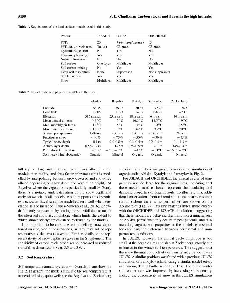
Table 1. Key features of the land surface models used in this study.

Process JSBACH JULES ORCHIDEE

PFTs 20 9 (+4 crop/pasture) 13PFT that grows/is used Tundra C3 grass C3 grassDynamic vegetation No Yes NoDynamic phenology Yes Yes YesNutrient limitation No No NoSoil carbon One layer Multilayer MultilayerSoil carbon mixing No Yes YesDeep soil respiration None Suppressed Not suppressedSoil latent heat Yes Yes YesSnow Multilayer Multilayer Multilayer

Table 2. Key climatic and physical variables at the sites.

Abisko Bayelva Kytalyk Samoylov Zackenberg

Latitude 68.35 78.92 70.83 72.22 74.5Longitude 19.05 11.93 147.5 126.28 −20.6Elevation 385 m a.s.l. 25 m a.s.l. 10 m a.s.l. 6 m a.s.l. 40 m a.s.l.Mean annual air temp. −0.6 ◦C −5 ◦C −10.5 ◦C −12.5 ◦C −9 ◦CMax. monthly air temp. 11 ◦C 5 ◦C 10 ◦C 10 ◦C 6.5 ◦CMin. monthly air temp. −11 ◦C −13 ◦C −34 ◦C −33 ◦C −20 ◦CAnnual precipitation 350 mm 400 mm 230 mm ∼ 190 mm 260 mmFraction as snow ∼ 40 % ∼ 75 % ∼ 50 % ∼ 30 % ∼ 85 %Typical snow depth 0.1 m 0.5–0.8 m 0.2–0.4 m 0.2–0.4 m 0.1–1.3 mActive-layer depth 0.55–1.2 m 1–2 m 0.25–0.5 m < 1 m 0.45–0.8 mPermafrost temperature ∼ 0 ◦C −2 to −3 ◦C −8 ◦C −10 ◦C −6.5 to −7 ◦CSoil type (mineral/organic) Organic Mineral Organic Organic Mineral

tall (up to 1 m) and can lead to a lower albedo in themodels than reality, and thus faster snowmelt (this is mod-elled by interpolating between snow-covered and snow-freealbedo depending on snow depth and vegetation height). AtBayelva, where the vegetation is particularly small (∼ 5 cm),there is a notable underestimation of the snow depth andearly snowmelt in all models, which supports this hypoth-esis (snow at Bayelva can be modelled very well when veg-etation is not included; López-Moreno et al., 2016). Snow-drift is only represented by scaling the snowfall data to matchthe observed snow accumulation, which limits the extent towhich snowpack dynamics can be recreated by the models.

It is important to be careful when modelling snow depthbased on single-point observations, as they may not be rep-resentative of the area as a whole. Further details on the rep-resentativity of snow depths are given in the Supplement. Thesensitivity of carbon cycle processes to increased or reducedsnowfall is discussed in Sect. 3.5 and 3.6.1.

3.2 Soil temperature

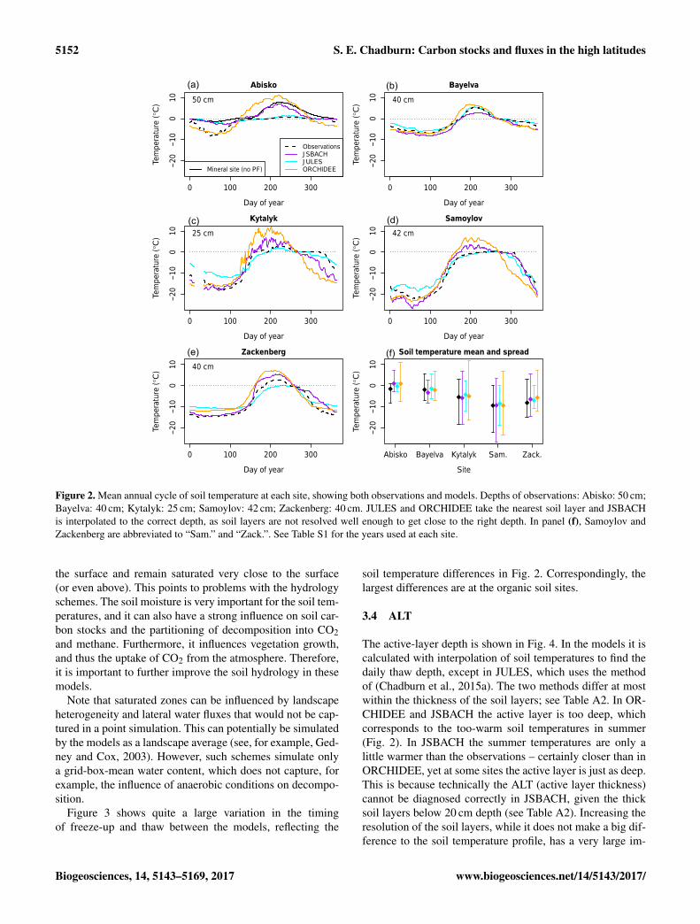
Soil temperature annual cycles at∼ 40 cm depth are shown inFig. 2. In general the models simulate the soil temperature atmineral soil sites quite well: see the Bayelva and Zackenberg

sites in Fig. 2. There are greater errors in the simulation oforganic soils: Abisko, Kytalyk and Samoylov in Fig. 2.

For JSBACH and ORCHIDEE, the annual cycles of tem-perature are too large for the organic sites, indicating thatthese models need to better represent the insulating anddamping properties of organic soils. To illustrate this, addi-tional observations from mineral soil at the nearby researchstation (where there is no permafrost) are shown on theAbisko plot (Fig. 2). This line matches much more closelywith the ORCHIDEE and JSBACH simulations, suggestingthat these models are behaving thermally like a mineral soil.At Abisko, permafrost only occurs in peat plateaus, and thusincluding organic soil properties in the models is essentialfor capturing the difference between permafrost and non-permafrost conditions.

In JULES, however, the annual cycle amplitude is toosmall at the organic sites and also at Zackenberg, mostly dueto biases in the winter soil temperatures. This suggests thatthe snow thermal conductivity or density may be too low inJULES. A similar problem was found with a previous JULESsimulation of Samoylov island, using a similar model set-upand forcing data (Chadburn et al., 2015a). There, the wintersoil temperature was improved by increasing snow density.Indeed, the conductivity of snow in the JULES simulations



Table 3. Mean NEE budget (g C m−2 yr−1), showing that in general this is smaller than the errors in simulated GPP; therefore, the noise islarger than the signal in this data. Positive numbers represent a carbon source.

Site JSBACH JULES ORCHIDEE Observations

Abisko −6.6 −16.0 −79.2 −162.0Bayelva −8.8 −15.1 −34.7 −13.9Kytalyk −19.0 −18.9 −24.3 −108.0Samoylov +1.5 −15.1 −58.9 −49.6Zackenberg +35.9 −5.2 +0.01 −12.0Mean absolute error in GPP 100.2 123.6 88.4 –

2 4 6 8 10 12

0.0

0.4

0.8

Abisko

Month of year

Sno

w d

epth

(m

)

JSBACHJULESORCHIDEEObservations

0 100 200 300

0.0

0.4

0.8

Bayelva

Day of yearS

now

dep

th (

m)

0 100 200 300

0.0

0.4

0.8

Kytalyk

Day of year

Sno

w d

epth

(m

)

0 100 200 300

0.0

0.4

0.8

Samoylov

Day of year

Sno

w d

epth

(m

)

0 100 200 300

0.0

0.4

0.8

Zackenberg

Day of year

Sno

w d

epth

(m

)

0.0

0.4

0.8

Snow depth mean and spread

Site

Sno

w d

epth

(m

)

Abisko Bayelva Kytalyk Sam. Zack.

●

●

●

●

●

●

●

●

●

●

●

●

●

●

●

●

●

●

●

●

(a) (b)

(c) (d)

(e) (f)

Figure 1. Mean annual cycle of snow depth at each site, showing both observations and models. In panel (f), Samoylov and Zackenbergare abbreviated to “Sam.” and “Zack.”. Mean annual cycle is calculated from a single site over a number of years, except for Abisko, wheremeasurements were taken at several different locations in the mire. See Table S1 for the years used at each site.

is between 0.03 and 0.1 Wm−1 K−1 at the sites with shal-low snow (and in the upper layers of the snowpack at siteswith deeper snow), which is considerably lower than typ-ical values for similar tundra sites, which are around 0.2–0.3 Wm−1 K−1, at least for the upper part of the snowpack(Gouttevin et al., 2012b; Domine et al., 2016). See the Sup-plement for further discussion on snow conductivity and den-sity.

3.3 Soil moisture

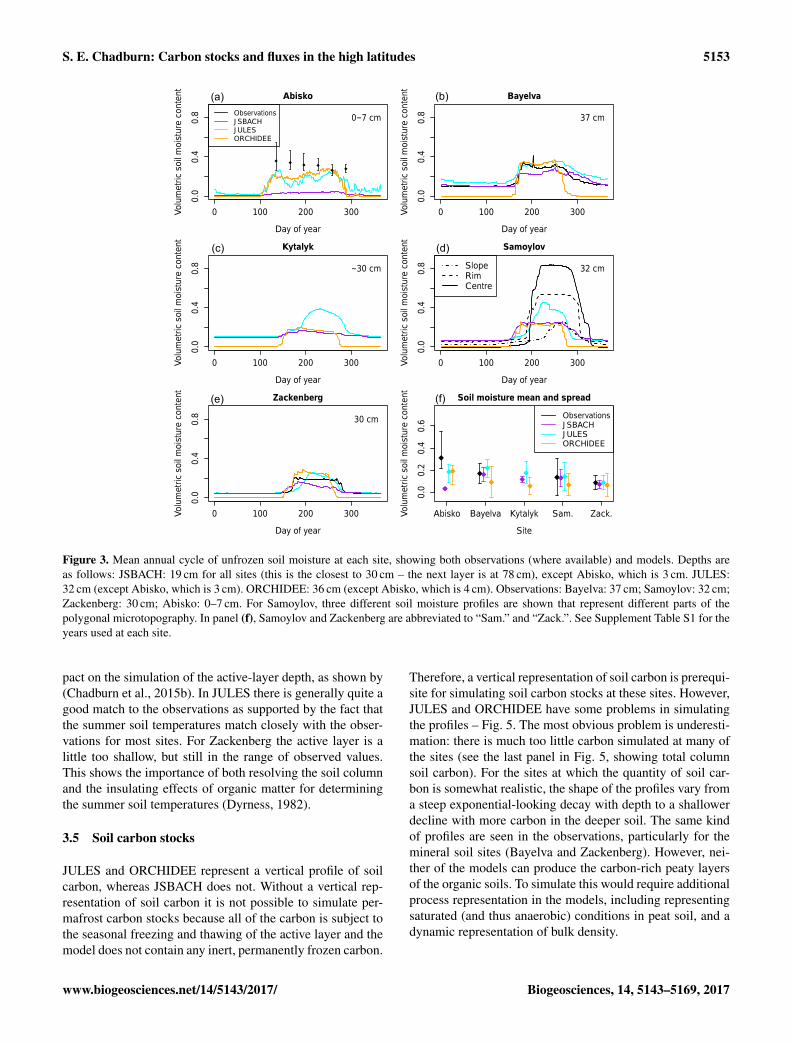
As with temperature, the (unfrozen) soil moisture is simu-lated well at mineral soil sites – see Bayelva and Zackenbergin Fig. 3. In the winter, ORCHIDEE does not represent theunfrozen water fraction in frozen soils, but the other modelssimulate a reasonable water content in winter. However, soilmoisture is in general too low at organic sites - Samoylovand Abisko mire. The soils should be able to hold water near



0 100 200 300

−20

−10

010

Abisko

Day of year

Tem

pera

ture

(°C

) 50 cm

ObservationsJSBACHJULESORCHIDEEMineral site (no PF)

0 100 200 300

−20

−10

010

Bayelva

Day of year

Tem

pera

ture

(°C

) 40 cm

0 100 200 300

−20

−10

010

Kytalyk

Day of year

Tem

pera

ture

(°C

) 25 cm

0 100 200 300

−20

−10

010

Samoylov

Day of year

Tem

pera

ture

(°C

) 42 cm

0 100 200 300

−20

−10

010

Zackenberg

Day of year

Tem

pera

ture

(°C

) 40 cm−2

0−1

00

10

Soil temperature mean and spread

Site

Tem

pera

ture

(°C

)


● ●

●

●●

●●

●

●●

●

●

●

●

●

●

●●

●

●

(a) (b)

(c) (d)

(e) (f)

Figure 2. Mean annual cycle of soil temperature at each site, showing both observations and models. Depths of observations: Abisko: 50 cm;Bayelva: 40 cm; Kytalyk: 25 cm; Samoylov: 42 cm; Zackenberg: 40 cm. JULES and ORCHIDEE take the nearest soil layer and JSBACHis interpolated to the correct depth, as soil layers are not resolved well enough to get close to the right depth. In panel (f), Samoylov andZackenberg are abbreviated to “Sam.” and “Zack.”. See Table S1 for the years used at each site.

the surface and remain saturated very close to the surface(or even above). This points to problems with the hydrologyschemes. The soil moisture is very important for the soil tem-peratures, and it can also have a strong influence on soil car-bon stocks and the partitioning of decomposition into CO2and methane. Furthermore, it influences vegetation growth,and thus the uptake of CO2 from the atmosphere. Therefore,it is important to further improve the soil hydrology in thesemodels.

Note that saturated zones can be influenced by landscapeheterogeneity and lateral water fluxes that would not be cap-tured in a point simulation. This can potentially be simulatedby the models as a landscape average (see, for example, Ged-ney and Cox, 2003). However, such schemes simulate onlya grid-box-mean water content, which does not capture, forexample, the influence of anaerobic conditions on decompo-sition.

Figure 3 shows quite a large variation in the timingof freeze-up and thaw between the models, reflecting the

soil temperature differences in Fig. 2. Correspondingly, thelargest differences are at the organic soil sites.

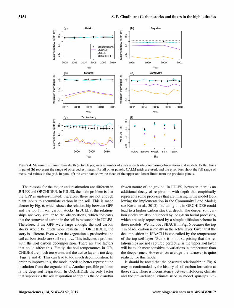
3.4 ALT

The active-layer depth is shown in Fig. 4. In the models it iscalculated with interpolation of soil temperatures to find thedaily thaw depth, except in JULES, which uses the methodof (Chadburn et al., 2015a). The two methods differ at mostwithin the thickness of the soil layers; see Table A2. In OR-CHIDEE and JSBACH the active layer is too deep, whichcorresponds to the too-warm soil temperatures in summer(Fig. 2). In JSBACH the summer temperatures are only alittle warmer than the observations – certainly closer than inORCHIDEE, yet at some sites the active layer is just as deep.This is because technically the ALT (active layer thickness)cannot be diagnosed correctly in JSBACH, given the thicksoil layers below 20 cm depth (see Table A2). Increasing theresolution of the soil layers, while it does not make a big dif-ference to the soil temperature profile, has a very large im-



0 100 200 300

0.0

0.4

0.8

Abisko

Day of year

Volu

met

ric s

oil m

oist

ure

cont

ent

0−7 cmObservationsJSBACHJULESORCHIDEE

0 100 200 300

0.0

0.4

0.8

Bayelva

Day of year

Volu

met

ric s

oil m

oist

ure

cont

ent

37 cm

0 100 200 300

0.0

0.4

0.8

Kytalyk

Day of year

Volu

met

ric s

oil m

oist

ure

cont

ent

~30 cm

0 100 200 300

0.0

0.4

0.8

Samoylov

Day of year

Volu

met

ric s

oil m

oist

ure

cont

ent

32 cmSlopeRimCentre

0 100 200 300

0.0

0.4

0.8

Zackenberg

Day of year

Volu

met

ric s

oil m

oist

ure

cont

ent

30 cm0.

00.

20.

40.

6

Soil moisture mean and spread

Site

Volu

met

ric s

oil m

oist

ure

cont

ent


●

●●

●

●●

●●

●

●

●● ● ●

●

●● ●

●

ObservationsJSBACHJULESORCHIDEE

(a) (b)

(c) (d)

(e) (f)

Figure 3. Mean annual cycle of unfrozen soil moisture at each site, showing both observations (where available) and models. Depths areas follows: JSBACH: 19 cm for all sites (this is the closest to 30 cm – the next layer is at 78 cm), except Abisko, which is 3 cm. JULES:32 cm (except Abisko, which is 3 cm). ORCHIDEE: 36 cm (except Abisko, which is 4 cm). Observations: Bayelva: 37 cm; Samoylov: 32 cm;Zackenberg: 30 cm; Abisko: 0–7 cm. For Samoylov, three different soil moisture profiles are shown that represent different parts of thepolygonal microtopography. In panel (f), Samoylov and Zackenberg are abbreviated to “Sam.” and “Zack.”. See Supplement Table S1 for theyears used at each site.

pact on the simulation of the active-layer depth, as shown by(Chadburn et al., 2015b). In JULES there is generally quite agood match to the observations as supported by the fact thatthe summer soil temperatures match closely with the obser-vations for most sites. For Zackenberg the active layer is alittle too shallow, but still in the range of observed values.This shows the importance of both resolving the soil columnand the insulating effects of organic matter for determiningthe summer soil temperatures (Dyrness, 1982).

3.5 Soil carbon stocks

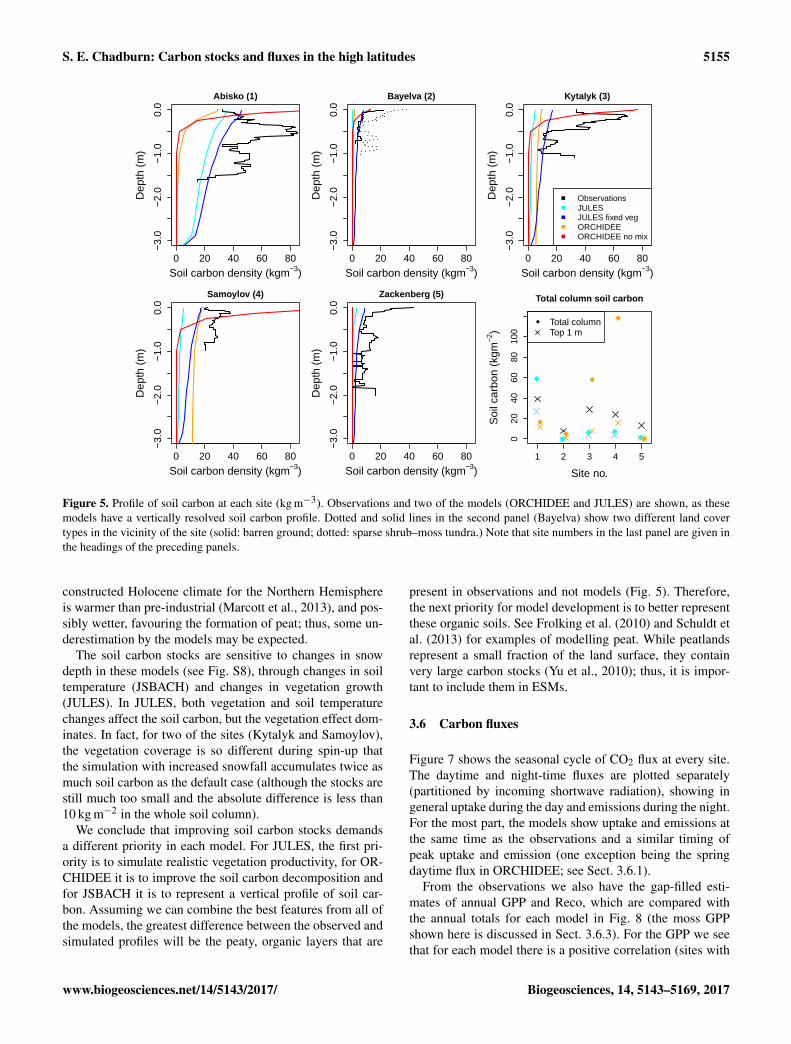
JULES and ORCHIDEE represent a vertical profile of soilcarbon, whereas JSBACH does not. Without a vertical rep-resentation of soil carbon it is not possible to simulate per-mafrost carbon stocks because all of the carbon is subject tothe seasonal freezing and thawing of the active layer and themodel does not contain any inert, permanently frozen carbon.

Therefore, a vertical representation of soil carbon is prerequi-site for simulating soil carbon stocks at these sites. However,JULES and ORCHIDEE have some problems in simulatingthe profiles – Fig. 5. The most obvious problem is underesti-mation: there is much too little carbon simulated at many ofthe sites (see the last panel in Fig. 5, showing total columnsoil carbon). For the sites at which the quantity of soil car-bon is somewhat realistic, the shape of the profiles vary froma steep exponential-looking decay with depth to a shallowerdecline with more carbon in the deeper soil. The same kindof profiles are seen in the observations, particularly for themineral soil sites (Bayelva and Zackenberg). However, nei-ther of the models can produce the carbon-rich peaty layersof the organic soils. To simulate this would require additionalprocess representation in the models, including representingsaturated (and thus anaerobic) conditions in peat soil, and adynamic representation of bulk density.



2005 2006 2007 2008 2009 2010

−2.

5−

1.5

−0.

5

Abisko

Year

Max

imum

thaw

dep

th (

m)

● ● ● ● ● ●


−2.

5−

1.5

−0.

5

Bayelva

Year

Max

imum

thaw

dep

th (

m)

1998 1999 2000 2001

2007 2008 2009 2010 2011

−2.

5−

1.5

−0.

5

Kytalyk

Year

Max

imum

thaw

dep

th (

m)

●●

●● ●

2002 2004 2006 2008 2010

−2.

5−

1.5

−0.

5

Samoylov

Year

Max

imum

thaw

dep

th (

m)

● ● ● ● ● ●●

●

2000 2005 2010

−2.

5−

1.5

−0.

5

Zackenberg

Year

Max

imum

thaw

dep

th (

m)

● ● ● ● ● ●● ● ● ● ● ● ● ● ● ● ●

−3.

0−

2.0

−1.

00.

0

Site

Mea

n A

LT (

m) ●

●

●●

●


(a) (b)

(c) (d)

(e) (f)

Figure 4. Maximum summer thaw depth (active layer) over a number of years at each site, comparing observations and models. Dotted linesin panel (b) represent the range of observed estimates. For all other panels, CALM grids are used, and the error bars show the full range ofmeasured values in the grid. In panel (f) the error bars show the mean of the upper and lower limits from the previous panels.

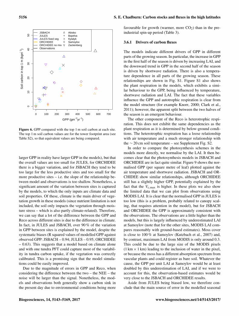
The reasons for the major underestimation are different inJULES and ORCHIDEE. In JULES, the main problem is thatthe GPP is underestimated; therefore, there are not enoughplant inputs to accumulate carbon in the soil. This is madeclearer by Fig. 6, which shows the relationship between GPPand the top 1 m soil carbon stocks. In JULES, the relation-ships are very similar to the observations, which indicatesthat the turnover of carbon in the soil is reasonable in JULES.Therefore, if the GPP were large enough, the soil carbonstocks would be much more realistic. In ORCHIDEE, thestory is different. Even when the vegetation is productive, thesoil carbon stocks are still very low. This indicates a problemwith the soil carbon decomposition. There are two factorsthat could affect this. Firstly, the soil temperatures in OR-CHIDEE are much too warm, and the active layer is too deep(Figs. 2 and 4). This can lead to too much decomposition. Inorder to improve this, the model needs to better represent theinsulation from the organic soils. Another possible problemis the deep soil respiration. In ORCHIDEE the only factorthat suppresses the soil respiration at depth is the cold and/or

frozen nature of the ground. In JULES, however, there is anadditional decay of respiration with depth that empiricallyrepresents some processes that are missing in the model (fol-lowing the implementation in the Community Land Model;see Koven et al., 2013). Including this in ORCHIDEE couldlead to a higher carbon stock at depth. The deeper soil car-bon stocks are also influenced by long-term burial processes,which are only represented by a simple diffusion scheme inthese models. We include JSBACH in Fig. 6 because the top1 m of soil carbon is mostly in the active layer. Given that thedecomposition in JSBACH is controlled by the temperatureof the top soil layer (3 cm), it is not surprising that the re-lationships are not captured perfectly, as the upper soil layerwill be much more sensitive to variations in temperature thanthe deeper ones. However, on average the turnover is quiterealistic for this model.

It should be noted that the observed relationship in Fig. 6may be confounded by the history of soil carbon formation atthese sites. There is inconsistency between Holocene climateand the pre-industrial climate used in model spin-ups. Re-



0 20 40 60 80

−3.

0−

2.0

−1.

00.

0

Abisko (1)

Soil carbon density (kgm−3)

Dep

th (

m)

0 20 40 60 80

−3.

0−

2.0

−1.

00.

0

Bayelva (2)


Dep

th (

m)

0 20 40 60 80

−3.

0−

2.0

−1.

00.

0

Kytalyk (3)


Dep

th (

m)

ObservationsJULESJULES fixed vegORCHIDEEORCHIDEE no mix

0 20 40 60 80

−3.

0−

2.0

−1.

00.

0

Samoylov (4)


Dep

th (

m)

0 20 40 60 80

−3.

0−

2.0

−1.

00.

0

Zackenberg (5)


Dep

th (

m)

1 2 3 4 5

020

4060

8010

0

Total column soil carbon

Site no.

Soi

l car

bon

(kgm

−2)

Total columnTop 1 m

Figure 5. Profile of soil carbon at each site (kg m−3). Observations and two of the models (ORCHIDEE and JULES) are shown, as thesemodels have a vertically resolved soil carbon profile. Dotted and solid lines in the second panel (Bayelva) show two different land covertypes in the vicinity of the site (solid: barren ground; dotted: sparse shrub–moss tundra.) Note that site numbers in the last panel are given inthe headings of the preceding panels.

constructed Holocene climate for the Northern Hemisphereis warmer than pre-industrial (Marcott et al., 2013), and pos-sibly wetter, favouring the formation of peat; thus, some un-derestimation by the models may be expected.

The soil carbon stocks are sensitive to changes in snowdepth in these models (see Fig. S8), through changes in soiltemperature (JSBACH) and changes in vegetation growth(JULES). In JULES, both vegetation and soil temperaturechanges affect the soil carbon, but the vegetation effect dom-inates. In fact, for two of the sites (Kytalyk and Samoylov),the vegetation coverage is so different during spin-up thatthe simulation with increased snowfall accumulates twice asmuch soil carbon as the default case (although the stocks arestill much too small and the absolute difference is less than10 kg m−2 in the whole soil column).

We conclude that improving soil carbon stocks demandsa different priority in each model. For JULES, the first pri-ority is to simulate realistic vegetation productivity, for OR-CHIDEE it is to improve the soil carbon decomposition andfor JSBACH it is to represent a vertical profile of soil car-bon. Assuming we can combine the best features from all ofthe models, the greatest difference between the observed andsimulated profiles will be the peaty, organic layers that are

present in observations and not models (Fig. 5). Therefore,the next priority for model development is to better representthese organic soils. See Frolking et al. (2010) and Schuldt etal. (2013) for examples of modelling peat. While peatlandsrepresent a small fraction of the land surface, they containvery large carbon stocks (Yu et al., 2010); thus, it is impor-tant to include them in ESMs.

3.6 Carbon fluxes

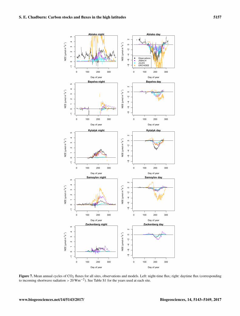
Figure 7 shows the seasonal cycle of CO2 flux at every site.The daytime and night-time fluxes are plotted separately(partitioned by incoming shortwave radiation), showing ingeneral uptake during the day and emissions during the night.For the most part, the models show uptake and emissions atthe same time as the observations and a similar timing ofpeak uptake and emission (one exception being the springdaytime flux in ORCHIDEE; see Sect. 3.6.1).

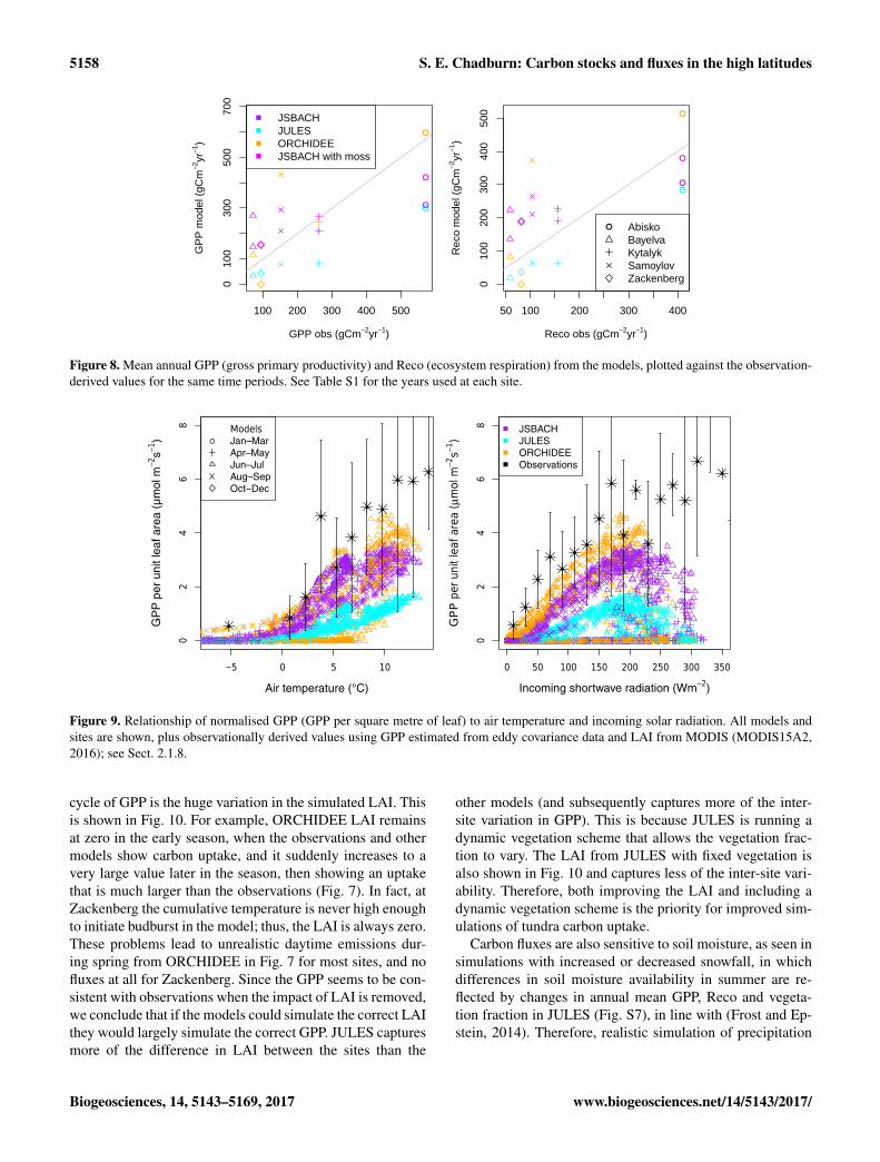
From the observations we also have the gap-filled esti-mates of annual GPP and Reco, which are compared withthe annual totals for each model in Fig. 8 (the moss GPPshown here is discussed in Sect. 3.6.3). For the GPP we seethat for each model there is a positive correlation (sites with



0 100 200 300 400 500 600 700

010

2030

4050

GPP (gm−2yr−1)

−S

oil c

arbo

n in

top

1 m

(kg

m 2 )

JSBACHJULESJULES fixed vegORCHIDEEORCHIDEE no mixObservations

AbiskoBayelvaKytalykSamoylovZackenberg

Figure 6. GPP compared with the top 1 m soil carbon at each site.The top 1 m soil carbon values are for the tower footprint area (seeTable S2), so that equivalent values are being compared.

larger GPP in reality have larger GPP in the models), but thatthe overall values are too small for JULES, for ORCHIDEEthere is a bigger variation, and for JSBACH they tend to betoo large for the less productive sites and too small for themore productive sites – i.e. the slope of the relationship be-tween model and observations is too shallow. Nonetheless, asignificant amount of the variation between sites is capturedby the models, to which the only inputs are climate data andsoil properties. Of these, climate is the main driver of vege-tation growth in these models (since nutrient limitation is notincluded, the soil only impacts the vegetation through mois-ture stress – which is also partly climate-related). Therefore,we can say that a lot of the difference between the GPP andReco across different sites is due to the difference in climate.In fact, in JULES and JSBACH, over 90 % of the variationin GPP between sites is explained by the model, despite thesystematic biases (R squared values of modelled GPP againstobserved GPP: JSBACH – 0.94; JULES – 0.95; ORCHIDEE– 0.63). This suggests that a model based on climate aloneand with one tundra PFT could capture most of the variabil-ity in tundra carbon uptake, if the vegetation was correctlycalibrated. This is a promising sign that the model simula-tions could be easily improved.

Due to the magnitude of errors in GPP and Reco, whenconsidering the difference between the two – the NEE – thenoise will be larger than the signal. Nonetheless, the mod-els and observations both generally show a carbon sink inthe present day due to environmental conditions being more

favourable for growth (warmer, more CO2) than in the pre-industrial spin-up period (Table 3).

3.6.1 Drivers of carbon fluxes

The models indicate different drivers of GPP in differentparts of the growing season. In particular, the increase in GPPin the first half of the season is driven by increasing LAI, andthe downward trend in GPP in the second half of the seasonis driven by shortwave radiation. There is also a tempera-ture dependence in all parts of the growing season. Theserelationships are shown in Fig. S1. Figure S1 also showsthe plant respiration in the models, which exhibits a simi-lar behaviour to the GPP, being influenced by temperature,shortwave radiation and LAI. The fact that these variablesinfluence the GPP and autotrophic respiration is clear fromthe model structure (for example Knorr, 2000; Clark et al.,2011); however, the apparent split between the two halves ofthe season is an emergent behaviour.

The other component of the Reco is heterotrophic respi-ration. This does not exhibit the same dependencies as theplant respiration as it is determined by below-ground condi-tions. The heterotrophic respiration has a loose relationshipwith air temperature and a much stronger relationship withthe ∼ 20 cm soil temperature – see Supplement Fig. S2.

In order to compare the photosynthesis schemes in themodels more directly, we normalise by the LAI. It then be-comes clear that the photosynthesis models in JSBACH andORCHIDEE are in fact quite similar. Figure 9 shows the nor-malised GPP (per square metre of leaf) plotted against theair temperature and shortwave radiation. JSBACH and OR-CHIDEE show similar relationships, although ORCHIDEEstill has a slightly higher GPP, potentially explained by thefact that the Vc,max is higher. In these plots we also showthe limited data that we can plot from observations usingMODIS LAI. It is clear that the normalised GPP in JULES istoo low (this is a problem, probably related to canopy scal-ing, that requires attention in the model), but for JSBACHand ORCHIDEE the GPP is approximately consistent withthe observations. The observations are a little higher than themodels, but this is largely influenced by underestimated LAIat Samoylov (note that for the other sites, MODIS LAI com-pares reasonably with ground-based estimates). Moss coveris close to 100 % at Samoylov (Kutzbach et al., 2007) and,by contrast, maximum LAI from MODIS is only around 0.3.This could be due to the large size of the MODIS pixels(1 km× 1 km) leading to the inclusion of water in the pixel,or because the moss has a different absorption spectrum fromvascular plants and could register as bare soil. Whatever thecause, the GPP per unit LAI at Samoylov would be at leastdoubled by this underestimation of LAI, and if we were toaccount for this, the observation-based estimates would bevery close to the JSBACH and ORCHIDEE results.

Aside from JULES being biased low, we therefore con-clude that the main source of error in the modelled seasonal



0 100 200 300−1

01

23

45

Abisko night

Day of year

NEE

(µm

olm

−2s−1

)

0 100 200 300

−8−6

−4−2

02

Abisko day

Day of year

NEE

(µm

olm

−2s−1

)


0 100 200 300

−10

12

34

5

Bayelva night

Day of year

NEE

(µm

olm

−2s−1

)

0 100 200 300

−8−6

−4−2

02

Bayelva day

Day of yearN

EE (µ

mol

m−2

s−1)

0 100 200 300

−10

12

34

5

Kytalyk night

Day of year

NEE

(µm

olm

−2s−1

)

0 100 200 300

−8−6

−4−2

02

Kytalyk day

Day of year

NEE

(µm

olm

−2s−1

)

0 100 200 300

−10

12

34

5

Samoylov night

Day of year

NEE

(µm

olm

−2s−1

)

0 100 200 300

−8−6

−4−2

02

Samoylov day

Day of year

NEE

(µm

olm

−2s−1

)

0 100 200 300

−10

12

34

5

Zackenberg night

Day of year

NEE

(µm

olm

−2s−1

)

0 100 200 300

−8−6

−4−2

02

Zackenberg day

Day of year

NEE

(µm

olm

−2s−1

)

Figure 7. Mean annual cycles of CO2 fluxes for all sites, observations and models. Left: night-time flux; right: daytime flux (correspondingto incoming shortwave radiation > 20 Wm−2). See Table S1 for the years used at each site.



●

100 200 300 400 500

010

030

050

070

0

GPP obs (gCm−2yr−1)

GP

P m

odel

(gC

m−2

yr−1

)●

●

●

JSBACHJULESORCHIDEEJSBACH with moss

●

50 100 200 300 400

010

020

030

040

050

0

Reco obs (gCm−2yr−1)

Rec

o m

odel

(gC

m−2

yr−1

)

●

●

●

● AbiskoBayelvaKytalykSamoylovZackenberg

Figure 8. Mean annual GPP (gross primary productivity) and Reco (ecosystem respiration) from the models, plotted against the observation-derived values for the same time periods. See Table S1 for the years used at each site.

−5 0 5 10

02

46

8

Air temperature (°C)

GP

P p

er u

nit l

eaf a

rea

(µm

ol m

s)

−2−1

●●● ●●●● ● ●●●●●●●●●●●● ●●●●● ●●●● ●●●●● ● ● ● ●●●● ●●●●●●● ● ●●●●●●● ●● ● ● ●●● ●●●●● ●●●●●●●●● ● ●●● ●●●● ● ●●●● ●●●● ● ●●●●●●●●●●●● ●●●●● ●●●● ●●●●● ● ● ● ●●●● ●●●●●●● ● ●●●●●●● ●● ● ● ●●● ●●●●● ●●●●●●●●● ● ●●● ●●●● ● ●●●● ●●●● ● ●●●●●●●●●●●● ●●●●● ●●●● ●●●●● ● ● ● ●●●● ●●●●●●● ● ●●●●●●● ●● ● ● ●●● ●●●●● ●●●●●●●●● ● ●●● ●●●● ● ●● ●●●●●● ●●●●●● ●● ●●●● ●●●●●● ●● ●●●●●● ●● ●●● ● ●●●●●●●●●● ●●●●●● ●●●● ●●●●● ● ● ●●●●●●● ●●●●●●●● ● ●●●●● ● ●●●●●● ●●●●●● ●● ●●●● ●●●●●● ●● ●●●●●● ●● ●●● ● ●●●●●●●●●● ●●●●●● ●●●● ●●●●● ● ● ●●●●●●● ●●●●●●●● ● ●●●●● ● ●●●●●● ●●●●●● ●● ●●●● ●●●●●● ●● ●●●●●● ●● ●●● ● ●●●●●●●●●● ●●●●●● ●●●● ●●●●● ● ● ●●●●●●● ●●●●●●●● ● ●●●●●

●

●

●

●

●

●

● ●

● ●

●

●

●●

ModelsJan–MarApr–MayJun–JulAug–SepOct−Dec

0 50 100 150 200 250 300 350

02

46

8

Incoming shortwave radiation (Wm )−2

GP

P p

er u

nit l

eaf a

rea

(µm

ol m

−2s−1

)

●●●●●●●●●●●●●●●●●●●●●●●●●●●●●●●●●●●●●●●●●●●●●●●●●●●●●●● ●●●●● ●● ●● ●●●●●●●●●● ●●● ●●●● ●●●●● ●●●●●●●●●●●●●●●●●●●●●●●●●●●●●●●●●●●●●●●●●●●●●●●●●●●●●●●●●●● ●●●●● ●● ●● ●●●●●●●●●● ●●● ●●●● ●●●●● ●●●●●●●●●●●●●●●●●●●●●●●●●●●●●●●●●●●●●●●●●●●●●●●●●●●●●●●●●●● ●●●●● ●● ●● ●●●●●●●●●● ●●● ●●●● ●●●●● ●●●●●●●●●●●●●●●●●●●●●●●●●●●●●●●●●●●●●●●●●●●●●●●●●●●●●●●●●●●●●●●●●●●●●●●●●●●●●●●●●●●●●●●●●●●●●●●●●●●●●●●●●●●●●●●●●●●●●●●●●●●●●●●●●●●●●●●●●●●●●●●●●●●●●●●●●●●●●●●●●●●●●●●●●●●●●●●●●●●●●●●●●●●●●●●●●●●●●●●●●●●●●●●●●●●●●●●●●●●●●●●●●●●●●●●●●●●●●●●●●●●●●●●●●●●●●●●●●●●●●●●●●●●●●●●●●●●●●●●●●●●●●●●●●●●●●●●●●●●●●●●●●●●●●●●●●●●●●●●●●●●●●●●●●●●●●●●●●●●●●●●●●●●●●●●●●●●●●● ● ● ● ●●●●●●●●●●●●●●●●●●●●●●●●●●●●●●●●●●●●●●●●●●●●●●●●●●●●●●●●●●●●●●●●●●●●●●●●●●●●●●●●●●●●●●● ● ● ● ●●●●●●●●●●●●●●●●●●●●●●●●●●●●●●●●●●●●●●●●●●●●●●●●●●●●●●●●●●●●●●●●●●●●●●●●●●●●●●●●●●●●●●● ● ● ● ●●●●●●●●●●●●●●●●●●●●●●●●●●●●●●●●●●●●●●●●●●●●●●●●●●●●●●●●●●●●●●●●●●●●●●●●●●●● ●●● ●●●●● ●●●●●●●●●●●●●●●●●●●●●●●●●●●●●●●●●●●●●●●●●●●●●●●●●●●●●●●●●●●●●●●●●●●●●●●●●●●●●●●●●● ●●● ●●●●● ●●●●●●●●●●●●●●●●●●●●●●●●●●●●●●●●●●●●●●●●●●●●●●●●●●●●●●●●●●●●●●●●●●●●●●●●●●●●●●●●●● ●●● ●●●●● ●●●●●●●●●●●●●●●●●●●●●●●●●●●●●●●●●●●●●●●●●●●●●●●●●●●●●●●●●●●●●●●●●●●●●●●●●●●●●●●●●●●●●●●● ●●● ●●● ●●●●●●●●●●●●●●●●●●●●●●●●●●●●●●●●●●●●●●●●●●●●●●●●●●●●●●●●●●●●●●●●●●●●●●●●●●●●●●●●●●●● ●●● ●●● ●●●●●●●●●●●●●●●●●●●●●●●●●●●●●●●●●●●●●●●●●●●●●●●●●●●●●●●●●●●●●●●●●●●●●●●●●●●●●●●●●●●● ●●● ●●● ●●●●●

●

●

●

●

●

●

●

●

●

●

●

●

●

●

●

●

●

●

●

JSBACHJULESORCHIDEEObservations

Figure 9. Relationship of normalised GPP (GPP per square metre of leaf) to air temperature and incoming solar radiation. All models andsites are shown, plus observationally derived values using GPP estimated from eddy covariance data and LAI from MODIS (MODIS15A2,2016); see Sect. 2.1.8.

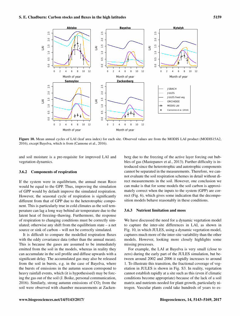
cycle of GPP is the huge variation in the simulated LAI. Thisis shown in Fig. 10. For example, ORCHIDEE LAI remainsat zero in the early season, when the observations and othermodels show carbon uptake, and it suddenly increases to avery large value later in the season, then showing an uptakethat is much larger than the observations (Fig. 7). In fact, atZackenberg the cumulative temperature is never high enoughto initiate budburst in the model; thus, the LAI is always zero.These problems lead to unrealistic daytime emissions dur-ing spring from ORCHIDEE in Fig. 7 for most sites, and nofluxes at all for Zackenberg. Since the GPP seems to be con-sistent with observations when the impact of LAI is removed,we conclude that if the models could simulate the correct LAIthey would largely simulate the correct GPP. JULES capturesmore of the difference in LAI between the sites than the

other models (and subsequently captures more of the inter-site variation in GPP). This is because JULES is running adynamic vegetation scheme that allows the vegetation frac-tion to vary. The LAI from JULES with fixed vegetation isalso shown in Fig. 10 and captures less of the inter-site vari-ability. Therefore, both improving the LAI and including adynamic vegetation scheme is the priority for improved sim-ulations of tundra carbon uptake.

Carbon fluxes are also sensitive to soil moisture, as seen insimulations with increased or decreased snowfall, in whichdifferences in soil moisture availability in summer are re-flected by changes in annual mean GPP, Reco and vegeta-tion fraction in JULES (Fig. S7), in line with (Frost and Ep-stein, 2014). Therefore, realistic simulation of precipitation



0 2 4 6 8 10 12

0.0

0.5

1.0

1.5

2.0

2.5

Abisko

Month of year

LAI

0 2 4 6 8 10 12

0.0

0.5

1.0

1.5

2.0

2.5

Bayelva

Month of year

LAI

●

0 2 4 6 8 10 12

0.0

0.5

1.0

1.5

2.0

2.5

Kytalyk

Month of year

LAI

0 2 4 6 8 10 12

0.0

0.5

1.0

1.5

2.0

2.5

Samoylov

Month of year

LAI

0 2 4 6 8 10 12

0.0

0.5

1.0

1.5

2.0

2.5

Zackenberg

Month of year

LAI

●

JSBACH

JULES

JULES fixed veg

ORCHIDEE

MODIS LAI

Cannonne et al. (2016)

Figure 10. Mean annual cycles of LAI (leaf area index) for each site. Observed values are from the MODIS LAI product (MODIS15A2,2016), except Bayelva, which is from (Cannone et al., 2016).

and soil moisture is a pre-requisite for improved LAI andvegetation dynamics.

3.6.2 Components of respiration

If the system were in equilibrium, the annual mean Recowould be equal to the GPP. Thus, improving the simulationof GPP would by default improve the simulated respiration.However, the seasonal cycle of respiration is significantlydifferent from that of GPP due to the heterotrophic compo-nent. This is particularly true in cold climates as the soil tem-perature can lag a long way behind air temperature due to thelatent heat of freezing–thawing. Furthermore, the responseof respiration to changing conditions must be correctly sim-ulated; otherwise any shift from the equilibrium state – a netsource or sink of carbon – will not be correctly simulated.

It is difficult to compare the modelled respiration fluxeswith the eddy covariance data (other than the annual mean).This is because the gases are assumed to be immediatelyemitted from the soil in the models, whereas in reality theycan accumulate in the soil profile and diffuse upwards with asignificant delay. The accumulated gas may also be releasedfrom the soil in bursts, e.g. in the case of Bayelva, wherethe bursts of emissions in the autumn season correspond toheavy rainfall events, which (it is hypothesised) may be forc-ing the gas out of the soil (J. Boike, personal communication,2016). Similarly, strong autumn emissions of CO2 from thesoil were observed with chamber measurements at Zacken-

berg due to the freezing of the active layer forcing out bub-bles of gas (Mastepanov et al., 2013). Further difficulty is in-troduced since the heterotrophic and autotrophic componentscannot be separated in the measurements. Therefore, we can-not evaluate the soil respiration schemes in detail without di-rect measurements in the soil. However, one conclusion wecan make is that for some models the soil carbon is approxi-mately correct when the inputs to the system (GPP) are cor-rect (Fig. 6), which gives some indication that the decompo-sition models behave reasonably in these conditions.

3.6.3 Nutrient limitation and moss

We have discussed the need for a dynamic vegetation modelto capture the inter-site differences in LAI, as shown inFig. 10, in which JULES, using a dynamic vegetation model,captures much more of the inter-site variability than the othermodels. However, looking more closely highlights somemissing processes.

For example, the LAI at Bayelva is very small (close tozero) during the early part of the JULES simulation, but be-tween around 2002 and 2006 it rapidly increases to around1. To illustrate this transition, the fractional coverage of veg-etation in JULES is shown in Fig. S3. In reality, vegetationcannot establish rapidly at a site such as this (even if climaticconditions become appropriate) because of the lack of a soilmatrix and nutrients needed for plant growth, particularly ni-trogen. Vascular plants could take hundreds of years to es-



tablish once climatic conditions become appropriate due tothe large timescales involved in soil development. The veg-etation at Bayelva is largely mosses and lichens, which cangrow in nutrient-poor conditions but photosynthesise moreslowly than vascular plants (Yuan et al., 2014). Therefore, tosimulate the CO2 flux at a very nutrient-limited site, it is nec-essary to have a different PFT that represents the low-nutrientbut low-GPP vegetation such as moss and to include nutrientlimitation for the other PFTs.

A similar problem can be seen at Samoylov, where around90 % of the site is covered by moss (Boike et al., 2013), andJULES simulates an LAI similar to that of Kytalyk (as theclimatic conditions are similar), but in reality the LAIs of thetwo sites are very different; at Samoylov the LAI (of vascu-lar plants) and CO2 flux should be much smaller than thatof Kytalyk. At Samoylov, the moss contributes around 40 %to the total photosynthesis (Kutzbach et al., 2007), showingits importance in the carbon budget of this site. It is hypoth-esised that there are fewer vascular plants at Samoylov be-cause the more waterlogged conditions (due to many poly-gon centre ponds) could reduce vegetation growth. In fact,reduced vegetation growth is also seen in areas with manypolygon centre ponds at Kytalyk. Moreover, nitrogen may belost in these waterlogged environments due to denitrification(Palmer et al., 2012), making it a more nutrient-limited envi-ronment.

Thus, to really capture the inter-site differences in GPP,it is necessary to include nutrient limitation and other soil–plant interactions in the model. And once nutrient limitationis introduced, then moss is required (which grows in nutrient-deficient and very wet conditions in which the vascular plantswill not grow) in order to recreate the observed carbon up-take.

In JSBACH, moss carbon fluxes can be included – seeFig. 8. This shows that the moss model can contribute signif-icantly to the carbon budget at the mossy sites. However, atthe sites with less vascular vegetation in reality (Bayelva andSamoylov), including the moss makes the total fluxes muchtoo large, as JSBACH (like JULES) simulates too much vas-cular vegetation.

At Samoylov there is an early-season peak of carbon up-take that is missed in the models (Fig. 7). It is possiblethat this could correspond to the wet ground directly fol-lowing snowmelt, which leads the moss to start photosynthe-sising. However, it is difficult to make conclusions from thedata available, and we also know that eddy covariance meth-ods can have some problems around the time of snowmelt(for example Pirk et al., 2017). Nonetheless, we can get aclue from the moss model in JSBACH. Figure S4 showsthe annual cycle of moss GPP along with the GPP fromJSBACH (without moss), demonstrating that it captures anearly-season peak before the vascular plant uptake starts inJSBACH. This plot also shows the moisture content of themoss layer, making it clear that there is a strong relationshipbetween moisture content and moss photosynthesis. Thus, it

becomes even more important to simulate soil moisture cor-rectly once moss is included in the models.

It could also be important to consider lichens separatelyfrom mosses, as their physical and biological properties canbe very different. For example, the high albedo of lichens canimpact the Earth’s radiation budget (Bernier et al., 2011).

4 Conclusions

Based on the analysis above, we can identify priority devel-opments that would improve the carbon stocks and fluxes inthe models. Assuming that “state-of-the-art” is representedby a combination of the best parts of each model, we pro-vide the following priorities for the next steps to advance thestate-of-the-art models:

1. Improve vegetation phenology and dynamics to simu-late realistic LAI (including nutrient limitation and dy-namic vegetation).

2. Include moss for both photosynthesis and peat accumu-lation.

3. Improve the soil carbon profile for organic soils (includ-ing peat processes).

There is also a need to address remaining issues in themodel physics, particularly for soil moisture and snow. Thereare feedbacks between the vegetation and the soil physicalstate (e.g. Sturm et al., 2001); thus, incorporating more real-istic vegetation such as Arctic shrubs could also lead to animproved simulation of soil temperature and moisture.

Tundra vegetation should ideally be represented using sev-eral different PFTs, for example grasses and shrubs differ incarbon storage and their interactions with snow. Note thatJULES includes a shrub PFT, but these are large shrubs(∼ 1.5 m tall), which would not be expected to grow at thecold sites. Smaller, cold-tolerant shrubs should be added asa separate PFT. There are few modelling studies to datein which tundra phenology is explicitly considered, but seeVan Wijk et al. (2003) for one example.

In JSBACH the moss photosynthesis is already simulated,and the coupling to the soil carbon will be available in thenext version. This provides clear guidance for other mod-els to follow; see Porada et al. (2013, 2016). However, sinceJSBACH does not include nutrient limitation, the combinedGPP and Reco from vascular vegetation and moss is too high(Fig. 8). Including nutrient limitation is an essential part ofthese priority developments.

In order to facilitate improvements to the vegetationschemes, better site-level measurements of LAI are required.This was identified as one of the largest modelling uncer-tainties, but only indirect satellite-derived LAI products areavailable, which are not sufficiently detailed or accurate fordeveloping the model schemes. Furthermore, in order to im-prove the simulation of soil carbon profiles, better observa-



tions and understanding of all below-ground processes suchas in situ decomposition rates and the dynamics of cryotur-bation mixing are required (Beer, 2016).

Future changes in NEE are key to understanding the roleof the Arctic in a global context. We can see in Table 3 thatthe size of the NEE is much smaller than the errors we arecurrently seeing in, for example, the simulated GPP. Thissupports the need for the model improvements highlightedabove.

Future changes in the carbon balance will come both fromchanges in vegetation productivity and type, and decompo-sition of old soil carbon due to thawing permafrost. There-fore, dynamic vegetation (including nutrient limitation) is re-quired for future simulations as well as for simulating thecorrect LAI in the present day. The vertical representationof soil carbon is therefore also particularly important forthe fluxes in the future. However, soil carbon release willalso be triggered by landscape dynamics like ground col-lapse and thermokarst formation, which are not yet repre-sented in any of these models. See (Schneider von Deimlinget al., 2015) for a modelling study in which some of these im-pacts are included. This is another important aspect that mustbe taken into account in future model development (Rowlandand Coon, 2015).

The feedbacks between the Arctic and the global climateare strongly dependent on whether carbon is released into theatmosphere from heterotrophic respiration as carbon dioxideor methane. The modelling capability at the time of this studywas not sufficient to simulate the methane flux. However,this development is in progress (see, e.g. Kaiser et al., 2017),and represents an important topic for future work. Lakes andponds also play a major role in methane and carbon diox-ide exchange with the atmosphere (Bouchard et al., 2015;Langer et al., 2015) and should also be considered in futureland surface models.

Accurate process representation at a site level will not nec-essarily transfer the same level of accuracy to a global simu-lation. In particular, there are issues with using a single grid-box-mean value to represent a large area of land (heterogene-ity in soil and microtopography exerts non-linear controlson carbon and vegetation dynamics) and with obtaining re-alistic large-scale observations for quantities such as soil pa-rameters. Conversely, the sites used in this study representtypical tundra sites, and the model development prioritiesthat we identify are consistent across sites, indicating thatthese would also lead to improved tundra carbon dynamicsin global simulations. This study has allowed us to quantifydeficiencies in the models that we could not have robustlyidentified using global datasets due to the quantity and qual-ity of observational data available. This work also opens upopportunities for further process studies in the future.

Data availability. The land surface model JSBACH used in thisstudy is intellectual property of the Max Planck Society for the

Advancement of Science, Germany. The JSBACH source codeis distributed under the Software License Agreement of the MaxPlanck Institute for Meteorology and it can be accessed on per-sonal request. The steps to gain access are explained underthe following link: http://www.mpimet.mpg.de/en/science/models/license/. The model version JULES vn4.3_permafrost was used inthis study. This version is described in Burke et al. (2017) and avail-able via the Met Office Science Repository Service (on request foraccess) at https://code.metoffice.gov.uk/trac/jules/browser/main/branches/dev/eleanorburke/vn4.3_permafrost. The ORCHIDEE-MICT high latitude model version used in the study is de-scribed in Guimberteau et al. (2017). The SVN version ofthe code branch is https://forge.ipsl.jussieu.fr/orchidee/browser/branches/ORCHIDEE-MICT. Please contact the corresponding au-thor for the code of the ORCHIDEE-MICT if you plan an ap-plication of the model and envisage longer-term scientific col-laboration. Carbon dioxide flux data and meteorological data forall sites are available from the European Fluxes Database Clusterhttp://www.europe-fluxdata.eu under site codes: SE-St1 (Abisko),NO-Blv (Bayelva), RU-Cok (Kytalyk), RU-Sam (Samoylov) andDK-ZaH (Zackenberg). Samoylov and Abisko are “closed” sitesmeaning that the site principal investigator (PI) must approve anydownload of the data. Site PI’s should be invited to join any studyusing this data – see the website for detailed policies. CALM datafor active layers can be accessed via the following database: https://www2.gwu.edu/~calm/. Soil carbon profiles are being processedfor inclusion into the next generation of the International Soil Car-bon Network database (https://doi.org/10.17040/ISCN/1305039),and until then they are available upon request. Other data (includ-ing snow depth, soil temperature) for Samoylov and Bayelva sitesare described in Boike et al. (2013) and Boike et al. (2017) (re-spectively) and available via permanent repositories detailed within.All other data from Kytalyk is available on request. All other datafrom Zackenberg is available via the Greenland Ecosystem Mon-itoring Programme (http://data.g-e-m.dk). Abisko meteorologicaldata and snow depth data are available on request from the AbiskoScientific Research Station (https://polar.se/en/research-in-abisko),and the soil temperature data is archived in the GTN-P database(https://gtnp.arcticportal.org/).


http://www.mpimet.mpg.de/en/science/models/license/

http://www.mpimet.mpg.de/en/science/models/license/

https://code.metoffice.gov.uk/trac/jules/browser/main/branches/dev/eleanorburke/vn4.3_permafrost

https://code.metoffice.gov.uk/trac/jules/browser/main/branches/dev/eleanorburke/vn4.3_permafrost

https://forge.ipsl.jussieu.fr/orchidee/browser/branches/ORCHIDEE-MICT

https://forge.ipsl.jussieu.fr/orchidee/browser/branches/ORCHIDEE-MICT

http://www.europe-fluxdata.eu

https://www2.gwu.edu/~calm/

https://www2.gwu.edu/~calm/

https://doi.org/10.17040/ISCN/1305039

http://data.g-e-m.dk

https://polar.se/en/research-in-abisko

https://gtnp.arcticportal.org/


Appendix A: Details of model set-up

Mineral soil properties were calculated from sand–silt–clayfractions. Slightly different pedotransfer functions are usedin each model, but they are all taken from the same baselinesoil texture (see Table A1). For JULES, the organic soil frac-tion as a function of depth was estimated using the bulk den-sity and carbon density. The combined organic and mineralsoil properties were then calculated as in (Chadburn et al.,2015a).

The assumed “fresh” snow density for creating snowfalltime series from snow depth depends on the resolution ofthe data. If we have low-resolution snow depth data, theremay be some compaction between the snow landing and themeasurement being taken; thus, we will use a higher den-sity to generate the time series. The density used for mostsites, hourly to daily resolution, is 180 kg m−3. At Abisko,only 5-daily snow depth data were available, and this wasat the research station rather than the mire. Since this is arelatively warm site leading to more melting, and due to thelong time interval between readings, in order to give enoughsnow in the models, a density of 240 kg m−3 was used. Forthe Abisko mire there were just a handful of snow depthmeasurements each year. All available values taken duringa given month were averaged to give a monthly average timeseries of snow depth. We compared the depth with the modeloutput from JULES using the forcing data prepared from theresearch station. The snowfall was then scaled according tothe ratio of monthly snow depth in the model vs. the obser-vations. This approach introduces uncertainties that would bereduced by the availability of a higher-resolution snow depthdataset from Stordalen mire.



Table A1. Parameters for the sites. 1 (Klaminder et al., 2008). 2 J. Boike, personal communication, 2015. 3 (Van Huissteden et al., 2005).4 (van der Molen et al., 2007). 5 (Boike et al., 2013). 6 (Hollesen et al., 2011). 7 (Rydén et al., 1980). 8 (Roth and Boike, 2001). 9 S. Zubrzycki,soil carbon data. 10 PAGE21 catalogue of physical parameters. 11 (Bartholomeus et al., 2012). 12 (Elberling et al., 2008). In most cases soiltypes (see Sect. 2.3) were translated to approximate sand–silt–clay fractions using Table 1 in (Beringer et al., 2001). Topographic index isfrom a global dataset: a 0.5◦ aggregate from US Geological Survey (2000).

Abisko Bayelva Kytalyk Samoylov Zackenberg

Organic layer thickness (cm) ∼ 50 1 0 2∼ 20 3,4

∼ 30 5 5 6

Sand fraction 0.1 0.17 0.17 0.58 0.8 6

Silt fraction 0.9 0.7 0.7 0.32 0.1 6

Clay fraction 0.0 0.13 0.13 0.1 0.1 6

Bulk density 1.3 7 1.7 8 0.6 4 0.8 9 0.9–1.8 10

C below organic layer (kg m−3) 14∗ 0∗ 17 11 ∗ 35 9 10 12

Topographic index mean 4.0 3.9 6.2 5.9 6.7Topographic index st.dev. 2.5 1.6 2.8 2.2 1.2

∗ Estimated from bulk density.

Table A2. Soil layer thicknesses in the models.

Model Layer thicknesses (m)

JSBACH 0.06, 0.26, 0.92, 2.88, 5.72, 13.2, 30.1JULES 0.05, 0.08, 0.11, 0.14, 0.17, 0.19, 0.22, 0.24, 0.26, 0.28, 0.30, 0.32, 0.34, 0.36, 0.38, 0.40,

0.42, 0.44, 0.46, 0.47, 0.49, 0.51, 0.53, 0.54, 0.56, 0.58, 0.59, 0.61ORCHIDEE 0.0005, 0.002, 0.01, 0.01, 0.03, 0.06, 0.12, 0.25, 0.50, 1.00, 1.75hydrologicalORCHIDEE 0.0005, 0.002, 0.01, 0.01, 0.03, 0.06, 0.12, 0.25, 0.50, 1.00, 1.75, 2.50, 3.50, 4.55, 5.66,thermal 6.81, 8.03, 9.31, 10.65, 12.06, 13.54, 15.09, 16.72, 18.43, 20.23, 22.12, 24.10, 26.18,

28.37, 30.66, 33.07, 35.60



The Supplement related to this article is available onlineat https://doi.org/10.5194/bg-14-5143-2017-supplement.

Competing interests. The authors declare that they have no conflictof interest.

Special issue statement. This article is part of the special issue“Changing Permafrost in the Arctic and its Global Effects in the21st Century (PAGE21) (BG/ESSD/GMD/TC inter-journal SI)”. Itis not associated with a conference.

Acknowledgements. The authors acknowledge financial support bythe European Union Seventh Framework Programme (FP7/2007–2013) project PAGE21, under GA282700. Sarah E. Chadburn,Sebastian Westermann and Gustaf Hugelius acknowledge supportfrom COUP (Constraining uncertainties in permafrost–climatefeedback) Joint Programming Initiative project (Sarah E. Chadburn:National Environment Research Council grant NE/M01990X/1;Gustaf Hugelius: Swedish Research Council grant no. E0689701;Sebastian Westermann: Research Council of Norway projectno. 244903/E10). Data from Zackenberg were provided by theGreenland Ecosystem Monitoring Programme.

Edited by: Isabelle LaurionReviewed by: Florent Dominé and one anonymous referee

References

Abermann, J., Hansen, B., Lund, M., Wacker, S., Karami, M., andCappelen, J.: Hotspots and key periods of Greenland climatechange during the past six decades, Ambio, 46, 3–11, 2017.

Åkerman, H. J. and Johansson, M.: Thawing permafrost and thickeractive layers in sub-arctic Sweden, Permafrost Periglac, 19, 279–292, 2008.

Atkin, O. K.: Reassessing the nitrogen relations of Arcticplants: a mini-review, Plant Cell Environ., 19, 695–704,https://doi.org/10.1111/j.1365-3040.1996.tb00404.x, 1996.

Barr, A., Richardson, A., Hollinger, D., Papale, D., Arain, M.,Black, T., Bohrer, G., Dragoni, D., Fischer, M., Gu, L., Law, B.E., Margolis, H. A., McCaughey, J. H., Munger, J. W., Oechel,W., and Schaeffer, K.: Use of change-point detection for friction–velocity threshold evaluation in eddy-covariance studies, Agr.Forest Meteorol., 171, 31–45, 2013.

Bartholomeus, H., Schaepman-Strub, G., Blok, D., Sofronov,R., and Udaltsov, S.: Spectral estimation of soil prop-erties in Siberian tundra soils and relations with plantspecies composition, Appl. Environ. Soil Sci., 2012, 241535,https://doi.org/10.1155/2012/241535, 2012.

Beer, C.: Permafrost sub-grid heterogeneity of soil properties keyfor 3-D soil processes and future climate projections, Front. EarthSci., 4, 81, https://doi.org/10.3389/feart.2016.00081, 2016.

Beringer, J., Lynch, A. H., Chapin, F. S., Mack, M., andBonan, G. B.: The Representation of Arctic Soils in

the Land Surface Model: The Importance of Mosses,J. Clim., 14, 3324–3335, https://doi.org/10.1175/1520-0442(2001)014<3324:TROASI>2.0.CO;2, 2001.

Bernier, P., Desjardins, R., Karimi-Zindashty, Y., Worth, D.,Beaudoin, A., Luo, Y., and Wang, S.: Boreal lichen wood-lands: A possible negative feedback to climate change ineastern North America, Agr. Forest Meteorol., 151, 521–528,https://doi.org/10.1016/j.agrformet.2010.12.013, 2011.

Best, M. J., Pryor, M., Clark, D. B., Rooney, G. G., Essery, R. L. H.,Ménard, C. B., Edwards, J. M., Hendry, M. A., Porson, A., Ged-ney, N., Mercado, L. M., Sitch, S., Blyth, E., Boucher, O., Cox,P. M., Grimmond, C. S. B., and Harding, R. J.: The Joint UKLand Environment Simulator (JULES), model description Part1: Energy and water fluxes, Geosci. Model Dev., 4, 677–699,https://doi.org/10.5194/gmd-4-677-2011, 2011.

Boike, J., Roth, K., and Ippisch, O.: Seasonal snow cover on frozenground: Energy balance calculations of a permafrost site nearNy-Ålesund, Spitsbergen, J. Geophys. Res.-Atmos., 108, 8163,https://doi.org/10.1029/2001JD000939, 2003.

Boike, J., Ippisch, O., Overduin, P. P., Hagedorn, B., and Roth, K.:Water, heat and solute dynamics of a mud boil, Spitsbergen, Ge-omorphology, 95, 61–73, 2008a.

Boike, J., Wille, C., and Abnizova, A.: Climatology and sum-mer energy and water balance of polygonal tundra in the LenaRiver Delta, Siberia, J. Geophys. Res.-Biogeo., 113, G03025,https://doi.org/10.1029/2007JG000540, 2008b.

Boike, J., Kattenstroth, B., Abramova, K., Bornemann, N.,Chetverova, A., Fedorova, I., Fröb, K., Grigoriev, M., Grüber,M., Kutzbach, L., Langer, M., Minke, M., Muster, S., Piel, K.,Pfeiffer, E.-M., Stoof, G., Westermann, S., Wischnewski, K.,Wille, C., and Hubberten, H.-W.: Baseline characteristics of cli-mate, permafrost and land cover from a new permafrost obser-vatory in the Lena River Delta, Siberia (1998–2011), Biogeo-sciences, 10, 2105–2128, https://doi.org/10.5194/bg-10-2105-2013, 2013.

Bouchard, F., Laurion, I., Preskienis, V., Fortier, D., Xu, X., andWhiticar, M. J.: Modern to millennium-old greenhouse gasesemitted from ponds and lakes of the Eastern Canadian Arc-tic (Bylot Island, Nunavut), Biogeosciences, 12, 7279–7298,https://doi.org/10.5194/bg-12-7279-2015, 2015.

Brovkin, V., Raddatz, T., Reick, C. H., Claussen, M., andGayler, V.: Global biogeophysical interactions betweenforest and climate, Geophys. Res. Lett., 36, L07405,https://doi.org/10.1029/2009GL037543, 2009.

Brown, J., Ferrians Jr., O. J., Heginbottom, J., and Melnikov, E.:Circum-arctic map of permafrost and ground ice conditions, Na-tional Snow and Ice Data Center, http://nsidc.org/data/docs/fgdc/ggd318_map_circumarctic (last access: 23 October 2017), 1998.

Burke, E. J., Hartley, I. P., and Jones, C. D.: Uncertaintiesin the global temperature change caused by carbon releasefrom permafrost thawing, The Cryosphere, 6, 1063–1076,https://doi.org/10.5194/tc-6-1063-2012, 2012.

Burke, E. J., Jones, C. D., and Koven, C. D.: Estimating thepermafrost-carbon climate response in the CMIP5 climate mod-els using a simplified approach, J. Clim., 26, 4897–4909, 2013.

Burke, E. J., Chadburn, S. E., and Ekici, A.: A vertical repre-sentation of soil carbon in the JULES land surface scheme(vn4.3_permafrost) with a focus on permafrost regions, Geosci.


https://doi.org/10.5194/bg-14-5143-2017-supplement

https://doi.org/10.1111/j.1365-3040.1996.tb00404.x

https://doi.org/10.1155/2012/241535

https://doi.org/10.3389/feart.2016.00081

https://doi.org/10.1175/1520-0442(2001)014<3324:TROASI>2.0.CO;2

https://doi.org/10.1175/1520-0442(2001)014<3324:TROASI>2.0.CO;2

https://doi.org/10.1016/j.agrformet.2010.12.013

https://doi.org/10.5194/gmd-4-677-2011

https://doi.org/10.1029/2001JD000939

https://doi.org/10.1029/2007JG000540

https://doi.org/10.5194/bg-10-2105-2013

https://doi.org/10.5194/bg-10-2105-2013

https://doi.org/10.5194/bg-12-7279-2015

https://doi.org/10.1029/2009GL037543

http://nsidc.org/data/docs/fgdc/ggd318_map_circumarctic

http://nsidc.org/data/docs/fgdc/ggd318_map_circumarctic

https://doi.org/10.5194/tc-6-1063-2012


Model Dev., 10, 959–975, https://doi.org/10.5194/gmd-10-959-2017, 2017.

Cahoon, S. M. P., Sullivan, P. F., Shaver, G. R., Welker,J. M., and Post, E.: Interactions among shrub cover and thesoil microclimate may determine future Arctic carbon bud-gets, Ecol. Lett., 15, 1415–1422, https://doi.org/10.1111/j.1461-0248.2012.01865.x, 2012.

Callaghan, T. V., Bergholm, F., Christensen, T. R., Jonas-son, C., Kokfelt, U., and Johansson, M.: A new cli-mate era in the sub-Arctic: Accelerating climate changesand multiple impacts, Geophys. Res. Lett., 37, L14705,https://doi.org/10.1029/2009GL042064, 2010.

Cannone, N., Augusti, A., Malfasi, F., Pallozzi, E., Calfapietra, C.,and Brugnoli, E.: The interaction of biotic and abiotic factorsat multiple spatial scales affects the variability of CO2 fluxes inpolar environments, Polar Biol., 39, 1581–1596, 2016.

Chadburn, S., Burke, E., Essery, R., Boike, J., Langer, M.,Heikenfeld, M., Cox, P., and Friedlingstein, P.: An im-proved representation of physical permafrost dynamics in theJULES land-surface model, Geosci. Model Dev., 8, 1493–1508,https://doi.org/10.5194/gmd-8-1493-2015, 2015a.

Chadburn, S. E., Burke, E. J., Essery, R. L. H., Boike, J., Langer,M., Heikenfeld, M., Cox, P. M., and Friedlingstein, P.: Impactof model developments on present and future simulations ofpermafrost in a global land-surface model, The Cryosphere, 9,1505–1521, https://doi.org/10.5194/tc-9-1505-2015, 2015b.

Christiansen, H. H., Etzelmüller, B., Isaksen, K., Juliussen, H., Far-brot, H., Humlum, O., Johansson, M., Ingeman-Nielsen, T., Kris-tensen, L., Hjort, J., Holmlund, P., Sannel, A. B. K., Sigsgaard,C., Åkerman, H. J., Foged, N., Blikra, L. H., Pernosky, M. A.,and Ødegård, R. S.: The thermal state of permafrost in the Nordicarea during the International Polar Year 2007–2009, PermafrostPeriglac., 21, 156–181, 2010.

Clark, D. B., Mercado, L. M., Sitch, S., Jones, C. D., Gedney, N.,Best, M. J., Pryor, M., Rooney, G. G., Essery, R. L. H., Blyth, E.,Boucher, O., Harding, R. J., Huntingford, C., and Cox, P. M.:The Joint UK Land Environment Simulator (JULES), modeldescription – Part 2: Carbon fluxes and vegetation dynamics,Geosci. Model Dev., 4, 701–722, https://doi.org/10.5194/gmd-4-701-2011, 2011.

Cohen, W. B., Maiersperger, T. K., Turner, D. P., Ritts, W. D., Pflug-macher, D., Kennedy, R. E., Kirschbaum, A., Running, S. W.,Costa, M., and Gower, S. T.: MODIS land cover and LAI col-lection 4 Product quality across nine sites in the western hemi-sphere, IEEE T. Geosci. Remote, 44, 1843–1857, 2006.

Cristóbal, J., Prakash, A., Anderson, M. C., Kustas, W. P., Eu-skirchen, E. S., and Kane, D. L.: Estimation of surface energyfluxes in the Arctic tundra using the remote sensing thermal-based Two-Source Energy Balance model, Hydrol. Earth Syst.Sci., 21, 1339–1358, https://doi.org/10.5194/hess-21-1339-2017,2017.

Domine, F., Barrere, M., and Sarrazin, D.: Seasonal evolution of theeffective thermal conductivity of the snow and the soil in highArctic herb tundra at Bylot Island, Canada, The Cryosphere, 10,2573–2588, https://doi.org/10.5194/tc-10-2573-2016, 2016.

Dyrness, C.: Control of depth to permafrost and soil temperature bythe forest floor in black spruce/feathermoss communities, PacificNorthwest Forest and Range Experiment Station (Portland, Or.),396 pp., 1982.

Ekici, A., Beer, C., Hagemann, S., Boike, J., Langer, M., and Hauck,C.: Simulating high-latitude permafrost regions by the JSBACHterrestrial ecosystem model, Geosci. Model Dev., 7, 631–647,https://doi.org/10.5194/gmd-7-631-2014, 2014.

Ekici, A., Chadburn, S., Chaudhary, N., Hajdu, L. H., Marmy, A.,Peng, S., Boike, J., Burke, E., Friend, A. D., Hauck, C., Krin-ner, G., Langer, M., Miller, P. A., and Beer, C.: Site-level modelintercomparison of high latitude and high altitude soil thermaldynamics in tundra and barren landscapes, The Cryosphere, 9,1343–1361, https://doi.org/10.5194/tc-9-1343-2015, 2015.

Elberling, B., Tamstorf, M. P., Michelsen, A., Arndal, M. F., Sigs-gaard, C., Illeris, L., Bay, C., Hansen, B. U., Christensen, T. R.,Hansen, E. S., Jakobsen, B. H., and Beyens, L.: Soil and plantcommunity-characteristics and dynamics at Zackenberg, Adv.Ecol. Res., 40, 223–248, 2008.

Elberling, B., Michelsen, A., Schädel, C., Schuur, E. A., Chris-tiansen, H. H., Berg, L., Tamstorf, M. P., and Sigsgaard, C.:Long-term CO2 production following permafrost thaw, NatureClimate Change, 3, 890–894, 2013.

Epstein, H., Bhatt, U., Raynolds, M., Walker, D., Forbes, B.,Macias-Fauria, M., Loranty, M., Phoenix, G., and Bjerke, J.:Tundra Greenness, www.arctic.noaa.gov/reportcard (last access:13 October 2017), p. 59, 2016.

Boike, J., Juszak, I., Lange, S., Chadburn, S., Burke, E., Overduin,P. P., Roth, K., Ippisch, O., Bornemann, N., Stern, L., Gouttevin,I., Hauber, E., and Westermann, S.: A 20-year record (1998–2017) of permafrost, active layer, and meteorological conditionsat a High Arctic permafrost research site (Bayelva, Spitsbergen):an opportunity to validate remote sensing data and land surface,snow, and permafrost models, Earth Syst. Sci. Data Discuss.,https://doi.org/10.5194/essd-2017-100, in review, 2017.

Fedorova, I., Chetverova, A., Bolshiyanov, D., Makarov, A., Boike,J., Heim, B., Morgenstern, A., Overduin, P. P., Wegner, C.,Kashina, V., Eulenburg, A., Dobrotina, E., and Sidorina, I.:Lena Delta hydrology and geochemistry: long-term hydrologicaldata and recent field observations, Biogeosciences, 12, 345–363,https://doi.org/10.5194/bg-12-345-2015, 2015.

Frolking, S., Roulet, N. T., Tuittila, E., Bubier, J. L., Quillet, A.,Talbot, J., and Richard, P. J. H.: A new model of Holocenepeatland net primary production, decomposition, water bal-ance, and peat accumulation, Earth Syst. Dynam., 1, 1–21,https://doi.org/10.5194/esd-1-1-2010, 2010.

Frost, G. V. and Epstein, H. E.: Tall shrub and tree expansion inSiberian tundra ecotones since the 1960s, Glob. Change Biol.,20, 1264–1277, https://doi.org/10.1111/gcb.12406, 2014.

Gedney, N. and Cox, P. M.: The Sensitivity of Global ClimateModel Simulations to the Representation of Soil Moisture,J. Hydrometeorol., 4, 1265–1275, https://doi.org/10.1175/1525-7541(2003)004<1265:TSOGCM>2.0.CO;2, 2003.

Goll, D. S., Brovkin, V., Liski, J., Raddatz, T., Thum, T., and Todd-Brown, K. E.: Strong dependence of CO2 emissions from anthro-pogenic land cover change on initial land cover and soil carbonparametrization, Global Biogeochem. Cy., 29, 1511–1523, 2015.

Gouttevin, I., Krinner, G., Ciais, P., Polcher, J., and Legout, C.:Multi-scale validation of a new soil freezing scheme for a land-surface model with physically-based hydrology, The Cryosphere,6, 407–430, https://doi.org/10.5194/tc-6-407-2012, 2012a.

Gouttevin, I., Menegoz, M., Dominé, F., Krinner, G., Koven, C.,Ciais, P., Tarnocai, C., and Boike, J.: How the insulating prop-


https://doi.org/10.5194/gmd-10-959-2017

https://doi.org/10.5194/gmd-10-959-2017

https://doi.org/10.1111/j.1461-0248.2012.01865.x

https://doi.org/10.1111/j.1461-0248.2012.01865.x

https://doi.org/10.1029/2009GL042064

https://doi.org/10.5194/gmd-8-1493-2015

https://doi.org/10.5194/tc-9-1505-2015

https://doi.org/10.5194/gmd-4-701-2011

https://doi.org/10.5194/gmd-4-701-2011

https://doi.org/10.5194/hess-21-1339-2017

https://doi.org/10.5194/tc-10-2573-2016

https://doi.org/10.5194/gmd-7-631-2014

https://doi.org/10.5194/tc-9-1343-2015

www.arctic.noaa.gov/reportcard

https://doi.org/10.5194/essd-2017-100

https://doi.org/10.5194/bg-12-345-2015

https://doi.org/10.5194/esd-1-1-2010

https://doi.org/10.1111/gcb.12406

https://doi.org/10.1175/1525-7541(2003)004<1265:TSOGCM>2.0.CO;2

https://doi.org/10.1175/1525-7541(2003)004<1265:TSOGCM>2.0.CO;2

https://doi.org/10.5194/tc-6-407-2012


erties of snow affect soil carbon distribution in the continen-tal pan-Arctic area, J. Geophys. Res.-Biogeo., 117, G02020,https://doi.org/10.1029/2011JG001916, 2012b.

Guimberteau, M., Zhu, D., Maignan, F., Huang, Y., Yue, C., Dantec-Nédélec, S., Ottlé, C., Jornet-Puig, A., Bastos, A., Laurent, P.,Goll, D., Bowring, S., Chang, J., Guenet, B., Tifafi, M., Peng,S., Krinner, G., Ducharne, A., Wang, F., Wang, T., Wang, X.,Wang, Y., Yin, Z., Lauerwald, R., Joetzjer, E., Qiu, C., Kim, H.,and Ciais, P.: ORCHIDEE-MICT (revision 4126), a land surfacemodel for the high-latitudes: model description and validation,Geosci. Model Dev. Discuss., https://doi.org/10.5194/gmd-2017-122, in review, 2017.

Hagemann, S. and Stacke, T.: Impact of the soil hydrology schemeon simulated soil moisture memory, Clim. Dynam., 44, 1731–1750, 2015.

Harper, A. B., Cox, P. M., Friedlingstein, P., Wiltshire, A. J., Jones,C. D., Sitch, S., Mercado, L. M., Groenendijk, M., Robertson,E., Kattge, J., Bönisch, G., Atkin, O. K., Bahn, M., Cornelis-sen, J., Niinemets, U., Onipchenko, V., Peñuelas, J., Poorter, L.,Reich, P. B., Soudzilovskaia, N. A., and Bodegom, P. V.: Im-proved representation of plant functional types and physiologyin the Joint UK Land Environment Simulator (JULES v4.2) us-ing plant trait information, Geosci. Model Dev., 9, 2415–2440,https://doi.org/10.5194/gmd-9-2415-2016, 2016.

Hayes, D. J., McGuire, A. D., Kicklighter, D. W., Gurney, K. R.,Burnside, T. J., and Melillo, J. M.: Is the northern high-latitudeland-based CO2 sink weakening?, Global Biogeochem. Cy., 25,GB3018, https://doi.org/10.1029/2010GB003813, 2011.

Hollesen, J., Elberling, B., and Jansson, P.-E.: Future active layerdynamics and carbon dioxide production from thawing per-mafrost layers in Northeast Greenland, Glob. Change Biol., 17,911–926, 2011.

Hugelius, G., Strauss, J., Zubrzycki, S., Harden, J. W., Schuur, E.A. G., Ping, C.-L., Schirrmeister, L., Grosse, G., Michaelson,G. J., Koven, C. D., O’Donnell, J. A., Elberling, B., Mishra, U.,Camill, P., Yu, Z., Palmtag, J., and Kuhry, P.: Estimated stocksof circumpolar permafrost carbon with quantified uncertaintyranges and identified data gaps, Biogeosciences, 11, 6573–6593,https://doi.org/10.5194/bg-11-6573-2014, 2014.

Jammet, M., Crill, P., Dengel, S., and Friborg, T.: Large methaneemissions from a subarctic lake during spring thaw: Mecha-nisms and landscape significance, J. Geophys. Res.-Biogeo., 120,2289–2305, 2015.

Jammet, M., Dengel, S., Kettner, E., Parmentier, F.-J. W., Wik, M.,Crill, P., and Friborg, T.: Year-round CH4 and CO2 flux dy-namics in two contrasting freshwater ecosystems of the subarc-tic, Biogeosciences Discuss., https://doi.org/10.5194/bg-2016-466, in review, 2017.

Johansson, M., Christensen, T. R., Akerman, H. J., and Callaghan,T. V.: What determines the current presence or absence of per-mafrost in the Torneträsk Region, a sub-Arctic landscape inNorthern Sweden?, AMBIO, 35, 190–197, 2006.

Johansson, M., Åkerman, J., Keuper, F., Christensen, T. R., Lantuit,H., and Callaghan, T. V.: Past and present permafrost temper-atures in the Abisko area: Redrilling of boreholes, Ambio, 40,558–565, 2011.

Johansson, M., Callaghan, T. V., Bosiö, J., Åkerman, H. J.,Jackowicz-Korczynski, M., and Christensen, T. R.: Rapid re-sponses of permafrost and vegetation to experimentally increased

snow cover in sub-arctic Sweden, Environ. Res. Lett., 8, 035025,https://doi.org/10.1088/1748-9326/8/3/035025, 2013.

Kaiser, S., Göckede, M., Castro-Morales, K., Knoblauch, C., Ekici,A., Kleinen, T., Zubrzycki, S., Sachs, T., Wille, C., and Beer, C.:Process-based modelling of the methane balance in periglaciallandscapes (JSBACH-methane), Geosci. Model Dev., 10, 333–358, https://doi.org/10.5194/gmd-10-333-2017, 2017.

Klaminder, J., Yoo, K., Rydberg, J., and Giesler, R.: Anexplorative study of mercury export from a thawingpalsa mire, J. Geophys. Res.-Biogeo., 113, G04034,https://doi.org/10.1029/2008JG000776, 2008.

Knorr, W.: Annual and interannual CO2 exchanges of the terrestrialbiosphere: Process-based simulations and uncertainties, GlobalEcol. Biogeogr., 9, 225–252, 2000.

Koven, C., Friedlingstein, P., Ciais, P., Khvorostyanov, D., Krinner,G., and Tarnocai, C.: On the formation of high-latitude soil car-bon stocks: Effects of cryoturbation and insulation by organicmatter in a land surface model, Geophys. Res. Lett., 36, L21501,https://doi.org/10.1029/2009GL040150, 2009.

Koven, C. D., Riley, W. J., Subin, Z. M., Tang, J. Y., Torn, M. S.,Collins, W. D., Bonan, G. B., Lawrence, D. M., and Swenson,S. C.: The effect of vertically resolved soil biogeochemistryand alternate soil C and N models on C dynamics of CLM4,Biogeosciences, 10, 7109–7131, https://doi.org/10.5194/bg-10-7109-2013, 2013.

Koven, C. D., Schuur, E., Schädel, C., Bohn, T., Burke, E., Chen,G., Chen, X., Ciais, P., Grosse, G., Harden, J. W., Hayes, D. J.,Hugelius, G., E. Jafarov, E., Krinner, G., Kuhry, P., Lawrence, D.M., MacDougall, A. H., Marchenko, S. S., McGuire, A. D., Na-tali, S. M., Nicolsky, D. J., Olefeldt, D., Peng, S., Romanovsky,V. E., Schaefer, K. M., Strauss, J., Treat, C. C., and Turetsky,M.: A simplified, data-constrained approach to estimate the per-mafrost carbon–climate feedback, Phil. Trans. R. Soc. A, 373,20140423, https://doi.org/10.1098/rsta.2014.0423, 2015.

Krinner, G., Viovy, N., de Noblet-Ducoudré, N., Ogée, J., Polcher,J., Friedlingstein, P., Ciais, P., Sitch, S., and Prentice, I. C.:A dynamic global vegetation model for studies of the cou-pled atmosphere-biosphere system, Global Biogeochem. Cy., 19,GB1015, https://doi.org/10.1029/2003GB002199, 2005.

Kutzbach, L., Wille, C., and Pfeiffer, E.-M.: The exchange of car-bon dioxide between wet arctic tundra and the atmosphere at theLena River Delta, Northern Siberia, Biogeosciences, 4, 869–890,https://doi.org/10.5194/bg-4-869-2007, 2007.

Langer, M., Westermann, S., Muster, S., Piel, K., and Boike, J.:The surface energy balance of a polygonal tundra site in north-ern Siberia – Part 1: Spring to fall, The Cryosphere, 5, 151–171,https://doi.org/10.5194/tc-5-151-2011, 2011a.

Langer, M., Westermann, S., Muster, S., Piel, K., and Boike, J.:The surface energy balance of a polygonal tundra site in north-ern Siberia – Part 2: Winter, The Cryosphere, 5, 509–524,https://doi.org/10.5194/tc-5-509-2011, 2011b.

Langer, M., Westermann, S., Walter Anthony, K., Wischnewski, K.,and Boike, J.: Frozen ponds: production and storage of methaneduring the Arctic winter in a lowland tundra landscape in north-ern Siberia, Lena River delta, Biogeosciences, 12, 977–990,https://doi.org/10.5194/bg-12-977-2015, 2015.

Lasslop, G., Reichstein, M., Papale, D., Richardson, A. D., Ar-neth, A., Barr, A., Stoy, P., and Wohlfahrt, G.: Separation ofnet ecosystem exchange into assimilation and respiration using


https://doi.org/10.1029/2011JG001916

https://doi.org/10.5194/gmd-2017-122

https://doi.org/10.5194/gmd-2017-122

https://doi.org/10.5194/gmd-9-2415-2016

https://doi.org/10.1029/2010GB003813

https://doi.org/10.5194/bg-11-6573-2014

https://doi.org/10.5194/bg-2016-466

https://doi.org/10.5194/bg-2016-466

https://doi.org/10.1088/1748-9326/8/3/035025

https://doi.org/10.5194/gmd-10-333-2017

https://doi.org/10.1029/2008JG000776

https://doi.org/10.1029/2009GL040150

https://doi.org/10.5194/bg-10-7109-2013

https://doi.org/10.5194/bg-10-7109-2013

https://doi.org/10.1098/rsta.2014.0423

https://doi.org/10.1029/2003GB002199

https://doi.org/10.5194/bg-4-869-2007

https://doi.org/10.5194/tc-5-151-2011

https://doi.org/10.5194/tc-5-509-2011

https://doi.org/10.5194/bg-12-977-2015


a light response curve approach: critical issues and global evalu-ation, Glob. Change Biol., 16, 187–208, 2010.

Lawrence, D. and Slater, A.: Incorporating organic soil intoa global climate model, Clim. Dynam., 30, 145–160,https://doi.org/10.1007/s00382-007-0278-1, 2008.

López-Moreno, J., Boike, J., Sanchez-Lorenzo, A., and Pomeroy, J.:Impact of climate warming on snow processes in Ny-Ålesund, apolar maritime site at Svalbard, Glob. Planet. Change, 146, 10–21, 2016.

Lüers, J., Westermann, S., Piel, K., and Boike, J.: Annual CO2budget and seasonal CO2 exchange signals at a high Arcticpermafrost site on Spitsbergen, Svalbard archipelago, Biogeo-sciences, 11, 6307–6322, https://doi.org/10.5194/bg-11-6307-2014, 2014.

Lund, M., Falk, J. M., Friborg, T., Mbufong, H. N., Sigsgaard, C.,Soegaard, H., and Tamstorf, M. P.: Trends in CO2 exchange in ahigh Arctic tundra heath, 2000–2010, J. Geophys. Res.-Biogeo.,117, G02001, https://doi.org/10.1029/2011JG001901, 2012.

Lund, M., Hansen, B. U., Pedersen, S. H., Stiegler, C., and Tam-storf, M. P.: Characteristics of summer-time energy exchangein a high Arctic tundra heath 2000–2010, Tellus B, 66, 21631,https://doi.org/10.3402/tellusb.v66.21631, 2014.

Lund, M., Stiegler, C., Abermann, J., Citterio, M., Hansen, B. U.,and van As, D.: Spatiotemporal variability in surface energy bal-ance across tundra, snow and ice in Greenland, Ambio, 46, 81–93, 2017.

MacDougall, A. H. and Knutti, R.: Projecting the release of car-bon from permafrost soils using a perturbed parameter en-semble modelling approach, Biogeosciences, 13, 2123–2136,https://doi.org/10.5194/bg-13-2123-2016, 2016.

Marcott, S. A., Shakun, J. D., Clark, P. U., and Mix, A. C.: A recon-struction of regional and global temperature for the past 11,300years, Science, 339, 1198–1201, 2013.

Mastepanov, M., Sigsgaard, C., Dlugokencky, E. J., Houweling, S.,Ström, L., Tamstorf, M. P., and Christensen, T. R.: Large tundramethane burst during onset of freezing, Nature, 456, 628–630,2008.

Mastepanov, M., Sigsgaard, C., Tagesson, T., Ström, L., Tam-storf, M. P., Lund, M., and Christensen, T. R.: Revisiting fac-tors controlling methane emissions from high-Arctic tundra,Biogeosciences, 10, 5139–5158, https://doi.org/10.5194/bg-10-5139-2013, 2013.

Meinshausen, M., Smith, S. J., Calvin, K., Daniel, J. S., Kainuma,M. L. T., Lamarque, J.-F., Matsumoto, K., Montzka, S. A., Raper,S. C. B., Riahi, K., Thomson, A., Velders, G. J. M., and van Vu-uren, D. P.: The RCP greenhouse gas concentrations and theirextensions from 1765 to 2300, Climatic Change, 109, 213–241,https://doi.org/10.1007/s10584-011-0156-z, 2011.

MODIS15A2: NASA EOSDIS Land Processes DAAC, USGSEarth Resources Observation and Science (EROS) Center, SiouxFalls, South Dakota (https://lpdaac.usgs.gov), last access: 13 De-cember 2016.

Morgenstern, A., Ulrich, M., Günther, F., Roessler, S., Fedorova,I. V., Rudaya, N. A., Wetterich, S., Boike, J., and Schirrmeister,L.: Evolution of thermokarst in East Siberian ice-rich permafrost:A case study, Geomorphology, 201, 363–379, 2013.

Ohtsuka, T., Adachi, M., Uchida, M., and Nakatsubo, T.: Relation-ships between vegetation types and soil properties along a topo-

graphical gradient on the northern coast of the Brgger Peninsula,Svalbard, Polar Bioscience, 19, 63–72, 2006.

Palmer, K., Biasi, C., and Horn, M. A.: Contrasting denitrifier com-munities relate to contrasting N2O emission patterns from acidicpeat soils in arctic tundra, ISME J., 6, 1058–1077, 2012.

Palmtag, J., Hugelius, G., Lashchinskiy, N., Tamstorf, M. P.,Richter, A., Elberling, B., and Kuhry, P.: Storage, Landscape Dis-tribution, and Burial History of Soil Organic Matter in Contrast-ing Areas of Continuous Permafrost, Arct. Antarct. Alp. Res., 47,71–88, https://doi.org/10.1657/AAAR0014-027, 2015.

Papale, D., Reichstein, M., Aubinet, M., Canfora, E., Bernhofer, C.,Kutsch, W., Longdoz, B., Rambal, S., Valentini, R., Vesala, T.,and Yakir, D.: Towards a standardized processing of Net Ecosys-tem Exchange measured with eddy covariance technique: algo-rithms and uncertainty estimation, Biogeosciences, 3, 571–583,https://doi.org/10.5194/bg-3-571-2006, 2006.

Parmentier, F., Van Der Molen, M., Van Huissteden, J., Karsanaev,S., Kononov, A., Suzdalov, D., Maximov, T., and Dolman, A.:Longer growing seasons do not increase net carbon uptake inthe northeastern Siberian tundra, J. Geophys. Res.-Biogeo., 116,G04013, https://doi.org/10.1029/2011JG001653, 2011.

Pedersen, E., Elberling, B., and Michelsen, A.: Seasonal variationsin methane fluxes in response to summer warming and leaf lit-ter addition in a subarctic heath ecosystem, J. Geophys. Res.-Biogeo., 122, 2137–2153, 2017.

Pedersen, S. H., Tamstorf, M. P., Abermann, J., Westergaard-Nielsen, A., Lund, M., Skov, K., Sigsgaard, C., Mylius, M. R.,Hansen, B. U., Liston, G. E., and Schmidt, N. M.: Spatiotempo-ral characteristics of seasonal snow cover in Northeast Greenlandfrom in situ observations, Arct. Antarct. Alp. Res., 48, 653–671,2016.

Peters, G. P., Andrew, R. M., Solomon, S., and Friedlingstein,P.: Measuring a fair and ambitious climate agreement us-ing cumulative emissions, Environ. Res. Lett., 10, 105004,https://doi.org/10.1088/1748-9326/10/10/105004, 2015.

Pirk, N., Sievers, J., Mertes, J., Parmentier, F.-J. W., Mastepanov,M., and Christensen, T. R.: Spatial variability of CO2 uptakein polygonal tundra: assessing low-frequency disturbances ineddy covariance flux estimates, Biogeosciences, 14, 3157–3169,https://doi.org/10.5194/bg-14-3157-2017, 2017.

Porada, P., Weber, B., Elbert, W., Pöschl, U., and Kleidon, A.:Estimating global carbon uptake by lichens and bryophyteswith a process-based model, Biogeosciences, 10, 6989–7033,https://doi.org/10.5194/bg-10-6989-2013, 2013.

Porada, P., Ekici, A., and Beer, C.: Effects of bryophyte andlichen cover on permafrost soil temperature at large scale, TheCryosphere, 10, 2291–2315, https://doi.org/10.5194/tc-10-2291-2016, 2016.

Qian, H., Joseph, R., and Zeng, N.: Enhanced terrestrial car-bon uptake in the Northern High Latitudes in the 21st centuryfrom the Coupled Carbon Cycle Climate Model Intercompari-son Project model projections, Glob. Change Biol., 16, 641–656,https://doi.org/10.1111/j.1365-2486.2009.01989.x, 2010.

Quegan, S., Beer, C., Shvidenko, A., McCallum, I., Handoh, I. C.,Peylin, P., Roedenbeck, C., Lucht, W., Nilsson, S., and Schmul-lius, C.: Estimating the carbon balance of central Siberia usinga landscape-ecosystem approach, atmospheric inversion and Dy-namic Global Vegetation Models, Glob. Change Biol., 17, 351–365, 2011.


https://doi.org/10.1007/s00382-007-0278-1

https://doi.org/10.5194/bg-11-6307-2014

https://doi.org/10.5194/bg-11-6307-2014

https://doi.org/10.1029/2011JG001901

https://doi.org/10.3402/tellusb.v66.21631

https://doi.org/10.5194/bg-13-2123-2016

https://doi.org/10.5194/bg-10-5139-2013

https://doi.org/10.5194/bg-10-5139-2013

https://doi.org/10.1007/s10584-011-0156-z

https://lpdaac.usgs.gov

https://doi.org/10.1657/AAAR0014-027

https://doi.org/10.5194/bg-3-571-2006

https://doi.org/10.1029/2011JG001653

https://doi.org/10.1088/1748-9326/10/10/105004

https://doi.org/10.5194/bg-14-3157-2017

https://doi.org/10.5194/bg-10-6989-2013

https://doi.org/10.5194/tc-10-2291-2016

https://doi.org/10.5194/tc-10-2291-2016

https://doi.org/10.1111/j.1365-2486.2009.01989.x


Raddatz, T., Reick, C., Knorr, W., Kattge, J., Roeckner, E., Schnur,R., Schnitzler, K.-G., Wetzel, P., and Jungclaus, J.: Will the trop-ical land biosphere dominate the climate–carbon cycle feedbackduring the twenty-first century?, Clim. Dynam., 29, 565–574,2007.

Reichstein, M., Falge, E., Baldocchi, D., Papale, D., Aubinet,M., Berbigier, P., Bernhofer, C., Buchmann, N., Gilmanov, T.,Granier, A., Grünwald, T., Havránková, K., Ilvesniemi, H.,Janous, D., Knohl, A., Laurila, T., Lohila, A., Loustau, D., Mat-teucci, G., Meyers, T., Miglietta, F., Ourcival, J.-M., Pumpanen,J., Rambal, S., Rotenberg, E., Sanz, M., Tenhunen, J., Seufert, G.,Vaccari, F., Vesala, T., Yakir, D., and Valentini, R.: On the separa-tion of net ecosystem exchange into assimilation and ecosystemrespiration: review and improved algorithm, Glob. Change Biol.,11, 1424–1439, 2005.

Ridefelt, H., Etzelmüller, B., Boelhouwers, J., and Jonasson, C.:Statistic-empirical modelling of mountain permafrost distribu-tion in the Abisko region, sub-Arctic northern Sweden, Norsk.Geogr. Tidsskr, 62, 278–289, 2008.

Roth, K. and Boike, J.: Quantifying the thermal dynamics of a per-mafrost site near Ny-Ålesund, Svalbard, Water Resour. Res., 37,2901–2914, 2001.

Rowland, J. C. and Coon, E. T.: From documentation to prediction:raising the bar for thermokarst research, Hydrogeol. J., 24, 645–648, 2015.

Rydén, B., Fors, L., and Kostov, L.: Physical properties of the tundrasoil-water system at Stordalen, Abisko, Ecol. Bull., 30, 27–54,1980.

Schaphoff, S., Heyder, U., Ostberg, S., Gerten, D., Heinke,J., and Lucht, W.: Contribution of permafrost soils tothe global carbon budget, Environ. Res. Lett., 8, 014026,https://doi.org/10.1088/1748-9326/8/1/014026, 2013.

Schneider von Deimling, T., Meinshausen, M., Levermann, A., Hu-ber, V., Frieler, K., Lawrence, D. M., and Brovkin, V.: Estimatingthe near-surface permafrost-carbon feedback on global warm-ing, Biogeosciences, 9, 649–665, https://doi.org/10.5194/bg-9-649-2012, 2012.

Schneider von Deimling, T., Grosse, G., Strauss, J., Schirrmeister,L., Morgenstern, A., Schaphoff, S., Meinshausen, M., and Boike,J.: Observation-based modelling of permafrost carbon fluxeswith accounting for deep carbon deposits and thermokarst activ-ity, Biogeosciences, 12, 3469–3488, https://doi.org/10.5194/bg-12-3469-2015, 2015.

Schuldt, R. J., Brovkin, V., Kleinen, T., and Winderlich, J.: Mod-elling Holocene carbon accumulation and methane emissions ofboreal wetlands – an Earth system model approach, Biogeo-sciences, 10, 1659–1674, https://doi.org/10.5194/bg-10-1659-2013, 2013.

Schuur, E. A. G., McGuire, A. D., Schadel, C., Grosse, G., Harden,J. W., Hayes, D. J., Hugelius, G., Koven, C. D., Kuhry, P.,Lawrence, D. M., Natali, S. M., Olefeldt, D., Romanovsky, V. E.,Schaefer, K., Turetsky, M. R., Treat, C. C., and Vonk, J. E.: Cli-mate change and the permafrost carbon feedback, Nature, 520,171–179, https://doi.org/10.1038/nature14338, 2015.

Siewert, M. B., Hanisch, J., Weiss, N., Kuhry, P., Maximov,T. C., and Hugelius, G.: Comparing carbon storage of Siberiantundra and taiga permafrost ecosystems at very high spa-tial resolution, J. Geophys. Res.-Biogeo., 120, 1973–1994,https://doi.org/10.1002/2015JG002999, 2015.

Siewert, M. B., Hugelius, G., Heim, B., and Faucherre, S.: Land-scape controls and vertical variability of soil organic carbon stor-age in permafrost-affected soils of the Lena River Delta, Catena,147, 725–741, 2016.

Stiegler, C., Lund, M., Christensen, T. R., Mastepanov, M., andLindroth, A.: Two years with extreme and little snowfall: ef-fects on energy partitioning and surface energy exchange in ahigh-Arctic tundra ecosystem, The Cryosphere, 10, 1395–1413,https://doi.org/10.5194/tc-10-1395-2016, 2016.

Sturm, M., Holmgren, J., McFadden, J. P., Liston, G. E., Chapin III,F. S., and Racine, C. H.: Snow–shrub interactions in Arctic tun-dra: a hypothesis with climatic implications, J. Clim., 14, 336–344, 2001.

Tape, K., Sturm, M., and Racine, C.: The evidence for shrub expan-sion in Northern Alaska and the Pan-Arctic, Glob. Change Biol.,12, 686–702, https://doi.org/10.1111/j.1365-2486.2006.01128.x,2006.

Tucker, C. J., Slayback, D. A., Pinzon, J. E., Los, S. O., My-neni, R. B., and Taylor, M. G.: Higher northern latitudenormalized difference vegetation index and growing seasontrends from 1982 to 1999, Int. J. Biometeorol., 45, 184–190,https://doi.org/10.1007/s00484-001-0109-8, 2001.

Uchida, M., Nakatsubo, T., Kanda, H., and Koizumi, H.: Estimationof the annual primary production of the lichen Cetrariella deliseiin a glacier foreland in the High Arctic, Ny-Ålesund, Svalbard,Polar Res., 25, 39–49, 2006.

Uchida, M., Kishimoto, A., Muraoka, H., Nakatsubo, T., Kanda, H.,and Koizumi, H.: Seasonal shift in factors controlling net ecosys-tem production in a high Arctic terrestrial ecosystem, J. PlantRes., 123, 79–85, 2009.

US Geological Survey: HYDRO1k Elevation derivative database,US Geological Survey Earth Resources Observation and Science(EROS) Center, Sioux Falls, South Dakota, https://lta.cr.usgs.gov/HYDRO1K (last access: 13 October 2017), 2000.

van der Molen, M. K., van Huissteden, J., Parmentier, F. J. W., Pe-trescu, A. M. R., Dolman, A. J., Maximov, T. C., Kononov, A.V. ., Karsanaev, S. V., and Suzdalov, D. A.: The growing sea-son greenhouse gas balance of a continental tundra site in theIndigirka lowlands, NE Siberia, Biogeosciences, 4, 985–1003,https://doi.org/10.5194/bg-4-985-2007, 2007.

Van Huissteden, J., Maximov, T., and Dolman, A.: Highmethane flux from an arctic floodplain (Indigirka lowlands,eastern Siberia), J. Geophys. Res.-Biogeo., 110, G02002,https://doi.org/10.1029/2005JG000010, 2005.

Van Wijk, M. T., Williams, M., Laundre, J., and Shaver, G.:Interannual variability of plant phenology in tussock tundra:modelling interactions of plant productivity, plant phenology,snowmelt and soil thaw, Glob. Change Biol., 9, 743–758,https://doi.org/10.1046/j.1365-2486.2003.00625.x, 2003.

Wang, T., Ottlé, C., Boone, A., Ciais, P., Brun, E., Morin, S.,Krinner, G., Piao, S., and Peng, S.: Evaluation of an im-proved intermediate complexity snow scheme in the ORCHIDEEland surface model, J. Geophys. Res.-Atmos., 118, 6064–6079,https://doi.org/10.1002/jgrd.50395, 2013.

Weedon, G. P.: Readme file for the “WFDEI” dataset, http://www.eu-watch.org/gfx_content/documents/README-WFDEI.pdf(last access: 13 October 2017), 2013.

Weedon, G. P., Gomes, S., Viterbo, P., Shuttleworth, W. J., Blyth,E., Österle, H., Adam, J. C., Bellouin, N., Boucher, O., and


https://doi.org/10.1088/1748-9326/8/1/014026

https://doi.org/10.5194/bg-9-649-2012

https://doi.org/10.5194/bg-9-649-2012

https://doi.org/10.5194/bg-12-3469-2015

https://doi.org/10.5194/bg-12-3469-2015

https://doi.org/10.5194/bg-10-1659-2013

https://doi.org/10.5194/bg-10-1659-2013

https://doi.org/10.1038/nature14338

https://doi.org/10.1002/2015JG002999

https://doi.org/10.5194/tc-10-1395-2016

https://doi.org/10.1111/j.1365-2486.2006.01128.x

https://doi.org/10.1007/s00484-001-0109-8

https://lta.cr.usgs.gov/HYDRO1K

https://lta.cr.usgs.gov/HYDRO1K

https://doi.org/10.5194/bg-4-985-2007

https://doi.org/10.1029/2005JG000010

https://doi.org/10.1046/j.1365-2486.2003.00625.x

https://doi.org/10.1002/jgrd.50395

http://www.eu-watch.org/gfx_content/documents/README-WFDEI.pdf

http://www.eu-watch.org/gfx_content/documents/README-WFDEI.pdf


Best, M.: Creation of the WATCH forcing data and its use toassess global and regional reference crop evaporation over landduring the twentieth century, J. Hydrometeorol., 12, 823–847,https://doi.org/10.1175/2011JHM1369.1, 2011.

Westermann, S., Lüers, J., Langer, M., Piel, K., and Boike,J.: The annual surface energy budget of a high-arctic per-mafrost site on Svalbard, Norway, The Cryosphere, 3, 245–263,https://doi.org/10.5194/tc-3-245-2009, 2009.

Westermann, S., Wollschläger, U., and Boike, J.: Monitoring of ac-tive layer dynamics at a permafrost site on Svalbard using multi-channel ground-penetrating radar, The Cryosphere, 4, 475–487,https://doi.org/10.5194/tc-4-475-2010, 2010.

Westermann, S., Boike, J., Langer, M., Schuler, T. V., and Et-zelmüller, B.: Modeling the impact of wintertime rain events onthe thermal regime of permafrost, The Cryosphere, 5, 945–959,https://doi.org/10.5194/tc-5-945-2011, 2011.

Westermann, S., Elberling, B., Højlund Pedersen, S., Stendel, M.,Hansen, B. U., and Liston, G. E.: Future permafrost conditionsalong environmental gradients in Zackenberg, Greenland, TheCryosphere, 9, 719–735, https://doi.org/10.5194/tc-9-719-2015,2015.

Wieder, W. R., Bonan, G. B., and Allison, S. D.: Global soil car-bon projections are improved by modelling microbial processes,Nature Climate Change, 3, 909–912, 2013.

Wieder, W. R., Cleveland, C. C., Smith, W. K., and Todd-Brown,K.: Future productivity and carbon storage limited by terrestrialnutrient availability, Nat. Geosci., 8, 441–444, 2015.

Xenakis, G. and Williams, M.: Comparing microbial and chemicalkinetics for modelling soil organic carbon decomposition usingthe DecoChem v1.0 and DecoBio v1.0 models, Geosci. ModelDev., 7, 1519–1533, https://doi.org/10.5194/gmd-7-1519-2014,2014.

Yang, D., Kane, D., Zhang, Z., Legates, D., and Goodison, B.:Bias corrections of long-term (1973–2004) daily precipitationdata over the northern regions, Geophys. Res. Lett., 32, L19501,https://doi.org/10.1029/2005GL024057, 2005.

Yu, Z., Loisel, J., Brosseau, D. P., Beilman, D. W., andHunt, S. J.: Global peatland dynamics since the LastGlacial Maximum, Geophys. Res. Lett., 37, L13402,https://doi.org/10.1029/2010GL043584, 2010.

Yuan, W., Liu, S., Dong, W., Liang, S., Zhao, S., Chen, J., Xu, W.,Li, X., Barr, A., Black, T. A., Wende Yan, Goulden, M. L., Kul-mala, L., Lindroth, A., Margolis, H. A., Matsuura, Y., Moors,E., van der Molen, M., Ohta, T., Pilegaard, K., Varlagin, A., andVesala, T.: Differentiating moss from higher plants is critical instudying the carbon cycle of the boreal biome, Nat. Commun., 5,4270, https://doi.org/10.1038/ncomms5270, 2014.

Zhu, D., Peng, S., Ciais, P., Zech, R., Krinner, G., Zimov, S., andGrosse, G.: Simulating soil organic carbon in yedoma depositsduring the Last Glacial Maximum in a land surface model, Geo-phys. Res. Lett., 43, 5133–5142, 2016.


https://doi.org/10.1175/2011JHM1369.1

https://doi.org/10.5194/tc-3-245-2009

https://doi.org/10.5194/tc-4-475-2010

https://doi.org/10.5194/tc-5-945-2011

https://doi.org/10.5194/tc-9-719-2015

https://doi.org/10.5194/gmd-7-1519-2014

https://doi.org/10.1029/2005GL024057

https://doi.org/10.1029/2010GL043584

https://doi.org/10.1038/ncomms5270

Carbon stocks and ﬂuxes in the high latitudes: using site ...

Documents

Transcript of Carbon stocks and ﬂuxes in the high latitudes: using site ...