
Comparação de Tecnologias de Gaseificação de Biomassa para ...
163
UNIVERSIDADE FEDERAL DE MINAS GERAIS ESCOLA DE ENGENHARIA DA UFMG DEPARTAMENTO DE ENGENHARIA QUÍMICA PROGRAMA DE PÓS-GRADUAÇÃO EM ENGENHARIA QUÍMICA MARIANA MACHADO DE O. CARVALHO Comparação de Tecnologias de Gaseificação de Biomassa para Substituição do Gás Natural em Plantas de Pelotização de Minério de Ferro Belo Horizonte 2014
Transcript of Comparação de Tecnologias de Gaseificação de Biomassa para ...

UNIVERSIDADE FEDERAL DE MINAS GERAIS
ESCOLA DE ENGENHARIA DA UFMG
DEPARTAMENTO DE ENGENHARIA QUÍMICA
PROGRAMA DE PÓS-GRADUAÇÃO EM ENGENHARIA QUÍMICA
MARIANA MACHADO DE O. CARVALHO
Comparação de Tecnologias de Gaseificação de Biomassa para Substituição
do Gás Natural em Plantas de Pelotização de Minério de Ferro
Belo Horizonte
2014

MARIANA MACHADO DE O. CARVALHO
Comparação de Tecnologias de Gaseificação de Biomassa para Substituição
do Gás Natural em Plantas de Pelotização de Minério de Ferro
Dissertação apresentada ao Programa de Pós-
Graduação em Engenharia Química do Depar-
tamento de Engenharia Química da Universida-
de Federal de Minas Gerais, como requisito
parcial para obtenção do título de Mestre em
Engenharia Química.
Área de concentração: Engenharia Química
Orientador: Prof. Dr. Marcelo Cardoso
Coorientador: Prof. Dr. Esa K. Vakkilainen
Belo Horizonte
2014
Carvalho, Mariana Machado de Oliveira. C331c Comparação de tecnologias de gaseificação de biomassa para substituição do
gás natural em plantas de pelotização de minério de ferro [manuscrito] / Mariana Machado de O. Carvalho. - 2014.
153 f., enc.
Orientador: Marcelo Cardoso. Coorientador: Esa K. Vakkilainen.
Dissertação (mestrado) – Universidade Federal de Minas Gerais, Escola de Engenharia.
Anexos: f. 120-153. Bibliografia: f. 113-119.
1. Engenharia química - Teses. 2. Biomassa - Teses. 3. Minérios de ferro -
Teses. 4. PeIotização (Beneficiamento de minério) - Teses. I. Cardoso, Marcelo. II. Vakkilainen, Esa K. III. Universidade Federal de Minas Gerais. Escola de Engenharia. IV. Título.
CDU: 66.0(043)

AGRADECIMENTOS
Gostaria de agradecer ao Professor Marcelo Cardoso (UFMG), Professor Esa Vakkilainen
(LUT) e ao Engenheiro Gustavo Praes por esta oportunidade. Sem seus esforços e supervisão,
a realização deste trabalho não seria possível. Também gostaria de agradecer à Universidade
Tecnológica de Lappeenranta pelo apoio financeiro. Agradeço também aos meus colegas que
me ajudaram nesta jornada. Agradecimentos especiais ao meu marido, quem me deu suporte
incondicional durante este período e à minha mãe e irmã, que sempre estiveram disponíveis
nos momentos que eu mais precisei.

Comparison of Biomass Gasification Technologies for Natural Gas Substi-
tution in Iron Ore Pelletizing Plants
ABSTRACT
The iron ore pelletizing process consumes high amounts of energy, including non-renewable
sources, such as natural gas. Due to fossil fuel scarcity and increasing concerns regarding sus-
tainability and global warming, at least partial substitution by renewable energy seems inevi-
table. Gasification projects are being successfully developed in Northern Europe, and large-
scale circulating fluidized bed biomass gasifiers have been commissioned in e.g. Finland. As
Brazil has abundant biomass resources, biomass gasification is a promising technology in the
near future. Biomass can be converted into product gas through gasification. This work com-
pares different technologies, such as air, oxygen and steam gasification, focusing on the use of
the product gas in the indurating machine. The use of bio-synthetic natural gas is also evaluat-
ed. The main parameters utilized to assess the suitability of product gas were adiabatic flame
temperature and volumetric flow rate. It was found that low energy content product gas could
be utilized in the traveling grate, but it would require burners to be changed. On the other
hand, bio-SGN could be utilized without any adaptions. Economical assessment showed that
all gasification plants are feasible for sizes greater than 60 MW. Bio-SNG production is still
more expensive than natural gas in any case.
Keywords: Biomass gasification, bio-synthetic natural gas, iron ore pelletizing.


Comparação de Tecnologias de Gaseificação de Biomassa para Substituição
do Gás Natural em Plantas de Pelotização de Minério de Ferro
RESUMO
O processo de pelotização de minério de ferro consome grandes quantidades de energia, in-
cluindo fontes não renováveis, como o gás natural. Devido à escassez de combustíveis fósseis
e as preocupações crescentes a respeito do desenvolvimento sustentável e aquecimento global,
a substituição ao menos parcial por fontes de energia renováveis parece inevitável. Projetos de
gaseificação estão sendo desenvolvidos com sucesso nos países Nórdicos, e gaseificadores de
biomassa industriais tipo leito fluidizado circulante já são uma tecnologia madura na Finlân-
dia. Como o Brasil tem recursos de biomassa abundantes, a gaseificação é uma tecnologia
promissora em um futuro próximo. Neste processo, a biomassa é convertida em gás de sínte-
se. Este trabalho compara diferentes tecnologias, tais como gaseificação a ar, oxigênio e vapor
d’água, com ênfase no uso do gás de síntese nos fornos de pelotização. O uso de gás natural
sintético também é avaliado. Os principais parâmetros utilizados para avaliar a adequação do
uso do gás de síntese foram temperatura adiabática de chama e a vazão volumétrica do gás.
Verificou-se que o gás de síntese de baixo poder calorífico poderia ser utilizada no forno tipo
grelha, mas isso exigiria mudanças no projeto dos queimadores. Por outro lado, o gás natural
sintético poderia ser utilizado sem necessidade de quaisquer adaptações. A avaliação econô-
mica mostrou que todas as plantas de gaseificação são viáveis para tamanhos superiores a 60
MW. Entretanto, a produção de gás natural sintético ainda é mais cara do que o gás natural,
em qualquer caso.
Palavras-chave: gaseificação de biomassa, gás natural sintético, pelotização de minério de
ferro.


TABLE OF CONTENTS
LIST OF SYMBOLS AND ACRONYMS ................................................................................ 3
1 INTRODUCTION .............................................................................................................. 7
2 NATURAL GAS AND IRON ORE PELLETIZING ........................................................ 9
2.1 Brazilian Scenario ........................................................................................................ 9
2.2 Iron Ore Pelletizing Process....................................................................................... 12
2.3 Energy Consumption in Iron Ore Pelletizing............................................................. 14
3 CONVERSION OF BIOMASS TO FUEL GAS ............................................................. 16
3.1 Biomass Supply Chain ............................................................................................... 16
3.2 Biomass Gasification ................................................................................................. 25
3.3 Gasifying Agent ......................................................................................................... 29
3.4 Biomass Gasifiers ...................................................................................................... 31
3.5 CFB Gasifiers............................................................................................................. 36
3.6 Product Gas Contaminants ......................................................................................... 38
3.7 Gas Cleaning .............................................................................................................. 43
3.8 Methanation and Gas Upgrading ............................................................................... 44
3.9 State-of-the-art of Biomass Gasification ................................................................... 48
4 CALCULATION METHODOLOGY .............................................................................. 50
4.1 Gas Balance ............................................................................................................... 50
4.2 Biomass Properties..................................................................................................... 51
4.3 Fuel Composition and Properties Estimation ............................................................ 52
4.4 Combustion Air .......................................................................................................... 64
4.5 Flue Gas Composition................................................................................................ 65
4.6 Adiabatic Flame Temperature.................................................................................... 65
4.7 Product gas/Bio-SNG Flow Rates ............................................................................. 66
4.8 Biomass Demand ....................................................................................................... 67
4.9 Gasification Efficiency .............................................................................................. 68
4.10 Substitution Scenarios ............................................................................................ 68
4.11 Economical Evaluation Approach .......................................................................... 69
5 RESULTS AND DISCUSSION ....................................................................................... 72
5.1 Indurating Machine’s Energy Consumption .............................................................. 72

5.2 Gas Balance ............................................................................................................... 73
5.3 NG and Solid Fuel Combustion ................................................................................ 73
5.4 Air Gasification ......................................................................................................... 76
5.5 Oxygen Gasification .................................................................................................. 81
5.6 Steam Gasification .................................................................................................... 86
5.7 Bio-SNG Production ................................................................................................. 92
5.8 Substitution Scenarios ............................................................................................... 98
6 ECONOMICAL ASSESSMENT .................................................................................. 101
6.1 CFB Air Gasification............................................................................................... 101
6.2 CFB Oxygen Gasification ....................................................................................... 102
6.3 DFB Steam Gasification .......................................................................................... 103
6.4 Bio-SNG Production ............................................................................................... 105
7 SUMMARY ................................................................................................................... 106
8 CONCLUSIONS & FUTURE WORK .......................................................................... 111
REFERENCES....................................................................................................................... 113
APPENDIX A: Shomate Equation’s Parameters ................................................................... 120
APPENDIX B: Enthalpy Calculation Results ....................................................................... 121
APPENDIX C: Detailed Investment Costs Methodology ..................................................... 124
APPENDIX D: Detailed Investment Costs Results ............................................................... 126
APPENDIX E: Excel Spreadsheet Designed for Calculation ................................................ 134

3
LIST OF SYMBOLS AND ACRONYMS
Roman Symbols
%A Ash content on a dry basis [%]
AF Annuity factor [-]
c Equipment cost [EUR]
%C Carbon content on a dry basis [%]
CC Carbon conversion [%]
ER Equivalence ratio [-]
GR Gasifying ratio [-]
%H Hydrogen content on a dry basis [%]
H0 Standard enthalpy [J mol
-1]
Hf0 Standard enthalpy of formation [J mol
-1]
HHV High heating value [MJ kg-1
]
IRR Internal Return rate [-]
k Equilibrium constant [-]
L Estimated energy loss [%]
l Plant’s economic lifecycle [years]
LHV Low Heating value [MJ kg-1
], [MJ kmol-1
], [MJ Nm-3
]
Mass flow [kg s-1
]
MM Molar mass [kg kmol-1
]
%N Nitrogen content on a dry basis [%]
N Number of moles per GJ of fuel [kmol GJ-1
]
total number of moles in the gas [kmol kgwood-1
]
n Number of moles [kmol]
%O Oxygen content on a dry basis [%]
p Pressure [Pa]
R Ideal gas constant [J kmol-1
K-1
]
RH Relative humidity [-]
s Equipment size [-]
%S Sulfur content on a dry basis [%]
S0 Standard entropy [J mol
-1 K
-1]
SB Steam biomass ratio [-]
4
SOR Steam oxygen ratio [-]
T Absolute temperature [K]
t Shomate parameter T/1,000 [-]
TD&IC Total direct and indirect costs [EUR]
Molar volume [Nm3 kmol
-1]
Volumetric flow rate [Nm3 s
-1]
V Volume [m3]
w Mass fraction on a dry basis [-]
y Molar fraction in wet basis [-]
Greek Symbols
α combustion air ratio [-]
Δh Sensible heat [J mol-1
]
ΔcH0 Standard enthalpy of combustion [J mol
-1]
ΔrH0 Standard enthalpy of reaction [J mol
-1 K
-1]
ΔrG0 Gibbs free energy change of reaction [J mol
-1 K
-1]
ΔrS0 Standard entropy change of reaction [J mol
-1 K
-1]
Φ Energy flow [MW]
η Efficiency [-]
θ Temperature [°C]
νi stoichiometric number [-]
Superscripts
actual Real value in the plant, e.g. gas from the balance
dried Characteristic of the biomass after drying
eq Equilibrium
flue gas Flue gas
fuel Final fuel (solid + gas)
harvested Characteristic of the biomass after harvesting
input Gasifier input
NG Natural gas
product gas Product gas
reactor Added to the methanation reactor

5
SNG Synthetic natural gas
stoich Stoichiometric
Subscripts
DAF Dry ash free basis
dry Dry basis
NG Natural gas
product
gas
Product gas
ref Reference
th Thermal
wet Wet basis
Abbreviations
AAEM Alkali and Alkaline Earth Metals
AEI Automation, electrification and instrumentation
AF Annuity factor
ANEEL Brazilian National Electric Energy Agency
ASU Air Separation Unit
BFB Bubbling Fluidized Bed
Bio-SNG Bio-Synthetic Natural Gas
BRL Brazilian Reais
CEPCI Chemical engineering plant cost index
CFB Circulating Fluidized Bed
CFD Computational Fluid Dynamics
CHP Combined Heat and Power
DAF Dry Ash Free Basis
DEA Diethanolamine
DFB Dual Fluidized Bed
DNPM Brazilian National Department of Mineral Production
DOE Department of Energy
ECN Energy Research Center of the Netherlands
EF Entrained Flow
6
EPE Brazilian Energy Research Company
ER Equivalence Ratio
EUR Euro
FB Fluidized Bed
FICFB Fast Internal Circulating Fluidized Bed
GC Gas Chromatography
GHG Greenhouse gases
GR Gasifying Ratio
HHV High Heating Value
HTHP High Temperature/High Pressure
IEA International Energy Agency
IRR Interest Return Rate
ISBL Inside battery limits
LHV Low Heating Value
MC Moisture Content
MEA Monoethanolamine
MM Molar Mass
MME Ministry of Mines and Energy
NG Natural gas
PAH Polycyclic Aromatic Hydrocarbons
RH Relative Humidity
SB Steam Biomass Ratio
SOR Steam Oxygen Ratio
SRF Solid Recovered Fuel
TDC Total direct costs
TD&IC Total direct and indirect costs
TIC Total indirect costs
USD United States Dollar

7
1 INTRODUCTION
Iron and its derivative products are present, to some extent, in the production chain of all con-
temporary goods. The world’s main iron ore producers, in decreasing order, are: China, Aus-
tralia, Brazil, India, Russia and Ukraine (Jesus 2012). These six countries account for almost
90% of the world’s total iron ore production. In 2011, the Brazilian iron ore production was
2.8 billion tons, which corresponds to 14.2% of the global production. According to data pro-
vided by the Brazilian National Department of Mineral Production (DNPM), the iron ore re-
serves in the country in 2011 were 29.6 billion tons, equivalent to approximately 17% of the
world’s total reserves.
Although large amounts of iron ore are extracted every year, only a fraction of this material
can be directly utilized in pig iron manufacturing. Most of the crude iron ore is composed of
small particles, which are not suitable for conventional reduction processes. Therefore, iron
ore agglomeration processes, such as pelletizing and sintering, are fundamental in order to
guarantee the maximum use of this natural resource.
The iron and steel industry is a great energy consumer, demanding globally about 28.6 EJ per
year (International Energy Agency 2013). In particular, the iron ore pelletizing process con-
sumes considerable amounts of electricity, natural gas (NG) and solid fossil fuels, such as
coal and coke breeze. The Brazilian Energy Research Company (EPE) estimates that, on av-
erage, pelletizing processes consume 49 kWh of electricity per ton of iron pellets (EPE 2011),
129 kWh t-1
of NG, and 182 kWh t-1
of solid fossil fuels, mainly coke breeze (EPE 2012). It is
also estimated that the mining and pelletizing sector consumed 1.3% of the country’s primary
energy.
Apart from electricity, which is mainly produced from renewable sources in Brazil, iron ore
pelletizing utilizes large amounts of non-renewable energy in the firing stage. However, fossil
fuel reserves are finite, and their scarcity might lead to high prices and uncertain supply in the
future. In addition, greenhouse gas (GHG) emissions and consequences to global warming are
a matter of great concern (Rockström et al. 2009). Also, in the specific case of NG, Brazil is
still not self-sufficient. According to the Ministry of Mines and Energy (MME), 51% of the
NG consumed in the country in 2013 was imported, from which 68% came from Bolivia
8
(MME 2013). Therefore, the Brazilian mining companies are interested in new technologies
which are able to provide sustainable energy solutions for its processes.
Regarding NG substitution, one of the most promising technologies is biomass gasification
followed (or not) by methanation reaction. In this process, charcoal and other suitable bio-
masses can be thermally converted into product gas, which mainly contains H2, CO, CO2 and
CH4. If a fuel with properties similar to NG is required, bio-synthetic natural gas (bio-SNG)
can be obtained by e.g. catalytic hydrogenation of carbon oxides (Gao et al. 2012). In fact, the
idea of utilizing product gas in iron pellet manufacturing has been published before. Zahl and
Nigro (1979) proposed the utilization of low heating value product gas from lignite coal gasi-
fication in a rotary indurating machine. Further studies demonstrated that commercial quality
iron pellets could be successfully produced from a product gas with low heating value (LHV)
of approximately 6 MJ Nm-3
(Nigro 1982). Although preliminary results seemed promising,
no further references were found, probably due to new NG reserve discoveries and the end of
the oil crisis. Nevertheless, after many years this topic rises again, and the application of bio-
mass-derived product gas in iron ore pelletizing might be a solution to sustainability and envi-
ronmental issues in this sector. (Zahl et al. 1979)
In this context, the objective of this work is to investigate the substitution of NG with product
gas/bio-SNG in the iron ore pelletizing process. Firstly, the current Brazilian scenario and the
iron ore pelletizing process are briefly presented. Energy consumption is also addressed. Next,
a literature review regarding biomass gasification and bio-SNG is provided. The fuel substitu-
tion analysis is developed under technical and economical perspectives, and the project feasi-
bility is discussed. Finally, main findings and future work are summarized.

9
2 NATURAL GAS AND IRON ORE PELLETIZING
Iron ore mining, transporting and crushing operations generate large quantities of fine parti-
cles, which are not suitable for conventional reduction in blast furnaces. Therefore, agglomer-
ation processes are required to recover these fine particles and assure the maximum economic
mine yield. Pelletizing is one of the main iron ore agglomeration processes currently utilized
and it is suitable for ultra-fine particles, ranging between 0.01 and 0.15 mm (Castro et al.
2004). This process is based on thermal treatment at high temperatures, usually varying be-
tween 1,200 and 1,400 °C. In general, iron pellets present better metallurgical properties than
crude ore lumps; thus, this product is presently an essential feed stock in large blast furnaces,
improving process energy efficiency.
In the pellet firing stage, the main fuels are NG or heavy oil (utilized in burners) and coal
and/or petcoke, which are added to the green pellet blend. It is estimated that roughly 50% of
the total energy input is provided by NG. In this chapter, the current NG scenario in Brazil is
briefly presented, as well as pelletizing process details and energy consumption.
2.1 Brazilian Scenario
According to the United Nations International Merchandise Trade Statistics, iron ores and
concentrates were the largest export commodity in Brazil in 2012, accounting for more than
30 million USD (United Nations Statistics Division 2013). From the 2.8 billion tons extracted
in 2011, the DNPM estimates that 61.4% was composed by sinter feed and 26.6% by pellet
feed (Jesus 2012). The national iron pellet production in 2011 was 62.4 Mt, from which ap-
proximately 90% were exported to China (51.0%), Japan (11.0%), Germany (5.0%), South
Korea (4.0%) and The Netherlands (3.0%).
On the other hand, Brazil still relies on NG imports, which is one of the main fuels utilized by
the iron pellet manufacturing process. According to the MME, approximately 50% of all NG
consumed in Brazil in the last five years was imported, mainly from Bolivia (MME 2013).
Proven NG reserves in 2012 are estimated at 459,178 million m³, which would last 21 years at
the current consumption rate (MME 2013). Inferred reserves were 472,155 million m³ in 2011
(EPE 2012). The Brazilian NG grid in 2007 is shown in Figure 1; red lines correspond to
pipelines under operation and green lines to those under construction.

10
Figure 1: Brazilian NG grid in 2007. (Source: ANEEL, n.d.)
(ANEEL n.d.)
According to the National Energy Balance, the share of NG in the country’s primary energy
consumption was 10% in 2011 (EPE 2012). In that year, 24.1 billion m3 were produced in the
country and 10.5 billion m3 were imported (EPE 2012). Accounting all losses, NG actual con-
sumption in Brazil in 2011 was 28.7 billion m3, from which 40% was used by industry. The
mining and pelletizing sector accounted for 789 million m3, corresponding to a 7% share of
the total industrial use. Despite the abundance of indigenous resources, no biomass was con-
sumed as an energy resource by the mining and pelletizing sector in 2011.
NG prices have been rising since 2002, as shown in Figure 2. Data in the chart corresponds to
prices to industrial consumers (including taxes) in some Brazilian states, converted to USD
utilizing the average currency in each year (EPE 2012).

11
Figure 2: Average NG prices in Brazil. (Data source: EPE, 2012)
In Brazil, NG prices vary considerably depending on the consumption, geographical region
and type of contract, e.g. if the gas is national or imported. Values from July 2013 are shown
in Table 1. The US dollar exchange rate in the same month was considered as BRL 2.2522 per
USD (MME 2013).
Table 1: NG prices in Brazil in July 2013. (Source: MME, 2013)
Region Contract PRICE USD/MWh
2,000 m3/day 20,000 m
3/day 50,000 m
3/day
Northeast National 53.14 51.17 49.84
Southeast National 65.32 53.22 51.04
Southeast International 65.32 53.22 51.04
South International 61.64 55.85 54.66
Center-west International 73.06 62.27 61.56
In addition to increasing prices, security of supply is also a concern in Brazil. Until 2019, a
supply agreement with Bolivia assures the purchase of 30 million m3 of NG per day (Kaup
2010), which corresponds to 40% of the daily availability. Back in 2006, hydrocarbon re-
source nationalization in Bolivia caused combined royalties and taxes to increase from 18% to
50% (Kaup 2010). At that time, it was not possible to modify the amount supplied. In addi-
tion, President Morales’ government openly declared that the priority is to use NG to promote
industrialization in his country. In this scenario, alternative technologies such as biomass gasi-
2002 2003 2004 2005 2006 2007 2008 2009 2010 201110
15
20
25
30
35
40
45
50
55
60
Year
NG
price [
US
$/M
wh]
12
fication and bio-SNG production are fundamental in order to guarantee long-term NG supply
in Brazil at reasonable costs and low environmental footprint.
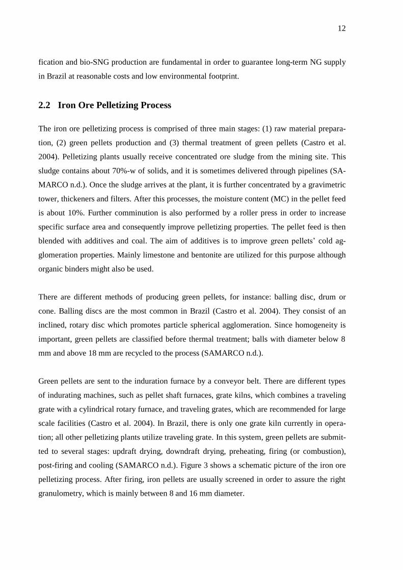
2.2 Iron Ore Pelletizing Process
The iron ore pelletizing process is comprised of three main stages: (1) raw material prepara-
tion, (2) green pellets production and (3) thermal treatment of green pellets (Castro et al.
2004). Pelletizing plants usually receive concentrated ore sludge from the mining site. This
sludge contains about 70%-w of solids, and it is sometimes delivered through pipelines (SA-
MARCO n.d.). Once the sludge arrives at the plant, it is further concentrated by a gravimetric
tower, thickeners and filters. After this processes, the moisture content (MC) in the pellet feed
is about 10%. Further comminution is also performed by a roller press in order to increase
specific surface area and consequently improve pelletizing properties. The pellet feed is then
blended with additives and coal. The aim of additives is to improve green pellets’ cold ag-
glomeration properties. Mainly limestone and bentonite are utilized for this purpose although
organic binders might also be used.
There are different methods of producing green pellets, for instance: balling disc, drum or
cone. Balling discs are the most common in Brazil (Castro et al. 2004). They consist of an
inclined, rotary disc which promotes particle spherical agglomeration. Since homogeneity is
important, green pellets are classified before thermal treatment; balls with diameter below 8
mm and above 18 mm are recycled to the process (SAMARCO n.d.).
Green pellets are sent to the induration furnace by a conveyor belt. There are different types
of indurating machines, such as pellet shaft furnaces, grate kilns, which combines a traveling
grate with a cylindrical rotary furnace, and traveling grates, which are recommended for large
scale facilities (Castro et al. 2004). In Brazil, there is only one grate kiln currently in opera-
tion; all other pelletizing plants utilize traveling grate. In this system, green pellets are submit-
ted to several stages: updraft drying, downdraft drying, preheating, firing (or combustion),
post-firing and cooling (SAMARCO n.d.). Figure 3 shows a schematic picture of the iron ore
pelletizing process. After firing, iron pellets are usually screened in order to assure the right
granulometry, which is mainly between 8 and 16 mm diameter.

13
Figure 3: Scheme of iron ore pelletizing process.
14
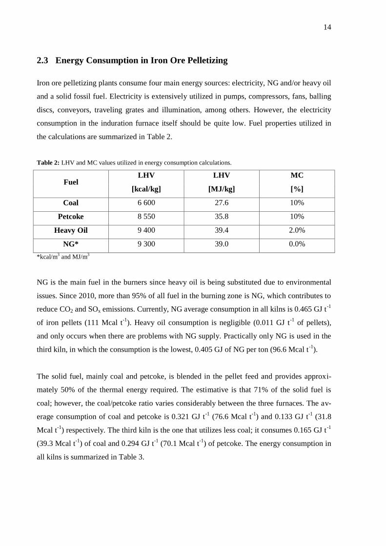
2.3 Energy Consumption in Iron Ore Pelletizing
Iron ore pelletizing plants consume four main energy sources: electricity, NG and/or heavy oil
and a solid fossil fuel. Electricity is extensively utilized in pumps, compressors, fans, balling
discs, conveyors, traveling grates and illumination, among others. However, the electricity
consumption in the induration furnace itself should be quite low. Fuel properties utilized in
the calculations are summarized in Table 2.
Table 2: LHV and MC values utilized in energy consumption calculations.
Fuel LHV LHV MC
[kcal/kg] [MJ/kg] [%]
Coal 6 600 27.6 10%
Petcoke 8 550 35.8 10%
Heavy Oil 9 400 39.4 2.0%
NG* 9 300 39.0 0.0%
*kcal/m3 and MJ/m
3
NG is the main fuel in the burners since heavy oil is being substituted due to environmental
issues. Since 2010, more than 95% of all fuel in the burning zone is NG, which contributes to
reduce CO2 and SOx emissions. Currently, NG average consumption in all kilns is 0.465 GJ t-1
of iron pellets (111 Mcal t-1
). Heavy oil consumption is negligible (0.011 GJ t-1
of pellets),
and only occurs when there are problems with NG supply. Practically only NG is used in the
third kiln, in which the consumption is the lowest, 0.405 GJ of NG per ton (96.6 Mcal t-1
).
The solid fuel, mainly coal and petcoke, is blended in the pellet feed and provides approxi-
mately 50% of the thermal energy required. The estimative is that 71% of the solid fuel is
coal; however, the coal/petcoke ratio varies considerably between the three furnaces. The av-
erage consumption of coal and petcoke is 0.321 GJ t-1
(76.6 Mcal t-1
) and 0.133 GJ t-1
(31.8
Mcal t-1
) respectively. The third kiln is the one that utilizes less coal; it consumes 0.165 GJ t-1
(39.3 Mcal t-1
) of coal and 0.294 GJ t-1
(70.1 Mcal t-1
) of petcoke. The energy consumption in
all kilns is summarized in Table 3.

15
Table 3: Indurating machine typical thermal energy consumption.
Fuel Furnace 01
[GJ/t]
Furnace 02
[GJ/t]
Furnace 03
[GJ/t]
Average
[GJ/t]
Coal 0.449 0.348 0.165 0.321
Petcoke 0.000 0.105 0.294 0.133
Total Solid 0.449 0.453 0.458 0.454
Heavy oil 0.016 0.016 0.000 0.011
Natural gas 0.488 0.503 0.405 0.465
Total burners 0.504 0.520 0.405 0.476
Total thermal 0.953 0.973 0.863 0.930
In order to compare, the Brazilian average specific energy consumption in the pelletizing pro-
cess was extrapolated from the National Energy Balance (EPE 2012). As the data included
mining and pelletizing sectors together, it was assumed that all NG, coal, coke and petcoke
were utilized exclusively for pelletizing and other fuels were utilized only for mining. As a
result, the average consumption is estimated at 0.466 GJ t-1
of NG and 0.656 GJ t-1
of solid
fuel. Total thermal energy consumption is estimated at 1.122 GJ t-1
, which is 17% higher than
values considered in this thesis.

16
3 CONVERSION OF BIOMASS TO FUEL GAS
In this chapter, practical issues regarding biomass gasification and bio-SNG production are
discussed. Firstly, biomass harvesting, handling, and pretreatment are covered. Secondly, a
theoretical background regarding biomass gasification is provided. In the sequence, possible
gasifying media and gasifier models are presented. Special attention is given to circulating
fluidized bed (CFB) gasification, which is the main large-scale option. In addition, down-
stream operations such as gas cleaning, methanation and gas upgrading are discussed. Finally,
the commercial plants currently under operation and their main characteristics are listed.
3.1 Biomass Supply Chain
Fuel supply is possibly one of the main issues in biomass energy conversion systems. Cost-
effective harvesting, transportation, comminution, storage, handling pretreatment and feeding
are crucial to assure a project’s feasibility. In contrast to fossil solid fuels, biomass character-
istics may vary according to location (soil), climate and season. Therefore, quality control is
necessary in order to guarantee a fuel’s minimum requirements, especially regarding MC,
particle size and ash characteristics. Quality control measures can be taken from the growing
stage. For instance, type and quantity of fertilizers can influence chlorine and nitrogen con-
tents of the biomass (Van Loo et al. 2008).
The supply chain characteristics depend on the type of biomass utilized, e.g. harvested or non-
harvested. The latter generally includes granular materials, such as wood chips, rice husk and
bark (Basu 2010). The former group refers to high MC fuels, such as straw, grass, and ba-
gasse. Harvested biomass is beyond the scope of this work, in which the focus is eucalyptus
chips and their utilization in large-scale CFB gasification facilities. For detailed information
concerning other fuels, refer to Basu (2010) or Van Loo (2008).
3.1.1 Harvesting
Many options are available for cost-effective energy biomass harvesting, and some of them
can be similar to those utilized in the pulp industry (Van Loo et al. 2008). For timber, extrac-
tion of whole trees is recommended, utilizing one-grip harvesters at the stump for cutting and
delimbing (Kallio et al. 2005). Technologies for mechanized harvesting of short rotation euca-
17
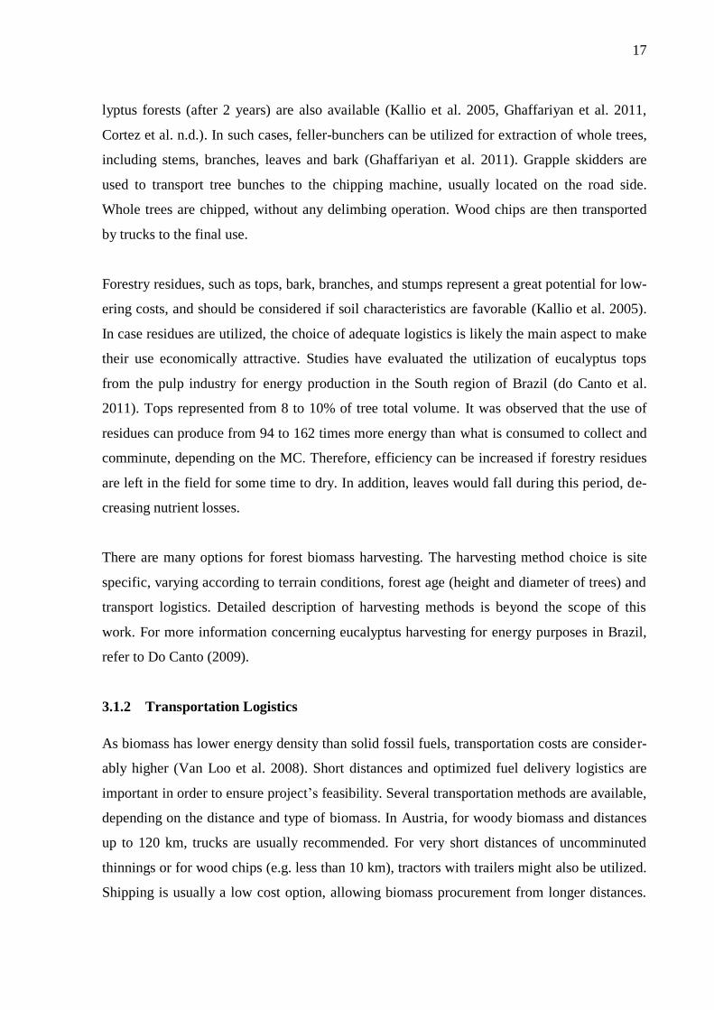
lyptus forests (after 2 years) are also available (Kallio et al. 2005, Ghaffariyan et al. 2011,
Cortez et al. n.d.). In such cases, feller-bunchers can be utilized for extraction of whole trees,
including stems, branches, leaves and bark (Ghaffariyan et al. 2011). Grapple skidders are
used to transport tree bunches to the chipping machine, usually located on the road side.
Whole trees are chipped, without any delimbing operation. Wood chips are then transported
by trucks to the final use.
Forestry residues, such as tops, bark, branches, and stumps represent a great potential for low-
ering costs, and should be considered if soil characteristics are favorable (Kallio et al. 2005).
In case residues are utilized, the choice of adequate logistics is likely the main aspect to make
their use economically attractive. Studies have evaluated the utilization of eucalyptus tops
from the pulp industry for energy production in the South region of Brazil (do Canto et al.
2011). Tops represented from 8 to 10% of tree total volume. It was observed that the use of
residues can produce from 94 to 162 times more energy than what is consumed to collect and
comminute, depending on the MC. Therefore, efficiency can be increased if forestry residues
are left in the field for some time to dry. In addition, leaves would fall during this period, de-
creasing nutrient losses.
There are many options for forest biomass harvesting. The harvesting method choice is site
specific, varying according to terrain conditions, forest age (height and diameter of trees) and
transport logistics. Detailed description of harvesting methods is beyond the scope of this
work. For more information concerning eucalyptus harvesting for energy purposes in Brazil,
refer to Do Canto (2009). (do Canto 2009)
3.1.2 Transportation Logistics
As biomass has lower energy density than solid fossil fuels, transportation costs are consider-
ably higher (Van Loo et al. 2008). Short distances and optimized fuel delivery logistics are
important in order to ensure project’s feasibility. Several transportation methods are available,
depending on the distance and type of biomass. In Austria, for woody biomass and distances
up to 120 km, trucks are usually recommended. For very short distances of uncomminuted
thinnings or for wood chips (e.g. less than 10 km), tractors with trailers might also be utilized.
Shipping is usually a low cost option, allowing biomass procurement from longer distances.

18
However, these values are specific, and detailed studies should be performed within the Bra-
zilian context.
The employed logistics for biomass supply is usually developed based on the location of size
reduction, which is commonly defined by type of biomass. For instance, when early thinnings
(15 to 20 cm diameter) and loose forest residues are being utilized, comminution at the har-
vesting site might be the best option (Kallio et al. 2005). For timber, large-scale centralized
chipping at the plant site might be economical. In case of centralized chipping, residual bio-
mass can be transported in bales or bundles. It is estimated that transportation of bales can
save up to 10% of the costs if compared to the transport of wood chips (Van Loo et al. 2008).
3.1.3 Comminution
CFB gasifiers are considered quite tolerant regarding fuel particle size, and fine particles are
not required. Thus, chipping should be the best comminution alternative once particle sizes
between 5 and 50 mm can be obtained (Van Loo et al. 2008). Wood chips are approximately 8
mm thick, 25 mm wide and up to 55 mm long. As shown in Figure 4, there are two main
types of chipping equipment: disc and drum. Although both types are able to adjust the chip
size within a certain range, the former usually results in a more uniform particle distribution.
If necessary, size classification can be performed after chipping utilizing trummels (Basu
2010).
Figure 4: Disc and drum chippers. (Source: Marutzky & Seeger, 1999 cited in Van Loo et al., 2008, p. 64)
The energy required for chipping can be estimated at 1–3% of the total fuel energy content
(Van Loo et al. 2008). MC might affect this energy consumption; for instance, higher water

19
content reduces the friction factor, resulting in a lower energy demand. The chipper size de-
pends on the delivering logistics (e.g. centralized or decentralized) and on the diameter of the
logs/bundles. Chipper sizes and their respective characteristics are presented in Table 4.
Table 4: Characteristics of various sizes of chippers. (Source: Marutzky & Seeger, 1999 cited in Van Loo et al.,
2008, p. 65)
Size Productivity
[m3 bulk/h]
Diameter
[cm] Feeding system
Power
[kW]
Small-scale 3–25 8–35 Manual or crane 20–100
Medium-scale 25–40 35–40 Crane 60–200
Large-scale 40–100 40–55 Crane 200–550
3.1.4 Drying
Fuel MC commonly varies according to the type of biomass, season, harvesting method and
time of storage. Therefore, drying the material beforehand provides a more homogenous feed-
stock, which reduces the costs with process control (Van Loo et al. 2008). Despite beneficial
reactions with water occur inside the gasifier, drying improves the overall energy efficiency
for several reasons. Firstly, high MC means lower fuel net energy content. Secondly, heat is
consumed to vaporize the water fed into the gasifier. Additionally, storage of wet biomass
might increase the risk of biological degradation.
Fresh wood might contain between 30 and 60% moisture after cutting (Basu 2010). However,
2,260 kJ of thermal energy are required per each kg of water fed into the gasifier. Water ex-
cess also reduces the producer gas energy content. Surface moisture can be effectively re-
moved by pre-drying. MC can be reduced to 10-20%, which is ideal for most gasification pro-
cesses. Depending on climate conditions, simple outside storage might reduce the MC to 20-
30% (Van Loo et al. 2008, Basu 2010); however, exposure to rainfall should be avoided.
Drying systems’ feasibility depends on the biomass price, plant size, and availability of waste
heat (Van Loo et al. 2008). In all cases, economic analysis should consider possible indirect
savings; for instance, impacts in feeding system size, energy consumption and product gas
LHV. In gasification plants, drying medium can be hot product gas, combustion exhausts, hot
air or steam, preferably heated by some source of waste heat (Brammer et al. 1999). During
20
the drying process, biomass temperature should be kept below 100 ºC in order to avoid haz-
ardous emissions and/or thermal degradation. In addition, it is recommended that the O2 con-
tent in the drying medium is below 10%-v in order to minimize the risk of fire, especially if
higher temperatures are used. Several dryer models are available for biomass. In this work,
the most relevant continuous large-scale dryers suitable for wood chips are briefly presented.
For more detailed information, refer to Brammer et al. (1999).
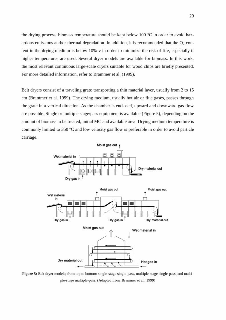
Belt dryers consist of a traveling grate transporting a thin material layer, usually from 2 to 15
cm (Brammer et al. 1999). The drying medium, usually hot air or flue gases, passes through
the grate in a vertical direction. As the chamber is enclosed, upward and downward gas flow
are possible. Single or multiple stage/pass equipment is available (Figure 5), depending on the
amount of biomass to be treated, initial MC and available area. Drying medium temperature is
commonly limited to 350 ºC and low velocity gas flow is preferable in order to avoid particle
carriage.
Figure 5: Belt dryer models; from top to bottom: single-stage single-pass, multiple-stage single-pass, and multi-
ple-stage multiple-pass. (Adapted from: Brammer et al., 1999)

21
Rotary cascade dryers are commonly utilized for wood chips. The main advantage is technol-
ogy maturity, which decreases risks (Brammer et al. 1999). Air or exhaust gases are the usual
drying medium, and flow can be either co-current or counter-current. As shown in Figure 6, it
is comprised of a rotary, slightly inclined cylinder equipped with longitudinal flights (Figure
7) able to lift the material and improve mixing. Typical sizes range between 4 and 10 m long,
from 1 to 6 m diameter and rotating speed from 1 to 10 rpm. For safety reasons, inlet gas tem-
perature is limited to approximately 250 ºC. Gas velocity is commonly between 2 and 3 m s-1
although it can range from 0.5 up to 5 m s-1
. Dryer efficiency can be between 50 and 75%,
depending on the initial MC and gas inlet temperature. Exhaust gas cleaning is usually neces-
sary in order to separate entrained particles, which can increase capital and operational costs.
Figure 6: Rotary cascade dryer. (Source: Brammer et al., 1999)
Figure 7: Longitudinal flights in a frontal view. (Source: Brammer et al., 1999)
Other options for wood chip drying are also available. For instance, indirect steam-tube rotary
dryers are based on conductive heating of biomass; however, they are only suitable when me-
dium pressure saturated steam is available. Fluidized bed (FB) dryers are also appropriate for
wood chips, as long as particle size is relatively uniform. Nevertheless, these two technologies
are not extensively used in commercial, large-scale gasification plants yet. In practice, the

22
most common configuration in biomass gasification plants is the belt dryer combined with hot
air as drying media.
3.1.5 Storage
Biomass storage is fundamental in large-scale gasification plants in order to guarantee contin-
uous operation. Adequate storage design might significantly reduce costs since large biomass
volumes are utilized (Van Loo et al. 2008). Usually, separate long and short-term storage are
necessary, the latter directly connected to the feeding system.
Mounds are the most common option for long-term storage. However, studies have shown
that storing comminutes materials (e.g. wood chips) in piles may increase biological degrada-
tion. As a consequence, wood chips should be stored in piles for no longer than two weeks
(Kallio et al. 2005). Long-term storage of uncomminuted material is a possible solution if
longer storage is needed. Biological activity increases the pile’s temperature and consequently
the risk of fire, as well as dry mass losses and health hazards (Van Loo et al. 2008). High MC
also increases microbial growth in the fuel; thus if storage of wood chips is necessary, MC
should be kept below 30%-w (Van Loo et al. 2008, Kallio et al. 2005). Risk of self-ignition
can be reduced when lower piles are utilized; for example, less than 8 m for bark (Van Loo et
al. 2008). Piles should not be compacted and should contain homogeneous material. In order
to prevent incidents, temperature and CO2 release along the pile can be monitored. Outside
piles should be avoided, especially in the rainy season due to increase in MC and leaching.
Construction of paved storage surfaces is also advisable in order to avoid contamination with
soil and stones.
Short-term storage provides fuel directly to the feeding system, usually after drying. Silos and
hoppers are the most common apparatus. Adequate hopper design is important to ensure con-
tinuous operation. Common problems with hopper discharge (Figure 8) are: arching, rat-
holing and funnel flow (Basu 2010). Mass flow is the best discharge regime, in which the
biomass is withdrawn homogeneously.
23
Figure 8: Flow regimes in hoppers. (Source: Basu, 2010)
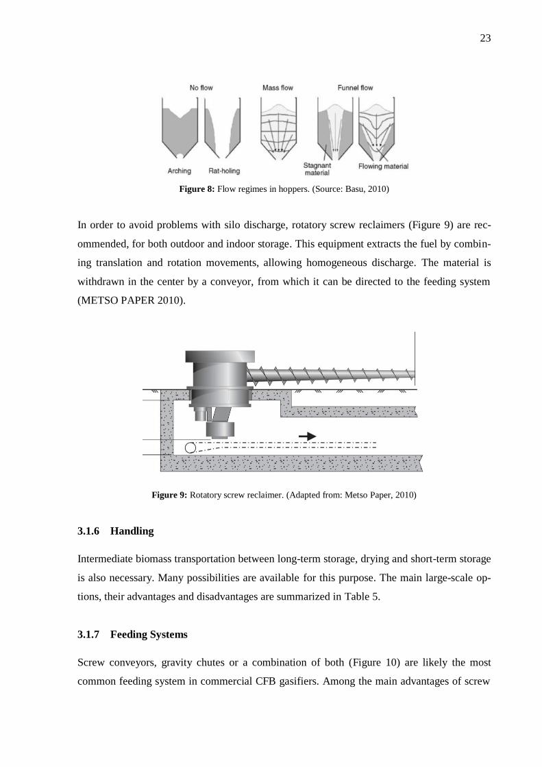
In order to avoid problems with silo discharge, rotatory screw reclaimers (Figure 9) are rec-
ommended, for both outdoor and indoor storage. This equipment extracts the fuel by combin-
ing translation and rotation movements, allowing homogeneous discharge. The material is
withdrawn in the center by a conveyor, from which it can be directed to the feeding system
(METSO PAPER 2010).
Figure 9: Rotatory screw reclaimer. (Adapted from: Metso Paper, 2010)
3.1.6 Handling
Intermediate biomass transportation between long-term storage, drying and short-term storage
is also necessary. Many possibilities are available for this purpose. The main large-scale op-
tions, their advantages and disadvantages are summarized in Table 5.
3.1.7 Feeding Systems
Screw conveyors, gravity chutes or a combination of both (Figure 10) are likely the most
common feeding system in commercial CFB gasifiers. Among the main advantages of screw
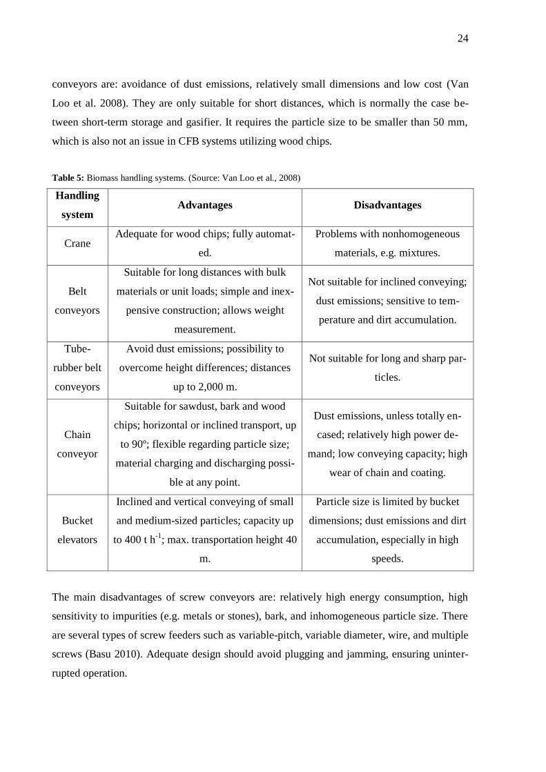
24
conveyors are: avoidance of dust emissions, relatively small dimensions and low cost (Van
Loo et al. 2008). They are only suitable for short distances, which is normally the case be-
tween short-term storage and gasifier. It requires the particle size to be smaller than 50 mm,
which is also not an issue in CFB systems utilizing wood chips.
Table 5: Biomass handling systems. (Source: Van Loo et al., 2008)
Handling
system Advantages Disadvantages
Crane Adequate for wood chips; fully automat-
ed.
Problems with nonhomogeneous
materials, e.g. mixtures.
Belt
conveyors
Suitable for long distances with bulk
materials or unit loads; simple and inex-
pensive construction; allows weight
measurement.
Not suitable for inclined conveying;
dust emissions; sensitive to tem-
perature and dirt accumulation.
Tube-
rubber belt
conveyors
Avoid dust emissions; possibility to
overcome height differences; distances
up to 2,000 m.
Not suitable for long and sharp par-
ticles.
Chain
conveyor
Suitable for sawdust, bark and wood
chips; horizontal or inclined transport, up
to 90º; flexible regarding particle size;
material charging and discharging possi-
ble at any point.
Dust emissions, unless totally en-
cased; relatively high power de-
mand; low conveying capacity; high
wear of chain and coating.
Bucket
elevators
Inclined and vertical conveying of small
and medium-sized particles; capacity up
to 400 t h-1
; max. transportation height 40
m.
Particle size is limited by bucket
dimensions; dust emissions and dirt
accumulation, especially in high
speeds.
The main disadvantages of screw conveyors are: relatively high energy consumption, high
sensitivity to impurities (e.g. metals or stones), bark, and inhomogeneous particle size. There
are several types of screw feeders such as variable-pitch, variable diameter, wire, and multiple
screws (Basu 2010). Adequate design should avoid plugging and jamming, ensuring uninter-
rupted operation.
25
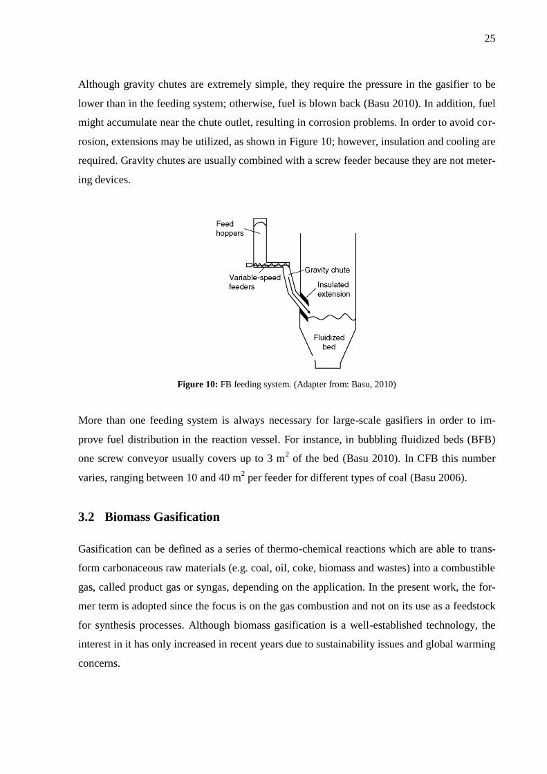
Although gravity chutes are extremely simple, they require the pressure in the gasifier to be
lower than in the feeding system; otherwise, fuel is blown back (Basu 2010). In addition, fuel
might accumulate near the chute outlet, resulting in corrosion problems. In order to avoid cor-
rosion, extensions may be utilized, as shown in Figure 10; however, insulation and cooling are
required. Gravity chutes are usually combined with a screw feeder because they are not meter-
ing devices.
Figure 10: FB feeding system. (Adapter from: Basu, 2010)
More than one feeding system is always necessary for large-scale gasifiers in order to im-
prove fuel distribution in the reaction vessel. For instance, in bubbling fluidized beds (BFB)
one screw conveyor usually covers up to 3 m2 of the bed (Basu 2010). In CFB this number
varies, ranging between 10 and 40 m2 per feeder for different types of coal (Basu 2006).
3.2 Biomass Gasification
Gasification can be defined as a series of thermo-chemical reactions which are able to trans-
form carbonaceous raw materials (e.g. coal, oil, coke, biomass and wastes) into a combustible
gas, called product gas or syngas, depending on the application. In the present work, the for-
mer term is adopted since the focus is on the gas combustion and not on its use as a feedstock
for synthesis processes. Although biomass gasification is a well-established technology, the
interest in it has only increased in recent years due to sustainability issues and global warming
concerns.

26
In biomass gasification, renewable carbon resources, such as charcoal, wood chips, energy
crops (e.g. short rotation coppice, miscanthus, switchgrass, etc.), forestry residues (e.g. bark,
tops, branches, small logs, etc.), agricultural wastes (e.g. cobs, straw, bagasse, stalks, shells,
etc.), and other wastes (plastics, municipal solid waste, sawdust, etc.) are transformed into
combustible gases. In general, the carbon source (often called fuel) reacts with a gasifying
medium, which can be air (or oxygen), steam or a combination of both. Each gasification me-
dium has its own reaction mechanism, which usually defines the reactor’s heat source. For
instance, when air or oxygen is utilized, biomass partial oxidation provides the heat required
by endothermic reactions. In these cases, the system can be considered autothermal. On the
other hand if only steam is utilized, an external heat source must be utilized. In such situa-
tions, the system is called allothemal. The gasifying medium and its amount have considera-
ble impact on the gasification process, operation and resulting product gas. Therefore, this
matter is discussed in more detail in the next section.
The main combustible components in the product gas are H2 and CO although CH4 and small
hydrocarbons containing 2-3 atoms of C are formed in minor concentrations. However, non-
combustible products are also present in this mixture, such as H2O, CO2 and possibly N2, de-
pending on the reagents and/or reactor design. Undesirable products from biomass gasifica-
tion such as tars and alkali are formed as well.
Although this thermo-chemical process is generally called gasification, several partially over-
lapping phenomena occur inside a gasifying reactor. A gasifier can be divided into preheating,
drying, pyrolysis, char gasification and combustion zones (Chen et al. 2003). These stages are
schematically represented in Figure 11. Depending on the gasifier design, there might also be
tar cracking and shift reaction zones.
Preheating and drying stages are of special importance for biomass gasification. Although
pre-drying is usually performed, final drying can only occur inside the gasifier, at tempera-
tures above 100ºC. Volatiles are also released in the preheating zone, when temperatures are
above 200ºC.

27
Figure 11: Gasification stages. (Adapted from Basu, 2010, p. 119)
Thermal cracking of large hydrocarbons present in the solid phase occurs in the pyrolysis
zone, forming char, liquids and gases. Further decomposition of liquids also occurs in this
stage, in which condensable and non-condensable gases are produced (Basu 2010). Conden-
sable gases are generically called tars, and should be avoided as much as possible since their
condensation causes clogging in downstream equipment. Measures for tar reduction are dis-
cussed later in this chapter.
At the gasification zone, reactions between pyrolysis products and gasifying agents occur, in
both solid and gaseous phases. The most typical gasification reactions, as well as combustion
reactions, are listed in Table 6, together with their respective enthalpies of reaction (ΔrH0) at
25ºC. Enthalpy data in Table 6 were compiled from several sources by Basu (2010, p. 121).
Char gasification reactions are kinetically the limiting ones. This is explained by the fact that
they occur in solid phase, and therefore mass transfer plays an important role in the reaction
rate. Char reaction speed also depends on the gasifying agent. Reactions with oxygen are the
fastest ones, and thus the remaining oxygen is quickly consumed, favoring CO formation
(Basu 2010). Those are followed by the char-steam reaction, which may be from 103 to 10
5
times slower. The char-carbon dioxide reaction (Boudouard) is even slower, from 106
to 107
times if compared with char-oxygen. At temperatures below 1,000 K (727 ºC), the rate of
Boudouard reaction can be considered insignificant. Nonetheless, the slowest of all char reac-
tions is hydrogasification, which can be 108 times slower.
Biomass Drying Pyrolysis
Liquids
(tar, oil, naphta)
Gases
(CO, H2, CH4,
H2O)
Oxygenated
compounds
(phenols, acid)
Solid
(char)
CO, H2, CH4,
H2O, CO2,
cracking +5%
products
CO, H2, CH4,
H2O, CO2,
unconverted
carbon
Char gasification
reactions
(gasification,
combustion, shift)
Gas-phase
reactions
(cracking,
reforming,
combustion, shift)

28
Table 6: Main gasification reactions. (Data compiled by Basu, 2010, p. 121)
Reaction Type Reaction ΔrH0 at 25ºC [kJ/mol]
Carbon Reactions
R1 (Boudouard) C + CO2 ↔ 2 CO +172
R2 (water-gas or steam) C + H2O ↔ CO + H2 +131
R3 (hydrogasification) C + 2 H2 ↔ CH4 -74.8
R4 C + ½ O2 → CO -111
Oxidation Reactions
R5 C + O2 → CO2 -394
R6 CO + ½ O2 → CO2 -284
R7 CH4 + 2 O2 ↔ CO2 + 2 H2O -803
R8 H2 + ½ O2 → H2O -242
Water-gas Shift Reaction
R9 CO + H2O ↔ CO2 + H2 -41.2
Methanation Reactions
R10 2 CO + 2 H2 → CH4 + CO2 -247
R11 CO + 3 H2 ↔ CH4 + H2O -206
R12 CO2 + 4 H2 ↔ CH4 + 2 H2O -165
Steam-reforming Reactions
R13 CH4 + H2O ↔ CO + 3 H2 +206
R14 CH4 + ½ O2 → CO + 2 H2 -36.0
Combustion is usually faster than gasification given the same pressure and temperature.
Therefore, the amount of air or oxygen utilized should be carefully determined since unneces-
sary combustion results into heat wastage and low energy content product gas. Shift reaction
is also important for the process, but at temperatures above 1,000 ºC, it rapidly reaches equi-
librium, compromising the hydrogen yield (Basu 2010). Methanation reactions are very im-
portant in bio-SNG production; nonetheless, they are not favored inside the gasifier, and only
occur to a minor extent under normal operating conditions. As the use of catalysts is required,
methanation is often carried downstream. This process is also discussed later in this chapter.
29
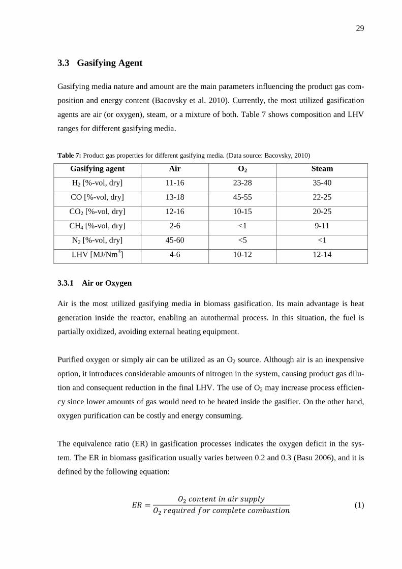
3.3 Gasifying Agent
Gasifying media nature and amount are the main parameters influencing the product gas com-
position and energy content (Bacovsky et al. 2010). Currently, the most utilized gasification
agents are air (or oxygen), steam, or a mixture of both. Table 7 shows composition and LHV
ranges for different gasifying media.
Table 7: Product gas properties for different gasifying media. (Data source: Bacovsky, 2010)
Gasifying agent Air O2 Steam
H2 [%-vol, dry] 11-16 23-28 35-40
CO [%-vol, dry] 13-18 45-55 22-25
CO2 [%-vol, dry] 12-16 10-15 20-25
CH4 [%-vol, dry] 2-6 <1 9-11
N2 [%-vol, dry] 45-60 <5 <1
LHV [MJ/Nm3] 4-6 10-12 12-14
3.3.1 Air or Oxygen
Air is the most utilized gasifying media in biomass gasification. Its main advantage is heat
generation inside the reactor, enabling an autothermal process. In this situation, the fuel is
partially oxidized, avoiding external heating equipment.
Purified oxygen or simply air can be utilized as an O2 source. Although air is an inexpensive
option, it introduces considerable amounts of nitrogen in the system, causing product gas dilu-
tion and consequent reduction in the final LHV. The use of O2 may increase process efficien-
cy since lower amounts of gas would need to be heated inside the gasifier. On the other hand,
oxygen purification can be costly and energy consuming.
The equivalence ratio (ER) in gasification processes indicates the oxygen deficit in the sys-
tem. The ER in biomass gasification usually varies between 0.2 and 0.3 (Basu 2006), and it is
defined by the following equation:
(1)
30
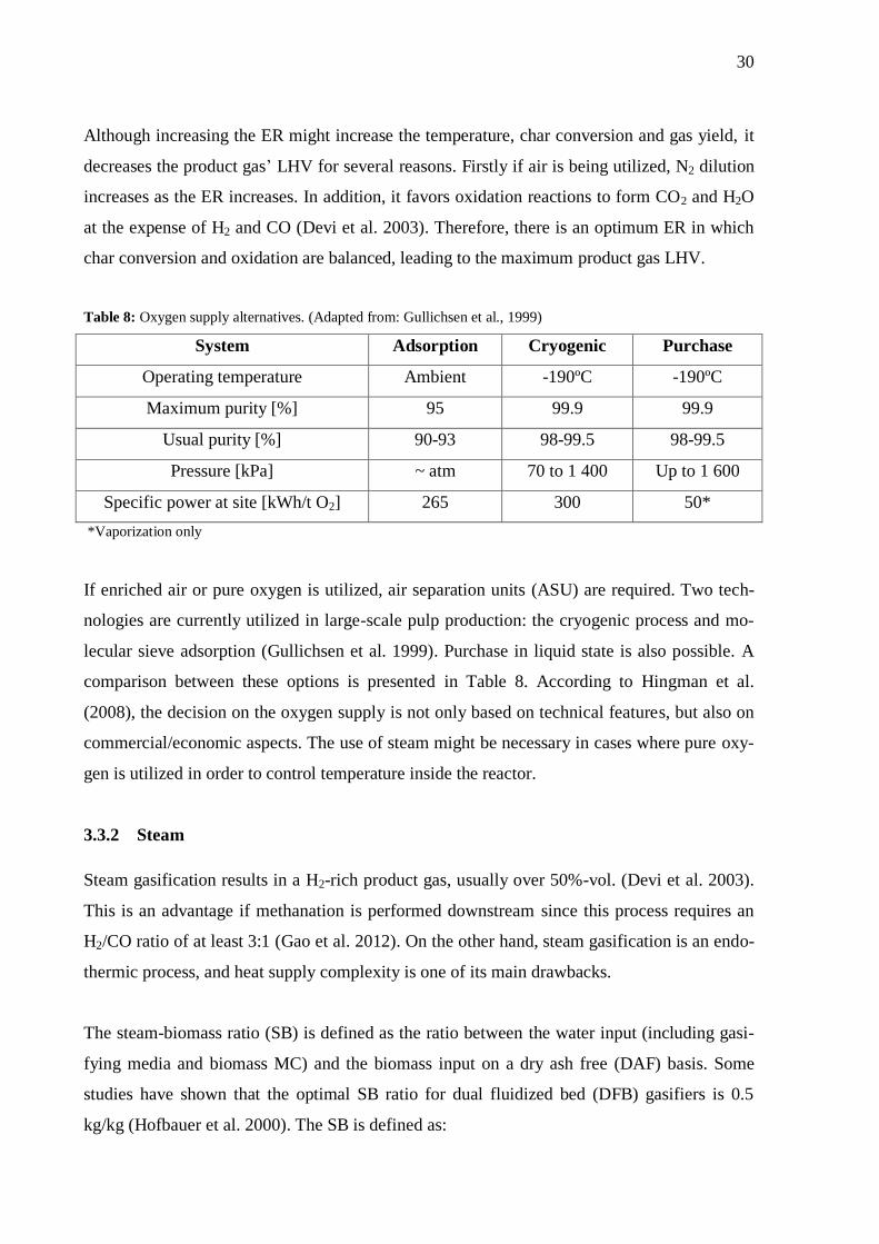
Although increasing the ER might increase the temperature, char conversion and gas yield, it
decreases the product gas’ LHV for several reasons. Firstly if air is being utilized, N2 dilution
increases as the ER increases. In addition, it favors oxidation reactions to form CO2 and H2O
at the expense of H2 and CO (Devi et al. 2003). Therefore, there is an optimum ER in which
char conversion and oxidation are balanced, leading to the maximum product gas LHV.
Table 8: Oxygen supply alternatives. (Adapted from: Gullichsen et al., 1999)
System Adsorption Cryogenic Purchase
Operating temperature Ambient -190ºC -190ºC
Maximum purity [%] 95 99.9 99.9
Usual purity [%] 90-93 98-99.5 98-99.5
Pressure [kPa] ~ atm 70 to 1 400 Up to 1 600
Specific power at site [kWh/t O2] 265 300 50*
*Vaporization only
If enriched air or pure oxygen is utilized, air separation units (ASU) are required. Two tech-
nologies are currently utilized in large-scale pulp production: the cryogenic process and mo-
lecular sieve adsorption (Gullichsen et al. 1999). Purchase in liquid state is also possible. A
comparison between these options is presented in Table 8. According to Hingman et al.
(2008), the decision on the oxygen supply is not only based on technical features, but also on
commercial/economic aspects. The use of steam might be necessary in cases where pure oxy-
gen is utilized in order to control temperature inside the reactor.
3.3.2 Steam
Steam gasification results in a H2-rich product gas, usually over 50%-vol. (Devi et al. 2003).
This is an advantage if methanation is performed downstream since this process requires an
H2/CO ratio of at least 3:1 (Gao et al. 2012). On the other hand, steam gasification is an endo-
thermic process, and heat supply complexity is one of its main drawbacks.
The steam-biomass ratio (SB) is defined as the ratio between the water input (including gasi-
fying media and biomass MC) and the biomass input on a dry ash free (DAF) basis. Some
studies have shown that the optimal SB ratio for dual fluidized bed (DFB) gasifiers is 0.5
kg/kg (Hofbauer et al. 2000). The SB is defined as:

31
(2)
When the SB increases, H2 and CO2 formation are favored, whereas CO concentration de-
creases (Herguido et al. 1992 cited in Devi et al. 2003, p. 129). Therefore, the product gas
LHV decreases with increasing SB. On the other hand, increasing SB improves carbon con-
version only up to a certain point (Hofbauer et al. 2000). It is estimated that the water conver-
sion in DFB gasifiers is usually as low as 10-15%. Therefore, increasing the SB might de-
crease the process thermal efficiency since considerable amounts of sensible heat are lost in
water removal from the product gas (Corella et al. 2007).
3.3.3 Steam/O2
Gasifying with a mixture of steam and oxygen (or air) brings together advantages of both me-
dia. Firstly, the presence of oxygen provides the necessary heat. Secondly, costs with oxygen
or dilution of nitrogen decreases due to the use of steam. Similarly to the SB, the gasifying
ratio (GR) indicates the quantitative relation between media and biomass, as follows (Devi et
al. 2003):
(3)
Following the same trend as ER and SB parameters, increasing GR results in a product gas
with lower energy content due to formation of more CO2 instead of H2 and CO (Devi et al.
2003).
3.4 Biomass Gasifiers
Several gasifier models have been developed in the past 20 years (Bridgwater 2002). Regard-
ing biomass gasification, reactors can be divided into three main groups: fixed (or moving)
bed (e.g. downdraft and updraft), FB (e.g. BFB, CFB, DFB), and entrained flow (EF) gasifi-
ers. Each model is suitable for certain fuel quality and input, as shown in Figure 12. This sec-
tion aims at briefly presenting the most relevant biomass gasifiers. Detailed information con-
cerning this matter can be found elsewhere, such as Olofsson et al. (2005).

32
Figure 12: Typical size of biomass gasifiers. (Source: Basu, 2010)
3.4.1 Fixed Bed Gasifiers
Fixed or moving bed gasifiers are probably the oldest gasification technology (Olofsson et al.
2005). The main advantage of this type of gasifier is its simplicity and consequent low capital
cost. However due to temperature homogeneity and process control issues, scaling-up to more
than 10 MWfuel is not possible. Additionally, ash melting is also a concern since high tempera-
tures are usually achieved. Air is usually the gasifying medium since costs of oxygen or indi-
rect heating would compromise the economic feasibility of such equipment. Three models are
currently relevant (Figure 13): updraft, downdraft and crossdraft gasifiers.
Figure 13: From left to right: updraft, downdraft and crossdraft gasifiers. (Source: Olofsson et al., 2005)
In updraft models, fuel is fed from the top and air from the bottom. The product gas is collect-
ed at the top of the equipment. As combustion reactions occur in the lower part, a gas with
relatively high energy content can be obtained – from 4 to 5 MJ Nm-3
when air is utilized (Ol-
ofsson et al. 2005). Another advantage is its relative low sensitivity to fuel size and MC.
However, the product gas’ tar content is extremely high, reaching 10 to 20%-w.
33
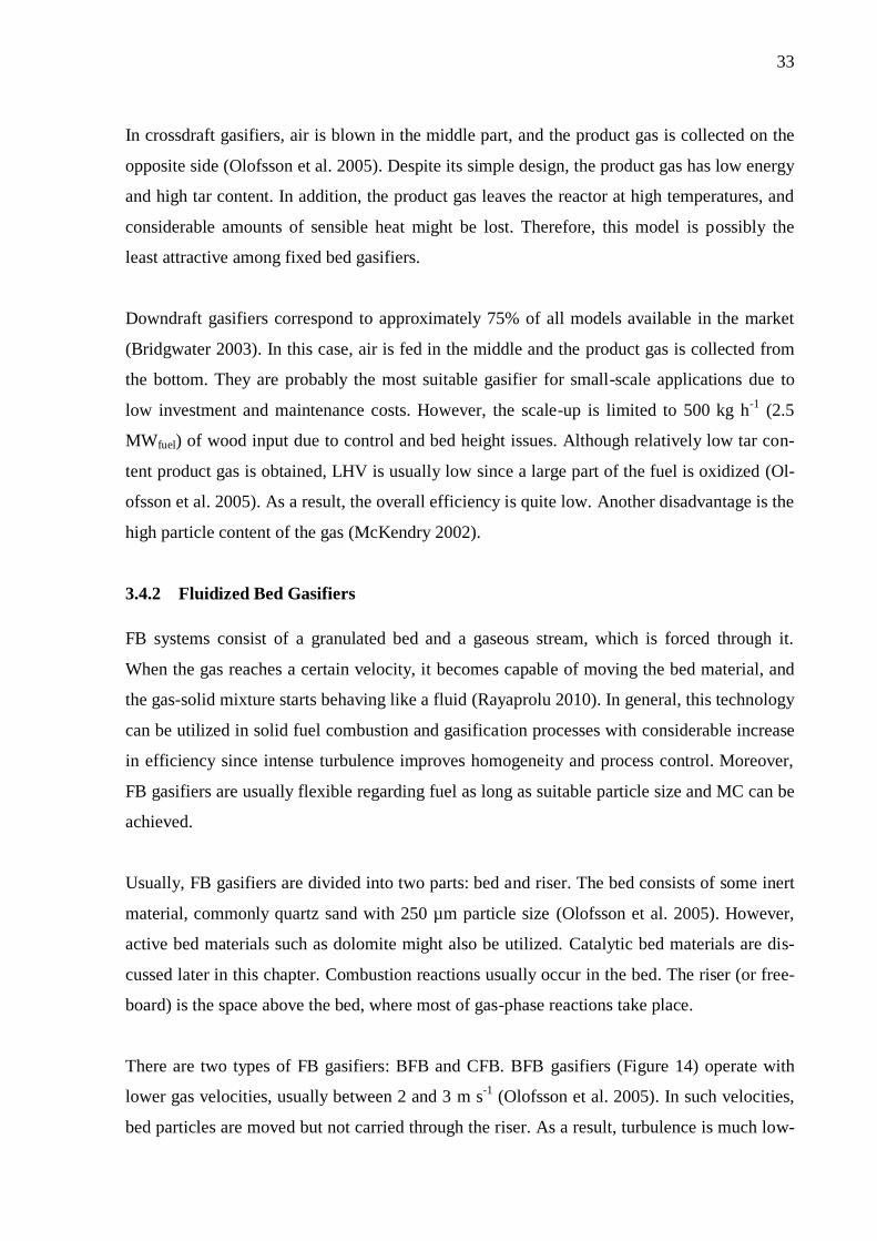
In crossdraft gasifiers, air is blown in the middle part, and the product gas is collected on the
opposite side (Olofsson et al. 2005). Despite its simple design, the product gas has low energy
and high tar content. In addition, the product gas leaves the reactor at high temperatures, and
considerable amounts of sensible heat might be lost. Therefore, this model is possibly the
least attractive among fixed bed gasifiers.
Downdraft gasifiers correspond to approximately 75% of all models available in the market
(Bridgwater 2003). In this case, air is fed in the middle and the product gas is collected from
the bottom. They are probably the most suitable gasifier for small-scale applications due to
low investment and maintenance costs. However, the scale-up is limited to 500 kg h-1
(2.5
MWfuel) of wood input due to control and bed height issues. Although relatively low tar con-
tent product gas is obtained, LHV is usually low since a large part of the fuel is oxidized (Ol-
ofsson et al. 2005). As a result, the overall efficiency is quite low. Another disadvantage is the
high particle content of the gas (McKendry 2002).
3.4.2 Fluidized Bed Gasifiers
FB systems consist of a granulated bed and a gaseous stream, which is forced through it.
When the gas reaches a certain velocity, it becomes capable of moving the bed material, and
the gas-solid mixture starts behaving like a fluid (Rayaprolu 2010). In general, this technology
can be utilized in solid fuel combustion and gasification processes with considerable increase
in efficiency since intense turbulence improves homogeneity and process control. Moreover,
FB gasifiers are usually flexible regarding fuel as long as suitable particle size and MC can be
achieved.
Usually, FB gasifiers are divided into two parts: bed and riser. The bed consists of some inert
material, commonly quartz sand with 250 µm particle size (Olofsson et al. 2005). However,
active bed materials such as dolomite might also be utilized. Catalytic bed materials are dis-
cussed later in this chapter. Combustion reactions usually occur in the bed. The riser (or free-
board) is the space above the bed, where most of gas-phase reactions take place.
There are two types of FB gasifiers: BFB and CFB. BFB gasifiers (Figure 14) operate with
lower gas velocities, usually between 2 and 3 m s-1
(Olofsson et al. 2005). In such velocities,
bed particles are moved but not carried through the riser. As a result, turbulence is much low-
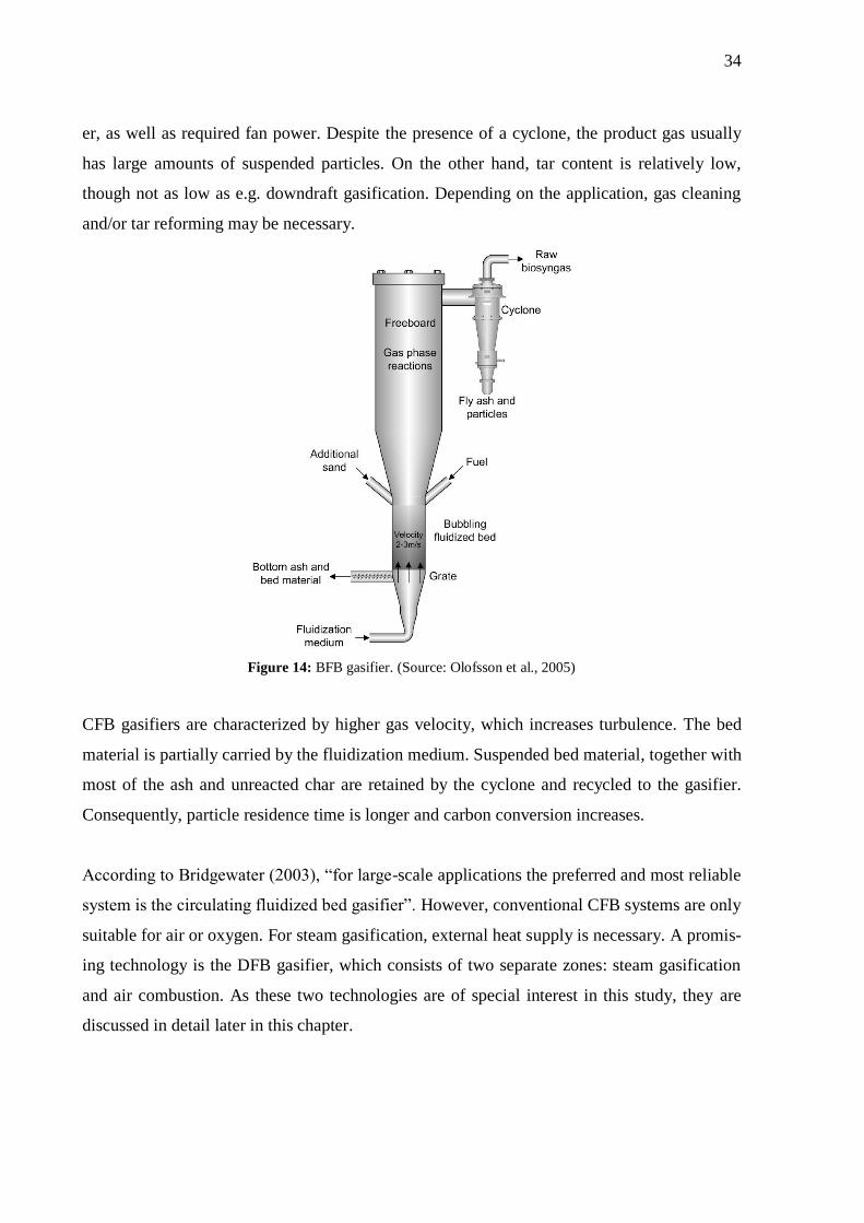
34
er, as well as required fan power. Despite the presence of a cyclone, the product gas usually
has large amounts of suspended particles. On the other hand, tar content is relatively low,
though not as low as e.g. downdraft gasification. Depending on the application, gas cleaning
and/or tar reforming may be necessary.
Figure 14: BFB gasifier. (Source: Olofsson et al., 2005)
CFB gasifiers are characterized by higher gas velocity, which increases turbulence. The bed
material is partially carried by the fluidization medium. Suspended bed material, together with
most of the ash and unreacted char are retained by the cyclone and recycled to the gasifier.
Consequently, particle residence time is longer and carbon conversion increases.
According to Bridgewater (2003), “for large-scale applications the preferred and most reliable
system is the circulating fluidized bed gasifier”. However, conventional CFB systems are only
suitable for air or oxygen. For steam gasification, external heat supply is necessary. A promis-
ing technology is the DFB gasifier, which consists of two separate zones: steam gasification
and air combustion. As these two technologies are of special interest in this study, they are
discussed in detail later in this chapter.

35
3.4.3 Entrained Flow Gasifiers
In EF gasifiers, a mixture of fuel and gasifying medium (e.g. oxygen or a mixture of
steam/O2) is injected in the reactor, generating a high temperature flame (Basu 2010, Olofsson
et al. 2005). In EF models, the fuel must be in the form of gas, powder or slurry (Olofsson et
al. 2005). Therefore, there are still some issues in utilizing biomass in this type of reactor
since it must be either ground to powder, pyrolysed to liquid and/or gas, or transformed into
charcoal slurry. In addition, the high alkali content in biomass ash makes it harmful to refrac-
tory and metal parts.
As ash melting is not a concern in EF gasifiers, temperatures between 1,200 and 1,400ºC and
pressures from 20 to 70 bars are commonly utilized (Basu 2010, Olofsson et al. 2005). Under
such conditions, the product gas is almost free of tars. On the other hand, large amounts of
sensible heat might make this process inefficient if proper heat recovery systems are not
available (Olofsson et al. 2005).
There are several types of EF gasifiers. The CHOREN’s Carbo-V® process is the most suc-
cessful EF model utilizing biomass (Higman et al. 2008). In this process, fuel is pre-gasified
at low temperature, and a mixture of pyrolysis gas, tars and char are further gasified in a down
EF gasifier (Figure 15).
Figure 15: Choren process for biomass gasification. (Source: Higman et al., 2008)

36
3.5 CFB Gasifiers
CFB technology (Figure 16) is currently the main commercial alternative for large-scale oxy-
gen/air biomass gasification. It is especially suitable for biomass since it provides long parti-
cle residence times and has relative high tolerance to the presence of volatiles (Basu 2010).
Figure 16: CFB gasifier. (Source: Olofsson et al., 2005)
In CFB gasifiers, the fluidization medium velocity is relatively high, usually between 5 and
10 m s-1
(Olofsson et al. 2005). Therefore, bed particles are partially carried by the gas stream
and dispersed over the riser. These solids are then separated from the product gas by a cyclone
and recycled to the reactor. The hydrodynamic regime inside a CFB is called a fast fluidized
bed (Basu 2010). In such a regime, relatively uniform temperatures can be achieved inside the
reactor, typically between 800 and 1,000 ºC for biomass. In addition, intense turbulence effec-
tively promotes heat and mass transfer. CFB is also flexible regarding different fuels such as
agricultural residues, wood and solid recovered fuels (SRF). Within a certain range, CFB gas-
ifiers are tolerant to variations in particle size and MC (Olofsson et al. 2005). Tar content in
the product gas can be considered quite low although not as low as downdraft or EF gasifiers.
On the other hand, the product gas might contain relatively high amounts of particulate mat-
ter. Additionally, bed agglomeration is still an issue, which limits the operating temperature.
37
Appropriate bed material extraction must be performed periodically in order to avoid bed ag-
glomeration. Despite the tolerance to particle size, larger particles require a higher fluidization
velocity, which increases the energy consumption and may result in equipment erosion.
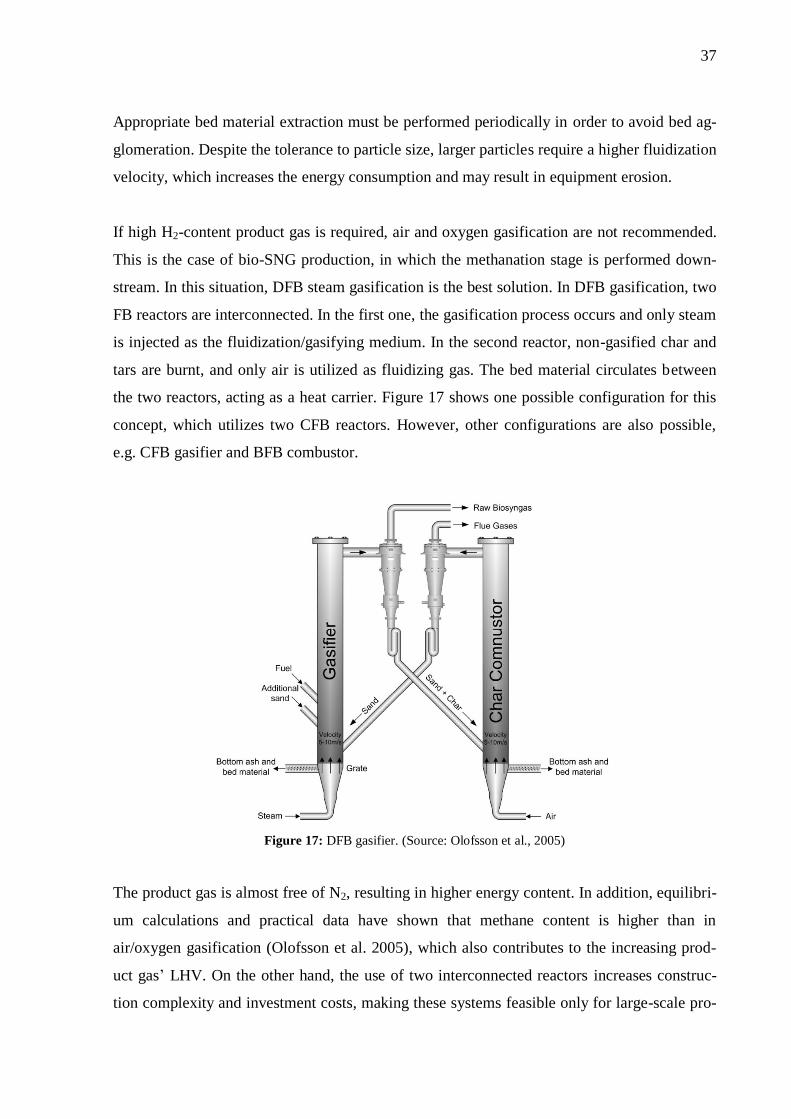
If high H2-content product gas is required, air and oxygen gasification are not recommended.
This is the case of bio-SNG production, in which the methanation stage is performed down-
stream. In this situation, DFB steam gasification is the best solution. In DFB gasification, two
FB reactors are interconnected. In the first one, the gasification process occurs and only steam
is injected as the fluidization/gasifying medium. In the second reactor, non-gasified char and
tars are burnt, and only air is utilized as fluidizing gas. The bed material circulates between
the two reactors, acting as a heat carrier. Figure 17 shows one possible configuration for this
concept, which utilizes two CFB reactors. However, other configurations are also possible,
e.g. CFB gasifier and BFB combustor.
Figure 17: DFB gasifier. (Source: Olofsson et al., 2005)
The product gas is almost free of N2, resulting in higher energy content. In addition, equilibri-
um calculations and practical data have shown that methane content is higher than in
air/oxygen gasification (Olofsson et al. 2005), which also contributes to the increasing prod-
uct gas’ LHV. On the other hand, the use of two interconnected reactors increases construc-
tion complexity and investment costs, making these systems feasible only for large-scale pro-

38
cesses. In addition, it is estimated that only 10 to 15% of the steam is actually converted in
DFB gasifiers. Therefore, the product gas must be dried and high amounts of sensible heat
might be lost in this stage, decreasing the process overall efficiency (Hofbauer et al. 2000,
Corella et al. 2007).
Many commercial CFB gasifiers are currently under operation in Europe (Vakkilainen et al.
2013). The main CFB biomass gasifiers are presented later in this chapter. However, the fea-
sibility of DFB gasifiers is still contradictory. According to Corella et al. (2007), several DFB
plants commissioned before mid-90s were dismantled for unknown reasons. On the other hand,
successful results of an 8 MWfuel demonstration plant in Güssing (Austria) have been recently
reported by Hofbauer and co-workers (2002). Unlike CFB gasification, large-scale plants utilizing
the DFB concept are still not available. The largest plant is located in Herten (Germany), with 15
MWfuel input (Göransson et al. 2011).
3.6 Product Gas Contaminants
Biomass fuels are complex mixtures, mainly composed of organic C and O, but also H, N,
and possibly S in very small quantities (compared to e.g. coal). The organic fraction consists
of cellulose, hemicellulose and lignin. Inorganic materials such as alkali and alkaline earth
metals (AAEM), silica and chlorine can also be found (Turn et al. 1998). The amount of each
component depends on several factors, such as species, environment, harvesting conditions,
handling, and the part of the plant from which the fuel is made. This variable composition,
combined with operating conditions, contributes to formation of certain contaminants, such as
tars (organic), inorganic oxides (ash), ammonia, and other undesirable substances. This sec-
tion introduces possible contaminants, their impacts and primary measures that can be taken
to reduce or even avoid their formation.
3.6.1 Tars
Tar formation is one of the main issues in biomass gasification (Devi et al. 2003). The term
‘tar’ has different definitions, depending on the application or research group. According to
Devi et al. (2003, p.126), tar can be defined as “a complex mixture of condensable hydrocar-
bons, which includes single to 5-ring aromatic compounds along with other oxygen-
containing hydrocarbons and complex polycyclic aromatic hydrocarbons” (PAH). Many rele-

39
vant institutions such as the International Energy Agency (IEA), the U.S. Department of En-
ergy (DOE) and the European Commission define tar as any gasification byproduct with a
molecular weight higher than benzene (Basu 2010, Devi et al. 2003). Compounds present in
tars depend on the type of biomass and gasification process that is being utilized (Abu El-Rub
et al. 2004). Due to the diversity of compounds present in tars, they are usually divided into
five groups (Li et al. 2009), as shown in Table 9.
The main problem caused by the presence of tars is plugging or clogging of pipes and ducts
due to condensation when the product gas is cooled down. Other issues involve aerosol for-
mation and possibility of polymerization (Basu 2010, Li et al. 2009). Tar deposition also re-
duces the effectiveness of heat transfer surfaces (Li et al. 2009). Additionally, tars may con-
tain toxic substances and decrease the overall gas yield since they contain considerable
amounts of energy (Abu El-Rub et al. 2004).
Table 9: Composition of tars. (Source: Li & Suzuki, 2009)
Class Class name Property Representative compounds
1 GC-
undetectable
Very heavy tars, cannot be
detected by GC
Total gravimetric tar minus GC-
detectable fraction
2 Heterocyclic
aromatics
Contain hetero atoms; highly
water soluble
Pyridine, phenol, cresols, quinoline,
isoquinoline, dibenzophenol
3
Light
aromatic
(1 ring)
Light hydrocarbons with
single ring; usually not con-
densable
Toluene, ethylbenzene, xylenes, sty-
rene
4
Light PAH
compounds
(2–3 rings)
2 and 3 ring compounds;
condense at low temperature
even at very low concentra-
tion
Indene, naphthalene, methylnaphtha-
lene, biphenyl, acenaphthalene, fluo-
rene, phenanthrene, anthracene
5
Heavy PAH
compounds
(4–7 rings)
Larger than 3-ring; condense
at high-temperatures even at
low concentrations
Fluoranthene, pyrene, chrysene,
perylene, coronene
In order to reduce tar content in the product gas, primary and secondary measures can be ap-
plied. Primary tar removal measures basically consist of changes in operation parameters.
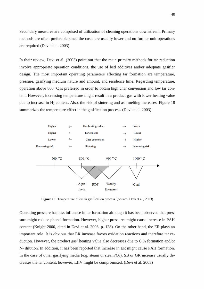
40
Secondary measures are comprised of utilization of cleaning operations downstream. Primary
methods are often preferable since the costs are usually lower and no further unit operations
are required (Devi et al. 2003).
In their review, Devi et al. (2003) point out that the main primary methods for tar reduction
involve appropriate operation conditions, the use of bed additives and/or adequate gasifier
design. The most important operating parameters affecting tar formation are temperature,
pressure, gasifying medium nature and amount, and residence time. Regarding temperature,
operation above 800 ºC is preferred in order to obtain high char conversion and low tar con-
tent. However, increasing temperature might result in a product gas with lower heating value
due to increase in H2 content. Also, the risk of sintering and ash melting increases. Figure 18
summarizes the temperature effect in the gasification process. (Devi et al. 2003)
Figure 18: Temperature effect in gasification process. (Source: Devi et al., 2003)
Operating pressure has less influence in tar formation although it has been observed that pres-
sure might reduce phenol formation. However, higher pressures might cause increase in PAH
content (Knight 2000, cited in Devi et al. 2003, p. 128). On the other hand, the ER plays an
important role. It is obvious that ER increase favors oxidation reactions and therefore tar re-
duction. However, the product gas’ heating value also decreases due to CO2 formation and/or
N2 dilution. In addition, it has been reported that increase in ER might cause PAH formation.
In the case of other gasifying media (e.g. steam or steam/O2), SB or GR increase usually de-
creases the tar content; however, LHV might be compromised. (Devi et al. 2003)
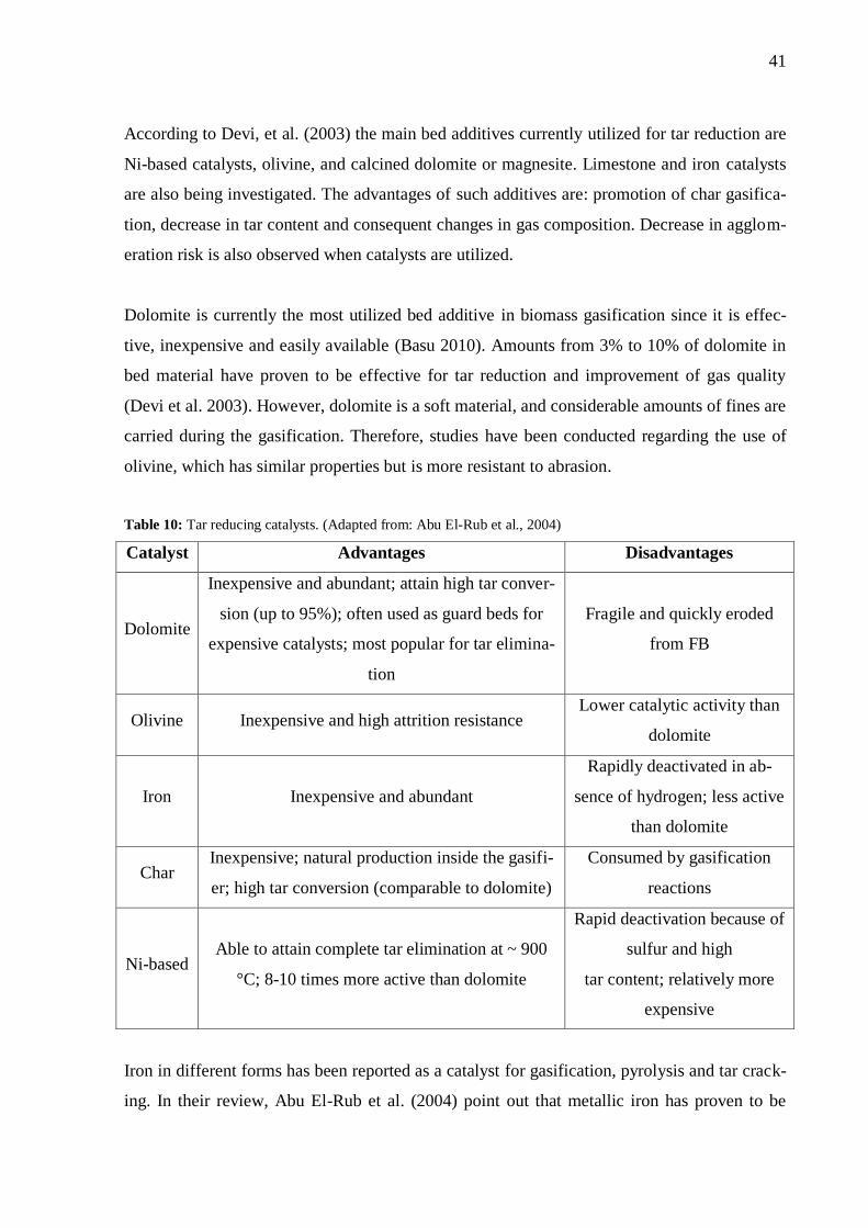
41
According to Devi, et al. (2003) the main bed additives currently utilized for tar reduction are
Ni-based catalysts, olivine, and calcined dolomite or magnesite. Limestone and iron catalysts
are also being investigated. The advantages of such additives are: promotion of char gasifica-
tion, decrease in tar content and consequent changes in gas composition. Decrease in agglom-
eration risk is also observed when catalysts are utilized.
Dolomite is currently the most utilized bed additive in biomass gasification since it is effec-
tive, inexpensive and easily available (Basu 2010). Amounts from 3% to 10% of dolomite in
bed material have proven to be effective for tar reduction and improvement of gas quality
(Devi et al. 2003). However, dolomite is a soft material, and considerable amounts of fines are
carried during the gasification. Therefore, studies have been conducted regarding the use of
olivine, which has similar properties but is more resistant to abrasion.
Table 10: Tar reducing catalysts. (Adapted from: Abu El-Rub et al., 2004)
Catalyst Advantages Disadvantages
Dolomite
Inexpensive and abundant; attain high tar conver-
sion (up to 95%); often used as guard beds for
expensive catalysts; most popular for tar elimina-
tion
Fragile and quickly eroded
from FB
Olivine Inexpensive and high attrition resistance Lower catalytic activity than
dolomite
Iron Inexpensive and abundant
Rapidly deactivated in ab-
sence of hydrogen; less active
than dolomite
Char Inexpensive; natural production inside the gasifi-
er; high tar conversion (comparable to dolomite)
Consumed by gasification
reactions
Ni-based Able to attain complete tar elimination at ~ 900
°C; 8-10 times more active than dolomite
Rapid deactivation because of
sulfur and high
tar content; relatively more
expensive
Iron in different forms has been reported as a catalyst for gasification, pyrolysis and tar crack-
ing. In their review, Abu El-Rub et al. (2004) point out that metallic iron has proven to be
42
more effective than iron oxides. However, hydrogen should be present in the medium in order
to avoid coke formation and deposition. In addition, hematite ores have shown better results
than magnetite ones for coal gasification (Cypers et al. 1980 cited in Abu El-Rub et al. 2004,
p. 6 914). Table 10 summarizes possible tar reducing catalysts and their main features.
The main reactor design characteristics that promote tar reduction and improve gas yield are:
secondary air injection, which also contributes to higher temperature; utilization of two-stage
gasification, e.g. separation of pyrolysis and reduction zones; and addition of char during the
gasifier start-up (Devi et al. 2003). Fast internal fluidized bed (FICFB) gasifiers, in which
gasification and combustion zones are separate, were reported to provide a high LHV gas with
low tar content (Fercher et al. 1998). Nevertheless, it seems that a compromise between tar
content and gas LHV must usually be made.
3.6.2 Alkali/Alkaline Earth Metals and Other Inorganic
Besides Alkali and Alkaline Earth Metals (AAEM - mainly Na, K, Ca and Mg), inorganic
substances such as Al, Cl, Fe, P, Si and Ti are commonly present in biomass. During gasifica-
tion, these elements can form ash, attach to the bed material or be carried by the gaseous
stream, contaminating the product gas. The distribution of inorganics in the gasification sys-
tem depends on their content in the fuel, gasifier model, bed material type, and possibly on
operation time. (Turn et al. 1998)
Alkali compounds usually present in biomasses are Na and K, the latter in higher concentra-
tion, up to 5%-w of dry matter (Turn et al. 1998). According to Turn et al. (1998), most alkali
after gasification is found either in the ash or associated with the bed material, and only a
small fraction (approximately 6%-w of the Na input) is actually released with the gases. Ex-
periments conducted in a bench-scale BFB utilizing alumina silicate as bed material and ba-
gasse as fuel confirmed that the main concern regarding alkali contaminants is the possibility
of bed agglomeration due to low melting point ash. Ca, Mg, Al, Fe, P, Si and Ti mostly were
found in the solid phase as well, representing no concern to downstream processes.
Studies regarding alfalfa gasification in pressurized FB have shown that only a small fraction
of alkali and trace metals present in the fuel are carried by the gaseous stream (Salo et al.
1998). The fuel’s Na and K content was 280 and 24,600 ppm (wt) respectively, whereas the
43
product gas contained only 0.04 ppm (wt) of total alkali content (Na + K) after being cooled
to 432ºC and filtered. Additionally, it was demonstrated that the amount of trace metals (Hg,
Cd, Pb, Se, Sb, Co, Be and As) in the product gas after high temperature/high pressure
(HTHP) ceramic filter was below European Union regulations.
In order to reduce agglomeration risk, periodic substitution of bed material is the most im-
portant measure (Basu 2010). Addition of limestone or dolomite also avoids agglomeration
once the presence of calcium produces a eutectic, higher melting point ash (Turn et al. 1998).
Dolomite is recommended for in-bed tar removal. Biomass pretreatment has been considered
as a possible solution for AAEM reduction in gasification systems as well (Turn et al. 1998,
Lv et al. 2010). However, it has been shown that AAEM increase char reactivity, and their
removal would result in a higher gasification initial temperature (Lv et al. 2010, Yip et al.
2009). Studies conducted by Yip et al. (2009) have shown that K, Na and Ca are (in this or-
der) the most active catalysts present in bio-char when steam gasification is performed. Par-
ticularly, it was observed that the presence of AAEM has a positive effect in the water-gas
shift reaction rate.
Another relevant inorganic substance formed during gasification is ammonia. The same study
conducted by Turn et al. (1998) has shown that the greater the amount of nitrogen present in
the fuel, the higher is the NH3 concentration on a dry product gas. Chlorine is also a concern
since most of it is released with the gas in the form of HCl. Temperatures should therefore be
kept above the product gas dew point in order to avoid corrosion.
3.7 Gas Cleaning
Depending on the product gas application and environmental regulations, gas cleaning must
be performed downstream of the gasifier. In case product gas is directly combusted, as occurs
in the indurating machine, tars are unlikely to cause any problems to the system as long as
they are maintained above the dew point (Milne et al. 1998), which is usually between 150
and 350 ºC (Cummer et al. 2002). The only issue in this case concerns air emissions. Howev-
er, other contaminants such as AAEM and chlorine may cause problems in the induration fur-
nace. No literature reference was found regarding this matter and further studies concerning
the fate of alkali and chlorine are needed. In addition, particulate matter is usually present in

44
CFB gasification product gas, and its removal may be necessary. On the other hand, methana-
tion catalysts might be deactivated due to tar/soot deposition, and previous gas cleaning is
mandatory.
Although other methods are available, hot gas cleaning is usually preferred since tar conden-
sation is thereby avoided. This operation is carried out at approximately 550 ºC; thus, the
product gas must be first cooled (Olofsson et al. 2005). After sulfur removal, HTHP ceramic
filters are utilized at pressures between 15 and 25 bars. The inorganic fraction is removed
downstream, usually by adsorption (Cummer et al. 2002). Nonetheless, efficient and econom-
ical product gas cleaning is still an issue.
Studies conducted at the Energy Research Centre of the Netherlands (ECN) developed a
promising technology for product gas cleaning (Zwart et al. 2006). In this concept, the prod-
uct gas is cooled to approximately 400 ºC in a fire tube cooler before dust removal. In this
manner, particles in the gas continuously erode the heat exchanger surface, preventing tar
deposition. After cooling, particulate matter is separated by a cyclone or hot-gas filter. Tars
are removed by an oil-based gas washer (OLGA). This system is comprised of two absorption
columns, in which the scrubbing liquid is oil-based. Regeneration is done by air stripping,
which is further recycled to the gasifier. Afterwards, chloride and sulfur components are re-
moved by commercial adsorbents. One advantage of this system is that no water is condensed,
avoiding contamination and need of waste water treatment. This system has been successfully
implemented in a 4 MWth demonstration plant in France (Zwart et al. 2009).
3.8 Methanation and Gas Upgrading
The product gas mainly consists of H2 and CO, which leads to a relatively low energy content
compared to NG. Methanation process can be used to convert carbon oxides (mainly CO) into
methane. The most important reactions are water-gas shift and methanation, shown previously
by equations R9 to R12 in Table 6. It is relevant to note that reactions R10 and R12 are a line-
ar combination of R09 and R11 (Kopyscinski et al. 2010).
(R09)
(R10)
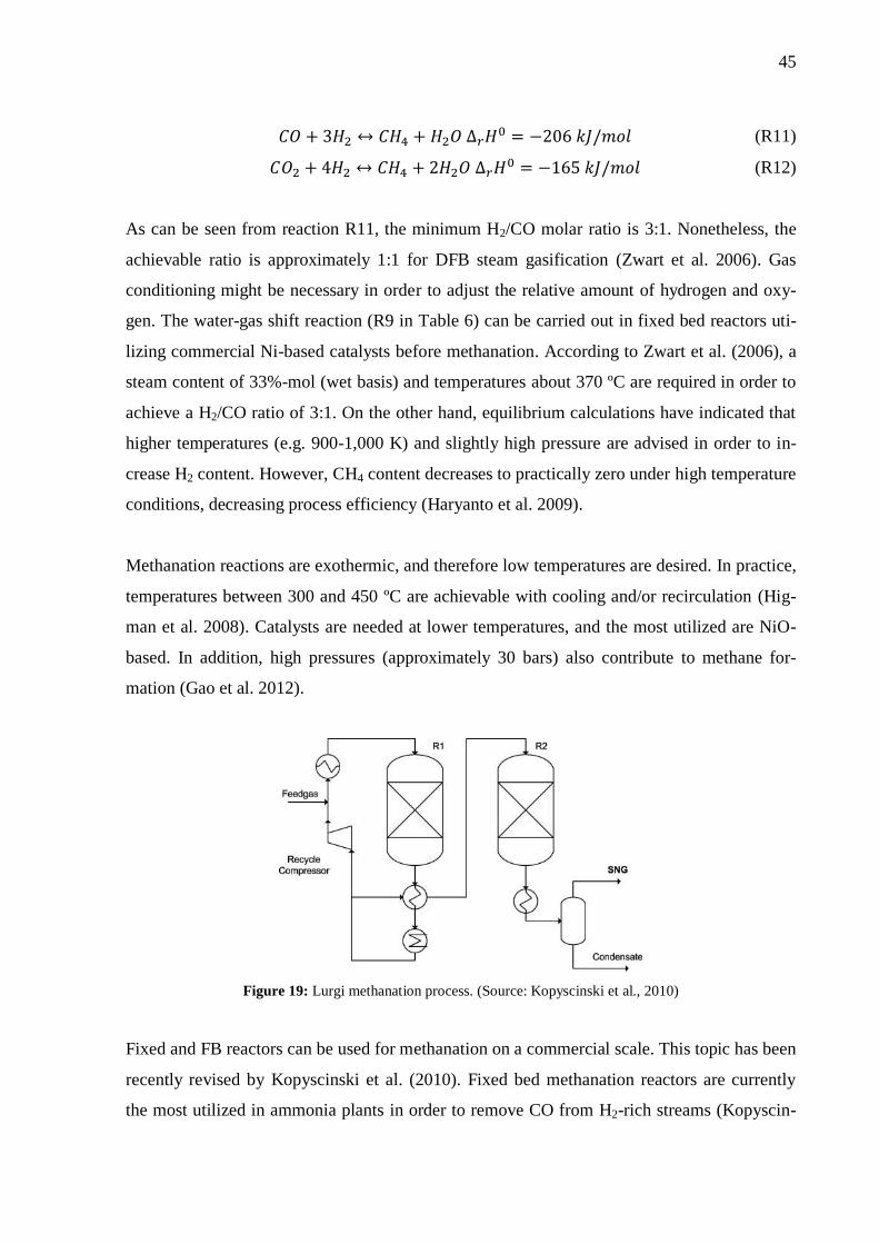
45
(R11)
(R12)
As can be seen from reaction R11, the minimum H2/CO molar ratio is 3:1. Nonetheless, the
achievable ratio is approximately 1:1 for DFB steam gasification (Zwart et al. 2006). Gas
conditioning might be necessary in order to adjust the relative amount of hydrogen and oxy-
gen. The water-gas shift reaction (R9 in Table 6) can be carried out in fixed bed reactors uti-
lizing commercial Ni-based catalysts before methanation. According to Zwart et al. (2006), a
steam content of 33%-mol (wet basis) and temperatures about 370 ºC are required in order to
achieve a H2/CO ratio of 3:1. On the other hand, equilibrium calculations have indicated that
higher temperatures (e.g. 900-1,000 K) and slightly high pressure are advised in order to in-
crease H2 content. However, CH4 content decreases to practically zero under high temperature
conditions, decreasing process efficiency (Haryanto et al. 2009).
Methanation reactions are exothermic, and therefore low temperatures are desired. In practice,
temperatures between 300 and 450 ºC are achievable with cooling and/or recirculation (Hig-
man et al. 2008). Catalysts are needed at lower temperatures, and the most utilized are NiO-
based. In addition, high pressures (approximately 30 bars) also contribute to methane for-
mation (Gao et al. 2012).
Figure 19: Lurgi methanation process. (Source: Kopyscinski et al., 2010)
Fixed and FB reactors can be used for methanation on a commercial scale. This topic has been
recently revised by Kopyscinski et al. (2010). Fixed bed methanation reactors are currently
the most utilized in ammonia plants in order to remove CO from H2-rich streams (Kopyscin-

46
ski et al. 2010). Lurgi’s methanation process (Figure 19) consists of two fixed bed adiabatic
reactors with internal recycle. Temperature range is between 250 and 400 ºC. The first (and
only) commercial coal-SNG plant in the USA utilizes this system.
The TREMPTM
(Topsøe’s Recycle Energy Efficient Methanation) technology is comprised of
three adiabatic fixed bed reactors with recirculation and intermediate cooling (Kopyscinski et
al. 2010). This process is shown in Figure 20. Methanation is performed at temperatures be-
tween 250 and 700 ºC and pressures up to 30 bars. High pressure superheated steam is a by-
product of this process.
Figure 20: TREMPTM
methanation process. (Source: Kopyscinski et al., 2010)
Other fixed bed methanation processes were also developed on commercial/semi-commercial
scales. For instance, HICOM process is able to perform gas conditioning and methanation in
the same unit, consisting of several adiabatic reactors (Kopyscinski et al. 2010). Linde’s
methanation process utilizes one isothermal indirect heated fixed bed and one adiabatic reac-
tor, but this concept is currently utilized for methanol synthesis. The RMP process does not
utilize gas recycling, comprising 4-6 reactors with intermediate gas cooling. Although it has
not reached commercial scale, ECN has proposed the utilization of a similar concept recently
(Zwart et al. 2006).
FB methanation has many advantages, for instance: improved mass and heat transfer, iso-
thermal operation, and easy catalyst handling. Although several projects have been developed
in the 60-70s, only the Thyssengas Comflux process (Figure 21) still seems promising for
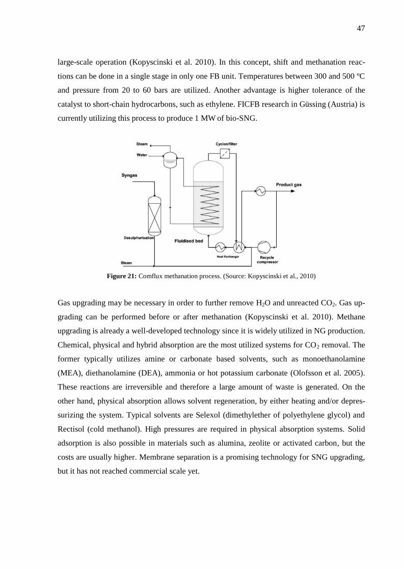
47
large-scale operation (Kopyscinski et al. 2010). In this concept, shift and methanation reac-
tions can be done in a single stage in only one FB unit. Temperatures between 300 and 500 ºC
and pressure from 20 to 60 bars are utilized. Another advantage is higher tolerance of the
catalyst to short-chain hydrocarbons, such as ethylene. FICFB research in Güssing (Austria) is
currently utilizing this process to produce 1 MW of bio-SNG.
Figure 21: Comflux methanation process. (Source: Kopyscinski et al., 2010)
Gas upgrading may be necessary in order to further remove H2O and unreacted CO2. Gas up-
grading can be performed before or after methanation (Kopyscinski et al. 2010). Methane
upgrading is already a well-developed technology since it is widely utilized in NG production.
Chemical, physical and hybrid absorption are the most utilized systems for CO2 removal. The
former typically utilizes amine or carbonate based solvents, such as monoethanolamine
(MEA), diethanolamine (DEA), ammonia or hot potassium carbonate (Olofsson et al. 2005).
These reactions are irreversible and therefore a large amount of waste is generated. On the
other hand, physical absorption allows solvent regeneration, by either heating and/or depres-
surizing the system. Typical solvents are Selexol (dimethylether of polyethylene glycol) and
Rectisol (cold methanol). High pressures are required in physical absorption systems. Solid
adsorption is also possible in materials such as alumina, zeolite or activated carbon, but the
costs are usually higher. Membrane separation is a promising technology for SNG upgrading,
but it has not reached commercial scale yet.

48
Although biomass conversion into bio-SGN is not yet commercially utilized, Gao et al. (2012)
estimate that at least 15 coal-to-SNG projects are being developed in the US and more than 20
are proposed or under construction in China.
3.9 State-of-the-art of Biomass Gasification
Many commercial biomass gasification plants are currently under operation, mainly in North-
ern Europe. The ten largest gasifiers in 2012 are outlined in Table 11, as well as their location,
purpose and fuel.
Table 11: Ten largest biomass gasification plants by 2012. (Data source: Vakkilainen et al., 2013)
No Company Purpose Location Fuel MWfuel
1 Lahti Energia CHP Lahti, Finland SRF 160
2 Vaskiluodon Voi-
ma CHP Vaasa, Finland
Local
biomass 140
3 Rüdersdorfer Ze-
ment Calciner
Rüdersdorf,
Germany
Biomass
waste 100
4 Essent CHP Geertruidenberg,
Netherlands Waste wood 85
5 Electrabel Boiler Ruien, Belgium Wood chips 50
6 Metsä Fibre Lime kiln Joutseno, Finland Bark 48
7 Södra Cell Värö Lime kiln Väro, Sweden Bark 35
8 Agnion
Technologies CHP
Pfaffenhofen,
Germany Waste wood 33
9 Corenso United CHP Varkaus, Finland Packaging 32
10 Skive
Fjernvarme CHP Skive, Denmark Wood pellets 32
The world’s largest gasifier is actually the number 3 on the list since the two first ones have
two identical units in parallel. Figure 22 and Figure 23 show schemes of the two first plants
on the list, which are both connected to steam boilers for combined heat and power (CHP)
production. (Palonen et al. 2005, Breitholtz 2001)

49
Figure 22: Kymijärvi II gasification process in Lahti, Finland. (Source: Palonen et al., 2005)
Figure 23: Vaskiluodon Voima biomass gasification plant. (Adapted from: Breitholtz, 2011)

50
4 CALCULATION METHODOLOGY
In this study, different gasification technologies are compared, focusing on their applications
in the iron ore pelletizing process. Mass and energy balances for the current case and several
alternative fuels are calculated. Adiabatic flame temperature and gas flows in preheating and
firing zones were considered as key technical parameters for this analysis. In this chapter, the
calculation methodology is described and the main model assumptions are explained.
4.1 Gas Balance
The gas balance is used to estimate average gas flows through the system, based on design
and plant data, under normal operating conditions. The third indurating machine’s gas balance
was calculated based on compilation of operating data. In situations which conflicting data
were found from different sources, those values shown by the gas flow schema were chosen.
The main assumptions made in this calculation were:
Firing and preheating zones were considered as a single control volume in which all
NG and combustion air are injected and all fuel (solid and gas) is burnt;
Combustion of NG and solid fuel is considered to occur uniformly inside the control
volume, according to the following chemical reactions:
(4)
(5)
(6)
(7)
(8)
(9)
All gases involved were considered to be ideal, therefore following the equation of
state below. This assumption allows streams measured in normal cubic meters (Nm3)
to be simply summed or subtracted. Nonetheless, it is known that after combustion
the total number of moles in the gas phase changes due to the reactions represented
by Equations 5, 6 and 8. Therefore, the gas flow in Nm3 in the kiln hood (above the
grate) is not necessarily equal to the flow underneath the grate (in the wind boxes);
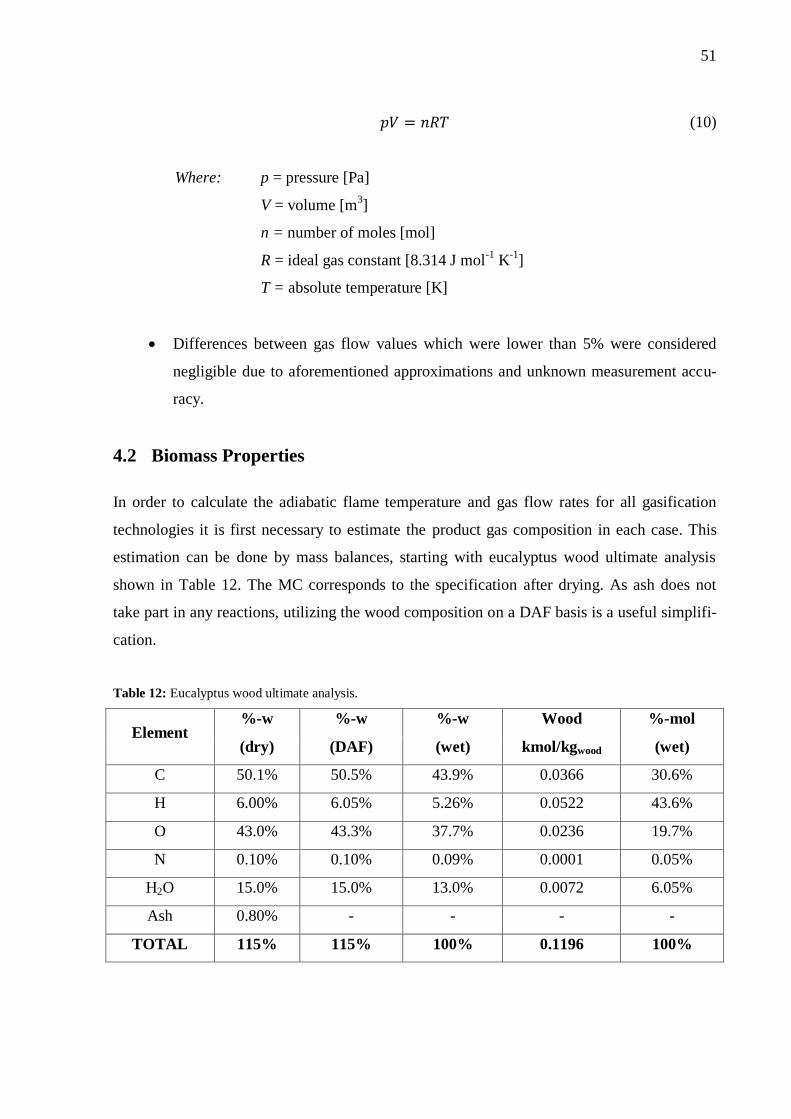
51
(10)
Where: p = pressure [Pa]
V = volume [m3]
n = number of moles [mol]
R = ideal gas constant [8.314 J mol-1
K-1
]
T = absolute temperature [K]
Differences between gas flow values which were lower than 5% were considered
negligible due to aforementioned approximations and unknown measurement accu-
racy.
4.2 Biomass Properties
In order to calculate the adiabatic flame temperature and gas flow rates for all gasification
technologies it is first necessary to estimate the product gas composition in each case. This
estimation can be done by mass balances, starting with eucalyptus wood ultimate analysis
shown in Table 12. The MC corresponds to the specification after drying. As ash does not
take part in any reactions, utilizing the wood composition on a DAF basis is a useful simplifi-
cation.
Table 12: Eucalyptus wood ultimate analysis.
Element %-w %-w %-w Wood %-mol
(dry) (DAF) (wet) kmol/kgwood (wet)
C 50.1% 50.5% 43.9% 0.0366 30.6%
H 6.00% 6.05% 5.26% 0.0522 43.6%
O 43.0% 43.3% 37.7% 0.0236 19.7%
N 0.10% 0.10% 0.09% 0.0001 0.05%
H2O 15.0% 15.0% 13.0% 0.0072 6.05%
Ash 0.80% - - - -
TOTAL 115% 115% 100% 0.1196 100%
52
Wood’s high heating value (HHV), in MJ kg-1
, was calculated based on a unified correlation
represented by Equation 11 (Channiwala et al. 2002). LHV on a dry basis and wet basis (15%
MC) were calculated according to Equations 12 and 13, accordingly.
(11)
Where: %C = carbon content, dry basis [%-w]
%H = hydrogen content, dry basis [%-w]
%S = sulfur content, dry basis [%-w]
%O = oxygen content, dry basis [%-w]
%N = nitrogen content, dry basis [%-w]
%A = ash content, dry basis [%-w]
(
)
(12)
(13)
Where: w = mass fraction, dry basis [-]
4.3 Fuel Composition and Properties Estimation
Several types of fuels were evaluated in this study, such as NG, producer gases from different
gasification processes, bio-SNG, coal, petcoke, and a gas/solid blend, which was considered
as the final fuel fed into the traveling grate. Each fuel composition calculation and properties
estimation is discussed separately.
4.3.1 NG
Average dry NG in Brazil was considered to contain methane, ethane, propane, carbon diox-
ide and nitrogen (COMPAGAS n.d.). Other hydrocarbons might also be present (e.g. butane
and pentane), but their amount was considered negligible. NG composition, as well as each
component’s chemical properties is shown in Table 13.

53
Table 13: NG composition (COMPAGAS n.d.) and component’s properties.
Component %-mol MM Mass Molar V %-vol
(wet) kg/kmolgas kg/kmolgas Nm3/kmolgas (wet)
CH4 89.1% 14.29 79.1% 19.94 89.2%
C2H6 5.90% 1.774 9.81% 1.308 5.85%
C3H8 2.90% 1.279 7.07% 0.6362 2.85%
CO2 0.90% 0.396 2.19% 0.2004 0.90%
N2 1.20% 0.336 1.86% 0.2688 1.20%
H2O 0.00% 0.000 0.00% 0.000 0.00%
TOTAL 100% 18.08 100% 22.36 100%
NG’s LHV is estimated based on the standard enthalpy of combustion of each combustible
component at 298.15 K and 1 atm. The net energy content in the gaseous mixtures is therefore
defined by:
∑ (14)
Where: yi = molar fraction of component i, wet basis [-]
ΔcH0 = standard enthalpy of combustion [J mol
-1]
Other properties, such as MM [kg kmol-1
] and molar volume [Nm3 kmol
-1], can also be de-
termined similarly to Equation 14, substituting the LHV by the property of interest:
∑ (15)
∑ (16)
Where: = molar volume [Nm3 kmol
-1]
4.3.2 Solid Blend
Coal and petcoke are the main solid fuels added to the green pellets. According to the third
indurating machine’s average consumption, approximately 33%-w corresponds to the former,

54
while the remaining 67%-w to the latter. LHV and MC remain as shown in Table 2, resulting
in an energy content of 33.1 MJ kg-1
(297 MJ kmol-1
) for this solid blend. Typical ultimate
analysis for coal and petcoke (Fermoso et al. 2009) as well as the final solid fuel composition
is shown in Table 14.
Table 14: Solid fuel composition.
Element Coal Petcoke Solid Solid Solid Solid
%-wDAF %-wDAF %-wDAF %-wwet kmol/kgsolid %-mol
C 71.2% 87.6% 82.2% 74.7% 0.0622 56.0%
H 4.80% 3.80% 4.13% 3.75% 0.0372 33.5%
O 20.8% 0.90% 7.47% 6.79% 0.0042 3.82%
N 1.50% 1.50% 1.50% 1.36% 0.0010 0.88%
S 1.70% 6.20% 4.72% 4.29% 0.0013 1.20%
H2O 10.0% 10.0% 10.0% 9.09% 0.0050 4.54%
TOTAL 110% 110% 110% 100% 0.1111 100%
4.3.3 Air/Oxygen Gasification Product Gas Composition
In air or oxygen gasification, the biomass is partially combusted in order to provide sufficient
heat for endothermic gasification reactions. Therefore, the amount of O2 fed into the gasifier
must be estimated. The ER, defined by Equation 1, is the ratio between actual and theoretical
amount of O2 necessary for complete combustion. Based on the eucalyptus elemental compo-
sition shown in Table 12, the theoretical oxygen required for complete combustion is deter-
mined considering that only carbon and hydrogen are oxidized. The oxygen present in the
wood accounts negatively. Thus, the stoichiometric amount of oxygen per kilogram of wood
is given by:
(17)
For air gasification, the stoichiometric air must be determined based on predefined properties.
Ambient air entering the gasifier was considered to be at 25 °C, sea level pressure (101,325
Pa) and 60% of relative humidity (RH). Its MC can be calculated based on the RH:

55
(18)
Where: pH2O = water partial pressure in atmosphere [Pa]
psat = saturation pressure of water at 25 °C [Pa]
The water saturation pressure at 25 °C can be evaluated utilizing water/steam tables, and it is
approximately 1,902 Pa. According to Raoult’s Law, the water molar fraction in air equals the
ratio between water partial pressure and atmospheric pressure (patm), as follows:
(19)
Assuming that dry air contains 21%-mol of oxygen and 79%-mol of nitrogen, O2 and N2 per-
centages on wet basis are estimated considering the number of water moles (nH2O) present in 1
mol of wet air, as shown by Equations 20 to 22:
(20)
(21)
(22)
Air gasifier inlet composition considers the sum of all wood and wet air components. For in-
stance, no carbon and hydrogen enter with air; therefore, these quantities remain the same
(e.g. the carbon input in the gasifier equals the amount of carbon in the wood). However, ox-
ygen, nitrogen and water coming from air must be added. For this purpose, wood and air
compositions, as well as the ER are utilized, as follows:
(23)
(
) (24)
56
(
) (25)
Similar equations were adopted for oxygen gasification. Nevertheless, a mixture of 95% O2
and 5% N2 was considered as the gasifying media. In addition, some steam might be added in
the riser in order to control the temperature. The amount of steam is represented by the steam
oxygen ratio (SOR), which is defined as the mass of steam added per kilogram of oxygen (van
der Meijden et al. 2010). In this case, the gasifier input is calculated as follows:
(26)
(
)
(27)
(
)
(28)
The product gas was considered to be a mixture of CH4, CO2, CO, H2, N2 and H2O for all gas-
ification technologies. Short-chain hydrocarbons, such as ethane, might also be formed; how-
ever, their amount was considered negligible. Mass balances relating the gasifier inlet, in
terms of C, H, O, N and H2O, to the product gas composition are presented below. Firstly,
carbon balance must contemplate CH4, CO2 and CO amounts discounting any unconverted
carbon withdrawn with the ashes:
(29)
Where: CC = carbon conversion [%]
Hydrogen balance takes into account that it is transformed into CH4, H2 and also H2O. In ad-
dition, some water is also fed into the system, and this value should be subtracted, as follows:
(30)

57
Oxygen fed into the system completely reacts with C and H, forming CO2, CO and H2O. As
occurred in Equation 30, the water input must also be subtracted. Finally, nitrogen balance is
the simplest one since all N was considered to form N2:
(31)
(32)
The amount of water in the product gas equals to the water input, plus water formed by hy-
drogen oxidation minus water consumed by gasification reactions (refer to reactions R2, R9
and R13 from Table 6). The water balance is based on oxygen and hydrogen balances; for
instance, the unreacted oxygen (after carbon reactions) must combine with hydrogen to form
water, as no oxygen shall remain in the product gas. At this point, it should be noted that the
water balance is a linear combination of oxygen and hydrogen balances. As a result, there are
four independent mass balances (Equations 29 to 32) and six unknown variables, correspond-
ing to the amount of each component in the product gas. In order to decrease the problem’s
degree of freedom and find a solution, it is necessary to introduce two other restricting equali-
ties.
Firstly, it is known that the CO/CO2 ratio is a function of temperature. For example, a fre-
quently used expression gives this ratio as a function of char surface temperature (Arthur
1951, cited in Basu 2010, p. 126):
(
) (33)
Where: θ = temperature [°C]
Methane molar fraction in the product gas (dry basis) was also specified. According to several
studies, methane formation is difficult to predict utilizing simple gasification models, such as
those based on equilibrium constants or Gibbs free energy (Baratieri et al. 2008, Puig-Arnavat
et al. 2010). Typical methane concentrations within the ranges presented in Table 7 were test-
ed, and the chosen value corresponds to that one resulting in better agreement with the other
compounds’ concentrations. For example, the acceptable range for methane concentration in
58
air gasification product gas is between 2 and 6%-mol on a dry basis. Several values were test-
ed within this range, and finally the CH4 concentration was set as 4.70%, which makes the
other component’s concentrations to be as close as possible to the typical values when the
mass balance is closed. Since the methane molar fraction is given on a dry basis, the total
number of moles is unknown; thus, an iterative procedure is necessary in order to determine
wet basis molar fraction.
Once all required parameters were specified, the system of equations can be solved. CO2 and
CO amounts were calculated by solving Equations 29 and 33 simultaneously, in which the
char surface temperature was considered to be equal to the gasifier average temperature. The
results were then used in Equation 31, from which the amount of water in the product gas was
determined. Finally, H2 and N2 amounts are found through Equations 30 and 32, respectively.
A new CH4 number of moles must be introduced if its molar fraction on a dry basis is differ-
ent from the value established. The calculation procedure starts over, until conversion is
reached. Excel goal seek tool was utilized in this case. LHV of product gas was estimated by
Equation 14, considering CH4, CO and H2 as combustibles. MM and molar volume were also
determined by similar equations.
4.3.4 Steam Gasification Product Gas Composition
In steam gasifiers, fuel biomass and steam are fed into the system and heat is provided indi-
rectly; for example, by circulating bed material from a combustion chamber. Therefore, the
input composition is the sum of elements present in wood and water, which is given by the SB
ratio (Equation 2). The SB ratio is often expressed in terms of total mass of water (including
biomass MC) per kilogram of wood on a DAF basis; the water input can be found by convert-
ing the SB into kmol per kilogram of wet wood according to the following equation:
( )
(34)
At this point, CC has to be set. In this case, the value is much lower than for air/oxygen gasi-
fication, based on the premise that part of the char is burnt in the combustion zone in order to
provide energy to gasification reactions. Contrary to air or oxygen gasification, the combus-
tion products and nitrogen do not mix with the product gas. Thus, the burnt char must be sub-

59
tracted from the mass balance in order to obtain an accurate product gas composition. Van der
Meijden (2010) proposed a relation between CC and gasifier temperature for allothemal sys-
tems:
(35)
Once the gasifier input and CC are defined, the product gas composition can be determined.
Equations 29 to 33 and corresponding assumptions were also adopted. Methane content on a
dry basis was fixed in 11%, and the iteration follows the same procedure. The product gas
LHV was estimated by Equation 14, considering CH4, CO and H2 as combustibles. MM and
molar volume were determined by Equations 15 and 16.
4.3.5 Bio-SNG Composition
In order to estimate the bio-SNG composition, a chemical equilibrium approach was utilized.
Only water-gas shift (R9) and methanation reactions R11 and R12 were considered to occur.
Equilibrium constants at a fixed temperature (T) and 101,325 Pa were calculated as follows
(Moran et al. 2006):
(36)
Where: k = equilibrium constant at T and 1 atm
ΔrG0 = Gibbs free energy change of reaction [J mol
-1 K
-1]
The standard Gibbs free energy change for each reaction can be calculated utilizing pure spe-
cies enthalpies and entropies. As entropy and enthalpy are functions of state, their variation
always equals the difference between products and reactants:
∑
(37)
∑
(38)
Where: νi = stoichiometric number [-]
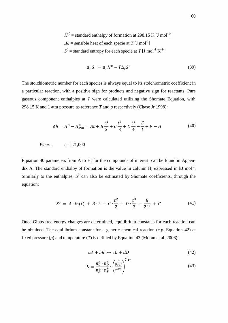
60
Hf0 = standard enthalpy of formation at 298.15 K [J mol
-1]
Δh = sensible heat of each specie at T [J mol-1
]
S0 = standard entropy for each specie at T [J mol
-1 K
-1]
(39)
The stoichiometric number for each species is always equal to its stoichiometric coefficient in
a particular reaction, with a positive sign for products and negative sign for reactants. Pure
gaseous component enthalpies at T were calculated utilizing the Shomate Equation, with
298.15 K and 1 atm pressure as reference T and p respectively (Chase Jr 1998):
(40)
Where: t = T/1,000
Equation 40 parameters from A to H, for the compounds of interest, can be found in Appen-
dix A. The standard enthalpy of formation is the value in column H, expressed in kJ mol-1
.
Similarly to the enthalpies, S0 can also be estimated by Shomate coefficients, through the
equation:
(41)
Once Gibbs free energy changes are determined, equilibrium constants for each reaction can
be obtained. The equilibrium constant for a generic chemical reaction (e.g. Equation 42) at
fixed pressure (p) and temperature (T) is defined by Equation 43 (Moran et al. 2006):
(42)
(
)
∑
(43)

61
Where: ∑
neq
= number of moles in the equilibrium [kmol kmolgas-1
]
Applying this definition to reactions R9, R11 and R12, Equations 45, 47 and 49 are obtained,
respectively. However, three equations are written for five variables. Therefore, it is necessary
to write the number of moles in the equilibrium in terms of the variables x, y and z, introduced
in Equations 44, 46 and 48, respectively.
(44)
(45)
(46)
(
)
(47)
(48)
(
)
(49)
The number of moles of each species when chemical equilibrium is reached can be written as
a function of initial amounts in steam gasification product gas and the variables x, y and z.
These relations are written below. As can be seen from Equation 54, water might be added to
the reactor inlet in order to avoid soot formation.
(50)
(51)
(52)
(53)
(54)
(55)

62
Where: nreactor
= water added to the reactor [kmol kmolgas-1
]
Substituting the expressions above in Equations 45, 47 and 49, a system of three equations
and three variables can be solved. Once variables x, y and z are determined, the equilibrium
composition in the methanation reactor outlet can be found. After methanation, the gas is
cooled to 25 °C and water is removed. The final water molar fraction can be estimated based
on the saturation pressure at 25 °C and Equation 19. Carbon dioxide is further removed by
absorption. During this process, some methane may be lost. CH4 and CO2 amounts are ex-
pressed as:
(56)
Where: ηCH4 = methane removal efficiency [-]
(57)
Where: ηCO2 = CO2 removal efficiency [-]
As previously, bio-SNG’s LHV was estimated by Equation 14, considering CH4, CO and H2
as the only combustible compounds. MM and molar volume were also determined by similar
equations.
4.3.6 Combined Gas and Solid Composition
Gaseous and solid fuels are utilized in the pelletizing kiln. In order to simplify the calculation
of stoichiometric oxygen required for complete combustion, the elemental composition (in
terms of C, H, O, N, S and H2O) of both gaseous and solid fuels were combined, and the final
fuel (gas + solid) composition and its combustion properties were determined. The calculation
basis was chosen to be 1 GJ of fuel. Thus, the elemental composition for NG is given by:
(58)

63
Where: N = number of moles per GJ of fuel [kmol GJ-1
]
(59)
(60)
(61)
(62)
On the other hand, product gas and bio-SNG are considered to contain only CH4, CO, CO2,
H2, N2 and H2O. Although Equations 61 and 62 remain the same, the elemental composition
for C, H and O is determined by the following equations:
(63)
(64)
(65)
Similarly, the solid elemental composition, in kmol GJ-1
, can be determined by dividing the
amount of each element (in kmol kg-1
) by its LHV in GJ kg-1
. The final fuel composition, as
well as its LHV, is obtained by the weighted average:
(66)
(67)
Where: Φgas = energy provided by gaseous fuel [MW]
Φsolid = energy provided by solid fuel [MW]
Φth = total thermal energy input [MW]
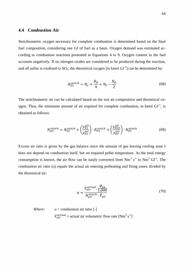
64
4.4 Combustion Air
Stoichiometric oxygen necessary for complete combustion is determined based on the final
fuel composition, considering one GJ of fuel as a basis. Oxygen demand was estimated ac-
cording to combustion reactions presented in Equations 4 to 9. Oxygen content in the fuel
accounts negatively. If no nitrogen oxides are considered to be produced during the reaction,
and all sulfur is oxidized to SO2, the theoretical oxygen (in kmol GJ-1
) can be determined by:
(68)
The stoichiometric air can be calculated based on the wet air composition and theoretical ox-
ygen. Thus, the minimum amount of air required for complete combustion, in kmol GJ-1
, is
obtained as follows:
(
) (
) (69)
Excess air ratio is given by the gas balance since the amount of gas leaving cooling zone I
does not depend on combustion itself, but on required pellet temperature. As the total energy
consumption is known, the air flow can be easily converted from Nm3 s
-1 to Nm
3 GJ
-1. The
combustion air ratio (α) equals the actual air entering preheating and firing zones divided by
the theoretical air:
(70)
Where: α = combustion air ratio [-]
= actual air volumetric flow rate [Nm
3 s
-1]

65
4.5 Flue Gas Composition
In order to estimate the flue gas composition, complete combustion is considered and the only
species present in flue gas are CO2, N2, O2, SO2 and H2O. The amount of water in flue gas is
the sum of the water present in the gaseous and solid fuels, air moisture and the water formed
by hydrogen oxidation during combustion. One approximation made was that the solid fuel is
practically not dried in the updraft and downdraft drying zones. The total nitrogen is provided
by combustion air and nitrogen content in the fuel. Oxygen corresponds to the amount re-
maining after combustion due to excess. Thus:
(71)
(72)
(73)
(74)
(75)
Once the number of moles of each flue gas’ component per GJ of fuel is determined, their
molar fraction on a wet basis can be calculated. Flue gas properties, such as MM and molar
volume, are estimate based on Equations 15 and 16.
4.6 Adiabatic Flame Temperature
The adiabatic flame temperature is the hypothetical temperature that exhaust gases would
achieve if no energy is lost. Thus, the energy balance is calculated when no other heat output
than the flue gas is present. Incoming energy streams are: preheated air from cooling zone I,
energy provided by fuel combustion and gas sensible heat. Solid sensible heat is considered
negligible. Net calorific values can directly substitute the enthalpies of combustion. Equation
76 shows the energy balance:
(76)
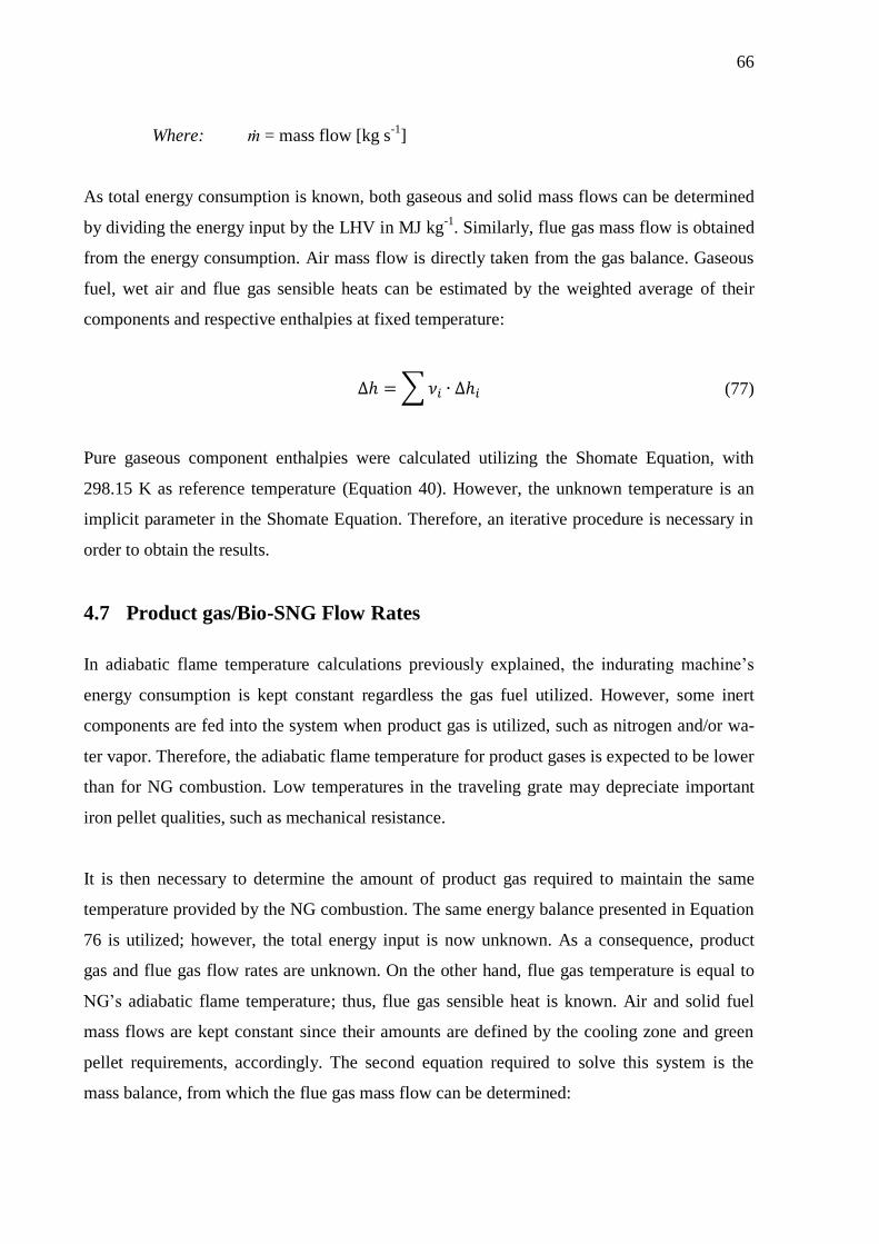
66
Where: ṁ = mass flow [kg s-1
]
As total energy consumption is known, both gaseous and solid mass flows can be determined
by dividing the energy input by the LHV in MJ kg-1
. Similarly, flue gas mass flow is obtained
from the energy consumption. Air mass flow is directly taken from the gas balance. Gaseous
fuel, wet air and flue gas sensible heats can be estimated by the weighted average of their
components and respective enthalpies at fixed temperature:
∑ (77)
Pure gaseous component enthalpies were calculated utilizing the Shomate Equation, with
298.15 K as reference temperature (Equation 40). However, the unknown temperature is an
implicit parameter in the Shomate Equation. Therefore, an iterative procedure is necessary in
order to obtain the results.
4.7 Product gas/Bio-SNG Flow Rates
In adiabatic flame temperature calculations previously explained, the indurating machine’s
energy consumption is kept constant regardless the gas fuel utilized. However, some inert
components are fed into the system when product gas is utilized, such as nitrogen and/or wa-
ter vapor. Therefore, the adiabatic flame temperature for product gases is expected to be lower
than for NG combustion. Low temperatures in the traveling grate may depreciate important
iron pellet qualities, such as mechanical resistance.
It is then necessary to determine the amount of product gas required to maintain the same
temperature provided by the NG combustion. The same energy balance presented in Equation
76 is utilized; however, the total energy input is now unknown. As a consequence, product
gas and flue gas flow rates are unknown. On the other hand, flue gas temperature is equal to
NG’s adiabatic flame temperature; thus, flue gas sensible heat is known. Air and solid fuel
mass flows are kept constant since their amounts are defined by the cooling zone and green
pellet requirements, accordingly. The second equation required to solve this system is the
mass balance, from which the flue gas mass flow can be determined:

67
(78)
Flue gas composition and properties depend on energy consumption; thus, an iterative proce-
dure is necessary in order to close these balances. An initial value for product gas mass flow
is given, from which the total energy consumption and the percentage correspondent to gas
and solid fuel is calculated. Once the energy consumption and proportions are known, flue gas
composition and properties can be determined. Product gas mass flow is changed until the
system converges. Goal seek tool was utilized in this case.
4.8 Biomass Demand
Biomass demand was determined based on the gas flow, in kmol s-1
, for constant temperature.
The amount of wood necessary can be obtained simply by dividing the gas flow by the total
number of moles in the gas per kilogram of wood. The result, expressed in kg of wood per
second, does not include ash, carbon or energy losses. When everything is considered, the
total amount of wood necessary is given by:
[
∑
] (
) (79)
Where: = total number of moles in the gas [kmol kgwood-1
]
L = estimated energy loss [%]
For each gasification technology, the amount of wet biomass, planted area and total area re-
quired were estimated, assuming the following data:
Eucalyptus productivity of 113 wet (56 dry) tons (with bark) per hectare after 5 years1
in other words, the total area required corresponds to five times the annual area;
All harvested biomass is utilized for energy purposes;
Losses in comminution operation are negligible;
1 Studies suggest that this value is quite conservative for Brazil, and it is possible to achieve 96 t ha
-1 (dry) in 5
years with 3x3 m spacing. Refer to QUÉNO, Laurent M. R., et al. Custo de produção das biomassas de eucalip-
to e capim elefante para energia. pp. 417-426.
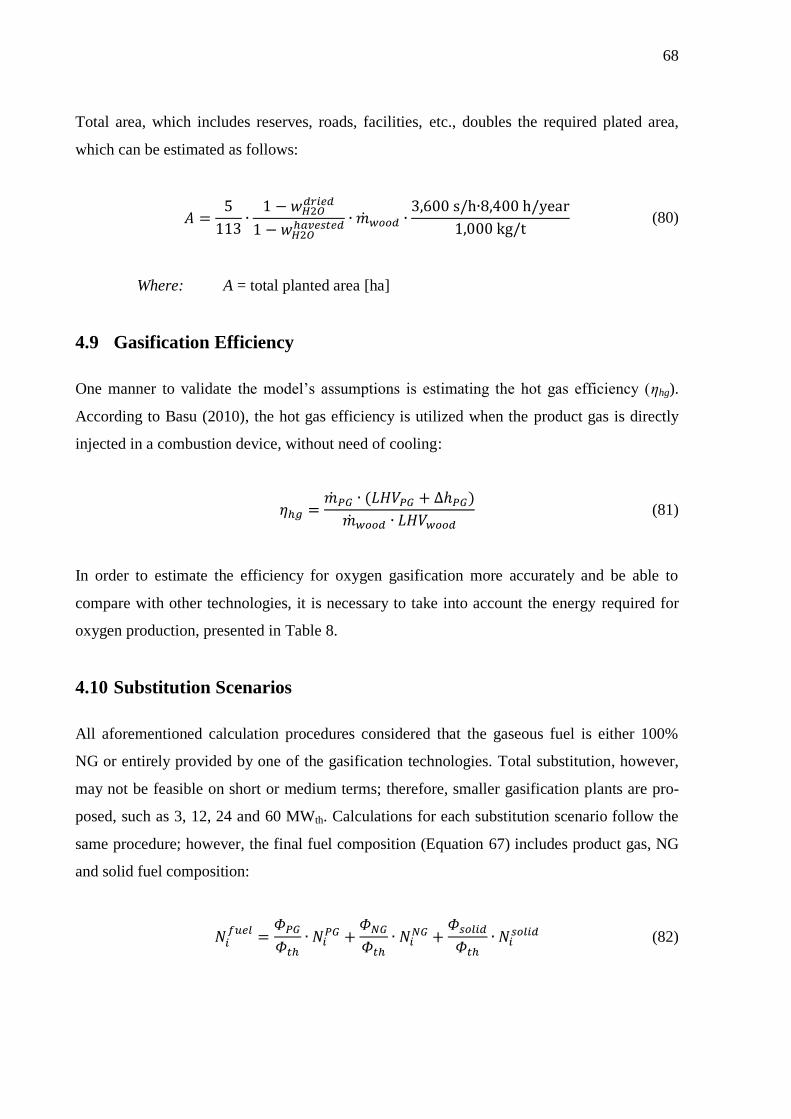
68
Total area, which includes reserves, roads, facilities, etc., doubles the required plated area,
which can be estimated as follows:
(80)
Where: A = total planted area [ha]
4.9 Gasification Efficiency
One manner to validate the model’s assumptions is estimating the hot gas efficiency (ηhg).
According to Basu (2010), the hot gas efficiency is utilized when the product gas is directly
injected in a combustion device, without need of cooling:
(81)
In order to estimate the efficiency for oxygen gasification more accurately and be able to
compare with other technologies, it is necessary to take into account the energy required for
oxygen production, presented in Table 8.
4.10 Substitution Scenarios
All aforementioned calculation procedures considered that the gaseous fuel is either 100%
NG or entirely provided by one of the gasification technologies. Total substitution, however,
may not be feasible on short or medium terms; therefore, smaller gasification plants are pro-
posed, such as 3, 12, 24 and 60 MWth. Calculations for each substitution scenario follow the
same procedure; however, the final fuel composition (Equation 67) includes product gas, NG
and solid fuel composition:
(82)
69
4.11 Economical Evaluation Approach
The project’s economical evaluation is an important parameter to compare different gasifica-
tion technologies and support decision making process. As a preliminary assessment, the
numbers presented here are based on basic design information and values available in the lit-
erature. Therefore, this analysis should be regarded only as an order of magnitude estimate
and the actual prices may vary within ± 30-50% (Towler et al. 2012).
4.11.1 Investment Costs
The total investment is divided into total direct (TDC) and indirect costs (TIC). Direct costs
mainly concern equipment purchase prices, installation and construction. These costs were
based on values or correlations available in the literature. Biomass harvesting and chipping
are out of the scope. Only the main equipment and installations were considered in this evalu-
ation, divided in the following groups:
Biomass pretreatment: includes wet wood chip handling and storage (H&S), drying
operation and conveying after drying;
Gasification: includes pre-feeding H&S, biomass feeding system, CFB gasifier, com-
bustion reactor (for steam gasification and bio-SNG only), bed material and ash H&S,
and heat exchangers (for dry product gas from steam gasification only);
Gasifying media supply: includes air compressor, ASU (for oxygen) or steam genera-
tor, depending on the gasification technology;
Methanation: includes gas conditioning system, methanation reactor and raw SNG up-
grading, for bio-SNG production only;
Other inside battery limits (ISBL): includes nitrogen supply for instrumentation and
safety equipment, as well as equipment installation costs (mainly labor);
Other direct costs: include civil works and foundations, buildings, piping, automation,
electrification and instrumentation (AEI), insulation and painting works.
In many cases, costs for equipment of other sizes than those presented in this study were
found. In such cases, the cost curve method was utilized, with an exponential factor of 0.7
(Towler et al. 2012):
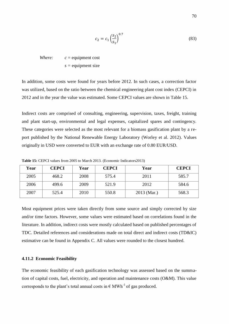
70
(
)
(83)
Where: c = equipment cost
s = equipment size
In addition, some costs were found for years before 2012. In such cases, a correction factor
was utilized, based on the ratio between the chemical engineering plant cost index (CEPCI) in
2012 and in the year the value was estimated. Some CEPCI values are shown in Table 15.
Indirect costs are comprised of consulting, engineering, supervision, taxes, freight, training
and plant start-up, environmental and legal expenses, capitalized spares and contingency.
These categories were selected as the most relevant for a biomass gasification plant by a re-
port published by the National Renewable Energy Laboratory (Worley et al. 2012). Values
originally in USD were converted to EUR with an exchange rate of 0.80 EUR/USD.
Table 15: CEPCI values from 2005 to March 2013. (Economic Indicators2013)
Year CEPCI Year CEPCI Year CEPCI
2005 468.2 2008 575.4 2011 585.7
2006 499.6 2009 521.9 2012 584.6
2007 525.4 2010 550.8 2013 (Mar.) 568.3
Most equipment prices were taken directly from some source and simply corrected by size
and/or time factors. However, some values were estimated based on correlations found in the
literature. In addition, indirect costs were mostly calculated based on published percentages of
TDC. Detailed references and considerations made on total direct and indirect costs (TD&IC)
estimative can be found in Appendix C. All values were rounded to the closest hundred.
4.11.2 Economic Feasibility
The economic feasibility of each gasification technology was assessed based on the summa-
tion of capital costs, fuel, electricity, and operation and maintenance costs (O&M). This value
corresponds to the plant’s total annual costs in € MWh-1
of gas produced.
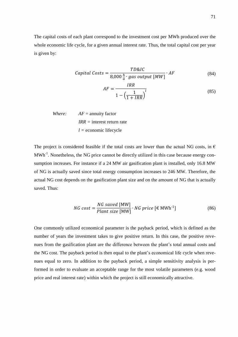
71
The capital costs of each plant correspond to the investment cost per MWh produced over the
whole economic life cycle, for a given annual interest rate. Thus, the total capital cost per year
is given by:
(84)
(
) (85)
Where: AF = annuity factor
IRR = interest return rate
l = economic lifecycle
The project is considered feasible if the total costs are lower than the actual NG costs, in €
MWh-1
. Nonetheless, the NG price cannot be directly utilized in this case because energy con-
sumption increases. For instance if a 24 MW air gasification plant is installed, only 16.8 MW
of NG is actually saved since total energy consumption increases to 246 MW. Therefore, the
actual NG cost depends on the gasification plant size and on the amount of NG that is actually
saved. Thus:
(86)
One commonly utilized economical parameter is the payback period, which is defined as the
number of years the investment takes to give positive return. In this case, the positive reve-
nues from the gasification plant are the difference between the plant’s total annual costs and
the NG cost. The payback period is then equal to the plant’s economical life cycle when reve-
nues equal to zero. In addition to the payback period, a simple sensitivity analysis is per-
formed in order to evaluate an acceptable range for the most volatile parameters (e.g. wood
price and real interest rate) within which the project is still economically attractive.

72
5 RESULTS AND DISCUSSION
In this chapter, calculation results are presented and discussed. Firstly, the indurating ma-
chine’s energy consumption and gas balance were evaluated based on operating data. NG
combustion parameters, such as adiabatic flame temperature and gas flows were determined
based on the methodology presented previously. In the sequence, each gasification technology
is compared with NG values, focusing on the main impacts the use of product gas can have in
the traveling grate. Finally, different substitution scenarios are discussed.
5.1 Indurating Machine’s Energy Consumption
As stated earlier, only the third indurating machine presented is considered in this study. In
order to assess its energy consumption, monthly fuel input data were utilized. The total ther-
mal power required was estimated considering an average of 8,400 operation hours and a pro-
duction of 8.4 Mt of iron pellets per year. The average energy consumption of each fuel, as
well as the corresponding percentages, is shown in Table 16.
Table 16: Energy consumption in the indurating machine considered for calculations.
Source Energy Consumption Percentage
[%] GJ/t Mcal/t MWth
Coal 0.165 29.7 34.6 14%
Petcoke 0.294 79.2 92.1 39%
Total Solid 0.458 109 127 53%
Heavy oil 0.000 0.06 0.08 0.0%
Natural gas 0.405 96.6 112 47%
Total burners 0.405 96.7 112 47%
Total thermal 0.863 206 239 100%
As can be seen from Table 16, at least 112 MWth are required if all NG is to be substituted by
renewable resources. The third indurating machine has a total of 46 burners, from which 42
are used under normal operating conditions. As a result, each burner represents an energy load
of approximately 2.67 MWth, usually provided by NG. This corresponds to a total of 173 Nm3
min-1
of NG or 4.12 Nm3 min
-1 per burner.
73
It is important to highlight that the use of product gas causes injection of considerable
amounts of inert substances in the kiln. Consequently, the thermal input would have to be
increased to prevent temperature decrease.
5.2 Gas Balance
The gas balance was calculated based on operating data, under assumptions addressed in
Chapter 4. The most important value taken from the gas balance is the air flow in preheating
and firing zones. Total gas flow entering the control volume was estimated at 22,240 Nm3
min-1
, including air and NG. In fact, the amount of NG appears to be negligible; however, as it
can be easily evaluated, it is subtracted in all cases in order to accurately estimate the actual
air input. NG flow rate depends on the kiln energy consumption, which was considered to be
the current average (239 MW), from which 112 MW corresponds to NG. As a result, it is es-
timated that 22,067 Nm3 min
-1 or 368 Nm
3 s
-1 of air flows through the control volume.
5.3 NG and Solid Fuel Combustion
NG composition was shown in Table 13. As can be seen from this table, combustibles in NG
are only methane (CH4), ethane (C2H6) and propane (C3H8). Their standard enthalpies of
combustion are 803 kJ mol-1
, 1,560 kJ mol-1
and 2,220 kJ mol-1
respectively. Utilizing Equa-
tion 14, the LHV was estimated at approximately 872 MJ kmol-1
of NG or 39.0 MJ Nm-3
.
According to the third indurating machine’s energy consumption, 47% of the total energy in
the preheating and firing zones is provided by NG and the remaining 53% by the solid blend.
Following Equation 67, the final fuel (solid + gas) LHV was estimated at 568 MJ kmol-1
or
40.2 MJ kg-1
. Considering the solid fuel properties shown in Table 14 and Equations 58 to 62,
the final fuel composition was determined. In the sequence, the stoichiometric amount of ox-
ygen was calculated, utilizing Equation 68. Table 17 shows the results per GJ of fuel.
Wet air composition was determined based on Equations 18 to 22. The results, as well as
some basic properties of wet air (obtained from Equations 15 and 16) are presented in Table
18. These results were combined in Equation 69, from which the amount of stoichiometric
wet air is obtained.
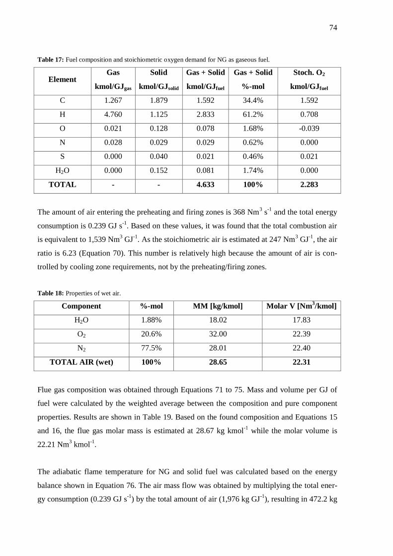
74
Table 17: Fuel composition and stoichiometric oxygen demand for NG as gaseous fuel.
Element Gas Solid Gas + Solid Gas + Solid Stoch. O2
kmol/GJgas kmol/GJsolid kmol/GJfuel %-mol kmol/GJfuel
C 1.267 1.879 1.592 34.4% 1.592
H 4.760 1.125 2.833 61.2% 0.708
O 0.021 0.128 0.078 1.68% -0.039
N 0.028 0.029 0.029 0.62% 0.000
S 0.000 0.040 0.021 0.46% 0.021
H2O 0.000 0.152 0.081 1.74% 0.000
TOTAL - - 4.633 100% 2.283
The amount of air entering the preheating and firing zones is 368 Nm3 s
-1 and the total energy
consumption is 0.239 GJ s-1
. Based on these values, it was found that the total combustion air
is equivalent to 1,539 Nm3 GJ
-1. As the stoichiometric air is estimated at 247 Nm
3 GJ
-1, the air
ratio is 6.23 (Equation 70). This number is relatively high because the amount of air is con-
trolled by cooling zone requirements, not by the preheating/firing zones.
Table 18: Properties of wet air.
Component %-mol MM [kg/kmol] Molar V [Nm3/kmol]
H2O 1.88% 18.02 17.83
O2 20.6% 32.00 22.39
N2 77.5% 28.01 22.40
TOTAL AIR (wet) 100% 28.65 22.31
Flue gas composition was obtained through Equations 71 to 75. Mass and volume per GJ of
fuel were calculated by the weighted average between the composition and pure component
properties. Results are shown in Table 19. Based on the found composition and Equations 15
and 16, the flue gas molar mass is estimated at 28.67 kg kmol-1
while the molar volume is
22.21 Nm3 kmol
-1.
The adiabatic flame temperature for NG and solid fuel was calculated based on the energy
balance shown in Equation 76. The air mass flow was obtained by multiplying the total ener-
gy consumption (0.239 GJ s-1
) by the total amount of air (1,976 kg GJ-1
), resulting in 472.2 kg
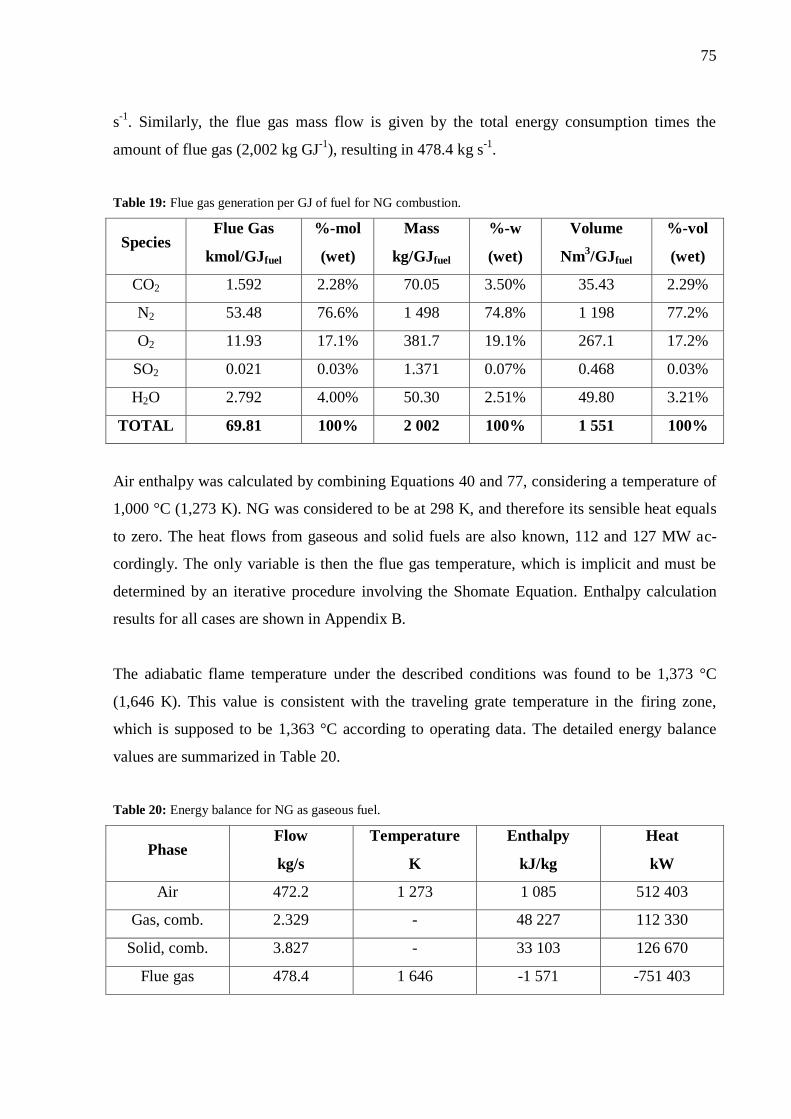
75
s-1
. Similarly, the flue gas mass flow is given by the total energy consumption times the
amount of flue gas (2,002 kg GJ-1
), resulting in 478.4 kg s-1
.
Table 19: Flue gas generation per GJ of fuel for NG combustion.
Species Flue Gas %-mol Mass %-w Volume %-vol
kmol/GJfuel (wet) kg/GJfuel (wet) Nm3/GJfuel (wet)
CO2 1.592 2.28% 70.05 3.50% 35.43 2.29%
N2 53.48 76.6% 1 498 74.8% 1 198 77.2%
O2 11.93 17.1% 381.7 19.1% 267.1 17.2%
SO2 0.021 0.03% 1.371 0.07% 0.468 0.03%
H2O 2.792 4.00% 50.30 2.51% 49.80 3.21%
TOTAL 69.81 100% 2 002 100% 1 551 100%
Air enthalpy was calculated by combining Equations 40 and 77, considering a temperature of
1,000 °C (1,273 K). NG was considered to be at 298 K, and therefore its sensible heat equals
to zero. The heat flows from gaseous and solid fuels are also known, 112 and 127 MW ac-
cordingly. The only variable is then the flue gas temperature, which is implicit and must be
determined by an iterative procedure involving the Shomate Equation. Enthalpy calculation
results for all cases are shown in Appendix B.
The adiabatic flame temperature under the described conditions was found to be 1,373 °C
(1,646 K). This value is consistent with the traveling grate temperature in the firing zone,
which is supposed to be 1,363 °C according to operating data. The detailed energy balance
values are summarized in Table 20.
Table 20: Energy balance for NG as gaseous fuel.
Phase Flow Temperature Enthalpy Heat
kg/s K kJ/kg kW
Air 472.2 1 273 1 085 512 403
Gas, comb. 2.329 - 48 227 112 330
Solid, comb. 3.827 - 33 103 126 670
Flue gas 478.4 1 646 -1 571 -751 403

76
Besides the temperature, gas flows are the other important parameter to assess the impacts of
gasification technology in the indurating machine. In order to compare values for NG and
product gas, flow rates are shown in different units in Table 21.
Table 21: Air, gas, solid and flue gas flow rates in several units.
Phase kg/s kmol/s Nm3/s Nm
3/min
Air 472.2 16.48 367.8 22 067
Gas 2.329 0.129 2.880 173
Solid 3.827 0.425 - -
Flue gas 478.4 16.69 370.6 22 237
TOTAL IN - - 370.7 22 240
5.4 Air Gasification
Air gasification is the simplest technology among all the options assessed in this study. In this
case, biomass is firstly dried from 50% to 15% MC. Inside the gasifier the biomass is partially
combusted in order to provide heat for gasification reactions. The ER, defined by Equation 1,
was chosen to be 30% based on typical values. In addition, the gasifier temperature was con-
sidered to be 850 °C and 95% of the carbon input was assumed to be converted into gas; in
other words, 5% of all carbon input is removed with ashes. The product gas leaves the cy-
clone at 873 K (600 °C) and it is burnt in the indurating machine without any gas cleaning
operation. Figure 24 presents the process flow chat and summarizes the main considerations.
Figure 24: Air gasification flow chart.
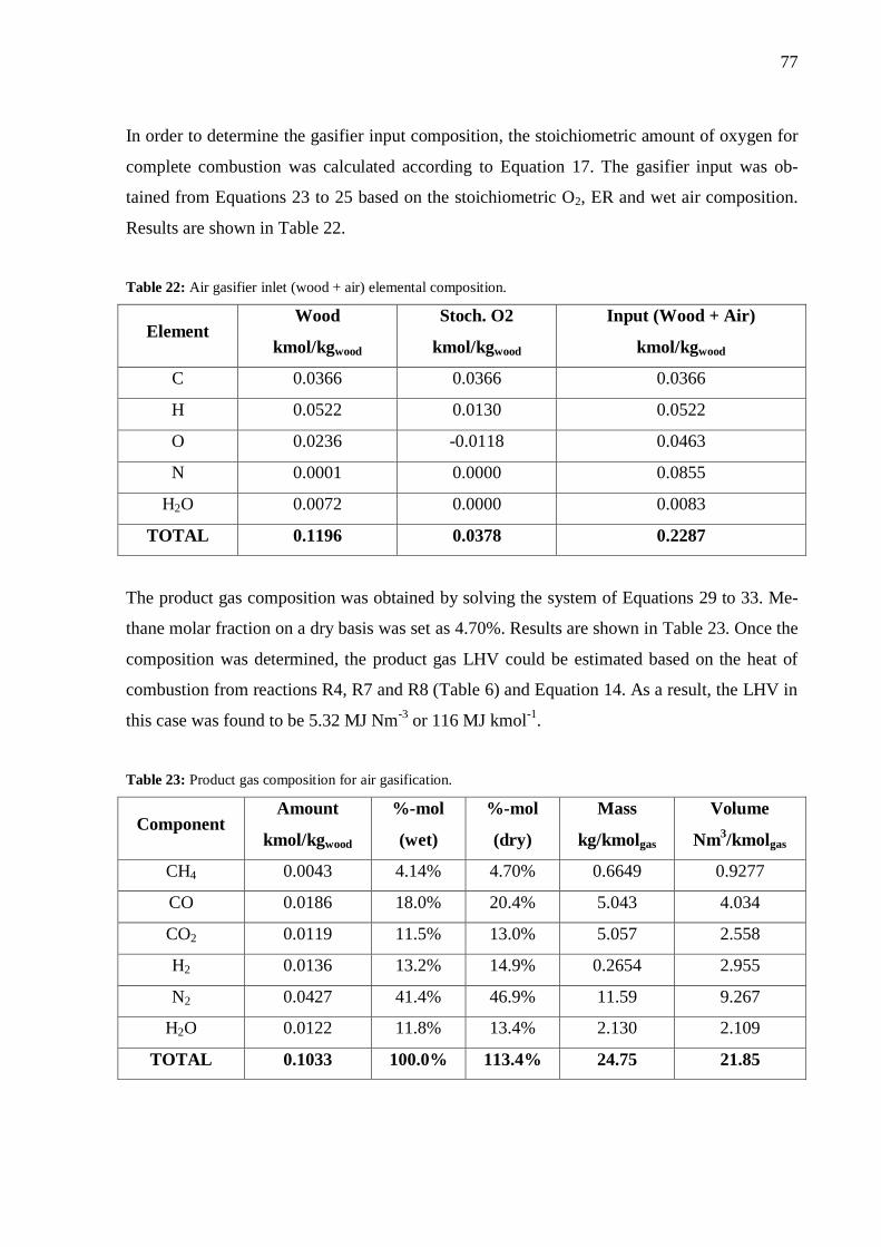
77
In order to determine the gasifier input composition, the stoichiometric amount of oxygen for
complete combustion was calculated according to Equation 17. The gasifier input was ob-
tained from Equations 23 to 25 based on the stoichiometric O2, ER and wet air composition.
Results are shown in Table 22.
Table 22: Air gasifier inlet (wood + air) elemental composition.
Element Wood Stoch. O2 Input (Wood + Air)
kmol/kgwood kmol/kgwood kmol/kgwood
C 0.0366 0.0366 0.0366
H 0.0522 0.0130 0.0522
O 0.0236 -0.0118 0.0463
N 0.0001 0.0000 0.0855
H2O 0.0072 0.0000 0.0083
TOTAL 0.1196 0.0378 0.2287
The product gas composition was obtained by solving the system of Equations 29 to 33. Me-
thane molar fraction on a dry basis was set as 4.70%. Results are shown in Table 23. Once the
composition was determined, the product gas LHV could be estimated based on the heat of
combustion from reactions R4, R7 and R8 (Table 6) and Equation 14. As a result, the LHV in
this case was found to be 5.32 MJ Nm-3
or 116 MJ kmol-1
.
Table 23: Product gas composition for air gasification.
Component Amount %-mol %-mol Mass Volume
kmol/kgwood (wet) (dry) kg/kmolgas Nm3/kmolgas
CH4 0.0043 4.14% 4.70% 0.6649 0.9277
CO 0.0186 18.0% 20.4% 5.043 4.034
CO2 0.0119 11.5% 13.0% 5.057 2.558
H2 0.0136 13.2% 14.9% 0.2654 2.955
N2 0.0427 41.4% 46.9% 11.59 9.267
H2O 0.0122 11.8% 13.4% 2.130 2.109
TOTAL 0.1033 100.0% 113.4% 24.75 21.85
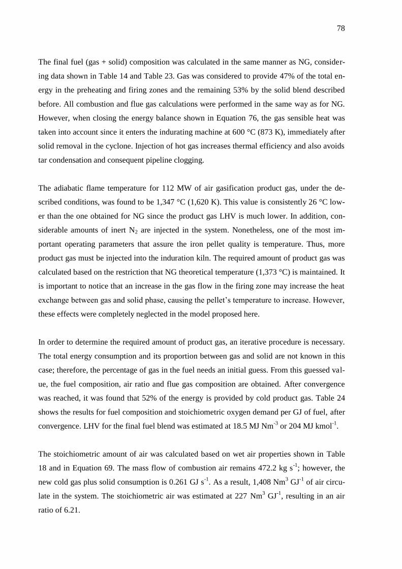
78
The final fuel (gas + solid) composition was calculated in the same manner as NG, consider-
ing data shown in Table 14 and Table 23. Gas was considered to provide 47% of the total en-
ergy in the preheating and firing zones and the remaining 53% by the solid blend described
before. All combustion and flue gas calculations were performed in the same way as for NG.
However, when closing the energy balance shown in Equation 76, the gas sensible heat was
taken into account since it enters the indurating machine at 600 °C (873 K), immediately after
solid removal in the cyclone. Injection of hot gas increases thermal efficiency and also avoids
tar condensation and consequent pipeline clogging.
The adiabatic flame temperature for 112 MW of air gasification product gas, under the de-
scribed conditions, was found to be 1,347 °C (1,620 K). This value is consistently 26 °C low-
er than the one obtained for NG since the product gas LHV is much lower. In addition, con-
siderable amounts of inert N2 are injected in the system. Nonetheless, one of the most im-
portant operating parameters that assure the iron pellet quality is temperature. Thus, more
product gas must be injected into the induration kiln. The required amount of product gas was
calculated based on the restriction that NG theoretical temperature (1,373 °C) is maintained. It
is important to notice that an increase in the gas flow in the firing zone may increase the heat
exchange between gas and solid phase, causing the pellet’s temperature to increase. However,
these effects were completely neglected in the model proposed here.
In order to determine the required amount of product gas, an iterative procedure is necessary.
The total energy consumption and its proportion between gas and solid are not known in this
case; therefore, the percentage of gas in the fuel needs an initial guess. From this guessed val-
ue, the fuel composition, air ratio and flue gas composition are obtained. After convergence
was reached, it was found that 52% of the energy is provided by cold product gas. Table 24
shows the results for fuel composition and stoichiometric oxygen demand per GJ of fuel, after
convergence. LHV for the final fuel blend was estimated at 18.5 MJ Nm-3
or 204 MJ kmol-1
.
The stoichiometric amount of air was calculated based on wet air properties shown in Table
18 and in Equation 69. The mass flow of combustion air remains 472.2 kg s-1
; however, the
new cold gas plus solid consumption is 0.261 GJ s-1
. As a result, 1,408 Nm3 GJ
-1 of air circu-
late in the system. The stoichiometric air was estimated at 227 Nm3 GJ
-1, resulting in an air
ratio of 6.21.

79
Table 24: Fuel composition and stoichiometric oxygen demand for air gasification product gas.
Element Gas Solid Gas + Solid Gas + Solid Stoch. O2
kmol/GJgas kmol/GJsolid kmol/GJfuel %-mol kmol/GJfuel
C 2.893 1.879 2.401 21.8% 2.401
H 3.690 1.125 2.447 22.2% 0.612
O 3.525 0.128 1.878 17.0% -0.939
N 7.117 0.029 3.680 33.4% 0.000
S 0.000 0.040 0.020 0.18% 0.020
H2O 1.017 0.152 0.598 5.42% 0.000
TOTAL - - 11.02 100% 2.094
The flue gas flow rate was calculated based on the same premises and equations utilized for
NG. The results are shown in Table 25. In this case, the molecular mass of the flue gas was
estimated at 28.80 kg kmol-1
while the molar volume was found to be 22.19 Nm3 kmol
-1.
Table 25: Flue gas generation per GJ of fuel for air gasification case.
Species Flue Gas %-mol Mass %-w Volume %-vol
kmol/GJfuel (wet) kg/GJfuel (wet) Nm3/GJfuel (wet)
CO2 2.401 3.58% 105.7 5.47% 53.46 3.58%
N2 50.75 75.7% 1 422 73.6% 1 130 75.7%
O2 10.91 16.3% 349.1 18.1% 242.9 16.3%
SO2 0.020 0.03% 1.254 0.06% 0.436 0.03%
H2O 3.005 4.48% 54.14 2.80% 66.91 4.48%
TOTAL 67.09 100% 1 932 100% 1 494 100%
As temperatures and composition of all gaseous streams were known, the specific enthalpies
could be calculated by means of the Shomate Equation. Specific enthalpy results after itera-
tion are shown in Appendix B. Other known parameters in Equations 76 were: LHV of solid
and gaseous fuels, and air and solid mass flows, which were kept as constants from NG calcu-
lations. Thus, the only unknowns were then the product gas and flue gas mass flows, which
could be found by solving Equations 76 and 78 simultaneously. The results are shown in Ta-
ble 26.

80
Table 26: Energy balance for air gasification product gas.
Phase Flow Temperature Enthalpy Heat
kg/s [K] kJ/kg kW
Air 472.2 1 273 1 085 512 403
Gas, sensible 28.64 873 780 22 337
Gas, comb. 28.64 - 4 698 134 564
Solid, comb. 3.827 - 33 103 126 670
Flue gas 504.7 1 646 1 577 -795 973
At this point, the total energy consumption and the solid/gas percentages could be determined.
If they were not equal to initial values, the calculation restarted with new values, until they
converge. In this case, it was found that 284 MW are required to maintain the NG tempera-
ture, from which 157 MW (55%) is provided by hot product gas. It represents an increase of
18.6% in energy consumption.
Specific and volumetric flows of air, product gas and flue gas are shown in different units in
Table 27. The increased percentages compared to NG values (Table 21) are also presented. As
can be seen from the table, 778% more fuel gas would be injected in the case of air gasifica-
tion. Although this increase is very high, the fuel gas inlet is still much smaller than the air
flow rate. In fact, the total gas input in preheating and firing zones increases only approxi-
mately 6% and flue gas flow rate increases less than 5%. Significant impact is therefore ex-
pected only in the burners, which would possibly require substitution/adaption; for example,
flow area should increase by increasing pipe diameter. In addition, the burner’s material
would be required to resist higher temperatures (600 °C in this case).
Table 27: Air, gas, solid and flue gas flow rates in several units, for air gasification case.
Phase kg/s kmol/s Nm3/s Nm
3/min Increase [%]
Air 472.2 16.48 367.8 22 067 0.00%
Gas 28.64 1.157 25.29 1 517 778%
Solid 3.827 0.425 - - -
Flue gas 504.7 17.53 388.9 23 332 4.93%
TOTAL IN - - 393.1 23 585 6.05%

81
The wood input was calculated based on Equation 79. If the losses are estimated at 2% of the
net energy content in wood, 11.8 kg s-1
(42.4 t h-1
) of wood chips with 15% MC would be re-
quired. This corresponds to approximately 27,000 ha of planted area, and a total area of
54,000 ha. It is relevant to highlight that this value can be further reduced by short-rotation
forests and/or denser planting.
Finally, the LHV of wood was calculated through Equations 11 to 13. It was found that the
energy content of eucalyptus wood considered in this study is 15.6 MJ kg-1
with 15% MC.
Thus, the gasifier energy input and output are 184 MW and 157 MW, respectively. The hot
gas efficiency for air gasification is 85.4%. This value does not take into consideration other
possible incoming energy streams, such as air preheating.
5.5 Oxygen Gasification
Oxygen gasification is one alternative to avoid dilution of the product gas by nitrogen. Same
calculations were performed as for air gasification although some assumptions were changed.
For instance, gasifier temperature was estimated at 950 °C, as less cold gases are fed into the
system. ER and CC were kept at the same values as air gasification. In order to control tem-
perature and favor hydrogen formation, SOR was set at 1 kg of steam per kg of oxygen (van
der Meijden et al. 2010). Figure 25 shows the oxygen gasification main parameters.
Figure 25: Oxygen gasification flow chart.

82
The calculations of product gas composition for oxygen gasification are very similar to those
for air as gasifying medium. Equation 17 is still valid, and it was considered that the gasifying
medium is composed of 95% O2 and 5% N2. Stoichiometric oxygen was determined accord-
ing to Equations 26 to 28. Results are shown in Table 28.
Table 28: Oxygen gasifier inlet (wood + oxygen) elemental composition.
Element Wood Stoch. O2 Wood + O2 + H2O
kmol/kgwood kmol/kgwood kmol/kgwood
C 0.0366 0.0366 0.03656
H 0.0522 0.0130 0.05218
O 0.0236 -0.0118 0.04626
N 0.0001 0.0000 0.00126
H2O 0.0072 0.0000 0.01363
TOTAL 0.1196 0.0378 0.1499
The product gas composition was obtained from Equations 29 to 33. Methane molar fraction
was considered to be 1.0% on a dry basis. All other assumptions remained the same. The iter-
ative procedure was developed in the same manner, and its results are presented in Table 29.
LHV was found to be 8.22 MJ Nm-3
or 175 MJ kmol-1
.
Table 29: Product gas composition for oxygen gasification.
Component Amount %-mol %-mol Mass Volume
kmol/kgwood (wet) (dry) kg/kmolgas Nm3/kmolgas
CH4 0.0006 0.76% 1.00% 0.122 0.170
CO 0.0264 35.7% 47.1% 9.995 7.995
CO2 0.0078 10.5% 13.9% 4.631 2.343
H2 0.0207 27.9% 36.9% 0.563 6.274
N2 0.0006 0.85% 1.12% 0.238 0.190
H2O 0.0179 24.2% 32.0% 4.367 4.323
TOTAL 0.0740 100% 132% 19.92 21.30
For comparison with NG, the adiabatic flame temperature for product gas combustion was
calculated considering data shown in Table 14 and Table 29. Gas was considered to provide
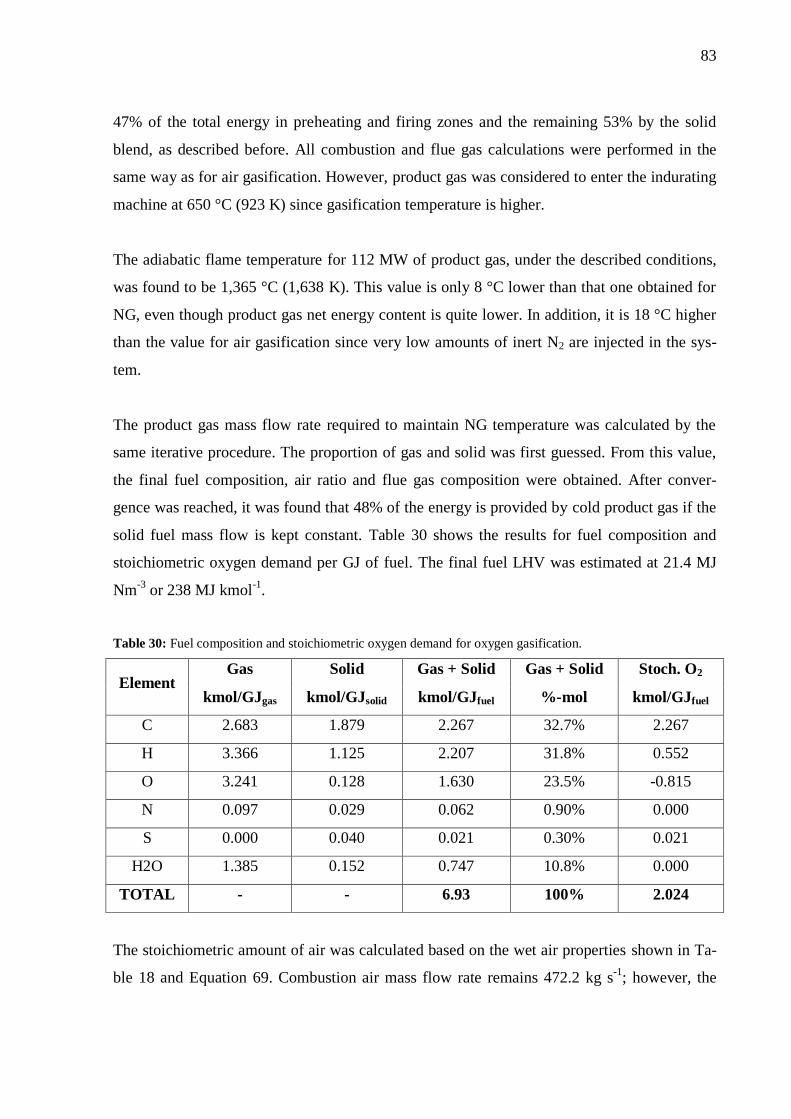
83
47% of the total energy in preheating and firing zones and the remaining 53% by the solid
blend, as described before. All combustion and flue gas calculations were performed in the
same way as for air gasification. However, product gas was considered to enter the indurating
machine at 650 °C (923 K) since gasification temperature is higher.
The adiabatic flame temperature for 112 MW of product gas, under the described conditions,
was found to be 1,365 °C (1,638 K). This value is only 8 °C lower than that one obtained for
NG, even though product gas net energy content is quite lower. In addition, it is 18 °C higher
than the value for air gasification since very low amounts of inert N2 are injected in the sys-
tem.
The product gas mass flow rate required to maintain NG temperature was calculated by the
same iterative procedure. The proportion of gas and solid was first guessed. From this value,
the final fuel composition, air ratio and flue gas composition were obtained. After conver-
gence was reached, it was found that 48% of the energy is provided by cold product gas if the
solid fuel mass flow is kept constant. Table 30 shows the results for fuel composition and
stoichiometric oxygen demand per GJ of fuel. The final fuel LHV was estimated at 21.4 MJ
Nm-3
or 238 MJ kmol-1
.
Table 30: Fuel composition and stoichiometric oxygen demand for oxygen gasification.
Element Gas Solid Gas + Solid Gas + Solid Stoch. O2
kmol/GJgas kmol/GJsolid kmol/GJfuel %-mol kmol/GJfuel
C 2.683 1.879 2.267 32.7% 2.267
H 3.366 1.125 2.207 31.8% 0.552
O 3.241 0.128 1.630 23.5% -0.815
N 0.097 0.029 0.062 0.90% 0.000
S 0.000 0.040 0.021 0.30% 0.021
H2O 1.385 0.152 0.747 10.8% 0.000
TOTAL - - 6.93 100% 2.024
The stoichiometric amount of air was calculated based on the wet air properties shown in Ta-
ble 18 and Equation 69. Combustion air mass flow rate remains 472.2 kg s-1
; however, the
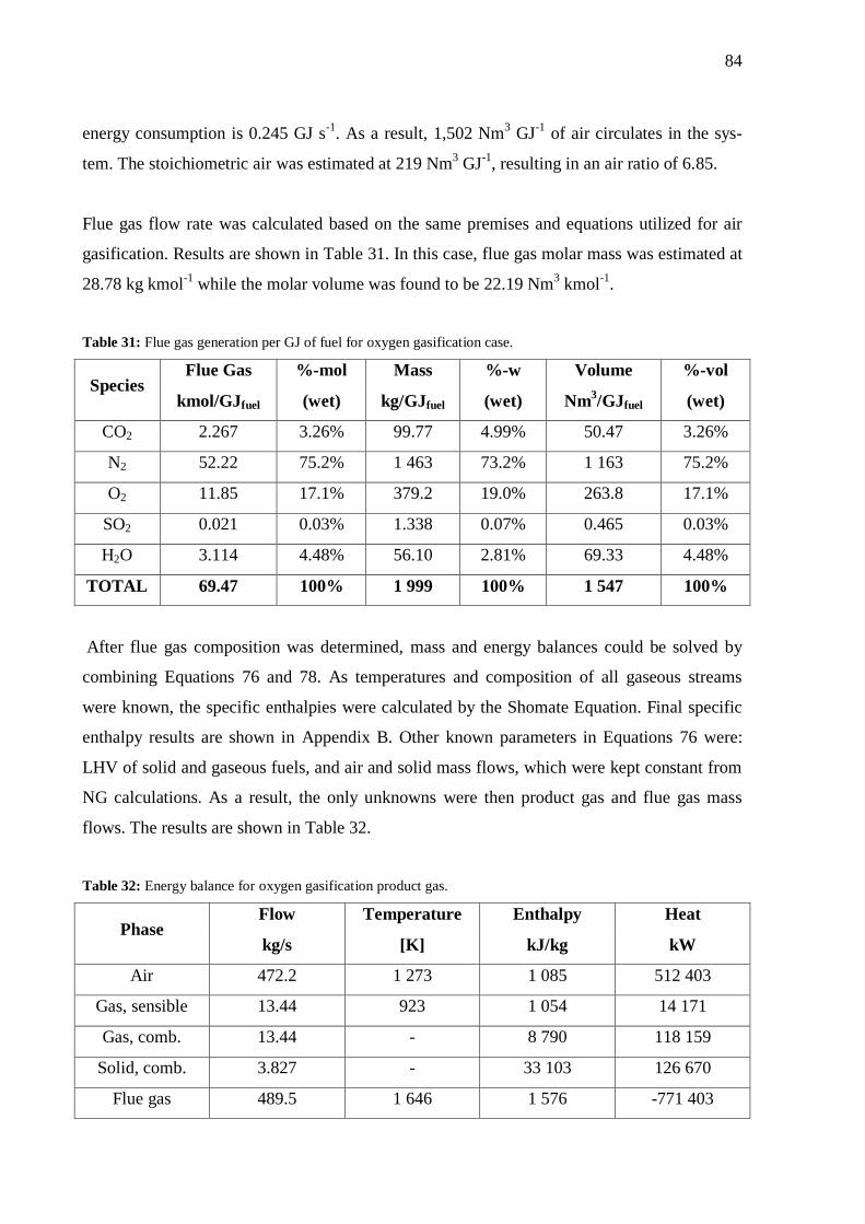
84
energy consumption is 0.245 GJ s-1
. As a result, 1,502 Nm3 GJ
-1 of air circulates in the sys-
tem. The stoichiometric air was estimated at 219 Nm3 GJ
-1, resulting in an air ratio of 6.85.
Flue gas flow rate was calculated based on the same premises and equations utilized for air
gasification. Results are shown in Table 31. In this case, flue gas molar mass was estimated at
28.78 kg kmol-1
while the molar volume was found to be 22.19 Nm3 kmol
-1.
Table 31: Flue gas generation per GJ of fuel for oxygen gasification case.
Species Flue Gas %-mol Mass %-w Volume %-vol
kmol/GJfuel (wet) kg/GJfuel (wet) Nm3/GJfuel (wet)
CO2 2.267 3.26% 99.77 4.99% 50.47 3.26%
N2 52.22 75.2% 1 463 73.2% 1 163 75.2%
O2 11.85 17.1% 379.2 19.0% 263.8 17.1%
SO2 0.021 0.03% 1.338 0.07% 0.465 0.03%
H2O 3.114 4.48% 56.10 2.81% 69.33 4.48%
TOTAL 69.47 100% 1 999 100% 1 547 100%
After flue gas composition was determined, mass and energy balances could be solved by
combining Equations 76 and 78. As temperatures and composition of all gaseous streams
were known, the specific enthalpies were calculated by the Shomate Equation. Final specific
enthalpy results are shown in Appendix B. Other known parameters in Equations 76 were:
LHV of solid and gaseous fuels, and air and solid mass flows, which were kept constant from
NG calculations. As a result, the only unknowns were then product gas and flue gas mass
flows. The results are shown in Table 32.
Table 32: Energy balance for oxygen gasification product gas.
Phase Flow Temperature Enthalpy Heat
kg/s [K] kJ/kg kW
Air 472.2 1 273 1 085 512 403
Gas, sensible 13.44 923 1 054 14 171
Gas, comb. 13.44 - 8 790 118 159
Solid, comb. 3.827 - 33 103 126 670
Flue gas 489.5 1 646 1 576 -771 403

85
For oxygen gasification, it was found that 259 MW are required to maintain the NG tempera-
ture, from which 132 MW (51%) are provided by hot product gas. These values consider that
the solid fuel mass flow rate is kept constant from NG combustion. It represents an increase of
8.37% in the energy consumption compared to NG.
Air, product gas and flue gas specific and volumetric flows are shown in different units in
Table 33. The increase percentages compared to NG values (Table 21) are also presented. As
can be seen from the table, 339% more fuel gas would be injected in the case of oxygen gasi-
fication. Although this increase is very high, the fuel gas inlet is still much smaller than the air
flow rate. The total gas input in preheating and firing zones increases only 3% and flue gas
flow rate increases less than 2%. Therefore, significant impact is expected only in the burners,
which would probably require substitution/adaption. In addition, burner’s material would be
required to resist higher temperatures (650 °C in this case).
Table 33: Air, gas, solid and flue gas flow rates in several units, for oxygen gasification case.
Phase kg/s kmol/s Nm3/s Nm
3/min Increase [%]
Air 472.2 16.48 367.8 22 067 0.00%
Gas 13.44 0.675 14.37 862 399%
Solid 3.827 0.425 - - -
Flue gas 489.5 17.01 377.4 22 644 1.83%
TOTAL IN - - 382.2 22 930 3.10%
The wood input was calculated based on Equation 79. Again, the losses were estimated at 2%
of wood’s net energy content, and 9.59 kg s-1
(34.5 t h-1
) of wood chips with 15% MC would
be required. This corresponds to approximately 22,000 ha of planted area, and a total area of
44,000 ha.
The oxygen gasification energy input and output are 150 MW and 132 MW, respectively.
Thus, the hot gas efficiency for oxygen gasification equals 88.4%. This value does not take
into consideration other possible incoming energy streams such as the energy required for
oxygen production. According to Table 8, 300 kWh per ton of oxygen are necessary for the
air purification process with highest energy consumption, resulting in 3,761 kW required for
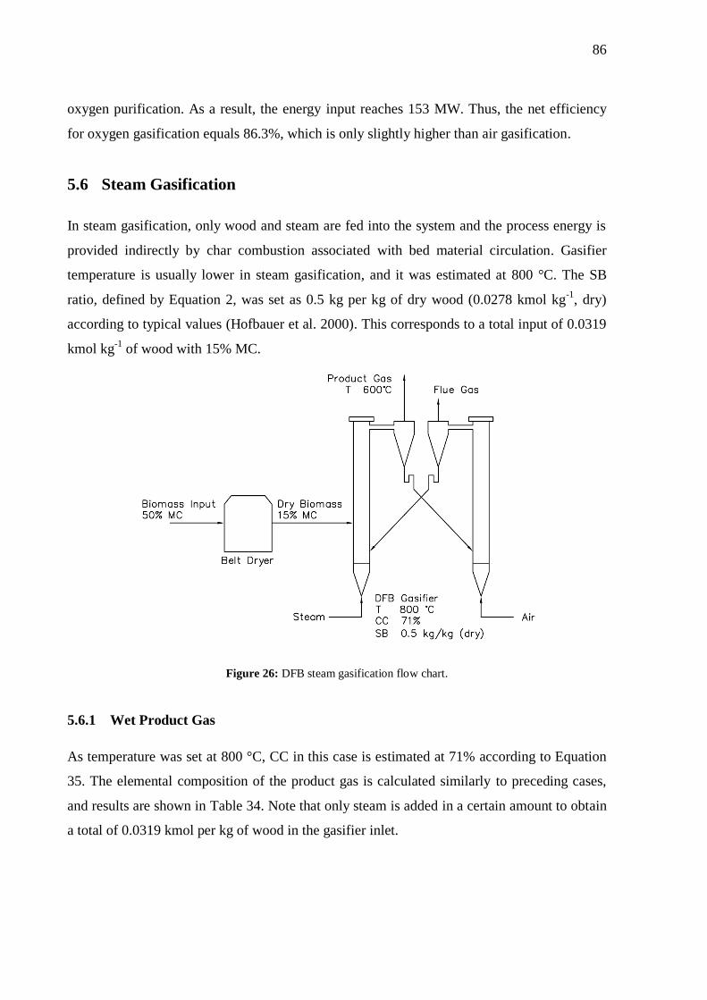
86
oxygen purification. As a result, the energy input reaches 153 MW. Thus, the net efficiency
for oxygen gasification equals 86.3%, which is only slightly higher than air gasification.
5.6 Steam Gasification
In steam gasification, only wood and steam are fed into the system and the process energy is
provided indirectly by char combustion associated with bed material circulation. Gasifier
temperature is usually lower in steam gasification, and it was estimated at 800 °C. The SB
ratio, defined by Equation 2, was set as 0.5 kg per kg of dry wood (0.0278 kmol kg-1
, dry)
according to typical values (Hofbauer et al. 2000). This corresponds to a total input of 0.0319
kmol kg-1
of wood with 15% MC.
Figure 26: DFB steam gasification flow chart.
5.6.1 Wet Product Gas
As temperature was set at 800 °C, CC in this case is estimated at 71% according to Equation
35. The elemental composition of the product gas is calculated similarly to preceding cases,
and results are shown in Table 34. Note that only steam is added in a certain amount to obtain
a total of 0.0319 kmol per kg of wood in the gasifier inlet.

87
Table 34: Steam gasifier inlet (wood + steam) elemental composition.
Element Wood Steam Total
kmol/kgwood kmol/kgwood kmol/kgwood
C 0.03656 0.00000 0.0366
H 0.05218 0.00000 0.0522
O 0.02356 0.00000 0.0236
N 0.00006 0.00000 6.26E-05
H2O 0.00724 0.02468 0.0319
TOTAL 0.1196 0.02468 0.1443
Equations 29 to 33 were utilized to calculate the product gas composition. Methane molar
fraction was considered to be 11% on a dry basis. Results are presented in Table 35. LHV was
found to be 8.32 MJ Nm-3
or 174 MJ kmol-1
.
Table 35: Product gas composition for steam gasification.
Component Amount %-mol %-mol Mass Volume
kmol/kgwood (wet) (dry) kg/kmolgas Nm3/kmolgas
CH4 0.0054 7.32% 11.0% 1.174 1.638
CO 0.0103 14.0% 21.0% 3.919 3.135
CO2 0.0103 14.1% 21.2% 6.215 3.144
H2 0.0228 31.1% 46.7% 0.626 6.971
N2 0.0000 0.04% 0.06% 0.012 0.010
H2O 0.0245 33.5% 50.3% 6.031 5.971
TOTAL 0.0733 100% 150.3% 17.98 20.87
In order to compare the adiabatic flame temperature, final fuel (gas + solid) composition was
calculated in the same manner as for air/oxygen gasification, considering data shown in Table
14 and Table 35. Combustion and flue gas calculations were also performed in the same way
as for previous gasification technologies. The product gas was considered to enter the indurat-
ing machine at 600 °C (873 K). The adiabatic flame temperature for 112 MW of steam gasifi-
cation wet product gas was found to be 1,361 °C (1,634 K). This value is 12 °C lower than
that obtained for NG although the product gas LHV is notably lower. In addition, it is 4 °C
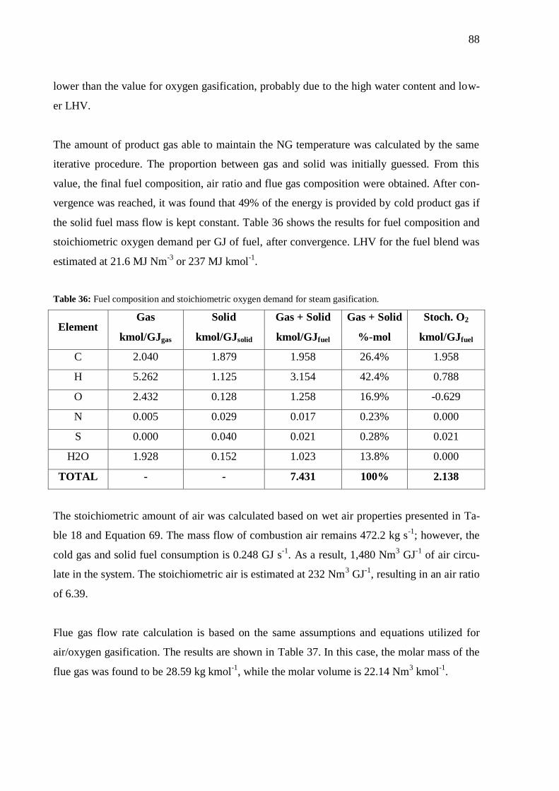
88
lower than the value for oxygen gasification, probably due to the high water content and low-
er LHV.
The amount of product gas able to maintain the NG temperature was calculated by the same
iterative procedure. The proportion between gas and solid was initially guessed. From this
value, the final fuel composition, air ratio and flue gas composition were obtained. After con-
vergence was reached, it was found that 49% of the energy is provided by cold product gas if
the solid fuel mass flow is kept constant. Table 36 shows the results for fuel composition and
stoichiometric oxygen demand per GJ of fuel, after convergence. LHV for the fuel blend was
estimated at 21.6 MJ Nm-3
or 237 MJ kmol-1
.
Table 36: Fuel composition and stoichiometric oxygen demand for steam gasification.
Element Gas Solid Gas + Solid Gas + Solid Stoch. O2
kmol/GJgas kmol/GJsolid kmol/GJfuel %-mol kmol/GJfuel
C 2.040 1.879 1.958 26.4% 1.958
H 5.262 1.125 3.154 42.4% 0.788
O 2.432 0.128 1.258 16.9% -0.629
N 0.005 0.029 0.017 0.23% 0.000
S 0.000 0.040 0.021 0.28% 0.021
H2O 1.928 0.152 1.023 13.8% 0.000
TOTAL - - 7.431 100% 2.138
The stoichiometric amount of air was calculated based on wet air properties presented in Ta-
ble 18 and Equation 69. The mass flow of combustion air remains 472.2 kg s-1
; however, the
cold gas and solid fuel consumption is 0.248 GJ s-1
. As a result, 1,480 Nm3 GJ
-1 of air circu-
late in the system. The stoichiometric air is estimated at 232 Nm3 GJ
-1, resulting in an air ratio
of 6.39.
Flue gas flow rate calculation is based on the same assumptions and equations utilized for
air/oxygen gasification. The results are shown in Table 37. In this case, the molar mass of the
flue gas was found to be 28.59 kg kmol-1
, while the molar volume is 22.14 Nm3 kmol
-1.

89
Table 37: Flue gas generation per GJ of fuel for steam gasification case.
Species Flue Gas %-mol Mass %-w Volume %-vol
kmol/GJfuel (wet) kg/GJfuel (wet) Nm3/GJfuel (wet)
CO2 1.958 2.85% 86.18 4.38% 43.60 2.85%
N2 51.43 74.8% 1 441 73.3% 1 145 74.8%
O2 11.53 16.8% 368.9 18.8% 256.7 16.8%
SO2 0.021 0.03% 1.319 0.07% 0.458 0.03%
H2O 3.845 5.59% 69.26 3.52% 85.60 5.59%
TOTAL 68.78 100% 1 966 100% 1 531 100%
After the flue gas composition was obtained, mass and energy balances could be solved. As
temperatures and composition of all gaseous streams are known, the specific enthalpies can be
calculated by the Shomate Equation. Final specific enthalpy results are shown in Appendix B.
As in the previous calculations, product gas and flue gas mass flow rates were obtained solv-
ing Equations 76 and 78 simultaneously. Results are shown in Table 38.
Table 38: Energy balance for steam gasification product gas.
Phase Flow Temperature Enthalpy Heat
kg/s K kJ/kg kW
Air 472.2 1 273 1 085 512 403
Gas, sens. 12.61 873 1 145 14 447
Gas, comb. 12.61 - 9 659 121 837
Solid, comb. 3.827 - 33 103 126 670
Flue gas 488.7 1 646 1 587 -775 358
For steam gasification wet product gas combustion, 263 MW are required to maintain the NG
temperature, from which 136 MW (52%) are provided by hot product gas. It represents an
increase of 10.0% in the energy consumption.
Specific and volumetric flows of air, product gas and flue gas are shown in different units in
Table 39. The increase percentages compared to NG values (Table 21) are also presented. As
can be seen from the table, 408% more fuel gas would be injected in the case of steam gasifi-
cation, without product gas drying. Although this increase is quite high, the fuel gas inlet is
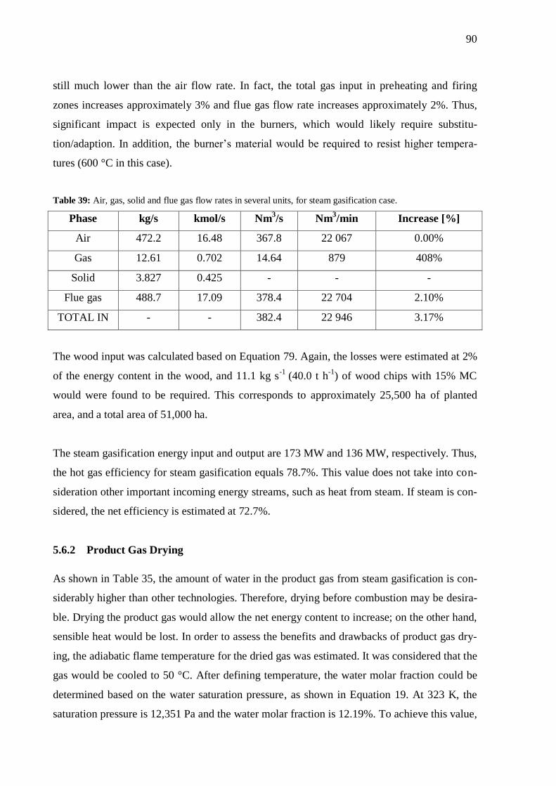
90
still much lower than the air flow rate. In fact, the total gas input in preheating and firing
zones increases approximately 3% and flue gas flow rate increases approximately 2%. Thus,
significant impact is expected only in the burners, which would likely require substitu-
tion/adaption. In addition, the burner’s material would be required to resist higher tempera-
tures (600 °C in this case).
Table 39: Air, gas, solid and flue gas flow rates in several units, for steam gasification case.
Phase kg/s kmol/s Nm3/s Nm
3/min Increase [%]
Air 472.2 16.48 367.8 22 067 0.00%
Gas 12.61 0.702 14.64 879 408%
Solid 3.827 0.425 - - -
Flue gas 488.7 17.09 378.4 22 704 2.10%
TOTAL IN - - 382.4 22 946 3.17%
The wood input was calculated based on Equation 79. Again, the losses were estimated at 2%
of the energy content in the wood, and 11.1 kg s-1
(40.0 t h-1
) of wood chips with 15% MC
would were found to be required. This corresponds to approximately 25,500 ha of planted
area, and a total area of 51,000 ha.
The steam gasification energy input and output are 173 MW and 136 MW, respectively. Thus,
the hot gas efficiency for steam gasification equals 78.7%. This value does not take into con-
sideration other important incoming energy streams, such as heat from steam. If steam is con-
sidered, the net efficiency is estimated at 72.7%.
5.6.2 Product Gas Drying
As shown in Table 35, the amount of water in the product gas from steam gasification is con-
siderably higher than other technologies. Therefore, drying before combustion may be desira-
ble. Drying the product gas would allow the net energy content to increase; on the other hand,
sensible heat would be lost. In order to assess the benefits and drawbacks of product gas dry-
ing, the adiabatic flame temperature for the dried gas was estimated. It was considered that the
gas would be cooled to 50 °C. After defining temperature, the water molar fraction could be
determined based on the water saturation pressure, as shown in Equation 19. At 323 K, the
saturation pressure is 12,351 Pa and the water molar fraction is 12.19%. To achieve this value,
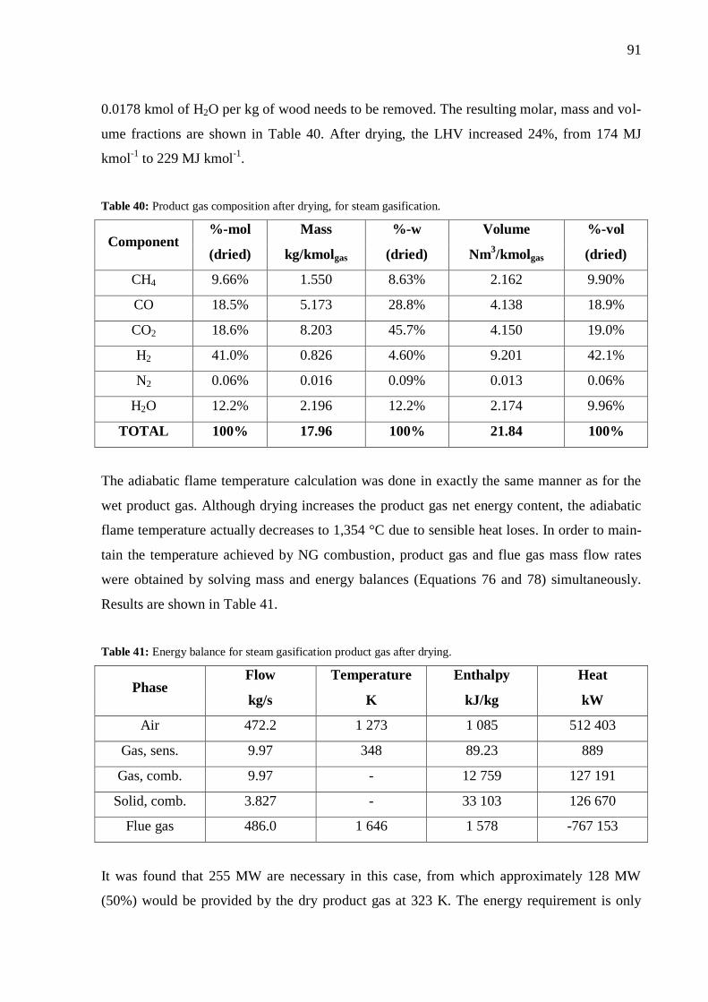
91
0.0178 kmol of H2O per kg of wood needs to be removed. The resulting molar, mass and vol-
ume fractions are shown in Table 40. After drying, the LHV increased 24%, from 174 MJ
kmol-1
to 229 MJ kmol-1
.
Table 40: Product gas composition after drying, for steam gasification.
Component %-mol Mass %-w Volume %-vol
(dried) kg/kmolgas (dried) Nm3/kmolgas (dried)
CH4 9.66% 1.550 8.63% 2.162 9.90%
CO 18.5% 5.173 28.8% 4.138 18.9%
CO2 18.6% 8.203 45.7% 4.150 19.0%
H2 41.0% 0.826 4.60% 9.201 42.1%
N2 0.06% 0.016 0.09% 0.013 0.06%
H2O 12.2% 2.196 12.2% 2.174 9.96%
TOTAL 100% 17.96 100% 21.84 100%
The adiabatic flame temperature calculation was done in exactly the same manner as for the
wet product gas. Although drying increases the product gas net energy content, the adiabatic
flame temperature actually decreases to 1,354 °C due to sensible heat loses. In order to main-
tain the temperature achieved by NG combustion, product gas and flue gas mass flow rates
were obtained by solving mass and energy balances (Equations 76 and 78) simultaneously.
Results are shown in Table 41.
Table 41: Energy balance for steam gasification product gas after drying.
Phase Flow Temperature Enthalpy Heat
kg/s K kJ/kg kW
Air 472.2 1 273 1 085 512 403
Gas, sens. 9.97 348 89.23 889
Gas, comb. 9.97 - 12 759 127 191
Solid, comb. 3.827 - 33 103 126 670
Flue gas 486.0 1 646 1 578 -767 153
It was found that 255 MW are necessary in this case, from which approximately 128 MW
(50%) would be provided by the dry product gas at 323 K. The energy requirement is only
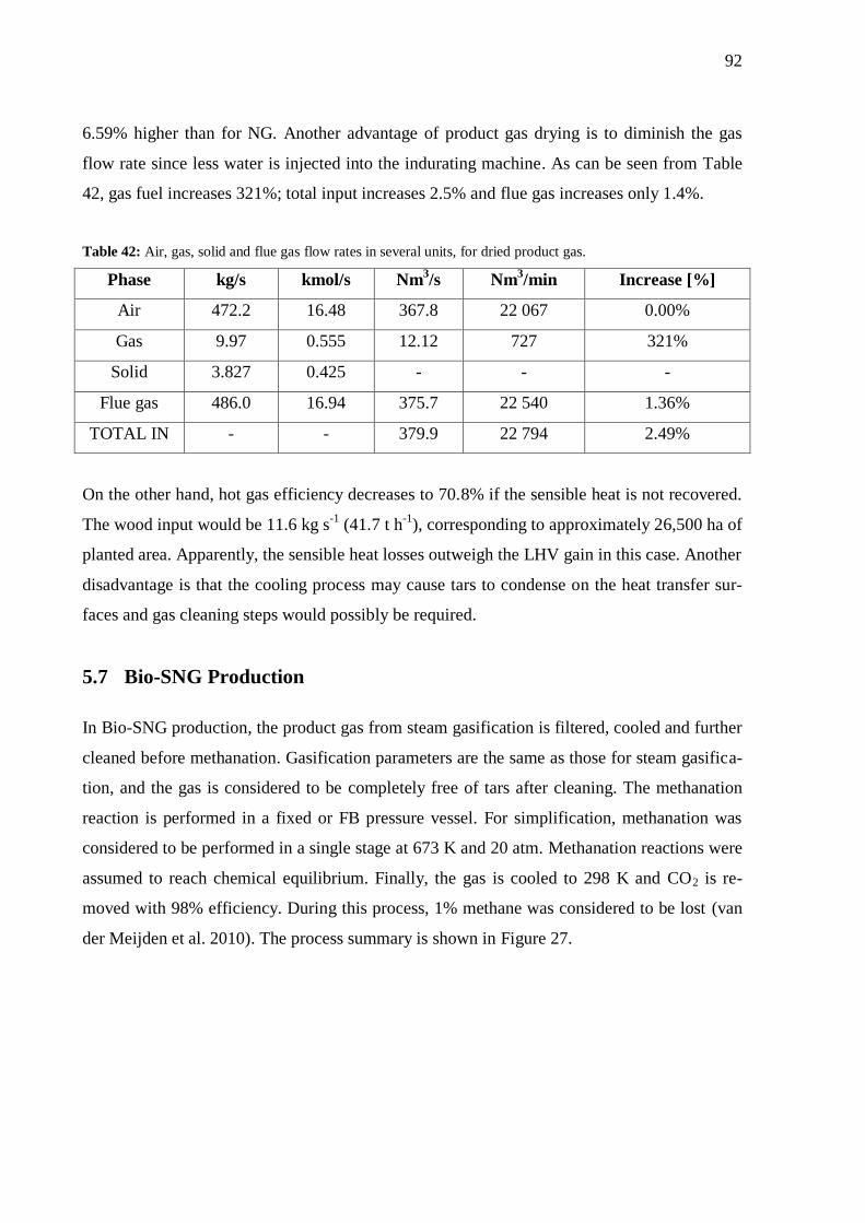
92
6.59% higher than for NG. Another advantage of product gas drying is to diminish the gas
flow rate since less water is injected into the indurating machine. As can be seen from Table
42, gas fuel increases 321%; total input increases 2.5% and flue gas increases only 1.4%.
Table 42: Air, gas, solid and flue gas flow rates in several units, for dried product gas.
Phase kg/s kmol/s Nm3/s Nm
3/min Increase [%]
Air 472.2 16.48 367.8 22 067 0.00%
Gas 9.97 0.555 12.12 727 321%
Solid 3.827 0.425 - - -
Flue gas 486.0 16.94 375.7 22 540 1.36%
TOTAL IN - - 379.9 22 794 2.49%
On the other hand, hot gas efficiency decreases to 70.8% if the sensible heat is not recovered.
The wood input would be 11.6 kg s-1
(41.7 t h-1
), corresponding to approximately 26,500 ha of
planted area. Apparently, the sensible heat losses outweigh the LHV gain in this case. Another
disadvantage is that the cooling process may cause tars to condense on the heat transfer sur-
faces and gas cleaning steps would possibly be required.
5.7 Bio-SNG Production
In Bio-SNG production, the product gas from steam gasification is filtered, cooled and further
cleaned before methanation. Gasification parameters are the same as those for steam gasifica-
tion, and the gas is considered to be completely free of tars after cleaning. The methanation
reaction is performed in a fixed or FB pressure vessel. For simplification, methanation was
considered to be performed in a single stage at 673 K and 20 atm. Methanation reactions were
assumed to reach chemical equilibrium. Finally, the gas is cooled to 298 K and CO2 is re-
moved with 98% efficiency. During this process, 1% methane was considered to be lost (van
der Meijden et al. 2010). The process summary is shown in Figure 27.

93
Figure 27: Bio-SNG production flow chart.
The methanation reactor is considered to be fed with product gas obtained from steam gasifi-
cation (Table 35), without any water removal. Excess water is important in order to promote
the water-gas shift reaction (R9 in Table 6) and achieve adequate H2 to CO ratio. It is also
known that excess moisture can avoid carbon formation and consequent catalyst poisoning.
Nonetheless, the water content in the product gas (33.5%-mol) was considered to be enough
to avoid soot inside the reactor (Deurwaarder et al. 2005) and therefore no more water is add-
ed.
In order to evaluate the gas composition after methanation, equilibrium constants were calcu-
lated according to Equation 36. Results of enthalpy change, entropy change, Gibbs free ener-
gy change and equilibrium constants at 673 K and 1 atm for reactions R9, R11 and R12 are
shown in Table 43.
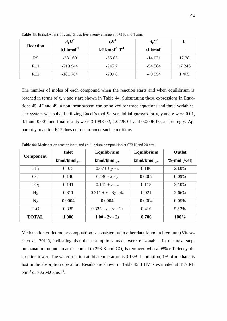
94
Table 43: Enthalpy, entropy and Gibbs free energy change at 673 K and 1 atm.
Reaction ΔrH
0 ΔrS
0 ΔrG
0 k
kJ kmol-1
kJ kmol-1
T-1
kJ kmol-1
-
R9 -38 160 -35.85 -14 031 12.28
R11 -219 944 -245.7 -54 584 17 246
R12 -181 784 -209.8 -40 554 1 405
The number of moles of each compound when the reaction starts and when equilibrium is
reached in terms of x, y and z are shown in Table 44. Substituting these expressions in Equa-
tions 45, 47 and 49, a nonlinear system can be solved for three equations and three variables.
The system was solved utilizing Excel’s tool Solver. Initial guesses for x, y and z were 0.01,
0.1 and 0.001 and final results were 3.199E-02, 1.072E-01 and 0.000E-00, accordingly. Ap-
parently, reaction R12 does not occur under such conditions.
Table 44: Methanation reactor input and equilibrium composition at 673 K and 20 atm.
Component Inlet Equilibrium Equilibrium Outlet
kmol/kmolgas kmol/kmolgas kmol/kmolgas %-mol (wet)
CH4 0.073 0.073 + y - z 0.180 23.0%
CO 0.140 0.140 - x - y 0.0007 0.09%
CO2 0.141 0.141 + x - z 0.173 22.0%
H2 0.311 0.311 + x - 3y - 4z 0.021 2.66%
N2 0.0004 0.0004 0.0004 0.05%
H2O 0.335 0.335 - x + y + 2z 0.410 52.2%
TOTAL 1.000 1.00 - 2y - 2z 0.786 100%
Methanation outlet molar composition is consistent with other data found in literature (Vitasa-
ri et al. 2011), indicating that the assumptions made were reasonable. In the next step,
methanation output stream is cooled to 298 K and CO2 is removed with a 98% efficiency ab-
sorption tower. The water fraction at this temperature is 3.13%. In addition, 1% of methane is
lost in the absorption operation. Results are shown in Table 45. LHV is estimated at 31.7 MJ
Nm-3
or 706 MJ kmol-1
.

95
Table 45: Bio-SNG composition.
Component Moles %-mol Mass %-w Volume %-vol
kmol/kmol (wet) kg/kmol (wet) Nm3/kmol (wet)
CH4 0.1786 84.7% 13.60 89.2% 18.97 85.3%
CO 0.0007 0.34% 0.096 0.63% 0.077 0.34%
CO2 0.0035 1.64% 0.724 4.75% 0.366 1.65%
H2 0.0209 9.94% 0.200 1.31% 2.231 10.0%
N2 0.0004 0.20% 0.057 0.37% 0.045 0.20%
H2O 0.0066 3.13% 0.564 3.70% 0.558 2.51%
TOTAL 0.2107 100% 15.24 100% 22.25 100%
In order to compare the adiabatic flame temperature with NG, the final fuel composition was
calculated in the same manner as that for NG, considering data shown in Table 14 and Table
45. Combustion and flue gas calculations were also performed in the same way as for NG.
Bio-SNG was considered to enter the indurating machine at 298 K, and therefore no sensible
heat is present. The adiabatic flame temperature for 112 MW of bio-SNG was found to be
approximately the same as for NG (1,373 °C). The total energy consumption is also the same,
as well as the percentages provided by solid and gaseous fuels. Table 46 shows the results for
fuel composition and stoichiometric oxygen demand per GJ of fuel for bio-SNG. LHV for the
fuel blend was estimated at 39.3 MJ Nm-3
or 489 MJ kmol-1
.
Table 46: Fuel composition and stoichiometric oxygen demand for bio-SNG.
Element Gas Solid Gas + Solid Gas + Solid Stoch. O2
kmol/GJgas kmol/GJsolid kmol/GJfuel %-mol kmol/GJfuel
C 1.229 1.879 1.574 32.8% 1.574
H 5.086 1.125 2.988 62.3% 0.747
O 0.051 0.128 0.092 1.92% -0.046
N 0.006 0.029 0.018 0.38% 0.000
S 0.000 0.040 0.021 0.45% 0.021
H2O 0.044 0.152 0.102 2.12% 0.000
TOTAL - - 4.795 100% 2.296
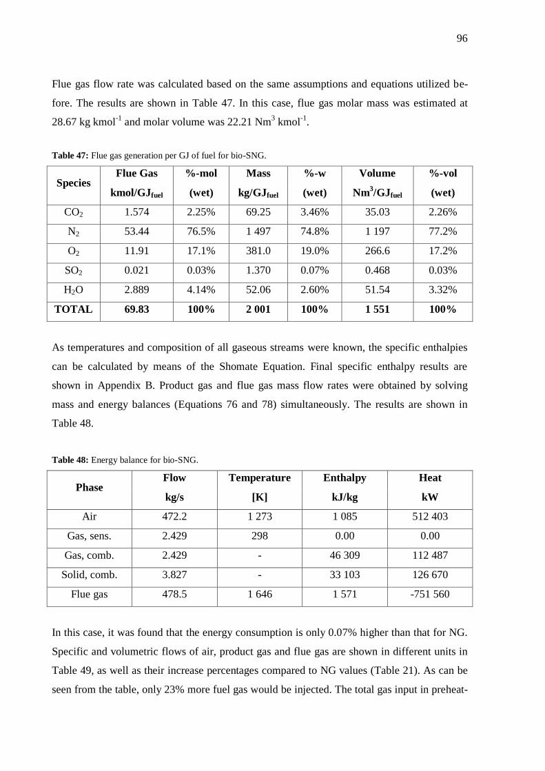
96
Flue gas flow rate was calculated based on the same assumptions and equations utilized be-
fore. The results are shown in Table 47. In this case, flue gas molar mass was estimated at
28.67 kg kmol-1
and molar volume was 22.21 Nm3 kmol
-1.
Table 47: Flue gas generation per GJ of fuel for bio-SNG.
Species Flue Gas %-mol Mass %-w Volume %-vol
kmol/GJfuel (wet) kg/GJfuel (wet) Nm3/GJfuel (wet)
CO2 1.574 2.25% 69.25 3.46% 35.03 2.26%
N2 53.44 76.5% 1 497 74.8% 1 197 77.2%
O2 11.91 17.1% 381.0 19.0% 266.6 17.2%
SO2 0.021 0.03% 1.370 0.07% 0.468 0.03%
H2O 2.889 4.14% 52.06 2.60% 51.54 3.32%
TOTAL 69.83 100% 2 001 100% 1 551 100%
As temperatures and composition of all gaseous streams were known, the specific enthalpies
can be calculated by means of the Shomate Equation. Final specific enthalpy results are
shown in Appendix B. Product gas and flue gas mass flow rates were obtained by solving
mass and energy balances (Equations 76 and 78) simultaneously. The results are shown in
Table 48.
Table 48: Energy balance for bio-SNG.
Phase Flow Temperature Enthalpy Heat
kg/s [K] kJ/kg kW
Air 472.2 1 273 1 085 512 403
Gas, sens. 2.429 298 0.00 0.00
Gas, comb. 2.429 - 46 309 112 487
Solid, comb. 3.827 - 33 103 126 670
Flue gas 478.5 1 646 1 571 -751 560
In this case, it was found that the energy consumption is only 0.07% higher than that for NG.
Specific and volumetric flows of air, product gas and flue gas are shown in different units in
Table 49, as well as their increase percentages compared to NG values (Table 21). As can be
seen from the table, only 23% more fuel gas would be injected. The total gas input in preheat-
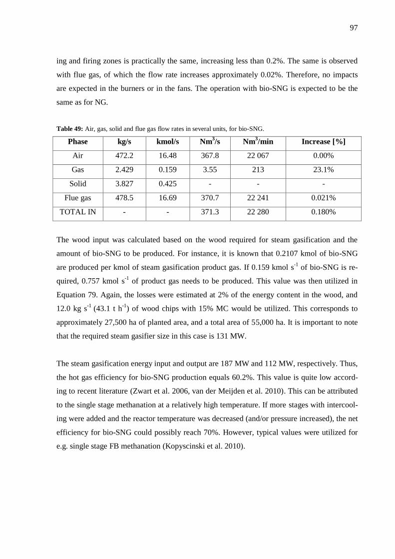
97
ing and firing zones is practically the same, increasing less than 0.2%. The same is observed
with flue gas, of which the flow rate increases approximately 0.02%. Therefore, no impacts
are expected in the burners or in the fans. The operation with bio-SNG is expected to be the
same as for NG.
Table 49: Air, gas, solid and flue gas flow rates in several units, for bio-SNG.
Phase kg/s kmol/s Nm3/s Nm
3/min Increase [%]
Air 472.2 16.48 367.8 22 067 0.00%
Gas 2.429 0.159 3.55 213 23.1%
Solid 3.827 0.425 - - -
Flue gas 478.5 16.69 370.7 22 241 0.021%
TOTAL IN - - 371.3 22 280 0.180%
The wood input was calculated based on the wood required for steam gasification and the
amount of bio-SNG to be produced. For instance, it is known that 0.2107 kmol of bio-SNG
are produced per kmol of steam gasification product gas. If 0.159 kmol s-1
of bio-SNG is re-
quired, 0.757 kmol s-1
of product gas needs to be produced. This value was then utilized in
Equation 79. Again, the losses were estimated at 2% of the energy content in the wood, and
12.0 kg s-1
(43.1 t h-1
) of wood chips with 15% MC would be utilized. This corresponds to
approximately 27,500 ha of planted area, and a total area of 55,000 ha. It is important to note
that the required steam gasifier size in this case is 131 MW.
The steam gasification energy input and output are 187 MW and 112 MW, respectively. Thus,
the hot gas efficiency for bio-SNG production equals 60.2%. This value is quite low accord-
ing to recent literature (Zwart et al. 2006, van der Meijden et al. 2010). This can be attributed
to the single stage methanation at a relatively high temperature. If more stages with intercool-
ing were added and the reactor temperature was decreased (and/or pressure increased), the net
efficiency for bio-SNG could possibly reach 70%. However, typical values were utilized for
e.g. single stage FB methanation (Kopyscinski et al. 2010).
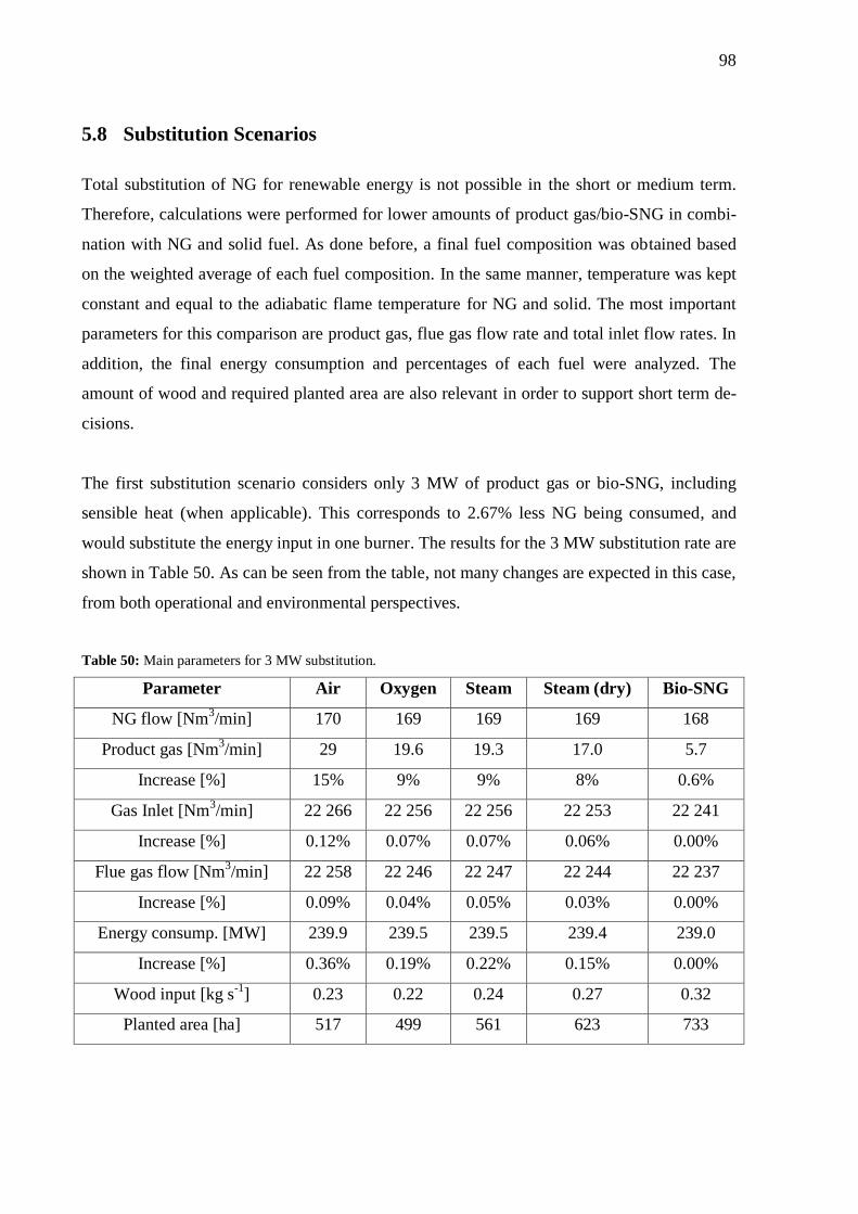
98
5.8 Substitution Scenarios
Total substitution of NG for renewable energy is not possible in the short or medium term.
Therefore, calculations were performed for lower amounts of product gas/bio-SNG in combi-
nation with NG and solid fuel. As done before, a final fuel composition was obtained based
on the weighted average of each fuel composition. In the same manner, temperature was kept
constant and equal to the adiabatic flame temperature for NG and solid. The most important
parameters for this comparison are product gas, flue gas flow rate and total inlet flow rates. In
addition, the final energy consumption and percentages of each fuel were analyzed. The
amount of wood and required planted area are also relevant in order to support short term de-
cisions.
The first substitution scenario considers only 3 MW of product gas or bio-SNG, including
sensible heat (when applicable). This corresponds to 2.67% less NG being consumed, and
would substitute the energy input in one burner. The results for the 3 MW substitution rate are
shown in Table 50. As can be seen from the table, not many changes are expected in this case,
from both operational and environmental perspectives.
Table 50: Main parameters for 3 MW substitution.
Parameter Air Oxygen Steam Steam (dry) Bio-SNG
NG flow [Nm3/min] 170 169 169 169 168
Product gas [Nm3/min] 29 19.6 19.3 17.0 5.7
Increase [%] 15% 9% 9% 8% 0.6%
Gas Inlet [Nm3/min] 22 266 22 256 22 256 22 253 22 241
Increase [%] 0.12% 0.07% 0.07% 0.06% 0.00%
Flue gas flow [Nm3/min] 22 258 22 246 22 247 22 244 22 237
Increase [%] 0.09% 0.04% 0.05% 0.03% 0.00%
Energy consump. [MW] 239.9 239.5 239.5 239.4 239.0
Increase [%] 0.36% 0.19% 0.22% 0.15% 0.00%
Wood input [kg s-1
] 0.23 0.22 0.24 0.27 0.32
Planted area [ha] 517 499 561 623 733

99
The second substitution scenario considers 12 MW of product gas or bio-SNG, including sen-
sible heat. This corresponds to 10.7% less NG being consumed. The results are shown in Ta-
ble 51. Again, not many operational and environmental impacts are expected in this scenario.
Table 51: Main parameters for 12 MW substitution.
Parameter Air Oxygen Steam Steam (dry) Bio-SNG
NG flow [Nm3/min] 160 157 158 157 154
Product gas [Nm3/min] 116 78.2 77.4 68.1 22.7
Increase [%] 60% 36% 36% 30% 2.5%
Gas Inlet [Nm3/min] 22 343 22 303 22 302 22 292 22 244
Increase [%] 0.46% 0.28% 0.28% 0.23% 0.02%
Flue gas flow [Nm3/min] 22 320 22 274 22 278 22 265 22 237
Increase [%] 0.38% 0.17% 0.19% 0.13% 0.00%
Energy consump. [MW] 242.4 240.8 241.1 240.5 239.0
Increase [%] 1.43% 0.76% 0.88% 0.62% 0.01%
Wood input [kg s-1
] 0.90 0.87 0.98 1.09 1.28
Planted area [ha] 2 067 1 996 2 243 2 492 2 931
The third substitution scenario considers 24 MW of product gas or bio-SNG, which is already
a medium scale facility. This would correspond to 21.4% in NG savings. As can be seen from
the results shown in Table 52, impacts in the indurating machine are more relevant; for in-
stance, in air gasification the fuel gas volumetric flow rate already increases 119%. In the
same manner, GHG reduction is expected to be significant.
Table 52: Main parameters for 24 MW substitution.
Parameter Air Oxygen Steam Steam (dry) Bio-SNG
NG flow [Nm3/min] 146 141 142 140 136
Product gas [Nm3/min] 232 156.4 154.7 136.2 45.4
Increase [%] 119% 72% 72% 60% 4.9%
Gas Inlet [Nm3/min] 22 446 22 365 22 364 22 344 22 249
Increase [%] 0.92% 0.56% 0.56% 0.47% 0.04%
Flue gas flow [Nm3/min] 22 404 22 311 22 319 22 293 22 238

100
Increase [%] 0.75% 0.33% 0.37% 0.26% 0.00%
Energy consump. [MW] 245.8 242.6 243.2 242.0 239.0
Increase [%] 2.85% 1.52% 1.77% 1.23% 0.01%
Wood input [kg s-1
] 1.80 1.74 1.95 2.17 2.55
Planted area [ha] 4 134 3 991 4 486 4 983 5 861
The last substitution scenario considers 60 MW gasification plants, which would already be
within the world’s largest facilities. This corresponds to 53.4% in NG savings. The results are
shown in Table 53.
Table 53: Main parameters for 60 MW substitution.
Parameter Air Oxygen Steam Steam (dry) Bio-SNG
NG flow [Nm3/min] 107 94 97 92 81
Product gas [Nm3/min] 580 391.0 386.8 340.6 113.5
Increase [%] 298% 181% 180% 150% 12.3%
Gas Inlet [Nm3/min] 22 754 22 553 22 551 22 500 22 261
Increase [%] 2.31% 1.41% 1.40% 1.17% 0.10%
Flue gas [Nm3/min] 22 656 22 422 22 443 22 379 22 239
Increase [%] 1.88% 0.83% 0.93% 0.64% 0.01%
Energy consump. [MW] 256.0 248.1 249.5 246.4 239.1
Increase [%] 7.13% 3.79% 4.41% 3.09% 0.04%
Wood input [kg s-1
] 4.50 4.35 4.89 5.43 6.38
Planted area [ha] 10 336 9 978 11 215 12 458 14 653
Further studies also need to be performed in order to assess in which scenarios the burners
would require substitution. Changing the burner design and material would be required due to
higher temperature and high gas fuel flow rate. However, in case of low NG substitution, the
product gas could be injected somewhere else, such as in the kiln hood. Alternative locations
for product gas injection and how much it can be injected at a particular place in order to
avoid premature combustion also need further analysis.

101
6 ECONOMICAL ASSESSMENT
In this chapter, the economic assessment of different gasification alternatives is provided,
under different NG substitution scenarios. Air-blown CFB gasification and utilization of low
energy content gas is discussed first, as this is the simplest and lowest cost large-scale option.
Oxygen/steam gasification is presented as another possibility. Finally, DFB steam gasification
and conversion of product gas into bio-SNG is taken as the choice with least impact on the
system since fuel gas with similar properties compared to NG can be obtained. Detailed re-
sults of TD&IC calculations, for all technologies can be found in Appendix D.
The gasification plant’s economic life cycle was considered as 20 years in all cases. The in-
terest rate was preliminary considered as the Brazilian interest rate target (SELIC) for 2013,
which was 9.5% in November. As a result, the AF in all cases is 11.3%. In order to be more
conservative, 8,000 operation hours per year were assumed. The biomass price in Brazil was
assumed as 15 € MWh-1
and the plant electricity consumption were considered to be 30 kWe
per MWh of gas produced, except for oxygen gasification, in which the electricity consump-
tion of ASU needs to be added, resulting in a total of 60 kWe MWh-1
. In addition, annual
O&M costs were considered to be 2% of the investment costs in € MWh-1
. Costs with ash
disposal and steam production, among others, were included in variable O&M, which was
assumed to be 65% of the annual O&M costs. The exchange rate was assumed as 3.00
BRL/EUR. Price of NG (before correction) and electricity in Brazil were considered to be 40
€ MWh-1
(MME 2013) and 80 € MWh-1
(ANEEL 2013) respectively.
6.1 CFB Air Gasification
The CFB air gasification plant is the simplest and therefore the least expensive among all op-
tions. In order to calculate the total fuel costs, the hot gas efficiency calculated in Chapter 05
was utilized, which is 85.4%. As can be seen from the results (Table 54), 3 MW and 12 MW
gasification plants are not economically feasible since their total costs exceed actual NG
costs. For all other sizes the project can be considered feasible; especially for the 157 MW
plant, for which the payback is estimated at less than 6 years.

102
Table 54: Economic analysis for CFB air gasification plant.
Parameter Unit Plant Size [MW]
3 12 24 60 157
TD&IC M€ 2.21 5.89 9.50 18.1 35.5
Capital costs €/MWh 10.45 6.96 5.61 4.29 3.21
Fuel costs €/MWh 17.56 17.56 17.56 17.56 17.56
Electricity MWhe/a 720 2 880 5 760 14 400 37 680
Electricity costs k€ 58 230 461 1 152 3 014
Electricity costs €/MWh 2.40 2.40 2.40 2.40 2.40
Annual O&M €/MWh 1.84 1.23 0.99 0.76 0.57
Variable O&M €/MWh 3.42 2.28 1.84 1.40 1.05
O&M Cost €/MWh 5.26 3.51 2.83 2.16 1.62
TOTAL €/MWh 35.68 30.43 28.41 26.41 24.79
NG saving MW 1.82 8.26 16.8 42.6 112
Real NG cost €/MWh 24.27 27.53 28.00 28.40 28.54
Difference €/MWh -11.41 -2.90 -0.41 1.99 3.75
Payback period Years - - 26 9.4 5.4
Max. IRR % - - 8.45% 15.7% 24.3%
Max. Fuel cost €/MWh - - 14.65 16.70 18.20
6.2 CFB Oxygen Gasification
The CFB oxygen gasification plant is one alternative to increase the LHV of the product gas
by avoiding excessive dilution by nitrogen. In order to calculate the total fuel costs, a hot gas
efficiency of 88.4% was assumed. As can be seen from the results (Table 55), 3 MW and 12
MW gasification plants are not economically feasible. For all other sizes the project can be
considered economical; especially for the 132 MW plant, for which the payback is also esti-
mated at less than 6 years.

103
Table 55: Economic analysis for CFB oxygen gasification plant.
Parameter Unit Plant Size [MW]
3 12 24 60 132
TD&IC M€ 2.99 7.94 12.9 24.5 42.5
Capital costs €/MWh 14.14 9.39 7.59 5.79 4.57
Fuel costs €/MWh 16.97 16.97 16.97 16.97 16.97
Electricity MWhe/a 1 440 5 760 11 520 28 800 63 360
Electricity costs k€ 115 461 922 2 304 5 069
Electricity costs €/MWh 4.80 4.80 4.80 4.80 4.80
Annual O&M €/MWh 2.49 1.65 1.34 1.02 0.80
Variable O&M €/MWh 4.63 3.07 2.49 1.90 1.49
O&M Cost €/MWh 7.12 4.73 3.82 2.92 2.30
TOTAL €/MWh 43.02 35.88 33.19 30.48 28.64
NG saving MW 2.22 9.86 20.0 50.6 112
Real NG cost €/MWh 29.60 32.87 33.33 33.73 33.94
Difference €/MWh -13.42 -3.01 0.15 3.26 5.30
Payback period Years - - 19 8.5 5.4
Max. IRR % - - 9.78% 17.0% 24.2%
Max. Fuel cost €/MWh - - 15.13 17.88 19.69
6.3 DFB Steam Gasification
The DFB steam gasification plant is another alternative to avoid excessive product gas dilu-
tion and consequently increase the LHV, especially if the product gas can be dried. Addition-
ally, this system is more flexible since it is ideal for bio-SNG production. In order to calculate
the total fuel costs, the hot gas efficiency calculated previously was utilized, which is 78.7%
for wet product gas and 70.8% for dry product gas. As can be seen from the results (Table 56
and Table 57), 3 to 24 MW gasification plants are not economically feasible.
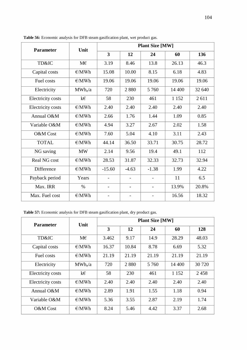
104
Table 56: Economic analysis for DFB steam gasification plant, wet product gas.
Parameter Unit Plant Size [MW]
3 12 24 60 136
TD&IC M€ 3.19 8.46 13.8 26.13 46.3
Capital costs €/MWh 15.08 10.00 8.15 6.18 4.83
Fuel costs €/MWh 19.06 19.06 19.06 19.06 19.06
Electricity MWhe/a 720 2 880 5 760 14 400 32 640
Electricity costs k€ 58 230 461 1 152 2 611
Electricity costs €/MWh 2.40 2.40 2.40 2.40 2.40
Annual O&M €/MWh 2.66 1.76 1.44 1.09 0.85
Variable O&M €/MWh 4.94 3.27 2.67 2.02 1.58
O&M Cost €/MWh 7.60 5.04 4.10 3.11 2.43
TOTAL €/MWh 44.14 36.50 33.71 30.75 28.72
NG saving MW 2.14 9.56 19.4 49.1 112
Real NG cost €/MWh 28.53 31.87 32.33 32.73 32.94
Difference €/MWh -15.60 -4.63 -1.38 1.99 4.22
Payback period Years - - - 11 6.5
Max. IRR % - - - 13.9% 20.8%
Max. Fuel cost €/MWh - - - 16.56 18.32
Table 57: Economic analysis for DFB steam gasification plant, dry product gas.
Parameter Unit Plant Size [MW]
3 12 24 60 128
TD&IC M€ 3.462 9.17 14.9 28.29 48.03
Capital costs €/MWh 16.37 10.84 8.78 6.69 5.32
Fuel costs €/MWh 21.19 21.19 21.19 21.19 21.19
Electricity MWhe/a 720 2 880 5 760 14 400 30 720
Electricity costs k€ 58 230 461 1 152 2 458
Electricity costs €/MWh 2.40 2.40 2.40 2.40 2.40
Annual O&M €/MWh 2.89 1.91 1.55 1.18 0.94
Variable O&M €/MWh 5.36 3.55 2.87 2.19 1.74
O&M Cost €/MWh 8.24 5.46 4.42 3.37 2.68
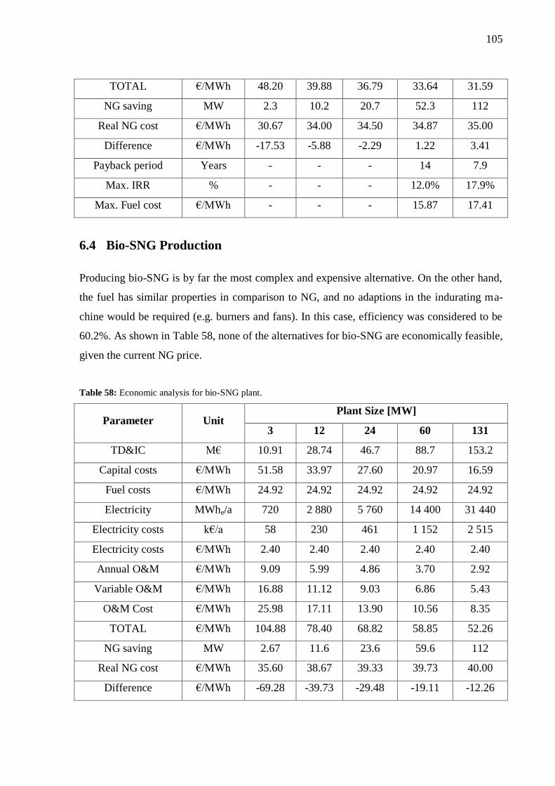
105
TOTAL €/MWh 48.20 39.88 36.79 33.64 31.59
NG saving MW 2.3 10.2 20.7 52.3 112
Real NG cost €/MWh 30.67 34.00 34.50 34.87 35.00
Difference €/MWh -17.53 -5.88 -2.29 1.22 3.41
Payback period Years - - - 14 7.9
Max. IRR % - - - 12.0% 17.9%
Max. Fuel cost €/MWh - - - 15.87 17.41
6.4 Bio-SNG Production
Producing bio-SNG is by far the most complex and expensive alternative. On the other hand,
the fuel has similar properties in comparison to NG, and no adaptions in the indurating ma-
chine would be required (e.g. burners and fans). In this case, efficiency was considered to be
60.2%. As shown in Table 58, none of the alternatives for bio-SNG are economically feasible,
given the current NG price.
Table 58: Economic analysis for bio-SNG plant.
Parameter Unit Plant Size [MW]
3 12 24 60 131
TD&IC M€ 10.91 28.74 46.7 88.7 153.2
Capital costs €/MWh 51.58 33.97 27.60 20.97 16.59
Fuel costs €/MWh 24.92 24.92 24.92 24.92 24.92
Electricity MWhe/a 720 2 880 5 760 14 400 31 440
Electricity costs k€/a 58 230 461 1 152 2 515
Electricity costs €/MWh 2.40 2.40 2.40 2.40 2.40
Annual O&M €/MWh 9.09 5.99 4.86 3.70 2.92
Variable O&M €/MWh 16.88 11.12 9.03 6.86 5.43
O&M Cost €/MWh 25.98 17.11 13.90 10.56 8.35
TOTAL €/MWh 104.88 78.40 68.82 58.85 52.26
NG saving MW 2.67 11.6 23.6 59.6 112
Real NG cost €/MWh 35.60 38.67 39.33 39.73 40.00
Difference €/MWh -69.28 -39.73 -29.48 -19.11 -12.26

106
7 SUMMARY
This study assessed the use of several gasification technologies for NG substitution in a trav-
elling grate induration furnace. CFB air and oxygen gasification and DFB steam gasification
and bio-SNG production were discussed as the most promising large-scale models. The main
findings are summarized in this chapter.
First, product gas/bio-SNG compositions for each technology were calculated, based on mass
balances. Thus, product gases compositions in molar percentage (wet basis) as well as main
thermochemical and combustion properties are summarized in Table 59.
Table 59: Product gas composition and LHV for several gasification technologies.
Property Air Oxygen Steam Steam (dry) Bio-SNG
CH4 [%-mol] 4.14% 0.76% 7.32% 9.66% 84.7%
CO [%-mol] 18.0% 35.7% 14.0% 18.5% 0.34%
CO2 [%-mol] 11.5% 10.5% 14.1% 18.6% 1.64%
H2 [%-mol] 13.2% 27.9% 31.1% 41.0% 9.94%
N2 [%-mol] 41.4% 0.85% 0.04% 0.06% 0.20%
H2O [%-mol] 11.8% 24.2% 33.5% 12.2% 3.13%
LHV [MJ/Nm3] 5.32 8.22 8.32 10.5 31.7
MM [kg/kmol] 24.75 19.92 17.98 17.96 15.24
[Nm3/kmol] 21.85 21.30 20.87 21.84 22.25
Combustion air ratio 6.21 6.85 6.39 6.26 6.19
The most important comparison parameters between different gasification technologies were
found to be adiabatic flame temperature for 112 MW of gaseous fuel, the kiln’s final energy
consumption, required gasifier size and increase in the gas flow. Wood input and estimated
planted area are also important decision making parameters. These values are summarized in
Table 60.
Short and medium term substitution scenarios were proposed; for instance 3, 12, 24 and 60
MW. As expected, increase in energy consumption, gas flow rates and other key parameters

107
were found to be a linear function of the gasifier size. Therefore, small gasification facilities
are expected to have no or very low impact on the system.
Table 60: Comparison of gasification technologies for total substitution of NG.
Parameter Air Oxygen Steam (wet) Steam (dry) Bio-SNG
Flame temperature for
112 MW [°C] 1 347 1 365 1 361 1 354 1 373
Energy consumption
[MW] 284 259 263 255 239
Increase in energy con-
sumption [%] 18.6% 8.37% 10.0% 6.59% 0.07%
Gasifier Size [MW] 157 132 136 128 131
Gaseous fuel flow
increase [%] 778% 399% 408% 321% 23.1%
Kiln hood gas flow in-
crease [%] 6.05% 3.10% 3.17% 2.49% 0.18%
Flue gas increase [%] 4.93% 1.83% 2.10% 1.36% 0.021%
Hot gas efficiency [%] 85.4% 88.4% 78.7% 70.8% 60.2%
Wood input at 15% MC
[t h-1
] 42.4 34.5 40.0 41.7 43.1
Planted area [ha] 27 000 22 000 25 500 26 500 27 500
The main data obtained in the economical assessment were investment costs, payback period,
maximum interest rate and maximum wood price for which each technology is still economi-
cally feasible. Except for the TD&IC, all other values were calculated based on a corrected
NG price since the energy consumption increases differently in each case and size. The results
are summarized in Figures 29 to 32.
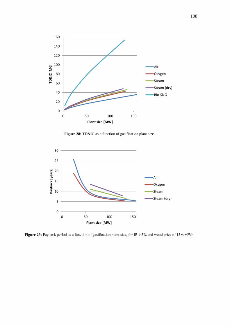
108
Figure 28: TD&IC as a function of gasification plant size.
Figure 29: Payback period as a function of gasification plant size, for IR 9.5% and wood price of 15 €/MWh.
0
20
40
60
80
100
120
140
160
0 50 100 150
TD&
IC [
M€]
Plant size [MW]
Air
Oxygen
Steam
Steam (dry)
Bio-SNG
0
5
10
15
20
25
30
0 50 100 150
Pay
bac
k [y
ears
]
Plant size [MW]
Air
Oxygen
Steam
Steam (dry)

109
Figure 30: Maximum interest rate as a function of gasification plant size, for 20 years lifecycle and wood price
of 15 €/MWh.
Figure 31: Maximum wood price as a function of gasification plant size, for IR 9.5% and 20 years lifecycle.
Finally, it is important to address that each technology discussed in this study has unique
characteristics, advantages and disadvantages which must be taken into account when making
the final decision. The most important advantages and disadvantages are summarized in Table
61.
0%
5%
10%
15%
20%
25%
0 50 100 150
Max
imu
m IR
[%
]
Plant size [MW]
Air
Oxygen
Steam
Steam (dry)
0.00
2.00
4.00
6.00
8.00
10.00
12.00
14.00
16.00
18.00
20.00
0 50 100 150
Max
imu
m w
oo
d p
rice
[€/
MW
h]
Plant size [MW]
Air
Oxygen
Steam
Steam (dry)
Bio-SNG
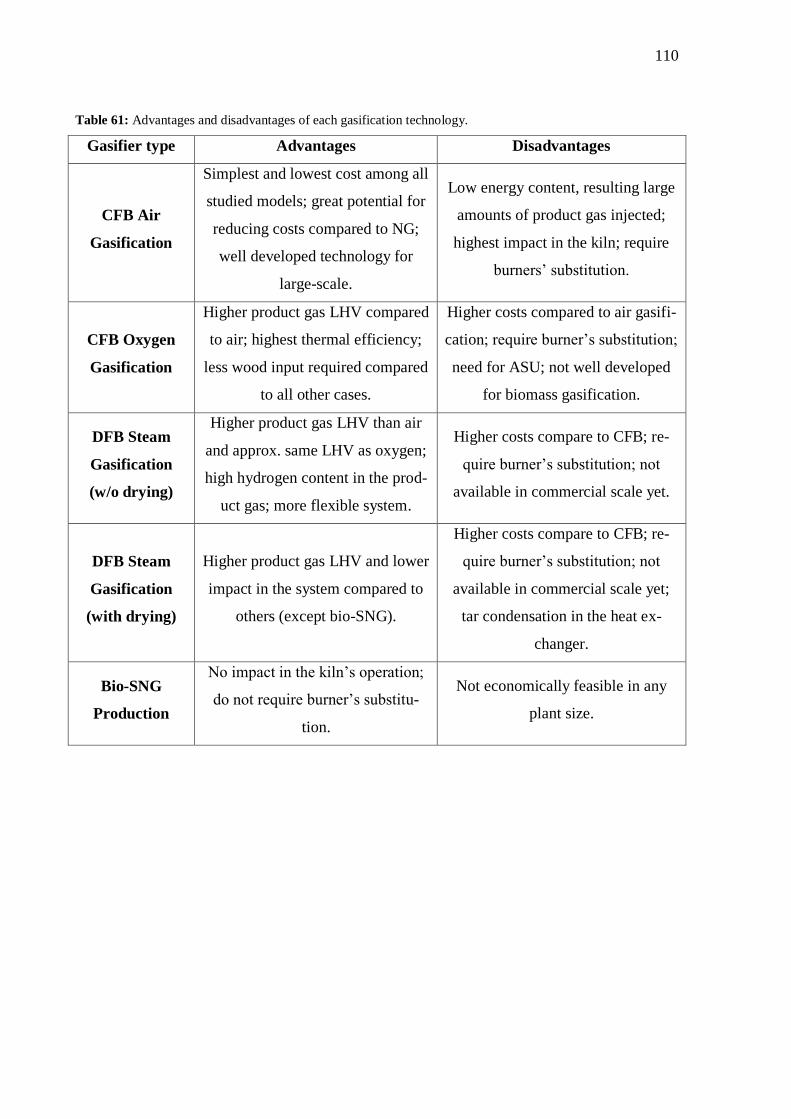
110
Table 61: Advantages and disadvantages of each gasification technology.
Gasifier type Advantages Disadvantages
CFB Air
Gasification
Simplest and lowest cost among all
studied models; great potential for
reducing costs compared to NG;
well developed technology for
large-scale.
Low energy content, resulting large
amounts of product gas injected;
highest impact in the kiln; require
burners’ substitution.
CFB Oxygen
Gasification
Higher product gas LHV compared
to air; highest thermal efficiency;
less wood input required compared
to all other cases.
Higher costs compared to air gasifi-
cation; require burner’s substitution;
need for ASU; not well developed
for biomass gasification.
DFB Steam
Gasification
(w/o drying)
Higher product gas LHV than air
and approx. same LHV as oxygen;
high hydrogen content in the prod-
uct gas; more flexible system.
Higher costs compare to CFB; re-
quire burner’s substitution; not
available in commercial scale yet.
DFB Steam
Gasification
(with drying)
Higher product gas LHV and lower
impact in the system compared to
others (except bio-SNG).
Higher costs compare to CFB; re-
quire burner’s substitution; not
available in commercial scale yet;
tar condensation in the heat ex-
changer.
Bio-SNG
Production
No impact in the kiln’s operation;
do not require burner’s substitu-
tion.
Not economically feasible in any
plant size.
111
8 CONCLUSIONS & FUTURE WORK
The present work discussed the use of product gas/bio-SNG as a renewable substitute for NG
in iron ore pelletizing processes. An analysis of the Brazilian NG market has shown that the
country is not yet self-sufficient in NG, and that more than half of imported NG comes from
the same supplier, namely Bolivia. The supply agreement between these two countries is valid
until 2019, and there are uncertainties concerning the amount and price of NG supply after
this period. In addition, sustainability and global warming issues contribute even more to the
necessity of investments in renewable energy.
Biomass gasification has proven to be one of the most promising technologies for NG re-
placement. Product gases can be obtained from different gasification technologies assessed in
this study. Currently, the most relevant large-scale biomass gasification model is the CFB. It
cannot only handle a wide range of alternative fuels but also different gasification media, such
as air, oxygen and steam. Each gasifying medium leads to different product gas characteris-
tics, such as composition and LHV. Bio-SNG can be best obtained by DFB steam gasification
followed by methanation.
The aforementioned thermochemical processes were compared under technical and economic
perspectives. First, adiabatic flame temperature for the current fuels (NG, petcoke and coal)
was determined. The amount of product gas and bio-SNG required to maintain this constant
temperature was calculated in each case, as well as the gas flow through the indurating ma-
chine. The air flow was kept constant since it is defined by the requirements in the cooling
zone. It was found that, for all gasification processes except bio-SNG production, the specific
energy consumption would increase as well as the gas flow rate through the kiln.
Burner substitution seems inevitable in all cases, except for bio-SNG. On the other hand, it is
possible that the fans would not require substitution in any of the cases since the maximum
increase in the flue gas flow is approximately 5%. Lower substitution scenarios were also
evaluated, such as 3, 12, 24 and 60 MW. As expected, the lower the substitution the less im-
pact product gas would have on the system. However, reductions in GHG emissions may not
be relevant, and the plant costs are considerably higher.

112
Preliminary economic assessment has shown that small-scale gasification plants (e.g. up to 24
MW) are not feasible. On the other hand, from 60 MW the use of product gas appears to be
slightly less costly than NG in all cases except bio-SNG production. However, adaptations in
the induration furnace were not taken into account in the economic assessment, and it is pos-
sible that this enterprise would be less attractive. Nonetheless, sustainability, environmental
and security of supply aspects should be also considered in this investment.
Based on the results of this study, it is possible to conclude that air gasification is a suitable
technology for NG substitution in iron ore pelletizing traveling grates. However, further stud-
ies should be performed before making the final decision:
Impacts of increasing gas flow rate on the burners should be evaluated by computa-
tional fluid dynamics (CFD) analysis. In addition, new burner design and temperature
resistant materials must be specified;
One possible solution for the burners is to inject the gas partially or entirely (depend-
ing on the substitution rate) in another location, e.g. in the kiln hood. Further studies
are needed to confirm this possibility; for example, determine the maximum amount of
gas to avoid premature combustion.
The economic assessment presented here covers only the order of magnitude of in-
vestment costs. Although the numbers are in agreement with recent budgets, all the
numbers do not necessarily represent the Brazilian reality;
Process economics may be improved if an optimized waste heat recovery solution for
steam/electricity production is considered, especially in the case of bio-SNG. Howev-
er, this would require a detailed project;
Effects on pelletizing gaseous emissions, such as ammonia and nitrogen oxides. Possi-
ble costs of air pollution control equipment (if needed) should be taken into account in
the economic assessment.
In addition, other studies should be also done in order to improve process economics and rein-
force the necessity/advantages of investments in renewable energy, such as:
Assess the best eucalyptus harvesting technology and optimize biomass costs;
Evaluate the availability of low-cost alternative fuels, such as energy crops and/or ag-
ricultural;
Life cycle analysis would help other benefits of a biomass gasification plant to be
clearly defined and assessed.

113
REFERENCES
Economic Indicators. Chemical Engineering, 2013. vol. 120, no. 07, p. 60.
ABU EL-RUB, Z., BRAMER, E. and BREM, G., 2004. Review of Catalysts for Tar Elimina-
tion in Biomass Gasification Processes. Industrial & Engineering Chemistry Research, vol.
43, no. 22, pp. 6911-6919.
ANEEL., n.d. Atlas De Energia Elétrica do Brasil. Agência Nacional de Energia Elétrica
[viewed 08 July 2013]. Available from:
http://www.aneel.gov.br/arquivos/PDF/atlas_par3_cap6.pdf
ANEEL., 2013. Tarifa Média Por Classe De Consumo e Por Região. Agência Nacional de
Energia Elétrica [viewed 04 November 2013]. Available from:
http://relatorios.aneel.gov.br/_layouts/xlviewer.aspx?id=/RelatoriosSAS/RelSampRegCC.xlsx
&Source=http://relatorios.aneel.gov.br/RelatoriosSAS/Forms/AllItems.aspx&DefaultItemOpe
n=1.
BACOVSKY, D., DALLOS, M., WÖRGETTER, M. and TASK, I.B., 2010. Status of 2nd
Generation Biofuels Demonstration Facilities in June 2010. IEA Bioenergy Task 39: Com-
mercializing 1st and 2nd Generation Liquid Biofuels from Biomass.
BARATIERI, M., BAGGIO, P., FIORI, L. and GRIGIANTE, M., 2008. Biomass as an Ener-
gy Source: Thermodynamic Constraints on the Performance of the Conversion Process. Bio-
resource Technology, vol. 99, no. 15, pp. 7063-7073.
BASU, P., 2010. Biomass Gasification and Pyrolysis: Practical Design and Theory. Academ-
ic press.
BASU, P., 2006. Solid Handling Systems for Fluidized Beds. In: Combustion and gasifica-
tion in fluidized beds, CRC press, pp. 337-357.
BRAMMER, J.G. and BRIDGWATER, A.V., 1999. Drying Technologies for an Integrated
Gasification Bio-Energy Plant. Renewable and Sustainable Energy Reviews, 12, vol. 3, no. 4,
pp. 243-289 ISSN 1364-0321.
BREITHOLTZ, C., 2001. The Biomass Gasification Plant to Vaskiluodon Voima in Vaasa
and Two More Ongoing Gasification Projects. Presentation given in Solander Symposium

114
2011 [viewed 14 November 2013]. Available from:
http://www.zelenaenergija.org/blobs/eb16f372-fa48-42fe-b621-e9cf0b5fdc7a.pdf.
BRIDGWATER, A.V., 2002. The Future for Biomass Pyrolysis and Gasification: Status,
Opportunities and Policies for Europe. Birmingham: University of Aston.
BRIDGWATER, A., 2003. Renewable Fuels and Chemicals by Thermal Processing of Bio-
mass. Chemical Engineering Journal, vol. 91, no. 2, pp. 87-102.
CASTRO, L.F.A., FIGUEIRA, R.M. and TAVARES, R.P., 2004. Princípios Básicos is Pro-
cessos De Fabricação do Gusa Ao Aço Líquido. Belo Horizonte: Universidade Federal de
Minas Gerais.
CHANNIWALA, S. and PARIKH, P., 2002. A Unified Correlation for Estimating HHV of
Solid, Liquid and Gaseous Fuels. Fuel, vol. 81, no. 8, pp. 1051-1063.
CHASE JR, M.W., 1998. NIST-JANAF Thermochemical Tables. J. Phys. Chem. Ref. Data.
Fourth ed., pp. 1-1951.
CHEN, G., ANDRIES, J. and SPLIETHOFF, H., 2003. Biomass Conversion into Fuel Gas
using Circulating Fluidised Bed Technology: The Concept Improvement and Modelling Dis-
cussion. Renewable Energy, vol. 28, no. 6, pp. 985-994.
COMPAGAS., n.d. Manual do Consumidor Industrial. Companhia Paranaense de Gás [vie-
wed 18 October 2013]. Available from:
http://www.compagas.com.br/index.php/web/onde_e_como_usar_o_gas_natural/gn_para_em
presa/manual_do_consumidor_industrial.
CORELLA, J., TOLEDO, J.M. and MOLINA, G., 2007. A Review on Dual Fluidized-Bed
Biomass Gasifiers. Industrial & Engineering Chemistry Research, vol. 46, no. 21, pp. 6831-
6839.
CORTEZ, C.L., VELÁZQUEZ, S., COELHO, S.T. and ROBERTO, J., n.d. Análise do Pro-
cesso Produtivo do Eucalipto no Sistema “Short Rotation” Para Uso Como Combustível Em
Uma Usina Termoelétrica. Universidade de São Paulo [viewed 30 July 2013]. Available
from: http://cenbio.iee.usp.br/download/publicacoes/congbioen_cortez.pdf.
CUMMER, K.R. and BROWN, R.C., 2002. Ancillary Equipment for Biomass Gasification.
Biomass and Bioenergy, vol. 23, no. 2, pp. 113-128.
115
DEURWAARDER, E.P., et al., 2005. Methanation of MILENA Product Gas for the Produc-
tion of Bio-SNG. 14th European Biomass Conference & Exhibition: Paris.
DEVI, L., PTASINSKI, K.J. and JANSSEN, F.J., 2003. A Review of the Primary Measures
for Tar Elimination in Biomass Gasification Processes. Biomass and Bioenergy, vol. 24, no. 2,
pp. 125-140.
DO CANTO, J.L., 2009. Colheita Mecanizada De Biomassa Florestal Para Energia. Univer-
sidade Federal de Viçosa.
DO CANTO, J.L., et al, 2011. Evaluation of a Wood Chipping System for Eucalyptus Tops
for Energy. Revista Árvore, vol. 35, no. 6, pp. 1327-1334.
EPE., 2012. Balanço Energético Nacional 2012 - Ano Base 2011. Brasília: Ministério das
Minas e Energia [viewed 29 March 2013]. Available from:
https://ben.epe.gov.br/downloads/Resultados_Pre_BEN_2012.pdf.
EPE., 2011. Projeção Da Demanda De Energia Elétrica Para Os Próximos 10 Anos (2012-
2021). Rio de Janeiro: Ministério das Minas e Energia [viewed 29 March 2013]. Available
from:
http://www.epe.gov.br/mercado/Documents/S%C3%A9rie%20Estudos%20de%20Energia/20
120104_1.pdf.
FERCHER, E., et al., 1998. Two Years Experience with the FICFB-Gasification Process.
10th European Conference and Technology Exhibition on Biomass for Energy and Industry.
FERMOSO, J., et al, 2009. High-Pressure Co-Gasification of Coal with Biomass and Petrole-
um Coke. Fuel Processing Technology, vol. 90, no. 7, pp. 926-932.
GAO, J., et al, 2012. A Thermodynamic Analysis of Methanation Reactions of Carbon Oxides
for the Production of Synthetic Natural Gas. RSC Advances, vol. 2, no. 6, pp. 2358-2368.
GASSNER, M. and MARÉCHAL, F., 2009. Thermo-Economic Process Model for Thermo-
chemical Production of Synthetic Natural Gas (SNG) from Lignocellulosic Biomass. Biomass
and Bioenergy, vol. 33, no. 11, pp. 1587-1604.
GHAFFARIYAN, M., et al, 2011. Biomass Harvesting in Eucalyptus Plantations in Western
Australia. Southern Forests: A Journal of Forest Science, vol. 73, no. 3-4, pp. 149-154.
116
GÖRANSSON, K., SÖDERLIND, U., HE, J. and ZHANG, W., 2011. Review of Syngas Pro-
duction Via Biomass DFBGs. Renewable and Sustainable Energy Reviews, vol. 15, no. 1, pp.
482-492.
GULLICHSEN, J. and FOGELHOLM, C., 1999. Preparation and Handling of Bleaching
Chemicals. In: Book 6B: Chemical pulping, Helsinki: Fapet Oy, pp. 391-410.
HARYANTO, A., FERNANDO, S.D., PORDESIMO, L.O. and ADHIKARI, S., 2009. Up-
grading of Syngas Derived from Biomass Gasification: A Thermodynamic Analysis. Biomass
and Bioenergy, vol. 33, no. 5, pp. 882-889.
HIGMAN, C. and VAN DER BURGT, M., 2008. Gasification. 2nd. Gulf Professional Pub-
lishing, USA.
HOFBAUER, H. and RAUCH, R., 2000. Stoichiometric Water Consumption of Steam Gasi-
fication by the FICFB-Gasification Process. Progress in Thermochemical Biomass Conver-
sion, vol. 1, pp. 199-208.
International Energy Agency, 2013. Tracking Clean Energy Progress 2013. Paris: IEA Input
to the Clean Energy Ministerial.
JESUS, C.A.G., 2012. Economia Mineral: Sumário Mineral 2012. Departamento Nacional de
Produção Mineral (DNPM) [viewed 20 May 2013]. Available from:
https://sistemas.dnpm.gov.br/publicacao/mostra_imagem.asp?IDBancoArquivoArquivo=7390
KALLIO, M. and LEINONEN, A., 2005. Production Technology of Forest Chips in Finland.
Jyväskylä: Technical Research Center of Finland (VTT).
KAUP, B.Z., 2010. A Neoliberal Nationalization? the Constraints on Natural-Gas-Led Devel-
opment in Bolivia. Latin American Perspectives, vol. 37, no. 3, pp. 123-138.
KOPYSCINSKI, J., SCHILDHAUER, T.J. and BIOLLAZ, S., 2010. Production of Synthetic
Natural Gas (SNG) from Coal and Dry biomass–A Technology Review from 1950 to 2009.
Fuel, vol. 89, no. 8, pp. 1763-1783.
LI, C. and SUZUKI, K., 2009. Tar Property, Analysis, Reforming Mechanism and Model for
Biomass gasification—an Overview. Renewable and Sustainable Energy Reviews, vol. 13, no.
3, pp. 594-604.
117
LV, D., et al, 2010. Effect of Cellulose, Lignin, Alkali and Alkaline Earth Metallic Species on
Biomass Pyrolysis and Gasification. Fuel Processing Technology, vol. 91, no. 8, pp. 903-909.
MCKENDRY, P., 2002. Energy Production from Biomass (Part 3): Gasification Technolo-
gies. Bioresource Technology, vol. 83, no. 1, pp. 55-63.
METSO PAPER., 2010. Rotatory Screw Reclaimers. [viewed 05 September 2013]. Available
from: http://www.metso.com/MP/marketing/Vault2MP.nsf/BYWID/WID-030328-2256C-
57B5E/$File/WHDU_B_2080_013-02.pdf?OpenElement.
MILNE, T.A., ABATZOGLOU, N. and EVANS, R.J., 1998. Biomass Gasifier "Tars": Their
Nature, Formation, and Conversion. National Renewable Energy Laboratory Golden, CO.
MME., 2013. Boletim Mensal De Acompanhamento Da Indústria De Gás Natural. Ministério
das Minas e Energia [viewed 07 November 2013]. Available from:
http://www.mme.gov.br/sproduct
gas/galerias/arquivos/publicacoes/boletim_mensal_acompanhamento_industria_gas_natural/B
oletim_Gas_Natural_nr_74_mai_13.pdf.
MORAN, M.J., SHAPIRO, H.N., BOETTNER, D.D. and BAILEY, M., 2006. Fundamentals
of Engineering Thermodynamics. Fifth ed. John Wiley & Sons, Inc.
NIGRO, J.C., 1982. Firing an Iron Ore Pelletizing Kiln with Low-Btu Gas from Lignite. US
Department of the Interior, Bureau of Mines.
OLOFSSON, I., NORDIN, A. and SÖDERLIND, U., 2005. Initial Review and Evaluation of
Process Technologies and Systems Suitable for Cost-Efficient Medium-Scale Gasification for
Biomass to Liquid Fuels. Umeå Universitet.
PALONEN, J., OY, F.W.E., ANTTIKOSKI, T. and ERIKSSON, T., 2005. The Foster
Wheeler Gasification Technology for Biofuels: Refuse-Derived Fuel (RDF) Power Genera-
tion.
PUIG-ARNAVAT, M., BRUNO, J.C. and CORONAS, A., 2010. Review and Analysis of
Biomass Gasification Models. Renewable and Sustainable Energy Reviews, vol. 14, no. 9, pp.
2841-2851.
QUÉNO, L.M.R., et al, 2011. Custo De Produção Das Biomassas De Eucalipto e Capim Ele-
fante Para Energia. Cerne, Lavras, vol. 17, no. 3, pp. 417-426.
118
RAYAPROLU, K., 2010. Fluidized Bed Combustion. In: Boilers for power and process,
CRC Press, pp. 505-558.
REILLY, B.G., 2011. International Silo Association. [viewed 30 October 2013]. Available
from: http://www.silo.org/costs.htm.
ROCKSTRÖM, J., et al, 2009. A Safe Operating Space for Humanity. Nature, vol. 461, no.
7263, pp. 472-475.
SALO, K. and MOJTAHEDI, W., 1998. Fate of Alkali and Trace Metals in Biomass Gasifi-
cation. Biomass and Bioenergy, vol. 15, no. 3, pp. 263-267 ISSN 0961-9534.
SAMARCO., n.d. Samarco Technical Information. [viewed 28 March 2013]. Available from:
http://www.samarco.com.br/uploads/xgccbf.pdf.
SZTABERT, Z.T. and KUDRA, T., 2006. Cost-Estimation Methods for Drying. A.S. MU-
JUMDAR ed., In: Handbook of industrial drying, CRC Press.
TOWLER, G.P. and SINNOTT, R.K., 2012. Chapter 07: Capital Costs Estimating. In: Chem-
ical Engineering Design: Principles, Practice, and Economics of Plant and Process Design,
Second Edition ed. Access Online via Elsevier, pp. 307-354.
TURN, S.Q., KINOSHITA, C.M., ISHIMURA, D.M. and ZHOU, J., 1998. The Fate of Inor-
ganic Constituents of Biomass in Fluidized Bed Gasification. Fuel, vol. 77, no. 3, pp. 135-
146.
United Nations Statistics Division., 2013. 2012 International Trade Statistics Yearbook. New
York: United Nations [viewed 05 July 2013] Available from:
http://comtrade.un.org/pb/CountryPagesNew.aspx?y=2012.
VAKKILAINEN, E., KUPARINEN, K. and HEINIMÖ, J., 2013. Industrial Users of Energy
Biomass. Lappeenranta: IEA Bioenergy - Task 40.
VAN DER MEIJDEN, C., VERINGA, H. and RABOU, L., 2010. The Production of Synthet-
ic Natural Gas (SNG): A Comparison of Three Wood Gasification Systems for Energy Bal-
ance and overall Efficiency. Biomass and Bioenergy, vol. 34, no. 3, pp. 302-311.
VAN LOO, S. and KOPPEJAN, J., 2008. Biomass Fuel Supply and Pre-treatment. In: The
handbook of biomass combustion and co-firing, Earthscan, pp. 44-108.

119
VITASARI, C.R., JURASCIK, M. and PTASINSKI, K.J., 2011. Exergy Analysis of Bio-
mass-to-Synthetic Natural Gas (SNG) Process Via Indirect Gasification of various Biomass
Feedstock. Energy, vol. 36, no. 6, pp. 3825-3837.
WORLEY, M. and YALE, J., 2012. Biomass Gasification Technology Assessment: Consoli-
dated Report. Golden, CO.: National Renewable Energy Laboratory (NREL).
YIP, K., TIAN, F., HAYASHI, J. and WU, H., 2009. Effect of Alkali and Alkaline Earth Me-
tallic Species on Biochar Reactivity and Syngas Compositions during Steam Gasification.
Energy & Fuels, vol. 24, no. 1, pp. 173-181.
ZAHL, R. and NIGRO, J., 1979. The use of Low-Btu Gas for Iron Oxide Pellet Induration:
An Interim Report. Symposium proceedings, Environmental Aspects of Fuel Conversion
Technology, IV (April 1979, Hollywood, FL)US Environmental Protection Agency, Industrial
Environmental Research Laboratory.
ZWART, R., et al., 2006. Production of Synthetic Natural Gas (SNG) from Biomass. Energy
Research Centre of the Netherlands (ECN).
ZWART, R., et al, 2009. Oil based Gas washing—Flexible Tar Removal for high efficient
Production of Clean Heat and Power as Well as Sustainable Fuels and Chemicals. Environ-
mental Progress & Sustainable Energy, vol. 28, no. 3, pp. 324-335.
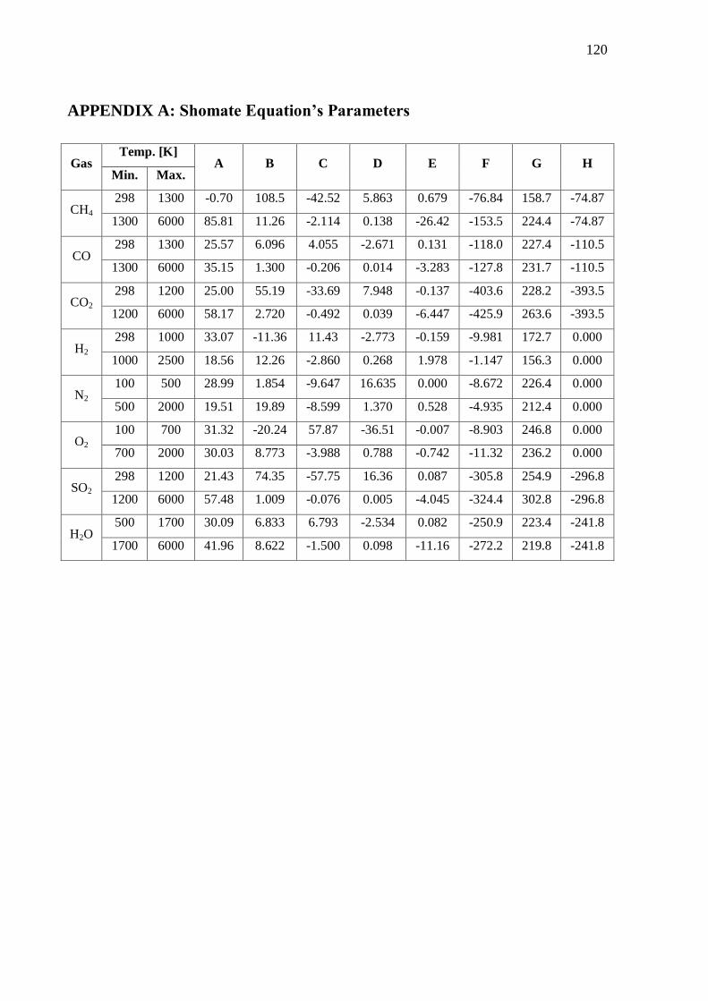
120
APPENDIX A: Shomate Equation’s Parameters
Gas Temp. [K]
A B C D E F G H Min. Max.
CH4 298 1300 -0.70 108.5 -42.52 5.863 0.679 -76.84 158.7 -74.87
1300 6000 85.81 11.26 -2.114 0.138 -26.42 -153.5 224.4 -74.87
CO 298 1300 25.57 6.096 4.055 -2.671 0.131 -118.0 227.4 -110.5
1300 6000 35.15 1.300 -0.206 0.014 -3.283 -127.8 231.7 -110.5
CO2 298 1200 25.00 55.19 -33.69 7.948 -0.137 -403.6 228.2 -393.5
1200 6000 58.17 2.720 -0.492 0.039 -6.447 -425.9 263.6 -393.5
H2 298 1000 33.07 -11.36 11.43 -2.773 -0.159 -9.981 172.7 0.000
1000 2500 18.56 12.26 -2.860 0.268 1.978 -1.147 156.3 0.000
N2 100 500 28.99 1.854 -9.647 16.635 0.000 -8.672 226.4 0.000
500 2000 19.51 19.89 -8.599 1.370 0.528 -4.935 212.4 0.000
O2 100 700 31.32 -20.24 57.87 -36.51 -0.007 -8.903 246.8 0.000
700 2000 30.03 8.773 -3.988 0.788 -0.742 -11.32 236.2 0.000
SO2 298 1200 21.43 74.35 -57.75 16.36 0.087 -305.8 254.9 -296.8
1200 6000 57.48 1.009 -0.076 0.005 -4.045 -324.4 302.8 -296.8
H2O 500 1700 30.09 6.833 6.793 -2.534 0.082 -250.9 223.4 -241.8
1700 6000 41.96 8.622 -1.500 0.098 -11.16 -272.2 219.8 -241.8
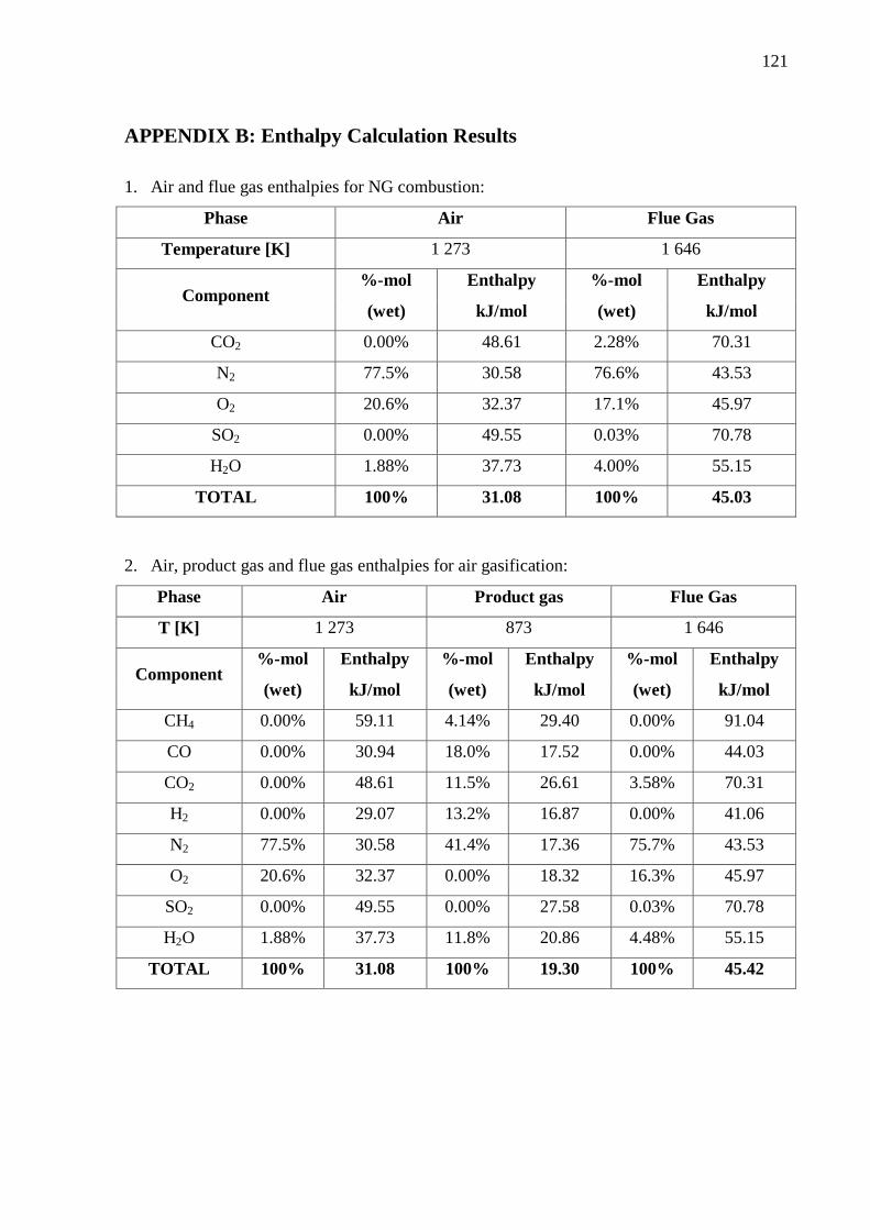
121
APPENDIX B: Enthalpy Calculation Results
1. Air and flue gas enthalpies for NG combustion:
Phase Air Flue Gas
Temperature [K] 1 273 1 646
Component %-mol Enthalpy %-mol Enthalpy
(wet) kJ/mol (wet) kJ/mol
CO2 0.00% 48.61 2.28% 70.31
N2 77.5% 30.58 76.6% 43.53
O2 20.6% 32.37 17.1% 45.97
SO2 0.00% 49.55 0.03% 70.78
H2O 1.88% 37.73 4.00% 55.15
TOTAL 100% 31.08 100% 45.03
2. Air, product gas and flue gas enthalpies for air gasification:
Phase Air Product gas Flue Gas
T [K] 1 273 873 1 646
Component %-mol Enthalpy %-mol Enthalpy %-mol Enthalpy
(wet) kJ/mol (wet) kJ/mol (wet) kJ/mol
CH4 0.00% 59.11 4.14% 29.40 0.00% 91.04
CO 0.00% 30.94 18.0% 17.52 0.00% 44.03
CO2 0.00% 48.61 11.5% 26.61 3.58% 70.31
H2 0.00% 29.07 13.2% 16.87 0.00% 41.06
N2 77.5% 30.58 41.4% 17.36 75.7% 43.53
O2 20.6% 32.37 0.00% 18.32 16.3% 45.97
SO2 0.00% 49.55 0.00% 27.58 0.03% 70.78
H2O 1.88% 37.73 11.8% 20.86 4.48% 55.15
TOTAL 100% 31.08 100% 19.30 100% 45.42

122
3. Air, product gas and flue gas enthalpies for oxygen gasification:
Phase Air Product gas Flue Gas
T [K] 1 273 873 1 646
Component %-mol Enthalpy %-mol Enthalpy %-mol Enthalpy
(wet) kJ/mol (wet) kJ/mol (wet) kJ/mol
CH4 0.00% 59.11 0.76% 32.77 0.00% 91.04
CO 0.00% 30.94 35.7% 19.15 0.00% 44.03
CO2 0.00% 48.61 10.5% 29.25 3.26% 70.31
H2 0.00% 29.07 27.9% 18.36 0.00% 41.06
N2 77.5% 30.58 0.85% 18.96 75.2% 43.53
O2 20.6% 32.37 0.00% 20.03 17.1% 45.97
SO2 0.00% 49.55 0.00% 30.26 0.03% 70.78
H2O 1.88% 37.73 24.2% 22.86 4.48% 55.15
TOTAL 100% 31.08 100% 21.00 100% 45.35
4. Air, product gas and flue gas enthalpies for steam gasification (wet gas):
Phase Air Product gas Flue Gas
T [K] 1 273 873 1 646
Component %-mol Enthalpy %-mol Enthalpy %-mol Enthalpy
(wet) kJ/mol (wet) kJ/mol (wet) kJ/mol
CH4 0.00% 59.11 7.32% 29.40 0.00% 91.04
CO 0.00% 30.94 14.0% 17.52 0.00% 44.03
CO2 0.00% 48.61 14.1% 26.61 2.85% 70.31
H2 0.00% 29.07 31.1% 16.87 0.00% 41.06
N2 77.5% 30.58 0.04% 17.36 74.8% 43.53
O2 20.6% 32.37 0.00% 18.32 16.8% 45.97
SO2 0.00% 49.55 0.00% 27.58 0.03% 70.78
H2O 1.88% 37.73 33.5% 20.86 5.59% 55.15
TOTAL 100% 31.08 100% 20.59 100% 45.36

123
5. Air, product gas and flue gas enthalpies for steam gasification (dry gas):
Phase Air Product Gas Flue Gas
T [K] 1 273 348 1 646
Component %-mol Enthalpy %-mol Enthalpy %-mol Enthalpy
(wet) kJ/mol (wet) kJ/mol (wet) kJ/mol
CH4 0.00% 59.11 9.7% 1.83 0.00% 91.04
CO 0.00% 30.94 18.5% 1.46 0.00% 44.03
CO2 0.00% 48.61 18.6% 1.91 2.94% 70.31
H2 0.00% 29.07 41.0% 1.45 0.00% 41.06
N2 77.5% 30.58 0.06% 1.46 75.4% 43.53
O2 20.6% 32.37 0.00% 1.48 16.8% 45.97
SO2 0.00% 49.55 0.00% 2.04 0.03% 70.78
H2O 1.88% 37.73 12.2% 1.69 4.74% 55.15
TOTAL 100% 31.08 100% 1.60 100% 45.29
6. Air and flue gas enthalpies for bio-SNG combustion:
Phase Air Flue Gas
Temperature [K] 1 273 1 646
Component %-mol Enthalpy %-mol Enthalpy
(wet) kJ/mol (wet) kJ/mol
CH4 0.00% 59.11 0.00% 91.04
CO 0.00% 30.94 0.00% 44.03
CO2 0.00% 48.61 2.28% 70.31
H2 0.00% 29.07 0.00% 41.06
N2 77.5% 30.58 76.6% 43.53
O2 20.6% 32.37 17.1% 45.97
SO2 0.00% 49.55 0.03% 70.78
H2O 1.88% 37.73 4.00% 55.15
TOTAL 100% 31.08 100% 45.03
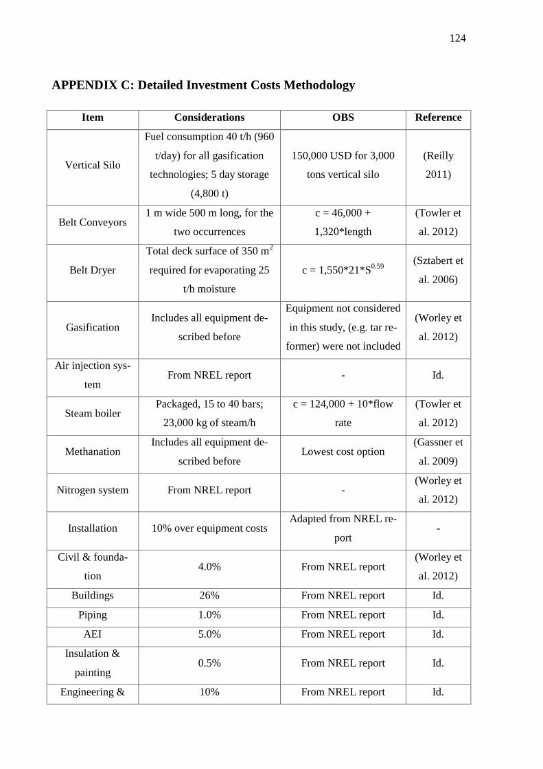
124
APPENDIX C: Detailed Investment Costs Methodology
Item Considerations OBS Reference
Vertical Silo
Fuel consumption 40 t/h (960
t/day) for all gasification
technologies; 5 day storage
(4,800 t)
150,000 USD for 3,000
tons vertical silo
(Reilly
2011)
Belt Conveyors 1 m wide 500 m long, for the
two occurrences
c = 46,000 +
1,320*length
(Towler et
al. 2012)
Belt Dryer
Total deck surface of 350 m2
required for evaporating 25
t/h moisture
c = 1,550*21*S0.59
(Sztabert et
al. 2006)
Gasification Includes all equipment de-
scribed before
Equipment not considered
in this study, (e.g. tar re-
former) were not included
(Worley et
al. 2012)
Air injection sys-
tem From NREL report - Id.
Steam boiler Packaged, 15 to 40 bars;
23,000 kg of steam/h
c = 124,000 + 10*flow
rate
(Towler et
al. 2012)
Methanation Includes all equipment de-
scribed before Lowest cost option
(Gassner et
al. 2009)
Nitrogen system From NREL report - (Worley et
al. 2012)
Installation 10% over equipment costs Adapted from NREL re-
port -
Civil & founda-
tion 4.0% From NREL report
(Worley et
al. 2012)
Buildings 26% From NREL report Id.
Piping 1.0% From NREL report Id.
AEI 5.0% From NREL report Id.
Insulation &
painting 0.5% From NREL report Id.
Engineering & 10% From NREL report Id.

125
Supervision
Pre-project cost 0.5% From NREL report Id.
Outside engineer-
ing & construc-
tion
2.0% From NREL report Id.
Sales taxes 3.5% From NREL report Id.
Freight 5.0% Adapted from NREL re-
port -
Training & start-
up 2.0% From NREL report
(Worley et
al. 2012)
Owner engineer-
ing 2.0% From NREL report Id.
Environmental
and legal expens-
es
1.0% From NREL report Id.
Capitalized spares 3.0% From NREL report Id.
Contingency 15% From NREL report Id.

126
APPENDIX D: Detailed Investment Costs Results
1. Air Gasification:
Size [MW] 3 12 24 60 157
Factor 0.063 0.165 0.269 0.510 1.000
Item k€ k€ k€ k€ k€
DRYING 170 450 720 1 380 2 700
Storage Silo 10 30 50 100 200
Conveyor (wet) 40 100 160 310 600
Belt Dryer 90 250 400 770 1 500
Conveyor (dry) 30 70 110 200 400
GASIFIER 810 2 170 3 510 6 690 13 100
H&S Distribution 410 1 090 1 770 3 370 6 600
H&S Feeding 90 250 400 770 1 500
H&S Bed Mat. 10 30 50 100 200
CFB gasifier 290 780 1 260 2 400 4 700
H&S Gasifier ash 10 20 30 50 100
Air system 10 20 30 50 100
OTHER ISBL 140 380 620 1 180 2 300
Nitrogen system 40 120 190 360 700
Installation 100 260 430 820 1 600
EQUIPMENT 1 130 3 020 4 880 9 300 18 200
OTHER DIRECT 410 1 100 1 770 3 370 6 600
Civil & foundation 40 120 190 360 700
Buildings 290 780 1 260 2 400 4 700
Piping 10 30 50 100 200
AEI 60 150 240 460 900
Insulation & painting 10 20 30 50 100
TDC 1 540 4 120 6 650 12 670 24 800
INDIRECT (ISBL) 360 930 1 490 2 860 5 600
Engineering & Supervision 150 400 640 1 220 2 400
Pre-project cost 10 20 30 50 100
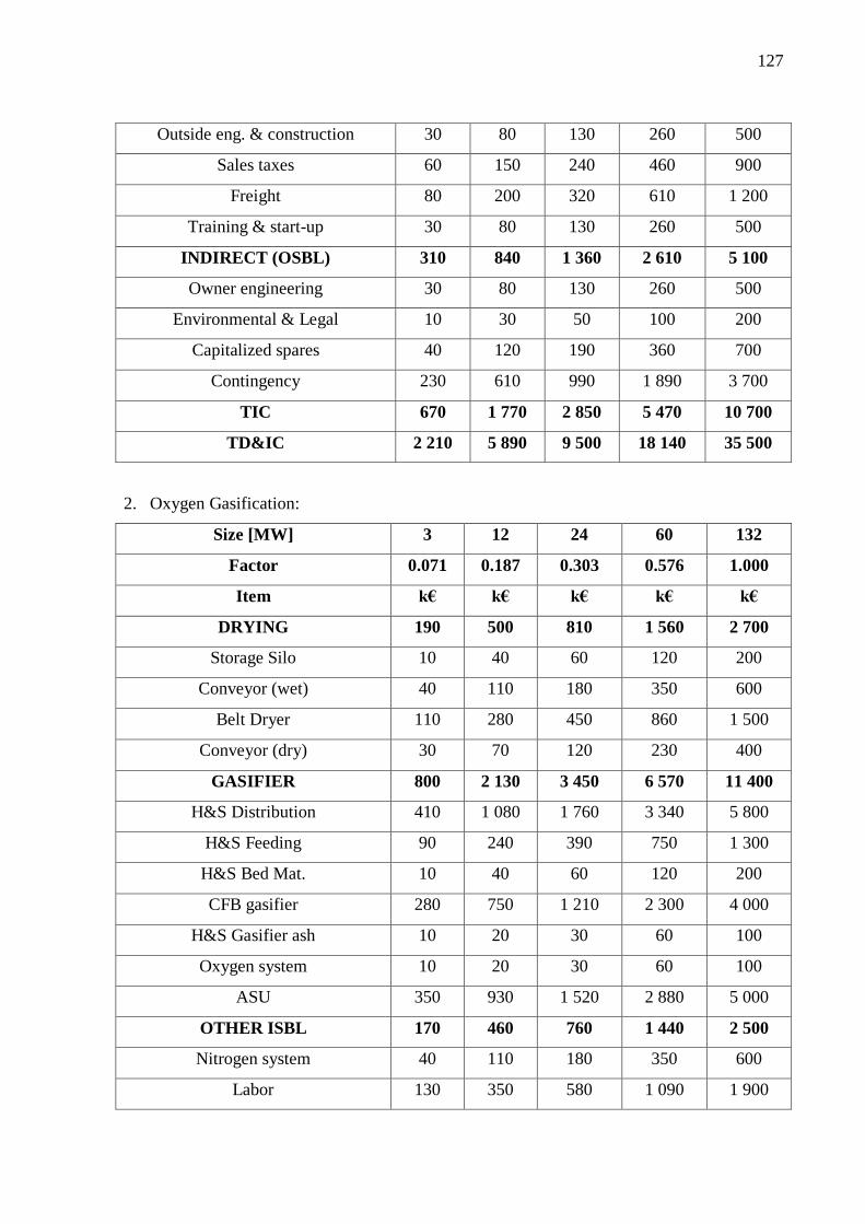
127
Outside eng. & construction 30 80 130 260 500
Sales taxes 60 150 240 460 900
Freight 80 200 320 610 1 200
Training & start-up 30 80 130 260 500
INDIRECT (OSBL) 310 840 1 360 2 610 5 100
Owner engineering 30 80 130 260 500
Environmental & Legal 10 30 50 100 200
Capitalized spares 40 120 190 360 700
Contingency 230 610 990 1 890 3 700
TIC 670 1 770 2 850 5 470 10 700
TD&IC 2 210 5 890 9 500 18 140 35 500
2. Oxygen Gasification:
Size [MW] 3 12 24 60 132
Factor 0.071 0.187 0.303 0.576 1.000
Item k€ k€ k€ k€ k€
DRYING 190 500 810 1 560 2 700
Storage Silo 10 40 60 120 200
Conveyor (wet) 40 110 180 350 600
Belt Dryer 110 280 450 860 1 500
Conveyor (dry) 30 70 120 230 400
GASIFIER 800 2 130 3 450 6 570 11 400
H&S Distribution 410 1 080 1 760 3 340 5 800
H&S Feeding 90 240 390 750 1 300
H&S Bed Mat. 10 40 60 120 200
CFB gasifier 280 750 1 210 2 300 4 000
H&S Gasifier ash 10 20 30 60 100
Oxygen system 10 20 30 60 100
ASU 350 930 1 520 2 880 5 000
OTHER ISBL 170 460 760 1 440 2 500
Nitrogen system 40 110 180 350 600
Labor 130 350 580 1 090 1 900
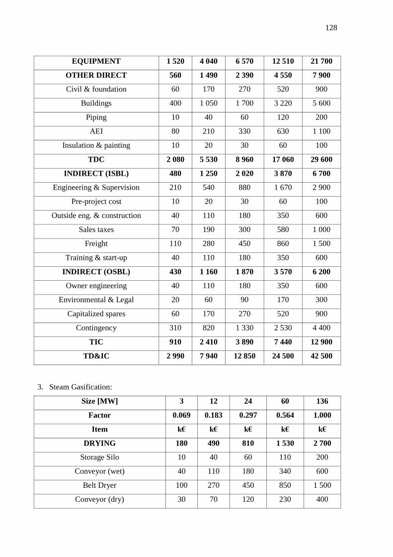
128
EQUIPMENT 1 520 4 040 6 570 12 510 21 700
OTHER DIRECT 560 1 490 2 390 4 550 7 900
Civil & foundation 60 170 270 520 900
Buildings 400 1 050 1 700 3 220 5 600
Piping 10 40 60 120 200
AEI 80 210 330 630 1 100
Insulation & painting 10 20 30 60 100
TDC 2 080 5 530 8 960 17 060 29 600
INDIRECT (ISBL) 480 1 250 2 020 3 870 6 700
Engineering & Supervision 210 540 880 1 670 2 900
Pre-project cost 10 20 30 60 100
Outside eng. & construction 40 110 180 350 600
Sales taxes 70 190 300 580 1 000
Freight 110 280 450 860 1 500
Training & start-up 40 110 180 350 600
INDIRECT (OSBL) 430 1 160 1 870 3 570 6 200
Owner engineering 40 110 180 350 600
Environmental & Legal 20 60 90 170 300
Capitalized spares 60 170 270 520 900
Contingency 310 820 1 330 2 530 4 400
TIC 910 2 410 3 890 7 440 12 900
TD&IC 2 990 7 940 12 850 24 500 42 500
3. Steam Gasification:
Size [MW] 3 12 24 60 136
Factor 0.069 0.183 0.297 0.564 1.000
Item k€ k€ k€ k€ k€
DRYING 180 490 810 1 530 2 700
Storage Silo 10 40 60 110 200
Conveyor (wet) 40 110 180 340 600
Belt Dryer 100 270 450 850 1 500
Conveyor (dry) 30 70 120 230 400

129
GASIFIER 1 240 3 280 5 320 10 100 17 900
H&S Distribution 440 1 170 1 900 3 610 6 400
H&S Feeding 100 260 420 790 1 400
H&S Bed Mat. 10 40 60 110 200
CFB gasifier 310 820 1 340 2 540 4 500
H&S Gasifier ash 10 20 30 60 100
Comb. Chamber 360 950 1 540 2 930 5 200
H&S Combustion ash 10 20 30 60 100
Air system 10 20 30 60 100
Steam system 10 20 30 60 100
Steam boiler 20 50 90 170 300
OTHER ISBL 190 490 800 1 520 2 700
Nitrogen system 40 110 180 340 600
Labor 150 380 620 1 180 2 100
EQUIPMENT 1 650 4 350 7 080 13 440 23 800
OTHER DIRECT 580 1 560 2 530 4 800 8 500
Civil & foundation 60 160 270 510 900
Buildings 420 1 120 1 810 3 440 6 100
Piping 10 40 60 110 200
AEI 80 220 360 680 1 200
Insulation & painting 10 20 30 60 100
TDC 2 230 5 910 9 610 18 240 32 300
INDIRECT (ISBL) 500 1 330 2 180 4 110 7 300
Engineering & Supervision 220 580 950 1 800 3 200
Pre-project cost 10 40 60 110 200
Outside eng. & construction 40 110 180 340 600
Sales taxes 80 200 330 620 1 100
Freight 110 290 480 900 1 600
Training & start-up 40 110 180 340 600
INDIRECT (OSBL) 460 1 220 2 000 3 780 6 700
Owner engineering 40 110 180 340 600
Environmental & Legal 20 50 90 170 300

130
Capitalized spares 70 180 300 560 1 000
Contingency 330 880 1 430 2 710 4 800
TIC 960 2 550 4 180 7 890 14 000
TD&IC 3 190 8 460 13 790 26 130 46 300
4. Steam Gasification with product gas Drying:
Size [MW] 3 12 24 60 128
Factor 0.072 0.191 0.310 0.588 1.000
Item k€ k€ k€ k€ k€
DRYING 190 520 830 1 590 2 700
Storage Silo 10 40 60 120 200
Conveyor (wet) 40 110 190 350 600
Belt Dryer 110 290 460 880 1 500
Conveyor (wet) 30 80 120 240 400
GASIFIER 1 332 3 530 5 700 10 850 18 430
H&S Distribution 470 1 240 2 010 3 820 6 500
H&S Feeding 110 290 460 880 1 500
H&S Bed Mat. 10 40 60 120 200
CFB gasifier 330 880 1 430 2 710 4 600
H&S Gasifier ash 10 20 30 60 100
Comb. Chamber 390 1 030 1 670 3 180 5 400
H&S Combustion ash 10 20 30 60 100
Heat Exchangers 2.0 10.0 10.0 20.0 30.0
GASIFYING MEDIA 40.0 100 150 300 500
Air system 10 20 30 60 100
Steam system 10 20 30 60 100
Steam boiler 20 60 90 180 300
OTHER ISBL 200 530 870 1 650 2 800
Nitrogen system 50 130 220 410 700
Labor 150 400 650 1 240 2 100
EQUIPMENT 1 762 4 680 7 550 14 390 24 430
OTHER DIRECT 640 1 680 2 720 5 190 8 800

131
Civil & foundation 70 190 310 590 1 000
Buildings 460 1 200 1 950 3 710 6 300
Piping 10 40 60 120 200
AEI 90 230 370 710 1 200
Insulation & painting 10 20 30 60 100
TOTAL DIRECT 2 402 6 360 10 270 19 580 33 230
INDIRECT (ISBL) 560 1 480 2 420 4 590 7 800
Engineering & Supervision 240 630 1 020 1 940 3 300
Pre-project cost 10 40 60 120 200
Outside eng. & construction 50 130 220 410 700
Sales taxes 90 230 370 710 1 200
Freight 120 320 530 1 000 1 700
Training & start-up 50 130 220 410 700
INDIRECT (OSBL) 500 1 330 2 170 4 120 7 000
Owner engineering 50 130 220 410 700
Environm./legal expenses 20 60 90 180 300
Capitalized spares 70 190 310 590 1 000
Contingency 360 950 1 550 2 940 5 000
TOTAL INDIRECT 1 060 2 810 4 590 8 710 14 800
TOTAL INVESTMENT 3 462 9 170 14 860 28 290 48 030
5. Bio-SNG Production:
Size [MW] 3 12 24 60 112
Factor 0.079 0.209 0.340 0.646 1.000
Item k€ k€ k€ k€ k€
DRYING 220 560 920 1 750 2 700
Storage Silo 20 40 70 130 200
Wet fuel conveyor 50 130 200 390 600
Belt Dryer 120 310 510 970 1 500
Dry fuel conveyor 30 80 140 260 400
GASIFIER 1 490 3 900 6 360 12 070 18 700
H&S Distribution 520 1 380 2 250 4 260 6 600

132
H&S Feeding 120 310 510 970 1 500
H&S Bed Material 20 40 70 130 200
CFB gasifier 370 980 1 600 3 040 4 700
H&S Gasifier ash 10 20 30 60 100
Combustion Chamber 440 1 150 1 870 3 550 5 500
H&S Combustion ash 10 20 30 60 100
Air system 10 20 30 60 100
Steam system 10 20 30 60 100
Steam boiler 20 60 100 190 300
METHANATION 3 670.0 9 680 15 720 29 850 46 200
Gas Conditioning 830 2 180 3 540 6 720 10 400
Reactor 1 310 3 460 5 610 10 660 16 500
SNG-Upgrading 1 530 4 040 6 570 12 470 19 300
OTHER ISBL 600 1 570 2 550 4 840 7 500
Nitrogen system 60 150 240 450 700
Labor 540 1 420 2 310 4 390 6 800
EQUIPMENT 6 020 15 810 25 710 48 820 75 600
OTHER DIRECT 2 190 5 810 9 420 17 900 27 700
Civil & foundation 240 630 1 020 1 940 3 000
Buildings 1 560 4 130 6 700 12 730 19 700
Piping 60 170 270 520 800
AEI 300 800 1 290 2 450 3 800
Insulation & painting 30 80 140 260 400
TDC 8 210 21 620 35 130 66 720 103 300
INDIRECT (ISBL) 1 900 4 980 8 080 15 380 23 800
Engineering & Supervision 820 2 160 3 500 6 650 10 300
Pre-project cost 40 100 170 320 500
Outside eng. & construction 170 440 710 1 360 2 100
Sales taxes 290 750 1 220 2 330 3 600
Freight 410 1 090 1 770 3 360 5 200
Training & start-up 170 440 710 1 360 2 100
INDIRECT (OSBL) 1 730 4 550 7 370 14 020 21 700

133
Owner engineering 170 440 710 1 360 2 100
Environmental & Legal 80 210 340 650 1 000
Capitalized spares 250 650 1 050 2 000 3 100
Contingency 1 230 3 250 5 270 10 010 15 500
TIC 3 630 9 530 15 450 29 400 45 500
TD&IC 11 840 31 150 50 580 96 120 148 800
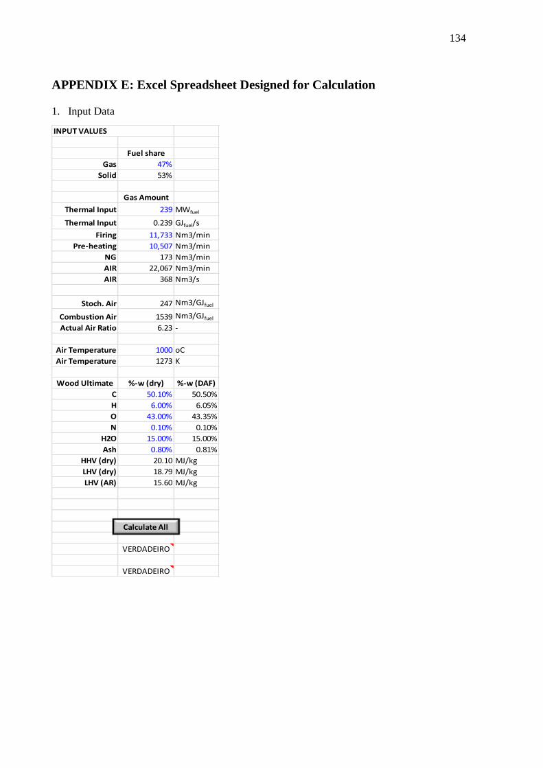
134
APPENDIX E: Excel Spreadsheet Designed for Calculation
1. Input Data
Fuel share
Gas 47%
Solid 53%
Gas Amount
Thermal Input 239 MWfuel
Thermal Input 0.239 GJfuel/s
Firing 11,733 Nm3/min
Pre-heating 10,507 Nm3/min
NG 173 Nm3/min
AIR 22,067 Nm3/min
AIR 368 Nm3/s
Stoch. Air 247 Nm3/GJfuel
Combustion Air 1539 Nm3/GJfuel
Actual Air Ratio 6.23 -
Air Temperature 1000 oC
Air Temperature 1273 K
Wood Ultimate %-w (dry) %-w (DAF)
C 50.10% 50.50%
H 6.00% 6.05%
O 43.00% 43.35%
N 0.10% 0.10%
H2O 15.00% 15.00%
Ash 0.80% 0.81%
HHV (dry) 20.10 MJ/kg
LHV (dry) 18.79 MJ/kg
LHV (AR) 15.60 MJ/kg
VERDADEIRO
VERDADEIRO
INPUT VALUES
Calculate All
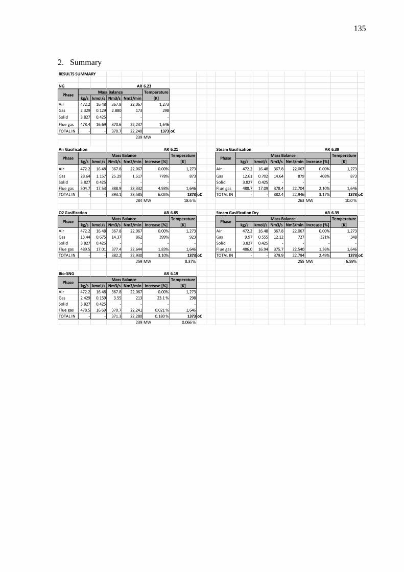
135
2. Summary
NG AR 6.23
Temperature
kg/s kmol/s Nm3/s Nm3/min [K]
Air 472.2 16.48 367.8 22,067 1,273
Gas 2.329 0.129 2.880 173 298
Solid 3.827 0.425 - - -
Flue gas 478.4 16.69 370.6 22,237 1,646
TOTAL IN - - 370.7 22,240 1373 oC
239 MW
AR 6.21 AR 6.39
Temperature Temperature
kg/s kmol/s Nm3/s Nm3/min Increase [%] [K] kg/s kmol/s Nm3/s Nm3/min Increase [%] [K]
Air 472.2 16.48 367.8 22,067 0.00% 1,273 Air 472.2 16.48 367.8 22,067 0.00% 1,273
Gas 28.64 1.157 25.29 1,517 778% 873 Gas 12.61 0.702 14.64 879 408% 873
Solid 3.827 0.425 - - - - Solid 3.827 0.425 - - - -
Flue gas 504.7 17.53 388.9 23,332 4.93% 1,646 Flue gas 488.7 17.09 378.4 22,704 2.10% 1,646
TOTAL IN - - 393.1 23,585 6.05% 1373 oC TOTAL IN - - 382.4 22,946 3.17% 1373 oC
284 MW 18.6 % 263 MW 10.0 %
AR 6.85 AR 6.39
Temperature Temperature
kg/s kmol/s Nm3/s Nm3/min Increase [%] [K] kg/s kmol/s Nm3/s Nm3/min Increase [%] [K]
Air 472.2 16.48 367.8 22,067 0.00% 1,273 Air 472.2 16.48 367.8 22,067 0.00% 1,273
Gas 13.44 0.675 14.37 862 399% 923 Gas 9.97 0.555 12.12 727 321% 348
Solid 3.827 0.425 - - - - Solid 3.827 0.425 - - - -
Flue gas 489.5 17.01 377.4 22,644 1.83% 1,646 Flue gas 486.0 16.94 375.7 22,540 1.36% 1,646
TOTAL IN - - 382.2 22,930 3.10% 1373 oC TOTAL IN - - 379.9 22,794 2.49% 1373 oC
259 MW 8.37% 255 MW 6.59%
AR 6.19
Temperature
kg/s kmol/s Nm3/s Nm3/min Increase [%] [K]
Air 472.2 16.48 367.8 22,067 0.00% 1,273
Gas 2.429 0.159 3.55 213 23.1 % 298
Solid 3.827 0.425 - - - -
Flue gas 478.5 16.69 370.7 22,241 0.021 % 1,646
TOTAL IN - - 371.3 22,280 0.180 % 1373 oC
239 MW 0.066 %
Steam Gasification
Steam Gasification Dry
Phase
Phase
Phase
Bio-SNG
Mass Balance
Mass Balance
Mass Balance
PhaseMass Balance
O2 Gasification
RESULTS SUMMARY
PhaseMass Balance
PhaseMass Balance
Air Gasification
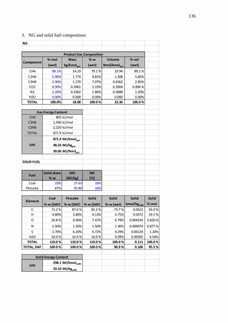
136
3. NG and solid fuel composition:
%-mol Mass %-w Volume %-vol
(wet) kg/kmolgas (wet) Nm3/kmolgas (wet)
CH4 89.1% 14.29 79.1 % 19.94 89.2 %
C2H6 5.90% 1.774 9.81% 1.308 5.85%
C3H8 2.90% 1.279 7.07% 0.6362 2.85%
CO2 0.90% 0.3961 2.19% 0.2004 0.896 %
N2 1.20% 0.3362 1.86% 0.2688 1.20%
H2O 0.00% 0.000 0.00% 0.000 0.00%
TOTAL 100.0% 18.08 100.0 % 22.36 100.0 %
CH4 803 kJ/mol
C2H6 1,560 kJ/mol
C3H8 2,220 kJ/mol
TOTAL 871.9 kJ/mol
871.9 MJ/kmolgas
48.23 MJ/kggas
39.00 MJ/Nm3gas
Solid share LHV MC
%-w [MJ/kg] [%]
Coal 33% 27.63 10%
Petcoke 67% 35.80 10%
Coal Petcoke Solid Solid Solid Solid
%-w (DAF) %-w (DAF) %-w (DAF) %-w (wet) kmol/kgsolid %-mol
C 71.2 % 87.6 % 82.2 % 74.7 % 0.0622 56.0 %
H 4.80% 3.80% 4.13% 3.75% 0.0372 33.5 %
O 20.8 % 0.90% 7.47% 6.79% 0.004243 3.820 %
N 1.50% 1.50% 1.50% 1.36% 0.000974 0.877 %
S 1.70% 6.20% 4.72% 4.29% 0.00134 1.20%
H2O 10.0 % 10.0 % 10.0 % 9.09% 0.00505 4.54%
TOTAL 110.0 % 110.0 % 110.0 % 100.0 % 0.111 100.0 %
TOTAL, DAF 100.0 % 100.0 % 100.0 % 90.9 % 0.106 95.5 %
298.1 MJ/kmolsolid
33.10 MJ/kgsolid
Gas Energy Content
LHV
SOLID FUEL
LHV
Fuel
Element
Solid Energy Content
NG
Product Gas Composition
Component

137
4. NG and solid fuel combustion:
47% Gas
Basis 1 GJfuel 53% Solid
Gas Gas Solid FUEL FUEL Stoch. O2
kmol/kmolgas kmol/GJgas kmol/GJsolid kmol/GJfuel %-mol kmol/GJfuel
C 1.105 1.267 1.879 1.592 34.4 % 1.592
H 4.150 4.760 1.125 2.833 61.2 % 0.708
O 0.01800 0.02064 0.12817 0.07763 1.675 % -0.03882
N 0.02400 0.02753 0.02941 0.02852 0.616 % 0.0000
S 0.000 0.000 0.04038 0.02140 0.462 % 0.0214
H2O 0.000 0.000 0.1524 0.08079 1.74% 0.0000
TOTAL - - - 4.633 100.0 % 2.283
Air ratio 6.23
kmol kg Nm3 kmol kg Nm3 kmol kg Nm3
GJfuel 2.283 73.04 51.12 11.08 317.3 247.2 68.97 1,976 1,539
kmolfuel 1.296 41.47 29.02 6.289 180.2 140.3 39.16 1,122 873.7
kgfuel 0.092 2.937 2.055 0.445 12.76 9.94 2.773 79.45 61.88
Flue Gas %-mol Mass %-w Volume %-vol
kmol/GJfuel (wet) kg/GJfuel (wet) Nm3/GJfuel (wet)
CO2 1.592 2.28% 70.05 3.50% 35.43 2.29%
N2 53.48 76.6 % 1498 74.8 % 1198 77.2 %
O2 11.93 17.1 % 381.7 19.1 % 267.1 17.2 %
SO2 0.02140 0.0307 % 1.371 0.0685 % 0.4684 0.0302 %
H2O 2.792 4.00% 50.30 2.51% 49.80 3.21%
TOTAL 69.81 100.0 % 2002 100.0 % 1551 100.0 %
TOTAL, dry 67.02 96.0 % 1951 97.5 % 1501 96.8 %
567.8 MJ/kmolfuel
40.21 MJ/kgfuel
Comb. Air (wet)Fuel
Stoch. O2 Stoch. Air (wet)
Fuel Energy Content
LHV
Flue Gas Composition
Component
Combustion
Fuel Elemental Composition
Element
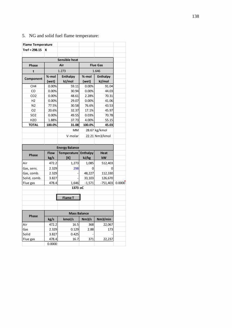
138
5. NG and solid fuel flame temperature:
Tref = 298.15 K
Phase
t
%-mol Enthalpy %-mol Enthalpy
(wet) kJ/mol (wet) kJ/mol
CH4 0.00% 59.11 0.00% 91.04
CO 0.00% 30.94 0.00% 44.03
CO2 0.00% 48.61 2.28% 70.31
H2 0.00% 29.07 0.00% 41.06
N2 77.5% 30.58 76.6% 43.53
O2 20.6% 32.37 17.1% 45.97
SO2 0.00% 49.55 0.03% 70.78
H2O 1.88% 37.73 4.00% 55.15
TOTAL 100.0% 31.08 100.0% 45.03
MM 28.67 kg/kmol
V-molar 22.21 Nm3/kmol
Flow Temperature Enthalpy Heat
kg/s [K] kJ/kg kW
Air 472.2 1,273 1,085 512,403
Gas, sens. 2.329 298 0 0
Gas, comb. 2.329 - 48,227 112,330
Solid, comb. 3.827 - 33,103 126,670
Flue gas 478.4 1,646 -1,571 -751,403 0.0000
1373 oC
kg/s kmol/s Nm3/s Nm3/min
Air 472.2 16.5 368 22,067
Gas 2.329 0.129 2.88 173
Solid 3.827 0.425 - -
Flue gas 478.4 16.7 371 22,237
0.0000
Air
1.273
Component
Energy Balance
Mass BalancePhase
Phase
Flue Gas
1.646
Sensible heat
Flame Temperature
Flame T
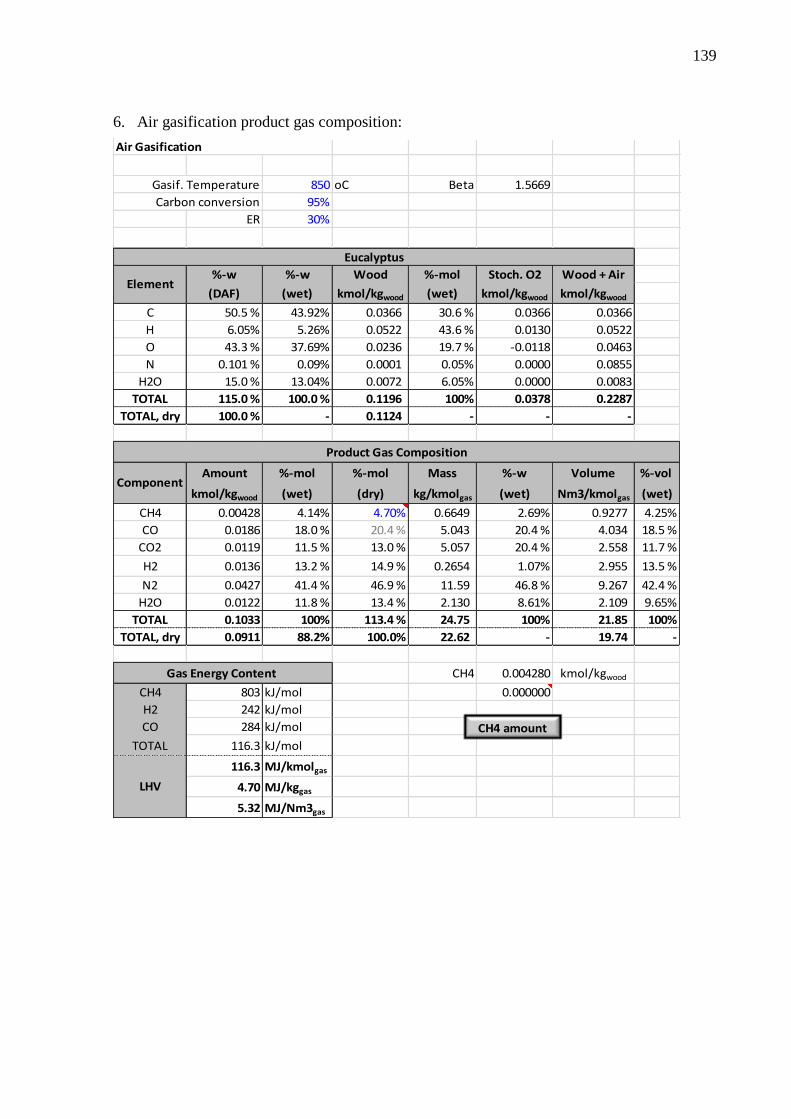
139
6. Air gasification product gas composition:
850 oC Beta 1.5669
95%
ER 30%
%-w %-w Wood %-mol Stoch. O2 Wood + Air
(DAF) (wet) kmol/kgwood (wet) kmol/kgwood kmol/kgwood
C 50.5 % 43.92% 0.0366 30.6 % 0.0366 0.0366
H 6.05% 5.26% 0.0522 43.6 % 0.0130 0.0522
O 43.3 % 37.69% 0.0236 19.7 % -0.0118 0.0463
N 0.101 % 0.09% 0.0001 0.05% 0.0000 0.0855
H2O 15.0 % 13.04% 0.0072 6.05% 0.0000 0.0083
TOTAL 115.0 % 100.0 % 0.1196 100% 0.0378 0.2287
TOTAL, dry 100.0 % - 0.1124 - - -
Amount %-mol %-mol Mass %-w Volume %-vol
kmol/kgwood (wet) (dry) kg/kmolgas (wet) Nm3/kmolgas (wet)
CH4 0.00428 4.14% 4.70% 0.6649 2.69% 0.9277 4.25%
CO 0.0186 18.0 % 20.4 % 5.043 20.4 % 4.034 18.5 %
CO2 0.0119 11.5 % 13.0 % 5.057 20.4 % 2.558 11.7 %
H2 0.0136 13.2 % 14.9 % 0.2654 1.07% 2.955 13.5 %
N2 0.0427 41.4 % 46.9 % 11.59 46.8 % 9.267 42.4 %
H2O 0.0122 11.8 % 13.4 % 2.130 8.61% 2.109 9.65%
TOTAL 0.1033 100% 113.4 % 24.75 100% 21.85 100%
TOTAL, dry 0.0911 88.2% 100.0% 22.62 - 19.74 -
CH4 0.004280 kmol/kgwood
CH4 803 kJ/mol 0.000000
H2 242 kJ/mol
CO 284 kJ/mol
TOTAL 116.3 kJ/mol
116.3 MJ/kmolgas
4.70 MJ/kggas
5.32 MJ/Nm3gas
Element
Air Gasification
Carbon conversion
Gasif. Temperature
Gas Energy Content
Product Gas Composition
Component
Eucalyptus
LHV
CH4 amount

140
7. Air gasification fuel combustion:
52% Gas
Basis 1 GJfuel 48% Solid
Gas Gas Solid FUEL FUEL Stoch. O2
kmol/kmolgas kmol/GJgas kmol/GJsolid kmol/GJfuel %-mol kmol/GJfuel
C 0.3364 2.893 1.879 2.401 21.8 % 2.401
H 0.4291 3.690 1.125 2.447 22.2 % 0.612
O 0.4098 3.525 0.128 1.878 17.0 % -0.939
N 0.8275 7.117 0.029 3.680 33.4 % 0.000
S 0.0000 0.000 0.040 0.020 0.18% 0.020
H2O 0.1182 1.017 0.152 0.598 5.42% 0.000
TOTAL - - - 11.02 100% 2.094
Air ratio 6.21
kmol kg Nm3 kmol kg Nm3 kmol kg Nm3
GJfuel 2.094 67.00 46.89 10.16 291.1 226.7 63.10 1,808 1,408
kmolfuel 0.428 13.70 9.59 2.077 59.50 46.35 12.90 369.5 287.8
kgfuel 0.039 1.238 0.866 0.188 5.377 4.188 1.166 33.39 26.01
Flue Gas %-mol Mass %-w Volume %-vol
kmol/GJfuel (wet) kg/GJfuel (wet) Nm3/GJfuel (wet)
CO2 2.401 3.58% 105.69 5.47% 53.46 3.58%
N2 50.75 75.7 % 1,422 73.6 % 1,130 75.7 %
O2 10.91 16.3 % 349.1 18.1 % 242.9 16.3 %
SO2 0.020 0.03% 1.254 0.06% 0.436 0.03%
H2O 3.005 4.48% 54.14 2.80% 66.91 4.48%
TOTAL 67.09 100% 1,932 100% 1,494 100%
TOTAL, dry 64.08 95.5 % 1878 97.2 % 1427 95.5 %
204.4 MJ/kmolfuel
18.47 MJ/kgfuel
Input Value Unit Value Unit
Wood 11.21 kg/s Wood in 11.8 kg/s 42.4 t/h dry
Carbon 0.25 kg/s Planted 27,028 ha 72.1 t/h wet
Ash 0.09 kg/s Required 54,055 ha
Loss 0.23 kg/s Gasif. Size 157 MW
Wood 183,743 kW TOTAL 284 MW
Gas 156,900 kW Gas 55%
Efficiency 85.4 % - Cold gas 261 MW
Element
Combustion
Fuel Elemental Composition
Fuel Energy Content
LHV
Flue Gas Composition
Hot Gas Efficiency
Fuel GasStoch. O2
Component
Stoch. Air (wet)
SUMMARY
Comb. Air (wet)

141
8. Air gasification flame temperature:
Phase
t
%-mol Enthalpy %-mol Enthalpy %-mol Enthalpy
(wet) kJ/mol (wet) kJ/mol (wet) kJ/mol
CH4 0.00% 59.11 4.14% 29.40 0.00% 91.04
CO 0.00% 30.94 18.0 % 17.52 0.00% 44.03
CO2 0.00% 48.61 11.5 % 26.61 3.58% 70.31
H2 0.00% 29.07 13.2 % 16.87 0.00% 41.06
N2 77.5 % 30.58 41.4 % 17.36 75.7 % 43.53
O2 20.6 % 32.37 0.00% 18.32 16.3 % 45.97
SO2 0.00% 49.55 0.00% 27.58 0.03% 70.78
H2O 1.88% 37.73 11.8 % 20.86 4.48% 55.15
TOTAL 100% 31.08 100% 19.30 100% 45.42
MM 28.80 kg/kmol
V-molar 22.19 Nm3/kmol
Flow Temperature Enthalpy Heat
kg/s [K] kJ/kg kW
Air 472.2 1,273 1,085 512,403
Gas, sens. 28.64 873 780 22,337
Gas, comb. 28.64 - 4,698 134,564
Solid, comb. 3.827 - 33,103 126,670
Flue gas 504.7 1,646 1,577 -795,973 0.0000
1373 oC
kg/s kmol/s Nm3/s Nm3/min
Air 472.2 16.48 367.8 22,067
Gas 28.64 1.157 25.29 1,517
Solid 3.827 0.425 - -
Flue gas 504.7 17.53 388.9 23,332
0.00000
Flame Temperature
0.873
Sensible heat
Air Product Gas
Component
Tref = 298.15 K
1.646
Flue Gas
1.273
Mass BalancePhase
Phase
Energy Balance
Gas Flow

142
9. Oxygen gasification product gas composition:
SOR 1.00 kgH2O/kgO2
950 oC Beta 3.3910
95% O2 95.0%
ER 30% N2 5.0%
%-w %-w Wood %-mol Stoch. O2 Wood + O2
(DAF) (wet) kmol/kgwood (wet) kmol/kgwood kmol/kgwood
C 50.5 % 43.9 % 0.0366 30.6 % 0.0366 0.03656
H 6.05% 5.26% 0.0522 43.6 % 0.0130 0.05218
O 43.3 % 37.7 % 0.0236 19.7 % -0.0118 0.04626
N 0.101 % 0.088 % 0.0001 0.052 % 0.0000 0.00126
H2O 15.0 % 13.0 % 0.0072 6.05% 0.0000 0.01363
TOTAL 115.0 % 100.00% 0.1196 100.0 % 0.0378 0.1499
TOTAL, dry 100.0 % - 0.112 - - -
Amount %-mol %-mol Mass %-w Volume %-vol
kmol/kgwood (wet) (dry) kg/kmolgas (wet) Nm3/kmolgas (wet)
CH4 0.0006 0.76% 1.00% 0.122 0.61% 0.170 0.80%
CO 0.0264 35.7 % 47.1 % 9.995 50.2 % 7.995 37.5 %
CO2 0.0078 10.5 % 13.9 % 4.631 23.3 % 2.343 11.0 %
H2 0.0207 27.9 % 36.9 % 0.563 2.83% 6.274 29.5 %
N2 0.0006 0.85% 1.12% 0.238 1.20% 0.190 0.89%
H2O 0.0179 24.2 % 32.0 % 4.367 21.9 % 4.323 20.3 %
TOTAL 0.0740 100% 132% 19.92 100% 21.30 100%
TOTAL, dry 0.0560 75.8% 100% 15.55 - 16.97 -
CH4 0.000560 kmol/kgwood
CH4 803 kJ/mol 0.000000
H2 242 kJ/mol
CO 284 kJ/mol
TOTAL 175.1 kJ/mol
175.1 MJ/kmolgas
8.79 MJ/kggas
8.22 MJ/Nm3gas
Eucalyptus
O2 Gasification
Gasif. Temperature
Carbon conversion
Element
LHV
Gas Energy Content
Product Gas Composition
Component
CH4 amount
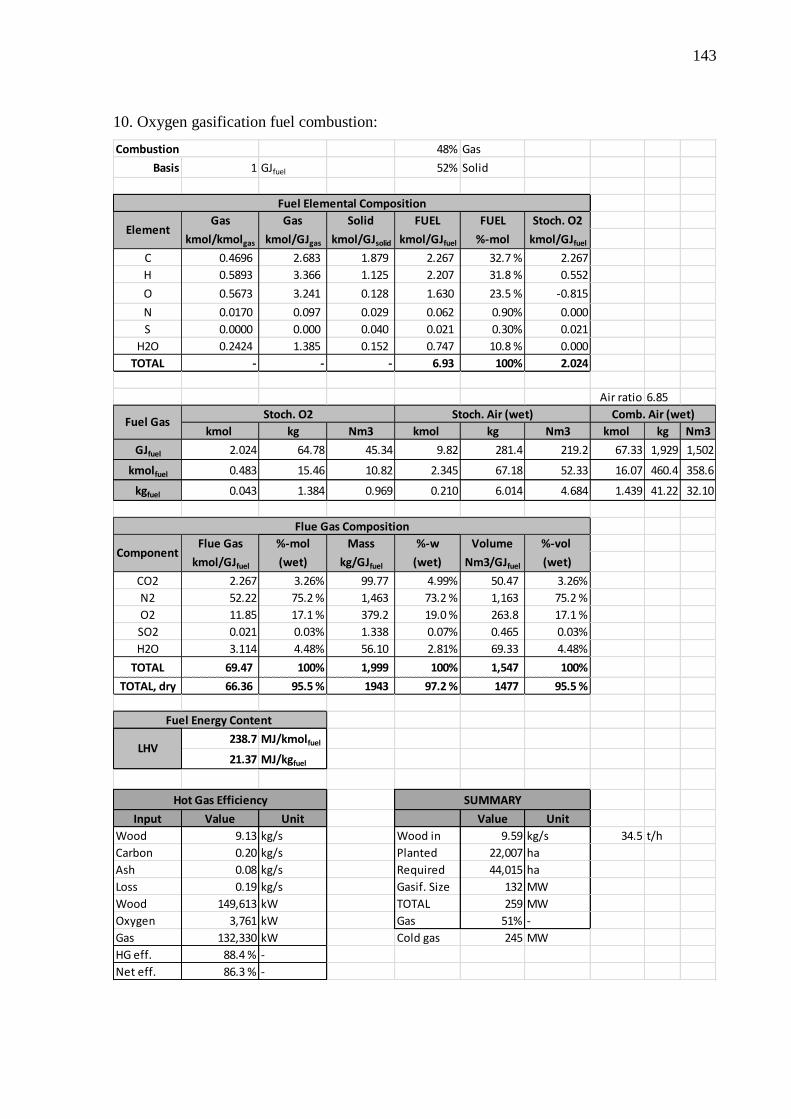
143
10. Oxygen gasification fuel combustion:
48% Gas
Basis 1 GJfuel 52% Solid
Gas Gas Solid FUEL FUEL Stoch. O2
kmol/kmolgas kmol/GJgas kmol/GJsolid kmol/GJfuel %-mol kmol/GJfuel
C 0.4696 2.683 1.879 2.267 32.7 % 2.267
H 0.5893 3.366 1.125 2.207 31.8 % 0.552
O 0.5673 3.241 0.128 1.630 23.5 % -0.815
N 0.0170 0.097 0.029 0.062 0.90% 0.000
S 0.0000 0.000 0.040 0.021 0.30% 0.021
H2O 0.2424 1.385 0.152 0.747 10.8 % 0.000
TOTAL - - - 6.93 100% 2.024
Air ratio 6.85
kmol kg Nm3 kmol kg Nm3 kmol kg Nm3
GJfuel 2.024 64.78 45.34 9.82 281.4 219.2 67.33 1,929 1,502
kmolfuel 0.483 15.46 10.82 2.345 67.18 52.33 16.07 460.4 358.6
kgfuel 0.043 1.384 0.969 0.210 6.014 4.684 1.439 41.22 32.10
Flue Gas %-mol Mass %-w Volume %-vol
kmol/GJfuel (wet) kg/GJfuel (wet) Nm3/GJfuel (wet)
CO2 2.267 3.26% 99.77 4.99% 50.47 3.26%
N2 52.22 75.2 % 1,463 73.2 % 1,163 75.2 %
O2 11.85 17.1 % 379.2 19.0 % 263.8 17.1 %
SO2 0.021 0.03% 1.338 0.07% 0.465 0.03%
H2O 3.114 4.48% 56.10 2.81% 69.33 4.48%
TOTAL 69.47 100% 1,999 100% 1,547 100%
TOTAL, dry 66.36 95.5 % 1943 97.2 % 1477 95.5 %
238.7 MJ/kmolfuel
21.37 MJ/kgfuel
Input Value Unit Value Unit
Wood 9.13 kg/s Wood in 9.59 kg/s 34.5 t/h
Carbon 0.20 kg/s Planted 22,007 ha
Ash 0.08 kg/s Required 44,015 ha
Loss 0.19 kg/s Gasif. Size 132 MW
Wood 149,613 kW TOTAL 259 MW
Oxygen 3,761 kW Gas 51% -
Gas 132,330 kW Cold gas 245 MW
HG eff. 88.4 % -
Net eff. 86.3 % -
SUMMARY
Combustion
Fuel Elemental Composition
Hot Gas Efficiency
Element
Fuel GasStoch. O2 Stoch. Air (wet) Comb. Air (wet)
Flue Gas Composition
Component
Fuel Energy Content
LHV
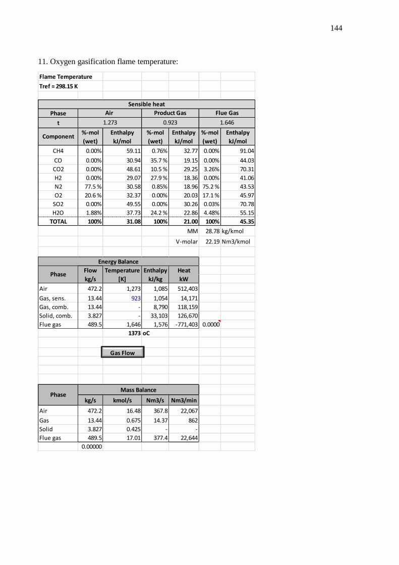
144
11. Oxygen gasification flame temperature:
Phase
t
%-mol Enthalpy %-mol Enthalpy %-mol Enthalpy
(wet) kJ/mol (wet) kJ/mol (wet) kJ/mol
CH4 0.00% 59.11 0.76% 32.77 0.00% 91.04
CO 0.00% 30.94 35.7 % 19.15 0.00% 44.03
CO2 0.00% 48.61 10.5 % 29.25 3.26% 70.31
H2 0.00% 29.07 27.9 % 18.36 0.00% 41.06
N2 77.5 % 30.58 0.85% 18.96 75.2 % 43.53
O2 20.6 % 32.37 0.00% 20.03 17.1 % 45.97
SO2 0.00% 49.55 0.00% 30.26 0.03% 70.78
H2O 1.88% 37.73 24.2 % 22.86 4.48% 55.15
TOTAL 100% 31.08 100% 21.00 100% 45.35
MM 28.78 kg/kmol
V-molar 22.19 Nm3/kmol
Flow Temperature Enthalpy Heat
kg/s [K] kJ/kg kW
Air 472.2 1,273 1,085 512,403
Gas, sens. 13.44 923 1,054 14,171
Gas, comb. 13.44 - 8,790 118,159
Solid, comb. 3.827 - 33,103 126,670
Flue gas 489.5 1,646 1,576 -771,403 0.0000
1373 oC
kg/s kmol/s Nm3/s Nm3/min
Air 472.2 16.48 367.8 22,067
Gas 13.44 0.675 14.37 862
Solid 3.827 0.425 - -
Flue gas 489.5 17.01 377.4 22,644
0.00000
Flue Gas
1.273 0.923 1.646
Phase
PhaseMass Balance
Energy Balance
Component
Flame Temperature
Sensible heat
Tref = 298.15 K
Product GasAir
Gas Flow
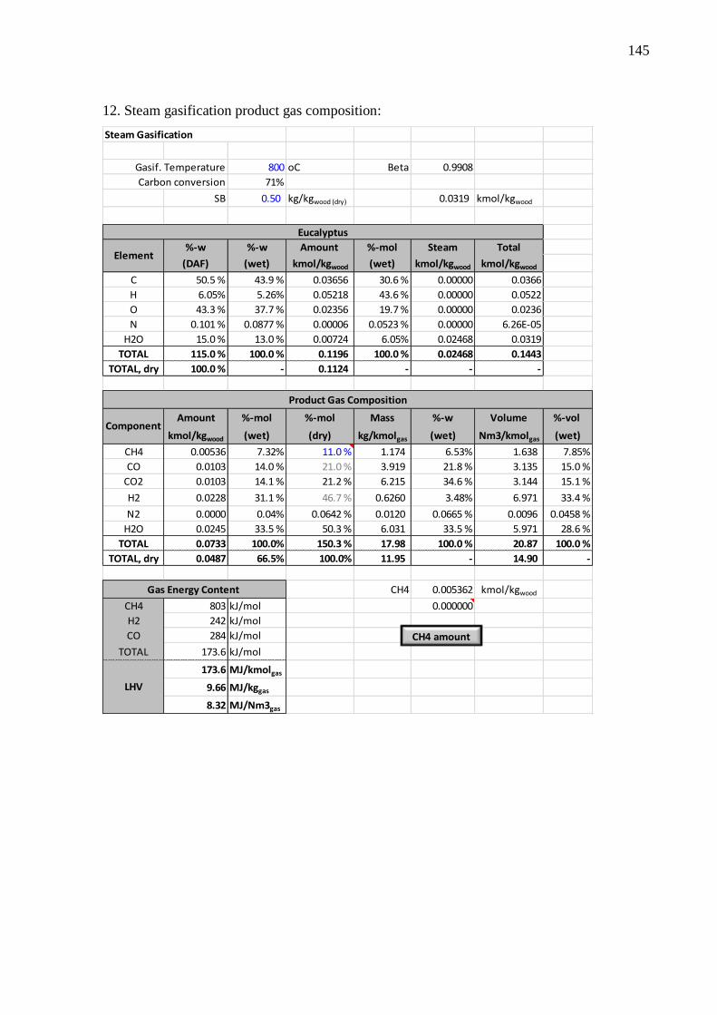
145
12. Steam gasification product gas composition:
800 oC Beta 0.9908
71%
SB 0.50 kg/kgwood (dry) 0.0319 kmol/kgwood
%-w %-w Amount %-mol Steam Total
(DAF) (wet) kmol/kgwood (wet) kmol/kgwood kmol/kgwood
C 50.5 % 43.9 % 0.03656 30.6 % 0.00000 0.0366
H 6.05% 5.26% 0.05218 43.6 % 0.00000 0.0522
O 43.3 % 37.7 % 0.02356 19.7 % 0.00000 0.0236
N 0.101 % 0.0877 % 0.00006 0.0523 % 0.00000 6.26E-05
H2O 15.0 % 13.0 % 0.00724 6.05% 0.02468 0.0319
TOTAL 115.0 % 100.0 % 0.1196 100.0 % 0.02468 0.1443
TOTAL, dry 100.0 % - 0.1124 - - -
Amount %-mol %-mol Mass %-w Volume %-vol
kmol/kgwood (wet) (dry) kg/kmolgas (wet) Nm3/kmolgas (wet)
CH4 0.00536 7.32% 11.0 % 1.174 6.53% 1.638 7.85%
CO 0.0103 14.0 % 21.0 % 3.919 21.8 % 3.135 15.0 %
CO2 0.0103 14.1 % 21.2 % 6.215 34.6 % 3.144 15.1 %
H2 0.0228 31.1 % 46.7 % 0.6260 3.48% 6.971 33.4 %
N2 0.0000 0.04% 0.0642 % 0.0120 0.0665 % 0.0096 0.0458 %
H2O 0.0245 33.5 % 50.3 % 6.031 33.5 % 5.971 28.6 %
TOTAL 0.0733 100.0% 150.3 % 17.98 100.0 % 20.87 100.0 %
TOTAL, dry 0.0487 66.5% 100.0% 11.95 - 14.90 -
CH4 0.005362 kmol/kgwood
CH4 803 kJ/mol 0.000000
H2 242 kJ/mol
CO 284 kJ/mol
TOTAL 173.6 kJ/mol
173.6 MJ/kmolgas
9.66 MJ/kggas
8.32 MJ/Nm3gas
Steam Gasification
Gasif. Temperature
Carbon conversion
Product Gas Composition
Component
Eucalyptus
Element
Gas Energy Content
LHV
CH4 amount

146
13. Steam gasification fuel combustion:
49% Gas
Basis 1 GJfuel 51% Solid
Gas Gas Solid FUEL FUEL Stoch. O2
kmol/kmolgas kmol/GJgas kmol/GJsolid kmol/GJfuel %-mol kmol/GJfuel
C 0.3543 2.040 1.879 1.958 26.4 % 1.958
H 0.9137 5.262 1.125 3.154 42.4 % 0.788
O 0.4223 2.432 0.128 1.258 16.9 % -0.629
N 0.0009 0.005 0.029 0.017 0.23% 0.000
S 0.0000 0.000 0.040 0.021 0.28% 0.021
H2O 0.3348 1.928 0.152 1.023 13.8 % 0.000
TOTAL - - - 7.431 100% 2.138
Air ratio 6.39
kmol kg Nm3 kmol kg Nm3 kmol kg Nm3
GJfuel 2.138 68.42 47.89 10.38 297.3 231.5 66.33 1,900 1,480
kmolfuel 0.507 16.22 11.35 2.460 70.47 54.89 15.73 450.5 350.9
kgfuel 0.046 1.479 1.035 0.224 6.424 5.003 1.433 41.06 31.98
Flue Gas %-mol Mass %-w Volume %-vol
kmol/GJfuel (wet) kg/GJfuel (wet) Nm3/GJfuel (wet)
CO2 1.958 2.85% 86.18 4.38% 43.60 2.85%
N2 51.43 74.8 % 1,441 73.3 % 1,145 74.8 %
O2 11.53 16.8 % 368.9 18.8 % 256.7 16.8 %
SO2 0.021 0.03% 1.319 0.07% 0.458 0.03%
H2O 3.845 5.59% 69.26 3.52% 85.60 5.59%
TOTAL 68.78 100% 1,966 100% 1,531 100%
TOTAL, dry 64.94 94.4 % 1897 96.5 % 1446 94.4 %
237.1 MJ/kmolfuel
21.61 MJ/kgfuel
Input Value Unit Value Unit
Wood 9.58 kg/s Wood in 11.10 kg/s 40.0 t/h
Carbon 1.22 kg/s Planted 25,475 ha
Ash 0.09 kg/s Required 50,949 ha
Loss 0.22 kg/s Gasif. Size 136 MW
Steam 4.72 kg/s TOTAL 263 MW
Wood 173,185 kW Gas 52% -
Steam 14333 kW Cold gas 249 MW
Gas 136,285 kW
HG eff. 78.7 % -
Net eff. 72.7 %
Combustion
Fuel Elemental Composition
Element
Fuel GasStoch. O2 Stoch. Air (wet) Comb. Air (wet)
Flue Gas Composition
Component
Fuel Energy Content
LHV
Hot Gas Efficiency SUMMARY
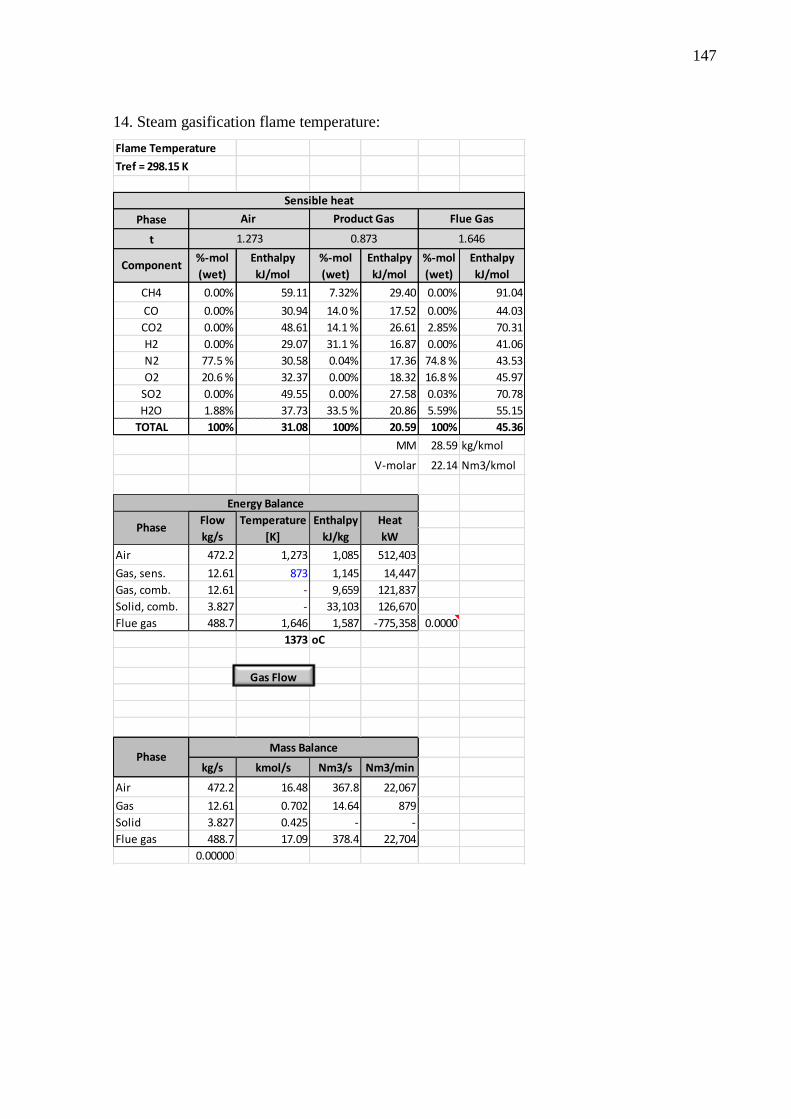
147
14. Steam gasification flame temperature:
Phase
t
%-mol Enthalpy %-mol Enthalpy %-mol Enthalpy
(wet) kJ/mol (wet) kJ/mol (wet) kJ/mol
CH4 0.00% 59.11 7.32% 29.40 0.00% 91.04
CO 0.00% 30.94 14.0 % 17.52 0.00% 44.03
CO2 0.00% 48.61 14.1 % 26.61 2.85% 70.31
H2 0.00% 29.07 31.1 % 16.87 0.00% 41.06
N2 77.5 % 30.58 0.04% 17.36 74.8 % 43.53
O2 20.6 % 32.37 0.00% 18.32 16.8 % 45.97
SO2 0.00% 49.55 0.00% 27.58 0.03% 70.78
H2O 1.88% 37.73 33.5 % 20.86 5.59% 55.15
TOTAL 100% 31.08 100% 20.59 100% 45.36
MM 28.59 kg/kmol
V-molar 22.14 Nm3/kmol
Flow Temperature Enthalpy Heat
kg/s [K] kJ/kg kW
Air 472.2 1,273 1,085 512,403
Gas, sens. 12.61 873 1,145 14,447
Gas, comb. 12.61 - 9,659 121,837
Solid, comb. 3.827 - 33,103 126,670
Flue gas 488.7 1,646 1,587 -775,358 0.0000
1373 oC
kg/s kmol/s Nm3/s Nm3/min
Air 472.2 16.48 367.8 22,067
Gas 12.61 0.702 14.64 879
Solid 3.827 0.425 - -
Flue gas 488.7 17.09 378.4 22,704
0.00000
Flame Temperature
Sensible heat
Tref = 298.15 K
Flue Gas
1.273 0.873 1.646
Component
Air Product Gas
Energy Balance
Phase
PhaseMass Balance
Gas Flow

148
15. Steam gasification dry product gas composition:
800 oC Beta 0.9908
71%
SB 0.50 kg/kgwood (dry) 0.0319 kmol/kgwood
%-w %-w Amount %-mol Steam Total
(DAF) (wet) kmol/kgwood (wet) kmol/kgwood kmol/kgwood
C 50.50% 43.92% 0.037 30.57% 0.0000 0.0366
H 6.05% 5.26% 0.052 43.63% 0.0000 0.0522
O 43.35% 37.69% 0.024 19.70% 0.0000 0.0236
N 0.10% 0.09% 0.000 0.05% 0.0000 0.0001
H2O 15.00% 13.04% 0.007 6.05% 0.0247 0.0319
TOTAL 115.00% 100.00% 0.120 100.00% 0.0247 0.1443
TOTAL, dry 100.00% - 0.112 - - -
Amount %-mol Mass %-w Volume %-vol
kmol/kgwood (wet) kg/kmolgas (wet) Nm3/kmolgas (wet)
CH4 0.00536 9.66% 1.550 8.63% 2.162 9.90%
CO 0.0103 18.5 % 5.173 28.8 % 4.138 18.9 %
CO2 0.0103 18.6 % 8.203 45.7 % 4.150 19.0 %
H2 0.0228 41.0 % 0.8263 4.60% 9.201 42.1 %
N2 0.0000 0.06% 0.01579 0.0879 % 0.01263 0.0578 %
H2O 0.0245 12.2 % 2.196 12.2 % 2.174 9.96%
H2O rem. 0.0178 - - - - -
TOTAL 0.0555 100.0% 17.96 100.0 % 21.84 100.0 %
CH4 803 kJ/mol
H2 242 kJ/mol
CO 284 kJ/mol 0.0000
TOTAL 229.2 kJ/mol
229.2 MJ/kmolgas 24%
12.76 MJ/kggas
10.50 MJ/Nm3gas
50
101,325
12,351
12.19%
Gasif. Temperature
Carbon conversion
Product Gas Composition
Eucalyptus
Steam Gasification
yH2O
Psat, H2O [Pa]
Component
Local Pressure [Pa]
Temperature [oC]
Product Gas Humidity
Element
Gas Energy Content
LHV
Adjust MC
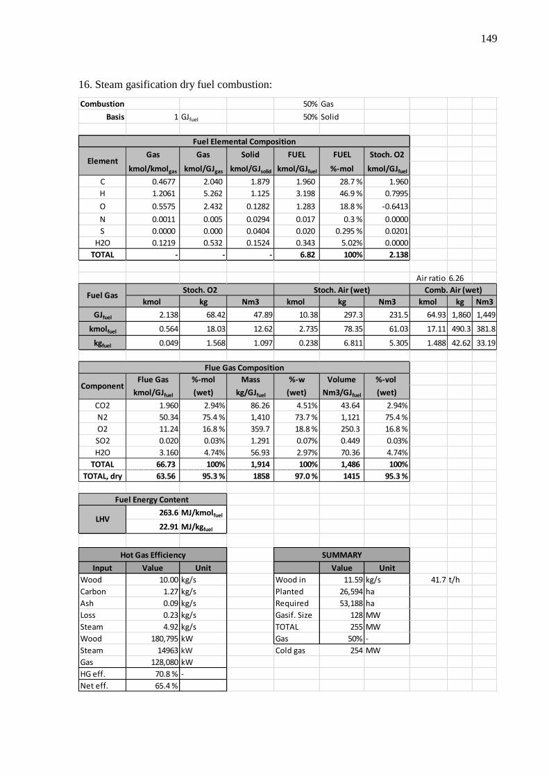
149
16. Steam gasification dry fuel combustion:
50% Gas
Basis 1 GJfuel 50% Solid
Gas Gas Solid FUEL FUEL Stoch. O2
kmol/kmolgas kmol/GJgas kmol/GJsolid kmol/GJfuel %-mol kmol/GJfuel
C 0.4677 2.040 1.879 1.960 28.7 % 1.960
H 1.2061 5.262 1.125 3.198 46.9 % 0.7995
O 0.5575 2.432 0.1282 1.283 18.8 % -0.6413
N 0.0011 0.005 0.0294 0.017 0.3 % 0.0000
S 0.0000 0.000 0.0404 0.020 0.295 % 0.0201
H2O 0.1219 0.532 0.1524 0.343 5.02% 0.0000
TOTAL - - - 6.82 100% 2.138
Air ratio 6.26
kmol kg Nm3 kmol kg Nm3 kmol kg Nm3
GJfuel 2.138 68.42 47.89 10.38 297.3 231.5 64.93 1,860 1,449
kmolfuel 0.564 18.03 12.62 2.735 78.35 61.03 17.11 490.3 381.8
kgfuel 0.049 1.568 1.097 0.238 6.811 5.305 1.488 42.62 33.19
Flue Gas %-mol Mass %-w Volume %-vol
kmol/GJfuel (wet) kg/GJfuel (wet) Nm3/GJfuel (wet)
CO2 1.960 2.94% 86.26 4.51% 43.64 2.94%
N2 50.34 75.4 % 1,410 73.7 % 1,121 75.4 %
O2 11.24 16.8 % 359.7 18.8 % 250.3 16.8 %
SO2 0.020 0.03% 1.291 0.07% 0.449 0.03%
H2O 3.160 4.74% 56.93 2.97% 70.36 4.74%
TOTAL 66.73 100% 1,914 100% 1,486 100%
TOTAL, dry 63.56 95.3 % 1858 97.0 % 1415 95.3 %
263.6 MJ/kmolfuel
22.91 MJ/kgfuel
Input Value Unit Value Unit
Wood 10.00 kg/s Wood in 11.59 kg/s 41.7 t/h
Carbon 1.27 kg/s Planted 26,594 ha
Ash 0.09 kg/s Required 53,188 ha
Loss 0.23 kg/s Gasif. Size 128 MW
Steam 4.92 kg/s TOTAL 255 MW
Wood 180,795 kW Gas 50% -
Steam 14963 kW Cold gas 254 MW
Gas 128,080 kW
HG eff. 70.8 % -
Net eff. 65.4 %
Combustion
Fuel Elemental Composition
Element
Fuel GasStoch. O2 Stoch. Air (wet) Comb. Air (wet)
Flue Gas Composition
Component
Fuel Energy Content
LHV
Hot Gas Efficiency SUMMARY
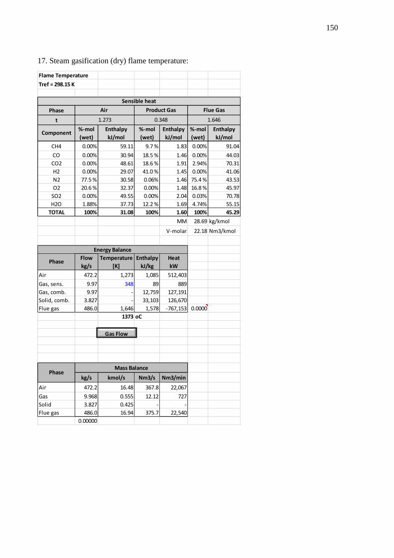
150
17. Steam gasification (dry) flame temperature:
Phase
t
%-mol Enthalpy %-mol Enthalpy %-mol Enthalpy
(wet) kJ/mol (wet) kJ/mol (wet) kJ/mol
CH4 0.00% 59.11 9.7 % 1.83 0.00% 91.04
CO 0.00% 30.94 18.5 % 1.46 0.00% 44.03
CO2 0.00% 48.61 18.6 % 1.91 2.94% 70.31
H2 0.00% 29.07 41.0 % 1.45 0.00% 41.06
N2 77.5 % 30.58 0.06% 1.46 75.4 % 43.53
O2 20.6 % 32.37 0.00% 1.48 16.8 % 45.97
SO2 0.00% 49.55 0.00% 2.04 0.03% 70.78
H2O 1.88% 37.73 12.2 % 1.69 4.74% 55.15
TOTAL 100% 31.08 100% 1.60 100% 45.29
MM 28.69 kg/kmol
V-molar 22.18 Nm3/kmol
Flow Temperature Enthalpy Heat
kg/s [K] kJ/kg kW
Air 472.2 1,273 1,085 512,403
Gas, sens. 9.97 348 89 889
Gas, comb. 9.97 - 12,759 127,191
Solid, comb. 3.827 - 33,103 126,670
Flue gas 486.0 1,646 1,578 -767,153 0.0000
1373 oC
kg/s kmol/s Nm3/s Nm3/min
Air 472.2 16.48 367.8 22,067
Gas 9.968 0.555 12.12 727
Solid 3.827 0.425 - -
Flue gas 486.0 16.94 375.7 22,540
0.00000
Flame Temperature
Sensible heat
Tref = 298.15 K
Air Product Gas Flue Gas
1.273 0.348 1.646
Component
Energy Balance
Phase
PhaseMass Balance
Gas Flow
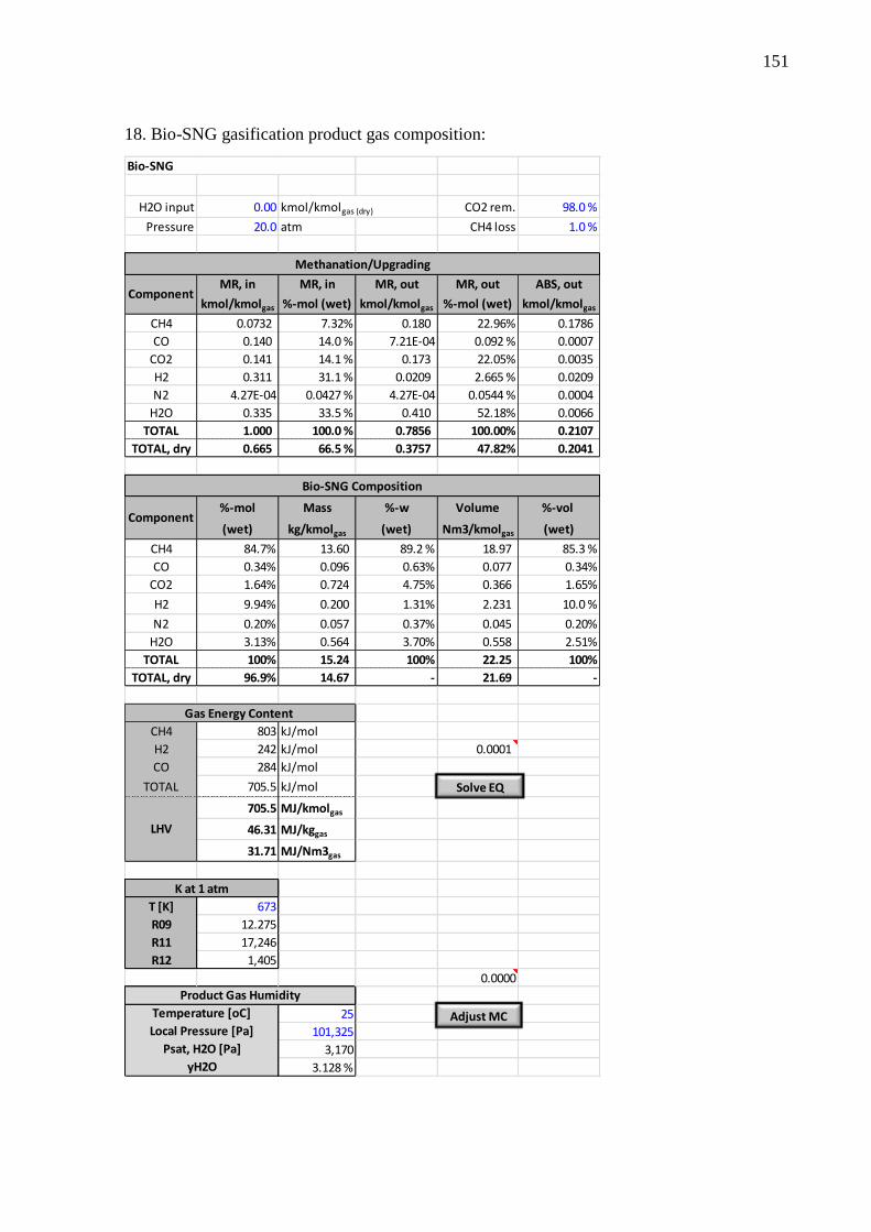
151
18. Bio-SNG gasification product gas composition:
H2O input 0.00 CO2 rem. 98.0 %
Pressure 20.0 atm CH4 loss 1.0 %
MR, in MR, in MR, out MR, out ABS, out
kmol/kmolgas %-mol (wet) kmol/kmolgas %-mol (wet) kmol/kmolgas
CH4 0.0732 7.32% 0.180 22.96% 0.1786
CO 0.140 14.0 % 7.21E-04 0.092 % 0.0007
CO2 0.141 14.1 % 0.173 22.05% 0.0035
H2 0.311 31.1 % 0.0209 2.665 % 0.0209
N2 4.27E-04 0.0427 % 4.27E-04 0.0544 % 0.0004
H2O 0.335 33.5 % 0.410 52.18% 0.0066
TOTAL 1.000 100.0 % 0.7856 100.00% 0.2107
TOTAL, dry 0.665 66.5 % 0.3757 47.82% 0.2041
%-mol Mass %-w Volume %-vol
(wet) kg/kmolgas (wet) Nm3/kmolgas (wet)
CH4 84.7% 13.60 89.2 % 18.97 85.3 %
CO 0.34% 0.096 0.63% 0.077 0.34%
CO2 1.64% 0.724 4.75% 0.366 1.65%
H2 9.94% 0.200 1.31% 2.231 10.0 %
N2 0.20% 0.057 0.37% 0.045 0.20%
H2O 3.13% 0.564 3.70% 0.558 2.51%
TOTAL 100% 15.24 100% 22.25 100%
TOTAL, dry 96.9% 14.67 - 21.69 -
CH4 803 kJ/mol
H2 242 kJ/mol 0.0001
CO 284 kJ/mol
TOTAL 705.5 kJ/mol
705.5 MJ/kmolgas
46.31 MJ/kggas
31.71 MJ/Nm3gas
T [K] 673
R09 12.275
R11 17,246
R12 1,405
0.0000
25
101,325
3,170
3.128 %yH2O
K at 1 atm
Product Gas Humidity
Temperature [oC]
Local Pressure [Pa]
LHV
Psat, H2O [Pa]
Gas Energy Content
Methanation/Upgrading
Component
Bio-SNG Composition
Component
Bio-SNG
kmol/kmolgas (dry)
Solve EQ
Adjust MC

152
19. Bio-SNG gasification fuel combustion:
47% Gas
Basis 1 GJfuel 53% Solid
Gas Gas Solid FUEL FUEL Stoch. O2
kmol/kmolgas kmol/GJgas kmol/GJsolid kmol/GJfuel %-mol kmol/GJfuel
C 0.867 1.229 1.879 1.574 32.8 % 1.574
H 3.589 5.086 1.125 2.988 62.3 % 0.747
O 0.036 0.051 0.128 0.092 1.92% -0.046
N 0.004 0.006 0.029 0.018 0.38% 0.000
S 0.000 0.000 0.040 0.021 0.45% 0.021
H2O 0.031 0.044 0.152 0.102 2.12% 0.000
TOTAL - - - 4.795 100% 2.296
Air ratio 6.19
kmol kg Nm3 kmol kg Nm3 kmol kg Nm3
GJfuel 2.296 73.47 51.42 11.14 319.2 248.6 68.93 1,975 1,538
kmolfuel 1.124 35.98 25.18 5.457 156.3 121.7 33.75 966.9 753.1
kgfuel 0.090 2.888 2.021 0.438 12.55 9.77 2.710 77.63 60.46
Component Flue Gas %-mol Mass %-w Volume %-vol
kmol/GJfuel (wet) kg/GJfuel (wet) Nm3/GJfuel (wet)
CO2 1.574 2.25% 69.25 3.46% 35.03 2.26%
N2 53.44 76.5 % 1,497 74.8 % 1,197 77.2 %
O2 11.91 17.1 % 381.0 19.0 % 266.6 17.2 %
SO2 0.021 0.03% 1.370 0.07% 0.468 0.03%
H2O 2.889 4.14% 52.06 2.60% 51.54 3.32%
TOTAL 69.83 100% 2,001 100% 1,551 100%
TOTAL, dry 66.94 95.9 % 1949 97.4 % 1499 96.7 %
489.7 MJ/kmolfuel
39.31 MJ/kgfuel
Input Value Unit Value Unit
PG 0.757 kmol PG/s Wood in 12.0 kg/s 43.1 t/h
Wood 10.33 kg/s Planted 27,472 ha
Carbon 1.32 kg/s Required 54,944 ha
Ash 0.09 kg/s Gasif. Size 112 MW
Loss 0.23 kg/s TOTAL 239 MW
Steam 5.09 kg/s Gas 47% -
Wood 186,763 kW Cold gas 239 MW
Steam 15457 kW
Gas 112,487 kW
HG eff. 60.2 % - 131 MW
Net eff. 55.6 %
Hot Gas Efficiency SUMMARY
LHV
Fuel Energy Content
Fuel GasStoch. O2 Stoch. Air (wet) Comb. Air (wet)
Flue Gas Composition
Combustion
Fuel Elemental Composition
Element

153
20. Bio-SNG gasification flame temperature:
Tref = 298.15 K
Phase
t
%-mol Enthalpy %-mol Enthalpy
(wet) kJ/mol (wet) kJ/mol
CH4 0.00% 59.11 0.00% 91.04
CO 0.00% 30.94 0.00% 44.03
CO2 0.00% 48.61 2.28% 70.31
H2 0.00% 29.07 0.00% 41.06
N2 77.5 % 30.58 76.6 % 43.53
O2 20.6 % 32.37 17.1 % 45.97
SO2 0.00% 49.55 0.03% 70.78
H2O 1.88% 37.73 4.00% 55.15
TOTAL 100% 31.08 100% 45.03
MM 28.67 kg/kmol
V-molar 22.21 Nm3/kmol
Phase Flow Temperature Enthalpy Heat
kg/s [K] kJ/kg kW
Air 472.2 1,273 1,085 512,403
Gas, sens. 2.429 298 0.00 0.00
Gas, comb. 2.429 - 46,309 112,487 239.2
Solid, comb. 3.827 - 33,103 126,670
Flue gas 478.5 1,646 1,571 -751,560 0.0000
1373 oC
kg/s kmol/s Nm3/s Nm3/min
Air 472.2 16.484 368 22,067
Gas 2.429 0.159 3.55 213
Solid 3.827 0.425 - -
Flue gas 478.5 16.689 371 22,241
0.0000
Component
PhaseMass Balance
Energy Balance
Flame Temperature
Air Flue Gas
Sensible heat
1.6461.273
Gas Flow