COOPERATIVE MOTION CONTROL OF A FORMATION OF U AVs · in the research community towards cooperative...
82
COOPERATIVE MOTION CONTROL OF A FORMATION OF UAVs RÔMULO TEIXEIRA RODRIGUES DISSERTAÇÃO DE MESTRADO APRESENTADA À FACULDADE DE ENGENHARIA DA UNIVERSIDADE DO PORTO EM AUTOMAÇÃO E ROBÓTICA M 2014
Transcript of COOPERATIVE MOTION CONTROL OF A FORMATION OF U AVs · in the research community towards cooperative...
COOPERATIVE MOTION CONTROL OF A
FORMATION OF UAVs
RÔMULO TEIXEIRA RODRIGUES DISSERTAÇÃO DE MESTRADO APRESENTADA À FACULDADE DE ENGENHARIA DA UNIVERSIDADE DO PORTO EM AUTOMAÇÃO E ROBÓTICA
M 2014

FACULDADE DE ENGENHARIA DA UNIVERSIDADE DO PORTO
Cooperative Motion Control of a
Formation of UAVs
Romulo Teixeira Rodrigues
Dissertation
Advisor: Dr. Antonio Pedro Aguiar
Co-advisor: Dr. Marcelo Becker
July 31, 2014
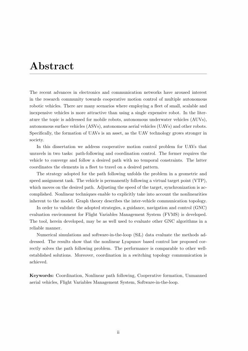
Abstract
The recent advances in electronics and communication networks have aroused interest
in the research community towards cooperative motion control of multiple autonomous
robotic vehicles. There are many scenarios where employing a fleet of small, scalable and
inexpensive vehicles is more attractive than using a single expensive robot. In the liter-
ature the topic is addressed for mobile robots, autonomous underwater vehicles (AUVs),
autonomous surface vehicles (ASVs), autonomous aerial vehicles (UAVs) and other robots.
Specifically, the formation of UAVs is an asset, as the UAV technology grows stronger in
society.
In this dissertation we address cooperative motion control problem for UAVs that
unravels in two tasks: path-following and coordination control. The former requires the
vehicle to converge and follow a desired path with no temporal constraints. The latter
coordinates the elements in a fleet to travel on a desired pattern.
The strategy adopted for the path following unfolds the problem in a geometric and
speed assignment task. The vehicle is permanently following a virtual target point (VTP),
which moves on the desired path. Adjusting the speed of the target, synchronization is ac-
complished. Nonlinear techniques enable to explicitly take into account the nonlinearities
inherent to the model. Graph theory describes the inter-vehicle communication topology.
In order to validate the adopted strategies, a guidance, navigation and control (GNC)
evaluation environment for Flight Variables Management System (FVMS) is developed.
The tool, herein developed, may be as well used to evaluate other GNC algorithms in a
reliable manner.
Numerical simulations and software-in-the-loop (SiL) data evaluate the methods ad-
dressed. The results show that the nonlinear Lyapunov based control law proposed cor-
rectly solves the path following problem. The performance is comparable to other well-
established solutions. Moreover, coordination in a switching topology communication is
achieved.
Keywords: Coordination, Nonlinear path following, Cooperative formation, Unmanned
aerial vehicles, Flight Variables Management System, Software-in-the-loop.
ii

Resumo
Os avancos recentes na eletronica e redes de computadores tem despertado interesse na
comunidade cientıfica quanto ao controlo de movimento cooperativo de multiplos veıculos
roboticos autonomos. Existem varias situacoes em que a utilizacao de um conjunto de
veıculos pequenos, escalaveis e de baixo custo e vantajosa relativamente ao uso de um
unico robo de alto custo. Na literatura este topico e abordado para robos moveis, veıculos
submarinos autonomos (AUVs - Autonomous Underwater Vehicle), veıculos de superfıcie
autonomos (ASVs – Autonomous Surface Vehicle), veıculos aereos autonomos (UAVs –
Unmanned Aerial Vehicle) e outros robos. Particularmente, a formacao de UAVs e um
foco de interesse, uma vez que se tem observado uma expansao dos UAVs na sociedade.
Esta dissertacao foca o problema de controlo de movimento cooperativo de UAVs
que e dividido em duas tarefas: o seguimento de caminhos e o controlo de coordenacao.
O seguimento de caminhos tem por objetivo que o veıculo convirja para um percurso
desejado e o siga, sem quaisquer restricoes temporais. A segunda tarefa trata de coordenar
os elementos de um conjunto de veıculos para que estes se movimentem de acordo com
um padrao desejado.
A estrategia adotada para o seguimento de caminhos divide o problema em duas com-
ponentes, nomeadamente uma tarefa geometrica e uma tarefa de atribuicao de velocidade.
O veıculo segue constantemente um alvo virtual (VTP – Virtual Target Point), que se
move no percurso desejado. Ao ajustar a velocidade do alvo e possıvel obter sincronizacao.
Tecnicas nao-lineares permitem considerar nao-linearidades inerentes ao modelo de forma
explıcita. A topologia de comunicacao entre veıculos e descrita atraves de teoria de grafos.
A fim de validar as estrategias adotadas, um ambiente de seguimento, navegacao e
controlo (GNC – Guidance, Navigation and Control) e desenvolvido para um sistema
de geral que relaciona as varias variaveis de voo (FVMS - Flight Variables Management
System). A ferramenta desenvolvida pode tambem ser usada para avaliar outros algoritmos
GNC de forma fidedigna.
Simulacoes numericas e dados software-in-the-loop (SiL) sao usados para avaliar os
metodos abordados. Segundo os resultados, a lei de controlo baseada em Lyapunov nao-
linear proposta resolve corretamente o problema de seguimento de caminhos. Para alem
de a sua performance ser comparavel a de outras solucoes bem estabelecidas, e conseguida
a coordenacao numa topologia alternada no tempo.
Palavras-chave: Coordenacao, Seguimento, Formacao cooperativa, Veıculos aereos nao-
tripulados, Flight Variables Management System, Software-in-the-loop .
iii

Acknowledgments
I am very grateful for all my friends and relatives who assisted me along the years. Special
thanks to
Prof. Antonio Pedro Aguiar for offering me the chance to research beyond regular
lectures. Despite the distance, he was always available to help and guide me.
Prof. Marcelo Becker and Rafael Coronel for letting me join their team. Their solici-
tude before and during this journey was a comfort.
LSTS/FEUP team for the support and field test invitation.
the friends I collected in these five years (hopefully our friendship will last for the
next fifty): Tiago, Nuno, Gilbert, Antony, Hugo and, more recently, Rafael. Thanks for
receiving me in your home and families. For sure, these years would not had been as
enjoyable without our discussions, laughs and coffee breaks.
to Ana Rita for supporting and taking care of me through this journey. Also to her
family for welcoming me in their home and sharing their time with me.
to my dad, mom and sisters whose unconditional love gives me strength for improving
daily.
iv
Contents
Abstract ii
Resumo iii
Contents v
List of Figures vii
1 Introduction 1
1.1 Motivation . . . . . . . . . . . . . . . . . . . . . . . . . . . . . . . . . . . . 1
1.2 Problem Statement . . . . . . . . . . . . . . . . . . . . . . . . . . . . . . . . 5
1.3 Previous work and contributions . . . . . . . . . . . . . . . . . . . . . . . . 5
1.4 Thesis Outline . . . . . . . . . . . . . . . . . . . . . . . . . . . . . . . . . . 7
2 Mathematical Preliminaries 9
2.1 Basic definitions . . . . . . . . . . . . . . . . . . . . . . . . . . . . . . . . . 9
2.2 Nonlinear System . . . . . . . . . . . . . . . . . . . . . . . . . . . . . . . . . 11
2.3 Graph theory . . . . . . . . . . . . . . . . . . . . . . . . . . . . . . . . . . . 18
3 UAV System Model 22
3.1 Coordination Frames . . . . . . . . . . . . . . . . . . . . . . . . . . . . . . . 22
3.2 Equations of Motion . . . . . . . . . . . . . . . . . . . . . . . . . . . . . . . 23
3.3 Dynamic modelling . . . . . . . . . . . . . . . . . . . . . . . . . . . . . . . . 25
3.4 Cessna 172SP Skyhawk . . . . . . . . . . . . . . . . . . . . . . . . . . . . . 28
4 UAV Motion Control 29
4.1 Introduction . . . . . . . . . . . . . . . . . . . . . . . . . . . . . . . . . . . . 29
4.2 Carrot chasing control algorithm . . . . . . . . . . . . . . . . . . . . . . . . 30
4.3 Nonlinear Lyapunov based control algorithm . . . . . . . . . . . . . . . . . 31
5 Cooperative Motion Control 36
5.1 Introduction . . . . . . . . . . . . . . . . . . . . . . . . . . . . . . . . . . . . 36
5.2 Problem Statement . . . . . . . . . . . . . . . . . . . . . . . . . . . . . . . . 37
5.3 Constant communication . . . . . . . . . . . . . . . . . . . . . . . . . . . . . 37
5.4 Switching communication topology . . . . . . . . . . . . . . . . . . . . . . . 39
v
Contents Contents
6 Software Architecture 41
6.1 Introduction . . . . . . . . . . . . . . . . . . . . . . . . . . . . . . . . . . . . 41
6.2 Flight Variable Management System . . . . . . . . . . . . . . . . . . . . . . 42
6.3 GNC Module . . . . . . . . . . . . . . . . . . . . . . . . . . . . . . . . . . . 45
7 Simulation Results 51
7.1 Numerical simulator . . . . . . . . . . . . . . . . . . . . . . . . . . . . . . . 51
7.2 SiL Simulation . . . . . . . . . . . . . . . . . . . . . . . . . . . . . . . . . . 56
7.3 Summary . . . . . . . . . . . . . . . . . . . . . . . . . . . . . . . . . . . . . 61
8 Conclusions 62
8.1 Summary . . . . . . . . . . . . . . . . . . . . . . . . . . . . . . . . . . . . . 62
8.2 Future work . . . . . . . . . . . . . . . . . . . . . . . . . . . . . . . . . . . . 62
Bibliography 64
A Appendix - FVMS GNC libraries and functions 68
A.1 Types and conversions . . . . . . . . . . . . . . . . . . . . . . . . . . . . . . 68
A.2 Navigation library . . . . . . . . . . . . . . . . . . . . . . . . . . . . . . . . 70
A.3 Control library . . . . . . . . . . . . . . . . . . . . . . . . . . . . . . . . . . 71
A.4 Controllers library . . . . . . . . . . . . . . . . . . . . . . . . . . . . . . . . 71
vi

List of Figures
1.1 Humming bird quadcopter and tower assembled by UAVs . . . . . . . . . . 2
1.2 Outback Joe waiting for UAV rescue since 2007 . . . . . . . . . . . . . . . . 3
1.3 Multiple autonomous vehicle cooperation . . . . . . . . . . . . . . . . . . . 4
2.1 A stable system . . . . . . . . . . . . . . . . . . . . . . . . . . . . . . . . . . 13
2.2 An asymptotically stable system . . . . . . . . . . . . . . . . . . . . . . . . 13
2.3 Undirected and directed graph representation . . . . . . . . . . . . . . . . . 18
2.4 Graph topologies . . . . . . . . . . . . . . . . . . . . . . . . . . . . . . . . . 19
2.5 Uniformly quasi strongly connected graph . . . . . . . . . . . . . . . . . . . 21
3.1 UAV Coordinate frame . . . . . . . . . . . . . . . . . . . . . . . . . . . . . . 22
3.2 Unicycle kinematic model . . . . . . . . . . . . . . . . . . . . . . . . . . . . 25
3.3 UAV Coordinate frame projected in the xy plane. . . . . . . . . . . . . . . . 26
3.4 Roll, pitch and yaw on a wing-fixed airplane . . . . . . . . . . . . . . . . . . 27
3.5 Important forces acting on a coordinated turn. . . . . . . . . . . . . . . . . 27
3.6 Cessna 172SP Skyhawk specifications . . . . . . . . . . . . . . . . . . . . . . 28
4.1 Carrot chasing frame . . . . . . . . . . . . . . . . . . . . . . . . . . . . . . . 30
4.2 Path following frame on the xy plane . . . . . . . . . . . . . . . . . . . . . . 32
4.3 Nonlinear Lyapunov base path following controller . . . . . . . . . . . . . . 34
5.1 Different topology for coordination controllers . . . . . . . . . . . . . . . . . 36
5.2 Cooperative path-following controller . . . . . . . . . . . . . . . . . . . . . . 39
6.1 Software in the loop simulation . . . . . . . . . . . . . . . . . . . . . . . . . 42
6.2 AscTec Pelican in MSFS04 . . . . . . . . . . . . . . . . . . . . . . . . . . . 43
6.3 Squidy and Shark UAVs . . . . . . . . . . . . . . . . . . . . . . . . . . . . . 44
6.4 Cessna 172SP Skyhawk in MSFS04 . . . . . . . . . . . . . . . . . . . . . . . 44
6.5 FVMS Conceptual Diagram . . . . . . . . . . . . . . . . . . . . . . . . . . . 45
6.6 Guidance, navigation and control . . . . . . . . . . . . . . . . . . . . . . . . 46
6.7 FVMS architecture . . . . . . . . . . . . . . . . . . . . . . . . . . . . . . . . 47
6.8 GNC module information flow . . . . . . . . . . . . . . . . . . . . . . . . . . 47
6.9 FVMS GNC user interface . . . . . . . . . . . . . . . . . . . . . . . . . . . . 50
7.1 Path following comparison . . . . . . . . . . . . . . . . . . . . . . . . . . . . 52
7.2 3D path following results . . . . . . . . . . . . . . . . . . . . . . . . . . . . 53
vii
List of Figures List of Figures
7.3 Coordination in a constant topology . . . . . . . . . . . . . . . . . . . . . . 54
7.4 Coordination in a switching topology . . . . . . . . . . . . . . . . . . . . . . 55
7.5 FVMS and MSFS SiL environment. . . . . . . . . . . . . . . . . . . . . . . 56
7.6 SiL: carrot chasing vs nonlinear . . . . . . . . . . . . . . . . . . . . . . . . . 57
7.7 SiL: robust control . . . . . . . . . . . . . . . . . . . . . . . . . . . . . . . . 58
7.8 SiL: nonlinear PF robust control . . . . . . . . . . . . . . . . . . . . . . . . 59
7.9 SiL: 3D path following . . . . . . . . . . . . . . . . . . . . . . . . . . . . . . 60
viii
1. Introduction
This chapter introduces the topic of the dissertation which is cooperative control of a
formation of unmanned aerial vehicles. Its relevance in the modern society and some
open challenges are addressed in Section 1.1. Afterwards, in Section 1.2 the problem to be
solved in the dissertation is formulated. Then, Section 1.3 presents a collection of previous
work related to the topic and the contribution of this work. Section 1.4 introduces a brief
scope of the document.
1.1 Motivation
Unmanned Aerial Vehicles (UAVs) are no longer science fiction but an expanding technol-
ogy. It may be employed in a wide range of applications, from border patrolling and fire
detection to aerobiological sampling and crop monitoring. These platforms do not only
prevent human pilots from hazardous situations, but they are also a cheap and reliable
solution when contrasted to other manned vehicles. It is not a fortuity, UAVs are robotics
industry fastest growing market segment (Cheng and Kumar, 2008). The military UAV
market will consume about $61.37 billion between 2011 and 2020 (Roundup, 2013). The
civilian market as well is expect to increase, considering the growth of its usage among
universities, environmental entities and media companies. In 2013, there were 57 countries
producing more than 960 distinct UAVs (Roundup, 2013). Each year this number grows,
as nations develop their own indigenous aircraft to comply with specific requirements.
The popularization of UAVs and recent advents in communication networks, renewed
interest in UAV Coordinated Control. A single vehicle may be enough in a simple ap-
plication. However, the success of more challenging missions requires the employment of
multiple vehicles working in cooperation towards the same goal. This concept is based
on the advantages of distributed systems, such as robustness, flexibility and scalability,
which endow a fleet of simple and cheap vehicles to perform tasks that are not feasible for
an expensive single unit. For instance, inexpensive sensors can be distributed along the
vehicles and data fusion occurs periodically or sporadically. A set of possible applications
is shown next.
1
Chapter 1. Introduction 1.1. Motivation
Aerial Robotic Construction
Over the past few decades, land robots have populated modern industries. However, they
have a limited working area due to their rigid body constraints. On the other hand, aerial
vehicles can operate freely in space. Taking advantages of such system, a new field named
Aerial Robotic Construction (ARC) emerged. It was first described in (Lindsey et al.,
2011). In this pioneering work, a set of UAVs capable of assembling three-dimensional
small scale structures, like the ones for building high-voltage towers and skyscrapers, were
developed. The pieces were specially manufactured to be transported by quadcopters.
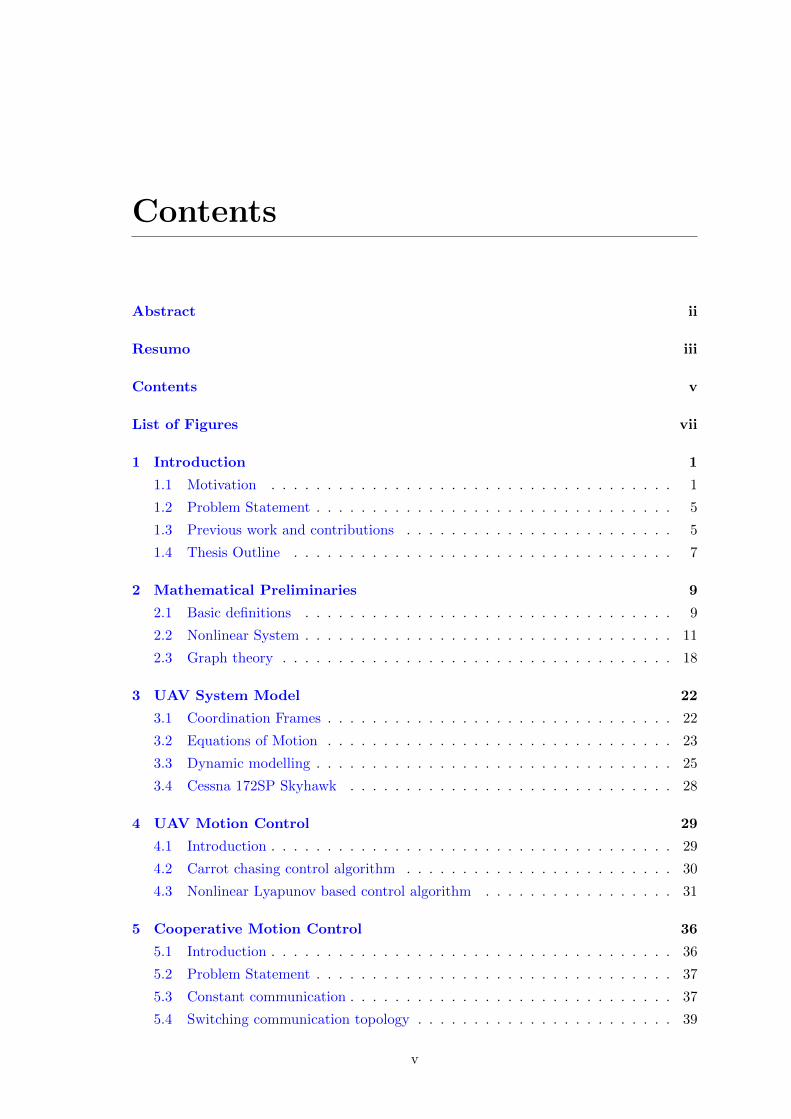
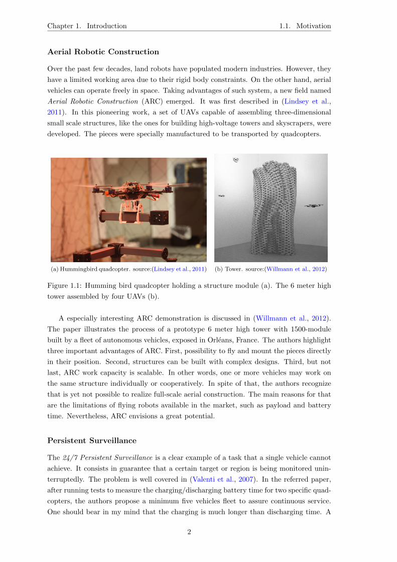
(a) Hummingbird quadcopter. source:(Lindsey et al., 2011) (b) Tower. source:(Willmann et al., 2012)
Figure 1.1: Humming bird quadcopter holding a structure module (a). The 6 meter high
tower assembled by four UAVs (b).
A especially interesting ARC demonstration is discussed in (Willmann et al., 2012).
The paper illustrates the process of a prototype 6 meter high tower with 1500-module
built by a fleet of autonomous vehicles, exposed in Orleans, France. The authors highlight
three important advantages of ARC. First, possibility to fly and mount the pieces directly
in their position. Second, structures can be built with complex designs. Third, but not
last, ARC work capacity is scalable. In other words, one or more vehicles may work on
the same structure individually or cooperatively. In spite of that, the authors recognize
that is yet not possible to realize full-scale aerial construction. The main reasons for that
are the limitations of flying robots available in the market, such as payload and battery
time. Nevertheless, ARC envisions a great potential.
Persistent Surveillance
The 24/7 Persistent Surveillance is a clear example of a task that a single vehicle cannot
achieve. It consists in guarantee that a certain target or region is being monitored unin-
terruptedly. The problem is well covered in (Valenti et al., 2007). In the referred paper,
after running tests to measure the charging/discharging battery time for two specific quad-
copters, the authors propose a minimum five vehicles fleet to assure continuous service.
One should bear in my mind that the charging is much longer than discharging time. A
2
1.1. Motivation Chapter 1. Introduction
regular battery, in a four rotor vehicle, last in average 20 minutes, while the charging time
is around an hour.
In the 24/7 Persistent Surveillance there may be only one vehicle in the air for each time
instant, but there is a net of vehicles performing the same task. For instances, the vehicles
may be disputing one or more charging stations. In this case a more complex cooperative
control is required, inasmuch as the vehicles compete for a resource. The problem consists
in assuring persistent surveillance and appropriating charging management.
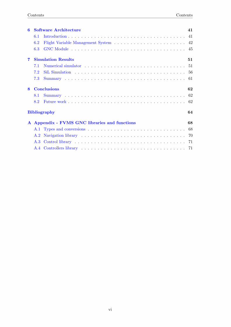
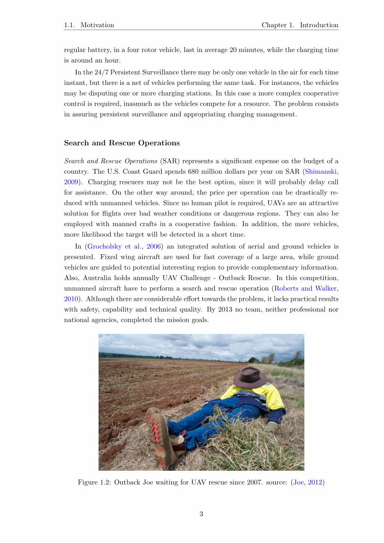
Search and Rescue Operations
Search and Rescue Operations (SAR) represents a significant expense on the budget of a
country. The U.S. Coast Guard spends 680 million dollars per year on SAR (Shimanski,
2009). Charging rescuers may not be the best option, since it will probably delay call
for assistance. On the other way around, the price per operation can be drastically re-
duced with unmanned vehicles. Since no human pilot is required, UAVs are an attractive
solution for flights over bad weather conditions or dangerous regions. They can also be
employed with manned crafts in a cooperative fashion. In addition, the more vehicles,
more likelihood the target will be detected in a short time.
In (Grocholsky et al., 2006) an integrated solution of aerial and ground vehicles is
presented. Fixed wing aircraft are used for fast coverage of a large area, while ground
vehicles are guided to potential interesting region to provide complementary information.
Also, Australia holds annually UAV Challenge - Outback Rescue. In this competition,
unmanned aircraft have to perform a search and rescue operation (Roberts and Walker,
2010). Although there are considerable effort towards the problem, it lacks practical results
with safety, capability and technical quality. By 2013 no team, neither professional nor
national agencies, completed the mission goals.
Figure 1.2: Outback Joe waiting for UAV rescue since 2007. source: (Joe, 2012)
3

Chapter 1. Introduction 1.1. Motivation
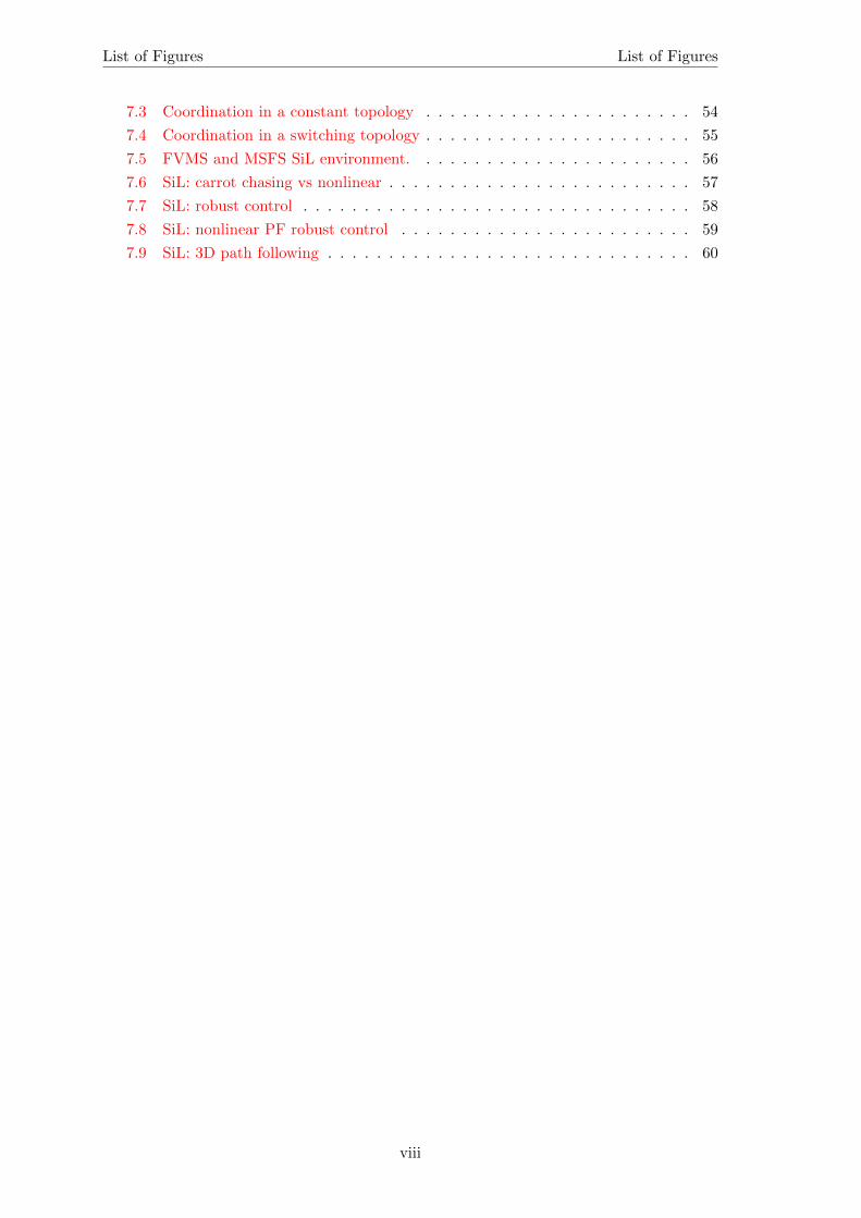
Inter Vehicle Cooperation
There are different configurations of autonomous robots, like fixed-wing aircraft, quad-
copters, submarines, boats, hovercraft and others. They are designed and built to operate
in the more diversified environments like air, dry land, sea, dam and rivers. The integra-
tion of these systems is a vanguard field that has gained much interest of researchers in
the last few years. For instance, consider the search for a specific target in the sea. UAVs
carrying radars able to detect contact on the water surface are employed for a wide search.
The information is transmitted to an Autonomous Surface Vessel (ASV) that contacts a
Autonomous Underwater Vehicle (AUV) for direct inspection of the possible target. Oper-
ations in that scale are costly due to equipment and specialized crew. Cooperative robotic
is a relatively cheap platform that will improve the success in large scale mission.
Figure 1.3: Multiple autonomous vehicle cooperation
4

1.2. Problem Statement Chapter 1. Introduction
For more applications the reader is referred to (Etter et al., 2011) and (Sahin, 2005)
where a variety of multiple UAV tasks are explored.
1.2 Problem Statement
Many challenges arise in a multi-UAV scenario: data fusion, collaborative assignment, col-
lision avoidance and coordination, just to name a few. The present dissertation focuses on
coordinated path following, defined here as a desired inter-vehicle pattern where multiple
vehicles are required to follow pre-specified paths.
In order to decrease the complexity, the problem was divided in two parts. The first
topic is path-following (PF) motion control, where a single vehicle is required to converge
and keep track of a pre-specified spatial path with a desired speed assignment without
temporal requirements. The second topic is coordinated control, in which the vehicles
are required to follow a desired inter-vehicle formation.
The path following problem task is a desired capability of an autonomous robot. It aims
to bring the vehicle to a desired geometric path parametrized in space such as a straight
line or a circle (typically called loiter). As stated in (Sujit et al., 2013), a satisfactory
PF algorithm must steer the vehicle towards the path, follow it precisely and be robust
against wind disturbances.
The coordinated control of autonomous vehicles is important in a multi-UAV scenario,
relieving the burden over human operators that can focuses on high level decisions. The
coordination task is particularly challenging, since the nature of the communication net-
works restricts the information exchanged among vehicles (Fax and Murray, 2004). No
aircraft will possible be able to continuously communicate with every unit in the fleet
during the entire mission. Furthermore, the coordination strategy must be robust against
link failure amid the vehicles. These constraints limit the use of centralized control strate-
gies, where a central unit (ex: ground station) process all information required to achieve
a certain goal, for instance. In the last few years, decentralized strategies have come to
forum to discuss multi-agent networks with application in engineering and science. This
approach is more reliable in terms of flexibility, robustness and scalability.
In this framework, a decentralized multi-vehicle control structure, where the vehicles
and communication topology constraints are taken into account is addressed. The pre-
sented solution focus on the kinematics, consequently it may be implement in different
aerial vehicles morphologies. Numerical simulation and data collect from software-in-the-
loop (SiL) experiments evaluate the performance of the methods.
1.3 Previous work and contributions
1.3.1 Path Following Motion Control
As a human pilot is not present to take decisions, the guidance system is a major com-
ponent in UAV systems. The path following guidance problem requires that a vehicle
converge to and follow a path without time constraints. For fully actuated system the
5
Chapter 1. Introduction 1.3. Previous work and contributions
problem is well solved. However, it is usually expensive and impractical to fully actuate
autonomous vehicle (Aguiar and Hespanha, 2003). Motivated by these limitations, huge
effort has been directed towards underactuated autonomous vehicles. In an underactu-
ated system the independent generalized coordinates outnumber the control inputs, e.g.
wheeled robots, surface vessels, underwater vehicles, helicopters and flying wings.
The motion control problem for these systems are particularly interesting because
underactuated vehicles are mostly not fully feedback linearizable and exhibit nonholonomic
constraints. A traditional solution is linearize the model for a specific operating point and
design a PID controller or apply any other classic control method. The performance could
be low, except for the neighborhood of the operating point that the system was initially
designed to. Gain scheduling solves the problem of a single operating point on the cost
of increase complexity. In the scope of this dissertation, nonlinear control techniques are
preferred to classic control strategies. As highlighted in (Vanni, 2007), this decision is
based on the fact that nonlinear control explicitly takes into account the nonlinearities
inherent to the model rather than opposing it.
Pioneering work on the PF problem for wheeled mobile robots is described in (Samson,
1992). The approach is further extended for the three-dimensional case in (Encarnacao
and Pascoal, 2000) using Lyapunov based control laws for an autonomous underwater
vehicle (AUV). In these works a virtual target point (VTP) is placed on the position of
the path closest to the vehicle. The vehicle is projected on the desired path and a tangent
frame associated to the projection point. This frame is called Serret-Franet {F}. In this
solution, the vehicle converges and remains inside a tube that involves the path. However,
the radius of the tube must be less than the shortest curvature of the path, otherwise a
singularity may arise. The work in (Lapierre et al., 2003) proposes an alternative solution
to remove the singularity. The origin of the Serret-Frenet frame is not attached to the
projection point, instead evolves in time according to a certain function.
In (Aguiar and Hespanha, 2007) an elegant solution by decomposing the problem in
two tasks (geometric and dynamic) is presented. The geometric task aims to bring the
vehicle and assures it remains inside a tube centered around the desired path. The control
signals actuate on the vehicle’s orientation. The dynamic assignment task assigns a speed
profile to the path. In (Oliveira et al., 2013) the path following problem is generalized for
the case of moving path following (MPF), in which the path is not stationary but dynamic.
The authors evaluates the method for a fixed-wing UAV with hardware-in-the-loop (HiL)
simulations.
As many authors adopt different approaches to solve the PF problem, the work in
(Sujit et al., 2013) evaluates five different methods: carrot chasing, nonlinear guidance
law, pure pursuit, vector field and linear quadratic regulator. Nonlinear guidance law
described by (Park et al., 2007) consumes the least control effort with acceptable response
under different wind conditions for straight and loiter path.
1.3.2 Coordinated Control
In the last years a large interest raised towards coordinated control of a fleet of autonomous
vehicles. The work described by (Encarnacao and Pascoal, 2000) for a single vehicle is
6

1.4. Thesis Outline Chapter 1. Introduction
extended for coordination control of fully actuated vehicles in (Encarnacao and Pascoal,
2001). The authors explore a scenario where an underwater vehicle (slave) must follow
a surface vessel (master). The strategy adopted requires a large amount of information
exchange between vehicles. Consequently, it cannot be fairly extended for more than two
robots.
In (Egerstedt and Hu, 2001) a model-independent for multi-agent formation control
is proposed. Each vehicle is assigned to follow a respective reference virtual target. If
the tracking errors are bounded, a formal proof is given that states the formation error
stabilizes. This allows to decouple the coordination problem into a planning and tracking
problem. But the communication constraints of the inter-vehicle communication networks
are not considered.
In theory, vehicles could share all internal and external information to improve coor-
dination performance. However, such approach is heavily punished in terms of bandwidth
and computational complexity. Moreover, the communication topology may vary over
time due to link or even vehicle failure. A suitable communication constraints represen-
tation is a methodology based on a framework as addressed in (Fax and Murray, 2004).
It relates the concept of Graph Laplacian to represent links between vehicles. Particu-
larly, the work demonstrated in (Fax and Murray, 2002) explicitly shows how the Graph
Laplacian associated to a formation interconnection structure plays a fundamental role in
assessing stability of the behavior of the components in coordination.
In (Ghabcheloo et al., 2007) the authors borrow results from the fore mentioned work to
explicitly address communication constraints for the problem of coordinated path following
for a group of wheeled robots. Lyapunov techniques and graph theory are applied. (Aguiar
and Pascoal, 2007) discusses a framework that takes into account the topology of the
communication links, the logic based nature of communications and the cost of exchanging
information. The strategy is further developed in (Ghabcheloo et al., 2009) for a three-
dimensional robot. The authors consider two different communication topologies. In the
first scenario, the communication graph is alternately connected and disconnected, therein
called brief connectivity losses. The second scenario, named uniformly connected in mean,
captures union of communication graphs connected over uniform intervals of time.
1.3.3 Contributions
In order to validate guidance algorithms, a robust and reliable platform is required. The
Flight Management Variables System (FVMS), a SiL platform, was the chosen tool. In
the scope of this project, a new guidance, navigation and control (GNC) module was
developed for the platform. This platform was used to validate the algorithms reported in
this work. It may be as well employed in different contexts to evaluate or teach a variety
of GNC related algorithms.
1.4 Thesis Outline
The structure of this dissertation is as following
7
Chapter 1. Introduction 1.4. Thesis Outline
Chapter 2 introduces basic results about nonlinear stability and graph theory. The
definitions and theorems presented support the remainder of this thesis.
Chapter 3 : discusses the kinematic and dynamic model of an aircraft. Focus is given
towards the kinematic model, which is simplified to the horizontal plane.
Chapter 4 : addresses the path-following control strategy adopted.
Chapter 5 : the coordination formation problem is discussed. It is first introduced an
ideal model, with continuous communication. Afterwards, a discrete communication
topology is analyzed.
Chapter 6 : describes the simulator that was employed to validate the control laws. The
Guidance module, designed in the context of this dissertation, is presented.
Chapter 7 : the main results to validate the control laws described in previous chapters
are reported.
Chapter 8 : presents a summary of the results obtained and future work.
8

2. Mathematical Preliminaries
This chapter exposes the mathematical background that subsequent chapters are based on.
In Section 2.1, the notations and basic definitions are settled. Next, Section 2.2 introduces
nonlinear system theory and some tools concerned with stability of dynamic systems. In
Section 2.3, a brief overview of graph theory is reported.
2.1 Basic definitions
2.1.1 Notations
The notations in this work are normalized as follow. In order to be easily distinguished
in the text, mathematical variables are in italics. The scalars are typed in lower-case. Let
γ be a scalar variable, then |γ| represents its absolute value. Vectors are represented in
lower case bold. The vector x = [x1, ..., xn]T ∈ Rn is a n-dimensional vector. The element
in the ith position is referred as xi. The norm of x, denoted by ‖x‖, typically considered
is the class of p-norms, given by:
‖x‖p = (|x1|p + ...+ |xn|p)1/p, 1 ≤ p ≤ ∞
and
‖x‖∞ = maxi|xi|
The most commonly used p-norms are ‖x‖1, ‖x‖2, ‖x‖∞, but the basic properties are
satisfied by any p-norm. It is possible to define an inequality that relates any two different
p-norms. In the scope of this work it will be considered the Euclidean norm:
‖x‖2 = (|x1|2 + ...+ |xn|2)1/2 = (xTx)1/2
For the sake of simplicity, along the report, the 2-norm will be referred as ‖x‖. The fol-
lowing two norms support the concepts of input-to-state stability (ISS) that are introduced
later in this chapter.
The supremum norm
‖x[to,∞]‖ = supt≥t0‖x(t)‖
9
Chapter 2. Mathematical Preliminaries 2.1. Basic definitions
and the asymptotic norm
‖xa‖ = limt→∞‖x(t)‖
The vector 1 contains all elements equal to the unity. The same way, all the values of
vector 0 are null. The length of the vector is implicit within the context.
Matrices are denoted in upper upper case. For instance, the element aij lies in the ith
row and jth column of the matrix A. The most commonly used induced matrix norms are
the p-norm, with p=1,2 and ∞ and the Frobenius norm, defined as follow:
Let Am×n ∈ Rm×n, then
• pnorm: ‖A‖p = max ‖Ax‖p : ‖x‖p = 1
• ∞norm: ‖A‖∞ = maxi∑n
j=1 |aij |
• Frobenius: ‖A‖F =√∑n
i=1
∑nj=1 a
2ij
The Frobenius norm can be simplified as ‖A‖F = trace(ATA), where the function
trace(·) is defined as the sum of the elements of the main diagonal. The transpose of a
matrix, represented by AT , contains the elements of A reflected over its main diagonal. A
square matrix has the same number of rows and columns. A square matrix is said to be
symmetric if it is equal to its transpose, A = AT . The size of the matrix is implicit in the
context where it belongs.
Definition 2.1. A symmetric matrix A ∈ Rn×n is
• positive definite if and only if
xTAx > 0, ∀x ∈ Rn,x 6= 0
This fact is stated as A � 0
• semipositive definite if and only if
xTAx ≥ 0, ∀x ∈ Rn,x 6= 0
This fact is stated as A � 0
A skew-symmetric matrix S is equal to the negative of its transpose, S = −ST .
Coordinate frames, sets and graphs are typed in calligraphic letters, except the number
sets, which are represented with blackboard bold.
2.1.2 Sets
A subset S ⊂ Rn is said to be open if for every vector x ∈ S one can find an ε-
neighbourhood of x:
N(x, ε) = {z ∈ Rn| ‖z − x‖ < ε}, such that N(x, ε) ⊂ S
The set composed by all points inside a circle is an open set. On the other way round,
a set is closed if and only if its complement in Rn is open. In other words, S is closed
10
2.2. Nonlinear System Chapter 2. Mathematical Preliminaries
if and only if every convergence sequence ‖xk‖, with elements in S, converges to a point
within the set. The set composed of the points in the edge of a circle is a closed set. A
set S is subject to range of properties which the following are brought out:
1. Boundness: a set is called bounded if there is a real positive number r such that
‖x‖ ≤ r, ∀x ∈ S.
2. Compact: a set is compact if it is both closed and bounded.
3. Connected: a set is said to be connected if its points can be linked by an arc lying
within the set .
2.1.3 Continuous Function
A function f that maps Rn into Rm, denoted by f : Rn → Rm, is said to be continuous at
a point x if f(xk)→ f(x) as xk → x, that is, if given ε > 0 there is δ > 0 such that
‖x− y‖ < δ =⇒ ‖f(x)− f(y)‖ < ε
Definition 2.2. A function is said to be
• continuous on a set S if it is continuous at every point of S.
• uniformly continuous on S if given ε > 0 there is δ > 0 such that
‖x− y‖ < δ ⇒ ‖f(x)− f(y)‖, ∀x,y ∈ S.
2.2 Nonlinear System
This section presents a summary of the most relevant concepts from nonlinear systems the-
ory that are used in this work. The theorems and definitions here presented are borrowed
from (Khalil, 2002). The reader finds in the cited reference proof and further details.
2.2.1 System Representation
Dynamical systems are described by first order differential equations:
x1 = f1(t, x1, . . . , xn, u1, . . . , up)
...
xn = fn(t, x1, . . . , xn, u1, . . . , up)
where xi, xi and ui to i = 1, . . . , n are the state variable, time derivative of xi and
input variable, respectively. It is possible to rewrite the n-differential equations as one
n-dimensional first-order vector differential equation:
x =
x1
...
xn
, u =
u1
...
un
, f(t,x,u) =
f1(t,x,u)
...
fn(t,x,u)
11

Chapter 2. Mathematical Preliminaries 2.2. Nonlinear System
In a compact form, the state equation is given by
x = f(t,x,u) (2.1)
When there is no explicit dependence of the input, it is called unforced state equation
or nonautonomous system:
x = f(t,x) (2.2)
When the system does not depended explicitly on time t, it is named as time-invariant
or autonomous system. In this case the system is invariant to shifts in the time origin.
x = f(x) (2.3)
2.2.2 Lipschitz Function
The properties of existence and uniqueness are fundamental for a state equation correctly
model a dynamic system. The Lipschitz condition, expressed by
‖f(t,x)− f(t,y)‖ ≤ L‖x− y‖ (2.4)
is a tool to verify that the initial-value problem stated as
x = f(t,x), x(t0) = x0 (2.5)
has a unique solution.
Theorem 2.1. (Local Existence and Uniqueness): Let f(t,x) be a piecewise con-
tinuous function in t that satisfies the Lipschitz condition for all (t,x) and (t,y) in some
neighbourhood of (t0,x0). Then there exist some δ > 0 such that the initial-value problem
has a unique solution over the interval [t0, t0 + δ].
According to the domain which the Lipschitz condition holds true the following clas-
sifications take place.
Definition 2.3. A function f : R× Rn → Rm is
• Lipschitz in x on [a, b]×W if it satisfies (2.4) with the same Lipschitz constant L
• Locally Lipschitz in x on [a, b] × D if every point in x ∈ D has a neighbourhood D′that satisfies (2.4) with given Lipschitz constant L0
• Globally Lipschitz if it is Lipschitz in Rn
2.2.3 Autonomous systems
Consider the autonomous system described by x = f(x), where f is locally Lipschitz on a
domain D and suppose x∗ ∈ D
Definition 2.4. If the system starts with on x = x∗ at t = t0 and remains there for all
future time t > t0, then x∗ is called an equilibrium point of f.
12

2.2. Nonlinear System Chapter 2. Mathematical Preliminaries
The equilibrium point can be shifted to any state-vector on the domain through a
simple change of variables. Let y = x− x∗, then
y = f(x) = f(y + x∗) = g(y), where g(0) = 0 (2.6)
Therefore, with no loss of generality, it is assumed the equilibrium point is always at
the origin.
Definition 2.5. The equilibrium point at x = 0 of (2.3) is
• stable if for each ε > 0, there is a δ > 0 such that ‖x(0)‖ < δ, implies ‖x(t)‖ < ε
for all future time.
δ
δ
||x(t)||
t
Figure 2.1: A stable system
• asymptotically stable if it stable, but also converges to the zero as time approach
infinity. (t→∞, ‖x‖ → 0).
δ
δ
||x(t)||
t
Figure 2.2: An asymptotically stable system
• unstable if it is not stable
The previous definition uses ε − δ requirement for stability. In many cases, it is
challenging to provide a value of δ, given a ball ε. The generalized approach requires
finding all the solutions of (2.3) for determining that the system once started at the δ
neighborhood of the origin will never leave the specified ε neighborhood. Such task may
be hard or not feasible. However, it is possible to determine stability without having to
know explicitly the solution of (2.3) through the Lyapunov stability theorem.
13

Chapter 2. Mathematical Preliminaries 2.2. Nonlinear System
Theorem 2.2. Let D be a domain that contains x = 0, an equilibrium point for (2.3).
Let V : D → R be a continuously differentiable function, such that
V (0) = 0 and V (x) > 0 in D − {0} (2.7)
V (x) ≤ 0 in {D} (2.8)
Then x = 0 is stable. if
V (x) < 0 in D − {0}
then x = 0 is asymptotically stable.
A continuously differentiable function V (x) that holds (2.7) and (2.8) is named Lya-
punov function. The Lyapunov function expresses the energy of the system. If there is an
equilibrium point, the energy stored decreases until reaches the minimum value on that
point. The following definition is introduced
Definition 2.6. A function V (x) is
• positive (negative) definite if V (x) > 0 (V (x) < 0)
• positive (negative) semidefinite if V (x) ≥ 0 (V (x) ≤ 0)
Theorem 2.3. Let x = 0 be an equilibrium point for (2.3). Let V : Rn → R be a
continuously differentiable function such that
V (0) = 0 and V (x) > 0, ∀x 6= 0 (2.9)
‖x‖ → ∞ ⇒ V (x)→∞ (2.10)
V (x) < 0, ∀x 6= 0 (2.11)
then x = 0 is globally asymptotically stable.
A function satisfying (2.10) is said to be radially unbounded.
2.2.4 Nonautonomous systems
Consider the nonautonomous system x = f(t,x), where f is piece continuous in t, locally
Lipschitz in x and its domain contains the origin x = 0. The origin is an equilibrium
point at t = 0 if
f(t, 0) = 0, t ≥ 0
As discussed for autonomous systems, a nonzero equilibrium point may be represented
as an equilibrium point at the origin by means of an appropriate transformation. The
notions of stability and asymptotic stability introduced in Definition 2.5 for autonomous
systems are very much alike for nonautonomous systems. However, while the solution of
an autonomous system depends only on (t− t0), a nonautonomous system relies on both
t and t0. Consequently, the stability behavior depends on the origin at the initial time t0,
that is, the constant δ is a function of t0. As a result, Definition 2.5 is redefined.
Definition 2.7. The equilibrium point x = 0 is
14

2.2. Nonlinear System Chapter 2. Mathematical Preliminaries
• stable if, for each ε > 0, there is a δ = δ(ε, t0) > 0, such that
‖x(t0)‖ < δ ⇒ ‖x(t)‖ < ε, 0 ≤ t ≤ t0
• uniformly stable if, for each ε > 0, there is δ = δ(ε) > 0, independent of t0, such
that the stable condition is satisfied.
• unstable if it is not stable.
• asymptotically stable if it is stable and there is a positive constant c = c(t0) such
that x(t)→ 0 as t→∞, for all ‖x(t0)‖ < c.
• uniformly asymptotically stable if it is uniformly stable and there is a positive
constant c, independent of t0, such that for all ‖x(t0)‖ < c, x(t) → 0 as t → ∞uniformly in t0; that is, for each η > 0, there is T = T (η) > 0 such that
‖x(t)‖ < η, ∀t ≥ t0 + T (η), ∀‖x(t0)‖ < c
• globally uniformly asymptotically stable if it is uniformly stable, δ(ε) can be
chosen to satisfy limε→∞
δ(ε) = ∞, and, for each pair of positive numbers η and c,
there is a T = T (η, c) > 0 such that
‖x(t)‖ < η, ∀t ≥ t0 + T (η, c), ∀‖x(t0)‖ < c
The control problems derived in this dissertation requires a more convenient and trans-
parent definition of uniform stability and uniform asymptotic stability. To this end we
need to introduce the following classes of functions.
Definition 2.8. A continuous function α : [0, a) → [0,∞] is said to belong to class Kif it is strictly increasing and α(0) = 0. It is said to belong to class K∞ if a = ∞ and
α(r)→∞ as r →∞.
Definition 2.9. A continuous function β : [0, a) × [0,∞) → [0,∞] is said to belong to
class KL if, for each fixed s, the mapping β(r, s) belongs to class K with respect to r and,
for each fixed r, the mapping β(r, s) is decreasing with respect to s and β(r, s) → 0 as
s→∞.
It is now possible to redefine uniform stability and uniform asymptotic stability.
Lemma 2.1. The equilibrium point at x = 0 of (2.2) is
• uniformly stable if and only if there exist a class K function α and a positive
constant c, independent of t0, such that
‖x(t)‖ ≤ α(‖x(t0)‖), ∀t ≥ t0 ≥ 0, ∀‖x(t0)‖ < c
• uniformly asymptotically stable if and only if there exist a class KL function β
and a positive constant c, independent of t0, such that
‖x(t)‖ ≤ β(‖x(t0)‖, t− t0), ∀t ≥ t0 ≥ 0, ∀‖x(t0)‖ < c
15
Chapter 2. Mathematical Preliminaries 2.2. Nonlinear System
• globally uniformly asymptotically stable if and only if uniformly asymptotically
stable definition holds for any initial state x(t0).
The class KL function β(r, s) = kre−λs arises as special case of uniform asymptotic
stability, as defined next.
Definition 2.10. The equilibrium point x = 0 of (2.2) is exponentially stable if there
existe positive constants c, k and λ such that
‖x(t)‖ ≤ k‖x(t0)‖e−λ(t−t0), ∀‖x(t0)‖ < c (2.12)
and globally exponentially stable if the fore mentioned equation is satisfied for any initial
state x(t0).
Lyapunov theory for autonomous systems can be extended to nonautonomous systems.
Theorem 2.4. Let x = 0 be an equilibrium point for (2.2) and D ⊂ Rn be a domain
contains it. Let V : [0,∞)×D → R be a continuously differentiable function such that
W1(x) ≤ V (t,x) ≤W2(x) (2.13)
∂V
∂t+∂V
∂xf(t,x) ≤ 0 (2.14)
∀t ≥ 0 and ∀x ∈ D, where W1(x) and W2(x) are continuous positive definite functions on
D. Then, x = 0 is uniformly stable.
Theorem 2.5. Suppose the assumptions of Theorem (2.4) are satisfied with inequality
2.14 strengthened to∂V
∂t+∂V
∂xf(t,x) ≤ −W3(x)
∀t ≥ 0 and ∀x ∈ D, where W3(x) is continuous positive definite functions on D. Then,
x = 0 is uniformly asymptotically stable. Moreover, if positive constant r and c are chosen
such that Br = {‖x‖ ≤ r} ⊂ D and c < min‖x‖=rW1(x), then every trajectory starting in
{x ∈ Br|W2(x) ≤ c} satisfies
‖x(t)‖ ≤ β(‖x(t0)‖, t− t0), ∀t ≥ t0 ≥ 0
for some class KL function β. Finally, if D = Rn and W1(x) is radially unbounded, then
x = 0 is globally uniformly asymptotically stable.
Theorem 2.6. Let x = 0 be an equilibrium point for (2.2) and D ⊂ Rn be a domain
containing x = 0. Let V : [0,∞)×D → R be a continuously differentiable function, such
that
k1‖x‖a ≤V (t,x) ≤ k2‖x‖a
∂V
∂t+∂V
∂xf(t,x) ≤ −k3‖x‖a
∀t ≥ 0 and ∀x ∈ D, where k1, k2, k3 and a are positive constants. Then, x = 0 is
exponentially stable. If the assumptions hold globally, then the equilibrium point is globally
exponentially stable.
16

2.2. Nonlinear System Chapter 2. Mathematical Preliminaries
2.2.5 Boundedness
Lyapunov analysis can be used for showing boundedness of the solution of state equations,
even when no equilibrium point at the origin exists. The bound gives a better estimate of
the solution after the transient period finishes.
Definition 2.11. The solutions of (2.2) are
• uniformly bounded if there exists a positive constance c, independent of t0 ≥ 0,
and for every a ∈ (0, c), there is β = β(a), independent of t0, such that
‖x(t0)‖ ≤ a⇒ ‖x(t)‖ ≤ β, ∀ t ≥ t0 (2.15)
• globally uniformly bounded if it holds (2.15) for arbitrarily large a.
• uniformly ultimately bounded with ultimate bound b if there exist positive con-
stants b and c, independent of t0 ≥ 0, and for every a ∈ (0, c), there is T = T (a, b) ≥0, independent of t0, such that
‖x(t0)‖ ≤ a⇒ ‖x(t)‖ ≤ b, ∀ t ≥ t0 + T (2.16)
• globally uniformly ultimately bounded if it holds (2.16) for arbitrarily large a.
For autonomous system, the word ”uniform” is not employed, as the solution depends
exclusively on (t− t0).
2.2.6 Input-to-state stability
Consider the system described by x = f(t,x,u), where f is piecewise continuous in t and
locally Lipschitz in x and u. Consider that the unforced system
x = f(t,x,0)
has a globally uniformly asymptotically stable equilibrium point at the origin x = 0. The
system described by (2.1) can be viewed as a perturbation of the unforced system. If u is
bounded, then it may be possible, in some cases, to show that x(t) is also bounded. This
fact leads to the introduction of input-to-state stability.
Definition 2.12. The system described by (2.1) is said to be input-to-state stable if there
exist a class KL function β and a class K function γ such that for any initial state x(t0)
and any bounded input u(t), the solution x(t) exists for all t ≥ t0 and satisfies
‖x(t)‖ ≤ β(‖x(t0)‖, t− t0) + γ(‖u[t0,t]‖) (2.17)
The inequality (2.17) ensures that for any bounded u, the state x(t) will be bounded.
Further, as t increases, the state x(t) will be ultimately bounded by a class K function of
‖u[t0,∞)‖. Moreover, if u(t) converges to zero as t → ∞, so does ‖x(t)‖. The following
theorems give sufficient conditions for input-to-state stability.
17
Chapter 2. Mathematical Preliminaries 2.3. Graph theory
Theorem 2.7. Let V : [0,∞) × Rn → R be a continuously differentiable function such
that
α1(x) ≤ V (t,x) ≤ α2(x) (2.18)
∂V
∂t+∂V
∂xf(t,x,u) ≤ −W3(x), ∀ ‖x‖ ≥ ρ(‖u‖) > 0 (2.19)
∀ (t,x,u) ∈ [0,∞) × Rn × Rm, where α1 and α2 are class K∞ functions ρ is a class
K function and W3(x) is a continuous positive definite function on Rn. Then, the system
(2.17) is input-to-state stable with γ = α−11 oα2 o ρ
The conditions (2.18) and (2.19) are also necessary for autonomous systems. A function
V that satisfies Theorem 2.7 is named ISS-Lyapunov function.
2.3 Graph theory
Graph theory is used in this work to model the communication between vehicles in a fleet.
This tool allows modelling and studying the impact of different communication topologies
on the performance of the coordinated system. This section introduces elementary con-
cepts about digraphs. The notations and definitions presented for digraphs are borrowed
from (Mesbahi and Egerstedt, 2010) and (Aguiar and Hespanha, 2007).
2.3.1 Basic concepts
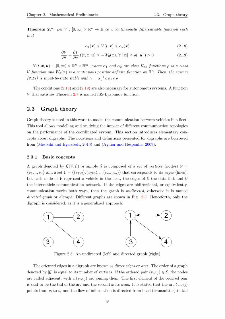
A graph denoted by G(V, E) or simple G is composed of a set of vertices (nodes) V =
{v1, .., vn} and a set E = {(v1v2), (v2v3), .., (vn−1vn)} that corresponds to its edges (lines).
Let each node of V represent a vehicle in the fleet, the edges of E the data link and Gthe intervehicle communication network. If the edges are bidirectional, or equivalently,
communication works both ways, then the graph is undirected, otherwise it is named
directed graph or digraph. Different graphs are shown in Fig. 2.3. Henceforth, only the
digraph is considered, as it is a generalized approach.
1 2
3
1
3
2
4 4
Figure 2.3: An undirected (left) and directed graph (right)
The oriented edges in a digraph are known as direct edges or arcs. The order of a graph
denoted by |G| is equal to its number of vertices. If the ordered pair (vi,vj) ∈ E , the nodes
are called adjacent, with a (vi,vj) arc joining them. The first element of the ordered pair
is said to be the tail of the arc and the second is its head. It is stated that the arc (vi, vj)
points from vi to vj and the flow of information is directed from head (transmitter) to tail
18
2.3. Graph theory Chapter 2. Mathematical Preliminaries
(receiver). If for every arc in E the tail is different from the head and each element of E is
unique, then the graph is oriented. The in-degree of a node vi is the number of arcs with
vi as its head. Analogously, the out-degree of a node vi is the number of arcs with vi as
its tail. A graph is said to be complete if all vertices are pairwise adjacent.
The operation of union and intersection are defined as following
Definition 2.13. Let G1(V1, E1) and G2(V2, E2)
• G1 ∪ G2 = (V1 ∪ V2, E1 ∪ E2)
• G1 ∩ G2 = (V1 ∩ V2, E1 ∩ E2)
If G1 ∩ G2 = ∅, then the graphs are disjoint.
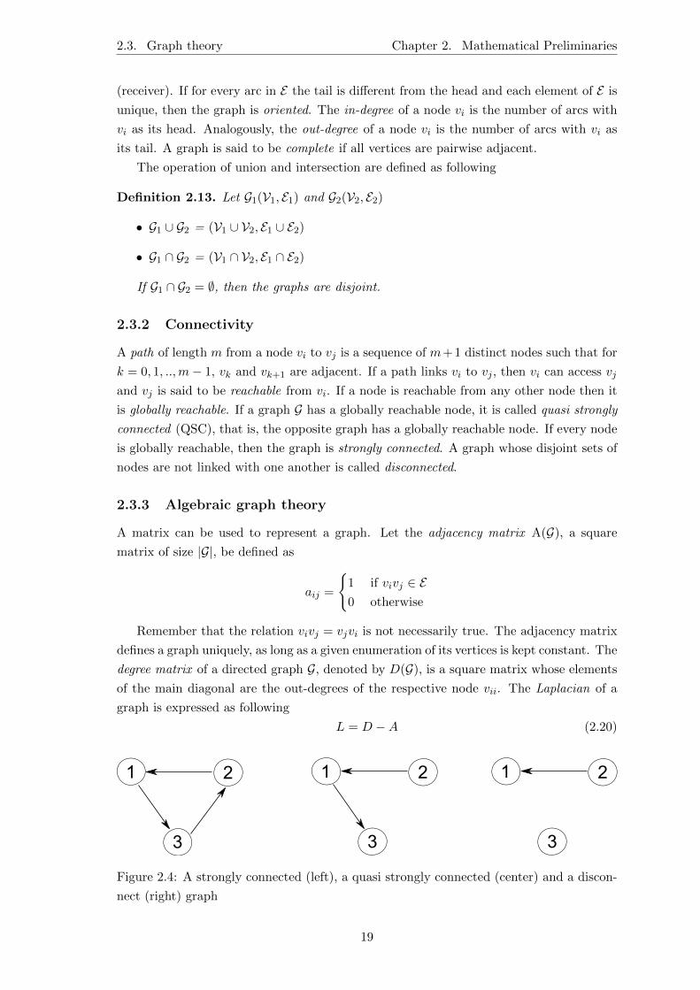
2.3.2 Connectivity
A path of length m from a node vi to vj is a sequence of m+1 distinct nodes such that for
k = 0, 1, ..,m− 1, vk and vk+1 are adjacent. If a path links vi to vj , then vi can access vj
and vj is said to be reachable from vi. If a node is reachable from any other node then it
is globally reachable. If a graph G has a globally reachable node, it is called quasi strongly
connected (QSC), that is, the opposite graph has a globally reachable node. If every node
is globally reachable, then the graph is strongly connected. A graph whose disjoint sets of
nodes are not linked with one another is called disconnected.
2.3.3 Algebraic graph theory
A matrix can be used to represent a graph. Let the adjacency matrix A(G), a square
matrix of size |G|, be defined as
aij =
{1 if vivj ∈ E0 otherwise
Remember that the relation vivj = vjvi is not necessarily true. The adjacency matrix
defines a graph uniquely, as long as a given enumeration of its vertices is kept constant. The
degree matrix of a directed graph G, denoted by D(G), is a square matrix whose elements
of the main diagonal are the out-degrees of the respective node vii. The Laplacian of a
graph is expressed as following
L = D −A (2.20)
1
3
2 1
3
2 1
3
2
Figure 2.4: A strongly connected (left), a quasi strongly connected (center) and a discon-
nect (right) graph
19

Chapter 2. Mathematical Preliminaries 2.3. Graph theory
By definition, each row of the matrix L sums up to zero, therefore the vector 1 belongs to
its kernel K(L). The matrix associated to the digraphs shown in Fig. 2.4 are:
A1 =
0 0 1
1 0 0
0 1 0
D1 =
1 0 0
0 1 0
0 0 1
L1 =
1 0 −1
−1 1 0
0 −1 0
A2 =
0 0 1
1 0 0
0 0 0
D2 =
1 0 0
0 1 0
0 0 0
L2 =
1 0 −1
−1 1 0
0 0 0
A3 =
0 0 0
1 0 0
0 0 0
D3 =
0 0 0
0 1 0
0 0 0
L3 =
0 0 0
−1 1 0
0 0 0
2.3.4 Switching Topology
Let G be a complete graph, i.e., all possible arcs 1 . . . n exist. Consider the piecewise
continuous function pi(t) : [0,∞)→ {0, 1}, where i = 1, . . . , n.
pi(t) =
{1, existence of arc i at time t
0, otherwise(2.21)
The switching signal is defined as the column vector p(t) = [pi]n×1. For each time
instant, the graph Gp(t) is defined by (V, Ep(t)).
Consider that in a given interval of time T, there are q graphs defined, Gi; i = 1, · · · , q.Each graph has associated a Laplacian matrix Li. The union graph, denoted as G = ∪iGi,is the graph whose arcs are the union of the arcs Ei of Gi; i = 1, · · · , q.
Definition 2.14. A graph Gp(t) is said to be uniformly quasi strongly connected
(UQSC), if, for every t0 > 0, there is a T > 0, such that the union graph G([t, t+ T )) is
QSC.
In Fig. 2.5, the graphs G1, G2 and G3, represented at the top left, right and bottom
left, respectively, are disconnected. However, the union graph (bottom right) is uniformly
quasi strongly connected.
20
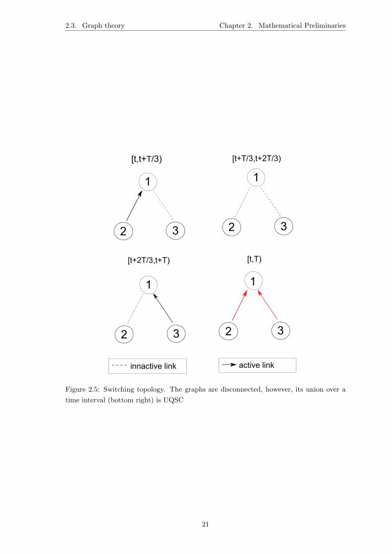
2.3. Graph theory Chapter 2. Mathematical Preliminaries
2
1
3 2
1
3
2
1
3 2
1
3
innactive link active link
[t,t+T/3) [t+T/3,t+2T/3)
[t+2T/3,t+T) [t,T)
Figure 2.5: Switching topology. The graphs are disconnected, however, its union over a
time interval (bottom right) is UQSC
21
3. UAV System Model
This chapter discusses the mathematical model of a UAV. In Section 3.1 the coordinate
frames employed to describe the mathematical model are introduced. Then, the kinematic
equations are derived, as well as a simplified model usually considered in practical UAV
missions (Section 3.2). This simplified model is based on the assumption that the dynamics
of small wing-fixed UAV can be built on the unicycle model (Jackson, 2011). This approach
is also used to introduce wind perturbations in the model. The dynamics of the UAV and
its basic working principles are presented in Section 3.3.
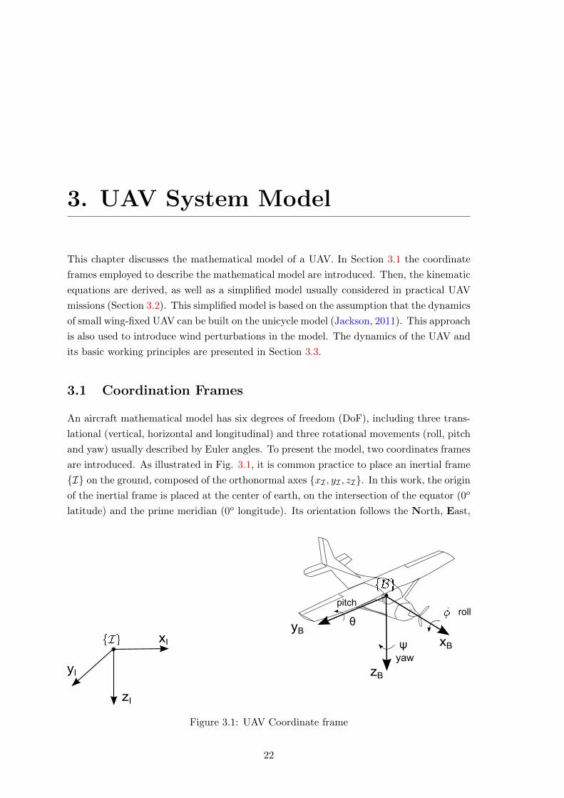
3.1 Coordination Frames
An aircraft mathematical model has six degrees of freedom (DoF), including three trans-
lational (vertical, horizontal and longitudinal) and three rotational movements (roll, pitch
and yaw) usually described by Euler angles. To present the model, two coordinates frames
are introduced. As illustrated in Fig. 3.1, it is common practice to place an inertial frame
{I} on the ground, composed of the orthonormal axes {xI , yI , zI}. In this work, the origin
of the inertial frame is placed at the center of earth, on the intersection of the equator (0o
latitude) and the prime meridian (0o longitude). Its orientation follows the North, East,
xByB
zB
rollpitch
yaw
θ
ψ
yI
xI
zI
Figure 3.1: UAV Coordinate frame
22
3.2. Equations of Motion Chapter 3. UAV System Model
Down (NED) system, as described next
• {xI} pointing North;
• {yI} pointing East;
• {zI} pointing Down.
It is also considered a body fixed frame {B} composed of the orthonormal axes {xB, yB, zB},according to the NED-system orientation. This frame can be fixed anywhere in the body.
However, to simplify the equation model, its origin usually lies in the center of gravity
(CG) of the vehicle, with two of its axes aligned with main inertial axes of the vehicle:
• {xB} in the longitudinal axis, from the tail to the nose of the vehicle, parallel to the
fuselage;
• {yB} in the lateral axis, pointing to the right side, parallel to the right wing;
• {zB} in the vertical axis, pointing downward, from top to bottom.
The position and orientation of the UAV are relative to the inertial reference frame
{I}. The linear velocities of the craft are measured relatively to {I}, expressed in the
body frame {B}. The following notation is used:
• p = [x, y, z]T : The position of the origin of {B}, expressed in {I};
• η = [φ, θ, ψ]T : The orientation of {B} with respect to {I};
• vgs = [u, v, w]T : The linear velocities of the origin {B} in relation to {I}, expressed
in {B};
• w = [p, q, r]T : The angular velocities of {B} with respect to {I}, expressed in {B}
The orientation is also known as attitude of the aircraft. It is composed of the angles
of roll (φ), pitch (θ) and yaw( ψ). The linear velocities vector contains the forward (u),
lateral (v) and vertical (w) speed of the vehicle.
3.2 Equations of Motion
This section describes the kinematic equations of an unmanned aerial vehicle. The first
model is based on underactuated autonomous vehicles moving in the 3D space. For in-
stance, it represents the model of an aircraft or an underwater vehicle. The second model
represents a vehicle that moves in a plane, for example a mobile robot. As explained in
Section 3.2.2, in practical application, this is a valid model for UAVs at constant altitude.
23
Chapter 3. UAV System Model 3.2. Equations of Motion
3.2.1 Kinematic equations
According to the notation introduced in section 3.1, the velocity of the vehicle expressed
in the body fixed coordinates vgs relates to the inertial frame by the following equations:xyz
= R(η)
uvw
where R(η) is the matrix that performs roll, pitch and yaw rotations, respectively. The
rotation sequence is important, as a different order alters the final result.
R(η) = Rz(ψ)Ry(θ)Rx(φ) =
cψcθ cψsθsφ− sψcθ cψsθcφ+ sψsφ
sψcθ sψsθsφ+ cψcθ sψsθcφ− cψsφ−sθ cθsφ cθcφ
(3.1)
The body-fixed angular rates w relate to the derivatives of Euler angles according toφθψ
= T (η)
pqr
where the matrix T (η) is given by
T (η) =
cθ sθsφ sθcφ
0 cθcφ −cθsφ0 sφ cφ
(3.2)
The system may be compressed into the following form:[p
η
]=
[R(η) 0
0 T (η)
][vgs
w
](3.3)
3.2.2 Simplified kinematic equations
In practical UAV missions, an independent altitude controller is responsible for the dis-
placement in the z-axis and the movement is restricted to the xy plane. Thus the kinematic
model presented in Section 3.2.1 can be reduced to the 2-dimensional space. In this case,
the model of an unicycle is a good approximation to the UAV motion.
The unicycle is well studied in the literature, being a foundation for more complex
systems. Approximating the UAV to an unicycle, removing its dynamics, is fairly used in
research topics that are primarily concerned with the aircraft position. In fact, most mid
to high level controllers reduce the complexity of aircraft’s dynamics (Jackson, 2011). The
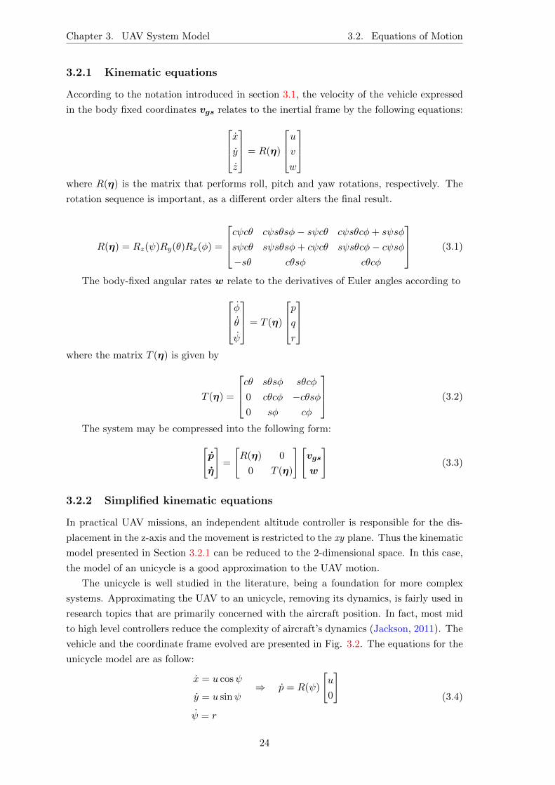
vehicle and the coordinate frame evolved are presented in Fig. 3.2. The equations for the
unicycle model are as follow:
x = u cosψ
y = u sinψ⇒ p = R(ψ)
[u
0
]ψ = r
(3.4)
24
3.3. Dynamic modelling Chapter 3. UAV System Model
xB
xI
yI
yB
u
Figure 3.2: Unicycle kinematic model
Following the notation introduced in Section 3.1, u is the first component of the ground
speed vector vgs. If the UAV is not subject to perturbations, then (3.4) is a sufficient
model. However, taking advantage of the simplified 2D model, the wind component is
introduced. The reader is referred to Fig. 3.3. The ground speed component may be
decomposed as
vgs = v +RT (ψ)vw (3.5)
where v = [va, 0] is the airspeed vector and vw = [vwx , vwy ] is the wind speed vector
expressed in the inertial frame. Assume that the aircraft has approximately zero roll and
pitch angles. The UAV kinematic equations yield
x = va cosψ + vwx
y = va sinψ + vwy
ψ = r
or in a more compact fashion, the 2D model is expressed by
p = R(ψ)v + vw
ψ = r(3.6)
For the 3D kinematic model, with a slight abuse of notation, r(t) and q(t) are considered
the yaw rate and pitch rate, respectively. Then, the system described by (3.3) can be
rewritten in function of wind and airspeed by
p = R(η)v + vw (3.7a)
θ = q (3.7b)
ψ = r (3.7c)
The size of the vectors must be consistent.
3.3 Dynamic modelling
This section borrows the dynamic models from (Roskam, 2001). The physical interpreta-
tion and mathematical analysis are not showed.
25
Chapter 3. UAV System Model 3.3. Dynamic modelling
xB
xI
yI
yB
va
vgs
vw
Figure 3.3: UAV Coordinate frame projected in the xy plane.
Neglecting the gyroscopic moments exerted by spinning rotors, the general linear and
angular momentum equations in the body fixed axis {B} are given by:
Fx = m(u− vr + wq) +mg sin θ + T (3.8a)
Fy = m(v + ru− pw)−mg cos θ sinφ (3.8b)
Fz = m(w + pv − qu)−mg cos θ sinφ (3.8c)
Mx = Ixp+ Ixy r + (Iz − Iy)qr + Ixzqp (3.9a)
My = Iy q + (Ix − Iz)pr + Ixz(r2 − p2) (3.9b)
Mz = Iz r + Ixz p+ (Iy − Ix)qp− Ixzqr (3.9c)
where Fx, Fy and Fz are the linear aerodynamic forces on the vehicle, Mx, My and Mz
are the momentum around the aircraft axis, m is the mass of the vehicle, Ix, Iy and Iz are
the inertia relative to each axis and T the trust exerted by the engine.
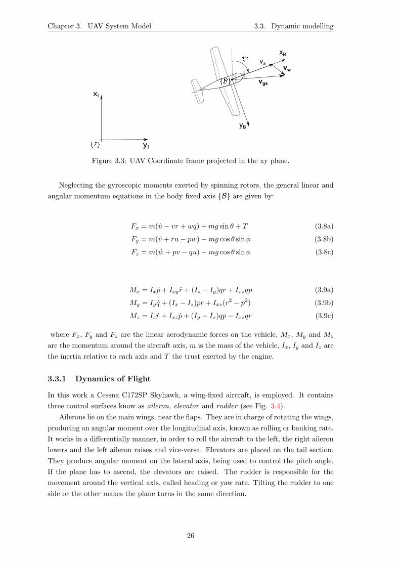
3.3.1 Dynamics of Flight
In this work a Cessna C172SP Skyhawk, a wing-fixed aircraft, is employed. It contains
three control surfaces know as aileron, elevator and rudder (see Fig. 3.4).
Ailerons lie on the main wings, near the flaps. They are in charge of rotating the wings,
producing an angular moment over the longitudinal axis, known as rolling or banking rate.
It works in a differentially manner, in order to roll the aircraft to the left, the right aileron
lowers and the left aileron raises and vice-versa. Elevators are placed on the tail section.
They produce angular moment on the lateral axis, being used to control the pitch angle.
If the plane has to ascend, the elevators are raised. The rudder is responsible for the
movement around the vertical axis, called heading or yaw rate. Tilting the rudder to one
side or the other makes the plane turns in the same direction.
26

3.3. Dynamic modelling Chapter 3. UAV System Model
Figure 3.4: Roll, pitch and yaw on a wing-fixed airplane. Source: (Shaw, 2014)
In the framework of this dissertation the control surfaces available are ailerons and
elevators. Therefore, to control the heading of the vehicle a technique known as banked
turn or coordinated turn is employed. This concept is very used in aircraft and even ground
vehicles applications, like high-speed railways and highways.
When an aircraft banks, the lift force Fz may be broken down in two components.
The vertical component cancels out with the weight of the vehicle, so that the vehicle
keeps a constant altitude. If the vertical forces are not equivalent, a possible drop in
altitude occurs. The second component of the lift force acts in the radial direction. The
aircraft tries to minimize the Fy to zero, since, in regular conditions, the plane do not
drift. Assuming that the pitch angle is nearly zero (θ ≈ 0), the linear force (3.8b) on the
y-axis becomes
0 = mrva −mg sinφ (3.10)
The yaw rate is obtained from (3.2) assuming θ ≈ 0,
r = ψ cosφ
Substituting in (3.10), the following equation is obtained:
mψ cosφva = mg sinφ (3.11)
tanφ =vaψ
g(3.12)
FL
FC
FG
roll or bankangle
Figure 3.5: Important forces acting on a coordinated turn.
27
Chapter 3. UAV System Model 3.4. Cessna 172SP Skyhawk
The equation described by (3.12) is known as coordinated turn assumption. For a more de-
tailed reading and the acquaintance of high order model the reader is referred to (Jackson,
2011)
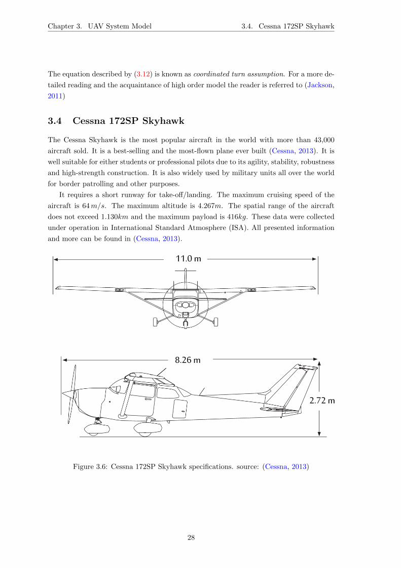
3.4 Cessna 172SP Skyhawk
The Cessna Skyhawk is the most popular aircraft in the world with more than 43,000
aircraft sold. It is a best-selling and the most-flown plane ever built (Cessna, 2013). It is
well suitable for either students or professional pilots due to its agility, stability, robustness
and high-strength construction. It is also widely used by military units all over the world
for border patrolling and other purposes.
It requires a short runway for take-off/landing. The maximum cruising speed of the
aircraft is 64m/s. The maximum altitude is 4.267m. The spatial range of the aircraft
does not exceed 1.130km and the maximum payload is 416kg. These data were collected
under operation in International Standard Atmosphere (ISA). All presented information
and more can be found in (Cessna, 2013).
11.0 m
8.26 m
2.72 m
Figure 3.6: Cessna 172SP Skyhawk specifications. source: (Cessna, 2013)
28

4. UAV Motion Control
This chapter addresses the path following motion control problem. In Section 4.1 a brief
overview of the topic is introduced. Then, Section 4.2 presents the first solution for the
PF problem, namely carrot chasing algorithm. Section 4.3 addresses a nonlinear path
following algorithm. The latter is employed in the coordination controller.
4.1 Introduction
Path following is a motion control problem concerned with driving the vehicle to a desired
path parametrized in space, without temporal constraints. When contrasted to other
motion control topics addressed in the literature, namely trajectory tracking1, the path
following shows some conveniences that makes it particularly interesting in the framework
of this dissertation. The following advantages are pointed out by (Aguiar and Hespanha,
2007) and (Vanni, 2007).
• The vehicle is not imposed to move from its initial position to the starting point of
the trajectory;
• Performance limitations due to unstable zero-dynamics can be avoided;
• Control signals are less likely to saturate.
The path following resolution typically lies in keeping a constant speed or follow a
desired speed profile, while adjusting the orientation of the aircraft. The first is referred
as dynamic assignment task and the second as geometric task.
In order to carry a performance comparison, two different solutions are addressed.
Although not suitable for coordination control, the carrot chasing, presented in (Sujit
et al., 2013), is a lightweight and robust to disturbances algorithm that solves the geometric
task. It was chosen because its basic working principle does not require the introduction of
further theoretical concepts. Afterwards, a nonlinear path following solution derived from
(Aguiar and Hespanha, 2007) is presented. The latter solves both geometric and dynamic
1The trajectory tracking problem requires the vehicle to reach and follow a desired path associated with
a timing law.
29
Chapter 4. UAV Motion Control 4.2. Carrot chasing control algorithm
assignment task. Both strategies use a virtual target point (VTP) that moves along the
path according to a specified law particular to each algorithm.
4.2 Carrot chasing control algorithm
Suppose the aircraft keeps a constant speed at a certain altitude. Its kinematic model is
described as (3.6). Then, the path following problem may be formally stated as next.
Problem Statement 4.1. Assume a desired spatial path pd(γ):R → R2, where γ ∈ Ris a parametric variable. Consider the following control input, u = r(t), where r(t) is the
yaw rate. Design a feedback control law for u such that the position of the vehicle converges
and follows the reference path, i.e. ‖p− pd‖ → 0 as t → ∞.
Since the vehicle cruises at a constant speed, this first approach is restricted to the
geometric task. Applying trigonometric concepts, the carrot chasing solves the problem
appropriately.
Consider the straight line path that joins an initial Wi and final waypoint Wi+1, as
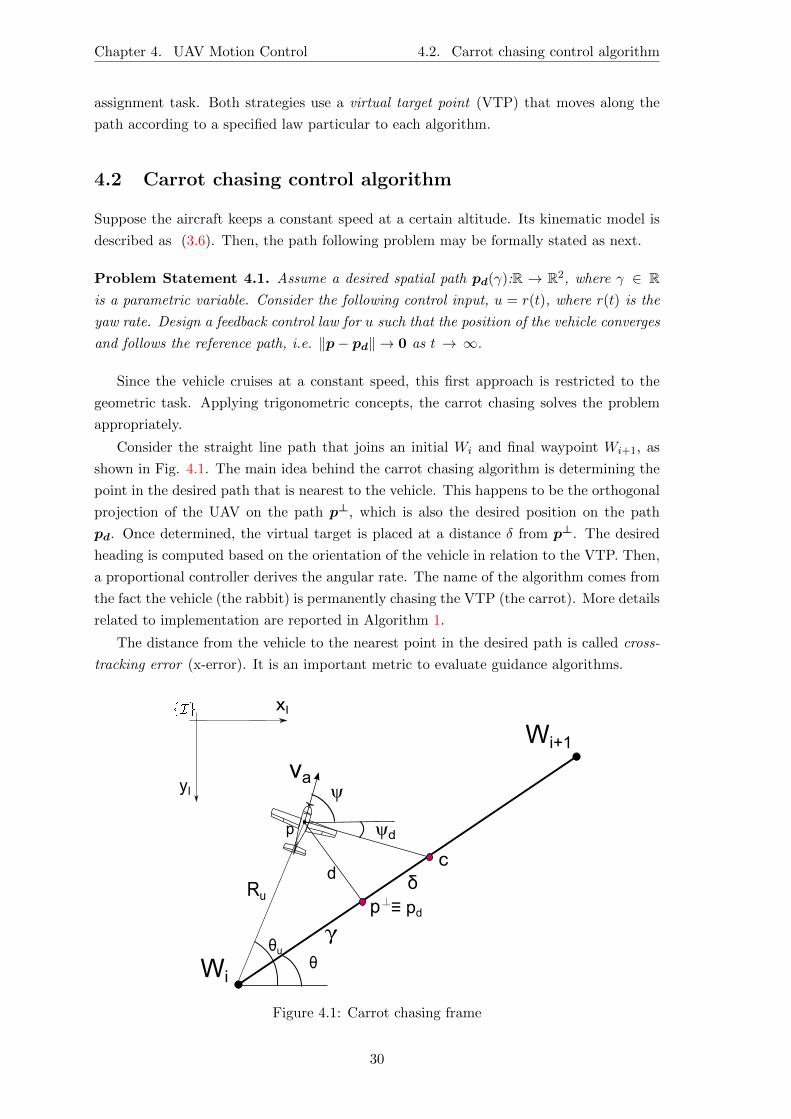
shown in Fig. 4.1. The main idea behind the carrot chasing algorithm is determining the
point in the desired path that is nearest to the vehicle. This happens to be the orthogonal
projection of the UAV on the path p⊥, which is also the desired position on the path
pd. Once determined, the virtual target is placed at a distance δ from p⊥. The desired
heading is computed based on the orientation of the vehicle in relation to the VTP. Then,
a proportional controller derives the angular rate. The name of the algorithm comes from
the fact the vehicle (the rabbit) is permanently chasing the VTP (the carrot). More details
related to implementation are reported in Algorithm 1.
The distance from the vehicle to the nearest point in the desired path is called cross-
tracking error (x-error). It is an important metric to evaluate guidance algorithms.
ψ
Wi+1
Wi
p
p⊥
va
ψd
cδ
θθu
dRu
≡ pd
γ
xI
yI
Figure 4.1: Carrot chasing frame
30
4.3. Nonlinear Lyapunov based control algorithm Chapter 4. UAV Motion Control
The parametric variable, consequently the desired position on the path, is determined
by the position of the vehicle relatively to the trajectory. The position error ‖p − pd‖converges to zero as ‖p − c‖ → δ. If wind is taken into account, then course angle and
desired course angle must be considered instead of heading angle and desired heading
angle, respectively.
Algorithm 1 Carrot Chasing
Initialize:WPi = (xi, yi), WPi+1 = (xi+1, yi+1), θ
1: Ru = ‖WPi − p‖, θu = atan2(y − yi, x− xi)2: β = normalizeAnglea(θ − θu)
3: γ =√R2u − (Ru sinβ)2
4: [cd, cd] = [(γ + δ) cos θ + xi, (γ + δ) sin θ + yi]
5: ψd = k ∗ atan2(cd − y, cd − x)
6: ψ = w1 = normalizeAngle(ψd − ψ)
aGiven an input angle, the function normalizeAngle returns an
equivalent angle in the domain [-π,π]
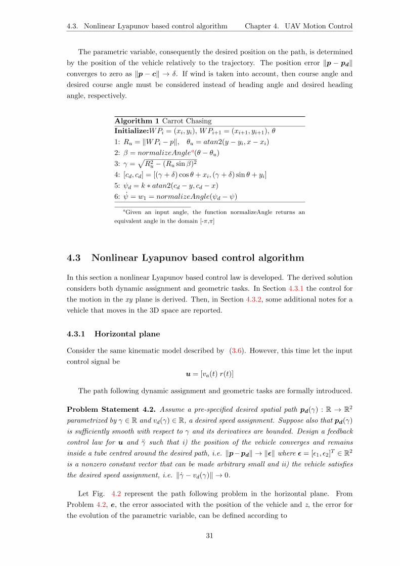
4.3 Nonlinear Lyapunov based control algorithm
In this section a nonlinear Lyapunov based control law is developed. The derived solution
considers both dynamic assignment and geometric tasks. In Section 4.3.1 the control for
the motion in the xy plane is derived. Then, in Section 4.3.2, some additional notes for a
vehicle that moves in the 3D space are reported.
4.3.1 Horizontal plane
Consider the same kinematic model described by (3.6). However, this time let the input
control signal be
u = [va(t) r(t)]
The path following dynamic assignment and geometric tasks are formally introduced.
Problem Statement 4.2. Assume a pre-specified desired spatial path pd(γ) : R → R2
parametrized by γ ∈ R and vd(γ) ∈ R, a desired speed assignment. Suppose also that pd(γ)
is sufficiently smooth with respect to γ and its derivatives are bounded. Design a feedback
control law for u and γ such that i) the position of the vehicle converges and remains
inside a tube centred around the desired path, i.e. ‖p−pd‖ → ‖ε‖ where ε = [ε1, ε2]T ∈ R2
is a nonzero constant vector that can be made arbitrary small and ii) the vehicle satisfies
the desired speed assignment, i.e. ‖γ − vd(γ)‖ → 0.
Let Fig. 4.2 represent the path following problem in the horizontal plane. From
Problem 4.2, e, the error associated with the position of the vehicle and z, the error for
the evolution of the parametric variable, can be defined according to
31
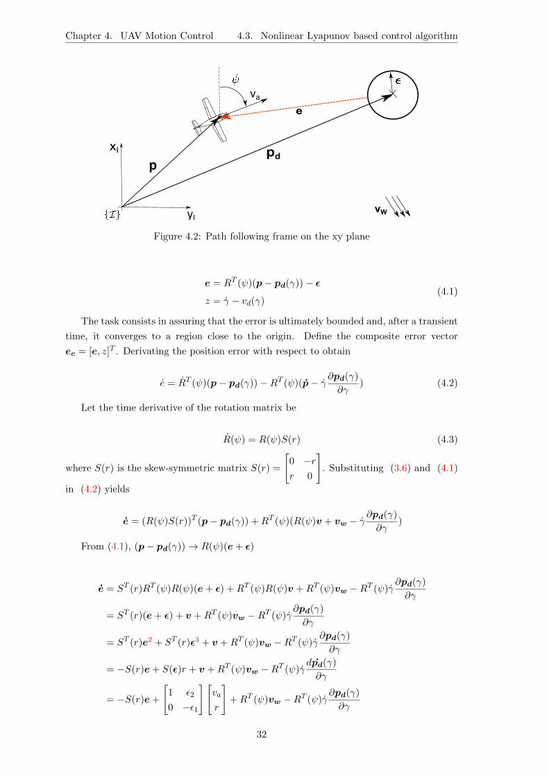
Chapter 4. UAV Motion Control 4.3. Nonlinear Lyapunov based control algorithm
xI
yI
va
vW
pd
e
p
Figure 4.2: Path following frame on the xy plane
e = RT (ψ)(p− pd(γ))− ε
z = γ − vd(γ)(4.1)
The task consists in assuring that the error is ultimately bounded and, after a transient
time, it converges to a region close to the origin. Define the composite error vector
ec = [e, z]T . Derivating the position error with respect to obtain
e = RT (ψ)(p− pd(γ))−RT (ψ)(p− γ ∂pd(γ)
∂γ) (4.2)
Let the time derivative of the rotation matrix be
R(ψ) = R(ψ)S(r) (4.3)
where S(r) is the skew-symmetric matrix S(r) =
[0 −rr 0
]. Substituting (3.6) and (4.1)
in (4.2) yields
e = (R(ψ)S(r))T (p− pd(γ)) +RT (ψ)(R(ψ)v + vw − γ∂pd(γ)
∂γ)
From (4.1), (p− pd(γ))→ R(ψ)(e+ ε)
e = ST (r)RT (ψ)R(ψ)(e+ ε) +RT (ψ)R(ψ)v +RT (ψ)vw −RT (ψ)γ∂pd(γ)
∂γ
= ST (r)(e+ ε) + v +RT (ψ)vw −RT (ψ)γ∂pd(γ)
∂γ
= ST (r)e2 + ST (r)ε3 + v +RT (ψ)vw −RT (ψ)γ∂pd(γ)
∂γ
= −S(r)e+ S(ε)r + v +RT (ψ)vw −RT (ψ)γdpd(γ)
∂γ
= −S(r)e+
[1 ε2
0 −ε1
][va
r
]+RT (ψ)vw −RT (ψ)γ
∂pd(γ)
∂γ
32
4.3. Nonlinear Lyapunov based control algorithm Chapter 4. UAV Motion Control
Let ∆ =
[1 ε2
0 −ε1
]. The position error dynamics is expressed by (4.4)
e = −S(r)e+ ∆u+RT (ψ)vw −RT (ψ)γ∂pd(γ)
∂γ(4.4)
By now, it shall be clear to the reader why the vehicle was set to converge and remain
inside a tube centered around pd(γ), and not the desired position itself. If ε had not been
introduced, the control variable r (yaw rate) would not appear in (4.4). As a result, the
error would not converge to zero.
Meanwhile the the dynamic of the parametric variable error is described by
z = γ + γ∂pd(γ)
∂γ
In most mission scenarios, except for a transitional phase, the desired speed profile
is set to be constant. In the scope of this text, it will be considered constant with no
exception. As a consequence of that, we can simplify the notation to vd(γ) = vd and the
foregoing expression may be stated as
z = γ (4.5)
Proposition 4.1. Consider the system described by (3.6) in a closed-loop with the control
laws
u = ∆−1(RT (ψ)vd∂pd(γ)
∂γ−RT (ψ)vw −Kpε)
γ = eRT (ψ)∂pd(γ)
∂γ− kγz
(4.6)
where Kp =
[kx 0
0 ky
]is a diagonal matrix whose eigenvalues are positive and kγ is a
positive constant. The origin ec = 0 is a globally asymptotically stable equilibrium point
for the system.
Proof. Define a Lyapunov function Ve for the position error and a second Lyapunov func-
tion Vγ for the speed assignment error.
Ve =1
2‖e‖2 =
1
2eTe (4.7a)
Vz =1
2z2 (4.7b)
and define a composite Lyapunov function
Vc = Ve + Vz
Vc =1
2eTe+
1
2z2
Then take the derivative of Vc with respect to time
Vc = Ve + Vz = eT e+ zz
2From the definition of skew-symmetric matrix: ST (r)e = −r × e = −S(r)e3From the definition of ske-symmetrix matrix and cross product: ST (r)ε = −r × ε = ε× r = S(ε)r
33

Chapter 4. UAV Motion Control 4.3. Nonlinear Lyapunov based control algorithm
Substituting e by (4.4) and z by (4.5) yields
Vc = eT (−S(r)e+ ∆u+RT (ψ)vw −RT (ψ)γ∂pd(γ)
∂γ) + zγ
According to (4.1), γ = vd + z. Hence, the last equation becomes
Vc = eT (−S(r)e+ ∆u+RT (ψ)vw −RT (ψ)vd∂pd(γ)
∂γ) + z(γ − eTRT (ψ)
∂pd(γ)
∂γ)
Now let the control variables u and γ be as expressed in (4.6)
Vc = eT (−S(r)e−Kpe) + z(−kγz)
Vc = −eTS(r)e− eTKpe+−kγz2
Vc = −eTKpe− kγz2 ≤ −ecTKcec
where Kc =
[Kp 0
0 kγ
]. The following inequalities hold true
1
2‖ec‖ ≤ Vc ≤
1
2‖ec‖
∂Vc∂t
+∂Vc∂ec
f(t, ec) ≤− ecTKcec ≤ 0
The function 12‖ec‖
2 is radially unbounded and the conditions stated in Theorem 2.5
are satisfied. Therefore, the origin ec = 0 is a globally uniformly asymptotically stable
equilibrium point. It is proved that the position error e converges to a neighborhood of ε
and the speed assignment error z converges to zero.
The smaller the values of ε are, the closest to the neighborhood of the desired path the
vehicle converges. However, the input signal is pushed towards saturation. Analyzing the
matrix ∆, the value ε2 may be set to null, but ε1 cannot be zero, or a singularity arises.
Fig. 4.3 represents the discussed path following controller. The parametric variable is
an internal variable that determines the position of the VTP. The demonstrated control
assures that the target moves slower if the vehicle is behind it. If the vehicle is ahead,
Pathdfollowingcontroller
InnerdLoop(UAVdDynamics)d
UAVdKinematics
u
vw
p, v,
∫∫
PathdGenerator
udpd(dd),vd(dd)
Figure 4.3: Nonlinear Lyapunov base path following controller
34
4.3. Nonlinear Lyapunov based control algorithm Chapter 4. UAV Motion Control
the target moves faster. Also, optimization techniques may be employed to determine the
initial value γ(0). A straightforward possibility is to set the initial value to the point in
the path nearest to the vehicle. Controlling the parametric variable rate γ is essential for
the coordination controller explored in Chapter 5.
4.3.2 3D space
Consider the kinematic model described by (3.7) for a vehicle that moves freely in the
3-dimensional space. Take the control input
u = [va(t) w(t)]
where w(t) = [p, q, r] is the body angular velocity vector. Let the variables and matrices
in Section 4.3.1 defined in R2 and R2×2 be restated to its equivalents in R3 and R3×3,
respectively. Also, assume
∆ =
1 0 −ε3 ε2
0 ε3 0 −ε10 −ε2 ε1 0
(4.8)
and ∆ = ∆T (∆∆T )−1 its pseudo-inverse. Then, consider Problem 4.2, where the desired
path is defined as pd(γ) : R → R3. The origin ec = 0 of the closed loop system with
control law (4.6) is a globally stable equilibrium point. The proof is not addressed, since
it is similar to the one in the previous section.
35

5. Cooperative Motion Control
In this chapter the cooperative control of a fleet of autonomous vehicles, which forms
the core of this dissertation, is addressed. Section 5.1 clarifies the context in which the
controller is inserted. Then, in Section 5.2 the coordination problem is formally stated.
Next, the problem is tackled in the frame of two different topologies. Section 5.3 assumes
a constant communication topology and Section 5.4 assumes a switched communication
topology.
5.1 Introduction
According to the decision-making level, the coordination controller is distinguished as
centralized or decentralized. Fig. 5.1a shows a centralized architecture with four nodes,
namely three UAVs and a ground station, which is responsible for taking decisions. Cen-
tralized controllers are not robust, as a single failure point may lead to undesired behavior
of the entire system. In Fig. 5.1b a decentralized architecture is illustrated. These con-
trollers are not as vulnerable to failure points as the centralized model. In addition, the
solution may be less complex, since each controller does not need to take directly into
account all the vehicles in the fleet. This work focuses on decentralized strategies.
(a) Centralized Controller (b) Decentralized Controller
Figure 5.1: Different topology for coordination controllers
In Chapter 4, closed loop control laws for the motion control problem of a single
UAV were discussed. In particular, in the solution addressed in Section 4.3, the vehicle
approaches a virtual target that moves along the desired path, according to a reference
speed profile vd(γ). In this chapter, the speed profile of the VTP is redefined, in order to
36

5.2. Problem Statement Chapter 5. Cooperative Motion Control
achieve cooperation among multiple vehicles.
5.2 Problem Statement
Consider a fleet of n vehicles denoted by the set N = {1, . . . , n}. The parametric variable
γi defines the position of the VTP associated to the ith vehicle in a precise manner. Each
vehicle converges to its respective virtual target point. Therefore, if the n virtual target
points asymptotically synchronize, the vehicles asymptotically reach a desired formation.
In other words, coordination is achieved if and only if γij = γi − γj = 0, ∀i,j ∈ N . The
parameter γi is said to be the coordination state.
The dynamic of each state is strictly dependent of vd(γ). Therefore the definition of
desired speed profile is extended to
vd = vL1 + vr (5.1)
where the elements of vd = [vd1, . . . , vdn] and vr = [vr1, . . . , vrn] correspond to desired and
correction speeds of each vehicle i ∈ N , respectively. The formation speed, denoted by
vL(γ), is common to all vehicles in the flock.
Let Ni be the set of vehicles that the ith UAV is able to receive information from.
Recall from the graph theory concepts introduced in Section 2.3 that is not necessarily
true that j ∈ Ni ⇒ i ∈ Nj , as unidirectional communication is considered.
Problem Statement 5.1. Assume that for each vehicle i ∈ Ni, the variables γi and γj,
j ∈ Ni are available. Derive a control law for vri, such that, for all i, j ∈ N , (γi− γj) and
(γi − γj) converges to zero as t→∞.
5.3 Constant communication
Assume a quasi strongly connected communication topology, i.e. there is a transmitter
vehicle from whom any other element in the fleet receives information. Suppose that
this topology is constant over time and let L be the associated Laplacian matrix. The
coordination error for each vehicle is defined as
ξi =∑j∈Ni
γi − γj
Consider the coordination error vector ξ = [ξ1, . . . , ξn] and the coordinate state vector
γ = [γ1, . . . , γn]. Then,
ξ = Lγ (5.2)
The dynamic of the coordination error is given by
ξ = Lγ
Substituting (5.1) in (4.1) and applying to the dynamic of the coordination error,
yields
37
Chapter 5. Cooperative Motion Control 5.3. Constant communication
ξ = L(z + vL1 + vr)
with z = [z1, . . . , zn]. Recalling the fact that L1 = 0, we obtain
ξ = Lz − Lvr (5.3)
Proposition 5.1. Consider n vehicles driven by the control law specified in (4.6). Let
the connected inter-vehicle communication topology be represented by the Laplacian matrix
L. Assume that the vehicles exchange their coordination state γi continuously with the
neighbouring nodes. Let the coordination control law be
vr = −KξLγ (5.4)
where Kξ is a diagonal matrix whose elements are positive. Then, the coordination error
ξ and the speed profile converge to a neighbourhood of the origin and vL, respectively, as
t→∞.
Proof. Consider the candidate Lyapunov function
Vξ =1
2‖ξ‖2
and its time derivative
Vξ = ξT ξ
Substitute (5.2) in the control law (5.4) and the remainder result in the time derivative
of the candidate Lyapunov function
Vξ = ξT (Lz − LKξξ)
= ξTLz − ξTLKξξ
= ξTLz − (1 + θ − θ)ξTLKξξ
= −(1− θ)ξTLKξξ + ξTLz − θξTLKξξ
where θ is any variable such that 0 ≤ θ ≤ 1. Assume that the control law expressed
by (4.6) assures that the speed assignment error vector z remains bounded. It is then
possible to see that for a ξ large enough such that
‖ξ‖ ≥ ‖1
θK−1ξ z‖
we obtain
Vξ ≤ −(1− θ)ξTLKξξ ≤ 0
The solutions for the equality are ξ = 0 and ξ = 1. The latter solution requires
ξ = Lγ = 1. However, the unit vector spans the kernel of L, i.e. L1 = 0. Therefore, as it
cannot be a base of its image, the solution is impossible. Applying Theorem 2.7, we can
conclude that ξ is ISS with respect to z. Further, it follows that
‖ξ‖a ≤1
θK−1ξ ‖z‖
38
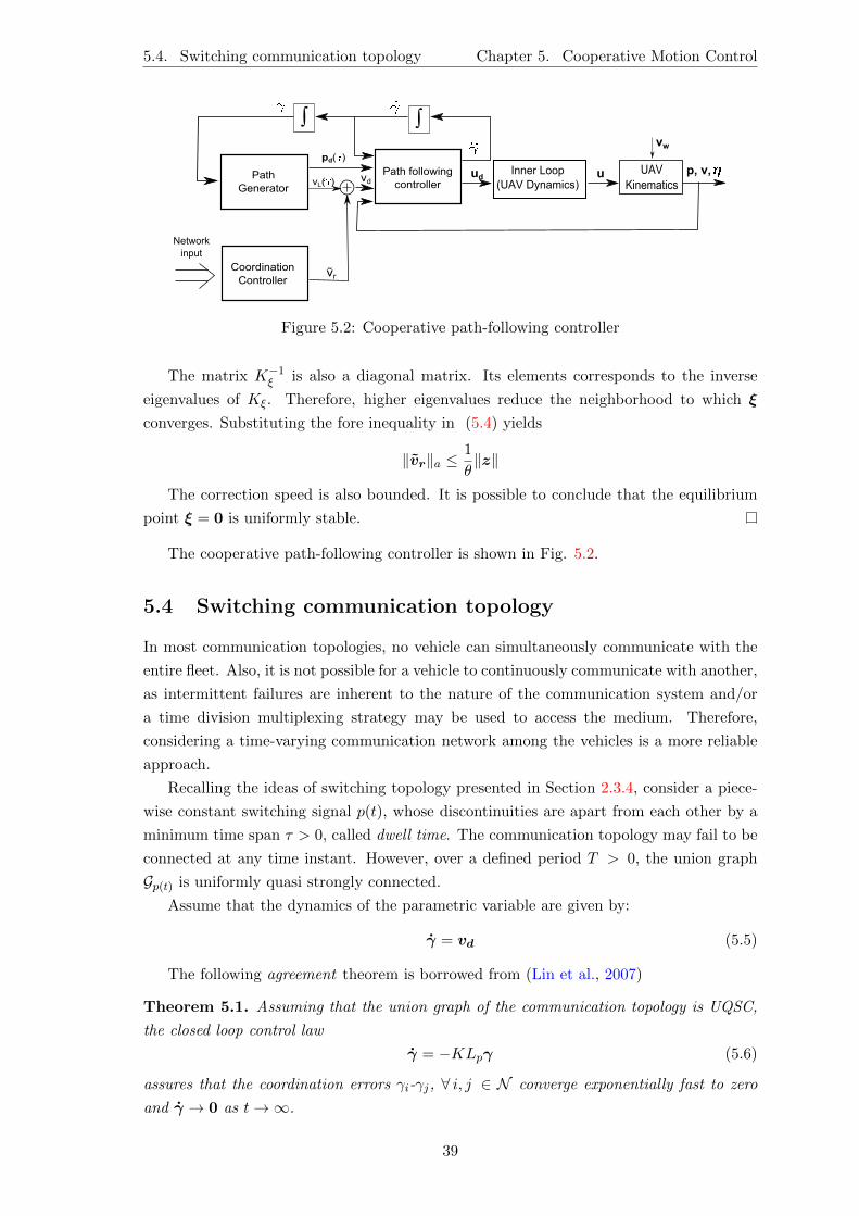
5.4. Switching communication topology Chapter 5. Cooperative Motion Control
Pathdfollowingcontroller
InnerdLoop(UAVdDynamics)d
UAVdKinematics
u
vw
p, v,
∫∫
PathdGenerator
ud
pd(dd)
vL(dd)
CoordinationController
ṽr
vd
Networkdinput
Figure 5.2: Cooperative path-following controller
The matrix K−1ξ is also a diagonal matrix. Its elements corresponds to the inverse
eigenvalues of Kξ. Therefore, higher eigenvalues reduce the neighborhood to which ξ
converges. Substituting the fore inequality in (5.4) yields
‖vr‖a ≤1
θ‖z‖
The correction speed is also bounded. It is possible to conclude that the equilibrium
point ξ = 0 is uniformly stable.
The cooperative path-following controller is shown in Fig. 5.2.
5.4 Switching communication topology
In most communication topologies, no vehicle can simultaneously communicate with the
entire fleet. Also, it is not possible for a vehicle to continuously communicate with another,
as intermittent failures are inherent to the nature of the communication system and/or
a time division multiplexing strategy may be used to access the medium. Therefore,
considering a time-varying communication network among the vehicles is a more reliable
approach.
Recalling the ideas of switching topology presented in Section 2.3.4, consider a piece-
wise constant switching signal p(t), whose discontinuities are apart from each other by a
minimum time span τ > 0, called dwell time. The communication topology may fail to be
connected at any time instant. However, over a defined period T > 0, the union graph
Gp(t) is uniformly quasi strongly connected.
Assume that the dynamics of the parametric variable are given by:
γ = vd (5.5)
The following agreement theorem is borrowed from (Lin et al., 2007)
Theorem 5.1. Assuming that the union graph of the communication topology is UQSC,
the closed loop control law
γ = −KLpγ (5.6)
assures that the coordination errors γi-γj, ∀ i, j ∈ N converge exponentially fast to zero
and γ → 0 as t→∞.
39
Chapter 5. Cooperative Motion Control 5.4. Switching communication topology
In (Ghabcheloo et al., 2009), the authors generalize the theorem for vL 6= 0. Assume
(5.5) and
γ = vL1−KLpγ (5.7)
and the change of variables
γ = γ − 1
∫ t
1vL(τ)dτ
Substituting (5.7) in the derivative of the fore mentioned equation, obtain
˙γ = vL1−KLpγ − vL1
= −KLpγ
Applying Theorem 5.1, γi-γj and ˙γ converges to zero as t → ∞. Consequently, γi-γj
and γ converge exponentially fast to zero and vL, respectively, as t→∞.
These results are also valid when the dynamics of the parametric variable are given by
the control law (4.6). However, the coordinate vector γ does not converge to vL1, but to
a neighborhood close to that value.
40
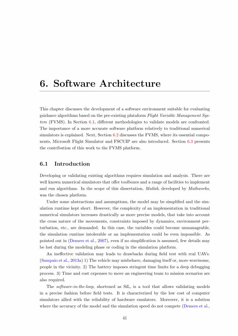
6. Software Architecture
This chapter discusses the development of a software environment suitable for evaluating
guidance algorithms based on the pre-existing plataform Flight Variable Management Sys-
tem (FVMS). In Section 6.1, different methodologies to validate models are confronted.
The importance of a more accurate software platform relatively to traditional numerical
simulators is explained. Next, Section 6.2 discusses the FVMS, where its essential compo-
nents, Microsoft Flight Simulator and FSCUIP are also introduced. Section 6.3 presents
the contribution of this work to the FVMS platform.
6.1 Introduction
Developing or validating existing algorithms requires simulation and analysis. There are
well known numerical simulators that offer toolboxes and a range of facilities to implement
and run algorithms. In the scope of this dissertation, Matlab, developed by Mathworks,
was the chosen platform.
Under some abstractions and assumptions, the model may be simplified and the sim-
ulation runtime kept short. However, the complexity of an implementation in traditional
numerical simulators increases drastically as more precise models, that take into account
the cross nature of the movements, constraints imposed by dynamics, environment per-
turbation, etc., are demanded. In this case, the variables could become unmanageable,
the simulation runtime intolerable or an implementation could be even impossible. As
pointed out in (Demers et al., 2007), even if no simplification is assumed, few details may
be lost during the modeling phase or coding in the simulation platform.
An ineffective validation may leads to drawbacks during field test with real UAVs.
(Sampaio et al., 2013a) 1) The vehicle may misbehave, damaging itself or, more worrisome,
people in the vicinity. 2) The battery imposes stringent time limits for a deep debugging
process. 3) Time and cost expenses to move an engineering team to mission scenarios are
also required.
The software-in-the-loop, shortened as SiL, is a tool that allows validating models
in a precise fashion before field tests. It is characterized by the low cost of computer
simulators allied with the reliability of hardware emulators. Moreover, it is a solution
where the accuracy of the model and the simulation speed do not compete (Demers et al.,
41

Chapter 6. Software Architecture 6.2. Flight Variable Management System
2007), unlike traditional numerical simulators.
In an academic environment, as real UAVs are too expensive for a lecture budget, the
SiL is a tool to teach and understand better the concepts behind real UAVs.
Figure 6.1: Software in the loop simulation
6.2 Flight Variable Management System
The FVMS is a recent but well-succeeded program to evaluate controllers for autonomous
UAVs. The application was fully developed by ART Team at Engineering School of Sao
Carlos (EESC-USP). It consists in a custom Graphical User Interface (GUI) that allows
SiL simulation using Microsoft Flight Simulator 2004 (MSFS04) flying dynamics. The
FVMS was originally written in C/C#. For the reasons enumerated in Sampaio et al.
(2014a), the platform migrated to Borland Delphi 7.0.
It was first presented in Aeroconf 2013. This is well documented in (Sampaio et al.,
2013a), where the architecture and potentialities are highlighted. The dynamic behavior
of a quadcopter is fully modeled in the MSFS04. Sensors are emulated and the aircraft
controlled in closed loop with different methods. In (Sampaio et al., 2013b) an optimal
MIMO H∞ robust controller to stabilize the attitude of a quadcopter is demonstrated. In
(Sampaio et al., 2014a), the FVMS is configured in a hardware in the loop (HiL) fashion.
6.2.1 Microsoft Flight Simulator
The Microsoft Flight Simulator was launched in 1982 and, since then, the simulator has
been continuously updated. It is a robust flight simulator provided with both game features
and aerospace engineering. This powerful software is capable of mimicking with great
accuracy the dynamics of an aircraft and perturbations from outer environment.
The weather can be configured, simulating rain, snow, clear skies, as well as gust,
atmospheric instability, turbulence and more complex disturbances. It also includes flight
analysis tools that record data such as altitude, heading, speed and more, like a real-world
plane. Combined with outstanding graphical scenery database, the fidelity of MSFS makes
of it an asset.
The choice for the specific version Microsoft Flight Simulator 2004 lies in the following
reasons:
42
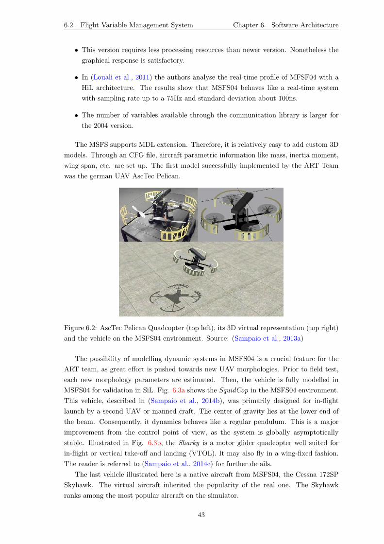
6.2. Flight Variable Management System Chapter 6. Software Architecture
• This version requires less processing resources than newer version. Nonetheless the
graphical response is satisfactory.
• In (Louali et al., 2011) the authors analyse the real-time profile of MFSF04 with a
HiL architecture. The results show that MSFS04 behaves like a real-time system
with sampling rate up to a 75Hz and standard deviation about 100ns.
• The number of variables available through the communication library is larger for
the 2004 version.
The MSFS supports MDL extension. Therefore, it is relatively easy to add custom 3D
models. Through an CFG file, aircraft parametric information like mass, inertia moment,
wing span, etc. are set up. The first model successfully implemented by the ART Team
was the german UAV AscTec Pelican.
Figure 6.2: AscTec Pelican Quadcopter (top left), its 3D virtual representation (top right)
and the vehicle on the MSFS04 environment. Source: (Sampaio et al., 2013a)
The possibility of modelling dynamic systems in MSFS04 is a crucial feature for the
ART team, as great effort is pushed towards new UAV morphologies. Prior to field test,
each new morphology parameters are estimated. Then, the vehicle is fully modelled in
MSFS04 for validation in SiL. Fig. 6.3a shows the SquidCop in the MSFS04 environment.
This vehicle, described in (Sampaio et al., 2014b), was primarily designed for in-flight
launch by a second UAV or manned craft. The center of gravity lies at the lower end of
the beam. Consequently, it dynamics behaves like a regular pendulum. This is a major
improvement from the control point of view, as the system is globally asymptotically
stable. Illustrated in Fig. 6.3b, the Sharky is a motor glider quadcopter well suited for
in-flight or vertical take-off and landing (VTOL). It may also fly in a wing-fixed fashion.
The reader is referred to (Sampaio et al., 2014c) for further details.
The last vehicle illustrated here is a native aircraft from MSFS04, the Cessna 172SP
Skyhawk. The virtual aircraft inherited the popularity of the real one. The Skyhawk
ranks among the most popular aircraft on the simulator.
43
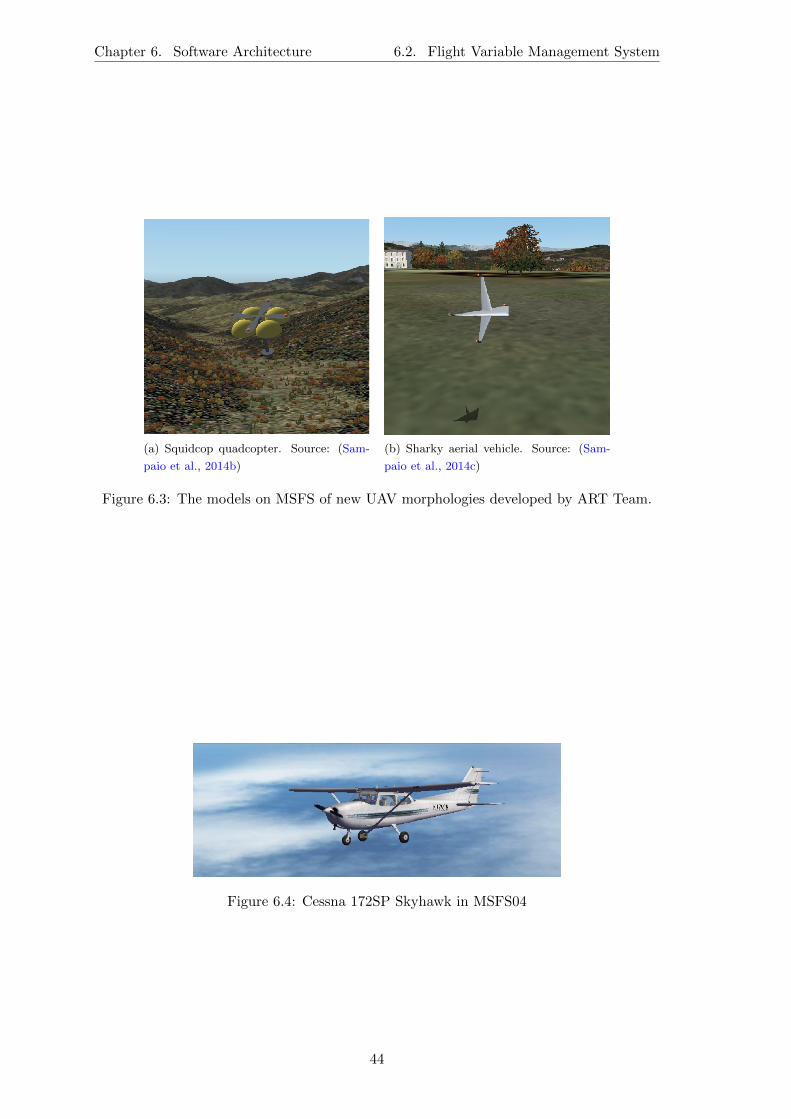
Chapter 6. Software Architecture 6.2. Flight Variable Management System
(a) Squidcop quadcopter. Source: (Sam-
paio et al., 2014b)
(b) Sharky aerial vehicle. Source: (Sam-
paio et al., 2014c)
Figure 6.3: The models on MSFS of new UAV morphologies developed by ART Team.
Figure 6.4: Cessna 172SP Skyhawk in MSFS04
44
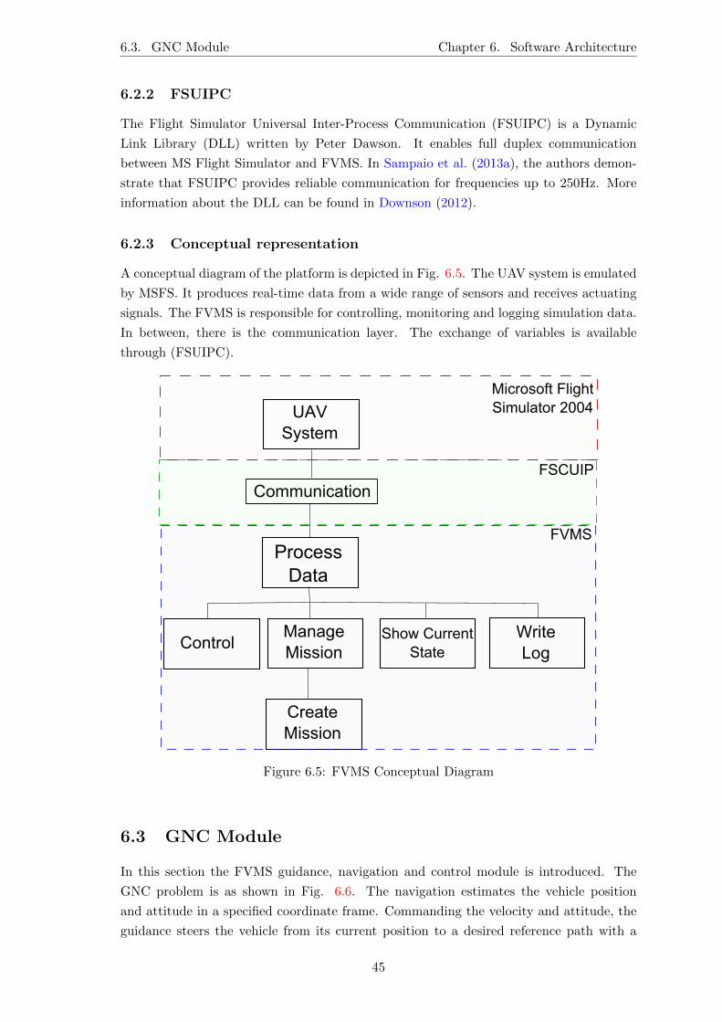
6.3. GNC Module Chapter 6. Software Architecture
6.2.2 FSUIPC
The Flight Simulator Universal Inter-Process Communication (FSUIPC) is a Dynamic
Link Library (DLL) written by Peter Dawson. It enables full duplex communication
between MS Flight Simulator and FVMS. In Sampaio et al. (2013a), the authors demon-
strate that FSUIPC provides reliable communication for frequencies up to 250Hz. More
information about the DLL can be found in Downson (2012).
6.2.3 Conceptual representation
A conceptual diagram of the platform is depicted in Fig. 6.5. The UAV system is emulated
by MSFS. It produces real-time data from a wide range of sensors and receives actuating
signals. The FVMS is responsible for controlling, monitoring and logging simulation data.
In between, there is the communication layer. The exchange of variables is available
through (FSUIPC).
UAV4System
Communication
Process4Data4
ControlManage4Mission
Show4Current4State
WriteLog
Create4Mission
Microsoft4FlightSimulator42004
FSCUIP
FVMS
Figure 6.5: FVMS Conceptual Diagram
6.3 GNC Module
In this section the FVMS guidance, navigation and control module is introduced. The
GNC problem is as shown in Fig. 6.6. The navigation estimates the vehicle position
and attitude in a specified coordinate frame. Commanding the velocity and attitude, the
guidance steers the vehicle from its current position to a desired reference path with a
45
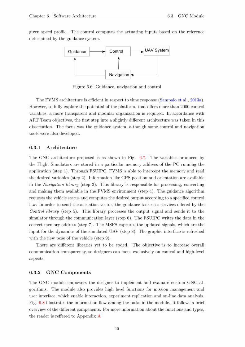
Chapter 6. Software Architecture 6.3. GNC Module
given speed profile. The control computes the actuating inputs based on the reference
determined by the guidance system.
Guidance
Navigation
Control UAV System
Figure 6.6: Guidance, navigation and control
The FVMS architecture is efficient in respect to time response (Sampaio et al., 2013a).
However, to fully explore the potential of the platform, that offers more than 2000 control
variables, a more transparent and modular organization is required. In accordance with
ART Team objectives, the first step into a slightly different architecture was taken in this
dissertation. The focus was the guidance system, although some control and navigation
tools were also developed.
6.3.1 Architecture
The GNC architecture proposed is as shown in Fig. 6.7. The variables produced by
the Flight Simulators are stored in a particular memory address of the PC running the
application (step 1). Through FSUIPC, FVMS is able to intercept the memory and read
the desired variables (step 2). Information like GPS position and orientation are available
in the Navigation library (step 3). This library is responsible for processing, converting
and making them available in the FVMS environment (step 4). The guidance algorithm
requests the vehicle status and computes the desired output according to a specified control
law. In order to send the actuation vector, the guidance task uses services offered by the
Control library (step 5). This library processes the output signal and sends it to the
simulator through the communication layer (step 6). The FSUIPC writes the data in the
correct memory address (step 7). The MSFS captures the updated signals, which are the
input for the dynamics of the simulated UAV (step 8). The graphic interface is refreshed
with the new pose of the vehicle (step 9).
There are different libraries yet to be coded. The objective is to increase overall
communication transparency, so designers can focus exclusively on control and high-level
aspects.
6.3.2 GNC Components
The GNC module empowers the designer to implement and evaluate custom GNC al-
gorithms. The module also provides high level functions for mission management and
user interface, which enable interaction, experiment replication and on-line data analysis.
Fig. 6.8 illustrates the information flow among the tasks in the module. It follows a brief
overview of the different compenents. For more information about the functions and types,
the reader is reffered to Appendix A
46
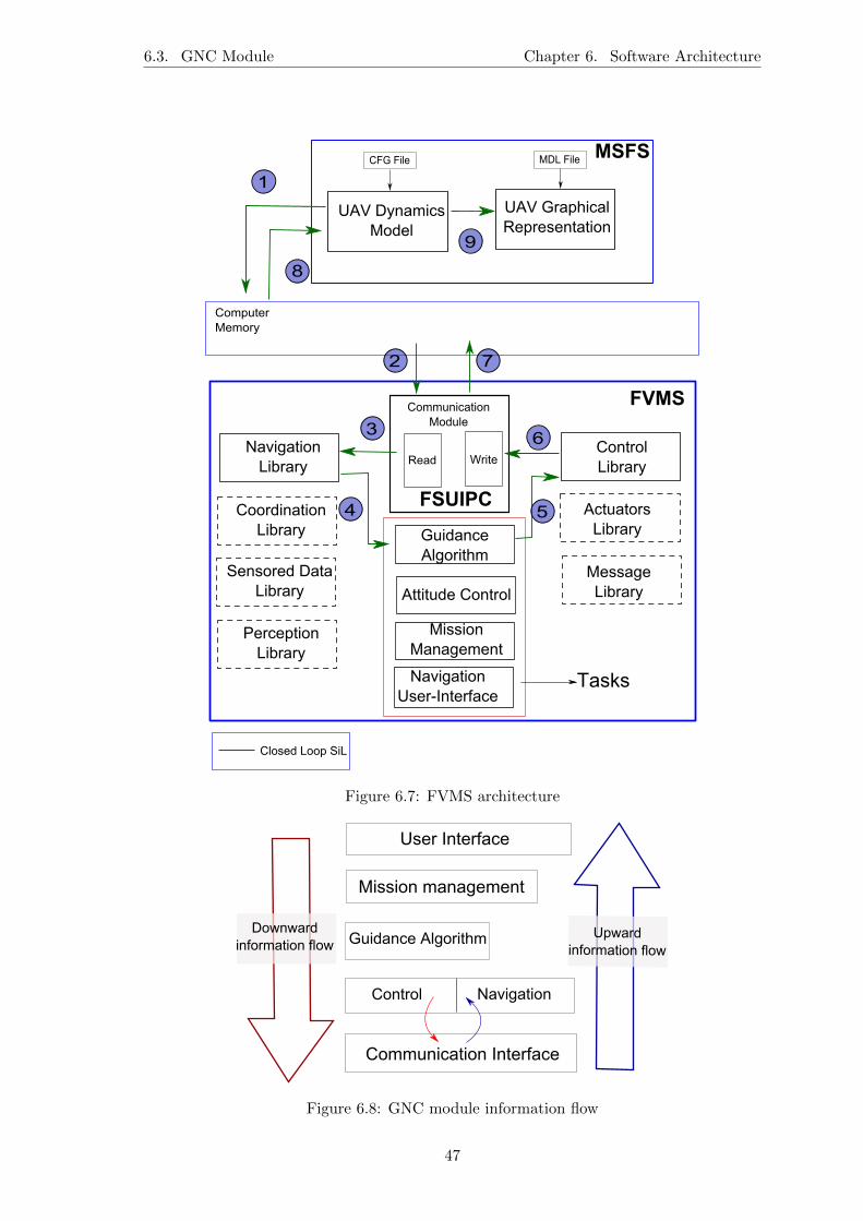
6.3. GNC Module Chapter 6. Software Architecture
UAVSDynamicsSModel
UAVSGraphicalRepresentation
MDLSFileCFGSFile
PerceptionLibrary
GuidanceSAlgorithm
WriteRead
CommunicationModule
ControlLibrary
ComputerSMemory
ClosedSLoopSSiL
1
5
6
7
4
2
3
8
9
MSFS
FVMS
NavigationLibrary
CoordinationLibrary
SensoredSDataLibrary AttitudeSControl
ActuatorsLibrary
MissionSManagement
NavigationUserIInterface
MessageLibrary
FSUIPC
Tasks
Figure 6.7: FVMS architecture
User Interface
Mission management
Guidance Algorithm
Control Navigation
Downwardinformation flow
Upwardinformation flow
Communication Interface
Figure 6.8: GNC module information flow
47

Chapter 6. Software Architecture 6.3. GNC Module
User Interface
The user interface was developed with the support of Google Maps API. Based on this
javascript interface, the user selects the desired waypoints by clicking on the map. The
WGS84 latitude, longitude and altitude of the waypoint may be manually inserted if
replication is required. It is possible to choose whether the waypoint is a straight line or
a loiter (circle pattern) with a given radius. The path is automatically generated and the
flight plan saved on a specific structure.
The FVMS GNC user interface is depicted in Fig. 6.9. On the left panel, information
about attitude, position and speed is displayed. The map is exposed on the center. It con-
tains an animation of the vehicle and footprint, VTP and additional features as displayed.
On the left most panel it is possible to verify the connection with MFSF04. Buttons allow
executing, stopping and cancelling a mission. More functionalities are indicated in the
referred figure.
Mission Management
When the user runs a mission the mission management task is activated. It receives
the flight plan and manages its execution. The initial and final waypoint, cross-tracking
error, azimuth angle, distance to target, path pattern and radius are stored in a structure.
The fore mentioned structure is sent to the desired guidance control algorithm. Currently,
FVMS supports two guidance control algorithms. By default, a nonlinear Lyapunov Based
Control is responsible for the guidance system. If the distance to the desired waypoint
reaches a minimum value (default 100m), the target waypoint changes to the next in the
list. If the cross-tracking error grows too large (default 1000m), the mission manager
automatically changes to default guidance control into loiter mode.
Guidance Algorithm
The guidance algorithm is responsible for executing a path. The controller designer is
free to develop new guidance algorithms. The variables related to the path are sent by
the mission manager. The navigation library provides the vehicle current status. Once
the control law is determined the control library offers services to send desired angular
position and airspeed. Therefore, the communication layer is transparent to designers,
who can focus on the kinematic problem.
Navigation
The navigation library offers a set of data from MFSF04. It is an extension of class SEN-
SOR from previous versions, emulating GPS, IMU, Gyro, altimeters and other sensoring
devices present in real UAVs. As discussed in Sampaio et al. (2013a), MSFS reproduces
real sensors affected by noisy influence of disturbing environmental conditions.
The navigation library provides for FVMS tasks updated information about vehicle
status received from MSFS. In order to use the library, the FVMSNavigation must be
declared in the use section.
48
6.3. GNC Module Chapter 6. Software Architecture
Control
The control library is responsible for generating the actuation signals for MSFS. It is
possible to send roll, pitch, yaw and airspeed to the simulator. By the writing of this
dissertation, the FVMS control library supports two vehicles. An H∞ attitude controller
for quadcopters is available. (for more information consult Sampaio et al. (2013b)). In
addition, PID controllers were developed and validated for attitude and speed control of
a Cesnne Skyhawk wing-fixed aircraft. These features are also available for any FVMS
task. To use the library, the FVMSNavigation must be declared in the use section.
49
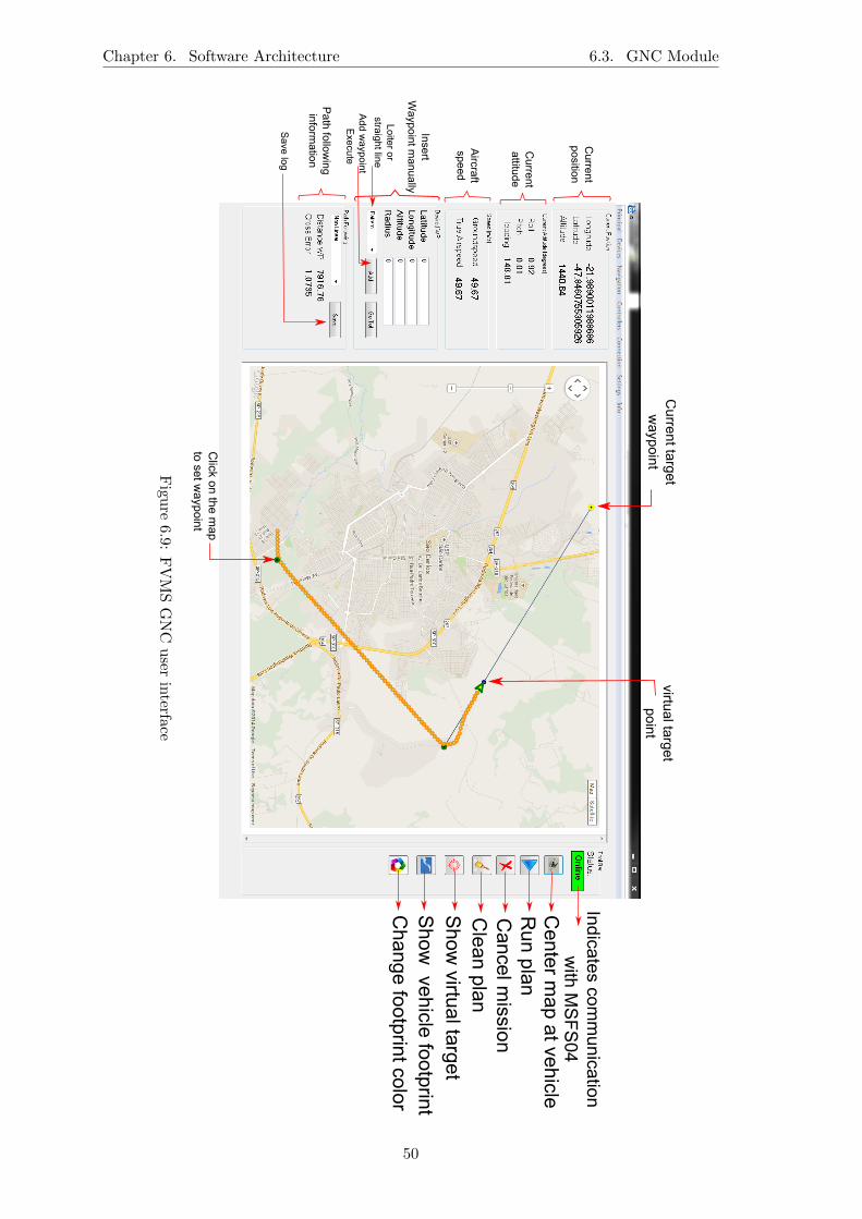
Chapter 6. Software Architecture 6.3. GNC Module
CenterLm
apLatLvehicleR
unLplanC
ancelLmission
CleanLplan
Show
LvirtualLtarget
Show
LLvehicleLfootprint
Change
LfootprintLcolor
IndicatesLcomm
unicationL
withLM
SF
S04
InsertW
aypointLman
ually
Current
position
Current
attitude
AircraftL
speed
LoiterLorLstraightLlin
e
AddLw
aypoint
Execute
PathLfollow
inginform
ation
CurrentLtargetLw
aypoint
SaveLlog
virtualLtargetpoint
ClickLonLtheLm
ap
toLsetLwaypoint
Figu
re6.9:
FV
MS
GN
Cu
serin
terface
50
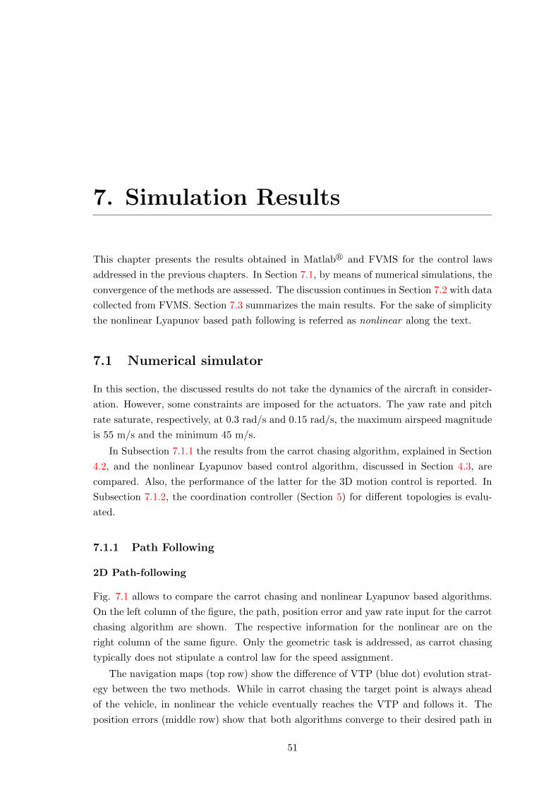
7. Simulation Results
This chapter presents the results obtained in Matlabr and FVMS for the control laws
addressed in the previous chapters. In Section 7.1, by means of numerical simulations, the
convergence of the methods are assessed. The discussion continues in Section 7.2 with data
collected from FVMS. Section 7.3 summarizes the main results. For the sake of simplicity
the nonlinear Lyapunov based path following is referred as nonlinear along the text.
7.1 Numerical simulator
In this section, the discussed results do not take the dynamics of the aircraft in consider-
ation. However, some constraints are imposed for the actuators. The yaw rate and pitch
rate saturate, respectively, at 0.3 rad/s and 0.15 rad/s, the maximum airspeed magnitude
is 55 m/s and the minimum 45 m/s.
In Subsection 7.1.1 the results from the carrot chasing algorithm, explained in Section
4.2, and the nonlinear Lyapunov based control algorithm, discussed in Section 4.3, are
compared. Also, the performance of the latter for the 3D motion control is reported. In
Subsection 7.1.2, the coordination controller (Section 5) for different topologies is evalu-
ated.
7.1.1 Path Following
2D Path-following
Fig. 7.1 allows to compare the carrot chasing and nonlinear Lyapunov based algorithms.
On the left column of the figure, the path, position error and yaw rate input for the carrot
chasing algorithm are shown. The respective information for the nonlinear are on the
right column of the same figure. Only the geometric task is addressed, as carrot chasing
typically does not stipulate a control law for the speed assignment.
The navigation maps (top row) show the difference of VTP (blue dot) evolution strat-
egy between the two methods. While in carrot chasing the target point is always ahead
of the vehicle, in nonlinear the vehicle eventually reaches the VTP and follows it. The
position errors (middle row) show that both algorithms converge to their desired path in
51
Chapter 7. Simulation Results 7.1. Numerical simulator
a quite similar fashion. However, the difference in the yaw rate input (bottom row) is
noticeable.
0 500 1000 1500 2000
-500
0
500
1000
1500
Navigation Map
x (m)
y (m
)
Desired PathActual Path
-500 0 500 1000 1500 2000
-500
0
500
1000
1500Navigation Map
x (m)
y (m
)
Desired PathActual Path
0 10 20 30 40 50 600
250
500
750
1000
1200Error norm
||p-p
d|| (m
)
0 10 20 30 40 50 600
250
500
750
1000
1250
1400Displacement Error
time (s)
Error norm
||p-p
d|| (m
)
0 10 20 30 40 50 60-0.2
-0.1
0
0.1
0.2
0.3
time (s)
Yaw
ra
te (
rad
/s)
Yaw rate reference
yaw rate
0 10 20 30 40 50 60-0.2
-0.1
0
0.1
0.2
0.3
time (s)
Yaw
ra
te (
rad/
s)
Yaw rate reference
yaw rate
Figure 7.1: Horizontal plane path following comparison. Carrot chasing results on the left
column and nonlinear Lyapunov based on the right column
In overall, the nonlinear Lyapunov based algorithm has a good performance. It is
52

7.1. Numerical simulator Chapter 7. Simulation Results
comparable to carrot chasing, whose performance has been confronted with a number of
solutions in (Sujit et al., 2013)
3D Path-following
In order to validate the nonlinear 3D path-following, an ascending loiter path, as shown
in Fig. 7.2a, is employed. The radius of the loiter is 2000m and the speed assignment is
set to vd = 502000 = 0.025. The latter is directly related to the angular speed of the vehicle,
in this specific test.
The convergence of the errors to of the equilibrium points e = 0 and z = 0 is illustrated
in Fig. 7.2b and Fig. 7.2c, respectively.
-20000
2000-2000
0
2000
0500
Navigation Map
x (m)
y (m)
Desired PathActual Path
(a)
0 100 200 300 400 5000
500
1000
1500
2000Displacement Error
time(s)
Error norm
(b)
0 100 200 300 400 5000
0.005
0.01
0.015
0.02
0.025
0.03
0.035Parametric variable rate
time(s)
.
(c)
Figure 7.2: 3D path following. Path visualization (a), distance from desired point (b) and
parametric variable rate (c)
53

Chapter 7. Simulation Results 7.1. Numerical simulator
7.1.2 Coordination control
Consider a fleet of three vehicles. Each element runs the nonlinear path following algorithm
previously evaluated. In this context, the coordination controllers for different topologies
are analyzed.
Constant topology
Consider a quasi strongly connected inter-vehicle communication topology. Vehicle 1
communicates its coordination state to the other vehicles. Vehicle 2 and Vehicle 3 do
not communicate each other. Fig. 7.3a shows how the flock evolves in time. This figure is
better interpreted if visualized from right to left. It is possible to see that the fleet achieved
coordination near the footprint before the last. Moreover, Fig. 7.3b clearly shows that
vehicle 1 and vehicle 2 are in coordination after a short time interval. Vehicle 3 takes
longer to be in coordination, but eventually synchronization is accomplished.
0 1000 2000 3000 4000 5000
-1000
-500
0
500
1000
1500
2000
2500
3000
Navigation Map
x (m)
y (m
)
vehicle 2
vehicle 1
vehicle 3
(a)
0 50 100 150 200 250 300-1200
-1000
-800
-600
-400
-200
0
200
time (s)
ampl
itude
Coordination error
γ1-γ2γ1-γ3
(b)
Figure 7.3: Constant topology. Illustration of the fleet (a) and coordination error (b)
Switching topology
Consider once again a fleet of three vehicles. The initial configuration and paths are as
in the constant communication example. However, this time, let the communication be
uniformly quasi strongly connected. The switching signal pi(t) = [v2v1, v3v1, 0, · · · , 0] is a
periodic signal with period T = 30s, described as next:
pi(τ) =
[1, 0, 0, · · · , 0]T , for 0< τ ≤T/3
[0, 1, 0, · · · , 0]T , for T/3< τ ≤ 2T/3
[0, 0, 0, · · · , 0]T , for 2T/3< τ ≤T
In other words, in the first third vehicle1 transmits its coordination state to vehicle2
(link v2v1 active). In the second third, vehicle3 is able to receive the state of vehicle1
54

7.1. Numerical simulator Chapter 7. Simulation Results
0 2000 4000 6000-2000
-1000
0
1000
2000
3000
4000
Navigation Map
x (m)
y (m
)
vehicle 2
vehicle 1
vehicle 3
(a)
0 100 200 300 400 500-1200
-1000
-800
-600
-400
-200
0
200
time (s)
Am
plitu
de
Coordination error
γ1-γ2γ1-γ3
(b)
0 100 200 300 400 5000
200
400
600
800
1000
time (s)
||p1
- p d1
||
Error norm
Vehicle 1
(c)
0 100 200 300 400 5000
20
40
60
80
100
120
140Displacement Error
time (s)
||p2
- p d2
|| (m
)
Error norm
Vehicle 2
(d)
0 100 200 300 400 5000
5
10
15
20
25
30
35
40
45
time (s)
||p3
- p d3
|| (m
)
Error norm
Vehicle 3
(e)
Figure 7.4: Switching topology. Fleet evolution (a) and coordination error (b) over time.
55
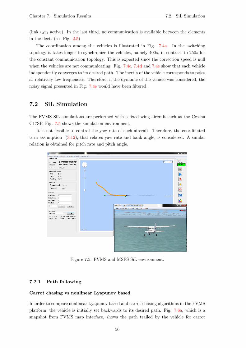
Chapter 7. Simulation Results 7.2. SiL Simulation
(link v3v1 active). In the last third, no communication is available between the elements
in the fleet. (see Fig. 2.5)
The coordination among the vehicles is illustrated in Fig. 7.4a. In the switching
topology it takes longer to synchronize the vehicles, namely 400s, in contrast to 250s for
the constant communication topology. This is expected since the correction speed is null
when the vehicles are not communicating. Fig. 7.4c, 7.4d and 7.4e show that each vehicle
independently converges to its desired path. The inertia of the vehicle corresponds to poles
at relatively low frequencies. Therefore, if the dynamic of the vehicle was considered, the
noisy signal presented in Fig. 7.4e would have been filtered.
7.2 SiL Simulation
The FVMS SiL simulations are performed with a fixed wing aircraft such as the Cessna
C17SP. Fig. 7.5 shows the simulation environment.
It is not feasible to control the yaw rate of such aircraft. Therefore, the coordinated
turn assumption (3.12), that relates yaw rate and bank angle, is considered. A similar
relation is obtained for pitch rate and pitch angle.
Figure 7.5: FVMS and MSFS SiL environment.
7.2.1 Path following
Carrot chasing vs nonlinear Lyapunov based
In order to compare nonlinear Lyapunov based and carrot chasing algorithms in the FVMS
platform, the vehicle is initially set backwards to its desired path. Fig. 7.6a, which is a
snapshot from FVMS map interface, shows the path trailed by the vehicle for carrot
56
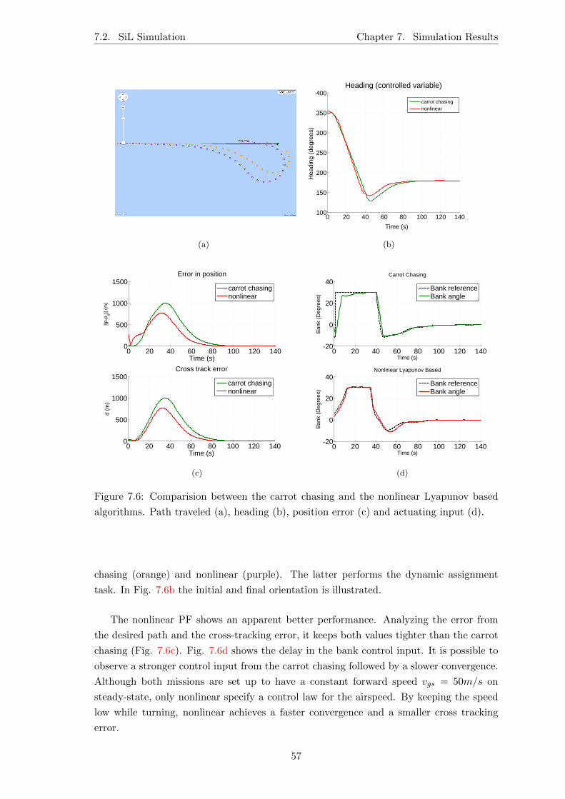
7.2. SiL Simulation Chapter 7. Simulation Results
(a)
0 20 40 60 80 100 120 140100
150
200
250
300
350
400Heading (controlled variable)
Time (s)
Hea
ding
(de
gree
s)
carrot chasingnonlinear
(b)
0 20 40 60 80 100 120 1400
500
1000
1500Error in position
Time (s)
||p-p
d|| (m
)
0 20 40 60 80 100 120 1400
500
1000
1500Cross track error
Time (s)
d (m
)
carrot chasingnonlinear
carrot chasingnonlinear
(c)
0 20 40 60 80 100 120 140-20
0
20
40Carrot Chasing
Time (s)
Ban
k (D
egre
es)
Bank referenceBank angle
0 20 40 60 80 100 120 140-20
0
20
40Nonlinear Lyapunov Based
Time (s)
Ban
k (D
egre
es)
Bank referenceBank angle
(d)
Figure 7.6: Comparision between the carrot chasing and the nonlinear Lyapunov based
algorithms. Path traveled (a), heading (b), position error (c) and actuating input (d).
chasing (orange) and nonlinear (purple). The latter performs the dynamic assignment
task. In Fig. 7.6b the initial and final orientation is illustrated.
The nonlinear PF shows an apparent better performance. Analyzing the error from
the desired path and the cross-tracking error, it keeps both values tighter than the carrot
chasing (Fig. 7.6c). Fig. 7.6d shows the delay in the bank control input. It is possible to
observe a stronger control input from the carrot chasing followed by a slower convergence.
Although both missions are set up to have a constant forward speed vgs = 50m/s on
steady-state, only nonlinear specify a control law for the airspeed. By keeping the speed
low while turning, nonlinear achieves a faster convergence and a smaller cross tracking
error.
57

Chapter 7. Simulation Results 7.2. SiL Simulation
0 5000 10000
-10,000
-8,000
-6,000
-4,000
Carrotlchasing
xl(m)
yl(m
)
DesiredlPathActuallPath
vw
N
S
(a)
0 5000 10000-10000
-8000
-6000
-4000
-2000
0
NonlineartLyapunovtbased
xt(m)
yt(m
)
DesiredtPathActualtPath
vw
N
S
(b)
0 50 100 150 200 250-100
-80
-60
-40
-20
0
20
40Heading
Time (s)
Hea
ding
(de
gree
s)
Carrot chasingNonlinear
(c)
0 50 100 150 200 2500
1000
2000
3000Error in position
Time (s)
||p-p
d|| (m
)
0 50 100 150 200 2500
1000
2000
3000Cross track error
Time (s)
d (m
)
Carrot chasingNonlinear
Carrot chasingNonlinear
(d)
0 50 100 150 200 250 300-30
-20
-10
0
10Carrot chasing
Time (s)
Ban
k (d
egre
es)
Bank referenceBank angle
0 50 100 150 200 250 300-40
-20
0
20Nonlinear Lyapunov based
Time (s)
Ban
k (d
egre
es)
Bank referenceBank angle
(e)
Figure 7.7: robustness test. Wind directed from north to south, wind speed = 18 m/s,
gust = 28m/s around 125s. Path travelled for carrot chasing (a) and nonlinear PF (b),
heading angle (c), error (d), actuating signal (e).
58

7.2. SiL Simulation Chapter 7. Simulation Results
Robust control
The robustness of both carrot chasing and nonlinear path following is tested in an adverse
scenario. The wind is set to 18 m/s, directed from north to south. The flight is disturbed
with gust of winds (28 m/s) and moderate turbulence at approximately t = 125s. The
desired path is orthogonal to the wind direction. The speed assignment is adjusted to
vd = 50. In this specific case, it corresponds to the desired ground speed.
In order to fly in the right direction, the vehicle slightly faces the wind (Fig. 7.7a
and Fig. 7.7b). While the desired path orientation is around 0o, the vehicle is oriented
around 20o, as shown in Fig. 7.7c. Analyzing the heading, it is possible to visualize when
each simulation is disturbed by gusts and turbulence. However, the controllers’ behavior
assure that the error, depicted inf Fig. 7.7d, remain bounded. The bank control input is
illustrated in Fig. 7.7e.
Specifically, for the nonlinear PF, Fig. 7.8 illustrates the parametric variable rate
evolution and the speed control input. The disturbance directly affects the position of the
vehicle. Consequently, the parametric variable rate is also disturbed, as its control law
has a term that depends on the vehicle position.
30
40
50
60
70
80
90Parametric variable rate
dγ/d
t
dγ/dt
0 50 100 150 200 250
Time (s)
(a)
0 50 100 150 200 25040
45
50
55
60
65
70Speed (control input)
Time (s)
Spe
ed (
m/s
)
Speed referenceSpeed
(b)
Figure 7.8: Nonlinear PF, parametric variable rate (a) and speed control input (b).
3D path following
An ascending loiter is parametrized to evaluate the 3D nonlinear path following. The
radius is set to 1800m and vd = 481800 = 0.0267. The evolution of the vehicle along the
path is shown in Fig. 7.9a. As depicted in Fig. 7.9b and Fig. 7.9c, the error stabilizes
at its equilibrium point. When analyzing the control input (Fig. 7.9d), the importance
of delay filters is noticeable. FVMS provides filters for both roll and pitch references, but
it does not implement a filter for airspeed assignment. Once the filter is implemented, a
smoother convergence may be achieved.
59

Chapter 7. Simulation Results 7.2. SiL Simulation
-2000-1000
01000
-1000
0
1000500
1000
y (m)
Navigation Map
x (m)
Desired PathActual Path
(a)
0 100 200 300 400 500 6000
300
600
900
1200
1500
1800Error in position
Time (s)
erro
r (m
)
error norm
(b)
0 100 200 300 400 500 6000.016
0.018
0.02
0.022
0.024
0.026
0.028
time (s)
Am
plitu
de
Parametric variable rate
(c)
0 100 200 300 400 500 60040
60
80Speed
Time (s)
Spe
ed (
m/s
)
Speed referenceSpeed
0 100 200 300 400 500 600-20
0
20Bank angle
Time (s)
Ban
k (d
egre
es)
Bank referenceBank angle
0 100 200 300 400 500 600-20
0
20 Pitch angle
Time (s)
Pitc
h (d
egre
es)
Pitch referencePitch angle
(d)
Figure 7.9: SiL: 3D path folllowing. Path travelled (a), position error (b), parametric
variable rate (c) and input (d).
60
7.3. Summary Chapter 7. Simulation Results
7.3 Summary
In this chapter it is shown that the performance of the nonlinear Lyapunov based algorithm
is as good as for the carrot chasing. The coordination control is achieved in both constant
and switching topologies. The synchronization in a switching topology takes longer, as
expected, but the communication effort is much smaller. In addition, simulations carried
in the FVMS SiL platform confirm some of the previous results. Also, the controller
robustness under weather disturbances is evaluated. The results show that the nonlinear
algorithm is able to keep the vehicle on track despite outer disturbances.
61

8. Conclusion
8.1 Summary
This dissertation focused on cooperative control of a formation of UAVs. In order to tackle
the problem in a clear and transparent manner, the cooperative motion control problem
was divided in path following and coordinate control. The former assures that the vehicle
follows a virtual target, whose evolution in time is adjusted by the latter. Nonlinear
Lyapunov stability theorems and graph theory support the control laws herein addressed.
The results from SiL simulations show that the performance of nonlinear path following
is comparable to the one of other techniques in the literature. The obtained results are
encouraging for both 2D and 3D scenarios. The dynamics of the vehicle are not explicitly
addressed. This allows the kinematic controller to be extended to other vehicles, equipped
with a dynamic controller. The coordination results confirm that it is possible to achieve
coordination in a switching inter-vehicle communication topology. Moreover, the results
report that in a uniformly quasi strongly connected topology, even under intermittent link
failures, coordination is accomplished.
Equipping the FVMS with a GNC module opens up new possibilities for the platform.
The software was upgraded with a more friendly user-interface. Guidance algorithms
may be evaluated in a reliable fashion. In addition, the tool shows great potential in the
academic scope, assisting students in the learning process.
8.2 Future work
Cooperation in SiL
The MS Flight Simulator does not allow more than one aircraft per simulation. There-
fore, achieving communication between FVMS running in different machines is a point
which deserves further attention. Running MSFS and FVMS in different machines would
allow evaluating cooperative controllers with SiL simulations. The communication may
be implemented in a TCP/IP network.
62
8.2. Future work Chapter 8. Conclusions
Communication topology
In this work the existing delays in communication links are not addressed. However,
according to the dynamic of the system, the delay may play an important role in vehicle
synchronization. Studying the delay impact is left as a future topic to be explored.
Obstacle avoidance
Obstacle avoidance is a topic that naturally emerges when discussing autonomous robots.
This topic requires special attention when dealing with multiple autonomous vehicles, as
the systems have to interact with each other to avoid collisions. The problem requires
generating a collision-free trajectory and online information to evasion maneuvers, if nec-
essary. The SiL platform discussed, FVMS, allows to use optical flow techniques to map
the ambient and sense possible obstacles.
63
Bibliography
Outback joe. Internet, September 2012. URL http://southburnett.com.au/news2/
2012/09/can-anyone-find-outback-joe/.
Antonio Pedro Aguiar and Joao Pedro Hespanha. Position tracking of underactuated
vehicles. In American Control Conference, 2003. Proceedings of the 2003, volume 3,
pages 1988–1993 vol.3, June 2003.
A.P. Aguiar and J.P. Hespanha. Trajectory-tracking and path-following of underactuated
autonomous vehicles with parametric modeling uncertainty. Automatic Control, IEEE
Transactions on, 52(8):1362–1379, Aug 2007.
A.P. Aguiar and A.M. Pascoal. Coordinated path-following control for nonlinear systems
with logic-based communication. In Decision and Control, 2007 46th IEEE Conference
on, pages 1473–1479, Dec 2007.
Cessna. Skyhawk - the best-selling and most-flow aircraft ever built, 2013. URL http:
//www.cessna.com/single-engine/skyhawk.
Peng Cheng and Vijay Kumar. An almost communication-less approach to task allocation
for multiple unmmaned aeria vehicles. In IEEE International Conference on Robotics
and Automation, pages 19–23, Pasadena, CA, USA, May 2008.
S. Demers, P. Gopalakrishnan, and L. Kant. A generic solution to software-in-the-loop.
In Military Communications Conference, 2007. MILCOM 2007. IEEE, pages 1–6, Oct
2007.
Peter Downson. Fsuipc: Application interfacing module for microsoft flight simulator,
August 2012. URL http://www.schiratti.com/dowson.
M. Egerstedt and Xiaoming Hu. Formation constrained multi-agent control. Robotics and
Automation, IEEE Transactions on, 17(6):947–951, December 2001.
P. Encarnacao and A. Pascoal. 3d path following for autonomous underwater vehicle. In
Decision and Control, 2000. Proceedings of the 39th IEEE Conference on, volume 3,
pages 2977–2982 vol.3, 2000.
P. Encarnacao and A. Pascoal. Combined trajectory tracking and path following: an
application to the coordinated control of autonomous marine craft. In Decision and
Control, 2001. Proceedings of the 40th IEEE Conference on, volume 1, pages 964–969
vol.1, 2001.
64
Bibliography Bibliography
William Etter, Paul Martin, and Raul Mangharam. Cooperative flight guidance of au-
tonomous unmanned aerial vehicles, 2011.
J. Alexander Fax and Richard M. Murray. Graph laplacians and stabilization of vehicle
formations. In Proceedings 2002 IFAC World Congress, Barcelona, Spain, 2002.
J.A. Fax and R.M. Murray. Information flow and cooperative control of vehicle formations.
Automatic Control, IEEE Transactions on, 49(9):1465–1476, September 2004.
R. Ghabcheloo, A. Pascoal, C. Silvestre, and I. Kaminer. Nonlinear coordinated path fol-
lowing control of multiple wheeled robots with bidirectional communication constraints.
International Journal of Adaptive Control and Signal Processing, 21(2-3):133–157, 2007.
R. Ghabcheloo, A. Aguiar, A. Pascoal, C. Silvestre, I. Kaminer, and J. Hespanha. Coor-
dinated path-following in the presence of communication losses and time delays. SIAM
Journal on Control and Optimization, 48(1):234–265, 2009.
B. Grocholsky, J. Keller, V. Kumar, and G. Pappas. Cooperative air and ground surveil-
lance. Robotics Automation Magazine, IEEE, 13(3):16–25, September 2006.
Stephen Philip Jackson. Controlling Small Fixed Wing UAVs to Optimize Image Quality
from On-Board Cameras. PhD thesis, Universiry of California, Berkley, U.S.A, 2011.
Hassan K. Khalil. Nonlinear System. Prentice Hall, 2002.
L. Lapierre, D. Soetanto, and A. Pascoal. Nonlinear path following with applications to the
control of autonomous underwater vehicles. In Decision and Control, 2003. Proceedings.
42nd IEEE Conference on, volume 2, pages 1256–1261 Vol.2, Dec 2003.
Zhiyun Lin, Bruce Francis, and Manfredi Maggiore. State agreement for continuous-time
coupled nonlinear systems. SIAM J. Control Optim., 46(1):288–307, March 2007.
Quentin Lindsey, Daniel Mellinger, and Vijay Kumar. Construction of cubic structures
with quadrotor teams. In Proceedings of Robotics: Science and Systems, Los Angeles,
CA, USA, June 2011.
R. Louali, A. Belloula, M.S. Djouadi, and S. Bouaziz. Real-time characterization of mi-
crosoft flight simulator 2004 for integration into hardware in the loop architecture. In
Control Automation (MED), 2011 19th Mediterranean Conference on, pages 1241–1246,
June 2011.
M. Mesbahi and M. Egerstedt. Graph Theoretic Methods in Multiagent Networks. Prince-
ton University Press, 2010.
T. Oliveira, P. Encarnacao, and A.P. Aguiar. Moving path following for autonomous
robotic vehicles. In Control Conference (ECC), 2013 European, pages 3320–3325, July
2013.
65
Bibliography Bibliography
S. Park, J. Deyst, and J. P. How. Performance and lyapunov stability of a nonlinear
path-following guidance method. AIAA Journal on Guidance, Control, and Dynamics,
30(6):1718–1728, November-December 2007.
J. Roberts and R. Walker. Flying robots to the rescue [competitions]. Robotics Automation
Magazine, IEEE, 17(1):8–10, March 2010.
Jan Roskam. Airplane Flight Dynamics and Automatic Flight Controls, Part I. DARco-
poration, Lawrence, KS, U.S.A., 2001.
UAV Roundup. Uav roundup 2013. Aerospace America, pages 26–36, July-August 2013.
Erol Sahin. Swarm robotics: From sources of inspiration to domains of application.
In Swarm Robotics, volume 3342 of Lecture Notes in Computer Science, pages 10–20.
Springer Berlin Heidelberg, 2005.
Rafael C.B. Sampaio, Marcelo Becker, Adriano A.G. Siqueira, Leonardo W. Freschi, and
Marcelo P. Montanher. Fvms: A novel sil approach on the evaluation of controllers for
autonomous mav. In Aerospace Conference, 2013 IEEE, pages 1–8, March 2013a.
Rafael C.B. Sampaio, Marcelo Becker, Adriano A.G. Siqueira, Leonardo W. Freschi, and
Marcelo P. Montanher. Novel sil evaluation of an optimal h∞ controller on the stability
of a mav in flight simulator. In Aerospace Conference, 2013 IEEE, pages 1–8, March
2013b.
Rafael C.B. Sampaio, Andre C. Hernandes, Marcelo Becker, , Eduardo Cazarini, Daniel V.
Magalhaes, and Adriano A.G. Siqueira. New hil evaluation of an h∞ controller on the
stabilization of a mav in flight simulation. In Aerospace Conference, 2014 IEEE, pages
1–7, March 2014a.
Rafael C.B. Sampaio, Andre C. Hernandes, Marcelo Becker, , Fabio M. Zanin, Joao E. M.
Nobrega, Caio A. C. Martins, and Fabio M. Catalano. Squidcop design and evalua-
tion of a novel quadrotor mav for in-flight launching airground missions. In Aerospace
Conference, 2014 IEEE, pages 1–7, March 2014b.
Rafael C.B. Sampaio, Andre C. Hernandes, Marcelo Becker, , Fabio M. Zanin, Joao E. M.
Nobrega, Caio A. C. Martins, and Fabio M. Catalano. A new hybrid motor glider-
quadrotor mav for v-stol launching. In Aerospace Conference, 2014 IEEE, pages 1–7,
March 2014c.
Claude Samson. Path-following and time-varying feedback stabilization of a wheeled mo-
bile robot. In Proceedings of the ICARCV, Singapore, 1992.
Robert J. Shaw. Dynamics of flight, 2014. URL http://www.grc.nasa.gov/WWW/k-12/
UEET/StudentSite/dynamicsofflight.html.
Charley Shimanski. Mountain rescue association reaffirms its position opposing charging
subjects for the costs of their rescues. Charge Position, August 2009.
66

Bibliography Bibliography
P.B. Sujit, S. Saripalli, and J.B. Sousa. An evaluation of uav path following algorithms.
In Control Conference (ECC), 2013 European, pages 3332–3337, July 2013.
M. Valenti, D. Dale, J. How, and J. Vian. Mission health management for 24/7 persistent
surveillance operations. In Proceedings of the AIAA Guidance, Navigation, and Control
Conference, Myrtle Beach, SC, August 2007.
Francesco Vanni. Coordination motion control of multiple autonomous underwater vehi-
cles. Master’s thesis, Department of Mechanical Engineering, Insituto Superior Tecnico,
Universidade Tecnica de Lisboa, 2007.
Chris Veness. Calculate distance, bearing and more between latitude/longitude points,
January 2010. URL http://www.movable-type.co.uk/scripts/latlong.html.
Jan Willmann, Federico Augugliaro, Thomas Cadalbert, Raffaello D’Andrea, Fabio Gra-
mazio, and Matthias Kohler. Aerial robotic construction: Towards a new field of archi-
tectural research. International Journal of Architectural Computing, 10-3, 2012.
67
Appendix - FVMS GNC libraries
and functions
A.1 Types and conversions
New types were created to support motion control algorithms. They are available in the
FVMSTypes library. In order to use any of the types developed, the user needs to include
the library in proper section (use section). The following types are highlighted:
TCartesian: Cartesian coordinates (x,y,z).
Name Type Unit Description
x double meter position of the vehicle in inertial x-axis
y double meter position of the vehicle in inertial y-axis
z double meter position of the vehicle in inertial z-axis
TWGS84: Global coordinate specified in WGS84 normalization.
Name Type Unit Description
Latitude double degree Latitude
Longitude double degree Longitude
Altitude double meter Altitude
TAttitude: Attitude of the aircraft in respect to mathcalI, expressed in mathcalB.
Name Type Unit Description
roll double radian roll angle
pitch double radian pitch angle
yaw double radian yaw angle
68
A.1. Types and conversionsAppendix A. Appendix - FVMS GNC libraries and functions
TVehicleState: Stores current state of the vehicle.
Name Type Unit Description
pos TCartesian - position of the vehicle
attitude TAttitude - attitude of the aircraft
tas double meter/second true air speed norm
gs double meter/second ground speed norm
vx double meter/second forward ground speed value
vy double meter/second lateral ground speed value
vz double meter/second vertical ground speed value
TPath: Stores current state of the vehicle.
Name Type Unit Description
WPi TCartesian - coordinates of initial waypoint
WPf TAttitude - coordinates of final waypoint
losAngle double radians LoS Angle
crossTrError double meter cross tracking error
loiter boolean - 0-straight line, 1-loiter
radius double meter loiter radius in meters. 1-straight line
active boolean - 0-path is not active, 1-path active
As the information needs to be processed or show in different formats, a conversion
library was developed. The user can use the following functions through FVMSConversion
library.
function WGS84ToCartesian(WGS84 coord: TWGS84): TCartesian;
notes: Converts coordinates specified in WGS84 into cartesian coordinates
function cartesianToWGS84(cartesian coord: TCartesian): TWGS84;
notes: Converts cartesian coordinates into WGS84 standard
There are several ways to transform WGS84 coordinates into cartesian. The complex-
ity increases as more precision is required. It was not in the scope of this project to deep
investigate this matter. Therefore a simple transformation was employed. As the earth
radius is assumed constant, high values of latitude are distorted during conversion. For
more information the reader is referred to (Veness, 2010)
function degToCoord(deg: Double): TCoordinate;
notes: Converts a coordinate specified in degree to (degree, minutes and
seconds)
69

Appendix A. Appendix - FVMS GNC libraries and functions A.2. Navigation library
A.2 Navigation library
The navigation library is able to read the computer memory by means of FSCUIP DLL.
It focuses on reading data from the vehicle, like IMU and GPS sensors. As long as a
connection exist between FVMS and simulator. By default, the state of the vehicle is
refreshed at a rate of 2Hz. This rate may be easily modified. This library offers reading
function to a range of variables that are employed in navigation algorithms, as described
next.procedure UpdateVehicleState;
notes: Responsible to read the memory and store in a TVehicle type
The following data are referred to the last updated values.
function getVehicleStatus: TVehicleState;
notes: Returns the state of the vehicle. This function shall be used with
cautions as may generate excessive overhead.
function getPosition: TCartesian;
notes: Returns the current cartesian position (x,y,z) of the vehicle
function getAttitude: TAttitude;
notes: Returns the attitude of the aircraft
function getBank: double;
notes: Returns the bank angle in radians
function getPitch: double;
notes: Returns the pitch angle in radians
function getHeading: double;
notes: Returns the yaw angle (heading) in radians
function getTrueAirSpeed: double;
notes: Returns the module of true airspeed of the vehicle in m/s
function getGroundSpeed: double;
notes: Returns the module of groundspeed of the vehicle in m/s
function getVx: double;
notes: Returns the groundspeed forward component (x-axis) in m/s
function getVy: double;
notes: Returns the groundspeed lateral component (y-axis) in m/s
70
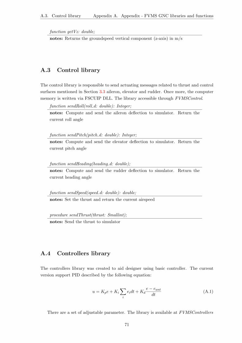
A.3. Control library Appendix A. Appendix - FVMS GNC libraries and functions
function getVz: double;
notes: Returns the groundspeed vertical component (z-axis) in m/s
A.3 Control library
The control library is responsible to send actuating messages related to thrust and control
surfaces mentioned in Section 3.3 aileron, elevator and rudder. Once more, the computer
memory is written via FSCUIP DLL. The library accessible through FVMSControl.
function sendRoll(roll d: double): Integer;
notes: Compute and send the aileron deflection to simulator. Return the
current roll angle
function sendPitch(pitch d: double): Integer;
notes: Compute and send the elevator deflection to simulator. Return the
current pitch angle
function sendHeading(heading d: double);
notes: Compute and send the rudder deflection to simulator. Return the
current heading angle
function sendSpeed(speed d: double): double;
notes: Set the thrust and return the current airspeed
procedure sendThrust(thrust: Smallint);
notes: Send the thrust to simulator
A.4 Controllers library
The controllers library was created to aid designer using basic controller. The current
version support PID described by the following equation:
u = Kpe+Ki
∑i
eidt+Kde− eantdt
(A.1)
There are a set of adjustable parameter. The library is available at FVMSControllers
71
Appendix A. Appendix - FVMS GNC libraries and functions A.4. Controllers library
TPID: PID controller structure.
Name Type Unit Description
Kp double - proportional gain
Ki double - integral gain
Kd double - derivative gain
e sum double inherited error sum
e ant double inherited previous error
antiWindUp double - Anti wind up value
saturation double - Output saturation value
dt double seconds sample time
constructor Create; overload;
notes: Default constructor
constructor Create(Kp, Ki, Kd: double); overload;
notes: Customized constructor
function controlLoop(error: double): Double;
notes: Calculate and return the PID output for a single iteration
procedure setParameters(Kp, Ki, Kd: double);
notes: Set proportion, integral and derivative gains
procedure setAntiWindUp(antiWindUp: Double);
notes: Modify anti wind up value
procedure setSampleTime(dt: double);
notes: Modify sample time
procedure cleanSum;
notes: Clean the integral sum
72


![Manual Variador [e]-MOTION SACI](https://static.fdocumentos.com/doc/165x107/62df00c57f1bbd34273adde0/manual-variador-e-motion-saci.jpg)