
Daniel Jos Taveira Gomes Voxel Based Real-Time Global...
85
Universidade do Minho Escola de Engenharia Daniel José Taveira Gomes Voxel Based Real-Time Global Illumination Techniques Abril de 2015
-
Upload
nguyenkhanh -
Category
Documents
-
view
238 -
download
3
Transcript of Daniel Jos Taveira Gomes Voxel Based Real-Time Global...

Universidade do Minho
Escola de Engenharia
Daniel José Taveira GomesVoxel Based Real-Time Global Illumination Techniques
Abril de 2015
Universidade do Minho
Dissertação de Mestrado
Escola de Engenharia
Departamento de Informática
Daniel José Taveira GomesVoxel Based Real-Time Global Illumination Techniques
Mestrado em Engenharia Informática
Trabalho realizado sob orientação deProfessor António Ramires Fernandes
Abril de 2015

AC K N OW L E D G E M E N T S
I would like to express my deep gratitude to Professor Ramires for his patient guidance andvaluable suggestions and critiques throughout the development of this thesis.
I would also like to express my gratitude to all my friends, who heard my complaints whenthings did not go as planned and provided advice whenever they could.
Finally, I wish to thank my parents for their invaluable support and encouragement during mystudies.
A B S T R AC T
One of the greater objectives in computer graphics is to be able to generate fotorealistic imagesand do it in real time. Unfortunately the actual lighting algorithms are not able to satisfy bothobjectives at the same time.
Most of the algorithms nowadays are based on rasterization to generate images in real timeat the expense of realism, or based on ray tracing, achieving fotorealistic results but lackingperformance, which makes them impossible to compute at interactive frame rates with the com-putational power available in the present.
Over the last years, some new techniques have emerged that try to combine the best featuresof both types of algorithms.
What is proposed in this thesis is the study and analysis of a class of algorithms based on voxelsto approximate global illumination in 3D scenes at interactive frame rates. These techniques usea volumetric pre-filtered representation of the scene and a rendering algorithm based on conetracing to compute an approximation to global illumination in real time.
What is pretended through this study is an analysis on the practicability of such algorithms inreal-time applications and apply the new capabilities of the OpenGL API to simplify/optimizethe implementation of these algorithms.
a
R E S U M O
Um dos maiores objectivos da computacao grafica e conseguir gerar imagens fotorealistas e emtempo real. Infelizmente os algoritmos de iluminacao actuais nao conseguem atingir ambos osobjectivos simultaneamente.
A maioria dos algoritmos actuais baseiam-se na rasterizacao para gerar imagens em tempo real,a custa da perda de realismo, ou entao em ray-tracing, conseguindo obter imagens fotorealistas,a custa da perda de interactividade.
Nos ultimos anos, tem surgido novas tecnicas para tentar juntar o melhor dos dois tipos dealgoritmos.
Propoe-se neste trabalho o estudo e analise de uma classe de algoritmos baseados em vox-els para calcular uma aproximacao a iluminacao global, de forma interactiva. Estas tecnicasusam uma pre-filtragem da cena usando uma representacao volumetrica da cena e um algoritmobaseado em cone tracing para calcular uma aproximacao da iluminacao global em tempo real.
Atraves deste estudo pretende-se por um lado analisar a viabilidade dos algoritmos em aplicacoesem tempo real e aplicar as novas capacidades da API do OpenGL de forma a simplificar/opti-mizar a sua implementacao.
b
C O N T E N T S
Contents iii
1 I N T RO D U C T I O N 31.1 Objectives . . . . . . . . . . . . . . . . . . . . . . . . . . . . . . . . . . . . . . 61.2 Document structure . . . . . . . . . . . . . . . . . . . . . . . . . . . . . . . . . 6
2 R E L AT E D W O R K 72.1 Shadow Mapping . . . . . . . . . . . . . . . . . . . . . . . . . . . . . . . . . . 72.2 Deferred Rendering . . . . . . . . . . . . . . . . . . . . . . . . . . . . . . . . . 72.3 Reflective Shadow Maps . . . . . . . . . . . . . . . . . . . . . . . . . . . . . . 92.4 Ray Tracing . . . . . . . . . . . . . . . . . . . . . . . . . . . . . . . . . . . . . 92.5 Voxelization . . . . . . . . . . . . . . . . . . . . . . . . . . . . . . . . . . . . . 11
3 R E A L - T I M E VOX E L - B A S E D G L O B A L I L L U M I N AT I O N A L G O R I T H M S 123.1 Interactive Indirect Illumination Using Voxel Cone Tracing . . . . . . . . . . . . 13
3.1.1 Voxelization . . . . . . . . . . . . . . . . . . . . . . . . . . . . . . . . . 153.1.2 Sparse Voxel Octree . . . . . . . . . . . . . . . . . . . . . . . . . . . . . 183.1.3 Mipmapping . . . . . . . . . . . . . . . . . . . . . . . . . . . . . . . . 213.1.4 Voxel Cone Tracing . . . . . . . . . . . . . . . . . . . . . . . . . . . . . 23
3.2 Real-Time Near-Field Global Illumination Based on a Voxel Model . . . . . . . . 303.2.1 Voxelization . . . . . . . . . . . . . . . . . . . . . . . . . . . . . . . . . 303.2.2 Binary Voxelization . . . . . . . . . . . . . . . . . . . . . . . . . . . . . 323.2.3 Data Structure/Mip-Mapping . . . . . . . . . . . . . . . . . . . . . . . . 323.2.4 Rendering . . . . . . . . . . . . . . . . . . . . . . . . . . . . . . . . . . 33
3.3 Rasterized Voxel-Based Dynamic Global Illumination . . . . . . . . . . . . . . . 373.3.1 Creation of the Voxel Grid Representation . . . . . . . . . . . . . . . . . 383.3.2 Creation of Virtual Point Lights in Voxel Space . . . . . . . . . . . . . . 403.3.3 Virtual Point Lights Propagation . . . . . . . . . . . . . . . . . . . . . . 403.3.4 Indirect Lighting Application . . . . . . . . . . . . . . . . . . . . . . . . 41
4 I M P L E M E N TAT I O N 424.1 Technological Choices . . . . . . . . . . . . . . . . . . . . . . . . . . . . . . . 424.2 Interactive Indirect Illumination Using Voxel Cone Tracing . . . . . . . . . . . . 43
iii
CONTENTS
4.2.1 Voxel Cone Tracing with a Full Voxel Grid . . . . . . . . . . . . . . . . 434.2.2 Voxel Cone Tracing with a Sparse Voxel Octree . . . . . . . . . . . . . . 51
4.3 Rasterized Voxel-Based Dynamic Global Illumination . . . . . . . . . . . . . . . 584.3.1 Data Structures . . . . . . . . . . . . . . . . . . . . . . . . . . . . . . . 584.3.2 Buffer Clearing . . . . . . . . . . . . . . . . . . . . . . . . . . . . . . . 594.3.3 Voxelization . . . . . . . . . . . . . . . . . . . . . . . . . . . . . . . . . 604.3.4 Direct Light Injection . . . . . . . . . . . . . . . . . . . . . . . . . . . . 614.3.5 Direct Light Propagation . . . . . . . . . . . . . . . . . . . . . . . . . . 614.3.6 Reflection Grid Creation . . . . . . . . . . . . . . . . . . . . . . . . . . 624.3.7 Reflection Grid Mipmapping . . . . . . . . . . . . . . . . . . . . . . . . 624.3.8 Global Illumination Rendering . . . . . . . . . . . . . . . . . . . . . . . 63
4.4 Real-Time Near-Field Global Illumination Based on a Voxel Model . . . . . . . . 644.4.1 Data Structures . . . . . . . . . . . . . . . . . . . . . . . . . . . . . . . 654.4.2 Binary Atlas Creation . . . . . . . . . . . . . . . . . . . . . . . . . . . . 654.4.3 Pixel Display List Creation . . . . . . . . . . . . . . . . . . . . . . . . . 664.4.4 Voxel Grid Creation . . . . . . . . . . . . . . . . . . . . . . . . . . . . . 664.4.5 Mipmapping . . . . . . . . . . . . . . . . . . . . . . . . . . . . . . . . 674.4.6 Indirect Lighting Computation . . . . . . . . . . . . . . . . . . . . . . . 67
5 C O N C L U S I O N S 69
iv
L I S T O F F I G U R E S
Figure 1 Rasterization vs Ray tracing. Source: http://www.cs.utah.edu/ jstrat-to/state of ray tracing/ . . . . . . . . . . . . . . . . . . . . . . . . . . . 3
Figure 2 Geometry simplification. Information about the geometry is lost withan increasing level of filtering. Source: Daniels et al. (2008) . . . . . . . 4
Figure 3 Indirect illumination on a scene with a hidden object behind the column.In the left image, only objects in camera space are taken into accountand thus the hidden objects are disregarded since they are not visible bythe current camera. Source: Thiedemann et al. (2011) . . . . . . . . . . 5
Figure 4 Voxels used to view medical data. Source: URL . . . . . . . . . . . . . 5Figure 5 Voxel-based Global Illumination. Source: Crassin et al. (2011) . . . . . 12Figure 6 Voxel Lighting. Source: Crassin (2011) . . . . . . . . . . . . . . . . . . 13Figure 7 Voxel Cone Tracing. Source: Crassin et al. (2011); Crassin (2011) . . . 14Figure 8 Voxelization. Red: projection along x-axis. Green: projection along
y-axis. Blue: projection along z-axis . . . . . . . . . . . . . . . . . . . 15Figure 9 Voxelization Pipeline. Source: Crassin and Green (2012) . . . . . . . . 16Figure 10 Conservative Voxelization. Source: Schwarz and Seidel (2010) . . . . . 17Figure 11 Triangle Expansion in Conservative Rasterization. Source: Crassin and
Green (2012) . . . . . . . . . . . . . . . . . . . . . . . . . . . . . . . . 17Figure 12 Sparse Voxel Octree Structure. Source: Crassin et al. (2010) . . . . . . . 18Figure 13 Voxel Brick. Source: Crassin et al. (2011) . . . . . . . . . . . . . . . . 19Figure 14 Steps for the creation of the sparse voxel octree structure. Source:
Crassin and Green (2012) . . . . . . . . . . . . . . . . . . . . . . . . . 20Figure 15 Node Subdivision and Creation. Source: Crassin and Green (2012) . . . 20Figure 16 Mipmapping Weighting Kernel. Source: Crassin et al. (2011) . . . . . . 21Figure 17 Normal Distribution Function (NDF). . . . . . . . . . . . . . . . . . . . 22Figure 18 Opacity is stored as a single value inside a voxel, causing a lack of view
dependency. . . . . . . . . . . . . . . . . . . . . . . . . . . . . . . . . 23Figure 19 Direct lighting injection and indirect lighting computation. Source:
Crassin et al. (2011) . . . . . . . . . . . . . . . . . . . . . . . . . . . . 23
v
LIST OF FIGURES
Figure 20 Voxel Cone Tracing. Source: Crassin et al. (2010) . . . . . . . . . . . . 24Figure 21 Estimating Soft Shadows trough Voxel Cone Tracing. Source: Crassin
(2011) . . . . . . . . . . . . . . . . . . . . . . . . . . . . . . . . . . . 26Figure 22 Estimating Depth of Field Effects trough Voxel Cone Tracing. Source:
Crassin (2011) . . . . . . . . . . . . . . . . . . . . . . . . . . . . . . . 26Figure 23 Data transfer between neighboring bricks and distribution over levels.
Source: Crassin et al. (2011) . . . . . . . . . . . . . . . . . . . . . . . 27Figure 24 Node Map. Source: Crassin et al. (2011) . . . . . . . . . . . . . . . . . 28Figure 25 Anisotropic Voxel Representation. Source: Crassin et al. (2011) . . . . . 29Figure 26 Directions distribution. Source: Crassin et al. (2011) . . . . . . . . . . . 30Figure 27 Binary Voxelization. Source: Thiedemann et al. (2012) . . . . . . . . . 31Figure 28 Mip-mapping. Source: Thiedemann et al. (2012) . . . . . . . . . . . . . 33Figure 29 Hierarchy traversal. Blue lines: bounding box of the voxels in the actual
texel. Green and red lines: bitmask of the active texel (empty - greenand non empty - red). The green and red cuboids: history of the traversalfor the texel (no hit - green and possible hit - red). Source: Thiedemannet al. (2012) . . . . . . . . . . . . . . . . . . . . . . . . . . . . . . . . 34
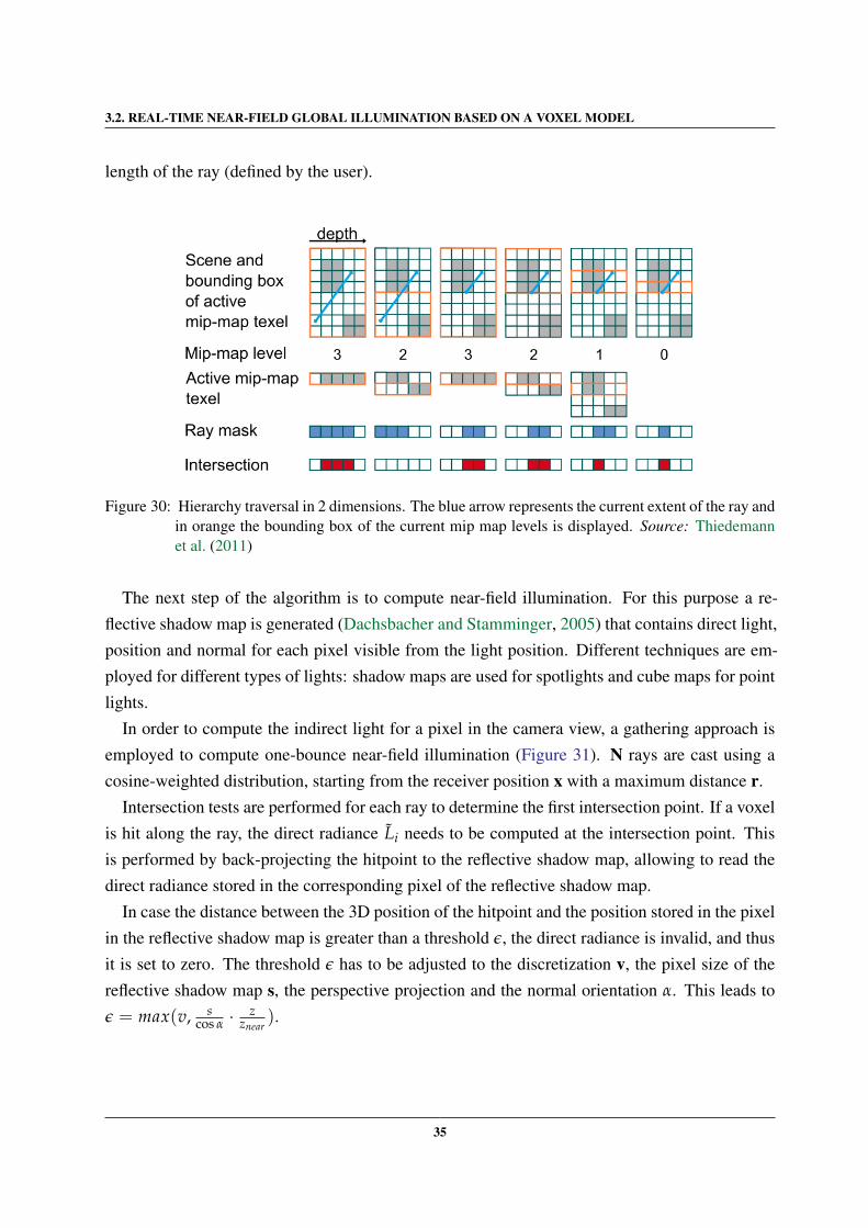
Figure 30 Hierarchy traversal in 2 dimensions. The blue arrow represents the cur-rent extent of the ray and in orange the bounding box of the current mipmap levels is displayed. Source: Thiedemann et al. (2011) . . . . . . . . 35
Figure 31 Near-field Indirect Illumination. Source: Thiedemann et al. (2011) . . . 36Figure 32 Nested Voxel Grids . . . . . . . . . . . . . . . . . . . . . . . . . . . . 37Figure 33 Pipeline of the algorithm . . . . . . . . . . . . . . . . . . . . . . . . . 38Figure 34 Orthographic Projection with a Voxel Grid in the View Frustum . . . . . 39Figure 35 Lit surfaces are treated as secondary light sources and clustered into a
voxel grid . . . . . . . . . . . . . . . . . . . . . . . . . . . . . . . . . 40Figure 36 Virtual Point Light are propagated in the Voxel Grid . . . . . . . . . . . 41Figure 37 Projection of a triangle trough the three main axis of the scene. The Y
axis is chosen for the voxelization since it is the one that will generatemaximum number of fragments during rasterization. Source: https://developer.nvidia.com/content/basics-gpu-voxelization . . . . . . . . . . . . . . . . . . . . . . . . . . . . . . 45
Figure 38 Octree and Octree Pools. . . . . . . . . . . . . . . . . . . . . . . . . . 52Figure 39 Octree Subdivision. . . . . . . . . . . . . . . . . . . . . . . . . . . . . 53Figure 40 Octree Mipmapping. . . . . . . . . . . . . . . . . . . . . . . . . . . . . 56
vi
L I S T O F L I S T I N G S
4.1 Voxel Fragment List . . . . . . . . . . . . . . . . . . . . . . . . . . . . . . . . . 444.2 Computation of screen coordinates with vertex swizzling . . . . . . . . . . . . . 454.3 Indirect Draw Structure . . . . . . . . . . . . . . . . . . . . . . . . . . . . . . . 474.4 RGBA8 Image Atomic Average Function . . . . . . . . . . . . . . . . . . . . . 484.5 Sparse Voxel Octree Structure . . . . . . . . . . . . . . . . . . . . . . . . . . . 524.6 Indirect draw structure storing the nodes for each level of the octree . . . . . . . 544.7 struct definition of a voxel in the voxel grid . . . . . . . . . . . . . . . . . . . . 59
vii
1
I N T RO D U C T I O N
One of the greater objectives in computer graphics is to generate fotorealistic images.The efficient and realistic rendering of scenes on a large scale and with very detailed objects
is a great challenge, not just for real-time aplications, but also for offline rendering (e.g. specialeffects in movies). The most widely used techniques in the present are extremely inefficientto compute indirect illumination, and the problem is aggravated for very complex scenes, sincecalculating the illumination in this kind of scene is deeply dependent on the number of primitivespresent on the scene.
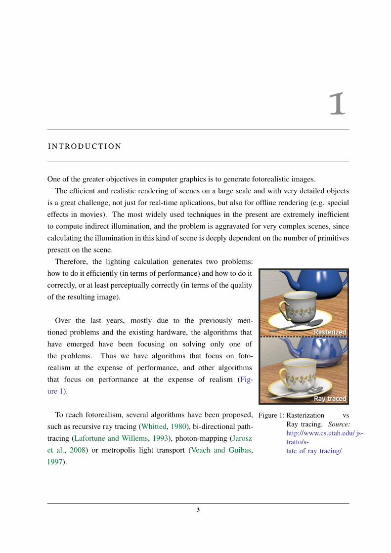
Figure 1: Rasterization vsRay tracing. Source:http://www.cs.utah.edu/ js-tratto/s-tate of ray tracing/
Therefore, the lighting calculation generates two problems:how to do it efficiently (in terms of performance) and how to do itcorrectly, or at least perceptually correctly (in terms of the qualityof the resulting image).
Over the last years, mostly due to the previously men-tioned problems and the existing hardware, the algorithms thathave emerged have been focusing on solving only one ofthe problems. Thus we have algorithms that focus on foto-realism at the expense of performance, and other algorithmsthat focus on performance at the expense of realism (Fig-ure 1).
To reach fotorealism, several algorithms have been proposed,such as recursive ray tracing (Whitted, 1980), bi-directional path-tracing (Lafortune and Willems, 1993), photon-mapping (Jaroszet al., 2008) or metropolis light transport (Veach and Guibas,1997).
3
However, all these algorithms share a drawback: their performance. All these algorithms tryto mimic the interactions of light rays between the objects in a scene, reflecting and refracting thephotons according to the characteristics of the materials of each object. This kind of simulationis very computationally expensive, existing however some implementations that can generateseveral frames per second and with a very good graphic result (e.g. Brigade 3).
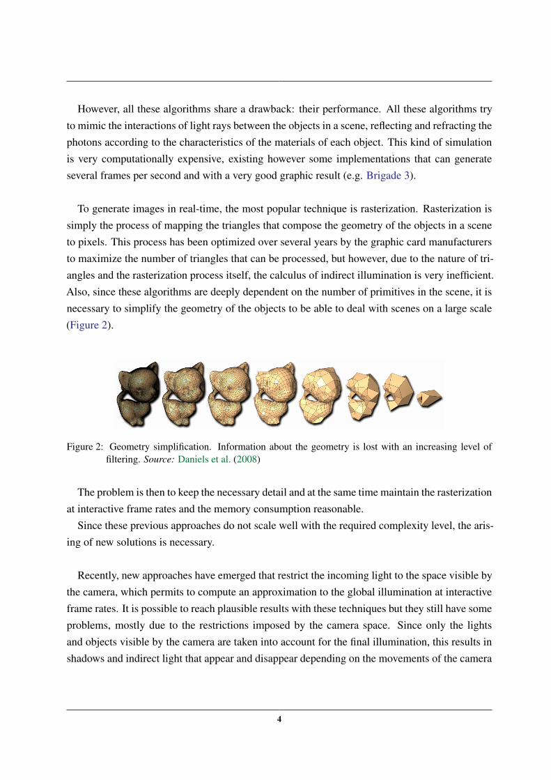
To generate images in real-time, the most popular technique is rasterization. Rasterization issimply the process of mapping the triangles that compose the geometry of the objects in a sceneto pixels. This process has been optimized over several years by the graphic card manufacturersto maximize the number of triangles that can be processed, but however, due to the nature of tri-angles and the rasterization process itself, the calculus of indirect illumination is very inefficient.Also, since these algorithms are deeply dependent on the number of primitives in the scene, it isnecessary to simplify the geometry of the objects to be able to deal with scenes on a large scale(Figure 2).
Figure 2: Geometry simplification. Information about the geometry is lost with an increasing level offiltering. Source: Daniels et al. (2008)
The problem is then to keep the necessary detail and at the same time maintain the rasterizationat interactive frame rates and the memory consumption reasonable.
Since these previous approaches do not scale well with the required complexity level, the aris-ing of new solutions is necessary.
Recently, new approaches have emerged that restrict the incoming light to the space visible bythe camera, which permits to compute an approximation to the global illumination at interactiveframe rates. It is possible to reach plausible results with these techniques but they still have someproblems, mostly due to the restrictions imposed by the camera space. Since only the lightsand objects visible by the camera are taken into account for the final illumination, this results inshadows and indirect light that appear and disappear depending on the movements of the camera
4
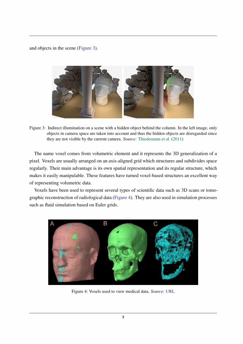
and objects in the scene (Figure 3).
Figure 3: Indirect illumination on a scene with a hidden object behind the column. In the left image, onlyobjects in camera space are taken into account and thus the hidden objects are disregarded sincethey are not visible by the current camera. Source: Thiedemann et al. (2011)
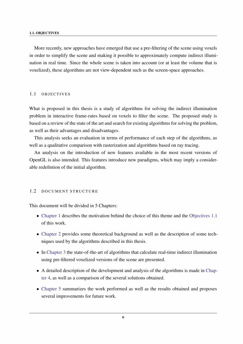
The name voxel comes from volumetric element and it represents the 3D generalization of apixel. Voxels are usually arranged on an axis-aligned grid which structures and subdivides spaceregularly. Their main advantage is its own spatial representation and its regular structure, whichmakes it easily manipulable. These features have turned voxel-based structures an excellent wayof representing volumetric data.
Voxels have been used to represent several types of scientific data such as 3D scans or tomo-graphic reconstruction of radiological data (Figure 4). They are also used in simulation processessuch as fluid simulation based on Euler grids.
Figure 4: Voxels used to view medical data. Source: URL
5
1.1. OBJECTIVES
More recently, new approaches have emerged that use a pre-filtering of the scene using voxelsin order to simplify the scene and making it possible to approximately compute indirect illumi-nation in real time. Since the whole scene is taken into account (or at least the volume that isvoxelized), these algorithms are not view-dependent such as the screen-space approaches.
1.1 O B J E C T I V E S
What is proposed in this thesis is a study of algorithms for solving the indirect illuminationproblem in interactive frame-rates based on voxels to filter the scene. The proposed study isbased on a review of the state of the art and search for existing algorithms for solving the problem,as well as their advantages and disadvantages.
This analysis seeks an evaluation in terms of performance of each step of the algorithms, aswell as a qualitative comparison with rasterization and algorithms based on ray tracing.
An analysis on the introduction of new features available in the most recent versions ofOpenGL is also intended. This features introduce new paradigms, which may imply a consider-able redefintion of the initial algorithm.
1.2 D O C U M E N T S T RU C T U R E
This document will be divided in 5 Chapters:
• Chapter 1 describes the motivation behind the choice of this theme and the Objectives 1.1of this work.
• Chapter 2 provides some theoretical background as well as the description of some tech-niques used by the algorithms described in this thesis.
• In Chapter 3 the state-of-the-art of algorithms that calculate real-time indirect illuminationusing pre-filtered voxelized versions of the scene are presented.
• A detailed description of the development and analysis of the algorithms is made in Chap-ter 4, as well as a comparison of the several solutions obtained.
• Chapter 5 summarizes the work performed as well as the results obtained and proposesseveral improvements for future work.
6
2
R E L AT E D W O R K
2.1 S H A D O W M A P P I N G
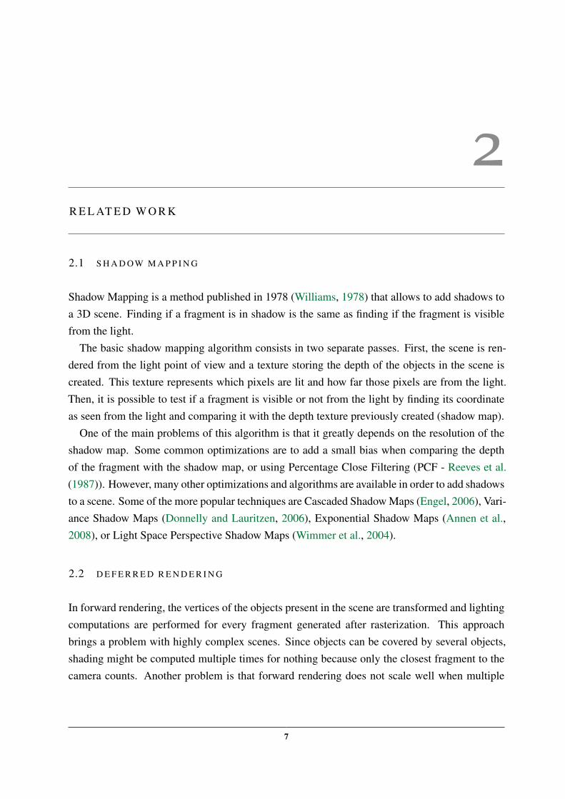
Shadow Mapping is a method published in 1978 (Williams, 1978) that allows to add shadows toa 3D scene. Finding if a fragment is in shadow is the same as finding if the fragment is visiblefrom the light.
The basic shadow mapping algorithm consists in two separate passes. First, the scene is ren-dered from the light point of view and a texture storing the depth of the objects in the scene iscreated. This texture represents which pixels are lit and how far those pixels are from the light.Then, it is possible to test if a fragment is visible or not from the light by finding its coordinateas seen from the light and comparing it with the depth texture previously created (shadow map).
One of the main problems of this algorithm is that it greatly depends on the resolution of theshadow map. Some common optimizations are to add a small bias when comparing the depthof the fragment with the shadow map, or using Percentage Close Filtering (PCF - Reeves et al.(1987)). However, many other optimizations and algorithms are available in order to add shadowsto a scene. Some of the more popular techniques are Cascaded Shadow Maps (Engel, 2006), Vari-ance Shadow Maps (Donnelly and Lauritzen, 2006), Exponential Shadow Maps (Annen et al.,2008), or Light Space Perspective Shadow Maps (Wimmer et al., 2004).
2.2 D E F E R R E D R E N D E R I N G
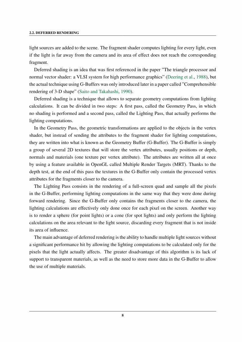
In forward rendering, the vertices of the objects present in the scene are transformed and lightingcomputations are performed for every fragment generated after rasterization. This approachbrings a problem with highly complex scenes. Since objects can be covered by several objects,shading might be computed multiple times for nothing because only the closest fragment to thecamera counts. Another problem is that forward rendering does not scale well when multiple
7
2.2. DEFERRED RENDERING
light sources are added to the scene. The fragment shader computes lighting for every light, evenif the light is far away from the camera and its area of effect does not reach the correspondingfragment.
Deferred shading is an idea that was first referenced in the paper ”The triangle processor andnormal vector shader: a VLSI system for high performance graphics” (Deering et al., 1988), butthe actual technique using G-Buffers was only introduced later in a paper called ”Comprehensiblerendering of 3-D shape” (Saito and Takahashi, 1990).
Deferred shading is a technique that allows to separate geometry computations from lightingcalculations. It can be divided in two steps: A first pass, called the Geometry Pass, in whichno shading is performed and a second pass, called the Lighting Pass, that actually performs thelighting computations.
In the Geometry Pass, the geometric transformations are applied to the objects in the vertexshader, but instead of sending the attributes to the fragment shader for lighting computations,they are written into what is known as the Geometry Buffer (G-Buffer). The G-Buffer is simplya group of several 2D textures that will store the vertex attributes, usually positions or depth,normals and materials (one texture per vertex attribute). The attributes are written all at onceby using a feature available in OpenGL called Multiple Render Targets (MRT). Thanks to thedepth test, at the end of this pass the textures in the G-Buffer only contain the processed vertexattributes for the fragments closer to the camera.
The Lighting Pass consists in the rendering of a full-screen quad and sample all the pixelsin the G-Buffer, performing lighting computations in the same way that they were done duringforward rendering. Since the G-Buffer only contains the fragments closer to the camera, thelighting calculations are effectively only done once for each pixel on the screen. Another wayis to render a sphere (for point lights) or a cone (for spot lights) and only perform the lightingcalculations on the area relevant to the light source, discarding every fragment that is not insideits area of influence.
The main advantage of deferred rendering is the ability to handle multiple light sources withouta significant performance hit by allowing the lighting computations to be calculated only for thepixels that the light actually affects. The greater disadvantage of this algorithm is its lack ofsupport to transparent materials, as well as the need to store more data in the G-Buffer to allowthe use of multiple materials.
8
2.3. REFLECTIVE SHADOW MAPS
2.3 R E F L E C T I V E S H A D O W M A P S
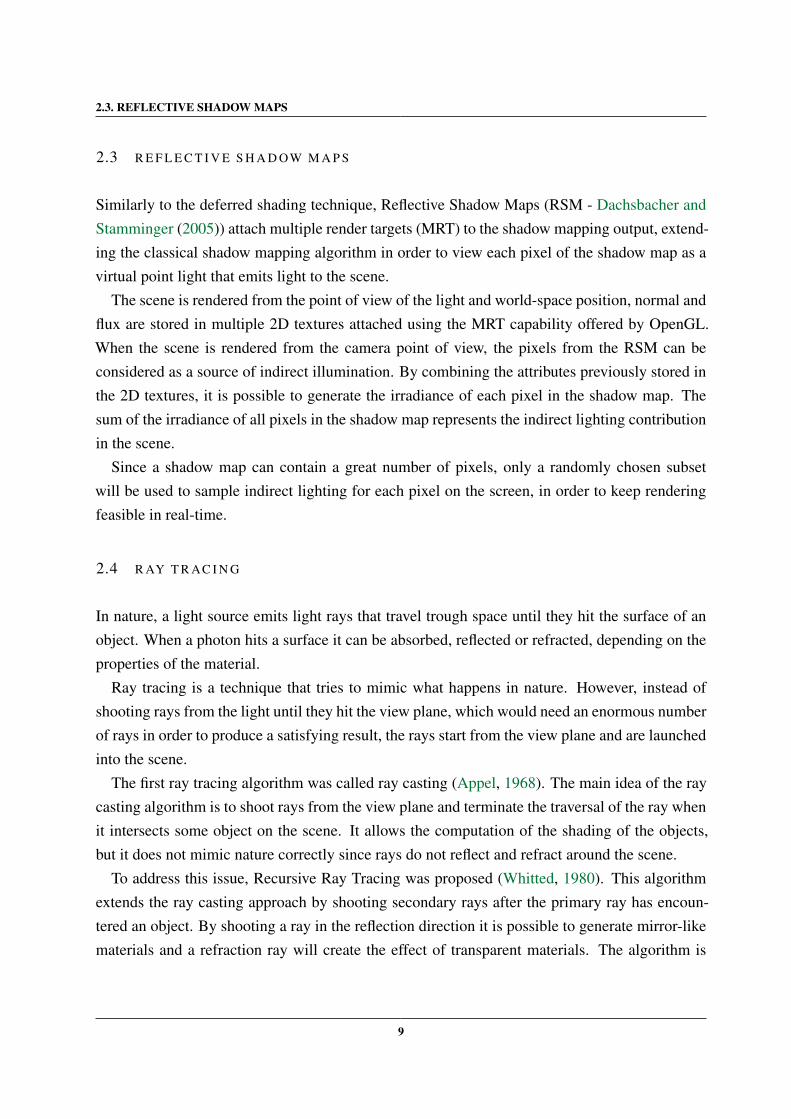
Similarly to the deferred shading technique, Reflective Shadow Maps (RSM - Dachsbacher andStamminger (2005)) attach multiple render targets (MRT) to the shadow mapping output, extend-ing the classical shadow mapping algorithm in order to view each pixel of the shadow map as avirtual point light that emits light to the scene.
The scene is rendered from the point of view of the light and world-space position, normal andflux are stored in multiple 2D textures attached using the MRT capability offered by OpenGL.When the scene is rendered from the camera point of view, the pixels from the RSM can beconsidered as a source of indirect illumination. By combining the attributes previously stored inthe 2D textures, it is possible to generate the irradiance of each pixel in the shadow map. Thesum of the irradiance of all pixels in the shadow map represents the indirect lighting contributionin the scene.
Since a shadow map can contain a great number of pixels, only a randomly chosen subsetwill be used to sample indirect lighting for each pixel on the screen, in order to keep renderingfeasible in real-time.
2.4 R AY T R AC I N G
In nature, a light source emits light rays that travel trough space until they hit the surface of anobject. When a photon hits a surface it can be absorbed, reflected or refracted, depending on theproperties of the material.
Ray tracing is a technique that tries to mimic what happens in nature. However, instead ofshooting rays from the light until they hit the view plane, which would need an enormous numberof rays in order to produce a satisfying result, the rays start from the view plane and are launchedinto the scene.
The first ray tracing algorithm was called ray casting (Appel, 1968). The main idea of the raycasting algorithm is to shoot rays from the view plane and terminate the traversal of the ray whenit intersects some object on the scene. It allows the computation of the shading of the objects,but it does not mimic nature correctly since rays do not reflect and refract around the scene.
To address this issue, Recursive Ray Tracing was proposed (Whitted, 1980). This algorithmextends the ray casting approach by shooting secondary rays after the primary ray has encoun-tered an object. By shooting a ray in the reflection direction it is possible to generate mirror-likematerials and a refraction ray will create the effect of transparent materials. The algorithm is
9
2.4. RAY TRACING
recursive, which means it is possible to continue the traversal of the rays after hitting multipleobjects, rendering multiple reflections.
Apart from the rendering time, these ray tracing approaches also suffer from problems relatedto aliasing and sampling. The problem is that shooting only one ray per pixel on the screen fails tocapture enough information in order to produce an anti-aliased output. One common solution tothis problem is using multisampling and sample each pixel multiple times with different offsets,instead of always shooting rays trough the center of the pixels. However this increases even morethe amount of computation needed for the algorithm.
Cone Tracing (Amanatides, 1984) was proposed as a solution that allowed to perform anti-aliasing with only one ray per pixel. The main idea is to shoot cones trough the screen insteadof rays, by attaching the angle of spread and virtual origin of the ray to its previous definition,which only included its origin and direction. The pixels on the screen are viewed as an area ofthe screen instead of a point, and setting the angle of spread of the cone such that it covers theentire pixel on the view plane will guarantee that no information is lost during the intersectionprocess, producing an anti-aliased image. However, calculating the intersections between conesand objects is complex. The intersection test must not return only information about whether thecone has intersected any object, but also the fraction of the cone that is blocked by the object.
Since then, multiple algorithms have been proposed to speed the rendering process or generatea higher quality rendering such as Bi-Directional Path Tracing (Lafortune and Willems, 1993),Photon-Mapping (Jensen, 1996) or Metropolis Light Transport (Veach and Guibas, 1997).
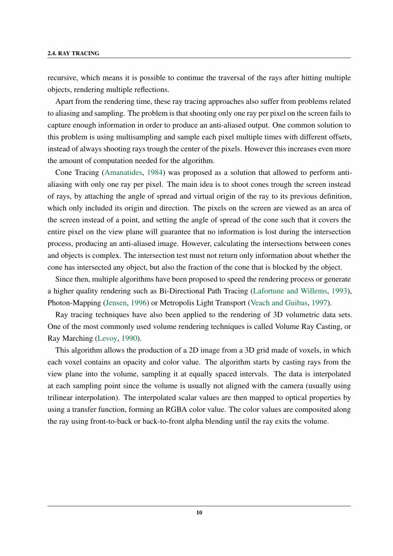
Ray tracing techniques have also been applied to the rendering of 3D volumetric data sets.One of the most commonly used volume rendering techniques is called Volume Ray Casting, orRay Marching (Levoy, 1990).
This algorithm allows the production of a 2D image from a 3D grid made of voxels, in whicheach voxel contains an opacity and color value. The algorithm starts by casting rays from theview plane into the volume, sampling it at equally spaced intervals. The data is interpolatedat each sampling point since the volume is usually not aligned with the camera (usually usingtrilinear interpolation). The interpolated scalar values are then mapped to optical properties byusing a transfer function, forming an RGBA color value. The color values are composited alongthe ray using front-to-back or back-to-front alpha blending until the ray exits the volume.
10
2.5. VOXELIZATION
2.5 VOX E L I Z AT I O N
Voxelization or 3D scan conversion is the process of mapping a 3D object made of polygonsinto a 3D axis aligned grid, obtaining a volumetric representation of the object made of voxels.The term ’voxelization’ was first referenced on the paper ”3D scan-conversion algorithms forvoxel-based graphics” (Kaufman and Shimony, 1987). Since then, multiple approaches havebeen proposed to convert the surface of a triangle-based model into a voxel-based representationstored as a voxel grid (Eisemann and Decoret, 2008; Zhang et al., 2007; Dong et al., 2004).These can be classified in two categories: surface voxelization algorithms and solid voxelizationalgorithms.
On surface voxelization, only the voxels that are touched by the triangles are set, thus creatinga representation of the surface of the object. Solid voxelization demands a closed object since italso sets the voxels that are considered interior to the object (using a scanline fill algorithm forexample).
The voxelization process can store multiple values on the voxel grid (or grids), such as colorand normal values of the voxelized model, or simply store an occupancy value (0 or 1), in whichcase it is usually referenced as a binary voxelization.
11
3
R E A L - T I M E VOX E L - BA S E D G L O BA L I L L U M I NAT I O NA L G O R I T H M S
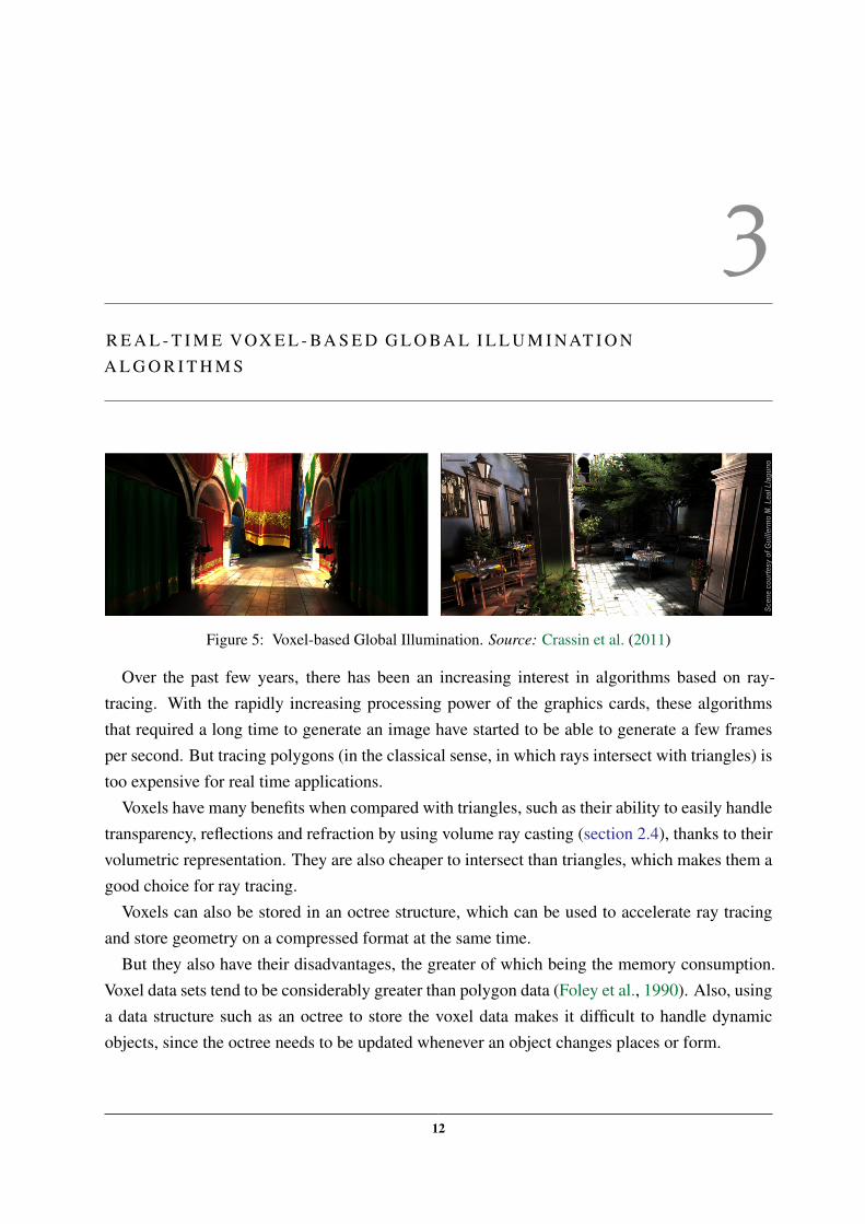
Figure 5: Voxel-based Global Illumination. Source: Crassin et al. (2011)
Over the past few years, there has been an increasing interest in algorithms based on ray-tracing. With the rapidly increasing processing power of the graphics cards, these algorithmsthat required a long time to generate an image have started to be able to generate a few framesper second. But tracing polygons (in the classical sense, in which rays intersect with triangles) istoo expensive for real time applications.
Voxels have many benefits when compared with triangles, such as their ability to easily handletransparency, reflections and refraction by using volume ray casting (section 2.4), thanks to theirvolumetric representation. They are also cheaper to intersect than triangles, which makes them agood choice for ray tracing.
Voxels can also be stored in an octree structure, which can be used to accelerate ray tracingand store geometry on a compressed format at the same time.
But they also have their disadvantages, the greater of which being the memory consumption.Voxel data sets tend to be considerably greater than polygon data (Foley et al., 1990). Also, usinga data structure such as an octree to store the voxel data makes it difficult to handle dynamicobjects, since the octree needs to be updated whenever an object changes places or form.
12
3.1. INTERACTIVE INDIRECT ILLUMINATION USING VOXEL CONE TRACING
Voxels have been used for diverse applications, such as fluid simulation (Crane et al., 2007)and collision detection (Allard et al., 2010), but recently new algorithms for computing globalillumination in real time have been introduced. These algorithms are very similar in their struc-ture, as will be demonstrated in the following chapter. These algorithms start by voxelizing thescene, storing voxel data into some data structure and then use this structure to compute an ap-proximation of the light interactions between the objects in the scene by utilizing a ray-tracingbased approach (Figure 5).
There are several algorithms and data structures to perform each of these steps, each of themwith advantages and disadvantages, but this dissertation will be focused on the recent algorithmsfor computing global illumination in real time.
3.1 I N T E R AC T I V E I N D I R E C T I L L U M I N AT I O N U S I N G VOX E L C O N E T R AC I N G
In order to maintain the performance, data storage, and rendering quality scalable with the com-plexity of the scene geometry, we need a way to pre-filter the appearance of the objects on thescene. Pre-filtering not just the textures but the geometry as well will provide a scalable solutionto compute global illumination, only dependent on the rendering resolution, scaling with verycomplex scenes (Crassin et al., 2011).
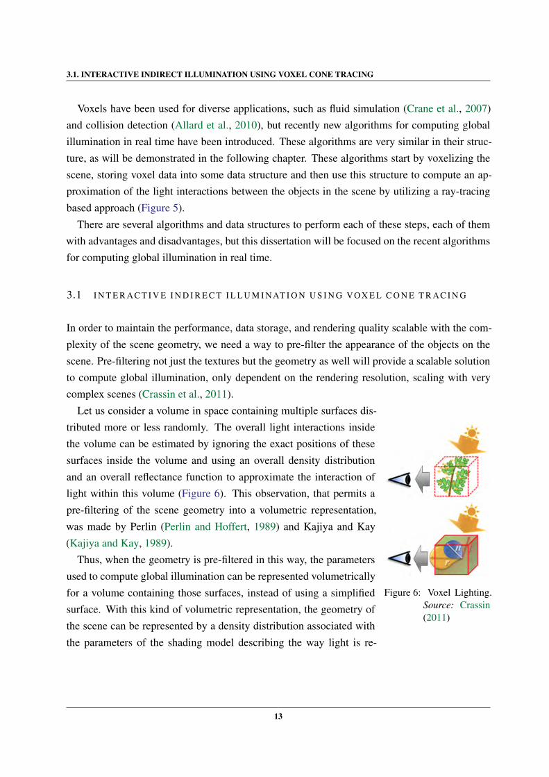
Figure 6: Voxel Lighting.Source: Crassin(2011)
Let us consider a volume in space containing multiple surfaces dis-tributed more or less randomly. The overall light interactions insidethe volume can be estimated by ignoring the exact positions of thesesurfaces inside the volume and using an overall density distributionand an overall reflectance function to approximate the interaction oflight within this volume (Figure 6). This observation, that permits apre-filtering of the scene geometry into a volumetric representation,was made by Perlin (Perlin and Hoffert, 1989) and Kajiya and Kay(Kajiya and Kay, 1989).
Thus, when the geometry is pre-filtered in this way, the parametersused to compute global illumination can be represented volumetricallyfor a volume containing those surfaces, instead of using a simplifiedsurface. With this kind of volumetric representation, the geometry ofthe scene can be represented by a density distribution associated withthe parameters of the shading model describing the way light is re-
13
3.1. INTERACTIVE INDIRECT ILLUMINATION USING VOXEL CONE TRACING
flected inside a volume. One of the main advantages of transforming geometry in density distri-butions is that filtering this kind of distribution is turned into a linear operation (Neyret, 1998).
This linear filtering is important since it allows us to obtain a multiresolution representationof the voxel grid based on mipmapping, making it possible to automatically control the level ofdetail by sampling to different mipmap levels of the voxel grid.
The general idea of this technique is to pre-filter the scene using a voxel representation (3.1.1)and store the values in a sparse octree structure in order to get a hierarchical representation of thescene (3.1.2). The leaves of the octree will contain the data at maximum resolution and all theupper levels of the octree will mipmap the lower levels to generate data at different resolutions(3.1.3), thereby obtaining the basis for controlling the level of detail based on the distance fromthe camera.
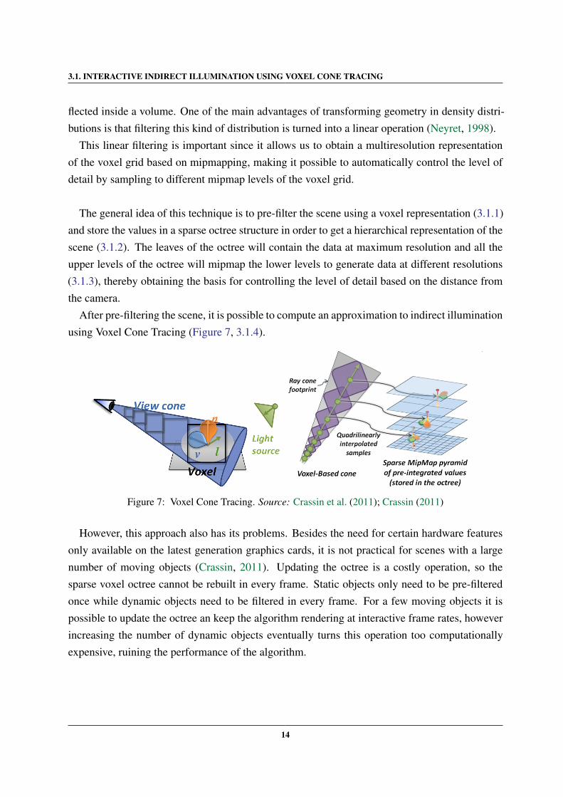
After pre-filtering the scene, it is possible to compute an approximation to indirect illuminationusing Voxel Cone Tracing (Figure 7, 3.1.4).
Figure 7: Voxel Cone Tracing. Source: Crassin et al. (2011); Crassin (2011)
However, this approach also has its problems. Besides the need for certain hardware featuresonly available on the latest generation graphics cards, it is not practical for scenes with a largenumber of moving objects (Crassin, 2011). Updating the octree is a costly operation, so thesparse voxel octree cannot be rebuilt in every frame. Static objects only need to be pre-filteredonce while dynamic objects need to be filtered in every frame. For a few moving objects it ispossible to update the octree an keep the algorithm rendering at interactive frame rates, howeverincreasing the number of dynamic objects eventually turns this operation too computationallyexpensive, ruining the performance of the algorithm.
14
3.1. INTERACTIVE INDIRECT ILLUMINATION USING VOXEL CONE TRACING
The update of dynamic elements in this kind of data structures is a problem that still needs tobe solved and new approaches to update these structures in a faster way need to emerge, or newdata structures that are more rapidly updated while keeping the advantages offered by octrees.
3.1.1 Voxelization
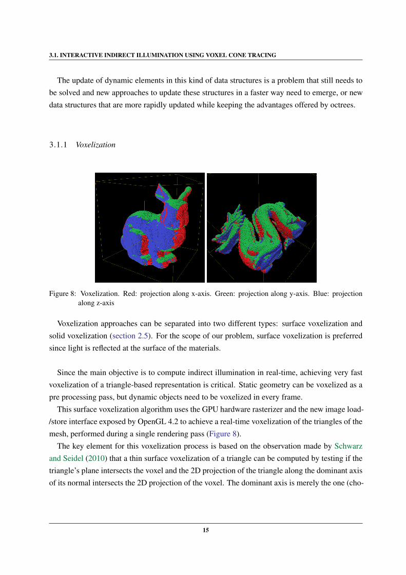
Figure 8: Voxelization. Red: projection along x-axis. Green: projection along y-axis. Blue: projectionalong z-axis
Voxelization approaches can be separated into two different types: surface voxelization andsolid voxelization (section 2.5). For the scope of our problem, surface voxelization is preferredsince light is reflected at the surface of the materials.
Since the main objective is to compute indirect illumination in real-time, achieving very fastvoxelization of a triangle-based representation is critical. Static geometry can be voxelized as apre processing pass, but dynamic objects need to be voxelized in every frame.
This surface voxelization algorithm uses the GPU hardware rasterizer and the new image load-/store interface exposed by OpenGL 4.2 to achieve a real-time voxelization of the triangles of themesh, performed during a single rendering pass (Figure 8).
The key element for this voxelization process is based on the observation made by Schwarzand Seidel (2010) that a thin surface voxelization of a triangle can be computed by testing if thetriangle’s plane intersects the voxel and the 2D projection of the triangle along the dominant axisof its normal intersects the 2D projection of the voxel. The dominant axis is merely the one (cho-
15
3.1. INTERACTIVE INDIRECT ILLUMINATION USING VOXEL CONE TRACING
sen from the three main axes of the scene) that maximizes the surface of the projected triangle.
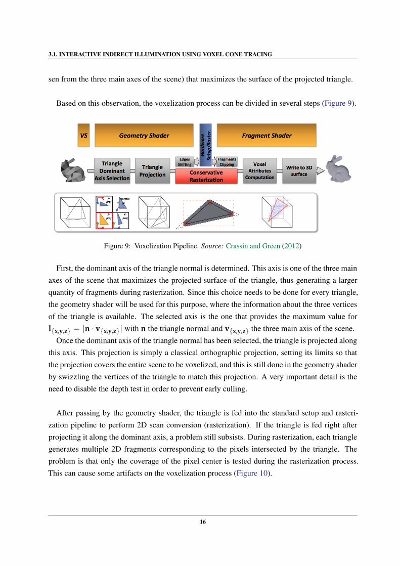
Based on this observation, the voxelization process can be divided in several steps (Figure 9).
Figure 9: Voxelization Pipeline. Source: Crassin and Green (2012)
First, the dominant axis of the triangle normal is determined. This axis is one of the three mainaxes of the scene that maximizes the projected surface of the triangle, thus generating a largerquantity of fragments during rasterization. Since this choice needs to be done for every triangle,the geometry shader will be used for this purpose, where the information about the three verticesof the triangle is available. The selected axis is the one that provides the maximum value forlx,y,z = |n · vx,y,z| with n the triangle normal and vx,y,z the three main axis of the scene.
Once the dominant axis of the triangle normal has been selected, the triangle is projected alongthis axis. This projection is simply a classical orthographic projection, setting its limits so thatthe projection covers the entire scene to be voxelized, and this is still done in the geometry shaderby swizzling the vertices of the triangle to match this projection. A very important detail is theneed to disable the depth test in order to prevent early culling.
After passing by the geometry shader, the triangle is fed into the standard setup and rasteri-zation pipeline to perform 2D scan conversion (rasterization). If the triangle is fed right afterprojecting it along the dominant axis, a problem still subsists. During rasterization, each trianglegenerates multiple 2D fragments corresponding to the pixels intersected by the triangle. Theproblem is that only the coverage of the pixel center is tested during the rasterization process.This can cause some artifacts on the voxelization process (Figure 10).
16
3.1. INTERACTIVE INDIRECT ILLUMINATION USING VOXEL CONE TRACING
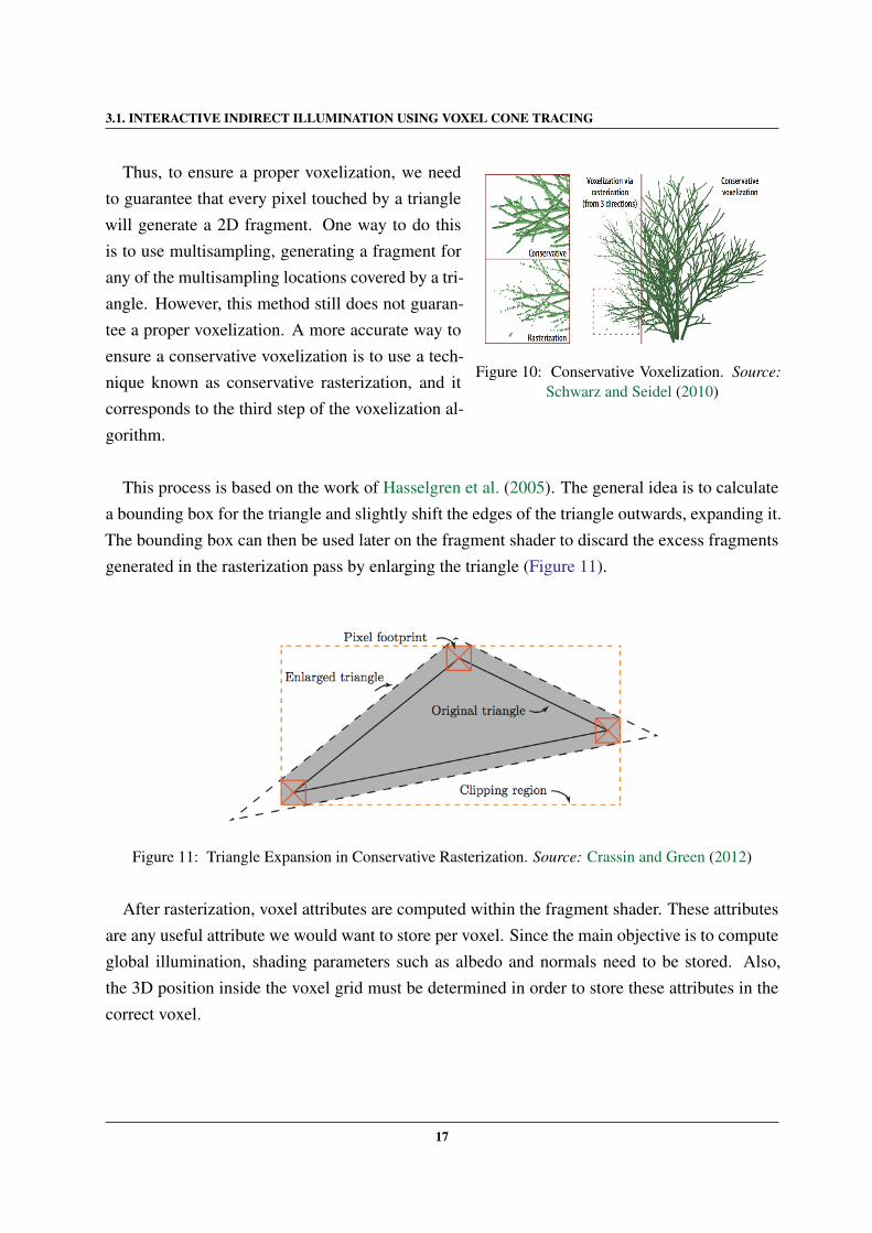
Figure 10: Conservative Voxelization. Source:Schwarz and Seidel (2010)
Thus, to ensure a proper voxelization, we needto guarantee that every pixel touched by a trianglewill generate a 2D fragment. One way to do thisis to use multisampling, generating a fragment forany of the multisampling locations covered by a tri-angle. However, this method still does not guaran-tee a proper voxelization. A more accurate way toensure a conservative voxelization is to use a tech-nique known as conservative rasterization, and itcorresponds to the third step of the voxelization al-gorithm.
This process is based on the work of Hasselgren et al. (2005). The general idea is to calculatea bounding box for the triangle and slightly shift the edges of the triangle outwards, expanding it.The bounding box can then be used later on the fragment shader to discard the excess fragmentsgenerated in the rasterization pass by enlarging the triangle (Figure 11).
Figure 11: Triangle Expansion in Conservative Rasterization. Source: Crassin and Green (2012)
After rasterization, voxel attributes are computed within the fragment shader. These attributesare any useful attribute we would want to store per voxel. Since the main objective is to computeglobal illumination, shading parameters such as albedo and normals need to be stored. Also,the 3D position inside the voxel grid must be determined in order to store these attributes in thecorrect voxel.
17
3.1. INTERACTIVE INDIRECT ILLUMINATION USING VOXEL CONE TRACING
This generates voxel fragments. A voxel fragment is the 3D generalization of the 2D fragmentand corresponds to a voxel intersected by a triangle.
Once the voxel fragments are generated, they can be written into a buffer using image load/-store operations, generating a voxel fragment list. This voxel fragment list is a linear vector ofentries stored inside a preallocated buffer object. It contains several arrays of values, one con-taining the 3D coordinate of each voxel fragment, and all the others containing the attributes wewant to store for each voxel. To manage this list, a counter of the number of fragments of the listis maintained as a single value stored inside another buffer object and updated with an atomiccounter.
Since we want to generate fragments corresponding to the maximum resolution of the octree,the viewport resolution is set to match the lateral resolution of the voxel grid (e.g. 512× 512 fora 5123 grid). Also, all framebuffer operations can be disabled since image access is used to writethe voxel data.
3.1.2 Sparse Voxel Octree
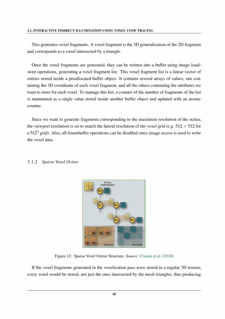
Figure 12: Sparse Voxel Octree Structure. Source: Crassin et al. (2010)
If the voxel fragments generated in the voxelization pass were stored in a regular 3D texture,every voxel would be stored, not just the ones intersected by the mesh triangles, thus producing
18
3.1. INTERACTIVE INDIRECT ILLUMINATION USING VOXEL CONE TRACING
a full grid and wasting a lot of memory with empty voxels. In order to handle large and complexscenes, there is a need to use an efficient data structure to handle the voxels.
The data structure chosen is a Sparse Voxel Octree (Crassin et al., 2009; Laine and Karras,2010), which has several benefits in this context, such as storing only the voxels that are inter-sected by mesh triangles and providing a hierarchical representation of the scene, which is veryuseful for the LOD control mechanism.
The sparse voxel octree is a very compact pointer-based structure (Figure 12). The root nodeof the tree represents the entire scene and each of its children represents an eight of its volume.
Octree nodes are organized as 2× 2× 2 node tiles stored on linear video memory.In order to efficiently distribute the direct illumination over all levels of the octree afterwards,
the structure also has neighbor pointers, allowing to rapidly visit neighboring nodes and the par-ent node.
Figure 13: Voxel Brick. Source:Crassin et al. (2011)
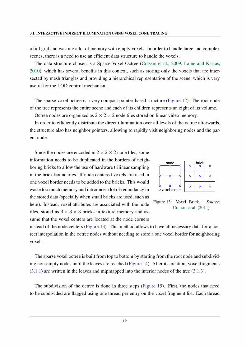
Since the nodes are encoded in 2× 2× 2 node tiles, someinformation needs to be duplicated in the borders of neigh-boring bricks to allow the use of hardware trilinear samplingin the brick boundaries. If node centered voxels are used, aone voxel border needs to be added to the bricks. This wouldwaste too much memory and introduce a lot of redundancy inthe stored data (specially when small bricks are used, such ashere). Instead, voxel attributes are associated with the nodetiles, stored as 3× 3× 3 bricks in texture memory and as-sume that the voxel centers are located at the node cornersinstead of the node centers (Figure 13). This method allows to have all necessary data for a cor-rect interpolation in the octree nodes without needing to store a one voxel border for neighboringvoxels.
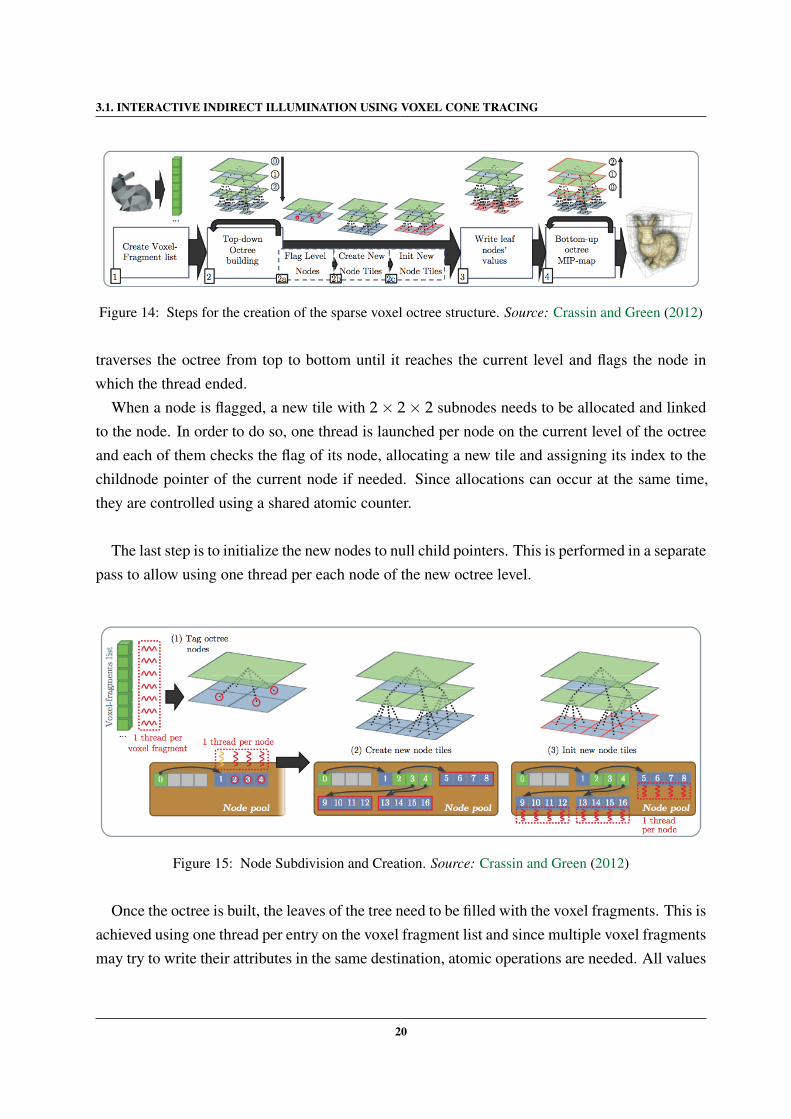
The sparse voxel octree is built from top to bottom by starting from the root node and subdivid-ing non-empty nodes until the leaves are reached (Figure 14). After its creation, voxel fragments(3.1.1) are written in the leaves and mipmapped into the interior nodes of the tree (3.1.3).
The subdivision of the octree is done in three steps (Figure 15). First, the nodes that needto be subdivided are flagged using one thread per entry on the voxel fragment list. Each thread
19
3.1. INTERACTIVE INDIRECT ILLUMINATION USING VOXEL CONE TRACING
Figure 14: Steps for the creation of the sparse voxel octree structure. Source: Crassin and Green (2012)
traverses the octree from top to bottom until it reaches the current level and flags the node inwhich the thread ended.
When a node is flagged, a new tile with 2× 2× 2 subnodes needs to be allocated and linkedto the node. In order to do so, one thread is launched per node on the current level of the octreeand each of them checks the flag of its node, allocating a new tile and assigning its index to thechildnode pointer of the current node if needed. Since allocations can occur at the same time,they are controlled using a shared atomic counter.
The last step is to initialize the new nodes to null child pointers. This is performed in a separatepass to allow using one thread per each node of the new octree level.
Figure 15: Node Subdivision and Creation. Source: Crassin and Green (2012)
Once the octree is built, the leaves of the tree need to be filled with the voxel fragments. This isachieved using one thread per entry on the voxel fragment list and since multiple voxel fragmentsmay try to write their attributes in the same destination, atomic operations are needed. All values
20
3.1. INTERACTIVE INDIRECT ILLUMINATION USING VOXEL CONE TRACING
falling in the same destination voxel will be averaged. To do so, all values are added using anatomic add operation, updating at the same time a counter, so that the summed value can then bedivided by the counter value in a subsequent pass.
After the sparse voxel octree has its leaves filled with the voxel fragments, these values aremipmapped into the interior nodes of the tree (3.1.3).
Dynamic and static objects are both stored in the same sparse voxel octree structure for aneasy traversal and unified filtering. Since fully dynamic objects need to be revoxelized everyframe and static or semi-static objects only need to be revoxelized when needed, a time-stampmechanism is used in order to differentiate each type of object and prevent overwriting of staticnodes and bricks.
3.1.3 Mipmapping
In order to generate an hierarchic representation of the voxel grid, the leaves of the sparse voxeloctree are mipmapped into the upper levels. The interior nodes of the sparse voxel octree struc-ture are filled from bottom to top, in n-1 steps for an octree with n levels. At each step, onethread is used to average the values contained in the eight subnodes of each non empty node inthe current level.
Figure 16: Mipmapping WeightingKernel. Source: Crassinet al. (2011)
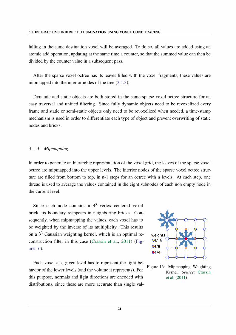
Since each node contains a 33 vertex centered voxelbrick, its boundary reappears in neighboring bricks. Con-sequently, when mipmapping the values, each voxel has tobe weighted by the inverse of its multiplicity. This resultson a 33 Gaussian weighting kernel, which is an optimal re-construction filter in this case (Crassin et al., 2011) (Fig-ure 16).
Each voxel at a given level has to represent the light be-havior of the lower levels (and the volume it represents). Forthis purpose, normals and light directions are encoded withdistributions, since these are more accurate than single val-
21
3.1. INTERACTIVE INDIRECT ILLUMINATION USING VOXEL CONE TRACING
ues (Han et al., 2007). However, to reduce the memory footprint, these distributions are notstored using spherical harmonics. Instead, Gaussian lobes characterized by an average vector Dand a standard deviation σ are used. To ease the interpolation, the variance is encoded using thenorm |D| such that σ2 = 1−|D|
|D| (Toksvig, 2005). For example, the Normal Distribution Function(NDF) can be computed from the length of the averaged normal vector |N| stored in the voxelsand σ2
n = 1−|N||N| .
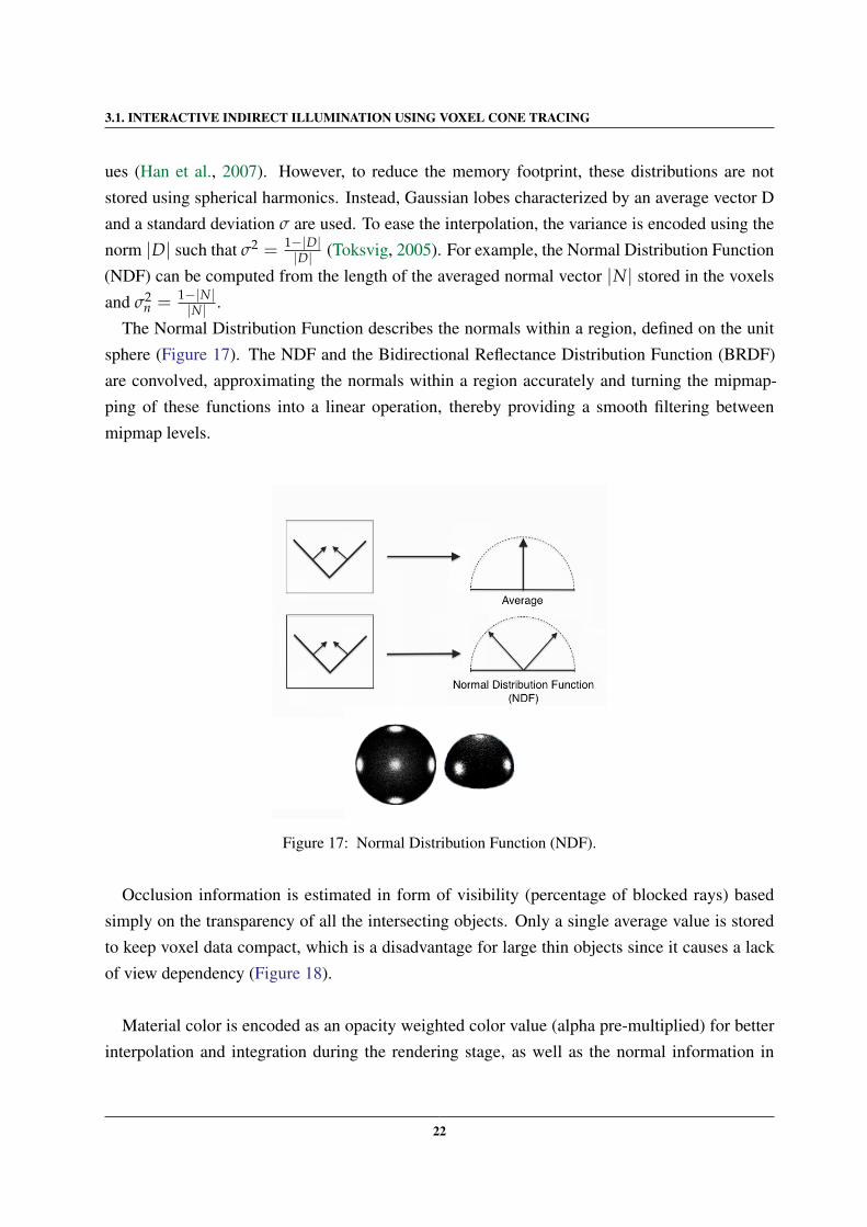
The Normal Distribution Function describes the normals within a region, defined on the unitsphere (Figure 17). The NDF and the Bidirectional Reflectance Distribution Function (BRDF)are convolved, approximating the normals within a region accurately and turning the mipmap-ping of these functions into a linear operation, thereby providing a smooth filtering betweenmipmap levels.
Figure 17: Normal Distribution Function (NDF).
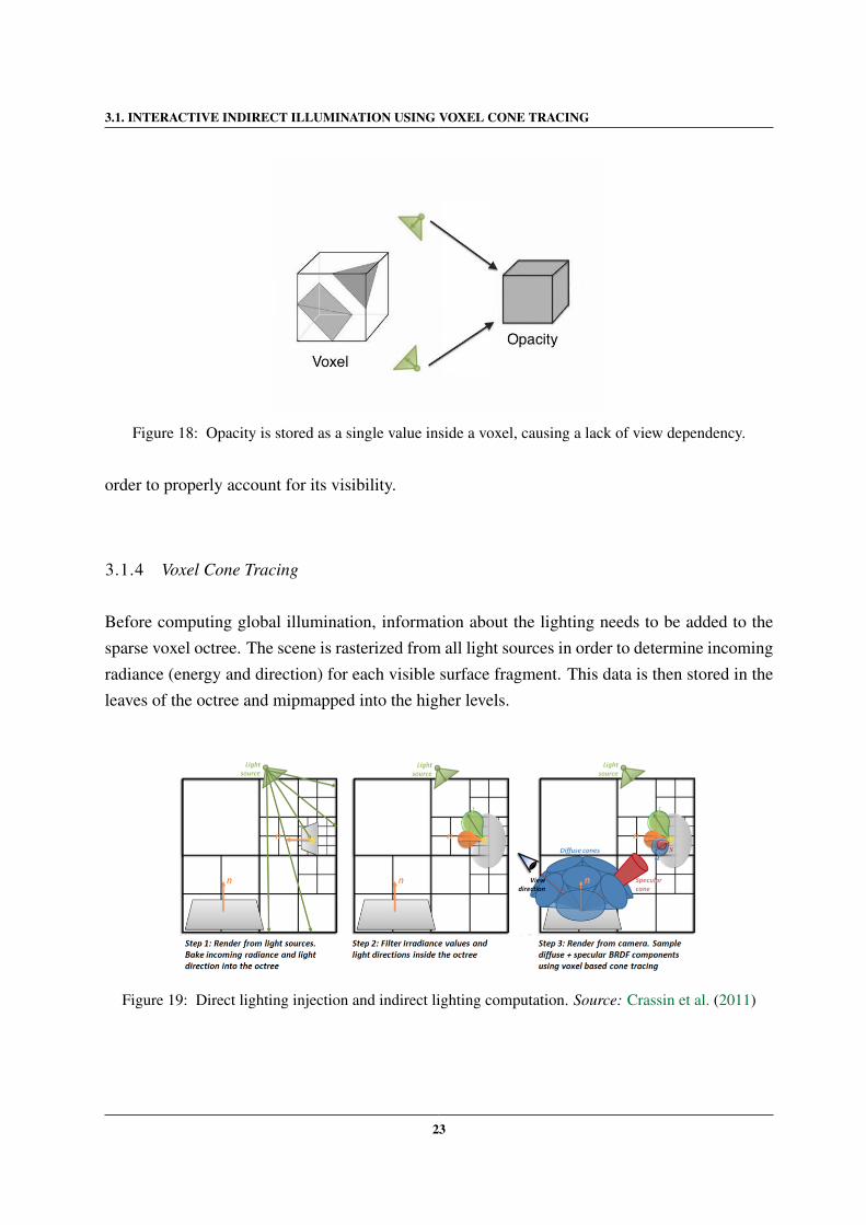
Occlusion information is estimated in form of visibility (percentage of blocked rays) basedsimply on the transparency of all the intersecting objects. Only a single average value is storedto keep voxel data compact, which is a disadvantage for large thin objects since it causes a lackof view dependency (Figure 18).
Material color is encoded as an opacity weighted color value (alpha pre-multiplied) for betterinterpolation and integration during the rendering stage, as well as the normal information in
22
3.1. INTERACTIVE INDIRECT ILLUMINATION USING VOXEL CONE TRACING
Figure 18: Opacity is stored as a single value inside a voxel, causing a lack of view dependency.
order to properly account for its visibility.
3.1.4 Voxel Cone Tracing
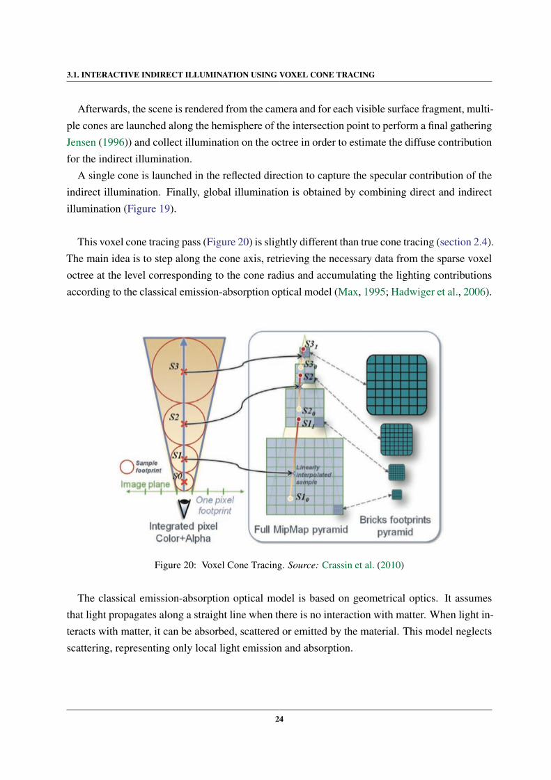
Before computing global illumination, information about the lighting needs to be added to thesparse voxel octree. The scene is rasterized from all light sources in order to determine incomingradiance (energy and direction) for each visible surface fragment. This data is then stored in theleaves of the octree and mipmapped into the higher levels.
Figure 19: Direct lighting injection and indirect lighting computation. Source: Crassin et al. (2011)
23
3.1. INTERACTIVE INDIRECT ILLUMINATION USING VOXEL CONE TRACING
Afterwards, the scene is rendered from the camera and for each visible surface fragment, multi-ple cones are launched along the hemisphere of the intersection point to perform a final gatheringJensen (1996)) and collect illumination on the octree in order to estimate the diffuse contributionfor the indirect illumination.
A single cone is launched in the reflected direction to capture the specular contribution of theindirect illumination. Finally, global illumination is obtained by combining direct and indirectillumination (Figure 19).
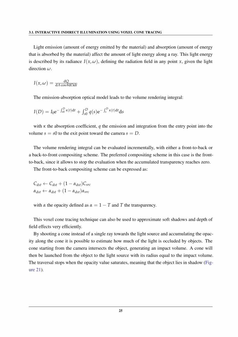
This voxel cone tracing pass (Figure 20) is slightly different than true cone tracing (section 2.4).The main idea is to step along the cone axis, retrieving the necessary data from the sparse voxeloctree at the level corresponding to the cone radius and accumulating the lighting contributionsaccording to the classical emission-absorption optical model (Max, 1995; Hadwiger et al., 2006).
Figure 20: Voxel Cone Tracing. Source: Crassin et al. (2010)
The classical emission-absorption optical model is based on geometrical optics. It assumesthat light propagates along a straight line when there is no interaction with matter. When light in-teracts with matter, it can be absorbed, scattered or emitted by the material. This model neglectsscattering, representing only local light emission and absorption.
24
3.1. INTERACTIVE INDIRECT ILLUMINATION USING VOXEL CONE TRACING
Light emission (amount of energy emitted by the material) and absorption (amount of energythat is absorbed by the material) affect the amount of light energy along a ray. This light energyis described by its radiance I(x, ω), defining the radiation field in any point x, given the lightdirection ω.
I(x, ω) = dQdA cos θdΩdt
The emission-absorption optical model leads to the volume rendering integral:
I(D) = I0e−∫ D
s0 κ(t)dt +∫ D
s0 q(s)e−∫ D
s κ(t)dtds
with κ the absorption coefficient, q the emission and integration from the entry point into thevolume s = s0 to the exit point toward the camera s = D.
The volume rendering integral can be evaluated incrementally, with either a front-to-back ora back-to-front compositing scheme. The preferred compositing scheme in this case is the front-to-back, since it allows to stop the evaluation when the accumulated transparency reaches zero.
The front-to-back compositing scheme can be expressed as:
Cdst ← Cdst + (1− αdst)Csrc
αdst ← αdst + (1− αdst)αsrc
with α the opacity defined as α = 1− T and T the transparency.
This voxel cone tracing technique can also be used to approximate soft shadows and depth offield effects very efficiently.
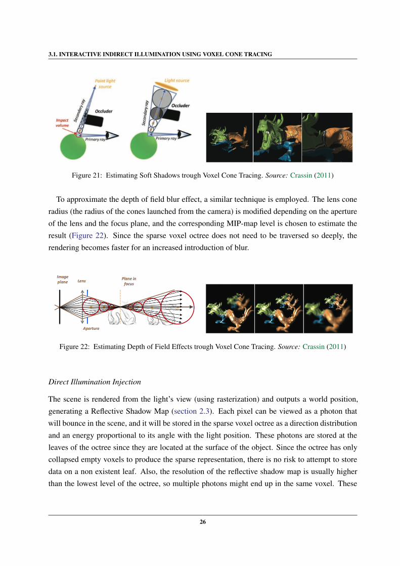
By shooting a cone instead of a single ray towards the light source and accumulating the opac-ity along the cone it is possible to estimate how much of the light is occluded by objects. Thecone starting from the camera intersects the object, generating an impact volume. A cone willthen be launched from the object to the light source with its radius equal to the impact volume.The traversal stops when the opacity value saturates, meaning that the object lies in shadow (Fig-ure 21).
25
3.1. INTERACTIVE INDIRECT ILLUMINATION USING VOXEL CONE TRACING
Figure 21: Estimating Soft Shadows trough Voxel Cone Tracing. Source: Crassin (2011)
To approximate the depth of field blur effect, a similar technique is employed. The lens coneradius (the radius of the cones launched from the camera) is modified depending on the apertureof the lens and the focus plane, and the corresponding MIP-map level is chosen to estimate theresult (Figure 22). Since the sparse voxel octree does not need to be traversed so deeply, therendering becomes faster for an increased introduction of blur.
Figure 22: Estimating Depth of Field Effects trough Voxel Cone Tracing. Source: Crassin (2011)
Direct Illumination Injection
The scene is rendered from the light’s view (using rasterization) and outputs a world position,generating a Reflective Shadow Map (section 2.3). Each pixel can be viewed as a photon thatwill bounce in the scene, and it will be stored in the sparse voxel octree as a direction distributionand an energy proportional to its angle with the light position. These photons are stored at theleaves of the octree since they are located at the surface of the object. Since the octree has onlycollapsed empty voxels to produce the sparse representation, there is no risk to attempt to storedata on a non existent leaf. Also, the resolution of the reflective shadow map is usually higherthan the lowest level of the octree, so multiple photons might end up in the same voxel. These
26
3.1. INTERACTIVE INDIRECT ILLUMINATION USING VOXEL CONE TRACING
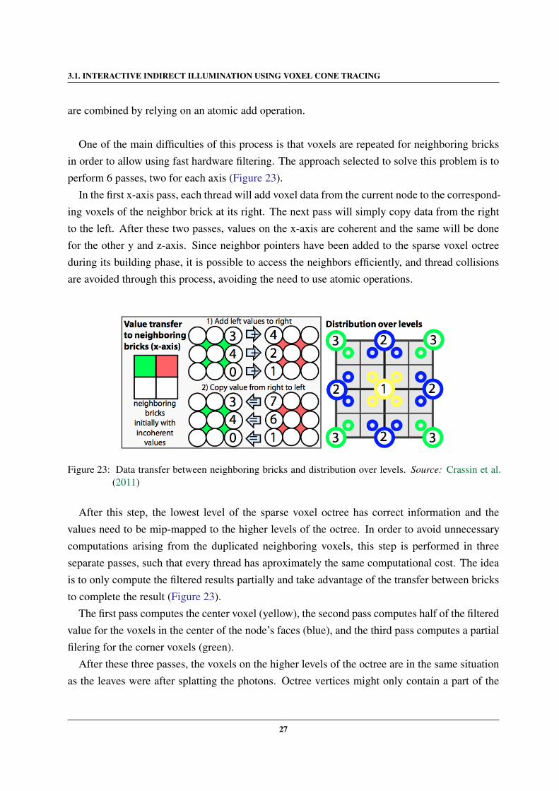
are combined by relying on an atomic add operation.
One of the main difficulties of this process is that voxels are repeated for neighboring bricksin order to allow using fast hardware filtering. The approach selected to solve this problem is toperform 6 passes, two for each axis (Figure 23).
In the first x-axis pass, each thread will add voxel data from the current node to the correspond-ing voxels of the neighbor brick at its right. The next pass will simply copy data from the rightto the left. After these two passes, values on the x-axis are coherent and the same will be donefor the other y and z-axis. Since neighbor pointers have been added to the sparse voxel octreeduring its building phase, it is possible to access the neighbors efficiently, and thread collisionsare avoided through this process, avoiding the need to use atomic operations.
Figure 23: Data transfer between neighboring bricks and distribution over levels. Source: Crassin et al.(2011)
After this step, the lowest level of the sparse voxel octree has correct information and thevalues need to be mip-mapped to the higher levels of the octree. In order to avoid unnecessarycomputations arising from the duplicated neighboring voxels, this step is performed in threeseparate passes, such that every thread has aproximately the same computational cost. The ideais to only compute the filtered results partially and take advantage of the transfer between bricksto complete the result (Figure 23).
The first pass computes the center voxel (yellow), the second pass computes half of the filteredvalue for the voxels in the center of the node’s faces (blue), and the third pass computes a partialfilering for the corner voxels (green).
After these three passes, the voxels on the higher levels of the octree are in the same situationas the leaves were after splatting the photons. Octree vertices might only contain a part of the
27
3.1. INTERACTIVE INDIRECT ILLUMINATION USING VOXEL CONE TRACING
result, but by applying the previously mentioned process to sum values across bricks, the correctresult is obtained.
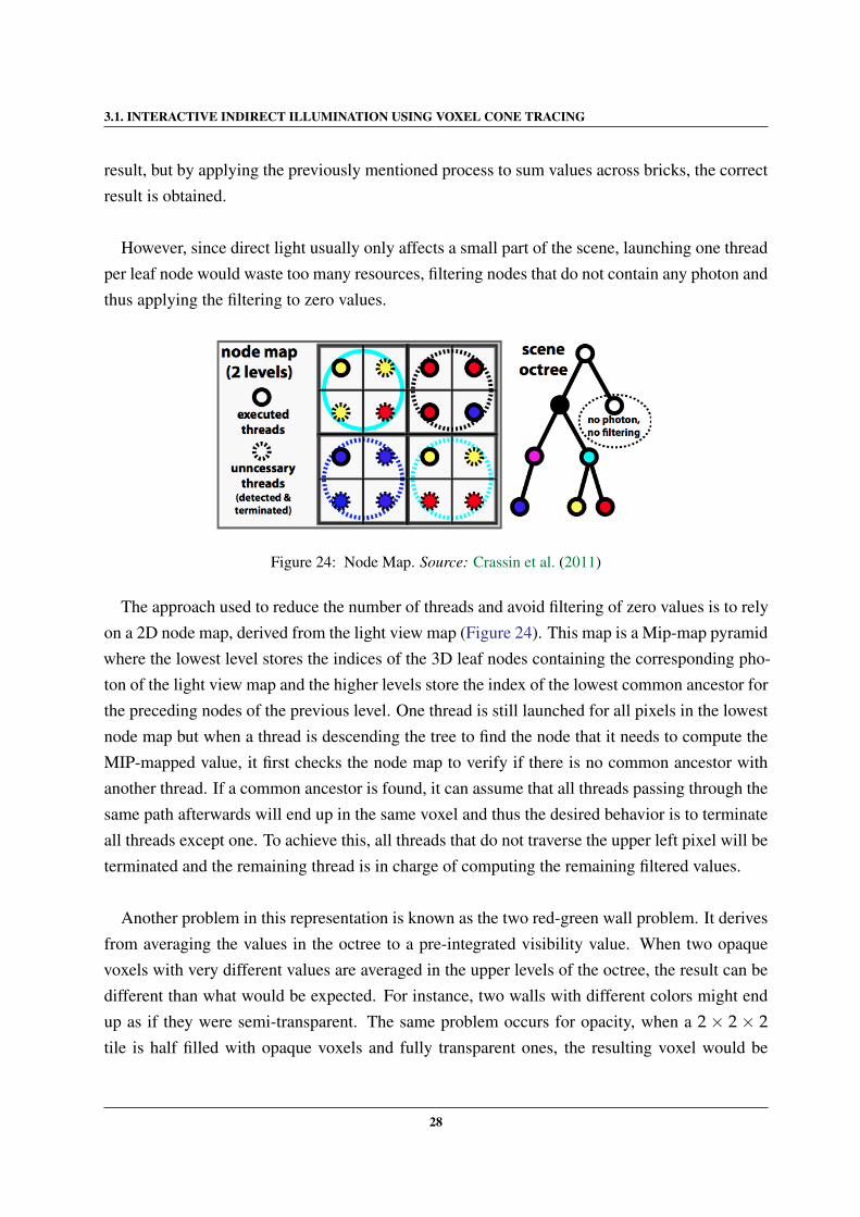
However, since direct light usually only affects a small part of the scene, launching one threadper leaf node would waste too many resources, filtering nodes that do not contain any photon andthus applying the filtering to zero values.
Figure 24: Node Map. Source: Crassin et al. (2011)
The approach used to reduce the number of threads and avoid filtering of zero values is to relyon a 2D node map, derived from the light view map (Figure 24). This map is a Mip-map pyramidwhere the lowest level stores the indices of the 3D leaf nodes containing the corresponding pho-ton of the light view map and the higher levels store the index of the lowest common ancestor forthe preceding nodes of the previous level. One thread is still launched for all pixels in the lowestnode map but when a thread is descending the tree to find the node that it needs to compute theMIP-mapped value, it first checks the node map to verify if there is no common ancestor withanother thread. If a common ancestor is found, it can assume that all threads passing through thesame path afterwards will end up in the same voxel and thus the desired behavior is to terminateall threads except one. To achieve this, all threads that do not traverse the upper left pixel will beterminated and the remaining thread is in charge of computing the remaining filtered values.
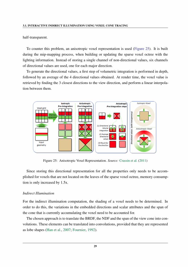
Another problem in this representation is known as the two red-green wall problem. It derivesfrom averaging the values in the octree to a pre-integrated visibility value. When two opaquevoxels with very different values are averaged in the upper levels of the octree, the result can bedifferent than what would be expected. For instance, two walls with different colors might endup as if they were semi-transparent. The same problem occurs for opacity, when a 2× 2× 2tile is half filled with opaque voxels and fully transparent ones, the resulting voxel would be
28
3.1. INTERACTIVE INDIRECT ILLUMINATION USING VOXEL CONE TRACING
half-transparent.
To counter this problem, an anisotropic voxel representation is used (Figure 25). It is builtduring the mip-mapping process, when building or updating the sparse voxel octree with thelighting information. Instead of storing a single channel of non-directional values, six channelsof directional values are used, one for each major direction.
To generate the directional values, a first step of volumetric integration is performed in depth,followed by an average of the 4 directional values obtained. At render time, the voxel value isretrieved by finding the 3 closest directions to the view direction, and perform a linear interpola-tion between them.
Figure 25: Anisotropic Voxel Representation. Source: Crassin et al. (2011)
Since storing this directional representation for all the properties only needs to be accom-plished for voxels that are not located on the leaves of the sparse voxel octree, memory consump-tion is only increased by 1.5x.
Indirect Illumination
For the indirect illumination computation, the shading of a voxel needs to be determined. Inorder to do this, the variations in the embedded directions and scalar attributes and the span ofthe cone that is currently accumulating the voxel need to be accounted for.
The chosen approach is to translate the BRDF, the NDF and the span of the view cone into con-volutions. These elements can be translated into convolutions, provided that they are representedas lobe shapes (Han et al., 2007; Fournier, 1992).
29
3.2. REAL-TIME NEAR-FIELD GLOBAL ILLUMINATION BASED ON A VOXEL MODEL
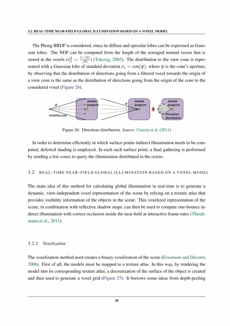
The Phong BRDF is considered, since its diffuse and specular lobes can be expressed as Gaus-sian lobes. The NDF can be computed from the length of the averaged normal vector that isstored in the voxels (σ2
n = 1−|N||N| ) (Toksvig, 2005). The distribution to the view cone is repre-
sented with a Gaussian lobe of standard deviation σv = cos(ψ), where ψ is the cone’s aperture,by observing that the distribution of directions going from a filtered voxel towards the origin ofa view cone is the same as the distribution of directions going from the origin of the cone to theconsidered voxel (Figure 26).
Figure 26: Directions distribution. Source: Crassin et al. (2011)
In order to determine efficiently in which surface points indirect illumination needs to be com-puted, deferred shading is employed. In each such surface point, a final gathering is performedby sending a few cones to query the illumination distributed in the octree.
3.2 R E A L - T I M E N E A R - F I E L D G L O B A L I L L U M I N AT I O N B A S E D O N A VOX E L M O D E L
The main idea of this method for calculating global illumination in real-time is to generate adynamic, view-independent voxel representation of the scene by relying on a texture atlas thatprovides visibility information of the objects in the scene. This voxelized representation of thescene, in combination with reflective shadow maps, can then be used to compute one-bounce in-direct illumination with correct occlusion inside the near-field at interactive frame-rates (Thiede-mann et al., 2011).
3.2.1 Voxelization
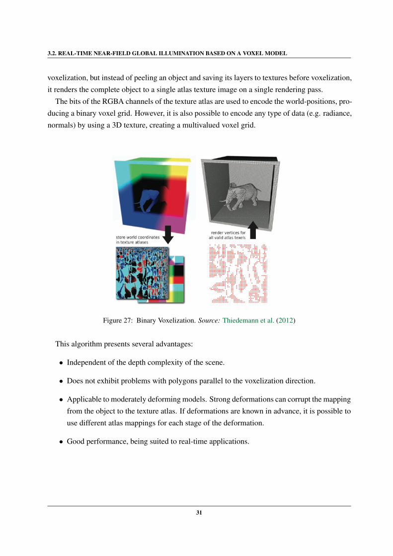
The voxelization method used creates a binary voxelization of the scene (Eisemann and Decoret,2006). First of all, the models must be mapped to a texture atlas. In this way, by rendering themodel into its corresponding texture atlas, a discretization of the surface of the object is createdand then used to generate a voxel grid (Figure 27). It borrows some ideas from depth-peeling
30
3.2. REAL-TIME NEAR-FIELD GLOBAL ILLUMINATION BASED ON A VOXEL MODEL
voxelization, but instead of peeling an object and saving its layers to textures before voxelization,it renders the complete object to a single atlas texture image on a single rendering pass.
The bits of the RGBA channels of the texture atlas are used to encode the world-positions, pro-ducing a binary voxel grid. However, it is also possible to encode any type of data (e.g. radiance,normals) by using a 3D texture, creating a multivalued voxel grid.
Figure 27: Binary Voxelization. Source: Thiedemann et al. (2012)
This algorithm presents several advantages:
• Independent of the depth complexity of the scene.
• Does not exhibit problems with polygons parallel to the voxelization direction.
• Applicable to moderately deforming models. Strong deformations can corrupt the mappingfrom the object to the texture atlas. If deformations are known in advance, it is possible touse different atlas mappings for each stage of the deformation.
• Good performance, being suited to real-time applications.
31
3.2. REAL-TIME NEAR-FIELD GLOBAL ILLUMINATION BASED ON A VOXEL MODEL
3.2.2 Binary Voxelization
The algorithm can be divided in two steps. First, all objects are rendered, storing their world-space positions to one or multiple atlas textures. However, having one texture atlas for eachobject allows for a flexible scene composition, since objects can be added or removed withouthaving to recreate the whole atlas.
Before inserting the voxels into the grid, it is necessary to set the camera on the scene. Itsfrustum will define the coordinate system of the voxel grid.
Then, for every valid texel in the texture atlas, a vertex is generated and inserted into a voxelgrid using point rendering. In order to identify valid texels, the texture atlas is cleared with aninvalid value (outside of the range of values) and this value is used as a threshold.
Altough the selection process could be done in the GPU (e.g. using a geometry shader toemit only valid texels), it is done as a preprocess on the CPU. After an initial rendering into thetexture atlas, the values are read back to the the CPU and a display list is created, holding onlythe vertices for the valid texels.
The display list is then rendered using point rendering, transforming the world-space positionfrom the texture atlas into the coordinate system of the voxel grid, according to the voxelizationcamera. The depth of the point is then used in combination with a bitmask to determine theposition of the bit that represents the voxel in the voxel grid, and finally setting the correct bit onthe voxel grid. This is possible by relying on a unidimensional texture previously created on theCPU that maps a depth value to a bitmask representing a full voxel at that certain depth interval.
In this way, each texel of a 2D texture represents a stack of voxels along the depth of thevoxelization camera, making it possible to encode a voxel grid as a 2D texture.
The atlas resolution should be chosen carefully. Using a low resolution for the texture atlascan create holes in the voxel grid. However, if the resolution is too high, the same voxel willbe filled repeatedly, hurting the performance of the algorithm since the performance is directlyrelated to the number of vertices generated and rendered using the display list.
3.2.3 Data Structure/Mip-Mapping
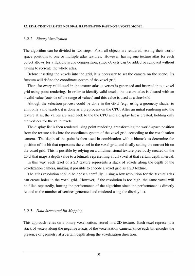
This approach relies on a binary voxelization, stored in a 2D texture. Each texel represents astack of voxels along the negative z-axis of the voxelization camera, since each bit encodes thepresence of geometry at a certain depth along the voxelization direction.
32
3.2. REAL-TIME NEAR-FIELD GLOBAL ILLUMINATION BASED ON A VOXEL MODEL
This 2D texture is used to create a mip-map hierarchy by joining the texels along the x and yaxis. The depth resolution along the z axis is kept at each mip-map level in order to allow therendering algorithm to decide more precisely if the traversal of this hierarchical structure can bestopped earlier. Each of the mip-map levels are generated manually and stored in the differentmip-map levels of a 2D texture by joining four adjacent texels of the previous mip-map level(Figure 28).
Figure 28: Mip-mapping. Source: Thiedemann et al. (2012)
3.2.4 Rendering
In order to compute visibility, a ray-voxel intersection test is employed. A hierarchical binaryvoxelized scene is used to compute the intersection of a ray with the voxel grid.
Since the binary voxelization is a hierarchical structure, it allows to decide on a coarse levelif an intersection is to be expected in a region of the voxel grid or if the region can be skippedentirely (Figure 29).
This rendering method is based on the algorithm proposed by (Forest et al., 2009), but someimprovements have been made in order to increase its performance and functionality.
The first step of the algorithm is to find if there is an intersection with the ray. The traversalstarts at the texel of the hierarchy that covers the area of the scene in which the starting pointof the ray is located. To determine this texel, the starting point of the ray is projected onto themip-map texture and used to select the appropriate texel at the current mip-map level. If the texelis found, a test is performed in order to determine if the ray hits any voxels inside the region itrepresents.
33
3.2. REAL-TIME NEAR-FIELD GLOBAL ILLUMINATION BASED ON A VOXEL MODEL
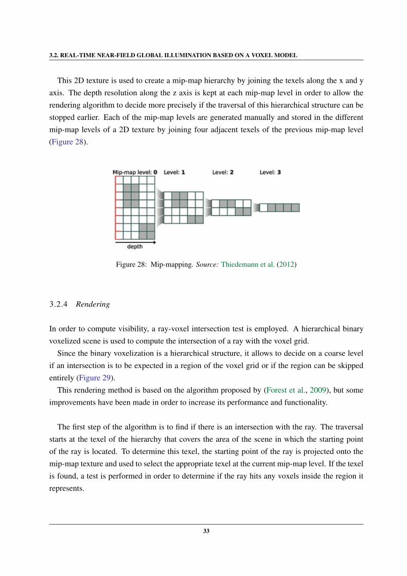
Figure 29: Hierarchy traversal. Blue lines: bounding box of the voxels in the actual texel. Green andred lines: bitmask of the active texel (empty - green and non empty - red). The green and redcuboids: history of the traversal for the texel (no hit - green and possible hit - red). Source:Thiedemann et al. (2012)
A bitmask is stored at each texel, representing a stack of voxels along the direction of depth3.2.1. It is thus possible to use this bitmask to compute the bounding box covering the volume.The size of the bounding box depends on the current mip-map level.
After computing the bounding box corresponding to the current texel, the ray is intersectedwith it, generating two values: the depth where the ray enters the bounding box and the depthwhere it leaves the bounding box. With these two values, another bitmask can be generated, rep-resenting the voxels the ray intersects inside the bounding box. This bitmask (called ray bitmask)is compared with the bitmask stored in the texel of the mip-map hierarchy in order to determineif an intersection occurs and the node’s children have to be traversed (Figure 30). If there is nointersection, the starting point of the ray is moved to the last intersection point with the boundingbox and the mip-map level is increased. If an intersection occurs, the mip-map level is decreasedto check if there is still an intersection on a finer resolution of the voxelization until the finestresolution is reached. The algorithm stops if a hit is detected or if it surpasses the maximum
34
3.2. REAL-TIME NEAR-FIELD GLOBAL ILLUMINATION BASED ON A VOXEL MODEL
length of the ray (defined by the user).
Figure 30: Hierarchy traversal in 2 dimensions. The blue arrow represents the current extent of the ray andin orange the bounding box of the current mip map levels is displayed. Source: Thiedemannet al. (2011)
The next step of the algorithm is to compute near-field illumination. For this purpose a re-flective shadow map is generated (Dachsbacher and Stamminger, 2005) that contains direct light,position and normal for each pixel visible from the light position. Different techniques are em-ployed for different types of lights: shadow maps are used for spotlights and cube maps for pointlights.
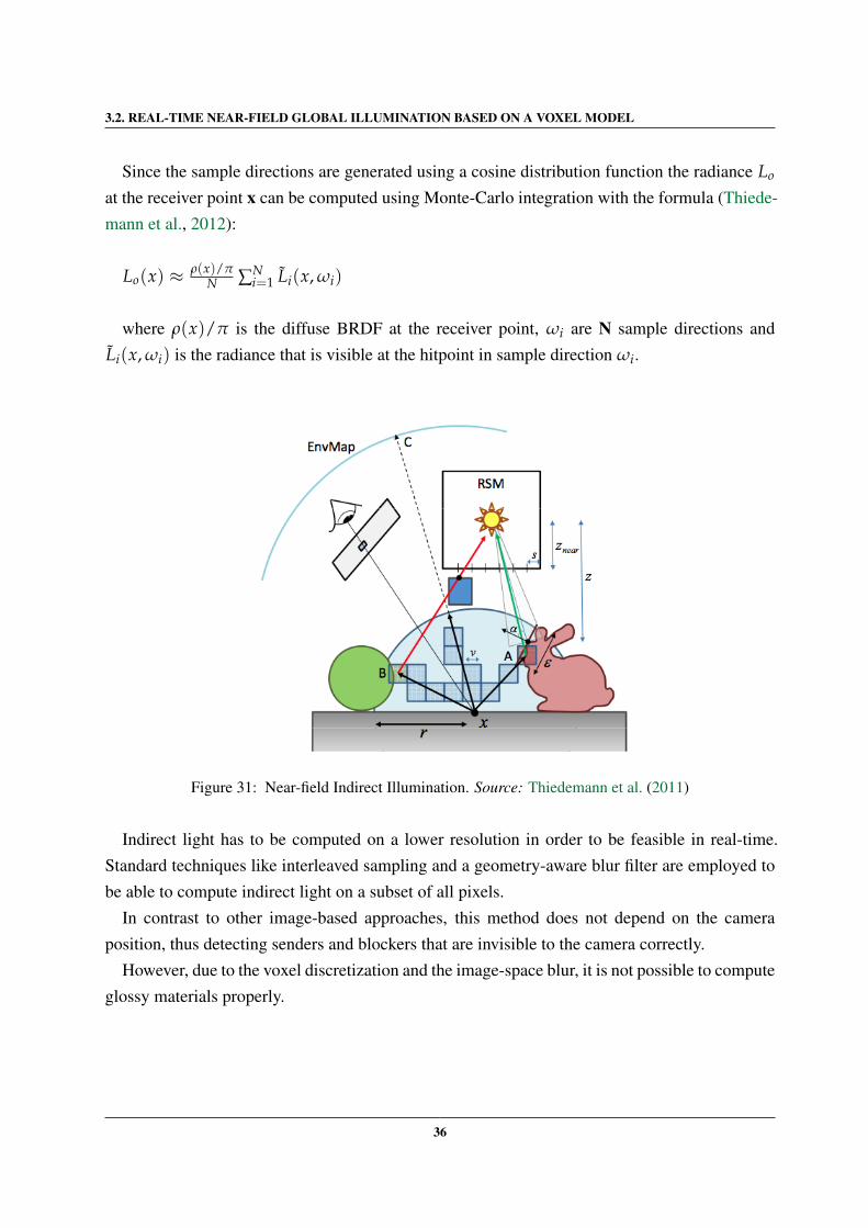
In order to compute the indirect light for a pixel in the camera view, a gathering approach isemployed to compute one-bounce near-field illumination (Figure 31). N rays are cast using acosine-weighted distribution, starting from the receiver position x with a maximum distance r.
Intersection tests are performed for each ray to determine the first intersection point. If a voxelis hit along the ray, the direct radiance Li needs to be computed at the intersection point. Thisis performed by back-projecting the hitpoint to the reflective shadow map, allowing to read thedirect radiance stored in the corresponding pixel of the reflective shadow map.
In case the distance between the 3D position of the hitpoint and the position stored in the pixelin the reflective shadow map is greater than a threshold ε, the direct radiance is invalid, and thusit is set to zero. The threshold ε has to be adjusted to the discretization v, the pixel size of thereflective shadow map s, the perspective projection and the normal orientation α. This leads toε = max(v, s
cos α ·z
znear).
35
3.2. REAL-TIME NEAR-FIELD GLOBAL ILLUMINATION BASED ON A VOXEL MODEL
Since the sample directions are generated using a cosine distribution function the radiance Lo
at the receiver point x can be computed using Monte-Carlo integration with the formula (Thiede-mann et al., 2012):
Lo(x) ≈ ρ(x)/πN ∑N
i=1 Li(x, ωi)
where ρ(x)/π is the diffuse BRDF at the receiver point, ωi are N sample directions andLi(x, ωi) is the radiance that is visible at the hitpoint in sample direction ωi.
Figure 31: Near-field Indirect Illumination. Source: Thiedemann et al. (2011)
Indirect light has to be computed on a lower resolution in order to be feasible in real-time.Standard techniques like interleaved sampling and a geometry-aware blur filter are employed tobe able to compute indirect light on a subset of all pixels.
In contrast to other image-based approaches, this method does not depend on the cameraposition, thus detecting senders and blockers that are invisible to the camera correctly.
However, due to the voxel discretization and the image-space blur, it is not possible to computeglossy materials properly.
36
3.3. RASTERIZED VOXEL-BASED DYNAMIC GLOBAL ILLUMINATION
It is possible to modify the rendering algorithm in order to extend its capabilities to betterapproximate global illumination, including compute glossy reflections. It is possible to create apath tracer based on the voxelized scene representation and to evaluate the visibility of virtualpoint lights ((Keller, 1997)) using the presented intersection test. Altough this technique presentsa better approximation to global illumination, it does not compute in real-time, and is thus out ofthis context.
3.3 R A S T E R I Z E D VOX E L - B A S E D DY N A M I C G L O B A L I L L U M I N AT I O N
This method uses recently introduced hardware features to compute an approximation to globalillumination in real-time (Doghramachi, 2013).
First, a voxel grid representation for the scene is created using the hardware rasterizer. Thevoxelization algorithm is similar to the one previously explained in Section 3.1.1.
Figure 32: Nested Voxel Grids
The scene is rendered and written into a 3D texturebuffer (voxel grid) using atomic functions, creating a3D grid representation of the scene. This grid containsthe diffuse albedo and normal information of the ge-ometry on the scene and is recreated each frame, thusit is fully dynamic and does not rely on precalcula-tions.
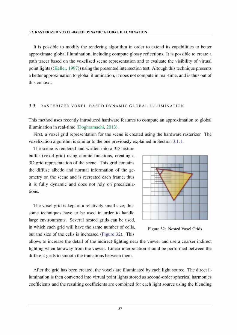
The voxel grid is kept at a relatively small size, thussome techniques have to be used in order to handlelarge environments. Several nested grids can be used,in which each grid will have the same number of cells,but the size of the cells is increased (Figure 32). Thisallows to increase the detail of the indirect lighting near the viewer and use a coarser indirectlighting when far away from the viewer. Linear interpolation should be performed between thedifferent grids to smooth the transitions between them.
After the grid has been created, the voxels are illuminated by each light source. The direct il-lumination is then converted into virtual point lights stored as second-order spherical harmonicscoefficients and the resulting coefficients are combined for each light source using the blending
37
3.3. RASTERIZED VOXEL-BASED DYNAMIC GLOBAL ILLUMINATION
stage of the graphics hardware.
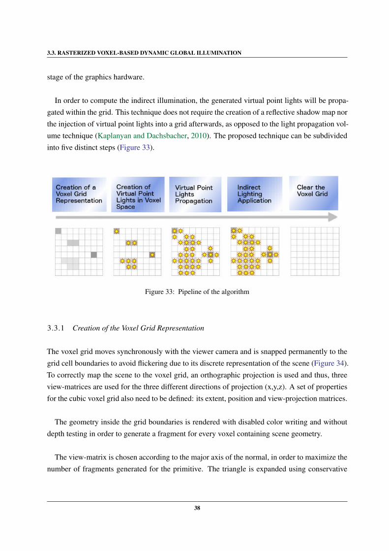
In order to compute the indirect illumination, the generated virtual point lights will be propa-gated within the grid. This technique does not require the creation of a reflective shadow map northe injection of virtual point lights into a grid afterwards, as opposed to the light propagation vol-ume technique (Kaplanyan and Dachsbacher, 2010). The proposed technique can be subdividedinto five distinct steps (Figure 33).
Figure 33: Pipeline of the algorithm
3.3.1 Creation of the Voxel Grid Representation
The voxel grid moves synchronously with the viewer camera and is snapped permanently to thegrid cell boundaries to avoid flickering due to its discrete representation of the scene (Figure 34).To correctly map the scene to the voxel grid, an orthographic projection is used and thus, threeview-matrices are used for the three different directions of projection (x,y,z). A set of propertiesfor the cubic voxel grid also need to be defined: its extent, position and view-projection matrices.
The geometry inside the grid boundaries is rendered with disabled color writing and withoutdepth testing in order to generate a fragment for every voxel containing scene geometry.
The view-matrix is chosen according to the major axis of the normal, in order to maximize thenumber of fragments generated for the primitive. The triangle is expanded using conservative
38
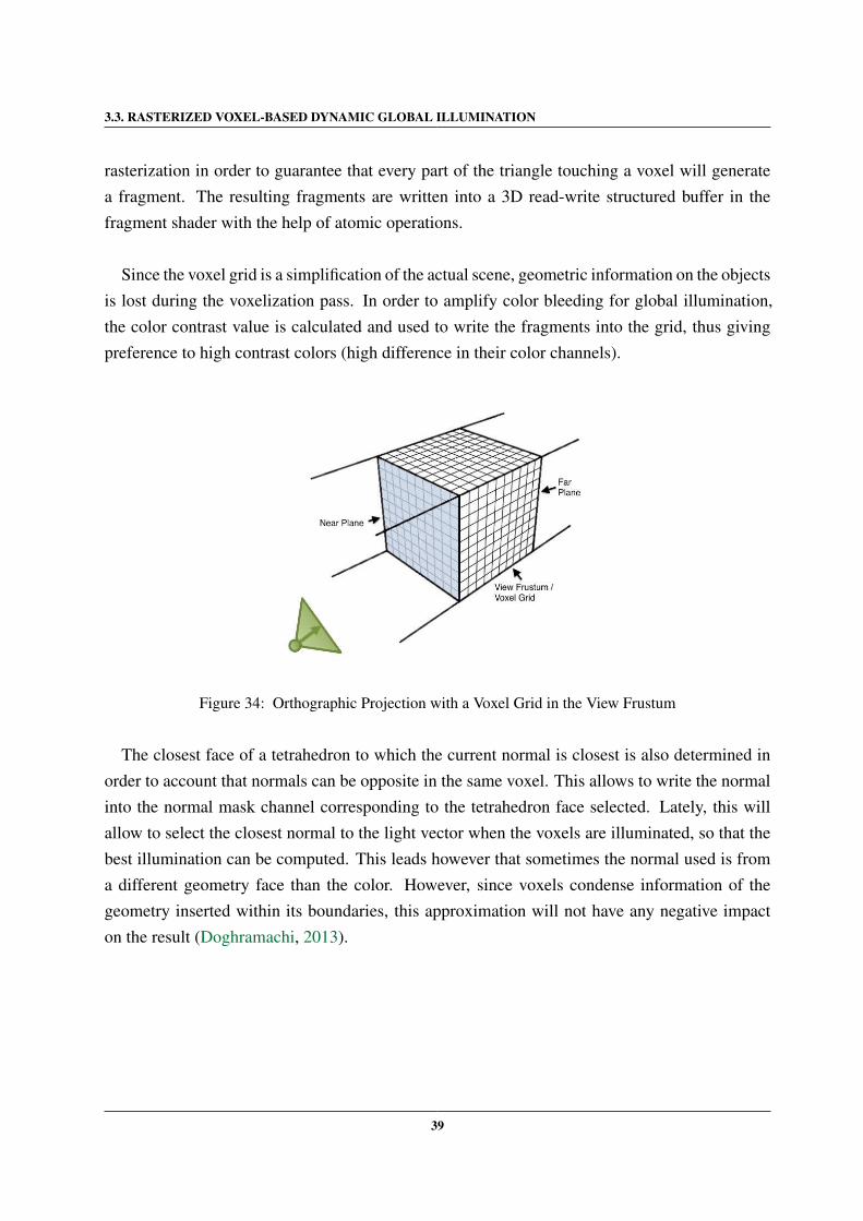
3.3. RASTERIZED VOXEL-BASED DYNAMIC GLOBAL ILLUMINATION
rasterization in order to guarantee that every part of the triangle touching a voxel will generatea fragment. The resulting fragments are written into a 3D read-write structured buffer in thefragment shader with the help of atomic operations.
Since the voxel grid is a simplification of the actual scene, geometric information on the objectsis lost during the voxelization pass. In order to amplify color bleeding for global illumination,the color contrast value is calculated and used to write the fragments into the grid, thus givingpreference to high contrast colors (high difference in their color channels).
Figure 34: Orthographic Projection with a Voxel Grid in the View Frustum
The closest face of a tetrahedron to which the current normal is closest is also determined inorder to account that normals can be opposite in the same voxel. This allows to write the normalinto the normal mask channel corresponding to the tetrahedron face selected. Lately, this willallow to select the closest normal to the light vector when the voxels are illuminated, so that thebest illumination can be computed. This leads however that sometimes the normal used is froma different geometry face than the color. However, since voxels condense information of thegeometry inserted within its boundaries, this approximation will not have any negative impacton the result (Doghramachi, 2013).
39
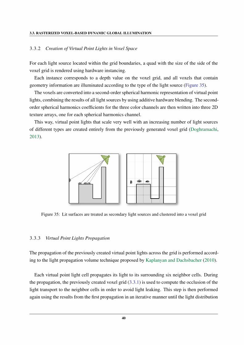
3.3. RASTERIZED VOXEL-BASED DYNAMIC GLOBAL ILLUMINATION
3.3.2 Creation of Virtual Point Lights in Voxel Space
For each light source located within the grid boundaries, a quad with the size of the side of thevoxel grid is rendered using hardware instancing.
Each instance corresponds to a depth value on the voxel grid, and all voxels that containgeometry information are illuminated according to the type of the light source (Figure 35).
The voxels are converted into a second-order spherical harmonic representation of virtual pointlights, combining the results of all light sources by using additive hardware blending. The second-order spherical harmonics coefficients for the three color channels are then written into three 2Dtexture arrays, one for each spherical harmonics channel.
This way, virtual point lights that scale very well with an increasing number of light sourcesof different types are created entirely from the previously generated voxel grid (Doghramachi,2013).
Figure 35: Lit surfaces are treated as secondary light sources and clustered into a voxel grid
3.3.3 Virtual Point Lights Propagation
The propagation of the previously created virtual point lights across the grid is performed accord-ing to the light propagation volume technique proposed by Kaplanyan and Dachsbacher (2010).
Each virtual point light cell propagates its light to its surrounding six neighbor cells. Duringthe propagation, the previously created voxel grid (3.3.1) is used to compute the occlusion of thelight transport to the neighbor cells in order to avoid light leaking. This step is then performedagain using the results from the first propagation in an iterative manner until the light distribution
40
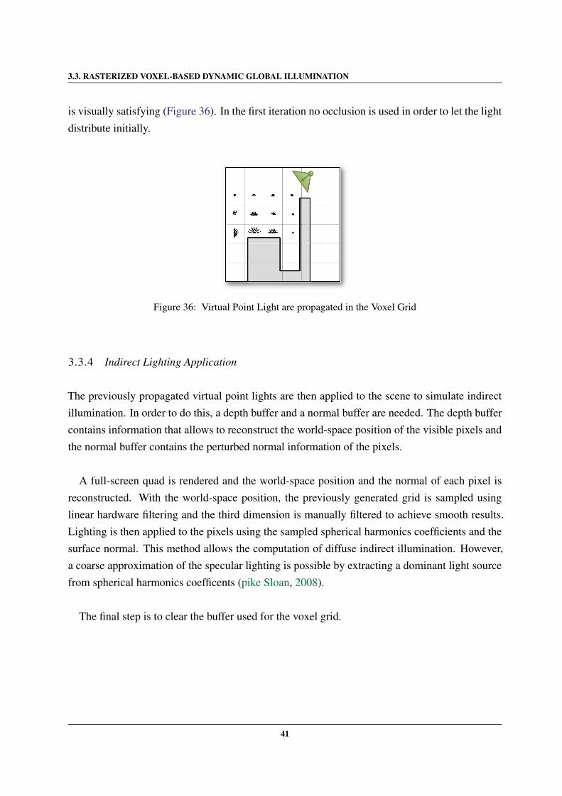
3.3. RASTERIZED VOXEL-BASED DYNAMIC GLOBAL ILLUMINATION
is visually satisfying (Figure 36). In the first iteration no occlusion is used in order to let the lightdistribute initially.
Figure 36: Virtual Point Light are propagated in the Voxel Grid
3.3.4 Indirect Lighting Application
The previously propagated virtual point lights are then applied to the scene to simulate indirectillumination. In order to do this, a depth buffer and a normal buffer are needed. The depth buffercontains information that allows to reconstruct the world-space position of the visible pixels andthe normal buffer contains the perturbed normal information of the pixels.
A full-screen quad is rendered and the world-space position and the normal of each pixel isreconstructed. With the world-space position, the previously generated grid is sampled usinglinear hardware filtering and the third dimension is manually filtered to achieve smooth results.Lighting is then applied to the pixels using the sampled spherical harmonics coefficients and thesurface normal. This method allows the computation of diffuse indirect illumination. However,a coarse approximation of the specular lighting is possible by extracting a dominant light sourcefrom spherical harmonics coefficents (pike Sloan, 2008).
The final step is to clear the buffer used for the voxel grid.
41
4
I M P L E M E N TAT I O N
4.1 T E C H N O L O G I C A L C H O I C E S
For the implementation of the chosen algorithms, several technological choices had to be made.The most important choices are between the programming language and the graphics program-
ming interface to use.For real-time computer graphics, there are mainly two APIs that we can choose from: OpenGL
and DirectX.OpenGL is a cross-platorm graphics API for drawing 2D and 3D graphics. It is well docu-
mented and a wide quantity of books and examples are available for free trough the internet.Altough it is multi-platform, it lacks some functionalities such as resource loading and windowand input handling. There are however free libraries that offer these functionalities, turning thisinto a small issue.
DirectX is a collection of APIs that can handle a large amount of functions related not justto graphics, but multimedia in general. It provides libraries that can handle for example 3Dgraphics, sound and input. However, it is closely bound to the Microsoft Windows platform.
Both are very capable and very well maintained APIs, but since OpenGL presents the advan-tage of being cross-platform and its lack of some functionalities can be easily surpassed by usingsome extra libraries, this has been the technology chosen to deal with the 3D graphics of theapplications.
The programming language chosen was C++. Since it will deal with the core of our appli-cations, it has to be closely related to the other libraries used. Most of the libraries related tocomputer graphics are written in C++, so it is an obvious choice since it allows to use the li-braries without having to rely on additional wrappers. It also offers great performance, which isessential for this kind of applications.
42
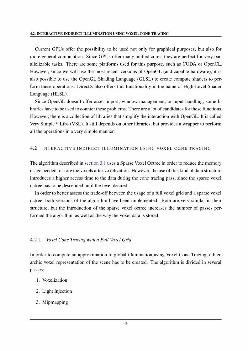
4.2. INTERACTIVE INDIRECT ILLUMINATION USING VOXEL CONE TRACING
Current GPUs offer the possibility to be used not only for graphical purposes, but also formore general computation. Since GPUs offer many unified cores, they are perfect for very par-allelizable tasks. There are some platforms used for this purpose, such as CUDA or OpenCL.However, since we will use the most recent versions of OpenGL (and capable hardware), it isalso possible to use the OpenGL Shading Language (GLSL) to create compute shaders to per-form these operations. DirectX also offers this functionality in the name of High-Level ShaderLanguage (HLSL).
Since OpenGL doesn’t offer asset import, window management, or input handling, some li-braries have to be used to counter these problems. There are a lot of candidates for these functions.However, there is a collection of libraries that simplify the interaction with OpenGL. It is calledVery Simple * Libs (VSL). It still depends on other libraries, but provides a wrapper to performall the operations in a very simple manner.
4.2 I N T E R AC T I V E I N D I R E C T I L L U M I N AT I O N U S I N G VOX E L C O N E T R AC I N G
The algorithm described in section 3.1 uses a Sparse Voxel Octree in order to reduce the memoryusage needed to store the voxels after voxelization. However, the use of this kind of data structureintroduces a higher access time to the data during the cone tracing pass, since the sparse voxeloctree has to be descended until the level desired.
In order to better assess the trade-off between the usage of a full voxel grid and a sparse voxeloctree, both versions of the algorithm have been implemented. Both are very similar in theirstructure, but the introduction of the sparse voxel octree increases the number of passes per-formed the algorithm, as well as the way the voxel data is stored.
4.2.1 Voxel Cone Tracing with a Full Voxel Grid
In order to compute an approximation to global illumination using Voxel Cone Tracing, a hier-archic voxel representation of the scene has to be created. The algorithm is divided in severalpasses:
1. Voxelization
2. Light Injection
3. Mipmapping
43
4.2. INTERACTIVE INDIRECT ILLUMINATION USING VOXEL CONE TRACING
4. Voxel Cone Tracing
Data Structures
In order to compute an approximation to global illumination using cone tracing, a voxel basedrepresentation of the scene must be created. The first step is to voxelize the scene in order todetermine the necessary information to fill the voxel grid. After voxelization, voxel fragmentsare outputted to a buffer called a voxel fragment list (Listing 4.1).
// Voxel fragment
struct FragmentData
uint position;
uint color;
uint normal;
;
// Voxel fragment list
layout(binding = 1, std430) buffer Fragments
FragmentData fragmentList[];
;
Listing 4.1: Voxel Fragment List
The voxel fragments will be used later in the light injection pass to fill a 3D texture with thelighting information in the scene. This 3D texture is created with a size matching the voxelizationresolution and with a RGBA8 texture format.
Voxelization
Each time the scene is voxelized, the voxel grid must first be cleared in order to avoid inconsis-tencies. This is done using an empty framebuffer object.
During initialization, a framebuffer object is created having no texture attachments bound toit. Then, when the grid has to be cleared, the framebuffer is bound, the 3D texture storing thevoxel grid is attached to one of the color attachments of the framebuffer object and the texture iscleared using the glClear command.
44
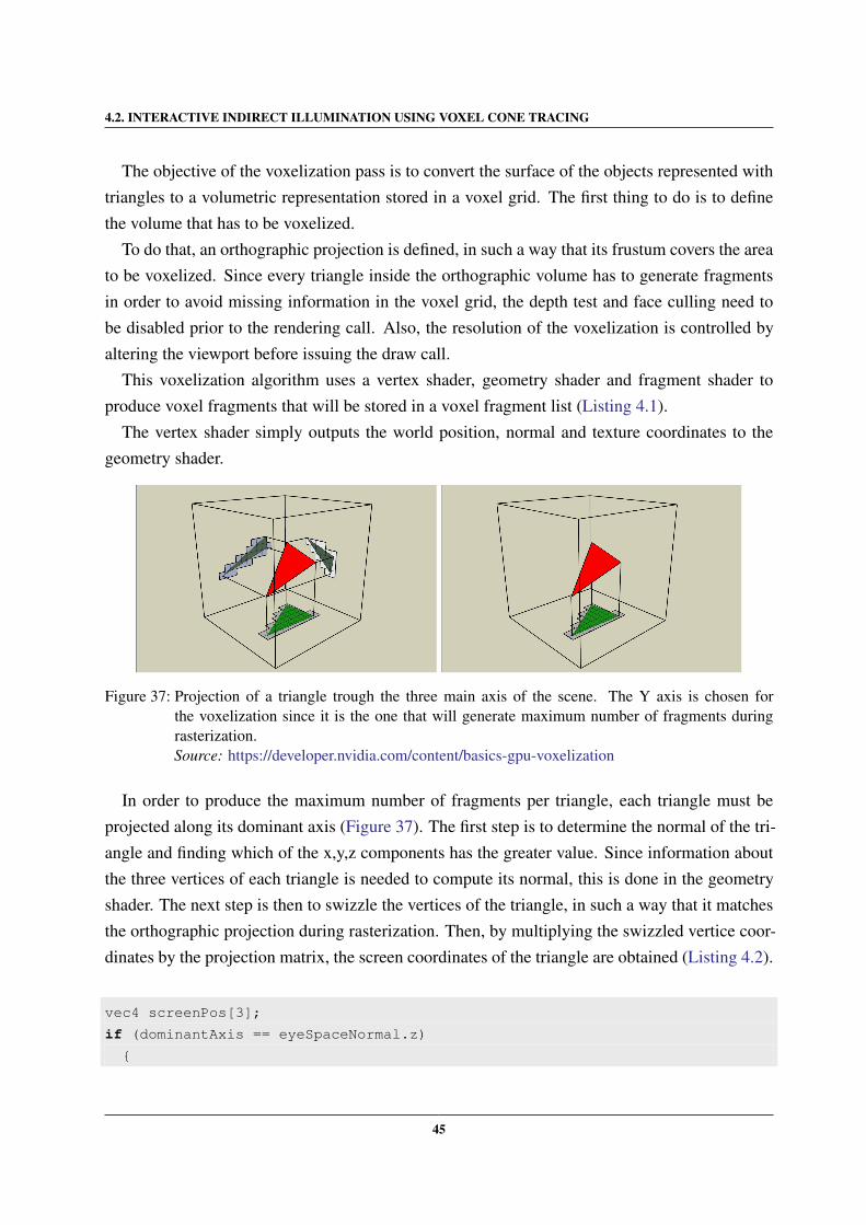
4.2. INTERACTIVE INDIRECT ILLUMINATION USING VOXEL CONE TRACING
The objective of the voxelization pass is to convert the surface of the objects represented withtriangles to a volumetric representation stored in a voxel grid. The first thing to do is to definethe volume that has to be voxelized.
To do that, an orthographic projection is defined, in such a way that its frustum covers the areato be voxelized. Since every triangle inside the orthographic volume has to generate fragmentsin order to avoid missing information in the voxel grid, the depth test and face culling need tobe disabled prior to the rendering call. Also, the resolution of the voxelization is controlled byaltering the viewport before issuing the draw call.
This voxelization algorithm uses a vertex shader, geometry shader and fragment shader toproduce voxel fragments that will be stored in a voxel fragment list (Listing 4.1).
The vertex shader simply outputs the world position, normal and texture coordinates to thegeometry shader.
Figure 37: Projection of a triangle trough the three main axis of the scene. The Y axis is chosen forthe voxelization since it is the one that will generate maximum number of fragments duringrasterization.Source: https://developer.nvidia.com/content/basics-gpu-voxelization
In order to produce the maximum number of fragments per triangle, each triangle must beprojected along its dominant axis (Figure 37). The first step is to determine the normal of the tri-angle and finding which of the x,y,z components has the greater value. Since information aboutthe three vertices of each triangle is needed to compute its normal, this is done in the geometryshader. The next step is then to swizzle the vertices of the triangle, in such a way that it matchesthe orthographic projection during rasterization. Then, by multiplying the swizzled vertice coor-dinates by the projection matrix, the screen coordinates of the triangle are obtained (Listing 4.2).
vec4 screenPos[3];
if (dominantAxis == eyeSpaceNormal.z)
45
4.2. INTERACTIVE INDIRECT ILLUMINATION USING VOXEL CONE TRACING
screenPos[0] = projection * vec4(vPosition[0].xyz, 1.0);
screenPos[1] = projection * vec4(vPosition[1].xyz, 1.0);
screenPos[2] = projection * vec4(vPosition[2].xyz, 1.0);
else if (dominantAxis == eyeSpaceNormal.y)
screenPos[0] = projection * vec4(vPosition[0].xzy, 1.0);
screenPos[1] = projection * vec4(vPosition[1].xzy, 1.0);
screenPos[2] = projection * vec4(vPosition[2].xzy, 1.0);
else if (dominantAxis == eyeSpaceNormal.x)
screenPos[0] = projection * vec4(vPosition[0].zyx, 1.0);
screenPos[1] = projection * vec4(vPosition[1].zyx, 1.0);
screenPos[2] = projection * vec4(vPosition[2].zyx, 1.0);
Listing 4.2: Computation of screen coordinates with vertex swizzling
Since the 2D fragments generated after rasterization only take into account pixels that intersecttriangles trough their center, the triangles must be expanded so that every pixel touched by atriangle generates a fragment. This is done by shifting the screen coordinates of the triangleoutwards by the size of a pixel’s diagonal.
This process, known as conservative rasterization (Figure 10) implies the computation of ascreen space bounding box of the triangle before shifting its vertices outwards. This boundingbox will serve to discard extra fragments generated during rasterization in the fragment shader.
Finally, the fragment shader is in charge of storing the voxel fragments into the voxel fragmentlist. First, the fragment is tested against the bounding box passed by the geometry shader. If thefragment is not inside the bounding box, it is discarded, and thus not appended to the voxelfragment list. Then, the voxel data is stored with the help of an atomic counter in order to avoidvoxel fragments overwriting each other.
Light Injection
In order to fill the voxel grid with the voxel fragments, the number of fragments written in theprevious pass need to be determined. This information is stored in the atomic counter used tostore the voxel fragments in the voxel fragment list.
46
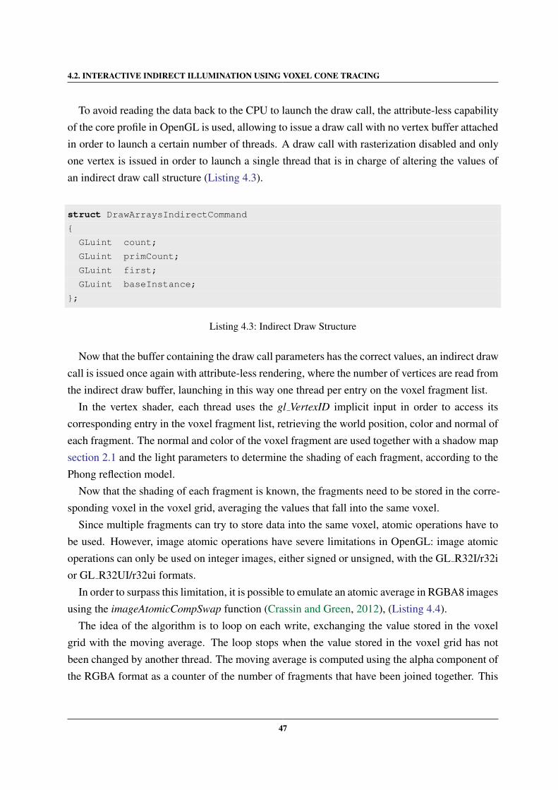
4.2. INTERACTIVE INDIRECT ILLUMINATION USING VOXEL CONE TRACING
To avoid reading the data back to the CPU to launch the draw call, the attribute-less capabilityof the core profile in OpenGL is used, allowing to issue a draw call with no vertex buffer attachedin order to launch a certain number of threads. A draw call with rasterization disabled and onlyone vertex is issued in order to launch a single thread that is in charge of altering the values ofan indirect draw call structure (Listing 4.3).
struct DrawArraysIndirectCommand
GLuint count;
GLuint primCount;
GLuint first;
GLuint baseInstance;
;
Listing 4.3: Indirect Draw Structure
Now that the buffer containing the draw call parameters has the correct values, an indirect drawcall is issued once again with attribute-less rendering, where the number of vertices are read fromthe indirect draw buffer, launching in this way one thread per entry on the voxel fragment list.
In the vertex shader, each thread uses the gl VertexID implicit input in order to access itscorresponding entry in the voxel fragment list, retrieving the world position, color and normal ofeach fragment. The normal and color of the voxel fragment are used together with a shadow mapsection 2.1 and the light parameters to determine the shading of each fragment, according to thePhong reflection model.
Now that the shading of each fragment is known, the fragments need to be stored in the corre-sponding voxel in the voxel grid, averaging the values that fall into the same voxel.
Since multiple fragments can try to store data into the same voxel, atomic operations have tobe used. However, image atomic operations have severe limitations in OpenGL: image atomicoperations can only be used on integer images, either signed or unsigned, with the GL R32I/r32ior GL R32UI/r32ui formats.
In order to surpass this limitation, it is possible to emulate an atomic average in RGBA8 imagesusing the imageAtomicCompSwap function (Crassin and Green, 2012), (Listing 4.4).
The idea of the algorithm is to loop on each write, exchanging the value stored in the voxelgrid with the moving average. The loop stops when the value stored in the voxel grid has notbeen changed by another thread. The moving average is computed using the alpha component ofthe RGBA format as a counter of the number of fragments that have been joined together. This
47
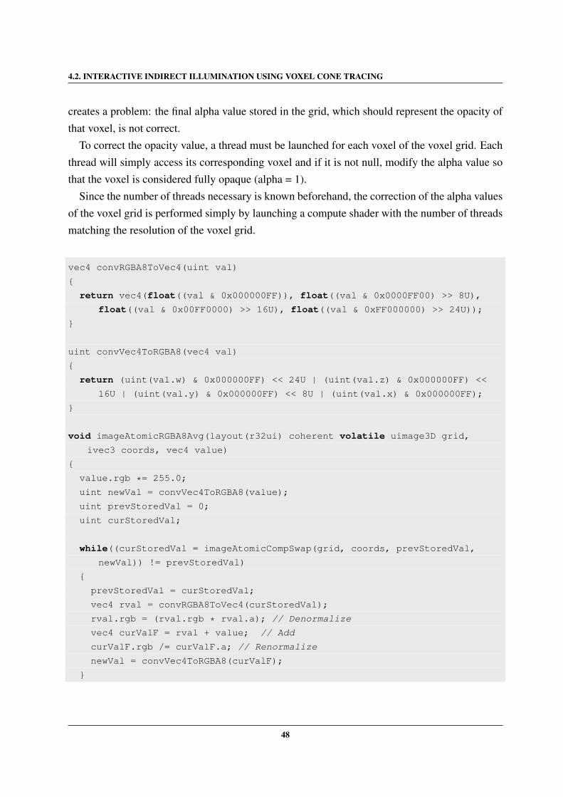
4.2. INTERACTIVE INDIRECT ILLUMINATION USING VOXEL CONE TRACING
creates a problem: the final alpha value stored in the grid, which should represent the opacity ofthat voxel, is not correct.
To correct the opacity value, a thread must be launched for each voxel of the voxel grid. Eachthread will simply access its corresponding voxel and if it is not null, modify the alpha value sothat the voxel is considered fully opaque (alpha = 1).
Since the number of threads necessary is known beforehand, the correction of the alpha valuesof the voxel grid is performed simply by launching a compute shader with the number of threadsmatching the resolution of the voxel grid.
vec4 convRGBA8ToVec4(uint val)
return vec4(float((val & 0x000000FF)), float((val & 0x0000FF00) >> 8U),
float((val & 0x00FF0000) >> 16U), float((val & 0xFF000000) >> 24U));
uint convVec4ToRGBA8(vec4 val)
return (uint(val.w) & 0x000000FF) << 24U | (uint(val.z) & 0x000000FF) <<
16U | (uint(val.y) & 0x000000FF) << 8U | (uint(val.x) & 0x000000FF);
void imageAtomicRGBA8Avg(layout(r32ui) coherent volatile uimage3D grid,
ivec3 coords, vec4 value)
value.rgb *= 255.0;
uint newVal = convVec4ToRGBA8(value);
uint prevStoredVal = 0;
uint curStoredVal;
while((curStoredVal = imageAtomicCompSwap(grid, coords, prevStoredVal,
newVal)) != prevStoredVal)
prevStoredVal = curStoredVal;
vec4 rval = convRGBA8ToVec4(curStoredVal);
rval.rgb = (rval.rgb * rval.a); // Denormalize
vec4 curValF = rval + value; // Add
curValF.rgb /= curValF.a; // Renormalize
newVal = convVec4ToRGBA8(curValF);
48
4.2. INTERACTIVE INDIRECT ILLUMINATION USING VOXEL CONE TRACING
Listing 4.4: RGBA8 Image Atomic Average Function
Mipmapping
Now that the 3D texture has data about the lighting on the scene at maximum resolution, it isnecessary to create the lower mipmap levels in order to have an hierarchic representation of thelighting in the scene to use during the voxel cone tracing pass.
This is done level by level, launching a compute shader with a number of threads equal to theresolution of the mipmap level to be filled. Each thread accesses the next higher mipmap leveland samples the eight voxels that correspond to the voxel to be filled, averaging their values andstoring the result using an image store operation. Since the mipmapping is performed level bylevel, no atomic operations are needed in order to ensure that the results stay coherent.
Voxel Cone Tracing
The voxel grid encodes information about the geometry of the scene (all voxels containing geome-try have an occlusion higher than zero) and the direct lighting information at multiple resolutions,providing an hierarchic representation of the scene.
With this information it is possible to compute an approximation to indirect illumination bylaunching cones and sampling the voxel grid at different resolutions, according to the cone aper-ture.
This pass is performed using a deferred rendering approach (section 2.2). A full-screen quadis rendered and the fragment shader simply samples the geometry buffer in order to retrieve thepositions, normals, colors and direct illumination.
With this information it is possible to compute the direction of the reflected ray and a singlecone with a small aperture is launched in order to capture the specular contribution to indirectillumination. For the diffuse indirect illumination, 5 cones with a large aperture are launched inthe hemisphere around the normal. A cone is launched in the direction of the normal, while theother four are launched in different directions, making an angle of 45 degrees with the normal,with the help of the tangent and bitangent vectors. The cones are weighted according to the anglemade with the normal.
Tracing cones trough the voxel grid is very similar to using volume ray casting (section 2.4).The difference is that instead of shooting rays and sampling them at equally spaced intervals,
49
4.2. INTERACTIVE INDIRECT ILLUMINATION USING VOXEL CONE TRACING
the rays have a thickness that increases along the tracing path and the distance between samplesincreases as the sampling position gets farthest from the cone apex.
The information needed to trace a cone is: its starting point, its direction, its aperture and themaximum distance that will be traveled until the tracing is stopped.
The first thing to do is set the starting point. The fragment position that has been retrieved fromthe geometry buffer corresponds to the world position of the surface of an object to which indirectillumination has to be computed. However, that surface also has had its lighting contributionadded to the voxel grid. So, in order to avoid self intersection, the starting point of the cone hasto be advanced by the size of the diameter of a voxel on the last level of the voxel grid.
The maximum distance and the aperture are set by the user, but the aperture is actually repre-sented as the the cone diameter to height ratio. The idea is then to sample the voxel grid fromthe starting position along the direction of the cone, accumulating the samples using front-to-back alpha blending, until the maximum distance set by the user is surpassed or the alpha valuecontaining the accumulated occlusion saturates.
The distance to the next sample is increased by the cone’s diameter of the current sampleand by associating the volume that a voxel represents in each sample with the diameter of thecone, the volume increases increases between each sample. The proper mipmap level is chosenaccording to the size of that volume, since each voxel corresponds to a different volume in spacein different mipmap levels. Since the full grid is stored in a 3D texture, it is possible to samplethe voxels using hardware quadrilinear filtering.
This algorithm already allows to compute a very good approximation to indirect illumination.However, some artifacts are noticeable. Since the start position and stepping size between eachsample during the cone tracing is the same for every cone with the same aperture, some bandingartifacts can appear when tracing glossy reflections. This is a well-known problem on volumerendering approaches , and common ways to solve the problem are to reduce the stepping size,increasing in this way the number of samples taken for each cone, and jittering the start positionof the cone. The approach taken was to reduce the stepping size by half during the traversal, thusdoubling the number of samples taken. This approach had a small impact on performance, andit was sufficient to remove visible banding on the scene.
Another problem is that since voxels define a volume in space, when tracing cones it is possibleto accumulate some lighting contributions from objects that are occluded from the view point,thus leading to light leaking. To reduce these artifacts, five more voxel grids are needed, onefor each direction, in order to be able to filter the irradiance anisotropically during the mipmappass. The mipmap pass is altered in order to perform alpha blending in one of the six directions,
50
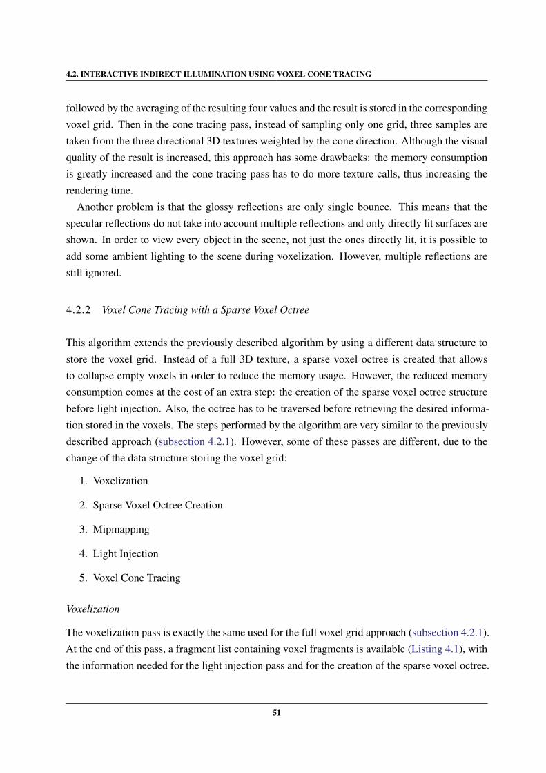
4.2. INTERACTIVE INDIRECT ILLUMINATION USING VOXEL CONE TRACING
followed by the averaging of the resulting four values and the result is stored in the correspondingvoxel grid. Then in the cone tracing pass, instead of sampling only one grid, three samples aretaken from the three directional 3D textures weighted by the cone direction. Although the visualquality of the result is increased, this approach has some drawbacks: the memory consumptionis greatly increased and the cone tracing pass has to do more texture calls, thus increasing therendering time.
Another problem is that the glossy reflections are only single bounce. This means that thespecular reflections do not take into account multiple reflections and only directly lit surfaces areshown. In order to view every object in the scene, not just the ones directly lit, it is possible toadd some ambient lighting to the scene during voxelization. However, multiple reflections arestill ignored.
4.2.2 Voxel Cone Tracing with a Sparse Voxel Octree
This algorithm extends the previously described algorithm by using a different data structure tostore the voxel grid. Instead of a full 3D texture, a sparse voxel octree is created that allowsto collapse empty voxels in order to reduce the memory usage. However, the reduced memoryconsumption comes at the cost of an extra step: the creation of the sparse voxel octree structurebefore light injection. Also, the octree has to be traversed before retrieving the desired informa-tion stored in the voxels. The steps performed by the algorithm are very similar to the previouslydescribed approach (subsection 4.2.1). However, some of these passes are different, due to thechange of the data structure storing the voxel grid:
1. Voxelization
2. Sparse Voxel Octree Creation
3. Mipmapping
4. Light Injection
5. Voxel Cone Tracing
Voxelization
The voxelization pass is exactly the same used for the full voxel grid approach (subsection 4.2.1).At the end of this pass, a fragment list containing voxel fragments is available (Listing 4.1), withthe information needed for the light injection pass and for the creation of the sparse voxel octree.
51
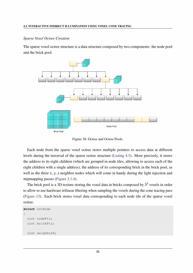
4.2. INTERACTIVE INDIRECT ILLUMINATION USING VOXEL CONE TRACING
Sparse Voxel Octree Creation
The sparse voxel octree structure is a data structure composed by two components: the node pooland the brick pool.
Figure 38: Octree and Octree Pools.
Each node from the sparse voxel octree stores multiple pointers to access data at differentlevels during the traversal of the sparse octree structure (Listing 4.5). More precisely, it storesthe address to its eight children (which are grouped in node tiles, allowing to access each of theeight children with a single address), the address of its corresponding brick in the brick pool, aswell as the three x, y, z neighbor nodes which will come in handy during the light injection andmipmapping passes (Figure 3.1.4).
The brick pool is a 3D texture storing the voxel data in bricks composed by 33 voxels in orderto allow to use hardware trilinear filtering when sampling the voxels during the cone tracing pass(Figure 13). Each brick stores voxel data corresponding to each node tile of the sparse voxeloctree.
struct OctNode
uint nodePtr;
uint brickPtr;
uint neighborX;
52
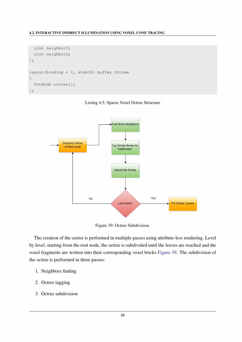
4.2. INTERACTIVE INDIRECT ILLUMINATION USING VOXEL CONE TRACING
uint neighborY;
uint neighborZ;
;
layout(binding = 1, std430) buffer Octree
OctNode octree[];
;
Listing 4.5: Sparse Voxel Octree Structure
Figure 39: Octree Subdivision.
The creation of the octree is performed in multiple passes using attribute-less rendering. Levelby level, starting from the root node, the octree is subdivided until the leaves are reached and thevoxel fragments are written into their corresponding voxel bricks Figure 39. The subdivision ofthe octree is performed in three passes:
1. Neighbors finding
2. Octree tagging
3. Octree subdivision
53
4.2. INTERACTIVE INDIRECT ILLUMINATION USING VOXEL CONE TRACING
Before starting the octree subdivision, the number of threads for the indirect draw call must beset. Similarly to 4.2.1, a draw call is issued in order to read the atomic fragment counter valueand modify the indirect draw structure parameters in order to be able to launch 1 thread for eachentry in the voxel fragment list.
The first pass is in charge of finding the three x, y, z neighbors of a voxel and storing theiraddresses in the octree node. To do that, each thread reads the world position from the voxelfragment list and traverses the octree using the kd-restart algorithm. The traversal starts from theroot node, computing the volume dimensions for the node and comparing it to the world positionretrieved from the voxel fragment list in order to find out to which child the traversal must becontinued. Traversal stops when an empty node is found. Now that the current leaf node is found,the world position is increased in each axis separately by the size of the current node’s volumeand the traversal is restarted with each neighbors world position until the same depth is reachedand the neighbor node address is written into the corresponding field in the octree node.
The second pass tags the octree nodes in order to distinguish which ones should be subdivided.To do that a draw call is issued, launching one thread for each entry in the voxel fragment list.Each thread in the vertex shader accesses its corresponding world position in the voxel fragmentlist and uses it to traverse the octree until an empty or tagged node is found. The 30th bit of thenode pointer of the octree node is then set in order to mark the node for subdivision.
Since the octree is sparse, only some nodes have been marked for subdivision and only thosenodes have to subdivided. In order to be able to launch one thread per node on each level ofthe octree, the nodes per level have to be kept on each step of the octree subdivision. The drawindirect structure has been extended in order to store an array of unsigned integers correspondingto the number of nodes on each level of the octree (Listing 4.6).
layout (std430, binding = 0) buffer IndirectBuffer
uint count;
uint primCount;
uint first;
uint baseInstance;
uint nodesPerLevel[];
DrawArraysCommand;
Listing 4.6: Indirect draw structure storing the nodes for each level of the octree
So, before launching the octree subdivision pass, a draw call with one single thread is issuedfor the purpose of altering the indirect draw structure parameters so that the next indirect draw
54
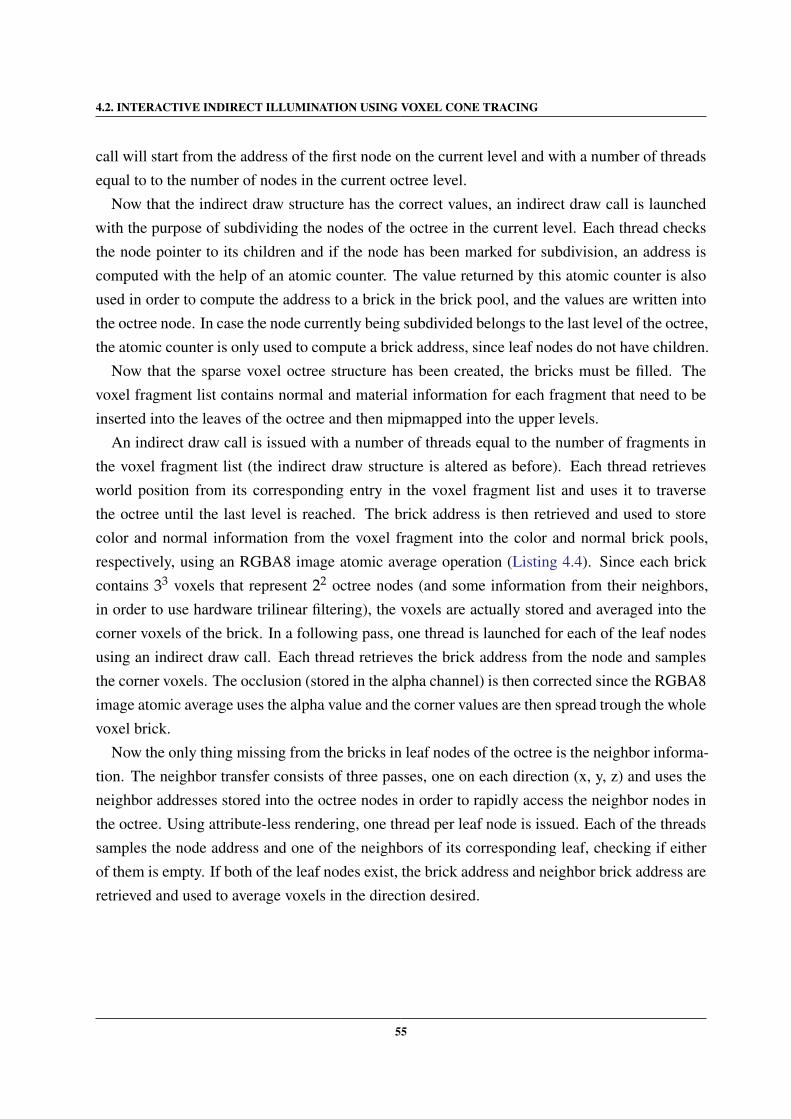
4.2. INTERACTIVE INDIRECT ILLUMINATION USING VOXEL CONE TRACING
call will start from the address of the first node on the current level and with a number of threadsequal to to the number of nodes in the current octree level.
Now that the indirect draw structure has the correct values, an indirect draw call is launchedwith the purpose of subdividing the nodes of the octree in the current level. Each thread checksthe node pointer to its children and if the node has been marked for subdivision, an address iscomputed with the help of an atomic counter. The value returned by this atomic counter is alsoused in order to compute the address to a brick in the brick pool, and the values are written intothe octree node. In case the node currently being subdivided belongs to the last level of the octree,the atomic counter is only used to compute a brick address, since leaf nodes do not have children.
Now that the sparse voxel octree structure has been created, the bricks must be filled. Thevoxel fragment list contains normal and material information for each fragment that need to beinserted into the leaves of the octree and then mipmapped into the upper levels.
An indirect draw call is issued with a number of threads equal to the number of fragments inthe voxel fragment list (the indirect draw structure is altered as before). Each thread retrievesworld position from its corresponding entry in the voxel fragment list and uses it to traversethe octree until the last level is reached. The brick address is then retrieved and used to storecolor and normal information from the voxel fragment into the color and normal brick pools,respectively, using an RGBA8 image atomic average operation (Listing 4.4). Since each brickcontains 33 voxels that represent 22 octree nodes (and some information from their neighbors,in order to use hardware trilinear filtering), the voxels are actually stored and averaged into thecorner voxels of the brick. In a following pass, one thread is launched for each of the leaf nodesusing an indirect draw call. Each thread retrieves the brick address from the node and samplesthe corner voxels. The occlusion (stored in the alpha channel) is then corrected since the RGBA8image atomic average uses the alpha value and the corner values are then spread trough the wholevoxel brick.
Now the only thing missing from the bricks in leaf nodes of the octree is the neighbor informa-tion. The neighbor transfer consists of three passes, one on each direction (x, y, z) and uses theneighbor addresses stored into the octree nodes in order to rapidly access the neighbor nodes inthe octree. Using attribute-less rendering, one thread per leaf node is issued. Each of the threadssamples the node address and one of the neighbors of its corresponding leaf, checking if eitherof them is empty. If both of the leaf nodes exist, the brick address and neighbor brick address areretrieved and used to average voxels in the direction desired.
55
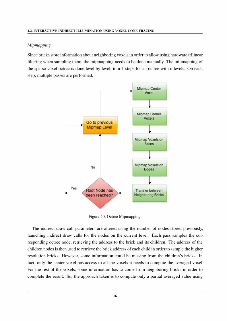
4.2. INTERACTIVE INDIRECT ILLUMINATION USING VOXEL CONE TRACING
Mipmapping
Since bricks store information about neighboring voxels in order to allow using hardware trilinearfiltering when sampling them, the mipmapping needs to be done manually. The mipmapping ofthe sparse voxel octree is done level by level, in n-1 steps for an octree with n levels. On eachstep, multiple passes are performed.
Figure 40: Octree Mipmapping.
The indirect draw call parameters are altered using the number of nodes stored previously,launching indirect draw calls for the nodes on the current level. Each pass samples the cor-responding octree node, retrieving the address to the brick and its children. The address of thechildren nodes is then used to retrieve the brick address of each child in order to sample the higherresolution bricks. However, some information could be missing from the children’s bricks. Infact, only the center voxel has access to all the voxels it needs to compute the averaged voxel.For the rest of the voxels, some information has to come from neighboring bricks in order tocomplete the result. So, the approach taken is to compute only a partial averaged value using
56
4.2. INTERACTIVE INDIRECT ILLUMINATION USING VOXEL CONE TRACING
the children bricks, and then complete the result using the same neighbor transfer scheme usedto complete the result on the leaves of the sparse voxel octree. Corners, edges, sides and centervoxels are mipmapped in separate passes, since they need information about a different numberof voxels from the higher resolution bricks and because voxels sampled from the children bricksreappear in neighboring bricks, the sampled values have to be weighted in accordance to theirmultiplicity in order to generate a correct result (subsection 3.1.3).
Light Injection
Since the color, opacity and normal of the fragments have already been averaged into two brickpools, there is no need to compute the irradiance directly from the fragments and storing them inthe voxel grid. Instead, a reflective shadow map is generated section 2.3 containing informationabout the world position from the fragments seen from the light’s perspective, and a full-screenquad with a viewport corresponding to the reflective shadow map is rendered. The world posi-tion is sampled in the fragment shader and converted to voxel grid coordinates ([0, voxel gridresolution]) and the sparse voxel octree is traversed until the leaf node is encountered, retrievingthe address corresponding to one of the four corners of the corresponding brick in the brick pool.Now that the brick address where the light has to be injected has been found, the averaged colorand normal can be sampled from their corresponding brick pools and used to compute the irra-diance using the Phong reflection model , storing the result in the irradiance brick pool. Afterfilling the leaf nodes of the sparse voxel octree with the direct lighting information, the irradiancebrick pool is completed with the lower mipmap levels by performing a mipmap pass in the sameway as before for the color and normal brick pools.
Voxel Cone Tracing
The voxel cone tracing pass is essentially the same described in subsection 4.2.1. The differencelies in the way voxels are sampled during the traversal of the cone. For the full voxel grid, the 3Dtexture was sampled using hardware quadrilinear filtering, using simply the voxel grid coordinate.Now, the sparse voxel octree has to be traversed up to the desired mipmap level, retrieving thebrick address in order to perform sampling of the desired voxel in the brick pool. Since voxels arestored in bricks, it is not possible to simply use the quadrilinear filtering offered by the hardware.To bypass this limitation, hardware trilinear filtering is used and the filtering between mipmaplevels is performed manually.
57
4.3. RASTERIZED VOXEL-BASED DYNAMIC GLOBAL ILLUMINATION
4.3 R A S T E R I Z E D VOX E L - B A S E D DY N A M I C G L O B A L I L L U M I N AT I O N
The algorithm has suffered some changes since the original work (Doghramachi, 2013) was pub-lished. It initially only allowed to compute an approximation of the diffuse indirect illumination.However, it has been later extended to be able to approximate glossy reflections. This comesto the cost of an extra higher resolution grid that will be sampled using Voxel Cone Tracing toapproximate glossy reflections.
This changes not only the data structures needed for the execution of the algorithm, but alsoits structure, since some extra steps are needed during its execution.
Also, the buffers clearing pass has been moved in this implementation from the last to theinitial step. This was simply a choice that does not really change the behavior of the algorithm,it just allows to avoid clearing the buffer after its creation during the initialization.
Thus, the algorithm can now be subdivided into 7 distinct steps:
1. Clear Buffers
2. Voxelization
3. Direct Light Injection
4. Direct Light Propagation
5. Reflection Grid Creation
6. Reflection Grid Mipmapping
7. Global Illumination Rendering
4.3.1 Data Structures
For this implementation, two grids are used for diffuse indirect illumination. They both have thesame size (323), but cover a different frustum. The grids can be static and thus cover always thesame volume on the scene, or they can move along with the camera, defining a volume aroundit. For the grids to move along with the camera without introducing artifacts, some care must betaken during the voxelization pass. Since each voxel represents a small volume in space, movingthe frustum slightly may cause different fragments to be joined together, causing flickering eachtime the camera moves. To avoid this problem, the frustum must be adjusted so that it moves
58
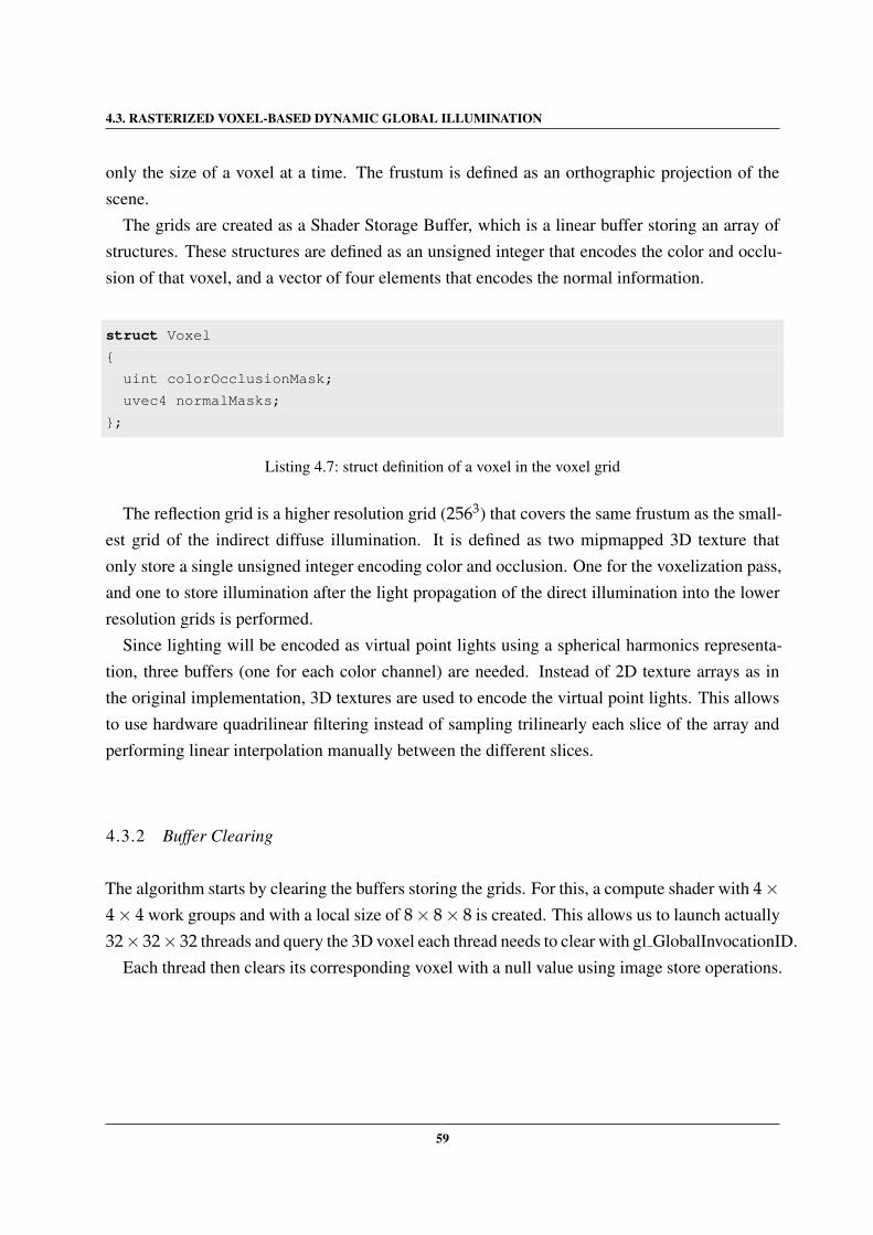
4.3. RASTERIZED VOXEL-BASED DYNAMIC GLOBAL ILLUMINATION
only the size of a voxel at a time. The frustum is defined as an orthographic projection of thescene.
The grids are created as a Shader Storage Buffer, which is a linear buffer storing an array ofstructures. These structures are defined as an unsigned integer that encodes the color and occlu-sion of that voxel, and a vector of four elements that encodes the normal information.
struct Voxel
uint colorOcclusionMask;
uvec4 normalMasks;
;
Listing 4.7: struct definition of a voxel in the voxel grid
The reflection grid is a higher resolution grid (2563) that covers the same frustum as the small-est grid of the indirect diffuse illumination. It is defined as two mipmapped 3D texture thatonly store a single unsigned integer encoding color and occlusion. One for the voxelization pass,and one to store illumination after the light propagation of the direct illumination into the lowerresolution grids is performed.
Since lighting will be encoded as virtual point lights using a spherical harmonics representa-tion, three buffers (one for each color channel) are needed. Instead of 2D texture arrays as inthe original implementation, 3D textures are used to encode the virtual point lights. This allowsto use hardware quadrilinear filtering instead of sampling trilinearly each slice of the array andperforming linear interpolation manually between the different slices.
4.3.2 Buffer Clearing
The algorithm starts by clearing the buffers storing the grids. For this, a compute shader with 4×4× 4 work groups and with a local size of 8× 8× 8 is created. This allows us to launch actually32× 32× 32 threads and query the 3D voxel each thread needs to clear with gl GlobalInvocationID.
Each thread then clears its corresponding voxel with a null value using image store operations.
59
4.3. RASTERIZED VOXEL-BASED DYNAMIC GLOBAL ILLUMINATION
4.3.3 Voxelization
The voxelization pass is actually very similar to the one previously explained in section 4.2. Itis performed once for each grid (fine, coarse and reflection grids). A viewport size of 64× 64is used for the low resolution grids and a viewport size of 512 × 512 is used for the higherresolution reflection grid.
As before, depth testing and the color mask/depth mask are disabled and an orthographicprojection is used. The difference now is that the frustum of the orthographic projection isdifferent between the fine/reflection grids and the coarse grid. These parameters are set by theuser and will affect the voxelized area of the scene, and thus the area that will have approximateindirect illumination.
The vertex shader simply passes the world position, texture coordinates and normal to thegeometry shader.
The geometry shader finds the dominant axis for the normal and computes its projection alongthat axis. Instead of using three different matrices for the projection of the triangle along thedominant axis, the same method used before is employed and a swizzle matrix is computed andused to swizzle the vertices of the triangle towards the dominant axis of its normal. The edgesof the triangle are then expanded outwards in order for the rasterizer to generate fragments forevery pixel touched by a triangle. This time however, no bounding box is computed to discardthe excess fragments later in the fragment Shader.
The fragment shader retrieves the RGB material color and encodes it in linear space into thelast 24 bits of an unsigned integer. The higher 8 bits are then used to encode the contrast value(difference between the color channels) computed from the retrieved color in linear space, as wellas the occlusion. Since the values are written into the buffer/3D texture using atomicMax/im-ageAtomicMax operations, colors with a higher contrast value will automatically dominate.For the fine and coarse grids it is still needed to compute and encode normal information forwriting in the buffers. Since fragments in the same voxel can have opposite normals, specialcare has to be given when writing normal values. The dot product between the normal and theface of a tetrahedron is determined and written into the highest 5 bits of the normal mask. Eachchannel of the normal is then encoded in 9 bits (1 for the sign and 8 for the value) and written inthe remaining bits of the normal mask. Finally, according to the dot product, the normal mask iswritten into the corresponding channel of the vector in the buffer using an atomicMax operation.This way, the closest normal to the tetrahedron will automatically dominate.
60
4.3. RASTERIZED VOXEL-BASED DYNAMIC GLOBAL ILLUMINATION
4.3.4 Direct Light Injection
For the light injection, a 32× 32 quad is rendered using instanced rendering. 32 instances arerendered in each pass, and this is performed for the fine and coarse grid only.
The vertex shader simply outputs the vertex position and the gl InstanceID to the geometryshader. The geometry shader then emits the vertices and the corresponding instance ID of thetriangle to the fragment shader. Finally, the fragment shader uses the input variable gl FragCoordand the instance ID passed by the geometry shader to retrieve the corresponding voxel from theattached buffer. The color and normal are then decoded and the world-space position is computedusing the voxel grid coordinate. With this information, a shadow map is used to compute diffusedirect illumination depending on the type of the light.
The last step is to encode the diffuse albedo into a virtual point light using a second order spher-ical harmonics representation and write each channel into the corresponding 3D texture. For this,a clamped cosine lobe function oriented in the Z direction is encoded as spherical harmonics.Since it possesses rotational symmetry around the Z axis, the spherical harmonic projection re-sults in zonal harmonics, which are simpler to rotate than general spherical harmonics. This way,each channel of the diffuse albedo is multiplied by zonal harmonics, rotated into the direction ofthe voxel normal and stored into the corresponding 3D texture using image store operations.
4.3.5 Direct Light Propagation
Now that the spherical harmonics grids (which represent our virtual point lights) are lit with thedirect illumination, they have to be propagated trough the grid in order to add their contributionto neighbor voxels. To do this, a compute shader with 4× 4× 4 work groups and with a localsize of 8× 8× 8 is created. Similarly to the buffer clearing pass, this allows to obtain the indexinto the voxel grid of each thread by querying the gl GlobalInvocationID input variable. Weinitialize the voxel values with the spherical harmonics coefficients of the current grid positionand then the contributions from the six neighboring voxels is computed. We start by determiningthe direction from the neighbor voxel to the current cell and its corresponding solid angle. Fromhere, it is possible to obtain the spherical harmonics coefficients for that direction and computethe flux from the neighbor cell to the face of the current cell by weighting them by the solidangle. However, we also need to account for the occlusion in order to perform the light propa-gation accurately. The grid buffer that contains the color/occlusion mask and the normal masks
61
4.3. RASTERIZED VOXEL-BASED DYNAMIC GLOBAL ILLUMINATION
is accessed to obtain the information for the neighboring voxel. The normals are decoded andthe closest to the specified direction is calculated. By using the same zonal harmonics functionutilized in the previous pass, the occlusion coefficients are computed. Finally, summing all thecontributions from the neighboring voxels correcly weighted by the occlusion coefficients pro-vides the lighting contribution of the neighboring virtual point lights. This contribution is addedto the initial value and each channel is stored in the corresponding 3D texture using image storeoperations. This process is repeated multiple times to allow the lighting to propagate trough thegrid. In the first pass, no occlusion weight is used to allow an initial propagation of the virtualpoint lights.
4.3.6 Reflection Grid Creation
The creation of the reflection grid is done using a compute shader with 32 × 32 × 32 workgroups and with a local size of 8× 8× 8, since the 3D texture for this reflection grid has a 2563
resolution. First, the color/occlusion is retrieved from the grid previously generated during thevoxelization pass. Then, the spherical harmonics coefficients of the finest voxel grid are sampled(since the reflection grid has the same frustum). In this way, an ambient term is extracted fromthe corresponding voxel. If the grid center is snapped to the camera position, glossy reflectionsonly cover a small area around the camera. To ensure that no popping artifacts are introducedwhen the camera is moving, the ambient term is faded out with the distance to the grid center.This ambient term is then stored in the lit reflections 3D texture and the previously generatedreflection grid is cleared. In this way, no extra pass is needed to clear the grid.
4.3.7 Reflection Grid Mipmapping
In the original algorithm, the author used the DirectX API to automatically generate 4 mipmaplevels for the 3D texture. In OpenGL however, altough the specification states that the mipmapgeneration function (glGenerateMipmap) accepts 3D textures as the target to generate the mipmaps,in practice the function call would not operate properly and no mipmaps were created in the hard-ware used for testing. To bypass this issue, a manual mipmapping was implemented using thecompute shader capabilities. First of all, the memory for the mipmaps has to be allocated duringthe initialization. Since only 4 mipmaps are needed, only 4 levels need to be allocated. However,
62
4.3. RASTERIZED VOXEL-BASED DYNAMIC GLOBAL ILLUMINATION
OpenGL once again would not behave properly if only 4 texture levels were allocated/defined.For the texture object to function properly, all mipmap levels needed to be allocated. To performthe mipmapping, the compute shader is invoked 3 times, one for each lower mipmap level, andwith a decreasing number of thread groups for each level (16, 8 and 4) in order to launch thecorrect number of threads for each level. The local size continues with the same size as withthe other compute shader invocations in previous passes. Each thread will then sample the eightvoxels on the upper level corresponding to the voxel grid coordinate (once again determined withgl GlobalInvocationID), average them and store the result using an image store operation.
4.3.8 Global Illumination Rendering
To compute global illumination, a full-screen quad is rendered using deferred rendering, andworld-space positions, normals and material are retrieved.
Global illumination can be subdivided in two components: direct and indirect illumination.Direct illumination has already been computed in a previous pass using deferred shading. Indi-rect lighting can in its turn be subdivided in two other components: diffuse and specular (in thiscase, glossy) indirect lighting.
To compute diffuse indirect illumination, we start by computing spherical harmonics coeffi-cients for the normal in the current world-space position. Once again, zonal harmonics are usedto generate these coefficients. Then, the 3D texture coordinates for the corresponding positionare computed and the three 3D textures containing the propagated virtual point lights are sam-pled and weighted by the normal coefficients to generate indirect diffuse illumination. Since twogrids are being used, both have to be sampled and the distance from the center of the grid is usedto interpolate between their results to obtain a smooth transition between them.
For glossy reflections, a very different process is used. Similarly to section 4.2, voxel conetracing is used to accumulate lighting contributions from the voxels along the cone axis. Westart by computing the reflected direction from the eye to the world-position of the fragment andlaunch a ray in that direction, accumulating color and occlusion from the lit reflection grid untiltotal occlusion is reached. Since different mipmap levels are sampled depending on the traceddistance from the starting point and the cone aperture, the ray actually resembles a cone. Thedifference now is that the sampled values are faded out according to the maximum propagationdistance and the distance to the grid center in order to ensure a smooth fade-out of the reflectionas the camera moves trough the scene.
63
4.4. REAL-TIME NEAR-FIELD GLOBAL ILLUMINATION BASED ON A VOXEL MODEL
Finally, direct, diffuse indirect and glossy reflections are added together to generate the ap-proximation to global illumination.
Since the center of the voxel grids can be kept synchronous with the viewer camera and keepsthe global illumination to a limited frustum around it, this algorithm does not depend on thesize of the scene, being perfectly capable of handling large scenes without losing its interactivity.Another great advantage is that the reflection grid is created in separate passes, making it veryeasy to disable it and spare memory and processing time if the indirect diffuse contribution issufficient for the current scene.
4.4 R E A L - T I M E N E A R - F I E L D G L O B A L I L L U M I N AT I O N B A S E D O N A VOX E L M O D E L
Differently from the other algorithms implemented, this one also performs some computationon the CPU. First of all, it computes some bitmasks and stores them into 1D and 3D textures inorder to send them to the shaders when needed. Also, after the voxelization process, a displaylist is created in order to discard invalid texel values from the texture atlas. However, its greatestdisadvantage is the need for the models surfaces used during the voxelization process to bemapped to a texture atlas. This is done simply by generating another definition of the object (forexample using a Wavefront .obj format) in which the texture coordinates are used to map thevertices of the object to a position in the texture atlas. Then, when rendering the object duringvoxelization, the atlas texture coordinates are simply read from the texture coordinates passed tothe shader.
The algorithm can be subdivided into several passes:
1. Voxelization
a) Binary Atlas Creation
b) Pixel Display List Creation
c) Voxel Grid Creation
2. MIP-mapping
3. Indirect Lighting Computation
The main difference with the other algorithms described in this thesis is that no direct lightinjection pass is performed. Since the voxel grid only encodes a binary representation of the
64
4.4. REAL-TIME NEAR-FIELD GLOBAL ILLUMINATION BASED ON A VOXEL MODEL
scene, direct lighting will have to be sampled differently. Direct lighting will be sampled duringthe indirect lighting computation pass, using a Reflective Shadow Map generated previously.
4.4.1 Data Structures
Several bitmasks need to be created. These are simply 1D textures storing information about thebitmasks in an unsigned integer RGBA format of size 128. .
A 2D texture is used to encode the bitmasks for the rays launched during the indirect ilumi-nation pass. This texture is created by attaching the texture to the framebuffer and drawing afull-screen quad with a viewport of size 128, using one of the bitmasks previously created. Then,in the fragment shader, the x and y coordinates of the fragment (retrieved using the gl FragCoordvariable) are used to fetch the bitmask for each coordinate and generate the final result using thebitwise exclusive or operator (XOR).
For storing the binary atlas, a 2D texture with half size floating point RGBA values is created.Its size is a user-defined value, since it greatly depends on the object, in order to avoid holes oroverdraw during the voxelization and creation of the voxel grid (section 3.2).
The voxel grid will be used to store the binary representation in our scene after voxelization.It is a MIP-mapped 2D texture storing RGBA unsigned integers. Its size is defined in accordancewith the voxelization resolution and each texel represents a stack of oxels along the voxelizationdepth.
To compute the diffuse indirect lighting, two buffers are needed. One is used to bounce the raysaround the scene and the other actually stores the diffuse indirect illumination after computation,so that it can be added to direct lighting afterwards. Both are defined as 2D textures storing RGBvalues at half floating point precision and with a size matching the window extents.
For a better sampling of the diffuse indirect illumination, an auxiliar texture is used to rotatethe rays randomly. It is defined as a small 2D texture storing random data in RGB floating pointformat.
4.4.2 Binary Atlas Creation
In order to be able to insert or remove objects to the scene without having to recompute thewhole atlas, the scene is rendered once for each object, with different atlas textures attached to
65
4.4. REAL-TIME NEAR-FIELD GLOBAL ILLUMINATION BASED ON A VOXEL MODEL
the framebuffer, so that each object will have its corresponding texture atlas. The model loadeduses a previously generated description of the object that contains the mapping of the surfaces ofthe object to a texture atlas in the texture coordinates definition. The vertex shader simply com-putes the world-space position, sending it to the fragment shader, and transforms the atlas texturecoordinate into Normalized Device Coordinates (NDC). The fragment shader simply outputs thereceived world-space position into its corresponding position in the atlas texture. In order to beable to identify invalid texels in the next pass, the atlas texture is cleared with some value thatwill serve as a threshold to discard invalid texels.
4.4.3 Pixel Display List Creation
Now that the atlas texture contains the world-space positions of the surfaces of the object, itwould be possible to generate one vertice for each texel in the texture atlas and issue a draw callthat would insert these vertices into the voxel grid. However, a lot of texels contain invalid valuesthat we wish to discard to reduce the amount of vertices issued in the draw call. For this, the atlastexture is read back to the CPU and traversed, discarding all invalid texels using the previouslydefined threshold value with which the atlas texture was cleared. For each valid texel, a pointis generated using the texture coordinates (which vary between 0 and the atlas resolution) andinserted into a pixel display list. The point size can be increased in order to attempt to close holesif the resolution of the texture atlas is too small.
4.4.4 Voxel Grid Creation
The next step is to generate the voxel grid. For this purpose, the pixel display list is renderedwith the voxel grid texture bound to the framebuffer. An orthographic projection is defined inorder to be able to transform the world-space positions into voxel grid coordinates. This way, theextents of the orthographic projection control the region that is voxelized. Since we are usinga binary voxelization, the channels of the voxel grid texture encode the voxels using a bitmask.To be able to do this, a logical OR operation has to be defined for the framebuffer (Eisemannand Decoret, 2006). The vertex shader fetches the world-space position from the atlas textureusing the texture coordinate (passed as a vertex). The vertex coordinate is transformed (usingthe orthographic view and projection matrices) and the Z coordinate of the vertex is passed to
66
4.4. REAL-TIME NEAR-FIELD GLOBAL ILLUMINATION BASED ON A VOXEL MODEL
the fragment shader, mapped to [0, 1] . Since each texel of the voxel grid actually represents astack of voxels along a certain depth, this Z coordinate is actually the coordinate that needs tobe retrieved from the bitmask texture and outputted by the fragment shader in order to set thecorrect bit in the voxel grid.
4.4.5 Mipmapping
The voxel grid needs to be mipmapped in order to generate a binary hierarchic representation ofthe scene. To perform the mipmapping, a full-screen quad is rendered for each of the lower levelsof the mipmapped texture and with the respective mipmap level bound to the framebuffer. Thefragment shader then samples the 4 neighbor texels in the upper level of the mipmap hierarchy.Since a texel represents a stack of voxels along the depth axis, the depth is kept for each mipmaplevel, so only the x and y axis are joined. To achieve this, the 4 texels are simply joined using alogical OR operation.
4.4.6 Indirect Lighting Computation
To compute diffuse indirect lighting, several rays will be launched for each pixel. For each ofthese rays, the voxel grid is used to compute a ray/voxel intersection, writing the hit positionsinto a buffer called the hit buffer. The hit buffer is then read in another pass and diffuse indirectillumination is computed with the help of reflective shadow maps.
Let us start with the creation of the hit buffer. A full-screen quad is rendered and the world-position is fetched from the g-buffer. This world-space position is the starting point of the re-flected ray. By using a cosine weighted distribution, a direction for the reflected ray is computed.Then, to avoid self-shadowing, the starting point of the ray is advanced by an offset at least thesize of the voxel diagonal. The start and end point of the ray are then defined. The intersectiontest is performed in a loop, advancing the ray in small steps and testing against the mipmaphierarchy if an intersection is encountered. In order to limit the computation time, a numberof maximum iterations is defined by the user. Also, the sampling does not initiate at the finestmipmap level (the root node), but is advanced by at least 1 level since the intersection with theroot node was already computed. Since voxels are encoded in groups, they can be representedwith an Axis Aligned Bounding Box (AABB). So, to perform the intersection test, a ray/AABB
67
4.4. REAL-TIME NEAR-FIELD GLOBAL ILLUMINATION BASED ON A VOXEL MODEL
test is employed. If the ray intersects the bounding box, the bitmask is tested against the ray’sbitmask computed during initialization using a bitwise operation AND to check whether thereare bits that intersect the ray. The intersection point is then used to compute and write the voxelposition of the intersection point (in unit-coordinates) into the hit buffer.
Now that the hit buffer is filled with the hit positions, all the information necessary to com-pute diffuse indirect illumination is available. The algorithm starts by fetching the intersectionpoint from the hit buffer and transform it into light space using the view and projection matricesfrom the shadow map pass. Then, this coordinate is projected into the reflective shadow maps toretrieve the corresponding position, normal and direct lighting color. The direct radiance is onlyvalid if the distance from the hit position to the world-space position retrieved from the reflectiveshadow map is smaller than certain threshold, or else the hit point lies in the shadow of the source.Also, since only front faces are lit and reflect indirect light, the normal is used to check whetherthe hit point lies in the front face of the surface.
Finally, direct and indirect illumination are combined by rendering a full-screen quad andsumming the contributions of each pixel. However, since indirect lighting is computed for a muchlower resolution that the window size, the indirect lighting result is blurred using a geometryaware blur before adding its contribution to the global illumination result.
68
5
C O N C L U S I O N S
Several algorithms for computing an approximation to global illumination in real-time appli-cations were presented in this thesis. It has been shown that these algorithms share a similarstructure, requiring the scene to be pre-filtered using some kind of voxelization algorithm.
In section 4.2, the voxelization pass creates a fragment list storing information about the worldpositions, colors and normals of the scene by rasterizing the triangles of the scene in the directionof the dominant axis of their normal.
This fragment list is then used to create a pre-filtered hierarchic representation of the lightingin the scene in order to be able to launch cones to gather indirect illumination. One cone islaunched in the direction of the reflection in order to gather the specular contribution to indirectillumination, while five cones are launched in the the hemisphere around the normal vector inorder to gather the diffuse indirect illumination.
The cone tracing pass steps along the cone axis, sampling the data structure storing voxel dataat different mipmap levels based on the cone diameter, and alpha-blending is used to accumulatethe samples (thus treating voxels as a participating media) until opacity saturates.
The voxel cone tracing approach was tested against a full voxel grid, which allowed for aneasier and faster access to the data structure, speeding most of the steps of the algorithm, at thecost of an higher memory usage. To reduce memory usage, a sparse voxel octree was createdentirely on the GPU, allowing to reduce the memory footprint of the voxel grid, at the cost ofhaving to traverse the octree each time a voxel has to be sampled or updated.
The algorithm presented in section 4.3 shares some similarities with the voxel cone tracingapproaches. The main differences are in the way diffuse indirect illumination is computed. Ituses two cascaded grids for the diffuse indirect illumination and one higher resolution grid tocompute glossy reflections.
69
The first thing to do is to create a voxelized representation of the scene by rasterizing thetriangles in the direction of the dominant axis of their normal. Then, the resulting fragments areused to encode color based on their contrast, and normals using the closest face to a tetrahedron,storing them in a buffer.
Next, the fragments in the buffer are used together with a shadow map to compute diffusealbedo, storing the result into the voxel grids using a second order spherical harmonics represen-tation. This generates voxel grids containing virtual point lights that are then propagated alongthe three axes of the grid.
The grids storing the propagated virtual point lights are sampled in order to generate diffuseindirect illumination, while the higher resolution grid is mipmapped in order to use voxel conetracing to sample glossy reflections.
The algorithm described in section 4.4 maps the vertices of the objects in the scene to a 2Dtexture atlas. This process, called binary voxelization, encodes the world positions of all thegeometry in the scene into the texture atlas, generating a binary representation of the scene.
The texture atlas is read back to the CPU and all valid texels are used to generate a pixeldisplay list. This pixel display list is the rendered in order to insert all the texels into a voxel grid,encoded as a 2D texture. Since a 2D texture is being used, each texel in the voxel grid representsa stack of voxels in the voxelization depth and a texture storing bitmaps (previously generatedon the CPU) is used in order to encode the voxels correctly.
The voxel grid is then mipmapped by joining the texels in the x and y directions, keeping thedepth with the same precision between mipmap levels since it is already limited by the choice touse each texel as a stack of voxels.
Diffuse indirect illumination is then computed by launching rays trough the scene, intersect-ing them with the voxel grid. When an intersection is found, a reflective shadow map is used tosample the direct lighting contribution of the sampling position.
All these approaches use a voxel grid representation of the scene in order to compute an ap-proximation to global illumination. This voxel grid can be encoded in multiple ways, such as a3D texture, a 2D texture or a sparse voxel octree. All of these data structures have advantagesand disadvantages. Full grids stored in 3D textures waste a lot of memory with empty voxels,but are accessed faster. Sparse voxel octrees in the other side are costly to generate and maintainupdated, but reduce the memory footprint of the voxel grid by collapsing empty voxels. 2D tex-tures are smaller than 3D textures but they are only suitable to store a binary representation of
70

the scene, due to the need to use the texels to store a stack of voxels along the voxelization depth,which in turn decreases the visual quality of the obtained result.
In order to counter these problems, new approaches need to arise in order to decrease thememory cost of the voxel grids, allowing at the same time to rapidly update and access them. Oneway to decrease the wasted memory is to use the empty space of the 3D texture storing the voxelgrid to encode necessary data to compute other visual effects. For example, voxel grids havebeen used for atmospheric effects (Vos, 2014) and fluid simulation (Roble et al., 2005). Morerecently, Nvidia has presented a new technique in order to approximate global illumination basedon voxel cone tracing, called VXGI (https://developer.nvidia.com/vxgi) that uses 3D clipmaps toencode voxel data.
71
B I B L I O G R A P H Y
Allard, Jeremie; Faure, Francois; Courtecuisse, Hadrien; Falipou, Florent; Duriez, Christian,and Kry, Paul G. Volume contact constraints at arbitrary resolution. ACM Trans. Graph., 29(4):82:1–82:10, July 2010. ISSN 0730-0301. doi: 10.1145/1778765.1778819. URL http:
//doi.acm.org/10.1145/1778765.1778819.
Amanatides, John. Ray tracing with cones. SIGGRAPH Comput. Graph., 18(3):129–135, Jan-uary 1984. ISSN 0097-8930. doi: 10.1145/964965.808589. URL http://doi.acm.org/
10.1145/964965.808589.
Annen, Thomas; Mertens, Tom; Seidel, Hans-Peter; Flerackers, Eddy, and Kautz, Jan. Exponen-tial shadow maps. In Proceedings of Graphics Interface 2008, GI ’08, pages 155–161, Toronto,Ont., Canada, Canada, 2008. Canadian Information Processing Society. ISBN 978-1-56881-423-0. URL http://dl.acm.org/citation.cfm?id=1375714.1375741.
Appel, Arthur. Some techniques for shading machine renderings of solids. In Proceedings of
the April 30–May 2, 1968, Spring Joint Computer Conference, AFIPS ’68 (Spring), pages37–45, New York, NY, USA, 1968. ACM. doi: 10.1145/1468075.1468082. URL http:
//doi.acm.org/10.1145/1468075.1468082.
Crane, Keenan; Llamas, Ignacio, and Tariq, Sarah. Real Time Simulation and Rendering of 3D
Fluids, chapter 30. Addison-Wesley, 2007.
Crassin, Cyril. GigaVoxels: A Voxel-Based Rendering Pipeline For Efficient Exploration Of
Large And Detailed Scenes. PhD thesis, UNIVERSITE DE GRENOBLE, July 2011. URLhttp://maverick.inria.fr/Publications/2011/Cra11. English and web-optimized version.
Crassin, Cyril and Green, Simon. CRC Press, Patrick Cozzi and Christophe Ric-cio, 2012. URL http://www.seas.upenn.edu/˜pcozzi/OpenGLInsights/
OpenGLInsights-SparseVoxelization.pdf,ChapterPDF.
Crassin, Cyril; Neyret, Fabrice; Lefebvre, Sylvain, and Eisemann, Elmar. Gigavoxels : Ray-guided streaming for efficient and detailed voxel rendering. In ACM SIGGRAPH Symposium
72
BIBLIOGRAPHY
on Interactive 3D Graphics and Games (I3D), Boston, MA, Etats-Unis, feb 2009. ACM, ACMPress. URL http://maverick.inria.fr/Publications/2009/CNLE09. to ap-pear.
Crassin, Cyril; Neyret, Fabrice; Sainz, Miguel, and Eisemann, Elmar. Efficient Rendering of
Highly Detailed Volumetric Scenes with GigaVoxels. In book: GPU Pro, chapter X.3, pages643–676. A K Peters, 2010. URL http://maverick.inria.fr/Publications/
2010/CNSE10.
Crassin, Cyril; Neyret, Fabrice; Sainz, Miguel; Green, Simon, and Eisemann, Elmar. Interactiveindirect illumination using voxel cone tracing. Computer Graphics Forum (Proc. of Pacific
Graphics 2011), 2011. URL http://research.nvidia.com/publication/
interactive-indirect-illumination-using-voxel-cone-tracing,
NVIDIApublicationwebpage.
Dachsbacher, Carsten and Stamminger, Marc. Reflective shadow maps. In Proceedings of the
2005 Symposium on Interactive 3D Graphics and Games, I3D ’05, pages 203–231, New York,NY, USA, 2005. ACM. ISBN 1-59593-013-2. doi: 10.1145/1053427.1053460. URL http:
//doi.acm.org/10.1145/1053427.1053460.
Daniels, Joel; Silva, Claudio T.; Shepherd, Jason, and Cohen, Elaine. Quadrilateral meshsimplification. ACM Trans. Graph., 27(5):148:1–148:9, December 2008. ISSN 0730-0301.doi: 10.1145/1409060.1409101. URL http://doi.acm.org/10.1145/1409060.
1409101.
Deering, Michael; Winner, Stephanie; Schediwy, Bic; Duffy, Chris, and Hunt, Neil. The triangleprocessor and normal vector shader: A vlsi system for high performance graphics. SIGGRAPH
Comput. Graph., 22(4):21–30, June 1988. ISSN 0097-8930. doi: 10.1145/378456.378468.URL http://doi.acm.org/10.1145/378456.378468.
Doghramachi, Hawar. Rasterized voxel-based dynamic global illumination. In Engel, Wolfgang,editor, GPU Pro 4, pages 155–171. CRC Press, 2013.
Dong, Zhao; Chen, Wei; Bao, Hujun; Zhang, Hongxin, and Peng, Qunsheng. Real-time vox-elization for complex polygonal models. In Proceedings of the Computer Graphics and Appli-
cations, 12th Pacific Conference, PG ’04, pages 43–50, Washington, DC, USA, 2004. IEEEComputer Society. ISBN 0-7695-2234-3. URL http://dl.acm.org/citation.cfm?
id=1025128.1026026.
73
BIBLIOGRAPHY
Donnelly, William and Lauritzen, Andrew. Variance shadow maps. In Proceedings of the 2006
Symposium on Interactive 3D Graphics and Games, I3D ’06, pages 161–165, New York, NY,USA, 2006. ACM. ISBN 1-59593-295-X. doi: 10.1145/1111411.1111440. URL http:
//doi.acm.org/10.1145/1111411.1111440.
Eisemann, Elmar and Decoret, Xavier. Fast scene voxelization and applications. In ACM SIG-
GRAPH Symposium on Interactive 3D Graphics and Games, pages 71–78. ACM SIGGRAPH,2006. URL http://maverick.inria.fr/Publications/2006/ED06.
Eisemann, Elmar and Decoret, Xavier. Single-pass gpu solid voxelization for real-time appli-cations. In Proceedings of Graphics Interface 2008, GI ’08, pages 73–80, Toronto, Ont.,Canada, Canada, 2008. Canadian Information Processing Society. ISBN 978-1-56881-423-0.URL http://dl.acm.org/citation.cfm?id=1375714.1375728.
Engel, Woflgang F. page 197–206. Charles River Media, Boston, Massachusetts, 2006.
Foley, James D.; van Dam, Andries; Feiner, Steven K., and Hughes, John F. Computer Graphics:
Principles and Practice (2Nd Ed.). Addison-Wesley Longman Publishing Co., Inc., Boston,MA, USA, 1990. ISBN 0-201-12110-7.
Forest, Vincent; Barthe, Loıc, and Paulin, Mathias. Real-time hierarchical binary-scene voxeliza-tion. J. Graphics, GPU, & Game Tools, 14(3):21–34, 2009.
Fournier, Alain. Normal distribution functions and multiple surfaces. In Graphics Interface ’92
Workshop on Local Illumination, pages 45–52, Vancouver, BC, Canada, 11 May 1992.
Hadwiger, Markus; Kniss, Joe M.; Rezk-salama, Christof; Weiskopf, Daniel, and Engel, Klaus.Real-time Volume Graphics. A. K. Peters, Ltd., Natick, MA, USA, 2006. ISBN 1568812663.
Han, Charles; Sun, Bo; Ramamoorthi, Ravi, and Grinspun, Eitan. Frequency domain normalmap filtering. ACM Trans. Graph., 26(3), July 2007. ISSN 0730-0301. doi: 10.1145/1276377.1276412. URL http://doi.acm.org/10.1145/1276377.1276412.
Hasselgren, Jon; Akenine-Mo ller, Tomas, and Ohlsson, Lennart. Conservative Rasterization,pages 677–690. GPU Gems 2. Addison-Wesley Professional, 2005.
Jarosz, Wojciech; Jensen, Henrik Wann, and Donner, Craig. Advanced global illumination usingphoton mapping. In ACM SIGGRAPH 2008 Classes, SIGGRAPH ’08, pages 2:1–2:112, NewYork, NY, USA, 2008. ACM. doi: 10.1145/1401132.1401136. URL http://doi.acm.
org/10.1145/1401132.1401136.
74
BIBLIOGRAPHY
Jensen, Henrik Wann. Global illumination using photon maps. In Proceedings of the Eu-
rographics Workshop on Rendering Techniques ’96, pages 21–30, London, UK, UK, 1996.Springer-Verlag. ISBN 3-211-82883-4. URL http://dl.acm.org/citation.cfm?
id=275458.275461.
Kajiya, J. T. and Kay, T. L. Rendering fur with three dimensional textures. SIGGRAPH Comput.
Graph., 23(3):271–280, July 1989. ISSN 0097-8930. doi: 10.1145/74334.74361. URL http:
//doi.acm.org/10.1145/74334.74361.
Kaplanyan, Anton and Dachsbacher, Carsten. Cascaded light propagation volumes for real-timeindirect illumination. In Proceedings of the 2010 ACM SIGGRAPH Symposium on Interactive
3D Graphics and Games, I3D ’10, pages 99–107, New York, NY, USA, 2010. ACM. ISBN978-1-60558-939-8. doi: 10.1145/1730804.1730821. URL http://doi.acm.org/10.
1145/1730804.1730821.
Kaufman, Arie and Shimony, Eyal. 3d scan-conversion algorithms for voxel-based graphics. InProceedings of the 1986 Workshop on Interactive 3D Graphics, I3D ’86, pages 45–75, NewYork, NY, USA, 1987. ACM. ISBN 0-89791-228-4. doi: 10.1145/319120.319126. URLhttp://doi.acm.org/10.1145/319120.319126.
Keller, Alexander. Instant radiosity. In Proceedings of the 24th Annual Conference on
Computer Graphics and Interactive Techniques, SIGGRAPH ’97, pages 49–56, New York,NY, USA, 1997. ACM Press/Addison-Wesley Publishing Co. ISBN 0-89791-896-7. doi:10.1145/258734.258769. URL http://dx.doi.org/10.1145/258734.258769.
Lafortune, Eric P. and Willems, Yves D. Bi-directional path tracing. In PROCEEDINGS OF
THIRD INTERNATIONAL CONFERENCE ON COMPUTATIONAL GRAPHICS AND VISU-
ALIZATION TECHNIQUES (COMPUGRAPHICS ’93, pages 145–153, 1993.
Laine, Samuli and Karras, Tero. Efficient sparse voxel octrees. In Proceedings of the 2010 ACM
SIGGRAPH Symposium on Interactive 3D Graphics and Games, I3D ’10, pages 55–63, NewYork, NY, USA, 2010. ACM. ISBN 978-1-60558-939-8. doi: 10.1145/1730804.1730814.URL http://doi.acm.org/10.1145/1730804.1730814.
Levoy, Marc. Efficient ray tracing of volume data. ACM Trans. Graph., 9(3):245–261, July 1990.ISSN 0730-0301. doi: 10.1145/78964.78965. URL http://doi.acm.org/10.1145/
78964.78965.
75
BIBLIOGRAPHY
Max, Nelson. Optical models for direct volume rendering. IEEE Transactions on Visualization
and Computer Graphics, 1(2):99–108, June 1995. ISSN 1077-2626. doi: 10.1109/2945.468400. URL http://dx.doi.org/10.1109/2945.468400.
Neyret, Fabrice. Modeling, animating, and rendering complex scenes using volumetric textures.IEEE Transactions on Visualization and Computer Graphics, 4(1):55–70, January 1998. ISSN1077-2626. doi: 10.1109/2945.675652. URL http://dx.doi.org/10.1109/2945.
675652.
Perlin, K. and Hoffert, E. M. Hypertexture. SIGGRAPH Comput. Graph., 23(3):253–262, July1989. ISSN 0097-8930. doi: 10.1145/74334.74359. URL http://doi.acm.org/10.
1145/74334.74359.
pike Sloan, Peter. Stupid spherical harmonics (sh) tricks, 2008.
Reeves, William T.; Salesin, David H., and Cook, Robert L. Rendering antialiased shadows withdepth maps. SIGGRAPH Comput. Graph., 21(4):283–291, August 1987. ISSN 0097-8930.doi: 10.1145/37402.37435. URL http://doi.acm.org/10.1145/37402.37435.
Roble, Doug; Zafar, Nafees bin, and Falt, Henrik. Cartesian grid fluid simulation with irregularboundary voxels. In ACM SIGGRAPH 2005 Sketches, SIGGRAPH ’05, New York, NY, USA,2005. ACM. doi: 10.1145/1187112.1187279. URL http://doi.acm.org/10.1145/
1187112.1187279.
Saito, Takafumi and Takahashi, Tokiichiro. Comprehensible rendering of 3-d shapes. SIG-
GRAPH Comput. Graph., 24(4):197–206, September 1990. ISSN 0097-8930. doi: 10.1145/97880.97901. URL http://doi.acm.org/10.1145/97880.97901.
Schwarz, Michael and Seidel, Hans-Peter. Fast parallel surface and solid voxelization on gpus.ACM Trans. Graph., 29(6):179:1–179:10, December 2010. ISSN 0730-0301. doi: 10.1145/1882261.1866201. URL http://doi.acm.org/10.1145/1882261.1866201.
Thiedemann, Sinje; Henrich, Niklas; Grosch, Thorsten, and Muller, Stefan. Voxel-based globalillumination. In Symposium on Interactive 3D Graphics and Games, I3D ’11, pages 103–110,New York, NY, USA, 2011. ACM. ISBN 978-1-4503-0565-5. doi: 10.1145/1944745.1944763.URL http://doi.acm.org/10.1145/1944745.1944763.
76
BIBLIOGRAPHY
Thiedemann, Sinje; Henrich, Niklas; Grosch, Thorsten, and Muller, Stefan. Real-time near-fieldglobal illumination based on a voxel model. In Engel, Wolfgang, editor, GPU Pro 3, pages209–229. A K Peters, 2012.
Toksvig, Michael. Mipmapping normal maps. J. Graphics Tools, 10(3):65–71,2005. URL http://dblp.uni-trier.de/db/journals/jgtools/jgtools10.
html#Toksvig05.
Veach, Eric and Guibas, Leonidas J. Metropolis light transport. In Proceedings of the 24th An-
nual Conference on Computer Graphics and Interactive Techniques, SIGGRAPH ’97, pages65–76, New York, NY, USA, 1997. ACM Press/Addison-Wesley Publishing Co. ISBN 0-89791-896-7. doi: 10.1145/258734.258775. URL http://dx.doi.org/10.1145/
258734.258775.
Vos, Nathan. Volumetric light effects in killzone: Shadow fall. In Engel, Wolfgang, editor, GPU
Pro 5, pages 127–147. CRC Press, 2014.
Whitted, Turner. An improved illumination model for shaded display. Commun. ACM, 23(6):343–349, June 1980. ISSN 0001-0782. doi: 10.1145/358876.358882. URL http://doi.
acm.org/10.1145/358876.358882.
Williams, Lance. Casting curved shadows on curved surfaces. SIGGRAPH Comput. Graph.,12(3):270–274, August 1978. ISSN 0097-8930. doi: 10.1145/965139.807402. URL http:
//doi.acm.org/10.1145/965139.807402.
Wimmer, Michael; Scherzer, Daniel, and Purgathofer, Werner. Light space perspective shadowmaps. In Proceedings of the Fifteenth Eurographics Conference on Rendering Techniques,EGSR’04, pages 143–151, Aire-la-Ville, Switzerland, Switzerland, 2004. Eurographics As-sociation. ISBN 3-905673-12-6. doi: 10.2312/EGWR/EGSR04/143-151. URL http:
//dx.doi.org/10.2312/EGWR/EGSR04/143-151.
Zhang, Long; Chen, Wei; Ebert, David S., and Peng, Qunsheng. Conservative voxelization. Vis.
Comput., 23(9):783–792, August 2007. ISSN 0178-2789. doi: 10.1007/s00371-007-0149-0.URL http://dx.doi.org/10.1007/s00371-007-0149-0.
77


![[Drum] Pepi Taveira - Jazz Principales Estilos.pdf](https://static.fdocumentos.com/doc/165x107/55cf97bc550346d033934c41/drum-pepi-taveira-jazz-principales-estilospdf-5682016284859.jpg)