ECOLOGIA COGNITIVA E FORRAGEAMENTO DE · inferir a presença de mapas mentais em bugios, eles...
100
ECOLOGIA COGNITIVA E FORRAGEAMENTO DE Alouatta guariba clamitans CABRERA, 1940: OS BUGIOS-RUIVOS POSSUEM MAPAS MENTAIS? Thiago da Silva Pereira
Transcript of ECOLOGIA COGNITIVA E FORRAGEAMENTO DE · inferir a presença de mapas mentais em bugios, eles...

ECOLOGIA COGNITIVA E FORRAGEAMENTO DE
Alouatta guariba clamitans CABRERA, 1940:
OS BUGIOS-RUIVOS POSSUEM MAPAS MENTAIS?
Thiago da Silva Pereira

PONTIFÍCIA UNIVERSIDADE CATÓLICA DO RIO GRANDE DO SUL
FACULDADE DE BIOCIÊNCIAS
PROGRAMA DE PÓS-GRADUAÇÃO EM ZOOLOGIA
ECOLOGIA COGNITIVA E FORRAGEAMENTO DE
Alouatta guariba clamitans CABRERA, 1940:
OS BUGIOS RUIVOS POSSUEM MAPAS MENTAIS?
Thiago da Silva Pereira
Orientador: Prof. Dr. Júlio César Bicca-Marques
DISSERTAÇÃO DE MESTRADO
PORTO ALEGRE – RS – BRASIL
2008

SUMÁRIO
DEDICATÓRIA ______________________________________________________iv
AGRADECIMENTOS _________________________________________________v
RESUMO ___________________________________________________________vii
ABSTRACT ________________________________________________________viii
INTRODUÇÃO GERAL ______________________________________________01
INTRODUCTION ____________________________________________________17
MATERIAL AND METHODS _________________________________________26
Study site and subjects ____________________________________________26
Data collection procedure _________________________________________28
Behavioral data collection _________________________________________30
Data Analysis ___________________________________________________34
RESULTS ___________________________________________________________36
Tree use ________________________________________________________41
Visibility ________________________________________________________47
Monitoring ______________________________________________________49
Memory load ____________________________________________________50
Distance traveled _________________________________________________53
Energy gain _____________________________________________________58
Angular deviation _______________________________________________60
DISCUSSION ________________________________________________________63
REFERENCES ______________________________________________________74
APPENDIX __________________________________________________________88

Dedico este trabalho a meus pais, Nanci e Dilson, e a
minha irmã, Tatiana, por sempre estarem ao meu lado,
independente da distância, e incondicionalmente me respeitarem e
apoiarem. Devo tudo que sou a vocês! A minha melhor amiga e
parceira de campo, Flávia e ao nosso grupo de bugios, Woody,
Rebordosa, Margot, Agostinho, Tuco, Ademar e Joélson por
aceitarem nossa presença, permitindo que os seguíssemos, e
compartilhássemos um pouco da singela perfeição dos seus dias.
iv

AGRADECIMENTOS
Ao Professor Júlio César Bicca-Marques pela orientação, conselhos críticos e,
principalmente, por acreditar, desde o começo, no projeto e no meu potencial em
executá-lo, incentivando e me guiando durante esse período.
A CAPES (Coordenação de Aperfeiçoamento de Pessoal de Nível Superior) pela
bolsa de estudos concedida, sem a qual, nada disso teria sido possível.
Ao Professor Alexandre Souto Martinez pela quase co-orientação que somente
não se concretizou pelos curtos prazos e longos dias de coleta. Agradeço a atenção,
prestatividade e disposição para aceitar tarefa tão indigesta de ajudar um ex-aluno com
interesses tão distintos. Assim como Rodrigo Gonzalez que dedicou tempo, paciência e
perspicácia para o desenvolvimento do programa de computador para análise de dados
que ainda há de render frutos.
À família Duarte pela permissão em realizar esse trabalho em sua propriedade e
possibilitar, de forma irrepreensível, sua execução. Em especial, agradeço à Dona
Teresa e Seu Adão pela convivência que sempre terei saudades, ensinamentos que
valem várias vidas e momentos mais que inesquecíveis proporcionados. Além disso,
agradeço aos amigos Carlos, Diogo, Guilherme, Rodrigo, Luana, Talita, Morgana,
Estela e Tânia por inúmeros momentos únicos e prazerosos, conversas e risadas de uma
época que sempre estará comigo.
À indispensável e prazerosa ajuda e parceria de todos aqueles que contribuíram
para tornar os dias no campo mais divertidos e produtivos, principalmente na escolha da
área, mapeamento, identificação e localização de inúmeras árvores – Carina, Lucas,
Felipe, Guilherme, Gabriela, Rodrigo Bergamin e Adri.
v

Aos colegas de laboratório, Felipe, Valeska, Vanessa, Guilherme, Sabine,
Rodrigo, Gabriela, Renata e Aline por uma convivência das mais divertidas neste
período e as amigas sempre parceiras Helissandra e Daniela por uma época incrível
cheia de momentos mágicos (e culinários!).
Às minhas amigas de várias vidas, Flávia e Carina. Carina pelas risadas que
animam, palavras que trazem prazer à vida e presença que sempre leva à felicidade. E
Flávia, a metade que não sabia ter, por vidas e vidas que me traz em risadas, conversas,
olhares, gestos, pensamentos, músicas, sentimentos e sensações que ainda hei de viver
para entender e admira-la ainda mais. Aquelas linhas que se cruzam e mudam seu
sentido...
Aos meus amigos sinceros e que sempre estiveram e estarão comigo, seja qual
for a distancia – Rogério, Ramon, Flávio, Juliano, Alessandra, Cláudia, Olívia, Gisele,
Rafael, Eduardo....e aos muitos outros que tive a sorte e a honra de compartilhar
momentos incríveis! Sem esquecer dos meus mais sinceros, amáveis e devotados
parceiros, Thoby e Negão!
À minha incrível família que, nas diferenças, forma uma unidade perfeita que
sempre será base do que sou. Saudades e lembranças de um passado que sempre será
presente! Em especial ao meu Vô Zé que, mesmo após tantos anos, ainda é muito
presente no que sou hoje.
Aos meus pais/amigos, Nanci e Dílson, e à minha melhor irmã/amiga Tati. Cada
passo meu sempre será reflexo de vocês, dos seus valores e das pessoas infinitamente
admiráveis que vocês são. Tenho muito orgulho sempre de tê-los em mim e devo o
TUDO a vocês!
O meu mais sincero MUITO OBRIGADO!
vi

RESUMO
Este estudo teve como objetivo caracterizar os padrões de forrageamento de um grupo de bugios ruivos (Alouatta guariba clamitans), a fim de avaliar o uso de informações espaciais na localização de recursos alimentares em um fragmento de floresta de 5 ha em Barra do Ribeiro, RS, Brasil. O grupo de 6-7 indivíduos foi acompanhado durante 20 dias, os quais foram divididos em três períodos entre março e outubro de 2007. O comportamento focal do grupo foi estimado por tempo e todas as árvores utilizadas (n = 654) foram identificadas, medidas e mapeadas. A visibilidade das árvores mais utilizadas pelos bugios (n = 26) foi estimada e comparada com a de outras árvores menos visitadas (n = 77). O levantamentto fitossociologico identificou 54 espécies (n = 267) das quais 12, descritas como importantes recursos alimentares para os bugios, tiveram todos seus exemplares mapeados e medidos (n = 417). No padrão de atividades, os comportamentos descanso (57.6 ± 8.3%) e alimentação (17.1 ± 5.2%) predominaram e a dieta foi baseada em folhas (53.3 ± 15.2%; 35 spp.), frutos (34.3 ± 17.4%, 10 spp.) e flores (12.2 ± 12.3%; 15 spp.) (n =38 spp., 239 árvores). Em média 919 ± 256 m foram percorridos por dia em 81.6 ± 20.6 árvores de 26.9 ± 5.3 spp. A maioria das árvores foi utilizada em apenas 1 ou 2 dias, mas 67% das árvores utilizadas por dia já haviam sido visitadas previamente. O grupo concentrou suas atividades naquelas árvores maiores e de maior visibilidade. Conforme mais árvores de uma espécie eram visitadas, maior era o consumo desta, porém maior era a seletividade das árvores usadas para alimentação. Em 45% dos registros de alimentação foi utilizada a árvore mais próxima daquela espécie, apesar de em 78% haver uma árvore de alimentação de outra espécie mais próxima. Os segmentos de árvores utilizados foram concentrados em uma direção, principalmente devido ao uso das espécies de figueiras. Os bugios apresentaram estratégias de forrageio distintas nos períodos amostrados que confirmam nossas predições baseadas em estratégias de primatas frugívoros, apesar da alta folivoria do grupo. O grupo utilizou rotas de locomoção com árvores de grande visibilidade com nódulos de decisão. Tais rotas possibilitaram o monitoramento da disponibilidade de importantes fontes de frutos, principalmente de figueiras. A distancia percorrida foi minimiza com o uso de fontes próximas e o ganho energético foi maximizado pelo uso de árvores mais produtivas. Apesar de tais dados não permitirem inferir a presença de mapas mentais em bugios, eles demonstram que o grupo observado fez uso de informações espaciais do meio para otimizar o seu forrageio, inclusive em períodos de baixa disponibilidade de frutos.
vii

ABSTRACT This study aimed to characterize the foraging patterns of a brown howler monkey group (Alouatta guariba clamitans), evaluating the use of spatial information during resource feeding use in a 5 ha forest fragment located in Barra do Ribeiro, RS, Brazil. The group was composed by 6-7 individuals and was observed over 20 days distributed in three periods between March and October/2007. The behavioral method was used to estimate the time spent in each behavior. All trees visited by the group (n = 654) were identified, measured and mapped. The visibility of the most used trees (n = 26) was estimated and compared with other less frequently used trees (n = 77). The phytosociological survey identified 54 plant species (n = 267) of which 12, described as important feeding sources for howlers, had all their trees mapped and measured (n = 417). Their activity budget was based on resting (57.6 ± 8.3%) and feeding (17.1 ± 5.2%) and their diet was composed by leaves (53.3 ± 15.2%; 35 spp.), fruits (34.3 ± 17.4%, 10 spp.) and flowers (12.2 ± 12.3%; 15 spp.) (n =38 spp., 239 trees). The mean day range was 919 ± 256 m in which they used a mean of 81.6 ± 20.6 trees and 26.9 ± 5.3 species each day. Most of the trees were used for only 1 or 2 days, however 67% of the trees used daily had already been used at a previous sampling day. The group concentrated their activities on large high visibility trees. The greater the visitation percentage within specific tree species, the higher the consumption rate and greater was the selectivity within these species’ trees used for feeding. The closest feeding source of a given species was used in 45% of the feeding bouts, however in 78% of the feeding records there was non-used feeding tree closer than the one used. Besides, the overall route segments were aligned in a specific direction, due, especially, the use fig species. Throughout the study, the group presented foraging strategies that corroborate with our predictions that were made based on evidence gathered that indicate spatial knowledge in frugivorous primates, even with the high degree of folivory observed. They used traveling routes that include high visibility trees as decision nodes. These routes enhanced the monitoring of fruits availability, particularly within fig species. The distance travel was minimized by using closer feeding sources and energetic gain was maximized by using the most productive trees. Although we can’t infer that howler monkeys have mental maps based on this data, they do show that our group used spatial information of the environment to optimize foraging, even during lean periods.
viii

INTRODUÇÃO GERAL
Cognição Animal
Desde a década de 60, o estudo do comportamento animal sofreu profundas
alterações relacionadas à sua abordagem e pressupostos. A visão de que o
comportamento dos animais resulta de processos simples que agem relacionando
estímulos pontuais a respostas comportamentais específicas, predominante desde
Lorenz (1941 apud Kamil 1998), foi, gradualmente, substituída por uma abordagem em
que o desenvolvimento cognitivo de cada espécie está intimamente relacionado às
respostas comportamentais observadas (Kamil 1998). Tal “revolução cognitiva”, como
Balda et al.(1998, p. vii) tratam, resulta do desenvolvimento simultâneo em diferentes
áreas de estudo do comportamento animal, desde a psicologia à ecologia
comportamental, de estudos nos quais o comportamento é abordado como reflexo do
desenvolvimento cognitivo de cada espécie.
Apesar de historicamente terem se desenvolvido independentemente, os
campos da etologia e da psicologia animal tem cada vez mais se aproximado no sentido
de reconhecer as implicações e influências da evolução e ecologia no comportamento
(Shettleworth 1998). Diversas linhas de estudo foram propostas neste sentido, podendo-
se citar a etologia cognitiva (Griffin 1978), a ecologia cognitiva (Dukas 1998, Real
1994), a psicologia evolucionista (Daly & Wilson 1999) e a cognição comparada
(Wasserman 1993). Independente das diferenças destes campos de estudo (ver Dukas
1998, Kamil 1998, Shettleworth 1998), o processamento de informações e a tomada de
decisões em animais passaram a ser tratados como produto da evolução das espécies,
sendo, assim, passíveis de processos de seleção.
Se considerado que a origem de novas estruturas morfológicas no curso da
evolução das espécies tem relação causal em alterações comportamentais (Futuyama

1986) e que muitos dos comportamentos, então fixados, necessitam de subsídio de
processos cognitivos para ocorrerem, logo, as características morfológicas e
comportamentais observadas hoje estão intrinsecamente correlacionadas ao
desenvolvimento cognitivo característico em cada espécies. Por cognição entendem-se
todos os mecanismos pelos quais os animas adquirem, processam, armazenam e aplicam
as informações do meio (Shettleworth 1998), como a percepção, aprendizagem,
memória e tomada de decisões.
Grande parte dos estudos que investigaram as interpretações e representações
que os animais fazem do meio abordaram as características do uso de tempo e espaço
(ver para revisão Healy & Braithwaite 2000) e, como conseqüência das profundas e
evidentes relações que o último tem com a aptidão das espécies, este tem sido mais
extensiva e intensivamente estudado.
Desde a dispersão, migração, territorialidade e relações com predadores até a
procura de parceiros sexuais, seleção de locais para nidificação, armazenamento de
alimentos e forrageio, diferentes atividades requerem a movimentação precisa no espaço
e influem diretamente na adequação de uma espécie a um nicho (Sherry 1998).
Em 1978, O’Keefe & Nadel propuseram que uma estrutura ancestral no
encéfalo de vertebrados, o hipocampo, tem marcante função no processamento de
informações relacionadas à orientação espacial, propondo ainda a existência de mapas
cognitivos que seriam representações do meio conforme a percepção de cada espécie.
Apesar da existência de mapas cognitivos ser considerada controversa por alguns (ver
Bennett 1996), diversas evidências, de fato, apontam para um importante papel do
hipocampo na orientação espacial de alguns vertebrados. Estudos feitos com aves
(Krebs et al.1989, Sherry et al.1989) e roedores (Jacob et al. 1990) indicam uma
correlação positiva entre o tamanho do hipocampo e os comportamentos que necessitam
2

de memória espacial. Entretanto, até então não foram encontradas diferenças e variações
no tamanho relativo do hipocampo nas diferentes espécies primatas (Barton 2000).
Porém, se os comportamentos espaciais necessitam de substrato cognitivo para
ocorrerem, que evidências existiriam em primatas que apontariam para um maior
desenvolvimento cognitivo selecionado por pressões ambientais?
Após Jerison (1973 apud Barton 2000) propor a idéia da “encefalização”, em
que a massa cerebral é relacionada à massa corpórea, diversos estudos apontaram para o
maior tamanho relativo do cérebro dos primatas comparado a outros vertebrados
(Harvey & Krebs 1990). Estudos posteriores indicaram que, em análise mais refinada, o
grande tamanho relativo do cérebro de primatas se dá devido a um tamanho diferencial
do neocórtex (Dunbar 1992, Barton 1994), que representa até 60% do volume cerebral
em primatas não humanos (Barton 2000). Esta estrutura está relacionada às funções
sensoriais, locomotoras e inclui o sistema límbico responsável, entre outros, pela
aprendizagem e memória espacial, tendo em vista o hipocampo que o compõe (Krebs et
al. 1989).
Com o objetivo de identificar possíveis causas de tal volume cerebral relativo,
diferentes autores realizaram estudos comparativos das estruturas cerebrais de primatas
com diferentes características de vida observadas (ver Barton 2000). Entre estes,
Clutton-Brock & Harvey (1980) e Harvey & Krebs (1990), ao relacionar a massa
cerebral à dieta de primatas, encontraram uma correlação positiva entre encefalização e
frugivoria. A partir disso, maiores índices de encefalização de frugívoros, quando
comparados a folívoros, foram apontados como evidência de um maior
desenvolvimento cognitivo de primatas de hábito frugívoro. Tal hipótese se baseia em
uma suposta maior dependência do uso de memória espacial para o forrageio de
3

frugívoros, uma vez que frutos estão dispersamente localizados no tempo e espaço
enquanto folhas são mais uniformemente distribuídas (Milton 1981a, 1988).
A partir do momento que a folivoria teria co-evoluído com menores
requerimentos cognitivos para localização espacial (Clutton-Brock & Harvey 1980,
Harvey & Krebs 1990), tendo em vista o alto gasto energético associado aos processos
neurais (Armstrong 1983, Martin 1981), a baixa oferta energética das folhas quando
comparadas aos frutos e flores (Milton 1980, 1981a) e as teorias de adequação
energética ao nicho ocupado (Rosenberger 1992, Rosenberger & Strier 1989), Milton
(1981a, 1988, 2000) propôs que primatas folívoros utilizariam estratégias de forrageio
baseadas no monitoramento de algumas poucas fontes alimentares principais para
construir sua dieta, e não, necessariamente, fariam uso para seu deslocamento ou,
sequer, possuiriam representais mentais do espaço. Entretanto se, de fato, tal hipótese
for válida, porque não seriam evidenciadas especializações nas estruturas cognitivas
relacionadas à orientação espacial, como o hipocampo, nas espécies de primatas que
ocupam nichos ecológicos distintos, como apontado por Kappeler (2000)? Será que, de
fato, primatas com hábitos alimentares diferentes têm desenvolvimento cognitivo
correlato a este devido ao uso diferencial do espaço ou as diferenças nas características
neocorticais observada em haplorrhinos – társios, macacos, grandes símios e homem –
se devem, acima de tudo, à especialização de estruturas visuais, como apóia Barton
(2000)? Segundo este autor, o reconhecimento e a comunicação visual intraespecífica
(Brothers 1990), seriam as principais forças seletivas atuantes no aumento do tamanho
relativo do neocórtex, e conseqüentemente, do cérebro dos primatas.
Se assim for e o menor tamanho relativo do cérebro de folívoros não tiver
relação com sua orientação espacial, será que primatas folívoros usam o espaço de
forma a aumentar sua aptidão conforme a variação temporal, espacial e a
4

disponibilidade de recursos, como proposto para frugívoros (Milton 1981a, 1988)?
Apesar de folhas serem uniformemente dispersar no espaço, pode-se dizer que a
composição nutricional varia nas diferentes partes vegetais e espécies (Garber 1987),
que, por sua vez, têm disponibilidade e localização variáveis. Será que uma composição
nutritiva da dieta diversa tem reflexo no uso do espaço por primatas folívoros?
Schoener (1971) propõe que a eficiência do forrageio é maximizada por
seleção natural. A partir disso, um forrageio que maximize o aporte de energia com o
menor gasto em deslocamento combinado a uma diversificação nutricional é esperado,
se considerado que os comportamentos de deslocamento caracterizados nos táxons
terminais tendem a se aproximar de um forrageio ótimo.
Orientação espacial
De forma a se locomover eficientemente no espaço, os animais, incluindo o
homem, utilizam características externas provenientes do meio e representações internas
que compreendem a forma como estas informações são integradas cognitivamente
(Garber 2000). Com estudos sobre a orientação espacial em distintos animais, diferentes
variáveis do meio que influenciam no deslocamento espacial foram identificadas e suas
relações com a aprendizagem, estabelecidas.
Apesar de a aprendizagem ser, usualmente, considerada benéfica por
possibilitar ajustes comportamentais conforme a situação, essa pode se mostrar
desvantajosa em condições em que as características do meio variam muito lentamente
em relação à duração das gerações de determinada espécie (Dyer 1998). Se uma
condição ambiental, por exemplo, se modifica pouco ao longo do tempo, as respostas
comportamentais a tal situação tenderiam a ser similares para as diferentes gerações de
uma espécie. Nesse cenário, a aprendizagem individual destas respostas não
5

representaria uma característica benéfica à aptidão da espécie, uma vez que diferentes
soluções comportamentais associadas à aprendizagem representariam um aumento na
probabilidade dos animais não se adequarem às condições do meio ou o fazerem de
forma sub-ótima. A partir disso, pode-se dizer que respostas independentes de
experiência prévia, ou comportamentos inatos, tenderiam a ser selecionadas em
condições ambientais relativamente estáticas (Dukas 1998).
Do ponto de vista da movimentação espacial, características como o campo
magnético da Terra, utilizado como referência espacial por aves migratórias (Wiltschko
& Wiltschko 1996), pingüins (Walcott & Green 1974 apud Balda et al. 1998) e abelhas
(Collet & Baron 1994), e a posição dos corpos celestes, de uso descrito para aves de
migração noturna (Able & Able 1996, Wiltschko & Wiltschko 1991 apud Dyer 1998),
podem ser citados como exemplos de condições do meio relativamente estáticas no
tempo e que são utilizadas para orientação espacial em comportamentos inatos.
Já em condições ambientais de curta previsibilidade, a aprendizagem de
estratégias comportamentais que possibilitem rápida adaptação a tais condições seria
benéfica. Nesse sentido, a identificação e associação de características fixas em um
ambiente em constante mutação à recompensas alimentares, por exemplo, deveria ser
uma estratégia selecionada. E, de fato, o uso de marcos referenciais (landmarks), que
são objetos ou superfícies fixas utilizados como referência na identificação de um local
no espaço (Sherry 1998), é amplamente descrito tanto em vertebrados quanto em
invertebrados (ver Dyer 1998, Potí et al. 2005). Tais marcos referenciais são, em geral,
detectados visualmente pelo animal, mas também podem ser detectados por outros
sentidos, tais como o olfato, conforme as características da espécie (ver Bicca-Marques
2000, Garber 2000).
6

Entretanto, nem sempre existem características do ambiente que podem ser
reconhecidas para orientação. Em tais situações, estudos controlados em laboratório
demonstraram que, ainda assim, os animais têm capacidade de se orientarem
espacialmente a partir de representações internas do meio (ver Cheng & Newcombe
2005). Tal orientação pode ocorrer a partir de um ponto de vista egocêntrico, no qual
um sistema de coordenadas é estabelecido com referência ao corpo do animal, e a partir
de um referencial geocêntrico, em que a referência é um ponto fixo no espaço (Gallistel
& Cramer 1996).
A partir disso, diferentes representações cognitivas do meio foram propostas.
Em uma delas, a representação interna do espaço se dá, a partir de coordenadas
egocêntricas e geocêntricas, de forma geométrica, onde a disposição geométrica de
características do espaço é utilizada para localização de um ponto (Cheng 1986 apud
Cheng & Newcombe 2005). Nessa representação, os marcos referenciais são utilizados
para o referenciamento espacial, sendo que a relação entre eles possibilita a orientação
no espaço. Descrita em distintas espécies, principalmente em estudos controlados em
laboratório (ver Cheng & Newcombe 2005), esta representação é limitada a situações
em que o animal tem prévio conhecimento dos pontos referenciais no ambiente.
Já em outra representação proposta, tal conhecimento prévio do meio não é
pré-requisito para orientação. A path integration ou dead reckoning considera que o
espaço é representado por sucessivas atualizações da localização do animal com relação
à direção e distância da movimentação a partir de um ponto de partida, ou seja, de uma
coordenada geocentrada (Etienne & Jeffery 2004, Gallistel 1990, Poucet 1993). Este
processo é amplamente descrito para vertebrados e invertebrados (ver Dyer 1998,
Ettiene et al.1996, Etienne & Jeffery 2004, Poucet 1993,) e pode ser usado tanto durante
a navegação por ambientes desconhecidos, como na movimentação por locais familiares
7

(Etienne & Jeffery 2004). Além disso, sua atualização é tida como automática e
constante durante a movimentação (Gallistel & Cramer 1996).
A partir do conceito de path integration, Gallistel (1989) propôs que a
combinação da orientação obtida por pontos geocentrados e o uso de marcos
referenciais do meio resulta em mapas cognitivos de representação do espaço.
Anteriormente, o conceito de mapas cognitivos havia sido proposto por Toolman, em
1948, e estendido por O’Kneefe & Nadel, em 1978, como a capacidade de representar o
espaço de forma a navegar por pontos conhecidos utilizando caminhos desconhecidos e
inferidos pelo mapa (novos atalhos). Entretanto, como já citado, este conceito é muito
controverso por explicar comportamentos que podem ter explicações mais simples
baseadas em outros conceitos, a ponto de Bennet (1996) desaconselhar seu uso. Muitos
autores, apesar disso, consideram que diferentes espécies possuem mapas cognitivos
(ver Poucet 1993).
Movimentação espacial em primatas
Estudos de orientação espacial em primatas foram, experimentalmente,
desenvolvidos tanto em laboratório (Andrews 1988, Cramer & Gallistel 1997, Gallistel
& Cramer 1996, Hemmi & Menzel 1995, Menzel 1991, Menzel Jr. 1973, 1996, Menzel
& Juno 1982, 1985), quanto em campo (Bicca-Marques 2005, 2006, Bicca-Marques &
Garber 2003, 2004, Di Bitetti & Janson 2001, Garber & Dolins 1996, Garber & Paciulli
1997, Janson 1996, 1998, Janson & Di Bitetti 1997). Enquanto a primeira abordagem
tem como vantagem o controle sistemático das variáveis que podem influenciar no
comportamento, a outra possibilita a averiguação do uso das informações disponíveis ao
animal em seu ambiente natural, além de permitir a determinação da organização
hierárquica destas informações durante o forrageio (Garber 2000). Condições artificiais
8

de estudos em laboratório, ademais, não refletem, necessariamente, comportamentos
selecionados naturalmente e desconsideram influências sociais durante a movimentação
espacial (King & Fobes 1982).
Apesar da grande contribuição de abordagens experimentais, entretanto,
estudos naturalísticos descritivos da utilização do espaço por primatas foram
historicamente mais utilizados, respondendo por grande parte do conhecimento
acumulado sobre a movimentação espacial destes animais (p.e. Milton 1980, 1981, Sigg
& Stolba 1981, Terborgh 1983, Boesch & Boesch 1984, Estrada & Coates-Estrada
1984, Chapman 1988, Chapman et al. 1989, Garber 1988, 1989, Norconk & Kinsey
1994, Ostro et al. 1999, Pochron 2001, Ramos-Fernández et al. 2004, Janmaat et al.
2006, Cunningham and Janson 2007, Di Fiore and Suarez 2007, Valero and Byrne
2007).
Em geral, os primatas tendem a deslocar-se em linha reta durante o forrageio
utilizando fontes alimentares previamente já visitadas. Garber (2000) considera que este
padrão comportamental é remanescente do traplinig, observado em insetos, pássaros e
outros mamíferos. Este conceito descreve um padrão de forrageamento em que o animal
tem conhecimento da localização das fontes alimentares e visita estas minimizando a
distancia percorrida, sem, entretanto, re-visitar fontes já inspecionadas à uma curto
intervalo de tempo (Thomson et al.1997). Janson (1998), da mesma forma, observou tal
padrão no deslocamento em Cebus apella nigritus e o comparou ao padrão de “inércia”
definido por Cody (1971 apud Janson 1998) para pássaros, considerando-o, entretanto,
como uma fraca evidência do uso de memória espacial.
Outros estudos evidenciam que, durante o forrageio, os primatas fazem uso de
uma série de regras e estratégias que tendem a maximizar o retorno energético líquido
da alimentação. Tal forrageio baseado em regras (rule-guided) (Menzel 1996) consiste
9
na habilidade de utilizar informações de eventos de alimentação passados na resolução
de problemas presentes de aquisição de alimento, de forma a gerar soluções efetivas
sem a necessidade de re-aprender relações de causa e efeito a cada nova situação
(Garber 2000). Como a disponibilidade de recursos no meio varia temporal e
espacialmente, saber quando e onde utilizar uma determinada fonte de alimento ou
seguir para outra área previamente visitada tende a aumentar a eficiência do forrageio
ao minimizar o tempo e a energia gastos em deslocamento aleatório (Gallistel 1989).
A efetividade da regra utilizada varia conforme a fenologia e a taxa de
renovação da fonte de alimento, assim como com o número de indivíduos e grupos
explorando o recurso simultaneamente (Bicca-Marques 2000). Fobes & King (1982)
descreveram nove possíveis regras ou estratégias de forrageio que poderiam ser
utilizadas na resolução de problemas relacionados à tomada de decisões em
experimentos de laboratório com Macaca mulatta. Destas, pode-se dizer que win-
stay/lose-shift, win-shift/lose-stay e lose-return são aquelas de uso mais recorrente por
primatas (ver Menzel & Juno 1982, 1985, Andrews 1988, Garber & Dolins 1996, Bicca-
Marques 2005). É importante ressaltar que as características das árvores utilizadas por
primatas para alimentação influenciam diretamente nas regras de forrageio adotadas
(Garber 1989).
Entretanto, primatas tendem a avaliar não apenas informações ecológicas para
a decisão das regras de forrageio a serem utilizadas, mas também sociais (Bicca-
Marques 2005). Assim como outros animais sociais (ver Galef & Giraldeau 2001 para
uma revisão), o forrageio de primatas que vivem em grupos é baseado tanto em
informações públicas, que são aquelas obtidas pelo monitoramento dos padrões de
forrageio, alimentação, vocalização e outras formas de comunicação intraespecíficas,
10

quanto em informações privadas, as quais respondem ao conhecimento individual
gerado e acumulado (Garber 2000).
Em grupos que forrageiam de forma coesa a informação pública e privada
tende a ser muito similar (Boinski 2000). Já em primatas que utilizam recursos
espacialmente dispersos e que se deslocam por grandes distâncias, muitas vezes
distribuídos em subgrupos, o acesso às informações do meio é distinto entre os
indivíduos e o sucesso do forrageio pode ser diferencial (ver Chapman et al.1989,
Symington 1988, Janson & Di Bitetti 2001).
Gênero Alouatta Lacépède, 1799
Alouatta é o gênero mais amplamente distribuído de primatas Neotropicais e,
talvez como conseqüência, seja o gênero mais estudado destes (Crockett e Eisenberg
1987, Neville et al. 1988). Da península Yucatán no México, a 20°N, à cidade de Canta
Galo no Estado do Rio Grande do Sul, Brasil, a 31°S, o gênero é encontrado em toda
extensão latitudinal (Printes et al. 2001). São encontrados em uma grande variedade de
ambientes, desde o nível do mar até 3200 metros de altitude (Crockett 1998). É
característica marcante do gênero a habilidade de sobreviver em ecossistemas intactos
ou antropogenicamente alterado, como fragmentos florestais de poucos hectares
associados à agricultura e pecuária (ver Bicca-Marques 2003 para revisão).
Popularmente conhecidos como bugios, barbados, guaribas, roncadores ou
“howler monkeys” em inglês e “monos aulladores” em espanhol, os animais do gênero
recebem diversa denominação em sua extensa distribuição.
Das características morfológicas marcantes do grupo, destaca-se a presença de
um osso hióide hipertrofiado, formando uma câmara de ressonância; mandíbula
desenvolvida; dimorfismo sexual acentuada dos caninos; achatamento da caixa
11

craniana, principalmente nos machos e; grande alongamento do terceiro molar inferior
comparado aos demais gêneros de Atelidae (Gregorin 2006), o que, segundo Degusta et
al. (2003) em estudo com A. palliata, representaria uma característica selecionada para
folivoria. Todas as espécies do gênero, como também observado nas demais espécies de
Atelidae, apresentam cauda preênsil com terço inferior distal nu, agindo como um
quinto membro (Neville et al. 1988). Em indivíduos adultos, é característico o
dimorfismo sexual no peso e tamanho, sendo que, em A. caraya e A. guariba clamitans,
também ocorre o dicromatismo sexual (Neville et al., 1988). Hirano (2004) atribuiu o
dicromatismo em A.guariba clamitans à existência de uma glândula sudorípara
modificada que produz pigmento vermelho.
É característica a organização social no gênero em grupos que tem composição
entre 2 e 23 indivíduos, com média de 10,7 animais por grupo, sendo que a variação
deste número ocorre tanto dentro da mesma espécie como entre as diferentes espécies,
tendo relações com as características do habitat ocupado (Chapman & Balcomb 1998,
Crockett 1998). A proporção entre machos e fêmeas por grupo varia de 1:0,71 a 1:4,11 e
entre fêmeas e imaturos de 1:0 a 1:1,18 (Chapman & Balcomb 1998). Formam grupos
sociais compostos por um a poucos machos reprodutores não aparentados, duas a quatro
fêmeas organizadas hierarquicamente e seus infantes (Clarke et al. 1998). Indivíduos de
ambos os sexo migram (Zucker & Clarke 1998), sendo característico a organização
social em torno de um macho dominante em populações de baixa densidade e
multimachos com hierarquização etária em altas densidades (Ostro et al. 2001).
Em primatas neotropicais de grande porte, como é o caso do gênero Alouatta,
os comportamentos evoluíram de forma a suprir grandes necessidades energéticas
(Rosenberger 1992). Alouatta é descrito como um gênero de primatas folívoro-
frugívoro (Crockett & Eisenberg 1987), sendo a maior parte da sua dieta composta por
12

folhas, itens pobres em carboidratos e ricos em proteínas de difícil digestão (Milton
1980, 1981). Além da baixa constituição energética das folhas, compostos secundários e
a parede celular constituintes dificultam a digestão dos outros componentes foliares,
acarretando em uma digestão lenta, retardada ainda mais por bactérias intestinais
simbiontes (Milton 1998, 2000). Tendo em vista a dieta do mais folívoro primata
neotropical (Eisenberg et al. 1972, Neville et al. 1988), diferentes autores propuseram
hipóteses que possibilitassem a maximização do ganho enérgico, uma vez seu grande
tamanho corporal.
Milton (1980) propôs que o baixo valor energético da dieta implica em
comportamentos de baixo custo energético, exemplificados pelos grandes períodos de
inatividade descritos para o gênero. Já Zunino (1986), complementa a idéia de Milton
(1980) ao sugerir que esses animais empregam duas estratégias para maximização do
aporte de energia. Em situações as quais a disponibilidade de energia é baixa, com
poucos frutos e flores, ocorreria uma redução nos gastos energéticos, com longos
períodos de inatividade e redução do tempo gasto em locomoção, sendo adotada uma
estratégia de baixa recompensa - baixo custo. Em situações de grande disponibilidade
de alimentos energeticamente ricos, entretanto, maiores deslocamentos seriam
vantajosos ao possibilitar maior qualidade na dieta que supri os gastos energéticos
envolvidos na locomoção, sendo adotado, assim, uma estratégia de alta recompensa -
alto custo.
Tal hipótese é consistente com a correlação positiva observada entre a
disponibilidade de frutos e a porcentagem de frugivoria na dieta, que está ainda
relacionada a um aumento da área de uso em tais períodos (Milton 1980, Marsh 1999).
Bicca-Marques (2003) aponta que o tamanho da área de uso é correlacionado
positivamente com o tamanho do fragmento utilizado, porém não está relacionado ao
13

tamanho do grupo e à distância diária percorrida, que é similar nas diferentes espécies e
varia de 11 a 1564 metros (média de 497 metros). Por sua vez, a distância diária média
percorrida está correlacionada positivamente ao número de espécies utilizados na dieta
por dia, mas não tem relação com o tamanho do fragmento habitado (Bicca-Marques
2003). A partir disso e da grande sobreposição de área de diferentes grupos (Milton
1980), pode-se dizer que a disponibilidade de itens energeticamente ricos no meio e a
relacionada qualidade da dieta dos bugios são os principais fatores limitantes na
utilização do meio por estes animais, explicando sua grande adaptabilidade a áreas
fragmentadas.
Foi observado que os bugios tendem a concentrar seu forrageio em agregados
de algumas espécies preferenciais, com grande destaque para o gênero Fícus (Milton
1980), o que poderia estar relacionado a uma assincronia na produção de frutos entre os
indivíduos e espécies do gênero (Milton 1991). A assincronia na disponibilidade de
frutos de Fícus sp. (Milton 1991) e o cálculo de que a localização de árvores do gênero
por bugios seria acima do esperado em um forrageio aleatório (Milton 2000), levaram a
autora a concluir que estes animais adotam como estratégia de forrageio o
monitoramento do estado fenológico de algumas poucas árvores em sua área de uso,
sendo evidência disso, o uso de cerca de 50% da área de uso anual a cada cinco dias, em
média (Milton 2000). Como já citado (ver item 1.1), tais dados são subsidio da hipótese
que relaciona um menor tamanho relativo do cérebro de primatas folívoros a um menor
requerimento para orientação espacial (Milton 1981a, 1988).
Porém, se tal estratégia de forrageio em bugios “descarta uma dependência de
memória espacial de longo prazo” (Milton 2000, p. 391), como explicar o forrageio de
populações que não baseiam sua alimentação em espécies frutíferas assincrônicas?
Bicca-Marques (2003) evidencia que em 59% dos estudos revisados com o gênero,
14

Fícus representou uma das duas principais fontes de alimentos. Porém, além de Julliot
(1994) afirmar que tal preferência tem o viés da família Moraceae ser muito abundante
em florestas secundárias, onde a maioria dos estudos com bugios foram realizados, a
dieta no gênero é altamente adaptável à composição florestal disponível (Crockett &
Eisenberg 1987, Crockett 1998, Bicca-Marques 2003, Silver & Marsh 2003), sendo,
inclusive, descrito grande dependência em espécies exóticas (Bicca-Marques &
Calegaro-Marques 1994). Será, então, que a grande adaptabilidade do gênero não
poderia também estar relacionada a uma plasticidade no forrageio que garantisse a
maximização do ganho energético em ambientes de grande heterogeneidade e em
constante variação?
Para responder tais perguntas, baseado em evidencias de uso de informações
espaciais em outros primatas, prevemos que um primata folivoro-frugivoro:
1) Realize movimentos retilíneos a mais próxima arvore disponível de algumas espécies
importantes de alimentação, minimizando a distancia percorrida;
2) Monitore a disponibilidade de grandes fontes de frutos, principalmente figueiras,
maximizando o ganho energético com a utilização de fontes mais produtivas;
3) Faça uso repetido de rotas de locomoção composta por árvores de grande porte, fonte
de maiores quantidades de alimentos e que possibilitam grande visibilidade da sua área
de uso, reduzindo a quantidade de informação armazenada para o forrageio;
4) Use árvores de grande visibilidade como nódulos ou pontos de decisão, onde
diferentes rotas se cruzam, padrão característico de espécies que apresentam mapas
mentais topológicos ou baseados em rotas (Byrne 1979, Poucet 1993).
Este estudo tem como objetivos principais caracterizar o padrão de atividade, o
comportamento alimentar e o uso de espaço por um grupo de Alouatta guariba
clamitans em um fragmento de mata no município de Barra do Ribeiro, RS, Brasil.
15

Cognitive ecology and foraging of
Alouatta guariba clamitans Cabrera, 1940:
Do brown howler monkeys have mental maps?

INTRODUCTION
Since the so called “cognitive revolution” (Balda et al. 1998, p.vii) that has
gradually become more influential since the 1960´s and has developed into several
research programs, such as cognitive ethology (Griffin 1978), cognitive ecology (Real
1994, Dukas 1998a), evolutionary psychology (Daly and Wilson 1999) and comparative
cognition (Wasserman 1993), animal behavior has been studied as more than simple
processes that related simple stimuli to specific behaviors (Lorenz 1981). Although an
evolutionary origin of differentiation in mental function has been noted since Darwin
(Richards 1987), it was not until Real’s view that “all organisms are information
processors that may have undergone various degrees of evolutionary specialization for
processing information in specific ways” (Real 1994, p.127) that studies focusing on
cognitive traits of behavior started to be more intensively developed (reviewed in Healy
and Braithwaite 2000). Most studies conducted since then, focusing on a better
understanding of animals’ subjective representation of environmental patterns,
investigated their use of space and the processes involved in decision-making (Healy
and Jones 2002).
Behaviors that require accurate movements across space (such as dispersion,
migration, territoriality, mate searching, nest site selection, predator avoidance, food
storing and foraging) have direct influence on niche segregation and individual fitness
(Sherry 1998). Therefore, they have been studied as ideal models for understanding how
spatial knowledge is mentally integrated by animals.
Space can be internally represented through egocentric or geocentric, also
known as allocentric, mechanisms. The use of egocentric mechanisms implies that the
animal locates the environmental framework with respect to itself. Path integration or

“dead reckoning”, in which the animal continually updates information on distance and
direction of its current position to the goal, is an example of an egocentric mechanism
(reviewed by Gallistel 1990; Wehner and Wehner 1990; Dyer 1994). On the other hand,
geocentric mechanisms locate the animal with respect to some external frame of
reference in the environment. Landmarks, as fixed features of the environment, are
extensively studied as reference marks that can guide animals to a goal (Collett and
Graham 2004), but other frames like the sun (Wehner et al. 1996), the earth’s magnetic
field (Wiltschko and Wiltschko 1996) and other celestial cues (Muheim et al. 2006) are
also known to be used as reference points in space.
Apart from the neural machinery background involved, similar spatial
representations are found in distinct taxa. Path integration, for example, has been
described for arthropods, such as ants, bees and spiders (Wehner 1992; Dyer 1994) and
mammals (Ettienne et al. 1996; Ettienne and Jeffery 2004), including humans (Cornell
and Heth 2004). Similarly, the use of landmarks has been documented in both
vertebrates and invertebrates (see Blaisdell and Cook 2005), whereas the earth’s
magnetic field and the sun compass are usually described for migratory species
(Wiltschko and Wiltschko 1998). In fact, the use of different mechanisms
simultaneously is usually described for the orientation of animals when reaching a goal
(see Collet et al. 1992, Dyer 1994).
Although different mechanisms are known to guide foraging, it is commonly
believed that animals have mental maps, also called cognitive maps, where the
environment is represented in distance and direction vectors that can be mentally
operated. This concept was first proposed by Toolman (1948) and its basic property was
the ability to make novel shortcuts to a goal. O’Keefe and Nadel (1978) extended the
concept to an allocentric, connected and unitary spatial representational framework in
18

which experience locates objects and events, also highlighting the importance of novel
shortcuts and proposing a differentiation between maps and routes, being the first not
based on goals and allowing more flexible behaviors. On the other hand, Gallistel
(1990) proposed a cognitive map to be a combination of geocentric representations of
points and angles with egocentric representations of the environment, accepting almost
every computation of direction and distance as evidence of a cognitive map.
Although a map, as a ‘view from above’, is a powerful metaphor for spatial
knowledge, the different concepts and their interpretations, in addition to the simpler
mechanisms that would explain the same patterns of spatial orientation attributed to
cognitive maps, were considered by Bennet (1996) when suggesting the avoidance of
the term. Besides, proving the existence of such a detailed representation would be
extremely difficult since it would have to be demonstrated that the animal is choosing
both efficient and novel travel routes (Janson 2000).
Even though different authors don’t support the concept of cognitive maps
(Poucet 1993, Benhamou 1996, Bennet 1996), another proposition made by O’Keefe
and Nadel (1978), that a cognitive module located in the hippocampus of vertebrates is
related to spatial memory, has been, at least for some species, well established. The
hippocampus of food-storing birds is as much as twice the size of this module in birds
with comparable brain and body size that do not store food (Sherry et al. 1989, Krebs et
al. 1989). In fact, hippocampal size correlates with the amount of food typically stored
in food-storing corvid and parid species (Healy and Krebs 1992, Hampton et al. 1995,
Basil et al. 1996), with age and migratory experience in passerine migrants (Healy et al.
1996) and is also larger in homing pigeons strains than in non-homing strains
(Rehkämper et al. 1988). Although birds and mammals have evolved independently for
at least 310 million years, Jacobs and Spencer (1994) demonstrated that a scatter
19

hoarder kangaroo rat species has a larger hippocampus than a non-scatter hoarder and
the hippocampal size is sex-related in polygamous vole species, since males, that have
larger home ranges during the breeding season, have larger hippocampus than females,
but not in monogamous vole species (Jacobs et al. 1990).
Even though there are clear evidences of hippocampal specialization, the
hippocampus is a small brain structure and differences in hippocampus size are not
related with differences in the overall brain size (Sherry et al. 1989). Primates, for
example, that are usually considered to posses larger brains relative to other mammals
(assumption based only on monkeys and apes, since strepsirhines are much smaller
brained than haplorhines), show no correlation of ecological features and hippocampal
size (Barton 2000). In fact, although primate’s large brains show evidence of selection
on specific regions, any mental structure or other proximate mechanisms has yet been
identified to act specifically on primate’s spatial orientation and have differentially
evolved for it (Barton 2000).
Different selective pressures have already been proposed to explain primates’
larger brain size relative to body size. Particularly, the apparently ‘great knowledge’ of
their area in frugivorous primate species with large home ranges was proposed to be an
evidence of a selective trait that favored the enhancement of mental processing capacity,
that would explain the large brain observed in those species (Mackinnon 1978, Milton
1981a, 1988, 2000, Taylor and van Schaik 2007). When comparing a large number of
primate species, Clutton-Brock and Harvey (1980) found a positive correlation between
brain size and both range area and degree of frugivory. Thus, detecting patchy and
sparsely distributed resources, which availability varies in time and space with the
complex seasonality of tropical forest would be a fair reason, according to these authors,
for an increased memory dependence and, therefore, development.
20

Although different authors disagree that the spatial cognition explains why
frugivores have larger brains than folivorous species (Byrne 1994, 1996, Barton 2000,
Byrne and Bates 2007), most of the studies done specifically on primates’ spatial ability
in nature focused on mainly frugivores species (Japanese monkeys – Menzel 1991;
mangabeys – Janmaat et al. 2006; saki monkeys – Cunningham and Janson 2007; saki
and spider monkeys – Norconk and Kinsey 1994; spider monkeys – Milton 1981b,
1988, Chapman et al. 1989, Ramos-Fernández et al. 2004, Valero and Byrne 2007; titi
monkeys – Bicca-Marques and Garber 2004, Bicca-Marques 2005; woolly and spider
monkeys – Di Fiore and Suarez 2007), insectivores/gummivores (tamarins – Garber
1988, 1989, Garber and Dolins 1996, Menzel and Beck 2000, Bicca-Marques and
Garber 2003, 2005, Bicca-Marques 2005, 2006, Bicca-Marques and Nunes 2007;
tamarins and night monkeys – Bicca-Marques and Garber 2004) and omnivores
(baboons – Sigg and Stolba 1981; Pochron 2001, Noser and Byrne 2006, 2007;
capuchin monkeys – Janson 1996, Garber and Paciulli 1997, Janson and Di Bitetti 1997,
Janson 1998, Garber and Brown 2006, Gomes 2006; chimpanzees: Boesch and Boesch
1984). Whether it is a consequence of the spatial cognition hypothesis or its
conditioning characteristics (that is, primates with large home ranges and/or with
dietary habits that are based on sparsely and patchily distributed ephemeral resources),
the fact is that little knowledge has been gathered on folivorous primates’ spatial
abilities (Milton 1980, 1981b, Chapman 1988, Ostro et al. 1999, Garber and Jelinek
2006).
It is known that primates tend to forage on nearly direct or “straight-line” travel
paths through previously visited food patches, what is considered to be reminiscent of
traplining, a behavioral pattern also described for insects, birds and other mammals
(Garber 2000). Janson (1998) describes it as an evidence of inertia, like in finch flocks
21

(Cody 1971 apud Janson 1998), rejecting the possibility of taking this as an evidence of
spatial knowledge (Janson 1998, 2000, Janson and Byrne 2007). Since most primates
live in social groups, the social environment, habits and the private/public information
available for the group also play important roles on their foraging and group cohesion
(Symington 1988, Chapman et al. 1989, Boinski 2000, Garber 2000, Bicca-Marques
and Garber 2005). Besides, foraging rules, such as win-stay/lose-shift or win-shift/lose-
stay, are extensively described to maximize primates’ foraging success (Fobes and King
1982, Menzel and Juno 1982, 1985, Andrews 1988, Garber and Dolins 1996, Menzel
1996, Garber 2000, Bicca-Marques 2005, Bicca-Marques and Nunes 2007).
It is commonly considered that a primate aware of resource knowledge locations
would increase its fitness by: 1) minimizing the distance traveled, moving to the closest
available resource (Menzel 1973, Garber 1988, Janson 1998); 2) maximizing energy net
gain by using the best available resources, avoiding low-productive resources nearby in
favor of more distant but much more productive ones (Garber 1989, Janson 1998,
Noser and Byrne 2006, Cunningham and Janson 2007, Valero and Byrne 2007); 3)
increasing speed of movement when approaching target resources, considering this
target to be more distant than the maximum distance where resource perception can
occur (Janson 1998, Pochron 2001, Janmaat et al. 2006); 4) reducing memory load by
the use of repeated travel pathways, in a way of remembering only a set of route
segments that lead to many potential food sources, simplifying its monitoring, instead of
remembering the location of hundreds of individual trees (Sigg and Stolba 1981,
Terborgh 1983, Noser and Byrne 2006, 2007, Di Fiore and Suarez 2007); and 5)
monitoring the state of ripeness of important fruit trees (Milton 1980, Terborgh 1983,
Di Fiore 2003, Janmaat et al. 2006). Janson and Byrne (2007) critically reviewed those
evidences of spatial knowledge on primates, highlighting the importance, among others,
22

of accurately predicting in simple habits or in lean seasons “the movements of an
individual or a group, if one possessed the same information that they do about food
source location, the costs of potential travel paths, resource value and preference”
(p.365).
Howler monkeys (Alouatta sp), a large folivorous-frugivorous neotropical
primate, tend to travel in a single line progression as a cohesive unit (Carpenter 1964,
Milton 1980, Bicca-Marques and Calegaro-Marques 1997, Garber & Jelinek 2006), and,
as a consequence, all group members have access to the same ecological information
(Milton 2000). Studies with different species of the genus, the most widely distributed
of neotropical primates (Crockett and Eisenberg 1987), indicate a great adaptability to
varying habitat types and floristic composition through a highly flexible diet and a
conservative activity budget (Crockett and Eisenberg 1987, Neville et al. et al. 1988,
Crockett 1998, Bicca-Marques 2003). Howlers may both present a strong dependence
on leaf resources during periods when higher nutritional quality items are scarce (Prates
and Bicca-Marques 2008) and an effective use of fruits when available (Milton 1980).
The species of the genus Ficus, particularly, are known as important components of
howlers’ diet (Milton 1980, Estrada 1984, Marsh 1999, Bicca-Marques 2003, Serio-
Silva et al. 2002, Asensio et al. 2007). Thus, Milton (1980, 2000) suggests that the use
of repetitive route paths along a few pivotal trees, specially Ficus species, would be an
efficient strategy that would “permit a troop to keep a fairly close eye on phenological
activity within its total home range without the need for strong dependence on long-
term memory” (Milton 2000, p.391).
According to the optimal foraging theory (Emlen 1966, MacArthur and Pianka
1966, Schoener 1971, Charnov 1976), an optimal folivorous species would tend to be
much more selective on their feeding behavior than frugivorous species to deal with
23

possible overloads of toxins present on leafs, although sampling of unfamiliar plants
and mixing small amounts of different species should be favored (Charnov 1976).
Dealing with the avoidance of a high level secondary compounds diet requires
sophisticated gustatory, digestive and sensory feedback systems (Garber 1987).
Beecham (2001), modeling the way an herbivore cognitive ability would evolve in a
competing environment, suggests that they would tend to occupy a cognitive niche that
is complementary to other competing species, processing information in a way of
maximizing energy gain and avoiding competition with other species.
If foraging efficiency is to be maximized by natural selection (Schoener 1971),
we hypothesize that a “behavioral folivore” species, as referred to by Milton (1980) for
howler monkeys, should adopt foraging strategies that maximize energy and nutrient net
gain, even in low fruit availability periods, by an efficient use of the spatial information
in their range area. Considering the evidences proposed to be indicative of primates’
spatial knowledge, it is further hypothesized that an Alouatta species:
1) Use straight-line movements to the nearest available tree of a few target species,
thereby minimizing travel distance;
2) Monitor the availability of larger or preferred fruit sources, particularly fig species,
thereby maximizing energy net gain using the most productive trees available;
3) Repeat travel pathways that include large and high visibility trees, allowing both the
use of large leaf resources and an enhanced visibility of the forest fragment from some
trees, thereby reducing the memory load of information;
4) Use high visibility trees as nodes or decision points, where different routes intersect,
indicative of topological, network or, also called, route-based maps (Byrne 1979, Poucet
1993).
24

In this research, these predictions are tested using behavioral data from a group
of a group of brown howler monkeys (Alouatta guariba clamitans Cabrera, 1940) and
the floristic composition of its habitat, a small forest fragment in Barra do Ribeiro, State
of Rio Grande do Sul, Brazil.
25

MATERIAL AND METHODS
Study site and subjects
This study was carried out on a 5-hectare subtropical forest fragment
(30°22’29”- 30°22’37”S, 51°27’25”- 51°27’37”W) located on a private farm at Barra
do Ribeiro, State of Rio Grande do Sul, Brazil. Ten additional forest fragments (five of
which inhabited by howler monkeys) varying in size from 1 to 75 hectares (mean ± s.d.
= 14 ± 24 ha) and average distance of 98 ± 33 m from each other are also found at this
farm. Within 16 months (July/2006-October/2007) of field study, no movement of
howler groups across fragments was witnessed, although local people reported that it
occasionally occurs. The main activities developed in the region are extensive cattle
ranching and extensive tobacco, rice and Eucaliptus monocultures. Thus, historically
the native forest area has been reduced to isolated and small forest fragments with
decreasing animal diversity.
The climate of the region is strongly influenced by cold air masses migrating
from Polar Regions, especially in Fall and Winter. The seasons are well defined and the
rainfall is well distributed throughout the year (all months have at least 60 mm rainfall),
with winter being the rainiest season. According to Köppen’s international climate
classification, the region presents a humid subtropical climate (Cfa). Monthly rainfall
averaged 115 ± 20 mm during the behavioral data collection period, March to
October/2007 (minimum: 86 mm in April; maximum: 140 mm in August and
September). Air temperature averaged 18 ± 3°C during the same period (minimum:
14°C in June and July; maximum: 23°C in March) (data available on
http://br.weather.com/weather/climatology).
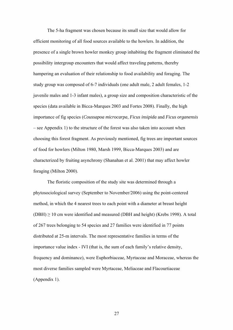
The 5-ha fragment was chosen because its small size that would allow for
efficient monitoring of all food sources available to the howlers. In addition, the
presence of a single brown howler monkey group inhabiting the fragment eliminated the
possibility intergroup encounters that would affect traveling patterns, thereby
hampering an evaluation of their relationship to food availability and foraging. The
study group was composed of 6-7 individuals (one adult male, 2 adult females, 1-2
juvenile males and 1-3 infant males), a group size and composition characteristic of the
species (data available in Bicca-Marques 2003 and Fortes 2008). Finally, the high
importance of fig species (Coussapoa microcarpa, Ficus insipida and Ficus organensis
– see Appendix 1) to the structure of the forest was also taken into account when
choosing this forest fragment. As previously mentioned, fig trees are important sources
of food for howlers (Milton 1980, Marsh 1999, Bicca-Marques 2003) and are
characterized by fruiting asynchrony (Shanahan et al. 2001) that may affect howler
foraging (Milton 2000).
The floristic composition of the study site was determined through a
phytosociological survey (September to November/2006) using the point-centered
method, in which the 4 nearest trees to each point with a diameter at breast height
(DBH) ≥ 10 cm were identified and measured (DBH and height) (Krebs 1998). A total
of 267 trees belonging to 54 species and 27 families were identified in 77 points
distributed at 25-m intervals. The most representative families in terms of the
importance value index - IVI (that is, the sum of each family’s relative density,
frequency and dominance), were Euphorbiaceae, Myrtaceae and Moraceae, whereas the
most diverse families sampled were Myrtaceae, Meliaceae and Flacourtiaceae
(Appendix 1).
27

Before the start of the behavioral data collection the area was totally mapped
(July to September/2006) by dividing it into 25x25-m quadrants limited by individually
numbered wood stakes. The stakes were attached to each other by strings to facilitate
the tree mapping described below. The grid of quadrants was arranged along N-S and E-
W axes, so the position of the group or the location of a single tree could be accurately
mapped using X and Y coordinates (Figure 1). Following this mapping and the
phytosociological survey, 12 plant species (belonging to 10 families) known to be
important food sources for brown howler monkeys based on a literature review (Prates
1989, Jardim 1992, Cunha 1994, Limeira 1996, Marques 1996, 2001, Gaspar 1997,
Martins 1997, Fortes 1999, Fialho 2000, Lunardelli 2000, Liesenfeld 2003) were chosen
for monitoring their tree use. All 417 trees with DBH ≥ 10 cm belonging to these
species were mapped, tagged and measured (DBH and height) (November/2006 to
February/2007) (Table 1). This was the best method for predicting the potential most
important food sources available to the study group, because this was the first study on
howler monkey ecology and behavior at this region.
Data collection procedure
After habituation (February/2007), the study group was followed from dusk to
dawn for 26 days (243 hours of observation) distributed in three periods between March
and October 2007 (8 days in March/2007 - Summer; 8 days in May and June/2007 –
Fall; 10 days in September and October/2007 - Winter and beginning of Spring). Since
determining tree use and foraging patterns of the study group was the main goal of this
study, sampling days (1) that started with at least one animal moving or away from the
sleeping tree; (2) with gaps of more than four continuous trees of the group’s pathway
while moving; (3) in which sight of view from at least a half plus 1 individuals of the
28

group was lost for a minimum of 20 minutes; (4) without an accurate determination of
the night sleeping tree; and (5) with severe weather conditions (rainy or windy days)
were excluded from the analysis, decreasing the sample to 20 days (205 hours of
observation). These limitations impeded having more than three continuous sampling
days in each period.
Figure 1 – Study area and grid of quadrants positioned on N-S and E-W axes.
29

Table 1 – Representation of selected plant species at the study site (n – number of trees;
DBH – average ± s.d. diameter at breast height in centimeters; height – average ± s.d.
height in meters) (See text for details on the selection criterion).
Family Species n DBH (cm) HEIGHT (m)Moraceae Ficus organensis 15 105.4 ± 27.3 19.8 ± 4.7Cecropiaceae Coussapoa microcarpa 68 48.7 ± 25.3 16.8 ± 4.5Moraceae Ficus insipida 12 38.9 ± 25.0 16.1 ± 3.9Tiliaceae Luehea divaricata 28 35.1 ± 13.1 15.4 ± 6.0Myrtaceae Campomanesia xanthocarpa 7 29.7 ± 15.4 13.2 ± 3.5Nyctaginaceae Guapira opposita 101 26.8 ± 11.2 13.8 ± 3.3Sapotacea Chrysophyllum gonocarpum 3 24.0 ± 14.3 17.1 ± 0.8Ebenaceae Diospyros inconstans 50 23.1 ± 27.0 13.3 ± 3.7Arecaceae Syagrus romanzoffiana 11 18.3 ± 4.5 12.8 ± 2.7Sapindaceae Allophyllus edulis 4 18.1 ± 3.3 11.4 ± 1.4Rutaceae Zanthoxylum hyemalis 70 12.2 ± 6.1 10.0 ± 3.4Rutaceae Zanthoxylum rhoifolium 48 11.1 ± 4.6 10.1 ± 2.4
TOTAL 417 36.6 ± 14.7 14.2 ± 3.4
Data collection periods were conducted 2 to 3 months apart in a way of
representing seasons varying in food availability. Each period comprised at least 8 days
and was conducted through at most a month, while the phenological pattern of the forest
fragment could be considered relatively the same and, theoretically, the foraging
patterns of the group would be similar between the days sampled.
A total of 175 days (~1800 hours) were spent in the field throughout this 16-
month study: 20 days for mapping the area, 30 days for the phytosociological survey, 55
days for identifying, mapping and measuring trees belonging to the selected species, 10
days for identifying, mapping and measuring trees used by the study group belonging to
other species, and 60 days for studying the behavior.
Behavioral data collection
30
The behavioral data collection consisted in the focal group behavioral method
(Altmann 1974) by which the group was followed continuously and each behavior
(feeding, resting, moving/traveling and social interaction) was recorded and timed.
Feeding was defined as handling and ingesting plant material. Resting was defined as a
period of inactivity. Moving/traveling was defined as any locomotion between trees of a
half plus one individual of the group. Social interactions included vocalizations directed
at other group members, physical contact, displacement, threats, huddling, and
grooming.
Because the group was usually found as a cohesive unit at one or two adjacent
trees, it was possible to record the group’s behavior continuously. Besides, the presence
of a second observer on most sampling days guaranteed the behavioral sampling when
some individuals were located distant from the rest of the group. Behavioral recording
began each day by the moment howlers woke up in the morning (which varied from
5:30 to 9:30 am) until their activities stopped for night sleep. In a way of standardizing
the night resting timing, as the group was invariably sampled sleeping on the night
sleeping tree at 6:00 pm, the behavioral timing analysis lasted until 6:00 pm.
All trees visited by the group in a given day were tagged, identified, mapped and
measured (DBH), and the behavior of each individual howler visiting them recorded. At
the end of each behavioral data collection period, the visibility index (VI – modified of
the field-of-view index in Garber and Jelinek 2006) of all trees used for at least 2% of
the total time recorded (11, 14 and 10 trees at each period, respectively) and at least 2%
of the total feeding time (14, 16 and 6 trees at each period, respectively), was estimated.
This measure took into account the height of all adjacent trees and the percentage of the
target tree’s crown that was covered at each stratum (1 – bottom of the crown; 2 –
middle of the crown; 3 – top of the crown) and at each direction. For example, if the
31

crowns of four of five trees that surround the target tree to the north overlapped the
bottom of its crown, a 20% VI was scored for that height and coordinate. At the same
time, if only one out of five tree crowns at this same coordinate obstructs the field of
view of a howler located at the top of the target tree crown, an 80% VI was assigned. As
already discussed by Garber and Jelinek (2006, pp 293), this only functions as “a crude
and relative measure of the degree to which howlers could sight directly to a subsequent
feeding/resting site”. The visibility index of random trees was also estimated to test
whether visibility influences tree selection during foraging.
Several howler species have been described to move in single-line progressions
(Carpenter 1964, Bicca-Marques and Calegaro-Marques 1997, Milton 2000, Garber and
Jelinek 2006) through repeated pathways. To test if the study group follows the same
pattern, all trees used for resting and moving by most group members were marked. In
addition, every tree used for feeding, even by a single individual, was marked. A route
was defined as a sequence of consecutive trees used by most group members,
irrespective of its direction (i.e. A-B-C = C-B-A).
The item ingested (mature leaf – ML; young leaf – YL; leaf bud – LB;
unidentified leaf – UL; ripe fruit – RFR; unripe fruit – UFR; open flower – OFL; flower
bud – FLB) and the amount of time each howler spent feeding on the item at each tree
was recorded during all feeding bouts. As preferences for different and specific plant
parts have already been described for distinct primate species (Garber 1987) as well as
indicative of monitoring of fruit ripeness (Janmaat et al. 2006), I observed the ripening
state of the plant parts eaten to verify its influence on foraging. The contribution of each
item, species or individual tree to the diet of the group at each period was estimated
based on the average time spent feeding on them. Data on infant feeding was not
included in these analyses.
32

The spatial distribution of trees used by howlers and of those trees belonging to
prospective important food sources was determined by plotting their X and Y
coordinates using a computer program developed by R. S. González and A. S. Martinez.
These representations allowed an accurate determination of the group’s day range based
on the sum of the distances between used trees, since all tree coordinates were
accurately measured in-situ with a high-precision laser distance meter (Leica DISTOTM
A2).
Two different analyses were used to quantify the deviation from straight-line
travel. First, the ratio between the most efficient route between two points (D), that was
considered to be the straight line between them, and the observed route distance (L) was
calculated, especially between feeding trees (D/L - Seguinot et al. 1998, Pochron 2001).
A ratio of 1 indicates that the most efficient route was taken. In addition, the null
hypothesis that segments between feeding trees were independent and uniformly
distributed around a circumference rather than concentrated around a specific direction
was tested for verifying the organization of successive segments. Clustering around
0/360° would indicate a dependent relationship between segments alignment, possibly
over an efficient route traveling. For this analysis, the magnitude of the clockwise
rotation needed to align with the bearing of a route segment i when arriving at a feeding
tree to the bearing of the route segment i + 1 when leaving this tree was computed. The
daily computed bearing vectors between feeding trees were analyzed with circular
statistics (Kovach 1999).
To test the hypothesis that brown howler monkeys minimize distance traveled,
the straight-line distance between consecutive feeding trees was compared with the
distance between the first tree of a given species visited and the nearest tree of the same
33

species and the nearest tree used for feeding during the same sampling period
independently of which species it belonged to.
Howler monkeys usually present 1 to 3 long-lasting periods of resting each day,
that have been suggested to be important behavioral adaptations to maximize the
digestion of fibrous and high-structured nutrients ingested (Smith 1977, Milton 1980,
Glander 1982). Di Fiore and Suarez (2007) identified several nodes intersecting travel
routes of spider and woolly monkeys that would act as decision points where the group
could decide which route to take next. Using resting trees as nodes, or decision-points
where different routes segments intersect, could be used as a strategy on howlers
foraging since their repetitive use connecting distinct travel routes would favor a
variation on the diet’s composition throughout the day, as already described for howlers
(Ganzhorn and Wright 1994). Certain routes may lead to important ephemeral fruit
sources worth monitoring at the beginning of the day when the group still has time to
forage in other locations if those items are not available, while other routes may end up
at staple food sources that will guarantee a feeding bout before the night sleep. To
identify whether resting trees used by howlers act as nodes, as described for spider and
wooly monkeys (Di Fiore and Suarez 2007), it was considered the number of times each
resting tree has been used, the distinct direction the had been reached and the angular
deviation observed between the bearing the of the arrival route leading to it before
resting and the direction of the route taken when leaving it was considered.
Changes in speed of travel have been used to infer spatial knowledge of the
location of a goal (Pochron 2001, Janmaat et al. 2006). In the current research, it was
impossible to determine whether change in travel speed was influenced by resource
detection because average distance between consecutive feeding sources was inferior to
34

40 m. Histograms of the distances between feeding sites were plotted to analyze
whether and how this variable acted on howlers’ foraging.
Data Analysis
All analyses were performed separately for each data collection period. Activity
budgets were calculated based on the average time spent by the group in each behavior.
Similarly, the contribution of each food item or species to the diet was based on the
average time spent eating it in the feeding bouts. Only bouts lasting at least 5 minutes
and in which more than two howler monkeys were feeding on the same tree were
considered feeding target trees in the analyses of the minimum distance traveled
between feeding trees, the straight-line distance and the angular deviation between
them. The DBH was used as a surrogate of food abundance of individual trees. DBH is
considered the most accurate method for comparing resource productivity by different
plant species (Chapman et al. 1992).
Data were analyzed to observe statistical differences using One-Way Analysis of
Variance (ANOVA), Student-t test and Z test for parametric data according to the
number of observations at each sample and its variance, and, for non-parametric data,
the Kruskal-Wallis test and two-sample Mann-Whitney test were used for independent
samples of equal variance. Whenever two or more variables were tested simultaneously,
the Bonferroni post-hoc test was used. To measure the strength of the relationship
between independent variables, regression analyses were performed, whereas Spearman
rank correlation coefficient (rs) and Pearson correlation coefficient (rp) were used to
verify the correlation between non-parametric and parametric dependent variables,
respectively. The Rayleigh test was used for the circular analyses on angular deviation
between trees. All tests were two-tailed and performed using the software Biostat 5.0
35

(Ayres et al. 2007), except the circular statistic where it was used the software Oriana
1.06 (Kovach 1999).
36

RESULTS
In 20 days of behavioral data collection the study group fed, rested and traveled
in 654 trees (311, 301 and 418 trees in each period, respectively). The mean daily range
was 919 ± 256 m, a distance that did not vary significantly between the sampling
periods (F = 1.2761, p = 0.3046, df = 17). The howler group concentrated their activity
budget on resting (57.6 ± 8.3%) and feeding (17.1 ± 5.2%), with a diet based on leaves
(53.3 ± 15.2%), fruits (34.3 ± 17.4%) and flowers (12.2 ± 12.3%) (Table 2).
The group spent significantly more time resting during the Fall sampling period
than it did in the Winter-Spring sampling period (t = 2.7055, p = 0.0191, df = 12). This
difference was not observed between Summer and Fall (t = -1.0112, p = 0.3318, df =
12) and Summer and Winter-Spring (t = 0.5925, p = 0.5666, df = 10) (Figure 2). At the
same time, the Winter-Spring sampling period was the only in which the percentage
time resting was not significantly correlated with day range (rp = -0.4968, p = 0.3161, df
= 4). Day range was negatively related to resting during Summer (rp = -0.08482, p =
0.0328, df = 4), Fall (rp = -0.07367, p = 0.037, df = 6) and the entire study (rp = -
0.7403, p = 0.0002, df = 18).
Both percentage time feeding and total time (in minutes) spent feeding were
significantly higher in Winter-Spring than in Summer (t = -3.3495, p = 0.0073, df = 10;
t = -3.5486, p = 0.0053, df = 10), but no difference was observed between Summer and
Fall (t = -1.5637, p = 0.1438, df = 12; t = -1.5593, p = 0.1488, df = 10), and Fall and
Winter-Spring (t = -1.3391, p = 0.2053, df=12; t = -1.4500, p = 0.1726, df = 10). The
contribution of leaves to the diet was similar throughout the study (F = 0.5094, p =
0.6147, df = 17).

Table 2 – Mean daily activity budget, tree use and diet composition during the study.
Summer Fall Winter-Spring Meanresting (%) 56.7 ± 12 61.4 ± 5.3 53.5 ± 5.6 57.6 ± 8.3feeding (%) 13.4 ± 2.6 17.1 ± 5.3 20.8 ± 4.7 17.1 ± 5.2day range (m) 1043.1 ± 361.1 825.5 ± 185.7 920.8 ± 193.5 919.4 ± 255.8used trees (n) 77.2 ± 23.2 73.8 ± 20.4 96.5 ± 10.3 81.6 ± 20.6 feeding trees (n) 17.7 ± 4.3 19 ± 3.9 29 ± 6.6 21.6 ± 6.9 resting trees (n) 6.3 ± 2.9 5.6 ± 2 5 ± 2.6 5.7 ± 2.4 traveling trees (n) 55.8 ± 19.1 50.8 ± 18.1 72.3 ± 7.2 58.8 ±17.8 feeding trees (%) 24.3 ± 7.8 26.6 ± 4.6 29.8 ± 4.2 26.9 ± 5.7 resting trees (%) 8.2 ± 2.4 8.6 ± 4.7 5.2 ± 2.8 7.4 ± 3.7 traveling trees (%) 70.4 ±7.8 70.4 ± 6.5 66.4 ± 10 69.9 ± 7.8Leaves (%) 55.7 ± 14.4 49.3 ± 15.2 57 ± 17.4 53.3 ± 15.2 mature (%) 37.2 ± 13.5 19.8 ± 16.6 14.8 ± 12.5 23.5 ± 16.7 young (%) 6.3 ± 4.7 21.3 ± 9.4 27.1 ± 15.4 18.5 ± 13.2 bud (%) 8.7 ± 7.5 4.1 ± 5.1 14.8 ± 9.5 8.7 ± 8.3 unknown (%) 3.6 ± 2.7 4 ± 5.1 0.4 ± 0.5 2.8 ± 3.8 Fruits (%) 42.5 ± 10.7 38.8 ± 13.7 20 ± 20.4 34.3 ± 17.4 unripe (%) 29.3 ± 5.9 37.8 ± 12.6 18.7 ± 19.7 29.5 ± 15.4 ripe (%) 13.2 ± 14.6 0.9 ± 2 1.4 ± 2.8 4.7 ± 9.6Flowers (%) 1.7 ± 4.1 12 ± 5.3 22.9 ± 15.8 12.2 ± 12.3 open (%) 1.7 ± 4.1 3.3 ± 3.9 10.9 ± 6.7 5.1 ± 6.1 bud (%) 0.1 ± 0.1 8.7 ± 3.2 12.1 ± 16 7.1 ± 9.8
0
10
20
30
40
50
60
70
80
Summer Fall Winter-Spring
%
Figure 2 – Mean percentage of time spent resting (black box) and feeding (gray box)
by brown howler monkeys at each sampling period.
37

Similar results were found for fruits during Summer and Fall (t = 0.5466, p =
0.5946, df = 12) and Fall and Winter-Spring (t = 2.0653, p = 0.0611, df = 12) and for
flowers during Fall and Winter-Spring (F=3.4613, p = 0.0847, df = 12). However, fruits
contributed significantly more during the Summer than the Winter-Spring (t = 2.3845, p
= 0.0383, df = 10). In the latter sampling period the study group ate significantly more
flowers than in the Summer (Z = 2.5820, p = 0.0098, U = 4) and Fall (Z = 2.7222, p =
0.0065, U = 1). Figure 3 shows the mean percentage contribution of each food item per
sampling period.
Figure 3 – Mean percentage of time spent eating each food item during each sampling period
(summer – orange; fall – green; winter-spring – blue). ML = mature leaf, YL = young leaf, LB =
leaf bud, UL = unidentified leaf, UFR = unripe fruit, RFR = ripe fruit, OFL = open flower, FLB =
flower bud, LEAVES = ML + YL + LB + UL, FRUITS = UFR + RFR, FLOWERS = OFL +
FLB. Pairs that present statistical differences are indicated (* and ° p < 0.05; ** and °° p < 0.01).
Each sampling period showed distinct patterns of foraging and tree use. The
Summer was marked by similar contributions of mature leaves (40.6%) and total fruits
(43.0%; 9.2%=ripe fruits), long mean day range (1043 ± 361 m; range: 538 – 1505 m),
and a low mean percentage feeding (13.4 ± 2.6%) (Table 2). During the Summer, day
range was positively correlated with the percentage feeding on unripe fruits (rp =
38

0.8818, p = 0.0201, n = 6) that was related to the period feeding percentage (rp = 0.8552,
p = 0.0299, n = 6), while the minutes spent eating were positively related to the feeding
time spent eating mature leaves (rp = 0.9167, p = 0.0101, n = 6). The distance traveled
also varied according to the number of trees used per day, as expected, (rp = 0.8365, p =
0.0375, n = 6) and those used for resting (rs = 0.971, p = 0.0012, n = 6), while the latter
was positively related to the feeding percentage of unripe fruits (rs = 0.9122, p = 0.0112,
n = 6). The greater the amount of time the howlers spent eating unripe fruits, the less
time they spent resting (rp = -0.8466, p = 0.033, n = 6).
During this same sampling period, the feeding on ripe fruits showed a distinct
pattern from the one described above for unripe fruits, since it was negatively related to
the distance traveled (rp = -0.848, p = 0.0329, n = 6). Moreover, the percentage of ripe
fruits eaten also presented a negative relationship with the total number of trees used per
day (rp = -0.8139, p = 0.0489, n = 6).
On the other hand, during the Fall sampling period a short mean distance
traveled was characterized (825.5 ± 185.7 m ; 467 – 990 m) and long periods of resting
(61.4 ± 5.3%). The consumption of unripe fruits during the Fall sampling days was the
highest among the sampling periods (32%) and the total consumption of flowers
increased (17.6%) compared to the previous period, accompanied by a decrease in the
total consumption of leaves (49.7%). As before, the distance traveled was positively
related to the daily number of trees used (rp = 0.9623, p = 0.0001, n = 8) and those used
for feeding (rp = 0.7593, p = 0.0288, n = 8), but, during this period, the latter varied with
the amount of flower buds eaten (rp = 0.7481, p = 0.0327, n = 8) and with the total
consumption of leaves (rp = 0.8852, p = 0.0035, n = 8). Likewise, the distance traveled
was positively related to the total number of minutes spent eating leaves (rp = 0.7611, p
= 0.0284, n = 8). The more trees used, the more of them were used for feeding (rp =
39

0.8913, p = 0.0029, n = 8), and the greater the percentage of trees used for feeding, the
greater was the percentage of resting trees (rs = 0.7381, p = 0.0365, n = 8). The
percentage of daily feeding time was related to the percentage ingested of open flowers
(rp = 0.7751, p = 0.0238, n = 8), unripe fruits (rp = 0.8902, p = 0.0003, n = 8) and total
consumption of fruits (rp = 0.8629, p = 0.0058, n = 8).
The last period sampled was marked by a high mean feeding percentage (20.8 ±
4.7%), which at the same time characterized a high mean number of trees used daily
(96.5 ± 10.3%) as feeding trees (29 ± 6.6%) and trees used exclusively for locomotion
(72.3 ± 7.2%). As a consequence, although the daily mean number of trees used for
resting (5 ± 2.6) was similar to the patterns observed for Summer and Fall (6.3 ± 2.9 and
5.6 ± 2, respectively), the percentage of trees used daily for resting decreased during the
Winter-Spring sampling period (5.2 ± 2.8%). During this period, the total consumption
of leaves (64%) and flowers (22.7%) was as high as the consumption of young leafs
(29.8%) and leaf buds (14.4%), while the percentage of time spent eating fruits (13.6%)
was the lowest among the sampled periods. The daily feeding percentage increased
along with the number of trees used daily (rp = 0.8977, p = 0.0152, n = 6), those used
daily for feeding (rp = 0.9568, p = 0.0028, n = 6) and was negatively related to the
feeding percentage of young leaves (rp = -0.885, p = 0.019, n = 6). The higher the
number of trees used, the higher was the number of those trees used for feeding (rp =
0.9159, p = 0.0103, n = 6). On the other hand, to the contrary of the pattern observed
during the other sampling periods, the daily mean distance traveled was not
significantly correlated with the mean number of trees used daily (rp = 0.7481, p =
0.0871, n = 6), although small sample size might have influenced these results.
40

Tree use
Describing the study group tree use patterns was our first approach to better
understand how the environmental features might influence howler behavior. The 654
trees used belonged to 57 plant species (Shannon-Wiener species richness index: H’ =
3.357) (311 trees of 50 species in Summer, 299 trees of 46 species in Fall and 412 trees
of 51 species during the Winter-Spring period). The overall mean number of trees used
per day was 81.6 ± 20.6. The number of trees used daily was greater in Winter-Spring
(96.5 ± 10.3) than in the Fall (74.6 ± 20.8: t = -2.4833, p = 0.0287, df = 12) (see
Appendix 2). The group traveled through an average of 26.9 ± 5.3 species each day and
used significantly more species in the Winter-Spring than in the two other sampling
periods (F = 6.4477, p = 0.0083, df = 17). Likewise, the mean daily number of feeding
species used during the Winter-Spring period (13.5 ± 3.3 plant species) was
significantly greater (F = 6.6832, p = 0.0073, df = 17) than the means observed during
the Summer (9.0 ± 1.4) and Fall (9.8 ± 2.0) periods. Ten of the 12 species previously
selected as putative important food sources were responsible for 68.7% of the total time
spent feeding by the study group.
The number of individual trees of a given species used was strongly related to
the species importance value (IVI) in the forest fragment (Linear regression: R2 = 45.66,
p < 0.0001, n = 46). However, an analysis of residuals considering the species’ IVIs as
the predictor variable of tree use indicated that the howlers passed more through trees of
three species (Guapira opposita, Myrsine guianensis and Coussapoa microcarpa) and
through trees of Sebastiania commersoniana, the most frequently sampled species in the
phytosociology, less that the predicted value (Figure 4A). Although the previous
analyses did not indicate any statistically significant difference in the pattern of use,
considering the number of visits per species predicted by species’ IVIs (R2 = 46.11, p <
41

0.0001, n = 46), Coussapoa microcarpa was visited significantly more than expected
(ESD = 3.3181, p < 0.05, n = 50), while Sebastiania commersoniana was visited
significantly less than expected (ESD = 3.3607, p < 0.05, n = 50) (Figure 4B).
Figure 4 – A) Residual number of trees used per species (1 - Guapira opposita; 2 - Myrsine
guianensis; 3 - Coussapoa microcarpa and 4 - Sebastiania commersoniana) and B) Residual
number of visits per species predicted by each species IVI value (1 - Coussapoa microcarpa
and 2 - Sebastiania commersoniana. Dashed lines indicate mean residuals value ± SD.
Although the number of feeding trees varied from one period to another, being
significantly higher during the Winter-Spring period than in the other two seasons
sampled (t = -3.5068, p = 0.0056, df = 10; t = -3.5417, p = 0.0040, df = 12,
respectively), the howlers used a similar percentage of feeding trees during the sampling
periods (H = 2.2323, p = 0.3275, df = 2). Similarly, the percentage of resting trees and
traveling trees also did not vary between the different seasons (F = 1.6384, p = 0.2225,
df = 17; F = 3.2079, p = 0.0646, df = 17, respectively) (Figure 5).
42

0
10
20
30
40
50
60
70
80
90
100
total (n) resting (n) feeding (n) traveling (n) resting (%) feeding (%) traveling (%)
Figure 5 – Mean tree use patterns (n and % of trees used) at each sampling period (Summer
– orange; Fall – green; Winter-Spring – blue).
The same species that was used more than expected, as shown in the residual
analysis plotted above (Figure 4a and b), also accounted for the highest numbers of
feeding trees used (Appendix 3). Coussapoa microcarpa was the second most important
feeding species during the days sampled (13.3% of the groups’ feeding time),
contributing with both leaves and fruits in all the periods sampled (Table 3).
The most important food source, Ficus organensis, contributed 18.5% of the
total feeding time and accounted for 57.4% of the fruit feeding records (92.3% of those
were unripe fruits). All 15 trees of Ficus organensis in the forest fragment were used,
considering that 11 were used for feeding and 11 accounted for the greatest percentage
of time spent resting in a single species in the study, 37.8% (Table 4). The 11 trees used
for resting and those 11 trees used for feeding overlap in 10 individuals and 8 of them
were among the 20 most used trees during the study. The time spent using this species
comprised 26.0% of the group’s tree use during the study, while the use of Coussapoa
microcarpa represented 23.4%, also being the second most used species for resting.
43

Table 3 – Plant species used for feeding and the relative contribution of its items to the group’s diet
during the study (mature leaf – ML; young leaf – YL; leaf buds – LB; unidentified leaf – UL; ripe
fruit – RFR; unripe fruit – UFR; opened flower – OFL; flower bud – FLB).
Species % Feeding ML YL LB UL RFR UFR OFL FLBFicus organensis 18.5 1.26 0.83 1.03 0.45 1.15 13.82 0 0Coussapoa microcarpa 13.3 1.14 0.83 1.12 0.52 1.19 7.55 0.60 0.39Ficus insipida 9.2 2.47 4.59 1.30 0.32 0 0.51 0 0Guapira opposita 8.8 0.71 0.73 0.24 0.22 0 0 3.05 3.80Zanthoxylum hyemalis 6.3 3.12 0.79 1.24 0.92 0 0 0.26 0Diospyros inconstans 6.0 3.10 2.08 0 0 0 0 0.40 0.40Dasyphilum spineeis 4.6 1.26 2.51 0.50 0 0 0 0 0.38Zanthoxylum rhoifolium 4.0 3.38 0.28 0.31 0 0 0 0 0vine sp. 3.7 0 1.00 0.19 0 0 0 1.23 1.33Sorocea bonplandii 3.4 0.47 2.88 0 0 0 0 0 0Myrsine guianensis 2.5 0.23 0.08 0.04 0.12 0.07 0.61 0.26 1.11Banara parviflora 1.9 1.13 0.30 0.20 0.22 0.05 0 0 0Trichilia clausenii 1.5 0.81 0 0 0.24 0 0.49 0 0Esenbeckia grandiflora 1.4 0.85 0.36 0.19 0.05 0 0 0 0Chrysophyllum gonocarpum 1.2 0.68 0 0.52 0.02 0 0 0 0Nectandra megapotamica 1.2 0.12 0 0.67 0 0 0 0.05 0.39Lithraea brasiliensis 1.1 0.38 0.46 0.04 0.24 0 0 0 0Luehea divaricata 0.9 0 0.46 0.16 0 0.07 0 0.25 0Vitex megapotamica 0.8 0.46 0.30 0 0 0 0 0 0.07Sebastiania commersoniana 0.7 0.13 0 0.33 0 0.11 0 0.06 0.06Casearia decandra 0.6 0 0 0 0 0 0 0.30 0.32Ocotea pulchella 0.6 0 0.60 0 0 0 0 0 0Myrcianthes gigantea 0.6 0.24 0.11 0 0.02 0.12 0.07 0 0Sloanea monosperma 0.5 0.49 0 0 0.05 0 0 0 0Campomanesia xanthocarpa 0.5 0.23 0.05 0 0.12 0 0 0.04 0.04Allophyllus edulis 0.4 0 0.12 0.29 0 0 0 0 0Solanum peseudo-quina 0.4 0.21 0.16 0 0 0 0 0 0Inga uruguensis 0.3 0.33 0 0 0 0 0 0 0Myrsine coreaceae 0.3 0.28 0 0 0 0 0 0 0Psidium cattleianum 0.2 0.24 0 0 0 0 0 0 0Xylosma pseudosalzmanii 0.2 0 0 0 0 0 0 0.19 0.05Ilex brevisuspis 0.2 0 0.09 0.12 0 0 0 0 0Matayba elaeagnoides 0.2 0 0.17 0 0 0 0 0 0Cytharexyllum myrianthum 0.2 0 0 0 0 0.17 0 0 0Miconia rigidiuscula 0.1 0.14 0 0 0 0 0 0 0Cabralea canjerana 0.1 0 0.09 0 0 0 0 0 0Ilex dumosa 0.1 0.09 0 0 0 0 0 0 0Erythroxylum argentinum 0.1 0 0 0 0.07 0 0 0 0Myrcia glabra 0.1 0 0 0 0.07 0 0 0 0undeterm. spp 3.1 0.95 0.25 0.83 0.39 0.12 0 0.23 0.32
TOTAL 100 24.9 20.1 9.3 4.0 3.0 23.1 6.9 8.7
44

Table 4 – Tree species used for resting during the study and its respective contribution, average
use/per individual tree and DBH.
Speciesn tree % resting mean use/tree min max DBH
Ficus organensis 11 37.80 3.44 ± 3.27 0.15 10.25 97.8 ± 35.2Coussapoa microcarpa 19 36.21 1.91± 2.20 0.04 7.35 74.6 ± 23.8Myrsine guianensis 5 6.03 1.21 ± 1.86 0.01 4.32 30.4 ± 5.2Ficus insipida 4 2.85 0.71 ± 1.18 0.09 2.49 55.5 ± 11.9Banara parviflora 3 2.32 0.77 ± 0.19 0.62 0.99 29.3 ± 9.4Nectandra megapotamica 1 1.70 56Diospyros inconstans 3 1.35 0.45 ± 0.55 0.13 1.09 27.5 ± 5.3Myrcianthes gigantea 3 1.10 0.37 ± 0.45 0.02 0.88 46.20Guapira opposita 2 0.90 0.45 ± 0.56 0.05 0.85 36.1 ± 2.9Trichilia clausenii 2 0.52 0.26 ± 0.14 0.16 0.36 35.6 ± 2.3Myrcia glabra 1 0.49 24.8Sebastiania commersoniana 1 0.42 21Inga uruguensis 1 0.29Chionanthus trichotomus 1 0.27 41.1Luehea divaricata 2 0.19 0.09 ± 0.05 0.05 0.13 53.2 ± 12.6Cabralea canjerana 2 0.13 0.07 ± 0.06 0.02 0.11 52.2 ± 7.2Gymnanthes concolor 1 0.12Maytenos casineformis 1 0.12Prunus selloi 1 0.04Zanthoxylum rhoifolium 1 0.04 12.7Sloanea monosperma 1 0.04 54.1undeterm. spp 8 7.05 0.88 ± 1.14 0.04 3.39 38.4 ± 27.1
TOTAL 66 93 59.6 ± 32.5
use/tree
To classify the target trees used in each sampling period was considered the
percentage of days sampled that each tree was used and the percentage of feeding and
resting time observed for each individual tree (see Methods). Although the study group
used a large number of trees, 39.0% were used for only a day and another 23.1% were
visited in two days (Figure 6A). When only the feeding trees were considered, this
percentage was even higher, since 66.3% and 16.9% of the trees were used for just a
day or two, respectively (Figure 6B), while 37.8% of the resting trees were used for a
single day and 12.2% for two days (Figure 6C). On the other hand, 18% of the overall
trees, 7% of the feeding trees and 27% of the resting trees were used in at least five
45

Figure 6 – Intensity of tree use in accumulative days per sampling period
observed, indicating total tree use (A), feeding tree use (B) and resting tree use (C)
(Summer – orange; Fall – green; Winter-Spring – blue; total - dark line).
46

47
days. Among those, 11 trees were used for 32.8% of the total time recorded, being
classified as target trees (five trees in Summer, five in Fall and three in Winter-Spring)
(Table 5, but see data on angular deviation below).
Visibility
The visibility index (VI) was determined for the trees used for the greatest
percentage of feeding and total time (see Methods). This accounted for 14 trees during
the Summer (12 feeding trees), 19 trees during the Fall (9 feeding trees), 13 trees during
the Winter-Spring (3 feeding trees) and 16 trees for the entire study period (6 feeding
trees), comprising a total of 26 trees (>2% of the total time recorded). Measures of VI
values of other 77 trees widespread throughout the forest fragment were taken for
comparison with the VI of the most used trees.
The forest fragment shows an irregular slope along its length, with the north
coordinate facing up the hill. As a consequence, none of the trees used by the howlers
showed significantly greater visibility in the north coordinate than the control trees.
Another consequence of the forest fragment terrain, besides its shape, are the
differences found between the visibility at each coordinate, where the south and east
coordinate present a higher VI than the north and west coordinates (H = 11.8535, p =
0.0079, df = 3).
All the coordinates total visibility values, except the north coordinates, were
significantly higher than those of the control trees (Table 6).The mean visibility at the
bottom portion of the tree crowns was 22.3 ± 18.5%, in the middle portion of the crown
was 47.8 ± 24.7% , and at its top was 63.8 ± 29.1. The visibility of the most used trees
during each period and throughout the entire study did not differ from one another (F =
0.2659, p = 0.8508, df = 3).

bottom middle top TOTAL bottom middle top TOTAL bottom middle top TOTAL bottom middle top TOTAL bottom middle top TOTALsummer 14 ± 15 31 ± 34 46 ± 39 30 ± 26 37 ± 40 56 ± 39** 70 ± 38 54 ± 37** 7 ± 10 36 ± 40 57 ± 40** 33 ± 28 27 ± 25** 55 ± 38 72 ± 39 51 ± 31 21 ± 16** 45 ± 26** 61 ± 32 42 ± 23**fall 11 ± 16 28 ± 31 51 ± 37 30 ± 25 43 ± 40* 65 ± 39* 77 ± 37* 62 ± 36* 11 ± 18 49 ± 40* 68 ± 36* 43 ± 28* 27 ± 33** 51 ± 39 73 ± 36** 50 ± 32** 23 ± 19* 49 ± 26* 67 ± 28* 46 ± 23*winter-spring 12 ± 16 34 ± 34 46 ± 35 31 ± 27 38 ± 37* 66 ± 37* 77 ± 36** 60 ± 34* 10 ± 18 35 ± 33* 61 ± 36* 35 ± 26* 20 ± 22 57 ± 41 74 ± 37** 50 ± 30 20 ± 18 48 ± 24* 64 ± 25** 44 ± 22**TOTAL 13 ± 17 30 ± 33 50 ± 36 31 ± 26 48 ± 42* 69 ± 37* 83 ± 33* 67 ± 35* 11 ± 17 51 ± 39* 76 ± 34* 46 ± 26* 29 ± 31** 56 ± 40 77 ± 34** 54 ± 32** 25 ± 18* 52 ± 24* 71 ± 25* 49 ± 21*
TOTALNorth South West East
Tree ID Speciessummer fall winter-spring TOTAL summer fall winter-spring TOTAL summer fall winter-spring TOTAL summer fall winter-spring TOTAL
1.05 Ficus organensis 100.0 13.0 50.0 50.0 3.0 - 0.0 0.6 25.1 2.6 3.9 8.7 15.3 1.7 2.2 5.49.12 Coussapoa microcarpa - 50.0 86.0 45.0 - 4.8 3.1 3.0 - 13.1 5.1 6.7 - 9.3 4.0 4.97.03 Ficus organensis - 38.0 50.0 30.0 - - 3.9 1.9 - 6.9 13.3 7.4 - 4.1 8.9 4.61.01 Coussapoa microcarpa 100.0 38.0 33.0 55.0 3.1 3.2 0.4 2.0 15.1 6.7 6.3 9.1 4.8 0.2 4.11.12 Ficus organensis 100.0 38.0 33.0 55.0 12.5 - - 2.6 4.1 3.8 5.4 4.5 5.6 2.8 3.1 3.62.66 Ficus insipida 83.0 50.0 33.0 55.0 9.7 3.6 2.9 4.6 8.4 - - 2.1 6.8 1.0 1.0 2.510.16 Myrsine guianensis - 63.0 17.0 30.0 - 1.5 3.4 0.5 - 6.9 - 3.8 - 4.8 1.9 2.41.40 Ficus organensis 33.0 100.0 17.0 55.0 - 11.3 - 4.0 - 2.6 - 1.0 0.1 4.9 0.0 1.82.39 Ficus organensis 67.0 13.0 50.0 40.0 2.2 - - 0.5 3.0 - 3.5 2.1 2.6 0.2 2.0 1.516.08 Coussapoa microcarpa - - 50.0 15.0 - - 0.8 0.5 - - 6.9 2.1 - - 3.3 1.39.02 Dasyphilum spineeis - 63.0 33.0 35.0 - 6.7 0.1 2.4 - - - - - 1.9 0.0 0.7
TOTAL 100 100 100 100 30.5 31.1 14.6 22.6 55.7 42.6 38.1 44.7 39.5 35.5 26.5 32.8
% days used % feeding % resting % total use
Table 6 – Mean ± s.d. tree visibility index (VI, in %) for the most used trees during each period. Significant differences with the visibility of
control trees are indicated (* indicates p < 0.01 and ** p < 0.05).
Table 5 – Trees classified as target trees due the intensity of their use and contribution on the group’s feeding, resting and total time used.

Monitoring
Three species during the Summer, four species during the Fall and five species
in the Winter-Spring sampling period accounted for 50% of the feeding records, while
nine, eight and 11 species accounted for 80% of them in each period, respectively.
Overall, five and 11 species accounted for 50 and 80% of the group’s diet, respectively,
during the study.
The number of trees used of a given species was significantly correlated with its
contribution to the group’s diet during all the periods sampled (Summer: rs = 0.5606, p
= 0.0044, n = 24; Fall: rs = 0.4815, p = 0.0171, n = 24; Winter-Spring: rs = 0.5763, p =
0.002, n = 26). However, when only those species that have contributed more than 2%
of the feeding time in each period are considered, a significant relationship was only
observed during the Winter-Spring period (rp = 0.7019, p = 0.0075, n = 13).
The greater contribution of a large number of trees to the group’s diet during the
Winter-Spring period was also seen when the ratio of feeding trees to total number of
trees used of each species was considered. While during the Summer period, of those
species that contributed 50% to the group’s diet, an average of 49% of the trees visited
were consumed, during the Fall period this value increased to 62% of the trees used and
reached its maximum use during the Winter-Spring period with a contribution of 71%
of feeding use (Figure 7). Besides, in all the sampling periods, the more a species was
visited, the less the number of trees used for feeding of that species (Summer: rs = -
0.6368, p = 0. 0008, n = 24; Fall: rs = -0.5633, p = 0.0041, n = 24; Winter-Spring: rs = -
0.4542, p = 0.0197, n = 26). In other words, the greater the tree use of a plant species,
the greater was the selectivity of its consumption.
49

Figure 7 – Percentage of feeding trees of the total number of trees used per species
(Summer – orange; Fall – green; Winter-Spring – blue). Data are presented in feeding
contribution per interval of percentage of trees used for feeding (from the total number of
each species used trees). Numbers of species representative of each value are presented
(feeding of vine species not included).
Memory load
Although the study group used 654 trees and the consumption of the 249 feeding
trees was highly variable, route-based foraging patterns can be identified. The first
evidence that indicates the use of travel routes in our study was the repetition of tree use
patterns observed (Figure 8). A daily average of 67% of repetitive tree use was observed
during the study period. In the Winter-Spring, the last sampling period, an average of
74% of the trees used daily had already been visited before. When only feeding trees
were considered, a daily average of 67% of the trees has already been used in previous
days (47% in the Summer, 81% in the Fall and 66% in the Winter-Spring), as
summarized in Figure 9. It should be noted that, although the number of trees that can
50
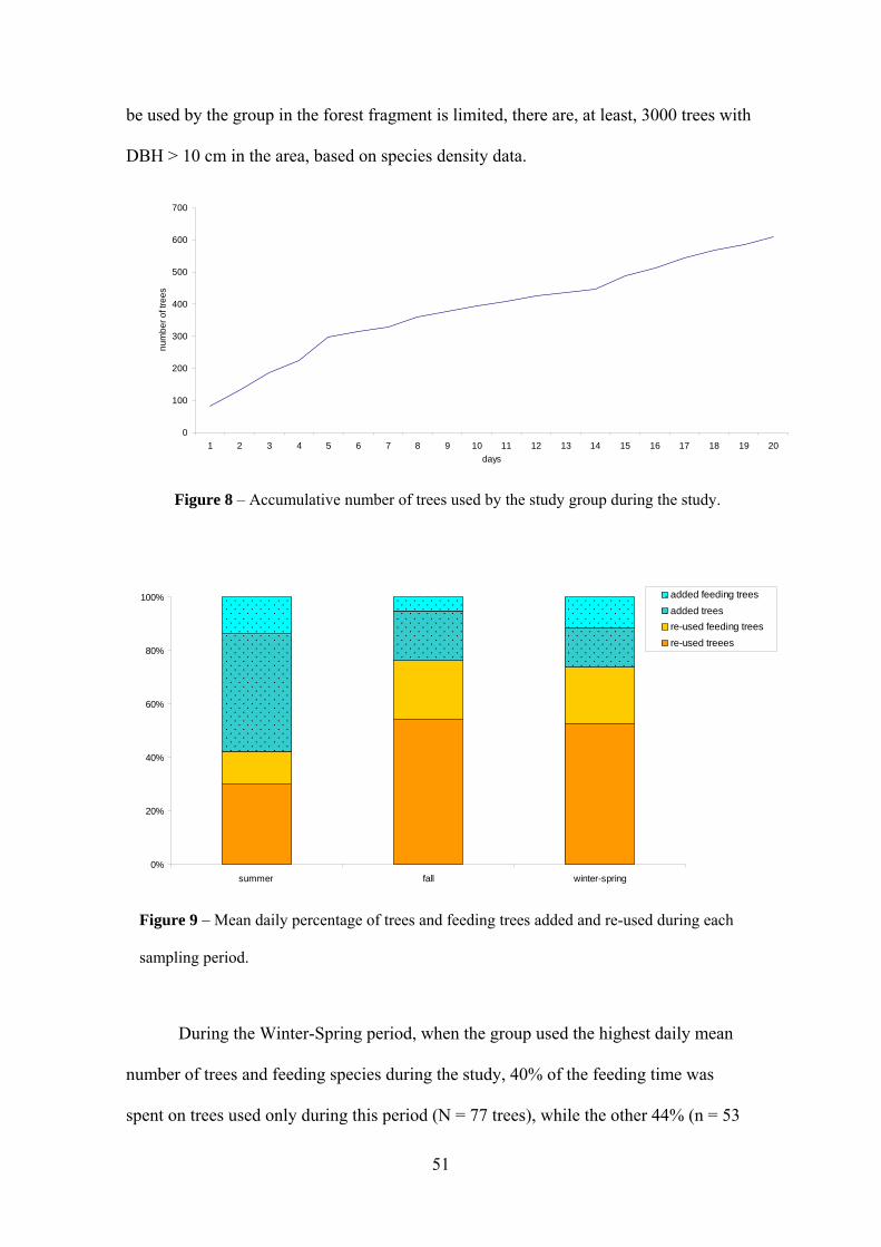
be used by the group in the forest fragment is limited, there are, at least, 3000 trees with
DBH > 10 cm in the area, based on species density data.
0
100
200
300
400
500
600
700
1 2 3 4 5 6 7 8 9 10 11 12 13 14 15 16 17 18 19 20days
num
ber o
f tre
es
Figure 8 – Accumulative number of trees used by the study group during the study.
0%
20%
40%
60%
80%
100%
summer fall winter-spring
added feeding treesadded treesre-used feeding treesre-used treees
Figure 9 – Mean daily percentage of trees and feeding trees added and re-used during each
sampling period.
During the Winter-Spring period, when the group used the highest daily mean
number of trees and feeding species during the study, 40% of the feeding time was
spent on trees used only during this period (N = 77 trees), while the other 44% (n = 53
51

trees) and 16% (n = 19 trees) were consumed on trees first used during the Summer and
Fall periods, respectively. During the Fall period, on the other hand, of the 75 feeding
trees used in Summer, 55 were re-used and represented 71% of the group’s diet, while
30 newly used trees in the Fall period comprised the other 29% of their feeding time.
Similar patterns observed on large-scale analyses were also seen when a small-
scale tree to tree use pattern was considered. In order to address this question, the
number of neighboring trees of 389 randomly selected trees used by the group was
counted. Then, the number of surrounding trees that were used from the target tree and a
ratio between the trees used and the possibilities of use from the target tree was
determined. From 41% of the target trees (n = 389 trees), up to 40% of the neighboring
trees were used (Figure 10). If only the target trees used for traveling are considered,
this percentage increases to 50% of the trees used. On the other hand, of 69% of the
trees used for resting, more than 60% of the surrounding trees were used, highlighting
their use as important pivotal trees (see further evidence below).
0
5
10
15
20
25
30
35
40
45
0-20% 20-40% 40-60% 60-80% 80-100%neighboring trees used
% o
f tre
es
used treesfeeding treesresting treestraveling trees
Figure 10 – Intensity of use of neighboring trees considering the activity observed at each
target tree (feeding, resting and traveling).
52

Distance traveled
To analyze the extent to which the howlers minimize the distance traveled
between feeding sites, the efficiency of the routes taken compared to the shortest
distance between the used feeding trees (D/L – see Methods) was first tested. While the
mean distance traveled between feeding trees was 81.6 m in Summer, 71.9 m in Fall
and 52.8 m in Winter-Spring, the mean shorter distance between those trees was 39.6 m,
40.6 m and 28.0 m at each period sampled, respectively. These values were significantly
lower than the patterns observed in all sampling periods (U = 24660.5, p < 0.0001, n =
265). During Summer and Fall, respectively, 33 and 42% of the steps between feeding
trees were shorter than 40 m, while in the Winter-Spring sampling period this value
increased significantly to 53% of the distance traveled (H = 9.6667, p = 0.0019, df = 1;
H = 5.1932, p = 0.0227, df = 1, respectively), as shown in Figure 11A. Likewise, when
considered the straight-line distance between consecutive feeding trees, up to 75% of
consecutive feeding trees where less than 40 m apart of one another in the Winter-
Spring period (Figure 11B), significantly higher than the pattern observed during the
Summer (62%) and Fall (63%) (H = 5.9945, p = 0.0144, df = 1; H = 9.5443, p = 0.002,
df = 1, respectively).
The average straight-line distance between used feeding trees was 35.5 m and
the mean efficiency value of traveling (D/L) was 0.67 (Figure 12), being significantly
lower during the Summer sampling period (0.59) only when compared with the higher
efficiency rate observed during the Fall sampling period (0.70) (H = 5.5932, p = 0.018,
df = 2), which was similar to the pattern observed during the Winter-Spring period
(0.68) (H = 0.292, p = 0.589, df = 2) (Table 7).
53

Figure 11 – (A) Distance traveled (l) and (B) straight-line distance (d) between
feeding trees used consecutively during each sampling period (Summer – orange;
Fall – green; Winter-Spring – blue; total - dark line).
0
5
10
15
20
25
30
0-0.1 0.1-0.2 0.2-0.3 0.3-0.4 0.4-0.5 0.5-0.6 0.6-0.7 0.7-0.8 0.8-0.9 0.9-1 1efficiency rate (D/L)
%
Figure 12 – Average efficiency rate (straight line distance between feeding
trees/observed distance) of tree use during the periods sampled (Summer –
orange; Fall – green; Winter-Spring – blue; total - dark line).
54

Table 7 – Average efficiency rate (straight line distance between feeding trees/observed distance)
observed per species in each period sampled (number of feeding trees indicated in parenthesis).
Species Summer Fall Winter-spring TOTALMiconia rigidiuscula - 1.00 (1) - 1.00 (1)Nectandra megapotamica - - 0.96 (2) 0.96 (2)Sloanea monosperma 0.91 (1) - - 0.91 (1)Diospyros inconstans - 0.83 (3) 0.92 (8) 0.89 (11)Matayba elaeagnoides 1.00 (1) - 0.64 (1) 0.82 (2)Banara parviflora 0.83 (3) 0.62 (1) 0.79 (5) 0.78 (9)Trichilia clausenii 0.73 (3) - - 0.73 (3)Guapira opposita 0.63 (6) - 0.74 (19) 0.71 (25)Casearia decandra - - 0.71 (1) 0.71 (1)Sorocea bonplandii 0.74 (1) - 0.67 (7) 0.68 (8)Zanthoxylum hyemalis 0.34 (1) 0.74 (8) 0.66 (8) 0.68 (17)Ficus organensis 0.64 (24) 0.73 (22) 0.58 (5) 0.68 (51)Ficus insipida 0.57 (11) 0.75 (13) 0.67 (10) 0.67 (34)Coussapoa microcarpa 0.37 (7) 0.66 (21) 0.81 (10) 0.65 (38)Solanum peseudo-quina - 0.64 (2) 0.64 (2)Myrsine guianensis 0.42 (1) 0.68 (6) 0.64 (3) 0.61 (10)Zanthoxylum rhoifolium 0.77 (2) 0.68 (5) 0.50 (6) 0.61 (13)Allophyllus edulis - - 0.59 (3) 0.59 (3)Dasyphilum spineeis 0.26 (1) 0.71 (6) 0.49 (6) 0.57 (13)Psidium cattleianum - 0.56 (1) - 0.56 (1)Myrcianthes gigantea 0.56 (1) - - 0.56 (1)Vitex megapotamica 0.29 (1) 1.00 (1) 0.39 (1) 0.56 (3)Inga uruguensis - 0.52 (1) - 0.52 (1)Campomanesia xanthocarpa - 0.51 (1) - 0.51 (1)Luehea divaricata 0.84 (1) - 0.29 (2) 0.47 (3)Chrysophyllum gonocarpum 0.46 (4) - 0.32 (1) 0.43 (5)Lithraea brasiliensis 0.18 (1) 0.59 (1) - 0.38 (2)Sebastiania commersoniana - 0.31 (2) 0.43 (1) 0.35 (3)Ocotea pulchella - - 0.30 (1) 0.30 (1)
TOTAL 0.59 (70) 0.70 (93) 0.68 (102) 0.67 (265)
A second analysis verified the difference between the straight-line distance
connecting two consecutive feeding trees (A-B) and the distance between A and the
nearest tree to A belonging to the same species as B. In 45.5% of the feeding trees
analyzed the howlers utilized the nearest tree of species B (41.4% in Summer, 42.6% in
55

Fall and 51% in Winter-Spring) and in 38% of the cases the distance to the nearest tree
belonging to species B was only 30 m shorter than the distance to the tree used for
feeding (41.4% in Summer, 36.2% in Fall and 37.3% in Winter-Spring) (Figure 13).
Only during the Fall sampling period the group fed from trees located significantly
more distant than those available of the same species as B (H = 5.4516, p = 0.0196, df =
1). When species with a higher contribution to the group’s diet are considered, only the
feeding trees of Coussapoa microcarpa and Guapira opposita were located more distant
than those available from these species (H = 10.0739, p = 0.0015, df = 1; F = 9.5713, p
= 0.0036, df = 1, respectively). This pattern was not observed in relation to feeding trees
of Ficus organensis (H = 0.6832, p = 0.4085, df = 1), Ficus insipida (H = 0.2348, p =
0.628, df = 1), Zanthoxylum hyemalis (H = 1.7139, p = 0.1905, df = 1) and Diospyros
inconstans (H = 2.9165, p = 0.0877, df = 1).
0
10
20
30
40
50
60
0 0-10 10-20 20-30 30-40 40-50 50-60 60-70 70-80 80-90 90-100 >100distance (m)
%
Figure 13 – Difference between the distance to the nearest feeding tree of species B after
departing from tree A to the distance between the feeding tree of species B used from tree A
at each period sampled (Summer – orange; Fall – green; Winter-Spring – blue; total - dark
line). Data are presented in percentage of trees per distance difference interval.
56

On the other hand, when the straight-line distance between consecutive feeding
trees (A-B) and the distance between A and the nearest tree used for feeding in each
sampled period, apart from its identification, were compared, another pattern was
observed. Only 21.8% of the feeding trees used were the nearest feeding tree from tree
A (17.1% in Summer, 16% in Fall and 30.4% in Winter-Spring), while 47.4% were at
most 30 m more distant than another tree used for feeding during the same period
(50% in Summer, 48.9% in Fall and 44.1% in Winter-Spring) (Figure 14).
Feeding trees were significantly more clumped during the Summer than in Fall
(H = 5.4322, p = 0.0198, df = 1), but in every period sampled there was a feeding tree
located significantly closer to feeding tree A than the following feeding tree used
(Summer: H = 51.8458, p < 0.0001, df = 1; Fall: H = 45.2025, p < 0.0001, df = 1;
Winter-Spring: H = 16.8006, p < 0.0001, df = 1) (Table 8).
0
10
20
30
40
50
60
0 0-10 10-20 20-30 30-40 40-50 50-60 60-70 70-80 80-90 90-100 >100distance (m)
%
Figure 14 – Difference between the distance of the closest feeding tree used at each period
from tree A to the distance between the feeding tree used from tree A at each period sampled
(Summer – orange; Fall – green; Winter-Spring – blue; total - dark line). Data are presented in
percentage of trees per distance difference interval.
57

Table 8 – Species distances between tree A and the used feeding tree B, the closest tree from species
B and the closest feeding tree, apart from its identification. If the closest tree was the one being used,
the next was considered. Number of feeding bouts considered per species is indicated.
Species straight-line distance between A-B closest tree (spp B) closest tree (feeding tree) nFicus organensis 49.0 ± 43.3 37.7 ± 22.7 12.4 ± 8.0 51Coussapoa microcarpa 37.3 ± 40.5 18.3 ± 10.5 15.1 ± 9.9 38Ficus insipida 45.3 ± 40.2 31.8 ± 16.4 13.1 ± 7.5 34Guapira opposita 30.1 ± 24.8 13.8 ± 9.1 13.1 ± 7.6 25Zanthoxylum hyemalis 27.9 ± 22.9 18.4 ± 14.7 9.6 ± 6.9 17Dasyphilum spineeis 36.2 ± 25.2 56.3 ± 35.9 12.6 ± 7.2 14Zanthoxylum rhoifolium 20.4 ± 18.1 15.8 ± 17.9 12.9 ± 9.4 13Diospyros inconstans 10.2 ± 11.0 14.7 ± 9.1 15.6 ± 5.4 11Myrsine guianensis 26.7 ± 19.1 20.4 ± 10.9 16.0 ± 11.7 10Banara parviflora 35.5 ± 26.1 38.3 ± 28.0 11.6 ± 10.2 9Sorocea bonplandii 25.0 ± 27.3 50.6 ± 40.5 13.0 ± 8.9 8Chrysophyllum gonocarpum 14.4 ± 5.3 17.4 ± 8.3 8.8 ± 3.3 5Vitex megapotamica 39.7 ± 49.2 39.1 ± 11.5 13.6 ± 3.2 3Luehea divaricata 37.2 ± 33.5 34.1 ± 21.5 9.6 ± 4.7 3Allophyllus edulis 32.2 ± 32.3 48.8 ± 37.9 22.7 ± 17.2 3Trichilia clausenii 22.4 ± 5.1 20.6 ± 9.6 17.9 ± 9.6 3Sebastiania commersoniana 16.7 ± 14.3 20.5 ± 4.3 8.2 ± 9.1 3Solanum peseudo-quina 58.7 ± 16.9 154.5 ± 1.2 27.7 ± 5.2 2Lithraea brasiliensis 26.2 ± 15.0 22.7 ± 1.0 21.7 ± 6.9 2Nectandra megapotamica 20.2 ± 5.6 19.2 ± 11.1 9.5 ± 3.5 2Matayba elaeagnoides 13.3 ± 6.5 32.6 ± 4.0 5.9 ± 4.8 2Myrcianthes gigantea 94.9 13.4 20.8 1Ocotea pulchella 67.4 96.3 8.7 1Campomanesia xanthocarpa 40.8 16.6 10.5 1Psidium cattleianum 39.9 40.4 6.1 1Casearia decandra 23.0 32.1 23.1 1Miconia rigidiuscula 22.3 13.6 9.3 1Inga uruguensis 17.7 11.9 12.4 1Sloanea monosperma 16.8 5.5 13.6 1
TOTAL 35.5 ± 34.0 29.1 ± 25.0 13.2 ± 8.4 266
Energy gain
DBH of the major feeding trees was compared with the DBH of trees of the
same species that were not used for feeding to analyze the extent to which howlers
maximize energy gain by using the largest resources available. DBH of the 58 feeding
trees belonging to eight species was significantly greater than the DBH of those trees
not used for feeding (H = 16.3412, p < 0.0001, df = 1). However, a per species analysis
indicates only feeding trees of Coussapoa microcarpa (t = 3.6775, p = 0.0005, df = 66)
and Guapira opposita (F = 10.6051, p = 0.0019, df = 99) were significantly greater than
their not used conspecifics. When associating the overall species consumption of the
58
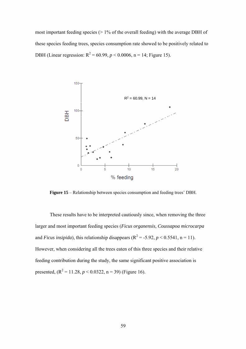
most important feeding species (> 1% of the overall feeding) with the average DBH of
these species feeding trees, species consumption rate showed to be positively related to
DBH (Linear regression: R2 = 60.99, p < 0.0006, n = 14; Figure 15).
R2 = 60.99, N = 14R2 = 60.99, N = 14
Figure 15 – Relationship between species consumption and feeding trees’ DBH.
These results have to be interpreted cautiously since, when removing the three
larger and most important feeding species (Ficus organensis, Coussapoa microcarpa
and Ficus insipida), this relationship disappears (R2 = -5.92, p < 0.5541, n = 11).
However, when considering all the trees eaten of this three species and their relative
feeding contribution during the study, the same significant positive association is
presented, (R2 = 11.28, p < 0.0322, n = 39) (Figure 16).
59

R2 =11.28, N = 39R2 =11.28, N = 39
Figure 16 – Relationship between tree consumption and feeding trees’
DBH of Ficus organensis, Coussapoa microcarpa and Ficus insipida.
Angular deviation
If the group moves through independent route segments, it could be expected the
angular deviation between consecutive feeding trees to be uniformly distributed around
a 360o circumference rather than concentrated in a particular direction. On the other
hand, such a concentration would support the idea howler monkeys forage over aligned,
possibly more efficient, traveling routes. The Rayleigh test (Z), in fact, indicated that
during the Fall (r = 0.0929, Z = 0.8715, u = 2.9881, p = ns, n = 101) and Winter-Spring
(r = 0.0802, Z = 0.733, u = 2.9894, p = ns, n = 114) the routes between feeding trees
were not clumped in any specific direction. However, angles are significantly clumped
during the Summer (r = 0.2351, Z = 5.0294, u = 4.5723, p < 0.01, n = 91) and when all
routes between feeding trees used throughout the study are analyzed together (r =
0.1024, Z = 3.2112, u = 2.992, p < 0.05, n = 306) (Figure 17). The clumping observed
during the Summer sampling period may be partially attributed to non-uniform
60

distribution of the angular deviation in feeding trees of Ficus organensis (Figure 18),
the most important feeding species in this period (r = 0.3779, Z = 3.5699, u = 2.966, p <
0.05, n = 25). This distribution was also presented for Ficus insipida during the Fall
sampling period (r = 0.5644, Z = 3.5039, u = 2.926, p < 0.05, n = 11) and when all
feeding bouts at this species were analyzed together (r = 0.3232, Z = 3.2375, u =
2.9715, p < 0.05, n = 31; Figure 19).
Figure 17 – Circular distribution plot of the turning angle between consecutive feeding trees in
the periods sampled and during the entire study.
61

Figure 18 – Circular distribution plot of the turning angle between feeding bouts on trees of
Ficus organensis during the Summer.
Figure 19 – Circular distribution plot of the turning angle between feeding bouts on trees of
Ficus insipida in the Fall and during the entire study.
As the number of feeding records per tree (see Material and Methods) was
insufficient to perform statistical analyses at each sampling period, it was only analyzed
the sum of the total angular deviation observed at each tree. None of the target trees (see
memory load results) angular deviation was clumped around specific directions. Similar
results were found when only resting trees were considered in the analyses.
62

DISCUSSION
Evaluating the extent to which animals use spatial information during foraging
can be as difficult as affirming they don’t (see Bennet 1996, Janson and Byrne 2007).
Based on existing evidence of primate spatial knowledge, four predictions were tested
on how environmental features influence the foraging behavior of a folivore-frugivore
primate species. Overall, the differences found at each period sampled indicate that
environmental features used by animals to obtain positional and directional information
during foraging vary spatially and temporally (Dyer 1998).
The prediction that howlers minimize the distance traveled by consecutively
visiting the nearest tree of a few preferred species was partially confirmed. In almost
half of the feeding bouts analyzed, the group used the nearest available feeding tree of a
given species. Besides, they used more distant feeding trees of only two of the six most
consumed species, considering that they both occur at high densities at the forest
fragment. On the other hand, in 78% of the feeding bouts there was a closer feeding tree
of a different species available and, in addition, the feeding trees used in Fall were
located significantly further away than the closest tree available of particular species,
indicating that minimizing distance traveled was not always the foraging strategy used
by the group.
Primates are usually described to move to the nearest resource available,
considering that previous studies reported that 44 to 85% of the moves between feeding
patches follow this pattern (Menzel 1973, Garber 1989, Janson 1998). Whenever
primates do not move to the nearest resource available, it is suggested they bypass them
in favor of more productive sources (Garber 1989, Janson 1998, Cunningham and
Janson 2007) or irreplaceable ones, such as water holes (Sigg and Stolba 1981, Noser

and Byrne 2007). If traveling to the nearest resource indicates the monkeys know the
spatial location of their targets and ways to minimize energy spent traveling, the
movements to more distant patches also may be interpreted as evidence of spatial
knowledge. In this case, this strategy could maximize energy gain if the resources
located farther away are more productive (Prediction 2). In fact, during the only period
when howlers fed from trees significantly more distant than the nearest sources
belonging to the same species, they used a lesser number of Ficus organensis trees for
consumption that in Summer (9 trees in Summer and 5 in Fall, although similar number
of trees of this species were visited during these periods – 14 and 12, respectively), but
ate a similar amount of fruits from this species in both periods. Besides, during Fall they
also visited this species in a lesser degree than in Summer (9% of the visited trees in
Summer and 6% in Fall).
Although seasonal variations in trees’ productivity were not analyzed, if
considered that howlers tend to intensively use fruits when available (Milton 1980,
Julliot 1996, Silver et al. 1998, Pavelka and Knoff 2004, Cristóbal-Azkarate and
Arroyo-Rodríguez 2007), the greater fruits availability during Fall of a few Ficus
organensis trees, can also be inferred once a few fruiting trees were used for more
consecutive days and more intensively (greater consumption per visit) than during the
previous period. These results during Fall, thus, corroborate with the second prediction
that the troop used intensively a few highly productive feeding sources, responding for
the high fruit consumption of the species during the period, in expense of closer, but
less valuable, trees of this species.
The second prediction is also confirmed when considering DBH as a surrogate
for estimating tree productivity (Chapman et al. 1992). Not only the average species
DBH was positively related with species consumption, but feeding trees were
64

significantly larger than those of the same species that were visited but not used as food
sources. However, larger targets are also visible from longer distances than small ones
(Janson and Di Bitetti 1997, Noser and Byrne 2006, 2007). The mean straight line
distance between feeding trees was similar or smaller than the field of visual perception
of forest-dwelling primates (Terborgh 1983 – 10 to 15 m, Garber and Hannon 1993 – 20
m, Janson and Di Bitetti 1997 – 25-50 m, Dominy et al. 2001 – 20 to 30 m). This field
of visual detection may vary as a consequence of resource type (Noser and Byrne 2007),
resource size (Janson and Di Bitteti 1997) and forest type (Terborgh 1983). But if the
distance between consecutive feeding trees was within the field of perception, why did
the study group traveled significantly farther to reach them?
Although direct travel to feeding trees would be a good strategy to minimize
distance traveled and optimize energy gain, another strategy may be inferred from the
pattern observed. The third tested prediction states that howlers would use a repetitive
number of trees and paths in a way of both reducing the memory input of information
and monitoring the availability of potential food sources. By the end of the study, the
group visited only 20% of the available trees with DBH ≥10 cm, although tree use rates
were strongly predicted by species IVI, and presented a daily mean repetitive tree use of
67%. Although the number of days analyzed was small, the trees that were added in the
last two periods were located next to sources already visited. Carperter (1964) notes that
howlers move “roughly over the same route”, while Milton (1977, 1980, 2000) notes
that, at times, it can be predicted where the troop is going by the time they begin to
travel and what they will eat when they get there. Translocated troops were described to
progressively limit their range area and establish traveling paths over areas of greater
relative cover of major feeding species, whereas established groups showed greater
65

knowledge of travel paths and more intensive use of quality food resources (Ostro et al.
1999, 2000).
Traveling longer distances would be favored if monitoring a few preferred
species enhances the net energy gain, especially if it is considered that the energetic
costs of traveling are, usually, overrated (Steudel 2000). The howlers presented a tree
use pattern of the most important feeding species inversely associated with the amount
of those trees used for feeding. This outcome may suggest monitoring of a few staple
food species, if considered that the detection of an important ephemeral item in one of
these sources would lead to the visit of a great number of individual trees of that species
and the selective consumption of those most productive individual trees.
At the same time, the howlers’ feeding species consumption rate being
positively related with species tree use indicates the opportunistic consumption of many
different plant species described for howlers (Milton 2000). A folivorous species should
favor the sampling and an opportunistic diet, favoring the reduction in the ingestion of
toxic secondary components (Garber 1987).
Diverse foraging strategies characterized seasonal varying exploitation of
different resources. During Summer, the overall great availability of F. organensis
fruits, shown by the intensive use of most of this species trees for feeding, led to a
distinctive foraging pattern according the consumption of ripe or unripe fruits of this
species. Previous studies with wolly monkeys (Di Fiore 2003) and mangabeys (Janmaat
et al. 2006) report that keeping track of species unripe fruits availability is a way of
predicting future ripe fruits production. The more the troop fed on unripe fruits in
Summer more they traveled and less they slept, making use of a greater number of
resting trees for shorter periods of inactivity. Ripe fruits are a high-energy resource rich
in nonstructural carbohydrates and simple sugars, easily digested, while unripe fruits
66

may contain considerable amounts of fiber and secondary compounds (Milton 1998),
making it worth to seek for ripe fruits. During Summer, accordingly, the greater was the
consumption of ripe fruits of F. organensis, less they traveled and lower was the
number of trees visited, corroborating with the monitoring of fruit species ripeness of
prediction two.
Unlike the Summer and the Fall, a period also characterized by a high
consumption of unripe fruits of Coussapoa microcarpa and vine flowers, the Winter-
Spring presented a different foraging pattern possibly coupled with a decrease in fruit
consumption. The high leaf, particularly young leaves, and flowers feeding was
accompanied by a high linearity rate between feeding trees, mostly attributed to the
clumped fashion they were distributed and the high use of a greater number of species
and trees for feeding. The majority of the diet was obtained from species that the
howlers used most of the visited trees for feeding, particularly on leaves. Leaves are
usually considered as being uniformly distributed in space (Schoener 1971), however
foods eaten by howlers, apparently, must provide them with high-quality protein and
energy (Milton 1998). At this period, the high feeding percentage, the greater diversity
of leaf species eaten and, especially, the great contribution of young leaves on diet, that
usually have lower concentrations of secondary compounds and higher in protein
(Garber 1987), infer a selectiveness over a higher nutritional and low toxic compounds
diet.
And, although more than 50% of the feeding trees of this period haven’t been
used at the previous periods (44% of the added trees were used for feeding), 60% of the
diet was based on trees already used by the group. Also, if considered the 74% daily
mean travel over previously marked trees and the 92% of resting at those trees (21 of 27
trees used for resting had been used at the previous periods), it was concluded that the
67
troop intensively used known travel paths and fed, opportunistically, from small
amounts of newly used trees located adjacent to the routine travel paths. This pattern
has been suggested by Milton (2000) as a strategy that would avoid cognitive overload,
while Janson and Byrne (2007), applying optimal patch-foraging rules (Stephens and
Krebs 1987), point that the use of less valuable resources include short movements and
fewer skipped resources, which is opposite of the patterns observed during Fall.
A route-based foraging pattern implies that the animal navigates effectively and
relatively more efficient over a network of nodes in the environment (Di Fiore and
Suarez 2007). From the 654 used trees, 33% of the time recorded was spent on 11 trees
that were labeled as target trees of the study group. Those trees were reached from
different directions during the study, connecting distinct route segments, and allowed
greater visibility of the forest canopies as predicted. Although Garber and Jelinek
(2006) reported distinct tree use (the mean number of trees used per day was nearly half
the number used by the study group) and ranging pattern (travel paths were as low as
one third the observed at the present study), possibly due to environmental, activity
patterns, social influences, species-specific and methodological differences, they also
reported Alouatta palliata to concentrate their foraging on a few larger trees of greater
visibility that could be reached from different directions. Likewise, Milton (2000)
highlights that the frequent use of routes between pivotal trees and along important
feeding sources (acting as nodes or decision points) would increase howlers’ foraging
efficiency. Although major resting trees were not used as major feeding trees, their role
as important decision-points still can be addressed, since the highest mean use of
neighboring trees from these trees was observed, leading to diverse feeding patches,
while the minority of neighboring trees was used from traveling tree, where more
directional movement would occur. This would be an important characteristic in
68

howlers’ foraging once different dietary requirements throughout the day would be
sufficed through distinct foraging paths, as already proposed.
Animals are generally known to use landmarks for location in familiar
environments (Collett and Graham 2004) and lab studies on primates indicate that they
have egocentric views of space (Poti 2000), consistent with the use of landmark in
nature (Di Fiore and Suarez 2007, Noser and Byrne 2007). Following obvious fixed
features of the environment may simplify the memorization and learning of specific
routes between feeding patches (Di Fiore and Suarez 2007). The forest fragment
presents a smooth declivity along its length, but as the density of trees canopies were
quite regular, the probability of long distance orientation through visual detection field
was reduced. However, the howlers did use more intensively trees of greater visibility
and the shape of the forest fragment, similar to a “horseshoe” (see Figure 1), also led to
distinct visibility from different directions (South and East coordinates presented higher
visibility than North and West). Could this be interpreted as evidence that the howlers
were using environmental features to visually locate feeding sources?
No, if considered that all fruits eaten by the group are cryptic in trees canopy
(fruits of Ficus organensis and Coussapoa microcarpa length, at most, 2 cm) and the
direction alignment of movements leading to F. organensis during Summer and F.
insipida during Fall and the overall results were presented due the intensive use of two
individual trees (tree IDs 1.05 and 2.66, considering the last was used 4 times more than
the following most used F. insipida tree – see table 5) that were mostly reached through
north oriented movements, where visibility was lower. Besides, the forest terrain
presents declivity only in a small upper portion, and the majority of the routes and most
used trees were located at a largest even portion. But yes, if considered that in large
trees, food availability is relatively greater, particularly important if the species is
69

regarded as staple source, as identified target trees (Ficus organensis, F. insipida and
Coussapoa microcarpa), and that the location of the majority of those most used trees
were peripheral to the fragment. Then, rather than affirming the troop used visual
perception for foraging, it can be said that the shape of the forest fragment influences
the use of large pivotal trees located in its peripheries that can, thus, be label as
landmarks.
The model of mental maps proposed by Gallistel (1990) and Gallistel and
Cramer (1996) suggests that cognitive maps consist of landmarks placed on a geocentric
frame of reference by vector addition. In other words, geocentric position is determined
by path integration and positional fixes on known landmarks are used to deal with the
error accumulation of path integration. Further models of mental map (Toolman 1948,
O’Keefe and Nadel 1978) usually rely on the use of novel shortcuts, but Bennet’s
review (1996) of such pattern in distinct taxa points as premature such premise. Besides,
identifying novel shortcuts would imply that the observer has complete knowledge of
animals past experience, extremely rare in studies on nature.
Di Fiore and Suarez (2007), proposing the use of route-based maps in wolly and
spider monkeys, consider that the use of routes would require only the store of distance
information and linked views that would allow the recognition of routes during
foraging, reinforced by repetitive use. This would, theoretically, reduce the need for
“on-line processing” and continuously updating of distance and direction moved,
attribute on path integration (Poucet 1993), leading the authors to conclude that the
most probable representation of space used by their study groups was route-based maps.
Our data on brown howler monkeys is not sufficient to reach such conclusions.
However, all four predictions proposed to explain howler foraging were, in some extent,
supported by the group’s foraging patterns. They not only used the nearest feeding tree
70

of a few species, but also maximized energy gain by using more distant high productive
sources. Networks of fixed routes of repetitive use between great visibility pivotal trees
were observed, avoiding a cognitive overload in foraging and, indeed, were built along
major feeding species that were monitored, especially during fruits availability periods,
but also in lean high-energy food periods.
Our predictions were made based on evidence of non-folivore species, however
they suit the behavior of howlers, apart from the greater overall contribution of leaves
on their diet. Feeding on leaves would, actually, be a viable option for primates, since
their abundance and availability, even of young parts, is much greater than flowers and
green or ripe fruits (Milton 1998). Still, although advantageous, very few species base
their diet on leaves as howlers (Eisenberg et al. 1972), since a great number of feeding
adaptations, among digestive, anatomical and behavioral (see Crockett and Eisenberg
1987, Neville et al. et al. 1988, Crockett 1998, Milton 1998), have been reported to have
evolved allowing such diet. Lucas et al. (2003) proposed that the evolution of
trichromatic vision in catarrhine, routinely trichromatic (Kainz et al. 1998), and in
Alouatta, what is unusual for platyrrhine species (Jacobs et al. 1996), is an adaptation
that favors the consumption of higher quality leaves, namely young leaves. Dominy et
al. (2003) went further, proposing that trichromatic vision was related with the
biogeographic history of figs and palms, where evolved trichromacy would allow the
exploitation of protein-rich young leaves as a replacement resource during periods of
fruits shortage of these staple sources.
If different biological features, including sensory, evolved in the genus favoring
its diet composition, why the spatial ability should be different? Our data supports that,
although leaves are uniformly distributed on space, howlers present efficient use of
spatial information that optimize a high-nutrient foraging intake, even in lean fruit
71

periods. Considering that, brain size differences should not predict spatial skills and
dietary patterns in primates, as already proposed (Mackinnon 1978, Clutton-Brock and
Harvey 1980, Milton 1981a, 1988, 2000, Taylor and van Schaik 2007). Instead, the way
neural network is organized, the amount of synapses presented and its plasticity are
more likely to influence a species’ cognitive capabilities.
Cognitive phenotypes are determined by genes and environment (Dukas 2004)
and determining how cognitive demands posed by each species’ environment should be
further investigated, mainly on plastic phenotypes. Models, like mental maps, are
useful for a better understand of congruent animals’ evolution, but the diverse evidences
of efficient use of spatial information, already observed at distinct taxa (see Dukas
1998, Sherry 1998, Shettleworth 1998), highlight the need for a better understand on
how each species environment information are interpreted and represented, influencing
on niche segregation (Beecham 2001).
This study presents evidences that brown howler monkeys use spatial
information of the environment and its temporal varying productivity patterns during
foraging. As primates that depend on ephemeral and sparsely located fruit sources, this
frugivore-folivorous species also optimizes high-nutrient foraging intake using nearest
resources available and high-productivity trees through travel routes composed of large
and high-visibility trees that enhance the monitoring of important fruit sources. The
travel routes used also contribute to the opportunistic consumption of several leaves’
sources, reducing the ingestion of toxic compounds and maximizing nutrient intake
during lean periods. These data don’t allow the conclusion that brown howler monkeys
have mental maps as the concepts defines it (Toolman 1948, O’Keefe and Nadel 1978,
Gallistel 1990), or route-based maps (Poucet 1993), once it can’t be stated they used
neither novel shortcuts or path integration during foraging. However, the use of spatial
72

information and varying strategies during foraging, as other behaviors described to
enhance the species adaptability in different environments (see Crockett and Eisenberg
1987, Neville et al. et al. 1988, Crockett 1998, Bicca-Marques 2003), was observed
allowing an optimization of nutrient intake in different availability periods.
Future studies indicating quantitative measures of nutrient intake and how they
relate with plant species use and behavioral patterns observed might clarify the extent to
which howlers optimize foraging intake. Besides, social influences during route
traveling, how those routes are used through longer periods and their establishment over
time, particularly in newly released troops, are important questions that should be
answered to the better understand of how howlers use spatial information of the
environment.
73

REFERENCES
Able KP, Able MA (1996) The flexible migratory orientation system of the savannah
sparrow (Passerculus sanwichensis). J Exp Biol 199: 3-8
Altmann J (1974) Observational study of behavior: Sampling methods. Behaviour 49:
227–267
Andrews MW (1988) Selection of food sites by Callicebus moloch and Saiiri sciureus
under spatially and temporally varying food distribution. Learn and Motiv 19:
254-268
Armstrong E (1983) Relative brain size and metabolism in mammals. Science 200:
1302-4
Asensio N, Cristobal-Azkarate J, Dias PAD, Vea JJ, Rodríguez-Luna E (2007) Foraging
habits of Alouatta palliata mexicana in three forest fragments. Folia Primatol 78:
141-153
Ayres M, Ayres Jr M, Ayres DL, Santos AAS (2007) BioEstat: aplicações estatísticas
nas áreas das ciências bio-médicas. Belém, Sociedade Civil Mamirauá, MCT,
Imprensa Oficial do Estado do Pará
Balda RP, Bednekoff PA, Kamil AC (eds) (1998) Animal cognition in nature.
Academic Press, New York
Barton RA (2000) Primate brain evolution: cognitive demands of foraging or of social
life? In: Boinski S, Garber PA (eds) On the move: how and why animals travel in
groups. University of Chicago Press, Chicago, pp 204–237
Barton RA, Purvis AJ (1994) Primate brains and ecology: Looking beneath the surface.
In: Anderson JR, Herrenschmidt N (eds) Current primatology 1. University Press,
Strasbourg, pp 1-10
Basil JA, Kamil AC, Balda RP, Fite KV (1996) Differences in hippocampal volume
among food storing corvids. Brain Behav and Evol 47: 156-164
Beecham JA (2001) Towards a cognitive niche: divergent foraging strategies resulting
from limited cognitive ability of foraging herbivores in a spatially complex
environment. BioSystems 61: 55–68
Benhamou S (1996) No evidence for cognitive mapping in rats. Anim Behav 52: 201-
212
Bennett ATD (1996) Do animals have cognitive maps? J Exp Biol 199: 219-224

Bicca-Marques JC (2000) Cognitive aspects of within-patch foraging decisions in wild
diurnal and nocturnal new world monkeys. Ph.D Thesis, University of Illinois,
Urbana, USA
Bicca-Marques JC (2003) How do howler monkeys cope with habitat fragmentation?
In: Marsh LK (ed) Primates in fragments: ecology and conservation. Kluwer
Academic/Plenum Publ, New York, pp 283-303
Bicca-Marques JC (2005) The win-stay rule in foraging decisions by free-ranging titi
monkeys (Callicebus cupreus cupreus) and tamarins (Saguinus imperator
imperator and Saguinus fuscicollis weddelli). J Comp Psych 119(3): 343-351
Bicca-Marques JC (2006) Distance influences the foraging decisions of emperor and
saddleback tamarins. J Zool 269 (2): 221-224
Bicca-Marques JC, Calegaro-Marques C (1997) Single line progression in black-and-
gold howler monkeys (Alouatta caraya): Is there an ordered position? Am J
Primat 42: 95
Bicca-Marques JC, Garber PA (2003) Experimental field study of the relative costs and
benefits to wild tamarins (Saguinus imperator and S fuscicollis) of exploiting
contestable food patches as single- and mixed-species troops. Am J Primatol
60:139– 153
Bicca-Marques JC, Garber PA (2004) The use of spatial, visual, and olfactory
information during foraging in wild nocturnal and diurnal anthropoids: A field
experiment comparing Aotus, Callicebus, and Saguinus. Am J Primatol 62: 171–
187
Bicca-Marques JC, Garber PA (2005) Use of social and ecological information in
tamarin foraging decisions. Int J Prim 26(6): 1321-1344
Bicca-Marques JC, Nunes AM (2007) Individual foraging rules of Saguinus imperator
imperator and Saguinus fuscicollis weddelli searchers. In: Bicca-Marques JC (ed)
A Primatologia no Brasil – 10. Sociedade Brasileira de Primatologia, Porto
Alegre, pp 401-422
Blaisdell AP, Cook RG (2005) Integration of spatial maps in pigeons. Anim Cogn 8: 7-
16
Boesch C, Boesch H (1984) Mental map in wild chimpanzees: an analysis of hammer
transports for nut cracking. Primates 25: 160-70
75

Boinski S (2000) Social manipulation within and between troops mediates primate
group movement. In: Boinski S, Garber PA (eds) On the move: how and why
animals travel in groups. University of Chicago Press, Chicago, pp 421–469
Brothers L (1990) The social brain: A project for integrating primate behavior and
neurophysiology in a new domain. Conscepts Neurosci 1:27-51
Byrne RW (1979) Memory for urban geography. Q J Exp Psychol 31:147–154
Byrne RW (1994) The evolution of intelligence. In: Slater PJB, Halliday TR (eds)
Behaviour and evolution. Cambridge University Press, Cambridge, pp 223– 65
Byrne RW (1996) Relating brain size to intelligence in primates. In: Mellars PA,
Gibson KR (eds) Modelling the early human mind. Macdonald Institute for
Archaeological Research, Cambridge, pp 49–56
Byrne RW, Bates RA (2007) Sociality, Evolution and Cognition. Curr Biol 17(16): 714-
723
Carpenter CR (1964) Naturalistis behavior of nonhumam primates. Pennsylvania State
University Press, University Park, VII
Chapman CA (1988) Patch use and patch depletion depletion by the spyder and howling
monkeys of Santa Rosa National Parl, Costa Rica. Behaviour 105: 88-116
Chapman CA, Balcomb SR (1998) Population characteristics of howlers: Ecological
conditions or group history. Int J Primat 19(3): 385-403
Chapman CA, Chapman LJ, Mclaughlin RL (1989) Multiple central place foraging by
spider monkeys: Travel consequences of using many sleeping sites. Oecologia
79(4): 506-511
Chapman CA, Chapman LJ, Wangham R, Hunt K, Gebo D, Gardner L (1992)
Estimators of fruit abundance of tropical trees. Biotropica 24(4): 527-531
Charnov EL (1976) Optimal foraging. The marginal value theorem. Theor Pop Biol 9:
129–136
Cheng K, Newcombe NS (2005) Is there a geometric module for spatial orientation?
Squaring theory and evidence. Psychol Bullet & Review 12(1): 1-23
Clarke MR, Glander KE, Zucker EL (1998) Infant–nonmother interactions of free-
ranging mantled howlers (Alouatta palliata) in Costa Rica. Int J Primatol 19: 451–
472
Clutton-Brock TH, Harvey PH (1980) Primates, brain and ecology. J Zool (Lond) 190:
309-323
Cody ML (1971) Finch flocks in the Mohave Desert. Theor Pop Biol 2:142–148.
76

Collett TS, Baron J (1994) Biological compasses and the coordinate frame of landmarks
memories in honeybees. Nature 368: 137-40.
Collett TS, Dillmann E, Giger A, Wehner R (1992) Visual landmarks and route
following in desert ants. J Comp Pshych A 170: 435-442
Collett TS, Graham P (2004) Animal navigation: path integration, visual landmarks and
cognitive maps. Curr Biol 14(12): R475-7
Cornell EH, Heth CD (2004) Memories of travel: Dead reckoning within the cognitive
map. In: Allen GL (ed) Human spatial memory: Remembering where. Lawrence
Erlbaum Associates, Mahwah, pp 191–215
Cramer AE, Gallistel CR (1997) Vervet monkeys as travelling salesmen. Nature 387:
464
Cristóbal-Azkarate J, Arroyo-Rodríguez V (2007) Diet and activity pattern of howler
monkeys (Alouatta palliata) in Los Tuxtlas, Mexico: effects of habitat
fragmentation and implications for conservation. Am J Primat 69(9): 1013-1029
Crockett CM (1998) Conservation biology of the genus Alouatta. Int J Primat 19(3):
549-578
Crockett CM, Eisenberg JF (1987) Howlers: Variations in group size and demography.
In: Smuts BB, Cheney DL, Seyfarth RM, Wrangham RW, Struhsaker TT (eds)
Primates societies. University of Chicago Press, Chicago, pp 54-68
Cunha AS (1994) Aspectos sócio-ecológicos de um grupo de bugios (Alouatta fusca
clamitans) do Parque Estadual de Itapuã, RS. Master thesis, Federal University of
Rio Grande do Sul, Porto Alegre, Brazil.
Cunningham EP, Janson CH (2007) Integrating information about location and value of
resources by white faced-saki monkeys (Pithecia pithecia). Anim Cogn 10(3):
293-304
Daly M, Wilson MI (1999) Human evolutionary psychology and animal behaviour.
Anim Behav 57: 509–519
Degusta D, Everett MA, Milton K (2003). Natural selection on molar size in a wild
population of howler monkeys (Alouatta palliata). Proc R Soc London B (Suppl)
270: S15-S17
Di Bitetti MS, Janson CH (2001) Social foraging and the finder’s share in capuchin
monkeys, Cebus apella. Anim Behav 62: 47-56
77

Di Fiore A, Suarez SA (2007) Route-based travel and shared routes in sympatric spider
and woolly monkeys: cognitive and evolutionary implications. Anim Cogn
10(3):317-329
Di Fiore AD (2003) Ranging behavior and foraging ecology of lowland woolly
monkeys (Lagothrix lagotricha poeppigii) in Yasuni National Park, Ecuador. Am
J Primatol 59:47–66
Dominy NJ, Lucas PW, Osorio D, Yamashita N (2001) The sensory ecology of primate
food perception. Evol Anthrop 10(5): 171-186
Dominy NJ, Svenning JC, Li WH (2003) Historical contingency in the evolution of
primate color vision. J Hum Evol 44(1): 25-45
Dukas R (2004) Evolutionary biology of animal cognition. Annu Rev Ecol Evol Syst
35: 347-374
Dukas R (Ed) (1998) Cognitive ecology. University of Chicago Press, Chicago
Dunbar RIM (1992) Neocortex size as a constraint on group size in primates. J Hum
Evol 20: 287-296
Dyer FC (1994) Spatial cognition and navigation in insects. In: Real LA (ed) Behavioral
mechanisms in evolutionary ecology. University of Chicago Press, Chicago, pp
66-98
Dyer FC (1998) Cognitive ecology of navigation. In: Dukas R (Ed) Cognitive ecology.
University of Chicago Press, Chicago, pp 201–260
Eisenberg JF, Muckenhirn NA, Rudran R (1972) The relation between ecology and
social structure in primates. Science 176: 863-874
Emlen JM (1966) The role of time and energy in food preference. Amer Natur 100:611-
17
Estrada A (1984) Resource use by howler monkeys (Alouatta palliata) in the rain forest
of Los Tuxtlas,Veracruz, Mexico. Int. J Primatol 5:105–131
Estrada A, Coates-Estrada R (1984) Fruit eating and seed dispersal by howling monkeys
(Alouatta palliata) in the tropical rain forest of Los Tuxtlas, Mexico. Amer J
Primatol 6(2): 77-91
Etienne AS, Jeffery KJ (2004) Path integrarion in mammals. Hippocampus 14: 180-192
Etienne AS, Maurer R, Séguinot V (1996) Path integration in mammals and its
interaction with visual landmarks. J Exp Biol 199: 201–209
Fialho MS (2000) Ecologia de Alouatta guariba em floresta de encosta e de restinga no
sul do Brasil. Master thesis, University of Campinas, Campinas, Brazil
78

Fobes JL, King JE (1982) Measuring primate learning abilities. In: Fobes JL, King JE
(eds) Primate behavior. Academic Press, New York, pp 289-326
Fortes VB (1999). Dieta, atividades e uso do espaço por Alouatta fusca (Geoffroy,
1812, Primates: Cebidae), na Depressão Central do Rio Grande do Sul. Master
thsesis, Federal University of Rio Grande do Sul, Porto Alegre, Brazil
Forte VB (2008) Ecologia e comportamento de Alouatta guariba clamitans Cabrera,
1940 em fragmentos florestais na Depressão Central do Rio Grande do Sul. PhD
Thesis, Catholic University of Rio Grande do Sul, Porto Alegre, Brazil
Futuyama DJ (1986) Evolutionary biology (2 ed), Sinauer, Sunderland, Mass, USA
Galef BG, Giraldeau L (2001) Social influences on foraging in vertebrates: causal
mechanisms and adaptive functions. Anim Behav 61: 3-15
Gallistel CR, Cramer AE (1996) Computations on metric maps in mammals: getting
oriented and choosing a multi-destination route. J Exp Biol 199:211–217
Gallistel CR(1989) Animal cognition: The representation of space, time and number.
Ann.Rev.Psychol 40: 155-189
Gallistel, CR (1990) The Organization of Learning. MIT Press, Cambridge,
Massachusetts
Ganzhorn JU, Wright PC (1994) Temporal patterns in primate leaf eating: The possible
role of leaf chemistry. Folia Primatol 63(4): 203-208
Garber PA (1987) Foraging strategies among living primates. Ann Rev Anthrop 16:
339-364
Garber PA (1988) Foraging decisions during nectar-feeding by tamarin monkeys
(Saguinus mystax and Saguinus fuscicollis). Biotropica 20:100–106
Garber PA (1989) Role of spatial memory in primate foraging patterns: Saguinus
mystax and Saguinus fuscicollis. Am J Primatol 19:203–216
Garber PA (2000) Evidence for the use of spatial, temporal, and social information by
some primate foragers. In: Boinski S, Garber PA (eds) On the move: how and why
animals travel in groups. University of Chicago Press, Chicago, pp 261-198
Garber PA, Brown E (2006) Use of Landmark Cues to Locate Feeding Sites in Wild
Capuchin Monkeys (Cebus capucinus): An Experimental Field Study. In: Estrada
A, Garber PA, Pavelka M, Luecke L (eds) New Perspectives in the Study of
Mesoamerican Primates: Distribution, Ecology, Behavior and Conservation.
Kluwer, New York, pp 311-332
79

Garber PA, Dolins FL (1996) Testing learning paradigms in the field: evidence for use
of spatial and peceptual information and rule-based foraging in wild moustached
tamarins. In: Norconk M, Rosenberger AL, Garber PA (eds) Adaptive Radiations
in Neotropical Primates. Plenum Press, New York, pp 201-216
Garber PA, Hannon B (1993) Modeling monkeys: a comparison of computer-generated
and naturally occurring foraging patterns in two species of neotropical primates.
Int J Primatol 14: 827–852
Garber PA, Jelinek PE (2006) Travel Patterns and Spatial Mapping in Nicaraguan
Mantled Howler Monkeys (Alouatta palliata). In: Estrada A, Garber PA, Pavelka
M, Luecke L (eds) New Perspectives in the Study of Mesoamerican Primates:
Distribution, Ecology, Behavior and Conservation. Kluwer, New York, pp 287-
310
Garber PA, Paciulli LM (1997) Experimental field study of spatial memory and learning
in wild capuchin monkeys (Cebus capucinus). Folia Primatol 68: 236-254
Gaspar DA (1997) Ecologia e comportamento do bugio ruivo, Alouatta fusca (Geoffroy,
1812, Primates: Cebidae), em fragmento de mata de Campinas, SP. Master thesis,
São Paulo State University, Rio Claro, Brazil
Glander, KE (1982) The impact of plant secondary compounds on primate feeding
behavior. Yearb Phys Anthropol 25: 1-18
Gomes DF (2006) Ecologia cognitiva e forrageio social em macacos-prego, Cebus
nigritus (Goldfuss, 1809). Master thesis, Cathocic University of Rio Grande do
Sul, Porto Alegre, Brazil
Gregorin R (2006) Taxonomia e variação geograficadas espécies do gênero Alouatta
Lacépède (Primates, Atelidae) no Brasil. Rev Bras Zoo 23(1): 64-144
Griffin DR (1978) Prospects for a cognitive ethology. Behav and Brain Scienc 4: 527–
538
Hampton RR, Sherry DF, Shettleworth SJ, Khurgel M, Ivy G (1995) Hippocampal
volume and food-storing behavior are related in parids. Brain Behav Evol 45: 54–
61
Harvey PH, Krebs JR (1990) Comparing brains. Science 249: 140–146
Healy SD, Braithwaite V (2000) Cognitive ecology: a field of substance? Tree 15(1):
22-26
Healy SD, Gwinner E, Krebs JR (1996) Hippocampal volume in migrating and non-
migrating warblers: effects of age and experience. Behav Brain Res 81: 61–68
80

Healy SD, Jones CM (2002) Animal learning and memory: an integration of cognition
and ecology. Zoology 105: 321–327
Healy, SD and Krebs, JR (1992) Food storing and the hippocampus in corvids: amount
and size are correlated. Proc R Soc London Ser B 248: 241–245
Hemmi JM, Menzel Jr EW (1995) Foraging strategies of long-tailed macaques, Macaca
fscicularis: directional extrapolation. Anim Behav 49: 457-464
Hirano ZMB (2004) Secreção epidérmica de Alouatta guariba clamitans (Primates:
Atelidae). Ph.D thesis, University of São Paulo, Ribeirão Preto, SP, Brazil
Jacobs GH, Neitz M, Deegan JF, Neitz J (1996) Trichromatic colour vision in New
World monkeys. Nature 382(6587): 156-158
Jacobs LF, Gaulin SJC, Sherry DF, Hofman GE (1990) Evolution of spatial cognition:
Sex-specific patterns of spatial behavior predict hippocampal size. Proc Nat Acad
Sci 87: 6349-52
Jacobs LF, Spencer WD (1994) Natural space-use patterns and hippocampal size in
kangaroo rats. Brain Behav and Evol 44: 125-132
Janmaat KRL, Byrne RW, Zuberbühler K (2006) Evidence for a spatial memory of
fruiting states of rainforest trees in wild mangabeys. Anim Behav 72: 797–807
Janson CH (1996) Toward an experimental socioecology of primates: examples from
Argentine brown capuchin monkeys (Cebus paella nigritus). In: Norconk MA,
Rosenberger AL, Garber PA (eds) Adaptive radiations of neotropical primates.
Plenum, New York, pp 309–325
Janson CH (1998) Experimental evidence for spatial memory in foraging wild capuchin
monkeys, Cebus paella. Anim Behav 55:1229–1243
Janson CH (2000) Spatial movement strategies: theory, evidence and challenges. In:
Boinski S, Garber PA (eds) On the move: how and why animals travel in groups.
University of Chicago Press, Chicago, pp 165-203
Janson CH, Byrne R (2007) What wild primates know about resources: opening up the
black box. Anim Cogn 10:357–367
Janson CH, Di Bitetti MS (1997) Experimental analysis of food detection in capuchin
monkeys: eVects of distance, travel speed, and resource size. Behav Ecol
Sociobiol 41:17–24
Jardim MMA (1992) Aspectos ecológicos e comportamentais de Alouatta fusca
clamitans (Cabrera, 1940) na Estação Ecológica de Aracuri, RS, Brasil (Primates,
81

Cebidae). Graduation monografy, Federal University of Rio Grande do Sul, Porto
Alegre, Brazil
Julliot C (1994) Diet diversity and habitat of howler monkeys. In: Thierry B, Anderson
JR, Roeder JJ, Herrenschmidt N (eds) Current Primatology - Vol. I: Ecology and
Evolution. ULP, Strasbourg, pp 67–71
Julliot C (1996) Fruit choice by red howler monkeys (Alouatta seniculus) in a tropical
rain forest. Am J Primat 40(3): 261-282
Kainz PM, Neitz J, Neitz M (1998) Recent evolution of uniform trichromacy in a New
World monkey. Vis Res 38(21): 3315-3320
Kamil AC (1998) On the proper definition of cognitive ethology. In: Balda RP,
Bednekoff PA, Kamil AC (eds) Animal cognition in nature. Academic Press, New
York, pp 1-28
Kappeler PM (2000) Grouping and movement patterns in malagasy primates. In:
Boinski S, Garber PA (eds) On the move: how and why animals travel in groups.
University of Chicago Press, Chicago, pp 470-490
King BJ, Fobes JL (1982) Complex learning in primates. In: Fobes JL, King BJ (eds)
Primate behavior. Academic Press, New York, pp 327-360
Kovach WL (1999) Oriana for Windows (ver. 1.06). Pentraeth, Wales, Kovach
Computing Services
Krebs CJ (1998) Ecological Methodology. (2 ed), Harper & Row, Cambridge
Krebs JR, Sherry DF, Healy SD, Perry VH, Vaccarino AL (1989) Hippocampal
specialization of food-storing birds. Proc Nat Acad Sc(USA) 86: 1388–92
Liesenfeld MVA (2003) Ecologia da dispersão de sementes de maria-preta (Diospyros
inconstans) pelo bugio-ruivo (Alouatta guariba) em uma mata subtropical de
Porto Alegre, RS, Brasil. Master thesis, University of Campinas, Campinas, Brazil
Limeira VLAG (1996) Comportamento alimentar, padrões de atividade e uso de espaço
por Aloutta fusca clamitans (Primate, Plathyrhini) em um fragmento degradado de
Floresta Atlântica no estado do Rio de Janeiro. Master thesis, University of Rio de
Janeiro, Rio de Janeiro, Brazil
Lorenz KZ (1981) The Foundations of Ethology. Springer-Verlag, New York
Lucas PW, Dominy NJ, Riba-Hernandez P, Stoner KE, Yamashita N, Loria-Calderon E,
Petersen-Pereira W, Rojas-Duran Y, Salas-Pena R, Solis-Madrigal S, Osorio D,
Darvell BW (2003) Evolution and function of routine trichromatic vision in
primates. Evolution 57(11): 2636-2643
82

Lunardelli MC (2000) Padrões de atividade e efeitos de compostos fenólicos na
ecologia alimentar de um grupo de bugios-ruivos (Alouatta fusca) no Sudeste
Brasileiro. Master thesis, University of São Paulo, São Paulo, Brazil
MacArthur RH, Pianka ER (1966) On optimal use of a patchy environment. Amer Natur
100:603-609
MacKinnon J (1978) The ape with us. Collins, London
Marques AAB (1996) O bugio ruivo Alouatta fusca clamitans (Cabrera, 1940)
(Primates, Cebidae) na Estação Ecológica de Aracuri, RS: Variações sazonais de
forrageamento. Master thesis, Catholic University of Rio Grande do Sul, Porto
Alegre, Brazil
Marques AAB (2001) Estratégias de uso do espaço por Alouatta guariba clamitans
(Cabrera, 1940) em hábitats temperado e subtropical no sul do Brasil. Ph.D thesis,
Federal University of Minas Gerais, Belo Horizonte, Brazil
Marsh LK (1999) Ecological effect of the black howler monkey (Alouatta pigra) on
fragmented forests in the Community Baboon Sanctuary, Belize. Ph.D. thesis,
Washington University, St. Louis
Martin RD (1981) Relative brain size and basal metabolic rate in terrestrial vertebrate.
Nature 293: 57-60
Martins CS (1997) Uso do habitat pelo bugio-ruivo, Alouatta fusca clamitans, em um
fragmento florestal em Lençóis Paulista-SP. Master thesis, University of
Campinas, Campinas, Brazil
Menzel CR (1991) Cognitive aspects of foraging in Japanese monkeys. Anim Behav
41:397–402
Menzel CR, Beck BB (2000) Homing and detour behavior in golden lion tamarin social
groups. In: Boinski S, Garber PA (eds) On the move: how and why animals travel
in groups. University of Chicago Press, Chicago, pp 299–326
Menzel EW Jr (1973) Chimpanzee spatial memory organization. Science 182: 943–945
Menzel EW Jr (1996) Structure-guided foraging in long-tailed macaques. Am J Primat
38: 117-32
Menzel EW Jr, Juno C (1982) Marmosets (Saguinus fuscicollis): Are learning sets
learned? Science 217: 750-52
Menzel EW Jr, Juno C (1985) Social foraging in marmoset monkeys and the question of
intelligence. Phil Trans R Soc Ser B 308: 145–158
83

Milton K (1980) The foraging strategy of howler monkeys: A study in primate
economic. Columbia University Press, New York
Milton K (1981a) Diversity of plant foods in tropical forests as a stimulus to mental
development in primates. Am Anthropol 83:534–548
Milton K (1981b) Food choice and digestive strategies of two sympatric primate
species. AmNat 117: 476-495
Milton K (1988) Foraging behaviour and the evolution of primate cognition In: Whiten
A, Widdowson EM (eds) Machiavellian intelligence: Social strategies and natural
diets of monkeys, apes and humans. Clarendon Press, Oxford, pp 93-103
Milton K (1991). Annual patterns of leaf and fruit prodution by six Neotropical
Moraceae species. J Ecol 79: 1-26
Milton K (1998) Physiological ecology of howlers (Alouatta): Energetic and digestive
considerations and comparison with the Colobinae. Int J Primat 19(3): 513-548
Milton K (2000) Quo vadis? Tactics of food search and group movement in primates an
other animals In: Boinski S, Garber PA (eds) On the move: how and why animals
travel in groups. University of Chicago Press, Chicago, pp 375-417
Muheim R, Moore FR, Phillips JB (2006) Calibration of magnetic and celestial compass
cues in migratory birds-a review of cue-conflict experiments. J Exp Biol 209(Pt
1): 2-17
Neville et al. MK, Glander KE, Braza F, Rylands AB (1988) The howling monkeys,
genus Alouatta. In: Mittermeier RA, Rylands AB, Coimbra- Filho AF, Fonseca
GAB (eds) Ecology and Behavior of Neotropical Primates - Vol 2. World Wildlife
Fund, Washington, DC, pp 349-453
Norconk MA, Kinzey WG (1994) Challenge of neotropical frugivory: travel patterns of
spider monkeys and bearded sakis. Am J Primat 34: 171-183
Noser R, Byrne RW (2006) Travel routes and planning of visits to out-of-sight
resources in wild chacma baboons, Papio ursinus. Anim Behav 73(2): 257-266
Noser R, Byrne RW (2007) Mental maps in chacma baboons (Papio ursinus): using
intergroup encounters as a natural experiment. Anim Cogn 10(3): 331-340
O’Keefe J, Nadel L (1978) The Hippocampus as a Cognitive Map. Oxford: Oxford
University Press
Ostro LET, Silver SC, Koontz FW, Horwich RH, Brockett R (2001) Shifts in social
structure of black howler (Alouatta pigra) groups associated with natural and
experimental variation in population density. Int J Prim 22(5): 733-48
84

Ostro LET, Silver SC, Koontz FW, Young TP (2000) Habitat selection by translocated
black howler monkeys in Belize. Anim Conserv 3(2): 175-181
Ostro LET, Silver SC, Koontz FW, Young TP, Horwich RH (1999) Ranging behavior
of translocated and established groups of black howler monkeys Alouatta pigra in
Belize, Central America. Biol Conserv 87(2): 181-190
Pavelka MSS, Knopff KH (2004) Diet and activity in black howler monkeys (Alouatta
pigra) in southern Belize: does degree of frugivory influence activity level?
Primates 45(2): 105-111
Pochron ST (2001) Can concurrent speed and directness of travel indicate locational
knowledge in free-ranging yellow baboons (Papio h cynocephalus) of Ruaha
National Park, Tanzania? Inter J Primatol 22:773–785
Potì P (2000) Aspects of spatial cognition in capuchins (Cebus apella) frames of
reference and scale of space. Anim Cogn 3: 69–77
Potì P, Bartolommei P, Saporiti M (2005) Landmark use by Cebus apella. Int J Prim
26(4): 921-948.
Poucet B (1993) Spatial cognitive maps in animals: New hypotheses on their structure
and neural mechanisms. Psych Rev 100(2): 163-182
Prate JC (1989) Dados preliminares sobre a sazonalidade na dieta frugívora de Alouatta
fusca clamitans (Primates, Cebidae). Master thesis, Federal University of Rio
Grande do Sul, Porto Alegre, Brazil.
Prates HM, Bicca-Marques JC (2008) Age-sex analysis of activity budget, diet, and
positional behaviour in Alouatta caraya in an orchand forest. Int J Primat 29: 703-
715.
Printes RC, Liesenfeld MVA, Jerusalinsky L (2001) Alouatta guariba clamitans
Cabrera, 1940: A new southern limit for the species and for neotropical primates.
Neotr Primates 9(3): 118-121
Ramos-Fernandez G, Mateos JL, Miramontes O, Cocho G, Larralde H, Ayalda-Orozco
B (2004) Levy walk patterns in the foraging movements of spider monkeys (Ateles
geoVroyi). Behav Ecol Sociobiol 55:223–230
Real LA (1994) Information processing and the evolutionary ecology of cognitive
architecture. In: Real LA (ed) Behavioral mechanisms in evolutionary ecology.
University of Chicago Press, Chicago, pp 99-132
85

Rehkämper G, Haase E, Frahm HD (1988) Allometric comparison of brain weight and
brain structure volumes in different breeds of the domestic pigeon, Columba livia f
d (fantails, home pigeons, strassers). Brain Behav and Evol 31: 141-149
Richards RJ (1987) Darwin and the emergence of evolutionary theories of mind and
behavior. University of Chicago Press, Chicago
Rosenberger AL (1992) Evolution of feeding niches in New World monkeys. Am J
Phys Anthrop 88(4): 525-562
Rosenberger AL, Strier KB (1989) Adaptive radiation of the ateline primates. J Hum
Evol 18(7): 717-750
Schoener TW (1971) Theory of feeding strategies. Ann Rev of Ecol and Syst II: 369-
404
Seguinot V, Cattet J, Benhamou S (1998) Path integration in dogs. Anim Behav 55:
787–797
Serio-Silva JC, Rico-Gray V, Hernández-Salazar LT, Espinosa-Gómez R (2002) The
role of Ficus (Moraceae) in the diet and nutrition of a troop of mexican howler
monkeys, Alouatta palliata mexicana, released on an island in southern Veracruz,
Mexico. Journal of Tropical Ecology 18: 913–928
Shanahan M, So S, Compton SG, Corlett R (2001) Fig-eating by vertebrate frugivores:
a global review. Biol Rev 76: 529-572
Sherry D, Vaccarino AL, Buckenham K, Herz RS (1989) The hippocampal complex of
food-storing birds. Brain, Behavior and Evolution 34: 308-317
Sherry DF (1998) The ecology and neurobiology of spatial memory. In: Dukas R (ed)
Cognitive ecology - The evolutionary ecology of information processing and
decision making. University of Chicago Press, Chicago, pp 261–296
Shettleworth SJ (1998) Cognition, evolution, and behavior. Oxford University Press,
New York
Sigg H, Stolba A (1981) Home range and daily march in a Hamadryas baboon troop.
Folia Primatol 36: 40–75
Silver SC, Marsh LK (2003) Dietary flexibility, behavioral plasticity, and survival in
fragments: Lessons from translocated howlers. In: Marsh LK (ed) Primates in
fragments: ecology and conservation. Kluwer Academic/Plenum Publ, New York,
pp 251-265
Silver SC, Ostro LET, Yeager CP, Horwich R (1998) Feeding ecology of the black
howler monkey (Alouatta pigra) in northern Belize. Am J Primat 45(3): 263-279
86

Smith CC (1977) Feeding behavior and social organization in howling monkeys. In:
Clutton-Brock TH (ed) Primate ecology. Academic Press, London, pp 97-126
Stephens DW, Krebs JR (1987) Foraging theory. Princeton University Press, Princeton
Steudel K (2000) The physiology and energetics of movement: Effects on individuals
and groups. In: Boinski S, Garber PA (eds) On the move: how and why animals
travel in groups. University of Chicago Press, Chicago, pp 9-23
Symington MM (1988) Food competition and foraging party size in the black spider
monkey (Ateles paniscus chamek). Behaviour 105: 117-134
Taube JS, Goodridge JP, Golob EJ, Dudchenko PA, Stackman RW (1996) Processing
the head direction cell signal: a review and commentary. Brain Res Bull 40: 477–
484
Taylor AB, van Schaik CP (2007) Variation in brain size and ecology in Pongo. J Hum
Evol 52(1): 59-71
Terborgh JW (1983) Five new world primates. Princeton University Press, Princeton
Thomson JD, Slatkin M, Thonson B (1997) Trapline foraging in bumble bees: II.
Definition and detection from sequence data. Behav Ecol 8: 199-210
Tolman E (1948) Cognitive maps in rats and men. Psychol Ver 55:189–208
Valero A, Byrne RW (2007) Spider monkey ranging patterns in Mexican subtropical
forest: Do travel routes reflect planning? Anim Cogn 10(3): 305-315
Wasserman EA (1993). Comparative cognition: Toward a general understanding of
cognition in behavior. Psychol Science 4(3): 156-161
Wehner R (1992) Arthropods. In: Papi F (ed) Animal Homing. Chapman & Hall,
London, pp 45–144
Wehner R, Michel B, Antonsen P (1996) Visual navigation in insects: coupling of
egocentric and geocentric information. J Exp Biol 199: 129:140
Wehner R, Wehner S (1990) Insect navigation: use of maps or Ariadne’s thread? Ethol
Ecol Evol 2: 27–48
Wiltschko W, Wiltschko R (1996) Magnetic orientation in birds. J Exp Biol 199: 29-38
Wiltschko W, Wiltschko R (1998) The navigation system of birds and its development.
In: Balda RP, Bednekoff PA, Kamil AC (eds) Animal cognition in nature.
Academic Press, New York, pp 155-199
Zucker EL, Clarke MR (1998) Agonistic and affiliative relationships of adult female
howlers (Alouatta palliata) in Costa Rica over a 4-year period. Int J Primatol 19:
433-449
87

Zunino GE (1986) Algunos aspectos de la ecologia y etología del mono aullador negro
(Alouatta caraya) en habitats fragmentados. PhD Thesis, Facultad de Ciências
Exatas y Naturales de la Universidad de Buenos Aires, Buenos Aires, Argentina.
88

Appendix 1 – Results of the phytosociology at the study area (n – number of individuals sampled
per species; RDe – relative density; RF – relative frequency; RDm – relative dominance; IVI –
importance value index; IVI family – sum of each species IVI per family).
Family Species n Rde RF RDm IVI IVI familyEuphorbiaceae Sebastiania commersoniana 51 0.175 0.123 0.11062 0.408
Gymnanthes concolor 13 0.045 0.040 0.01523 0.099 0.508Myrtaceae Myrtus selloi 3 0.010 0.012 0.00682 0.029
Blepharocalix salicifolius 3 0.010 0.012 0.02132 0.043Campomanesia rhombea 1 0.003 0.004 0.01830 0.026Campomanesia xanthocarpa 1 0.003 0.004 0.00632 0.014Eugenia schueschiana 7 0.024 0.028 0.02064 0.072Eugenia uniflora 1 0.003 0.004 0.00010 0.007Myrcia glabra 6 0.021 0.024 0.00725 0.052Myrcia palustris 1 0.003 0.004 0.00144 0.009Myrcianthes gigantea 6 0.021 0.024 0.01520 0.060 0.312
Moraceae Sorocea bonplandii 3 0.010 0.012 0.00214 0.024Ficus insipida 3 0.010 0.012 0.01693 0.039Ficus organensis 4 0.014 0.016 0.17978 0.209 0.273
Cecropiaceae Coussapoa microcarpa 18 0.062 0.059 0.12767 0.249 0.249Nyctaginaceae Guapira opposita 22 0.076 0.067 0.07789 0.221 0.221Meliaceae Guarea macrophylla 1 0.003 0.004 0.00165 0.009
Trichilia clausenii 19 0.065 0.063 0.02636 0.155Cabralea canjerana 1 0.003 0.004 0.00002 0.007Cedrela fissilis 1 0.003 0.004 0.00813 0.016 0.187
Flacourtiaceae Xylosma pseudosalzmanii 1 0.003 0.004 0.00193 0.009Banara parviflora 4 0.014 0.016 0.01287 0.042Casearia decandra 5 0.017 0.020 0.01178 0.049Casearia sylvestris 10 0.034 0.036 0.01468 0.085 0.185
Myrsinaceae Myrsine guianensis 15 0.052 0.055 0.03465 0.142Myrsine laetevirens 1 0.003 0.004 0.00033 0.008 0.149
Ebenaceae Diospyros inconstans 17 0.058 0.063 0.02518 0.147 0.147Lauraceae Ocotea pulchella 4 0.014 0.016 0.01053 0.040
Nectandra megapotamica 3 0.010 0.012 0.01247 0.035Nectandra oppositifolia 1 0.003 0.004 0.02115 0.029 0.103
Verbenaceae Vitex megapotamica 4 0.014 0.016 0.00992 0.039Cytharexyllum myrianthum 3 0.010 0.012 0.02724 0.049 0.089
Melastomataceae Miconia rigidiuscula 11 0.038 0.043 0.00775 0.089 0.089Sapidanceae Dodonaea viscosa 1 0.003 0.004 0.00143 0.009
Allophyllus edulis 1 0.003 0.004 0.00103 0.008Matayba elaeagnoides 4 0.014 0.016 0.02653 0.056 0.073
Rutaceae Zanthoxylum rhoifolium 2 0.007 0.008 0.00916 0.024Esenbeckia grandiflora 3 0.010 0.012 0.00124 0.023Zanthoxylum hyemalis 1 0.003 0.004 0.01018 0.018 0.065
Tiliaceae Luehea divaricata 3 0.010 0.012 0.02369 0.046 0.046Rubiaceae Faramea montevidensis 5 0.020 0.020 0.00395 0.041 0.041Anacardiaceae Lithraea brasiliensis 4 0.014 0.016 0.01147 0.041 0.041Sapotacea Chrysophyllum marginatum 1 0.003 0.004 0.00184 0.009
Chrysophyllum gonocarpum 2 0.007 0.008 0.01425 0.029 0.038Mimosoideae Inga uruguensis 3 0.010 0.008 0.01752 0.036 0.036Clusiaceae Garcinia gardneriana 4 0.014 0.016 0.00585 0.035 0.035Erythroxylaceae Erythroxylum argentinum 4 0.014 0.016 0.00540 0.035 0.035Proteaceae Roupala brasiliensis 2 0.007 0.008 0.00358 0.018 0.018Aquifoliaceae Ilex dumosa 1 0.003 0.004 0.00033 0.008
Ilex brevicuspis 1 0.003 0.004 0.00111 0.008 0.016Celastraceae Maytenos casineformis 1 0.003 0.004 0.00450 0.012 0.012Asteraceae Dasyphilum spineeis 1 0.003 0.004 0.00122 0.009 0.009Icacianaceae Citronella spp. 1 0.003 0.004 0.00056 0.008 0.008Oleaceae Chionanthus trichotomus 1 0.003 0.004 0.00033 0.008 0.008
3.000
89

90
Summer Fall Winter-Spring TOTAL Summer Fall Winter-Spring TOTALGuapira opposita 9.3 (29) 5.7 (17) 8.7 (36) 8.0 (52) 7.7 4.7 8.3 6.8Coussapoa microcarpa 10.9 (34) 11.0 (33) 8.9 (37) 7.8 (51) 14.3 12.7 10.6 12.3Myrsine guianensis 3.9 (12) 8.4 (25) 6.5 (27) 6.6 (43) 5.5 8.0 6.0 6.5Trichilia clausenii 5.8 (18) 1.7 (5) 3.4 (14) 4.1 (27) 5.3 1.0 2.8 2.9
Diospyros inconstans 3.5 (1) 3.7 (11) 4.3 (18) 4.0 (26) 3.6 3.9 3.9 3.8Sebastiania commersoniana 2.9 (9) 4.7 (14) 4.1 (17) 3.7 (24) 3.2 3.2 4.4 3.5Miconia rigidiuscula 1.9 (6) 3.0 (9) 3.6 (15) 3.1 (20) 2.8 2.4 3.0 2.7Lithraea brasiliensis 3.5 (11) 3.7 (11) 3.1 (13) 2.9 (19) 2.6 5.2 2.8 3.6Luehea divaricata 3.2 (10) 2.7 (8) 3.6 (15) 2.9 (19) 3.4 2.4 3.0 2.9Zanthoxylum hyemalis 2.3 (7) 2.3 (7) 2.9 (12) 2.9 (19) 1.7 2.4 2.3 2.1Zanthoxylum rhoifolium 2.3 (7) 1.7 (5) 2.7 (11) 2.6 (17) 1.5 1.5 2.3 1.8Ficus organensis 4.5 (14) 4.0 (12) 3.1 (13) 2.5 (16) 8.7 6.1 4.4 6.3
Banara parviflora 2.8 (8) 2.7 (8) 1.9 (8) 2.3 (15) 3.0 2.9 2.1 2.6Myrcianthes gigantea 2.6 (8) 2.0 (6) 1.0 (1) 2.3 (15) 1.7 1.5 1.2 1.5Sorocea bonplandii 0.6 (2) - 3.1 (13) 2.0 (13) 0.4 - 2.3 0.9Ficus insipida 1.9 (6) 2.3 (7) 1.7 (7) 1.8 (12) 2.8 3.4 2.3 2.8Myrcia glabra 1.3 (4) 1.7 (5) 1.4 (4) 1.7 (11) 0.9 1.0 1.2 1.0Xylosma pseudosalzmanii 1.0 (3) 1.0 (3) 2.2 (9) 1.5 (10) 0.6 0.5 1.8 1.0VitexCabrCasearNectandr
Ilex brevi
CasearDasypPsidiuIlex dumCampoErythroCampoSloanRoupaCytharInga urAllophylusEugeniEugeniBlephTabebuiNectandrMyrsinGarcinChryChiChrypau leiSolanuGymnaOcoteaCupanAlchorOcoteaPrEsenb
Myrsinunidenti
% of total trees used (n trees) % of visits/period
Appendix 2 – Total use of trees during each sampled period. The number of trees used per species is
indicated in parenthesis and the highest mean values at each sampling period are indicated in dark.
megapotamica 0.6 (2) 0.3 (1) 1.7 (7) 1.5 (10) 0.4 0.2 1.6 0.7alea canjerana 1.9 (3) 1.3 (4) 1.9 (8) 1.4 (9) 0.6 2.9 1.8 1.9
ia decandra 0.3 (1) 1.3 (4) 1.4 (6) 1.4 (9) 0.2 0.8 1.8 1.0a megapotamica 1.3 (4) 0.7 (2) 1.7 (7) 1.2 (8) 1.1 0.5 1.6 1.0
Matayba elaeagnoides 1.3 (4) 1.3 (4) 1.0 (4) 1.1 (7) 1.5 2.0 1.1 1.7cuspis 1.0 (3) 1.0 (3) 1.4 (6) 1.1 (7) 1.3 1.0 1.9 1.4ia sylvestris 1.3 (4) 0.3 (1) 0.7 (3) 0.9 (6) 1.1 0.2 0.5 0.6
hilum spineeis 0.6 (2) 1.0 (3) 1.2 (5) 0.8 (5) 0.6 1.7 1.2 1.2m cattleianum 1.3 (4) 0.3 (1) - 0.8 (5) 0.9 0.3 - 0.3
osa - 0.3 (1) 1.0 (4) 0.8 (5) - 0.3 0.9 0.4manesia xanthocarpa 1.0 (3) 1.0 (3) 0.7 (3) 0.6 (4) 0.9 1.5 0.7 1.0xylum argentinum 0.3 (1) 1.0 (3) 1.0 (4) 0.6 (4) 0.2 1.2 0.7 0.7manesia rhombea 0.3 (1) 1.3 (4) 0.7 (3) 0.6 (4) 0.2 1.2 0.7 0.7
ea monosperma 1.0 (3) 1.3 (4) 1.0 (4) 0.6 (4) 0.6 1.0 0.7 1.1la brasiliensis 0.6 (2) 1.0 (3) 0.7 (3) 0.5 (3) 0.4 0.7 1.1 0.7exyllum myrianthum 0.3 (1) 0.7 (2) 0.2 (1) 0.5 (3) 0.2 0.3 0.5 0.4uguensis 0.3 (1) 0.7 (2) 0.5 (2) 0.5 (3) 0.9 0.3 0.4 0.5
edulis - - 0.2 (2) 0.3 (2) - - 0.7 0.2a rostrifolia 0.3 (1) - 0.2 (1) 0.3 (2) 0.2 - 0.4 0.2a schueschiana - - 0.5 (2) 0.3 (2) - - 0.4 0.1
arocalix salicifolius 0.3 (1) - 0.2 (1) 0.3 (2) 0.2 - 0.2 0.1a cassinoides 0.3 (1) 0.7 (2) 0.2 (1) 0.3 (2) 0.6 1.0 0.4 0.7a oppositifolia 0.3 (1) 0.7 (2) - 0.3 (2) 0.4 0.7 - 0.4
e latevirens 0.3 (1) 0.7 (2) 0.5 (2) 0.3 (2) 0.4 0.7 0.5 0.6ia gardneriana 0.3 (1) 0.3 (1) - 0.3 (2) 0.2 0.3 - 0.2
sophyllum marginatum 0.6 (2) 0.7 (2) 0.5 (2) 0.3 (2) 0.4 0.3 0.5 0.4onanthus trichotomus 0.3 (1) 0.7 (2) 0.5 (2) 0.3 (2) 0.2 0.3 0.5 0.4
sophyllum gonocarpum 0.6 (2) 0.3 (1) 0.2 (1) 0.3 (2) 1.1 0.2 0.5 0.6teiro 0.3 (1) - - 0.2 (1) 0.2 - - 0.1m peseudo-quina - - 0.2 (1) 0.2 (1) - - 0.5 0.2nthes concolor 0.3 (1) - 0.2 (1) 0.2 (1) 0.2 - 0.4 0.2 pulchella - - 0.2 (1) 0.2 (1) - - 0.4 0.1
ia vernalis 0.3 (1) - 0.2 (1) 0.2 (1) 0.2 - 0.2 0.1nea triplinervia - - 0.2 (1) 0.2 (1) - - 0.2 0.1 catarinensis - - 0.2 (1) 0.2 (1) - - 0.2 0.1
unus selloi 0.3 (1) 0.3 (1) 0.2 (1) 0.2 (1) 0.2 1.4 0.4 0.7eckia grandiflora 0.3 (1) 0.3 (1) - 0.2 (1) 0.2 0.5 - 0.2
Maytenos casineformis 0.3 (1) 0.3 (1) - 0.2 (1) 0.2 0.3 - 0.2e coreacea 0.3 (1) 0.3 (1) 0.2 (1) 0.2 (1) 0.2 0.2 0.4 0.2
f. spp 17.7 (55) 17.4 (52) 11.8 (49) 17.6 (115) 13.9 15.1 11.5 13.6100 (311) 100 (299) 100 (411) 100 (653) 100 100 100 100

Appendix 3 – Relative species contribution on feeding during the study. The number of trees used per species is indicated in parenthesis and the highest mean
values at each sampling period are indicated in dark. Species
Summer Fall Winter-Spring TOTAL Summer Fall Winter-Spring TOTAL Summer Fall Winter-Spring TOTAL Summer Fall Winter-Spring TOTALGuapira opposita 5.3 (8) 1.4 (3) 18.1 (23) 8.8 (28) 5.3 0.7 0.5 1.9 0 0 0 0 0 0.7 17.6 6.9Coussapoa microcarpa 9.9 (8) 14.9 (13) 11.5 (13) 13.3 (24) 6.0 1.0 4.8 3.6 3.9 13.4 6.8 8.7 0 0.5 0 1.0Zanthoxylum hyemalis 3.6 (6) 7.1 (6) 7.1 (12) 6.3 (18) 3.6 7.1 6.4 6.1 0 0 0 0 0 0 0.7 0.3Myrsine guianensis 1.2 (3) 3.3 (8) 2.1 (6) 2.5 (17) 1.0 0.1 0.2 0.5 0 0 1.6 0.7 0.2 3.2 0.3 1.4
undenterm. spp 3.0 (6) 4.0 (5) 2.1 (6) 3.1 (16) 2.5 2.8 1.9 2.4 0.5 0 0 0.1 0 1.2 0.2 0.5Zanthoxylum rhoifolium 0.5 (1) 4.2 (5) 5.8 (10) 4.0 (15) 0.5 4.2 5.8 4.0 0 0 0 0 0 0 0 0Diospyros inconstans 2.9 (2) 3.7 (3) 7.9 (11) 6.0 (12) 2.9 3.7 7.9 5.2 0 0 0 0 0 0 0 0.8Sorocea bonplandii 1.3 (1) - 8.1 (12) 3.4 (12) 1.3 - 8.1 3.4 0 - 0 0 0 - 0 0Ficus organensis 33.6 (9) 20.8 (5) 4.7 (2) 18.5 (11) 9.8 1.6 0.1 3.6 23.8 19.2 4.7 15.0 0 0 0 0vine spp 5.5 (3) 14.4 (14) 1.7 (3) 3.7 (20) 5.5 3.5 1.7 1.2 0 0.2 0 0 0 10.7 0 2.6Ficus insipida 12.1 (4) 9.9 (5) 6.4(6) 9.2 (9) 10.0 9.9 6.4 8.7 2.1 0 0 0.5 0 0 0 0
Banara parviflora 0.7 (3) 0.9 (1) 3.6 (4) 1.9 (6) 0.5 0.9 3.6 1.9 0.2 0 0 0 0 0 0 0Trichilia clausenii 5.7 (6) - - 1.5 (6) 3.7 - - 1.0 2.0 - - 0.5 0 - - 0Nectandra megapotamica - - 3.3 (6) 1.2 (6) - - 2.1 0.8 - - 0 0 - - 1.4 0.4Vitex megapotamica 0.5 (1) 0.7 (1) 1.2 (4) 0.8 (6) 0.5 0.7 1.0 0.8 0 0 0 0 0 0 0.2 0.1Luehea divaricata 1.0 (1) - 1.8 (4) 0.9 (5) 0.0 - 1.7 0.6 0 - 0.2 0.1 1.1 - 0 0.3Sebastiania commersoniana - 0.8 (2) 1.0 (3) 0.7 (5) - 0.5 0.7 0.5 - 0 0.3 0.1 - 0.3 0 0.1Dasyphilum spineeis - 9.6 (3) 3.6 (4) 4.6 (4) - 8.6 3.6 4.3 - 0 0 0 - 1.0 0 0.4
Lithraea brasiliensis 2.0 (1) 1.0 (2) 0.7 (2) 1.1 (4) 2.0 1.0 0.7 1.1 0 0 0 0 0 0 0 0Casearia decandra - - 1.7 (4) 0.6 (4) - - 0.0 0.0 - - 0 0 - - 1.7 0.6Myrcianthes gigantea 1.9 (3) 0.3 (1) - 0.6 (3) 1.1 0.3 - 0.4 0.8 0 - 0.2 0 0 - 0Xylosma pseudosalzmanii - - 0.6 (3) 0.2 (3) - - 0.0 0.0 - - 0 0 - - 0.6 0.2Ilex brevicuspis - - 0.6 (3) 0.2 (3) - - 0.6 0.2 - - 0 0 - - 0 0Esenbeckia grandiflora 2.5 (2) - - 1.4 (2) 2.5 - - 1.4 0 - - 0 0 - - 0Chrysophyllum gonocarpum 2.3 (2) - 1.8 (1) 1.2 (2) 2.3 - 1.8 1.2 0 - 0 0 0 - 0 0Allophyllus edulis - - 1.1 (2) 0.4 (2) - - 1.1 0.4 - - 0 0 - - 0 0Miconia rigidiuscula 0.2 (1) 0.2 (1) - 0.1 (2) 0.2 0.2 - 0.1 0 0 - 0 0 0 - 0Myrcia glabra 0.2 (1) 0.1 (1) - 0.1 (2) 0.2 0.1 - 0.1 0 0 - 0 0 0 - 0Ocotea pulchella - - 1.6 (1) 0.6 (1) - - 1.6 0.6 - - 0 0 - - 0 0Sloanea monosperma 2.0 (1) - 0.1 (1) 0.5 (1) 2.0 - 0.1 0.5 0 - 0 0 0 - 0 0Campomanesia xanthocarpa 0.2 (1) 0.6 (1) - 0.5 (1) 0.2 0.6 - 0.4 0 0 - 0 0 0 - 0.1Solanum peseudo-quina - - 1.0 (1) 0.4 (1) - - 1.0 0.4 - - 0 0 - - 0 0Inga uruguensis - 0.9 (1) - 0.3 (1) - 0.9 - 0.3 - 0 - 0 - 0 - 0Myrsine coreaceae 0.3 (1) 0.5 (1) - 0.3 (1) 0.3 0.5 - 0.3 0 0 - 0 0 0 - 0Psidium cattleianum 1.0 (1) - - 0.2 (1) 1.0 - - 0.2 0 - - 0 0 - - 0Matayba elaeagnoides - 0.4 (1) 0.4 (1) 0.2 (1) - 0.4 0.4 0.2 - 0 0 0 - 0 0 0Cytharexyllum myrianthum 0.7 (1) - - 0.2 (1) 0.0 - - 0.0 0.7 - - 0.2 0 - - 0Cabralea canjerana - 0.2 (1) - 0.1 (1) - 0.2 - 0.1 - 0 - 0 - 0 - 0Ilex dumosa - - 0.3 (1) 0.1 (1) - - 0.3 0.1 - - 0 0 - - 0 0Erythroxylum argentinum - 0.2 (1) - 0.1 (1) - 0.2 - 0.1 - 0 - 0 - 0 - 0
TOTAL 100 (74) 100 (72) 100 (145) 100 (239) 64.9 49.7 64.0 58.3 34.0 32.7 13.6 26.1 1.2 17.6 22.7 15.6
% Feeding (n trees) Leaves Fruits Flowers