Ensaios Econômicos

Escola de

Pós-Graduação

em Economia

da Fundação

Getulio Vargas

N◦ 341 ISSN 0104-8910

The Political Economy of Exchange Rate

Policy in Brazil: 1964-1997

Marco Antônio Cesar Bonomo, Maria Cristina T. Terra

Janeiro de 1999

URL: http://hdl.handle.net/10438/929

Os artigos publicados são de inteira responsabilidade de seus autores. Asopiniões neles emitidas não exprimem, necessariamente, o ponto de vista daFundação Getulio Vargas.

ESCOLA DE PÓS-GRADUAÇÃO EM ECONOMIA

Diretor Geral: Renato Fragelli CardosoDiretor de Ensino: Luis Henrique Bertolino BraidoDiretor de Pesquisa: João Victor IsslerDiretor de Publicações Cientí�cas: Ricardo de Oliveira Cavalcanti

Antônio Cesar Bonomo, Marco

The Political Economy of Exchange Rate Policy in Brazil:

1964-1997/ Marco Antônio Cesar Bonomo, Maria Cristina T. Terra �

Rio de Janeiro : FGV,EPGE, 2010

(Ensaios Econômicos; 341)

Inclui bibliografia.

CDD-330

THE POLITICAL ECONOMY OF EXCHANGE RATE POLICY IN BRAZIL:

1964-1997*

MARCO BONOMO

CRISTINA TERRA**

GRADUATE SCHOOL OF ECONOMICS

GETULIO VARGAS FOUNDATION, RIO

MARCH 1999

* This paper was developed as part of a broader research program on the political economy of exchange rate policies in Latin America and theCaribbean. We are grateful for helpful comments and suggestions from Jeff Frieden, Ernesto Stein, Jorge Streb, Marcelo Neri and seminarparticipants at Getulio Vargas Foundation, PUC-Rio, IDB workshop on The Political Economy of Exchange Rate Policies in Latin America and theCaribbean, and LACEA meeting in Buenos Aires. We thank René Garcia for providing us with a Fortran program for estimating the MarkovSwitching Model, Ilan Goldfajn for sending us updated estimates of the real exchange rate series of Goldfajn and Valdés (1996), Altamir Lopes andRicardo Markwald for kindly furnishing data on Brazilian external accounts, and Carla Bernardes, Gabriela Domingues, Juliana Pessoa de Araújo,and, specially, Marcelo Pinheiro for excellent research assistant. Both authors thank CNPq for a research fellowship.

** Corresponding author:

Getulio Vargas FoundationPraia de Botafogo 190 sala 112522253-900 Rio de Janeiro, RJ, Brasile-mail: terra@FGV.BR

22

TABLE OF CONTENTS

I. INTRODUCTION

II. ANALYTICAL FRAMEWORK

III. HISTORY OF EXCHANGE RATE POLICY IN BRAZIL:1964-97

IV. EXCHANGE RATE LEVELS AS REGIMES: AQUANTITATIVE ASSESSMENT

V. CONCLUSIONS

VI. REFERENCES

APPENDIX I: ESTIMATION RESULTS USING REAL

EXCHANGE RATE

APPENDIX II: EXCHANGE RATE SERIES

33

,��,QWURGXFWLRQBrazilian economic history has been extremely rich over the past thirty years. The period had authoritarian anddemocratic governments. Brazil has undergone chronic high inflation periods and severe balance of payments crisis,in which the exchange rate has always had crucial roles. Brazil had numerous heterodox stabilization attempts, whereonly the first, launched by the first military government, and the last - the Real Plan - were successful.

Our period starts with a regime of fixed exchange rate with infrequent adjustments. Then, a crawling peg is introducedin 1968, lasting through the whole high inflation period. When the successful Real Plan was launched in 1994, theissue of what kind of regime was adequate to the infant stabilization became important, with the government essayinga free float regime at first, passing to a band, but effectively ending again in a crawling peg like regime. Hence, exceptfor two short periods in the beginning and in the end of the time period studied, exchange rate regime wascharacterized by a crawling peg. The different rules of adjustment were mostly attempts to keep the real exchange rateinvariant on average. Nevertheless, the real exchange rate was let to depreciate, as in 1984, or appreciate, as in the endof 1994. This paper focuses on studying political economy factors that influenced the management of the crawlingpeg, leading to the alternation of periods of real exchange rate depreciation and appreciation.

This paper analyzes political economy determinants of exchange rate policy in Brazil over the past thirty years. Twocomplementary methodologies are used. The first one consists of investigating the exchange rate policy historicalcontext over this period. Thus, part of the paper is dedicated to an historical account of the political economy of theexchange rate policy in Brazil from 1964 to 1997. The driving force affecting exchange rate policy was the tradeoffbetween the positive effect of a depreciated exchange rate on the balance of payments and its negative effect oninflation. The exchange rate policy resulting from this tradeoff depended on the political environment. An analyticalframework is sketched to interpret the real exchange rate policy history, and then it is extended to encompass short-run election cycles.

The second methodology is statistical. A Markov Switching Model is used to characterize statistically the exchangerate regimes, defined as valued or devalued real exchange rates, and the influence of political economy variables onregime changes. The results support the interpretation pursued in the analytical part. We found statistical evidencethat the probability of an appreciated exchange rate is higher under democracy than under dictatorship. Furthermore,according to our statistical results there is also an election cycle: the probability of having an appreciated exchangerate is higher in the months preceding elections while the probability of having a depreciated exchange rate is higherin the months succeeding elections.

Section two develops an analytical framework to interpret the evolution of the real exchange rate in Brazil. The thirdsection describes the evolution of exchange rate regime in Brazil from 1964 to 1997, under a political economyperspective. Section four provides a quantitative assessment of the main political economy factor that influencedexchange rate regime in Brazil, as identified in the second section. Section five concludes.

,,��$QDO\WLFDO�IUDPHZRUNDuring most of the time period studied, exchange rate regime in Brazil has been a crawling peg.2 There was no changein exchange rate regime in the conventional sense, i.e., alternation of fixed rates, flexible rates, exchange rate bands,or crawling pegs. Therefore, it is not possible to study exchange rate regime change in Brazil in the customary sense.There were clear changes in the administration of the peg, however. The frequency and size of exchange rateadjustments have changed over time, resulting in the alternation of periods of appreciation and periods of depreciationof the real exchange rate. We believe that the choice of exchange rate adjustment procedure was intentional, aimingthe desired real exchange rate path.

This section provides an analytical framework which will guide the interpretation for the history of exchange ratepolicy in Brazil. This framework does not intend to encompass all the complexity of the different forces affecting themaking of exchange rate policy over the period studied. It does, however, identifies and highlights the main recursivedilemmas around exchange rate policy choice.

2 There are two exceptions: from 1964 to 1967 exchange rate policy was characterized by infrequent and large devaluations, and from July 1994 toFebruary 1995 there was a floating exchange rate regime.

44

First, it is important to say that we believe that nominal rigidities in the economy allow nominal exchange ratechanges to affect its real value. This belief is crucial, otherwise a political economy investigation of the determinantsof the exchange rate level might not make much sense. There is a limit to this discretion, though. If one sets a realexchange level that produces large imbalances on the balance of payments, this level should not be sustainable in thelong run. It is plausible to assume that in the long run the real exchange rate level is determined by economicvariables: external constraints and structural economic variables. Thus, the concept of equilibrium real exchange rateis appropriate as representing the real exchange rate long run trend. It, then, makes sense to study the short runmisalignment produced by the exchange rate policy, as determined by political economy variables.

,,��� 7KH� LQIODWLRQ� YV�� EDODQFH� RI� SD\PHQWV� WUDGHRII� DQG� WKH� SROLF\PDNHUSUHIHUHQFHV

It is out of the scope of this paper to formulate a rigorous model which encompass all the aspects of the determinationof the exchange rate level in the short run in Brazil. However, it is useful to characterize the policymaker preferencesin terms of the main tradeoff identified in Brazilian recent history: a more devalued exchange rate is bad for inflationand good for the balance of payments. The government preferences can be modeled in terms of the variables includedin this tradeoff. The policymaker dislikes current account deviations from the level compatible with the country’sintertemporal budget constraint, and she also dislikes inflation rate deviations from its optimal level.

Policymakers indirect preferences can then be represented as a weighted average of a function of the discrepancybetween the current account and its intertemporal equilibrium level, and a function of inflation rate deviations from its

optimal level: ( ) ( ) ( )( ) ( )( )*,),(**, ππα π −+−= ;HI;;H&$;H&$IH8F

, where α is a relative weight

which measures the importance of the current account to the policymaker vis-a-vis the inflation rate, ( );H&$ ,represents the current account as a function of the real exchange rate�H and a vector�; of exogenous (to our simpleframework) variables, ( );H,π represents the inflation rate also as a function of H and ;, CA* the current account

level consistent with an equilibrium real exchange rate level and π∗ represents the optimal level of inflation. Weassume that both

FI and πI functions increase in the negative range up to zero, and then start to decrease. We also

assume that they decrease at an increasing rate when the absolute value of the discrepancy increases. It is usual in thepolitical economy literature to have quadratic functions, for its simplicity, although here it is plausible to assume thatthe first function is asymmetric, with negative deviations from the sustainable level being penalized more thanpositive deviations.

Current account is posited as a positive function of the real exchange rate due to the effect of the real exchange rate ontrade balance. As we argued before, the short run real exchange rate behavior is different than that of its long runtrend. The equilibrium real exchange rate is the rate which would produce a smooth trajectory for current account pathcompatible with the country’s intertemporal budget constraint.

As for the effect on the inflation rate, first observe that to depreciate the RER, it is necessary to devalue the nominalexchange rate at a faster pace than the difference between domestic and foreign inflation. The faster devaluation pacefosters tradables prices inflation, fueling back into the overall inflation rate. This short run inflationary impactbecomes permanent when there is widespread formal and informal indexation. To keep the RER at the new moredepreciated level, the RER devaluation rate must be the same as the new (higher) inflation differential. Hence, inindexed high inflation economies, a more depreciated RER will engender, ceteris paribus, a higher inflation rate.

The weights attributed to the two functions describing the policymaker’s preferences as economic policy objectivesshould vary through policymakers. A more appreciated exchange rate has impacts, such as lower inflation and cheaperimport products, that benefit a large number of dispersed economic agents, in detriment of a small number ofconcentrated economic interests, as exporters and domestic tradable producers. A policymaker may place a very highweight on current account balance in detriment of inflation control because he favors exporters and import competingproducers. On the other extreme, he could have very low weight on current account adjustment because he needspolitical support, and inflation control is essential for that. We argue that a democracy tends to favor a lower currentaccount weight, as compared to a dictatorship. This is because, in a democracy, elections become important and theinterest of a dispersed large number of small economic agents have a better chance of being represented. However,even a dictatorship needs some political support. Sometimes the dictatorship is in a fragile political situation andneeds to take decisions geared to gain, or at least not loose, political support. In this case it will place a higher weighton inflation.

55

In summary, the government chooses the optimal real exchange rate so as to maximize its welfare function, balancingthe trade off between current account and inflation. The weight given to each policy objective depends, among othervariables, on political economy factors, as the policy choice affects different groups in society in a distinct way.

This simple framework is useful to interpret several episodes of the exchange rate policy in Brazil.

,,����'LIIHUHQW�SROLF\PDNHUV�DQG�DV\PPHWU\�RI�LQIRUPDWLRQ

The historical account of exchange rate policy identifies electoral cycles. The real exchange rate tends to be moreappreciated in periods preceding elections, and more depreciated after elections. This pattern is captured for Braziliandata in the econometric exercise performed in section IV, and for other Latin American countries in Frieden, Stein andGhezzi (1998). We will argue that the observed electoral cycles can be explained by imperfect information on thepolicymaker preferences. Let us consider the situation where there are two different types of policymakers: one typeplaces a higher relative weight on the current account than the other. As a consequence the type that places a higherrelative weight on the current account would choose a more depreciated real exchange rate.

If policymakers’ preferences were known by the public, the policymaker more concerned with inflation would alwayswin the elections. An interesting, and realistic, situation arises when the public cannot observe the policymakers’preferences. In such a situation, it may be worth for the policymaker concerned with the external sector performanceto mimic the policymaker concerned with inflation so as to have some chance of being reelected.

Bonomo and Terra (1998) construct a formal model inspired by this insight. The model assumes two possible types ofpolicymakers: one type is committed to the tradable sector and the other to the non-tradable sector.3 However, sincethe non-tradable sector has a higher number of votes, if the policymakers' preferences were known by the public, thepolicymaker which represents the non-tradable sector would always win the elections. The policymaker may affect therelative gains for the two sectors by choosing its expenditures on non-tradables goods, and in this way altering theequilibrium real exchange rate. The public tries to extract information about the policymaker preferences by observingthe real exchange rate. However, economic policy is observed with a noise, since there are exogenous shocks to theexternal sector after the policy is chosen. Thus a given external sector performance is compatible with differentcombination of policies and shocks. The policymaker that represents the tradable sector tries to disguise herself bychoosing expenditures so as to appreciate the real exchange rate and improve the likelihood of her reelection.However, due to the noise, it is not necessary that she imitates perfectly the other type to maintain a chance of beingreelected. Moreover, since the tradable sector is hurt by a more appreciated exchange rate, she will choose theexchange rate policy by weighting their immediate interests (the depreciated exchange rate raises the sector's gain),against their long-run interests, that depend on her reelection (which probability increases with a more appreciated realexchange rate). A political budget cycle is also generated in the model, as government intervenes in the exchange ratemarket by taxing the tradable goods producers, and spending in non-tradable goods.

There is a vast literature on economic policy cycles generated by political economy considerations of policymakers, inasymmetric information contexts. In Persson and Tabellini (1990) unemployment cycles are generated duringelections periods, whereas in Rogoff and Sibert (1988) and Rogoff (1990) cycles are in taxes and expenditures. Steinand Streb (1997) relates more closely to the idea presented here. They explain exchange rate valuation/devaluationcycles during elections periods, but the motive for the cycles is different from the one presented in this paper. In theone good model of Stein and Streb (1997), exchange rate devaluation is equal to inflation rate, and inflation tax is onefinancing source for the government. There are two types of policymakers: competent and incompetent. Thecompetent policymaker needs to tax less than the incompetent one does. Hence, the incompetent policymaker could bewilling to mimic the competent policymaker by devaluing less before election, and raise its chances of beingreelected.

Here, we think of exchange rate policy as being used to deal with the external and internal imbalances, and differentpolicymakers will have different trade-offs between the two policy objectives. The main difference is that onepreference is more popular than the other is, and therefore has more chances of being reelected. Similarly to Stein andStreb (1997), before elections policymakers, independent of their tastes, would have a bias towards fighting inflationand pursue a more valued than average real exchange rate. If the policymaker committed to the tradable good sector is

3 Policymakers in Alesina (1987) also have different preferences. However, in that paper the probability of reelection is exogenous, whereas inBonomo and Terra (1998) the probability of reelection depends on the policymakers’ actions.

66

elected, there will be a real devaluation after the election. As a consequence one should observe an electoral cycle,where, on average, the real exchange rate appreciates before elections and depreciates after elections.

,,,��+LVWRU\�RI�([FKDQJH�5DWH�3ROLF\�LQ�%UD]LO���������The history of exchange rate policy in Brazil is presented in this section, divided in sub-periods, according toimportant political changes4. The analytical framework presented in the previous section will serve as a guide to thehistorical study, although it will not account for all the complexity of several episodes. We will try to identify themain beneficiaries and losers of exchange rate policy throughout the period studied. The balance of payments vs.inflation trade off is identified, as well as the election cycle.

,,,����,QIUHTXHQW�DQG�/DUJH�'HYDOXDWLRQV�����������

Our analysis starts in 1964, the first year of the military government, which would last for two decades. The militarygovernment inherited a precarious macroeconomic environment, with high inflation and large current account deficit.A system of multiple exchange rates had been introduced in 1953 by SUMOC (the agency responsible forcoordinating monetary and exchange rate policy), in the context of the Bretton Woods agreement. The substantialdifference between domestic and international inflation rates made it difficult for the economy to comply with therequirement of fixed exchange. Thus, a system of licenses for imports and multiple exchange rates had been created toattenuate the balance of payments disequilibrim that could have been generated by a fixed basic exchange rate.

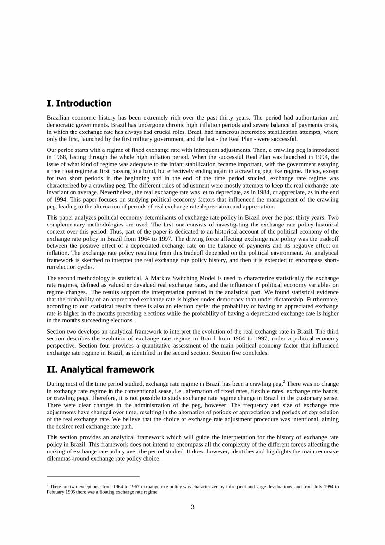
In 1964 the exchange rate was unified. Until 1967 the exchange rate policy was characterized by infrequent and largedevaluations, causing substantial real exchange rate variability. The inflation stabilization plan set forth in 1964 aimeda considerable inflation rate reduction, but the strategy adopted was gradualist. During the transition period, the highdomestic inflation rate, as compared to international standards, combined with a fixed nominal exchange rate led to arapid real exchange rate appreciation. When the real exchange rate appreciation would reach a certain level, thegovernment would make a large devaluation, characterizing an appreciation-depreciation cycle that lasted from eightto fourteen months in average, as shown in figure I RER jumps and slides. According to Simonsen (1995), foreigncurrency supply also had a corresponding cycle: there would be a boost in external credit supply immediately after thelarge devaluation, which was reduced while the nominal exchange rate remained fixed, until eventually an intensespeculative movement would make inevitable a new devaluation.

60.00

80.00

100.00

120.00

140.00

160.00

180.00

200.00

220.00

240.00

Abr/64 Dez/64 Ago/65 Abr/66 Dez/66 Ago/67 Abr/68

5(5

)LJXUH�,�

In average, there was a real exchange rate appreciation over the period. However, since real wages fell even more (seeDIEESE), this did not lead to a loss of exports competitiveness. In fact, there was substantial current accountimprovement, possibly due to the 1964-65 recession. During this period, the level of protectionism in the Brazilian

4 Two useful sources for an economic perspective of the recent history of exchange rate policy are Dib (1985) and Baumgarten (1996). Dib (1985)provides an account of the external sector policy, including exchange rate policy, from the fifties to the end of the seventies. Baumgarten (1996)analyzes the exchange rate policy until, and including, the Real Plan.

5 Figures I to VII present the evolution of the real exchange rate for each time period separately. The data used is described in section IV, and thevalues presented in appendix II.

77

economy was extremely high. In 1965, imports reached their lowest value in three decades. In 1967-68, a short livedimport liberalization was essayed, to be reverted at the end of 1968. In the end, only capital goods and basic inputsremained as beneficiaries of tariff reduction.

Who were the beneficiaries of the exchange rate policy in the period 1964-67? Because of the high level of tariffprotection, a small appreciation of the real exchange rate would not affect the demand for domestic tradable goods.But it would improve the profitability of domestic industry, since imported inputs would become cheaper. If we takeinto account that labor was also becoming cheaper in real terms, the domestic industry was the major beneficiary ofthe policy in this period. However, in order to fight inflation and to please the IMF, aggregate demand was controlledthrough traditional monetary and fiscal restrictions, in addition to the non-orthodox wage policy. The economy faced arecession in 1964-65, which would make the benefits of the policy unequal. Since restrictions to profit remittanceimposed in 1962 were lifted, Brazilian subsidiaries from multinational firms were stimulated to look for capital fromtheir foreign counterpart. The small national firms did not have the same alternative, being subject to the unfavorablecredit conditions of the period. Thus, among the firms, because of the recession, only the survivors, and in special themultinational subsidiaries, could have gained with the policy.

Exporters were not necessarily losers, because the fall in real wages possibly more than compensated for the realexchange rate appreciation. However, coffee exports had a share larger than 50% of total exports in 1964 (see TableI), and the price guaranteed by the government deteriorated substantially in this period, improving the fiscal account.Therefore, if some exporters were winners, among those were not included coffee exporters.

Workers were the main losers of the period. Besides the recession that increased unemployment, even those whoremained employed lost because of the real wage reduction. That reduction was the result of government’s activepolicy. In a repressive environment, where the main union leaders were banned, a national wage policy was instituted,where wages were adjusted accordingly to a formula which would imply real wages reductions whenever thegovernment underestimated the inflation rate for the period, which happened systematically. On the other hand,workers did not benefit from the real exchange rate appreciation: the coefficient of imports reached the extreme lowvalue of 4% of GDP in 1965, with the imports being concentrated in oil, intermediate, and capital goods.

There was a gain to all members of society due to the inflation rate decrease achieved during this period (as shown inTable I, from 84% a year in 1964 to 24% in 1967). The real wages reduction policy during this period made it possibleto conceal inflation fighting and trade balance improvement: the potential negative effect of real exchangeappreciation on trade balance was more than compensated by real wages reduction.

,,,����0LQL�GHYDOXDWLRQV�DQG�WKH�%UD]LOLDQ�0LUDFOH�����������

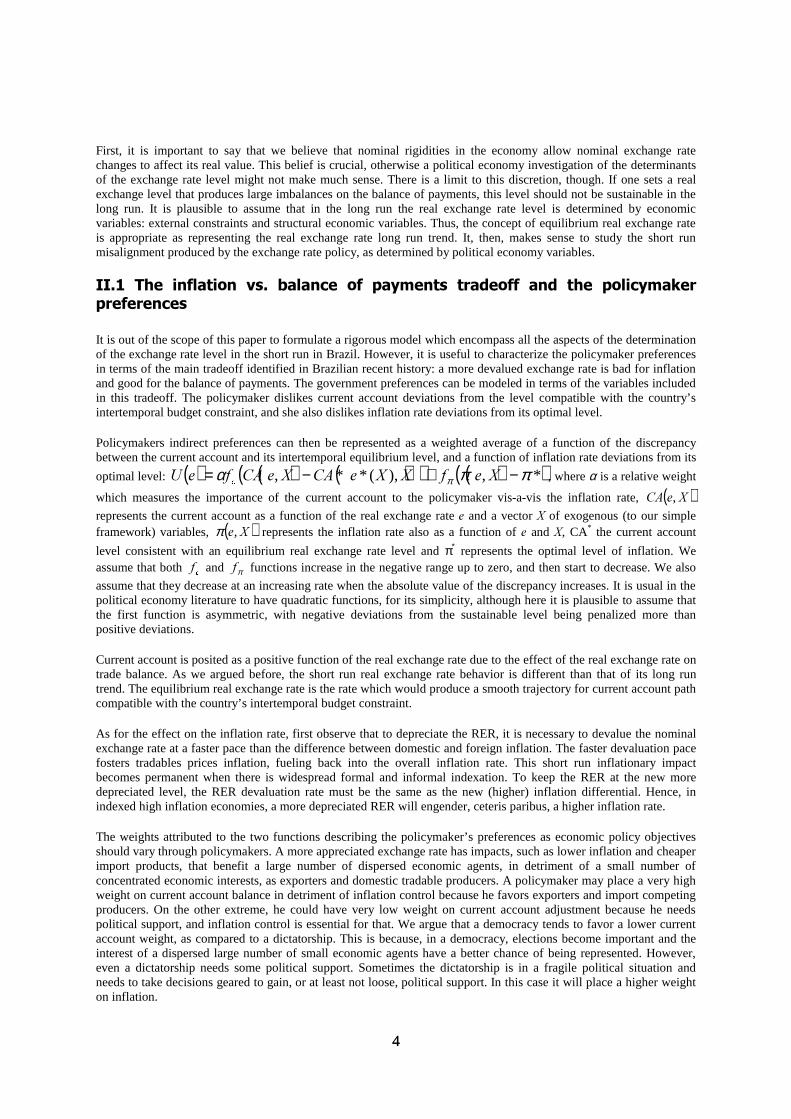
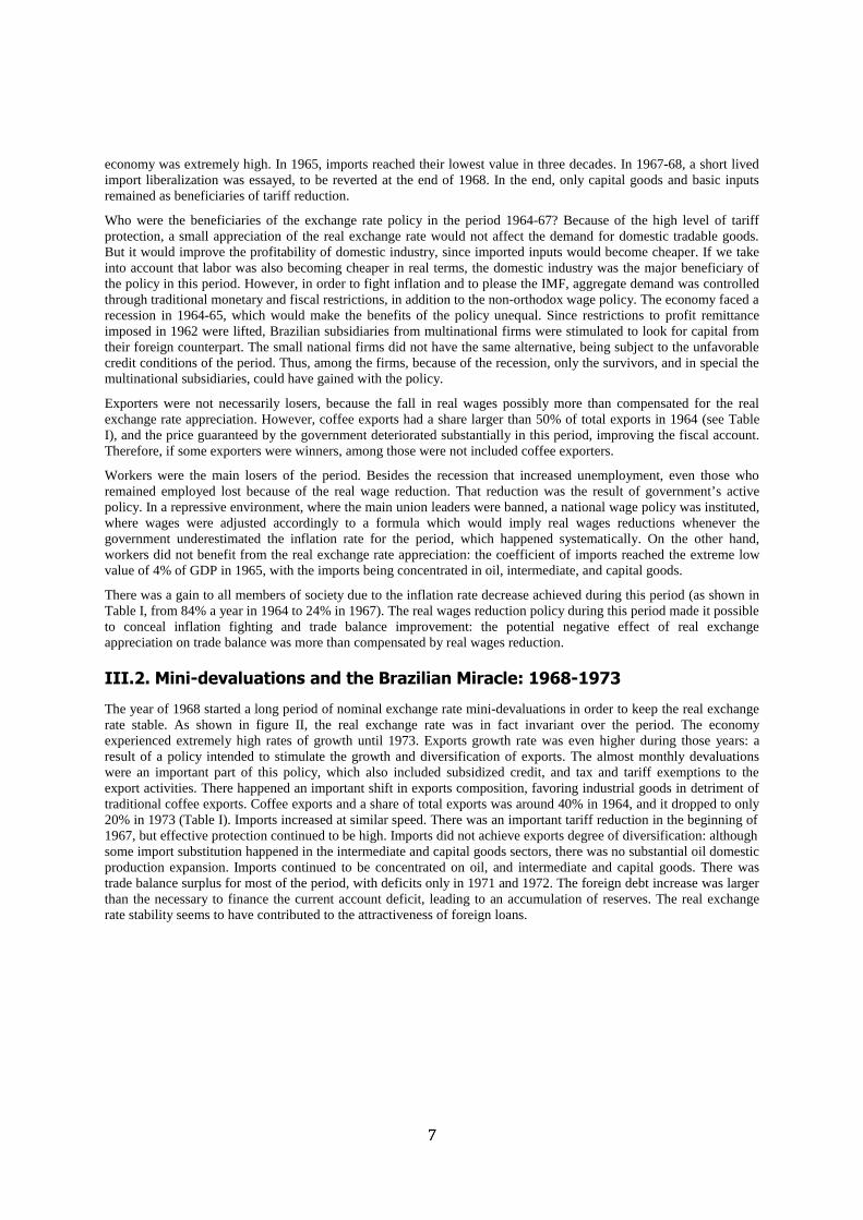
The year of 1968 started a long period of nominal exchange rate mini-devaluations in order to keep the real exchangerate stable. As shown in figure II, the real exchange rate was in fact invariant over the period. The economyexperienced extremely high rates of growth until 1973. Exports growth rate was even higher during those years: aresult of a policy intended to stimulate the growth and diversification of exports. The almost monthly devaluationswere an important part of this policy, which also included subsidized credit, and tax and tariff exemptions to theexport activities. There happened an important shift in exports composition, favoring industrial goods in detriment oftraditional coffee exports. Coffee exports and a share of total exports was around 40% in 1964, and it dropped to only20% in 1973 (Table I). Imports increased at similar speed. There was an important tariff reduction in the beginning of1967, but effective protection continued to be high. Imports did not achieve exports degree of diversification: althoughsome import substitution happened in the intermediate and capital goods sectors, there was no substantial oil domesticproduction expansion. Imports continued to be concentrated on oil, and intermediate and capital goods. There wastrade balance surplus for most of the period, with deficits only in 1971 and 1972. The foreign debt increase was largerthan the necessary to finance the current account deficit, leading to an accumulation of reserves. The real exchangerate stability seems to have contributed to the attractiveness of foreign loans.

88

60,0080,00

100,00120,00140,00160,00180,00200,00220,00240,00

Jul/68 Mai/69 Mar/70 Jan/71 Nov/71 Set/72 Jul/73

5(5

)LJXUH�,,

From a macroeconomic perspective, the introduction of a mini-devaluations regime represented an explicitacknowledgment that future inflation rates would be far superior than international rates. In fact, the new economicteam led by Delfim Neto, which started as minister during President Costa e Silva term in 1967 and would continueuntil 1974, had put a much higher emphasis in growth. According to them, inflation reduction should be achievedgradually without sacrificing the goal of high economic growth. They also had a different diagnosis of the causes ofinflation, which they identified in the cost side.

Thus, one may conclude that the mini-devaluations system, which represented exchange rate indexation to inflation,was designed to stimulate exports and foreign indebtedness, at the cost of increasing the inflation inertia. This was incontrast to the treatment given to wages, which had a system of adjustment designed to prevent past inflation fromfueling future inflation. Before 1968, wages were adjusted according to future inflation expectations dictated by thegovernment. In 1968, the wage formula was changed to correct partially for the loss of real wage incurred due toinflation underestimation by the government. Thus, there was an increase in wage indexation.

Despite the average minimum wage continued fall, the high rates of growth in this period led to increases in wages,although they were far lower than productivity growth. Given the constant real exchange rate, once again firms in thetradable sector have benefited from additional reductions of labor cost in dollars. In particular, exporters were furtherstimulated by the other policies mentioned above, which included tariff exemptions.

Although, the high growth benefits were widespread, they were unequal. Employment increased at a rate far higherthan population, and real wages increased for almost all segments. Nonetheless, the real wages increase was extremelyunequal, with high wages increasing much more than low wages. And profits increased much more than wages, sincereal wages increased less than productivity. Thus, those who were rich, or belonged to the upper middle class,benefited more from the miracle years compared to the poor. For all accounts, there was an increase in incomeinequality, which had already worsened during the first military government.

The mini-devaluations system and the increase in wage indexation were measures which helped society to live withinflation. On the other hand, these measures also increased the cost of fighting inflation. In fact, after falling graduallyuntil 1972, inflation started to increase in 1973, despite the official numbers which showed an artificially low inflationrate for that year.

The higher indexation introduced during this period had two effects on the policymaker’s choice. On the one hand, itdecreased the cost of a given level of inflation to society and, therefore, to the policymaker. On the other hand, as thecost of fighting inflation increased, the real exchange rate appreciation necessary to achieve a given inflation reductionbecame higher. Thus, the weight given to inflation in the policymaker loss function decreased, and the trade offbetween balance of payments improvement and inflation fighting was worsened.

,,,����7KH�ODFN�RI�UHDFWLRQ�WR�WKH�ILUVW�RLO�VKRFN�����������

Oil prices quadrupled at the end of 1973. Since oil was an important part of Brazilian imports (20% in 1974, as shownin Table I), this had a severe impact on the trade balance, which changed from a modest surplus to a deficit of 4.7billion dollars in 1974. The current account deteriorated substantially, changing from a deficit of 1.7 billion in 1973 toa deficit of 7.1 billion in 1974 (Table I). Most oil importer countries reacted to the oil shock devaluating the exchangerate and controlling aggregate demand through monetary and fiscal restrictions. Aggregate demand control wouldlessen the oil shock inflationary impact, but would also cause a, at least temporary, recession. The relative prices

99

change would stimulate the production of tradable goods, and would reduce spending on imported goods, particularlyoil. The temporary recession would improve trade balance in the very short run, while the effect of the relative pricechange would be building up.

60,0080,00

100,00120,00140,00160,00180,00200,00220,00240,00

Jan/74 Jan/75 Jan/76 Jan/77 Jan/78 Jan/79

5(5

)LJXUH�,,,

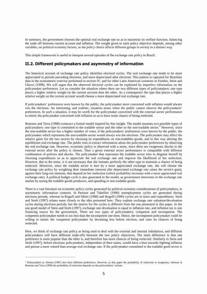
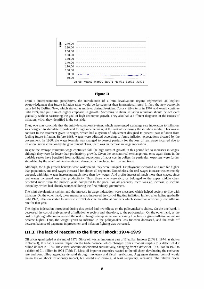
However, the Brazilian government chose a different strategy. The real exchange rate was kept constant (see figureIII) and there was no severe aggregate demand control. Imports were reduced through a menu of measures, whichwere aimed at restricting imports while, at the same time, stimulating import substitutes production.6 Oil imports wereexcluded from the restrictions, indicating that the government’s objective could have been to minimize the effect ofthe oil price shock on inflation and growth.

Thus, differently from the adjustment prevalent among most oil importer countries, the Brazilian strategy aimed atcontinuing the accelerated growth trajectory. The adjustment should be made through a later stage of the importsubstitution process, involving capital and intermediary goods. The import restriction had immediate effect: thecoefficient of imports fell from 12% in 1974, an historical high, to 7.25% in 1978. The country grew at a rate of 6.7%while imports value remained constant. Exports performance was disappointing, due to the world recession.Meanwhile, the country made use of the large liquidity in international capital markets to finance the current accountdeficit, which averaged US$5.7 billions in the period. Foreign debt increased by US$20 billion in those years, with theamount of interest paid increasing from US$500 millions to US$2.7 billions in 1978. Industrial policy for exportsstimulation and import substitution had a high cost in terms of fiscal performance, causing a substantial budgetdeterioration. This policy left the next government an unpleasant heritage: high inflation rate, extremely heavyexternal debt service, and a deteriorated fiscal position (see Carneiro, 1990).

Why did the government choose that unusual strategy? Was not a military government in a better position to imposemacroeconomic adjustments than a democratic one? First, one should note that there was no unity in the armed forces.There were basically two groups: on the one side there was the moderate and more intellectual group associated toPresident Castelo Branco, the first military president (1964-1967), and the hard liners were on the other side7. A hardliner, Emílio Garrastazu Médici, was president during the miracle years (1969-1974). Brazil had the mostauthoritarian government in those thirty three years, which, aided by favorable external conditions, had also the mostspectacular economic performance. President Geisel (1974-1979), who succeeded Médici, was a moderate. In order tomaintain legitimacy among the militaries, the performance of his government, measured mainly by growth rates,should not be disappointing. That is probably why, in face of unfavorable external conditions, he chose the strategyconceived by the Minister of Planning, Reis Veloso. One should not neglect that the military government reliedheavily on the entrepreneurs support for some civil legitimacy, and that the government lost the parliamentaryelections of 1974, despite the extraordinary economic performance during the preceding years. The entrepreneurswere enthusiastic with the high growth rates and they were unwilling to buy the macroeconomic adjustment policy, ashistory would reveal during the 1979 Simonsen resignation episode. The Brazilian response to the first oil shockshows that, contrary to widespread believe, a dictatorship may be less able to take necessary bitter measures than ademocratic regime, exactly because of its fragile legitimacy.

6 The measures designed to restrict imports included tariff increases, the interdiction imposed to Brazilian state enterprises to buy foreign goods forwhich there was a similar Brazilian product, and the compulsory deposit of 100% of the imports value during six months, without any interest paid. Inorder to stimulate import substitution of capital and intermediary goods, subsidized credit and tax exemptions were granted to the activity linked tothe production of such goods. Also, substantial public investments were devoted to this goal, including investment in oil prospection (see Carneiro,1990).

7 Skidmore (1988) analyzes the dispute between the two military groups during the period of military government.

1010

Although the oil shock depreciated the equilibrium real exchange rate, the government chose to keep the realexchange rate constant, inducing its overvaluation. It is then very important to note that real exchange rate stabilityover the period, shown in figure III actually represents a change of exchange rate policy, because it represents andovervaluation of the real exchange rate with respect to its equilibrium level.

In terms of our framework, the need of political legitimacy made the government prioritize inflation over balance ofpayments. In search for political support, the policymaker placed a lower weight on current account misalignment.The main concern at that moment, though, was not only inflation fighting as in our simple analytical frameworksketched in the previous section, but also preventing the recession that would have been caused by the current accountadjustment. That is, a sharp real exchange rate depreciation could equilibrate the current account, at some output andinflation cost during the transition period.

,,,���� 3UHVHWWLQJ� H[FKDQJH� UDWH� DGMXVWPHQW� WR� DIIHFW� LQIODWLRQDU\H[SHFWDWLRQV�����������

In March 1979, a new military president, João Figueiredo, succeeded President Geisel. The former Minister ofFinance, Mário Henrique Simonsen, was nominated Minister of Planning, in a new institutional design where thisMinistry would concentrate all the important economic decisions. He was determined in pursuing a more traditionalmacroeconomic adjustment policy. His main objective was to control aggregate demand, imposing strict control to thefiscal and monetary accounts, in order to reduce growth, control inflation and improve external accounts. As the firstmoderate measures were not producing the desired results in the first semester, he decided to take more drasticmeasures in the second semester. Political pressures led him to resign. His substitute, Delfim Neto, announced aheterodox stabilization approach, which would conciliate growth with inflation stabilization and current accountdeficit reduction.

What kind of pressures did lead to Simonsen’s resignation? The entrepreneurs in general were not satisfied with theperspective of an orthodox adjustment. According to a survey conducted by the biweekly magazine ([DPH in July of1979, only 19.29% of businessmen considered the minister prestige excellent or good (see Goldenstein, 1985).Exporters were dissatisfied with the fiscal incentives withdrawal, and the lack of compensation through a fasterexchange rate devaluation, which was kept constant in real terms. Farmers were not satisfied with Simonsenopposition to more agriculture subsidies, defended by Delfim Neto, the Minister of Agriculture and former Minister ofFinance during the “miracle years”. In Brazil, farmers had always had strong political congress support, whichcontributed to reinforce the pressure over Simonsen. President Figueiredo was probably not very pleased with havingall the political cost of unpopular measures for himself, while his predecessors enjoyed the benefits of imprudentexpansionary policies. Delfim promised a new miracle - external adjustment and inflation reduction with fast growth -and the political establishment was glad to give him an opportunity to do so.

60,0080,00

100,00120,00140,00160,00180,00200,00220,00240,00

Jul/79 Out/79 Jan/80 Abr/80 Jul/80 Out/80

5(5

)LJXUH�,9

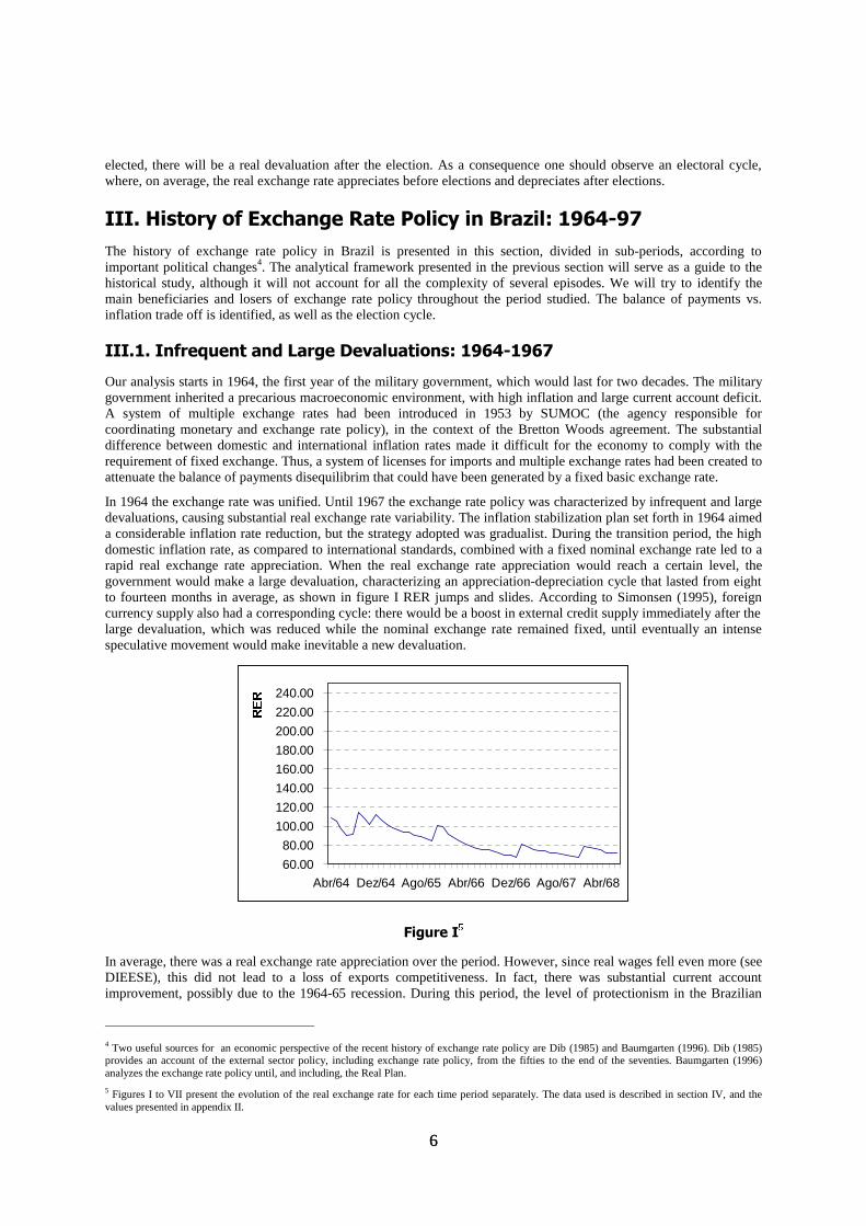
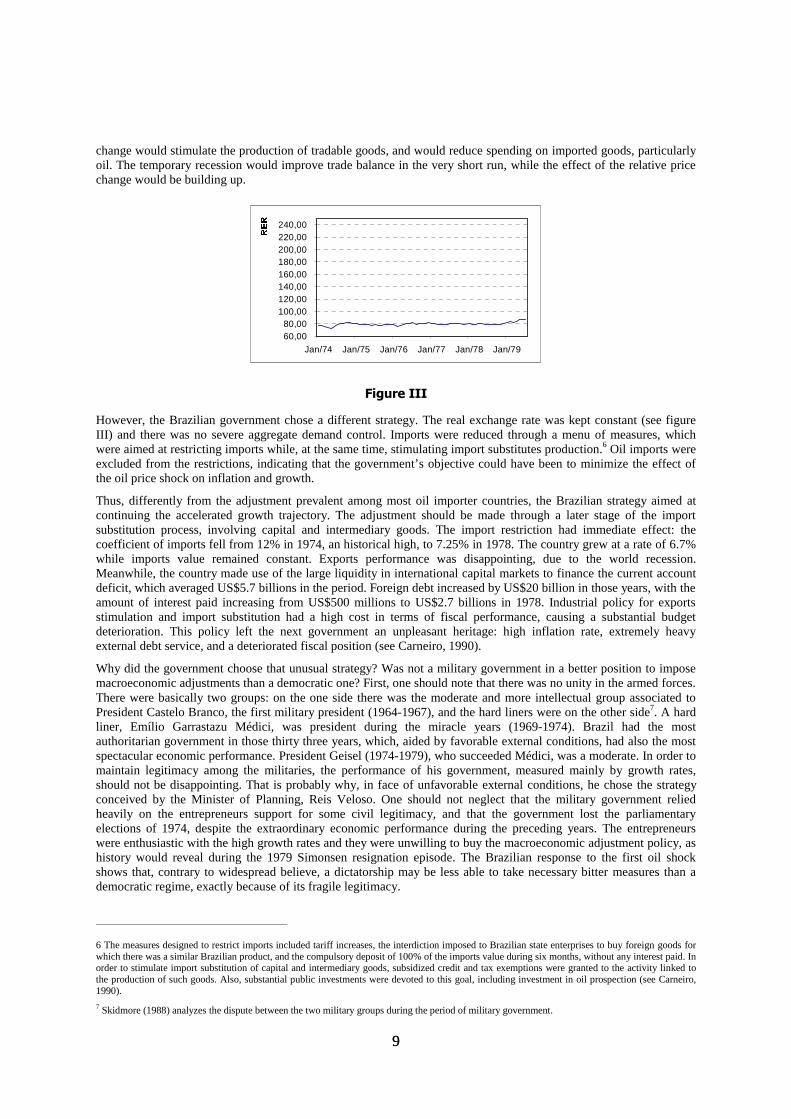
At first, Delfim followed a heterodox strategy, basing his policies on price controls. By the end of 1979 the exchangerate was devaluated in 30%, causing a RER depreciation, as can be seen in figure IV. Simultaneously, primaryproducts exports were taxed in 30%, fiscal incentives to manufacture exports were removed, and the imports valuedeposit requirement for 360 days was lifted. Thus, the devaluation was complemented with measures with oppositeeffects on exports and imports, in such a way that the overall effect was unchanged incentives to exporters and

1111

importers, and an increase in government revenue due to the fiscal changes. For the year of 1980, exchange ratedevaluation was predetermined in 40%, a rate much lower than the inflation rate of 1979, which was 77%. Theobjective was to influence inflation expectations. It aimed also to make compatible the lower interest rates, necessaryfor the growth strategy, and the incentive to foreign indebtedness, necessary to close the balance of payments gap dueto the current account deficit.

This endeavor took one year, and failed completely. Inflation accelerated, RER appreciation was almost as large as theone prevalent before the maxi-devaluation at the end of 1979, and the balance of payments continued to deteriorate,leading to substantial reserves loss.8 The balance of payments deterioration had several causes. On the one hand, tradebalance was negatively affected by the second oil shock, and by speculative imports anticipation and exportspostponement due to the exchange rate policy lack of credibility. On the other hand, besides the international interestrate increase (see Table I), there was a rise of the spread charged to Brazil, due to the worsening of internationalBrazilian policy credibility. These factors contributed to further increase the current account deficit. Domestic interestrates control, and increased uncertainty over the future exchange rate policy and over the country’s capacity to honorits external debt contributed to the foreign loans retraction, resulting in substantial reserves loss. The heterodox policywas, therefore, abandoned, and the orthodox approach reestablished.

Why did the government choose the currency maxi-devaluation instead of accelerating the mini-devaluations?Suppose, for a moment, that after the maxi-devaluation the government would keep the real exchange rate constant, insuch a way that at the end there would be a real exchange rate devaluation. In what respect would this have differenteffects compared to a policy of mini-devaluations acceleration, as was previously promised to exporters? First, themaxi-devaluation price effect would be instantaneous, thus benefiting exporters instantaneously, whereas the mini-devaluations acceleration would change relative prices gradually. In fact, the government imposed offsetting policieson exports and imports, and there was no substantial instantaneous effect on the incentives to increase exports and toreduce imports.

Second, a maxi-devaluation would impose an instantaneous loss to debt holders, but it would not decrease new loansincentives, while mini-devaluations acceleration would make new foreign loans more expensive. Since foreign loandebtors were allowed to have “dollar” deposits in the Central Bank, which were remunerated according to exchangerate devaluation with respect to the US dollar, if they anticipated correctly the maxi-devaluation and deposited theirmoney, they would have no loss. The ones who did not deposit their money would have a tax credit equivalent to theloss, to be used along five years. In this way, the government intended to absorb most of the maxi-devaluation loss,and, at the same time, new loans would not be burdened with a higher rate of devaluation. As a complement to themaxi-devaluation, the government decided to forbid “foreign currency” deposits withdrawals that had already beenmade in the Central Bank, hoping to stimulate further foreign indebtedness. At the end, because the mini-devaluationrule was broken, the effect could be the opposite, since uncertainty about future policy increased.

As we argue throughout this article, in our view the main cause of exchange rate policy tension is the trade offbetween inflation and balance of payments: a more appreciated exchange rate is good for inflation and bad for thebalance of payments, while the opposite is true for depreciated exchange rate. Delfim tried to avoid this dilemma withhis heterodox approach. The maxi-devaluation should provide balance of payments incentives in the short run, whilethe preset lower devaluation rate should influence expectations and reduce inflation in the middle run. However, thefailure of his policy towards inflation undermined the balance of payments incentives. As we will see, the same realexchange rate pattern would be reproduced during most heterodox stabilization attempts, after democracy wasreestablished.

,,,������([WHUQDO�$GMXVWPHQW�DV�D�3ULRULW\�����������

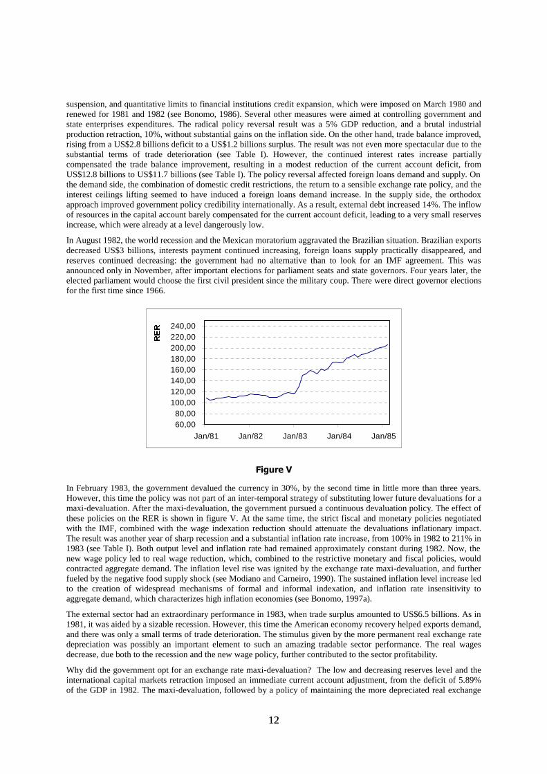
During 1980, the government gradually abandoned the heterodox policy in favor of an orthodox approach. Theexchange rate policy was reverted to the old mini-devaluations policy based on inflation differential, which stabilizedthe real exchange rate (see figure V). There were restrictive measures on the monetary side, including interest ceilings

8 One important cause of the inflation acceleration was the new wage policy, implemented in October 1979, whenwage adjustments periodicity was increased to twice a year. Had inflation remained constant, this would amount to asubstantial real wages increase, in a context where the second oil shock and the balance of payment adjustment wouldhave required a fall in real wages. As mentioned by Simonsen (1995), inflation increased from 45% a year (betweenJuly 1978 and July 1979) to 45% a semester, or 110% a year (between December 1979 and December 1980) – seeTable I. Moreover, wages between one and three minimum wages (a large proportion in Brazil) would be adjustedevery semester by 1.10 times the inflation rate. As a consequence, the higher the inflation, the higher the real wageincrease.

1212

suspension, and quantitative limits to financial institutions credit expansion, which were imposed on March 1980 andrenewed for 1981 and 1982 (see Bonomo, 1986). Several other measures were aimed at controlling government andstate enterprises expenditures. The radical policy reversal result was a 5% GDP reduction, and a brutal industrialproduction retraction, 10%, without substantial gains on the inflation side. On the other hand, trade balance improved,rising from a US$2.8 billions deficit to a US$1.2 billions surplus. The result was not even more spectacular due to thesubstantial terms of trade deterioration (see Table I). However, the continued interest rates increase partiallycompensated the trade balance improvement, resulting in a modest reduction of the current account deficit, fromUS$12.8 billions to US$11.7 billions (see Table I). The policy reversal affected foreign loans demand and supply. Onthe demand side, the combination of domestic credit restrictions, the return to a sensible exchange rate policy, and theinterest ceilings lifting seemed to have induced a foreign loans demand increase. In the supply side, the orthodoxapproach improved government policy credibility internationally. As a result, external debt increased 14%. The inflowof resources in the capital account barely compensated for the current account deficit, leading to a very small reservesincrease, which were already at a level dangerously low.

In August 1982, the world recession and the Mexican moratorium aggravated the Brazilian situation. Brazilian exportsdecreased US$3 billions, interests payment continued increasing, foreign loans supply practically disappeared, andreserves continued decreasing: the government had no alternative than to look for an IMF agreement. This wasannounced only in November, after important elections for parliament seats and state governors. Four years later, theelected parliament would choose the first civil president since the military coup. There were direct governor electionsfor the first time since 1966.

60,0080,00

100,00120,00140,00160,00180,00200,00220,00240,00

Jan/81 Jan/82 Jan/83 Jan/84 Jan/85

5(5

)LJXUH�9

In February 1983, the government devalued the currency in 30%, by the second time in little more than three years.However, this time the policy was not part of an inter-temporal strategy of substituting lower future devaluations for amaxi-devaluation. After the maxi-devaluation, the government pursued a continuous devaluation policy. The effect ofthese policies on the RER is shown in figure V. At the same time, the strict fiscal and monetary policies negotiatedwith the IMF, combined with the wage indexation reduction should attenuate the devaluations inflationary impact.The result was another year of sharp recession and a substantial inflation rate increase, from 100% in 1982 to 211% in1983 (see Table I). Both output level and inflation rate had remained approximately constant during 1982. Now, thenew wage policy led to real wage reduction, which, combined to the restrictive monetary and fiscal policies, wouldcontracted aggregate demand. The inflation level rise was ignited by the exchange rate maxi-devaluation, and furtherfueled by the negative food supply shock (see Modiano and Carneiro, 1990). The sustained inflation level increase ledto the creation of widespread mechanisms of formal and informal indexation, and inflation rate insensitivity toaggregate demand, which characterizes high inflation economies (see Bonomo, 1997a).

The external sector had an extraordinary performance in 1983, when trade surplus amounted to US$6.5 billions. As in1981, it was aided by a sizable recession. However, this time the American economy recovery helped exports demand,and there was only a small terms of trade deterioration. The stimulus given by the more permanent real exchange ratedepreciation was possibly an important element to such an amazing tradable sector performance. The real wagesdecrease, due both to the recession and the new wage policy, further contributed to the sector profitability.

Why did the government opt for an exchange rate maxi-devaluation? The low and decreasing reserves level and theinternational capital markets retraction imposed an immediate current account adjustment, from the deficit of 5.89%of the GDP in 1982. The maxi-devaluation, followed by a policy of maintaining the more depreciated real exchange

1313

rate level through mini-devaluations, increased the price incentives to the tradable sector production. Thus, itcomplemented the stimulus given by the aggregate demand contraction, fiscal incentives, and the favorable creditconditions granted to exports and import substitutes production.

In 1984, the vigorous American economy growth, and the substantial terms of trade improvement, helped exports toachieve an exceptional performance: a level 23.3% larger than that of the preceding year. Exports growth was mainlydue to manufacture exports, and induced the Brazilian industry recovery. Trade balance reached the extraordinarysurplus of US$13.1 billions, which was more than enough to balance the current account, allowing an addition ofUS$7 billions to foreign reserves. The import substitutes production increase also contributed for this result, as wellfor the industry growth9 (see Carneiro and Modiano, 1990). The main macroeconomic problem was high inflationrate, which remained practically at the same level as in 1983.

By doing a maxi-devaluation, balance of payments improvement was chosen as priority in detriment of fightinginflation. The policy had clearly distributive effects. By decreasing real wages and increasing real exchange rate,income was redistributed from workers to tradable sector entrepreneurs.

,,,����7KH�1HZ�5HSXEOLF�DQG�,QIODWLRQ�)LJKWLQJ�����������

60,0080,00

100,00120,00140,00160,00180,00200,00220,00240,00

Mar/85 Mar/87 Mar/89 Mar/91 Mar/93

5(5

)LJXUH�9,

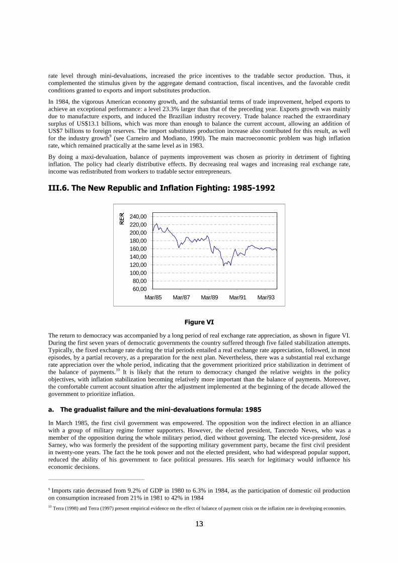
The return to democracy was accompanied by a long period of real exchange rate appreciation, as shown in figure VI.During the first seven years of democratic governments the country suffered through five failed stabilization attempts.Typically, the fixed exchange rate during the trial periods entailed a real exchange rate appreciation, followed, in mostepisodes, by a partial recovery, as a preparation for the next plan. Nevertheless, there was a substantial real exchangerate appreciation over the whole period, indicating that the government prioritized price stabilization in detriment ofthe balance of payments.10 It is likely that the return to democracy changed the relative weights in the policyobjectives, with inflation stabilization becoming relatively more important than the balance of payments. Moreover,the comfortable current account situation after the adjustment implemented at the beginning of the decade allowed thegovernment to prioritize inflation.

D�� 7KH�JUDGXDOLVW�IDLOXUH�DQG�WKH�PLQL�GHYDOXDWLRQV�IRUPXOD������

In March 1985, the first civil government was empowered. The opposition won the indirect election in an alliancewith a group of military regime former supporters. However, the elected president, Tancredo Neves, who was amember of the opposition during the whole military period, died without governing. The elected vice-president, JoséSarney, who was formerly the president of the supporting military government party, became the first civil presidentin twenty-one years. The fact the he took power and not the elected president, who had widespread popular support,reduced the ability of his government to face political pressures. His search for legitimacy would influence hiseconomic decisions.

9 Imports ratio decreased from 9.2% of GDP in 1980 to 6.3% in 1984, as the participation of domestic oil productionon consumption increased from 21% in 1981 to 42% in 198410 Terra (1998) and Terra (1997) present empirical evidence on the effect of balance of payment crisis on the inflation rate in developing economies.

1414

The ministry inherited from Tancredo Neves had an orthodox, his nephew, Francisco Dornelles, as Minister ofFinance, and a Keynesian, João Sayad, as Minister of Planning. Tancredo wanted Dornelles to be the strong man inthe economy. However, his policy of severe government expenditure and monetary control could not achievesubstantial short-term inflation reduction and was not politically very palatable. Sarney, as opposed to Tancredo, hadnot much political capital to spend with unpopular or politically costly measures without a clear and immediatereward. Thus, the failure in bringing inflation down in six months produced the substitution of Dornelles by DilsonFunaro. Funaro was more aligned with the Minister of Planning, and with the presidential aspiration of short runpopularity.

During the first year, the inherited exchange rate policy of daily mini-devaluations was maintained. However, thebasis for the exchange rate adjustment, as well as the basis for contracts monetary indexation, were immediatelychanged by Dornelles. The adjustment formulas were now based on inflation geometric mean for the three previousmonths, whereas before they were based only on current inflation. This new adjustment formula had two mainimpacts. On the one hand it reduced uncertainty over future nominal devaluation, as past inflation was known inadvance, whereas current inflation would be known only by the end of the month. On the other hand, real exchangerate would become more sensitive to inflation movements, appreciating with inflation acceleration, and depreciatingwith inflation reduction. When Funaro took office, it was clear that the government was more worried about the effectof the exchange rate movements on inflation than about the effects of inflation on real exchange rates. However, thenew rule appeared to have bad dynamic properties, since high past inflation would feed back on future inflationthrough the mini-devaluations, increasing inflation inertia. Funaro, who prioritized inflation reduction, decided torestore the old rule of basing exchange rate devaluations and monetary indexation on current inflation. By doing soafter the inflation peak of 14% in August, he had an opportunistic gain of preventing this high rate from feeding backinto future inflation through the future exchange rate devaluation. Opportunistic rules change of this kind would occurvery often during Sarney’s government.

E�� 7KH�&UX]DGR�3ODQ������

Inflation continued accelerating during the second semester of 1985, reaching approximately 15% a month, partiallyas a result of a dry that hit the crop. Since the orthodox gradualist approach was rejected, and there would be governorand parliament elections in November 1986, the alternative of a heterodox stabilization plan became politicallyappealing. The Argentinean Austral Plan and the Israeli stabilization program were examples of heterodoxstabilization plans where prices were frozen in order to coordinate price setting to a new equilibrium with low or zeroinflation. (See Heymann, 1991, for Argentina, and Bruno, 1989, for Israel.) However, it was largely believed in Brazilthat both plans hurt workers, either by increasing unemployment, or by reducing real wages. So, in order to make theBrazilian plan palatable, ingredients were inserted to assure that growth would continue at high rates: veryexpansionist monetary and fiscal policies, and a wage conversion rule which assured substantial immediate real gains.Furthermore, real wages gains would be protected against inflation erosion through an escalator clause in the wageadjustment formula. The nominal exchange rate was fixed at the level prevalent the day before the plan wasintroduced. The Cruzado Plan was unexpectedly announced on February 28, with a discourse that appealed to thecitizens, which would guard the Plan against illegal price rises. As real interest rates become negative and real wagesincreased 12%, the result was a huge excess demand. Sales increased 22.8% during the first six months of 1986 withrespect to the same months the year before, the consumption of durable goods increased 33,2% in one year, and thepractice of charging a premium over the legal price of goods was becoming widespread (see Modiano, 1990).

Inflation repression induced a black market premium increase over the official exchange rate from 26% to 50%. Afixed exchange rate should help fighting inflation by two mechanisms: by preventing an imports price increase indomestic currency and by signaling commitment to low inflation rates.

Excess demand did not cause much damage to trade balance during the first six months, in part due to favorableexternal conditions, such as the dollar depreciation with respect to the other strong currencies. From September on,exports started to fall and imports continued to rise, which caused substantial trade balance reduction. Trade balancereduction fed the speculation of a maxi-devaluation, which itself fed back into the trade balance, through exportspostponement and imports anticipation. When the black market premium increased to 90%, the government broke upthe fixed exchange rate rule and devalued it in 1.8% in October. At the same time, a return to the mini-devaluationspolicy was announced, although without specifying the exact timing of devaluations (see Modiano, 1990). However,the exchange rate was still considered appreciated - between February and November the RER had appreciated by12%. The rules breaking, without a clear alternative, in an environment where the exchange rate was consideredovervalued, only contributed to increase the perceived likelihood of a maxi-devaluation, with further negative tradebalance impact.

1515

The exchange rate rigidity contributed to real wages increase. Since protection was high in the tradables sector,producers could redirect production towards domestic market, which was overheated. The situation was notsustainable in many aspects. Producers had an incentive to increase prices and profits, fueling inflation, and erodingreal wage gains. The current account deterioration, which would be aggravated without the price controls, wouldmake unsustainable the maintenance of a fixed exchange rate. However, there is evidence that the government wasable to provide some credibility for the unsustainable regime, since it won the November elections by landslide. If thepolicy were believed sustainable, so would be the gains. The fact that there were no losers in the short run contributedfor its electoral success.

One week after elections, a new bundle of measures was announced, aiming at correcting the disequilibria generatedby the Cruzado Plan. The measures aimed at controlling aggregate demand through an increase in governmentrevenues of 4% of GDP. The higher revenues should be obtained through indirect taxes over some products and pricesincrease for goods produced by state enterprises. The repressed inflation was stimulated by the important pricesincrease implicit on those measures.

At the same time, the government would restart the daily exchange rate devaluations. Trade balance became negativestarting in October. As reserves were being quickly eroded, decreasing from US$10.4 billions to US$5 billions fromJune 1986 to February 1987, the government decided to stop paying interests on the part of the external debt ownedby the private banks. This decision, which had in part the political intention of recovering some of the lost popularityby exploiting nationalist feelings, failed completely. The government popularity was not recovered, and betterconditions for external debt payment were not obtained.

The exchange rate cycle was clear in the Cruzado Plan: an appreciating exchange rate policy was used to help theinflation stabilization plan implemented before elections, and after election the bitter corrective measures were taken,including exchange rate devaluation.

F�� 2WKHU�VWDELOL]DWLRQ�DWWHPSWV�����������

%UHVVHU�3ODQ

In February 1987, price controls were lifted. When inflation reached 20% a month in April, Funaro left the Ministry ofFinance, being substituted by Bresser Pereira. The new minister was more conservative: he announced a productiongrowth deceleration and that he would evaluate the convenience of negotiating with the IMF. From May to July heinduced a real exchange rate appreciation of 10.5%. On June 12 he introduced a Plan with both orthodox andheterodox features. The idea was to superimpose rigid monetary and fiscal control to heterodox rent control anddeindexation measures in order to prevent the Cruzado Plan mistakes. From then on this movement was reverted, withthe total appreciation amounting 6.4% until December. Thus, the idea seemed to be to generate some real exchangerate depreciation before the Plan, and to use the slack generated to decelerate the devaluation during the Plan’simplementation. The lower exchange rate devaluation rate should help to obtain inflation reduction, while theprevious devaluation would prevent the balance of payments deterioration during the plan implementation. However,the stabilization attempt failed and inflation gradually increased to reach 14% in December, when Bresser Pereiraresigned. Overall, when his term was finished, the real exchange rate was slightly more depreciated than before.

5LFH�DQG�%HDQV�SROLF\

Minister Mailson da Nóbrega took office promising to attain to a simple monetary and fiscal control policy,denominated “Rice and Beans Policy”, as a reference to workers’ traditional dish. After the former stabilization trialsfailures, the main objective seemed to be to prevent hyperinflation. During the first semester inflation was kept below20% a month. In the second semester, however, it accelerated quickly, reaching 28.8% in December. In January 1989,the Minister gave up fis initial plecge and formulated a new heterodox plan, called Summer Plan.

6XPPHU�3ODQ

This Plan was similar in spirit to Bresser Plan, in the sense that heterodox deindexation and rent controls wereassociated with orthodox measures of monetary and fiscal controls. Exchange rate was devalued in 18%, to reach theparity of one new Cruzado for one dollar. Since the real exchange rate had depreciated 4.5% during the “Rice andBeans” period, when there was a current account surplus of 1.37% of GDP, this would bring the real exchange rate toa comfortable level. As in the Cruzado Plan, the nominal exchange rate rigidity would be used to affect futureinflation. Differently from then, however, the exchange rate was devaluated beforehand to very comfortable level.Furthermore, the parity of one to one was chosen to influence psychologically expectations of further devaluations.First, since this was a focal level, it should remain there for some time. Second, it could give the impression that thedomestic currency had become “as strong as the dollar”.

1616

The plan failed due to heterodox plans lack of credibility caused by the defeat of its predecessors. Inflation wasalready up to 6.1% in March. The exchange rate was devalued in 3.2% on April 18, but it was not enough to preventfurther devaluation speculation. Devaluations were resumed, but at irregular time intervals. The black market dollarpremium, which was stable in 70% during the first two months of the plan, reached 200% in May. Thus, on June 15,the government decided to devaluate the currency in 4.5%, and to announce the return of the mini-devaluations and arule of adjustments: the total devaluation rate would be equal to current inflation rate, being achieved through sixmini-devaluations during the month, without pre-established dates.

The general real exchange rate pattern during the Summer Plan was similar to that of the Bresser Plan: a preparatoryreal devaluation followed by a real appreciation, which, in this case, amounted to 22% from January to June. Themain difference is that the Summer Plan was in place long enough for the exchange rate valuation to exceed thedevaluation produced before the plan. Presidential elections took place at the end of the year, and the real exchangerate appreciation continued until the next president took office, in March 1990.

The Central Bank created an official market for financial transactions in 1989, the floating market. The commercialtransactions continued to be centralized by the Central Bank, and to be realized under the administered exchange rate.

G��7KH�&ROORU�3ODQV�����������

In October and November 1989, the first direct elections for President during democracy were held in two rounds.Fernando Collor was elected in the second round after defeating by small margin the leftist candidate Luis Inacio Lulada Silva. At the beginning, he had no support of any major political force. In the second round the major conservativeforces were allied to him, who became the only alternative to the leftist candidate.

His mandate started on March 15, 1990. During the preceding months, inflation was increasing at a high pace, fromabout 40% a month in November to more than 80% in March. The nominal exchange rate was not adjusted at thesame pace, leading to a real appreciation of approximately 35% from October to March. The reason for the realappreciation was probably the government attempt to prevent open hyperinflation before the new government takingoffice. The black market premium on exchange rate increased substantially due to expectations that the newstabilization plan would contain strong measures, among them the imposition of some public debt restructuring.

The newly elected president proved to have plenty of political capital. He surprised economy analysts with anextremely radical plan. Most liquid financial assets were frozen, reducing the liquidity from 30% of GDP to about 8%of GDP. Government debt payments were suspended for eighteen months. Price adjustments would be coordinated bythe government according to figures for future inflation projected by the economic team.

The government also announced an important exchange rate regime change. Legal transactions in foreign currencywould no longer be centralized in the Central Bank. An official foreign exchange market, called commercial market,was created, in parallel to the floating market for restricted financial transactions, which had been created in 1989.Although the change was operationally important, in practice the government continued to determine the exchangerate level through massive intervention in the newly created market.

The real exchange rate was devalued from March to July to make up for the currency overvaluation occurred in themonths preceding the plan. Then, probably because high inflation was already showing signs of convalescence and anincrease in international oil prices should further inflame the inflation rate, the government maintained the nominalexchange rate stable for the next two months. As the inflation rate exceeded 12% a month, the real exchange ratereturned in September to the appreciated level of March. As trade surplus was narrowing, and inflation persisted, theCentral Bank intervened causing a continuous real currency devaluation from September to January.

Another heterodox stabilization plan, the 2nd Collor Plan, was launched in January, when inflation mounted over 20%a month. Relying heavily in the rotten prices freezing instrument, the plan had only short run success: the monthlyinflation rate reached the minimum level of 5% in April, returning to two digit in June. The Minister of Finance wassubstituted in May. The economic team was more orthodox, and soon started to release the price controls. The realexchange rate appreciated during the two first months of the 2nd Collor Plan. After the new economic team took office,it depreciated slightly and was kept stable until September, when two months of fast erosion of reserves prompted adevaluation of 14% on September 30. The Central Bank kept slowly devaluating the currency until February 92, whenthe attained real level was kept stable until mid 93.

This period was characterized by extremely high inflation rates, on the verge of hyperinflation. The exchange ratepolicy had alternation periods of lagging behind in an attempt to prevent hyperinflation, and faster devaluation tomake up to the large over-valuation that could be built up very fast given domestic inflation rates. On average, the realexchange rate was kept more appreciated than in preceding periods.

1717

An important aspect of the Collor Government was that it promoted structural reforms in the economy, some of themaffecting directly the external sector. The state companies privatization contributed to the capital inflow, which wouldenable a lower real exchange rate level. On the other hand, tariffs reduction, from an average level of 34% in 1990 to14% in July 1993, would make the exchange rate policy more effective for regulating the competition betweenimports and domestically produced goods for the internal market.

Over his term, Collor lost all political capital that he showed to have at first. His prestige declined among the peoplebecause he imposed the bitter assets freezing medicine, but failed to defeat inflation. On the other hand, both the tradereform and the more appreciated RER level hurt the tradable sector. As a consequence, he also lost the elite support.In September 1992, President Collor was impeached due to charges of corruption, being replaced by the elected vice-president Itamar Franco.

,,,����7KH�5HDO�3ODQ�DQG�$QWHFHGHQWV�����������

D�� $QWHFHGHQWV

In May 1993, Fernando Henrique Cardoso was chosen Minister of Finance. His economic team would formulate theReal Plan and would remain in the center of economic decisions until now. After the failure of several Plans based ongovernment intervention on individual economic decisions, either through price setting or wealth allocation, a newstabilization plan, less interventionist, was implemented. The nature of the democratic process placed inflationstabilization as a priority, as its level reached 40% a month and continued to increase. Were a government successfulin this endeavor, it would enjoy years of popularity. Fernando Henrique Cardoso, who was part of a governmentwhich was supported by congress majority, had great political ability, and he chose his technical team among the bestavailable economists in Brazil. He was himself candidate to succeed Itamar Franco in the presidential elections ofOctober 1994. The opposition candidate, the leftist Luís Inácio da Silva, was leading the pools of beginning of 1994by a comfortable difference.

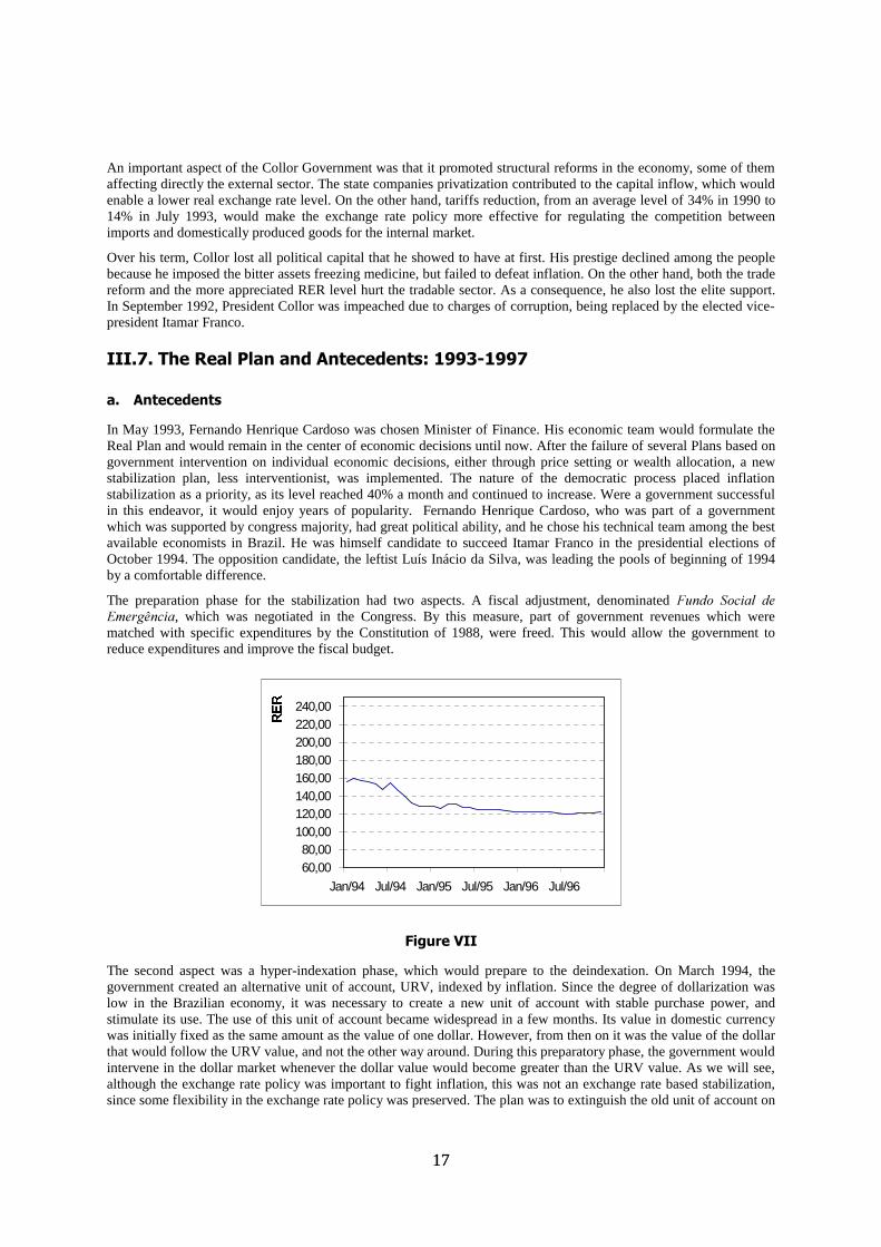
The preparation phase for the stabilization had two aspects. A fiscal adjustment, denominated )XQGR� 6RFLDO� GH(PHUJrQFLD, which was negotiated in the Congress. By this measure, part of government revenues which werematched with specific expenditures by the Constitution of 1988, were freed. This would allow the government toreduce expenditures and improve the fiscal budget.

60,0080,00

100,00120,00140,00160,00180,00200,00220,00240,00

Jan/94 Jul/94 Jan/95 Jul/95 Jan/96 Jul/96

5(5

)LJXUH�9,,

The second aspect was a hyper-indexation phase, which would prepare to the deindexation. On March 1994, thegovernment created an alternative unit of account, URV, indexed by inflation. Since the degree of dollarization waslow in the Brazilian economy, it was necessary to create a new unit of account with stable purchase power, andstimulate its use. The use of this unit of account became widespread in a few months. Its value in domestic currencywas initially fixed as the same amount as the value of one dollar. However, from then on it was the value of the dollarthat would follow the URV value, and not the other way around. During this preparatory phase, the government wouldintervene in the dollar market whenever the dollar value would become greater than the URV value. As we will see,although the exchange rate policy was important to fight inflation, this was not an exchange rate based stabilization,since some flexibility in the exchange rate policy was preserved. The plan was to extinguish the old unit of account on

1818

July 1, and to transform the URV into the new currency. From then on the value of the dollar could departure from thevalue of the new currency (see Bonomo, 1997b).

During this preparatory phase, the government wanted all prices to be adjusted simultaneously, according to URVmovements, including the price of foreign currency. That is, during the period the government had no intention ofusing active exchange rate policy, affecting its real value.

An interesting issue is why this kind of stabilization was chosen instead of an exchange rate based stabilization wherethe value of the currency would be pegged to the dollar. Stabilization with a system of free convertibility regime andfixed exchange rate, as in the Cavallo Plan, could buy credibility but would also reduce the policy instruments in thefuture. Since Brazil is a big country with a relatively closed economy and low dollarization, this kind of stabilizationin principle is not as appealing as in small open dollarized economies. Second, since a possible victory of the leftwould lead to a substantial capital outflow, it was not prudent to have a policy of free convertibility.

E�� )ORDWLQJ�H[FKDQJH�UDWH�DQG�UHDO�DSSUHFLDWLRQ��-XO\������)HEUXDU\�����

Inflation fell abruptly from rates of more than 40% before July to rates around 3.5% during the third quarter of theyear. As a result the Minister Fernando Henrique Cardoso would elected president in a landslide victory in October.

When the new currency, Real, was introduced, the initial parity to the dollar was one to one. The government decidednot to intervene, by letting the currency to appreciate up to R$0.83 by the end of October, as a result of capitalinflows. For the next months, the government would intervene to maintain the currency in an informal mini-band withlimits 0.83-0.86. This policy lasted until February 1995. At this point the real exchange rate appreciation during theReal Plan amounted 18%.

There was an important discussion about the exchange rate level in Brazil during this period. Entrepreneurs andexporters through the CNI (1DWLRQDO� ,QGXVWU\� &RQIHGHUDWLRQ) and AEB (([WHUQDO� 7UDGH� $VVRFLDWLRQ) complainedabout the exchange rate policy. It was affecting exporters and producers of goods who were suffering from externalcompetition. On the other hand, the lower real exchange rate could benefit consumers through lower imports prices,and induced lower tradable prices. This effect differs from what happened during a currency appreciation in thesixties, because now protection level was much lower. The society as a whole would benefit from some reduction ofinflation rate caused by the lower exchange rate level. Elections and democracy allowed the dispersed interest ofmillions of persons to be prevalent over the organized and concentrated power of the tradable industry. In the mediumrun, a more appreciated exchange rate would stimulate an increase in industry efficiency.

As a result of the real exchange rate appreciation and of the boom during the second semester of 1994, trade balancestarted to deteriorate: the monthly US$1 billion surplus turned into US$700 millions deficit. The Mexican crisis at theend of December brought uncertainties about the possibility of financing large future current account deficits. Theexchange rate policy was altered in March 1995, with the formal bands regime creation, and a currency devaluation.

F�� 7KH�PLQL�GHYDOXDWLRQV�UHWXUQ�����������

In March 1995, an exchange rate band regime was announced. The exchange rate was devalued in 6%. The real wasallowed to float in a band of roughly 5%. This band would change from time to time. Exchange rates became verystable since the government established periodic spread exchange rate auctions in July 1995. As a result, the CentralBank signalized a very small band, which has been effective. The Central Bank has been able to fix the exchange ratewithin very narrow limits, and the wider band, although it still exists, lost its importance. Thus, in practice, the regimeis a crawling peg.

The real exchange rate remained stable with a slight real devaluation trend. The nominal exchange rate has beendevalued at a rate of roughly 0.6% since the end of 1996. With the continuous fall of inflation, the same nominaldevaluation rate meant higher real devaluation. The real devaluation amounted to approximately 2.5% in 1997.

There was a large debate about the exchange rate policy sustainability, due to the current account deficit, whichstarted to grow at the end of 1994. The exchange rate appreciation in the second semester of 1994 and the tariffprotection reduction during the Collor government stimulated imports, which had an impressive growth. In somesense that was natural and desirable, since the imports coefficient in Brazil was one of the smallest of the world, andthe imports would help stabilization by relieving excess demand and increasing the competition faced by domesticproducts. Inflation fall contributed to relative prices transparency, enhancing their effect. The question was whetherthe current account deficit would be sustainable. The trade deficit decreased as the government took measures to slowdown the economy in the second quarter of 1995, but it started growing again when the economy resumed growing in1996, as a result of the suspension of the restrictive measures. This trend continued through 1997, although the currentaccount deficit seemed to have met a stationary level of about 4% of the GDP.

1919

The ability to maintain the real exchange rate stable with a considerable current account deficit depends on the foreigncapital inflow. The Mexican crisis of December 1994 prompted a sharp capital inflows reduction, which was reversedduring the year of 1995. The Asian crisis of October 1997 caused a second shock to capital inflows, which was againreversed at the end of that year and beginning of 1998. The Russian crisis again affected the capital inflows in 1998.Despite the oscillation of capital inflows caused by external shocks, exchange rate policy has resisted even atemptative speculative attack, with an overall reserve accumulation trend which amounts to more than US$70 billions.The large state companies privatization, which has attracted a continuous foreign direct investment flow, is one of thereasons for the success of the strategy chosen by the government.

,9��([FKDQJH�UDWH�OHYHOV�DV�UHJLPHV��D�TXDQWLWDWLYH�DVVHVVPHQW

The choice of a real exchange rate level results from pure economic factors and political economy factors. We assumethat economic factors should have a more permanent effect on the real exchange rates, whereas the political economyfactors should influence its cyclical component. If the economic factors were constant, it would suffice to look at thebehavior of the observed real exchange rate in order to extract the impact of political economy components onexchange rate policy choice. That is not the case, however. Over the time period studied there were substantialchanges in the terms of trade, in the international financial environment, and in domestic imbalances, just to name afew variables, which have affected the equilibrium real exchange rate.

The evolution of the equilibrium RER captures the real exchange rate long run trend, and, hence, the economicvariables effect on it. The difference between the actual real exchange rate and its equilibrium value, denoted byPLVDOLJQPHQW, is the part of RER movements that is not being explained by the economic variables used. In thisempirical study, we will test whether political economy variables can explain the RER misalignment.

We characterize the influence of political economy variables in the following way. The government has a discretepolicy choice of maintaining the misalignment fluctuating around an over-valued or undervalued level, that is, itchooses from two different regimes for the misalignment rate mean. Since changing policy is costly, one shouldexpect this choice to have some persistence. Observable political economy variables are the explanatory variables ofmisalignment regime choice. This is captured by political economy variables affecting the probability of changingregimes, rather than determining the regime. Moreover, unobserved variables may also affect regime choice which,for this reason, is modeled as stochastic.

A Markov Switching Model (MSM) captures the exchange rate regime choice characterization described above. Insuch a model, the dependent variable time series behavior follows an auto-regressive process ruled by alternativestates (or regimes), which have different means and/or variances. In the model specification used, there are twopossible states, which differ on their means: an over-valued, and an undervalued regime. Hence, the RERmisalignment is modeled as following an auto-regressive process, and the process mean may change over time,depending on which regime is prevalent. Political economy variables enter the model by affecting the probability ofregime change.

An important advantage of using the MSM over other empirical specifications that characterize discrete choices, isthat it does not require previous identification of the regimes by the researchers. The characterization of regimes –their means and variances – is a result of the estimation procedure. As a by product we also have the probability forwhich regime generated the data at each period.

Other alternative would be to estimate jointly the effect of purely economic and political economy variables and tolook at the coefficients of the political economy variables. A Markov Switching Model, however, is a nonlinear modelwith a relatively large number of parameters, even for a few independent variables. Thus, we simplify by choosingmisalignment as our dependent variable. The choice of the Markov Switching Model can be justified both by its goodcharacterization of the empirical features of the exchange rate series (see Kaminsky 1993, Bollen, Gray and Whaley1998, and Diebold, Lee and Weinbach 1993) and its appealing interpretation.

,9���0DUNRY�6ZLWFKLQJ�0RGHO

In the specification of the Markov Switching Model we chose, there are two possible states (or regimes), that we willlabel 0 and 1. If the economy in t is in state 0 the behavior of the dependent variable in t will be that of an AR1 withauto-regressive parameter α and mean µ(0). Otherwise, the behavior in t will be that of an AR1 process with the same

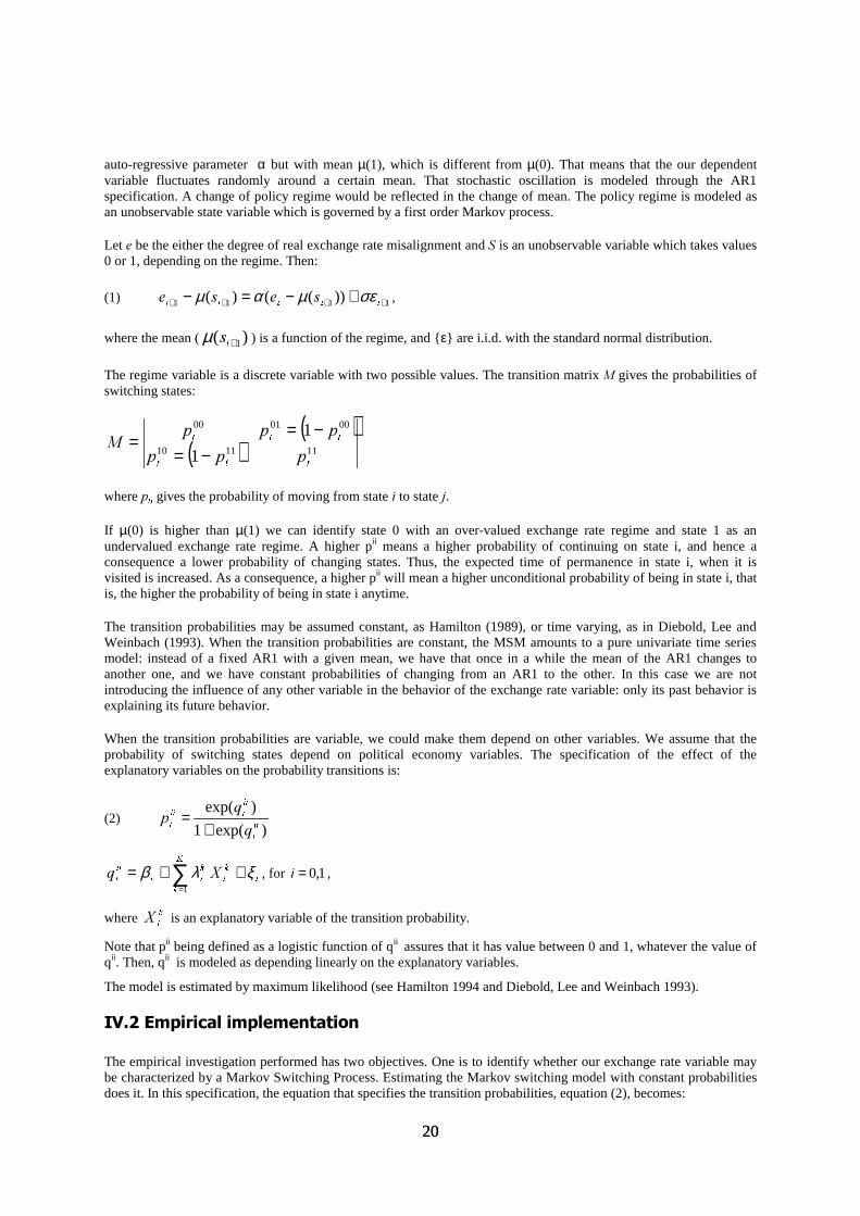
2020

auto-regressive parameter α but with mean µ(1), which is different from µ(0). That means that the our dependentvariable fluctuates randomly around a certain mean. That stochastic oscillation is modeled through the AR1specification. A change of policy regime would be reflected in the change of mean. The policy regime is modeled asan unobservable state variable which is governed by a first order Markov process.

Let H be the either the degree of real exchange rate misalignment and�6�is an unobservable variable which takes values0 or 1, depending on the regime. Then:

(1) 1111 ))(()( ++++ +−=−WWWWW

VHVH σεµαµ ,

where the mean ( µ( )VW+1 ) is a function of the regime, and {ε} are i.i.d. with the standard normal distribution.

The regime variable is a discrete variable with two possible values. The transition matrix 0 gives the probabilities ofswitching states:

( )( ) 111110

000100

1

1

WWW

WWW

SSS

SSS0

−=−=

=

where SLM�gives the probability of moving from state L to state M.

If µ(0) is higher than µ(1) we can identify state 0 with an over-valued exchange rate regime and state 1 as anundervalued exchange rate regime. A higher pii means a higher probability of continuing on state i, and hence aconsequence a lower probability of changing states. Thus, the expected time of permanence in state i, when it isvisited is increased. As a consequence, a higher pii will mean a higher unconditional probability of being in state i, thatis, the higher the probability of being in state i anytime.

The transition probabilities may be assumed constant, as Hamilton (1989), or time varying, as in Diebold, Lee andWeinbach (1993). When the transition probabilities are constant, the MSM amounts to a pure univariate time seriesmodel: instead of a fixed AR1 with a given mean, we have that once in a while the mean of the AR1 changes toanother one, and we have constant probabilities of changing from an AR1 to the other. In this case we are notintroducing the influence of any other variable in the behavior of the exchange rate variable: only its past behavior isexplaining its future behavior.

When the transition probabilities are variable, we could make them depend on other variables. We assume that theprobability of switching states depend on political economy variables. The specification of the effect of theexplanatory variables on the probability transitions is:

(2))exp(1

)exp(LL

W

LL

WLL

W T

TS

+=

W

.

N

N

L

N

LL

LL

W;T ξλβ ++= ∑

=1

, for 1,0=L ,

where N

L; is an explanatory variable of the transition probability.

Note that pii being defined as a logistic function of qii assures that it has value between 0 and 1, whatever the value ofqii. Then, qii is modeled as depending linearly on the explanatory variables.

The model is estimated by maximum likelihood (see Hamilton 1994 and Diebold, Lee and Weinbach 1993).

,9���(PSLULFDO�LPSOHPHQWDWLRQ

The empirical investigation performed has two objectives. One is to identify whether our exchange rate variable maybe characterized by a Markov Switching Process. Estimating the Markov switching model with constant probabilitiesdoes it. In this specification, the equation that specifies the transition probabilities, equation (2), becomes:

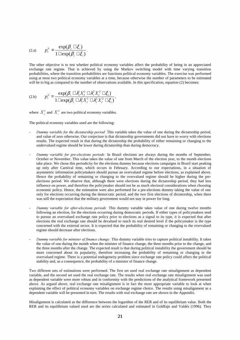
2121

(2.a))exp(1

)exp(

LL

LLLL

WS

ξβξβ++

+= .

The other objective is to test whether political economy variables affect the probability of being in an appreciatedexchange rate regime. That is achieved by using the Markov switching model with time varying transitionprobabilities, where the transition probabilities are functions political economy variables. The exercise was performedusing at most two political economy variables at a time, because otherwise the number of parameters to be estimatedwill be to big as compared to the number of observations available. In this specification, equation (2) becomes:

(2.b))exp(1

)exp(2211

2211

LWLWLL

LWLWLLLL

W ;;

;;S

ξλλβξλλβ++++

+++= ,

where 1L

; and 2L

; are two political economy variables.

The political economy variables used are the following:

- 'XPP\�YDULDEOH�IRU�WKH�GLFWDWRUVKLS�SHULRG� This variable takes the value of one during the dictatorship period,and value of zero otherwise. Our conjecture is that dictatorship governments did not have to worry with electionsresults. The expected result in that during the dictatorship the probability of either remaining or changing to theundervalued regime should be lower during dictatorship than during democracy.

- 'XPP\� YDULDEOH� IRU� SUH�HOHFWLRQV� SHULRGV� In Brazil elections are always during the months of September,October or November. This value takes the value of one from March of the election year, to the month electionstake place. We chose this periodicity for the elections dummy because elections campaigns in Brazil start peakingup only after Carnival time, which occurs in February. According to our expectations, in a situation ofasymmetric information policymakers should pursue an overvalued regime before elections, as explained above.Hence the probability of remaining or changing to the overvalued regime should be higher during the pre-elections period. We observe that, although there were elections during the dictatorship period, they had lessinfluence on power, and therefore the policymaker should not be as much electoral considerations when choosingeconomic policy. Hence, the estimation were also performed for a pre-elections dummy taking the value of oneonly for elections occurring during the democratic period, and the two first elections of dictatorship, when therewas still the expectation that the military government would not stay in power for long.

- 'XPP\� YDULDEOH� IRU� DIWHU�HOHFWLRQV� SHULRGV� This dummy variable takes value of one during twelve monthsfollowing an election, for the elections occurring during democratic periods. If either types of policymakers tendto pursue an overvalued exchange rate policy prior to elections as a signal to its type, it is expected that afterelections the real exchange rate should be devalued to reach its real desired level if the policymaker is the typeconcerned with the external sector. It is expected that the probability of remaining or changing to the overvaluedregime should decrease after elections.

- 'XPP\�YDULDEOH�IRU�PLQLVWHU�RI�ILQDQFH�FKDQJH� This dummy variable tries to capture political instability. It takesthe value of one during the month when the minister of finance change, the three months prior to the change, andthe three months after the change. The expected result is that during political instability the government should bemore concerned about its popularity, therefore increasing the probability of remaining or changing to theovervalued regime. There is a potential endogeneity problem since exchange rate policy could affect the politicalstability and, as a consequence, the probability of a minister of finance change.

Two different sets of estimations were performed. The first set used real exchange rate misalignment as dependentvariable, and the second set used the real exchange rate. The results when real exchange rate misalignment was usedas dependent variable were more robust and in conformity with the predictions of the analytical framework presentedabove. As argued above, real exchange rate misalignment is in fact the more appropriate variable to look at whenexplaining the effect of political economy variables on exchange regime choice. The results using misalignment as adependent variable will be presented in turn. The results with real exchange rate are shown in the Appendix.

Misalignment is calculated as the difference between the logarithm of the RER and of its equilibrium value. Both theRER and its equilibrium valued used are the series calculated and estimated in Goldfajn and Valdés (1996). They

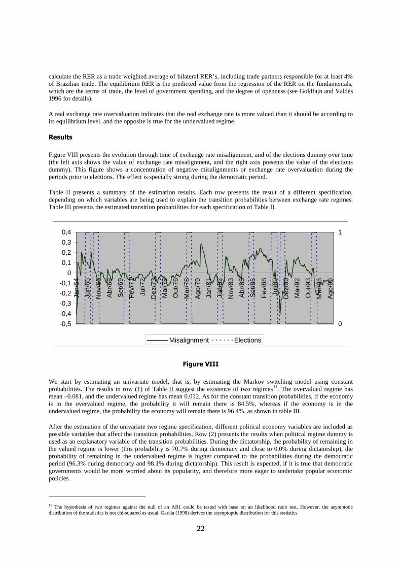
2222

calculate the RER as a trade weighted average of bilateral RER’s, including trade partners responsible for at least 4%of Brazilian trade. The equilibrium RER is the predicted value from the regression of the RER on the fundamentals,which are the terms of trade, the level of government spending, and the degree of openness (see Goldfajn and Valdés1996 for details).

A real exchange rate overvaluation indicates that the real exchange rate is more valued than it should be according toits equilibrium level, and the opposite is true for the undervalued regime.

5HVXOWV

Figure VIII presents the evolution through time of exchange rate misalignment, and of the elections dummy over time(the left axis shows the value of exchange rate misalignment, and the right axis presents the value of the electionsdummy). This figure shows a concentration of negative misalignments or exchange rate overvaluation during theperiods prior to elections. The effect is specially strong during the democratic period.

Table II presents a summary of the estimation results. Each row presents the result of a different specification,depending on which variables are being used to explain the transition probabilities between exchange rate regimes.Table III presents the estimated transition probabilities for each specification of Table II.

-0,5

-0,4

-0,3

-0,2

-0,1

0

0,1

0,2

0,3

0,4

Jan/

64

Jun/

65

Nov

/66

Abr

/68

Set

/69

Fev

/71

Jul/7

2

Dez

/73

Mai

/75

Out

/76

Mar

/78

Ago

/79

Jan/

81

Jun/

82

Nov

/83

Abr

/85

Set

/86

Fev

/88

Jul/8

9

Dez

/90

Mai

/92

Out

/93

Mar

/95

Ago

/96

0

1

Misalignment Elections

)LJXUH�9,,,

We start by estimating an univariate model, that is, by estimating the Markov switching model using constantprobabilities. The results in row (1) of Table II suggest the existence of two regimes11. The overvalued regime hasmean –0.081, and the undervalued regime has mean 0.012. As for the constant transition probabilities, if the economyis in the overvalued regime, the probability it will remain there is 84.5%, whereas if the economy is in theundervalued regime, the probability the economy will remain there is 96.4%, as shown in table III.

After the estimation of the univariate two regime specification, different political economy variables are included aspossible variables that affect the transition probabilities. Row (2) presents the results when political regime dummy isused as an explanatory variable of the transition probabilities. During the dictatorship, the probability of remaining inthe valued regime is lower (this probability is 70.7% during democracy and close to 0.0% during dictatorship), theprobability of remaining in the undervalued regime is higher compared to the probabilities during the democraticperiod (96.3% during democracy and 98.1% during dictatorship). This result is expected, if it is true that democraticgovernments would be more worried about its popularity, and therefore more eager to undertake popular economicpolicies.

11 The hypothesis of two regimes against the null of an AR1 could be tested with base on an likelihood ratio test. However, the asymptoticdistribution of the statistics is not chi-squared as usual. Garcia (1998) derives the asymptoptic distribution for this statistics.

2323

The second set of political economy variables used to explain the transition probabilities are the pre-electiondummies, and the results are in rows (3), (4), and (5) in Table II. Rows (3) and (4) present the results when a dummyvariable for pre-elections period is used as possible explanatory variable of the transition probabilities. In row (3), thepre-elections dummy has value of one during the period previous to all elections occurred from 1964 to 1996, whereasin row (4) the pre-elections dummy has value of one only during democracy and the first two elections of the militarydictatorship (when the dictatorship was believed to be transitory). Both the pre-election and the pre-election duringdemocracy dummies have the same qualitative impact over the transition probabilities: the proximity of electionsincreases the probability of remaining in the overvalued regime, and decreases the probability of the economyremaining in the depreciated regime. However, both results are not statistically significative. On the other hand, thereis a significative negative impact of the pre-elections dummy on the probability of the economy remaining in theundervalued regime, if the economy is there. This means that the probability of changing from the undervalued regimeto the valued one is higher before elections.

Comparing rows (3) and (4), Table III, the negative impact of pre-elections is larger when only pre-elections duringdemocratic periods are taken into account: for the pre-elections dummy the probability of the economy remaining inthe undervalued regime changes from 98% in normal times to 90.1% during pre-elections periods, whereas for thepre-election during democracy dummy the probability changes from 97.8% during normal times to 83% during pre-election periods.

The difference between the impact of pre-election during democracy and during dictatorship is made clear inestimation (5), which uses both a pre-election during democracy dummy and pre-election during dictatorship dummy.All coefficients have the expected sign, but only the coefficient of the pre-elections during democracy dummy for theundervalued regime is significative (Table II). The probability of the economy remaining in the undervalued regimewhen it is there in normal times is 98%. In pre-elections during dictatorship the probability changes to 96.5%, whereasin pre-elections periods during democracy this probability changes to 82.9% (Table III). In summary, during pre-election periods the probability of the economy remaining in the undervalued regime decreases, and the effect is largerduring democratic periods than during dictatorship periods. These results are in conformity with the expectation thatprevious to elections the policymaker would be more willing to undertake popular measures, such as an exchange rateover-valuation policy.

If during pre-elections periods there is a higher probability of the exchange rate regime moving to a valued one, oneshould expect that in after-election periods the opposite is true, in order to reestablish equilibrium in the economy. Theestimation using after-election dummy, presented in Table III row (6), yields exactly the expected result: afterelection, the probability the economy will remain in the valued regime if it is already there decreases (from 49.6% to0.2%), and the probability it will remain in the undervalued regime increases (from 98.4% to value close to 100%).Furthermore, all coefficients are statistically significative (Table III).

Row (7) combines the political regime and the pre-elections during democracy dummies. All coefficients estimatedhave high t-statistic, and the sign are in conformity with our expectations. The probability of remaining in the over-valued regime is smaller during dictatorship and larger during pre-elections periods (increases from a value close to 0to 42.6%). The probability of remaining in the undervalued regime is larger during dictatorship period and smallerduring pre-elections periods (Table III).

The next specification uses the political regime and the after-elections dummies as explanatory variables for thetransition probabilities. As shown in Table II row (8), the political regime dummy has a negative impact on theprobability of remaining in the over-valued regime (during democracy the probability is 42.1% and duringdictatorship it is close to 0), and a negative impact on the probability of remaining in the undervalued regime (theprobabilities are 98.0% and 98.3% for the democratic and dictatorial periods, respectively). The after-electionsdummy has a negative impact on both probabilities. However, in absolute value, the coefficient of this variable ismuch larger for the probability of remaining in the over-valued regime, and the t-statistics for the coefficient of theprobability of remaining in the undervalued regime is very low (-0.25). Hence, the results indicates that after-electionsdummy has a significative negative impact only on the probability of the economy remaining on the over-valuedregime once it is there (probability changes from 42.1% in normal times to 12.8% after elections).

Finally, as the results in row (9) show, the minister of finance change dummy has a positive impact on the probabilityof the economy remaining in the over-valued regime, and a negative impact on the probability of remaining in theundervalued regime, although the t-statistics for this latter impact is very low (-0.22). The probability of remaining inover-valued regime is 91.5% during normal times, and it increases to a value close to 100% during minister changeperiods. On the other hand, the probability of remaining in the undervalued regime decreases from 98.4% in normal

2424

times to 97.9% during minister change periods. These results are in conformity with the expectation that duringpolitically turbulent time the government is more willing to undertake more popular measures.

In summary, we found that the dictatorship favored an undervalued currency. We identified a misalignment cyclearound elections: an overvalued currency is more likely before elections, while there is a higher probability ofchanging from a overvalued to a devalued currency immediately after elections. The election cycle showed to bestronger during the democratic period than during the dictatorial period. We also detected a political instability effecton the exchange rate: an overvalued exchange rate is more likely when there is a finance minister change.

9��&RQFOXVLRQThis paper studied exchange rate policy in Brazil, from a political economy perspective. The method of analysis wasthe following. First exchange rate policy was studied from a historical perspective, identifying the political economicfactors that influenced the exchange rate policy choice in Brazil from 1964 to 1997. Next, an analytical frameworkwas construct to try and encompass the main forces at work as identified in the historical analysis. Finally, aquantitative assessment of the analytical framework was performed, using Brazilian data for the period studied.

Exchange rate policy in Brazil has been a crawling peg throughout the period studied, except for two short periods.The policy choice has basically been the administration of the crawling peg, which could lead to real exchange rateappreciation or depreciation. The historical appraisal showed that throughout the period studied the main forcesguiding this exchange rate policy choice were the result from a trade off between inflation and balance of payments.Exchange rate policy that results in a real exchange rate appreciation helps reducing inflation, but deteriorates thebalance of payments, and the reverse is true for a real exchange rate depreciation. It was also identified that these twoeffects of exchange rate policy do not have a symmetric effect on the different members of society: inflation reductionbenefits a large number of dispersed agents, whereas balance of payments improvement benefits a more concentratedgroup of exporters and import competing domestic industries.

The analytical framework posited that policymakers policy choice depends on the relative weight she places on thebalance of payments as opposed to inflation reduction. In particular, policymakers in need of popular support wouldplace a relatively higher weight on inflation reduction. Hence, democratic governments should place more weight oninflation reduction, as opposed to dictatorial governments. An elections cycle could also be generated if policymakersdiffered on the relative weights they place on their policy objectives, and the public could not observe thepolicymakers preferences, but only their policy choices.

The analytical framework predictions were tested empirically. A Markov switching model with varying transitionprobabilities was used to characterize the exchange rate regimes, and the influence of political economy variable onthem. Two alternative dependent variables were considered: the real exchange rate evolution, and real exchange ratemisalignment with respect to its equilibrium level. We argue that real exchange rate misalignment is a moreappropriate measure for the exercise we perform. In trying to identify SROLWLFDO�HFRQRP\ factors that affect exchangerate policy we do not want to capture the effects of other exogenous purely economic variables. The misalignmentmeasure controls for the effects of the economic variables, and the political economy variables should explain theremaining variations. In fact, the empirical evaluation is more robust and in conformity with the predictions of theanalytical framework when exchange rate misalignment is being studied, instead of the real exchange rate itself.

The main predictions of the analytical framework were captured in the empirical exercise. We found the duringthe dictatorship period the probability of the economy remaining in the undervalued regime was larger thanduring the democratic period, and the reverse is true for the probability of remaining in the over-valued regime.The elections cycle was also identified: the probability of having an appreciated exchange rate is higher in themonths preceding elections while the probability of having a depreciated exchange rate is higher in the monthssucceeding elections. Moreover, the elections cycle showed to be stronger during the democratic period, thanduring the dictatorial period.

VI. ReferencesAlesina, Alberto (1987), “Macroeconomic Policy in a Two-Party System as a Repeated Game,” 4XDUWHUO\�-RXUQDO�RI

(FRQRPLFV 102: 651-78.

Baumgarten, Mônica (1996), 0RGHORV�GH�7D[D�GH�&kPELR�5HDO�GH�(TXLOtEULR��XPD�$SOLFDomR�SDUD�R�%UDVLO, M.A.Thesis, PUC-Rio.

Bollen, N., S. Gray and R. Whaley (1998), “Regime Switching in Foreign Exchange Rates: Evidence from CurrencyOption Prices,” forthcoming -RXUQDO�RI�(FRQRPHWULFV.

2525

Bonomo, Marco (1986), &RQWUROH�GH�&UpGLWR�H�3ROtWLFD�0RQHWiULD�HP�����, M.A. thesis, PUC-Rio.

Bonomo, Marco (1997a), “A Volta da Curva de Phillips e a Âncora do Real”, Nota Técnica, Macrométrica.

Bonomo, Marco (1997b), La Economia Brasileña e el Plano Real, in %UDVLO� � LQ� 6tQWHVLV, Fundación Centro deEstudos Brasileiros, Buenos Aires.

Bonomo, Marco and Cristina Terra (1998), “Election and Exchange Rate Cycles”, mimeo, PUC-Rio and EPGE-Getulio Vargas Foundation.

Bruno, Michael (1989), “Israel’s Crisis and Economic Reform: A Historical Perspective”, NBER Working Paper n.3075.

Carneiro, Dionísio (1990), “Crise e Esperança:1974-80,” in Marcelo Abreu (ed.), $�2UGHP�GR�3URJUHVVR, Rio deJaneiro: Editora Campus.

Carneiro, Dionísio e Eduardo Modiano (1990), “Ajuste Externo e Desequilíbrio Interno,” in Marcelo Abreu (ed.), $2UGHP�GR�3URJUHVVR, Rio de Janeiro: Editora Campus.

Dib, Maria de Fátima (1985), ,PSRUWDo}HV�%UDVLOHLUDV��3ROtWLFDV�GH�&RQWUROH�H�'HWHUPLQDQWHV�GD�'HPDQGD, Riode Janeiro, BNDES.

Diebold, F.X., J.H. Lee, and G.C. Weinbach (1993), “Regime-Switching with time-varying transition probabilities”,in C. Hargreaves, 1RQVWDWLRQDU\�7LPH�6HULHV�DQG�&RLQWHJUDWLRQ, Oxford University Press.

Frieden, Jeffry, Ernesto Stein, and Piero Ghezzi (1998), “The Political Economy of Exchange Rate Policy in LatinAmerica”, mimeo, IDB, Johns Hopkins University and Harvard University.

Garcia, René (1998), "Asymptotic Null of the Likelihood Ratio Test in Markov Switching Models," -RXUQDO� RI,QWHUQDWLRQDO�(FRQRPLFV 39:763-788

Goldenstein, Lídia (1985), 'D� +HWHURGR[LD� DR� )0,� �� D� SROtWLFD� HFRQ{PLFD� GH� ����� D� ����, M.A. Thesis,UNICAMP.

Goldfajn, Ilan, and Rodrigo Valdés (1996), “The Aftermath of Appreciations”, NBER Working Paper 5650.

Hamilton, James (1989), "A New Approach to the Economic Analysis of Nonstationary Time Series and the BusinessCycle," (FRQRPHWULFD 57:357-384.

Hamilton, J. (1994), 7LPH�6HULHV�$QDO\VLV, Princeton University Press.

Heymann, Daniel (1991), “From Sharp Disinflation to Hyperinflation, Twice: The Argentine Experience, 1985-1989”,in M. Bruno, S.Fischer, E.Helpman and N.Liviatan, with L.Meridor (eds), /HVVRQV� RI� (FRQRPLF6WDELOL]DWLRQ�DQG�LWV�$IWHUPDWK, The MIT Press.

Kaminsky, Graciela (1993), “Is There a Peso Problem? Evidence from Dollar/Pound Exchange Rate: 1976-1987,”American Economic Review 83: 450-472.

Modiano, Eduardo (1990), “A Ópera dos Três Cruzados,” in Marcelo Abreu (ed.), $�2UGHP�GR�3URJUHVVR, Rio deJaneiro: Editora Campus.

Persson, Torsten and Guido Tabellini (1990), 0DFURHFRQRPLF�3ROLF\��&UHGLELOLW\�DQG�3ROLWLFV, Harwood AcademicPublishers.

Rogoff, Kenneth (1990), “Equilibrium Political Budget Cycles,” $PHULFDQ�(FRQRPLF�5HYLHZ 80: 21-36.

Rogoff, Kenneth and Anne Sibert (1988), “Elections and Macroeconomic Policy Cycles,” 5HYLHZ� RI� (FRQRPLF6WXGLHV LV: 1-16.

Skidmore, Thomas (1998), 'H�&DVWHOR�D�7DQFUHGR, ed. Paz e Terra.

Simonsen, Mário Henrique (1995), “Inflação e Política Cambial”, in ���$QRV�GH� ,QGH[DomR, Editora da FundaçãoGetulio Vargas.

Stein, Ernesto and Jorge Streb (1997), “Elections and the Timing of Devaluations”, mimeo, IDB and CEMA.

Svensson, Lars (1993), “An Interpretation of Recent research on exchange rate target zones”, in L.Leiderman andA.Razin (eds.) &DSLWDO�0RELOLW\�� 7KH� ,PSDFW� RQ� &RQVXPSWLRQ�� ,QYHVWPHQW� DQG� *URZWK, CambridgeUniversity Press.

2626

Terra, Maria Cristina T. (1998), “Openness and inflation: a new assessment”, 7KH�4XDUWHUO\�-RXUQDO�RI�(FRQRPLFV113: pages?.

Terra, Maria Cristina T. (1997), “Debt crisis and inflation”, 5HYLVWD�GH�(FRQRPHWULD, forthcoming.

Williamson, John (1994) (VWLPDWLQJ� (TXLOLEULXP� ([FKDQJH� 5DWHV, Institute forInternational Economics.

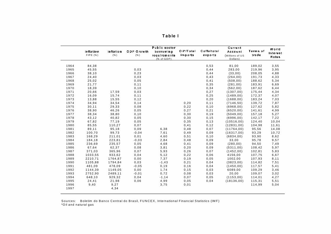
���������7 DE OH �,

,Q IOD WLR Q �����F IP E (% )

,Q IOD WLR Q ���(% )

*'3 �* URZ WK ��(% )

3XE OLF �VHF WR U�

E R UURZ LQJ �

UHTX LUHP HQ WV �(% o f G D P )

2 LO �7 R WD O�

LP SR UWV

& R IIH �WR WD O�

H[SR UWV

& X UUHQ W�

$FFRXQ W�����

(M illion s o f U S D o lla rs )

7HUP V �R I�

WUDGH

: R UOG �

,Q WH UHVW�

5 D WHV

1 96 4 8 4 ,3 8 0 ,5 3 8 1 ,00 1 8 9 ,02 3 ,5 51 96 5 4 5 ,5 5 0 ,03 0 ,4 4 2 8 3 ,0 0 2 1 9 ,96 3 ,9 51 96 6 3 8 ,1 0 0 ,23 0 ,4 4 (33 ,0 0) 2 0 8 ,05 4 ,8 81 96 7 2 4 ,4 0 0 ,03 0 ,4 3 (26 4 ,00 ) 1 9 1 ,73 4 ,3 31 96 8 2 5 ,0 2 0 ,05 0 ,4 1 (50 8 ,00 ) 1 8 8 ,62 5 ,3 41 96 9 2 1 ,7 7 0 ,11 0 ,3 5 (28 1 ,00 ) 1 8 3 ,91 6 ,6 91 97 0 1 8 ,3 9 0 ,10 0 ,3 4 (56 2 ,00 ) 1 8 7 ,62 6 ,4 41 97 1 2 0 ,6 6 17 ,59 0 ,03 0 ,2 7 (1 30 7 ,00 ) 1 7 5 ,44 4 ,3 41 97 2 1 6 ,0 9 15 ,74 0 ,11 0 ,2 5 (1 48 9 ,00 ) 1 7 2 ,37 4 ,0 71 97 3 1 3 ,8 8 15 ,55 0 ,12 0 ,2 0 (1 68 8 ,00 ) 1 8 3 ,24 7 ,0 31 97 4 3 4 ,9 4 34 ,54 0 ,14 0 ,20 0 ,1 1 (7 14 6 ,50 ) 1 3 9 ,72 7 ,8 71 97 5 3 0 ,1 1 29 ,33 0 ,08 0 ,22 0 ,1 0 (6 96 8 ,00 ) 1 2 7 ,62 5 ,8 21 97 6 3 8 ,9 0 46 ,26 0 ,05 0 ,27 0 ,2 1 (6 52 0 ,00 ) 1 4 1 ,61 4 ,9 91 97 7 3 8 ,3 4 38 ,80 0 ,10 0 ,30 0 ,1 9 (5 04 9 ,00 ) 1 5 7 ,18 5 ,2 71 97 8 4 3 ,1 2 40 ,82 0 ,05 0 ,30 0 ,1 5 (6 99 6 ,00 ) 1 4 2 ,17 7 ,2 21 97 9 6 7 ,8 2 77 ,19 0 ,05 0 ,35 0 ,1 3 (1 05 1 6 ,0 0 ) 1 2 4 ,40 10 ,0 41 98 0 8 5 ,5 5 110 ,27 0 ,07 0 ,41 0 ,1 2 (1 28 3 1 ,0 0 ) 1 0 4 ,98 11 ,6 11 98 1 8 9 ,1 1 95 ,18 0 ,09 6 ,38 0 ,48 0 ,0 7 (1 17 6 4 ,0 0 ) 9 5 ,56 14 ,0 81 98 2 1 0 0,7 0 99 ,73 -0 ,04 7 ,61 0 ,49 0 ,0 9 (1 63 1 7 ,0 0 ) 9 3 ,29 10 ,7 21 98 3 1 6 8,2 9 211 ,01 0 ,01 4 ,60 0 ,51 0 ,1 0 (6 83 4 ,00 ) 9 3 ,90 8 ,6 21 98 4 1 8 4,1 8 223 ,81 -0 ,03 2 ,84 0 ,48 0 ,0 9 3 3 ,00 9 5 ,78 9 ,5 71 98 5 2 3 6,6 9 235 ,57 0 ,05 4 ,68 0 ,41 0 ,0 9 (28 0 ,00 ) 9 4 ,50 7 ,4 91 98 6 6 7 ,6 4 62 ,37 0 ,08 3 ,81 0 ,20 0 ,0 9 (5 31 1 ,00 ) 1 0 8 ,42 5 ,9 71 98 7 3 7 1,0 3 365 ,96 0 ,07 5 ,93 0 ,26 0 ,0 7 (1 45 2 ,00 ) 1 0 2 ,81 5 ,8 31 98 8 1 0 3 3,5 5 933 ,62 0 ,04 5 ,12 0 ,22 0 ,0 6 4 1 5 6,0 0 1 0 7 ,75 6 ,6 71 98 9 2 2 1 0,7 1 1764,87 0 ,00 7 ,37 0 ,19 0 ,0 5 1 0 0 2,0 0 1 0 7 ,93 8 ,1 11 99 0 1 1 0 5,8 8 1794,84 0 ,03 -1 ,43 0 ,21 0 ,0 4 (3 82 3 ,00 ) 1 1 4 ,82 7 ,5 11 99 1 4 8 1,0 9 478 ,09 -0 ,05 0 ,19 0 ,16 0 ,0 4 (1 45 0 ,00 ) 1 1 7 ,57 5 ,4 11 99 2 1 1 4 4,3 9 1149,05 0 ,00 1 ,74 0 ,15 0 ,0 3 6 0 8 9,0 0 1 0 9 ,29 3 ,4 61 99 3 2 7 5 2,9 0 2489,11 -0 ,01 0 ,72 0 ,08 0 ,0 3 2 0 ,00 1 0 9 ,07 3 ,0 21 99 4 6 4 8,1 0 929 ,32 0 ,04 -1 ,14 0 ,07 0 ,0 5 (1 15 3 ,00 ) 1 1 4 ,01 4 ,2 71 99 5 2 4 ,4 1 21 ,98 0 ,06 4 ,99 0 ,05 0 ,0 4 (1 81 3 6 ,0 0 ) 1 1 5 ,31 5 ,5 11 99 6 9 ,40 9 ,27 3 ,75 0 ,01 1 1 4 ,99 5 ,0 41 99 7 4 ,34

S o u rce s : B o le tim d o B anco C en tra l do B ras il, F U N C E X , In te rna tiona l F inanc ia l S ta tis tics (IM F )*O il a n d n a tu ra l ga s

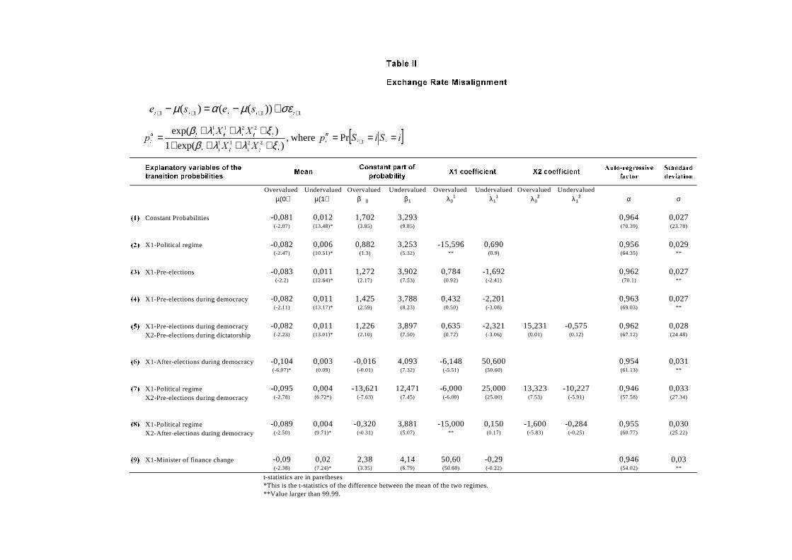
7DEOH�,,

([FKDQJH�5DWH�0LVDOLJQPHQW

([SODQDWRU\�YDULDEOHV�RI�WKH�

WUDQVLWLRQ�SUREDELOLWLHV$XWR�UHJUHVVLYH�

IDFWRU

6WDQGDUG�

GHYLDWLRQ

Overvalued Undervalued Overvalued Undervalued Overvalued Undervalued Overvalued Undervaluedµ(0) µ(1) β0 β1 λ0

1 λ11 λ0

2 λ12 α σ

��� Constant Probabilities -0,081 0,012 1,702 3,293 0,964 0,027(-2.07) (13.48)* (3.85) (9.85) (70.39) (23.78)

��� X1-Political regime -0,082 0,006 0,882 3,253 -15,596 0,690 0,956 0,029(-2.47) (10.51)* (1.3) (5.32) ** (0.9) (64.35) **

��� X1-Pre-elections -0,083 0,011 1,272 3,902 0,784 -1,692 0,962 0,027(-2.2) (12.64)* (2.17) (7.53) (0.92) (-2.41) (70.1) **

��� X1-Pre-elections during democracy -0,082 0,011 1,425 3,788 0,432 -2,201 0,963 0,027(-2.11) (13.17)* (2.59) (8.23) (0.50) (-3.08) (69.03) **

��� X1-Pre-elections during democracy -0,082 0,011 1,226 3,897 0,635 -2,321 15,231 -0,575 0,962 0,028X2-Pre-elections during dictatorship (-2.23) (13.01)* (2.10) (7.50) (0.72) (-3.06) (0.01) (0.12) (67.12) (24.48)

��� X1-After-elections during democracy -0,104 0,003 -0,016 4,093 -6,148 50,600 0,954 0,031(-6.07)* (0.09) (-0.01) (7.32) (-5.51) (50.60) (61.13) **

��� X1-Political regime -0,095 0,004 -13,621 12,471 -6,000 25,000 13,323 -10,227 0,946 0,033X2-Pre-elections during democracy (-2.78) (6.72*) (-7.63) (7.45) (-6.00) (25.00) (7.53) (-5.91) (57.58) (27.34)

��� X1-Political regime -0,089 0,004 -0,320 3,881 -15,000 0,150 -1,600 -0,284 0,955 0,030X2-After-elections during democracy (-2.50) (9.71)* (-0.31) (5.07) ** (0.17) (-5.83) (-0.25) (60.77) (25.22)

��� X1-Minister of finance change -0,09 0,02 2,38 4,14 50,60 -0,29 0,946 0,03(-2.38) (7.24)* (3.35) (6.79) (50.60) (-0.22) (54.02) **

t-statistics are in paretheses*This is the t-statistics of the difference between the mean of the two regimes.**Value larger than 99.99.

0HDQ&RQVWDQW�SDUW�RI�

SUREDELOLW\;��FRHIILFLHQW ;��FRHIILFLHQW

1111 ))(()( ++++ +−=−WWWWW

VHVH σεµαµ

[ ]L6L6S;;

;;S

WW

LL

W

LWLWLL

LWLWLLLL

W===

+++++++

= +12211

2211

Pr where,)exp(1

)exp(

ξλλβξλλβ

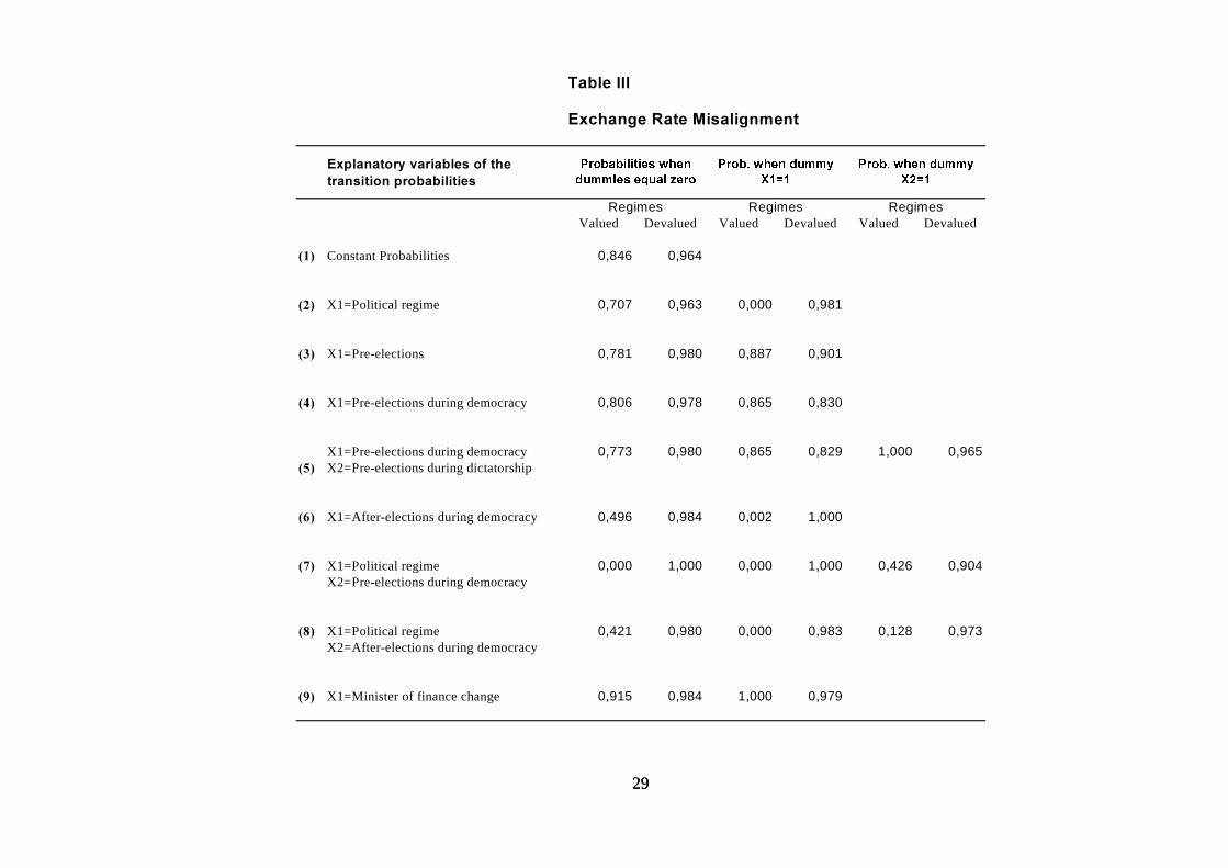
2929

7DEOH�,,,

([FKDQJH�5DWH�0LVDOLJQPHQW

([SODQDWRU\�YDULDEOHV�RI�WKH�WUDQVLWLRQ�SUREDELOLWLHV

Valued Devalued Valued Devalued Valued Devalued

��� Constant Probabilities 0,846 0,964

��� X1=Political regime 0,707 0,963 0,000 0,981

��� X1=Pre-elections 0,781 0,980 0,887 0,901

��� X1=Pre-elections during democracy 0,806 0,978 0,865 0,830

X1=Pre-elections during democracy 0,773 0,980 0,865 0,829 1,000 0,965��� X2=Pre-elections during dictatorship

��� X1=After-elections during democracy 0,496 0,984 0,002 1,000

��� X1=Political regime 0,000 1,000 0,000 1,000 0,426 0,904X2=Pre-elections during democracy

��� X1=Political regime 0,421 0,980 0,000 0,983 0,128 0,973X2=After-elections during democracy

��� X1=Minister of finance change 0,915 0,984 1,000 0,979

3UREDELOLWLHV�ZKHQ�

GXPPLHV�HTXDO�]HUR

3URE��ZKHQ�GXPP\�

;� �

3URE��ZKHQ�GXPP\�

;� �

Regimes Regimes Regimes

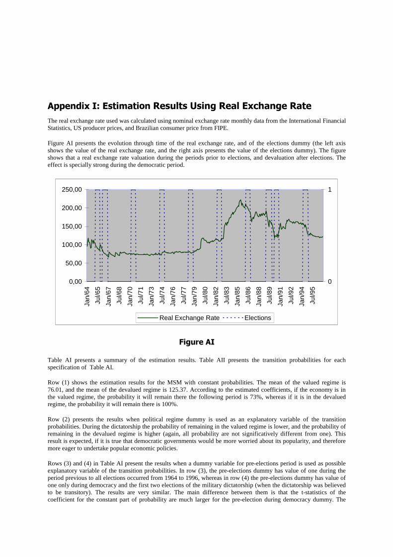
$SSHQGL[�,��(VWLPDWLRQ�5HVXOWV�8VLQJ�5HDO�([FKDQJH�5DWHThe real exchange rate used was calculated using nominal exchange rate monthly data from the International FinancialStatistics, US producer prices, and Brazilian consumer price from FIPE.

Figure AI presents the evolution through time of the real exchange rate, and of the elections dummy (the left axisshows the value of the real exchange rate, and the right axis presents the value of the elections dummy). The figureshows that a real exchange rate valuation during the periods prior to elections, and devaluation after elections. Theeffect is specially strong during the democratic period.

0,00

50,00

100,00

150,00

200,00

250,00

Jan/

64

Jul/6

5

Jan/

67

Jul/6

8

Jan/

70

Jul/7

1

Jan/

73

Jul/7

4

Jan/

76

Jul/7

7

Jan/

79

Jul/8

0

Jan/

82

Jul/8

3

Jan/

85

Jul/8

6

Jan/

88

Jul/8

9

Jan/

91

Jul/9

2

Jan/

94

Jul/9

5

0

1

Real Exchange Rate Elections

)LJXUH�$,

Table AI presents a summary of the estimation results. Table AII presents the transition probabilities for eachspecification of Table AI.

Row (1) shows the estimation results for the MSM with constant probabilities. The mean of the valued regime is76.01, and the mean of the devalued regime is 125.37. According to the estimated coefficients, if the economy is inthe valued regime, the probability it will remain there the following period is 73%, whereas if it is in the devaluedregime, the probability it will remain there is 100%.

Row (2) presents the results when political regime dummy is used as an explanatory variable of the transitionprobabilities. During the dictatorship the probability of remaining in the valued regime is lower, and the probability ofremaining in the devalued regime is higher (again, all probability are not significatively different from one). Thisresult is expected, if it is true that democratic governments would be more worried about its popularity, and thereforemore eager to undertake popular economic policies.

Rows (3) and (4) in Table AI present the results when a dummy variable for pre-elections period is used as possibleexplanatory variable of the transition probabilities. In row (3), the pre-elections dummy has value of one during theperiod previous to all elections occurred from 1964 to 1996, whereas in row (4) the pre-elections dummy has value ofone only during democracy and the first two elections of the military dictatorship (when the dictatorship was believedto be transitory). The results are very similar. The main difference between them is that the t-statistics of thecoefficient for the constant part of probability are much larger for the pre-election during democracy dummy. The

3131

dummy variables have a negative effect on the probability of the valued regime, and a positive effect on theprobability of the devalued regime. This means that if the economy is in the valued regime, the probability ofremaining there decreases during the periods previous to elections (from 0.9997 to 0.9871 for row (3), and from0.9998 to 0.9835 for row (4)), and the probability of changing to the devalued regime increases before elections (from0.0003 to 0.0129 for row (3) specification, and from 0.0002 to 0.0165 for row (4) specification). On the other hand, ifthe economy is in the devalued regime, the probability of remaining in that regime increases before elections(although it is not significatively different from 1.00 in both cases), whereas the probability of moving to the valuedregime increases (again, approximately 0.00 in both cases).

Row (5) presents the results for the specification which uses the pre-elections dummy under democracy, and a pre-elections during dictatorship dummy, which takes value 1 before the election not counted in the pre-elections duringdemocracy dummy. The results indicate a positive effect of both pre-elections dummy on the probability of remainingin either current regime, although the probability of remaining in the valued regime is never significatively differentfrom zero, and the probability of remaining in the devalued regime is never significatively different from one.

These results are not in conformity with a reasonable political economy explanation for exchange rate regime choice.Before elections, the policymaker would prefer to undertake more popular economic policies, and a valued exchangerate regime is one of them. We should then expect a positive effect of the pre-elections dummy on the probability ofremaining in the valued regime, and a negative effect on the probability of remaining in the devalued regime.

The next political economy variable used was an after-elections dummy. According to the result presented in row (6),if the economy is in the valued regime, the probability of remaining there decreases after elections, whereas if theeconomy is in the devalued regime, the probability of remaining there increases after elections (although allprobability are not significatively different from one, as shown in Table AII).

This result is the expected one: given the conjecture that before elections policymakers have a tendency to pursue amore valued exchange rate regime, after election the reverse must be true in order to make up for the disequilibriumgenerated by the pre-election exchange rate valuation policy.

In row (7) the political regime and the pre-elections during democracy dummies are used at the same time to explainthe transition probabilities. The effect of the political regime dummy is the same as in the previous estimation, and thepre-elections during democracy dummy affects positively both transition probabilities.

In row (8) the political regime and the after-elections dummies are used to explain the transition probabilities. Theeffect is the same as when they are used in turn, and in conformity with the prediction of our analytical framework. Inthis estimation, the probability of remaining in the valued regime is never significatively different from zero, and theprobability of remaining in the devalued regime is never significatively different from one.

Finally, row (9) presents the results when a dummy for minister of finance change is used. This variable affectspositively both transition probabilities, although the probability of remaining in the valued regime is neversignificatively different from zero, and the probability of remaining in the devalued regime is never significativelydifferent from one.

Summing up, only two of the various political economy variables used to explain the time series behavior of theexchange rate are totally in conformity to the predictions of our analytical framework. They are the after elections andthe political regime dummies.

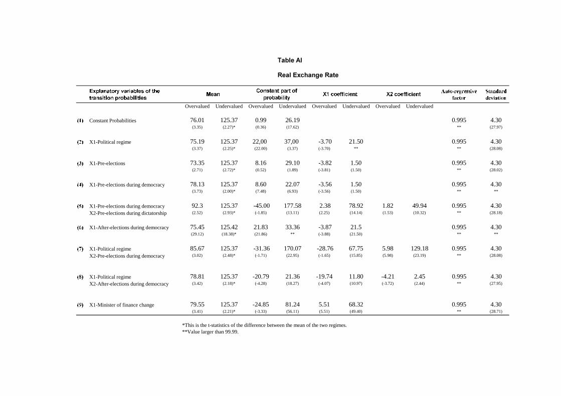
7DEOH�$,

5HDO�([FKDQJH�5DWH

([SODQDWRU\�YDULDEOHV�RI�WKH�

WUDQVLWLRQ�SUREDELOLWLHV

$XWR�UHJUHVVLYH�

IDFWRU

6WDQGDUG�

GHYLDWLRQ

Overvalued Undervalued Overvalued Undervalued Overvalued Undervalued Overvalued Undervalued

��� Constant Probabilities 76.01 125.37 0.99 26.19 0.995 4.30(3.35) (2.27)* (0.36) (17.62) ** (27.97)

��� X1-Political regime 75.19 125.37 22,00 37,00 -3.70 21.50 0.995 4.30(3.37) (2.25)* (22.00) (3.37) (-3.70) ** ** (28.08)

��� X1-Pre-elections 73.35 125.37 8.16 29.10 -3.82 1.50 0.995 4.30(2.71) (2.72)* (0.52) (1.89) (-3.81) (1.50) ** (28.02)

��� X1-Pre-elections during democracy 78.13 125.37 8.60 22.07 -3.56 1.50 0.995 4.30(3.73) (2.00)* (7.48) (6.93) (-3.56) (1.50) ** **

��� X1-Pre-elections during democracy 92.3 125.37 -45.00 177.58 2.38 78.92 1.82 49.94 0.995 4.30X2-Pre-elections during dictatorship (2.52) (2.93)* (-1.85) (13.11) (2.25) (14.14) (1.53) (10.32) ** (28.18)

��� X1-After-elections during democracy 75.45 125.42 21.83 33.36 -3.87 21.5 0.995 4.30(29.12) (18.38)* (21.86) ** (-3.88) (21.50) ** **

��� X1-Political regime 85.67 125.37 -31.36 170.07 -28.76 67.75 5.98 129.18 0.995 4.30X2-Pre-elections during democracy (3.02) (2.48)* (-1.71) (22.95) (-1.65) (15.85) (5.98) (23.19) ** (28.08)

��� X1-Political regime 78.81 125.37 -20.79 21.36 -19.74 11.80 -4.21 2.45 0.995 4.30X2-After-elections during democracy (3.42) (2.18)* (-4.28) (18.27) (-4.07) (10.97) (-3.72) (2.44) ** (27.95)

��� X1-Minister of finance change 79.55 125.37 -24.85 81.24 5.51 68.32 0.995 4.30(3.41) (2.21)* (-3.33) (56.11) (5.51) (49.40) ** (28.71)

*This is the t-statistics of the difference between the mean of the two regimes.**Value larger than 99.99.

0HDQ&RQVWDQW�SDUW�RI�

SUREDELOLW\;��FRHIILFLHQW ;��FRHIILFLHQW

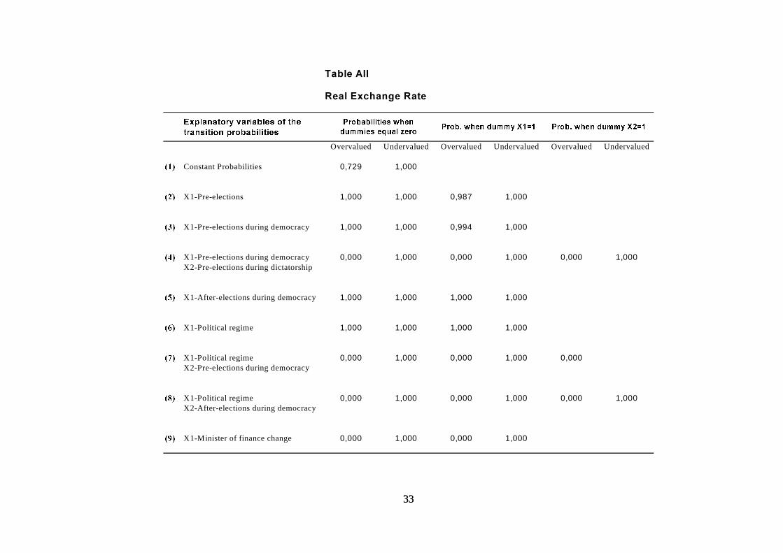
3333

7DEOH�$,,

5HDO�([FKDQJH�5DWH�

([SODQDWRU\�YDULDEOHV�RI�WKH�

WUDQVLWLRQ�SUREDELOLWLHV

Overvalued Undervalued Overvalued Undervalued Overvalued Undervalued

��� Constant Probabilities 0,729 1,000

��� X1-Pre-elections 1,000 1,000 0,987 1,000

��� X1-Pre-elections during democracy 1,000 1,000 0,994 1,000

��� X1-Pre-elections during democracy 0,000 1,000 0,000 1,000 0,000 1,000X2-Pre-elections during dictatorship

��� X1-After-elections during democracy 1,000 1,000 1,000 1,000

��� X1-Political regime 1,000 1,000 1,000 1,000

��� X1-Political regime 0,000 1,000 0,000 1,000 0,000X2-Pre-elections during democracy

��� X1-Political regime 0,000 1,000 0,000 1,000 0,000 1,000X2-After-elections during democracy

��� X1-Minister of finance change 0,000 1,000 0,000 1,000

3UREDELOLWLHV�ZKHQ�

GXPPLHV�HTXDO�]HUR3URE��ZKHQ�GXPP\�;� � 3URE��ZKHQ�GXPP\�;� �

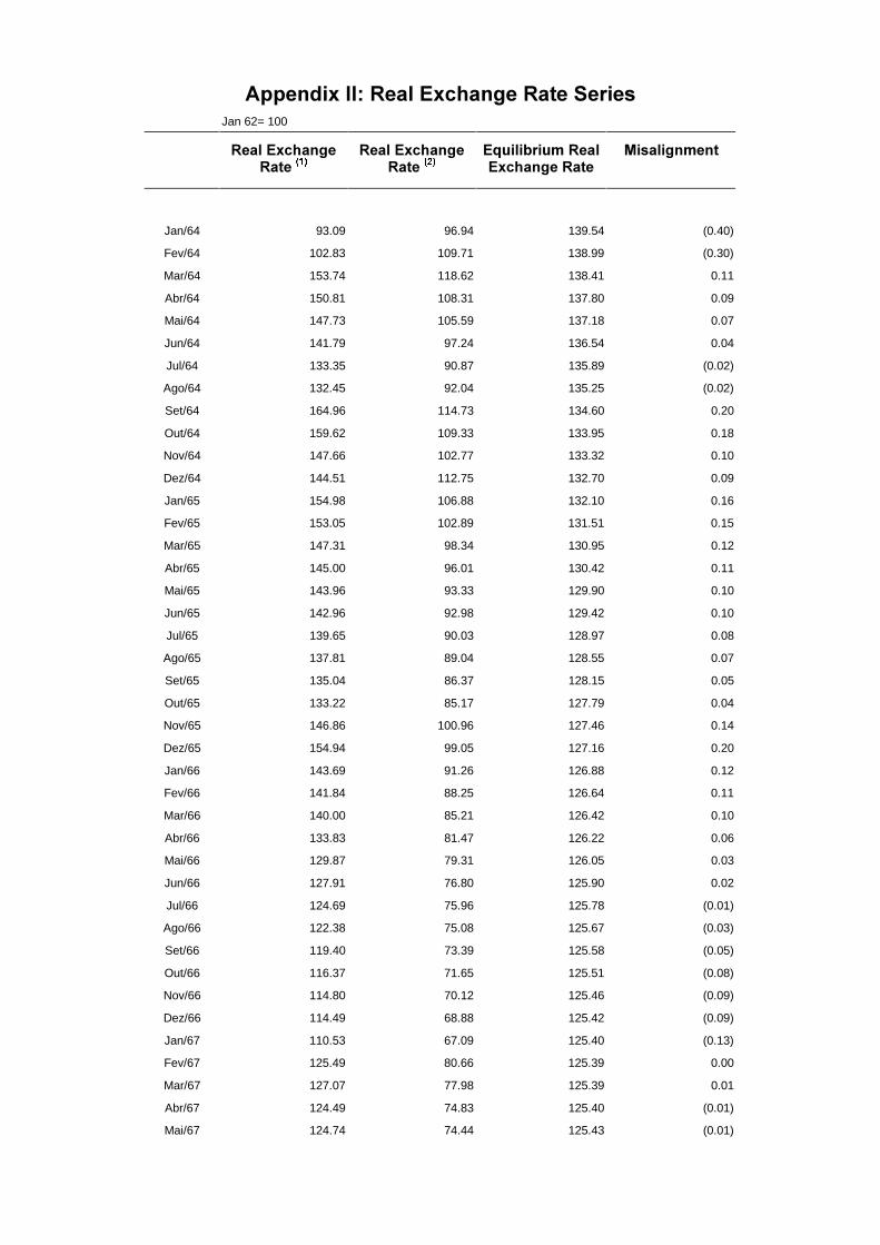
$SSHQGL[�,,��5HDO�([FKDQJH�5DWH�6HULHVJan 62= 100

5HDO�([FKDQJH5DWH����

5HDO�([FKDQJH5DWH����

(TXLOLEULXP�5HDO([FKDQJH�5DWH

0LVDOLJQPHQW

Jan/64 93.09 96.94 139.54 (0.40)

Fev/64 102.83 109.71 138.99 (0.30)

Mar/64 153.74 118.62 138.41 0.11

Abr/64 150.81 108.31 137.80 0.09

Mai/64 147.73 105.59 137.18 0.07

Jun/64 141.79 97.24 136.54 0.04

Jul/64 133.35 90.87 135.89 (0.02)

Ago/64 132.45 92.04 135.25 (0.02)

Set/64 164.96 114.73 134.60 0.20

Out/64 159.62 109.33 133.95 0.18

Nov/64 147.66 102.77 133.32 0.10

Dez/64 144.51 112.75 132.70 0.09

Jan/65 154.98 106.88 132.10 0.16

Fev/65 153.05 102.89 131.51 0.15

Mar/65 147.31 98.34 130.95 0.12

Abr/65 145.00 96.01 130.42 0.11

Mai/65 143.96 93.33 129.90 0.10

Jun/65 142.96 92.98 129.42 0.10

Jul/65 139.65 90.03 128.97 0.08

Ago/65 137.81 89.04 128.55 0.07

Set/65 135.04 86.37 128.15 0.05

Out/65 133.22 85.17 127.79 0.04

Nov/65 146.86 100.96 127.46 0.14

Dez/65 154.94 99.05 127.16 0.20

Jan/66 143.69 91.26 126.88 0.12

Fev/66 141.84 88.25 126.64 0.11

Mar/66 140.00 85.21 126.42 0.10

Abr/66 133.83 81.47 126.22 0.06

Mai/66 129.87 79.31 126.05 0.03

Jun/66 127.91 76.80 125.90 0.02

Jul/66 124.69 75.96 125.78 (0.01)

Ago/66 122.38 75.08 125.67 (0.03)

Set/66 119.40 73.39 125.58 (0.05)

Out/66 116.37 71.65 125.51 (0.08)

Nov/66 114.80 70.12 125.46 (0.09)

Dez/66 114.49 68.88 125.42 (0.09)

Jan/67 110.53 67.09 125.40 (0.13)

Fev/67 125.49 80.66 125.39 0.00

Mar/67 127.07 77.98 125.39 0.01

Abr/67 124.49 74.83 125.40 (0.01)

Mai/67 124.74 74.44 125.43 (0.01)

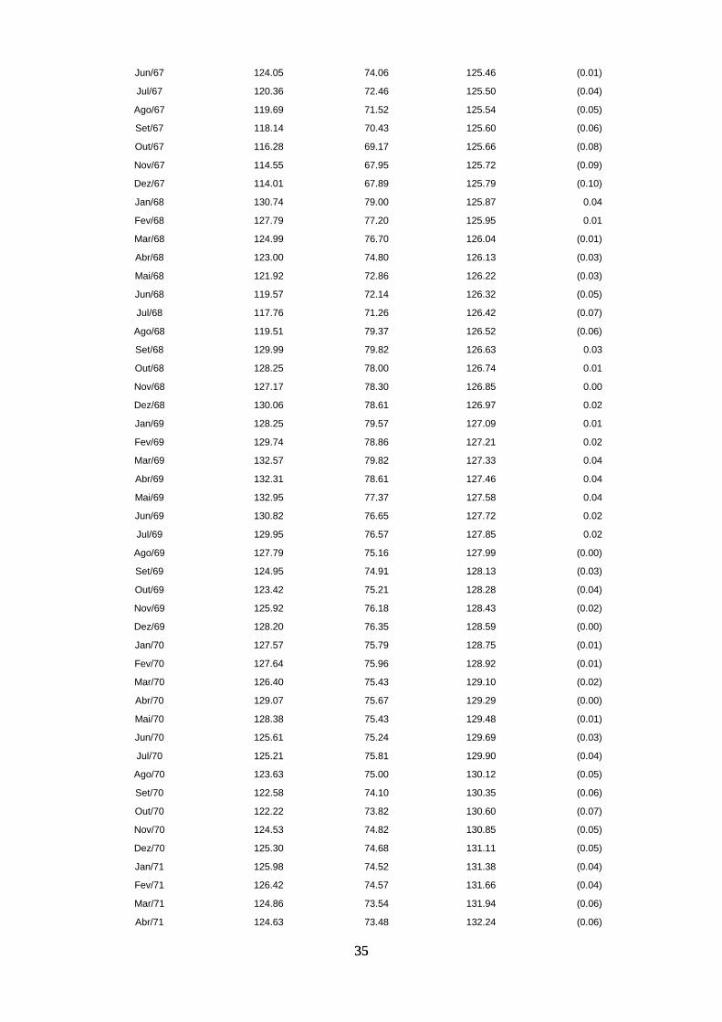
3535

Jun/67 124.05 74.06 125.46 (0.01)

Jul/67 120.36 72.46 125.50 (0.04)

Ago/67 119.69 71.52 125.54 (0.05)

Set/67 118.14 70.43 125.60 (0.06)

Out/67 116.28 69.17 125.66 (0.08)

Nov/67 114.55 67.95 125.72 (0.09)

Dez/67 114.01 67.89 125.79 (0.10)

Jan/68 130.74 79.00 125.87 0.04

Fev/68 127.79 77.20 125.95 0.01

Mar/68 124.99 76.70 126.04 (0.01)

Abr/68 123.00 74.80 126.13 (0.03)

Mai/68 121.92 72.86 126.22 (0.03)

Jun/68 119.57 72.14 126.32 (0.05)

Jul/68 117.76 71.26 126.42 (0.07)

Ago/68 119.51 79.37 126.52 (0.06)

Set/68 129.99 79.82 126.63 0.03

Out/68 128.25 78.00 126.74 0.01

Nov/68 127.17 78.30 126.85 0.00

Dez/68 130.06 78.61 126.97 0.02

Jan/69 128.25 79.57 127.09 0.01

Fev/69 129.74 78.86 127.21 0.02

Mar/69 132.57 79.82 127.33 0.04

Abr/69 132.31 78.61 127.46 0.04

Mai/69 132.95 77.37 127.58 0.04

Jun/69 130.82 76.65 127.72 0.02

Jul/69 129.95 76.57 127.85 0.02

Ago/69 127.79 75.16 127.99 (0.00)

Set/69 124.95 74.91 128.13 (0.03)

Out/69 123.42 75.21 128.28 (0.04)

Nov/69 125.92 76.18 128.43 (0.02)

Dez/69 128.20 76.35 128.59 (0.00)

Jan/70 127.57 75.79 128.75 (0.01)

Fev/70 127.64 75.96 128.92 (0.01)

Mar/70 126.40 75.43 129.10 (0.02)

Abr/70 129.07 75.67 129.29 (0.00)

Mai/70 128.38 75.43 129.48 (0.01)

Jun/70 125.61 75.24 129.69 (0.03)

Jul/70 125.21 75.81 129.90 (0.04)

Ago/70 123.63 75.00 130.12 (0.05)

Set/70 122.58 74.10 130.35 (0.06)

Out/70 122.22 73.82 130.60 (0.07)

Nov/70 124.53 74.82 130.85 (0.05)

Dez/70 125.30 74.68 131.11 (0.05)

Jan/71 125.98 74.52 131.38 (0.04)

Fev/71 126.42 74.57 131.66 (0.04)

Mar/71 124.86 73.54 131.94 (0.06)

Abr/71 124.63 73.48 132.24 (0.06)

3636

Mai/71 125.77 73.82 132.55 (0.05)

Jun/71 124.11 73.52 132.87 (0.07)

Jul/71 123.54 73.16 133.20 (0.08)

Ago/71 126.34 73.77 133.54 (0.06)

Set/71 128.61 73.97 133.88 (0.04)

Out/71 128.65 73.57 134.25 (0.04)

Nov/71 129.78 73.88 134.62 (0.04)

Dez/71 128.24 74.39 135.00 (0.05)

Jan/72 132.31 73.33 135.39 (0.02)

Fev/72 134.76 74.73 135.80 (0.01)

Mar/72 134.12 74.31 136.22 (0.02)

Abr/72 134.07 73.98 136.66 (0.02)

Mai/72 135.27 74.57 137.11 (0.01)

Jun/72 134.88 74.37 137.58 (0.02)

Jul/72 133.97 73.48 138.06 (0.03)

Ago/72 132.26 72.70 138.56 (0.05)

Set/72 132.66 72.37 139.08 (0.05)

Out/72 132.47 71.46 139.62 (0.05)

Nov/72 133.16 71.95 140.18 (0.05)

Dez/72 135.25 73.89 140.77 (0.04)

Jan/73 135.24 74.44 141.38 (0.04)

Fev/73 137.96 73.85 142.01 (0.03)

Mar/73 140.31 73.21 142.67 (0.02)

Abr/73 139.86 72.54 143.35 (0.02)

Mai/73 142.64 74.00 144.05 (0.01)

Jun/73 145.76 74.90 144.78 0.01

Jul/73 147.29 73.56 145.53 0.01

Ago/73 149.70 77.30 146.29 0.02

Set/73 147.85 74.84 147.07 0.01

Out/73 146.96 73.92 147.85 (0.01)

Nov/73 142.90 73.58 148.62 (0.04)

Dez/73 143.59 74.70 149.39 (0.04)

Jan/74 141.85 76.97 150.15 (0.06)

Fev/74 146.45 77.85 150.88 (0.03)

Mar/74 145.37 76.35 151.57 (0.04)

Abr/74 141.66 74.26 152.22 (0.07)

Mai/74 139.79 71.85 152.82 (0.09)

Jun/74 140.02 75.22 153.36 (0.09)

Jul/74 145.69 78.46 153.84 (0.05)

Ago/74 147.67 80.65 154.23 (0.04)

Set/74 147.53 80.75 154.55 (0.05)

Out/74 149.82 81.53 154.79 (0.03)

Nov/74 152.27 82.13 154.94 (0.02)

Dez/74 151.53 80.90 155.00 (0.02)

Jan/75 148.80 80.17 154.97 (0.04)

Fev/75 149.55 79.31 154.85 (0.03)

Mar/75 147.07 78.35 154.64 (0.05)

3737

Abr/75 147.70 78.75 154.35 (0.04)

Mai/75 148.52 79.14 153.98 (0.04)

Jun/75 143.48 77.90 153.53 (0.07)

Jul/75 142.94 78.39 153.00 (0.07)

Ago/75 138.74 78.01 152.41 (0.09)

Set/75 134.37 77.90 151.76 (0.12)

Out/75 132.83 78.25 151.06 (0.13)

Nov/75 133.46 78.70 150.31 (0.12)

Dez/75 133.33 79.82 149.52 (0.11)

Jan/76 133.57 78.83 148.70 (0.11)

Fev/76 133.72 76.15 147.85 (0.10)

Mar/76 137.23 76.89 146.99 (0.07)

Abr/76 141.57 79.79 146.11 (0.03)

Mai/76 140.50 80.33 145.23 (0.03)

Jun/76 141.28 81.19 144.35 (0.02)

Jul/76 138.06 81.40 143.48 (0.04)

Ago/76 136.37 79.89 142.63 (0.04)

Set/76 136.56 80.09 141.79 (0.04)

Out/76 137.31 80.24 140.98 (0.03)

Nov/76 139.20 81.19 140.19 (0.01)

Dez/76 135.31 81.75 139.44 (0.03)

Jan/77 135.80 81.12 138.72 (0.02)

Fev/77 135.84 80.39 138.05 (0.02)

Mar/77 133.05 79.26 137.42 (0.03)

Abr/77 132.21 78.99 136.83 (0.03)

Mai/77 131.85 79.80 136.29 (0.03)

Jun/77 134.28 79.48 135.80 (0.01)

Jul/77 138.45 80.13 135.37 0.02

Ago/77 139.89 80.23 134.99 0.04

Set/77 140.61 80.31 134.66 0.04

Out/77 141.69 79.95 134.39 0.05

Nov/77 141.49 79.49 134.17 0.05

Dez/77 144.76 80.05 134.01 0.08

Jan/78 144.33 80.65 133.91 0.07

Fev/78 143.68 79.65 133.86 0.07

Mar/78 144.05 79.86 133.86 0.07

Abr/78 143.36 81.00 133.92 0.07

Mai/78 142.11 81.08 134.03 0.06

Jun/78 143.00 79.59 134.19 0.06

Jul/78 144.68 78.18 134.40 0.07

Ago/78 147.13 78.06 134.66 0.09

Set/78 147.54 78.82 134.97 0.09

Out/78 149.61 78.75 135.32 0.10

Nov/78 147.25 79.03 135.72 0.08

Dez/78 151.11 81.16 136.16 0.10

Jan/79 153.72 81.94 136.64 0.12

Fev/79 154.90 84.11 137.16 0.12

3838

Mar/79 151.53 82.92 137.71 0.10

Abr/79 150.09 84.07 138.29 0.08

Mai/79 155.54 87.38 138.90 0.11

Jun/79 157.53 87.88 139.54 0.12

Jul/79 156.89 86.95 140.20 0.11

Ago/79 155.01 87.43 140.87 0.10

Set/79 154.59 89.00 141.56 0.09

Out/79 153.81 90.40 142.25 0.08

Nov/79 152.17 90.80 142.95 0.06

Dez/79 185.20 109.47 143.65 0.25

Jan/80 192.37 115.87 144.34 0.29

Fev/80 192.57 117.58 145.02 0.28

Mar/80 185.97 117.70 145.69 0.24

Abr/80 182.25 117.96 146.33 0.22

Mai/80 181.03 114.80 146.95 0.21

Jun/80 178.49 113.33 147.55 0.19

Jul/80 170.40 112.86 148.11 0.14

Ago/80 164.52 112.03 148.63 0.10

Set/80 163.36 109.59 149.12 0.09

Out/80 157.21 107.87 149.57 0.05

Nov/80 150.01 105.79 149.98 0.00

Dez/80 148.28 105.64 150.35 (0.01)

Jan/81 149.56 107.95 150.68 (0.01)

Fev/81 143.46 104.99 150.98 (0.05)

Mar/81 141.91 106.17 151.25 (0.06)

Abr/81 141.24 108.09 151.49 (0.07)

Mai/81 138.64 108.49 151.69 (0.09)

Jun/81 137.03 110.09 151.88 (0.10)

Jul/81 139.35 111.55 152.04 (0.09)

Ago/81 139.48 109.34 152.18 (0.09)

Set/81 143.21 110.15 152.31 (0.06)

Out/81 146.27 111.58 152.43 (0.04)

Nov/81 147.72 112.31 152.54 (0.03)

Dez/81 151.29 113.91 152.65 (0.01)

Jan/82 148.17 116.19 152.76 (0.03)

Fev/82 144.80 115.05 152.87 (0.05)

Mar/82 141.60 114.40 152.99 (0.08)

Abr/82 139.04 114.09 153.12 (0.10)

Mai/82 140.17 113.31 153.26 (0.09)

Jun/82 133.50 110.29 153.42 (0.14)

Jul/82 126.52 109.55 153.58 (0.19)

Ago/82 128.88 109.56 153.76 (0.18)

Set/82 134.88 112.65 153.95 (0.13)

Out/82 136.77 116.21 154.15 (0.12)

Nov/82 139.39 118.17 154.36 (0.10)

Dez/82 143.86 117.01 154.58 (0.07)

Jan/83 142.03 116.75 154.79 (0.09)

3939

Fev/83 161.03 129.92 155.01 0.04

Mar/83 183.46 149.95 155.21 0.17

Abr/83 178.00 153.15 155.41 0.14

Mai/83 182.03 159.58 155.60 0.16

Jun/83 173.79 156.22 155.76 0.11

Jul/83 167.40 153.29 155.91 0.07

Ago/83 168.87 161.89 156.02 0.08

Set/83 160.65 158.70 156.11 0.03

Out/83 159.26 162.53 156.17 0.02

Nov/83 160.24 172.38 156.19 0.03

Dez/83 160.99 173.89 156.17 0.03

Jan/84 156.90 173.38 156.10 0.01

Fev/84 159.07 174.81 156.00 0.02

Mar/84 166.75 181.53 155.85 0.07

Abr/84 165.70 183.94 155.66 0.06

Mai/84 162.52 187.79 155.42 0.04

Jun/84 161.04 182.94 155.13 0.04

Jul/84 157.54 187.52 154.80 0.02

Ago/84 157.98 189.84 154.42 0.02

Set/84 153.74 191.26 153.99 (0.00)

Out/84 148.08 194.56 153.52 (0.04)

Nov/84 150.24 198.41 153.01 (0.02)

Dez/84 148.04 201.03 152.46 (0.03)

Jan/85 144.25 202.00 151.87 (0.05)

Fev/85 145.56 205.87 151.24 (0.04)

Mar/85 141.38 204.99 150.58 (0.06)

Abr/85 154.26 215.00 149.89 0.03

Mai/85 160.87 219.53 149.18 0.08

Jun/85 164.22 222.14 148.45 0.10

Jul/85 168.37 215.80 147.69 0.13

Ago/85 159.25 207.42 146.93 0.08

Set/85 160.10 213.03 146.15 0.09

Out/85 166.30 210.15 145.37 0.13

Nov/85 156.30 204.25 144.59 0.08

Dez/85 159.28 202.02 143.81 0.10

Jan/86 152.41 201.33 143.04 0.06

Fev/86 149.31 206.17 142.28 0.05

Mar/86 160.73 212.11 141.54 0.13

Abr/86 162.17 205.87 140.82 0.14

Mai/86 164.25 202.80 140.11 0.16

Jun/86 163.07 200.67 139.43 0.16

Jul/86 164.77 197.56 138.78 0.17

Ago/86 165.30 193.72 138.15 0.18

Set/86 164.38 191.18 137.54 0.18

Out/86 164.51 187.77 136.96 0.18

Nov/86 161.55 181.79 136.40 0.17

Dez/86 155.76 169.78 135.86 0.14

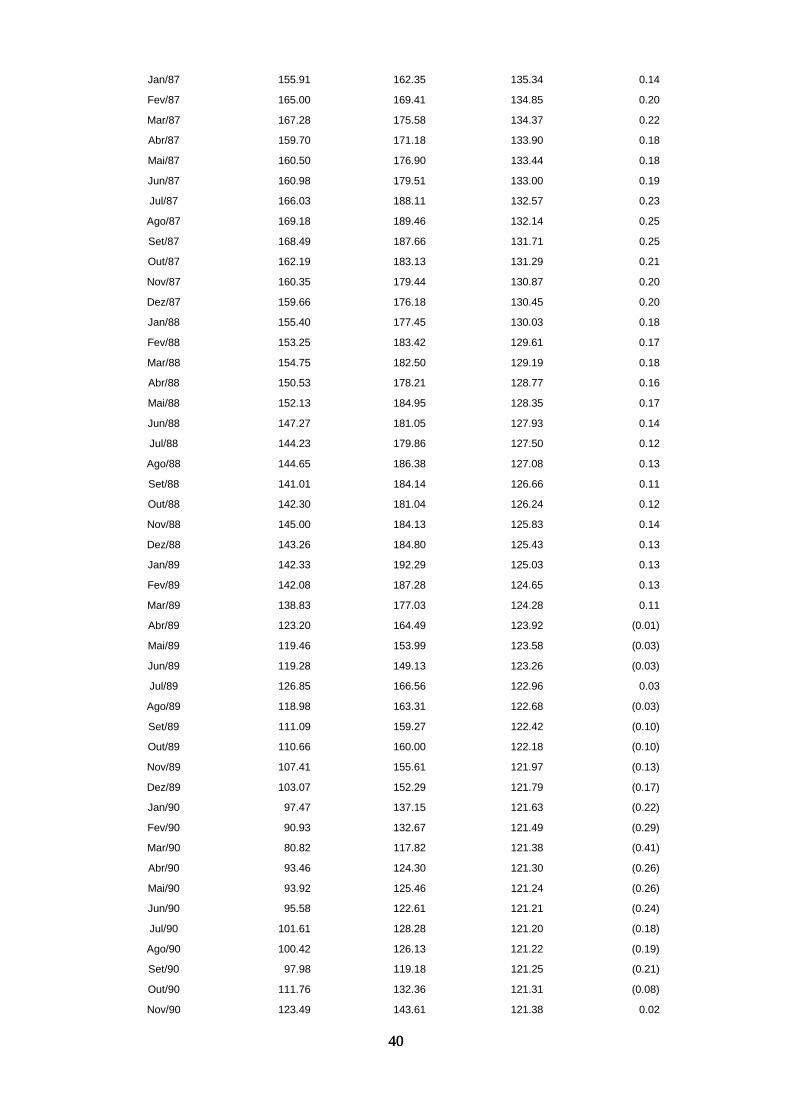
4040

Jan/87 155.91 162.35 135.34 0.14

Fev/87 165.00 169.41 134.85 0.20

Mar/87 167.28 175.58 134.37 0.22

Abr/87 159.70 171.18 133.90 0.18

Mai/87 160.50 176.90 133.44 0.18

Jun/87 160.98 179.51 133.00 0.19

Jul/87 166.03 188.11 132.57 0.23

Ago/87 169.18 189.46 132.14 0.25

Set/87 168.49 187.66 131.71 0.25

Out/87 162.19 183.13 131.29 0.21

Nov/87 160.35 179.44 130.87 0.20

Dez/87 159.66 176.18 130.45 0.20

Jan/88 155.40 177.45 130.03 0.18

Fev/88 153.25 183.42 129.61 0.17

Mar/88 154.75 182.50 129.19 0.18

Abr/88 150.53 178.21 128.77 0.16

Mai/88 152.13 184.95 128.35 0.17

Jun/88 147.27 181.05 127.93 0.14

Jul/88 144.23 179.86 127.50 0.12

Ago/88 144.65 186.38 127.08 0.13

Set/88 141.01 184.14 126.66 0.11

Out/88 142.30 181.04 126.24 0.12

Nov/88 145.00 184.13 125.83 0.14

Dez/88 143.26 184.80 125.43 0.13

Jan/89 142.33 192.29 125.03 0.13

Fev/89 142.08 187.28 124.65 0.13

Mar/89 138.83 177.03 124.28 0.11

Abr/89 123.20 164.49 123.92 (0.01)

Mai/89 119.46 153.99 123.58 (0.03)

Jun/89 119.28 149.13 123.26 (0.03)

Jul/89 126.85 166.56 122.96 0.03

Ago/89 118.98 163.31 122.68 (0.03)

Set/89 111.09 159.27 122.42 (0.10)

Out/89 110.66 160.00 122.18 (0.10)

Nov/89 107.41 155.61 121.97 (0.13)

Dez/89 103.07 152.29 121.79 (0.17)

Jan/90 97.47 137.15 121.63 (0.22)

Fev/90 90.93 132.67 121.49 (0.29)

Mar/90 80.82 117.82 121.38 (0.41)

Abr/90 93.46 124.30 121.30 (0.26)

Mai/90 93.92 125.46 121.24 (0.26)

Jun/90 95.58 122.61 121.21 (0.24)

Jul/90 101.61 128.28 121.20 (0.18)

Ago/90 100.42 126.13 121.22 (0.19)

Set/90 97.98 119.18 121.25 (0.21)

Out/90 111.76 132.36 121.31 (0.08)

Nov/90 123.49 143.61 121.38 0.02

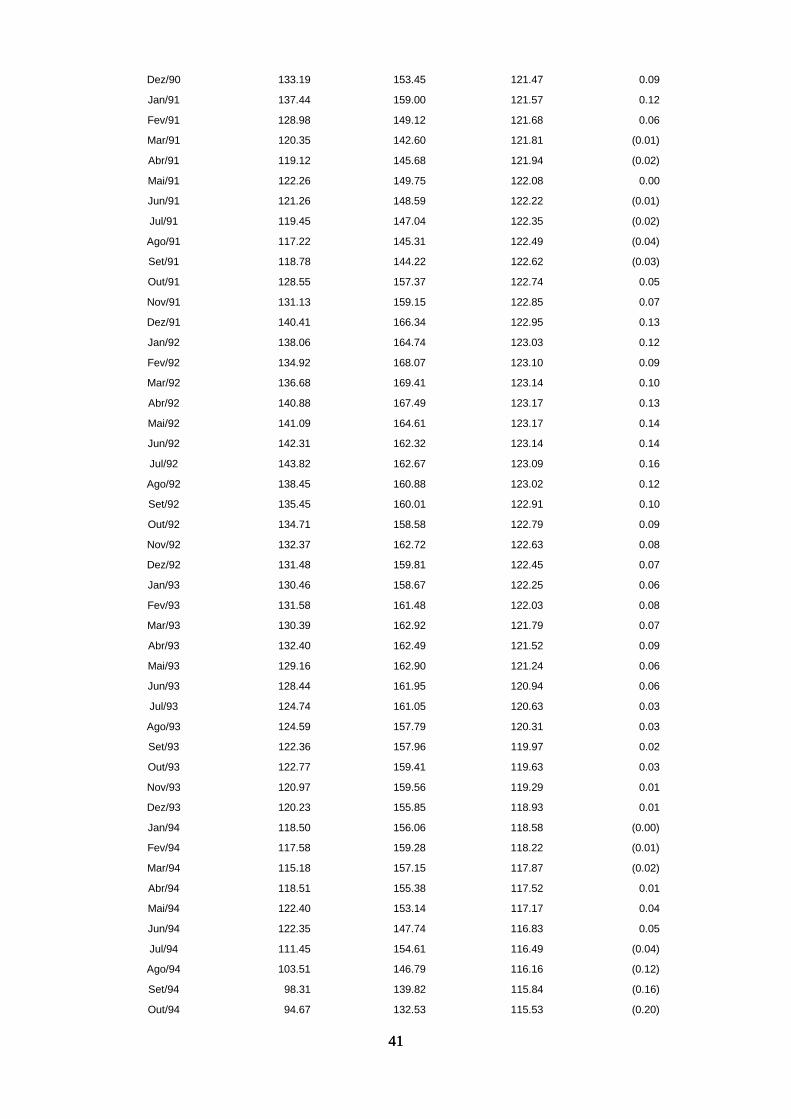
4141

Dez/90 133.19 153.45 121.47 0.09

Jan/91 137.44 159.00 121.57 0.12

Fev/91 128.98 149.12 121.68 0.06

Mar/91 120.35 142.60 121.81 (0.01)

Abr/91 119.12 145.68 121.94 (0.02)

Mai/91 122.26 149.75 122.08 0.00

Jun/91 121.26 148.59 122.22 (0.01)

Jul/91 119.45 147.04 122.35 (0.02)

Ago/91 117.22 145.31 122.49 (0.04)

Set/91 118.78 144.22 122.62 (0.03)

Out/91 128.55 157.37 122.74 0.05

Nov/91 131.13 159.15 122.85 0.07

Dez/91 140.41 166.34 122.95 0.13

Jan/92 138.06 164.74 123.03 0.12

Fev/92 134.92 168.07 123.10 0.09

Mar/92 136.68 169.41 123.14 0.10

Abr/92 140.88 167.49 123.17 0.13

Mai/92 141.09 164.61 123.17 0.14

Jun/92 142.31 162.32 123.14 0.14

Jul/92 143.82 162.67 123.09 0.16

Ago/92 138.45 160.88 123.02 0.12

Set/92 135.45 160.01 122.91 0.10

Out/92 134.71 158.58 122.79 0.09

Nov/92 132.37 162.72 122.63 0.08

Dez/92 131.48 159.81 122.45 0.07

Jan/93 130.46 158.67 122.25 0.06

Fev/93 131.58 161.48 122.03 0.08

Mar/93 130.39 162.92 121.79 0.07

Abr/93 132.40 162.49 121.52 0.09

Mai/93 129.16 162.90 121.24 0.06

Jun/93 128.44 161.95 120.94 0.06

Jul/93 124.74 161.05 120.63 0.03

Ago/93 124.59 157.79 120.31 0.03

Set/93 122.36 157.96 119.97 0.02

Out/93 122.77 159.41 119.63 0.03

Nov/93 120.97 159.56 119.29 0.01

Dez/93 120.23 155.85 118.93 0.01

Jan/94 118.50 156.06 118.58 (0.00)

Fev/94 117.58 159.28 118.22 (0.01)

Mar/94 115.18 157.15 117.87 (0.02)

Abr/94 118.51 155.38 117.52 0.01

Mai/94 122.40 153.14 117.17 0.04

Jun/94 122.35 147.74 116.83 0.05

Jul/94 111.45 154.61 116.49 (0.04)

Ago/94 103.51 146.79 116.16 (0.12)

Set/94 98.31 139.82 115.84 (0.16)

Out/94 94.67 132.53 115.53 (0.20)

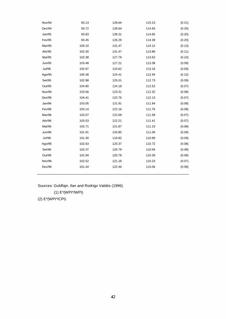
4242

Nov/94 93.13 128.64 115.23 (0.21)

Dez/94 93.72 128.64 114.93 (0.20)

Jan/95 93.83 128.31 114.65 (0.20)

Fev/95 93.45 126.29 114.38 (0.20)

Mar/95 100.10 131.47 114.12 (0.13)

Abr/95 102.30 131.47 113.86 (0.11)

Mai/95 102.38 127.79 113.62 (0.10)

Jun/95 103.48 127.21 113.38 (0.09)

Jul/95 102.97 124.62 113.16 (0.09)

Ago/95 100.48 124.41 112.94 (0.12)

Set/95 102.98 125.01 112.73 (0.09)

Out/95 104.80 124.18 112.52 (0.07)

Nov/95 103.56 123.31 112.32 (0.08)

Dez/95 104.41 122.76 112.13 (0.07)

Jan/96 103.05 121.91 111.94 (0.08)

Fev/96 103.14 122.16 111.76 (0.08)

Mar/96 103.57 122.69 111.58 (0.07)

Abr/96 103.53 122.21 111.41 (0.07)

Mai/96 102.71 121.87 111.23 (0.08)

Jun/96 101.91 120.80 111.06 (0.09)

Jul/96 101.30 119.82 110.89 (0.09)

Ago/96 102.63 120.37 110.72 (0.08)

Set/96 102.37 120.79 110.56 (0.08)

Out/96 101.94 120.78 110.39 (0.08)

Nov/96 102.52 121.18 110.23 (0.07)

Dez/96 101.44 122.46 110.06 (0.08)

Sources: Goldfajn, Ilan and Rodrigo Valdés (1996).

(1) E*(WPI*/WPI)

(2) E*(WPI*/CPI)