EXTENSIONS TO DENOISING SOURCE SEPARATIONmscla/MA_pdfs/MarianaSCAlmeida_TFC_05.pdf · EXTENSIONS TO...
81
HELSINKI UNIVERSITY OF TECHNOLOGY UNIVERSIDADE TÉCNICA DE LISBOA INSTITUTO SUPERIOR TÉCNICO EXTENSIONS TO DENOISING SOURCE SEPARATION Mariana Sá Correia Leite de Almeida, nº49419, AE: Sistemas, Decisão e Controlo. LICENCIATURA EM ENGENHARIA ELECTROTÉCNICA E DE COMPUTADORES Relatório de Trabalho Final de Curso 143/2004/M Supervisor at Helsinki University of Technology: Dr. Jaakko Särelä Supervisor at Instituto Superior Técnico: Prof. Luís Borges de Almeida September 2005
Transcript of EXTENSIONS TO DENOISING SOURCE SEPARATIONmscla/MA_pdfs/MarianaSCAlmeida_TFC_05.pdf · EXTENSIONS TO...

HELSINKI UNIVERSITY OF TECHNOLOGY
UNIVERSIDADE TÉCNICA DE LISBOA
INSTITUTO SUPERIOR TÉCNICO
EXTENSIONS TO DENOISING SOURCE SEPARATION
Mariana Sá Correia Leite de Almeida, nº49419, AE: Sistemas, Decisão e Controlo.
LICENCIATURA EM ENGENHARIA ELECTROTÉCNICA E DE COMPUTADORES
Relatório de Trabalho Final de Curso 143/2004/M
Supervisor at Helsinki University of Technology: Dr. Jaakko Särelä Supervisor at Instituto Superior Técnico: Prof. Luís Borges de Almeida
September 2005

Mariana Sá Correia Leite de Almeida - Extensions to Denoising Source Separation
i
Acknowledgements
The accomplishment of this work was only possible thanks to the help and support of many.
First, I would like to thank Professor Luís Borges de Almeida for his guidance and support, during the first phase of this work at Instituto Superior Técnico, and for the encouragement to go abroad. I am also very grateful to him for all the help during the writing of this final report.
This work was performed at the Neural Networks Research Center of the Helsinki University of Technology (HUT), Espoo, Finland, in the context of the Erasmus/Socrates programme. Very special thanks to my supervisor Dr. Jaakko Särelä for his continuous guidance. I am also very grateful to Dr. Harri Valpola for having suggested the nonlinear DSS problem and for many helpful discussions. I would also like to thank Dr. Ricardo Vigário for helpful discussions related with the extension of DSS to an online algorithm.
I am also very grateful to my family and friends, in Portugal and in Helsinki, for all the support given during my stay abroad, especially to my parents who made this project possible.
Mariana Sá Correia Leite de Almeida - Extensions to Denoising Source Separation
ii
Abstract
Data from the real world appears combined with undesired information, denominated noise. The relevant information can be extracted from these data by applying source separation (SS) methods. This work is focused on a recent method of SS, denoising source separation (DSS). In order to perform a fast and robust separation, DSS includes a denoising step that takes advantage of a small amount of information about the sources that is usually available. DSS performs separation of instantaneous and linear mixtures in a fixed point algorithm and the aim of the present work is the development of an online version of DSS able to separate mixtures that would change in time, and of a version of DSS suitable for nonlinear mixtures.
The online version was successfully implemented to separate mixtures of two stationary synthetic signals. The application of the algorithm results in a stationary solution with unit variance. Consequently, the proposed extension is not useful for mixtures of non-stationary sources. The restriction to stationary sources results from the scaling indetermination inherent to linear source separation methods, namely DSS. This can only be overcome with additional information on the data or mixture process.
The extension of DSS to a nonlinear mixture was studied using a specific real-life mixture of images. To achieve this separation, a new version of DSS useful to be applied to nonlinear mapping was developed. Different denoising functions were implemented to perform the separation. The separation was achieved but the generalization of the DSS to nonlinear mappings is restricted to particular mixtures, for which it is possible to develop useful denoising functions.
Keywords: Independent Component Analysis (ICA), Principal component analysis
(PCA), Denoising Source Separation (DSS), Whitening, Non-linear mixtures, Neural network

Mariana Sá Correia Leite de Almeida - Extensions to Denoising Source Separation
iii
Resumo Os dados provenientes do mundo real encontram-se, frequentemente contaminados com
informação indesejada, denominada ruído. A informação indesejada pode ser extraída dos dados através da utilização de métodos de separação de fontes (Source Separation - SS). Este trabalho teve por base um método recente de separação de fontes, denoising source separation (DSS). De modo a obter uma convergência rápida e robusta, o método DSS inclui um passo que elimina o ruído (“denoising”), usando para tal a alguma informação sobre as fontes, a qual é normalmente conhecida. DSS realiza SS de misturas lineares e instantâneas através de um algoritmo de ponto fixo, tendo o presente trabalho consistido no desenvolvimento de uma versão online do algoritmo capaz de separar misturas não estacionárias, assim como outra versão capaz de separar misturas não lineares.
A versão online do algoritmo DSS foi implementada com sucesso permitindo separar misturas sintéticas de dois sinais estacionários. A aplicação do algoritmo tem como solução sinais estacionários de variância unitária, sendo somente aplicável a sinais estacionários. A restrição da extensão do método a sinais estacionários, resulta da indeterminação de escala inerente a vários métodos de separação, nomeadamente DSS. Esta indeterminação só poderá ser ultrapassada caso exista informação adicional sobre os sinais ou sobre o processo de mistura.
A extensão do método DSS a misturas não lineares foi desenvolvido, tendo por base um problema real de misturas não lineares de duas imagens. Para alcançar a separação das imagens, uma nova versão do método foi desenvolvida conjuntamente com funções de redução de ruído (“denoising functions”). A separação das imagens foi alcançada com sucesso, mas a generalização do método a misturas não lineares encontra-se restringida a misturas particulares, para as quais é possível desenvolver funções de redução de ruído úteis.
Palavras-chave: Análise em Componentes Independentes (ICA), Análise em
Componentes Principais (PCA), Denoising Source Separation (DSS), Branqueamento, Misturas não lineares, Redes neuronais
Mariana Sá Correia Leite de Almeida - Extensions to Denoising Source Separation
iv
Contents
1 Inroduction 1 1.1 Motivations and application of Source Seapration………………………….…….2 1.2 Independent Component Analysis………………………………………….……..2 1.2.1 Preprocessing……………………………………………………………….3 1.2.2 Infomax…………………………………………………………………………….4 1.2.3 FastICA……………………………………………………………………..6 1.2.4 MISEP………………………………………………………………………8 1.2.4 Other methods………………………………………………………………9 1.3 Denoising Source Separation…………………………………………….............10 1.4 Problems to be solved……………………………………………………………12
2 DSS extension to an online version 13 2.1 Online DSS………………………………………………………………............13 2.2 Results…………………………………………………………………………....16 2.2.1 Synthetic non-stationary mixture applied to pre-whiten data……………..16 2.2.2 Synthetic non-stationary mixture………………………………………….18 2.2.3 Synthetic non-stationary mixtures with non-singular stages……………...19 2.3 Conclusions………………………………………………………………………21
3 DSS extension to separate nonlinear mixtures of two images 23 3.1 The real-life problem to be solved……………………………………………… 23 3.2 Theoretical description……………………………………………………….….27 3.2.1 Initializations…………………………………………………………..….28 3.2.2 Desoising functions…………………………………………………….…31 3.2.3 MLP Traning……………………………………………………………...39 3.2.4 Speedup analysis………………………………………………………….39 3.2.5 Quality measures………………………………………………………….40 3.3 Results…………………………………………………………………………...41 3.3.1 Linear separation of linear synthetic mixtures……………………………42 3.3.2 Linear separation of nonlinear real-life mixtures…………………………44 3.3.3 Nonlinear separation of nonlinear real-life mistures.……………………..47 3.3.4 Experiments with more denoising iterations.……………………………..50 3.4 Conclusions……………………………………………………………………...52
4 Conclusions 53 4.1 Conclusions related with online DSS……………………………………………53 4.2 Future work related with online DSS……………………………………………53 4.3 Conclusions related with nonlinear DSS………………………………………...53 4.4 Future work related with nonlinear DSS………………………………………...54
A Initialized images 55
B Interface 58

Mariana Sá Correia Leite de Almeida - Extensions to Denoising Source Separation
v
List of Figures
1.1 Orthonormalization Methods (comparison).………...……………………………...4 1.2 Schematic representation of the network used by Infomax in order to separate two
sources. The F bloc performs ICA and iS are the extracted components. ψ‘s are the auxiliary blocs of training (adapted from [21]). ………...………...………………..4
1.3 Gaussian, Laplacian (Super-Gaussian) and uniform (Sub-Gaussian) distributions with unit variance. Their kurtosis are 0, 3 and -2 respectively. (from [25]) ……….6
1.4 Esquematic representation of the network used by MISEP. The top part corresponds to figure 1.5, drawn in a different way. The lower part, which computes the Jacobian proper, is essentially a linearization of the upper part, but propagates matrix. It has as input the identity matrix, and provides at its output the Jacobian J. (Adapted from [21]).…………………………………………………...8
1.5 Data evolution during the three steps of the classical version of DSS (adaptedted from [33])..………………………………………………………………………...10
2.1 Weight evolution of matrix W obtained for the first synthetic mixture. The
demixing matrix (inverse of M) is represented by the light green line. The evolution of W11 (in dark blue) is overlapped by the evolution of W22 (in light blue) ………...………….……………………...……17
2.2 Results obtained for the second synthetic mixture. The value of γwas 0.002 and βwas 0.002. The demixing matrix (inverse of M) is represented by the light green line……..………...………...………...………...………...………...………...………...………......18
2.3 Description of the third synthetic mixture. The evolution of W11 (in dark blue) is covered by the evolution of W22 (in light blue). The evolution of W12 (in green) is covered by the evolution of W21 (in red). ………...………...…………...…………...........19
2.4 Results obtained for the third synthetic mixture. The value of γwas 0.005 and βwas 0.005. The demixing matrix (inverse of M) is represented by the light green line………………………………………………………………………………....20
2.5 Results obtained for the fourth synthetic mixture. The value of γwas 0.005 and βwas 0.005. The demixing matrix (inverse of M) is represented by the light green line and the symmetric matrix of M (-M) is represented in black………………...21
3.1 The first three pairs of source images used in this study………...………….....….24 3.2 The last two pairs of source images used in this study. ………...………...….…25 3.3 The first three pairs of mixtures. ………...………...………...………...………….26 3.4 The last two pairs of mixtures. ………...………...………...………...…………....27 3.5 Scheme of the proposed nonlinear DSS to separate two nonlinearly mixed
images……………………………………………………………………………..28 3.6 Results of the application of isotropic whitening to the natural scenes
mixtures………………...………...………...………...………...………...………..29

Mariana Sá Correia Leite de Almeida - Extensions to Denoising Source Separation
vi
3.7 Natural scenes mixtures initialized with Rsymmetric………………...…31 3.8 High frequencies of the third pair of images, before and after competition. ……..33 3.9 Schematic representation of the second denoising function. On left it is shown the
scheme of one image wavelet decomposition in n levels (the components represented by bold boxes are the ones that will be submitted to the competition). On right it is shown the scheme of the denoising decomposition and the reconstruction of the denoised images. ………...………...………...………..........34
3.10 Results of the application of the wavelet based denoising function to the second (331x438 pixels) and third (330x443 pixels) pairs of mixtures and sources, using a deep level of decomposition (application of wavelet decomposition until the size of one dimensions is lower than 20).. ………...………...………...……….................35
3.11 Result of the application of the wavelet-based denoising function to the second (331x438 pixels) and third (330x443 pixels) pairs of mixtures and sources, using a shallow level of decomposition (application of wavelet decomposition until the size of one dimensions is lower than 160). ………...………...………...………...……….........36
3.12 Images resulted from the application of the denoising function to the natural scenes mixtures already initialized. Wavelet decomposition applied until the size of one dimensions be lower than 80. ………...………...………...………...………...………...........37
3.13 Result of the application of the specific denoising function created for bar images to the first pair of mixtures, already initialized. Wavelet decomposition was applied until the size of one dimension becomes lower than 20. ………...………...…………...38
3.14 Result of the application of the specific denoising function created for text images to the half upper part of the fifth pair of mixture already initialize……………….38
3.15 Schematic representation of the MLP used……….…………………………..…..39 3.16 “Good” results obtained with the proposed algorithm using linear separation…...45 3.17 “Bad” results obtained with the proposed algorithm using linear separation..……46 3.18 Results obtained by applying the proposed nonlinear DSS to the first, second and
third pairs of real-life mixtures..…………………………………………………..49 3.19 Scatter plot of the five pair of sources…………………………………………….50 3.20 Result of DSS’ applied to the second and third pairs of mixtures after 50 denoising
iterations.…………………………………………………………………………..51 A.1 First, fourth, and fifth pair of mixtures after the application of isotropic
whitening..................................................................................................................56 A.2 First, fourth, and fifth pair of mixtures initialized with Rsymmetric………………....57 B.1 Main interface……………………………………………………………………..58 B.2 Infomax interface………………………………………………………………….59 B.3 FastICA interface………………………………………………………………….60 B.4 MISEP interface…………………………………………………………………...61 B.5 DSS interface……………………………………………………………………...62 B.6 Online DSS interface……………………………………………………………...63 B.7 Nonlinear DSS interface…………………………………………………………..64

Mariana Sá Correia Leite de Almeida - Extensions to Denoising Source Separation
vii
List of Tables
3.1 Quality measures calculated for the five pairs of sources and mixtures…………..41 3.2 Separation results obtained for the first linear mixture with DSS without sphering
and without orthonormalization. The angle of the separation vectors and the number of iterations are shown……………………………………………………42
3.3 Separation results obtained with the original DSS applied to the second linear mixture. The angle of the separation vectors obtained with DSS (w), the correct angle of separation (wref) and the number of iterations are shown…………..……43
3.4 Separation vector angles obtained by applying nonlinear DSS (DSS’) and MSE to real mixtures………………………………………………………………………44.
3.5 The four quality measures for the separation results of the real mixture obtained with DSS’, with MSE and with MISEP…………………………………………...47
3.6 The four quality measures for the nonlinear separation results of the real mixtures obtained applying DSS’, MSE and with MISEP………………………………….48

Mariana Sá Correia Leite de Almeida - Extensions to Denoising Source Separation
viii
Mathematical notation
Scalars, vectors, matrices, random variables: a,s,x (lightface, lowercase): Scalars a,s,x (boldface, lowercase): Vectors A,S,X (lightface, uppercase): Scalar random variables A,S,X (boldface, uppercase): Random vectores; also Matrices A T The transpose of matrix A A -T The transpose of the inverse of matrix A detA The determinant of matrix A
Variables and function related to the mixtures and separations S,s Source vectors X,x Mixture vectors Y,y Sphered mixture vectors
sS ˆ,ˆ Vectors of separated components Xden,xden Denoised vectors Z,z Auxiliary output vectors in Infomax and MISEP M Mixing matrix F,f Separating vectors A Sphering matrix W,w Separating vectors for sphered data M(.) Nonlinear mixture function F(.) Nonlinear separation function Fden, fden(.) Denoising function

Mariana Sá Correia Leite de Almeida - Extensions to Denoising Source Separation
ix
Acronyms
BSS - Blind Source Separation CDF - Cumulative density function CLT - Central Limit theorem DS-CDMA - Direct-Sequence Code Division Multiple Access DSS - Denoising Source Separation EEG - Electroencephalogram ESS - Exploratory Source Separation fMRI - functional Magnetic Resonance Imaging ICA - Independent Component Analysis LMS - Least-Mean-Squares MEG - Magnetoencephalogram MLP - Multi-Layer Preceptron NPCA - Nonlinear Principal Component Analysis PCA - Principal Component Analysis pdf - probability density function SNR - Signal-to-Noise Ratio SAR - Synthetically Aperture Radar SS - Source Separation

Mariana Sá Correia Leite de Almeida - Extensions to Denoising Source Separation
1
1. Introduction
Science deals with analyses of data from the real word, that appear combined with undesired information (noise). In order to extract the relevant information, Source Separation (SS) of mixtures has been in the focus of the work of several researchers during the last three decades. SS consists in recovering the original sources from the mixtures (observations). If we have the same number of mixtures and sources and provided the mixing is an invertible function, the sources can be recovered under rather general conditions.
SS can be performed without knowing almost anything about the sources. In this case, SS is usually done through Independent Component Analysis (ICA), assuming that the sources are statistically independent. This is called Blind Source Separation (BSS), since no more information about the sources is used. The central method of this work, Denoising Source Separation (DSS), is part of the Exploratory Source Separation (ESS) group of methods that perform SS with a scarce knowledge about the sources. DSS performs the separation of instantaneous and linear mixtures in a fixed point algorithm using information on the sources. This information is used in a denoising step that emphasizes the desired sources versus the other sources in the mixture.
This project was carried out in two phases. The first phase was carried out during the summer term of 2003/2004 and the winter term of 2004/2005 as part of the activities of the Neural Network and Signal Processing Group of INESC-ID under the supervision of Professor Luis Borges de Almeida. The second phase, between February and July of 2005, was developed in the context of the ERASMUS/SOCRATES programme, in the Neural Networks Research Center of the Helsinki University of Technology (HUT - Finland) under the supervision of Dr. Jaakko Särelä.
During the first part of this work the student was introduced to the independent component analysis (ICA) and to the blind source separation (BSS) techniques so that she would be prepared for the second part of the project. The Infomax, FastICA and MISEP methods were examined and implemented. In the second part of the work, two extensions of the DSS algorithm were proposed to the student. The first extension consists in the online implementation of the algorithm and the second extension consists in the application of the algorithm to solve a real-life nonlinear mixtures of two images resulting from the nonlinear mixture of the front- and back-page images of an "onion skin" paper when the front-page is acquired using a scanner. All the methods detailed in this work were implemented and collected in an interface.
This report is organized in five chapters. The first chapter is an introduction to the subject and is organized as follows: Section 1.1 describes the motivations and applications of SS; section 1.2 presents a theoretical description of ICA emphasizing the three methods related with the work (infomax, FastICA and MISEP); in section 1.3 the theoretical basis of the DSS method are presented and, in section 1.4, the problems to be solved are described. The second chapter is dedicated to the online version of DSS developed during this work. The third chapter is dedicated to the nonlinear DSS developed in this work in order to separate the real-life mixtures of images. Finally, the conclusions and future work are included in the fourth chapter.

Mariana Sá Correia Leite de Almeida - Extensions to Denoising Source Separation
2
1.1 Motivations and applications of Source Separation The problem of Source Separation (SS) has been attracting the attention of several
researchers during the last three decades, and it can be applied to several real life problems in different scientific areas.
A classical problem of SS is the cocktail-party effect. Let us consider that we are in a party where there are several persons talking at the same time. If we have several microphones placed in different places of the room, we will be able to record different mixtures of the conversations. The problem is to recover from these recordings (mixtures) the speech of each individual person talking. In the case of two speakers, the problem can be easily solved by a human being. However, if the number of persons talking increases, this detection becomes more difficult. The computational problem is not so simple, but is easier to be extended to a higher dimension (more speakers).
Source Separation (SS) can be applied in different areas of science in several real-life linear and nonlinear mixture problems.
An important application consists in biomedical problems. SS, preformed by ICA or DSS, proved to be an efficient tool for artifact identification and extraction from electroencephalographic (EEG) and magnetoencephalogram (MEG) recordings [1] , [2] and [3]. ICA showed also to be useful for analyzing functional Magnetical Resonance Images (fMRI) data, used in the study of brain function [4].
Another relevant application of SS concerns telecommunication problems such as: blind echo cancellation [5], receivers for block fading DS-CDMA (direct-sequence code division multiple access) [6] and watermarking for digital images music or video [7] and [8].
There are several application areas of SS related with image processing, as exemplified in the present work. SS can be successfully preformed by ICA in order to separate nonlinear mixtures of scanned images [9], in the separation of artifacts of astrophysical images data [10]; to perform face recognition [11], and to analyse synthetically aperture radar (SAR) images [12].
SS also proved to be useful in other applications: feature extraction [13]; financial data analysis [14], weather data analysis [15] by detecting el Niño phenomenon, and document analysis [16].
1.2 Independent Component Analysis Independent component analysis (ICA) is a method that can be used to solve the BSS
problem. The separation is achieved by assuming that the sources are statistically independent and that at most one of the sources has a Gaussian distribution.
Consider a matrix S with n lines representing n statistically independent sources iS and a matrix X with m lines given by:
MSX = (1.1) where X can be seen as a linear mixing of the sources iS though the mixing matrix M.
If nm ≥ , it is possible to recover the original n sources. The estimated sources S are given by:
FXS =ˆ , (1.2)

Mariana Sá Correia Leite de Almeida - Extensions to Denoising Source Separation
3
where F is the matrix that performs the linear separation. By choosing F such that the lines of S become statistical independent, S will be the original sources S , apart from a possible permutation and/or scaling [17]. It is common to assume that mn = and consequently
1−= MF is a solution. When the mixture is nonlinear, the mixing equation can not be given by (1.2), but it is
given by: )(SMX = , (1.3)
where (.)M performs a nonlinear transformation. In these circumstances the separation function (.)F is also nonlinear
( )XFS =ˆ . (1.4) The nonlinear ICA is a much more complex problem compared to the linear one. While
the linear ICA gives a unique solution apart from a permutation and scaling, the nonlinear ICA gives a solution not only apart from permutation and scaling but also apart from a nonlinear transformation. In the nonlinear case there is an infinite set of independent components but only one corresponds to the original sources apart from a permutation and scaling [18]
Three ICA algorithms related with the present work were implemented and the theoretical basis is described in section 1.2.2 (Infomax method), in section 1.2.3 (FastICA) and in section 1.2.4 (MISEP).
1.2.1 Preprocessing In order to simplify the linear ICA algorithms, the data are usually preprocessed (by
centering and whitening).
Centering The simplest preprocessing method is the centering, i.e., subtract the mean mx of the
signal to make X a zero mean variable: }{Xm Ex = . (1.5)
This preprocessing will not change the solution. After linear ICA, the mean can be recovered as follows:
xxE FmmMS == −1}{ (1.6)
Whitening Whitening or sphering is another useful preprocessing method used especially before
linear ICA. Through whitening the data Y become uncorrelated and normalized: AXY = (1.7)
IYY =}{ TE . (1.8) To satisfy (1.8), whitening contains centering.
Uncorrelation is a weaker imposition then independency. However, in linear mixtures, the independent components become orthogonal after whitening, a fact used in some ICA algorithms that, after spheering, restrict ICA into a rotation [19]
Whitening can be obtained through a linear transformation of a zero-mean data. This implies that the data have already been centered.

Mariana Sá Correia Leite de Almeida - Extensions to Denoising Source Separation
4
An easy way of whitening data is performing PCA followed by normalization. Data can also be whitened in an isotropic way. There are infinitely many matrices that perform whitening, but there is only one which does it isotropically. The isotropic whitening can be obtained by rotation of the data to principal components, normalizing and finally by undoing the rotation performed by PCA.
Figure 1.1 - Orthonormalization Methods (comparison).
1.2.2 Infomax Infomax is a method developed by Bell and Sejnowski in 1995 [20], that performs BSS
of linear mixtures using ICA. The method uses a network as shown, for two sources, in figure 1.2. The F block represents the separation (F matrix) and the ψ’s are increasing bounded nonlinear functions.
Figure 1.2 – Schematic representation of the network used by Infomax in order to separate two sources. The F bloc performs ICA and iS are the extracted components. ψ ‘s are the auxiliary
blocs of training ( adapted from [21] ).
The name Infomax is due to the way the method performs ICA, maximizing, through a stochastic learning rule, the mutual information that the output Z of the network contains about the input X. There is a know relation between the mutual information and the entropy:
)|()(),( XZZXZ HHI −= , (1.9) where I(.,.) is the mutual information and (.)H the Shannon’s differential entropy given by:
∫−= dxxpxpZH ZZ )(log)()( (1.10)
where )( xp Z is the probability density function (pdf) of the random variable Z.

Mariana Sá Correia Leite de Almeida - Extensions to Denoising Source Separation
5
Taking (1.9) into consideration, the optimization proposed in infomax can also be seen as the maximization of the entropy of the outputs of the network, since 0)|( =XZH due to the fact that Z is completely determined by X.
The mutual information of the components of the estimated sources iS is given by:
∑=
−=n
ii HSHI
1)ˆ()ˆ()ˆ( SS , (1.11)
where TT
nTT SSS ⎥⎦
⎤⎢⎣⎡= ˆ...ˆˆˆ
21S and (.)H is the differential entropy. Since the ψ
nonlinearities are monotonic functions, the mutual information of the components of the output )ˆ( iii SZ φ= is equal to the mutual information of the components of the estimated
sources iS :
∑=
−=
=n
ii HZHI
II
1)()()ˆ(
)()ˆ(
ZS
ZS. (1.12)
If the ψ’s nonlinearities are the cumulative distribution function (CDF) of the desired sources, )( iZH takes the maximum possible value (Zi has uniform distribution) and the
maximization of the entropy of the output ∑=
−=n
ii IZHH
1)ˆ()()( SZ will correspond to the
minimization of the mutual information between the estimated sources iS . Since the mutual information is always non-negative and is zero only for independent variables, the minimization of the mutual information will lead to the independence of the estimated sources.
The application of the ascendant gradient learning rule to the objective function )(ZH , results in an adaptation of the separation F matrix given by [22]:
)ln( TT ZF
FF∂∂
+= −∆ , (1.13)
where the second term of (1.14) can be calculated for the nonlinearity ψ used. In order to get independent estimated sources, the nonlinearities ψ should be the
cumulative distribution functions (CDF) of the sources. However, due to the small number of parameters, most of the time the ψ nonlinearities do not have to be the exact CDF. It is usually enough to classify the distribution of the signals into a super- or sub- Gaussian distributions. Super-Gaussian distributions have positive value of kurtosis and Sub- Gaussian distributions have negative value of kurtosis. Kurtosis is the fourth cumulant (defined ahead) and it is given, for a zero mean variable, by [23, 24]:
( )2244 }{3}{)( AEAEkAkurt −== (1.14)
Cumulant Consider a variable A with E{A}=0. The characteristic function )(ˆ th of A is

Mariana Sá Correia Leite de Almeida - Extensions to Denoising Source Separation
6
}{)(ˆ itAeEth = . (1.15) If the logarithm of the characteristic function is expanded into Taylor series it gives rise
to:
( ) ( ) ...!
...2
)()(ˆlog2
21 ++++=r
itkitkitkthr
r (1.16)
where the coefficients ki are called cumulants. Super-Gaussian random variables have typically a probability distribution function (pdf)
with a central “spike” and heavy tails. Sub-Gaussian random variables, on the other hand, have typically a “flat” pdf, which are rather constant near zero, and with small variations for large values of the variable. These differences are exemplified in figure 1.3.
Figure 1.3 – Gaussian, Laplacian (Super-Gaussian) and uniform (Sub-Gaussian) distributions
with unit variance. Their kurtosis are 0, 3 and -2 respectively. (from [25]).
Natural Gradient The natural gradient results form the application of the gradient method in a different
space, where the maximization of the objective function is more efficient [26]. Infomax, using natural gradient, consists, in practice, of multiplying the right side of the gradient in the
Euclidian space (1.13) by FFT [26] and the learning rule is:
FFzF
FF TTT )ln(∂∂
+=∆ . (1.17)
The application of the natural gradient results not only in faster adaptation of the weight but also avoids the calculation of the inverse of the F matrix which is necessary in Infomax (1.13).
1.2.3 FastICA FastICA performs ICA by maximization of a measure of non-Gaussianity, the
negentropy. The known central limit theorem (CLT) [27] states that the distribution of the sum of independent variables tends to a Gaussian when the number of variables increases. FastICA
Mariana Sá Correia Leite de Almeida - Extensions to Denoising Source Separation
7
follows the inverse intuition assuming that the less Gaussian a projection from a sphered data Y is, the more independent it is of the other orthogonal projections.
Negentropy Non-Gausianity of a random variable A, can be measured by its negentropy:
)()()( AHVHAN −= , (1.18) where H (.) represents the differential entropy given by (1.10) and V is a Gaussian variable with the same variance as A.
To calculate the negentropy value of a variable it is required to know its distribution which is difficult and computationally very demanding. Thus, the negentropy is sometimes approximated based in cumulants [24].
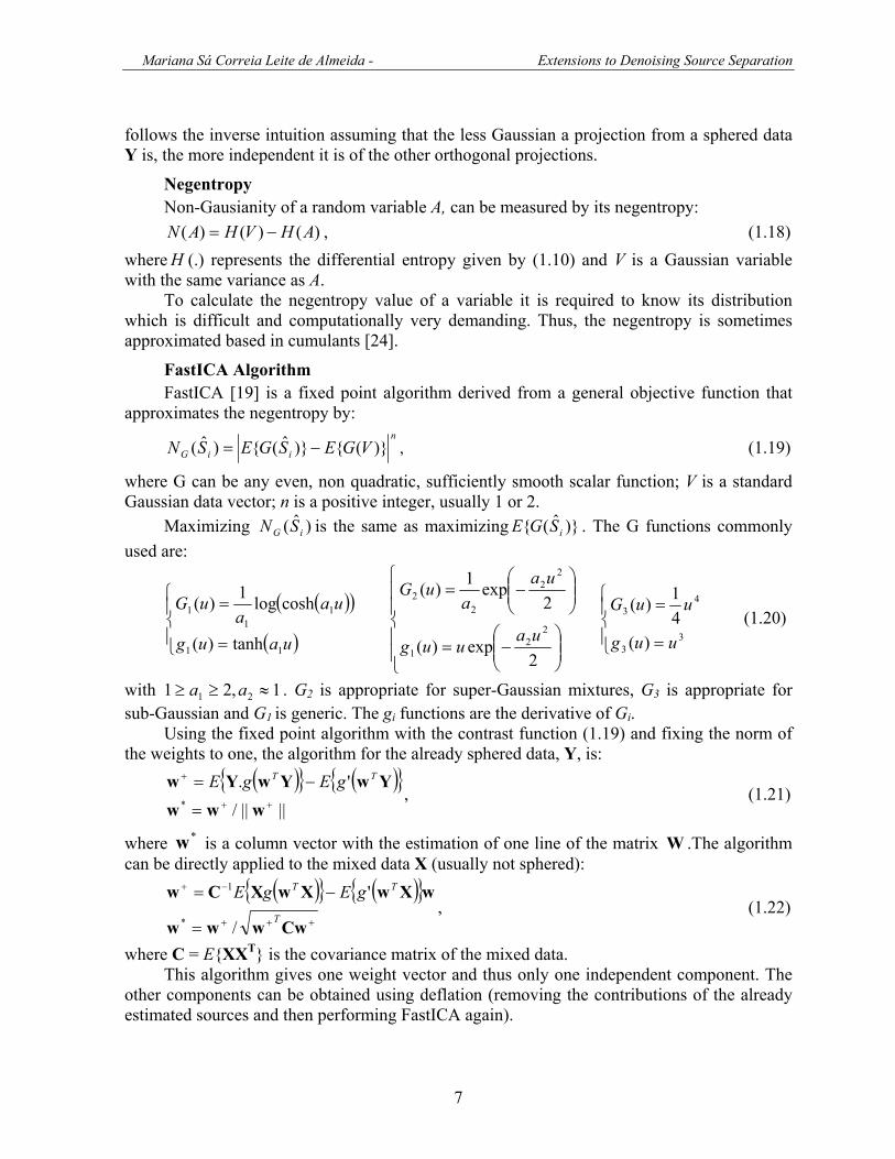
FastICA Algorithm FastICA [19] is a fixed point algorithm derived from a general objective function that
approximates the negentropy by: n
iiG VGESGESN )}({)}ˆ({)ˆ( −= , (1.19)
where G can be any even, non quadratic, sufficiently smooth scalar function; V is a standard Gaussian data vector; n is a positive integer, usually 1 or 2.
Maximizing )ˆ( iG SN is the same as maximizing )}ˆ({ iSGE . The G functions commonly used are:
( )( )
( )⎪⎩
⎪⎨
⎧
=
=
uaug
uaa
uG
11
11
1
tanh)(
coshlog1)(
⎪⎪
⎩
⎪⎪
⎨
⎧
⎟⎟⎠
⎞⎜⎜⎝
⎛−=
⎟⎟⎠
⎞⎜⎜⎝
⎛−=
2exp)(
2exp1)(
22
1
22
22
uauug
uaa
uG
⎪⎩
⎪⎨⎧
=
=
33
43
)(41)(
uug
uuG (1.20)
with 1,21 21 ≈≥≥ aa . G2 is appropriate for super-Gaussian mixtures, G3 is appropriate for sub-Gaussian and G1 is generic. The gi functions are the derivative of Gi.
Using the fixed point algorithm with the contrast function (1.19) and fixing the norm of the weights to one, the algorithm for the already sphered data, Y, is:
( ){ } ( ){ }||||/
'.* ++
+
=
−=
wwwYwYwYw TT gEgE
, (1.21)
where *w is a column vector with the estimation of one line of the matrix W .The algorithm can be directly applied to the mixed data X (usually not sphered):
( ){ } ( ){ }+++
−+
=
−=
Cwwww
wXwXwXCwT
TT gEgE
/
'*
1
, (1.22)
where C = E{XXT} is the covariance matrix of the mixed data. This algorithm gives one weight vector and thus only one independent component. The
other components can be obtained using deflation (removing the contributions of the already estimated sources and then performing FastICA again).

Mariana Sá Correia Leite de Almeida - Extensions to Denoising Source Separation
8
1.2.4 MISEP The MISEP algorithm [21] performs BSS of linear and nonlinear mixtures using ICA
and can be seen as an extended version of infomax for non-linear mappings. In order to separate nonlinear mixtures, the algorithm substitutes the demixing F block of figure 1.2 by an MLP (A-Φ-B in figure 1.4). Like infomax, MISEP maximizes the entropy of the output though a gradient learning rule, which corresponds to maximize the following objective function [21]:
xzJ
J
∂∂
=
= ∑=
K
k
k
KE
1
|det|log1
. (1.23)
where kJ is the value of J of the k-th training pattern, and K is the number of training patterns. Since the network of the demixing system is a more complex network, the gradient
learning rule is obtained by backpropagating the error derivative, requiring for that the computation of the jacobian J, as can be concluded from (1.23). This computation is preformed in an auxiliary network (lower of the net represented in figure 1.4). The MISEP network, corresponding to the Infomax network shown in figure 1.2, can be seen in figure 1.4
Figure 1.4 – Esquematic representation of the network used by MISEP. The top part
corresponds to figure 1.2, drawn in a different way. The lower part, which computes the Jacobian proper, is essentially a linearization of the upper part, but propagates matrices. It has
as input the identity matrix, and provides at its output the Jacobian J. (Adapted from [21]).
In the upper part of the net, the three first blocs (A-Φ-B) correspond to the F block of infomax (in the present case nonlinear) and perform the separation. The last three block’s of the upper part of the net (C-Φ-D), corresponding to the ψ’s of infomax, and estimate the cumulative distribution of the original sources. In Infomax ψ’s are increasing limited nonlinear functions, in MISEP is a function with values in [0,1], i.e., )ˆ( iii sz φ= is restricted in order to zi ∈[0,1] . The lower part of the net is the one that computes the Jacobian J that is required to the learning rule, as shown in (1.23). The backpropagation is preformed though the net, but the input is only applied to the lower part and is given by:
TE −=∂∂ J
J. (1.24)

Mariana Sá Correia Leite de Almeida - Extensions to Denoising Source Separation
9
Note that there is no input to the backpropagation in the upper part of the net:
0=∂∂
zE . (1.25)
MISEP minimizes the mutual information of the estimated sources, making them more independent, as far as the net (C-Φ–D) gets the closer to the respective cumulative function [21]. This estimation of the cumulative function is crucial to the success of the separation.
1.2.5 Other Methods: Two other important methods in linear ICA should be referred: JADE and TDSEP. The
first was developed by Cardoso [28] and uses fourth-order joint cumulants to perform ICA. The joint cumulant kkl of two random variables 1S and 2S are given by the joint cummulant-generative function, as follows:
( ) ( )∑∞
=
=0,
2121 !!),(ˆlog
lk
lk
kl ljt
kjtktth . (1.26)
JADE takes advantage on the fact that joint cumulants are zero for two or more independent random variables. Denote by cumklmn=cum( kS , lS , mS , nS ) the joint cumulant corresponding to the coefficient of (jtk) (jtl)(jtm)(jtn) in the expression of the joint cumulate-generative function. JADE finds the linear transformation FXS =ˆ such that the components of S are independent by diagonalizing a part of the four-index array cumklmn [28].
The TDSEP (Temporal Decorrelation source SEParation) method [29] is essentially identical to SOBI (Second order Blind Identification) and exploits the time-domain structure to perform ICA. TDSEP assumes that sources S(t) and mixtures X(t) are function of time. If the sources S(t) are zero mean stochastic processes independent from one another, then Si(t) must be uncorrelated with Sj(t-τ), if ji ≠ , for any delay τ. If the sources have temporal correlation it is normal to find sets of delays that force the problem to have the solution that corresponds to independent components. TDSEP starts by whitening the data AXY = , and afterwards finds the rotation WYS =ˆ such that the lines of S would be simultaneously uncorrelated for several delays [29].
The Nonlinear ICA problem provides, without any extra constrains, an infinite set of solutions. Post-nonlinear mixtures are an important special case with structural constraints and consist in a nonlinear transformation of each component come from a linear mixtures. Those mixtures exist in real problems and are interesting because this nonlinear ICA problem presents almost the same indeterminations as linear ICA. The separation of post-nonlinear mixtures is performed by minimizing the mutual information of the estimated sources and uses for that the inverse mixtures process [30].
Some nonlinear ICA methods are based on variational Bayesian learning methods, which are Bayesian methods designed for greater computational efficiency. Variational Bayesian learning methods provide in practice the regularization needed for BSS and ICA. The application of these methods to BSS consists in estimating the sources S and the mixing mapping )ˆ(SM , which have most probably generated the observed data X. [31].

Mariana Sá Correia Leite de Almeida - Extensions to Denoising Source Separation
10
A recent nonlinear ICA method is kernel-based nonlinear ICA (kTDSEP) [32]. The method uses the temporal structure of data, a fact that gives kTDSEP the particular interesting capacity of successfully dealing with indetermination of nonlinear ICA. The method performs nonlinear ICA based on the fact that if we make a linear mapping from the space of mixtures χ , into another space χ (usually called feature space) and then perform linear separation in
that space, that will correspond to a nonlinear transformation in the original space. The choice of this nonlinear mapping is perform by choosing a kernel [32].
1.3 Denoising Source Separation Denoising Source Separation (DSS) is a recent algorithm [3, 25, 33] that separates linear
mixtures. Usually in real-life problems some information about the desired sources is available and DSS takes advantage of this knowledge to perform a robust and faster separation.
The classical version of DSS explains the idea of DSS in three steps (figure 1.5). First the data is sphered (figure 1.5 (b)). Afterwards a denoising function is applied to the sphered data, in order to make thinner the undesired sources (figure 1.5 (c)). Finally, the desired source is given by the principal component of the denoised data (figure 1.5 (c)).
Figure 1.5 – Data evolution during the three steps of the classical version of DSS
(adaptedted from [33]).
Considering that DSS uses some information about the sources, the method is not completely blind. However, DSS does not require too much information about the sources; it only needs to differentiate the sources. Differently from ICA, DSS can be seen as a semi-blind algorithm and is able to separate mixtures of Gaussian and non-Gaussian distributions. The iterative version of DSS is given by [25, 33]:
)(
)(
+
+
=
=
==
ww
Yxw
sfxYws
new
den
denden
norm
T
T
,
)30.1()29.1()28.1()27.1(
neww is a column vector with the estimation of one line of the matrix W ; )(sfden is the denoising function. The resulting +w , in each iteration, is the one that transforms s in denx in the least-mean-squares (LMS) sense. The iterative application of (1.27) to (1.30) consists in a modified power method [34] with the addition of a denoising step (1.28). If the denoising function is instantaneous, DSS results in a nonlinear principal component analysis (NPCA).
If the denoising function applied to all data (classical version of DSS) is linear:

Mariana Sá Correia Leite de Almeida - Extensions to Denoising Source Separation
11
*YDXden = , (1.31)
the denoising step (1.28) is also linear and is given by: sDsfden =)( , (1.32)
T**DDD = . (1.33) In DSS with linear denoising (when the denoising function is linear), the corresponding
objective function is [25]: TTT
ling sDswZZws ==)( . (1.34)
If the denoising function is nonlinear, we have DDS with nonlinear denoising and the approximation suggested to the objective function [25] is:
)()(ˆ ssfs denTg = (1.35)
The use of the denoising function )(sfden in the iterative version of the algorithm does not give the same solution as applying )(Yfden to all data and then performing PCA. If the denoising function in the iterative version )(sfden is linear, there is simple correspondence to
)(Yfden , as given in (1.32) and (1.33). To a nonlinear denoising function )(sfden there is no simple correspondence.
There is a version of the algorithm that can determine more than one source at the same time. In this case, the iterative algorithm can be compared to the symmetric power method and is given by:
)(
)(
+
+
=
=
==
WW
YXW
SFXWYS
new
den
denden
orth
T
)39.1()38.1()37.1()36.1(
In the simultaneous version, given by (1.36) to (1.39), the normalization step is replaced by the orthomornalization step in order to keep the estimated sources separated. This modification is essential to ensure that the algorithm does not converge to identical solutions. The orthonormalization used in step (1.39) is symmetric and it is given by:
( ) WWWW 21
)( −= Torth (1.40)
An example of a denoising function that can be usefully used in the simultaneous version is 3)( ssfden = (resulted from masking the signal s by s2). This will correspond to FastICA with G3 apart from an additional term s3 in the denoising function that does not change the fixed point, as will be seen.
Speed up One way to accelerate DSS is by applying spectral shifting, a method usually used to
speed up the convergence of the power method [34]. The spectral shifting is achieved in DSS by applying the denoising function
[ ]sssfss den )()()( βα +=+ , (1.41)

Mariana Sá Correia Leite de Almeida - Extensions to Denoising Source Separation
12
instead of )(sfden . The fixed point is the same but the convergence can be achieved in a faster way if the scalar functions )(sα and )(sβ are correctly chosen. A reasonable spectral shifting is, for instance, the one that cancels the Gaussian noise and can be approximately implemented by [25]:
TVVTVgβ T /)(/)(ˆ denf=−= , (1.42)
where V is the standardized Gaussian variable and T the size of V. The function that results from the application of spectral shifting proposed (1.42) to the
deniosing function 3)(' ssfden = is:
sssfden 33)('' 3 −= , (1.43)
and the DSS algorithm would be the same as FastICA with G3. Other way of achieving a faster convergence is to use an adaptive rule for γ step:
∆www adapt γ+= (1.44) 2||||/ oldold ∆w∆w∆w T
oldnew γγ += , (1.45)
where w+ will be substituted by wadapt, the new estimated vector before the normalization step; ∆w is defined as w+-w; the step of the next iteration will be γnew and γold is the step of the present iteration. The technique of using an adaptive step is also useful to improve stability. In contrast with other adaptive step methods [35] DSS does not have any control that uses the objective/cost function. The corresponding control is done by the denoising step jointly with the orthonormalization of the weights.
1.4 Problems to be solved The aim of this work was to develop two extensions to DSS. The first one consisted in
an online extension to DSS and was not applied to a real-life problem. The problems to be solved with the developed online version of DSS were synthesized: the sources used were two dimensional super-Gaussian synthesized signals and the mixtures were also synthesized. Three synthetic non-stationary mixtures with different characteristics were studied.
The extensions of DSS to nonlinear mixtures were performed focusing on a specific real-life nonlinear problem. The problem under study results from the nonlinear mixture of the front- and back- page images of an "onion skin" paper when the front page is acquired with a scanner. The resulting mixture is strongly nonlinear and linear separation does not perform acceptable results. The images used in this study were carefully acquired with a Cannon LIDE 50 desktop scanner and processed in order to align as much as possible the mixed images with each other and the source images with the mixture mixtures. The characteristics of the images used in this work are described on more detail in section 3.1.
This problem had already been studied by L. B. Almeida in [9]. In this work the images were reasonably separated by the application of the MISEP method. Since the original images are not fully independent, a nonlinear version of DSS, which is not based on independency criteria, would be able to have a better performance.
Mariana Sá Correia Leite de Almeida - Extensions to Denoising Source Separation
13
2 DSS extension to an online version This chapter is dedicated to the extension of DSS, developed in order to be applied in a
stochastic way (online). The theoretical extensions proposed are described in section 2.1. The results are presented in Section 2.2 followed by the conclusions, in Section 2.3.
2.1 Online DSS Algorithms can be implemented either in batch mode, by processing the whole signal in
each iteration, or in a stochastic or online way, by processing one sample at a time. One advantage of implementing an online version of DSS is the simplification of the computation complexity, when the data and the mixing matrix are large. Another advantage is the possibility of handling mixtures that change in the sample dimension (usually time).
To implement DSS online all DSS phases need to implement in a stochastic version. These phases are pre-whitening and the application of the algorithm itself:
)()()( ttt AWF = , (2.1) where t is the indexes the sample dimension, A(t) performs whitening and W(t) is the W rotation matrix already defined for the DSS method.
To perform an online DSS that follows non-stationary mixtures, the two previous phases of DSS have to be implemented online and should be able to follow changes in the sample dimension. Since algorithms that perform whitening online already exist, this step will be discussed afterwards the online determination of W (last step of DSS).
Online DSS The determination of matrix W(t) to be applied to previously sphered data, Y, will
involve steps similar to those involved in the iterative DSS. However, they are applied to only one sample at a time. In the original version of DSS (batch), the direction of the new separation vector w is estimated taking in to account the contribution of each sample (1.29), consequently each sample has part of the information about the global w. Based on the fact that each sample gives a contribution to the estimated vector, the proposed online version of DSS is given by:
)(
)(
)()(
+
+
+=
=
==
www
yw
yw
new γnorm
xt
sfxts
den
denden
T
,
)5.2()4.2()3.2()2.2(
where t indexes the sample dimension and the parameter γ is the step size, which can be used to accelerate (if increased) or to stabilize (if decreased) the convergence of the method. Compared with the batch version, the basic difference relies on the fact that w+ in the online version is, for each sample, the increment of w related to the sample, instead of the new estimated w.
If the vector w is pointing in the right direction, the increments +w will, on average, point to the same direction and the vector w will be stable, due to the normalization step (2.5). Equation (2.5) gives a wnew vector that is closer to w+ than w was. The proposed adaptation will only work if the γ step is small enough such that the norm of the increment is much

Mariana Sá Correia Leite de Almeida - Extensions to Denoising Source Separation
14
smaller than one. Otherwise, the new w can suffer a deviation instead of stochastic oscillation and get closer to other demixing vector. The fact that the increment has to be small restricts the dynamics of the mixture that the algorithm is able to follow.
The proposed online algorithm can be modified to act in a simultaneous way. In this version, (2.6) to (2.9), the normalization step is substituted by an orthonormalization step. Using the simultaneous version we can not only extract more components, but also stabilize the algorithm. If all the components are extracted at the same time, all the space generated by the mixtures will be covered and the possibility of a switch of components will be reduced by the use of the orthonormalization step. In the simultaneous version that extracts all the components the γ parameter and the increment matrix γW+ can be much larger, thus allowing the following of mixtures with faster dynamics.
)(
)(
)()(
+
+
+=
=
==
WWW
yxW
sfxWys
new
den
denden
γorth
t
t
T .
)9.2()8.2()7.2()6.2(
In DSS (batch) the γ step could be adapted in order to achieve stability and speedup at the same time, but it was performed after the analysis of all data. In this online version of DSS the γ parameter is chosen in order to achieve a compromise between stability (smaller values of γ) and adaptation speed (larger values of γ). An suitable adaptation rule for the γ parameter will be different from the one proposed for the original version of DSS (batch) and will probably require more memory than only one sample. No automatic choice of γ was implemented, and the choice was performed manually according to the problem.
Since the adaptation of γ is not done, the speedup is only implemented with the spectral shifting, that would be included in the denoising function. This choice has also to be done by the user, but a reasonable choice would be the one proposed for the batch version (1.41).
Sphering online There are several algorithms to whiten or sphere data and usually, they are already
implemented in a stochastic version. An easy way of whiten data is performing PCA followed by normalization (Figure 1.9(b)
and Figure 1.9(c)). However, the online algorithms that whiten data based on online PCA are not prepared to follow changes of the whitening matrix, once they do not have the normalization step online, but only the ortogonalization step.
The algorithm developed by Silva F. M. and Almeida L. B. [36] performs whitening online and in a isotropic way. This algorithm has a hebbian and an anti-hebbian term and is able to follow the dynamics of the data. In the online version of this algorithm the whitening matrix A is adapted in each sample as follows:
))()(()1()()(
)()(
Tnew
T
ttββtt
tt
vyAAyAv
Axy
−+=
=
=
, )12.2()11.2()10.2(
where y is the estimated whitened signal and β is a parameter that must be small enough in order to ensure that the algorithm converges. The larger this β parameter is, the higher the

Mariana Sá Correia Leite de Almeida - Extensions to Denoising Source Separation
15
importance of the present sample is and more easily the algorithm will adapt to different data, but less stable it will become.
Mean extraction The method used to whiten data should be applied to zero mean data. Consequently, if
data do not have zero mean, the mean should be also extracted online. The mean can be estimated using the mean of all of the already analyzed samples:
[ ] [ ]( )
[ ] [ ]K
kkEkkE
kmeankE)()1()1()(
)(...)2()1()(xXX
xxxX+−⋅−
=
=.
)14.2(
)13.2(
Assuming that the mean also changes in time, a time window should be considered. In this case the estimation of the mean can be given, for instance, by
[ ] [ ]
rr
kkErkE j 1)1(1)()1().1()( +−−
+−−=
xXX , 10 << r (2.15)
Smoothing the results The capability of the proposed online DSS to follow mixtures will depend on the
dynamics of the mixture, as well as on the parameters β and γ that will control the dynamics (stability and velocity) of the evolution of the two adaptive matrix, W and A, respectively.
The evolution of these matrices shows a “turbulence” typical of stochastic algorithms. This undesired oscillation can be overcome by filtering the evolution of the matrix.
The smoothing used consists in an approximation of a Gaussian filter and it can be more or less strong according to the variance of the Gaussian, which is another parameter to be chosen according to the problem.
The smoothing technique used was implemented to be applied to the A matrix after obtaining its evolution in the sample dimension. This technique was applied in batch mode because it was easier and the main objective was to detect changes in the sample dimension. However, the implementation can be done online; it only requires a delay due to the filtering process.
Initialization In order to follow a variable mixture, it is much easier to track than to converge and
track. In the online DSS case the difficulty level is even more representative, since two matrices must be estimated.
A procedure is implemented to estimate the initial values of A and W. This procedure receives a window of samples and calculates the matrices A and W for this group of samples in batch mode. The initial matrix A is obtained by isotropic whitening and the matrix W is obtained by applying DSS using a fixed number of iterations.
Restricted application to stationary signals As mentioned before in this report (section 1.2), linear SS is usually achieved apart from
a permutation and scaling. If the mixtures changes in the sample dimension, the separation matrix F has to be determined for each sample, thus the indetermination of scaling and permutation will be present in each sample. As explained in this section the permutation

Mariana Sá Correia Leite de Almeida - Extensions to Denoising Source Separation
16
problem can be controlled considering the estimated matrix F during the previous iteration/sample and assuming that the demixture matrix is smooth enough in the sample dimension. On the other hand, the scaling can not be predicted without any extra information on the data or mixture process.
The present algorithm gives the correct separation angle. The separation norm is such that the estimated sources are stationary with unit variance. This occurs due to the separation process that is given, in each sample, by to the orthonormalization followed by the matrix W that is orthonormalized. In the original DSS (in batch) the estimated sources have unit variance; in the proposed online version of the algorithm, the estimated sources are stationary with unit variance. The proposed online version is able to separate the stationary part of the sources.
2.2 Results The data used were stationary. As referred in section 2.1, the data should be stationary
such that a non-stationary mixture could be detected. To test the performance of the proposed online implementation, a number of experiments
were carried out. First, the performance of W(t) was tested with a pre-whiten data. Subsequently experiments with both W(t) and A(t) were carried out. For all the experiments the mean was previously extracted. Synthetic mixtures of super-Gaussian signals were used in the experiments. The two dimensional super-Gaussian signals used were generated in Matlab as follows:
2),2()),2((_ TrandnTrandnsignorigX ⋅= , (2.16) where T is the number of samples of the signal.
The denoising function used gives DSS equal to FastICA, sssf 3)( 3
2 −= , (2.17) consequently, all the conclusions taken from the experiences of this chapter are also valid for FastICA.
Practical considerations The implementation of the online DSS version is collected, with other methods, in an
interface. More information about the interface and the functions used is given in Appendix B.
2.2.1 Synthetic non-stationary mixtures applied to pre-whiten data: Two synthetic source signals given by (2.16) were generated. The data were pre-
whitened and a variable orthonormal mixture was applied, so that the mixture will change but the observed data were still white, i.e., the first synthetic mixture consisted in a rotation. W(t) was calculated online with the instructions given by (2.6) to (2.9). The evolution of W(t) was finally filtered in order to eliminate the stochastic oscillations. In order to filter W(t), an approximation of a Gaussian filter was used, by applying a FIR filter (function filter.m in Matlab). The filter used was a Gaussian filter with standard deviation correspondent to 200 samples and with the size restricted to 1001 samples. The size of the filter used results in a 500 samples delay. The results obtained for W(t), after undoing the delay, are exposed in figure 2.1 .

Mariana Sá Correia Leite de Almeida - Extensions to Denoising Source Separation
17
Figure 2.1 - Weight evolution of matrix W obtained for the first synthetic mixture. The
demixing matrix (inverse of M) is represented by the light green line. The evolution of W11 (in dark blue) is overlapped by the evolution of W22 (in light blue).
The capability of tracking the mixture depends on the value of the γ step size parameter, which should be large enough. By comparing the evolution of W before and after filtering, the

Mariana Sá Correia Leite de Almeida - Extensions to Denoising Source Separation
18
stochastic noise is eliminated by the filter used. However, this post-filtering reduces the high frequencies and sudden changes can not be followed so well, as can be seen in the last 2000 iterations of figure 2.1 (f). There is a compromise between stability and speed.
The same experiment was done in order to track only one source. The applied algorithm only normalizes the separation vector (2.2) to (2.5).The mixture represented in figure 2.1 was applied and the γ parameter could not be larger then 0.005 in order to follow the mixture without switching the sources. The value of the step size parameter and the dynamics of the mixture are considerably less restricted in the case of the application of the algorithm used to extract all the components simultaneously (2.6) to (2.9) (γ not larger then 0.04).
2.2.2 Synthetic non-stationary mixture: The performance of the proposed online version of DSS was evaluated by applying a
synthetic mixture that contains a non-stationary rotation and scaling (second synthetic mixture) to a two dimensional source generated by (2.16) followed by variance normalization. The results obtained in this experiment are shown in figure 2.2.
Figure 2.2 - Results obtained for the second synthetic mixture. The value of γ was 0.002 and βwas 0.002. The demixing matrix (inverse of M) is represented by the light green line.

Mariana Sá Correia Leite de Almeida - Extensions to Denoising Source Separation
19
As can be seen in figure 2.2, the non-stationary mixture was followed. Both A(t) and W(t) matrix changed in time in order to adapt to the dynamics of the mixture and the stationary of the sources was essential for that.
The filter used in this experiment is the same already used in the experiment described in section 2.3.1 and the correspondent delay was compensated in order to analyze the results. Once the filter was applied twice in this experiment (to A and to W), the delay of the final separation matrix F is the double of the experiment described in section 2.2.1 (1000 samples).
2.2.3 Synthetic non-stationary mixtures with a singular stage: Considering non-stationary mixtures, the mixture may change such that will pass
through a singular stage. This corresponds to a dimension reduction due to the fact that two mixtures collapse in one. The reduction of dimension affects the performance of the developed solution, especially due to the determination of the matrix A(t) that performs the whitening and diverges in this situation. If the singular stage is fast, the matrix A will not have time to diverge and will continue adapting with the correct values after the singularity has passed. In order to analyse non-stationary mixtures that passes through a singular stage, two inverse mixtures were synthesized (the third and the fourth synthetic mixtures). The third synthetic mixture is shown in figure 2.3 (a) and the corresponding demixture is in figure 2.3 (b). The fourth mixture generated is the inverse of the third one, so the fourth mixture still possible to observe in figure 2.3.
Figure 2.3 – Description of the third synthetic mixture. The evolution of W11 (in dark blue) is covered by the evolution of W22 (in light blue). The evolution of W12 (in green) is covered by
the evolution of W21 (in red).
The evolution of the third synthetic mixture and of the fourth synthetic demixture (figure 2.3 (b)) is zoomed due to the existence of a discontinuity near the iteration 5000. The weights go to infinite and “come back” switched.
For both experiments the initial values of A and W were estimated using the first 150 samples of the mixture. The values of the dynamic parameters β and γ were manually adapted to the problem. The results obtained by applying the third mixture to the same sources used in the experiment described in section 2.2.2, are shown in figure 2.4.

Mariana Sá Correia Leite de Almeida - Extensions to Denoising Source Separation
20
Figure 2.4 - Results obtained for the third synthetic mixture. The value of γwas 0.005 and βwas 0.005. The demixing matrix (inverse of M) is represented by the light green line.
The separation of the third synthetic mixture was correctly followed in most of the samples (green line in figure 2.4 (d)). However, the estimated sources were exchanged close to the iteration 5000 due to a discontinuity of the separation matrix resulting from the singularity of the mixture, as shown in figure 2.3. The algorithm presumes that the separation matrix is relatively smooth (never discontinuous) and the absence of this requirement compromises the matrix estimation. In this case the angle of mixture may not be correctly followed, resulting in a switch of sources and/or in a switch of the sources sign.
The fourth mixture was applied to the same sources. The results related to the fourth synthetic mixtures are shown in figure 2.5.

Mariana Sá Correia Leite de Almeida - Extensions to Denoising Source Separation
21
Figure 2.5 - Results obtained for the fourth synthetic mixture. The value of γwas 0.005 and βwas 0.005. The demixing matrix (inverse of M) is represented by the light green line and the
symmetric matrix of M (-M) is represented in black.
The separation of the fourth synthetic mixtures was also followed most of the time. As occurred for the second synthetic mixtures, the estimated matrix is not correctly followed close to the 5000 iteration, which is due to the singularity of the demixture. In the present experiment the sources switched and the sign of the first estimated source (represented by lines blue and red of figure 2.5) also switched.
The filter used in both experiments with a nonsingular stage (second and fourth synthetic mixtures) was the same used in section 2.2.1 and 2.2.2, consequently the corresponding delay of matrix F is 1000 samples.
2.3 Conclusions The possibility of implementing DSS online that would be able to follow mixtures in
time was examined. A stochastic version to performs isotropic the whitening [36] was used and the iterative DSS was also modified in order to implement a successful online version.

Mariana Sá Correia Leite de Almeida - Extensions to Denoising Source Separation
22
This online implementation of the DSS was tested with two stationary sources and was able to follow the changes.
The implemented online DSS was able to follow mixtures of two stationary super-Gaussians sources that changes in time. However, in the presence of a singularity in the mixture or demixture process, the condition required to follow the sources (continuity of separation and sphered data followed by orthonormalization) are not satisfied and the estimated sources may switch.
The choice of the parameters β and γ depends on the specific problem under study and will affect the stability and adaptability of the separation dynamics.
The proposed online version for DSS gives a solution with unit and stationary variance. Even if not all the components are necessary, the use of the simultaneous version (2.6) to (2.9) with a square matrix W is preferable, since it allows the use of a larger γ step value without switching the sources.

Mariana Sá Correia Leite de Almeida - Extensions to Denoising Source Separation
23
3 DSS extensions to separate nonlinear mixtures of two images
This chapter is dedicated to the extension of DSS, developed in order to be successfully applied to separate the real-life problem of nonlinear mixtures of two images. The real life-problem to be solved is exposed in section 3.1 and the theoretical extensions proposed are described in section 3.2. The results are presented in Section 3.3 followed by the conclusions in Section 3.4.
3.1 The real-life problem to be solved The extensions of DSS to nonlinear mixtures were performed focusing on a specific real-
life nonlinear problem. The problem under study results from the nonlinear mixture of the front- and back- page images of an "onion skin" paper when the front page is acquired with a scanner.
Experiences with the five different pairs of mixtures shown from figure 3.1 to figure 3.4 were carried out. The first four pairs of images are the same used by L. B. Almeida in [9].The fifth pair of images used in [9] corresponds to the half upper part of the fifth pair of images used in the present work (figure 3.2 and figure 3.4). The images were carefully acquired with a Cannon LIDE 50 desktop scanner and processed in order to align as much as possible the mixed images with each other and the sources images with the mixtures ones.
Natural images usually have the majority of the information in the high frequency, the edges. The majority of the energy of the high frequency is concentrated in a few points of the images, spread all over the image. Consequently, the high frequency is a sparse space and it will be used to perform separation of the images. The five pairs of images under study (figure 3.1 to figure 3.4) have the high frequency as a sparse space, but they have different characteristics.
1. The first pair consists in a synthetic image generated by 25 uniform bars randomly ordered with intensities uniformly distributed between white and black. One of the original images has vertical bars and the second consists in the rotation of the first by 90º. This construction leads to an independency between the intensities of the two images and an intensity distribution close to the uniform distribution. The images are not a natural scene but the high frequency contains the main part of the information mostly concentrated in a few points that are spread among the image.
2. The second pair of images consists in two natural scenes with small details. The high frequency is scattered all over the image.
3. The third pair also consists in a natural scene but with less details and more uniform areas. Consequently, the intensity of the two original images is less close to independency, but the high frequency of the images is still sparse.
4. The fourth pair is a natural scene mixed with a text image. 5. The fifth pair consists of two text images. Since they are black and white images, the
high frequency contains all the information. Since the sources have much more area of white than of black, only a small percentage of pixels are simultaneously black in both sides of the paper.
The original images (sources) can be observed in figure 3.1 and figure 3.2.

Mariana Sá Correia Leite de Almeida - Extensions to Denoising Source Separation
24
Figure 3.1 - The first three pairs of source images used in this study.

Mariana Sá Correia Leite de Almeida - Extensions to Denoising Source Separation
25
Figure 3.2 - The last two pairs of source images used in this study.
The mixed images can be observed in figure 3.3 and figure 3.4. Besides the mixtures having a considerable linear component, the mixtures under study are strongly nonlinear and a linear separation does not provide reasonable results.

Mariana Sá Correia Leite de Almeida - Extensions to Denoising Source Separation
26
Figure 3.3 - The first three pairs of mixtures.

Mariana Sá Correia Leite de Almeida - Extensions to Denoising Source Separation
27
Figure 3.4 - The last two pairs of mixtures.
3.2 Theoretical description If we want to implement DSS in order to separate nonlinear mixtures, the mapping has to
be nonlinear and the separation matrix W has to be substituted by a nonlinear function. The idea is to substitute the step of DSS that can be seen as minimum square error
(MSE) problem (1.29) with a nonlinear function. This step can be performed, for instance, by using a multilayer preceptron (MLP). The scheme in figure 3.5 summarizes this procedure.
Mariana Sá Correia Leite de Almeida - Extensions to Denoising Source Separation
28
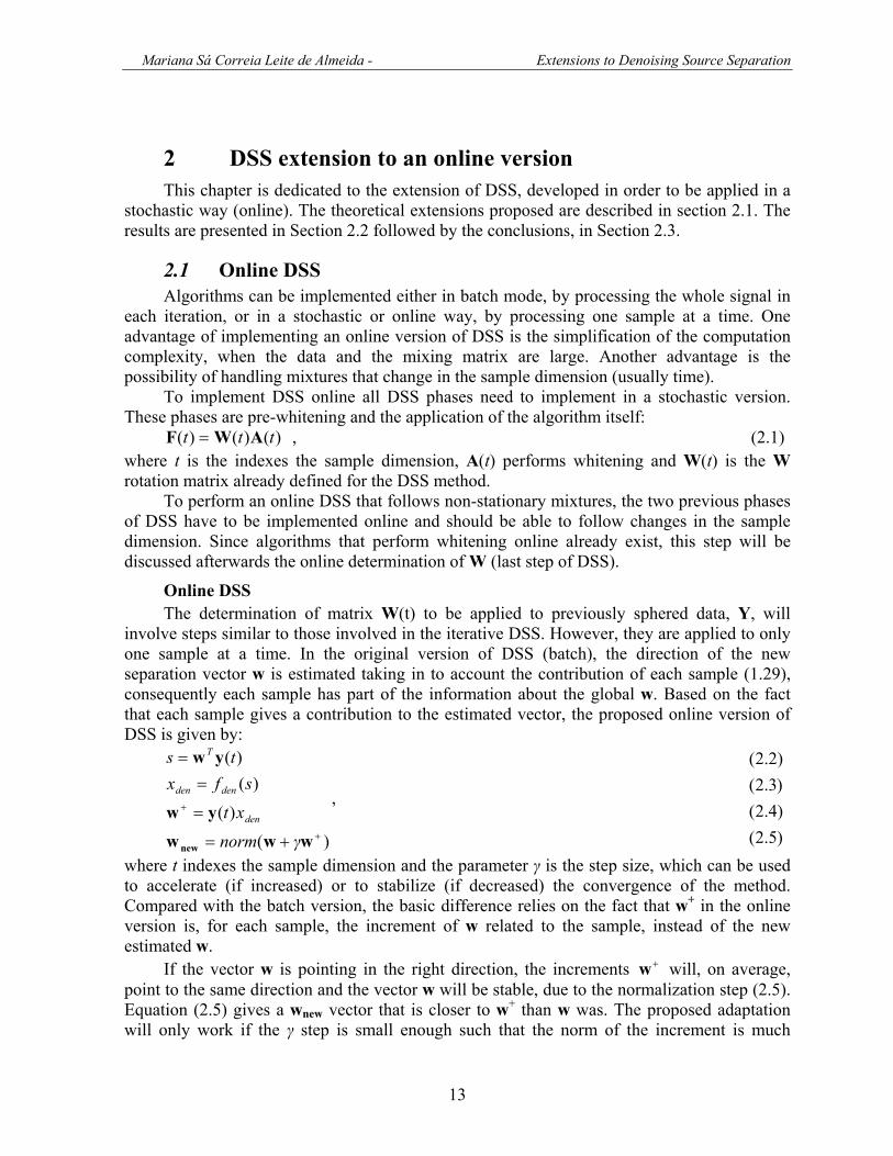
Figure 3.5- Scheme of the proposed nonlinear DSS to separate two nonlinearly mixed images.
The mixed images, X, are the input of each MLP, which should learn, in the end of the algorithm, the nonlinear transformation to separate each source. In each denoinsing iteration, the denoinsing is applied to the estimated sources S (resulting from the previous MLP learning) originating two denoised images (Xden1 and Xden2) that will be the MLP’s target to the next denoising iteration. The denoising function used performs competition in high frequency as follows: the function decomposes the received estimated sources iS in high and low frequency, performs competition in the high frequency and, finally, reconstructs the images with the original low frequency, and with the high frequency resulting from the competition.
If we have a nonlinear mapping, some of the DSS assumptions valid for linear mapping are not valid anymore. In the linear mapping the pre-whitening of data is essential so that the sources can be kept separated through an orthonormalized (rotation) matrix. If the mapping is nonlinear, the separation can not be given by the principal components after denoising the already sphered data. In this case, the function that we want to find is nonlinear and the sources have to be kept separated only by denoising. Therefore the denoising function should not only differentiate the sources but should also separate them as much as possible. To achieve this, a competition among the sources is suggested.
Like linear DSS, nonlinear DSS appears to be useful especially when the sources (in the present case images) are not close to independency, since ICA methods are not appropriate to such situations.
During this work, several denoising functions were implemented to solve the specific real-life problem described in section 3.1.
3.2.1 Initializations In DSS and in other iterative methods some initialization procedures are useful and
sometimes essential. In nonlinear DSS the whitening is not needed as an essential step of the algorithm. However, if the whitening is done in a isotropic way (isotropic whitening), it performs linear transformations that make the mixtures more separated. After whitening the source components become orthogonal (not correlated) and consequently it is expected that they will become more different. The separation preformed by applying isotropic whitening to the mixed images:

Mariana Sá Correia Leite de Almeida - Extensions to Denoising Source Separation
29
XAX ⋅=whiten , (3.1) can be observed in figure 3.6.
Figure 3.6 – Results of the application of isotropic whitening to the natural scenes mixtures.
Another information used in the initialization process relies on the fact that the mixing process is approximately symmetric, i.e., the mixture that generates the first mixed image is the same that generates the second mixed image, but with the inputs switched. To take advantage on this information we should find a linear transformation matrix Rsymmetric such that:
⎪⎪⎩
⎪⎪⎨
⎧
=
=
=
2,21,1
1,22,1
.
symmetricsymmetric
symmetricsymmetric
symmetricini
RRRR
XRX
. (3.2)
In order to maintain the initial estimated sources uncorrelated we would like to find
( ) ( )( ) ( )⎪
⎩
⎪⎨
⎧
⎥⎦
⎤⎢⎣
⎡=
=
θcosθsin-θsinθcos
symmetric
R
ARR .
⇒ (3.3)

Mariana Sá Correia Leite de Almeida - Extensions to Denoising Source Separation
30
( ) ( ) ( ) ( )( ) ( ) ( ) ( )⎩
⎨⎧
−=+
+=−
θsinθcosθcosθsin θcosθsinθsinθcos
2,1
1,1
2,22,11,1
2,21,22,1
AAAAAAAA
. (3.4)
If we square both sides of equations (3.4) and add them, the restriction (3.5) to the matrix A results.
( ) ( ) ( ) ( ) ( ) ( ) ( ) ( )( ) ( ) ( ) ( ) ( ) ( ) ( ) ( )⎪⎩
⎪⎨⎧
+−=++
++=+−
θsinθsinθcosθcos θcosθcosθsinθsin
θcosθcosθsinθsinθsinθsinθcosθcos 2222
2,122
1,222
222,2
2222221,1
2,22,21,22,11,11,1
2,21,21,22,12,11,1
22
22
AAAAAAAA
AAAAAAAA
22,2
21,2
22,1
21,1 AAAA +=+ . (3.5)
Since most of the times matrix A does not satisfy (3.5), it is not possible to perform whitening that corresponds to a symmetric operation on the two mixture components (not to be confused with the isotropic whitening mentioned in section 1.2.1). However, it is possible to take advantage on both informations at the same time. The matrices A obtained for all the pairs of images mixtures are close to symmetric operation. We can make them a symmetric process by applying:
XRX ⋅= symmetricinit (3.6)
222112112
21122211⎥⎦
⎤⎢⎣
⎡++++
=AAAAAAAA
R symmetric , (3.7)
using the matrix A, that performs isotropic whitening. The initial processing that was used (3.6) still close to the isotropic whitening, but it is a symmetric operation.
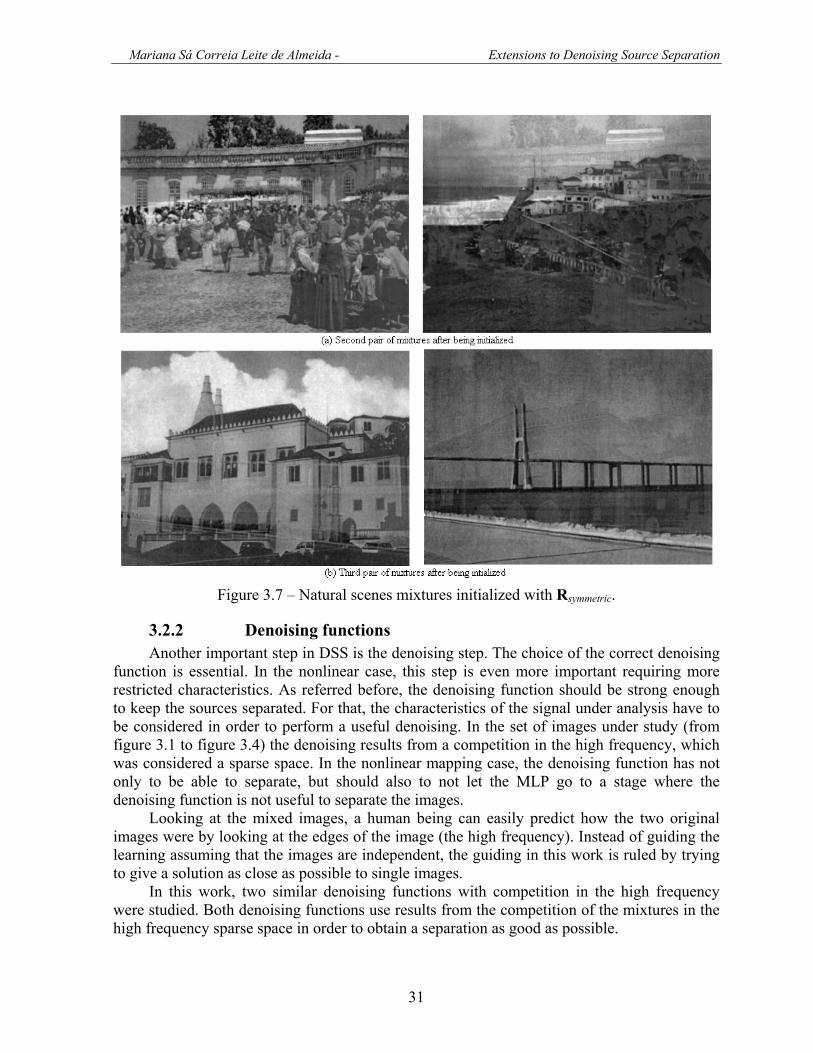
The results using this initialization are considerably better than the ones obtained using isotropic whitening and they are presented, for the natural scenes (pairs especially focused by the present work), in figure 3.7. The application of the initialization given by (3.6) and (3.7) to the other pairs of mixtures also provides an improvement to the result obtained with the isotropic whitening. These results can be observed in Appendix A.
Mariana Sá Correia Leite de Almeida - Extensions to Denoising Source Separation
31
Figure 3.7 – Natural scenes mixtures initialized with Rsymmetric.
3.2.2 Denoising functions Another important step in DSS is the denoising step. The choice of the correct denoising
function is essential. In the nonlinear case, this step is even more important requiring more restricted characteristics. As referred before, the denoising function should be strong enough to keep the sources separated. For that, the characteristics of the signal under analysis have to be considered in order to perform a useful denoising. In the set of images under study (from figure 3.1 to figure 3.4) the denoising results from a competition in the high frequency, which was considered a sparse space. In the nonlinear mapping case, the denoising function has not only to be able to separate, but should also to not let the MLP go to a stage where the denoising function is not useful to separate the images.
Looking at the mixed images, a human being can easily predict how the two original images were by looking at the edges of the image (the high frequency). Instead of guiding the learning assuming that the images are independent, the guiding in this work is ruled by trying to give a solution as close as possible to single images.
In this work, two similar denoising functions with competition in the high frequency were studied. Both denoising functions use results from the competition of the mixtures in the high frequency sparse space in order to obtain a separation as good as possible.

Mariana Sá Correia Leite de Almeida - Extensions to Denoising Source Separation
32
Other two specific denoising functions were implemented for the first and fifth pairs of mixtures. Due to the mixing process itself, one of the original sources is more intense in each mixture. This fact was explored in order to get denoising functions in which the competition may separate the sources.
Competition in high frequency The competition function used in this work was created to be applied to the high
frequencies of the estimated sources and the competition is given by:
iii Maskuuuncompetitio ⋅=),( 21 , (3.8)
⎟⎟
⎠
⎞
⎜⎜
⎝
⎛
⎟⎟⎠
⎞⎜⎜⎝
⎛
+
−⋅−+
=
22
22
exp1
1
ji
ji
i
uu
uua
Mask . (3.9)
These equations must be applied following the normalization of the energy of the signals, as follows.
2ii x=σ (3.10)
⎟⎟⎠
⎞⎜⎜⎝
⎛⋅=
j
j
i
iiii
xxncompetitioXden
σσσ , . (3.11)
The corresponding value of the energy is re-inserted after the competition process, as shown in (3.11).
The larger the positive parameter a is in (3.9), the stronger the competition becomes. If the value of a is large enough, the competition can be seen as a “winner take all”.
The competition function is such that: • if x1 >> x2, the pixel of x1 will be masked by 1 and x2 by 0. • if x1=x2 the mask for both signals is 0.5. • if x1 << x2, the pixel of x1 will be masked by 0 and x2 by 1. • if x1 and x2 are exchanged the masks also are exchanged (symmetric property) • the mask of x1 plus the mask of x2 is always equal to 1. This symmetric and local competition (each pixel competes separately) is applied to the
high-frequencies components of the images, after the normalization of their energies. This normalization makes the global process of competition not local. For the function with wavelet competition (to be presented ahead) this normalization is essential. Otherwise, both outputs may converge to the same solution.
The performance of the competition can be seen in figure 3.8 In figure 3.8 (a) the high frequencies of the two images of the third pair of mixtures is shown. As can be seen in figure 3.1 the house is slightly more intense in the first mixture while the bridge is more intense in the second mixture. The different intensity of the both sources can also be seen in the high frequency (figure 3.8 (a)). The competition performs correctly this separation in the high frequency, as shown in figure 3.8 (b).

Mariana Sá Correia Leite de Almeida - Extensions to Denoising Source Separation
33
Figure 3.8 - High frequencies of the third pair of images, before and after competition.
Denoising function using a filter (first denoising function) Since the high frequency is a sparse space, this denoising function uses a filter to obtain
the low and high frequency components of the images, and performs the competition in the high frequencies components. The denoised images, which will be used as MLPs’ target, result from the composition of the unchanged low frequency of each image with the corresponding high frequency images after competition.
The experiments presented, were not obtained using this denoising function, but using instead another function that has the same basis but uses wavelet decomposition. The same generic conclusion that will be taken for the denoising function with wavelet decomposition can be taken for this denoising function. However, the one with wavelet decomposition proved to be more powerful.
Denoising function using wavelets (second denoising function) In this denoising function the images are decomposed into wavelet components. The four
components resulting from the wavelet decomposition have ¼ of the pixels of the images before the decomposition. One of the components (A in figure 3.9) is an image similar to the image before decomposition but four times smaller. The other three images contain vertical, horizontal, and diagonal edges. The competition is applied in the three vertical (V in figure 3.9), horizontal (H in figure 3.9) and diagonal (D in figure 3.9) components of the mixed

Mariana Sá Correia Leite de Almeida - Extensions to Denoising Source Separation
34
images. After competition, these three components are used for the reconstruction of the denoised images. The level of wavelet decomposition should be higher than one (n in figure 3.9) and the denoised images result from the wavelet reconstruction after all Hi, Vi and Di components have competed. The number of times that the wavelet decomposition is performed (recalls of the denoising function) is controlled using the size of the low frequency components. This control requires that both dimensions of these components be larger than a fixed number of pixels (N in figure 3.9).
Figure 3.9 - Schematic representation of the second denoising function. On left it is shown the scheme of one image wavelet decomposition in n levels (the components represented by bold boxes are the ones that will be submitted to the competition). On right it is shown the scheme
of the denoising decomposition and the reconstruction of the denoised images.
A “stronger” separation can be performed by using a deeper wavelet decomposition, as well as a larger value of parameter a. In general, it is better to have a stronger separation when the images are more mixed. A deeper level of wavelet decomposition is better to forget the background of the undesired source, as can be seen by comparing figure 3.10 (a) with figure 3.11 (a). On the other hand, a lower level of wavelet decomposition helps to maintain the image definition (figure 3.10 (b) with figure 3.11 (b)).

Mariana Sá Correia Leite de Almeida - Extensions to Denoising Source Separation
35
Figure 3.10 – Results of the application of the wavelet based denoising function to the second (331x438 pixels) and third (330x443 pixels) pairs of mixtures and sources, using a deep level of decomposition (application of wavelet decomposition until the size of one dimensions is
lower than 20).

Mariana Sá Correia Leite de Almeida - Extensions to Denoising Source Separation
36
Figure3.11 – Result of the application of the wavelet-based denoising function to the second (331x438 pixels) and third (330x443 pixels) pairs of mixtures and sources, using a shallow
level of decomposition (application of wavelet decomposition until the size of one dimensions is lower than 160).
In general, it is suitable to a stronger competition (deeper level and higher value of a) for the initial part of the algorithm and to use a softer one in a further stage of the separation.
The wavelet decomposition level that was applied to all remaining tests is given by the requirement that both dimensions of the decomposed images should be larger than 80. The application of this denoising function to the second and third pairs of mixed images after being initialized (figure 3.7) can be seen in figure 3.12. Several 2-D wavelet decompositions are

Mariana Sá Correia Leite de Almeida - Extensions to Denoising Source Separation
37
available in Matlab. After a practical inspection the images were denoised with the wavelet ‘rbio1.5’. Due to the use of a sparse space the images in figure 3.12 are quite separated already.
Figure 3.12 - Images resulted from the application of the denoising function to the natural scenes mixtures already initialized. Wavelet decomposition applied until the size of one
dimensions be lower than 80.
Denoising function for bar images (third denoising function) When we look at the first pair of pictures we may guess that the original sources are
probably composed by a mixture of vertical and horizontal bars. Based on this visual information we can design a specific denoising function where one of the outputs only has vertical edges and the other only has horizontal edges. This function can be obtained by making wavelet decomposition and, subsequently, by reconstructing the respective images with the horizontal or the vertical high frequencies set to zero (specific competition). The level of the wavelet decomposition can also be changed. As can be seen in figure 2.13, this denoising function is very efficient, due to the characteristics of the sources that were easy to observe and detect.

Mariana Sá Correia Leite de Almeida - Extensions to Denoising Source Separation
38
Figure 3.13 - Result of the application of the specific denoising function created for bar
images to the first pair of mixtures, already initialized. Wavelet decomposition was applied until the size of one dimension becomes lower than 20.
Denoising function for text images (fourth denoising function) Looking at the fifth pair of mixtures we may understand that this is a mixture of two
black and white images from text. The fact that the sources are black and white simplifies the separation. A simple and efficient denoising function for this kind of mixtures should attribute fixed levels for intensity values higher or lower than a determinate intensity value. For the images initialized with (3.6) and (3.7), an appropriated bounding value is the middle intensity value, as the quite separated denoised images confirm (figure 3.14).
Figure 3.14 – Result of the application of the specific denoising function created for text
images to the half upper part of the fifth pair of mixture already initialize.
The result shown in figure 3.14 has the pages practically separated. After training the MLP, the middle intensity value may not be the best to perform separation. This happens
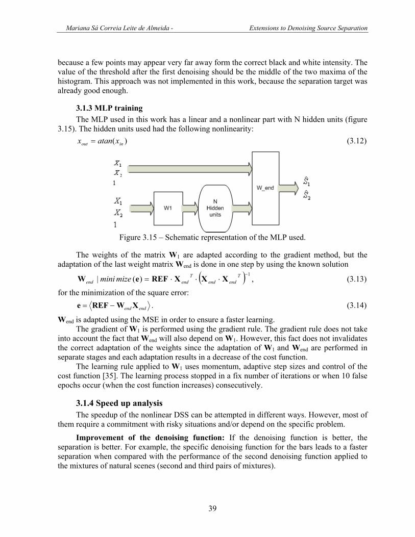
Mariana Sá Correia Leite de Almeida - Extensions to Denoising Source Separation
39
because a few points may appear very far away form the correct black and white intensity. The value of the threshold after the first denoising should be the middle of the two maxima of the histogram. This approach was not implemented in this work, because the separation target was already good enough.
3.1.3 MLP training The MLP used in this work has a linear and a nonlinear part with N hidden units (figure
3.15). The hidden units used had the following nonlinearity: )( inout xatanx = (3.12)
Figure 3.15 – Schematic representation of the MLP used.
The weights of the matrix W1 are adapted according to the gradient method, but the adaptation of the last weight matrix Wend is done in one step by using the known solution
( ) 1)(|
−⋅⋅⋅= T
endendT
endend mizemini XXXREFeW , (3.13)
for the minimization of the square error:
endend XWREFe −= . (3.14)
Wend is adapted using the MSE in order to ensure a faster learning. The gradient of W1 is performed using the gradient rule. The gradient rule does not take
into account the fact that Wend will also depend on W1. However, this fact does not invalidates the correct adaptation of the weights since the adaptation of W1 and Wend are performed in separate stages and each adaptation results in a decrease of the cost function.
The learning rule applied to W1 uses momentum, adaptive step sizes and control of the cost function [35]. The learning process stopped in a fix number of iterations or when 10 false epochs occur (when the cost function increases) consecutively.
3.1.4 Speed up analysis The speedup of the nonlinear DSS can be attempted in different ways. However, most of
them require a commitment with risky situations and/or depend on the specific problem.
Improvement of the denoising function: If the denoising function is better, the separation is better. For example, the specific denoising function for the bars leads to a faster separation when compared with the performance of the second denoising function applied to the mixtures of natural scenes (second and third pairs of mixtures).

Mariana Sá Correia Leite de Almeida - Extensions to Denoising Source Separation
40
It can be difficult to improve the denoising function and this will depend on the problem under analysis and on the information available to perform the separation.
Reduction of the number of points for the MLP learning: The MLP learning is a time consuming task. One way of reducing the duration of the MLP learning is by decreasing the number of points of the image used in the learning. The reduction of points used in learning without an extra control is also dangerous, since, if the selected points are not significantly representative of the image, a deviation may occur and the algorithm my not be able to recover.
Reduction of the number of iterations of the MLP: Reducing the number of the MLP iterations will produce a faster MLP response. Most of the learning occurs during the first steps of the MLP learning. The learning is stopped after a small number of iterations and it will continue in the next iteration of the algorithm having the next denoised images as MLP target.
Using fewer hidden units: By reducing the complexity of the MLP, the learning complexity is reduced. However, the reduction of hidden units is restricted by the complexity of the separation problem.
3.1.5 Quality measures The images resulting from the application of nonlinear DSS can be visually analysed.
However, this visual inspection is observer dependent. A good quality measure for the level of separation would be one that compares the
solutions with the original sources. The mutual information can be used to measure how close the solutions are from the original sources. Mutual information is given by (1.9) where Shannon’s deferential entropy is, for continuous variables, given by (1.6). For discreet variables the Shannon’s entropy is given by (3.16).
)()()( YY HYHIi
i −= ∑ (3.15)
))(log()()( kk
k ypypYH ∑−= , (3.16)
where k indexes the discreet variable Y and p(yk) is the probability of yk. In order to calculate the mutual information the expressions (1.9) and (3.16) were
initially used. The solutions were shifted and scaled between 0 and 255 (as well as the sources).
In order to compare the results obtained with the ones obtained by Almeida L. B. in [9] the same mutual information (MI) estimator was used. This estimator is the one described in [37] with k=3 and the code was directly downloaded from [38]. Two measures based on mutual information were computed:
withSSIQ
SSIQ
ji
ii
),ˆ,(
)ˆ,(
4
3
=
=
ij ≠
)18.3()17.3(
Two other measures used in [9] were also calculated. One of the measures is the signal to noise ratio (SNR) between the original sources and the estimated images:
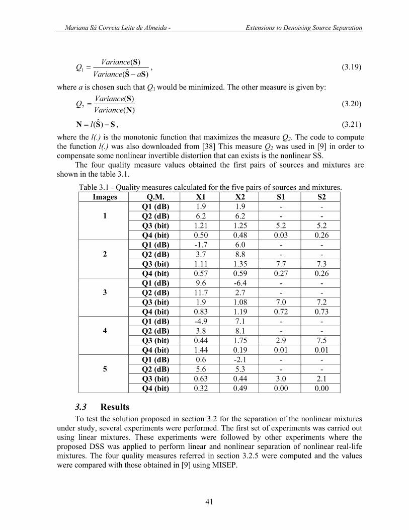
Mariana Sá Correia Leite de Almeida - Extensions to Denoising Source Separation
41
)ˆ()(
1 SSS
aVarianceVarianceQ
−= , (3.19)
where a is chosen such that Q1 would be minimized. The other measure is given by:
)()(
2 NS
VarianceVarianceQ = (3.20)
SSN −= )ˆ(l , (3.21) where the l(.) is the monotonic function that maximizes the measure Q2. The code to compute the function l(.) was also downloaded from [38] This measure Q2 was used in [9] in order to compensate some nonlinear invertible distortion that can exists is the nonlinear SS.
The four quality measure values obtained the first pairs of sources and mixtures are shown in the table 3.1.
Table 3.1 - Quality measures calculated for the five pairs of sources and mixtures. Images Q.M. X1 X2 S1 S2
Q1 (dB) 1.9 1.9 - - Q2 (dB) 6.2 6.2 - - Q3 (bit) 1.21 1.25 5.2 5.2
1
Q4 (bit) 0.50 0.48 0.03 0.26 Q1 (dB) -1.7 6.0 - - Q2 (dB) 3.7 8.8 - - Q3 (bit) 1.11 1.35 7.7 7.3
2
Q4 (bit) 0.57 0.59 0.27 0.26 Q1 (dB) 9.6 -6.4 - - Q2 (dB) 11.7 2.7 - - Q3 (bit) 1.9 1.08 7.0 7.2
3
Q4 (bit) 0.83 1.19 0.72 0.73 Q1 (dB) -4.9 7.1 - - Q2 (dB) 3.8 8.1 - - Q3 (bit) 0.44 1.75 2.9 7.5
4
Q4 (bit) 1.44 0.19 0.01 0.01 Q1 (dB) 0.6 -2.1 - - Q2 (dB) 5.6 5.3 - - Q3 (bit) 0.63 0.44 3.0 2.1
5
Q4 (bit) 0.32 0.49 0.00 0.00
3.3 Results To test the solution proposed in section 3.2 for the separation of the nonlinear mixtures
under study, several experiments were performed. The first set of experiments was carried out using linear mixtures. These experiments were followed by other experiments where the proposed DSS was applied to perform linear and nonlinear separation of nonlinear real-life mixtures. The four quality measures referred in section 3.2.5 were computed and the values were compared with those obtained in [9] using MISEP.
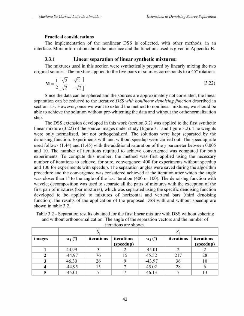
Mariana Sá Correia Leite de Almeida - Extensions to Denoising Source Separation
42
Practical considerations The implementation of the nonlinear DSS is collected, with other methods, in an
interface. More information about the interface and the functions used is given in Appendix B.
3.3.1 Linear separation of linear synthetic mixtures: The mixtures used in this section were synthetically prepared by linearly mixing the two
original sources. The mixture applied to the five pairs of sources corresponds to a 45º rotation:
⎥⎦
⎤⎢⎣
⎡
−=
2222.
21M . (3.22)
Since the data can be sphered and the sources are approximately not correlated, the linear separation can be reduced to the iterative DSS with nonlinear denoising function described in section 1.3. However, once we want to extend the method to nonlinear mixtures, we should be able to achieve the solution without pre-whitening the data and without the orthonormalization step.
The DSS extension developed in this work (section 3.2) was applied to the first synthetic linear mixture (3.22) of the source images under study (figure 3.1 and figure 3.2). The weights were only normalized, but not orthogonalized. The solutions were kept separated by the denoising function. Experiments with and without speedup were carried out. The speedup rule used follows (1.44) and (1.45) with the additional saturation of the γ parameter between 0.005 and 10. The number of iterations required to achieve convergence was computed for both experiments. To compute this number, the method was first applied using the necessary number of iterations to achieve, for sure, convergence: 400 for experiments without speedup and 100 for experiments with speedup. The separation angles were saved during the algorithm procedure and the convergence was considered achieved at the iteration after which the angle was closer than 1º to the angle of the last iteration (400 or 100). The denoising function with wavelet decomposition was used to separate all the pairs of mixtures with the exception of the first pair of mixtures (bar mixtures), which was separated using the specific denoising function developed to be applied to mixtures of horizontal and vertical bars (third denoising function).The results of the application of the proposed DSS with and without speedup are shown in table 3.2.
Table 3.2 - Separation results obtained for the first linear mixture with DSS without sphering and without orthonormalization. The angle of the separation vectors and the number of
iterations are shown.
1S 2S images w1 (º) iterations iterations
(speedup) w2 (º) iterations
iterations (speedup)
1 44,99 3 2 -45.01 2 2 2 -44.97 76 15 45.52 217 28 3 46.30 26 9 -43.97 36 10 4 -44.95 15 7 45.02 28 6 5 -45.01 7 7 46.13 7 13

Mariana Sá Correia Leite de Almeida - Extensions to Denoising Source Separation
43
Since the results obtained correspond to rotations near +/- 45º, the separation was correctly performed for experiments with and with out speedup. The fact that the correct result was achieved means that, if the denoising function is competitive enough, as it is in the present case, it is possible to perform linear separation without pre-whitening the data and without the orthonormalization step. Actually, experiments using the proposed DSS and the denoising function sssfden 3)( 3 −= showed that this denoising function is also competitive enough to be used without the orthonormalization step and without sphered data (only normalized data). The speedup used reduced successfully the number of iterations needed to converge.
The original DSS was applied to the second linear synthetic mixture of images, which consists in a rotation of 45º from the isotropically pre-whitened sources. If the sources were orthogonal the solution would be the rotation of 45º. However, the sources are not exactly orthogonal and the correct demixture will not correspond to a rotation. The denoising functions and the speedup technique used in the present experiment were the same used before in the experiment with the proposed DSS. The iterative DSS was applied using a large enough number of iterations to guaranty convergence: 200 for experiments without speedup and 100 for experiments with speedup. The iteration where the convergence was considered achieved was computed using the same criterion used in the previous experiment (iteration after which the angle will be closer than 1º to the last angle).The results obtained by the application of the original DSS with and without the speedup are shown in table 3.3.
Table 3.3 - Separation results obtained with the original DSS applied to the second linear mixture. The angle of the separation vectors obtained with DSS (w), the correct angle of
separation (wref) and the number of iterations are shown. images w1 (º) w1ref(º) W2 (º) w2ref(º) iterations
iterationsspeedup
1 44.99 45.00 -45.01 -45.00 2 2 2 -44.93 -44.96 45.08 44.95 32 10 3 46.26 46.36 -43.74 -47.80 20 6 4 45.59 43.94 -44.41 -44.05 13 15 5 -44.43 -44.35 45.57 44.46 7 10
The results obtained using DSS also converged to a solution very close to the correct sources, indicating that the denoising functions were appropriate. This outcome was expected since the algorithm already converged without the orthonormalization step. The fact that the denoising function proposed does not require the orthonormalization step makes the algorithm suitable to obtain solutions that correspond to correlated sources, while the original DSS is restricted to uncorrelated solutions.
The solutions obtained with the original DSS without any speedup technique required less iterations to converge than the results obtained with the proposed DSS (without the orthonormalization step). In general, the application of the speed up technique reduces the number of iterations required to achieve convergence. However, the application of the original DSS to the fourth and fifth pair of mixtures required a slightly higher number of iteration to converge (2 and 3 iterations respectively). This fact indicates a failure of the speed up technique used. The number of iterations required to achieve convergence using the proposed DSS and the speedup technique is similar to the number of iterations required when the original DSS when the speedup technique was used.

Mariana Sá Correia Leite de Almeida - Extensions to Denoising Source Separation
44
3.3.2 Linear separation of nonlinear real-life mixtures: The nonlinear DSS proposed in this work was applied to perform linear separation of the
five pairs of nonlinear mixtures (figure 3.3 and figure 3.4), aiming at obtaining linear separations that approximate the sources (figure 3.1 and figure 3.2).
The specific denoising function for the images with vertical or horizontal lines was used to separate the first mixture of images (synthetic bars images). The denoising function with wavelet decomposition was used to separate the second, third and fourth pairs of images. In order to separate the last mixture of images the specific denoising function for mixtures of text images was used.
The solutions obtained for the linear separation of the first, third and fifth pairs of images were visually and numerically acceptable. These results are shown in figure 3.16 and in table 3.4. Since the fifth pair of mixtures occupies a large space, figure 3.16 only shows the representative half upper part of the images obtained from the application of the algorithm to this pair of mixtures.
For the second and fourth pairs of mixtures, the algorithm did not give separated solutions (figure 3.17). This may be due to the fact that, for these images, the linear separations were not able to get close enough to the initial denoised images, converging to stable points far from an acceptable linear separation. The linear application of the proposed DSS to the second pair of mixtures gave rise to a solution where the different sources are more visible in different areas of the same image (figure 3.17).
Table 3.4 shows the rotation in degrees suffered by the normalized mixed images with the application of the algorithm proposed (DSS’), as well as the best rotation obtained by using the minimum square error (MSE) relative to the sources.
Table 3.4 - Separation vector angles obtained by applying nonlinear DSS (DSS’) and MSE to real mixtures.
DSS’ MSE Rotation
for 1S 2S 1S 2S
Pair 1 (º) 33.21 56.83 33.75 56.28 Pair 2 (º) 54.48 84.72 37.35 62.96 Pair 3 (º) 21.71 50.00 23.92 48.24 Pair 4 (º) 64.62 55.99 41.17 58.46 Pair 5 (º) 37.97 50.38 36.68 51.18
Consistent with visual observations, the algorithm gives for the first, third, and fifth pairs of mixtures, solutions close to those obtained by minimization of the square error using the original images as targets. Also in agreement with visual observations, the solutions obtained for the second and fourth pairs of mixtures are far from the ones obtained with MSE.
The measures Q1, Q2, Q3 and Q4 defined in section 3.2.5 are given in table 3.5. For better results Q1, Q2 and Q3 values should be higher, while Q4 should be smaller. These measures were calculated using the results obtained in the experiments described in this section (DSS’). The quality measures calculated for the minimization of the square error (MSE) as well as for the results obtained in [9] using MISEP with linear separation, are also shown in table 3.5. For the last pair of images, the quality measures of DSS’ and linear MISEP can not be compared (MISEP only used the half upper part of the fifth pair of mixtures).

Mariana Sá Correia Leite de Almeida - Extensions to Denoising Source Separation
45
Figure 3.16 – “Good” results obtained with the proposed algorithm using linear separation.

Mariana Sá Correia Leite de Almeida - Extensions to Denoising Source Separation
46
Figure 3.17 - “Bad” results obtained with the proposed algorithm using linear separation.
The quality measures shown in table 3.5 indicate that the proposed algorithm preformed well for the separation of the first, third, and fifth pairs of mixtures but was not suitable to separate the other pairs of mixtures. The values of the four quality measures are, for the first and third pairs of mixtures, similar to those obtained with linear MISEP. The Q4 values obtained using MSE indicate that the solutions are not independent.
Since the mixture is nonlinear, the best linear demixing does not have to be orthogonal in order to separate the whitened data. However, the “best” images resulting from the linear approximation are probably not correlated and thus, the application of the original DSS (with orthonormalization) would have been correct. The results obtained using MISEP reinforce the idea that it is correct to assume the independency of the sources. Nevertheless, the quality measures computed for the images resulted from the application of the proposed DSS to the first and third pair of mixtures (the only pairs of mixtures that gave rise to comparable satisfactory results) are slightly better than those obtained with MISEP.

Mariana Sá Correia Leite de Almeida - Extensions to Denoising Source Separation
47
Table 3.5 – The four quality measures for the separation results of the real mixture obtained with DSS’, with MSE and with MISEP.
Img. QM S1 DSS’
S2 DSS’
S1 MSE
S2 MSE
S1 MISEP
S2 MISEP
Q1(dB) 9.7 9.5 9.7 9.5 9.0 8.7 Q2(dB) 11.9 11.7 11.8 11.6 11.9 11.6 Q3 (bit) 2.1 2.1 2.2 2.1 2.03 1.96
1
Q4 (bit) 0.51 0.60 0.58 0.55 0.48 0.46 Q1(dB) -8.7 6.7 7.4 11.0 5.2 10.5 Q2(dB) 2.1 9.7 10.0 13.2 8.1 12.9 Q3 (bit) 0.72 1.49 1.6 1.6 1.56 1.78
2
Q4 (bit) 1.38 0.56 0.28 0.55 0.37 0.53 Q1(dB) 13.4 7.13 13.6 7.8 13.4 6.6 Q2(dB) 15.3 8.3 15.2 8.8 14.7 7.9 Q3 (bit) 2.2 1.4 2.2 1.4 2.13 1.34
3
Q4 (bit) 0.72 0.46 0.76 0.47 0.71 0.46 Q1(dB) -7.93 12.2 4.1 12.9 4.5 11.2 Q2(dB) 1.42 13.3 7.4 13.8 7.8 12.4 Q3 (bit) 0.36 2.0 0.85 2.2 0.80 1.99
4
Q4 (bit) 1.6 0.22 0.41 0.18 0.36 0.18 Q1(dB) 5.0 3.5 5.1 3.6 - - Q2(dB) 7.8 6.7 8.2 6.9 - - Q3 (bit) 0.84 0.65 0.85 0.66 - -
5
Q4 (bit) 0.15 0.18 0.19 0.19 - -
3.3.3 Nonlinear separation of nonlinear real-life mixtures: The DSS with nonlinear mapping was applied to the second and third pairs of mixtures
(natural scenes mixtures) as well as to the synthetic mixtures of bars (first pair of mixtures). For the two mixtures with natural scenes the denoising function with wavelet decomposition was used. This denoising function was developed according to the characteristics of the natural scenes considering that it explores the sparsity of the high frequency, as detailed in section 3.2.2. The a parameter used in the competition was set to 40 and the competition was essentially a “winner take all” function. For the bar images, the specific denoising function was used.
Figure 3.18 shows the images resulting from 10 denoising iterations using one MLP with 5 hidden units to learn each denoised image. Each MLP uses, to learn, 50 iterations at the most. The simple criterion used to stop the proposed DSS extension and the separation consisted in using a fixed number of denoising iterations. The values of the measures Q1, Q2, Q3 and Q4 for the results obtained in these experiments are shown in table 3.6. This table also shows the measures obtained using MISEP with the nonlinear separation [9] and the measures obtained by minimizing the square error (MSE) using an MLP with 5 hidden units.
As expected, for all the images under study, the value of Q3 (mutual information) is higher for the original sources (table 3.1) than for the approximation of the sources by using

Mariana Sá Correia Leite de Almeida - Extensions to Denoising Source Separation
48
two MLPs with 5 hidden units (table 3.6 - MSE). All the measures indicate that the results obtained with the application of the proposed nonlinear DSS in this section (DSS’ in table 3.6) are better than those obtained with the linear application of the same method (DSS’ in table 3.5). In summary, the nonlinear version of the proposed algorithm gives advantages to the linear one.
Although the proposed DSS with linear mapping did not succeed when applied to the second and fourth pairs of mixtures, the same algorithm with nonlinear mapping (using an MLP) can be used with reasonable results, as indicated by the results obtained in this section for the second pair of mixtures.
The measures concerning the images obtained by training an MLP with the correct sources as target (table 3.6 - MSE) are better than the measures concerning the images obtained with the application of nonlinear DSS’ (table 3.6). However, they still are very far from the values obtained with the correct source (table 3.1). This difference may be due to the loss of information during the mixing process (non invertible function) or by the fact that the topology of the MLP is not the best one. It is possible that the demixing is a discontinuous function or that it consists in a more complex transformation.
The separation level of the results obtained in this section is similar to the separation level of the results obtained using MISEP with nonlinear separation in [9]. The measures corresponding to the first pair of images indicate that the proposed algorithm shows the best performance, most probably due to the good and specific denoising function used. MISEP is better for separation of the second pair of images, while the proposed nonlinear DSS is better to separate the third pair of images. This improvement is probably due to the fact that the original sources of this pair are the most dependent sources. The images of the third pair of images have fewer interceptions in the high frequency compared with the second pair of images. Consequently the denoising function is more suitable. The nonlinear DSS proposed is especially interesting when the sources are considerably dependent.
Table 3.6 – The four quality measures for the nonlinear separation results of the real mixtures obtained applying DSS’, MSE and with MISEP.
Pairs QM S1 DSS’
S2 DSS’
S1 MSE
S2 MSE
S1 MISEP
S2 MISEP
Q1 (dB) 14.6 14.1 15.1 14.6 13.8 13.1 Q2 (dB) 15.3 14.7 15.5 15.0 14.7 14.2 Q3 (bit) 2.57 2.5 2.6 2.5 2.45 2.39
1 Q4 (bit) 0.29 0.27 0.21 0.22 0.23 0.26
Q1 (dB) 6.44 13.6 11.2 15.6 9.3 13.9 Q2 (dB) 9.45 15.1 11.6 15.9 11.0 15.0 Q3 (bit) 1.62 1.93 1.9 2.1 1.83 1.95
2 Q4 (bit) 0.44 0.39 0.32 0.32 0.24 0.40
Q1 (dB) 13.5 9.2 15.2 9.7 14.2 6.4 Q2 (dB) 15.5 9.9 15.8 10.4 15.3 7.8 Q3 (bit) 2.23 1.62 2.2 1.7 2.19 1.29
3
Q4 (bit) 0.74 0.56 0.54 0.64 0.56 0.49
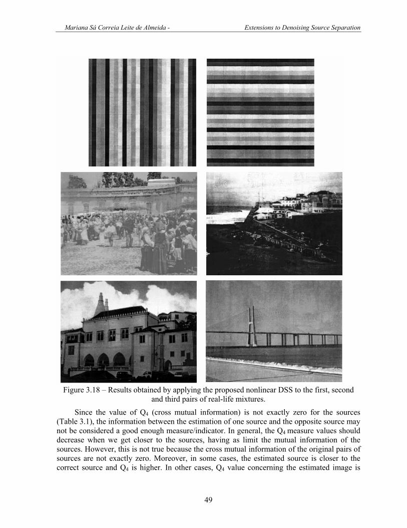
Mariana Sá Correia Leite de Almeida - Extensions to Denoising Source Separation
49
Figure 3.18 – Results obtained by applying the proposed nonlinear DSS to the first, second
and third pairs of real-life mixtures.
Since the value of Q4 (cross mutual information) is not exactly zero for the sources (Table 3.1), the information between the estimation of one source and the opposite source may not be considered a good enough measure/indicator. In general, the Q4 measure values should decrease when we get closer to the sources, having as limit the mutual information of the sources. However, this is not true because the cross mutual information of the original pairs of sources are not exactly zero. Moreover, in some cases, the estimated source is closer to the correct source and Q4 is higher. In other cases, Q4 value concerning the estimated image is

Mariana Sá Correia Leite de Almeida - Extensions to Denoising Source Separation
50
bellow the Q4 value obtained for the original source. The relation between the estimated source and the opposite original source may indicate good or bad separation depending on what makes them more or less similar. The original images are not fully independent. This fact is more remarkable for the third pair of sources and quite irrelevant for first, fourth and fifth pairs of sources (see scatter plots of the sources in figure 3.19).
Figure 3.19 – Scatter plot of the five pair of sources.
3.3.4 Experiments with more denoising iterations The experiments described in section 3.3.3 were carried out using a fixed number of
denoising iterations (10 iterations). If we let the proposed DSS continue during more denoising iterations, the estimated sources start to degenerate. This may occur due to the fact that the high frequencies of the pair of images share a few common pixels. As stated in section 3.2.2, a deeper separation should be carried out at the beginning of the algorithm and a lower separation at the end.
The proposed DSS was applied to the three fist pairs of mixtures under the same condition of experiment described in section 3.3.3 but using 50 denoising iterations. The images resulting from the application of this procedure to the second and third pair of mixtures are shown in figure 3.20. They differ significantly from the desired solutions. The edges of the palace present in the third pair of images seem to disappear and the building becomes darker. The edges of the house present in the second pair of mixtures were cut by edges of the sea and of the houses present in the other image of the pair. The inspection of the second pair of images indicates that the areas of the first solution (the degenerated) where it is still possible to unveil the original image are the areas where the second solution (not degenerated) does not have strong edges. This is the case of areas such as the sky and the floor.
The application of the proposed nonlinear DSS using more than a few number of iterations is not sustainable, except when it is applied to the first pair of mixtures (bars). A very good and specific denoising function was used to separate this pair of mixtures. However, the problem of the bar images is simpler. The ambiguity of nonlinear ICA was overcome with the proposed nonlinear DSS, but other undesired solutions appeared when the method was applied using a larger number of iterations. In section 3.3.3 the number of iterations was fixed to stop the separation. Although other more developed criterion could have been also used, the results obtained using this one (section 3.3.3) were considered satisfactory.
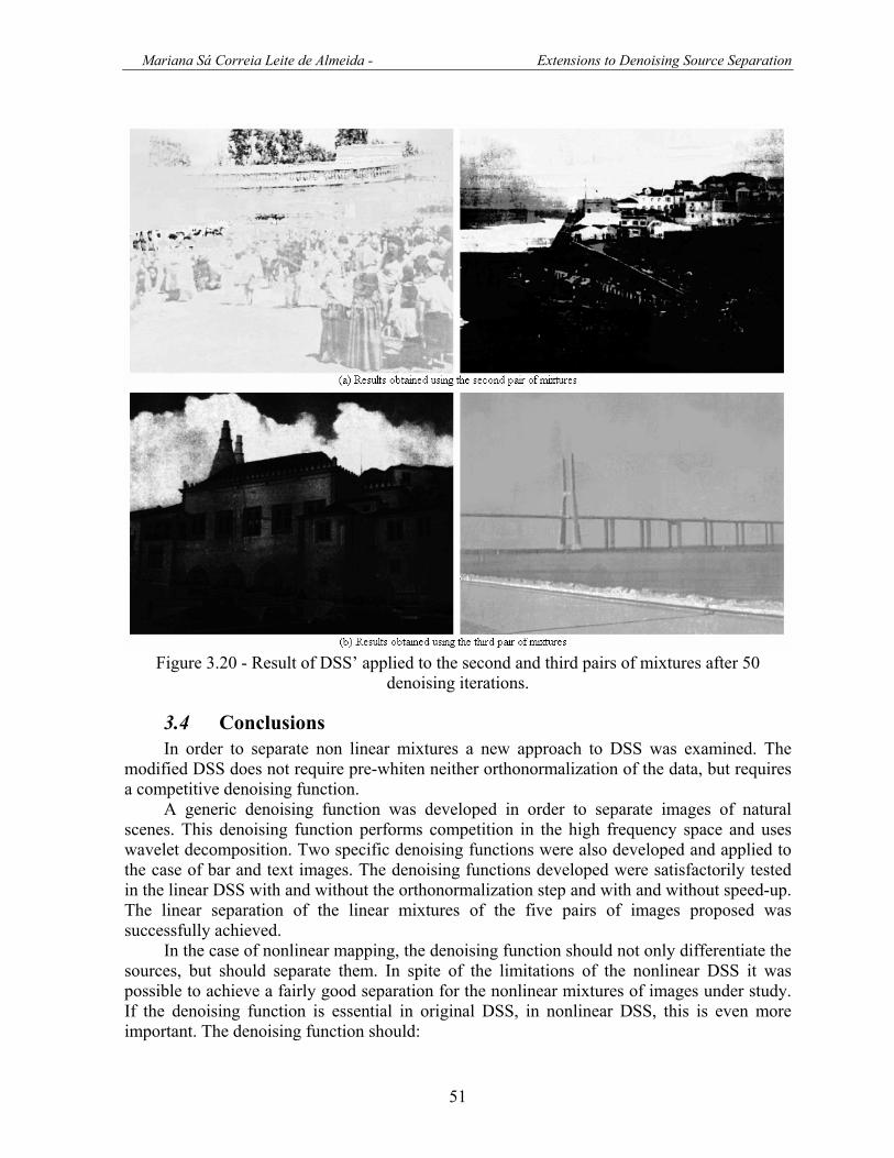
Mariana Sá Correia Leite de Almeida - Extensions to Denoising Source Separation
51
Figure 3.20 - Result of DSS’ applied to the second and third pairs of mixtures after 50
denoising iterations.
3.4 Conclusions In order to separate non linear mixtures a new approach to DSS was examined. The
modified DSS does not require pre-whiten neither orthonormalization of the data, but requires a competitive denoising function.
A generic denoising function was developed in order to separate images of natural scenes. This denoising function performs competition in the high frequency space and uses wavelet decomposition. Two specific denoising functions were also developed and applied to the case of bar and text images. The denoising functions developed were satisfactorily tested in the linear DSS with and without the orthonormalization step and with and without speed-up. The linear separation of the linear mixtures of the five pairs of images proposed was successfully achieved.
In the case of nonlinear mapping, the denoising function should not only differentiate the sources, but should separate them. In spite of the limitations of the nonlinear DSS it was possible to achieve a fairly good separation for the nonlinear mixtures of images under study. If the denoising function is essential in original DSS, in nonlinear DSS, this is even more important. The denoising function should:

Mariana Sá Correia Leite de Almeida - Extensions to Denoising Source Separation
52
- make the sources more separated (using some competition) - not return a target that makes the MLP going to a state where the denoising function
will not be able to continue the separation. To solve the problem of image mixtures, denoising functions that have the above
referred characteristics must be used. However, it is apparently very difficult to obtain a denoising function that can be successfully applied to a different problem, especially to high dimensional problems.
Apart for the specific case of the images with bars, the application of the proposed algorithm using a larger number of iterations is not sustainable. The case of the bar images is simpler and the specific denoising function does not lead to degenerated solutions. When applied to the pairs of mixtures of natural scenes, the method has to be stopped after a few iterations or another control of the applied denoising has to be used.
The proposed DSS is particularly interesting and useful when applied to sources that are partially dependent and the other source separation methods do not work. Nevertheless a denoising function capable of being successfully used for other problems may be difficult or sometimes impossible to find out.

Mariana Sá Correia Leite de Almeida - Extensions to Denoising Source Separation
53
4 Conclusions
4.1 Conclusions related with online DSS: An online version of DSS was successfully implemented. The online implementation of
DSS requires online data pre-whitening, which was performed using a stochastic isotropic algorithm. The new version of DSS yields a separation method able to follow non-stationary mixtures. The correct application of the developed online DSS is restricted to stationary signals and to continuous, non-singular (de)mixtures. The algorithm has some parameters that must be adjusted to the problem under study.
4.2 Future work related with online DSS: In order to evaluate the performance of the proposed online version of DSS, experiments
using high dimensional mixtures should be carried out. The online version proposed for DSS has several parameters that have to be manually
adapted to the characteristics of the problem under study. One way of improving the algorithm would consist of the development of an automatic strategy to determine the dynamic parameters β and γ as well as the parameters of the filter used to smooth the evolution of the weights (size and standard deviation of the filter).
Due to the scaling indetermination inherent to ICA and DSS, the implemented online version of DSS is restricted to problems with stationary sources. New strategies can be developed in order to overcome this limitation, for example, by exploring prior knowledge about the mixture or the data characteristics (using different and specific denoising functions). Independently of the strategy used, this will require extra information. Additional information can also overcome the permutation ambiguity that appears in problems where the (de)mixture becomes singular.
4.3 Conclusions related with nonlinear DSS: In order to extend DSS to nonlinear mixtures, two original steps were removed: the pre-
whitening and the orthonormalization of the data. These steps being removed, the separation is essentially performed by the denoising function, which should not only differentiate the sources but also separate them as much as possible.
In order to solve the real-life problem of nonlinear mixtures of images, specific denoising functions were developed. These denoising functions proved to be useful to separate a synthetic linear mixture of images. In the present work, the data were not pre-whitened but a useful initialization process was developed taking into account some information about the mixture process. The application of this initialization process together with the denoising functions provided a reasonable separation of the nonlinear real-life mixtures.
The objective of this work was achieved, but the application of the method to natural images proved to be unsustainable without an early stop criterion.
The application of the method to other problems may be difficult, especially in the case of high dimensional problems.
Mariana Sá Correia Leite de Almeida - Extensions to Denoising Source Separation
54
4.4 Future work related with nonlinear DSS: In order to get a better separation of mixed images and to avoid undesired solutions, a
network with the demixture may be developed. To achieve this it is crucial to understand the mixture process.
It would be interesting to develop another quality measure that would take into consideration the assumptions done for the proposed algorithm, for example, focusing on the high frequencies of the images. This measure would be more appropriate to the proposed algorithm and would assess the proposed assumptions.
In order to confirm the advantages of the method proposed in this work compared with the currently available methods, new pairs of figures should be tested. It is recommended that the images to be tested are more dependent and with fewer interceptions in high frequency
The proposed solution only takes into consideration the data characteristics. We could try to conjugate the information given by the data structure with the independence criterion.

Mariana Sá Correia Leite de Almeida - Extensions to Denoising Source Separation
55
Appendix A
Initialized images The application of isotropic whitening to the mixed images (figure 1.3 and figure 1.4)
results in two images more separated than the mixed ones. The result of the isotropic whitening to the first, fourth, and fifth pairs of mixtures can be seen in figure A.1. However, the initialization used (3.6) and (3.7) was not the isotropic whitening, but another linear transformation that conciliates the fact that the isotropic whitening separates the images and that the mixtures are close to a symmetric operation. The results of initialization of the pairs of mixtures number one, four, and five are in figure A.2.
The observation of figures A.1 and A.2 indicates that the application of the initialization given by (3.6) and (3.7), leads to a slightly better separation of the mixed images compared with the application of the isotropic whitening.

Mariana Sá Correia Leite de Almeida - Extensions to Denoising Source Separation
56
Figure 1 – First, fourth, and fifth pair of mixtures after the application of isotropic whitening.

Mariana Sá Correia Leite de Almeida - Extensions to Denoising Source Separation
57
Figure 2 – First, fourth, and fifth pair of mixtures initialized with Rsymmetric.

Mariana Sá Correia Leite de Almeida - Extensions to Denoising Source Separation
58
Appendix B
Interface During this work four source separation (SS) methods were implemented: Infomax,
FastICA, MISEP and DSS. Besides the implementation of these methods, two extensions were developed for the last method (DSS). In order to collect all the methods, a simplified interface was implemented in MatLab. The main interface can be opened by the command Guia_TFC.m , a function present in the folder “Guia”. This interface consists in a main menu where the different methods can be chosen (figure B.1).
Figure B.1 – Main interface
All the interfaces have parameters to fill as well as choices to make. The understanding of the parameters and choices is easy after reading the theoretical basis of each method (section 1.3, section 1.4, section 2.1 and section 3.1).
Figures B.2, B.3, B.4, B.5, B.6 and B.7 show the interfaces of methods Infomax, FastICA, MISEP, DSS, online DSS, and nonlinear DSS, respectively. Most of the parameters presented in these figures are the ones set by default.
Most of the methods were implemented and tested in two dimensional signals. Although the implementation has been performed in order to be applied to high dimensional signals, this was not fully tested for all the methods.
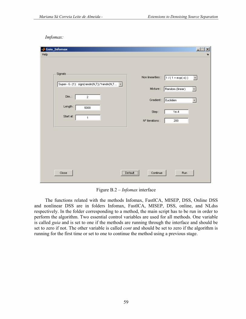
Mariana Sá Correia Leite de Almeida - Extensions to Denoising Source Separation
59
Imfomax:
Figure B.2 – Infomax interface
The functions related with the methods Infomax, FastICA, MISEP, DSS, Online DSS and nonlinear DSS are in folders Infomax, FastICA, MISEP, DSS, online, and NLdss respectively. In the folder corresponding to a method, the main script has to be run in order to perform the algorithm. Two essential control variables are used for all methods. One variable is called guia and is set to one if the methods are running through the interface and should be set to zero if not. The other variable is called cont and should be set to zero if the algorithm is running for the first time or set to one to continue the method using a previous stage.

Mariana Sá Correia Leite de Almeida - Extensions to Denoising Source Separation
60
FastICA:
Figure B.3 – FastICA interface
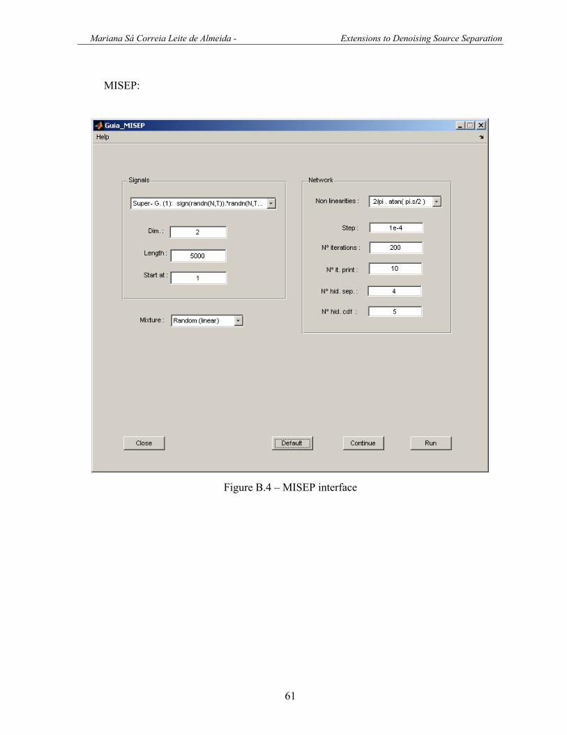
Mariana Sá Correia Leite de Almeida - Extensions to Denoising Source Separation
61
MISEP:
Figure B.4 – MISEP interface

Mariana Sá Correia Leite de Almeida - Extensions to Denoising Source Separation
62
DSS:
Figure B.5 – DSS interface

Mariana Sá Correia Leite de Almeida - Extensions to Denoising Source Separation
63
Online DSS
Figure B.6 – Online DSS interface

Mariana Sá Correia Leite de Almeida - Extensions to Denoising Source Separation
64
Nonlinear DSS:
Figure B.2 – Nonlinear DSS interface
Finally a brief description, for each method, of all the functions/scripts implemented is
presented below:
Infomax : det_nlin - Script that determines, for the nonlinearity function chosen, the terms
that are required for the learning rule. Infomax - Script that performs Infomax algorithm (main). init - Script that performs initializations required when the graphical
interface is not in use (used by initial.m). initial - Script that performs all initializations. nlin_new - Function that should be edited to implement different nonlinearities. save_inf - Script that saves to the workspace variables that may be required to
continue the algorithm or to show the results.

Mariana Sá Correia Leite de Almeida - Extensions to Denoising Source Separation
65
FastICA : esf.m - Function that performs isotropic whitening FastICA.m - Script that performs FastICA algorithm (main). initial.m - Script that performs all initializations. Initializations.m - Script that performs initializations required when the graphical
interface is not in use (used by initial.m). normliza.m - Function that normalizes the data. pca.m - Function that performs PCA. save_fast.m - Script that saves to the workspace variables that may be required to
continue the algorithm or to show the results. MISEP : const.m - Function that sets some constants required for the beginning
of each batch iteration. constantes - Function that sets MISEP constants. gera_d_sigm.m - Function that determines sigmoid derivatives for the sigmoid
chosen. gera_mistura.m - Function that mixes the sources. gera_sinais.m - Function that generates the sources. inic_red.m - Function that initializes the network. initial.m - Script that performs all initializations. Misep.m - Script that performs the algorithm MISEP (main). mostra.m - Function that displaces the scatter plots of the estimated
sources and of the variable Z. The function also shows the estimated cumulative functions.
passos_com_momento.m- Function that adapts the network weights, using an adaptive learning rule.
propaga_baixo - Function that propagates in the lower part of the net. propaga_cima - Function that propagates in the upper part of the net. rectropropaga_baixo - Function that backpropagates in the lower part of the net. rectropropaga_cima - Function that backpropagates in the upper part of the net. save_misep.m - Script that saves to the workspace variables that may be
required to continue the algorithm or to show the results. DSS : comptn.m - Function that performs the competition. comptt_.m - Auxiliary function to perform the competition (used by comtn.m). den_new.m - Function that should be edited to implement a different denoising
function. dss.m - Script that performs dss (main).
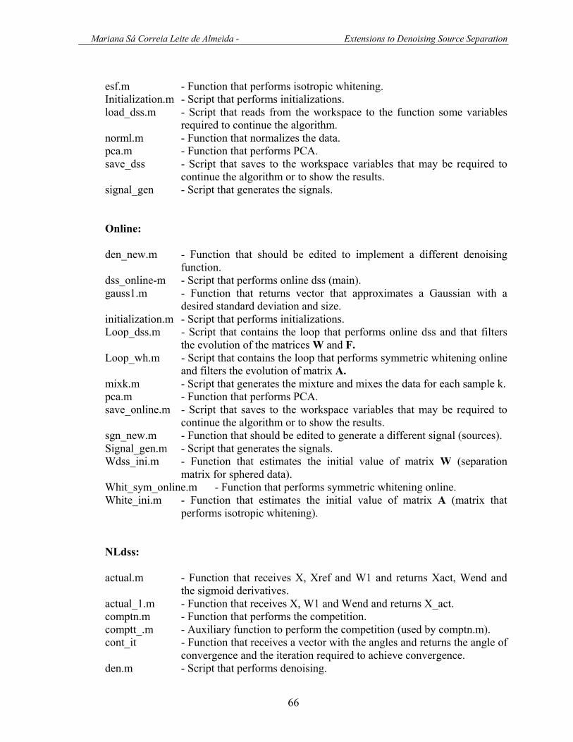
Mariana Sá Correia Leite de Almeida - Extensions to Denoising Source Separation
66
esf.m - Function that performs isotropic whitening. Initialization.m - Script that performs initializations. load_dss.m - Script that reads from the workspace to the function some variables
required to continue the algorithm. norml.m - Function that normalizes the data. pca.m - Function that performs PCA. save_dss - Script that saves to the workspace variables that may be required to
continue the algorithm or to show the results. signal_gen - Script that generates the signals. Online: den_new.m - Function that should be edited to implement a different denoising
function. dss_online-m - Script that performs online dss (main). gauss1.m - Function that returns vector that approximates a Gaussian with a
desired standard deviation and size. initialization.m - Script that performs initializations. Loop_dss.m - Script that contains the loop that performs online dss and that filters
the evolution of the matrices W and F. Loop_wh.m - Script that contains the loop that performs symmetric whitening online
and filters the evolution of matrix A. mixk.m - Script that generates the mixture and mixes the data for each sample k. pca.m - Function that performs PCA. save_online.m - Script that saves to the workspace variables that may be required to
continue the algorithm or to show the results. sgn_new.m - Function that should be edited to generate a different signal (sources). Signal_gen.m - Script that generates the signals. Wdss_ini.m - Function that estimates the initial value of matrix W (separation
matrix for sphered data). Whit_sym_online.m - Function that performs symmetric whitening online. White_ini.m - Function that estimates the initial value of matrix A (matrix that
performs isotropic whitening). NLdss: actual.m - Function that receives X, Xref and W1 and returns Xact, Wend and
the sigmoid derivatives. actual_1.m - Function that receives X, W1 and Wend and returns X_act. comptn.m - Function that performs the competition. comptt_.m - Auxiliary function to perform the competition (used by comptn.m). cont_it - Function that receives a vector with the angles and returns the angle of
convergence and the iteration required to achieve convergence. den.m - Script that performs denoising.

Mariana Sá Correia Leite de Almeida - Extensions to Denoising Source Separation
67
den_new.m - Function that should be edited to implement a different denoising function.
den_txt.m - Function used by den.m that performs the fourth denoising function (for text images).
den_V.m - Function used by den_HV.m that sets the horizontal wavelet components to zero.
den_HV.m - Function used by den.m that performs the third denoising function (bar images).
den_waven.m - Function used by den.m that performs the second denoising function (natural scenes).
esf.m - Function that performs isotropic whitening. esf_sym.m - Function that computes the initialization matrix Rsymmetric and
initializes a pair of images. inic_net.m - Script that initializes the MLPs. initial.m - Script that performs all initializations. initializations.m - Script that performs initializations required when the graphical
interface is not in use (used by initial.m). load_nl_dss.m - Function that reads from the workspace to the function variable
required to continue the algorithm. mlp_adapt - Script that performs the adaptation/learning of the weight W1. mlp_const - Script with the constants used by the MLP. mlp_dss - Script that performs nonlinear DSS (main). mlp_funct_mom - Function that performs the MLP learning. norml.m - Function that normalizes the data. pca.m - Function that performs PCA. plfig.m - Function that prints/shows pairs of images. plfig7.m - Function that prints/shows one image. plwave.m - Function that prints/shows wavelet components during the denoising Qs - Script that calculates the quality measures. save_nl_dss - Function that saves to the workspace variables that may be required to
continue the algorithm or to show the results. speed_up - Script that performs speedup (only possible to use when the mixture is
linear). zero_um - Function that shifts and scales a received variable in order to return a
variable with values between zero and one.
Mariana Sá Correia Leite de Almeida - Extensions to Denoising Source Separation
68
5 References
[1] R. Vigario , J. Särelä, V. Jousmäki, M Hämäläinen and E. Oja, “Independent
Component Approach to the Analyses of EEG and MEG Recordings”, IEEE
transactions on Biomedical Engeneering, Vol. 47, No 5, May, 2000, pp 589-93.
[2] J Särelä, H. Valpola, R. Vigário and E. Oja, “Dynamical Factor Analysis of
Rhythmic Encephalogram Activity”, Proceeding of the 3rd international Conference
Analysis and Blind Signal Separation, ICA’01 (San Diego, California, USA), 2001,
pp. 451-456.
[3] J. Särelä H. Valpola, “Denoising Source Separation”, Journal of Machine Learning
Research , Vol.6 , Mar, 2005, pp. 233-272.
[4] H,Calhoun and G. Pearlson, “Indpendent Component Analysis Applied to fMRI
Data: A Generative Model for Validating Results”, Journal of VLSI Signal
Processing, Vol. 37, 2004, pp. 281-291.
[5] K. Torkkola, “Blind Deconcolution, Information Maximization and Recursive
Filters”, Proceedings of the IEEE international conference on Acoustucs, Speech and
Signal Processing, Munich, Germany, April 21-24, 1997, pp 3301-3304.
[6] T. Ristaniemi, J. Joutsensalo, “Advanced ICA-based receivers for block fading DS-
CDMA channels”, Signal Processing, Vol. 82, 2001, pp. 417- 431.
[7] H. Szu, S. Noel, S.-B. Yim, J. Willey, J. Landa, “Multimedia authenticity with ICA
watermarking and digital bacteria vaccination”, Neural Networks, Vol. 16, 2003, pp.
907-914.
[8] S. Bounkong, B. Toch, D. Saad, D. Lowe “ICA for watermarking Digital Images”,
Journal of Machine Learning Research, Vol. 4, Dez,2003, pp. 1471-1498.
[9] L. B. Almeida, “Separating a Real-life Nonlinear Image Mixture”, Journal of
Machine Learning Research, Vol. 6, 2005, pp. 1199-1232.
[10] M. Funaro, E. Oja, H. Valpola, “Independent component analysis for artefact
separation in astrophysical images”, ,Neural Networks, Vol.16, 2003, pp. 469-478.
[11] B. A. Draper, K. Baek, M. S. Bartlett and J. R. Beveridge, “Recognizing faces with
PCA and ICA”,Computer Vision and Image Understanding ,Vol. 91, Fev. 2003, pp.
115-137.
Mariana Sá Correia Leite de Almeida - Extensions to Denoising Source Separation
69
[12] X. Zhang and C.H. Chen, “Independent Component Analysis by Using Joint
Cumulants and its Application to Remote Sensing Images”, Journal of VLSI Signal
Processing , Vol. 37, 2004, pp. 293-303.
[13] N. Kwark and C.-H. Choi, “Feature Extraction Based on ICA for Binary
Classification Problems”, IEEE transactions on knowledge and data engineenig,
Vol. 5, No. 6, Nov/Dec 2003, pp.1374-1388.
[14] E. Oja, K. Kiviluoto and S. Malaroiu, “Independent component analysis for
financial time series”, Proc. IEEE 2000 symp. On adapt. Systems for Signal Proc.,
comm.. and control, AS-SPCC, Lake Louise, Oct.1-4, 2000.
[15] A. Ilin, H. valpola, E. Oja, “Seminlind Source Separation of Climate Data Detects
El Nino as the Component with the Highest Interanual Varaibility”, In Proceedings
of the International Joint Conference on Neural Networks (IJCNN 2005), Montréal,
Québec, Canada, 2005, pp. 1722-1727.
[16] E. Bingham, J, Kuusisto and K, Lagus, “ICA and SOM in Text Document
Analysis”, The 25th ACM SIGIR 2002 International Conference on Research and
Development in Information Retrieval, Tampere, Finland, Aug. 11-15, 2002, pp. 361-
362 .
[17] P. Comon, “Independent component analysis, a new concept?”, Signal Processing,
Vol. 36, 1994, pp. 287-314.
[18] A. Hyvärinen and P. Pajunen, “Nonlinear independent component analysis:
Existence and uniqueness results”. Neural networks, Vol. 12, No. 3, 1999, pp 429-
439. [online]. Available http://www.cis.hut.fi/~aapo/ps/NN99.ps
[19] A. Hyvärinen, “Fast and Robust Fixed-Point Algorithm for Independent
Component Analysis”, IEEE trans. on Neural Networks, Vol. 10, 1999, pp. 626-634.
[20] A. Bell and T.J.Sejnowski, “An information-maximization approach to blind
separation and blind deconvolution”,.Neural Computation, Vol. 7, No. 6 , Nov. 1995,
pp. 1129 – 1159.
[21] L.B. Almeida, “MISEP – Linear and nonlinear ICA based on mutual information.”
Journal of Machine Learning Research, Vol. 4, Dec. 2003, pp. 1297-1318.

Mariana Sá Correia Leite de Almeida - Extensions to Denoising Source Separation
70
[22] S.-I. Amari. “Natural Gradient works efficiently in learning”. Neural Computation,
Vol. 10, No. 2, Fev. 1998, pp. 251-276.
[23] C. Nikias and J. Mendel, “Signal Processing with high order spectra”, IEEE signal
Processing Magazine, .Jul. 10–37, 1993, pp. 10-37.
[24] M. Kendel, A. Stuart, The advanced Theory of statistics, Charles Griffin &
Company, London, UK, 1958.
[25] J. Särelä, “Exploratory Source Separation in Biomedical Systems”, Ph. D. Thesis,
Helsinki University of Technology, Espoo, Finland, 2004
[26] S. Amari, “Natural Gradient Works Efficiently in Learning”, Neural Computation,
Vol. 10, 1998, pp. 251-276.
[27] A. Papoulis, Probability, Random Variables, and stochastic Processes, McGraw-
Hill, 3rd edition, New York, USA, 1991.
[28] J.F. Cardoso and A. Souloumiac, “Blind beamforming for non Gaussian signals”,
IEEE proceedings.F, Vol.140, No. 6 ,1993, pp.362-379. [Online]. Available :
http://www.tsi.enst.fr/~cardoso/Papers.PDF/iee.pdf
[29] A. Ziehe and K.-R. Müller, “TDSEP – an efficient algorithm for blind separation
using time structure”, in Proc. Int. Conf. on Artificial Neural Networks, Skövde,
Sweden, 1998, pp 675-680. [Online]. Available:
http://wwwold.first.gmd.de/persons/Muller.Klaus-Robert/ICANN_tdsep.ps.gz
[30] A. Taleb and C. Jutten , “Source separation in post-nonlinear mixtures” IEEE trans.
Sig. Proc., Vol. 47, 1999, pp 2807-2820.
[31] H. Lappalainen and X. Giannakopoulos, “Multi-layer preceptrons as nonlinear
generative models for unsupervised learning: a Bayesian treatment”, in Proc.
ICANN, Edinburgh, Scotland, 1999, pp. 19-24. [Online]. Avalable:
http://www.cis.hut.fi/harri/icann99.ps.z
[32] S. Harmeling, A. Ziehe, M. Kawanabed, and K.-R. Müller, “Kernel-base nonlinear
blind source separation”,Neural Computation, Vol. 15, 2003, pp. 1089-1124.
[Online]. Available:
http://ida.first.fraunhofer.de/~harmeli/papers/article_on_ktdsep.pdf.

Mariana Sá Correia Leite de Almeida - Extensions to Denoising Source Separation
71
[33] H. Valpola and J. Särelä, “Acurate, Fast and Stable Denoising Source Separation
Algorithms”, Proceedings of the First International Workshop on the Independent
Component Analysis and Blind Signal Separation, ICA’04 (Granada, Spain), 2003,
pp. 65-72.
[34] J.H. Wilkinson. The algebric eigvalue problem, Monographs on numerical
analysis, Clarendon press, London, UK, 1995.
[35] F. M. Silva, L. B. Almeida, “Acceleration Techniques for the Backpropagation
Algorithm”, Neural Networks - Proceedings EURASIP Workshop 1990 on Neural
Networks, Sesimbra, Portugal, Springer Verlag, Feb 15-17, 1990.
[36] F. M. Silva, L. B. Almeida, “A Distributed Decorrelation Algorithm”, in Neural
Networks: Advances and Applications, E. Gelenbe, Ed., North-Holland, 1991.
[37] A. Kraskov, H. Strögbauer and P. Grassber. “Estimating mutual information”
Physical Review E, 96:066138, 2004. URL http://arxiv.org/pdf/cond-mat/0305641
[38] http://www.lx.it.pt/~lbalmeida/ica/seethrough/code/jmlr05.


![ANÁLISEDODESEMPENHODAVIRTUALIZAÇÃOLEVEPARA ... · In order to do so, comparisons of CPU, memory, disk I/O, network ... Open Source Router [1] e o strongSwan IPsec Gateway [2] que](https://static.fdocumentos.com/doc/165x107/5c44a00b93f3c34c5f8046a8/analisedodesempenhodavirtualizacaolevepara-in-order-to-do-so-comparisons.jpg)