FUNDAMENTAL STUDY AND MODELING OF NANOFLUIDS · 2017-02-20 · 2 Mineral oil-based nano uids 23 2.1...
119
Alma Mater Studiorum · Universita’ di Bologna Dottorato di ricerca in Ingegneria Elettrotecnica-Ciclo XXIX Settore Concorsuale di afferenza: 09E2 Settore scientifico disciplinare: ING IND/33 FUNDAMENTAL STUDY AND MODELING OF NANOFLUIDS Fabrizio Negri Tutor: Prof. Andrea Cavallini Coordinatore: Prof. Domenico Casadei ANNO ACCADEMICO 2016-2017
Transcript of FUNDAMENTAL STUDY AND MODELING OF NANOFLUIDS · 2017-02-20 · 2 Mineral oil-based nano uids 23 2.1...

Alma Mater Studiorum · Universita’ diBologna
Dottorato di ricerca in Ingegneria Elettrotecnica-Ciclo XXIX
Settore Concorsuale di afferenza: 09E2
Settore scientifico disciplinare: ING IND/33
FUNDAMENTAL STUDY AND MODELING OFNANOFLUIDS
Fabrizio Negri
Tutor:Prof. Andrea Cavallini
Coordinatore:Prof. Domenico Casadei
ANNO ACCADEMICO 2016-2017

2
A mia madre...che grazie ai suoi sacrifici
mi ha permesso di raggiungere questo traguardo.
To my mother...who lets me reach this goalthanks to all her sacrifices.
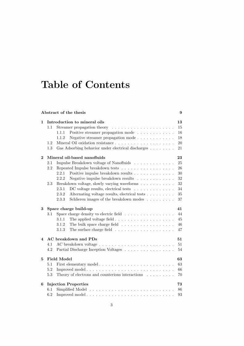
Table of Contents
Abstract of the thesis 9
1 Introduction to mineral oils 13
1.1 Streamer propagation theory . . . . . . . . . . . . . . . . . . . . 15
1.1.1 Positive streamer propagation mode . . . . . . . . . . . . 16
1.1.2 Negative streamer propagation mode . . . . . . . . . . . . 18
1.2 Mineral Oil oxidation resistance . . . . . . . . . . . . . . . . . . . 20
1.3 Gas Adsorbing behavior under electrical discharges . . . . . . . . 21
2 Mineral oil-based nanofluids 23
2.1 Impulse Breakdown voltage of Nanofluids . . . . . . . . . . . . . 25
2.2 Repeated Impulse breakdown tests . . . . . . . . . . . . . . . . . 26
2.2.1 Positive impulse breakdown results . . . . . . . . . . . . . 30
2.2.2 Negative impulse breakdown results . . . . . . . . . . . . 32
2.3 Breakdown voltage, slowly varying waveforms . . . . . . . . . . . 32
2.3.1 DC voltage results, electrical tests . . . . . . . . . . . . . 34
2.3.2 Alternating voltage results, electrical tests . . . . . . . . . 35
2.3.3 Schlieren images of the breakdown modes . . . . . . . . . 37
3 Space charge build-up 41
3.1 Space charge density vs electric field . . . . . . . . . . . . . . . . 44
3.1.1 The applied voltage field . . . . . . . . . . . . . . . . . . . 45
3.1.2 The bulk space charge field . . . . . . . . . . . . . . . . . 46
3.1.3 The surface charge field . . . . . . . . . . . . . . . . . . . 47
4 AC breakdown and PDs 51
4.1 AC breakdown voltage . . . . . . . . . . . . . . . . . . . . . . . . 51
4.2 Partial Discharge Inception Voltages . . . . . . . . . . . . . . . . 54
5 Field Model 63
5.1 First elementary model . . . . . . . . . . . . . . . . . . . . . . . . 63
5.2 Improved model . . . . . . . . . . . . . . . . . . . . . . . . . . . . 66
5.3 Theory of electrons and counterions interactions . . . . . . . . . 70
6 Injection Properties 73
6.1 Simplified Model . . . . . . . . . . . . . . . . . . . . . . . . . . . 86
6.2 Improved model . . . . . . . . . . . . . . . . . . . . . . . . . . . . 93
3

4 TABLE OF CONTENTS
7 Dielectric Spectroscopy 977.1 Nanofluid electrical permittivity . . . . . . . . . . . . . . . . . . 977.2 Electrical conductivity of nanofluids . . . . . . . . . . . . . . . . 106
Conclusions 111

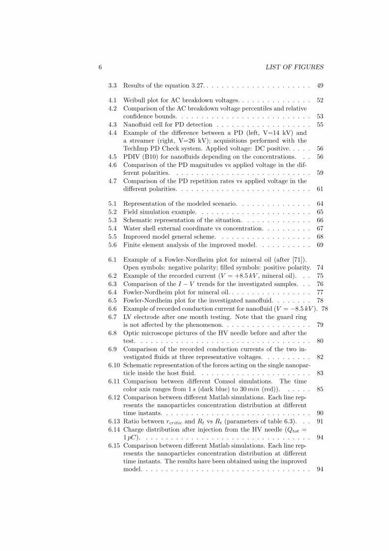
List of Figures
1.1 General scheme of a petroluem refinery (the mineral oil step iscircled). . . . . . . . . . . . . . . . . . . . . . . . . . . . . . . . . 14
1.2 Example of a possible molecule structure of mineral oil (after [4]). 151.3 Positive streamer general propagation mechanism (after [13]).
The positively charged tip is the head of the streamer. . . . . . . 161.4 Positive streamer acquisitions (shadowgraph technique). Each
image refer to a specific time instant after the streamer initiation[microseconds] (after [12]). . . . . . . . . . . . . . . . . . . . . . . 17
1.5 Negative streamer propagation mechanism, after [19]. . . . . . . 181.6 Negative streamer acquisitions (shadowgraph technique). Each
image refer to a specific time instant after the streamer initiation[microseconds] (after [12]). . . . . . . . . . . . . . . . . . . . . . . 19
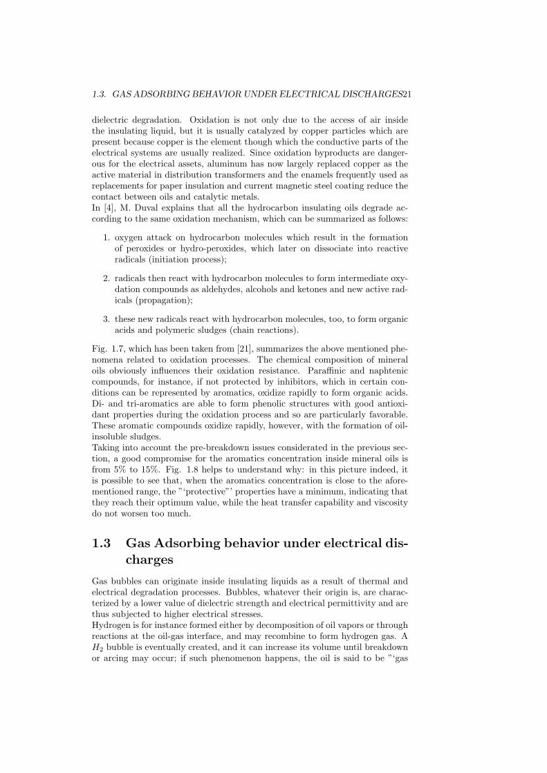
1.7 Oxidation processes in hydrocarbon oils. . . . . . . . . . . . . . . 201.8 Influence of the aromatic content on the physical and chemical
properties of mineral oils (after [4], [22], [23]). . . . . . . . . . . . 22
2.1 Chemical structure of oleic acids, the most used surfactant forferrofluids manufacturing process. . . . . . . . . . . . . . . . . . . 24
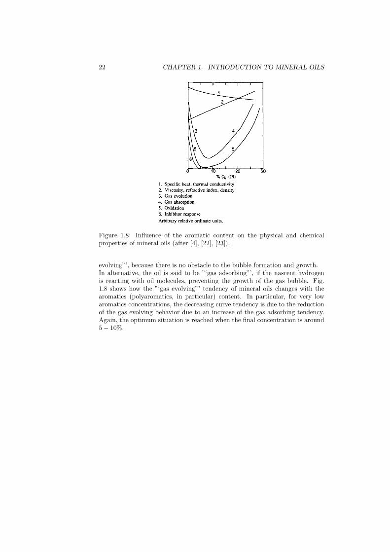
2.2 Effect of surfactants on the nanoparticles mean distance. . . . . . 242.3 Results of the tests presented in [24]. . . . . . . . . . . . . . . . . 252.4 Adopted test procedure to evaluate the breakdown strength, after
[35]. . . . . . . . . . . . . . . . . . . . . . . . . . . . . . . . . . . 262.5 Summary of the results about mineral oil samples. . . . . . . . . 282.6 Streamer propagation speed vs applied voltage. Note that in the
negative voltage case, the speed refers to the maximum one (atthe needle tip). . . . . . . . . . . . . . . . . . . . . . . . . . . . . 29
2.7 Summary of the results about impulse breakdown tests. . . . . . 302.8 Electric field lines distortion (after [31]). . . . . . . . . . . . . . . 312.9 DC breakdown voltages for nanofluids under divergent conditions. 342.10 Weibull charts for DC breakdown data and B10 percentiles. . . . 362.11 Breakdown results for alternating applied voltages. . . . . . . . . 362.12 Schlieren images of breakdown modes, DC negative voltage, 15 kV . 372.13 Schlieren images of breakdown modes, Square wave applied volt-
age, 500Hz, breakdown inception. . . . . . . . . . . . . . . . . . 39
3.1 Spherical capacitor. . . . . . . . . . . . . . . . . . . . . . . . . . . 423.2 Charge trapping scenario at a generic time instant t: volume
charge (colored region) and surface charge layer (bold line). . . 45
5
6 LIST OF FIGURES
3.3 Results of the equation 3.27. . . . . . . . . . . . . . . . . . . . . . 49
4.1 Weibull plot for AC breakdown voltages. . . . . . . . . . . . . . . 52
4.2 Comparison of the AC breakdown voltage percentiles and relativeconfidence bounds. . . . . . . . . . . . . . . . . . . . . . . . . . . 53
4.3 Nanofluid cell for PD detection . . . . . . . . . . . . . . . . . . . 55
4.4 Example of the difference between a PD (left, V=14 kV) anda streamer (right, V=26 kV); acquisitions performed with theTechImp PD Check system. Applied voltage: DC positive. . . . . 56
4.5 PDIV (B10) for nanofluids depending on the concentrations. . . 56
4.6 Comparison of the PD magnitudes vs applied voltage in the dif-ferent polarities. . . . . . . . . . . . . . . . . . . . . . . . . . . . 59
4.7 Comparison of the PD repetition rates vs applied voltage in thedifferent polarities. . . . . . . . . . . . . . . . . . . . . . . . . . . 61
5.1 Representation of the modeled scenario. . . . . . . . . . . . . . . 64
5.2 Field simulation example. . . . . . . . . . . . . . . . . . . . . . . 65
5.3 Schematic representation of the situation. . . . . . . . . . . . . . 66
5.4 Water shell external coordinate vs concentration. . . . . . . . . . 67
5.5 Improved model general scheme. . . . . . . . . . . . . . . . . . . 68
5.6 Finite element analysis of the improved model. . . . . . . . . . . 69
6.1 Example of a Fowler-Nordheim plot for mineral oil (after [71]).Open symbols: negative polarity; filled symbols: positive polarity. 74
6.2 Example of the recorded current (V = +8.5 kV , mineral oil). . . 75
6.3 Comparison of the I − V trends for the investigated samples. . . 76
6.4 Fowler-Nordheim plot for mineral oil. . . . . . . . . . . . . . . . . 77
6.5 Fowler-Nordheim plot for the investigated nanofluid. . . . . . . . 78
6.6 Example of recorded conduction current for nanofluid (V = −8.5 kV ). 78
6.7 LV electrode after one month testing. Note that the guard ringis not affected by the phenomenon. . . . . . . . . . . . . . . . . . 79
6.8 Optic microscope pictures of the HV needle before and after thetest. . . . . . . . . . . . . . . . . . . . . . . . . . . . . . . . . . . 80
6.9 Comparison of the recorded conduction currents of the two in-vestigated fluids at three representative voltages. . . . . . . . . . 82
6.10 Schematic representation of the forces acting on the single nanopar-ticle inside the host fluid. . . . . . . . . . . . . . . . . . . . . . . 83
6.11 Comparison between different Comsol simulations. The timecolor axis ranges from 1 s (dark blue) to 30min (red)). . . . . . 85
6.12 Comparison between different Matlab simulations. Each line rep-resents the nanoparticles concentration distribution at differenttime instants. . . . . . . . . . . . . . . . . . . . . . . . . . . . . . 90
6.13 Ratio between rcritic and Rt vs Rt (parameters of table 6.3). . . 91
6.14 Charge distribution after injection from the HV needle (Qtot =1 pC). . . . . . . . . . . . . . . . . . . . . . . . . . . . . . . . . . 94
6.15 Comparison between different Matlab simulations. Each line rep-resents the nanoparticles concentration distribution at differenttime instants. The results have been obtained using the improvedmodel. . . . . . . . . . . . . . . . . . . . . . . . . . . . . . . . . . 94

LIST OF FIGURES 7
7.1 Plane-plane configuration of a nanofluid: the dots represent thenanoparticles. . . . . . . . . . . . . . . . . . . . . . . . . . . . . . 98
7.2 Relative permittivity from the model of equation 7.8. . . . . . . . 1007.3 Schematic representation of the used cell . . . . . . . . . . . . . . 1017.4 Example of a capacitance acquisitions vs frequency performed
with the Alpha Beta Analyzer: real and imaginary part of therelative permittivity. Measurements performed at 40 degrees. . . 102
7.5 Example of the AC conductivity obtained for mineral oil. . . . . 1037.6 Comparison between the permittivity model and the measured
values. . . . . . . . . . . . . . . . . . . . . . . . . . . . . . . . . . 1047.7 Imaginary part of the relative permittivity for 0.2 g
L nanofluid. . 1057.8 Electrical conductivity vs nanofluid concentration. . . . . . . . . 1067.9 Generical situation where a particle with energy E has to over-
come a potential wall U . . . . . . . . . . . . . . . . . . . . . . . 1077.10 Electric field distribution between two consecutive nanoparticles
(dashed lines refer to the background field). Case a: distancebetween nanoparticles bigger than 2Rp; case b: distance lowerthan 2Rp, being Rp the nanoparticles radius. . . . . . . . . . . . 108
7.11 Tunneling global probability vs concentration. . . . . . . . . . . . 1087.12 Simple diagram representing the fields acting close to the nanopar-
ticle. . . . . . . . . . . . . . . . . . . . . . . . . . . . . . . . . . . 109

8 LIST OF FIGURES

Abstract of the thesis
In spite of all the recent studies (see e.g. [1], [2], [3]), the insulating materialsemployed for high voltage (HV) transformer manufacturing are still those in usesince several decades. Economic (development costs) and strategic issues (un-certainty about design rules and long-term performance) are the reasons for ageneral hostility of small manufacturers to technological changes. In a specularway, big market players with significant R&D expenditures are interested inimproving the transformer technology and acquire a monopolistic position.For the fluid insulation, mineral oil (MO) still dominates thanks to its excel-lent dielectric and cooling performances [5]. However, being MO a carcinogenicagent, the electric industry searched alternatives for applications where envi-ronmental concerns are of greater concern (e.g., offshore equipment, trains). Inthis context, many efforts have been done to study green fluids, mostly naturaland synthetic esters, to replace MO [6]. However, green alternatives have alow resistance to electrical discharge propagation [7]. Therefore, they are usednowadays almost exclusively for medium voltage equipment and remain a nicheproduct.Despite the predominance of MO, industry is interested in liquid dielectrics withenhanced cooling properties. If available, these fluids could reduce the insula-tion volumes and increase the power densities, thus becoming a driver for amarket revolution.Some researchers [8], [9] have started to experiment with MO-based nanofluids(i.e., colloidal solutions of nanoparticles in a base fluid), with the aim of im-proving the MO heat exchange capabilities. Common sense suggests that thedispersion of conductive particles in an insulating liquids tends to reduce thedielectric withstand properties of the fluid. On the contrary, nanofluids show en-hanced properties explained by the electrical properties of the nanoparticles (inparticular, electron attachment properties) under the condition that nanopar-ticles are well dispersed inside the base fluid. Therefore, a good dispersion ofnanoparticles is a key point to pursue to manufacture a good nanodielectric. Itis not easy to understand how to obtain a good, stable dispersion of the nanopar-ticles; a logical starting point is avoid using nanofluids with high concentrationof nanoparticles. This way, the mean free path between nanoparticles increasesweakening the van der Waals attractive forces. Since these forces might lead tonanoparticle aggregation, lower concentrations favor the stability of nanoparti-cles within the fluid. A second key point, after the fluid stability requirement,is the insulating performance. Researchers have started to study nanofluids be-cause of their outstanding thermal properties, but these fluids should be excel-lent also regarding all the electrical properties, ranging from the power losses tothe discharge propagation resistance. Furthermore, these properties, if proved,
9

10 LIST OF FIGURES
shall also be stable during time, that is, they should not be affected by aging toomuch. The aim of this thesis is hence to give an answer to all of these questions:
1. what is the best nanofluid concentration in terms of electrical propertiesand stability?
2. what are the basic properties of nanofluids compared to those of mineraloil?
3. how do these properties change with time, or, what about the long termstability?
4. are there any risks for the nanofluid stability?
Since the world of nanodielectrics, and that of nanofluid too, is too wide, wehave limited our investigation to the field of mineral oil-based nanofluids, wherethe added nanoparticles have been magnetite (Fe3O4).The following chapters are structured in the following way:
• chapter one starts with a brief introduction to the features an insulatingliquid shall possess and then introduces mineral oils, which are still themost used insulating fluids. Their basic properties in terms of dischargeand aging resistance are reported and discussed;
• chapter two contains the first results about nanofluids. First, a general in-troduction about the manufacturing process of nanofluids is reported, andthen some literature studies are discussed. Later on, some electrical testsare discussed, considering the already published works about nanofluids.Finally, Schlieren imaging results are presented to discuss the dischargedevelopment in nanofluids.
• chapter three is the first theoretical chapter, with the aim to propose amathematical model to give the basis to a general idea about the nanopar-ticle interaction with the injected charge; in this chapter we would like toprove that nanoparticles are likely to create a homocharge layer close tothe HV electrode injecting charge;
• chapter four presents the results of an investigation about slow voltagewaveforms (50Hz sinusoidal and DC). Breakdown and partial dischargeissues are studied and reported. At the end of the chapter some importantkey points are introduced, opening the second part of the thesis;
• chapter five is the second theoretical chapter, presenting different modelswith the aim to derive an analytical expression for the electric field distri-bution close to the nanoparticles, which is claimed to be the responsibleof all the phenomena taking place in their proximity;
• chapter six can be considered the most important one of the thesis inthe sense that contains the most important results. First, a comparativestudy is carried out to understand the injection of charge carriers fromelectrodes of different polarities to the nanofluid; later on we have com-pared the conductive behavior of a low concentration nanofluid with ahigher concentration one, verifying the existence of different conduction

LIST OF FIGURES 11
modes.At the end of the chapter we have discussed a non stable behavior ofnanofluids, when exposed to highly non uniform fields;
• chapter seven contains some experimental results about the dielectricproperties of nanofluids (relative permittivity and AC conductivity), to-gether with some simple models able to explain them.
At the beginning of each chapter, a brief abstract will introduce its content.

12 LIST OF FIGURES

Chapter 1
Introduction to mineral oilinsulating fluids
Abstract
This chapter introduces the insulating fluids which are used in the electrical ap-paratuses.First, a brief overview about the features an insulating liquids should own is pre-sented, and then more attention has been given to mineral oils, because they willbe the basis of the investigated nanofluids and because they are the most usedinsulators in power transformers and cables insulation systems. Mineral oils arenot described in details, because they are quite known nowadays and there are alot of references about them, but the main properties and theories are recalled,because they will be used in the following chapters.
Dielectric fluids are an important part of the insulation systems for a lot oftypes of electrical apparatuses, such as transformers, bushings, cables and ca-pacitors. Depending on the application, different electric features are requiredfor such insulating devices: high values of electrical permittivity are necessaryto reduce the physical sizes of capacitors for instance, lower ones are desired touniform stresses in solids-liquids composites insulations, while all should havelow dissipation factors in common, to reduce energy losses and thus increase theefficiencies.Anyway, liquids are used in these equipment not only for their electrical prop-erties, but also for their thermal exchange ones, which can be summarized inhigh values of specific heat and thermal conductivity together with low viscosityvalues and pour points.The different properties which are requested for insulating liquids result in aproblem to define a unique fluid which can be used everywhere; synthetic flu-ids are usually preferred in capacitors thanks to their high dielectric constants,while hydrocarbon liquids were widely used in the past in cables, before beingreplaced by solid extruded insulators.Anyway, despite what it could be thought from the above mentioned consid-erations, mineral oils are nowadays the most used solution in the electricalapplications ([4]).
13

14 CHAPTER 1. INTRODUCTION TO MINERAL OILS
Mineral oil is a class of insulating fluids refined from petroleum crude stocks,which find their natural application in transformer insulation, because of theiroptimal electrical properties and good thermal exchange ones. Even if they arenot environmental friendly, it is estimated that in the US, at the end of the lastcentury, more than two billion gallons were present inside transformers ([4]).Some transformer manufacturers, in order to overcome the environmental criti-calities of mineral oils, have started to investigate and use vegetable fluids, but ithas been demonstrated that they can be used only for distribution applications([7]), because of their low electrical withstand properties at large gaps whichare necessary for high voltages.Fig. 1.1 represents the working scheme of a general petroleum refinery. With-
Figure 1.1: General scheme of a petroluem refinery (the mineral oil step iscircled).
out entering the details of each step of the refinement process, we can easilysee that mineral oils are the results of the first step of the distillation proce-dure, according to a defined boiling temperature range, which depends on thenature of the mineral oil the refinery wants to produce ([10]). Mineral oilsindeed, being manufactured starting from crude oil, share most of the chemi-cal properties with it; as reported in fig. 1.2, they are a mixture of paraffinic(chemical formula C2nH2n+2), nafthenic (chemical formula C2nH2n) and aro-matic compounds (chemical formula CnHn), whose ratio defines their macro-scopic behavior. In particular, aromatic compounds are usually a minor partand a mineral oil can be ”‘paraffinic”’ or ”‘naphtenic”’ depending on which ofthe other components is the prevailing.
”‘Paraffinic”’ oils are more viscous in general, but they have higher boilingtemperatures (and thus higher distillation temperatures), while ”‘naphtenic”’ones are less viscous and with lower boiling temperatures.

1.1. STREAMER PROPAGATION THEORY 15
Figure 1.2: Example of a possible molecule structure of mineral oil (after [4]).
It is clear from this consideration that the majority, but not the totality ofthe in service transformers, are insulated with ”‘naphtenic”’ mineral oils, be-cause of the better heat exchange capabilities due to a reduced viscosity. If the”‘paraffinic”’ and ”‘naphtenic”’ content of the oil mainly influences the ther-mal exchange properties of mineral oil, different considerations have to be madeabout the ”‘aromatic”’ content, even if, as already said, it is the minor part. Alot of studies in the past ([11]-[12]) have confirmed that the aromatics compo-nents have a remarkable influence on the pre-breakdown (streamer) propagationproperties of insulating fluids. In particular, aromatics are characterized by twoproperties:
• ”‘Low ionization potential”’: it means that it is easy to ionize an aromaticcomponent. This feature is related to the positive streamer propagation,which relies on the ionization properties of the medium in which it prop-agates;
• ”‘High electronegativity”’: this is related to the negative streamer initi-ation, which is facilitated since such behavior tends to extract electronsfrom the electrodes surfaces.
1.1 Streamer propagation theory (after [12])
This section describes the results obtained by Devins in [12], which analyzedthe pre-breakdown phenomena related to different types of insulating fluids,including transformer oils. As already anticipated in the previous paragraph,pre-breakdown phenomena are usually referred as streamers and their study ismainly focused on two of their properties:
1. ”‘Initiation”’, i.e. how they originate inside the fluids;
2. ”‘Propagation”’, that is if and how they reach the opposite electrode.
Usually, we are more interested in propagation issues, because they are likelyto lead to the streamer-to-leader transition, thus causing the breakdown of theinsulator. Since divergent field configurations are likely to highlight the ”‘prop-agation”’ mode of the streamers, a lot of studies, including [12], are focused onthis particular experimental condition. In the following, we summarize the re-sults obtained by Devins about the positive and negative streamer propagation

16 CHAPTER 1. INTRODUCTION TO MINERAL OILS
inside mineral oil, because they will be referred to in the following chapters.Before doing that, it is necessary to point out that Devins did not study therelation between the streamer propagation and voltage, which is for instancereviewed in [11], but he only limited himself to study the basic mechanismsleading to the streamer propagation.
1.1.1 Positive streamer propagation mode
In the case in which the high voltage electrode creating the field inside the insu-lating liquid is positively charged, it is clear that no electron injection can takeplace; thus, a pre-breakdown phenomenon is evidently not initiated from chargeinjection. In order for a streamer to start, it is necessary that a free electronis available inside the fluid, and this is usually liberated by random processesincluding field ionization or natural cosmic rays or radioactivity ([14], [15], [11]).The free electron is then accelerated towards the positive electrode, increasingthe electric field which in turn becomes so high to induce a more deterministicfield ionization, which is the responsible of the generation of an avalanche pro-cess, as it is possible to see from fig. 1.3. This picture, besides clarifying the
Figure 1.3: Positive streamer general propagation mechanism (after [13]). Thepositively charged tip is the head of the streamer.
positive streamer initiation and propagation mechanism, lets understand whyit is usually reported that positive streamers are filamentary (1) and very fast(2):
1. ”‘filamentary”’: this is due to the fact that the process proceeds via localionization where the field is above the ionization threshold and it is notinduced, as it will be shown in the following, by charge extraction fromthe electrodes;
2. ”‘fast”’: this is connected to the field increase due to the presence of afilamentary charged structure (the streamer itself). Since the streamerincreases the electrical field (needle effect), the ionization process goesfurther at a higher rate than at the beginning.
Fig. 1.4 shows some acquisitions taken from [12], which refer to shadowgraphimages of a positive streamer propagating inside a ”‘naphtenic”’ transformer

1.1. STREAMER PROPAGATION THEORY 17
Figure 1.4: Positive streamer acquisitions (shadowgraph technique). Each imagerefer to a specific time instant after the streamer initiation [microseconds] (after[12]).
oil subjected to rectangular step voltage, which later on converts to a leader,causing the complete breakdown of the insulating gap. It is possible to see that,as reported in the previous considerations, the streamer shape is nearly filamen-tary.The nature of positive streamers, which has now been clarified, helps under-
stand why in the previous section aromatics were said to facilitate the streamerpropagation: being easily ionized, they speed up the avalanche process, leadingto a lower voltage breakdown. A simple model suggested by Devins in [12],based on the Zener ionization theory1, lets estimate the streamer propagationvelocity as:
v = r0
√ae3E0
3
πmϵ3n
cerfc(
√π2maW 2
h0eE0) (1.1)
where:
1. r0 represents the streamer radius which has been modeled as a conductivecylindrical channel;
2. a represents the average molecular separation;
1The Zener ionization theory should be applied only to solid insulation materials and notto fluids, but it is anyway sufficient to catch some important aspects of the liquid state, too.For a more detailed quantitative description of the problem, refer to [16].

18 CHAPTER 1. INTRODUCTION TO MINERAL OILS
3. e represents the elementary charge;
4. h represents the Planck constant;
5. m represents the electron mass;
6. W represents the liquid phase ionization potential (band gap);
7. E0 represents the electric field at the streamer tip;
8. n represents the molecule density;
9. c represents the concentration of positive and negative carriers;
10. erfc represents the complementary error function, defined as:
erfc(x) =2√π
ˆ +∞
0
e−t2dt (1.2)
Looking at the parameter ϵ in equation 1.1, it is then evident that a reductionof the liquid phase ionization potential due to the presence of aromatics canfavour the streamer propagation.
1.1.2 Negative streamer propagation mode
Negative streamers, i.e. pre-breakdwon phenomena taking place when the highvoltage electrodes are negatively charged, are somehow different. In this caseindeed, when the maximum electric field exceeds the injection threshold, elec-trons are injected inside the insulating fluid ([11], [12], [17]). The interactionsbetween the injected charge and the molecules of the liquid is then able to raiselocally the temperature till the evaporation ([14], [18]). In this way a gas bub-ble is usually generated and, because of the electrical permittivity mismatchbetween the air and the liquid, the electric field inside the bubble is higher thanin the fluid, letting the electrons to gain sufficient energy to ionize later theliquids molecules. Electrons release indeed the acquired energy to the fluid viaattachment reactions, as schematically represented in fig. 1.5.
Figure 1.5: Negative streamer propagation mechanism, after [19].

1.1. STREAMER PROPAGATION THEORY 19
Figure 1.6: Negative streamer acquisitions(shadowgraph technique). Each image refer toa specific time instant after the streamer initia-tion [microseconds] (after [12]).
This energy exchange phe-nomenon increases the sizeof the original bubble, giv-ing rise to an avalanche pro-cess which tends to be bushierthan the previous describedone. Generally speaking, neg-ative streamers have a bushyshape and a lower speed thanpositive streamers, as it ispossible to see from fig. 1.6.
The reduced, and non uni-form speed of the negativestreamer, has been explainedby Chadband and Wrigth in[20], who calculated the elec-trical field distribution gener-ated by a growing conduct-ing sphere (a schematic modelof the streamer growth) andfound that the field at itsedge goes through a minimumat approximately 60% of thegap.In order to explain the re-sults obtained from the ob-servation about the negativestreamer propagation, Devins
([12]) formulated the following ”‘two step model”’:
• electron injection and trapping: during this first step, electrons are in-jected and trapped at the gas-liquid interface, as it is possible to see fromfig. 1.5. The extracted electron concentration and its distance from thehigh voltage electrode depends upon the electron scavenger concentrationinside the insulating fluid. This results in a space charge layer close to thehigh voltage electrode, which acts as homocharge, i.e. reduces the fieldclose to the electrode, but increase it at the streamer tip;
• ionization: once the field increase is sufficient to ionize the liquid molecule,the avalanche process can start and propagate towards the other electrode.
The ”‘two step model”’ states that the average streamer velocity (which is atleast one order of magnitude lower than the positive streamer one) can be ob-tained by averaging the time spent by the electrons in each phase: the higherthe time in the first step, the lower the streamer propagation speed and viceversa.Electron scavenger components, like the aromatics, are likely to reduce the timespent in the first step, because they facilitate the charge extraction. In this way,the field at the streamer tip increases faster and the streamer assumes the shapeand the features of the positive one.

20 CHAPTER 1. INTRODUCTION TO MINERAL OILS
Figure 1.7: Oxidation processes in hydrocarbon oils.
The previous two sections clarify that the presence of aromatics is an in-dex facilitating pre-breakdown mechanisms reducing in this way the withstandcapability of the insulating fluids. These considerations suggest that it is neces-sary to reduce the aromatics concentration as mush as possible, but this is notpossible for an obvious economic reason concerning the distillation process, andbecause aromatics can also have a positive effect for liquids. They have in facttwo important positive effects:
1. they protect the insulating fluid from oxidation, and thus from ageingeffects;
2. they prevent the gas bubbles formation, reducing the risk of partial dis-charges and their consequent ageing process.
There is a third, but minor reason why aromatics have a positive influence oninsulating oils; they increase in fact the viscosity of the fluid itself and thisaspect can help to hinder the effect of contaminants. Indeed, contaminantsusually increase dielectric losses, unless their mobility is very low; by increasingthe viscosity, the mobility of contaminants is obviously reduced, preventing themto increase the dielectric losses2.
1.2 Mineral Oil oxidation resistance
The oxidation of insulating oils, and mineral oils in particular, results in theformation of organic weak acids, sludges (which are composed of insoluble con-densed matter) and polar byproducts ([4]).Weak acids and polar byproducts increase dielectric losses and conductive prop-erties, and may be deleterious for the applications in which polarization currentshave to be minimized (cables and transformers for instance), while sludges areable to increase locally the viscosity of the insulating liquid thus reducing itsheat transfer properties creating thermal hot spots which can accelerate the
2This is true in the limit of temperature operations, which, as known, tend to reduce thevalues of the viscosity. The increase in viscosity is anyway dangerous in terms of reduced heattransfer capabilities of the insulating fluid.
1.3. GAS ADSORBING BEHAVIOR UNDER ELECTRICAL DISCHARGES21
dielectric degradation. Oxidation is not only due to the access of air insidethe insulating liquid, but it is usually catalyzed by copper particles which arepresent because copper is the element though which the conductive parts of theelectrical systems are usually realized. Since oxidation byproducts are danger-ous for the electrical assets, aluminum has now largely replaced copper as theactive material in distribution transformers and the enamels frequently used asreplacements for paper insulation and current magnetic steel coating reduce thecontact between oils and catalytic metals.In [4], M. Duval explains that all the hydrocarbon insulating oils degrade ac-cording to the same oxidation mechanism, which can be summarized as follows:
1. oxygen attack on hydrocarbon molecules which result in the formationof peroxides or hydro-peroxides, which later on dissociate into reactiveradicals (initiation process);
2. radicals then react with hydrocarbon molecules to form intermediate oxy-dation compounds as aldehydes, alcohols and ketones and new active rad-icals (propagation);
3. these new radicals react with hydrocarbon molecules, too, to form organicacids and polymeric sludges (chain reactions).
Fig. 1.7, which has been taken from [21], summarizes the above mentioned phe-nomena related to oxidation processes. The chemical composition of mineraloils obviously influences their oxidation resistance. Paraffinic and naphteniccompounds, for instance, if not protected by inhibitors, which in certain con-ditions can be represented by aromatics, oxidize rapidly to form organic acids.Di- and tri-aromatics are able to form phenolic structures with good antioxi-dant properties during the oxidation process and so are particularly favorable.These aromatic compounds oxidize rapidly, however, with the formation of oil-insoluble sludges.Taking into account the pre-breakdown issues considerated in the previous sec-tion, a good compromise for the aromatics concentration inside mineral oils isfrom 5% to 15%. Fig. 1.8 helps to understand why: in this picture indeed, itis possible to see that, when the aromatics concentration is close to the afore-mentioned range, the ”‘protective”’ properties have a minimum, indicating thatthey reach their optimum value, while the heat transfer capability and viscositydo not worsen too much.
1.3 Gas Adsorbing behavior under electrical dis-charges
Gas bubbles can originate inside insulating liquids as a result of thermal andelectrical degradation processes. Bubbles, whatever their origin is, are charac-terized by a lower value of dielectric strength and electrical permittivity and arethus subjected to higher electrical stresses.Hydrogen is for instance formed either by decomposition of oil vapors or throughreactions at the oil-gas interface, and may recombine to form hydrogen gas. AH2 bubble is eventually created, and it can increase its volume until breakdownor arcing may occur; if such phenomenon happens, the oil is said to be ”‘gas
22 CHAPTER 1. INTRODUCTION TO MINERAL OILS
Figure 1.8: Influence of the aromatic content on the physical and chemicalproperties of mineral oils (after [4], [22], [23]).
evolving”’, because there is no obstacle to the bubble formation and growth.In alternative, the oil is said to be ”‘gas adsorbing”’, if the nascent hydrogenis reacting with oil molecules, preventing the growth of the gas bubble. Fig.1.8 shows how the ”‘gas evolving”’ tendency of mineral oils changes with thearomatics (polyaromatics, in particular) content. In particular, for very lowaromatics concentrations, the decreasing curve tendency is due to the reductionof the gas evolving behavior due to an increase of the gas adsorbing tendency.Again, the optimum situation is reached when the final concentration is around5− 10%.

Chapter 2
Introduction to mineral oilbased nanofluids
Abstract
This chapter will introduce the field of nanofluids and in particular those man-ufactured starting from mineral oil. These liquids are a relatively new class ofinsulating materials, aiming at replacing the traditional ones, because of theiroutstanding possibilities in terms of power densities increase.First, a review about the preliminary results concerning ferrofluids-based nanoflu-ids is carried on; later on in this chapter the first measurement results about ourinvestigated fluids are reported and discussed, considering the theories presentedin the previous chapter.
One of the first studies about the electrical properties of nanofluids has been re-ported in [24]. Generally speaking, researchers have always doubted about thepossibility of adding particles inside insulating fluids, especially if they wereconductive, because of the reduction of the withstand capabilities ([25]-[26]for instance). In [24] instead, the authors explored the benefits obtained byadding magnetite nanosized particles inside mineral oil, knowing that conduc-tive nanoparticles could increase the thermal exchange properties of insulatingfluids in such a way to reduce the size of the electrical equipment and so toincrease their power densities ([27], [28], [29]).Magnetite nanoparticles (Fe3O4) dispersed inside a blendant fluid based on or-ganic solvents are generally referred in literature as ferrofluids. They were firstinvented in 1963 by NASA’s Steve Papell as a liquid rocket fuel which could bedrawn toward a pump inlet in a weightless environment by applying a magneticfield ([30]). In order to be used for final purposes, ferrofluids must necessarilyhave a stable behavior, i.e. magnetite nanoparticles should not agglomerate. Inparticular, they should behave as colloids and not suspensions, meaning thata suspension is not a stable mixture of particles and blendant fluid. It is verydifficult to manufacture a stable colloid made of magnetite nanoparticles (usu-ally the mean radius of such nanoparticles is bigger than 10nm), because of theforces which tend to collect them tending to form an agglomerate. The solutionwhich is generally adopted to produce a final usable product is the use of surfac-
23

24 CHAPTER 2. MINERAL OIL-BASED NANOFLUIDS
Figure 2.1: Chemical structure of oleic acids, the most used surfactant for fer-rofluids manufacturing process.
tants, i.e. long chain molecules which are able to keep nanoparticles separated,preventing them to attract. From a chemical point of view surfactants are:
• oleic acid;
• tetramethylammonium hydroxide;
• soy lecithin;
• citric acid.
Oleic acid is the most used surfactant in commercial ferrofluids, and in par-ticular it is the one which has been used in the ferrofluid which has been used tomanufacture the nanofluids which are the object of this work. Without enteringtoo much into the details of the chemical structure (which is shown in Fig. 2.1),we only say that it is a fatty acid, in which one termination is hydrophobic andthe other one hydrophilic, containing the hydroxyl group OH. Fig. 2.2, whichhas been taken from [31], shows how surfactants act in order to prevent the Wander Waals attractive forces to agglomerate nanoparticles.
The idea to increase the distance among nanoparticles in order to improvethe colloidal solution stability can find a mathematical explanation in the Darjanguin-Landan-Verwey-Overbeek (DLVO) theory ([32]), which states that the totalinteraction energy of the nanoparticles, i.e. the sum of the van der Walls at-traction and the electrostatic repulsion, develops an energy barrier the particlesmust overcome in order to aggregate. If this energy barrier is higher than 15 kT,then the nanofluid is considered stable ([33]); the increase of the mean distance
Figure 2.2: Effect of surfactants on the nanoparticles mean distance.
2.1. IMPULSE BREAKDOWN VOLTAGE OF NANOFLUIDS 25
among nanoparticles has the obvious effect of increasing the energy barrier be-tween them, because it shifts the balance between Wan der Walls forces andrepulsive ones to the latter. Another equivalent approach to study the stabil-ity of nanoparticles inside a nanofluid has been reported in [34] and [31] andconsists in the analysis of the ratio between the thermal energy kT and theattractive gravitational and magnetic energies. The result of this investigationis the maximum size nanoparticles should have to be considered stable, which isusually less than 10 nm. Commercial magnetite nanoparticles have an averageradius of about 10−15nm and this causes an instability mechanism which takesplace at longer times, even in the presence of surfactants.
2.1 Impulse Breakdown voltage of Nanofluids(after [24])
This section has the aim to introduce the results obtained by Seagal in [24]. Inthis work, there is no indication about the concentration of the nanoparticleswhich have been dispersed inside the mineral oil, but the authors say thatthey refer to the ”‘optimum concentration”’. Apart from this aspect, theyhave performed impulse (1.2 − 50µs) breakdown tests under divergent fields(needle to sphere electrode configuration), as done by Devins in [12]. In thisway, they focalized their attention to the streamer (and leader) propagationfeatures inside oil (benchmark) and the corresponding nanofluids. The results,presented in figure 2.3, refer to a 25.4mm inter-electrode gap and two differentbase naphtenic mineral oils: Univolt 60 and Nytro 10X. The first column, aboutthe breakdown voltage values, clearly shows the asymmetry between positiveand negative polarity; this is a quite known effect in literature, which is due tothe different propagation modes of positive and negative streamers and whichis explained by Devins in [12]. The different streamer propagation modes areclearly visible looking at the third column, where the average avalanche velocityis reported, showing how positive streamers are much faster than negative ones.The third and fourth rows of fig. 2.3 are relative to nanofluids manufacturedstarting from the previously introduced mineral oils, without any indicationsabout the magnetite concentration. The results about this class of fluids areparticularly interesting:
• under positive polarity, there is a significant increase of the withstand ca-pabilities of the insulating fluid: the breakdown voltage is almost doubled;
• under negative polarity there is a slight reduction, even if we do not knowif it is an actual reduction or if it is due to the normal scattering of the
Figure 2.3: Results of the tests presented in [24].
26 CHAPTER 2. MINERAL OIL-BASED NANOFLUIDS
measurement results; in other words, we have no information about theconfidence levels of the presented results.
Apart from the slight apparent reduction under negative polarity, the high in-crease under the positive polarity indicates that the resulting fluids have higherimpulse breakdown strengths compared to mineral oil ones, that is, the contri-bution of the magnetite nanoparticles is evidently positive.From Seagal work anyway, it is not possible to see if the improving behavioris concentration-dependent or not, because, as already stated in the previousstatements, nothing is said about the way to produce the ”‘optimum”’ nanofluid.The word ”‘optimum”’ lets suppose that the behavior can be concentration-dependent, but we do not know if there is an improving trend with the concen-tration or not and no final conclusions can be drawn from the negative polarity.In order to give an answer to such questions, the experiments presented in [24]have been repeated with different nanofluids concentrations.
2.2 Repeated Impulse breakdown tests
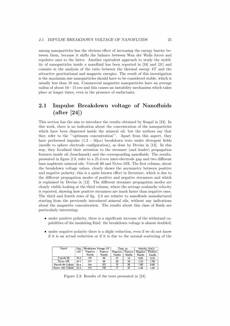
Impulse breakdown tests have been performed using a Passoni Villa 600 kV/20 kJ6 stages generator; the divergent field configuration has been obtained by usinga needle (15µm average radius of curvature, controlled by optic microscope) toplane electrode; gap spacing was 10mm. The test procedure which has beenadopted to evaluate breakdown voltage values is represented in fig. 2.4, whichhas been taken from [35]. The starting voltage value has always been 20 kV , the
Figure 2.4: Adopted test procedure to evaluate the breakdown strength, after[35].
∆U was 5 kV , the ∆T1 time value between two unsuccessful tests was 1 minute,while the ∆T2 time value after the electrical discharge was 5 minutes. For eachsample and each polarity, 8 tests have been performed. Because of the highenergy value of the HV generator, needles electrodes have been changed aftereach discharge, because it was impossible to protect them with series resistors.Mineral oil base fluid has been BergOil Transag G11, a naphtenic type oil whichis generally used for power transformers; ferrofluid has been purchased by Mag-nacol, UK. Particles shape is spherical and their dimension is in the 10− 50nmrange; they are treated on the surface with oleic acid acting as surfactant to im-prove their dispersion; coated particles are then dispersed in a blending liquidwith 50% weight concentration. Samples have prepared according to a general

2.2. REPEATED IMPULSE BREAKDOWN TESTS 27
rule which has been adopted for the preparation of all the samples which areobject of this thesis and which is summarized in the following:
1. mineral oil filtering with a pore filter of 2µm pore size (24 hours);
2. mineral oil degassing, at a pressure of 50Pa for 24 hours;
3. ferrofluid dispersion, in correct mass quantity, with the help of a magneticstirrer;
4. final nanofluid degassing (50Pa), to remove the moisture absorbed by theblendant fluid (12 hours).
The presence of oleic acid on the surface of the nanoparticles and the compati-bility between mineral oil and ferrofluid, which has been proved by the Seagal’swork [24], made the dispersion of nanoparticles quite easy inside mineral oilmaking the use of a sonicator probe unnecessary. In the case of more viscousand different fluids, such as synthetic esters, such a device is of fundamentalimportance to obtain well dispersed samples. The final treatment, for the mois-ture reduction, is also necessary to let the fluid reach a ”‘moisture steady state”’condition. As reported in the previous section, oleic acid is characterized by ahydrophobic (nanoparticle side) and a hydrophilic (fluid side) termination, andthis aspect produces a moisture shift towards the nanoparticles, which then actas moisture trap sites. The result is a formation of a water shell close to thenanoparticles, which is able to increase the ”‘apparent”’ relative permittivity ofthe nanoparticles themselves, with the effect to distort the electric field lines, asit will be shown in the following.Four different insulating fluid samples have been tested:
• Mineral oil, hereafter referred as FF0;
• 0.2 gL nanofluid, hereafter name as FF0.2;
• 0.5 gL nanofluid, hereafter labeled as FF0.5;
• 1.0 gL nanofluid, hereafter called FF1.0.
The results have been elaborated through the 2 parameters Weibull distribution[36], i.e.:
F (V ) = 1− e−(Vα )β (2.1)
where F indicates the cumulative breakdown voltage distribution function, V in-dicated the random variable of the breakdown voltages, α represents the Weibullscale parameter and β the shape parameter. Since the number of performed testis limited, the third parameter of the Weibull distribution has not been used, andthe confidence intervals (p = 0.9) have been calculated with the Monte-Carlopivotal method, which is the most reliable method and has been described in[36].The elaboration results for mineral oil, presented alone in fig. 2.5, show thesame results obtained by Seagal in [24] about the asymmetry between positiveand negative polarity. In particular, the two Weibull distributions are charac-terized by the same β values, which indicated that the final breakdown is due to
28 CHAPTER 2. MINERAL OIL-BASED NANOFLUIDS
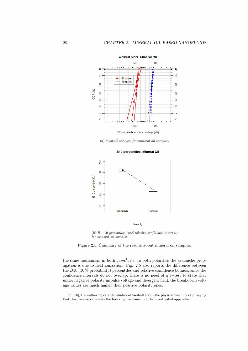
(a) Weibull analysis for mineral oil samples.
(b) B − 10 percentiles (and relative confidence interval)for mineral oil samples.
Figure 2.5: Summary of the results about mineral oil samples.
the same mechanism in both cases1, i.e. in both polarities the avalanche prop-agation is due to field ionization. Fig. 2.5 also reports the difference betweenthe B10 (10% probability) percentiles and relative confidence bounds; since theconfidence intervals do not overlap, there is no need of a t−test to state thatunder negative polarity impulse voltage and divergent field, the breakdown volt-age values are much higher than positive polarity ones.
1In [36], the author reports the studies of Weibull about the physical meaning of β, sayingthat this parameter reveals the breaking mechanism of the investigated apparatus.

2.2. REPEATED IMPULSE BREAKDOWN TESTS 29
Figure 2.6: Streamer propagation speed vs applied voltage. Note that in thenegative voltage case, the speed refers to the maximum one (at the needle tip).
A very simple model which helps to understand this result can be obtainedremembering what it has been found by Devins in [12] and summarized inthe previous chapter: positive polarity streamers are not slowed down by theavalanche shape like negative ones, but they are fastened. Generally speaking,the following equation is valid, in the case of breakdown:
ˆ b
a
dx = L (2.2)
where L is the gap distance between the two electrodes, which are at positionsa and b.Equation 2.2 can be now rewritten considering that dx = v(t)dt, thus obtainingthe following relationship: ˆ t2
t1
vdt = L (2.3)
At the same voltage value, but opposite polarity, the different relation speed−voltageis able then to explain why positive streamers are easier to lead to the finalbreakdown than negative ones. Devins, in [38], for small radii of curvature anda particular mineral oil (Marcol 70), found two different expression correlatingthe streamer propagation speed and the applied impulse voltage:
v = v0 +KV (2.4)
v(r) =AV
r2( 1r − 1L )
(2.5)
where v0 is equal to 1.64 ·105 cms , K is equal to 0.62 cm
V s , A is equal to 0.016 cm2
V s ,r is the linear coordinate and L represents the gap distance.
Equation 2.4 is relative to the positive applied impulse, and shows thatthe propagation speed is uniform across the gap, while in equation 2.5 thesecond case (i.e. in the case of negative applied impulse), the propagationvelocity depends on the radial coordinate2, because of the shielding effect the
2For the sake of simplicity, when dealing with needle to plane geometries, it is possible tosuppose that the electrode configuration is like a cylindrical capacitance.

30 CHAPTER 2. MINERAL OIL-BASED NANOFLUIDS
avalanche has on itself. Equation 2.5 is represented in fig. 2.6 considering thegeometrical parameters of our performed tests, and finally shows the differencesin the propagation speed with the applied polarity.The results about the nanofluids are presented in fig. 2.7 (positive polarity
(a) Weibull analysis for positive po-larity.
(b) Weibull analysis for negative po-larity.
(c) B10 percentiles (and relative con-fidence interval) for positive polarity.
(d) B10 percentiles (and relative con-fidence interval) for negative polarity.
Figure 2.7: Summary of the results about impulse breakdown tests.
left, negative polarity right).
2.2.1 Positive impulse breakdown results
The results which are relative to the positive applied polarity clearly show, asin [24], the positive effect due to the addition of nanoparticles to the insulatingmineral oil. Apart from the lowest concentration (FF0.2) in which there is apartial overlap of the confidence bounds, in the other cases there is an evidentstatistically significant improvement of the breakdown voltage which is due tothe presence of nanoparticles. Further on, it seems, but it is not sure from astatistically point of view, that FF0.5 behaves better than FF1.0, i.e. it isnot true generally speaking that the breakdown voltage increases monotonicallywith the nanoparticles concentration.The explanation of the results is quite puzzling, because we do not know what

2.2. REPEATED IMPULSE BREAKDOWN TESTS 31
is the exact interaction between nanoparticles and hot electrons, because it in-volves the nanometric scale, and this is not a known matter yet. Anyway, wecan try to give a possible explanation of the phenomenon, taking into accountthe known aspects regarding the effect of nanoparticles addition. In [31], theauthor made the hypothesis that magnetite nanoparticles can distort the elec-tric field due to the high value of their relative permittivity. It is not easy toestimate the permittivity of nanosized particles, but in the case of surfactantstreated nanoparticles, the formation of a water shell around them allows us tosay that their relative permittivity is high and very close to that of water, thatis ϵr = 81.The permittivity mismatch (transformer oil relative permittivity ranges from
Figure 2.8: Electric field lines distortion (after [31]).
2.1 to 2.3) creates the situation depicted in fig. 2.8, where the field lines areattracted by the nanoparticles. Since the electrons speed vector is related tothe field lines (v = µE, where µ refers to the electrons mobility), it followsthat nanoparticles act as electrons (or charge carriers, generally speaking) scav-engers.Devins, in [12], analyzing the effect of aromatics on the propagation of electricalstreamers, observed that the electron scavenging property does not have anyinfluence on the positive streamer propagation, despite what we have obtainedand what Seagal found in [24]. A possible explanation of this macroscopic resultcan be anyway found observing that the field lines distortion has an effect onthe increase of the attachment cross section for hot electrons. Electrons, whilepropagating from the cathode to the anode, collide against nanoparticles, beingtrapped on their surfaces, modifying their mobility and reducing the electricfield3. The combined effect of field reduction and mobility reduction affects themacroscopic velocity of the positive streamer (v = µE).A quite puzzling result is the apparent worsening effect which seems to start af-ter the 0.5 g
L concentration. According to the previously mentioned mechanism,the improving effect should increase monotonically with the concentration, be-cause a concentration increase further increases the attachment cross sectionand prevents the electrons velocity to raise at the propagation beginning. In
3They reduce the electric field because, propagating from the cathode to the anode, theyact as homocharge.

32 CHAPTER 2. MINERAL OIL-BASED NANOFLUIDS
this considerations, however, no mention has been done to the distance amongnanoparticles, which can have a role in the charge carriers transfer dynamics.If the distance among nanoparticles is high (some tens of nanometers), it istrue that they act as trapping sites, reducing the dangerousness of the electronsavalanche, but if the distance starts to reduce below ten nanometers, it is pos-sible to activate some fast exchange charge transfer mechanisms, like tunnelingeffects.These phenomena would result in a higher value of the charge carriers mobilityand a reduced homocharge effect, possibly explaining the results obtained forhigher concentrations nanofluids.
2.2.2 Negative impulse breakdown results
The results about negative streamers propagation are quite in agreement with[24]. Fig. 2.7 (right) shows a clear, statistically significant, breakdown voltagereduction due to the presence of nanoparticles. Even if the reduction in the meanvalue is not as evident as the increase in the case of positive applied polarity,the Weibull distributions fitting the experimental values are quite interesting,because they reveal a change in the β value. Unlike the positive distributionfunctions, which were all parallel, these ones cross revealing a change of phe-nomenon which they describe. In [36], the author reported that the value ofβ usually takes information about the breaking mechanism of the investigatedsystem.It is possible then, that in the negative applied polarity, nanoparticles effect islikely to change the streamer propagation mode. Again, Devins’ theory can beof help in the interpretation of the results.When a negative polarity impulse is applied, the two stage model reveals that,at the beginning, charge carriers have to be extracted from the cathode andthen, when the field at the tip of the electrons cloud overcomes the ionizationthreshold, the avalanche can start towards the anode. Nanoparticles, with theirelectron scavenging effect which has been introduced in the previous subsection,are likely to reduce the time duration of the first stage, increasing in this waythe propagation speed of the streamer which should then resemble the positivepolarity one. Unfortunately, it has not been possible to detect the streamershape to prove such statement, but the concentration trend seems to confirm itanyway, because the situation is the same of the previous case, where a changeof trend started to take place after the 0.5 g
L concentration. The loose of theelectrons scavenging property of the nanofluid after that concentration makesthe streamer more similar to that propagating inside transfomer oil, justifyingthe increase in the mean breakdown value.
2.3 Breakdown voltage under divergent fields.Slowly varying waveforms
The measurements which have been described in the previous section have beenperformed using an impulse generator with a high energy value. This aspectprevented us to take pictures of the discharges, because it was impossible tohighlight the streamer shape during the flash-over, since all the generator en-

2.3. BREAKDOWN VOLTAGE, SLOWLY VARYING WAVEFORMS 33
ergy was released after each discharge4. In order to take some pictures of theelectrical discharges involving nanofluids, different tests have been carried out,using a different high voltage generator of lower energy. The choice of thegenerator fell on a Trek 30/20 power amplifier, used in combination with anAgilent 33120a function generator to generate the reference voltage. The ad-vantage in using the Trek power amplifier instead of the Passoni Villa Impulsegenerator is that it is possible to limit the output current in case of breakdown(Ilim = 0.1mA), which also allows to reduce the number of used needles pre-venting the replacement after each breakdown. The disadvantage is that poweramplifiers are characterized by a limited bandwidth which prevents them to gen-erate lightning impulse waveforms. The test setup is the same of the previouslydescribed tests: needle to plane configuration, but 1mm gap spacing. Tungstensteel needles (1µm radius tip and 0.5mm diameter) have been protected by a1MΩ resistor connected in series with the insulating fluid sample.The following voltage waveforms have been tested:
• DC, both positive and negative polarity;
• 50Hz, 250Hz, 500Hz sinusoidal voltage;
• 50Hz, 250Hz, 500Hz square wave voltage with 50µs rising time (slowsquare voltage).
These three voltage waveforms are characterized by slow slew rates comparedto the 1.2 − 50µs lightning impulse one, allowing space charge to be injectedand influence the pre-breakdown phenomena, which are of second importanceotherwise [31]. A second aspect to be considered for such applied waveformsis that moisture can play a significant role for the breakdown voltage results.Unfortunately, Karl Fisher titration techniques [37] cannot be used on nanofluidsto check the moisture level after the sample manufacture and treatment, becausethe presence of conductive nanoparticles can produce unacceptable noise on themoisture measurement chain. Mineral oil final moisture value is, anyway, lessthan 5 ppm.Schlieren images have been captured to highlight the breakdown propagationmodes. They have been taken using a Z-type configuration setup ([39],[40]).The light source was a tungsten halogen low voltage lamp equipped with arear reflector. The condenser of the optical system was a Schneider-KreuznachXenon 40 mm double - Gauss lens with an f=1.9 focal ratio. The light beamwas reflected by two off-axis parabolic mirrors 138 mm in diameter and with anf=3.5 focal ratio. The knife edge was parallel to the needle so that the Schlierendiagnostic could record density gradients perpendicular to it. The images weredetected by a PCO CCD camera equipped with a super-video-graphics arrayresolution with a pixel size of (6 x 6) m [40]. The camera has been triggeredvia a TTL signal generated by the TREK when the discharge occurred, with 1s exposure time.Insulating fluid samples have been manufactured according to the procedurewhich has been described previously in this chapter. Three different nanofluidshave been prepared:
1. Mineral oil (MO), which is used as benchmark;
4This is also the reason why, after each measurement, the high voltage needle electrodehas been changed.

34 CHAPTER 2. MINERAL OIL-BASED NANOFLUIDS
Figure 2.9: DC breakdown voltages for nanofluids under divergent conditions.
2. 0.1 gL (LC), as an intermediate concentration;
3. 0.2 gL (HC), as maximum concentration.
Higher concentrations, although were supposed to behave better according tothe previous results, could not be tested, because the resulting fluids were todark to let the Schlieren technique catch streamers images.Breakdown tests have been implemented following the same procedure shown infig. 2.4: a LabView software has been written in order to remotely control thefunction generator and thus the TREK amplifier. Whatever the applied voltageshape, the starting applied value has always been 1 kV , the voltage step 150Vand the time duration of each applied step 40 s; voltage values, in the case ofsine or square wave, are meant to refer to the peak value.For each type of voltage waveform and polarity, 6 breakdown voltages have beenobtained.
2.3.1 DC voltage results, electrical tests
The results about the DC applied voltage are presented in fig. 2.9 for positiveand negative polarity. Each value on that plot represents the average breakdownvalue and the confidence intervals have been obtained through the Tukey hon-estly significant difference (HSD) formula [41] with 5% significance level. Suchintervals indicate when the difference between two mean values is statistically
2.3. BREAKDOWN VOLTAGE, SLOWLY VARYING WAVEFORMS 35
significant and they have been calculated as follows:
HSD = q(1−α),k,N−kσ√n
(2.6)
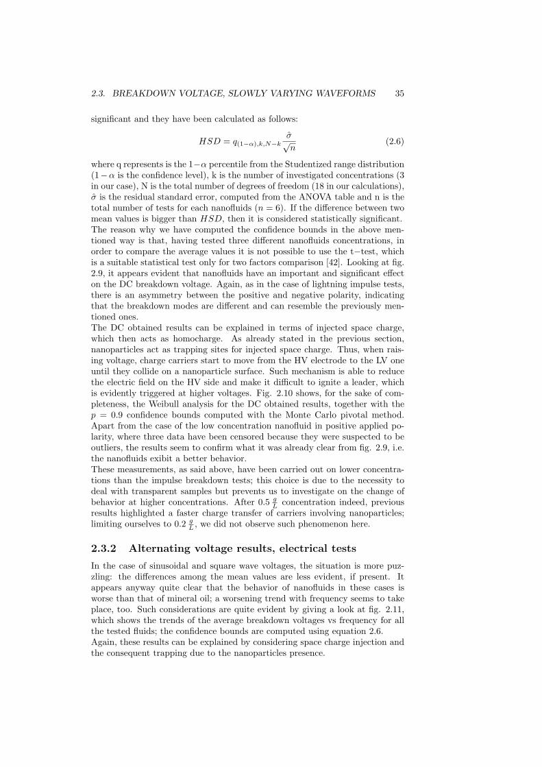
where q represents is the 1−α percentile from the Studentized range distribution(1−α is the confidence level), k is the number of investigated concentrations (3in our case), N is the total number of degrees of freedom (18 in our calculations),σ is the residual standard error, computed from the ANOVA table and n is thetotal number of tests for each nanofluids (n = 6). If the difference between twomean values is bigger than HSD, then it is considered statistically significant.The reason why we have computed the confidence bounds in the above men-tioned way is that, having tested three different nanofluids concentrations, inorder to compare the average values it is not possible to use the t−test, whichis a suitable statistical test only for two factors comparison [42]. Looking at fig.2.9, it appears evident that nanofluids have an important and significant effecton the DC breakdown voltage. Again, as in the case of lightning impulse tests,there is an asymmetry between the positive and negative polarity, indicatingthat the breakdown modes are different and can resemble the previously men-tioned ones.The DC obtained results can be explained in terms of injected space charge,which then acts as homocharge. As already stated in the previous section,nanoparticles act as trapping sites for injected space charge. Thus, when rais-ing voltage, charge carriers start to move from the HV electrode to the LV oneuntil they collide on a nanoparticle surface. Such mechanism is able to reducethe electric field on the HV side and make it difficult to ignite a leader, whichis evidently triggered at higher voltages. Fig. 2.10 shows, for the sake of com-pleteness, the Weibull analysis for the DC obtained results, together with thep = 0.9 confidence bounds computed with the Monte Carlo pivotal method.Apart from the case of the low concentration nanofluid in positive applied po-larity, where three data have been censored because they were suspected to beoutliers, the results seem to confirm what it was already clear from fig. 2.9, i.e.the nanofluids exibit a better behavior.These measurements, as said above, have been carried out on lower concentra-tions than the impulse breakdown tests; this choice is due to the necessity todeal with transparent samples but prevents us to investigate on the change ofbehavior at higher concentrations. After 0.5 g
L concentration indeed, previousresults highlighted a faster charge transfer of carriers involving nanoparticles;limiting ourselves to 0.2 g
L , we did not observe such phenomenon here.
2.3.2 Alternating voltage results, electrical tests
In the case of sinusoidal and square wave voltages, the situation is more puz-zling: the differences among the mean values are less evident, if present. Itappears anyway quite clear that the behavior of nanofluids in these cases isworse than that of mineral oil; a worsening trend with frequency seems to takeplace, too. Such considerations are quite evident by giving a look at fig. 2.11,which shows the trends of the average breakdown voltages vs frequency for allthe tested fluids; the confidence bounds are computed using equation 2.6.Again, these results can be explained by considering space charge injection andthe consequent trapping due to the nanoparticles presence.
36 CHAPTER 2. MINERAL OIL-BASED NANOFLUIDS
(a) Weibull analysis for positive po-larity.
(b) Weibull analysis for negative po-larity.
(c) Weibull B10 for positive polarity. (d) Weibull B10 for negative polarity.
Figure 2.10: Weibull charts for DC breakdown data and B10 percentiles.
(a) Breakdown voltages for sinewaves.
(b) Breakdown voltages for squarewaves.
Figure 2.11: Breakdown results for alternating applied voltages.
While raising voltage, when the space charge injection threshold is reached,charge carriers are injected and then trapped on nanoparticles surfaces as re-ported for the DC applied voltage in the previous subsection. However, in this

2.3. BREAKDOWN VOLTAGE, SLOWLY VARYING WAVEFORMS 37
(a) Breakdown mode for mineral oil. (b) Breakdown mode for FF 0.2 gL.
Figure 2.12: Schlieren images of breakdown modes, DC negative voltage, 15 kV .
case, voltage polarity reverses every ∆t = 1f , being f the voltage frequency;
therefore, at the polarity reversal, the trapped space charge switches from ho-mocharge to heterocharge, increasing in this way the electric field close to the HVelectrode [43]. Such phenomenon is able to predict that nanofluids performanceworsen at higher concentrations, while the worsening trend with frequency canbe explained by considering the nanoparticles detachment time constant. Infact, charge carriers are trapped on nanoparticles surfaces, but they are thendetached, after a certain time period, which is determined by the detachmenttime constant. Higher frequencies mean lower time intervals before the polarityreversal and so less time for the charge carriers to be detached; Measurementresults indicate that the detachment constant is of the order of some ms.Square wave breakdown voltages are lower than sinusoidal ones, as it appearsclear from fig. 2.11. Such results can be explained as follows:
• the amount of injected space charge is higher because the lower rise timeleads to a higher injected charge for the same voltage peak value;
• the faster polarity reversal does not let trapped charge to detach fromnanoparticles and reduce their enhancement field effect.
2.3.3 Schlieren images of the breakdown modes
This subsection presents some acquisitions of the breakdown modes, under bothDC and alternating voltage. The aim of such experiments, as already discussedin the previous subsections, was to highlight the different space charge mecha-nisms which are likely to take place because of the presence of nanoparticles.The first observation is that the results have been very difficult to analyze, be-cause of the small differences among the nanofluids concentrations; in order tobetter visualize the differences, we have decided to present only the results re-garding mineral oil samples and FF 0.2 g
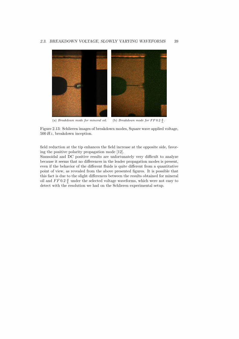
L , i.e. the maximum concentration. ForDC negative voltage, the results are represented in fig. 2.12. They are relativeto a breakdown event which took place at 12 kV , i.e. the breakdown inception

38 CHAPTER 2. MINERAL OIL-BASED NANOFLUIDS
for the nanofluid and a higher voltage breakdown for mineral oil, as shown in fig.2.10. A first look at the two figures reveals a difference in luminescence, whichis due to the fact that the two fluids have a different color: mineral oil is yellow,while ferrofluid is dark. Anyway, it is possible to see some small differences inthe breakdown region:
• mineral oil leader seems to have a ”‘kanal”’ shape, that is it seems to befilamentary. This can be due to two different reasons:
1. the aromatic content of the oil is high enough to change the negativestreamer propagation mode, as referred by Devins in [12];
2. the higher voltage at which the breakdown event is captured canbe able to ignite a different propagation mode of the streamer, evenif it seems difficult that this can happen only at twice the averageinception breakdown voltage. For a review about the streamers prop-agation modes, refer to, for instance, [31], [11], [44], [45], [46].
• nanofluid leader seems to have a different shape, as the dark circle reveals.This circle can be the proof of the trapping tendency of nanoparticles; in[12] the author says indeed that the bushy shape of the negative streamer isdue to the charge trapping tendency of aromatics, which is also responsibleof its reduced propagation speed [20]. Since nanoparticles seem to havethe same behavior, then it is possible that the bushy shape visible from theSchlieren image can be due to that. There is also a second explanation ofthat dark circle: it is possible that it represents the shock wave originatedafter the breakdown. Negative streamer propagation speed, as proved bySeagal in [24], are generally faster in conductive nanofluids and so, underthe same camera conditions, it is possible that in the mineral oil case wewere not able to capture the shock wave, while in the nanofluid case yes.If this was true, the streamer shape should be filamentary, according tothe ”‘two step model”’ of Devins [12], but the image resolution and theluminescence difference are not able to clarify this issue at all.
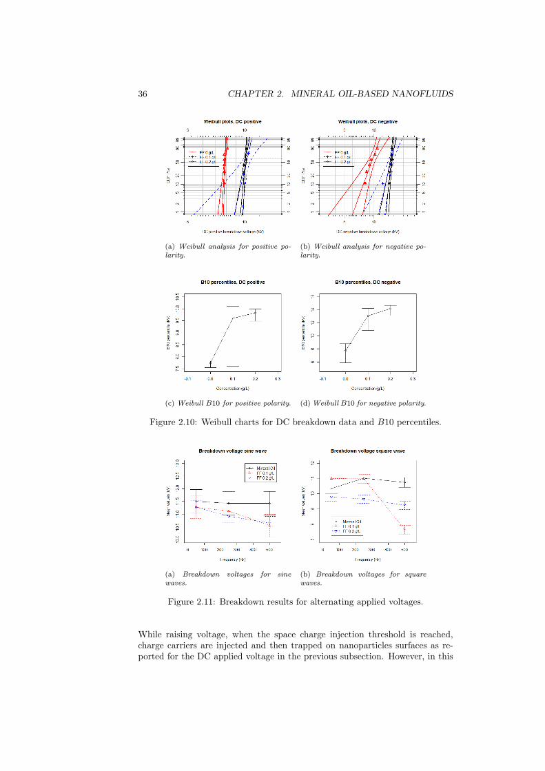
Fig. 2.13 represents, instead, the captured breakdown modes under square waveapplied voltage, at 500Hz, i.e. the frequency at which the higher difference seemto arise between the two fluids. Unlike the previous case, where the images weretaken at the same voltage value, in this case we decided to consider the situationof breakdown inception (10.5 kV for mineral oil and 9.5 kV for FF 0.2 g
L ). Thispicture reveals again a luminescence difference, but it seems to clarify what washappening in the previous image. In fact, looking at the nanofluid breakdownmode, it is quite reasonable to say that the phenomenon is faster and morefilamentary than that taking place inside mineral oil.The explanation of this fact can be found in the switch from homocharge (andits reducing field effect) to heterocharge (and its increasing field effect); the fieldincrease, after the charge injection, is able to explain why the propagation speedis higher and why the leader seems to be more filamentary, i.e. there is no timefor it to branch.It is then possible, after what we have said, that in the DC negative appliedvoltage case, the nanofluid leader is more filamentary and faster than that prop-agating inside mineral oil: because of the injected and trapped charge, the strong
2.3. BREAKDOWN VOLTAGE, SLOWLY VARYING WAVEFORMS 39
(a) Breakdown mode for mineral oil. (b) Breakdown mode for FF 0.2 gL.
Figure 2.13: Schlieren images of breakdown modes, Square wave applied voltage,500Hz, breakdown inception.
field reduction at the tip enhances the field increase at the opposite side, favor-ing the positive polarity propagation mode [12].Sinusoidal and DC positive results are unfortunately very difficult to analyzebecause it seems that no differences in the leader propagation modes is present,even if the behavior of the different fluids is quite different from a quantitativepoint of view, as revealed from the above presented figures. It is possible thatthis fact is due to the slight differences between the results obtained for mineraloil and FF 0.2 g
L under the selected voltage waveforms, which were not easy todetect with the resolution we had on the Schlieren experimental setup.

40 CHAPTER 2. MINERAL OIL-BASED NANOFLUIDS

Chapter 3
Space charge build-up dueto nanoparticles
Abstract
The previous chapter has introduced the general phenomena regarding mineraloil-based nanofluids starting from ferrofluid. In particular, it is well acceptedthat nanoparticles, at least when their concentration is not high, act as electronscavengers, modifying the electric field distribution. The aim of this chapter isto try to analyze the charge build-up phenomenon due to nanoparticles and itsconsequent effects.
In the previous chapter, in order to explain the experimental results, the chargetrapping tendency of nanoparticles has been frequently used. This idea, firstintroduced in [31], has been able to explain the results obtained by Seagal in[24] and what we have obtained with slower waveforms. In order to understandbetter the phenomenon, we decided to propose a very simple model trying todepict the situation in a divergent field configuration.The model we propose is indeed based on the assumption that the electric fielddistribution is not uniform, with an electrode configuration which resembles theneedle to plane one; since the experiments described in the previous chapterhave been performed in a divergent field configuration, the results of the follow-ing model can be used to give an interpretation to them.It is well known in literature [47], that under these conditions the field distri-bution inside one single material is hyperbolic and very difficult to obtain froman analytical point of view, unless we want to estimate the field on the HV tip,which is equal to:
Etip =2V
rlog(1 + 4dr )
(3.1)
where V is the applied voltage, r is the needle radius of curvature and d theinsulating gap.In the following, we will need a field formula for the trapped charge estimation,and so we will assume that our field configuration is like a spherical capacitor,like the one shown in fig. 3.1. In this figure, R1 represents the radius of the innerelectrode, representing in our model the radius of curvature of the HV needle,
41

42 CHAPTER 3. SPACE CHARGE BUILD-UP
while R2 represents the radius of the external conductor, which is related to theinsulating gap, d. It follows indeed that d = R2 − R1 ≈ R2, since R2 ≫ R1.Under this hypothesis, below considering a single material, the electric field canbe easily determined from the Laplace equation and the spherical symmetry ofthe problem:
∇2V = 0 (3.2)
1
r
∂
∂r
(r∂V
∂r
)= 0 (3.3)
where the second equation is the development of the first one, considering thepolar coordinates and that under spherical symmetry ∂
∂Φ and ∂∂θ are equal to
0. Equation 3.3 has to be solved for r ∈ [R1, R2] and so the 1r term can be
simplified without any problem because r is always different from 0. In thisway, it is possible to state that the electric voltage distribution can be writtenas:
V (r) =V
1R2
− 1R1
(1
R2− 1
r
)(3.4)
while the electric field, being easily E = −∇V , can be estimated as follows:
E(r) ≈ V R1
r2(3.5)
always considering that R2 ≫ R1. The field distribution obtained with formula3.5 has to be analyzed before being used for successive computations:
• can this formula be applied for nanofluids, where two different materials(oil and nanoparticles, with different permittivities) are mixed?
• it is then necessary to verify if it can be applied in the real case of needleto plane geometry and understand what is the relationship between thereal hyperbolic field distribution and the spherical obtained one.
The first question refers to the fact that equation 3.3 is obtained by simplifyingthe electrical permittivity of the material where voltage is applied; the realequation is in fact:
∇ · (−ϵ∇V ) = 0 (3.6)
Figure 3.1: Spherical capacitor.

43
In the hypothesis of a single material with no dependence of the relative permit-tivity upon the spatial coordinates, ϵ can be simplified, thus obtaining equation3.3. It is clear then that, generally speaking, it is not possible to use equation3.3 to estimate the electrical field distribution inside a nanofluid, where ϵ is afunction of the position. In that case, the correct equation to solve should be:
∇ · (−ϵ(r)∇V ) = 0 (3.7)
where r represents the position. ϵ(r) is equal to ϵoil if r indicates a point inwhich the material is mineral oil, while it is equal to ϵnanoparticles if r is placedon one nanoparticle.Since the solution of equation 3.7 is impossible to be found from an analyticalpoint of view, it is necessary to understand if it is possible to approximate thereal solution by using equation 3.5. In [48] and [49], the authors proved thatthe global increase of the permittivity switching from mineral oil to mineraloil-based nanofluid is negligible in first approximation and so it is possible tostate that ϵ(r) = ϵoil ∀r. This finally authorizes the use of equation 3.5 evenfor nanofluids, assuming a uniform particles distribution and reasonable con-centrations.The second question, i.e. if the spherical field formula is similar to the hyperbolicone obtained for the same applied voltage and the same electrode geometry, canbe solved considering the field value at the needle tip, derived using formulae3.1 and 3.5, that is:
Ehyp(R1) ≈2V
R1log(1 +4R2
R1)
(3.8)
Esph(R1) ≈V
R1(3.9)
It is obvious that the two field distributions are different, but generally speaking,the spherical one, for the same applied voltage and same geometrical parameters,is bigger than the hyperbolic one, as reported also in some milestone works ([16],[50]). Since, as it will be clear later, we are interested in the region close to theHV needle, for us it is sufficient that the two fields are comparable there. In otherwords, even if in the reality a certain voltage V is applied and a hyperbolic fieldis produced, in the model we will use a fictional voltage V0, which will producea spherical field which is similar to the real one close to the HV electrode. Sucha voltage can be obtained with the following equation:
2Vapplied
R1log(1 +4R2
R1)=
V0
R1(3.10)
2
log(1 + 4R2
R1)=
V0
Vapplied(3.11)
By considering a radius of curvature R1 equal to 1µm and an insulating gapR2 of 1mm, i.e. the parameter of the experiments described in the previouschapter, the criterion of equation 3.11 states that the ratio between the realapplied voltage and the fictional one is 4.2, meaning that in order to obtain thesame field we have in the reality, in the model we have to underestimate theapplied voltage of a factor equal to 4.2.We are now able to proceed with the charge build-up model, by formulating thegeneral hypotheses which will be used in the following:

44 CHAPTER 3. SPACE CHARGE BUILD-UP
1. spherical geometry: the electric field distributions will be calculated byassuming this particular geometry, with the above mentioned voltage cor-rection;
2. electric charge is injected via a current Dirac pulse of amplitude Qtot.The charging current is therefore assumed to be i(t) = Qtotδ(t), and so
the total injected charge is equal to Qinj =´ +∞0
i(t)dt = Qtot for theproperties of the Dirac δ(t) function.This hypothesis means that, as soon as charge is injected, the electric fieldis reduced to block the injection.
3. nanoparticles are not supposed to be a discrete system, but a continuum,so that the relative permittivity is not a function of spatial coordinates.This means that the stored space charge density on nanoparticles is acontinuous function;
4. the linear superposition principle is valid;
5. transient phenomena are neglected, and a steady state space charge trap-ping expression is used.
The last hypothesis requires the knowledge of a formula, which lets evaluate theamount of charge which is trapped by each nanoparticle. In [31] the author, an-alyzing the charge trapping tendency of nanoparticles, calculated the saturationstored charge on each nanoparticle as:
Qsat = −12πϵR2pE0 (3.12)
where ϵ is the permittivity of the host fluid, i.e. the mineral oil, Rp is the meanradius of the nanoparticles and E0 refers to the electric field before the chargetrapping mechanism.Equation 3.12, after proper modifications, can be used to estimate the spacecharge density induced by the charge injection from the HV electrode, Qtot,and the trapping behavior of nanoparticles. In fact:
ρ(r) =Qs(r)
Vp(3.13)
E0(r) = f(ρ(r)) (3.14)
where Vp refers to the volume occupied by the single nanoparticle and f(ρ(r))means that the electric field is a function of the space charge density.In the following section we will try to find the relation between the space chargedensity ρ and the electric field.
3.1 Relation between space charge density andelectric field
In the previous section, we have found the expression of the electric field gen-erated by the applied voltage, supposing that non space charge was injected.At the end of that section, anyway, we have introduced the charge trapping be-havior of nanoparticles, which requires the charge injection from the electrodes;

3.1. SPACE CHARGE DENSITY VS ELECTRIC FIELD 45
Figure 3.2: Charge trapping scenario at a generic time instant t: volume charge(colored region) and surface charge layer (bold line).
such charge will obviously have an influence on the electric field distribution.The aim of this section is to express the electric field E0 of equation 3.12 as afunction of the stored space charge density, ρ. Let us suppose that, after theinjection of Qtot, charge is trapped on each nanoparticle up to the limit definedby equation 3.12. This means that, after a certain time t, the global situationis:
• a certain amount of charge, Qtrapped ≤ Qtot, is already stored on thenanoparticles close to the HV electrode;
• the remaining one, Qtot−Qtrapped constitutes a surface charge layer trav-eling toward the LV electrode until it is completely trapped.
Such situation is shown in fig. 3.2, where the colored section represents thealready stored charge, while the remaining one is placed on the surface layerin position Ri and will be trapped in the following instants until it vanishescompletely.
The global electric field, according to the linear superposition principle hy-pothesis, is then related to the following three contributions:
1. the applied voltage;
2. the bulk space charge, which has already been trapped by nanoparticles;
3. the surface space charge which is traveling towards the LV electrode andwhich has not been trapped yet.
3.1.1 The applied voltage field
The first field contribution, which is only due to the applied voltage, withoutany charge inside the insulation, can be easily obtained by using equation 3.3,
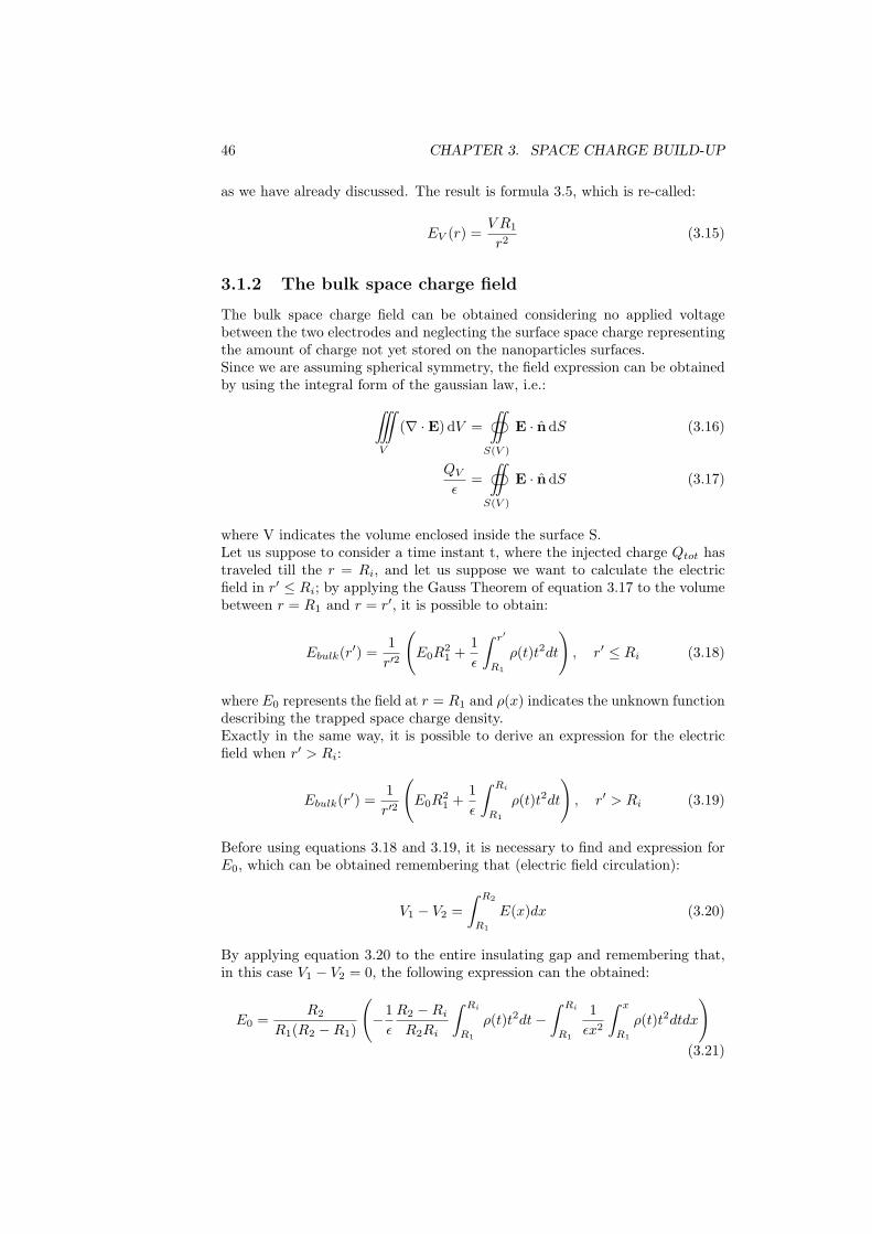
46 CHAPTER 3. SPACE CHARGE BUILD-UP
as we have already discussed. The result is formula 3.5, which is re-called:
EV (r) =V R1
r2(3.15)
3.1.2 The bulk space charge field
The bulk space charge field can be obtained considering no applied voltagebetween the two electrodes and neglecting the surface space charge representingthe amount of charge not yet stored on the nanoparticles surfaces.Since we are assuming spherical symmetry, the field expression can be obtainedby using the integral form of the gaussian law, i.e.:
˚
V
(∇ ·E) dV =
‹
S(V )
E · ndS (3.16)
QV
ϵ=
‹
S(V )
E · ndS (3.17)
where V indicates the volume enclosed inside the surface S.Let us suppose to consider a time instant t, where the injected charge Qtot hastraveled till the r = Ri, and let us suppose we want to calculate the electricfield in r′ ≤ Ri; by applying the Gauss Theorem of equation 3.17 to the volumebetween r = R1 and r = r′, it is possible to obtain:
Ebulk(r′) =
1
r′2
(E0R
21 +
1
ϵ
ˆ r′
R1
ρ(t)t2dt
), r′ ≤ Ri (3.18)
where E0 represents the field at r = R1 and ρ(x) indicates the unknown functiondescribing the trapped space charge density.Exactly in the same way, it is possible to derive an expression for the electricfield when r′ > Ri:
Ebulk(r′) =
1
r′2
(E0R
21 +
1
ϵ
ˆ Ri
R1
ρ(t)t2dt
), r′ > Ri (3.19)
Before using equations 3.18 and 3.19, it is necessary to find and expression forE0, which can be obtained remembering that (electric field circulation):
V1 − V2 =
ˆ R2
R1
E(x)dx (3.20)
By applying equation 3.20 to the entire insulating gap and remembering that,in this case V1 − V2 = 0, the following expression can the obtained:
E0 =R2
R1(R2 −R1)
(−1
ϵ
R2 −Ri
R2Ri
ˆ Ri
R1
ρ(t)t2dt−ˆ Ri
R1
1
ϵx2
ˆ x
R1
ρ(t)t2dtdx
)(3.21)

3.1. SPACE CHARGE DENSITY VS ELECTRIC FIELD 47
3.1.3 The surface charge field
The surface charge field can be obtained considering no applied voltage betweenthe two electrodes and neglecting the bulk charge we have dealt with in theprevious subsection. The only term which contributes to create an electric fieldis the surface charge layer ρΣ representing the charge which has not been trappedyet, whose value can be calculated according to the following balance equation:
Qtot = 4π
(ρΣR
2i +
ˆ Ri
R1
ρ(t)t2dt
)(3.22)
which refers to the usual time instant t, where the space charge has alreadyreached the position r = Ri. By using the Gauss theorem of equation 3.17for the volume between r = R1 and r = r′ < Ri, it is possible to obtain thefollowing expression:
Esurf (r′) =
E0R21
r′2, r′ < Ri (3.23)
where E0 represents, as before, the field at r = R1.In the same way, the field at r = r′ > Ri is equal to:
Esurf (r′) =
E0R21
r′2+
ρΣϵ, r′ > Ri (3.24)
The constant E0 can be easily obtained by applying the electric field circulation(equation 3.20), which lets us obtain:
E0 = −ρΣRi (R2 −Ri)
ϵR1 (R2 −R1)(3.25)
The expression for the electric field inside the insulating gap between the twoelectrodes will simply be E = EV + Ebulk + Esurf . We are now able to useequation 3.12 to find the expression of ρ. The first term of equation 3.12 canbe re-written in terms of ρ by remembering that ρ 4
3πR3p = Q, where Rp is the
nanoparticles mean radius, while the second one requires the knowledge of theelectric field which is generated by a charge distribution between r = R1 andr = r′, i.e.:
ρ(r′)4
3πR3
p = 12πϵR2p (Echarge till r′) (3.26)
The electric field of equation 3.26 can be determined with the expressions foundin the previous sections and, after some calculations, it is possible to obtain thefollowing charge density equation:
ρ(r′) =9ϵ
Rp
(V R1
r′2+
QtotR2(r′ −R1)
4πϵr′3(R2 −R1)− R2
ϵr′2(R2 −R1)
ˆ r′
R1
ρ(t)t(t−R1)dt
)(3.27)
which is an equation of the type:
ρ(x) = f(x) +
ˆ x
R1
g(x, t)ρ(t)dt (3.28)

48 CHAPTER 3. SPACE CHARGE BUILD-UP
Parameter Symbol Value [Unit]
Nanoparticles radius Rp 10 [nm]Applied Voltage V 2 [kV]HV electrode radius of curvature R1 1 [µm]LV electrode coordinate R2 1 [mm]Total injected charge Qtot 100 [pC]
Oil permittivity ϵ 19.5 [pFm ]
Table 3.1: Values of the parameters appearing in equation 3.27.
i.e. a second kind volterra integral equation, which depends on the parameterQtot. In [51], the author reports all the studies about the Volterra integralequations and refers that, in the case of the second kind equation, a procedureto find the analytical solution exists and leads to the following result:
ρ(x) = f(x) +
ˆ x
R1
Γ(x, s)f(s)ds (3.29)
where Γ(x, s) is called the resolvent kernel of equation 3.28 and is determined byan iterative procedure. It is possible indeed to prove that Γ(x, s) =
∑+∞i=1 ki(t, s),
where:
k1(t, s) = g(t, s); (3.30)
k2(t, s) =
ˆ t
s
g(t, τ)g(τ, s)dτ (3.31)
ki(t, s) =
ˆ t
s
g(t, τ)ki−1(τ, s)dτ (3.32)
For the purposes of this thesis, we do not want to solve equation 3.27 in ananalytical way, but we simply propose a numerical scheme, which is derivedfrom [51]. Let us suppose that we know the solution, for a given integrationstep h, at points ri = ih, i = 0, 1, 2, n− 1. An approximate value for ρ(rn) canbe obtained by replacing the integral on the right side of equation 3.27 with anumerical integration rule using the values of the integrand at ri, i = 0, 1, n andsolving the resulting equation for ρ(rn). Since ρ(r0) = f(r0), the approximatesolution can be computed in this step-by-step fashion.Before solving equation 3.27 with this numerical procedure, it is anyway neces-sary to define the value of all its parameters, which are defined in table 3.1.In table 3.1, the only parameter which has to be explained is Qtot = 100 pC.
Usually, charge is injected from HV needles because of the partial discharges(PDs) or streamers presence; in the following, we will present some results aboutPDs activity inside nanofluids and we will show that Q = 100 pC represents theorder of magnitude of the worst case in terms of charge injection before PDs startto be ignited. This means that our choice for the simulation has been intendedto consider the worst case. After such clarification, it is possible to presentthe results of the simulation, which are reproduced in figure 3.3. This pictureshows the solution of the above mentioned Volterra equation for r ∈ [R1, 5R1]for the sake of clarity in the final representation. In fact, it is reasonable thatthe trapped charge is placed only in a narrow region close to the HV electrode

3.1. SPACE CHARGE DENSITY VS ELECTRIC FIELD 49
Figure 3.3: Results of the equation 3.27.
from which it is injected. In this chapter we are not interested in the value ofthe space charge density which results from the solution of the equation, butit is noteworthy that the trend is not monotonous, but it presents a clear peakvery close to the HV needle. Such a peak, being constituted of homocharge,and remembering that it is a low mobility charge peak, is the responsible of thephenomena which have been discussed in the previous chapter. Under DC volt-age, such a charge build-up is able to hinder the nanofluid breakdown voltage,by reducing the field on the HV side, increasing in this way the voltage whichis necessary to ignite a leader and thus a discharge, while under alternatingvoltage, the low mobility of such a layer is dangerous at the polarity reversalwhen it reverses into heterocharge, thus increasing field values when voltagesare still low.The presence of the above mentioned peak can also reveal that, for nanofluids,the injection mechanism can be a real pulsed-like phenomenon as we have sup-posed, because the charge build-up is able to reduce the field below the injectionthreshold. A new injection pulse can be activated only when the complete chargeis depleted or shifted towards the lower voltage electrode. This interpretation ofthe results of equation 3.27 will be used to understand the polarization currentsmeasurements which will be conducted on nanofluids, which should reveal sucha pulsed injection behavior.

50 CHAPTER 3. SPACE CHARGE BUILD-UP

Chapter 4
AC Breakdown voltagesand Partial Dischargemeasurements
Abstract
The previous chapter has been a sort of break in the presentation of the measure-ment results about nanofluids, but it has been necessary in order to understandtheir behavior. With this chapter, we continue dealing with breakdown resultsdescription under sinusoidal AC voltages and we introduce partial discharges(PDs) measurements, carried out in order to compare the inception voltagesboth for nanofluids and mineral oils.
4.1 AC breakdown voltage
In this section we present the sinusoidal AC breakdown voltage results obtainedon our performed nanofluids, under quasi-uniform conditions. These measure-ments, unlike the ones obtained in the previous chapters, are more subjected tothe samples manufacturing process (contaminants and moisture for instance),and therefore more attention to avoid sample contamination has been paid.Four different fluid samples have been prepared, according to the proceduredescribed previously:
• Mineral Oil, used as benchmark, and hereafter labeled as MO;
• 0.1 gL ferrofluid-based nanofluid, hereafter labeled as FF0.1;
• 0.2 gL ferrofluid-based nanofluid, hereafter labeled as FF0.2;
• 0.5 gL ferrofluid-based nanofluid, hereafter labeled as FF0.1.
No other concentrations have been considered, because preliminary tests re-vealed that the ”‘optimum”’ concentration for impulse breakdown tests was
51

52 CHAPTER 4. AC BREAKDOWN AND PDS
Figure 4.1: Weibull plot for AC breakdown voltages.
0.5 gL . The breakdown voltage (BDV) of the samples has been measured using
an automated test kit with maximum test voltage of 75 kV, 60 Hz (Baur DPA75C). Four sets of measurements, each consisting of 10 tests, were carried outto reduce confidence bounds amplitude and thus to achieve a large statisticalsignificance. The adopted test procedure is specified in the IEC 60156 standard[52]. The electrode cell was modified to operate with a low quantity of NF, 50ml. The cell contains two stainless steel semi-spherical electrodes having a bodydiameter of 7.8 mm, a tip radius of 4 mm and spaced 2.5 mm. For the samefluid, the BDV were, on average, lower than those observed using a standard cell[53]. The reason why the obtained results are lower than the ones which can befound on literature is anyway explained in [53], where the author refers to theso-called ”‘dimensional”’ effect regarding the electrode surfaces: the bigger theactive electrode surfaces, the lower the obtained breakdown voltages, becauseof the higher probability to find local asperities (hot spots) where streamers canoccur leading to the complete discharge. Anyway, since in this work we haveconducted a comparative study, the dimensional effect is not a problem. Theresults have been elaborated by using the 2-parameter Weibull model, whichhas already been introduced in equation 2.1; the final plot comparing the dif-ferent concentrations is reported in fig. 4.1. Differently from the breakdowntests under lightning impulse voltages, for AC the best concentration seems tobe 0.2 g
L . Beta values, revealing the physical mechanism behind the failure ofthe investigated system ([36]), are quite similar for the MO, FF0.1 and FF0.5,but it is higher for FF0.2; this sort of determinism indicates that, probably, theaddition of nanoparticles in that selected concentration creates the maximumbenefit to the base insulating fluid.Fig. 4.1 does not report any confidence bounds for the sake of clarity; a data-set
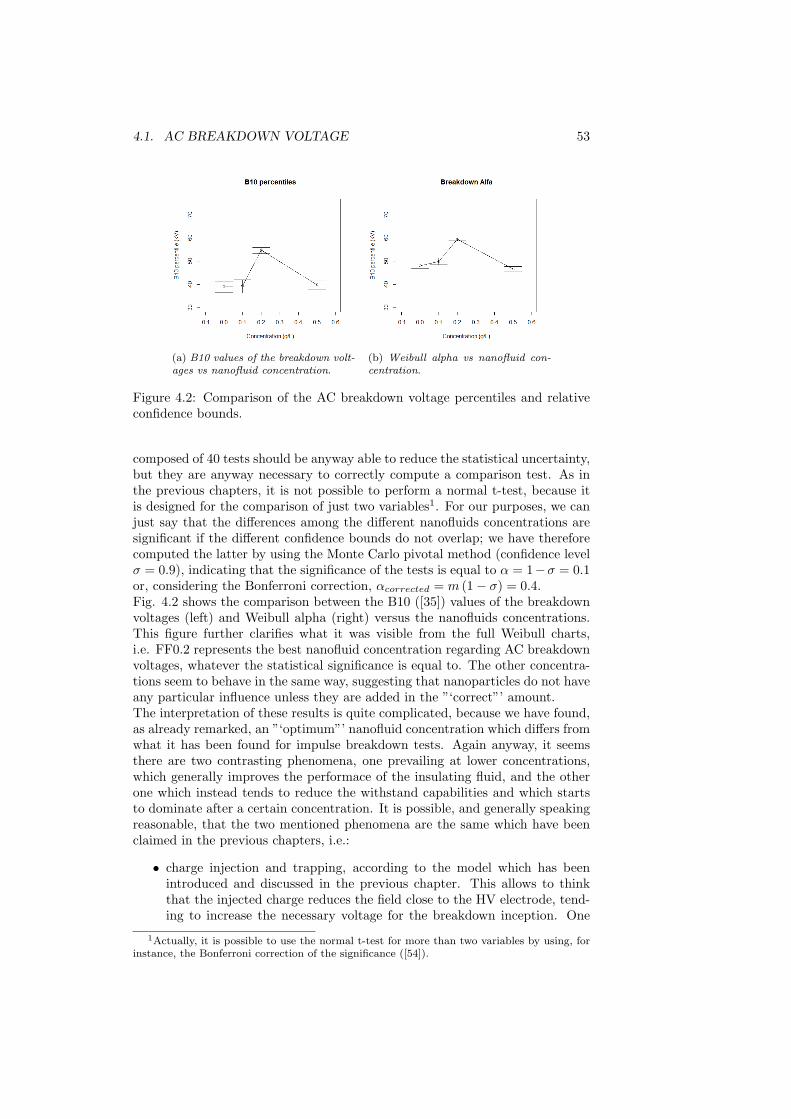
4.1. AC BREAKDOWN VOLTAGE 53
(a) B10 values of the breakdown volt-ages vs nanofluid concentration.
(b) Weibull alpha vs nanofluid con-centration.
Figure 4.2: Comparison of the AC breakdown voltage percentiles and relativeconfidence bounds.
composed of 40 tests should be anyway able to reduce the statistical uncertainty,but they are anyway necessary to correctly compute a comparison test. As inthe previous chapters, it is not possible to perform a normal t-test, because itis designed for the comparison of just two variables1. For our purposes, we canjust say that the differences among the different nanofluids concentrations aresignificant if the different confidence bounds do not overlap; we have thereforecomputed the latter by using the Monte Carlo pivotal method (confidence levelσ = 0.9), indicating that the significance of the tests is equal to α = 1−σ = 0.1or, considering the Bonferroni correction, αcorrected = m (1− σ) = 0.4.Fig. 4.2 shows the comparison between the B10 ([35]) values of the breakdownvoltages (left) and Weibull alpha (right) versus the nanofluids concentrations.This figure further clarifies what it was visible from the full Weibull charts,i.e. FF0.2 represents the best nanofluid concentration regarding AC breakdownvoltages, whatever the statistical significance is equal to. The other concentra-tions seem to behave in the same way, suggesting that nanoparticles do not haveany particular influence unless they are added in the ”‘correct”’ amount.The interpretation of these results is quite complicated, because we have found,as already remarked, an ”‘optimum”’ nanofluid concentration which differs fromwhat it has been found for impulse breakdown tests. Again anyway, it seemsthere are two contrasting phenomena, one prevailing at lower concentrations,which generally improves the performace of the insulating fluid, and the otherone which instead tends to reduce the withstand capabilities and which startsto dominate after a certain concentration. It is possible, and generally speakingreasonable, that the two mentioned phenomena are the same which have beenclaimed in the previous chapters, i.e.:
• charge injection and trapping, according to the model which has beenintroduced and discussed in the previous chapter. This allows to thinkthat the injected charge reduces the field close to the HV electrode, tend-ing to increase the necessary voltage for the breakdown inception. One
1Actually, it is possible to use the normal t-test for more than two variables by using, forinstance, the Bonferroni correction of the significance ([54]).

54 CHAPTER 4. AC BREAKDOWN AND PDS
of the postulated breakdown mechanism for industrial-grade oils is thatsuspended polar particles are attracted towards microscopic protrusionat the electrodes through dielectrophoretic forces. If a partial bridge isformed between the electrodes, this can become the site at which break-down takes place ([55]). Since the dielectrophoretic forces are linked tothe square value of the electric field, a voltage reduction can slow downsuch failure mode;
• fast charge transfer phenomena, which tend to deteriorate the performanceof the insulating fluid transforming the latter in a conducting fluid. Whenthe nanoparticles distance gets too small, secondary charge emission isable to ”‘bypass”’ the trapping behavior of nanoparticles and increasethe global conductivity. In this way, the nanofluid first loses its betterproperties, and then it even worsens at higher concentrations.
4.2 Partial Discharge Inception Voltages
This section reports the results about the partial discharge (PD) measurementsperformed on nanoluids. For general information about partial discharges, thereader can refer, for example, to [56] or [57].PD features have been investigated, as usual, using a divergent field configura-tion, just to highlight high field effects at reduced voltage; point/plane electrodeconfiguration has been hence adopted. Tungsten steel needles (1µm radius ofcurvature and 0.5mm diameter) have been manufactured by Fine Science ToolsGmbH; gap spacing was 20mm. Since PDs are fast pulses events, they prefer tocirculate inside capacitive branches, as for instance the insulating sample itself.For this reason, a coupling capacitor is usually needed for PD measurements([57]), but it tends to reduce the signal sensitivity, increasing the path the pulsehas to travel before being measured. In order to improve the sensitivity and thusincrease the measurement bandwidth, some researchers ([58], [59]), have startedto use the sample itself as coupling capacitor, by designing the LV electrodewith a guard ring. For PD detection, the measurement impedance (50Ω) wasconnected between the low voltage electrode and the guard ring. Fig. 4.3 showsthe cell which has been used during the experiments. As it is possible to see,in this particular case, the coupling capacitor is not represented by the sampleitself but, in order to minimize the amount of nanofluid to be used, a filler ringwith a high permittivity fluid (natural ester FR3, described, for instance, in[60]) has been used.PDs have been measured under different voltage conditions:
• 50Hz sinusoidal voltage;
• DC, both positive and negative.
The AC test setup consisted of a 220 V/30 kV transformer and a capacitivedivider (used only to measure the applied voltage, as the coupling capacitor isnot necessary as we have said). PD signals were recorded by a Techimp PDCheckdetector. For testing under DC voltages, a Fug - HCN 35-35000 bipolar 35 kVDC source was used. The entire test setup was placed in a shielded cabinet toreduce the effect of the external noise and thus increase the signal to noise ratio.The sensitivity of the system was better than 1 pC and tested with a TechImp

4.2. PARTIAL DISCHARGE INCEPTION VOLTAGES 55
Figure 4.3: Nanofluid cell for PD detection
calibrator; anyway, since the test cell capacitance is very low, one should expectcalibration errors ([57]). To overcome this problem, the PD pulse DC componenthas been estimated as the median of the 20 lowest harmonics of the PD currentspectrum. Partial discharge inception voltage (PDIV) was measured startingwith an initial voltage of 2 kV; the voltage was raised in steps of 1 kV, eachlasting 5 minutes, till the occurrence of the first PD pulses. Measurementswere repeated to get 5 PDIV values. By further increasing the voltage, PDmagnitudes increase, but the pulse waveform does not change. However, abovea given threshold, the pulse tends to spread in the time domain transferringmore charge, as shown in Figure 4.4 ([61], [62]). This suggests the developmentof more intense streamers. In order to study this behavior, the applied voltagewas raised above PDIV till a substantial change in the PD pulse shape couldbe observed. Since for short gaps (as the one used in these experiments), whenstreamers are observed, breakdown follows after increasing the applied voltageonly slightly, tests were stopped when pulses as the one shown in Figure 4.4 (onthe right) were first observed.The results of the PDIV measurements have been modeled considering the
2-parameters Weibull distribution of equation 2.1 and the corresponding B10values (and relative confidence bounds, computed with the Monte Carlo pivotalmethod with 90% confidence level) have been summarized in fig. 4.5.Such results correlate the applied voltage to the electric field, which has beencomputed considering the Mason’s formula, which has been introduced in theprevious chapter in equation 3.1. A rapid look at the results indicate that,under AC conditions, the PDIV values are higher than the DC obtained ones(both for positive and negative polarity); furthermore under DC, the negative

56 CHAPTER 4. AC BREAKDOWN AND PDS
Figure 4.4: Example of the difference between a PD (left, V=14 kV) and astreamer (right, V=26 kV); acquisitions performed with the TechImp PD Checksystem. Applied voltage: DC positive.
polarity results are lower than the corresponding ones obtained under positivepolarity. The difference between AC and DC conditions can be interpreted in adifference between the electrical parameters of the nanofluids, in particular:
• under AC conditions, the electric field is permittivity dependent;
• under DC conditions, the electric field depends on the conductivities.
Since both the permittivity and the conductivity of magnetite nanoparticles arehigher than the corresponding values for mineral oil, it is quite clear that thebase oil is subjected to a larger electrical stress both in AC and DC, which tends
Figure 4.5: PDIV (B10) for nanofluids depending on the concentrations.

4.2. PARTIAL DISCHARGE INCEPTION VOLTAGES 57
to increase the local field close to the HV needle in the presence of nanoparticles.Moreover, as the conductivity mismatch is much higher than the permittivityone, it is reasonable that PDIV values are lower for DC applied voltages.Apart from the differences between AC and DC applied voltages, which canbe explained in terms of the different parameters determining the local electricfield, it is surprising that, once more, the ”‘optimum”’ concentration nanofluidis different from the previously determined one. Summarizing, we have threedifferent best concentrations:
1. 0.5 gL , for lightning impulse breakdown tests;
2. 0.2 gL , for AC breakdown tests;
3. 0.1 gL , for PDIV tests.
The reason why the ”‘optimum”’ concentration changes with the performed testis not easy to understand; it is for sure connected to the different mechanismsa particular test highlights, but it is anyway very difficult to define a globaltheory trying to predict the best concentration for a certain test. For lightningimpulse breakdown tests, we have said that a key parameter can be representedby the attachment constant increase due to the presence of nanoparticles, andthis can be obtained with very high concentrations, until the distance betweennanoparticles starts to ignite fast charge transfer phenomena.For AC breakdown tests the same considerations should be done, but we haveto say that in this case moisture plays a significant role [63]. The moisturetrapping behavior of the surfactant-nanoparticles system is able to create a wa-ter shell around the nanoparticles themselves; this would ease secondary chargetransfer reducing the concentration at which they take place. Furthermore, if inthe previously reported results, the test setup was able to highlight the stream-ers propagation issues, AC breakdown tests are designed to be done in uniformfield configurations, where the streamers inception mechanism dominates. It ispossible, as Devins said in [12], that in case of inception, a lower attachmentconstant is needed to slow down electrons, differently from the case in whichthey are already accelerated and ”‘hotter”’.The setup of PDIV tests is designed to highlight discharge inception under nonuniform fields; as in the previous case, inceptions are optimized by low concen-trations. It is anyway interesting to notice that, under DC applied voltage, itis not sure that the best concentration is 0.1 g
L , as the trend seems to increaseafter the maximum tested concentration.As for the interpretation of the other measurements, the charge build-up modelcan help to understand the trend we have obtained. At low voltages, whenthe charge is injected from the HV needle, the field can be estimated thanksto the Mason’s formula; this is generally true, according to what we have saidin the previous chapter, but at a molecular level the field is enhanced in theoil because of the permittivity (or conductivity, in DC) mismatch between oiland nanoparticles. The enhancement lets the PDIV be lower than in the caseof fresh oil, but this cannot be proved because it would require very high val-ues of the measurement sensitivity. The injected charge is then trapped by thenanoparticles surfaces according to the general model which has been presentedin the previous chapter, leading to a field reduction which hinders the previousfield enhancement. It is clear now that, the higher the concentration, the higher

58 CHAPTER 4. AC BREAKDOWN AND PDS
the trapped charge (Qtot = 12πϵENpR2p, being Np the number of nanoparti-
cles); this charge is then moved towards the lower voltage electrode, until thepolarity reversal transforms it into heterocharge. The latter, as already said,increases the field close to the HV needle, leading to a higher discharge proba-bility. Higher concentrations do not only increase the trapped charge, but theyalso increase the fluid conductivity and the charge transfer ratio, which tends toreduce the heterocharge effect. A sort of balance between these two phenomenais claimed to explain the obtained results.To investigate the behavior at voltages higher than PDIV, the voltage was raisedabove PDIV till the transition from fast to slow streamers; the maximum dis-charge magnitude and the repetition rate at the different voltage levels wasrecorded. Given the low repetition rate of PD in oil, the results are somehowerratic.The results of such experiments have been summarized in fig. 4.6 and com-
pared with the mineral oil, which acts as a benchmark as usual.Starting from the results under AC applied voltage, it is clear that the maxi-mum investigated concentration has the worst behavior, since the PD inducedcharge diverges at moderately low voltages, meaning that at such voltages thefirst streamers are incepted. The other cases are quite similar, in the sense that0.2 g
L behaves in the same way as mineral oil, while 0.1 gL shows a lower charge
until the streamer inception voltage, which seems to take place at the samevoltage of the base fluid.The trend under DC applied voltage is less clear. Fig. 4.5 reveals that theimprovement at the best concentrations is less marked than in AC, and this,as already said, is due to the fact that magnetite nanoparticles are conductiveand lead to an increase of the electric field in the oil. The strange thing is thatthe concentration which seems to behave better in this case is 0.2 g
L , becauseit shows a lower charge until 25 kV , while the best concentration has a suddenworsening at 17 kV , even if it is possible that there may have been some errorsdue to the reduced PD rate under DC voltages. Apart from this behavior, thehigher concentration still continues to have a lower PD to streamer transition,revealing that above 0.2 g
L the fluid is too conductive. A comparison with theAC case shows that the streamer injection voltage takes place at lower voltages,confirming the role of conductivity in the determination of the electric fieldwhich leads to the Fowler-Nordheim injection current, which is here re-called:
jc =e3E2
8πhΦt2(∆ΦΦ
)e− 8π√
2mΦ23
3heE2 v(∆ΦΦ ) (4.1)
where:
• e represents the elementary charge;
• E represents the electric field;
• h represents the Planck constant;
• Φ represents the work function of the metal inside the nanofluid;
• m represents the mass of the electron;
• t2 and v represent two experimental functions. According to [31], v(y) =0.95− y2 and t2(y) = 1.1.

4.2. PARTIAL DISCHARGE INCEPTION VOLTAGES 59
(a) Trend of PD magnitude vs applied voltage in AC.
(b) Trend of PD magnitude vs applied voltage in DCpositive polarity.
(c) Trend of PD magnitude vs applied voltage in DCnegative polarity.
Figure 4.6: Comparison of the PD magnitudes vs applied voltage in the differentpolarities.
Equation 4.1 indicates a strong dependence of jc (and thus the injected charge)from the electric field; the higher the field, the higher the injected current, or,

60 CHAPTER 4. AC BREAKDOWN AND PDS
equivalently, the higher the conductivity, the higher the injected current.DC negative voltage confirms the considerations which have been made for DCpositive. A first observation directly comes from figure 4.5, where DC negativeresults are the lowest which have been measured; this is due to two differentreason:
1. the first reason is that the electric field is higher than the case of ACapplied voltage, and the same of DC positive applied voltage because ofthe dependence upon the conductivity;
2. the second reason is that electron injection is generally easier than holeinjection or, alternatively, electron injection is easier than field ionization[17]. This explains why DC negative results are different from the positiveones.
The relation between nanofluid concentration and voltage is the same also inthis last case: the streamer inception voltage is lower if the concentration getshigher (0.5 g
L is still the worst fluid, because its transition voltage takes place at10 kV ), while the other two concentrations behave better than mineral oil; as inthe previous case, 0.2 g
L seems to behave better than the optimum concentrationin terms of PDIV.
Figure 4.7 compares the PD repetition rates with the applied voltages in thedifferent configurations. Repetition rates, as known from the general PD theory([59]-[64]), are connected to charge depletion issues from the region where PDstake place: higher repetition rates mean higher conductivities while lower onesare connected to a more intense trapping behavior of the insulating materialunder test.The measured trend for AC2 partially supports this statement, because the0.5 g
L is the one which tends to explode at low voltages, even if 0.2 gL showed
the highest rates. 0.1 gL nanofluid is in this case the best fluid without any
doubt (at least until 17.5 kV ), and this suggests that at this concentration, theconductivity increase is able to limit the homocharge-heterocharge switch.Under DC applied voltage, repetition rates of nanofluids are always lower thanmineral oil and the best concentration fluid is 0.2 g
L . Since in DC there is noheterocharge switch, because there is no polarity reversal, this behavior is surelyconnected to the trapping tendency of nanoparticles, which contrasts with theconductivity increase (and thus the repetition rate increase, as explained in[64]).
The results presented in this section and the previous one are not clear andsomehow contrasting, but it is anyway noteworthy that three different mecha-nisms have to be investigated to gain more experience on nanofluids behavior:
• charge injection properties: it is necessary to understand the mechanismsof injection involving nanofluids. Are they similar to that of the base fluidor not?
• nanofluid conductivity: what is the relation between nanoparticles con-centration and the conduction mechanisms?
2In AC applied voltage, the PD repetition rates are measured in pulses per voltage cycle.

4.2. PARTIAL DISCHARGE INCEPTION VOLTAGES 61
(a) Trend of PD repetition rate vs applied voltage in AC.
(b) Trend of PD repetition rate vs applied voltage in DCpositive polarity.
(c) Trend of PD repetition rate vs applied voltage in DCnegative polarity.
Figure 4.7: Comparison of the PD repetition rates vs applied voltage in thedifferent polarities.
• nanofluid dielectric spectroscopy: do nanoparticles introduce particularmechanisms related to the electrical permittivity?

62 CHAPTER 4. AC BREAKDOWN AND PDS
The following chapters will try to give an answer to the postulated questions bypresenting some models and experimental evidence.

Chapter 5
Electrical field model
Abstract
As stated at the end of the previous chapter, we have three different questionsto answer. This short chapter presents a simple semi-empirical model tryingto predict the field variation due to the nanoparticles presence. First, a simplemodel is derived, considering the only geometrical effect of spherical nanopar-ticles, while in the second part of the chapter a sort of generalization is doneconsidering also the contribution of surfactants and the space charge which isinduced by nanoparticles.
5.1 First elementary model
The aim of this section is to introduce a geometrical model trying to determinethe electric field which is created in a nanofluid. In chapter 3 we have dealt withsuch a problem, neglecting the discrete nature of nanofluids and thus avoidingto treat the local enhancement of the field due to the nanoparticles. Here wewould like to overcome the latter hypothesis, and we propose a model startingfrom the following hyphoteses:
1. nanoparticles are supposed to be perfectly spherical;
2. the mean free path between nanoparticles is ≫ than the nanoparticlesradius;
3. the ratio between the conductivity of magnetite nanoparticles and mineraloil is = ∞;
4. the enhancement effect is confined in a region which is proportional to thenanoparticles radius;
5. we neglect the presence of surfactant particles.
The second and third hypotheses mean that nanoparticles do not interact amoungeach other and it is like there is only one of them. Such situation is depicted
63

64 CHAPTER 5. FIELD MODEL
in figure 5.1. Let us suppose to apply a constant voltage V and suppose toconsider a steady state situation; the electrical field can be determined thanksto the following equations:
ˆ b
a
E(x)dx = V (a)− V (b) (5.1)
divΣj = 0 (5.2)
j = σE (5.3)
By applying these equations to fig. 5.1, we easily obtain the solving equations:
E1 (d1 + d2) + 2E3d3 + E4d4 = V (5.4)
σ3E3 − σ4E4n = 0 (5.5)
E4n = E4sin(θ) (5.6)
In the case of AC applied voltage, the solving equations are the same, with theonly difference that divΣD = 0, and hence ϵ3E3 − ϵ4E4n = 0. This means that,by applying AC, we only have to change the conductivity with the permittivity.The solution of the group equations 5.4-5.6 is:
E1 =V
d(5.7)
E4 =d3 +R
R+ d3σ4
σ3
E1 (5.8)
E3 =σ4
σ3E4sin(θ) (5.9)
The solved equations show the dependence from d3. In order to give a finalformula we need to express d3 as a function of the other geometrical parameters.In particular, the adopted procedure is semi-empirical, because the value of d3has been determined by comparisons with finite element simulations. Followingthis approach, we have found that:
Figure 5.1: Representation of the modeled scenario.

5.1. FIRST ELEMENTARY MODEL 65
• d3 is equal to R in the case of a two dimensional computation;
• d3 is equal to R2 in the case of three dimensional computations.
In order to test the goodness of the obtained formula, we compare the analyticalresult with the one obtained with a finite element simulation in two dimensions;the latter is presented in figure 5.2. Such simulation is obtained considering thefollowing parameters:
1. d = 1m and V = 1V , i.e. the applied electric field is equal to 1 Vm ;
2. σ3 = 1 Sm and σ4 = 1000 S
m .
Fig. 5.2 shows a maximum electric field of 2.06 Vm , while the obtained formula
lets us estimate a value of 2.0 Vm , with a very small prevision error (less than
3%).For a reason which will be clear in the following (in particular in chapter 7), it isnecessary to evaluate the field between two nanoparticles which are closer than2R in the case of a bi-dimensional situation. Figure 5.3 shows the model of thesituation we would like to study. Two nanoparticles of radius R are supposedto be at a distance x < 2R and we would like to calculate the different fieldvalues, supposing to know the background field.Let us suppose the insulating gap, where the voltage V is applied, is equal tod + 4R, being d a geometrical variable. Using the labels of figure 5.3, it ispossible to write the following equations:
4REp + 2RE0 + xEi +V
d+ 8R(2R+ d− x) = V (5.10)
Epσp = E0σo (5.11)
Epσp = Eiσo (5.12)
Figure 5.2: Field simulation example.

66 CHAPTER 5. FIELD MODEL
Figure 5.3: Schematic representation of the situation.
After some calculations, it is possible to derive the following expression for theinternal field (assumed to be uniform):
Ei =V
d+ 8R
6R+ x
x+ 2R+ 4Rσo
σp
(5.13)
which can be written in an easier way remembering that Ebackground = Vd+8R :
Ei = Ebackground6R+ x
x+ 2R+ 4Rσo
σp
(5.14)
Equation 5.14, remembering that σo
σp< 1 in the case of magnetite nanoparticles,
reveals that the field between the two nanoparticles is always higher that thebackground one, with a limit of 3, when the distance x gets to 0.
5.2 Improved model
In this section we want to improve the above introduced model, in order to takeinto account the presence of surfactant particles which, as we have already saidin previous chapters, are able to keep nanoparticles kept out.The surfactant which Magnacol has used to manufacture Ferrofluid is oleic acid,presented in figure 2.1. As we said, it is characterized by a hydrophilic tip, at-tracting water molucules and thus creating a water shell around. The thicknessof such a water shell can be estimated by a simple analysis considering thestarting moisture of the base mineral oil. Let us suppose to consider a sphericalnanoparticle of radius Rp and we want to determine the external radius of the

5.2. IMPROVED MODEL 67
water shell, x. Moreover, let m be the moisture level of mineral oil (typically inthe 5− 30 ppm range); it follows that:
4
3π (x−Rp)
3Np [1L] = m (5.15)
where Np [1L] represents the number of nanoparticles which are present in 1Lnanofluid.Considering a nanofluid of concentration c
[gL
], the following relation can be
written:
c[ gL
]= 1000
43πR
3pNp [1L] ρ
[kgm3
][1L]
(5.16)
Equation 5.16 can be used to determine Np [1L], which in turn can be insertedinside equation 5.15 to estimate the thickness of the water shell. The result is:
x = Rp +3
√√√√1000mR3pρ[
kgm3
]c[gL
] (5.17)
Equation 5.17, and in particular x−Rp, is represented in figure 5.4 for differentmoisture levels.The improvement of the field model consists in the analysis of the contributionthe water shell can have on the electric field distribution and the introductionof a region, which is know in literature with the name ”‘interphase”’, whichconsists in a transition region between the water shell and the host fluid ([65]-[66]-[67]-[68]). The model we propose here is represented in figure 5.5 and startsfrom these considerations:
• since magnetite nanoparticles and water have a very similar permittivity,we suppose to consider an ideal nanoparticle with radius R = Rp +WSt,where Rp is the mean radius of magnetite nanoparticles and WSt rep-resents the thickness of the water shell obtained with the above writtenequations (this region is labeled with the number ”‘2”’ in figure 5.5;
Figure 5.4: Water shell external coordinate vs concentration.

68 CHAPTER 5. FIELD MODEL
Figure 5.5: Improved model general scheme.
• we consider the interphase thickness t1 (region ”‘1”’ in figure 5.5) equalto the nanoparticles radius Rp;
• we consider also a region labeled as ”‘a”’, where we suppose the fieldvariations are confined. Such a region has a thickness which is equal toR if we consider a two dimensional case, while R
2 if we switch to a threedimensional case, as in the previous model.
In figure 5.5 there is the indication of the field line we consider to simplify theproblem; we suppose indeed that the field lines are aligned with those inside the”‘equivalent”’ nanoparticle, even if this is not generally true.Simple geometrical considerations allow to state the following things:
1. d0 + 2dasin(θ) + 2d1 + 2d2 = d, where d is an auxiliary thickness wherethe voltage V is applied;
2. d2 =√R2 − (t1 +R)2cos2(θ);
3. d1 = (t1 +R)sin(θ)−√
R2 − (t1 +R)2cos2(θ).
Starting from these results, it is possible to write the same equations of theprevious section:
E0d0 + 2daEasin(θ) + 2E1d1 + 2E2d2 = V (5.18)
ϵ2E2 = ϵ1E1 (5.19)
ϵaEa = ϵ1E1sin(θ) (5.20)

5.2. IMPROVED MODEL 69
Parameter Symbol Value [Unit]
Nanoparticle+WS radius R 0.05 [m]Interphase thickness t1 0.05 [m]Inter-oil region da 0.1 [m]Oil Permittivity ϵa 2Interphase relative permittivity ϵ1 4Particle relative permittivity ϵ2 8Background field Eb 0.33 [ Vm ]
Table 5.1: Values of the parameters of the simulation of figure 5.6.
After some calculations, it is possible to obtain the following expressions:
E2 = Ebd1 + d2 + dasin(θ)
d2 + d1ϵ2ϵ1
+ daϵ2ϵa
(5.21)
E1 =ϵ2ϵ1E2 (5.22)
Ea =ϵ2ϵa
E2sin(θ) (5.23)
where Eb =Vd refers to the background field. These equations have been again
compared with finite element simulations to verify their correctness; the Comsolsimulation result is shown in figure 5.6, with the parameters of table 5.1. Thederived equations are able to estimate the maximum and minimum field asfollows:
• maximum field, predicted value: 0.48 Vm , obtained value: 0.47 V
m ;
• minimum field, predicted value: 0.12 Vm , obtained value: 0.14 V
m .
Figure 5.6: Finite element analysis of the improved model.

70 CHAPTER 5. FIELD MODEL
Apart from the comparison between the obtained formula and the finite ele-ment simulation result, where the parameters have been randomly chosen, it isnecessary to spend few words about the relative permittivity of the interphaseregion. According to the ”‘Lewis”’ nanocomposites model ([65]), ”‘the intensityIα of a material property α does not change abruptly but gradually over thecourse of several nanometers. Each atom or molecule in this interfacial area willinteract with its surroundings via short- and long-range forces.”’ (after [69]).This means that the permittivity ϵ1 differs from that of mineral oil and it is notuniform as we have supposed. For the sake of simplicity, we neglect this factand simply consider ϵ1 = ϵa+ϵ2
2 , i.e. the average value between mineral oil andthe nanoparticle-water shell corona around.
There is a last model which considers all the phenomena induced by nanoparti-cles. We have said in the previous chapters that nanoparticles bahave as chargetraps when voltage is applied; this induces charge to create a layer around thenanoparticles, which in turn is able to attract opposite polarity particles. Inother words, if nanoparticles are able to attract electrons on their surfaces, elec-trons are then able to attract positive ions which form a counterion layer andforce them to move only along precise trajectories. This particular phenomenonhas been firstly studied by Schwarz in [70] for micrometric colloidal solutions,but the described mechanism is likely to interest also nanoparticles-based col-loidal solutions.
5.3 Theory of electrons and counterions inter-actions
This section recalls the theory presented in [70] about the interaction betweenfixed charges which are trapped on particles surfaces and the counterions whichare attracted. Schwarz considered a fluid of complex conductivity Σa = σa +jωϵa, while particles are supposed to have a mean radius R and complex con-ductivity Σi = σi + jωϵi. The sphere is electrically charged and surroundedby counterions of electric charge e0 and mechanical mobility u1, which can bemoved only along the particles surface, but not perpendicular to it; in otherwords, the counterions motion is assumed to be tangentially. It is then clearthat the counterions density is a function of the electric field, in particular:
σ(E) = σ0 + ¯σ(E) (5.24)
where σ0 is the constant value representing the counterions density when noelectric field is applied and σ is the variation due to the electric field. Theinduced ions current density is made of two contributions:
je = e0σµE (5.25)
jd = −ukT
R
∂σ
∂θ(5.26)
which are, respectively, the electric field and the diffusion contribution. Inthe previous equations, µ refers to the ions mobility, k is the Boltzmann con-stant and θ is the angular coordinate which has been introduced because of the
1The mechanical mobility is defined as the velocity per unit force, i.e. u = vF
= vqE
= uelq
,
where uel refers to the electrical mobility.

5.3. THEORY OF ELECTRONS AND COUNTERIONS INTERACTIONS71
spherical symmetry of the problem. The equation which allows to determinethe counterions density is:
∂σ
∂t− div(je + jd) = 0 (5.27)
i.e. the continuity equation which has to be coupled with the Laplace equation:
∇2Ψa = 0(r > R) (5.28)
∇2Ψi = 0(r < R) (5.29)
with the following boundary conditions:
limr→R
Ψa = limr→R
Ψi = Ψs (5.30)
Ψa −→ −Ercos(θ) for r −→ +∞ (5.31)
limr→0
Ψi = ∞ (5.32)
Σa∂Ψa
∂r− Σi
∂Ψi
∂r= −iωe0σ (5.33)
These solving equations can be solved with standard methods, as for instance byrepresenting the unknown variables by means of Legendre polynomials Pn(cosθ).In this way, it is possible to find that:
σ = σ0 −1
1 + iωτ
e0σ0
kTΨs (5.34)
where τ = R2
2ukT represents a relaxation of the change in the counterion density,which depends, not surprisingly, on the ions mobility: the higher the mobility,the higher the relaxation frequency.After some calculations, the electric potential can be determined as:
Ψa = −Ercosθ +Ki −Ka
Ki + 2KaR3E
cosθ
r2(r ≥ R) (5.35)
Ψi = − 3Ka
2Ka + KiErcosθ (r ≤ R) (5.36)
where Ki = Ki + iωϵ02ϵ⋆sR and ϵ⋆s = 1
1+iωτe20σ0uτ
ϵ0.
Equations (5.35) and (5.36) are very important because they let formulate thefollowing equivalence principle: The dielectric behavior of a sphere with thecounterion layer is identical with that of a sphere without such a layer but withapparent dielectric constant:
ϵi = ϵi +1
1 + iωτ
e20σ0R
ϵ0kT(5.37)
Equation (5.37) will let us use the model formulated in the first section ofthis chapter to take into account the space charge effect on the electric fielddistribution, without further complicating the analytical procedure.

72 CHAPTER 5. FIELD MODEL
Chapter 6
Injection at electrodes
Abstract
This chapter contains a study aimed at analyzing the injection of charge carriersin ferrofluid-based nanofluids. Conductivity tests in divergent field conditionsare described and discussed to compare the different mechanisms with respect tomineral oil. Long tests have been realized too, in order to highlight the stabilityof nanofluids under divergent fields. Nanofluids will reveal to be unstable underDC applied voltages; a simple model to interpret this phenomenon will be pro-posed.
This chapter will introduce some results about conductivity tests at differentregimes. Such tests have been proposed for simple liquids in [17] or [50], butnobody has ever performed them on mineral oils, because of the complexity ofthe chemical structure which characterizes them [17]. Recently, Butcher et alia([71]) have made conductivity measurements on mineral oils under divergentfield configurations and different voltage levels. Usually, when performing suchtests, three conduction regimes can be seen:
• Ohmic regime, for relatively low voltages, where current and voltages arelinearly correlated, i.e. it is possible to assume a voltage-current relationof the type I = V
R , where R stands for the resistance of the insulatingfluid;
• Fowler-Nordheim regime, for intermediate voltages, where the followingrelation correlates current and applied voltage ([72]):
I = KV 2e−BV (6.1)
where K and B are constants; in particular:
B =3χdϵ
2∆d(6.2)
where χ is the electron affinity barrier, ∆d the barrier thickness (assumedto be few nanometers), d is the gap width and ϵ represents the electricalpermittivity;
73

74 CHAPTER 6. INJECTION PROPERTIES
• space charge saturation regime (SCLC), for high voltages. Halpern andGomer in [50] have studied such regime, approximating the geometry witha simpler model and found the following voltage-current relation:
I =3α
8
µϵ
dV 2app (6.3)
where α ≈ 0.6π represents the emission solid angle and µ is the chargecarriers mobility.
The values of voltages which are needed to enter a well precise regime dependon the geometry of the used cell, because the key parameter is, as always, theelectric field. Figure 6.1 shows an example of a voltage-current plot highlightingthe three above mentioned regimes. It refers to mineral oil as insulating sample,d = 10mm gap, needle to plane electrode configuration and different voltagepolarities (open symbols: negative, closed symbols: positive). As it is possibleto see from the axes labels, the plot represents ln
(IV 2
)vs 1
V and so, if the voltageis high enough to ignite the Fowler-Nordheim regime, a linear trend is expected,as revealed from equation (6.1): for such a reason, the plot represented in fig.6.1 is know in literature as ”‘Fowler-Nordheim”’ plot. The three regimes areclearly visible in this picture:
1. for low voltages (V ≤ 4 kV ), the regime is ohmic;
2. for intermediate voltages (4 ≤ V ≤ 10 kV ) the trend is linear and theFowler-Nordheim regime dominates this voltage interval;
3. for higher voltages a saturation effect is visible, highlighting the lastregime, which is the SCLC, from which the mobility of the carriers can beoutlined.
Measuring the slope of the voltage-current plot in the Fowler-Nordheim regime,it is possible to estimate the parameters which define the constant B of equation
Figure 6.1: Example of a Fowler-Nordheim plot for mineral oil (after [71]). Opensymbols: negative polarity; filled symbols: positive polarity.

75
Figure 6.2: Example of the recorded current (V = +8.5 kV , mineral oil).
(6.2), in particular the electron affinity barrier. Comparing the positive andnegative trends of figure 6.1, the following considerations can be done:
• the ohmic region seems to be different, and this is documented also in [17],where the author refers to the different mobility of positive and negativeions, since the conduction in fluids is due to the ion motion;
• the Fowler-Nordheim injection threshold is higher for positive polarity,because, as known in literature, electron emission is easier than field ion-ization (i.e. hole injection).
The tests described in this chapter have been performed on samples of the samenature of the ones defined in the previous chapters, but only one concentra-tion has been tested; 0.2 g
L nanofluid has indeed been considered because it hasproved to be one of the best concentration regarding injection phenomena.The divergent field conditions have been realized with a needle to plane electrodeconfiguration; a tungsten steel needle (1µm radius tip and 0.5mm diameter)manufactured by Fine Science Tools GmbH was used as the high voltage elec-trode. The ground electrode was a brass plane with pseudo-Rogowsky; gapspacing was 20mm.The voltage source was either a Spelmann DC Generator PCM50P120 for pos-itive polarity, or a PCM50N120 for negative polarity; DC current has beenrecorded with a Keithley 388 electrometer.For each specimen, voltage has been raised from a lower value (4 kV ) to a highervalue (from 11 to 13 kV ), by steps of 500V . Both positive and negative polar-ities are considered; to avoid the full breakdown of the oil (or nanofluid) gap,the maximum voltage level was lower using positive polarity, because positivestreamers are considered the most dangerous events leading to breakdown ([12]).A first question to be answered, before starting with the tests, is the time inter-val which is needed to reach the steady state; this is an important issue, becauseit is necessary to understand when voltage has to be raised. The theory suggeststhat the transient current is dominated by the time constant τ = ϵ
σ , with obvi-ous meaning of the symbols; in the case of oil, the time constant is of the orderof tens of seconds. Figure 6.2 confirms that the transient behavior is very shortand that the steady state condition is reached after one hundred seconds. As

76 CHAPTER 6. INJECTION PROPERTIES
(a) I − V trend comparison for posi-tive voltage.
(b) I −V trend comparison for nega-tive voltage.
Figure 6.3: Comparison of the I − V trends for the investigated samples.
final current, we have considered the median value of the last recorded 200 s. Aglobal overview of the obtained results highlights the conductivity increase dueto the presence of nanoparticles. Figure 6.3 shows this aspect and anticipatesthat:
• the nanofluid conductivity is more or less one order of magnitude higherthan that of mineral oil;
• for nanofluid, the I − V trend has a linear shape till higher voltages.
The second consideration allows us to state that, before analyzing better theobtained currents, nanofluids have a higher injection voltage compared to min-eral oil; mineral oil trends indeed start to deviate from the linear shape at lowervoltages. From figure 6.3, it is not definitely clear if the non-linear trend refersonly to the Fowler-Nordheim regime or also to the SCLC one, as it may seemfrom the slope reduction of the last few points; in order to understand betterthe issue, the Fowler-Nordheim plot is needed and represented in figure 6.4.This figure highlights the different regimes and, as expected, in the case of neg-ative polarity, there is the transition between the Fowler-Nordheim to the SCLCone; unfortunately, this was not visible for positive polarity as the tests werestopped at lower voltages to prevent streamer inception. As outlined earlier,the following considerations can be done for our investigated mineral oil:
1. the ohmic conduction is different in the case of positive and negative po-larity, because of the different mobilities of positive and negative ions, asreported in some milestone works ([4],[17]);
2. the injection threshold voltage is different, in the sense that electrons aremore easily injected than holes;
3. the slopes of the linear lines are different, indicating that the affinitiesare different in the case of positive and negative charges. In particular,positive polarity slope is higher, indicating a higher energy required toinject, which is in agreement with the necessity of higher electric fields;

77
4. unlike figure 6.1, where the separation between the ohmic and injectionregime is quite marked, in our case it seems to be rather blurred, suggestingthat an intermediate phenomenon may take place, as for instance theSchottky injection, which usually starts at a lower voltage than the Fowler-Nordheim one. For more details about the difference between the twotypes of injections, the reader can refer to several works, as for instance[4],[17] or [31];
5. a Schottky injection process may be possible, because the calculated en-ergy barriers are, for positive and negative voltage, 0.09 eV and 0.22 eV ,i.e. not so higher than 10kT at room temperature.
The case of 0.2 gL nanofluid is shown in figure 6.5, where the Fowler-Nordheim
plot is reported. As supposed when looking at figure 6.3, nanofluid provideresults different from mineral oil. In particular, the injection threshold voltageis higher than that of mineral oil.The plot of figure 6.5 does not reveal a problem that had to be solved to arriveto it. The negative charging current, above a certain voltage value, showed avery strange behavior, which is reported in figure 6.6. Such behavior was likelyto take place only when the negative polarity was considered; similar effectswere not observed on the positive polarity. We might expect to observe them athigher voltages, however the inception of streamers in oil, at such high voltages,might hinder the observation, destroy the electrometer used for the measure-ments, or change the order of the nanoparticles in the fluid.The pulsed-like mechanism represented in figure 6.6 does never reach a steadystate value within reasonable time intervals, indicating that this is not a phe-nomenon connected with the electrical properties of the nanofluid, like in thecase of mineral oil. Before trying to entering the details of such phenomenon, wehave to say that the ”‘steady state current”’ reported in figure 6.5 is equivalentto the minimum value of the recorded trend in a window of 10000 s maximum.This choice does not take into account the real intrinsic steady state currentbecause, as we will see in the following, the minimum current is influenced by
Figure 6.4: Fowler-Nordheim plot for mineral oil.

78 CHAPTER 6. INJECTION PROPERTIES
Figure 6.5: Fowler-Nordheim plot for the investigated nanofluid.
a sort of space charge like mechanism. Therefore, comparing the FN plots ob-tained earlier in this chaper for positive and negative polarities should be donein a very cautious way.If we think to the scenario close to the HV electrode, the needle is in contactwith oil both in the case of mineral oil sample and in the case of the nanofluid; itis then difficult to think that there is a change of electron affinity switching fromthe base fluid to the nanoparticles-based one. It is possible, on the contrary,that the electric field changes the equivalent barrier charges have to overcome
Figure 6.6: Example of recorded conduction current for nanofluid (V =−8.5 kV ).

79
in order to be injected inside the investigated fluid. Taking the case of min-eral oil as reference, we have already shown in the previous chapters how lowconcentration nanofluids act as electron traps, causing a reduction of the elec-tric field close to the region where they are injected (homocharge effect). Thisphenomenon, again, can be the cause of the behavior observed for nanofluids,because:
1. first, an enlargement of the linear regime can be explained by a fieldreduction, i.e. at the same voltages, the highest electric field is lower thanthe one inside mineral oil;
2. second, the pulsed-like polarization currents can find their explanationin the change of mobility due to the charge trapping on nanoparticlessurfaces.
The last consideration arises from the fact that, the shape of the conductioncurrent is like the one of figure 6.6 only when the applied polarity is negativeand the voltage is above a certain threshold (in the case of our experiment, thisthreshold was about −8.5 kV ). Since nanoparticles are more conductive thanmineral oil, the electric field distribution is higher inside the latter, causing aninjection at lower voltages; such charge is then trapped by the nanoparticles sur-faces in a negligible time interval [31] and reduces the field causing the apparentbetter behavior observed in figure 6.5. At higher voltages, i.e. for V > 8.5 kV(negative polarity), the electric field is anyway so high to let charge injectiontake place; this injection brings a current increase due to the increase of chargecarriers [17]. At this point, the injection is inhibited again, but the electric fieldcauses a charge shift towards the low voltage electrode; such movement takesplace according to the mobility of the carriers, which is equal to the mobilityof the nanoparticles because charges are trapped on their surfaces. As chargesmoves towards the LV electrode, the current reduces because carriers leave thehigh field region, till re-injection takes place again when the field on the HV tiprestores to the starting value.If this phenomenon is really likely to take place, after several pulses we shouldfind traces of nanoparticles on the low voltage electrode. Figure 6.7 representsthe LV electrode after one months testing. In the picture, a clear nanoparticles
Figure 6.7: LV electrode after one month testing. Note that the guard ring isnot affected by the phenomenon.

80 CHAPTER 6. INJECTION PROPERTIES
(a) HV needle before the conductiontest.
(b) HV needle after the conductiontest.
Figure 6.8: Optic microscope pictures of the HV needle before and after thetest.
aggregation is evident in a circle inside a rounded brass region. The latter is theguard ring allowing the bulk conduction current measurement and so it is notaffected by the phenomenon, which is likely to take place only on the measuringLV electrode in the middle.A real interesting thing which has been observed after the same time interval isthat a nanoparticles aggregation has been observed on the HV electrode, too:this is clearly visible in figure 6.8. Such aggregation cannot be justified by theconsiderations which have been made previously, and it will be explained witha simple model in the following section. Instead, we would like now to verify ifthe pulsed-like mechanism of figure 6.6 is really linked to the charge trappingbehavior of low concentration nanofluid.The way to verify it consists in the comparison of the recorded conductioncurrent under negative polarity of a low concentration nanofluid and a highconcentration one, that is:
• 0.2 gL nanofluid, as the low concentration one;
• 1.0 gL nanofluid, as the high concentration one.
The experimental setup and the preparing procedure of the fluids is the samedescribed above. The only thing which changes in the two fluids is the meandistance among nanoparticles which can be estimated considering, in first ap-proximation, the theory of gases presented, for example, in [73].Let us suppose that the nanoparticles distribution is uniform, as it should bethanks to the presence of the surfactants which prevents the agglomeration dueto Wan der Waals forces; neglecting the electron dimensions (which are morethan one order of magnitude lower than the nanoparticles dimensions), the meanfree path among nanoparticles can be written as:
λ =1
NπR2(6.4)
where N represents the mean number of nanoparticles per unit volume and Rtheir average radius. The nanoparticles density inside the fluid can be expressedin terms of the nanoparticles concentration c and their density ρ, thus obtainingthe following expression for the mean free path λ:
λ =k
c(6.5)

81
Sample Mean free path among nanoparticles [Unit]
0.2 gL 1040.0 [nm]
1.0 gL 210.0 [nm]
Table 6.1: Mean distance among nanoparticles inside the two investigated fluids.
where k is a constant which depends on the nanoparticles type and their con-centration x inside the blending fluid:
k =ρR
750x(6.6)
Considering the macroscopic density of the magnetite (5.2 gcm3 ), the ferrofluid
concentration (50%) and the mean radius of the nanoparticles (15nm), it ispossible to obtain the values of the mean free paths shown in table 6.1. Figure6.9 compares the conduction currents for the two investigated fluids at threerepresentative voltages.For the lowest concentration, the recorded current at the lowest voltage showsthe transient current before the steady state, but apart from a noisy behavior,no particular phenomena seem to take place. The subfigures at higher voltagesare completely different because of the presence of slow current peaks of similaramplitude and time duration, as previously reported in figure 6.6. The peakamplitude is of about 10 − 15nA, while the time duration is of about 30000 s.Excluding the current peaks, the current value is of the same order of magnitudein both cases (about 6− 7nA). The observed peaks disappear after one monthof testing, when visual inspection revealed the separation between the host min-eral oil and the nanoparticles and aggregation phenomena on both electrodes.The figures relative to the highest concentration nanofluid do not show similarpeaks, but present the same noisy behavior. The same aggregation phenomenainterest this concentration, too. This apparent incongruity can be explainedconsidering that different nanofluid concentrations mean different conductionmechanisms, as already pointed out in the previous chapters.At low concentrations, nanoparticles act as trapping sites for charges, thustending to reduce their apparent mobility. Charge is therefore likely to alterthe injection mechanisms as explained before, when dealing with the Fowler-Nordheim plot of the 0.2 g
L nanofluid. Higher concentrations force nanoparticlesto be closer allowing the inception of faster charge transfer mechanisms involv-ing nanoparticles themselves.To understand the two different behavior, it is useful to consider the distributionof free paths between the nanoparticles. The theory of the random walk [74]indeed states that, in the case of uniformly distributed particles distribution,the path distribution λ between nanoparticles is of exponential type:
f(λ) =1
λe−
λλ (6.7)
where f indicates the probability density function and λ refers to the mean freepath which has been calculated, in the case of our investigated concentrations,in table 6.1. Whatever the mean free path, the probability theory states that the
probability to find a path which is smaller than λ is equal to´ λ0f(λ)dλ = 1− 1
e .

82 CHAPTER 6. INJECTION PROPERTIES
This means that particles are very close in the case of the higher concentrationnanofluid, allowing tunneling charge transfer to take place; in such case thehomocharge effect due to the charge trapping phenomenon is not likely to takeplace, and charge does not affect the electric field distribution. This is in agree-ment with the results presented in figure 6.9, where no current peaks appear.Trapping phenomena, as already stated before, are not likely to explain thenanoparticles aggregation close to the HV needle; it is possible they explain theaggregation at the lower voltage electrode (figure 6.7), but it is necessary toadmit the existence of another force acting on nanoparticles to explain figure6.8.Let us analyze which forces act on the single nanoparticle inside the host fluid;they are summarized in figure 6.10.As the picture says, the nanoparticle is supposed to be negatively charged,
and so the coulombic force is the one explaining the aggregation on the lower
(a) Applied voltage: 4 kV (0.2 gL). (b) Applied voltage: 4 kV (1.0 g
L).
(c) Applied voltage: 8.5 kV (0.2 gL). (d) Applied voltage: 8.5 kV (1.0 g
L).
(e) Applied voltage: 11 kV (0.2 gL). (f) Applied voltage: 11 kV (1.0 g
L).
Figure 6.9: Comparison of the recorded conduction currents of the two investi-gated fluids at three representative voltages.

83
Figure 6.10: Schematic representation of the forces acting on the single nanopar-ticle inside the host fluid.
voltage electrode of figure 6.7. The Brownian force describes the interactionbetween nanoparticles and the structure of the host fluid and for this reasonhas a random orientation; it is then difficult to think that they are responsibleof a net movement. When dealing with such interactions in simulations, thefollowing expression is generally used to model it:
FB = ζ
√12πkbµTRp
∆t(6.8)
where ζ is a normally distributed parameter, kb is the Boltzmann constant, µis the dynamic viscosity of the fluid , T the absolute temperature of the fluid,Rp the mean radius of the nanoparticle and ∆t is the simulation time step.The di-electrophoretic force is connected to the permittivity mismatch betweenthe nanoparticle and the host fluid and exists only when the electric field is notuniform [75]:
FDEP = 2πR3pϵ0ϵfRe
(ϵp − ϵfϵp + 2ϵf
)∇2E (6.9)
where ϵf is the relative permittivity of the host fluid and ϵp is the relativepermittivity of the nanoparticles. It is clear by looking equation 6.9 that thedi-electrophoretic force is present only when ϵp − ϵf = 0 and the field sec-ond derivatives are different from 0. As picture 6.10 reveals, di-electrophoreticforces are directed towards the HV electrode, thus justifying the agglomera-tion of nanoparticles there. Anyway, in order agglomeration to take place, itis necessary that the resultant of the forces close to the HV needle is upwarddirected, or, in other words, that di-electrophoretic forces are more intense thancoulombic ones. Before continuing, for the sake of completeness, it is necessaryto mention also a frictional force, which acts on nanoparticles when they startto move. The Stoke’s law can be used to evaluate this force, because of the low

84 CHAPTER 6. INJECTION PROPERTIES
Parameter Value [Unit]
c0 0.4 [ gL ]n 10 [-]µ 5 [cSt]ρp 5.5 [ gL ]Rp 10 [nm]Rt 1 [µm]R 1 [mm]ϵf 2.2 [-]ϵp 80 [-]T 300 [K]
Table 6.2: Parameters used in the Comsol simulation for the study of thenanoparticles behavior.
Reynolds numbers:
Fv = − 18µ
ρpD2p
v2 (6.10)
where ρp refers to the particles density, Dp = 2Rp is their diameter and v theirspeed. Viscous forces will be neglected in the following, but their effect is aslowing down of the macroscopic shifts.A key point is now to understand whether di-electrophoretic forces are higherthan coulombic ones close to the HV needle. This is the necessary condition forthe agglomeration to take place. We will do it with a finite element simulationand by using the expressions we have presented above with some simplistic as-sumptions to estimate the electric field.Simulations have been performed using Comsol simulation toolkit, and consid-ering the following model:
∇ · (−ϵ∇V ) = ρ∑i Fj,i =
d(mpvj)dt j = 1...N
(6.11)
where N is equal to the number of nanoparticles, vj is the velocity of the j − thparticle, mp its mass and the sum operator refers to all the forces which havebeen mentioned before; it is then evident from the set of equations 6.11 that thegeneral approach consists in the consideration of the single particle behavior.The above introduced model requires the knowledge of the charge the nanopar-ticles trap on their surfaces, which can be determined considering the chargedynamics after the injection from the needle. For the sake of simplicity, consid-ering that the trap equations are nonlinear and the time constant of the chargingtransient is very small [31], the charge dynamics is neglected and the trappedcharge is supposed to be the same for all the nanoparticles. In particular, wehave supposed that the number of stored electrons on each nanoparticle is 10,which is a reasonable number considering the considerations presented in [31].Table 6.2 summarizes all the parameters which are of interest for the above
mentioned simulation, in particular:
• c0 represents the nanofluid concentration;

85
• n is the number of electrons which have been stored on the nanoparticlessurfaces;
• µ represents the kinematic viscosity of the base fluid, and it has beenchosen close to that of naphtenic mineral oils [4];
• ρp is the mean density of the nanoparticles;
• Rp, Rt and R represent, respectively, the mean radius of nanoparticles, ofthe needle tip and the gap distance.
Preliminary simulations revealed that, changing the applied voltage, differentphenomena were likely to happen:
1. Starting from 0 kV to a voltage level which was approximately −2 kV ,Brownian forces were the dominating ones, for simulation times of theorder of tens of hours;
2. A further raise in the applied voltage caused the increase of both thedielectrophoretic force and the electrical one, resulting in a change of thenanoparticles distribution.
In order to show the results of such simulations and highlight the nanoparticlesmovement, we present the time variation of the nanoparticles distribution den-sity, considering different values of applied voltage. Figure 6.11 shows two timevarying distributions revealing the nanoparticles behavior. In particular, the x-axis represents the distance from the center of the high voltage electrode, whilethe y-axis is the nanoparticles distribution density between the HV electrodeand the corresponding value on the x-axis; the time axis is indicated by thecolor. In the case of low applied voltage, it is quite clear that no global chargeshifts toward the HV electrode are likely to happen. The proof of such statementis the absence of a significant time variation of the number of nanoparticles at acertain x value; a noisy trend appears in the case of a large number of simulatednanoparticles because of the Brownian forces which have a random distribu-tion. Differently, if the applied voltage is −2 kV there is a clear time effect onthe nanoparticles distribution, revealing that coulombic and di-electrophoreticforces are not compensating. More in detail, it seems that there are two globalmovements:
(a) V = −0.2 kV . (b) V = −2 kV .
Figure 6.11: Comparison between different Comsol simulations. The time coloraxis ranges from 1 s (dark blue) to 30min (red)).

86 CHAPTER 6. INJECTION PROPERTIES
1. The first one, which is driven by the di-electrophoretic forces, towards theHV electrode;
2. A second one, towards the LV electrode, which can be driven only by theelectric field and which takes place far from the needle.
The obvious result of such a combination is that, even if the average concen-tration is always the same (c0), because the number of nanoparticles inside thefluid does not change, there are regions in which the concentration is higher anda central region in which it is lower.The above discussed method, although it contains a simplification in the numberof trapped electrons, is able to depict the time scale which is needed to activatethe nanofluid instability, i.e. some days, but it does not allow us to catch allthe parameters having influence on the investigated phenomenon. From theabove introduced simulation result, it is not clear if the predominance of thedi-electrophoretic force upon the coulombic one is geometry dependent or notand if some other parameters are likely to interfere with this phenomenon. Asimple analytical model is therefore presented in the following sections aimingto give an answer to all these questions.
6.1 Simplified Model
In Chapter 3, we have already shown the way to evaluate the electric fielddistribution assuming that the needle to plane geometry can be representedby two concentric spheres1. The nanoparticles concentration will obviously betime and position dependent, because of the action of the di-electrophoretic andcoulombic forces, so we can state that c = c(r, t). It is possible to express theconcentration in the following way:
c(r, t) = c0 +∆c(r, t) (6.12)
where c0 is the ”‘nominal”’ particles concentration; simple considerations allowus to state that ∆c(r, t) has a mean value equal to 0:
1
V
ˆ R
Rt
c(r, t)r2dr = c0 = c0 +1
V
ˆ R
Rt
∆c(r, t)r2dr (6.13)
where V represents here the volume and not the applied voltage, which willindicated in the following with the symbol V0. For small time instants, it ispossible to suppose that |∆c(r, t)| ≪ c0, which obviously fails at longer timesbecause otherwise it will contrast with the observation that nanoparticles canaggregate.Equation 3.5 showed that:
E(r) =V0Rt
r2(6.14)
supposing that R ≫ Rt. Knowing the electric field distribution, we are ableto give the expression of all the forces acting on the nanoparticles at the time
1This hypothesis leads to an overestimation of the field, but in Chapter 3 we have deter-mined the scale factor to consider the same electric field close to the HV region.

6.1. SIMPLIFIED MODEL 87
(t=0) the voltage is applied, which will cause their movement and the conse-quent concentration variation. The equation which can allow us to analyze thenanoparticles concentration is the well-known continuity equation:
∂c
∂t+∇ · j = 0 (6.15)
where c is the nanoparticles concentration and j represents the nanoparticlesconcentration flux. Considering the spherical simmetry of the problem, equation6.15 can be simplified as follows:
∂c
∂t+
1
r2∂(r2jr)
∂r= 0 (6.16)
where jr represents the radial component of the flux. In order to solve equation6.16, it is necessary to express jr, which, for the sake of simplicity, depends on:
• a di-electrophoretic term, jdiel = −µnpcFD, where µnp is the nanoparticlemechanical mobility;
• an electric term, jel = µnpcenE, where n is the number of stored electronson the nanoparticle surface and e is the elementary charge;
• a diffusive term, which takes into account the nanoparticle motion due todiffusion, jdiff = −µnpkbT
∂c∂r , where kb is the Boltzmann constant.
For the sake of simplicity, we decided to neglect the following terms:
1. Gravitational and Brownian forces: we suppose that they are of lesserimportance;
2. Drag forces, because, as we have already anticipated in the previous sec-tion, their effect is only a delay of the results.
The problem described by equations 6.14 and 6.16 is not physically true, becauseof several simplifications:
• some forces have been neglected, but this is a minor issue;
• the electric field is considered to be non influenced by the nanoparticlesmovement. The latter results in a change of concentration, as described inequation 6.12, which, in turn, has an influence on the relative permittivityof the fluid. Generally speaking, the following relation holds:
ϵ = ϵ(c) = ϵ(r, t) (6.17)
which told us that the electric field is a time dependent variable, which isdetermined by solving the Poisson equation:
∇ · (−ϵ(c)∇V ) = ρ (6.18)
where ϵ cannot be simplified because of its dependence on the radial co-ordinate and ρ represents the injected charge which is then stored on thenanoparticles surfaces: this charge can indeed have an influence on theelectric field.
88 CHAPTER 6. INJECTION PROPERTIES
The complete set of equation of the ”‘rigorous”’ solution should be, finally:∇ · (−ϵ(c)∇V ) = ρ∂c∂t +∇ · j = 0
F (ρ, c, V ) = 0
(6.19)
where the last equation allows to determine the charge distribution accordingto the nanoparticles re-distribution. A possible equation to be used is the onepresented in the previous chapter, i.e. equation 3.27.For the moment, let us consider the simplified problem consisting in the singleequation 6.16, assuming constant field and stored charge. Considering the termswhich define the radial component of the nanoparticles flux jr, equation 6.16,can be written as:
∂c
∂t− k3
∂2c
∂r2+
∂c
∂r
(−2k3
r+
k2r2
− k1r5
)+
3k1c
r6= 0 (6.20)
where the parameters k1, k2 and k3 are defined as follows:
k1 = 8µnpπR3pϵ0ϵf
ϵp − ϵfϵp + 2ϵf
V 20 R
2t (6.21)
k2 = nµnpV eRt (6.22)
k3 = µnpkbT (6.23)
Equation 6.20 has to be defined within a radial coordinate range, which is[Rt, R], while the time interval ranges from 0 s to t0, which is a positive, finitetime instant. Since the domain where equation 6.20 is defined is not R2, weneed to define some boundary conditions, which are of the following type:
c(r, 0) = c0 (6.24)
jr(R, t) = 0 (6.25)
1
V
ˆ R
Rt
c(r, t)4πr2dr = c0 (6.26)
where (6.24) represents the initial solution, (6.25) indicates that there is no par-ticles flux outside the domain and the last condition ((6.26)) is an equivalentway to state that the particles number is a constant quantity. From a mathe-matical point of view, the two boundary conditions (6.25) and (6.26) define amixed Neumann-Dirichlet problem.For the sake of simplicity, without loosing generality, we have preferred to solvean equivalent problem, with easier Dirichlet boundary conditions:
c(r, 0) = c0 (6.27)
c(R, t) = c0 (6.28)
1
V
ˆ R
Rt
c(r, t)4πr2dr = c0 (6.29)
i.e., we have transformed (6.25) in a Dirichlet boundary condition. Figure 6.8shows that this condition is not definitely true, because we have observed aggre-gation on the LV electrode, where r = R. Since we have empirically observed

6.1. SIMPLIFIED MODEL 89
Parameter Value [Unit]
c0 0.4 [ gL ]n 10 [-]
µnp 107 [m2
Js ]Rp 10 [nm]Rt 1 [µm]R 1 [mm]ϵf 2.2 [-]ϵp 80 [-]T 300 [K]
Table 6.3: Parameters used in the Matlab simulation for the study of thenanoparticles behavior.
that aggregation on the ground electrode occurs at times much longer than ag-gregation on the needle tip, we solve the model for a time window in which theconcentration on the LV electrode can be considered fixed, i.e. t0 has been cho-sen in the order of seconds. The defined problem is then a linear problem withnon-constant coefficients, which has been solved with a Crank-Nicolson scheme[76], which has been proposed to solve parabolic equations of the following type:
∂f
∂t= m1
∂2f
∂r2+m2
∂f
∂r+m3f (6.30)
After meshing the radial domain in N points, the second member of equation6.30 has to be discretized and evaluated in a precise time instant. In fact:
f(t+1)i − f t
i
∆t= F (fi+1, fi,∆r, t?) (6.31)
where the t? on the second member means that the function F can be computedin every time instant between ti and ti+1. Crank-Nicolson solution scheme canbe obtained by computing F in the time instant t+ 1
2 , using the following linearinterpolation:
F (fi+1, fi,∆r, t+1
2) =
F (fi+1, fi,∆r, t) + F (fi+1, fi,∆r, t+ 1)
2(6.32)
Simulation parameters have been chosen according to the FEM analysis per-formed in the previous section and summarized in table 6.3.By varying the three parameters k1, k2 and k3, the ratio between the consideredforces (and then the resulting macroscopic phenomenon) changes. In particular,once fixed the geometrical parameters and simply varying the voltage values,we obtain the two different set of trends shown in fig. 6.12, where each linerepresents the radial dependence of the concentration at one time instant andshows a double tendency. Fig. 6.12 (b) refers to V0 = −2 kV and revealsthat the particles which are closest to the high voltage needle move upward (i.e.the di-electrophoretic force is upward directed). A region with a low concen-tration of nanoparticles grows up, forcing a diffusion controlled movement. Farfrom the needle, where the di-electrophoretic force is negligible, the electric one

90 CHAPTER 6. INJECTION PROPERTIES
should prevail. However, at short times such effect is not visible, because farfrom the needle the electric field tends to 0, thus requiring major times for thenanoparticles to shift.A simple reduction of the applied voltage can cause a completely different sce-nario. Figure 6.12 (a) shows indeed that, in the case of −200V as theoreticalapplied voltage, the nanoparticles concentration is completely different fromthe previous picture. In this case, because of the reduced voltage level, the di-electrophoretic forces do not prevail upon the electric ones and thus the nanopar-ticles movement is downward directed.Apart from the discussion and interpretation of the results of the model, whichagain are obtained for different particular configurations, the different behaviorof nanoparticle concentration can be easily predicted with a simple observation.Under the assumptions of this model, the aggregation phenomenon at the highvoltage needle takes place if the following condition holds:
FD > enE (6.33)
where FD represents the di-electrophoretic force. If we substitute the expres-sions of the di-electrophoretic force and the electric field in inequality 6.33, weobtain the following condition for the di-electrophoretic force to prevail:
r < 3
√8πR3
pϵ0ϵf (ϵp − ϵf )V0Rt
(ϵp + 2ϵf )en= rcritic (6.34)
(a) V = −0.2 kV .
(b) V = −2 kV .
Figure 6.12: Comparison between different Matlab simulations. Each line rep-resents the nanoparticles concentration distribution at different time instants.

6.1. SIMPLIFIED MODEL 91
Figure 6.13: Ratio between rcritic and Rt vs Rt (parameters of table 6.3).
The rcritic value, defined in equation 6.34, represents the radial coordinate belowwhich the di-electrophoretic force prevails over the electric one and is dependent,among the other factors, on the tip radius Rt. Obviously, in order to have a realaggregation phenomenon, equation 6.34 has to be coupled with the followingrelation:
rcritic > Rt (6.35)
Even if expression 6.34 has been obtained by neglecting some important contri-butions and by making some simplifying assumptions, it can help us to explainwhy in our experiments the same voltage level sometimes allowed aggregationto occur and why in other cases not. Applying the same voltage level to tipswhich have a random distribution of the radius of curvature, it is possible thatin some cases rcritic is higher than Rt and in other cases it is lower, i.e. rcritichas a random behavior as the parameter from which it depends.Figure 6.13 shows, for different values of the parameter n, the dependence ofrcritic upon the needle tip radius; in particular it is interesting to notice that,although rcritic increases with Rt, after a certain point it becomes lower thanit. This confirms that di-electrophoretic contribution can be appreciated only inthe case of very sharp needle electrodes. The simplified model we have discussedis then able to predict the particle agglomeration which takes place at negativeDC voltage, i.e. when electron injection takes place.The aggregation phenomenon has been outlined even in the case of DC positiveapplied voltage; in that case, anyway, no nanoparticles aggregation has beenseen on the ground electrode. If we think to the forces represented in fig. 6.10,we can easily make some considerations:
• the coulombic force acts on the nanoparticles because they are electricallycharged, because of the charge injection phenomenon;
• under DC negative applied voltage, electrons are really injected from theHV needle and charge nanoparticles;
• under DC positive applied voltage, we may assume that positive holes are

92 CHAPTER 6. INJECTION PROPERTIES
injected from the HV tip, but actually electrons are extracted from theinsulation gap.
The last consideration allows us to neglect the coulombic effect, which is re-sponsible of the aggregation of the LV side, while the di-electrophoretic termcannot be neglected, because it is linked to the permittivity mismatch and thenon-uniformity of the electric field but not to the field polarity. An obvious con-sequence of these phenomena is that the aggregation on the HV needle is fasterthan the case of negative polarity, where the coulombic forces slow it down; thisresult seems to have a correspondence with the physical reality.A question which is not easy to answer is what can happen if the applied voltageis time dependent, in particular sinusoidal. A first answer, which is influencedby the fact that under AC space charge is not problem, is that nothing happensbecause there is no net space charge injection and this answer seems to be inagreement with the experimental results which showed no particles agglomera-tion at V0 = 7 kVrms. Under DC, we have found that V0 = 8.5 − 9 kV is theminimum voltage required for the aggregation to take place; remembering theconsiderations made in the previous chapters (see in particular equation 3.11),the equivalent voltage to be used in the model is V0 = 2 kV , as considered inour simulations. The selected AC voltage has been chosen in order to considerthe same applied peak value, because the same square root value would havetriggered partial discharges, as shown in chapter 4.A more careful analysis of the problem shows that, even under AC applied volt-age, di-electrophoretic forces have a mean value different from 0, as the followingFourier decomposition reveals:
FD ∝ V (t)2 = V 20 sin
2(ωt) =V 20
2− V 2
0 cos(2ωt) (6.36)
ans thus, after considering the average operator:
⟨FD⟩ ∝ V 20
2= V 2
rms (6.37)
It is then clearer from this equation why we have not observed any aggregationphenomenon under AC:
• both coulombic and di-electrophoretic forces have a pulsating behavior,but di-electroforetic forces have an average values which is different from0 and is proportional to the square of the root mean square of the appliedvoltage;
• in order for aggregation to occur, it is necessary that the di-electrophoreticforce overcomes a certain value, and this happens when DC voltage isabove 8.5 kV . Equation 6.37 shows that, under AC, the inception voltagefor aggregation is 8.5 kVrms, i.e. far above what we have used for ourexperiments.
One of the weakest points of the presented model is the constancy of the param-eter n, i.e. the number of electrons on the nanoparticles surfaces, on the wholedomain. This hypothesis leads to an error in the estimate of the nanoparticlesdistribution, especially in the region where the electric forces prevail over thedi-electrophoretic ones. In this region indeed, one should expect an increase of

6.2. IMPROVED MODEL 93
the nanoparticles concentration compared to the nominal value, but this is notvisible by looking at fig. 6.12. By analyzing the values of the concentration morein details, it is possible to conclude that the described behavior takes place, butit is not visible because it is distributed in the whole region where r > rcritic.It is more reasonable instead to suppose that the nanoparticles concentrationincreases only in a region close to rcritic, at least for time instants which are inthe order of seconds. Obviously, if we consider a non-uniform charge distribu-tion on the nanoparticles, the model can become too complicated. Thus, in thenext section we would like to understand if a more complex model leads to asignificant change of the results.
6.2 Improved model
Before starting to improve the previous model, few words have to be spentabout the nature of the parameter n. As already said, it is a consequence ofthe charge injection taking place from the HV electrode and the nanoparticlestrapping behavior. This charge trapping tendency is able to reduce the electricfield at the needle tip, inhibiting the injection itself. We assume then that thecharge injection process is a pulse like mechanism, i.e. each time it consists in apulse of magnitude Qtot. The time between two consecutive injection pulses isthe time needed to deplete the region close to the HV needle. For the followingsimulations, we assume Qtot = 1 pC as the PD injected charge was found to beat least one order of magnitude higher [77]. Lower charge values can obviouslybe injected too, but as the nanoparticles movement driving force is representedby the charge, Qtot = 1 pC represents the worst case. In chapter 3 we havepresented a simple model to estimate the charge distribution on the nanoparti-cles at the end of the charging transient, starting from the expression found bySullivan in [31]:
Qs = −12πϵR2pE0 (6.38)
where Qs indicated the global charge accumulating on the single nanoparticle.The result of the investigation presented in chapter 3 led us to the formulationof equation 3.27, which is represented in figure 6.14 in the case of Qtot = 1 pC.The result of equation 3.27, shown in figure 6.14, will be used in the followingin place of the uniform constant parameter n; this will produce a more reliablesimulation result, even if it will be considered, as done before, a constant term.Since the number of stored electrons is now a variable, we need to slightly modifyequation 6.20 to take this effect into account; the final equation to be solved isthe following one:
∂c
∂t− k3
∂2c
∂r2+
∂c
∂r
(−2k3
r+
k2r2
− k1r5
)+ c
(3k1r6
+k2nr2
∂n
∂r
)= 0 (6.39)
where k1, k2 and k3 have the same definition of the previous case.In order to obtain a more refined solution close to the needle, where the solutionis expected to change with the fastest rate, we have decided to solve equation6.39 with a Galerkin finite element method with initial and boundary conditionsexpressed in (6.27), (6.28), (6.29) and thus using a non uniform mesh. Usingthe same parameters of table 6.3, and choosing for Qtot a value of 1 pC, we haveobtained the results shown in figure 6.15, where we have considered different

94 CHAPTER 6. INJECTION PROPERTIES
voltage levels. Like the profiles which have been shown in the previous section,the voltage effect is still evident here and no upward movement is observed atthe lowest voltage level. Moreover, as we expected from the nanoparticles con-servation, the reduction of the concentration close to the needle is compensated
Figure 6.14: Charge distribution after injection from the HV needle (Qtot =1 pC).
(a) V = −0.2 kV .
(b) V = −2 kV .
Figure 6.15: Comparison between different Matlab simulations. Each line rep-resents the nanoparticles concentration distribution at different time instants.The results have been obtained using the improved model.

6.2. IMPROVED MODEL 95
by an increase immediately after. A more reasonable nanoparticles distributionis obtained even in figure 6.15-b, where the effect of the coulombic forces islikely to be evident. Unfortunately, no time effect is present, because we do notupdate the n(r) variable at each simulation step, reducing in this way the max-imum time instant t0 at which we have to stop the simulation. As we are notable to obtain an easy analytical expression for the charge density ρ and thus forthe number of charge carriers stored on the nanoparticles surfaces, n(r), for thiscase we cannot find a criterion able to understand when the di-electrophoreticforces are stronger than the electrical ones, but from the simulations we havefound that, for the particular investigated geometry, the critical voltage is ofthe same order of magnitude as the one found with the simplified model. Sincethe results of this model are quite in agreement with the ones obtained with thesimpler one, the higher complexity does not justify its use.The output of the presented models highlight the weakness of nanofluids to-wards charge injection. First experimental evidence has shown that the tunnel-ing regime is somehow shifted towards higher voltages compared to the typicalones found for mineral oil, but the stability when it is triggered is evidentlylower. This has been demonstrated and verified for DC applied voltages of bothpolarity, and only demonstrated for AC voltages and does not depend upon thenanofluid concentration. It is true indeed that higher concentration nanofluidsdo not suffer of the problem of charge trapping, but we have demonstrated thatthe non stable phenomenon which has been investigated in this chapter is con-nected only to the presence of nanoparticles and the degree of non uniformity ofthe electrical field. Higher concentration nanofluid, not presenting the coulom-bic repulsion effect, are likely to behave worse than lower concentration fluids,confirming that the latter are the only ones which could be used for insulatingpurposes.

96 CHAPTER 6. INJECTION PROPERTIES

Chapter 7
Dielectric properties ofmineral oil-based nanofluids
Abstract
We have said in previous chapters that the positive results obtained for nanoflu-ids could be due to either the effect nanoparticles may have on the electric fieldor other mechanisms like charge trapping or transport. In this chapter we ex-plore the dielectric and conduction properties of nanofluids trying to understandmore deeply their interactions with the base mineral oil.
7.1 Nanofluid electrical permittivity
In chapter 5, we have presented different models which could evaluate the electricfield inside a nanofluid considering different aspects which determined a higher(or lower) analytical complexity of the final derived formulas. Looking at allof them, it is evident how the nanoparticles electrical permittivity plays a keyrole, influencing the electrical permittivity of the whole nanofluid.Different models to predict the permittivity have been proposed recently ([48]-[49]), but none of them considered the ”‘interphase”’ role or, in equivalent terms,the gradual charge of permittivity moving from the nanoparticle, ϵp, to the hostfluid, ϵf
1.For this reason, and to better understand the microscopic interaction betweennanoparticles and host fluids, we have devoted our attention to the dielectricproperties of nanofluids.At the beginning of our considerations, we re-call the first results obtained in
1To be precise, the ”‘interphase”’ region existence has been postulated for solid nanocom-posites. We assume therefore that such a region exist for nanofluids, too.
97

98 CHAPTER 7. DIELECTRIC SPECTROSCOPY
Figure 7.1: Plane-plane configuration of a nanofluid: the dots represent thenanoparticles.
chapter 5, for a general 3−D plane-plane electrode configuration scenario:
E1 =V
d(7.1)
E4 =d3 +R
R+ d3σ4
σ3
E1 (7.2)
E3 =σ4
σ3E4sin(θ) (7.3)
where E1 represents the background field, E4 the field inside the nanoparticleand E3 the ”‘connecting”’ field around the nanoparticle (refer to figure 5.1 for abetter understanding). The above equations depend on the parameter d3, whichhas been defined equal to R
2 (the nanoparticle radius), for the sake of simplicityand according to a FEM simulation.The electrical permittivity, as remarked in [4], does depend only on the materialand not on the geometry which is used to its estimation; such statement allowsthen the use of a simple plane to plane configuration for our following purposes.The latter configuration does not ignite any di-electrophoretic phenomenon,either. Figure 7.1 represents the situation we would like to use for our simplifiedpermittivity model. We suppose to apply a voltage value V0between two parallelsurfaces of the external parallelepiped representing the cell where the nanofluidis placed, and we write a simple energy balance, i.e.:
1
2CV 2
0 =
˚
V
1
2ϵE2dV (7.4)
where the first term represents the electrostatic energy stored by the globalcapacitor of capacitance C, while the second term represents the sum of theenergies of the subsystems composing the capacitor. The system represented infigure 7.1 is indeed composed of three different sub-components:
• host mineral oil, far from the nanoparticles;

7.1. NANOFLUID ELECTRICAL PERMITTIVITY 99
• mineral oil, around the nanoparticles;
• nanoparticles.
Each of these sub-components is exposed to a different field value, when thevoltage value V0 is applied:
1. E1 is the field which is applied to the host mineral oil;
2. E4 is the field inside the single nanoparticle;
3. E3 is the field in the region around nanoparticles of thickness d3 = R2 .
Each sub-component is characterized even by a different electrical permittivity,which is obvious for the host mineral oil and the single nanoparticle, but it isless obvious for the remaining region, where we suppose that the permittivity isthe average between that of mineral oil and that of moisture/nanoparticle (theyare similar):
ϵf around =ϵf + ϵp
2(7.5)
For the sake of clarity, the field equations presented in chapter 5 have beendetermined supposing that ϵfaround
= ϵf (at least in the first part of the chap-ter). In this chapter, we have decided to use those simple field equations, butsupposing that the permittivity does not change abruptly from nanoparticlesto the host mineral oil; in the following, we will try to give the general correctmodel, showing that the complexity it adds is not required because of the slightchange of the permittivity it produces.The additive property of integrals allows us to make the following simplification:˚
V
1
2ϵE2dV =
˚
Voil
1
2ϵfE
21dV +
˚
Vnp
1
2ϵpE
24dV +
˚
Voil around
1
2ϵf aroundE
23dV
(7.6)while the first term of equation 7.4 can be writted as:
1
2CV 2
0 =1
2ϵnanofluid
S
dV 20 (7.7)
because, in the plane-plane configuration, C = Sϵd , where S represents the elec-
trode surface and d the thickness.If we use the expressions of the field which have been re-called before and cal-culate the three integrals of equation 7.6, the energy balance 7.4 allows us todetermine an expression for the relative permittivity of a nanofluid2:
ϵnf =d
S
ϵp
c
ρp
9ϵ2oild2(2ϵoil + ϵp)2
+ ϵoil1
d2
(Sd− 27c
8ρp
)+ ϵint
9ϵ2pNpR3p
d2(2ϵoil + ϵp)219π2
24
(7.8)
where ϵint represents the permittivity which we have derived by equation 7.5and Np is the number of nanoparticles inside the volume V = Sd. By makingsimple considerations, it is possible to find the following relation:
Np =3cSd
4πR3pρp
(7.9)
2The presented formula is valid for every insulating system in which there is an additionof spherical particles.

100 CHAPTER 7. DIELECTRIC SPECTROSCOPY
Material Permittivity
Mineral Oil 2.2Moisture 81.0Nanoparticles 80.0
Table 7.1: Relative permittivities far from the frequency interval where spacecharge phenomena are likely to take place (data taken from [31].
Formula 7.8 is obviously valid in the frequency interval far from that in whichspace charge phenomena are likely to take place, i.e., when the basic permittiv-ities are defined by table 7.1.Equation 7.8 has been represented, for different nanofluid concentrations, in
figure 7.2. The model which has been developed clearly shows that the per-mittivity increase due to the presence of nanoparticles is not very high evenin the case of high permittivity nanoparticles, like magnetite particles. In [49],the authors underline that, in the case of nanoparticles, the simple Maxwellcomposition rule is not sufficient to justify the small increase of permittivity;in our case, we have supposed that the moisture trapping behavior of nanopar-ticles and the inter-phase existence can be enough to explain the permittivitymismatch between the experimental value and the Maxwell predicted value.It is then necessary to perform some experimental measurements to verify if ourhypothesis is correct or not.Mineral oil and mineral oil-based nanofluids have been prepared in the sameway as already described in previous chapters and tested with a Alpha BetaNovocontrol Dielectric Analyzer. In order to measure the dielectric propertiesof the fluids, an ad-hoc cell has been built according to the IEC 60247 : 2004standard, and which is represented in figure 7.3. As it is possible to see fromthis picture, it is a vertical cylindrical capacitor with some devices aimed atreducing the stray effects and ensure that the measured capacitance is equal tothe one defined by the theory:
C =2πϵ0ϵrL
log(
R2
R1
) (7.10)
where L is the length of the active part of the cell, R2 is the external radiusand R1 the internal one. The Alpha Beta Analyzer, after applying 3Vrms tothe cell, performs a frequency span between two selected frequencies, which in
Figure 7.2: Relative permittivity from the model of equation 7.8.

7.1. NANOFLUID ELECTRICAL PERMITTIVITY 101
Figure 7.3: Schematic representation of the used cell
our case have been 1mHz and 100 kHz, measuring the impedance between itstwo terminals, i.e. the quantity Zp = 1
ωC . Knowing at this point the geomet-rical capacitance of the cell, C0, it is possible to derive the real and imaginaryparts of the relative permittivity vs the frequency. An example of the abovementioned trends for mineral oil are presented in figure 7.4, which refers to ageneric frequency span performed at 40 degrees.Such acquisition shows that minearal oil relative permittivity is quite constantin a wide frequency range, apart from low values, as already known in literaturebecause of space charge related phenomena [4]. These phenomena are likelyto create electrical layers in the proximity of the electrodes and thus have theultimate effect to increase the relative permittivity; in the following, we willnot focus on such frequency spectrum, because we have not the possibility tofurther investigate on such space charge phenomena.Mineral oil relative permittivity usually ranges between 2.1 and 2.5, depending

102 CHAPTER 7. DIELECTRIC SPECTROSCOPY
(a) Real part of the permittivity.
(b) Imaginary part of the permittivity.
Figure 7.4: Example of a capacitance acquisitions vs frequency performed withthe Alpha Beta Analyzer: real and imaginary part of the relative permittivity.Measurements performed at 40 degrees.
on several factors, such as the aromatic content or antioxidant additives [4]; ourmineral oil shows a permittivity close to 2.17 at 40 degrees, but considering thetemperature effect, we may assume that at room temperature its real value is2.2. A quantity which is usually less easy to understand is the imaginary part ofthe permittivity, ϵ′′, which seems to be proportional to 1
ω , being ω the angularfrequency; this is confirmed in several works, like for instance [4] and [17], wherethe AC conductivity, σAC = σDC + ωϵ′′ is calculated and shown to be constantin a wide frequency range. Obviously, if the AC conductivity is constant, itfollows that ϵ′′ ∝ 1
ω .An example of the measured AC conductivity is presented in figure 7.5, whichalways refers to 40 degrees; it is possible to verify from this picture that the ACconductivity is constant in a large range of frequencies and equal to 4 ·10−12 S
m ,which is in agreement with some other results relative to the same oil [78].Another important parameter, which is usually considered by the technicianstrying to give a quantitative measure of the dielectric losses of the insulation

7.1. NANOFLUID ELECTRICAL PERMITTIVITY 103
Figure 7.5: Example of the AC conductivity obtained for mineral oil.
material, is the loss tangent, tanδ, which is calculated as follows:
tanδ =σAC
ωϵ′(7.11)
which reveals that, in the case of oils, where both the real part of the permittivityand the AC conductivity are quite constant, is proportional to 1
ω . Usually, andthis is the case for our measurements, mineral oils are characterized by a tanδequal to 10−3 at 50Hz and room temperature (the results are not reported herefor the sake of brevity).The permittivity measurements have been performed on different nanofluids,which have been prepared according to the already meantioned procedures; thefollowing concentrations have been considered:
• mineral oil, i.e. 0 gL nanofluid concentration, as benchmark;
• 0.1 gL nanofluid concentration;
• 0.2 gL nanofluid concentration;
• 0.5 gL nanofluid concentration;
• 1.0 gL nanofluid concentration.
These concentrations are similar to all the ones testes throughout this thesis,because for different reasons have proved to be the best in terms of insulatingpurposes, especially the lower ones. In the following, we would like to show if themodel of equation 7.8 is able to predict the obtained results; moreover, for thesake of completeness, we will also presents a representative acquisition result,i.e. the one which is relative to 0.2 g
L concentration, because such concentrationhas been the one showing the best properties in more situations.Figure 7.6 has been obtained by comparing the model of equation 7.8 with the50Hz obtained measurements. The figure shows an interesting thing, that is,the obtained data are fitted in a good way till the concentration 0.5 g
L ; aftersuch concentration, it is evident that the model predicts always higher permit-tivities than the measured ones. In order to understand why the model fails to

104 CHAPTER 7. DIELECTRIC SPECTROSCOPY
predict all the obtained data, it is necessary to remember that it is obtainedusing the field expressions calculated in chapter 5, where the distance betweennanoparticles is always higher than 2R, being R the nanoparticles radius. Itis then clear that, the model prediction linearly raises with the concentration,while a saturation effect is expected when the distances among the nanoparticlesreduce, as it is possible to see from figure 7.6. It is anyway quite difficult tounderstand why such saturation starts at intermediate concentrations, which,after all, are still so small in terms of mean free path between nanoparticles;possible other phenomena are likely to take place.Apart from such problems at higher concentrations, the good quality of the pre-dictions at low concentrations suggests that ”‘interphase”’ issues are likely toexplain the nanoparticles effect on the dielectric properties of mineral oil basednanofluid. It is therefore unnecessary to obtain a more refined permittivitymodel, taking into account:
• the more precise electrical field model, obtained in the second section ofchapter 5;
• the different distribution of the paths between nanoparticles to try to catchthe saturation effect.
At the end of chapter 5, we have re-called the theory of the electrical doublelayer for colloidal solutions [70], according to which counterions are attracted bycharged particles and forced to move only on tangential directions. This phe-nomenon is particularly important, because it is the proof that nanoparticlesare able to attract charges, as postulated by O’Sullivan in [31], and furthermoreare able to attract free charges which are able then to determine non stablebehaviors, like the one shown in the previous chapter.A way to detect if electrical double layers exists on the nanoparticles of thenanofluids tested in this thesis consists in analyzing the trend of the imaginarypart of the relative permittivity; if a loss peak does appear at intermediate-upper frequencies, this can be explained only in terms of counterions-relaxationissues, according to definition of τ in formula 5.34.
Figure 7.6: Comparison between the permittivity model and the measured val-ues.
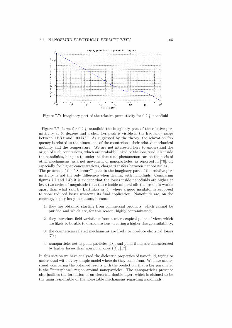
7.1. NANOFLUID ELECTRICAL PERMITTIVITY 105
Figure 7.7: Imaginary part of the relative permittivity for 0.2 gL nanofluid.
Figure 7.7 shows for 0.2 gL nanofluid the imaginary part of the relative per-
mittivity at 40 degrees and a clear loss peak is visible in the frequency rangebetween 1 kHz and 100 kHz. As suggested by the theory, the relaxation fre-quency is related to the dimensions of the counterions, their relative mechanicalmobility and the temperature. We are not interested here to understand theorigin of such counterions, which are probably linked to the ions residuals insidethe nanofluids, but just to underline that such phenomenon can be the basis ofother mechanisms, as a net movement of nanoparticles, as reported in [70], or,especially for higher concentrations, charge transfers between nanoparticles.The presence of the ”‘Schwarz”’ peak in the imaginary part of the relative per-mittivity is not the only difference when dealing with nanofluids. Comparingfigures 7.7 and 7.4b it is evident that the losses inside nanofluids are higher atleast two order of magnitude than those inside mineral oil: this result is worldsapart than what said by Bartnikas in [4], where a good insulator is supposedto show reduced losses whatever its final application. Nanofluids are, on thecontrary, highly lossy insulators, because:
1. they are obtained starting from commercial products, which cannot bepurified and which are, for this reason, highly contaminated;
2. they introduce field variations from a microscopical point of view, whichare likely to be able to dissociate ions, creating a higher charge availability;
3. the counterions related mechanisms are likely to produce electrical losses[70];
4. nanoparticles act as polar particles [48], and polar fluids are characterizedby higher losses than non polar ones ([4], [17]).
In this section we have analyzed the dielectric properties of nanofluid, trying tounderstand with a very simple model where do they come from. We have under-stood, comparing the obtained results with the prediction, that a key parameteris the ”‘interphase” region around nanoparticles. The nanoparticles presencealso justifies the formation of an electrical double layer, which is claimed to bethe main responsible of the non-stable mechanisms regarding nanofluids.

106 CHAPTER 7. DIELECTRIC SPECTROSCOPY
Figure 7.8: Electrical conductivity vs nanofluid concentration.
7.2 Electrical conductivity of nanofluids
In this section we will deal with conductivity issues. The electrical conductivitycan be obtained from a measure of the loss tangent, using the following formula:
σAC = ωϵ′tanδ (7.12)
Since in the case of insulating fluids, as already remarked in the previous section,the electrical conductivity is quite constant over a large range of frequencies, wecan use, as reference, the values obtained for a particular frequency, for instance1 kHz. Figure 7.8 shows the conductivities of the investigated nanofluids at40 degrees, revealing an already observed behavior, that is, the conductivityincrease reaches a saturation plateau at the concentration level which providesthe optimum dielectric properties (0.2 g
l ). It is therefore evident that somethinghappens at those particular concentrations.The aim of such section is to try to understand the reason of such behavior, byproposing again a simple model. Before starting, it is necessary to remember,because it will be our starting hypothesis, that the testing voltage is 3Vrms,i.e., a very low voltage, which, considering the geometry of the cell, generates avery low field, unable to ionize any species of the fluid, neither to cause chargeinjection. In other terms, nanoparticles are supposed to be free of charges, butfree charges can be present inside the nanofluid for other reasons, as for instancecontamination.We would like to study the conduction process of a charge carrier betweentwo nanoparticles, by calculating the tunneling probability, using a very simpleapproach. Let us suppose to consider the situation of figure 7.9, where a particlewith global energy E is traveling towards a potential wall of amplitude U andthickness x; the classical theory states that the particle is able to overcome thepotential barrier if and only if E > U .The Schrodinger equation [79], on the contrary, admits the possibility for theparticle to overcome such a barrier, by defining a transmission probability, whichcan be expressed in the following way, in the case of a simple barrier, like theone shown in figure 7.9:
p = e−2x√
8π2m(U−E)
h2 (7.13)
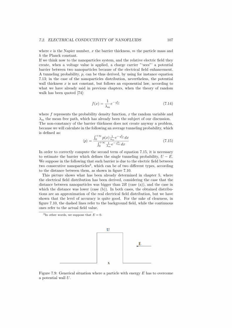
7.2. ELECTRICAL CONDUCTIVITY OF NANOFLUIDS 107
where e is the Napier number, x the barrier thickness, m the particle mass andh the Planck constant.If we think now to the nanoparticles system, and the relative electric field theycreate, when a voltage value is applied, a charge carrier ”‘sees”’ a potentialbarrier between two nanoparticles because of the electrical field enhancement.A tunneling probability, p, can be thus derived, by using for instance equation7.13; in the case of the nanoparticles distribution, nevertheless, the potentialwall thickness x is not constant, but follows an exponential law, according towhat we have already said in previous chapters, when the theory of randomwalk has been quoted [74]:
f(x) =1
λme−
xλm (7.14)
where f represents the probability density function, x the random variable andλm the mean free path, which has already been the subject of our discussion.The non-constancy of the barrier thickness does not create anyway a problem,because we will calculate in the following an average tunneling probability, whichis defined as:
⟨p⟩ =´ +∞0
p(x) 1λm
e−x
λm dx´ +∞0
1λm
e−x
λm dx(7.15)
In order to correctly compute the second term of equation 7.15, it is necessaryto estimate the barrier which defines the single tunneling probability, U − E.We suppose in the following that such barrier is due to the electric field betweentwo consecutive nanoparticles3, which can be of two different types, accordingto the distance between them, as shown in figure 7.10.This picture shows what has been already determined in chapter 5, where
the electrical field distribution has been derived, considering the case that thedistance between nanoparticles was bigger than 2R (case (a)), and the case inwhich the distance was lower (case (b)). In both cases, the obtained distribu-tions are an approximation of the real electrical field distribution, but we haveshown that the level of accuracy is quite good. For the sake of clearness, infigure 7.10, the dashed lines refer to the background field, while the continuousones refer to the actual field value.
3In other words, we suppose that E = 0.
Figure 7.9: Generical situation where a particle with energy E has to overcomea potential wall U .

108 CHAPTER 7. DIELECTRIC SPECTROSCOPY
Figure 7.10: Electric field distribution between two consecutive nanoparticles(dashed lines refer to the background field). Case a: distance between nanopar-ticles bigger than 2Rp; case b: distance lower than 2Rp, being Rp the nanopar-ticles radius.
In order to estimate the barrier height U , the following relation has been con-sidered:
U =
ˆ x
0
Edx (7.16)
where E represents the electric field distribution represented in figure 7.10.Equation 7.15 has been computed for different values of the concentration andunitary background field; unfortunately, being the potential barrier inside a nonlinear quantity, an analytical solution has not been possible to determine. Theresults of the above mentioned calculations are shown in figure 7.11.The figure shows that the tunneling probability, although the investigated
concentrations, as we have said, are not too high, increases rapidly, becauseof the contribution of the small paths between nanoparticles, which have themaximum probability, according to equation 7.14.The probability theory states that, if a random event has a probability equal top, the mean time between two consecutive observation of the event is ∆t = 1
p ;it follows that the probability represents a measure of the mean frequency ofthe tunnel event. This perspective allows us to express the global nanofluid
Figure 7.11: Tunneling global probability vs concentration.
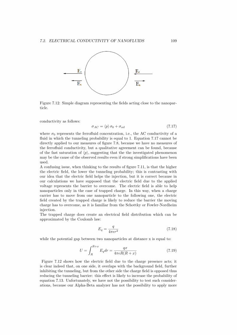
7.2. ELECTRICAL CONDUCTIVITY OF NANOFLUIDS 109
Figure 7.12: Simple diagram representing the fields acting close to the nanopar-ticle.
conductivity as follows:σAC = ⟨p⟩σ0 + σoil (7.17)
where σ0 represents the ferrofluid concentration, i.e., the AC conductivity of afluid in which the tunneling probability is equal to 1. Equation 7.17 cannot bedirectly applied to our measures of figure 7.8, because we have no measures ofthe ferrofluid conductivity, but a qualitative agreement can be found, becauseof the fast saturation of ⟨p⟩, suggesting that the the investigated phenomenonmay be the cause of the observed results even if strong simplifications have beenused.A confusing issue, when thinking to the results of figure 7.11, is that the higherthe electric field, the lower the tunneling probability; this is contrasting withour idea that the electric field helps the injection, but it is correct because inour calculations we have supposed that the electric field due to the appliedvoltage represents the barrier to overcome. The electric field is able to helpnanoparticles only in the case of trapped charge. In this way, when a chargecarrier has to move from one nanoparticle to the following one, the electricfield created by the trapped charge is likely to reduce the barrier the movingcharge has to overcome, as it is familiar from the Schottky or Fowler-Nordheiminjection.The trapped charge does create an electrical field distribution which can beapproximated by the Coulomb law:
Eq =q
4πϵr2(7.18)
while the potential gap between two nanoparticles at distance x is equal to:
U =
ˆ R+x
R
Eqdr =qx
4πϵR(R+ x)(7.19)
Figure 7.12 shows how the electric field due to the charge presence acts; itis clear indeed that, on one side, it overlaps with the background field, furtherinhibiting the tunneling, but from the other side the charge field is opposed thusreducing the tunneling barrier: this effect is likely to increase the probability ofequation 7.13. Unfortunately, we have not the possibility to test such consider-ations, because our Alpha-Beta analyzer has not the possibility to apply more

110 CHAPTER 7. DIELECTRIC SPECTROSCOPY
than 3Vrms. High voltage DC conductivity measurements will be the only wayto verify the correctness of our hypotheses system and will be performed in thefollowing.

Conclusions
Our target, at the beginning of this thesis, has been the study of the main prop-erties characterizing mineral oil-based nanofluids aimed to understand if theycould be considered as good alternatives for mineral oil for insulation purposes.At the end of the work, our first answer is surely positive, i.e., nanofluids haveproved to behave better than mineral oil, especially in the case of alternatingvoltages and when the concentrations were not too high to ignite secondary phe-nomena, like tunneling conduction or anything else. We have seen indeed thatAC breakdown voltage, maybe thanks to the surfactant help, is much higherthan that of the benchmark oil, and the same conclusion can be drawn for im-pulse voltages, where the asymmetry between the positive and negative voltageis somehow reduced favoring the dielectric strength.DC results, on the other hand, highlight that the situation is not so easy todismiss; they have in fact introduced the problem of space charge trapping,a problem which was already known in literature [31], but whose implicationshad not been explored yet. The developed model has let us to finally provethe tendency of the nanoparticles to create, with low concentrations, a chargepeak characterized by a low mobility, which is likely to undermine the stabilityof the fluid, especially in the case of non uniform fields, as largely investigatedin chapter 6. This is an important results, which proves that although at thebeginning the performance of the fluid can be optimal, as shown in chapter 2,after some days the intrinsic nanofluid instability can become manifest, causingdeleterious results for the whole application where they are installed. From thisperspective, it is difficult to think that the research about nanofluids can findan immediate application. Big manufacturers need stable and repetitive resultsand the situation concerning nanofluids is, at the moment, quite confused, be-cause a lot of research groups are interested in the single results, immediatelyafter the manufacture process. The previous statement and the results of thisthesis should have proved that, when dealing with nanofluids, the situation is incontinuous evolution, showing the uselessness of all the studies about the out-standing properties they have. The latter have been necessary in a first stage,when we needed to learn if the nanoparticles technology could be of help in thecase of liquid insulation.The problems arose in this thesis and in the world, where some ferrofluid-based transformers have been installed showing the same aggregation phenom-ena which have been studied in this thesis, allow us to think that the researchefforts have to be shifted towards insulated nanoparticles-based nanofluids, likefor instance SiO2 or TiO2, which have been proved to behave as good as con-ductive nanoparticles [80],[77], [81].The immediate consequence of such tendency will be, as obvious, the loss of the
111

112 CHAPTER 7. DIELECTRIC SPECTROSCOPY
huge increase in the thermal exchange properties presented by the nanofluid,which, in a certain sense, has been one of the reason which has driven a lot ofpeople to start studying them. If we remain anyway linked to the idea of thenanofluid starting from mineral oil, after all we are not scared of the thermalexchange properties, because they would not change too much after the inser-tion of low concentration nanoparticles. The little increase in the viscosity [86],[87] does not represent a problem, either.All these issues, on the contrary, can represent a criticality if the nanofluids willbe performed starting from vegetable derived fluids or synthetic esters, whichare known to be less conductive because more viscous in general. In these thesiswe have not dealt with such kinds of fluids, which are now on fair because oftheir ”‘green”’ behavior; their performance have proved to be comparable withthat of mineral oil, regarding the inception phenomena, but the resistance tothe streamer and leader propagation in such fluids is lower than that in mineraloil [7], [35]. For such a reason, vegetable fluids are still nowadays used in low-medium voltage applications rather than high voltage ones. The more and moreinsistent requests for environmental free insulation liquids, however, will carryresearchers to focus on these kind of fluids as starting point for the nanofluidsmanufacture; it is indeed more interesting to improve the properties of theseclass of fluids, rather then the optimal properties of mineral oil, which has theproblem of the toxicity and the disposal.[82], [83] [84] and [85] are only few examples of the results of the researchers’work on this subject; we believe that in the future the list will be more populatedand we hope some manufacturers will risk the final application, too.

Bibliography
[1] Goetter, R. W., Innovations in unsaturated polyester resins for electricalinsulation, Electrical Manufacturing and Coil Winding Expo 2010-2013, pp.119-121.
[2] Arief, Y.Z., Ismail, M.I., Makmud, M.Z.H., Adzis, Z., Muhamad, N.A.,Partial discharge characteristics of natural rubber blends with inorganicnanofiller as electrical insulating material, Applied Mechanics and Materials284-287, pp. 188-192.
[3] Akmal, M.J.-N., Afendi, M.P.-M., Asiah, M.-N., Addawiyah, Z.-R., Faizal,K.-N., Effects of SiO2 and TiO2 nanofillers on conductivity level of LLDPE-NR nanocomposite HV insulator, Applied Mechanics and Materials 284-287,pp. 305-309.
[4] Bartnikas, R., Electrical insulating liquids (Engineering Dielectrics), R.Bartnikas Editor, sponsored by ASTM Committee D9, Vol. 3, 1994.
[5] Feil, D.L.P., Silva, P.R., Bernardon, D.P., Sperandio, M., Medeiros, L.H.,Development of an efficient distribution transformer using amorphous coreand vegetable insulating oil, Electric Power Systems Research 144, pp. 268-279.
[6] Hrkac, M., Papageorgiou, P., Kosmoglou, I., Miatto, G., BIOTEMP trans-former technology for innovative compact substation, IET Conference Pub-lications 2010 (572 CP).
[7] Liu Q., Wang Z. D., Streamer Characteristic and Breakdown in Syntheticand Natural Ester Transformer Liquids under Standard Lightning ImpulseVoltage, IEEE Transactions on Dielectrics and Electrical Insulation Vol. 18,No. 1; February 2011.
[8] Yang, L., Du, K., A comprehensive review on heat transfer characteristicsof TiO2 nanofluids, International Journal of Heat and Mass Transfer 108,pp. 11-31.
[9] Sridhara, V., Satapathy, L.N., Effect of Nanoparticles on Thermal PropertiesEnhancement in Different Oils-A Review, Critical Reviews in Solid State andMaterials Sciences 40 (6), pp. 399-424, 2015.
[10] Lipscomb, T.G., Electrical Insulating Oils, ASTM STP 998, American So-ciety for Testing and Materials, Philadelphia, 1988, pp. 5-24.
113

114 BIBLIOGRAPHY
[11] Par Wedin, Electrical Breakdown in Dielectric Liquids, a Short Overview,IEEE Electrical Insulation Magazine, November/December Vol. 30, No. 6,2014.
[12] Devins J. C., Rzad S. J., and Schwabe R. J., Breakdown and prebreakdownphenomena in liquids, Journal of Applied Physics, 52, 4531 (1981); DOI:10.1063/1.329327.
[13] Chadband W. G., On variations in the propagation of positive dischargesbetween transformer oil and silicone fluids, J. Phys. D: Appl. Phys., vol.13,no. 7, pp. 12991307, 1980.
[14] Denat A., Gosse J. P., and B. Gosse, Electrical conduction of purified cy-clohexane in a divergent electric field, IEEE Trans. Electr. Insul., vol.23, no.4, pp. 545554, 1988
[15] Ingebrigtsen S., Lundgaard L. E., and strand P. O., Effects of additives onprebreakdown phenomena in liquid cyclohexane: I. Streamer initiation, J.Phys. D: Appl. Phys., vol. 40, no. 17, pp. 5161516, 2007.
[16] Halpern B. and R. Gomer, Field Ionization in Liquids, J. Chem. Phys.51,1048 (1969).
[17] Schidt W., Liquid state electronics of insulating fluids, CRC Press, 1997.
[18] Dumitrescu L., Lesaint O., Bonifaci N., Denat A. and P. Notingher, Studyof streamer inception in cyclohexane with a sensitive charge measurementtechnique under impulse voltage, J. Electrostat., vol. 53, no. 2, pp. 135146,2001.
[19] Ingebrigtsen S., The influence of chemical composition on streamer initia-tion and propagation in dielectric liquids, PhD dissertation, Dept. Chemistry,Norwegian Univ. Sci. Technol., Trondheim, 2008.
[20] Chadband W. G. and Wright G. T. A pre-breakdown phenomenon in theliquid dielectric hexane, Brit. J. Appl. Phys. 16, 305 (1965).
[21] Murray D.W., McDonald J.M., White A.M., and Wright P.G., Proceedingsof World Petroleum Congress, Vol. 11, No. 4, 1983, pp. 447-457.
[22] Wilson A. C. M., Insulating Liquids: Their Uses, Manufacture, and Prop-erties, Peter Peregrinus Publication, Stevenage, UK, 1980.
[23] Hobson C. D. and Pohl W., Modern Petroleum Technology Wiley, NewYork, 1973.
[24] Seagal V. et al, AC (60Hz) and Impulse Breakdown Streangth of a ColloidalFluid Based on Transformer Oil and Magnetite Nanoparticles, IEEE Int.Symp. on Electrical Insulation, Arlington, Virginia, USA, June 7−10, 1998.
[25] Ibrahim K. et alia, Realization of Partial Discharge Signals in TransformerOils Utilizing Advanced Computational Techniques, IEEE Transactions onDielectrics and Electrical Insulation Vol. 19, No. 6; December 2012.

BIBLIOGRAPHY 115
[26] Cleary G. P., Judd M. D., UHF and current pulse measurements of partialdischarge activity in mineral oil, IEE Proceedings - Science, Measurementand Technology, Volume: 153, Issue 2, 9 March 2006.
[27] Bianco V., Manca O., Nardini S., Vafai K., Heat Transfer Enhancementwith Nanofluids, Taylor&Francis Publisher, 2015.
[28] Das S. K., Choi S. U., Wenhua Y., Pradeep T., Nanofluids: Science andTechnology, Wiley-Interscience Publisher, 2007.
[29] Segal V. and Raj K., An investigation of Power Transformer Cooling withMagnetic Fluid, Indian Journal of Engineering and Material Sciences, 1998.
[30] US Patent N. 3215572 A, Low viscosity magnetic fluid obtained by the col-loidal suspension of magnetic particles, filed Oct 9, 1963.
[31] Sullivan F. M. O., A Model for the Initiation and propagation of ElectricalStreamers in transformer oil and Transformer based nanofluids, Ph.D degreethesis, Massachusetts Institute of Technology, USA, 2007.
[32] Hiroyuki Ohshima, Electrical Phenomena at Interfaces and Biointerfaces,John Wiley & Sons, Inc. DOI: 10.1002/9781118135440, Jan 2012.
[33] Lagaly O. S. R. Z. G. , Dispersionen und Emulsionen, Darmstadt: DietrichSteinkopff Verlag, 1997.
[34] Rosensweig R. E., Ferrohydrodynamics, Cambridge University Press, 1985.
[35] Liu Q., Wang Z. D., Breakdown and Withstand Strengths of Ester Trans-former Liquids in a Quasi-uniform Field under Impulse Voltages, IEEETransactions on Dielectrics and Electrical Insulation Vol. 20, No. 2; April2013.
[36] Abernethy R. B., The New Weibull Handbook, published and distributedby Robert B. Abernethy, December 2006.
[37] Mettler-Toledo International, GTPR - Good Titration Practice in Karl Fis-cher Titration, 2011.
[38] Rzad S. J., Devins J. C. and R. J. Schwabe, Transient behavior in trans-former oils: prebreakdown and breakdown phenomena,IEEE Transactions onElectrical Insulation Vol. ET-14, N.6, December 1979.
[39] Settles, Gary S., Schlieren and shadowgraph techniques: visualizing phe-nomena in transparent media, Springer Science & Business Media, 2012.
[40] Cristofolini, A., et al., Schlieren imaging in a dielectric barrier dischargeactuator for airflow control, Journal of Applied Physics 111.3 (2012).
[41] Montgomery, Douglas, Design and analysis of Experiments, Eigth Edition,Wiley Press, 2013, Section 3.5.7.
[42] Current J. M., Introduction to Data Analysis with R for forensic scientists,CRC Press, 2009.

116 BIBLIOGRAPHY
[43] Mazzanti G., Marzinotto M., Extruded cables for high voltage direct currenttransmission: advances in research and development, Wiley−IEEE press,2013.
[44] Liu Q., Wang Z. D., Lesaint O., Comparison of streamer propaga-tion in mineral oils under lightning and step impulse voltages, 2014IEEE 18th International Conference on Dielectric Liquids (ICDL), DOI:10.1109/ICDL.2014.6893151.
[45] Denat A., Lesaint O., Mc Cluskey F., Streamer and breakdown phenomenaunder step and lightning impulses in various hydrocarbon liquids, 2014 IEEEConference on Electrical Insulation and Dielectric Phenomena (CEIDP),DOI: 10.1109/CEIDP.2014.6995862.
[46] Lesaint O., Tobazeon R., Streamer generation and propagation in trans-former oil under divergent field conditions, 1987 Ninth International Con-ference on Conduction and Breakdown in Dielectric Liquids.
[47] Mason J. H., Breakdown of solid dielectrics in divergent fields, Proc. IEEB, Radio and Electronic Engineering, Vol.102, No.5, pp. 725727, 1955.
[48] Rajnak M., Kurimsky J., Dolnik B., Marton K., Tomco L., Taculescu A.,Vekas L., Kovac J., Vavra I., Tothova J., Kopcansky P., Timko M., Dielectricresponse of transformer oil based ferrofluid in low frequency range, Journalof Applied Physics, 114, 034313 (2013).
[49] Miao J., Dong M., Ren M., Wu X., Shen L., Effect of nanoparticle polar-ization on relative permittivity of transformer oil-based nanofluids, Journalof Applied Physics, 113, 204103 (2013).
[50] Halpern B. and R. Gomer, Field Emission in Liquids, J. Chem. Phys.51,1031 (1969).
[51] Linz P., Analytical and Numerical Methods for Volterra Equations, SIAM(Studies in Applied Mathematics), Philadelphia, 1985.
[52] IEC 60156, Insulating liquidsDetermination of the breakdown voltage atpower frequencyTest method, 2003-11.
[53] Lesaint, O., ”‘Streamers” in liquids: relation with practical high voltage in-sulation and testing of liquids, IEEE Intern. Conf. Dielectr. Liquids (ICDL),Poitiers, France, pp.120-125, 2008.
[54] Dunne, O. J., Multiple Comparisons Among Means, Jour-nal of the American Statistical Association. 56 (293): 5264.doi:10.1080/01621459.1961.10482090.
[55] Forster, E. O., Partial discharges and streamers in liquid dielectrics-thesignificance of the inception voltage, IEEE Trans. Electr. Insul., vol. 28, no.6, pp. 941946, 1993.
[56] Hauschild W., Lemke E., High-Voltage Test and Measuring Techniques,Springer-Verlag Berlin Heidelberg, 2014.
BIBLIOGRAPHY 117
[57] IEC 60270, High-voltage test techniques - Partial discharge measurements,2000.
[58] Morshuis, P. H.F, Partial discharge mechanism: mechanisms leading tobreakdown analyzed by fast electrical and optical measurements, PhD thesis,Delft University of Technology, 1993.
[59] Wang, L., Physical model of PD behavior and relevant damage growth frommicro cavities in polyethylene based material under AC voltage, PhD thesis,Department of Electrical Engineering, University of Bologna, Italy, 2011.
[60] Wilhelm, H.M., Franch, V., Franch, A.F., Compatibility of TransformerConstruction Materials with Natural Ester-based Insulating Fluids, IEEETransactions on Dielectrics and Electrical Insulation, Vol. 22, Issue 5, Pag.2703-2708, 2015.
[61] Pompili, M., Mazzetti, C., Bartnikas, R., Phase relationship of PD pulsesin dielectric liquids under ac conditions, IEEE Transactions on Dielectricsand Electrical Insulation, Vol. 7, Issue 1, Pag. 113-117, 2000.
[62] Mazzetti, C., Pompili, M., Yamashita, H., Comparison of streamer andpartial discharge inception voltages in liquid dielectrics, Sixth InternationalConference on Dielectric Materials, Measurements and Applications, 1992.
[63] Lewis, T. J., A new model for the primary process of electrical breakdownin liquids, IEEE Transactions on Dielectrics and Electrical Insulation, Vol.5, Issue 3, Pag. 306-315, 1998.
[64] Niemeyer, L., A generalized approach to partial discharge modeling, IEEETransactions on Dielectrics and Electrical Insulation, Vol. 2, Issue 4, Pag.510-528, 2002.
[65] Lewis, T., Interfaces are the dominant feature of dielectrics at the nano-metric level, IEEE Transactions on Dielectrics and Electrical Insulation, Vol.11, No. 5, pp. 739-753, 2004.
[66] Ratzke, S., Kindersberger, J., Role of interphase on the resistance to high-voltage arcing, on tracking and erosion of silicone/SiO2 nanocomposites,IEEE Trans. DEI, Vol. 17, No. 2, pp. 607-614, 2010.
[67] Tanaka, T., Kozako, M., Fuse, N., Ohki, Y., Proposal of a multi-core modelfor polymer nanocomposite dielectrics, IEEE Trans DEI, Vol. 12, No. 4, pp.669-681, 2005.
[68] Andrisch, T., Kochetov, R., Morshuis P.H.F., Proposal of the polymer chainalignment model, Proc. IEEE CEIDP, pp. 624-627, 2011.
[69] Morshuis, P.H.F, Interfaces: to be avoided or to be treasured?, Proc. IEEEICSD, pp. 1-9, 2013.
[70] Schwarz, G., A theory of the low-frequency dielectric dispersion of the col-loidal particles in elecrtolyte solutions, J. Phys. Chem., 1962, 66 (12), pp26362642.

118 BIBLIOGRAPHY
[71] Butcher, M., Member, S., Neuber, A. et alia, Conduction and BreakdownMechanisms in Transformer Oil, IEEE Transactions on Plasma Science, Vol.34, No. 2, April 2006.
[72] Butcher, M., Neuber, A., Krompholz, H., Dickens, J., Pre-breakdown cur-rent behavior in dc volume breakdown in transformer oil, Proc. 14th IEEEInt. Pulsed Power Conf., vol. 1, Jun. 1518, 2003, pp.289292.
[73] Meek, J., Crags, J., Electrical breakdown in gases, Oxford at the ClarendonPress
[74] Kuffel, E., Zaengl, W. S., Kuffel, J., High Voltage Engineering: Fundamen-tals, Newnes, 2000.
[75] Jones, T. B., Electromechanics of particles, Cambridge University Press,Cambridge, 1995.
[76] Crank, J., Nicolson, P., A practical method for numerical evaluation ofsolutions of partial differential equations of the heat conduction type, Proc.Camb. Phil. Soc. 43 (1): 5067.
[77] Cavallini, A., Karthik, Negri, F., The Effect of Magnetite, Graphene Oxideand Silicone Oxide Nanoparticles on Dielectric Withstand Characteristics ofMineral Oil, IEEE Trans DEI, Vol. 22, No. 5, pp. 2592 - 2600, 2015.
[78] Azcarraga, C. G., Partial Discharge Phenomena in Converter and TractionTransformers: Identification and Reliability, Ph.D thesis, DEI Unibo, 2014.
[79] Schrodinger, E., An Undulatory Theory of the Mechanics of Atoms andMolecules, Physical Review, vol. 28, issue 6, 1926, pp. 10491070.
[80] Jin, H., Andritsch, T., Tsekmes, A., Kochetov, R., Morshuis, PHF., Smit,JJ., Properties of mineral oil based silica nanofluids, IEEE Transactions onDielectrics and Electrical Insulation, Vol. 21, No. 3, 2014, p. 1100-1108.
[81] Du Yue fan, Lv Yu Zhen, Zhou Jian-quan, Chen Mu-tian, Li xiao- xin,Li cheng rong, Effect of ageing on Insulating property of mineral oil basedTiO2 nanofluids, IEEE International Conference on Dielectric Liquids, pp.1-4, 2011.
[82] Peppas, G.D., Bakandritsos, A., Charalampakos, V.P., Zboril, R., Gonos,I.F., Ultrastable Natural Ester-Based Nanofluids for High Voltage InsulationApplications, ACS Applied Materials and Interfaces 8 (38), pp. 25202-25209,2016.
[83] Du, Y., Li, C., L, Y., Chen, M., Zhou, Y., Insulating properties andcharge characteristics of natural ester fluid modified by TiO2 semiconductivenanoparticles, IEEE Transactions on Dielectrics and Electrical Insulation 20(1), 6451351, pp. 135-140, 2013.
[84] Li, J., Zhang, Z., Zou, P., Grzybowski, S., Zahn, M., Preparation of avegetable oil-based nanofluid and investigation of its breakdown and dielectricproperties, IEEE Electrical Insulation Magazine 28 (5), 6268441, pp. 43-50,2012.
BIBLIOGRAPHY 119
[85] Zou, P., Li, J., Sun, C.-X., Zhang, Z.-T., Liao, R.-J., Dielectric proper-ties and electrodynamic process of natural ester-based insulating nanofluid,Modern Physics Letters B 25 (25), pp. 2021-2031, 2011.
[86] Aref, A.H., Entezami, A.A., Erfan-Niya, H., Zaminpayma, E., Thermophys-ical properties of paraffin-based electrically insulating nanofluids containingmodified graphene oxide, Journal of Materials Science, 52 (5), pp. 2642-2660,2017.
[87] Dalkilic, A.S., Kkyldrm, B.O., Akdogan Eker, A., (...), Jumpholkul, C.,Wongwises, S., Experimental investigation on the viscosity of Water-CNTand Antifreeze-CNT nanofluids, International Communications in Heat andMass Transfer, 80, pp. 47-59, 2017.