
Simulação de Redes de Sensores Sem Fio Utilizando Bluetooth e RFID

EDUARDO FREIRE NAKAMURA
FUSÃO DE DADOS EM
REDES DE SENSORES SEM FIO
Belo Horizonte
Janeiro de 2007


EDUARDO FREIRE NAKAMURA
Orientador: Antonio Alfredo Ferreira Loureiro
FUSÃO DE DADOS EM
REDES DE SENSORES SEM FIO
Tese apresentada ao Programa de Pós-Graduação em Ciência da Computaçãoda Universidade Federal de Minas Geraiscomo requisito parcial para a obtençãodo grau de Doutor em Ciência da Com-putação.
Belo Horizonte
Janeiro de 2007


EDUARDO FREIRE NAKAMURA
Advisor: Antonio Alfredo Ferreira Loureiro
INFORMATION FUSION IN
WIRELESS SENSOR NETWORKS
Thesis presented to the Graduate Pro-gram in Computer Science of the FederalUniversity of Minas Gerais in partial ful-fillment of the requirements for the degreeof Doctor in Computer Science.
Belo Horizonte
January 2007


UNIVERSIDADE FEDERAL DE MINAS GERAIS
FOLHA DE APROVAÇÃO
Fusão de Dados em
Redes de Sensores sem Fio
EDUARDO FREIRE NAKAMURA
Tese defendida e aprovada pela banca examinadora constituída por:
Prof. Antônio Alfredo Ferreira Loureiro – OrientadorDepartamento de Ciência da Computação – ICEx – UFMG
Prof. Alejandro César Frery Orgambide
Departamento de Tecnologia da Informação – UFAL
Prof. Claudio Luis de Amorim
Programa de Engenharia de Sistemas e Computação, COPPE – UFRJ
Profa. Linnyer Beatrys Ruiz
Departamento de Computação – UEL
Prof. Geraldo Robson Mateus
Departamento de Ciência da Computação – ICEx – UFMG
Prof. José Marcos Silva Nogueira
Departamento de Ciência da Computação – ICEx – UFMG
Belo Horizonte, Janeiro de 2007


To my beloved wife and my little princess
that should be born in February 2008
(can’t wait to carry you in my arms)


Acknowledgments
Thanks to God for everything, I mean everything!
This thesis is the winning post of a four-year journey (four and a half years,
actually) to obtain my D.Sc. degree in Computer Science. A journey like that
is always easier when you travel together, and I am happy to say that I have been
accompanied and supported by many people who I proudly call friends. I am pleased
to formally have the chance to express my grateful and appreciative feelings for all
of them.
The first person I would like to thank is my wife. Thank you for being part of
my life, giving birth to our daughter, and supporting me in every possible way. All
these years you have been my love, heart, memory, spell checker, grammar checker,
style advisor, shoulder, listener,. . . (I should stop here because this list is endless).
They say behind every great man there’s a woman. I may not be a great man, but
you certainly are a great woman behind me. Thanks for choosing me.
I am grateful to my parents for years of unconditional love and support, I hope
someday my kids will be as proud of me as I am proud of you guys. You will
always be my heros and no words can express my gratitude for you. Thanks dad
for reviewing my texts ,.
I express my deep sense of gratitude and sincere thanks to my thesis advisor
Loureiro who was always more thrilled than me about my own work. During these
years you have guided me to become a scientist. Getting a D.Sc. degree was just a
result of such a process. For being concerned about my future and teaching me the
crafts of science, I dare to call you friend. Thank you.
I also thank for the opportunity to scientifically cooperate with my friends Alla
(Beanwatcher was my first international paper), Horácio, Mateus, and Mauricio
(alphabetically sorted!).
My schoolmate friends, thank you very much for companionship that made the
process much easier. I will not list your names because you are too many, but you
know who you are!
For making me feel closer to home, I thank to the distinct Manauara community
iii

in BH: Pinheiro (since day #1), Michele, Larissa, Juju, Mauricio, Ingrid (Sam-
mineida), Thais (Thaizette), Ruiter, Ruth, Agatha, Vilar, Giselle, Dudu, Mariana,
Pio, Renata, Sidney (Magal), Ceu (Fernando thanks for Bodocó). And the Hon-
orary Manauara Citizens: Alla, Raquel, Júlia, Pedrão, Aracelly, Sofia, Deivid1 (Zé
Mané), Elbena, and Peru.
Thanks to the glorious Curucu soccer team and all players for receiving me with
wide open arms. It is true that I was a team co-founder, but that is just a tiny detail
,! Two years of good, enjoyable, and artistic soccer presentations in the Computer
Science Soccer Cup. What a team!
Thanks to the staff of the Computer Science Department for all supporting,
special thanks for Renata, Cida, Túlia, Sônia, and Sheila.
I am thankful to the FUCAPI institute for the financial support and for releasing
me from my duties so I could put all my efforts to accomplish is journey. Special
thanks to the executive president Isa Assef dos Santos and the department directors
Evandro Xerez Vieiralves and Niomar Lins Pimenta.
I apologize if I have misspelled any name.
The writing of this acknowledgement section should be a two-week work (maybe
more) to remember and list everyone properly, but I had only one day / to finish
the job. So, I apologize if I did not directly mentioned someone, but be sure I
remember you and I am grateful for everything. Besides, you all know how “leaky”
my memory is.
Whoops, I almost forgot. Thanks Minas Gerais for the Cachaça Mineira
,,,!
iv

Resumo
Este trabalho oferece uma discussão geral sobre o tema de fusão de dados em redes de
sensores sem fio (RSSFs) que permite: (i) a identificação de problemas em aberto e
(ii) o entendimento dos requisitos e implicações do uso de fusão de dados em RSSFs.
Esta discussão é feita através de um levantamento bibliográfico do estado-da-arte
envolvendo fusão de dados em RSSFs. Analisando as arquiteturas, modelos e méto-
dos de fusão de dados identificados neste levantamento bibliográfico, é proposto um
arcabouço (framework), chamado Diffuse, que compreende as principais funções e
atividades de um processo genérico de fusão de dados e uma API que implementa
métodos de fusão freqüentemente utilizados em RSSFs. O Diffuse é, portanto, uma
ferramenta que permite ao projetista refletir e avaliar quais tipos e quais métodos de
fusão de dados podem ser utilizados em sua solução, e como especificamente estes
métodos podem ser usados para compor uma tarefa ou uma aplicação de fusão de
dados. Embora o Diffuse possa ser aplicado em diferentes contextos, como prova-
de-conceito, este trabalho mostra como o Diffuse pode ser usado para projetar uma
solução econômica (em termos de consumo de energia) que ofereça um serviço con-
fiável (tolerante a falhas) de roteamento. Os resultados aqui apresentados mostram
que a abordagem proposta é capaz de reduzir o custo de comunicação para prover
tal serviço. Em alguns casos, o tráfego gerado por esta abordagem chega a ser 85%
inferior ao tráfego gerado por soluções freqüentemente utilizadas em RSSFs. Além
disso, este trabalho propõe uma estratégia de roteamento, baseada em atribuição
de papéis, para garantir a execução de uma aplicação de fusão de dados. Neste
caso, baseando-se na premissa de que fusão de dados é utilizada pela aplicação para
detecção de eventos, é proposto um algoritmo de atribuição de papéis, chamado
InFRA, que organiza a rede somente quando um evento é detectado. De maneira
resumida, o InFRA é um algoritmo reativo de atribuição de papéis que procura
pelas menores rotas (conectando os nós fontes aos sorvedouros) que maximizam a
agregação de dados. Os resultados apresentados mostram que, em alguns casos, o
InFRA utiliza apenas 70% da energia gasta por outros algoritmos de roteamento
usualmente adotados em RSSFs.
v

Abstract
This work provides a general discussion for information fusion in wireless sensor net-
works (WSNs), allowing us to identify open issues and understand the requirements
and the implications regarding information fusion and the resource-constrained
WSNs. In this discussion, we survey the state-of-the-art about information fusion in
WSNs. By assessing the architectures, models, and methods of information fusion
identified in the survey, we propose a framework, called Diffuse, that comprises the
main functions and activities of a general fusion process and a specific API that im-
plements useful algorithms for WSNs. The Diffuse framework is a helpful tool that
allows the designer to reason about what types of information fusion, what methods
should be used, and how they should be used to accomplish an information-fusion
task or application. Although the applicability of Diffuse is ample, as a proof of con-
cept, we show how it can be used to achieve energy-efficient reliability in tree-based
routing protocols. Results show that our approach efficiently avoids unnecessary
routing topology constructions. In some cases, the traffic overhead generated by
this approach is 85% smaller than the traffic generated by classical algorithms. In
addition, we introduce a routing strategy, based on a role assignment algorithm, to
support an information-fusion application. In this case, we consider that WSNs ap-
ply information fusion techniques to detect events in the sensor field, and propose a
role assignment algorithm, called InFRA, to organize the network only when events
are detected. In a nutshell, InFRA is an event-based role assignment algorithm that
tries to reactively find the shortest routes (connecting source nodes to the sink) that
maximize data aggregation. Results show that, in some cases, the InFRA algorithm
uses only 70% of the energy spent by other tree-based routing algorithms that are
commonly used in WSNs.
vii


Resumo Estendido
Originalmente, o documento desta tese redigido na língua inglesa sob o título Infor-
mation Fusion in Wireless Sensor Networks. Com o objetivo de facilitar o acesso ao
texto aos leitores da língua portuguesa, e para atender às normas da Universidade
Federal de Minas Gerais, este resumo faz uma abreviada descrição, em português,
de cada capítulo contido na tese.
Capítulo 1 - Introdução
Em diversas situações, as redes de sensores sem fio (RSSFs) podem ser depositadas
em ambientes inóspitos, sob condições que podem interferir nas leituras dos sensores
ou mesmo danificar alguns nós sensores. Por exemplo, considere uma RSSF que
monitora a ocorrência de incêndios e o comportamento de animais em uma floresta.
Em um ambiente como este, falhas não são eventos raros, pois sensores podem ser
destruídos pelo fogo, animais, ou mesmo aventureiros humanos. Além disso, os
sensores podem apresentar defeitos de fabricação e podem “morrer” devido à falta
de energia. Como resultado as leituras dos sensores podem ser mais imprecisas do
que o esperado, reduzindo a cobertura de sensoriamento da rede como um todo.
Uma solução natural para suplantar falhas e leituras imprecisas consiste no uso de
nós redundantes que cooperam entre si para monitorar o ambiente. Entretanto, esta
estratégia traz um novo desafio de escalabilidade causado pelo potencial aumento
de colisões e pela transmissão de dados redundantes. Como resposta a este desafio,
a fusão de dados tem sido adotada como solução para as RSSFs. De maneiras
sucinta, fusão de dados lida com teorias, algoritmos e ferramentas utilizadas para
processar múltiplas fontes de dados, gerando um dado de saída que é, de alguma
forma, melhor quando comparado com os dados de entrada individualmente. Neste
caso a definição precisa de “melhor” depende da aplicação. Para as RSSFs, o termo
“melhor” possui pelo menos dois sentidos: (1) menor custo e (2) maior precisão.
Este trabalho tem como objetivo discutir o uso de fusão de dados em RSSFs,
ix

permitindo: (1) a identificação de questões em aberto; (2) o entendimento dos re-
quisitos e implicações do uso de fusão de dados em redes de recursos limitados
como as RSSFs. Esta discussão avalia o estado-da-arte relacionado com fusão de
dados em RSSFs. Baseado no conhecimento resultante deste estudo, neste trabalho,
são especificadas técnicas de fusão de dados para aprimorar algoritmos de rotea-
mento através do provimento de uma solução tolerante a falhas e de baixo consumo
energético. Além disso, é projetada uma solução eficiente de roteamento quando a
aplicação faz o uso de fusão de dados, por exemplo, para monitorar a ocorrência
de eventos. Portanto, este trabalho oferece duas visões complementares de fusão de
dados em RSSFs. No primeiro caso, estas técnicas são utilizadas para aprimorar
um algoritmo de roteamento, ou seja, a fusão de dados é utilizada como meio. No
segundo caso, é projetado um algoritmo de roteamento para dar suporte à fusão de
dados na aplicação, ou seja, a fusão de dados é utilizada como fim.
As contribuições desta tese, em ordem de ocorrência no texto, são as seguintes:
1. Um survey de fusão de dados em RSSFs. Esta não é a principal con-
tribuição da tese, mas merece destaque pois provê uma ampla visão do estado-
da-arte que permite a identificação de questões em aberto.
2. Diffuse: Um arcabouço (framework) de fusão de dados. Este ar-
cabouço é, originalmente, voltado para o uso de fusão de dados em RSSFs,
especificando os fluxos de informação e os sub-processos que podem vir a ser
executados em uma tarefa de fusão de dados.
3. Roteamento tolerante a falhas. Embora a aplicação do Diffuse seja ampla,
como prova de conceito, este arcabouço é utilizado para prover uma solução de
roteamento tolerante a falhas, onde a fusão de dados é utilizada para detectar
falhas que necessitem a reconfiguração da infra-estrutura lógica de roteamento.
4. Uma estratégia de roteamento baseada em atribuição de papéis para
detecção e notificação de eventos. Esta contribuição tem como objetivo
mostrar como projetar uma solução de roteamento tendo em mente os requi-
sitos de uma aplicação de fusão de dados.
Capítulo 2 - Uma Visão Geral de Fusão de Dados
Fusão de dados tem sido apontada como uma alternativa para pré-processar os dados
de uma RSSF de forma distribuída aproveitado a capacidade de processamento
dos sensores. Neste capítulo são explorados diversos aspectos do uso de fusão de
x

dados em RSSFs, oferecendo uma visão geral relacionada com o estado-da-arte,
terminologia, classificações, métodos, arquiteturas e paradigmas computacionais.
Os modelos de fusão de dados aqui apresentados são, na maioria, modelos de
processos, i.e., modelos que descrevem um conjunto de processos e como estes se
relacionam. Estes modelos descrevem as funcionalidades que um sistema de fusão
deve possuir abstraindo-se de possíveis implementações ou instâncias específicas.
Observe que os modelos descritos neste capítulo incluem não somente a atividade
de fusão propriamente dita mas também a obtenção dos dados sensoriais e a tomada
de ações baseada na interpretação dos dados fundidos.
Em relação aos métodos, os mais comuns são os métodos de: (1) agregação, (2)
inferência, (3) estimação. Os métodos de agregação são os mais simples e produzem
como resultado um dado de menor representatividade do que o conjunto dos dados
utilizados na fusão. A vantagem destes métodos reside na redução do volume de
dados que trafegam pela rede e inclui operações de agregação como média, máximo,
e mínimo. Os métodos de inferência têm como objetivo processar dados e tirar
conclusões a respeito dos mesmos. Exemplos destes métodos incluem inferência
Bayesiana e Dempster-Shafer. Os métodos de estimação têm como objetivo estimar
o vetor de estado de um processo a partir de um vetor ou seqüência de vetores de
medições de sensores. Estes métodos incluem Quadrados Mínimos, filtros de média
móvel, filtros de Kalman, e filtros de partículas.
Os paradigmas computacionais utilizados para fusão de dados em redes de sen-
sores também possuem particularidades. Tipicamente, as RSSFs são consideradas
redes centradas em dados, ou seja, o interesse nos dados sensoriados não se res-
tringe à aplicação sendo comum a todas as atividades que possam tirar proveito
da correlação existente entre estes dados. Assim, as atividades como roteamento
devem permitir que os dados sejam analisados no nível da aplicação para decidir de
estes serão retransmitidos, fundidos ou suprimidos. Uma alternativa ao roteamento
centrado em dados é a utilização de agentes móveis onde os dados permanecem ar-
mazenados localmente nos sensores e o código executável move-se pelos nós da rede.
Nesta abordagem, um ou mais agentes transitam pela RSSF seguindo seu itinerário.
Os sensores fazem suas leituras do ambiente e armazenam os dados localmente. O
agente móvel ao se hospedar em um nó consulta os dados locais do sensor hospedeiro,
executa a fusão destes com os dados parcialmente fundidos, armazena o resultado
em seu buffer e segue seu itinerário até voltar ao sink para reportar o resultado final
da fusão.
xi

Capítulo 3 - Diffuse: Um Arcabouço de Fusão de
Dados para RSSFs
Neste capítulo é proposta um arcabouço genérico de fusão de dados em RSSFs,
chamada Diffuse, que especifica os fluxos de dados e os sub-processos envolvidos
em uma tarefa de fusão de dados. A aplicabilidade do Diffuse é discutida de forma
ampla e, em seguida, é apresentada, como prova de conceito, um algoritmo de
roteamento tolerante a falhas que ilustra passo-a-passo como o arcabouço Diffuse
pode ser utilizado no projeto de uma solução de fusão de dados em RSSFs.
A escolha do algoritmo de roteamento tolerante a falhas como prova de conceito
tem como motivação o fato de que uma das principais atividades de uma RSSF é a
coleta dados do ambiente e seu envio a um nó sink para posterior processamento e
avaliação. Conseqüentemente, a disseminação de dados é uma tarefa fundamental
que, devido à limitação do alcance dos rádios e às restrições de consumo, é tipica-
mente executada de forma plana em um esquema multi-saltos. A disseminação de
dados pode ser executada segundo um modelo contínuo, onde a aplicação recebe
continuamente os dados coletados do ambiente.
Topologias em árvore são freqüentemente usadas para disseminar dados em re-
des de sensores planas contínuas. Neste cenário a Difusão Direcionada (Directed
Diffusion) provê uma variante chamada One-Phase Pull Diffusion baseada na es-
trutura em árvore. Embora a topologia em árvore seja explorada em diferentes
soluções (veja detalhes no capítulo), nenhum dos trabalhos correntes considera o
momento em que a árvore deve ser reconstruída. Estratégias como a reconstrução
periódica ou a reconstrução solicitada pelo usuário podem resultar em reconstruções
desnecessárias e/ou atrasadas.
A solução de roteamento projetada faz uso de mecanismos de fusão de dados, o
Filtro de Média Móvel e a inferência de Dempster-Shafer, para prover uma solução
viável que detecta de maneira automática quando a topologia de disseminação pre-
cisa ser reconstruída. A solução de detecção de falhas e reconstrução da infraestru-
tura de roteamento é apresentada em duas variantes: uma centralizada e outra
distribuída. O capítulo apresenta resultados teóricos e de simulação que mostram
como a abordagem proposta evita construções de topologia desnecessárias. Em al-
guns casos, apenas uma construção adicional é suficiente para garantir a entrega
dos dados (o que representa uma redução de 85% no número de construções de
topologia).
xii

Capítulo 4 - Atribuição de Papéis Sob Demanda
para Detecção de Eventos em RSSFs
O Capítulo 4 mostra como projetar uma solução de roteamento baseada na pre-
missa de que uma aplicação de fusão de dados é executada pela RSSF. A solução é
projetada através da atribuição de papéis.
O problema de atribuição de papéis é comum em aplicações baseadas em times
onde as entidades envolvidas recebem diferentes papéis que demandam diferentes
recursos para cumprir diferentes tarefas. Um desafio na atribuição de papéis é a mu-
dança reativa de papéis na resposta às situações dinâmicas que são identificadas. No
contexto das RSSFs, uma atribuição de papel pode ser desencadeada por diferentes
razões como a detecção de eventos, ocorrência de falhas e tarefas de gerenciamento.
Além disso, a atribuição de papéis pode ser realizada com objetivos diferentes como
formação de clusters, cobertura, controle de densidade, agregação de dados e balan-
ceamento de energia.
Neste capítulo, a atribuição de papéis é utilizada para encontrar uma árvore de
transmissão mínima que maximiza a agregação de dados dentro da rede. As soluções
atuais para este problema procuram otimizar a coleta dos dados atribuindo papéis
de forma pró-ativa independente da ocorrência de eventos, desperdiçando energia
durante os momentos de inatividade da rede.
A principal contribuição deste capítulo é a proposta de um algoritmo reativo
de atribuição de papéis que procura pelas menores rotas que maximizam a agre-
gação de dados. Este algoritmo, denominado InFRA (Information Fusion-based
Role Assignment), estabelece uma organização híbrida da rede onde os nós fonte
são organizados em clusters e a comunicação de um cluster com o sink é realizada
por múltiplos saltos. A topologia resultante é uma solução aproximada da árvore
de Steiner conectando nós fonte ao nó sorvedouro.
Portanto, o esquema proposto é uma heurística distribuída para a árvore de
Steiner conectando os nós fonte ao nó sorvedouro. Os resultados teóricos e de
simulação mostram que apesar do InFRA apresentar um maior overhead, ele obtém
melhores resultados que outras soluções, pois suas rotas possuem maiores taxas de
agregação de dados. Em alguns casos, o InFRA consegue utilizar apenas 70% da
energia gasta por outras soluções atuais.
xiii

Capítulo 5 - Conclusões
O capítulo final da tese resume as contribuições, conclusões e limitações identificadas
no projeto de pesquisa desenvolvido e documentado nesta tese.
Primeiramente, o survey apresentado foi resultado de três anos de pesquisa onde
foi levantado o estado-da-arte, problemas atuais e questões em aberto relacionadas à
fusão dados em RSSFs. A tese apresenta também o arcabouço Diffuse para auxiliar
no desenvolvimento de soluções baseadas em fusão de dados para RSSFs. Embora
seu propósito seja genérico e sua aplicação diversificada, foi apresentada uma prova
de conceito onde o Diffuse é aplicado para detecção e recuperação de falhas de rotea-
mento Evita reconstruções desnecessárias e reduz o tráfego em até 85%. Em uma
contribuição complementar, foi apresentado uma solução de roteamento, chamada
InFRA, que com base no conhecimento de que a RSSFs é utilizada para detectar
eventos (aplicação de fusão de dados), busca encontrar rotas que maximizem a fusão
de dados. Em alguns casos, o InFRA consegue utilizar apenas 70% da energia gasta
por outras soluções atuais, representando assim, uma economia significativa dos
recursos da rede.
Algumas limitações também são identificadas. Por exemplo, o Diffuse é princi-
palmente uma metodologia que especifica passos a serem considerados no desenvolvi-
mento de uma solução de fusão de dados. Sua API é ainda limitada, podendo ser
expandida no futuro. A solução de roteamento proposta para tolerar falhas possui
ainda um custo computacional não despresível necessitando a execução de operações
de ponto flutuante, e com características exponenciais quando o número de eventos
(estados) a serem detectados cresce. A solução InFRA representa um avanço em
relação às soluções atuais de roteamento em RSSFs para detecção de eventos. Entre-
tanto, a versão atual considera apenas eventos estáticos e seu fator de aproximação
é ainda alto quando comparado com as melhores heurísticas centralizadas para o
problema de Steiner.
xiv

Contents
1 Introduction 1
1.1 Motivation . . . . . . . . . . . . . . . . . . . . . . . . . . . . . . . . . 1
1.2 Objectives . . . . . . . . . . . . . . . . . . . . . . . . . . . . . . . . . 2
1.3 Thesis Contributions . . . . . . . . . . . . . . . . . . . . . . . . . . . 3
1.4 Document Outline . . . . . . . . . . . . . . . . . . . . . . . . . . . . 4
2 Information Fusion: An Overview 7
2.1 Introduction . . . . . . . . . . . . . . . . . . . . . . . . . . . . . . . . 8
2.1.1 The Name of the Game . . . . . . . . . . . . . . . . . . . . . . 8
2.1.2 The Whys and Wherefores of Information Fusion . . . . . . . 11
2.1.3 Some Limitations . . . . . . . . . . . . . . . . . . . . . . . . . 12
2.2 Classifying Information Fusion . . . . . . . . . . . . . . . . . . . . . . 13
2.2.1 Classification Based on Relationship Among the Sources . . . 13
2.2.2 Classification Based on Levels of Abstraction . . . . . . . . . . 15
2.2.3 Classification Based on Input and Output . . . . . . . . . . . 16
2.3 Methods, Techniques, and Algorithms . . . . . . . . . . . . . . . . . . 17
2.3.1 Inference . . . . . . . . . . . . . . . . . . . . . . . . . . . . . . 17
2.3.2 Estimation . . . . . . . . . . . . . . . . . . . . . . . . . . . . . 24
2.3.3 Feature Maps . . . . . . . . . . . . . . . . . . . . . . . . . . . 32
2.3.4 Reliable Abstract Sensors . . . . . . . . . . . . . . . . . . . . 34
2.3.5 Aggregation . . . . . . . . . . . . . . . . . . . . . . . . . . . . 37
2.3.6 Compression . . . . . . . . . . . . . . . . . . . . . . . . . . . . 38
2.4 Architectures and Models . . . . . . . . . . . . . . . . . . . . . . . . 40
2.4.1 Information-Based Models . . . . . . . . . . . . . . . . . . . . 41
2.4.2 Activity-Based Models . . . . . . . . . . . . . . . . . . . . . . 45
2.4.3 Role-Based Models . . . . . . . . . . . . . . . . . . . . . . . . 48
2.5 Information Fusion and Data Communication . . . . . . . . . . . . . 51
2.5.1 Distributed-Computing Paradigms . . . . . . . . . . . . . . . 52
xv

xvi Contents
2.5.2 Information Fusion and Data Communication Protocols . . . . 54
2.6 Chapter Remarks . . . . . . . . . . . . . . . . . . . . . . . . . . . . . 58
3 Diffuse: An Information Fusion Framework for Sensor Networks 61
3.1 Related Work . . . . . . . . . . . . . . . . . . . . . . . . . . . . . . . 62
3.2 Diffuse: An Information Fusion Framework for WSNs . . . . . . . . . 64
3.2.1 Framework Overview . . . . . . . . . . . . . . . . . . . . . . . 64
3.2.2 Applicability . . . . . . . . . . . . . . . . . . . . . . . . . . . 66
3.2.3 Design Issues . . . . . . . . . . . . . . . . . . . . . . . . . . . 66
3.3 Diffuse for Failure Recovery . . . . . . . . . . . . . . . . . . . . . . . 67
3.3.1 Problem Statement . . . . . . . . . . . . . . . . . . . . . . . . 68
3.3.2 Looking Closer into the Problem . . . . . . . . . . . . . . . . 68
3.3.3 Component Details . . . . . . . . . . . . . . . . . . . . . . . . 70
3.4 Diffuse and Rebuilding Approaches . . . . . . . . . . . . . . . . . . . 74
3.4.1 Periodic Rebuilding . . . . . . . . . . . . . . . . . . . . . . . . 75
3.4.2 Sink-Centered Diffuse . . . . . . . . . . . . . . . . . . . . . . . 76
3.4.3 Source-Centered Diffuse . . . . . . . . . . . . . . . . . . . . . 78
3.4.4 Further Scenarios . . . . . . . . . . . . . . . . . . . . . . . . . 80
3.5 Evaluation . . . . . . . . . . . . . . . . . . . . . . . . . . . . . . . . . 82
3.5.1 Deployment Model . . . . . . . . . . . . . . . . . . . . . . . . 82
3.5.2 Failure Model . . . . . . . . . . . . . . . . . . . . . . . . . . . 83
3.5.3 Simulation Parameters and Algorithms’ Setup . . . . . . . . . 83
3.5.4 Metrics . . . . . . . . . . . . . . . . . . . . . . . . . . . . . . 84
3.5.5 Results . . . . . . . . . . . . . . . . . . . . . . . . . . . . . . . 84
3.6 Why Diffuse? . . . . . . . . . . . . . . . . . . . . . . . . . . . . . . . 86
3.6.1 Is Heartbeat a Better Solution? . . . . . . . . . . . . . . . . . 86
3.6.2 Extending Diffuse: A Road Map . . . . . . . . . . . . . . . . . 86
3.7 Chapter Remarks . . . . . . . . . . . . . . . . . . . . . . . . . . . . . 87
4 On Demand Role Assignment for Event Detection in WSNs 89
4.1 Related Work . . . . . . . . . . . . . . . . . . . . . . . . . . . . . . . 90
4.2 Background . . . . . . . . . . . . . . . . . . . . . . . . . . . . . . . . 92
4.2.1 Network and Event Model . . . . . . . . . . . . . . . . . . . . 92
4.2.2 Deployment Model . . . . . . . . . . . . . . . . . . . . . . . . 93
4.2.3 Role Assignment Model . . . . . . . . . . . . . . . . . . . . . 93
4.3 Problem Statement . . . . . . . . . . . . . . . . . . . . . . . . . . . . 94
4.4 InFRA: Information-Fusion-based Role Assignment . . . . . . . . . . 95
4.4.1 Cluster Formation . . . . . . . . . . . . . . . . . . . . . . . . 95

Contents xvii
4.4.2 Route Formation . . . . . . . . . . . . . . . . . . . . . . . . . 97
4.4.3 Information Fusion . . . . . . . . . . . . . . . . . . . . . . . . 99
4.4.4 Role Migration . . . . . . . . . . . . . . . . . . . . . . . . . . 100
4.5 Theoretical Results . . . . . . . . . . . . . . . . . . . . . . . . . . . . 101
4.5.1 Approximation Ratio . . . . . . . . . . . . . . . . . . . . . . . 101
4.5.2 A Complexity Analysis . . . . . . . . . . . . . . . . . . . . . . 104
4.6 Simulation Results . . . . . . . . . . . . . . . . . . . . . . . . . . . . 105
4.6.1 Methodology . . . . . . . . . . . . . . . . . . . . . . . . . . . 106
4.6.2 Reactive vs. Proactive Role Assignment . . . . . . . . . . . . 107
4.6.3 Communication Range . . . . . . . . . . . . . . . . . . . . . . 108
4.6.4 Network Scalability . . . . . . . . . . . . . . . . . . . . . . . . 109
4.6.5 Event Scalability . . . . . . . . . . . . . . . . . . . . . . . . . 109
4.6.6 Event Size . . . . . . . . . . . . . . . . . . . . . . . . . . . . . 111
4.7 Chapter Remarks . . . . . . . . . . . . . . . . . . . . . . . . . . . . . 112
5 Final Remarks 115
5.1 Conclusions . . . . . . . . . . . . . . . . . . . . . . . . . . . . . . . . 115
5.2 Limitations . . . . . . . . . . . . . . . . . . . . . . . . . . . . . . . . 116
5.3 Outlook . . . . . . . . . . . . . . . . . . . . . . . . . . . . . . . . . . 117
5.4 Comments on Publications . . . . . . . . . . . . . . . . . . . . . . . . 118
A Wireless Sensor Networks: An Information Fusion Perspective 123
A.1 Network Organization . . . . . . . . . . . . . . . . . . . . . . . . . . 123
A.1.1 Location Discovery . . . . . . . . . . . . . . . . . . . . . . . . 124
A.1.2 Node Scheduling . . . . . . . . . . . . . . . . . . . . . . . . . 125
A.1.3 Mobility Coordination . . . . . . . . . . . . . . . . . . . . . . 126
A.1.4 Role Assignment . . . . . . . . . . . . . . . . . . . . . . . . . 127
A.1.5 Topology Organization . . . . . . . . . . . . . . . . . . . . . . 129
A.1.6 Node Placement . . . . . . . . . . . . . . . . . . . . . . . . . . 130
A.2 Data Communication . . . . . . . . . . . . . . . . . . . . . . . . . . . 131
A.2.1 The Physical Layer . . . . . . . . . . . . . . . . . . . . . . . . 131
A.2.2 The Link Layer . . . . . . . . . . . . . . . . . . . . . . . . . . 131
A.2.3 The Network Layer . . . . . . . . . . . . . . . . . . . . . . . . 132
A.2.4 The Transport Layer . . . . . . . . . . . . . . . . . . . . . . . 134
A.3 Data Management . . . . . . . . . . . . . . . . . . . . . . . . . . . . 135
A.3.1 Query Processing . . . . . . . . . . . . . . . . . . . . . . . . . 135
A.3.2 Data Storage . . . . . . . . . . . . . . . . . . . . . . . . . . . 136
A.4 Network Management . . . . . . . . . . . . . . . . . . . . . . . . . . 136

xviii Contents
A.4.1 Network Health . . . . . . . . . . . . . . . . . . . . . . . . . . 136
A.4.2 Coverage and Exposure . . . . . . . . . . . . . . . . . . . . . . 138
A.4.3 Security . . . . . . . . . . . . . . . . . . . . . . . . . . . . . . 139
A.5 Remarks . . . . . . . . . . . . . . . . . . . . . . . . . . . . . . . . . . 140
B Symbol Reference 141
C Abbreviations 143
Bibliography 145

List of Figures
2.1 The relationship among the fusion terms. . . . . . . . . . . . . . . . . . . 10
2.2 Types of Information Fusion based on the relationship among the sources. 14
2.3 Example of the Fault-Tolerant Averaging algorithm. . . . . . . . . . . . . 35
2.4 Example of the Fault-Tolerant Interval function. . . . . . . . . . . . . . . 36
2.5 Example of data compression for WSNs using DISCUS. . . . . . . . . . . 38
2.6 The JDL model. . . . . . . . . . . . . . . . . . . . . . . . . . . . . . . . 41
2.7 The DFD model. . . . . . . . . . . . . . . . . . . . . . . . . . . . . . . . 44
2.8 The OODA loop. . . . . . . . . . . . . . . . . . . . . . . . . . . . . . . . 46
2.9 The Intelligence Cycle. . . . . . . . . . . . . . . . . . . . . . . . . . . . . 47
2.10 The Object-Oriented model for information fusion. . . . . . . . . . . . . 49
2.11 The Frankel-Bedworth architecture. . . . . . . . . . . . . . . . . . . . . . 50
3.1 Diffuse architecture. . . . . . . . . . . . . . . . . . . . . . . . . . . . . . 64
3.2 Examples of reasons to rebuild the routing tree. . . . . . . . . . . . . . . 66
3.3 Behavior of the traffic signal. . . . . . . . . . . . . . . . . . . . . . . . . 70
3.4 Measured traffic. . . . . . . . . . . . . . . . . . . . . . . . . . . . . . . . 71
3.5 The routing tree and a node failure. . . . . . . . . . . . . . . . . . . . . . 74
3.6 The Periodic Rebuilding approach. . . . . . . . . . . . . . . . . . . . . . 75
3.7 The Sink-Centered Diffuse approach. . . . . . . . . . . . . . . . . . . . . 76
3.8 The Source-Centered Diffuse approach. . . . . . . . . . . . . . . . . . . . 78
3.9 Diffuse with data aggregation. . . . . . . . . . . . . . . . . . . . . . . . . 81
3.10 Interval-based Diffuse for event-driven scenarios. . . . . . . . . . . . . . . 81
3.11 Other traffic patterns. . . . . . . . . . . . . . . . . . . . . . . . . . . . . 82
3.12 Deployment model. . . . . . . . . . . . . . . . . . . . . . . . . . . . . . . 83
3.13 Scalability. . . . . . . . . . . . . . . . . . . . . . . . . . . . . . . . . . . . 84
3.14 Reliability. . . . . . . . . . . . . . . . . . . . . . . . . . . . . . . . . . . . 85
4.1 Example of the clustering process. . . . . . . . . . . . . . . . . . . . . . . 96
4.2 Role assignment fusing multiple clusters. . . . . . . . . . . . . . . . . . . 99
xix

xx List of Figures
4.3 Coordinator role migration. . . . . . . . . . . . . . . . . . . . . . . . . . 101
4.4 Scenario in which the InFRA algorithm retrieves the worst solution. . . . 101
4.5 Packet transmissions along the time. . . . . . . . . . . . . . . . . . . . . 107
4.6 Communication range. . . . . . . . . . . . . . . . . . . . . . . . . . . . . 108
4.7 Network scalability. . . . . . . . . . . . . . . . . . . . . . . . . . . . . . . 110
4.8 Event scalability. . . . . . . . . . . . . . . . . . . . . . . . . . . . . . . . 111
4.9 Event size. . . . . . . . . . . . . . . . . . . . . . . . . . . . . . . . . . . . 112
A.1 Position estimation methods. . . . . . . . . . . . . . . . . . . . . . . . . 124
A.2 An example of node scheduling. . . . . . . . . . . . . . . . . . . . . . . . 125
A.3 The influence of node scheduling in the fusion task. . . . . . . . . . . . . 126
A.4 An example of role assignment in WSNs. . . . . . . . . . . . . . . . . . . 128
A.5 Topology organization. . . . . . . . . . . . . . . . . . . . . . . . . . . . . 130
A.6 Communication patterns in WSNs. . . . . . . . . . . . . . . . . . . . . . 133

List of Tables
2.1 Example of data compressing using Coding by Ordering. . . . . . . . . . 40
4.1 Related work comparison (all solutions are proactive). . . . . . . . . . . . 92
4.2 Default scenario configuration. . . . . . . . . . . . . . . . . . . . . . . . . 105
xxi


List of Algorithms
3.1 Applying Diffuse for failure recovery in other contexts. . . . . . . . . . 80
3.2 Extending Diffuse. . . . . . . . . . . . . . . . . . . . . . . . . . . . . . 87
4.1 Cluster formation. . . . . . . . . . . . . . . . . . . . . . . . . . . . . . 97
4.2 Route formation. . . . . . . . . . . . . . . . . . . . . . . . . . . . . . . 98
xxiii

“He who has begun has half done. Dare to be wise; begin!”
Horace (65 BC – 8 BC), Epistles.
1Introduction
1.1 Motivation
Wireless Sensor Networks (WSNs) are composed of a large number of nodes with
sensing capability [Pottie and Kaiser 2000; Akyildiz et al. 2002]. The applicability of
such networks includes several areas such as environmental, medical, industrial, and
military applications. Usually, wireless sensor networks have strong constraints re-
garding the power resources and the computational capacity. In addition, these net-
works demand self-organizing features to autonomously adapt themselves to even-
tual changes resulting from external interventions, reaction to a detected event, or
requests performed by an external entity.
In general, WSNs are deployed in environments where sensors can be exposed to
conditions that might interfere with the sensor readings or even destroy the sensor
nodes. For instance, let us consider a WSN that monitors a forest to detect an event
such as fire or the presence of an animal. In such environments, failures are not an
exception. Sensor nodes might be destroyed by fire, animals, or even human beings;
they might present manufacturing problems; and stop working due to the lack of
energy. As a result, sensor measurements may be more imprecise than expected,
and the sensing coverage may be reduced.
A natural solution to overcome failures and imprecise measurements is to use
redundant nodes that cooperate with each other to monitor the environment. How-
ever, redundancy poses a new scalability challenge caused by potential packet colli-
sions and transmissions of redundant data. To overcome such a problem, information
1

2 Chapter 1. Introduction
fusion is frequently used. Briefly, information fusion comprises theories, algorithms,
and tools used to process several sources of information generating an output that
is, in some sense, better than the individual sources. The proper meaning of “better”
depends on the application. For WSNs, “better” has at least two meanings: cheaper
and more accurate.
As a matter of fact, information fusion has been used in WSNs with two purposes:
(1) to take advantage of the redundancy and improve the quality of the gathered
information [Schmid and Schossmaier 2001; Chakrabarty et al. 2002] and (2) to
reduce the overall data traffic and save energy [Krishnamachari et al. 2002; Zhou
and Krishnamachari 2003]. Nevertheless, current proposals do not discuss how the
particularities of WSNs affect information fusion, nor how information fusion can
be used by internal tasks in WSNs, such as finding the location of the nodes.
1.2 Objectives
The purpose, hardware, and software of WSNs are different from the ones of regular
ad hoc and infrastructured networks. Accordingly, not only the applications are
different from the ones running in regular ad hoc networks, but also the network
itself is different. The particularities of WSNs, such as energy constraints and
computational limitations, pose new challenges to information fusion, demanding
energy-efficient solutions that are able to properly detect events and gather accurate
information from the environment.
This work aims to provide a general discussion for information fusion in WSNs,
allowing us to identify open issues, understand the requirements and the implications
regarding information fusion and the resource-constrained WSNs. This discussion
surveys the state-of-the-art about the use of information fusion in WSNs. Based on
the knowledge provided by this survey, we specify information fusion methods to
improve data routing algorithms by providing an energy-efficient mechanism to pur-
sue reliability. In addition, we design a routing strategy to support an information
fusion application, such as event detection. The idea is to provide two complemen-
tary views of information fusion in WSNs. In the first case, we use information
fusion methods to design a mechanism to improve the performance of a routing
protocol (information fusion as a supporting role). In the second case, we design
a routing protocol to improve the performance of an information-fusion application
(information fusion as a leading role).

1.3. Thesis Contributions 3
1.3 Thesis Contributions
Let us list the thesis contributions in the order they appear in this document.
A survey about information fusion in WSNs. Although this is not the thesis
central contribution, this comprehensive survey about information fusion in WSNs
is worth to be mentioned. The survey provides an ample view of information fusion
in the domain of wireless sensor networks. It shows the methods and architectures
that have been proposed and their corresponding benefits and limitations. Every
method and architecture is contextualized by making references to the available
literature about WSNs. As a result, the survey allows us to identify open issues and
opportunities to use information fusion in WSNs.
Diffuse: an information-fusion framework. By assessing the architectures,
models, and methods identified in the survey, we propose a framework, called Dif-
fuse, to apply information fusion in WSNs. This framework encompasses the main
functions and activities of a general fusion process, and a specific API that im-
plements some useful algorithms for WSNs. The Diffuse framework has an ample
applicability and should be seen as a tool for helping the designer to reason about
what types of information fusion, what methods should be used, and how these
methods should be used to accomplish an information-fusion task or application.
Although its applicability is ample, as a proof of concept we show how the Diffuse
framework can be used to achieve reliability in tree-based routing protocols. How-
ever, we also illustrate how we can use the framework in other scenarios, such as
how to adapt the routing tree to improve data aggregation and avoid low-energy
areas (nodes).
Using information fusion to achieve reliability in data routing. This con-
tribution consists in specifying a data routing protocol that applies information
fusion techniques to achieve reliability in an environment with failures. In this case,
information fusion plays a supporting role in the data routing task, illustrating how
to use information fusion in a different application domain. This contribution is
designed by using the Diffuse framework.
A role assignment and routing strategy for event detection. Solutions
of information fusion for event detection, usually evaluate the detection efficiency.
However, communication aspects are often put aside. This contribution comprises a
data routing strategy that specifies the communication behavior during the detection

4 Chapter 1. Introduction
and notification phases. Such a strategy must consider the fusion requirements
imposed by the application to guarantee the desired quality of service (QoS). Hence,
this contribution aims to provide an example of how we should design internal tasks
in WSNs having in mind an information-fusion application.
1.4 Document Outline
Chapter 2 provides an overview about information fusion. The chapter discusses the
terminology used to describe the discipline of information fusion, and presents the
main motivations that lead to the use of information fusion techniques. In addition,
this chapter presents the main techniques and discusses the current classifications
and process models of information fusion.
Chapter 3 presents the Diffuse framework and shows how information fusion
can be used in different applications. To be more specific, we use information
fusion to determine the moment when the routing topology needs to be rebuilt.
First, the scope is limited and the problem is defined, then the problem is carefully
investigated. As a solution, we present the Diffuse framework that applies the
Moving Average Filter and the Evidential Reasoning theory to determine when the
routing topology should be rebuilt. The chapter presents theoretical and simulation
results. We also discuss in this chapter how the proposed solution can still use
the Diffuse framework to include other aspects that may lead to a routing-topology
rebuilding, such as data aggregation and energy savings.
In Chapter 4, we consider that WSNs apply information fusion techniques to
detect possible events in the sensor field. Hence, based on the premise that we have
an information-fusion application for event detection, we propose a role assignment
algorithm to organize the network by assigning roles to nodes, only when events are
detected, thus, taking advantage of periods when the network is not detecting any
event. The major contribution of this chapter is an event-based role assignment
algorithm that tries to reactively find the shortest routes (connecting source nodes
to the sink) that maximize data aggregation.
Chapter 5 summarizes the thesis results by presenting the current contributions
and future directions.
In Appendix A, we briefly survey the main tasks or activities in a WSN. These
tasks are categorized based on the task purposes, which results in the Network
Organization, Data Communication, Data Management, and Network Management
classes. The appendix provides an information fusion perspective for each task, by
identifying how information fusion can be related to such tasks.

1.4. Document Outline 5
A list of several symbols used in the document is available in Appendix B.
Appendix C includes a list of abbreviations and acronyms used in the text.


“When you use information from one source, it’s plagia-rism; When you use information from many, it’s infor-mation fusion.”
Belur V. Dasarathy
2Information Fusion: An Overview
Information fusion is currently referred to with different terms. The main
reason is that information fusion involves several different areas, such as con-
trol, robotics, statistics, computer vision, geosciences and remote sensing, ar-
tificial intelligence, and digital image/signal processing. This terminology confusion
is discussed in Section 2.1, which also presents the common motivation to use infor-
mation fusion. Information fusion is commonly classified based on different criteria.
Such classifications are the subject of Section 2.2. The most representative fusion
methods are presented in Section 2.3. Section 2.4 discusses the current architec-
tures and models used to design complex information fusion systems. Section 2.5
discusses the relationship between information fusion and data communication. The
chapter remarks are presented in Section 2.6.
An improved version of this chapter is currently under evaluation in the ACM
Computing Surveys, and an algorithmic evaluation and implementation of some
methods presented in this chapter — namely, the Bayesian and Dempster-Shafer
inference, the Kalman and Moving Average filters, and the Marzullo function — is
published as the chapter Information Fusion Algorithms for Wireless Sensor Net-
works in the Handbook of Algorithms for Wireless and Mobile Networks and Com-
puting [Nakamura et al. 2005a].
7
8 Chapter 2. Information Fusion: An Overview
2.1 Introduction
Several different terms (e.g. data fusion, sensor fusion, and information fusion) have
been used to describe the aspects regarding the fusion subject (including theories,
processes, systems, frameworks, tools, and methods). Consequently, there is a ter-
minology confusion. This section discusses common terms and factors that motivate
and encourage the practical use of information fusion in WSNs.
2.1.1 The Name of the Game
The terminology related to systems, architectures, applications, methods, and the-
ories about the fusion of data from multiple sources is not unified. Different terms
have been adopted, usually associated with specific aspects that characterize the
fusion. For example, Sensor/Multisensor Fusion is commonly used to specify that
sensors provide the data being fused. Despite the philosophical issues about the
difference between data and information, the terms Data Fusion and Information
Fusion are usually accepted as overall terms.
Many definitions of data fusion have been provided along the years, most of
them were born in military and remote sensing fields. In 1991, the data fusion work
group of the Joint Directors of Laboratories (JDL) organized an effort to define a
lexicon [U.S. Department of Defence 1991] with some terms of reference for data
fusion. They define data fusion as a “multilevel, multifaceted process dealing with
the automatic detection, association, correlation, estimation, and combination of
data and information from multiple sources.” Klein [1993] generalizes this definition
stating that data can be provided by a single source or by multiple sources. Both
definitions are general and can be applied in different fields including remote sensing.
Although, they suggest the combination of data without specifying its importance
nor its objective, the JDL data fusion model provided by the U.S. Department of
Defence [1991] deals with quality improvement, which will be further discussed in
Section 2.4.
Hall and Llinas [1997] define data fusion as “the combination of data from mul-
tiple sensors, and related information provided by associated databases, to achieve
improved accuracy and more specific inferences that could be achieved by the use
of a single sensor alone.” Here, data fusion is performed with an objective, which is
accuracy improvement. However, this definition is restricted to data provided only
by sensors, and it does not foresee the use of data from a single source.
Claiming that all previous definitions are focused on methods, means and sen-
sors, Wald [1999] changes the focus to the framework used to fuse data. Wald states

2.1. Introduction 9
that “data fusion is a formal framework in which are expressed means and tools for
the alliance of data originating from different sources. It aims at obtaining infor-
mation of greater quality; the exact definition of ‘greater quality’ will depend upon
the application.” In addition, Wald considers data taken from the same source at
different instants as distinct sources. The word “quality” is a loose term intention-
ally adopted to denote that the fused data is somehow more appropriate to the
application than the original data. In particular, for WSNs data can be fused with
at least two objectives: accuracy improvement and energy saving.
Although Wald’s definition and terminology are well accepted by the Geoscience
and Remote Sensing Society [2004], and officially adopted by the Data Fusion Server
[2004], the term Multisensor Fusion has been used with the same meaning by other
authors, such as Hall [1992], and Waltz and Llinas [1990].
Multisensor Integration is another term used in robotics/computer vision [Luo
and Kay 1995] and industrial automation [Brokmann et al. 2001]. According to Luo
et al. [2002], multisensor integration “is the synergistic use of information provided
by multiple sensory devices to assist in the accomplishment of a task by a system;
and multisensor fusion deals with the combination of different sources of sensory
information into one representational format during any stage in the integration
process.” Multisensor integration is a broader term than multisensor fusion. It
makes explicit how the fused data is used by the whole system to interact with the
environment. However, it might suggest that only sensory data is used in the fusion
and integration processes.
This confusion of terms is highlighted by Dasarathy [1997] who adopted the
term Information Fusion [Dasarathy 2001] stating that “in the context of its usage
in the society, it encompasses the theory, techniques and tools created and applied
to exploit the synergy in the information acquired from multiple sources (sensor,
databases, information gathered by human, etc.) in such a way that the resulting
decision or action is in some sense better (qualitatively or quantitatively, in terms of
accuracy, robustness, etc.) than would be possible if any of these sources were used
individually without such synergy exploitation.” Possibly, this is the broadest defi-
nition embracing any type of source, knowledge, and resource used to fuse different
pieces of information. The term Information Fusion and the Dasarathy’s definition
are also adopted by the International Society of Information Fusion [2004].
The term Data Aggregation has become popular in the wireless sensor network
community as a synonym for information fusion [Kalpakis et al. 2003; van Renesse
2003]. According to Cohen et al. [2001], “data aggregation comprises the collection
of raw data from pervasive data sources, the flexible, programmable composition
of the raw data into less voluminous refined data, and the timely delivery of the

10 Chapter 2. Information Fusion: An Overview
refined data to data consumers.” By using ‘refined data’, accuracy improvement
is suggested. However, as van Renesse [2003] defines, “aggregation is the ability to
summarize,” which means that the amount of data is reduced. For instance, by
means of summarization functions, such as maximum and average, the volume of
data being manipulated is reduced. However, for applications that require origi-
nal and accurate measurements, such a summarization may represent an accuracy
loss [Boulis et al. 2003a]. In fact, although many applications might be interested
only in summarized data, we cannot always assert whether or not the summarized
data is more accurate than the original data set. For this reason, the use of data ag-
gregation as an overall term should be avoided because it also refers to one instance
of information fusion, which is summarization.
Figure 2.1 depicts the relationship among the concepts of multisensor/sensor fu-
sion, multisensor integration, data aggregation, data fusion, and information fusion.
Here, we understand that both terms, data fusion and information fusion, can be
used with the same meaning. Multisensor/sensor fusion is the subset that operates
with sensory sources. Data aggregation defines another subset of information fusion
that aims to reduce the data volume (typically, summarization), which can manip-
ulate any type of data/information, including sensory data. On the other hand,
multisensor integration is a slightly different term in the sense that it applies infor-
mation fusion to make inferences using sensory devices and associated information
(e.g., from database systems) to interact with the environment. Thus, multisen-
sor/sensor fusion is fully contained in the intersection of multisensor integration
and information/data fusion.
Sensor Fusion
Multisensor Integration
Information/Data Fusion
Data Aggregation
Figure 2.1: The relationship among the fusion terms: multisensor/sensor fusion,multisensor integration, data aggregation, data fusion and information fusion.
Here, we chose to use information fusion as the overall term so that sensor and
multisensor fusion can be considered as the subset of information fusion that handles
data acquired by sensory devices. However, as data fusion is also accepted as an
overall term, we reinforce Elmenreich’s recommendation [Elmenreich 2002], which

2.1. Introduction 11
states that fusion of raw (or low level) data should be explicitly referred to as raw
data fusion or low level data fusion to avoid confusion with the data fusion term
used by the Geoscience and Remote Sensing Society [2004].
2.1.2 The Whys and Wherefores of Information Fusion
WSNs are intended to be deployed in environments where sensors can be exposed
to conditions that might interfere with measurements provided. Such conditions
include strong variations of temperature and pressure, electromagnetic noise and
radiation. Therefore, sensors’ measurements may be imprecise (or even useless) in
such scenarios. Even when environmental conditions are ideal, sensors may not
provide perfect measurements. Essentially, a sensor is a measurement device, and
imprecisions are usually associated with its observation. Such imprecision repre-
sents the imperfections of the technology and methods used to measure a physical
phenomenon or property.
Failures are not an exception in WSNs. For instance, consider a WSN that
monitors a forest to detect an event, such as fire or the presence of an animal. Sensor
nodes can be destroyed by fire, animals, or even human beings; they might present
manufacturing problems; and they might stop working due to a lack of energy. Each
node that becomes inoperable might compromise the overall perception and/or the
communication capability of the network. Here, perception capability is equivalent
to the exposure concept [Meguerdichian et al. 2001b; Megerian et al. 2002].
Both spatial and temporal coverage also pose limitations to WSNs. The sens-
ing capability of a node is restricted to a limited region. For example, a ther-
mometer in a room reports the temperature near the device but it might not
represent fairly the overall temperature inside the room. Spatial coverage in
WSNs [Meguerdichian et al. 2001a] has been explored in different scenarios, such
as target tracking [Chakrabarty et al. 2002], node scheduling [Tian and Georganas
2002], and sensor placement [Dhillon et al. 2002]. Temporal coverage can be under-
stood as the ability to fulfill the network purpose during its lifetime. For instance,
in a WSN for event detection, temporal coverage aims at assuring that no relevant
event will be missed because there was no sensor perceiving the region at the specific
time the event occurred. Thus, temporal coverage depends on the sensor’s sampling
rate, communication delays, and node’s duty cycle (time when it is awake or asleep).
To overcome sensor failures, technological limitations, spatial and temporal cov-
erage problems, three properties must be ensured: cooperation, redundancy, and
complementarity [Durrant-Whyte 1988; Luo et al. 2002]. Usually, a region of inter-
est can only be fully covered by the use of several sensor nodes, each cooperating
12 Chapter 2. Information Fusion: An Overview
with a partial view of the scene; and information fusion can be used to compose
the complete view from the pieces provided by each node. Redundancy makes the
WSN less vulnerable to failure of a single node, and overlapping measurements can
be fused to obtain more accurate data. Complementarity can be achieved by using
sensors that perceive different properties of the environment; information fusion can
be used to combine complementary data so the resultant data allows inferences that
might be not possible to be obtained from the individual measurements (e.g., angle
and distance of an imminent threat can be fused to obtain its position).
Due to redundancy and cooperation properties, WSNs are often composed of a
large number of sensor nodes posing a new scalability challenge caused by potential
collisions and transmissions of redundant data. Regarding the energy restrictions,
communication should be reduced to increase the lifetime of the sensor nodes. Thus,
information fusion is also important to reduce the overall communication load in
the network, by avoiding the transmission of redundant messages. In addition, any
task in the network that handles signals or needs to make inferences can potentially
use information fusion.
2.1.3 Some Limitations
Information fusion should be considered a critical step in designing a wireless sensor
network. The reason is that information fusion can be used to extend the net-
work lifetime and is commonly used to fulfill the application objectives, such as
target tracking, event detection, and decision making. Hence, blundering informa-
tion fusion may result in waste of resources and misleading assessments. Therefore,
we must be aware of possible limitations of information fusion to avoid blundering
situations.
Because of resource rationalization needs of WSNs, data processing is commonly
implemented as in-network algorithms [Akyildiz et al. 2002; Intanagonwiwat et al.
2003; Madden et al. 2005]. Hence, whenever possible, information fusion should
be performed in a distributed (in-network) fashion to extend the network lifetime.
Nonetheless, we must be aware of the limitations of distributed implementations of
information fusion.
In the early 1980’s, Tenney and Sandell Jr. [1981] argued that, regarding the
communication load, a centralized fusion system may outperform a distributed one.
The reason is that centralized fusion has a global knowledge in the sense that all
measured data is available, whereas distributed fusion is incremental and localized
since it fuses measurements provided by a set of neighbor nodes and the result might
be further fused by intermediate nodes until a sink node is reached. Such a drawback

2.2. Classifying Information Fusion 13
of decentralized fusion might often be present in WSNs wherein, due to resource
limitations, distributed and localized algorithms are preferable to centralized ones.
In addition, the lossy nature of wireless communication challenges information fusion
because losses mean that input data may not be completely available.
Another issue regarding information fusion is that, intuitively, one might believe
that in fusion processes the more data the better, since the additional data should
add knowledge (e.g., to support decisions or filter embedded noise). However, as
Dasarathy [2000] shows, when the amount of additional incorrect data is greater
than the amount of correct data, the overall performance of the fusion process can
be reduced.
2.2 Classifying Information Fusion
Information fusion can be categorized based on several aspects. Relationships among
the input data may be used to segregate information fusion into classes (e.g., co-
operative, redundant, and complementary data). Also, the abstraction level of the
manipulated data during the fusion process (measurement, signal, feature, decision)
can be used to distinguish among fusion processes. Another common classification
considers the abstraction level, and it makes explicit the abstraction level of the
input and output of a fusion process. These common classifications of information
fusion are explored in this section.
2.2.1 Classification Based on Relationship Among the
Sources
According to the relationship among the sources, information fusion can be clas-
sified as complementary, redundant, or cooperative [Durrant-Whyte 1988]. Thus,
according to the relationship among sources, information fusion can be:
Complementary When information provided by the sources represents different
portions of a broader scene, information fusion can be applied to obtain a
piece of information that is more complete (broader). In Figure 2.2, sources
S1 and S2 provide different pieces of information, a and b, respectively, that
are fused to achieve a broader information, denoted by (a + b), composed of
non-redundant pieces a and b that refer to different parts of the environment
(e.g., temperature of west and east sides of the monitored area).
Redundant If two or more independent sources provide the same piece of informa-
tion, these pieces can be fused to increase the associated confidence. Sources
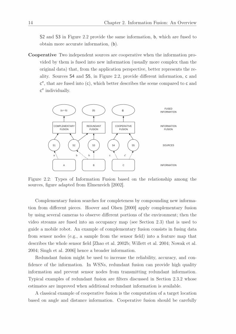
14 Chapter 2. Information Fusion: An Overview
S2 and S3 in Figure 2.2 provide the same information, b, which are fused to
obtain more accurate information, (b).
Cooperative Two independent sources are cooperative when the information pro-
vided by them is fused into new information (usually more complex than the
original data) that, from the application perspective, better represents the re-
ality. Sources S4 and S5, in Figure 2.2, provide different information, c and
c′′, that are fused into (c), which better describes the scene compared to c and
c′′ individually.
(a + b)
A B C
(b) ( c )
COMPLEMENTARY FUSION
REDUNDANT FUSION
COOPERATIVE FUSION
S1 S2 S3 S4 S5 SOURCES
INFORMATION
INFORMATION FUSION
FUSED INFORMATION
a b b c c' '
Figure 2.2: Types of Information Fusion based on the relationship among thesources, figure adapted from Elmenreich [2002].
Complementary fusion searches for completeness by compounding new informa-
tion from different pieces. Hoover and Olsen [2000] apply complementary fusion
by using several cameras to observe different portions of the environment; then the
video streams are fused into an occupancy map (see Section 2.3) that is used to
guide a mobile robot. An example of complementary fusion consists in fusing data
from sensor nodes (e.g., a sample from the sensor field) into a feature map that
describes the whole sensor field [Zhao et al. 2002b; Willett et al. 2004; Nowak et al.
2004; Singh et al. 2006] hence a broader information.
Redundant fusion might be used to increase the reliability, accuracy, and con-
fidence of the information. In WSNs, redundant fusion can provide high quality
information and prevent sensor nodes from transmitting redundant information.
Typical examples of redundant fusion are filters discussed in Section 2.3.2 whose
estimates are improved when additional redundant information is available.
A classical example of cooperative fusion is the computation of a target location
based on angle and distance information. Cooperative fusion should be carefully

2.2. Classifying Information Fusion 15
applied since the resultant data is subject to the inaccuracies and imperfections of
all participating sources [Brooks and Iyengar 1998].
2.2.2 Classification Based on Levels of Abstraction
Luo et al. [2002] use four levels of abstraction to classify information fusion: signal,
pixel, feature, and symbol. Signal level fusion deals with single or multidimensional
signals from sensors. It can be used in real-time applications or as an intermedi-
ate step for further fusions. Pixel level fusion operates on images and can be used
to enhance image-processing tasks. Feature level fusion deals with features or at-
tributes extracted from signals or images, such as shape and speed. In symbol level
fusion, information is a symbol that represents a decision, and it is also referred
to as decision level. Typically, the feature and symbol fusions are used in object
recognition tasks. Such a classification presents some drawbacks and is not suitable
for all information fusion applications. First, both signals and images are considered
raw data usually provided by sensors, so they might be included in the same class.
Second, raw data may not be only from sensors, since information fusion systems
might also fuse data provided by databases or human interaction. Third, it suggests
that a fusion process cannot deal with all levels simultaneously.
In fact, information fusion deals with three levels of data abstraction: measure-
ment, feature, and decision [Dasarathy 1997; Iyengar et al. 2001]. According to the
level of abstraction of the manipulated data, information fusion can be classified
into four categories:
Low-Level Fusion Also referred to as signal (measurement) level fusion. Raw
data are provided as inputs, combined into new data that are more accurate
(reduced noise) than the individual inputs. Polastre et al. [2004] provide an
example of low-level fusion by applying a moving average filter (Section 2.3.2.4
discusses the moving average filters) to estimate ambient noise and determine
whether or not the communication channel is clear.
Medium-Level Fusion Attributes or features of an entity (e.g., shape, texture,
position) are fused to obtain a feature map that may be used for other tasks
(e.g., segmentation or detection of an object). This type of fusion is also known
as feature/attribute level fusion. Examples of this type of information fusion
include estimation of fields or feature maps [Nowak et al. 2004; Singh et al.
2006] and energy maps [Zhao et al. 2002b; Mini et al. 2004] (see Section 2.3.3
for a feature map description).

16 Chapter 2. Information Fusion: An Overview
High-Level Fusion Also known as symbol or decision level fusion. It takes de-
cisions or symbolic representations as input and combines them to obtain a
more confident and/or a global decision. An example of high-level fusion is
the Bayesian approach for binary event detection proposed by Krishnamachari
and Iyengar [2004] that detects and corrects measurement faults.
Multilevel Fusion When the fusion process encompasses data of different abstrac-
tion levels, i.e., when both input and output of fusion can be of any level (e.g.,
a measurement is fused with a feature to provide a decision), multilevel fusion
takes place. In Chapter 3, we provide an example of multilevel fusion by ap-
plying the Dempster-Shafer (see Section 2.3.1.2) theory to detect node failures
based on traffic decay features.
Although the first three levels of fusion are specified by Iyengar et al. [2001],
they do not specify the Multilevel Fusion. Typically, only the first three cate-
gories of fusion (low, medium, and high level fusion) are considered, usually with
the terms pixel/measurement, feature, and decision fusion [Pohl and van Genderen
1998]. However, such a categorization does not foresee the fusion of information of
different levels of abstraction at the same time. For example, the fusion of a signal
or an image with a feature resulting in a decision [Dasarathy 1997; Wald 1999].
2.2.3 Classification Based on Input and Output
Another well-known classification that considers the abstraction level is provided
by Dasarathy [1997], in which information fusion processes are categorized based
on the level of abstraction of the input and output information. Dasarathy [1997]
identifies five categories:
Data In – Data Out (DAI-DAO) In this class, information fusion deals with
raw data and the result is also raw data, possibly more accurate or reliable.
Data In – Feature Out (DAI-FEO) Information fusion uses raw data from
sources to extract features or attributes that describe an entity. Here, “en-
tity” means any object, situation, or world abstraction.
Feature In – Feature Out (FEI-FEO) FEI-FEO fusion works on a set of fea-
tures to improve/refine a feature, or extract new ones.
Feature In – Decision Out (FEI-DEO) In this class, information fusion takes
a set of features of an entity generating a symbolic representation or a decision.

2.3. Methods, Techniques, and Algorithms 17
Decision In - Decision Out (DEI-DEO) Decisions can be fused in order to ob-
tain new decisions or give emphasis on previous ones.
In comparison to the classification presented in Section 2.2.2, this classification
can be seen as an extension of the previous one with a finer granularity where
DAI-DAO corresponds to Low Level Fusion, FEI-FEO to Medium Level Fusion,
DEI-DEO to High Level Fusion, DAI-FEO and FEI-DEO are included in Multilevel
Fusion. Therefore, contextualizing the examples in Section 2.2.2, Polastre et al.
[2004] use DAI-DAO fusion for ambient noise estimation through a moving aver-
age filter; Singh et al. [2006] use FEI-FEO fusion for building feature maps that
geographically describe a sensed parameter such as temperature; Luo et al. [2006]
use DEI-DEO fusion for binary event detection by fusing several single detections
(sensor reports) to decide about an actual event detection; and, in Chapter 3, we
apply FEI-DEO fusion when they fuse features describing the traffic decay to infer
about node failures.
The main contribution of Dasarathy’s classification relies on the fact that it
specifies the abstraction level of both input and output of a fusion process avoiding
possible ambiguities. However, it does not allow in the same process, the fusion, for
instance, of features and signals to refine a given feature or provide a decision.
2.3 Methods, Techniques, and Algorithms
Methods, techniques, and algorithms used to fuse data can be classified based on
several criteria, such as the data abstraction level, purpose, parameters, type of
data, and mathematical foundation. The classification presented in this section is
based on the method’s purpose. According to this criterion, information fusion can
be performed with different objectives such as inference, estimation, classification,
feature maps, abstract sensors, aggregation, and compression.
2.3.1 Inference
Inference methods are often applied in decision fusion. In this case, a decision is
taken based on the knowledge of the perceived situation. Here, inference refers to the
transition from one likely true proposition to another, which its truth is believed to
result from the previous one. Classical inference methods are based on the Bayesian
inference and Dempster-Shafer Belief Accumulation theory.
18 Chapter 2. Information Fusion: An Overview
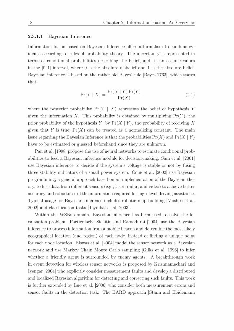
2.3.1.1 Bayesian Inference
Information fusion based on Bayesian Inference offers a formalism to combine ev-
idence according to rules of probability theory. The uncertainty is represented in
terms of conditional probabilities describing the belief, and it can assume values
in the [0, 1] interval, where 0 is the absolute disbelief and 1 is the absolute belief.
Bayesian inference is based on the rather old Bayes’ rule [Bayes 1763], which states
that:
Pr(Y | X) =Pr(X | Y ) Pr(Y )
Pr(X), (2.1)
where the posterior probability Pr(Y | X) represents the belief of hypothesis Y
given the information X. This probability is obtained by multiplying Pr(Y ), the
prior probability of the hypothesis Y , by Pr(X | Y ), the probability of receiving X
given that Y is true; Pr(X) can be treated as a normalizing constant. The main
issue regarding the Bayesian Inference is that the probabilities Pr(X) and Pr(X | Y )
have to be estimated or guessed beforehand since they are unknown.
Pan et al. [1998] propose the use of neural networks to estimate conditional prob-
abilities to feed a Bayesian inference module for decision-making. Sam et al. [2001]
use Bayesian inference to decide if the system’s voltage is stable or not by fusing
three stability indicators of a small power system. Coué et al. [2002] use Bayesian
programming, a general approach based on an implementation of the Bayesian the-
ory, to fuse data from different sensors (e.g., laser, radar, and video) to achieve better
accuracy and robustness of the information required for high-level driving assistance.
Typical usage for Bayesian Inference includes robotic map building [Moshiri et al.
2002] and classification tasks [Tsymbal et al. 2003].
Within the WSNs domain, Bayesian inference has been used to solve the lo-
calization problem. Particularly, Sichitiu and Ramadurai [2004] use the Bayesian
inference to process information from a mobile beacon and determine the most likely
geographical location (and region) of each node, instead of finding a unique point
for each node location. Biswas et al. [2004] model the sensor network as a Bayesian
network and use Markov Chain Monte Carlo sampling [Gilks et al. 1996] to infer
whether a friendly agent is surrounded by enemy agents. A breakthrough work
in event detection for wireless sensor networks is proposed by Krishnamachari and
Iyengar [2004] who explicitly consider measurement faults and develop a distributed
and localized Bayesian algorithm for detecting and correcting such faults. This work
is further extended by Luo et al. [2006] who consider both measurement errors and
sensor faults in the detection task. The BARD approach [Stann and Heidemann

2.3. Methods, Techniques, and Algorithms 19
2005] uses the Bayesian inference to reduce the communication costs related to re-
source and route discovery by limiting the associated communication to the nodes
that are most likely to connect a source to a sink node. The infer algorithm [Hartl
and Li 2005] is a distributed solution that uses Bayesian inference to determine the
missing data from the nodes that are not active (sleep mode) during a sensing epoch.
2.3.1.2 Dempster-Shafer Inference
The Dempster-Shafer Inference is based on the Dempster-Shafer Belief Accumula-
tion (also referred as Theory of Evidence or Dempster-Shafer Evidential Reasoning),
which is a mathematical theory introduced by Dempster [1968] and Shafer [1976]
that generalizes the Bayesian theory. It deals with beliefs or mass functions just as
Bayes’ rule does with probabilities. The Dempster-Shafer theory provides a formal-
ism that can be used for incomplete knowledge representation, belief updates, and
evidence combination [Provan 1992].
A fundamental concept in a Dempster-Shafer reasoning system is the frame of
discernment, which is defined as follows. Let Θ = {θ1, θ2, . . . , θN} be the set of all
possible states that describe the system, such that Θ is exhaustive and mutually
exclusive in the sense that the system is certainly in one, and only one, state θi ∈ Θ,
where 1 ≤ i ≤ N . We call Θ the frame of discernment because its elements are used
to discern the actual system states.
The elements of the power set 2Θ are called hypotheses. In the Dempster-Shafer
theory, based on evidence E, a probability is assigned to every hypothesis H ∈ 2Θ
according to a basic probability assignment (bpa), or mass function, m : 2Θ → [0, 1]
that satisfies:
m(∅) = 0 (2.2)
m(H) ≥ 0,∀ H ∈ 2Θ (2.3)∑
H∈2Θ
m(H) = 1. (2.4)
To express the overall belief in a hypothesis H, the Dempster-Shafer defines the
belief function bel : 2Θ → [0, 1] over Θ as:
bel(H) =∑
A⊆H
m(A), (2.5)
where bel(∅) = 0, and bel(Θ) = 1.
The degree of doubt in H can be intuitively expressed in terms of the belief

20 Chapter 2. Information Fusion: An Overview
function bel : 2Θ → [0, 1] as:
dou(H) = bel(¬H) =∑
A⊆¬H
m(A). (2.6)
To express the plausibility of each hypothesis, the function pl : 2Θ → [0, 1] over
Θ is defined as:
pl(H) = 1− dou(H) =∑
A∩H=∅
m(A). (2.7)
The plausibility intuitively states that the less the doubt in hypothesis H, the
more plausible. In this context, the confidence interval [bel(H), pl(H)] defines the
true belief of the hypothesis H.
To combine the effects of two bpa’s m1 and m2, the Dempster-Shafer theory
defines a combination rule, m1 ⊕m2, which is given by:
m1 ⊕m2(∅) = 0, (2.8)
m1 ⊕m2(H) =
∑
X∩Y =H
m1(X)m2(Y )
1− ∑
X∩Y =∅
m1(X)m2(Y ). (2.9)
According to Luo and Kay [1992], the use of the Dempster-Shafer theory for
information fusion of sensory data was introduced in 1981 by Garvey et al. [1981].
In contrast to the Bayesian Inference, the Dempster-Shafer theory is more flexible,
for it allows each source to contribute with information in different levels of detail.
To illustrate this assertion, let us suppose we have two sensors, A and B, able to
distinguish the roar of male from female felines; and we also have a third sensor,
C, that distinguishes a cheetah roar from a lion roar. In this scenario, we can
easily use the Dempster-Shafer theory to fuse data from the three sensors to detect
male/female lions and male/female cheetahs, while such an inference would be more
difficult with a Bayesian method. The reason is that, in contrast to the Bayesian
Inference, the Dempster-Shafer theory allows us to fuse data provided by different
types of sensors. Furthermore, in the Dempster-Shafer inference we do not need
assign a priori probabilities to unknown propositions. Instead, probabilities are
assigned only when the supporting information is available.
Choosing between the Bayesian Inference and the Theory of Evidence is not a
trivial task because, among other things, there is a tradeoff between the Bayesian
accuracy and the Dempster-Shafer flexibility [Bracio et al. 1997]. Comparisons
between these two inference methods are provided by Buede [1988] and Cheng and

2.3. Methods, Techniques, and Algorithms 21
Kashyap [1988].
Pinto et al. [2004] discuss in-network implementations of the Dempster-Shafer
and the Bayesian inference in such a way that event detection and data routing are
unified into a single algorithm. By using a WSN composed of Unmanned Aerial
Vehicles (UAVs) as sensor nodes, Yu et al. [2004] use the Dempster-Shafer inference
to build dynamic operational pictures of battlefields for situation assessment. How-
ever, the particular challenges of in-network fusion in such a mobile network are
not evaluated. In the Data Service Middleware (DSWare) for WSNs designed by Li
et al. [2004], every decision is associated with a confidence value that is computed by
a pre-specified confidence function based on the belief and plausibility functions of
the Dempster-Shafer theory. In Chapter 3, we propose an algorithm that analyzes
the data traffic and uses the Dempster-Shafer inference to detect routing failures
and trigger a topology reconstruction (route re-discovery) only when necessary.
2.3.1.3 Fuzzy logic
Fuzzy logic generalizes probability [Banon 1981] and, therefore, is able to deal with
approximate reasoning [Novák et al. 1999] to draw (possibly imprecise) conclusions
from imprecise premises. Each quantitative input is fuzzyfied by a membership
function. The fuzzy rules of an inference system produce fuzzy outputs which, in
turn, are defuzzyfied by a set of output rules. This framework has been successfully
used in real world situations that defy exact modelling, from rice cookers to complex
control systems [Lee 1990].
Cui et al. [2004] study the problem of controlling the position of sensors for
localizing of hazardous contaminant sources. They propose a fuzzy logic position
control algorithm able to cope with the incomplete, uncertain, and approximate
information the sensor gathers. The purpose of the algorithm is manyfold, namely,
exploring the whole area, keeping connectivity and finding the emission source.
Aiming at optimizing mobile sensor deployment, Shu and Liang [2005] update the
position of each node using a fuzzy optimization algorithm. This technique fuzzyfies
the number of neighbors of each sensor and the average distance among them in order
to derive an updating rule.
An intelligent sensor network and fuzzy logic control are used by Chan Yet and
Qidwai [2005] to develop an autonomous navigational robotic vehicle with obstacle
avoidance capability. The navigation is guided by two controllers: one for detecting
potholes and another for avoiding obstacles. The input to each controller is the
stereoscopic information gathered by ultrasonic sensors, and the fuzzyfication is
performed using training data obtained beforehand. These two sub-systems feed

22 Chapter 2. Information Fusion: An Overview
the main controller that decides the best path to follow.
Gupta et al. [2005] and Halgamuge et al. [2003] use fuzzy reasoning for deciding
the best cluster-heads in a WSN. The former use three features to guide the choice:
node concentration, energy level, and centrality. After fuzzyfication, these features
are turned into linguistic variables and a rule is obtained. The technique proves to
be better than the stochastic procedure proposed by Heinzelman et al. [2000]. The
latter use energy measures and a fuzzy clustering algorithm, and their results are
better than those of a substractive clustering technique [Bezdek 1981].
Regarding the design of Medium Access Control (MAC) protocols, Wallace et al.
[2005] propose a two-stage fuzzy-based control aiming at prolonging the network
lifetime. The inputs for the first stage are, for each node, size of the current transmit
queue, remaining battery level, and collision of previous packages. The second stage
gives priority to access the medium to nodes with high transmit queue using the three
previous inputs as well. The authors show that their sleeping duty cycles extend
the network lifetime with respect to a fixed cycle strategy. With the same purpose,
Liang and Ren [2005b] propose a MAC protocol with a fuzzy logic rescheduling
scheme that improves existing energy-efficient protocols. Their input variables are
the ratios of nodes (i) with overflowed buffer, (ii) with high failing transmission rate,
and (iii) experiencing unsuccessful transmission.
Efficient routing is another area where fuzzy logic is used aiming at the opti-
mization of energy usage in WSNs. Yusuf and Haider [2005] assume a cluster-based
architecture and study gateway centralized inter-cluster routing. They use trans-
mission energy, remaining energy, rate of energy consumption queue size, distance
from the gateway and current status as input variables; the fuzzy output is the cost.
Liang and Ren [2005a] use battery capacity, mobility, and distance to the destina-
tion as variables for a fuzzy system that improves network lifetime by deciding the
possibility of each node being included in the path. Srinivasan et al. [2006] use a
fuzzy system to infer the ability of each node to transmit data using its battery
power and the type of data being forwarded; and during route discovery, the output
of the fuzzy logic controller is used to decide whether or not to forward a packet.
2.3.1.4 Neural Networks
According to Bonissone [1997], neural networks were originated in the early 1960’s
with Rosenblatt [1959] and Widrow and Hoff [1960]. They are structures that im-
plement supervised learning mechanisms, that starting from examples are able to
generalize. There are also unsupervised neural networks as, for instance, the Ko-
honen maps [Kohonen 1997]. Neural Networks represent an alternative to Bayesian

2.3. Methods, Techniques, and Algorithms 23
and Dempster-Shafer theories, being used by classification and recognition tasks in
the information fusion domain.
A key feature of neural networks is the ability of learning from examples of
input/output pairs in a supervised fashion. For that reason, neural networks can be
used in learning systems while fuzzy logic [Zadeh 1994] is used to control its learning
rate [Bonissone 1997].
Neural networks have been applied to information fusion mainly for Automatic
Target Recognition (ATR) using multiple complementary sensors [Luo and Kay 1992;
Roth 1990; Filippidis et al. 2000]. The reason is that neural networks provide highly
parallel means of processing yielding, thus, robustness before different issues such
as noise [Castelaz 1988]. Baran [1989] proposes an information fusion approach
for ATR that uses a neural network acting as an associative memory that guides
the pattern-matching process for target recognition. Cain et al. [1989] use neural
networks to classify targets based on information acquired from a multispectral
infrared sensor and an ultraviolet laser radar.
Neural networks for information fusion can also be found in other applications
besides ATR. Lewis and Powers [2002] use neural networks to fuse audio-visual
information for audio-visual speech recognition. Cimander et al. [2002] use a two-
stage fusion method that operates on signals from bioreactors (e.g., temperature, pH
and oxygen) to control the yogurt fermentation process. Yiyao et al. [2001] propose
a fusion scheme named Knowledge-Based Neural Network Fusion (KBNNF) to fuse
edge maps from multispectral sensor images acquired from radars, optical sensors,
and infrared sensors.
2.3.1.5 Semantic Information Fusion
Semantic Information Fusion is essentially an in-network inference process in which
raw sensor data is processed so that nodes exchange only the resulting semantic
interpretations. The semantic abstraction allows a WSN to optimize its resource
utilization when collecting, storing, and processing data. Semantic Information Fu-
sion usually comprises two phases: knowledge base construction and pattern match-
ing (inference). The first phase (usually off-line) aggregates the most appropriate
knowledge abstractions into semantic information, which is then used in the sec-
ond phase (on-line), a pattern matching phase, for fusing relevant attributes and
providing a semantic interpretation of sensor data [Friedlander and Phoha 2002;
Friedlander 2005; Whitehouse et al. 2006].
To the best of our knowledge, Friedlander and Phoha [2002] are the ones who
introduced the concept of Semantic Information Fusion, which was applied for tar-

24 Chapter 2. Information Fusion: An Overview
get classification. This work is further extended by Friedlander [2005] who describes
techniques for extracting semantic information from sensor networks. The idea is
to integrate and convert sensor data into formal languages. Then, the resulting lan-
guage, obtained from the environment observations, is compared with the languages
with known behaviors stored in a knowledge base. The idea behind this strategy
is that behaviors represented by similar formal languages are semantically similar.
Thus, this method extends traditional pattern-matching techniques that measure
the distances between the feature vectors of an observed entity and a set of known
behaviors.
Friedlander [2005] applies the proposed techniques to recognize the behavior of
robots based on their trajectories, but they can also be used for saving resources.
For instance, energy can be saved by making sensor nodes transmit only the formal
language describing the perceived data, rather than every raw sensor data. Then,
at the external processing entity, the formal language can be used to classify the
application behavior or to generate sensor data that are statistically equivalent to
the original observations. In any case it is necessary to have a set of known behaviors
stored in a database, which in some cases may be difficult to obtain.
In another approach, Whitehouse et al. [2006] describe the Semantic Streams
framework that allows the user to formulate queries over semantic values without
addressing which data or operations are to be used. Thus, the query answers are
semantic interpretations acquired by in-network inference processes. Parallel to
that work, Liu and Zhao [2005] propose the SONGS architecture that, by means of
automatic service planning, converts declarative queries into a service composition
graph, and performs optimizations for resource-aware execution of the service com-
posite. These optimizations may include the avoidance of redundant computation
of shared tasks that compose the queries issued by the user [Liu et al. 2005].
2.3.2 Estimation
Estimation methods were inherited from control theory and use the laws of proba-
bility to compute a process state vector from a measurement vector or a sequence of
measurement vectors [Bracio et al. 1997]. In this section, we present the estimation
methods known as: Maximum Likelihood, Maximum A Posteriori, Least Squares,
Moving Average filter, Kalman filter, and Particle filter.
2.3.2.1 Maximum Likelihood (ML)
Estimation methods based on Likelihood are suitable when the state being estimated
is not the outcome of a random variable [Brown et al. 1992].

2.3. Methods, Techniques, and Algorithms 25
In the context of information fusion, given x, the state being estimated, and
z = (z(1), . . . , z(k)), a sequence of k observations of x, the likelihood function λ(x)
is defined as the probability density function (pdf) of the observation sequence z
given the true value of the state x:
λ(x) = p (z | x) . (2.10)
Note that the likelihood function is no longer a pdf.
The Maximum Likelihood estimator (MLE) searches for the value of x that
maximizes the likelihood function
x̂(k) = arg maxx
p (z | x) (2.11)
that can be obtained from empirical or analytical sensor models.
Xiao et al. [2005] propose a distributed and localized MLE that is robust to the
unreliable communication links of WSNs. In this method, every node computes
a local unbiased estimate that converges towards the global Maximum Likelihood
solution. The authors further extended this method to support asynchronous and
timely delivered measurements, i.e., measurements taken at different time steps that
happen asynchronously in the network [Xiao et al. 2006]. Other distributed imple-
mentations of MLEs for WSNs include the Decentralized Expectation Maximization
(EM) algorithm [Nowak 2003] and the Local Maximum Likelihood Estimator [Blatt
and Hero 2004] that relax the requirement of sharing all the data.
In the network tomography domain, Hartl and Li [2004] use the MLE to estimate
per-node loss rates during the aggregation and reporting of data from source to sink
nodes. Such a strategy may be useful, for example, for routing algorithms to bypass
lossy areas.
The MLE is commonly used to solve location discovery problems. In this context,
the method is often used to obtain accurate distance (or direction, angle) estimations
that are used to compute the location of nodes [Patwari et al. 2003; Fang et al. 2005]
or sources (targets) [Sheng and Hu 2005; Niu and Varshney 2006; Li et al. 2006; Chen
et al. 2006a]. An example of “node location” is the Knowledge-based Positioning
System (KPS) [Fang et al. 2005] that assumes a prior knowledge about the pdf
of the nodes’ deployment so that sensor nodes can use the MLE to estimate their
locations by observing the group memberships of their neighbors. An example of
“source location” is a bird monitoring application described by Chen et al. [2006a],
which uses an approximate MLE to process acoustic measurements and estimate
the source direction-of-arrival and perform beamforming for signal enhancement.

26 Chapter 2. Information Fusion: An Overview
Then, the direction information is used to localize the birds while enhanced signals
are used to classify the birds.
2.3.2.2 Maximum A Posteriori (MAP)
This method is based on the Bayesian theory, therefore, it is used when the param-
eter x to be discovered is the outcome of a random variable with known pdf p(x).
The measurement sequence is characterized by the sensor model (conditional pdf of
the measurement sequence).
In the context of information fusion, given x, the state being estimated, and
z = (z(1), . . . , z(k)), a sequence of k observations of x, the Maximum A Posteri-
ori estimator searches for the value of x that maximizes the posterior distribution
function
x̂(k) = arg maxx
p (x | z) . (2.12)
Both methods, Maximum Likelihood and Maximum A Posteriori, try to find
the most likely value for the state x. However, the first method assumes that x
is a fixed though unknown point of the parameter space, while the last takes x as
the outcome of a random variable with prior pdf known. These two methods are
equivalent when the prior pdf of x is not informative, e.g., when p(x) is Gaussian
with σ →∞ [Brown et al. 1992].
Schmitt et al. [2002] use the MAP estimator to find the joint positions of mobile
robots in a known environment and track the positions of autonomously moving
objects. The collision resolution algorithm proposed by Yuan and Kam [2004] to
manage traffic between local detectors (e.g., source nodes) and a fusion center (e.g.,
a cluster-head) use a MAP estimator to compute the number of nodes that wish to
transmit so these nodes properly update their retransmission probability.
Traditional approaches for a MAP estimator may be too costly to be employed in
WSNs [Rachlin et al. 2006]. However, a couple of efficient distributed solutions for
WSNs have been proposed. Shah et al. [2005] present a distributed implementation
in which MAP estimators are found as the maximum of concave functions so that
simple numerical maximization algorithms can be used. Saligrama et al. [2006]
use a variant of belief propagation [Pearl 1988; Ihler et al. 2005] as collaboration
strategy for distributed classification that reaches a consensus to the centralized
MAP estimate.
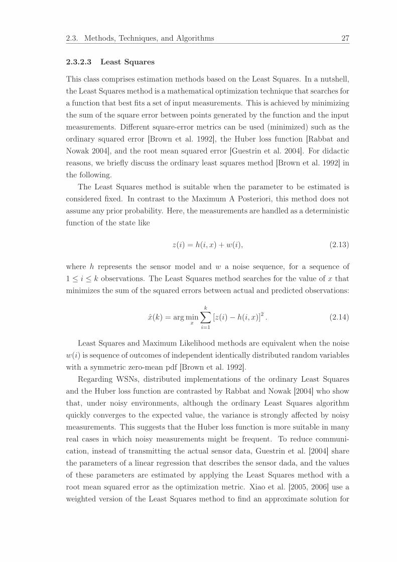
2.3. Methods, Techniques, and Algorithms 27
2.3.2.3 Least Squares
This class comprises estimation methods based on the Least Squares. In a nutshell,
the Least Squares method is a mathematical optimization technique that searches for
a function that best fits a set of input measurements. This is achieved by minimizing
the sum of the square error between points generated by the function and the input
measurements. Different square-error metrics can be used (minimized) such as the
ordinary squared error [Brown et al. 1992], the Huber loss function [Rabbat and
Nowak 2004], and the root mean squared error [Guestrin et al. 2004]. For didactic
reasons, we briefly discuss the ordinary least squares method [Brown et al. 1992] in
the following.
The Least Squares method is suitable when the parameter to be estimated is
considered fixed. In contrast to the Maximum A Posteriori, this method does not
assume any prior probability. Here, the measurements are handled as a deterministic
function of the state like
z(i) = h(i, x) + w(i), (2.13)
where h represents the sensor model and w a noise sequence, for a sequence of
1 ≤ i ≤ k observations. The Least Squares method searches for the value of x that
minimizes the sum of the squared errors between actual and predicted observations:
x̂(k) = arg minx
k∑
i=1
[z(i)− h(i, x)]2 . (2.14)
Least Squares and Maximum Likelihood methods are equivalent when the noise
w(i) is sequence of outcomes of independent identically distributed random variables
with a symmetric zero-mean pdf [Brown et al. 1992].
Regarding WSNs, distributed implementations of the ordinary Least Squares
and the Huber loss function are contrasted by Rabbat and Nowak [2004] who show
that, under noisy environments, although the ordinary Least Squares algorithm
quickly converges to the expected value, the variance is strongly affected by noisy
measurements. This suggests that the Huber loss function is more suitable in many
real cases in which noisy measurements might be frequent. To reduce communi-
cation, instead of transmitting the actual sensor data, Guestrin et al. [2004] share
the parameters of a linear regression that describes the sensor dada, and the values
of these parameters are estimated by applying the Least Squares method with a
root mean squared error as the optimization metric. Xiao et al. [2005, 2006] use a
weighted version of the Least Squares method to find an approximate solution for

28 Chapter 2. Information Fusion: An Overview
a distributed Maximum Likelihood estimation.
In another example, Willett et al. [2004] propose a spatial sampling algorithm in
which a Least Squares method is used to define a small subset of sensor nodes that
provide an initial estimate of the environment being sensed. This technique aims at
building spatial maps describing properties of the sensor field [Nowak et al. 2004],
and guiding mobile nodes in the construction of such maps [Singh et al. 2006].
Instead of transmitting the complete data stream from source to sink, Santini
and Römer [2006] use a dual prediction scheme, based on Least Squares filters,
both in the source and in the sink. Only when the predicted value differs from
the actual value by more than a given error, the value is transmitted to the sink.
Liu et al. [2006] propose a robust and interactive Least Squares method for node
localization in which, at each iteration, nodes are localized by using a least-squares
based algorithm that explicitly considers noisy measurements.
2.3.2.4 Moving Average Filter
The moving average filter [Smith 1999] is widely adopted in digital signal processing
(DSP) solutions because it is simple to understand and use. Furthermore, this filter
is optimal for reducing random white noise while retaining a sharp step response.
This is the reason that makes the moving average the main filter for processing
encoded signals in the time domain. As the name suggests, this filter computes the
arithmetic mean of a number of input measurements to produce each point of the
output signal.
Given an input digital signal z = (z(1), z(2), . . . ), the true signal x =
(x̂(1), x̂(2), . . . ) is estimated by
x̂(k) =1
M
M−1∑
i=0
z(k − i) (2.15)
for every k ≥M , where M is the filter’s window, i.e., the number of input observa-
tions to be fused.
Observe that M is also the number of steps the filter takes to detect the change
in the signal level. The lower the value of M , the sharper the step edge. On the
other hand, the greater the value of M , the cleaner the signal. When a step signal
has a random white noise, the Moving Average filter manages to reduce the noise
variance by a factor√
M [Smith 1999]. Thus, M should be the smallest value in
which this noise reduction meets the application requirements.
Woo et al. [2003] study the use of moving average filters within adaptive link
estimators so that link connectivity statistics are dynamically collected and exploited

2.3. Methods, Techniques, and Algorithms 29
by routing protocols to improve reliability. In Chapter 3, we use the Moving Average
filter to estimate the data traffic of continuous WSNs, and such an estimate is further
used for routing-failure detection. Yang et al. [2005a] apply the Moving Average filter
on target locations to reduce errors of tracking applications in WSNs. In the NED
algorithm [Jin and Nittel 2006], sensor nodes estimate events and event boundaries
based on simple Moving Average filters that are used to improve the sensor readings.
Weighted Moving Average filters are also commonly used in WSNs, especially
the Exponentially Weighted Moving Average (EWMA) filter. An EWMA filter
has multiplying factors to give different weights, which decrease exponentially, to
different data points. EWMA filters have been used by Medium Access Control
protocols to estimate ambient noise [Polastre et al. 2004] and determine whether
the channel is clear, and for local clock synchronization [Rhee et al. 2005] used
for contention purposes. Applications have used EWMA filters to obtain refined
estimations from sensors for detection and classification tasks [Gu et al. 2005] and
to estimate distances for localization algorithms [Blumenthal et al. 2006]. Another
example is the use of EWMA filters to detect incipient congestion [Rangwala et al.
2006] for fair and efficient rate control. Due to the increasing popularity of Moving
Average filters, Tinker [Elson and Parker 2006], a high-level tool for application
development in WSNs, includes a time-efficient implementation of the EWMA filter.
2.3.2.5 Kalman Filter
The Kalman filter is a very popular fusion method. It was originally proposed in
1960 by Kalman [1960] and it has been extensively studied since then [Luo and Kay
1992; Jacobs 1993; Brown and Hwang 1996].
The Kalman filter is used to fuse low-level redundant data. If a linear model can
describe the system and the error can be modelled as Gaussian noise, the Kalman
filter recursively retrieves statistically optimal estimates [Luo and Kay 1992]. How-
ever, to deal with non-linear dynamics and non-linear measurement models other
methods should be adopted. According to Jazwinski [1970], the variation named
Extended Kalman filter (EKF) [Welch and Bishop 2001] is a popular approach to
implement recursive nonlinear filters. More recently, the Unscented Kalman Filter
(UKF) [Julier and Uhlmann 1997] has gained attention since it does not have a lin-
earization step and the associated errors. The UKF uses a deterministic sampling
technique to choose a minimal set of sample points around the mean. These points
are propagated through the nonlinear functions so the covariance of the estimate
is recovered. The standard Kalman Filter can be extended to improve its perfor-
mance [Gao and Harris 2002] or to provide decentralized implementations [Grime

30 Chapter 2. Information Fusion: An Overview
and Durrant-Whyte 1994].
In WSNs, we can find schemes to approximate distributed Kalman filtering,
in which the solution is computed based on reaching an average consensus among
sensor nodes [Spanos et al. 2005; Olfati-Saber 2005]. An important concern is the
data loss due to the unreliable communication channels in WSNs. In this context,
Sinopoli et al. [2004] assess the performance of the Kalman filter in a scenario with
intermittent observations and show the existence of a critical value for the arrival
rate of the observations that, if exceeded, the Kalman filter becomes unstable.
Another issue regarding the use of a Kalman filter in WSNs is that it requires a
proximate clock synchronization among sensor nodes [Ganeriwal et al. 2003]. This
is evidenced by Manzo et al. [2005] who show how synchronization problems caused
by an attack on the time synchronization can affect the Kalman filter performance
leading to incorrect estimates.
For a long time, Kalman filters have been used in algorithms for source local-
ization and tracking, especially in robotics [Brown et al. 1992]. Wireless sensor
networks inherited such an application trend and, aiming at accuracy improvement,
the Kalman filter has been applied to refine location and distance estimates [Sav-
vides et al. 2003; Hongyang et al. 2005], and track different sources [Li et al. 2006].
In particular, Li et al. [2006] propose a source localization algorithm for a system
equipped with asynchronous sensors, and show that the UKF outperforms the EKF
for source tracking because of the linearization error present in the EKF.
A MAC protocol can also benefit from the applicability of a Kalman filter to
predict, for instance, its frame size. In this direction, Ci et al. [2004] use the UKF
for frame size prediction, while Raviraj et al. [2005] use the EKF for the same
purpose. As a conclusion, Ci and Sharif [2005] show that the UKF approach is
better than the EKF, especially under noise conditions.
Still in the context of data communication, Jain et al. [2004] use a dual Kalman
Filter approach in which both source and sink nodes predict the sensed value so
the source node sends data only when it knows the sink prediction is incorrect.
In the SCAR routing algorithm [Mascolo and Musolesi 2006], a sensor node uses
the Kalman filter to predict context information (mobility and resources) about its
neighbors, and based on such predictions it chooses the best neighbor for routing
its data.
2.3.2.6 Particle Filter
Particle filters are recursive implementations of statistical signal processing [Gilks
et al. 1996] known as sequential Monte Carlo methods (SMC) [Crisan and Doucet

2.3. Methods, Techniques, and Algorithms 31
2002]. Although the Kalman filter is a classical approach for state estimation, par-
ticle filters represent an alternative for applications with non-Gaussian noise, espe-
cially when computational power is rather cheap and sampling rate is slow [Nordlund
et al. 2002].
Particle filters attempt to build the posterior pdf based on a large number of
random samples, called particles. The particles are propagated over time sequen-
tially combining sampling and resampling steps. At each time step, the resampling is
used to discard some particles increasing the relevance of regions with high posterior
probability.
In such a filtering process, multiple particles (samples) of the same state variable
x are used, and each particle has an associated weight that indicates the particle
quality. Then, the estimate is the result of the weighted sum of all particles. The
Particle filter algorithm has two phases: prediction and update. In the prediction
phase, each particle is modified according to the existing model, including the ad-
dition of random noise in order to simulate the effect of noise. Then, in the update
phase, the weight of each particle is reevaluated based on the latest sensory infor-
mation available so that particles with small weights are eliminated (resampling
process).
Arulampalam et al. [2002] discuss the use of particle filters and the extended
Kalman filter for tracking applications. Further analysis comparing the use of ex-
tended Kalman filter and particle filters for state estimation is provided by Yuen
and MacDonald [2002]. Zeng and Ma [2002] propose the active particle filtering
where every particle is first driven to its local maximum of the likelihood before it
is weighted; as a result, the efficiency of every particle is improved and the number
of required particles is reduced.
In WSNs, target tracking is currently the principal research problem wherein
particle filters have been used. Aslam et al. [2003] propose a tracking algorithm
based on particle filtering that explores geometric properties of a network composed
of sensors using a binary detection model (one bit representing whether a target
is moving toward the sensor or away from the sensor). Coates [2004] investigates
the use of distributed particle filters for target tracking within hierarchical networks
in which the cluster-heads are responsible for computation and information sharing
while remaining cluster members are responsible for sensing only. Wong et al. [2004]
also adopt an hierarchical collaborative data fusion scheme based on particle filters
for cross-sensor (information from multiple sensors) fusion and cross-modality (in-
formation from different sensing modes) fusion for target tracking. Guo and Wang
[2004] propose a novel SMC solution for target tracking that makes use of an aux-
iliary particle filter technique for data fusion, and a reduced representation of the

32 Chapter 2. Information Fusion: An Overview
a posteriori distribution to reduce the amount of data transmitted among sensor
nodes.
In contrast to single target tracking, multiple target tracking is a more difficult
and more general problem, whose solutions may also use particle filters. Sheng
et al. [2005] propose two distributed particle filters for multiple target tracking
that run on uncorrelated sensor cliques that are dynamically organized based on
target trajectories. Vercauteren et al. [2005] propose a collaborative solution based
on the SMC methodology for jointly tracking several targets and classifying them
according to their motion pattern. By using range data, Chakravarty and Jarvis
[2005] propose a real-time system based on particle filters, for tracking an unknown
number of targets that incorporates a clustering algorithm to discern legitimate from
fake targets. Kreucher et al. [2005] propose a particle filter algorithm that explicitly
enforces the multiple target nature of the problem. The algorithm estimates the
number and states of a group of moving targets occupying a surveillance region.
Another natural application of particle filters within WSNs is to find the nodes’
locations. In this context, Hu and Evans [2004] use the particle filter for obtaining
nodes’ locations in a network composed of mobile nodes. The proposed solution
works as a tracking solution applied to all nodes. Interestingly, the authors show
that, despite the contrary intuition, mobility can improve the accuracy and reduce
the costs of localization. Miguez and Artes-Rodriguez [2006] propose a Monte Carlo
method for joint node location and target tracking that uses a particle filter for both
target tracking and refinement of node position estimates.
Other interesting applications of particle filters include multiuser parameter
tracking in communication systems [Guo et al. 2005] based on code division mul-
tiple access (CDMA), and blind symbol detection of orthogonal frequency-division
multiplexing (OFDM) systems [Yang et al. 2005b] — a digital modulation scheme
for high-rate wireless communications.
2.3.3 Feature Maps
For some applications, such as guidance and resource management, it might not be
feasible to directly use raw sensory data. In such cases, features representing aspects
of the environment have to be extracted and used by the application. Usually,
diverse fusion methods of estimation and inference can be used to generate a feature
map. Here, we present two special types of feature maps: occupancy grid and
network scans.

2.3. Methods, Techniques, and Algorithms 33
2.3.3.1 Occupancy Grid
Occupancy grids, also called occupancy maps or certainty grids, define a multidi-
mensional (2D or 3D) representation of the environment describing which areas are
occupied by an object and/or which areas are free spaces. According to Elfes [1989],
an occupancy grid is “a multidimensional random field that maintains stochastic es-
timates of the occupancy state of the cells”, i.e., the observed space is divided into
square or cubic cells and each cell contains a value indicating its probability of being
occupied. Usually, such probability is computed — based on information provided
by several sensors — using different methods, such as Bayesian theory, Dempster-
Shafer reasoning, and fuzzy set theory [Ribo and Pinz 2001].
Occupancy grids were initially used to build an internal model of static envi-
ronments based on ultrasonic data [Elfes 1987], and since then several variations
have been proposed. Arbuckle et al. [2002] introduce the temporal occupancy grid
as a method to model and classify spatial areas according to their time properties.
Hoover and Olsen [1999, 2000] use a 2D raster as an occupancy map where each
map pixel contains a binary value indicating if the respective space is occupied or
empty.
Typical applications of occupancy grids include position estimation [Wongngam-
nit and Angluin 2001], robot perception [Hoover and Olsen 2000] and navigation [Pa-
gac et al. 1998]. There are also applications in computer graphics, such as simulation
of graphical creatures behavior [Isla and Blumberg 2002] and collisions detection of
volumetric objects [Gagvani and Silver 2000].
2.3.3.2 Network Scans
Network Scans are defined by Zhao et al. [2002b] as a sort of resource/activity map
for wireless sensor networks. Analogous to a weather map, the network scan depicts
the geographical distribution of resources or activity of a WSN. By considering a
resource of interest, instead of providing detailed information about each sensor node
in the network, these scans offer a summarized view of the resource distribution.
The network scan implemented by Zhao et al. [2002b] is called eScan and it retrieves
information about the residual energy in the network in a distributed in-network
fashion.
The algorithm is quite simple. First, an aggregation tree is formed to determine
how the nodes will communicate. Second, each sensor computes its local eScan and
whenever the energy level drops significantly, since the last report, the node sends
its eScan towards the sink. The eScans are aggregated whenever a node receives two
or more topologically adjacent eScans that have the same or similar energy level.
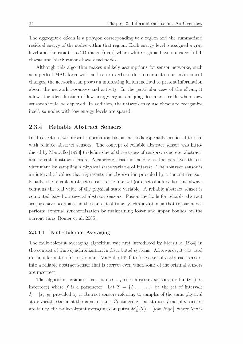
34 Chapter 2. Information Fusion: An Overview
The aggregated eScan is a polygon corresponding to a region and the summarized
residual energy of the nodes within that region. Each energy level is assigned a gray
level and the result is a 2D image (map) where white regions have nodes with full
charge and black regions have dead nodes.
Although this algorithm makes unlikely assumptions for sensor networks, such
as a perfect MAC layer with no loss or overhead due to contention or environment
changes, the network scan poses an interesting fusion method to present information
about the network resources and activity. In the particular case of the eScan, it
allows the identification of low energy regions helping designers decide where new
sensors should be deployed. In addition, the network may use eScans to reorganize
itself, so nodes with low energy levels are spared.
2.3.4 Reliable Abstract Sensors
In this section, we present information fusion methods especially proposed to deal
with reliable abstract sensors. The concept of reliable abstract sensor was intro-
duced by Marzullo [1990] to define one of three types of sensors: concrete, abstract,
and reliable abstract sensors. A concrete sensor is the device that perceives the en-
vironment by sampling a physical state variable of interest. The abstract sensor is
an interval of values that represents the observation provided by a concrete sensor.
Finally, the reliable abstract sensor is the interval (or a set of intervals) that always
contains the real value of the physical state variable. A reliable abstract sensor is
computed based on several abstract sensors. Fusion methods for reliable abstract
sensors have been used in the context of time synchronization so that sensor nodes
perform external synchronization by maintaining lower and upper bounds on the
current time [Römer et al. 2005].
2.3.4.1 Fault-Tolerant Averaging
The fault-tolerant averaging algorithm was first introduced by Marzullo [1984] in
the context of time synchronization in distributed systems. Afterwards, it was used
in the information fusion domain [Marzullo 1990] to fuse a set of n abstract sensors
into a reliable abstract sensor that is correct even when some of the original sensors
are incorrect.
The algorithm assumes that, at most, f of n abstract sensors are faulty (i.e.,
incorrect) where f is a parameter. Let I = {I1, . . . , In} be the set of intervals
Ii = [xi, yi] provided by n abstract sensors referring to samples of the same physical
state variable taken at the same instant. Considering that at most f out of n sensors
are faulty, the fault-tolerant averaging computesMfn (I) = [low, high], where low is

2.3. Methods, Techniques, and Algorithms 35
the smallest value in at least n− f intervals in I, and high is the largest value in at
least n− f intervals in I. Marzullo [1990] shows that the algorithm has O(n log n)
complexity.
As the algorithm computes an intersection of intervals, depending on the inter-
vals in I, the result Mfn (I) can be more accurate than any sensor in I, i.e., the
resultant interval can sometimes be tighter than the original ones. However,Mfn (I)
cannot be more accurate than the most accurate sensor in I when n = 2f + 1.
The result ofM certainly contains the correct value when the number of faulty
sensors is at most f . However, it may present an unstable behavior in the sense
that minor changes in the input may produce quite different outputs.
S 2
S 1
S 3
S 4
M 4 ( S 1 , S 2 , S 3 , S 4 ) 1
real value
(a)
S 2
S 1
S 2 '
S 3
S 4
M 4 ( S 1 , S 2 , S 3 , S 4 )
M 4 ( S 1 , S 2 , S 3 , S 4 ) 1
1
'
real value
(b)
Figure 2.3: Example of the Fault-Tolerant Averaging algorithm.
Figure 2.3(a) depicts a scenario with four sensors {S1, S2, S3, S4} with a faulty
one. In this example, S2 and S3 do not have any intersection, consequently, one of
them is the faulty sensor. Since it is not possible to discover which one provides
the correct interval, both must be covered to securely include the true value. Thus,
M14 (S1, S2, S3, S4) returns the interval [low, high], where low is the smallest value
in at least n− f = 4− 1 = 3 intervals (which is the left edge of S1), and high is the
largest value in at least n− f = 4− 1 = 3 intervals (which is the right edge of S4).
Figure 2.3(b) illustrates the instability of M. In this case, if the right edge of
S2 moves to the left, as given by S ′2, then the left edge of the result becomes the left
edge of S3. Thus, a small change in S2, but large enough to avoid an intersection
with S1, causes a great variation in the final result.
Chew and Marzullo [1991] extend the original single-dimensional fault-tolerant
averaging algorithm to fuse data from multidimensional sensors. Other extension of
Marzullo’s original work is provided by Jayasimha [1994], who improves the detec-
tion of faulty sensors for the linear case.
Blum et al. [2004] show the worst-case (when all clocks run with maximal drift)
optimality of the M function, and propose an improved algorithm, the Back-Path

36 Chapter 2. Information Fusion: An Overview
Interval Synchronization Algorithm (BP-ISA), which also is worst-case-optimal but
yields better results in the average case wherein every node stores, maintains, com-
municates, and uses the bounds from its last communication with other nodes. In
this context, Meier et al. [2004] show that, although optimal interval-based syn-
chronization can only be achieved by having nodes that store and communicate
their entire history, efficient average-case-optimal synchronization can be obtained
by using only recent data.
2.3.4.2 The Fault-Tolerant Interval Function
The Fault-Tolerant Interval (FTI) function, or simply the F function, was proposed
by Schmid and Schossmaier [2001]. FTI is an alternative integration function that
considers the width of the intervals being fused.
The algorithm also assumes that, at most, f of n abstract sensors are faulty
where f is a parameter. Let I be the set of intervals provided by n abstract sensors,
as defined in Section 2.3.4.1. The FTI intersection function is Ffn (I) = [low, high],
where low corresponds to the (f + 1)th largest of the left edges {x1, . . . , xn}, and
high is the (f + 1)th smallest of the right edges {y1, . . . , yn}.The F function is robust. This means that it assures that minor changes in the
input intervals will result in minor changes in the integrated result.
S 1
S 2
S 3
S 4
F 4 ( S 1 , S 2 , S 3 , S 4 ) 1
real value
M 4 ( S 1 , S 2 , S 3 , S 4 ) 1
(a)
S 1
S 2
S 2
S 3
S 4
F 4 ( S 1 , S 2 , S 3 , S 4 )
F 4 ( S 1 , S 2 , S 3 , S 4 )
1
1
'
'
real value
(b)
Figure 2.4: Example of the Fault-Tolerant Interval function.
To illustrate the behavior of F we consider in Figure 2.4 the same example
provided before (in Figure 2.3). The resulting interval is slightly larger than the
intervals returned by M (Figure 2.4(a)). However, the resulting interval does not
change when S ′2 is used instead of S2 (Figure 2.4(b)). As a general result,M tends
to achieve tighter intervals than F . However, F is less vulnerable to small changes
in the input intervals.

2.3. Methods, Techniques, and Algorithms 37
Although the analysis of Blum et al. [2004] and Meier et al. [2004] (see Section
2.3.4.1) considers the M function as a proof-of-concept, the authors’ findings are
also extensible to the F function.
2.3.5 Aggregation
Kulik et al. [2002] define data aggregation as a technique used to overcome two
problems: implosion and overlap. In the former, data sensed by one node is dupli-
cated in the network due to the data routing strategy (e.g., flooding). The overlap
problem happens when two different nodes disseminate the same data. This might
occur when the sensors are redundant, i.e., they sense the same property in the
same place). In both cases, redundancy, which occurs due to different reasons,
might have its negative impact (e.g., waste of energy and bandwidth) reduced by
data aggregation and information fusion.
Aggregation techniques are the common summarization functions used by query
languages (e.g., SQL) to retrieve summarized data in database systems [Madden
et al. 2002]. The use of data aggregation in WSNs and its impact in the energy
consumption is the subject for further research. Krishnamachari et al. [2002] pro-
vide theoretical results regarding the NP-completeness related to the formation of
an optimal aggregation tree. Intanagonwiwat et al. [2002] evaluate the impact (la-
tency and robustness) of a greedy aggregation algorithm in high-density networks.
Boulis et al. [2003a] discuss the trade-off between energy consumption and accuracy
when aggregation functions are used to summarize data from a WSN. The seminal
TinyDB [Madden et al. 2005] is a distributed query processor that offers simple
extensions to SQL for controlling data acquisition and allowing the user to specify
temporal and event-based aggregates.
Other aggregation functions can be identified in WSNs, which are the suppres-
sion [Intanagonwiwat et al. 2000] and packaging [He et al. 2004]. The former func-
tion simply suppresses redundant data by discarding duplicates. For example, if a
node senses the temperature 45◦ C and receives the same observation from a neigh-
bor, then only one packet containing a 45◦ C observation will be forwarded. The
second aggregation function groups several observations in one single packet. The
objective of this strategy is to avoid the overhead of the MAC protocol when sending
several packets. Therefore, packaging may not be classified as a fusion technique
because it does not exploit the synergy among the data. Packaging is a solution to
optimize the usage of a communication protocol, which is independent of any fusion
method.
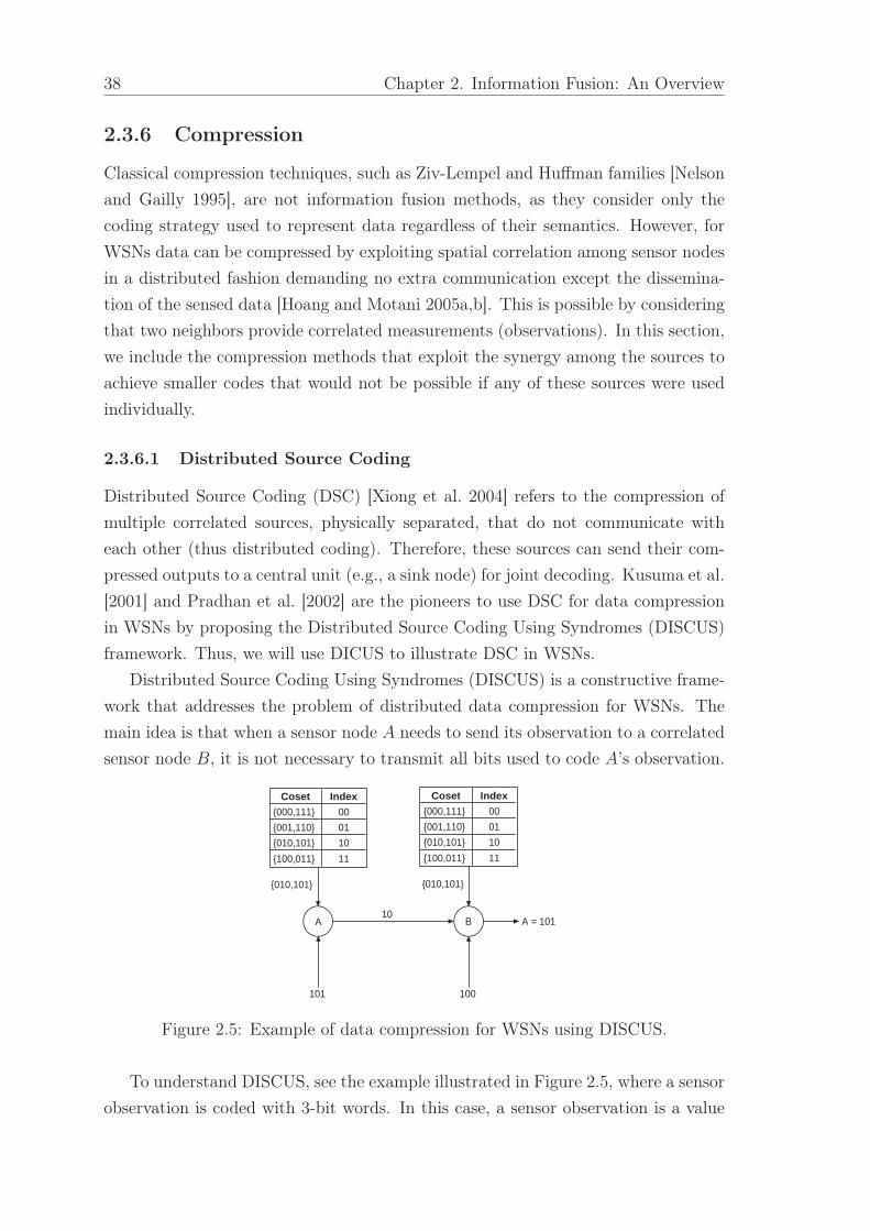
38 Chapter 2. Information Fusion: An Overview
2.3.6 Compression
Classical compression techniques, such as Ziv-Lempel and Huffman families [Nelson
and Gailly 1995], are not information fusion methods, as they consider only the
coding strategy used to represent data regardless of their semantics. However, for
WSNs data can be compressed by exploiting spatial correlation among sensor nodes
in a distributed fashion demanding no extra communication except the dissemina-
tion of the sensed data [Hoang and Motani 2005a,b]. This is possible by considering
that two neighbors provide correlated measurements (observations). In this section,
we include the compression methods that exploit the synergy among the sources to
achieve smaller codes that would not be possible if any of these sources were used
individually.
2.3.6.1 Distributed Source Coding
Distributed Source Coding (DSC) [Xiong et al. 2004] refers to the compression of
multiple correlated sources, physically separated, that do not communicate with
each other (thus distributed coding). Therefore, these sources can send their com-
pressed outputs to a central unit (e.g., a sink node) for joint decoding. Kusuma et al.
[2001] and Pradhan et al. [2002] are the pioneers to use DSC for data compression
in WSNs by proposing the Distributed Source Coding Using Syndromes (DISCUS)
framework. Thus, we will use DICUS to illustrate DSC in WSNs.
Distributed Source Coding Using Syndromes (DISCUS) is a constructive frame-
work that addresses the problem of distributed data compression for WSNs. The
main idea is that when a sensor node A needs to send its observation to a correlated
sensor node B, it is not necessary to transmit all bits used to code A’s observation.
A B
101
Coset Index
{000,111} 00
{001,110} 01
{010,101} 10
{100,011} 11
10
100
Coset Index
{000,111} 00
{001,110} 01
{010,101} 10
{100,011} 11
{010,101} {010,101}
A = 101
Figure 2.5: Example of data compression for WSNs using DISCUS.
To understand DISCUS, see the example illustrated in Figure 2.5, where a sensor
observation is coded with 3-bit words. In this case, a sensor observation is a value

2.3. Methods, Techniques, and Algorithms 39
in the set {000, 001, 010, 011, 100, 101, 110, 111}. Suppose that A and B are
equiprobable 3-bit words correlated, such that the Hamming distance1 between A
and B is at most one, i.e., the difference of A and B can be only one bit. Now
the possible values for an observation are grouped into four cosets such that the
Hamming distance among the elements of a coset is three: {000, 111}, {001, 110},
{010, 101}, {100, 011}. Node A can send only the index of the coset containing
its observation, and B can decode this index based on the fact that the Hamming
distance between its own observation and the one provided by A is at most one.
Thus, if A senses 101 it can send to B only the index (10) of the coset {010, 101}.
When B receives the index 10 from A, it accesses its own reading (100) and concludes
that, as the Hamming distance from its own observation and the one provided by
A is at most one, the value provided by A should be 101.
Details about the design and construction of DISCUSS are presented by Prad-
han and Ramchandran [2003]. Tang et al. [2003] propose a DSC scheme for data
compression based on a cost function that considers the energy necessary for en-
coding, transmitting, and decoding the bitstream being compressed. Marco and
Neuhoff [2004] study the impact of packet losses in compression schemes based on
DSC, and try to characterize the tradeoff between the compression rate and the
loss factor of such encoding schemes. Hua and Chen [2005] propose an improved
Viterbi algorithm [Forney 1973] (decoder algorithm) for DSC that takes advantage
of known parity bits at the decoder for error correction. Zhang and Wicker [2005]
provide a framework for the design and analysis of distributed, joint source and
network coding [Ahlswede et al. 2000] algorithms that optimize the tradeoff be-
tween compression efficiency and network robustness. Motivated by complexity of
such a problem, Ramamoorthy et al. [2006] investigate whether or not source cod-
ing can be separated from network coding, and conclude that, in general, such a
separation is not possible, but in the case of two sources and two receivers, a separa-
ble solution always exists. Complementarily, Barros and Servetto [2006] show that
separation holds in a fairly general network situation that allows only independent
point-to-point channels between pairs of nodes, and not multiple-access or broadcast
channels.
2.3.6.2 Coding by Ordering
Petrovic et al. [2003] propose a compression strategy called Coding by Ordering. In
this case, every node in a region of interest sends its data to one node in the region,
1The Hamming distance is the number of bits in two binary strings of equal length for which
the corresponding elements are different.
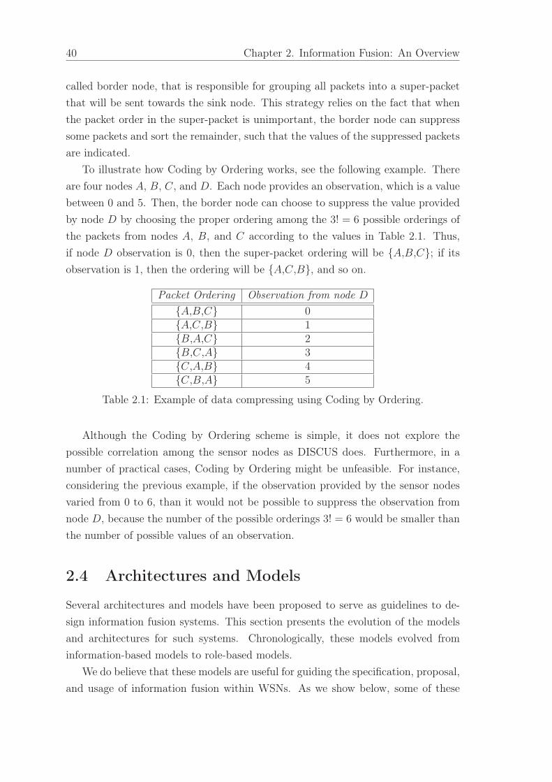
40 Chapter 2. Information Fusion: An Overview
called border node, that is responsible for grouping all packets into a super-packet
that will be sent towards the sink node. This strategy relies on the fact that when
the packet order in the super-packet is unimportant, the border node can suppress
some packets and sort the remainder, such that the values of the suppressed packets
are indicated.
To illustrate how Coding by Ordering works, see the following example. There
are four nodes A, B, C, and D. Each node provides an observation, which is a value
between 0 and 5. Then, the border node can choose to suppress the value provided
by node D by choosing the proper ordering among the 3! = 6 possible orderings of
the packets from nodes A, B, and C according to the values in Table 2.1. Thus,
if node D observation is 0, then the super-packet ordering will be {A,B,C}; if its
observation is 1, then the ordering will be {A,C,B}, and so on.
Packet Ordering Observation from node D
{A,B,C} 0{A,C,B} 1{B,A,C} 2{B,C,A} 3{C,A,B} 4{C,B,A} 5
Table 2.1: Example of data compressing using Coding by Ordering.
Although the Coding by Ordering scheme is simple, it does not explore the
possible correlation among the sensor nodes as DISCUS does. Furthermore, in a
number of practical cases, Coding by Ordering might be unfeasible. For instance,
considering the previous example, if the observation provided by the sensor nodes
varied from 0 to 6, than it would not be possible to suppress the observation from
node D, because the number of the possible orderings 3! = 6 would be smaller than
the number of possible values of an observation.
2.4 Architectures and Models
Several architectures and models have been proposed to serve as guidelines to de-
sign information fusion systems. This section presents the evolution of the models
and architectures for such systems. Chronologically, these models evolved from
information-based models to role-based models.
We do believe that these models are useful for guiding the specification, proposal,
and usage of information fusion within WSNs. As we show below, some of these

2.4. Architectures and Models 41
models, such as the JDL and Frankel-Bedworth, provide a systemic view of infor-
mation fusion, whereas others, such as the Intelligent Cycle and the Boyd Control
Loop, provide a task view of information fusion.
2.4.1 Information-Based Models
Models and architectures proposed to design information fusion systems can be cen-
tered on the abstraction of the data generated during fusion. This section discusses
the models that specify their stages based on the abstraction levels of information
manipulated by the fusion system.
2.4.1.1 JDL Model
JDL is a popular model in the fusion research community, being commented on
and revised in other references, such as Steinberg et al. [1999]. It was originally
proposed by the U.S. Joint Directors of Laboratories (JDL) and the U.S. Department
of Defense (DoD) [Kessler et al. 1992]. The model is composed of five processing
levels, an associated database, and an information bus connecting all components.
Its structure is depicted in Figure 2.6 and its components are described as follows:
Fusion Domain
Level 0
Source Pre-processing
Level 1
Object Refinement
Level 2
Situation Refinement
Level 3
Threat Refinement
Level 4
Process Refinement
Information Bus Human
Computer Interaction
Database Management System
Sources
Figure 2.6: The JDL model, figure from Hall and Llinas [1997].
Sources Sources are responsible for providing the input information and can be
sensors, a priori knowledge (e.g., reference and geographical information),
databases, or human input.
Database Management System This system supports the maintenance of the
data used and provided by the information fusion system. This is a critical
function as it supposedly handles a large and varied amount of data. In WSNs,
42 Chapter 2. Information Fusion: An Overview
this function might be simplified to fit the sensors’ restrictions of resources.
Central to this issue is the proposal of data-centric storage systems that allow
the network to efficiently answer queries without the need for directly querying
all sensor nodes. Such a system stores data by name into a node (or a set of
nodes) so that when the user (or another sensor node) needs data, it may
directly query the node storing that type of data [Ratnasamy et al. 2003; Li
et al. 2003a; Gummadi et al. 2005; Sheng et al. 2006; Ahn and Krishnamachari
2006].
Human Computer Interaction (HCI) HCI is a mechanism that allows human
input, such as commands and queries, and the notification of fusion results
through alarms, displays, graphics, and sounds. Commonly, human interac-
tion with WSNs occurs through the query-based interfaces such as the ones
used by the Cougar [Yao and Gehrke 2002], TiNA [Sharaf et al. 2003], and
TinyDB [Madden et al. 2005] projects.
Level 0 (Source Preprocessing) Also referred to as Process Alignment, this
level aims to reduce the processing load by allocating data to appropriate
processes and selecting appropriate sources. In WSNs, source selection is a
key issue for achieving intelligent resource usage while keeping the quality
of information fusion. In this context, Zhao et al. [2002a, 2003a] propose an
information-directed approach in which sources are chosen by dynamically op-
timizing the information utility of data for a given cost of communication and
computation.
Level 1 (Object Refinement) Object refinement transforms the data into a con-
sistent structure. Source localization, and therefore, all tracking algorithms
are in Level 1, since they transform different types of data, such as images,
angles, and acoustic data, into a target locations. Section 2.3.2 presents some
examples of tracking algorithms.
Level 2 (Situation Refinement) Situation refinement tries to provide a contex-
tual description of the relationship between objects and observed events. It
uses a priori knowledge and environmental information to identify a situation.
As an example, Chen et al. [2006a] observe the acoustic signals from birds and,
based on a predefined set of bird sound patterns, a contextual description of
the relationship between the collected acoustic signals and that pattern base
is provided, so we can infer the bird’s class.
2.4. Architectures and Models 43
Level 3 (Threat Refinement) Threat refinement evaluates the current situation
projecting it in the future to identify possible threats, vulnerabilities, and
opportunities for operations. This is a difficult task because it deals with
computation complexities and “enemies” intent assessment. The prediction
step of tracking algorithms are in Level 3. By identifying a target and predict-
ing its future location, we can identify whether or not it represents a threat.
Examples of tracking algorithms are discussed in Section 2.3.2.
Level 4 (Process Refinement) This is a meta-process2 responsible for monitor-
ing the system performance and allocating the sources according to the spec-
ified goals. This function may be outside the domain of specific data fusion
functions. Therefore, it is shown partially outside the data fusion process. A
WSN should be monitored continuously (e.g., by using the tools provided by
Zhao et al. [2003b]), collect management information (e.g., energy maps [Mini
et al. 2004]) and provide QoS (e.g., coverage [Meguerdichian et al. 2001a] and
exposure information [Megerian et al. 2002]) to support source allocation. For
instance, the SCAR routing algorithm [Mascolo and Musolesi 2006] uses re-
source information to choose the best node to forward a packet. Zhao et al.
[2003a] may also use resource information to select sources in a target tracking
application.
The JDL model was proposed for military research so its terminology and original
application is defense-oriented. Another drawback of the JDL model is that it does
not make explicit the interaction among the processing elements. Moreover, it
suppresses any feedback, i.e., it does not specify how current or past results of
fusion can be used to enhance future iterations.
The JDL model provides a systemic view of the network that performs infor-
mation fusion. Therefore, it guides the designer through the identification of the
major solutions to incorporate in the network. For instance, from the discussion
above, the project might include the TinyDB query system [Madden et al. 2005],
a target tracking algorithm with information-driven source selection [Zhao et al.
2003a], the GHT data-centric storage system [Ratnasamy et al. 2003] for efficient
data distribution, and an energy map [Mini et al. 2004] for resource management.
2.4.1.2 Dasarathy Model
The Dasarathy or DFD (Data-Feature-Decision) model [Dasarathy 1997] is a fine-
grained information centered model in which the elements of information fusion are
2A meta-process is a process that deals with and manipulates other processes.

44 Chapter 2. Information Fusion: An Overview
specified based on their inputs and outputs. Figure 2.7 depicts the DFD model.
The primary input is raw data and the main output is a decision. The components
responsible for the several fusion stages are the elements DAI-DAO, DAI-FEO, FEI-
FEO, FEI-DEO and DEI-DEO, described in Section 2.2.3.
Feature
Decision
Data
DAI - FEO
FEI - DEO
Decision DEI - DEO
Feature
Data DAI - DAO
FEI - FEO
Multilevel Fusion
Low Level Fusion
Intermediate Level Fusion
High Level Fusion
Figure 2.7: The DFD model.
The DFD model is successful in specifying the main types of fusion regarding
their input and output data. For this reason it is also used to classify information
fusion (see Section 2.2.3). Although it is not clear in Figure 2.7 how the architecture
handles quality improvement, the system performance is enhanced by the decision
blocks that use the system’s feedback to tune its decision ability.
As Wald [1999] highlights, the input and output of a fusion process can be of
any level (data, feature, decision). Therefore, the DFD model is limited in the sense
that Dasarathy’s functional blocks should be combined to provide more complex
fusion blocks. For example, to provide a block that fuses a feature with two signals
to obtain a refined feature, the signals should be fused by a DAI-FEO (Data In –
Feature Out) block, then its output should be fused with the given feature by a
FEI-FEO (Feature In – Feature Out) block.
In contrast to the JDL model, the DFD model does not provide a systemic
view, instead it provides a fine-grained way to specify fusion tasks by means of the
expected input and output data. Therefore, the DFD model is useful for specifying
and designing fusion algorithms in WSNs with different purposes such as ambient
noise estimation [Polastre et al. 2004] (DAI-DAO), feature map building [Singh
et al. 2006] (FEI-FEO), event detection [Luo et al. 2006] (DEI-FEO), and failure
detection [Nakamura et al. 2005d] (FEI-FEO).
2.4.1.3 Some Remarks on the Information-Based Models
Information-based models represent the first generation of models for information
fusion, which focuses on the abstraction level of the information handled by the

2.4. Architectures and Models 45
fusion tasks. In general, a limitation of such models is that they do not specify the
execution sequence of the fusion tasks. Historically, the JDL model represents the
first serious effort to provide a detailed model and a common terminology for the
fusion domain. However, as it was born of military applications, the terminology
adopted is threat-oriented.
The DFD model is possibly the most mature representative of these models.
It is a fine-grained model that makes explicit the abstraction level of both input
and output information of each fusion task. The DFD model differs from the JDL
in the terminology adopted and in the approach used in the model. The JDL is
oriented to military applications and the fusion tasks identified in the model reflect
the peculiarities of such an application domain. On the other hand, the DFD model
is oriented to the input and output of a fusion task regardless of the application
domain. As a consequence, the specified functional blocks are “purely” focused on
the fusion domain no matter the application. A key difference between the JDL
and the DFD models is that the former provides a system-oriented perspective
of information fusion — which is suitable for designing systems that incorporate
fusion tasks —, whereas the latter provides an input-output-oriented perspective of
information fusion — which is suitable for understanding the relationship among
fusion tasks and the manipulated data.
Within the WSN domain, these models can be used to facilitate understanding
of the requirements and limitations introduced by fusion techniques. Although such
models do not specify the network aspects (distributed nature) of WSNs, they work
as a guide to specify which methods can be used and how they can be integrated
with a given application.
2.4.2 Activity-Based Models
Some models are specified based on the activities that must be performed by an
information fusion system. In such models, the activities and their correct sequence
of execution are explicitly specified.
2.4.2.1 Boyd Control Loop
The Boyd Control Loop or OODA (Observe, Orient, Decide, Act) Loop [Boyd 1987]
is a cyclic model composed of four stages (Figure 2.8). According to Bass [2000]
this model is a representation of the classic decision-support mechanism of military
information systems, and because such systems are strongly coupled with fusion
systems, the OODA loop has been used to design information fusion systems. The
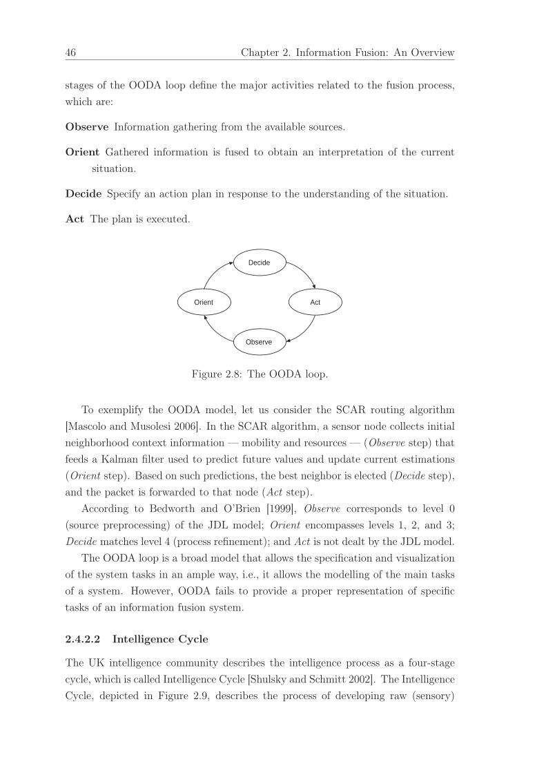
46 Chapter 2. Information Fusion: An Overview
stages of the OODA loop define the major activities related to the fusion process,
which are:
Observe Information gathering from the available sources.
Orient Gathered information is fused to obtain an interpretation of the current
situation.
Decide Specify an action plan in response to the understanding of the situation.
Act The plan is executed.
Decide
Orient
Observe
Act
Figure 2.8: The OODA loop.
To exemplify the OODA model, let us consider the SCAR routing algorithm
[Mascolo and Musolesi 2006]. In the SCAR algorithm, a sensor node collects initial
neighborhood context information — mobility and resources — (Observe step) that
feeds a Kalman filter used to predict future values and update current estimations
(Orient step). Based on such predictions, the best neighbor is elected (Decide step),
and the packet is forwarded to that node (Act step).
According to Bedworth and O’Brien [1999], Observe corresponds to level 0
(source preprocessing) of the JDL model; Orient encompasses levels 1, 2, and 3;
Decide matches level 4 (process refinement); and Act is not dealt by the JDL model.
The OODA loop is a broad model that allows the specification and visualization
of the system tasks in an ample way, i.e., it allows the modelling of the main tasks
of a system. However, OODA fails to provide a proper representation of specific
tasks of an information fusion system.
2.4.2.2 Intelligence Cycle
The UK intelligence community describes the intelligence process as a four-stage
cycle, which is called Intelligence Cycle [Shulsky and Schmitt 2002]. The Intelligence
Cycle, depicted in Figure 2.9, describes the process of developing raw (sensory)

2.4. Architectures and Models 47
information into finished intelligence used in decision-making and action. The stages
(activities) of the Intelligence Cycle are:
Collection Raw information is collected from the environment.
Collation Collected information is analyzed, compared, and correlated. Irrelevant
and unreliable information is discarded.
Evaluation Collated information is fused and analyzed.
Dissemination Fusion results are delivered to users who utilize the fused informa-
tion to produce decisions and actions in response to the detected situation.
Collection
Dissemination
Evaluation
Collation
Figure 2.9: The Intelligence Cycle.
All tracking algorithms previously mentioned can be used to depict the Intelli-
gence Cycle. For instance, Li et al. [2006] propose a source localization algorithm
for a system equipped with asynchronous sensors wherein range data is collected
(Collection step) and selected (Collation step). Then, the UKF is applied to esti-
mate and predict the targets’ locations (Evaluation step) that can be used to guide
surveillance decisions (Dissemination step).
In comparison to the JDL model, Collection matches level 0 of the JDL model;
Collation includes level 1; Evaluation comprises levels 2 and 3; and Dissemination
corresponds to level 4 of the JDL model. Unlike the OODA model, the Intelligence
Cycle does not make explicit the planning (Decide) and the execution (Act) phases,
which are presumably included in the Evaluation and Dissemination phases. Again,
this model does not to represent the specific tasks of an information fusion system.
2.4.2.3 Some Remarks on Activity-Based Models
The first two activity-based models (OODA and Intelligence Cycle) are general and
can be employed in any application domain. As a result, they do not fulfill the

48 Chapter 2. Information Fusion: An Overview
specific aspects of the fusion domain demanding, thus, experience and expertise to
model fine-grained fusion tasks.
2.4.3 Role-Based Models
Role-based models represent a change of focus on how information fusion systems
can be modelled and designed. In such models, information fusion systems are spec-
ified based on the fusion roles and the relationships among them providing a more
fine-grained model for the fusion system. The two members of this generation are
the Object-Oriented Model [Kokar et al. 2000] and the Frankel-Bedworth Archi-
tecture [Frankel and Bedworth 2000]. Like the JDL model, the role-based models
herein also provide a systemic view of information fusion. However, in contrast
to the previous models, role-based models do not specify fusion tasks or activities.
Instead, they provide a set of roles and specify the relationships among them.
2.4.3.1 Object-Oriented Model
Kokar et al. [2000] propose an object-oriented model for information fusion systems.
This model also uses cyclic architecture. However, unlike the previous models,
it does not specify fusion tasks or activities. Instead, the Object-oriented model
provides a set of roles and specifies the relationship among them. Figure 2.10 is a
simplification of the object-oriented model provided by Kokar et al. [2000] in which
four roles are identified:
Actor Responsible for the interaction with the world, collecting information and
acting on the environment.
Perceiver Once information is gathered, the perceiver assesses such information
providing a contextualized analysis to the director.
Director Based on the analysis provided by the perceiver, the director builds an
action plan specifying the system’s goals.
Manager The manager controls the actors to execute the plans formulated by the
director.
From the realization perspective (role of the objects), human and computer ob-
jects are not distinct. For this reason, the Object-Oriented model will not likely
be directly mapped onto actual system implementations based on object-oriented
programming languages. Nonetheless, it deserves this brief discussion, for it is an
intermediate model towards the Frankel-Bedworth architecture [Frankel and Bed-
worth 2000] that we discuss below.

2.4. Architectures and Models 49
+evaluateInformation()+provideContext()
Perceiver
+executeThePlan()
Manager
+actuate()+sense()
Actor
+buildAnActionPlan()+provideGoals()
Director
inform
1
1..*
feed
1..*
1
manage
1..*
1
provide a plan1
1..*
Figure 2.10: The Object-Oriented model for information fusion, figure adaptedfrom Kokar et al. [2000].
2.4.3.2 Frankel-Bedworth Architecture
Frankel [1999] describes an architecture for human fusion composed of two self-
regulatory processes: local and global. The local estimation process manages the
execution of the current activities based on goals and timetables provided by the
global process. The global process updates the goals and timetables according to
the feedback provided by the local process. Frankel’s architecture is then trans-
ported to a machine fusion architecture that separates control and estimation, goal-
setting and goal-achieving behaviors. This model is called Frankel-Bedworth archi-
tecture [Frankel and Bedworth 2000] and is depicted in Figure 2.11.
The local and global processes have different objectives and, consequently, dif-
ferent roles. The local process tries to achieve the specified goals and maintain the
specified standards. Thus the local process has the Estimator role, which is similar
to the previous fusion models and includes the following tasks:
Sense Raw information is gathered by the information sources.
Perceive Stimuli retrieved by sensing are dealt according to its relevance (focus),
and the Controller is informed which stimuli are being used (awareness).
Direct Based on the comprehension of the perception (semantics) the Estimator
can provide a feedback (alert) to the Controller. The disparity between current
situation and desired situation is evaluated. Then, the Estimator is fed forward
with desires that specify new goals and timetables.
Manage Based on the objectives, the Controller is activated to define what is practi-
cal (pragmatics) so the Estimator can provide an appropriate response. Then,

50 Chapter 2. Information Fusion: An Overview
the Estimator provides a feedback to the Controller by reporting the expecta-
tions about the provided decision (sensitivity).
Effect Selected decisions (responses) are applied and the control loop is closed by
sensing the changes in the environment.
effect
sensestimuli
focus
desires
pragmatics
expectations
alert
awareness
prediction
prioritiessemantics
objectives
responses
Estimator Controller
perceive
direct
manage
environment
orient
prefer
expect
Figure 2.11: The Frankel-Bedworth architecture, figure adapted from Frankel andBedworth [2000].
Global control process manages the goals and the performance of the system
during the execution of the local process. Thus, the global process has the Con-
troller role, which is responsible for controlling and managing the Estimator role
and includes the following tasks:
Orient The importance or relevance of sensed stimuli is configured.
Prefer Priority is given to the aspects that are most relevant to the goal-achieving
behavior, detailing the local goals (desires).
Expect Predictions are made and the intentional objectives are filtered, determin-
ing what is practical to the Estimator pragmatics.
The Frankel-Bedworth architecture introduces the notion of a global process
separated from the local process. The global control process rules the local pro-
cess by controlling and defining its goals and monitoring its performance. On the
other hand, the local process is supposed to implement and perform fusion methods
and algorithms to accomplish the system’s objectives. This architecture extends
the previous models that were concerned only with the local process aspects. How-
ever, further discussions on how to effectively use this architecture to design and
implement real information fusion systems are still desirable.
In real WSNs, the global control process will most likely be performed by hu-
man beings who feed the network with operation guidelines (priorities, desires, and
2.5. Information Fusion and Data Communication 51
pragmatics), whereas the local estimation process should be implemented within the
computational system (sensor nodes and integrated systems). In this context, when-
ever necessary, the global process can feed the local process through interest dissem-
ination by using, for instance, the Directed Diffusion communication paradigm [In-
tanagonwiwat et al. 2003] or a query interface such as the TinyDB [Madden et al.
2005].
For the sake of illustration, let us consider a combined application of environ-
mental data gathering and target tracking. The Sense task is performed by sensor
units that provide observations, which are selected by the Perceive task according to
the focus. For instance, when a target is being detected, environmental data, such
as temperature, may be discarded since trajectory information is more relevant in
this case. During the Direct task, if the local process (Estimator) detects that the
target is not a threat, it should alert the global process (Controller), which can ask
again for low rate environmental data (new desires). Based on the new objective,
the local process may change routes and notification rates in the Manage task that
is implemented by the sensor nodes (Effect task). Among other things, the global
process can be used to: (i) specify an aggregation algorithm [Madden et al. 2002;
Boulis et al. 2003a; Hellerstein et al. 2003] depending on current objectives (e.g.,
energy savings or data quality); (ii) reconfigure parameters of fusion algorithms such
as the window size of moving average filters [Nakamura et al. 2005b] and the num-
ber of samples of particle filters [Sheng et al. 2005]; and (iii) select the best routing
strategy based on the data generation profile [Figueiredo et al. 2004, 2007].
2.4.3.3 Some Remarks on Role-Based Models
Role-based models are fine-grained models that specify the actors and their roles
in the fusion task. These models represent the evolved maturity level in the fu-
sion domain. Although these models provide a better understanding of the fusion
task, they do not explicitly consider the particularities of the WSNs (so do the
information-based and activity-based models).
2.5 Information Fusion and Data Communication
In WSNs, information fusion is closely related to data communication. The reason is
that due to the limited power sources of current sensor nodes, it is usually desirable
to take advantage of the limited computation capacity of sensor nodes to perform
in-network fusion and reduce the overall data traffic (see Section 2.1.2). Thus, in
52 Chapter 2. Information Fusion: An Overview
this section we discuss some relevant aspects regarding the relationship between
information fusion and data communication.
2.5.1 Distributed-Computing Paradigms
Different distributed-computing paradigms have been adopted in WSNs, and de-
pending on the chosen paradigm, information fusion occurs in different ways. In
this section, we discuss the use of information fusion within different distributed-
computing paradigms, namely the In-Network Aggregation, Client-Server, Active
Networks, and Mobile Agents paradigms.
2.5.1.1 In-Network Aggregation
The In-Network Aggregation is the most popular distributed-computing paradigm
in WSNs. The idea is to take advantage of the node computation capacity and
perform the desired fusion algorithm while data is routed towards the sink node.
For that reason, this paradigm is also referred to as Data-Centric Routing. Finding
an optimal routing tree, connecting sources to sinks, is shown to be an NP-complete
problem [Krishnamachari et al. 2002]. The Directed Diffusion solution [Intanagonwi-
wat et al. 2000, 2003] is the pioneer work for using the publish-subscribe approach
with in-network data aggregation in WSNs. A key feature of Directed Diffusion is
that events are sent and arrive asynchronously, and when they arrive at a node,
they trigger callbacks to relevant applications (subscribers), thus performing the
in-network data processing. These applications are the ones that implement and
execute the desired information fusion algorithms. In this solution, the details of
how published data are delivered to subscribers depend on the implementation of
the so called filters, which are actually the routing and fusion algorithms.
Depending on the network organization, in-network aggregation may occur in
different ways, which basically depends on the routing strategy. In flat networks,
every node is functionally the same and data are routed in a multihop fashion
since not every node directly reaches the sink. Thus, information fusion should
be executed by every node that takes part of routing process, and all fusion algo-
rithms must be implemented by every node. Examples of multihop communication
with in-network aggregation include the Directed Diffusion family of algorithms [In-
tanagonwiwat et al. 2003; Heidemann et al. 2003] and tree-based routing algorithms
[Sohrabi et al. 2000; Krishnamachari et al. 2002; Zhou and Krishnamachari 2003].
In hierarchical networks, we usually have a two-hop communication. One hop for
the cluster members to reach the cluster-head, and another hop for cluster-heads to
reach the sink node. In this type of communication, information fusion is performed

2.5. Information Fusion and Data Communication 53
by cluster-heads that send the results to the sink. The first hierarchical solution for
WSNs was the LEACH [Heinzelman et al. 2000], but several others have been pro-
posed ever since [Halgamuge et al. 2003; Kochhal et al. 2003; Mhatre and Rosenberg
2004; Hoang and Motani 2005a; Gupta et al. 2005]. In a hybrid solution, we might
have multiple hops connecting source nodes to their cluster-head and/or multiple
hops connecting cluster-heads to the sink. Thus, in such a scenario we may combine
the flat and hierarchical in-network aggregation. The strategy we propose in Chap-
ter 4 illustrates a routing algorithm for hybrid networks performing in-network data
aggregation.
2.5.1.2 Client-Server
The traditional client-server model, as we have in the Internet, demands the knowl-
edge, at every node, of the existence of the communicating nodes (servers) along
with their addresses. In WSNs, however, we can relax this restriction into a data-
centric approach wherein instead of knowing the nodes’ addresses we need only to
know data names (e.g., temperature and movement). In this context, data-centric
storage systems may be seen as a data-centric-client-server variant in the sense that,
in such systems, data are stored by name into a node or a set of nodes (data servers),
and when a user or another sensor node (data client) searches for a specific data,
it may directly query the node storing that type of data [Ratnasamy et al. 2003;
Li et al. 2003a; Gummadi et al. 2005; Sheng et al. 2006; Ahn and Krishnamachari
2006]. In addition, instead of knowing nodes’ addresses we only have to know data
names. From the fusion perspective, nodes storing data may answer the query by
performing the desired fusion algorithm before (especially aggregation functions)
and forwarding only the result. When the fusion algorithm requires different types
of data from different data servers, we can combine the Client-Server and the In-
Network Data Aggregation paradigms so that information fusion is also performed
along the routing path. A less interesting approach of the client-server paradigm
occurs when sensor nodes (fusion clients) send their data to the sink (fusion server)
and data fusion is executed. Xu and Qi [2004] show that this last approach is only
interesting when we have few sources and small-scale networks.
2.5.1.3 Active Networks
Active networks allow the injection of customized programs into the network
nodes [Psounis 1999]. Accordingly, this paradigm allows high complexity and cus-
tomizable computations to be performed within the network. In this case, informa-
tion fusion may travel in the network as active packets, allowing different methods

54 Chapter 2. Information Fusion: An Overview
and applications (even unpredicted ones) to be executed at different moments, in-
stead of storing every possible fusion algorithm into the nodes. Particularly, the
Maté [Levis and Culler 2002] and the SensorWare [Boulis et al. 2003b] frameworks
were proposed to implement the Active Networks paradigm into sensor networks.
This paradigm is especially interesting for at least two scenarios: (i) when we cannot
predict the application’s behavior (e.g., an exploratory WSN deployed in Mars); and
(ii) when we need to design long-lived networks whose applications may need to be
remotely changed.
2.5.1.4 Mobile Agents
Mobile agents are programs that can migrate from node to node in a network, at
times and to places of their own choosing. The state of the running program is
saved, sent to the new node and restored, so the program can continue from the
point it stopped [Kotz and Gray 1999]. Xu and Qi [2004] evaluate the use of mobile
agents to perform information fusion in WSNs and show that, in contrast to the
client-server model, this paradigm saves the network bandwidth and provides an
effective way to overcome network latency when the number of nodes is large, which
should often be the case. Similar conclusions were related by Qi et al. [2002] who
took an example of target classification to describe the design and implementation of
the mobile-agent-based distributed sensor network and illustrate the efficiency of the
Mobile Agents paradigm. The order that nodes are visited in a WSN by the agent
along the route affects the quality and cost of the fused data. In fact, computing a
route for a mobile agent that fuses data as it visits nodes is NP-complete [Wu et al.
2004]. Wu et al. [2004] present an optimization formulation and a genetic algorithm
for statically (off-line) finding the best route for an information fusion mobile agent
executing a target tracking function.
2.5.2 Information Fusion and Data Communication
Protocols
Regarding the relationship of information fusion and data communication protocols
in WSNs, information fusion can play a supporting role or a leading role. In the
former, we have information fusion acting as a tool to assist the communication
protocol establishment, whereas in the latter, the communication protocols are de-
signed to support an information fusion application (e.g., data aggregation target
tracking).
2.5. Information Fusion and Data Communication 55
2.5.2.1 Information Fusion as a Supporting Role
All tasks demanding any sort of parameter estimation can benefit from the meth-
ods discussed in Section 2.3.2. Similarly, every inference-based decision may use the
techniques presented in Section 2.3.1. Currently, information fusion has started to
be used as a supporting role to assist communication protocols but its potential is
far from being fully explored.
MAC protocols are the ones that have used information fusion techniques more
intensively. Fuzzy logic is used by Wallace et al. [2005] and Liang and Ren [2005b]
to define nodes’ duty cycle in the MAC layer. Particularly, Wallace et al. [2005] pro-
pose a fuzzy-based approach that — based on nodes’ transmit-queue size, residual
energy, and collision rate — defines the nodes’ duty cycle so that nodes with high
transmit queue have priority to access the medium. Moving average filters have
been used by MAC protocols with different purposes such as: estimating ambient
noise to determine whether the channel is clear [Polastre et al. 2004]; local clock
synchronization for contention purposes [Rhee et al. 2005]; and detecting incipient
congestion for fair and efficient rate control [Rangwala et al. 2006]. Kalman filters
have been used to predict the frame size avoiding the transmission of large frames
whenever possible [Ci et al. 2004; Raviraj et al. 2005; Ci and Sharif 2005].
We can also point out some routing solutions that use information fusion search-
ing for an improved performance. Fuzzy logic has been used to decide the nodes
participating in the routing path [Liang and Ren 2005a; Srinivasan et al. 2006].
More specifically, aiming at improving the network lifetime, Liang and Ren [2005a]
use fuzzy logic to evaluate different parameters — such as battery capacity, mobility,
and distance to the destination — and choose the nodes to be included in the routing
path. Woo et al. [2003] use moving average filters within adaptive link estimators so
that link connectivity statistics are exploited by routing protocols to reduce packet
losses. Nakamura et al. [2005d] use the moving average filter to estimate the data
traffic of continuous WSNs, and that estimate is further used to detect routing-
failure by means of the Dempster-Shafer inference. The SCAR algorithm [Mascolo
and Musolesi 2006] uses the Kalman filter to predict context information (mobility
and resources) about its neighbors, and choose the best neighbor for routing its
data. Hartl and Li [2004] use maximum likelihood to estimate per-node loss rates
during the aggregation and reporting of data from sources to sink nodes, which can
be used to bypass lossy areas.
Localized algorithms, wherein nodes make decisions based on neighbors’ infor-
mation (e.g., link quality, residual energy, connectivity, and mobility), can take

56 Chapter 2. Information Fusion: An Overview
advantage of dual prediction schemes to reduce communication. In this scheme, two
neighbor nodes simultaneously apply a predictive estimator (e.g., the Kalman filter)
so that a node only exchanges data when it knows its parameters are not being
correctly predicted by its neighbor. Furthermore, besides using information fusion
methods to estimate parameters, such as residual energy, inference techniques can
also be used to make decisions. For instance, MAC protocols may use Bayesian
inference or neural networks to accurately decide whether or not it is worth trying
to transmit data given the current link quality, resources, and QoS requirements.
To determine whether or not the applicability of fusion methods in such situations
is feasible, we must evaluate the computational cost of the fusion algorithms, the
resultant delay, the energy consumed, and the impact on the quality of the service
provided by communication protocol.
2.5.2.2 Information Fusion as a Leading Role
In many cases, we cannot distinguish information fusion algorithms from the appli-
cation, in the sense that, to accomplish the application objectives we execute one or
multiple information fusion algorithms. For instance, target tracking is essentially
the application of information fusion algorithms such as Kalman or particle filters;
an event detection is essentially an inference task that may use an information fusion
technique such as Bayesian or Dempster-Shafer inference. When information fusion
plays such a leading role (application) in the network, the way communication is
established may affect the results regarding data quality and energy consumption.
In the following, we discuss a few solutions that were proposed aiming at optimizing
the performance of specific information fusion applications.
Having in mind the different applications, the Directed Diffusion paradigm [In-
tanagonwiwat et al. 2003] provides a communication framework wherein virtually
any information fusion application can be implemented by using filters. These fil-
ters are special components responsible for guiding the routing process and the fu-
sion processes simultaneously. In order to improve the detection ability of a WSN,
Kochhal et al. [2003] propose a role-based clustering algorithm, which considers the
sensing ability of the nodes, that organizes the network by recursively finding con-
nected dominating sets. Those sets are used to define coordinators (cluster-heads),
routing nodes, and the remaining nodes become sensing collaborators (sources).
In data aggregation applications, a sink node is interesting in collecting aggre-
gated data from a subset of nodes. In this context, data communication should use
as few nodes and resources as possible to ensure the delivery and aggregation of
data generated by source nodes. This is essentially an NP-complete problem similar

2.5. Information Fusion and Data Communication 57
to the Steiner tree and some heuristics have been proposed for that problem. Three
heuristics are evaluated by Krishnamachari et al. [2002], which are the centered-at-
nearest-source tree (CNS), the shortest-path tree (SPT) and the greedy incremental
tree (GIT). In the CNS, each source sends its data directly to the source closest
to the sink; in the SPT, each source sends its data to the sink along the shortest
path between both nodes; and in the GIT, the routing tree starts with the short-
est path between the sink and the nearest source, and at each step after that, the
source closest to the current tree is included in the tree. As Krishnamachari et al.
[2002] show, the GIT heuristic is the best of the three. However, its distributed
version [Bauer and Varma 1996] demands a lot of communication and memory us-
age, because every node needs to know its shortest paths to every other node in the
network. Motivated by that unfeasible cost, we propose, in Chapter 4, the InFRA
heuristic that finds the shortest paths that maximize data aggregation, and has
an O(1)-approximation ratio. Zhu et al. [2005] present a heuristic, called Seman-
tic/Spatial Correlation-aware Tree (SCT), that is constructed during the course of
a query delivery. The SCT builds a fixed aggregation backbone that simplifies the
generation of efficient aggregation trees, and is independent of source distribution
and density. However, in contrast to the InFRA heuristics (see Chapter 4), the SCT
needs to be pro-actively rebuilt, leading to energy waste. For the same problem,
Ding et al. [2003] propose a tree-based routing algorithm based on nodes’ residual
energy, so that nodes with more energy are likely to perform data aggregation and
routing. Once the tree is built, leaf nodes are turned-off to save energy, but no
approximation ratio is provided for this heuristic.
Another approach to the aforementioned problem is the use of role assignment
algorithms to define which nodes are to be used and what actions those nodes
should take. Bhardwaj and Chandakasan [2002] derive upper bounds on the lifetime
of WSNs that perform information fusion by assigning roles (sensor, relay, and
aggregator), and model the optimal role assignment as a linear problem that finds
the assignment that maximizes the network lifetime. By computing a user-defined
cost function, Bonfils and Bonnet [2003] propose an adaptive and decentralized
solution that progressively refines the role assignment. The SPRING algorithm
[Dasgupta et al. 2003], for mobile sensor networks, defines two roles (sensor and
relay/aggregator) and places nodes and assigns roles to them so the system’s lifetime
is maximized and the region of interest is covered by at least one sensor node. In
the DFuse framework [Kumar et al. 2003], role assignment is provided by a heuristic
in which a tree with a naive role assignment is created, then, nodes exchange health
information and the role is transferred to the neighbor with the best health regarding
a given cost function. Frank and Römer [2005] propose a basic structure of a generic

58 Chapter 2. Information Fusion: An Overview
role assignment framework with applications for coverage, clustering, and in-network
aggregation. Similarly to the filter approach of Directed Diffusion, the network
designer should specify roles and assignment rules.
When we have information fusion as a leading role, source selection and route
selections are problems of major concern. Taking target tracking applications based
on particle filters as an example, selecting good particles (samples) for estimating a
target’s trajectory is challenging because the fewer particles the cheaper the compu-
tation. In this context, Zhao et al. [2002a, 2003a] propose an information-directed
approach in which sources (and communicating nodes) are chosen by dynamically
optimizing the information utility of data for a given cost of communication and
computation.
Chen et al. [2006c] propose the Energy-Efficient Protocol for Aggregator Selec-
tion (EPAS) for selecting nodes that perform information fusion. The authors derive
the optimal number of aggregators, and present fully distributed algorithms for the
aggregator selection. A key contribution is that these algorithms are independent
of routing protocols. Chen et al. [2006b] use a cluster-based communication archi-
tecture, based on the LEACH [Heinzelman et al. 2000], wherein data aggregation
runs parallel to the cluster-heads, improving the energy efficiency via meta-data
negotiation. In addition, for each event and each cluster, only one of the cluster
members is selected to send data to the cluster-head. Zhou et al. [2004] use the Di-
rected Diffusion to provide a hierarchical aggregation scheme for WSNs to improve
reliability and provide more applicable data aggregation.
2.6 Chapter Remarks
This chapter presents the background necessary to answer some questions about
information fusion, such as: (1) what is information fusion?, (2) why should a de-
signer use it?, (3) what are the available techniques?, and (4) how should a designer
use such techniques? In simple words, the answers are:
1. Information fusion is the set of resources used to combine multiple sources
such that the result is, in some sense, better than the individual inputs.
2. Information fusion should be used to improve the performance of a task by
understanding the current situation and supporting decisions.
3. The techniques include filters, Bayesian and Dempster-Shafer inference, aggre-
gation functions, interval combination functions, and data compression meth-
ods.

2.6. Chapter Remarks 59
4. The use of the fusion techniques should be guided by architectures and models,
such as the JDL model.
The provided background supports the design of fusion-based solutions for differ-
ent levels of applications in a WSN, such as internal tasks (e.g., data routing) and
system applications (e.g., target detection). However, there are some limitations
regarding the methods and the architectures that should be considered.
Depending on the adopted model, some of the listed methods might be too
expensive to be executed by current sensor nodes. For example, in the Dempster-
Shafer inference, the combination rule has exponential cost regarding the number
of states in the frame of discernment. Thus, if two logically different states are
functionally the same, from the application perspective, they should be modelled as
a single state for the sake of performance.
Other methods might be improved to operate in a distributed fashion. One of
the great challenges is to assure the temporal and spatial correlation among the
sources while the data is fused and disseminated at the same time.
Current fusion architectures are weak in considering WSNs particularities, being
the main reason that they are not network-driven. However, we understand that
such architectures may be applied within specific models for WSNs, i.e., the whole
network is designed based on a global architecture for WSNs; then, the fusion task
can be designed based on a fusion model, respecting the requirements established
by the global architecture.
In the next chapters, we explore the two views discussed in Section 2.5.2.1
and Section 2.5.2.2, respectively. Particularly, in the next chapter, we propose an
information-fusion framework that encompasses general fusion steps, which we have
extracted from the architectures in Section 2.4, and some of the fusion algorithms
that we discussed in Section 2.3. Then, by using information fusion as a supporting
role, we apply this framework to provide reliability in tree-based routing protocols
for continuous WSNs. Having in mind an information-fusion application (informa-
tion fusion as a leading role), in Chapter 4, we design a routing strategy to improve
the performance of that application.


“By far the best proof is experience.”
Sir Francis Bacon (1561 – 1626)
3Diffuse: An Information Fusion
Framework for Sensor Networks
In this chapter, we propose an information fusion framework, called Dif-
fuse, that is sufficiently generic to design different applications, such as event
detection, target tracking, and in-network query processing. However, Diffuse
can also be used to design different tasks that use information fusion as a supporting
role. Although the Diffuse applicability is ample, as a proof of concept, we use it
to provide a fault-tolerant routing tree. In particular, we use information fusion to
determine the moment when the routing topology of a WSN needs to be rebuilt.
Our solution is based on the data traffic that is pre-processed with a tunable Mov-
ing Average Filter and translated into evidences that indicate failure probabilities.
These evidences are combined by using the Dempster-Shafer Theory to determine
when the topology needs to be rebuilt. We provide theoretical bounds for our pro-
posed solution that is evaluated through simulation. Our experiments show that, in
some cases, our solution can reduce the control traffic by a scale factor of 9.
The solutions presented in this chapter are partially published in the
SBRC’05 [Nakamura et al. 2005c] and ICN’05 [Nakamura et al. 2005b] conferences,
as well as in the Telecommunication Systems journal [Nakamura et al. 2005d].
The chapter is organized as follows. Section 3.1 presents the related work about
tree topologies for multihop routing and failure detection for WSNs. Section 3.2 pro-
vides an overview of the Diffuse framework, which is the building block we propose
to detect the need for topology reconstructions. In Section 3.3, we show how we use
61
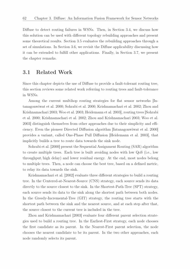
62 Chapter 3. Diffuse: An Information Fusion Framework for Sensor Networks
Diffuse to detect routing failures in WSNs. Then, in Section 3.4, we discuss how
this solution can be used with different topology rebuilding approaches and present
some theoretical results. Section 3.5 evaluates the rebuilding approaches through a
set of simulations. In Section 3.6, we revisit the Diffuse applicability discussing how
it can be extended to fulfill other applications. Finally, in Section 3.7, we present
the chapter remarks.
3.1 Related Work
Since this chapter depicts the use of Diffuse to provide a fault-tolerant routing tree,
this section reviews some related work referring to routing trees and fault-tolerance
in WSNs.
Among the current multihop routing strategies for flat sensor networks [In-
tanagonwiwat et al. 2000; Sohrabi et al. 2000; Krishnamachari et al. 2002; Zhou and
Krishnamachari 2003; Woo et al. 2003; Heidemann et al. 2003], routing trees [Sohrabi
et al. 2000; Krishnamachari et al. 2002; Zhou and Krishnamachari 2003; Woo et al.
2003] distinguish themselves from other approaches due to their simplicity and effi-
ciency. Even the pioneer Directed Diffusion algorithm [Intanagonwiwat et al. 2000]
provides a variant, called One-Phase Pull Diffusion [Heidemann et al. 2003], that
implicitly builds a tree to route data towards the sink node.
Sohrabi et al. [2000] present the Sequential Assignment Routing (SAR) algorithm
to create multiple trees. Each tree is built avoiding nodes with low QoS (i.e., low
throughput/high delay) and lower residual energy. At the end, most nodes belong
to multiple trees. Then, a node can choose the best tree, based on a defined metric,
to relay its data towards the sink.
Krishnamachari et al. [2002] evaluate three different strategies to build a routing
tree. In the Centered-at-Nearest-Source (CNS) strategy, each source sends its data
directly to the source closest to the sink. In the Shortest-Path-Tree (SPT) strategy,
each source sends its data to the sink along the shortest path between both nodes.
In the Greedy-Incremental-Tree (GIT) strategy, the routing tree starts with the
shortest path between the sink and the nearest source, and at each step after that,
the source closest to the current tree is included in the tree.
Zhou and Krishnamachari [2003] evaluate four different parent selection strate-
gies used to build a routing tree. In the Earliest-First strategy, each node chooses
the first candidate as its parent. In the Nearest-First parent selection, the node
chooses the nearest candidate to be its parent. In the two other approaches, each
node randomly selects its parent.

3.1. Related Work 63
One-Phase Pull Diffusion [Heidemann et al. 2003] is a variant of the Directed
Diffusion algorithm [Intanagonwiwat et al. 2000] that builds a routing tree. In this
algorithm, there is no exploratory data. The sink node simply disseminates its
interests, and the source nodes send their data to the neighbors that first sent the
interest. The resulting routing tree is equivalent to the Earliest-First strategy [Zhou
and Krishnamachari 2003].
Woo et al. [2003] show that the asymmetric and lossy nature of the wireless links
impacts on the success rate of the routing tree. As a turnaround, they suggest the
collection and exploitation of connectivity statistics to estimate the link quality and
achieve reliability.
In a tree topology, when a routing node fails, all of its children nodes stop deliv-
ering data. A solution is to rebuild the routing topology such that the disconnected
nodes are reconnected, if possible. Zhou and Krishnamachari [2003] suggest to pe-
riodically rebuild the routing topology to accommodate eventual network changes.
The One-Phase Pull Diffusion algorithm allows periodic and user-triggered dissem-
ination of interests, which rebuilds the routing topology. However, such solutions
do not autonomously detect when the topology needs to be rebuilt.
The necessity for topology reconstructions may be triggered by different reasons
such as to pursue failure recovery, energy balance, and data aggregation improve-
ments. In this chapter, we illustrate how information fusion methods can be used
to allow the network to detect routing failures and trigger a topology reconstruc-
tion. Within the failure detection domain, different approaches have been proposed.
Wang and Kuo [2003] provide a set of communication strategies, based on gossiping,
for heartbeat-style failure detectors. Although this approach can be used to trig-
ger topology reconstructions, it introduces additional communication to diffuse the
heartbeat information. This solution is particularly interest when all nodes need to
be aware of the failures.
Tai et al. [2004] propose a failure detection service useful for cluster-based ad
hoc networks, including sensor networks. In their solution, heartbeat information is
diffused within the clusters and failure reports are disseminated through the cluster-
heads. This solution also adds additional communication to diffuse the heartbeat
information.
Our solution is based on the Diffuse framework that can be used, for example,
to detect routing failures and autonomously rebuild the routing tree. This problem
differs from the ones addressed by Wang and Kuo [2003] and Tai et al. [2004] in the
sense that we are working with flat sensor networks and nodes do not need to be
aware of the failures.

64 Chapter 3. Diffuse: An Information Fusion Framework for Sensor Networks
3.2 Diffuse: An Information Fusion Framework for
WSNs
To attend the fusion requirements of the discussed applications, we propose Diffuse,
which is an information fusion framework for data-driven WSNs. The framework
includes a fusion API (Application Programming Interface) that is used to process
different abstraction levels of sensor data (signal, feature, state, decision). Figure 3.1
depicts the Diffuse framework, and its components are discussed below.
Signal Processor Feature Processor State Estimator Decision Maker
Information Fusion API
Signal Feature State Decision
Aggregation
Average, Count,Minimum, Maximum,...
Estimation
Moving Average, Kalman,Particle Filter, ...
Bayesian Inference,Dempster-Shafer,...
Inference
Figure 3.1: Diffuse architecture.
3.2.1 Framework Overview
The elements to be implemented by each component of the architecture in Figure 3.1
depend on the application in which Diffuse is used. In this section, we discuss each
component.
Information Fusion API This API includes the basic fusion methods demanded
by sensor networks, which are used by the other framework components. The API
is organized in three sub-components:
• Aggregation functions. This sub-component includes the aggregation func-
tions that might be performed by the user queries. Current implemented
functions are average, maximum, and minimum.
• Estimation functions. Signals (e.g., radio signals and sound waves) and fea-
tures (e.g., temperature, size, speed) can be filtered and predicted by estima-
tion methods. These functions are meant to clean noisy measurements and
3.2. Diffuse: An Information Fusion Framework for WSNs 65
fulfill the requirements of tracking applications. Currently, Diffuse includes
the Kalman and Moving Average filters.
• Inference functions. The primitives that allow the use of inference methods
are grouped within this sub-component. Typical inference methods include
Bayesian inference and Dempster-Shafer reasoning. The functions of this sub-
component allow event detection and/or classification. Diffuse currently im-
plements the primitives related to the Dempster-Shafer reasoning.
Signal Processor Input signals measured by sensor nodes may embed some noise.
The Signal Processor is responsible for choosing the proper information fusion meth-
ods to filter the noise and/or predict the signal behavior. The choice of the proper
method depends on the signal behavior and the application requirements. As we
show later on, the traffic signal can be used to detect node failures in the routing
tree.
Feature Processor Measurements or signals are generated by sensors. Such sig-
nals describe a measurable property of the sensed entity. However, to use such data,
we usually translate signals into features that better describe the monitored entity.
As an example of an input feature, the energy map (which is a feature) may be used
to detect the need for a topology rebuilding aiming the energy balance. Also, the
connectivity map (another possible feature) may be used to infer if it is possible to
improve data aggregation by rebuilding the routing tree.
State Estimator Once the features describing the sensed entity are provided,
inference methods may be used to estimate the state of a monitored entity. Infer-
ence methods commonly adopted are the Bayesian Inference, Neural Networks, and
Dempster-Shafer Evidential Reasoning.
Decision Maker It takes as input the state of the monitored entity, and decides
which action should be taken in response to the identified state.
Information Flow Figure 3.1 shows an information flow from the Signal Pro-
cessor towards the Decision Maker component. The reason is that features might
be extracted from signals, the entity state (scene description) might be estimated
based on features, and decisions are definitely taken based on the identified state of
the monitored entity. Thus, the decision making can pass through all components.
However, as the figure illustrates, each component can be isolatedly used by the
application.

66 Chapter 3. Diffuse: An Information Fusion Framework for Sensor Networks
3.2.2 Applicability
Diffuse is an information fusion framework that has an ample applicability in the
sense that it can be used to detect the necessity for topology reconstructions in
different contexts. For example, Figure 3.2(a) depicts a scenario in which a node
failure results in the disconnection of four other nodes that might be reconnected
after a topology rebuilding. In Figure 3.2(b), the routing tree is rebuilt to avoid
a low energy area. In Figure 3.2(c), the routing tree is rebuilt to improve data
aggregation during event detection.
sink failure sink failure
(a) Failure.
sinklowenergy
lowenergy
sink
(b) Energy.
sink event sink event
(c) Data aggregation.
Figure 3.2: Examples of reasons to rebuild the routing tree.
The Diffuse framework is not designed to be suitable to every possible application
of wireless sensor networks, but as we show in Section 3.4.4 and Section 3.6, it can be
used in different scenarios such as continuous data gathering, event-driven networks,
and networks with in-network data aggregation.
3.2.3 Design Issues
This section briefly discusses issues to be considered by the system designer, such as
the input data used by Diffuse and the adopted processing strategy (sink-centered
or source-centered).
3.3. Diffuse for Failure Recovery 67
3.2.3.1 Input Data
The input data used by Diffuse depends on the goal to be achieved, as discussed
above (e.g., failure recovery, energy balancing, and data aggregation). For example,
if we use Diffuse to rebuild the routing topology to recover from routing failures, the
measured traffic (a signal input) may be used as a failure indicator in continuous data
delivery models, as discussed in Section 3.3 and depicted in Figure 3.2(a). In event-
driven applications, we can use Diffuse to rebuild the routing topology to avoid low
energy areas, as depicted in Figure 3.2(b). In this case, the energy map (a feature
input) might be used as input data. To detect the need for topology rebuilding
aiming to improve the in-network data aggregation, as depicted in Figure 3.2(c),
the connectivity map (a feature input) and the existing routes may be used as input
data.
3.2.3.2 Sink-Centered vs. Source-Centered
Regarding the topology construction, Diffuse is designed to operate in two different
modes: Sink-Centered and Source-Centered. In the first mode, the sink node applies
Diffuse to detect the need for topology reconstructions. In this case, the sink node
is responsible for triggering a global topology reconstruction, i.e., the whole routing
topology will be rebuilt. In the second mode, source nodes use Diffuse to detect
the need for topology reconstructions. In this case, the source nodes trigger a local
topology reconstruction, i.e., only part of the routing topology is rebuilt.
On one hand, the Sink-Centered mode may lead to better routes at a greater cost
because the rebuilding process includes all nodes. On the other hand, the Source-
Centered mode may fail to find new routes because the local rebuilding process
may not reach the necessary nodes. However, the communication cost of a local
reconstruction is clearly smaller compared to the cost of the Sink-Centered mode.
An intermediate solution consists in using the Source-Centered mode to trigger
local reconstructions and forcing periodical global reconstructions to reduce the
impact of unsuccessful local reconstructions that might occur.
3.3 Diffuse for Failure Recovery
As discussed in Section 3.2.2, Diffuse can be used in different contexts. For the
sake of exemplification, this section considers only the aspects that allow Diffuse to
detect routing failures and rebuild the routing tree to reach disconnected nodes. In
Section 3.6.2, we discuss again the applicability of Diffuse.

68 Chapter 3. Diffuse: An Information Fusion Framework for Sensor Networks
3.3.1 Problem Statement
The problem addressed in this section is the topology rebuilding for data routing
algorithms as a mechanism to achieve fault tolerance. Particularly, we choose a tree
as the routing topology. The reason is that, tree topologies are simple, efficient,
and popular structures used to deliver data in flat WSNs [Sohrabi et al. 2000;
Krishnamachari et al. 2002; Zhou and Krishnamachari 2003; Woo et al. 2003].
The main issue regarding this problem is to detect the occurrence of routing
failures and rebuild the routing topology. Since we are dealing with a tree as the
routing topology, the scope of the problem and the problem itself can be defined
as follows. Further scenarios related to topology rebuilding for failure recovery are
discussed in Section 3.4.4.
Definition 3.1 (Problem Scope) Let us consider a flat sensor network, with con-
tinuous data routing and symmetric communication links, as having one sink node
and n − 1 source nodes generating data packets at a rate R (packets per second)
during a lifetime T (seconds). Given the network topology, we represent the routing
tree as a directed graph G = (V,E), with the following properties:
• V = {v1, v2, . . . , vn} is the set of sensor nodes, such that |V| = n, v1 is the
sink node, and vi is a source node for every 2 ≤ i ≤ n;
• 〈i, j〉 ∈ E, iff vj is the parent of vi, i.e., vi sends its data towards the sink
through vj;
• The sink node does not have a parent, i.e., 〈1, i〉 /∈ E for every 1 ≤ i ≤ n;
• A node can have only one parent, i.e., if 〈i, j〉 ∈ E and 〈i, k〉 ∈ E, then j = k
for every 2 ≤ i ≤ n and 1 ≤ j, k ≤ n.
Definition 3.2 (Problem Definition) Given that the routing tree represented
by G = (V,E) is first constructed at instant t = 0, we want to determine at which
instants t ∈ (0, T ] the graph G = (V,E) needs to be rebuilt due to the disconnection
of a sub-tree of G.
3.3.2 Looking Closer into the Problem
The traffic indicates how much data is being delivered per unit of time. This mea-
surement can be provided in different units, such as bits per seconds (bps), bytes
per second (B/s), or packets per second (pps). The last unit might be a weak mea-
surement when the packets’ sizes are different. However, for the sake of simplicity,

3.3. Diffuse for Failure Recovery 69
let us consider that data packets have the same fixed size, so we can use the pps
unit.
The traffic can be handled as a discrete signal function δ(t), with sampling rate
S (samples per second), that computes the amount of packets received during a
specific time interval. Thus, a traffic sample, measured at instant ts, is given by
δ(ts) =packets(ts)
ts − ts−1
, (3.1)
where packets(ts) is the number of packets received during the interval [ts−1, ts], and
ts−1 is the time of the previous sample. Assuming that the first sample t0 is taken
at time instant t = 0, δ(t0) = 0 pps.
For continuous networks, the data rate R remains the same for all nodes during
the network lifetime. Thus, making S numerically equal to R should provide a good
estimate of the data traffic. However, the measured traffic is still vulnerable to noise
due to packet losses, queue delays, and clock-drifts.
Ideally, in a continuous data-gathering scenario, the traffic should remain con-
stant until new nodes are added or failures occur. This behavior is depicted in
Figure 3.3(a), where the traffic δ(t) remains unchanged until new nodes are added
(leading to a higher traffic level) or failures occur (leading to a lower traffic level).
The ideal measured traffic (Figure 3.3(b)) may not be reached due to the embedded
noise (Figure 3.3(c)). Thus, the raw measurement should be filtered to provide a
more realistic estimate of the current traffic (Figure 3.3(d)).
Given the sampling rate S and an arbitrary sample ts, in a scenario of continuous
data gathering (further scenarios are discussed in Section 3.4.4), we can state that
for every s > 0 ∈ N (set of natural numbers):
• If no node is added and failures occur, δ(ts) < δ(ts−1);
• If no node is added and no failure occurs, δ(ts) = δ(ts−1);
• If nodes are added and no failure occurs, δ(ts) > δ(ts−1).
The failure impact depends on the activity load of the failing node in the routing
tree. If a leaf node fails, the decrease in the traffic depends only on the traffic of
the node itself. On the other hand, if a routing node fails, the decrease in the traffic
is greater because it routes packets from other nodes. The failure of a leaf node is
called a peripheral failure, while the failure of a relay node is called a routing
failure. In the latter case, the greater the disconnected subtree, the more critical
the failure. Therefore, the challenge is to identify when critical failures occur to
rebuild the routing tree.
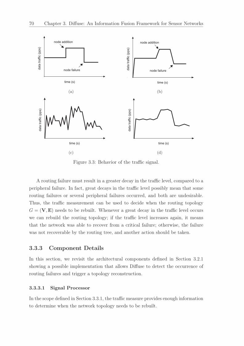
70 Chapter 3. Diffuse: An Information Fusion Framework for Sensor Networks
node additiond
ata
tra
ffic
(p
ps)
node failure
time (s)
(a)
node addition
da
ta t
raffic
(p
ps)
node failure
time (s)
(b)
da
ta t
raffic
(p
ps)
time (s)
(c)
da
ta t
raffic
(p
ps)
time (s)
(d)
Figure 3.3: Behavior of the traffic signal.
A routing failure must result in a greater decay in the traffic level, compared to a
peripheral failure. In fact, great decays in the traffic level possibly mean that some
routing failures or several peripheral failures occurred, and both are undesirable.
Thus, the traffic measurement can be used to decide when the routing topology
G = (V,E) needs to be rebuilt. Whenever a great decay in the traffic level occurs
we can rebuild the routing topology; if the traffic level increases again, it means
that the network was able to recover from a critical failure; otherwise, the failure
was not recoverable by the routing tree, and another action should be taken.
3.3.3 Component Details
In this section, we revisit the architectural components defined in Section 3.2.1
showing a possible implementation that allows Diffuse to detect the occurrence of
routing failures and trigger a topology reconstruction.
3.3.3.1 Signal Processor
In the scope defined in Section 3.3.1, the traffic measure provides enough information
to determine when the network topology needs to be rebuilt.

3.3. Diffuse for Failure Recovery 71
The measured traffic should be filtered to reduce the embedded noise. The
behavior of the traffic signal (Figure 3.3(a)) is very similar to the step function,
except that the step level changes according to node failures and additions. Due
to this similarity, we have chosen the moving average to clean the traffic signal
because this filter is optimal for a common problem, reducing noise while keeping
the sharpest step response, i.e., it provides the lowest noise possible for a given edge
sharpness [Smith 1999].
3.3.3.2 Feature Extractor
Once the traffic is filtered, Diffuse extracts two features from the signal: the short-
term observation and the long-term observation. The short-term observation
evaluates the traffic change between two traffic samples in a row, and the long-term
observation shows how the traffic changed since the last topology reconstruction.
δ(ts)
δ(ts−1)
traffic (pps)
π/2
−π/2
αshort
αworstshort
ts−1 ts
sample time (s)
(a) Short-term observation.
δ(tbuild+1)
δ(ts)
traffic (pps)
π/2
−π/2
αlongαworstlong
tstbuild tbuild+1
topology building
sample time (s)
(b) Long-term observation.
Figure 3.4: Measured traffic.
Short-term Observation. Given two samples in a sequence, ts−1 and ts, and the
short-term observation angles, αshort and αworstshort, depicted in Figure 3.4(a), we
define the short-term observation as
φshort =αshort
αworstshort
, (3.2)

72 Chapter 3. Diffuse: An Information Fusion Framework for Sensor Networks
where
αshort = arctanδ(ts)− δ(ts−1)
ts − ts−1
(3.3)
αworstshort = arctan−δ(ts−1)
ts − ts−1
. (3.4)
The value φshort allows us to measure the intensity of the traffic decay, which is
not possible if we use only αshort. The possible values of φshort are:
• φshort = 0, the traffic remains the same since the last observation;
• 0 < φshort < 1, the traffic decreased since the last observation;
• φshort = 1, no data is being delivered (the worst case for data gathering appli-
cations).
Long-term Observation. Given the first sample after the last topology build-
ing, tbuild+1, the current sample, ts, and the long-term observation angles αlong and
αworstlong(Figure 3.4(b)), we define the long-term observation as
φlong =αlong
αworstlong
, (3.5)
where
αlong = arctanδ(ts)− δ(tbuild+1)
ts − tbuild+1
(3.6)
αworstlong = arctan−δ(tbuild+1)
ts − tbuild+1
. (3.7)
Again, the value φlong allows us to measure the intensity of the long-term traffic
decay, which is not possible if we use only αlong. The possible values of φlong are:
• φlong = 0, the traffic remains the same since the last topology building;
• 0 < φlong < 1, the traffic decreased since the last topology building;
• φlong = 1, no data is being delivered anymore.
The features, φshort and φlong, are defined in terms of the decay angles, instead of
the simple traffic decays, because the angles also considers the time spent to change
the traffic level.
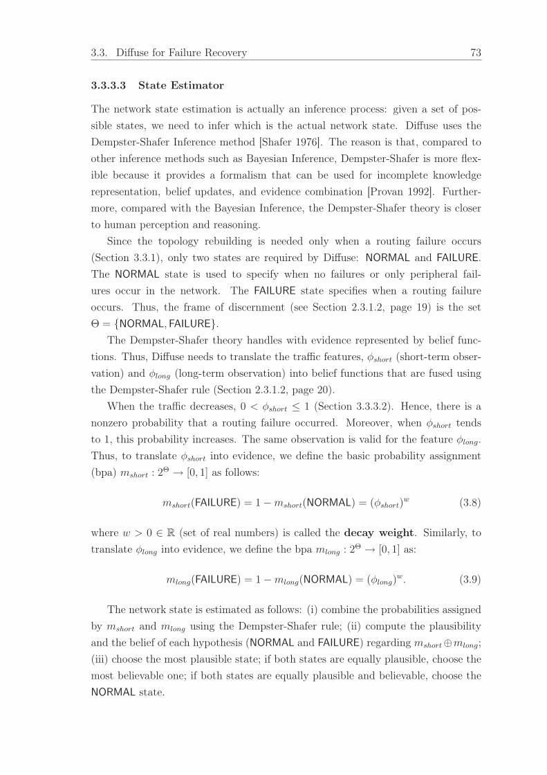
3.3. Diffuse for Failure Recovery 73
3.3.3.3 State Estimator
The network state estimation is actually an inference process: given a set of pos-
sible states, we need to infer which is the actual network state. Diffuse uses the
Dempster-Shafer Inference method [Shafer 1976]. The reason is that, compared to
other inference methods such as Bayesian Inference, Dempster-Shafer is more flex-
ible because it provides a formalism that can be used for incomplete knowledge
representation, belief updates, and evidence combination [Provan 1992]. Further-
more, compared with the Bayesian Inference, the Dempster-Shafer theory is closer
to human perception and reasoning.
Since the topology rebuilding is needed only when a routing failure occurs
(Section 3.3.1), only two states are required by Diffuse: NORMAL and FAILURE.
The NORMAL state is used to specify when no failures or only peripheral fail-
ures occur in the network. The FAILURE state specifies when a routing failure
occurs. Thus, the frame of discernment (see Section 2.3.1.2, page 19) is the set
Θ = {NORMAL, FAILURE}.The Dempster-Shafer theory handles with evidence represented by belief func-
tions. Thus, Diffuse needs to translate the traffic features, φshort (short-term obser-
vation) and φlong (long-term observation) into belief functions that are fused using
the Dempster-Shafer rule (Section 2.3.1.2, page 20).
When the traffic decreases, 0 < φshort ≤ 1 (Section 3.3.3.2). Hence, there is a
nonzero probability that a routing failure occurred. Moreover, when φshort tends
to 1, this probability increases. The same observation is valid for the feature φlong.
Thus, to translate φshort into evidence, we define the basic probability assignment
(bpa) mshort : 2Θ → [0, 1] as follows:
mshort(FAILURE) = 1−mshort(NORMAL) = (φshort)w (3.8)
where w > 0 ∈ R (set of real numbers) is called the decay weight. Similarly, to
translate φlong into evidence, we define the bpa mlong : 2Θ → [0, 1] as:
mlong(FAILURE) = 1−mlong(NORMAL) = (φlong)w. (3.9)
The network state is estimated as follows: (i) combine the probabilities assigned
by mshort and mlong using the Dempster-Shafer rule; (ii) compute the plausibility
and the belief of each hypothesis (NORMAL and FAILURE) regarding mshort⊕mlong;
(iii) choose the most plausible state; if both states are equally plausible, choose the
most believable one; if both states are equally plausible and believable, choose the
NORMAL state.
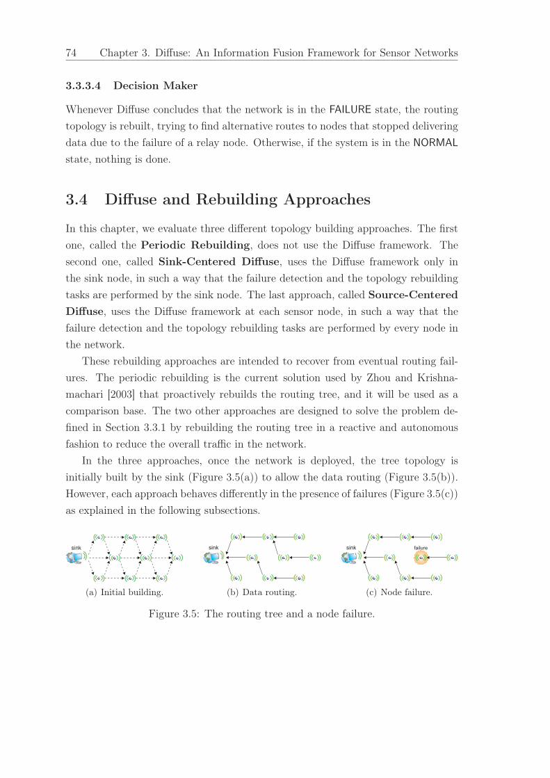
74 Chapter 3. Diffuse: An Information Fusion Framework for Sensor Networks
3.3.3.4 Decision Maker
Whenever Diffuse concludes that the network is in the FAILURE state, the routing
topology is rebuilt, trying to find alternative routes to nodes that stopped delivering
data due to the failure of a relay node. Otherwise, if the system is in the NORMAL
state, nothing is done.
3.4 Diffuse and Rebuilding Approaches
In this chapter, we evaluate three different topology building approaches. The first
one, called the Periodic Rebuilding, does not use the Diffuse framework. The
second one, called Sink-Centered Diffuse, uses the Diffuse framework only in
the sink node, in such a way that the failure detection and the topology rebuilding
tasks are performed by the sink node. The last approach, called Source-Centered
Diffuse, uses the Diffuse framework at each sensor node, in such a way that the
failure detection and the topology rebuilding tasks are performed by every node in
the network.
These rebuilding approaches are intended to recover from eventual routing fail-
ures. The periodic rebuilding is the current solution used by Zhou and Krishna-
machari [2003] that proactively rebuilds the routing tree, and it will be used as a
comparison base. The two other approaches are designed to solve the problem de-
fined in Section 3.3.1 by rebuilding the routing tree in a reactive and autonomous
fashion to reduce the overall traffic in the network.
In the three approaches, once the network is deployed, the tree topology is
initially built by the sink (Figure 3.5(a)) to allow the data routing (Figure 3.5(b)).
However, each approach behaves differently in the presence of failures (Figure 3.5(c))
as explained in the following subsections.
sink
(a) Initial building.
sink
(b) Data routing.
failuresink
(c) Node failure.
Figure 3.5: The routing tree and a node failure.

3.4. Diffuse and Rebuilding Approaches 75
3.4.1 Periodic Rebuilding
In the Periodic Rebuilding, no failure detection is performed by the sensor nodes
(Figure 3.6(a)). However, the whole routing tree is periodically rebuilt (Fig-
ure 3.6(b)) to recover from eventual failures (Figure 3.6(c)). The periodicity in
which the routing tree is rebuilt is defined by the building rate B, which is mea-
sured in buildings per second. The proper value for B depends on the application
and environmental conditions. Environments with high failure rates demand higher
building rates.
sink failure
(a) No failure detection.
failuresink
(b) Periodic rebuilding.
failuresink
(c) Data routing.
Figure 3.6: The Periodic Rebuilding approach — continuation of Figure 3.5(c).
Definition 3.3 (Node Failure) In the context of this work, a node failure occurs
when, due to any reason, a node becomes inoperable, i.e., it cannot deliver its data
packets. The node failure starts at time t0 (0 ≤ t0 < T ), and finishes at time tf
(t0 < tf ≤ T ), so the failure duration is ∆t = tf − t0.
Considering the Periodic Rebuilding approach, let B be the building rate, in
buildings per second, and βper the number of building packets sent to the network. In
the Periodic Rebuilding approach, the first building occurs at t = 0, then the routing
topology is reconstructed bB × T c times. Thus, the number of topology buildings is
exactly 1+bB × T c, independent from the failure occurrences. However, the number
of building packets occurring in the network depends on the failure occurrences. The
minimum number of building packets occurs when the sink node sends the building
packets but, due to failures, none of the source nodes receives such packets, i.e.,
βper = (1 + bB × T c) × (1 packet/building). The maximum number of building
packets occurs when no failure occurs and all n nodes forward the building packets
once, i.e., βper = (1 + bB × T c)× (n packets/building).
Theorem 3.1 In the Periodic Rebuilding approach, the total number of building
packets, βper, sent by the nodes in G = (V,E) has the following bounds:
βper ≥ 1 + bB × T c ,βper ≤ n× (1 + bB × T c) ,

76 Chapter 3. Diffuse: An Information Fusion Framework for Sensor Networks
where n = |V|.
Proof (Direct). The proof is divided in two parts: lower bound and upper bound.
Lower bound: βper ≥ 1 + bB × T c. G is initially constructed and is reconstructed
exactly bB × T c times. Thus, at least the sink node sends 1 + bB × T c building
packets (one packet per building).
Upper bound: βper ≤ n × (1 + bB × T c). Each building packet is forwarded only
once by each node that receives such a packet. Thus, if no failures occur, βper =
n× (1 + bB × T c).Thus, 1 + bB × T c ≤ βper ≤ n× (1 + bB × T c). 2
3.4.2 Sink-Centered Diffuse
The Sink-Centered Diffuse uses the Diffuse framework only in the sink node. Thus,
whenever the sink node detects a critical failure in the network (Figure 3.7(a)),
the routing tree is fully rebuilt (Figure 3.7(b)) to try to reach the disconnected
nodes (Figure 3.7(c)). However, to avoid excessive reconstructions, the minimum
time between two successive reconstructions should be specified. In a low failure
scenario, this approach leads to lower communication overhead compared to the
periodic rebuilding.
sink failure
(a) Failure detection.
failuresink
(b) Global rebuilding.
failuresink
(c) Data routing.
Figure 3.7: Sink-Centered Diffuse approach — continuation of Figure 3.5(c).
Let tmin be the minimum time allowed between two successive reconstructions
and βsnk the number of building packets occurring in the network using the Sink-
Centered Diffuse approach.
In the Sink-Centered Diffuse approach, the first building occurs at t = 0, then
if no failure occurs, no additional rebuilding is done. Thus, the minimum number
of topology buildings is 1, and if none of the source nodes can receive the building
packet from the sink node, the total number of building packets in the network
will be 1 packet, which is the lower bound. Due to the minimum allowed time
between two successive reconstructions (tmin), in the worst case, the network will be
rebuilt periodically with a building rate of 1/tmin buildings per second, which means
that we will have at most 1 + bT/tminc topology buildings. Thus, the maximum

3.4. Diffuse and Rebuilding Approaches 77
number of building packets occurs when we have 1 + bT/tminc topology buildings,
and all n nodes forward the building packets once, i.e., βsnk = (1 + bT/tminc) ×(n packets/building).
Theorem 3.2 In the Sink-Centered Diffuse approach, the total number of building
packets, βsnk, sent by the nodes in G = (V,E) has the following bounds:
βsnk ≥ 1
βsnk ≤ n× (1 + bT/tminc) ,
where n = |V| and tmin > 0.
Proof (Direct). The proof is divided in two parts:
Lower bound: the sink does not detect the need for topology reconstructions. In
this case, at least the sink node sends one building packet referring to the initial
construction. Thus, βsnk ≥ 1.
Upper bound: the sink detects the need for topology reconstructions. Since the min-
imum time between two successive topology reconstructions is tmin, the maximum
number of topology buildings is 1 + bT/tminc. Thus, βsnk ≤ n× (1 + bT/tminc).Thus, 1 ≤ βsnk ≤ n× (1 + bT/tminc). 2
Corollary 3.2.1 In the Sink-Centered Diffuse approach, if no failure occurs, the
total number of building packets sent by the nodes in G = (V,E) is βsnk = n = |V|.
Proof . Trivial. 2
Let f be the number of critical failures during [0, T ).
Corollary 3.2.2 If no failure occurs, i.e., f = 0, as the network lifetime T increases,
βsnk becomes irrelevant compared to βper of the Periodic Rebuilding approach with
B = 1/tmin buildings per second, i.e.,
limT→∞
βsnk
βper
= 0.
Proof (Direct). Since no failures occur, according to Theorem 3.1 and Corol-
lary 3.2.1, we can say that
limT→∞
βsnk
βper
=n
n× (1 + bB × T c) =1
1 + bB × T c = 0.2
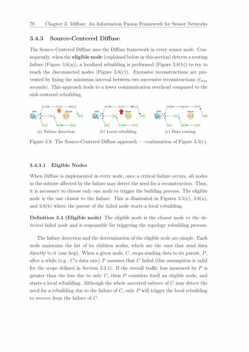
78 Chapter 3. Diffuse: An Information Fusion Framework for Sensor Networks
3.4.3 Source-Centered Diffuse
The Source-Centered Diffuse uses the Diffuse framework in every sensor node. Con-
sequently, when the eligible node (explained below in this section) detects a routing
failure (Figure 3.8(a)), a localized rebuilding is performed (Figure 3.8(b)) to try to
reach the disconnected nodes (Figure 3.8(c)). Excessive reconstructions are pre-
vented by fixing the minimum interval between two successive reconstructions (tmin
seconds). This approach leads to a lower communication overhead compared to the
sink-centered rebuilding.
sink failure
(a) Failure detection.
failuresink
(b) Local rebuilding.
failuresink
(c) Data routing.
Figure 3.8: The Source-Centered Diffuse approach — continuation of Figure 3.5(c).
3.4.3.1 Eligible Nodes
When Diffuse is implemented in every node, once a critical failure occurs, all nodes
in the subtree affected by the failure may detect the need for a reconstruction. Thus,
it is necessary to choose only one node to trigger the building process. The eligible
node is the one closest to the failure. This is illustrated in Figures 3.5(c), 3.8(a),
and 3.8(b) where the parent of the failed node starts a local rebuilding.
Definition 3.4 (Eligible node) The eligible node is the closest node to the de-
tected failed node and is responsible for triggering the topology rebuilding process.
The failure detection and the determination of the eligible node are simple. Each
node maintains the list of its children nodes, which are the ones that send data
directly to it (one hop). When a given node, C, stops sending data to its parent, P ,
after a while (e.g., C’s data rate) P assumes that C failed (this assumption is valid
for the scope defined in Section 3.3.1). If the overall traffic loss measured by P is
greater than the loss due to only C, then P considers itself an eligible node, and
starts a local rebuilding. Although the whole ancestral subtree of C may detect the
need for a rebuilding due to the failure of C, only P will trigger the local rebuilding
to recover from the failure of C.

3.4. Diffuse and Rebuilding Approaches 79
3.4.3.2 Local Rebuilding
A global rebuilding is prevented by fixing the TTL (time to live) of the building
packet to a given depth. In addition, only nodes with a missing parent will update
its parent information. This detection feature can be provided by the MAC protocol
that might warn the upper layer when a communication cannot be established with
the destination node. However, for the sake of exemplification, we provide two
alternatives for this issue. First, since the node that detects the failure and triggers
the local building can identify the failed node, the rebuilding packet can include
the list of nodes that failed. Thus, only a node with its parent identified chooses
a new parent. Second, the communication can be performed in the promiscuous
mode. Then, a node can send a packet and listen to the wireless channel. If such
a packet is not forwarded, the node may assume that its parent failed. This is a
cheaper solution compared to the previous one, which increases the communication
overhead by adding the list of nodes that failed in the rebuilding packet.
Definition 3.5 (Network diameter) The network diameter D is the number of
hops in the shortest path connecting the farthest node v ∈ V to the sink node.
Let D be the network diameter, d the depth (in hops) of the rebuilding packets,
and βsrc the number packets sent by the nodes in a network using the Source-
Centered Rebuilding approach.
Theorem 3.3 Suppose that all critical failures are properly detected. In the
Source-Centered Rebuilding approach, the total number of building packets, βsrc,
sent by the nodes in G = (V,E) has the following bound:
βsrc ≤ βsnk,
where βsnk is the total number of building packets using the Sink-Centered Rebuild-
ing approach.
Proof (Cases). Since all critical failures are properly detected, both the Sink-
Centered and the Source-Centered Rebuilding approaches will trigger the same
number of reconstructions. Thus, we have the following cases:
Case 1: d < D. When the depth d is smaller than the network diameter, building
packets of the Source-Centered approach are not forwarded by nodes distant [d,D)
hops from the sink. Thus, βsrc < βsnk.
Case 2: d = D. When the depth d is equal to the network diameter, building
packets of the Source-Centered approach are not forwarded by nodes at D hops
from the sink (leaf nodes). Thus, βsrc < βsnk.

80 Chapter 3. Diffuse: An Information Fusion Framework for Sensor Networks
Case 3: d > D. When the depth d is greater than the network diameter, building
packets of the Source-Centered approach are forwarded by all nodes. Thus, βsrc =
βsnk.
Thus, βsrc ≤ βsnk. 2
3.4.4 Further Scenarios
The applicability of Diffuse for failure recovery (routing failures) goes beyond the
simple continuous data delivery model for flat sensor networks defined in Sec-
tion 3.3.1. In this section, we describe how to adapt the proposed solution to other
scenarios.
if P is reducible to A then1
Reduce P to A;2
Apply Diffuse on A;3
else4
Find a function δP(t) that describes the data traffic in P ;5
Apply Diffuse using δP(t);6
end7
Algorithm 3.1: Applying Diffuse for failure recovery in other contexts.
The procedure to apply Diffuse in other contexts is presented in Algorithm 3.1.
In a nutshell, we try to reduce our new context P to a known scenario A, then
we apply Diffuse (lines 2 and 3). If we are not able to reduce the new scenario
to a known scenario, we need to determine the function that describes the traffic
and implement the proper filters to apply Diffuse (lines 5 and 6). In the following
sections, we exemplify how this procedure can be applied.
3.4.4.1 In-Network Data Aggregation
When the network performs in-network aggregation the overall data traffic is reduced
in such a way that the traffic measured by the sink node will be proportional to the
number of its children nodes. Thus, the aggregated traffic does not represent the
whole network data traffic.
This scenario can be reduced to the one defined in Section 3.3.1 by making the
sensor nodes inform what is the original traffic that Diffuse should consider. Thus,
the sensor nodes only need to append the number of data packets that were used to
obtain the aggregated packet.
Figure 3.9 depicts how we can use Diffuse in a scenario with in-network data
aggregation. In this example, we adopt a data aggregation method that sends one

3.4. Diffuse and Rebuilding Approaches 81
sink
A
B
C
D
E
F
G
H
I
Node Received Agg
Sink 3 9
A 1 5
B 0 1
C 1 3
D 2 4
E 1 2
F 1 2
G 0 1
H 0 1
I 0 1
Figure 3.9: Diffuse with data aggregation.
packet per node. Consequently, each node receives only one aggregated packet from
each of its child node (“Received” column in Figure 3.9). For the sake of exemplifi-
cation, let us analyze the path I→F→D→A→Sink. First, I sends one packet to F
informing that it represents only one packet (“Agg” column in Figure 3.9). Second,
F sends one packet to D informing that it was obtained from two packets (I and
F ). Third, D sends one packet to A telling that is was obtained from four packets
(I, F , G, and D). Finally, A sends one packet to the sink node informing that it was
obtained from five packets (I, F , G, D, and A). Thus, the sink node knows that
the aggregated packet received from A refers to five original data packets (traffic
without data aggregation). Now Diffuse can be applied because the nodes know
what the traffic would be without data aggregation.
3.4.4.2 Event-Based Applications
For event-driven scenarios, we can use reactive trees that are built only when an
event is detected. In this case, Diffuse will be used only during the event detection.
traffic
(pps)
elapsed time (s)
event
event
no event no eventno event
Figure 3.10: Interval-based Diffuse for event-driven scenarios.
When a reactive tree is used, sensor nodes that detect the event should contin-
uously notify the sink node. Thus, the traffic assumptions made in Section 3.3.1
hold while the event is being detected (Figure 3.10), and Diffuse can be used. When
the event ceases, Diffuse triggers one extra rebuilding as it cannot determine if the
traffic decrease refers to either a failure or the event ceasing. Thus, Diffuse is applied
only during the time intervals in which events occur.

82 Chapter 3. Diffuse: An Information Fusion Framework for Sensor Networks
3.4.4.3 Other Traffic Patterns
Eventually, we may not reduce our scenario to a known one. In such cases, Diffuse
needs to know (or estimate) the function that describes the traffic pattern, which
can be of any type (Figure 3.11), and use the appropriated filter, not necessarily
the moving average. If we are not able to describe the traffic by a mathematical
function, a probabilistic density function may be used. Again, the point here is
to be able to identify the traffic behavior so we can infer about the occurrence of
routing failures.
tra
ffic
(p
ps)
elapsed time (s)
(a)
tra
ffic
(p
ps)
elapsed time (s)
(b)tr
affic
(p
ps)
elapsed time (s)
(c)
Figure 3.11: Other traffic patterns.
3.5 Evaluation
The evaluation is performed through simulations that compare the Diffuse schemes
with the Periodical Rebuilding. The ns-2 simulator [NS-2 2004] is the simulation
environment used for the experiments — which are executed with 33 different seeds
to compute the arithmetic average and the asymptotic confidence interval at the
95% confidence level (1−α = 0.95). In the graphs, the curves represent the average
values, while the error bars represent the confidence intervals.
3.5.1 Deployment Model
We consider that the network is intended to be deployed as the grid depicted in
Figure 3.12(a). However, considering a non-deterministic deployment strategy (e.g.,
using an aircraft), uncontrolled variables (e.g., wind and environmental obstacles)
should lead to a disturbed grid, such as the grid in Figure 3.12(b).
The disturbed grid is simulated by introducing random errors in the horizontal
and vertical coordinates of each node in the grid. Such position errors, measured
in meters, are modelled as zero-mean normal censored variables with a standard
deviation of 5 (meters).

3.5. Evaluation 83
(a) Regular grid. (b) Disturbed grid.
Figure 3.12: Deployment model.
3.5.2 Failure Model
Reliability is evaluated by using an independent failures model. In this model,
the inter-arrival time (time between two failures) is a continuous exponentially dis-
tributed random variable with the following probability density function (pdf):
p(t) = λe−λt, (3.10)
where t, λ > 0.
3.5.3 Simulation Parameters and Algorithms’ Setup
The simulation parameters are based on the Mica2 sensor node [Crossbow 2004]:
transmission, reception, and sensing power are 45.0mW, 24.0mW, and 15.0mW,
respectively; the bandwidth is 19.2 kbps; and the communication radius is fixed in
40m. The MAC layer uses the 802.11 protocol.
In all scenarios, the sink node is placed in the bottom left corner (0,0) of the
sensor field. Data packets and control packets have 20 bytes. The chosen data rate
is one packet every 20s. For the Periodic Rebuilding, the tree topology is rebuilt
every 200s. The simulation time is 4000s for all scenarios.
Two parameters need to be configured in Diffuse: the window size (M) of the
moving average filter and the decay weight (w), used to translate features into evi-
dences. Due to our sampling strategy (S is numerically equal to R, see Section 3.3.2),
in the specified scenarios the filter takes 20M seconds to converge to a new signal
level. The embedded noise represents less than 3% of the signal level, and M = 5
showed to be enough to filter such a noise. In a previous work, Nakamura et al.
[2005b] show that when w = 1/7, Diffuse presents the best results regarding the de-
livery ratio. Thus, the decay weight is set to 1/7. For the Source-Centered Diffuse,
we choose d = 2 (depth parameter), so the local rebuilding is limited to 2 hops.

84 Chapter 3. Diffuse: An Information Fusion Framework for Sensor Networks
3.5.4 Metrics
The evaluated metrics are: delivery ratio, delay per hop, number of queue drops,
and number of building packets in the network. The delivery ratio provides an
efficacy measurement about the network ability to deliver the sensed data. Delay
per hop and queue drops evaluate the impact of network constructions in the overall
traffic. The number of building packets shows the control traffic necessary to assure
a certain delivery ratio.
3.5.5 Results
Scalability is evaluated by using network sizes of 100, 121, 144, and 169 nodes, and
a constant failure rate (λ = 0.005 failures/s). The network density is kept constant
in 0.02 nodes/m2. The result is depicted in Figure 3.13. The three rebuilding
approaches are equally scalable regarding the delivery ratio and the delay per hop,
as depicted in Figure 3.13(a) and Figure 3.13(b). Figure 3.13(a) shows that the
three rebuilding approaches deliver more than 95% of the data packets, which is a
high delivery ratio.
0.8
0.85
0.9
0.95
1
100 125 150 175
Deliv
ery
Ratio
Network Size
Periodic SchemeSink-Centered
Source-Centered
(a) Delivery ratio.
0
0.5
1
1.5
2
2.5
3
3.5
100 125 150 175
Tim
e (
s)
Network Size
Periodic SchemeSink-Centered
Source-Centered
(b) Delay.
0
200
400
600
800
1000
1200
1400
100 125 150 175
Build
ing p
ackets
Network Size
Periodic SchemeSink-Centered
Source-Centered
(c) Construction Overhead.
0
20
40
60
80
100
120
140
100 125 150 175
Queue D
rops (
packets
)
Network Size
Periodic SchemeSink-Centered
Source-Centered
(d) Queue Drops.
Figure 3.13: Scalability.

3.5. Evaluation 85
Figure 3.13(c) shows that the Source-Centered Diffuse introduces less traffic
than the other schemes. As a result, fewer packets are lost in the node queues
when we use the Source-Centered Diffuse scheme (Figure 3.13(d)). Furthermore,
Figure 3.13(c) shows that the greater the network size, the greater the difference
between the periodic rebuilding and the Diffuse schemes. For networks with 169
nodes, the traffic overhead generated by the Source-Centered Diffuse is nearly 85%
smaller than the traffic generated by the periodic rebuilding.
Reliability is evaluated by using failure rates of 0.003, 0.008, 0.013, and 0.018
failures/s in networks with 169 nodes. The three rebuilding approaches present
the same behavior regarding the delivery ratio and the delay per hop, as depicted
in Figure 3.14(a) and Figure 3.14(b), respectively. However, due to the limited
rebuilding, the Source-Centered Diffuse does not recover from all failures, delivering
fewer packets compared with the Sink-Centered Diffuse and the Periodic schemes.
0.85
0.9
0.95
1
0.005 0.01 0.015 0.02
Deliv
ery
Ratio
Failure ratio (failures/s)
Periodic SchemeSink-Centered
Source-Centered
(a) Delivery ratio.
1.5
2
2.5
3
0.005 0.01 0.015 0.02
Tim
e (
s)
Failure ratio (failures/s)
Periodic SchemeSink-Centered
Source-Centered
(b) Delay.
0
200
400
600
800
1000
1200
1400
1600
1800
2000
2200
0.005 0.01 0.015 0.02
Build
ing p
ackets
Failure ratio (failures/s)
Periodic SchemeSink-Centered
Source-Centered
(c) Construction Overhead.
20
40
60
80
100
120
140
160
180
0.005 0.01 0.015 0.02
Queue D
rops (
packets
)
Failure ratio (failures/s)
Periodic SchemeSink-Centered
Source-Centered
(d) Queue Drops.
Figure 3.14: Reliability.
Regarding the construction overhead and queue drops, Figure 3.14(c) and Fig-
ure 3.14(d) show that the Source-Centered Diffuse is less affected by failures than
the other schemes. In addition, when the failure rate increases, the traffic generated
by the Sink-Centered Diffuse and the Periodic Rebuilding schemes becomes closer.

86 Chapter 3. Diffuse: An Information Fusion Framework for Sensor Networks
3.6 Why Diffuse?
Since we use Diffuse to detect node failure, one might ask why use Dempster-Shafer
if similar results could obtained using a heartbeat approach. In this section, we try
to elucidate when Diffuse is preferable to a failure detector based on heartbeats.
3.6.1 Is Heartbeat a Better Solution?
Heartbeat-based solutions, such as Wang and Kuo [2003] and Tai et al. [2004], can
be use used to detect node failures and trigger topology reconstructions. From
the computational perspective, these solutions are simpler than the Diffuse-based
solutions that we propose. However, those solutions introduce additional commu-
nication (gossip-like algorithms) to inform nodes about detected failures. In this
context, Diffuse is better because it does not introduce additional communication.
However, even simpler heartbeat-based solutions can be used effectively and, at some
level, Diffuse solutions are based on heartbeats since they use the data traffic to infer
about failures. Thus, why should we use Diffuse if we have simpler alternative?
The main motivation to use Diffuse is that once we use the Dempster-Shafer
framework, we can easily extend our solution to consider other factors that might
trigger a topology reconstruction. Extensions and simplifications are made easy
because the Dempster-Shafer inference combines information as it becomes avail-
able [Shafer 1976], and such a solution is not obvious in a simple heartbeat solution.
In the next section, we sketch how to extend Diffuse. Furthermore, surveillance sys-
tems commonly use inference mechanisms (Bayesian or Dempster-Shafer) to detect,
recognize, or classify events (targets). Thus, nodes can reuse the Dempster-Shafer
mechanisms to infer about event occurrences.
3.6.2 Extending Diffuse: A Road Map
As stated in Section 3.2.2, Diffuse can be used to trigger topology reconstructions
prompted by other goals besides routing failures, such as data aggregation or energy
balancing. Since we use Dempster-Shafer as an inference framework, we can easily
extend Diffuse to accommodate such extensions. The general procedure to extend
Diffuse is depicted in Algorithm 3.2. To exemplify how the algorithm can be used,
let us suppose we want to extend Diffuse to rebuild the routing tree to avoid low
energy areas. In this example, we do not provide detailed information about the
methods and algorithms used. Instead, we only illustrate how to extend Diffuse
using the algorithm depicted in Figure 3.2:

3.7. Chapter Remarks 87
begin1
Define the input;2
Define how to process the input (signals or features);3
Add the new states to Diffuse;4
Add the new bpa’s to Diffuse;5
Define the action for each new state;6
end7
Algorithm 3.2: Extending Diffuse.
• Line 2 (Define the input): A possible input in this case is the energy
map [Mini et al. 2005].
• Line 3 (Process the input): To detect avoidance regions (low energy) we
can use segmentation methods on the map (image map) or specify low-energy
nodes (node map).
• Line 4 (Add new states): We need to add a new state ENERGY to our frame
of discernment to describe the need for a topology reconstruction to achieve
energy balancing.
• Line 5 (Add new bpa’s): The energy consumption should be translated into
bpa’s such that if the energy consumption of a node is too high we should
avoid it or reduce its load in the next reconstruction).
• Line 6 (Define the action for the new state): If the ENERGY state is
recognized, the routing tree needs to be rebuilt indicating the nodes or regions
to be avoided.
Similarly, we could extend Diffuse to rebuild the routing tree aiming to improve
data aggregation. In this case, we would add a new state AGGREGATION, and the
evidence (bpa) about this state might be obtained from the connectivity map. Note
that, although current bpa’s mshort and mlong do not provide information about the
ENERGY and AGGREGATION states, they can still be used because Dempster-Shafer
allows the representation of incomplete knowledge (Bayesian inference does not).
3.7 Chapter Remarks
In order to assist in the design of information fusion tasks in WSNs, in this chapter,
we propose the Diffuse framework. This framework specifies the steps of a general
fusion process that shows how raw data can evolved towards a high-level decision.
In contrast to the models and architectures presented in Section 2.4, Diffuse offers

88 Chapter 3. Diffuse: An Information Fusion Framework for Sensor Networks
a basic API and does not force the execution of every specified step. Instead,
the user can use the resources for data filtering or decision making individually.
The applicability of the Diffuse framework is ample, and besides the example that
we provide for routing topology construction, other applications can benefit from
Diffuse, as we discuss in Section 3.2.2 and Section 3.6.2.
The mechanism we propose to make tree-based routing algorithms more reliable
(by reconstructing the routing topology when necessary) has two variants: the Sink-
Centered Diffuse and the Source-Centered Diffuse. The Sink-Centered Diffuse and
the Source-Centered Diffuse implement the Diffuse framework and collect data traffic
measurements, and based on such measurements, Diffuse uses information fusion
mechanisms to determine when the routing topology needs to be rebuilt.
The results show that the Diffuse-based solutions efficiently avoid unnecessary
topology constructions. In some cases, the traffic overhead generated by the Diffuse-
based solutions is 85% smaller than the traffic generated by the Periodic Rebuilding,
which is one of the current solutions adopted to rebuild the routing topology.
In the next chapter, we present the InFRA algorithm, which is a reactive role
assignment algorithm, for event-based applications, that is designed to improve in-
network data aggregation while event data is routed towards the sink node.

“When I’m working on a problem, I never think aboutbeauty. I think only how to solve the problem. But whenI have finished, if the solution is not beautiful, I know itis wrong.”
Richard Buckminster Fuller (1895 – 1983)
4On Demand Role Assignment for
Event Detection in WSNs
Assuming that a WSN runs an information fusion application, we show
how we can design the network to support our application. Regarding the
application, we consider that WSNs apply information fusion techniques
to detect events in the sensor field. Particularly, in event-driven scenarios there
might be long intervals of inactivity. However, at a given instant, multiple sensor
nodes might detect one or more events, resulting in high traffic. To save energy, the
network should be able to remain in a latent state until an event occurs, then the
network should organize itself to properly detect and notify the event. Based on
the premise that we have an information fusion application for event detection, we
propose a role assignment algorithm to organize the network by assigning roles to
nodes, only when events are detected.
This algorithm, called Information-Fusion-based Role Assignment (InFRA), es-
tablishes a hybrid network organization in which source nodes are organized into
clusters and the cluster-to-sink communication occurs in a multihop fashion. The
resulting topology is a distributed heuristic to the minimal Steiner tree. Although
there are several heuristics for the Steiner tree [Takahashi and Matsuyama 1980;
Bauer and Varma 1996; Robins and Zelikovsky 2000; Krishnamachari et al. 2002],
in our investigation, the InFRA algorithm is the first distributed heuristic that
explicitly benefits from the geographical correlation by assuming that an event is
probably detected by multiple neighbor nodes.
89

90 Chapter 4. On Demand Role Assignment for Event Detection in WSNs
Theoretical analysis shows that our algorithm has a O(1)-approximation ratio
when the network diameter remains constant and, in large-scale networks it has a
k-approximation ratio, where k is the number of simultaneous events. Simulation
results show that InFRA can save energy compared to a proactive and other reactive
algorithms.
Preliminary versions of this chapter appear in the proceedings of the
SBRC’05 [Nakamura et al. 2006a] and the ISCC’06 [Nakamura et al. 2006b] confer-
ences.
The chapter is organized as follows. Section 4.1 discusses some role assignment
solutions. Section 4.2 presents the background knowledge supporting the work pre-
sented in this chapter. The problem of finding the minimum transmission routing
tree is formalized in Section 4.3. Our role assignment algorithm (InFRA) is pre-
sented in Section 4.4. Theoretical results of our heuristic are presented in Section 4.5
and simulation results in Section 4.6. Section 4.7 presents the chapter remarks.
4.1 Related Work
This section presents some role assignment solutions for data gathering in wireless
sensor networks.
Bhardwaj and Chandakasan [2002] derive upper bounds on the lifetime of WSNs
that perform information fusion. In this case, three roles are identified: sensor (a
node that senses and generates data packets), relay (a node that forwards data
packets with no data processing), and aggregator (a node that fuses two or more
data streams into a single one). The optimal role assignment is modeled as a linear
problem that finds the role assignment that maximizes the network lifetime. The
authors compare the lifetime bounds of networks that perform information fusion
with networks that do not.
Bonfils and Bonnet [2003] propose an adaptive and decentralized solution that
progressively refines the role assignment by evaluating neighbor nodes. Their solu-
tion searches for the role assignment that minimizes the amount of data transmitted
in the network. In that solution, each node computes a cost function of the amount
of data received and produced. At regular intervals these cost estimates are evalu-
ated and the role is migrated to the node of lowest cost. The communication cost
introduced by the solution is not considered.
The Sensor Placement and Role Assignment for Energy-Efficient Information
Gathering (SPRING) algorithm [Dasgupta et al. 2003] was proposed for mobile
sensor networks. SPRING defines two roles in a WSN, namely, sensor and relay

4.1. Related Work 91
(a node that fuses and forwards data packets). The problem that SPRING tries
to solve is to place nodes and assign roles to them in such a way that the system
lifetime is maximized, and the region of interest is covered by at least one sensor
node. SPRING moves nodes across the field and assigns roles (sensor or relay) so
that the region of interest is covered by the minimum number of nodes with the
sensor role. The relay role is assigned to all other nodes that are not in the region
of interest.
The DFuse framework proposed by Kumar et al. [2003] addresses the role assign-
ment problem providing two modules: fusion module and placement module. The
fusion module allows the application to be built using a dataflow graph that specifies
the roles of each node in the graph. The placement module maps this graph onto
the network and dynamically adapts the mapping by migrating the roles according
to a specified cost function. DFuse uses the same roles defined by Bhardwaj and
Chandakasan [2002]. The role assignment is provided by a heuristic divided in three
phases. The first phase creates a tree with a naive role assignment. In the second,
the nodes exchange their health information (an indicator of how well the node hosts
that role) and the role is transferred to the neighbor with the best health regarding
a given cost function. The third is a maintenance stage similar to the optimization
phase, i.e., the same role transfer semantics is adopted.
Frank and Römer [2005] propose a basic structure of a generic role assignment
framework with applications for coverage, clustering, and in-network aggregation.
The proposed framework allows the user to specify roles and assignment rules. The
framework defines three core elements. The first element is a property directory
used to access capabilities and parameters of the sensor nodes. The second is the
role specification that defines the roles and the assignment rules. The third is the
assignment algorithm that assigns the roles based on role specifications and node
properties.
Kochhal et al. [2003] propose a role-based clustering algorithm that organizes
the network by recursively finding connected dominating sets. The connected dom-
inating sets are used to define coordinators (cluster-heads) and routing nodes, the
remainder of the nodes become sensing collaborators (sources). The clustering pro-
cess considers the sensing ability of the nodes, so the detection capability of the
clusters is enhanced.
Table 4.1 presents a summary of the related work, identifying the objective of
the proposed solution, the kind of network where it operates, the types of roles it
uses, and how the algorithm executes.

92 Chapter 4. On Demand Role Assignment for Event Detection in WSNs
Algorithm/Solution Objective Network Roles Execution
Bhardwaj and Chan-dakasan [2002]
data gathering flat sensor, relay,aggregator
centralized
Bonfils and Bonnet[2003]
query process-ing
flat source, correla-tor, filter, ag-gregator, sup-pressor
decentralized
Kumar et al. [2003] data gathering flat sensor, relay,collator
decentralized
Kochhal et al. [2003] data gather-ing, clustering
hierarchical collaborator,coordinator,router
decentralized
Dasgupta et al. [2003] data gathering flat sensor, relay centralized
Frank and Römer[2005]
generalframework
hierarchicalor flat
user-defined decentralized
Table 4.1: Related work comparison (all solutions are proactive).
4.2 Background
4.2.1 Network and Event Model
In this chapter, we consider a sensor network composed of n nodes of which one of
them is the sink node. For the sake of simplification, we consider symmetric links,
i.e., for any two nodes u and v, u reaches v if, and only if, v reaches u.
All events are static and described by an influence region (area). We assume
a binary detection model, i.e., every node within the influence region of an event
detects that event. Thus, we represent the network by the graph G = (V,E) with
the following properties:
• V = {v1, v2, . . . , vn} is the set of sensor nodes, such that |V| = n and v1 is the
sink node;
• S = {s1, s2, . . . , sm} is the set of sources, i.e., nodes detecting an event, such
that |S| = m and S ⊆ V;
• 〈i, j〉 ∈ E iff vi and vj are neighbors.
Definition 4.1 (Closed Neighborhood) The closed neighborhood N is com-
posed of the node itself and its neighbors. Thus, the closed neighborhood of node
vi is given by
Ni = {vi}⋃
⋃
〈i,j〉∈E
{vj}
. (4.1)

4.2. Background 93
In a sensor network, the network state is often used to guide decision-making
processes. Alternatively, in localized algorithms nodes make decisions based on the
state of the node itself and the state of its neighbors.
Let xi be the state of node vi ∈ V.
Definition 4.2 (Network State) The network can be described by its state vec-
tor
X =⋃
vi∈V
xi. (4.2)
The definition of the node state depends on the application. It can be a large
set that includes all sorts of information about the node, such as residual energy,
workload, bandwidth, noise level, and location; or a simple value such as a flag
indicating whether or not the node is a source. From the network state we can
derive the neighborhood state of each node, which is a subset of the network state.
Definition 4.3 (Neighborhood State) For each node vi ∈ V, we define its
neighborhood state as
Xi =⋃
vj∈Ni
xj. (4.3)
4.2.2 Deployment Model
We consider the same deployment model used in Chapter 3 and described in Sec-
tion 3.5.1, i.e., the node deployment results in a disturbed grid where the location
of each node is disturbed by a random zero-mean Gaussian error. Therefore, nodes
will tend to uniformly occupy the sensor field but without forming a regular grid,
as depicted in Figure 3.12(b).
4.2.3 Role Assignment Model
In this section, we formalize the concepts of role and role assignment in the context
of this work.
Definition 4.4 (Role) A role specifies the actions and computations executed by a
node in the presence of a specific data stream and an identified condition. Thus, for a
given node a role defines the expected behavior patterns associated with a particular
data stream. A node may aggregate multiple roles only to process different data
streams, i.e., a single node cannot have two different roles to process the same data
stream.

94 Chapter 4. On Demand Role Assignment for Event Detection in WSNs
As an example, we can have a network in which a node A can use a fusion role
to process the data streams from nodes B and C, and use a relay role to process the
data stream originated by node D. Alternatively, a node A can use a fusion role to
process any temperature data, and a relay role to process humidity data.
Definition 4.5 (Space of Roles) The space of roles, or script, defines the set of
all possible roles that can be assigned to a node and is represented by Ψ.
Let ∆ be the set of all data streams produced by these sensor nodes.
Definition 4.6 (Global Role Assignment – GRA) In a GRA, roles are as-
signed based on the whole network state. Formally, a GRA is a surjective function
g : X ×V ×∆ → Ψ that maps the network state, a node, and a data stream onto
a role in the script.
A global role assignment demands the knowledge of the whole network state,
which is often unfeasible. Typically, sensor nodes must make decisions based only
on local information (node state) and local interactions (neighborhood state). Thus,
a local role assignment is usually preferable to a global one.
Definition 4.7 (Local Role Assignment – LRA) In a LRA, roles are assigned
based on the neighborhood state. Formally, a LRA is a surjective function l : Xi ×V×∆→ Ψ that maps a neighborhood state, a node, and a data stream onto a role
in the script.
In this work, we propose a LRA to find a minimum transmission tree. This
problem and our proposed solution are described in the next sections.
4.3 Problem Statement
Let us assume that all nodes do not necessarily reach the sink node in one hop. Once
an event is detected, we want to find a multihop routing structure that maximizes
data aggregation with the minimum number of hops, i.e., a minimum transmission
tree.
Definition 4.8 (Problem Definition) Given a multihop network G = (V,E),
we want to reactively find the minimum transmission tree connecting all u ∈ S to
the sink node.
The minimum transmission tree is actually a minimum Steiner tree connect-
ing the nodes that detect the event to the sink node, i.e., this is a NP-complete

4.4. InFRA: Information-Fusion-based Role Assignment 95
problem [Hwang et al. 1992]. In this chapter, we provide a reactive solution that
dynamically chooses the next hop minimizing the impact of eventual link losses.
Our solution relies on reactively assigning roles when an event is detected.
4.4 InFRA: Information-Fusion-based Role
Assignment
In our role assignment algorithm, when multiple nodes detect the same event,
they organize themselves into clusters. Then, cluster-heads aggregate data from
all cluster-members and send event data towards the sink. Since all nodes may not
directly reach the sink node, notification packets are relayed in a multihop fashion.
Our algorithm considers the following roles to set up a routing infrastructure:
• sink – node interested in a set of events;
• collaborator – node that detects an event (cluster-member);
• coordinator – node that detects an event and is responsible for notifying its
occurrence (cluster-head);
• relay – node that forwards a data stream received by another node.
Thus, our space of roles is Ψ = {sink , collaborator , coordinator , relay}.
When no event is being detected, all sensor nodes except the sink have the
relay role. When at least one node detects an event, the role assignment algorithm
executes the following procedures:
• Clusters are formed by assigning the collaborator and coordinator roles to
nodes detecting events;
• The relay is assigned to the other nodes and routes are formed connecting
clusters to the sink;
• Information is fused to reduce communication costs.
4.4.1 Cluster Formation
The idea is to build clusters in such a way that we have only one cluster for each event
being detected and cluster members are the detecting nodes. We might have different
strategies to select the node with the coordinator role (cluster-head). For instance,
we can choose the node with the smallest id, greatest degree, largest residual energy,

96 Chapter 4. On Demand Role Assignment for Event Detection in WSNs
Communication range Collaborator Coordinator
1
3
2
5
6
4
7
(a) Detecting nodes.
1
3
2
5
6
4
7
(b) Connectivity graph.
1
3
2
5
6
4
7
(c) Coordinator candidates.
1
3
2
5
6
4
7
(d) Cluster coordinator.
Figure 4.1: Example of the clustering process.
shortest distance to the sink, or other metrics such as those suggested by Kochhal
et al. [2003]. Such information, used in the election process, is included in the node
state that composes the network and neighborhood states defined in Section 4.2.1.
For the sake of simplicity we choose the node with the smallest id because this
strategy leads to smaller communication cost during the election phase. Thus, our
node state will be xi = {id(vi)} for every vi ∈ V. The cluster formation algorithm
is presented in Algorithm 4.1.
This phase includes only the nodes that detect an event, i.e., the sources u ∈ S.
First, the nodes announce the event detection (line 3). Second, nodes assess their

4.4. InFRA: Information-Fusion-based Role Assignment 97
forall u ∈ S do1
roleu ← collaborator ;2
Announce detection; /* one broadcast */3
forall w ∈ Nu, such that w 6= u do4
if id(u) < id(w) then5
roleu ← coordinator ;6
end7
end8
if roleu = coordinator then9
C← C ∪ {id(u)}; /* C is the set of coordinators */10
Announce coordinator intention; /* event-scoped flooding */11
Update C with other coordinator candidates;12
end13
if id(u) = smallestid(C) then14
Announce coordinator condition; /* network-scoped */15
else16
roleu ← collaborator ;17
end18
end19
Algorithm 4.1: Cluster formation.
neighborhood, and the one with the smallest id becomes a coordinator (lines 4 to
8). Current coordinators announce their condition in an event-scoped flooding1
(line 11). Then, only the coordinator of the smallest id keeps its role and floods
its condition to the whole network, the other ones become collaborators (lines 14 to
18).
Figure 4.1 depicts the clustering process. Figure 4.1(a) depicts the communica-
tion range of the detecting nodes, and Figure 4.1(b) the corresponding connectivity
graph. Based on the neighborhood state, the nodes with smallest id in their neigh-
borhood become coordinators (nodes 1, 2, and 4 in Figure 4.1(c)). However, only
the coordinator of the smallest id keeps the role (node 1 in Figure 4.1(d)).
4.4.2 Route Formation
Routes are formed by choosing the best neighbor at each hop. The function that
defines the best neighbor depends on the application. In this case, we consider the
best node as the one that leads to the shortest path to the sink and fuses as many
clusters as possible, i.e., the resulting routes form a tree with the minimum number
of edges connecting the coordinators to the sink node (see Section 4.3). This is done
1An event-scoped flooding is a controlled flooding in which only source nodes participate in
the packet forwarding process.

98 Chapter 4. On Demand Role Assignment for Event Detection in WSNs
by choosing the neighbor closest to the sink node, and, in case of a tie, we choose the
one that minimizes the distance to the other coordinators. This takes into account
the aggregated coordinators-distance, which is defined as follows.
Definition 4.9 (Aggregated Coordinators-Distance) For every node vi ∈ V,
its aggregated coordinators-distance, dist-co (vi), is the sum of the distances (in
hops) between vi and all coordinator nodes, i.e.,
dist-co (vi) =∑
u∈CoordSet
distance(vi, u), (4.4)
where distance(vi, u) is the distance in hops between nodes vi and u, and CoordSet
is the set of all coordinator nodes.
The routing strategy is depicted in Algorithm 4.2. First, the relay is assigned
to the nodes that are neither coordinators nor collaborators (line 2). Then, the
node chooses as the next hop a neighbor node closer to the sink and to the current
coordinators (lines 4 to 12). When the node is ready it sends the aggregated data
to the next hop (lines 13 to 15).
forall u ∈ (V − S) do1
roleu ← relay ;2
skdistu ←∞;3
forall w ∈ Nu, such that w 6= u do4
test1 u ← dist-sk (w) < skdistu;5
test2 u ← (dist-sk (w) = skdistu);6
test3 u ← (dist-co (w) < dist-co (nexthopu));7
if test1u or (test2u and test3u) then8
nexthopu ← w;9
skdistu ← dist-sk (u);10
end11
end12
when node is ready to relay data do13
Aggregate and send all data to nexthopu;14
end15
end16
Algorithm 4.2: Route formation.
This routing strategy searches for the shortest path in such a way that the nodes
in the relay process minimize the distance to the current coordinators. As result,
chances of route overlapping and, consequently, data aggregation are enhanced.
To illustrate the benefits of this routing strategy, let us consider the example of
Figure 4.2. When a simple shortest path is used, data aggregation may not occur

4.4. InFRA: Information-Fusion-based Role Assignment 99
because the shortest paths chosen for each cluster may not overlap (Figure 4.2(a)).
However, the routing strategy adopted by InFRA searches for the shortest path
that leads to a minimum transmission tree, increasing data aggregation chances
(Figure 4.2(b)). In Figure 4.2(b), by using the InFRA algorithm, node L aggregates
data streams from nodes H and X, and node F aggregates data streams from nodes
L and O.
B(2,8) G(2,6) L(2,5) Q(3,5) V(4,6)
E(1,8) J(2,7) O(3,6) T(4,7)Sink
A(1,9) F(1,7) K(2,5) P(3,5) U(4,6)
C(3,8) H(3,6) M(3,6) R(3,6) X(4,6)
D(4,9) I(4,8) N(4,7) S(4,7) Y(4,8)
(a) Shortest path.
B(2,8) G(2,6) L(2,5) Q(3,5) V(4,6)
E(1,8) J(2,7) O(3,6) T(4,7)Sink
A(1,9) F(1,7) K(2,5) P(3,5) U(4,6)
C(3,8) H(3,6) M(3,6) R(3,6) X(4,6)
D(4,9) I(4,8) N(4,7) S(4,7) Y(4,8)
(b) InFRA routing.
Figure 4.2: Role assignment fusing multiple clusters: the notation a(b, c) used tolabel the nodes represents the distance table of each node, which means that node ais b hops from the sink, and c is the sum of the distances (aggregated coordinators-distance) of node a to the current coordinators.
4.4.3 Information Fusion
In the proposed network organization, we might have two different types of infor-
mation fusion: intra-cluster and inter-cluster fusion. In the former, only data from
collaborator nodes are fused, while in the latter, only data from coordinator nodes
are fused or aggregated.
4.4.3.1 Intra-Cluster Fusion
Within the cluster, a shortest-path tree is formed so that each collaborator sends
its data to the coordinator (tree root) using the shortest path composed only of
collaborator nodes. Then, coordinator nodes fuse data from the cluster members
(collaborator nodes). When a collaborator is distant more than one hop from the
100 Chapter 4. On Demand Role Assignment for Event Detection in WSNs
coordinator , collaborator nodes that are used as intra-cluster relay, fuse or aggregate
the packets being relayed. By doing this, regarding the number of resulting edges,
the tree strategy used to connect collaborators to coordinators is not important. The
reason is that the tree is composed only of collaborators, so each one of them sends
only one packet (multiple packets are aggregated) at every notification interval.
4.4.3.2 Inter-Cluster Fusion
Our algorithm searches for the shortest paths (connecting the cluster-heads to the
sink node) that allow data aggregation of multiple clusters. For instance, let us
consider the example depicted in Figure 4.2(b). In this example, nodes H, O, and X
are coordinators for three correlated events. The notation a(b, c) used to label the
nodes represents the distance table of each node, which means that node a is b hops
from the sink and c is its aggregated coordinators-distance in hops.
If the simple shortest path is used, we might have non-overlapping routes so that
cluster data are not fused, as depicted in Figure 4.2(a). However, in our algorithm,
we search for a tree that assures the shortest-path but enables the aggregation of
data from multiple clusters, as depicted in Figure 4.2(b). In this example, InFRA is
able to find a minimum shortest-path tree connecting all source nodes to the sink,
in such a way that intra-cluster fusion is performed by nodes H, O, and X, and
inter-cluster fusion is performed by nodes F and L.
4.4.4 Role Migration
In some cases, due to the strategy used for the coordinator election, a collaborator
node may be chosen to relay its coordinator packets, which leads to waste of re-
sources. To avoid such an undesirable situation, InFRA provides role migration
function. Once a collaborator node identifies that it has to relay its coordinator
packets, it assumes the coordinator role and broadcasts its condition to its neigh-
bors. Then, all collaborator neighbors and the old coordinator send their data to the
new coordinator . Nodes distant more than one hop from the new coordinator will
not be aware of the new cluster organization. However, this scenario does not lead
to malfunctioning, because these nodes will send their data to the old coordinator
that fuses them and forwards the result to the new coordinator .
Figure 4.3 depicts the role-migration process. In the initial role assignment
(Figure 4.3(a)), node B becomes the coordinator and nodes D, E, and F become
collaborators. However, after the intra-cluster fusion, node B sends its data towards
the sink through the route B→D→G→A→Sink. This situation leads to waste of
resources, since node D needs to send two packets every notification interval (one to

4.5. Theoretical Results 101
node B and one to node G). When node D detects that it is relaying packets from
its coordinator , it assumes that role and informs its neighbors. After that, all nodes
send only one packet every notification interval (Figure 4.3(b)).
Sink
A
G
C
D
E
F
B
(a) Initial role assignment: B is the coordinator .
Sink
A
G
C
D
E
F
B
(b) After the role migration: D is thecoordinator .
Figure 4.3: Coordinator role migration.
4.5 Theoretical Results
In this section, we present some theoretical results of the InFRA algorithm referring
to the its efficacy in finding a solution to the minimum routing tree for event-driven
WSNs, and discuss the feasibility of our solution compared to other heuristics.
Sink
group 1
D hops
D hops
D hops
D hops
2 hops
2 hops
2 hops
group 2
group k-1
group k
...
(a) Critical scenario.
Sink
group 1
D hops
D hops
2 hops
2 hops
2 hops
group 2
group k-1
group k
...
(b) Optimal solution.
Sink
group 1
D hops
D hops
D hops
D hopsgroup 2
group k-1
group k
...
(c) InFRA solution.
Figure 4.4: Scenario in which the InFRA algorithm retrieves the worst solution.
4.5.1 Approximation Ratio
To derive analytical bounds for the approximation ratio of the InFRA algorithm,
we use the concept of network diameter of Definition 3.5 in page 79.

102 Chapter 4. On Demand Role Assignment for Event Detection in WSNs
Let us analyze the scenario in which our algorithm finds the worst solution
compared to the optimal algorithm. Suppose we have k ≤ m groups of connected
sources such that the shortest paths, between each of the groups and the sink node,
have D hops and are disjointed (no route overlapping), and these k groups are
separated by 2 hops from each other, as depicted in Figure 4.4(a). In this case, an
optimal solution consists of a group reaching the sink node at D hops, the other
k−1 groups reaching a neighbor group at 2 hops, as depicted in Figure 4.4(b). Plus,
each of the remaining m− k source nodes use one transmission link. Thus, in such
a scenario, the communication cost of the optimal solution is
cost(opt) = 2(k − 1) + D + (m− k)
= k + m + D − 2. (4.5)
Although the InFRA algorithm tries to increase data aggregation, it priorizes
the shortest paths (see Section 4.4.2), which might lead to sub-optimal solutions.
In the InFRA algorithm, each group of connected source nodes becomes a cluster.
The m− k collaborators use one transmission link, and the coordinators send their
data through the disjointed shortest-paths. Thus, the communication cost of the
InFRA solution is
cost(infra) = kD + (m− k)
= k(D − 1) + m. (4.6)
Equation (4.6) represents the cost of the InFRA solution in the worst scenario
— i.e., the worst case of the InFRA algorithm as a heuristic for the problem defined
in Section 4.3 (a Steiner tree) — and equation (4.5) is the optimal cost in the
same scenario. Thus, we can define the general approximation ratio of the InFRA
algorithm as follows.
Theorem 4.1 The approximation ratio of the InFRA algorithm is
cost(infra) ≤ k(D − 1) + m
k + D + m− 2cost(opt). (4.7)
By exploiting the upper bound (4.7) in Theorem 4.1, we can determine the cases
in which we surely obtain the optimal solution, and simpler bounds given certain
conditions.
Theorem 4.2 The approximation ratio of the InFRA algorithm decreases as k
decreases in such a way that when k = 1, cost(infra) = cost(opt).

4.5. Theoretical Results 103
Proof . Looking at (4.7), we see that the contribution of k in the numerator propor-
tional to D − 1, while its contribution in the denominator is constant. Thus, the
smaller the value of k, the smaller the result of (4.7). When we replace k = 1 in
(4.7), we obtain cost(infra) = cost(opt). 2
Corollary 4.2.1 If for every u ∈ S exists a v ∈ S such that 〈u, v〉 ∈ E, then the
minimum routing tree is not NP-complete, and cost(infra) = cost(opt).
Proof . When such a hypothesis holds, i.e., for all u ∈ S exists a v ∈ S such that
〈u, v〉 ∈ E, then the InFRA algorithm builds only one cluster, i.e., k = 1. Therefore,
according to Theorem 4.2 cost(infra) = cost(opt). 2
Corollary 4.2.1 shows that when the network is detecting only one event, which is
reasonable for several applications, the InFRA algorithm finds the optimal solution.
Theorem 4.3 The InFRA algorithm always finds the optimal solution when D ≤ 2.
Proof . When D = 1, every coordinator node sends its packets directly to the sink
node, i.e., no relay node is used. When D = 2, by replacing the D value in (4.7),
we obtain cost(infra) = cost(opt). 2
Theorem 4.4 When D > 2, the approximation ratio of the InFRA algorithm is
limited by D − 1, i.e.,
cost(infra)
cost(opt)≤ k(D − 1) + m
k + m + D − 2< D − 1. (4.8)
Proof . If we develop inequality (4.8), we obtain
k(D − 1) + m < (D − 1)(k + m + D − 2)
k(D − 1) + m < (D − 1)k + (D − 1)m + (D − 1)(D − 2)
m < (D − 1)m + (D − 1)(D − 2). (4.9)
Since D > 2, we have (D − 1) > 1 and (D − 2) > 0. Thus, (4.9) is true, which
means that (4.8) is also true, i.e., cost(infra) < (D − 1)× cost(opt). 2
Corollary 4.4.1 When the network has a constant diameter, the approximation
ratio of the InFRA algorithm is O(1).
Proof . When D is constant, according to Theorem 4.4, the approximation ratio is
O(1). 2
104 Chapter 4. On Demand Role Assignment for Event Detection in WSNs
This result shows that if a network does not increase its diameter — which
is a reasonable assumption for many applications — despite the number of event
detections m, the InFRA algorithm has a O(1)-approximation ratio.
Theorem 4.4 shows that cost(infra) < (D − 1)× cost(opt), which in some cases
means that cost(infra) < O(1)× cost(opt) (see Corollary 4.4.1). However, in large-
scale networks, D can be too large. Therefore, we must have a better approximation
ratio for such cases.
Theorem 4.5 When D → ∞, the approximation ratio of the InFRA algorithm is
k.
Proof . When D →∞, we have:
cost(infra)
cost(opt)≤ lim
D→∞
k(D − 1) + m
k + D + m− 2=
kD
D= k.
Therefore, cost(infra) ≤ k × cost(opt). 2
When m/D → 0, we have the same behavior as D → ∞. Thus, in this case,
cost(infra) < k × cost(opt) as well.
4.5.2 A Complexity Analysis
In this section, we compare the communication complexity of the InFRA algorithm
with other heuristics for the Steiner tree problem.
The best known heuristic for the Steiner Tree has a 1.55-approximation ra-
tio [Robins and Zelikovsky 2000]. However, this heuristic is not suitable for dis-
tributed implementation. The best distributed algorithm that we know of is
the Greedy Incremental Tree (GIT) [Krishnamachari et al. 2002] that has a 2-
approximation ratio [Takahashi and Matsuyama 1980]. In the GIT heuristic, the
tree initially consists of the shortest path between the sink and the nearest source,
and at each step after that the source closest to the current tree is connected to the
tree.
Although the GIT heuristic is able to find good approximations, its distributed
version [Bauer and Varma 1996] presents severe limitations for WSNs. First, all
nodes need to know their shortest paths to the other nodes in the network. The
communication cost for obtaining such information is O(n2) because every node
needs to flood its location. Second, the memory space to store those paths locally
(at each sensor node) is O(D × n) because the maximum route can have D hops
(the network diameter). Once these shortest paths are available, the algorithm takes

4.6. Simulation Results 105
Parameter Value
sensor field 700×700m2
sink nodes 1 (bottom left)size 529 nodes (disturbed grid)
communication range 50mbandwidth 250 kbps
simultaneous events 1 (top right)event radius 80m
event start time 1000sevent stop time 4000ssimulation time 5000snotification rate 60s
Table 4.2: Default scenario configuration.
O(mn) messages to build the routing tree [Bauer and Varma 1996]. These costs are
not affordable for large-scale networks composed of limited-memory sensor nodes.
As we demonstrate in Theorem 4.5, the approximation ratio of the InFRA algo-
rithm can be k×cost(opt) for large-scale networks. When k > 2, this is clearly worse
than the GIT’s approximation ratio. However, the InFRA algorithm takes O(m)
transmissions to create the clusters and O(kn) to flood the clusters’ information. In
addition, each node maintains a routing table with an entry for each neighbor, and
each entry contains only the node id, the coordinators-aggregated distance, and the
sink distance referring to that neighbor.
As Woo et al. [2003] show, static trees are very susceptible to the lossy nature
of wireless links. Thus, another drawback of the GIT heuristic is that the algorithm
needs to be executed every time a node in the routing tree fails, which demands
O(mn) messages per failure. On the other hand, since in the InFRA heuristic each
node chooses its parent only when a packet is available, if the best node fails, the
second best node is chosen without additional communication cost.
4.6 Simulation Results
The simulation experiments of the InFRA algorithm use the ns-2 simulator [NS-2
2004]. In all graphs, the curves represent the average values, while the error bars
represent the confidence interval at the 95% confidence level (1 − α = 0.95) for
100 different instances (seeds). The simulation parameters are based on the MicaZ
sensor node [Crossbow 2006], which uses the 802.15.4 standard. The values for
the current during transmission, reception, and sensing are 17.4mA, 19.7mA, and
8.0mA, respectively. The default parameters for the experiments are presented in
Table 4.2.

106 Chapter 4. On Demand Role Assignment for Event Detection in WSNs
4.6.1 Methodology
The experiments compare InFRA with one proactive solution and two reactive
solutions. For the sake of simplicity, we use the Earliest-First Aggregation Tree
(EFAT) [Zhou and Krishnamachari 2003] to represent the proactive role assign-
ment. This is a simple and popular solution to deliver data to the sink node. In
this strategy, the sink node periodically broadcasts a building packet. Each node
chooses the first candidate as its parent node and forwards the building packet.
For the reactive candidate, we choose a reactive variant of the EFAT algo-
rithm, namely Reactive Earliest-First Aggregation Tree (REFAT), and the reactive
Centered-at-Nearest-Source tree (CNS) [Krishnamachari et al. 2002]. In the REFAT
algorithm, when an event is detected, source nodes flood a notification packet to the
sink node. When the sink receives that packet it triggers the building process used
by the EFAT strategy. In practice, the REFAT algorithm builds a tree very close to
the Shortest-Path tree (SPT) [Krishnamachari et al. 2002]. In the CNS aggregation
scheme, all sources send their data to the source nearest to the sink. Then, the
source nearest to the sink sends the aggregated information to the sink through
the shortest path. However, once an event is detected a flooding is performed to
announce the event detection and another flooding is performed to build the tree.
We evaluate the algorithms using the metrics:
• Data packets – total number of data packet transmissions in the network. It
shows how well the algorithms are relaying the data packets.
• Packet overhead – total number of control packet transmissions in the network.
It shows the cost to assign roles for event notification.
• Energy efficiency – total energy used to process all data packets generated by
source nodes. It is measured in Joules per data processed.
In all experiments, the delivery ratio was greater than 95% for all algorithms,
therefore, we decided not to show the graphs for the success ratio. The reason for
such a high delivery ratio is that we did not introduce any failures in our simulations.
Because of the difficulty to compute the optimal solution we define the lower
bound cost of a routing tree in the same way as Krishnamachari et al. [2002], which
is composed of the shortest path between the source closest to the sink plus one hop
for each remaining source:
cost(lowerbound) = shortest-path(u, v1) + (m− 1), (4.10)
where u ∈ S is the source closest to the sink v1.

4.6. Simulation Results 107
In the simulation scenarios with only one event, (4.10) represents the optimal so-
lution, and in scenarios with multiple events we have cost(opt) ≥ cost(lowerbound).
In the following sections, data packets graphics show this theoretical lower bound.
4.6.2 Reactive vs. Proactive Role Assignment
In a proactive approach, roles are assigned even when no event is being detected.
Thus, such a role assignment needs to be executed periodically to recover from
topological changes (e.g., node failures). In reactive strategies, roles are assigned
only when an event is detected avoiding the need for periodical executions. Thus,
it is not fair to compare a proactive role assignment with a reactive one because
in the reactive case the algorithm will easily outperform proactive strategies if the
network is inactive for a long time. To illustrate our viewpoint, we simulate a 529-
node network in a 700×700m2 field. We placed the sink node in the bottom left
corner of the sensor field and generated one event with a 90m radius in the opposite
corner. This event starts at instant 200s and stops at 800s. For the proactive role
assignment, we choose the Earliest-First Aggregation Tree (EFAT) — the Earliest-
First Tree [Zhou and Krishnamachari 2003] with opportunistic data aggregation. In
the EFAT strategy, roles are reassigned every 200s to build the routing tree.
0
500
1000
1500
2000
2500
3000
3500
4000
4500
5000
0 100 200 300 400 500 600 700 800 900
Pa
cke
ts
Time (s)
EFATREFATINFRA
Figure 4.5: Packet transmissions along the time.
Figure 4.5 depicts the behavior for the first 900s of simulation. In this graph,
the vertical axis represents the total amount of packets sent by all nodes in the
network. Clearly, the proactive strategy sends more packets because it rebuilds the
tree periodically. However, when we compare InFRA with REFAT, we can see that
although in the InFRA strategy more packets are used in the role assignment phase,

108 Chapter 4. On Demand Role Assignment for Event Detection in WSNs
data aggregation is enhanced in such a way that if the event remains active long
enough, the initial overhead is compensated by the savings due to data aggregation.
In the next experiments, we compare the InFRA algorithm only to the reactive
algorithms, since we could easily find a scenario in which the reactive solutions
outperform the proactive EFAT.
4.6.3 Communication Range
Here, we evaluate the impact of the communication range in the algorithms by
changing the communication range from 50m to 100m (maximum range for the
micaZ sensor node). The results are shown in Figure 4.6.
1200
1600
2000
2400
2800
3200
3600
50 60 70 80 90 100
Packets
Communication radius (m)
INFRAREFAT
CNSLower bound
(a) Data packets.
1050
1100
1150
1200
1250
1300
50 60 70 80 90 100
Packets
Communication radius (m)
INFRAREFAT
CNS
(b) Packet overhead.
0.08
0.1
0.12
0.14
0.16
0.18
0.2
50 60 70 80 90 100
Joule
s p
er
data
pro
cessed
Communication radius (m)
INFRAREFAT
CNS
(c) Energy efficiency.
5
10
15
20
25
30
35
50 60 70 80 90 100
Nodes
Communication radius (m)
Node DegreeSource Nodes
(d) Node degree and source nodes.
Figure 4.6: Communication range.
As a result from the increasing communication range, the node degree also in-
creases (Figure 4.6(d)), which means that routes are smaller because the number
of nodes and the area of the sensor field remain constant. Consequently, the three
algorithms send less data packets when the communication range increases (Fig-
ure 4.6(a)). However, InFRA sends less packets due to better data aggregation.
Particularly, when the communication range is 50m, the REFAT algorithm uses
nearly 45% more packets to deliver the sensed data.

4.6. Simulation Results 109
Figure 4.6(b) shows that independently of the communication range, REFAT and
CNS always have the same overhead to assign the relay/aggregation roles. However,
the InFRA overhead decreases as the communication range increases. The reason is
that a communication range smaller than the event radius (80m) increases the prob-
ability of multihop communication within the clusters. As a result, the probability
of multiple coordinator candidates is greater, and occasionally one coordinator can-
didate may not receive the notification of another candidate. Consequently, we may
have two or more coordinators (per event) flooding their condition. This experiment
shows how packet losses can affect a Steiner-tree heuristic algorithm. When the re-
lation communication range is large enough (100m), the InFRA algorithm finds the
optimal solution, but this situation changes as the communication range gets smaller
(Figure 4.6(a)). Despite this fact, because InFRA aggregates more packets, it still
uses the energy resource more efficiently than REFAT and CNS (Figure 4.6(c)).
4.6.4 Network Scalability
To evaluate the network scalability we increase the network size from 121 to 1024
nodes, and resize the sensor field to keep a constant network density of 8.48. We
consider the network density as the relation nπr2/A, where n is the number of nodes,
r is the communication range, and A is the area of the sensor field. The objective
of keeping a constant network density is to isolate the scale influence by keeping a
constant node degree and a constant number of sources (Figure 4.7(d)).
Figure 4.7 shows that the InFRA is more scalable than the other algorithms.
The reason is that the InFRA reduces the data transmissions by increasing data
aggregation (Figure 4.7(a)). However, during the role assignment phase, the InFRA
sends more packets than the REFAT and the CNS because the source nodes perform
a coordinator election (Figure 4.7(b)). The most important result is that, as the
network size increases, the InFRA spends less energy to process the data packets
generated by source nodes (Figure 4.7(c)). Particularly, when the network size is
1024, even though InFRA has greater overhead, it spends nearly 70% of the energy
used by REFAT.
4.6.5 Event Scalability
To evaluate how the algorithms behave when the number of simultaneous events
increases, we simulate 529-node networks, increasing the number of simultaneous
events from 2 to 6 (randomly placed in the sensor field). In this particular case,
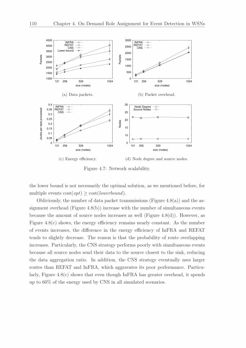
110 Chapter 4. On Demand Role Assignment for Event Detection in WSNs
1000
1500
2000
2500
3000
3500
4000
4500
1024 529 256 121
Packets
size (nodes)
INFRAREFAT
CNSLower bound
(a) Data packets.
0
500
1000
1500
2000
2500
3000
1024 529 256 121
Packets
size (nodes)
INFRAREFAT
CNS
(b) Packet overhead.
0
0.05
0.1
0.15
0.2
0.25
0.3
0.35
0.4
1024 529 256 121
Joule
s p
er
data
pro
cessed
size (nodes)
INFRAREFAT
CNS
(c) Energy efficiency.
5
10
15
20
25
30
1024 529 256 121
Nodes
size (nodes)
Node DegreeSource Nodes
(d) Node degree and source nodes.
Figure 4.7: Network scalability.
the lower bound is not necessarily the optimal solution, as we mentioned before, for
multiple events cost(opt) ≥ cost(lowerbound).
Obliviously, the number of data packet transmissions (Figure 4.8(a)) and the as-
signment overhead (Figure 4.8(b)) increase with the number of simultaneous events
because the amount of source nodes increases as well (Figure 4.8(d)). However, as
Figure 4.8(c) shows, the energy efficiency remains nearly constant. As the number
of events increases, the difference in the energy efficiency of InFRA and REFAT
tends to slightly decrease. The reason is that the probability of route overlapping
increases. Particularly, the CNS strategy performs poorly with simultaneous events
because all source nodes send their data to the source closest to the sink, reducing
the data aggregation ratio. In addition, the CNS strategy eventually uses larger
routes than REFAT and InFRA, which aggravates its poor performance. Particu-
larly, Figure 4.8(c) shows that even though InFRA has greater overhead, it spends
up to 60% of the energy used by CNS in all simulated scenarios.

4.6. Simulation Results 111
0
2000
4000
6000
8000
10000
12000
14000
16000
2 3 4 5 6
Packets
# of events
INFRAREFAT
CNSLower bound
(a) Data packets.
1000
1500
2000
2500
3000
3500
4000
2 3 4 5 6
Packets
# of events
INFRAREFAT
CNS
(b) Packet overhead.
0.08
0.1
0.12
0.14
0.16
0.18
0.2
2 3 4 5 6
Joule
s p
er
data
pro
cessed
# of events
INFRAREFAT
CNS
(c) Energy efficiency.
0
20
40
60
80
100
120
2 3 4 5 6
Nodes
# of events
Node DegreeSource Nodes
(d) Node degree and source nodes.
Figure 4.8: Event scalability.
4.6.6 Event Size
We also evaluate the impact of the event size, i.e., the influence region in which
a sensor node can detect an event. This is accomplished by increasing the event
radius from 50m to 100m and keeping the communication range fixed at 80m. The
results are shown in Figure 4.9.
As a general result, InFRA outperforms REFAT and CNS by reducing the num-
ber of data packet transmissions (Figure 4.9(a)) and, consequently, using the energy
resources more efficiently (Figure 4.9(c)). However, in this evaluation we stress that
when the relation between the event radius and communication range increases, the
overhead introduced by InFRA also increases (Figure 4.9(b)). The reason is that
we eventually have multiple coordinator candidates per event, which occasionally
results in multiple coordinators per event, especially when the number of source
nodes per event increases (Figure 4.9(d)).

112 Chapter 4. On Demand Role Assignment for Event Detection in WSNs
900
1200
1500
1800
2100
2400
2700
3000
50 60 70 80 90 100
Packets
Event radius (m)
INFRAREFAT
CNSLower bound
(a) Data packets.
1050
1060
1070
1080
1090
1100
1110
50 60 70 80 90 100
Packets
Event radius (m)
INFRAREFAT
CNS
(b) Packet overhead.
0.05
0.1
0.15
0.2
0.25
0.3
0.35
0.4
50 60 70 80 90 100
Joule
s p
er
data
pro
cessed
Event radius (m)
INFRAREFAT
CNS
(c) Energy efficiency.
4
6
8
10
12
14
50 60 70 80 90 100
Nodes
Event radius (m)
Node DegreeSource Nodes
(d) Node degree and source nodes.
Figure 4.9: Event size.
4.7 Chapter Remarks
In this chapter, we formalize a role assignment model and propose a reactive al-
gorithm, called InFRA, that starts the assignment process only when an event is
detected, therefore, saving energy during the periods of inactivity. The objective of
this algorithm is to build a routing infrastructure to deliver data to the sink and
increase the data aggregation probability. The proposed scheme is a distributed
heuristic to find a minimum Steiner tree connecting source nodes to the sink.
Our theoretical results show that this heuristic has O(1)-approximation ratio
when the network diameter remains constant and, in large-scale networks it has a
k-approximation ratio.
Our experimental evaluation compares the InFRA algorithm with reactive trees
that use the earliest-first parent selection strategy (REFAT) and the nearest-source
parent selection (CNS). This evaluation covers the assessment of different factors:
network scalability, event scalability, communication range, and event size. The
results show that although the InFRA algorithm presents a higher overhead, it
outperforms REFAT and CNS by finding routes of higher data aggregation ratios. In
some cases, the InFRA algorithm uses only 70% of the energy spent by REFAT, and

4.7. Chapter Remarks 113
for multiple events it uses only 60% of the energy spend by CNS. These experiments
also show how packet losses can affect the performance of a distributed Steiner-tree
heuristic.
The presented evaluation comprehends static events of fixed radius. We plan
to work on the assessment of InFRA when events present dynamic size (events of
increasing and decreasing sizes) and can move across the sensor field.


“Now this is not the end. It is not even the beginning ofthe end. But it is, perhaps, the end of the beginning.”
Sir Winston Churchill (1874 – 1965), Speech inNovember 1942
5Final Remarks
This chapter summarizes the thesis conclusions and future directions. The
objective is to reinforce the contributions we achieved and point out some
possible directions we envision for proceeding the research. In this context,
we first present the thesis conclusions in Section 5.1. Then, in Section 5.3, we
present future directions of this work, and we finish the document by presenting, in
Section 5.4, the list of publications we achieved during the conception of this thesis.
5.1 Conclusions
In this work, we have provided an ample perspective of information fusion in WSNs
by surveying the available state-of-the-art. This survey allows us to understand how
information fusion has been used in WSN, and how it can still be used to address
open issues of WSNs.
Based on the discussion the survey presents, we have proposed a general
framework, called Diffuse, to assist in the design of information fusion tasks in
WSNs. Thus, we do understand that the Diffuse framework is a key contribution
of this thesis. It establishes the steps of a general fusion process that specifies how
raw data can evolved towards a high-level decision. In contrast to the models and
architectures presented in Section 2.4, Diffuse offers a basic API and does not force
the execution of every specified step. Instead, the user can use the resources for data
filtering or decision making individually. In addition, besides the application and
extensions discussed in Chapter 3, we could also use the Diffuse framework to design
115
116 Chapter 5. Final Remarks
the application that runs in the network, such as a target tracking or an event detec-
tion application using an extension of the Kalman Filter and the Dempster-Shafer
reasoning, respectively.
Another contribution of this thesis is the mechanism we propose to make tree-
based routing algorithms more reliable by reconstructing the routing topology only
when critical failures occur. This mechanism, which results from the use of the
Diffuse framework, has two variants: the Sink-Centered Diffuse and the Source-
Centered Diffuse. The results show that energy can be save by determining the
moment when the routing topology needs to be rebuilt, since unnecessary traffic is
avoided. Both variants, the Sink-Centered Diffuse and the Source-Centered Diffuse,
collect data traffic measurements, and based on such measurements, Diffuse uses
information fusion mechanisms (the Moving Average Filter and the Dempster-Shafer
Inference) to determine when the routing topology needs to be rebuilt. In some
cases, the traffic overhead generated by the Source-Centered Diffuse scheme is 85%
smaller than the traffic generated by the Periodic Rebuilding, which is one of the
current solutions adopted to rebuild the routing topology.
The final contribution of this thesis is the InFRA algorithm. The InFRA al-
gorithm saves energy by searching for the shortest paths that maximizes data ag-
gregation, and by starting the assignment process only when an event is detected,
therefore, saving energy during the periods of inactivity. The proposed scheme is
a distributed heuristic to find a minimum Steiner tree connecting the source nodes
to the sink. Theoretical results show that this heuristic has O(1)-approximation
ratio when the network diameter remains constant and, in large-scale networks it
has a k-approximation ratio, where k is the number of simultaneous events. Our
experimental evaluation shows that although the InFRA algorithm presents a higher
overhead, it outperforms other reactive algorithms, such as REFAT and CNS, by
finding routes of higher data aggregation ratios. In some cases, the InFRA algo-
rithm uses only 70% of the energy spent by REFAT, and for multiple events it uses
only 60% of the energy spend by CNS.
5.2 Limitations
Some limitations can be identified in the current state of the research, and such lim-
itations lead to future directions. First, the Diffuse framework specifies a method-
ology, as a guideline, that identifies important steps towards the design of an
information-fusion-based solution in WSNs. Currently, the API (application pro-
gram interface) available is still limited to a few filters, inference methods, and

5.3. Outlook 117
data aggregation techniques that have been used during our experiments. This API
should improve and include new functionalities when new case studies and solutions
are designed and implemented.
The tradeoff between the energy efficiency and the computational cost of the
Source-Centered Diffuse needs a more detailed investigation according to the target
application of the WSN being designed. Different environments and applications
present constraints and requirements that may differ from the ones investigated
in the present work. For some sensor-node architectures, the computational cost of
the Dempster-Shafer may be prohibitive depending on the number of events (states)
being monitored.
The InFRA algorithm represents an improvement on distributed heuristics for
the Steiner problem when we have resource-constrained networks, especially when
energy, memory, and bandwidth are restrictive. However, the current version con-
siders only static events, and the theoretical approximation ratio still needs further
reduction compared to the best centralized heuristics.
5.3 Outlook
Regarding the Diffuse framework, we believe it gives us the opportunity for sev-
eral other applications. For instance, we could use Diffuse to apply information
fusion methods and reduce the errors of the current methods for estimating the
location of the nodes in a WSN [Oliveira et al. 2005a,b]. Possibly, the field of WSNs
more suitable for using the Diffuse framework is actually the design of applications,
especially in event-based scenarios. The reason is that filters, feature maps, and
inference methods are natural candidates for improving data accuracy and making
decisions and inferences about the environment being perceived. A very promis-
ing extension of this work is the integrated use of Diffuse to provide a reliable and
energy-efficient routing algorithm for a network executing an information-fusion ap-
plication that also uses the Diffuse framework to detect events and make inferences
about the environment. For instance, an environmental application to monitor and
track animals in process of extinction.
For the InFRA algorithm, the presented evaluation comprehends only static
events of fixed radius. As we mentioned in Chapter 4, the work could be extended
to scenarios with events of dynamic size (events of increasing and decreasing sizes)
that can move across the sensor field. To be more general, we could redesign the
InFRA strategy when the information-fusion application is more complex than an
in-network data aggregation process. In this case, the role assignment strategy could

118 Chapter 5. Final Remarks
be used to specify local cooperation by defining how nodes exchange data to make,
for instance, high-level inferences and correctly detect events.
5.4 Comments on Publications
We list all the publications (alphabetically sorted by authors) obtained during the
doctorate below. Papers in bold are direct results of this thesis. Other papers result
from the opportunity to interact and apply information fusion concepts to other
research projects.
• Periodical papers
Boukerche, A., Oliveira, H. A. B. F, Nakamura, E. F., Loureiro, A. A.
(2007a). Secure Localization Algorithms and Protocols for Wireless Sen-
sor Networks. IEEE Communications Magazine (accepted).
Boukerche, A., Oliveira, H. A. B. F, Nakamura, E. F., Loureiro, A. A.
(2007b). Localization Systems for Wireless Sensor Networks. IEEE
Wireless Magazine (accepted).
Nakamura, E. F., Loureiro, A. A., Frery, A. C. (2007a). Infor-
mation fusion for wireless sensor networks: Methods, models,
and classifications. ACM Computing Surveys, 39(3):9/1–9/55,
2007.
Nakamura, E. F., Figueiredo, C. M. S., Nakamura, F. G., and
Loureiro, A. A. (2007b). Diffuse: A Topology Building Engine
for Wireless Sensor Networks. Signal Processing, 87(12):2991–
3009, 2007.
Nakamura, E. F., Nakamura, F. G., Figueiredo, C. M., and
Loureiro, A. A. (2005d). Using information fusion to assist
data dissemination in wireless sensor networks. Telecommuni-
cation Systems, 30(1–3):237–254.
• Book chapters
Figueiredo, C. M., Nakamura, E. F., and Loureiro, A. A. (2005a). Self-
organization algorithms for wireless sensor networks. In Boukerche, A.,
editor, Handbook of Algorithms for Wireless and Mobile Networks and
Computing, pages 517–532. Chapman & Hall/CRC Press.

5.4. Comments on Publications 119
Nakamura, E. F., Figueiredo, C. M., and Loureiro, A. A. (2005a).
Information fusion algorithms for wireless sensor networks. In
Boukerche, A., editor, Handbook of Algorithms for Wireless and
Mobile Networks and Computing, pages 841–864. Chapman &
Hall/CRC Press.
• Conferences papers
Boukerche, A., Oliveira, H. A., Nakamura, E. F., Loureiro, A. A. (2007a).
A Novel Lightweight Algorithm for Time-Space Localization in Wireless
Sensor Networks. In Proceedings of the 10-th ACM/IEEE International
Symposium on Modeling, Analysis and Simulation of Wireless and Mobile
Systems (MSWiM’07), pages 336–343, Chania, Greece, October, 2007.
ACM.
Boukerche, A., Oliveira, H. A., Nakamura, E. F., Loureiro, A. A. (2007b). A
Voronoi Approach for Scalable and Robust DV-Hop Localization System
for Sensor Networks. In Proceedings of the 16th IEEE International
Conference on Computer Communications and Networks (ICCCN’07),
pages 497–502, Honolulu, USA, August, 2007. IEEE.
Costa, M. B., Resende, R. F., Segatto, M. V., Nakamura, E. F., and Fonseca,
N. (2007). BASS: Business Application Support through Software Ser-
vices. In Proceedings of the 19th International Conference on Software
Engineering and Knowledge Engineering (SEKE’07), pages 523–528, Hy-
att Harborside, USA, July, 2007.
Figueiredo, C. M., Nakamura, E. F., and Loureiro, A. A. (2004a). Avaliação
de desempenho de algoritmos de disseminação de dados para redes de sen-
sores sem fio. In VI Workshop de Comunicação sem Fio e Computação
Móvel, Fortaleza, pages 1–16, Brazil.
Figueiredo, C. M., Nakamura, E. F., and Loureiro, A. A. (2004b). Multi:
A hybrid adaptive dissemination protocol for wireless sensor networks.
In Proceedings of the 1st International Workshop on Algorithmic As-
pects of Wireless Sensor Networks (ALGOSENSORS 2004), volume 3121
of Lecture Notes in Computer Science, pages 171–186, Turku, Finland.
Springer.
Figueiredo, C. M., Nakamura, E. F., and Loureiro, A. A. (2004c). Protocolo
adaptativo híbrido para disseminação de dados em redes de sensores sem
fio auto-organizáveis. In 22o. Simpósio Brasileiro de Redes de Computa-
dores (SBRC 2004), pages 43–56, Gramado, Brazil. SBC.
120 Chapter 5. Final Remarks
Figueiredo, C. M., Nakamura, E. F., and Loureiro, A. A. (2007). An Event-
Detection Estimation Model for Hybrid Adaptive Routing in Wireless
Sensor Networks. In Proceedings of the 2007 IEEE International Con-
ference on Communications (ICC’07), pages 3887–3894, Glasgow, UK,
June, 2007. IEEE.
Lins, A., Nakamura, E. F., Loureiro, A. A., and Coelho Jr., C. J. (2003a).
Beanwatcher: A tool to generate multimedia monitoring applications for
wireless sensor networks. In Marshall, A. and Agoulmine, N., editors,
Proceedings of the 6th IFIP/IEEE International Conference on Manage-
ment of Multimedia Networks and Services (MMNS 2003), volume 2839
of Lecture Notes in Computer Science, pages 128–141, Belfast, Northern
Ireland. Springer.
Lins, A., Nakamura, E. F., Loureiro, A. A., and Coelho Jr., C. J. (2003b).
Semi-automatic generation of monitoring applications for wireless net-
works. In Proceedings of the 9th IEEE International Conference on
Emerging Technologies and Factory Automation (ETFA 2003), volume 1,
pages 506–511, Lisbon, Portugal. IEEE.
Lins, A., Figueiredo, C. M., Nakamura, E. F., Buriol, L. S., Loureiro,
A. A., Coelho Jr., C. J., and Fernandes, A. O. (2007a). A Sampling
Data Stream Algorithm For Wireless Sensor Networks In Proceedings of
the 2007 IEEE International Conference on Communications (ICC’07),
pages 3207–3212, Glasgow, UK, June. IEEE.
Lins, A., Figueiredo, C. M., Nakamura, E. F., Buriol, L. S., Loureiro, A. A.,
Coelho Jr., C. J., and Fernandes, A. O. (2007b). On The Use Data Re-
duction Algorithms for Real-Time Wireless Sensor Networks In Proceed-
ings of the 2007 IEEE Symposium on Computers and Communications
(ISCC’07), pages 583–588, Aveiro, Portugal, July, 2007. IEEE.
Lins, A., Figueiredo, C. M., Nakamura, E. F., Buriol, L. S., Loureiro, A. A.,
Coelho Jr., C. J., and Fernandes, A. O. (2007c). Data Stream Based
Algorithms For Wireless Sensor Network In Proceedings of the IEEE
21st International Conference on Advanced Information Networking and
Applications (AINA-07), pages 869–876, Niagara Falls, Canada, May,
2007. IEEE.
Nakamura, E. F., Oliveira, H. A., Pontello, L. F., and Loureiro,
A. A. (2006a). Atribuição dinâmica de papéis para agregação
de dados em redes de sensores sem fio. In 24o. Simpósio

5.4. Comments on Publications 121
Brasileiro de Redes de Computadores (SBRC 2005), pages 779–
794, Curitiba, PR, Brasil. SBC.
Nakamura, E. F., Oliveira, H. A., Pontello, L. F., and Loureiro,
A. A. (2006b). On demand role assignment for event-detection
in sensor networks. In Bellavista, P., Chen, C.-M., Corradi, A.,
and Daneshmand, M., editors, Proceedings of the 11th IEEE
International Symposium on Computers and Communication
(ISCC’06), pages 941–947, Cagliari, Italy. IEEE.
Nakamura, E. F., Figueiredo, C. M., and Loureiro, A. A. (2004). Dissemi-
nação adaptativa de dados em redes de sensores sem fio auto-organizáveis.
In 22o. Simpósio Brasileiro de Redes de Computadores (SBRC 2004),
pages 29–42, Gramado, Brazil. SBC.
Nakamura, E. F., Figueiredo, C. M., and Loureiro, A. A. (2005b).
Information fusion for data dissemination in self-organizing
wireless sensor networks. In Lorenz, P. and Dini, P., editors,
Proceedings of the 4th International Conference on Network-
ing (ICN 2005), volume 3420 of Lecture Notes in Computer
Science, pages 585–593, Reunion Island, France. Springer.
Nakamura, E. F., Nakamura, F. G., Figueiredo, C. M., and
Loureiro, A. A. (2005c). Detecção de falhas em redes de
sensores sem fio baseada na medição do tráfego e em técni-
cas de fusão de dados. In 23o. Simpósio Brasileiro de Redes de
Computadores (SBRC 2005), pages 579–592, Fortaleza, Brazil.
SBC.
Oliveira, H. A., Nakamura, E. F., Loureiro, A. A., and Boukerche, A. (2005a).
Directed position estimation: A recursive localization approach for wire-
less sensor networks. In Thuel, S. R, Yang, Y., and Park, E. K., edi-
tors, Proceedings of the 14th IEEE International Conference on Computer
Communications and Networks (IC3N’05), pages 557–562, San Diego,
USA. IEEE.
Oliveira, H. A., Nakamura, E. F., Loureiro, A. A., and Boukerche, A. (2005b).
Error analysis of localization systems in sensor networks. In Shahabi, C.
and Boulcema, O., editors, Proceedings of the 13th ACM International
Symposium on Geographic Information Systems (ACM-GIS’05), pages
71–78, Bremen, Germany. ACM.

122 Chapter 5. Final Remarks
Oliveira, H. A., Nakamura, E. F., Loureiro, A. A., and Boukerche, A. (2007a).
Localization in Time and Space for Sensor Networks In Proceedings of the
IEEE 21st International Conference on Advanced Information Network-
ing and Applications (AINA-07), pages 539-546, Niagara Falls, Canada,
May, 2007. IEEE.
Oliveira, H. A., Nakamura, E. F., Loureiro, A. A., and Boukerche, A. (2007b).
Towards an Integrated Solution for Node Localization and Data Rout-
ing in Sensor Networks In Proceedings of the 2007 IEEE Symposium
on Computers and Communications (ISCC’07), pages 449–454, Aveiro,
Portugal, July, 2007. IEEE.
• Tutorials
Nakamura, E. F., Loureiro, A. F., (2008). Information fusion in
wireless sensor networks. In IEEE 8th International Conference
on Computer and Information Technology (CIT’08), Sydney,
Australia (to be presented in July 2008).
Loureiro, A. F., Nogueira, J. M. S., Ruiz, L. B., de Freitas Mini, R. A.,
Nakamura, E. F., and Figueiredo, C. M. S. (2003). Redes de sensores sem
fio (minicurso). In 21o Simpósio Brasileiro de Redes de Computadores
(SBRC 2003), Natal, Brazil. SBC.
Ruiz, L. B., Correia, L. H. A., Vieira, L. F. M., Macedo, D. F., Nakamura,
E. F., Figueiredo, C. M. S., Vieira, M. A. M., Bechelane, E. H., Camara,
D., Loureiro, A. A., Nogueira, J. M. S., da Silva Jr., D. C., and Fernandes,
A. O. (2004). Arquiteturas para redes de sensores sem fio (minicurso). In
22o Simpósio Brasileiro de Redes de Computadores (SBRC 2004), pages
167–218, Gramado, Brazil. SBC.
• Papers under evaluation:
Nakamura, E. F., Oliveira, H. A., and Loureiro, A. A. (2007c).
InFRA: An Information-Fusion-Based Role Assignment for
Event-Driven Sensor Networks. Computer networks, (submit-
ted).

“It’s very dangerous for kids though, because they getreally small.”
Steve Martin (1945 – ), Let’s Get Small
AWireless Sensor Networks:
An Information Fusion Perspective
This appendix presents the main tasks or activities executed in a WSN.
These tasks are organized based on their purposes: Network Organization,
Data Communication, Data Management, and Network Management. Each
task is examined through an information fusion perspective, which points out how
information fusion can be related to such tasks. This analysis has two different
perspectives:
Information fusion as a leading role. The application running in the network
is essentially an information fusion application, such as target detection and
aggregated queries retrieval. In this case, we try to investigate how the task
being analyzed is affected by the information fusion application.
Information fusion as a supporting role. Information fusion is seen as a sup-
porting mechanism for other tasks. In this case, we try to identify how the
task being analyzed can use information fusion techniques to improve its per-
formance.
A.1 Network Organization
This group includes all activities directly related to the network organizational as-
pects. These aspects can be structural (e.g., location discovery and node scheduling)
123

124 Appendix A. Wireless Sensor Networks: An Information Fusion Perspective
or logical (e.g., mobility coordination, role assignment, topology organization, and
node placement).
A.1.1 Location Discovery
The location problem consists in finding the geographic location of the nodes in a
WSN, and the location can be computed by a central unit [Doherty et al. 2001]
or by sensor nodes in a distributed manner [Savvides et al. 2002; Niculescu and
Nath 2001; Savarese et al. 2001]. Essentially, location discovery can be split in two
stages: distance estimation and location computation [Savarese et al. 2001]. Usu-
ally, distance between two nodes is estimated based on methods, such as Received
Signal Strength Indicator (RSSI), Time of Arrival (ToA), and Time Difference of
Arrival (TDoA) [Savarese et al. 2001]. Once the distance is estimated, at least three
methods (Figure A.1) can be used to compute the node location: Multilateration,
Trilateration, and Triangulation [Gibson 1999]. Another method to estimate the
node location is called the Angle of Arrival (AoA) , which uses the angle in which
the received signal arrives and the distance between the sender and receiver.
A
bc
a B
C
(a) (b) (c)
Figure A.1: Position estimation methods: (a) triangulation, (b) trilateration, and(c) multilateration (adapted from Savvides et al. [2001]).
RSSI, ToA, and TDoA methods are subject to noise and environmental inter-
ference. Therefore, it is not possible to assure the precision of their estimates. In
this context, information fusion can be applied in two different ways to reduce the
impact of bad estimates. First, the estimates provided by RSSI, ToA, and TDoA
methods can be fused to improve the distance estimate before computing the node
location. Second, this computed estimate could be fused with an AoA estimate to
obtain refined coordinates.
Kleine-Ostmann and Bell [2001] use a similar approach to solve the location
problem for cellular network fusing ToA and TDoA estimates with the Least Square
method, and fusing location estimates with a Bayesian fuser. The Kalman filter is
used by Savvides et al. [2002] to refine the initial location estimates computed by
the sensor nodes.
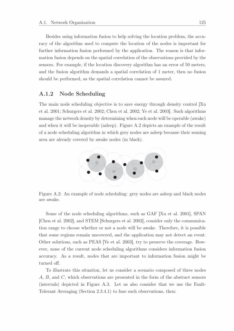
A.1. Network Organization 125
Besides using information fusion to help solving the location problem, the accu-
racy of the algorithm used to compute the location of the nodes is important for
further information fusion performed by the application. The reason is that infor-
mation fusion depends on the spatial correlation of the observations provided by the
sensors. For example, if the location discovery algorithm has an error of 50 meters,
and the fusion algorithm demands a spatial correlation of 1 meter, then no fusion
should be performed, as the spatial correlation cannot be assured.
A.1.2 Node Scheduling
The main node scheduling objective is to save energy through density control [Xu
et al. 2001; Schurgers et al. 2002; Chen et al. 2002; Ye et al. 2003]. Such algorithms
manage the network density by determining when each node will be operable (awake)
and when it will be inoperable (asleep). Figure A.2 depicts an example of the result
of a node scheduling algorithm in which grey nodes are asleep because their sensing
area are already covered by awake nodes (in black).
Figure A.2: An example of node scheduling: grey nodes are asleep and black nodesare awake.
Some of the node scheduling algorithms, such as GAF [Xu et al. 2001], SPAN
[Chen et al. 2002], and STEM [Schurgers et al. 2002], consider only the communica-
tion range to choose whether or not a node will be awake. Therefore, it is possible
that some regions remain uncovered, and the application may not detect an event.
Other solutions, such as PEAS [Ye et al. 2003], try to preserve the coverage. How-
ever, none of the current node scheduling algorithms considers information fusion
accuracy. As a result, nodes that are important to information fusion might be
turned off.
To illustrate this situation, let us consider a scenario composed of three nodes
A, B, and C, which observations are presented in the form of the abstract sensors
(intervals) depicted in Figure A.3. Let us also consider that we use the Fault-
Tolerant Averaging (Section 2.3.4.1) to fuse such observations, then:

126 Appendix A. Wireless Sensor Networks: An Information Fusion Perspective
A
B
C
M02 (A,B)
M02 (A,C)
M02 (B,C)
Figure A.3: The influence of node scheduling in the fusion task using the Fault-Tolerant Averaging (Section 2.3.4.1).
• If node A is turned off, the fused result will beM02 (B,C);
• If node B is turned off, the fused result will beM02 (A,C);
• If node C is turned off, the fused result will beM02 (A,B).
Note that the width (accuracy) of the fused result depends on which sensor is
used. If the node scheduling algorithm turns off node C the fused result will be
more accurate compared to the result when nodes A or B are turned off. Thus,
information fusion can become less accurate if the wrong nodes are turned off.
A.1.3 Mobility Coordination
Node mobility can be controllable (programmable or predictable) or uncontrollable
(unpredictable or undesirable). In the first situation, the nodes can be coordinated
so they move themselves to strategic locations to improve the performance of the
fusion task, or adapt the network to the environmental dynamics. An example of
mobility coordination supporting the fusion task is the SPRING algorithm [Das-
gupta et al. 2003] that searches for the best node placement and role assignment.
In addition, mobility coordination may be used to fix the roles and migrate the
necessary nodes instead of their roles. This might be of interest in heterogeneous
networks in which the mobile nodes are not strong resource-limited (e.g., energy,
processing, and memory are not a problem).
Node mobility must be carefully used due to the restrictions identified by Kansal
et al. [2004]: it requires the capacity of accurately determining their locations and
navigating across the deployed terrain; errors in the node location introduce extra
complications for the sensing and detection algorithms; and the energy spent to
physically move the node on arbitrary terrain might be prohibitive.

A.1. Network Organization 127
The mobility coordination can be reactive or proactive. In the first case, the
occurrence of an event might trigger the reorganization of the mobile nodes, which
should move themselves to the location that provides the best results for information
fusion. In the second case, mobile nodes may evaluate historical data (information
fusion may be applied to make inferences about these data) and identify critical
areas (e.g., uncovered areas or areas covered only by low precision sensor nodes), so
they explore such areas to overcome possible weaknesses before an event occurs.
Node mobility may be expensive and impracticable (e.g., due to the environment
restrictions). Thus, it might be interesting to change (move) the roles of the nodes
instead of moving them physically. Hence, a dynamic role assignment may replace
the node mobility in a WSN.
A.1.4 Role Assignment
The role of a node in the network might change over time, sometimes due to the
application dynamics and other times due to the state (health) of the nodes [Kumar
et al. 2003]. Optimal role assignment is a challenge that must be autonomously per-
formed by the network to achieve the application goals. Furthermore, it is necessary
to define what is an optimal role assignment, and which aspects of the WSN are
used to weigh the role assignment. A natural answer regarding the energy usage is
that the optimal role assignment leads to the longest lifetime of the network. One
idealistic scenario for the role assignment problem can be described as follows. First,
the network is deployed, no topology is formed and no role is assigned. Then, when
an event is detected, the network instantly assigns the roles without exchanging any
message, and this role assignment is optimal in the sense that the best possible qual-
ity of the fused information is achieved using the lowest possible amount of energy.
Fusion role should be as close as possible to the event to increase the correlation
probability among the data and reduce the network traffic (assuming that fusion
results in data reduction not data expansion). Thus, as events can occur with any
intensity, anywhere in the sensor field, at any time, an a priori role assignment might
reduce the fusion performance as it cannot perfectly predict the event behavior.
The definition of the roles may vary. Common roles for flat networks are: sink,
relay (routing nodes), aggregator, and sensor (Figure A.4(a)). For hierarchical net-
works, typical roles include: sink, cluster-head (which might be responsible for
information fusion) and sensor (Figure A.4(b)). In some cases, a node might be
assigned more than one role. For example, in networks with data centric routing, a
node may aggregate sensing, relay, and fusion roles at the same time.
Bhardwaj and Chandakasan [2002] derive upper bounds on the lifetime of WSNs

128 Appendix A. Wireless Sensor Networks: An Information Fusion Perspective
sink
relay
relay
aggregator
sensor
sensor
sensor
(a)
sink
cluster-head
sensor
sensor
sensor
(b)
Figure A.4: An example of role assignment in WSNs: (a) flat networks and (b)hierarchical networks.
that perform information fusion. In this case, three roles are identified: sensor (a
node that senses and generates data packets), relay (a node that forwards data
packets with no data processing), and aggregator (a node that fuses two or more
data streams into a single stream). Then, the optimal role assignment is modelled as
a linear problem that finds the role assignment that maximizes the network lifetime.
The authors also provide examples comparing the lifetime bounds of networks that
perform data fusion and networks that do not.
Dasgupta et al. [2003] define two roles in a WSN: sensor and relay (a node
that aggregates and forwards data packets). They address the problem of placing
nodes and assigning roles to them so the system lifetime is maximized, ensuring that
the region of interest is covered by at least one sensor node. This solution, called
Sensor Placement and Role Assignment for Energy-Efficient Information Gathering
(SPRING), moves the nodes across the field and assigns roles (sensor or relay) to
them in such a way that the region of interest is covered by the minimum number
of nodes with the sensor role. The relay role is assigned to all other nodes that are
not in the region of interest. SPRING presents a lifetime up to 49% greater than
a random placement and role assignment. The weakest point of SPRING is that it
needs to be computed a priori, or the nodes must have controlled mobility. Besides,
SPRING tries to maximize the system lifetime regardless of the uncertainty of the
resulting information.
The DFuse framework proposed by Kumar et al. [2003] addresses the role assign-
ment problem providing two modules: fusion module and placement module. The
fusion module allows the application to be built using a dataflow graph that specifies

A.1. Network Organization 129
the roles of each node in the graph. The placement module maps this graph onto
the network and dynamically adapts the mapping by migrating the roles according
to a specified cost function. DFuse use the same roles defined by Bhardwaj and
Chandakasan [2002]. The role assignment is provided by a heuristic divided in three
phases. The first creates a tree with a naive role assignment. In the second, the
nodes exchange their health information (an indicator of how well the node hosts
that role) and the role is transferred to the neighbor with the best health regarding
a given cost function. The third is a maintenance phase similar to the optimization
phase, i.e., the same role transfer semantics is adopted. Theoretically, DFuse can in-
clude the information quality in the cost function, although this is not mentioned by
the authors. However, the main criticism about DFuse is that it is not yet supported
by the current sensor nodes, such as the Mica family [Crossbow 2004].
Dynamic role assignment may be implemented by parameterized algorithms,
so every node has all roles implemented, and based on the parameters (dynam-
ically defined) it chooses the proper role. Another possibility is the use of the
paradigm of mobile agents and active networks present in frameworks, such as Sen-
sorWare [Boulis et al. 2003b] and Maté [Levis and Culler 2002], which allow code
migration. In this case, the role itself can migrate through the network as agents or
active packets.
A.1.5 Topology Organization
The topology organization of the network (flat or hierarchical) impacts on the way
communication is performed and fusion role is assigned. For a flat network (Fig-
ure A.5(a)), simple aggregation roles (e.g., maximum and minimum) are commonly
used, and every node in the network computes the aggregation function with the
received and sensed data during the routing phase [Kalpakis et al. 2003; Krishna-
machari et al. 2002; Intanagonwiwat et al. 2000; Zhou and Krishnamachari 2003].
However, for more sophisticated fusion methods, such as the ones for target de-
tection, fusion must be performed by the nodes that detect the event (close to the
event), not by distant nodes because such nodes may receive uncorrelated data from
distant regions.
In hierarchical networks (Figure A.5(b)), the cluster-head is usually responsible
for receiving data from the sensors of its cluster, fusing all data, and sending the
results towards the sink node [Heinzelman et al. 2000; Lindsey et al. 2002; Deb
et al. 2002]. In this class of networks, the way the clusters are formed impacts on
the performance of information fusion. For example, in widely spaced clusters it
might be difficult to correlate the data from all cluster members. The hierarchical

130 Appendix A. Wireless Sensor Networks: An Information Fusion Perspective
sink
(a)
cluster
cluster
sink
(b)
Figure A.5: Topology organization: (a) flat networks and (b) hierarchical networks.
topology should be built and rebuilt considering information fusion performance as
a factor that impacts on the overall system’s performance. Another issue is that,
in some cases, an event is detected by nodes from different clusters. Information
fusion should be more effective if a new cluster is built with all nodes that detected
such an event. To the best of our knowledge, there is no strategy for hierarchy
formation that adapts itself (reorganizing the clusters) to improve the information
fusion performance when an event is detected.
A.1.6 Node Placement
In some applications, instead of throwing the sensor nodes on the environment
(e.g., by airplane), they can be strategically placed in the sensor field according
to an a priori planning. In this approach, there is no need to discover the nodes’
location. However, good planning depends on the knowledge of the terrain and
the environmental particularities that might interfere in the operation of the sensor
nodes and the quality of the gathered data.
The node placement problem has been addressed using different approaches
[Dhillon et al. 2002; Chakrabarty et al. 2002; Biagioni and Sasaki 2003]. How-
ever, current solutions are basically concerned with assuring spatial coverage while
minimizing the energy cost. Putting aside the importance of strategically placing
the fusing nodes may lead to performance losses regarding the quality of collected
data and the application objectives. To the best of our knowledge, the SPRING
algorithm is the only node placement algorithm that involves information fusion.
However, SPRING also migrates the fusion role. In a previous planning, besides
spatial coverage [Dhillon et al. 2002; Biagioni and Sasaki 2003], other aspects should
be considered, such as node diversity [Chakrabarty et al. 2002] and the fusion per-
formance.
The relationship between node placement and information fusion is closely re-

A.2. Data Communication 131
lated to role assignment, i.e., nodes can be strategically placed in such a way that
the fusion points can achieve the best results in terms of data quality and energy
efficiency. Improper node placements may lead to the degradation of information
fusion as illustrated by Hegazy and Vachtsevanos [2003].
A.2 Data Communication
This section discusses the use of information fusion techniques with communication
tasks in the physical, link, network, and transport layers. In data-centric networks,
information fusion is commonly performed along the routes used in data routing.
Therefore, information fusion is tightly coupled with the data routing task.
A.2.1 The Physical Layer
The physical layer is responsible for the physical transmission and reception of bits.
It encompasses, for instance, modulation (e.g., FSK and GFSK) and encoding (e.g.,
NRZ and Manchester) techniques. In this case, it is difficult to find a way to design
a data-centric physical layer that exploits the synergy of information gathered by
sensors. This situation arises from the fact that the physical layer does not access
the semantics of what is being sent or received.
A.2.2 The Link Layer
The Link or Medium Access Control (MAC) layer controls the node access to the
communication medium by means of techniques such as contention [Woo and Culler
2001; Polastre et al. 2004] and time division [Ye et al. 2002; Rajendran et al. 2003].
Basically, the MAC layer must manage the communication channels available for the
node avoiding collisions and errors in the communication. One possibility to make
the MAC layer data-centric is to bring activities, such as topology discovery and
maintenance, to this layer. Thus, if the application uses a tree topology to retrieve
the average temperature in the sensor field, the MAC layer can optimize the channel
allocation for a tree topology. For instance, using a Time Division Multiple Access
(TDMA) scheme, the time slots of a given node can be allocated only for its parent
and children nodes (instead of all neighbors). In this case, we can compute the
aggregation function in the MAC layer, simplifying the design of routing protocols.
As a side effect, this approach makes the MAC layer application-specific reducing
its reusability.

132 Appendix A. Wireless Sensor Networks: An Information Fusion Perspective
Another possibility is to include in the MAC layer compression mechanisms that
take advantage of the data correlation, such as DISCUS (Section 2.3.6.1). In addi-
tion, the compression and decompression tasks may be implemented by hardware
improving the performance regarding the delay and energy consumption.
Fusion methods may be used on any data besides sensor observations. For exam-
ple, consider a MAC protocol that samples the channel to determine what is noise,
so the node can avoid transmitting under noisy conditions. In this case, estimation
methods (e.g., Kalman Filter) may be used to accurately estimate the noise. Fur-
thermore, an inference method (e.g., Bayesian inference) may be used to decide if
the current condition is suitable for transmission or not. To determine whether or
not the applicability of fusion methods in such situations is feasible, we must evalu-
ate the computational cost of the fusion algorithms, the resultant delay, the energy
consumed, and the impact on the quality of the service provided by the MAC layer.
A.2.3 The Network Layer
The network layer is responsible for finding paths (routes) to be used in data com-
munication. For WSNs, the network layer behavior is usually different from the
traditional networks. Three communication patterns are common in WSNs:
Local collaboration. When an event occurs in the network, nodes may perform
in-network processing exchanging messages with their neighbors, as depicted
in Figure A.6(a). Also, nodes may perform local collaboration (with neigh-
bors only) to exchange health information to support other activity, such as
topology maintenance or information fusion.
Source reporting. When a local event is detected and nodes report data, commu-
nication flows from source nodes towards one or more sink nodes, as depicted
in Figure A.6(b). Messages from different nodes may be fused along the way.
Sink publishing. In some cases, the sink node needs to publish information to all
nodes or a group of nodes. This communication pattern is used by the sink
node to publish interests or to query the network, as depicted in Figure A.6(c).
These patterns may not use the routing structure of the protocols for ad hoc
network, such as DSR [Johnson and Maltz 1996] or AODV [Perkins and Royer
1999]. For the first pattern, a simple unicast/broadcast may solve the problem.
For the second, little information needs to be maintained. For example, in a tree
structure each node must keep track only of its parent. For the third pattern, the

A.2. Data Communication 133
sink
event
(a)
sink
event
(b)
sink
event
(c)
Figure A.6: Communication patterns in WSNs: (a) local collaboration, (b) sourcereporting, (c) sink publishing.
sink node may flood the network with its information, as in the Directed Diffusion
algorithm [Intanagonwiwat et al. 2000].
The network layer is tightly coupled with information fusion because it addresses
the problem of delivering the sensed information to the sink node(s), and it is natural
to think of performing the fusion while the pieces of data become available. However,
the way information is fused depends on the network organization (flat or hierarchi-
cal), which directly affects how the role can be assigned. Hierarchical networks are
organized into clusters where each node responds only to its respective cluster-head,
which might perform special operations such as data fusion/aggregation. In flat net-
works, communication is performed hop-by-hop and every node may be functionally
equivalent.
For the hierarchical topology several algorithms are provided in the literature.
LEACH [Heinzelman et al. 2000] is a cluster-based protocol that randomly rotates
the cluster-heads to evenly distribute the energy load among the sensors in the
network. PEGASIS [Lindsey et al. 2002] is an improvement of LEACH in which
sensors form chains, and each node communicates only with a close neighbor and
takes turns to transmit messages to the sink node. Deb et al. [2002] propose the
TopDisc algorithm that organizes the network into a tree of clusters. In these
hierarchical, solutions clusters are formed and the fusion task is performed by the
cluster-head. The main disadvantage of this approach is that the fusion performance
is not considered by the cluster formation and, consequently, the resultant clusters
may not be the best choice once an event arises.
While in hierarchical topologies only the cluster-heads perform data fusion, in flat
topologies any node may fuse or aggregate data. Directed Diffusion [Intanagonwi-
wat et al. 2000] is a pioneer protocol that tries to find the best paths from sources to
sink nodes that might receive data from multiple paths with different data delivery
frequencies. If the best path fails, another path with lower data delivery frequency
assures the data delivery. Ganesan et al. [2001] propose a routing solution, which
134 Appendix A. Wireless Sensor Networks: An Information Fusion Perspective
evolved from Directed Diffusion, that tries to discover and maintain alternative
paths, connecting sources to sinks, to make the network more fault-tolerant. Al-
though Directed Diffusion introduces the data-centric approach by supporting fusion
in the network layer, no special consideration is stated in the sense of how to fuse
and achieve the best result.
A natural routing scheme for flat networks is the formation of routing trees.
Krishnamachari et al. [2002] provide analytical bounds on the energy costs and
savings that can be obtained with data aggregation using tree topologies. Zhou and
Krishnamachari [2003] evaluate the tree topology with four different parent selection
strategies (earliest-first, randomized, nearest-first and weighted-randomized) based
on the metrics, such as node degree, robustness, channel quality, data aggregation,
and latency. Tian and Georganas [2003] identify drawbacks of pure single-path and
multipath routing schemes in terms of packet delivery and energy consumption.
A common consideration in the above algorithms for flat networks is that infor-
mation fusion is performed whenever two or more data are available, maximizing
the energy savings. However, it might be meaningless to fuse data acquired in the
eastern quadrant with data acquired in the western (uncorrelated data).
Another interesting solution for routing in flat networks is the Data Funneling
presented by Petrovic et al. [2003]. In this algorithm, the sink node publishes (by
flooding) the region that it is interested in monitoring (target region). During this
phase, a routing tree is formed connecting the nodes that are not in the target region
(the relay nodes). Once the border nodes (nodes inside the target region that are
neighbors of relay nodes) receive the sink interest, they become a sort of local sink
node and flood their interests for the remaining nodes within the target region. Once
the topology is formed, every event (or, alternatively, sensor observation) inside the
target region is forwarded to the border nodes that fuse the information and send
the results towards the sink node.
A positive point of Data Funneling is that the region sizes may be dimensioned
in such a way that the sensors within the target region are likely correlated. The
case when an event occurs in the frontier of two target regions must be considered,
because the two regions are correlated and their information should be fused.
A.2.4 The Transport Layer
In general, transport protocols are concerned with the provision of a reliable com-
munication service for the application layer. This is the main objective of Pump
Slowly, Fetch Quickly (PSFQ) protocol [Wan and Campbell 2002]. PSFQ is an adap-
tive protocol that makes local error correction using hop-by-hop acknowledgement.

A.3. Data Management 135
In this case, the adaptation means that under low failure rates, the communica-
tion is similar to a simple forward, and when failures are frequent, it presents a
store-and-forward scheme. Another transport protocol that tries to provide reli-
able communication is the Reliable Data Transport in Sensor Networks (RMST)
[Stann and Heidemann 2003] that also implements a hop-by-hop acknowledgement.
However, RMST is designed to operate in conjunction with Directed Diffusion.
An interesting approach is introduced by the Event-to-Sink Reliable Transfer
(ESRT) protocol [Sankarasubramaniam et al. 2003]. This protocol is designed for
event-based sensor networks, and it changes the focus of traditional transport pro-
tocols. The authors state that for WSNs a transport protocol should be reliable
regarding the event detection task. ESRT assumes that an event must be detected
when the sink node receives a minimum number of event reports from sensor nodes.
If this threshold is not achieved, the sink node does not recognize the event. Thus,
ESRT adjusts the transmission rate of each node in such a way that the desired
threshold is achieved and the event is reliably detected.
It is natural to think of using information fusion instead of tuning the number of
messages, to make the event detection (or data gathering) reliable. Of course, there
are factors, such as the computational capacity and the energy consumption of the
algorithms, that will determine whether or not the information fusion is feasible.
A.3 Data Management
In the context of this work, activities of data management refer to how data acquired
from sensors are manipulated. Thus, strategies for data storage and query processing
will be discussed in the context of information fusion for wireless sensor networks.
A.3.1 Query Processing
Different solutions explore the query approach using in-network processing to fil-
ter and/or aggregate the data during the routing process. Directed Diffusion [In-
tanagonwiwat et al. 2000] introduces the concept of interests to specify which data
will be delivered through a publish/subscribe scheme, but no query language is
specified.
Another possibility is to model the sensor network as a database so data access
is performed by declarative queries. TinyDB [Madden et al. 2005] provides a sim-
ple query language to specify the data of interest. The Cougar Project [Yao and
Gehrke 2002] handles the network as a distributed database in which each piece of
data is locally stored in a sensor node and data is retrieved performing aggrega-

136 Appendix A. Wireless Sensor Networks: An Information Fusion Perspective
tion along a query tree. Sensor Information Networking Architecture (SINA) [Shen
et al. 2001] is a cluster-based architecture that abstracts a WSN as a dense col-
lection of distributed objects where users access information through declarative
queries and execute tasks through programming scripts. Temporal coherency-aware
in-Network Aggregation (TiNA) [Sharaf et al. 2003] uses temporal coherency toler-
ances to reduce the communication load and improve quality of data when not all
sensor readings can be propagated within a given time constraint.
A.3.2 Data Storage
Data storage is closely related to the routing (data retrieval) strategy. In the Cougar
database system, stored data is represented as relations while sensor data is repre-
sented as time series. A query formulated over a sensor network specifies a persistent
view, which is valid during a given period [Bonnet et al. 2001]. Shenker et al. [2003]
introduce the concept of data-centric storage, which is also explored by Ratnasamy
et al. [2003] and Ghose et al. [2003]. In this approach, relevant data is labeled
(named) and stored by the sensor nodes. Data with the same name are stored by
the same sensor node. Queries for data with a particular name are sent directly to
the node storing that named data, avoiding the flooding of interests or queries.
In data-centric storage, information fusion may be used during the storing phase,
i.e., the data being stored may be fused with the data already stored in the sensor
node. In this case, the correlation problem is still an issue, and although the data
structure used to store may consider geographical information guaranteeing spatial
correlation [Ratnasamy et al. 2003], other solutions should be proposed to optimize
the tradeoff between data quality and energy consumption.
A.4 Network Management
This section includes the tasks and activities responsible for tracking the perfor-
mance of the network and tuning its operation according to the desired quality
of service (QoS) and available resources. In addition, network management tasks
should track the resource utilization in the network balancing the tradeoff between
QoS and the resource usage.
A.4.1 Network Health
An important issue underlying WSNs is the monitoring of the network itself, i.e.,
the sink node needs to be aware of the health of all the sensors. Jaikaeo et al. [2001]

A.4. Network Management 137
defines diagnosis as the process of monitoring the state of a sensor network and
figuring out the problematic nodes. This is a management activity that assesses
the network health, i.e., how well the network elements and the resources are being
applied.
Managing individual nodes in a large scale WSN may result in a response implo-
sion problem that happens when a high number of replies are triggered by diagnostic
queries. Jaikaeo et al. [2001] suggest the use of three operations, built on the top
of the SINA architecture [Shen et al. 2001], to overcome the implosion problem:
sampling, self-orchestrated, and diffused computation. In a sampling operation, in-
formation from each node is sent to the manager without intermediate processing.
To avoid the implosion problem, each node decides whether or not it will send its
information based on a probability assigned by the manager (based on the density).
In a self-orchestrated operation, each node schedules its replies. This approach in-
troduces some delay, but reduces the collision chances. In a diffused computation,
mobile scripts are used (enabled by SINA architecture) to assign diagnosis logic to
sensor nodes so they know how to perform information fusion and route the re-
sult to the manager. Although diffused computation optimizes bandwidth use, it
introduces greater delay and the resultant information is less accurate. The three
operations provide different levels of granularity and delay, therefore they should
be used in different stages: diffused computation and self-orchestrated operations
should be continuously performed to identify problems, and sampling should be used
to identify problematic elements.
Hsin and Liu [2002] propose a two-phase timeout system to monitor the node
liveliness. In the first phase, if a node (A) receives no message from a neighbor (D)
in a given period of time (monitoring time), A assumes that D is dead, entering in
the second phase. Once in the second phase, during another period of time (query
time) A queries its neighbors about D; if any neighbor claims that D is alive, then
A assumes it was a false alarm and discards this event. Otherwise, if A does not
hear anything before query time expires, it assumes that D is really dead, firing
an alarm. This monitoring algorithm can be seen as a simple information fusion
method for liveliness detection where the operator (fuser) is a logical OR with n
inputs such as input i is true if neighbor i considers that D is alive and otherwise
false.
Zhao et al. [2003b] propose a three-level health monitoring architecture for WSN.
The first level includes the digests that are aggregates of some network property,
like minimum residual energy. The second comprises the network scans, a sort
of feature map that represents abstracted views of resource utilization within a
section of the (or entire) network [Zhao et al. 2002b]. Finally, the third is composed

138 Appendix A. Wireless Sensor Networks: An Information Fusion Perspective
by node dumps that provide detailed node states over the network for diagnosis.
In this architecture, digests should be continuously computed in background and
piggybacked in neighbor-to-neighbor communication. Once an anomaly is detected
in the digests, a network scan may be collected to identify the problematic sections
in the network. Finally, dumps of problematic sections can be requested to identify
what is the problem. The information granularity increases from digests to dumps,
and the finer the granularity, the greater the cost. Therefore, network scans and,
especially, dumps should be carefully used.
As we can see, information fusion is well related with the network health as-
sessment. It can be used to avoid false alarms by means of event correlation [Hsin
and Liu 2002] or provide cheap global aggregates — e.g., digests [Zhao et al. 2003b]
— and more expensive feature maps — e.g., energy maps [Zhao et al. 2002b; Mini
et al. 2004]. In addition, detailed information (e.g., dumps) provides the symptoms
of a problem, information fusion can be used to infer which problem causes those
symptoms.
A.4.2 Coverage and Exposure
Coverage (spatial) comprises the problem of determining the area covered by the
sensors in the network [Dhillon et al. 2002; Chakrabarty et al. 2002; Li et al. 2003b;
Meguerdichian et al. 2001a]. Coverage allows the identification of regions that can
be properly monitored and regions that cannot. This information associated with
the energy map [Zhao et al. 2002b] can be used to schedule sensor nodes to optimize
the network lifetime without compromising the quality of the gathered information.
Meguerdichian et al. [2001a] define coverage in terms of the best case (regions
of high observability) and the worst case (regions of low observability), and it is
computed in a centralized fashion by means of geometric structures (Delaunay tri-
angulation and Voronoi diagram) and algorithms for graph searching. Li et al.
[2003b] extend this work considering a sensing model in which the sensor accuracy
is inversely proportional to the distance to the sensed event, and provide distributed
algorithms to compute the best case of coverage and the path of greater observabil-
ity. Chakrabarty et al. [2002] compare coverage to the Art Gallery Problem (AGP),
which consists in finding the smallest number of guards to monitor a whole art
gallery. Dhillon et al. [2002] consider coverage as the lowest detection probability
of an event by any sensor. Exposure is closely related with coverage and it specifies
how well an object, moving arbitrarily, can be observed by the WSN over a period
of time [Megerian et al. 2002].
As coverage and exposure provide information about observability, the fusion

A.4. Network Management 139
role may be assigned to areas of lower observability, possibly combining data of
neighbor regions to increase the quality of data gathered in such areas.
A.4.3 Security
Although information fusion can reduce communication overhead significantly, fus-
ing data packets makes security assurance more complex. The reason is that inter-
mediate nodes can modify, forge, or drop data packets. Data encryption cannot be
done source-to-sink because the intermediate nodes must understand the data to
perform information fusion.
Hu and Evans [2003] present a protocol to provide secure aggregation for flat
WSNs that is resilient to intruder devices and single device key compromises, but
their protocol may become vulnerable when a parent and a child node are compro-
mised. The Energy-efficient and Secure Pattern-based Data Aggregation protocol
(ESPDA) [Cam et al. 2003] is a secure protocol for hierarchical sensor networks that
does not require the encrypted data to be decrypted by cluster-heads to perform
data aggregation. In ESPDA, the cluster-head first requests nodes to send the cor-
responding pattern code for the sensed data. If the same pattern code is sent to the
cluster-head by different nodes, then only one of them is allowed to send its data.
The pattern code is generated based on a seed provided by the cluster-head. No spe-
cial fusion method is actually applied in the ESPDA protocol, which simply avoids
the transmission of redundant data, so any information fusion must be performed by
the sensor nodes, not the cluster-head. Secure Information Aggregation in Sensor
Networks (SIA) [Przydatek et al. 2003] presents a fuse-commit-prove approach in
which fuser nodes need to prove that they perform fusion tasks correctly. To avoid
cheating by fuser nodes, SIA adopts cryptographic techniques of commitments, and
provides random sampling mechanisms and interactive proofs to allow the user to
verify the data given by fuser nodes, even when the fuser nodes or some sensor nodes
are corrupted.
Information fusion in WSNs poses severe security challenges, yet it has been
little explored. In heterogeneous networks, we can conceive that only some special
nodes play the fusion role (fuser nodes), in this case, data encryption might be
performed source-to-fuser, such that intermediate nodes play the simple relay role
without any need to access the packets being forwarded. However, it is important
to evaluate the security-energy tradeoff, which might be intensified by information
fusion. In addition, we still expect to see security proposals following the “data-
centric” approach introduced by Directed Diffusion [Intanagonwiwat et al. 2000].

140 Appendix A. Wireless Sensor Networks: An Information Fusion Perspective
A.5 Remarks
The fusion technique affects the overall system performance. However, in all groups
of tasks explored above (network organization, data communication, data manage-
ment, and network management), finding the best nodes to perform information
fusion is critical to achieve data quality and energy efficiency. Therefore, a key
issue to improve information fusion quality is the sensor configuration. This sen-
sor configuration may be logical (e.g., role assignment, network organization, and
communication algorithms) or physical (e.g., node placement and node scheduling
algorithms).
Regarding information fusion as a supporting role, we understand that any task
that needs to filter, make predictions or inferences about an entity, might use infor-
mation fusion methods. However, we must evaluate if the cost of the fusion solution
is affordable by the current models of sensor nodes.
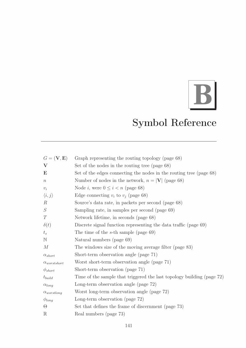
BSymbol Reference
G = (V,E) Graph representing the routing topology (page 68)
V Set of the nodes in the routing tree (page 68)
E Set of the edges connecting the nodes in the routing tree (page 68)
n Number of nodes in the network, n = |V| (page 68)
vi Node i, were 0 ≤ i < n (page 68)
〈i, j〉 Edge connecting vi to vj (page 68)
R Source’s data rate, in packets per second (page 68)
S Sampling rate, in samples per second (page 69)
T Network lifetime, in seconds (page 68)
δ(t) Discrete signal function representing the data traffic (page 69)
ts The time of the s-th sample (page 69)
N Natural numbers (page 69)
M The windows size of the moving average filter (page 83)
αshort Short-term observation angle (page 71)
αworstshort Worst short-term observation angle (page 71)
φshort Short-term observation (page 71)
tbuild Time of the sample that triggered the last topology building (page 72)
αlong Long-term observation angle (page 72)
αworstlong Worst long-term observation angle (page 72)
φlong Long-term observation (page 72)
Θ Set that defines the frame of discernment (page 73)
R Real numbers (page 73)
141
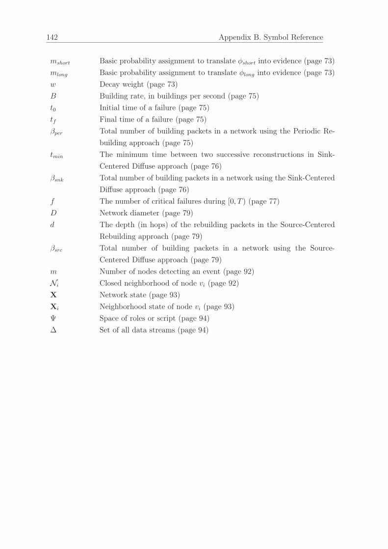
142 Appendix B. Symbol Reference
mshort Basic probability assignment to translate φshort into evidence (page 73)
mlong Basic probability assignment to translate φlong into evidence (page 73)
w Decay weight (page 73)
B Building rate, in buildings per second (page 75)
t0 Initial time of a failure (page 75)
tf Final time of a failure (page 75)
βper Total number of building packets in a network using the Periodic Re-
building approach (page 75)
tmin The minimum time between two successive reconstructions in Sink-
Centered Diffuse approach (page 76)
βsnk Total number of building packets in a network using the Sink-Centered
Diffuse approach (page 76)
f The number of critical failures during [0, T ) (page 77)
D Network diameter (page 79)
d The depth (in hops) of the rebuilding packets in the Source-Centered
Rebuilding approach (page 79)
βsrc Total number of building packets in a network using the Source-
Centered Diffuse approach (page 79)
m Number of nodes detecting an event (page 92)
Ni Closed neighborhood of node vi (page 92)
X Network state (page 93)
Xi Neighborhood state of node vi (page 93)
Ψ Space of roles or script (page 94)
∆ Set of all data streams (page 94)

CAbbreviations
AGP Art Gallery Problem
AoA Angle of Arrival
AODV Ad-hoc On-demand Distance Vector Routing
bpa basic probability assignment
DAI-DAO Data In - Data Out
DAI-FEO Data In - Feature Out
DEI-DEO Decision In - Decision Out
DFD Data-Feature-Decision
DISCUS Distributed Source Coding Using Syndromes
DSP Digital Signal Processing
DSR Dynamic Source Routing
ESPDA Energy-efficient and Secure Pattern-based Data Aggregation pro-
tocol
ESRT Event-to-Sink Reliable Transfer
FEI-DEO Feature In - Decision Out
143

144 Appendix C. Abbreviations
FEI-FEO Feature In - Feature Out
FSK Frequency Shift Keying
FTI Fault-Tolerant Interval
GAF Geographic Adaptive Fidelity
GFSK Gaussian Frequency Shift Keying
LEACH Low-Energy Adaptive Clustering Hierarchy
MAC Media Access Control
NRZ Non-Return to Zero
OODA Observe-Orient-Decide-Act
pdf Probability Density Function
PEGASIS Power-Efficient GAthering in Sensor Information Systems
PSFQ Pump Slowly, Fetch Quickly
QoS Quality of Service
RMST Reliable Data Transport in Sensor Networks
RSSI Received Signal Strength Indicator
SIA Secure Information Aggregation in Sensor
SINA Sensor Information Networking Architecture
SPRING Sensor Placement and Role assignment for energy-efficient INfor-
mation Gathering
STEM Sparse Topology and Energy Management
TDMA Time Division Multiple Access
TDoA Time Difference of Arrival
TiNA Temporal coherency-aware in-Network Aggregation
ToA Time of Arrival
TTL Time to live
WSN Wireless Sensor Network

Bibliography
Ahlswede, R., Cai, N., Li, S. R., and Yeung, R. W. (2000). Network information
flow. IEEE Transactions on Information Theory, 46(4):1204–1216.
Ahn, J. and Krishnamachari, B. (2006). Fundamental scaling laws for energy-
efficient storage and querying in wireless sensor networks. In Proceedings of the
7th ACM International Symposium on Mobile Ad Hoc Networking and Computing
(MobiHoc’06), pages 334–343, Florence, Italy. ACM.
Akyildiz, I. F., Estrin, D., Culler, D. E., and Srivastava, M. B., editors (2003).
Proceedings of the 1st International Conference on Embedded Networked Sensor
Systems (SenSys’03), Los Angeles, USA. ACM.
Akyildiz, I. F., Su, W., Sankarasubramaniam, Y., and Cyirci, E. (2002). Wireless
sensor networks: A survey. Computer Networks, 38(4):393–422.
Arbuckle, D., Howard, A., and Mataric, M. J. (2002). Temporal occupancy grids:
A method for classifying spatio-temporal properties of the environment. In Pro-
ceedings of the IEEE/RSJ International Conference on Intelligent Robots and
Systems, pages 409–414, Switzerland. IEEE.
Arulampalam, M. S., Maskell, S., Gordon, N., and Clapp, T. (2002). A tutorial
on particle filters for online nonlinear/non-Gaussian Bayesian tracking. IEEE
Transactions on Signal Processing, 50(2):174–188.
Aslam, J., Butler, Z., Constantin, F., Crespi, V., Cybenko, G., and Rus, D. (2003).
Tracking a moving object with a binary sensor network. In Akyildiz et al. [2003],
pages 150–161.
Banon, G. (1981). Distinction between several subsets of fuzzy measures. Fuzzy
Sets and Systems, 5(3):291–305.
145

146 Bibliography
Baran, R. H. (1989). A collective computation approach to automatic target recog-
nition. In Proceedings of the International Joint Conference on Neural Networks,
volume I, pages 39–44, Washington, D.C., USA. IEEE.
Barros, J. and Servetto, S. D. (2006). Network information flow with correlated
sources. IEEE Transactions on Information Theory, 52(1):155–170.
Bass, T. (2000). Intrusion detection systems and multisensor data fusion. Commu-
nications of the ACM, 43(4):99–105.
Bauer, F. and Varma, A. (1996). Distributed algorithms for multicast path setup
in data networks. IEEE Transactions on Networking, 4(2):181–191.
Bayes, T. R. (1763). An essay towards solving a problem in the doctrine of chances.
Philosophical Transactions of the Royal Society, 53:370–418.
Bedworth, M. D. and O’Brien, J. C. (1999). The omnibus model: A new model for
data fusion? In Proceedings of the 2nd International Conference on Information
Fusion (FUSION’99), pages 437–444, Sunnyvale, USA. ISIF.
Bezdek, J. C. (1981). Pattern Recognition with Fuzzy Objective Function Algorithms.
Advanced Applications in Pattern Recognition. Kluwer Academic Publishers, Nor-
well, MA, USA.
Bhardwaj, M. and Chandakasan, A. P. (2002). Bounding the lifetime of sensor
networks via optimal role assignment. In INFOCOM [2002], pages 1587–1596.
Biagioni, E. S. and Sasaki, G. (2003). Wireless sensor placement for reliable and
efficient data collection. In Hawaii International Conference on Systems Sciences
(HICSS 2003), pages 127–136, Hawaii, USA. IEEE.
Biswas, R., Thrun, S., and Guibas, L. J. (2004). A probabilistic approach to infer-
ence with limited information in sensor networks. In Ramchandran et al. [2004],
pages 269–276.
Blatt, D. and Hero, A. (2004). Distributed maximum likelihood estimation for sensor
networks. In Proceedings of the IEEE International Conference on Acoustics,
Speech, and Signal Processing (ICASSP’04), volume 3, pages 929–932, Montreal,
Canada. IEEE.
Blum, P., Meier, L., and Thiele, L. (2004). Improved interval-based clock synchro-
nization in sensor networks. In Ramchandran et al. [2004], pages 349–358.

Bibliography 147
Blumenthal, J., Timmermann, D., Buschmann, C., Fischer, S., Koberstein, J.,
and Luttenberger, N. (2006). Minimal transmission power as distance estima-
tion for precise localization in sensor networks. In Proceeding of the 2006 Inter-
national Conference on Communications and Mobile Computing (IWCMC’06),
pages 1331–1336, Vancouver, British Columbia, Canada. ACM.
Bonfils, B. J. and Bonnet, P. (2003). Adaptive and decentralized operator placement
for in-network query processing. In Zhao and Guibas [2003], pages 47–62.
Bonissone, P. P. (1997). Soft computing: The convergence of emerging reasoning
technologies. Soft Computing, 1(1):6–18.
Bonnet, P., Gehrke, J., and Seshadri, P. (2001). Towards sensor database systems.
In Tan, K.-L., Franklin, M. J., and Lui, J. C. S., editors, Proceedings of the 2nd
International Conference on Mobile Data Management, volume 1987 of Lecture
Notes in Computer Science, pages 3–14, Hong Kong, China. Springer.
Boulis, A., Ganeriwal, S., and Srivastava, M. B. (2003a). Aggregation in sensor net-
works: An energy-accuracy trade-off. Ad Hoc Networks, 1(2–3):317–331. Special
Issue on Sensor Network Protocols and Applications.
Boulis, A., Han, C.-C., and Srivastava, M. B. (2003b). Design and implementation
of a framework for efficient and programmable sensor networks. In Proceedings of
the 1st International Conference on Mobile Systems, Applications, and Services
(MobiSys’03), pages 187–200, San Francisco, CA, USA. USENIX.
Boyd, J. R. (1987). A discourse on winning and losing. Unpublished set of briefing
slides available at Air University Library, Maxwell AFB, Alabama, USA.
Bracio, B. R., Horn, W., and Möller, D. P. F. (1997). Sensor fusion in biomedi-
cal systems. In Proceedings of the 19th Annual International Conference of the
IEEE Engineering in Medicine and Biology Society, volume 3, pages 1387–1390,
Chicago, IL, USA. IEEE.
Brokmann, G., March, B., Romhild, D., and Steinke, A. (2001). Integrated multi-
sensors for industrial humidity measurement. In Proceedings of the IEEE Interna-
tional Conference on Multisensor Fusion and Integration for Intelligent Systems,
pages 201–203, Baden-Baden, Germany. IEEE.
Brooks, R. R. and Iyengar, S. (1998). Multi-Sensor Fusion: Fundamentals and
Applications with Software. Prentice Hall PTR, Upper Saddle River, NJ, USA.
148 Bibliography
Brown, C., Durrant-Whyte, H., Leonard, J., Rao, B., and Steer, B. (1992). Dis-
tributed data fusion using Kalman filtering: A robotics application. In Abidi,
M. A. and Gonzalez, R. C., editors, Data Fusion in Robotics and Machine Intel-
ligence, chapter 7, pages 267–309. Academic Press, Inc., San Diego, CA, USA.
Brown, R. G. and Hwang, P. Y. C. (1996). Introduction to Random Signals and
Applied Kalman Filtering. John Wiley & Sons, New York, NY, USA, 3rd edition.
Buede, D. M. (1988). Shafer-Dempster and Bayesian reasoning: A response to
Shafer-Dempster reasoning with applications to multisensor target identification
systems’. IEEE Transactions on Systems, Man and Cybernetics, 18(6):1009–1011.
Cain, M. P., Stewart, S. A., and Morse, J. B. (1989). Object classification using
multispectral sensor data fusion. In Proceedings of SPIE Sensor Fusion II, volume
1100, pages 53–61, Orlando, FL, USA. SPIE.
Cam, H., Ozdemir, S., Nair, P., and Muthuavinashiappan, D. (2003). ESPDA:
Energy-efficient and secure pattern-based data aggregation for wireless sensor
networks. In Proceedings of the IEEE Sensors, volume 2, pages 732–736, Toronto,
Canada. IEEE.
Castelaz, P. F. (1988). Neural networks in defense applications. In Proceedings of the
IEEE International Conference on Neural Networks, volume II, pages 473–480,
San Diego, CA, USA. IEEE.
Chakrabarty, K., Iyengar, S. S., Qi, H., and Cho, E. (2002). Grid coverage for
surveillance and target location in distributed sensor networks. IEEE Transactions
on Computers, 51(12):1448–1453.
Chakravarty, P. and Jarvis, R. (2005). Multiple target tracking for surveillance:
A particle filter approach. In Proceedings of the 2nd International Conference
on Intelligent Sensors, Sensor Networks and Information Processing Conference
(ISSNIP’05), pages 181–186, Melbourne, Australia. IEEE.
Chan Yet, W. and Qidwai, U. (2005). Intelligent sensor network for obstacle avoid-
ance strategy. In Proceedings of the 4th IEEE Conference on Sensors, Irvine,
USA. IEEE.
Chen, B., Jamieson, K., Balakrishnan, H., and Morris, R. (2002). Span: An energy-
efficient coordination algorithm for topology maintenance in ad hoc wireless net-
works. Wireless Networks, 8(5):481–494.
Bibliography 149
Chen, C., Ali, A. M., and Wang, H. (2006a). Design and testing of robust acoustic
arrays for localization and enhancement of several bird sources. In Stankovic et al.
[2006], pages 268–275.
Chen, H., Mineno, H., and Mizuno, T. (2006b). A meta-data-based data aggregation
scheme in clustering wireless sensor networks. In Proceedings of the 7th Interna-
tional Conference on Mobile Data Management (MDM’06), pages 154–154, Nara,
Japan. IEEE.
Chen, Y. P., Liestman, A. L., and Liu, J. (2006c). A hierarchical energy-efficient
framework for data aggregation in wireless sensor networks. IEEE Transactions
on Vehicular Technology, 55(3):789–796.
Cheng, Y. and Kashyap, R. L. (1988). Comparison of Bayesian and Dempster’s
rules in evidence combination. In Erickson, G. J. and Smith, C. R., editors,
Maximum-Entrophy and Bayesian Methods in Science and Engineering, pages
427–433. Kluwer Academic Publishers, Dordrecht, Netherlands.
Chew, P. and Marzullo, K. (1991). Masking failures of multidimentional sensors.
In Proceedings of the 10th IEEE Symposium on Reliable Distributed Systems
(SDRS’91), pages 32–41, Pisa, Italy. IEEE.
Ci, S. and Sharif, H. (2005). Performance comparison of Kalman filter based ap-
proaches for energy efficiency in wireless sensor networks. In Proceedings of the
3rd ACS/IEEE International Conference on Computer Systems and Applications
(AICCSA’05), pages 58–65, Cairo, Egypt. IEEE.
Ci, S., Sharif, H., and Nuli, K. (2004). A UKF-based link adaptation scheme to
enhance energy efficiency in wireless sensor networks. In Proceedings of the 15th
IEEE International Symposium on Personal, Indoor and Mobile Radio Commu-
nications (PIMRC’04), volume 4, pages 2483–2488, Barcelona, Spain. IEEE.
Cimander, C., Carlsson, M., and Mandenius, C. (2002). Sensor fusion for on-line
monitoring of yoghurt fermentation. Journal of Biotechnology, 99(3):237–248.
Coates, M. (2004). Distributed particle filters for sensor networks. In Ramchandran
et al. [2004], pages 99–107.
Cohen, N. H., Purakayastha, A., Turek, J., Wong, L., and Yeh, D. (2001). Challenges
in flexible aggregation of pervasive data. IBM Research Report RC 21942 (98646),
IBM Research Division, Yorktown Heights, NY, USA.

150 Bibliography
Coué, C., Fraichard, T., Bessiere, P., and Mazer, E. (2002). Multi-sensor data
fusion using Bayesian programming: An automotive application. In IEEE/RSJ
International Conference on Intelligent Robots and System, volume 1, pages 141–
146, Lausanne, Switzerland. IEEE.
Crisan, D. and Doucet, A. (2002). A survey of convergence results on particle
filtering methods for practitioners. IEEE Transactions on Signal Processing,
50(3):736–746.
Crossbow (2004). Mica2 - wireless measurement system. Available: http://www.
xbow.com/Products/productsdetails.aspx?sid=72.
Crossbow (2006). MicaZ - wireless measurement system. Available: http://www.
xbow.com/Products/productsdetails.aspx?sid=101.
Cui, X., Hardin, T., Ragade, R., and Elmaghraby, A. (2004). A swarm-based
fuzzy logic control mobile sensor network for hazardous contaminants localization.
In Proceedings of the 1st IEEE International Conference on Mobile Ad-hoc and
Sensor Systems (MASS’04), pages 194–203, Fort Lauderdale, USA. IEEE.
Dasarathy, B. V. (1997). Sensor fusion potential exploitation-innovative architec-
tures and illustrative applications. Proceedings of the IEEE, 85(1):24–38.
Dasarathy, B. V. (2000). More the merrier. . . or is it? – sensor suite augmentation
benefits assessment. In Proceedings of 3th International Conference on Informa-
tion Fusion (Fusion 2000), volume 2, pages WEC3/20–WEC3/25, Paris, France.
IEEE.
Dasarathy, B. V. (2001). What, where, why, when, and how? Information Fusion,
2(2):75–76. Editorial.
Dasgupta, K., Kukreja, M., and Kalpakis, K. (2003). Topology-aware placement
and role assignment for energy-efficient information gathering in sensor networks.
In Proceedings of the 8th IEEE International Symposium on Computers and Com-
munication (ISCC’03), volume 1, pages 341–348, Antalya, Turkey. IEEE.
Data Fusion Server (2004). Available: http://www.data-fusion.org.
Deb, B., Bhatangar, S., and Nath, B. (2002). A topology discovery algorithm
for sensor networks with applications to network management. In IEEE CAS
Workshop on Wireless Communications and Networking, Pasadena, CA, USA.
Poster Session 2.

Bibliography 151
Dempster, A. P. (1968). A generalization of Bayesian inference. Journal of the Royal
Statistical Society, Series B, 30:205–247.
Dhillon, S. S., Chakrabarty, K., and Iyengar, S. S. (2002). Sensor placement for
grid coverage under imprecise detections. In Proceedings of 5th International
Conference on Information Fusion (Fusion 2002), volume 2, pages 1581–1587,
Annapolis, Maryland, USA. IEEE.
Ding, M., Cheng, X., and Xue, G. (2003). Aggregation tree construction in sen-
sor networks. In Proceedings of the 58th IEEE Vehicular Technology Conference
(VTC-Fall 2003), volume 4, pages 2168–2172, Orlando, USA. IEEE.
Doherty, L., Pister, K. S. J., and Ghaoui, L. E. (2001). Convex position estimation
in wireless sensor networks. In INFOCOM [2001], pages 1655–1663.
Durrant-Whyte, H. F. (1988). Sensor models and multisensor integration. Interna-
tional Journal of Robotics Research, 7(6):97–113.
Elfes, A. (1987). Sonar-based real-world mapping and navigation. IEEE Journal of
Robotics and Automation, RA-3(3):249–265.
Elfes, A. (1989). Using occupancy grids for mobile robot perception and navigation.
IEEE Computer, 22(6):46–57.
Elmenreich, W. (2002). Sensor Fusion in Time-Triggered Systems. PhD the-
sis, Institut für Technische Informatik, Vienna University of Technology, Tre-
itlstr. 3/3/182-1, 1040 Vienna, Austria. http://www.vmars.tuwien.ac.at/php/
pserver/extern/docdetail.php?DID=1084&viewmode=thesis.
Elson, J. and Parker, A. (2006). Tinker: A tool for designing data-centric sensor
networks. In Stankovic et al. [2006], pages 350–357.
Fang, L., Du, W., and Ning, P. (2005). A beacon-less location discovery scheme for
wireless sensor networks. In INFOCOM [2005], pages 161–171.
Figueiredo, C. M., Nakamura, E. F., and Loureiro, A. A. (2004). Multi: A hybrid
adaptive dissemination protocol for wireless sensor networks. In Proceedings of the
1st International Workshop on Algorithmic Aspects of Wireless Sensor Networks
(ALGOSENSORS 2004), volume 3121 of Lecture Notes in Computer Science,
pages 171–186, Turku, Finland. Springer.

152 Bibliography
Figueiredo, C. M., Nakamura, E. F., and Loureiro, A. A. (2007). An event-
detection estimation model for hybrid adaptive routing in wireless sensor net-
works. In Proceedings of the 2007 IEEE International Conference on Communi-
cations (ICC’07), Glasgow, Scottland. IEEE. To appear.
Filippidis, A., Jain, L. C., and Martin, N. (2000). Fusion of intelligent agents for
the detection of aircraft in SAR images. IEEE Transactions on Pattern Analysis
and Machine Intelligence, 22(4):378–384.
Forney, G. D. (1973). The Viterbi algorithm. Proceedings of the IEEE, 61(3):268–
278.
Frank, C. and Römer, K. (2005). Algorithms for generic role assignment in wireless
sensor networks. In Redi et al. [2005], pages 230–242.
Frankel, C. B. (1999). Such Order From Confusion Sprung: Adaptive Competence
and Affect Regulation. PhD thesis, Pacific Graduate School of Psychology, Palo
Alto, CA, USA.
Frankel, C. B. and Bedworth, M. D. (2000). Control, estimation and abstraction in
fusion architectures: Lessons from human information processing. In Proceedings
of 3th International Conference on Information Fusion (Fusion 2000), volume 1,
pages MoC5/3–MoC5/10, Paris, France. IEEE.
Friedlander, D. S. (2005). Semantic information extraction. In Iyengar, S. S. and
Brooks, R. R., editors, Distributed Sensor Networks, chapter 21, pages 409–417.
CRC Press, Boca Raton, USA.
Friedlander, D. S. and Phoha, S. (2002). Semantic information fusion for coordi-
nated signal processing in mobile sensor networks. International Journal of High
Performance Computing Applications, 16(3):235–241.
Gagvani, N. and Silver, D. (2000). Shape-based volumetric collision detection. In
Proceedings of the 2000 IEEE Symposium on Volume Visualization, pages 57–61,
Salt Lake City, Utah, USA. IEEE.
Ganeriwal, S., Kumar, R., and Srivastava, M. B. (2003). Timing-sync protocol for
sensor networks. In Akyildiz et al. [2003], pages 138–149.
Ganesan, D., Govindan, R., Shenker, S., and Estrin, D. (2001). Highly-resilient,
energy-efficient multipath routing in wireless sensor networks. ACM SIGMOBILE
Mobile Computing and Communications Review, 5(4):11–25.

Bibliography 153
Gao, J. B. and Harris, C. J. (2002). Some remarks on Kalman filters for the multi-
sensor fusion. Information Fusion, 3(3):191–201.
Garvey, T. D., Lowrance, J. D., and Fischler, M. A. (1981). An inference technique
for integrating knowledge from disparate sources. In Proceedings of the 7th Inter-
national Joint Conference on Artificial Intelligence (IJCAI’81), pages 319–325,
Vancouver, British Columbia, Canada. William Kaufmann.
Geoscience and Remote Sensing Society (2004). Available: http://www.dfc-grss.
org.
Ghose, A., Grossklags, J., and Chuang, J. (2003). Resilient data-centric storage in
wireless ad-hoc sensor networks. In Chen, M., Chrysanthis, P. K., Sloman, M.,
and Zaslavsky, A. B., editors, Proceedings of the 4th International Conference on
Mobile Data Management, volume 2574 of Lecture Notes in Computer Science,
pages 45–62, Melbourne, Australia. Springer.
Gibson, J. D., editor (1999). The Mobile Communication Handbook. CRC Press,
Boca Raton, USA, 2nd edition.
Gilks, W., Richardson, S., and Spie, D., editors (1996). Markov Chain Monte Carlo
in Practice. Chapman & Hall/CRC, London, UK.
Grime, S. and Durrant-Whyte, H. F. (1994). Data fusion in decentralized sensor
networks. Control Engineering Practice, 2(5):849–863.
Gu, L., Jia, D., Vicaire, P., Yan, T., Luo, L., Tirumala, A., Cao, Q., He, T.,
Stankovic, J. A., Abdelzaher, T., and Krogh, B. H. (2005). Lightweight detection
and classification for wireless sensor networks in realistic environments. In Redi
et al. [2005], pages 205–217.
Guestrin, C., Bodik, P., Thibaux, R., Paskin, M., and Madden, S. (2004). Dis-
tributed regression: an efficient framework for modeling sensor network data. In
Ramchandran et al. [2004], pages 1–10.
Gummadi, R., Li, X., Govindan, R., Shahabi, C., and Hong, W. (2005). Energy-
efficient data organization and query processing in sensor networks. SIGBED
Review, 2(1):7–12.
Guo, D. and Wang, X. (2004). Dynamic sensor collaboration via sequential Monte
Carlo. IEEE Journal on Selected Areas in Communications, 22(6):1037–1047.

154 Bibliography
Guo, D., Wang, X., and Chen, R. (2005). New sequential Monte Carlo methods for
nonlinear dynamic systems. Statistics and Computing, 15(2):135–147.
Gupta, I., Riordan, D., and Sampalli, S. (2005). Cluster-head election using fuzzy
logic for wireless sensor networks. In Proceedings of the 3rd Annual Communi-
cation Networks and Services Research Conference (CNSR’05), pages 255–260,
Halifax, Canada. IEEE.
Halgamuge, M. N., Guru, S. M., and Jennings, A. (2003). Energy efficient cluster
formation in wireless sensor networks. In Proceedings of the 10th International
Conference on Telecommunications (ICT’03), volume 2, pages 1571–1576, Pa-
peete, French Polynesia. IEEE.
Hall, D. L. (1992). Mathematical Techniques in Multisensor Data Fusion. Artech
House, Norwood, Massachusetts, USA.
Hall, D. L. and Llinas, J. (1997). An introduction to multi-sensor data fusion.
Proceedings of the IEEE, 85(1):6–23.
Hartl, G. and Li, B. (2004). Loss inference in wireless sensor networks based on
data aggregation. In Ramchandran et al. [2004], pages 396–404.
Hartl, G. and Li, B. (2005). infer : A Bayesian inference approach towards energy
efficient data collection in dense sensor networks. In Proceedings of the 25th IEEE
International Conference on Distributed Computing Systems (ICDCS’05), pages
371–380, Washington, USA. IEEE.
He, T., Blum, B. M., Stankovic, J. A., and Abdelzaher, T. (2004). AIDA: Adap-
tive application independent data aggregation in wireless sensor network. ACM
Transactions on Embedded Computing System, 3(2):426–457. Special issue on
Dynamically Adaptable Embedded Systems.
Hegazy, T. and Vachtsevanos, G. J. (2003). Sensor placement for isotropic source
localization. In Zhao and Guibas [2003], pages 432–441.
Heidemann, J., Silva, F., and Estrin, D. (2003). Matching data dissemination algo-
rithms to application requirements. In Akyildiz et al. [2003], pages 218–229.
Heinzelman, W., Chandrakasan, A., and Balakrishnan, H. (2000). Energy-efficient
communication protocol for wireless microsensor networks. In Proceedings of
the 33rd Hawaii International Conference on System Sciences (HICSS’00), pages
8020–8029, Maui, USA. IEEE.

Bibliography 155
Hellerstein, J. M., Hong, W., Madden, S., and Stanek, K. (2003). Beyond average:
Towards sophisticated sensing with queries. In Zhao and Guibas [2003], pages
63–79.
Hoang, A. T. and Motani, M. (2005a). Collaborative broadcasting and compression
in cluster-based wireless sensor networks. In Proceeedings of the Second European
Workshop on Wireless Sensor Networks (EWSN’05), pages 197–206, Istanbul,
Turkey. IEEE.
Hoang, A. T. and Motani, M. (2005b). Exploiting wireless broadcast in spatially
correlated sensor networks. In Proceedings of the 2005 IEEE International Con-
ference on Communications (ICC’05), volume 4, pages 2807–2811, Seoul, Korea.
IEEE.
Hongyang, C., Ping, D., Yongjun, X., and Xiaowei, L. (2005). A robust location al-
gorithm with biased extended Kalman filtering of TDOA data for wireless sensor
networks. In Proceedings of the International Conference on Wireless Communica-
tions, Networking and Mobile Computing (WCNM’05), volume 2, pages 883–886,
Wuhan, China. IEEE.
Hoover, A. and Olsen, B. D. (1999). A real-time occupancy map from multiple
video streams. In Proceedings of the IEEE International Conference Robotics and
Automation, volume 3, pages 2261–2266, Detroit, Michigan, USA. IEEE.
Hoover, A. and Olsen, B. D. (2000). Sensor network perception for mobile robotics.
In Proceedings of the IEEE International Conference Robotics and Automation,
volume 1, pages 342–347, San Fransico, California, USA. IEEE.
Hsin, C. and Liu, M. (2002). A distributed monitoring mechanism for wireless sensor
networks. In Proceedings of the ACM Workshop on Wireless Security (WiSe’02),
pages 57–66, Atlanta, GA, USA. ACM.
Hu, L. and Evans, D. (2003). Secure aggregation for wireless networks. In Workshop
on Security and Assurance in Ad hoc Networks, pages 384–391, Orlando,FL,USA.
IEEE.
Hu, L. and Evans, D. (2004). Localization for mobile sensor networks. In Pro-
ceedings of the 10th Annual International Conference on Mobile Computing and
Networking (MobiCom’04), pages 45–57, Philadelphia, PA, USA. ACM.
Hua, G. and Chen, C. W. (2005). Distributed source coding in wireless sensor
networks. In Proceedings of the 2nd International Conference on Quality of Service

156 Bibliography
in Heterogeneous Wired/Wireless Networks (Qshine’05), page 6, Orlando, USA.
IEEE.
Hwang, F., Richards, D., and Winter, P. (1992). The Steiner Problem. Annals of
Discrete Mathematics. North-Holland, Amsterdam, Holland.
Ihler, A. T., John W. Fisher, I., Moses, R. L., and Willsky, A. S. (2005). Nonpara-
metric belief propagation for self-localization of sensor networks. IEEE Journal
on Selected Areas in Communications, 23(4):809–819.
INFOCOM, editor (2001). 20th Annual Joint Conference of the IEEE Computer
and Communications Societies (INFOCOM 2001), Anchorage, AK, USA. IEEE.
INFOCOM, editor (2002). 21st Annual Joint Conference of the IEEE Computer
and Communications Societies (INFOCOM 2002), New York, NY, USA. IEEE.
INFOCOM, editor (2005). 24th Annual Joint Conference of the IEEE Computer
and Communications Societies (INFOCOM 2005), Miami, USA. IEEE.
Intanagonwiwat, C., Estrin, D., Govindan, R., and Heidemann, J. (2002). Impact of
network density on data aggregation in wireless sensor networks. In Proceedings
of the 22nd IEEE International Conference on Distributed Computing Systems
(ICDCS’02), pages 457–458, Vienna, Austria. IEEE.
Intanagonwiwat, C., Govindan, R., and Estrin, D. (2000). Directed diffusion: A
scalable and robust communication paradigm for sensor networks. In Proceedings
of the 6th Annual International Conference on Mobile Computing and Networking
(MobiCom’00), pages 56–67, Boston, MA, USA. ACM.
Intanagonwiwat, C., Govindan, R., Estrin, D., Heidemann, J., and Silva, F. (2003).
Directed diffusion for wireless sensor networking. IEEE/ACM Transactions on
Networking, 11(1):2–16.
International Society of Information Fusion (2004). Available: http://www.
inforfusion.org.
IPSN, editor (2005). Proceedings of the 4th International Symposium on Information
Processing in Sensor Networks (IPSN’05), Los Angeles, USA. IEEE.
Isla, D. A. and Blumberg, B. M. (2002). Object persistence for synthetic creatures.
In Proceedings of the 1st International Joint Conference on Autonomous Agents
and Multiagent Systems, pages 1356–1363, Bologna, Italy. ACM.
Bibliography 157
Iyengar, S. S., Chakrabarty, K., and Qi, H. (2001). Introduction to special issue on
“distributed sensor networks for real-time systems with adaptive configuration”.
Journal of the Franklin Institute, 338(6):651–653.
Jacobs, O. L. R. (1993). Introduction to Control Theory. Oxford University Press,
Oxford, UK, 2nd edition.
Jaikaeo, C., Srisathapornphat, C., and Shen, C. (2001). Diagnosis of sensor net-
works. In Proceedings of the 2001 IEEE International Conference on Communi-
cations (ICC’01), volume 1, pages 1627–1632, Helsinki, Finland. IEEE.
Jain, A., Chang, E. Y., and Wang, Y.-F. (2004). Adaptive stream resource man-
agement using Kalman filters. In Proceedings of the 2004 ACM SIGMOD Inter-
national Conference on Management of Data (SIGMOD’04), pages 11–22, Paris,
France. ACM.
Jayasimha, D. N. (1994). Fault tolerance in a multisensor environment. In Proceed-
ings of the 13th IEEE Symposium on Reliable Distributed Systems (SDRD’94),
pages 2–11, Dana Point, CA, USA. IEEE.
Jazwinski, A. H. (1970). Stochastic Processes and Filtering Theory. Academic Press,
New York, USA.
Jin, G. and Nittel, S. (2006). NED: An efficient noise-tolerant event and event
boundary detection algorithm in wireless sensor networks. In Proceedings of the
7th International Conference on Mobile Data Management (MDM’06), pages 153–
161, Washington, USA. IEEE.
Johnson, D. B. and Maltz, D. A. (1996). Dynamic source routing in ad hoc wireless
networks. In Imielinski, T. and Korth, H., editors, Mobile Computing, volume
353, chapter 5, pages 153–181. Kluwer Academic Publishers.
Julier, S. J. and Uhlmann, J. K. (1997). New extension of the Kalman filter to
nonlinear systems. In Signal Processing, Sensor Fusion, and Target Recognition
VI, volume 3068, pages 182–193, San Diego, USA. SPIE.
Kalman, R. E. (1960). A new approach to linear filtering and prediction problems.
Transaction of the ASME: Journal of Basic Engineering, 82:35–45.
Kalpakis, K., Dasgupta, K., and Namjoshi, P. (2003). Efficient algorithms for max-
imum lifetime data gathering and aggregation in wireless sensor networks. Com-
puter Networks, 42(6):697–716.
158 Bibliography
Kansal, A., Yuen, E., Kaiser, W., Pottie, G., and Srivastava, M. (2004). Sensing
uncertainty reduction using low complexity actuation. In Ramchandran et al.
[2004], pages 388–395.
Kessler et al., J. (1992). Functional description of the data fusion process. Technical
report, Naval Air Development Center, Warminster, PA, USA. Report prepared
for the Office of Naval Technology.
Klein, L. A. (1993). Sensor and Data Fusion Concepts and Applications, volume
TT14. SPIE Optical Engineering Press, USA.
Kleine-Ostmann, T. and Bell, A. E. (2001). A data fusion architecture for en-
hanced position estimation in wireless networks. IEEE Communications Letters,
5(8):343–345.
Kochhal, M., Schwiebert, L., and Gupta, S. (2003). Role-based hierarchical self orga-
nization for wireless ad hoc sensor networks. In Proceedings of the 2nd ACM Inter-
national Conference on Wireless Sensor Networks and Applications (WSNA’03),
pages 98–107, San Diego, CA, USA. ACM.
Kohonen, T. (1997). Self-Organizing Maps. Springer-Verlag, Secaucus, NJ, USA.
Kokar, M. M., Bedworth, M. D., and Frankel, C. B. (2000). A reference model for
data fusion systems. In Sensor Fusion: Architectures, Algorithms and Applica-
tions IV, pages 191–202, Orlando, FL, USA. SPIE.
Kotz, D. and Gray, R. S. (1999). Mobile agents and the future of the internet. ACM
SIGOPS Operating Systems Review, 33(3):7–13.
Kreucher, C., Kastella, K., and Hero III, A. O. (2005). Sensor management using
an active sensing approach. Signal Processing, 85(3):607–624.
Krishnamachari, B., Estrin, D., and Wicker, S. (2002). The impact of data aggrega-
tion in wireless sensor networks. In International Workshop of Distributed Event
Based Systems (DEBS), pages 575–578, Vienna, Austria. IEEE.
Krishnamachari, B. and Iyengar, S. (2004). Distributed Bayesian algorithms for
fault-tolerant event region detection in wireless sensor networks. IEEE Transac-
tions on Computers, 53(3):241–250.
Kulik, J., Heinzelman, W., and Balakrishnan, H. (2002). Negotiation-based proto-
cols for disseminating information in wireless sensor networks. Wireless Networks,
8(2–3):169–185.

Bibliography 159
Kumar, R., Wolenetz, M., Agarwalla, B., Shin, J., Hutto, P., Paul, A., and Ra-
machandran, U. (2003). Dfuse: A framework for distributed data fusion. In
Akyildiz et al. [2003], pages 114–125.
Kusuma, J., Doherty, L., and Ramchandran, K. (2001). Distributed compression for
sensor networks. In Proceedings of the 2001 International Conference on Image
Processing (ICIP’01), volume 1, pages 82–85, Thessaloniki, Greece. IEEE.
Lee, C. C. (1990). Fuzzy logic in control systems: Fuzzy logic controller – part I.
IEEE Transactions on Systems, Man and Cybernetics, 20(2):404–418.
Levis, P. and Culler, D. (2002). Maté: A tiny virtual machine for sensor networks.
In Proceedings of the 10th International Conference on Architectural Support for
Programming Languages and Operating Systems (ASPLOS), pages 85–95, San
Jose, CA, USA. ACM.
Lewis, T. W. and Powers, D. M. W. (2002). Audio-visual speech recognition us-
ing red exclusion and neural networks. In Proceedings of the 25th Australasian
Conference on Computer Science, pages 149–156, Melbourne, Victoria, Australia.
Australian Computer Society, Inc.
Li, S., Lin, Y., Son, S. H., Stankovic, J. A., and Wei, Y. (2004). Event detection
services using data service middleware in distributed sensor networks. Telecom-
munication Systems, 26(2–4):351–368.
Li, T., Ekpenyong, A., and Huang, Y. (2006). Source localization and tracking
using distributed asynchronous sensor. IEEE Transactions on Signal Processing,
54(10):3991–4003.
Li, X., Kim, Y. J., Govindan, R., and Hong, W. (2003a). Multi-dimensional range
queries in sensor networks. In Akyildiz et al. [2003], pages 63–75.
Li, X., Wan, P., and Frieder, O. (2003b). Coverage in wireless ad-hoc sensor net-
works. IEEE Transactions on Computers, 52(6):753–763.
Liang, Q. and Ren, Q. (2005a). Energy and mobility aware geographical multipath
routing for wireless sensor networks. In 2005 IEEE Wireless Communications and
Networking Conference (WCNC’05), volume 3, pages 1867–1871, New Orleans,
USA. IEEE.
Liang, Q. and Ren, Q. (2005b). An energy-efficient MAC protocol for wireless
sensor networks. In 2005 IEEE Global Telecommunications Conference (GLOBE-
COM’05), volume 1, St. Louis, USA. IEEE.
160 Bibliography
Lindsey, S., Raghavendra, C., and Sivalingam, K. M. (2002). Data gathering algo-
rithms in sensor networks using energy metrics. IEEE Transactions on Parallel
and Distributed Systems, 13(9):924–935.
Liu, J., Cheong, E., and Zhao, F. (2005). Semantics-based optimization across un-
coordinated tasks in networked embedded systems. In Wolf, W., editor, Proceed-
ings of the 5th ACM International Conference On Embedded Software (EMSOFT
2005), pages 273–281, Jersey City, USA. ACM.
Liu, J., Zhang, Y., and Zhao, F. (2006). Robust distributed node localization with
error management. In Proceedings of the 7th ACM International Symposium on
Mobile Ad Hoc Networking and Computing (MobiHoc’06), pages 250–261, Flo-
rence, Italy. ACM.
Liu, J. and Zhao, F. (2005). Towards semantic services for sensor-rich informa-
tion systems. In Proceedings of the 2nd International Conference on Broadband
Networks (BROADNETS 2005), pages 967–974, Boston, USA. IEEE.
Luo, R. C. and Kay, M. G. (1992). Data fusion and sensor integration: State-of-
the-art 1990s. In Abidi, M. A. and Gonzalez, R. C., editors, Data Fusion in
Robotics and Machine Intelligence, chapter 3, pages 7–135. Academic Press, Inc.,
San Diego, CA, USA.
Luo, R. C. and Kay, M. G., editors (1995). Multisensor Integration and Fusion for
Intelligent Machines and Systems. Computer Engineering and Computer Science.
Ablex Publishing, New Jersey, USA, reissue edition.
Luo, R. C., Yih, C.-C., and Su, K. L. (2002). Multisensor fusion and integration:
Approaches, applications, and future research directions. IEEE Sensors Journal,
2(2):107–119.
Luo, X., Dong, M., and Huang, Y. (2006). On distributed fault-tolerant detection
in wireless sensor networks. IEEE Transactions on Computers, 55(1):2006.
Madden, S. R., Franklin, M. J., Hellerstein, J. M., and Hong, W. (2002). TAG: a
Tiny AGgregation service for ad-hoc sensor networks. ACM SIGOPS Operating
Systems Review, 36(SI):131–146.
Madden, S. R., Franklin, M. J., Hellerstein, J. M., and Hong, W. (2005). TinyDB:
An acqusitional query processing system for sensor networks. ACM Transactions
on Database Systems, 30(1):122–173.

Bibliography 161
Manzo, M., Roosta, T., and Sastry, S. (2005). Time synchronization attacks in
sensor networks. In Proceedings of the 3rd ACM Workshop on Security of Ad Hoc
and Sensor Networks (SASN’05), pages 107–116, Alexandria, USA. ACM.
Marco, D. and Neuhoff, D. L. (2004). Reliability vs. efficiency in distributed source
coding for field-gathering sensor networks. In Ramchandran et al. [2004], pages
161–168.
Marzullo, K. (1984). Maintaining the Time in a Distributed System: An Exam-
ple of a Loosely-Coupled Distributed Service. PhD thesis, Stanford University,
Department of Electrical Engineering, Stanford, CA, USA.
Marzullo, K. (1990). Tolerating failures of continuous-valued sensors. ACM Trans-
actions on Computer Systems, 8(4):284–304.
Mascolo, C. and Musolesi, M. (2006). SCAR: Context-aware adaptive routing in
delay tolerant mobile sensor networks. In Proceeding of the 2006 International
Conference on Communications and Mobile Computing (IWCMC’06), pages 533–
538, Vancouver, Canada. ACM.
Megerian, S., Koushanfar, F., Qu, G., Veltri, G., and Potkonjak, M. (2002). Ex-
posure in wireless sensor networks: Theory and practical solutions. Wireless
Networks, 8(5):443–454.
Meguerdichian, S., Koushanfar, F., Potkonjak, M., and Srivastava, M. (2001a).
Coverage problems in wireless ad-hoc sensor networks. In INFOCOM [2001],
pages 1380–1387.
Meguerdichian, S., Slijepcevic, S., Karayan, V., and Potkonjak, M. (2001b). Lo-
calized algorithms in wireless ad-hoc networks: Location discovery and sensor
exposure. In Proceedings of the 2001 ACM International Symposium on Mobile
Ad Hoc Networking & Computing, pages 106–116, Long Beach, CA, USA. ACM.
Meier, L., Blum, P., and Thiele, L. (2004). Internal synchronization of drift-
constraint clocks in ad-hoc sensor networks. In Proceedings of the 5th ACM Inter-
national Symposium on Mobile Ad Hoc Networking and Computing (MobiHoc’04),
pages 90–97, Tokyo, Japan. ACM.
Mhatre, V. and Rosenberg, C. (2004). Homogeneous vs heterogeneous clustered
sensor networks: A comparative study. In Proceedings of the 2004 IEEE Inter-
national Conference on Communications (ICC’04), volume 6, pages 3646–3651,
Paris, France. IEEE.

162 Bibliography
Miguez, J. and Artes-Rodriguez, A. (2006). A Monte Carlo method for joint node
location and maneuvering target tracking in a sensor network. In Proceedings of
the IEEE International Conference on Acoustics, Speech, and Signal Processing
(ICASSP’06), volume 4, pages 989–992, Toulouse, France. IEEE.
Mini, R., Machado, M., Loureiro, A., and Nath, B. (2005). Prediction-based energy
map for wireless sensor networks. Ad Hoc Networks Journal, 3(2):235–253.
Mini, R. A., Loureiro, A. A., and Nath, B. (2004). The distinctive design character-
istics of a wireless sensor network: The energy map. Computer Communications,
7(10):935–945.
Mobicom, editor (2001). Proceedings of the 7th Annual ACM/IEEE International
Conference on Mobile Computing and Networking (Mobicom’01), Rome, Italy.
ACM.
Moshiri, B., Asharif, M. R., and HoseinNezhad, R. (2002). Pseudo information
measure: A new concept for extension of Bayesian fusion in robotic map building.
Information Fusion, 3(1):51–68.
Nakamura, E. F., Figueiredo, C. M., and Loureiro, A. A. (2005a). Information fusion
algorithms for wireless sensor networks. In Boukerche, A., editor, Handbook of
Algorithms for Wireless and Mobile Networks and Computing, pages 841–864.
Chapman & Hall/CRC Press.
Nakamura, E. F., Figueiredo, C. M., and Loureiro, A. A. (2005b). Information fu-
sion for data dissemination in self-organizing wireless sensor networks. In Lorenz,
P. and Dini, P., editors, Proceedings of the 4th International Conference on Net-
working (ICN 2005), volume 3420 of Lecture Notes in Computer Science, pages
585–593, Reunion Island, France. Springer.
Nakamura, E. F., Nakamura, F. G., Figueiredo, C. M., and Loureiro, A. A. (2005c).
Detecção de falhas em redes de sensores sem fio baseada na medição do tráfego
e em técnicas de fusão de dados. In 23o. Simpósio Brasileiro de Redes de Com-
putadores (SBRC 2005), pages 579–592, Fortaleza, CE, Brasil. SBC.
Nakamura, E. F., Nakamura, F. G., Figueiredo, C. M., and Loureiro, A. A. (2005d).
Using information fusion to assist data dissemination in wireless sensor networks.
Telecommunication Systems, 30(1–3):237–254.
Nakamura, E. F., Oliveira, H. A., Pontello, L. F., and Loureiro, A. A. (2006a).
Atribuição dinâmica de papéis para agregação de dados em redes de sensores sem
Bibliography 163
fio. In 24o. Simpósio Brasileiro de Redes de Computadores (SBRC 2005), pages
779–794, Curitiba, PR, Brasil. SBC.
Nakamura, E. F., Oliveira, H. A., Pontello, L. F., and Loureiro, A. A. (2006b). On
demand role assignment for event-detection in sensor networks. In Bellavista, P.,
Chen, C.-M., Corradi, A., and Daneshmand, M., editors, Proceedings of the 11th
IEEE International Symposium on Computers and Communication (ISCC’06),
pages 941–947, Cagliari, Italy. IEEE.
Nelson, M. and Gailly, J.-L. (1995). The Data Compression Book. M & T Books,
New York, NY, USA, 2nd edition.
Niculescu, D. and Nath, B. (2001). Ad hoc positioning system (APS). In 2001 IEEE
Global Telecommunications Conference (GLOBECOM’01), volume 5, pages 2926–
2931, San Antonio, TX, USA. IEEE.
Niu, R. and Varshney, P. K. (2006). Target location estimation in sensor networks
with quantized data. IEEE Transactions on Signal Processing, 64(12):4519–4528.
Nordlund, P.-J., Gunnarsson, F., and Gustafsson, F. (2002). Particle filters for posi-
tioning in wireless networks. In Proceedings of the XI European Signal Processing
Conference (EURSIPCO’02), volume II, pages 311–314, Toulouse, France. TeSA.
Novák, V., Perfilieva, I., and Mockor, J. (1999). Mathematical Principles of Fuzzy
Logic. The International Series in Engineering and Computer Science. Kluwer
Academic Publishers, Norwell, USA.
Nowak, R., Mitra, U., and Willett, R. (2004). Estimating inhomogeneous fields using
wireless sensor networks. IEEE Journal on Selected Areas in Communications,
22(6):999–1006.
Nowak, R. D. (2003). Distributed em algorithms for density estimation and cluster-
ing in sensor networks. IEEE Transactions on Signal Processing, 51(8):2245–2253.
NS-2 (2004). The network simulator - ns-2. Available: http://www.isi.edu/nsnam/
ns/.
Olfati-Saber, R. (2005). Distributed Kalman filter with embedded consensus filters.
In Proceedings of the 44th IEEE Conference on Decision and Control (CDC’05),
pages 8179–8184, Seville, Spain. IEEE.
Oliveira, H. A., Nakamura, E. F., Loureiro, A. A., and Boukerche, A. (2005a).
Directed position estimation: A recursive localization approach for wireless sensor

164 Bibliography
networks. In Thuel, S. R., Yang, Y., and Park, E., editors, Proceedings of the
14th IEEE International Conference on Computer Communications and Networks
(IC3N’05), pages 557–562, San Diego, USA. IEEE.
Oliveira, H. A., Nakamura, E. F., Loureiro, A. A., and Boukerche, A. (2005b). Error
analysis of localization systems in sensor networks. In Shahabi, C. and Boulcema,
O., editors, Proceedings of the 13th ACM International Symposium on Geographic
Information Systems (ACM-GIS’05), pages 71–78, Bremen, Germany. ACM.
Pagac, D., Nebot, E. M., and Durrant-Whyte, H. (1998). An evidential approach
to map-building for autonomous vehicles. IEEE Transactions on Robotics and
Automation, 14(4):623–629.
Pan, H., Anastasio, Z.-P., and Huang, T. (1998). A hybrid NN-Bayesian architecture
for information fusion. In Proceedings of the 1998 International Conference on
Image Processing (ICIP’98), volume 1, pages 368–371, Chicago, IL, USA. IEEE.
Patwari, N., Hero, A. O., Perkins, M., Correal, N. S., and O’Dea, R. J. (2003).
Relative location estimation in wireless sensor networks. IEEE Transactions on
Signal Processing, 51(8):2137–2148.
Pearl, J. (1988). Probabilistic Reasoning in Intelligent Systems: Networks of Plau-
sible Inference. Morgan Kaufmann Publishers Inc., San Francisco, USA.
Perkins, C. E. and Royer, E. M. (1999). Ad-hoc on-demand distance vector rout-
ing. In Proceedings of the 2nd IEEE Workshop on Mobile Computer Systems and
Applications (WMCSA’99), pages 90–100, New Orleans, Louisiana, USA. IEEE.
Petrovic, D., Shah, R. C., Ramchandran, K., and Rabaey, J. (2003). Data funneling:
Routing with aggregation and compression for wireless sensor networks. In Pro-
ceedings of the First IEEE International Workshop on Sensor Network Protocols
and Applications (SNPA 2003), pages 156–162, Anchorage, AK, USA. IEEE.
Pinto, A. J., Stochero, J. M., and de Rezende, J. F. (2004). Aggregation-aware
routing on wireless sensor networks. In Proceedings of the IFIP TC6 9th Inter-
national Conference on Personal Wireless Communications (PWC’04), volume
3260 of Lecture Notes in Computer Science, pages 238–247, Delft, The Nether-
lands. Springer.
Pohl, C. and van Genderen, J. L. (1998). Multisensor image fusion in remote sensing:
Concepts, methods and applications. International Journal of Remote Sensing,
19(5):823–854.
Bibliography 165
Polastre, J., Hill, J., and Culler, D. (2004). Versatile low power media access for
wireless sensor networks. In Stankovic, J. A., Arora, A., and Govindan, R.,
editors, Proceedings of the 2nd International Conference on Embedded Networked
Sensor Systems (SenSys’04), pages 95–107, Baltimore, USA. ACM.
Pottie, G. J. and Kaiser, W. J. (2000). Wireless integrated network sensors. Com-
munications of the ACM, 43(5):51–58.
Pradhan, S. S., Kusuma, J., and Ramchandran, K. (2002). Distributed compression
in a dense microsensor network. IEEE Signal Processing Magazine, 19(2):51–60.
Pradhan, S. S. and Ramchandran, K. (2003). Distributed source coding using syn-
dromes (DISCUS): design and construction. IEEE Transactions on Information
Theory, 49(3):626–643.
Provan, G. M. (1992). The validity of Dempster-Shafer belief functions. Interna-
tional Journal of Approximate Reasoning, 6(3):389–399.
Przydatek, B., Song, D., and Perrig, A. (2003). SIA: Secure information aggregation
in sensor networks. In Akyildiz et al. [2003], pages 255–265.
Psounis, K. (1999). Active networks: Applications, security, safety and architec-
tures. IEEE Communications Surveys, 2(1):2–16.
Qi, H., Wang, X., Iyengar, S. S., and Chakrabarty, K. (2002). High performance sen-
sor integration in distributed sensor networks using mobile agents. International
Journal of High Performance Computing Applications, 16(3):325–335.
Rabbat, M. and Nowak, R. D. (2004). Distributed optimization in sensor networks.
In Ramchandran et al. [2004], pages 20–27.
Rachlin, Y., Negi, R., and Khosla, P. (2006). On the interdependence of sensing
and estimation complexity in sensor networks. In Stankovic et al. [2006], pages
160–167.
Rajendran, V., Obraczka, K., and Garcia-Luna-Aceves, J. (2003). Energy-efficient,
collision-free medium access control for wireless sensor networks. In Akyildiz et al.
[2003], pages 181–192.
Ramamoorthy, A., Jain, K., Chou, P. A., and Effros, M. (2006). Separating dis-
tributed source coding from network coding. IEEE Transactions on Information
Theory, 52(6):2785–2795.

166 Bibliography
Ramchandran, K., Sztipanovits, J., Hou, J. C., and Pappas, T. N., editors (2004).
Proceedings of the 3rd International Symposium on Information Processing in
Sensor Networks (IPSN’04), Berkeley, USA. ACM.
Rangwala, S., Gummadi, R., Govindan, R., and Psounis, K. (2006). Interference-
aware fair rate control in wireless sensor networks. In Proceedings of the 2006
Conference on Applications, Technologies, Architectures, and Protocols for Com-
puter Communications (SIGCOMM’06), pages 63–74, Pisa, Italy. ACM.
Ratnasamy, S., Karp, B., Shenker, S., Estrin, D., Govindan, R., Yin, L., and Yu,
F. (2003). Data-centric storage in sensornets with ght, a geographic hash table.
Mobile Networks and Applications, 8(4):427–442.
Raviraj, P., Sharif, H., Hempel, M., and Ci, S. (2005). MOBMAC - an energy
efficient and low latency mac for mobile wireless sensor networks. In Proceedings
of the 2005 Systems Communications, pages 370–375, Montreal, Canada. IEEE.
Redi, J., Balakrishnan, H., and Zhao, F., editors (2005). Proceedings of the 3rd
International Conference on Embedded Networked Sensor Systems (SenSys’05),
San Diego, USA. ACM.
Rhee, I., Warrier, A., Aia, M., and Min, J. (2005). Z-MAC: A hybrid MAC for
wireless sensor networks. In Redi et al. [2005], pages 90–101.
Ribo, M. and Pinz, A. (2001). A comparison of three uncertainty calculi for building
sonar-based occupancy grids. Robotics and Autonomous Systems, 35(3–4):201–
209.
Robins, G. and Zelikovsky, A. (2000). Improved Steiner tree approximation in
graphs. In Proceedings of the 11th Annual ACM-SIAM Symposium on Discrete
Algorithms (SODA’00), pages 770–779, San Francisco, California, United States.
SIAM.
Römer, K., Blum, P., and Meier, L. (2005). Time synchronization and calibration in
wireless sensor networks. In Stojmenovic, I., editor, Handbook of Sensor Networks:
Algorithms and Architectures, pages 199–237. John Wiley & Sons, Hoboken, NJ,
USA.
Rosenblatt, F. (1959). Two theorems of statistical separability in the perceptron.
In Mechanization of Thought Processes, pages 421–456, London, UK. National
Physical Laboratory.

Bibliography 167
Roth, M. R. (1990). Survey of neural network technology for automatic target
recognition. IEEE Transactions on Neural Networks, 1(1):28–33.
Saligrama, V., Alanyali, M., and Savas, O. (2006). Distributed detection in sensor
networks with packet losses and finite capacity links. IEEE Transactions on Signal
Processing, 54(11):4118–4132.
Sam, D., Nwankpa, C., and Niebur, D. (2001). Decision fusion of voltage stabil-
ity indicators for small sized power systems. In IEEE Power Engineering Soci-
ety Summer Meeting, volume 3, pages 1658–1663, Vancouver, British Columbia,
Canada. IEEE.
Sankarasubramaniam, Y., Akan, O. B., and Akyildiz, I. F. (2003). ESRT: Event-
to-sink reliable transport in wireless sensor networks. In Proceedings of the 4th
ACM International Symposium on Mobile Ad Hoc Networking and Computing
(MobiHoc’03), pages 177–188, Annapolis, USA. ACM.
Santini, S. and Römer, K. (2006). An adaptive strategy for quality-based data
reduction in wireless sensor networks. In Proceedings of the 3rd International
Conference on Networked Sensing Systems (INSS 2006), pages 29–36, Chicago,
USA. TRF.
Savarese, C., Rabaey, J. M., and Beutel, J. (2001). Locationing in distributed ad-
hoc wireless sensor networks. In Proceedings of the IEEE Signal Processing So-
ciety International Conference on Acoustics, Speech, and Signal Processing 2001
(ICASSP’01), volume 4, pages 2037–2040, Salt Lake City, UT, USA. IEEE.
Savvides, A., Han, C., and Strivastava, M. B. (2001). Dynamic fine-grained local-
ization in ad-hoc networks of sensors. In Mobicom [2001], pages 166–179.
Savvides, A., Han, C., and Strivastava, M. B. (2003). The n-hop multilateration
primitive for node localization. Mobile Networks and Applications, 8(4):443–451.
Savvides, A., Park, H., and Srivastava, M. B. (2002). The bits and flops of the n-
hop multilateration primitive for node localization problems. In Proceedings of the
1st ACM International Workshop on Wireless Sensor Networks and Applications
(WSNA’02), pages 112–121, Atlanta, Georgia, USA. ACM.
Schmid, U. and Schossmaier, K. (2001). How to reconcile fault-tolerant interval
intersection with the Lipschitz condition. Distributed Computing, 14(2):101–111.

168 Bibliography
Schmitt, T., Hanek, R., Beetz, M., Buck, S., and Radig, B. (2002). Cooperative
probabilistic state estimation for vision-based autonomous mobile robots. IEEE
Transactions on Robotics and Automation, 18(5):670–684.
Schurgers, C., Tsiatsis, V., Ganeriwal, S., and Srivastava, M. (2002). Optimizing
sensor networks in the energy-latency-density design space. IEEE Transactions
on Mobile Computing, 1(1):70–80.
Shafer, G. (1976). A Mathematical Theory of Evidence. Princenton University Press,
Princenton, USA.
Shah, S. F. A., Ribeiro, A., and Giannakis, G. B. (2005). Bandwidth-constrained
MAP estimation for wireless sensor networks. In Conference Record of the 39th
Asilomar Conference on Signals, Systems and Computers, pages 215–219, Pacific
Grove, USA. IEEE.
Sharaf, M. A., Beaver, J., Labrinidis, A., and Chrysanthis, P. K. (2003). TiNA:
A scheme for temporal coherency-aware in-network aggregation. In Proceedings
of the 3rd ACM International Workshop on Data Engineering for Wireless and
Mobile Access, pages 69–76, San Diego, CA, USA. ACM.
Shen, C., Srisathapornphat, C., and Jaikaeo, C. (2001). Sensor information network-
ing architecture and applications. IEEE Personal Communications Magazine,
8(4):52–59.
Sheng, B., Li, Q., and Mao, W. (2006). Data storage placement in sensor net-
works. In Proceedings of the 7th ACM International Symposium on Mobile Ad
Hoc Networking and Computing (MobiHoc’06), pages 344–355, Florence, Italy.
ACM.
Sheng, X. and Hu, Y.-H. (2005). Maximum likelihood multiple-source localization
using acoustic energy measurements with wireless sensor networks. IEEE Trans-
actions on Signal Processing, 53(1):44–53.
Sheng, X., Hu, Y. H., and Ramanathan, P. (2005). Distributed particle filter with
GMM approximation for multiple targets localization and tracking in wireless
sensor network. In IPSN [2005], pages 181–188.
Shenker, S., Ratnasamy, S., Karp, B., Govindan, R., and Estrin, D. (2003). Data-
centric storage in sensornets. ACM SIGCOMM Computer Communication Re-
view, 33(1):137–142.

Bibliography 169
Shu, H. and Liang, Q. (2005). Fuzzy optimization for distributed sensor deployment.
In 2005 IEEE Wireless Communications and Networking Conference (WCNC’05),
volume 3, pages 1903–1908, New Orleans, USA. IEEE.
Shulsky, A. N. and Schmitt, G. J. (2002). Silent Warfare: Understanding the World
of Intelligence. Brasseys, Inc., New York, NY, USA, 3 edition.
Sichitiu, M. L. and Ramadurai, V. (2004). Localization of wireless sensor networks
with a mobile beacon. In Proceedings of the 1st IEEE International Conference on
Mobile Ad hoc and Sensor Systems (MASS 2004), pages 174–183, Fort Lauderdale,
FL, USA. IEEE.
Singh, A., Nowak, R., and Ramanathan, P. (2006). Active learning for adaptive
mobile sensing networks. In Stankovic et al. [2006], pages 60–68.
Sinopoli, B., Schenato, L., Franceschetti, M., Poolla, K., Jordan, M., and Sastry, S.
(2004). Kalman filtering with intermittent observations. IEEE Transactions on
Automatic Control, 49(9):1453–1464.
Smith, S. W. (1999). The Scientist and Engineer’s Guide to Digital Signal Process-
ing. California Technical Publishing, San Diego, CA, USA, 2nd edition.
Sohrabi, K., Gao, J., Ailawadhi, V., and Pottie, G. J. (2000). Protocols for
self-organization of a wireless sensor network. IEEE Personal Communications,
7(5):16–27.
Spanos, D., Olfati-Saber, R., and Murray, R. M. (2005). Approximate distributed
Kalman filtering in sensor networks with quantifiable performance. In IPSN
[2005], pages 133–139.
Srinivasan, T., Chandrasekar, R., and Vijaykumar, V. (2006). A fuzzy, energy-
efficient scheme for data centric multipath routing in wireless sensor networks.
In 2006 IFIP International Conference on Wireless and Optical Communications
Networks, Bangalore, India. IEEE.
Stankovic, J. A., Gibbons, P. B., Wicker, S. B., and Paradiso, J. A., editors (2006).
Proceedings of the 5th International Conference on Information Processing in Sen-
sor Networks (IPSN’06), Nashville, USA. ACM.
Stann, F. and Heidemann, J. (2003). RMST: Reliable data transport in sensor
networks. In Proceedings of the First IEEE International Workshop on Sensor
Network Protocols and Applications (SNPA 2003), pages 102–112, Anchorage,
AK, USA. IEEE.

170 Bibliography
Stann, F. and Heidemann, J. (2005). BARD: Bayesian-assisted resource discovery
in sensor networks. In INFOCOM [2005], pages 866–877.
Steinberg, A. N., Bowman, C. L., and White, F. E. (1999). Revisions to the JDL
data fusion model. In Proceedings of the SPIE, volume 3719, pages 430–441,
Orlando, USA. SPIE.
Tai, A. T., Tso, K. S., and Sanders, W. H. (2004). Cluster-based failure detection
service for large-scale ad hoc wireless network applications. In Proceedings of the
2004 International Conference on Dependable Systems and Networks (DSN’04),
pages 805–814, Los Alamitos, USA. IEEE.
Takahashi, H. and Matsuyama, A. (1980). An approximate solution for the Steiner
problem in graphs. Mathematica Japonica, 24(6):573–577.
Tang, C., Raghavendra, C. S., and Prasanna, V. K. (2003). An energy efficient adap-
tive distributed source coding scheme in wireless sensor networks. In Proceedings
of the 2003 IEEE International Conference on Communications (ICC’03), vol-
ume 1, pages 732–737, Anchorage, USA. IEEE.
Tenney, R. R. and Sandell Jr., N. R. (1981). Detection with distributed sensors.
IEEE Transactions on Aerospace and Electronic Systems, 17(4):501–510.
Tian, D. and Georganas, N. D. (2002). A coverage-preserving node scheduling
scheme for large wireless sensor networks. In Proceedings of the 1st ACM Inter-
national Workshop on Wireless Sensor Networks and Applications (WSNA’02),
pages 32–41, Atlanta, Georgia, USA. ACM.
Tian, D. and Georganas, N. D. (2003). Energy efficient routing with guaranteed
delivery in wireless sensor networks. In IEEE Wireless Communications and
Networking Conference (WCNC 2003), volume 3, pages 1923–1929, New Orleans,
Louisiana, USA. IEEE.
Tsymbal, A., Puuronen, S., and Patterson, D. W. (2003). Ensemble feature selection
with the simple Bayesian classification. Information Fusion, 4(2):87–100.
U.S. Department of Defence (1991). Data fusion lexicon. Published by Data Fusion
Subpanel of the Joint Directors of Laboratories. Tecnichal Panel for C3 (F.E.
White, Code 4202, NOSC, San Diego, CA, USA).
van Renesse, R. (2003). The importance of aggregation. In Schiper, A., andHakim
Weatherspoon, A. A. S., and Zhao, B. Y., editors, Future Directions in Dis-

Bibliography 171
tributed Computing: Research and Position Papers, volume 2584 of Lecture Notes
in Computer Science, pages 87–92, Bologna, Italy. Springer.
Vercauteren, T., Guo, D., and Wang, X. (2005). Joint multiple target tracking and
classification in collaborative sensor networks. IEEE Journal on Selected Areas
in Communications, 23(4):714–723.
Wald, L. (1999). Some terms of reference in data fusion. IEEE Transactions on
Geoscience and Remote Sensing, 13(3):1190–1193.
Wallace, J., Pesch, D., Rea, S., and Irvine, J. (2005). Fuzzy logic optimisation of
MAC parameters and sleeping duty-cycles in wireless sensor networks. In 62nd
Vehicular Technology Conference, 2005. VTC-2005-Fall, volume 3, pages 1824–
1828, Dallas, USA. IEEE.
Waltz, E. L. and Llinas, J. (1990). Multisensor Data Fusion. Artech House, Nor-
wood, Massachucetts, USA.
Wan, C. and Campbell, A. (2002). PSFQ: A reliable transport protocol for wireless
sensor networks. In Proceedings of the 1st ACM International Workshop on Wire-
less Sensor Networks and Applications (WSNA’02), pages 1–11, Atlanta, Georgia,
USA. ACM.
Wang, S.-C. and Kuo, S.-Y. (2003). Communication strategies for heartbeat-style
failure detectors in wireless ad hoc networks. In Proceedings of the 2003 Interna-
tional Conference on Dependable Systems and Networks (DSN’03), pages 361–370,
San Francisco, USA. IEEE.
Welch, G. and Bishop, G. (2001). An introduction to the Kalman filter. In SIG-
GRAPH 2001 Course Notes, Los Angeles, CA, USA. ACM. Course 8.
Whitehouse, K., Liu, J., and Zhao, F. (2006). Semantic streams: A framework for
composable inference over sensor data. In Römer, K., Karl, H., and Mattern, F.,
editors, 3rd European Workshop on Wireless Sensor Networks (EWSN’06), vol-
ume 3868 of Lecture Notes in Computer Science, pages 5–20, Zurich, Switzerland.
Springer.
Widrow, B. and Hoff, M. E. (1960). Adaptive switching circuits. 1960 IRE Western
Electric Show and Convention Record, 4:96–104.
Willett, R., Martin, A., and Nowak, R. (2004). Backcasting: Adaptive sampling for
sensor networks. In Ramchandran et al. [2004], pages 124–133.
172 Bibliography
Wong, Y., Wu, J., Ngoh, L., and Wong, W. (2004). Collaborative data fusion
tracking in sensor networks using Monte Carlo methods. In Proceedings of the 29th
Annual IEEE International Conference on Local Computer Networks (LCN’04),
pages 563–564, Tampa, USA. IEEE.
Wongngamnit, C. and Angluin, D. (2001). Robot localization in a grid. Information
Processing Letters, 77(5–6):261–267.
Woo, A. and Culler, D. E. (2001). A transmission control scheme for media access
in sensor networks. In Mobicom [2001], pages 221–235.
Woo, A., Tong, T., and Culler, D. (2003). Taming the underlying challenges of
reliable multihop routing in sensor networks. In Akyildiz et al. [2003], pages
14–27.
Wu, Q., Rao, N. S., Barhen, J., Iyengar, S. S., Vaishnavi, V. K., Qi, H., and
Chakrabarty, K. (2004). On computing mobile agent routes for data fusion in
distributed sensor networks. IEEE Transactions on Knowledge and Data Engi-
neering, 16(6):740–753.
Xiao, L., Boyd, S., and Lall, S. (2005). A scheme for robust distributed sensor fusion
based on average consensus. In IPSN [2005], pages 63–70.
Xiao, L., Boyd, S., and Lall, S. (2006). A space-time diffusion scheme for peer-to-
peer least-squares estimation. In Stankovic et al. [2006], pages 168–176.
Xiong, Z., Liveris, A. D., and Cheng, S. (2004). Distributed source coding for sensor
networks. IEEE Signal Processing Magazine, 21(5):80–94.
Xu, Y., Heidemann, J., and Estrin, D. (2001). Geography-informed energy conser-
vation for ad-hoc routing. In Mobicom [2001], pages 16–21.
Xu, Y. and Qi, H. (2004). Distributed computing paradigms for collaborative signal
and information processing in sensor networks. Journal of Parallel and Distributed
Computing, 64(8):945–959.
Yang, C.-L., Bagchi, S., and Chappell, W. J. (2005a). Location tracking with direc-
tional antennas in wireless sensor networks. In 2005 IEEE MTT-S International
Microwave Symposium Digest, Long Beach, USA. IEEE.
Yang, Z., Guo, D., and Wang, X. (2005b). Blind decoding of multiple descrip-
tion codes over ofdm systems via sequential Monte Carlo. EURASIP Journal on
Wireless Communications and Networking, 2005(2):141–154.
Bibliography 173
Yao, Y. and Gehrke, J. (2002). The cougar approach to in-network query processing
in sensor networks. Sigmod Record, 31(3):9–18.
Ye, F., Zhong, G., Cheng, J., Lu, S., and Zhang, L. (2003). PEAS: A robust
energy conserving protocol for long-lived sensor networks. In Proceedings of the
23rd International Conference on Distributed Computing Systems, pages 28–37,
Providence, Rhode Island, USA. IEEE.
Ye, W., Heidemann, J., and Estrin, D. (2002). An energy-efficient MAC protocol
for wireless sensor networks. In INFOCOM [2002], pages 1567–1576.
Yiyao, L., Venkatesh, Y. V., and Ko, C. C. (2001). A knowledge-based neural net-
work for fusing edge maps of multi-sensor images. Information Fusion, 2(2):121–
133.
Yu, B., Sycara, K., Giampapa, J. A., and Owens, S. R. (2004). Uncertain informa-
tion fusion for force aggregation and classification in airborne sensor networks. In
AAAI-04 Workshop on Sensor Networks, San Jose, USA. AAAI Press.
Yuan, Y. and Kam, M. (2004). Distributed decision fusion with a random-access
channel for sensor network applications. IEEE Transactions on Instrumentation
and Measurement, 53(4):1339–1344.
Yuen, D. C. K. and MacDonald, B. A. (2002). A comparison between extended
Kalman filtering and sequential Monte Carlo techniques for simultaneous local-
isation and map-building. In Friedrich, W. and Lim, P., editors, Proceedings of
the 2002 Australasian Conference on Robotics and Automation, pages 111–116,
Auckland, New Zealand. ARAA.
Yusuf, M. and Haider, T. (2005). Energy-aware fuzzy routing for wireless sensor net-
works. In IEEE International Conference on Emerging Technologies (ICET’05),
pages 63–69, Islamiabad, Pakistan. IEEE.
Zadeh, L. A. (1994). Fuzzy logic and soft computing: Issues, contentions and per-
spectives. In Proceedings of the 3rd International Conference on Fuzzy Logic,
Neural Nets and Soft Computing, pages 1–2, Iisuka, Japan. Fuzzy Logic Systems
Institute.
Zeng, Z. and Ma, S. (2002). Head tracking by active particle filtering. In Proceed-
ings of the 5th IEEE International Conference on Automatic Face and Gesture
Recognition (FGR’02), pages 82–87, Washington, D.C., USA. IEEE.

174 Bibliography
Zhang, X. and Wicker, S. B. (2005). Robustness vs. efficiency in sensor networks.
In IPSN [2005], pages 225–230.
Zhao, F. and Guibas, L. J., editors (2003). Information Processing in Sensor Net-
works: 2nd International Workshop (IPSN’03), volume 2634 of Lecture Notes in
Computer Science, Palo Alto, USA. Springer.
Zhao, F., Liu, J., Liu, J., Guibas, L., and Reich, J. (2003a). Collaborative signal
and information processing: An information directed approach. Proceedings of
the IEEE, 91(8):1199–1209.
Zhao, F., Shin, J., and Reich, J. (2002a). Information-driven dynamic sensor collab-
oration for tracking applications. IEEE Signal Processing Magazine, 19(2):61–72.
Zhao, J., Govindan, R., and Estrin, D. (2002b). Residual energy scans for monitoring
wireless sensor networks. In Proceedings of the IEEE Wireless Communications
and Networking Conference (WCNC’02), volume 1, pages 356–362, Orlando, FL,
USA. IEEE.
Zhao, J., Govindan, R., and Estrin, D. (2003b). Computing aggregates for mon-
itoring wireless sensor networks. In Proceedings of the 1st IEEE International
Workshop on Sensor Network Protocols and Applications (SNPA 2003), pages
139–148, Anchorage, AK, USA. IEEE.
Zhou, B., Ngoh, L. H., Lee, B. S., and Fu, C. P. (2004). A hierarchical scheme for
data aggregation in sensor network. In Proceedings of the 12th IEEE International
Conference on Networks (ICON’04), volume 2, pages 525–529, Singapore. IEEE.
Zhou, C. and Krishnamachari, B. (2003). Localized topology generation mechanisms
for self-configuring sensor networks. In 2003 IEEE Global Telecommunications
Conference (GLOBECOM’03), volume 22, pages 1269–1273, San Francisco, USA.
IEEE.
Zhu, Y., Vedantham, R., Park, S.-J., and Sivakumar, R. (2005). A scalable correla-
tion aware aggregation strategy for wireless sensor networks. In Proceedings of the
1st International Conference on Wireless Internet (WICON’05), pages 122–129,
Budapest, Hungary. IEEE.