INSTITUTO NACIONAL DE PESQUISAS DA AMAZÔNIA...

1

INSTITUTO NACIONAL DE PESQUISAS DA AMAZÔNIA – INPA

PROGRAMA DE PÓS-GRADUAÇÃO EM CIÊNCIAS DE FLORESTAS TROPICAIS

AVALIAÇÃO DE SUSCEPTIBILIDADE E IMPACTO DE INCÊNDIOS

EM FLORESTA ALAGÁVEL (IGAPÓ) E TERRA-FIRME NA AMAZÔNIA

CENTRAL POR MEIO DE LIDAR TERRESTRE PORTÁTIL.

Danilo Roberti Alves de Almeida

Manaus, Amazonas

Fevereiro, 2015

2

Danilo Roberti Alves de Almeida

AVALIAÇÃO DE SUSCEPTIBILIDADE E IMPACTO DE INCÊNDIO

EM FLORESTA ALAGÁVEL (IGAPÓ) E TERRA-FIRME NA AMAZÔNIA

CENTRAL POR MEIO DE LIDAR TERRESTRE PORTÁTIL.

Orientação:

Dr. Bruce Walker Nelson

Dra. Juliana Schietti de Almeida

Fonte financiadora: CAPES e FAPEAM

Dissertação apresentada ao Programa de Pós-

Graduação em Ciências de Florestas

Tropicais, do Instituto de Pesquisas da

Amazônia, como parte dos requisitos para

obtenção do título de Mestre em Ciências de

Florestas Tropicais área de concentração em

Manejo Florestal.

Manaus, Amazonas

3

Fevereiro, 2015

4

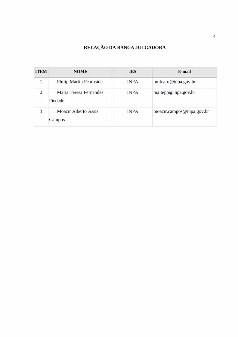
RELAÇÃO DA BANCA JULGADORA

ITEM NOME IES E-mail

1 Philip Martin Fearnside INPA [email protected]

2 Maria Teresa Fernandes

Piedade

INPA [email protected]

3 Moacir Alberto Assis

Campos

INPA [email protected]

5

A447 Almeida, Danilo Roberti Alves de

Avaliação de susceptibilidade e impacto de incêndio em floresta alagável

(igapó) e terra-firme na Amazônia central por meio de lidar terrestre

portátil / Danilo Roberti Alves de Almeida. --- Manaus: [s.n.], 2014.

x, 54 f. : il. color.

Dissertação (Mestrado) --- INPA, Manaus, 2014.

Orientador : Bruce Walker Nelson.

Coorientador : Juliana Schietti de Almeida.

Área de concentração : Ciências de Florestas Tropicais.

1. Incêndios florestais. 2. Sensoriamento remoto. 3. Laser de varredura.

I. Título.

CDD 634.956

Sinopse:

Avaliou-se a susceptibilidade à incêndios florestais e os danos pós fogo em floresta

sazonalmente alagável (igapó) e terra-firmeno entorno do Lago Mamori, Município de

Careiro Castanho, Amazonas. Atributos como altura média da floresta, abertura de dossel e o

índice de área foliar foram estimados por meio de LiDAR terrestre portátil.

Palavras-chave: índice de área foliar, estrutura florestal, sensoriamento remoto.

6

AGRADECIMENTOS

À vida, à saúde, à beleza e a tudo que nos rodeia neste infinito universo que conspira a

nosso favor.

À minha querida e muito amada família que sempre estiveram presentes desde o meu

primeiro dia de vida até hoje e sempre. Minha Mãe Cláudia Roberti Alves de Almeida, meu

Pai Marcos Alves de Almeida e meus irmãos Vitor Roberti Alves de Almeida e Paulo Roberti

Alves de Almeida. Eles são a maior riqueza que eu tenho desde que nasci.

Aos meus excelentes orientadores Bruce Nelson e Juliana Schietti pelo generoso e

dedicado apoio. As suas revisões, indicações e métodos com certeza irão me influenciar de

forma muito positiva no meu futuro como pesquisador.

Aos pesquisadores que fizeram parte nas revisões. Ao INPA pelo apoio Institucional, ao

Bernardo Flores que foi o responsável por conseguir o apoio financeiro.

Ao grande apoio do Pesquisador e amigo Eric Gorgens. Muitos trabalhos ainda virão pela

frente.

Aos mateiros que me ajudaram em campo Lucas, João, Sabá, Pedro e Ednaldo.

À Angélica Resende que faz parte dessa minha caminhada desde 2007 (Viçosa, MG),

percorrendo caminhos muitos semelhantes comigo como amiga, companheira de Republicas e

de estudos, sempre.

Aos CAMARADAS (amigos, irmãos) de Manaus, São Paulo, Minas Gerais, do mundo

todo que sempre estão presentes. Eles são a maior riqueza que eu conquistei durante a minha

vida. Em especial às meninas da Republica “Casa Verde”, Ana, Elisa, Gel, Lu e Sabine pela

amizade, apoio e principalmente paciência comigo, rs, sempre. E por último e muito

importante, ao meu anjo da guarda que sempre olha por mim Felipe Santos Franco

(Kachacinha).

7

MUITO OBRIGADO!

8

“Nosso sonho NUNCA vai terminar…”

Leonardo Sambudio Lins

RESUMO

As florestas sazonalmente alagáveis por águas pretas e pobres em nutrientes (igapó) têm

sofrido altos impactos por incêndios florestais. Durante os períodos secos estas florestas

apresentam menores extremos de umidade relativa do ar e maioresextremos de temperatura

comparada com a terra-firme, favorecendo a proliferação do fogo. Estas características

microclimáticas podem ser controladas por atributos estruturais da floresta (abertura de

dossel, altura da floresta e densidade de sub-bosque). O sub-bosque mais denso (com

vegetação úmida) controla a proliferação do fogo. A altura da floresta e a abertura de dossel

controlam a estabilidade do microclima no interior da floresta. O objetivo do estudo foi

avaliar estes três atributos (densidade de sub-bosque, altura da floresta e abertura de dossel)

como determinantesda susceptibilidade aos incêndios florestais e os impactos pós-fogo nessas

florestas. Foi utilizadoum sistema portátil de sensoriamento remoto ativo equipado com

LiDAR RIEGL LD90-3100VHS-FLP para estimar os atributos. A coleta dos dados em campo

é rápida e fácil, comparada com outros sistemas que também utilizam o LiDAR. Os atributos

das florestas são extraídos de nuvens bidimensionais com primeiros e últimos retornos

(2000Hz), onde pode ser estimado por exemplo a densidade de área foliar (LAD) ao longo do

perfil vertical da floresta. O pulso emitido pelo equipamento, com comprimento de onda de

900nm (espectro infravermelho próximo) é fortemente refletido pelas folhas. O instrumento é

montado em um gimbal mantido na orientação do zênite e é carregado à um metro acima do

solo. Dez transectos de 250 m foram percorridos em velocidade constante para cada situação:

(1) igapó não queimado, (2) igapó queimado, (3) terra-firme não queimada e (4) terra-firme

queimada. O igapó apresentou maiores danos pós-fogo, com perda de 71% de sua vegetação,

e também maior susceptibilidade à ocorrência de incêndios devido a abertura de dossel, duas

vezes maior que a terra-firme (aumentando a iluminação solar), altura da floresta 15% mais

baixa (maior vulnerabilidade de alteração do microclima) e 43% menos vegetação no sub-

bosque (menos vegetação úmida que dificulta a proliferação do fogo). As florestas de igapó

9

são fitofisionomias extremamente frágeis aos incêndios, sendo mais susceptíveis à ocorrência

de incêndios, com maiores danos pós fogo e menor regeneração, que é dificuldade pelo

período de alagamento

Palavras-chave: estrutura florestal, laser de varredura, densidade de área foliar.

ABSTRACT

SUSCEPTIBILITY AND FIRE DAMAGE ON A FLOODED FOREST (IGAPO) AND

UPLAND FOREST IN THE CENTRAL AMAZON ACCESSED WITH PORTABLE

GROUND LIDAR

Nutrient-poor and seasonally flooded Amazon forests have suffered high impacts from forest

fires. During the dry periods, seasonally flooded forests can present higher air temperature

and lower humidity compared to upland forests, enabling the occurrence and spread of fire.

These microclimatic conditions may be related to structural attributes of the forest (canopy

gap fraction, height and density of understory) that favor changing the microclimate. A high

densityof vegetation in the understory (with wet vegetation) can control the spread of fire and

the forest canopy height and opening can control the stability of the microclimate inside the

forest.The aim of this study was to evaluate these attributes to determine susceptibility and

impacts of fires in these forests. To estimate these forest structure attributes we used a

portable active remote sensing system equipped with LiDAR RIEGL LD90-3100VHS-FLP.

The operation of the data collection in the field is quick and easy, compared to other systems

that also use LiDAR device. Forest structural attributes, such as the leaf area density (LAD)

along the vertical profile of the forest were extracted from two-dimensional clouds of first and

last returns at 2000 Hz. The pulse emitted by the equipment, with a wavelength of 900 nm

(near infrared spectrum)is strongly reflected by leaves. The instrument was mounted on a

gimbal to maintain a zenith shot angle and it was carried 1m above the ground. Ten transects

of 250m length were, sampled at constant speed for each situation: (1) unburned flooded

forest (2) burned flooded forest (3) unburned upland forest and (4) burned upland forest. The

flooded forest showed a more damage after fire, with loss of 71% of this vegetation, and also

it was more susceptible to fire occurrence due to the higher gap fraction (at least two times

10

higher than the upland increasing the entry of sunlight). Canopy height was 15%lower (what

makes flooded forests more vulnerable to the external environment) and the density of the

understory, 43%lower (less living moist vegetation to limit the spread of fire). The flooded

forest are extremely fragile to fires, being more susceptible to occur, with higher post fire

damage and lower regeneration, which is hard by flooding period.

Keywords: forest structure, laser scanner, leaf area density

SUMÁRIO

LISTA DE FIGURAS ....................................................................................................... 9

LISTA DE TABELAS ....................................................................................................... 9

LISTA DE ABREVIAÇÕES ............................................................................................. 10

INTRODUÇÃO GERAL ................................................................................................. 10

OBJETIVOS ................................................................................................................ 10

Objetivos gerais ............................................................................................................... 10

Objetivos Específicos ........................................................................................................ 11

CAPÍTULO 1 ............................................................................................................... 12

Abstract ........................................................................................................................... 13

MATERIAL AND METHODS ............................................................................................... 13

DISCUSSION AND CONCLUSIONS ...................................................................................... 17

REFERENCES..................................................................................................................... 19

CONCLUSÃO GERAL ................................................................................................... 20

REFERÊNCIAS BIBLIOGRÁFICAS .................................................................................. 20

APÊNDICE A– Material Suplementar .......................................................................... 23

Figuras do material e métodos ......................................................................................... 23

Tabela geral ..................................................................................................................... 25

Fotos de campo ............................................................................................................... 25

APÊNDICE B– Script para o software R para análises dos dados LiDAR........................ 26

Produtosdo Script ............................................................................................................ 43

11

LISTA DE FIGURAS

LISTA DE TABELAS

LISTA DE ABREVIAÇÕES

DAF - Densidade de Área Foliar

ENSO - Oscilação Sul do El Niño

FLP – First and Last Pulse

IAF - Índice de Área Foliar

LD – Laser Distance

LiDAR -Light Detection and Ranging

LTP - LiDAR Terrestre Portátil

VHS – Very High Speed

12

INTRODUÇÃO GERAL

Os incêndios afetam a maioria dos ecossistemas do mundo há milhões de anos,

contribuindo para a evolução das espécies e alterando processos hidrológicos,

geomorfológicos, geoquímicos e ecológicos (Bond e Midgley, 2012). Porém, a frequência de

ocorrência dos incêndios tem aumentado consideravelmente devido, principalmente, às

mudanças do uso do solo onde o fogo funciona como um método barato de limpeza e

condução de sistemas agrícolas (Nepstad et al., 2001, Alencar et al., 2004). Estes, quando não

controlados causam grandes incêndios florestais principalmente em períodos secos (Asner e

Alencar, 2010; Aragão et al., 2007). Alguns fenômenos como a Oscilação Sul do El Niño

(ENSO) (Marengo et al., 2011) e o aquecimento anômalo da superfície do Oceano Atlântico

norte tropical (Marengo et al., 2008) aumentam a severidade das secas nas florestas da

Amazônia, contribuindo para o aumento na frequência de ocorrência de incêndios. Nos anos

de 1997-1998 (ocorrência do ENSO) cerca de 40.000 Km2 de florestas (no sul e leste da

Amazônia) tiveram os sub-bosques afetados pelo fogo rasteiro (ou fogo de superfície), isso

significa ser 13 vezes maior que os incêndios em um ano sem ENSO e duas vezes a taxa

média de desmatamento anual nas mesmas regiões (Alencar et al., 2004). No período

compreendido entre 1999 e 2010 estima-se, a partir de imagens de satélite, que o fogo rasteiro

afetou 85.500 Km2 da floresta, somente no sul da Amazônica (Morton et al., 2013), e apesar

dessas observações ainda necessitarem de observações e experimentos in loco,os autores

sugerem que as áreas incendiadas são maiores que todo o desmatamentos para o mesmo

período de tempo. Alguns autores sugerem que os incêndios florestais são uma das maiores

ameaças de empobrecimento e transformação das florestas na Amazônia (Nepstad et al.,

2001; Alencar et al., 2011; Aragão et al., 2007).

Os incêndios contribuem para a mudança climática global, tanto pela emissão de gases do

efeito estufa como pela destruição das florestas responsáveis pelos equilíbrios hídrico e

térmico do planeta e da região (Fearnside, 2005). A ocorrência de incêndios altera também os

regimes dos incêndios, que tendem a ser mais frequentes, em um processo sinérgico e

complexo, em que é difícil prever quais serão as consequências no futuro (Cochrane e Barber,

2009, Nepstad et al., 2001; Coe et al., 2013).

13

Além dos fatores climáticos os incêndios dependem basicamente de outros dois

fatores: ignição e combustível. A ignição pode ocorrer de forma natural (pela ocorrência de

relâmpagos, faíscas de rocha, queda de meteoros ou combustão espontânea) ou, mais

provável, pela ação humana, em áreas onde há maior proximidade de centros urbanos e acesso

antrópico (Cochrane & Schulze 1998; Morton et al. 2013). Toda a biomassa presente na

floresta pode ser considerada material combustível se for susceptível à queima e propagação

do fogo. A susceptibilidade do combustível à queima depende de condições do material, tais

como umidade, tamanho e composição química (Kauffman et al. 1988). Felizmente as florestas

altas e densas (fatores estruturais) da Amazônia são resistentes à seca e pouco susceptíveis aos

incêndios, uma vez que seu interior sombreado e cheio de vegetação viva mantem úmido o

material combustível fino (Uhl et al., 1988).

Contudo, florestas densas que já sofreram alteração estrutural pela exploração

madeireira e/ou algum incêndio no passado são mais vulneráveis à ocorrência de incêndios

florestais (Uhl e Kauffman, 1990; Holdsworth e Uhl, 1997). Isso se deve ao aumento do

material combustível no solo e à alteração estrutural proporcionando uma maior entrada de

iluminação solar, devido à maior abertura no dossel, no interior da floresta (Uhl e Kauffman,

1990, Ray et al., 2005), causando o aumento da temperatura e diminuição da umidade relativa

do ar do sub-bosque. Quando a umidade do ar é menor que 65%, o material combustível se

torna vulnerável a ignição e proliferação do fogo (Uhl et al., 1988).

As fitofisionomias naturais das florestas Amazônicas possuem diferentes estruturas

florestais ligadas a condições edafoclimáticas (Sombroek, 2000, Quesada et al 2012), e assim,

possuem também diferentes susceptibilidades aos incêndios e impactossofridos (severidade)

pela ocorrência destes (Uhl et al.,1988, Ray et al., 2005). As florestas alagáveis, por exemplo,

estão sob regimes hídricos bem distintos das florestas de terra-firme. De maneira intuitiva,

pensamos que as florestas sazonalmente alagáveis não correm risco de serem incendiadas,

devido ao acúmulo de água durante um período do ano. Mas na realidade essas florestas

podem ser mais suscetíveis aos incêndios, e sofrem danos ainda maiores que florestas não

alagáveis (terra-fime). Nelson (2001) e Resende et al. (2014) observaram maior dano pós

fogo, em florestas sazonalmente alagáveis por águas pretas pobres em nutrientes (igapó), em

relação à terra-firme, num local onde as duas fitofisionomias se encontravam próximas e

foram penetradas pelo mesmo incêndio. Flores et al. (2014) utilizando inventário de campo e

imagens de satélite de alta resolução encontraram uma mortalidade pós-fogo de 90% de

14

árvores em cicatrizes de fogo em florestas de igapó no médio Rio Negro. Estudos sobre

incêndios em terra-firme relatam percentuais de mortalidade menores(Barlow e Peres, 2004;

Cochrane et al., 1999).

A bacia amazônica abriga mais da metade das florestas tropicais remanescentes no mundo

(Laurance et al., 2011), com mais de 5,4 milhões de Km2, e mais de 11,5 % é coberta por

florestas sazonalmente alagáveis (Melack e Hess, 2010), estudos sugerem que esse percentual

pode ser muito maior chegando à 30% (Junk et al., 2011). Os igapós são florestas

sazonalmente alagáveis por águas pretas, ácidas e pobres em nutrientes (Junk et al., 2011). As

taxas de crescimento e recrutamento das árvores são baixas quando comparadas com

ambientes de solos relativamente mais férteis e sem dinâmica de inundação(Junk et al., 2011).

Com isso postulamos que as florestas de igapó são(1) menos densas no sub-bosque, (2)

mais baixas e (3) com maior abertura de dossel que florestas de terra-firme, resultando numa

maior vulnerabilidade às alterações do seu microclima. A maior densidade de vegetação viva

no sub-bosque da terra-firme ajuda a manter o ambiente úmido e funciona como uma barreira

que dificulta a passagem do vento ao solo, dificultando a proliferação do fogo. Em algumas

florestas de igapó, no período em que estão secas, o sub-bosque possui menores extremos de

umidade relativa do ar, maioresextremos de temperatura (Resende et al., 2014) e há também

um maior acúmulo de material combustível fino no solo (Kauffman et al. 1988; Dos Santos e

Nelson, 2013). A serapilheira do igapó se decompõe lentamente provavelmente devido à

baixa atividade de fungos saprófitos (Singer, 1988) e uma menor densidade de

decompositores, cupins e outros organismos xilófagos nesse tipo de floresta sazonalmente

inundável (Capps et al., 2011).

A distribuição da vegetação ao longo do perfil vertical da floresta (fatores estruturais)

influência nos mecanismos de fotossíntesee controle de crescimento e produção (Cavaleri et

al., 2010; Domingues et al., 2005), afetando o microclima em várias escalas (Ray et al., 2005)

e gerando diferentes habitats para diversidade florestal (MacArthur e MacArthur, 1961). As

mensuraçõesdos atributos físicos estruturais das florestas tais como abertura do dossel, altura

da floresta, densidade de área foliar (DAF) e o índice de área foliar (IAF) são fundamentais

para determinar a susceptibilidade, dos diferentes tipos florestais, aos incêndios e também na

mensuração de danos pós fogo, além de fornecer informações sobre estágios de sucessão

florestal, podendo predizer outros atributos importantes para o manejo desses ambientes como

área basal, densidade de árvores e biomassa acima do solo (d'Oliveira et al., 2012). A DAF é a

15

quantidade de folhas (área foliar) que existe em um determinado volume de floresta, o

somatório do DAF corresponde ao IAF que é área de folha por área de solo.

Estes e outros atributospodem ser mensurados pelo sistema de sensoriamento remoto

ativo Light Detection and Ranging (LiDAR) terrestre portátil (Parker et al., 2004, Sumida et

al. 2009, Stark et al., 2012). A tecnologia LiDAR, do tipo rangefinder, mede a distância das

estruturas em função do tempo percorrido entre a emissão e o retorno de raios laser, com

comprimento no espectro do infravermelho próximo, que é altamente refletido pela vegetação

(Lefsky et al., 2002). O sistema LiDAR terrestre portátil (LPT) realiza o escaneamento da

vegetação com mira vertical (eixo y) para cima e utiliza uma plataforma terrestre movida por

meio de uma caminhada em velocidade constante (eixo x). Os dados gerados nesse sistema

são bidimensionais. Apesar dessa tecnologia apresentar algumas limitações e vieses, os efeitos

são relativamente pequenos nos resultados de estimativas das estruturas do dossel (Parker et.

al., 2004). Portanto, o uso do LPT parece ser uma ferramenta promissora para avaliação de

susceptibilidade ao fogo e danos causados por incêndios por meio de estimativas dos atributos

estruturais da floresta.

OBJETIVOS

Objetivos gerais

• Determinar se as diferenças estruturais entre dois tipos florestais (igapó e terra-firme)

favorecem a ocorrência de fogo.

• Determinar se o igapó sofreu mais dano que a floresta de terra firme quando ambos

foram expostos ao mesmo incêndio.

Objetivos Específicos

Testar as seguintes hipóteses em relação à floresta de terra-firme:

(a) o igapó tem menor densidade de vegetação no sub-bosque;

(b) o igapó tem menor altura de dossel;

(c) o igapó tem maior abertura do dossel e

(d) os danos pós-fogo são maiores no igapó.

16

CAPÍTULO 1 ___________________________________________________________________________

Almeida, D. R. A.; Nelson, B. W.; Schetti, J.; Gorgens, E. B.; Resende, A. F. 2015.

Contrasting fire susceptibility and fire damage between seasonally flooded forest and upland

forest in the Central Amazon using portable terrestrial lidar. Manuscrito formatado nas

normas da Forest Ecology and Management

Title:

Contrasting fire susceptibility and fire damage between seasonally flooded forest

and upland forest in the Central Amazon using portable terrestrial lidar

17

Danilo Roberti Alves de Almeidaac, Bruce Walker Nelsona, Juliana Schiettia, Eric Bastos

Gorgensb, Angélica Faria Resendea

a) INPA -Brazil’s National Institute for Amazon Research;Av. André Araújo,

2936;69067-375 Manaus,AM, Brazil

b)USP/ESALQ - University of São Paulo; Av. Pádua Dias, 11;13418-900 Piracicaba, SP,

Brazil

c) Corresponding author: <[email protected]>

18

Abstract

Fire is an increasingly important agent of forest degradation in the Amazon. Satellite images

suggest that forests flooded seasonally by nutrient-poor waters are more susceptible to fire

and suffer greater fire damage than do nearby upland forests. Reasons for this include

presence of a root mat, more fine fuel as litter and a drier understory in the floodplain. We

employed a portable terrestrial lidar (Riegl model LD90-3100VHS-FLP) to detect and

describe differences in canopy structure that contribute to different micro-climates in these

two forest types at a site in the Central Brazilian Amazon. We also compared lidar-derived

metrics of post-burn damage. The lidar was mounted on a gimbal to maintain a zenith shot

angle and was carried 1m above the ground. Ten transects of 250m length were traversed at

constant speed for each situation: (1) unburned flooded forest, (2) burned flooded forest, (3)

unburned upland forest and (4) burned upland forest. Structure attributes were extracted from

two-dimensional clouds of first or last returns, each captured at 1000 Hz. Four years after the

fire, the lidar data showed much higher damage in the floodplain and slower recovery in

floodplain burn gaps. Leaf Area Index did not differ between the unburned upland and

floodplain forests, but their vertical and horizontal distributions of leaves were distinct. The

floodplain had less leafy vegetation in the understory, higher canopy openness, and lower

height -- all favoring higher extremes of temperature and lower extremes of relative humidity

near the litter layer.

Keywords: structural attributes, laser scanner, leaf area density, igapó, terra-firme

19

INTRODUCTION

Tall and dense mature forests of Amazonia are resistant to drought and penetration of

surface fires from ignition sources in nearly pastures or swiddens. The deep shade of the

understory, with few gaps, maintains high relative humidity (Ray et al., 2005, Uhl et al.,

1988). Rapid microbial decomposition of litter keeps fine fuel stock low (Martius et al.,

2004). Forests that have suffered structural damage by mechanized logging and/or by a recent

fire, however, are more vulnerable to recurring fire (Holdsworth and Uhl, 1997; Uhl and

Kauffman, 1990), especially in drought years (Alencar et al., 2011; Flores et al., 2012). These

two disturbances increase coarse and fine fuel loads on the ground and open large sunlit gaps

(Ray et al., 2005; Uhl and Kauffman, 1990), leading to hotter temperatures and lower relative

humidity. When the understory relative humidity is less than 65%, fine fuel becomes

vulnerable to ignition and fire spread (Uhl et al., 1988).

Natural Amazon forest types have different canopy structures, some of which lead to

differences in both the susceptibility to fire penetration and the degree of damage during a fire

(Ray et al., 2005; Uhl et al., 1988). Forests flooded annually by nutrient-poor acid black

waters, called igapó (Junk et al., 2011), suffer much greater post-fire impact than do upland

terra-firme forests (Flores et al., 2012; Nelson, 2001; Resende et al., 2014). When compared

to nearby dense upland forest, the igapó forest has a greater accumulation of fine combustible

leaf litter above the ground and a thicker mat of fine roots just below the litter and above the

mineral soil, both of which are a consequence of slow leaf decomposition under water (Dos

Santos and Nelson, 2013; Kauffman et al., 1988). The root mat and canopy structure

differences may also facilitate faster drying of leaf litter, making this layer flammable more

days of the year in the igapó. In the period when the igapó forest is not flooded, the

understory attains lower extremes of relative humidity and higher temperature extremes than

nearby upland forest (Resende et al., 2014). Very low growth and recruitment rates of trees in

igapó forests (Junk et al., 2011), may leave these in a state of prolonged or stagnated

succession, with low stature canopy maintained for decades after a rare severe fire (Williams

et al., 2005, Ritter et al., 2013).

20

Structural attributes that control the internal microclimate of the forest, such as density

of understory, canopy height and canopy cover, can be measured by the active remote sensing

technique of Light Detection and Ranging (LiDAR) (Parker et al., 2004). This technology

measures the distance to structures as a function of elapsed time between emission and return

of a near infrared laser pulse, which is strongly reflected by vegetation (Lefsky et al., 2002).

The objectives of this study are to (1) determine whether structural differences

between the two types of forest -- nutrient-poor seasonally flooded and upland -- favor the

occurrence of fire and (2) using only lidar-derived metrics, confirm whether the seasonally

flooded forest suffers higher damage post-fire than upland forest, when the two forest types

are exposed to the same fire. We test four hypotheses: (a) the unburned flooded forest has

lower vegetation density in the understory, compared to unburned upland; (b) the unburned

flooded forest has lower height compared to unburned upland; (c) the unburned flooded forest

has more open canopy than unburned upland and (d) post-fire damage is higher in flooded

forest than in upland forest.

MATERIAL AND METHODS

Field site

The field site is about 100 km from Manaus in forests surrounding Mamori Lake,

centered at 03°43' S and 60°14' W. The climate is tropical, warm and moist, with an average

temperature of 27.2°C and average annual rainfall of 2171mm (Af in the Köppen

classification).

The seasonally flooded forest has a ten meter annual flood pulse controlled by the

Amazon River, but only minor influence of nutrient-rich waters. Four aspects of the site make

it particularly favorable for our study. First, the two vegetation types are spatially

interspersed. A network of dendritic valleys holds the seasonally flooded forests and the

narrow intervening interfluves are covered by upland forests. Secondly, there are no scarps or

broad river channels between the two vegetation types, which could act as firebreaks.

Consequently, the chance of ignition and of fire spread (from management fires in swiddens

and pastures) were similar between both forest types. Thirdly, a large tract of preserved land

within the study area provides unburned forests of both types used in the study of comparative

forest structure related to fire susceptibility. These also served as control plots, proxies for

21

pre-burn structure in the comparative study of post-fire damage. Finally, the sampled areas

suffered only one past forest fire, in November of 2009 when only part of the overall study

area was burned.

This study was conducted four years after the 2009 fire, enough time to accrue delayed

tree mortalities (Barlow et al., 2003). All samples were collected in a single month

(November 2013), avoiding any structural differences related to seasonal changes in leaf

amount (Haugaasen and Perez, 2005). This month was also the minimum annual water stage

when the igapó forest was unflooded.

LiDAR data collection

Each of the four situations: (1a) unburned flooded forest, (1b) burned flooded forest,

(2a) unburned upland forest and (2b) burned upland forest, was sampled along ten transects of

250 meters each, using a system equipped with a rangefinder type LiDAR, model LD90-

3100VHS-FLP manufactured by Riegl, of Horn, Austria. The distance between the emitter

and the detected object is determined from the time between emission and return of the laser

pulse.

A two-dimensional cloud of returns is produced, where the Y-dimension is height

above the ground and the X-dimension is provided by the operator walking along the ground

at a constant speed with the lidar aimed toward the sky. Laser wavelength is 900 nm, which is

strongly reflected by vegetation. With accuracy of ± 25 mm and nominal range of 200 m

without a retro-reflector, the equipment alternately records the first and the last return from

each pulse, at a frequency of 1000 pulses per second for each return type. Those pulses that do

not reach a target, and therefore do not return, are called skyshots, useful to measure canopy

openness.

The complete portable terrestrial LiDAR system (PTL) is easy to use and of moderate

cost at ~US$20,000. The operator carries the lidar in a portable gimbal one meter above the

ground with a fixed zenith view. A small 12 v battery and a water-resistant computer

complete the system. With training and aid of an audible metronome and a 250 m tape, it is

possible to keep the walking speed constant within ± 5%. Each 250 m transect map position

was recorded by collecting 11 evenly spaced GPS points per transect.

LiDAR data analysis

22

To evaluate the four hypotheses about structural differences related to differences in

the pre-burn susceptibility to fire penetration and the post-fire degree of damage, we obtained

leaf area density (LAD) in the understory from 1-4 meters height; average height of the upper

canopy; and three metrics of canopy openness.

To obtain LAD of the understory we first estimated LAD for every cell of 1m vertical

x 1m horizontal increments in each 250 m transect. We then averaged the 1-4m values for all

250 columns per transect. The upper canopy height of each transect was the average of the

250 highest pulse returns, i.e. the maximum heights in each column of cells. Our first metric

of canopy openness was the number of sky shots per 250 m transect. Our second metric of

openness per transect was the fraction of all 250 columns whose highest pulse returns were

less than 15 m above the ground. We call this the gap fraction, following the definition of

Runkle (1982). Our third metric of openness was the leaf area index (LAI) of each transect,

from the average LAI of all 250 columns in that transect. The LAI of a single column is the

sum of all LAD values in that column. All differences between means -- between unburned

terra-firme and unburned igapó or between burned upland and burned igapó -- were evaluated

using the Mann-Whitney test.

The LAD of each 1m x 1m cell in a column is derived from the raw pulse returns from

that cell, corrected for the number of “consumed pulses” that did not reach the base of the

cell. We used the equation of MacArthur-Horn (1969), similar to the Beer-Lambert Law,

which relates the concentration of a chemical solution in a cuvette to its absorbance (A) of

light at a particular wavelength. Thus, A = - ln(I/I0), where I is the radiant intensity on the

output side of the cuvette and I0 is the radiant intensity on the input side. The absorbance can

also be calculated by a linear equation (A = D * C * K), as it is the product of the distance D

(width of the cuvette containing the solution), the solution concentration C and a substance-

specific constant K, which is related to the rate of change of absorbance of the solution as

concentration changes. Combining the two equations and isolating concentration as the

variable of interest, we have Equation 1:

𝑟𝑎𝑑𝑖𝑎𝑛𝑐𝑒. ∈𝑟𝑎𝑑𝑖𝑎𝑛𝑐𝑒. 𝑜𝑢𝑡⁄

𝐶 = −𝑙𝑛 (1)

23

Where C is the concentration of the substance in the solution; “radiance.in” and

“radiance.out” are self-explanatory, D is the width of the cuvette and K is the constant for the

substance.

The equation for calculating the leaf area density of the forest in each one meter high cell

in a stack is analogous, as shown by equation (2):

𝑝𝑢𝑙𝑠𝑒𝑠. ∈

𝑝𝑢𝑙𝑠𝑒𝑠. 𝑜𝑢𝑡⁄

𝐿𝐴𝐷 = −𝑙𝑛 (2)

Where LAD is the leaf area density of one cell in a stack; “pulses.in” is the number of

pulses which strike the bottom of the cell; “pulses.out” is the number of pulses that come out

at the top of that cell; D is the height of the cell. Note that varying walking speed of the lidar

operator along the transect does not affect the pulse ratio. The second term (1/D) cancels

because a cell is one meter high. The constant K describes the change in absorbed pulses as

leaf density (concentration) increases. K remains constant if all of the following remain fixed:

lidar beam width, pulse intensity, pulse wavelength, distribution of leaf blade angles and

degree of clustering of leaves. Prior studies using a similar instrument to ours have assumed

K=1 (Parker et al. 2004, Sumida et al. 2009, Todd et al. 2003). Recent work (Scott Stark,

unpublished) also found K=1 for the same brand and model used here, so the third term (1/K)

also cancels in Equation 2.

RESULTS

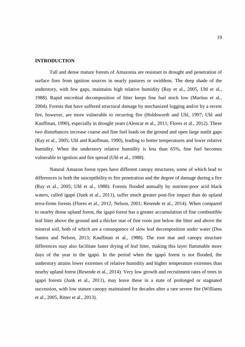
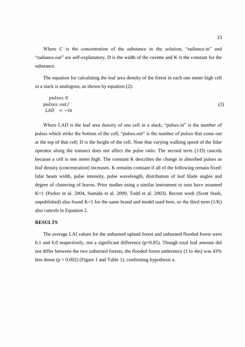
The average LAI values for the unburned upland forest and unburned flooded forest were

6.1 and 6.0 respectively, not a significant difference (p=0.85). Though total leaf amount did

not differ between the two unburned forests, the flooded forest understory (1 to 4m) was 43%

less dense (p = 0.002) (Figure 1 and Table 1), confirming hypothesis a.

24

Figure Erro! Nenhuma sequência foi especificada.. Leaf area density, LAD, with 95% confidence

intervals, along vertical profile (left) and curves of cumulative leaf area index, LAI (right) in

the unburned seasonally flooded forest (solid) and unburned upland forest (dashed). The

horizontal lines at 4 and 22 m height indicate where the LAD curves cross; the line at 31m is

where the total flooded forest LAI is reached.

From 4 to 22 meters high, the flooded forest was 19% more dense (p = 0.002), with

the two forests’ cumulative LAI curves crossing at 8 m height. Above 22 meters the upland

forest had 43% more vegetation density (p = 0.002) and the cumulative curves met again at 31

meters. Above this height only upland forest showed any increase in the LAI (p = 0.009). The

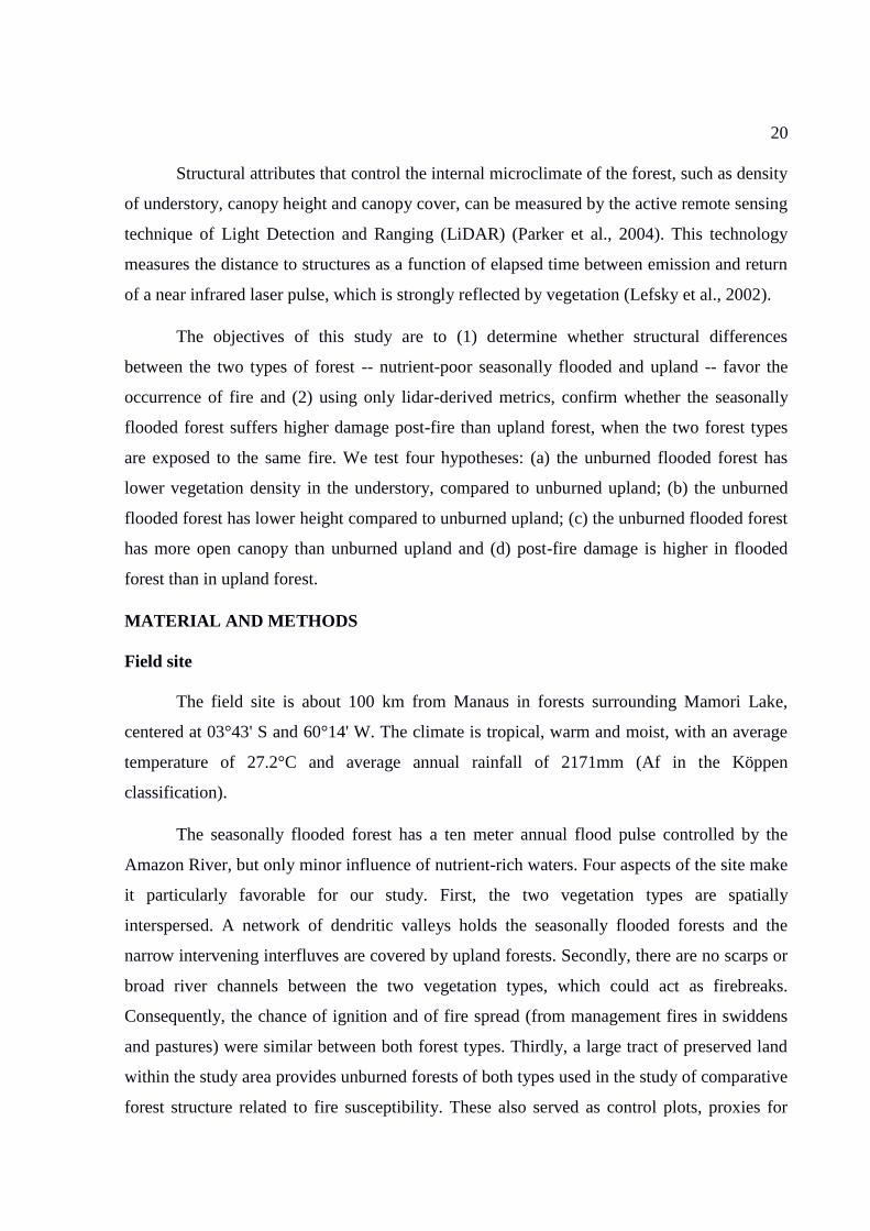
flooded forest was on average 15% lower than the upland forest (p < 0.001) (Figure 2 and

Table 1), confirming our hypothesis b.

25

Figure Erro! Nenhuma sequência foi especificada.. Canopy heights. Each point represents the average

of 250 maximum height values measured in 1 m wide columns along one of the 250 m

transects.

Table Erro! Nenhuma sequência foi especificada.. Averages, standard deviations and p-values (Mann-

Whitney test) for the metrics relevant to the evaluation of susceptibility to fire, compared

between unburned plots of the two forest types.

Floodplain Forest Upland Forest

Metric Average

Standar

d deviation

Averag

e

Standard

deviation

p-

value

LAD (1 a 4m) 0.33 0.15 0.59 0.09

0.001

5

LAD (4 a 22m) 5.16 0.56 4.35 0.46

0.002

1

LAD (> 22m) 0.93 0.40 1.63 0.40

0.002

1

26

LAI 6.00 0.41 6.10 0.18

0.853

4

Mean height 19.77 1.53 23.34 1.56

0.000

2

PS 0.04 0.03 0.01 0.01

0.000

7

LCF (15

meters) 0.19 0.07 0.09 0.05

0.001

0

Where,

LAD – Leaf Area Density (m2/m3);

LAI – Leaf Area Index (m2/ m2);

Mean height – mean of 250 maximum heights (m);

PS – Proportion of Sky Shots;

LCF – Low Canopy Fraction (% below 15 m threshold)

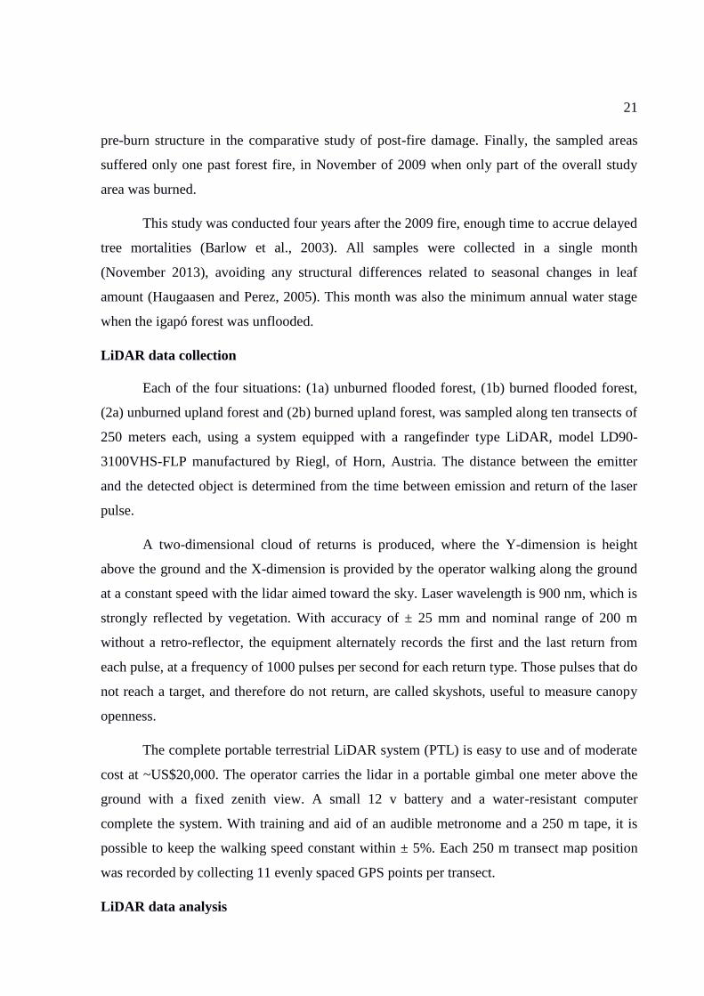
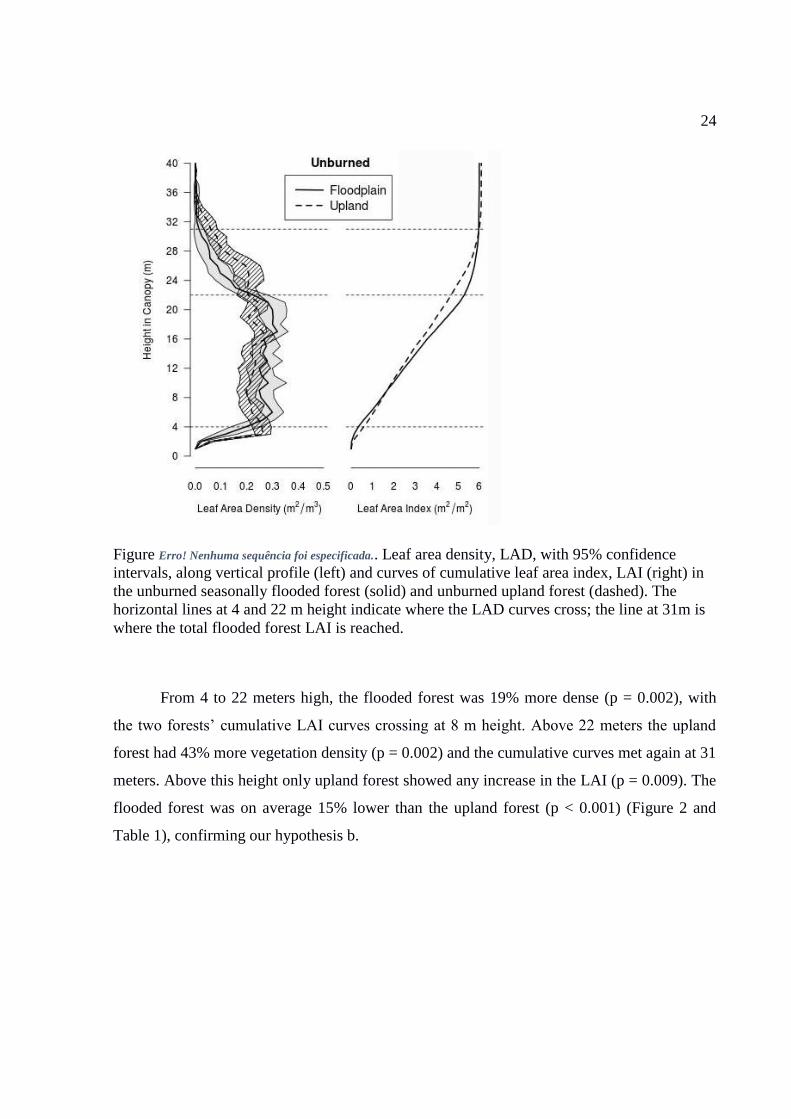
As postulated by hypothesis c, the flooded forest also features a more open canopy,

with almost three times more skyshots (Figure 3) and two times more gap fraction (< 15 m) (p

= 0.001) (Figure 4 and Table 1).

Figure Erro! Nenhuma sequência foi especificada.. Skyshots (pulses that did not return), a metric of

canopy openness.

27

The four attributes, canopy openness, average canopy height, understory density and LAI

were significantly altered after the same fire event penetrated the two forest types. These four

indicators of damage had much greater pre- to post-fire change in the flooded forest,

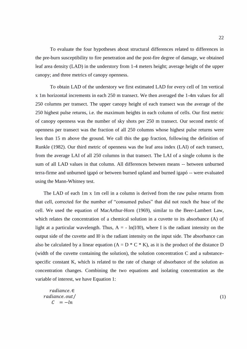
corroborating hypothesis d (Table 2). Reduction of LAI was only 9% for upland forest but

was 71% in the flooded forest, a significant difference (p< 0.001) (Figure 5).

Figure Erro! Nenhuma sequência foi especificada.. Cumulative frequency histograms of maximum

canopy heights, averaged for the ten transects of each forest class. At the threshold height of

15 m this is the same as the “low canopy fraction” or “gap fraction” (Runkle, 1982). The p-

value refers to the tested difference between the two unburned forests at 15m height.

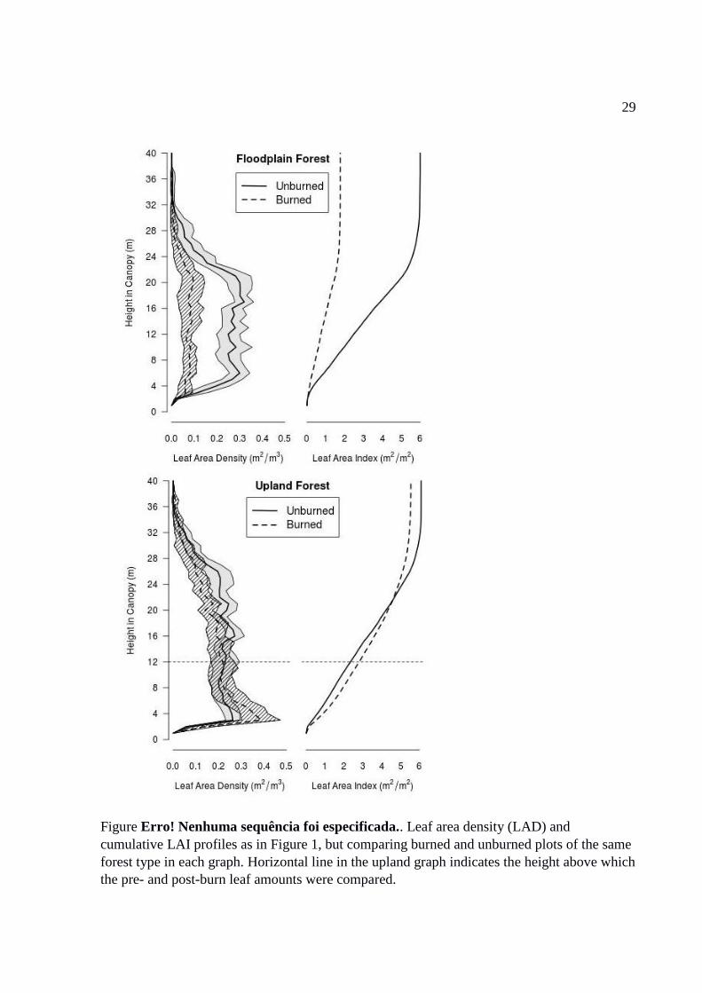
There was a loss of vegetation along the entire vertical profile of burned seasonally

flooded forest. In upland, incipient regrowth caused a post-burn increase of 50% in the leaf

area density in the understory (1 to 4 m), whereas floodplain lost 57% of its understory leaf

area density, also a significant difference in post-burn damage (p <0.001). Above 12 m height

(i.e. above the height of new regeneration in the upland forest profile) there was a significant

28

post-burn loss of 26% of leaf area density in upland forest (p <0.001). At 22 meters, the

cumulative LAI curves crossed and so that the total LAI of unburned upland forest exceeded

that of burned upland forest (Figure 5).

29

Figure Erro! Nenhuma sequência foi especificada.. Leaf area density (LAD) and

cumulative LAI profiles as in Figure 1, but comparing burned and unburned plots of the same

forest type in each graph. Horizontal line in the upland graph indicates the height above which

the pre- and post-burn leaf amounts were compared.

30

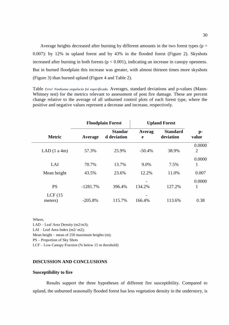
Average heights decreased after burning by different amounts in the two forest types (p =

0.007): by 12% in upland forest and by 43% in the flooded forest (Figure 2). Skyshots

increased after burning in both forests (p < 0.001), indicating an increase in canopy openness.

But in burned floodplain this increase was greater, with almost thirteen times more skyshots

(Figure 3) than burned upland (Figure 4 and Table 2).

Table Erro! Nenhuma sequência foi especificada. Averages, standard deviations and p-values (Mann-

Whitney test) for the metrics relevant to assessment of post fire damage. These are percent

change relative to the average of all unburned control plots of each forest type, where the

positive and negative values represent a decrease and increase, respectively.

Floodplain Forest Upland Forest

Metric Average

Standar

d deviation

Averag

e

Standard

deviation

p-

value

LAD (1 a 4m) 57.3% 25.9% -50.4% 38.9%

0.0000

2

LAI 70.7% 13.7% 9.0% 7.5%

0.0000

1

Mean height 43.5% 23.6% 12.2% 11.0% 0.007

PS -1281.7% 396.4%

-

134.2% 127.2%

0.0000

1

LCF (15

meters) -205.8% 115.7%

-

166.4% 113.6% 0.38

Where,

LAD – Leaf Area Density (m2/m3);

LAI – Leaf Area Index (m2/ m2);

Mean height – mean of 250 maximum heights (m);

PS – Proportion of Sky Shots

LCF – Low Canopy Fraction (% below 15 m threshold)

DISCUSSION AND CONCLUSIONS

Susceptibility to fire

Results support the three hypotheses of different fire susceptibility. Compared to

upland, the unburned seasonally flooded forest has less vegetation density in the understory, is

31

less tall and has more open canopy. The microclimate inside the unburned floodplain forest is

a product of a synergy among these structural attributes. An understory with less deep shade,

filled with fewer green leaves and a shorter covering canopy provides the seasonally flooded

forest’s litter layer with a weaker buffer against external extremes of high temperature and

low humidity. The seasonally flooded forest is further conducive to fires due to more canopy

gaps (skyshots) and more area where the canopy dips below 15 m height. Gaps allow higher

input of solar radiation to lower layers of the forest (Stark et al. 2012). Places with low

canopy height are weak spots in the blanketing buffer against external extremes of high heat

and low humidity (Hutyra et al., 2008). Haugaasen and Peres (2006) also found higher canopy

openness in flooded forest compared with upland.

Recent work in the same study area (Resende et al., 2014) compared litter layer

microclimate between seasonally flooded and upland forests. They found that the seasonally

flooded forest, during its low water phase, had higher temperature and lower humidity during

the hottest period of the day (10-14h), dropping below 65% relative humidity. Uhl et al.

(1988) found that when the understory relative humidity is less than 65%, the forest litter

layer can be ignited and sustain fire. They were able to set fire to the litter layer of a low-

canopy seasonally flooding forest after just nine days without rain. The litter layer of tall-

canopy upland forest was not flammable even after 41 days without rain.

Post-fire damage and regrowth

Both forests suffered post-fire impacts, but damage was greater in the seasonally

flooded forest, losing 71% of its vegetation and corroborating our hypothesis d, about

differential damage. A root mat and a higher volume of fine combustible material contribute

to higher damage in igapó, as noted by previous studies (Dos Santos and Nelson, 2013;

Kauffman et al., 1988). Here we show that structural differences such as lower density

vegetation in the understory, lower canopy height and more gaps are consistent with the drier

microclimate in igapó, increasing the number of days per year that ignition is possible.

Damage is not only greater, it persists longer in floodplain forests than in upland. For reasons

not yet understood, post-fire succession in igapó is slow (Flores et al., 2012). Burned igapó

sites remain dominated for years by low shrubs, forbs, sedges and grasses, all susceptible to

reburning (Woods, 1989; Ritter et al., 2013).

In upland it was more difficult to measure the loss of post-fire vegetation comparative

to igapó due to more rapid regrowth. Four years after the fire, the upland forest showed a

32

higher density of understory compared with unburned upland. This development of dense

understory vegetation in upland occurred where there were canopy openings caused by fire,

favoring the entry of light in the lower strata of the forest.

Forest structure attributes from LiDAR

The portable terrestrial LiDAR (PTL) system proved to be very effective for

evaluating fire damage and susceptibility, providing metrics of relevant structural attributes in

the two forests. Rapid and efficient collection of a suite of useful structural attributes using

the PTL has been reported in previous studies (Stark et al., 2012, Sumida et al., 2009), though

this is the first use of this technology for forest fire risk and damage assessment in the

Amazon. The PTL does have some limitations and biases. Portions of the upper canopy can

be completely occluded, affecting estimates of upper canopy total height, rugosity and leaf

area density (Parker et. al., 2004). If the lidar beam widens or if leaf angles change from

planophile to random with increasing height in the canopy, the coefficent K will vary. Unlike

airborne lidar, only 2D transects rather than 3D volumes with voxels are output. An advantage

over airborne data is that the operator follows the ground surface, removing variation caused

by changes in land elevation. No post-processing removal of ground height is required.

Resende et al. (2014), in their study conducted in the same area, postulated that the

LAI in the flooded forest might be lower than the upland, to explain the greater extremes of

high temperature and of low humidity found in the igapó. We found that the LAI did not

differ between the two unburned forest types. However, the distribution of vegetation is

different along the vertical profiles of these two forest types before fire. The results indicate

that the use of the total LAI profile as an absolute value is insufficient to explain differences

in microclimate of different forests. When used at ground level, hemispherical cameras and

the LAI 2000 (LI-COR Inc., Lincoln, Nebraska, USA) provide only one LAI value for the

whole profile (Richardson et al., 2009). The fine-scale distribution of vegetation in the

vertical profile provided by the PTL constitutes a wealth of information beyond LAI that can

clarify ecological mechanisms of forest fire resistance.

The PTL system shows promise for measuring other vegetation types, generating

predictive variables in models of fire susceptibility and damage. Vegetation sub-types within

the broader “floodplain forest” class are in some cases difficult to distinguish (Junk et al.,

2011). The PTL provides a set of structural characteristics of forests useful to describe and

separate these vegetation types.

33

Future of igapó forests

The igapó forests are extremely fragile in the face of forest fires. They are susceptible

to fire penetration, suffer high damage from fire and recover very slowly after fire. This is of

concern in a world of changing climate, increasing ignition sources and more frequent

reburning (Cochrane and Barber, 2009; Coe et al, 2013; Nepstad et al., 2001). Public policy

should aim to raise awareness and monitor fire risk. However, some of the local population

may see fire as beneficial. Shortcuts through burned igapó forest reduce travel times in

motorized canoes during the high water season.

Fire as a threat to igapó forests is little known in wider academic circles. Fire was not

mentioned in a recent review of threats to Amazonian freshwater ecosystems (Castello et al.,

2013). Further studies are needed to understand post-fire succession of these forests and the

fire ecology of other flooded ecosystems, such as várzea -- forest seasonally flooded by fertile

muddy waters (Junk et al., 2011).

ACKNOWLEDGMENTS

We thank the Amazonas State Foundation for Research Support (FAPEAM 2011 Universal

Call) and the Brazilian National Council for Scientific and Technological Development

(CNPq process 479722/2012-9) for financial support; the Higher Education Personnel

Training Coordination (CAPES) for a student fellowship to author DRA; Bernardo Monteiro

Flores for preparing grant proposals; the Study Group on LiDAR technology (Get-LiDAR /

ESALQ) for technical assistance in data analysis; Pedro Gama, João Rocha, Angélica

Resende, Aline Lopes and Sebastião Salvino for help in the field; and the Correa and Ribeiro

families for authorizing field work on their land.

34

REFERENCES

Alencar, A., Asner, G.P., Knapp, D., Zarin, D., 2011. Temporal variability of forest fires in

Eastern Amazonia. Ecological Applications, 21(7):2397-2412. doi: 10.1890/10-1168.1

Barlow, J., Peres, C.A., Lagan, B.O., Haugaasen, T., 2003. Large tree mortality and the

decline of forest biomass following Amazonian wildfires. Ecology Letters, 6(1):6-8.

doi: 10.1046/j.1461-0248.2003.00394.x

Castello, L., McGrath, D.G., Hess, L.L., Coe, M.T., Lefebvre, P.A., Petry, P., Macedo, M.N.,

Renó, F.V., Arantes, C.C., 2013. The vulnerability of Amazon freshwater ecosystems.

Conservation Letters, 6(4): 217-229. doi: 10.1111/conl.12008

Cochrane, M.A., Barber, C.P., 2009. Climate change, human land use and future fires in the

Amazon. Global Change Biology, 15(3): 601-612. doi: 10.1111/j.1365-

2486.2008.01786.x

Coe, M.T., Mathews, T.R., Costa, M.H., Galbraith, D.R., Greenglass, N.L., Imbuzeiro, H.M.,

Levine, N.M., Malhi, Y., Moorcroft, P.R., Muza, M.N., Powell, T.L., Saleska, S.R.,

Solorzano L.A., Wang, J., 2013. Deforestation and climate feedbacks threaten the

ecological integrity of south-southeastern Amazonia. Philosophical Transactions of the

Royal Society B: Biological Sciences, 368(1619): 20120155.

doi: 10.1098/rstb.2012.0155

Dos Santos, A.R., Nelson, B.W., 2013. Leaf decomposition and fine fuels in floodplain

forests of the Rio Negro in the Brazilian Amazon. Journal of Tropical Ecology, 29: 455-

458. doi: 10.1017/S0266467413000485

Flores, B.M., Piedade M.T.F., Nelson, B.W., 2012. Fire disturbance in Amazonian blackwater

floodplain forests. Plant Ecology and Diversity, 7(1-2): 319-327.

doi:10.1080/17550874.2012.716086

Haugaasen, T., Peres, C.A., 2005. Tree phenology in adjacent Amazonian flooded and

unflooded forests 1. Biotropica, 37(4): 620-630. doi: 10.1111/j.1744-7429.2005.00079.x

http://dx.doi.org/10.1890/10-1168.1

http://dx.doi.org/10.1017/S0266467413000485

35

Holdsworth, A.R., Uhl, C., 1997. Fire in Amazonian selectively logged rain forest and the

potential for fire reduction. Ecological Applications, 7(2): 713-725. doi: 10.1890/1051-

0761(1997)007[0713:FIASLR]2.0.CO;2

Hutyra, L.R., Munger, J.W., Gottlieb, E.W., Daube, B.C., Camargo, P.B., Wofsy, S.C., 2008.

LBA-ECO CD-10 Temperature Profiles at km 67 Tower Site, Tapajos National Forest.

Data set. Oak Ridge National Laboratory Distributed Active Archive Center, Oak Ridge,

Tennessee, U.S.A. [http://www.daac.ornl.gov] doi:10.3334/ORNLDAAC/863

Junk, W.J., Piedade, M.T.F., Schöngart, J., Cohn-Haft, M., Adeney, J.M., Wittmann, F., 2011.

A classification of major naturally-occurring Amazonian lowland wetlands. Wetlands,

31(4): 623-640. doi: 10.1007/s13157-011-0190-7

Kauffmann, J.B., Uhl C., Cummings D.L., 1988. Fire in the Venezuelan Amazon 1: Fuel

biomass and fire chemistry in the evergreen rainforest of Venezuela. Oikos, 53: 167-175.

Lefsky, M.A., Cohen, W.B., Parker, G.G., Harding, D.J., 2002. Lidar remote sensing for

ecosystem studies. BioScience, 52(1): 19-30. doi: 10.1641/0006-

3568(2002)052[0019:LRSFES]2.0.CO

MacArthur, R., Horn, H., 1969. Foliage profile by vertical measurements. Ecology, 50: 802-

804.

Martius, C., Höfer, H., Garcia, M.V., Römbke, J., Hanagarth, W., 2004. Litter fall, litter

stocks and decomposition rates in rainforest and agroforestry sites in central Amazonia.

Nutrient Cycling in Agroecosystems, 68(2): 137-154. doi:

10.1023/B:FRES.0000017468.76807.50

Nelson, B.W., 2001. Fogo em Florestas da Amazônia Central em 1997. In: ProceedingsTenth

Brazilian Remote Sensing Symposium, Foz de Iguaçu, 1675-1682.

[http://www.dsr.inpe.br/sbsr2001/oral/246.pdf] Access 02/02/2015.

Nepstad, D., Carvalho, G., Barros, A.C., Alencar, A., Capobianco, P.J., Bishop, J., Moutinho

P., Lefebvre, P., Silva, U.L., Prins E., 2001. Road paving, fire regime feedbacks, and the

36

future of Amazon forests. Forest Ecology and Management, 154(3): 395-407.

doi:10.1016/S0378-1127(01)00511-4

Parker, G.G., Harding, D.J., Berger, M.L., 2004. A portable LiDAR system for rapid

determination of forest canopy structure. Journal of Applied Ecology, 41(4): 755-767.

doi: 10.1111/j.0021-8901.2004.00925.x

Ray, D., Nepstad, D., Moutinho, P., 2005. Micrometeorological and canopy controls of fire

susceptibility in a forested Amazon landscape. Ecological Applications, 15(5): 1664-

1678. doi: 10.1890/05-0404

Richardson, J.J., Moskal, L.M., Kim, S.H., 2009. Modeling approaches to estimate effective

leaf area index from aerial discrete-return LIDAR. Agricultural and Forest Meteorology,

149(6): 1152-1160. doi:10.1016/j.agrformet.2009.02.007

Ritter, C.D., Andretti, C.B., Nelson, B.W., 2012. Impact of past forest fires on bird

populations in flooded forests of the Cuini River in the lowland Amazon. Biotropica,

44(4): 449-453.doi: 10.1111/j.1744-7429.2012.00892.x

Resende, A.F., Nelson, B.W., Flores, B.M., Almeida, D.R.A., 2014. Fire damage in

seasonally flooded and upland forests of the Central Amazon. Biotropica, 46(6): 643-646.

doi: 10.1111/btp.12153

Runkle, J.R., 1982. Patterns of disturbance in some old-growth mesic forests of eastern North

America. Ecology, 63(5): 1533-1546. doi: 10.2307/1938878

Stark, S.C., Leitold, V., Wu, J. L., Hunter, M.O., de Castilho, C.V., Costa, F.R., McMahon,

S.M., Parker, G.G., Shimabukuro, M.T., Lefsky, M.A., Keller, M., Alves, L.F., Schietti,

J., Shimabukuro, Y.E., Brandão, D.O., Woodcock, T.K., Higuchi, N., Camargo, P.B.,

Oliveira, R.C., Saleska S.R., 2012. Amazon forest carbon dynamics predicted by profiles

of canopy leaf area and light environment. Ecology Letters, 15(12): 1406-1414.

doi: 10.1111/j.1461-0248.2012.01864.x

http://dx.doi.org/10.1016/S0378-1127(01)00511-4

http://dx.doi.org/10.1890/05-0404

http://dx.doi.org/10.1016/j.agrformet.2009.02.007

http://dx.doi.org/10.2307/1938878

37

Sumida, A., Nakai, T., Yamada, M., Ono, K., Uemura, S., Hara, T., 2009.Ground-based

estimation of leaf area index and vertical distribution of leaf area density in a Betula

ermanii forest. Silva Fennica, 43(5): 799-816.

Todd, K.W., Csillad, F., Atkinson, P.M., 2003. Three-dimensional mapping of light

transmittance and foliage distribution using lidar. Canadian Journal of Remote Sensing

29(5): 544-555. doi: 10.5589/m03-021

Uhl, C., Kauffman J.B., Cummings, D.L., 1988. Fire in the Venezuelan Amazon 2:

environmental conditions necessary for forest fires in the evergreen rainforest of

Venezuela. Oikos, 53(2): 176-184.

Uhl, C., Kauffman, J.B., 1990. Deforestation, fire susceptibility, and potential tree responses

to fire in the eastern Amazon. Ecology, 71(2): 437-449. doi: 10.2307/1940299

Williams, E., Dall'Antonia, A., Dall'Antonia, V., Almeida, J.M.D., Suarez, F., Liebmann, B.,

Malhado, A.C.M., 2005. The drought of the century in the Amazon Basin: An analysis of

the regional variation of rainfall in South America in 1926. Acta Amazonica, 35(2): 231-

238. doi: 10.1590/S0044-59672005000200013

Woods, P., 1989. Effects of logging, drought, and fire on structure and composition of

tropical forests in Sabah, Malaysia. Biotropica, 21(4): 290-298.

CONCLUSÃO GERAL

As florestas de igapó são florestas importantes do bioma amazônico junto com outras

fitofisionomias de florestas alagáveis que ocupam mais de 11,5% da bacia amazônica.

Contudo, essas florestas estão fortemente ameaçadas pelo fato de serem susceptíveis aos

incêndios florestais, onde são severamente destruídas pelo fogo e apresentam uma lenta

regeneração. Em um cenário de aquecimento global e mudanças nos regimes dos incêndios os

riscos se tornam ainda maiores. Portanto, é preciso, com urgência, conscientizar as

populações ribeirinhas que vivem próximas a essas florestas, melhorar a fiscalização, e

comunicar com eficiência as autoridades governamentais. A falta de fiscalização é agravada

http://dx.doi.org/10.2307/1940299

38

pelo conhecimento popular em que se acredita que florestas na Amazônia raramente pegam

fogo, e menos ainda as florestas alagadas, o que é falso.

O sistema LPT demostrou ser bastante eficiente na estimativa de atributos estruturais

como indicadores de susceptibilidade e danos ao fogo em diferentes tipos de floresta. Todo o

sistema (computador, plataforma fixadora e LiDAR) é relativamente barato, em torno de US$

20.000,00, e sua coleta em campo é rápida e fácil. Os resultados obtidos com ele fornecem

muitas informações estruturais que podem ser utilizadas nos diversos campos das ciências

florestais, como modelagem (estimar biomassa, volume), classificação de florestas a partir de

atributos estruturais, estudos de sazonalidade com a perda de vegetação ao longo dos meses e

investigações de impactos de desmatamento, exploração florestal ou incêndios e também nos

estudos de regeneração florestal.

REFERÊNCIAS BIBLIOGRÁFICAS

Alencar, A. A.; Solórzano, L. A.; Nepstad, D. C. 2004. Modeling forest understory fires in an

eastern Amazonian landscape. Ecological Applications,14(4):139-149.

Alencar, A., Asner, G.P., Knapp, D., Zarin, D., 2011. Temporal variability of forest fires in

Eastern Amazonia. Ecological Applications, 21(7): 2397-2412.

Aragao, L. E. O.; Malhi, Y.; Roman‐Cuesta R. M.; Saatchi, S.; Anderson, L. O.;

Shimabukuro, Y. E. 2007. Spatial patterns and fire response of recent Amazonian

droughts. Geophysical Research Letters, 34(7).

Asner, G. P.; Alencar, A. 2010. Drought impacts on the Amazon forest: the remote sensing

perspective. New Phytologist, 187(3):569-578.

Barlow, J.; Peres, C. A.; Lagan, B. O.,; Haugaasen, T. 2003. Large tree mortality and the

decline of forest biomass following Amazonian wildfires.Ecology letters, 6(1):6-8

Barlow, J.; Peres, C. A. 2004. Ecological responses to El Niño–induced surface fires in

central Brazilian Amazonia: management implications for flammable tropical

forests. Philosophical Transactions of the Royal Society of London. Series B: Biological

Sciences, 359(1443):367-380.

Bond, W. J.; Midgley, J. J. 2012. Fire and the angiosperm revolutions.International Journal

of Plant Sciences, 173(6):569-583.

Capps, K. A.; Graça, M. A.; Encalada, A. C.; Flecker, A. S. 2011. Leaf-litter decomposition

across three flooding regimes in a seasonally flooded Amazonian watershed. Journal of

Tropical Ecology, 27(02):205-210.

39

Cavaleri, M. A.; Oberbauer, S. F.; Clark, D. B.; Clark, D. A.; Ryan, M. G. (2010). Height is

more important than light in determining leaf morphology in a tropical forest. Ecology, 91(6):

1730-1739.

Cochrane, M. A.; Schulze, M. D. 1998. Forest fires in the Brazilian Amazon. Conservation

Biology, 948-950.

Cochrane, M. A.; Alencar, A., Schulze, M. D.; Souza, C. M.; Nepstad, D. C.; Lefebvre, P.;

Davidson, E. A. 1999. Positive feedbacks in the fire dynamic of closed canopy tropical

forests. Science, 284(5421):1832-1835.

Cochrane, M. A.; Barber, C. P. 2009. Climate change, human land use and future fires in the

Amazon. Global Change Biology, 15(3):601-612.

Coe, M. T., Marthews, T. R., Costa, M. H., Galbraith, D. R., Greenglass, N. L., Imbuzeiro, H.

M., ... Wang, J. 2013. Deforestation and climate feedbacks threaten the ecological integrity of

south–southeastern Amazonia. Philosophical Transactions of the Royal Society B: Biological

Sciences,368(1619:20120155.

d'Oliveira, M. V.; Reutebuch, S. E.; McGaughey, R. J.; Andersen, H. E. (2012). Estimating

forest biomass and identifying low-intensity logging areas using airborne scanning lidar in

Antimary State Forest, Acre State, Western Brazilian Amazon. Remote Sensing of

Environment, 124:479-491.

Domingues, T. F.; Berry, J. A.; Martinelli, L. A.; Ometto, J. P.; Ehleringer, J. R. (2005).

Parameterization of canopy structure and leaf-level gas exchange for an eastern Amazonian

tropical rain forest (Tapajos National Forest, Para, Brazil). Earth Interactions, 9(17):1-23.

Dos Santos, A. R.; B. W. Nelson. 2013.Leaf Decomposition and Fine Fuels in Floodplain

Forests of the Rio Negro in the Brazilian Amazon. Journal of Tropical Ecology. 29:455-458.

Fearnside, P. M. 2005. Deforestation in Brazilian Amazonia: history, rates, and consequences.

Conservation biology, 19(3):680-688.

Flores, B. M.; M. T. F. Piedade; B. W. Nelson. 2012. Fire disturbance in Amazonian

blackwater floodplain forests. Plant Ecology and Diversity, 7(1-2):319-327.

Holdsworth, A. R., & Uhl, C. 1997. Fire in Amazonian selectively logged rain forest and the

potential for fire reduction. Ecological applications, 7(2):713-725.

Kauffmann, J. B.;Uhl C.;Cummings D. L. 1988. Fire in the Venezuelan Amazon 1: Fuel

biomass and fire chemistry in the evergreen rainforest of Venezuela. Oikos 53: 167–175.

Junk, W. J.; Piedade, M. T. F.; Schöngart, J.; Cohn-Haft; M., Adeney; J. M.; Wittmann, F.

2011. A classification of major naturally-occurring Amazonian lowland wetlands. Wetlands,

31(4):623-640.

40

Laurance, W. F.; Camargo, J. L.; Luizão, R. C.; Laurance, S. G.; Pimm, S. L., Bruna E. M.; ...

Lovejoy, T. E. 2011. The fate of Amazonian forest fragments: a 32-year

investigation. Biological Conservation, 144(1), 56-67.

Lefsky, M. A.; Cohen, W. B.; Parker, G. G.; Harding, D. J. 2002. Lidar Remote Sensing for

Ecosystem Studies Lidar, an emerging remote sensing technology that directly measures the

three-dimensional distribution of plant canopies, can accurately estimate vegetation structural

attributes and should be of particular interest to forest, landscape, and global ecologists.

BioScience, 52(1):19-30.

MacArthur, R. H.; MacArthur, J. W. (1961). On bird species diversity.Ecology, 42(3):594-

598.

Marengo, J. A.; Nobre, C. A.; Tomasella, J.; Oyama, M. D.; Sampaio de Oliveira, G.; De

Oliveira, R.; ... Brown, I. F. 2008. The drought of Amazonia in 2005. Journal of

Climate, 21(3):495-516.

Marengo, J. A.; Tomasella, J.; Alves, L. M.; S.; Wagner R.; Rodriguez, D. A. 2011. The

Drought of 2010 in the Context of Historical Droughts in the Amazon Region. Geophysical

Research Letters, 38(12).

Melack, J. M.; Hess L. L. 2010. Remote sensing of the distribution and extent of wetlands in

the Amazon basin. In: Junk W. J.; PiedadeM. T. F.; WittmannF.;SchcongartJ.; ParolinP.

(Eds.). Amazonian floodplain forests, Springer Berlin Heidelberg, p. 43–59.

Morton, D. C.; Le Page, Y.; DeFries, R.; Collatz, G. J., & Hurtt; G. C. 2013. Understorey fire

frequency and the fate of burned forests in southern Amazonia. Philosophical Transactions of

the Royal Society B: Biological Sciences, 368(1619), 20120163.

Nelson, W. B. 2001. Fogo em Florestas da Amazônia Central em 1997. In: Simpósio

Brasileiro de Sensoriamento Remoto, Anais X SBSR, Foz de Iguaçu, 1675-1682

http://www.dsr.inpe.br/sbsr2001/oral/246.pdf Acesso em 27/08/2014.

Nepstad, D.; Carvalho, G.; Cristina Barros, A.; Alencar, A.; Paulo Capobianco, J.; Bishop,

J.;... Lefebvre, P. 2001. Road paving, fire regime feedbacks, and the future of Amazon

forests. Forest ecology and management, 154(3):395-407.

Parker, G. G.; Harding, D. J.; Berger, M. L. 2004. A portable LiDAR system for rapid

determination of forest canopy structure. Journal of Applied Ecology, 41(4):755-767.

Quesada, C. A.; Phillips, O. L.; Schwarz, M.; Czimczik, C. I.; Baker, T. R.; PatiÃ±o, S.; ...

Lloyd, J. (2012). Basin-wide variations in Amazon forest structure and function are mediated

by both soils and climate.Biogeosciences, 9(6).

Ray, D.; Nepstad, D.;Moutinho, P. 2005. Micrometeorological and canopy controls of fire

susceptibility in a forested Amazon landscape.Ecological Applications, 15(5):1664-1678.

41

Resende, A. F.; Nelson, B. W.; Flores, B. M.; Almeida, D. R. A. 2014. Fire Damage in

Seasonally Flooded and Upland Forests of the Central Amazon. Biotropica, 46(6):643-646.

Singer, R. 1988. The role of fungi in periodically inundated Amazonian forests. Vegetatio,

78(1-2):27-30.

Sombroek, W. (2000). Amazon landforms and soils in relation to biological diversity. Acta

Amazonica, 30(1):81-100.

Stark, S. C.; Leitold, V.; Wu, J. L.; Hunter, M. O.; de Castilho; C. V., Costa; F. R.; ... Saleska,

S. R. 2012. Amazon forest carbon dynamics predicted by profiles of canopy leaf area and

light environment. Ecology Letters, 15(12):1406-1414.

Sumida, A., Nakai, T.; Yamada, M., Ono, K.; Uemura, S.; Hara, T. 2009. Ground-based

estimation of leaf area index and vertical distribution of leaf area density in a Betula ermanii

forest. Silva Fennica, 43(5), 799-816.

Uhl, C.; Kauffman J. B.; Cummings, D. L. 1988. Fire in the Venezuelan Amazon 2:

environmental conditions necessary for forest fires in the evergreen rainforest of Venezuela.

Oikos, 176-184.

Uhl, C.; KAUFFMAN, J. B. 1990. Deforestation, fire susceptibility, and potential tree

responses to fire in the eastern Amazon. Ecology, 71(2):437-449.

APÊNDICE A– Material Suplementar

Figuras do material e métodos

Essas figuras foram colocadas no apêndice porque não irão fazer parte do artigo. Porem são

importantes para melhor compreensão do estudo.

42

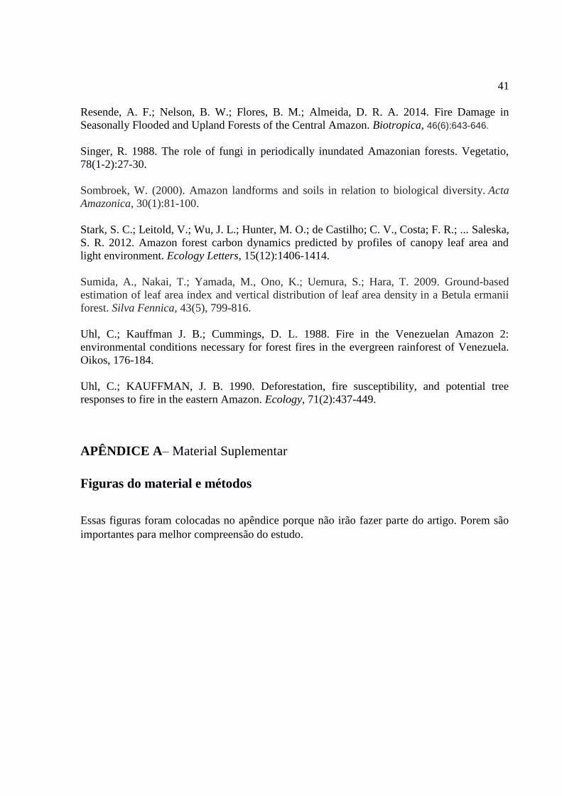
Figura Erro! Nenhuma sequência foi especificada.– Localização da Área de estudo (Lago Mamori). As

setas indicam a provável influência de águas brancas, ricas em nutrientes no período de maior

cheia.

43

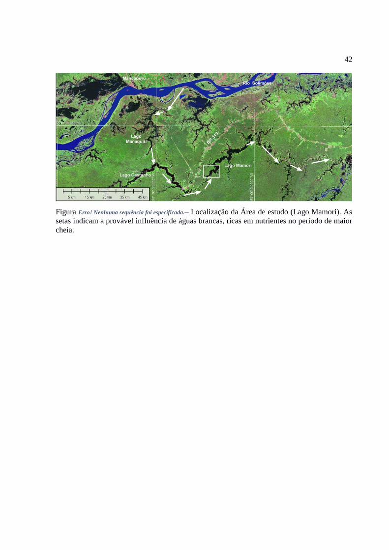
Figura Erro! Nenhuma sequência foi especificada. – Distribuição das parcelas para cada situação.

Figura Erro! Nenhuma sequência foi especificada. – Dados bidimensionais do LiDAR. Exemplo de um

transecto de 250 metros em uma situação de igapó não queimado.

44

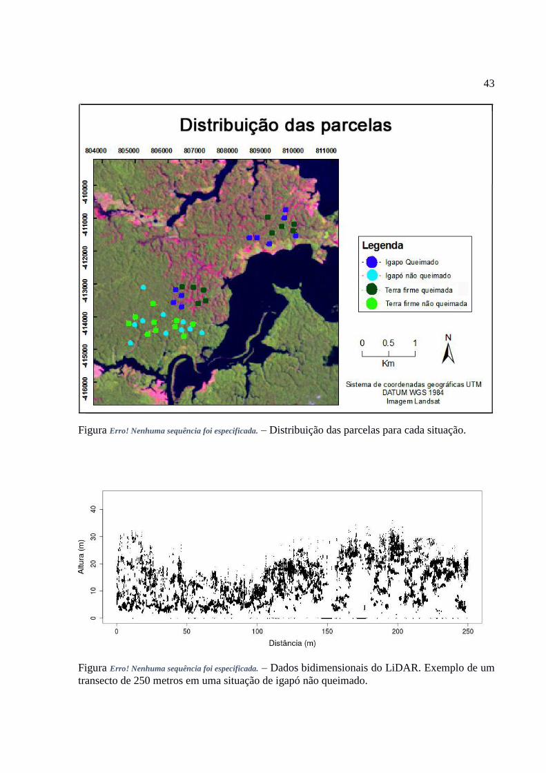
Figura Erro! Nenhuma sequência foi especificada. – Sistema LiDAR (A) sendo carregado pelo coletor

na estrutura metálica a 1 metro acima do solo e (B) o equipamento LiDAR, bateria 12V e

computador.

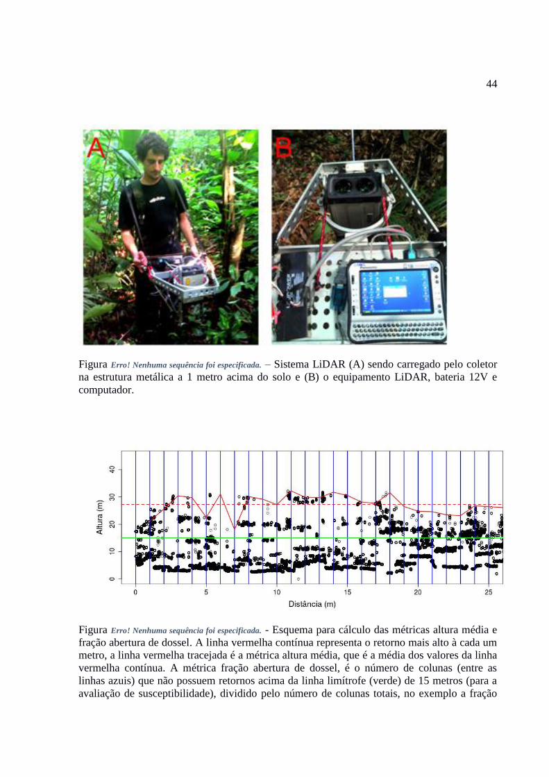
Figura Erro! Nenhuma sequência foi especificada. - Esquema para cálculo das métricas altura média e

fração abertura de dossel. A linha vermelha contínua representa o retorno mais alto à cada um

metro, a linha vermelha tracejada é a métrica altura média, que é a média dos valores da linha

vermelha contínua. A métrica fração abertura de dossel, é o número de colunas (entre as

linhas azuis) que não possuem retornos acima da linha limítrofe (verde) de 15 metros (para a

avaliação de susceptibilidade), dividido pelo número de colunas totais, no exemplo a fração

45

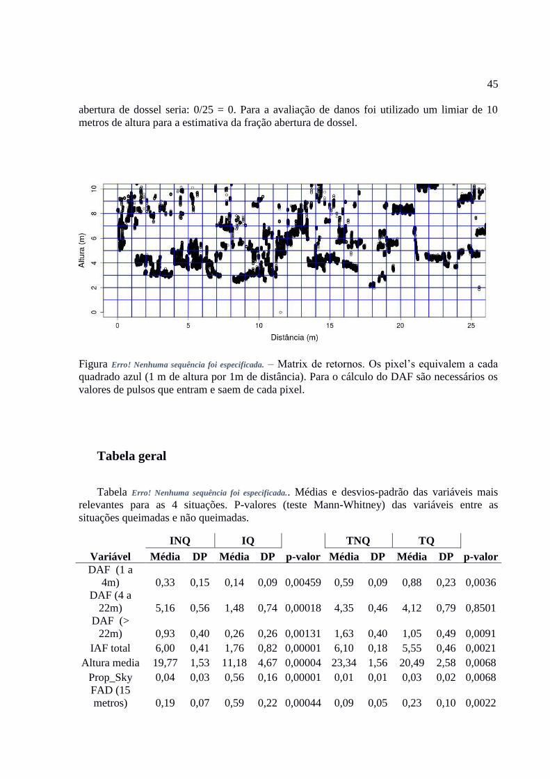
abertura de dossel seria: 0/25 = 0. Para a avaliação de danos foi utilizado um limiar de 10

metros de altura para a estimativa da fração abertura de dossel.

Figura Erro! Nenhuma sequência foi especificada. – Matrix de retornos. Os pixel’s equivalem a cada

quadrado azul (1 m de altura por 1m de distância). Para o cálculo do DAF são necessários os

valores de pulsos que entram e saem de cada pixel.

Tabela geral

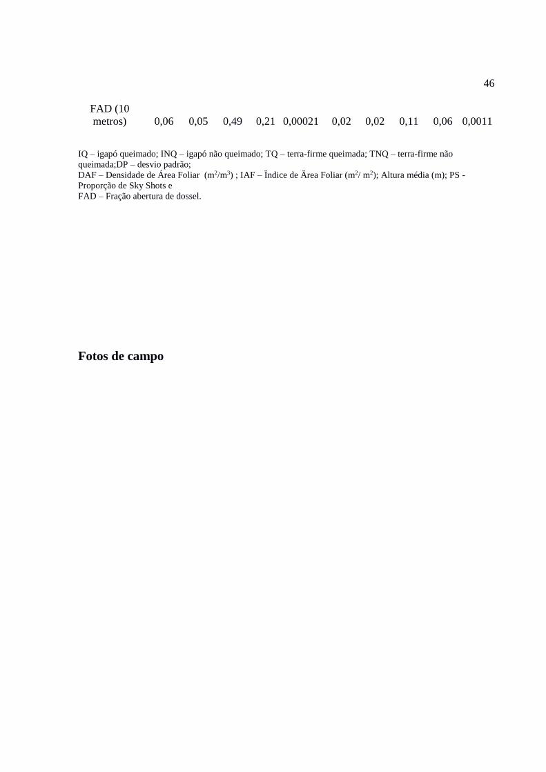
Tabela Erro! Nenhuma sequência foi especificada.. Médias e desvios-padrão das variáveis mais

relevantes para as 4 situações. P-valores (teste Mann-Whitney) das variáveis entre as

situações queimadas e não queimadas.

INQ IQ TNQ TQ

Variável Média DP Média DP p-valor Média DP Média DP p-valor

DAF (1 a

4m) 0,33 0,15 0,14 0,09 0,00459 0,59 0,09 0,88 0,23 0,0036

DAF (4 a

22m) 5,16 0,56 1,48 0,74 0,00018 4,35 0,46 4,12 0,79 0,8501

DAF (>

22m) 0,93 0,40 0,26 0,26 0,00131 1,63 0,40 1,05 0,49 0,0091

IAF total 6,00 0,41 1,76 0,82 0,00001 6,10 0,18 5,55 0,46 0,0021

Altura media 19,77 1,53 11,18 4,67 0,00004 23,34 1,56 20,49 2,58 0,0068

Prop_Sky 0,04 0,03 0,56 0,16 0,00001 0,01 0,01 0,03 0,02 0,0068

FAD (15

metros) 0,19 0,07 0,59 0,22 0,00044 0,09 0,05 0,23 0,10 0,0022

46

FAD (10

metros) 0,06 0,05 0,49 0,21 0,00021 0,02 0,02 0,11 0,06 0,0011

IQ – igapó queimado; INQ – igapó não queimado; TQ – terra-firme queimada; TNQ – terra-firme não

queimada;DP – desvio padrão;

DAF – Densidade de Área Foliar (m2/m3) ; IAF – Ïndice de Ärea Foliar (m2/ m2); Altura média (m); PS -

Proporção de Sky Shots e

FAD – Fração abertura de dossel.

Fotos de campo

47

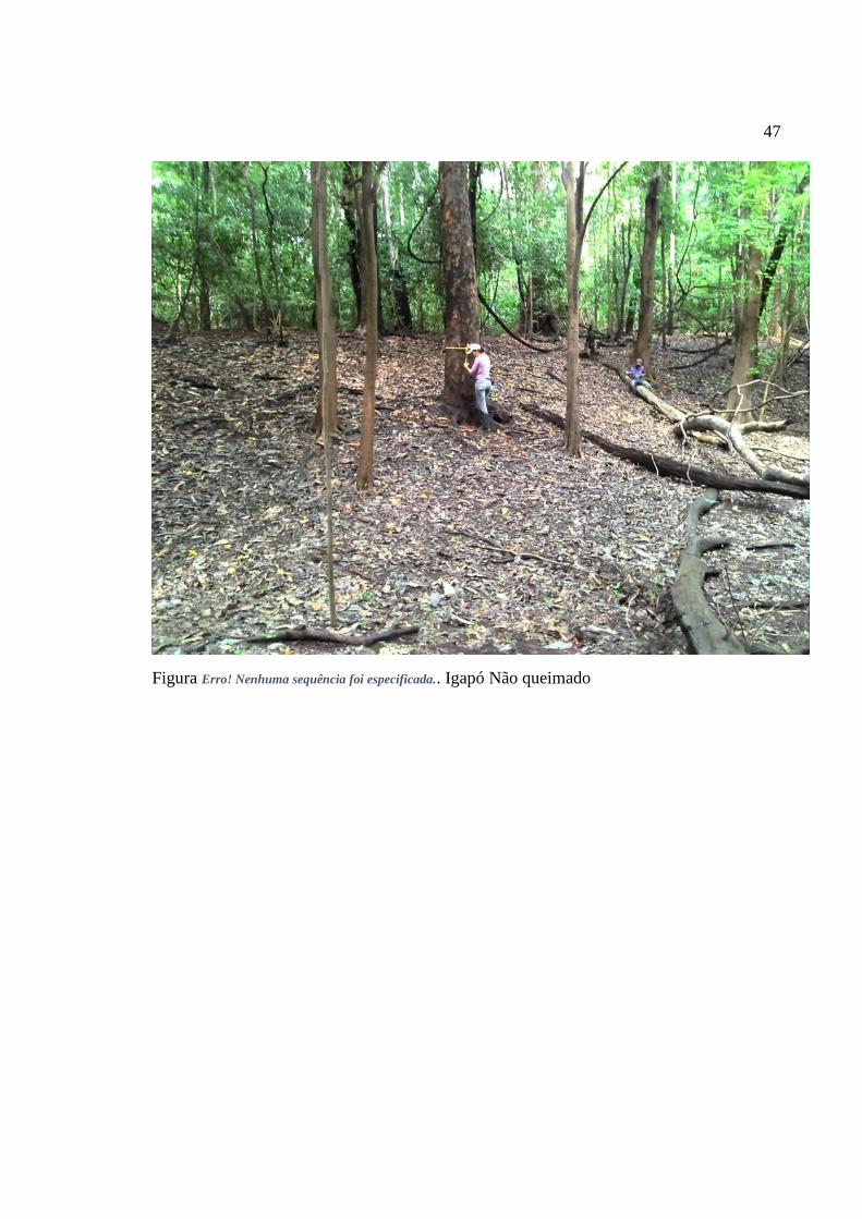
Figura Erro! Nenhuma sequência foi especificada.. Igapó Não queimado

48

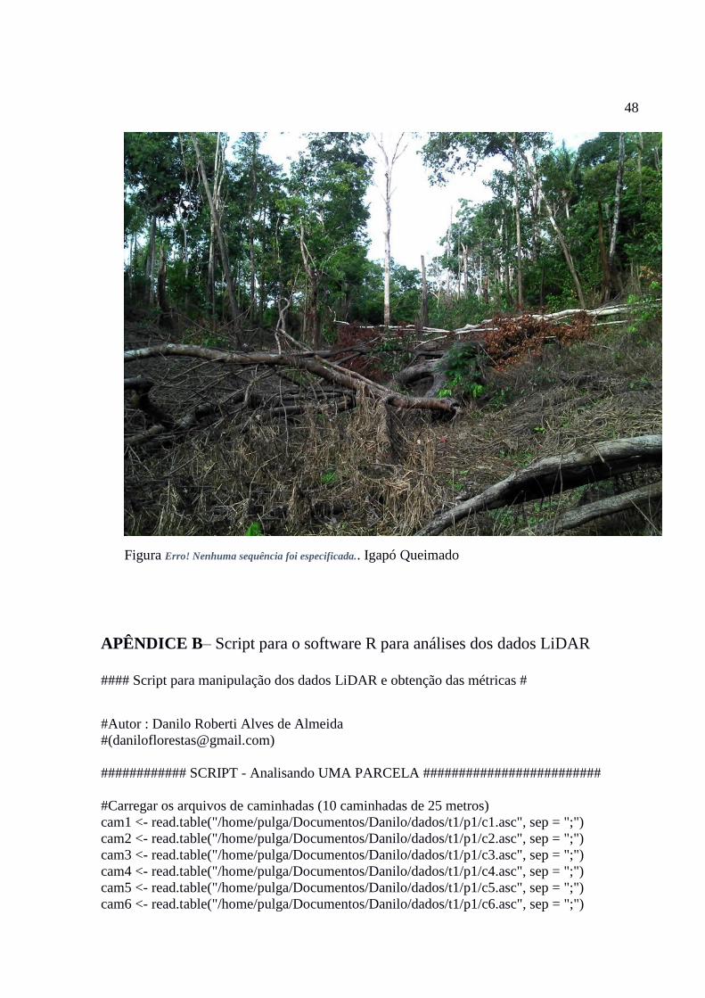
Figura Erro! Nenhuma sequência foi especificada.. Igapó Queimado

APÊNDICE B– Script para o software R para análises dos dados LiDAR

#### Script para manipulação dos dados LiDAR e obtenção das métricas #

#Autor : Danilo Roberti Alves de Almeida

#([email protected])

############ SCRIPT - Analisando UMA PARCELA #########################

#Carregar os arquivos de caminhadas (10 caminhadas de 25 metros)

cam1 <- read.table("/home/pulga/Documentos/Danilo/dados/t1/p1/c1.asc", sep = ";")






49





#retirar dados adjacentes e transformar em dados numéricos

#para cada caminhada

h1 <- substr(cam1[, 1], 2, 1000)

h1 <- data.frame (altura = as.numeric(as.character(h1)))

h2 <- substr(cam2[, 1], 2, 1000)


h3 <- substr(cam3[, 1], 2, 1000)


h4 <- substr(cam4[, 1], 2, 1000)


h5 <- substr(cam5[, 1], 2, 1000)


h6 <- substr(cam6[, 1], 2, 1000)


h7 <- substr(cam7[, 1], 2, 1000)


h8 <- substr(cam8[, 1], 2, 1000)


h9 <- substr(cam9[, 1], 2, 1000)


h10 <- substr(cam10[, 1], 2, 1000)


rm(cam1, cam2, cam3, cam4, cam5, cam6, cam7, cam8, cam9, cam10)

##Padronizando, primeira linha=first return e ultima linha=last return.

#ajuste da primeira linha

if(h1[1,1]>100){h1 <- data.frame(h1[-1,]);names(h1) <- "altura"}







50




#ajuste da ultima linha

if(h1[nrow(h1),1]<100 & h1[nrow(h1),1] != 0)

{h1 <- data.frame(h1[-nrow(h1),]);names(h1) <- "altura"}

if(h2[nrow(h2),1]<100 & h2[nrow(h2),1] != 0){

h2 <- data.frame(h2[-nrow(h1),]);names(h2) <- "altura"}

if(h3[nrow(h3),1]<100 & h3[nrow(h3),1] != 0)


if(h4[nrow(h4),1]<100 & h4[nrow(h4),1] != 0)


if(h5[nrow(h5),1]<100 & h5[nrow(h5),1] != 0)


if(h6[nrow(h6),1]<100 & h6[nrow(h6),1] != 0)


if(h7[nrow(h7),1]<100 & h7[nrow(h7),1] != 0)


if(h8[nrow(h8),1]<100 & h8[nrow(h8),1] != 0)


if(h9[nrow(h9),1]<100 & h9[nrow(h9),1] != 0)


if(h10[nrow(h10),1]<100 & h10[nrow(h10),1] != 0)


##Distancia (gerando o eixo X de distancia)

#(POSIÇÃO (repetida duas vezes, firs and last return)) *

#(25 metros dividido pelo numero de posicoes)

#Substitua o 25 pelas distancias de sua caminhada e altere os intervalos (0,25,50,75)

dist1 <- 0 + (rep(1:(nrow(h1)/2),each=2))*(25/(nrow(h1)/2))










#criando a tabela (data frame) com os vetores caminhada, distancia e os objetos "cam"

cam1 <- data.frame(cam=1, distancia = dist1, h1)



51








rm(dist1, dist2, dist3, dist4, dist5, dist6, dist7, dist8, dist9, dist10,

h1, h2, h3, h4, h5, h6, h7, h8, h9, h10)

#agrupar todos os objetos em um unico objeto (parcela)

parcela <- rbind(cam1, cam2, cam3, cam4, cam5, cam6, cam7, cam8, cam9, cam10)

rm(cam1, cam2, cam3, cam4, cam5, cam6, cam7, cam8, cam9, cam10)

#Determina tipo de retorno: primeiro = 1 e ultimo = 2

tipo <- rep(1:2, nrow(parcela)/2)

#retirando 100 dos ultimos retornos e somando 1 a todos (menos nos skyshots)

h <- data.frame(parcela$altura)

h <- apply(h, c(1, 2), function(x) ifelse (x > 100, x - 100, x))

h <- apply(h, c(1, 2), function(x) ifelse(x > 0, x + 1, x))# 1 é a altura do equipamento na

cintura do operador

parcela$altura <- data.frame (altura = as.numeric(as.character(h)))

rm(h)

#construir a tabela final

parcela <- data.frame(trat = "1", parc = "1", cam = parcela$cam, tipo, distancia =

parcela$distancia, altura = parcela$altura)

rm(tipo)

#filtrando dados. Escolha um valor de altura que saiba que é o limite da floresta

parcela <- parcela[parcela$altura < 40,]

#Grafico exploratorio (GRAFICO 1)

jpeg("plot_p1.jpeg", width=1000, height=450)

plot(parcela$altura~parcela$distancia,

xlab = "Distância (m)", ylab = ("Altura (m)"),

ylim = c(0,45), cex.axis = 1.3, cex.lab = 1.6,

pch = 16, cex = 0.3)

dev.off()

save(parcela, file = "uma_parcela.Rdata")

52

#################################################################

############ METRICAS

######ALTURA MEDIA

#criando vetor para entrada dos valores

list.max <- vector()

#looping geral

#esse looping selecionada uma coluna (1 m de distancia) em cada ciclo e obtem

#a altuma máxima dessa coluna, depois ele joga o valor no vetor (list.max)

system.time({ #a funcao system.time() nos fornece o tempo percorrido durante o looping

for(j in 0:249){ #0:249 metros

#selecionada a sessao (coluna)

sessao <- parcela[parcela$distancia > j & parcela$distancia <= j+1,]

#obtem o valor maximo

max <- max(sessao$altura)

#alimenta o vetor final com os resultados

list.max <- c(list.max, max)

rm(max, sessao)#remove objetos nao mais utilizado

print(j)#esse comando serve para podermos acompanhar o processamento do looping

}

})

rm(j)

mean.max <- mean(list.max)#metrica altura média

rugosidade <- sd(list.max)#metrica rugosidade (nao utilizada no artigo do mestrado)

rm(list.max)

##Proporção de skyshots

n.sky <- length(which(parcela$altura==0))#numero total de Sky na parcela

n.total <- nrow(parcela) #numero total de retornos na parcela

prop.sky <- n.sky/n.total #metrica proporcao de sky shots

rm(n.sky, n.total )

53

####Gap Fraction (fracao abertura de dossel)

#neste caso vamos obter a fracao abertura de dossel com 9 altura limitrofes

#Looping

gaps <- vector() #vetor que vai receber os valores ao final de cada looping

h <- c(5,7.5,10,12.5,15,17.5,20,22.5,25) #alturas limitrofes

system.time({

for(i in 1:9){ #1:9 alturas limitrofes

limitrofe <- parcela[parcela$altura >= h[i],]#define a linha limitorfe

#gerar uma tabela com 250 colunas, se serão preenchidas com o numero

# de sky shots em cada coluna acima da linha limitrofe

table.gap <-data.frame(matrix(0, ncol=250, nrow = 1))

#looping para selecionar as colunas

for(j in 0:249){ #0:249 metros

#estabelece a coluna, e conta o numero de sky acima da linha limitrofe

s <- length(which(limitrofe$distancia > j & limitrofe$distancia <= j+1))

table.gap[,j+1] <- s#alimenta a tabela das colunas

rm(s)

print(c(i,j))#comando para acompanhar o desenvolvimento do looping

}

gap <- length(which(table.gap[1,]==0))/ncol(table.gap)#calculo do gap fraction

gaps <- c(gaps, gap)#alimenta o vetor final

rm(table.gap, limitrofe, gap)

}

})

rm(i,j)

#Grafico GAP FRACTION (GRAFICO 2)

plot(h,gaps, type = "b", ylab = "Gap Fraction",

xlab = "Altura Limitrofe (m)")

###LAI (Leaf Area Index) ou IAF (indice de area foliar)

## e o LAD (leaf area density) ou DAF (densidade de area foliar)

##Gerando 3 objetos: (1) tabela (altura, distancia) de retornos,

#(2)sky.shots em cada coluna e (3)pulsos totais em cada coluna de distancia.

54

#retornos, matrix de retornos que será alimentada com os valores obtidos no looping

retornos <- data.frame(matrix(0, ncol = 250, nrow = 40))

system.time({

for(i in 0:39){ #looping q seleciona a altura

sessao <- parcela[parcela$altura > i & parcela$altura <= i+1,]

for (j in 0:249){ #looping que seleciona a distancia

s <- length(which(sessao$distancia > j & sessao$distancia <= j+1))

retornos[i+1,j+1] <- s#alimenta a matrix retornos

rm(s)

print(c(i,j))

}

rm(sessao)

}

})

rm(i,j)

#Grafico perfil de retornos (GRAFICO 3)

plot(rowMeans(retornos), 1:40, type = "l",

ylab = "Altura (m)", xlab = "Número de retornos")

##sky.shots, matrix que sera alimentada

sky.shots <- data.frame(matrix(0, ncol = 250, nrow = 1))

#gera um objeto somente com os sky shots

sky <- parcela[parcela$altura == 0,]

for (i in 0:249){ #looping seleciona a coluna

#conta qntos sky shots tem em cada coluna

s <- length(which(sky$distancia > i & sky$distancia <= i+1))

#alimenta a matrix sky.shots

sky.shots[1,i+1] <- s

rm(s)

print(i)

}

rm(i, sky)

##pulsos.totais

#caminho semelhante aos sky.shots porem com todos os pulsos emitidos pelo LiDAR

#em cada coluna

55

#matrix que sera alimentada

pulsos.totais <- data.frame(matrix(0, ncol = 250, nrow = 1))

for (i in 0:249){ #looping seleciona as colunas

#conta os pulsos em cada coluna

s <- length(which(parcela$distancia > i & parcela$distancia <= i+1))

pulsos.totais[1,i+1] <- s #alimenta a matrix final pulsos.totais

rm(s)

print(i)

}

rm(i)

#Juntando retornos, sky.shots e pulsos totais em um unico objeto (list())

#ii

parcela.pix <- list()

parcela.pix$retornos <- retornos

parcela.pix$sky.shots <- sky.shots

parcela.pix$pulsos.totais <- pulsos.totais

rm(retornos, sky.shots, pulsos.totais)

#salvando

save(parcela.pix, file = "parcela_pix.Rdata")

#exemplo de como carrega os dados salvos anteriormente

load("parcela_pix.Rdata")

#carregar pacote para gerar algumas imagens

require(fields)

#grafico pixels de retornos (GRAFICO 4)

image.plot(t(parcela.pix$retornos), 1:40, col=c("grey75", tim.colors(10000)),

ylim = c(0,40))

#Calculando LAD com a equação MacArthur-Horn

#criando a tabela de entrada

#Gerar uma matrix com o numero de pulsos por cada coluna

#essa matrix sera utilizada junto com a cumsum para calculo de pulsos

#que entraram e sairam em cada voxel

parcela.pix$pulsos.totais <- as.numeric(parcela.pix$pulsos.totais)

total.shots.col <- matrix(parcela.pix$pulsos.totais, nrow = nrow(parcela.pix$retornos), ncol =

ncol(parcela.pix$retornos), byrow=T) #C

# Gerar a matriz de retornos acumulados

56

cum.shots <- apply(parcela.pix$retornos, 2, cumsum)

#Subtrair os retornos acumulados pela matrix de pulsos totais

#e obtendo a matrix pulsos que sairam de cada voxel

pulse.out <- total.shots.col - cum.shots

rm(total.shots.col, cum.shots)

#os pulsos q sairam no pixel 1, sao os mesmos que entram em dois

#portanto pulse.in é igual o pul.se out retirando a ultima linha e acrescentando

#como primeira a linha de pulsos.totais

pulse.in <- rbind(parcela.pix$pulsos.totais, pulse.out[-nrow(pulse.out),])

# Equação MacArthur para obtencao do LAD

# LAD = ln(pulse.in/pulse.out)*(1/(d * K))

# Calculo MacArthur-Horn com d = 1 and K = 1

#a formula tbm pode ser pulse.out/pulse.in contando que acrescente um sinal de negativo

#no inicio da esquacao

LAD <- log(pulse.in/pulse.out)

rm(pulse.in, pulse.out)

# Remove valores infinitos e NA

LAD[is.infinite(LAD)] <- 0

LAD[is.nan(LAD)] <- 0

#media das linhas, para obter o perfil LAD

LAD.profile <- apply(LAD, 1, mean)

#obtendo o LAI

LAI <- sum(LAD.profile)

#GRAFICO DAF (GRAFICO 5)

image.plot(t(LAD), col=c("grey75", tim.colors(100)))

#grafico perfil de DAF (GRAFICO 6)

par(mar=c(5,5,2,3))

plot(LAD.profile,1:40, type="l", ylab = "Altura (m)",

xlab= expression(paste("DAF (", m^2/m^3, ")", sep = "")))

#LAI em diferentes alturas

######IMPORTANTE (AQUI DEFINE O INTERVALO DESEJADO)

lai_0_5m <- sum(LAD.profile[1:5])

lai_10_15m <- sum(LAD.profile[10:15])

#TEBELA FINAL DE METRICAS

metricas <- data.frame(mean.max, prop.sky, LAI, lai_0_5m, lai_10_15m,

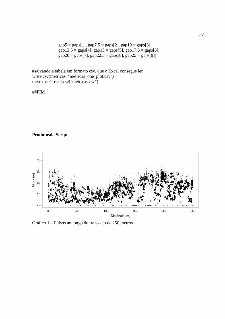
57

gap5 = gaps[1], gap7.5 = gaps[2], gap10 = gaps[3],

gap12.5 = gaps[4], gap15 = gaps[5], gap17.5 = gaps[6],

gap20 = gaps[7], gap22.5 = gaps[8], gap25 = gaps[9])

#salvando a tabela em formato csv, que o Excel consegue ler

write.csv(metricas, "metricas_one_plot.csv")

metricas <- read.csv("metricas.csv")

##FIM

Produtosdo Script

Gráfico 1 – Pulsos ao longo do transecto de 250 metros

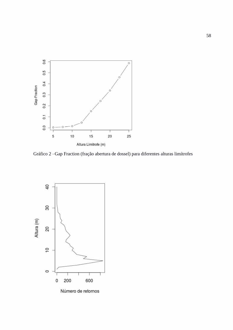
58

Gráfico 2 –Gap Fraction (fração abertura de dossel) para diferentes alturas limítrofes

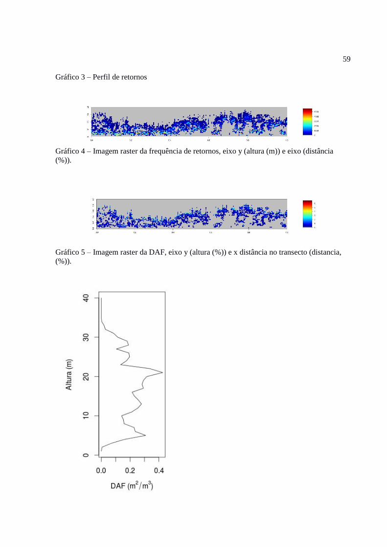
59

Gráfico 3 – Perfil de retornos

Gráfico 4 – Imagem raster da frequência de retornos, eixo y (altura (m)) e eixo (distância

(%)).

Gráfico 5 – Imagem raster da DAF, eixo y (altura (%)) e x distância no transecto (distancia,

(%)).

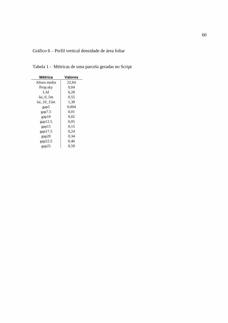
60

Gráfico 6 – Perfil vertical densidade de área foliar

Tabela 1 - Métricas de uma parcela geradas no Script

Métrica Valores

Altura media 22,64

Prop.sky 0,04

LAI 6,28

lai_0_5m 0,55

lai_10_15m 1,38

gap5 0,004

gap7.5 0,01

gap10 0,02

gap12.5 0,05

gap15 0,15

gap17.5 0,24

gap20 0,34

gap22.5 0,46

gap25 0,59

INSTITUTO NACIONAL DE PESQUISAS DA AMAZÔNIA...

Documents

Transcript of INSTITUTO NACIONAL DE PESQUISAS DA AMAZÔNIA...