Universidade de AveiroDepartamento de Eletrónica,Telecomunicações e Informática

2014

José LucasLemos Mendonça

Comportamentos para robôs humanóidessimulados

Behaviours for simulated humanoid robots

Universidade de AveiroDepartamento de Eletrónica,Telecomunicações e Informática

2014

José LucasLemos Mendonça

Comportamentos para robôs humanóidessimulados

Behaviours for simulated humanoid robots

Dissertação apresentada à Universidade de Aveiro para cumprimento dosrequisitos necessários à obtenção do grau de Mestre em Engenharia de Com-putadores e Telemática, realizada sob a orientação científica do Doutor JoséNuno Panelas Nunes Lau, Professor Auxiliar do Departamento de Eletrónica,Telecomunicações e Informática da Universidade de Aveiro, e do Doutor Ar-tur José Carneiro Pereira, Professor Auxiliar do Departamento de Electrónica,Telecomunicações e Informática da Universidade de Aveiro.

o júri / the jury

presidente / president Prof. Doutor Luís Filipe de Seabra LopesProfessor Associado da Universidade de Aveiro

vogais / examiners committee Prof. Doutor Luis Paulo Gonçalves dos ReisProfessor Associado da Escola de Engenharia da Universidade do Minho

Prof. Doutor José Nuno Panelas Nunes LauProfessor Auxiliar da Universidade de Aveiro (orientador)

agradecimentos /acknowledgements

Agradeço o tempo, disponibilidade e paciência aos que se cruzaram comigono desenvolvimento da tese, desde os orientadores Nuno Lau e Artur Pereira,à equipa do FC Portugal 3D, Rui Ferreira, Abbas, Nima e aos meus colegas.

Palavras Chave Humanóide, Bípede, Optimização, Ferramentas de desenvolvimento e depu-ração, Simulação de Futebol, Robô

Resumo Esta tese está inserida na equipa FC Portugal 3D, que compete na liga defutebol robótico simulado 3D. Os objetivos da tese são melhorar os compor-tamentos já existentes e desenvolver ferramentas de suporte ao desenvolvi-mento e depuração para o agente robótico.Nesse sentido, foi melhorado o processo de optimização de comportamentosde forma a torná-lo mais eficiente e adaptado para incluir os novos mode-los heterogéneos disponibilizados. Ao executar o processo de optimização,usando o algoritmo de estado de arte CMA-ES, foi obtido reduções para me-tade do tempo nos comportamentos de levantar-se. Seguidamente o agentefoi colocado a correr em modo síncrono, o que permite que as simulaçõescorram à velocidade de processamento do computador em uso, e não à velo-cidade da simulação da competição em que cada ciclo demora 20ms. Assimé possível executar simulações e consequentemente inferir conclusões muitomais rapidamente.Passou-se a usar a informação de giroscópio e o cálculo dos ângulos de eulerpara obter uma melhor estimativa da rotação do robô. Por outro lado, devidoao lançamento de novos tipos de robôs, a arquitectura do agente teve de seratualizada e novos comportamentos foram criados e optimizados para estesnovos modelos. Em relação ao modelo original, alguns comportamentos sãoexecutados mais rapidamente e melhor pelos modelos novos, devido às suasalterações físicas. Por fim, nos comportamentos foi dada a possibilidade dedefinir pré condições em etapa do mesmo, para que possa ser abortado casoas condições não se verifiquem. Esta alteração veio reduzir o tempo desper-diçado a executar a totalidade do comportamento em situações em que nãoé provável o seu sucesso .Em termos de ferramentas, foi colocada uma Janela de Monitor de Agentepara cada agente que, apresenta em tempo de simulação variáveis que ocódigo do agente disponibiliza, interage com código através de widgets deseleção ou preenchimento, e se a simulação estiver a correr em modo sín-crono, permite definir o tempo de ciclo da simulação, pausá-la e executar cicloa ciclo, o que permite vantagens óbvias em termos de análise de execuçãodos agentes. Seguidamente, foi criada uma ferramenta de teste para compor-tamentos definidos em XML, que permite, em tempo de execução, alterar oficheiro a testar, alterar o seu conteúdo, agrupar vários ficheiros em sequên-cias e executar vários agentes em paralelo. Por fim, a última ferramenta éum Analizador de Logs gerados pelos agentes e pelo simulador que permite,entre outras funcionalidades, ver em forma de gráficos variáveis da simula-ção, exportar para diferentes formatos, filtrar a simulação usando informaçãoda mesma e correr um servidor de forma a ser possível analizar em paralelo,gráficos de variáveis escolhidas e a simulação num visualizador.

Keywords Humanoid, Biped, Optimization, Development and Debugging Tools, SoccerSimulation, Robot

Abstract This thesis in inserted in the FC Portugal 3D team, which competes in thehumanoid simulation league 3D from RoboCup. The objectives of this thesisare to improve the behaviours already created and to develop tools to supportthe development and debugging of the robotic agent.With this in mind, the process of optimization was improved to make it more ef-ficient and adapted to include the new heterogeneous models. Executing theoptimization process, using the state of the art algorithm CMA-ES, the time ofthe getup was reduced by half. Afterwards, the agent was put running in syncmode, which allows the simulations to run as fast as the computer in use canprocess, and not the simulation speed of the competion with cycles of 20ms.In the agent posture, it is now used the information from the gyroscope and theeuler angles are calculated to get a better estimative of the robot orientation.On the other hand, the agent architecture was updated and new behaviourswere created and optimized to support the new heterogeneous models. In re-lation to the standard model, some behaviours execute faster because of theirphysical difference.In the slot behaviours, it is now possible to defined preconditions in each step,so the agent can abort the behaviour when any condition does not comply.This change reduces the time wasted executing all the behaviour in situationsin which the success is improbable.In terms of tools, a Agent Monitor Window was created for each agent whichcan: present in runtime variables from the agent code; interact with the codetrough widgets; and if the simulation is in sync mode, defined the simulationcycle time, with the possibility to pause it and execute step by step, whichgives a great advantage in terms of analysing the agent execution. The sec-ond tool was a behaviour testes for behaviours defined in XML, which allows,in runtime, to change the behaviour to test, edit its content, aggregate differentfiles in sequence and finally the tolls can execute various agents in parallel.The last tools is Log Analyser of the logs generated by the agents and theserver, which allows: exporting in different formats, see in form of plots thevariables parsed, filtrate the simulation information; and create a server simu-lation which can be used to analyse, in parallel, the plots of chosen variablesand the simulation in a monitor.

Contents

Contents . . . . . . . . . . . . . . . . . . . . . . . . . . . . . . . . . . . . . . . . . . i

List of Figures . . . . . . . . . . . . . . . . . . . . . . . . . . . . . . . . . . . . . . . iii

List of Tables . . . . . . . . . . . . . . . . . . . . . . . . . . . . . . . . . . . . . . . v

List of Acronyms . . . . . . . . . . . . . . . . . . . . . . . . . . . . . . . . . . . . . vii

1 Introduction . . . . . . . . . . . . . . . . . . . . . . . . . . . . . . . . . . . . . . 11.1 Motivation . . . . . . . . . . . . . . . . . . . . . . . . . . . . . . . . . . . . . 11.2 Objectives . . . . . . . . . . . . . . . . . . . . . . . . . . . . . . . . . . . . . 11.3 Structure . . . . . . . . . . . . . . . . . . . . . . . . . . . . . . . . . . . . . . 2

2 RoboCup Simulation3D . . . . . . . . . . . . . . . . . . . . . . . . . . . . . . 32.1 Simspark and Rcssserver3d . . . . . . . . . . . . . . . . . . . . . . . . . . . . 5

2.1.1 Monitor . . . . . . . . . . . . . . . . . . . . . . . . . . . . . . . . . . 52.2 Network Protocol . . . . . . . . . . . . . . . . . . . . . . . . . . . . . . . . . 6

2.2.1 Server/Agent . . . . . . . . . . . . . . . . . . . . . . . . . . . . . . . 62.2.2 Server/Monitor . . . . . . . . . . . . . . . . . . . . . . . . . . . . . . 6

2.3 Summary . . . . . . . . . . . . . . . . . . . . . . . . . . . . . . . . . . . . . . 9

3 Humanoid Behaviours . . . . . . . . . . . . . . . . . . . . . . . . . . . . . . . 113.1 Stability . . . . . . . . . . . . . . . . . . . . . . . . . . . . . . . . . . . . . . 11

3.1.1 Center of Mass . . . . . . . . . . . . . . . . . . . . . . . . . . . . . . 113.1.2 Center of Pressure . . . . . . . . . . . . . . . . . . . . . . . . . . . . 123.1.3 Zero Moment Point . . . . . . . . . . . . . . . . . . . . . . . . . . . 123.1.4 Static vs Dynamic Stability . . . . . . . . . . . . . . . . . . . . . . . 133.1.5 Other Approaches . . . . . . . . . . . . . . . . . . . . . . . . . . . . 14

3.2 FC Portugal . . . . . . . . . . . . . . . . . . . . . . . . . . . . . . . . . . . . 143.2.1 Slot Behaviour . . . . . . . . . . . . . . . . . . . . . . . . . . . . . . 143.2.2 Central Pattern Generators Behaviour . . . . . . . . . . . . . . . . . 153.2.3 Omnidirectional walk . . . . . . . . . . . . . . . . . . . . . . . . . . 163.2.4 Omnidirectional Kick . . . . . . . . . . . . . . . . . . . . . . . . . . 18

3.3 Summary . . . . . . . . . . . . . . . . . . . . . . . . . . . . . . . . . . . . . . 20

4 Population Based Optimization . . . . . . . . . . . . . . . . . . . . . . . . . 214.1 Genetic Algorithms . . . . . . . . . . . . . . . . . . . . . . . . . . . . . . . . 21

i

4.2 Particle Swarm Optimization . . . . . . . . . . . . . . . . . . . . . . . . . . 244.3 CMA-ES . . . . . . . . . . . . . . . . . . . . . . . . . . . . . . . . . . . . . . 26

5 Behaviours and Agent Improvement . . . . . . . . . . . . . . . . . . . . . . 295.1 Improving Posture Estimate . . . . . . . . . . . . . . . . . . . . . . . . . . . 29

5.1.1 Euler angles . . . . . . . . . . . . . . . . . . . . . . . . . . . . . . . . 295.1.2 Gyroscope . . . . . . . . . . . . . . . . . . . . . . . . . . . . . . . . . 315.1.3 Agent Posture State . . . . . . . . . . . . . . . . . . . . . . . . . . . 33

5.2 Preconditions . . . . . . . . . . . . . . . . . . . . . . . . . . . . . . . . . . . 33

6 Optimization Process Improvement . . . . . . . . . . . . . . . . . . . . . . 376.1 Sync Mode . . . . . . . . . . . . . . . . . . . . . . . . . . . . . . . . . . . . . 37

6.1.1 Sync Mode Usage . . . . . . . . . . . . . . . . . . . . . . . . . . . . 376.2 Constraint Free Environment . . . . . . . . . . . . . . . . . . . . . . . . . . 38

6.2.1 Solution . . . . . . . . . . . . . . . . . . . . . . . . . . . . . . . . . . 386.3 Optimization Agent . . . . . . . . . . . . . . . . . . . . . . . . . . . . . . . . 396.4 Update Optimization Parameters . . . . . . . . . . . . . . . . . . . . . . . . 416.5 Heterogeneous Models . . . . . . . . . . . . . . . . . . . . . . . . . . . . . . 416.6 Results . . . . . . . . . . . . . . . . . . . . . . . . . . . . . . . . . . . . . . . 42

7 Development and Debugging Tools . . . . . . . . . . . . . . . . . . . . . . . 457.1 Agent Monitor Window . . . . . . . . . . . . . . . . . . . . . . . . . . . . . . 45

7.1.1 Developer API . . . . . . . . . . . . . . . . . . . . . . . . . . . . . . 467.1.2 Controlling the Cycle Time . . . . . . . . . . . . . . . . . . . . . . . 48

7.2 Log Analyser . . . . . . . . . . . . . . . . . . . . . . . . . . . . . . . . . . . 497.2.1 Extracting Information . . . . . . . . . . . . . . . . . . . . . . . . . 497.2.2 Export Options . . . . . . . . . . . . . . . . . . . . . . . . . . . . . . 497.2.3 Interface . . . . . . . . . . . . . . . . . . . . . . . . . . . . . . . . . . 517.2.4 Configuration Save . . . . . . . . . . . . . . . . . . . . . . . . . . . . 547.2.5 Server Simulation . . . . . . . . . . . . . . . . . . . . . . . . . . . . . 55

7.3 XML Defined Behaviour Tester . . . . . . . . . . . . . . . . . . . . . . . . . 56

8 Conclusion . . . . . . . . . . . . . . . . . . . . . . . . . . . . . . . . . . . . . . . 598.1 Future Work . . . . . . . . . . . . . . . . . . . . . . . . . . . . . . . . . . . . 59

References . . . . . . . . . . . . . . . . . . . . . . . . . . . . . . . . . . . . . . . . . 61

ii

List of Figures

2.1 SoccerSimulation Field . . . . . . . . . . . . . . . . . . . . . . . . . . . . . . . . 42.2 RobovizVsRcssmonitor3d . . . . . . . . . . . . . . . . . . . . . . . . . . . . . . . 52.3 Environment information message example . . . . . . . . . . . . . . . . . . . . . 62.4 Representation of a Frame in a Fixed Reference Frame [13] . . . . . . . . . . . . 72.5 Homogeneous transformation matrix . . . . . . . . . . . . . . . . . . . . . . . . . 82.6 Static Mesh node format . . . . . . . . . . . . . . . . . . . . . . . . . . . . . . . 82.7 Static Mesh node example . . . . . . . . . . . . . . . . . . . . . . . . . . . . . . 82.8 Static Mesh Node (SMN) format . . . . . . . . . . . . . . . . . . . . . . . . . . . 82.9 SMN node example . . . . . . . . . . . . . . . . . . . . . . . . . . . . . . . . . . 9

3.1 ZMP support polygon . . . . . . . . . . . . . . . . . . . . . . . . . . . . . . . . . 133.2 Slot behaviour example . . . . . . . . . . . . . . . . . . . . . . . . . . . . . . . . 153.3 CPG example behaviour . . . . . . . . . . . . . . . . . . . . . . . . . . . . . . . . 163.4 Omnidirectional walk architecture . . . . . . . . . . . . . . . . . . . . . . . . . . 173.5 Omnidirectional walk Cart-table model from [31] . . . . . . . . . . . . . . . . . . 173.6 Omnidirectional walk preview controller . . . . . . . . . . . . . . . . . . . . . . . 183.7 Omnidirectional kick parameters . . . . . . . . . . . . . . . . . . . . . . . . . . . 193.8 Omnidirectional kick sequence . . . . . . . . . . . . . . . . . . . . . . . . . . . . 20

4.1 Pseudo code version of GA algorithm from [37]. . . . . . . . . . . . . . . . . . . 234.2 Pseudo code version of the standard PSO algorithm . . . . . . . . . . . . . . . . 254.3 Pseudocode version of the CMA-ES algorithm. . . . . . . . . . . . . . . . . . . . 26

5.1 Comparison between vertical inclination front using the old method versus com-puting pitch. Green is the ground truth from the server, red is using the oldmethod and blue is the computed pitch. . . . . . . . . . . . . . . . . . . . . . . 30

5.2 Comparison between lateral vertical inclination using old method versus computingroll. Green is the ground truth from the server, red is using the old method andblue is the computed roll. . . . . . . . . . . . . . . . . . . . . . . . . . . . . . . . 31

5.3 Comparison between only computing pitch versus using gyroscope. Green is theground truth from the server, blue is only using euler angles and red using alsothe gyroscope. . . . . . . . . . . . . . . . . . . . . . . . . . . . . . . . . . . . . . 32

5.4 Comparison between only computing roll versus using gyroscope. Green is theground truth from the server, blue is only using euler angles and red using alsothe gyroscope. . . . . . . . . . . . . . . . . . . . . . . . . . . . . . . . . . . . . . 32

5.5 Preconditions example . . . . . . . . . . . . . . . . . . . . . . . . . . . . . . . . . 35

iii

6.1 Trainer Proxy . . . . . . . . . . . . . . . . . . . . . . . . . . . . . . . . . . . . . 396.2 Example of XML behaviour file to optimize . . . . . . . . . . . . . . . . . . . . . 406.3 Initial part of nao3.xml file . . . . . . . . . . . . . . . . . . . . . . . . . . . . . . 426.4 Optimization Flow . . . . . . . . . . . . . . . . . . . . . . . . . . . . . . . . . . . 43

7.1 Agent Monitor Window running 11 agents, each with his window. . . . . . . . . 467.2 Agent Monitor Window show variables . . . . . . . . . . . . . . . . . . . . . . . 467.3 Register Combo Box in Agent Monitor Window . . . . . . . . . . . . . . . . . . 477.4 Agent Monitor Window with ComboBox . . . . . . . . . . . . . . . . . . . . . . 477.5 Register Spin Button in Agent Monitor Window . . . . . . . . . . . . . . . . . . 477.6 Agent Monitor Window with SpinButton . . . . . . . . . . . . . . . . . . . . . . 477.7 Register keyboard key in Agent Monitor Window . . . . . . . . . . . . . . . . . . 487.8 Agent Monitor Window with cycle time controls . . . . . . . . . . . . . . . . . . 487.9 Two types of plots available . . . . . . . . . . . . . . . . . . . . . . . . . . . . . . 507.10 Log Analyser XLS export example . . . . . . . . . . . . . . . . . . . . . . . . . . 507.11 Example of the exported Extensible Markup Language (XML) file. . . . . . . . . 517.12 Log Analyser agent log selected . . . . . . . . . . . . . . . . . . . . . . . . . . . . 517.13 Log Analyser server log selected . . . . . . . . . . . . . . . . . . . . . . . . . . . 527.14 Example of the configs.xml file. . . . . . . . . . . . . . . . . . . . . . . . . . . . . 557.15 Server running with one plot selecting the time . . . . . . . . . . . . . . . . . . . 567.16 Behaviour Tester . . . . . . . . . . . . . . . . . . . . . . . . . . . . . . . . . . . . 57

iv

List of Tables

3.1 Omnidirectional kick parameters description . . . . . . . . . . . . . . . . . . . . 19

6.1 GetUpBack . . . . . . . . . . . . . . . . . . . . . . . . . . . . . . . . . . . . . . . 446.2 GetUpFront . . . . . . . . . . . . . . . . . . . . . . . . . . . . . . . . . . . . . . . 44

v

List of Acronyms

PIDProportional Integral Derivative

TCPTransmission Control Protocol

CPGCentral Pattern Generator

CoPCenter of Pressure

CMCenter of Mass

GCoMGround projection of the Center of Mass

ZMPZero Moment Point

FZMPFictitious Zero Moment Point

PSOParticle Swarm Optimization

CMA-ESCovariance Matrix Adaptation - EvolutionStrategy

SPLStandard Platform League

SMNStatic Mesh Node

AIArtificial Intelligence

RoboCupRobot Soccer World Cup

XMLExtensible Markup Language

RDSRuby Diff Scene

RSGRuby Scene Graph

GTKGIMP Toolkit

GUIGraphical User Interface

GRALGRAphing Library

WBMPWireless Application Protocol Bitmap For-mat

BMPBitmap image file

PNGPortable Network Graphics

JPEGJoint Photographic Experts Group

PDFPortable Document Format

GIFGraphics Interchange Format

SVGScalable Vector Graphics

EPSEncapsulated PostScript

SimsparkSpark Generic Physical Multiagent Simula-tor

vii

chapter 1Introduction1.1 Motivation

In the Robot Soccer World Cup (RoboCup) initiative there are researchers trying to push the areaof Artificial Intelligence and Robotics further. The environment of robotic soccer is a great benchmarkto test the progress made in the area and each league has its set of problems and research focus. In thisthesis the focus is in the 3D Simulation League, in which it is necessary to create a soccer humanoidagent, with the challenges that come with it.

For the aforementioned initiative, the FC Portugal[1] team was created. Since 2000, it participatedin 2D and 3D and had achieved some great results. Recently the team got 4th place in 2014 RoboCup,1st in Robocup German Open and 1st in Robotica 2014 in Portugal.

Writing an agent that behaves autonomously and cooperates with its teammates is a difficult task,but the 2D simulation got some good results in that area. On the other hand, the 3D simulation,besides still having to deal with cooperation and coordination, has also does face the challenge ofhaving to control humanoid models. These models have particular needs, as the bipedal locomotionis difficult to achieve. Furthermore, the biped humanoid agent not only needs to walk stably, it alsoneeds to walk and rotate in all directions, kick and pass the ball, getup, and any other behaviour thatis expected from a humanoid soccer player.

1.2 ObjectivesIn the context of the FC Portugal team and the 3D Simulation League, the objectives of this thesis

are:

• Develop robust and efficient behaviours of kick, getup, dribble and any other behaviour needed,using manual control of the joints, or inverse kinematic or using optimization techniques.

• Create tools to support the development and debugging process, make it more efficient and/oreasier.

1

1.3 StructureThe structure of this thesis is as follows:

• Chapter 1: As seen, this chapter presents this thesis motivation and its objectives

• Chapter 2: Present the RoboCup, its leagues, challenges and software used.

• Chapter 3: Description of the problems faced when working in humanoid behaviours, somesolutions and concepts used nowadays, and some RoboCup teams research in that area.

• Chapter 4: Brief description of some optimization algorithms used in the FC Portugal team.

• Chapter 5: Improvements in the optimization process and its results.

• Chapter 6: Adaptation to the new heterogeneous models, use of the gyroscope and addition ofconditions in some behaviours.

• Chapter 7: Tools developed to make development process easier and quicker.

• Chapter 8: Present the conclusion and some future work that can be done in sequence to thisthesis.

2

chapter 2RoboCup Simulation3DThis chapter outlines the RoboCup project and its Simulation 3D competition, where this thesis isinserted, and execution environment.

Founded in 1997, RoboCup is a project to promote Artificial Intelligence (AI) and robotics research.It has set a challenging long term goal:

“By the middle of the 21st century, a team of fully autonomous humanoid robot

soccer players shall win a soccer game, complying with the official rules of FIFA,

against the winner of the most recent World Cup.” [2][3]For that purpose, there is an annual international robotics competition an integrated research task

covering broad areas of AI and robotics. Such areas include: real-time sensor fusion, reactive behaviour,strategy acquisition, learning, real-time planning, multiagent systems, context recognition,vision,strategic decision-making, motor control, intelligent robot control.

In order to reach the proposed goal, various competitions were created, separating the researchtasks, each one of them focusing in a different set of problems.

• Middle-Size League

• Small-Size League

• Standard Platform League

• Humanoid League

• Simulation League

Besides soccer, there are others leagues with different lines of development in the form of rescuechallenges, either simulated [4] of real [5], and challenges aimed to develop service and supportive robottechnology with high relevance for future personal domestic applications [6].

In this competitions, the physical ones have some disadvantages, inherent of using physical models:

• The robot is subject to be damaged during its usage or even during its transporting, in additionto sometimes being costly to repair.

• The testing process is slow. Any change has to be loaded in the robot and its test runs at aslow rate.

3

• It is costly to always buy the newer versions, year after year, or just new components forrepairing.

• Multiple team members cannot work at the same time on one robot.

To address these issues, a simulated environment is a good option, but it needs to be as close aspossible to the physical environment. The RoboCup 3D Simulation Soccer League is a competitionwhere software agents control humanoid robots in a soccer game. The platform tries to simulatethe rules and physics of a soccer game, reproducing physical robot limitations, like hinges movementrestriction, sensors noise,etc. The soccer field dimensions are 30 by 20 meters as we can see in image2.1.

Figure 2.1: Field dimensions.

In 2004, the 3D Simulation was introduced, beginning with a spherical agent model. The firsthumanoid model was the Fujitsu HOAP-2, which changed the development from strategic behavioursto low level control and basic behaviours like walk, kick, getting up, turn, etc.

In 2008, both the Standard Platform League (SPL) and the 3D Simulation began to use the NAOrobot [7] from Aldebaran as their model. This permitted the researchers to try their development inthe simulated NAO version before putting the code in the physical robots from the SPL.

The number of robots in the game increased over the years, till 2012 when 11 vs 11 games whereimplemented. In 2013 the teams were able to use heterogeneous robot types, which are variationsof the standard NAO robot so the development would not be attached to only one humanoid model.With the new models, some behaviours work better in some models than others, making way to a newstrategic configurations.

Besides soccer simulation, other challenges were created to promote the resolution of some specificproblems. In 2013 the first Drop In Player Challenge proposes a game where there is one agent perleague team, so the communication between teammates is crucial. In 2014 the first running challengeoccurred, pushing the teams to develop running behaviours to be faster and more human alike.

4

2.1 Simspark and Rcssserver3dIn order to run the Robocup3D simulation Spark Generic Physical Multiagent Simulator (Simspark)

server was the elected tool. It is a generic physical multi-agent simulator system for agents in three-dimensional environments built on the flexible Spark application framework. On top of that, thercssserver3d was created, which is a 3D soccer simulation with the rules set for the RoboCup 3Dsimulation league.

2.1.1 MonitorWhile running the simulation, it is possible to visualize it by using a Simspark monitor. It connects

to a running Simspark server, then starts to receive periodic messages describing the simulationstate. Besides the game visualization, the messages contain the score, current playmode, time, etc.Furthermore, the monitors can send commands to the server stated in the next section or play backrecorded Log Files. There are three forms to use monitors:

• If network overhead is not intended, one can configure the Simspark server to render thesimulation itself.

• rcssmonitor3d is the basic monitor that comes with rcssserver3d. It can render the game andshow the game info, but it is somewhat limited.

• Another monitor used by the community is RoboViz [8] [9]. It has enhanced visualizationcapabilities and it was the one used in this thesis. Some of its features are:

– Enhanced Graphics which give a new dimension to the simulation and its move attractiveto the spectators.

– Interaction and control of the agents, ball position, switching play modes.– Debugging visual elements can be displayed such as circles, text and lines, which help in

the development process.

We can see the graphics difference between the two monitors in figure 2.2.

Figure 2.2: RoboViz(Left) vs rcssmonitor3d(Right)

5

2.2 Network ProtocolThe Simspark communications are based in Transmission Control Protocol (TCP) connections

between nodes, where messages in the form of S-expressions [10] are exchanged. These expressions arewell known in Lisp programming language for coding and data declaration, being easy to parse andare readable by humans.

In each message there is a 32 bit unsigned integer in network order, where the length of the payloadis declared. Furthermore, the messages use the default ASCII character set, which means one characteris encoded in one byte. [11]

The network communications are divided in two types, presented in the following sections.

2.2.1 Server/AgentIn this type of communication the server sends messages to the agent containing the agent’s

perceptors, hinge positions, heard messages, seen objects. In response, the agent sends message withcommands to be applied to its effectors and its beam.

2.2.2 Server/MonitorThe Simspark server binds to TCP port 3200 by default, where it listens for monitors connections.

When a monitor connects to it, the information arrives at the monitor in the following order:

• An environment information message followed by the full scene graph. A example message is asfollows

((FieldLength 18)(FieldWidth 12)(FieldHeight 40)(GoalWidth 2.1)(GoalDepth 0.6)(GoalHeight 0.8)(FreeKickDistance 1.3)(WaitBeforeKickOff 2)(AgentRadius 0.4)(BallRadius 0.042)(BallMass 0.026)(RuleGoalPauseTime 3)(RuleKickInPauseTime 1)(RuleHalfTime 300)(play_modes BeforeKickOff KickOff_Left KickOff_Right PlayOnKickIn_Left KickIn_Right corner_kick_left corner_kick_rightgoal_kick_left goal_kick_right offside_left offside_rightGameOver Goal_Left Goal_Right free_kick_left free_kick_right))

Figure 2.3: Environment information message example

• A game state message followed by the full scene graph [12].

6

• Periodically sends partial game state messages followed by a full or partial scene graph, dependingon what has been updated lately. The rate at which the server sends messages is defined in thefile spark.rb which is located in the installation directory.

For trainer purposes the monitors can send commands such as:

• Moving an Agent• Positioning the Ball• Setting the Play Mode• Drop the Ball• Kick Off• Select Agent• Kill Agent• Repositioning an Agent• Ack

The partial or full scene graph are composed by nodes of different types in order to describe thesimulation scenes. Two important nodes types used further in the thesis for developing a debuggingtool are the Transform and Geometry ones:

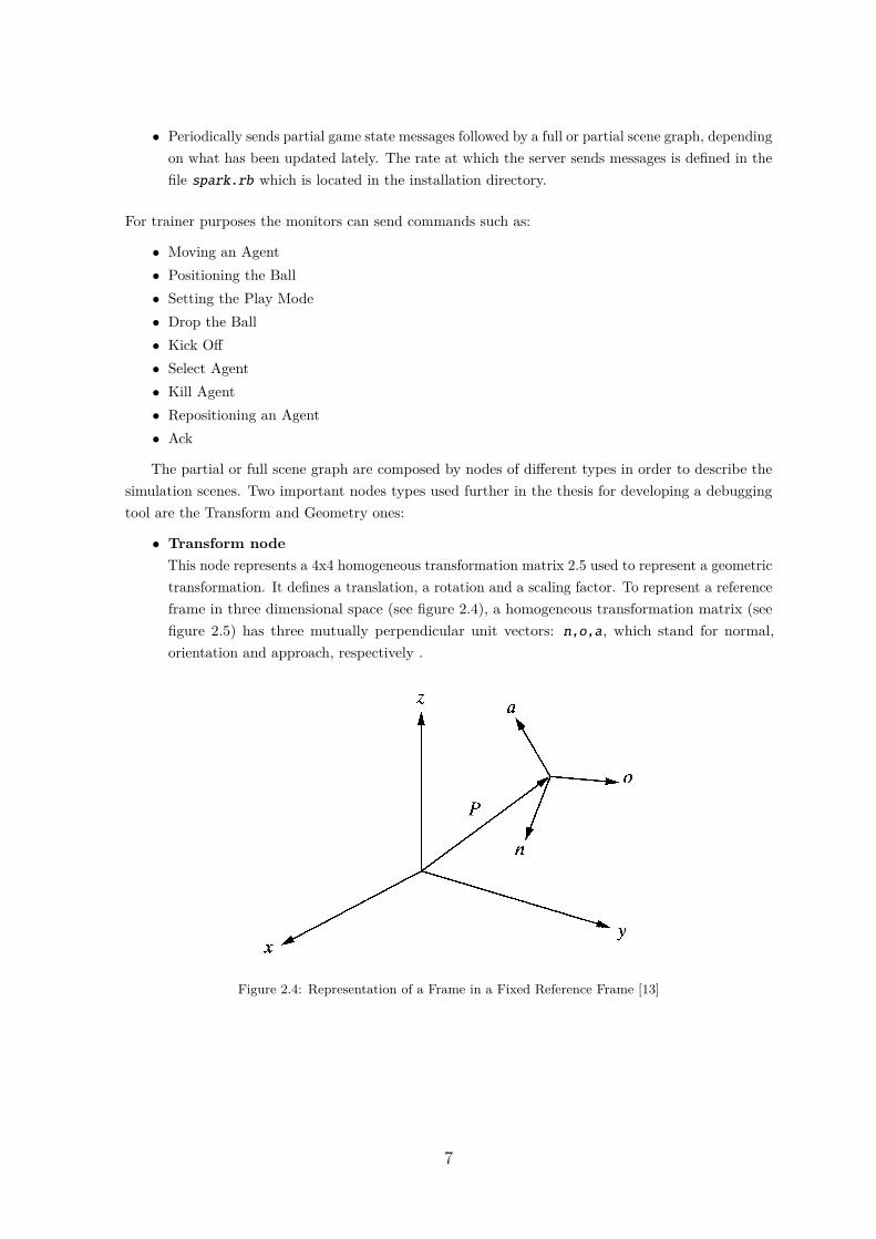
• Transform nodeThis node represents a 4x4 homogeneous transformation matrix 2.5 used to represent a geometrictransformation. It defines a translation, a rotation and a scaling factor. To represent a referenceframe in three dimensional space (see figure 2.4), a homogeneous transformation matrix (seefigure 2.5) has three mutually perpendicular unit vectors: n,o,a, which stand for normal,orientation and approach, respectively .

Figure 2.4: Representation of a Frame in a Fixed Reference Frame [13]

7

[nx ox ax Px]

[ny oy ay Py]

[nz oz az Pz]

[ 0 0 0 1]

Figure 2.5: Homogeneous transformation matrix

In Simspark, this transformation matrix is represented as:(nd TRF (SLT nx ny nz 0 ox oy oz 0 ax ay az 0 Px Py Pz 1 )) where TRF stands forTransform and SLT for Set Local Tranform which is a ruby function for setting the localtransformation of a given node in the scene graph.

• Geometry nodeThese nodes are used to describe the objects models, materials and scales. They are divided intwo types:

– StaticMeshDefines a mesh which should be loaded from a .obj file located in the Simspark path. Asa example we can see2.6 and 2.7.

(nd StaticMesh(load <model>)(sSc <x> <y> <z>)(setVisible 1)(setTransparent)(resetMaterials <material-list>)

)

Figure 2.6: Static Mesh node format

(nd StaticMesh(load models/naohead.obj)(sSc 0.1 0.1 0.1)(resetMaterials matLeft naoblack naogreynaowhite)

)

Figure 2.7: Static Mesh node example

– SMNDefines a mesh using one of the predefined models of the Simspark: StdUnitBox,StdUnitCylinder, StdUnitSphere, StdCapsule. A example is present in figure 2.8and 2.9.

(nd SMN(load <type> <params>)(sSc <x> <y> <z>)(setVisible 1)(setTransparent)(sMat <material-name>)

)

Figure 2.8: SMN format

8

(nd SMN(load StdUnitCylinder 0.015 0.08)(sSc 1 1 1)(sMat matDarkGrey)

)

Figure 2.9: SMN node example

2.3 SummaryEnding this chapter, the reader should be familiar with the simulation environment components

and its network protocol. A brief description of the messages exchanged between server-agents andserver-monitors is presented to help understand the type of interaction between components.

9

chapter 3Humanoid BehavioursThis chapter presents some concepts used in humanoid behaviours an some FC Portugal 3D currentwork on behaviours.

Humanoid models present multiple complex challenges such as the creation of stable behaviours indifferent circumstances. In order to create an omnidirectional walk, a kick or a getup behaviour thereare various methods and approaches to consider.

3.1 StabilityFor creating a stable and robust behaviour there needs to be some form of control, so the robot

mantains a motion in which it will not fall. The most used stability criteria are the Center of Mass (CM),Center of Pressure (CoP) and Zero Moment Point (ZMP)

3.1.1 Center of MassThe CM is the point where all of the mass of the object is concentrated. It represents the mean

position of the matter in a body. Normally, it is in the CM that external forces are considered to beapplied.

In a system of particles the CM is calculated as follows:

R = 1M

n∑i=1

miri (3.1)

where

• R denotes the coordinates of the center of mass

• n denotes the number of particles

• mi denotes the mass of the particle i

• ri denotes the coordinates of the particle i

11

• M is the sum of the masses of all the particles

In a volume V with a continuous mass distribution:

R = 1M

∫V

ρ(r)rdV (3.2)

where

• R denotes the coordinates of the center of mass

• ρ(r) denotes the density of a mass within the volume V

• r denotes the coordinates of the mass within the volume V

• M denotes the total mass of the volume

The projection of the CM in the ground it is known as Ground projection of the Center ofMass (GCoM). This criterion it used, for example, in static gait to check stability. For that, theGCoM must be in the foot-support area.

3.1.2 Center of PressureThe CoP in the humanoid model is the point where the sum of all the forces between its feet and

the ground are applied. The forces may be obtained from the force-torque sensors at the feet of therobot. In addition to the CM, normally the CoP its used to measure balance in bodies.

3.1.3 Zero Moment PointThe ZMP represents the point in the ground where the total of horizontal inertia and gravity

forces equals zero. In other words p is the point where Tx = 0 and Ty = 0, where Tx, Ty represent themoments around x- and y-axis generated by reaction force Fr and reaction torque Tr , respectively.When ZMP exists within the domain of the support polygon (see figure 3.1), the contact between theground and the support leg is stable [14].

12

Figure 3.1: ZMP support polygon

3.1.4 Static vs Dynamic StabilityUsing static stability the GCoM is maintained inside the support polygon so the robot does not

fall [15] [16] [17]. The support polygon is the convex hull of the foot support area. For this, the robotmust adjust its posture very slowly to minimize the dynamic effects [18]. The support polygon variesduring the walk; it is the contact area between the foot and the ground when the robot has only onefoot on the ground (single-support phase) and the convex hull of both contact areas between the feetand the ground, when both feet are on the ground (double-support phase).

In the human walk there is no static stability, since the humans walk in a state of constant falling,falling forward and catching themselves using the swinging foot while continuing to walk forward.In this falling movement, the GCoM moves forward getting outside the support polygon, withoutexpending energy to adjust itself. However, it has dynamic stability because it results in a stable walkif the walking motion is continuous. Its stability is assured by maintaining the ZMP or CoP inside thesupport polygon. In a dynamically stable walk, the ZMP coincides with the CoP [14] [19]. When theZMP leaves the support polygon the gait is not dynamically stable because the ground cannot exertthe forces needed to keep it from rotating around one of the edges of the support polygon. The ZMPoutside the support polygon is called the Fictitious Zero Moment Point (FZMP) and its distance tothe foot edge is proportional to the intensity of the instability.

The advantages of static stability is its simplicity and that the robot can pause its motion atany moment of the gait stably. However, it makes the walk slow and generally leads to more powerconsumption since the robot has to adjust its posture so that the GCoM is always inside the supportpolygon. On the other hand, using dynamic stability generally leads to faster and reliable walkinggaits.

13

3.1.5 Other ApproachesThe HFutEngine3D team use a 3D linear inverted pendulum to plan the walking pattern and

L3SIM, Mithras3D the ZMP and CM to detect stability in motion [20] [21][22]The RoboCanes team uses genetic algorithms to optimize motions created with sequence of

keyframes containing joint angles, and uses CMA-ES and PSO for making kinect based motionsrobust [23]

3.2 FC PortugalDuring the years of research in the FC Portugal, different approaches were implemented and tested

to tackle the challenges of walking, kicking the ball, getup, etc. The following sections present themost recent ones.

3.2.1 Slot BehaviourThis type of behaviour was implemented by Hugo Picado [24] as a simple version of the method

proposed in [25]. Basically it define an interpolation using sin functions over an amount of time betweenthe current and the target angles.

The definition of the behaviour is made using slots. They correspond to an interval of time from 0to δ where multiple joints can be moved in parallel. It’s possible to define multiple slots sequentially,each one with its δ interval of time. In each, besides the initial and final angle, one can define theinitial and final angular velocities, and the parameters of the Proportional Integral Derivative (PID).So, for each joint, the trajectory is generated as follows:

f(t) = A ∗ sin(φf − φi

δt+ φi

)+ α,∀t ∈ [0, δ] (3.3)

where

• f(t) is the trajectory function

• δ is the duration of the slot in milliseconds

• φi is the initial phase (influence the initial angular velocity)

• φf is the final phase (influence the final angular velocity)

• A is the amplitude

• α is the offset

A and α are calculated as follows:

A = θf − θisin(φf )− sin(φi)

(3.4)

α = θi −A ∗ sin(φi) (3.5)

where θi and θf are respectively, the initial and final angles, which should be defined between −πand π. A slot behaviour example is presented in figure 3.2.

14

<?xml version="1.0" encoding="ISO-8859-1"?>

<!DOCTYPE joints [<!ENTITY head1 "0" >...<!ENTITY rarm4 "21" >]>

<behavior name="FallBack" type="SlotBehavior">

<slot name="ForceFalling" delta="0.5" ><move id="&head1;" angle="0" /><move id="&head2;" angle="0" /><move id="&lleg1;" angle="0" /><move id="&rleg1;" angle="0" /><move id="&lleg2;" angle="0" /><move id="&rleg2;" angle="0" /><move id="&lleg3;" angle="0" /><move id="&rleg3;" angle="0" /><move id="&lleg4;" angle="0" /><move id="&rleg4;" angle="0" /><move id="&lleg5;" angle="-45" /><move id="&rleg5;" angle="-45" /><move id="&lleg6;" angle="0" /><move id="&rleg6;" angle="0" /><move id="&larm1;" angle="-90" /><move id="&rarm1;" angle="-90" /><move id="&larm2;" angle="0" /><move id="&rarm2;" angle="0" /><move id="&larm3;" angle="0" /><move id="&rarm3;" angle="0" /><move id="&larm4;" angle="0" /><move id="&rarm4;" angle="0" />

</slot><slot name="ResetPositionAndWait" delta="0.5"><move id="&lleg5;" angle="0" /><move id="&rleg5;" angle="0" />

</slot>

</behavior>

Figure 3.2: Slot behaviour example

3.2.2 Central Pattern Generators BehaviourCentral Pattern Generator (CPG) is a neural oscillator that produces rhythmic patterned outputs

without the need for any rhythmic input [26] [27]. In biology, there are many animals that have CPGfor their behaviours (i.e human walking), with different CPG controlling different limbs. The generatordoesn’t need sensory feedback information to generate its output, but it could be used to correctmotion and/or do compensation [28].

In robotics, by defining a mathematical model it’s possible to simulate these biological neuraloscillators. Based on that, Sven Behnke created an omnidirectional walk [29] with walk direction,speed and rotational speed as input. Despite that, normally it is hard to determine the parameterconfiguration that generates the desired walking pattern.

15

A CPG example is presented in figure 3.3.

<?xml version="1.0" encoding="ISO-8859-1"?>

<!DOCTYPE joints [<!ENTITY head1 "0" >...<!ENTITY rarm4 "21" ><!ENTITY amp1 "12"><!ENTITY amp2 "24"><!ENTITY amp3 "10"><!ENTITY amp4 "4"><!ENTITY amp5 "24"><!ENTITY period "0.25">]>

<behavior name="SideRight" type="CPGBehavior">

<patterns>&lleg2;: -&amp3; &period; 1.570796327 0;&rleg2;: &amp3; &period; 1.570796327 0;

&lleg3;: -&amp1; &period; 0 28.44;&rleg3;: &amp1; &period; 0 28.44;

&lleg4;: &amp2; &period; 0 -46.33;&rleg4;: -&amp2; &period; 0 -46.33

&lleg5;: -&amp1; &period; 0 31;&rleg5;: &amp1; &period; 0 31;

&lleg6;: &amp3; &period; 1.570796327 0;&rleg6;: -&amp3; &period; 1.570796327 0;

&lleg1;: &amp4; &period; 1.570796327 0;&rleg1;: &amp4; &period; 1.570796327 0;

&larm1;: 0 &period; 0 -90;&rarm1;: 0 &period; 0 -90;

</patterns>

<delta>&period;</delta>

</behavior>

Figure 3.3: CPG example behaviour

3.2.3 Omnidirectional walkFrom a turn and front walk to navigate the field, to CPG [24], passing by Truncated Fourier

Series [30], the walk behaviour has seen some implementations. The current one is the Nima Shaffiomnidirectional walk based on the ZMP criterion for its stability [31]. In this approach, the bipedwalking trajectory is derived from the desired ZMP by computing the feasible CM trajectory .Thistrajectory is calculated using an approximation for the dynamics of the biped robot, the 3D linearinverted pendulum model [32].

16

So, the architecture is divided in different modules as follows 3.4:

Figure 3.4: Omnidirectional walk architecture

The input of the walk is the desired speed in X,Y and its angle θ. Based on that input and therestrictions, like the foot reachability and feet inner collision, the foot planner generates the futuresupport steps positions in 2D. Using the planned steps, the support polygon of ZMP and its position,the ZMP trajectory is calculated. From there, the Cart-table model (see figure ??) is used to projectthe possible body swing and its CM trajectory.

(a) Cart-table in a humanoid robot (b) Cart-table schematic

Figure 3.5: Omnidirectional walk Cart-table model from [31]

This model assumes that all masses are concentrated on the cart and the support legs doesn’thave any mass. The simplification is not far from reality, as the legs have normally less mass than theupper body.

However, to apply the model, one must solve its differential equations, whose solution consists ofunbounded hyperbolic cosine functions, and the CM trajectory is very sensitive to time step variationof the walk.

So, another CM trajectory generation possibility is using ZMP Preview Controller, based on theKajita work [33] extended with the Park method [34]. Its equation and diagram 3.6 is:

u(k) = −Gik∑i=0

e(i)−Gxx(k) (3.6)

17

Figure 3.6: Preview controller

where

• Gi is the gain for the ZMP tracking error

• Gx is the gain for state feedback

• e(i) = p− pd is the controller error

• x(k) is the position of the CM in the k sample time

• k denotes the kth sample time

• pd is the desired ZMP position

• p is the ZMP position calculated from the cart-table model

With this controller is not sufficient to follow the reference ZMP because of the phase delay. For that,preview samples of ZMP in the future are used as follows:

u(k) = −Gik∑i=0

e(i)−Gxx(k)−NL∑j=1

Gppd(k + j) (3.7)

where

• NL is the number of samples in the future used

• Gp is the preview gain

• pd(k + j) is the ZMP previewed k + j in the future

Even after the walking trajectory calculations are done with the use of ZMP criteria, the stabilityis not totally guaranteed because of the leg’s effectors and the simplification of the cart-table. So,before sending the final feet position to the Inverse Kinematics module, there’s a need for an activebalance module. It tries to maintain the trunk still with zero pitch and roll. For that, it makes use ofa PID controller with the measures from the robot inertial measurement unit as input.

3.2.4 Omnidirectional KickBefore 2012, the team was using a Slot Behaviour for its kick, which consisted in keyframes defining

the motion required. This basically was a serie of static values for the joints and the movement wasinterpolated between keyframes. The problem with static values is that it makes the behaviour very

18

inflexible, working with a slow preparation phase, where the robot positions itself in a predefinedposition in relation to the ball (based on the desired direction) to kick it forward.

So, in 2012, Rui Ferreira tried a new approach to make the kick more flexible and to give control ofthe kick direction [35]. With this approach, the trajectory is created using Bézier curves (see figure 3.7and table 3.1) [36], steering the kicking foot to the ball, so it will be kicked in the intended direction.This trajectory is updated in case of any ball movement within the foot range.

Figure 3.7: Kick parameters

Parameter Description

a Distance between the ball and the curve startb Distance between the ball and the curve end

hP0

Bézier cubic curves parametershP1hP2hP3

duration Kick durationFoot Orientation Angle between foot orientation and vector Ball2Target, so it’s

possible to kick using different parts of the foot

Table 3.1: Parameters Description

With this parameters the trajectory is created. A global view of the architecture is presented in3.8.

19

Figure 3.8: Omnidirectional kick sequence

This sequence unfolds into 5 phases. They are:Lean_Phase

The robot shifts its CM to the support leg.Raise_Phase

The robot raises the kick foot to the curve start.Kick_Phase

The robot kicks the ball, executing the created trajectory.Return_Phase

The kick leg returns to the base position, without touching the ground.UnRaise_Phase

The robot shifts his CM to both legs, putting the kick foot in the ground.

Furthermore, there is the Inverse Kinematics module to calculate the leg joints values based onthe execution output and the Stability module which tries to stabilize the robot while performing themovement.

3.3 SummaryEnding this chapter, the reader should be familiar with some concepts used in humanoid behaviours

and the FC Portugal 3D behaviours work.

20

chapter 4Population Based OptimizationIn the elaboration of a behaviour there are multiple variables and constants involved. If manuallydefined, these values are not optimal, just ones that work more or less in each case. Thus, thereis potential to change the values so the result of the behaviour has better performance. Instead ofmanually trying each set of values, an optimization procedure can be applied in order to discoverbetter solutions.

The FC Portugal team has implemented some optimization algorithms till date, with the mostrecent being the following:

4.1 Genetic AlgorithmsAs the name states, this algorithm is a search heuristic inspired by the biological evolution, and,

as such, it belongs to the class of evolutionary algorithms. Basically, it is an iterative process whichgenerates a new population of individuals (chromosomes) in each iteration, also called generation.Each individual is a set of parameters (genes) representing a possible solution. The algorithm startswith a population of individuals, generated randomly across the solution space or seeded in a specificarea. For each generation each individual is evaluated using a function that returns a fitness value.

From there, the next generations are produced based on the current one by applying someoperators.Selection

In each iteration some individuals are selected to be parents for the next generation. Thisselection is done randomly, with each individual having a probability of being chosen proportionalwith its fitness (fitter solutions have greater probability).

CrossoverThis operator is analogous to the biological reproduction where two parents generate a child.Using some crossover technique, the child genes (parameters) are a combination of the ones fromits parents.

MutationAnalogous to biology mutation, it applies some mutation function to the children parameters,given a mutation probability.

21

ElitismCarry the best individuals to the next generation without alteration to guarantee that thesolution quality will not decrease during the iterations.

After each iteration, the next generation has normally better average fitness than the previous one,as the most fitter individuals have more probability to generate a child. Commonly, the algorithmterminates when either a maximum number of generations has been produced, or a satisfactory fitnesslevel has been reached for the population. Furthermore, the techniques to be used and parameters likethe percentage of mutation, selection, etc has to be adjusted depending on the context to be applied,resulting in very different times of convergence and best solution fitness. A example pseudo code isshowed in the figure 4.1.

22

Inputs: size α of population, rate β of elitism, and

rate γ of mutation and number δ of iterations

Output: solution X

//Initialization

generate α feasible solutions randomly;

save them in the population Pop;

//Loop until the teminal condition

for i = 1 to δ do

//Elitism based selection

number of elitism ne = α.β;

select the best ne solutions in Pop and save then in Pop1;

//Crossover

number of crossover nc = (α − ne)/2;for j = 1 to nc do

randomly select two solution XA and XB from Pop;

generate XC and XD by crossover to XA and

XB;

save XC and XD to Pop2;

endfor

//Mutation

for i = 1 to nc do

select a solution Xj from Pop2;

mutate Xj under the rate γ and generate a

new solution X ′j;

if X ′k is unfeasible

update X ′k with a feasible solution by repairing X ′

j;

endif

update Xj with X ′j in Pop2;

endfor

//Updating

update Pop = Pop1 + Pop2;

endfor

//Returning the best solution

return the best solution X in Pop;

Figure 4.1: Pseudo code version of GA algorithm from [37].23

4.2 Particle Swarm OptimizationParticle Swarm Optimization (PSO) is a population-based stochastic method used in continuous

and discrete optimization problems. In it, these called particles, where their position represent acandidate solution, that move iteratively in the search space trying to get to better positions bychanging their velocities. These particles move towards their best known position and the swarm’s bestknown position. In each iteration, improved positions may be discovered and override the previous oneswhich then take place on guiding the swarm, in hope to find a satisfactory solution for the problem.

For evaluating each candidate solution a cost function f is need with the objective of minimizingit. This function will return a real number for each candidate solution, representing its cost. The goalof the algorithm is to find a solution a for which f(a) ≤ f(b) for all b in the search-space, which wouldmean a is the global minimum.

The candidate solutions are particles (P = p1, p2, . . . , pk) in a swarm where there areneighbourhood(Ni ⊆ P ) relations between them are represented as a graph G={V,E}. V is avertex representing a particle and E is a edge representing a neighbour relation. Furthermore, at aspecific time step t, pi has a position ~xti, a velocity ~vti and the best position(particle’s personal best) itvisited, represented by ~bti.

A pseudo code example is presented in follow image 4.2.

24

Inputs: Objective function f : Θ → R , the initialization domain

Θ′ ⊆ Θ , the number of particles |P| = k, the parameters w , ϕ1,

ϕ2 , and the

stopping criterion S

Output: Best solution found

// Initialization

Set t := 0

for i := 1 to k do

Initialize Ni to a subset of P according to the desired topologyInitialize ~xt

i randomly within Θ′

Initialize ~v ti to zero or a small random value

Set ~b ti = ~x t

i

end for

// Main loop

while S is not satisfied do

// Velocity and position update loop

for i := 1 to k do

Set ~l ti : = arg min

~b tj ∈ Θ | pj ∈ Ni

f(~b tj )

Generate random matrices ~U t1 and ~U t

2

Set ~v t+1i : = w~v t

i + ϕ1~Ut

1 (~b ti − ~x t

i ) + ϕ2~Ut

2 (~l ti − ~x t

i )Set ~x t+1

i : = ~x ti + ~v t+1

i

end for

// Solution update loop

for i := 1 to k do

if f(~x ti ) < f(~b t

i )Set ~b t

i : = ~x ti

end if

end for

Set t := t + 1

end while

Figure 4.2: Pseudocode version of the standard PSO algorithm. [38].

25

4.3 CMA-ESCovariance Matrix Adaptation - Evolution Strategy (CMA-ES) is an evolutionary algorithm for

non-linear, non-convex black-box optimisation problems in continuous domain. Typically it s appliedto unconstrained or bounded constraint optimization problems, and search space dimensions betweenthree and a hundred. Furthermore, it should only be applied when derivative based methods fail dueto a rugged search landscape (discontinuities, sharp bends or peaks, noise, local optima, outliers) sincethey are usually faster.

As a evolution strategy, the candidate solutions are sampled according to a multivariate normaldistribution in the Rn, in which the pairwise dependencies between the variables are represented by acovariance matrix. This matrix is updated in each iteration, corresponding to a second order approachto a positive definite matrix. Thus it tries to learn the second order model of the underlying objectivefunction, similar to the approximation of the inverse Hessian matrix in the Quasi-Newton methods.

The algorithm does not need much parameter tuning from the user as the strategy parameters areconsidered as part of the algorithm design. As such, the user only need to provide a initial solution, aninitial standard deviation (step-size) σ, and an optional termination criteria [39] [40].A simple pseudo of the algorithm is shown in figure 4.3.

set λ // number of samples per iteration, at least two, generally > 4

// initialize state variables

initialize m, σ, C = I, pσ = 0, pc = 0while not terminate // iterate

// sample λ new solutions and evaluate them

for i in {1...λ}

xi = sample_multivariate_normal(mean=m,covariance_matrix=σ2 C)

fi = fitness(xi)

// sort solutions

x1...λ ← xs(1)...(λ) with s(i) = argsort(f1...λ, i)

m′ = m // we need later m − m′ and xi − m′

// move mean to better solutions

m ← update_m(x1, . . . , xλ)

// update isotropic evolution path

pσ ← update_ps(pσ, σ−1 C−1/2 (m − m′))

// update anisotropic evolution path

pc ← update_pc(pc, σ−1(m − m′), ||pσ||)

// update covariance matrix

C ← update_C(C, pc, (x1 − m′ )/σ,..., (xλ − m′)/σ)

//update step-size using isotropic path length

σ ← update_sigma(σ, ||pσ||)return m or x1

Figure 4.3: Pseudocode version of the CMA-ES algorithm. [41].

where

26

• m ∈ Rn is the distribution mean and current favorite solution

• pσ ∈ Rn, pc ∈ Rn are two evolution paths (isotropic and anisotropic correspondingly), initiallyset to the zero vector

• σ > 0 is the step-size

• C is the a symmetric and positive definite n× n covariance matrix initialized with the identitymatrix

27

chapter 5Behaviours and Agent ImprovementThe first steps taken in the code were some changes that could help achieve better results runningthe behaviours. Firstly, the sync mode was implemented to get faster simulations, then the gyroscopedata was used for improving the agent known posture and finally, preconditions were added in the SlotBehaviours so they could reduce the execution in case of probable failure.

5.1 Improving Posture EstimateDuring the course of the game, the agent must keep a model of the world state, and update it

when possible so it knowns how to act in a given situation. One important information for the agent isits vertical lateral and frontal inclination so it knows if it is up, falling or is on the ground. For this,the vision is used to estimate the agent position using field flags, and from there is calculated theTorso reference frame vectors Torsox, T orsoy, T orsoz.

Before, the frontal vertical inclination, as being calculated using the direction of the vector with thecomponents z and x of the unity vector TorsoZ 5.1. On the other hand, the lateral vertical inclinationused the components z and y of the same vector 5.2.

vertInclinFront = V ector(TorsoZz, T orsoZx).getDirection() (5.1)

vertInclinSide = V ector(TorsoZz, T orsoZy).getDirection() (5.2)

5.1.1 Euler anglesUsing the unit vectors Torsox, T orsoy, T orsoz, which correspond to a reference frame, it is possible

to calculate the euler angles [42] pitch 5.3 and roll 5.4, which are equivalent to vertical inclinationfrontal and lateral , respectively.

vertInclinFront = rad2degree(atan2(TorsoXz, T orsoZz)) (5.3)

29

vertInclinSide = rad2degree(atan2(−TorsoY.z,√TorsoXz2 + TorsoZ2

z )) (5.4)

As we can see in 5.1 the pitch error in the old method is large when the agent falls laterally.Besides that, the roll error is large when the agent falls on its back 5.2.

Furthermore, the correlation difference using the old method and using euler angles is:0.62495->0.83339 in the pitch and 0.70878->0.99945 in the roll.

Figure 5.1: Comparison between vertical inclination front using the old method versus computing pitch. Greenis the ground truth from the server, red is using the old method and blue is the computed pitch.

30

Figure 5.2: Comparison between lateral vertical inclination using old method versus computing roll. Green isthe ground truth from the server, red is using the old method and blue is the computed roll.

5.1.2 GyroscopeOne problem is that this perceptor is only available every third cycle, so there are a cycles where

the agent does not update its inclination data. In order to resolve this issue, it is used of the gyroscopesensor, which is received every cycle. In the cycles where the vision is not available, the gyro ratereceived in degrees per second is integrated between the cycle duration and added to the current valuesof the vertical inclination frontal 5.5 and lateral 5.6 (agent pitch and roll, respectively).

vertInclinFront− = GyroRatex ∗ CY CLE_DURATION_S (5.5)

vertInclinSide+ = GyroRatey ∗ CY CLE_DURATION_S (5.6)

With the use of gyroscope, the vertical inclination gets closer to the ground truth. As we can seein 5.3 and 5.4, the gyroscope removes that ladder effect resulted from the cycles in which the verticalinclination is not updated. Furthermore, the correlation difference using only euler angles and usinggyroscope is: 0.83339->0.83560 in the pitch and 0.99945->0.99992 in the roll.

31

Figure 5.3: Comparison between only computing pitch versus using gyroscope. Green is the ground truthfrom the server, blue is only using euler angles and red using also the gyroscope.

Figure 5.4: Comparison between only computing roll versus using gyroscope. Green is the ground truth fromthe server, blue is only using euler angles and red using also the gyroscope.

32

5.1.3 Agent Posture StateWith better values of the vertical and lateral inclination, a state for the agent was implemented,

so the developer gets a better understanding of the agent state, to simplify the conditions made in thecode and so the agent can react depending on the current situation. The various sates are:

UPThe agent is up and can execute the normal game behaviours.

GETTING_UPThe agent is executing a get up behaviour. While is not in successfully in UP state it must notexecute any game behaviour such as walk and kick.

FALLING_FRONT, FALLING_BACK, FALLING_SIDE_LEFT,FALLING_SIDE_RIGHT

The agent as passed a point of no return, where it cannot recover its balance. So it goes to Zero

Position behaviour, which reset all the joints positions to a standard start joint configuration,so when it hits the ground, a get up behaviour starts as fast as it can.

GROUND_BACK, GROUND_CHEST, GROUND_SIDE_LEFT,GROUND_SIDE_RIGHT

The agent is fallen on the ground. It calls the appropriate get up behaviour.

5.2 PreconditionsThe simulation environment is very dynamic and has many conditions that are difficult to manage

and to foresee. One behaviour could function well in one situation and fail in some other. In behavioursthat are not adaptable, they will run every time till they reach the finished condition, as nothingexterior happened. For example, when a agent is in the ground and is trying to getup, if it is pushed,the getup behaviour is executed till the end. This leads to a loss of time that can be critical in thegame, for example, in a ball dispute.

With this in mind, a solution was implemented based on preconditions and applied to SlotBehaviours. They are defined in XML files, where a behaviour is declared divided in various slots.In the beginning of the execution of each slot, the preconditions declared are verified. If they pass,the behaviour executes the corresponding slot, if not the behaviour considers that it must end and itactivates its finished flag. Till now, the parameters accepted are:

incl_front:gtFrontal inclination greater than

incl_front:ltFrontal inclination less than

incl_side:gtLateral inclination greater than

incl_side:ltLateral inclination less than

incl_front:outerFrontal inclination Outer interval

incl_front:innerFrontal inclination Inner interval

33

incl_side:outerLateral inclination Outer interval

incl_side:innerLateral inclination Inner interval

incl_front:abs_gtAbsolute Frontal inclination greater than

incl_front:abs_ltAbsolute Frontal inclination less than

incl_side:abs_gtAbsolute lateral inclination greater than

incl_side:abs_ltAbsolute lateral inclination less than

z_position:gtZ position of the agent greater than

z_position:ltZ position of the agent less than

As we can see in 5.5 there are conditions in the first slot incl_front:abs_lt="10"

incl_side:abs_lt="10", that must be meet for the slot to execute.

34

<?xml version="1.0" encoding="ISO-8859-1"?>

<!DOCTYPE joints [<!ENTITY head1 "0" >...<!ENTITY rarm4 "21" >]>

<behavior name="FallBack" type="SlotBehavior">

<slot name="ForceFalling" delta="0.5" incl_front:abs_lt="10"incl_side:abs_lt="10">↪→

<move id="&head1;" angle="0" /><move id="&head2;" angle="0" /><move id="&lleg1;" angle="0" /><move id="&rleg1;" angle="0" /><move id="&lleg2;" angle="0" /><move id="&rleg2;" angle="0" /><move id="&lleg3;" angle="0" /><move id="&rleg3;" angle="0" /><move id="&lleg4;" angle="0" /><move id="&rleg4;" angle="0" /><move id="&lleg5;" angle="-45" /><move id="&rleg5;" angle="-45" /><move id="&lleg6;" angle="0" /><move id="&rleg6;" angle="0" /><move id="&larm1;" angle="-90" /><move id="&rarm1;" angle="-90" /><move id="&larm2;" angle="0" /><move id="&rarm2;" angle="0" /><move id="&larm3;" angle="0" /><move id="&rarm3;" angle="0" /><move id="&larm4;" angle="0" /><move id="&rarm4;" angle="0" />

</slot><slot name="ResetPositionAndWait" delta="0.5" incl_front:gt="80"

incl_front:lt="100">↪→<move id="&lleg5;" angle="0" /><move id="&rleg5;" angle="0" />

</slot></behavior>

Figure 5.5: Preconditions example

35

chapter 6Optimization Process ImprovementIn the FC Portugal code, there are already some optimization algorithms implemented such as GeneticAlgorithms, PSO and CMA-ES. In this thesis the optimizations were performed using CMA-ES. Still,there was some room to improve and automatize the optimization process. The next sections describedwhat was done in that sense.

6.1 Sync ModeAccording to the competition rules the server runs in real-time, which means its cycles have a

duration of 20 ms, in which the server is listening for the agent effector commands. This creates twoproblems. The agent has limited time to process and send its commands within the cycle time, if it canot, the commands will only be applied in the next cycles, which worsen the expected behaviour. Theother problem is the usage of the resources that are not used to the maximum, since the server waitstill the end of the cycle to process, even if it has already received all the agent commands. For thecompetition, this problems makes sense as the cycle time provides a just processing time restriction toall the teams. But, for developing and optimization purposes, it is way better to run the simulationas fast as the CPU can. This way, the server only waits for the agent commands and a synchronisemessage which signals the end of the agent cycle. After it receives all the agents Sync message, theserver processes all the commands and proceeds to the next cycle. In addition to simulation speedtime improvement, it can also be used to detect strange cycle times from the agents.

6.1.1 Sync Mode UsageBefore this sync mode implementation, for each command the agent generated, one message was

sent to the server. This approach was not working when transiting to sync mode. To exploit this mode,the server connection code in the agent was changed so all messages from the same cycle are nowaggregated and for each message sent by the agent, a synchronize was added. Since then, the agentcode can support sync mode. If the server is not running in agent sync mode, the synchronize messages

37

are ignored. Finally, to configure the server in sync mode, enableRealTimeMode variable in the file/usr/local/share/rcssserver3d/rcssserver3d.rb file must be set to false and agentSyncMode

in /home/$USER/.simspark/spark.rb to true. To simplify changing between real time mode syncmode, a python script was created, which can be called as following:

./syncMode <true|false>

As a result the time a simulation takes is drastically decreased. Without sync mode, each cycletakes 20 ms and each part takes 5 minutes, regardless the number of agents in game. With sync mode,the simulations runs as fast as the computer can, so the number of agents in game affect the simulationtime. In a laptop with few agents the simulation time is drastically decreased, but with many agents,the difference between running in sync and real mode it is not visible. On the other hand, in a desktop,even when running with all the 22 agents, the simulation time is greatly reduced.

6.2 Constraint Free EnvironmentThe normal simulation execution is the same as during the competition games. Because of that,

there are some constraints such as: the game has limited time, 5 minutes for each part; the agents cannot move the ball and cannot beam themselves after the game have started. This affect badly theoptimization process because it needs to run for as long as needed without human intervention.

For that purpose, a constraint free environment was created as explicated below.

6.2.1 SolutionStep 1. The first step was to create a patch for the server code. It is a simple modification in thercssserver3d code so the playmode can be calculated based on the existence of a Linux environmentvariable named ALWAYS_PLAYON. When this variable exists and is set to 1, the server is always inPlayOn mode, otherwise the server runs normally. The PlayOn mode is used as the normal state ofthe game when the ball is running. With PlayOn mode always active the game never ends. After theapplication of this patch, the server code needs to be compiled and installed. To set the environmentvariable, "export ALWAYS_PLAYON=1" must be run in the console before calling the server executable,or defined in a ∼/.profile file or similar Linux file.

Step 2. According to the game rules, the agent can only beam itself during the kickoff, and theball only can be moved after the kickoff. To overcome this, it was created a trainer proxy (see image6.1), which allows the agent to call all the trainer commands (see section 2.2). The most useful trainercommands are those to control the robot and the ball, imperative to run kick behaviour optimizations.There was a tentative of connecting the agents directly to the server using the monitors port, but theconnections were failing, so a proxy was needed. The proxy allows connections from the agents andconnects itself to the server as a monitor. By default, it listen for agent incoming connections usingport 3300.

38

Figure 6.1: Trainer Proxy

./trainerProxy.py -pp <proxyport> -s <server_port>

proxy_portPort number to listen for agent incoming connections.(default=3300)

server_portPort number which rcssserver3d exposes for monitor connections (default=3200).

Step 3. Finally, the agent used for optimization purposes has to connect to both the server andthe proxy. A command line option is used to specify the port number. There is a argument called pp

<proxy_port>. For example, if the proxy uses the port 3400:./fcpagent -pp 3400

6.3 Optimization AgentNormally the optimization process of finding good value sets consumes a lot of time and resources,

as it needs to evaluate a lot of possible solutions, and for each solution, resample multiple times toaverage each individual cost value. Before, the process of optimization was being done running onlyone agent for server to optimize one behaviour each time. In order to improve this, a new executablewas created so multiple agents can run in the same server (maximum of 22 agents for server), runningdifferent optimizations with the same executable.

This executable was divided in multiple scenarios (GETUP, KICK and WALK), each one withits parameters and its behaviours.Currently any XML defined behaviour is supported for GETUPand KICK. This scenarios execute the behaviour passed as argument and each learning scenario hasspecific sequence and cost or fitness function.

GETUPScenario where the getup behaviours can be evaluated. This will execute a fall behaviour, followedby the getup behaviour. It has a cost function associated with the time it takes to execute. If, atthe end of the getup behaviour, the agent is not up, the cost function is affected greatly to reflectthe error. Furthermore, the fall type and the getup file path need to be passed as argument.

KICKScenario where kick behaviours can be optimized. The ball will be positioned in front of theagent and then the kick behaviour is executed. The fitness function is related to the distance

39

that the ball travels and if it goes straight forward. This fitness value is affected greatly if theball does not move, indicating that the agent missed it. The behaviour file path need to bepassed as argument.

WALKScenario used for optimizing the walk behaviour. Currently, it executes the ZMP walk in thegoal direction. The fitness function evaluates the distance covered during a limited defined timeand its deviation from the target position (goal). Furthermore, this fitness is affected greatly ifthe agent falls.

The optimization agent needs to know what parameters to optimize. In the slot behaviours thisis done adding new attributes to the XML file, stating the parameters to be optimized. The newattributes have the same name as the attributes representing the parameters with the prefix ’o:’

added. The value of the new attributes is just an enumeration and can be used to specify that two ormore parameters should have the same value during the optimization process. Figure 6.2 shows anexample with several parameters to be optimized. For instance, lines 10 and 11 show two parameterswhose values should be the same.

1 <?xml version=’1.0’ encoding=’ISO-8859-1’?>2 <!DOCTYPE behavior [3 <!ENTITY head1 "0">4 ...5 <!ENTITY rarm4 "21">6 ]>7 <behavior name="r0_GetUpFront" type="SlotBehavior" correctAnglesOutOfRange="false">89 <slot name="leftLegUp" delta="0.205311" o:delta="1">

10 <move id="&larm1;" angle="14.514300" o:angle="10"/>11 <move id="&rarm1;" angle="14.514300" o:angle="10"/>12 <move id="&larm4;" angle="0"/>13 <move id="&rarm4;" angle="0"/>14 <move id="&lleg3;" angle="0"/>15 <move id="&rleg3;" angle="0"/>16 <move id="&lleg4;" angle="0"/>17 <move id="&rleg4;" angle="0"/>18 <move id="&lleg5;" angle="0"/>19 <move id="&rleg5;" angle="0"/>20 <move id="&lleg5;" angle="0"/>21 <move id="&rleg5;" angle="0"/>22 </slot>2324 <slot name="leftLegUp" delta="0.079244" o:delta="2">25 <move id="&lleg3;" angle="259.929000" o:angle="11"/>26 <move id="&rleg3;" angle="259.929000" o:angle="11"/>27 <move id="&lleg4;" angle="-133.612000" o:angle="12"/>28 <move id="&rleg4;" angle="-133.612000" o:angle="12"/>29 <move id="&lleg5;" angle="124.630000" o:angle="13"/>30 <move id="&rleg5;" angle="124.630000" o:angle="13"/>31 </slot>32 ...33 </behavior>

Figure 6.2: Example of XML behaviour file to optimize

The current version of the optimization agent accepts the following configuration parameters:-r <robotType>

Heterogeneous model type to use.

40

-scenario <Getup,Kick,Walk> (default is Getup)

Optimization scenario to run.-b x y z

Agent initial beam position. As the server may be running with multiple agents, their positionsmust be disperse so they do not interfere with each other optimization.

-opt <behaviourFile>

Path of the behaviour to optimize.-fallType <None,FallFront,FallBack>

Fall behaviour to be used in the getup scenario.-res

Number of resamples to run (default is 5).-pop

Population (default is 20).

6.4 Update Optimization ParametersThe result of an optimization is a set of possible solutions, stored in a text file. The user must

manually test some of them and choose one before update the working behaviour. A tool was developedto aid in the updating of a slot behaviour. The tool receives as arguments the file to be updated andthe new parameter values.

The tool was implemented as a python script, which parses and updates the behaviour file. Everytime an attribute with the prefix ’o_’ is found, the corresponding normal attribute is updated withthe given new value. More details on the attributes format are in 6.3.

Requisites: Python2.7 python2-lxml

./updateOptParams.py [filename] [newValues]

Ex: ./updateOptParams.py movs/type0/getup/GetupFront.xml 0.2 0.3 0.4

6.5 Heterogeneous ModelsThe simulation league has evolved since the use of a sphere in 2004 to represent a agent till the use

of humanoid agents in 2007. In 2013, heterogeneous models were introduced and, in 2014, rules weremade mandatory to force their use in the teams (at least three different model types must be used). Inorder to fulfill these new requirements, some changes had to be done in the agent code/project.

1. In the FC Portugal project there exists a XML file describing the robot model used. It describesthe body parts, joints information like its position, etc. To support heterogeneity, one file for eachmodel type was used, with its custom information. The name of the file is nao%d.xml, replacing%d with the heterogeneous model number (0-4) . Furthermore, note the "nao/nao_hetero.rsg3" in the beginning of nao3.xml 6.3 which is the string that is sent to the Simspark server so itknowns which model to use.

41

<?xml version="1.0" encoding="ISO-8859-1"?>

<agentmodel name="nao" type="humanoid" rsgfile="nao/nao_hetero.rsg 3">

<bodypart name="head" mass="0.35" /><bodypart name="neck" mass="0.05" /><bodypart name="torso" mass="1.2171" /><bodypart name="lshoulder" mass="0.07" /><bodypart name="rshoulder" mass="0.07" /><bodypart name="lupperarm" mass="0.15" /><bodypart name="rupperarm" mass="0.15" /><bodypart name="lelbow" mass="0.035" /><bodypart name="relbow" mass="0.035" /><bodypart name="llowerarm" mass="0.2" /><bodypart name="rlowerarm" mass="0.2" /><bodypart name="lhip1" mass="0.09" /><bodypart name="rhip1" mass="0.09" /><bodypart name="lhip2" mass="0.125" /><bodypart name="rhip2" mass="0.125" /><bodypart name="lthigh" mass="0.275" /><bodypart name="rthigh" mass="0.275" /><bodypart name="lshank" mass="0.225" /><bodypart name="rshank" mass="0.225" /><bodypart name="lankle" mass="0.125" /><bodypart name="rankle" mass="0.125" /><bodypart name="lfoot" mass="0.2" /><bodypart name="rfoot" mass="0.2" />

<!-- joint 0 --><joint name="head1" perceptor="hj1" effector="he1" xaxis="0" yaxis="0"

zaxis="-1" min="-120" max="120">↪→<anchor index="0" part="neck" x="0" y="0" z="0.0" /><anchor index="1" part="torso" x="0" y="0" z="0.09" /></joint>...</agentmodel>

Figure 6.3: Initial part of nao3.xml file

2. In the code, the walk parameters and mid level skills had to be tuned for each model type.

3. At last, new behaviours for each heterogeneous type were created. First, it was used the standardmodel behaviours, then they were manually tuned for each type, so they behaved properly. Afterthat, each used behaviour defined in a XML files was optimized described in the OptimizationResults section 6.6.

6.6 ResultsThe process of optimization was automated to some extent.It envolves 4 applications: the optimization agent, the trainer proxy, the 3D soccer server, and

a matlab program running the CMA-ES algorithm. After connection, the optimization agent sendsthe required optimization data to the matlab program, that, afterwards, uses the agent as a server tocompute the cost function of the individuals. By its turn, the agent, in order to compute the valueof the cost function, runs a simulation in the soccer server, and returns the computed value to thematlab program. These interactions last until the optimization process ends. Figure 6.4 illustrate theinteraction among the different applications.

42

Figure 6.4: Optimization Flow

Some decisions were taken in how to configure the optimizations that were realized. Not all therobot joints were managed to be manipulated by the optimization algorithm, as it could be a very longprocess and unnecessary. It was decided to consider only the most important joints for each behaviour.

Different runs of the simulation of a behaviour, for the same initial conditions, can lead to differentresults. So, a single run should be avoided to calculate the cost function. It was decided to do severalruns and calculate the average of the values. However, the number of runs has a great influence inthe optimization process time. It was decided to use 5 runs. With 3 evaluations, it was verified thatthe behaviours were not consistent, and using more than 5 evaluations is just in cases where we wantreally consistency, which, on the other hand, affect the possible achievable fitness. The populationused was 30 because it is not so small to be a local search, neither is to big to be a global search.

As a result of this tuning, better times were obtained for the behaviours optimized as shownbelow. The robots type 1 and 3 were not optimized because they are not currently used in the teamheterogeneous setup.

For the getups, the Getup scenario was used, being obtained the following values 6.1 6.2 (inseconds).

43

Model Type0 2 4

Before 2.6 2.6 2.6After 1.12 0.74 0.98

Table 6.1: GetUpBack

Model Type0 2 4

Before 1.42 1.42 1.41After 0.74 0.68 0.72

Table 6.2: GetUpFront

44

chapter 7Development and Debugging Tools

In any software project, the development and debugging processes/tools are critical to quickly passfrom an idea into a fully working and robust solution. Furthermore, the understanding of what ishappening in the simulation is greatly increased. It became clear that the project could make good useof new tools. So, three tools were developed. The first is a monitoring interface for the agents where,in runtime, it is possible to see code variables, input data and control the cycle time. The second is apost simulation analyser which uses the logs from the agents and the server as input and then, parsingand filtering the data, it is possible to export in multiple formats, view plots of the data, etc. Finally,the last one is a tester for behaviours defined in XML files which gives, in runtime, the possibility toedit behaviours, run a sequence of behaviours, change the robot heterogeneous type, etc.

They are detailed in the following sections.

7.1 Agent Monitor WindowBefore, the analysis of each code change was being done by visualizing the result in the simulation

monitor, then, in the end of the simulation, analysing the log containing the standard output from theexecutable. This log normally contain thousands of lines just for one agent, so, to simply search fora game situation and understanding what is happening was quite difficult. Furthermore, during theexecution of a simulation it becomes greatly useful to have the possibility to see the values from thecode variables as they change in each situation, or other debug information.

The solution found was to use a graphical interface to monitor program variables specified by theuser through an API. Each agent can have its own windows. Thus, in order to allow all windows to beseen at the same time, their position on the screen depends on the id of the agent. Figure 7.1 showsthe 11 windows of 11 agents, partially overlapped by the server window.

45

Figure 7.1: Agent Monitor Window running 11 agents, each with his window.

The interface was implemented in GIMP Toolkit (GTK) [43] and runs in a separated thread. Touse the tool one must use the parameter -s.

Ex:./fcpagent -s

Requisites: >=libboost1.48-all-dev (Ubuntu), >=boost 1.48.0 (Arch Linux)

7.1.1 Developer APIDuring development, it is often necessary to change the values of given internal variables and

see the effect of such changes. Being possible to do this without recompiling the program is a majoradvantage. The API available to the developer/programmer, in addition to the possible visualizationof internal variables, allows for the change of given variables. The changes are done though the useof three different types of inputs, associated with callbacks. When a changed event is detected ina registered input, the corresponding callback will be triggered, and, from there, the new value isprocessed by the developer.

Show variableThe main feature is to give the ability to show any value/string and update it during the courseof the simulation. Giving a variable name and its value, one can call the following functions 7.2:

void showVariable(string variableName, float value);void showVariable(string variableName, string value);

Figure 7.2: Agent Monitor Window show variables

Register ComboBoxRegistering a ComboBox gives a set of possible selectable values (see figures 7.4a and 7.4b) that

46

can be used for example, for controlling which behaviour should the agent execute next. Theregister function is presented in the figure 7.3.

void registerComboBox(string comboBoxName, vector<string> values, int active, void*changedCallback);↪→

Figure 7.3: Register Combo Box in Agent Monitor Window

(a) ComboBox Closed (b) ComboBox Opened

Figure 7.4: Agent Monitor Window with ComboBox

Register SpinButtonRegistering a SpinButton (see figure 7.6) let the developer to write any string to be interpretedby the callback he wrote. One possible use is to test a parameter or multiple ones to achieve theexpected behaviour. The register function is presented in the figure 7.5.

void registerSpinButton(string spinButtonName, GtkAdjustment* spinnerAdjustment,void* valueChangedCallback);↪→

Figure 7.5: Register Spin Button in Agent Monitor Window

Figure 7.6: Agent Monitor Window with SpinButton

47

Register keyboard keyRegistering a keyboard key may be used, for example, to control an agent dribbling direction,testing different angles and situations. The register function is presented in the figure 7.7.

void registerKeyPressed(int keyValue, gboolean (*keyPressedCallback)(GtkWidget*,GdkEventKey*, gpointer));↪→

Figure 7.7: Register keyboard key in Agent Monitor Window

7.1.2 Controlling the Cycle TimeAs the simulation cycle is 20 ms in real mode, it is humanly impossible to see the variation of one

or more variables in each cycle. To give the developer total time control of the simulation, server syncmode was explored. The server, running in sync mode, will always wait for all agents’ synchronizemessages. Controlling the sending time of one agent synchronize message, one can control all thesimulation cycle time. To implement this, it was used the boost chrono library, available since version1.47.0, which contains a high resolution clock. With this clock, it is measured the agent cycle time:the time between the agent receives a message from the server and finish processing it. From there,the agent waits until the cycle time the user sets in the interface, to send the synchronize message.Calling the -ss parameter in one agent, the Agent Monitor Window show the cycle time controls (seeimage 7.8), in which is possible to:

1. Pause simulation

2. Go to next simulation cycle

3. Change simulation cycle time

Figure 7.8: Agent Monitor Window with cycle time controls

48

Ex:./fcpagent -u 2 -ss

7.2 Log AnalyserUsing the Agent Monitor Window, it is possible to view the simulation state in runtime. In other

cases, a developer may want to use the resulting agent and server logs to do after-simulation analysis.So, a Graphical User Interface (GUI) tool was developed, increasing also the information obtainedthrough the manipulation of the log files and the information visualization. Due to its simplicity todeal with strings and good documentation, Java was used for programming the GUI tool, with Swing[44] toolkit being used to display the interface elements.

7.2.1 Extracting InformationThe input for the application is the logs generated from the agents and the server. In

the server, the simulation must be configured to record a log file. In the ruby file in/usr/local/share/rcssserver3d/rcssserver3d.rb or similar path, there is a variable in the begin-ning of the file named recordLogfile that must be set to true.

In each execution of the server, a sparkmonitor.log file containing all the information needed fora monitor to reproduce the simulation is generated. This file contain S-expressions using the protocoldetailed in section 2.2.2.

On the other hand, the log files from the agents have their standard output from the executionof the code, without any standard format. So, to extract meaningful data, the program gives theuser the possibility to declare regex expressions with groups in it. Each group as a meaning, whichcurrently can be: the simulation time named time; a matrix position Ny, Nz, Zero3, Ox, Oy, Oz,

Zero7, Ax, Ay, Az, Zero11, Px, Py, Pz, One15; an Euler angle Pitch, Roll, Yaw; or a customvariable Val1, Val2, Val3, Val4. These regex expressions are applied in the agent logs, extractingthe groups data. An example expression can be gameTime:(FLOAT) vertInclinFront:(FLOAT) withthe Group 1 denoting the Time and Group 2 as the Pitch . This expression will search for lines in thelog file such as gameTime:2.4 vertInclinFront:45.2, extracting 2.4 and 45.2 as Time and Pitch ,respectively.

7.2.2 Export OptionsAs output, the application has various options such as:

LogThe Log export option will generate a file with the same format as the sparkmonitor.log

detailed in sub section2.2.2. The generated log can then be viewed in any simspark monitor. Itmay be helpful, for example, to put a 3D model of a ball in the positions that the agent thinksthe ball was. So, in this case, two balls would appear in the screen, and the user could see thedifference between the real position of the ball and the one it calculates from the vision system.

49

PlotsThe Plots export option produces either line or point plots (see figure 7.9 for an example ofeach type). This is helpful to see the variation of a variable through the simulation, and/or tocompare it with other variables.

(a) Lines Plot (b) Points Plot

Figure 7.9: Two types of plots available

XLSThe XLS export option produces a file like the figure 7.10.

Figure 7.10: XLS export example.

XMLWith the well known and used XML output (see figure 7.11), the data can them be used asinput for another program for further manipulation and processing.

50

<?xml version="1.0" encoding="UTF-8" standalone="no"?><elems><elem name="Left4_Torso"><matrix time="0.18">-0.00341114 -0.999994 -1.52527E-7 0.0 0.999994 -0.00341114

7.23039E-5 0.0 -7.2304E-5 9.41126E-8 1.0 0.0 -4.56328 1.19874 0.3837061.0 -0.004142708 8.739153E-6 1.5258789E-5</matrix>

↪→↪→<matrix time="0.38">-0.00341107 -0.999994 -1.7801E-7 0.0 0.999994 -0.00341107

1.09919E-4 0.0 -1.09919E-4 1.96932E-7 1.0 0.0 -4.56692 1.19875 0.378091.0 -0.0062978948 1.0199222E-5 1.5258789E-5</matrix>

↪→↪→<matrix time="0.46">-0.00341107 -0.999994 -2.13309E-7 0.0 0.999994 -0.00341107

8.19609E-5 0.0 -8.19612E-5 6.62669E-8 1.0 0.0 -4.56863 1.19876 0.3723251.0 -0.0046960134 1.2221705E-5 1.5258789E-5</matrix>

↪→↪→</elem></elems>

Figure 7.11: Example of the exported XML file.

7.2.3 InterfaceAfter launching the application, a graphical interface appears and the user can select the server

and/or agent log files to be manipulated. Then, a set of parse and process features are available forboth the server and the agent logs.

The interface is composed of a top common banner area and bottom agent/server specific area.Figures 7.12 and 7.13 show, respectively, the available options from the agent and server perspectives.Supported in these two figures, it follows an explanation of both the graphical elements and theoperation performed when they are selected.

Figure 7.12: Log Analyser agent log selected

51

Figure 7.13: Log Analyser server log selected

1. File path of the current selected log.

2. Button used to refresh all the program. This is useful, for example, when the logs selected inthe interface are changed because new simulation was run. This way, there is no need to selectthe log files again or restart the program. To refresh, the program begins by saving the currentinterface state (log tree selection, playmodes checkboxes, time, etc), then all the interface isreset and all the logs are parsed again. At the end, the initial interface state is applied and ifany plot is visible, iti s refreshed too.

3. Let the user select a server log. This log, called sparkmonitor.log, is generated by simspark ifrecordLogfile variable in simspark.rb file is set to true. Only one server log can be used bythe program at a time, corresponding to one simulation. After the file is selected, the programtries to parse it, and, if successful, presents in the log tree the agents present in the log, and itscomponents (Ex: head, neck, etc).

4. Let the user select a agent log. The agent logs are the files generated from the standard outputof the agents code. Multiple agent logs can be selected, as multiple agents can generate their login one simulation. After the file is selected, the program parses it, and adds it to the log tree.

5. Tree representation of the logs loaded in the program and its components. Using this treerepresentation it is possible to select which components to be used in the multiple export options.In the server node, the children are the agents and the ball present in the server log. In theagent, its children represent regex expressions added by the user. First, the user creates a newregex expression with 16, then fill the options 6,10,11-15. Afterwards, the user needs to save17. Finally, with a agent tree selected in the tree log, the button in 19 creates a new elementbased on the regex expression and adds it to the children of the agent log.

6. Identifier of the current selected regex expression (must be unique).

7. To simplify the regex visualization and its creation, there are two buttons corresponding to the

52

two most used expressions (Float, Integer), that are replaced with the correct regex when allthe expression is applied. Click in this button to insert FLOAT macro in current caret position.It will be replaced with:[-+]?[0-9]*\\.?[0-9]+([eE][-+]?[0-9]+)?

8. Click in this button to insert INTEGER macro in current caret position. It will be replacedwith:[-+]?[0-9]*

9. Click to preview the effect of the current regex expression applied in the selected agent log.

10. Input box with the regex expression to use. Each parentheses pair represents a regex group, orin other words, a value to be retrieved when applying the regex expression to the log file. Eachgroup has a meaning, it can represent the time, a transformation matrix element, pitch, roll,yaw or simply a custom value to analyse. For the former there are Val<n> from 1 to 4 in thecombo box to be used. The groups combo boxes are automatically updated as the user changesthe regex expression.

11. Groups combo Boxes actually present in the regex expression and its meanings.

12. Checkbox to indicate if the regex expression has a 3D model associated. If so, a group ofconfigurations for the 3D model are presented, otherwise they are hidden. With this feature,when exporting in log format, a new visual element is created using the 3D model options in13-15 and added to the server log. This way, when using a monitor to view the exported log,the selected model, a 3D model will appear in the positions extracted from the regex expressionin 10.

13. Select the 3D model to use. The ComboBox is filled with the known models used by the simulationserver, plus any .obj files found in /usr/local/share/rcssserver3d/models directory. Thestandard models StdUnit (Cylinder, Box and Sphere) are only displayed in the rcssmonitor3d,they don’t appear in Roboviz.

14. Define the scale in X,Y and Z.

15. Defined the material to use in the model. The ComboBox is filled with the known materialsused by the simulation server.

16. Create new regex expression. The new expression get as identifier the current date.

17. Save any changes to the selected expression.

18. Remove the selected expression.

19. Add selected regex expression to the selected agent log.

20. List with the identifiers of all the regex expressions the user has already created.

21. List where the first results of the preview appears.

22. Select the server time range to process.

23. Select simulation play modes to process.

53

24. Global group selection combo box. Used as a plot option.

25. Click to show Lines Plot. At least one log tree node must be selected. Then, the Group to beused in the plot can be selected globally in the combo box below the "Plot" label, or individually,in each log tree node. The former is used if the global group combo box has the value "-"

selected.After clicking the button, a new window is created in which the plot is presented, using GRAphingLibrary (GRAL), modified a little. Each group has a different colour and when a plot point isclicked, a label appears containing the clicked point time and value. Furthermore, the GRAL[45] gives the option to zoom, move, print and export the plot as image with multiple possibleformats using the right click menu (Wireless Application Protocol Bitmap Format (WBMP),Bitmap image file (BMP), Portable Network Graphics (PNG), Joint Photographic ExpertsGroup (JPEG), Portable Document Format (PDF), Graphics Interchange Format (GIF),Scalable Vector Graphics (SVG), Encapsulated PostScript (EPS)). The images presented in 5.1were generated using this export options.

26. Click to show Points Plot.

27. Click to export to a simspark log format. All the options in the interface are applied to theselected logs and its selected elements, then the server log is merged with the agent logs, resultingin the output log. This contains the 3D models information from the agent logs processing, sothey can be visualized in a simulation monitor.

28. Click to export the selected logs/elements to XLS format. It makes uses of the Java Excel API(Only one node can be selected for export). [46]

29. Click to export the selected elements to XML format.(Only one element can be selected)

7.2.4 Configuration SaveAs the program was being developed, it became useful to save some changes done in each program

execution. For this purpose a XML file was created named configs.xml (see figure 7.14). In it, it issaved all the logs previously selected by the user, regex expressions created and its options. When theprogram is executed, the configuration file existence it is verified. If the file exists, all logs presentedare loaded and all the regex expressions made available, otherwise the file is created.

54

<?xml version="1.0" encoding="UTF-8" standalone="no"?><configs><expressions><expression hasModel="false" identifier="vertInclinFront"><regex>gTime:(FLOAT) vertInclinFront:(FLOAT)</regex><groups><group>Time</group><group>Pitch</group>

</groups></expression><expression hasModel="true" identifier="ball"><regex>gTime:(FLOAT) .*BallPos (FLOAT) (FLOAT) (FLOAT)</regex><scale x="1.0" y="1.0" z="1.0"/><material>yellow</material><model>StdUnitSphere</model>chr<groups><group>Time</group><group>Px</group><group>Py</group><group>Pz</group>

</groups></expression></expressions><openLogs><log type="server">/home/test/fcp/sparkmonitor.log</log><log type="agent"><fileName>/home/test/fcp/L3</fileName><expressions><expression identifier="vertInclinFront"/><expression identifier="ball"/>

</expressions></log>

</openLogs></configs>

Figure 7.14: Example of the configs.xml file.

7.2.5 Server SimulationA great way to understand what is happening in a giving time is to see it appearing in the

simulation monitor. This is the purpose of this feature, which simulates the rcssserver3d server. Itbounds to the default rcssserver3d port(3200), waiting for monitors connections.

Starting from here, some options in the Log Analyser can be made visible in the monitors in realtime.

It works by cloning the Ruby Scene Graph (RSG) message previous to the current selected timeand applying all the Ruby Diff Scene (RDS) in between. After this aggregation, which creates thecurrent time RSG message, the resulting message is sent to all the monitors connected to this server.

When a monitor connects to the server, the current time message is sent to it.One must remember that the processed RSG message is the result of the options configured in the

interface, especially the log tree selection, so it is possible to show in the monitors only some agents, orsome agent elements or some processed regex expressions in the form of a 3D model. This make iteasy to analyse only one agent leg movement in a full game, for example.

In the figure 7.15, we can see a possible setup to analyse the agent torso inclination. Only theTorso, Neck and Head nodes of one agent are selected and, because of that, only that elements appearon the monitor. There are also two plots opened with the Torso Nx and Ny of the agent 4 of the Left

55

team. When the user changes the time in 2 or click on a point in any of the graphs, all the elementsare synchronized: the time in 2 will be updated; the plots opened will show a label with the value inthe selected time; and the monitor will be updated too.

Figure 7.15: Server running with one plot selecting a time value where we see the agent falling with a pitchof approximately 45o.

Based on the figure showed above, the description of the server simulation is presented below:

1. Click to start/stop the server simulation. If it is stopped, the current time indicator will beinvisible.

2. Change the server time using the arrows, introducing manually the value, or using the scrollwheel from the mouse. The possible time values are restricted between the server log last time,and its first time with all the agents connected.When the value changes, the current RSG message is sent to all the monitors connected, and allthe plots visible show a label corresponding to the current time.The time will not change if zero elements are selected in the log tree.

3. Clicking in any plot point, will move the current time indicator to the plot point time, thussending to the monitors connected to this server the new time RSG message. Furthermore, theother plots visible show a label corresponding to the current time.

7.3 XML Defined Behaviour TesterThere are different kinds of behaviours in the FC Portugal team, some of them are dynamically

calculated in runtime (ex:Walk) and others are statically defined in XML files (ex:SlotBehavior,CPGBehavior, StepBehavior, ImprovedSlotBehavior, ImprovedCPGBehavior). For the last ones, theprocess of testing and improving was being done by changing the code to run tests for each behaviours,

56

compiling and then using a text editor for editing the XML files. For each change in the XML file,running a new agent executable was needed to visualize the result.To improve the efficiency of this process, a new tool (see image 7.16) was created using GTK2, Scintillaand some agent code. GTK was used for the user interface and Scintilla is a open source library whichprovides text editing and XML syntax highlighting.

Figure 7.16: Behaviour Tester

Supported on figure 7.16, it follows an explanation of the features available in the application

1. Choose the behaviour file to use.

2. Edit time to wait after this behaviour ended.

3. Remove this line behaviour from the list.

4. Select how many agents to run in each test iteration.

5. Choose the robot type to use from the list of heterogeneous models.

6. Choose if the agent should fall back, front, side or not at all.

7. Choose first agent initial position

8. Select if the test iteration should be repeated.

9. Add new behaviour file.

10. Save file and run the test.

11. Editable area with syntax highlighting.

12. Save current editable file or choose to edit another file

Requisites: libgtk2.0-dev (Ubuntu), gtk2 (Arch Linux)

57

chapter 8ConclusionWhile objectives of this thesis were ambitious, they were mostly accomplished.

Starting with the optimizations, a good progress was done in terms of the process efficiency. Withthe optimization agent it is possible to start the process without changing any line of code. Theseparated agent also enables to have multiple agents optimizing in one simspark server, which is goodfor PCs with low resources or just for simplifying the number of consoles open and processes to control.

In terms of the behaviours, the newly optimized getup have good times, reducing by half the timetaken, depending on the robot model. This is clearly an advantage in the game and can be used inconjunction with tactics so the best robots are used in specific situations.

The tools developed are quite handy. There is the Agent Monitor Window that can show variablesin real time, for multiple agents. This in conjunction with sync mode, which can pause or change thegame speed, is like a debugger, but with easier access, and with the possibility to send messages orvalues to callbacks in the code, so the agent can be changed in execution time, with the advantagesthat come with that.

The tester for XML Defined Behaviour is a utility that can load multiple behaviours, from differentmodel types, in repetition and in execution time, reduces the time needed to rerun the agent for eachchange in the XML file and the time to open and edit different model types.

The last tool is the Log Analyser. It has lot of features, it can become useful for the developers toextract information from the logs, either the server one or the agents output. This information canthen be processed and be redirected to different outputs, like plots, XML, XSL, monitor visualization,each one with its own possibilities.

In conclusion, this tools gives the team developers new ways to approach the problems, savingtime and energy for other more important problems.

8.1 Future WorkIn the FC Portugal project, as part of the RoboCup community, there is always work to be done

and room for improvement. As such, some features that can be done in the future for the project oron top of this thesis are:

59

• The preconditions help reduce the time that some static behaviours consume when they areexpected to fail. Other possibility would be to develop behaviours in order to make themadaptable, taking in account the known world state and sensors to produce the expected output,cycle by cycle. This way, in some cases, the agent could recover from unexpected behaviourvariation.

• The optimization process could be further automated, with a flexible tool which should createthe simulations, agents, run multiple types of optimizations and manage all the elements allby itself. Furthermore, the optimization re-sampling could be made parallel with one agentrunning each resample needed, further increasing the efficiency, which could help to optimizemore variables and situations.

• The Log Analyser of the section 7.2 has already implemented the parser for the agents andserver logs, and added some useful features. With this base, the tool has potential to grow andbe extended based on the developers needs. The same applies to Agent Monitor Window andBehaviour Tester.

• The game is still a lot physical and the dispute for the ball is intense, so it could really helpintegrate some stabilization system using the walk and the arms.

• As new heterogeneous models are available for the competition, it could be interesting to seewhich types are better or have more potential at some specific behaviour, and incorporate thisknowledge in the tactical roles of the game.

• For the code stability and to assess each commit, could be of use having a battery of tests withsome criteria.

• For the students entering in the project, a wiki would be a good addition as it could help toexplain what already has been done. In it, the overall architecture, major classes description,documentation, tools descriptions, future and current issues and some tips can be placed.

60

References[1] FC Portugal website. [Online]. Available: http://paginas.fe.up.pt/~lpreis/FCPortugal.

htm.

[2] Robocup Objective. [Online]. Available: http://www.robocup.org/about-robocup/objective/(visited on 10/05/2014).

[3] RoboCup Wikipedia. [Online]. Available: http://en.wikipedia.org/wiki/RoboCup (visited on10/03/2014).

[4] Rescue Simulation League. [Online]. Available: http://wiki.robocup.org/wiki/Rescue%5C_Simulation%5C_League.

[5] Rescue League. [Online]. Available: http://wiki.robocup.org/wiki/Robot%5C_League.

[6] RoboCup@Home Official Website. [Online]. Available: http://www.robocupathome.org/.

[7] Nao Aldebaran Website. [Online]. Available: http://www.aldebaran.com/en/humanoid-robot/nao-robot.

[8] RoboViz Website. [Online]. Available: https://sites.google.com/site/umroboviz/.

[9] RoboViz Paper. [Online]. Available: http://link.springer.com/chapter/10.1007/978-3-642-32060-6%5C_24.

[10] Wikipedia, S-expression. [Online]. Available: http://en.wikipedia.org/wiki/S-expression(visited on 10/02/2014).

[11] R. Community, Simspark network protocol. [Online]. Available: http://simspark.sourceforge.net/wiki/index.php/Network%5C_Protocol (visited on 10/03/2014).

[12] C. Bustamante, “Simspark Monitor Protocol”, pp. 1–7, 2008. [Online]. Available: http://jeap-res.ams.eng.osaka-u.ac.jp/~joschka/simspark/monitorprotocol.pdf.

[13] E. M. University, Chapter 2- Robot Kinematics: Position Analysis.

[14] M. Vukobratovic and B. Borovac, “ZERO-MOMENT POINT — THIRTY FIVE YEARS OFITS LIFE”, International Journal of Humanoid Robotics, vol. 1, no. 1, pp. 157–173, 2004.[Online]. Available: https://www.cs.cmu.edu/~cga/legs/vukobratovic.pdf.

[15] Ching-Long Shih, “Ascending and descending stairs for a biped robot”, IEEE Transactions onSystems, Man, and Cybernetics - Part A: Systems and Humans, vol. 29, no. 3, pp. 255–268, May1999, issn: 10834427. doi: 10.1109/3468.759271. [Online]. Available: http://ieeexplore.ieee.org/lpdocs/epic03/wrapper.htm?arnumber=759271.

[16] C. L. Shih and C. J. Chiou, “The motion control of a statically stable biped robot on an unevenfloor.”, IEEE transactions on systems, man, and cybernetics. Part B, Cybernetics : a publicationof the IEEE Systems, Man, and Cybernetics Society, vol. 28, no. 2, pp. 244–9, Jan. 1998, issn:

61

1083-4419. doi: 10.1109/3477.662765. [Online]. Available: http://www.ncbi.nlm.nih.gov/pubmed/18255942.

[17] Y. Zheng and J. Shen, “Gait synthesis for the SD-2 biped robot to climb sloping surface”,IEEE Transactions on Robotics and Automation, vol. 6, no. 1, pp. 86–96, 1990, issn: 1042296X.doi: 10.1109/70.88120. [Online]. Available: http://ieeexplore.ieee.org/lpdocs/epic03/wrapper.htm?arnumber=88120.

[18] S. Carpin and E. Pagello, “The challenge of motion planning for humanoid robots playing soccer”,Proceedings of the Workshop on Humanoid Soccer Robots of the 2006 IEEE-RAS InternationalConference on Humanoid Robots. 2006., 2006. [Online]. Available: http://www.researchgate.net/publication/228916772%5C_The%5C_challenge%5C_of%5C_motion%5C_planning%5C_for%5C_humanoid%5C_robots%5C_playing%5C_soccer/file/5046351b650452edfb.pdf.

[19] P. Sardain and G. Bessonnet, “Forces acting on a biped robot. Center of pressure-zero momentpoint”, Systems, Man and Cybernetics, Part A: Systems and Humans, IEEE Transactions on34.5, pp. 630–637, 2004. [Online]. Available: http://ieeexplore.ieee.org/xpls/abs%5C_all.jsp?arnumber=1325327.

[20] Q. Zhang, C. Dong, W. Xie, G. Sun, and J. Pan, “HfutEngine3D Soccer Simulation TeamDescription Paper 2014”, Tech. Rep., 2014.

[21] V. Hugel and J. Nicolas, “L3M-SIM Team Description”, Tech. Rep., 2014.

[22] A. S. Ashraf, A. A. Moosavian, F. G. Gohar, F. T. Shadpour, R. Moradi, and S. Moayeri,“Mithras3D Team Description Paper 2014”, Tech. Rep., 2014.

[23] S. Abeyruwan, P. Nath, K. Poore, A. Seekircher, J. Stoecker, and U. Visser, “RoboCanes 3DSimulation League Team Description Paper 2014”, Tech. Rep.

[24] H. Picado, M. Gestal, and N. Lau, “Automatic generation of biped walk behavior using geneticalgorithms”, Bio-Inspired Systems, 2009. [Online]. Available: http://link.springer.com/chapter/10.1007/978-3-642-02478-8%5C_101.

[25] J. Lima and J. Gonçalves, “Humanoid robot simulation with a joint trajectory optimizedcontroller”, ETFA 2008, 2008. [Online]. Available: http://ieeexplore.ieee.org/xpls/abs%5C_all.jsp?arnumber=4638514.

[26] L. Righetti and A. Ijspeert, “Programmable central pattern generators: an application tobiped locomotion control”, Robotics and Automation, 2006. ICRA, 2006. [Online]. Available:http://ieeexplore.ieee.org/xpls/abs%5C_all.jsp?arnumber=1641933.

[27] A. Ijspeert, “Central pattern generators for locomotion control in animals and robots: a review”,Neural Networks, 2008. [Online]. Available: http://www.sciencedirect.com/science/article/pii/S0893608008000804.

[28] E. Kandel, J. Schwartz, and T. Jessell, Principles of neural science. 2000. [Online]. Avail-able: http : / / www . just . edu . jo / FacultiesandDepartments / FacultyofEngineering /Departments/BiomedicalEngineering/Documents/Neuroscience%20Syllabus.pdf.

[29] S. Behnke, “Online trajectory generation for omnidirectional biped walking”, Robotics andAutomation, 2006. ICRA 2006, 2006. [Online]. Available: http://ieeexplore.ieee.org/xpls/abs%5C_all.jsp?arnumber=1641935.

[30] N. Shafii, S. Aslani, O. Nezami, and S. Shiry, “Evolution of biped walking using truncatedfourier series and particle swarm optimization”, RoboCup 2009: Robot Soccer World Cup XIII.Springer Berlin Heidelberg, pp. 344–354, 2010. [Online]. Available: http://link.springer.com/chapter/10.1007/978-3-642-11876-0%5C_30.

62

[31] N. Shafii, A. Abdolmaleki, R. Ferreira, N. Lau, and L. P. Reis, “Omnidirectional Walking andActive Balance for Soccer Humanoid Robot”, Progress in Artificial Intelligence, pp. 283–294,2013.

[32] S. Kajita, F. Kanehiro, and K. Kaneko, “The 3D Linear Inverted Pendulum Mode: A simplemodeling for a biped walking pattern generation”, Robots and Systems, 2001. [Online]. Available:http://ieeexplore.ieee.org/xpls/abs%5C_all.jsp?arnumber=973365.

[33] S. Kajita and F. Kanehiro, “Biped walking pattern generation by using preview control ofzero-moment point”, ICRA’03. IEEE, 2003. [Online]. Available: http://ieeexplore.ieee.org/xpls/abs%5C_all.jsp?arnumber=1241826.

[34] J. Park and Y. Youm, “General ZMP preview control for bipedal walking”, Robotics andAutomation, 2007 IEEE, 2007. [Online]. Available: http://ieeexplore.ieee.org/xpls/abs%5C_all.jsp?arnumber=4209488.

[35] R. Ferreira, L. Reis, A. Moreira, and N. Lau, “Development of an Omnidirectional Kickfor a NAO Humanoid Robot”, Advances in Artificial Intelligence, 2012. [Online]. Available:http://link.springer.com/chapter/10.1007/978-3-642-34654-5%5C_58.

[36] T. Sederberg, Bézier Curves. [Online]. Available: http://www.tsplines.com/resources/class%5C_notes/Bezier%5C_curves.pdf.

[37] J. Xuan, H. Jiang, and Z. Ren, “Pseudo Code of Genetic Algorithm and Multi-Start StrategyBased Simulated Annealing Algorithm for Large Scale Next Release Problem”, update, 2011.[Online]. Available: http://chercheurs.lille.inria.fr/~xuan/page/project/nrp/tr2%5C_pseudocode.pdf.

[38] M. Dorigo, Particle swarm optimization, 2008. [Online]. Available: http://scholarpedia.org/article/Particle%5C_swarm%5C_optimization.

[39] N. Hansen, The CMA Evolution Strategy. [Online]. Available: https://www.lri.fr/~hansen/cmaesintro.html.

[40] H.-G. Beyer, “Covariance Matrix Adaptation Evolution Strategies CMA-ESs”, [Online]. Available:http://scholarpedia.org/article/Evolution%5C_strategies%5C#Covariance%5C_Matrix%5C_Adaptation%5C_Evolution%5C_Strategies%5C_CMA-ESs.

[41] CMA-ES Wikipedia, 2014. [Online]. Available: https://en.wikipedia.org/wiki/CMA-ES.

[42] L. Sciavicco and B. Siciliano, Modelling and Control of Robot Manipulators. Springer Science& Business Media, 2000, p. 33, isbn: 1852332212. [Online]. Available: http://books.google.com/books?id=v9PLbcYd9aUC%5C&pgis=1.

[43] Gtk2 Documentation. [Online]. Available: https://developer.gnome.org/gtk2/stable/(visited on 10/03/2014).

[44] Oracle, Swing. [Online]. Available: http://docs.oracle.com/javase/7/docs/technotes/guides/swing/ (visited on 10/02/2014).

[45] “GRAphing Library”, [Online]. Available: http://trac.erichseifert.de/gral/.

[46] Java Excel API Official Site. [Online]. Available: http://jexcelapi.sourceforge.net.

63