MAPAS DE VISIBILIDADE EM GRANDES TERRENOS …
80
MAPAS DE VISIBILIDADE EM GRANDES TERRENOS REPRESENTADOS POR GRADES REGULARES
Transcript of MAPAS DE VISIBILIDADE EM GRANDES TERRENOS …

MAPAS DE VISIBILIDADE EM GRANDES
TERRENOS REPRESENTADOS POR GRADES
REGULARES

CHAULIO DE RESENDE FERREIRA
MAPAS DE VISIBILIDADE EM GRANDES
TERRENOS REPRESENTADOS POR GRADES
REGULARES
Dissertação apresentada à UniversidadeFederal de Viçosa, como parte das exigên-cias do Programa de Pós-Graduação emCiência da Computação, para obtenção dotítulo de Magister Scientiae.
VIÇOSA
MINAS GERAIS - BRASIL
2014
Sumário
Lista de Figuras v
Lista de Tabelas vii
Resumo ix
Abstract x
1 Introdução geral 1
1.1 Objetivos . . . . . . . . . . . . . . . . . . . . . . . . . . . . . . . . . 3
1.2 Resultados obtidos . . . . . . . . . . . . . . . . . . . . . . . . . . . . 4
1.2.1 Algoritmo desenvolvido para memória externa . . . . . . . . . 4
1.2.2 Algoritmo desenvolvido para arquiteturas paralelas . . . . . . 5
2 Uma abordagem eficiente para o cálculo de viewshed em terrenos
armazenados em memória externa 7
2.1 Introdução . . . . . . . . . . . . . . . . . . . . . . . . . . . . . . . . . 7
2.2 Referencial teórico . . . . . . . . . . . . . . . . . . . . . . . . . . . . 9
2.2.1 Visibilidade em terrenos . . . . . . . . . . . . . . . . . . . . . 9
2.2.2 Algoritmos para cálculo de viewshed em memória interna . . . 10
2.2.3 Algoritmos eficientes para E/S . . . . . . . . . . . . . . . . . . 12
2.2.4 O método EMViewshed . . . . . . . . . . . . . . . . . . . . . 13
2.3 O método TiledVS . . . . . . . . . . . . . . . . . . . . . . . . . . . . 14
2.4 Complexidade do algoritmo . . . . . . . . . . . . . . . . . . . . . . . 16
2.5 Resultados . . . . . . . . . . . . . . . . . . . . . . . . . . . . . . . . . 18
2.6 Conclusões e trabalhos futuros . . . . . . . . . . . . . . . . . . . . . . 20
3 More efficient terrain viewshed computation on massive datasets
using external memory 21
ii
3.1 Introduction . . . . . . . . . . . . . . . . . . . . . . . . . . . . . . . . 21
3.2 Definitions and related work . . . . . . . . . . . . . . . . . . . . . . . 22
3.3 TiledVS method . . . . . . . . . . . . . . . . . . . . . . . . . . . . . 24
3.4 Experimental Results . . . . . . . . . . . . . . . . . . . . . . . . . . . 27
3.5 Conclusion . . . . . . . . . . . . . . . . . . . . . . . . . . . . . . . . . 28
4 A fast external memory algorithm for computing visibility on
grid terrains 30
4.1 Introduction . . . . . . . . . . . . . . . . . . . . . . . . . . . . . . . . 30
4.2 Some definitions for the viewshed problem . . . . . . . . . . . . . . . 32
4.3 Related Work . . . . . . . . . . . . . . . . . . . . . . . . . . . . . . . 34
4.3.1 Viewshed algorithms . . . . . . . . . . . . . . . . . . . . . . . 34
4.3.2 External memory viewshed algorithms . . . . . . . . . . . . . 37
4.4 TiledVS method . . . . . . . . . . . . . . . . . . . . . . . . . . . . . 38
4.4.1 Algorithm description . . . . . . . . . . . . . . . . . . . . . . 38
4.4.2 Demonstration of TiledVS effectiveness . . . . . . . . . . . . . 39
4.5 TiledVS complexity . . . . . . . . . . . . . . . . . . . . . . . . . . . . 42
4.5.1 I/O complexity . . . . . . . . . . . . . . . . . . . . . . . . . . 42
4.5.2 CPU complexity . . . . . . . . . . . . . . . . . . . . . . . . . 43
4.6 Experimental Results . . . . . . . . . . . . . . . . . . . . . . . . . . . 44
4.6.1 Comparison with Fishman et al. algorithms . . . . . . . . . . 44
4.6.2 Comparison with EMViewshed . . . . . . . . . . . . . . . . . 46
4.6.3 TiledVS scalability . . . . . . . . . . . . . . . . . . . . . . . . 47
4.6.4 The influence of compression . . . . . . . . . . . . . . . . . . . 47
4.6.5 TiledMatrix compared against the OS’s Virtual Memory system 48
4.7 Conclusion and future work . . . . . . . . . . . . . . . . . . . . . . . 49
5 A parallel sweep line algorithm for visibility computation 51
5.1 Introduction . . . . . . . . . . . . . . . . . . . . . . . . . . . . . . . . 51
5.2 Related work . . . . . . . . . . . . . . . . . . . . . . . . . . . . . . . 52
5.2.1 Terrain representation . . . . . . . . . . . . . . . . . . . . . . 52
5.2.2 The viewshed problem . . . . . . . . . . . . . . . . . . . . . . 52
5.2.3 Viewshed algorithms . . . . . . . . . . . . . . . . . . . . . . . 54
5.2.4 Parallel programming models . . . . . . . . . . . . . . . . . . 57
5.3 Our parallel sweep line algorithm . . . . . . . . . . . . . . . . . . . . 58
5.4 Experimental results . . . . . . . . . . . . . . . . . . . . . . . . . . . 59
5.5 Conclusions and future work . . . . . . . . . . . . . . . . . . . . . . . 61
iii

6 Conclusões gerais e trabalhos futuros 63
Referências Bibliográficas 65
iv
Lista de Figuras
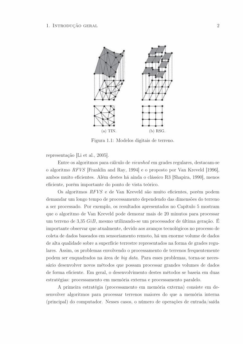
1.1 Modelos digitais de terreno. . . . . . . . . . . . . . . . . . . . . . . . . . 2
(a) TIN. . . . . . . . . . . . . . . . . . . . . . . . . . . . . . . . . . 2
(b) RSG. . . . . . . . . . . . . . . . . . . . . . . . . . . . . . . . . . 2
2.1 Cálculo da visibilidade em um corte vertical do terreno. O alvo T1 é
visível a partir de O e T2 não é visível. . . . . . . . . . . . . . . . . . . . 10
2.2 Algoritmo RFVS . a exemplos de segmentos em um terreno; (b) exemplo
de um corte vertical definido por um segmento. . . . . . . . . . . . . . . 12
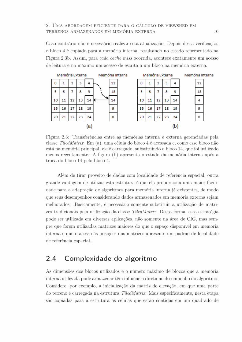
2.3 Transferências entre as memórias interna e externa gerenciadas pela
classe TiledMatrix. Em (a), uma célula do bloco 4 é acessada e, como
esse bloco não está na memória principal, ele é carregado, substituindo
o bloco 14, que foi utilizado menos recentemente. A figura (b) apresenta
o estado da memória interna após a troca do bloco 14 pelo bloco 4. . . . 16
2.4 Tempos de execução do EMViewshed (EMVS) e do TiledVS (TVS) uti-
lizando os 3 tamanhos de blocos com melhores desempenhos e alturas de
50 e 100 metros. . . . . . . . . . . . . . . . . . . . . . . . . . . . . . . . 20
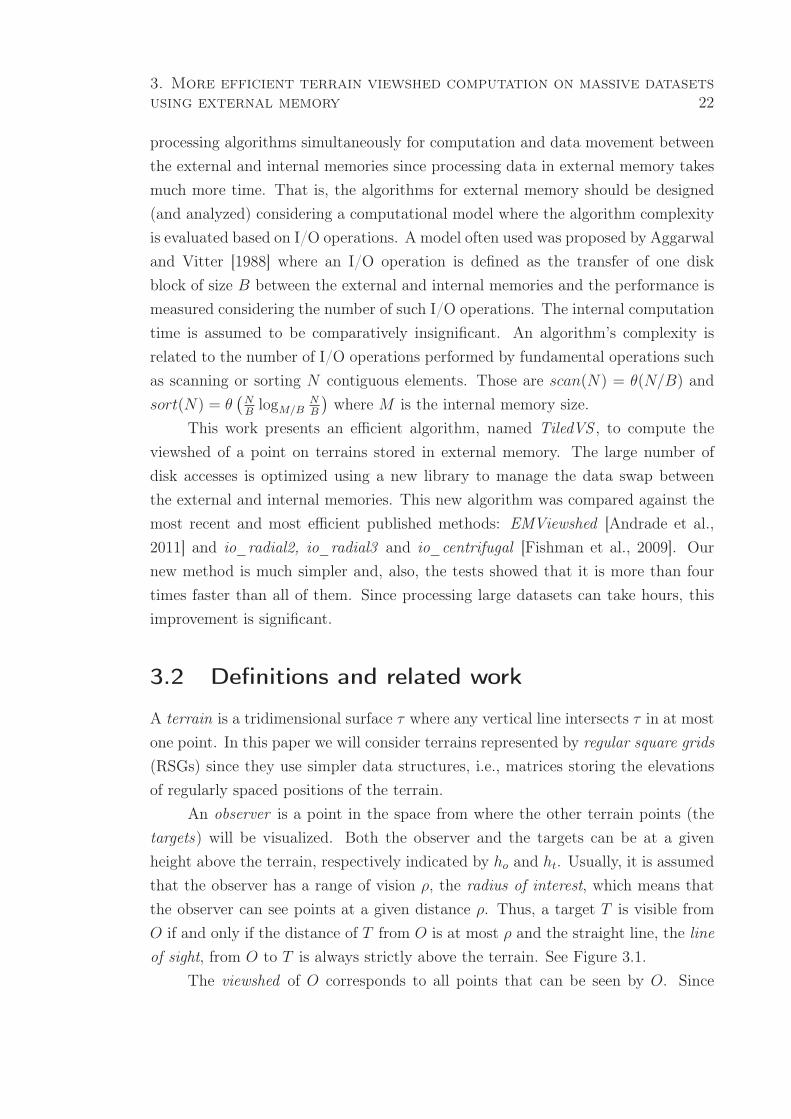
3.1 Target’s visibility: T1 and T3 are not visible but T2 is. . . . . . . . . . . . 23
3.2 Matrix partitioning. . . . . . . . . . . . . . . . . . . . . . . . . . . . . . 25
(a) square blocks with 3× 3 cells. . . . . . . . . . . . . . . . . . . . 25
(b) vertical bands with 3 columns. . . . . . . . . . . . . . . . . . . . 25
3.3 TiledVS algorithm. . . . . . . . . . . . . . . . . . . . . . . . . . . . . . 27
(a) Blocks intersected by two consecutive rays . . . . . . . . . . . . 27
(b) Block B′ is loaded because of ray r0, is evicted after ray rm and
loaded again for ray rn. . . . . . . . . . . . . . . . . . . . . . . 27
3.4 Comparing the running time of the four methods. . . . . . . . . . . . . . 29
4.1 Targets’ visibility: T1 and T3 are not visible but T2 is. . . . . . . . . . . . 33
4.2 The rasterization of the line of sight projection. . . . . . . . . . . . . . . 33
v
4.3 Viewshed algorithms. . . . . . . . . . . . . . . . . . . . . . . . . . . . . . 35
(a) RFVS algorithm. . . . . . . . . . . . . . . . . . . . . . . . . . . 35
(b) Van Kreveld’s algorithm. . . . . . . . . . . . . . . . . . . . . . . 35
4.4 Partitioning the elevation matrix into blocks and reorganizing the cells
in external memory to store the cells of each block in sequence. The
arrows indicate the writing sequence. . . . . . . . . . . . . . . . . . . . . 39
4.5 The terrain matrix partitioning. . . . . . . . . . . . . . . . . . . . . . . . 40
(a) Square blocks with 3× 3 cells. . . . . . . . . . . . . . . . . . . . 40
(b) Vertical bands with 3 columns. The radius of interest ρ = 10. . 40
4.6 Blocks intersected by two consecutive rays. . . . . . . . . . . . . . . . . . 41
4.7 Block B′ is loaded because of ray r0, is evicted after rm and loaded again
for rn. . . . . . . . . . . . . . . . . . . . . . . . . . . . . . . . . . . . . . 42
4.8 Comparing the running time of the four methods. . . . . . . . . . . . . 45
4.9 Number of cells processed per second by each method. . . . . . . . . . . 46
4.10 Running time of methods EMViewshed and TiledVS . . . . . . . . . . . . 47
5.1 Targets’ visibility: T1 and T3 are not visible but T2 is. . . . . . . . . . . . 53
5.2 The rasterization of the line of sight projection. . . . . . . . . . . . . . . 53
5.3 Viewshed algorithms. . . . . . . . . . . . . . . . . . . . . . . . . . . . . . 56
(a) RFVS . . . . . . . . . . . . . . . . . . . . . . . . . . . . . . . . 56
(b) Van Kreveld . . . . . . . . . . . . . . . . . . . . . . . . . . . . . 56
5.4 Sector definition. . . . . . . . . . . . . . . . . . . . . . . . . . . . . . . . 58
(a) Subdivision of the region of interest and the sector s, defined
by the interval [α, β). . . . . . . . . . . . . . . . . . . . . . . . . 58
(b) The cells in the perimeter of the region of interest, the rays
used to determine which cells are intersected by s and the cells
inserted into Es (shaded cells). . . . . . . . . . . . . . . . . . . 58
5.5 Experimental results. . . . . . . . . . . . . . . . . . . . . . . . . . . . . . 61
(a) Running times (in seconds) for the serial algorithm and the
parallel algorithm with different number of threads . . . . . . . 61
(b) Speedups achieved by our parallel algorithm, with different
number of threads. . . . . . . . . . . . . . . . . . . . . . . . . . 61
vi
Lista de Tabelas
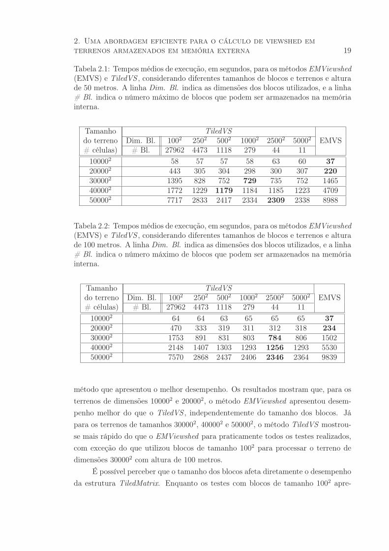
2.1 Tempos médios de execução, em segundos, para os métodos EMViewshed
(EMVS) e TiledVS , considerando diferentes tamanhos de blocos e terre-
nos e altura de 50 metros. A linha Dim. Bl. indica as dimensões dos
blocos utilizados, e a linha # Bl. indica o número máximo de blocos que
podem ser armazenados na memória interna. . . . . . . . . . . . . . . . . 19
2.2 Tempos médios de execução, em segundos, para os métodos EMViewshed
(EMVS) e TiledVS , considerando diferentes tamanhos de blocos e terre-
nos e altura de 100 metros. A linha Dim. Bl. indica as dimensões dos
blocos utilizados, e a linha # Bl. indica o número máximo de blocos que
podem ser armazenados na memória interna. . . . . . . . . . . . . . . . . 19
3.1 Running time (seconds) for io-radial2 (io-r2), io-radial3 (io-r3), io-
centrifugal (io-cent) and TiledVS with 512MiB RAM. . . . . . . . . . . 28
3.2 Running time (seconds) for EMViewshed (EMVS) and TiledVS with
1024MiB RAM. . . . . . . . . . . . . . . . . . . . . . . . . . . . . . . . . 28
3.3 TiledVS running time (seconds) using a RAM memory with 128MiB and
512MiB. . . . . . . . . . . . . . . . . . . . . . . . . . . . . . . . . . . . . 29
4.1 Running time (seconds) for io-radial2 (io-r2), io-radial3 (io-r3), io-
centrifugal (io-cent) and TiledVS with 512MiB RAM. . . . . . . . . . . 45
4.2 Running time (seconds) for EMViewshed (EMVS) and TiledVS with
1024MiB RAM. . . . . . . . . . . . . . . . . . . . . . . . . . . . . . . . 46
4.3 TiledVS running time (seconds) with either 128MiB or 512MiB RAM. . 47
4.4 Running time (seconds) of TiledVS using TiledMatrix with compression
enabled (w comp.) and disabled (w/o comp.). . . . . . . . . . . . . . . . 48
5.1 Running times (in seconds) for the serial algorithm and the parallel al-
gorithm with different number of threads. . . . . . . . . . . . . . . . . . 60
vii

5.2 Speedups achieved by our parallel algorithm, with different number of
threads. . . . . . . . . . . . . . . . . . . . . . . . . . . . . . . . . . . . . 60
viii
Resumo
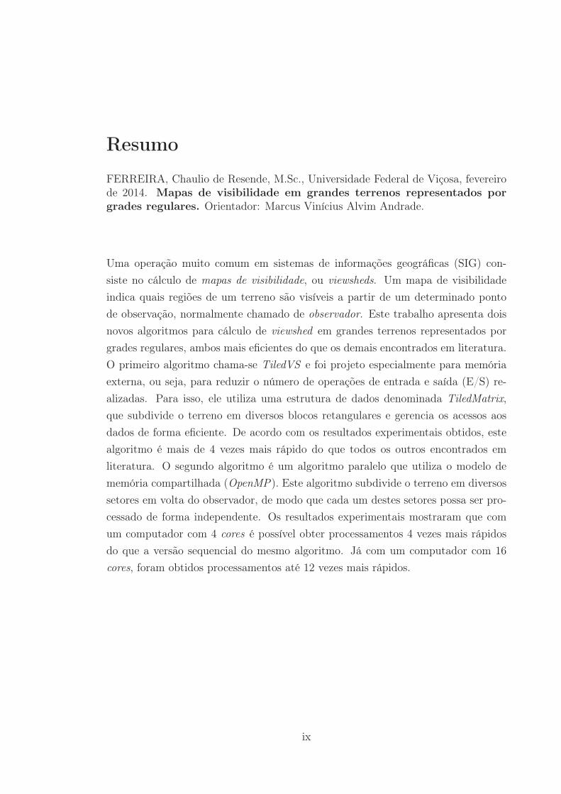
FERREIRA, Chaulio de Resende, M.Sc., Universidade Federal de Viçosa, fevereirode 2014. Mapas de visibilidade em grandes terrenos representados por
grades regulares. Orientador: Marcus Vinícius Alvim Andrade.
Uma operação muito comum em sistemas de informações geográficas (SIG) con-
siste no cálculo de mapas de visibilidade, ou viewsheds. Um mapa de visibilidade
indica quais regiões de um terreno são visíveis a partir de um determinado ponto
de observação, normalmente chamado de observador. Este trabalho apresenta dois
novos algoritmos para cálculo de viewshed em grandes terrenos representados por
grades regulares, ambos mais eficientes do que os demais encontrados em literatura.
O primeiro algoritmo chama-se TiledVS e foi projeto especialmente para memória
externa, ou seja, para reduzir o número de operações de entrada e saída (E/S) re-
alizadas. Para isso, ele utiliza uma estrutura de dados denominada TiledMatrix,
que subdivide o terreno em diversos blocos retangulares e gerencia os acessos aos
dados de forma eficiente. De acordo com os resultados experimentais obtidos, este
algoritmo é mais de 4 vezes mais rápido do que todos os outros encontrados em
literatura. O segundo algoritmo é um algoritmo paralelo que utiliza o modelo de
memória compartilhada (OpenMP). Este algoritmo subdivide o terreno em diversos
setores em volta do observador, de modo que cada um destes setores possa ser pro-
cessado de forma independente. Os resultados experimentais mostraram que com
um computador com 4 cores é possível obter processamentos 4 vezes mais rápidos
do que a versão sequencial do mesmo algoritmo. Já com um computador com 16
cores, foram obtidos processamentos até 12 vezes mais rápidos.
ix
Abstract
FERREIRA, Chaulio de Resende, M.Sc., Universidade Federal de Viçosa, February,2014. Visibility maps on large terrain represented as regular square grids.
Adviser: Marcus Vinícius Alvim Andrade.
In geographical information science (GIS) it is usual to compute the viewshed of
a given point on a terrain. This point is usually called observer, and its viewshed
indicates which terrain regions are visible from it. In this work we present two novel
algorithms for viewshed computation on large grid terrains, both more efficient
than other approaches found in related work. The first algorithm is called TiledVS .
It was specially designed for external memory processing, that is, it performs a
smaller number of in/out (I/O) operations. To do that, it uses a special library
called TiledMatrix, which subdivides the terrain into several rectangular blocks and
efficiently manages the accesses to the terrain cells. According to our experimental
results, TiledVS is more than 4 times faster than all other previous algorithms. The
second one is a parallel algorithm that uses the shared memory model (OpenMP).
It subdivides the terrain into several sectors around the observer, such that each
sector may be processed independently. Our experimental results showed that, using
a personal computer with 4 cores, it is possible to compute the viewshed 4 times
faster than with the serial implementation of the same algorithm. Using a computer
with 16 cores, we obtained up to 12 times speedups.
x
1. Introdução geral
Diversas aplicações em ciência da informação geoespacial (CIG) envolvem questões
de visibilidade. Exemplos são: determinar o número mínimo de torres de celular
necessárias para cobrir uma região [Ben-Moshe et al., 2002], otimizar o número e
a posição de guardas para vigiar uma região [Bespamyatnikh et al., 2001], analisar
as influências ambientais em preços de propriedades em um ambiente urbano [Lake
et al., 1998], entre outras. Essas aplicações geralmente requerem o cálculo de mapas
de visibilidade, ou viewsheds, de determinados pontos (chamados de observadores)
em um terreno. Mais especificamente, o viewshed de um observador O indica quais
regiões do terreno são visíveis a partir de O. Por exemplo, um observador pode
representar uma torre de telefonia celular, enquanto seu viewshed representa as
áreas do terreno onde espera-se que um usuário do serviço de telefonia consiga obter
sinal diretamente a partir dessa torre. Neste trabalho, será analisado o problema de
cálculo de mapas de visibilidade em grandes terrenos e serão propostos e avaliados
algoritmos mais eficientes do que os encontrados atualmente na literatura.
Estas aplicações utilizam informações sobre o terreno, principalmente relacio-
nadas à elevação de sua superfície, que geralmente são representadas por um modelo
digital de terreno (MDT) Segundo Câmara et al. [2001], a aquisição de dados geo-
gráficos para a geração de MDTs pode ser feita através da amostragem de pontos
espaçados de forma regular ou irregular. No caso de amostras irregularmente espaça-
das, normalmente utilizam-se estruturas de dados de malha triangular, denominadas
triangulated irregular networks (TINs). Já no caso de amostras regularmente espa-
çadas é possível utilizar estruturas de dados mais simples. Assim, normalmente são
utilizadas grades regulares (regular square grids - RSGs), que consistem em matrizes
que armazenam as elevações dos pontos amostrados. Estes dois formatos de MDT
são ilustrados na Figura 1.1.
Neste trabalho foi utilizada a representação baseada em grades regulares, uma
vez que esta é mais simples, mais fácil de ser analisada e atualmente existe uma
grande quantidade de dados disponíveis neste formato. Além disso, os algoritmos
propostos neste trabalho foram baseados em outros algoritmos que também traba-
lham com este formato. É importante ressaltar que a escolha de uma forma de
representação específica não resulta em uma restrição relevante na prática, uma
vez que existem métodos eficientes para a conversão entre as diversas formas de
1
1. Introdução geral 2
(a) TIN. (b) RSG.
Figura 1.1: Modelos digitais de terreno.
representação [Li et al., 2005].
Entre os algoritmos para cálculo de viewshed em grades regulares, destacam-se
o algoritmo RFVS [Franklin and Ray, 1994] e o proposto por Van Kreveld [1996],
ambos muito eficientes. Além destes há ainda o clássico R3 [Shapira, 1990], menos
eficiente, porém importante do ponto de vista teórico.
Os algoritmos RFVS e de Van Kreveld são muito eficientes, porém podem
demandar um longo tempo de processamento dependendo das dimensões do terreno
a ser processado. Por exemplo, os resultados apresentados no Capítulo 5 mostram
que o algoritmo de Van Kreveld pode demorar mais de 20 minutos para processar
um terreno de 3,35 GiB, mesmo utilizando-se um processador de última geração. É
importante observar que atualmente, devido aos avanços tecnológicos no processo de
coleta de dados baseados em sensoriamento remoto, há um enorme volume de dados
de alta qualidade sobre a superfície terrestre representados na forma de grades regu-
lares. Assim, os problemas envolvendo o processamento de terrenos frequentemente
podem ser enquadrados na área de big data. Para esses problemas, torna-se neces-
sário desenvolver novos métodos que possam processar grandes volumes de dados
de forma eficiente. Em geral, o desenvolvimento destes métodos se baseia em duas
estratégias: processamento em memória externa e processamento paralelo.
A primeira estratégia (processamento em memória externa) consiste em de-
senvolver algoritmos para processar terrenos maiores do que a memória interna
(principal) do computador. Nesses casos, o número de operações de entrada/saída
1. Introdução geral 3
(E/S) realizadas é tão grande que o tempo de processamento em CPU passa a ser
praticamente insignificante. Assim, é importante o projeto de algoritmos que re-
alizem menos acessos aos dados armazenados em memória externa (normalmente
discos), visto que o estes acessos são da ordem de 106 vezes mais lento do que os
acessos feitos à memória interna [Dementiev et al., 2005].
A segunda estratégia se baseia em desenvolver métodos paralelos para proces-
sar grandes volumes de dados. Esta estratégia tem atraído cada vez mais a atenção
de vários pesquisadores, principalmente porque atualmente é possível adquirir, a um
custo relativamente baixo, máquinas com grande capacidade computacional, isto é,
com grande quantidade de memória interna e também vários núcleos de processa-
mento paralelo.
Assim, neste trabalho serão apresentados dois algoritmos para cálculo de mapa
de visibilidade, ou viewshed : um primeiro algoritmo, chamado TiledVS , para pro-
cessamento em memória externa é descrito nos Capítulos 2, 3 e 4; e um segundo
algoritmo, descrito no Capítulo 5, baseado em processamento paralelo. Conforme
demonstrado pelos resultados experimentais apresentados, ambos são consideravel-
mente mais rápidos do que os algoritmos mais recentes e eficientes encontrados em
literatura.
1.1 Objetivos
O objetivo geral deste trabalho foi o desenvolvimento de algoritmos mais eficientes
para cálculo de viewshed considerando-se grandes volumes de dados. Para alcan-
çar este objetivo geral, destacam-se alguns objetivos específicos que precisaram ser
atingidos, como:
• Propor e implementar um algoritmo capaz de lidar com grandes terrenos ar-
mazenados em memória externa;
• Propor e implementar um algoritmo que utilize as modernas arquiteturas pa-
ralelas para realizar o processamento de forma mais eficiente;
• Realizar a análise de complexidade dos algoritmos desenvolvidos;
• Realizar revisão bibliográfica e avaliar experimentalmente os algoritmos de-
senvolvidos, comparando-os com outros métodos encontrados na literatura.
1. Introdução geral 4
1.2 Resultados obtidos
Nos Capítulos de 2 a 5 são apresentados os artigos que descrevem os resultados
obtidos neste trabalho. Mais especificamente, os Capítulos 2, 3 e 4 referem-se ao
algoritmo desenvolvido para cálculo de viewshed em memória externa, denominado
TiledVS , enquanto o Capítulo 5 apresenta o algoritmo desenvolvido para arquitetu-
ras paralelas.
1.2.1 Algoritmo desenvolvido para memória externa
Os Capítulos 2, 3 e 4 apresentam o algoritmo TiledVS , desenvolvido para processar
terrenos armazenados em memória externa de forma eficiente. Ele consiste em uma
adaptação do algoritmo RFVS , proposto por Franklin and Ray [1994]. Para minimi-
zar o número de operações de E/S realizadas durante o processamento, foi utilizada
uma biblioteca denominada TiledMatrix [Silveira et al., 2013], capaz de armazenar e
gerenciar grandes matrizes em memória externa de forma eficiente. Na prática, essa
biblioteca gerencia os acessos aos dados em memória externa reorganizando-os de
modo a realizar de forma eficiente os acessos aos dados que apresentem padrões de
localidade espacial bidimensional. Os dados da matriz são subdivididos em blocos
retangulares e as células de um mesmo bloco são armazenadas de forma contígua.
Quando é necessário acessar uma dessas células, o bloco inteiro que a contém é copi-
ado para a memória interna e nela continua armazenado por algum tempo. Assim,
a memória interna é gerenciada como uma memória cache controlada pela aplica-
ção que, diferentemente do sistema de paginação tradicional do sistema operacional,
considera a localização bidimensional dos dados na matriz.
Uma primeira versão do método TiledVS é apresentada no Capítulo 2, onde
é incluído o artigo “Uma abordagem eficiente para o cálculo de viewshed em ter-
renos armazenados em memória externa”, apresentado no SEMISH 2012 (XXXIX
Seminário Integrado de Software e Hardware) [Ferreira et al., 2012a]. Nesse artigo
o novo algoritmo foi comparado experimentalmente com outro método para cálculo
de viewshed em memória externa, também baseado no algoritmo RFVS : o método
EMViewshed [Andrade et al., 2011]. Os resultados mostraram que o novo algoritmo
conseguiu ser mais de 4 vezes mais rápido do que o EMViewshed. Além disso, nesse
artigo foram realizados experimentos iniciais para tentar avaliar a influência dos
tamanhos dos blocos utilizados na subdivisão da matriz feita pela TiledMatrix.
No Capítulo 3 é apresentado o artigo “More efficient terrain viewshed compu-
tation on massive datasets using external memory”, apresentado no ACM SIGSPA-
1. Introdução geral 5
TIAL 2012 (20th International Conference on Advances in Geographic Information
Systems) [Ferreira et al., 2012b]. Nesse artigo o novo método TiledVS foi compa-
rado também com outros algoritmos para cálculo de viewshed em memória externa
propostos por Fishman et al. [2009] e, mais uma vez, mostrou-se mais eficiente do
que todos eles. Nesse artigo também é apresentada uma análise formal do padrão
de acesso utilizado pelo algoritmo e são estabelecidas algumas condições com rela-
ção ao tamanho dos blocos utilizados e da memória interna disponível de modo a
garantir que o processamento seja sempre realizado de forma eficiente. Com essas
condições, o algoritmo foi alterado para, com base nos parâmetros de entrada, esta-
belecer automaticamente o tamanho dos blocos utilizados durante o processamento,
algo que anteriormente precisava ser escolhido explicitamente pelo usuário. Para
finalizar, também foram incluídos experimentos para avaliar o comportamento do
algoritmo em condições extremas como, por exemplo, o processamento de terrenos
até 320 vezes maiores do que a memória interna disponível.
O Capítulo 4 apresenta o artigo “A fast external memory algorithm for compu-
ting visibility on grid terrains”, submetido à revista ACM TSAS (ACM Transactions
on Spatial Algorithms and Systems) [Ferreira et al., 2014]. Este artigo corresponde
a uma versão estendida do artigo do Capítulo 3, onde foi utilizada uma estratégia
de compressão de dados aliada à biblioteca TiledMatrix que conseguiu reduzir os
tempos de processamento em até 42%. Mais especificamente, a biblioteca TiledMa-
trix passou a utilizar o algoritmo de compressão extremamente rápido LZ4 [Collet,
2012] para comprimir os dados de cada bloco antes de gravá-lo no disco, e também
para descomprimi-los ao acessá-los novamente. Além disso foram feitas as análises de
complexidade de E/S e de CPU do novo algoritmo, assim como alguns experimentos
analisando a influência da compressão de dados sobre os tempos de processamento.
1.2.2 Algoritmo desenvolvido para arquiteturas paralelas
O Capítulo 5 apresenta o artigo “A Parallel Sweep Line Algorithm for Visibility
Computation”, que recebeu o prêmio de melhor artigo no GeoInfo 2013 (XIV Bra-
zilian Symposium on Geoinformatics) [Ferreira et al., 2013].
Esse artigo descreve o algoritmo desenvolvido para cálculo de viewshed em ar-
quiteturas paralelas, que foi baseado no algoritmo sequencial proposto por Van Kre-
veld [1996]. Para calcular o viewshed utilizando vários processadores paralelos, o
algoritmo subdivide o terreno em diversos setores em volta do observador, de forma
que cada um desses setores possa ser processado independentemente dos demais se-
tores. Os resultados mostraram que, com 16 processadores paralelos, este algoritmo

1. Introdução geral 6
foi até 12 vezes mais rápido do que sua versão sequencial. Como trabalho futuro,
pretende-se melhorar o algoritmo e estender o artigo, visando sua submissão para
uma revista da área.
2. Uma abordagem eficiente para o cálculo
de viewshed em terrenos armazenados
em memória externa1
Abstract
An important GIS application is computing the viewshed of a point on
a DEM terrain, i.e. determining the visible region from this point. In some
cases, it is not possible to process high resolution DEMs entirely in internal
memory and, thus, it is important to develop algorithms to process such data
in the external memory. This paper presents an efficient algorithm for handling
huge terrains in external memory. As tests have shown, this new method is
more efficient than other methods described in the literature.
Resumo
Uma importante aplicação em ciência da informação geoespacial (CIG)
é o cálculo da região visível (viewshed) a partir de um determinado ponto em
um terreno representado por um modelo digital de terreno (MDT). Muitas
vezes, o processamento de MDTs de alta resolução não pode ser realizado em
memória interna e, portanto, é importante o desenvolvimento de algoritmos
para processar estes dados em memória secundária. Este trabalho apresenta
um algoritmo para cálculo de viewshed que é capaz de lidar com grande volume
de dados em memória externa de forma eficiente. Os testes realizados indicam
que o método proposto é mais eficiente do que outros métodos descritos em
literatura.
2.1 Introdução
Os recentes avanços tecnológicos em sensoriamento remoto têm produzido uma
grande quantidade de dados de alta resolução sobre a superfície terrestre, o que
1Neste capítulo é apresentada uma primeira versão do método TiledVS . Nele está incluído oartigo “Uma abordagem eficiente para o cálculo de viewshed em terrenos armazenados em memória
externa”, apresentado no SEMISH 2012 (XXXIX Seminário Integrado de Software e Hardware)[Ferreira et al., 2012a].
7
2. Uma abordagem eficiente para o cálculo de viewshed em
terrenos armazenados em memória externa 8
tem aumentado a necessidade de se desenvolver novas técnicas em ciência da infor-
mação geoespacial (CIG) para lidar com este enorme volume de dados [Laurini and
Thompson, 1992].
Uma forma muito utilizada para se representar a superfície da Terra de forma
aproximada é através de um Modelo Digital de Terreno (MDT) que armazena as
elevações de pontos amostrados sobre a superfície terrestre. Esses pontos podem
ser amostrados de maneira irregular e ser armazenados como uma rede triangular
irregular (TIN - triangulated irregular network) ou de maneira regular (RSG - regular
square grid), sendo armazenados numa matriz [Felgueiras, 2001]. Neste trabalho
será adotada a segunda forma de representação do MDT. Muitas vezes estas matrizes
necessitam de mais espaço de armazenamento do que tem-se disponível na memória
interna da maioria dos computadores atuais. Por exemplo, um terreno de 100km ×
100km mapeado com resolução de 1m resulta em 1010 pontos. Supondo que sejam
utilizados 2 bytes para armazenar a elevação de cada ponto, são necessários mais de
18 GB para representar este terreno.
Desta forma, é importante o desenvolvimento de algoritmos específicos para
processamento de dados armazenados em memória externa. Vale ressaltar que nor-
malmente os algoritmos tradicionais de análise e processamento de dados geográficos
buscam otimizar o tempo de processamento em CPU, sem grandes preocupações com
o tempo de acesso à memória. Mas, por outro lado, o projeto e análise de algoritmos
para memória externa devem focar-se em minimizar os acessos a disco, uma vez que
estes são da ordem de 106 vezes mais lentos do que os acessos à memória interna
[Dementiev et al., 2005].
Mais especificamente, algoritmos que processam dados em memória externa
devem ser projetados e analisados considerando um modelo computacional que os
avalie considerando as operações de transferência de dados em vez das operações
de processamento interno. Um desses modelos, proposto por Aggarwal and Vitter
[1988], determina a complexidade dos algoritmos com base no número de operações
de E/S (entrada/saída) executadas. Este modelo será descrito com maiores detalhes
na Seção 2.2.3.
Dentre as várias aplicações na área de CIG, há aquelas relacionadas a questões
de visibilidade, como determinar o número mínimo de torres de celular necessárias
para cobrir uma região [Ben-Moshe et al., 2002], otimizar o número e a posição de
guardas para vigiar uma região [Bespamyatnikh et al., 2001], etc. Tais aplicações
utilizam o conceito de observador e alvo: o observador tem o objetivo de visualizar
(observar) outros objetos (os alvos) em um terreno, sendo que os observadores pos-
suem um limite máximo para o alcance de sua visão, chamado de raio de interesse.
2. Uma abordagem eficiente para o cálculo de viewshed em
terrenos armazenados em memória externa 9
Por exemplo, uma torre de telefonia celular pode ser considerada um observador
cujo raio de interesse corresponde ao alcance do sinal da torre e cujos alvos são os
usuários do serviço de telefonia. A partir desse conceito, pode-se calcular o mapa
de visibilidade (viewshed) de um ponto p do terreno, que indica a região do ter-
reno que é visível por um observador posicionado em p. Há diversos métodos para
cálculo de viewshed em memória interna, como os propostos por Franklin and Ray
[1994] e Van Kreveld [1996]. Além disso, há também alguns métodos eficientes para
processar terrenos armazenados em memória externa, como o método proposto por
Haverkort and Zhuang [2007], que utiliza uma adaptação do método de Kreveld para
memória externa e o método EMViewshed recentemente proposto por Andrade et al.
[2011], descrito na seção 2.2.2, que é cerca de 6 vezes mais rápido do que o método
proposto por Haverkort.
Este trabalho apresenta um novo método denominado TiledVS , que é cerca
de 4 vezes mais eficiente do que o método EMViewshed. A idéia básica deste novo
método consiste em adaptar o algoritmo proposto por Franklin and Ray [1994]
alterando a forma como os dados em memória externa são acessados. Para isto,
foi utilizada uma estrutura de dados que gerencia as transferências de dados entre
as memórias interna e externa, buscando diminuir o número de acessos a disco.
Maiores detalhes sobre esta estrutura encontram-se na seção 2.3 e os resultados dos
testes da comparação deste novo método com o EMViewshed são apresentados na
seção 2.5.
2.2 Referencial teórico
2.2.1 Visibilidade em terrenos
Um terreno corresponde a uma região da superfície da Terra cujo relevo é repre-
sentado por uma Modelo Digital de Terreno (MDT) que pode ser representado por
uma malha triangular irregular (triangulated irregular network, ou TIN ), por linhas
de contorno ou por uma matriz que contém elevações de pontos posicionados em in-
tervalos regularmente espaçados. Devido à sua simplicidade e ao grande volume de
dados disponíveis na forma matricial, esta é a representação utilizada nos algoritmos
deste trabalho. É importante observar que há métodos eficientes para a conversão
entre as diferentes formas de representação, e portanto, esta escolha não representa
uma restrição relevante [Felgueiras, 2001].
Um observador é um ponto no espaço a partir do qual se deseja visualizar ou
comunicar com outros pontos no espaço, chamados de alvos. As notações usuais
2. Uma abordagem eficiente para o cálculo de viewshed em
terrenos armazenados em memória externa 10
para um observador e um alvo são, respectivamente, O e T e estes pontos podem
estar a certas alturas acima do terreno denotadas respectivamente por hO e hT . Os
pontos do terreno verticalmente abaixo de de O e T são denominados pontos-base
e são denotados por Ob e Tb, respectivamente.
O raio de interesse, ρ, de um observador O representa o alcance de sua visão,
ou seja, o valor máximo da distância em que ele é capaz de enxergar ou se comunicar.
Por conveniência, a distância entre um observador O e um alvo T é definida como
a distância entre Ob e Tb.
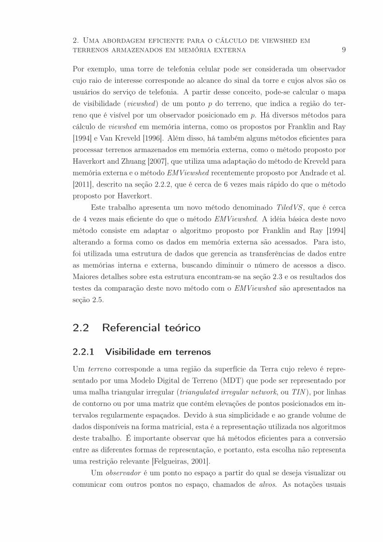
Um alvo T é visível a partir um observador O se, e somente se, |Tb−Ob| ≤ ρ e
não há nenhum ponto da superfície do terreno interceptando o segmento de reta OT ,
que é chamado de linha de visão, ou line of sight (LOS ). Um exemplo de cálculo de
visibilidade é mostrado na Figura 2.1: o alvo T1 é visível a partir de O, mas T2 não
é visível, pois OT2 é bloqueado por uma região do terreno.
Figura 2.1: Cálculo da visibilidade em um corte vertical do terreno. O alvo T1 évisível a partir de O e T2 não é visível.
É importante ressaltar que a verificação de que a linha de visão intercepta
ou não o terreno não é trivial. O problema é que a matriz de elevação contém
informações somente sobre alguns pontos discretos do terreno, enquanto as linhas
de visão são contínuas e geralmente passam entre pontos adjacentes, sem interceptá-
los, o que muitas vezes requer um método de interpolação entre os pontos conhecidos
[Magalhães et al., 2011].
O viewshed (ou mapa de visibilidade) de um observador O é o conjunto de
pontos do terreno cujos alvos correspondentes são visíveis a partir de O.
2.2.2 Algoritmos para cálculo de viewshed em memória
interna
Dados um terreno representado por uma matriz de elevação de dimensões n× n, as
coordenadas (x, y) do observador O, o seu raio de interesse ρ e as alturas hO e hT ,
2. Uma abordagem eficiente para o cálculo de viewshed em
terrenos armazenados em memória externa 11
o objetivo de um algoritmo de cálculo do viewshed de O é determinar, para cada
célula da matriz, se seu alvo correspondente é visível por O. Uma das maneiras
de representar o viewshed calculado é utilizando uma matriz de bits com dimensões
n×n onde um bit com valor 1 indica que o alvo T associado àquela célula do terreno
é visível por O, enquanto um bit com valor 0 indica que T não é visível.
O algoritmo proposto neste trabalho para o cálculo do viewshed em grandes
terrenos armazenados em memória externa é baseado no algoritmo para memória
interna proposto por Franklin and Ray [1994], que será descrito de forma resumida
a seguir.
Este algoritmo assume que todas as células são inicialmente não visíveis e
realiza um processamento iterativo para determinar quais células são visíveis a partir
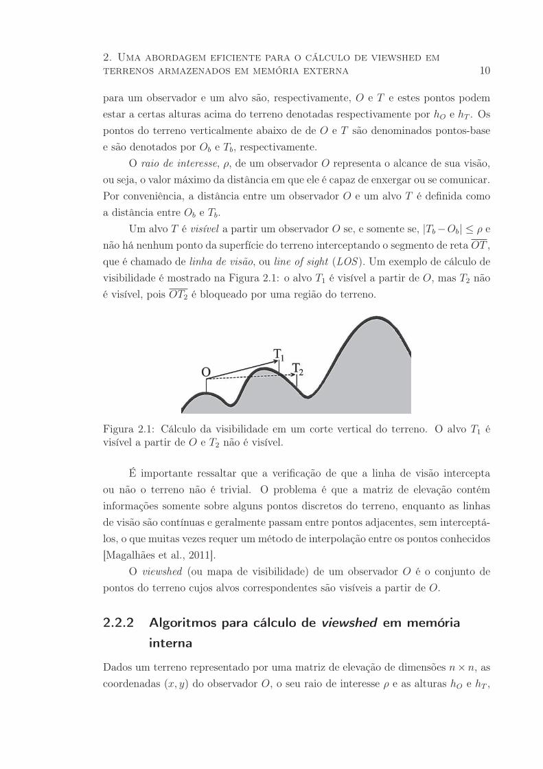
de O. Primeiramente é definida uma região quadrangular S que envolva o círculo
de raio ρ centrado em O (por exemplo, veja a figura 2.2a onde é mostrada esta
região para ρ = 4). Daí, são traçados 8ρ segmentos de reta ligando O a cada uma
das células na borda de S. Cada um destes segmentos define um corte vertical no
terreno - a figura 2.2 exibe um exemplo desses segmentos e de um desses cortes.
O passo seguinte consiste em determinar quais células fazem parte de cada
corte vertical. Para alguns casos, como os dos segmentos OA e OE mostrados na
figura 2.2a, é fácil determinar estas células. No entanto, para a maioria dos segmen-
tos essa determinação não é tão simples, como é o caso dos segmentos OB, OC e
OD, onde é necessário determinar quais células são mais relevantes para cada seg-
mento. Esse problema equivale à rasterização de segmentos e pode ser solucionado
utilizando o algoritmo de Bresenham [1965], de modo que seja selecionada apenas
uma célula para cada coordenada X ou Y (dependendo da inclinação do segmento).
Após a determinação das células de cada corte vertical, o próximo passo é
percorrer estas células verificando quais são visíveis a partir de O. Seja um segmento
composto pelas células c0, c1, · · · , ck, sendo que o observador está posicionado na
célula c0 e ck é a última célula na região S dentro do raio de visão do observador.
Então o processo consiste em inicialmente definir as células c0 e c1 como visíveis e
inicializar µ, que armazena a maior inclinação de uma linha de visão já processada,
com a inclinação da reta que passa pelos pontos c0 e c1. A partir daí, cada célula ci
é processada em ordem crescente de i, analisando-se a inclinação da reta que liga o
observador ao alvo que está posicionado acima de ci; se esta inclinação é maior ou
igual a µ então a célula ci é marcada como visível e µ é atualizado com o valor da
inclinação da reta que passa por O e ci.
Aplicando este algoritmo ao exemplo dado na figura 2.2b temos que os alvos
posicionados acima dos pontos 0, 1, 2, 3 e 7 são visíveis a partir do observador posi-
2. Uma abordagem eficiente para o cálculo de viewshed em
terrenos armazenados em memória externa 12
Figura 2.2: Algoritmo RFVS . a exemplos de segmentos em um terreno; (b) exemplode um corte vertical definido por um segmento.
cionado acima do ponto 0 (representado por um triângulo) e os alvos posicionados
acima dos pontos 4, 5 e 6 não são visíveis.
2.2.3 Algoritmos eficientes para E/S
Durante o processamento de grande volume de dados, a transferência de dados entre
a memória interna (mais rápida) e o armazenamento externo (mais lento) frequen-
temente torna-se o gargalo do processamento. Portanto, o projeto e análise de
algoritmos usados para processar esses dados precisam ser feitos sob um modelo
computacional que avalia as operações de entrada e saída (E/S). Um modelo fre-
quentemente utilizado foi proposto por Aggarwal and Vitter [1988]. Nesse modelo,
cada operação de E/S corresponde à transferência de um bloco de tamanho B entre
a memória externa e a memória interna. O desempenho do algoritmo é determinado
considerando-se o número de operações de E/S executadas.
A complexidade de um algoritmo é definida com base na complexidade de
problemas fundamentais como varredura (scan) e ordenação (sort) de N elementos
contíguos armazenados em memória externa. Se M é o tamanho da memória interna
disponível, estas complexidades são definidas como:
scan (N) = Θ
(
N
B
)
e sort (N) = Θ
(
N
Blog(M
B)
(
N
B
))
É importante salientar que normalmente scan(N) < sort(N) << N e, então,
um algoritmo que realiza O(sort(N)) operações de E/S é significantemente mais
2. Uma abordagem eficiente para o cálculo de viewshed em
terrenos armazenados em memória externa 13
eficiente do que um que realiza O(N) operações. Assim, muitos algoritmos tentam
reorganizar os dados na memória externa com o objetivo de diminuir o número de
operações de E/S feitas.
2.2.4 O método EMViewshed
A estratégia proposta por Andrade et al. [2011] consiste em gerar e armazenar
em memória externa uma lista com informações de todas as células do terreno
e ordená-la de acordo com a ordem em que estas células serão processadas pelo
algoritmo. Assim, o algoritmo pode percorrer esta lista sequencialmente, evitando
acessos aleatórios à memória externa.
Mais especificamente, o algoritmo cria uma lista Q de pares (c, i), onde c é
uma célula e i é um índice que indica “quando” c deveria ser processada. Isto é,
se uma célula c está associada a um índice k, então c seria a k-ésima célula a ser
processada.
Para determinar os índices é utilizado um processo similar ao descrito na seção
2.2.2, onde são traçadas diversas linhas de visão em sentido anti-horário, e as células
recebem índices numerados de forma crescente em cada linha de visão. Uma mesma
célula pode receber vários índices (e possuir várias cópias em Q) já que ela pode ser
interceptada por múltiplas linhas de visão.
Depois de criada, a lista Q é ordenada usando os índices como chave de com-
paração, e então as células são processadas na ordem da lista ordenada por um
algoritmo similar ao de memória interna que, neste caso, lê os dados de elevação
diretamente de Q. Além disso, este algoritmo utiliza uma outra lista Q′ onde as cé-
lulas visíveis são inseridas. Após o processamento de todas as células, Q′ é ordenada
lexicograficamente pelas coordenadas x e y e as células visíveis são armazenadas em
um arquivo de saída, onde as posições visíveis são indicadas por 1 e as não visíveis
por 0.
Um ganho de eficiência no processo é alcançado mantendo parte das matrizes
em memória interna. As células que estão em memória interna não são inseridas
em Q e Q′ e, quando uma célula precisa ser processada, o algoritmo verifica se esta
célula está na memória interna. Se estiver, ela é processada normalmente; caso
contrário, ela é lida de Q.
Para analisar a complexidade deste algoritmo, é necessário utilizar um modelo
como o descrito na Seção 2.2.3. Seja T o terreno representado por uma matriz de
elevação de dimensões n×n, ou seja, que contenha n2 células. No primeiro passo do
algoritmo, para ler as células do terreno e criar a lista Q, são realizadas O(scan(ρ2))
2. Uma abordagem eficiente para o cálculo de viewshed em
terrenos armazenados em memória externa 14
operações de E/S. Neste passo, como mostrado na seção 2.2.2, o algoritmo traça
8ρ linhas de visão, cada uma contendo ρ células. Assim, a lista Q contém O(ρ2)
elementos.
Em seguida esta lista é ordenada e então percorrida sequencialmente para
se calcular a visibilidade das células, operações que apresentam complexidades
O(sort(ρ2)) e O(scan(ρ2)), respectivamente.
Finalmente, a lista de pontos visíveis que contém, no máximo, O(ρ2) células
é ordenada e o viewshed do terreno é gravado em disco, operações que apresentam
complexidades O(sort(ρ2)) e O(scan(n2)), respectivamente. Como no pior caso
ρ = O(n), temos que a complexidade do algoritmo é:
O (sort (ρ2)) = O (sort (n2)) = O
(
n2
Blog(M
B)
(
n2
B
))
2.3 O método TiledVS
Ao analisar o algoritmo descrito na seção 2.3, pode-se perceber que o acesso às
posições das matrizes apresenta um padrão radial, ou seja, as células são acessadas
a partir daquela que contém o observador até cada célula que está no limite de seu
raio de interesse, traçando diversas linhas de forma circular. Este padrão de acessos
apresenta a propriedade de localidade de referência espacial: as células acessadas em
um curto espaço de tempo estão, na maioria das vezes, próximas umas das outras
na matriz. O problema é que, em geral, uma matriz bidimensional é armazenada
de forma linear na memória e, por isso, muitas vezes células que são vizinhas na
matriz ficam armazenadas em posições distantes umas das outras na memória. Como
normalmente a localidade de referência espacial utilizada pela hierarquia de memória
do computador é baseada no acesso sequencial [Patterson and Hennessy, 2008], esta
forma de representação não tira proveito da localidade de referência espacial em
termos bidimensionais, tornando o acesso ineficiente.
Para aproveitar a propriedade de localidade espacial e tentar diminuir o nú-
mero de acessos a disco, este trabalho propõe um método denominado TiledVS , cuja
estratégia consiste em adaptar o método RFVS , descrito na seção 2.2.2, de forma
que todos acessos realizados às matrizes sejam gerenciados por uma estrutura de
dados denominada TiledMatrix [Silveira et al., 2013], que é capaz de armazenar e
gerenciar grandes matrizes em memória externa. Mais especificamente, um objeto
do tipo TiledMatrix representa uma matriz que é dividida em blocos menores de
dimensões fixas que são armazenados de forma sequencial em um arquivo na memó-
2. Uma abordagem eficiente para o cálculo de viewshed em
terrenos armazenados em memória externa 15
ria externa. Então, esta estrutura de dados gerencia a transferência de blocos entre
as memórias interna e externa sempre que necessário. Em outras palavras, alguns
blocos do terreno ficam armazenados em memória interna enquanto estiverem sendo
processados, e podem voltar à memória externa quando não forem mais necessários,
dando lugar a outros blocos. Desta forma, a estrutura de dados funciona como uma
memória cache gerenciada pela aplicação, que busca predizer quais serão os próxi-
mos blocos do terreno a terem posições acessadas no processamento, mantendo-os
na memória interna.
Uma questão importante a se considerar na implementação desta estrutura
refere-se à política utilizada para determinar qual bloco será escolhido para ceder
espaço a novos blocos. Neste trabalho utilizou-se a estratégia de retirar da memória
interna aquele que está há mais tempo sem ser acessado pela aplicação. Em outras
palavras, sempre que uma célula de um bloco é acessada, este bloco é marcado com
um timestamp. Quando for necessário retirar um bloco da memória interna para
carregar outro, será escolhido aquele que tiver o menor timestamp. Esta estratégia
foi adotada baseado no fato de que há uma certa localidade no processamento das
células pelo algoritmo. Isto é, se há um bloco que está há algum tempo sem ser
acessado (nenhuma de suas células é processada) então há uma grande chance de que
todas as células daquele bloco já tenham sido processadas e o bloco não precisará
mais ser acessado.
Para ilustrar este processo, considere uma matriz que foi dividida em 5 × 5
blocos e uma memória interna capaz de armazenar no máximo 5 desses blocos.
Suponha que em determinado momento do processamento os blocos de números 8,
9, 12, 13 e 14 estejam na memória interna, como mostrado na Figura 2.3a. Se for
requisitado acesso a alguma célula que está contida em algum destes blocos, não
será necessário buscá-la na memória externa, e o acesso será feito de forma mais
eficiente. Por outro lado, se for requisitado acesso a alguma célula de outro bloco,
diz-se que ocorreu uma cache miss, e esta célula deverá ser buscada na memória
externa. Porém, por acreditar que logo em seguida serão requisitados acessos a
outras células deste mesmo bloco, a estrutura de dados transfere e carrega para a
memória interna o bloco inteiro que contêm a célula requisitada, substituindo um
dos blocos que já estavam carregados. Considere, por exemplo, uma requisição de
acesso a alguma célula do bloco 4, e que o bloco 14 é o que está há mais tempo
sem ser acessado dentre aqueles carregados em memória interna e, portanto, é o
que deverá ser substituído. Antes de realizar a substituição, é necessário verificar
se alguma instrução de escrita foi executada no bloco 14 enquanto ele esteve em
memória interna. Se sim, seus dados devem ser atualizados na memória externa.
2. Uma abordagem eficiente para o cálculo de viewshed em
terrenos armazenados em memória externa 16
Caso contrário não é necessário realizar esta atualização. Depois dessa verificação,
o bloco 4 é copiado para a memória interna, resultando no estado representado na
Figura 2.3b. Assim, para cada cache miss ocorrida, acontece exatamente um acesso
de leitura e no máximo um acesso de escrita a um bloco na memória externa.
Figura 2.3: Transferências entre as memórias interna e externa gerenciadas pelaclasse TiledMatrix. Em (a), uma célula do bloco 4 é acessada e, como esse bloco nãoestá na memória principal, ele é carregado, substituindo o bloco 14, que foi utilizadomenos recentemente. A figura (b) apresenta o estado da memória interna após atroca do bloco 14 pelo bloco 4.
Além de tirar proveito de dados com localidade de referência espacial, outra
grande vantagem de utilizar esta estrutura é que ela proporciona uma maior facili-
dade para a adaptação de algoritmos para memória interna já existentes, de modo
que seus desempenhos considerando dados armazenados em memória externa sejam
melhorados. Basicamente, é necessário somente substituir a utilização de matri-
zes tradicionais pela utilização da classe TiledMatrix. Desta forma, esta estratégia
pode ser utilizada em diversas aplicações, não somente na área de CIG, mas sem-
pre que forem utilizadas matrizes maiores do que o espaço disponível em memória
interna e que o acesso às posições das matrizes apresente um padrão de localidade
de referência espacial.
2.4 Complexidade do algoritmo
As dimensões dos blocos utilizados e o número máximo de blocos que a memória
interna utilizada pode armazenar têm influência direta no desempenho do algoritmo.
Considere, por exemplo, a inicialização da matriz de elevação, em que uma parte
do terreno é carregada na estrutura TiledMatrix. Mais especificamente, nesta etapa
são copiadas para a estrutura as células que estão contidas em um quadrado de
2. Uma abordagem eficiente para o cálculo de viewshed em
terrenos armazenados em memória externa 17
dimensões (2ρ + 1) × (2ρ + 1) com centro no observador O, onde ρ é o raio de
interesse de O.
Por questões de eficiência, é importante que a memória interna disponível seja
suficiente para armazenar no mínimo 2ρ+1t
blocos, onde t é a dimensão de cada
lado dos blocos. Esta condição é necessária para que a inicialização da estrutura
TiledMatrix possa ocorrer sem que seja necessário carregar um mesmo bloco mais de
uma vez, ou seja, para que não ocorram cache misses. Para ilustrar a necessidade
dessa condição, suponha que uma matriz de elevação de dimensões 50 × 50 seja
armazenada em uma TiledMatrix M que a divide em blocos de dimensões 10× 10 e
que a memória interna comporte apenas 4 desses blocos. Note que, devido ao padrão
que remove o bloco menos recentemente utilizado, quando os 10 últimos elementos da
primeira linha da matriz forem copiados para M o bloco que contém os 10 primeiros
elementos dessa linha deverá ser removido da memória interna. Porém, ao copiar os
10 primeiros elementos da próxima linha da matriz para M , esse bloco deverá voltar
novamente para a memória interna. Esse padrão de acesso ocorrerá diversas vezes
em todas as linhas de M e, assim, esse processo seria ineficiente. Portanto, para
realizar a análise de complexidade do algoritmo, será suposto que o tamanho da
memória interna atenda a esta restrição e, assim, cada bloco será carregado apenas
uma vez durante a inicialização dessa estrutura de dados.
Como o algoritmo precisa carregar da matriz de elevação (2ρ + 1) × (2ρ + 1)
células, a inicialização do algoritmo realiza O(scan(ρ2)) operações de E/S.
Durante a etapa do algoritmo onde são traçadas diversas linhas de visão em
sentido anti-horário para calcular o viewshed de O, também será necessário carregar
cada bloco do terreno uma vez, com exceção dos blocos que contém simultaneamente
células das primeiras e últimas linhas de visão a serem processadas, que precisarão
ser carregados duas vezes. Como o número de células processadas é O(ρ2) e cada
célula é transferida da memória externa no máximo duas vezes, esta etapa também
é realizada em O(scan(ρ2)) operações de E/S.
Depois de calculado, o viewshed é armazenado em um arquivo de saída com um
bit para cada célula do terreno. Se o terreno tiver dimensões n× n, serão efetuadas
O(scan(n2)) operações de E/S. Portanto, a complexidade do algoritmo TiledVS é:
O (scan (n2)) = O
(
n2
B
)
2. Uma abordagem eficiente para o cálculo de viewshed em
terrenos armazenados em memória externa 18
2.5 Resultados
Ométodo TiledVS foi implementado em C++ e compilado com o g++ 4.5.2. Optou-
se por realizar os testes em um computador com pouca memória RAM para que
fosse necessário realizar operações de processamento em memória externa mesmo
para terrenos não tão grandes (como os com 100002 e 200002 células). Por isso,
os testes foram executados em um PC Pentium 4 com 3.6GHz, 1GB de RAM,
HD Sata de 160GB e 7200RPM. O sistema operacional utilizado foi o o Linux,
distribuição Ubuntu 11.04 de 64bits. Dos 1024MB disponíveis em memória interna,
foram utilizados 800MB para armazenar os dados, e os demais foram reservados
para uso do sistema.
Os terrenos utilizados nos testes foram obtidos na página do The Shuttle Radar
Topography Mission (SRTM) [Rabus et al., 2003]. Os dados correspondem a duas
regiões distintas dos EUA amostradas em diferentes resoluções, gerando assim ter-
renos de diferentes tamanhos (100002, 200002, 300002, 400002 e 500002). Para cada
tamanho de terreno, foi calculada a média do tempo necessário para processamento
das duas regiões.
Em todos os testes foi considerado o pior caso, ou seja, o valor para o raio de
interesse utilizado foi grande o suficiente para cobrir todo o terreno. Para avaliar
a influência do número de pontos visíveis no tempo de execução, o observador foi
posicionado em diferentes alturas acima do terreno (50 e 100 metros). Além disso,
em todos os testes foi considerado que hO = hT , ou seja, os possíveis alvos estão
posicionados à mesma altura que o observador. Os tempos de execução do método
TiledVS foram comparados com os tempos do método EMViewshed, uma vez que
este mostrou-se mais eficiente que os demais métodos encontrados em literatura
[Andrade et al., 2011].
As Tabelas 2.1 e 2.2 mostram os tempos médios de execução, em segundos,
necessários para processar cada um dos terrenos, utilizando o método EMViewshed
(EMVS) e o método TiledVS considerando diferentes tamanhos de blocos (1002,
2502, 5002, 10002, 25002 e 50002), sendo que a Tabela 2.1 refere-se aos testes com
hO = hT = 50, enquanto a Tabela 2.2 refere-se aos testes com hO = hT = 100. A
linha Dim. Bl. indica o tamanhos dos blocos utilizados, e a linha # Bl. indica
o número máximo de blocos de cada tamanho que podem ser armazenados nos
800MB disponíveis na memória interna, ou seja, o tamanho da cache utilizada pela
TiledMatrix.
Para cada tamanho de terreno, o tempo médio destacado em negrito indica o
2. Uma abordagem eficiente para o cálculo de viewshed em
terrenos armazenados em memória externa 19
Tabela 2.1: Tempos médios de execução, em segundos, para os métodos EMViewshed(EMVS) e TiledVS , considerando diferentes tamanhos de blocos e terrenos e alturade 50 metros. A linha Dim. Bl. indica as dimensões dos blocos utilizados, e a linha# Bl. indica o número máximo de blocos que podem ser armazenados na memóriainterna.
Tamanho TiledVSdo terreno Dim. Bl. 1002 2502 5002 10002 25002 50002 EMVS# células) # Bl. 27962 4473 1118 279 44 11
100002 58 57 57 58 63 60 37
200002 443 305 304 298 300 307 220
300002 1395 828 752 729 735 752 1465400002 1772 1229 1179 1184 1185 1223 4709500002 7717 2833 2417 2334 2309 2338 8988
Tabela 2.2: Tempos médios de execução, em segundos, para os métodos EMViewshed(EMVS) e TiledVS , considerando diferentes tamanhos de blocos e terrenos e alturade 100 metros. A linha Dim. Bl. indica as dimensões dos blocos utilizados, e a linha# Bl. indica o número máximo de blocos que podem ser armazenados na memóriainterna.
Tamanho TiledVSdo terreno Dim. Bl. 1002 2502 5002 10002 25002 50002 EMVS# células) # Bl. 27962 4473 1118 279 44 11
100002 64 64 63 65 65 65 37
200002 470 333 319 311 312 318 234
300002 1753 891 831 803 784 806 1502400002 2148 1407 1303 1293 1256 1293 5530500002 7570 2868 2437 2406 2346 2364 9839
método que apresentou o melhor desempenho. Os resultados mostram que, para os
terrenos de dimensões 100002 e 200002, o método EMViewshed apresentou desem-
penho melhor do que o TiledVS , independentemente do tamanho dos blocos. Já
para os terrenos de tamanhos 300002, 400002 e 500002, o método TiledVS mostrou-
se mais rápido do que o EMViewshed para praticamente todos os testes realizados,
com exceção do que utilizou blocos de tamanho 1002 para processar o terreno de
dimensões 300002 com altura de 100 metros.
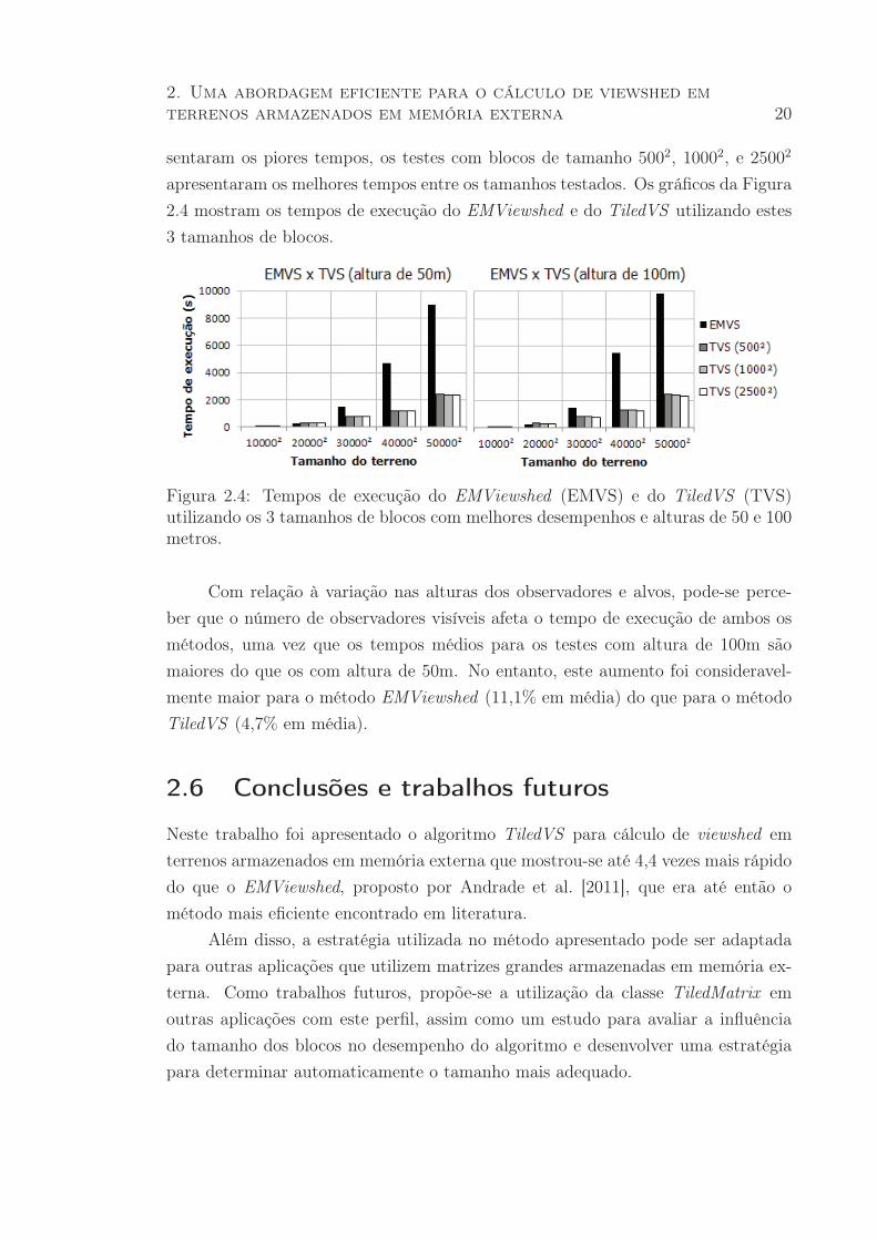
É possível perceber que o tamanho dos blocos afeta diretamente o desempenho
da estrutura TiledMatrix. Enquanto os testes com blocos de tamanho 1002 apre-
2. Uma abordagem eficiente para o cálculo de viewshed em
terrenos armazenados em memória externa 20
sentaram os piores tempos, os testes com blocos de tamanho 5002, 10002, e 25002
apresentaram os melhores tempos entre os tamanhos testados. Os gráficos da Figura
2.4 mostram os tempos de execução do EMViewshed e do TiledVS utilizando estes
3 tamanhos de blocos.
Figura 2.4: Tempos de execução do EMViewshed (EMVS) e do TiledVS (TVS)utilizando os 3 tamanhos de blocos com melhores desempenhos e alturas de 50 e 100metros.
Com relação à variação nas alturas dos observadores e alvos, pode-se perce-
ber que o número de observadores visíveis afeta o tempo de execução de ambos os
métodos, uma vez que os tempos médios para os testes com altura de 100m são
maiores do que os com altura de 50m. No entanto, este aumento foi consideravel-
mente maior para o método EMViewshed (11,1% em média) do que para o método
TiledVS (4,7% em média).
2.6 Conclusões e trabalhos futuros
Neste trabalho foi apresentado o algoritmo TiledVS para cálculo de viewshed em
terrenos armazenados em memória externa que mostrou-se até 4,4 vezes mais rápido
do que o EMViewshed, proposto por Andrade et al. [2011], que era até então o
método mais eficiente encontrado em literatura.
Além disso, a estratégia utilizada no método apresentado pode ser adaptada
para outras aplicações que utilizem matrizes grandes armazenadas em memória ex-
terna. Como trabalhos futuros, propõe-se a utilização da classe TiledMatrix em
outras aplicações com este perfil, assim como um estudo para avaliar a influência
do tamanho dos blocos no desempenho do algoritmo e desenvolver uma estratégia
para determinar automaticamente o tamanho mais adequado.
3. More efficient terrain viewshed compu-
tation on massive datasets using exter-
nal memory1
Abstract
We present a better algorithm and implementation for external memory
viewshed computation. It is about four times faster than the most recent and
most efficient published methods. Ours is also much simpler. Since processing
large datasets can take hours, this improvement is significant. To reduce the
total number of I/O operations, our method is based on subdividing the terrain
into blocks which are stored in a special data structure managed as a cache
memory.
The viewshed is that region of the terrain that is visible by a fixed
observer, who may be on or above the terrain. Its applications range from
visual nuisance abatement to radio transmitter siting and surveillance.
3.1 Introduction
Terrain modeling has been widely used in Geographical Information Science (GIS)
including applications in hydrology, visibility and routing. In visibility applications
it is usual to compute which points can be viewed from a given point (the observer)
and the region composed of such points, known as viewshed [Franklin and Ray,
1994]. Some applications include minimizing the number of cellular phone towers
required to cover a region [Ben-Shimol et al., 2007], optimizing the number and
position of guards to cover a region [Franklin and Vogt, 2006], etc.
There are various algorithms for viewshed computation but most of them
were designed assuming that the terrain data fits in internal memory. However,
the huge volume of high resolution terrestrial data available has become a challenge
for GIS since the internal memory algorithms do not run well for such volume
of data on most computers. Thus, it is important to optimize the massive data
1Neste capítulo é apresentado o artigo “More efficient terrain viewshed computation on massive
datasets using external memory”, apresentado no ACM SIGSPATIAL 2012 (20th International
Conference on Advances in Geographic Information Systems) [Ferreira et al., 2012b].
21
3. More efficient terrain viewshed computation on massive datasets
using external memory 22
processing algorithms simultaneously for computation and data movement between
the external and internal memories since processing data in external memory takes
much more time. That is, the algorithms for external memory should be designed
(and analyzed) considering a computational model where the algorithm complexity
is evaluated based on I/O operations. A model often used was proposed by Aggarwal
and Vitter [1988] where an I/O operation is defined as the transfer of one disk
block of size B between the external and internal memories and the performance is
measured considering the number of such I/O operations. The internal computation
time is assumed to be comparatively insignificant. An algorithm’s complexity is
related to the number of I/O operations performed by fundamental operations such
as scanning or sorting N contiguous elements. Those are scan(N) = θ(N/B) and
sort(N) = θ(
NBlogM/B
NB
)
where M is the internal memory size.
This work presents an efficient algorithm, named TiledVS , to compute the
viewshed of a point on terrains stored in external memory. The large number of
disk accesses is optimized using a new library to manage the data swap between
the external and internal memories. This new algorithm was compared against the
most recent and most efficient published methods: EMViewshed [Andrade et al.,
2011] and io_radial2, io_radial3 and io_centrifugal [Fishman et al., 2009]. Our
new method is much simpler and, also, the tests showed that it is more than four
times faster than all of them. Since processing large datasets can take hours, this
improvement is significant.
3.2 Definitions and related work
A terrain is a tridimensional surface τ where any vertical line intersects τ in at most
one point. In this paper we will consider terrains represented by regular square grids
(RSGs) since they use simpler data structures, i.e., matrices storing the elevations
of regularly spaced positions of the terrain.
An observer is a point in the space from where the other terrain points (the
targets) will be visualized. Both the observer and the targets can be at a given
height above the terrain, respectively indicated by ho and ht. Usually, it is assumed
that the observer has a range of vision ρ, the radius of interest, which means that
the observer can see points at a given distance ρ. Thus, a target T is visible from
O if and only if the distance of T from O is at most ρ and the straight line, the line
of sight, from O to T is always strictly above the terrain. See Figure 3.1.
The viewshed of O corresponds to all points that can be seen by O. Since
3. More efficient terrain viewshed computation on massive datasets
using external memory 23
Figure 3.1: Target’s visibility: T1 and T3 are not visible but T2 is.
we are working with regular square grids, we represent a viewshed by a square
(2ρ+ 1)× (2ρ+ 1) matrix of bits where 1 indicates that the corresponding point is
visible and 0 is not. By definition, the observer is in the center of this matrix.
Earlier works have presented different methods for viewshed computation.
Among the methods for RSG terrains, we can point out the one proposed by
Van Kreveld [1996], and the one by Franklin et al., named RFVS [Franklin and
Ray, 1994]. These two methods are very efficient and are particularly important
in this context because they were used as the base for some very recent and effi-
cient methods for the viewshed computation in external memory: Fishman et al.
[2009] adapted Van Kreveld’s method, and Andrade et al. [2011] adapted the RFVS
method. This work also presents an IO-efficient adaptation of the RFVS method.
Therefore, below we will give a short description of the RFVS method.
In that method, the terrain cells’ visibility is computed along rays connecting
the observer to all cells in the boundary of a square of side 2ρ + 1 centered at the
observer where ρ is the radius of interest. That is, the algorithm creates a ray
connecting the observer to a cell on the boundary of this square, and this ray is
counterclockwise rotated around the observer following the cells in that boundary
and the visibility of the cells in each ray is determined following the cells on the
segment. Thus, suppose the segment is composed by cells c0, c1, · · · , ck where c0
is the observer’s cell and ck is a cell in the square boundary. Let αi be the slope
of the line connecting the observer to ci and let µ be the highest slope among all
lines already processed, that is, when processing cell ci, µ = max{α1, α2, · · · , αi−1}.
Thus, the target on ci is visible if and only if the slope of the line from O to the
target above ci is greater than µ. If yes, the corresponding cell in the viewshed
matrix is set to 1; otherwise, to 0. Also, if αi > µ then µ is updated to αi. We
say that a cell ci blocks the visibility of the target above cj if cell ci belongs to
the segment c0cj and αi is greater or equal to the slope of the line connecting the
observer to the target above cj.
3. More efficient terrain viewshed computation on massive datasets
using external memory 24
3.3 TiledVS method
As mentioned in section 3.2, the RFVS sweeps the terrain cells rotating a ray
connecting the observer cell to a cell in the boundary of a bounding box and the
cells’ visibility is processed along this ray. Thus, the matrix access pattern presents
a spatial locality of reference, that is, in a short time interval, the accessed cells are
close in the matrix. However, this access pattern is not efficient in external memory
since the cells which are close in the (bidimensional) matrix may not be stored close
because, usually, a matrix is stored using a linear row-major order.
To reduce the number of non-sequential accesses, we present a new method,
called TiledVS , where the basic idea is to adapt the RFVS algorithm to manage
the access to the matrices stored in external memory using the library TiledMatrix
[Silveira et al., 2013].
In brief, this library subdivides the matrix in small rectangular blocks (tiles)
which are sequentially stored in the external memory. When a given cell needs
to be accessed, the whole block containing that cell is loaded into the internal
memory. The library keeps some of these blocks in the internal memory using a
data structure, named MemBlocks , which is managed as a “cache memory" and the
replacement policy adopted is based on least recently used - LRU. That is, when
a block is accessed it is labeled with a timestamp and if it is necessary to load
a new block into the cache (and there is no room for this block), the block with
smaller timestamp is replaced with the new block. When a block is evicted, it
is checked whether that block was updated (it is particularly important for the
viewshed matrix); if any cell was updated then the block is written back to the disk.
Now, we will show that it is possible to define the MemBlocks size such that
the adopted matrix partitioning associated with the LRU policy can be effective for
the RFVS algorithm, that is, we will prove that this process will load a block in the
cache, keep it there while it is accessed and it will be evicted only when it will be
no longer needed.
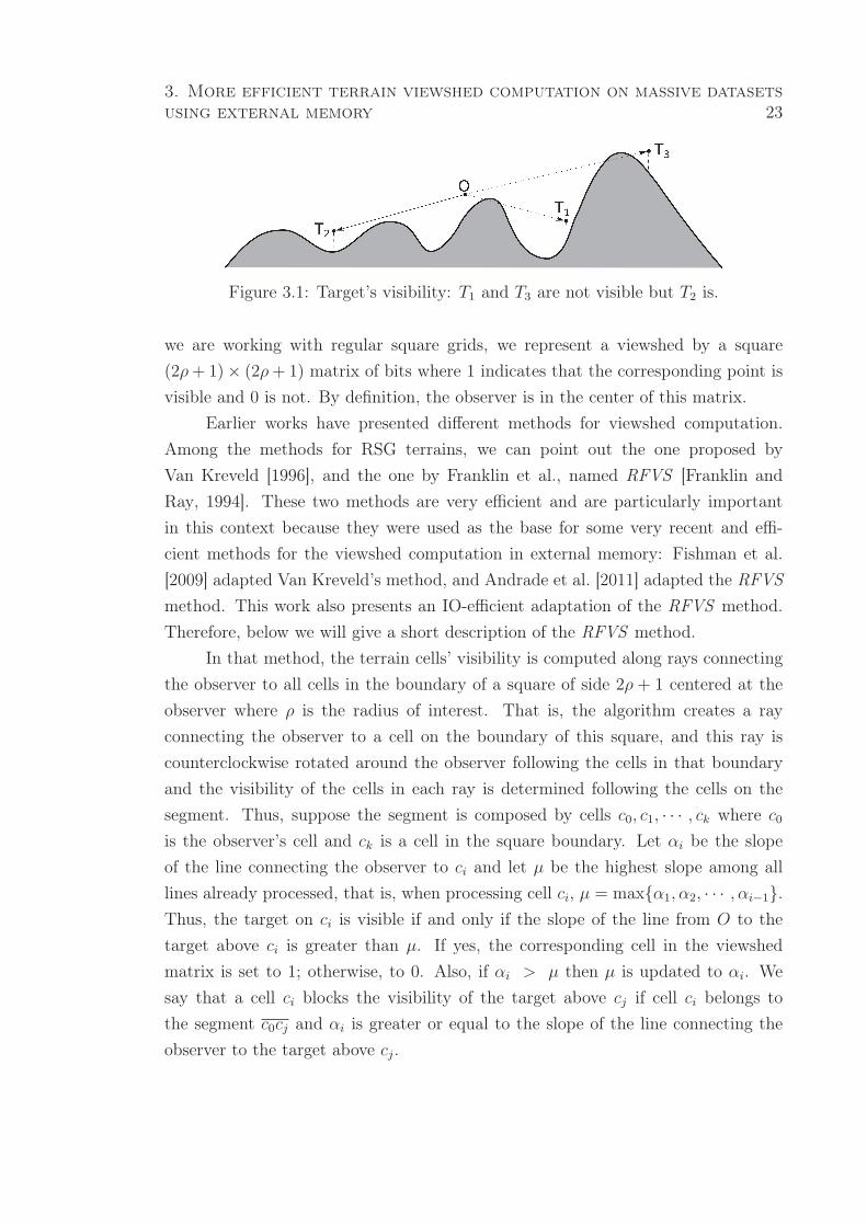
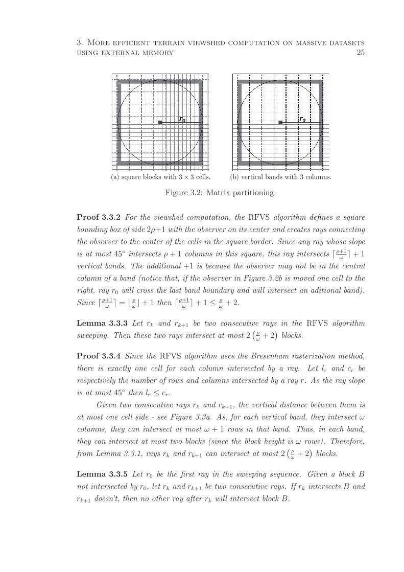
In the following, we will suppose that the matrix partitioning creates square
blocks with ω×ω cells and these blocks are grouped in vertical bands with ω columns
of cells. See figure 3.2. And, given a ray r defined by the RFVS algorithm, without
loss of generality, in the demonstrations below, we will consider rays whose slope is
at most 45◦. For rays with greater slope just replace rows with columns.
Lemma 3.3.1 Any ray intersects at most ρω+ 2 bands where ρ is the radius of
interest (in number of terrain cells).
3. More efficient terrain viewshed computation on massive datasets
using external memory 25
(a) square blocks with 3× 3 cells. (b) vertical bands with 3 columns.
Figure 3.2: Matrix partitioning.
Proof 3.3.2 For the viewshed computation, the RFVS algorithm defines a square
bounding box of side 2ρ+1 with the observer on its center and creates rays connecting
the observer to the center of the cells in the square border. Since any ray whose slope
is at most 45◦ intersects ρ+ 1 columns in this square, this ray intersects ⌈ρ+1ω⌉+ 1
vertical bands. The additional +1 is because the observer may not be in the central
column of a band (notice that, if the observer in Figure 3.2b is moved one cell to the
right, ray r0 will cross the last band boundary and will intersect an aditional band).
Since ⌈ρ+1ω⌉ = ⌊ ρ
ω⌋+ 1 then ⌈ρ+1
ω⌉+ 1 ≤ ρ
ω+ 2.
Lemma 3.3.3 Let rk and rk+1 be two consecutive rays in the RFVS algorithm
sweeping. Then these two rays intersect at most 2(
ρω+ 2
)
blocks.
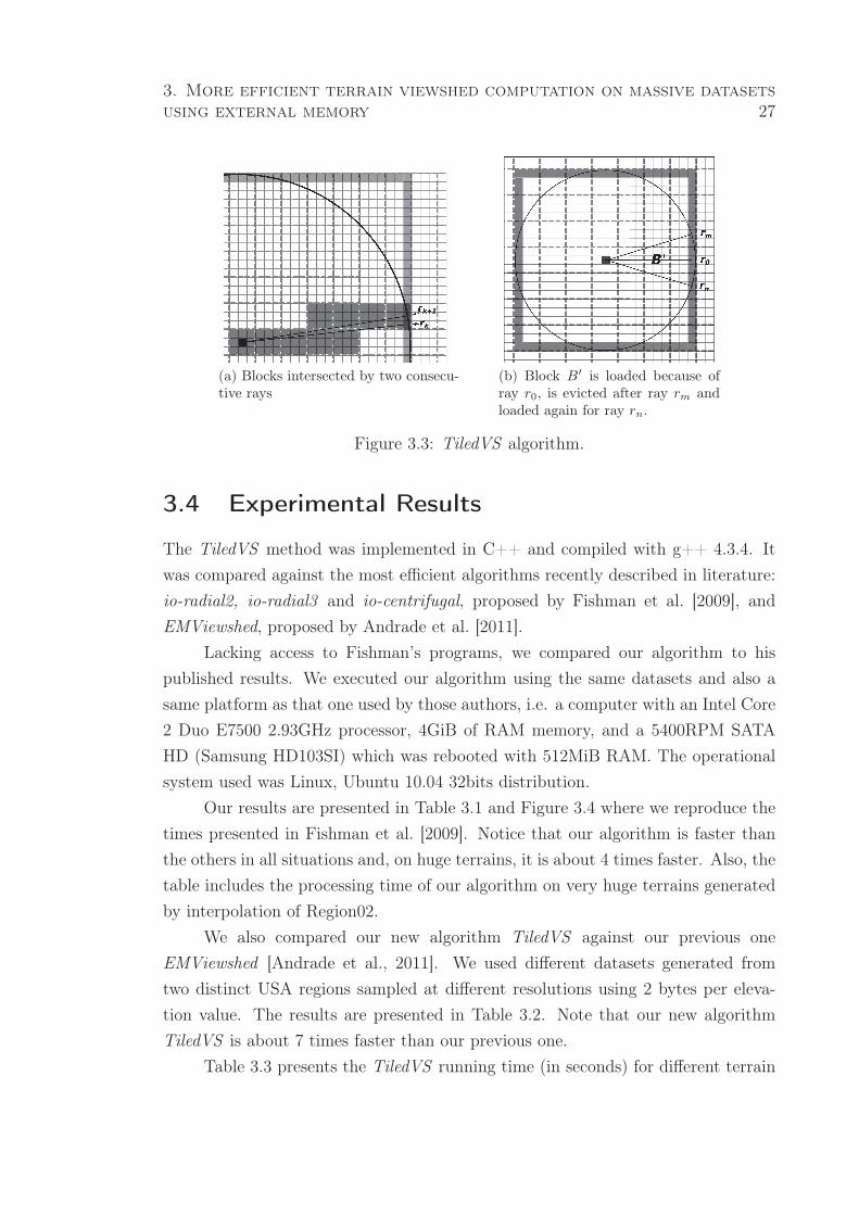
Proof 3.3.4 Since the RFVS algorithm uses the Bresenham rasterization method,
there is exactly one cell for each column intersected by a ray. Let lr and cr be
respectively the number of rows and columns intersected by a ray r. As the ray slope
is at most 45◦ then lr ≤ cr.
Given two consecutive rays rk and rk+1, the vertical distance between them is
at most one cell side - see Figure 3.3a. As, for each vertical band, they intersect ω
columns, they can intersect at most ω + 1 rows in that band. Thus, in each band,
they can intersect at most two blocks (since the block height is ω rows). Therefore,
from Lemma 3.3.1, rays rk and rk+1 can intersect at most 2(
ρω+ 2
)
blocks.
Lemma 3.3.5 Let r0 be the first ray in the sweeping sequence. Given a block B
not intersected by r0, let rk and rk+1 be two consecutive rays. If rk intersects B and
rk+1 doesn’t, then no other ray after rk will intersect block B.

3. More efficient terrain viewshed computation on massive datasets
using external memory 26
Proof 3.3.6 It is straightforward from the fact that the algorithm uses a radial
sweeping sequence and the blocks are convex. And it doesn’t work for the blocks
intersected by ray r0 because, considering the radial sweeping, these blocks can be
intersected again by the last rays. See Figure 3.3b.
Theorem 3.3.7 Given a block B not intersected by r0, if the MemBlocks size (in
number of blocks) is, at least, 2(
ρω+ 2
)
then the LRU policy will evict block B from
MemBlocks only if it is no longer needed.
Proof 3.3.8 Suppose that MemBlocks has 2(
ρω+ 2
)
slots to store the blocks. Let
rk and rk+1 be two consecutive rays such that rk intersects block B. At some point
during the processing of ray rk, block B will start to be processed and it is stored in
the MemBlocks (if rk is the first ray intersecting block B then B will be loaded in
MemBlocks). Now, if ray rk+1 also intersects block B, this block needs to be processed
again. But, the MemBlocks size is enough to avoid block B eviction because, let
B′1, B′
2, · · · , B′
j be the sequence of blocks that need to be processed among the twice
processing of B, that is, it is the sequence of blocks to be processed after B in the ray
rk and before B in ray rk+1. From lemma 3.3.3, j ≤ 2(
ρω+ 2
)
and since B is not
included in the sequence then j < 2(
ρω+ 2
)
. Thus, if MemBlocks size is 2(
ρω+ 2
)
then it has slots to store all blocks that need to be processed and B will not be evicted.
In other words, the LRU policy will not evict block B because the distinct blocks that
need to be accessed can be stored in MemBlocks.
On the other hand, if ray rk+1 doesn’t intersect block B then, from lemma 3.3.5,
no other ray after rk will intersect B and thus, it can be evicted since it is no longer
needed. There is a special situation for the blocks intersected by r0 because, after
being evicted, they can be loaded again when processing the last rays. But notice that
these blocks can be loaded at most twice. See Figure 3.3b where block B′ is loaded
in the processing of r0, is evicted after the processing of rm and it is loaded again
when processing rn.
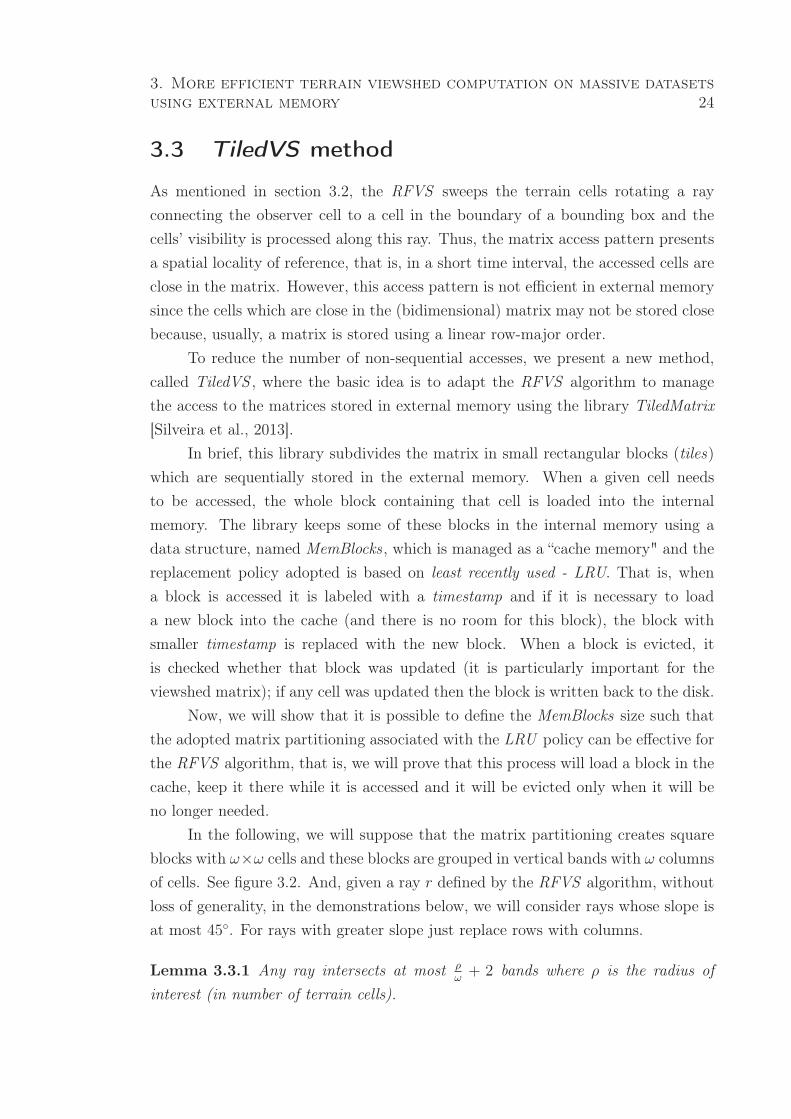
It is possible to demonstrate that the TiledVS algorithm does θ(scan(N)) I/O
operations and takes θ(N) time to process a terrain with N cells considering that
the memory can store 2(
ρω+ 2
)
blocks. This complexity works even if the radius of
interest ρ is large to cover the whole terrain.
3. More efficient terrain viewshed computation on massive datasets
using external memory 27
(a) Blocks intersected by two consecu-tive rays
(b) Block B′ is loaded because ofray r0, is evicted after ray rm andloaded again for ray rn.
Figure 3.3: TiledVS algorithm.
3.4 Experimental Results
The TiledVS method was implemented in C++ and compiled with g++ 4.3.4. It
was compared against the most efficient algorithms recently described in literature:
io-radial2, io-radial3 and io-centrifugal, proposed by Fishman et al. [2009], and
EMViewshed, proposed by Andrade et al. [2011].
Lacking access to Fishman’s programs, we compared our algorithm to his
published results. We executed our algorithm using the same datasets and also a
same platform as that one used by those authors, i.e. a computer with an Intel Core
2 Duo E7500 2.93GHz processor, 4GiB of RAM memory, and a 5400RPM SATA
HD (Samsung HD103SI) which was rebooted with 512MiB RAM. The operational
system used was Linux, Ubuntu 10.04 32bits distribution.
Our results are presented in Table 3.1 and Figure 3.4 where we reproduce the
times presented in Fishman et al. [2009]. Notice that our algorithm is faster than
the others in all situations and, on huge terrains, it is about 4 times faster. Also, the
table includes the processing time of our algorithm on very huge terrains generated
by interpolation of Region02.
We also compared our new algorithm TiledVS against our previous one
EMViewshed [Andrade et al., 2011]. We used different datasets generated from
two distinct USA regions sampled at different resolutions using 2 bytes per eleva-
tion value. The results are presented in Table 3.2. Note that our new algorithm
TiledVS is about 7 times faster than our previous one.
Table 3.3 presents the TiledVS running time (in seconds) for different terrain
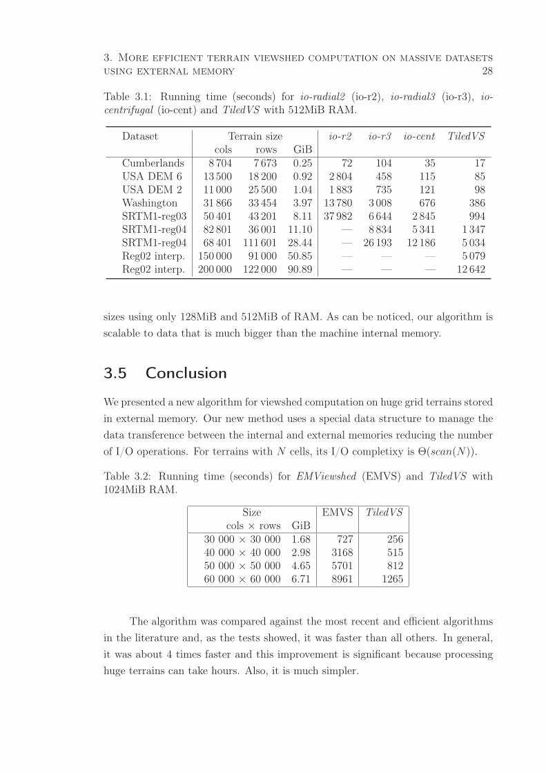
3. More efficient terrain viewshed computation on massive datasets
using external memory 28
Table 3.1: Running time (seconds) for io-radial2 (io-r2), io-radial3 (io-r3), io-centrifugal (io-cent) and TiledVS with 512MiB RAM.
Dataset Terrain size io-r2 io-r3 io-cent TiledVScols rows GiB
Cumberlands 8 704 7 673 0.25 72 104 35 17USA DEM 6 13 500 18 200 0.92 2 804 458 115 85USA DEM 2 11 000 25 500 1.04 1 883 735 121 98Washington 31 866 33 454 3.97 13 780 3 008 676 386SRTM1-reg03 50 401 43 201 8.11 37 982 6 644 2 845 994SRTM1-reg04 82 801 36 001 11.10 — 8834 5 341 1 347SRTM1-reg04 68 401 111 601 28.44 — 26 193 12 186 5 034Reg02 interp. 150 000 91 000 50.85 — — — 5079Reg02 interp. 200 000 122 000 90.89 — — — 12 642
sizes using only 128MiB and 512MiB of RAM. As can be noticed, our algorithm is
scalable to data that is much bigger than the machine internal memory.
3.5 Conclusion
We presented a new algorithm for viewshed computation on huge grid terrains stored
in external memory. Our new method uses a special data structure to manage the
data transference between the internal and external memories reducing the number
of I/O operations. For terrains with N cells, its I/O completixy is Θ(scan(N)).
Table 3.2: Running time (seconds) for EMViewshed (EMVS) and TiledVS with1024MiB RAM.
Size EMVS TiledVScols × rows GiB
30 000 × 30 000 1.68 727 25640 000 × 40 000 2.98 3168 51550 000 × 50 000 4.65 5701 81260 000 × 60 000 6.71 8961 1265
The algorithm was compared against the most recent and efficient algorithms
in the literature and, as the tests showed, it was faster than all others. In general,
it was about 4 times faster and this improvement is significant because processing
huge terrains can take hours. Also, it is much simpler.
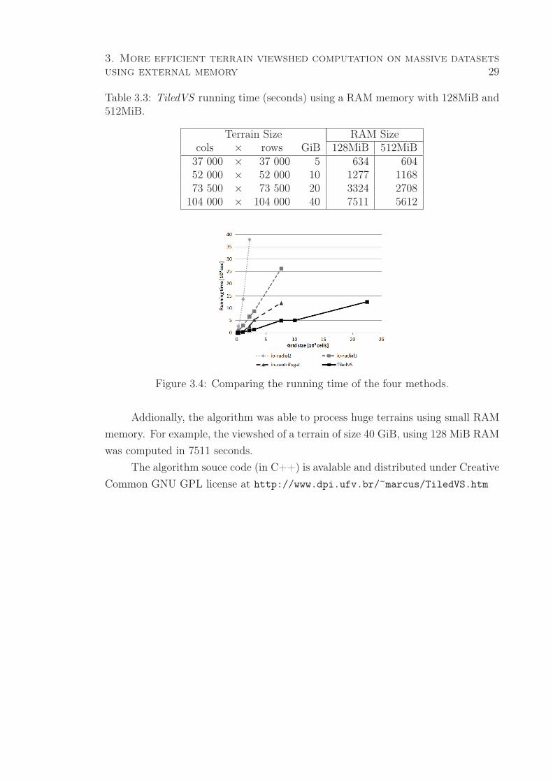
3. More efficient terrain viewshed computation on massive datasets
using external memory 29
Table 3.3: TiledVS running time (seconds) using a RAM memory with 128MiB and512MiB.
Terrain Size RAM Sizecols × rows GiB 128MiB 512MiB37 000 × 37 000 5 634 60452 000 × 52 000 10 1277 116873 500 × 73 500 20 3324 2708104 000 × 104 000 40 7511 5612
Figure 3.4: Comparing the running time of the four methods.
Addionally, the algorithm was able to process huge terrains using small RAM
memory. For example, the viewshed of a terrain of size 40 GiB, using 128 MiB RAM
was computed in 7511 seconds.
The algorithm souce code (in C++) is avalable and distributed under Creative
Common GNU GPL license at http://www.dpi.ufv.br/~marcus/TiledVS.htm
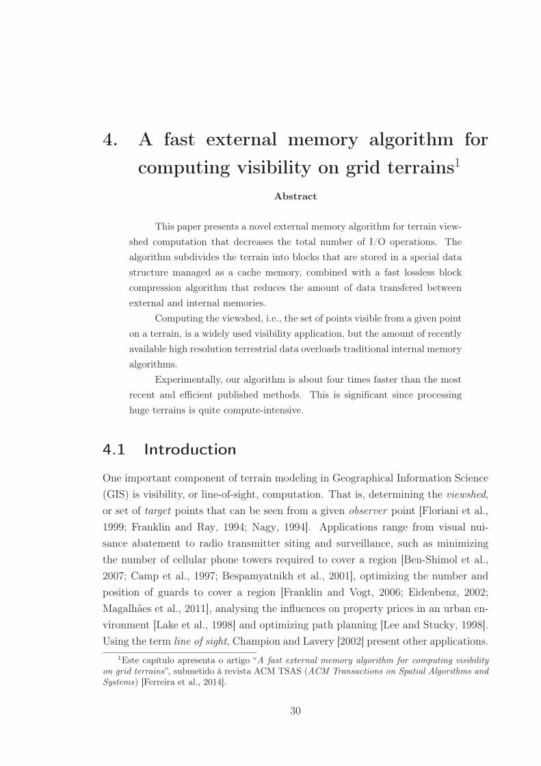
4. A fast external memory algorithm for
computing visibility on grid terrains1
Abstract
This paper presents a novel external memory algorithm for terrain view-
shed computation that decreases the total number of I/O operations. The
algorithm subdivides the terrain into blocks that are stored in a special data
structure managed as a cache memory, combined with a fast lossless block
compression algorithm that reduces the amount of data transfered between
external and internal memories.
Computing the viewshed, i.e., the set of points visible from a given point
on a terrain, is a widely used visibility application, but the amount of recently
available high resolution terrestrial data overloads traditional internal memory
algorithms.
Experimentally, our algorithm is about four times faster than the most
recent and efficient published methods. This is significant since processing
huge terrains is quite compute-intensive.
4.1 Introduction
One important component of terrain modeling in Geographical Information Science
(GIS) is visibility, or line-of-sight, computation. That is, determining the viewshed,
or set of target points that can be seen from a given observer point [Floriani et al.,
1999; Franklin and Ray, 1994; Nagy, 1994]. Applications range from visual nui-
sance abatement to radio transmitter siting and surveillance, such as minimizing
the number of cellular phone towers required to cover a region [Ben-Shimol et al.,
2007; Camp et al., 1997; Bespamyatnikh et al., 2001], optimizing the number and
position of guards to cover a region [Franklin and Vogt, 2006; Eidenbenz, 2002;
Magalhães et al., 2011], analysing the influences on property prices in an urban en-
vironment [Lake et al., 1998] and optimizing path planning [Lee and Stucky, 1998].
Using the term line of sight, Champion and Lavery [2002] present other applications.
1Este capítulo apresenta o artigo “A fast external memory algorithm for computing visibility
on grid terrains”, submetido à revista ACM TSAS (ACM Transactions on Spatial Algorithms and
Systems) [Ferreira et al., 2014].
30
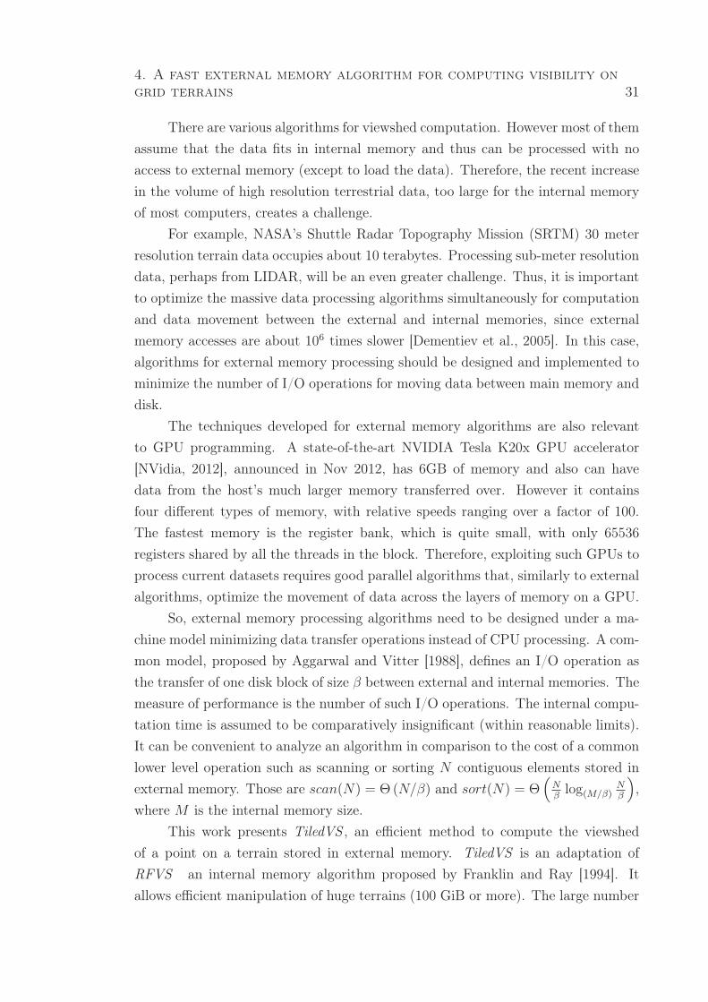
4. A fast external memory algorithm for computing visibility on
grid terrains 31
There are various algorithms for viewshed computation. However most of them
assume that the data fits in internal memory and thus can be processed with no
access to external memory (except to load the data). Therefore, the recent increase
in the volume of high resolution terrestrial data, too large for the internal memory
of most computers, creates a challenge.
For example, NASA’s Shuttle Radar Topography Mission (SRTM) 30 meter
resolution terrain data occupies about 10 terabytes. Processing sub-meter resolution
data, perhaps from LIDAR, will be an even greater challenge. Thus, it is important
to optimize the massive data processing algorithms simultaneously for computation
and data movement between the external and internal memories, since external
memory accesses are about 106 times slower [Dementiev et al., 2005]. In this case,
algorithms for external memory processing should be designed and implemented to
minimize the number of I/O operations for moving data between main memory and
disk.
The techniques developed for external memory algorithms are also relevant
to GPU programming. A state-of-the-art NVIDIA Tesla K20x GPU accelerator
[NVidia, 2012], announced in Nov 2012, has 6GB of memory and also can have
data from the host’s much larger memory transferred over. However it contains
four different types of memory, with relative speeds ranging over a factor of 100.
The fastest memory is the register bank, which is quite small, with only 65536
registers shared by all the threads in the block. Therefore, exploiting such GPUs to
process current datasets requires good parallel algorithms that, similarly to external
algorithms, optimize the movement of data across the layers of memory on a GPU.
So, external memory processing algorithms need to be designed under a ma-
chine model minimizing data transfer operations instead of CPU processing. A com-
mon model, proposed by Aggarwal and Vitter [1988], defines an I/O operation as
the transfer of one disk block of size β between external and internal memories. The
measure of performance is the number of such I/O operations. The internal compu-
tation time is assumed to be comparatively insignificant (within reasonable limits).
It can be convenient to analyze an algorithm in comparison to the cost of a common
lower level operation such as scanning or sorting N contiguous elements stored in
external memory. Those are scan(N) = Θ (N/β) and sort(N) = Θ(
Nβlog(M/β)
Nβ
)
,
where M is the internal memory size.
This work presents TiledVS , an efficient method to compute the viewshed
of a point on a terrain stored in external memory. TiledVS is an adaptation of
RFVS an internal memory algorithm proposed by Franklin and Ray [1994]. It
allows efficient manipulation of huge terrains (100 GiB or more). The large number
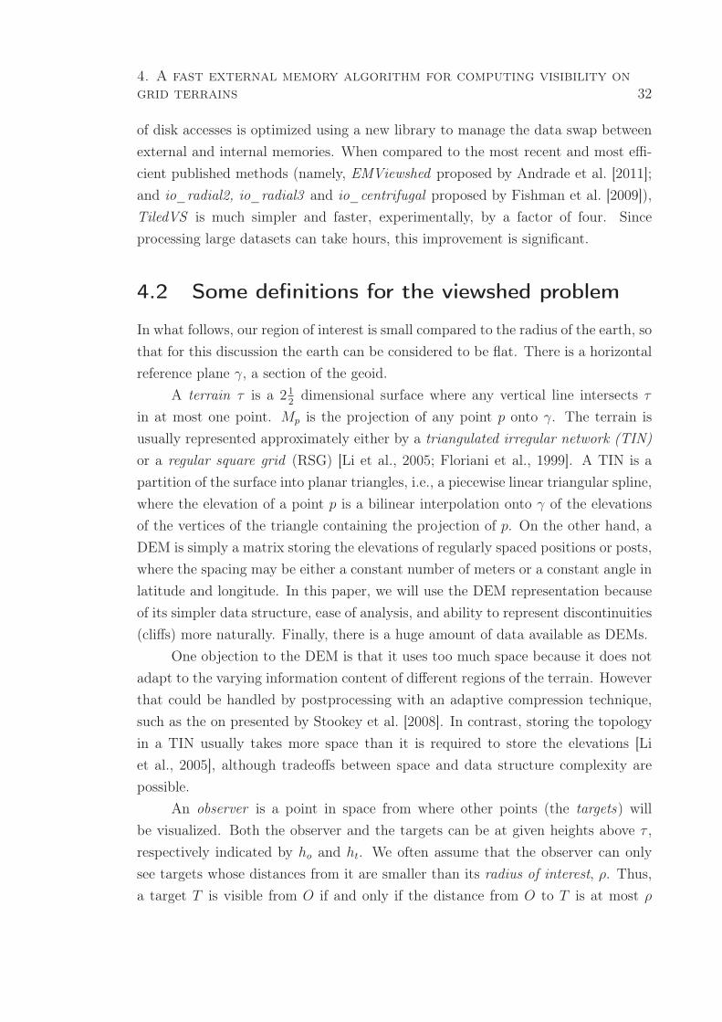
4. A fast external memory algorithm for computing visibility on
grid terrains 32
of disk accesses is optimized using a new library to manage the data swap between
external and internal memories. When compared to the most recent and most effi-
cient published methods (namely, EMViewshed proposed by Andrade et al. [2011];
and io_radial2, io_radial3 and io_centrifugal proposed by Fishman et al. [2009]),
TiledVS is much simpler and faster, experimentally, by a factor of four. Since
processing large datasets can take hours, this improvement is significant.
4.2 Some definitions for the viewshed problem
In what follows, our region of interest is small compared to the radius of the earth, so
that for this discussion the earth can be considered to be flat. There is a horizontal
reference plane γ, a section of the geoid.
A terrain τ is a 212dimensional surface where any vertical line intersects τ
in at most one point. Mp is the projection of any point p onto γ. The terrain is
usually represented approximately either by a triangulated irregular network (TIN)
or a regular square grid (RSG) [Li et al., 2005; Floriani et al., 1999]. A TIN is a
partition of the surface into planar triangles, i.e., a piecewise linear triangular spline,
where the elevation of a point p is a bilinear interpolation onto γ of the elevations
of the vertices of the triangle containing the projection of p. On the other hand, a
DEM is simply a matrix storing the elevations of regularly spaced positions or posts,
where the spacing may be either a constant number of meters or a constant angle in
latitude and longitude. In this paper, we will use the DEM representation because
of its simpler data structure, ease of analysis, and ability to represent discontinuities
(cliffs) more naturally. Finally, there is a huge amount of data available as DEMs.
One objection to the DEM is that it uses too much space because it does not
adapt to the varying information content of different regions of the terrain. However
that could be handled by postprocessing with an adaptive compression technique,
such as the on presented by Stookey et al. [2008]. In contrast, storing the topology
in a TIN usually takes more space than it is required to store the elevations [Li
et al., 2005], although tradeoffs between space and data structure complexity are
possible.
An observer is a point in space from where other points (the targets) will
be visualized. Both the observer and the targets can be at given heights above τ ,
respectively indicated by ho and ht. We often assume that the observer can only
see targets whose distances from it are smaller than its radius of interest, ρ. Thus,
a target T is visible from O if and only if the distance from O to T is at most ρ
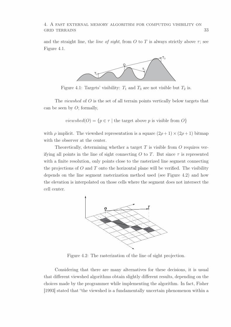
4. A fast external memory algorithm for computing visibility on
grid terrains 33
and the straight line, the line of sight, from O to T is always strictly above τ ; see
Figure 4.1.
O
T1
T2
T3
Figure 4.1: Targets’ visibility: T1 and T3 are not visible but T2 is.
The viewshed of O is the set of all terrain points vertically below targets that
can be seen by O; formally,
viewshed(O) = {p ∈ τ | the target above p is visible from O}
with ρ implicit. The viewshed representation is a square (2ρ+1)× (2ρ+1) bitmap
with the observer at the center.
Theoretically, determining whether a target T is visible from O requires ver-
ifying all points in the line of sight connecting O to T . But since τ is represented
with a finite resolution, only points close to the rasterized line segment connecting
the projections of O and T onto the horizontal plane will be verified. The visibility
depends on the line segment rasterization method used (see Figure 4.2) and how
the elevation is interpolated on those cells where the segment does not intersect the
cell center.
Figure 4.2: The rasterization of the line of sight projection.
Considering that there are many alternatives for these decisions, it is usual
that different viewshed algorithms obtain slightly different results, depending on the
choices made by the programmer while implementing the algorithm. In fact, Fisher
[1993] stated that “the viewshed is a fundamentally uncertain phenomenon within a
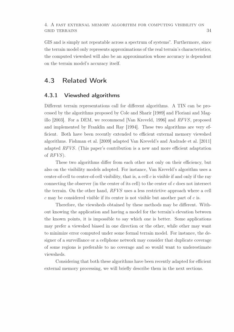
4. A fast external memory algorithm for computing visibility on
grid terrains 34
GIS and is simply not repeatable across a spectrum of systems”. Furthermore, since
the terrain model only represents approximations of the real terrain’s characteristics,
the computed viewshed will also be an approximation whose accuracy is dependent
on the terrain model’s accuracy itself.
4.3 Related Work
4.3.1 Viewshed algorithms
Different terrain representations call for different algorithms. A TIN can be pro-
cessed by the algorithms proposed by Cole and Sharir [1989] and Floriani and Mag-
illo [2003]. For a DEM, we recommend [Van Kreveld, 1996] and RFVS , proposed
and implemented by Franklin and Ray [1994]. These two algorithms are very ef-
ficient. Both have been recently extended to efficient external memory viewshed
algorithms. Fishman et al. [2009] adapted Van Kreveld’s and Andrade et al. [2011]
adapted RFVS . (This paper’s contribution is a new and more efficient adaptation
of RFVS ).
These two algorithms differ from each other not only on their efficiency, but
also on the visibility models adopted. For instance, Van Kreveld’s algorithm uses a
center-of-cell to center-of-cell visibility, that is, a cell c is visible if and only if the ray
connecting the observer (in the center of its cell) to the center of c does not intersect
the terrain. On the other hand, RFVS uses a less restrictive approach where a cell
c may be considered visible if its center is not visible but another part of c is.
Therefore, the viewsheds obtained by these methods may be different. With-
out knowing the application and having a model for the terrain’s elevation between
the known points, it is impossible to say which one is better. Some applications
may prefer a viewshed biased in one direction or the other, while other may want
to minimize error computed under some formal terrain model. For instance, the de-
signer of a surveillance or a cellphone network may consider that duplicate coverage
of some regions is preferable to no coverage and so would want to underestimate
viewsheds.
Considering that both these algorithms have been recently adapted for efficient
external memory processing, we will briefly describe them in the next sections.
4. A fast external memory algorithm for computing visibility on
grid terrains 35
4.3.1.1 The RFVS algorithm
RFVS [Franklin and Ray, 1994] is a fast algorithm that runs in Θ(n), where n =
Θ(ρ2). It computes the terrain cells’ visibility along rays (line segments) connecting
the observer (in the center of a cell) to the center of all cells in the boundary of a
square bounding box of side 2ρ+ 1 centered at the observer (see Figure 4.3a).
(a) RFVS algorithm. (b) Van Kreveld’s algorithm.
Figure 4.3: Viewshed algorithms.
RFVS creates a ray connecting the observer to a cell on the boundary of this
square, and then rotates it counter-clockwise around the observer to follow along
the boundary cells. The visibility of each ray’s cells is determined by walking along
the segment, which is rasterized following [Bresenham, 1965]. Suppose this segment
is composed of cells c0, c1, · · · , ck where c0 is the observer’s cell and ck is a cell in
the square boundary. Let αi be the slope of the line connecting the observer to ci.
For each cell ci, the algorithm compares αi against all αj with 0 < j < i. If, for any
such j, αi ≤ αj, then ci is not visible. Otherwise it is.
Formally, given a terrain τ represented by an elevation matrixM, the observer
position c0 on τ , the radius of interest ρ, and ho, the observer’s height above the
terrain, this algorithm computes the viewshed of O within a distance ρ of c0, as
follows:
1. Let c0’s coordinates be (x0, y0). Then the observer O will be at a distance ho
above cell (x0, y0) inM.
2. Imagine a square of side (2ρ+ 1)× (2ρ+ 1) centered on (x0, y0).
3. Iterate through the cells p of the square’s perimeter.
a) For each p, run a straight line inM from (x0, y0) to (xp, yp).
4. A fast external memory algorithm for computing visibility on
grid terrains 36
b) Find the cells intersected by that line, perhaps using Bresenham. From
c0 to p, in that order, let them be c0, c1, · · · ck−1, ck = p.
c) Let αi be the slope of the line from O to ci, that is,
αi =ζ(ci)− (ζ(c0) + ho)
dist(c0, ci)
where ζ(c0) and ζ(ci) are, respectively, the elevation of cells c0 and ci and
dist(c0, ci) is the “distance” (in number of cells) between these two cells.
d) Let µ be the greatest slope seen so far along this line. Initialize µ = −∞.
e) Iterate along the line from c0 to p.
i. For each cell ci, compute αi.
ii. If αi > µ, then set ci as visible in the viewshed (which is simply a
2ρ× 2ρ bitmap) and update µ = αi.
4.3.1.2 Van Kreveld’s algorithm
Van Kreveld’s algorithm [Van Kreveld, 1996] is another fast viewshed algorithm,
which runs in Θ(n log n), also with n = Θ(ρ2). Its basic idea is to rotate a sweep
line around the observer and compute the visibility of each cell when the sweep line
passes over its center (see Figure 4.3b). For that, it maintains a balanced binary
tree (the agenda) that stores the slope of all cells currently being intersected by
the sweep line, keyed by their distance from the observer. When this sweep line
passes over the center of a cell c, the agenda is searched to check c’s visibility. More
specifically, this algorithm works as follows:
For each cell, it defines three types of events: enter, center, and exit events to
indicate, respectively, when the sweep line starts to intersect the cell, passes over the
cell center and stops to intersect the cell. The algorithm creates a list E containing
these three types of events for all cells inside the region of interest. The events are
then sorted according to their azimuth angle.
To compute the viewshed, the algorithm sweeps list E and for each event it
decides what to do depending on the type of the event:
• If it is an enter event, the cell is inserted into the agenda.
• If it is a center event of cell c, the agenda is searched to check if it contains
any cell that lies closer to the observer than c and has slope greater or equal
4. A fast external memory algorithm for computing visibility on
grid terrains 37
to the slope of the line of sight to c; if yes, then c is not visible, otherwise it
is.
• If it is an exit event, the cell is removed from the agenda.
It is important to note that the agenda is implemented as a balanced binary
tree, that performs insertions, removals and queries in Θ(log n), which keeps the
algorithm efficiency in Θ(n log n).
4.3.2 External memory viewshed algorithms
4.3.2.1 EMViewshed
EMViewshed [Andrade et al., 2011] is an efficient external memory algorithm based
on RFVS . It creates and stores in external memory a list with data about all terrain
cells and sorts it according to the order that they will be processed by the RFVS
algorithm. Thus, it can sweep that list sequentially, avoiding random accesses to
external memory.
More specifically, it creates a list Q of pairs (c, k), where c is a terrain cell and
k is an index that illustrates when c will be processed. That is, if there is a pair (c, k)
in Q, then c will be the k-th cell to be processed. After creating Q, the algorithm
sorts Q according to these k indices using an external memory sorting algorithm
[Dementiev et al., 2005]. Then it sweeps Q to calculate the viewshed, making
only sequential accesses to external memory, which guarantees the algorithm I/O
efficiency.
Although EMViewshed is a fast I/O-efficient algorithm, our experiments in
Section 4.6 show that our new algorithm is about 10 times faster than it.
4.3.2.2 Algorithms based on Van Kreveld’s algorithm
Van Kreveld’s method was adapted for external memory processing by various au-
thors using different strategies: ioviewshed [Haverkort et al., 2007] creates a list of
events and sorts it with an external memory sorting algorithm. These events are
used to process the terrain with a sweep-line approach. This algorithm was renamed
io-radial1 in [Fishman et al., 2009] where the authors describe two other algorithms
also based on Van Kreveld, io-radial2 and io-radial3. They sweep the terrain by
rotating a ray around the viewpoint while maintaining the terrain profile along the
ray (similar to Van Kreveld). The difference between the two algorithms lies in the
preprocessing step before sweeping the terrain. In io-radial2, the grid points are
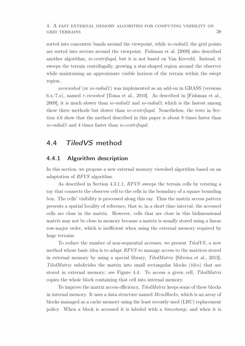
4. A fast external memory algorithm for computing visibility on
grid terrains 38
sorted into concentric bands around the viewpoint, while io-radial3, the grid points
are sorted into sectors around the viewpoint. Fishman et al. [2009] also described
another algorithm, io-centrifugal, but it is not based on Van Kreveld. Instead, it
sweeps the terrain centrifugally, growing a star-shaped region around the observer
while maintaining an approximate visible horizon of the terrain within the swept
region.
ioviewshed (or io-radial1 ) was implemented as an add-on in GRASS (versions
6.x/7.x), named r.viewshed [Toma et al., 2010]. As described in [Fishman et al.,
2009], it is much slower than io-radial2 and io-radial3, which is the fastest among
these three methods but slower than io-centrifugal. Nonetheless, the tests in Sec-
tion 4.6 show that the method described in this paper is about 8 times faster than
io-radial3 and 4 times faster than io-centrifugal.
4.4 TiledVS method
4.4.1 Algorithm description
In this section, we propose a new external memory viewshed algorithm based on an
adaptation of RFVS algorithm.
As described in Section 4.3.1.1, RFVS sweeps the terrain cells by rotating a
ray that connects the observer cell to the cells in the boundary of a square bounding
box. The cells’ visibility is processed along this ray. Thus the matrix access pattern
presents a spatial locality of reference, that is, in a short time interval, the accessed
cells are close in the matrix. However, cells that are close in this bidimensional
matrix may not be close in memory because a matrix is usually stored using a linear
row-major order, which is inefficient when using the external memory required by
huge terrains.
To reduce the number of non-sequential accesses, we present TiledVS , a new
method whose basic idea is to adapt RFVS to manage access to the matrices stored
in external memory by using a special library, TiledMatrix [Silveira et al., 2013].
TiledMatrix subdivides the matrix into small rectangular blocks (tiles) that are
stored in external memory; see Figure 4.4. To access a given cell, TiledMatrix
copies the whole block containing that cell into internal memory.
To improve the matrix access efficiency, TiledMatrix keeps some of these blocks
in internal memory. It uses a data structure namedMemBlocks , which is an array of
blocks managed as a cache memory using the least recently used (LRU) replacement
policy. When a block is accessed it is labeled with a timestamp; and when it is
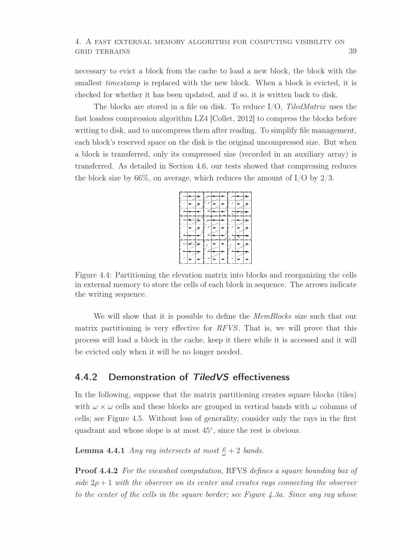
4. A fast external memory algorithm for computing visibility on
grid terrains 39
necessary to evict a block from the cache to load a new block, the block with the
smallest timestamp is replaced with the new block. When a block is evicted, it is
checked for whether it has been updated, and if so, it is written back to disk.
The blocks are stored in a file on disk. To reduce I/O, TiledMatrix uses the
fast lossless compression algorithm LZ4 [Collet, 2012] to compress the blocks before
writing to disk, and to uncompress them after reading. To simplify file management,
each block’s reserved space on the disk is the original uncompressed size. But when
a block is transferred, only its compressed size (recorded in an auxiliary array) is
transferred. As detailed in Section 4.6, our tests showed that compressing reduces
the block size by 66%, on average, which reduces the amount of I/O by 2/3.
Figure 4.4: Partitioning the elevation matrix into blocks and reorganizing the cellsin external memory to store the cells of each block in sequence. The arrows indicatethe writing sequence.
We will show that it is possible to define the MemBlocks size such that our
matrix partitioning is very effective for RFVS . That is, we will prove that this
process will load a block in the cache, keep it there while it is accessed and it will
be evicted only when it will be no longer needed.
4.4.2 Demonstration of TiledVS effectiveness
In the following, suppose that the matrix partitioning creates square blocks (tiles)
with ω × ω cells and these blocks are grouped in vertical bands with ω columns of
cells; see Figure 4.5. Without loss of generality, consider only the rays in the first
quadrant and whose slope is at most 45◦, since the rest is obvious.
Lemma 4.4.1 Any ray intersects at most ρω+ 2 bands.
Proof 4.4.2 For the viewshed computation, RFVS defines a square bounding box of
side 2ρ+ 1 with the observer on its center and creates rays connecting the observer
to the center of the cells in the square border; see Figure 4.3a. Since any ray whose
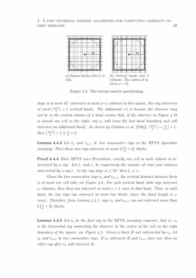
4. A fast external memory algorithm for computing visibility on
grid terrains 40
(a) Square blocks with 3×3cells.
(b) Vertical bands with 3columns. The radius of in-terest ρ = 10.
Figure 4.5: The terrain matrix partitioning.
slope is at most 45◦ intersects at most ρ+1 columns in this square, this ray intersects
at most ⌈ρ+1ω⌉ + 1 vertical bands. The additional +1 is because the observer may
not be in the central column of a band (notice that, if the observer in Figure 4.5b
is moved one cell to the right, ray r0 will cross the last band boundary and will
intersect an additional band). As shown by Graham et al. [1994], ⌈ρ+1ω⌉ = ⌊ ρ
ω⌋+ 1,
then ⌈ρ+1ω⌉+ 1 ≤ ρ
ω+ 2.
Lemma 4.4.3 Let rk and rk+1 be two consecutive rays in the RFVS algorithm
sweeping. Then these two rays intersect at most 2(
ρω+ 2
)
blocks.
Proof 4.4.4 Since RFVS uses Bresenham, exactly one cell in each column is in-
tersected by a ray. Let lr and cr be respectively the number of rows and columns
intersected by a ray r. As the ray slope is ≤ 45◦ then lr ≤ cr.
Given the two consecutive rays rk and rk+1, the vertical distance between them
is at most one cell side; see Figure 4.6. For each vertical band, both rays intersect
ω columns, then they can intersect at most ω + 1 rows in that band. Thus, in each
band, the two rays can intersect at most two blocks (since the block height is ω
rows). Therefore, from Lemma 4.4.1, rays rk and rk+1 can not intersect more than
2(
ρω+ 2
)
blocks.
Lemma 4.4.5 Let r0 be the first ray in the RFVS sweeping sequence, that is, r0
is the horizontal ray connecting the observer to the center of the cell on the right
boundary of the square; see Figure 4.5. Given a block B not intersected by r0, let
rk and rk+1 be two consecutive rays. If rk intersects B and rk+1 does not, then no
other ray after rk will intersect B.
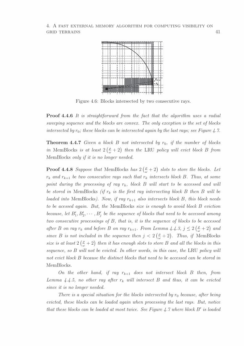
4. A fast external memory algorithm for computing visibility on
grid terrains 41
Figure 4.6: Blocks intersected by two consecutive rays.
Proof 4.4.6 It is straightforward from the fact that the algorithm uses a radial
sweeping sequence and the blocks are convex. The only exception is the set of blocks
intersected by r0; these blocks can be intersected again by the last rays; see Figure 4.7.
Theorem 4.4.7 Given a block B not intersected by r0, if the number of blocks
in MemBlocks is at least 2(
ρω+ 2
)
then the LRU policy will evict block B from
MemBlocks only if it is no longer needed.
Proof 4.4.8 Suppose that MemBlocks has 2(
ρω+ 2
)
slots to store the blocks. Let
rk and rk+1 be two consecutive rays such that rk intersects block B. Thus, at some
point during the processing of ray rk, block B will start to be accessed and will
be stored in MemBlocks (if rk is the first ray intersecting block B then B will be
loaded into MemBlocks). Now, if ray rk+1 also intersects block B, this block needs
to be acessed again. But, the MemBlocks size is enough to avoid block B eviction
because, let B′1, B′
2, · · · , B′
j be the sequence of blocks that need to be accessed among
two consecutive processings of B, that is, it is the sequence of blocks to be accessed
after B on ray rk and before B on ray rk+1. From Lemma 4.4.3, j ≤ 2(
ρω+ 2
)
and
since B is not included in the sequence then j < 2(
ρω+ 2
)
. Thus, if MemBlocks
size is at least 2(
ρω+ 2
)
then it has enough slots to store B and all the blocks in this
sequence, so B will not be evicted. In other words, in this case, the LRU policy will
not evict block B because the distinct blocks that need to be accessed can be stored in
MemBlocks.
On the other hand, if ray rk+1 does not intersect block B then, from
Lemma 4.4.5, no other ray after rk will intersect B and thus, it can be evicted
since it is no longer needed.
There is a special situation for the blocks intersected by r0 because, after being
evicted, these blocks can be loaded again when processing the last rays. But, notice
that these blocks can be loaded at most twice. See Figure 4.7 where block B′ is loaded
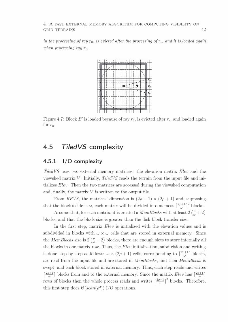
4. A fast external memory algorithm for computing visibility on
grid terrains 42
in the processing of ray r0, is evicted after the processing of rm and it is loaded again
when processing ray rn.
Figure 4.7: Block B′ is loaded because of ray r0, is evicted after rm and loaded againfor rn.
4.5 TiledVS complexity
4.5.1 I/O complexity
TiledVS uses two external memory matrices: the elevation matrix Elev and the
viewshed matrix V . Initially, TiledVS reads the terrain from the input file and ini-
tializes Elev. Then the two matrices are accessed during the viewshed computation
and, finally, the matrix V is written to the output file.
From RFVS , the matrices’ dimension is (2ρ + 1) × (2ρ + 1) and, supposing
that the block’s side is ω, each matrix will be divided into at most ⌈2ρ+1ω
⌉2 blocks.
Assume that, for each matrix, it is created aMemBlocks with at least 2(
ρω+ 2
)
blocks, and that the block size is greater than the disk block transfer size.
In the first step, matrix Elev is initialized with the elevation values and is
subdivided in blocks with ω × ω cells that are stored in external memory. Since
the MemBlocks size is 2(
ρω+ 2
)
blocks, there are enough slots to store internally all
the blocks in one matrix row. Thus, the Elev initialization, subdivision and writing
is done step by step as follows: ω × (2ρ + 1) cells, corresponding to ⌈2ρ+1ω
⌉ blocks,
are read from the input file and are stored in MemBlocks , and then MemBlocks is
swept, and each block stored in external memory. Thus, each step reads and writes
⌈2ρ+1ω
⌉ blocks from and to the external memory. Since the matrix Elev has ⌈2ρ+1ω
⌉
rows of blocks then the whole process reads and writes ⌈2ρ+1ω
⌉2 blocks. Therefore,
this first step does Θ(scan(ρ2)) I/O operations.
4. A fast external memory algorithm for computing visibility on
grid terrains 43
During the viewshed computation, as shown in Theorem 4.4.7, the blocks from
the Elev matrix intersected by the first ray are loaded from the disk at most twice
and all the other blocks are loaded once. Then, all ⌈2ρ+1ω
⌉2 blocks of this matrix are
loaded once and the (ρ+1ω
+ 2) blocks intercepted by the first ray are loaded once
more. And, at this step, the blocks of Elev do not need to be written back to disk
because no value of this matrix has been changed. Therefore, for Elev, Θ((ρ/ω)2)
blocks are read. For the viewshed matrix V , the blocks are accessed in the same
order as for Elev and so the number of block reads for this matrix is the same as
for Elev: Θ((ρ/ω)2). Additionally, the blocks of V may need to be written back to
disk as the cells’ visibility is computed. In the worst case when all blocks loaded in
the internal memory are written back, there are Θ((ρ/ω)2) blocks written. In total,
we have Θ((ρ/ω)2) I/O operations, or Θ(scan(ρ2)) as in the first step.
In the last step, matrix V is written in the disk. Again, since MemBlocks size
is enough to store at least one row of blocks, this step can be done using a standard
row-major sweep in V , leading to at most Θ((ρ/ω)2) blocks swapping which means
Θ(scan(ρ2)) I/O operations.
Therefore, the I/O complexity of TiledVS is Θ(scan(ρ2)) which is equivalent
to Θ(scan(n)) considering a terrain with n cells and the radius of interest ρ big
enough to cover the whole terrain.
Note that the MemBlocks size constraint is not too restrictive because it al-
lows processing huge terrains in computers with very small internal memory. For
example, with 512 MiB of RAM, it is possible to compute efficiently the viewshed
for terrains with more than 300 GiB.
4.5.2 CPU complexity
The (2ρ + 1) × (2ρ + 1) square centered at the observer usually contains (2ρ + 1)2
cells, with 8ρ perimeter cells. (The exception is that there are fewer cells when the
observer is near the terrain border.) Since the algorithm works by shooting rays
from the observer to the perimeter cells, it will shoot 8ρ rays, each one at most ρ+1
cells long. Therefore it will process at most 8ρ2 +8ρ cells. Since there are (2ρ+1)2
distinct cells, therefore on average, each cell will be processed 8ρ2+8ρ(2ρ+1)2
< 2 times.
That is, TiledVS is linear in the number of cells; for a terrain with n cells, it takes
Θ(n) CPU time. Since each cell must be read, at least once, that is asymptotically
optimal.
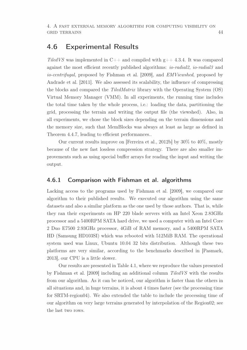
4. A fast external memory algorithm for computing visibility on
grid terrains 44
4.6 Experimental Results
TiledVS was implemented in C++ and compiled with g++ 4.3.4. It was compared
against the most efficient recently published algorithms: io-radial2, io-radial3 and
io-centrifugal, proposed by Fishman et al. [2009], and EMViewshed, proposed by
Andrade et al. [2011]. We also assessed its scalability, the influence of compressing
the blocks and compared the TiledMatrix library with the Operating System (OS)
Virtual Memory Manager (VMM). In all experiments, the running time includes
the total time taken by the whole process, i.e.: loading the data, partitioning the
grid, processing the terrain and writing the output file (the viewshed). Also, in
all experiments, we chose the block sizes depending on the terrain dimensions and
the memory size, such that MemBlocks was always at least as large as defined in
Theorem 4.4.7, leading to efficient performances..
Our current results improve on [Ferreira et al., 2012b] by 30% to 40%, mostly
because of the new fast lossless compression strategy. There are also smaller im-
provements such as using special buffer arrays for reading the input and writing the
output.
4.6.1 Comparison with Fishman et al. algorithms
Lacking access to the programs used by Fishman et al. [2009], we compared our
algorithm to their published results. We executed our algorithm using the same
datasets and also a similar platform as the one used by those authors. That is, while
they ran their experiments on HP 220 blade servers with an Intel Xeon 2.83GHz
processor and a 5400RPM SATA hard drive, we used a computer with an Intel Core
2 Duo E7500 2.93GHz processor, 4GiB of RAM memory, and a 5400RPM SATA
HD (Samsung HD103SI) which was rebooted with 512MiB RAM. The operational
system used was Linux, Ubuntu 10.04 32 bits distribution. Although these two
platforms are very similar, according to the benchmarks described in [Pasmark,
2013], our CPU is a little slower.
Our results are presented in Table 4.1, where we reproduce the values presented
by Fishman et al. [2009] including an additional column TiledVS with the results
from our algorithm. As it can be noticed, our algorithm is faster than the others in
all situations and, in huge terrains, it is about 4 times faster (see the processing time
for SRTM-region04). We also extended the table to include the processing time of
our algorithm on very large terrains generated by interpolation of the Region02; see
the last two rows.
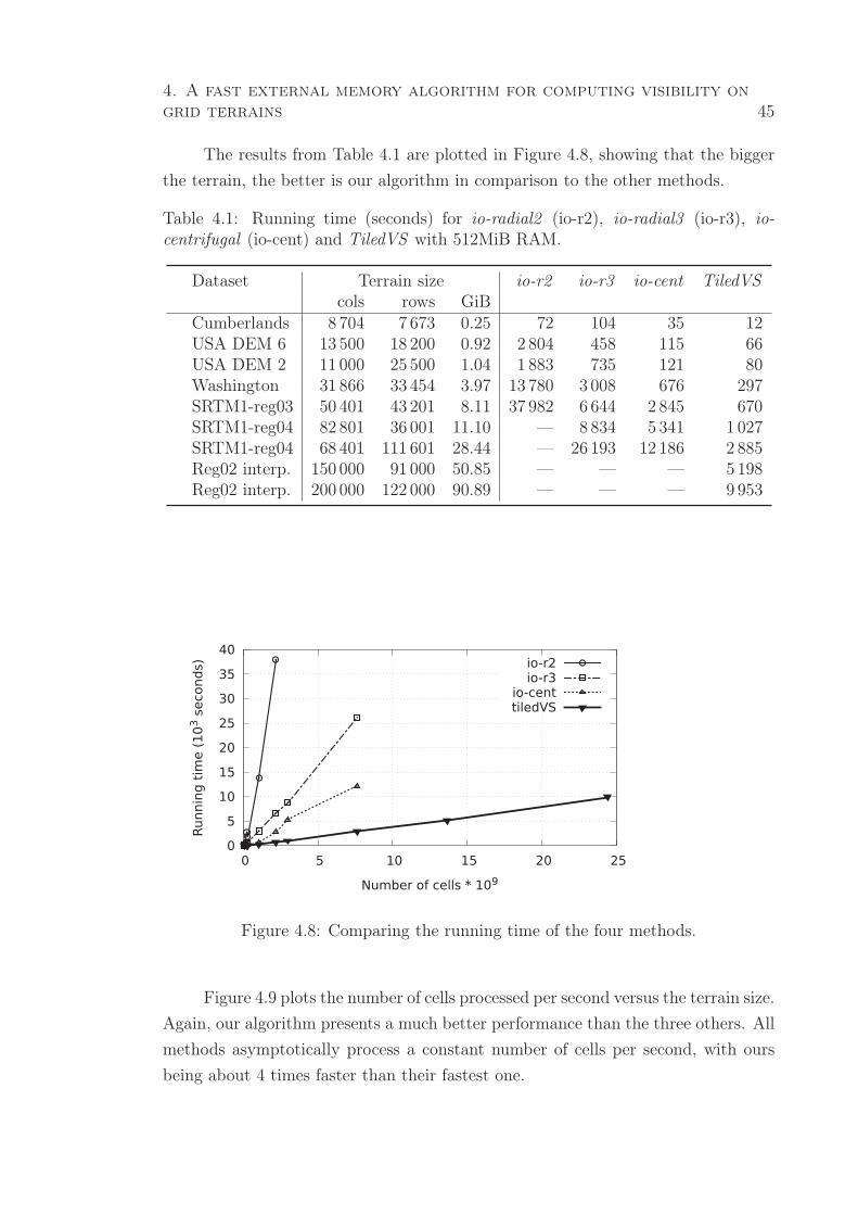
4. A fast external memory algorithm for computing visibility on
grid terrains 45
The results from Table 4.1 are plotted in Figure 4.8, showing that the bigger
the terrain, the better is our algorithm in comparison to the other methods.
Table 4.1: Running time (seconds) for io-radial2 (io-r2), io-radial3 (io-r3), io-centrifugal (io-cent) and TiledVS with 512MiB RAM.
Dataset Terrain size io-r2 io-r3 io-cent TiledVScols rows GiB
Cumberlands 8 704 7 673 0.25 72 104 35 12USA DEM 6 13 500 18 200 0.92 2 804 458 115 66USA DEM 2 11 000 25 500 1.04 1 883 735 121 80Washington 31 866 33 454 3.97 13 780 3 008 676 297SRTM1-reg03 50 401 43 201 8.11 37 982 6 644 2 845 670SRTM1-reg04 82 801 36 001 11.10 — 8834 5 341 1 027SRTM1-reg04 68 401 111 601 28.44 — 26 193 12 186 2 885Reg02 interp. 150 000 91 000 50.85 — — — 5198Reg02 interp. 200 000 122 000 90.89 — — — 9953
��
��
���
���
���
���
���
���
���
�� �� ��� ��� ��� ���
���� ��
��������������
��������������������
����������
����� ������
Figure 4.8: Comparing the running time of the four methods.
Figure 4.9 plots the number of cells processed per second versus the terrain size.
Again, our algorithm presents a much better performance than the three others. All
methods asymptotically process a constant number of cells per second, with ours
being about 4 times faster than their fastest one.
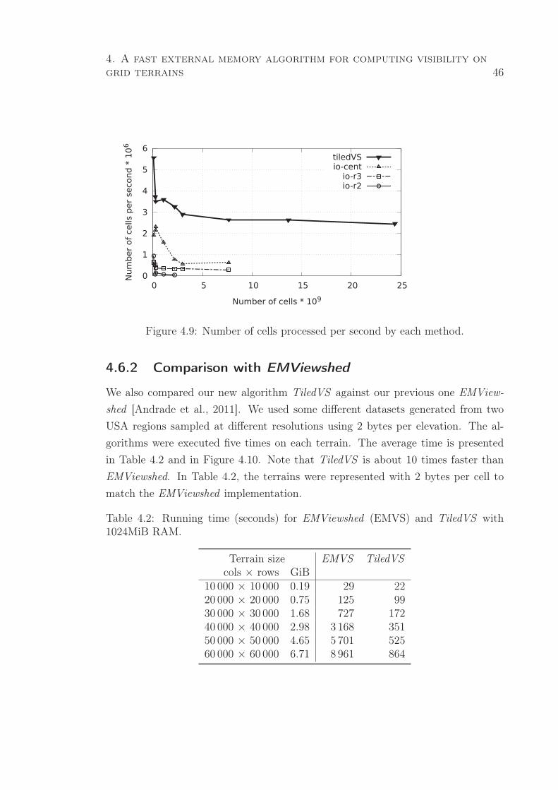
4. A fast external memory algorithm for computing visibility on
grid terrains 46
��
��
��
��
��
��
��
�� �� ��� ��� ��� ���
�� ������ ����� ��� ����������
�� ������ ���������
��� ������� ������������
Figure 4.9: Number of cells processed per second by each method.
4.6.2 Comparison with EMViewshed
We also compared our new algorithm TiledVS against our previous one EMView-
shed [Andrade et al., 2011]. We used some different datasets generated from two
USA regions sampled at different resolutions using 2 bytes per elevation. The al-
gorithms were executed five times on each terrain. The average time is presented
in Table 4.2 and in Figure 4.10. Note that TiledVS is about 10 times faster than
EMViewshed. In Table 4.2, the terrains were represented with 2 bytes per cell to
match the EMViewshed implementation.
Table 4.2: Running time (seconds) for EMViewshed (EMVS) and TiledVS with1024MiB RAM.
Terrain size EMVS TiledVScols × rows GiB
10 000 × 10 000 0.19 29 2220 000 × 20 000 0.75 125 9930 000 × 30 000 1.68 727 17240 000 × 40 000 2.98 3 168 35150 000 × 50 000 4.65 5 701 52560 000 × 60 000 6.71 8 961 864
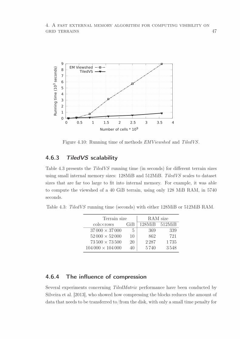
4. A fast external memory algorithm for computing visibility on
grid terrains 47
��
��
��
��
��
��
��
�
�
��
�� ���� �� ���� �� ���� �� ���� ��
����������
���������������
���������������� ����
!"�#��$�%��&����#'
Figure 4.10: Running time of methods EMViewshed and TiledVS .
4.6.3 TiledVS scalability
Table 4.3 presents the TiledVS running time (in seconds) for different terrain sizes
using small internal memory sizes: 128MiB and 512MiB. TiledVS scales to dataset
sizes that are far too large to fit into internal memory. For example, it was able
to compute the viewshed of a 40 GiB terrain, using only 128 MiB RAM, in 5740
seconds.
Table 4.3: TiledVS running time (seconds) with either 128MiB or 512MiB RAM.
Terrain size RAM sizecols×rows GiB 128MiB 512MiB
37 000× 37 000 5 369 33952 000× 52 000 10 862 72173 500× 73 500 20 2 287 1 735
104 000× 104 000 40 5 740 3 548
4.6.4 The influence of compression
Several experiments concerning TiledMatrix performance have been conducted by
Silveira et al. [2013], who showed how compressing the blocks reduces the amount of
data that needs to be transferred to/from the disk, with only a small time penalty for
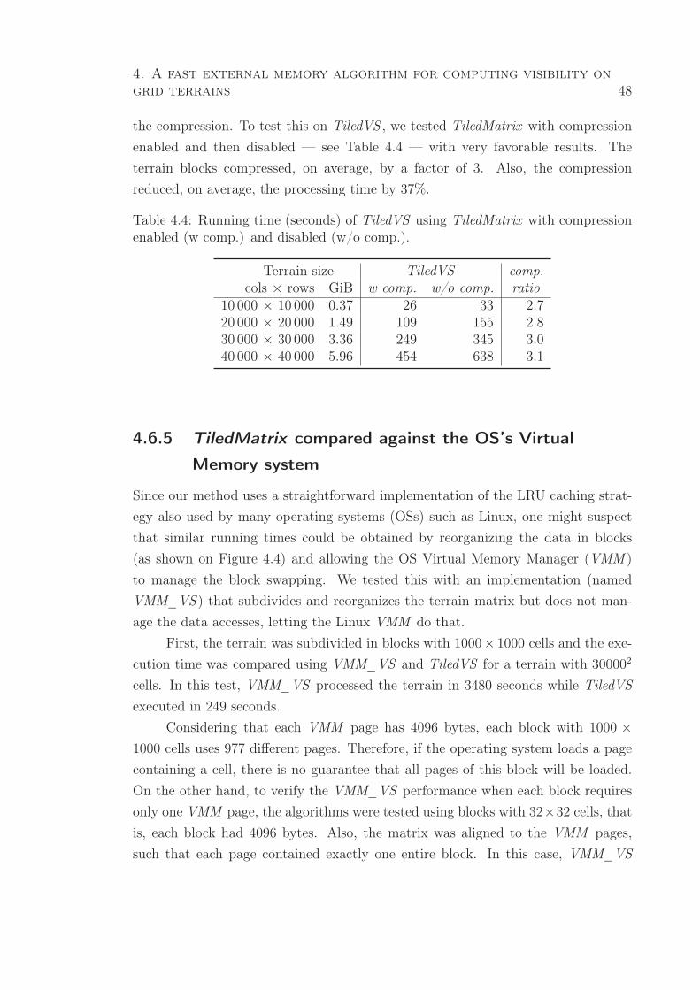
4. A fast external memory algorithm for computing visibility on
grid terrains 48
the compression. To test this on TiledVS , we tested TiledMatrix with compression
enabled and then disabled — see Table 4.4 — with very favorable results. The
terrain blocks compressed, on average, by a factor of 3. Also, the compression
reduced, on average, the processing time by 37%.
Table 4.4: Running time (seconds) of TiledVS using TiledMatrix with compressionenabled (w comp.) and disabled (w/o comp.).
Terrain size TiledVS comp.cols × rows GiB w comp. w/o comp. ratio
10 000 × 10 000 0.37 26 33 2.720 000 × 20 000 1.49 109 155 2.830 000 × 30 000 3.36 249 345 3.040 000 × 40 000 5.96 454 638 3.1
4.6.5 TiledMatrix compared against the OS’s Virtual
Memory system
Since our method uses a straightforward implementation of the LRU caching strat-
egy also used by many operating systems (OSs) such as Linux, one might suspect
that similar running times could be obtained by reorganizing the data in blocks
(as shown on Figure 4.4) and allowing the OS Virtual Memory Manager (VMM )
to manage the block swapping. We tested this with an implementation (named
VMM_VS ) that subdivides and reorganizes the terrain matrix but does not man-
age the data accesses, letting the Linux VMM do that.
First, the terrain was subdivided in blocks with 1000× 1000 cells and the exe-
cution time was compared using VMM_VS and TiledVS for a terrain with 300002
cells. In this test, VMM_VS processed the terrain in 3480 seconds while TiledVS
executed in 249 seconds.
Considering that each VMM page has 4096 bytes, each block with 1000 ×
1000 cells uses 977 different pages. Therefore, if the operating system loads a page
containing a cell, there is no guarantee that all pages of this block will be loaded.
On the other hand, to verify the VMM_VS performance when each block requires
only one VMM page, the algorithms were tested using blocks with 32×32 cells, that
is, each block had 4096 bytes. Also, the matrix was aligned to the VMM pages,
such that each page contained exactly one entire block. In this case, VMM_VS
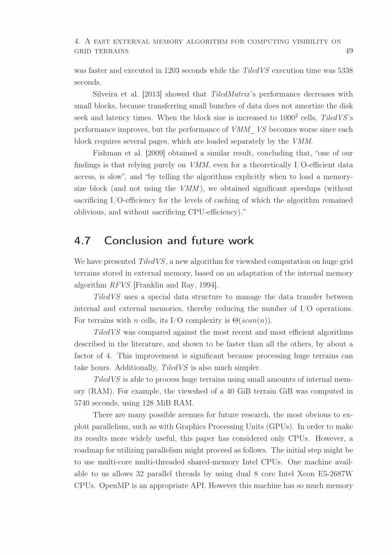
4. A fast external memory algorithm for computing visibility on
grid terrains 49
was faster and executed in 1203 seconds while the TiledVS execution time was 5338
seconds.
Silveira et al. [2013] showed that TiledMatrix ’s performance decreases with
small blocks, because transferring small bunches of data does not amortize the disk
seek and latency times. When the block size is increased to 10002 cells, TiledVS ’s
performance improves, but the performance of VMM_VS becomes worse since each
block requires several pages, which are loaded separately by the VMM.
Fishman et al. [2009] obtained a similar result, concluding that, “one of our
findings is that relying purely on VMM, even for a theoretically I/O-efficient data
access, is slow”, and “by telling the algorithms explicitly when to load a memory-
size block (and not using the VMM ), we obtained significant speedups (without
sacrificing I/O-efficiency for the levels of caching of which the algorithm remained
oblivious, and without sacrificing CPU-efficiency).”
4.7 Conclusion and future work
We have presented TiledVS , a new algorithm for viewshed computation on huge grid
terrains stored in external memory, based on an adaptation of the internal memory
algorithm RFVS [Franklin and Ray, 1994].
TiledVS uses a special data structure to manage the data transfer between
internal and external memories, thereby reducing the number of I/O operations.
For terrains with n cells, its I/O complexity is Θ(scan(n)).
TiledVS was compared against the most recent and most efficient algorithms
described in the literature, and shown to be faster than all the others, by about a
factor of 4. This improvement is significant because processing huge terrains can
take hours. Additionally, TiledVS is also much simpler.
TiledVS is able to process huge terrains using small amounts of internal mem-
ory (RAM). For example, the viewshed of a 40 GiB terrain GiB was computed in
5740 seconds, using 128 MiB RAM.
There are many possible avenues for future research, the most obvious to ex-
ploit parallelism, such as with Graphics Processing Units (GPUs). In order to make
its results more widely useful, this paper has considered only CPUs. However, a
roadmap for utilizing parallelism might proceed as follows. The initial step might be
to use multi-core multi-threaded shared-memory Intel CPUs. One machine avail-
able to us allows 32 parallel threads by using dual 8 core Intel Xeon E5-2687W
CPUs. OpenMP is an appropriate API. However this machine has so much memory

4. A fast external memory algorithm for computing visibility on
grid terrains 50
(128GB) that external algorithms are unnecessary. The next step would be to use
the NVIDIA Tesla K20x GPU accelerator mentioned earlier, which has 2688 CUDA
cores. Although each core has only about one tenth of the computing power of one
Intel thread, there are a lot of them. The problem is that efficiently using them is
not yet a totally solved problem. Nevertheless, we are pursuing this approach.
Our algorithm source code (in C++) is available, as open source
code distributed under a Creative Common GNU GPL license, at
http://www.dpi.ufv.br/∼marcus/TiledVS.htm
5. A parallel sweep line algorithm for visi-
bility computation1
Abstract
Visibility map (or viewshed) computation is required for many GIS ap-
plications. As terrain data continue to become available at higher resolutions,
there is a need for faster architectures and algorithms. Since the main im-
provements on modern processors come from multi-core architectures, parallel
programming provides a promising means for developing faster algorithms. In
this paper, we describe a new parallel algorithm, based on the model proposed
by Van Kreveld [1996]. Our algorithm uses the shared memory model, which
is relatively cheap and supported by most current processors. Experiments
have shown that, with 16 parallel cores, it was up to 12 times faster than the
serial implementation.
5.1 Introduction
An important group of Geographical Information Science (GIS) applications on
terrains concerns visibility, i.e., determining the set of points on the terrain that are
visible from some particular observer, which is usually located at some height above
the terrain. This set of points is known as viewshed [Franklin and Ray, 1994] and
its applications range from visual nuisance abatement to radio transmitter siting
and surveillance, such as minimizing the number of cellular phone towers required
to cover a region [Ben-Shimol et al., 2007], optimizing the number and position
of guards to cover a region [Magalhães et al., 2011], analysing the influences on
property prices in an urban environment [Lake et al., 1998] and optimizing path
planning [Lee and Stucky, 1998]. Other applications are presented in Champion
and Lavery [2002].
Since visibility computation is quite compute-intensive, the recent increase in
the volume of high resolution terrestrial data brings a need for faster platforms and
algorithms. Considering that some factors (such as processor sizes, transmission
1Este capítulo apresenta o artigo “A Parallel Sweep Line Algorithm for Visibility Computa-
tion”, que recebeu o prêmio de melhor artigo no GeoInfo 2013 (XIV Brazilian Symposium on
Geoinformatics) [Ferreira et al., 2013].
51
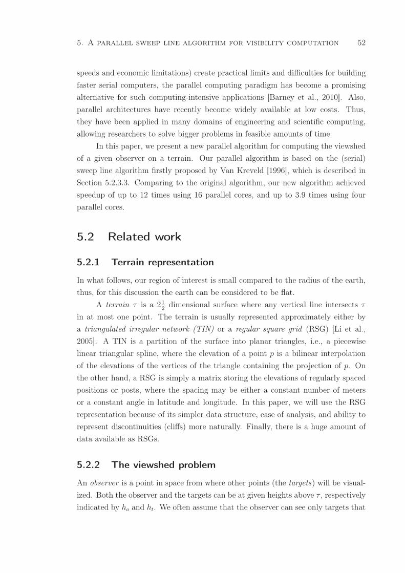
5. A parallel sweep line algorithm for visibility computation 52
speeds and economic limitations) create practical limits and difficulties for building
faster serial computers, the parallel computing paradigm has become a promising
alternative for such computing-intensive applications [Barney et al., 2010]. Also,
parallel architectures have recently become widely available at low costs. Thus,
they have been applied in many domains of engineering and scientific computing,
allowing researchers to solve bigger problems in feasible amounts of time.
In this paper, we present a new parallel algorithm for computing the viewshed
of a given observer on a terrain. Our parallel algorithm is based on the (serial)
sweep line algorithm firstly proposed by Van Kreveld [1996], which is described in
Section 5.2.3.3. Comparing to the original algorithm, our new algorithm achieved
speedup of up to 12 times using 16 parallel cores, and up to 3.9 times using four
parallel cores.
5.2 Related work
5.2.1 Terrain representation
In what follows, our region of interest is small compared to the radius of the earth,
thus, for this discussion the earth can be considered to be flat.
A terrain τ is a 212dimensional surface where any vertical line intersects τ
in at most one point. The terrain is usually represented approximately either by
a triangulated irregular network (TIN) or a regular square grid (RSG) [Li et al.,
2005]. A TIN is a partition of the surface into planar triangles, i.e., a piecewise
linear triangular spline, where the elevation of a point p is a bilinear interpolation
of the elevations of the vertices of the triangle containing the projection of p. On
the other hand, a RSG is simply a matrix storing the elevations of regularly spaced
positions or posts, where the spacing may be either a constant number of meters
or a constant angle in latitude and longitude. In this paper, we will use the RSG
representation because of its simpler data structure, ease of analysis, and ability to
represent discontinuities (cliffs) more naturally. Finally, there is a huge amount of
data available as RSGs.
5.2.2 The viewshed problem
An observer is a point in space from where other points (the targets) will be visual-
ized. Both the observer and the targets can be at given heights above τ , respectively
indicated by ho and ht. We often assume that the observer can see only targets that
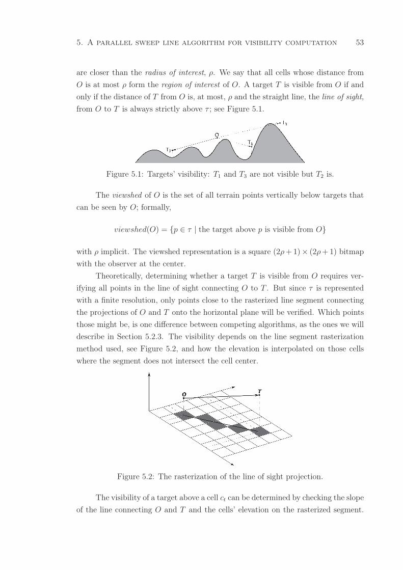
5. A parallel sweep line algorithm for visibility computation 53
are closer than the radius of interest, ρ. We say that all cells whose distance from
O is at most ρ form the region of interest of O. A target T is visible from O if and
only if the distance of T from O is, at most, ρ and the straight line, the line of sight,
from O to T is always strictly above τ ; see Figure 5.1.
Figure 5.1: Targets’ visibility: T1 and T3 are not visible but T2 is.
The viewshed of O is the set of all terrain points vertically below targets that
can be seen by O; formally,
viewshed(O) = {p ∈ τ | the target above p is visible from O}
with ρ implicit. The viewshed representation is a square (2ρ+1)× (2ρ+1) bitmap
with the observer at the center.
Theoretically, determining whether a target T is visible from O requires ver-
ifying all points in the line of sight connecting O to T . But since τ is represented
with a finite resolution, only points close to the rasterized line segment connecting
the projections of O and T onto the horizontal plane will be verified. Which points
those might be, is one difference between competing algorithms, as the ones we will
describe in Section 5.2.3. The visibility depends on the line segment rasterization
method used, see Figure 5.2, and how the elevation is interpolated on those cells
where the segment does not intersect the cell center.
Figure 5.2: The rasterization of the line of sight projection.
The visibility of a target above a cell ct can be determined by checking the slope
of the line connecting O and T and the cells’ elevation on the rasterized segment.
5. A parallel sweep line algorithm for visibility computation 54
More precisely, suppose the segment is composed of cells c0, c1, · · · , ct where c0 and
ct correspond to the projections of O and T respectively. Let αi be the slope of the
line connecting O to ci, that is,
αi =ζ(ci)− (ζ(c0) + ho)
dist(c0, ci)(5.1)
where ζ(c0) and ζ(ci) are, respectively, the elevation of cells c0 and ci and dist(c0, ci)
is the ‘distance’ (in number of cells) between these two cells. The target on ct is
visible if and only if the slope ζ(ct)+ht−(ζ(c0)+ho)dist(c0,ct)
is greater than αi for all 0 < i < t.
If yes, the corresponding cell in the viewshed matrix is set to 1; otherwise, to 0.
5.2.3 Viewshed algorithms
Different terrain representations call for different algorithms. A TIN can be pro-
cessed by the algorithms proposed by Cole and Sharir [1989] and Floriani and Mag-
illo [2003]. For a RSG, we can point out [Van Kreveld, 1996] and RFVS [Franklin
and Ray, 1994], two very efficient algorithms. Another option for processing RSGs
is the well-known R3 algorithm [Shapira, 1990]. Although this one is not as efficient
as the other two, it has higher accuracy and may be suitable for small datasets.
These three algorithms differ from each other not only on their efficiency, but
also on the visibility models adopted. For instance, R3 and Van Kreveld’s algorithms
use a center-of-cell to center-of-cell visibility, that is, a cell c is visible if and only if
the ray connecting the observer (in the center of its cell) to the center of c does not
intersect a cell blocking c. On the other hand, RFVS uses a less restrictive approach
where a cell c may be considered visible if its center is not visible but another part
of c is.
Therefore, the viewsheds obtained by these methods may be different. Without
knowing the application and having a model for the terrain’s elevation between the
known points, it is impossible to say which one is better. Some applications may
prefer a viewshed biased in one direction or the other, while others may want to
minimize error computed under some formal terrain model. For instance, since
Van Kreveld’s algorithm presents a great tradeoff between efficiency and accuracy
[Fishman et al., 2009], it may be indicated for applications that require a high degree
of accuracy. On the other hand, if efficiency is more important than accuracy, the
RFVS algorithm could be preferred.
Considering that each one of these algorithms might be suitable for different
applications, we will describe them briefly in the next sections.
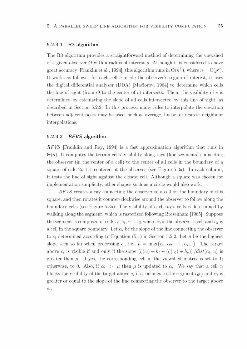
5. A parallel sweep line algorithm for visibility computation 55
5.2.3.1 R3 algorithm
The R3 algorithm provides a straightforward method of determining the viewshed
of a given observer O with a radius of interest ρ. Although it is considered to have
great accuracy [Franklin et al., 1994], this algorithm runs inΘ(n3
2 ), where n = Θ(ρ2).
It works as follows: for each cell c inside the observer’s region of interest, it uses
the digital differential analyzer (DDA) [Maćiorov, 1964] to determine which cells
the line of sight (from O to the center of c) intersects. Then, the visibility of c is
determined by calculating the slope of all cells intersected by this line of sight, as
described in Section 5.2.2. In this process, many rules to interpolate the elevation
between adjacent posts may be used, such as average, linear, or nearest neighbour
interpolations.
5.2.3.2 RFVS algorithm
RFVS [Franklin and Ray, 1994] is a fast approximation algorithm that runs in
Θ(n). It computes the terrain cells’ visibility along rays (line segments) connecting
the observer (in the center of a cell) to the center of all cells in the boundary of a
square of side 2ρ + 1 centered at the observer (see Figure 5.3a). In each column,
it tests the line of sight against the closest cell. Although a square was chosen for
implementation simplicity, other shapes such as a circle would also work.
RFVS creates a ray connecting the observer to a cell on the boundary of this
square, and then rotates it counter-clockwise around the observer to follow along the
boundary cells (see Figure 5.3a). The visibility of each ray’s cells is determined by
walking along the segment, which is rasterized following Bresenham [1965]. Suppose
the segment is composed of cells c0, c1, · · · , ck where c0 is the observer’s cell and ck is
a cell in the square boundary. Let αi be the slope of the line connecting the observer
to ci determined according to Equation (5.1) in Section 5.2.2. Let µ be the highest
slope seen so far when processing ci, i.e., µ = max{α1, α2, · · · , αi−1}. The target
above ci is visible if and only if the slope (ζ(ci) + ht − (ζ(c0) + ho)) /dist(c0, ci) is
greater than µ. If yes, the corresponding cell in the viewshed matrix is set to 1;
otherwise, to 0. Also, if αi > µ then µ is updated to αi. We say that a cell ci
blocks the visibility of the target above cj if ci belongs to the segment c0cj and αi is
greater or equal to the slope of the line connecting the observer to the target above
cj.
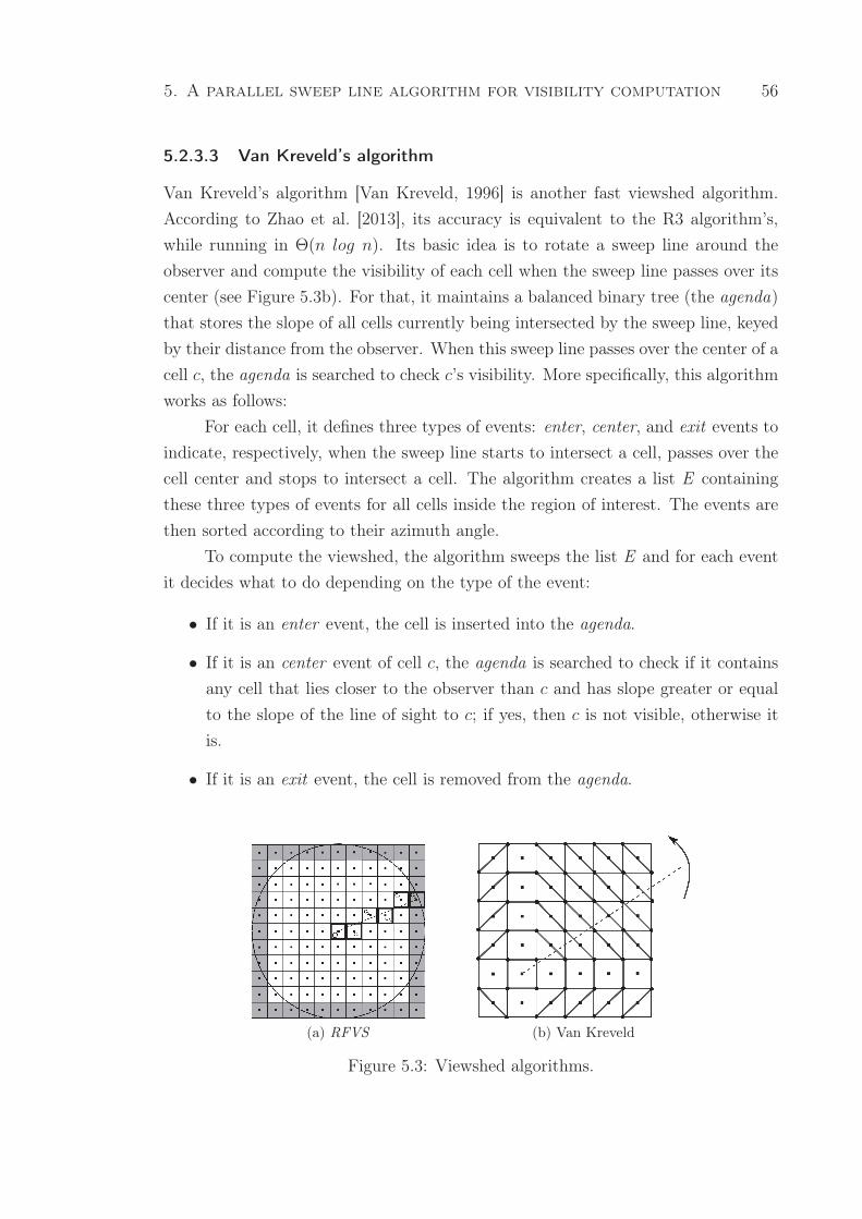
5. A parallel sweep line algorithm for visibility computation 56
5.2.3.3 Van Kreveld’s algorithm
Van Kreveld’s algorithm [Van Kreveld, 1996] is another fast viewshed algorithm.
According to Zhao et al. [2013], its accuracy is equivalent to the R3 algorithm’s,
while running in Θ(n log n). Its basic idea is to rotate a sweep line around the
observer and compute the visibility of each cell when the sweep line passes over its
center (see Figure 5.3b). For that, it maintains a balanced binary tree (the agenda)
that stores the slope of all cells currently being intersected by the sweep line, keyed
by their distance from the observer. When this sweep line passes over the center of a
cell c, the agenda is searched to check c’s visibility. More specifically, this algorithm
works as follows:
For each cell, it defines three types of events: enter, center, and exit events to
indicate, respectively, when the sweep line starts to intersect a cell, passes over the
cell center and stops to intersect a cell. The algorithm creates a list E containing
these three types of events for all cells inside the region of interest. The events are
then sorted according to their azimuth angle.
To compute the viewshed, the algorithm sweeps the list E and for each event
it decides what to do depending on the type of the event:
• If it is an enter event, the cell is inserted into the agenda.
• If it is an center event of cell c, the agenda is searched to check if it contains
any cell that lies closer to the observer than c and has slope greater or equal
to the slope of the line of sight to c; if yes, then c is not visible, otherwise it
is.
• If it is an exit event, the cell is removed from the agenda.
(a) RFVS (b) Van Kreveld
Figure 5.3: Viewshed algorithms.
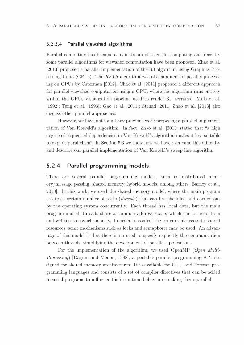
5. A parallel sweep line algorithm for visibility computation 57
5.2.3.4 Parallel viewshed algorithms
Parallel computing has become a mainstream of scientific computing and recently
some parallel algorithms for viewshed computation have been proposed. Zhao et al.
[2013] proposed a parallel implementation of the R3 algorithm using Graphics Pro-
cessing Units (GPUs). The RFVS algorithm was also adapted for parallel process-
ing on GPUs by Osterman [2012]. Chao et al. [2011] proposed a different approach
for parallel viewshed computation using a GPU, where the algorithm runs entirely
within the GPUs visualization pipeline used to render 3D terrains. Mills et al.
[1992]; Teng et al. [1993]; Gao et al. [2011]; Strnad [2011] Zhao et al. [2013] also
discuss other parallel approaches.
However, we have not found any previous work proposing a parallel implemen-
tation of Van Kreveld’s algorithm. In fact, Zhao et al. [2013] stated that “a high
degree of sequential dependencies in Van Kreveld’s algorithm makes it less suitable
to exploit parallelism”. In Section 5.3 we show how we have overcome this difficulty
and describe our parallel implementation of Van Kreveld’s sweep line algorithm.
5.2.4 Parallel programming models
There are several parallel programming models, such as distributed mem-
ory/message passing, shared memory, hybrid models, among others [Barney et al.,
2010]. In this work, we used the shared memory model, where the main program
creates a certain number of tasks (threads) that can be scheduled and carried out
by the operating system concurrently. Each thread has local data, but the main
program and all threads share a common address space, which can be read from
and written to asynchronously. In order to control the concurrent access to shared
resources, some mechanisms such as locks and semaphores may be used. An advan-
tage of this model is that there is no need to specify explicitly the communication
between threads, simplifying the development of parallel applications.
For the implementation of the algorithm, we used OpenMP (Open Multi-
Processing) [Dagum and Menon, 1998], a portable parallel programming API de-
signed for shared memory architectures. It is available for C++ and Fortran pro-
gramming languages and consists of a set of compiler directives that can be added
to serial programs to influence their run-time behaviour, making them parallel.
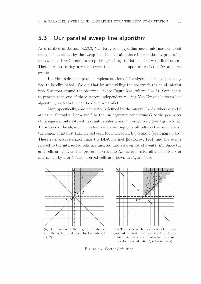
5. A parallel sweep line algorithm for visibility computation 58
5.3 Our parallel sweep line algorithm
As described in Section 5.2.3.3, Van Kreveld’s algorithm needs information about
the cells intersected by the sweep line. It maintains these information by processing
the enter and exit events to keep the agenda up to date as the sweep line rotates.
Therefore, processing a center event is dependent upon all earlier enter and exit
events.
In order to design a parallel implementation of this algorithm, this dependency
had to be eliminated. We did that by subdividing the observer’s region of interest
into S sectors around the observer, O (see Figure 5.4a, where S = 8). Our idea is
to process each one of these sectors independently using Van Kreveld’s sweep line
algorithm, such that it can be done in parallel.
More specifically, consider sector s defined by the interval [α, β), where α and β
are azimuth angles. Let a and b be the line segments connecting O to the perimeter
of its region of interest, with azimuth angles α and β, respectively (see Figure 5.4a).
To process s, the algorithm creates rays connecting O to all cells on the perimeter of
the region of interest that are between (or intersected by) a and b (see Figure 5.4b).
These rays are rasterized using the DDA method [Maćiorov, 1964] and the events
related to the intersected cells are inserted into s’s own list of events, Es. Since the
grid cells are convex, this process inserts into Es the events for all cells inside s or
intersected by a or b. The inserted cells are shown in Figure 5.4b.
(a) Subdivision of the region of interestand the sector s, defined by the interval[α, β).
(b) The cells in the perimeter of the re-gion of interest, the rays used to deter-mine which cells are intersected by s andthe cells inserted into Es (shaded cells).
Figure 5.4: Sector definition.
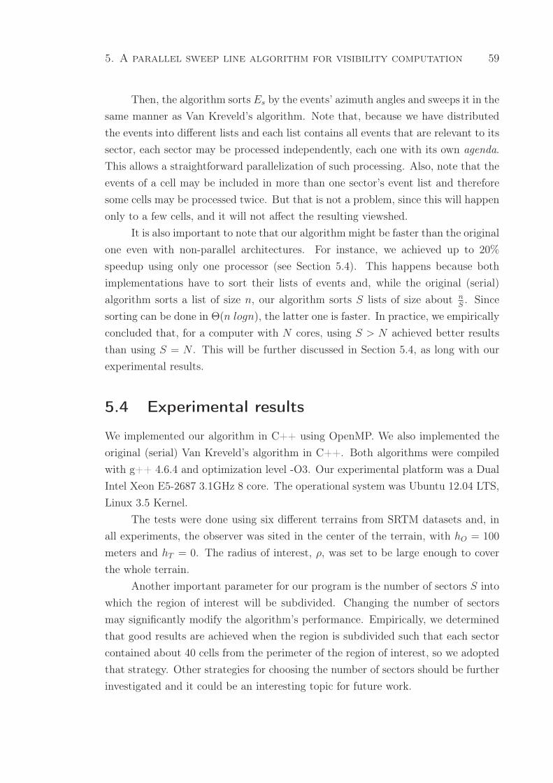
5. A parallel sweep line algorithm for visibility computation 59
Then, the algorithm sorts Es by the events’ azimuth angles and sweeps it in the
same manner as Van Kreveld’s algorithm. Note that, because we have distributed
the events into different lists and each list contains all events that are relevant to its
sector, each sector may be processed independently, each one with its own agenda.
This allows a straightforward parallelization of such processing. Also, note that the
events of a cell may be included in more than one sector’s event list and therefore
some cells may be processed twice. But that is not a problem, since this will happen
only to a few cells, and it will not affect the resulting viewshed.
It is also important to note that our algorithm might be faster than the original
one even with non-parallel architectures. For instance, we achieved up to 20%
speedup using only one processor (see Section 5.4). This happens because both
implementations have to sort their lists of events and, while the original (serial)
algorithm sorts a list of size n, our algorithm sorts S lists of size about nS. Since
sorting can be done in Θ(n logn), the latter one is faster. In practice, we empirically
concluded that, for a computer with N cores, using S > N achieved better results
than using S = N . This will be further discussed in Section 5.4, as long with our
experimental results.
5.4 Experimental results
We implemented our algorithm in C++ using OpenMP. We also implemented the
original (serial) Van Kreveld’s algorithm in C++. Both algorithms were compiled
with g++ 4.6.4 and optimization level -O3. Our experimental platform was a Dual
Intel Xeon E5-2687 3.1GHz 8 core. The operational system was Ubuntu 12.04 LTS,
Linux 3.5 Kernel.
The tests were done using six different terrains from SRTM datasets and, in
all experiments, the observer was sited in the center of the terrain, with hO = 100
meters and hT = 0. The radius of interest, ρ, was set to be large enough to cover
the whole terrain.
Another important parameter for our program is the number of sectors S into
which the region of interest will be subdivided. Changing the number of sectors
may significantly modify the algorithm’s performance. Empirically, we determined
that good results are achieved when the region is subdivided such that each sector
contained about 40 cells from the perimeter of the region of interest, so we adopted
that strategy. Other strategies for choosing the number of sectors should be further
investigated and it could be an interesting topic for future work.
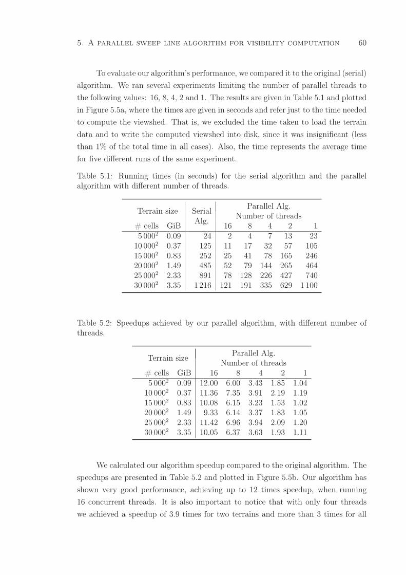
5. A parallel sweep line algorithm for visibility computation 60
To evaluate our algorithm’s performance, we compared it to the original (serial)
algorithm. We ran several experiments limiting the number of parallel threads to
the following values: 16, 8, 4, 2 and 1. The results are given in Table 5.1 and plotted
in Figure 5.5a, where the times are given in seconds and refer just to the time needed
to compute the viewshed. That is, we excluded the time taken to load the terrain
data and to write the computed viewshed into disk, since it was insignificant (less
than 1% of the total time in all cases). Also, the time represents the average time
for five different runs of the same experiment.
Table 5.1: Running times (in seconds) for the serial algorithm and the parallelalgorithm with different number of threads.
Terrain size SerialAlg.
Parallel Alg.Number of threads
# cells GiB 16 8 4 2 15 0002 0.09 24 2 4 7 13 2310 0002 0.37 125 11 17 32 57 10515 0002 0.83 252 25 41 78 165 24620 0002 1.49 485 52 79 144 265 46425 0002 2.33 891 78 128 226 427 74030 0002 3.35 1 216 121 191 335 629 1 100
Table 5.2: Speedups achieved by our parallel algorithm, with different number ofthreads.
Terrain sizeParallel Alg.
Number of threads# cells GiB 16 8 4 2 15 0002 0.09 12.00 6.00 3.43 1.85 1.0410 0002 0.37 11.36 7.35 3.91 2.19 1.1915 0002 0.83 10.08 6.15 3.23 1.53 1.0220 0002 1.49 9.33 6.14 3.37 1.83 1.0525 0002 2.33 11.42 6.96 3.94 2.09 1.2030 0002 3.35 10.05 6.37 3.63 1.93 1.11
We calculated our algorithm speedup compared to the original algorithm. The
speedups are presented in Table 5.2 and plotted in Figure 5.5b. Our algorithm has
shown very good performance, achieving up to 12 times speedup, when running
16 concurrent threads. It is also important to notice that with only four threads
we achieved a speedup of 3.9 times for two terrains and more than 3 times for all
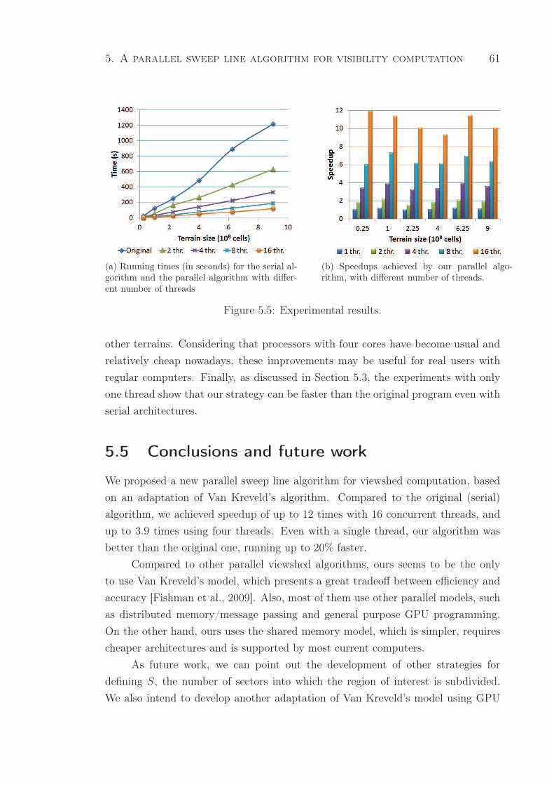
5. A parallel sweep line algorithm for visibility computation 61
(a) Running times (in seconds) for the serial al-gorithm and the parallel algorithm with differ-ent number of threads
(b) Speedups achieved by our parallel algo-rithm, with different number of threads.
Figure 5.5: Experimental results.
other terrains. Considering that processors with four cores have become usual and
relatively cheap nowadays, these improvements may be useful for real users with
regular computers. Finally, as discussed in Section 5.3, the experiments with only
one thread show that our strategy can be faster than the original program even with
serial architectures.
5.5 Conclusions and future work
We proposed a new parallel sweep line algorithm for viewshed computation, based
on an adaptation of Van Kreveld’s algorithm. Compared to the original (serial)
algorithm, we achieved speedup of up to 12 times with 16 concurrent threads, and
up to 3.9 times using four threads. Even with a single thread, our algorithm was
better than the original one, running up to 20% faster.
Compared to other parallel viewshed algorithms, ours seems to be the only
to use Van Kreveld’s model, which presents a great tradeoff between efficiency and
accuracy [Fishman et al., 2009]. Also, most of them use other parallel models, such
as distributed memory/message passing and general purpose GPU programming.
On the other hand, ours uses the shared memory model, which is simpler, requires
cheaper architectures and is supported by most current computers.
As future work, we can point out the development of other strategies for
defining S, the number of sectors into which the region of interest is subdivided.
We also intend to develop another adaptation of Van Kreveld’s model using GPU

5. A parallel sweep line algorithm for visibility computation 62
programming. Since GPU architectures are much more complex, this will not be a
straightforward adaptation.
6. Conclusões gerais e trabalhos futuros
Neste trabalho foram apresentados dois algoritmos para cálculo de viewshed em
grandes terrenos representados por grades regulares: um especialmente projetado
para ser eficiente em terrenos maiores do que a memória interna disponível, e ou-
tro capaz de utilizar arquiteturas paralelas de forma eficiente. Como mostraram
os resultados experimentais, ambos são mais eficientes do que algoritmos propostos
anteriormente em literatura. Os ganhos (speedups) obtidos por estes dois algoritmos
podem ser importantes para usuários de aplicações de visibilidade de duas diferentes
maneiras: primeiramente, com um algoritmo mais rápido é possível avaliar regiões
maiores em tempos razoáveis; além disso, também é possível avaliar uma determi-
nada região com dados em alta resolução, gerando resultados cada vez mais precisos
sem necessariamente aumentar o tempo de processamento.
Nos Capítulos de 2 a 4 foi apresentado o algoritmo para memória externa Ti-
ledVS . Este algoritmo consiste em uma adaptação do algoritmo RFVS , proposto por
Franklin and Ray [1994]. Para diminuir o número de operações de E/S realizadas,
é utilizada a biblioteca especial TiledMatrix [Silveira et al., 2013], que controla os
acessos às matrizes armazenadas em memória externa de forma eficiente. Para isso,
esta biblioteca reorganiza os dados da matriz em memória externa subdividindo-a
em blocos retangulares que são armazenados de forma contígua. A memória interna
é então gerenciada como uma memória cache gerenciada pela aplicação, que carrega
estes blocos à medida que são requisitados acessos a suas células, descarregando,
quando necessário, os blocos que estão a mais tempo sem ser acessados. Além disso,
na versão mais recente deste algoritmo (descrita no Capítulo 4), é utilizada também
uma estratégia de compressão rápida dos blocos, o que conseguiu diminuir os tem-
pos de processamento em até 42%. Os resultados experimentais mostraram que este
novo algoritmo é mais de 4 vezes mais rápido do que todos os demais algoritmos
encontrados em literatura.
Com relação ao algoritmo TiledVS , propõe-se acelerar ainda mais o proces-
samento através de algoritmos paralelos, possivelmente com a utilização de placas
gráficas (GPUs). Uma primeira abordagem seria a paralelização do algoritmo de
compressão utilizado pela TiledMatrix, para que esta compressão seja feita de forma
ainda mais rápida. A segunda ideia seria a paralelização do processo de rotação da
linha de visão utilizado pelo algoritmo RFVS . Esta segunda abordagem representa
63
6. Conclusões gerais e trabalhos futuros 64
uma tarefa bem mais complexa do que a primeira, uma vez que combinar processa-
mento em memória externa com processamento paralelo não é trivial. Porém, como
Zhao et al. [2013] mostraram recentemente, é possível alcançar bons resultados.
No Capítulo 5 foi proposto outro algoritmo para cálculo de viewshed, neste caso
baseado em arquiteturas paralelas. O novo algoritmo utiliza o modelo de progra-
mação paralela de memória compartilhada (OpenMP), disponível na maioria das
arquiteturas atuais, mesmo em computadores pessoais relativamente simples. O
novo algoritmo subdivide o terreno em diversos setores em torno do observador e
processa cada um destes setores de forma independente. Conforme mostrado pe-
los resultados experimentais, usando um computador com 4 cores pode-se obter
resultados até 4 vezes mais rápidos do que o algoritmo convencional (isto é, sequen-
cial). Além disso, com um computador com maior capacidade (por exemplo, com
16 cores), é possível obter processamentos até 12 vezes mais rápidos.
A intenção como trabalho futuro é adaptar este algoritmo utilizando progra-
mação em GPUs. Porém, esta adaptação não poderá ser feita forma direta, uma vez
que a arquitetura das GPUs apresenta diversas diferenças com relação à arquitetura
de um processador multi-core. Por exemplo, dentre as dificuldades que serão encon-
tradas ao fazer esta adaptação, podemos citar o alto custo das operações de cópia
de dados em uma GPU e a impossibilidade de utilizar ponteiros para implementar
a árvore binária balanceada utilizada pelo algoritmo de Van Kreveld. Assim, esta
tarefa exigirá um estudo mais detalhado da arquitetura das GPUs, que são mais
complexas e contém diversas camadas de memória com diferentes características.
Referências Bibliográficas
Aggarwal, A. and Vitter, J. S. (1988). The input/output complexity of sorting and
related problems. Communications of the ACM, 31(9):1116–1127.
Andrade, M. V. A., Magalhães, S. V. G., Magalhães, M. A., Franklin, W. R.,
and Cutler, B. M. (2011). Efficient viewshed computation on terrain in external
memory. Geoinformatica, 15(2):381–397.
Barney, B. et al. (2010). Introduction to parallel computing. Lawrence Livermore
National Laboratory, 6(13):10.
Ben-Moshe, B., Mitchell, J. S. B., Katz, M. J., and Nir, Y. (2002). Visibility
preserving terrain simplification — an experimental study. In Proceedings of
ACM Symposium of Computational Geometry, pages 303–311, Barcelona, Spain.
Ben-Shimol, Y., Ben-Moshe, B., Ben-Yehezkel, Y., Dvir, A., and Segal, M. (2007).
Automated antenna positioning algorithms for wireless fixed-access networks.
Journal of Heuristics, 13(3):243–263.
Bespamyatnikh, S., Chen, Z., Wang, K., and Zhu, B. (2001). On the planar two-
watchtower problem. In 7th International Computing and Combinatorics Confer-
ence, pages 121–130. Springer-Verlag London.
Bresenham, J. E. (1965). An incremental algorithm for digital plotting. IBM Systems
Journal, 4(1):25–30.
Câmara, G., Davis, C., and Monteiro, A. M. (2001). Introdução à Ciência da
Geoinformação. Instituto de Pesquisa Espacial- INPE, São Jose dos Campos, SP,
Brasil,Disponivel em: http://www.dpi.inpe.br/gilberto/livro/introd/ — Aces-
sado em 16 Novembro 2013.
Camp, R. J., Sinton, D. T., and Knight, R. L. (1997). Viewsheds: A complementary
management approach to buffer zones. Wildlife Society Bulletin, 25(3):612–615.
Champion, D. C. and Lavery, J. E. (2002). Line of sight in natural terrain deter-
mined by L1-spline and conventional methods. In 23rd Army Science Conference,
Orlando, Florida.
65
Referências Bibliográficas 66
Chao, F., Chongjun, Y., Zhuo, C., Xiaojing, Y., and Hantao, G. (2011). Parallel
algorithm for viewshed analysis on a modern GPU. International Journal of
Digital Earth, 4(6):471–486.
Cole, R. and Sharir, M. (1989). Visibility problems for polyhedral terrains. Journal
of Symbolic Computation, 7(1):11–30.
Collet, Y. (2012). Extremely fast compression algorithm.
http://code.google.com/p/lz4/.
Dagum, L. and Menon, R. (1998). Openmp: an industry standard api for shared-
memory programming. Computational Science & Engineering, IEEE, 5(1):46–55.
Dementiev, R., Kettner, L., and Sanders, P. (2005). Stxxl : Standard template
library for xxl data sets. Technical report, Fakultät für Informatik, Universität
Karlsruhe. http://stxxl.sourceforge.net/ — Acessado em 01 Dezembro 2013).
Eidenbenz, S. (2002). Approximation algorithms for terrain guarding. Information
Processing Letters, 82(2):99–105.
Felgueiras, C. A. (2001). Modelagem numérica de terreno. In G. Câmara, C. Davis,
A. M. V. M., editor, Introdução à Ciência da Geoinformação, volume 1. INPE.
Ferreira, C. R., Andrade, M. V., Magalhaes, S. V., and Franklin, W. R. (2014). A
fast external memory algorithm for computing visibility on grid terrains. Submit-
ted for publication. ACM Transactions on Spatial Algorithms and Systems.
Ferreira, C. R., Andrade, M. V. A., Magalhães, S. V. G., and Pompermayer, A. M.
(2012a). Uma abordagem eficiente para o cálculo de viewshed em terrenos ar-
mazenados em memória externa. In XXXIX Seminário Integrado de Software e
Hardware (SEMISH 2012).
Ferreira, C. R., Andrade, M. V. A., Magalhães, S. V. G., Franklin, W. R., and
Pena, G. C. (2013). A parallel sweep line algorithm for visibility computation. In
GeoInfo 2013 - XIV Brazilian Symposium on Geoinformatics, pages 85–96.
Ferreira, C. R., Magalhães, S. V. G., Andrade, M. V. A., Franklin, W. R., and
Pompermayer, A. M. (2012b). More efficient terrain viewshed computation on
massive datasets using external memory. In Proceedings of the 20th International
Conference on Advances in Geographic Information Systems, SIGSPATIAL ’12,
pages 494–497, New York, NY, USA. ACM.
Referências Bibliográficas 67
Fisher, P. F. (1993). Algorithm and implementation uncertainty in viewshed anal-
ysis. International Journal of Geographical Information Science, 7(4):331–347.
Fishman, J., Haverkort, H. J., and Toma, L. (2009). Improved visibility computation
on massive grid terrains. In Wolfson, O., Agrawal, D., and Lu, C.-T., editors, GIS,
pages 121–130. ACM.
Floriani, L. D. and Magillo, P. (2003). Algorithms for visibility computation on
terrains: a survey. Environment and Planning B: Planning and Design, 30(5):709–
728.
Floriani, L. D., Puppo, E., and Magillo, P. (1999). Applications of computational
geometry to geographic information systems. In J. R. Sack, J. U., editor, Handbook
of Computational Geometry, pages 303–311. Elsevier Science.
Franklin, W. R. and Ray, C. (1994). Higher is not necessarily better: Visibility
algorithms and experiments. In Waugh, T. C. and Healey, R. G., editors, Advances
in GIS Research: Sixth International Symposium on Spatial Data Handling, pages
751–770, Edinburgh. Taylor & Francis.
Franklin, W. R., Ray, C. K., Randolph, P. W., Clark, L., Ray, K., and Mehta, P. S.
(1994). Geometric algorithms for siting of air defense missile batteries.
Franklin, W. R. and Vogt, C. (2006). Tradeoffs when multiple observer siting on
large terrain cells. In Riedl, A., Kainz, W., and Elmes, G., editors, Progress in
Spatial Data Handling: 12th international symposium on spatial data handling,
pages 845–861, Vienna. Springer. ISBN 978-3-540-35588-5.
Gao, Y., Yu, H., Liu, Y., Liu, Y., Liu, M., and Zhao, Y. (2011). Optimization for
viewshed analysis on GPU. In Geoinformatics, 2011 19th International Confer-
ence on, pages 1–5. IEEE.
Graham, R. L., Knuth, D. E., and Patashnik, O. (1994). Concrete Mathematics:
A Foundation for Computer Science. Addison-Wesley Longman Publishing Co.,
Inc., Boston, MA, USA, 2nd edition.
Haverkort, H. and Zhuang, Y. (2007). Computing visibility on terrains in ex-
ternal memory. In Proceedings of the Ninth Workshop on Algorithm Engineer-
ing and Experiments / Workshop on Analytic Algorithms and Combinatorics
(ALENEX/ANALCO).
Referências Bibliográficas 68
Haverkort, H. J., Toma, L., and Zhuang, Y. (2007). Computing visibility on terrains
in external memory. In ALENEX.
Lake, I. R., Lovett, A. A., Bateman, I. J., and Langford, I. H. (1998). Modelling
environmental influences on property prices in an urban environment. Computers,
Environment and Urban Systems, 22(2):121–136.
Laurini, R. and Thompson, D. (1992). Fundamentals of Spatial Information Sys-
tems. Academic Press.
Lee, J. and Stucky, D. (1998). On applying viewshed analysis for determining least-
cost paths on digital elevation models. International Journal of Geographical
Information Science, 12(8):891–905.
Li, Z., Zhu, Q., and Gold, C. (2005). Digital Terrain Modeling — principles and
methodology. CRC Press.
Maćiorov, F. (1964). Electronic digital integrating computers: digital differential
analyzers. Iliffe Books (London and New York).
Magalhães, S. V. G., Andrade, M. V. A., and Franklin, W. R. (2011). Multiple
observer siting in huge terrains stored in external memory. International Journal
of Computer Information Systems and Industrial Management (IJCISIM), 3.
Mills, K., Fox, G., and Heimbach, R. (1992). Implementing an intervisibility analysis
model on a parallel computing system. Computers & Geosciences, 18(8):1047–
1054.
Nagy, G. (1994). Terrain visibility. Computers and Graphics, 18(6):763–773.
NVidia (2012). Tesla GPU high performance computing for servers. Available from:
http://www.nvidia.com/object/tesla-servers.html.
Osterman, A. (2012). Implementation of the r.cuda.los module in the open source
grass gis by using parallel computation on the NVIDIA CUDA graphic cards.
ELEKTROTEHNIËĞSKI VESTNIK, 79(1-2):19–24.
Pasmark (2013). Cpu benchmark. http://www.cpubenchmark.net/.
Patterson, D. A. and Hennessy, J. L. (2008). Computer Organization and Design,
Fourth Edition, Fourth Edition: The Hardware/Software Interface (The Morgan
Kaufmann Series in Computer Architecture and Design). Morgan Kaufmann
Publishers Inc., San Francisco, CA, USA, 4th edition.
Referências Bibliográficas 69
Rabus, B., Eineder, M., Roth, A., and Bamler, R. (2003). The Shuttle Radar
Topography Mission (SRTM). http://www2.jpl.nasa.gov/srtm/ — Acessado em
14 Janeiro 2014.
Shapira, A. (1990). Visibility and terrain labeling. Master’s thesis, Rensselaer
Polytechnic Institute.
Silveira, J. A., Magalhães, S. V. G., Andrade, M. V. A., and Conceição, V. S.
(2013). A library to support the development of applications that process huge
matrices in external memory. In Proceedings of 15th International Conference on
Enterprise Information Systems (ICEIS), pages 305–310, Angers, France.
Stookey, J., Xie, Z., Cutler, B., Franklin, W. R., Tracy, D. M., and Andrade, M. V.
(2008). Parallel ODETLAP for terrain compression and reconstruction. In Aref,
W. G. et al., editors, 16th ACM SIGSPATIAL International Conference on Ad-
vances in Geographic Information Systems (ACM GIS 2008), Irvine CA.
Strnad, D. (2011). Parallel terrain visibility calculation on the graphics processing
unit. Concurrency and Computation: Practice and Experience, 23(18):2452–2462.
Teng, Y. A., Dementhon, D., and Davis, L. S. (1993). Region-to-region visibility
analysis using data parallel machines. Concurrency: Practice and Experience,
5(5):379–406.
Toma, L., Zhuang, Y., and Richard, W. (2010). r.viewshed. https://trac.osgeo.org/
/grass/browser/grass-addons/raster/r.viewshed?rev=45442.
Van Kreveld, M. (1996). Variations on sweep algorithms: efficient computation
of extended viewsheds and class intervals. In Proceedings of the Symposium on
Spatial Data Handling, pages 15–27.
Zhao, Y., Padmanabhan, A., and Wang, S. (2013). A parallel computing approach
to viewshed analysis of large terrain data using graphics processing units. Inter-
national Journal of Geographical Information Science, 27(2):363–384.