
Master Dissertation -...
70
Universidade do Minho Escola de Engenharia Departamento de Inform ´ atica Master in Informatics Engineering Jo˜ ao Tiago Ara´ ujo da Silva Molecular dynamics simulation in hybrid systems Master Dissertation Supervised by: Jo˜ ao Lu´ ıs Ferreira Sobral Ant ´ onio Joaquim Andr ´ e Esteves Braga, January 31, 2016
-
Upload
truongkhuong -
Category
Documents
-
view
214 -
download
0
Transcript of Master Dissertation -...
Universidade do MinhoEscola de Engenharia
Departamento de Informatica
Master in Informatics Engineering
Joao Tiago Araujo da Silva
Molecular dynamics simulation in hybrid systems
Master Dissertation
Supervised by: Joao Luıs Ferreira Sobral
Antonio Joaquim Andre Esteves
Braga, January 31, 2016
AG R A D E C I M E N T O S
Antes de mais, gostaria de agradecer ao meu orientador Professor Doutor Joao Luıs Sobral eao meu co-orientador Professor Doutor Antonio Joaquim Andre Esteves pela disponibilidadeque sempre demonstraram na resolucao de problemas e duvidas surgidas no desenvolvimentodesta tese e pela realizacao de reunioes semanais. Tambem gostaria de agradecer ao aluno dedoutoramento Bruno Silvestre Medeiros pela disponibilidade demonstrada e pelos seus conselhose sugestoes. Finalmente gostaria de agradecer a minha famılia o apoio incondicional e peloincentivo que me deram a todos o nıveis.
a
A B S T R AC T
The molecular dynamics simulation is a topic fairly investigated because it solves countless prob-lems of physics, chemistry, or biology. From the computer engineering point of view it is aninteresting case study because it is a computationally complex problem. The complexity ariseswhen there are a high number of particles, thereby resulting in a high number of iterations tocompute on each iteration. Presently there are systems with millions of particles that need tobe simulated in the shortest time possible. This led to the development of molecular dynamicspackages that attempt to use all the resources available to improve the execution of simulations.
The main goal of this thesis is to run efficiently molecular dynamics simulations on hybrid sys-tems. Instead of starting a molecular dynamics implementation from scratch, it was used theMOIL package. Then it was developed an implementation based on MOIL with optimizationsthat allow the code to be automatically vectorized by the compiler. These optimizations focusedon the calculation of forces and the data structures. New data structures were introduced to de-compose the simulation domain into cells. The vectorization was used both in sequential andparallel implementations. In both cases, vectorization allowed a higher performance when usedwith cells. In order to achieve the best possible performance, the optimized code has been par-allelized using different strategies, including shared memory, distributed memory, and a hybridsolution. In the execution of the parallel code several combinations of processes and threadswere tested. Among all the developed versions, the one that achieved the best performance wasthe hybrid version. All implementations were compared to Gromacs, the reference in terms ofperformance of the molecular dynamics simulation.
b
R E S U M O
A simulacao de dinamica molecular e um tema bastante investigado porque permite resolverinumeros problemas da fısica, quımica, ou biologia. Do ponto de vista da engenharia informaticae um caso de estudo interessante por ser um problema computacionalmente complexo. A com-plexidade surge quando se utiliza um elevado numero de partıculas, necessitando assim de secalcular um grande numero de interacoes em cada iteracao. Atualmente ha sistemas com milhoesde partıculas que se pretende que sejam simulados no menor tempo possıvel. Este facto levou aodesenvolvimento de ferramentas de dinamica molecular que procuram utilizar todos os recursosdisponıveis para melhorar a execucao das simulacoes.
O principal objetivo desta tese e executar eficientemente simulacoes de dinamica molecular emsistemas hıbridos. Em vez implementar a simulacao de dinamica molecular desde o inıcio, foiutilizado a ferramenta MOIL. Depois foi desenvolvida uma implementacao baseada no MOILcom otimizacoes que permitem que o codigo seja vetorizado automaticamente pelo compilador.As otimizacoes realizadas focaram-se no calculo das forcas e nas estruturas de dados. Foramintroduzidas novas estruturas de dados para decompor o domınio em celulas. A vetorizacao foiutilizada nas implementacoes sequenciais e paralelas. Em ambos os casos a vetorizacao permitiuobter um desempenho melhor quando usada em conjunto com celulas. Para obter o melhor de-sempenho possıvel, o codigo otimizado foi paralelizado usando diferentes estrategias, incluindomemoria partilhada, memoria distribuıda e uma solucao hıbrida. Na execucao do codigo paraleloforam testadas varias combinacoes de processos e threads. De todas as implementacoes desen-volvidas a que permitiu melhores resultados foi a versao hıbrida. Todas as implementacoes foramcomparadas com o Gromacs que e uma referencia em termos de desempenho das simulacoes dedinamica molecular.
c
C O N T E N T S
Contents . . . . . . . . . . . . . . . . . . . . . . . . . . . . . . . . . . . . . . . . iii
I I N T RO D U C T O RY M AT E R I A L . . . . . . . . . . . . . . . . . . . . . . . . 1
1 I N T RO D U C T I O N . . . . . . . . . . . . . . . . . . . . . . . . . . . . . . . . 2
2 S TAT E O F T H E A RT . . . . . . . . . . . . . . . . . . . . . . . . . . . . . . . 52.1 Domain . . . . . . . . . . . . . . . . . . . . . . . . . . . . . . . . . . . 52.2 Algorithms . . . . . . . . . . . . . . . . . . . . . . . . . . . . . . . . . 82.3 Optimizations . . . . . . . . . . . . . . . . . . . . . . . . . . . . . . . . 10
2.3.1 Parallelism exploitation . . . . . . . . . . . . . . . . . . . . . . . 112.4 Molecular Dynamics Packages . . . . . . . . . . . . . . . . . . . . . . . 12
II C O R E O F T H E D I S S E RTAT I O N . . . . . . . . . . . . . . . . . . . . . . . . 14
3 I M P L E M E N TAT I O N O F M O L E C U L A R DY N A M I C S O P T I M I Z AT I O N S . . 153.1 Development Outline . . . . . . . . . . . . . . . . . . . . . . . . . . . . 153.2 MD Sequential Version . . . . . . . . . . . . . . . . . . . . . . . . . . . 163.3 MD Vectorization . . . . . . . . . . . . . . . . . . . . . . . . . . . . . . 20
3.3.1 Code modifications . . . . . . . . . . . . . . . . . . . . . . . . . 213.4 Parallelization . . . . . . . . . . . . . . . . . . . . . . . . . . . . . . . . 29
3.4.1 MD Shared Memory Implementation . . . . . . . . . . . . . . . 293.4.2 MD Distributed Memory Implementation . . . . . . . . . . . . . 303.4.3 MD Hybrid Implementation . . . . . . . . . . . . . . . . . . . . 31
4 R E S U LT S . . . . . . . . . . . . . . . . . . . . . . . . . . . . . . . . . . . . . 324.1 Test Environment . . . . . . . . . . . . . . . . . . . . . . . . . . . . . . 324.2 Case Study . . . . . . . . . . . . . . . . . . . . . . . . . . . . . . . . . . 334.3 MD Sequential Versions . . . . . . . . . . . . . . . . . . . . . . . . . . . 344.4 Vectorized MD . . . . . . . . . . . . . . . . . . . . . . . . . . . . . . . 354.5 Parallelisation of MD . . . . . . . . . . . . . . . . . . . . . . . . . . . . 36
4.5.1 Shared memory version . . . . . . . . . . . . . . . . . . . . . . . 364.5.2 Distributed memory version . . . . . . . . . . . . . . . . . . . . 40
iii
Contents
4.5.3 Hybrid version . . . . . . . . . . . . . . . . . . . . . . . . . . . 424.6 Gromacs . . . . . . . . . . . . . . . . . . . . . . . . . . . . . . . . . . . 48
5 C O N C L U S I O N S A N D F U T U R E W O R K . . . . . . . . . . . . . . . . . . . . 49
A A N N E X E S . . . . . . . . . . . . . . . . . . . . . . . . . . . . . . . . . . . . 54A.1 Code Snippets . . . . . . . . . . . . . . . . . . . . . . . . . . . . . . . . 54A.2 Vectorized MD . . . . . . . . . . . . . . . . . . . . . . . . . . . . . . . 57A.3 Parallelism . . . . . . . . . . . . . . . . . . . . . . . . . . . . . . . . . . 58
A.3.1 Shared Memory . . . . . . . . . . . . . . . . . . . . . . . . . . . 58A.3.2 Distributed Memory . . . . . . . . . . . . . . . . . . . . . . . . 59A.3.3 Hybrid . . . . . . . . . . . . . . . . . . . . . . . . . . . . . . . . 60
iv
L I S T O F F I G U R E S
Figure 1 Example of interactions between atoms. . . . . . . . . . . . . . 7Figure 2 Sequential optimizations. . . . . . . . . . . . . . . . . . . . . . 11Figure 3 Profiling of the Argon simulation in MOIL with the dynaopt tool. 17Figure 4 Nº instructions run in original MOIL and in code for vectorization 24Figure 5 Nº instructions and clock cycles in MOIL and in code with cells . 27Figure 6 Cache misses comparison between original and cells versions . . 28Figure 7 Texec comparison between original, not vect. cells, and vect. cells 29Figure 8 Sequential versions execution time. . . . . . . . . . . . . . . . . 35Figure 9 Execution time with different OpenMP locking methods . . . . . 37Figure 10 Execution time using static and dynamic scheduling in OpenMP 38Figure 11 Comparing vectorized and non-vectorized OpenMP implementations 38Figure 12 Speedup of non-vectorized OpenMP code for the 3 largest sizes . 39Figure 13 Speedup of vectorized OpenMP code for the 3 largest problem sizes 39Figure 14 MPI execution time in two nodes. . . . . . . . . . . . . . . . . . 41Figure 15 Speedup of the non-vectorized MPI version, using 2 nodes. . . . 41Figure 16 Speedup of the vectorized MPI version, using 2 nodes. . . . . . . 42Figure 17 Comparison between hybrid implementations in a single node . . 43Figure 18 Speedup without vect. hybrid version with one process per node 44Figure 19 Speedup without vectorization of hybrid NUMA version in one node 44Figure 20 Speedup with vectorization of hybrid version with 1 process per node 45Figure 21 Speedup with vectorization of hybrid version with NUMA in 1 node 45Figure 22 Comparison between hybrid implementations in 2 nodes . . . . . 46Figure 23 Speedup with vect. hybrid version with 1 proc. in each of 2 nodes 47Figure 24 Speedup with vect. of hybrid NUMA with 1 proc. in each of 2 nodes 47Figure 25 Comparison between 4 developed versions and Gromacs. . . . . 48Figure 26 Speedup without vect. of hybrid with 1 proc. in 1 node . . . . . 60Figure 27 Speedup with vect. of hybrid NUMA with 2 processes in 1 nodes. 61
v
L I S T O F L I S T I N G S
3.1 For cycles that calculate the forces exerted on each particle by its neighbors. . . . 183.2 Conditional statements related with the simulation box size. . . . . . . . . . . . . 213.3 Conditional statement related with the cut-off distance. . . . . . . . . . . . . . . 223.4 Removing conditional statements present in listing 3.2 to allow vectorization. . . 233.5 Removing conditional statement present in listing 3.3 to allow vectorization. . . . 233.6 For cycles that calculate the forces using cells. . . . . . . . . . . . . . . . . . . . 25
A.1 Full For cycles that calculate the forces exerted on each particle by its neighbors. 54
vi
L I S T O F TA B L E S
Table 1 Tools used for development. . . . . . . . . . . . . . . . . . . . . 32Table 2 Specifications of the nodes used in simulations. . . . . . . . . . 33Table 3 Number of particles used in the MD simulations. . . . . . . . . . 33Table 4 Execution time in seconds of the MD sequential versions. . . . . 34Table 5 Execution time of sequential version, with and without vectorization 57Table 6 OpenMP without vectorization. . . . . . . . . . . . . . . . . . . 58Table 7 OpenMP with vectorization. . . . . . . . . . . . . . . . . . . . . 58Table 8 Execution time in a single node and without vectorization. . . . . 59Table 9 Exec. time using processes distributed by 2 nodes without vect. . 59Table 10 Execution time using vectorization in a single node. . . . . . . . 60Table 11 Exec. time using processes distributed by 2 nodes using vect. . . 60
vii

Part I
I N T RO D U C T O RY M AT E R I A L
1
I N T RO D U C T I O N
Molecular dynamics (MD) is a method for computer simulation of complex systems at atomicscale. This method is used to understand and predict the properties of a system during a certaintime interval. The systems under evaluation are so complex that using experimental measure-ments to fully quantify the energy of all the large number of atoms or molecules contained in asystem, is not possible and likely will never be. Computer simulations make it possible to studythese complex systems, through the use of methods and algorithms. This way we can simulatethe interactions close to reality.
MD Simulations can provide a fine detail on the motions of individual particles. This way itis possible to know the properties of a system with great detail and on a time scale otherwiseinaccessible for this kind of complex systems. That is why MD methods have become an indis-pensable tool to study the molecular processes by researchers in areas like fundamental statisticalmechanics, material science, and biophysics (Ruymgaart et al., 2011).
After the first MD simulation, realized in 1957, several algorithms that allowed improvementsin calculations made in this simulations were researched. These methods are now used in soft-ware packages that try to simulate complex systems using the computational resources available.Two of the most used packages in molecular dynamics are the NAMD (NAnoscale MolecularDynamics program) (Phillips et al., 2005) and GROMACS (GROningen MAchine for ChemicalSimulations) (Berendsen et al., 1995). These packages can solve a large number of moleculardynamics problems efficiently, but because of the evolution of the hardware and technology therewas a need to make new implementations.
There are many ways to improve performance in an execution, but in most cases to use newarchitectures it is necessary to recode completely the original algorithms to make use of the newhardware and software resources. One important recent hardware evolution is the proliferation of
2
multi-core systems, where each core supports vector processing. Vectorization make it possibleto obtain a great improvement in an execution. This improvement is almost given to the developerwhen it is made automatically by the compiler.
The objective of this thesis is to use an existing implementation, namely the MOIL package (El-ber et al., 1995), as the guideline for the development of our code. The MOIL code was changedwith various optimizations in the calculation of forces and its structures. The optimizations per-formed have the purpose of exploiting the automatic vectorization by the compiler. Based on thevectorized implementation we developed other versions that exploit parallelism. These imple-mentations use two different ways of managing the memory, one uses shared memory (OpenMP(Dagum and Enon, 1998)) while the other uses distributed memory (MPI (Forum, 1993)). Bothwere developed with the objective of producing a hybrid implementation that takes advantage ofboth to increase its performance.
As already mentioned, it was decided to work on the MD implementation available in the MOILpackage. This implementation has brought some challenges to this thesis. This happened prin-cipally because of the validations present in MOIL and data structures in the base code resultedfrom a conversion from Fortran to C, which are sometimes hidden and not accessible. This limitssome of the development because there is a need to pay attention to the way validations are madeand where they are done by looking some times at the Fortran implementation. Another problemis related to the organization of the code, which is disorganized in its main execution. This exe-cution is not divided into different steps but written in a single file using only a single routine thathas many interrelated if conditions. This makes it difficult to look for most of the important vali-dations and the variables used for those validations. For this various reasons the implementationused in this thesis was substantially altered, only ensuring that the forces are calculated in thesame way as in MOIL. The main changes made were (i) a new organization of particles, whichallows to take advantage of the vectorization and (ii) to avoid some data structures included inMOIL, which are sometimes confusing. Thus, future developments will produce efficient codemore easily.
The thesis is organized by two major parts: the introductory material and the core of the dis-sertation. In chapter 2 it is presented the investigation and preparation to the development ofthe implementation. In this chapter is documented the basic molecular dynamics algorithm andthe notions used to make its different calculations. The principal objective was to have the ba-sic knowledge needed to understand the calculation made in MOIL package and the purpose ofthe simulation. After the domain analysis, it was carried out a literature review on works that
3
developed MD improvements and on works that describe methods to perform the most relevantMD calculations. The principal focus was to find improvements made to existing packages, forexample NAMD. After the state of art it is described the core of the dissertation, consisting of thechapters 3, 4 and 5. Chapter 3 describes the several steps of building efficient implementationsof the MD simulation. This chapter is divided in the explanation of the general implementation,each implementation strategy and decisions made during its development, presentation of theemployed optimization techniques, such as vectorization and parallelization with shared mem-ory, distributed memory and a hybrid solution. In chapter 4 are presented and discussed all theresults obtained with the different implementation strategies. The thesis is completed in chapter5, where we discuss the main achievements and present some ideas for future work.
4
2
S TAT E O F T H E A RT
This chapter addresses the molecular dynamics method, introducing its origins, the applicationdomain, the basic algorithm and main optimizations. It is also introduced the most relevantmolecular dynamics packages and the ones that will be used in this thesis.
2.1 D O M A I N
The molecular dynamics method was originally conceived within the theoretical physics commu-nity and first introduced by Alder and Wainwright in the late 1950’s. The first MD simulationwas performed by Alder and Wainwright in 1957 (Alder and Wainwright, 1957) to study the in-teractions of hard spheres. The next major advance was carried out by Rahman (Rahman, 1964),using a realistic potential for liquid argon. The first MD simulation of a realistic system wasdone by Rahman and Stillinger in 1974 with the simulation of liquid water. As the computersbecame widespread, MD simulations were developed for more complex systems, culminating in1976 with the first simulation of a protein (McCammon, 1976). Nowadays it is possible to makemillion-atoms simulations. This evolution brought even more attention to this method becauseof the information it allows to retrieve from the system.
There are many fields in which MD methods are applied, including structural biochemistry, bio-physics, enzymology, molecular biology, pharmaceutical chemistry, and biotechnology (Adcockand McCammon, 2006). MD simulations are indispensable for these fields because of the detailthey can provide concerning individual particle motions as a function of time. With this detailit is possible to address specific questions about the properties of a model system, often moreeasily than with experiments on the actual system (Karplus and McCammon, 2002). MD is usedfor example in physics to observe ion sub-plantation which cannot be observed directly. It is also
5
2.1. Domain
used in simulations of structural biology in biophysics. It also allows new drugs and materialsdesign, for example for aerospace industry.
In MD simulations there is an approach that is frequently used to model the system, which isknown as molecular mechanics (MM). MM refers to the use of a potential energy function tomodel molecular systems. Some authors call this function force field. There are various forcefields formulated. Two fairly typical and widely applied force fields are the CHARMM (Brookset al., 1983) and AMBER (Pearlman et al., 1995) force field.
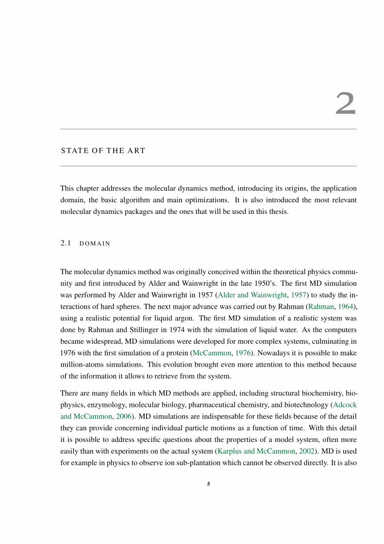
Force field (FF) is a molecular function generally tailored and calibrated in an empirical way.The function can be split into a sum of functionally simple and physically meaningful energeticterms. The terms are used to represent/model the potential energies and their derivative, theforces. Common terms of a FF are bonds, angles, dihedrals, van der Walls and electrostaticinteractions (eq. 1).
ETotal = Ebond + Eangle + Edihedral + Evan der Walls + EElectrostatic (1)
These terms can also be divided in two types of terms, bonded (eq. 2) and non-bonded terms (eq.3) (figure 1):
Ebonded = Ebond + Eangle + Edihedral (2)
Enon−bonded = Evan der Walls + EElectrostatic (3)
There are several alternatives to compute each term/interaction. The bond interactions includebond stretching (Ebond), angle bending (Eangle) and torsional or bond twisting (Edihedrals). Bondstretching is the energy required to stretch or compress a bond between two atoms. This is a2-body type interaction. Examples of potentials that can be used to compute Ebond are harmonic,fourth power, Morse and cubic bond stretching potentials. Angle bending is the energy requiredto bend a bond from its equilibrium angle. It is a 3-body type interaction type. The followingpotentials can be used to model angle bending: harmonic, cosine-based angle and Urey-Braleypotentials. The bond stretching and angle bending interactions require a great amount of sub-stantial energies to cause significant deformations. Most of its variations are related to the non-bonded and torsional contributions. A FF must be able to model flexible molecules in which
6
2.1. Domain
Figure 1.: Example of interactions between atoms.
they occur changes in conformations due to rotations. In order to simulate these interactionsthe FF needs torsional terms to properly represent energy profiles of the changes. The torsionalterm is a 4-body type interaction. Torsional potentials are, in most cases, expressed as a cosineseries expansion. Examples of its potentials are: periodic type, Ryckaert-Bellemans and Fourierpotentials.
The non-bonded terms represent the van der Waals and electrostatic two-body interactions. Asthe name suggests, a non-bonded interaction is made between atoms which are not connectedby covalent bonds. Usually these interactions are used when (i) two atoms are separated by adistance larger than 3 bonds and (ii) some times when there are two atoms, at the ends of atorsion configuration, which are separated by a 3-bond distance.
The van der Waals term represents the interactions between electron clouds around two non-bonded atoms. Depending on the distance between atoms, the resultant forces can be repulsive orattractive. The van der Waals interaction is strongly repulsive at short range distances, attractiveat intermediate range distances, and considered zero at long range distances. The dispersionforces, responsible by the attractive contribution, can be explained in quantum terms by theLondon dispersion forces. The common potential used to model the van der Waals interactionsare the Lennard-Jones and the Buckingham potentials. From these potentials the less expensiveto compute and most used is the Lennard-Jones potential (eq. 4).
VLJ(rij) =C(12)
ij
r12ij−
C(6)ij
r6ij
(4)
where Cij = 4εσ represents the particle properties, ε represents the potential well depth, and σ isthe collision diameter, r12
ij is the repulsive term and r6ij the attractive long range term for particles
i and j. The 12 exponent in equation 4 was chosen exclusively to simplify the computations.
7
2.2. Algorithms
The electrostatic interactions are one of the most important interactions and also one of themajor challenges in MD modeling. These interactions are described by the Coulomb law andcan expresses by equation 5.
VC(rij) = fqiqj
εrrij(5)
where qi and qj are the atomic charges in electron units, rij is the distance between atom i and j,εr is the dielectric constant and f is the conversion factor.
2.2 A L G O R I T H M S
A computer simulation can generate accurate values for the structural properties of a systemwithin a practical amount of time. It is possible to adjust a simulation, for different environmentsor lengths, changing only the simulation input parameters. This flexibility can be accomplishedusing MD simulations.
MD simulations follow a basic algorithm that imitates the steps done experimentally:
1. Initialize the system
2. Compute the potentials and forces
3. Compute the next positions
4. Increase time by a time step
5. Repeat steps 2-4, the desired number of simulation steps.
This algorithm is a basic representation of the steps that are made in an MD simulation. It startsby the system initialization, which defines the initial velocities and positions of the atoms and, insome cases, adjustments of parameters. The positions are generally defined in a file that containsinformation obtained by empirical experiments. After the initialization, the force field is used tocompute the potential energy that will be used to derive the forces among particles. In step 3 itis calculated the next position of all particles and then it is increased the simulation time. This isa basic MD algorithm. In a real implementation, most of these steps comprise several sub-stepssuch as energy minimization, temperature and pressure regulation (Leach, 2001).
8
2.2. Algorithms
Usually the most time consuming task is the calculation of forces, especially the computation ofnon-bonded interactions. In bonded interactions the number of bonds terms is proportional to thenumber of atoms in the system, but the number of non-bonded terms increases as the square ofthe number of atoms for the pairwise model. This means that the complexity of the non-bondedterm calculation is O(N2). In theory, the non-bonded interaction is calculated between every pairof atoms. This kind of approach is easy to implement, but is not feasible for large systems. Forexample, the Lennard-Jones potential gives very small values at long distances until it reacheszero: at 2.5σ the Lennard-Jones potential has just 1% of its value at σ (Leach, 2001). One wayto speed up the computation of the Lennard Jones interaction is to consider that the potential iszero beyond a specified cutoff distance, where atoms out of the cutoff distance are ignored.
There are two ways to calculate the long range electrostatic contributions, one is using lattice-summethods and the other is based on cut-off methods. The lattice-sum methods consist in using pe-riodic boundary conditions and Ewald summation. These methods replicate the cells (container),where the particle are in, through all sides to allow the calculation of the bulk properties. Thisis done to ignore the surface effects in a simulation. Lattice-sum methods can give good resultsfor highly charged system but since periodicity is enforced upon the system it is problematic inbio-molecular systems, resulting in over stabilization of the bio-molecules. The reaction field isan example of a cut-off method, where it is assumed that the molecule is surrounded by spaceof finite radius. Outside this space the system is treated as a dielectric continuum, which re-sponds with a counter charge distribution and interacts with the molecule. This method does notintroduce periodicity and is computationally fast, but can originate artifacts at the boundary incharged bio-molecular system and systems heating.
The calculation of the forces is used to compute the next position of the particles in the system.After computing the forces it is necessary to integrate the new position of every particle. Themost frequently used integration algorithm in MD simulations is the Verlet algorithm, which isused to integrate Newton’s equation of motion (eq. 6).
r(t + h) ≈ −r(t− h) + 2r(t) +h2F(t)
m(6)
where t is the time, h is the time step, F(t) is the second derivative of r(t), r is the position ofthe particle and m is the particle mass. The advantages of this algorithm are its simplicity andlow space requirements. The disadvantage is its moderated precision.
9
2.3. Optimizations
The force field calculation is essential in MD simulations and it is the most time consuming task.To reduce this time we need to optimize the calculation of the particles interactions, in order totake advantage of the computational resources.
After analyzing the application domain, we have a basic understanding of the calculations in-volved in MD simulations and we own an overview of the methods commonly used on thesecalculations. It is now possible to use the theoretical methods to understand the existing imple-mentations and investigate the methods that can be applied in a molecular dynamics simulation.In the next sections it will be presented some of the principal optimizations related to the cal-culation of forces. There are many other improvements that can be made in various sections ofthe code. For example, one can optimize the way the position of particles is updated after thecalculation of forces, but this type of optimization is not addressed in this thesis.
2.3 O P T I M I Z AT I O N S
The are two common optimizations that are based on Newton’s third law and the cut-off radiusmentioned above. The Newton’s third law says that when a body exerts a force on another bodythis body exerts a force with the same magnitude and opposite direction on the first body. Thismeans that by calculating the forces exerted on a certain particle, it is possible to know theinfluence of this particle over all the others, and there is no need to recalculate the influence ofthis particle on the others. This reduces the computation complexity from O(n2) to O(n2)/2.
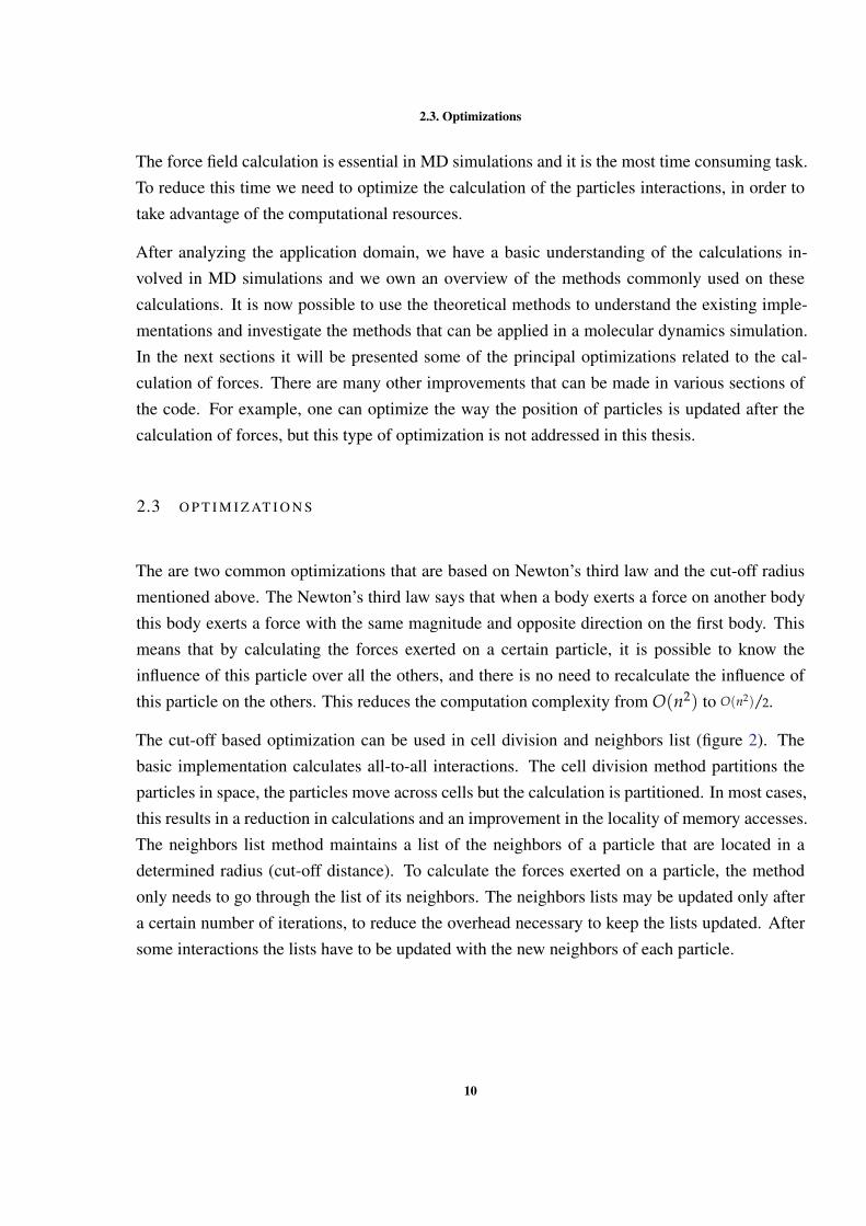
The cut-off based optimization can be used in cell division and neighbors list (figure 2). Thebasic implementation calculates all-to-all interactions. The cell division method partitions theparticles in space, the particles move across cells but the calculation is partitioned. In most cases,this results in a reduction in calculations and an improvement in the locality of memory accesses.The neighbors list method maintains a list of the neighbors of a particle that are located in adetermined radius (cut-off distance). To calculate the forces exerted on a particle, the methodonly needs to go through the list of its neighbors. The neighbors lists may be updated only aftera certain number of iterations, to reduce the overhead necessary to keep the lists updated. Aftersome interactions the lists have to be updated with the new neighbors of each particle.
10
2.3. Optimizations
(a) All pairs (b) Cell division (c) Neighbors list
Figure 2.: Sequential optimizations.
The optimization presented here are mostly related to how we can improve the calculation offorces using the knowledge from the domain, for example the use of the cut-off radius. Theseoptimizations can improve the execution time for sequential implementation but they cannotaddress code parallelization. In the next section we address stategies to explore parallelism.
2.3.1 Parallelism exploitation
Parallel implementations are based in a system decomposition. A system can be decomposed inthree ways:
1. Particle decomposition
2. Force decomposition
3. Space/cells decomposition.
Particle decomposition associates a subset of the particles to each process, or thread, and eachprocess calculates the interactions over its subset of particles. In this method every processneeds to know the position of every particle on the system, which requires global communication.Force decomposition, instead of particles, it assigns a subset of pairwise force computationsto each process or thread. It also suffers from global communication in the same way as thedecomposition of particles. Space decomposition is based on the already mentioned cell divisionmethod, where the domain of the simulation is divided in parts. In this case, the calculationsof the cell forces are associated to a process, or thread, and each one calculates the forces on adifferent cell. To calculate the forces in a cell, a process, or thread, needs to know the position ofthe particles from its neighbors cells. The communication complexity of these methods is O(N)
11
2.4. Molecular Dynamics Packages
for particle decomposition, O(N)√P
for force decomposition, and O(N)
P23
for space decomposition,
where N is the number of particles on P processors (Griebel et al., 2007).
2.4 M O L E C U L A R DY N A M I C S PAC K AG E S
There is a diversity of molecular dynamics packages that aim to have a broad number of capa-bilities. Every package has its advantages and features that set it apart from the others. Some ofthese packages are used on a regular basis for MD studies. Three of the most known packagesare GROMACS (Berendsen et al., 1995), NAMD(Phillips et al., 2005) and LAMMPS (Plimp-ton, 1995). These are all rich of features and large in code size. All of them have advantagesand disadvantages including, the number of features they implemented, the way they implementcomputations, and the time they take in simulations.
The MD field is greatly researched and improved and there are many studies using the pack-ages already mentioned. One example is the LAMMPS molecular dynamics package, whosedevelopers implemented a module to accelerate the neighbors lists building and the short-rangecalculations (Brown et al., 2011). Most of the actual studies are related to the use of accelera-tors as a way to improve execution. This happens because it is possible to greatly improve theexecutions time of a package using accelerators depending on the implementation.
The development done in this thesis is based on an existing implementation of a software pack-age named MOIL. MOIL was chosen as a reference package because of a previous work withthe package and because it was already tested. This package will be used as a reference for thedevelopment of all the implementations and to validate the obtained results. MOIL has all thefeatures that are needed by this thesis. It will also be used the Java Grand Forum (JGF) bench-mark (?), which provides a simple MD simulation code, ideal for to be altered and optimized.Another package that will be used in this thesis is Gromacs. Gromacs has top level performanceand it is one of the most used packages. This package will be used to have an overall assessmentof the code improvements made in present thesis.
The MOIL package has CPU, GPU and CPU/GPU hybrid implementations (Ruymgaart andElber, 2012). They use OpenMP, CUDA, FORTRAN and C code. We will focus on the MOILversion written in C. MOIL is composed of various tools that are responsible for validating andchanging the input data to use in its execution. For example, there is a tool to convert coordinatesfrom PDB to CHARMM format. The MOIL implementation tries to speed up the calculation of
12

2.4. Molecular Dynamics Packages
non-bonded interactions using different types of lists, which are selected according to the numberof particles, the type of atoms or molecules, and the selected execution platform. MOIL has thefollowing working modes (Ruymgaart et al., 2011):
1. Does not use lists and computes all-against-all interactions. This mode is aimed to non-uniform particle densities;
2. Uses space lists based on grid partitioning for GPU execution. The space is partitionedinto boxes.
3. Uses neighbors list based on chemical grouping.
4. Uses lists based on atoms for systems smaller than 100,000 atoms.
The evaluation and modification of the MOIL code is presented in the next chapter, where it willbe presented the motivations behind each optimization done on MOIL.
13

Part II
C O R E O F T H E D I S S E RTAT I O N
3
I M P L E M E N TAT I O N O F M O L E C U L A R DY NA M I C S O P T I M I Z AT I O N S
This chapter will explain in detail the actions taken to implement different modifications ofMOIL, the MD simulation code chosen as the starting point in the present work. The analysis ofMOIL and the motivations behind each modification, which resulted in a different sequential orparallel version, will be presented.
3.1 D E V E L O P M E N T O U T L I N E
The thesis is focused on the analysis of the MOIL implementation and the proposal of methodsto optimize its computations. The development work can be subdivided in the following phases:
• Research of both theory and development in Molecular Dynamics.
• Analyse and select a software package to use as starting point in our work.
• Evaluate a case study to find the most time-consuming parts.
• Investigate and implement ways of optimizing the code, and measure the gains of theoptimizations.
• Adapt the implementation to take advantage of parallelism in a shared memory model.
• Adapt the implementation to take advantage of parallelism in a distributed memory model.
• Implement a hybrid version using both shared and distributed memory parallelism.
• Evaluate all the implemented versions.
15
3.2. MD Sequential Version
The research made initially aimed to understand the MD technique and algorithms, in orderto perceive what was being computed by the existing code. This allowed us to have a basicunderstanding of the domain. The next step was the research of existing MD packages to knowwhat is already done in this field. The MOIL package was selected, as stated before. Afterthe selection of MOIL, it was necessary to choose one or more case studies to test the package.The choice of case studies was grounded on the reviewed literature. It were chosen case studiesinvolving the calculation of short-range forces (Brown et al., 2011). Having chosen a simulationpackage and the case studies, it was possible to profile the MD simulation execution to identifythe most time-consuming routines and the corresponding source code.
The cases studies evaluated were the Dihydrofolate reductase (DHFR)(Ruymgaart et al., 2011),available in the MOIL package, and a cube filled with Argon atoms. These two systems weresimulated with MOIL and their execution was profiled. After the measurement and profilingof both case studies, the Argon example was selected for rest of the thesis. This case studywas chosen because it only requires computing the van der Waals forces, which is one of thetwo most computational intensive tasks in MD simulations. Excluding the other forces, is aconscious strategy to focus our effort on improving the computation of the van der Waals forces.The decision of using Argon is also due to the fact that the MOIL execution flow is much morecomplex when using the other forces. After choosing the case study, it were created simulationinputs with different sizes, which require different memory resources. The next step, was toinitiate the development, implementation and assessment of several MOIL modifications. Thefollowing sections will present these modifications.
3.2 M D S E Q U E N T I A L V E R S I O N
The development and implementation of improvements to the sequential version of MOIL wasthe first step made in this thesis after the previous study. To make this implementation it was firstanalyzed and profiled the code of the MOIL package using the Argon case study. The profile ofthe code inform us which are the most time-consuming routines. After having a profile of thesequential version and after identifying the most time-consuming routine, there was a need tostudy this routine and the data structures it uses and what changes they suffer along the executionof code. This step proved important to improve the code to enable the automatic vectorizationby the compiler.
16
3.2. MD Sequential Version
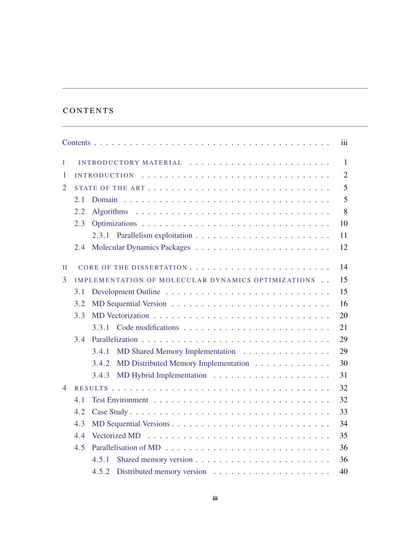
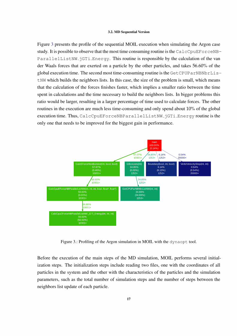
Figure 3 presents the profile of the sequential MOIL execution when simulating the Argon casestudy. It is possible to observe that the most time consuming routine is the CalcCpuEForceNB-ParallelListNW jGTi Energy. This routine is responsible by the calculation of the vander Waals forces that are exerted on a particle by the other particles, and takes 56.60% of theglobal execution time. The second most time-consuming routine is the GetCPUParNBNbrLis-tNW which builds the neighbors lists. In this case, the size of the problem is small, which meansthat the calculation of the forces finishes faster, which implies a smaller ratio between the timespent in calculations and the time necessary to build the neighbors lists. In bigger problems thisratio would be larger, resulting in a larger percentage of time used to calculate forces. The otherroutines in the execution are much less time-consuming and only spend about 10% of the globalexecution time. Thus, CalcCpuEForceNBParallelListNW jGTi Energy routine is theonly one that needs to be improved for the biggest gain in performance.
main100.00%(0.14%)
CalcEForceNonBonded(int, bool, bool)57.07%(0.46%)10001×
57.07%10001×
GBoxLists(int)34.85%(0.00%)1252×
34.85%1252×
Boundary(bool, int, bool)6.14%
(6.13%)1252×
6.14%1252×
VerletVelocityStep(int, int)0.54%
(0.54%)20000×
0.54%20000×
CalcCpuEForceNBParallelListNW(int, int, int, bool, float*, float*)56.60%(0.00%)10001×
56.60%10001×
GetCPUParNBNbrListNW(int, int)34.88%
(34.88%)1253×
34.85%1252×
CalcCpuEForceNBParallelListNW_jGTi_Energy(int, int, int)56.60%
(56.60%)10001×
56.60%10001×
Figure 3.: Profiling of the Argon simulation in MOIL with the dynaopt tool.
Before the execution of the main steps of the MD simulation, MOIL performs several initial-ization steps. The initialization steps include reading two files, one with the coordinates of allparticles in the system and the other with the characteristics of the particles and the simulationparameters, such as the total number of simulation steps and the number of steps between theneighbors list update of each particle.
17
3.2. MD Sequential Version
After identifying the initialization steps performed in MOIL, the most important data structureswere analyzed. The structures are used to store forces, velocities and positions. These threevector quantities are saved in nine arrays, since each one has three components: (Qx, Qy, Qz).These arrays are filled after certain validations and are obtained from data structures implementedin Fortran that are shared by several MOIL tools. In the Argon case study, the neighbors list ofall particles is updated every three steps. All the MOIL data structures, such as the neighborslists, are built from the mentioned nine arrays.
The code of the routine that calculates the forces exerted on each particle uses a neighbors list,as it can be seen in listing 3.1 (full for in listing A.1). The list of neighbors of a given particleincludes all the particles that are within a certain radius around that particle. The routine iteratesover this list to obtain the index of a neighbor particle. This index is then used to get the neighborparticle coordinates from the array of coordinates. With the coordinates of two particles, it is thencomputed the force exerted between them. This means that there are two steps to get a particlecoordinates: first it is obtained the index of the particle and later are read the coordinates of theneighbor particle. Next, the routine checks if the particle is inside the given radius. If true, theforce between the particles is calculated and its value is stored in the forces array, on the positioncorresponding to the particle being processed.
The calculation of a force is always done between two particles: (i) the principal particle, the onethat accumulates the forces exerted by all its neighbors, and (ii) the neighbor particle, the onethat calculates only the force exerted by the principal particle. Because this implementation usesthe third law of Newton, while the principal particle is accumulating the force exerted on it byall its neighbors, the force exerted by the principal particle on the neighbor is also updated. Thisreduces the number of forces calculated by the routine, but it introduces an additional complexitydue to the necessity to exclude the principal particle from the neighbors list of its neighbors.
// Iterate over all particles
for (int a=0; a<pend; a++)
{
//Number of neighbors for particle a
nnbrs = nrNbrAtomsPar[a];
...
// Iterate over the particle neighbors
for (int n=0; n<nnbrs; n++)
{
// Get neighbor information from the structure
struct NBPair nbr = NBPair[a*MAX_NR_NB_NBRS + n];
18
3.2. MD Sequential Version
// Index of the neighbor in the array of coordinates
j = nbr.x;
...
if (r2 < UCell.dMaxInnerCut2)
{
// Calculate vdW force using LJ
r =sqrt(r2); invr2=1.0f/r2; invr6=(invr2*invr2*invr2)*valid;
FLJ=-12.0f*nbr.y*invr6*invr6*invr2+6.0f*nbr.z*invr6*invr2;
// Calculate energy
Evdw = (nbr.y * invr6*invr6 - nbr.z * invr6);
float df = FLJ - Fe;
// Accumulate forces exerted on a particle
AtiFx += df*rx; AtiFy += df*ry; AtiFz += df*rz;
// Subtract particle force of the neighbor particle
StoreXDP[j + cpuForceSpacing*tid] -= df*rx;
StoreYDP[j + cpuForceSpacing*tid] -= df*ry;
StoreZDP[j + cpuForceSpacing*tid] -= df*rz;
ELJ += Evdw;
EElec += Eel;
}
...
}
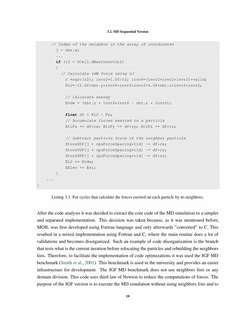
Listing 3.1: For cycles that calculate the forces exerted on each particle by its neighbors.
After the code analysis it was decided to extract the core code of the MD simulation to a simplerand separated implementation. This decision was taken because, as it was mentioned before,MOIL was first developed using Fortran language and only afterwards ”converted” to C. Thisresulted in a mixed implementation using Fortran and C, where the main routine does a lot ofvalidations and becomes disorganized. Such an example of code disorganization is the branchthat tests what is the current iteration before relocating the particles and rebuilding the neighborslists. Therefore, to facilitate the implementation of code optimizations it was used the JGF MDbenchmark (Smith et al., 2001). This benchmark is used in the university and provides an easierinfrastructure for development. The JGF MD benchmark does not use neighbors lists or anydomain division. This code uses third law of Newton to reduce the computations of forces. Thepurpose of the JGF version is to execute the MD simulation without using neighbors lists and to
19
3.3. MD Vectorization
allow us making modifications more easily. The changes made to JGF were in the computationof forces and the type of arrays to use a structure similar to the MOIL package. The values ofthe coordinates in JGF were saved as doubles while MOIL uses floats. After these changes thedevelopment with the JGF MD benchmark was similar to the one performed with MOIL. First weanalyzed the code, identifying the most time-consuming routine, and then the code was changedto improve its performance.
3.3 M D V E C T O R I Z AT I O N
Vectorization is a process of converting a scalar instruction, which process a single pair ofoperands at a time, to one where a single operation is applied to multiple elements (SIMDparadigm). This form of parallelism is called data parallelism. The processors that support thesetype of operations are called vector processors. One of the first processors supporting these op-erations was the Cray 1 (Russell, 1978). Recently, there was a growth of new technologies, suchas AVX and AVX2, that support vectorization. The vectorization extension used in this thesis isAVX, which was introduced with the Intel Sandy Bridge micro-architecture. The AVX instruc-tion set extension increased the width of the registers from 128- to 256-bit. This means thatAVX made it possible to execute 4 double precision FLOP per cycle or 8 single precision FLOPper cycle. These operations increase the number of operations per cycle, reduce the number ofcycles, and reducing the best case execution time by 8 times.
The process of transforming sequential to vectorized code is a hard task to be done manually.That is why it is so important that compilers automatically do this transformation. This dependson the calculations and the used data structures, but most of the essential changes are related withconditional expressions and arrays. The conditional expressions, like if conditions, have to beremoved to allow the compiler to apply vectorization. Arrays are important and essential. Usingarrays will allow multiple array elements to be processed in a single cycle. The changes relatedto arrays accesses are dictated by (i) the way arrays are aligned in memory, (ii) the knowledgethe compiler has over the pointers to arrays, and (iii) how arrays are accessed by the application.If an array is not aligned, or the pointer to that array has the possibility of being an alias forother array, then the compiler cannot use vectorization. In this case there is a need to manuallyspecify that the alias is restricted to that array and it is not used in another array. The way weaccess arrays also has to be known by the compiler. All accesses have to be aligned, the arraypositions have to be known at compile time, and have a stride 1 access with being depending on
20
3.3. MD Vectorization
conditions. For example, considering a for cycle that increases its counter by one, if we accessan array based on this counter then the compiler will know the accessed array positions and itwill be able to vectorize the calculations involving the array.
3.3.1 Code modifications
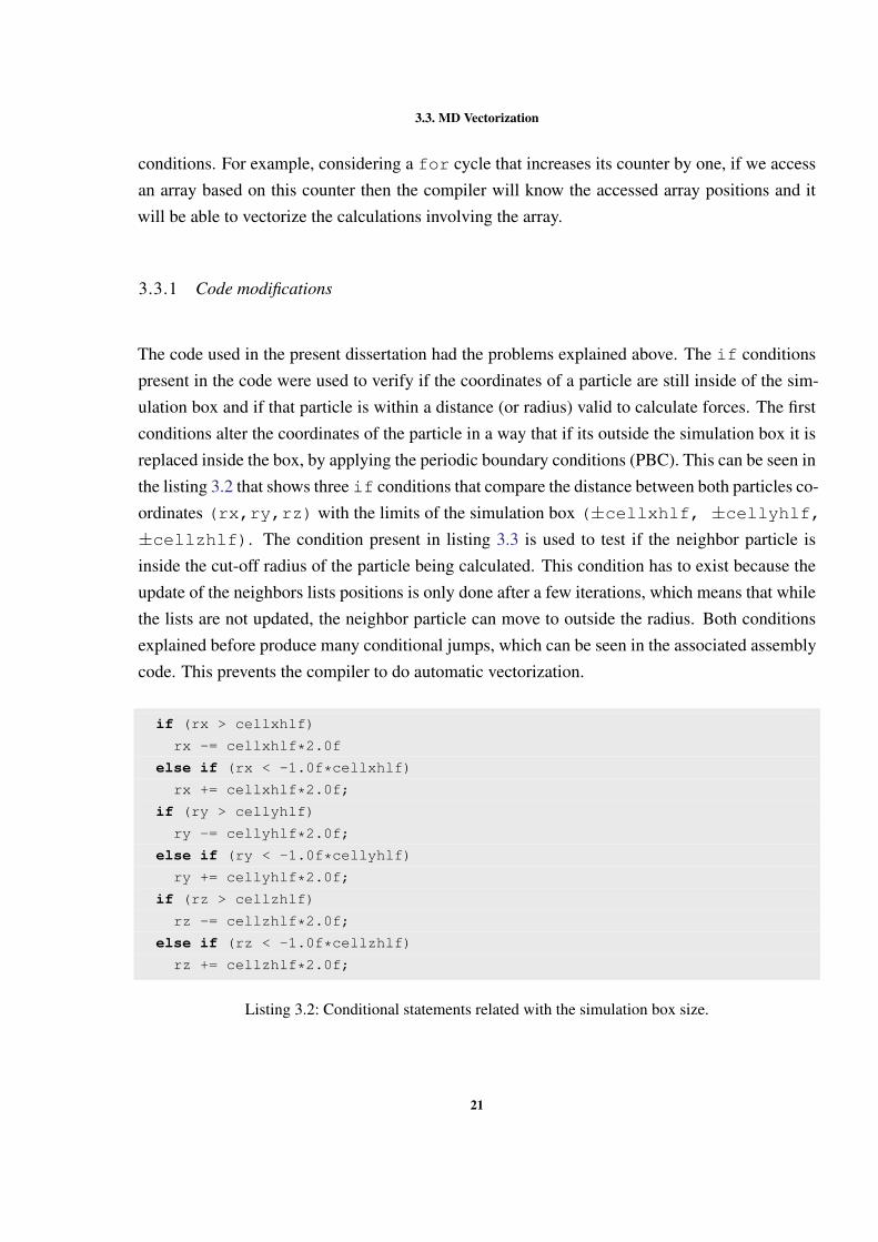
The code used in the present dissertation had the problems explained above. The if conditionspresent in the code were used to verify if the coordinates of a particle are still inside of the sim-ulation box and if that particle is within a distance (or radius) valid to calculate forces. The firstconditions alter the coordinates of the particle in a way that if its outside the simulation box it isreplaced inside the box, by applying the periodic boundary conditions (PBC). This can be seen inthe listing 3.2 that shows three if conditions that compare the distance between both particles co-ordinates (rx,ry,rz) with the limits of the simulation box (±cellxhlf, ±cellyhlf,±cellzhlf). The condition present in listing 3.3 is used to test if the neighbor particle isinside the cut-off radius of the particle being calculated. This condition has to exist because theupdate of the neighbors lists positions is only done after a few iterations, which means that whilethe lists are not updated, the neighbor particle can move to outside the radius. Both conditionsexplained before produce many conditional jumps, which can be seen in the associated assemblycode. This prevents the compiler to do automatic vectorization.
if (rx > cellxhlf)
rx -= cellxhlf*2.0f
else if (rx < -1.0f*cellxhlf)
rx += cellxhlf*2.0f;
if (ry > cellyhlf)
ry -= cellyhlf*2.0f;
else if (ry < -1.0f*cellyhlf)
ry += cellyhlf*2.0f;
if (rz > cellzhlf)
rz -= cellzhlf*2.0f;
else if (rz < -1.0f*cellzhlf)
rz += cellzhlf*2.0f;
Listing 3.2: Conditional statements related with the simulation box size.
21
3.3. MD Vectorization
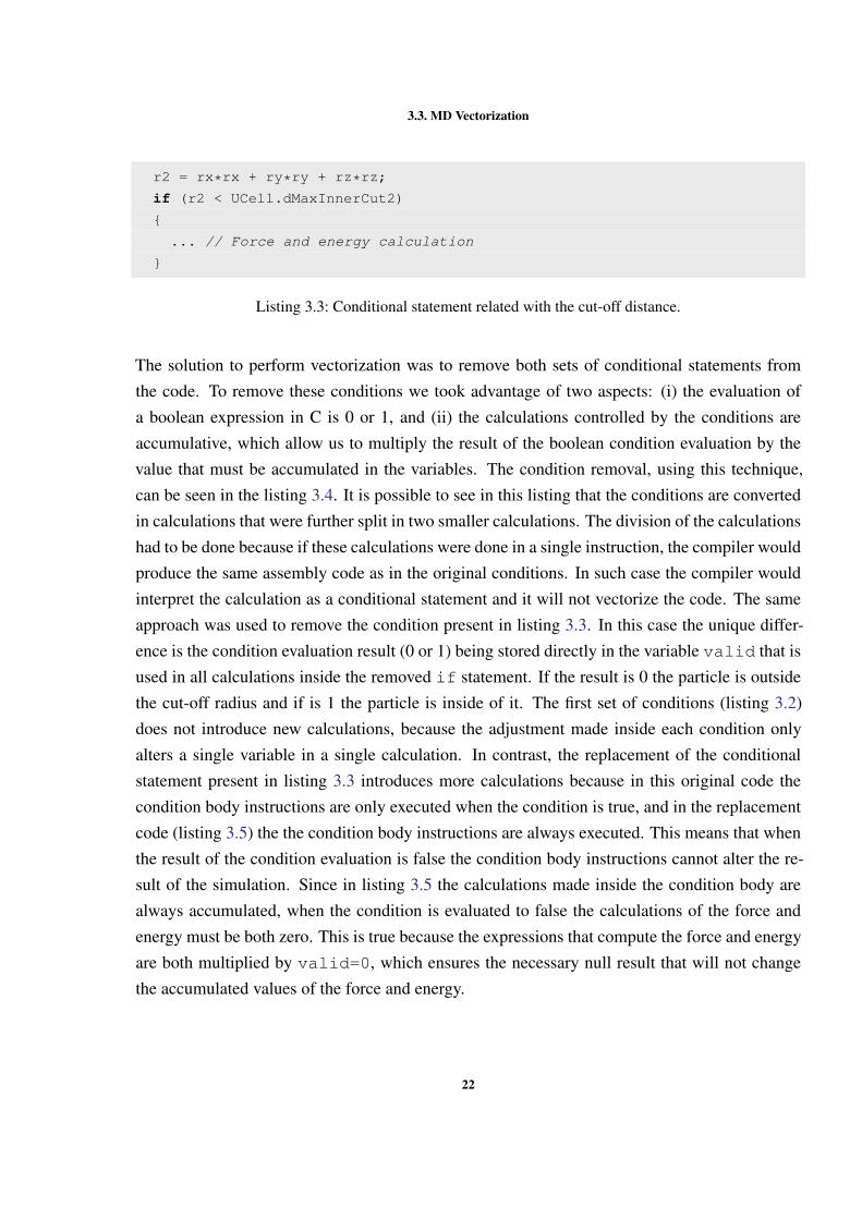
r2 = rx*rx + ry*ry + rz*rz;
if (r2 < UCell.dMaxInnerCut2)
{
... // Force and energy calculation
}
Listing 3.3: Conditional statement related with the cut-off distance.
The solution to perform vectorization was to remove both sets of conditional statements fromthe code. To remove these conditions we took advantage of two aspects: (i) the evaluation ofa boolean expression in C is 0 or 1, and (ii) the calculations controlled by the conditions areaccumulative, which allow us to multiply the result of the boolean condition evaluation by thevalue that must be accumulated in the variables. The condition removal, using this technique,can be seen in the listing 3.4. It is possible to see in this listing that the conditions are convertedin calculations that were further split in two smaller calculations. The division of the calculationshad to be done because if these calculations were done in a single instruction, the compiler wouldproduce the same assembly code as in the original conditions. In such case the compiler wouldinterpret the calculation as a conditional statement and it will not vectorize the code. The sameapproach was used to remove the condition present in listing 3.3. In this case the unique differ-ence is the condition evaluation result (0 or 1) being stored directly in the variable valid that isused in all calculations inside the removed if statement. If the result is 0 the particle is outsidethe cut-off radius and if is 1 the particle is inside of it. The first set of conditions (listing 3.2)does not introduce new calculations, because the adjustment made inside each condition onlyalters a single variable in a single calculation. In contrast, the replacement of the conditionalstatement present in listing 3.3 introduces more calculations because in this original code thecondition body instructions are only executed when the condition is true, and in the replacementcode (listing 3.5) the the condition body instructions are always executed. This means that whenthe result of the condition evaluation is false the condition body instructions cannot alter the re-sult of the simulation. Since in listing 3.5 the calculations made inside the condition body arealways accumulated, when the condition is evaluated to false the calculations of the force andenergy must be both zero. This is true because the expressions that compute the force and energyare both multiplied by valid=0, which ensures the necessary null result that will not changethe accumulated values of the force and energy.
22
3.3. MD Vectorization
cellxhlfm=-1.0f * cellxhlf;
cellyhlfm=-1.0f * cellyhlf;
cellzhlfm=-1.0f * cellzhlf;
...
rx += (rx > cellxhlf) * (cellxhlfm*2.0f);
rx += (rx < cellxhlfm) * (cellxhlf*2.0f);
ry += (ry > cellyhlf) * (cellyhlfm*2.0f);
ry += (ry < cellyhlfm) * (cellyhlf*2.0f);
rz += (rz > cellzhlf) * (cellzhlfm*2.0f);
rz += (rz < cellzhlfm) * (cellzhlf*2.0f);
r2 = rx*rx + ry*ry + rz*rz;
valid = (r2 < UCell.dMaxInnerCut2)
Listing 3.4: Removing conditional statements present in listing 3.2 to allow vectorization.
valid = (r2 < UCell.dMaxInnerCut2)
// Calculate vdW force using LJ
r = sqrt(r2); invr2 = 1.0f/r2; invr6 = (invr2*invr2*invr2) * valid;
FLJ = -12.0f * nbr.y * invr6*invr6*invr2 + 6.0f * nbr.z * invr6*invr2;
// Calculate the energy
Evdw = (nbr.y * invr6*invr6 - nbr.z * invr6);
Listing 3.5: Removing conditional statement present in listing 3.3 to allow vectorization.
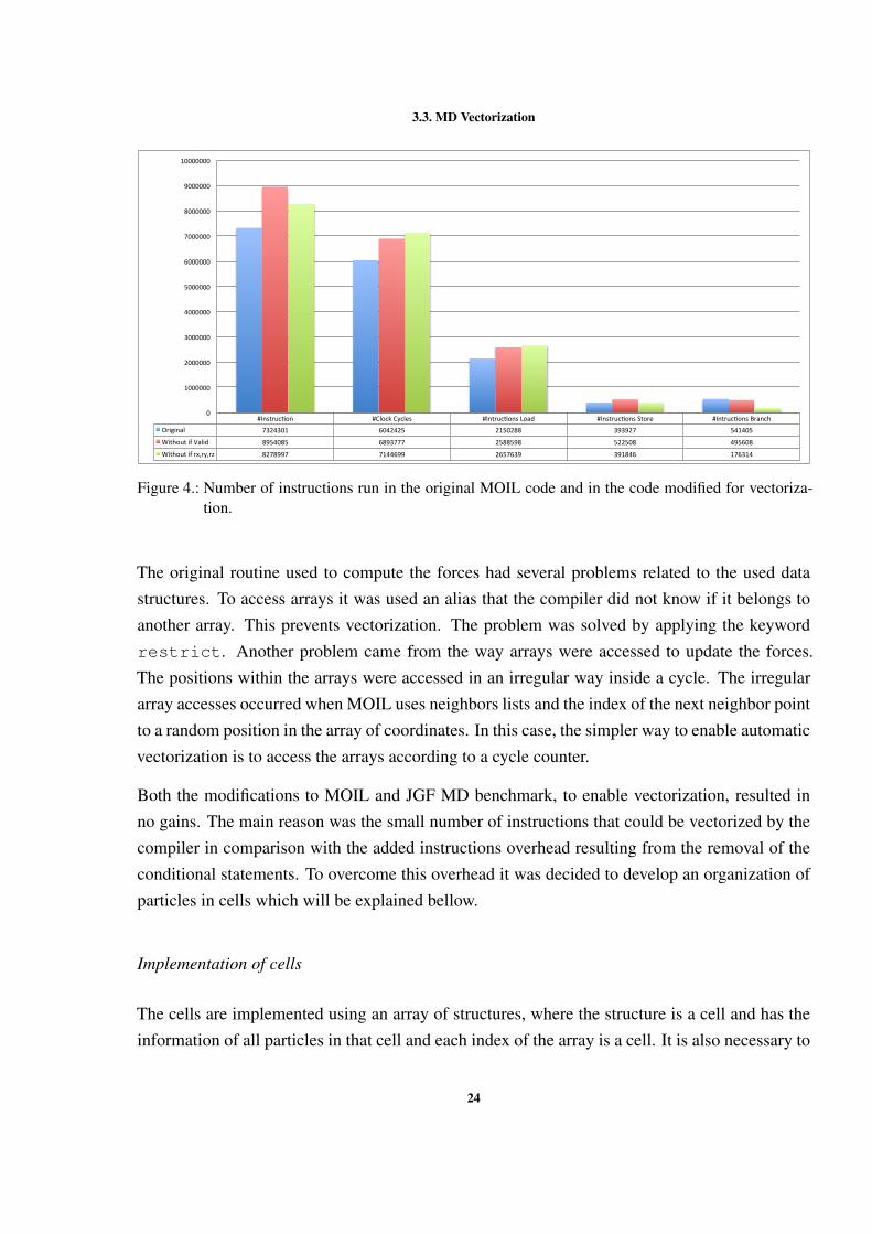
After having a modified code that is prepared for vectorization, it was analyzed using the PAPI.Figure 4 presents the number of executed instructions, with and without the if conditions. It ispossible to observe that when a set of if conditions is removed the total number of instructionincreases, while the number of branch instruction reduces. This happens because with the re-moval of both sets of if conditions, the calculations are always done, even if the if conditionsare evaluated to false.
23
3.3. MD Vectorization
#Instruc)on #ClockCycles #Intruc)onsLoad #Instruc)onsStore #Intruc)onsBranchOriginal 7324301 6042425 2150288 393927 541405
WithoutifValid 8954085 6893777 2588598 522508 495608
Withoutifrx,ry,rz 8278997 7144699 2657639 391846 176314
0
1000000
2000000
3000000
4000000
5000000
6000000
7000000
8000000
9000000
10000000
Figure 4.: Number of instructions run in the original MOIL code and in the code modified for vectoriza-tion.
The original routine used to compute the forces had several problems related to the used datastructures. To access arrays it was used an alias that the compiler did not know if it belongs toanother array. This prevents vectorization. The problem was solved by applying the keywordrestrict. Another problem came from the way arrays were accessed to update the forces.The positions within the arrays were accessed in an irregular way inside a cycle. The irregulararray accesses occurred when MOIL uses neighbors lists and the index of the next neighbor pointto a random position in the array of coordinates. In this case, the simpler way to enable automaticvectorization is to access the arrays according to a cycle counter.
Both the modifications to MOIL and JGF MD benchmark, to enable vectorization, resulted inno gains. The main reason was the small number of instructions that could be vectorized by thecompiler in comparison with the added instructions overhead resulting from the removal of theconditional statements. To overcome this overhead it was decided to develop an organization ofparticles in cells which will be explained bellow.
Implementation of cells
The cells are implemented using an array of structures, where the structure is a cell and has theinformation of all particles in that cell and each index of the array is a cell. It is also necessary to
24
3.3. MD Vectorization
create an array for each cell that has the index of its neighbors. Using an array of structures andneighbors we need to iterate through 4 different arrays to compute the forces. These arrays are,(i) array of cells, (ii) array of particles in the cell, (iii) array of the neighbors cells and (iv) thearray of the particles of the neighbor cell. To iterate over all these arrays it is needed four loops,one for each array. With the introduction of these loops the compiler can apply vectorization toa larger number of instruction, if the accesses to these arrays are stride 1.
The first step was to create a data structure to store the particles of the cells and to distributethe particles by the created cells. After creating the cells, it was necessary to create a list ofneighbors cells. This list is necessary to compute forces among particle that are close to thelimits of a cell. Concretely, accessing neighbor cells is necessary when there are particles indifferent cells separated by a distance smaller than the cut-off radius. In this case, to compute theforce exerted on such a particle we have to access some particles located in neighbor cells. Toconstruct the list of neighbor cells we have to identify all cells that are adjacent to each cell inthree-dimensional space. Since the cells are cubes, one cell has a maximum of 26 neighbor cells.Building the list of neighbor cells has to be done carefully because of two reasons. First, to findthe neighbors of a cell located in the limits of the simulation box we have to apply PBC. Considerthat a cell is identified by a 3D coordinate (cidZ,cidY,cidX). If the coordinate has a componentwith the maximum or minimum allowed value, for example cidX is equal to cidmax or cidmin, thePBC means that there is a neighbor cell with a X coordinate equal to the minimum (cidmin) ormaximum (cidmax) allowed value. Second, as we use Newton’s third law, it implies that if a cellB is in the neighbor list of cell A, then A can not be on the neighbor list of B. This means thatthe particles of cell A need not be used explicitly to calculate the forces exerted on the particlesof B, because these forces have already been calculated when the particles of A were processed.
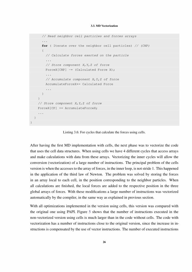
When the cell data structure was designed, the function responsible for calculating the forces hadto be modified to use this new structure. In the listing 3.6 we can see the introduction of newcycles to iterate over the different cells and particles. The new cycles made it possible to have agreater number of vectorized instructions.
for ( Iterate over all cells ) // (C)
{
for ( Iterate over all particles of the cell ) // (CP)
{
// Read cell particles and forces arrays
...
for ( Iterate over all neighbor cells ) // (CN)
{
25
3.3. MD Vectorization
// Read neighbor cell particles and forces arrays
...
for ( Iterate over the neighbor cell particles) // (CNP)
{
// Calculate forces exerted on the particle
...
// Store component X,Y,Z of force
ForceX[CNP] -= (Calculated Force X);
...
// Accumulate component X,Y,Z of force
AccumulateForceX+= Calculated Force
...
}
}
// Store component X,Y,Z of force
ForceX[CP] += AccumulateForceX;
...
}
}
Listing 3.6: For cycles that calculate the forces using cells.
After having the first MD implementation with cells, the next phase was to vectorize the codethat uses the cell data structures. When using cells we have 4 different cycles that access arraysand make calculations with data from these arrays. Vectorizing the inner cycles will allow theconversion (vectorization) of a large number of instructions. The principal problem of the cellsversion is when the accesses to the array of forces, in the inner loop, is not stride 1. This happenedin the application of the third law of Newton. The problem was solved by storing the forcesin an array local to each cell, in the position corresponding to the neighbor particles. Whenall calculations are finished, the local forces are added to the respective position in the threeglobal arrays of forces. With these modifications a large number of instructions was vectorizedautomatically by the compiler, in the same way as explained in previous section.
With all optimizations implemented in the version using cells, this version was compared withthe original one using PAPI. Figure 5 shows that the number of instructions executed in thenon-vectorized version using cells is much larger than in the code without cells. The code withvectorization has a number of instructions close to the original version, since the increase in in-structions is compensated by the use of vector instructions. The number of executed instructions
26
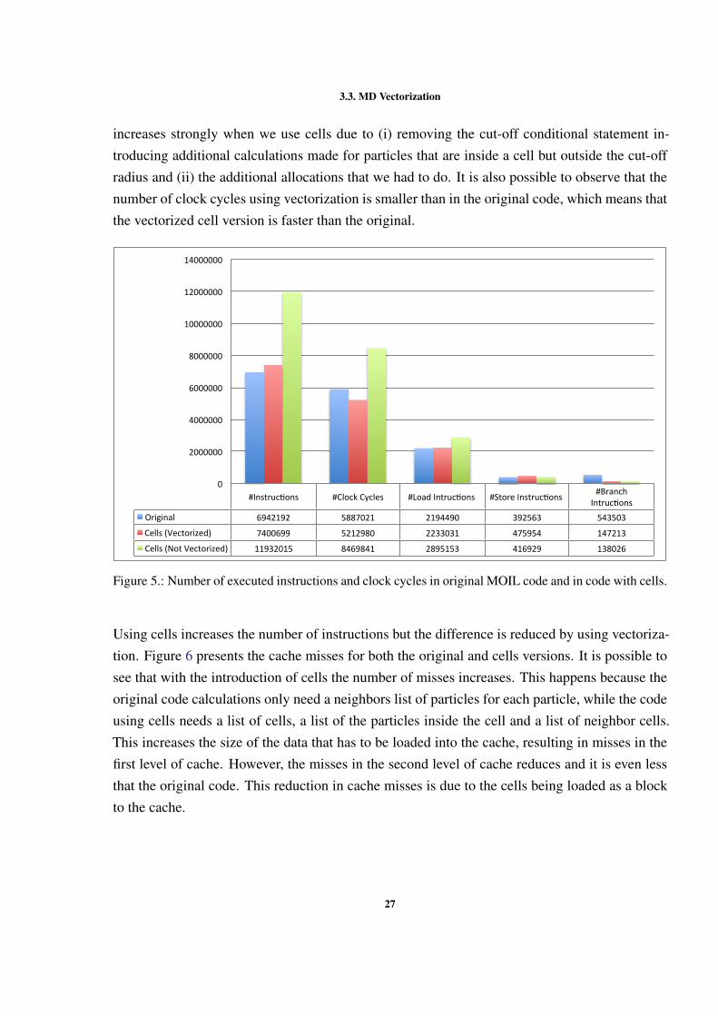
3.3. MD Vectorization
increases strongly when we use cells due to (i) removing the cut-off conditional statement in-troducing additional calculations made for particles that are inside a cell but outside the cut-offradius and (ii) the additional allocations that we had to do. It is also possible to observe that thenumber of clock cycles using vectorization is smaller than in the original code, which means thatthe vectorized cell version is faster than the original.
#Instruc)ons #ClockCycles #LoadIntruc)ons #StoreInstruc)ons #BranchIntruc)ons
Original 6942192 5887021 2194490 392563 543503
Cells(Vectorized) 7400699 5212980 2233031 475954 147213
Cells(NotVectorized) 11932015 8469841 2895153 416929 138026
0
2000000
4000000
6000000
8000000
10000000
12000000
14000000
Figure 5.: Number of executed instructions and clock cycles in original MOIL code and in code with cells.
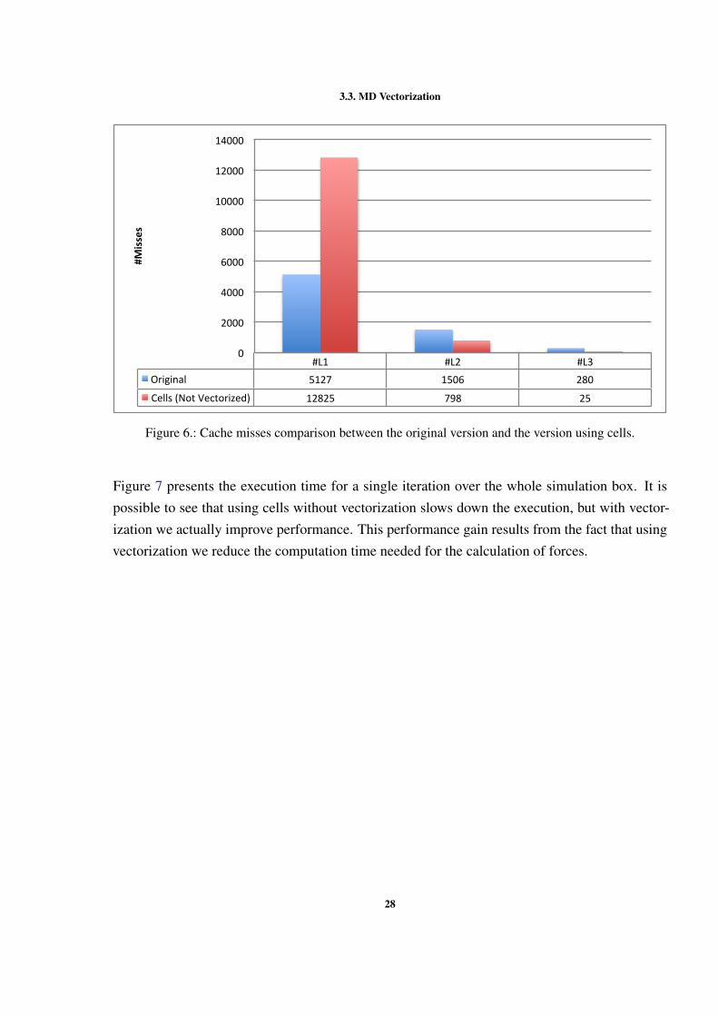
Using cells increases the number of instructions but the difference is reduced by using vectoriza-tion. Figure 6 presents the cache misses for both the original and cells versions. It is possible tosee that with the introduction of cells the number of misses increases. This happens because theoriginal code calculations only need a neighbors list of particles for each particle, while the codeusing cells needs a list of cells, a list of the particles inside the cell and a list of neighbor cells.This increases the size of the data that has to be loaded into the cache, resulting in misses in thefirst level of cache. However, the misses in the second level of cache reduces and it is even lessthat the original code. This reduction in cache misses is due to the cells being loaded as a blockto the cache.
27
3.3. MD Vectorization
#L1 #L2 #L3Original 5127 1506 280
Cells(NotVectorized) 12825 798 25
0
2000
4000
6000
8000
10000
12000
14000#M
isses
Figure 6.: Cache misses comparison between the original version and the version using cells.
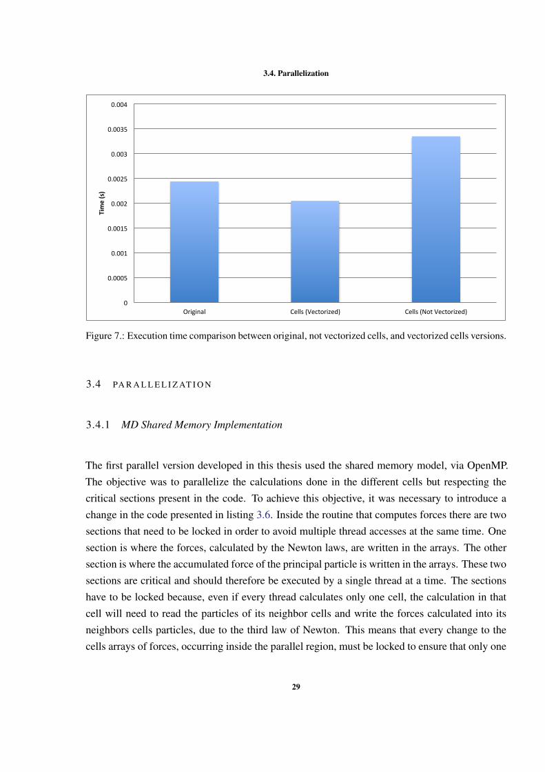
Figure 7 presents the execution time for a single iteration over the whole simulation box. It ispossible to see that using cells without vectorization slows down the execution, but with vector-ization we actually improve performance. This performance gain results from the fact that usingvectorization we reduce the computation time needed for the calculation of forces.
28
3.4. Parallelization
0
0.0005
0.001
0.0015
0.002
0.0025
0.003
0.0035
0.004
Original Cells(Vectorized) Cells(NotVectorized)
Time(s)
Figure 7.: Execution time comparison between original, not vectorized cells, and vectorized cells versions.
3.4 PA R A L L E L I Z AT I O N
3.4.1 MD Shared Memory Implementation
The first parallel version developed in this thesis used the shared memory model, via OpenMP.The objective was to parallelize the calculations done in the different cells but respecting thecritical sections present in the code. To achieve this objective, it was necessary to introduce achange in the code presented in listing 3.6. Inside the routine that computes forces there are twosections that need to be locked in order to avoid multiple thread accesses at the same time. Onesection is where the forces, calculated by the Newton laws, are written in the arrays. The othersection is where the accumulated force of the principal particle is written in the arrays. These twosections are critical and should therefore be executed by a single thread at a time. The sectionshave to be locked because, even if every thread calculates only one cell, the calculation in thatcell will need to read the particles of its neighbor cells and write the forces calculated into itsneighbors cells particles, due to the third law of Newton. This means that every change to thecells arrays of forces, occurring inside the parallel region, must be locked to ensure that only one
29
3.4. Parallelization
thread can write in the arrays of forces at a time. Since we only want to lock the critical regionsthere are two ways to do it. The first way is to implement a lock by cell. Thus, a thread canwrite into a cell only if that cell is free. The second method implements a lock by particle. Herewe lock the particle forces while a thread is writing. Both locking methods were implemented,using an array of locks, and tested. But the implementation using locks by particle prevented thecompiler to perform vectorization. The lock by particle had to be implemented inside the cyclethat calculates the forces, which means that it had to write in the array of locks in a calculatedposition that was not aligned. For this reason it was used locks by cell instead of particle.
3.4.2 MD Distributed Memory Implementation
Message Passing Interface (MPI) allows the developers to write portable message-passing code.MPI allows the data from one process to be moved to other processes in a high level and abstractway. The communication between processes is known as a distributed memory communicationenvironment.
When using OpenMP, for example, there is a limitation in the available resources because it onlyallows to create threads inside a single machine, but MPI expands the available resources becauseit allows the processes to communicate between different nodes in a easy and abstract way. Thismeans that if there are no bottlenecks, the performance of a program can be improved by usingmore nodes.
Comparing with the previously presented MD versions, the development of the MPI versionplaced less challenges. This is due to the fact that all forces are accumulative, which createsno problems to the task of writing the forces in the arrays. The approach followed in the MPIimplementation consisted in having several cells allocated to each process. This way, one processcalculates the forces in different cells and adds them to its local array of forces, in the same wayas referred before. After this, all processes communicate their forces to the other processesthat add them to their own arrays. Using MPI this operation can be done using a reduction ofthe forces followed by a broadcast of the result (all-reduce). This approach avoids severalproblems of the shared memory model such as the necessity to block the critical sections.
30
3.4. Parallelization
3.4.3 MD Hybrid Implementation
The MD hybrid version consisted in using both the shared and distributed memory models in theimplementation. This implementation eliminates the main limitation of the OpenMP code sincethe available resources are not limited to a single node. The MPI implementation had alreadysolved this limitation, but an hybrid implementation allows a much higher performance in somecases. For example, when there is a lot of communication between processes and when there arefew critical sections. In our code we benefit a little from each model. We can reduce the timespent in communication, because we have less processes that need to communicate, we also useless memory space because with threads it uses shared memory and because we have few criticalsections the execution seldom blocks in these sections.
The hybrid implementation simply combines the OpenMP with the MPI implementation, whileensuring that the critical sections and the cell organization are respected.
There are many ways to assess an hybrid implementation in order to reach the best performance.It is possible to test the code with different combinations of the number of threads, the numberof processes, and how to distribute processes and threads by nodes. Different combinations weretested in this work. The alternatives that resulted in best performance will be documented in thenext chapter.
31
4
R E S U LT S
In this chapter it is presented the results obtained with the different implementations. The resultsin this section are obtained using the Argon case study with different numbers of particles.
4.1 T E S T E N V I RO N M E N T
In order to evaluate the development made in this thesis the Services and Advanced ResearchComputing with HTC/HPC (SeARCH) cluster was used (University of Minho, 2015). It wasalso used various tools (table 1). The specifications of the nodes used in the simulations are intable 2.
Table 1.: Tools used for development.Tool Version DescriptionGNU gprof 2.25 Used to obtain the profiles of the code with the correspond-
ing weights of of each routine.GCC 4.9.0 The compiler used in most of the implemented code.OpenMPI 1.8.2 MPI version.PAPI 5.4.2 Used to obtain measurements of the hardware counters.
32
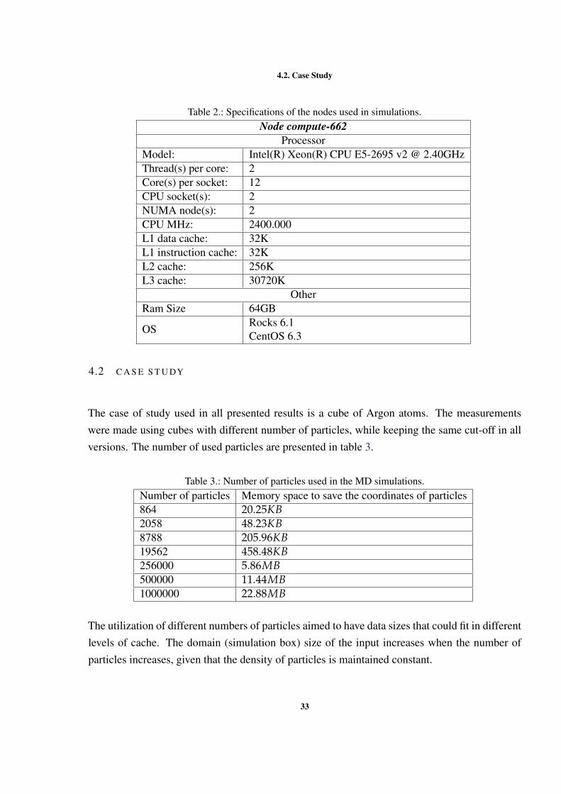
4.2. Case Study
Table 2.: Specifications of the nodes used in simulations.Node compute-662
ProcessorModel: Intel(R) Xeon(R) CPU E5-2695 v2 @ 2.40GHzThread(s) per core: 2Core(s) per socket: 12CPU socket(s): 2NUMA node(s): 2CPU MHz: 2400.000L1 data cache: 32KL1 instruction cache: 32KL2 cache: 256KL3 cache: 30720K
OtherRam Size 64GB
OSRocks 6.1CentOS 6.3
4.2 C A S E S T U DY
The case of study used in all presented results is a cube of Argon atoms. The measurementswere made using cubes with different number of particles, while keeping the same cut-off in allversions. The number of used particles are presented in table 3.
Table 3.: Number of particles used in the MD simulations.Number of particles Memory space to save the coordinates of particles864 20.25KB2058 48.23KB8788 205.96KB19562 458.48KB256000 5.86MB500000 11.44MB1000000 22.88MB
The utilization of different numbers of particles aimed to have data sizes that could fit in differentlevels of cache. The domain (simulation box) size of the input increases when the number ofparticles increases, given that the density of particles is maintained constant.
33
4.3. MD Sequential Versions
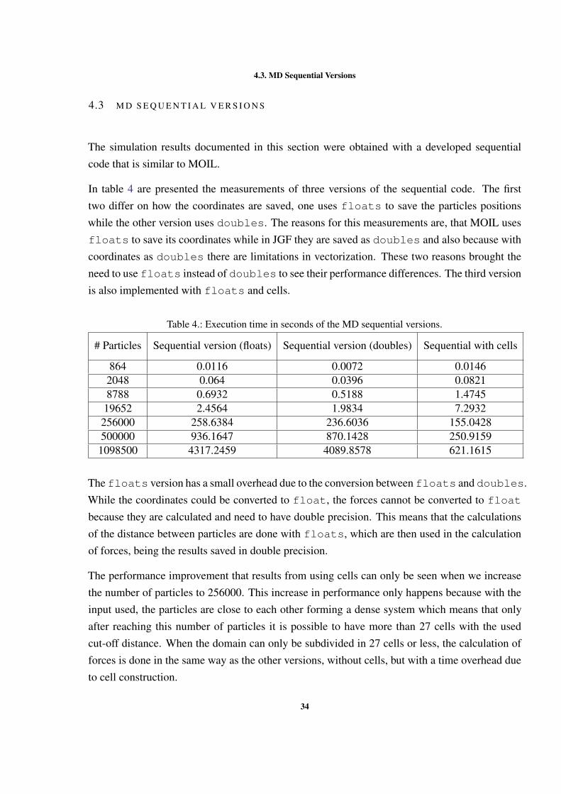
4.3 M D S E Q U E N T I A L V E R S I O N S
The simulation results documented in this section were obtained with a developed sequentialcode that is similar to MOIL.
In table 4 are presented the measurements of three versions of the sequential code. The firsttwo differ on how the coordinates are saved, one uses floats to save the particles positionswhile the other version uses doubles. The reasons for this measurements are, that MOIL usesfloats to save its coordinates while in JGF they are saved as doubles and also because withcoordinates as doubles there are limitations in vectorization. These two reasons brought theneed to use floats instead of doubles to see their performance differences. The third versionis also implemented with floats and cells.
Table 4.: Execution time in seconds of the MD sequential versions.
# Particles Sequential version (floats) Sequential version (doubles) Sequential with cells
864 0.0116 0.0072 0.01462048 0.064 0.0396 0.08218788 0.6932 0.5188 1.4745
19652 2.4564 1.9834 7.2932256000 258.6384 236.6036 155.0428500000 936.1647 870.1428 250.91591098500 4317.2459 4089.8578 621.1615
The floats version has a small overhead due to the conversion between floats and doubles.While the coordinates could be converted to float, the forces cannot be converted to floatbecause they are calculated and need to have double precision. This means that the calculationsof the distance between particles are done with floats, which are then used in the calculationof forces, being the results saved in double precision.
The performance improvement that results from using cells can only be seen when we increasethe number of particles to 256000. This increase in performance only happens because with theinput used, the particles are close to each other forming a dense system which means that onlyafter reaching this number of particles it is possible to have more than 27 cells with the usedcut-off distance. When the domain can only be subdivided in 27 cells or less, the calculation offorces is done in the same way as the other versions, without cells, but with a time overhead dueto cell construction.
34
4.4. Vectorized MD
4.4 V E C T O R I Z E D M D
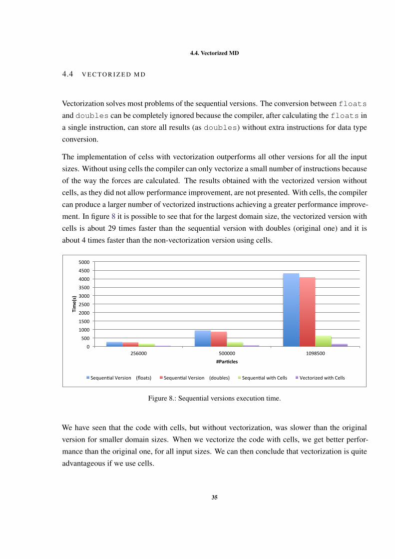
Vectorization solves most problems of the sequential versions. The conversion between floatsand doubles can be completely ignored because the compiler, after calculating the floats ina single instruction, can store all results (as doubles) without extra instructions for data typeconversion.
The implementation of celss with vectorization outperforms all other versions for all the inputsizes. Without using cells the compiler can only vectorize a small number of instructions becauseof the way the forces are calculated. The results obtained with the vectorized version withoutcells, as they did not allow performance improvement, are not presented. With cells, the compilercan produce a larger number of vectorized instructions achieving a greater performance improve-ment. In figure 8 it is possible to see that for the largest domain size, the vectorized version withcells is about 29 times faster than the sequential version with doubles (original one) and it isabout 4 times faster than the non-vectorization version using cells.
0
500
1000
1500
2000
2500
3000
3500
4000
4500
5000
256000 500000 1098500
Time(s)
#Par-cles
Sequen0alVersion(floats) Sequen0alVersion(doubles) Sequen0alwithCells VectorizedwithCells
Figure 8.: Sequential versions execution time.
We have seen that the code with cells, but without vectorization, was slower than the originalversion for smaller domain sizes. When we vectorize the code with cells, we get better perfor-mance than the original one, for all input sizes. We can then conclude that vectorization is quiteadvantageous if we use cells.
35
4.5. Parallelisation of MD
4.5 PA R A L L E L I S AT I O N O F M D
In this section we present and discuss the results of all parallel implementations. All these imple-mentations are based in the developed version with cells.
4.5.1 Shared memory version
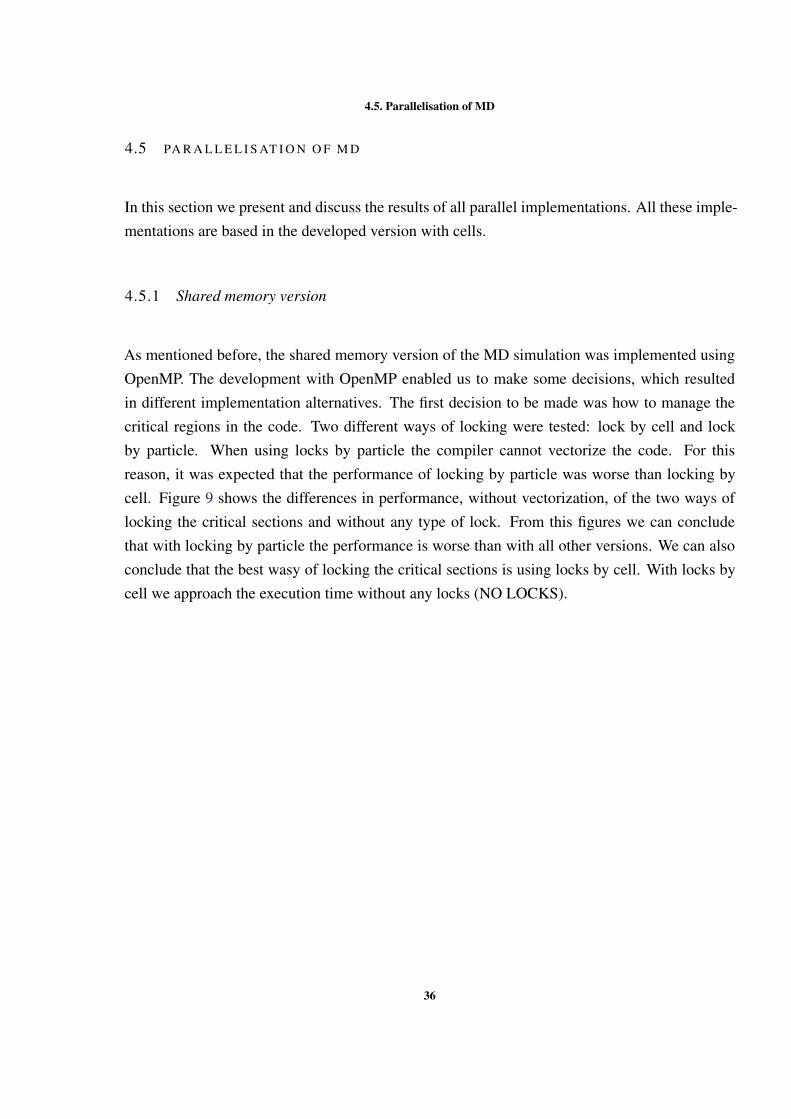
As mentioned before, the shared memory version of the MD simulation was implemented usingOpenMP. The development with OpenMP enabled us to make some decisions, which resultedin different implementation alternatives. The first decision to be made was how to manage thecritical regions in the code. Two different ways of locking were tested: lock by cell and lockby particle. When using locks by particle the compiler cannot vectorize the code. For thisreason, it was expected that the performance of locking by particle was worse than locking bycell. Figure 9 shows the differences in performance, without vectorization, of the two ways oflocking the critical sections and without any type of lock. From this figures we can concludethat with locking by particle the performance is worse than with all other versions. We can alsoconclude that the best wasy of locking the critical sections is using locks by cell. With locks bycell we approach the execution time without any locks (NO LOCKS).
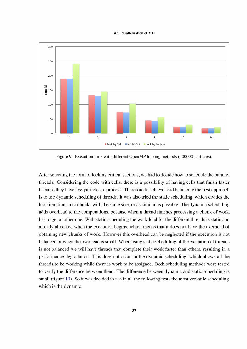
36
4.5. Parallelisation of MD
0
50
100
150
200
250
300
1 2 4 8 12 24
Time(s)
LockbyCell NOLOCKS LockbyPar9cle
Figure 9.: Execution time with different OpenMP locking methods (500000 particles).
After selecting the form of locking critical sections, we had to decide how to schedule the parallelthreads. Considering the code with cells, there is a possibility of having cells that finish fasterbecause they have less particles to process. Therefore to achieve load balancing the best approachis to use dynamic scheduling of threads. It was also tried the static scheduling, which divides theloop iterations into chunks with the same size, or as similar as possible. The dynamic schedulingadds overhead to the computations, because when a thread finishes processing a chunk of work,has to get another one. With static scheduling the work load for the different threads is static andalready allocated when the execution begins, which means that it does not have the overhead ofobtaining new chunks of work. However this overhead can be neglected if the execution is notbalanced or when the overhead is small. When using static scheduling, if the execution of threadsis not balanced we will have threads that complete their work faster than others, resulting in aperformance degradation. This does not occur in the dynamic scheduling, which allows all thethreads to be working while there is work to be assigned. Both scheduling methods were testedto verify the difference between them. The difference between dynamic and static scheduling issmall (figure 10). So it was decided to use in all the following tests the most versatile scheduling,which is the dynamic.
37
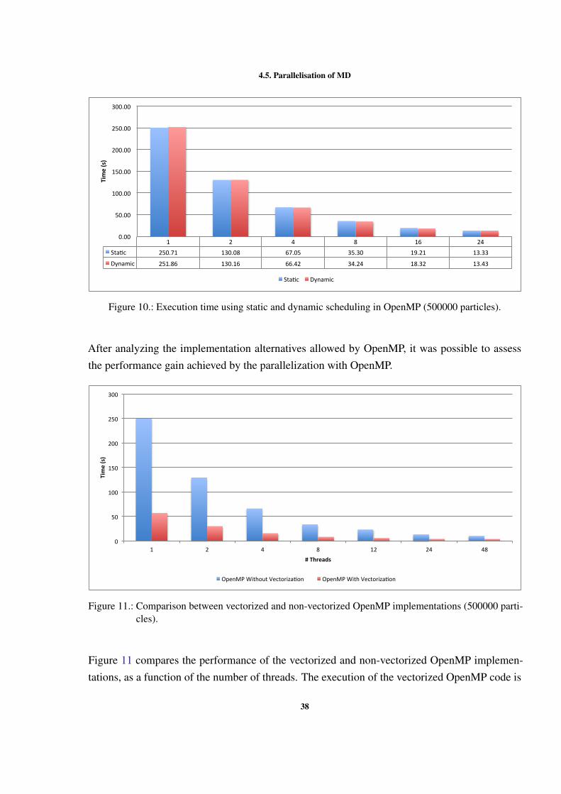
4.5. Parallelisation of MD
1 2 4 8 16 24Sta*c 250.71 130.08 67.05 35.30 19.21 13.33
Dynamic 251.86 130.16 66.42 34.24 18.32 13.43
0.00
50.00
100.00
150.00
200.00
250.00
300.00Time(s)
Sta*c Dynamic
Figure 10.: Execution time using static and dynamic scheduling in OpenMP (500000 particles).
After analyzing the implementation alternatives allowed by OpenMP, it was possible to assessthe performance gain achieved by the parallelization with OpenMP.
0
50
100
150
200
250
300
1 2 4 8 12 24 48
Time(s)
#Threads
OpenMPWithoutVectoriza:on OpenMPWithVectoriza:on
Figure 11.: Comparison between vectorized and non-vectorized OpenMP implementations (500000 parti-cles).
Figure 11 compares the performance of the vectorized and non-vectorized OpenMP implemen-tations, as a function of the number of threads. The execution of the vectorized OpenMP code is
38
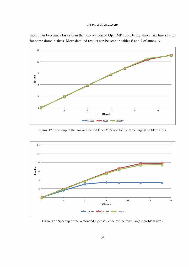
4.5. Parallelisation of MD
more than two times faster than the non-vectorized OpenMP code, being almost six times fasterfor some domain sizes. More detailed results can be seen in tables 6 and 7 of annex A.
1
2
4
8
16
32
1 2 4 8 16 32
Speedu
p
#Threads
256000 500000 1098500
Figure 12.: Speedup of the non-vectorized OpenMP code for the three largest problem sizes.
1
2
4
8
16
32
64
1 2 4 8 16 32 64
Speedu
p
#Threads
256000 500000 1098500
Figure 13.: Speedup of the vectorized OpenMP code for the three largest problem sizes.
39
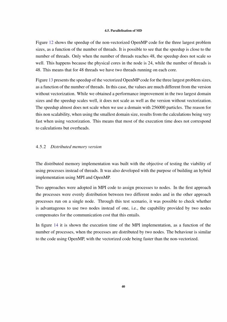
4.5. Parallelisation of MD
Figure 12 shows the speedup of the non-vectorized OpenMP code for the three largest problemsizes, as a function of the number of threads. It is possible to see that the speedup is close to thenumber of threads. Only when the number of threads reaches 48, the speedup does not scale sowell. This happens because the physical cores in the node is 24, while the number of threads is48. This means that for 48 threads we have two threads running on each core.
Figure 13 presents the speedup of the vectorized OpenMP code for the three largest problem sizes,as a function of the number of threads. In this case, the values are much different from the versionwithout vectorization. While we obtained a performance improvement in the two largest domainsizes and the speedup scales well, it does not scale as well as the version without vectorization.The speedup almost does not scale when we use a domain with 256000 particles. The reason forthis non scalability, when using the smallest domain size, results from the calculations being veryfast when using vectorization. This means that most of the execution time does not correspondto calculations but overheads.
4.5.2 Distributed memory version
The distributed memory implementation was built with the objective of testing the viability ofusing processes instead of threads. It was also developed with the purpose of building an hybridimplementation using MPI and OpenMP.
Two approaches were adopted in MPI code to assign processes to nodes. In the first approachthe processes were evenly distribution between two different nodes and in the other approachprocesses run on a single node. Through this test scenario, it was possible to check whetheris advantageous to use two nodes instead of one, i.e., the capability provided by two nodescompensates for the communication cost that this entails.
In figure 14 it is shown the execution time of the MPI implementation, as a function of thenumber of processes, when the processes are distributed by two nodes. The behaviour is similarto the code using OpenMP, with the vectorized code being faster than the non-vectorized.
40
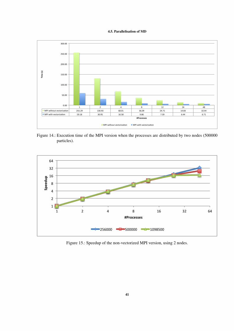
4.5. Parallelisation of MD
1 2 4 8 12 24 48MPIwithoutvectoriza5on 255.29 130.93 68.01 36.09 24.71 14.83 10.44
MPIwithvectoriza5on 59.18 30.95 16.58 9.86 7.39 6.44 6.71
0.00
50.00
100.00
150.00
200.00
250.00
300.00Time(s)
#Processes
MPIwithoutvectoriza5on MPIwithvectoriza5on
Figure 14.: Execution time of the MPI version when the processes are distributed by two nodes (500000particles).
1
2
4
8
16
32
64
1 2 4 8 16 32 64
Speedu
p
#Processes
256000 500000 1098500
Figure 15.: Speedup of the non-vectorized MPI version, using 2 nodes.
41
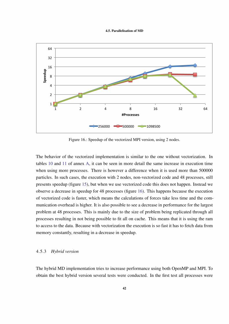
4.5. Parallelisation of MD
1
2
4
8
16
32
64
1 2 4 8 16 32 64
Speedu
p
#Processes
256000 500000 1098500
Figure 16.: Speedup of the vectorized MPI version, using 2 nodes.
The behavior of the vectorized implementation is similar to the one without vectorization. Intables 10 and 11 of annex A, it can be seen in more detail the same increase in execution timewhen using more processes. There is however a difference when it is used more than 500000particles. In such cases, the execution with 2 nodes, non-vectorized code and 48 processes, stillpresents speedup (figure 15), but when we use vectorized code this does not happen. Instead weobserve a decrease in speedup for 48 processes (figure 16). This happens because the executionof vectorized code is faster, which means the calculations of forces take less time and the com-munication overhead is higher. It is also possible to see a decrease in performance for the largestproblem at 48 processes. This is mainly due to the size of problem being replicated through allprocesses resulting in not being possible to fit all on cache. This means that it is using the ramto access to the data. Because with vectorization the execution is so fast it has to fetch data frommemory constantly, resulting in a decrease in speedup.
4.5.3 Hybrid version
The hybrid MD implementation tries to increase performance using both OpenMP and MPI. Toobtain the best hybrid version several tests were conducted. In the first test all processes were
42
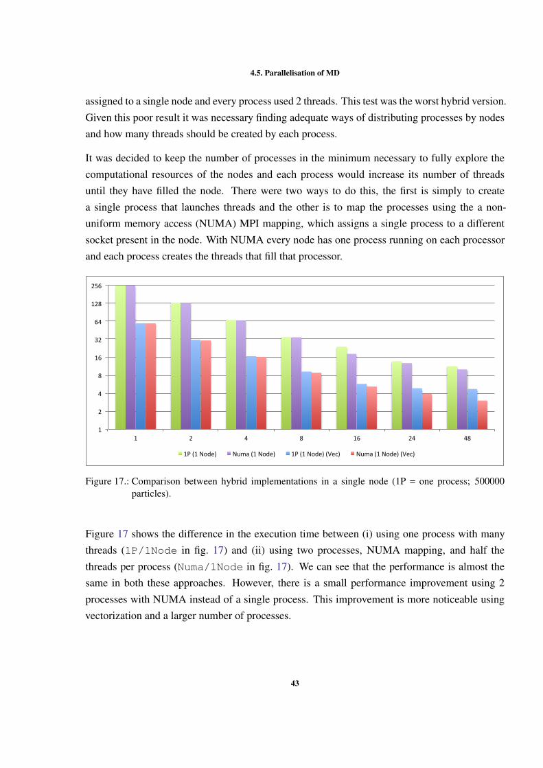
4.5. Parallelisation of MD
assigned to a single node and every process used 2 threads. This test was the worst hybrid version.Given this poor result it was necessary finding adequate ways of distributing processes by nodesand how many threads should be created by each process.
It was decided to keep the number of processes in the minimum necessary to fully explore thecomputational resources of the nodes and each process would increase its number of threadsuntil they have filled the node. There were two ways to do this, the first is simply to createa single process that launches threads and the other is to map the processes using the a non-uniform memory access (NUMA) MPI mapping, which assigns a single process to a differentsocket present in the node. With NUMA every node has one process running on each processorand each process creates the threads that fill that processor.
1
2
4
8
16
32
64
128
256
1 2 4 8 16 24 48
1P(1Node) Numa(1Node) 1P(1Node)(Vec) Numa(1Node)(Vec)
Figure 17.: Comparison between hybrid implementations in a single node (1P = one process; 500000particles).
Figure 17 shows the difference in the execution time between (i) using one process with manythreads (1P/1Node in fig. 17) and (ii) using two processes, NUMA mapping, and half thethreads per process (Numa/1Node in fig. 17). We can see that the performance is almost thesame in both these approaches. However, there is a small performance improvement using 2processes with NUMA instead of a single process. This improvement is more noticeable usingvectorization and a larger number of processes.
43
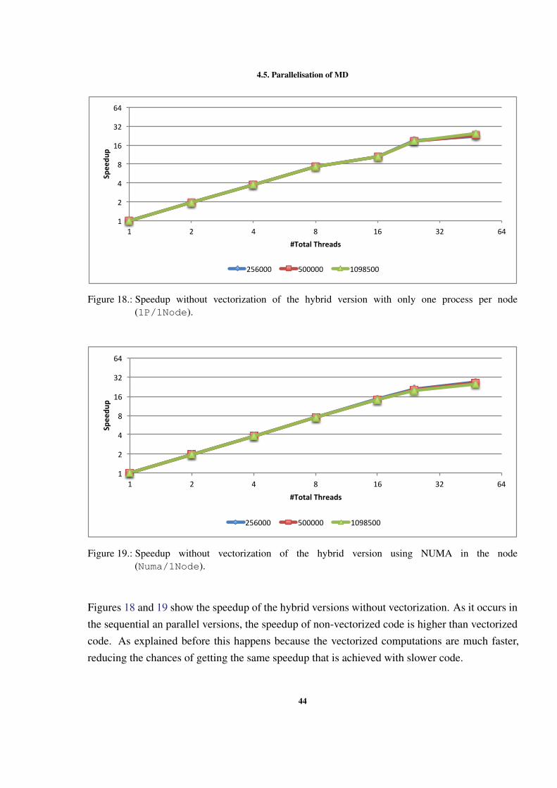
4.5. Parallelisation of MD
1
2
4
8
16
32
64
1 2 4 8 16 32 64
Speedu
p
#TotalThreads
256000 500000 1098500
Figure 18.: Speedup without vectorization of the hybrid version with only one process per node(1P/1Node).
1
2
4
8
16
32
64
1 2 4 8 16 32 64
Speedu
p
#TotalThreads
256000 500000 1098500
Figure 19.: Speedup without vectorization of the hybrid version using NUMA in the node(Numa/1Node).
Figures 18 and 19 show the speedup of the hybrid versions without vectorization. As it occurs inthe sequential an parallel versions, the speedup of non-vectorized code is higher than vectorizedcode. As explained before this happens because the vectorized computations are much faster,reducing the chances of getting the same speedup that is achieved with slower code.
44
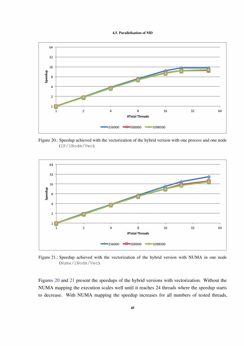
4.5. Parallelisation of MD
1
2
4
8
16
32
64
1 2 4 8 16 32 64
Speedu
p
#TotalThreads
256000 500000 1098500
Figure 20.: Speedup achieved with the vectorization of the hybrid version with one process and one node(1P/1Node/Vec).
1
2
4
8
16
32
64
1 2 4 8 16 32 64
Speedu
p
#TotalThreads
256000 500000 1098500
Figure 21.: Speedup achieved with the vectorization of the hybrid version with NUMA in one node(Numa/1Node/Vec).
Figures 20 and 21 present the speedups of the hybrid versions with vectorization. Without theNUMA mapping the execution scales well until it reaches 24 threads where the speedup startsto decrease. With NUMA mapping the speedup increases for all numbers of tested threads,
45
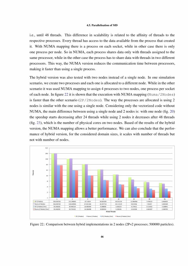
4.5. Parallelisation of MD
i.e., until 48 threads. This difference in scalability is related to the affinity of threads to therespective processes. Every thread has access to the data available from the process that createdit. With NUMA mapping there is a process on each socket, while in other case there is onlyone process per node. So in NUMA, each process shares data only with threads assigned to thesame processor, while in the other case the process has to share data with threads in two differentprocessors. This way, the NUMA version reduces the communication time between processors,making it faster than using a single process.
The hybrid version was also tested with two nodes instead of a single node. In one simulationscenario, we create two processes and each one is allocated to a different node. While in the otherscenario it was used NUMA mapping to assign 4 processes to two nodes, one process per socketof each node. In figure 22 it is shown that the execution with NUMA mapping (Numa/2Nodes)is faster than the other scenario (2P/2Nodes). The way the processes are allocated is using 2nodes is similar with the one using a single node. Considering only the vectorized code withoutNUMA, the main difference between using a single node and 2 nodes is: with one node (fig. 20)the speedup starts decreasing after 24 threads while using 2 nodes it decreases after 48 threads(fig. 23), which is the number of physical cores on two nodes. Based of the results of the hybridversion, the NUMA mapping allows a better performance. We can also conclude that the perfor-mance of hybrid version, for the considered domain sizes, it scales with number of threads butnot with number of nodes.
1 2 4 8 16 24 48 962P(2Nodes) 256.026762 131.396061 67.21814 34.855595 18.531219 12.966958 7.478152 6.460033
Numa(2Nodes) 256.026762 136.630945 67.051184 34.207714 18.111519 9.812456 7.05457 5.834349
2P(2Nodes)(Vec) 59.246292 30.940154 16.485949 9.288858 5.426223 4.170411 3.115032 3.168841
Numa(2Nodes)(Vec) 59.246292 30.733132 16.366408 8.903454 5.228101 3.312358 2.663297 2.268793
1
2
4
8
16
32
64
128
256
512
Time(s)
#TotalThreads
2P(2Nodes) Numa(2Nodes) 2P(2Nodes)(Vec) Numa(2Nodes)(Vec)
Figure 22.: Comparison between hybrid implementations in 2 nodes (2P=2 processes; 500000 particles).
46
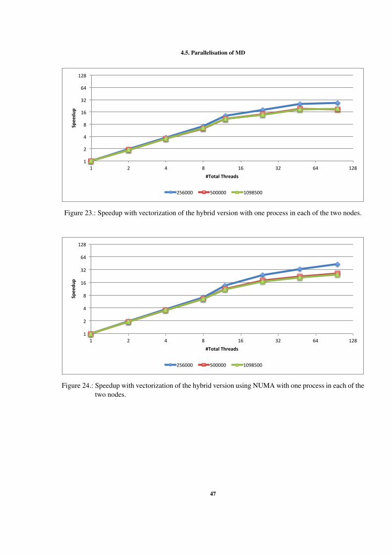
4.5. Parallelisation of MD
1
2
4
8
16
32
64
128
1 2 4 8 16 32 64 128
Speedu
p
#TotalThreads
256000 500000 1098500
Figure 23.: Speedup with vectorization of the hybrid version with one process in each of the two nodes.
1
2
4
8
16
32
64
128
1 2 4 8 16 32 64 128
Speedu
p
#TotalThreads
256000 500000 1098500
Figure 24.: Speedup with vectorization of the hybrid version using NUMA with one process in each of thetwo nodes.
47
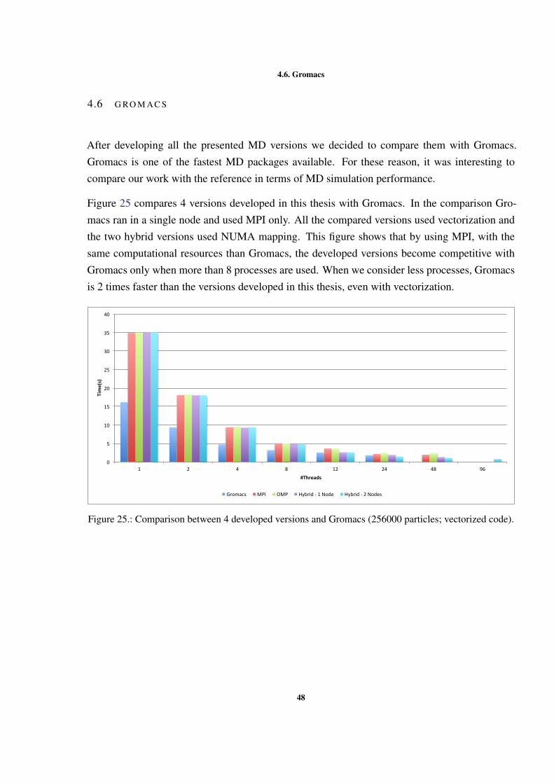
4.6. Gromacs
4.6 G RO M AC S
After developing all the presented MD versions we decided to compare them with Gromacs.Gromacs is one of the fastest MD packages available. For these reason, it was interesting tocompare our work with the reference in terms of MD simulation performance.
Figure 25 compares 4 versions developed in this thesis with Gromacs. In the comparison Gro-macs ran in a single node and used MPI only. All the compared versions used vectorization andthe two hybrid versions used NUMA mapping. This figure shows that by using MPI, with thesame computational resources than Gromacs, the developed versions become competitive withGromacs only when more than 8 processes are used. When we consider less processes, Gromacsis 2 times faster than the versions developed in this thesis, even with vectorization.
0
5
10
15
20
25
30
35
40
1 2 4 8 12 24 48 96
Time(s)
#Threads
Gromacs MPI OMP Hybrid-1Node Hybrid-2Nodes
Figure 25.: Comparison between 4 developed versions and Gromacs (256000 particles; vectorized code).
48
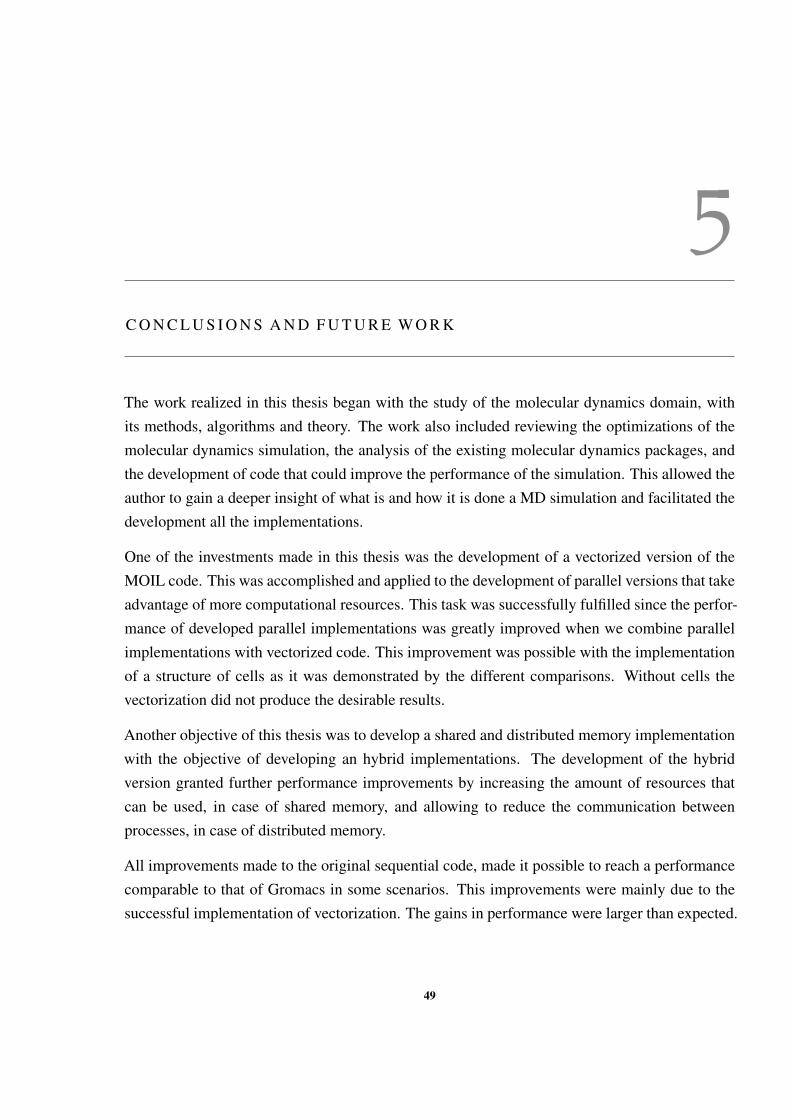
5
C O N C L U S I O N S A N D F U T U R E W O R K
The work realized in this thesis began with the study of the molecular dynamics domain, withits methods, algorithms and theory. The work also included reviewing the optimizations of themolecular dynamics simulation, the analysis of the existing molecular dynamics packages, andthe development of code that could improve the performance of the simulation. This allowed theauthor to gain a deeper insight of what is and how it is done a MD simulation and facilitated thedevelopment all the implementations.
One of the investments made in this thesis was the development of a vectorized version of theMOIL code. This was accomplished and applied to the development of parallel versions that takeadvantage of more computational resources. This task was successfully fulfilled since the perfor-mance of developed parallel implementations was greatly improved when we combine parallelimplementations with vectorized code. This improvement was possible with the implementationof a structure of cells as it was demonstrated by the different comparisons. Without cells thevectorization did not produce the desirable results.
Another objective of this thesis was to develop a shared and distributed memory implementationwith the objective of developing an hybrid implementations. The development of the hybridversion granted further performance improvements by increasing the amount of resources thatcan be used, in case of shared memory, and allowing to reduce the communication betweenprocesses, in case of distributed memory.
All improvements made to the original sequential code, made it possible to reach a performancecomparable to that of Gromacs in some scenarios. This improvements were mainly due to thesuccessful implementation of vectorization. The gains in performance were larger than expected.
49
Modifying the MOIL code revealed to be a hard task because of the utilization of a mixed C andFortran code and due to code be poorly structured.
The data structures used in MD developed versions were not thoroughly optimized, nor to reducethe occupied memory space neither for better exploring memory affinity.
The future work could be to integrate the developed code in MOIL, a much more complete MDpackage, in order to allow vectorization. This would improve the performance of MOIL, since itdoes not support vectorization.
The development of a better memory management would also permit performance improvementsas it is shown in the MPI execution for many processes.
Another topic to explore in the future would be to include in the calculation of forces othercomponents besides van der Waals, especially the electrostatic component.
50
B I B L I O G R A P H Y
Stewart A Adcock and J Andrew McCammon. Molecular dynamics: survey of methods forsimulating the activity of proteins. Chemical reviews, 106(5):1589–1615, 2006.
B. J. Alder and T. E. Wainwright. Phase transition for a hard sphere system. The
Journal of Chemical Physics, 27(5):1208–1209, 1957. doi: http://dx.doi.org/10.1063/1.1743957. URL http://scitation.aip.org/content/aip/journal/jcp/27/
5/10.1063/1.1743957.
Herman JC Berendsen, David van der Spoel, and Rudi van Drunen. Gromacs: A message-passing parallel molecular dynamics implementation. Computer Physics Communications, 91(1):43–56, 1995.
Bernard R Brooks, Robert E Bruccoleri, Barry D Olafson, David J States, S Swaminathan, andMartin Karplus. Charmm: A program for macromolecular energy, minimization, and dynam-ics calculations. Journal of computational chemistry, 4(2):187–217, 1983.
W Michael Brown, Peng Wang, Steven J Plimpton, and Arnold N Tharrington. Implementingmolecular dynamics on hybrid high performance computers–short range forces. Computer
Physics Communications, 182(4):898–911, 2011.
Leonardo Dagum and Rameshm Enon. Openmp: an industry standard api for shared-memoryprogramming. Computational Science & Engineering, IEEE, 5(1):46–55, 1998.
Ron Elber, Adrian Roitberg, Carlos Simmerling, Robert Goldstein, Haiying Li, GennadyVerkhivker, Chen Keasar, Jing Zhang, and Alex Ulitsky. Moil: A program for simulationsof macromolecules. Computer Physics Communications, 91(1):159–189, 1995.
The MPI Forum. Mpi: A message passing interface, 1993.
Michael Griebel, Stephan Knapek, and Gerhard Zumbusch. Numerical simulation in molecular
dynamics: numerics, algorithms, parallelization, applications, volume 5. Springer Science &Business Media, 2007.
51
Bibliography
Martin Karplus and J Andrew McCammon. Molecular dynamics simulations of biomolecules.Nature Structural & Molecular Biology, 9(9):646–652, 2002.
Andrew R. Leach. Molecular modelling: principles and applications. Pearson Education, 2001.
JA McCammon. Molecular dynamics study of the bovine pancreatic trypsin inhibitor. Models
for Protein Dynamics, page 137, 1976.
David A Pearlman, David A Case, James W Caldwell, Wilson S Ross, Thomas E Cheatham III,Steve DeBolt, David Ferguson, George Seibel, and Peter Kollman. Amber, a package of com-puter programs for applying molecular mechanics, normal mode analysis, molecular dynamicsand free energy calculations to simulate the structural and energetic properties of molecules.Computer Physics Communications, 91(1):1–41, 1995.
James C Phillips, Rosemary Braun, Wei Wang, James Gumbart, Emad Tajkhorshid, ElizabethVilla, Christophe Chipot, Robert D Skeel, Laxmikant Kale, and Klaus Schulten. Scalablemolecular dynamics with namd. Journal of computational chemistry, 26(16):1781–1802,2005.
Steve Plimpton. Fast parallel algorithms for short-range molecular dynamics. Journal of compu-
tational physics, 117(1):1–19, 1995.
A Rahman. Correlations in the motion of atoms in liquid argon. Physical Review, 136(2A):A405,1964.
Richard M Russell. The cray-1 computer system. Communications of the ACM, 21(1):63–72,1978.
A Peter Ruymgaart and Ron Elber. Revisiting molecular dynamics on a cpu/gpu system: Waterkernel and shake parallelization. Journal of chemical theory and computation, 8(11):4624–4636, 2012.
A Peter Ruymgaart, Alfredo E Cardenas, and Ron Elber. Moil-opt: Energy-conserving moleculardynamics on a gpu/cpu system. Journal of chemical theory and computation, 7(10):3072–3082, 2011.
Lorna A Smith, J Mark Bull, and J Obdrizalek. A parallel java grande benchmark suite. InSupercomputing, ACM/IEEE 2001 Conference, pages 6–6. IEEE, 2001.
52

Bibliography
University of Minho. Search - services and advanced research computing with htc/hpc clusters,2015. URL http://www4.di.uminho.pt/search/pt/.
53
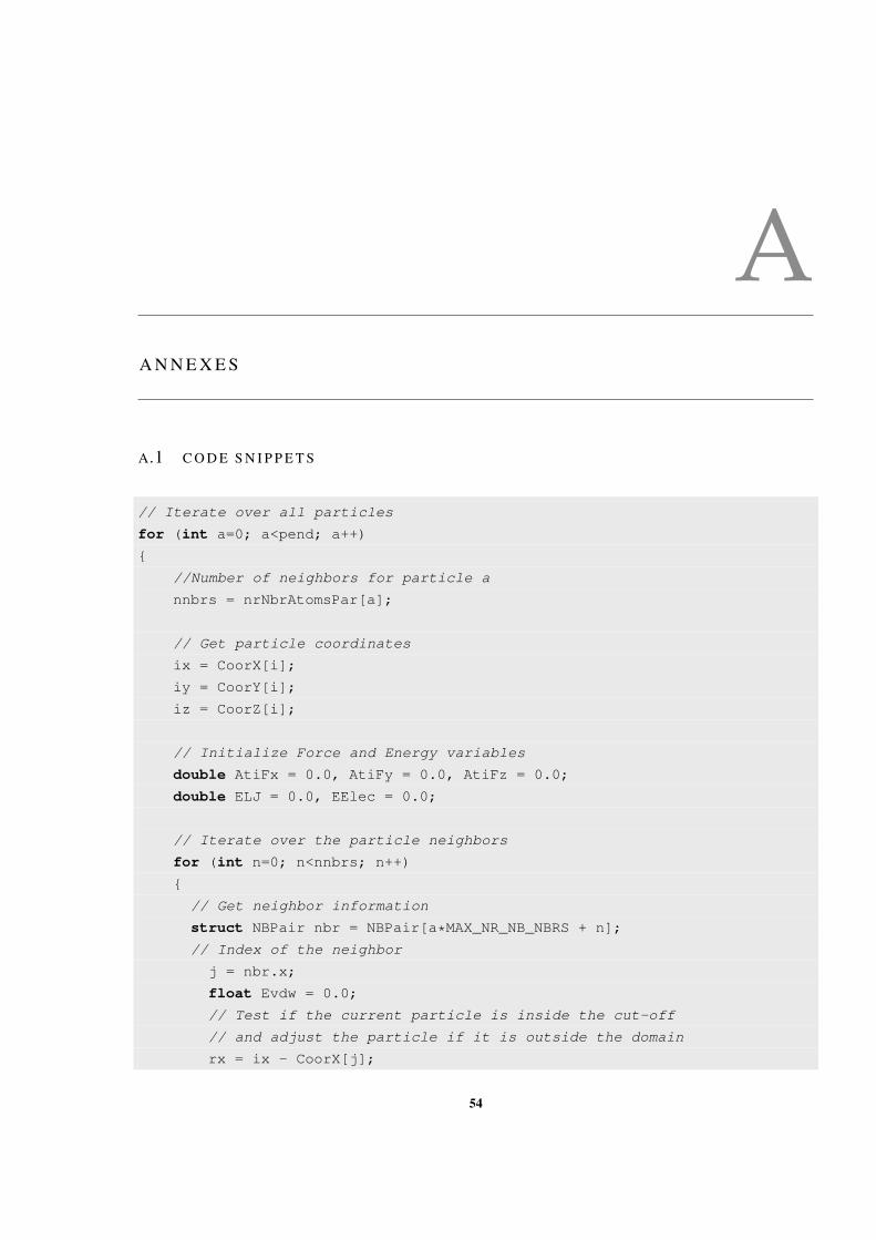
AA N N E X E S
A.1 C O D E S N I P P E T S
// Iterate over all particles
for (int a=0; a<pend; a++)
{
//Number of neighbors for particle a
nnbrs = nrNbrAtomsPar[a];
// Get particle coordinates
ix = CoorX[i];
iy = CoorY[i];
iz = CoorZ[i];
// Initialize Force and Energy variables
double AtiFx = 0.0, AtiFy = 0.0, AtiFz = 0.0;
double ELJ = 0.0, EElec = 0.0;
// Iterate over the particle neighbors
for (int n=0; n<nnbrs; n++)
{
// Get neighbor information
struct NBPair nbr = NBPair[a*MAX_NR_NB_NBRS + n];
// Index of the neighbor
j = nbr.x;
float Evdw = 0.0;
// Test if the current particle is inside the cut-off
// and adjust the particle if it is outside the domain
rx = ix - CoorX[j];
54
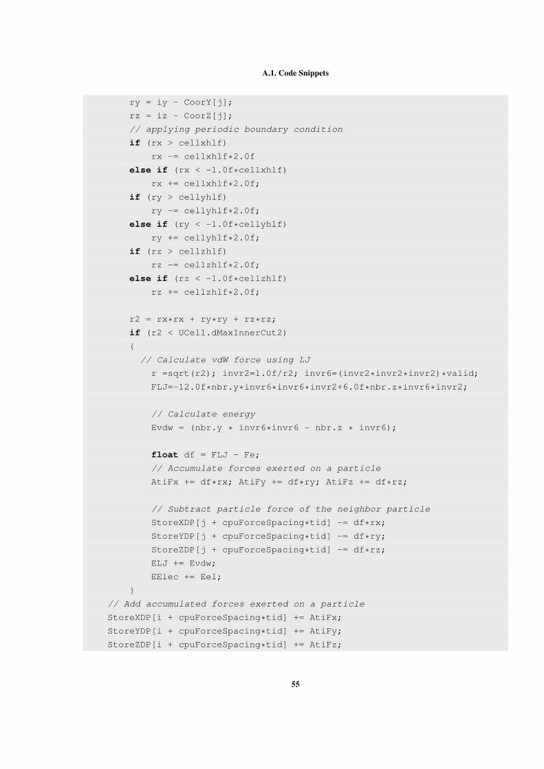
A.1. Code Snippets
ry = iy - CoorY[j];
rz = iz - CoorZ[j];
// applying periodic boundary condition
if (rx > cellxhlf)
rx -= cellxhlf*2.0f
else if (rx < -1.0f*cellxhlf)
rx += cellxhlf*2.0f;
if (ry > cellyhlf)
ry -= cellyhlf*2.0f;
else if (ry < -1.0f*cellyhlf)
ry += cellyhlf*2.0f;
if (rz > cellzhlf)
rz -= cellzhlf*2.0f;
else if (rz < -1.0f*cellzhlf)
rz += cellzhlf*2.0f;
r2 = rx*rx + ry*ry + rz*rz;
if (r2 < UCell.dMaxInnerCut2)
{
// Calculate vdW force using LJ
r =sqrt(r2); invr2=1.0f/r2; invr6=(invr2*invr2*invr2)*valid;
FLJ=-12.0f*nbr.y*invr6*invr6*invr2+6.0f*nbr.z*invr6*invr2;
// Calculate energy
Evdw = (nbr.y * invr6*invr6 - nbr.z * invr6);
float df = FLJ - Fe;
// Accumulate forces exerted on a particle
AtiFx += df*rx; AtiFy += df*ry; AtiFz += df*rz;
// Subtract particle force of the neighbor particle
StoreXDP[j + cpuForceSpacing*tid] -= df*rx;
StoreYDP[j + cpuForceSpacing*tid] -= df*ry;
StoreZDP[j + cpuForceSpacing*tid] -= df*rz;
ELJ += Evdw;
EElec += Eel;
}
// Add accumulated forces exerted on a particle
StoreXDP[i + cpuForceSpacing*tid] += AtiFx;
StoreYDP[i + cpuForceSpacing*tid] += AtiFy;
StoreZDP[i + cpuForceSpacing*tid] += AtiFz;
55
A.1. Code Snippets
// Store the calculated energies
StoreX[a + cpuForceSpacing*tid] = ELJ;
StoreY[a + cpuForceSpacing*tid] = EElec;
}
Listing A.1: Full For cycles that calculate the forces exerted on each particle by its neighbors.
56
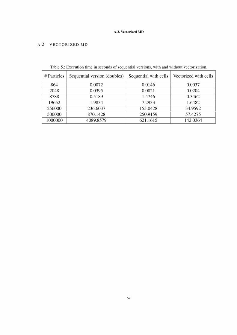
A.2. Vectorized MD
A.2 V E C T O R I Z E D M D
Table 5.: Execution time in seconds of sequential versions, with and without vectorization.
# Particles Sequential version (doubles) Sequential with cells Vectorized with cells
864 0.0072 0.0146 0.00372048 0.0395 0.0821 0.02048788 0.5189 1.4746 0.3462
19652 1.9834 7.2933 1.6482256000 236.6037 155.0428 34.9592500000 870.1428 250.9159 57.4275
1000000 4089.8579 621.1615 142.0364
57
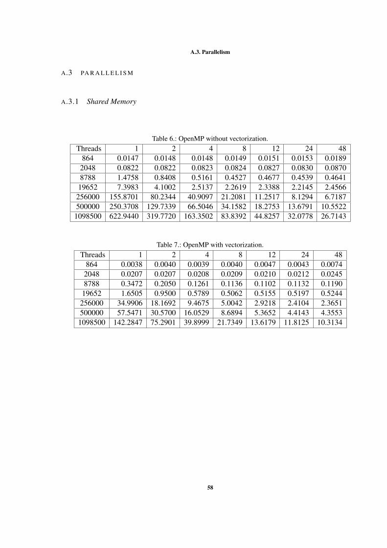
A.3. Parallelism
A.3 PA R A L L E L I S M
A.3.1 Shared Memory
Table 6.: OpenMP without vectorization.Threads 1 2 4 8 12 24 48
864 0.0147 0.0148 0.0148 0.0149 0.0151 0.0153 0.01892048 0.0822 0.0822 0.0823 0.0824 0.0827 0.0830 0.08708788 1.4758 0.8408 0.5161 0.4527 0.4677 0.4539 0.4641
19652 7.3983 4.1002 2.5137 2.2619 2.3388 2.2145 2.4566256000 155.8701 80.2344 40.9097 21.2081 11.2517 8.1294 6.7187500000 250.3708 129.7339 66.5046 34.1582 18.2753 13.6791 10.5522
1098500 622.9440 319.7720 163.3502 83.8392 44.8257 32.0778 26.7143
Table 7.: OpenMP with vectorization.Threads 1 2 4 8 12 24 48
864 0.0038 0.0040 0.0039 0.0040 0.0047 0.0043 0.00742048 0.0207 0.0207 0.0208 0.0209 0.0210 0.0212 0.02458788 0.3472 0.2050 0.1261 0.1136 0.1102 0.1132 0.119019652 1.6505 0.9500 0.5789 0.5062 0.5155 0.5197 0.5244
256000 34.9906 18.1692 9.4675 5.0042 2.9218 2.4104 2.3651500000 57.5471 30.5700 16.0529 8.6894 5.3652 4.4143 4.3553
1098500 142.2847 75.2901 39.8999 21.7349 13.6179 11.8125 10.3134
58
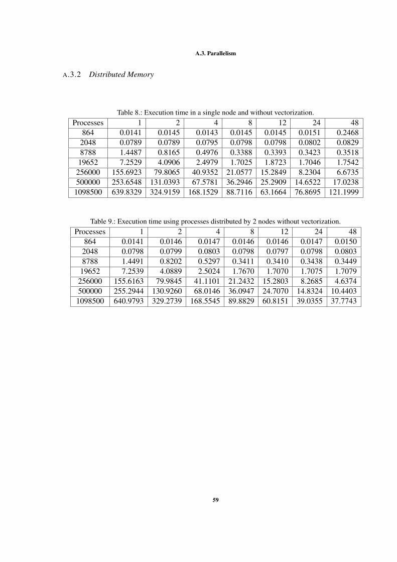
A.3. Parallelism
A.3.2 Distributed Memory
Table 8.: Execution time in a single node and without vectorization.Processes 1 2 4 8 12 24 48
864 0.0141 0.0145 0.0143 0.0145 0.0145 0.0151 0.24682048 0.0789 0.0789 0.0795 0.0798 0.0798 0.0802 0.08298788 1.4487 0.8165 0.4976 0.3388 0.3393 0.3423 0.3518
19652 7.2529 4.0906 2.4979 1.7025 1.8723 1.7046 1.7542256000 155.6923 79.8065 40.9352 21.0577 15.2849 8.2304 6.6735500000 253.6548 131.0393 67.5781 36.2946 25.2909 14.6522 17.02381098500 639.8329 324.9159 168.1529 88.7116 63.1664 76.8695 121.1999
Table 9.: Execution time using processes distributed by 2 nodes without vectorization.Processes 1 2 4 8 12 24 48
864 0.0141 0.0146 0.0147 0.0146 0.0146 0.0147 0.01502048 0.0798 0.0799 0.0803 0.0798 0.0797 0.0798 0.08038788 1.4491 0.8202 0.5297 0.3411 0.3410 0.3438 0.3449
19652 7.2539 4.0889 2.5024 1.7670 1.7070 1.7075 1.7079256000 155.6163 79.9845 41.1101 21.2432 15.2803 8.2685 4.6374500000 255.2944 130.9260 68.0146 36.0947 24.7070 14.8324 10.4403
1098500 640.9793 329.2739 168.5545 89.8829 60.8151 39.0355 37.7743
59
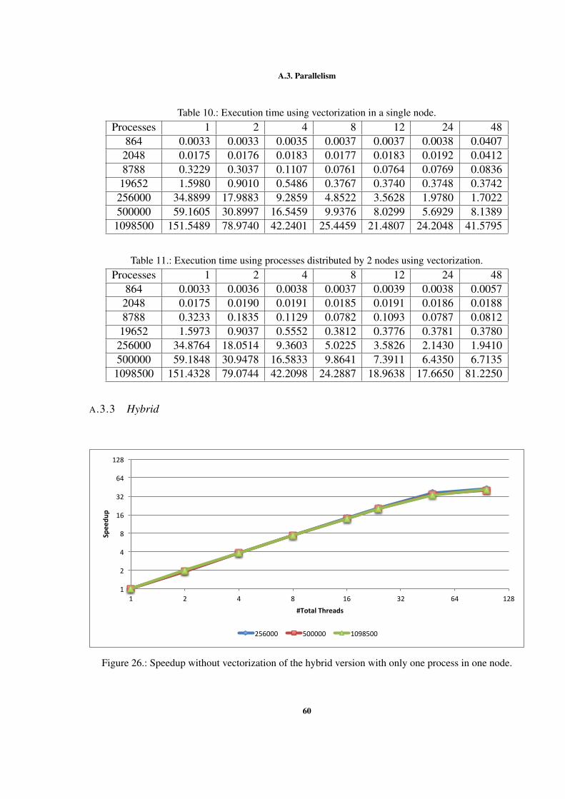
A.3. Parallelism
Table 10.: Execution time using vectorization in a single node.Processes 1 2 4 8 12 24 48
864 0.0033 0.0033 0.0035 0.0037 0.0037 0.0038 0.04072048 0.0175 0.0176 0.0183 0.0177 0.0183 0.0192 0.04128788 0.3229 0.3037 0.1107 0.0761 0.0764 0.0769 0.083619652 1.5980 0.9010 0.5486 0.3767 0.3740 0.3748 0.3742
256000 34.8899 17.9883 9.2859 4.8522 3.5628 1.9780 1.7022500000 59.1605 30.8997 16.5459 9.9376 8.0299 5.6929 8.1389
1098500 151.5489 78.9740 42.2401 25.4459 21.4807 24.2048 41.5795
Table 11.: Execution time using processes distributed by 2 nodes using vectorization.Processes 1 2 4 8 12 24 48
864 0.0033 0.0036 0.0038 0.0037 0.0039 0.0038 0.00572048 0.0175 0.0190 0.0191 0.0185 0.0191 0.0186 0.01888788 0.3233 0.1835 0.1129 0.0782 0.1093 0.0787 0.081219652 1.5973 0.9037 0.5552 0.3812 0.3776 0.3781 0.3780
256000 34.8764 18.0514 9.3603 5.0225 3.5826 2.1430 1.9410500000 59.1848 30.9478 16.5833 9.8641 7.3911 6.4350 6.7135
1098500 151.4328 79.0744 42.2098 24.2887 18.9638 17.6650 81.2250
A.3.3 Hybrid
1
2
4
8
16
32
64
128
1 2 4 8 16 32 64 128
Speedu
p
#TotalThreads
256000 500000 1098500
Figure 26.: Speedup without vectorization of the hybrid version with only one process in one node.
60
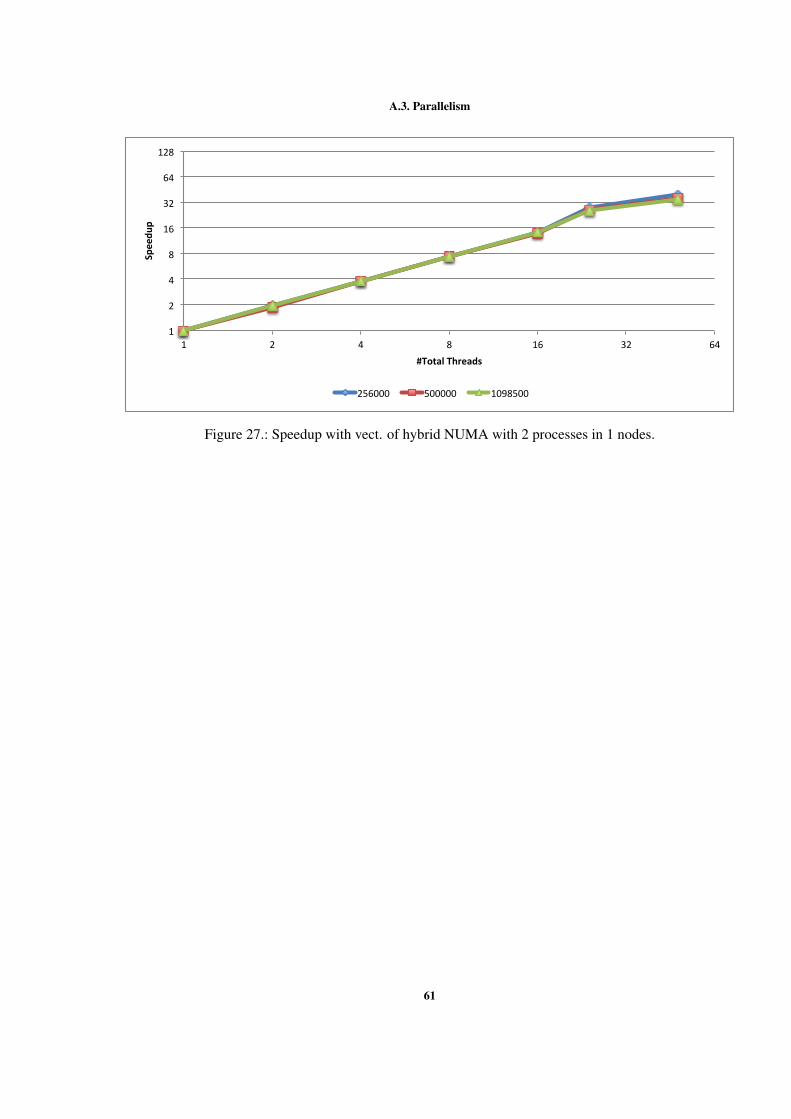
A.3. Parallelism
1
2
4
8
16
32
64
128
1 2 4 8 16 32 64
Speedu
p
#TotalThreads
256000 500000 1098500
Figure 27.: Speedup with vect. of hybrid NUMA with 2 processes in 1 nodes.
61