
Mathematical modeling of micro-textured lubricated contacts · atrito e os par^ametros de...
153
Mathematical modeling of micro-textured lubricated contacts Alfredo Del Carmen Jaramillo Palma
Transcript of Mathematical modeling of micro-textured lubricated contacts · atrito e os par^ametros de...

Mathematical modeling of
micro-textured lubricated contacts
Alfredo Del Carmen Jaramillo Palma


SERVIÇO DE PÓS-GRADUAÇÃO DO ICMC-USP
Data de Depósito: Assinatura:_______________________
Alfredo Del Carmen Jaramillo Palma
Modelação matemática de contatos lubrificados micro-texturizados
Dissertação apresentada ao Instituto de Ciências Matemáticas e de Computação - ICMC-USP, como parte dos requisitos para obtenção do título de Mestre em Ciências - Ciências de Computação e Matemática Computacional. VERSÃO REVISADA.
Área de Concentração: Ciências de Computação e Matemática Computacional.
Orientador: Prof. Dr. Gustavo Carlos Buscaglia.
USP – São Carlos Julho de 2015

Ficha catalográfica elaborada pela Biblioteca Prof. Achille Bassi e Seção Técnica de Informática, ICMC/USP,
com os dados fornecidos pelo(a) autor(a)
J37mJaramillo Palma, Alfredo Del Carmen Mathematical modeling of micro-texturedlubricated contacts / Alfredo Del Carmen JaramilloPalma; orientador Gustavo Carlos Buscaglia. -- SãoCarlos, 2015. 129 p.
Dissertação (Mestrado - Programa de Pós-Graduaçãoem Ciências de Computação e MatemáticaComputacional) -- Instituto de Ciências Matemáticase de Computação, Universidade de São Paulo, 2015.
1. Textured surfaces. 2. Reynolds equation. 3.Friction reduction. 4. Cavitation. 5. Numericalsimulation. I. Buscaglia, Gustavo Carlos , orient.II. Título.

SERVIÇO DE PÓS-GRADUAÇÃO DO ICMC-USP
Data de Depósito: Assinatura:_______________________
Alfredo Del Carmen Jaramillo Palma
Mathematical modeling of micro-textured lubricated contacts
Master dissertation submitted to the Instituto de Ciências Matemáticas e de Computação - ICMC-USP, in partial fulfillment of the requirements for the degree of the Master Program in Computer Science and Computational Mathematics. FINAL VERSION.
Concentration Area: Computer Science and Computational Mathematics.
Advisor: Prof. Dr. Carlos Gustavo Buscaglia.
USP – São Carlos July 2015


Para Ida y Victor. . .
vii

Acknowledgements (Agradecimientos)
Agradezco a mis padres, quienes a la distancia me han apoyado durante este proceso,
como durante toda mi vida; a Paola, por su carino, paciencia y apoyo;
a Hugo Checo, colega de pesquisa, y al profesor Mohammed Jai, por su ayuda y dis-
posicion; a Gustavo Buscaglia, mi orientador, por compartir su vision cientıfica y su
paciencia; al profesor Sergio Monari, por su ayuda en el estudio de EDP elıpticas. Fi-
nalmente, agradezco a las agencias CAPES (Coordenacao de Aperfeicoamento de Pessoal
de Nıvel Superior, processo DS-8434433/M) y CNPQ (Conselho Nacional de Desenvolvi-
mento Cientıfico e Tecnologico, processo 134105/2013-3), que apoyaron economicamente
este trabajo de maestrıa.
viii
“. . . La copa se hundio en el sol. Recogio un poco de la carne de Dios, la sangre del
universo, el pensamiento deslumbrante, la enceguecedora filosofıa que habıa amamantado
a una galaxia, que guiaba y llevaba a los planetas por sus campos y emplazaba o acallaba
vidas y subsistencias . . . ”
Las doradas manzanas del sol, Ray Bradbury.

Resumo
No desenho de mecanismos lubrificados, tais como Mancais hidrodinamicos ou aneis de
pistoes de Motores a Combustao, atrito e desgaste sao efeitos nao desejados. Por exem-
plo, e sabido que aproximadamente 5% da energia perdida em um motor a combustao
esta associada ao atrito presente no sistema de aneis/cilindro do pistao. Apos varios tra-
balhos experimentais e teoricos, as superfıcies texturizadas hao mostrado serem capazes
de reduzir o atrito em algumas condicoes de funcionamento. O estudo da relacao entre o
atrito e os parametros de texturizacao e um problema difıcil e de interesse tanto indus-
trial como academico. O contexto matematico e computacional destes trabalhos apresen-
tam desafios por si mesmos, como o estudo da boa colocacao dos modelos matematicos, a
consideracao adequada das descontinuidades das superfıcies. Este trabalho enfoca-se no
contexto matematico, apresentando e estudando a equacao de Reynolds junto com difer-
entes modelos de cavitacao que podem encontrar-se na literatura. Comecamos estudando
a matematica da equacao de Reynolds. Depois disso, modelos de cavitacao sao inclusos,
aumentando a complexidade da matematica envolvida. Seguidamente, como aplicacao
da teoria apresentada, um rolamento deslizante sera estudado junto com uma textur-
izacao da superfıcie movel. Os resultados deste estudo revelam mecanismos basicos de
reducao de atrito e propriedades gerais que nao haviam sido reportadas anteriormente.
Possıveis trabalhos futuros sao apresentados, tal como o uso de Metodos Descontınuos
de Galerkin em vez dos Metodos de Volumes Finitos. O ultimo em procura de uma
melhor acomodacao da formulacao matematica, tentando melhorar a flexibilidade da
malha e a precisao.
Palavras-chave: superfıcies texturizadas, Equacao de Reynolds, reducao de atrito,
cavitacao, simulacao numerica.

Abstract
In the design of lubricated mechanisms, such as Journal Bearings or Piston Rings of
Combustion Engines, friction and wear are undesirable effects. It is known, for instance,
that about 5% of the energy loss in a Combustion Engine is associated to friction taking
place in the Piston Rings/Cylinder system. Textured surfaces, after a significant number
of experimental and theoretical studies, have shown to reduce friction in some operating
conditions. The study of the relation between the friction and the texture parameters
is a challenging problem with both industrial and academic interest. The mathematical
and computational frameworks involved present challenges by themselves, such as es-
tablishing the well-posedness of the mathematical models with suitable consideration of
discontinuous surfaces. In this work we focus on the mathematical framework, present-
ing and studying the Reynolds equation along with different state-of-the-art cavitation
models. We begin by studying the Reynolds equation and then incorporate two different
cavitation models of increasing mathematical complexity. Next, as an application of the
theory already presented, a slider bearing is numerically studied considering a sinusoidal
texture on the runner. The results of this study unveil basic mechanisms of friction re-
duction and global quantitative trends that had not been previously reported. In this
way, the applicability of numerical tools for texture selection is established. Future
research directions are also identified, such as using Discontinuous Galerkin methods
instead of Finite Volume Methods, aiming at improving the mesh flexibility and thus
the accuracy of the discrete formulation.
Keywords: textured surfaces, Reynolds equation, friction reduction, cavitation, nu-
merical simulation.


Contents
Acknowledgements (Agradecimientos) viii
Abstract x
Contents xii
List of Figures xvii
List of Tables xix
List of Algorithms xxi
Symbols xxii
1 Motivation and scope of this manuscript 1
1.1 Representative Lubricated systems . . . . . . . . . . . . . . . . . . . . . 2
1.2 Lubrication regimes . . . . . . . . . . . . . . . . . . . . . . . . . . . . . 3
1.2.1 Hydrodynamic Lubrication . . . . . . . . . . . . . . . . . . . . . 5
1.2.2 Elastohydrodynamic Lubrication . . . . . . . . . . . . . . . . . . 5
1.2.3 Boundary Lubrication . . . . . . . . . . . . . . . . . . . . . . . . 5
1.2.4 Mixed Lubrication . . . . . . . . . . . . . . . . . . . . . . . . . . 5
1.2.5 Fully-flooded and starving conditions . . . . . . . . . . . . . . . . 5
1.3 Lubrication Theory Hypothesis . . . . . . . . . . . . . . . . . . . . . . . 6
2 The equations of lubrication 9
2.1 Lubrication Hypothesis in Navier-Stokes equation . . . . . . . . . . . . . 9
2.2 Reynolds Equation . . . . . . . . . . . . . . . . . . . . . . . . . . . . . . 11
2.3 Friction forces . . . . . . . . . . . . . . . . . . . . . . . . . . . . . . . . . 13
2.4 Comparison with Navier-Stokes equations . . . . . . . . . . . . . . . . . 16
2.4.1 Reynolds and Stokes roughness . . . . . . . . . . . . . . . . . . . 16
2.4.2 Numerical comparison addressing a sinusoidal texture case . . . 16
2.5 Some representative analytic solutions . . . . . . . . . . . . . . . . . . . 22
2.5.1 Step wedge and Rayleigh step . . . . . . . . . . . . . . . . . . . . 22
2.5.2 Disc wedge . . . . . . . . . . . . . . . . . . . . . . . . . . . . . . 27
3 Mathematics of Reynolds equation 31
3.1 From Stokes equations to Reynolds equation . . . . . . . . . . . . . . . . 31
xiii
Contents xiv
3.2 Weak formulation for Reynolds equation . . . . . . . . . . . . . . . . . . 36
3.2.1 Stability Analysis . . . . . . . . . . . . . . . . . . . . . . . . . . . 38
3.2.2 Spatial regularity . . . . . . . . . . . . . . . . . . . . . . . . . . . 40
3.3 Maximum Principle for Reynolds equation . . . . . . . . . . . . . . . . . 41
4 Cavitation and cavitation models 43
4.1 Basic cavitation physics . . . . . . . . . . . . . . . . . . . . . . . . . . . 43
4.2 Reynolds model . . . . . . . . . . . . . . . . . . . . . . . . . . . . . . . . 44
4.2.1 Variational Formulation for Reynolds cavitation model . . . . . . 46
4.3 Mass conservation in cavitation models . . . . . . . . . . . . . . . . . . . 51
4.4 Elrod-Adams model . . . . . . . . . . . . . . . . . . . . . . . . . . . . . 53
4.5 Analytical solution examples . . . . . . . . . . . . . . . . . . . . . . . . 56
4.5.1 Cavitation in Pure Squeeze Motion . . . . . . . . . . . . . . . . . 56
4.5.2 Cavitation in a flat pad with a traveling pocket . . . . . . . . . . 60
5 Numerical methods and illustrative examples 69
5.1 Finite volume discretization . . . . . . . . . . . . . . . . . . . . . . . . . 69
5.2 Numerical implementation of Reynolds equation and cavitation models . 71
5.2.1 Reynolds equation without cavitation . . . . . . . . . . . . . . . 71
5.2.2 Reynolds model . . . . . . . . . . . . . . . . . . . . . . . . . . . . 78
5.2.3 Elrod-Adams model . . . . . . . . . . . . . . . . . . . . . . . . . 79
5.3 Numerical solution examples . . . . . . . . . . . . . . . . . . . . . . . . 80
5.3.1 Numerical solution to the analytic examples . . . . . . . . . . . . 81
5.3.2 Incorporating dynamics . . . . . . . . . . . . . . . . . . . . . . . 84
6 Application: a study of sinusoidal textured slider bearings 89
6.1 Introduction . . . . . . . . . . . . . . . . . . . . . . . . . . . . . . . . . . 89
6.2 Simulation details and untextured cases . . . . . . . . . . . . . . . . . . 90
6.2.1 Quantities of interest . . . . . . . . . . . . . . . . . . . . . . . . . 92
6.2.2 Untextured cases . . . . . . . . . . . . . . . . . . . . . . . . . . . 93
6.3 Textures effects . . . . . . . . . . . . . . . . . . . . . . . . . . . . . . . . 94
6.3.1 General observations . . . . . . . . . . . . . . . . . . . . . . . . . 95
6.3.2 An effect of the traveling bubbles . . . . . . . . . . . . . . . . . . 95
6.3.3 Hysteresis of the slider . . . . . . . . . . . . . . . . . . . . . . . . 96
6.3.4 Cavitation induced oscillations . . . . . . . . . . . . . . . . . . . 97
7 Conclusions and future work 99
A Second order MAC scheme for Navier-Stokes equations 103
A.1 Discretization of advection and diffusion . . . . . . . . . . . . . . . . . . 104
A.2 Projection Method . . . . . . . . . . . . . . . . . . . . . . . . . . . . . . 106
B Mathematical background 109
B.1 Duality and Reflexivity . . . . . . . . . . . . . . . . . . . . . . . . . . . 110
B.2 Hilbert Spaces . . . . . . . . . . . . . . . . . . . . . . . . . . . . . . . . 110
B.3 Lp spaces . . . . . . . . . . . . . . . . . . . . . . . . . . . . . . . . . . . 112
B.4 Sobolev Spaces . . . . . . . . . . . . . . . . . . . . . . . . . . . . . . . . 113

Contents xv
Bibliography 121


List of Figures
1.1 Journal Bearing scheme . . . . . . . . . . . . . . . . . . . . . . . . . . . 3
1.2 Piston-Ring contact scheme . . . . . . . . . . . . . . . . . . . . . . . . . 4
1.3 Surface roughness scheme . . . . . . . . . . . . . . . . . . . . . . . . . . 4
1.4 Conformity of the circular-shaped slider bearing . . . . . . . . . . . . . . 4
1.5 Starved and fully-flooded conditions example. . . . . . . . . . . . . . . . 6
2.1 Two parallel lubricated surfaces scheme . . . . . . . . . . . . . . . . . . 9
2.2 Channel Problem scheme . . . . . . . . . . . . . . . . . . . . . . . . . . 12
2.3 2D surface normal orientations scheme . . . . . . . . . . . . . . . . . . . 15
2.4 An infinite 1D bearing with a sinusoidal texture. . . . . . . . . . . . . . 17
2.5 Dimensionless pressure from Navier-Stokes equations and from Reynoldsequation for different Reynolds number. . . . . . . . . . . . . . . . . . . 20
2.6 Dimensionless pressure from Navier-Stokes equations and Reynolds equa-tion for different depths. . . . . . . . . . . . . . . . . . . . . . . . . . . . 20
2.7 Dimensionless pressure differences (absolute and relative) between Reynoldsand Navier Stokes Equations with different Reynolds number . . . . . . 21
2.8 Relative differences in friction between Reynolds and Navier Stokes Equa-tions with several Reynolds number for the correct and wrong formulas 21
2.9 Step wedge pad scheme. . . . . . . . . . . . . . . . . . . . . . . . . . . . 23
2.10 Scheme of the “naive step wedge” versus the Rayleigh Step wedge . . . 26
2.11 Disc pad scheme. . . . . . . . . . . . . . . . . . . . . . . . . . . . . . . . 27
2.12 Disc pad scheme and pressure profile. . . . . . . . . . . . . . . . . . . . 29
3.1 Domain dependent on ε for studying the convergence of Stokes systemsolutions. . . . . . . . . . . . . . . . . . . . . . . . . . . . . . . . . . . . 32
3.2 Disc pad scheme and pressure profile. . . . . . . . . . . . . . . . . . . . 42
4.1 Illustration of gaseous cavitation . . . . . . . . . . . . . . . . . . . . . . 44
4.2 Scheme of a solution using Half-Sommerfeld cavitation model. . . . . . . 45
4.3 Obstacle problem for an elastic membrane. . . . . . . . . . . . . . . . . 46
4.4 2D cavitated domain scheme. . . . . . . . . . . . . . . . . . . . . . . . . 51
4.5 1D rupture and reformation scheme with Reynolds model . . . . . . . . 52
4.6 1D rupture and reformation scheme with Elrod-Adams model . . . . . . 55
4.7 Pure Squeeze problem scheme. . . . . . . . . . . . . . . . . . . . . . . . 56
4.8 Characteristic lines for Pure Squeeze Motion . . . . . . . . . . . . . . . 58
4.9 Comparison of cavitation models for a Pure Squeeze problem . . . . . . 59
4.10 Scheme of the rectangular wedges problem . . . . . . . . . . . . . . . . . 60
4.11 Scheme of the solution for a single honed pocket without cavitation. . . 61
xvii

List of Figures xviii
4.12 Scheme of an ansatz solution for a single honed pocket with Reynoldscavitation model. . . . . . . . . . . . . . . . . . . . . . . . . . . . . . . . 62
4.13 Characteristics lines of the transport equation of hθ . . . . . . . . . . . 65
4.14 Initial conditions of θ and p for the problem of a traveling pocket . . . . 65
4.15 Characteristic lines to find θ+(β). . . . . . . . . . . . . . . . . . . . . . . 66
4.16 Analytic solutions of Elrod-Adams and Reynolds cavitation models forthree different times of the traveling pocket . . . . . . . . . . . . . . . . 67
5.1 Finite volume control . . . . . . . . . . . . . . . . . . . . . . . . . . . . . 71
5.2 Scheme of flux functions 1D. . . . . . . . . . . . . . . . . . . . . . . . . 72
5.3 Convergence of the numerical solution for the Disc wedge presented inSection §2.5.2. . . . . . . . . . . . . . . . . . . . . . . . . . . . . . . . . 77
5.4 Numerical solution of the cavitation boundary for Elrod-Adams modelwith N = 100, 450 . . . . . . . . . . . . . . . . . . . . . . . . . . . . . . 82
5.5 Numerical solution of the cavitation boundary for Reynolds model withN = 100, 450 . . . . . . . . . . . . . . . . . . . . . . . . . . . . . . . . . 82
5.6 Numerical (N=450) and analytic solution of the saturation θ for t =0.3146, just before the reformation time tref . . . . . . . . . . . . . . . . 83
5.7 Analitic solutions of Elrod-Adams and Reynolds cavitation models forthree different times as done in Section §4.5.2 . . . . . . . . . . . . . . . 83
5.8 Convergence analysis for p and θ in the H10 (0, 1) and L2(0, 1) norms resp.
for the traveling pocket problem solved in Section §4.5.2. . . . . . . . . 84
5.9 Scheme of the rectangular wedges problem . . . . . . . . . . . . . . . . . 84
5.10 Profiles of p and θ for different time instants with dynamic behavior ofthe slider . . . . . . . . . . . . . . . . . . . . . . . . . . . . . . . . . . . 87
6.1 Slider bearing over and a sinusoidal textured runner scheme. . . . . . . 89
6.2 Slider evolution for the untextured case for load W a and R = 32. . . . . 93
6.3 Comparison of Cmin and f for several values of λ and d by relative differ-ences Vf (left side) and VC (right side) for R=32, 256 (upper and lowerfigures resp.). . . . . . . . . . . . . . . . . . . . . . . . . . . . . . . . . . 94
6.4 Sudden change of p and θ with a small change of d and λ fixed . . . . . 95
6.5 Hysteresis of the statationary state. . . . . . . . . . . . . . . . . . . . . 96
6.6 Hydrodynamic force and slider position oscillations induced by suddencavitation bubbles collapse . . . . . . . . . . . . . . . . . . . . . . . . . . 97
A.1 Staggered MAC discretization scheme . . . . . . . . . . . . . . . . . . . 104
A.2 Staggered MAC control volumes for velocities . . . . . . . . . . . . . . . 105
List of Tables
2.1 Non-dimensional variables for the stationary Reynolds equation (2.32). . 18
2.2 Non-dimensional variables for the step wedge problem. . . . . . . . . . . 22
2.3 Non-dimensional variables for the disc wedge problem. . . . . . . . . . . 27
5.1 Convergence of the truncation errors and global error for the numericalexample of the Disc wedge. . . . . . . . . . . . . . . . . . . . . . . . . . 77
5.2 Basic and derived scales for traveling pocket with dynamic behavior ofthe slider . . . . . . . . . . . . . . . . . . . . . . . . . . . . . . . . . . . 86
6.1 Basic and derived scales for the dynamic slider with sinusoidal textures. 91
6.2 Friction coefficient f and clearance Cmin for several values of R once theyreached the stationary state. . . . . . . . . . . . . . . . . . . . . . . . . . 93
xix


List of Algorithms
1 Gauss-Seidel for Reynolds equation . . . . . . . . . . . . . . . . . . . . . 78
2 Gauss-Seidel for Reynolds equation with Reynolds cavitation model . . . 79
3 Gauss-Seidel for Reynolds equation with Elrod-Adams cavitation model . 81
4 Dynamic Gauss-Seidel for Reynolds equation with Elrod-Adams cavitation
model . . . . . . . . . . . . . . . . . . . . . . . . . . . . . . . . . . . . . . 88
xxi


Symbols
∂Ω Boundary of the domain Ω
Ω Topological interior of Ω
Ω Closure of Ω: Ω = ∂Ω ∪ Ω
C0(Ω) Set of continuous functions over Ω
Ck(Ω) Set of functions over Ω having all derivatives of order ≤ k continuous in Ω
C∞(Ω) Set of infinitely differentiable functions over Ω
Ck0 (Ω) Functions in Ck(Ω) with compact support
C∞0 (Ω) Functions in C∞(Ω) with compact support
CjB u ∈ Cj(Ω) : ∂αu is bounded for|α| ≤ jL1(Ω) Lebesgue integrable functions on Ω
Lq(Ω) f : Ω→ R is in Lq(Ω) if |f |q ∈ L1(Ω)
H1(Ω) Sobolev space of functions in L2(Ω) with first order weak derivatives in L2(Ω)
H−1(Ω) Dual space of H1(Ω)
D′(Ω) Dual space of C∞0 (Ω)
∂x Denotes the operator ∂∂x
∇ ∇f is the vector with components ∂xf for each Cartesian coordinate
∇2 Denotes the Laplacian operator∑N
i=1∂2
∂x2i. N is the dimension of the problem.
xxiii


Chapter 1
Motivation and scope of this
manuscript
For many mechanical systems, designers deal with the proximity of surfaces in relative
motion in such a way that wear and friction appear. In general, to prevent such unde-
sirable effects, some substance (e.g., oil, grease, gas) is suitably placed to carry part of
the applied load. This way of addressing wear and friction is called lubrication and the
science that studies wear, friction and lubrication is called Tribology.
In the last ten years, novel fabrication techniques have opened the possibility of tai-
loring surfaces at micrometric scale [38]. Precision micromachining and high energy
pulsed lasers can engrave surfaces with micrometric motifs of practically any shape. En-
visioning large potential gains, industry has been promoting the scientific exploration of
engineered surfaces, designed so as to improve the friction, wear, stiction and lubricant
consumption characteristics of tribological systems. In fact, Holmberg [56] showed that
between 5 and 10% of a passenger car power is lost due to friction on the Piston-Ring
System (see Figure 1.2) and thus the better understanding of how engineered surfaces
work in those systems may have a great socio-economic impact.
For helping designers and engineers in the elaboration of efficient tribological systems,
computational simulations are need to provide insight on the dependence of those sys-
tems on their design variables. However, not only the analysis of simulation results
would be required but also the improvement of the mathematical models of the physics
involved and the numerical methods related to it. With this motivation, this work ad-
dresses the mathematical models and numerical methodologies involved in Lubrication
Theory.
1

Chapter 1. Motivation and scope of this manuscript 2
Apart from this mathematical study, simple tribological systems, such as the slider
bearing, were simulated and the results are exposed and analyzed. For these simula-
tions, an in-house computational program was used. Its source file can be found at
www.lcad.icmc.usp.br/ ∼buscaglia/download.html.
Next, the structure of this document is summarized:
Chapter 1 The scope of the work is given along with the description of some basic
tribological systems and some basic definitions of Lubrication Theory.
Chapter 2 The Reynolds equation and the friction formulas are deduced from a simple
asymptotic analysis. Also, results of both Navier-Stokes equations and Reynolds
equation are compared.
Chapter 3 Mathematical properties of the Reynolds equation are studied, showing
well-posedness (existence, uniqueness and stability) under the hypothesis of no
cavitation.
Chapter 4 Cavitation is considered and different mathematical models of it are pre-
sented and analyzed along with some analytical solutions.
Chapter 5 Numerical methods for Reynolds equation and cavitation models are stud-
ied and some numerical solutions are shown.
Chapter 6 A set of simulations are performed for the slider bearing tribological system.
Considering sinusoidal textures, the effects of several textures are measured and
some effects are presented when considering the Elrod-Adams cavitation model
(presented in Chapter 4).
Chapter 7 Conclusions and future work are presented.
1.1 Representative Lubricated systems
Journal Bearing (see Figure 1.1) This system consists of a rotating cylindrical shaft
(journal) enclosed by a cylindrical bush. The journal adopts an eccentric position
that creates a convergent-divergent profile for the fluid and in this way generates
pressure. This pressure, when integrated in the axial and circumferential direc-
tions, yields the load-carrying capacity of the journal.
Piston-Ring (see Figure 1.2) This system performs different important functions: the
Top Ring provides a gas seal and the Second Ring below assists in the sealing
and adjusts the action of the oil film. The rings also act carrying heat into the

Chapter 1. Motivation and scope of this manuscript 3
bearing liner
journal or shaftnarrow gap
A
B
applied load
hydrodynamic
pressure
ω
Figure 1.1: Journal Bearing scheme. Point A is the bush center (fixed). Point B isthe center of the journal (dynamically varying). The journal is rotating with angular
speed ω.
cooled cylinder wall (liner). This heat transfer function maintains acceptable tem-
peratures and stability in the piston and piston rings, so that sealing ability is
not impaired. Finally, the Oil Control Ring (OCL) acts in a scrapping manner,
keeping excess oil out of the combustion chamber. In this way, oil consumption is
held at an acceptable level and harmful emissions are reduced.
1.2 Lubrication regimes
This work is focused in fluid film lubrication phenomena, which take place when opposing
surfaces are separated by a lubricant film. We characterize the roughness of the surfaces
by a parameter σ that is the composite standard deviations of asperity height distribution,
given by σ =√σ2
1 + σ22 [69]. For characterizing the distance between the surfaces
we denote as h the average distance between them. Both parameters σ and h are
schematized in Figure 1.3.

Chapter 1. Motivation and scope of this manuscript 4
BDC TDC
narrow gap
Top RingSecond Ring
Oil Ring
combustion chamber
cilinder wall
Figure 1.2: Piston-Ring contact scheme. The piston has an oscillatory motion be-tween the TDC (Top Dead Center) and BDC (Bottom Dead Center) points.
planes
σA
σB
hReference
Surface A
Surface B
σ =√σ2
1 + σ22
Figure 1.3: Surface roughness scheme. Adapted from [69].
low conformity
high conformity
fixed surface
Figure 1.4: Conformity is a measure relating the curvatures of two surfaces in prox-imity. Adapted from [21].
Another important measure of surfaces in proximity is its degree of conformity. Roughly
speaking, we say that two surfaces are conformal if their curvatures are similar. On the

Chapter 1. Motivation and scope of this manuscript 5
contrary, the more dissimilar the curvatures are, the less conformal (see Figure 1.4). A
more accurate use of this concept can be found in Chapter 6.
Depending on how effective the fluid film is for separating the surfaces, the next classi-
fication arises:
1.2.1 Hydrodynamic Lubrication
In this case the fluid film separates the surfaces completely. Moreover, the generated
pressure is low enough to prevent the deformation of the surfaces. In this regime there
is no direct contact between the surfaces.
1.2.2 Elastohydrodynamic Lubrication (EHL)
As in Hydrodynamic Lubrication, in EHL the surfaces are completely separated (h σ).
In contrast, the pressure field deforms the surfaces. Material hardness and dependence
of viscosity on temperature play important roles.
1.2.3 Boundary Lubrication
This case (h ≈ σ) is associated with the highest levels of friction and wear due to direct
contact between the surfaces. These (normal) contact forces are calculated with some
model like the Greenwood-Williamson model [52, 69]. Some dry friction coefficient Cf
is used to calculate the contact friction force as F = CfN .
1.2.4 Mixed Lubrication
As the name would suggest, Mixed Lubrication occurs between boundary and hydrody-
namic lubrication. The fluid film thickness (h) is slightly greater than the surface rough-
ness (σ), so that asperity contacts are not as important as in Boundary Lubrication,
but the surfaces are still close enough as to affect each other (e.g., surface deformations
would take place).
1.2.5 Fully-flooded and starving conditions
In this work, the oil inflow rate Q is assumed to be high enough to assure Hydrodynamic
Lubrication regime and, at the same time, allow the tribological properties to not depend

Chapter 1. Motivation and scope of this manuscript 6
on Q (in the sense that if Q is augmented, the tribological properties will not change).
We name this condition as fully-flooded condition.
Figure 1.5 shows a numerical experiment that illustrates starved and fully-flooded condi-
tions. Focusing on Figure 1.5 a), the first red line from below represents a barrel-shaped
0.0 0.5 1.00
2
4
6
8
10
z
0
2
4
6
8
10
0
2
4
6
8
10
x
0
2
4
6
8
10
x
0.0 0.5 1.0
0.0 0.5 1.00.0 0.5 1.0
W = W0 W = 2W0
W = 4W0 W = 8W0
a) b)
c) d)
z
Figure 1.5: Starved and fully-flooded conditions example.
pad placed between x = 0 and x = 1 over which a vertical load of module W = W0 is
acting downwards. The pad, running to the left, is being separated from a second fixed
surface placed along z = 0 by an oil film entering from the left, which height is repre-
sented by the blue line with height-entry hd = 2. For this load and height-entry, the
minimum distance Cmin from the pad to the lower surface is approximately Cmin = 2.
When hd is incremented Cmin rises also. Notice that this rising is accompanied with an
augment of the area of contact between the fluid and the pad. As it can be observed
from Figure 1.5 b) to d), for each hd, the bigger is W the smaller is the minimal dis-
tance Cmin. For each of the showed cases, the steady state behavior of the pad does
not changes if we choose hd ≥ 10. Thus, setting hd = 10 we are assuring fully-flooded
conditions for any load W chosen for this example.
1.3 Lubrication Theory Hypothesis
In Chapter 2 we derive Reynolds equation for hydrodynamic lubricated systems. Before
doing so, the assumptions needed on the system are presented (see [18] Chapter 3):

Chapter 1. Motivation and scope of this manuscript 7
1. Body forces, such as gravitational forces, are neglected, i.e., there are no extra fields
of forces acting on the fluid. This is true except for magneto-hydrodynamics.
2. The pressure is constant through the thickness of the film.
3. The curvature of the surfaces being lubricated is large compared to the film thick-
ness.
4. There is no slip at the boundaries. The velocity of the oil layer adjacent to the
boundary is the same as that of the boundary. There has been much work on
this and it is universally accepted [18]. Nevertheless, some works criticizing this
condition have been done recently by Salant and Fortier [80, 42].
The next assumptions are put in for simplification. They are not necessarily true but
without them the equations get more complex, sometimes impossibly so.
5. Flow is laminar.
6. Fluid inertia is neglected. For the studied cases, the Reynolds number is of order
10 (see Section §2.4).
7. The lubricant is Newtonian.

Chapter 2
The equations of lubrication
z = hU (x, y, t)
L
H
z = hL(x, y, t)
h(x, y, t)z
x
y
B
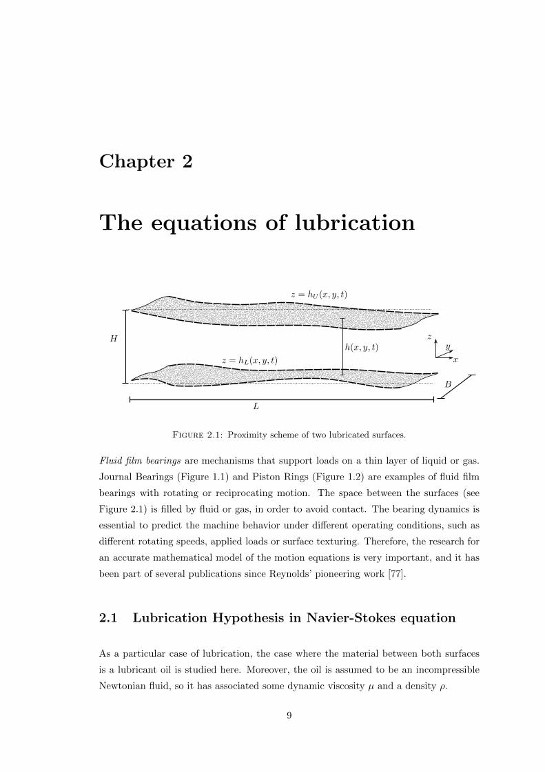
Figure 2.1: Proximity scheme of two lubricated surfaces.
Fluid film bearings are mechanisms that support loads on a thin layer of liquid or gas.
Journal Bearings (Figure 1.1) and Piston Rings (Figure 1.2) are examples of fluid film
bearings with rotating or reciprocating motion. The space between the surfaces (see
Figure 2.1) is filled by fluid or gas, in order to avoid contact. The bearing dynamics is
essential to predict the machine behavior under different operating conditions, such as
different rotating speeds, applied loads or surface texturing. Therefore, the research for
an accurate mathematical model of the motion equations is very important, and it has
been part of several publications since Reynolds’ pioneering work [77].
2.1 Lubrication Hypothesis in Navier-Stokes equation
As a particular case of lubrication, the case where the material between both surfaces
is a lubricant oil is studied here. Moreover, the oil is assumed to be an incompressible
Newtonian fluid, so it has associated some dynamic viscosity µ and a density ρ.
9

Chapter 2. The equations of lubrication 10
As the surfaces are very near each other, we suppose L, the characteristic length of
the longitudinal movement (x direction) of the surfaces, as being much greater than
H, which is the characteristic length of the transverse movement (z direction), i.e.,
ε = H/L 1 (typically ε ≈ 10−3).
Denoting by ~u = (u, v, w)T the lubricant velocity and p its pressure, Navier-Stokes
Equations for Newtonian fluids are valid, which can be written as
ρ
(∂~u
∂t+ (~u · ∇) ~u
)= −∇ p+ µ∇2~u +~f . (2.1)
Also, we consider the boundary conditions u(z = hU ) = UH , u(z = hL) = UL,
v(z = hU ) = VH and v(z = hL) = VL,
w(z = hU ) = WH =∂hU∂t
+ UH∂hU∂x
+ VH∂hU∂y
,
w(z = hL) = WL =∂hL∂t
+ UL∂hL∂x
+ VL∂hL∂y
,
where we used that WU can be written as the sum of a squeeze part ∂hU/∂t and a shape
part UH · ∂hU/∂x (analogously for WL).
Neglecting external forces~f , the hypothesis of surfaces proximity is introduced by making
the next non-dimensionalization
x =x
L, y =
y
L, z =
z
H, u =
u
U, (2.2)
v =v
U, w =
w
U HL
, t =t U
L, p = p
H2
µLU. (2.3)
This way, we obtain
ρU2
L
(∂u
∂t+ u
∂u
∂x+ v
∂u
∂y+ w
∂u
∂z
)=− 1
L
µLU
H2
∂p
∂x(2.4)
+ µ
(U
L2
∂2u
∂x2+U
L2
∂2u
∂y2+
U
H2
∂2u
∂z2
),
ρU2
L
(∂v
∂t+ u
∂v
∂x+ v
∂v
∂y+ w
∂v
∂z
)= − 1
L
µLU
H2
∂p
∂y(2.5)
+ µ
(U
L2
∂2v
∂x2+U
L2
∂2v
∂y2+
U
H2
∂2v
∂z2
)ρU2H
L2
(∂w
∂t+ u
∂w
∂x+ v
∂w
∂y+w
∂w
∂z
)= − µLU
H3
∂p
∂z(2.6)
+ µU
L
(H
L2
∂2w
∂x2+H
L2
∂2w
∂y2+
1
H
∂2w
∂z2
).

Chapter 2. The equations of lubrication 11
Introducing the Reynolds Number Re = inertiaviscous = ρUH/µ these equations can be written
as
∂p
∂x=∂2u
∂z2− εRe
(∂u
∂t+ u
∂u
∂x+ v
∂u
∂y+ w
∂u
∂z
)+O
(ε2)
∂p
∂y=∂2v
∂z2− εRe
(∂v
∂t+ u
∂v
∂x+ v
∂v
∂y+ w
∂v
∂z
)+O
(ε2)
∂p
∂z= − ε3 Re
(∂w
∂t+ u
∂w
∂x+ v
∂w
∂y+ w
∂w
∂z
)+ ε4
(∂2w
∂x2+∂2w
∂y2
)+ ε2
∂2w
∂z2= O
(ε2).
Now, neglecting terms of order ε and higher (including inertial terms!) and returning
to the original variables we obtain
∂p
∂x= µ
∂2u
∂z2(2.7)
∂p
∂y= µ
∂2v
∂z2, (2.8)
∂p
∂z= 0. (2.9)
From equation (2.9) we deduce that the pressure p only depends upon x and y. Inte-
grating two times on z between z = hL and z = hU , we have:
u(z) =1
2µ
∂p
∂x(z − hL)(z − hU ) +
z − hLhU − hL
UH +hU − zhU − hL
UL, (2.10)
v(z) =1
2µ
∂p
∂y(z − hL)(z − hU ) +
z − hLhU − hL
VH +hU − zhU − hL
VL. (2.11)
Integrating the last equations for z ∈ [hL, hU ] the flux functions are obtained:
Qx =
∫ hU
hL
u dz = − h3
12µ
∂p
∂x+UL + UH
2h, (2.12)
Qy =
∫ hU
hL
v dz = − h3
12µ
∂p
∂y+VL + VH
2, (2.13)
where h = hU−hL. Figure 2.2 shows a scheme of the linear and quadratic terms written
on equation (2.10). The linear one corresponds to a Couette flow, which is due to relative
motion between the surfaces, while the second represents a Poiseuille flow, which is due
to the presence of a pressure gradient.
2.2 Reynolds Equation
To obtain Reynolds Equation, we introduce the continuity equation, which in the in-
compressible case reads:
∇ · ~u = 0, (2.14)

Chapter 2. The equations of lubrication 12
Couette flow Poiseuille flow
UH = 0, UL = 0, ∂p/∂x < 0UH = 0, UL > 0, ∂p/∂x = 0
zx
Figure 2.2: Couette and Poisseuille profile flows in a Channel.
integrating along z we obtain:∫ hU (x,y,t)
hL(x,y,t)
(∂u
∂x+∂v
∂y+∂w
∂z
)dz = 0. (2.15)
The first two integrals above can be calculated by using Leibniz’s rule for time-dependent
domains. By using equations (2.10) and (2.11), this is written as
∫ hU (x,y,t)
hL(x,y,t)
∂u
∂xdz =
∂
∂xQx − UH
∂hU∂x
+ UL∂hL∂x
, (2.16)∫ hU (x,y,t)
hL(x,y,t)
∂v
∂ydz =
∂
∂yQy − VH
∂hU∂y
+ VL∂hL∂y
. (2.17)
Now, for the third integral we have:∫ hU (x,y,t)
hL(x,y,t)
∂w
∂zdz = WU −WL
=∂hU∂t
+ UH∂hU∂x
+ VH∂hU∂y−(∂hL∂t
+ UL∂hL∂x
+ VL∂hL∂y
)=∂h
∂t+ UH
∂hU∂x− UL
∂hL∂x
+ VH∂hU∂y− VL
∂hL∂y
, (2.18)
where h = hU −hL. Thus, summing equations (2.16), (2.17) and (2.18), equation (2.15)
can be written as∂
∂xQx +
∂
∂yQy +
∂h
∂t= ∇ ·Q+
∂h
∂t= 0.
Finally, we replace the flux function Q = [Qx, Qy]T for the Newtonian case from equa-
tions (2.12) and (2.13) to obtain:
∂
∂x
(h3
12µ
∂p
∂x− UL + UH
2h
)+
∂
∂y
(h3
12µ
∂p
∂y− VL + VH
2h
)=∂h
∂t, (2.19)

Chapter 2. The equations of lubrication 13
which is known as Reynolds Equation in Lubrication Theory.
To simplify notation we assume UL = U , UH = VL = VH = 0, so Reynolds equation can
be written in the conservative form
∂h
∂t+∇ · ~J = 0,
with
~J = − h3
12µ∇p+
U
2he1, (2.20)
where e1 is the unitary vector pointing positively in the x-axis. We say that ~J corre-
sponds to the mass-flux function.
2.3 Friction forces
Friction forces are some of the most important quantities to be analyzed in our study.
The dependence of such forces on the design variables of tribological devices has been
analyzed in several works during the last years [79, 86, 21, 64]. In this section, the for-
mula that gives the total friction force over some surface, due to hydrodynamic pressure
and viscosity effects, is calculated starting from the particular expression of the stress
tensor under our working hypotheses.
For Newtonian incompressible fluids, the stress tensor τ , which gives the forces per unit
area acting on a material surface, is given by the constitutive relation:
τij = −p δij + µ
(∂ui∂xj
+∂uj∂xi
), (2.21)
where i and j are indices corresponding to the three Cartesian dimensions, and δ is the
Kronecker delta. Since n is a normal unit vector pointing outward from some surface,
the force f exerted by the fluid over it in the direction e is given by the projection of
the total force ~f on e:
f = ~f · e = (τ · n) · e =∑ij
τijnj ei =∑ij
τij ejni, (2.22)
where the symmetry of τ was used in the last equality. The friction force is a force
opposing the motion when an object is moved or two objects are relatively moving [88].
To calculate the friction force, suppose the movement direction of a surface is given by
the unit vector ı as in Figure 2.3. There, the lower surface is moving to the right so we

Chapter 2. The equations of lubrication 14
put e = ı and we get
τ · ı = τ ·
1
0
0
=
τxx
τxy
τxz
=
−p+ 2µ ∂u
∂x
µ(∂u∂y + ∂v
∂x
)µ(∂u∂z + ∂w
∂x
) .
Using the proximity hypothesis, i.e., ε = H/L is very small, and the non-dimensionalizations
equations (2.2) and (2.3) we get
τxx = µU
H
(−1
εp+ 2ε
∂u
∂x
), τxy = µ
U
H
(ε∂u
∂y+ ε
∂v
∂x
), τxz = µ
U
H
(∂u
∂z+ ε
∂w
∂x
).
Now, the non-dimensional vector dS normal to the surface z = hL(x, y) with length
equal to the surface differential area element is given by
dS = n dS =
(−ε∂hL
∂xı− ε∂hL
∂y+ k
)L2 dx dy. (2.23)
The non-dimensional element df of the total friction force is given by
df = τ · ı · dS
= µU
H
[p∂hL∂x− 2ε2
∂u
∂x
∂hL∂x− ε2
(∂u
∂y+∂v
∂x
)∂hL∂y
+∂u
∂z+ ε
∂w
∂x
]L2dxdy,
dropping the terms of order ε and ε2 and returning to the original variables we obtain
for the dimensional force element
df ≈(p∂hL∂x
+ µ∂u
∂z
)dx dy. (2.24)
Now, using equation (2.10) we calculate
µ∂u
∂z
∣∣∣∣z=hL
=1
2
∂p
∂x(2z − hU − hL)
∣∣∣∣z=hL
−µ(UL − UH)
h= −h
2
∂p
∂x−µ(UL − UH)
h. (2.25)
Thus, the local friction force on the lower surface by unit area reads
dfL =
(p∂hL∂x− h
2
∂p
∂x− µ(UL − UH)
h
)dx dy. (2.26)
where Ω is the domain of interest. Analogously, for the upper surface we obtain
dfU =
(−p∂hU
∂x− h
2
∂p
∂x+ µ
(UL − UH)
h
)dx dy. (2.27)
Next, we analyze each term of equation (2.26). For this, please refer to Figure 2.3

Chapter 2. The equations of lubrication 15
where a curved portion of a surface hL is shown. In the figure, the surface is moving on
direction of vector e = ı with speed UL.
nd = k
na nb
nc
e = ı
Figure 2.3: 2D surface normal orientations scheme.
p∂hL∂x : projection of the force due to the pressure acting on the surface. At point
A, the normal vector na is oriented positively with respect to e (n · e > 0),
so pressure must generate a negative force, and this is what happens as
∂hL/∂x is negative there. The opposite situation occurs at C, where a
positive pressure force is expected and it happens since ∂hL/∂x > 0. On
the other hand, at points B and D the movement direction is perpendicular
to the surface orientation, e · nb = e · nd = 0, so a projection of any normal
force is null. This is reflected by ∂hL/∂x = 0.
−h2∂p∂x : viscous shear due to a Poiseuille flow. A positive pressure gradient on
the x-axis generates a parabolic profile negatively oriented which reduces
∂u/∂z.
−µ (UL−UH)h : viscous shear due to a Couette flow. Notice the direction of the relative
motion between the surfaces being reflected on the sign of this term.
It can be noticed from equations (2.26) and (2.27) that the local friction force might not
be the same on both surfaces. On the other hand, take for simplicity Ω = [0, 1]× [0, 1] ⊂R2 and write the periodic conditions p(0, y) = p(1, y), p(x, 0) = p(0, 1) for x, y ∈ [0, 1],
and h(0, y) = h(1, y), h(x, 0) = h(0, 1) for x, y ∈ [0, 1]. Now, let us integrate both
friction formula in Ω so we obtain
fL + fU = −∫
Ωp∂h
∂xdx dy −
∫Ωh∂p
∂xdx dy.
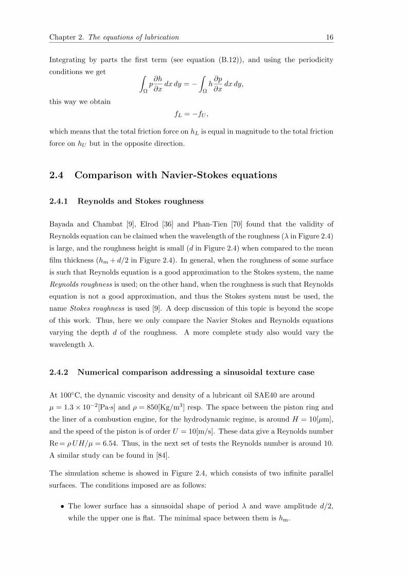
Chapter 2. The equations of lubrication 16
Integrating by parts the first term (see equation (B.12)), and using the periodicity
conditions we get ∫Ωp∂h
∂xdx dy = −
∫Ωh∂p
∂xdx dy,
this way we obtain
fL = −fU ,
which means that the total friction force on hL is equal in magnitude to the total friction
force on hU but in the opposite direction.
2.4 Comparison with Navier-Stokes equations
2.4.1 Reynolds and Stokes roughness
Bayada and Chambat [9], Elrod [36] and Phan-Tien [70] found that the validity of
Reynolds equation can be claimed when the wavelength of the roughness (λ in Figure 2.4)
is large, and the roughness height is small (d in Figure 2.4) when compared to the mean
film thickness (hm + d/2 in Figure 2.4). In general, when the roughness of some surface
is such that Reynolds equation is a good approximation to the Stokes system, the name
Reynolds roughness is used; on the other hand, when the roughness is such that Reynolds
equation is not a good approximation, and thus the Stokes system must be used, the
name Stokes roughness is used [9]. A deep discussion of this topic is beyond the scope
of this work. Thus, here we only compare the Navier Stokes and Reynolds equations
varying the depth d of the roughness. A more complete study also would vary the
wavelength λ.
2.4.2 Numerical comparison addressing a sinusoidal texture case
At 100C, the dynamic viscosity and density of a lubricant oil SAE40 are around
µ = 1.3× 10⁻²[Pa·s] and ρ = 850[Kg/m3] resp. The space between the piston ring and
the liner of a combustion engine, for the hydrodynamic regime, is around H = 10[µm],
and the speed of the piston is of order U = 10[m/s]. These data give a Reynolds number
Re = ρUH/µ = 6.54. Thus, in the next set of tests the Reynolds number is around 10.
A similar study can be found in [84].
The simulation scheme is showed in Figure 2.4, which consists of two infinite parallel
surfaces. The conditions imposed are as follows:
• The lower surface has a sinusoidal shape of period λ and wave amplitude d/2,
while the upper one is flat. The minimal space between them is hm.

Chapter 2. The equations of lubrication 17
• A Newtonian incompressible lubricant is placed between the surfaces, its density
is ρ and its dynamic viscosity is µ.
• The lower surface is not moving (UL = 0), while the upper one is moving with
speed UH > 0.
• No pressure gradient is imposed, instead we set p(x0) = p0 at some point x0 of
the domain Ω (to be determined).
• Setting H = hm+ d2 (the mean surface height), the Reynolds number Re=ρUHH/µ
is supposed to be low enough for assuring (along with other conditions) the system
reaching a steady state.
hm
d
λ
x = 0 x = λy = 0
y = hm + d
Ω
Figure 2.4: An infinite 1D bearing with a sinusoidal texture.
With all these assumptions, both Navier-Stokes and Reynolds equations can be solved
for this infinite system on just a representative block, as Figure 2.4 shown. Now, defining
the domain Ω = Ωd as
Ωd =
(x, y) ∈ R2 | 0 < x < λ, hL(x) < y < hm + d,
with hL(x) = d2 (1− cos(2π x/λ)), the first mathematical problem reads:
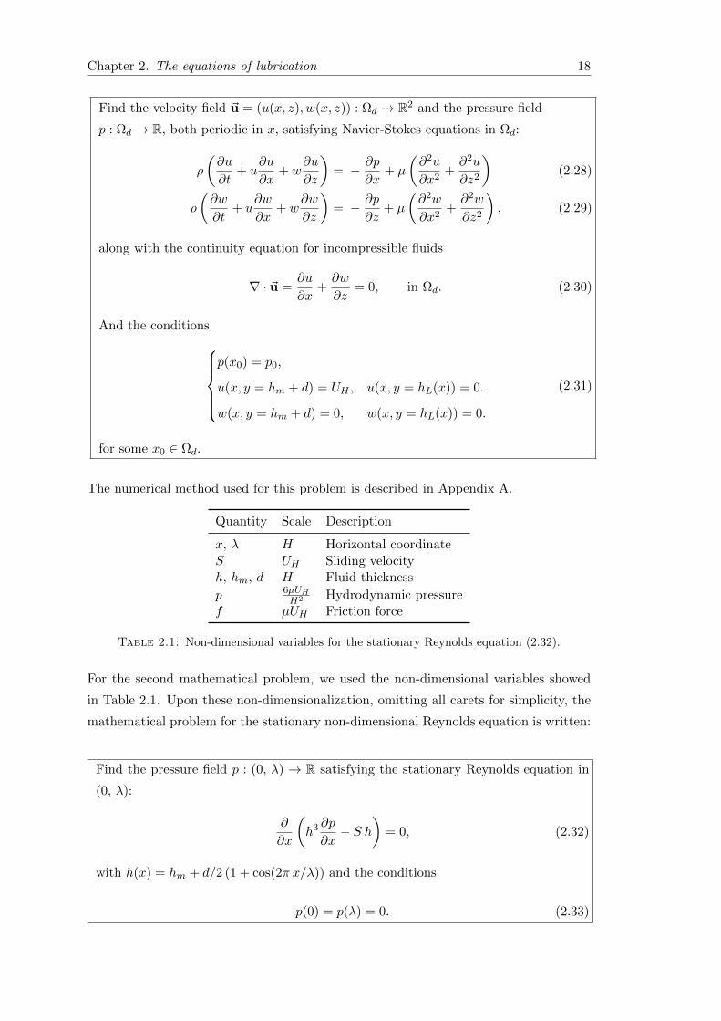
Chapter 2. The equations of lubrication 18
Find the velocity field ~u = (u(x, z), w(x, z)) : Ωd → R2 and the pressure field
p : Ωd → R, both periodic in x, satisfying Navier-Stokes equations in Ωd:
ρ
(∂u
∂t+ u
∂u
∂x+ w
∂u
∂z
)= − ∂p
∂x+ µ
(∂2u
∂x2+∂2u
∂z2
)(2.28)
ρ
(∂w
∂t+ u
∂w
∂x+ w
∂w
∂z
)= − ∂p
∂z+ µ
(∂2w
∂x2+∂2w
∂z2
), (2.29)
along with the continuity equation for incompressible fluids
∇ · ~u =∂u
∂x+∂w
∂z= 0, in Ωd. (2.30)
And the conditionsp(x0) = p0,
u(x, y = hm + d) = UH , u(x, y = hL(x)) = 0.
w(x, y = hm + d) = 0, w(x, y = hL(x)) = 0.
(2.31)
for some x0 ∈ Ωd.
The numerical method used for this problem is described in Appendix A.
Quantity Scale Description
x, λ H Horizontal coordinateS UH Sliding velocityh, hm, d H Fluid thickness
p 6µUHH2 Hydrodynamic pressure
f µUH Friction force
Table 2.1: Non-dimensional variables for the stationary Reynolds equation (2.32).
For the second mathematical problem, we used the non-dimensional variables showed
in Table 2.1. Upon these non-dimensionalization, omitting all carets for simplicity, the
mathematical problem for the stationary non-dimensional Reynolds equation is written:
Find the pressure field p : (0, λ) → R satisfying the stationary Reynolds equation in
(0, λ):
∂
∂x
(h3 ∂p
∂x− S h
)= 0, (2.32)
with h(x) = hm + d/2 (1 + cos(2π x/λ)) and the conditions
p(0) = p(λ) = 0. (2.33)

Chapter 2. The equations of lubrication 19
Since the problem is one-dimensional there is no need to impose conditions on the
pressure gradient. Please notice the great contrast in complexity between both problems.
The second one can be solved by a simple integration, yielding
p(x) =
∫ x
0
ζ + S h
h3dx, for x ∈ [0, λ] with ζ =
−S∫ λ
01h2dx∫ λ
01h3dx
.
Simulation parameters
We set UH = 10[m/s], H = 10[µm], λ = 10 and hm = 1 − d/2. This setup, along with
the non-dimensionalizations, makes the problem dependent only on d and Re. The sets
of values chosen for these quantities are
d ∈ 0, 0.2, 0.4, 0.6, 0.8, 1.0, 1.2, 1.4, 1.6, 1.8
Re ∈ 0.1, 1.0, 5.0, 10.0, 20.0, 50.0, 100.0.
In both problems (for Reynolds and Navier-Stokes equations) 600 uniform cells were
used in the x-axis which correspond to dx = 0.01667. For the 2D problem, dy = dx and
dt = 0.45 min
14dx
2Re, 210·Re
were set (see [73] Chapter 2 for the stability policy on
dt). These numerical parameters were chosen to assure both time and space convergence
along with numerical stability.
Results and discussion
As we are interested in the load that a certain system can support and the friction
losses involved in the process, the next two basic quantities are compared: 1) the hy-
drodynamic pressure generated between the surfaces; 2) the friction force opposing the
relative motion of the surfaces (see Section §2.3).
For the comparison, we denote as pr the pressure found by solving (Reynolds equa-
tion) equations (2.32) and (2.33) and as pn the averaged (in y) pressure obtained from
equations (2.28), (2.29) and (2.30) along the conditions (2.31).
Figure 2.5 shows the resulting non-dimensional pressure for both sets of equations for
the case Re=1, d = 0.4. The Reynolds solution is symmetric while the Navier-Stokes
solution develops a slightly asymmetrical shape. In fact, for this case
|max pr(x)| = |min pr(x)| = 0.327, but |max pn(x)| = 0.332 6= |min pn(x)| = 0.344.

Chapter 2. The equations of lubrication 20
0 2 4 6 8 10-0.8
-0.6
-0.4
-0.2
0
0.2
0.4d
imen
sion
less
pre
ssu
re
movement direction
Reynolds
NVS Re=1NVS Re=10NVS Re=50
Figure 2.5: Dimensionless pressure for Reynolds equation and for Navier-Stokes withRe=1, 10, 50, d = 0.4.
This asymmetry can only appear due to the inertial terms of the Navier-Stokes equations
which are neglected in the Reynolds approximation. The relative difference of these
solutions is 6% (in ‖ · ‖∞).
Figure 2.6 shows the pressure resulting from Reynolds equation and Navier-Stokes equa-
tions for Re = 5 and d = 0.4, 0.8, 1.2, 1.6. The bigger the depth d is the smaller the
minimal distance between the surfaces hm is. Because of this, the peak pressure rises
when d is augmented. We observe a good agreement for all the depths chosen, in fact,
from Figure 2.7 we obtain that the relative differences are around 15 to 20% (in ‖ · ‖∞).
0 2 4 6 8 10-4
-3
-2
-1
0
1
2
3
4
dim
ensi
onle
ssp
ress
ure
movement direction
2.5 3 3.5 4 4.5 5-0.2
0.2
0.6
1
1.4d=0.4d=0.8d=1.2d=1.6
Figure 2.6: Dimensionless pressure from Navier-Stokes equations and Reynolds equa-tion for different depth d and Re = 5. The continuous lines show the results fromReynolds equation, while the dashed lines show the results for Navier-Stokes equations.

Chapter 2. The equations of lubrication 21
0.2 0.4 0.6 0.8 1.0 1.2 1.4 1.6 1.8-3.5
d
log(a
bso
lute
diff
eren
ce)
0.2 0.4 0.6 0.8 1.0 1.2 1.4 1.6 1.80
20
40
60
80
100
d
per
centa
ge
diff
eren
ce
Re = 0.1Re = 1Re = 5Re = 10Re = 20Re = 50Re = 100
-3.0
-2.5
-2.0
-1.5
-1.0
-0.5
0
Figure 2.7: Dimensionless pressure difference (left) and relative difference (right) fordifferent Reynolds number.
0.2 0.4 0.6 0.8 1.0 1.2 1.4 1.6 1.80
1
2
3
4
5
6
7
d
per
centa
ge
diff
eren
ce
0
20
40
60
80
100
d
per
centa
ge
diff
eren
ce(w
rong
form
ula
)
0.2 0.4 0.6 0.8 1.0 1.2 1.4 1.6 1.8
Re = 0.1Re = 1Re = 5Re = 10Re = 20Re = 50Re = 100
(a) (b)
Figure 2.8: Left: relative difference in friction difference for Navier Stokes Reynoldsequation (using formula (2.26)) and for several Reynolds number. Right: analogous
calculation without the projection term hL
2∂p∂x .
As the Reynolds number grows, we expect the difference between the solutions (for
pressure and friction) of the Navier Stokes and Reynolds equations to grow. On the
other hand, for the validity of Reynolds the value λ/d = 10 is a well known lower bound
for the aspect ratio λ/d [34]. Therefore, as we fix λ = 10, we also expect the difference
between the solutions of the Navier Stokes and Reynolds equations to grow for d > 1.
In Figure 2.7 we show the differences for pressure for both sets of equations; at the left
side the absolute difference (log(‖pn − pr‖∞)) is showed; at the right side the relative
difference (100×‖pn − pr‖∞/‖pn‖∞) is showed.
Since the friction force is derived from the pressure and the velocity of the fluid, we
expect a similar behavior between the differences in pressure and the differences in
friction. Figure 2.8(a) shows the relative difference in friction (|fn − fr|/|fn|), for d < 1
friction results are very similar; for d > 1 the difference remains low (less than 7%

Chapter 2. The equations of lubrication 22
of difference) but it begins to grow. Figure 2.8(b) shows the relative difference when
calculated without including the projection term p ∂hL/∂x in formula (2.26). It can be
observed that for the cases considered the projection term cannot be neglected as done
in some published works [65, 86, 68].
The above results give us some insight about the accuracy of the calculations made in
this work. Clearly we are simplifying the problem, as we do not consider cavitation or
squeezing effects (temporal terms).
Remark 2.1. A better comparison has been done with a more sophisticated in-house code
developed by this research group, already tested in [14, 6]. This has been done since the
computation of the friction formula (2.26) requires a better treatment of the derivatives
at the boundaries. Therefore, the rectangular mesh used in this section is not suitable.
The results indicate clearly the validity of the formula (2.26).
2.5 Some representative analytic solutions
Two types of finite wedges are going to be analyzed in this section, more details of these
computations can be found in [18]. Optimal geometric parameters for these wedges will
be computed analytically. The selection of these optimal parameters depends on what
are we interested in maximize/minimize. In particular, the geometric configuration that
minimizes friction is not the configuration that maximizes the load-carrying capacity
(defined as the integral of the hydrodynamic pressure).
2.5.1 Step wedge and Rayleigh step
Quantity Scale Description
x, l L Horizontal coordinateS U Fluid velocityh, h0 H Fluid thicknessp 6µUL/H2 Hydrodynamic pressuref µUL/H Friction forcesW 6µUL2/H2 Load-carrying capacity
Table 2.2: Non-dimensional variables for the step wedge problem.
Figure 2.9 shows the scheme of the step wedge problem. In this case, the pad of finite
length L is still while a flat surface is moving to the right with constant speed U . To
find the hydrodynamic behavior of the lubricant oil between the surfaces, taking the
non-dimensionalizations written in Table 2.2, the mathematical problem reads

Chapter 2. The equations of lubrication 23
h1
L− l
l
H
x = 0 x = LU
Figure 2.9: Step wedge pad scheme.
Find the pressure scalar field p : [0, 1]→ R, satisfying the stationary Reynolds equation
in [0, 1]:
∂
∂x
(h3 ∂p
∂x− S h
)= 0 (2.34)
with h(x) = h1 for 0 ≤ x < 1 − l, and h(x) = 1 for 1 − l ≤ x ≤ 1. Along with the
boundary condition
p(0) = p(1) = 0. (2.35)
From equation (2.34) we see that the flux function
J(x) = −h3
2
∂p
∂x+S
2h (2.36)
is constant along the domain ]0, 1[.
From equation (2.34) and the definition of h we see that
∂2p
∂x2= 0 in ]0, 1− l[∪ ]1− l, 1[,
and so, using the boundary conditions given by (2.35), and assuming the continuity of
p, the pressure can be written as
p(x) =
x(∂p∂x
)left
, 0 ≤ x < 1− l
pmax + (x− 1 + l)(∂p∂x
)right
, 1− l ≤ x ≤ 1(2.37)

Chapter 2. The equations of lubrication 24
where(∂p∂x
)left
= pmax
1−l is the left pressure gradient,(∂p∂x
)right
= −pmax
l is the right
pressure gradient, and pmax is the peak pressure. To determine the peak pressure pmax
we impose mass-conservation on the flux function at x = 1− l:
limx→(1−l)−
J(x) = limx→(1−l)+
J(x),
so
−h31
2
(∂p
∂x
)left
+S
2h1 = −1
2
(∂p
∂x
)right
+S
2.
Replacing the expressions of the gradients for both left and right sides we obtain
pmax = Sl(h1 − 1)(1− l)1 + l(h3
1 − 1). (2.38)
We have solved the problem of looking for the pressure of the step wedge. Now, we
can ask for some tribological characteristics of the system. First, we look for the load-
carrying capacity and its optimal configuration. Next, we look for the friction force and
its optimal configuration too.
Load-carrying capacity of the step wedge
The load-carrying capacity W is just the integral of the pressure distribution. Thus,
using (2.37) and (2.38) we have
W =
∫ 1
0p(x) dx =
1
2pmax. (2.39)
Now, for finding the optimal configuration, i.e., the 2-tuple (h1, l) for which the maxi-
mum W is reached, we seek for the configurations that nullifies the gradient of W and,
between those configurations, the ones having a negative definite Hessian matrix. Doing
so, we obtain the optimal configuration:
h1 =
√3 + 2
2≈ 1.866, l =
4√27 + 9
≈ 0.282,1− ll
=
√27 + 5
4≈ 2.549,
which corresponds to a load-carrying capacity
W = S2
9
(4√
3 + 7
26√
3 + 45
)≈ 0.034S.
This configuration is known in the literature as the Rayleigh Step. Lord Rayleigh, in
1918 [76], found it by using calculus of variations to find the shape of the step wedge
that maximizes the load-carrying capacity.

Chapter 2. The equations of lubrication 25
Friction force of the step wedge
Friction force F can be calculated for the step wedge from equation (2.26) and the
pressure profiles found above. The computation reads
F =
∫ 1
0
(3h∂p
∂x+S
h
)dx
=
∫ 1−l
0
(3h∂p
∂x+S
h
)dx+
∫ 1
1−l
(3h∂p
∂x+S
h
)dx
=
[3h1
(pmax
1− l
)+S
h1
](1− l) +
[3
(−pmax
l
)+ S
]l
= S
(3l(1− l)(h1 − 1)2
1 + l(h31 − 1)
+1− lh1
+ l
), (2.40)
taking derivatives it is found that
∂F
∂l= S
(3h3
1(h1 − 1)
(h21 + h1 + 1)[(h3
1 − 1)l + 1]2+
(h1 − 1)3
h31 + h2
1 + h1
)and
∂F
∂h1= −S
(1− l)[(2h3
1 − 3h1 + 1)l − 1]2
h21
[(h3
1 − 1)l + 1]2 .
So we have
∂F
∂l> 0 and
∂F
∂h1< 0 , whenever h1 > 1 and l ∈ (0, 1) resp.
Therefore, the configuration that minimizes friction depends on the design restrictions
under the policy: “take l as small as possible, and h1 as large as possible”. However, from
equations (2.38) and (2.39) it can be observed that using this policy the load-carrying
capacity W goes to zero. In consequence, another quantity is needed to characterize the
friction relatively to the load-carrying capacity. In the literature, the friction coefficient
is defined as the quotient between the total friction force and the applied load. Thus,
considering the non-dimensionalizations presented before (see Table 2.2), the friction
coefficient reads
Cf =H
6L
F
W. (2.41)
This quantity was also studied by Lord Rayleigh in its classic work [76]. Making similar
calculations we made before for the maximum load-carrying capacity, the configuration
that minimizes Cf is found to be
h1 = 2, l =1
5,
1− ll
= 4,

Chapter 2. The equations of lubrication 26
for which
Cf = 4H
L,
while for the Rayleigh Step we have Cf = 4.098HL .
This results can be found also in a recent work by Rahmani et al. [75], where they made
an analysis of the Rayleigh Step analytically. They based their work on the Reynolds
equation considering non-homogeneous boundary conditions for pressure. Analytic rela-
tions for parameters as load capacity and friction force were also developed and studied
seeking for optimal configurations.
L/2 L/2
L/2
L/2
lower surface
Figure 2.10: Scheme of the “naive step wedge” (solid black line) versus the RayleighStep wedge (dashed blue line), and the wedged that minimizes Cf (dotted red line).
Comparison of Rayleigh Step with a naive step wedge
By naive step wedge we meant a 2-tuple (h1, l) chosen, arguably, as simple as possible.
The idea is to have a non trivial reference design to compare with the optimal designs
found above.
The design we choose for this comparison is shown in Figure 2.10. In that figure, the
blue dashed lines represent the real proportions of the Rayleigh Step wedge, while the
black line represents our simple step of length L with proportions (L − 1)/l = 1 and
h1/H = 2 (see Figure 2.9).

Chapter 2. The equations of lubrication 27
We use equations (2.39) and (2.40) to calculate the load carrying-capacity of both the
Rayleigh Step wedge and our naive step wedge, denoted by WR and W0 resp.. We also
calculate the friction force for both the Rayleigh Step and the naive step wedge, denoted
as FR and F0, respectively. Doing the computations, we found
W0
WR= 0.81 and
F0
FR= 1.08.
We observe that the Rayleigh Step augments 19% the load-carrying capacity and di-
minishes 8% the friction force when compared to the naive step wedge.
2.5.2 Disc wedge
L
x = −L/2 Ux = L/2x = 0
h0
R
Figure 2.11: Disc pad scheme.
In this case, the pad has a circular shape, symmetric along x-axis, centered at x = 0
(see Figure 2.11) with radius of curvature R. Non-dimensionalizations are the same as
in previous section, including this time the variable R with scale L (see Table 2.3).
Quantity Scale Description
x, R L Horizontal coordinateS U Fluid velocityh, h0 H Fluid thickness
p 6µULH2 Hydrodynamic pressure
Table 2.3: Non-dimensional variables for the disc wedge problem.

Chapter 2. The equations of lubrication 28
This problem has a major difference with the step wedge problem (previous section), as
in this geometry a divergent zone is present for 0 < x < L/2. Thus, negative pressures
are expected to appear at that divergent zone. The mathematical problem is written
(non-dimensionalization are shown in Table 2.3):
Find the pressure scalar field p : [−0.5, 0.5] → R, satisfying the stationary Reynolds
equation:
∂
∂x
(h3 ∂p
∂x− S h
)= 0, in (−0.5, 0.5) (2.42)
where the film thickness function is given by
h(x) = h0 +L
H
(R−
√R2 − x2
), x ∈ [−0.5, 0.5],
along with the boundary conditions for pressure
p(−0.5) = p(0.5) = 0. (2.43)
To simplify calculations we approximate the thickness function (up to an error of order
10−7 × L/H) by
h(x) = h0 +L
H
x2
2R, x ∈ [−0.5, 0.5].
From Reynolds equation (2.42) we have that the flux function
J = −h3
2
∂p
∂x+ S
h
2
is constant along the domain. This way, Reynolds equation can be rewritten as
∂p
∂x= S
(h− h)
h3, (2.44)
where h is some constant to determine. Now, we make the change of variables
tan γ =x√
2h0RH/L.
And so, the double integration of equation (2.44) gives (h = h0 sec2(γ))
p(γ) = S√
2RL/H
(γ
2+
sin 2γ
4− 1
cos2 γ
[3
8γ +
sin 2γ
4+
sin 4γ
32
])+ C, (2.45)
where γ and C are determined from boundary conditions (2.43).

Chapter 2. The equations of lubrication 29
Figure 2.12 shows the pressure profile for the case R = 80, S = 1, h0 = 1, L = 1×10⁻³[m]
and H = 1 × 10⁻⁶[m]. The anti-symmetric pressure profile is such that it is positive
at the convergent zone (where ∂xh < 0) and negative at the divergent zone (where
∂xh > 0). These negative pressures will be subject of study in Chapter 4.
-0.5 -0.3 -0.1 0.1 0.3 0.5-0.04
-0.02
0
0.02
0.04
movement direction
hyd
rod
yn
amic
pre
ssu
re
1
1.5
2
2.5
dis
cp
rofi
le
Figure 2.12: Disc pad scheme and pressure profile.


Chapter 3
Mathematics of Reynolds
equation
We have shown in Chapter 2 that Reynolds equation models the tribological variables
of two surfaces being lubricated. In this chapter a mathematical analysis is developed
in order to study the well-posedness of Reynolds equation. Using powerful tools of
Functional Analysis, like the Hilbert Spaces structure, existence, uniqueness and stability
of solutions of Reynolds equation will be addressed. Furthermore, we will seek for
regularity of the solutions, i.e., how much smooth the solutions are. As the reader may
guess, the last question will be related to the quality of the input: how regular is the
gap between the surfaces?; how regular is the boundary of the domain?.
For this we will consider a measurable domain Ω ⊂ R2, with Lebesgue measure
µ(Ω) < +∞, and a measurable subdomain ω ⊂ Ω where Reynolds equation holds.
In this chapter, ω is a data of the problem and it is supposed to be locally Lipschitz (see
definition B.29). The general problem, where ω is also an unknown, will be studied in
Chapter 4 where Ω \ ω will be determined by the cavitation phenomenon.
3.1 From Stokes equations to Reynolds equation
Along Sections §2.1 and §2.2 we have made asymptotic expansions for obtaining Reynolds
equation from Navier-Stokes equations. Bayada and Chambat (1986) [8] proved math-
ematically that Reynolds equation is an approximation of Stokes equations. In the
following, we summarize their results in order to give a mathematical comprehension of
the relation between both sets of equations.
31

Chapter 3. Mathematics of Reynolds equation 32
Consider two surfaces in proximity and in relative motion (see Figure 3.1). The first
surface (lower one), denoted by ω, is a planar bounded domain of R2 placed in the
plane z = 0 and its boundary ∂ω is locally Lipschitz. The second surface (upper one)
is characterized by z = H(x, y), (x, y) ∈ ω. The thin distance between both surfaces is
taken into account by introducing a small parameter ε, which will tend to 0, and a fixed
function h : ω → R+ such that
H(x, y) = ε h(x, y),
with h ∈ C1(ω) and h ≥ α > 0.
ω
H(x, y)
z
Ωε
y
x
ΓεL
Γε1
Figure 3.1: Ωε scheme. Based on Fig. 1 in [8].
Let us write the domain
Ωε = (x, y, z) ∈ R3, (x, y) ∈ ω, 0 < z < H(x, y),
and Γε = ∂Ωε = ω ∪ Γε1 ∪ Γ
εL its boundary (see Figure 3.1). On Ωε, the Stokes system1
and the continuity equation for a Newtonian fluid can be written resp. as
−µ∇2 Uε +∇pε = 0 (3.1)
∇ ·Uε = 0, (3.2)
1Assuming no source term on the right hand side of Equation (3.1) as generally occurs in LubricationTheory.

Chapter 3. Mathematics of Reynolds equation 33
where µ is the dynamic viscosity, Uε is the velocity field of the fluid and pε is its
hydrodynamic pressure. Dirichlet boundary conditions for the velocities Uε = (gε, 0, 0)
on Γε are imposed, where
gε = 0, on Γε1 (3.3)
gε = S > 0, on ω. (3.4)
Also, in order to make sure that the Stokes equations have a solution, the authors [8]
impose the condition
gε ∈ H1/2(Γε) and
∫ΓεL
gε cos(n, e1) dσ = 0, (3.5)
where n is the normal unit vector pointing outward Ωε and e1 is the unit vector pointing
positively along the x-axis. The first condition is a regularity requirement and the second
condition is for mass-conservation.
Existence and uniqueness for Stokes system
First, let us define the space L20(Ωε) = f ∈ L2(Ωε) :
∫Ωεf dV = 0, dV = dx dy dz,
which is the class of functions with zero average. This set is considered since the pressure
is uniquely determined up to an additive constant.
The next theorem establishes the existence and uniqueness of the Stokes problem defined
by equations (3.1)-(3.4). It is a well known result and it can be found, for instance, in
[47]:
Theorem 3.1. Under assumptions (3.3), (3.4) and (3.5), there exists a unique pair of
functions (Uε, pε) in (H1(Ωε))3 × L2
0(Ωε) such that
−µ∇2 Uε +∇pε = 0
∇ ·Uε = 0
Uε = (gε, 0, 0), on Γε.
Moreover, let us define the bilinear form a by a(U,V) =∑3
i=1
∫Ωε∇ui · ∇vi dV . Then,
(Uε, pε) satisfies the weak formulation:
µa(Uε,Φ) =
∫Ωε
pε∇ · Φ dV ∀Φ ∈ (H10 (Ωε))
3
0 =
∫Ωε
q∇ ·Uε dV, ∀q ∈ L20(Ωε),

Chapter 3. Mathematics of Reynolds equation 34
and there exists a function Gε ∈ H1(Ωε)3 such that
∇ ·Gε = 0, Gε −Uε ∈ (H10 (Ωε))
3. (3.6)
Now, set the domain Ω = (x, y, Z) ∈ R3, (x, y) ∈ ω, 0 < Z < h(x, y), and for any
function v(x, y, z) defined on Ωε associate the function v(x, y, Z) = v(x, y, ε Z) defined
on Ω.
Along this definitions and using Functional Analysis (e.g.2, Chapter “Banach and Hilbert
Spaces” in [87], Chapters III and V in [1]) the authors [8] obtained the next results
regarding convergence of the functions Uε and pε.
Convergence of the solutions
Theorem 3.2. Suppose there exists a constant K, not depending on ε, such that Gε in
Theorem 3.1 satisfies
‖∇Gεi‖(L2(Ω))3 ≤ K, i = 1, 2, 3, (3.7)
then, there exists U∗ in (L2(Ω))3 such that
Uε → U∗,∂Uε
∂Z→ ∂U∗
∂Z, ε
∂Uε
∂x→ 0, ε
∂Uε
∂y→ 0
weakly in (L2(Ω))3.
The proof of Theorem 3.2 is based on the following estimates that are proved by the
authors [8] (under the hypothesis of Theorem 3.2)
‖Uε‖(L2(Ω))3 ≤ K,∥∥∥∥∂uεi∂ξ
∥∥∥∥L2(Ω)
≤ K
ε,
∥∥∥∥∂uεi∂Z
∥∥∥∥L2(Ω)
≤ K, i = 1, 2, 3, ξ ∈ x, y.
Also a result on the convergence of pε is given, which is based on the next estimates∥∥∥∥∂pε∂x
∥∥∥∥H−1(Ω)
≤ K
ε2,
∥∥∥∥∂pε∂y∥∥∥∥H−1(Ω)
≤ K
ε2,
∥∥∥∥∂pε∂Z
∥∥∥∥H−1(Ω)
≤ K
ε.
Theorem 3.3. There exists p∗ in L20(Ω) such that ε2pε converges weakly to p∗; moreover
∂p∗
∂Z = 0.
2The reader can found a summary of the main results in Appendix B.

Chapter 3. Mathematics of Reynolds equation 35
Functional relations of the limit solutions
Once the existence of limit solutions was established, the authors found that these limits
accomplishes analogous equations as those found in Sections §2.1 and §2.2.
Theorem 3.4. Under the same hypothesis of Theorem 3.2, the components of the limit
field U∗ satisfies the equations:
∂p∗
∂x= µ
∂2u∗1∂Z2
, in H−1(Ω)
∂p∗
∂y= µ
∂2u∗2∂Z2
, in H−1(Ω)
u∗3 = 0, in Ω.
Now, for any function v(x, y, z) in H1(Ωε), or the corresponding v(x, y, Z) in H1(Ω),
define the average
v(x, y) =1
h
∫ h
0v(x, y, Z) dZ =
1
ε h
∫ ε h
0v(x, y, z) dz
so v lies in H1(ω).
Theorem 3.5. Under the same hypothesis of Theorem 3.2, the average velocity field u∗
satisfies
u∗1 =S
2− h2
12µ
∂p∗
∂x, u∗2 = − h2
12µ
∂p∗
∂yboth in H−1(ω),
u∗3 = 0 in ω.
Moreover, the average velocity field Uε
satisfies the “mass flow conservation” equation:
∂
∂x(huε1) +
∂
∂y(huε2) = 0 in D′(ω),
and the limit average velocity field satisfies the “mass-conservation” equation
∂
∂x(hu∗1) +
∂
∂y(hu∗2) = 0 in D′(ω).
Furthermore, regarding strong convergence the authors [8] found the next result:
Theorem 3.6. Under the hypothesis of Theorem 3.2, suppose there exists a function
g ∈ H1/2(Γ) that does not depends on ε, such that
gε(x, y, z) = g(x, y, z/ε) (3.8)

Chapter 3. Mathematics of Reynolds equation 36
then, it holds
• ε2pε, ε2 ∂pε
∂x , ε2 ∂pε
∂y and ε∂pε
∂Z converge strongly in L2(ω) to p∗, ∂p∗
∂x , ∂p∗
∂y and 0 resp.
• p∗ is unique and lies in H1(ω), also it satisfies
∇ ·(h3
12µ∇p∗
)=S
2
∂h
∂x,
which corresponds to Reynolds equation (2.19) in the steady case with UL = S,
UH = VH = VL = 0.
Conclusions
• Reynolds Equation is an approximation of the Stokes system when ε is small.
• The authors have shown that the solution of Stokes equations converges to the
solution of Reynolds equation when ε goes to 0.
• h ∈ C1(ω) is a strong hypothesis. It would be interesting to extend this work
under more realistic hypothesis like h ∈ L∞(ω). This kind of functions can be
found when considering discontinuous textures [5, 86, 46].
3.2 Weak formulation for Reynolds equation
Here we consider the non-dimensional velocity S as S = 1. From a classical point of
view, solving Reynolds equation consists in seek for a pressure field p ∈ C2(ω) satisfying
the non-dimensional Reynolds equation
∂
∂x
(h3 ∂p
∂x
)+
∂
∂y
(h3 ∂p
∂y
)=∂h
∂x+ 2
∂h
∂tin ω (3.9)
p = 0 in ∂ω, (3.10)
where ω is a domain in R2 of class C1 and h is continuously differentiable both in space
and time.
Please notice that in equation (3.9) time is only a parameter. In the analysis we will
show it will remain being a parameter.
Frequently, these hypotheses about the smoothness of p, h and ∂ω are too strong. For
instance, there are several works (both numerical and experimental) where textured
surfaces are described by h being discontinuous [91, 90, 82, 21]. For handling this,

Chapter 3. Mathematics of Reynolds equation 37
we need to look beyond the classical definition of derivative: here is where the tools
of Functional Analysis appear. First, we rewrite the problem below for accomplishing
weaker hypothesis. For this, first we multiply Reynolds equation (3.9) by some test
function φ ∈ H10 (ω) and make use of Green’s formula (see equation (B.12)) to obtain∫ωh3∇p∇φdA = −
∫ωφ∂h
∂x− 2
∫ωφ∂h
∂tdA
=
∫ωh∂φ
∂xdA− 2
∫ωφ∂h
∂tdA ∀φ ∈ H1
0 (ω), (3.11)
with dA = dx dy. Observe the boundary term is null since φ = 0 a.e. in ∂ω.
Now, take a gap function h : ω × [0,+∞)→ R+ such that
h(·, t) ∈ L∞(ω)∀t ∈ [0,+∞) and∂h(·, t)∂t
∈ H−1(ω)∀t ∈ [0,+∞), (3.12)
so, as ω has finite measure, we have h(·, t) ∈ Lp(ω) for any p ∈ [1,∞] (see Lemma B.14).
With this, given ω locally Lipschitz with measure µ(ω) <∞ and h accomplishing (3.12),
we can rewrite our original problem as: find a function p(·, t) ∈ H10 (ω) such that∫
ωh3∇p∇φdA =
∫ωh∂φ
∂xdA− 2
∫ωφ∂h
∂tdA ∀t ∈ [0,∞)∀φ ∈ H1
0 (ω). (3.13)
Now on, we use the norm on H10 (ω) given by
‖φ‖H10 (ω) = ‖∇φ‖L2(ω),
and let us assume h is such that:
there exist a, b ∈ R+ such that 0 < a ≤ h(x, y, t) ≤ b a.e. on ω ∀t ∈ [0,+∞). (3.14)
Also, define the bilinear form B(h) : H10 (ω)×H1
0 (ω)→ R as
B(h;u, v) =
∫ωh3∇u∇v dA. (3.15)
Since h(·, t) ∈ L2(ω) and ∂h(·,t)∂t ∈ H−1(ω), the functional `(h) : H1
0 (ω)→ R defined by
`(h;φ) =
∫ωh∂φ
∂xdA− 2
∫ω
∂h
∂tφ dA (3.16)
is a linear functional on H10 (ω).
Proposition 3.7. Suppose h satisfying (3.12) and (3.14), then B, defined in (3.15), is
a continuous coercive bilinear form on H10 (ω) and `, defined in (3.16), is a continuous

Chapter 3. Mathematics of Reynolds equation 38
linear functional on H10 (ω).
Proof. Bilinearity of B and linearity of ` are trivial from the linearity of the operators
involved. To prove continuity of B(h), using Cauchy-Schwarz inequality we have
B(h;u, v) =
∫ωh3∇u∇v dx ≤ b3 ‖∇u‖L2(ω)‖∇v‖L2(ω) = b3 ‖u‖H1
0 (ω)‖v‖H10 (ω).
For proving coercivity, we write
B(h; v, v) =
∫ωh3|∇v|2 dx ≥ a3 ‖∇v‖2L2(ω) = a3 ‖v‖2H1
0 (ω). (3.17)
Now, for `, from Cauchy-Schwarz inequality we have
|`(h;φ)| =∣∣∣∣∫ωh ∂xφdA− 2
∫ω∂thφ dA
∣∣∣∣ (3.18)
≤ ‖h(·, t)‖L2(ω) ‖∂xφ‖L2(ω) + 2 ‖∂th(·, t)‖H−1(ω) ‖φ‖H1(ω) (3.19)
≤ C(h(·, t), ω)‖φ‖H10 (ω), (3.20)
being C(h(·, t), ω) = ‖h(·, t)‖L2(ω) + C1(ω) ‖∂th(·, t)‖H−1(ω), and C1 is a Poincare con-
stant. Therefore, `(h; ·) is continuous on H10 (ω).
With all this, equation (3.13) can be written as, for each time t
B(h; p, φ) = `(h;φ), ∀φ ∈ H10 (ω), (3.21)
and by definition, we say a function p ∈ C1(0,+∞, C2(ω)
)accomplishing equations (3.9)
and (3.10) is a classical solution of (3.9)-(3.10). While a function p(·, t) ∈ H10 (ω) is a
weak solution of (3.9)-(3.10) if it satisfies equation (3.21).
Thus, as both B(h) and `(h) satisfy the hypothesis of Lax-Milgram Theorem (see Ap-
pendix B) we have the next result:
Theorem 3.8. The problem “to find p(·, t) ∈ H10 (ω) accomplishing equation (3.21) for
an arbitrary time t ∈ [0,+∞)” has a unique solution.
3.2.1 Stability Analysis
Does the unique solution of equation (3.21) depends continuously on h?. A first idea is
to take φ = p(·, t) in equation (3.21) and so, using equations (3.20) and (3.17), we have
‖p(·, t)‖H10 (ω) ≤
1
a3
‖h(·, t)‖L2(ω) + C1(ω)‖∂th(·, t)‖H−1(ω)
. (3.22)

Chapter 3. Mathematics of Reynolds equation 39
Suppose h appears only in R.H.S. of equation (3.9) and so the functional ` depends on
h, while B does not. This would be a typical case where, due to the linearity of the
equation, (3.22) is enough to assure stability of p with respect to small changes on h.
However, as h appears on the L.H.S. of equation (3.9), and so the bilinear form B also
depends on h (thus, we had written B(h)), stability of the solution with respect to h
requires some major development.
The next result is based in a similar analysis that can be found in [10].
To relax notation, for f : ω × [0,+∞) such that f(·, t) is in some normed space X, we
denote
|f |X = ‖f(·, t)‖X .
Theorem 3.9. Suppose p1(·, t), p2(·, t) ∈ H10 (ω) accomplish the weak formulations of
Reynolds equation for an arbitrary time t ≥ 0:∫ωh3
1∇p1∇φdA =
∫ωh1∂φ
∂xdA− 2
∫ω
∂h1
∂tφ dA ∀φ ∈ H1
0 (ω), (3.23)∫ωh3
2∇p2∇φdA =
∫ωh2∂φ
∂xdA− 2
∫ω
∂h2
∂tφ dA ∀φ ∈ H1
0 (ω). (3.24)
Suppose also that both h1 and h2, satisfying (3.12), are such that 0 < a1 ≤ h1(·, t) ≤ b1,
0 < a2 ≤ h2(·, t) ≤ b2 a.e. on ω with
|h1 − h2|L∞(ω) < ε,
and ∂th1, ∂th2 ∈ H−1(ω) are such that
|∂th1 − ∂th2|H−1(ω) < ε′.
Then, the next estimate holds
‖p1(·, t)− p2(·, t)‖H10 (ω) ≤
1
a32
ε
[C(b1 + b2, ω)
a31
(b1 + |∂th1|L2(ω)
)+ C(ω)
]+ ε′C(ω)
,
(3.25)
where C(·) are constants not depending on h1(·, t)− h2(·, t) nor ∂th1(·, t)− ∂th2(·, t).
Proof. Subtracting equation (3.24) from equation (3.23), rearranging terms and recalling
the definition of `(h) (with h = h1 − h2), for any φ ∈ H10 (ω) we have∫
ωh3
2∇(p1 − p2)∇φdA = −∫ω(h3
1 − h32)∇p1∇φdA+ `(h1 − h2;φ),

Chapter 3. Mathematics of Reynolds equation 40
taking φ = p1 − p2 this can be written as∫ωh3
2∇(p1 − p2)2 dA = −∫ω(h3
1 − h32)∇p1∇(p1 − p2) dA+ `(h; p1 − p2),
taking absolute value
a32 |p1 − p2|2H1
0 (ω) ≤ |h31 − h3
2|L∞(ω)
∣∣∣∣∫ω∇p1∇(p1 − p2) dA
∣∣∣∣+ |`(h; p1 − p2)|
≤ |h31 − h3
2|L∞(ω)|p1|H10 (ω)|p1 − p2|H1
0 (ω) + |`(h; p1 − p2)|. (3.26)
By equation (3.19) we have that
|`(h; p1 − p2)| ≤(|h1 − h2|L2(ω) + C1(ω) |∂t(h1 − h2)|H−1(ω)
)|p1 − p2|H1
0 (ω),
replacing this in equation (3.26) we obtain
a32 |p1 − p2|H1
0 (ω) ≤ |h31 − h3
2|L∞(ω)|p1|H10 (ω) + |h1 − h2|L2(ω) + C1(ω)|∂t(h1 − h2)|H−1(ω).
(3.27)
The estimate
|h1 − h2|L2(ω) ≤ µ(ω)12 |h1 − h2|L∞(ω),
and
|h31 − h3
2|L∞(ω) ≤ |h21 + h1h2 + h2
2|L∞(ω)|h1 − h2|L∞(ω)
≤ C(b1 + b2, ω) |h1 − h2|L∞(ω),
allow us to rewrite (3.27) as
a32 |p1 − p2|H1
0 (ω) ≤ ε(C(b1 + b2, ω)|p1|H1
0 (ω) + C(ω))
+ ε′C1(ω). (3.28)
Now, we use the estimate (3.22) for p1, so we get
|p1|H10 (ω) ≤
C(ω)
a31
(b1 + |∂th1|L2(ω)
).
Finally, putting the last inequality in equation (3.28) we obtain the result.
3.2.2 Spatial regularity
From Sobolev Imbeddings (see Section §B.4, and Lemma B.14) we have that, for the
two dimensional case (n = 2), the solution p is such that p(·, t) ∈ Lq(ω) ∀q ∈ [2,∞).
For the case n = 1, we have an analogous weak formulation with analogous results, but

Chapter 3. Mathematics of Reynolds equation 41
this time p(·, t) ∈ C0B(ω). Moreover, by Theorem B.35 we have that if h(·, t) ∈ L∞(Ω),
∂th(·, t) ∈ Lp(Ω) and considering the hypothesis of Ω having finite measure and with
Lipschitz boundary, if u ∈ H10 (Ω) is a weak solution of equations (3.9) and (3.10) then
p ∈ C0,α(Ω), and
‖p‖C0,α(Ω) ≤ C(|∂th|Lp(Ω) + |h|L2p(Ω)
).
where the constant C depends only on n, p, α,Ω and h.
Remark 3.10. The hypothesis made for h in (3.14) give us a huge freedom for treating
much more complex surfaces than those considered on the classical formulation.
Remark 3.11. Galerkin’s Methods is a robust family of methods for solving variational
problems as the one presented in this section. Those methods use the rich structure of
H10 (ω) as a Hilbert space whose elements can be approximated by smooth functions. We
recommend [12] for an approach to that theory.
3.3 Maximum Principle for Reynolds equation
The Maximum Principle is an important feature of elliptic PDEs that distinguishes them
from equations of higher order and systems of equations. In order to establish it, we
define first a notion of inequality at the boundary for functions in the Sobolev Space
H1(ω). Let us say that u ∈ H1(ω) satisfies u ≤ 0 on the boundary ∂ω if its positive
part u+ = maxu, 0 ∈ H10 (ω), which is equivalent to u+|∂ω = 0 (see the properties of
the trace operator in Appendix B). If u is continuous in a neighborhood of ∂ω, then u
satisfies u ≤ 0 on ∂ω if the inequality holds in the classical pointwise sense. We say that
u ≥ 0 on ∂ω if −u ≤ 0 on ∂ω, and u ≤ v (both in H1(ω)) on ∂ω if u− v ≤ 0 on ∂ω.
Theorem 3.12. Let p ∈ H1(ω) satisfy
∇ ·(h3∇p
)≤ 0 (≥ 0) , in ω,
in the weak sense, where h satisfies (3.14). Then
infωp ≥ inf
∂ωp−,
(supωp ≤ sup
∂ωp+
).
The proof of this theorem can be found in Chapter 8 of [87] and it is based on the
boundedness of h and the ellipticity of the equation.
As an example, stationary Reynolds equation can be written as
∇ ·(h3∇p
)= ∂xh,

Chapter 3. Mathematics of Reynolds equation 42
including the condition p = 0 in ∂ω and supposing the geometry is convergent (divergent)
everywhere, i.e., ∂xh ≤ 0 (≥ 0) on ω, the maximum Principle establishes that p must
be non-negative (non-positive) over all ω.
Figure 3.2 shows two instances of 1D lubrication on the domain ω = [0, 1] with boundary
conditions p(0) = p(1) = 0. The first geometry have bounds between y = 0 and the linear
represented by the continuous red line. Thus, as the velocity is assumed to be positive
(S = 1), the first geometry corresponds to a convergent geometry. Its corresponding
pressure profile is represented by the dashed red line. The pressure profile is non-negative
as the Maximum Principle establishes. On the other hand, a divergent geometry and its
non-positive pressure profile are represented by the blue line and the dashed blue line
resp.
0 0.2 0.4 0.6 0.8 1-1
-0.8
-0.6
-0.4
-0.2
0
0.2
0.4
0.6
0.8
1
x
gaph
convergent gap
divergent gappd
pc
Figure 3.2: Disc pad scheme and pressure profile. pc (pd) is the pressure correspondingto the convergent (divergent) gap.
Moreover, there is a stronger result
Theorem 3.13. Let p ∈ C2(ω) ∩ C0(ω), h ∈ C1(ω) and
∇ ·(h3∇p
)≤ 0 (≥ 0) , in ω,
in the classical sense on ω, which is of class C1. Then if u achieves its minimum
(maximum) at the interior of ω, u is constant.
The proof of this theorem can be found in Section 3.2 of [87].

Chapter 4
Cavitation and cavitation models
In Chapter 3 we have studied well-posedness of Reynolds equation in a subdomain
ω ⊂ Ω, where Ω ⊂ R2 is a measurable bounded domain. In this Chapter, we extend
our study to the rest of the domain. As a consequence, Ω \ ω will be a special area
where Reynolds equation does not apply. That area will be called cavitated region and
its existence is related to the incapability of fluids to sustain negative pressures below
some threshold called cavitation pressure. The boundary ∂ω will be a new unknown of
the problem determined by the cavitation model we choose.
4.1 Basic cavitation physics
Cavitation is a non-linear dynamic phenomenon that consists in the appearance, growth
and collapse of cavities or bubbles in fluids due to an adiabatic process. Contrary to
what happens in boiling, where the appearance of vapor bubbles takes place due to
a rise in temperature, cavitation appears when low pressures are reached at constant
temperature.
Vaporous cavitation takes place when pressure reaches the vapor pressure of the fluid.
Similarly, Gaseous cavitation happens when pressure reaches the saturation pressure of
gases dissolved in the fluid, Figure 4.1 shows an illustration of it.
Among others [59], the consequences of cavitation can be: damage on the surface bound-
aries; extraneous effects, like noise and vibrations of the mechanisms involved with the
flow; hydrodynamic effects due to the interruption of the continuity of the fluid phase.
Cavitation modeling is a keystone when studying lubrication of tribological systems with
textured surfaces, such as Journal Bearings or Piston-Ring/Liner [71, 5]. As an instance
43

Chapter 4. Cavitation and cavitation models 44
dissolved gases
gas nuclei
p ≥ pcav
p ≤ pcav
Figure 4.1: Illustration of gaseous cavitation. In the cavitated zone the pressure islower than some threshold p < pcav.
of this, in Section §4.5.1 we present the Pure Squeeze Motion problem, which is a well
known benchmark problem for cavitation modeling [67, 5].
Half-Sommerfeld cavitation model is the simplest cavitation model that can be found in
literature. It was proposed by Gumbel in 1921 [53] based on a previous work made by
Sommerfeld in 1904 [83]. Half-Sommerfeld cavitation model consists in solving Reynolds
equation in the whole domain Ω with Dirichlet boundary conditions p = 0, and once the
pressure is obtained, at any point where p < 0 the condition p = 0 is imposed. In the
next sections we describe the more sophisticated Reynolds and Elrod-Adams cavitation
models.
4.2 Reynolds model
Half-Sommerfeld model is a very simple model that suffers of an important defect: even
when considering stationary states, half-Sommerfeld model does not accomplish mass-
conservation. For showing this, first note that the non-dimensional mass flux function
for one dimensional Reynolds equation is given by
J = −h3
2
∂p
∂x+ S
h
2, (4.1)

Chapter 4. Cavitation and cavitation models 45
and, for any function, define the limits
f±(x) = limε→0+
f(x± ε).
This way, mass-conservation in any point x ∈ Ω can be written as
J+(x)− J−(x) = 0.
Suppose ζ ∈ ∂w and the cavitated zone (given by half-Sommerfeld) is placed at right of
ζ (see Figure 4.2). Suppose also that h is continuous at ζ. Then, we have(∂p
∂x
)+
= 0,
(∂p
∂x
)−< 0,
so
J+(ζ)− J−(ζ) =h3
2
(∂p
∂x
)−< 0,
where lack of mass conservation can be observed.
Half-Sommerfeld
Reynolds equation solution
∂p∂x ≤ 0
∂p∂x ≤ 0
x=ζ
Figure 4.2: Scheme of a solution using Half-Sommerfeld cavitation model.
Swift H.W. in 1931 and Stieber W. in 1933 formulated mathematically a film rupture
condition first suggested by Reynolds in 1886 (apud Dowson et al. [35]). Nowadays,
these conditions are known as the Reynolds cavitation model. This model imposes the
condition (∂p
∂x
)+
=
(∂p
∂x
)−
= 0, in ∂ω. (4.2)
These conditions are commonly used in the literature for defining Reynolds model [18,
35, 11]. In Section §4.2.1 we study this model from another point of view, beyond these
boundary conditions.

Chapter 4. Cavitation and cavitation models 46
4.2.1 Variational Formulation for Reynolds cavitation model
We present here the Reynolds cavitation model by using a variational formulation. This
can be found, for instance, in founding works of Kindelehrer and Stampacchia, which are
summarized in [58]. In the same context, in [8] it can be found an interesting comparison
with Elrod-Adams model.
The half-Sommerfeld model was the first attempt to consider cavitation along with
Reynolds equation. The heuristics of this model is simple: solve Reynolds equation and
then cut off every pressure below some threshold pcav (for simplicity, hereafter we take
pcav = 0). Reynolds model attempts to introduce this threshold in a smooth way, i.e.,
we may ask: given Reynolds equation and a domain Ω, can we find a solution of this
equation such that p is non-negative? If the answer is positive, how does the nature of
the mathematical problem change?
The obstacle problem
Trying to answer this last question we arrive to a general way of considering restrictions
to PDE’s: Variational Inequalities. A typical example of this kind of formulations arises
when modeling the deformation of an elastic membrane and some obstacle restricts the
deformation, as Figure 4.3 shows.
u(x)
obstacle u(x)
u(x, t2)
u(x, t1)
x = 0 x = 1x
y α
Figure 4.3: Obstacle problem for an elastic membrane. The black arrows representthe force applied on the membrane surface. t1 < t2 are two time steps of its evolution.u(x) (red continuous line), u(x) (red dashed line) are the final states with the obstacle
presence and without it resp.
Let us describe the 1D modeling of the obstacle problem. Denote by u(x, t) the position
of the membrane at time t. The ends of the membrane are fixed in such a way that
u(x = 0, t) = u(x = 1, t) = 0 ∀t ≥ 0.

Chapter 4. Cavitation and cavitation models 47
Also, denote by u(x) = limt→∞
u(x, t) the limit deformation of the membrane on time.
Without the presence of an obstacle, the deformation of the membrane is modeled by
the problem of finding u : [0, 1]→ [0,+∞) such that
−T
(u′(x)√
1 + u′(x)2
)′= f(x), in (0, 1)
u(0) = u(1) = 0,
where f(x) is the force per unit of length applied on the membrane surface, and T is
a parameter related to the tension on the membrane surface. If the deformations are
small, i.e., α ≈ 0 in figure 4.3, the last equation can be approximated by the Poisson
equation with boundary conditions
−T u′′(x) = f(x) in (0, 1)
u(0) = u(1) = 0.
When an obstacle is present, we model the displacement of the membrane by finding
u : [0, 1]→ [0,+∞) such that
−T u′′(x) = f(x) whenever u(x) < ψ(x)
u(x) ≤ ψ(x) in (0, 1)
u(0) = u(1) = 0,
where ψ > 0 is the function that describes the obstacle.
The variational formulation of this obstacle problem is similar to the one given by
equation (3.21). In fact, using the same notation as before, it reads
B(u, φ− u) ≥ 〈f, φ− u〉, ∀φ ∈ K, (4.3)
where this time K = K(ψ) is defined by
K = v ∈ H10 (0, 1) : v ≤ ψ,
and B is the coercive bilinear form on H10 (0, 1) given by
B(u, v) =
∫ 1
0u′(x)v′(x) dx.

Chapter 4. Cavitation and cavitation models 48
Reynolds cavitation model as a variational inequality
In Section §3.2 we established the next variational formulation: find p(·, t) such that
equation (3.13) is satisfied for any φ ∈ H10 (ω), where t is a parameter. However, this
time we are not looking for a solution in H10 (ω) since, as discussed before, p = 0 is a
“physical obstacle” for the hydrodynamic pressure. Instead, let us define
K = v ∈ H10 (Ω) : v ≥ 0, (4.4)
and seek for a function p(·, t) ∈ K such that∫Ωh3∇p∇(φ− p) dA ≥
∫Ωh∂
∂x(φ− p) dA− 2
∫Ω
∂h
∂t(φ− p) dA, ∀φ ∈ K. (4.5)
This variational inequality is well known [26, 58] and we will name it variational formu-
lation of the Reynolds cavitation model.
As in the case of Section §3.2, for assuring existence and uniqueness of p(·, t) ∈ K such
that equation (4.5) is fulfilled, all we need is ∂h∂t (·, t) ∈ H−1(Ω) and h(·, t) ∈ L∞(Ω)
as the Stampacchia Theorem B.8 establishes. Thus, we can relax the hypothesis on h
for the variational formulation of Reynolds equation. The regularity of the solution is
studied, for instance, in [58] and a particular result due to Rodrigues [78] is given in
Theorem B.36.
Distributional equations of Reynolds model
Here we suppose p ∈ H10 (Ω) ∩H2(Ω) is solution of equation (4.5), h ∈ H1(Ω) ∩ L∞(Ω)
and ∂th ∈ L2(Ω).
What would we obtain starting from the variational formulation of Reynolds cavitation
model and some suitable regularity hypothesis?
Integrating by parts equation (4.5) we get∫Ω
∇ ·(−h3∇p
)+∂h
∂x+ 2
∂h
∂t
(φ− p) dA ≥ 0, ∀φ ∈ K, (4.6)
where we have used Theorem B.26 and the fact that φ − p ∈ H10 (Ω). Remember the
definition pressurized zone and cavitated zone reads
ω = (x, y) ∈ Ω : p(x, y) > 0 and Ω \ ω

Chapter 4. Cavitation and cavitation models 49
resp.. It can be proved that Ω \ ω is closed and ω is open [58]. We also assume ∂ω is
locally Lipschitz.
Let us fix an arbitrary f ∈ C∞0 (ω). As p > 0 in ω, there exist some ε > 0 such that
p± εf ∈ K, and so p± εf = 0 in Ω \ ω. Putting φ = p± εf in equation (4.6) we get
ε
∫ω
∇ ·(−h3∇p
)+∂h
∂x+ 2
∂h
∂t
(±f) dA ≥ 0,
so we obtain ∫ω
∇ ·(−h3∇p
)+∂h
∂x+ 2
∂h
∂t
f dA = 0, ∀f ∈ C∞0 (ω)
thus, from Lemma B.17 we obtain
∇ ·(h3∇p
)=∂h
∂x+ 2
∂h
∂t, a.e. in ω. (4.7)
We have recovered Reynolds equation (in distributional sense) in the pressurized zone
ω.
To obtain an equation on Ω\ω, take any function ψ ∈ C∞0 (Ω\ω) : ψ ≥ 0, so ψ+p ∈ K.
Putting φ = ψ + p in equation (4.6) we obtain∫Ω\ω
(∂h
∂x+ 2
∂h
∂t
)ψ dA ≥ 0 ∀ψ ∈ C∞0 (Ω \ ω) : ψ ≥ 0
this way, by using Lemma B.18 we get
∂h
∂x+ 2
∂h
∂t≥ 0 a.e. in Ω \ ω. (4.8)
Remark 4.1. In fact, for some cases it is possible to show that ∂xh + 2 ∂th = µ in ω0,
where µ is a non-negative Radon measure with support in ω0. The interested reader may
review Section “The Obstacle Problem: First Properties” in [58].
Remark 4.2. For the stationary case, equation (4.8) implies ∂h∂x ≥ 0 in ω0. Therefore,
Reynolds cavitation model only accepts cavitated regions placed at zones of divergent
geometry. Analogously, for the pure squeeze motion, since the transport velocity is null
the term ∂xh does not appears, then we have ∂th ≥ 0, which also means that cavitation
only take place at zones of divergent geometry.
Implied boundary conditions for Reynolds model in stationary state
We seek for the boundary conditions Reynolds model implies for the stationary 1D case.
The main hypothesis will be continuity of the gap function h. In 1D Reynolds model

Chapter 4. Cavitation and cavitation models 50
reads ∫Ω
(h3 ∂p
∂x− h)∂
∂x(φ− p) dx ≥ 0, ∀φ ∈ K
where Ω = [a, b]. Suppose z ∈ Σ is a point placed at the boundary of the cavitated
region such that p(y) > 0 if z − ε < y < z and p(y) = 0 if z ≤ y < z + ε for some ε > 0
small enough. The variational formulation implies that for any φ ∈ H10 (V ), φ ≥ 0, with
V = [z − ε, z + ε], we have∫ z+ε
z−ε
(h3 ∂p
∂x− h)∂
∂x(φ− p) dx ≥ 0,
we split the domain as∫ z
z−ε
(h3 ∂p
∂x− h)∂
∂x(φ− p)−
∫ z+ε
zh∂
∂x(φ− p) dx ≥ 0.
Assuming h ∈ H1(V ) and p ∈ H2(V ), we integrate by parts (using Theorem B.26) to
obtain∫ z
z−ε
∂
∂x
(h3 ∂p
∂x− h)
(φ− p) +
(h3 ∂p
∂x− h)−φ(z) +
∫ z+ε
zφ∂
∂xh dx+ (h)+φ(z) ≥ 0,
where the sub-indices “-” and “+” denote the limits by the left and right of z resp.. By
equation (4.7), the first integral is null. And assuming h is continuous (h− = h+) in z
we obtain (h3 ∂p
∂x
)−φ(z) +
∫ z+ε
zφ∂
∂xh dx ≥ 0,
taking φ(z) > 0 and making ε tends to zero we obtain(h3 ∂p
∂x
)−≥ 0, which implies
(∂p
∂x
)−≥ 0
however, since p is positive at the left of z, we must have(∂p∂x
)−≤ 0 so we obtain the
well known boundary condition of Reynolds model(∂p
∂x
)−
= 0.
Therefore, if we have enough regularity on the solution, we recover condition equa-
tion (4.2), which is typically found in literature defining Reynolds cavitation model. A
scheme of this condition for the 2D case is shown in figure 4.4.
Remark 4.3. A more detailed proof (by using Theorem B.37) of the continuity of ∂xp,

Chapter 4. Cavitation and cavitation models 51
allowing the obstacle to have discontinuities of the type ∂xψ(x−) ≤ ∂xψ(x+), can be
found in Section 7, Chapter II of [58].
p = 0p > 0
∂ω
∂ω
∂p∂n
= 0
nn
ωΩ \ ω
Figure 4.4: Scheme of a 2D cavitated domain. The red lines represent the pressuregoing to zero smoothly near ω0 (cavitated zone) when h is sufficiently smooth.
4.3 Mass conservation in cavitation models
In the last years, mass-conservation has been proved to be a key issue in the study of
tribological systems involving textured surfaces. When considering textured surfaces,
Ausas et al. [5] showed that Reynolds model makes a large underestimate of the cavi-
tated area leading to inaccuracies in the calculated friction. This was done comparing
the results of Reynolds model to the ones returned by Elrod-Adams model, which en-
forces mass-conservation. Y. Qiu and M. Khonsari [74] also compared cavitation models,
they showed that due to the underestimate of the cavitated zone, Reynolds model over-
estimates the load-carrying capacity when compared to Elrod-Adams model. Also, they
showed a good correspondence between the cavitated zone found experimentally, in dim-
ples made over a rotating disk, and the cavitated zone predicted by Elrod-Adams model.
Consequently, it is interesting to study mass-flux behavior when considering Reynolds
model, as this can give us baseline knowledge for understanding the mass-conservative
model of Elrod-Adams.
For simplicity, in this section we will consider the one dimensional lubrication problem.
Thus, taking the non-dimensional transportation velocity S equal to the unity, Reynolds
equation reads∂
∂x
(h3 ∂p
∂x− h)
= 0.
Now, consider the flux function of Reynolds model
J = −h3
2
∂p
∂x+h
2.

Chapter 4. Cavitation and cavitation models 52
By equation (4.7) we know that in the pressurized zone ω, mass conservation is assured
at any point since∂J
∂x= 0, in ω.
However, by equation (4.8) and the condition p = 0, we know that in the cavitated zone
∂J
∂x=
1
2
∂h
∂x≥ 0, in Ω \ ω.
We observe that when the mass-flux is passing through a diverging region of the geometry
(∂xh > 0) there is an artificial mass-influx. Let us define as rupture point a point of
x ∈ ∂ω where the flux is “exiting” ω, i.e.,
e1 · n > 0,
where n is the normal vector pointing outward ω. Analogously, define as reformation
point a point of ∂ω where the flux is entering ω, i.e.,
e1 · n < 0.
Figure 4.5 shows an example of a lubrication problem where cavitation is present.
p = 0
reformation
ω0 ω0
rupture rupture
Figure 4.5: Rupture and deformation in a 1D tube section with Reynolds model.Black opaque lines represent the fluid flux. Notice the fluid flux “exiting” the pres-surized region at the left rupture point and “re-entering” the pressurized region at the
reformation point.
The blue continuous line represents the non-dimensional pressure. Please notice the
condition of the normal derivative ∂p∂x = 0 on both rupture and reformation points.
We already know that in the full-film region we have ∂J∂x = 0 and thus mass-conversation
holds. This is because the Poiseuille flux (−h3
2∂p∂x) compensates the Couette flux (h2 ) on

Chapter 4. Cavitation and cavitation models 53
that region. On the other hand, at the cavitated region there is no Poiseuille flux that
could compensate Couette flux variations. This is why, as the cavitated region is placed
at the divergent region, we have ∂J∂x = ∂h
∂x > 0 on the cavitated region.
Observing Figure 4.5 one can hope that, if the surfaces being lubricated consist only
of one pair of convergent and divergent zones, there will be only one cavitated region.
Thus, the effect of the non-conservation of mass along the cavitated zone would be
negligible. On the contrary, if there are several full-film regions sharing its boundaries
with cavitated regions, the accumulated effect of the lack of mass-conservation might be
important. Some good examples of this appear when considering textured surfaces, as
can be found in [5]. Similar examples will be presented in the next section considering
smooth textures.
4.4 Elrod-Adams model
In an effort for assuring mass-conservation, Jakobson [57], Olsson [66] and Floberg [40,
41] provided the base of a theory that nowadays is known as the Jakobson, Floberg
and Olsson (JFO) cavitation theory (apud [11]). In these works the authors take into
account the amount of liquid being transported through the cavitated zones, which can
be important as suggested in the previous section.
Making use of JFO theory, Elrod and Adams [37] exposed a generalized Reynolds equa-
tion and an algorithm for solving it by introducing a new variable θ that represents the
fraction of liquid content at each point of the domain [11]. The transported quantity
for this model is hθ. In the full-film region, or pressurized region, we have p > 0 and
θ = 1. In the cavitated region, we have p = 0 and 0 ≤ θ ≤ 1. Considering this new
variable, the non-dimensional Reynolds equation for Elrod-Adams cavitation model is
written (using scales analogous to those from Table 2.2 with time scale L/S)
∇ ·(h3
2∇p)− S
2
∂hθ
∂x=∂hθ
∂t, in Ω, (4.9)
where S is the non-dimensional relative velocity of the surfaces, which is supposed to
develop along the x-axis.
This time the non-dimensional mass-flux function is given by (taking the transport
velocity S equal to unity)
~J = −h3
2∇p+
hθ
2e1, in Ω. (4.10)

Chapter 4. Cavitation and cavitation models 54
For stationary states, where the cavitation boundaries are not moving, the mass-flux
entering Ω \ ω at x ∈ ∂ω, and the mass-flux exiting ω at the same point can be written
resp. as
limε→0+
~J(x+ ε n) · n and limε→0+
~J(x− ε n) · n,
where n is the unitary vector pointing outward ∂ω. Defining the limits in x ∈ ∂ω for
some function f
f± = limε→0+
f(x± ε n),
mass conservation implies the boundary conditions(limε→0+
~J(x+ ε n)− limε→0+
~J(x− ε n)
)· n = (h+θ+ − h−θ−) Σ′, ∀x ∈ ∂ω.
where Σ′ is the velocity at which ∂ω is moving. This condition is known as the Rankine-
Hugoniot Condition for mass-conservation (see, e.g., [61]). So the boundary condition
can also be written (~J+ − ~J−
)· n = (h+θ+ − h−θ−) Σ′. (4.11)
If the system reaches an steady state (so Σ′ = 0) and x is a rupture point, this boundary
condition implies
(−h3
+∇p+ + (hθ)+e1 + h3−∇p− − (hθ)−e1
)· n = 0 in x,
as h− = h+ = h, θ− = 1, ∇p+ = 0 and e1 · n > 0 we have
h3∇p− · n = h(1− θ+) e1 · n ≥ 0
moreover, as p is positive in ω we have ∇p− · n ≤ 0 and so
∇p− · n =
(∂p
∂n
)−
= 0,
which is the same boundary condition of Reynolds model for rupture points. On the
other hand, for reformation points (e1 · n < 0), applying condition (4.11) we obtain
h3
(∂p
∂n
)+
= −h(1− θ−) e1 · n ≥ 0.
Observe that this condition is different from the one from Reynolds model. If on the left
side of the reformation point the fluid is not complete (θ < 1), a jump (or discontinuity)
in the pressure gradient is developed in order to assure mass-conservation.

Chapter 4. Cavitation and cavitation models 55
p = 0
reformation
Ω \ ω Ω \ ω
rupture rupture
ωω
Figure 4.6: Rupture and reformation in a 1D tube section with Elrod-Adams model.Black opaque lines represent the fluid flux, the red line represents pressure from Elrod-
Adams model and the blue-dashed line represents pressure from Reynolds model.
A simple comparison with Reynolds model
Figure 4.6 shows the same example we used for Reynolds model (see Figure 4.5), this
time including Elrod-Adams solution. The red line and the blue-dashed line represent
the pressure given by Elrod-Adams and Reynolds models resp.. We observe that both
solutions coincide in the first convergent region (left side). However, the first cavitated
region of Elrod-Adams model (left side) is much larger than the one from Reynolds
model. The second cavitated region is also larger for Elrod-Adams model. All this leads
to a smaller pressure integral for Elrod-Adams model on Ω.
Remembering that for Reynolds model ∂J∂x = ∂h
∂x in the cavitated region, we can make
the next remark while observing Figure 4.5: the amount of fluid (Q1) leaving the left
pressurized region is bigger than the amount of fluid (Q2) entering the right pressurized
region. On the contrary, for Elrod-Adams model, the amount of fluid entering passing
through all Ω is always Q1. This is why Reynolds model exhibits a larger pressure profile.
This overestimation of pressure due to non mass-conservation of Reynolds model is also
presented in [5, 74].
Finally, we remark that the Elrod-Adams model can also be written as a variational
problem for the steady state. Its formulation is similar to the one exhibited for Reynolds
model in Section §4.2.1 and the interested reader can find it in [7].

Chapter 4. Cavitation and cavitation models 56
4.5 Analytical solution examples
4.5.1 Cavitation in Pure Squeeze Motion
In this section we illustrate the differences between cavitation models when solving a
simple benchmark problem. Pure Squeeze Motion between two parallel surfaces is going
to be used for this purpose. The scheme of the problem is showed in Figure 4.7.
h(t)
x = 0 x = 1
p = p0 p = p0
x = 0.5Fixed surface
Moving surface
Σ(t)1− Σ(t)
full-film zone cavitated zone full-film zone
ω Ω \ ω ω
Figure 4.7: Pure Squeeze problem scheme.
The lower surface is at rest, while the upper surface has a known motion in such a way
the space between the surfaces is equal to
h(t) = 0.125 cos(4πt) + 0.375,
and the sliding velocity for both surfaces is null. Also, the boundary conditions for
pressure are p(x = 0, t) = p(x = 1, t) = p0 = 0.025.
Initially, we assume the space between the surfaces is fulfilled with fluid. Therefore, as
immediately after t = 0 the gap h is shrinking, the pressure p is going to be positive
(Strong Maximum Principle, Theorem 3.13) and we will have ω = ]0, 1[ and Ω \ ω = ∅.After that shrinking, the gap h will expand and so there will be some time trup at which
the film ruptures and a cavitated zone appears.
In ω, Reynolds equation is valid and it can be written as
1
2
∂2p
∂x2=
1
h3
∂h
∂t, in ω. (4.12)
Thus, when the space between the surfaces diminish (h′(t) < 0) and cavitation is not
taken into account, the minimal pressure fall below the boundary conditions (Strong
Maximum Principle). When cavitation is taken into account, the models we already
exposed consider that pressure reaches some threshold level pcav, here we take pcav = 0.

Chapter 4. Cavitation and cavitation models 57
As the problem is symmetric around x = 0.5 in the x-axis, and the boundary conditions
in x = 0, 1 are equal, the cavitated zone will also be symmetric around x = 0.5, i.e.,
Ω\ω = [1−Σ(t), Σ(t)] where Σ(t) ∈ [0.5, 1[ is the right boundary of the cavitated zone.
Half-Sommerfeld model solution
In this case we only need to solve equation (4.12) in the whole domain Ω =]0, 1[ and,
for each time t, find the point Σ ∈ [0.5, 1[ such that p(Σ) = 0 (if there is any).
Reynolds model solution
For Reynolds model, we can integrate equation (4.12) on ]Σ(t), x[ with Σ(t) < x < 1, so∫ x
Σ
∂2p
∂x2dx =
∫ x
Σ2
1
h3
∂h
∂tdx
h3(p′(x)− p′(Σ)
)= 2 ∂th (x− Σ) ,
where p′ = ∂p∂x and we have used that h does not depend on x. Reynolds model implies
p′(Σ) = 0, so integrating again on ]Σ, x[ we obtain
p(x) = 2∂th
h3
(x2 − Σ2
2− Σ (x− Σ)
), x ∈ ]Σ(t), 1[.
To find Σ, we use the boundary condition p(1) = p0, so we have
h3p0 = ∂th (1− Σ)2 ,
thus, for Reynolds model the cavitation boundary Σr = Σ is given by
Σr(t) = 1−
√p0 h(t)3
∂th(t). (4.13)
Elrod-Adams model solution
As we said above, initially the whole domain Ω will be pressurized. Let us denote by
trup the time at which the cavitation begins. Denote also by tref the time for which the
cavitated zone is growing at any time t ∈ ]trup, tref[, which means that Σ(t) is a rupture
point on that time interval. Also, denote by tend the time for which the cavitated zone
disappears (if there is any), i.e., ]tref , tend[ is the time interval for which the cavitated
zone is shrinking and Σ(t) is a reformation point.

Chapter 4. Cavitation and cavitation models 58
For t ∈ [trup, tref[, Σ(t) is a rupture point. Thus, the boundary conditions ∂xp = 0 at
∂ω are the same for Reynolds and Elrod-Adams model. Therefore, for Elrod-Adams
model Σ(t) is given by equation (4.13). But for t ∈ ]tref, tend[ that equality is not valid
anymore.
To find Σ for t ∈ ]tref, tend[, we integrate equation (4.12) obtaining
h3(p′(x)− p′(Σ)
)= 2 ∂th (x− Σ) . (4.14)
And using equation (4.11) we obtain the next mass-conservation condition on Σ:
h3p′(Σ) = 2 Σ′h (θ− − 1) , (4.15)
where Σ′ is the velocity of Σ and θ− is the value of the saturation θ just at the left of
Σ. Putting this in equation (4.14) and integrating on [Σ, x] we get
p(x) =2
h3
∂th
(x2 − Σ2
2− Σ (x− Σ)
)+ Σ′h(θ− − 1)(x− Σ)
. (4.16)
In consequence, for finding p we need to calculate Σ. As before, we use the boundary
condition p(1) = p0 so we get the differential equation
Σ′(t) =(1− Σ)2 ∂th− p0 h
3
2h (1− Σ) (1− θ−(Σ)). (4.17)
Where θ−(Σ), the saturation just at the left of Σ, can be calculated by using the char-
acteristic lines method as it is illustrated in Figure 4.8.
1.0
0.5
trup
Σ(t)
ttendtref
0.75
rupture reformation
h(t2)θ−(t2)
h(t1)θ−(t1)
t1 t2 t3
θ−(t3) = h(t2)θ−(t2)h(t3)
t4
θ−(t4) = h(t1)θ−(t1)h(t4)
Figure 4.8: Characteristic lines of hθ.
Using as initial condition Σ(tref) = Σr(tref), equation (4.17) allows to find the boundary

Chapter 4. Cavitation and cavitation models 59
cavitation till the final time tend. Finally, putting Σ and Σ′ into equation (4.16) we can
find the pressure field for the Elrod-Adams model.
Comparison of the solutions
0.25 0.5 0.75 1 1.250.5
0.6
0.7
0.8
0.9
1
time
Σ(t
)
0.5
0.25
H(t
)
Reynolds model
Elrod-Adams model
Half-Sommerfeld model
Gap H(t)
Figure 4.9: Σ(t) for half Sommerfeld, Reynolds and Elrod-Adams cavitation models.The thickness function H(t) is shown the continuous sinusoidal line.
All models considered here show a rupture in the full-film region at time t = 0.25, just
when the space between the surfaces begins to expand (see Figure 4.9). By the other
hand, the collapse of the cavitated region is totally different when considering Elrod-
Adams model. At time t = 0.5, the upper surface is stopped, and immediately after that
time the distance h(t) will begin to shrink. When this occurs, both Half-Sommerfeld
and Reynolds models show a collapse of the cavitated zone, for both models there is no
cavitated zone until a rupture reappears at time t = 0.75, when the distance h(t) begins
to expand again. On the contrary, the cavitated zone resulting from Elrod-Adams model
does not collapse at t = 0.5 but it remains until approximately t = 0.73. Elrod-Adams
model predicts the presence of cavitation at great part of the time at which the space
h(t) is shrinking!.

Chapter 4. Cavitation and cavitation models 60
4.5.2 Cavitation in a flat pad with a traveling pocket
d1(t) d2(t) = d1(t) + `
∆h
h1
Ux = 0 x = 1
x
z
z = 0
Figure 4.10: Scheme of the problem. The dashed red line illustrates the pressureprofile.
In this section we study a 1D problem consisting of two parallel surfaces in relative
motion. As Figure 4.10 shows, the upper surfaces is flat and it is placed between x = 0
and x = 1. The lower surface is flat and placed at distance h1 from the upper one,
except for a pocket of depth ∆h = h2 − h1 and length `. This pocket is traveling at the
same sliding speed U of the lower surface. The pocket’s left side position is denoted by
d1(t) and its right side is denoted by d2(t) = d1(t) + `.
At time t = 0, we assume the pocket is just entering the region Ω = ]0, 1[, which is
written d1(t = 0) = −`. Also, we assume fully flooded conditions on x = 0 and null
pressure on x = 0 and x = 1, i.e.,
p(0, t) = p(1, t) = 0, θ(0, t) = 1, ∀t > 0. (4.18)
Reynolds model solution
As the pocket travels along Ω = [0, 1] with constant velocity S, the gap function is
described by h(x, t) = h(x − S t) and we have ∂th = −S ∂xh. This way, Reynolds
equation for this problem reads
∂
∂x
(h3 ∂p
∂x
)= −S∂h
∂x, ∀t ≥ 0, on Ω.
Also, the gap function can be written as
h(x, t) = h1 + ∆h (H(x+ l − S t)−H(x− S t)) ,
where H(x) is the Heaviside function (H(x) = 0 if x < 0, H(x) = 1 otherwise), which
weak derivative is the Dirac’s delta distribution ∂H(x)∂x = δ(x). With all this, we can

Chapter 4. Cavitation and cavitation models 61
write Reynolds equation as
∂
∂x
(h3 ∂p
∂x
)= −S∆h (δ(x+ `− S t)− δ(x− St)) , ∀t ≥ 0, on Ω. (4.19)
For t < `/S, before the pocket enters completely into Ω, equation (4.19) can be written
as:∂
∂x
(h3 ∂p
∂x
)= S∆h δ(x− d2), for 0 < t < `/S, on Ω,
where we have used that d2(t) = St. So, as the right hand side of this last equation
is positive, we must have p ≤ 0 because of the boundary conditions and the Maximum
Principle, and so, as we are looking for non-negative pressures we have p = 0 in Ω. This
result is clear from the observation that for t < `/S the geometry is strictly divergent.
For `/S < t < 1/S, the time interval for which the pocket is completely inside Ω, we
integrate equation (4.19) obtaining
∂p
∂x=C
h3− S∆h
h3(H(x− d1)−H(x− d2)) . (4.20)
As H10 (0, 1) ⊂ C0(0, 1) (see Section §B.4), this equation means that p is a piecewise linear
and continuous function that changes its slope only at x = d1(t) and x = d1(t)+`. Now,
outside the pocket equation (4.20), can be written
∂p
∂x=C
h31
, for x < St− ` or St < x. (4.21)
Since p(0) = 0 and p must be non-negative, we only can have C ≥ 0. Analogously, as
p(1) = 0 we must have C ≤ 0, and so we have C = 0. Thus, as p is continuous, p must
be null on Ω.
d1 d2
x = 1x
z
h1
U
∂p∂x = C
h31
∂p∂x = C
h31
x = 0
p = 0
∂p∂x = C
h32− S∆h
h3
Figure 4.11: Scheme of the solution for a single honed pocket without cavitation.
As the reader may guess, something has gone wrong with our “solution procedure”

Chapter 4. Cavitation and cavitation models 62
above. For illustrating our error let us reconsider the problem, this time without cav-
itation. From Figure 4.11 we infer that, for accomplishing equation (4.21), we need to
allow negative pressures.
The error we made before was due to consider Reynolds equation as being valid through
all Ω. But Reynolds equations is not valid on the cavitated zone Ω \ ω. Here, we will
guess (based on the illustration of Figure 4.11) that the cavitated zone corresponds to
[d2(t), 1] for any time t such that `/S < t < 1/S, and soon we will prove that such guess
is correct. This way, the region where Reynolds equation is valid is written ω = ]0, d2(t)[,
and the corresponding scheme of the solution is showed in Figure 4.12.
d1 d2
x = 1x
z
h1
U
∂p∂x = C
h31
x = 0
p = 0
∂p∂x = C
h32− S∆h
h3
p(d1)
ω0 = [d2, 1]ω =]0, d2[
Figure 4.12: Scheme of an ansatz solution for a single honed pocket with Reynoldscavitation model.
Now, Reynolds equation is valid in ω and we write it as
∂p
∂x=C
h3− S∆h
h3H(x− d1), on ω, (4.22)
p(0) = p(d2) = 0. (4.23)
For finding C we integrate equation (4.22) along with the boundary conditions so we
obtain
C =S` h3
1∆h
d1h32 + `h3
1
, (4.24)
and so
p(d1) =S` d1∆h
d1h32 + `h3
1
. (4.25)
In the next proposition we prove that this is, in fact, the solution for Reynolds cavitation
model.
Proposition 4.4. Let `/S < t < 1/S, then, the piecewise linear function p defined by
equation (4.22) on ω = ]0, d2[ and the boundary conditions (4.23) along with p = 0 on
ω0 = [d2, 1] is the solution of the Reynolds cavitation model for Ω = [0, 1].

Chapter 4. Cavitation and cavitation models 63
Proof. We need to prove that p accomplishes the variational formulation∫ 1
0h3 ∂xp ∂x(φ− p) dx ≥ S
∫ 1
0h ∂x(φ− p) dx− 2
∫ 1
0(φ− p) ∂th dx ∀φ ∈ K,
with K = φ ∈ H10 (0, 1) : φ ≥ 0.
We integrate the identity ∂th = −S ∂xh and integrate by parts, obtaining∫ 1
0h3 ∂xp ∂x(φ− p) dx ≥ −S
∫ 1
0h ∂x(φ− p) dx dx ∀φ ∈ K. (4.26)
Denote by I1 the integral of the left-hand side. We can decompose I1 as
I1 =
∫ d1
0h3
1 ∂xp ∂x(φ− p) dx+
∫ d2
d1
h32 ∂xp ∂x(φ− p) dx+
∫ 1
d2
h31 ∂xp ∂x(φ− p) dx.
Using (4.22) in this last equation, and the fact that p = 0 on [d2, 1], we have
I1 =
∫ d1
0h3
1 ∂xp ∂x(φ− p) dx+
∫ d2
d1
h32 ∂xp ∂x(φ− p) dx
=− C2
h31
d1 + (C − S∆h) (φ(d2)− φ(d1))− l
h32
(C − S∆h)2 . (4.27)
Denoting by I2 the integral of the right-hand side of equation (4.26) we have
I2 = −S(∫ d1
0h1 ∂x(φ− p) dx+
∫ d2
d1
h2 ∂x(φ− p) ∂x(φ− p) dx+
∫ 1
d2
h1 ∂x(φ− p) dx),
and using again (4.22) and p = 0 on [d2, 1] we obtain
I2 =− S∆h (φ(d2)− φ(d1)) + S C
(d1
h21
+`
h22
)− S2 `
∆h
h22
. (4.28)
Replacing equations (4.27) and (4.28) in equation (4.26), multiplying by h31h
32 and rear-
ranging the terms we obtain
Ch31h
32 φ(d2) ≥ h3
1` (C − S∆h)2 + d1C2h3
2 + S C(d1h
32h1 + `h2
1h2
)− S2 `h3
1h2∆h,
as C > 0 and this inequality must hold for any φ(d2) ≥ 0, this is equivalent to
h31` (C − S∆h)2 + d1C
2h32 + S C
(d1h
32h1 + `h2
1h2
)− S2 `h3
1h2∆h ≤ 0.
In fact, replacing ∆h = h2 − h1 and C by its definition (4.24), we obtain that the left-
hand side of the last inequality is equal to zero, and so the variational formulation holds
for p.

Chapter 4. Cavitation and cavitation models 64
Please observe that for 1 ≤ t < 1 + ` (while the pocket is exiting the domain), the
pressure can be found just replacing the right side of the pocket, d2, by 1.
Elrod-Adams model solution
In this section we solve once more the problem of a flat pad with a traveling pocket, this
time modeling cavitation through the Elrod-Adams model. We will find a significant
qualitative difference between the solutions of both models.
For Elrod-Adams cavitation model, the modified non-dimensional Reynolds equation
can be written as
∂
∂x
(h3 ∂p
∂x
)= S
∂hθ
∂x+ 2
∂hθ
∂t, on Ω = [0, 1], (4.29)
where p the hydrodynamic pressure, θ the saturation field, h the gap function and S the
velocity of the lower surface. This equation is not valid exclusively on the active region
ω ⊂ Ω but through all the domain Ω.
The variables that describe the pocket are the same as in the last section, i.e., the depth
∆h and its right and left side, d1 and d2 resp.. Also, the initial position of the pocket is
the same as before, d1(t = 0) = −`.
The mass-conservation (Rankine-Hugoniot condition) condition at an arbitrary point
x ∈ Ω moving at velocity Vx is written
S
2(hθ)+ −
h3
2∂xp+ −
S
2(hθ)− +
h3
2∂xp− =
((hθ)+ − (hθ)−
)Vx. (4.30)
Let us remember that cavitation prevents pressure to take values below pcav (here pcav =
0), and the geometry is divergent for 0 < t < `/S. This way, it is clear that the solution
for pressure, while the pocket is entering, is just p(x, t) = 0 ∀x ∈ Ω and 0 < t < `/S.
Now, imposing mass-conservation at d2 we have:
Sh1θ+ − h31∂xp+ − Sh2θ− + h3
2∂xp− = 2S (h1θ+ − h2θ−) ,
so
θ− =h1
h2+h3
1∂xp+ − h32∂xp−
Sh2, on x = d2. (4.31)
For 0 ≤ t < `/S we have ∂xp = 0 everywhere, so the saturation θ on the very left of d2
is given by
θ− = h1/h2. (4.32)

Chapter 4. Cavitation and cavitation models 65
As there is no pressure while the pocket is entering, by using (4.32) and the fully flooded
condition we can solve the saturation θ by the characteristics method for the transport
equation. This method is shown in Figure 4.13.
dx/dt = U/2
dx/dt = U
t = `/U
x = `
rupt
ure
poin
tpa
th
h2θ= h2
h2θ= h1
h1θ= h1
timex = 0
t = 0
x
Figure 4.13: Characteristics lines of the transport equation of hθ for 0 < t < t1.
This way, we obtain the profiles of both fields p and θ at t = `/S, i.e., p = 0 on all Ω
and
θ(x, `/S) =
h1/h2 `/2 ≤ x ≤ `,
1 elsewhere.
d2 x = 1
x
z
h1
U
x = d1 = 0
p = 0
θ = 1
θ = h1/h2
Figure 4.14: Values of p (lower pointed red line) and θ (upper dashed blue line) att = `/S.
The state of p and θ at t = `/S is shown in Figure 4.14. Initially we have no pressurized
zone. Now, consider `/S < t < 1 and denote by β(t) the right side of ω, we have

Chapter 4. Cavitation and cavitation models 66
β(t = `/S+) = `/2. We will show that, to find the behavior of p and θ after t = `/S,
we need to know the behavior of β(t).
Now, as β(t) depends continuously on time, we already know the dependency of pressure
with β. In fact, equations (4.22) and (4.23) are valid changing d2 by β, so we have
∂p
∂x=C
h3− S∆h
h3H(x− d1), on ω = ]0, β[, (4.33)
p(0) = p(β) = 0. (4.34)
Similarly, changing ` by β − d1, we have the equations
C =S(β − d1)h3
1∆h
d1h32 + (β − d1)h3
1
, (4.35)
and so
p(d1) =S(β − d1) d1∆h
d1h32 + (β − d1)h3
1
. (4.36)
Now, we need to find the time evolution of β. For this, let us write equation (4.30) for
β. Knowing that ∂xp+(β) = 0 and θ−(β) = 1 we get:
h32
2∂xp−(β) = h2 (θ+(β)− 1)
(β′ − S
2
), (4.37)
being β′ the velocity of β. As ∂xp−(β) < 0 and θ+(β) < 1, we get β′ > S/2. By the
characteristics method we get θ+(β) = h1/h2 (see Figure 4.15).
t
x
β(t)
β(0) β(t)− S2 t
dx/dt=S/2 θ = 1
θ = h1/h2
Figure 4.15: Characteristic lines to find θ+(β).

Chapter 4. Cavitation and cavitation models 67
Putting this on equation (4.37), we can write the relation
h32 ∂xp−(β) = (S − 2β′)∆h. (4.38)
And from equations (4.33) and (4.35) we have that
h32∂xp−(β) =
S(β − d1)h31∆h
d1h32 + (β − d1)h3
1
− S∆h.
Replacing this in equation (4.38) and rearranging terms we obtain that
dβ
dt=S
2
(1 +
h32
h32 + h3
1(β/d1 − 1)
). (4.39)
Integrating this equation and using the initial condition β(`/S) = `/2 we can find the
behavior of the cavitated zone (field θ) and thus the pressure field.
For 1 ≤ t < 1 + ` (while the pocket is exiting the domain), the solution we showed
continues to be valid whenever β < 1. After β reaches the right side of the domain it
must be replaced by 1 in equation (4.36).
Comparison of the solutions
0 0.2 0.4 0.6 0.8 1-1
-0.5
0
0.5
1
1.5
2
2.5
3
x
z
t = 0.17 t = 0.42 t = 0.77
Figure 4.16: Analytic solutions of Elrod-Adams (in red) and Reynolds (in blue)cavitation models for three different times. The non-dimensional pressure profiles were
amplified by a factor of 100.

Chapter 4. Cavitation and cavitation models 68
Figure 4.16 shows the analytic solutions found for both models, in blue the solution
for Reynolds model and in red the solution for Elrod-Adams model. The parameters
chosen for this example were ∆h = 1, ` = 0.2 and h1 = 1. Different moments are
shown, t = 0.17, 0.42, 0.77. Notice that Reynolds model solution overestimate the peak
on pressure approx. by a factor of 2. Also, the length of the cavitated zone for Elrod-
Adams model is more than half of the pocket, while for the Reynolds model there is no
cavitation at all.

Chapter 5
Numerical methods and
illustrative examples
In Chapter 4 we have presented the models involved in lubrication theory. In this
chapter we present how this models calculations can be done in a computer. For this,
we will use Finite Volume Methods that are known to give good numerical behavior
for conservative laws. Due to the non-linear nature of the cavitation models, Gauss-
Seidel like algorithms will be used. The details of the resulting resolution algorithms for
each model are presented. Finally, we give a simple example of what can be done with
this algorithms. This example consists in the resolution of the problem of the pocket
presented in Section §4.5.2 but this time allowing for a dynamic behavior of the slider
in the z-axis.
5.1 Finite volume discretization
Mass conservation is an important issue when considering cavitation modeling for
Reynolds equation [5, 74]. Because of this, when seeking for a discrete version of the
models we are dealing with, Finite Volume Methods are very helpful as they construct
the discretization from the flux functions associated to the transported quantity. Also,
these methods are useful when considering linear equations where the coefficients have
discontinuous jumps, like in lubrication with discontinuous gap functions [61].
Finite Difference Methods are also classical methods to discretize an equation, however,
these methods overview the nature of the model being discretized. Finite difference
methods viewpoint is the approximation of the differential operators at each point of
the discrete domain. On the other hand, Finite Volume Methods seek for a discrete
69
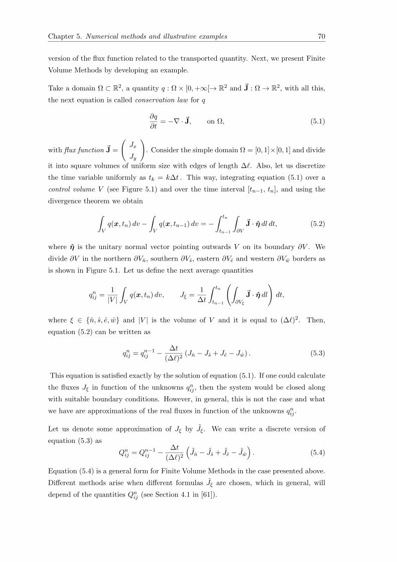
Chapter 5. Numerical methods and illustrative examples 70
version of the flux function related to the transported quantity. Next, we present Finite
Volume Methods by developing an example.
Take a domain Ω ⊂ R2, a quantity q : Ω× [0,+∞[→ R2 and ~J : Ω→ R2, with all this,
the next equation is called conservation law for q
∂q
∂t= −∇ · ~J, on Ω, (5.1)
with flux function ~J =
(Jx
Jy
). Consider the simple domain Ω = [0, 1]×[0, 1] and divide
it into square volumes of uniform size with edges of length ∆`. Also, let us discretize
the time variable uniformly as tk = k∆t . This way, integrating equation (5.1) over a
control volume V (see Figure 5.1) and over the time interval [tn−1, tn], and using the
divergence theorem we obtain∫Vq(x, tn) dv −
∫Vq(x, tn−1) dv = −
∫ tn
tn−1
∫∂V
~J · η dl dt, (5.2)
where η is the unitary normal vector pointing outwards V on its boundary ∂V . We
divide ∂V in the northern ∂Vn, southern ∂Vs, eastern ∂Ve and western ∂Vw borders as
is shown in Figure 5.1. Let us define the next average quantities
qnij =1
|V |
∫Vq(x, tn) dv, Jξ =
1
∆t
∫ tn
tn−1
(∫∂Vξ
~J · η dl
)dt,
where ξ ∈ n, s, e, w and |V | is the volume of V and it is equal to (∆`)2. Then,
equation (5.2) can be written as
qnij = qn−1ij − ∆t
(∆`)2(Jn − Js + Je − Jw) . (5.3)
This equation is satisfied exactly by the solution of equation (5.1). If one could calculate
the fluxes Jξ in function of the unknowns qnij , then the system would be closed along
with suitable boundary conditions. However, in general, this is not the case and what
we have are approximations of the real fluxes in function of the unknowns qnij .
Let us denote some approximation of Jξ by Jξ. We can write a discrete version of
equation (5.3) as
Qnij = Qn−1ij − ∆t
(∆`)2
(Jn − Js + Je − Jw
). (5.4)
Equation (5.4) is a general form for Finite Volume Methods in the case presented above.
Different methods arise when different formulas Jξ are chosen, which in general, will
depend of the quantities Qnij (see Section 4.1 in [61]).

Chapter 5. Numerical methods and illustrative examples 71
Qni,j Qni+1,jQni−1,j
Qni,j+1
Qni,j−1
V
∆`
∆`
VN
VS
VEVW
∂Vn
∂Ve
∂Vs
∂Vw
Figure 5.1: Staggered grid for Finite Volume Methods.
5.2 Numerical implementation of Reynolds equation and
cavitation models
In this section we solve numerically Reynolds equation by using the classical Gauss-
Seidel method. After this, we adequate this procedure for taking into account Reynolds
cavitation model by a projection of the partial solution into the cone of positive functions
on H10 (Ω). Finally, we present a version of the algorithm for the Elrod-Adams model.
Through all this section we suppose the behavior of the gap function h to be known in
space and time. In Section §5.3 we include a dynamic coupling between the upper surface
motion and the generated hydrodynamic pressure by means of the Newton equation.
5.2.1 Reynolds equation without cavitation
A Finite Volume Method is going to be used for a one dimensional problem (the general-
ization to two dimensions does not represent major difficulties) on the domain Ω = [0, 1].
The discretization obtained this way is going to be base for the discretization when tak-
ing into account some cavitation model.
First, let us set the problem of finding some function p that satisfies Reynolds equation
∂h
∂t= − ∂
∂x
(S
2h− h3
2
∂p
∂x
), (5.5)
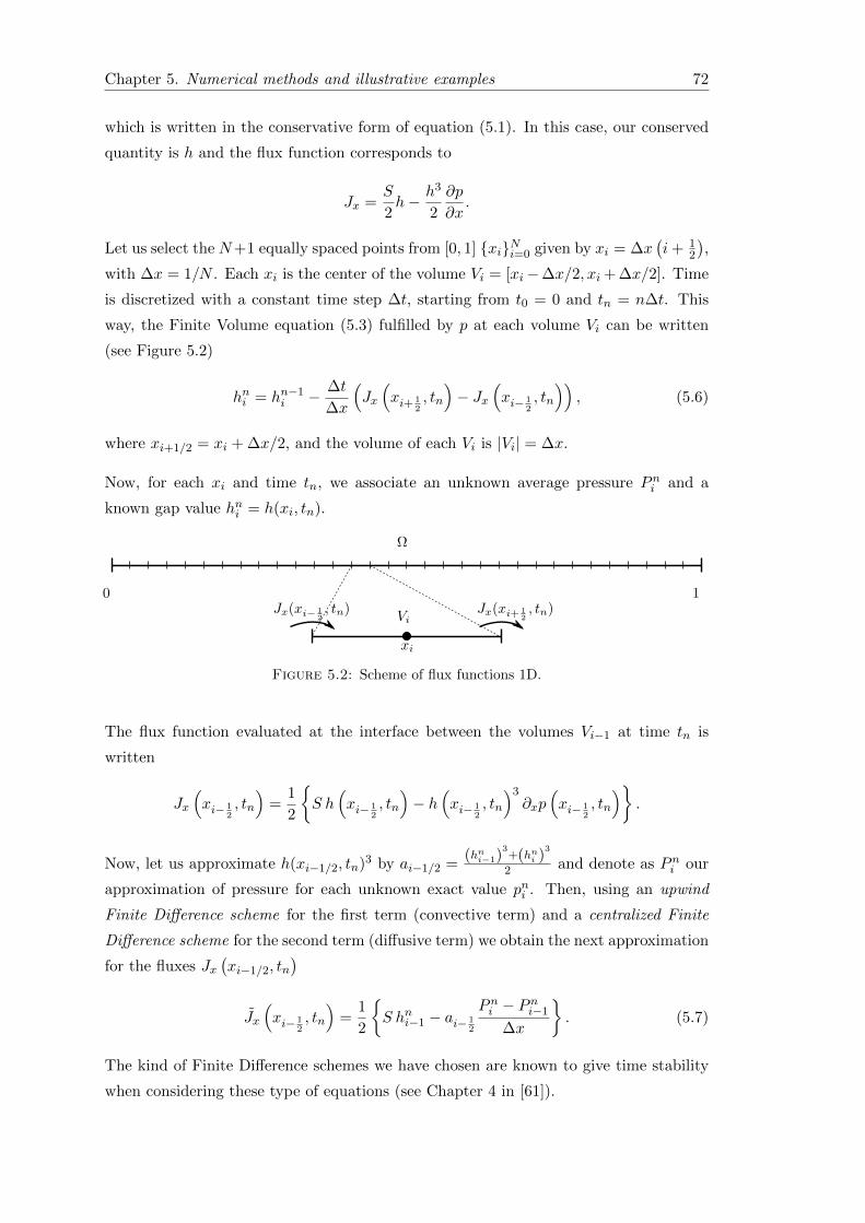
Chapter 5. Numerical methods and illustrative examples 72
which is written in the conservative form of equation (5.1). In this case, our conserved
quantity is h and the flux function corresponds to
Jx =S
2h− h3
2
∂p
∂x.
Let us select the N+1 equally spaced points from [0, 1] xiNi=0 given by xi = ∆x(i+ 1
2
),
with ∆x = 1/N . Each xi is the center of the volume Vi = [xi−∆x/2, xi + ∆x/2]. Time
is discretized with a constant time step ∆t, starting from t0 = 0 and tn = n∆t. This
way, the Finite Volume equation (5.3) fulfilled by p at each volume Vi can be written
(see Figure 5.2)
hni = hn−1i − ∆t
∆x
(Jx
(xi+ 1
2, tn
)− Jx
(xi− 1
2, tn
)), (5.6)
where xi+1/2 = xi + ∆x/2, and the volume of each Vi is |Vi| = ∆x.
Now, for each xi and time tn, we associate an unknown average pressure Pni and a
known gap value hni = h(xi, tn).
0 1
Vi
Ω
xi
Jx(xi+ 12, tn)Jx(xi− 1
2, tn)
Figure 5.2: Scheme of flux functions 1D.
The flux function evaluated at the interface between the volumes Vi−1 at time tn is
written
Jx
(xi− 1
2, tn
)=
1
2
S h(xi− 1
2, tn
)− h
(xi− 1
2, tn
)3∂xp
(xi− 1
2, tn
).
Now, let us approximate h(xi−1/2, tn)3 by ai−1/2 =(hni−1)
3+(hni )
3
2 and denote as Pni our
approximation of pressure for each unknown exact value pni . Then, using an upwind
Finite Difference scheme for the first term (convective term) and a centralized Finite
Difference scheme for the second term (diffusive term) we obtain the next approximation
for the fluxes Jx(xi−1/2, tn
)Jx
(xi− 1
2, tn
)=
1
2
S hni−1 − ai− 1
2
Pni − Pni−1
∆x
. (5.7)
The kind of Finite Difference schemes we have chosen are known to give time stability
when considering these type of equations (see Chapter 4 in [61]).
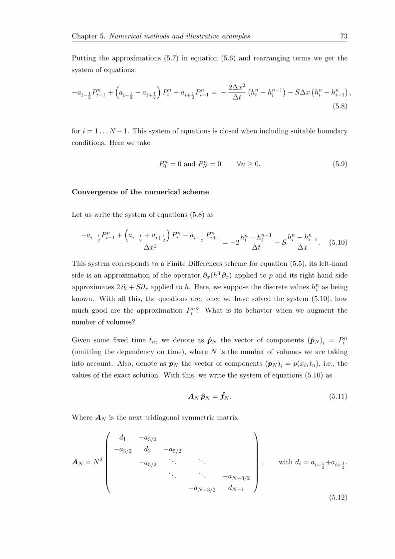
Chapter 5. Numerical methods and illustrative examples 73
Putting the approximations (5.7) in equation (5.6) and rearranging terms we get the
system of equations:
−ai− 12Pni−1 +
(ai− 1
2+ ai+ 1
2
)Pni − ai+ 1
2Pni+1 = − 2∆x2
∆t
(hni − hn−1
i
)− S∆x
(hni − hni−1
),
(5.8)
for i = 1 . . . N − 1. This system of equations is closed when including suitable boundary
conditions. Here we take
Pn0 = 0 and PnN = 0 ∀n ≥ 0. (5.9)
Convergence of the numerical scheme
Let us write the system of equations (5.8) as
−ai− 12Pni−1 +
(ai− 1
2+ ai+ 1
2
)Pni − ai+ 1
2Pni+1
∆x2= −2
hni − hn−1i
∆t− S
hni − hni−1
∆x. (5.10)
This system corresponds to a Finite Differences scheme for equation (5.5), its left-hand
side is an approximation of the operator ∂x(h3 ∂x) applied to p and its right-hand side
approximates 2 ∂t + S∂x applied to h. Here, we suppose the discrete values hni as being
known. With all this, the questions are: once we have solved the system (5.10), how
much good are the approximation Pni ? What is its behavior when we augment the
number of volumes?
Given some fixed time tn, we denote as pN the vector of components (pN )i = Pni
(omitting the dependency on time), where N is the number of volumes we are taking
into account. Also, denote as pN the vector of components (pN )i = p(xi, tn), i.e., the
values of the exact solution. With this, we write the system of equations (5.10) as
AN pN = fN . (5.11)
Where AN is the next tridiagonal symmetric matrix
AN = N2
d1 −a3/2
−a3/2 d2 −a5/2
−a5/2. . .
. . .
. . .. . . −aN−3/2
−aN−3/2 dN−1
, with di = ai− 1
2+ai+ 1
2.
(5.12)

Chapter 5. Numerical methods and illustrative examples 74
and fN = − 2∆tIN
(hnN − h
n−1N
)− S
∆xCNhnN corresponds to1 the right-hand side of the
system (5.10), IN is the identity matrix of order N − 1, and CN is the matrix such that(CN )i, j = 1 if j = i,
(CN )i, j = −1 if j = i− 1,
0 otherwise.
Denoting as fN the vector of components
(fN )i = −2 ∂th(xi, tn)− S ∂xh(xi, tn), i ∈ 1 . . . N − 1, (5.13)
we have that fN is an approximation of fN .
We define the quantities
τAN = ANpN − fN , and τ fN = fN − fN . (5.14)
τAN is the local truncation error due to the fact that AN is an approximation of the
functional relation between pN and fN . τ fN is the local truncation error due to the fact
that fN is an approximation of fN . We define also the global error EN = pN − pN ,
which represents the punctual differences between our approximation and the real values
of p. Putting all these definitions in equation (5.11) we get
AN EN = τ fN − τAN .
And so, if AN is non-singular we have
‖EN‖ ≤∥∥A−1
N
∥∥(∥∥∥τ fN∥∥∥+∥∥τAN∥∥) .
Using terms found in literature [62], we say that the numerical approximation of the
differential formulation (5.5) given by the system (5.11) is consistent if both
∥∥τAN∥∥ , ‖τ fN‖ → 0 as N →∞.
We say the same numerical scheme is stable if∥∥A−1
N
∥∥ remains bounded as N → ∞,
i.e., ∃C ∈ R, M ∈ N such that∥∥A−1
N
∥∥ ≤ C ∀N > M . Therefore, if our numerical
approximation is consistent and stable, then pN → pN as N →∞.
1If the boundary conditions are not null, they could be added in the first and last components of thisvector.

Chapter 5. Numerical methods and illustrative examples 75
From now on, if v is a vector of values over a uniform grid of m points with distance
∆x between those points, we use the grid norm (see [62]) given by2
‖v‖2 =
(∆x
m∑i=1
|vi|2) 1
2
.
Proposition 5.1. System (5.11) is consistent.
Proof. Using Taylor’s Series, it is easy to find that(τ fN
)i
= O (∆x) (h′′(xi)). Thus,
supposing the sum of the h′′(xi)2 is bounded, we obtain that∥∥∥τ fN∥∥∥
2= O(∆x). (5.15)
For proving∥∥τAN∥∥→ 0 as N →∞, again by Taylor’s series we have
−ai− 12pni−1 +
(ai− 1
2+ ai+ 1
2
)pni − ai+ 1
2pni+1
∆x2= −
ai+ 12p′i+ 1
2
− ai− 12p′i− 1
2
∆x+O(∆x2)
(ai p′′′i
)′= −
(ai p′i
)′+O
(∆x2
) ((ai p′′′i
)′+(aip′i
)′′′).
(5.16)
However, ai is not the exact value of h3 at the point xi but an approximation. In fact,
by Taylor’s series
ai =
(hni− 1
2
)3+(hni+ 1
2
)3
2= h (xi, tn)3 +O
(∆x2
)∂xx
(h (xi, tn)3
).
Putting this in the right side of equation (5.16) we get
−ai− 12pni−1 +
(ai− 1
2+ ai+ 1
2
)pni − ai+ 1
2pni+1
∆x2= −∂x
(h (xi, tn)3 ∂xp (xi, tn)
)+O(∆x2)Ci,
where Ci =((h3i
)′′′p′i
)′+ (ai p
′′′i )′ + (aip
′i)′′′. This way, we have proved that
(τAN)i
= O(∆x2
) (((h3i )′′′p′i)′
+ (ai p′′′i )′ +
(ai p′i
)′′′). (5.17)
Therefore, supposing the sum of the C2i is bounded, we have
∥∥τAN∥∥→ 0 as N →∞.
Stability is a property not easy to prove for the general definition of AN . The case
corresponding to h constant is studied in Chapter 2 of [62]. In that case we can write
AN = −N2 h3A, where A is the tridiagonal matrix with diagonal elements equal to
2As this norm is just a constant times the euclidean norm, the corresponding induced norm onmatrices also accomplishes the basic properties of Euclidean induced norms, e.g., ‖Av‖ ≤ ‖A‖‖v‖.
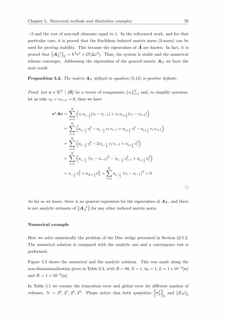
Chapter 5. Numerical methods and illustrative examples 76
−2 and the rest of non-null elements equal to 1. In the referenced work, and for that
particular case, it is proved that the Euclidean induced matrix norm (2-norm) can be
used for proving stability. This because the eigenvalues of A are known. In fact, it is
proved that∥∥A−1
N
∥∥2
= h3π2 + O(∆x2). Thus, the system is stable and the numerical
scheme converges. Addressing the eigenvalues of the general matrix AN we have the
next result.
Proposition 5.2. The matrix AN defined in equation (5.12) is positive definite.
Proof. Let v ∈ RN \ ~0 be a vector of components viNi=1 and, to simplify notation,
let us take v0 = vN+1 = 0, then we have
vᵀAv =N∑i=1
(vi ai− 1
2(vi − vi−1) + vi ai+ 1
2(vi − vi+1)
)=
N∑i=1
(ai− 1
2v2i − ai− 1
2vi vi−1 + ai+ 1
2v2i − ai+ 1
2vi vi+1
)=
N∑i=1
(ai− 1
2v2i − 2 ai− 1
2vi vi−1 + ai+ 1
2v2i
)=
N∑i=1
(ai− 1
2(vi − vi−1)2 − ai− 1
2v2i−1 + ai+ 1
2v2i
)= a− 1
2v2
1 + aN+ 12v2N +
N∑i=1
ai− 12
(vi − vi−1)2 > 0
As far as we know, there is no general expression for the eigenvalues of AN , and there
is not analytic estimate of∥∥A−1
N
∥∥ for any other induced matrix norm.
Numerical example
Here we solve numerically the problem of the Disc wedge presented in Section §2.5.2.
The numerical solution is compared with the analytic one and a convergence test is
performed.
Figure 5.3 shows the numerical and the analytic solution. This was made along the
non-dimensionalization given in Table 2.3, with R = 80, S = 1, h0 = 1, L = 1×10⁻³[m]
and H = 1× 10⁻⁶[m].
In Table 5.1 we resume the truncation error and global error for different number of
volumes, N = 26, 27, 28, 29. Please notice that both quantities∥∥∥τ fN∥∥∥
2and ‖EN‖2

Chapter 5. Numerical methods and illustrative examples 77
0 0.2 0.4 0.6 0.8 1-3
-2
-1
0
1
2
3
pre
ssu
rep
rofi
les
x
×10−2
N=27N=26
N=28
N=29
analytich
0
1
2
3
gap
fun
ction
h
Figure 5.3: Convergence of the numerical solution for the Disc wedge presented inSection §2.5.2.
N ∆x∥∥τAN∥∥2
∥∥∥τ fN∥∥∥2
∥∥A−1N
∥∥2
‖EN‖2
26 1.56× 10⁻² 5.71× 10⁻³ 9.69× 10⁻² 5.15× 10⁻⁶ 1.92× 10⁻³
27 7.81× 10⁻³ 1.44× 10⁻³ 4.86× 10⁻² 1.13× 10⁻⁶ 9.61× 10⁻⁴
28 3.91× 10⁻³ 3.62× 10⁻⁴ 2.44× 10⁻² 2.60× 10⁻⁷ 4.81× 10⁻⁴
29 1.95× 10⁻³ 9.07× 10⁻⁵ 1.22× 10⁻² 6.18× 10⁻⁸ 2.40× 10⁻⁴
Table 5.1: Convergence of the truncation errors and global error for the numericalexample of the Disc wedge.
are in linear relation with ∆x (∝ ∆x), while∥∥τAN∥∥2
is in quadratic relation with ∆x
(∝ ∆x2). These results agree with equations (5.15) and (5.17).
Gauss-Seidel iterations
We will present the Gauss-Seidel iterative method for the system of equations (5.8)
and (5.9). Gauss-Seidel is a classical iterative method for solving linear and non-linear
systems of equations [49, 5, 72]. First, we write
− ani− 1
2
Pni−1 +(ani− 1
2
+ ani+ 1
2
)Pni − ani+ 1
2
Pni+1 = fni , (5.18)
where fni = −2∆x2
∆t
(hni − h
n−1i
)− S∆x
(hni − hni−1
). We resume this procedure in Algo-
rithm 1.
Please notice that Gauss-Seidel uses the already calculated value Pn,ki−1 for calculating
the new value Pn,ki . If, instead of using Pn,ki−1, we use the older value Pn,k−1i−1 the iterative
procedure is known as the Jacobi iterative method, which is known to have a lower
convergence speed when compared to Gauss-Seidel [49].

Chapter 5. Numerical methods and illustrative examples 78
Algorithm 1: Gauss-Seidel for Reynolds equation
Input: hn: gap function, Pn−1: initial guess, tol: for stop criterionOutput: Pn pressure at time nbegin
k = 0
Pn,k = Pn−1
while change > tol dok = k + 1for i = 1 . . . N do
Pn,ki = 1ani− 1
2
+ani+1
2
(fni + an
i− 12
Pn,ki−1 + ani+ 1
2
Pn,k−1i+1
)end for
change = ‖Pn,k − Pn,k−1‖∞end while
return Pn,k
end
5.2.2 Reynolds model
Remembering what was exposed in Chapter 4, Reynolds cavitation model consists in
finding a weak solution of Reynolds equation not in the whole space H10 (Ω) but in the
cone of positive functions K ⊂ H10 (Ω) given by
K = φ ∈ H10 (Ω) : φ ≥ 0 a.e. on Ω,
which leads to the variational inequality (4.5).
The method we will use for solving Reynolds model was first exposed by Christopherson
in 1941 [25]. A detailed study of that method, applied to Journal Bearings, can be
found in [32]. This iterative methods can be described as: given an iterative method
for solving Reynolds equation (e.g., a Gauss-Seidel like method), at the end of each
iteration the partial solution is projected into the cone K. Such projection consists in
nullifying each component of Pn,k that is negative (see Section 2.8 in [48]). Therefore,
the Algorithm 1 for solving Reynolds equation only needs a little modification that is
presented in Algorithm 2.
The convergence study of this procedure is based in the contraction property of the
operator involved in each iteration composed with the projection operator into K, the
interested reader may review [19, 48]. In these last works, it is proved that Algorithm 2
converges to the solution of the next discrete problem (remember AN is positive definite
according to Proposition 5.2)
minv∈RN+
1
2vᵀANv − (fN )ᵀv,

Chapter 5. Numerical methods and illustrative examples 79
where RN+ = x ∈ RN : xi ≥ 0, i = 1 . . . N, AN and fN are given by equations (5.12)
and (5.13). In fact, Herbin and Marchand [55] showed that a discretization by Finite
Volume Methods converges to the solution of the associated variational inequality for
the obstacle problem [54]. Thus, we have good evidence of the convergence of Algorithm
2, although we are not going to prove it.
Algorithm 2: Gauss-Seidel for Reynolds equation with Reynolds cavitation model
Input: hn: gap function, Pn−1: initial guess, tol: for stop criterion
Output: Pn pressure at time n
begin
k = 0
Pn,k = Pn−1
while change > tol do
k = k + 1
for i = 1 . . . N do
Pn,ki = 1ani−1+ani
(fni + ani−1 P
n,ki−1 + ani P
n,k−1i+1
)Pn,ki = max
(0, Pn,ki
)end for
change = ‖Pn,k − Pn,k−1‖∞end while
return Pn,k
end
with ani =(hni+1/2
)3and fni = −2∆x2
∆t
(hni − h
n−1i
)− S∆x
(hni − hni−1
).
A linear obstacle
As another instance of Gauss-Seidel iterations with projections of the partial solution,
we refer to Figure 4.3. There, u(x) was generated solving the Poisson equation ∇2u = C
(where C < 0 is some constant source term) by Gauss-Seidel iterations and restricting
the partial solution uk by the assignation uk = min(ψ, uk), with ψ being the linear
function that describes the obstacle.
5.2.3 Elrod-Adams model
In Chapter 4 we presented the modified Reynolds equation when considering Elrod-
Adams cavitation model. In the 1D case we write this equation along the complementary

Chapter 5. Numerical methods and illustrative examples 80
conditions as
∂hθ
∂t= − ∂
∂x
(S
2hθ − h3
2
∂p
∂x
), (5.19)
p (1− θ) = 0, (5.20)
both in Ω. Notice not only the pressure field p is unknown but also the saturation field
θ. Making a similar discretization as before, we discretize θ as θni = θ(xi, tn). This way,
the transported quantity over each volume Vi is written Qni = hni θni , which corresponds
to the average amount of fluid present at each volume. This way, for Elrod-Adams
cavitation model, the equation analogous to equation (5.8) is
− γ(Qni −Qn−1
i − ν(Qni −Qni−1
))= −ani−1P
ni−1 +
(ani−1 + ani
)Pni − ani Pni+1, (5.21)
where ai =(hni+1/2
)3, γ = 2∆x2
∆t and ν = (S/2)∆t/∆x is the Courant number. Calcu-
lating first the pressures Pni by equation (5.21), we obtain the following equations for
Pni and θni for iteration k
Pn,ki =1
ani−1 + ani
(−γ(Qn,k−1i −Qn−1
i − ν(Qn,k−1i −Qn,k−1
i−1
))+ ani−1P
n,ki−1 + ani P
n,k−1i+1
)(5.22)
θn,ki =1
γ(1 + ν)
(γ(Qn−1i + ν Qn,ki−1
)+ ani−1P
n,ki−1 −
(ani−1 + ani
)Pn,ki + ani P
n,k−1i+1
).
(5.23)
The Gauss-Seidel like algorithm for Reynolds equation when considering cavitation
through Elrod-Adams model is shown in Algorithm 3. Notice the complementary equa-
tion (5.20) is used to project the partial solutions (pk, θk) into the subset of functions
such that, for every volume Vi, if p > 0 we must have θ = 1, and if 0 < θ < 1 we must
have p = 0.
5.3 Numerical solution examples
Gauss-Seidel is known to have a good numerical stability behavior for large systems of
equations [49]. On the other hand, it is also known for having too low convergence speed,
which means that the computational cost may be too high. To deal with this issue, we
used methods like over-relaxation and multigrid techniques, which are well known for
accelerating convergence speed [43], also see [20].

Chapter 5. Numerical methods and illustrative examples 81
Algorithm 3: Gauss-Seidel for Reynolds equation with Elrod-Adams cavitation model
Input: hn: gap function,(Pn−1, θn−1
): initial guess, tol: for stop criterion
Output: Pn, θn pressure and saturation fields at time n resp.begin
k = 0
Pn,k = Pn−1, θn,k = θn−1
while change > tol dok = k + 1for i = 1 . . . N do
if Pn,k−1i > 0 or θn,k−1
i == 1 then
Compute Pn,ki using equation (5.22)
if Pn,ki ≥ 0 then
θn,kk = 1else
Pn,ki = 0end if
end if
if Pn,ki ≤ 0 or θn,ki < 1 then
Compute θn,ki using equation (5.23)
if θn,ki < 1 then
Pn,ki = 0else
θn,ki = 1end if
end if
end for
change = ‖Pn,k − Pn,k−1‖∞ + ‖θn,k − θn,k−1‖∞end while
return(Pn,k, θn,k
)end
5.3.1 Numerical solution to the analytic examples
In this section we show the numerical solutions of the problems exposed in Section §4.5.
Cavitation in Pure Squeeze Motion
Here we search numerically for the analytic solution found for the Pure Squeeze Problem
in Section §4.5.1. For this, we used a coarse mesh of only 100 volumes and a finer mesh
of 450 volumes (same mesh used in [5]). The parameter tol of Algorithm 3 was chosen
to be tol = 5×10⁻⁶ and the time step was set as ∆t = 0.3×∆x (as the numeric scheme
is implicit in time, there is unconditional time-stability [62], so this parameter is chosen
just for having a good resolution in time), where ∆x = 1/100, 1/450.
Remembering Σ(t) denotes the right side of the cavitated zone, from Figure 5.4 we
observe a convergent behavior of the numerical solutions to the analytic solution of

Chapter 5. Numerical methods and illustrative examples 82
Elrod-Adams model. Similar behavior is found for the numerical solutions of Σ(t) when
considering the Reynolds model in Figure 5.5.
0.3 0.4 0.5 0.6 0.70.5
0.6
0.7
0.8
0.9
1
0.3 0.4 0.5 0.6 0.70.5
0.6
0.7
0.8
0.9
1
0.3 0.60.94
0.98
time
Σ(t
)
Σ(t
)
time
analytic solutionnum. solution, N=100num. solution, N=450
Figure 5.4: Numerical solution of Σ(t) for Elrod-Adams model with N = 100, 450.
time
Σ(t
)
Σ(t
)
time
analytic solutionnum. solution, N=100num. solution, N=450
0.25 0.3 0.35 0.4 0.45 0.50.5
0.6
0.7
0.8
0.9
1
0.25 0.3 0.35 0.4 0.45 0.50.5
0.6
0.7
0.8
0.9
1
0.25 0.35 0.450.94
0.96
0.98
Figure 5.5: Numerical solution of Σ(t) for Reynolds model with N = 100, 450.
Also, remember we denote as tref the time for which Σ(t) change from being a rupture
point to be a reformation point tref ≈ 0.3146. In Figure 5.6 a good agreement between
the numerical solution of θ for t = 0.3146 and the analytic solution can be observed.
This agreement is important since, as we said in Section §4.5.1, it influences the behavior
of the cavitated zone during the time interval for which Σ(t) is a reformation point (see
equation (4.15)).

Chapter 5. Numerical methods and illustrative examples 83
0 0.2 0.4 0.6 0.8 10.8
0.9
1 analytic sol.numerical sol.
θx
Figure 5.6: Numerical (N=450) and analytic solution of the saturation θ for t =0.3146, just before the reformation time tref .
Cavitation in a flat pad with a traveling pocket
In Section §4.5.2 we showed the analytic solutions of the pressure p and saturation field
θ for the stepped shape pocket traveling through the domain.
Let us take a number of volumes equal to N = 1024 over ]0, 1[, a time step ∆t = 2 ∆x/S
(Courant number equal to 1) and tol = 1 × 10⁻⁷. With this, by using Algorithm 3 we
reproduce in Figure 5.7 the analytic results found before in Figure 4.16. Moreover,
0 0.2 0.4 0.6 0.8 1-1
-0.5
0
0.5
1
1.5
2
2.5
3
x
z
t = 0.17 t = 0.42 t = 0.77
Figure 5.7: Analitic solutions of Elrod-Adams (in red) and Reynolds (in blue) cavi-tation models for three different times as done in Section §4.5.2. The non-dimensional
pressure profiles were amplified by a factor of 100.
a convergence analysis is performed comparing the numerical and analytic solutions
for t = 0.77. The differences between pressures is denoted ep and between the field
saturation is denoted by eθ. The norms of this errors are shown in Figure 5.8. From
those data, it is observed that ‖ep‖H10 (0,1) decays as ‖ep‖H1
0 (0,1) ∝ ∆x1.9 (quadratic
convergence rate), while ‖eθ‖L2(0,1) ∝ ∆x12 (under linear convergence rate). Please note
the rate convergence for pressure remains as calculated in Proposition 5.1. The low rate
convergence for θ should be associated to its discontinuities in ]0, 1[.

Chapter 5. Numerical methods and illustrative examples 84
δ1δ2
6 7 8 9 10-15
-10
-5pressure error
δ1
6 7 8 9 10
-7
-6
-5θ error
δ2
|δ1/δ2| = 1.9 |δ1/δ2| = 0.5
log
2
( ‖e p‖ H
1 0(0,1
))
log
2
( ‖e θ‖ L
2(0,1
))log2(N) log2(N)
Figure 5.8: Convergence analysis for p and θ in the H10 (0, 1) and L2(0, 1) norms resp.
for the traveling pocket problem solved in Section §4.5.2.
5.3.2 Incorporating dynamics
Until now we have always considered the gap function h as a known data. From now on,
we will consider h as an unknown, and its behavior will be coupled to the hydrodynamic
pressure p. For this, we revisit the problem of the traveling pocket, this time allowing
the upper surface (slider) to be depending on time hU (t) = Z(t).
d1(t) d2(t) = d1(t) + `
∆h
h(x, t) = Z(t)− hL(x)
Sx = 0 x = 1
z = 0
slider with mass m
x
z
Figure 5.9: Scheme of the traveling pocket with a dynamic dependence of the uppersurface.
We assume the slider has a non-dimensional inertial mass m. Also, let us denote as Z(t)
the distance between the slider and the lower surface (see Figure 5.9). Then, Z(t) is a
result of the interaction between the applied load W a (negative in the z-axis), which is
supposed to be constant, and the hydrodynamic force W h(t) given by
W h(t) =
∫ 1
0p(x, t) dx. (5.24)

Chapter 5. Numerical methods and illustrative examples 85
This way, the evolution of Z(t) can be modeled by solving the problem
mZ ′′(t) = W h(t)−W a, (5.25)
Z ′(t = 0) = V0, (5.26)
Z(t = 0) = Z0. (5.27)
Where Z ′ = U is the slider vertical velocity and Z ′′ its acceleration. We discretize time
by some constant time step ∆t with tn = n∆t, and for any function f(t) we denote
fn = f(tn). And we discretize the Newton Equation (5.25) in time by using the next
Newmark scheme for integration (which is unconditionally stable on time, e.g., [45]
Section 7.2)
Zn = Zn−1 + ∆t Un−1 +∆t2
2
W h,n −Wa
m, (5.28)
Un = Un−1 + ∆tW h,n −Wa
m. (5.29)
Observe that Wh,n−Wam is the acceleration at time tn. This numerical integration is
implicit in time, so the iterative procedure will include an update of the partial solution
Zn,k of Zn at each step. The Gauss-Seidel like algorithm resulting from including
dynamics through this Newmark scheme is described in Algorithm 4, at the end of this
section. A convergence result of it can be found in a recent work made by Buscaglia
and Talibi [17].
A simple example simulation
We will present a simulation done to exemplify the incorporation of dynamics in the
lubrication problem of the traveling pocket.
The scales used in this section are described in Table 5.2. The values of the basic
scales are U = 10[m/s], H = 10−6[m] and L = 10−3[m]. The non-dimensional mass
corresponds to 2× 10⁻⁵ and the non-dimensional applied load was W a = 1.666× 10⁻⁴.
The length of the pocket is ` = 0.2 and its depth d = 1. The number of volumes was
chosen to be N= 512 over ]0, 1[ and the time step ∆t = 2 ∆x/S (Courant number equal
to 1).
The initial conditions for the slider position are Z(t = 0) = 1 and Z ′(t = 0) = 0. And
at t = 0 the pocket is just entering into the domain, i.e., the right side of the pocket is
at x = 0.

Chapter 5. Numerical methods and illustrative examples 86
In Figure 5.10 we show the numerical solutions of p and θ obtained for different time
instants ti, i = 1 . . . 7. In blue, we plot the mass quantity hθ present at each point of
the domain. In red, we present the non-dimensional pressure amplified 200 times.
Quantity Scale Name
x L Horizontal coordinateS U Relative velocity
t LU Time
h H Gap thicknessZ, d H Slider vertical position, texture depth
p 6µULH2 Pressure
W a,W h 6µUL2
H2 Applied and hydrodynamic forces
m 6L4µH3U
Slider mass
Table 5.2: Basic and derived scales.
Let us remember that d1 denotes the position of the left side of the pocket while d2
denotes its right side. It can be observed that at time t1 = 0.19 a cavitated zone is
present at the very left of d2 due to the divergent geometry of the pocket. There,
the value of θ is approximated 1/2 as predicted by equation (4.32). This cavitation
bubble travels along the domain coupled to the divergent zone of the pocket and being
expanded since the transport velocity (S/2) is minor than the pocket velocity S. Also,
we can observe a small pressure profile due to the slow downward movement of the slider
(Z ′ < 0).
At t2 = 0.29 the convergent part of the pocket generates a pressurized region that
produces a small lifting of the slider (Z ≈ 1.05), this also causes the appearance of a
cavitated zone all along the interval ]d2, 1[.
The upward movement of the slider between t2 = 0.29 and t3 = 0.59, which corresponds
to a positive squeeze, produces the pressure profile to diminish and a cavitated zone
appears at the left side of the pressurized zone. Moreover, at t4 = 0.68 we observe
cavitation happening at almost the entire domain.
This lack of hydrodynamic support makes the slider to fall again as there is no force
to compensate the negative applied load. In fact, Z(t4) = 1.54 while Z(t5) = 1.44.
Because of this fall, the slider makes contact again with the fluid and new pressurized
zones appear due to a negative squeeze contribution. Interestingly, the slider does not
fall enough as to make contact with the fluid at the convergent zone of the pocket, and
so the pocket does not give any hydrodynamic support after approximately t4 = 0.68.
The last two frames, allow us to observe the cavitated zones traveling to the left and a
slow downward movement of the slider that produces a small pressure profile.

Chapter 5. Numerical methods and illustrative examples 87
0 0.2 0.4 0.6 0.8 1-1
0
1
2
0 0.2 0.4 0.6 0.8 1-1
0
1
2
0 0.2 0.4 0.6 0.8 1-1
0
1
2
0 0.2 0.4 0.6 0.8 1-1
0
1
2
0 0.2 0.4 0.6 0.8 1-1
0
1
2
0 0.2 0.4 0.6 0.8 1-1
0
1
2
0 0.2 0.4 0.6 0.8 1-1
0
1
2
flu
idm
asshθ
pre
ssu
refi
eld×
200
x
t1 = 0.19, Z(t1) = 1.0
t2 = 0.29, Z(t2) = 1.05
t3 = 0.59, Z(t3) = 1.49
t4 = 0.68, Z(t4) = 1.54
t5 = 0.88, Z(t5) = 1.44
t6 = 1.17, Z(t6) = 1.40
t7 = 2.34, Z(t7) = 1.39
Figure 5.10: Scheme of the traveling pocket with a dynamic dependence of the uppersurface.
Remark 5.3. It is difficult, maybe not possible, to generate analytic solutions for the
simulation we have just shown. In Chapter 6 we will perform even more complicated
simulations where the textures will have a sinusoidal profile.
Remark 5.4. To perform such simulations we require suitable computational techniques
that allow us to accelerate the convergence speed of the algorithms presented. Multigrid
and Parallel Computing Techniques are example of this and the interested reader may
review [20] and [23].
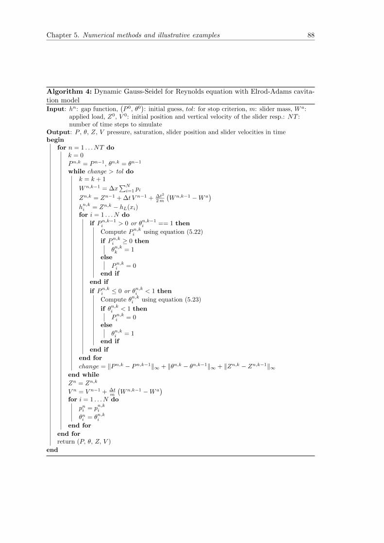
Chapter 5. Numerical methods and illustrative examples 88
Algorithm 4: Dynamic Gauss-Seidel for Reynolds equation with Elrod-Adams cavita-tion modelInput: hn: gap function,
(P 0, θ0
): initial guess, tol: for stop criterion, m: slider mass, W a:
applied load, Z0, V 0: initial position and vertical velocity of the slider resp.: NT :number of time steps to simulate
Output: P , θ, Z, V pressure, saturation, slider position and slider velocities in timebegin
for n = 1 . . . NT dok = 0
Pn,k = Pn−1, θn,k = θn−1
while change > tol dok = k + 1
Wn,k−1 = ∆x∑Ni=1 pi
Zn,k = Zn−1 + ∆t V n−1 + ∆t2
2m
(Wn,k−1 −W a
)hn,ki = Zn,k − hL(xi)for i = 1 . . . N do
if Pn,k−1i > 0 or θn,k−1
i == 1 then
Compute Pn,ki using equation (5.22)
if Pn,ki ≥ 0 then
θn,kk = 1else
Pn,ki = 0end if
end if
if Pn,ki ≤ 0 or θn,ki < 1 then
Compute θn,ki using equation (5.23)
if θn,ki < 1 then
Pn,ki = 0else
θn,ki = 1end if
end if
end for
change = ‖Pn,k − Pn,k−1‖∞ + ‖θn,k − θn,k−1‖∞ + ‖Zn,k − Zn,k−1‖∞end while
Zn = Zn,k
V n = V n−1 + ∆tm
(Wn,k−1 −W a
)for i = 1 . . . N do
pni = pn,kiθni = θn,ki
end for
end forreturn (P, θ, Z, V )
end

Chapter 6
Application: a study of sinusoidal
textured slider bearings
6.1 Introduction
During the last decade several studies have been done addressing the possibility of
improving the tribological behavior of hydrodynamic bearings with the use of surface
texturing technologies. Experimental and theoretical studies have shown reduction of
friction by the introduction of textured surfaces, e.g., [33, 44, 39, 21], but the mechanisms
behind this improvements are not yet well understood.
λ
hgap
R
L
h(x, t)
Ω+ Ω0Ω0 ΣΣ
z
x
lubricantZ(t)
gas gas
W a
Wh(t)
movement
direction
slider
runner
Figure 6.1: Slider bearing over and a sinusoidal textured runner scheme.
89

Chapter 6. Application: a study of sinusoidal textured slider bearings 90
In [16], by using Homogenization Technique, it is shown that if cavitation is not taken
into account, the introduction of textures only augment friction and diminishes the
minimal distance between surfaces (so-called minimum clearance). This means that for
having an improvement of the tribological behavior either, the perturbation of the sur-
face must be outside the validity of the Homogenization Theory employed (an example
of this is the Rayleigh step shown in Section §2.5), or other physical phenomenon such
as cavitation must be considered.
Recalling Figure 1.4, the degree of conformity between the bearing and the liner, for
the slider bearing (Figure 6.1), is computed by R/L. Making use of Reynolds model,
Gadeschi et al. [44], and later Checo et al. [21] employing Elrod-Adams model, showed
that for a fixed load it is possible to obtain a configuration that minimizes the friction
only for moderate R/L (≈ 10) or higher. These results are in agreement with pioneering
experiments made by Costa & Hutchins [31], and with latter studies by Tomanik [85,
86], Kovalchenko et al [60], Yin et al [90], Scaraggi et al [81], among others [33, 2, 50].
In this chapter we show that making use of the theory presented in the previous chapters,
and keeping the characteristics of the slider bearing as simple as we can, we are able to
perform interesting simulations whose results can reveal part of the nature of friction
reduction mechanisms. Thus, focusing in simple hypotheses, we choose to texturize the
runner with a sinusoidal shape of periodicity λ and depth d, as in Figure 6.1. Also, we
assume the profile of the slider to have a circular shape of curvature radius R.
In the next section we setup the simulations details and establish the range chosen for
the parameters λ, d, R/L, applied load W a and mass m of the slider.
6.2 Simulation details and untextured cases
The values chosen for the different basic scales were: runner velocity U = 10[m/s],
slider length L = 10−3[m], H = 1µ[m] (1 micron), fluid viscosity µ = 4× 10⁻³[Pa·s] and
for the mass of the slider m = 0.048[kg/m] per unit width. Those values are typical
for compression rings of car engines [22, 44]. We also chose the applied load as being
Wa = 40[N/m] per unit length, this value was selected as to assure Hydrodynamic
Lubrication conditions. The non-dimensionalization used are showed in Table 6.1.
For sake of clarity, we summarize the mathematical problem to be solved during the
simulations as:
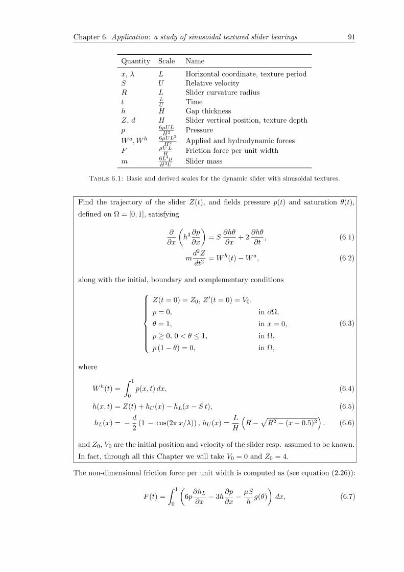
Chapter 6. Application: a study of sinusoidal textured slider bearings 91
Quantity Scale Name
x, λ L Horizontal coordinate, texture periodS U Relative velocityR L Slider curvature radius
t LU Time
h H Gap thicknessZ, d H Slider vertical position, texture depth
p 6µULH2 Pressure
W a,W h 6µUL2
H2 Applied and hydrodynamic forces
F µU LH Friction force per unit width
m 6L4µH3U
Slider mass
Table 6.1: Basic and derived scales for the dynamic slider with sinusoidal textures.
Find the trajectory of the slider Z(t), and fields pressure p(t) and saturation θ(t),
defined on Ω = [0, 1], satisfying
∂
∂x
(h3 ∂p
∂x
)= S
∂hθ
∂x+ 2
∂hθ
∂t, (6.1)
md2Z
dt2= W h(t)−W a, (6.2)
along with the initial, boundary and complementary conditions
Z(t = 0) = Z0, Z′(t = 0) = V0,
p = 0, in ∂Ω,
θ = 1, in x = 0,
p ≥ 0, 0 < θ ≤ 1, in Ω,
p (1− θ) = 0, in Ω,
(6.3)
where
W h(t) =
∫ 1
0p(x, t) dx, (6.4)
h(x, t) = Z(t) + hU (x)− hL(x− S t), (6.5)
hL(x) = − d
2(1 − cos(2π x/λ)) , hU (x) =
L
H
(R−
√R2 − (x− 0.5)2
). (6.6)
and Z0, V0 are the initial position and velocity of the slider resp. assumed to be known.
In fact, through all this Chapter we will take V0 = 0 and Z0 = 4.
The non-dimensional friction force per unit width is computed as (see equation (2.26)):
F (t) =
∫ 1
0
(6p∂hL∂x− 3h
∂p
∂x− µS
hg(θ)
)dx, (6.7)

Chapter 6. Application: a study of sinusoidal textured slider bearings 92
where g is taken as
g(θ) =
θ, if θ > θs
0, otherwise.(6.8)
This parameter θs is a threshold for the onset on friction, it can be interpreted as the
minimum lubricant fraction for shear forces to be transmitted from one surface to the
other. Here, we set θs = 0.95, in [21] it is observed that when choosing another value
for θs the behavior of the contact is not altered significantly.
Notice that the boundary condition θ(0, t) = 1 implies that the fluid film is always
complete at the entrance of the domain. This implies the fully-flooded condition (see
Section §1.2.5) and it guaranties, along with the applied-load chosen low enough, that
we will work in the Hydrodynamic Lubrication Regime.
As we consider the hydrodynamic regime, there is no necessity of including some model
for contact pressure, which only appears when considering mixed regimes of lubrication
or similar. The interested reader may review [86] where the Greenwood-Williamson [51]
model for contact pressure is used.
6.2.1 Quantities of interest
The simulations were done in such a way that a stationary state is reached at some time
T , after that time, the variables acquire a periodic behavior on time, that periodicity
has length λ equal to the textures period. With this, we denote the time interval where
the measures are going to be done as T = [T, T + λ].
This way, from the non-dimensional friction coefficient (see Section §2.5.1)
f(t) =H
6L
F (t)
W a, (6.9)
which varies through time, we define the average friction coefficient as
f =1
λ
∫Tf(t) dt, (6.10)
which characterizes the power lost due to friction. Observe the factor H6L appears since
F and W a are measured with different scales (see Table 6.1).
We also define the minimum clearance
Cmin = minx∈Ω, t∈T
h(x, t), (6.11)
which can be used to characterize surfaces wear in tribological systems.

Chapter 6. Application: a study of sinusoidal textured slider bearings 93
6.2.2 Untextured cases
The first simulations we run are in absence of texture (d = 0). This way, varying R
(which is equal to R/L since we fix the length of the slider to L = 1) as R = 2n,
n = 2 . . . 10, we obtain basis measures of f and Cmin that will be compared later with
the textured cases.
As an example, for R = 32, Z0 = 4 and V0 = 0, we show in Figure 6.2 the evolution of
Z(t), the friction coefficient f(t) and W h(t)/W a. It can be observed that W h(t) starts
being 8 times greater than the applied load so the slider tends first to rise, after that,
W h(t) remains being a bit small than W a. In fact, W h(t) converges to W a while the
slider decelerate and tend to the equilibrium position Z(t > T ) = 7.408. On the other
hand, the friction coefficient has no abrupt change while converging to f = 9.56× 10⁻².
0 1.0 2.0 3.0 4.0 5.0 6.0
4.0
5.0
6.0
7.0
8.0
0.0
1.0
Z(t)
time
f(t)
Wh(t)/W a
Figure 6.2: Slider evolution for the untextured case for load W a and R = 32.
R 4 8 16 32 64 128 256 512 1024
Cmin 6.36 7.81 8.02 7.41 6.36 5.23 4.33 3.70 3.32f × 102 7.61 7.45 8.12 9.56 11.9 15.4 20.3 26.1 28.7
Table 6.2: Friction coefficient f and clearance Cmin for several values of R once theyreached the stationary state.
Making the simulations for the values of R selected above, we obtain the reference values
showed in Table 6.2 for Cmin and f (amplified by a factor of 100). We remark that there
seems to be an optimal value for R in the sense that the maximum value of Cmin is
reached at R = 16, this is congruent with the existence of a shape of the liner that
maximizes the load-carrying capacity, as it was shown in Section §2.5.1 for the Rayleigh
step wedge. It is also in line with a similar analysis made in Section 5.7 of [18] for pad
bearings.

Chapter 6. Application: a study of sinusoidal textured slider bearings 94
6.3 Textures effects
Here we select values of λ around 1, more precisely λ ∈ 0.1 + k∆λ, k = 0 . . . 47,∆λ = 0.04, with maximum value 1.98. For the depth d ∈ k∆d, k = 1 . . . 51, ∆λ = 0.2,
with maximum value 10.2.
It is convenient to define the relative difference Vf between the friction coefficients for
the untextured and textured cases, which reads
Vf (d, λ) =f(d, λ)− funtextured
funtextured.
Analogously, the relative difference VC of the minimal clearance is defined as
VC(d, λ) =Cmin(d, λ)− Cmin,untextured
Cmin,untextured.
We select a moderate-conforming radius R=32 and a highly-conforming radius R=256.
The associated results for both curvatures are shown in Figure 6.3.
-14
-12
-10-8
-6-4
-2
-20 -30-14
-12
-40
-60-50
-70
-30
-25
-20
-15
0
-5-10
1020
30 50100
1 2 3 4 5 6 7 8 9 10d
-10
-20
-30
-40
-50
-60
-70
1.8
1.6
1.4
1.2
1.0
0.8
0.6
0.4
0.2
1 2 3 4 5 6 7 8 9 10d
λ
100
80
60
40
20
0
-20
1.8
1.6
1.4
1.2
1.0
0.8
0.6
0.4
0.2
λ
1 2 3 4 5 6 7 8 9 10d
1.8
1.6
1.4
1.2
1.0
0.8
0.6
0.4
0.2
λ
1 2 3 4 5 6 7 8 9 10d
1.8
1.6
1.4
1.2
1.0
0.8
0.6
0.4
0.2
λ
0
-10
-20
-30
-40
-50
-60
40
20
0
20
-40
-60
0
-60-50-40-30
-20
-10
0 10 20 30
40
-10 -20 -30
(a) (b)
(c) (d)
Figure 6.3: Comparison of Cmin and f for several values of λ and d by relativedifferences Vf (left side) and VC (right side) for R=32, 256 (upper and lower figures
resp.).

Chapter 6. Application: a study of sinusoidal textured slider bearings 95
6.3.1 General observations
As it can be observed, for the two curvatures selected there exist configurations of the
textures that diminish friction and there are other configurations that augment it. The
same can be observed for the minimum clearance. A smooth behavior of these quantities
is observed. Also, when d tends to zero both Cmin(d, λ) and f(d, λ) tend to the respective
values of the untextured case. In fact, additional simulations have shown that, for a fixed
depth d, both VC and Vf tend to zero as the period λ grows.
As mentioned in this chapter’s introduction, these results are in line with the existing
literature. In fact, the bigger R/L, the bigger the set of textures that allows an im-
provement in friction and minimum clearance is. These results were recently published
in [22], where a more extensive analysis can be found.
6.3.2 An effect of the traveling bubbles
Although both VC and Vf have a smooth dependence on the parameters, a discontinuous
behavior can be observed for small values of λ and d ≈ 8 in both Figure 6.3(a) and
Figure 6.3(b). To understand what happens there, we need to observe closer the behavior
of p and θ when the periodic state has been reached.
0 0.2 0.4 0.6 0.8 1
0
2
4
6
8
10
0 0.2 0.4 0.6 0.8 1
0
2
4
6
8
10
x x
pre
ssu
rep×
100
satu
ratio
nθ
0
0.5
1.0(a) (b)
Figure 6.4: Sudden change of p and θ with a small change of d (d = 8.1 on the left andd = 8.2 on the right). Both with fixed curvature R = 32 and an arbritrary time t > T .The red line is the pressure field amplified 100 times, the red dashed line correspondsto the pressure of the untextured case. The blue continuous line corresponds to the
path the minimum value of θ makes when traveling along the domain.
We fix the value of the periodicity as λ = 0.1 and select some arbitrary time t > T . The
resulting fields p and θ are shown in Figure 6.4(a) for d = 8.1 and in Figure 6.4(b) for
d = 8.12. In both figures the blue continues lines (with arrows) represent the path the
minimum value of θ (which depends on x) follows in time. Let us analyze both cases.

Chapter 6. Application: a study of sinusoidal textured slider bearings 96
For d = 8.1, it is observed the presence of cavitation bubbles in two very separated areas.
In the very left of the domain, a bubble grows and collapses almost immediately, while a
second bubble appears around x = 0.65 and instead of collapsing it is transported outside
the domain. As a consequence, the convergent region of the slider affects importantly
the buildup of pressure. In fact, the pressure profile area is similar to the one generated
in the untextured case (represented by the continuous red line), to which is summed up
the effects of each convergent region of the “sinusoidal pockets”.
For d = 8.2, we observe the bubbles generated in the left side of the domain travel all
along collapsing near x = 0.5, immediately after this collapse, a new bubble appears and
travels outside the domain. This presence of cavitation on most part of the domain af-
fects the pressure buildup. Thus, this time the convergence of the slider has less influence
in the pressure profile, it only modulates the peak of the pressurized zones generated by
the convergent parts of each sinusoidal pocket. This affects the load-carrying capacity
and, in order to support the applied load, the slider equilibrium position diminishes
dramatically.
6.3.3 Hysteresis of the slider
Would this abrupt change in the equilibrium position of the slider occurs if we change
the system configuration by successive approximations? For instance, if once the slider
reaches the stationary state we diminish d slightly, and diminish it again after reaching
the new stationary state. What would be the final equilibrium variables?.
0 5 10 15 20 25 302
4
6
Z(t
)
time
1.954.4
4.5
3.95 4.054.6
4.65
2.05
d(t < 10)=8.1 d(10 ≤ t < 20)=8.15 d(t ≥ 20)=8.2
d(t ≥ 0)=8.2
Figure 6.5: Hysteresis of the statationary state.
Two different simulations for a fixed curvature R = 32 are shown in Figure 6.5. The
first simulation, Case A with result in blue, is made with a constant depth d = 8.2. The
second simulation, Case B with result in red, is such that d(t) = 8.1 for 0 ≤ t < 10,
d(t) = 8.15 for 10 ≤ t < 20 and d(t) = 8.2 for 20 ≤ t. For the former case the stationary

Chapter 6. Application: a study of sinusoidal textured slider bearings 97
average position is equal to Z = 2.27; for the latter case, after the changes of d are done
and the stationary state is reached, the stationary average position is equal to Z = 4.62.
This unexpected fact is known as Hysteresis, which means that the state of the slider
at a particular time t depends on the history of the system.
6.3.4 Cavitation induced oscillations
Observing Figure 6.4, it can be noticed that for both cases considered, d = 8.1, 8.2, the
cavitation bubbles collapse in different places. For d = 8.1 the cavitation bubble col-
lapses at the left of the domain, near the entrance of fluid, and there exists a pressurized
zone that extends through more than half of the domain (among other small pressurized
zones). On the contrary, for d = 8.2 the bubble collapses at the middle of the domain
and the cavitation bubble reappears almost immediately, and so there are present many
pressurized zones with extension of order 1/λ.
These observations are also valid for both cases A and B presented in the last section.
These bubbles collapse were observed to occur during a very small lapse of time. The
last creates a sudden expansion of the pressurized zone located at the right of the bubble
just collapsed. This sudden change in pressure affects the hydrodynamic force creating
oscillations of the position of the slider. These oscillations are shown in Figure 6.6 for
the stationary state.
-30
-25
-20
-15
-10
-5
0
5
10
15
20
25
59.7 59.75 59.8 59.85 59.9 59.95 60time
100×(Wh(t)−Wa
)/Wa
rela
tive/
ab
solu
ted
iffer
ence
s
100×(Wh(t)−Wa
)/Wa
105 ×(Z(t)− Z
)105 ×
(Z(t)− Z
)
Figure 6.6: Hydrodynamic force and slider position oscillations induced by suddencavitation bubbles collapse for both cases A (in blue) and B (in red).

Chapter 6. Application: a study of sinusoidal textured slider bearings 98
Please note that the amplitude of the oscillations of the hydrodynamic force W h(t) is
about 5% and 20% of the applied charge W a for case A and B respectively. These
differences may be explained by observing that the pressurized zone placed at the right
of the collapsed bubble is around 6 times bigger for Case B than for Case A, which
leads to a bigger pressure build-up in Case B. On the other hand, the oscillations of
Z(t) are negligible since those are of order 1×10⁻⁵[µm]. Nevertheless, these oscillations
associated to sudden collapses of the cavitation bubbles may be an interesting source
of future work. Particularly, it would be interesting to address the dependence of these
oscillations with the mass of the slider.

Chapter 7
Conclusions and future work
In this work we have done a systematic compilation of theoretical and practical as-
pects of Lubrication Theory. These studies have involved Fluid Mechanics, Lubrication
Theory, Elliptic PDE’s from Functional Analysis, Calculus of Variations, and Numeri-
cal Analysis from varied aspects like numerical convergence, stability, simulations setup
and results interpretation. Nowadays, the organization made here cannot be found in
other publications. Therefore, this document could be used by undergraduate/graduate
students who want to have a global understanding of the theoretical and practical sub-
jects of the theory addressing modeling and simulation of lubricated contacts. Next, we
present particular conclusions from the contents.
We have seen in Chapter 2 that Reynolds equation for the stationary case is satisfied
by the limit solutions of the Stokes equations when the proximity parameter H/L goes
to zero. This interesting point of view gives more insight into the nature of Reynolds
equation when compared to just dropping the terms of order H/L (or higher), as is done
in Section §2.1, Lubrication Hypothesis in Navier-Stokes equation.
When considering discontinuities in the gap function h, the mathematical tools needed
rely on the theory of PDE’s from the Functional Analysis Theory, as it was shown in
Chapter 3. In this way, it is possible not just to study the well-posedness of Reynolds
equation in the presence of discontinuities but also to give a first approach to a cavitation
model by imposing an obstacle to the pressure solution (see Section §4.2, Reynolds
model).
The Reynolds cavitation model does not enforce mass-conservation. This key issue can
be tackled with the Elrod-Adams cavitation model as presented in Chapter 4. The
Elrod-Adams model introduces a change in the type of PDE that models the fluid’s
99

Chapter 7. Conclusions and future work 100
behavior. The analysis of the problem with that change in the PDE type is hard to do,
in such a way that nowadays only an existence result is available.
In Chapter 6 we have shown that the models and resolution algorithms presented and
studied along the previous chapters of this document can be used effectively for the
simulation of one-dimensional slider bearings. It is observed that these results are in
line with the literature. Moreover, interesting phenomena can be revealed, such as the
catastrophic event depending on the collapse of the cavitation bubbles, and the hysteresis
of the stationary state. Also, we have seen how the convergent-divergent geometries of
the sinusoidal pockets plays different roles depending on the size of the pressurized zone.
Nevertheless, we must emphasize that such discoveries depend upon the models used,
as neither the Reynolds model nor the Elrod-Adams model are free of criticism (see for
instance [68, 15]).
Next, we present different possibilities to continue the present work.
Limit equations
In Chapter 3 we discussed the work of Bayada and Chambat [8] where it is rigorously
proved that Reynolds equation is fulfilled by the limit solutions (in the sense of the
proximity of the surfaces) of the Stokes system. However, the hypothesis made on the
regularity of the domain, being of class C1, is very strong. Also, the gap function h is
supposed to be continuously differentiable over the closure of the domain, a hypothesis
that is not compatible with real applications as they might involve discontinuous sur-
faces. It would be interesting to study the possibility of extending this work for weaker
regularity hypothesis and, moreover, seek for a similar result for the limit formulas of
friction, which were found in Chapter 2 by making use of an asymptotic limit.
Elrod-Adams extensions
The Elrod-Adams model, as discussed by Buscaglia et al. [15] and also by Checo [20],
assume the transport velocity of the fluid in the cavitated zone to be S/2, i.e., equal to
the transport velocity that is obtained when the fluid film is complete. This assumption
is not realistic enough for the cases considered in this work, in which most of the lubricant
lies on the moving surface (the runner). To extend Elrod-Adams for allowing transport
greater than S/2 is a challenging problem, lack of uniqueness of solution is one of its
difficulties; and an algorithm that automatically keeps track of the cavitation boundary
(so-called front-capturing algorithms, e.g., Elrod-Adams algorithm) is not available yet
(some efforts on this issue can be found in [20]).

Chapter 7. Conclusions and future work 101
Discontinuous Galerkin
Currently the adopted method has poor mesh flexibility, since it is based on a rectan-
gular grid. Its convergence order is also low, as shown in Section §5.2 Numerical imple-
mentation of Reynolds equation and cavitation models, because it assumes a piecewise
constant interpolation of the variables. Standard high order methods cannot be applied
because of the spontaneously-generated discontinuities at cavitation boundaries. With
this perspective, it would be interesting to set focus on Discontinuous Galerkin (DG)
Methods, which overcome these issues for elliptic problems [29], hyperbolic problems
[27, 28], and elastohydrodynamic lubrication problems [63].
A deep study of DG methods can be found in [3]. The change of type of PDE, from
elliptic to hyperbolic at the cavitation boundaries, makes it an interesting application of
DG approximation techniques. Further, the generalized cavitation model developed by
Buscaglia et al [15, 4], which allows to vary the transport velocity, requires the imposition
of inflow boundary conditions at the cavitation boundary. This would certainly require
some specific development of DG techniques.
Boundary conditions for pressure
The current cavitation models only admit a constant cavitation pressure, and it must
be equal to the surrounding pressure. This has been questioned by several researchers
[82] and is a source of inaccuracy. At some instants in the engine cycle the pressure
difference between both sides of the ring pack can reach 100 [atm]. Therefore, it is
interesting to include this consideration when developing new cavitation models.


Appendix A
Second order MAC scheme for
Navier-Stokes equations
The finite volume method is presented here along with a staggered MAC (marker-and-
cell) mesh. The adopted notation corresponds to Chapter 2 of Computational Methods
for Multiphase Flow, Prosperetti and Tryggvason (2009). Further details can be found
in the referenced book.
The 2D Navier-Stokes equations (2.28) and (2.29) and the incompressibility condition
(2.30) resp. are written in the discrete version (dx ≡ h)
un+1 − un
∆t+ Ah(un) = −1
ρ∇hp+ µDhu
n, (A.1)
∇h · un+1 = 0, (A.2)
where n is the index of the time step and ∆t its length. Ah, Dh and ∇h are approxi-
mations of the advection, diffusion and gradient operators resp..
Figure A.1 shows the discretization scheme used for solving the Navier Stokes equations
in Section §2.4. The first step is to generate an approximated version Ωh of the domain
Ω (see Figure A.1). The volume schematized in Figure A.1 is used to determine the
equation involving the unknown pressure pi,j . The same is done to determine the equa-
tion for the velocity ui+1
2 ,j, but this time the control volume is shifted as the left scheme
of Figure A.2 shown. At the right side of that figure the scheme of the control volume
for vi,j+1
2
is shown.
103

Appendix A. Second order MAC scheme for Navier-Stokes equations 104
Ω Ωh
∂Ω ∂Ωh
pi,j
pi,j+1
pi,j−1
pi+1,j+1
pi+1,j−1
pi−1,j+1
pi−1,j−1
ui− 1
2 ,jpi−1,j pi+1,j
vi,j+1
2
vi,j− 1
2
ui+1
2 ,j
ui+1
2 ,j+1ui− 1
2 ,j+1
vi−1,j+1
2
vi+1,j+1
2
vi−1,j− 1
2
vi+1,j− 1
2
ui− 1
2 ,j−1ui+1
2 ,j−1
Figure A.1: Staggered MAC discretization by Finite Volume Methods. Control vol-ume for pressure.
A.1 Discretization of advection and diffusion
Over an arbitrary control volume, the advection of un can be approximated by the
average
A(un) =1
∆V
∫V∇ · (un ⊗ un) dv =
1
∆V
∮∂V
un(un · n)ds (A.3)

Appendix A. Second order MAC scheme for Navier-Stokes equations 105
Now, based on the corresponding control volume for ui+ 12,j and vi,j+ 1
2, the discrete
versions of Ax(un) and Ay(un) can be written resp. as
(Ax)ni+ 1
2,j
=1
h
(ui+ 3
2,j + un
i+ 12,j
2
)2
−
(uni+ 1
2,j
+ uni− 1
2,j
2
)2
+
(uni+ 1
2,j+1
+ uni+ 1
2,j
2
)(vni+1,j+ 1
2
+ vni,j+ 1
2
2
)
−
(uni+ 1
2,j
+ uni+ 1
2,j−1
2
)(vni+1,j− 1
2
+ vni,j− 1
2
2
),
(Ay)ni,j+ 1
2
=1
h
(uni+ 1
2,j
+ uni+ 1
2,j+1
2
)(vni,j+ 1
2
+ vni+1,j+ 1
2
2
)2
−
(uni− 1
2,j+1
+ uni− 1
2,j
2
)(vni,j+ 1
2
+ vni−1,j+ 1
2
2
)
+
(vni,j+ 3
2
+ vni,j+ 1
2
2
)2
−
(vni,j+ 1
2
+ vni,j− 1
2
2
)2 ,
and the diffusion of un can be approximated by the average
D(un) =1
∆V
∫V∇2undv. (A.4)
vi+1,j+1
2
vi+1,j− 1
2
pi,j
pi,j+1
pi,j−1
pi+1,j+1
pi+1,j−1
pi−1,j+1
pi−1,j−1
ui− 1
2 ,jpi−1,j pi+1,j
vi,j+1
2
vi,j− 1
2
ui+1
2 ,j
ui+1
2 ,j+1ui− 1
2 ,j+1
vi−1,j+1
2
vi−1,j− 1
2
ui− 1
2 ,j−1ui+1
2 ,j−1
pi,j
pi,j+1
pi,j−1
pi+1,j+1
pi+1,j−1
pi−1,j+1
pi−1,j−1
ui− 1
2 ,jpi−1,j pi+1,j
vi,j+1
2
vi,j− 1
2
ui+1
2 ,j
ui+1
2 ,j+1ui− 1
2 ,j+1
vi−1,j+1
2
vi+1,j+1
2
vi−1,j− 1
2
vi+1,j− 1
2
ui− 1
2 ,j−1ui+1
2 ,j−1
Figure A.2: Control volumes for u (left) and v (right). Adapted from [73].

Appendix A. Second order MAC scheme for Navier-Stokes equations 106
This way, the discrete version of the diffusion on ui+ 12,j and vi,j+ 1
2is given resp. by
(Dx)ni+ 1
2,j
=uni+ 3
2,j
+ uni− 1
2,j
+ uni+ 1
2,j+1
+ uni+ 1
2,j−1− 4un
i+ 12,j
h2,
(Dy)ni,j+ 1
2
=vni+1,j+ 1
2
+ vni−1,j+ 1
2
+ vni,j+ 3
2
+ vni,j− 1
2
− 4vni,j+ 1
2
h2.
A.2 Projection Method
The Projection Method was introduced by Chorin [24] and Yanenko [89]. In this ap-
proach the velocity is first advanced without taking into account the pressure, resulting
into a velocity field that, in general, does not accomplish the non-compressibility condi-
tion. After that, the pressure necessary to make the velocity field accomplish with the
non-compressibility condition is found, and the velocity field is corrected by adding the
pressure gradient.
For this, the momentum equation is split into two parts by introducing a temporal
velocity u∗ such that
un+1 − un =(un+1 − u∗
)+ (u∗ − un) .
Now, a predictor step is made (we adopt a second order Crank-Nicholson scheme [62])
such that the temporary velocity field is found by ignoring the pressure effects:
u∗ − un
∆t= −3
2Ah (un) +
1
2Ah
(un−1
)+µ
2(Dhu
n + Dhu∗) . (A.5)
Next, the correction step is
un+1 − u∗
∆t= −∇hφn+1, (A.6)
where φ is related to the pressure by the equation
−∇φn+1 = −1
ρ∇pn+1 +
µ
2
(Dhu
n+1 −Dhu∗) . (A.7)
Using central finite differences for the gradient of φ, the discrete version of equation (A.6)
is written
un+1i+ 1
2,j
= u∗i+ 1
2,j− ∆t
ρ h
(φn+1i+1,j − φ
n+1i,j
), (A.8)
vn+1i,j+ 1
2
= v∗i,j+ 1
2
− ∆t
ρ h
(φn+1i,j+1 − φ
n+1i,j
). (A.9)

Appendix A. Second order MAC scheme for Navier-Stokes equations 107
Deriving equation (A.6) and using (A.2) we get the next Poisson equation for φ
∇2hφ
n+1 =∇ · u∗
∆t. (A.10)
By using an analogous approximation used before for the velocity diffusion in equa-
tion (A.4), this time equation (A.10) is discretized as
φn+1i+1,j
+ φn+1i−1,j
+ φn+1i,j+1
+ φn+1i,j−1− 4φn+1
i,j
h2=
ρ
∆t
(u∗i+1
2 ,j− u∗
i− 12 ,j
+ v∗i,j+1
2
+ v∗i,j− 1
2
h
).
(A.11)
Summarizing, once the initial and boundary conditions are established, the steps of the
method are:
1. Find the temporal velocity u∗ by solving the equation (rearranging equation (A.5)):(1
∆tI− µ
2Dh
)u∗ = −3
2Ah (un) +
1
2Ah
(un−1
)+µ
2Dhu
n +1
∆tun,
where I is the identity operator.
2. Solve the Poisson equation (A.11) for finding the pseudo-pressure φ.
3. Find the velocity at time n+ 1 by using equations (A.8) and (A.9).
Remark A.1. If needed, at some time step the pressure p can be obtained by solving
equation (A.7).


Appendix B
Mathematical background
In this Appendix Ω will represent a Lebesgue-measurable subset of Rn.
Let us make some basic definitions:
Definition B.1. If α = (α1, . . . , αn) is an n-tuple of nonnegative integers, we call α a
multi-index and denote by xα the monomial xα11 · · ·xαnn , which has degree |α| =
∑ni=1 αi.
Similarly, if Dj = ∂∂xj
for 1 ≤ j ≤ n, then
Dα = Dα11 · · ·D
αnn
denotes a differential operator of order |α|, with D(0,...,0)u = u.
Definition B.2. We denote as CjB(Ω) the next class of differentiable functions
CjB(Ω) = u ∈ Cj(Ω) : Dαu is bounded on Ω for |α| ≤ j.
Definition B.3. Let 0 < λ ≤ 1, the Holder space Cm,λ(Ω) is the subspace of Cm(Ω) of
functions φ for which, for 0 ≤ |α| ≤ m, there exists a constant K such that
|Dαφ(x)−Dαφ(y)| ≤ K‖x− y‖λ, x, y ∈ Ω.
Definition B.4. Given a point x in Rn, an open ball B1 with center at x and an open
ball B2 not containing x, the set Cx = B1 ∩ x + λ(y − x) : y ∈ B2, λ > 0 is called a
finite cone in Rn having as vertex the point x.
109

Appendix B. Mathematical background 110
B.1 Duality and Reflexivity
Let E be a normed linear space. A functional on E is a mapping from E into R. The
space of all bounded linear on E is called the dual space of E and is denoted by E∗. It
can be shown that E∗ is a Banach space under the norm:
‖f‖E∗ = supx 6=0
|f(x)|‖x‖
.
The second dual E∗∗ = (E∗)∗ is called the bidual space of E∗. If E∗∗ isomorphic to E,
then E is called reflexive.
B.2 Hilbert Spaces
A mapping x ∗ y = (x, y) from E × E to R is an inner product on E if it satisfies
(i) (x, y) = (y, x) for all x, y ∈ E,
(ii) (αx+ β y, z) = α(x, y) + β(y, z) for all α, β ∈ R, x, y, z ∈ E,
(iii) (x, x) > 0 for all x 6= 0, x ∈ E.
Definition B.5. Let H be a Hilbert space and x, y ∈ H, we say x is orthogonal to y
if (x, y) = 0, and we denote it x ⊥ y. A subset V ⊂ H is orthogonal to some element
x ∈ H if x ⊥ y for any y ∈ V .
A linear space E equipped with an inner product is called an inner product space.
Writing ‖x‖ = (x, x)12 for x ∈ E, we have
Schwarz inequality
|(x, y)| ≤ ‖x‖‖y‖, (B.1)
Triangle inequality
‖x+ y‖ ≤ ‖x‖+ ‖y‖, (B.2)
Parallelogram law
‖x+ y‖2 + ‖x− y‖2 = 2 (‖x‖2 + ‖y‖2). (B.3)
As we can see, every inner product space is also a normed space. A Hilbert space is
defined to be a complete inner product space.
The next are two basic properties of a bilinear form.

Appendix B. Mathematical background 111
Definition B.6. Let a : H ×H → R be a bilinear form, with H a real Hilbert space,
then we say a is continuous if there exists a constant C > 0 such that
|a(x, y)| ≤ C ‖x‖‖y‖, ∀x, y ∈ H.
Definition B.7. Let H be a real Hilbert space. A bilinear form a : H × H → R is
coercive if there exists a constant α > 0 such that
a(x, x) ≥ α‖x‖2, ∀x ∈ H.
The Stampacchia and Lax-Milgram Theorems
Stampacchia and Lax-Milgram Theorems are very important analysis tools that permit
us to study the well-posedness of a large group of Partial Differential Equations (see, for
instance, Chapter 9 and 10 in [13]). Addressing well-posedness of problems for which it
variational formulation concerns a varitational inequality we have the next
Theorem B.8 (Stampacchia). Assume that a is a continuous coercive bilinear form on
the Hilbert space (H, (·, ·)). Let K ⊂ H be a nonempty closed and convex subset. Then,
given any φ ∈ H∗, there exists a unique element u ∈ K such that
a(u, v − u) ≥ (φ, v − u) , ∀v ∈ K. (B.4)
As a consequence of this theorem, we have
Corollary B.9 (Lax-Milgram Theorem). Assume that a is a continuous coercive bilin-
ear form on the Hilbert space (H, (·, ·)). Then, given any φ ∈ H∗, there exists a unique
element u ∈ H such that
a(u, v) = (φ, v) , ∀v ∈ H. (B.5)
Moreover, if a is symmetric, then u is characterized by the property
u ∈ H and1
2a(u, u)− (φ, u) = min
v∈H
1
2a(v, v)− (φ, v)
.
For a proof of Stampacchia and Lax-Milgram Theorems see [13].
Appendix B. Mathematical background 112
B.3 Lp spaces
Definition and some basic properties
Definition B.10. Given a real number 1 ≤ p <∞, we define the space Lp(Ω) by
Lp(Ω) = f : Ω→ R measurable such that
∫Ω|f |p dµ <∞.
And the next quantity can be proved to be a norm on Lp(Ω)
‖f‖Lp(Ω) =
(∫Ω|f |p dµ
) 1p
.
Definition B.11. Let f be a function from essential supremum of f as
ess supx∈Ωf(x) = infµ(A)=0
(supx∈Ω\A
f(x)
)= infM ∈ R : f(x) ≤M a.e. in Ω.
Definition B.12. We denote by L∞(Ω) the set of measurable functions from Ω to Rsuch that their essential supremum is finite. Moreover, it can be proved that
‖f‖L∞(Ω) = ess supx∈Ωf(x)
is a norm on L∞(Ω).
We call Holder conjugate of p, 1 < p <∞, the number p′ such that 1p + 1
p′ = 1. If p = 1
we take p′ =∞ and if p =∞ we take p′ = 1.
Lemma B.13 (Holder’s Inequality). Let p ∈ [1, ∞] and p′ be its Holder conjugate. Let
f ∈ Lp(Ω) and g ∈ Lp′(Ω). Then f g ∈ L1(Ω) and
‖fg‖L1(Ω) ≤ ‖f‖Lp(Ω)‖g‖Lp′ (Ω).
As immediate consequences of Holder’s Inequality we have
Lemma B.14. Let 1 < p ≤ q ≤ ∞, Ω ⊂ Rn, µ(Ω) <∞. Then
• Lq(Ω) ⊂ Lp(Ω),
• ‖f‖Lp(Ω) ≤ C‖f‖Lq(Ω), where C only depends on Ω.
Definition B.15. We define the class of locally integrable functions on Ω as
L1loc(Ω) =
f : f ∈ L1(ω) ∀ω compact measurable subset of Ω
.

Appendix B. Mathematical background 113
As a consequence of L1loc(Ω) definition and Lemma B.14 we have the next
Lemma B.16. For any p, 1 ≤ p ≤ ∞ we have
Lp(Ω) ⊂ L1loc(Ω).
Lemma B.17. Let f ∈ L1loc(Ω) such that∫
Ωf φ dx = 0, ∀φ ∈ C∞0 (Ω),
then f = 0 a.e. on Ω.
Lemma B.18. Let f ∈ L1loc(Ω) such that∫
Ωf φ dx ≥ 0, ∀φ ∈ C∞0 (Ω) : φ ≥ 0,
then f ≥ 0 a.e. on Ω.
Completeness and reflexivity
Theorem B.19 (Fischer-Riez). Let p ∈ [1, ∞], Ω ⊂ Rn, µ(Ω) > 0. Then Lp(Ω) is a
Banach space with the corresponding norm defined above.
Theorem B.20. The next identification holds
(L1(Ω)
)∗= L∞(Ω).
Theorem B.21. Lp(Ω) is reflexive if and only if 1 < p < ∞. Moreover, the next
identification holds
(Lp(Ω))∗ = Lp′(Ω).
Remark B.22. From this last theorem we have that L2(Ω) is a Hilbert space.
The proofs of all these results concerning Lp spaces can be found in Chapter 4 of [13].
B.4 Sobolev Spaces
This section starts introducing the concept of weak derivative. For this, let I = [0, 1] ⊂ R,
take some function f ∈ C1 (I) and suppose the function g is such that
df
dx= g on I. (B.6)
Appendix B. Mathematical background 114
Multiplying this last equation by some arbitrary function φ ∈ C∞0 (I), and integrating
on I we have ∫ 1
0φdf
dxdx =
∫ 1
0φ g dx,
(φ f) |10 −∫ 1
0fdφ
dxdx =
∫ 1
0φ g dx,
and as φ(0) = φ(1) = 0 we obtain∫ 1
0fdφ
dxdx = −
∫ 1
0φ g dx, ∀φ ∈ C∞0 (I). (B.7)
We see that for any function f ∈ C1(I), if g accomplishes equation (B.6) it will ac-
complish equation (B.7), and the inverse calculations are also true (using Lemma B.17
and some facts from Integration Theory), i.e., for any function f ∈ C1(I) for which g
accomplishes equation (B.7), then g will accomplish equation (B.6). In other words, g
will be the classical derivative of f . However, we can ask for solving equation (B.7)
when f have less regularity.
Take this time I = [−1, 1] and the function q(x) = |x|, we have q ∈ L2(I) but q /∈ C1(I).
We ask for a function Q ∈ L1loc(I) that solves the equation∫
Iqdφ
dxdx = −
∫IφQdx, ∀φ ∈ C∞0 (I). (B.8)
For this, consider the function Q ∈ L2(I) such that
Q(x) =
−1 if − 1 ≤ x ≤ 0,
+1 if 0 ≤ x ≤ 1,
It can be easily proved that Q accomplish equation (B.8) for q; moreover, as Q ∈L1
loc(I), by using Lemmas B.14 and B.17, it can be easily proved that Q is the only
function in L1loc(I) having that property (up to a set of zero measure). Thus, the
discontinuous function Q is some sort of “new derivative” for the continuous and not
classically differentiable function q. At the same time, we try to look for some function
Q ∈ L1loc(I) accomplishing now the equation∫
IQdφ
dxdx = −
∫IφQ dx, ∀φ ∈ C∞0 (I). (B.9)
But this time this will not be possible if we find for Q ∈ L1loc(I). In fact, equation (B.9)
can be solved in an even more general sense, but this is beyond the scope of this text.
The interested reader can look for Section “Distributions and Weak Derivatives”, Chap.
I of [1] and also in [30].

Appendix B. Mathematical background 115
Definitions
As we discussed above, there are cases where this new sense of derivative can be found
for functions in L1loc(Ω) and others where it cannot. With this in mind, we write down
the next
Definition B.23. Let f ∈ L1loc(Ω), we say that gα ∈ L1
loc(Ω) is the weak partial deriva-
tive of f if it satisfies∫Ωf Dαφdx = (−1)|α|
∫Ωgα φdx, ∀φ ∈ C∞0 (Ω). (B.10)
Definition B.24 (Sobolev Spaces). We denote as Wm, p(Ω) the class of weakly differ-
entiable functions in Lp(Ω) such that
Wm, p(Ω) = u ∈ Lp(Ω) : Dαu ∈ Lp(Ω) for 0 ≤ |α| ≤ m, Dαu: weak derivatives of u,
Wm, p0 (Ω) = the closure of C∞0 (Ω) in Wm, p(Ω).
(Wm, p(Ω), ‖ · ‖m,p) are called Sobolev Spaces over Ω with
‖u‖m,p =
(∑
0≤|α|≤m ‖Dαu‖pp) 1p
if 1 ≤ p <∞,
max0≤|α|≤m ‖Dαu‖∞ if p =∞.(B.11)
Also, we denote Hm(Ω) = Wm, 2(Ω), Hm0 (Ω) = Wm, 2
0 (Ω), H−m(Ω) = (Hm(Ω))∗ and
H−m0 (Ω) = (Hm0 (Ω))∗.
Next, we mention some important properties of Sobolev Spaces.
Theorem B.25. Wm, p(Ω) is a Banach space, Hm(Ω) is a Hilbert space.
Theorem B.26. Let u, v ∈ H1(Ω) ∩ L∞(Ω), then u v ∈ H1(Ω) ∩ L∞(Ω) and
∂
∂xi(u v) = v
∂u
∂xi+ u
∂v
∂xii = 1, 2 . . . n.
For the case Ω = ]a, b[ an open subset of R, the hypothesis can be relaxed to u, v ∈ H1(Ω)
(see Corollary 8.8 in [13]).
Theorem B.27. Wm, p(Ω) is separable for 1 ≤ p < ∞; also, it is uniformly convex,
and thus reflexive if 1 < p < ∞. In particular, Wm,2(Ω) is a separable Hilbert space
with inner product
(u, v)m =∑
0≤|α|≤m
(Dαu,Dαv) ,
where (u, v) =∫
Ω u v dx is the inner product in L2(Ω).

Appendix B. Mathematical background 116
Once the well-posedness of a problem is established, we may ask for the regularity of
the solution. Sobolev Imbeddings are a set of results addressing that kind of question.
Before presenting Sobolev Imbeddings, we need to talk about regularity of the domain
Ω ⊂ Rn on which the problem is being studied:
Definition B.28. Ω is said to have the cone property if there exists a finite cone C such
that each point x ∈ Ω is the vertex of a finite cone Cx contained in Ω and congruent to
C.
Definition B.29. Ω bounded is said to have the local Lipschitz property if at each point
x on the boundary of Ω there is a neighborhood Ux such that ∂Ω∩Ux is the graph of a
Lipschitz continuous function.
Sobolev Imbeddings and Trace Theory
A deep study of these Imbeddings can be found in [1], the interested reader can review
that work for the proofs of the next results.
Definition B.30. Let X, Y be to normed spaces, a linear application A : X → Y is
called compact if for any sequence (xn) ⊂ X there exists a subsequence (xnk) such that
the sequence (Axnk) is convergent in Y . We also say that X is imbedded in Y and it
is denoted X ⊂⊂ Y . This also means that there is a constant K, named the imbedding
constant such that, for any y ∈ X we have
‖y‖X ≤ K‖Ay‖Y .
Theorem B.31. Let Ω be a domain in Rn having the cone property.
• If mp < n, then Wm, p(Ω) ⊂⊂ Lq(Ω) for p ≤ q ≤ np/(n−mp).
• If mp = n, then Wm, p(Ω) ⊂⊂ Lq(Ω) for p ≤ q <∞.
• If mp > n, then W j+m, p(Ω) ⊂⊂ CjB(Ω).
The imbedding constants may be chosen to depend only on m, p, n, q and the cone C
determining the cone property for Ω.
Theorem B.32. Let Ω be a bounded domain in Rn having the local Lipschitz property,
and suppose that mp > n ≥ (m− 1)p. Then Wm, p(Ω) ⊂⊂ C0, λ(Ω) with
• 0 < λ ≤ m− n/p if n > (m− 1)p,
• 0 < λ < 1 if n = (m− 1)p,

Appendix B. Mathematical background 117
• 0 < λ ≤ 1 if p = 1, n = m− 1.
In particular Wm, p(Ω) ⊂⊂ C0(Ω). The imbedding constants depend on m, p and n.
Definition B.33 (Fractional Sobolev Spaces). Take Ω ⊂ Rn finite measurable subdo-
main, s, p ∈ R, 0 < s < 1 and 1 ≤ p < ∞, the fractional Sobolev Space W s, p(Ω)
as
W s, p(Ω) =
u ∈ Lp(Ω) :
|u(x)− u(y)|‖x− y‖s+n/p
∈ Lp(Ω× Ω)
,
equipped with the natural norm. And set Hs(Ω) = W s, 2(Ω).
We have the next fundamental
Lemma B.34. Let 1 ≤ p <∞. Let Ω = Rn+. There exists a constant C such that
(∫Rn−1
|u(x′, 0)|p dx′) 1p
≤ C ‖u‖W 1, p(Ω).
From this Lemma it can be deduced that the map u→ u|∂Ω = Rn−1×0 defined from
C10 (Rn) into Lp(Ω) extends, by density, to a bounded linear operator of W 1, p(Ω) into
Lp(∂Ω). We call this operator the trace of u on ∂Ω, denoted by u|∂Ω. Assuming Ω
accomplishes the local Lipschitz property, we have the next important properties of the
trace:
• If u ∈W 1, p(Ω), then in fact u|∂Ω ∈W 1−1/p, p(∂Ω). Furthermore, the trace opera-
tor u→ u|∂Ω is surjective from W 1, p(Ω) onto W 1−1/p, p(∂Ω).
• The kernel of the trace operator is W 1, p0 (Ω), i.e.,
W 1, p0 = u ∈W 1, p(Ω) : u|∂Ω = 0.
• We have Green’s formulas, for any u, v ∈ H1(Ω)
∫
Ω v∂u∂x dx = −
∫Ω u
∂v∂x +
∫∂Ω u v cos(n, e1) dσ∫
Ω v∂u∂y dx = −
∫Ω u
∂v∂y +
∫∂Ω u v cos(n, e2) dσ,
(B.12)
where n is the outward unit vector normal to ∂Ω and e1, e2 are the unitary vector
pointing positively along x and y resp.. Note that the surface integral have sense
since u, v ∈ L2(∂Ω).
Appendix B. Mathematical background 118
Regularity results
Consider the following PDELu = f0 +
∑ni=1
∂fi∂xi
, on Ω
u = 0, on ∂Ω,(B.13)
where Ω is an open set in Rn and L is a uniformly elliptic of the form
Lu = −n∑
i,j=1
∂
∂xi
(aij
∂u
∂xi
)
We have the following theorem (see for example [78], section 5.7)
Theorem B.35. Assume that aij ∈ L∞(Ω), fi ∈ Lp(Ω), f0 ∈ Lp/2(Ω), for p > n ≥ 2
and Ω a bounded set with Lipschitz-boundary. If u ∈ H10 (Ω) is a weak solution of (B.13)
then u ∈ C0,α(Ω), and
‖u‖C0,α(Ω) ≤ C
(‖f0‖Lp/2(Ω) +
n∑i=1
‖fi‖Lp(Ω)
)
where the constant C depends only on n, p, α,Ω and aij.
Consider now the corresponding obstacle problem in the variational inequality form
u ∈ Kψ : a(u, v − u) ≥∫
Ωf0(v − u)−
n∑i=1
∫Ωfi
∂
∂xi(v − u) (B.14)
where a(u, v) =∑n
i,j=1 aij∂xiu ∂xjv and
Kψ =v ∈ H1(Ω) : v ≥ ψ in Ω
. (B.15)
We have the next regularity result (see for instance [78], section 5.7)
Theorem B.36. Under the same assumptions of Theorem B.35, assume in addition
that for some 0 < β < 1, ψ ∈ C0,β(Ω). Then the unique solution of (B.14) is such that
u ∈ C0,γ(Ω) ∩Kψ
with 0 < γ < 1.
We have a stronger result for the one-dimensional obstacle problem. Suppose Ω = ]a, b[
is an open interval of R, then we have the next result

Appendix B. Mathematical background 119
Theorem B.37. Under the same assumptions of Theorem B.35, assume in addition
that
ψ ∈ H1(a, b), max]a,b[
ψ > 0, ψ(a) < 0, ψ(b) < 0
and that ψ′ has only discontinuities of the form
ψ′(x−) ≤ ψ′(x+).
The proof of this theorem can be found in Section 7, Chapter II of [58].


Bibliography
[1] Adams, R. A. Sobolev Spaces. Academic Press, 1st edition, 1975.
[2] Ali, F., Krupka, I., and Hartle, M. Analytical and experimental investigation
of friction of non-conformal point contacts under starved lubrication. Meccanica,
(48):545–553, October 2012.
[3] Arnold, D., Brezzi, F., Cockburn, B., and Marini, L. Unified Analysis of Discontin-
uous Galerkin Methods for Elliptic Problems. SIAM J. Numer. Anal., 39(5):1749–
1779, 2001.
[4] Ausas, R., Jai, M., Ciuperca, I. S., and Buscaglia, G. C. Conservative one-dimensional
finite volume discretization of a new cavitation model for piston-ring lubrication.
Tribol. Int., 57:54–66, 2013.
[5] Ausas, R., Ragot, P., Leiva, J., Jai M. Bayada, G., and Buscaglia, G. The impact
of the Cavitation model in the Analysis of Micro-Textured Lubricated Journal
bearings. ASME J. Tribol., 129:868–875, 2007.
[6] Ausas, R., Sousa, F. S., and Buscaglia, G. C. An improved finite element space
for discontinuous pressures. CMAME, in press, DOI: 10.1016/j.cma.2009.11.011,
2009.
[7] Bayada, G. and Chambat, M. Nonlinear Variational Formulation for a Cavita-
tion Problem in Lubrication. Journal of Mathematics Analysis and Applications,
89:286–298, 1982.
[8] Bayada, G. and Chambat, M. The transition between the Stokes equations and the
Reynolds equation: A mathematical proof. Applied Mathematics & Optimization,
14(1):73–93, 1986.
[9] Bayada, G. and Chambat, M. New models in the theory of the hydrodynamic
lubrication of rough surfaces. ASME J. Tribol., 110(3), 1988.
[10] Bonito, A., Devore, R. A., and Nochetto, R. H. Adaptive finite element methods for
elliptic problems with discontinuous coefficients. SIAM J. Numer. Anal., 51(6):24,
2013.
121

Bibliography 122
[11] Braun, M. and Hannon, W. Cavitation formation and modelling for fluid film
bearings: A review. J. Engineering Tribol., 224:839–863, 2010.
[12] Brenner, S. C. and Scott, R. The Mathematical Theory of Finite Element Methods.
Springer, 2nd edition, 2002.
[13] Brezis, H. Functional Analysis, Sobolev Spaces and Partial Differential Equations.
Springer, 1st edition, 2011.
[14] Buscaglia, G. C. and Ausas, R. Variational formulations for surface tension, cap-
illarity and wetting. Computer Methods in Applied Mechanics and Engineering,
70:829–850, 2012.
[15] Buscaglia, G. C., Ciuperca, I., Dalissier, E., and Jai, M. A new cavitation model in
lubrication: the case of two-zone cavitation. Journal of Engineering Mathematics,
83:57–79, 2013.
[16] Buscaglia, G. C., Ciuperca, I., and Jai, M. The effect of periodic textures on the
static characteristics of thrust bearings. ASME J. Tribol., 127:899–902, 2005.
[17] Buscaglia, G. C. and Talibi Mohamed E. Jai, M. Mass-conserving cavitation model
for dynamical lubrication problems. Part I: Mathematical analysis. Mathematics
and Computers in Simulation, December 2014.
[18] Cameron, A. Basic lubrication theory. Longman Group Ltd., 1971.
[19] Cea, J. Optimization - Theory and Algorithms. Tata Institute of Fundamental
Research, 1978.
[20] Checo, H. M. Models and methods for the direct simulation of rough and micropat-
terned surfaces. PhD thesis. Instituto de Ciencias Matematicas e de Computacao,
USP, forthcoming.
[21] Checo, H. M., Ausas, R., Jai, M., Cadalen, J., Choukroun, F., and Buscaglia,
G. C. Moving textures: Simulation of a ring sliding on a textured liner. Tribol.
Int., 72:131–142, 2014.
[22] Checo, H. M., Jaramillo, A., Jai, M., and Buscaglia, G. C. Texture-Induced cavita-
tion bubbles and friction reduction in the Elrod-Adams Model. Proc. Inst. Mech.
Eng. J. J. Eng. Tribol., 229(4):478–492, 2015.
[23] Checo, H. M., Jaramillo, A., Jai, M., and C., Buscaglia G. Tribological Perfor-
mance of Textured Surfaces in the Piston Ring/Liner Contact using the Elrod-
Adams Model. XXI Congreso sobre Metodos Numericos y sus Aplicaciones, ENIEF
2014. Instituto Balseiro - Centro Atomico Bariloche, 2014.
[24] Chorin, A. J. Numerical solution of the Navier-Stokes equations. Math. Comput.,
22(104):745–762, 1968.

Bibliography 123
[25] Christopherson, D. G. A new mathematical method for the solution of film lubri-
cation problems. 1941.
[26] Cimatti, G. On a problem of the theory of lubrication governed by a variational
inequality. English. Applied Mathematics and Optimization, 3(2-3):227–242, 1976.
[27] Cockburn, B. Devising discontinuous Galerkin methods for non-linear hyperbolic
conservation laws. Journal of Computational and Applied Mathematics, 128(1-
2):187–204, 2001.
[28] Cockburn, B. Discontinuous Galerkin Methods. AMS :1–25, 2003.
[29] Codina, R. and Badia, S. On the design of discontinuous Galerkin methods for
elliptic problems based on hybrid formulations. Computer methods in applied me-
chanics and engineering, 263:158–168, 2013.
[30] Cordaro, P. D. and Kawano, A. O delta de Dirac: uma introducao a teoria das
distribuicoes para a Engenharia. Livraria da Fısica, 2002.
[31] Costa, H. L. and Hutchings, I. M. Hydrodynamic lubrication of textured steel
surfaces under reciprocating sliding conditions. Tribol. Int., 40:1227–1238, 2007.
[32] Cryer, C. W. The method of Christopherson for solving free boundary problems
for infinite journal bearings by means of finite differences. Mathematics of Com-
putation, 25(115):435–435, September 1971.
[33] Dobrica, M. B., Fillon, M., Pascovici, M. D., and Cicone, T. Optimizing surface
texture for hydrodynamic lubricated contacts using a mass-conserving numerical
approach. Proc. IMechE, 224:737–750, 2010.
[34] Dobrica, M. and Fillon, M. About the validity of Reynolds equation and inertia
effects in textured sliders on infinite width. Proc. IMechE, 223:69–78, 2008.
[35] Dowson, D. and Taylor, C. Cavitation in bearings. Annu. Rev. Fluid Mech., 11:35–
66, 1979.
[36] Elrod, A. A general theory for laminar lubrication with Reynolds roughness. J.
Lubric. Tech-T ASME, 101:8–14, 1988.
[37] Elrod, H. G. and Adams, M. A computer program for cavitation. Technical re-
port 190. 1st LEEDS LYON Symposium on Cavitation and Related Phenomena
in Lubrication, I.M.E., 103:354, 1974.
[38] Etsion, I. State of the art in laser surface texturing. J. Tribol.: Trans. ASME,
127:248–253, 2005.
[39] Etsion, I. Modeling of surface texturing in hydrodynamic lubrication. Friction,
1(3):195–209, July 2013.

Bibliography 124
[40] Floberg, L. On journal bearing lubrication considering the tensile strenght of the
liquid lubricant. Transactions of the Machine Elements Division, Lund Technical
University :1–26, 1973.
[41] Floberg, L. Cavitation boundary conditions with regard to the number of streamers
and tensile strength of the liquid. Proceedings of the 1st Leed-Lyon Symposium on
Tribology :31–36, 1974.
[42] Fortier, A. E. and Salant, R. F. Numerical Analysis of a Journal Bearing With a
Heterogeneous Slip/No-Slip Surface. ASME J. Tribol., 127(4):820, 2005.
[43] Fulton, S. R., Ciesielski, P. E., and Schuber, W. H. Multigrid Methods for Elliptic
Problems: A Review. 1986.
[44] Gadeschi, G. B., Backhaus, K., and Knoll, G. Numerical Analysis of Laser-Textured
Piston-Rings in the Hydrodynamic Lubrication Regime. ASME J. Tribol., 134:1–
8, October 2012.
[45] Geradin, M. and Rixen, D. J. Mechanical Vibrations: Theory and Application to
Structural Dynamics. John Wiley & Sons, 3rd edition, 2015.
[46] Gherca, A., Fatu, A., Hajjam, M., and Maspeyrot, P. Effects of surface texturing
in steady-state and transient flow conditions: Two-dimensional numerical simula-
tion using a mass-conserving cavitation model. Proc. Inst. Mech. Eng. J. J. Eng.
Tribol., July 2014.
[47] Girault, V. and A., Raviart P. Finite Element Approximation of the Navier-Stokes
Equations. Springer, 1981.
[48] Glowinski, R. Lectures on Numerical Methods For Non-Linear Variational Prob-
lems. Tata Institute of Fundamental Research, 1980.
[49] Golub, G. H. and Van Loan, C. F. Matrix computations. Johns Hopkins University
Press, 3rd edition, 1996.
[50] Grabon, W., Koszela, W., Pawlus, P., and Ochwat, S. Improving tribological be-
haviour of piston ring–cylinder liner frictional pair by liner surface texturing. Tri-
bol. Int., (61):102–108, 2013.
[51] Greenwood, J. A. and Tripp, J. H. The Contact of Two Nominally Flat Rough
Surfaces. Proceedings of the Institution of Mechanical Engineers, 185(1):625–633,
1970.
[52] Greenwood, J. and Williamson, J. Contact of Nominally Flat Surfaces. Proceedings
of the Royal Society of London. Series A, Mathematical and Physical Sciences,
295:300–319, 1966.

Bibliography 125
[53] Gumbel, L. K. R. Vergleich der ergebrusse der rectinerischen behandling des
lagerschmieran-gsproblem mit neueren veisuchsergebrussen. Monatsbl. Berliner
Bez. Ver. Dtsch. Ing.:125–128, September 1921.
[54] Herbin, R. A Monotonic Method for the Numerical Solution of Some Free Bound-
ary Value Problems. SIAM Journal on Numerical Analysis, 40(6):2292–2310, 2002.
[55] Herbin, R. and Marchand, E. Finite volume approximation of a class of variational.
IMA Journal of Numerical Analysis, 21:553–585, 2001.
[56] Holmberg, K., Andersson, P., and Erdemir, A. Global energy consumption due to
friction in passenger cars. Tribol. Int., 47:221–234, 2012.
[57] Jakobson, B. and Floberg, L. The Finite Journal Bearing Considering Vaporiza-
tion. Tran. Chalmers University of Technology, 190:1–119, 1957.
[58] Kinderlehrer, D. and Stampacchia, G. An Introduction to Variational Inequalities
and Their Applications. Academic Press, 1st edition, 1980.
[59] Knapp, R. T., Daily, J. W., and Hammit, F. G. Cavitation. McGraw-Hill, 1st edi-
tion, 1970.
[60] Kovalchenko, A., Ajayi, O., Erdemir, A., and Fenske, G. Friction and wear behavior
of laser textured surface under lubricated initial point contact. Wear, 271:1719–
1725, 2011.
[61] Leveque, R. J. Finite Volume Methods for Hyperbolic Problems. Cambridge Uni-
versity Press, 1st edition, 2002.
[62] Leveque, R. J. Finite Difference Methods for Ordinary and Partial Differential
Equations. Society for Industrial and Applied Mathematics (SIAM), Philadelphia,
1st edition, 2007.
[63] Li, H., Berzins, M., Goodyer, C., and Jimack, P. Adaptive high-order Discontinu-
ous Galerkin solution of elastohydrodynamic lubrication point contact problems.
Advances in engineering software, 45(1):313–324, 2012.
[64] Medina, S., Fowell, M. T., Vladescu, S., Reddyhoff, T., Pegg, I., Olver, A. V., and
Dini, D. Transient effects in lubricated textured bearings. Proc. Inst. Mech. Eng.
J. J. Eng. Tribol.:1–15, 2015.
[65] Mezghani, S., Demirci, I., Zahouani, H., and El Mansori, M. The effect of groove
texture patterns on piston-ring pack friction. Precision Engineering, 36(2):210–
217, April 2012.
[66] Olsson, K. Cavitation in dynamically loaded bearings. Tran. Chalmers University
of Technology, 308, 1965.

Bibliography 126
[67] Optasanu, V. and Bonneau, D. Finite Element Mass-Conserving Cavitation Al-
gorithm in Pure Squeeze Motion. Validation/Application to a Connecting- Rod
Small End Bearing. ASME J. Tribol., 122(1):162–169, 2000.
[68] Organisciak, M. Optimisation de la microgeometrie des chemises de moteurs a
combustion interne. PhD thesis. Lyon, France: l’Institut National des Sciences
Appliquees de Lyon, 2007.
[69] Panayi, A. and Schock, H. Approximation of the integral of the asperity height
distribution for the Greenwood–Tripp asperity contact model. Proc. Inst. Mech.
Eng. J. J. Eng. Tribol., 222:165–169, 2008.
[70] Phan-Tien, N. On the effects of the reynolds and stokes surface roughnesses in
a two- dimensional slider bearing. Proceedings of the Royal Society of London.
Series A, Mathematical and Physical Sciences, 377(1770):349–362, 1981.
[71] Priest, M., Dowson, D., and M., Taylor C. Theoretical modelling of cavitation in
piston ring lubrication. Proc. Instn. Mech. Engrs, 214(1):435–447, 2000.
[72] Profito, F., Tomanik, E., and Zachariadis, D. Effect of Cylinder Liner Wear on the
Mixed Lubrication Regime of TLOCRs. Tribol. Int., 2015.
[73] Prosperetti, A. and Tryggvason, G. Computational Methods for Multiphase Flow.
Cambridge University Press, 2009.
[74] Qiu, Y. and Khonsari, M. On the Prediction of Cavitation in Dimples Using a
Mass-Conservative Algorithm. ASME, J. of Trib., 131:041702–1, 2009.
[75] Rahmani, R., Shirvani, A., and Shirvani, H. Analytical analysis and optimisation
of the Rayleigh step slider bearing. Tribol. Int., 42(5):666–674, May 2009.
[76] Rayleigh, Lord. Notes on the theory of lubrication. Philosophical Magazine Series
6, 35(205):1–12, January 1918.
[77] Reynolds, O. On the Theory of Lubrication and Its Application to Mr. Beauchamp
Tower’s Experiments, Including an Experimental Determination of the Viscosity
of Olive Oil. Phil. Trans., 177:157–234, 1886.
[78] Rodrigues, J. F. Obstacle Problems in Mathematical Physics. North-Holland: Math-
ematics Studies, 1987.
[79] Ryk, G. and Etsion, I. Testing piston rings with partial laser surface texturing for
friction reduction. Wear, 261:792–796, 2006.
[80] Salant, Richard F. and Fortier, A. E. Numerical Analysis of a Slider Bearing with a
Heterogeneous Slip/No-Slip Surface. Tribology Transactions, 47(3):328–334, 2004.
[81] Scaraggi, M., Mezzapesa, F. P., Carbone, G., Ancona, A., and Tricarico, L. Friction
Properties of Lubricated Laser-MicroTextured-Surfaces: An Experimental Study
from Boundary- to Hydrodynamic-Lubrication. Tribol. Lett., 49:117–125, 2013.

Bibliography 127
[82] Shen, C. and Khonsari, M. M. Effect of Dimple’s Internal Structure on Hydrody-
namic Lubrication. Tribol. Lett., 52:415–430, 2013.
[83] Sommerfeld, A. Zur hydrodynamiscien theorie der schmiermittehreibung. Z. Math.
Phys.:97–155, 1904.
[84] Song, D. J., Seo, D. K., and Schultz, W. W. A comparison study between navier-
stokes equation and reynolds equation in lubricating flow regime. KSME Interna-
tional Journal, 17(4), 2003.
[85] Tomanik, E. Friction and wear bench test of different engine liner surface finishes.
Tribol. Int., 41:1032–1038, 2008.
[86] Tomanik, E. Modelling the hydrodynamic support of cylinder bore and piston
rings with laser textured surfaces. Tribol. Int., 59:90–96, 2013.
[87] Trudinger, N. S. and Gilbar, D. Elliptic Partial Differential Equations of Second
Order. Springer-Verlag, 2nd edition, 1983.
[88] Wang, Q. J. and Chung, Y. Encyclopedia of Tribology. Springer, 1st edition, 2013.
[89] Yanenko, N. N. The method of fractional steps, the solution of problems of math-
ematical physics in several variables. Spriger-Verlag, 1971.
[90] Yin, B., Li, X., Fu, Y., and Yun, W. Effect of laser textured dimples on the
lubrication performance of cylinder liner in diesel engine. Lubrication Science,
24:293–312, 2012.
[91] Zhang, J. and Meng, Y. Direct observation of cavitation phenomenon and hydro-
dynamic lubrication analysis of textured surfaces. Tribol. Lett., 46:147–158, 2012.

Related Publications 128
TRIBOLOGICAL PERFORMANCE OF TEXTURED SURFACES INTHE PISTON RING/LINER CONTACT USING THE ELROD-ADAMS
MODEL
Hugo M. Checoa, Alfredo Jaramilloa, Mohammed Jaib and Gustavo C. Buscagliaa
aInst. de Ciências Matemáticas e de Computação, Universidade de São Paulo, 13560-970 São Carlos,Brazil, http://http://www.icmc.usp.br
bInstitut Camille Jordan, INSA de Lyon , 69621 Villeurbanne, France, http://http://math.univ-lyon1.fr
Keywords: Friction reduction, textured surfaces, piston ring, Elrod-Adams model.
Abstract. The possibility of improving the performance of lubricated surfaces through surface textur-ing has been a topic of intense research in the latest years. Considerable efforts in both experimentaland numerical works have been made to study the effects of micro-textures in load capacity, friction andwear. In the industry it has been known for a long time that some texturing is required in the liners ofcombustion engines to avoid stiction with the piston rings. The numerical simulation of that problemposes a challenge in modeling the intervening phenomena (cavitation, starvation, ring dynamics) andsolving it efficiently.
In this work we present numerical simulations of the piston ring/liner problem in the hydrodynamiclubrication regime using the Elrod-Adams model and a mass-conserving algorithm. Realistic values areassumed for the parameters defining the problem. The formation of cavitation bubbles and its relationwith the load-carrying capacity, friction and clearance is analyzed by considering different texture con-figurations and shapes in one-dimensional tests. Afterwards, two-dimensional dimpled surfaces are sim-ulated for more than a hundred different texture configurations in the hydrodynamic lubrication regimefor several Stribeck numbers. A robust code accelerated by means of a multigrid implementation al-lowed the realization of this extensive study. Results show that friction and wear reduction are attainableby virtue of dimples of the size of the contact, although the gain decreases or disappears as the mixedlubrication regime is approached.
Mecánica Computacional Vol XXXIII, págs. 129-145 (artículo completo)Graciela Bertolino, Mariano Cantero, Mario Storti y Federico Teruel (Eds.)
San Carlos de Bariloche, 23-26 Setiembre 2014
Copyright © 2014 Asociación Argentina de Mecánica Computacional http://www.amcaonline.org.ar

Related Publications 129
Original Article
Texture-induced cavitation bubblesand friction reduction in the Elrod–Adamsmodel
Hugo M Checo1, Alfredo Jaramillo1, Mohammed Jai2 and
Gustavo C Buscaglia1
Abstract
A thrust bearing consisting of an infinitely wide pad, subject to a constant load and sliding at constant speed on a runner
with transverse sinusoidal textures is considered. The analysis method consists of time- and mesh-resolved simulationswith a finite volume approximation of the Elrod–Adams model. Friction and clearance contours as functions of the
texture depth and wavelength are built by performing more than 10,000 simulations. Conclusions are drawn for bearings
of low, moderate and high conformity, unveiling basic mechanisms of friction reduction and global quantitative trends that
are useful for texture selection.
Keywords
Textured bearings, Elrod–Adams model, friction reduction, cavitation, numerical simulation
Date received: 16 December 2013; accepted: 7 August 2014
Introduction
Textured tribological surfaces have attracted much
attention of the research community lately. After a
significant number of experimental and theoretical
studies, the possibility of reducing friction by means
of microtextures has been established, together with a
basic understanding of why this happens (at least in
the hydrodynamic regime).1–4
That certain textures reduce friction in some
hydrodynamic bearings is by no means an obvious
phenomenon. Buscaglia et al.5,6 performed asymp-
totic analyses of general smooth (i.e., untextured) sur-
faces by introducing short-wavelength periodic
perturbations of arbitrary shape and obtained that
the untextured shape always (in the hydrodynamic
regime) maximizes the load carrying capacity and
minimizes the friction coefficient. This implies that,
for friction reduction to take place, there exist two
possibilities: It can be a consequence of a finite per-
turbation (outside the validity of asymptotic theory),
or involve physical mechanisms which were not con-
sidered in the aforementioned mathematical studies,
such as cavitation.
In a recent study, Checo et al.4 discussed several
hundred numerical simulations and concluded that in
fact both of the previous possibilities hold true in
textured bearings that exhibit less friction than their
untextured counterparts. As had already been
advanced by Etsion,3 friction reduction only occurs
in high-conformity bearings, in which the surfaces
are so parallel that a texture of some suitable size
and depth manages to produce local cavitation.
High-conformity bearings are not infrequent in
technology. Assuming a bearing of length L with a
nominally planar surface opposing a surface with
curvature radius R, the degree of conformity can be
measured by the quotient R/L. For the compression
ring of an internal combustion engine R/L is already
quite high (up to 52 in diesel engines, as discussed by
Gadeschi et al.2), and it is much higher for other
piston rings (oil rings in particular) and for other con-
tacts such as seals.
It was numerically shown by Gadeschi et al.2 with
a non-mass-conserving model, and later by Checo
et al.4 with a mass-conserving model, that for a
1Inst. de Ciencias Matematicas e de Computacao, Univ. Sao Paulo, Sao
Carlos, Brazil2ICJ, INSA de Lyon (Pole de Mathematiques), Villeurbanne, France
Corresponding author:
Gustavo C Buscaglia, University of Sao Paulo, 400, Av. Trab.
Sao-carlense, Sao Carlos 13560-970, Brazil.
Email: [email protected]
Proc IMechE Part J:
J Engineering Tribology
0(0) 1–15
! IMechE 2014
Reprints and permissions:
sagepub.co.uk/journalsPermissions.nav
DOI: 10.1177/1350650114550012
pij.sagepub.com