
Mathematical modelling of vanadium redox...
75
IN DEGREE PROJECT ENGINEERING MATERIALS SCIENCE 120 , SECOND CYCLE CREDITS , STOCKHOLM SWEDEN 2015 Mathematical modelling of vanadium redox batteries MILTON DE OLIVEIRA ASSUNÇÃO JUNIOR KTH ROYAL INSTITUTE OF TECHNOLOGY SCHOOL OF INDUSTRIAL ENGINEERING AND MANAGEMENT
-
Upload
truongkien -
Category
Documents
-
view
218 -
download
0
Transcript of Mathematical modelling of vanadium redox...
IN DEGREE PROJECT ENGINEERING MATERIALS SCIENCE 120, SECOND CYCLECREDITS
, STOCKHOLM SWEDEN 2015
Mathematical modelling ofvanadium redox batteries
MILTON DE OLIVEIRA ASSUNÇÃO JUNIOR
KTH ROYAL INSTITUTE OF TECHNOLOGY
SCHOOL OF INDUSTRIAL ENGINEERING AND MANAGEMENT

SERVIÇO DE PÓS-GRADUAÇÃO DO ICMC-USP
Data de Depósito: Assinatura:_______________________
Milton de Oliveira Assunção Junior
Modelagem matemática de baterias redox de vanádio
Dissertação apresentada ao Instituto de Ciências Matemáticas e de Computação - ICMC-USP, como parte dos requisitos para obtenção do título de Mestre em Ciências - Ciências de Computação e Matemática Computacional. VERSÃO REVISADA
Área de Concentração: Ciências de Computação e Matemática Computacional
Orientador: Prof. Dr. José Alberto Cuminato
USP – São Carlos Junho de 2015
Ficha catalográfica elaborada pela Biblioteca Prof. Achille Bassie Seção Técnica de Informática, ICMC/USP,
com os dados fornecidos pelo(a) autor(a)
Junior, Milton de Oliveira Assunção
J634m Modelagem matemática de baterias redox de vanádio
/ Milton de Oliveira Assunção Junior; orientador José
Alberto Cuminato. – São Carlos – SP, 2015.
69 p.
Master dissertation (Master student – Programa de
Pós-Graduação em Ciências de Computação e Matemática
Computacional) – Instituto de Ciências Matemáticas e de
Computação, Universidade de São Paulo, 2015.
1. modelagem matemática. 2. redução assintótica.
3. baterias redox de vanádio. I. Cuminato, José Alberto,
orient. II. Título.
Milton de Oliveira Assunção Junior
Mathematical modelling of vanadium redox batteries
Master dissertation submitted to the Instituto de Ciências Matemáticas e de Computação - ICMC-USP, in partial fulfillment of the requirements for the degree of the Master Program in Computer Science and Computational Mathematics. FINAL VERSION
Concentration Area: Computer Science and Computational Mathematics
Advisor: Prof. Dr. José Alberto Cuminato
USP – São Carlos June 2015

ACKNOWLEDGEMENTS
I would like to acknowledge the São Paulo Research Foundation – FAPESP for the
financial support provided to the this research in the form of a Master’s Degree grant identified
by the process n.2013/15875-2 and the grant conceded in the Program of Research Internships
Abroad (BEPE) n.2014/03787-4 from the same foundation.
Foremost, I would like to gratefully thank Dr. Michael Vynnycky, professor and resear-
cher from the Royal Institute of Technology (KTH), who supervised the progress of this research
throughout its development including the period of internship in that university. Without his
valuable contributions and guidance it would not have been possible to conduct this research.
Also, I thank the Royal Institute of Technology for granting me access to the housing
and research facilities during the period of internship.

RESUMO
ASSUNÇÃO JUNIOR, M. O.. Modelagem matemática de baterias redox de vanádio. 2015.69 f. Master dissertation (Master student em em Ciências – Ciências de Computação e Matemá-tica Computacional) – Instituto de Ciências Matemáticas e de Computação (ICMC/USP), SãoCarlos – SP.
A modelagem matemática por meio de equações diferenciais é uma importante ferramenta para
prever o comportamento de baterias redox de vanádio, pois ela pode contribuir para o aperfei-
çoamento do produto e melhor entendimento dos princípios da sua operação. Os estudos de
modelagem podem ser aliados à análise assintótica no intuito de promover reduções ou simplifica-
ções que tornem os modelos menos complexos, isso é feito a partir da observação da importância
que cada termo exerce sobre as equações. Tais simplificações são úteis neste contexto, visto que
os modelos geralmente abordam uma célula apenas - a menor unidade operacional da bateria
- enquanto aplicações reais exigem o uso de dezenas ou centenas delas implicando em uma
maximização do uso de recursos computacionais. Neste trabalho, foram investigadas múltiplas
formas de reduções assintóticas que empregadas na construção dos modelos puderam acelerar o
tempo de processamento em até 2,46 vezes ou reduzir os requisitos de memória principal em até
11,39%. As simulações computacionais foram executadas pelo software COMSOL Multiphysics
v. 4.4, e também por scripts desenvolvidos em ambiente de programação MATLAB. A valida-
ção dos resultados foi feita comparando-os a dados experimentais presentes na literatura. Tal
abordagem permitiu também validar as rotinas implementadas para a simulação dos modelos
comparando suas soluções com aquelas providas pelo COMSOL.
Palavras-chave: modelagem matemática, redução assintótica, baterias redox de vanádio.

ABSTRACT
ASSUNÇÃO JUNIOR, M. O.. Modelagem matemática de baterias redox de vanádio. 2015.69 f. Master dissertation (Master student em em Ciências – Ciências de Computação eMatemática Computacional) – Instituto de Ciências Matemáticas e de Computação (ICMC/USP),São Carlos – SP.
Mathematical modelling using differential equations is an important tool to predict the behavior
of vanadium redox batteries, since it may contribute to improve the device performance and lead
to a better understanding of the principles of its operation. Modelling can be complemented
by asymptotic analysis as a mean to promote reductions or simplifications that make models
less complex. Such simplifications are useful in this context, whereas these models usually
addresses one cell only – the smallest operating unit – while real applications demand tens
or hundreds cells implying on larger computational requirements. In this research, several
options for asymptotic reductions were investigated and, applied to different models, were able
to speed up the processing time in 2.46× or reduce the memory requirements up to 11.39%. The
computational simulations were executed by COMSOL Multiphysics v.4.4, also by in-house
code developed in MATLAB. The validation of results was done by comparing it to experimental
results available in literature. Additionally, correlating the results provided by COMSOL with
the ones arising from the implemented sub-routines allowed to validate the developed algorithm.
Key-words: mathematical modelling, asymptotic reduction, vanadium redox batteries.

LIST OF ILLUSTRATIONS
Figure 1 – Fundamental operation scheme for vanadium redox battery. Source: (VYNNYCKY,
2011) . . . . . . . . . . . . . . . . . . . . . . . . . . . . . . . . . . . . . . 16
Figure 2 – Internal operation in a VRB during charge cycle. Source: (VYNNYCKY,
2011) . . . . . . . . . . . . . . . . . . . . . . . . . . . . . . . . . . . . . . 17
Figure 3 – Current density, i, in absolute values as function of porosity, ε , for several
cell potentials, Ecell. . . . . . . . . . . . . . . . . . . . . . . . . . . . . . . 32
Figure 4 – Current density, i, as function of cell potential, Ecell, for different mesh
refinements. . . . . . . . . . . . . . . . . . . . . . . . . . . . . . . . . . . 33
Figure 5 – Over-potential values at the positive electrode and at the negative electrode,
ηc and ηa, as function of cell potential, Ecell. . . . . . . . . . . . . . . . . . 34
Figure 6 – Unidimensional domain used in Model D, the measures hcoll, hf, and hm are
present in Table 4. . . . . . . . . . . . . . . . . . . . . . . . . . . . . . . . 46
Figure 7 – Operation diagram of the quasi-steady model with unidimensional domain.
On the bottom lines can be seen the software used on each stage. . . . . . . 46
Figure 8 – Stencil for time discretization using BDF. . . . . . . . . . . . . . . . . . . 47
Figure 9 – Stencil for spatial discretization . . . . . . . . . . . . . . . . . . . . . . . . 48
Figure 10 – Electrolyte velocity on Y -direction in transversal cut to the positive and
negative electrodes, at X = L/2. . . . . . . . . . . . . . . . . . . . . . . . . 52
Figure 11 – Electrolyte velocity on X-direction in longitudinal cut to the positive and
negative electrodes, at Y = hcoll +hf/2 e Y = hcoll +hf +hm +hf/2. . . . . . 53
Figure 12 – Comparison between charge and discharge curve for model B . . . . . . . . 54
Figure 13 – H+ concentration at the positive electrode after 6500s of charge for model B 55
Figure 14 – H+ concentration at positive electrode after 13000s of charge for Model B . 55
Figure 15 – H+ concentration at positive electrode after 5500s of discharge for Model B 56
Figure 16 – H+ concentration at positive electrode after 13000s of discharge for Model B 56
Figure 17 – V3+ concentration at negative electrode after 10s of charge for Model B . . 57
Figure 18 – V3+ concentration at negative electrode after 6500s of charge for Model B . 57
Figure 19 – V3+ concentration at negative electrode after 13000s of charge for Model B 58
Figure 20 – V3+ concentration at negative electrode after 5500s of discharge for Model B 58
Figure 21 – V3+ concentration at the negative electrode after 13000s of discharge for
Model B . . . . . . . . . . . . . . . . . . . . . . . . . . . . . . . . . . . . 59
Figure 22 – Comparison between charge-discharge curve for Model C against experimen-
tal data . . . . . . . . . . . . . . . . . . . . . . . . . . . . . . . . . . . . . 59

Figure 23 – Comparison between charge-discharge curve for Models B and E . . . . . . 60
Figure 24 – Comparison between charge-discharge curve for the Model E implemented
in COMSOL . . . . . . . . . . . . . . . . . . . . . . . . . . . . . . . . . . 61
Figure 25 – Comparison between charge-discharge curve for the Model E implemented
in MATLAB . . . . . . . . . . . . . . . . . . . . . . . . . . . . . . . . . . 62

LIST OF SYMBOLS
ε — Porosity of carbon felt
ω — Volumetric electrolyte flux
φe — Liquid phase potential
φm — Membrane potential
φs — Solid phase potential
σcoll — Electrical conductivity of the current collector
σm — Electrical conductivity of the membrane
σs — Electrical conductivity of the carbon felt
A — Specific electroactive area
c0k — Initial concentration of specie k
df — Carbon felt fiber diameter
Deffk — Effective diffusion coefficient in electrode of specie k
Dmk — Effective diffusion coefficient in membrane k
Dk — Diffusion coefficient of specie k
F — Faraday constant
hcoll — Thickness of current collectors
hf — Thickness of the carbon felt
hm — Thickness of the membrane
icoll — Superficial current density vector in the collector
ie — Superficial current density vector in the liquid phase
is — Superficial current density vector in the solid phase
kφ — Electrokinetic permeability in membrane
km — Hydraulic permeability in membrane
L — Porous electrode length
Lt — Porous electrode width

Nk — Molar flux of specie k
R — Gas constant
Sk — Source term of specie k
T — Temperature in Kelvin
uin — Inlet electrolyte velocity
V — Electrolyte volume in each half-cell
zk — Charge number of specie k
SUMMARY
1 INTRODUCTION . . . . . . . . . . . . . . . . . . . . . . . . . . . . 15
1.1 Energy Storage Systems . . . . . . . . . . . . . . . . . . . . . . . . . . 15
1.2 Operation and electrochemical principles of VRBs . . . . . . . . . . 16
1.3 Performance and applications of VRBs . . . . . . . . . . . . . . . . . 17
1.4 Research description . . . . . . . . . . . . . . . . . . . . . . . . . . . . 19
1.4.1 General goal . . . . . . . . . . . . . . . . . . . . . . . . . . . . . . . . . 19
1.4.2 Specific goals . . . . . . . . . . . . . . . . . . . . . . . . . . . . . . . . . 19
1.4.3 Justification . . . . . . . . . . . . . . . . . . . . . . . . . . . . . . . . . 20
2 REVIEW . . . . . . . . . . . . . . . . . . . . . . . . . . . . . . . . . 21
2.1 Mass transfer . . . . . . . . . . . . . . . . . . . . . . . . . . . . . . . . . 21
2.2 Butler-Volmer equation . . . . . . . . . . . . . . . . . . . . . . . . . . 23
2.3 Mathematical modelling . . . . . . . . . . . . . . . . . . . . . . . . . . 24
2.3.1 Porose carbon electrodes . . . . . . . . . . . . . . . . . . . . . . . . . . 24
2.3.2 Proton-exchange membrane . . . . . . . . . . . . . . . . . . . . . . . . 27
2.3.3 Current collectors . . . . . . . . . . . . . . . . . . . . . . . . . . . . . . 28
2.3.4 Interfacial and initial conditions . . . . . . . . . . . . . . . . . . . . . . 29
2.3.5 Previous results . . . . . . . . . . . . . . . . . . . . . . . . . . . . . . . 32
3 MATERIALS AND METHODS . . . . . . . . . . . . . . . . . . . . 35
3.1 Mathematical modelling . . . . . . . . . . . . . . . . . . . . . . . . . . 35
3.1.1 Asymptotic reductions . . . . . . . . . . . . . . . . . . . . . . . . . . . 36
3.1.1.1 Electrolyte velocity . . . . . . . . . . . . . . . . . . . . . . . . . . . . . . . 36
3.1.1.2 Long and thin geometry . . . . . . . . . . . . . . . . . . . . . . . . . . . . 38
3.1.1.3 Quasi-steady nature . . . . . . . . . . . . . . . . . . . . . . . . . . . . . . 39
3.1.1.4 Boundary layer . . . . . . . . . . . . . . . . . . . . . . . . . . . . . . . . . 40
3.1.1.5 Cross-contamination by ions of vanadium . . . . . . . . . . . . . . . . . . 42
3.1.2 Computational simulations . . . . . . . . . . . . . . . . . . . . . . . . . 44
3.1.2.1 Model A: bidimensional transient formulation . . . . . . . . . . . . . . . . 44
3.1.2.2 Model B: bidimensional transient formulation with constant velocity . . . . 45
3.1.2.3 Model C: bidimensional quasi-steady formulation with constant velocity . . 45
3.1.2.4 Model D: unidimensional quasi-steady formulation with constant velocity,
and long and thin geometry. . . . . . . . . . . . . . . . . . . . . . . . . . . 45
3.1.2.5 Model E: quasi-steady formulation with consnta velocity, long and thin
geometry, and bidimensional domain. . . . . . . . . . . . . . . . . . . . . . 47
4 RESULTS AND DISCUSSION . . . . . . . . . . . . . . . . . . . . . 51
4.1 Model A . . . . . . . . . . . . . . . . . . . . . . . . . . . . . . . . . . . . 51
4.2 Model B . . . . . . . . . . . . . . . . . . . . . . . . . . . . . . . . . . . . 51
4.3 Model C . . . . . . . . . . . . . . . . . . . . . . . . . . . . . . . . . . . . 54
4.4 Model D . . . . . . . . . . . . . . . . . . . . . . . . . . . . . . . . . . . 54
4.5 Model E . . . . . . . . . . . . . . . . . . . . . . . . . . . . . . . . . . . . 60
4.6 Computational resources usage . . . . . . . . . . . . . . . . . . . . . . 61
5 FINAL CONSIDERATIONS . . . . . . . . . . . . . . . . . . . . . . . 65
References . . . . . . . . . . . . . . . . . . . . . . . . . . . . . . . . . . . . . . 67
CHAPTER
1
INTRODUCTION
This section talks about the strategic role of energy storage systems in intelligent models
of consumption, provides an introduction to the operation of a vanadium redox batteries (VRBs),
describes its structure, chemical reactions involved in the process of energy transformation,
shows a performance analysis compared to other batteries and lists some of the applications that
already use this technology. Then the details of the research will be presented by listing its main
objectives and justification.
1.1 Energy Storage Systems
Ensuring the availability of clean energy for the future is not just about improving clean
energy production processes, or reducing energy consumption, but it also requires its efficient
transport from the production source to the end user. The transport and storage of electrical
energy are tasks directly related to intelligent energy consumption.
Very often the production of electricity is not constant: many renewable sources such
as wind or solar are not available all the time. Storing the energy provided by these sources
allows the storage systems to meet the demand by making the electricity created from solar
sources available during night and day, for example. Furthermore, the stored energy can assist
in providing power during periods of high demand, helping to reduce the load on generating
systems.
Combining different sources of power generation - including renewable - and reducing
the demand on generating systems in peak times, storage systems enhance the cost/benefit ratio,
reliability, efficiency and reduce environmental impact the processes of generation, transmission
and distribution of energy. (NREL. . . , 2014)
The storage can be done using redox flow batteries (Redox Flow Batteries - RFB) in
which two electrolytes are stored separately in external tanks and circulate through the cell as
CHAPTER 1. INTRODUCTION
needed. These batteries have some technical advantages over other technologies as the excellent
combination of energy efficiency, low capital cost and low cost per life cycle. (PARASURAMAN
et al., 2013).
Vanadium redox battery (Vanadium Redox Batteries - VRB) is one among the batte-
ries of this kind, first developed in the 80s by the team coordinated by Maria Skyllas Kaza-
cos researcher in the University of New South Wales (SUM; SKYLLAS-KAZACOS, 1985)
(SKYLLAS-KAZACOS; SUM; RYCHCIK, 1985) (SKYLLAS-KAZACOS et al., 1986) .
1.2 Operation and electrochemical principles of VRBs
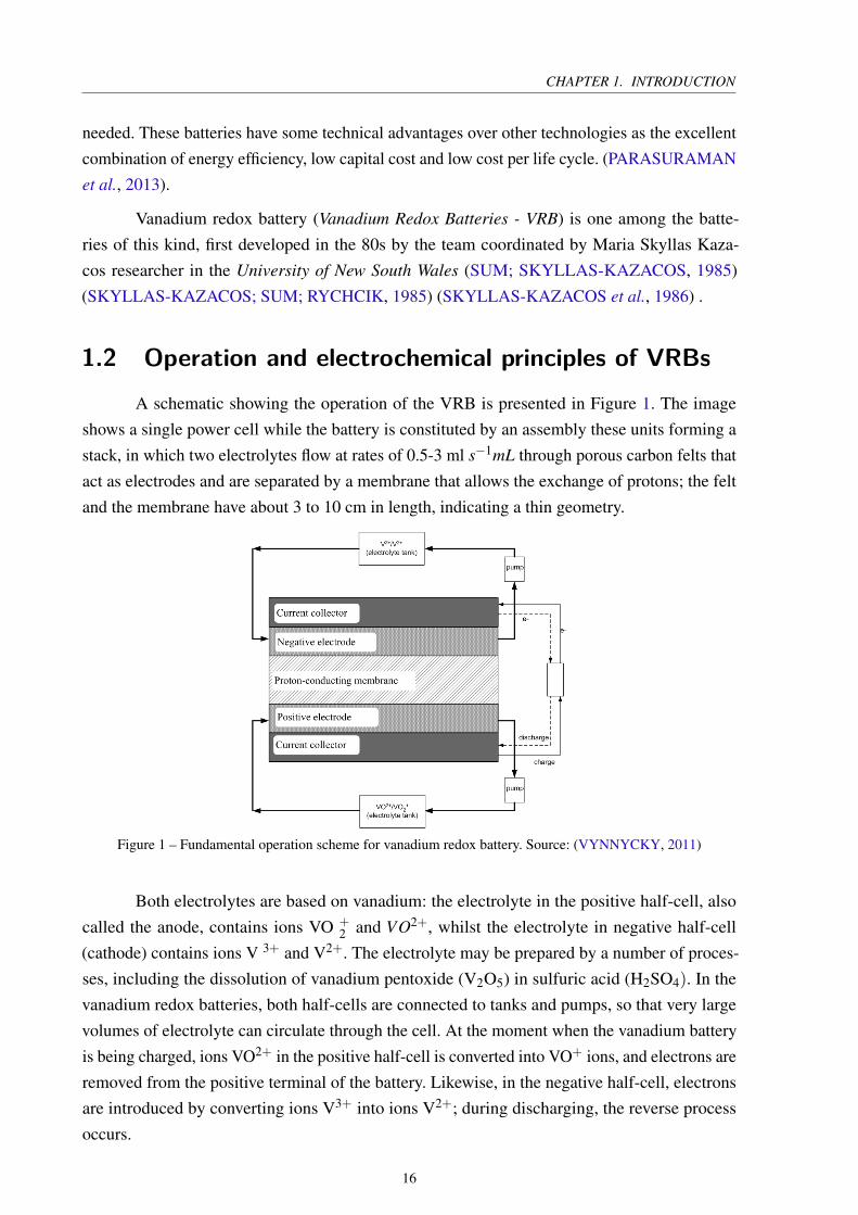
A schematic showing the operation of the VRB is presented in Figure 1. The image
shows a single power cell while the battery is constituted by an assembly these units forming a
stack, in which two electrolytes flow at rates of 0.5-3 ml s−1mL through porous carbon felts that
act as electrodes and are separated by a membrane that allows the exchange of protons; the felt
and the membrane have about 3 to 10 cm in length, indicating a thin geometry.
Figure 1 – Fundamental operation scheme for vanadium redox battery. Source: (VYNNYCKY, 2011)
Both electrolytes are based on vanadium: the electrolyte in the positive half-cell, also
called the anode, contains ions VO +2 and VO2+, whilst the electrolyte in negative half-cell
(cathode) contains ions V 3+ and V2+. The electrolyte may be prepared by a number of proces-
ses, including the dissolution of vanadium pentoxide (V2O5) in sulfuric acid (H2SO4). In the
vanadium redox batteries, both half-cells are connected to tanks and pumps, so that very large
volumes of electrolyte can circulate through the cell. At the moment when the vanadium battery
is being charged, ions VO2+ in the positive half-cell is converted into VO+ ions, and electrons are
removed from the positive terminal of the battery. Likewise, in the negative half-cell, electrons
are introduced by converting ions V3+ into ions V2+; during discharging, the reverse process
occurs.
16
1.3. PERFORMANCE AND APPLICATIONS OF VRBS
Charge and discharge can be summarized by:
charge
V3++e− ⇋ V2+ negative electrode,
VO2++H2O ⇋ VO+2 +e−+2H+ positive electrode,
discharge
(1.1)
Figure 2 – Internal operation in a VRB during charge cycle. Source: (VYNNYCKY, 2011)
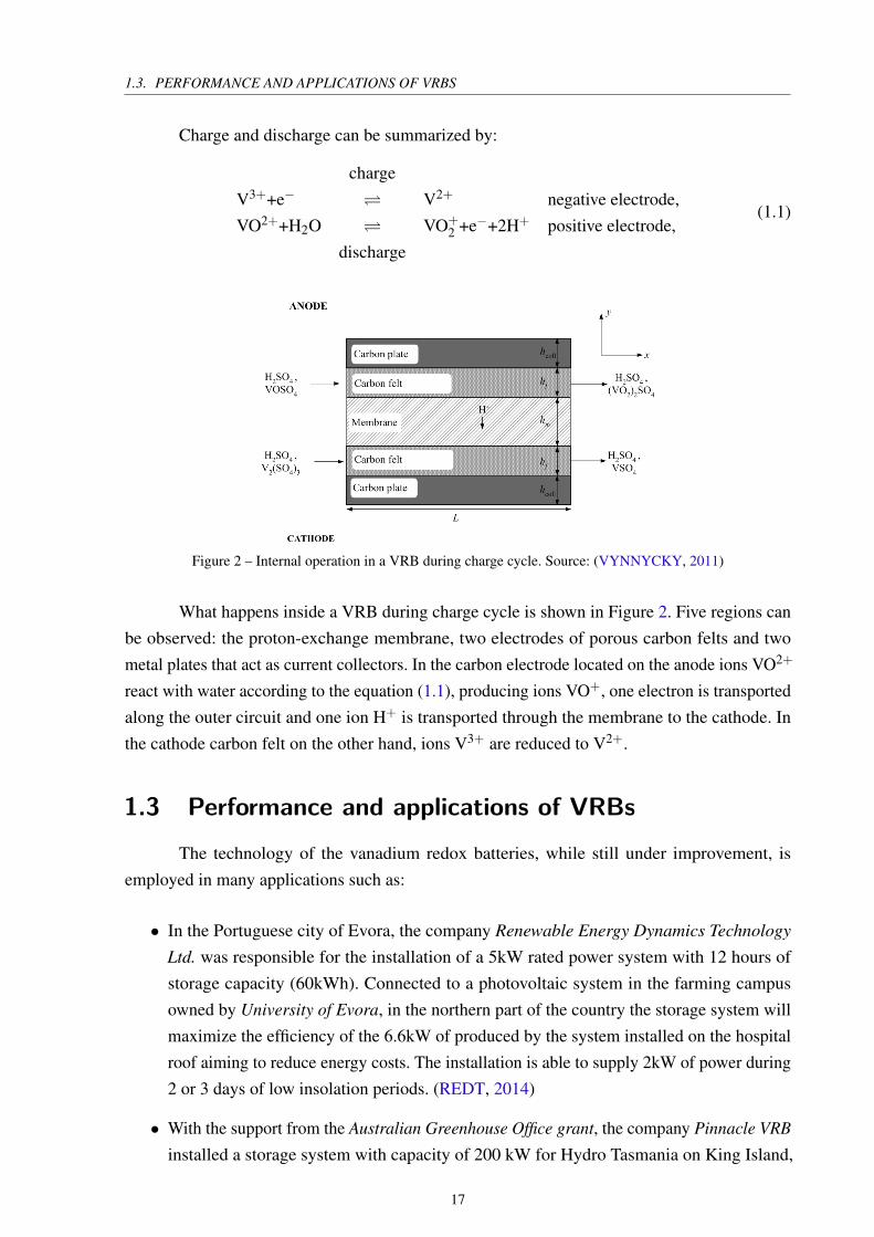
What happens inside a VRB during charge cycle is shown in Figure 2. Five regions can
be observed: the proton-exchange membrane, two electrodes of porous carbon felts and two
metal plates that act as current collectors. In the carbon electrode located on the anode ions VO2+
react with water according to the equation (1.1), producing ions VO+, one electron is transported
along the outer circuit and one ion H+ is transported through the membrane to the cathode. In
the cathode carbon felt on the other hand, ions V3+ are reduced to V2+.
1.3 Performance and applications of VRBs
The technology of the vanadium redox batteries, while still under improvement, is
employed in many applications such as:
∙ In the Portuguese city of Evora, the company Renewable Energy Dynamics Technology
Ltd. was responsible for the installation of a 5kW rated power system with 12 hours of
storage capacity (60kWh). Connected to a photovoltaic system in the farming campus
owned by University of Evora, in the northern part of the country the storage system will
maximize the efficiency of the 6.6kW of produced by the system installed on the hospital
roof aiming to reduce energy costs. The installation is able to supply 2kW of power during
2 or 3 days of low insolation periods. (REDT, 2014)
∙ With the support from the Australian Greenhouse Office grant, the company Pinnacle VRB
installed a storage system with capacity of 200 kW for Hydro Tasmania on King Island,
17
CHAPTER 1. INTRODUCTION
Tasmania. The main objective was to reduce spending on diesel fuel. Hydro Tasmania
applied this technology as a first experience on the construction and operation of VRB at
the commercial level.
(SKYLLAS-KAZACOS, 2004)
∙ Winafrique Technologies Ltd. from Kenya, implemented two 5kW system with 4 hours of
capacity each. The system was applied to two telecommunication stations in the country
as a partnership with mobile phone company Safaricom Limited. Usually the power supply
is held by diesel generators and lead acid batteries, but the rising cost of fuel, concerning
about pollutants emission and maintenance costs aroused interest on the combined use of
wind and solar energy with a system capable of withstanding numerous cycles of charge,
with high reliability, long lifespan and low maintenance cost, as the VRBs. The system
ensures the power supply to the stations up to 14 hours a day, reducing the consumption of
diesel fuel and increasing the lifespan of the entire station. (RICHMOND, 2014)
∙ In Oxnard, California, a storage system based on VRB with three 200kW modules capable
of providing power for 6 hours was implemented. Developed and operated by Prudent
Energy Corporation on behalf of the company Gills Onions, the main motivation was to
reduce costs involved in the shift of the generation system during the peak times. The
system may still be required to operate during short periods of high demand with 600kW
capacity available 24 hours a day or, if necessary, provide 50 % of additional load working
at 900kW for 10 minutes every hour. The estimated savings for the company is on hundreds
of thousands of dollars a year. (ESA, 2014)
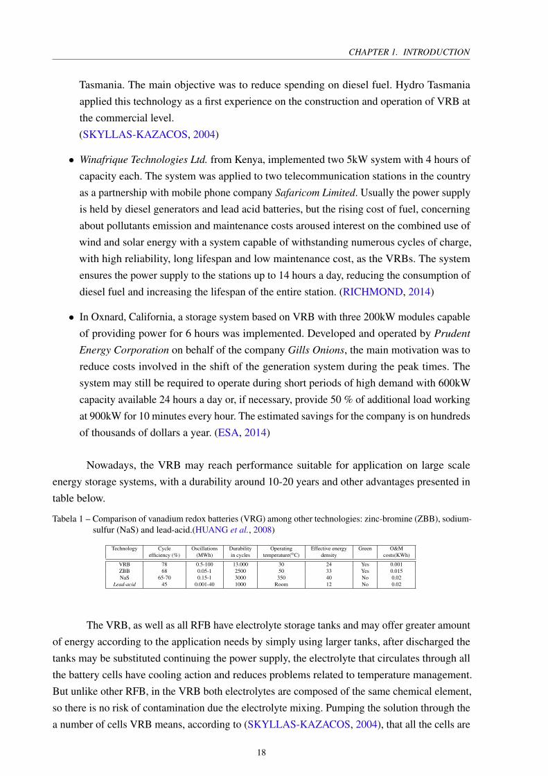
Nowadays, the VRB may reach performance suitable for application on large scale
energy storage systems, with a durability around 10-20 years and other advantages presented in
table below.
Tabela 1 – Comparison of vanadium redox batteries (VRG) among other technologies: zinc-bromine (ZBB), sodium-sulfur (NaS) and lead-acid.(HUANG et al., 2008)
Technology Cycle Oscillations Durability Operating Effective energy Green O&Mefficiency (%) (MWh) in cycles temperature(oC) density costs(KWh)
VRB 78 0.5-100 13.000 30 24 Yes 0.001ZBB 68 0.05-1 2500 50 33 Yes 0.015NaS 65-70 0.15-1 3000 350 40 No 0.02
Lead-acid 45 0.001-40 1000 Room 12 No 0.02
The VRB, as well as all RFB have electrolyte storage tanks and may offer greater amount
of energy according to the application needs by simply using larger tanks, after discharged the
tanks may be substituted continuing the power supply, the electrolyte that circulates through all
the battery cells have cooling action and reduces problems related to temperature management.
But unlike other RFB, in the VRB both electrolytes are composed of the same chemical element,
so there is no risk of contamination due the electrolyte mixing. Pumping the solution through the
a number of cells VRB means, according to (SKYLLAS-KAZACOS, 2004), that all the cells are
18
1.4. RESEARCH DESCRIPTION
in the same state of charge making monitoring and maintenance simpler since it is not necessary
to watch or individually adjust each cell .
However, there are some disadvantages about the VRB: the low rate of energy/volume
which is about 25Wh/kg of electrolyte, while the lead-acid battery has 30-40Wh/kg ration and
a lithium-ion has 80-200Wh/kg; and the high complexity of the system, compared to other
batteries. (VYNNYCKY, 2011)
1.4 Research description
In this situation, this research is developed in order to meet the objectives categorized
below.
1.4.1 General goal
Using the theoretical framework presented in (VYNNYCKY, 2011), it is proposed the
development of mathematical models based on multidimensional time-dependent differential
partial equations as a complement to existing experimental work. Such models would be delinea-
ted by an approach that emphasizes the use of asymptotic reductions to define a set of reduced
equations that describe from first principles the operation of VRBS, in the point of view of
electrochemistry and fluid mechanics.
1.4.2 Specific goals
1. Continue obtaining general knowledge about electrochemistry in (TICIANELLI; GON-
ZALEZ, 2005), (NAG, 2002), (NEWMAN; THOMAS-ALYEA, 2004), and others, as
well as recent papers published in the area as (CHEN; YEOH; CHAKRABARTI, 2014),
(PARASURAMAN et al., 2013), (KEAR; SHAH; WALSH, 2011), (SHARMA et al.,
2014) and others;
2. Using the theoretical framework to develop a multidimensional time-dependent models
compatible with experimental data found in literature;
3. With the software Comsol Multiphysics and based on existing implementation for stationary
1D model, develop and run computational simulation for the following models:
∙ Bi-dimensional transient model;
∙ Bi-dimensional quasi-steady model;
∙ Uni-dimensional quasi-steady model;
4. Validate the results for each model according to experimental data found in literature.
5. Compare different models according to its use of computational resources.
19

CHAPTER 1. INTRODUCTION
1.4.3 Justification
Altough numerical models for this system already exist in literature [(AL-FETLAWI;
SHAH; WALSH, 2009), (AL-FETLAWI; SHAH; WALSH, 2010), (SHAH; AL-FETLAWI;
WALSH, 2010), (SHAH; WATT-SMITH; WALSH, 2008) ], they are time-consuming and unwi-
eldy, particularly with respect to ultimate use an optimization tool.
The present approach emphasizes the use of asymptotic reduction, hand-in-hand with the
development of numerical algorithms to solve the resulting reduced model of equations.
The computational simulations are conducted using the software COMSOL Multiphysics
- an interactive environment for modeling and simulating scientific and engineering problems.
The software has already been successfully used by other researchers on similar projects.
20
CHAPTER
2
REVIEW
Mathematical modeling of a power device such as VRB includes several electrochemical
concepts, some of which are briefly presented in order to facilitate the understanding of the
reader less familiarized. In addition, the main strategies adopted in papers published in the area
that have significant contributions in modelling vanadium redox batteries will be presented.
2.1 Mass transfer
An electrochemical process may be viewed as the association of three steps: the transport
of the reactant species present in the electrolyte towards the electrode surface; the transfer
reaction at the electrode/solution interface characterized by the electron shift from electrode
to the reactant (cathodic reaction) or from reactant to the electrode (anode reaction); and the
transport of the resulting product away from the electrode.
The concentration of the reactant species near the electrode surface is thus one of the
factors that can affect or even dominate the overall rate of reaction. The events directly related to
the concentration are transport phenomena. In general the flow or movement of ions and neutral
molecules in a solution occurs by three different ways: diffusion, convection and migration,
described below. The terms of the equations that describe these movements will be explained
later, in the section that introduces the Nernst-Planck equation.
∙ Diffusion
Diffusion occurs in a solution due to the concentration gradient or chemical potential
gradient. This form of transport of ions and neutral molecules is significant in an electrolytic
experiment when the electrolytic reaction occurs only in the electrode surface, hence there
will be less reagent concentration near the electrode and a highest concentration within the
solution, the reverse is true for the concentration of the reaction products. According to
CHAPTER 2. REVIEW
(NEWMAN; THOMAS-ALYEA, 2004) the diffusive flux of chemical species is given by:
Nk,diffusion =−Dk∇ck. (2.1)
∙ Convection This transport phenomena occurs is due to the agitation of the solution caused
among other factors by pumping action, gas flow, temperature gradients, or gravity. The
equation that describes it is given by:
Nk,convection = ckvk. (2.2)
∙ Migration
According to (TICIANELLI; GONZALEZ, 2005), migration is the movement of ionic
species owing to the action of electric fields or electric potential gradients, responsible for
the conduction of electricity in electrolytes.
(NEWMAN; THOMAS-ALYEA, 2004) explains the phenomenona with the assumption of
two electrodes immersed in a solution in which an electric field is applied. That field will
cause the movement of charged species: the cations are taken toward the cathode electrode,
and anions are dragged to the anode electrode, whilst the cations move in the opposite
direction of the potential gradient. The velocity of ions k in response to the electric field is
called migration velocity:
vk,migration = zkMkF∇φ . (2.3)
The Nernst-Planck equation is a mass conservation equation relating the effects listed above to
describe the flow of chemical species in a fluid taking into account both the gradient of the ionic
concentration and the electric field. Based on the mass conservation equation for incompressible
fluids as (BAZANT, 2014), we have:
∂ck
∂ t+u∇ck +∇F = 0. (2.4)
Where the first term represents the change in concentration of species k, the second term
represents the convection phenomena and can be determined as the solvent velocity in a certain
solution, the latter term in turn, refers to flux density as expressed by:
Fk = Mk∇µkck. (2.5)
Mk is the particle mobility coefficient, that is, if a force G acts on a particle it acquires average
velocity v(G) due to this force. (RODENHAUSEN, 1989). By Einstein’s relation:
Mk =Dk
kbT, (2.6)
22
2.2. BUTLER-VOLMER EQUATION
to kb meaning the Boltzmann constant, T is the absolute temperature, and D is the diffusion
coefficient, ∇µk is the gradient of the chemical potential of the solution given by :
∇µk =kbT
ck∇ck + zke∇φ . (2.7)
The chemical potential is the quantity that allows to describe the state of balance of each
component of a chemical system in the definition above zk is the charge number of specie k, e
is the elementary charge, i.e., electric charge from a single proton and φ refers to the electric
potential. Substituting equations (2.7) and (2.6) in relation (2.5):
Fk = Dk
(
∇ck +zkeck∇φ
kbT
)
. (2.8)
Replacing in (2.6) the Boltzmann and Avogrado constants respectivelly by:
kb =R
Na,
Na =F
e.
Results in:
Fk =−Dk
(
∇ck +zkck∇φ
RT
)
. (2.9)
Finally, replacing (2.9) in (2.4), leads to equação de Nernst-Planck:
∂ck
∂ t+u∇ck +∇
[
−Dk
(
∇ck +zkck∇φ
RT
)]
= 0. (2.10)
2.2 Butler-Volmer equation
The Butler-Volmer equation describes the reaction rate compared to the overpotential:
i = i0
{
exp
(
−βFη
RT
)
− exp
[
(1−β )Fη
RT
]}
. (2.11)
According to (TICIANELLI; GONZALEZ, 2005), the concept of overpotential is linked
to the following situation: given an electrochemical system (in the scope of this work is the redox
battery of vanadium), the interface between the electrode and the solution has an intense electric
field, i.e. an electric potential difference between the electrode and the electrolyte represented
by∆φ . Such potential difference can be changed by a potentiostat, to this positive or negative
external contribution is given the name of overpotential expressed by the letter η . This value plus
the existing potential difference in the system in equilibrium ∆φe results in the total potential
difference:
∆φ = ∆φe +η . (2.12)
23
CHAPTER 2. REVIEW
The symmetry factor β represents the fraction of applied potential which promotes the
cathodic reaction. Likewise (1−β ) is the fraction of applied potential which promotes anodic
reaction. It is often assumed that β = 12 , according to (NEWMAN; THOMAS-ALYEA, 2004).
F , R and T are, respectively, the Faraday constant, the universal gas constant and the absolute
temperature, i0 refers to the exchange current density and depends on the composition of the
solution adjacent to the electrode and its temperature. Considering that at equilibrium state the
overpotential and current density are zero:
i0 = FkcCOexp
(
−∆−→G=o +Fβ∆φe
RT
)
,
i0 = FkaCRexp
(
−∆←−G=o −F(1−β )∆φe
RT
)
, (2.13)
where kc and ka are the rate constants of cathodic reactions (reduction - gain of electrons) and
anodic reaction (oxidation - loss of electrons), while CO and CR are the concentrations of reduced
and oxidized species respectively in the electrochemical system. In this study, the cathode process
takes place in the formation of V 2+ from V 3+ and VO2+ from VO+2 and the anodic process is
the reverse: oxidation of V 2+ in V 3+ and VO2+ in VO+2 , as expressed in reaction 1.1. The terms
∆←−G=o and ∆
−→G=o represent the activation energy of the anodic and cathodic reactions, respectively,
when there is no electric field (at equilibrium).
2.3 Mathematical modelling
This subsection shows the main strategies adopted by most researchers to model the
VRBs, the model is discussed separately for each of the battery components illustrated in Figure
1.
2.3.1 Porose carbon electrodes
Assuming that the transport of charged species occurs by hydrodynamic dispersion,
electrokinetic effects and convection. The molar flux Nk is expressed by the modified Nernst-
Planck equation, as (SHAH; WATT-SMITH; WALSH, 2008), (VYNNYCKY, 2011) and (AL-
FETLAWI; SHAH; WALSH, 2009):
Nk = ckva/c−zkckD
e f fk F
RT∇φe−D
e f fk ∇ck, (2.14)
where ck is the concentration of species k, φe is the electric potential in electrolyte, va/c is
the electrolyte velocity in the anode (a) and the cathode (c) zk is the number of charge. The
24
2.3. MATHEMATICAL MODELLING
modification of the equation is given when considering the additional effect of material porosity
ε on the effective diffusion coefficient Dk originally given by Bruggeman relation:
Deffk = ε
32 Dk. (2.15)
The electrolyte velocities vpos/neg on both electrodes are usually modeled by Darcy’s law:
vpos/neg =d2
f
KµH2O
ε3
(1− ε)2 ∇ppos/neg (2.16)
where ppos/neg are the pressures of the fluid in the positive and negative electrodes, µ is the
dynamic viscosity d f is the average diameter of the carbon fibers, and K is the constant Kozeny-
Karman.
Another modification resulting from the inclusion of porosity occurs in equation that
describes the material balance in the porous carbon electrode for species k, given by:
∂
∂ tεck +∇ ·nk =−Sk. (2.17)
Here Sk is the source term of the species k. The model presented in (VYNNYCKY, 2011)
distinguished from the others by assuming a constant concentration of water, so the species
represented by k do not include H2O, this simplification was based on the diluted electrolyte
theory and on low variation in the concentration of water in earlier numerical simulations.
In the equation 2.14, the first term models the ion transport phenomena due to convection,
the second is due to electromigration, and the third, in turn, is the hydrodynamic dispersion.
Some previous work as (CHEN; YEOH; CHAKRABARTI, 2014) and (YOU; ZHANG; CHEN,
2009) simplify this equation by neglecting the effect of electromigration on the transport of ionic
species, even for no apparent reason, resulting in:
Nk = ckva/c−Deffk ∇ck. (2.18)
The transfer current densities for the reactions that occur on the surface of porous carbon
electrodes are conveniently described by the Butler-Volmer expressions:
jc = εAFkc(csV 3+)
α−,c(csV 2+)
α+,c
{
exp
(
α+,cFηc
RT
)
−exp
(
−α−,cFηc
RT
)}
,
ja = εAFka(csVO2+)
α−,c(csVO+
2)α+,c
{
exp
(
α+,aFηa
RT
)
−exp
(
−α−,aFηa
RT
)}
, (2.19)
where jc e ja represents the current density transfer rate to the cathode and the anode, respectively,
ε is the porosity, A is the electroactive area, F the Faraday constant, kc and ka are constant
25
CHAPTER 2. REVIEW
reaction rates, α±,c and α±,a represent the transfer rates for reactions shown in Equation 1.1.
The overpotentials are defined by the letter η as:
ηa/c = φs−φe−Ea/c. (2.20)
csV 3+ , cs
V 2+ , csVO2+ and cs
VO+2
represent the vanadium concentrations of these species at
the electrode/solution interface, this value is usually different from those concentrations present
within the solution due to the additional resistance to the transport of species from the interior
bulk to the interfaces . (VYNNYCKY, 2011), (SHAH; AL-FETLAWI; WALSH, 2010) and
(CHEN; YEOH; CHAKRABARTI, 2014) assume the following expressions that replaced in 2.19
eliminate the concentrations in the surface substituting them with the values given as functions
of concentrations in the bulk:
csVO2+ =
cVO2+ + εkae−F(ψ−φ−E0,a)/2RT (cVO2+/γVO+2+ cVO+
2/γVO2+)
1+ εka
(
e−F(ψ−φ−E0,a)/2RT/γV + eF(ψ−φ−E0,a)/2RT/γVO2+
) ,
csVO+
2=
cVO+2+ εkae−F(ψ−φ−E0,a)/2RT (cVO2+/γVO+
2+ cVO+
2/γVO2+)
1+ εka
(
e−F(ψ−φ−E0,a)/2RT/γV + eF(ψ−φ−E0,a)/2RT/γVO2+
) ,
where γk is the ratio between the diffusion coefficient of the species k in the solution and the
average distance between the fibers of the carbon felt.
In the equation 2.20, Epos/neg are the potential balance described by the Nernst equation
brought below where E0,neg and E0,pos represent these potential for standard conditions.
Eneg = E0,neg +RT
Fln
(
aV3+
aV2+
)
,
where ak denotes the activity of the species k and is given by the concentration multiplied
by their activity coefficient. In the work presented in (CORCUERA; SKYLLAS-KAZACOS,
2012), it was assumed that this coefficient would be constant for each chemical species, while in
(KJEANG et al., 2007), activity coefficients of all redox species should be equal, both approaches
lead to neglect such coefficients of the equation resulting in:
Eneg = E0,neg +RT
Fln
(
cV3+
cV2+
)
, (2.21)
similarly sets up Epos, the equilibrium potential for the positive electrode, given by:
Epos = E0,pos +RT
Fln
(
aVO2+(aH+)2
aVO+2
)
,
or
Epos = E0,pos +RT
Fln
(
cVO2+(cH+)2
cVO+2
)
; (2.22)
26
2.3. MATHEMATICAL MODELLING
The porosity represented by the term ε indicates the portion of the ε not occupied by
carbon fibers, a space which is filled by the electrolyte during the battery operation. Thus,
two different currents are reported. The ionic currentie, and the electronic current is belonging
respectively to the felt portion occupied by the electrolyte, and to that occupied by the solid
portion of the porous felt and follow the equilibrium relation:
∇ · ie +∇ · is = 0 (2.23)
The divergent of ionic current results in the current density transfer rate defined in
equation 2.19, this adding to the equation 2.23 implies on:
∇ · ie = jpos/neg =−∇ · is (2.24)
Being ie defined as:
ie = ∑k
zkFNk (2.25)
where Nk is the molar flux from equation 2.14, resulting in:
ie = F ∑k
zkckva/c−z2
kckDeffk F
RT∇φe− zkDeff
k ∇ck (2.26)
Assuming the electroneutrality for the electrolyte, i.e., ∑k zkck = 0 eliminates the first
and the third terms of the equation 2.26 corresponding to the convective and diffusive transport,
respectively, leaving:
ie = F ∑k
−z2
kckDeffk F
RT∇φe (2.27)
The electronic current, in turn, is defined by Ohm’s law as:
is =−σ effs ∇φs, (2.28)
where φs is the potential in the solid phase, andσ effs relates the effective coefficient of conductivity,
since it takes into account the solid portion of the porous felt, it is calculated as σ effs = (1−ε)1.5σs
for conductivity coefficient σs.
2.3.2 Proton-exchange membrane
The membrane is a critical component of redox flow batteries, it is crucial for both
performance and economic viability of the battery. It acts separating two electrolyte to prevent
its mixture, and must allow positive ions to pass closing the circuit during the flow of electric
current. (PRIFTI et al., 2012)
The electroneutrality condition included in electrodes modelling, is not valid for the
liquid present in the membrane, which composed by water and protons. However, (VYNNYCKY,
27
CHAPTER 2. REVIEW
2011) and (SHAH; AL-FETLAWI; WALSH, 2010) argue that it can be used when fixed charge
sites are assumed resulting , as well as (AL-FETLAWI; SHAH; WALSH, 2009), in:
zH+cH+ + z f c f = 0, (2.29)
where z f is the charge number of fixed sites and c f is its concentration, while cH+ refers to the
concentration of the species H+, whose charge number zH+ is equal to 1. Hence it follows that
cH+ is a constant.
The velocity of the fluid within the membrane is described by the Schlögl equation:
v =−kφ
µH2O
FcH+∇φ −km
µH2O
∇pm, (2.30)
where v is the velocity, p is the pressure of the liquid, kφ is the electrokinetic permeability, km is
the hydraulic permeability, φ represents the electric potential µH2O is the viscosity of water, F
Faraday’s constant, and cH+is the concentration of protons. The current density is given by:
im = zH+FNH+ , (2.31)
the current conservation ∇im = 0, leads to:
∇
(
−F2
RTDm
H+cH+
)
= 0, (2.32)
with DmH+ as the proton diffusion coefficient in the membrane.
Following the electrolyte dilute theory over the concentrate electrolyte theory, (VYNNYCKY,
2011) considers that the concentration of water on the membrane will be the same constant value
as that on the porous electrode. While (SHAH; AL-FETLAWI; WALSH, 2010) incorporates the
next mass balance equation to the model:
∂cH2O
∂ t+∇ · (cH2Ov) = ∇
(
DeffH2O∇cH2O
)
. (2.33)
2.3.3 Current collectors
The current collectors are relatively simple components, its modeling usually relies on
Ohm’s law and the conservation of current, thus:
icoll =−σcoll∇φcoll,
−σcoll∇2φcoll = 0,
where icoll is the current density, φcoll is the electric potential, and σcoll is the electrical conducti-
vity of the current collectors plates.
28
2.3. MATHEMATICAL MODELLING
2.3.4 Interfacial and initial conditions
The boundary conditions are presented based on the geometry shown in Figure 2. n is
the vector normal for the interface.
∙ Horizontal interfaces
– Positive collector interface [y = 0]
A condition to electrical grounding must be imposed:
φcoll = 0 (2.34)
Charge or discharge current:
icoll =±I (2.35)
positive sign for charge cycle, negative for discharge.
– Coletor/positive electrode interface [y = hcoll]
Continuity of solid electrical potential between collector and electrode:
φcoll = φs (2.36)
Continuity of solid current density between collector and electrode:
icoll ·n = ie ·n (2.37)
Null molar flux for k = cH+,pos, cHSO−4 ,pos, cV 2+ , cV 3+:
Nk ·n = 0 (2.38)
– Positive electrode/membrane interface [y = hcoll +hf]
There is a potential difference for the liquid phase between the membrane and the
electrode represented by the Donnan potential:
φm = φe−RT
Fln
(
aH+,pos
aH+,mem
)
(2.39)
Continuity of electrolyte velocity between electrode and membrane:
vpos ·n = vm ·n (2.40)
Continuity of current density between membrane and electrode:
im ·n = ie ·n (2.41)
Null current density for solid phase:
is ·n = 0 (2.42)
Null molar flux for k = cHSO−4 ,pos, cV 2+ , cV 3+:
Nk ·n = 0 (2.43)
29
CHAPTER 2. REVIEW
– Membrane/negative electrode interface [y = hcoll +hf +hm]
Potential difference for the liquid phase between the membrane and the electrode
accounting for Donnan potential:
φm = φe−RT
Fln
(
aH+,neg
aH+,m
)
(2.44)
Continuity of electrolyte velocity between electrode and membrane:
vneg ·n = vm ·n (2.45)
Continuity of current density between membrane and electrode:
im ·n = ie ·n (2.46)
Null current density for liquid phase:
is ·n = 0 (2.47)
Null molar flux for k = cHSO−4 ,neg,cVO2+ ,cVO+2
:
Nk ·n = 0 (2.48)
– Interface eletrodo negativo/coletor [y = hcoll +2hf +hm]
Continuity of electric potential for solid phase:
φcoll = φs (2.49)
Continuity of electric current for solid phase:
icoll ·n = ie ·n (2.50)
Null molar flux for k = cH+,neg,cHSO−4 ,neg,cVO2+ ,cVO+2
:
Nk ·n = 0 (2.51)
– Negative collector interface[y = 2hcoll +2hf +hm]
Charge or discharge current:
icoll =±Inegativesign f orchargecycle, positive f ordischarge. (2.52)
∙ Vertical interfaces
– Positive collector interface [x = 0 or x = L;0≤ y≤ hcoll]
Electrical insulation:
icoll ·n = 0 (2.53)
30
2.3. MATHEMATICAL MODELLING
– Positive electrode inlet interface [x = 0;(hcoll)≤ y≤ (hcoll +h f )]
Electrical insulation:
ie ·n = 0, is ·n = 0 (2.54)
Electrolyte injection of tanks into the battery k= cH+,pos, cHSO−4 ,pos, cV 2+ , cV 3+:
ck = cink (t) (2.55)
– Positive electrode outlet interface [x = L;(hcoll)≤ y≤ (hcoll +h f )]
Electrical insulation:
ie ·n = 0, is ·n = 0 (2.56)
Outlet flux for k= cH+,pos, cHSO−4 ,pos, cV 2+ , cV 3+:
−Deffk ∇ck ·n = 0 (2.57)
– Membrane interface [x = 0 ou x = L;(hcoll +h f )≤ y≤ (hcoll +h f +hm)]
Electrical insulation:
im ·n = 0 (2.58)
– Negative electrode inlet interface [x = 0;(hcoll +h f +hm)≤ y≤ (hcoll +2h f +hm)]
Electrical insulation:
ie ·n = 0, is ·n = 0 (2.59)
Electrolyte injection of tanks into the battery k=cH+,neg,cHSO−4 ,neg,cVO2+ ,cVO+2
:
ck = cink (t) (2.60)
– Negative electrode outlet interface [x = L;(hcoll+h f +hm)≤ y≤ (hcoll+2h f +hm)]
Electrical insulation:
ie ·n = 0, is ·n = 0 (2.61)
Outlet flux for k=cH+,neg,cHSO−4 ,neg,cVO2+ ,cVO+2
:
−Deffk ∇ck ·n = 0 (2.62)
– Negative collector interface[x = 0 ou x = L;(hcoll +2h f +hm)≤ y≤ (2hcoll +2h f +
hm)]
Electrical insulation:
icoll ·n = 0 (2.63)
The conditions 2.55 and 2.60, cink (t) indicates the concentration of the chemical species k
in the battery tanks, where it is assumed instantaneous mixing between the liquid leaving
the battery and the electrolyte stored there with the following mass balance equation:
dcink
dt=
ω
V
(
coutk − cin
k
)
(2.64)
31
CHAPTER 2. REVIEW
in this equation, V is the total volume of electrolyte, ω is the volumetric flow, and coutk
indicates the average concentration in the electrolyte that leaves the battery defined for the
positive and negative electrodes respectively as:
coutk =
1
h f
∫ hcoll+h f
hcoll
(ck(t))x=Ldy (2.65)
coutk =
1
h f
∫ hcoll+2h f+hm
hcoll+h f+hm
(ck(t))x=Ldy (2.66)
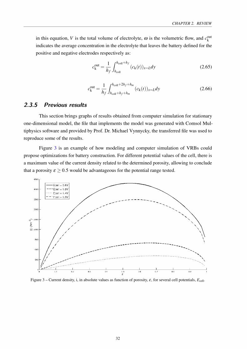
2.3.5 Previous results
This section brings graphs of results obtained from computer simulation for stationary
one-dimensional model, the file that implements the model was generated with Comsol Mul-
tiphysics software and provided by Prof. Dr. Michael Vynnycky, the transferred file was used to
reproduce some of the results.
Figure 3 is an example of how modeling and computer simulation of VRBs could
propose optimizations for battery construction. For different potential values of the cell, there is
a maximum value of the current density related to the determined porosity, allowing to conclude
that a porosity ε ≥ 0.5 would be advantageous for the potential range tested.
Figure 3 – Current density, i, in absolute values as function of porosity, ε , for several cell potentials, Ecell.
32
2.3. MATHEMATICAL MODELLING
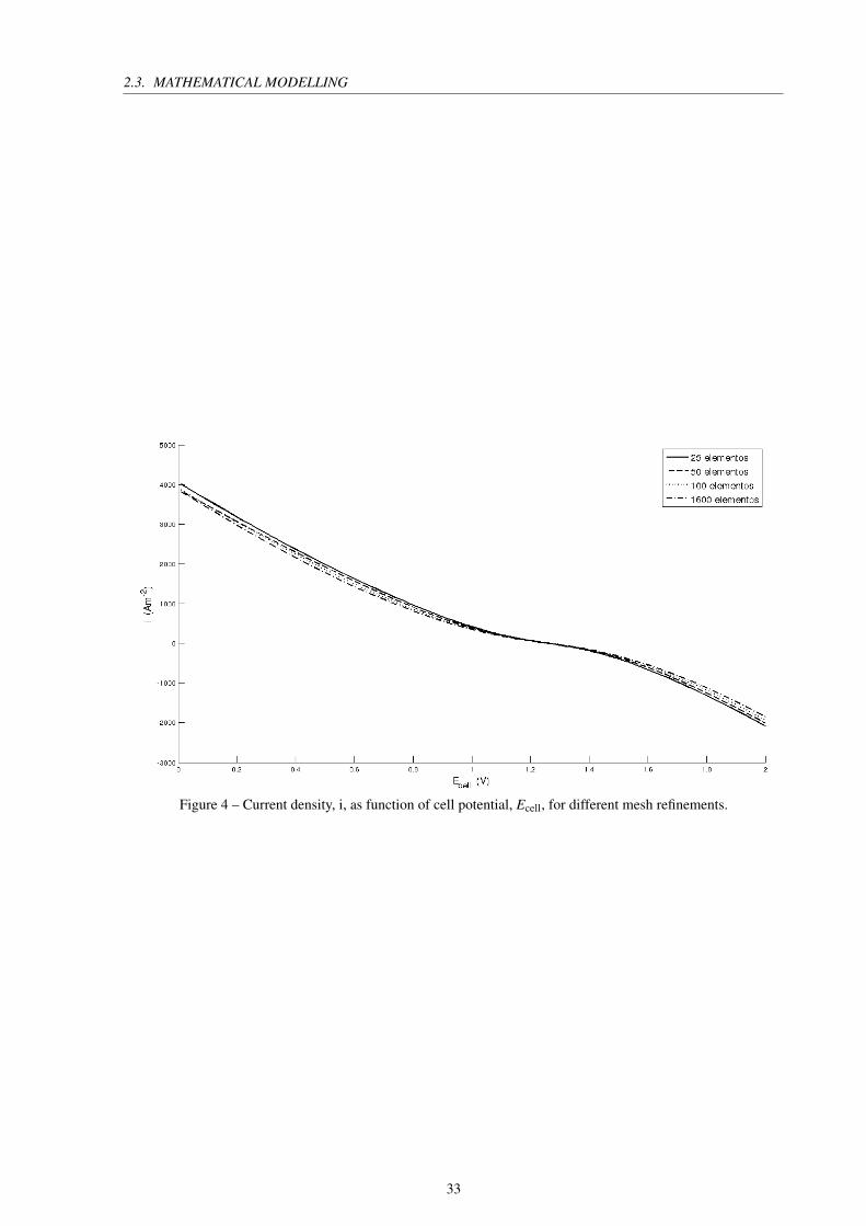
Figure 4 – Current density, i, as function of cell potential, Ecell, for different mesh refinements.
33
CHAPTER 2. REVIEW
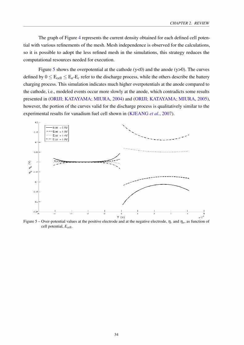
The graph of Figure 4 represents the current density obtained for each defined cell poten-
tial with various refinements of the mesh. Mesh independence is observed for the calculations,
so it is possible to adopt the less refined mesh in the simulations, this strategy reduces the
computational resources needed for execution.
Figure 5 shows the overpotential at the cathode (y<0) and the anode (y>0). The curves
defined by 0 ≤ Ecell ≤ Ea-Ec refer to the discharge process, while the others describe the battery
charging process. This simulation indicates much higher overpotentials at the anode compared to
the cathode, i.e., modeled events occur more slowly at the anode, which contradicts some results
presented in (ORIJI; KATAYAMA; MIURA, 2004) and (ORIJI; KATAYAMA; MIURA, 2005),
however, the portion of the curves valid for the discharge process is qualitatively similar to the
experimental results for vanadium fuel cell shown in (KJEANG et al., 2007).
Figure 5 – Over-potential values at the positive electrode and at the negative electrode, ηc and ηa, as function ofcell potential, Ecell.
34
CHAPTER
3
MATERIALS AND METHODS
This section describes the procedures used to build the mathematical models that will be
presented later as well as the tools employed on its computational implementation in order to
obtain the results that would be compared with experimental data found in the literature.
3.1 Mathematical modelling
In the next lines will be presented the equations and boundary conditions that characterize
the mathematical models for VRB. But first, some important assumptions valid for all models in
this research must detail.
As was assumed in (SHAH; AL-FETLAWI; WALSH, 2010), (VYNNYCKY, 2011),
(KNEHR et al., 2012), (CORCUERA; SKYLLAS-KAZACOS, 2012), (SHARMA et al., 2014),
among others, the cell is isothermal, i.e. not taking into account the Joule heating or ohmic
heating - heat generation process caused by passing electric current through a conductive material.
However, as was placed in (VYNNYCKY, 2011), it is argued that neglecting this phenomenon
does not imply that this model have significant losses in its accuracy, since the model for the fuel
cell studied in (VYNNYCKY et al., 2009) showed that the observed temperature gradient has
little influence in performance.
It is considered that the membrane is always humidified in order to allow the ions to
cross, assuming that H+ are the ones that pass through the membrane. A different approach
was taken, for example, in (KNEHR et al., 2012), in which was considered the flow vanadium
ions through the membrane. This phenomena implies on a change in vanadium concentrations,
however it can be disregarded in a single cycle, as will be shown later.
Also the validity of diluted electrolyte theory presented in Section 2.3.1 was assumed.
CHAPTER 3. MATERIALS AND METHODS
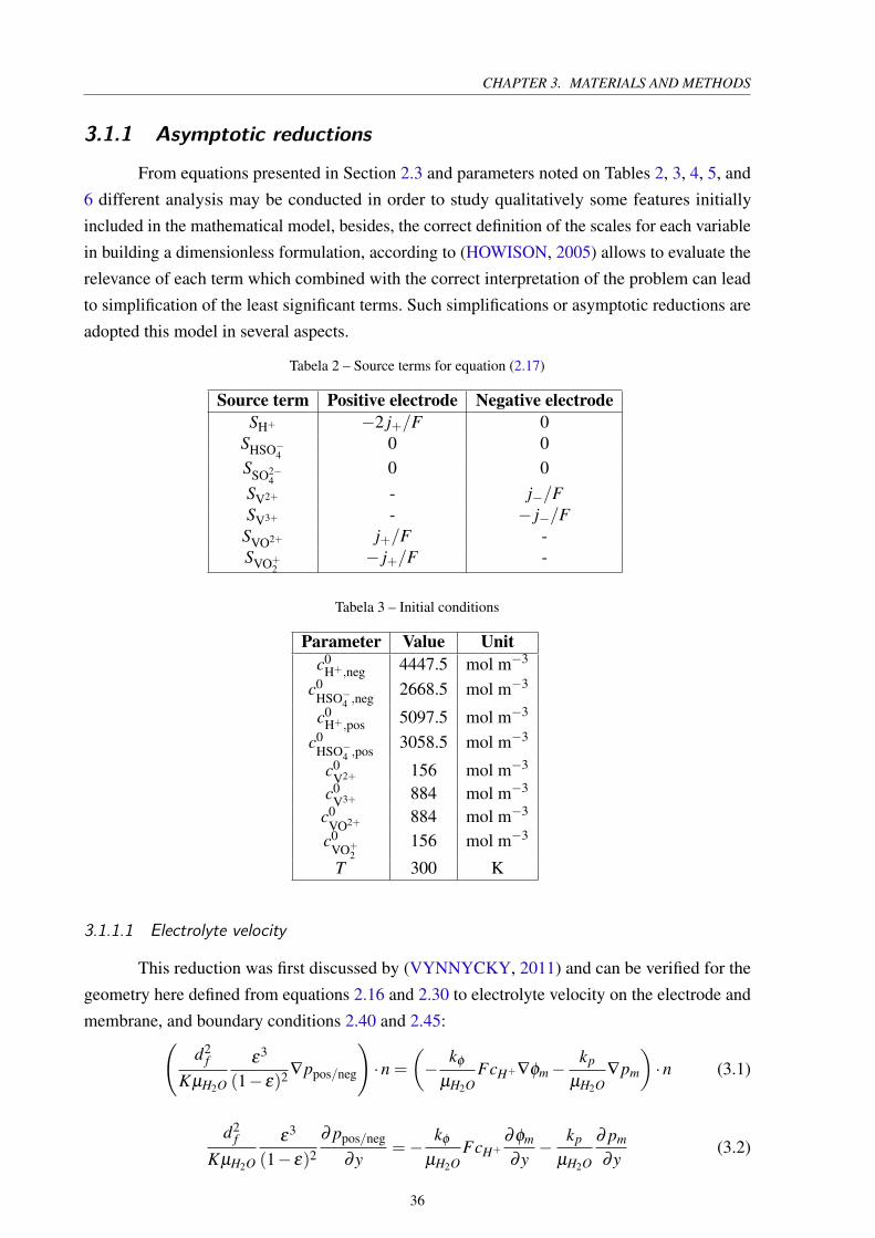
3.1.1 Asymptotic reductions
From equations presented in Section 2.3 and parameters noted on Tables 2, 3, 4, 5, and
6 different analysis may be conducted in order to study qualitatively some features initially
included in the mathematical model, besides, the correct definition of the scales for each variable
in building a dimensionless formulation, according to (HOWISON, 2005) allows to evaluate the
relevance of each term which combined with the correct interpretation of the problem can lead
to simplification of the least significant terms. Such simplifications or asymptotic reductions are
adopted this model in several aspects.
Tabela 2 – Source terms for equation (2.17)
Source term Positive electrode Negative electrode
SH+ −2 j+/F 0SHSO−4
0 0
SSO2−4
0 0
SV2+ - j−/F
SV3+ - − j−/F
SVO2+ j+/F -SVO+
2− j+/F -
Tabela 3 – Initial conditions
Parameter Value Unit
c0H+,neg 4447.5 mol m−3
c0HSO−4 ,neg
2668.5 mol m−3
c0H+,pos 5097.5 mol m−3
c0HSO−4 ,pos
3058.5 mol m−3
c0V2+ 156 mol m−3
c0V3+ 884 mol m−3
c0VO2+ 884 mol m−3
c0VO+
2156 mol m−3
T 300 K
3.1.1.1 Electrolyte velocity
This reduction was first discussed by (VYNNYCKY, 2011) and can be verified for the
geometry here defined from equations 2.16 and 2.30 to electrolyte velocity on the electrode and
membrane, and boundary conditions 2.40 and 2.45:(
d2f
KµH2O
ε3
(1− ε)2 ∇ppos/neg
)
·n =
(
−kφ
µH2O
FcH+∇φm−kp
µH2O
∇pm
)
·n (3.1)
d2f
KµH2O
ε3
(1− ε)2
∂ ppos/neg
∂y=−
kφ
µH2O
FcH+∂φm
∂y−
kp
µH2O
∂ pm
∂y(3.2)
36
3.1. MATHEMATICAL MODELLING
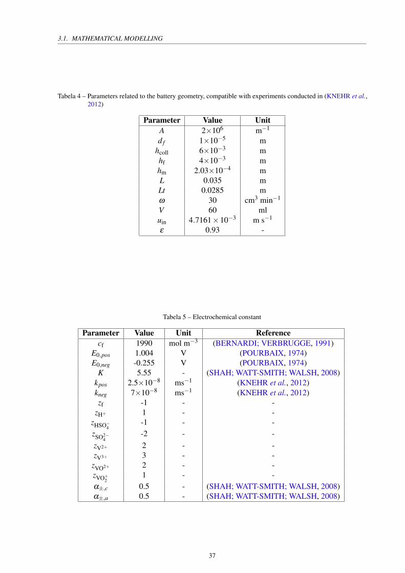
Tabela 4 – Parameters related to the battery geometry, compatible with experiments conducted in (KNEHR et al.,2012)
Parameter Value Unit
A 2×10⁶ m−1
d f 1×10⁻⁵ mhcoll 6×10⁻³ mhf 4×10⁻³ mhm 2.03×10⁻⁴ mL 0.035 mLt 0.0285 mω 30 cm3 min−1
V 60 mluin 4.7161×10⁻³ m s−1
ε 0.93 -
Tabela 5 – Electrochemical constant
Parameter Value Unit Reference
cf 1990 mol m−3 (BERNARDI; VERBRUGGE, 1991)E0,pos 1.004 V (POURBAIX, 1974)E0,neg -0.255 V (POURBAIX, 1974)
K 5.55 - (SHAH; WATT-SMITH; WALSH, 2008)kpos 2.5×10⁻⁸ ms−1 (KNEHR et al., 2012)kneg 7×10⁻⁸ ms−1 (KNEHR et al., 2012)zf -1 - -
zH+ 1 - -zHSO−4
-1 - -
zSO2−4
-2 - -
zV2+ 2 - -zV3+ 3 - -
zVO2+ 2 - -zVO+
21 - -
α±,c 0.5 - (SHAH; WATT-SMITH; WALSH, 2008)α±,a 0.5 - (SHAH; WATT-SMITH; WALSH, 2008)
37
CHAPTER 3. MATERIALS AND METHODS
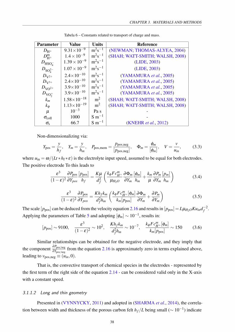
Tabela 6 – Constants related to transport of charge and mass.
Parameter Value Units Reference
DH+ 9.31×10⁻⁹ m2s−1 (NEWMAN; THOMAS-ALYEA, 2004)Dm
H+ 1.4×10⁻⁹ m2s−1 (SHAH; WATT-SMITH; WALSH, 2008)DHSO−4
1.39×10⁻⁹ m2s−1 (LIDE, 2003)
DSO2−4
1.07×10⁻⁹ m2s−1 (LIDE, 2003)
DV2+ 2.4×10⁻¹⁰ m2s−1 (YAMAMURA et al., 2005)DV3+ 2.4×10⁻¹⁰ m2s−1 (YAMAMURA et al., 2005)
DVO2+ 3.9×10⁻¹⁰ m2s−1 (YAMAMURA et al., 2005)DVO+
23.9×10⁻¹⁰ m2s−1 (YAMAMURA et al., 2005)
km 1.58×10⁻¹⁸ m2 (SHAH; WATT-SMITH; WALSH, 2008)kφ 1.13×10⁻¹⁹ m2 (SHAH; WATT-SMITH; WALSH, 2008)µ 10−3 Pa s -
σcoll 1000 S m−1 -σs 66.7 S m−1 (KNEHR et al., 2012)
Non-dimensionalizing via:
Ypos =y
h f
, Ym =y
hm, Ppos,mem =
ppos,neg
[ppos,neg], Φm =
φm
[φm], V =
v
uin, (3.3)
where uin = ω/(Lt *hf *ε) is the electrolyte input speed, assumed to be equal for both electrodes.
The positive electrode To this leads to
ε3
(1− ε)2
∂Ppos
∂Ypos
[ppos]
h f
=Kµ
d2f
(
kφ FcmH+
µH2O
∂Φm
∂Ym
[φm]
hm+
km
µ
∂Pm
∂Ym
[pm]
hm
)
(3.4)
ε3
(1− ε)2
∂Ppos
∂Ypos=
Kh f km
d2f hm
(
kφ FcmH+ [φm]
km[ppos]
∂Φm
∂Ym+
∂Pm
∂Ym
)
(3.5)
The scale [ppos] can be deduced from the velocity equation 2.16 and results in [ppos] =LµH2OKuind−2f .
Applying the parameters of Table 5 and adopting [φm]∼ 10−1, results in:
[ppos]∼ 9100,ε3
(1− ε)2 ∼ 102,Kh f km
d2f hm
∼ 10−7,kφ Fcm
H+ [φm]
km[ppos]∼ 150 (3.6)
Similar relationships can be obtained for the negative electrode, and they imply that
the component∂Ppos/neg
∂Ypos/negfrom the equation 2.16 is approximately zero in terms explained above,
leading to vpos,neg ≡ (uin,0).
That is, the convective transport of chemical species in the electrodes - represented by
the first term of the right side of the equation 2.14 - can be considered valid only in the X-axis
with a constant speed.
3.1.1.2 Long and thin geometry
Presented in (VYNNYCKY, 2011) and adopted in (SHARMA et al., 2014), the correla-
tion between width and thickness of the porous carbon felt h f /L being small (∼ 10−1) indicate
38
3.1. MATHEMATICAL MODELLING
that the second order derivatives with respect to Y are more significant than those taken in
relation to X. Hence, including reductions presented in Section 3.1.1.1 the equation 2.14 turns
into:
ε∂ck
∂ t+uin
∂ck
∂x=
∂
∂y
(
zkckDeffk F
RT
∂φe
∂y+Deff
k
∂ck
∂y
)
−Sk (3.7)
3.1.1.3 Quasi-steady nature
From the equation 3.7 it is evaluated the relevance of the derivative of concentration
with respect to time dimension t, as shown in (SHARMA et al., 2014) and (VYNNYCKY;
ASSUNçãO, in prep.), from the non-dimensionalization through the terms presented in the
equation 3.3 and also:
X =x
L, τ =
t
[t], Ck =
ck
[ck], Sk =
Sk
[Sk](3.8)
resulting in:
ε∂Ck
∂τ
[ck]
[t]+uin
∂Ck
∂X
[ck]
L=
1
hf
∂
∂Y
(
zkDeffk F
RT hfCk
∂Φe
∂Y
[φe][ck]
hf+Deff
k
∂Ck
∂Y
[ck]
hf
)
+[Sk]Sk. (3.9)
ε∂Ck
∂τ+
uin[t]
L
∂Ck
∂X=
∂
∂Y
(
zkDeffk F [φe][t]
RT h2f
Ck
∂Φe
∂Y+
Deffk [t]
h2f
∂Ck
∂Y
)
+
{
[Sk][t]
[ck]
}
Sk. (3.10)
To characterize the quasi-stationary nature of the problem (SHARMA et al., 2014) and
(VYNNYCKY; ASSUNçãO, in prep.) state that must be verified that:
[t]max
(
uin
L,zkDeff
k F [φe]
RT h2f
,Deff
k
h2f
,[Sk]
[ck]
)
≫ 1. (3.11)
Where the [φe] can be deduced from the equation 2.27 as:
[φe]∼IRT hf
F2[cmax]Deffk
(3.12)
where I is the current density imposed on the boundary conditions 2.35 and 2.52. The usual
concentration values indicate that [ck] ∼ 102− 103 mol m−3, i.e. [cmax] ∼ 103 mol m−3, and
implies that [φe]∼ 10−1.
Since the scale of the source term is obtained by relation exposed in Table 3 which implies
that: [Sk]∼ I/(hfF)∼ 1 mol m−3 s−1. Continuing the evaluation of terms in 3.11 according to
the parameters in Table 3, leads to:
39
CHAPTER 3. MATERIALS AND METHODS
uin
L∼ 0.1 s−1, (3.13)
zkDeffk F [φe]
RT h2f
∼ 10−4−10−3 s−1, (3.14)
Deffk
h2f
∼ 10−4−10−5 s−1, (3.15)
[Sk]
[ck]∼ 10−3−10−2 s−1. (3.16)
Replacing the higher value among the terms discussed in equation 3.11, it is obtained:
[t]uin
L≫ 1 (3.17)
It follows therefore that the process is quasi-stationary for [t]≫ 10 s. It means that it is
possible to excluding the time derivative of the concentration without major losses for the model
keeping time dependent terms solely in the boundary conditions 2.64, resulting in:
uin∂ck
∂x=
∂
∂y
(
zickDeffk F
RT
∂φe
∂y+Deff
k
∂ck
∂y
)
−Sk (3.18)
3.1.1.4 Boundary layer
The boundary layer was first found in (VYNNYCKY; ASSUNçãO, in prep.) and indicates
the existence of regions close to the borders between the membrane and the electrodes where
concentrations of chemical species vary quickly.
Performing the non-dimensionalization from the equation 3.18:
uin∂Ck
∂X
[ck]
L=
1
hf
∂
∂Y
(
zkDkF
RTCk
∂Φe
∂Y
[φe][ck][Deffk ]
hf+Dk
∂Ck
∂Y
[ck][Deffk ]
hf
)
+[Sk]Sk, (3.19)
∂Ck
∂X=
LDk[Deffk ]
h2f uin
∂
∂Y
(
zkF [φe]
RTCk
∂Φe
∂Y+
∂Ck
∂Y
)
+[Sk]L
[ck]Sk, (3.20)
or∂Ck
∂X=
Dk
Pe
∂
∂Y
(
zkΠCk
∂Φe
∂Y+
∂Ck
∂Y
)
+ΛSk, (3.21)
Pe =uinh2
f
L[Deffk ]
, Π =F [φe]
RT, Λ =
[Sk]L
[ck]uin(3.22)
Now taking [Deffk ] = Deff
min so that Dk ∼ O(1), it is obtained:
Pe∼ 10000, Π∼ 10, Λk ∼ 10−3−10−2 (3.23)
40
3.1. MATHEMATICAL MODELLING
Back to equation 3.21, the magnitude order of analyzed expressions allows to affirm that:
∂Ck
∂X∼ 0 (3.24)
That is, the concentrations of chemical species does not change significantly across the
electrode starting from the electrolyte input interface to the output. In addition, the boundary
conditions 2.55 and 2.60 indicate that:
ck ≡ cink (t) (3.25)
The next step adopted in (VYNNYCKY; ASSUNçãO, in prep.) is to expand to the regular
perturbation of concentrations Ck, of liquid phase potential Φe, and source term Sk, with that
expansion for Π/Pe that has the same magnitude order as Λk:
Ck =Ck,0 +
(
Π
Pe
)
Ck,1 +O
(
Π2
Pe2
)
; (3.26)
Φe = Φe,0 +
(
Π
Pe
)
Φe,1 +O
(
Π2
Pe2
)
; (3.27)
Sk = Sk,0 +
(
Π
Pe
)
Sk,1 +O
(
Π2
Pe2
)
; (3.28)
Restricting 3.26 to the order of O(Π/Pe):
∂Ck
∂X=
∂Ck,0
∂X+
(
Π
Pe
)
∂Ck,1
∂X(3.29)
accounting for the condition 3.24,
∂Ck,0
∂X+
(
Π
Pe
)
∂Ck,1
∂X= 0 (3.30)
remembering that, by condition 3.25, ck,0 ≡ cink,0(t)
(
Π
Pe
)
∂Ck,1
∂X=−
(
Dk
Pe
∂
∂Y
(
zkΠCink,0
∂
∂YΦe,0 +
∂Cink,0
∂Y
)
+ΛkSk,0
)
(3.31)
Replacing θk = ΛkPe/Π, as constant O(1)
∂Ck,1
∂X+Dk
∂
∂Y
(
zkCink,0
∂
∂YΦe,0
)
=−θkSk,0 (3.32)
Multiplying by zk and doing the sum for all k:
∑k
(
zk∂Ck,1
∂X+Dk
∂
∂Y
(
zkCink,0
∂
∂YΦe,0
))
=−∑k
zkθkSk,0 (3.33)
41
CHAPTER 3. MATERIALS AND METHODS
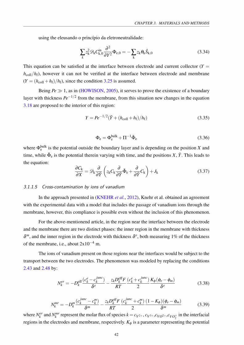
using the eleusando o princípio da eletroneutralidade:
∑k
z2kDkCin
k,0∂ 2
∂Y 2 Φe,0 =−∑k
zkθkSk,0 (3.34)
This equation can be satisfied at the interface between electrode and current collector (Y =
hcoll/hf), however it can not be verified at the interface between electrode and membrane
(Y = (hcoll +hf)/hf), since the condition 3.25 is assumed.
Being Pe≫ 1, as in (HOWISON, 2005), it serves to prove the existence of a boundary
layer with thickness Pe−1/2 from the membrane, from this situation new changes in the equation
3.18 are proposed to the interior of this region:
Y = Pe−1/2(Y +(hcoll +hf)/hf) (3.35)
Φe = Φbulke +Π−1Φe (3.36)
where Φbulke is the potential outside the boundary layer and is depending on the position X and
time, while Φe is the potential therein varying with time, and the positions X , Y . This leads to
the equation:∂Ck
∂X= Dk
∂
∂Y
(
zkCk∂
∂YΦe +
∂
∂YCk
)
+ Jk (3.37)
3.1.1.5 Cross-contamination by ions of vanadium
In the approach presented in (KNEHR et al., 2012), Knehr et al. obtained an agreement
with the experimental data with a model that includes the passage of vanadium ions through the
membrane, however, this compliance is possible even without the inclusion of this phenomenon.
For the above-mentionend article, in the region near the interface between the electrode
and the membrane there are two distinct phases: the inner region in the membrane with thickness
δ m, and the inner region in the electrode with thickness δ e, both measuring 1% of the thickness
of the membrane, i.e., about 2x10⁻⁴ m.
The ions of vanadium present on those regions near the interfaces would be subject to the
transport between the two electrodes. The phenomenon was modeled by replacing the conditions
2.43 and 2.48 by:
Nerk =−Deff
k
(cek− c
junck )
δ e−
zkDeffk F
RT
(cek + c
junck )
2
Kφ (φe−φm)
δ e(3.38)
Nmrk =−Dm
k
(cjunck − cm
k )
δ m−
zkDeffk F
RT
(cjunck + cm
k )
2
(1−Kφ )(φe−φm)
δ m(3.39)
where Nerk and Nmr
k represent the molar flux of species k = cV 2+ , cV 3+ ,cVO2+ ,cVO+2
in the interfacial
regions in the electrodes and membrane, respectively. Kφ is a parameter representing the potential
42
3.1. MATHEMATICAL MODELLING
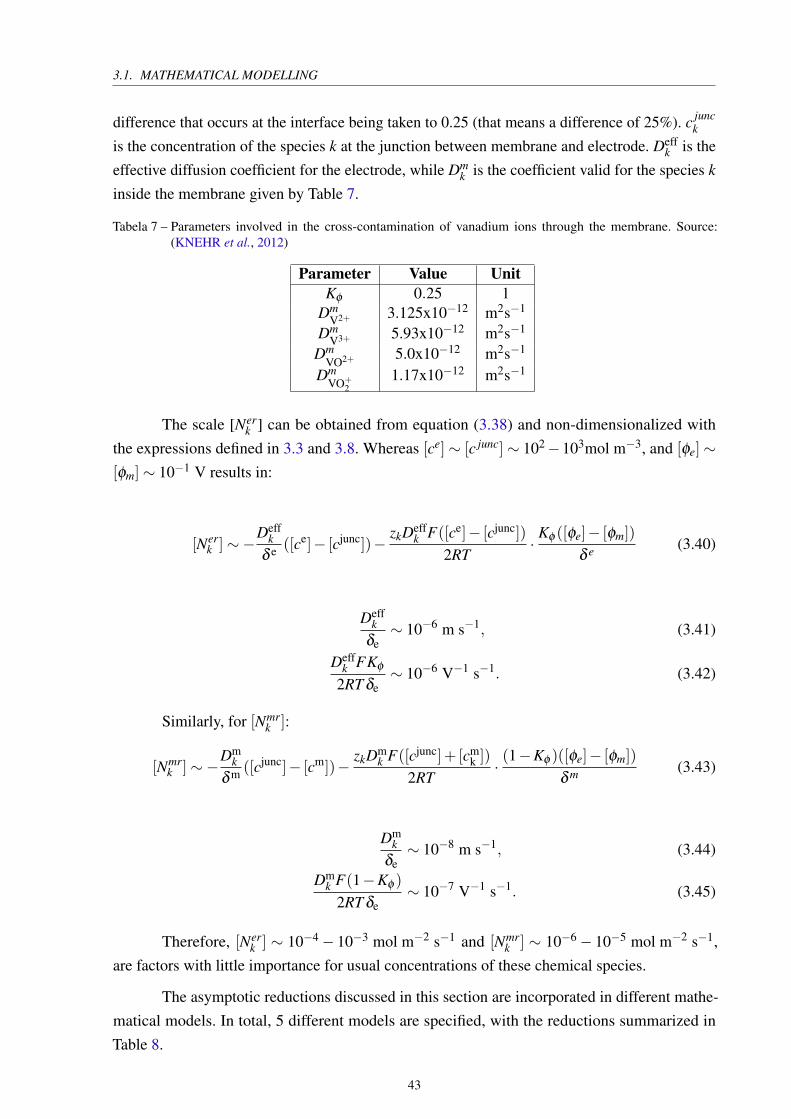
difference that occurs at the interface being taken to 0.25 (that means a difference of 25%). cjunck
is the concentration of the species k at the junction between membrane and electrode. Deffk is the
effective diffusion coefficient for the electrode, while Dmk is the coefficient valid for the species k
inside the membrane given by Table 7.
Tabela 7 – Parameters involved in the cross-contamination of vanadium ions through the membrane. Source:(KNEHR et al., 2012)
Parameter Value Unit
Kφ 0.25 1Dm
V2+ 3.125x10⁻¹² m2s−1
DmV3+ 5.93x10⁻¹² m2s−1
DmVO2+ 5.0x10⁻¹² m2s−1
DmVO+
21.17x10⁻¹² m2s−1
The scale [Nerk ] can be obtained from equation (3.38) and non-dimensionalized with
the expressions defined in 3.3 and 3.8. Whereas [ce]∼ [c junc]∼ 102−103mol m−3, and [φe]∼
[φm]∼ 10−1 V results in:
[Nerk ]∼−
Deffk
δ e ([ce]− [cjunc])−zkDeff
k F([ce]− [cjunc])
2RT·
Kφ ([φe]− [φm])
δ e(3.40)
Deffk
δe∼ 10−6 m s−1, (3.41)
Deffk FKφ
2RT δe∼ 10−6 V−1 s−1. (3.42)
Similarly, for [Nmrk ]:
[Nmrk ]∼−
Dmk
δ m ([cjunc]− [cm])−zkDm
k F([cjunc]+ [cmk ])
2RT·(1−Kφ )([φe]− [φm])
δ m(3.43)
Dmk
δe∼ 10−8 m s−1, (3.44)
Dmk F(1−Kφ )
2RT δe∼ 10−7 V−1 s−1. (3.45)
Therefore, [Nerk ] ∼ 10−4− 10−3 mol m−2 s−1 and [Nmr
k ] ∼ 10−6− 10−5 mol m−2 s−1,
are factors with little importance for usual concentrations of these chemical species.
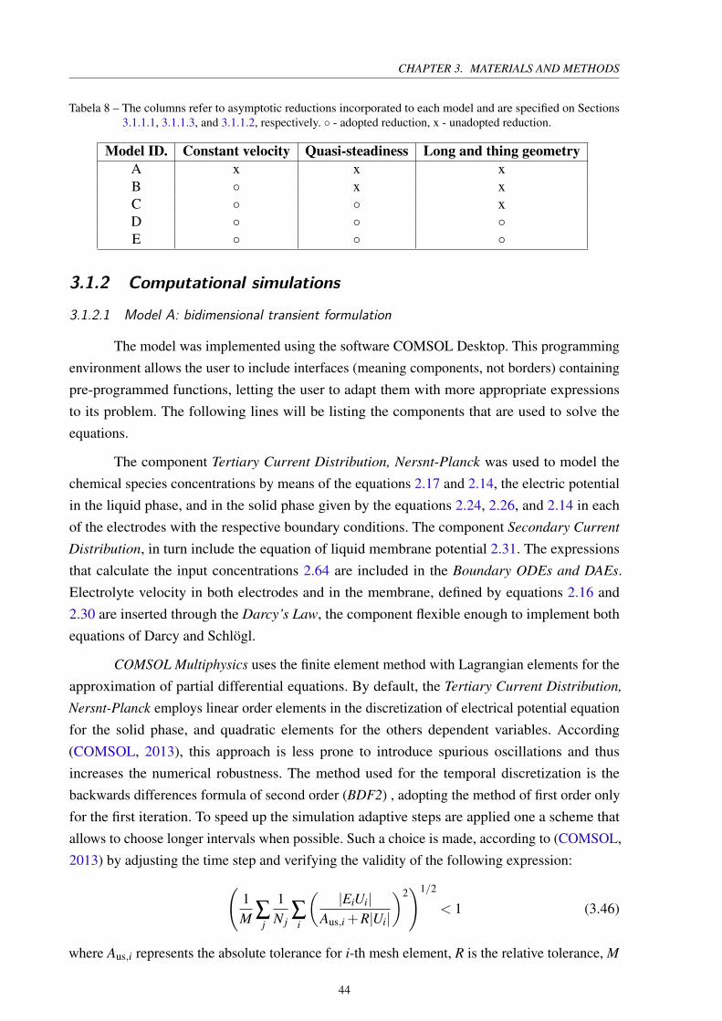
The asymptotic reductions discussed in this section are incorporated in different mathe-
matical models. In total, 5 different models are specified, with the reductions summarized in
Table 8.
43
CHAPTER 3. MATERIALS AND METHODS
Tabela 8 – The columns refer to asymptotic reductions incorporated to each model and are specified on Sections3.1.1.1, 3.1.1.3, and 3.1.1.2, respectively. ∘ - adopted reduction, x - unadopted reduction.
Model ID. Constant velocity Quasi-steadiness Long and thing geometry
A x x xB ∘ x xC ∘ ∘ xD ∘ ∘ ∘E ∘ ∘ ∘
3.1.2 Computational simulations
3.1.2.1 Model A: bidimensional transient formulation
The model was implemented using the software COMSOL Desktop. This programming
environment allows the user to include interfaces (meaning components, not borders) containing
pre-programmed functions, letting the user to adapt them with more appropriate expressions
to its problem. The following lines will be listing the components that are used to solve the
equations.
The component Tertiary Current Distribution, Nersnt-Planck was used to model the
chemical species concentrations by means of the equations 2.17 and 2.14, the electric potential
in the liquid phase, and in the solid phase given by the equations 2.24, 2.26, and 2.14 in each
of the electrodes with the respective boundary conditions. The component Secondary Current
Distribution, in turn include the equation of liquid membrane potential 2.31. The expressions
that calculate the input concentrations 2.64 are included in the Boundary ODEs and DAEs.
Electrolyte velocity in both electrodes and in the membrane, defined by equations 2.16 and
2.30 are inserted through the Darcy’s Law, the component flexible enough to implement both
equations of Darcy and Schlögl.
COMSOL Multiphysics uses the finite element method with Lagrangian elements for the
approximation of partial differential equations. By default, the Tertiary Current Distribution,
Nersnt-Planck employs linear order elements in the discretization of electrical potential equation
for the solid phase, and quadratic elements for the others dependent variables. According
(COMSOL, 2013), this approach is less prone to introduce spurious oscillations and thus
increases the numerical robustness. The method used for the temporal discretization is the
backwards differences formula of second order (BDF2) , adopting the method of first order only
for the first iteration. To speed up the simulation adaptive steps are applied one a scheme that
allows to choose longer intervals when possible. Such a choice is made, according to (COMSOL,
2013) by adjusting the time step and verifying the validity of the following expression:
(
1
M∑
j
1
N j∑
i
(
|EiUi|
Aus,i +R|Ui|
)2)1/2
< 1 (3.46)
where Aus,i represents the absolute tolerance for i-th mesh element, R is the relative tolerance, M
44
3.1. MATHEMATICAL MODELLING
is the number of variables computed, N j is the number elements in the domain of the dependent
variable j, E is the estimated error for the solution U committed during the tested time step. The
new solution is accepted if the above expression is true, otherwise the time step is reduced and a
new evaluation follows.
Newton’s method is employed by COMSOL for the solution of the nonlinear system, to
the intrinsic linear system the algorithm MUMPS (Massively Parallel Sparse Direct Multifrontal
Solver) is used, that is a routine incorporated into the software that allows to solve linear systems
with parallelization. The mesh used for spatial discretization of the domain has 40 elements
along the X axis, along the Y axis there are 40 elements for each electrode elements, 20 for each
current collector, and 10 elements for the membrane. In total 5200 elements are distributed with
smaller spacing near the interfaces between collector/electrode/membrane.
3.1.2.2 Model B: bidimensional transient formulation with constant velocity
The distinction between Model A and Model B is in the inclusion of asymptotic reduction
refered in Section 3.1.1.1 taken by adoption of constant velocity of the electrolyte across the
electrodes. The strategy for implementation also resembles the previous model, but does not
make use of the component Darcy’s Law to compute the velocity.
3.1.2.3 Model C: bidimensional quasi-steady formulation with constant velocity
The Model C results from the incorporation of reductions present in Sections 3.1.1.1 and
3.1.1.3 the original model. Also implemented making use of the software COMSOL Multiphysics,
the model counted on the flexibility of the component Tertiary Current Distribution, Nersnt-
Planck to vanish the time derivative of concentration in the equation 2.17 in order to solve for its
reduced form.
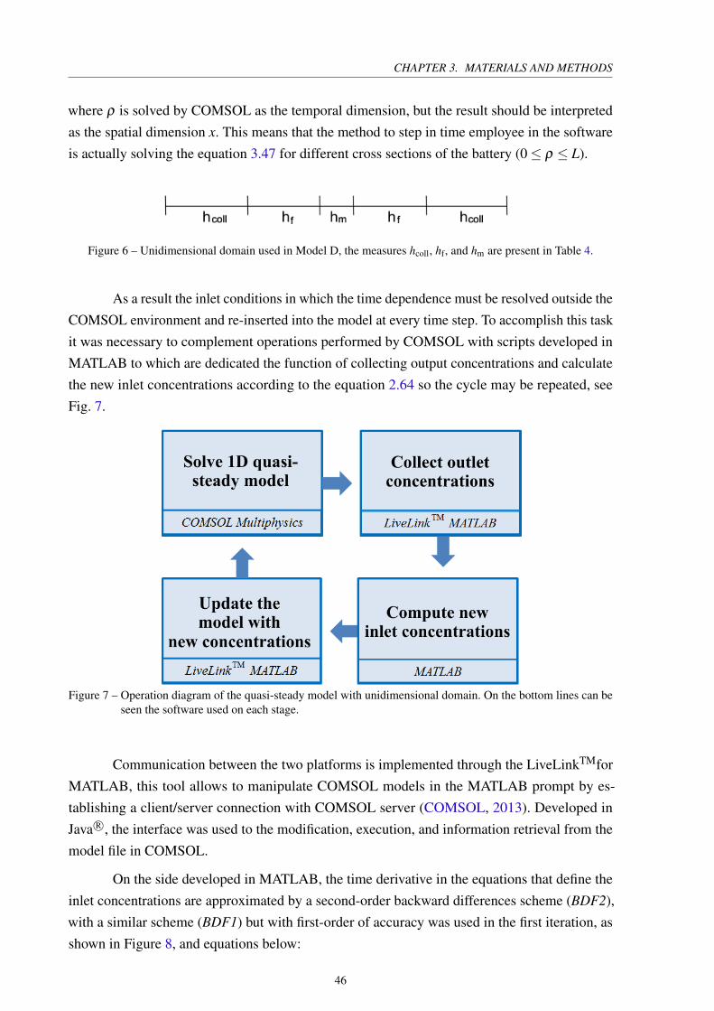
3.1.2.4 Model D: unidimensional quasi-steady formulation with constant velocity, and long
and thin geometry.
This model simplifies the previous one when considering the reduction seen in Section
3.1.1.2 about the long and thin geometry of the electrode leading to the equation 3.18.
As suggested in (VYNNYCKY, 2011) during the implementation the spatial dimension
X can exchange by the time dimension t, this enables the use of a one-dimensional domain as
in Fig.6 that preserves the dimension Y , since only the equations 2.64 to compute the input
concentrations are time dependent. More strictly, the equation inserted in the software is:
uin∂ck
∂ρ=
∂
∂y
(
zckDeffk F
RT
∂φe
∂y+Deff
k
∂ck
∂y
)
−Sk (3.47)
45
CHAPTER 3. MATERIALS AND METHODS
where ρ is solved by COMSOL as the temporal dimension, but the result should be interpreted
as the spatial dimension x. This means that the method to step in time employee in the software
is actually solving the equation 3.47 for different cross sections of the battery (0≤ ρ ≤ L).
Figure 6 – Unidimensional domain used in Model D, the measures hcoll, hf, and hm are present in Table 4.
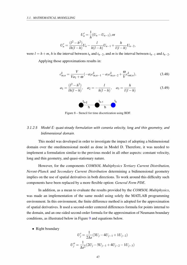
As a result the inlet conditions in which the time dependence must be resolved outside the
COMSOL environment and re-inserted into the model at every time step. To accomplish this task
it was necessary to complement operations performed by COMSOL with scripts developed in
MATLAB to which are dedicated the function of collecting output concentrations and calculate
the new inlet concentrations according to the equation 2.64 so the cycle may be repeated, see
Fig. 7.
Figure 7 – Operation diagram of the quasi-steady model with unidimensional domain. On the bottom lines can beseen the software used on each stage.
Communication between the two platforms is implemented through the LiveLinkTMfor
MATLAB, this tool allows to manipulate COMSOL models in the MATLAB prompt by es-
tablishing a client/server connection with COMSOL server (COMSOL, 2013). Developed in
Java R○, the interface was used to the modification, execution, and information retrieval from the
model file in COMSOL.
On the side developed in MATLAB, the time derivative in the equations that define the
inlet concentrations are approximated by a second-order backward differences scheme (BDF2),
with a similar scheme (BDF1) but with first-order of accuracy was used in the first iteration, as
shown in Figure 8, and equations below:
46
3.1. MATHEMATICAL MODELLING
U ′n =1
h(Un−Un−1),or
U ′n =(l2−h2)
lh(l−h)Un−
l
h(l−h)Un−1 +
h
l(l−h)Un−2,
were l = h+m, h is the interval between tn and tn−2, and m is the interval between tn−1 and tn−2.
Applying those approximations results in:
ckin,n =
V
Va1 +ω(−a2ck
in,n−1−a3ckin,n−2 +
ω
Vck
out,n), (3.48)
a1 =(l2−h2)
lh(l−h), a2 =−
l
h(l−h), a3 =
h
l(l−h)(3.49)
Figure 8 – Stencil for time discretization using BDF.
3.1.2.5 Model E: quasi-steady formulation with consnta velocity, long and thin geometry, and
bidimensional domain.
This model was developed in order to investigate the impact of adopting a bidimensional
domain over the onedimensional model as done in Model D. Therefore, it was needed to
implement a formulation similar to the previous model in all other aspects: constant velocity,
long and thin geometry, and quasi-stationary nature.
However, for the components COMSOL Multiphysics Tertiary Current Distribution,
Nersnt-Planck and Secondary Current Distribution determining a bidimensional geometry
implies on the use of spatial derivatives in both directions. To work around this difficulty such
components have been replaced by a more flexible option: General Form PDE.
In addition, as a mean to evaluate the results provided by the COMSOL Multiphysics,
was made an implementation of the same model using solely the MATLAB programming
environment. In this environment, the finite difference method is adopted for the approximation
of spatial derivatives. It used a second-order centered differences formula for points internal to
the domain, and an one-sided second-order formula for the approximation of Neumann boundary
conditions, as illustrated below in Figure 9 and equations below.
∙ Right boundary
U ′j =1
2∆x(3U j−4U j−1 +1U j−2)
U ′′j =1
∆x2 (2U j−5U j−1 +4U j−2−1U j−3)
47
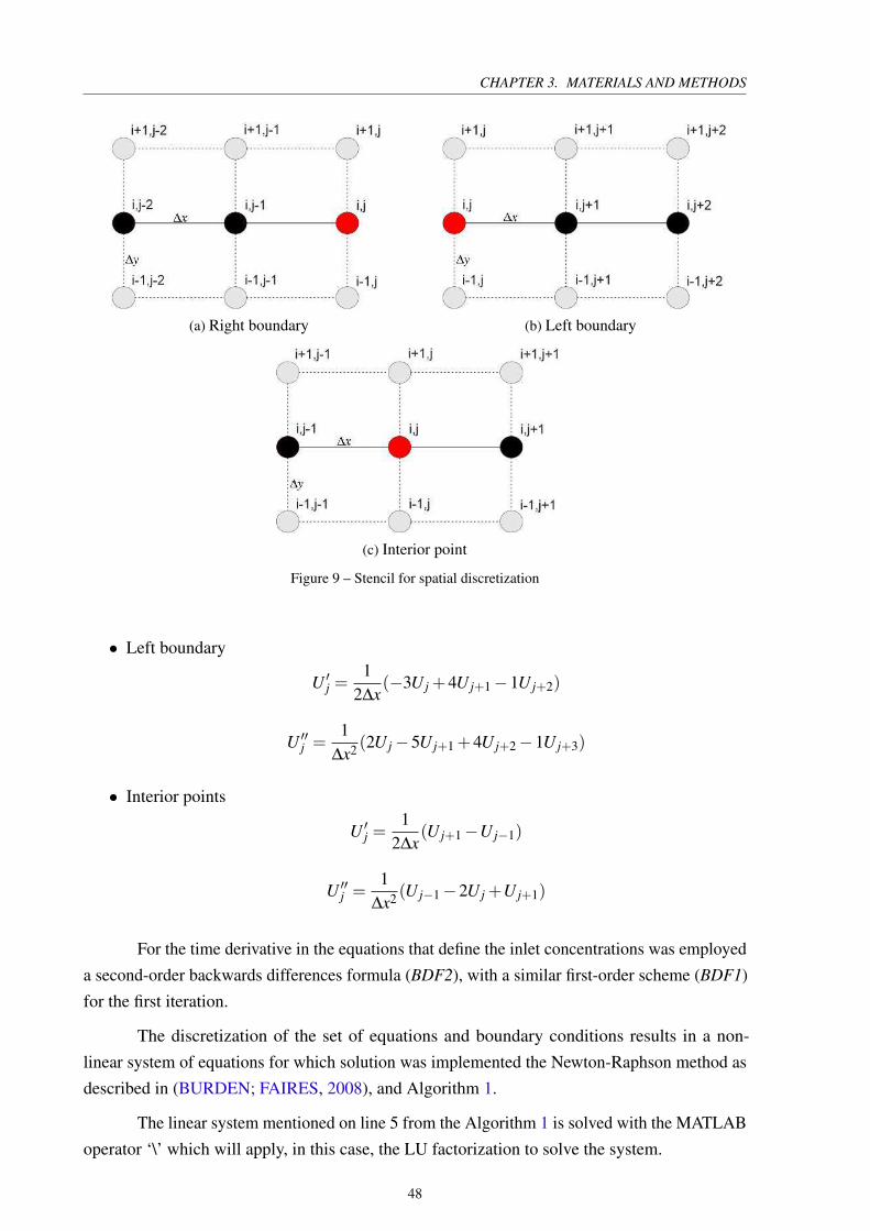
CHAPTER 3. MATERIALS AND METHODS
(a) Right boundary (b) Left boundary
(c) Interior point
Figure 9 – Stencil for spatial discretization
∙ Left boundary
U ′j =1
2∆x(−3U j +4U j+1−1U j+2)
U ′′j =1
∆x2 (2U j−5U j+1 +4U j+2−1U j+3)
∙ Interior points
U ′j =1
2∆x(U j+1−U j−1)
U ′′j =1
∆x2 (U j−1−2U j +U j+1)
For the time derivative in the equations that define the inlet concentrations was employed
a second-order backwards differences formula (BDF2), with a similar first-order scheme (BDF1)
for the first iteration.
The discretization of the set of equations and boundary conditions results in a non-
linear system of equations for which solution was implemented the Newton-Raphson method as
described in (BURDEN; FAIRES, 2008), and Algorithm 1.
The linear system mentioned on line 5 from the Algorithm 1 is solved with the MATLAB
operator ‘\’ which will apply, in this case, the LU factorization to solve the system.
48
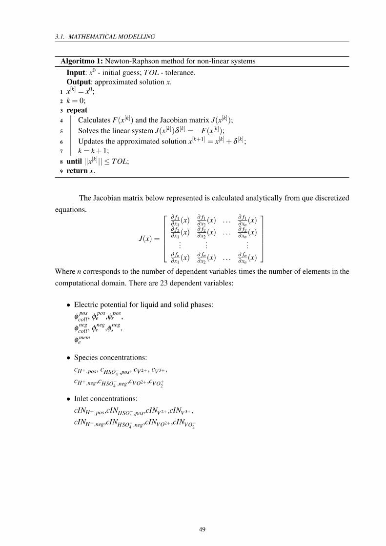
3.1. MATHEMATICAL MODELLING
Algoritmo 1: Newton-Raphson method for non-linear systems
Input: x0 - initial guess; TOL - tolerance.Output: approximated solution x.
1 x[k] = x0;2 k = 0;3 repeat
4 Calculates F(x[k]) and the Jacobian matrix J(x[k]);
5 Solves the linear system J(x[k])δ [k] =−F(x[k]);
6 Updates the approximated solution x[k+1] = x[k]+δ [k];7 k = k+1;
8 until ||x[k]|| ≤ TOL;9 return x.
The Jacobian matrix below represented is calculated analytically from que discretized
equations.
J(x) =
∂ f1∂x1
(x) ∂ f1∂x2
(x) . . . ∂ f1∂xn
(x)∂ f2∂x1
(x) ∂ f2∂x2
(x) . . . ∂ f2∂xn
(x)...
......
∂ fn∂x1
(x) ∂ fn∂x2
(x) . . . ∂ fn∂xn
(x)
Where n corresponds to the number of dependent variables times the number of elements in the
computational domain. There are 23 dependent variables:
∙ Electric potential for liquid and solid phases:
φposcoll , φ
pose ,φ pos
s ,
φnegcoll , φ
nege ,φ neg
s ,
φ meme
∙ Species concentrations:
cH+,pos, cHSO−4 ,pos, cV 2+ , cV 3+ ,
cH+,neg,cHSO−4 ,neg,cVO2+ ,cVO+2
∙ Inlet concentrations:
cINH+,pos,cINHSO−4 ,pos,cINV 2+ ,cINV 3+ ,
cINH+,neg,cINHSO−4 ,neg,cINVO2+ ,cINVO+2
49

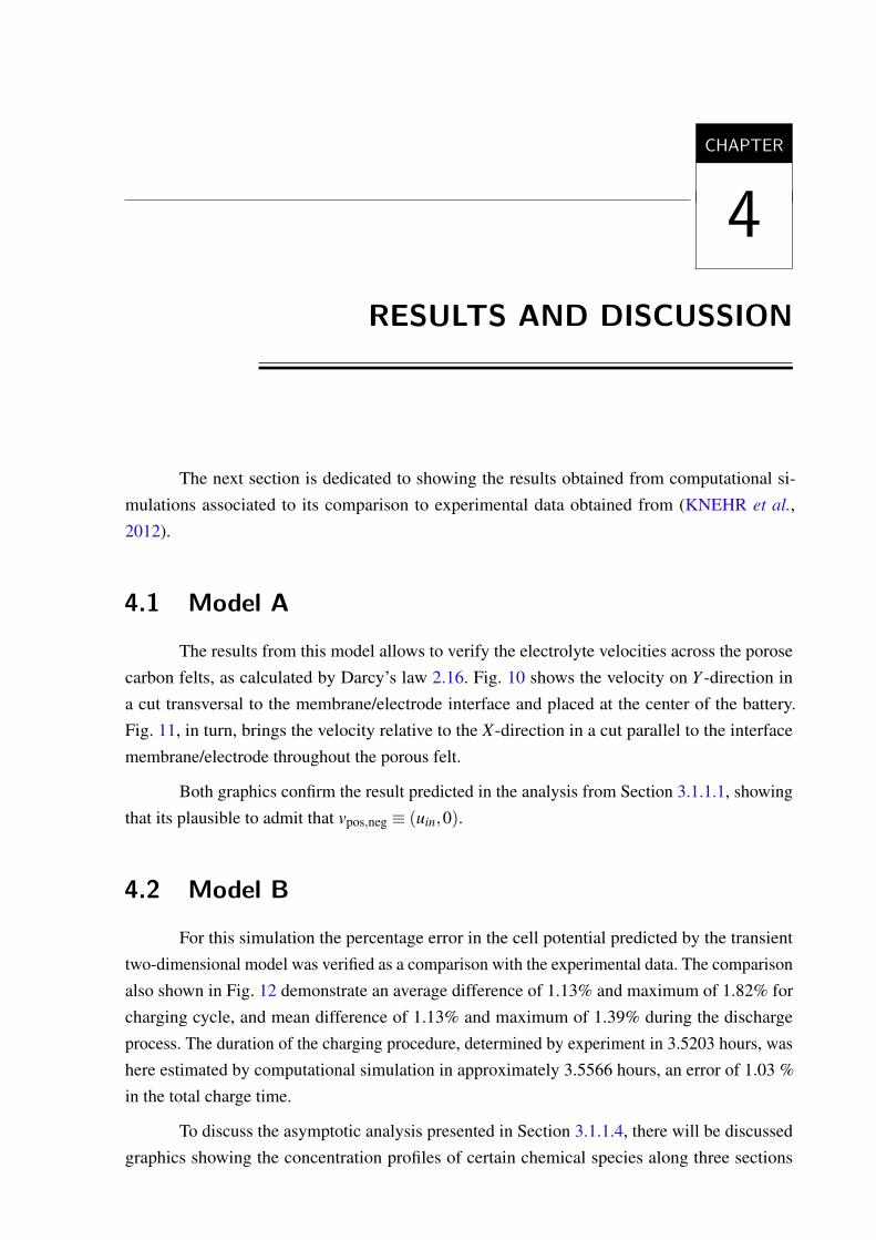
CHAPTER
4
RESULTS AND DISCUSSION
The next section is dedicated to showing the results obtained from computational si-
mulations associated to its comparison to experimental data obtained from (KNEHR et al.,
2012).
4.1 Model A
The results from this model allows to verify the electrolyte velocities across the porose
carbon felts, as calculated by Darcy’s law 2.16. Fig. 10 shows the velocity on Y -direction in
a cut transversal to the membrane/electrode interface and placed at the center of the battery.
Fig. 11, in turn, brings the velocity relative to the X-direction in a cut parallel to the interface
membrane/electrode throughout the porous felt.
Both graphics confirm the result predicted in the analysis from Section 3.1.1.1, showing
that its plausible to admit that vpos,neg ≡ (uin,0).
4.2 Model B
For this simulation the percentage error in the cell potential predicted by the transient
two-dimensional model was verified as a comparison with the experimental data. The comparison
also shown in Fig. 12 demonstrate an average difference of 1.13% and maximum of 1.82% for
charging cycle, and mean difference of 1.13% and maximum of 1.39% during the discharge
process. The duration of the charging procedure, determined by experiment in 3.5203 hours, was
here estimated by computational simulation in approximately 3.5566 hours, an error of 1.03 %
in the total charge time.
To discuss the asymptotic analysis presented in Section 3.1.1.4, there will be discussed
graphics showing the concentration profiles of certain chemical species along three sections
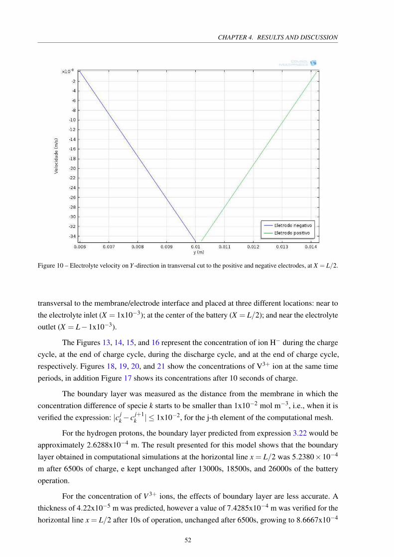
CHAPTER 4. RESULTS AND DISCUSSION
Figure 10 – Electrolyte velocity on Y -direction in transversal cut to the positive and negative electrodes, at X = L/2.
transversal to the membrane/electrode interface and placed at three different locations: near to
the electrolyte inlet (X = 1x10⁻³); at the center of the battery (X = L/2); and near the electrolyte
outlet (X = L−1x10⁻³).
The Figures 13, 14, 15, and 16 represent the concentration of ion H− during the charge
cycle, at the end of charge cycle, during the discharge cycle, and at the end of charge cycle,
respectively. Figures 18, 19, 20, and 21 show the concentrations of V3+ ion at the same time
periods, in addition Figure 17 shows its concentrations after 10 seconds of charge.
The boundary layer was measured as the distance from the membrane in which the
concentration difference of specie k starts to be smaller than 1x10⁻² mol m−3, i.e., when it is
verified the expression: |c jk− c
j+1k | ≤ 1x10⁻², for the j-th element of the computational mesh.
For the hydrogen protons, the boundary layer predicted from expression 3.22 would be
approximately 2.6288x10⁻⁴ m. The result presented for this model shows that the boundary
layer obtained in computational simulations at the horizontal line x = L/2 was 5.2380×10⁻⁴
m after 6500s of charge, e kept unchanged after 13000s, 18500s, and 26000s of the battery
operation.
For the concentration of V 3+ ions, the effects of boundary layer are less accurate. A
thickness of 4.22x10⁻⁵ m was predicted, however a value of 7.4285x10⁻⁴ m was verified for the
horizontal line x = L/2 after 10s of operation, unchanged after 6500s, growing to 8.6667x10⁻⁴
52
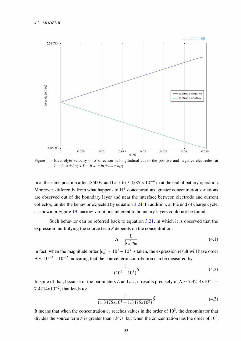
4.2. MODEL B
Figure 11 – Electrolyte velocity on X-direction in longitudinal cut to the positive and negative electrodes, atY = hcoll +hf/2 e Y = hcoll +hf +hm +hf/2.
m at the same position after 18500s, and back to 7.4285×10⁻⁴ m at the end of battery operation.
Moreover, differently from what happens to H+ concentrations, greater concentration variations
are observed out of the boundary layer and near the interface between electrode and current
collector, unlike the behavior expected by equation 3.24. In addition, at the end of charge cycle,
as shown in Figure 19, narrow variations inherent to boundary layers could not be found.
Such behavior can be referred back to equation 3.21, in which it is observed that the
expression multiplying the source term S depends on the concentration:
Λ =L
[ck]uin(4.1)
in fact, when the magnitude order [ck]∼ 102−103 is taken, the expression result will have order
Λ∼ 10−3−10−2 indicating that the source term contribution can be measured by:
1
(102−103)S (4.2)
In spite of that, because of the parameters L and uin, it results precisely in Λ∼ 7.4214x10⁻³−
7.4214x10⁻², that leads to:
1
(1.3475x101−1.3475x10²)S (4.3)
It means that when the concentration ck reaches values in the order of 103, the denominator that
divides the source term S is greater than 134.7, but when the concentration has the order of 102,
53
CHAPTER 4. RESULTS AND DISCUSSION
the same denominator is about 13.47 implying on a bigger significance of this term in equation
3.21. That is precisely the case for evaluated results: for the H+ ion, which concentration is
always greater than 5000 mol m−3, the source term plays a minor role and could be neglected in
the equation; nevertheless, for the specie V 3+ the source term mischaracterizes the relation 3.24
by the time when the ion reaches its lowest concentration.
Figure 12 – Comparison between charge and discharge curve for model B
4.3 Model C
The percentage error for this model during the charge process is around 1.25%, while
the maximum error reaches 3.14%. For the discharge the mean error is 2.47%, and the maximum
error is 3.82%. The estimated time for the charge cycle to complete is 3.3921 hours, representing
a difference of 3.64% on the real cycle duration.
4.4 Model D
The Figure 23 shows the curve of charge and discharge using the time steps provided
by the adaptive scheme from Model E. In other words, the same steps chosen by COMSOL
during the execution of Model E were saved and then employed in the time marching for Model
D. Were compared the predictions done through the uni-dimensional quasi-steady formulation
(Model D) and bi-dimensional quasi-steady (Model E).
54
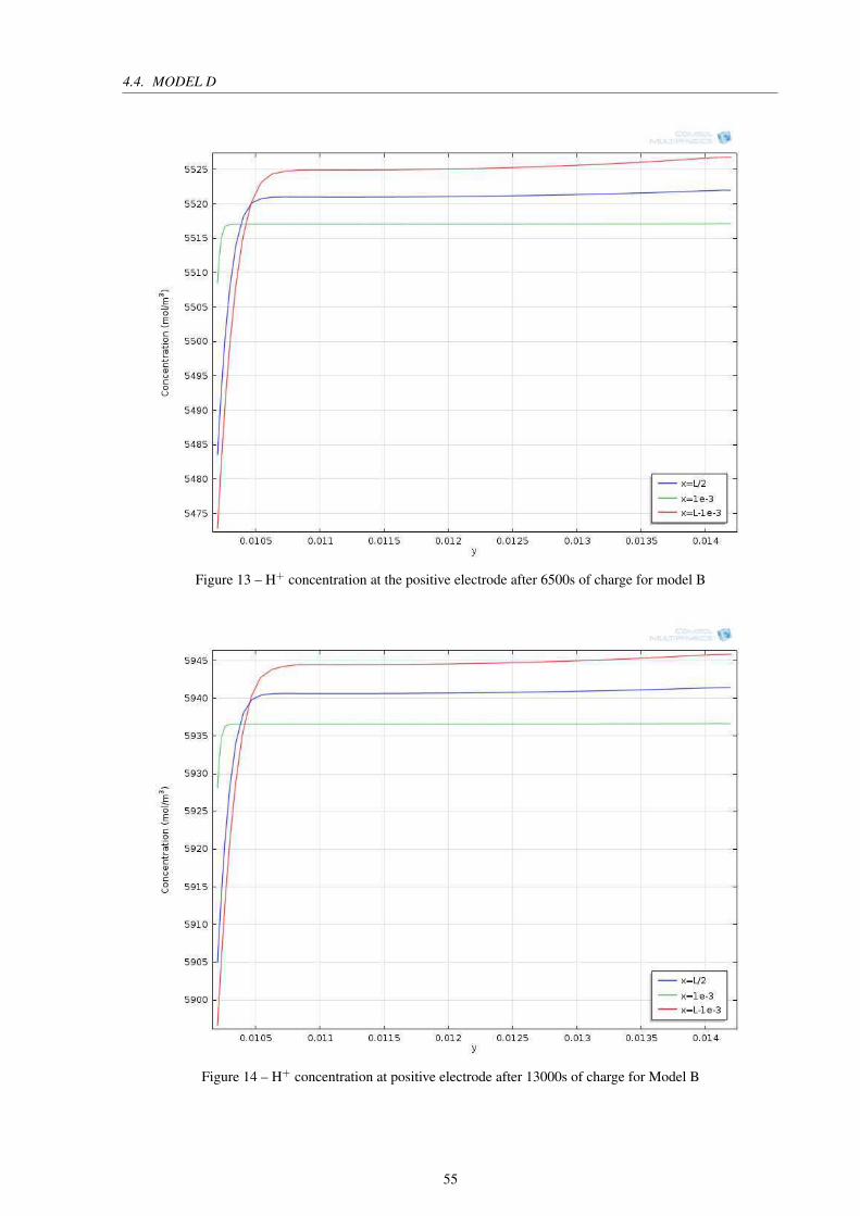
4.4. MODEL D
Figure 13 – H+ concentration at the positive electrode after 6500s of charge for model B
Figure 14 – H+ concentration at positive electrode after 13000s of charge for Model B
55
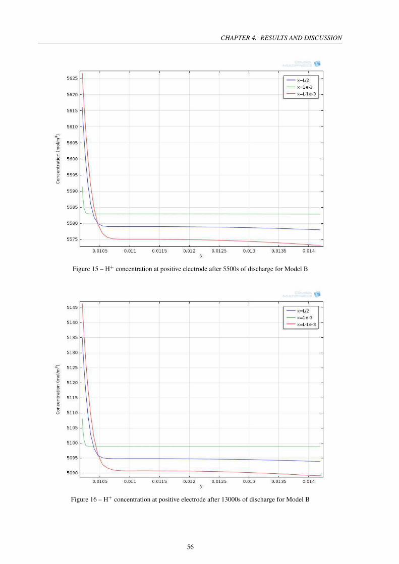
CHAPTER 4. RESULTS AND DISCUSSION
Figure 15 – H+ concentration at positive electrode after 5500s of discharge for Model B
Figure 16 – H+ concentration at positive electrode after 13000s of discharge for Model B
56
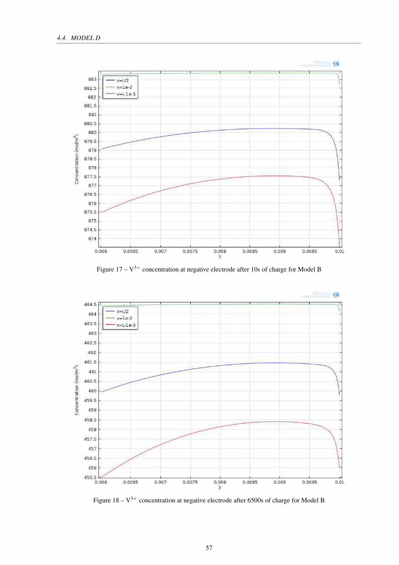
4.4. MODEL D
Figure 17 – V3+ concentration at negative electrode after 10s of charge for Model B
Figure 18 – V3+ concentration at negative electrode after 6500s of charge for Model B
57
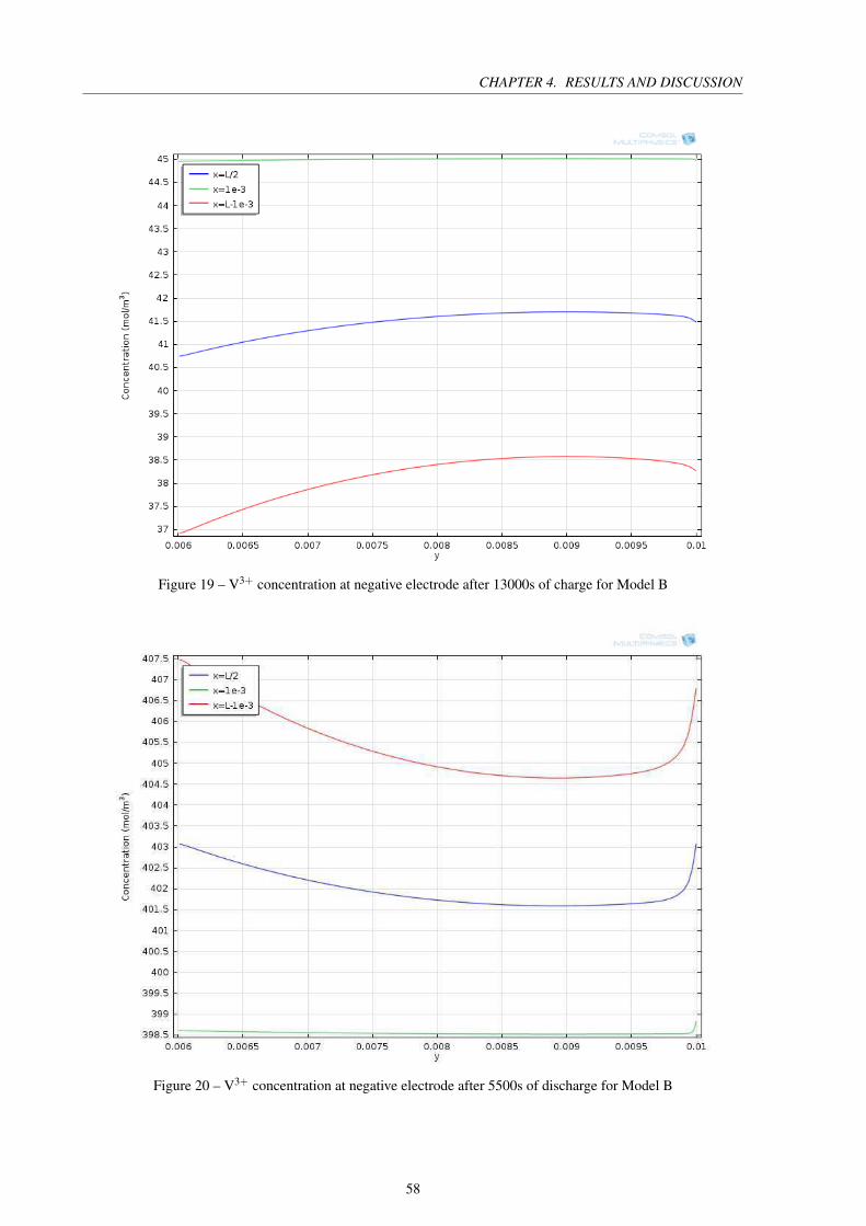
CHAPTER 4. RESULTS AND DISCUSSION
Figure 19 – V3+ concentration at negative electrode after 13000s of charge for Model B
Figure 20 – V3+ concentration at negative electrode after 5500s of discharge for Model B
58
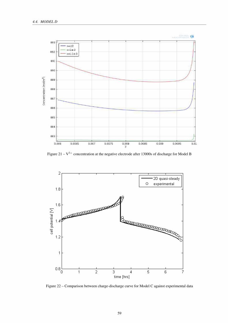
4.4. MODEL D
Figure 21 – V3+ concentration at the negative electrode after 13000s of discharge for Model B
Figure 22 – Comparison between charge-discharge curve for Model C against experimental data
59
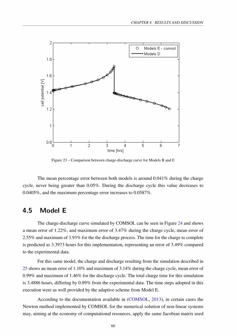
CHAPTER 4. RESULTS AND DISCUSSION
Figure 23 – Comparison between charge-discharge curve for Models B and E
The mean percentage error between both models is around 0.041% during the charge
cycle, never being greater than 0.05%. During the discharge cycle this value decreases to
0.0405%, and the maximum percentage error increases to 0.0587%.
4.5 Model E
The charge-discharge curve simulated by COMSOL can be seen in Figure 24 and shows
a mean error of 1.22%, and maximum error of 3.47% during the charge cycle, mean error of
2.55% and maximum of 3.93% for the the discharge process. The time for the charge to complete
is predicted as 3.3973 hours for this implementation, representing an error of 3.49% compared
to the experimental data.
For this same model, the charge and discharge resulting from the simulation described in
25 shows an mean error of 1.10% and maximum of 3.14% during the charge cycle, mean error of
0.99% and maximum of 1.46% for the discharge cycle. The total charge time for this simulation
is 3.4886 hours, differing by 0.89% from the experimental data. The time steps adopted in this
execution were as well provided by the adaptive scheme from Model E.
According to the documentation available in (COMSOL, 2013), in certain cases the
Newton method implemented by COMSOL for the numerical solution of non-linear systems
may, aiming at the economy of computational resources, apply the same Jacobian matrix used
60
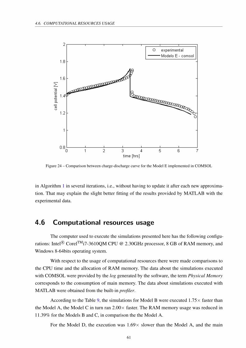
4.6. COMPUTATIONAL RESOURCES USAGE
Figure 24 – Comparison between charge-discharge curve for the Model E implemented in COMSOL
in Algorithm 1 in several iterations, i.e., without having to update it after each new approxima-
tion. That may explain the slight better fitting of the results provided by MATLAB with the
experimental data.
4.6 Computational resources usage
The computer used to execute the simulations presented here has the following configu-
rations: Intel R○ CorelTMi7-3610QM CPU @ 2.30GHz processor, 8 GB of RAM memory, and
Windows 8-64bits operating system.
With respect to the usage of computational resources there were made comparisons to
the CPU time and the allocation of RAM memory. The data about the simulations executed
with COMSOL were provided by the log generated by the software, the term Physical Memory
corresponds to the consumption of main memory. The data about simulations executed with
MATLAB were obtained from the built-in profiler.
According to the Table 9, the simulations for Model B were executed 1.75× faster than
the Model A, the Model C in turn ran 2.00× faster. The RAM memory usage was reduced in
11.39% for the Models B and C, in comparison the the Model A.
For the Model D, the execution was 1.69× slower than the Model A, and the main
61
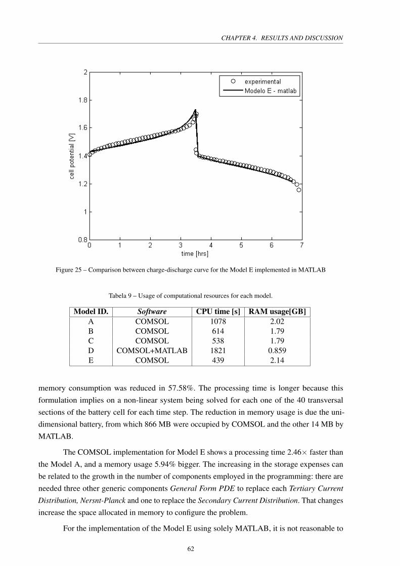
CHAPTER 4. RESULTS AND DISCUSSION
Figure 25 – Comparison between charge-discharge curve for the Model E implemented in MATLAB
Tabela 9 – Usage of computational resources for each model.
Model ID. Software CPU time [s] RAM usage[GB]
A COMSOL 1078 2.02B COMSOL 614 1.79C COMSOL 538 1.79D COMSOL+MATLAB 1821 0.859E COMSOL 439 2.14
memory consumption was reduced in 57.58%. The processing time is longer because this
formulation implies on a non-linear system being solved for each one of the 40 transversal
sections of the battery cell for each time step. The reduction in memory usage is due the uni-
dimensional battery, from which 866 MB were occupied by COMSOL and the other 14 MB by
MATLAB.
The COMSOL implementation for Model E shows a processing time 2.46× faster than
the Model A, and a memory usage 5.94% bigger. The increasing in the storage expenses can
be related to the growth in the number of components employed in the programming: there are
needed three other generic components General Form PDE to replace each Tertiary Current
Distribution, Nersnt-Planck and one to replace the Secondary Current Distribution. That changes
increase the space allocated in memory to configure the problem.
For the implementation of the Model E using solely MATLAB, it is not reasonable to
62
4.6. COMPUTATIONAL RESOURCES USAGE
make comparisons about the computational performance, since it does not employ a parallel
algorithm to solve the linear system, unlike what is done by the software COMSOL Multiphysics.
This execution was planned and executed as a mean to verify the numerical results provided
by COMSOL. The addition of a parallel solver to the MATLAB script may be effectuated in a
future work, as it is goes beyond the scope of this research.
63

CHAPTER
5
FINAL CONSIDERATIONS
In this research the use of asymptotic reduction in the mathematical modeling of vana-
dium redox battery was investigated, as well as the changes that its incorporation may have on
the usage of computational resources, and on the agreement with experimental data existing
in literature. Thus, it is built a reference that summarizes a variety of models discussed from
the point of view of asymptotic analysis and numerical solution, discussing formulations which
performance diversify in the computational requirements as RAM memory and CPU time.
Moreover, the comparison between the solutions provided by COMSOL and that one
resulting from the MATLAB script implemented in this research represents a mutual numerical
validation for the computational simulations executed by the referred software.

REFERENCES
AL-FETLAWI, A.; SHAH, A. A.; WALSH, F. Modelling the effects of oxy-gen evolution in theall-vanadium redox flow battery. Electrochimica Acta, p. 55:3192–3205, 2010. Cited on page20.
AL-FETLAWI, A.; SHAH, A. A.; WALSH, F. C. Non-isothermal modelling of the all-vanadiumredox-flow battery. Electrochimica Acta, p. 55:78–89, 2009. Cited 3 times on pages 20, 24e 28.
BAZANT, M. Lecture 24: Diffusive Charge in Electrolytes. 2014. No-tas de aula. Disponível em: <http://ocw.mit.edu/courses/chemical-engineering/10-626-electrochemical-energy-systems-spring-2011/lecture-notes/MIT10_626S11_lec24.pdf>. Acesso em: 25 jan. 2014. Cited on page 22.
BERNARDI, D. M.; VERBRUGGE, M. W. Mathematical model of a gas diffusion electrodebonded to a polymer electrolyte. AIChe Journal, v. 37, p. 1151–1163, 1991. Cited on page 37.
BURDEN, R. L.; FAIRES, J. D. Análise numérica. [S.l.]: Cengage Learning, 2008. Cited onpage 48.
CHEN, C. L.; YEOH, H. K.; CHAKRABARTI, M. H. An enhancement to vynnycky’s modelfor the all-vanadium redox flow battery. Electrochimica Acta, Elsevier, p. 120:167–179, 2014.Cited 3 times on pages 19, 25 e 26.
COMSOL MULTIPHYSICS. Reference Manual: Version 4.4. Rio de Janeiro, 2013. 1270 p.Cited 3 times on pages 44, 46 e 60.
CORCUERA, S.; SKYLLAS-KAZACOS, M. State-of-charge monitoring and electrolyte reba-lancing methods for the vanadium redox flow battery. European Chemical Bulletin, v. 1, n. 12,p. 511–519, 2012. Cited 2 times on pages 26 e 35.
ESA. Peak shaving and demand charge avoidance: prudent
energy vanadium redox battery storage system (VRB-ESS). 2014.Disponível em: <http://energystorage.org/energy-storage/case-studies/peak-shaving-and-demand-charge-avoidance-prudent-energy-vanadium-redox>. Acessoem: 19 jan. 2014. Cited on page 18.
HOWISON, S. Practical Applied Mathematics - Modelling, Analysis, Approximation. [S.l.]:Cambridge University Press, 2005. Cited 2 times on pages 36 e 42.
HUANG, K.-L.; LI, X. gang; LIU, S. qin; TAN, N.; CHEN, L. quan. Research progress hofvanadium redox flow battery for energy storage in china. Renewable Energy, p. 33:186–192,2008. Cited on page 18.
KEAR, G.; SHAH, A. A.; WALSH, F. C. Development of the all-vanadium redox flow battery forenergy storage: a review of technological, financial and policy aspects. International journal
of energy research, Wiley Online Library, p. 36:1105–1120, 2011. Cited on page 19.
References
KJEANG, E.; PROCTOR, B. T.; BROLO, A. G.; HARRINGTON, D. A.; DJILALI, N.; SINTON,D. High-performance microfluidic vanadium redox fuel cell. Electrochimica Acta, p. 52:4942–4946, 2007. Cited 2 times on pages 26 e 34.
KNEHR, K. W.; AGAR, E.; DENNISON, C. R.; KALIDINDI, A. R.; KUMBUR, E. C. Atransient vanadium flow battery model incorporating vanadium crossover and water transportthrough the membrane. J. Electrochem. Soc., v. 159, n. 9, p. A1446–A1459, 2012. Cited 6times on pages 35, 37, 38, 42, 43 e 51.
LIDE, D. R. Handbook of Chemistry and Physics. 84th. ed. [S.l.]: CRC Press, Inc. BocaRaton, Florida, 2003. Cited on page 38.
NAG, P. K. Basic and applied thermodynamics. First edition. [S.l.]: Tata McGraw-Hill, 2002.Cited on page 19.
NEWMAN, J.; THOMAS-ALYEA, K. E. Electrochemical Systems. Third edition. [S.l.]: JohnWiley & Sons, 2004. Cited 4 times on pages 19, 22, 24 e 38.
NREL - National Renewable Energy Laboratory. Learning About Renewable Energy. 2014.Disponível em: <http://www.nrel.gov/learning/>. Acesso em: 13 jan. 2014. Cited on page 15.
ORIJI, G.; KATAYAMA, Y.; MIURA, T. Investigation on v(iv)/v(v) species in vanadium redoxflow battery. Eletrochimica Acta, p. 49:3091–3095, 2004. Cited on page 34.
. Investigation on v(iv)/v(v) and v(ii)/v(iii) redox reactions by various electrochemicalmethods. Journal of Power Sources, p. 139:321–324, 2005. Cited on page 34.
PARASURAMAN, A.; LIM, T. M.; MENICTAS, C.; SKYLLAS-KAZACOS, M. Review ofmaterial reserch and development for vanadium redox flow battery applications. Electrochimica
Acta, Elsevier, p. 101:27–40, 2013. Cited 2 times on pages 16 e 19.
POURBAIX, M. Atlas of electrochemical equilibria in aqueous solutions. 2nd. ed. [S.l.]:NACE, Houston, TX, 1974. 234 p. Cited on page 37.
PRIFTI, H.; PARASURAMAN, A.; WINARDI, S.; LIM, T. M.; SKYLLAS-KAZACOS, M.Membranes for redox flow battery applications. Membranes, p. 2:275–306, 2012. Cited onpage 27.
REDT. Sucessful installationg of REDT’S storage system in collaboration with FP7 and the
european commission. 2014. Disponível em: <http://www.redtenergy.com/news/fp7>. Acessoem: 17 jan. 2014. Cited on page 17.
RICHMOND, B. C. VRB power sells two 5kW x 4hr VRB energy sto-
rage systems (TM) to Winafrique Technologies for Deployment with Safari-
com, in Kenya. 2014. Disponível em: <http://www.newswire.ca/fr/story/97801/vrb-power-sells-two-5kw-x-4hr-vrb-energy-storage-systems-tm-to-winafrique-technologies\-for-deployment-with-safaricom-in-kenya>. Acesso em: 17 jan. 2014. Cited on page 18.
RODENHAUSEN, H. Einstein’s relation between diffusion constant and mobility for a diffusionmodel. Journal of Statistical Physics, Kluwer Academic Publishers-Plenum Publishers, p.55(5–6):1065–1088, 1989. Cited on page 22.
68
References
SHAH, A. A.; AL-FETLAWI, A.; WALSH, F. Dynamic modelling of hydrogen evolution effectsin the all-vanadium redox flow battery. Electrochimica Acta, p. 55:1125–1139, 2010. Cited 4times on pages 20, 26, 28 e 35.
SHAH, A. A.; WATT-SMITH, M. J.; WALSH, F. A dynamic performance model for redox-flowbatteries involving soluble species. Electrochimica Acta, p. 53:8087–8100, 2008. Cited 4 timeson pages 20, 24, 37 e 38.
SHARMA, A. K.; VYNYCKY, M.; LING, C.; BIRGERSSON, E.; HAN, M. The quasi-steadystate of all-vanadium redox flow batteries: A scale analysis. Electrochimica Acta, v. 147, p.657–662, 2014. Cited 4 times on pages 19, 35, 38 e 39.
SKYLLAS-KAZACOS, M. The vanadium redox battery and fuel cell for large-scale energystorage. In: 19th World Energy Congress. [S.l.: s.n.], 2004. Sydney, Australia. Cited on page18.
SKYLLAS-KAZACOS, M.; ROBINS, R. G.; FANE, A. F.; GREEN, M. A.; RYCHCIK, M. Newall-vanadium redox flow cell. Journal of Electrochemical Society, p. 133:1057–1058, 1986.Cited on page 16.
SKYLLAS-KAZACOS, M.; SUM, E.; RYCHCIK, M. Investigation of the v(v)/v(iv) system foruse in the positive half-cell of a redox battery. Journal of Power Sources, p. 16:85–95, 1985.Cited on page 16.
SUM, E.; SKYLLAS-KAZACOS, M. A study of the v(ii)/v(iii) redox couple for redox flow cellapplications. Journal of Power Sources, p. 15179–190, 1985. Cited on page 16.
TICIANELLI, E. A.; GONZALEZ, E. R. Eletroquímica: princípios e aplicções. Segundaedição. [S.l.]: Edusp, 2005. Cited 3 times on pages 19, 22 e 23.
VYNNYCKY, M. Analysis of a model for the operation of a vanadium redox battery. Energy, p.36:2242–2256, 2011. Cited 12 times on pages 9, 16, 17, 19, 24, 25, 26, 28, 35, 36, 38 e 45.
VYNNYCKY, M.; ASSUNçãO, M. Asymptotic and numerical modelling of vanadium redox
flow batteries. in prep. Cited 3 times on pages 39, 40 e 41.
VYNNYCKY, M.; SHUGAI, G.; YAKUBENKO, P.; MELLGREN, N. Asymptotic reduction fornumerical modeling of polymer electrolyte fuel cells. SIAM J. Appl. Math., v. 70, p. 455–487,2009. Cited on page 35.
YAMAMURA, T.; WATANABE, N.; YANO, T.; SHIOKAWA, Y. Electron transfer kinetics ofNp3+/Np4+, NpO+
2 /NpO2+2 , V2+/V3+, and VO2+/VO+
2 at carbon electrodes. J. Electrochem.
Soc., v. 152, p. A830–A836, 2005. Cited on page 38.
YOU, D.; ZHANG, H.; CHEN, J. A simple model for the vanadium redox battery. Electrochi-
mica Acta, p. 54:6827–6836, 2009. Cited on page 25.
69


www.kth.se