Modelling Stochastic Optimization to Energy and Reserve ...
91
FACULDADE DE E NGENHARIA DA UNIVERSIDADE DO P ORTO Modelling Stochastic Optimization to Energy and Reserve Market in a Microgrid Environment Diogo Faria de Castro WORKING VERSION Mestrado Integrado em Engenharia Eletrotécnica e de Computadores Supervisor: Professor Manuel Matos, Ph.D. Co-Supervisor: Researcher Tiago Soares, Ph.D. August 6, 2018
Transcript of Modelling Stochastic Optimization to Energy and Reserve ...
FACULDADE DE ENGENHARIA DA UNIVERSIDADE DO PORTO
Modelling Stochastic Optimization toEnergy and Reserve Market in a
Microgrid Environment
Diogo Faria de Castro
WORKING VERSION
Mestrado Integrado em Engenharia Eletrotécnica e de Computadores
Supervisor: Professor Manuel Matos, Ph.D.
Co-Supervisor: Researcher Tiago Soares, Ph.D.
August 6, 2018

c© Diogo Castro, 2018
Resumo
Aqui é apresentado o resumo escrito em Português.
Nos últimos anos tem se assistido a um aumento da procura por eletricidade e essa tendenciadeve manter-se no futuro. Novas economias têm-se desenvolvido um pouco por todo o mundo ea forma tradicional de organização do sistema eletrico de energia não consegue dar resposta aosdesafios do mundo atual. A recente reestruturação dos mercados de eletricidade possibilitou umamaior competetividade do sector eletrico, trazendo benefícios aos produtores e consumidores.
A aposta num esquema descentralizado, com grande incidência de produção dispersa por partede recursos renováveis, trás inumeros benefícios, quer para os produtores e consumidores, querpara o ambiente. No entanto este tipo de geração, nomeadamente a geração renovável requerum maior e mais eficaz controlo, uma vez que há uma grande incerteza na disponibilidade destesrecursos, estando dependente das condições atmosféricas vigentes. A incerteza resultante destetipo de recursos tem custos para o sistema, pois o operador da rede não tem informação util sobrea sua disponibilidade e o despacho dos geradores pode não ser eficaz. Para fazer face ao aumentoda incerteza proveniente da proliferação deste tipo de recursos, a comunicação entre os váriosparticipantes do sistema assume uma maior importância.
Novos modelos organizacionais do sistema tem surgido tais como microredes e virtual powerplants, modelos estes que apresentam, em relação ao modelo tradicional, várias vantagens de-scritas ao longo da dissertação. Esta dissertação aborda a gestão de energia e reserva numa mi-crorede. O objectivo é determinar o despacho ótimo de energia e reserva que minimiza os custostotais para o operador da microrede.
Uma importante contribuição desta dissertação é a concepção, design e desenvolvimento deuma metodologia estocástica para o escalonamento de energia e reserva, na presença de incerteza,no âmbito de uma microrede. Neste contexto foi desenvolvido um programa estocástico de doisníveis, modulado por programação linear. A incerteza no sistema é representada por cenários coma respectiva probabilidade associada.
Esta dissertação contribui também com a incorporação de um modelo DC da rede com o obje-tivo de modular as restrições da microrede e evitar congestionamentos. O modelo DC implica umasérie de simplificações que linearizam e simplificam o problema, tornando mais fácil a sua imple-mentação. O resultado é um problema com menos dados que requer menos tempo e capacidadede processamento.
Outra contribuição fundamental desta dissertação é a inclusão de um modelo AC linearizado,permitindo uma mais correta aproximação ao comportamento de uma microrede real. Ao con-trário do modelo DC, o modelo AC é capaz de modular potencia ativa e reativa bem como omódulo e fase das tensões nos barramentos. Com a incorporação do modelo AC, o operador damigrorede está preparado para lidar com eventuais congestionamentos e sobretensões que pos-sam surgir numa rede com grande penetração de recursos renováveis, onde o transito de potenciasbidirecional é bastante frequente.
i

ii
Os modelos descritos são aplicados a uma microrede constituida por uma rede de distribuiçãode 11 kV, considerando um cenário de penetração renovavel para o ano de 2050. Estão conectadosà microrede 1 agregador external supplier (representando a ligação a rede de 33kV), 3 agregadoresde cogeração, 2 agregadores eólicos e 22 agregadores fotovoltaicos. Este teste permite validar osmodelos propostos, mostrando a sua aplicabilidade a futuros sistemas eletricos de energia comgrandes níveis de incerteza.
Abstract
In recent years there has been an increase in demand for electricity and this trend is expected tocontinue in the future. New economies have been developing around the world, and the traditionalway of organizing the power system fails to respond to the challenges of today’s world. Therecent restructuring of electricity markets and the shift to a decentralized scheme of the powersystem have made it possible to have a higher level of competition within the electricity sector,bringing benefits to consumers and producers.
A decentralized scheme, with a high incidence of distributed generation from renewable en-ergy sources, brings numerous benefits to producers, consumers and the environment. However,this type of generation, namely the renewable energy generation, requires a greater and more ef-fective control, since they have an uncertain and variable production behavior, depending on thecurrent atmospheric conditions. The uncertainty related to these resources implies costs to thesystem, since they are not fully dispatchable, and therefore network operators need to find waysto ensure system balance and reliability, like procuring more reserve. To cope with the increasein uncertainty arising from the proliferation of this type of resources, communication between thevarious participants of the system assumes greater importance.
New organizational models of the system have emerged, such as Microgrids (MG) and VirtualPower Plants (VPP). These models present several advantages over the traditional power system,as described throughout this dissertation. This dissertation deals with the energy and reservemanagement in a microgrid. The objective is to determine the optimal energy and reserve dispatchthat minimizes the total operating costs of the MG operator.
One important contribution of this work is the conception, design and development of astochastic energy and reserve scheduling to deal with uncertain generation in the scope of a MG.In this context, a two-stage stochastic technique modulated as linear programming was developed.The uncertainty in the system is represented by scenarios with an associated probability.
In addition, this dissertation also contributes with the incorporation of the DC Optimal PowerFlow (OPF) to the stochastic scheduling problem. This allows to model the network constraintsof the MG and avoid network congestion. The DC OPF implies a series of simplifications whichlinearize the problem and make it easier to implement. This results in a problem with less data,requiring less time and processing power to compute than the full AC OPF, which is a nonlinearand non-convex problem.
Another major contribution is the inclusion of a linearized AC OPF. This OPF models alsoreactive power and voltage magnitude, allowing a more accurate approximation of the natural MGbehavior. The method is able to model both active and reactive power and voltage magnitudeas opposed to DC OPF. This approach enables the MG operator to be ready to face potentialcongestion and voltage problems that may arise in the MG full of DER where bi-directional powerflow is common.
The models were applied to a MG composed by an 11kV distribution network, for a 2050scenario, with high penetration of renewable energy sources. To the MG are connected 1 external
iii

iv
supplier (representing the upstream connection with the 33kV Medium Voltage (MV) line), 3CHP aggregators, 2 wind aggregators and 22 PV aggregators. This test case allows the assessmentand validation of the proposed models, showing their applicability and scalability to future powersystems, full of distributed energy resources, with high levels of uncertainty.

Acknowledgements
I want to express the deepest gratitude to all those who contributed in some way to this work.First of all I would like to thank my family for supporting me with all the means necessary
during my academic education.I want to thank to my supervisors Professor Manuel Matos and Tiago Soares for their avail-
ability from the beginning till the end of the research. For guiding my work and for all the helpprovided, fundamental to overcome the difficulties encountered, I express my gratitude.
I would like to thank also all my friends, specially the ones of BEST Porto, for all the knowl-edge gained in the association which in some way helped me in the completion of this work.
Lastly am grateful to INESC TEC by the work conditions provided, and to my colleaguesof INESC TEC for the exchange of experiences and valuable knowledge applicable during thedevelopment of this work.
Everyone thank you so much.
Diogo Castro
v

vi

“The fewer moving parts, the better”
Christian Cantrell
vii

viii
Contents
1 Introduction 11.1 Background and motivation . . . . . . . . . . . . . . . . . . . . . . . . . . . . . 11.2 Dissertation objectives and contributions . . . . . . . . . . . . . . . . . . . . . . 41.3 Dissertation structure . . . . . . . . . . . . . . . . . . . . . . . . . . . . . . . . 5
2 State of art 72.1 Introduction . . . . . . . . . . . . . . . . . . . . . . . . . . . . . . . . . . . . . 72.2 Energy scheduling . . . . . . . . . . . . . . . . . . . . . . . . . . . . . . . . . 7
2.2.1 Energy scheduling problem associated with formulation type and objec-tive function . . . . . . . . . . . . . . . . . . . . . . . . . . . . . . . . 8
2.2.2 Solving methods for the energy scheduling problem . . . . . . . . . . . 92.2.3 Scheduling problem considering reactive power . . . . . . . . . . . . . . 102.2.4 Scheduling problem considering emissions . . . . . . . . . . . . . . . . 102.2.5 Scheduling problem under uncertainty of DER producers . . . . . . . . . 112.2.6 Scheduling problem considering demand response . . . . . . . . . . . . 12
2.3 Energy and reserve . . . . . . . . . . . . . . . . . . . . . . . . . . . . . . . . . 13
3 Energy and reserve market model 153.1 Introduction . . . . . . . . . . . . . . . . . . . . . . . . . . . . . . . . . . . . . 153.2 Optimization under uncertainty (two-stage stochastic programming) . . . . . . . 153.3 Optimal Power Flow (OPF) – Benchmark for a DC model . . . . . . . . . . . . . 173.4 Linear approximation of the ACOPF . . . . . . . . . . . . . . . . . . . . . . . . 19
3.4.1 Piecewise linearization of the power-flow equations . . . . . . . . . . . . 193.4.2 Piecewise approximation to quadratic equation of power triangle relation 20
3.5 Energy and reserve market model . . . . . . . . . . . . . . . . . . . . . . . . . 213.5.1 Problem description . . . . . . . . . . . . . . . . . . . . . . . . . . . . 21
3.5.1.1 DC benchmark model . . . . . . . . . . . . . . . . . . . . . . 223.5.1.2 Full linearized AC model . . . . . . . . . . . . . . . . . . . . 23
3.6 Mathematical formulation . . . . . . . . . . . . . . . . . . . . . . . . . . . . . 243.6.1 Mathematical formulation for the DC benchmark . . . . . . . . . . . . . 243.6.2 Mathematical formulation for the linearized AC model . . . . . . . . . . 27
4 Assessment of energy and reserve management model (case study) 314.1 Introduction . . . . . . . . . . . . . . . . . . . . . . . . . . . . . . . . . . . . . 314.2 Case study . . . . . . . . . . . . . . . . . . . . . . . . . . . . . . . . . . . . . . 314.3 Outline . . . . . . . . . . . . . . . . . . . . . . . . . . . . . . . . . . . . . . . 314.4 Results . . . . . . . . . . . . . . . . . . . . . . . . . . . . . . . . . . . . . . . . 35
4.4.1 Benchmark - DC model . . . . . . . . . . . . . . . . . . . . . . . . . . 35
ix
x CONTENTS
4.4.1.1 Quality of the solution - Expected Value of Perfect Information 404.4.1.2 Quality of the solution - Value of the Stochastic Solution . . . 41
4.4.2 Linearized AC model . . . . . . . . . . . . . . . . . . . . . . . . . . . . 424.4.2.1 Original case: R>X . . . . . . . . . . . . . . . . . . . . . . . 434.4.2.2 Simulation for R≈X . . . . . . . . . . . . . . . . . . . . . . . 474.4.2.3 Simulation for R<X . . . . . . . . . . . . . . . . . . . . . . . 514.4.2.4 Quality of the solution - VSS . . . . . . . . . . . . . . . . . . 544.4.2.5 Quality of the solution - EVPI . . . . . . . . . . . . . . . . . . 55
4.4.3 Conclusions of the chapter . . . . . . . . . . . . . . . . . . . . . . . . . 55
5 Conclusions and future work 575.1 Overview of contribution . . . . . . . . . . . . . . . . . . . . . . . . . . . . . . 575.2 Perspective of future research . . . . . . . . . . . . . . . . . . . . . . . . . . . . 58
References 59
List of Figures
1.1 Vision of the MG by CERTS, adapted from [9] . . . . . . . . . . . . . . . . . . 31.2 Vision of the MG by MICROGRID project, adapted from [9] . . . . . . . . . . . 4
3.1 Sequence of the decision-making process for the two-stage stochastic program-ming. Adapted from [121] . . . . . . . . . . . . . . . . . . . . . . . . . . . . . 16
3.2 Trigonometrical sine function of a small angle. . . . . . . . . . . . . . . . . . . 183.3 Piecewise linearization of the cosine function using 7 inequalities [61] . . . . . . 203.4 Optimization process of the two-stage stochastic model . . . . . . . . . . . . . . 213.5 Model of the problem considering the DC benchmark . . . . . . . . . . . . . . . 223.6 Model of the problem considering the full AC linearized model . . . . . . . . . . 233.7 Detail of the energy and reserve optimization . . . . . . . . . . . . . . . . . . . 24
4.1 37-bus distribution grid - MG adapted from [125]. . . . . . . . . . . . . . . . . . 324.2 Active power delivered on day-ahead stage by each one of the 28 aggregators
along the 24-time periods (considering 10, 50 and 100 scenarios). . . . . . . . . 374.3 Upward reserve scheduled on day-ahead stage by each one of the 28 aggregators
along the 24-time periods (considering 10, 50 and 100 scenarios). . . . . . . . . 384.4 Downward reserve scheduled on day-ahead stage by each one of the 28 aggrega-
tors along the 24-time periods (considering 10, 50 and 100 scenarios). . . . . . . 394.5 Congestion for each one of the 36 lines of the MG (considering 10 scenarios). . . 404.6 EVPI along the 24-time periods (considering 10, 50 and 100 scenarios). . . . . . 414.7 VSS along the 24-time periods (considering 10, 50 and 100 scenarios). . . . . . . 424.8 Active power delivered on day-ahead stage by each one of the 28 aggregators
along the 24-time periods (considering R>X). . . . . . . . . . . . . . . . . . . . 434.9 Reactive power delivered on day-ahead stage by each one of the 28 aggregators
along the 24-time periods (considering R>X). . . . . . . . . . . . . . . . . . . . 444.10 Upward reserve scheduled on day-ahead stage by each one of the 28 aggregators
along the 24-time periods (considering R>X). . . . . . . . . . . . . . . . . . . . 454.11 Downward reserve scheduled on day-ahead stage by each one of the 28 aggrega-
tors along the 24-time periods (considering R>X). . . . . . . . . . . . . . . . . . 454.12 Generation curtailment per scenario during the 24-time periods (considering R>X). 464.13 Load shedding per scenario during the 24-time periods (considering R>X). . . . . 464.14 Active power delivered on day-ahead stage by each one of the 28 aggregators
along the 24-time periods (considering R≈X). . . . . . . . . . . . . . . . . . . . 474.15 Reactive power delivered on day-ahead stage by each one of the 28 aggregators
along the 24-time periods (considering R≈X). . . . . . . . . . . . . . . . . . . . 484.16 Upward reserve scheduled on day-ahead stage by each one of the 28 aggregators
along the 24-time periods (considering R≈X). . . . . . . . . . . . . . . . . . . . 48
xi
xii LIST OF FIGURES
4.17 Downward reserve scheduled on day-ahead stage by each one of the 28 aggrega-tors along the 24-time periods (considering R≈X). . . . . . . . . . . . . . . . . 49
4.18 Generation curtailment per scenario on real-time stage by each one of the 28 ag-gregators along the 24-time periods (considering R≈X). . . . . . . . . . . . . . . 50
4.19 Apparent power flow and bus voltage on the worst case scenario and time periods(considering R≈X). . . . . . . . . . . . . . . . . . . . . . . . . . . . . . . . . . 50
4.20 Active power delivered on day-ahead stage by each one of the 28 aggregatorsalong the 24-time periods (considering R<X). . . . . . . . . . . . . . . . . . . . 51
4.21 Reactive power delivered on day-ahead stage by each one of the 28 aggregatorsalong the 24-time periods (considering R<X). . . . . . . . . . . . . . . . . . . . 52
4.22 Upward reserve scheduled on day-ahead stage by each one of the 28 aggregatorsalong the 24-time periods (considering R<X). . . . . . . . . . . . . . . . . . . . 52
4.23 Upward reserve scheduled on day-ahead stage by each one of the 28 aggregatorsalong the 24-time periods (considering R<X). . . . . . . . . . . . . . . . . . . . 53
4.24 Apparent power flow and bus voltage on the worst case scenario and time periods(considering R≈X). . . . . . . . . . . . . . . . . . . . . . . . . . . . . . . . . . 54
4.25 VSS along the 24-time periods (considering the 3rd case tested). . . . . . . . . . 544.26 EVPI along the 24-time periods (considering the 3 cases tested). . . . . . . . . . 55
List of Tables
4.1 General characteristics and operating point for DER. . . . . . . . . . . . . . . . 344.2 Consumers characteristics . . . . . . . . . . . . . . . . . . . . . . . . . . . . . 344.3 DER energy and reserve cost . . . . . . . . . . . . . . . . . . . . . . . . . . . . 354.4 Cost of the contingency balancing actions . . . . . . . . . . . . . . . . . . . . . 354.5 Different values for the resistance of the lines considered for the simulation . . . 43
xiii

xiv LIST OF TABLES
Abbreviations and nomenclature
AbbreviationsAC Alternate CurrentAS Ancillary ServicesCERTS Consortium for Electric Reliability Technology SolutionsDC Direct CurrentDG Distributed GenerationDNO Distribution Network OperatorCHP Combined Heat and PowerDER Distributed Energy ResourceDSO Distribution System OperatorESS Energy Storage SystemEMS Energy Management SystemEV Electric VehicleEVPI Expected Value of the Perfect InformationFERC Federal Energy Regulatory CommissionISO Independent System OperatorLDR Linear Decision RulesMG MicrogridMV Medium VoltageNERC North American Electric Reliability CorporationOPF Optimal Power FlowRES Renewable energy sourcesVPP Virtual Power PlantVSS Value of the Stochastic SolutionWECC Western Electricity Coordinating Council
xv
xvi ABBREVIATIONS AND NOMENCLATURE
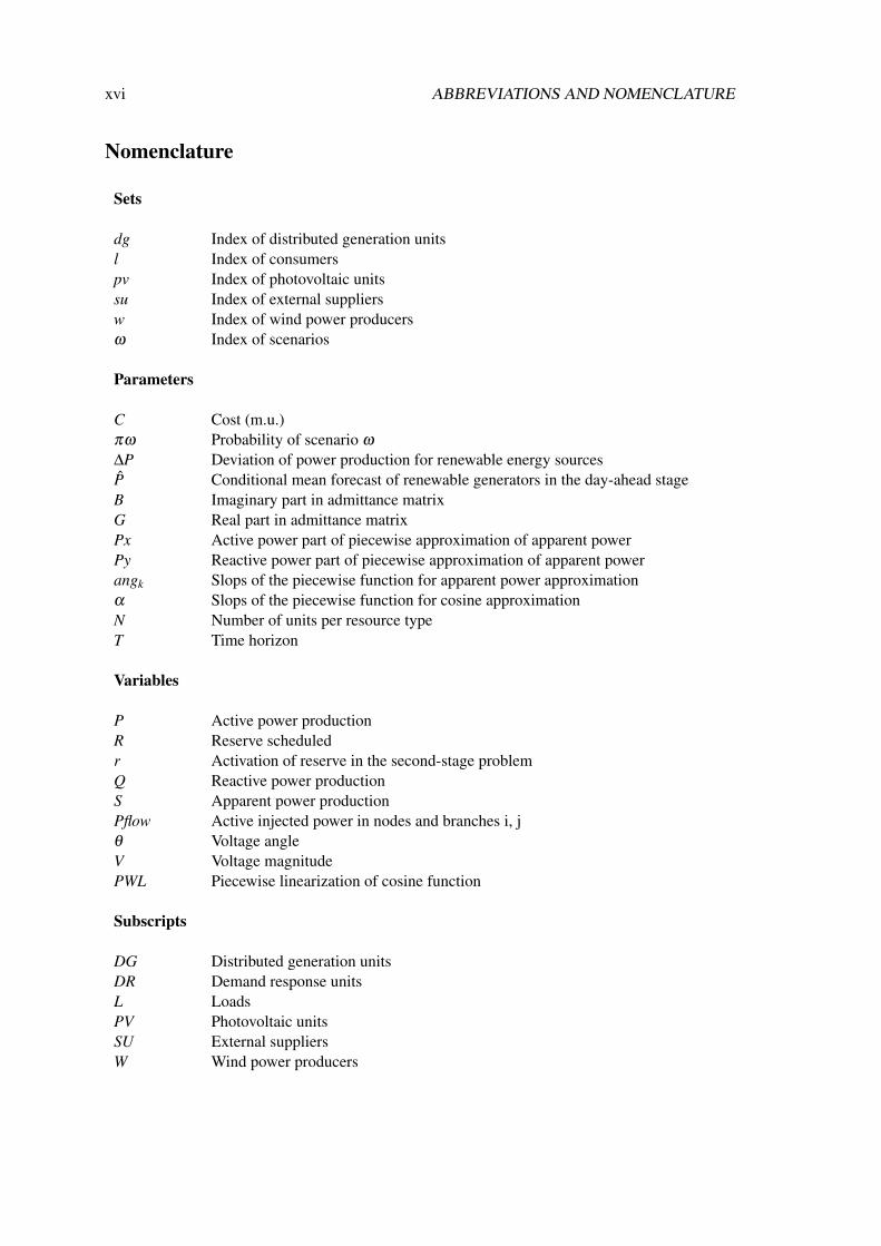
Nomenclature
Sets
dg Index of distributed generation unitsl Index of consumerspv Index of photovoltaic unitssu Index of external suppliersw Index of wind power producersω Index of scenarios
Parameters
C Cost (m.u.)πω Probability of scenario ω
∆P Deviation of power production for renewable energy sourcesP Conditional mean forecast of renewable generators in the day-ahead stageB Imaginary part in admittance matrixG Real part in admittance matrixPx Active power part of piecewise approximation of apparent powerPy Reactive power part of piecewise approximation of apparent powerangk Slops of the piecewise function for apparent power approximationα Slops of the piecewise function for cosine approximationN Number of units per resource typeT Time horizon
Variables
P Active power productionR Reserve scheduledr Activation of reserve in the second-stage problemQ Reactive power productionS Apparent power productionPflow Active injected power in nodes and branches i, jθ Voltage angleV Voltage magnitudePWL Piecewise linearization of cosine function
Subscripts
DG Distributed generation unitsDR Demand response unitsL LoadsPV Photovoltaic unitsSU External suppliersW Wind power producers

ABBREVIATIONS AND NOMENCLATURE xvii
Superscripts
E Energyup Upward reservedw Downward reserveDA Day-ahead stageRT Real-time stageact Activation of reservecut Generation curtailment power of DG unitsspill Spillage of renewable powershed Load sheddingMax Maximum threshold of a variableMin Minimum threshold of a variable

Chapter 1
Introduction
1.1 Background and motivation
Carbon emissions have caused an increase of 4 oC of the global temperature, this increase could
cause a sufficient eventual sea level rise to submerge land that is currently home to 470–760
million people globally [1]. Over the past years there has been an accelerated growth in the global
economy. As a consequence, the emissions resulting from the electricity demand have skyrocketed
and the trend is to maintain this level of growth as new economies are arising. An overview of
the past years situation considering the emissions topic can be found in [2]. The environmental
concerns have never been so important and these factors are preponderant to a change the power
production paradigm.
Despite the efforts made to develop more power systems fed by Renewable Energy Sources
(RES), reducing the emissions of greenhouse gases, the fact is that the actual panorama still implies
the use of large amount of fossil fuels to fulfill the energy needs of the populations specially in
developing countries.
What is still a reality today is a centralized scheme where the production is assured by large
power plants (working mainly on fossil fuels) and transported through long distances to the con-
sumers. This scheme has negative aspects such as:
• Efficiency: By generating the energy in large power plants and transporting it through large
distances the associated losses are high;
• Reliability: There is a high level of dependency on the power plants and if an outage occurs
on any of them, a large amount of consumers can face a blackout. In addition, a great
amount of the equipment in use today was designed to meet the requirements of the past
and is outdated today. These aspects make the system less reliable and the maintenance
more complex and expensive;
• Environment: The centralized generation is mainly assured by non-RES and that contributes
to a great set of concerns, like air pollution, water use and discharge, land use, and waste
generation.
1
2 Introduction
In this context, many countries are trying to move from this form of centralized power to a
national network of MGs [3], aiming to reduce power losses and move towards a clean power
system.
A MG is a network that comprises various Distributed Energy Resources (DER), such as wind
turbines, photovoltaic (PV) cells, small-hydro plants, Combined Heat and Power (CHP), small
diesel generators, etc. A DER can be defined as an electric power generator within the distribution
network or on the customer side of the network, usually with a capacity of the sources varying from
few kW to 1-2 MW [4], DER can also include Energy Storage Systems (ESS), such as batteries
or super capacitors [5, 6]. MGs can operate interconnected with the main distribution grid, or in
an autonomous way (island mode) in case of external faults. From the grid operator point of view,
a MG can be seen as a controlled entity within the power system that can be operated as a single
aggregated load or generator [7] and, given attractive remuneration, as a small source of power or
ancillary services supporting the network [4]. A VPP is an Energy Management System (EMS) in
charge of aggregating and managing the DER. The VPP enable the collective participation of DER
in electricity markets. The VPP provides a centralized control for multiple DERs [8], allowing
them to provide energy or even ancillary services. The VPP enable the collective participation of
DER in electricity markets
Most MGs and VPPs take advantage of RES such as solar, wind, and hydro power to being
able to participate in the market with low generation prices and low emissions. ESS, like batteries,
play an important role, by storing the energy generated by intermittent RES to increase the power
system reliability, and to ease the demand on the power grid. Distributed Generation (DG) solves
many of the centralized system most troubling issues such as:
• Efficiency: Generation is closer to the consumers, so the line losses and the costs of material
to the installation are minimized.
• Environmental: A system full of DER, particularly one that uses RES, has more positive
environmental impact than the traditional power system, specifically when it comes to land
use and air pollution;
• Reliability: The maintenance on the components and the potential increase on the installed
capacity is much easier to perform. The fact of being a decentralized scheme implies a
higher level of autonomy and reliability (a failure in one section does not disrupt the entire
system);
• Costs: Nowadays the cost of the non-RES is much higher than RES and it tends to increase
more and more in the future. Technological advances are bringing down the manufacturing
and maintenance costs of the DER. Thus, the tendency is to replace non-RES generation by
RES generation.
1.1 Background and motivation 3
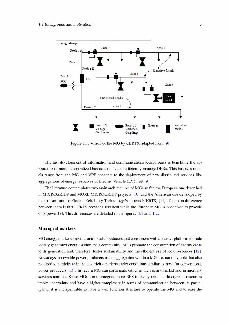
Figure 1.1: Vision of the MG by CERTS, adapted from [9]
The fast development of information and communications technologies is benefiting the ap-
pearance of more decentralized business models to efficiently manage DERs. This business mod-
els range from the MG and VPP concepts to the deployment of new distributed services like
aggregations of energy resources or Electric Vehicle (EV) fleet [9].
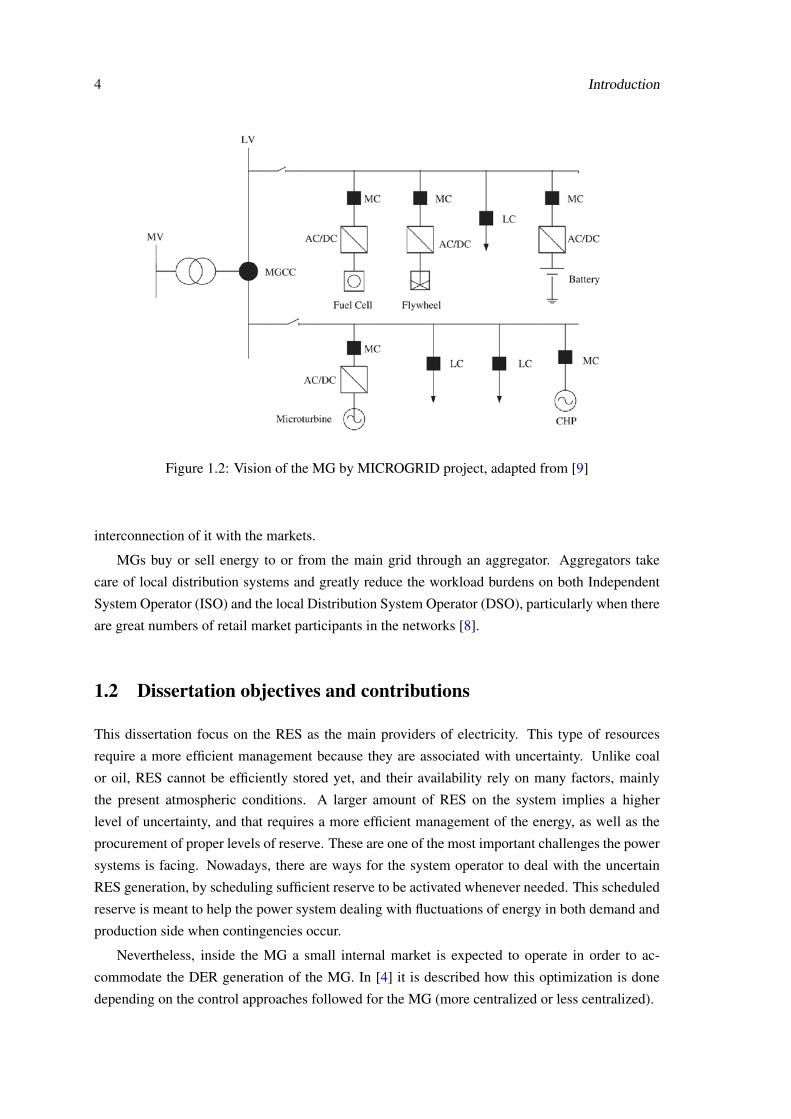
The literature contemplates two main architectures of MGs so far, the European one described
in MICROGRIDS and MORE MICROGRIDS projects [10] and the American one developed by
the Consortium for Electric Reliability Technology Solutions (CERTS) [11]. The main difference
between them is that CERTS provides also heat while the European MG is conceived to provide
only power [9]. This differences are detailed in the figures 1.1 and 1.2.
Microgrid markets
MG energy markets provide small-scale producers and consumers with a market platform to trade
locally generated energy within their community. MGs promote the consumption of energy close
to its generation and, therefore, foster sustainability and the efficient use of local resources [12].
Nowadays, renewable power producers as an aggregation within a MG are, not only able, but also
required to participate in the electricity markets under conditions similar to those for conventional
power producers [13]. In fact, a MG can participate either in the energy market and in ancillary
services markets. Since MGs aim to integrate more RES in the system and this type of resources
imply uncertainty and have a higher complexity in terms of communication between its partic-
ipants, it is indispensable to have a well function structure to operate the MG and to ease the
4 Introduction
Figure 1.2: Vision of the MG by MICROGRID project, adapted from [9]
interconnection of it with the markets.
MGs buy or sell energy to or from the main grid through an aggregator. Aggregators take
care of local distribution systems and greatly reduce the workload burdens on both Independent
System Operator (ISO) and the local Distribution System Operator (DSO), particularly when there
are great numbers of retail market participants in the networks [8].
1.2 Dissertation objectives and contributions
This dissertation focus on the RES as the main providers of electricity. This type of resources
require a more efficient management because they are associated with uncertainty. Unlike coal
or oil, RES cannot be efficiently stored yet, and their availability rely on many factors, mainly
the present atmospheric conditions. A larger amount of RES on the system implies a higher
level of uncertainty, and that requires a more efficient management of the energy, as well as the
procurement of proper levels of reserve. These are one of the most important challenges the power
systems is facing. Nowadays, there are ways for the system operator to deal with the uncertain
RES generation, by scheduling sufficient reserve to be activated whenever needed. This scheduled
reserve is meant to help the power system dealing with fluctuations of energy in both demand and
production side when contingencies occur.
Nevertheless, inside the MG a small internal market is expected to operate in order to ac-
commodate the DER generation of the MG. In [4] it is described how this optimization is done
depending on the control approaches followed for the MG (more centralized or less centralized).
1.3 Dissertation structure 5
In this context, this dissertation offers a contribution to the energy and reserve scheduling
within a MG, by introducing new approaches to solve the problem. The objective is to develop a
program capable of providing optimal solutions for energy and reserve schedule in a MG, at the
minimum cost for the MG operator. The main contributions under the scheduling problem of a
MG are threefold:
• Conception, design and development of a stochastic energy and reserve scheduling to deal
with uncertain production in the scope of a MG;
• Incorporation of the DC Optimal Power Flow (OPF) in the scheduling problem to avoid
network congestion;
• Integration of a recent AC OPF linearization to comply with distribution network charac-
teristics. This new AC OPF linearization approximates the natural behavior of the network
by considering both active and reactive power. Thus, the model is ready to give feasible
solutions to the decision-maker, by solving potential congestion and voltage problems that
may arise in a MG full of DER where bi-directional power flow is common.
1.3 Dissertation structure
This dissertation is organized into five chapters. In addition to the introduction chapter, four more
chapters are included, as described in the following paragraphs.
Chapter 2 covers the state of the art of this topic. The energy scheduling problem is explored,
taking into account the formulation type and objective function, solving method, uncertainty, de-
mand response, reactive power and emissions. It is covered the topic of energy and reserve in MGs
and VPPs. Also in this chapter previous work in this topic is presented.
Chapter 3 covers the energy and reserve market model. The two-stage stochastic linear pro-
gramming is described as a way of dealing with the uncertain generation within a MG. Two opti-
mization models were designed. Firstly, the stochastic problem under the DC model of the network
(simplest OPF model, also called in this dissertation as the benchmark model) was implemented.
Secondly, the design of the stochastic problem with a full linearized AC OPF. This approach is
convex and completely linear, as the non-convexities and nonlinearities of the standard AC OPF
were linearized.
Chapter 4 presents the outline of the MG test and the results of the simulation for both DC and
AC stochastic approaches. In addition, different network characteristics were assessed to evaluate
the effects of different system parameters on the solution such as the number of scenarios and the
reactance/resistance ratio of the distribution lines. Quality metrics (such as value of the stochastic
solution and expected value of perfect information) for the assessment of the stochastic solution
were also performed and discussed.
Chapter 5 highlights the most important conclusions of the work developed and described
in this dissertation. Future developments and ideas for improving the proposed approaches are
emphasized.

6 Introduction
Chapter 2
State of art
2.1 Introduction
MGs and VPPs are two distribution network concepts that can participate in active network man-
agement of a smart grid [8]. In chapter 1 it was given a definition of these two concepts, in this
chapter it will be discussed this two terms in a market overview and there will be presented the
reasons why MGs and VPPs can be the future paradigm of the electrical system. [4] and [10] in-
vestigate the market configurations in MV and LV networks inside a MG, the control approaches
followed and the security within the MICROGRIDS and MOREMICROGRIDS (Europe) project
framework and the main differences towards CERTS (USA) project framework. In [13] are pre-
sented the different electricity market designs in use today: Pool, Bilateral Contracts and the
combination of both. In addition to the conventional electricity markets this project covers also
the reserve markets, fundamental when dealing with RESs and their uncertainty and variability.
2.2 Energy scheduling
The MGs and VPPs market is predicted to increase 4000MW in capacity between 2017 and 2020
[3]. The growing penetration of DG, allied with the RES uncertainty generation, makes scheduling
them in a power system a fundamental task [14]. In literature, the most common aspects of the
energy scheduling problem for MGs and VPPs are:
• Formulation type and objective function;
• Solving method;
• Uncertainty (relatable to RES, load, price, etc.);
• Demand response;
• Reactive power;
• Emissions.
7
8 State of art
Taking into account aforementioned aspects of the scheduling problem, there is literature that
shows a suitable perspective for readers to select the best methods based on advantages to schedule
the DERs in the power system [15], are detailed in the following of this section.
2.2.1 Energy scheduling problem associated with formulation type and objectivefunction
In a MG the EMS collects information about the electricity market, load and DGs forecast, con-
sumer preferences. Based on that data, does the energy and reserve scheduling (how much power
to buy and whom to buy) [15]. In a VPP the aggregator provides the power production profile
based on the negotiations with the producers taking into account their expected production fore-
cast [15].
There are several approaches to do the optimization for MGs considering the formulation type
and the most common ones in the literature are based on: linear programming [16, 17, 18, 19];
non-linear programming [20]; mixed integer linear programming [21, 22, 23, 24, 25, 26, 27, 28,
29]; mixed integer non-linear programming [30, 31, 32, 33, 34]; quadratic programming [35, 36]
and constrained linear least-squares programming [37]. For VPPs, the formulation type can be
based on: linear programming [38, 39, 40, 41, 42, 43]; non-linear programming [44]; mixed
integer linear programming [45, 46, 47, 48, 49, 50, 51, 52, 53, 54, 55]; mixed integer non-linear
programming [56, 57, 58];dynamic programming [59] and quadratic programming [60].
The mixed integer linear programming is the most common class of formulation type used in
literature to model the energy scheduling problem in both MGs and VPPs. It’s has simplicity as
the biggest advantage, however it only admits linear, continuous and integer variables, so when the
problem is nonlinear, mathematic relaxation techniques need to be used to convert it into a mixed
integer linear problem. Some of those relaxation techniques are presented in [26, 27, 53, 61, 62,
63].
One of the main objectives of a MG is providing power to the consumers at the minimum
cost of production, so normally, for MGs, the objective function is cost minimization. The main
objective of a VPP is to maximize its profit, so, for VPPs, the objective function is the profit
maximization. However, other objective functions can also be a priority, minimization of the
emissions for example.
Most computational optimization methods have focused on solving single-objective energy
scheduling problems. However, there are a large number of applications that require the simul-
taneous optimization of several objectives which are often in conflict, and to face this challenge,
some authors have proposed multi-objective algorithms to solve it [64]. As an example, [62]
deals with the simultaneous scheduling of electrical vehicles and responsive loads to reduce both
operation cost and emission in presence of wind and PV powers in MGs. For a more complete
information about the energy scheduling problem associated with formulation type and objective
function, a table with formulation types and objective functions for a set of problems is highlighted
in [15].
2.2 Energy scheduling 9
2.2.2 Solving methods for the energy scheduling problem
Depending on the modeling of the energy scheduling problem for both MGs and VPPs, the prob-
lem can be solved using different solving methods, for example, deterministic, stochastic, iterative
or heuristic methods.
More precisely, there are various solving methods within the class of mathematical meth-
ods that have been used for solving MGs problems, such as: series and probabilistic methods
[65]; convolution method [18]; mesh adaptive direct search [35]; benders decomposition [29, 66];
connection matrix [67]; branch-and-bound algorithm [20]; Lagrangian relaxation decomposition
[68]; combinatorial optimization [69]; newton-raphson method [70] and constrained linear least-
squares programming [37]. Similarly, the following mathematical methods have been used for
VPPs optimization problems, such as: interior point method and primal-dual sub-gradient algo-
rithm [71, 72, 73]; point estimate method [56]; branch-and-bound method [60, 74]; decision Tree
[75, 76]; event-driven service-oriented framework [44]; hierarchical structure [77, 78]; game the-
ory [79]; area-based observe and focus algorithm [80] and fuzzy simulation and crisp equivalent
[10].
Other class of solving methods are heuristic, these methods can be seen as simple proce-
dures that provide satisfactory and quick solutions to large instances of complex problems rapidly.
Meta-heuristics are generalizations of heuristics in the sense that they can be applied to a wide
set of problems, needing few modifications to be adapted to a specific case [64]. The main dis-
advantages of these methods are the optimal solution being associated with estimations and the
possible situation related with divergence being more frequent than in mathematical methods.
Also, the solution may convert to a local minimum instead of a global one. There are various
Heuristic and Meta-Heuristic methods proposed to solve the problem associated with MGs, for
example: Particle Swarm Optimization (PSO) [62, 81, 82]; Binary Particle Swarm Optimiza-
tion (BPSO) [83]; θ -Particle Swarm Optimization (θ -PSO) [84]; Krill Herd Algorithm (KHA)
[85]; Teaching–Learning-Based Algorithm (TLBA) [50]; Genetic Algorithm (GA) [86, 87]; Non-
dominated Sorting Genetic Algorithm II(NSGA-II) [88, 89]; hybrid algorithm of Lagrangean Re-
laxation and GA Algorithm (LRGA) [90]; Adaptive Modified Firefly Algorithm(AMFA) [91];
Evolutionary Programming (EP) [92]; Hill Climbing Technique (HC) [92]; Differential Evolution
Algorithm(DEA) Accompanied with Fuzzy Technique [76, 93], Competitive Heuristic Algorithm
for Scheduling Energy-generation (CHASE) [36] and Habitat Isolation Niche Immune Genetic
Algorithm (HINIGA) [94], among others. The heuristic optimization methods addressing the
scheduling problem in VPP framework are Multi-Objective Genetic Algorithm [95], GA [96, 97],
PSO [98], Accelerated Particle Swarm Optimization (APSO) [99] and Hill Climber and Greedy
Randomized Adaptive Search Procedure (GRASP) [100].
In [101], a mathematical mixed integer linear program is formulated and an efficient heuristic
approach is designed and subsequently built into a simulated annealing framework to solve the
problem.
In some cases, the complexity of the problems to solve is so high that even mathematical
10 State of art
or heuristic and meta-heuristic methods are not able to obtain accurate solutions in reasonable
runtimes. In these cases parallel processing becomes an interesting alternative [102].
2.2.3 Scheduling problem considering reactive power
In the power system, the reactive power control is one of the main aspects related with the energy
scheduling problem. In the distribution system, the reactive power control is essential to ensure
the energy delivery with high level of power quality. The DSO is responsible for the active and
reactive power flow in the distribution system. Conventionally, the DSO controls the flow of
reactive power using static equipment’s as capacitor banks and through the reactive power that
comes from the upstream connection. Currently and under the smart grid paradigm, the DSO may
also be able to acquire active and reactive power from DERs as well as the from local electricity
markets to solve potential congestion and voltage problems [103].
In contrast, the MG operator may be able to purchase both active and reactive power require-
ments to fulfill the needs of its grid. This control, can include static equipment, as well as DER
within the MG. In addition, the MG operator must take into account some constraints related to re-
active power, as reactive loads in a bus (reactive power output of a unit and reactive load shedding
of a bus). In fact, reactive power generation has been commonly used for power loss minimiza-
tion and voltage profile improvement in power systems. However, the opportunity cost of reactive
power generation should be considered since it affects the frequency control capability of the gen-
erator to some degree. [104] proposed a distributed nonlinear control based algorithm to achieve
the optimal reactive power generation for multiple generators in a power grid.
For a complete review on the reactive power flow parameters and reactive power control, the
reader is recommended to consult [15].
2.2.4 Scheduling problem considering emissions
Considering the rising of the environmental concerns over the past years, one of the main ob-
jectives of the energy scheduling in a vast set of problems is the minimization of the emissions.
Some DERs, especially conventional ones have undesirable impacts on the environment, through
the greenhouse gases emitted as a sub product of electricity. For this reason, in the energy schedul-
ing problem, the literature have considered emission as a function that should be minimized. This
can be done by maximizing the output of renewable energy. In this section some of these functions
are investigated and the type of consideration is explained too [15].
The uncertainty associated with the availability of DER implies an uncertainty in the total
emissions produced in a power system. For example, in [62] due to the uncertainty associated
with Wind and PV powers, the emission function is formulated in two-stages. In the first-stage, the
pollution resulting from the scheduled power generation for load and reserve supplies is calculated.
In the second-stage, is calculated the pollution pertaining to the variations of scheduling of the
units caused by changes in the behaviors of wind and PV power producers. In this context, an
objective function related to the total emissions during the scheduling period is proposed in [31]. In
2.2 Energy scheduling 11
[105] is quantified the economical impact of DG on pollutant emission cost reduction in the form
of a new techno-economic factor. Using this innovative approach would enable system operators
to have simultaneous control on network losses and pollutants emission rate of thermal generation
unit in the case of deciding to obtain DER economical advantages.
For a complete survey on different emission functions and different types of consideration, the
reader is advised to consult [15].
2.2.5 Scheduling problem under uncertainty of DER producers
Current electricity markets designs do not properly cover the uncertain production of RES, mainly
PV and wind. In reality, the market follows a sequential and deterministic market design be-
tween day-ahead and real-time stages, since the whole information about the future is represented
through a single-value forecast at day-ahead stage.
Furthermore, the uncertain renewable production is cleared during the real-time market with
penalties for renewable producers that cannot supply the expected forecast established at day-
ahead market. In this context, one of the challenges of the current electricity markets is to revise
their deterministic market design by adapting advanced tools able to support decision-making
under uncertainty. There are several ways to deal with uncertainty such as stochastic programming,
robust optimization and optimization using linear decision rules (LDR).
The stochastic programming is one of the most used tools to address problems dealing with
uncertainty, it has the advantage of modeling problems where uncertainty can happen over differ-
ent time spans, originating different decision horizons, defining different stages where decisions
are taken. The use of stochastic integrated market that co-optimizes day-ahead and balancing
stages is a proposed path in the recent literature [106]. However, the performance of such model
will heavily depend on the quality of the input information, in this case of the forecast information
from renewable production [13]. It is used when the distribution of the error is know.
The robust optimization was developed to deal with the worst-case of the uncertainty in
optimization problems where the error distribution is not known and is inside an interval. This
characteristic makes it ideal to tackle problems with severe uncertainties, thereby based on the
worst case analysis and modeled by the Wald’s max-min model [107]. This type of optimization
returns a feasible solution for all the uncertainty realizations (scenarios) from the uncertainty set
and an optimal solution for the worst-case scenario.
The optimization using LDR approximates the stochastic programming providing a tractable
linear problem at the cost of a potential loss of optimality [108, 109]. It consists in modeling
the uncertain decision variable of stochastic model through an affine function. In electric power
systems, LDR has been recently used to solve problems in which the uncertainty is modeled by
linear functions. In these cases where the objective is obtaining a solution neither optimistic
(stochastic approach) neither pessimistic (robust approach), LDR is an alternative [13].
12 State of art
Decision-making under uncertainty in energy planning is essential for the proper functioning
of the power system, ensuring suitable levels of system reliability. Thus, the appropriate mod-
elling of the uncertainties in the energy scheduling problem has been studied. More precisely, un-
certainties can take the form of power generation and load deviations, market prices, atmospheric
conditions, natural catastrophes, etc.
In [22] it is considering uncertainty in EV driving schedule, the author proposes a new EV
fleet aggregator model in a stochastic formulation of DER, and it is used an optimization tool to
address DER investment and scheduling problems. The objective is to assess the impact of EV
interconnections on optimal DER solutions.
Uncertainties generate different scenarios with different parameters, and a problem with a
lot of scenarios can be an extremely complex and time consuming process, that is why scenario
reduction methods have been used in both MGs and VPPs to make the problem more efficient
without compromising the reliability of the results [15]. Some of these methods are detailed in
[50, 110].
2.2.6 Scheduling problem considering demand response
The United States Federal Regulatory Commission (FERC) defines Demand Response (DR) as
changes in electric usage by demand-side resources from their normal consumption patterns in
response to changes in the price of electricity over time, or to incentive payments designed to
induce lower electricity use at times of high wholesale market prices or when system reliability
is jeopardized. [111]. Loads are encouraged or required to reduce or modify their consumption
in benefit of grid operation. For example, demand response programs have been used to shift
loads (residential and industrial) away from peak periods [112]. In power systems with high
solar penetration there is a major interest in shifting the loads to the daytime period where the
solar generation is higher, while shifting other types of generation to other time periods. These
programs can be divided in two categories, time based and incentive-based programs. In time-
based programs the price of electricity varies according to the supply cost of electricity and there
is no incentive or penalty for this type of demand response programs. For instance, in Portugal
there are tariffs for the consumers called tarifa bi-horária and tri-horária and tetra-horária for
industry, in which the prices vary according to the demand in high peak or off-peak periods limited
in time intervals. Off-peak hours are nigh time and weekends in which the cost of electricity is
lower for the consumers in this demand response program, therefore there is a natural will for
shifting the load to these periods [113]. In incentive-based programs there are voluntary programs
to curtail without penalties, mandatory programs and programs in which customers can negotiate
the amount of load reduction at a negotiated price. This kind of programs are widely used in
various scheduling problems, mainly in MGs and VPPs. Interested readers on these types of
demand response programs are recommended to check [15].
2.3 Energy and reserve 13
2.3 Energy and reserve
In addition to the conventional energy markets, ancillary service markets are also essential to the
system by ensuring system reliability. These markets are tailored to cope with unforeseen events
which may disturb the normal balance of the power system, such as weather-related fluctuations
in consumption, short-term changes in major industrial consumption, breakdowns in production
facilities, power line outages, and other grid component breakdowns [114].
Ancillary services
FERC defines ancillary services (AS) as "Those services necessary to support the transmission
of electric power from seller to purchaser, given the obligations of control areas and transmitting
utilities within those control areas, to maintain reliable operations of the interconnected transmis-
sion system. Ancillary services supplied with generation include load following, reactive power-
voltage regulation, system protective services, loss compensation service, system control, load
dispatch services, and energy imbalance services" [115].
In United States, the North American Electric Reliability Corporation (NERC) and/or regional
Coordinating Councils, such as the Western Electricity Coordinating Council (WECC) are the
entity tasked to establish reliability standards where market operators look for AS from market
participants. Winning bids for energy and ancillary services are mutually exclusive, but a generator
can receive a compensation for both generation and ancillary service supply in the same period as
long as the capacities allocated to each one do not overlap [116].
This section of the project addresses the management of energy and AS in a MG context. As
it was referred, in the future there will be more and more RES generating electricity and therefore
the uncertainty will increase significantly. It is a good solution to interconnect the energy and
reserve to cope with that uncertainty. The following research works present innovative methods
for doing the management of energy and AS in a MG.
In [14] is presented a novel stochastic energy and reserve scheduling method for a MG which
considers various type of DR programs. In the proposed approach, all types of customers can
participate in demand response programs which will be considered in either energy or reserve
scheduling. Also, the uncertainties related to renewable DG are modeled by proper probability
distribution functions and are managed by reserve provided by both DGs and loads. In [117] is pre-
sented a coordinated control strategy for managing the active power reserve in isolated MGs. The
methodology can be applied in MGs where a generator assumes the role of the isochronous gen-
erator for the overall system. The algorithm evaluates control actions in the on-line environment
by solving a constrained dynamic optimization problem which maximizes the overall spinning
reserve and, in particular, the reserve offered by the master unit equipped with the isochronous
governor controller.
In [118] is proposed a bi–level formulation for a coupled MG power and reserve capacity
planning problem, cast within the jurisdiction of a DSO. The upper level problem of the pro-
posed bi–level model minimizes the planning and operational costs of a MG, while the lower level
14 State of art
problem ensures reliable power supply by the DSO.
In [119] is used a stochastic model predictive control (SMPC) approach to do the energy
management in a MG in the presence of RES where the uncertainties created by this resources are
represented by typical scenarios obtained through a two-stage scenario reduction technique and a
deterministic finite horizon mixed integer quadratic programming model is formulated based on
the selected typical scenarios.
In [120] the author proposes an efficient two-stage stochastic optimal energy and reserve man-
agement approach for a MG. It can consider all possible sources and levels of nodal power un-
certainties. In the first-stage, the optimal power schedule for possible uncertainties is determined
based on the load, wind and solar power forecasts. The actual reserve for the discrepancy between
the measured and forecasted data is directly dispatched at second-stage.
In [71] the author considers that operating reserve capacity in a power system is flexible and
that one should optimize it by cost-benefit analysis. Based on the reliability evaluation of the
generation system, a clearing model of the operating reserve market is proposed to determine the
optimal reserve capacity and simultaneously clear the operating reserve market by using a heuristic
method. The model is discussed on both uniform-price and pay-as-bid auction mechanisms.
In [96, 97] is addressed the bidding problem faced by a VPP in a joint market of energy and
spinning reserve. The proposed bidding strategy is based on the deterministic price-based unit
commitment which takes the supply-demand balancing constraint and security constraints of VPP
itself into account. The presented model creates a single operating profile from a composite of the
parameters characterizing each DER and incorporates network constraints into its description of
the capabilities of the portfolio.
Nevertheless of all innovative methods emerged in the scientific community on energy and
reserve scheduling of a MG under uncertain renewable production, there is still gaps in the models
that are partially covered by this dissertation in the following sections.
Chapter 3
Energy and reserve market model
3.1 Introduction
In the XXI century, the daily problems we face, in areas like finance, transportation, agriculture,
engineering, etc. require more and more decision making under uncertainty. Uncertainty has a
direct influence on the value of money, fuel prices, raw materials, etc.
Uncertain variables such as environmental conditions, military conflicts and natural catastro-
phes can have a substantial impact on the prices of products, services and goods. Thus, optimiza-
tion problems should include uncertain variables that enable decision makers to have complete
knowledge of system behaviour, and therefore be prepared for eventual undesirable events. The
result is a cost considering all possible scenarios with the associated probability of occurrence
(most of the time just the ones with a significant probability, to keep the problem simple) and
return the total expected cost.
The optimization problem proposed in this project contemplates the minimization of energy
and reserve costs within a MG following a stochastic approach.
3.2 Optimization under uncertainty (two-stage stochastic program-ming)
Optimization problems under uncertainty are characterized by the need of making decisions before
knowing how these decisions will affect the system. In this context several methodologies for
solving optimization problems under uncertainty were proposed and this project addresses the
two-stage stochastic programming.
The ability to model problems where uncertainty can realize over different decision horizons,
thereby defining a number of stages, makes the stochastic programming one of the most used tools
to solve problems and find optimal solution in expectation [13].
In a two-stage stochastic programming paradigm, the decision variables of the optimization
problem under uncertainty are partitioned into two sets: There are decision variables (x) that
must be decided prior to the realization of the contemplated uncertain events, and these variables
15
16 Energy and reserve market model
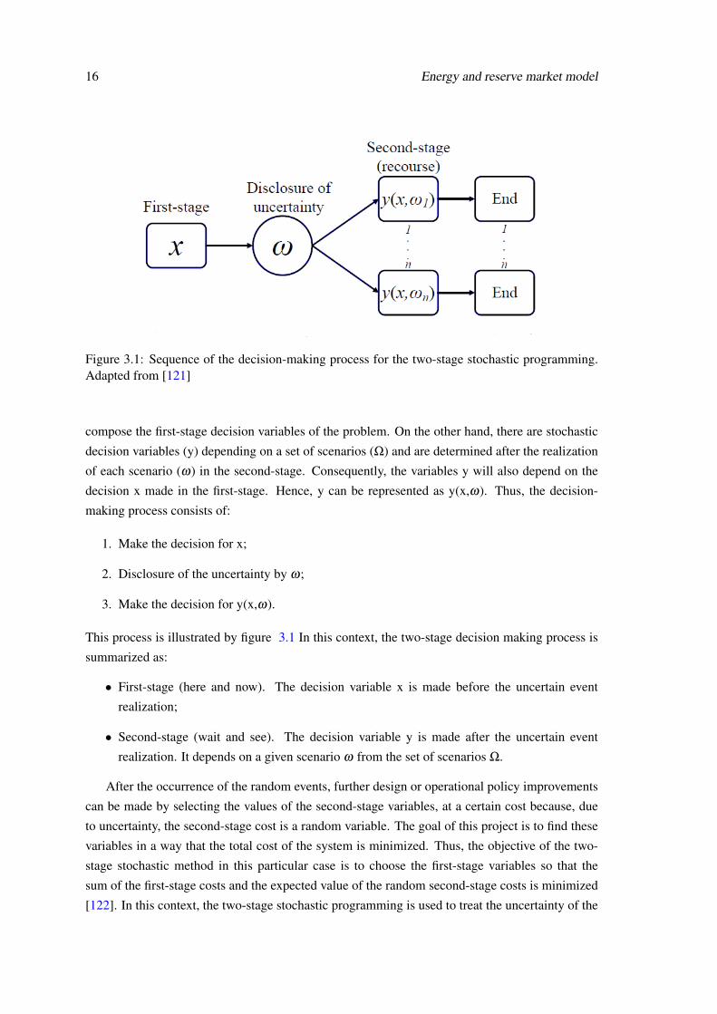
Figure 3.1: Sequence of the decision-making process for the two-stage stochastic programming.Adapted from [121]
compose the first-stage decision variables of the problem. On the other hand, there are stochastic
decision variables (y) depending on a set of scenarios (Ω) and are determined after the realization
of each scenario (ω) in the second-stage. Consequently, the variables y will also depend on the
decision x made in the first-stage. Hence, y can be represented as y(x,ω). Thus, the decision-
making process consists of:
1. Make the decision for x;
2. Disclosure of the uncertainty by ω;
3. Make the decision for y(x,ω).
This process is illustrated by figure 3.1 In this context, the two-stage decision making process is
summarized as:
• First-stage (here and now). The decision variable x is made before the uncertain event
realization;
• Second-stage (wait and see). The decision variable y is made after the uncertain event
realization. It depends on a given scenario ω from the set of scenarios Ω.
After the occurrence of the random events, further design or operational policy improvements
can be made by selecting the values of the second-stage variables, at a certain cost because, due
to uncertainty, the second-stage cost is a random variable. The goal of this project is to find these
variables in a way that the total cost of the system is minimized. Thus, the objective of the two-
stage stochastic method in this particular case is to choose the first-stage variables so that the
sum of the first-stage costs and the expected value of the random second-stage costs is minimized
[122]. In this context, the two-stage stochastic programming is used to treat the uncertainty of the
3.3 Optimal Power Flow (OPF) – Benchmark for a DC model 17
RES in the MG and as a result find the best energy and reserve management of the MG ensuring
proper levels of system stability and reliability, taking into consideration the uncertainty modelled
in the form of a scenario set. This type of two-stage stochastic problem can be modeled by:
Minx,y(ω)
CT x+ ∑ω∈Ω
π(ω)q(ω)T y(ω) (3.1)
s.t. Fx = f , (3.2)
T (ω)x+H(ω)y(ω) = h(ω), ∀ω (3.3)
x≥ 0, ∀ω (3.4)
y(ω)≥ 0, ∀ω (3.5)
To be noted that associated with each scenario is a probability of occurrence π(ω). The func-
tion 3.1 minimizes the total cost of both first and second-stages, considering the recourse cost of
the second-stage with weighted probability. Additionally, q(ω) stands for the matrix with the costs
related to the second-stage decision variable. This problem is subjected to first-stage constraints
3.2 and to constraints that connect the first-stage decision with the recourse decision 3.3. Thus,
the first-stage decision affects all the matrixes and vectors of the second-stage [13].
3.3 Optimal Power Flow (OPF) – Benchmark for a DC model
The DC OPF is a linearization of the AC OPF and commonly used as a standard method for
considering network behavior in power system problems. In this dissertation the DC OPF is firstly
implemented on the energy and reserve scheduling problem in a MG (also called as benchmark
model in the remaining of this project), and then further compared to the AC OPF.
The DC model implies a series of simplifications justified by operational considerations under
normal operating conditions. These approximations not only linearize the non-linear problem, but
also make the problem easier to implement. Some variables are not considered on this formulation
type and others disappear as a result of the simplification process. The outcome is a problem with
less data that requires less time and processing power to compute.
Approximation to the power flow equations
The AC power-flow equations in a line are the following
P f lowi, j = |Vi||Vj|(Gi j cos(θi−θ j)+Bi j sin(θi−θ j)) (3.6)
Q f lowi, j = |Vi||Vj|(Gi j sin(θi−θ j)−Bi j cos(θi−θ j)) (3.7)
There were made simplifications based on the following observations that characterize high volt-
age transmission lines. For the two-stage stochastic optimization problem using the DC model the
reactive part of the power is also not considered.
18 Energy and reserve market model
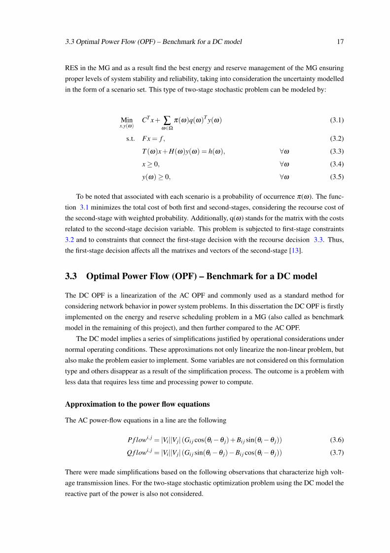
Figure 3.2: Trigonometrical sine function of a small angle.
Observation 1: The resistance of transmission circuits is significantly less than the reactance.
Usually, it is the case that the X/R ratio is between 2 and 10. So any given transmission circuit
with impedance of z = r+ jx will have an admittance of
y = 1z =
1r+ jx =
1r+ jx ×
r− jxr− jx =
r− jxr2+x2 ⇔
⇔ y = rr2+x2 − jx
r2+x2 = g+ jb(3.8)
From the equation above, and considering r«x:
g = 0 and b =−1x
(3.9)
Hence, the equation 3.6 can be converted into
P f lowi, j = |Vi||Vj|(Bi j sin(θi−θ j)) (3.10)
Observation 2: In the per-unit system, the numerical values of voltage magnitudes |Vi| and
|Vj| are very close to 1.0. The typical range under most operating conditions is located between
0.95 and 1.05 pu., therefore these values can be approximated to 1 and the equation 3.6 can be
approximated to:
P f lowi, j = Bi j sin(θi−θ j) (3.11)
Observation 3: For most typical operating conditions, the difference in angles of the voltage
phasors at two buses i and j connected by a circuit, which is θi−θ j for buses i and j, is very short,
so the approximation can be made. This approximation can be better seen in the figure 3.2, where
the length of the segments representing the sine of the angle and the angle itself are practically the
same. As a result, the active power flow of the active component of the power for a line i,j, given
by equation 3.6 is simplified as
P f lowi, j = Bi j× (θi−θ j) (3.12)
3.4 Linear approximation of the ACOPF 19
3.4 Linear approximation of the ACOPF
AC OPF is a non-convex nonlinear problem difficult to solve when together with other problems,
such as the energy and reserve scheduling problem under uncertainty. To improve computational
performance and reduce complexity, different linear methods of the AC OPF has emerged. In [61],
the author proposes a linear approximation of the AC OPF where functions for active and reactive
power flow in a transmission line are introduced, and linear approximation functions for the power
triangle equations.
For this linearization, the author considers the observations 2 and 3 of the DC model, however,
the observation 2 represents the voltage in a different way. In order to not adulterate the voltage
effects on the systems, it is taken into consideration the voltage angle in the reactive power flow.
This makes sense because the reactive power flow is influenced by the voltage angle in the buses.
3.4.1 Piecewise linearization of the power-flow equations
In the paper, the author uses the cold start Linear Programming AC (LPAC) model to approximate
the power flow equations. Within this scope, equations 3.6 and 3.7 can be approximated by
P f lowi, j = Gi j−Gi j cos(θi−θ j)−Bi j(θi−θ j) (3.13)
Q f lowi, j =−Bi j−Gi j(θi−θ j)+Bi jcos(θi−θ j)−Bi j(φi−φ j) (3.14)
where φ represents a voltage compensation so that this compensation plus the real bus base voltage
should not exceed the defined limits for bus voltage: |V | ≤ |V tn |+φn,∀n ∈ N.
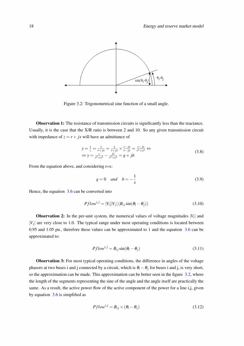
To be noted that the cosine function is a nonlinear function which can be linearized. Coffrin
et al presents the convex approximation of the cosine function through implementing a piecewise
linear function that produces a linear program in the following way [61]. A domain (l,h) must be
selected within the range (-π/2,π/2) to ensure convexity. In fact, the angle θi−θ j is typically very
small and a narrower domain is preferable. Then, a number of s tangent inequalities are placed
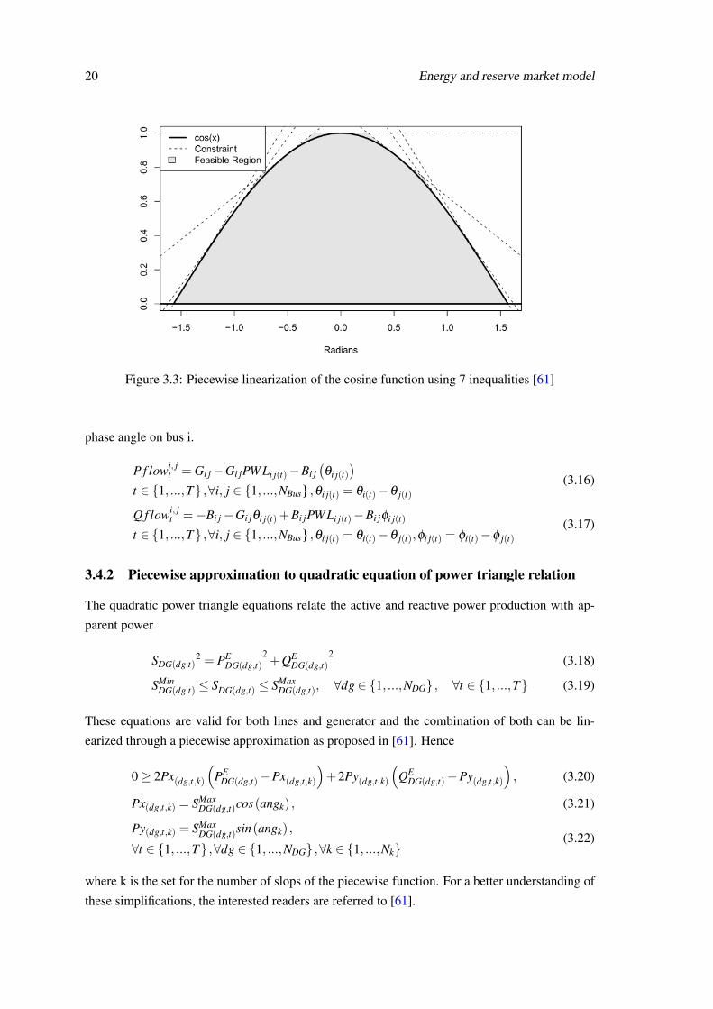
in the cosine function within the given domain to approximate the convex region. Figure 3.3
illustrates the approximation approach using seven linear inequalities. The dark black line shows
the cosine function, the dashed lines are the linear inequality constraints, and the shaded area is
the feasible region of the linear system formed by those constraints. The inequalities are obtained
from tangents lines at various points on the function.
The convex approximation of the cosine function is given by
PWLi j(t) ≤−sin(a)(θi j(t)−a
)+ cos(a)
t ∈ 1, ...,T ,∀i, j ∈ 1, ...,NBus ,a ∈ a1, ...,a7,θi j(t) = θi(t)−θ j(t)(3.15)
where α is the tangent point of each segment to the cosine function. In the case of the figure 3.3,
the feasible region is under all the 7 equations.
Hence, the equations 3.13 and 3.14 can be approximated by the following linear functions,
where PWL is the piecewise linear approximation of the cosine function as shown in [61]. θ is the
20 Energy and reserve market model
Figure 3.3: Piecewise linearization of the cosine function using 7 inequalities [61]
phase angle on bus i.
P f lowi, jt = Gi j−Gi jPWLi j(t)−Bi j
(θi j(t)
)t ∈ 1, ...,T ,∀i, j ∈ 1, ...,NBus ,θi j(t) = θi(t)−θ j(t)
(3.16)
Q f lowi, jt =−Bi j−Gi jθi j(t)+Bi jPWLi j(t)−Bi jφi j(t)
t ∈ 1, ...,T ,∀i, j ∈ 1, ...,NBus ,θi j(t) = θi(t)−θ j(t),φi j(t) = φi(t)−φ j(t)(3.17)
3.4.2 Piecewise approximation to quadratic equation of power triangle relation
The quadratic power triangle equations relate the active and reactive power production with ap-
parent power
SDG(dg,t)2 = PE
DG(dg,t)2+QE
DG(dg,t)2
(3.18)
SMinDG(dg,t) ≤ SDG(dg,t) ≤ SMax
DG(dg,t), ∀dg ∈ 1, ...,NDG , ∀t ∈ 1, ...,T (3.19)
These equations are valid for both lines and generator and the combination of both can be lin-
earized through a piecewise approximation as proposed in [61]. Hence
0≥ 2Px(dg,t,k)
(PE
DG(dg,t)−Px(dg,t,k)
)+2Py(dg,t,k)
(QE
DG(dg,t)−Py(dg,t,k)
), (3.20)
Px(dg,t,k) = SMaxDG(dg,t)cos(angk) , (3.21)
Py(dg,t,k) = SMaxDG(dg,t)sin(angk) ,
∀t ∈ 1, ...,T ,∀dg ∈ 1, ...,NDG ,∀k ∈ 1, ...,Nk(3.22)
where k is the set for the number of slops of the piecewise function. For a better understanding of
these simplifications, the interested readers are referred to [61].
3.5 Energy and reserve market model 21
3.5 Energy and reserve market model
3.5.1 Problem description
In this section, it is presented the energy and reserve market model in a MG context.
The modeling of the energy and reserve management problem in a MG environment requires
the use of the inherent characteristics of the network. A MG is a small network (distribution
system) that can operate in one of two modes: in grid connection or in isolated mode and is
composed by small-scale energy resources. Thus, modelling active and reactive energy as well
as reserve is essential in distribution systems, especially in systems under strong penetration of
renewable resources like MGs.
The MG studied on this project is a medium voltage MG with a substantial penetration of RES,
namely PV and Wind, and, as it was explained, these resources imply a high level of uncertainty.
To cope with that uncertainty, the scheduling of power reserve to be delivered on the MG when
needed is extremely important. There are a large number of events that can affect the generation
profiles, and these events are represented by scenarios associated with a certain probability of
occurrence. The problem analyses these scenarios and provides the optimal dispatch of energy
and reserve which minimizes the total operating costs of the MG.
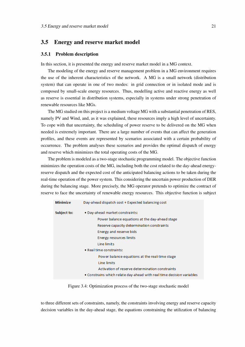
The problem is modeled as a two-stage stochastic programming model. The objective function
minimizes the operation costs of the MG, including both the cost related to the day-ahead energy-
reserve dispatch and the expected cost of the anticipated balancing actions to be taken during the
real-time operation of the power system. This considering the uncertain power production of DER
during the balancing stage. More precisely, the MG operator pretends to optimize the contract of
reserve to face the uncertainty of renewable energy resources. This objective function is subject
Figure 3.4: Optimization process of the two-stage stochastic model
to three different sets of constraints, namely, the constraints involving energy and reserve capacity
decision variables in the day-ahead stage, the equations constraining the utilization of balancing
22 Energy and reserve market model
resources and which relate day-ahead with real-time decision variables, the constraints declaring
the non-negative nature of energy- and reserve-related variables [123]. A generalization of such
optimization process is outlined in the figure 3.4.
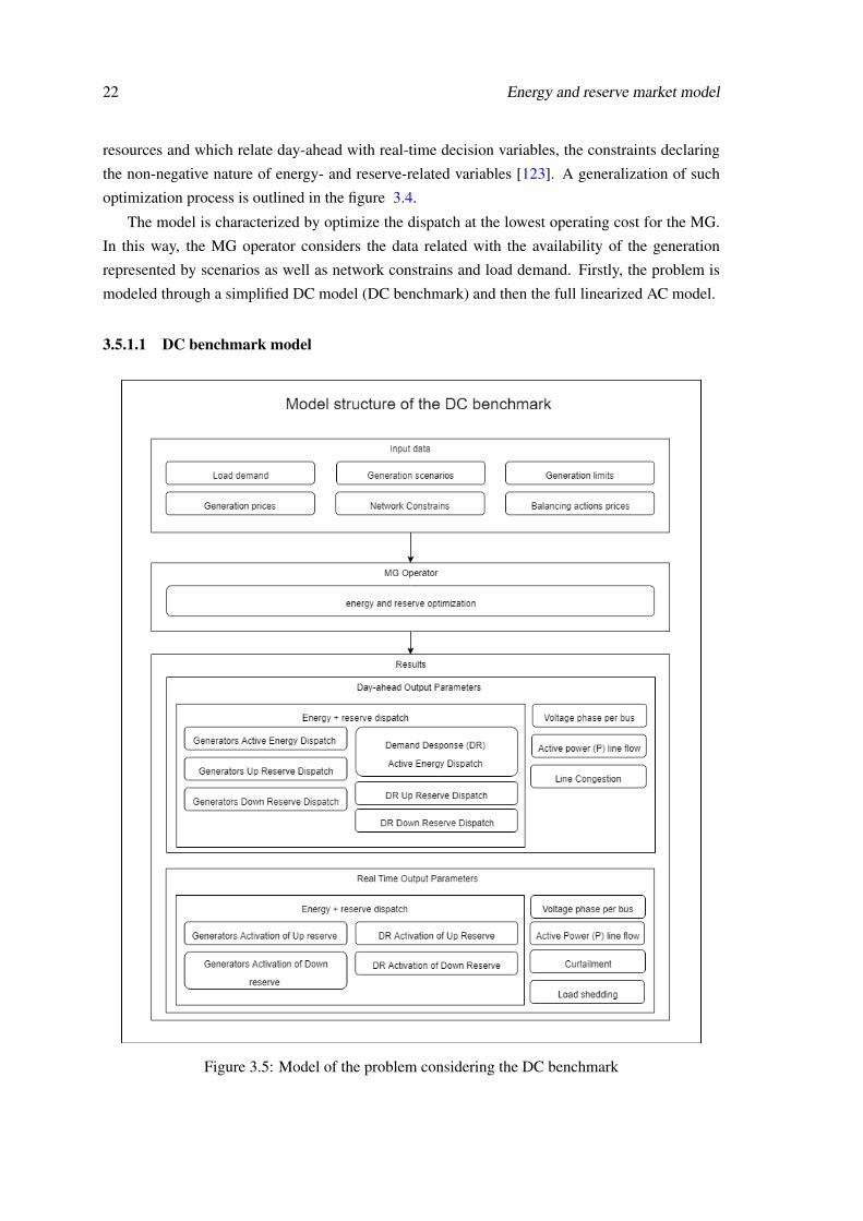
The model is characterized by optimize the dispatch at the lowest operating cost for the MG.
In this way, the MG operator considers the data related with the availability of the generation
represented by scenarios as well as network constrains and load demand. Firstly, the problem is
modeled through a simplified DC model (DC benchmark) and then the full linearized AC model.
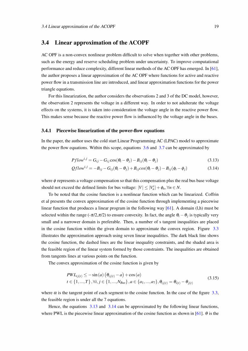
3.5.1.1 DC benchmark model
Figure 3.5: Model of the problem considering the DC benchmark
3.5 Energy and reserve market model 23
3.5.1.2 Full linearized AC model
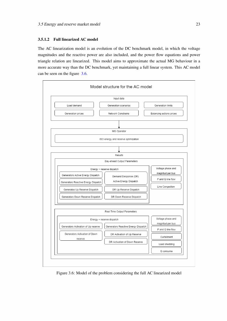
The AC linearization model is an evolution of the DC benchmark model, in which the voltage
magnitudes and the reactive power are also included, and the power flow equations and power
triangle relation are linearized. This model aims to approximate the actual MG behaviour in a
more accurate way than the DC benchmark, yet maintaining a full linear system. This AC model
can be seen on the figure 3.6.
Figure 3.6: Model of the problem considering the full AC linearized model
24 Energy and reserve market model
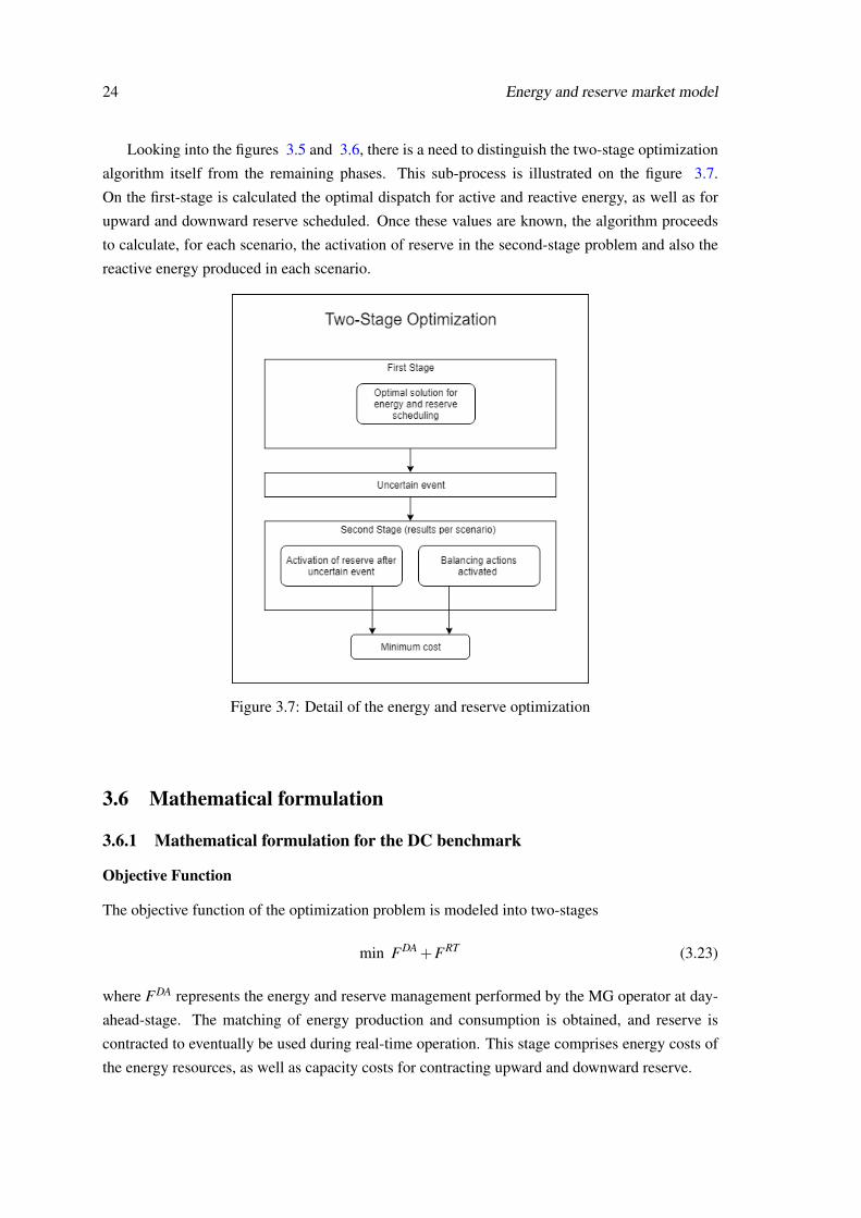
Looking into the figures 3.5 and 3.6, there is a need to distinguish the two-stage optimization
algorithm itself from the remaining phases. This sub-process is illustrated on the figure 3.7.
On the first-stage is calculated the optimal dispatch for active and reactive energy, as well as for
upward and downward reserve scheduled. Once these values are known, the algorithm proceeds
to calculate, for each scenario, the activation of reserve in the second-stage problem and also the
reactive energy produced in each scenario.
Figure 3.7: Detail of the energy and reserve optimization
3.6 Mathematical formulation
3.6.1 Mathematical formulation for the DC benchmark
Objective Function
The objective function of the optimization problem is modeled into two-stages
min FDA +FRT (3.23)
where FDA represents the energy and reserve management performed by the MG operator at day-
ahead-stage. The matching of energy production and consumption is obtained, and reserve is
contracted to eventually be used during real-time operation. This stage comprises energy costs of
the energy resources, as well as capacity costs for contracting upward and downward reserve.
3.6 Mathematical formulation 25
FDAt =
T
∑t=1
NDG
∑dg=1
(CE
DG(dg,t)PEDG(dg,t)+Cup
DG(dg,t)RupDG(dg,t)+Cdw
DG(dg,t)RdwDG(dg,t)
)+
NSU
∑su=1
(CE
SU(su,t)PESU(su,t)+Cup
SU(su,t)RupSU(su,t)+Cdw
SU(su,t)RdwSU(su,t)
)+
NW
∑w=1
(CE
W (w,t)PEW (w,t)+Cup
W (w,t)PupW (w,t)+Cdw
W (w,t)PdwW (w,t)
)+
NPV
∑pv=1
(CE
PV (pv,t)PEPV (pv,t)+Cup
PV (pv,t)PupPV (pv,t)+Cdw
PV (pv,t)PdwPV (pv,t)
)+
NL
∑l=1
(CE
DR(l,t)PEDR(l,t)+Cup
DR(l,t)PupDR(l,t)+Cdw
DR(l,t)PdwDR(l,t)
)
(3.24)
where, DG, wind, PV and DR are the energy resources available in the MG. In contrast, the
activation of the reserve during the real-time stage is given by
FRTt =
T∑
t=1
Nω
∑ω
πω
NDG
∑dg=1
[Cact
DG(dg,t)
(rup
DG(dg,t,ω)− rdwDG(dg,t,ω)
)+Ccut
DG(dg,t)PcutDG(dg,t,ω)
]+
NW
∑w=1
[Cact
W (w,t)
(∆PW (w,t,ω)+ rup
W (w,t,ω)− rdwW (w,t,ω)
)+Cspill
W (w,t)PspillW (w,t,ω)
]+
NPV
∑pv=1
[Cact
PV (pv,t)
(∆PPV (pv,t,ω)+ rup
PV (pv,t,ω)− rdwPV (pv,t,ω)
)+Cspill
PV (pv,t)PspillPV (pv,t,ω)
]+
NL
∑l=1
[Cact
DR(l,t)
(rup
DR(l,t,ω)− rdwDR(l,t,ω)
)+Cshed
L(l,t)PshedL(l,t,ω)
]
(3.25)
where activation costs for all energy resources are considered. In addition, enforced generation
and load curtailment penalties are considered to relax the system in cases insufficient generation
for network balance.
The objective function is subject to the following first-stage and second-stage constraints. The
first-stage constraints concern all constraints of the problem regarding the day-ahead energy re-
source scheduling, while the second-stage constraints concern the constraints of the problem dur-
ing the operating hour, as well as the non-anticipativity constraints.
First-stage constrains
The total power of DG is constrained by
PEDG(dg,t)+Rup
DG(dg,t) ≤ PMaxDG(dg,t) ,∀dg ∈ 1, ...,NDG ,∀t ∈ 1, ...,T (3.26)
PEDG(dg,t)−Rdw
DG(dg,t) ≥ PMinDG(dg,t) ,∀dg ∈ 1, ...,NDG ,∀t ∈ 1, ...,T (3.27)
where energy plus reserve must be within the active power limits of the generator.
26 Energy and reserve market model
In addition, the reserve provision can be constrained by the offers that DG may offer, such as
0≤ RupDG(dg,t) ≤ Rup,Max
DG(dg,t) ,∀dg ∈ 1, ...,NDG ,∀t ∈ 1, ...,T (3.28)
0≤ RdwDG(dg,t) ≤ Rdw,Max
DG(dg,t) ,∀dg ∈ 1, ...,NDG ,∀t ∈ 1, ...,T (3.29)
where both upward and downward reserve are constrained by the bid offered by the player in the
market. Constraints 3.26 to 3.29 are also applied to external suppliers, wind units, PV units
and loads with DR programs. External suppliers are units that represent the power at upstream
connections of the grid. The energy produced by wind and PV units is settled by parameter PEW (w,t),
that is the conditional mean forecast of wind and PV at the day-ahead stage. The active balance
equation at day-ahead stage is given by
NDG
∑dg=1
PE,iDG(dg,t)+
NSU
∑su=1
PE,iSU(su,t)+
NW
∑w=1
PE,iW (w,t)+
NPV
∑pv=1
PE,iPV (pv,t)+
NL
∑l=1
(PE,i
DR(l,t)−PiL(l,t)
)−
i6= j∑
j∈Nbus
P f lowi, jt = 0
t ∈ 1, ...,T ,∀i, j ∈ 1, ...,NBus
(3.30)
where P f lowi, jt represents the active power flow on the line ij, which is given by the equation 3.12
explained before.
Second-stage constrains
The second-stage constraints contemplates all the stochastic constraints dependent of scenario
ω . The activation of upward and downward reserve for DG units is limited by the upward and
downward offer contracted in the first-stage, respectively. In parallel, the generation curtailment
power is constrained by the difference between the current operating point and the downward offer
of the DG unit, hence
rupDG(dg,t,ω) ≤ Rup
DG(dg,t), ∀dg ∈ 1, ...,NDG ,∀t ∈ 1, ...,T ,∀ω ∈ 1, ...,Nω (3.31)
rdwDG(dg,t,ω) ≤ Rdw
DG(dg,t), ∀dg ∈ 1, ...,NDG ,∀t ∈ 1, ...,T ,∀ω ∈ 1, ...,Nω (3.32)
PcutDG(dg,t,ω) ≤ PE
DG(dg,t)− rdwDG(dg,t,ω),∀dg ∈ 1, ...,NDG ,∀t ∈ 1, ...,T ,∀ω ∈ 1, ...,Nω (3.33)
When the capacity of the line is not enough to transmit the desire amount of power, there is a
need to curtail generation at a certain cost and that curtailment or spillage is represented by PcutDG,
PspillPV or Pspill
W depending on the generator. Similarly, the equations 3.31 and 3.32 are valid for
wind and PV producers and the activation of spillage is given by
PspillW (w,t,ω) ≤ PE
W (w,t)− rdwW (w,t,ω) +∆PW (w,t,ω),
∀w ∈ 1, ...,NW ,∀t ∈ 1, ...,T ,∀ω ∈ 1, ...,Nω(3.34)
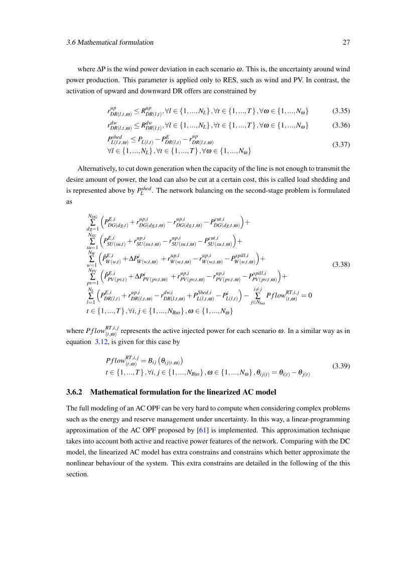
3.6 Mathematical formulation 27
where ∆P is the wind power deviation in each scenario ω . This is, the uncertainty around wind
power production. This parameter is applied only to RES, such as wind and PV. In contrast, the
activation of upward and downward DR offers are constrained by
rupDR(l,t,ω) ≤ Rup
DR(l,t),∀l ∈ 1, ...,NL ,∀t ∈ 1, ...,T ,∀ω ∈ 1, ...,Nω (3.35)
rdwDR(l,t,ω) ≤ Rdw
DR(l,t),∀l ∈ 1, ...,NL ,∀t ∈ 1, ...,T ,∀ω ∈ 1, ...,Nω (3.36)
PshedL(l,t,ω) ≤ PL(l,t)−PE
DR(l,t)− rupDR(l,t,ω)
∀l ∈ 1, ...,NL ,∀t ∈ 1, ...,T ,∀ω ∈ 1, ...,Nω(3.37)
Alternatively, to cut down generation when the capacity of the line is not enough to transmit the
desire amount of power, the load can also be cut at a certain cost, this is called load shedding and
is represented above by PshedL . The network balancing on the second-stage problem is formulated
as
NDG
∑dg=1
(PE,i
DG(dg,t)+ rup,iDG(dg,t,ω)− rup,i
DG(dg,t,ω)−Pcut,iDG(dg,t,ω)
)+
NSU
∑su=1
(PE,i
SU(su,t)+ rup,iSU(su,t,ω)− rup,i
SU(su,t,ω)−Pcut,iSU(su,t,ω)
)+
NW
∑w=1
(PE,i
W (w,t)+∆PiW (w,t,ω) + rup,i
W (w,t,ω)− rup,iW (w,t,ω)−Pspill,i
W (w,t,ω)
)+
NPV
∑pv=1
(PE,i
PV (pv,t)+∆PiPV (pv,t,ω) + rup,i
PV (pv,t,ω)− rup,iPV (pv,t,ω)−Pspill,i
PV (pv,t,ω)
)+
NL
∑l=1
(PE,i
DR(l,t)+ rup,iDR(l,t,ω)− rdw,i
DR(l,t,ω)+PShed,iL(l,t,ω)−Pi
L(l,t)
)−
i6= j∑
j∈Nbus
P f lowRT,i, j(t,ω) = 0
t ∈ 1, ...,T ,∀i, j ∈ 1, ...,NBus ,ω ∈ 1, ...,Nω
(3.38)
where P f lowRT,i, j(t,ω) represents the active injected power for each scenario ω . In a similar way as in
equation 3.12, is given for this case by
P f lowRT,i, j(t,ω) = Bi j
(θi j(t,ω)
)t ∈ 1, ...,T ,∀i, j ∈ 1, ...,NBus ,ω ∈ 1, ...,Nω ,θi j(t) = θi(t)−θ j(t)
(3.39)
3.6.2 Mathematical formulation for the linearized AC model
The full modeling of an AC OPF can be very hard to compute when considering complex problems
such as the energy and reserve management under uncertainty. In this way, a linear-programming
approximation of the AC OPF proposed by [61] is implemented. This approximation technique
takes into account both active and reactive power features of the network. Comparing with the DC
model, the linearized AC model has extra constrains and constrains which better approximate the
nonlinear behaviour of the system. This extra constrains are detailed in the following of the this
section.
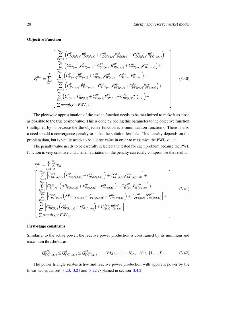
28 Energy and reserve market model
Objective Function
FDAt =
T
∑t=1
NDG
∑dg=1
(CE
DG(dg,t)PEDG(dg,t)+Cup
DG(dg,t)RupDG(dg,t)+Cdw
DG(dg,t)RdwDG(dg,t)
)+
NSU
∑su=1
(CE
SU(su,t)PESU(su,t)+Cup
SU(su,t)RupSU(su,t)+Cdw
SU(su,t)RdwSU(su,t)
)+
NW
∑w=1
(CE
W (w,t)PEW (w,t)+Cup
W (w,t)PupW (w,t)+Cdw
W (w,t)PdwW (w,t)
)+
NPV
∑pv=1
(CE
PV (pv,t)PEPV (pv,t)+Cup
PV (pv,t)PupPV (pv,t)+Cdw
PV (pv,t)PdwPV (pv,t)
)+
NL
∑l=1
(CE
DR(l,t)PEDR(l,t)+Cup
DR(l,t)PupDR(l,t)+Cdw
DR(l,t)PdwDR(l,t)
)−
∑ penalty×PWLi j
(3.40)
The piecewise approximation of the cosine function needs to be maximized to make it as close
as possible to the true cosine value. This is done by adding this parameter to the objective function
(multiplied by -1 because the the objective function is a minimization function). There is also
a need to add a convergence penalty to make the solution feasible. This penalty depends on the
problem data, but typically needs to be a large value in order to maximize the PWL value.
The penalty value needs to be carefully selected and tested for each problem because the PWL
function is very sensitive and a small variation on the penalty can easily compromise the results.
FRTt =
T∑
t=1
Nω
∑ω
πω
NDG
∑dg=1
[Cact
DG(dg,t)
(rup
DG(dg,t,ω)− rdwDG(dg,t,ω)
)+Ccut
DG(dg,t)PcutDG(dg,t,ω)
]+
NW
∑w=1
[Cact
W (w,t)
(∆PW (w,t,ω)+ rup
W (w,t,ω)− rdwW (w,t,ω)
)+Cspill
W (w,t)PspillW (w,t,ω)
]+
NPV
∑pv=1
[Cact
PV (pv,t)
(∆PPV (pv,t,ω)+ rup
PV (pv,t,ω)− rdwPV (pv,t,ω)
)+Cspill
PV (pv,t)PspillPV (pv,t,ω)
]+
NL
∑l=1
[Cact
DR(l,t)
(rup
DR(l,t,ω)− rdwDR(l,t,ω)
)+Cshed
L(l,t)PshedL(l,t,ω)
]−
∑ penalty×PWLi j
(3.41)
First-stage constrains
Similarly, to the active power, the reactive power production is constrained by its minimum and
maximum thresholds as
QMinDG(dg,t) ≤ QE
DG(dg,t) ≤ QMaxDG(dg,t) ,∀dg ∈ 1, ...,NDG ,∀t ∈ 1, ...,T (3.42)
The power triangle relates active and reactive power production with apparent power by the
linearized equations 3.20, 3.21 and 3.22 explained in section 3.4.2.
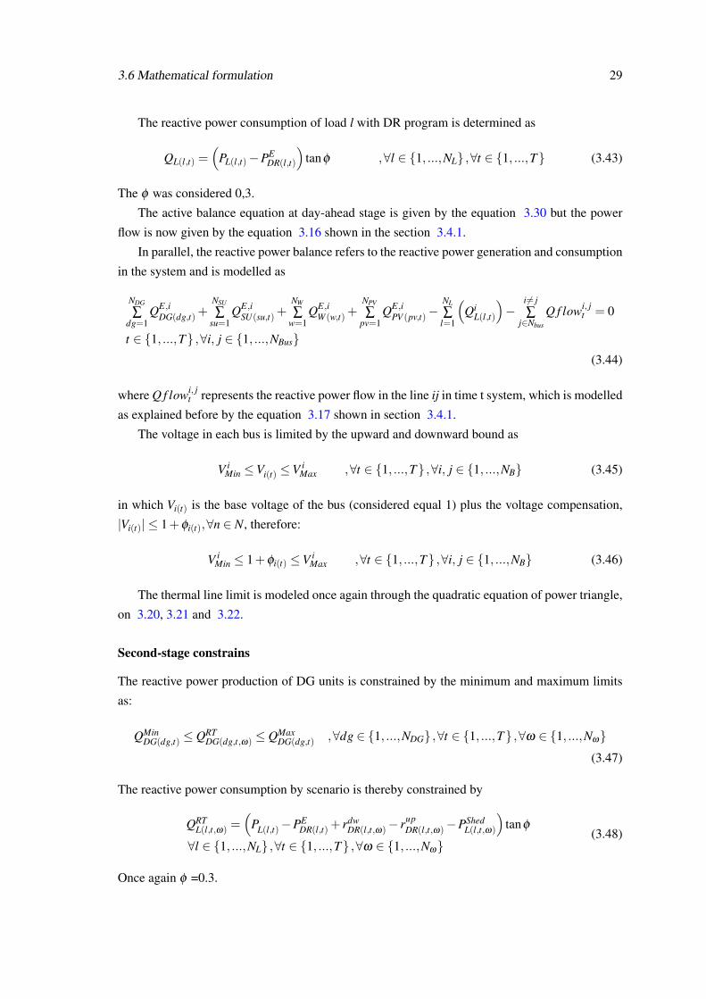
3.6 Mathematical formulation 29
The reactive power consumption of load l with DR program is determined as
QL(l,t) =(
PL(l,t)−PEDR(l,t)
)tanφ ,∀l ∈ 1, ...,NL ,∀t ∈ 1, ...,T (3.43)
The φ was considered 0,3.
The active balance equation at day-ahead stage is given by the equation 3.30 but the power
flow is now given by the equation 3.16 shown in the section 3.4.1.
In parallel, the reactive power balance refers to the reactive power generation and consumption
in the system and is modelled as
NDG
∑dg=1
QE,iDG(dg,t)+
NSU
∑su=1
QE,iSU(su,t)+
NW
∑w=1
QE,iW (w,t)+
NPV
∑pv=1
QE,iPV (pv,t)−
NL
∑l=1
(Qi
L(l,t)
)−
i6= j∑
j∈Nbus
Q f lowi, jt = 0
t ∈ 1, ...,T ,∀i, j ∈ 1, ...,NBus(3.44)
where Q f lowi, jt represents the reactive power flow in the line ij in time t system, which is modelled
as explained before by the equation 3.17 shown in section 3.4.1.
The voltage in each bus is limited by the upward and downward bound as
V iMin ≤Vi(t) ≤V i
Max ,∀t ∈ 1, ...,T ,∀i, j ∈ 1, ...,NB (3.45)
in which Vi(t) is the base voltage of the bus (considered equal 1) plus the voltage compensation,
|Vi(t)| ≤ 1+φi(t),∀n ∈ N, therefore:
V iMin ≤ 1+φi(t) ≤V i
Max ,∀t ∈ 1, ...,T ,∀i, j ∈ 1, ...,NB (3.46)
The thermal line limit is modeled once again through the quadratic equation of power triangle,
on 3.20, 3.21 and 3.22.
Second-stage constrains
The reactive power production of DG units is constrained by the minimum and maximum limits
as:
QMinDG(dg,t) ≤ QRT
DG(dg,t,ω) ≤ QMaxDG(dg,t) ,∀dg ∈ 1, ...,NDG ,∀t ∈ 1, ...,T ,∀ω ∈ 1, ...,Nω
(3.47)
The reactive power consumption by scenario is thereby constrained by
QRTL(l,t,ω) =
(PL(l,t)−PE
DR(l,t)+ rdwDR(l,t,ω)− rup
DR(l,t,ω)−PShedL(l,t,ω)
)tanφ
∀l ∈ 1, ...,NL ,∀t ∈ 1, ...,T ,∀ω ∈ 1, ...,Nω(3.48)
Once again φ =0.3.
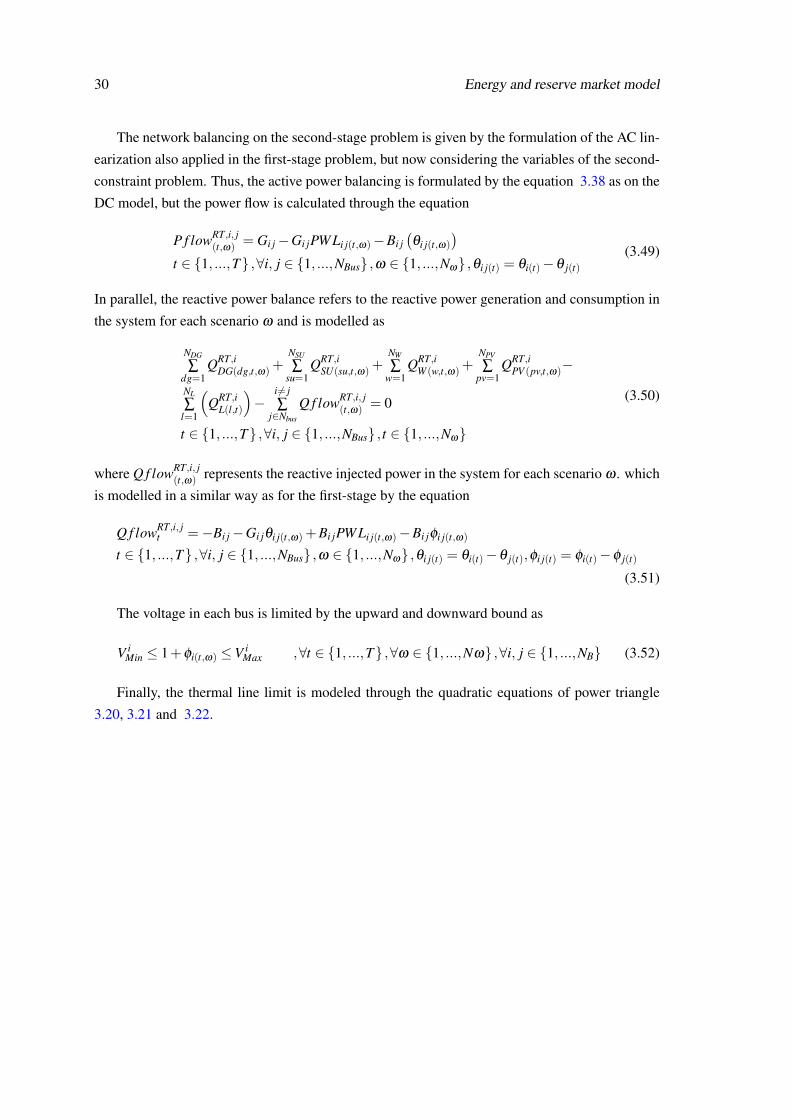
30 Energy and reserve market model
The network balancing on the second-stage problem is given by the formulation of the AC lin-
earization also applied in the first-stage problem, but now considering the variables of the second-
constraint problem. Thus, the active power balancing is formulated by the equation 3.38 as on the
DC model, but the power flow is calculated through the equation
P f lowRT,i, j(t,ω) = Gi j−Gi jPWLi j(t,ω)−Bi j
(θi j(t,ω)
)t ∈ 1, ...,T ,∀i, j ∈ 1, ...,NBus ,ω ∈ 1, ...,Nω ,θi j(t) = θi(t)−θ j(t)
(3.49)
In parallel, the reactive power balance refers to the reactive power generation and consumption in
the system for each scenario ω and is modelled as
NDG
∑dg=1
QRT,iDG(dg,t,ω)+
NSU
∑su=1
QRT,iSU(su,t,ω)+
NW
∑w=1
QRT,iW (w,t,ω)+
NPV
∑pv=1
QRT,iPV (pv,t,ω)−
NL
∑l=1
(QRT,i
L(l,t)
)−
i6= j∑
j∈Nbus
Q f lowRT,i, j(t,ω) = 0
t ∈ 1, ...,T ,∀i, j ∈ 1, ...,NBus , t ∈ 1, ...,Nω
(3.50)
where Q f lowRT,i, j(t,ω) represents the reactive injected power in the system for each scenario ω . which
is modelled in a similar way as for the first-stage by the equation
Q f lowRT,i, jt =−Bi j−Gi jθi j(t,ω)+Bi jPWLi j(t,ω)−Bi jφi j(t,ω)
t ∈ 1, ...,T ,∀i, j ∈ 1, ...,NBus ,ω ∈ 1, ...,Nω ,θi j(t) = θi(t)−θ j(t),φi j(t) = φi(t)−φ j(t)
(3.51)
The voltage in each bus is limited by the upward and downward bound as
V iMin ≤ 1+φi(t,ω) ≤V i
Max ,∀t ∈ 1, ...,T ,∀ω ∈ 1, ...,Nω ,∀i, j ∈ 1, ...,NB (3.52)
Finally, the thermal line limit is modeled through the quadratic equations of power triangle
3.20, 3.21 and 3.22.
Chapter 4
Assessment of energy and reservemanagement model (case study)
4.1 Introduction
In this chapter is presented the case study illustrating the application of the simulation of the two-
stage stochastic programming model proposed in the previous chapter under the MG context. This
case study was selected to cover a diversity of situations of the involved players in the MG, and
therefore test and validated the proposed models. The results obtained are presented and discussed
and some general conclusions are made.
4.2 Case study
The case study refers to a joint market model for energy and reserve in a MG. It is used the two-
stage stochastic optimization to obtain the optimal dispatch for energy and upward and downward
reserve in the MG. The main objective of this model is the minimization of the market costs for
the MG operator.
On a first phase of the work it was done the two-stage optimization program applied to a
DC model detailed on the chapter 3 of this project. After that, the results were analyzed and the
veracity of the optimal solution was tested using two quality metrics detailed on [124], namely the
Expected Value of Perfect Information (EVPI) and the Value of the Stochastic Solution (VSS) to
be further discussed. Once the results for the DC benchmark were satisfactory, the AC Model was
tested and the results for this model were collected and analyzed.
4.3 Outline
This subsection includes an outline of the problem, as well as, the input data necessary for the
simulation of the models. The results are reported together with some conclusions related to the
problem.
31
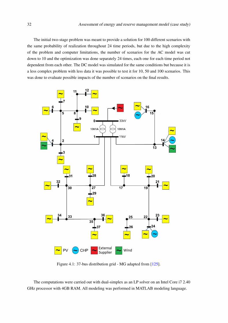
32 Assessment of energy and reserve management model (case study)
The initial two-stage problem was meant to provide a solution for 100 different scenarios with
the same probability of realization throughout 24 time periods, but due to the high complexity
of the problem and computer limitations, the number of scenarios for the AC model was cut
down to 10 and the optimization was done separately 24 times, each one for each time period not
dependent from each other. The DC model was simulated for the same conditions but because it is
a less complex problem with less data it was possible to test it for 10, 50 and 100 scenarios. This
was done to evaluate possible impacts of the number of scenarios on the final results.
Figure 4.1: 37-bus distribution grid - MG adapted from [125].
The computations were carried out with dual-simplex as an LP solver on an Intel Core i7 2.40
GHz processor with 4GB RAM. All modeling was performed in MATLAB modeling language.
4.3 Outline 33
The original distribution network is presented in [125], while the energy mix in 2050 used
for updating the network is proposed in [126]. The simulation runs for a 11kV MV MG, at the
distribution level, with 37 buses, 22 loads, 28 aggregators and 36 distribution lines. The design of
the MG is shown on the figure 4.1 and is composed by:
• 1 external supplier representing the upstream connection with the 33kV MV line.
• 3 CHP aggregators
• 2 Wind aggregators
• 22 PV aggregators
For a given time period in the future, the system operator must determine here-and-now both
the energy dispatch and the reserve capacity needs. Naturally, reserve capacity is required to cope
with the uncertain wind and PV power production, which is represented via scenarios, with the
same probability of occurrence. Specifically, the sequence of decisions that the system operator
has to face is as follows:
1. Determine the production levels of DG units and the allocation of reserves to deal with the
uncertain wind and PV power production;
2. Deployment of reserve in the form of balancing energy during the real-time operation of
the power system to accommodate the actual realization of wind and PV power production.
Four different types of balancing actions can be undertaken for this purpose, namely
(a) The power output of the generator unit g can be increased from P to P+rup, where rup
is the balancing energy obtained from the upward reserve capacity of unit i, denoted as
Rup. This action entails a cost given by Cactrup , where Cact is the marginal production
cost declared by unit g (g can be DG, PV or wind);
(b) Conversely, the power output of unit i can be decreased from P to P− rdw , where
rdw is the balancing energy resulting from the deployment of the downward reserve
capacity of unit i, represented by Rdw . This action implies cost savings of Cactrdw;
(c) A part of the production, Pcut (or Pspillin the case of wind generators) can be curtailed
(spilled) with the cost Ccut(Cspill);
(d) A part of the load l, PshedL , can be also curtailed. This action involves, though, the
so-called value of lost load associated with the cost CshedL .
The following tables contain relevant input data about the general characteristics of the DER
and consumers. They also show the unit prices for energy and reserve as well as for the contin-
gency balancing actions.
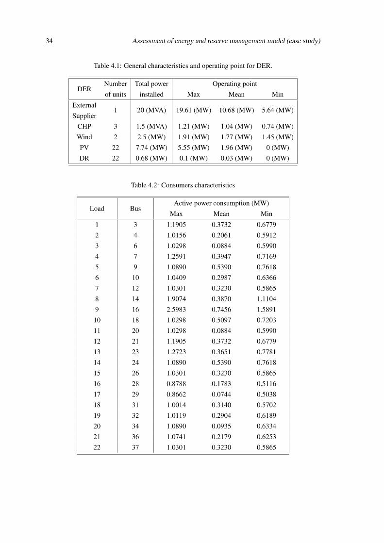
34 Assessment of energy and reserve management model (case study)
Table 4.1: General characteristics and operating point for DER.
DERNumber
of units
Total power
installed
Operating point
Max Mean Min
External
Supplier1 20 (MVA) 19.61 (MW) 10.68 (MW) 5.64 (MW)
CHP 3 1.5 (MVA) 1.21 (MW) 1.04 (MW) 0.74 (MW)
Wind 2 2.5 (MW) 1.91 (MW) 1.77 (MW) 1.45 (MW)
PV 22 7.74 (MW) 5.55 (MW) 1.96 (MW) 0 (MW)
DR 22 0.68 (MW) 0.1 (MW) 0.03 (MW) 0 (MW)
Table 4.2: Consumers characteristics
Load BusActive power consumption (MW)
Max Mean Min
1 3 1.1905 0.3732 0.6779
2 4 1.0156 0.2061 0.5912
3 6 1.0298 0.0884 0.5990
4 7 1.2591 0.3947 0.7169
5 9 1.0890 0.5390 0.7618
6 10 1.0409 0.2987 0.6366
7 12 1.0301 0.3230 0.5865
8 14 1.9074 0.3870 1.1104
9 16 2.5983 0.7456 1.5891
10 18 1.0298 0.5097 0.7203
11 20 1.0298 0.0884 0.5990
12 21 1.1905 0.3732 0.6779
13 23 1.2723 0.3651 0.7781
14 24 1.0890 0.5390 0.7618
15 26 1.0301 0.3230 0.5865
16 28 0.8788 0.1783 0.5116
17 29 0.8662 0.0744 0.5038
18 31 1.0014 0.3140 0.5702
19 32 1.0119 0.2904 0.6189
20 34 1.0890 0.0935 0.6334
21 36 1.0741 0.2179 0.6253
22 37 1.0301 0.3230 0.5865
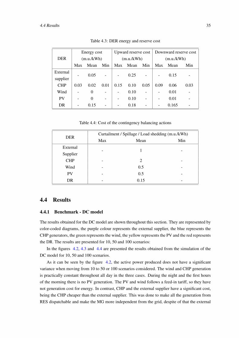
4.4 Results 35
Table 4.3: DER energy and reserve cost
DEREnergy cost
(m.u./kWh)
Upward reserve cost
(m.u./kWh)
Downward reserve cost
(m.u./kWh)
Max Mean Min Max Mean Min Max Mean Min
External
supplier- 0.05 - - 0.25 - - 0.15 -
CHP 0.03 0.02 0.01 0.15 0.10 0.05 0.09 0.06 0.03
Wind - 0 - - 0.10 - - 0.01 -
PV - 0 - - 0.10 - - 0.01 -
DR - 0.15 - - 0.18 - - 0.165 -
Table 4.4: Cost of the contingency balancing actions
DERCurtailment / Spillage / Load shedding (m.u./kWh)
Max Mean Min
External
Supplier- 1 -
CHP - 2 -
Wind - 0.5 -
PV - 0.5 -
DR - 0.15 -
4.4 Results
4.4.1 Benchmark - DC model
The results obtained for the DC model are shown throughout this section. They are represented by
color-coded diagrams, the purple colour represents the external supplier, the blue represents the
CHP generators, the green represents the wind, the yellow represents the PV and the red represents
the DR. The results are presented for 10, 50 and 100 scenarios:
In the figures 4.2, 4.3 and 4.4 are presented the results obtained from the simulation of the
DC model for 10, 50 and 100 scenarios.
As it can be seen by the figure 4.2, the active power produced does not have a significant
variance when moving from 10 to 50 or 100 scenarios considered. The wind and CHP generation
is practically constant throughout all day in the three cases. During the night and the first hours
of the morning there is no PV generation. The PV and wind follows a feed-in tariff, so they have
not generation cost for energy. In contrast, CHP and the external supplier have a significant cost,
being the CHP cheaper than the external supplier. This was done to make all the generation from
RES dispatchable and make the MG more independent from the grid, despite of that the external
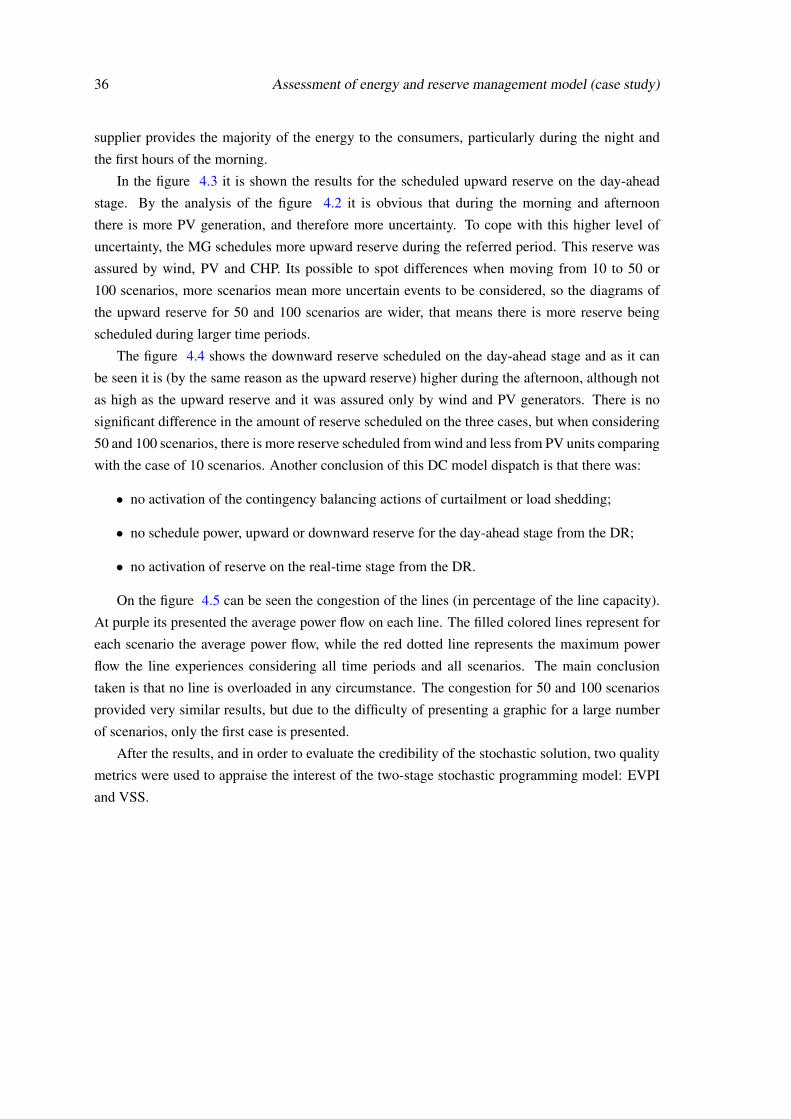
36 Assessment of energy and reserve management model (case study)
supplier provides the majority of the energy to the consumers, particularly during the night and
the first hours of the morning.
In the figure 4.3 it is shown the results for the scheduled upward reserve on the day-ahead
stage. By the analysis of the figure 4.2 it is obvious that during the morning and afternoon
there is more PV generation, and therefore more uncertainty. To cope with this higher level of
uncertainty, the MG schedules more upward reserve during the referred period. This reserve was
assured by wind, PV and CHP. Its possible to spot differences when moving from 10 to 50 or
100 scenarios, more scenarios mean more uncertain events to be considered, so the diagrams of
the upward reserve for 50 and 100 scenarios are wider, that means there is more reserve being
scheduled during larger time periods.
The figure 4.4 shows the downward reserve scheduled on the day-ahead stage and as it can
be seen it is (by the same reason as the upward reserve) higher during the afternoon, although not
as high as the upward reserve and it was assured only by wind and PV generators. There is no
significant difference in the amount of reserve scheduled on the three cases, but when considering
50 and 100 scenarios, there is more reserve scheduled from wind and less from PV units comparing
with the case of 10 scenarios. Another conclusion of this DC model dispatch is that there was:
• no activation of the contingency balancing actions of curtailment or load shedding;
• no schedule power, upward or downward reserve for the day-ahead stage from the DR;
• no activation of reserve on the real-time stage from the DR.
On the figure 4.5 can be seen the congestion of the lines (in percentage of the line capacity).
At purple its presented the average power flow on each line. The filled colored lines represent for
each scenario the average power flow, while the red dotted line represents the maximum power
flow the line experiences considering all time periods and all scenarios. The main conclusion
taken is that no line is overloaded in any circumstance. The congestion for 50 and 100 scenarios
provided very similar results, but due to the difficulty of presenting a graphic for a large number
of scenarios, only the first case is presented.
After the results, and in order to evaluate the credibility of the stochastic solution, two quality
metrics were used to appraise the interest of the two-stage stochastic programming model: EVPI
and VSS.
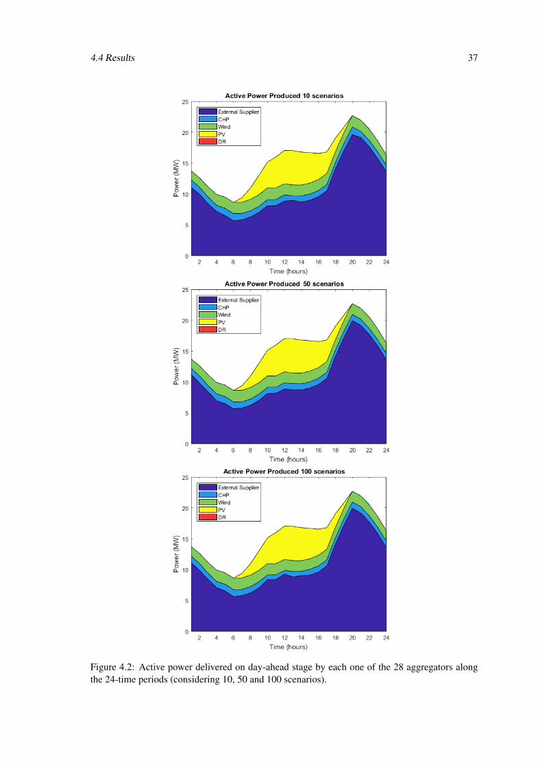
4.4 Results 37
Figure 4.2: Active power delivered on day-ahead stage by each one of the 28 aggregators alongthe 24-time periods (considering 10, 50 and 100 scenarios).
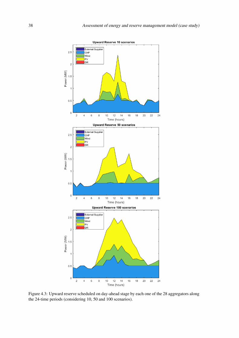
38 Assessment of energy and reserve management model (case study)
Figure 4.3: Upward reserve scheduled on day-ahead stage by each one of the 28 aggregators alongthe 24-time periods (considering 10, 50 and 100 scenarios).
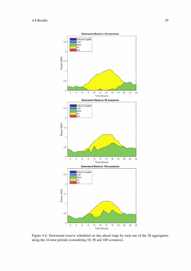
4.4 Results 39
Figure 4.4: Downward reserve scheduled on day-ahead stage by each one of the 28 aggregatorsalong the 24-time periods (considering 10, 50 and 100 scenarios).
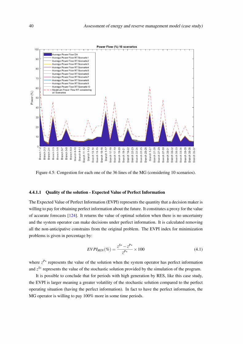
40 Assessment of energy and reserve management model (case study)
Figure 4.5: Congestion for each one of the 36 lines of the MG (considering 10 scenarios).
4.4.1.1 Quality of the solution - Expected Value of Perfect Information
The Expected Value of Perfect Information (EVPI) represents the quantity that a decision maker is
willing to pay for obtaining perfect information about the future. It constitutes a proxy for the value
of accurate forecasts [124]. It returns the value of optimal solution when there is no uncertainty
and the system operator can make decisions under perfect information. It is calculated removing
all the non-anticipative constrains from the original problem. The EVPI index for minimization
problems is given in percentage by:
EV PIMIN(%) =zS∗− zP∗
zP∗ ×100 (4.1)
where zP∗ represents the value of the solution when the system operator has perfect information
and zS∗ represents the value of the stochastic solution provided by the simulation of the program.
It is possible to conclude that for periods with high generation by RES, like this case study,
the EVPI is larger meaning a greater volatility of the stochastic solution compared to the perfect
operating situation (having the perfect information). In fact to have the perfect information, the
MG operator is willing to pay 100% more in some time periods.
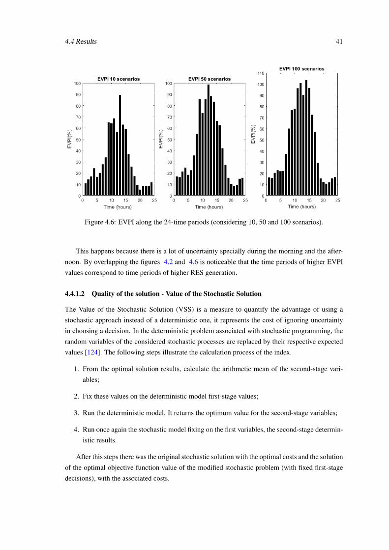
4.4 Results 41
Figure 4.6: EVPI along the 24-time periods (considering 10, 50 and 100 scenarios).
This happens because there is a lot of uncertainty specially during the morning and the after-
noon. By overlapping the figures 4.2 and 4.6 is noticeable that the time periods of higher EVPI
values correspond to time periods of higher RES generation.
4.4.1.2 Quality of the solution - Value of the Stochastic Solution
The Value of the Stochastic Solution (VSS) is a measure to quantify the advantage of using a
stochastic approach instead of a deterministic one, it represents the cost of ignoring uncertainty
in choosing a decision. In the deterministic problem associated with stochastic programming, the
random variables of the considered stochastic processes are replaced by their respective expected
values [124]. The following steps illustrate the calculation process of the index.
1. From the optimal solution results, calculate the arithmetic mean of the second-stage vari-
ables;
2. Fix these values on the deterministic model first-stage values;
3. Run the deterministic model. It returns the optimum value for the second-stage variables;
4. Run once again the stochastic model fixing on the first variables, the second-stage determin-
istic results.
After this steps there was the original stochastic solution with the optimal costs and the solution
of the optimal objective function value of the modified stochastic problem (with fixed first-stage
decisions), with the associated costs.
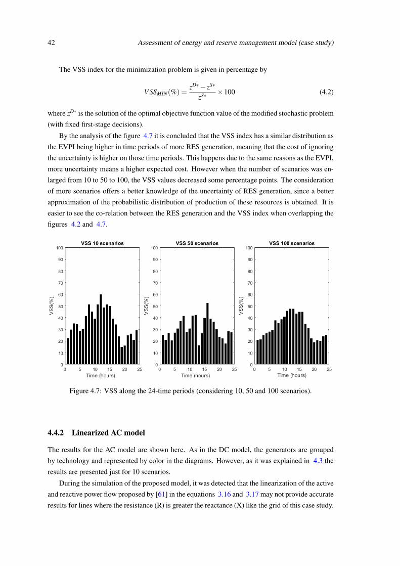
42 Assessment of energy and reserve management model (case study)
The VSS index for the minimization problem is given in percentage by
V SSMIN(%) =zD∗− zS∗
zS∗ ×100 (4.2)
where zD∗ is the solution of the optimal objective function value of the modified stochastic problem
(with fixed first-stage decisions).
By the analysis of the figure 4.7 it is concluded that the VSS index has a similar distribution as
the EVPI being higher in time periods of more RES generation, meaning that the cost of ignoring
the uncertainty is higher on those time periods. This happens due to the same reasons as the EVPI,
more uncertainty means a higher expected cost. However when the number of scenarios was en-
larged from 10 to 50 to 100, the VSS values decreased some percentage points. The consideration
of more scenarios offers a better knowledge of the uncertainty of RES generation, since a better
approximation of the probabilistic distribution of production of these resources is obtained. It is
easier to see the co-relation between the RES generation and the VSS index when overlapping the
figures 4.2 and 4.7.
Figure 4.7: VSS along the 24-time periods (considering 10, 50 and 100 scenarios).
4.4.2 Linearized AC model
The results for the AC model are shown here. As in the DC model, the generators are grouped
by technology and represented by color in the diagrams. However, as it was explained in 4.3 the
results are presented just for 10 scenarios.
During the simulation of the proposed model, it was detected that the linearization of the active
and reactive power flow proposed by [61] in the equations 3.16 and 3.17 may not provide accurate
results for lines where the resistance (R) is greater the reactance (X) like the grid of this case study.
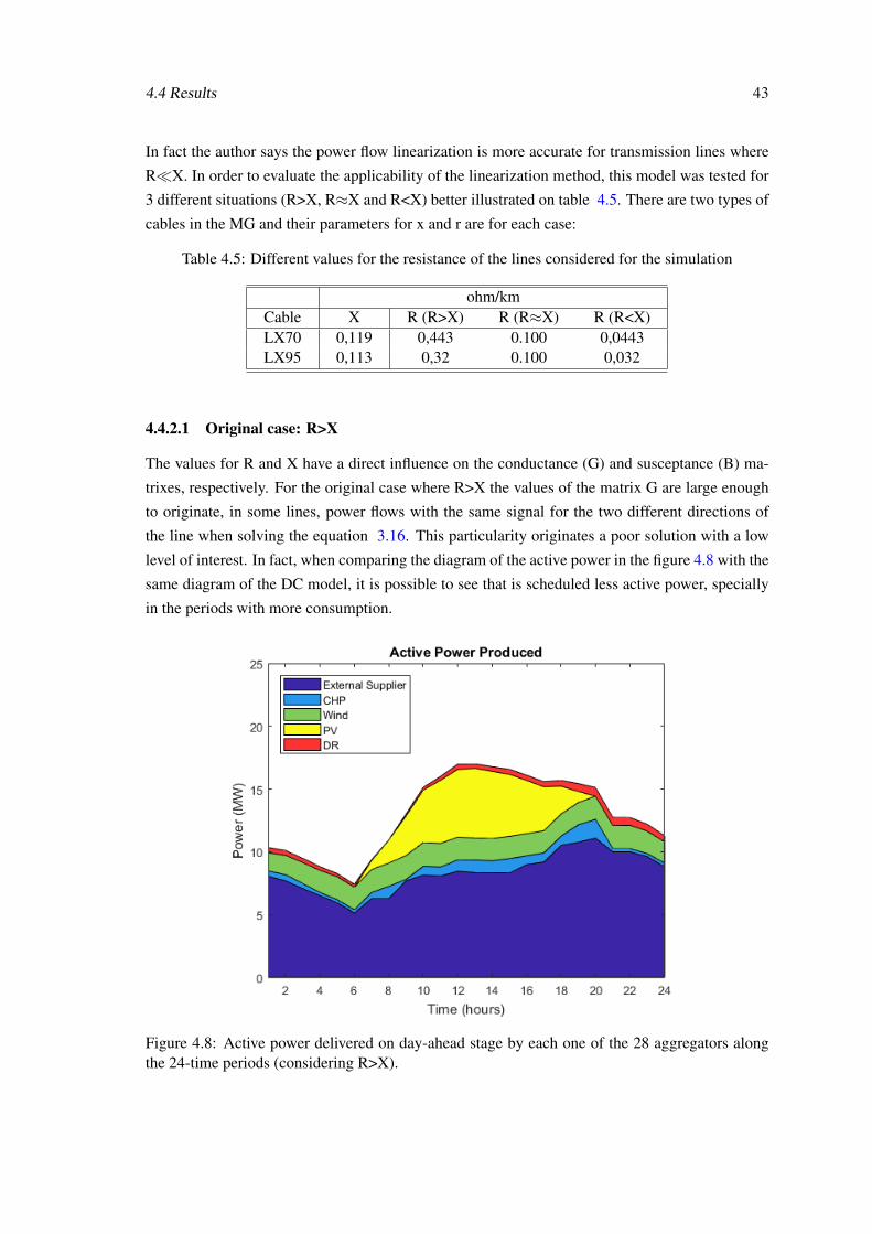
4.4 Results 43
In fact the author says the power flow linearization is more accurate for transmission lines where
RX. In order to evaluate the applicability of the linearization method, this model was tested for
3 different situations (R>X, R≈X and R<X) better illustrated on table 4.5. There are two types of
cables in the MG and their parameters for x and r are for each case:
Table 4.5: Different values for the resistance of the lines considered for the simulation
ohm/kmCable X R (R>X) R (R≈X) R (R<X)LX70 0,119 0,443 0.100 0,0443LX95 0,113 0,32 0.100 0,032
4.4.2.1 Original case: R>X
The values for R and X have a direct influence on the conductance (G) and susceptance (B) ma-
trixes, respectively. For the original case where R>X the values of the matrix G are large enough
to originate, in some lines, power flows with the same signal for the two different directions of
the line when solving the equation 3.16. This particularity originates a poor solution with a low
level of interest. In fact, when comparing the diagram of the active power in the figure 4.8 with the
same diagram of the DC model, it is possible to see that is scheduled less active power, specially
in the periods with more consumption.
Figure 4.8: Active power delivered on day-ahead stage by each one of the 28 aggregators alongthe 24-time periods (considering R>X).
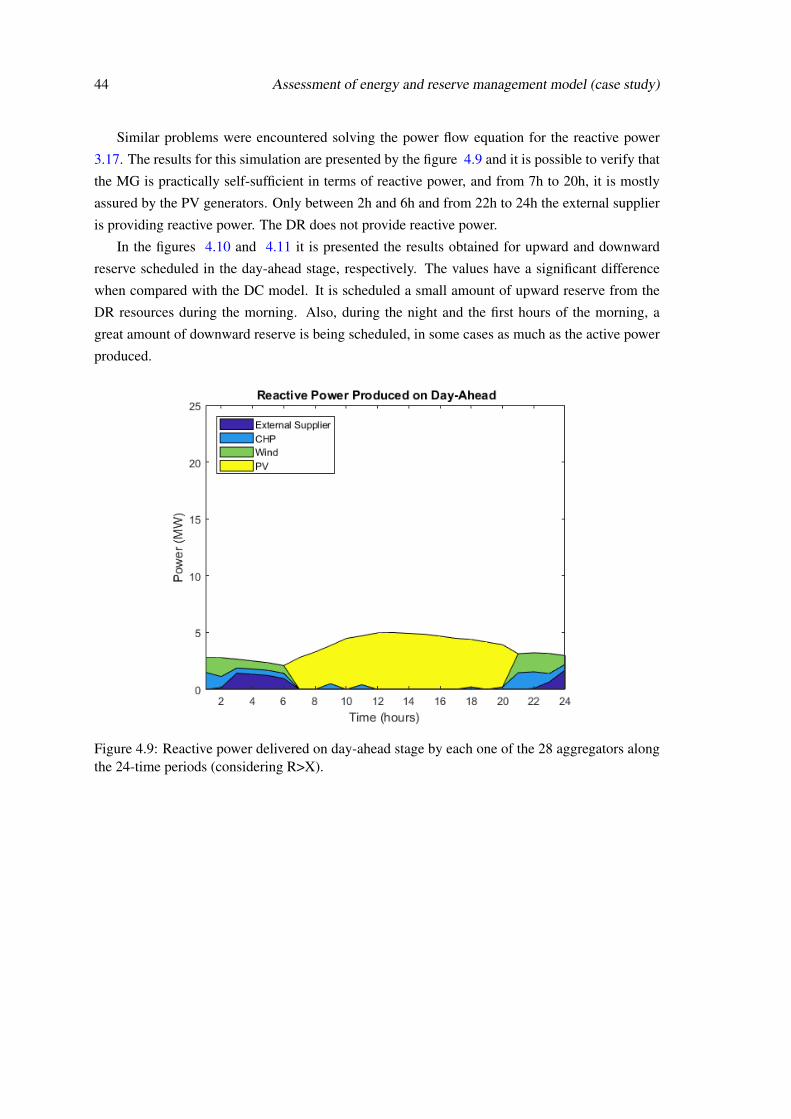
44 Assessment of energy and reserve management model (case study)
Similar problems were encountered solving the power flow equation for the reactive power
3.17. The results for this simulation are presented by the figure 4.9 and it is possible to verify that
the MG is practically self-sufficient in terms of reactive power, and from 7h to 20h, it is mostly
assured by the PV generators. Only between 2h and 6h and from 22h to 24h the external supplier
is providing reactive power. The DR does not provide reactive power.
In the figures 4.10 and 4.11 it is presented the results obtained for upward and downward
reserve scheduled in the day-ahead stage, respectively. The values have a significant difference
when compared with the DC model. It is scheduled a small amount of upward reserve from the
DR resources during the morning. Also, during the night and the first hours of the morning, a
great amount of downward reserve is being scheduled, in some cases as much as the active power
produced.
Figure 4.9: Reactive power delivered on day-ahead stage by each one of the 28 aggregators alongthe 24-time periods (considering R>X).
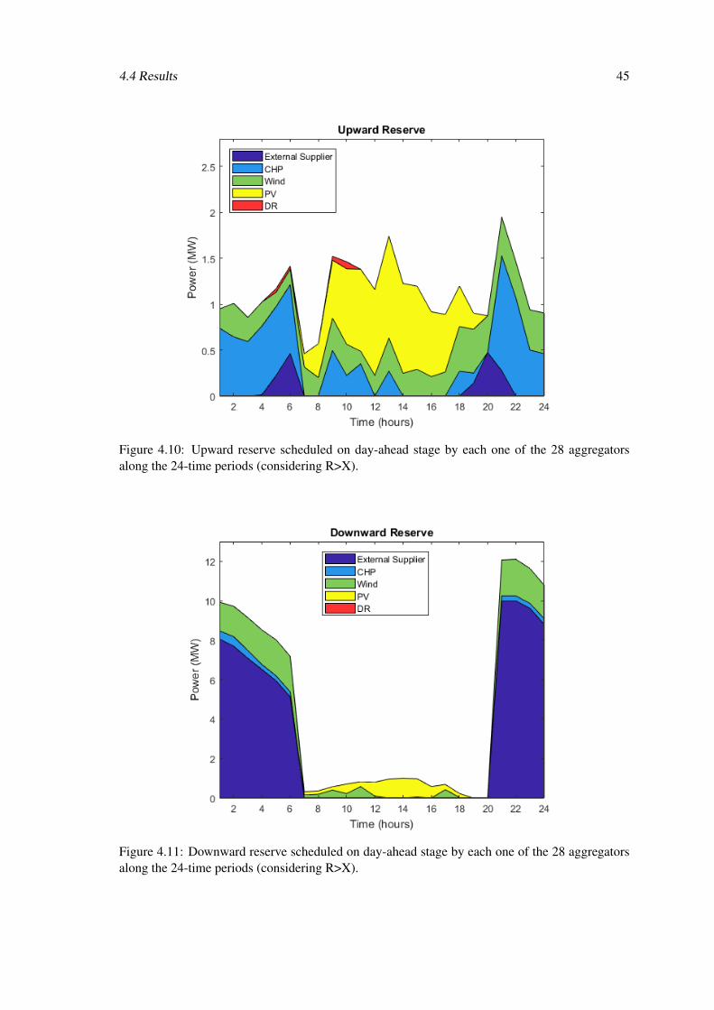
4.4 Results 45
Figure 4.10: Upward reserve scheduled on day-ahead stage by each one of the 28 aggregatorsalong the 24-time periods (considering R>X).
Figure 4.11: Downward reserve scheduled on day-ahead stage by each one of the 28 aggregatorsalong the 24-time periods (considering R>X).

46 Assessment of energy and reserve management model (case study)
Figure 4.12: Generation curtailment per scenario during the 24-time periods (considering R>X).
Figure 4.13: Load shedding per scenario during the 24-time periods (considering R>X).
For this conditions (R>X) a small amount of generation curtailment/spillage is activated as it
shows the figure 4.12. Also there is a great amount of load shedding in the second-stage as it
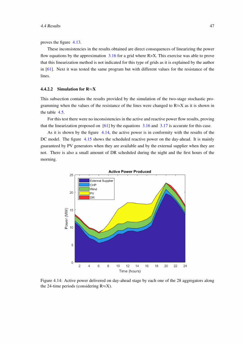
4.4 Results 47
proves the figure 4.13.
These inconsistencies in the results obtained are direct consequences of linearizing the power
flow equations by the approximation 3.16 for a grid where R>X. This exercise was able to prove
that this linearization method is not indicated for this type of grids as it is explained by the author
in [61]. Next it was tested the same program but with different values for the resistance of the
lines.
4.4.2.2 Simulation for R≈X
This subsection contains the results provided by the simulation of the two-stage stochastic pro-
gramming when the values of the resistance of the lines were changed to R≈X as it is shown in
the table 4.5.
For this test there were no inconsistencies in the active and reactive power flow results, proving
that the linearization proposed on [61] by the equations 3.16 and 3.17 is accurate for this case.
As it is shown by the figure 4.14, the active power is in conformity with the results of the
DC model. The figure 4.15 shows the scheduled reactive power on the day-ahead. It is mainly
guaranteed by PV generators when they are available and by the external supplier when they are
not. There is also a small amount of DR scheduled during the night and the first hours of the
morning.
Figure 4.14: Active power delivered on day-ahead stage by each one of the 28 aggregators alongthe 24-time periods (considering R≈X).

48 Assessment of energy and reserve management model (case study)
Figure 4.15: Reactive power delivered on day-ahead stage by each one of the 28 aggregators alongthe 24-time periods (considering R≈X).
Figure 4.16: Upward reserve scheduled on day-ahead stage by each one of the 28 aggregatorsalong the 24-time periods (considering R≈X).
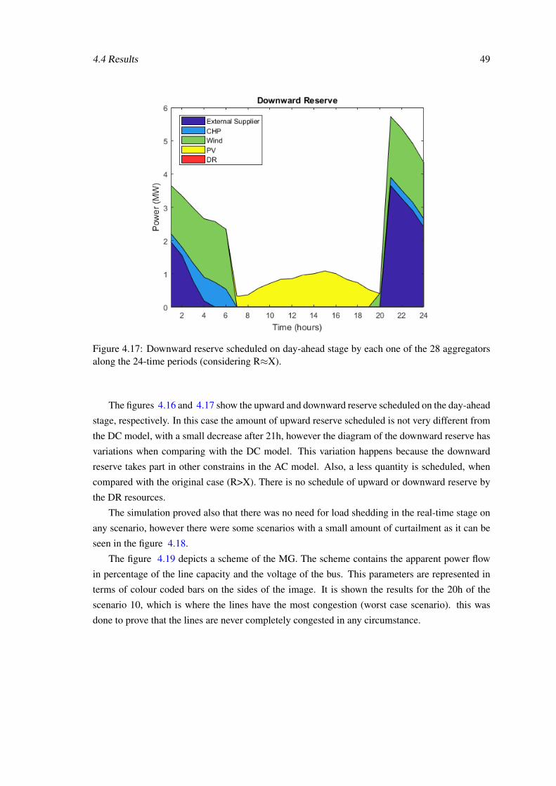
4.4 Results 49
Figure 4.17: Downward reserve scheduled on day-ahead stage by each one of the 28 aggregatorsalong the 24-time periods (considering R≈X).
The figures 4.16 and 4.17 show the upward and downward reserve scheduled on the day-ahead
stage, respectively. In this case the amount of upward reserve scheduled is not very different from
the DC model, with a small decrease after 21h, however the diagram of the downward reserve has
variations when comparing with the DC model. This variation happens because the downward
reserve takes part in other constrains in the AC model. Also, a less quantity is scheduled, when
compared with the original case (R>X). There is no schedule of upward or downward reserve by
the DR resources.
The simulation proved also that there was no need for load shedding in the real-time stage on
any scenario, however there were some scenarios with a small amount of curtailment as it can be
seen in the figure 4.18.
The figure 4.19 depicts a scheme of the MG. The scheme contains the apparent power flow
in percentage of the line capacity and the voltage of the bus. This parameters are represented in
terms of colour coded bars on the sides of the image. It is shown the results for the 20h of the
scenario 10, which is where the lines have the most congestion (worst case scenario). this was
done to prove that the lines are never completely congested in any circumstance.
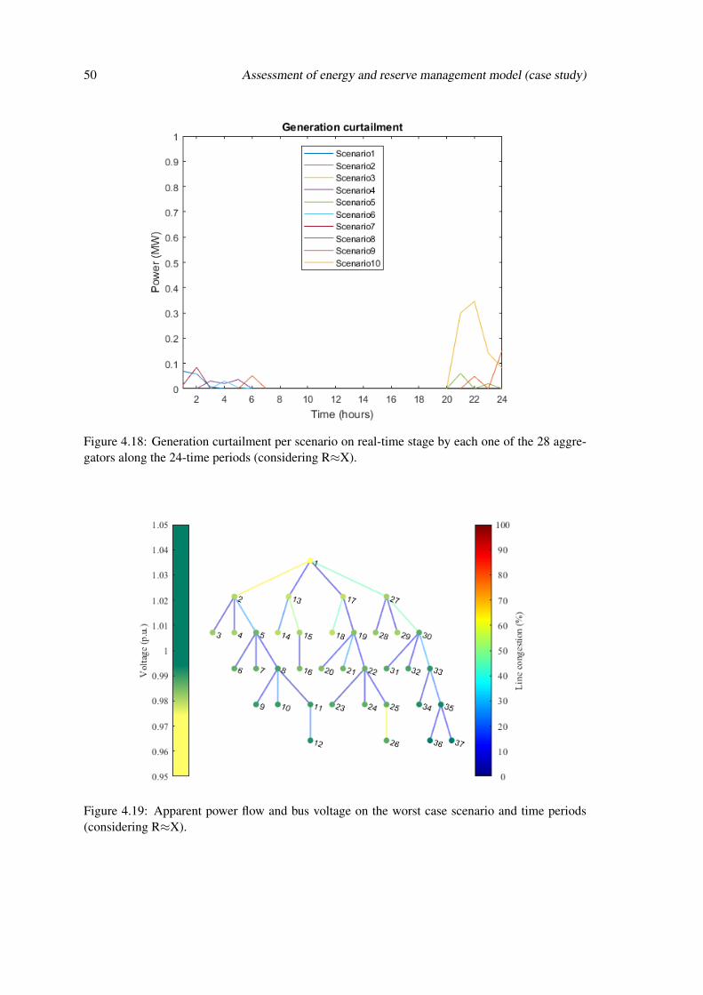
50 Assessment of energy and reserve management model (case study)
Figure 4.18: Generation curtailment per scenario on real-time stage by each one of the 28 aggre-gators along the 24-time periods (considering R≈X).
Figure 4.19: Apparent power flow and bus voltage on the worst case scenario and time periods(considering R≈X).
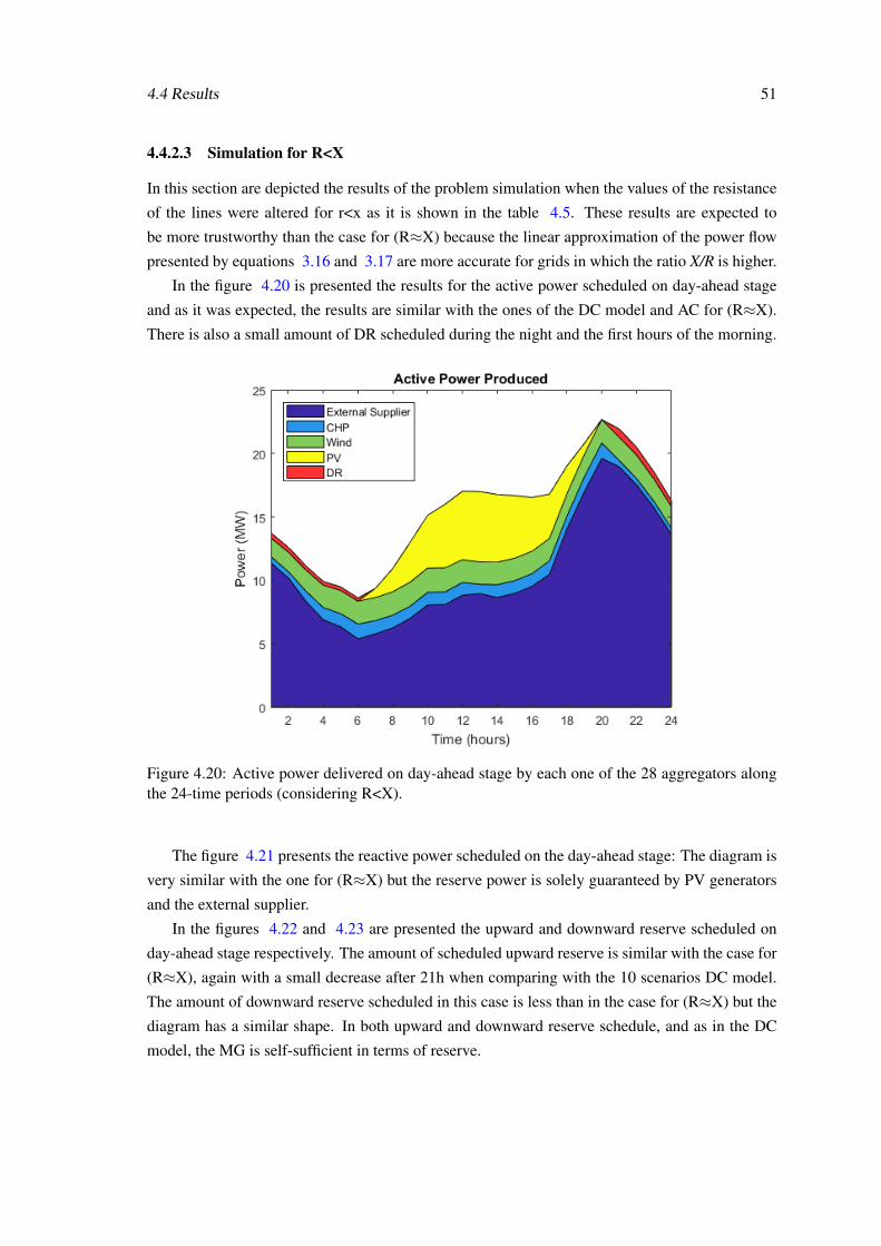
4.4 Results 51
4.4.2.3 Simulation for R<X
In this section are depicted the results of the problem simulation when the values of the resistance
of the lines were altered for r<x as it is shown in the table 4.5. These results are expected to
be more trustworthy than the case for (R≈X) because the linear approximation of the power flow
presented by equations 3.16 and 3.17 are more accurate for grids in which the ratio X/R is higher.
In the figure 4.20 is presented the results for the active power scheduled on day-ahead stage
and as it was expected, the results are similar with the ones of the DC model and AC for (R≈X).
There is also a small amount of DR scheduled during the night and the first hours of the morning.
Figure 4.20: Active power delivered on day-ahead stage by each one of the 28 aggregators alongthe 24-time periods (considering R<X).
The figure 4.21 presents the reactive power scheduled on the day-ahead stage: The diagram is
very similar with the one for (R≈X) but the reserve power is solely guaranteed by PV generators
and the external supplier.
In the figures 4.22 and 4.23 are presented the upward and downward reserve scheduled on
day-ahead stage respectively. The amount of scheduled upward reserve is similar with the case for
(R≈X), again with a small decrease after 21h when comparing with the 10 scenarios DC model.
The amount of downward reserve scheduled in this case is less than in the case for (R≈X) but the
diagram has a similar shape. In both upward and downward reserve schedule, and as in the DC
model, the MG is self-sufficient in terms of reserve.
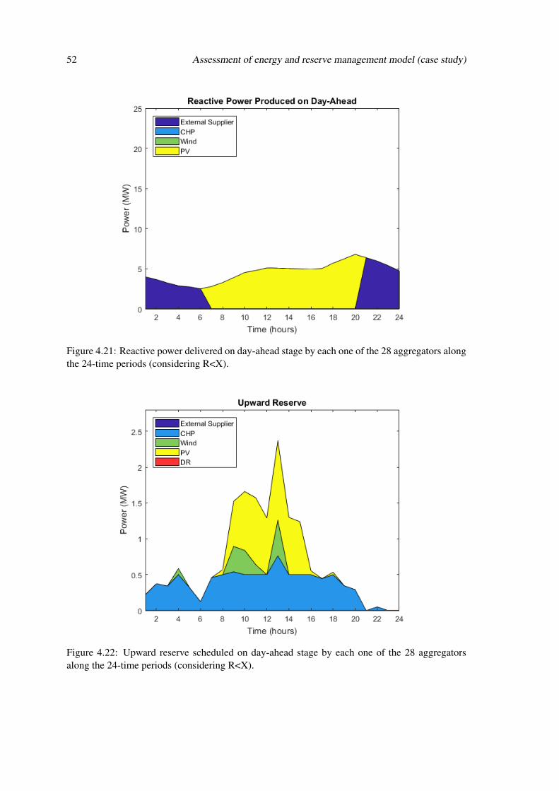
52 Assessment of energy and reserve management model (case study)
Figure 4.21: Reactive power delivered on day-ahead stage by each one of the 28 aggregators alongthe 24-time periods (considering R<X).
Figure 4.22: Upward reserve scheduled on day-ahead stage by each one of the 28 aggregatorsalong the 24-time periods (considering R<X).
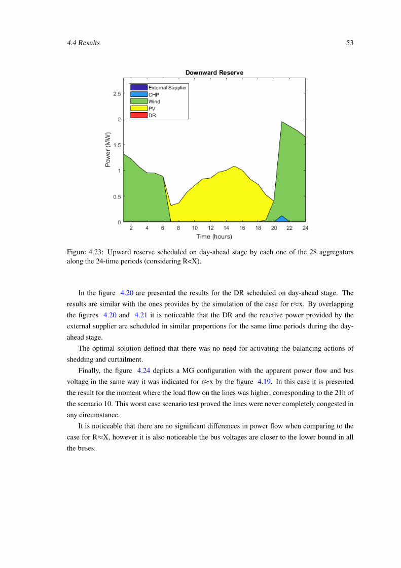
4.4 Results 53
Figure 4.23: Upward reserve scheduled on day-ahead stage by each one of the 28 aggregatorsalong the 24-time periods (considering R<X).
In the figure 4.20 are presented the results for the DR scheduled on day-ahead stage. The
results are similar with the ones provides by the simulation of the case for r≈x. By overlapping
the figures 4.20 and 4.21 it is noticeable that the DR and the reactive power provided by the
external supplier are scheduled in similar proportions for the same time periods during the day-
ahead stage.
The optimal solution defined that there was no need for activating the balancing actions of
shedding and curtailment.
Finally, the figure 4.24 depicts a MG configuration with the apparent power flow and bus
voltage in the same way it was indicated for r≈x by the figure 4.19. In this case it is presented
the result for the moment where the load flow on the lines was higher, corresponding to the 21h of
the scenario 10. This worst case scenario test proved the lines were never completely congested in
any circumstance.
It is noticeable that there are no significant differences in power flow when comparing to the
case for R≈X, however it is also noticeable the bus voltages are closer to the lower bound in all
the buses.
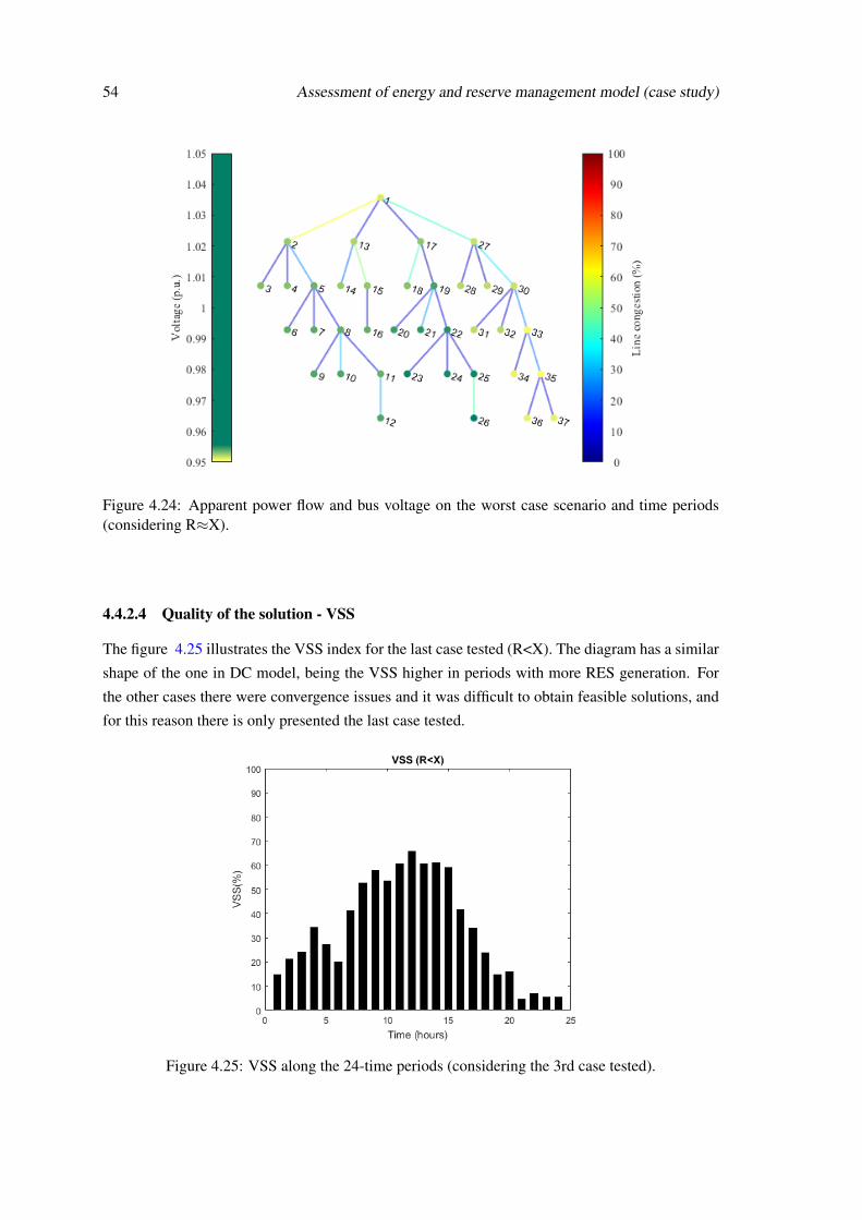
54 Assessment of energy and reserve management model (case study)
Figure 4.24: Apparent power flow and bus voltage on the worst case scenario and time periods(considering R≈X).
4.4.2.4 Quality of the solution - VSS
The figure 4.25 illustrates the VSS index for the last case tested (R<X). The diagram has a similar
shape of the one in DC model, being the VSS higher in periods with more RES generation. For
the other cases there were convergence issues and it was difficult to obtain feasible solutions, and
for this reason there is only presented the last case tested.
Figure 4.25: VSS along the 24-time periods (considering the 3rd case tested).
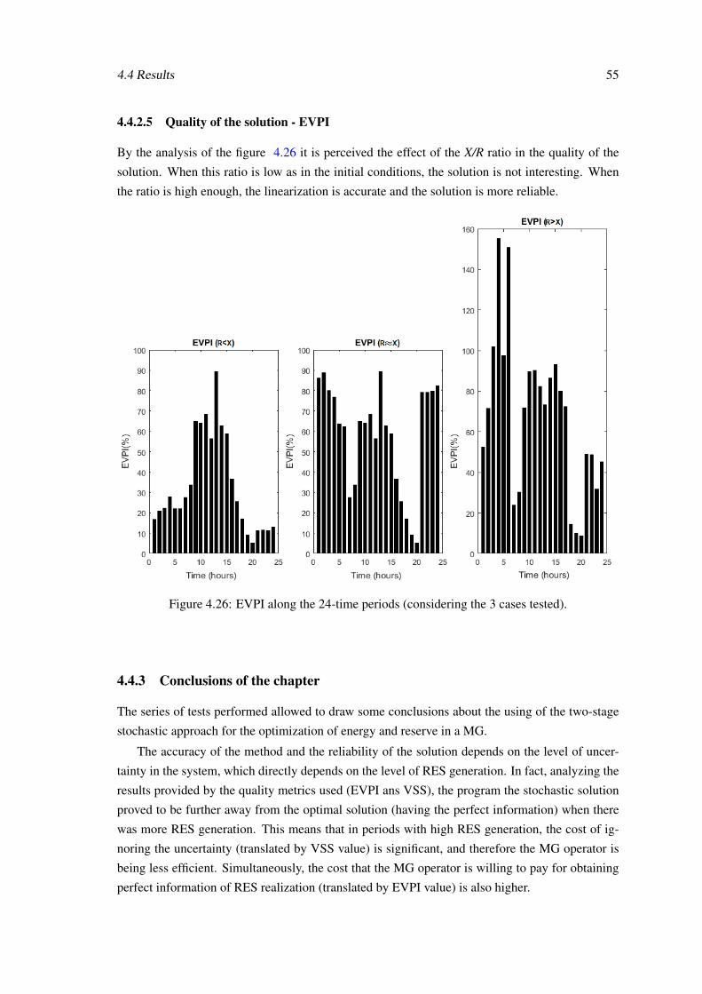
4.4 Results 55
4.4.2.5 Quality of the solution - EVPI
By the analysis of the figure 4.26 it is perceived the effect of the X/R ratio in the quality of the
solution. When this ratio is low as in the initial conditions, the solution is not interesting. When
the ratio is high enough, the linearization is accurate and the solution is more reliable.
Figure 4.26: EVPI along the 24-time periods (considering the 3 cases tested).
4.4.3 Conclusions of the chapter
The series of tests performed allowed to draw some conclusions about the using of the two-stage
stochastic approach for the optimization of energy and reserve in a MG.
The accuracy of the method and the reliability of the solution depends on the level of uncer-
tainty in the system, which directly depends on the level of RES generation. In fact, analyzing the
results provided by the quality metrics used (EVPI ans VSS), the program the stochastic solution
proved to be further away from the optimal solution (having the perfect information) when there
was more RES generation. This means that in periods with high RES generation, the cost of ig-
noring the uncertainty (translated by VSS value) is significant, and therefore the MG operator is
being less efficient. Simultaneously, the cost that the MG operator is willing to pay for obtaining
perfect information of RES realization (translated by EVPI value) is also higher.
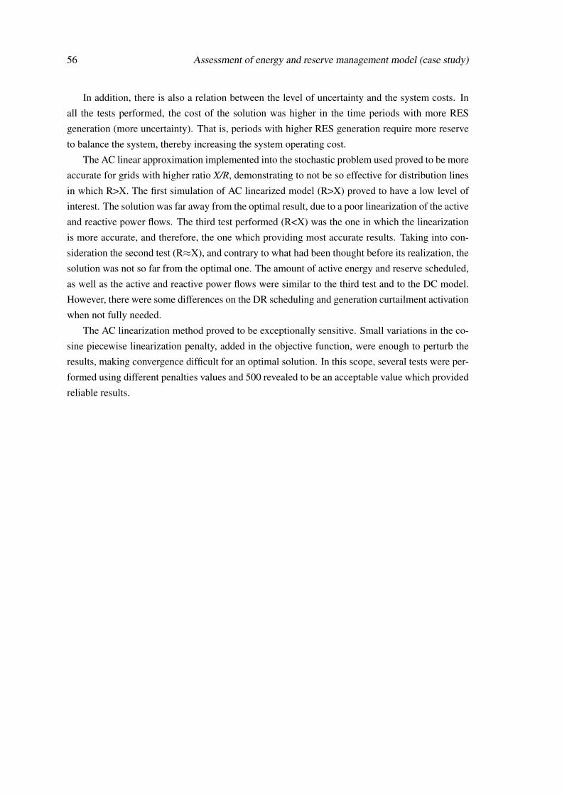
56 Assessment of energy and reserve management model (case study)
In addition, there is also a relation between the level of uncertainty and the system costs. In
all the tests performed, the cost of the solution was higher in the time periods with more RES
generation (more uncertainty). That is, periods with higher RES generation require more reserve
to balance the system, thereby increasing the system operating cost.
The AC linear approximation implemented into the stochastic problem used proved to be more
accurate for grids with higher ratio X/R, demonstrating to not be so effective for distribution lines
in which R>X. The first simulation of AC linearized model (R>X) proved to have a low level of
interest. The solution was far away from the optimal result, due to a poor linearization of the active
and reactive power flows. The third test performed (R<X) was the one in which the linearization
is more accurate, and therefore, the one which providing most accurate results. Taking into con-
sideration the second test (R≈X), and contrary to what had been thought before its realization, the
solution was not so far from the optimal one. The amount of active energy and reserve scheduled,
as well as the active and reactive power flows were similar to the third test and to the DC model.
However, there were some differences on the DR scheduling and generation curtailment activation
when not fully needed.
The AC linearization method proved to be exceptionally sensitive. Small variations in the co-
sine piecewise linearization penalty, added in the objective function, were enough to perturb the
results, making convergence difficult for an optimal solution. In this scope, several tests were per-
formed using different penalties values and 500 revealed to be an acceptable value which provided
reliable results.
Chapter 5
Conclusions and future work
This chapter describes the main conclusions taken from the addressed models on this dissertation.
It contains a critical analysis of the proposed methodologies and a discussion of the main results,
while highlighting the contributions to the state-of-the-art. Finally, the perspective of future de-
velopments in this topic is included.
5.1 Overview of contribution
A MG is a small network of electricity users with a local source of supply that is usually connected
to a centralized national grid but is able to function independently. By being a decentralized
network configuration, the MG can have numerous benefits for both producers and consumers,
comparing with the traditional centralized scheme of the power system. Generation in a MG is
provided by small generators with a capacity of the sources ranging from few kW to 1-2 MW, such
as wind turbines, PV cells, mini hydro plants, CHP, small diesel generators, etc. [4]. RES such
as wind and PV have numerous benefits and their impact on the power system will increase in
the future. The proliferation of this type of resources faces many challenges because their power
production is uncertain and variable, and therefore uncertainty is costly.
This dissertation focuses on energy and reserve management of a MG under high RES pene-
tration. The aim is to minimize the operating costs of the MG, by obtaining optimal energy and
reserve solutions. A two-stage stochastic approach was proposed to address the problem and deal
with the uncertain behavior of RES. Uncertainty was modeled in the form of scenarios with an as-
sociated probability. The DC OPF was implemented to the aforementioned approach to model the
network constraints of a MG, thus avoiding solutions with potential lines congestion. The method
shows some advantages. It shows good computational performance and sufficient accuracy to the
natural nonlinear behavior of the system. However, for a better approximation of the model to the
natural behavior of the MG, different power flow methods can be used, such as AC OPF.
Another important contribution of this dissertation is the inclusion of an recent linearized AC
OPF method that allows a better approximation of the natural MG behavior with a slight increase
in the computational simulation time. More precisely, the method is able to model active and
57
58 Conclusions and future work
reactive power and voltage magnitude as opposed to DC OPF. Thus, this approach enables the
MG operator to be ready to face potential congestion and voltage problems that may arise in the
MG full of DER where bi-directional power flow is common. It should be noted that the AC
OPF linearization proposed by [61] and implemented in this dissertation, provides more accurate
solutions for grids where the ratio X/R is higher. In other cases, the method has some difficulties of
convergence (e.g. for networks with RX), as explained and proven throughout this dissertation.
In fact, the analyses and comparison of different X/R ratios are among the contributions of this
thesis to the scientific literature under this area of research.
All simulated models were developed using MATLAB software as optimization tool, and
solved through the dual-simplex solver. Based on this technique, the most complex model pro-
posed in the development of this work reached 2 hours of simulation. In this way, the proposed
model fits the day-ahead market simulation.
5.2 Perspective of future research
Throughout the development of this dissertation, several ideas have arisen to potentially proceed
with the evolution of the present work.
Firstly, the reliability of the AC linearization method implemented in this dissertation, for the
active and reactive power flow linearization, depends on the impedance value of the lines. For
distribution lines like the ones in the MG tested, the ratio X/R is normally low and the linearization
does not provide an accurate approximation. The future work will focus on an alternative method
to do this linear approximation, and which could be applied accurately to distribution networks.
Secondly, a scenario reduction technique can be included. As explained in chapter 4, a large
number of scenarios make the problem very demanding in terms of computational resources and
with longer run-times. In the case tested, the scenarios had all the same probability and there
was no criteria when adding or removing scenarios to perform the tests. For further work, a
probabilistic analysis and use of a more efficient scenario reduction technique can be performed.
Lastly, it can be also included a research on the feasibility of integrating ESS on the MG by
evaluating the potential cost to be invested and the potential savings for the MG operator.
References
[1] BENJAMIN H. STRAUSS, SCOTT KULP, and ANDERS LEVERMANN. Mappingchoices. Climate Central Research Report, (November), 2015. URL: www.officer.com.
[2] Global carbon atlas <http://www.globalcarbonatlas.org>. URL: http://www.globalcarbonatlas.org/en/content/welcome-carbon-atlas.
[3] S. Massoud Amin. The Power of Microgrids. IEEE SmartGrid - Electric Today Magazine,(January/February/March), 2016.
[4] N.D. Hatziargyriou, A. Dimeas, A.G. Tsikalakis, J.A.P. Lopes, G. Karniotakis,and J. Oyarzabal. Management of microgrids in market environment. 2005International Conference on Future Power Systems, (December 2005):7 pp.–7,2005. URL: http://ieeexplore.ieee.org/document/1600498/, doi:10.1109/FPS.2005.204225.
[5] G Zhang, X Tang, and Z Qi. Research on Battery Supercapacitor Hybrid Storage and itsapplication in MicroGrid. In 2010 Asia-Pacific Power and Energy Engineering Conference,pages 1–4, 2010. doi:10.1109/APPEEC.2010.5448231.
[6] Chao Zhang, Yi-Li Wei, Peng-Fei Cao, and Meng-Chang Lin. Energy storagesystem: Current studies on batteries and power condition system. Renewableand Sustainable Energy Reviews, 82:3091–3106, 2 2018. URL: https://www.sciencedirect.com/science/article/pii/S1364032117314077, doi:10.1016/J.RSER.2017.10.030.
[7] Chen-Ching Liu, Stephen McArthur, and Seung-Jae Lee. Smart Grid Handbook. John Wiley& Sons, 2016. John Wiley & Sons, Inc., 2016.
[8] Omid Palizban, Kimmo Kauhaniemi, and Josep M. Guerrero. Microgrids in active net-work management - Part I: Hierarchical control, energy storage, virtual power plants, andmarket participation. Renewable and Sustainable Energy Reviews, 36:428–439, 2014.URL: http://dx.doi.org/10.1016/j.rser.2014.01.016, doi:10.1016/j.rser.2014.01.016.
[9] F. Martin-Martínez, A. Sánchez-Miralles, and M. Rivier. A literature review of Micro-grids: A functional layer based classification. Renewable and Sustainable Energy Reviews,62:1133–1153, 2016. doi:10.1016/j.rser.2016.05.025.
[10] Moremicrogrids project, microgrids project. www.microgrids.eu n.d. <http://www.microgrids.eu/default.php>.
59
60 REFERENCES
[11] Don Kondoleon, Laurie Ten-Hope, Terry Surles, and Robert L. Therkelsen. The CERTSMicroGrid Concept. Integration of Distributed Energy Resources – The CERTS Micro-Grid Concept, (October):32, 2003. URL: http://certs.lbl.gov/pdf/50829.pdf,doi:LBNL-50829.
[12] Esther Mengelkamp, Johannes Gärttner, Kerstin Rock, Scott Kessler, Lawrence Orsini, andChristof Weinhardt. Designing microgrid energy markets. A case study: The BrooklynMicrogrid. Applied Energy, 210:870–880, 2017. URL: https://doi.org/10.1016/j.apenergy.2017.06.054, doi:10.1016/j.apenergy.2017.06.054.
[13] Tiago Soares and Pierre Pinson. Renewable energy sources offering flexibility through elec-tricity markets. 2017.
[14] Alireza Zakariazadeh, Shahram Jadid, and Pierluigi Siano. Smart microgrid energy andreserve scheduling with demand response using stochastic optimization. InternationalJournal of Electrical Power and Energy Systems, 63:523–533, 2014. URL: http://dx.doi.org/10.1016/j.ijepes.2014.06.037, doi:10.1016/j.ijepes.2014.06.037.
[15] Seyyed Mostafa Nosratabadi, Rahmat Allah Hooshmand, and Eskandar Gholipour. A com-prehensive review on microgrid and virtual power plant concepts employed for distributedenergy resources scheduling in power systems. Renewable and Sustainable Energy Reviews,67:341–363, 2017. URL: http://dx.doi.org/10.1016/j.rser.2016.09.025,doi:10.1016/j.rser.2016.09.025.
[16] M.H. Moradi and A. Khandani. Evaluation economic and reliability issues for anautonomous independent network of distributed energy resources. InternationalJournal of Electrical Power & Energy Systems, 56:75–82, 3 2014. URL: https://www.sciencedirect.com/science/article/pii/S014206151300464X?via%3Dihub, doi:10.1016/J.IJEPES.2013.11.006.
[17] A.D. Hawkes and M.A. Leach. Modelling high level system design and unit commit-ment for a microgrid. Applied Energy, 86(7-8):1253–1265, 7 2009. URL: https://www.sciencedirect.com/science/article/pii/S0306261908002195?via%3Dihub, doi:10.1016/J.APENERGY.2008.09.006.
[18] Chiara Lo Prete, Benjamin F. Hobbs, Catherine S. Norman, Sergio Cano-Andrade, Ale-jandro Fuentes, Michael R. von Spakovsky, and Lamine Mili. Sustainability and reli-ability assessment of microgrids in a regional electricity market. Energy, 41(1):192–202, 5 2012. URL: https://www.sciencedirect.com/science/article/pii/S0360544211005585, doi:10.1016/J.ENERGY.2011.08.028.
[19] Stefano Bracco, Federico Delfino, Fabio Pampararo, Michela Robba, and Mansueto Rossi.A mathematical model for the optimal operation of the University of Genoa Smart Poly-generation Microgrid: Evaluation of technical, economic and environmental performanceindicators. Energy, 64:912–922, 1 2014. URL: https://www.sciencedirect.com/science/article/pii/S0360544213008918?via%3Dihub, doi:10.1016/J.ENERGY.2013.10.039.
[20] S. Y. Derakhshandeh, Amir S. Masoum, Sara Deilami, Mohammad A.S. Masoum, andM. E. Hamedani Golshan. Coordination of generation scheduling with PEVs charging
REFERENCES 61
in industrial microgrids. IEEE Transactions on Power Systems, 28(3):3451–3461, 2013.doi:10.1109/TPWRS.2013.2257184.
[21] H. Moghimi, A. Ahmadi, J. Aghaei, and A. Rabiee. Stochastic techno-economic operation of power systems in the presence of distributed energy re-sources. International Journal of Electrical Power & Energy Systems, 45(1):477–488, 2 2013. URL: https://www.sciencedirect.com/science/article/pii/S0142061512004449?via%3Dihub, doi:10.1016/J.IJEPES.2012.08.008.
[22] G. Cardoso, M. Stadler, M. C. Bozchalui, R. Sharma, C. Marnay, A. Barbosa-Póvoa, andP. Ferrão. Optimal investment and scheduling of distributed energy resources with un-certainty in electric vehicle driving schedules. Energy, 64:17–30, 2014. URL: http://dx.doi.org/10.1016/j.energy.2013.10.092, doi:10.1016/j.energy.2013.10.092.
[23] Wai Shin Ho, Sandro Macchietto, Jeng Shiun Lim, Haslenda Hashim, Zarina Ab. Muis,and Wen Hui Liu. Optimal scheduling of energy storage for renewable energy dis-tributed energy generation system. Renewable and Sustainable Energy Reviews, 58:1100–1107, 5 2016. URL: https://www.sciencedirect.com/science/article/pii/S136403211501480X?via%3Dihub, doi:10.1016/J.RSER.2015.12.097.
[24] Hadi Moghimi Ghadikolaei, Abdollah Ahmadi, Jamshid Aghaei, and Meysam Najafi.Risk constrained self-scheduling of hydro/wind units for short term electricity mar-kets considering intermittency and uncertainty. Renewable and Sustainable EnergyReviews, 16(7):4734–4743, 9 2012. URL: https://www.sciencedirect.com/science/article/pii/S1364032112002894?via%3Dihub, doi:10.1016/J.RSER.2012.04.019.
[25] M. Karami, H.A. Shayanfar, J. Aghaei, and A. Ahmadi. Scenario-based security-constrained hydrothermal coordination with volatile wind power generation. Re-newable and Sustainable Energy Reviews, 28:726–737, 12 2013. URL: https://www.sciencedirect.com/science/article/pii/S1364032113004978?via%3Dihub, doi:10.1016/J.RSER.2013.07.052.
[26] Tetsuya Wakui, Takahiro Kinoshita, and Ryohei Yokoyama. A mixed-integer linear pro-gramming approach for cogeneration-based residential energy supply networks with powerand heat interchanges. Energy, 68:29–46, 2014. URL: http://dx.doi.org/10.1016/j.energy.2014.01.110, doi:10.1016/j.energy.2014.01.110.
[27] Pavan Kumar Naraharisetti, I. A. Karimi, Abhay Anand, and Dong Yup Lee. A lineardiversity constraint - Application to scheduling in microgrids. Energy, 36(7):4235–4243,2011. URL: http://dx.doi.org/10.1016/j.energy.2011.04.020, doi:10.1016/j.energy.2011.04.020.
[28] E.D. Mehleri, H. Sarimveis, N.C. Markatos, and L.G. Papageorgiou. Optimal design andoperation of distributed energy systems: Application to Greek residential sector. Re-newable Energy, 51:331–342, 3 2013. URL: https://www.sciencedirect.com/science/article/pii/S0960148112005757?via%3Dihub, doi:10.1016/J.RENENE.2012.09.009.
[29] Multi-period Islanding Constraints and Amin Khodaei. Microgrid Optimal SchedulingWith. 29(3):1–10, 2013.
62 REFERENCES
[30] Jamshid Aghaei and Mohammad Iman Alizadeh. Multi-objective self-scheduling of CHP(combined heat and power)-based microgrids considering demand response programs andESSs (energy storage systems). Energy, 55:1044–1054, 2013. URL: http://dx.doi.org/10.1016/j.energy.2013.04.048, doi:10.1016/j.energy.2013.04.048.
[31] Alireza Zakariazadeh, Shahram Jadid, and Pierluigi Siano. Stochastic multi-objective op-erational planning of smart distribution systems considering demand response programs.Electric Power Systems Research, 111:156–168, 2014. URL: http://dx.doi.org/10.1016/j.epsr.2014.02.021, doi:10.1016/j.epsr.2014.02.021.
[32] J. Aghaei, H.A. Shayanfar, and N. Amjady. Joint market clearing in a stochas-tic framework considering power system security. Applied Energy, 86(9):1675–1682,9 2009. URL: https://www.sciencedirect.com/science/article/pii/S0306261909000336?via%3Dihub, doi:10.1016/J.APENERGY.2009.01.021.
[33] M.A. Fotouhi Ghazvini, Hugo Morais, and Zita Vale. Coordination between mid-termmaintenance outage decisions and short-term security-constrained scheduling in smartdistribution systems. Applied Energy, 96:281–291, 8 2012. URL: https://www.sciencedirect.com/science/article/pii/S0306261911007124, doi:10.1016/J.APENERGY.2011.11.015.
[34] Kamal Ranjbar, M Moradi Ghahderijani, and S Masoud Barakati. Effects of Time-Of-Use Demand Response Programs Based on Optimal Operation of a MicroGrid in MarketEnvironment. International Journal of Academic Research in Applied Science, 2(5):1–12,2013. URL: http://ijaras.isair.org/papers/2013/(05)May/IJARAS205.pdf.
[35] Faisal A. Mohamed and Heikki N. Koivo. System modelling and online op-timal management of MicroGrid using Mesh Adaptive Direct Search. In-ternational Journal of Electrical Power & Energy Systems, 32(5):398–407, 62010. URL: https://www.sciencedirect.com/science/article/pii/S0142061509001768?via%3Dihub, doi:10.1016/J.IJEPES.2009.11.003.
[36] G. W. Chang, H. J. Lu, and H. J. Su. Short-term Distributed Energy ResourceScheduling for a DC Microgrid. Energy and Power Engineering, 05(04):15–21,2013. URL: http://www.scirp.org/journal/PaperDownload.aspx?DOI=10.4236/epe.2013.54B003, doi:10.4236/epe.2013.54B003.
[37] A. Borghetti, M. Bosetti, C. Bossi, S. Massucco, E. Micolano, A. Morini, C. A. Nucci,M. Paolone, and F. Silvestro. An energy resource scheduler implemented in the auto-matic management system of a microgrid test facility. 2007 International Conference onClean Electrical Power, ICCEP ’07, pages 94–100, 2007. doi:10.1109/ICCEP.2007.384193.
[38] Matteo Vasirani, Ramachandra Kota, Renato L G Cavalcante, Sascha Ossowski, andNicholas R Jennings. An agent-based approach to virtual power plants of wind power gen-erators and electric vehicles. Smart Grid, IEEE Transactions on, 4(3):1314–1322, 2013.
[39] Okan Arslan and Oya Ekin Karasan. Cost and emission impacts of virtual power plantformation in plug-in hybrid electric vehicle penetrated networks. Energy, 60:116–124,
REFERENCES 63
10 2013. URL: https://www.sciencedirect.com/science/article/pii/S0360544213007159?via%3Dihub, doi:10.1016/J.ENERGY.2013.08.039.
[40] D Aloini, E Crisostomi, M Raugi, and R Rizzo. Optimal power scheduling in a VirtualPower Plant. In 2011 2nd IEEE PES International Conference and Exhibition on Inno-vative Smart Grid Technologies, pages 1–7, 2011. doi:10.1109/ISGTEurope.2011.6162768.
[41] M Soltani, M Raoofat, and M A Rostami. Optimal reliable strategy of virtual power plantin energy and frequency control markets. In 2012 Proceedings of 17th Conference on Elec-trical Power Distribution, pages 1–6, 2012.
[42] A Mnatsakanyan and S W Kennedy. A Novel Demand Response Model with an Applicationfor a Virtual Power Plant. IEEE Transactions on Smart Grid, 6(1):230–237, 2015. doi:10.1109/TSG.2014.2339213.
[43] Huanhai Xin, Deqiang Gan, Yun Liu, and Zhen Wang. Control of virtual powerplant in microgrids: a coordinated approach based on photovoltaic systems and con-trollable loads. IET Generation, Transmission & Distribution, 9(10):921–928, 2015.URL: http://digital-library.theiet.org/content/journals/10.1049/iet-gtd.2015.0392, doi:10.1049/iet-gtd.2015.0392.
[44] Stjepan Sucic, Tomislav Dragicevic, Tomislav Capuder, and Marko Delimar. Economicdispatch of virtual power plants in an event-driven service-oriented framework usingstandards-based communications. Electric Power Systems Research, 81(12):2108–2119,12 2011. URL: https://www.sciencedirect.com/science/article/pii/S0378779611001957?via%3Dihub, doi:10.1016/J.EPSR.2011.08.008.
[45] Evaggelos G. Kardakos, Christos K. Simoglou, and Anastasios G. Bakirtzis. Optimal Offer-ing Strategy of a Virtual Power Plant: A Stochastic Bi-Level Approach. IEEE Transactionson Smart Grid, 7(2):794–806, 2016. doi:10.1109/TSG.2015.2419714.
[46] Morteza Shabanzadeh, Mohammad-Kazem Sheikh-El-Eslami, and Mahmoud-Reza Haghifam. A medium-term coalition-forming model of heterogeneousDERs for a commercial virtual power plant. Applied Energy, 169:663–681, 52016. URL: https://www.sciencedirect.com/science/article/pii/S0306261916301817?via%3Dihub, doi:10.1016/J.APENERGY.2016.02.058.
[47] Anders Thavlov and Henrik W. Bindner. Utilization of flexible demand in a virtual powerplant set-up. IEEE Transactions on Smart Grid, 6(2):640–647, 2015. doi:10.1109/TSG.2014.2363498.
[48] Iman Gerami Moghaddam, Mostafa Nick, Farhad Fallahi, Mohsen Sanei, and SaeidMortazavi. Risk-averse profit-based optimal operation strategy of a combined windfarm–cascade hydro system in an electricity market. Renewable Energy, 55:252–259, 7 2013. URL: https://www.sciencedirect.com/science/article/pii/S0960148112007896?via%3Dihub, doi:10.1016/J.RENENE.2012.12.023.
[49] Hrvoje Pandžic, Juan M. Morales, Antonio J. Conejo, and Igor Kuzle. Offering modelfor a virtual power plant based on stochastic programming. Applied Energy, 105:282–292, 5 2013. URL: https://www.sciencedirect.com/science/article/pii/S0306261913000044?via%3Dihub, doi:10.1016/J.APENERGY.2012.12.077.
64 REFERENCES
[50] Taher Niknam, Rasoul Azizipanah-Abarghooee, and Mohammad Rasoul Narimani. An effi-cient scenario-based stochastic programming framework for multi-objective optimal micro-grid operation. Applied Energy, 99:455–470, 2012. URL: http://dx.doi.org/10.1016/j.apenergy.2012.04.017, doi:10.1016/j.apenergy.2012.04.017.
[51] Mohammad Amin Tajeddini, Ashkan Rahimi-Kian, and Alireza Soroudi. Risk averseoptimal operation of a virtual power plant using two stage stochastic program-ming. Energy, 73:958–967, 8 2014. URL: https://www.sciencedirect.com/science/article/pii/S0360544214008093?via%3Dihub, doi:10.1016/J.ENERGY.2014.06.110.
[52] Saeed Rahmani Dabbagh and Mohammad Kazem Sheikh-El-Eslami. Risk-based profit allocation to DERs integrated with a virtual power plant using co-operative Game theory. Electric Power Systems Research, 121:368–378, 42015. URL: https://www.sciencedirect.com/science/article/pii/S0378779614004325?via%3Dihub, doi:10.1016/J.EPSR.2014.11.025.
[53] Kristin Dietrich, Jesus M. Latorre, Luis Olmos, and Andres Ramos. Modelling and assess-ing the impacts of self supply and market-revenue driven Virtual Power Plants. ElectricPower Systems Research, 119:462–470, 2015. URL: http://dx.doi.org/10.1016/j.epsr.2014.10.015, doi:10.1016/j.epsr.2014.10.015.
[54] Hrvoje Pandžic, Igor Kuzle, and Tomislav Capuder. Virtual power plant mid-termdispatch optimization. Applied Energy, 101:134–141, 1 2013. URL: https://www.sciencedirect.com/science/article/pii/S0306261912004126?via%3Dihub, doi:10.1016/J.APENERGY.2012.05.039.
[55] Bernhard Wille-Haussmann, Thomas Erge, and Christof Wittwer. Decentralised op-timisation of cogeneration in virtual power plants. Solar Energy, 84(4):604–611,4 2010. URL: https://www.sciencedirect.com/science/article/pii/S0038092X09002412?via%3Dihub, doi:10.1016/J.SOLENER.2009.10.009.
[56] Malahat Peik-Herfeh, H. Seifi, and M.K. Sheikh-El-Eslami. Decision making of a vir-tual power plant under uncertainties for bidding in a day-ahead market using point es-timate method. International Journal of Electrical Power & Energy Systems, 44(1):88–98, 1 2013. URL: https://www.sciencedirect.com/science/article/pii/S0142061512003766?via%3Dihub, doi:10.1016/J.IJEPES.2012.07.016.
[57] H Morais, T Sousa, P Faria, and Z Vale. Reactive power management strategies in futuresmart grids. In 2013 IEEE Power & Energy Society General Meeting, pages 1–5, 2013.doi:10.1109/PESMG.2013.6672332.
[58] A Mnatsakanyan and S Kennedy. Optimal demand response bidding and pricing mecha-nism: Application for a virtual power plant. In 2013 1st IEEE Conference on Technologiesfor Sustainability (SusTech), pages 167–174, 2013. doi:10.1109/SusTech.2013.6617315.
[59] A Molderink, V Bakker, M G C Bosman, J L Hurink, and G J M Smit. Management andControl of Domestic Smart Grid Technology. IEEE Transactions on Smart Grid, 1(2):109–119, 2010. doi:10.1109/TSG.2010.2055904.
REFERENCES 65
[60] Miadreza Shafie-khah, Mohsen Parsa Moghaddam, Mohamad Kazem Sheikh-El-Eslami,and Mehdi Rahmani-Andebili. Modeling of interactions between market regulationsand behavior of plug-in electric vehicle aggregators in a virtual power market environ-ment. Energy, 40(1):139–150, 4 2012. URL: https://www.sciencedirect.com/science/article/pii/S0360544212001144?via%3Dihub, doi:10.1016/J.ENERGY.2012.02.019.
[61] Carleton Coffrin and Pascal Van Hentenryck. A linear-programming approximation of ACpower flows. INFORMS Journal on Computing, 26(4):718–734, 2014. doi:10.1287/ijoc.2014.0594.
[62] Abdorreza Rabiee, Mohammad Sadeghi, Jamshid Aghaeic, and Alireza Heidari. Optimaloperation of microgrids through simultaneous scheduling of electrical vehicles and respon-sive loads considering wind and PV units uncertainties. Renewable and Sustainable EnergyReviews, 57:721–739, 2016. URL: http://dx.doi.org/10.1016/j.rser.2015.12.041, doi:10.1016/j.rser.2015.12.041.
[63] G. A. LEONOV and N. V. KUZNETSOV. Time-Varying Linearization and thePerron Effects. International Journal of Bifurcation and Chaos, 17(04):1079–1107, 2007. URL: http://www.worldscientific.com/doi/abs/10.1142/S0218127407017732, doi:10.1142/S0218127407017732.
[64] R. Baños, F. Manzano-Agugliaro, F.G. Montoya, C. Gil, A. Alcayde, and J. Gómez.Optimization methods applied to renewable and sustainable energy: A review. Renew-able and Sustainable Energy Reviews, 15(4):1753–1766, 5 2011. URL: https://www.sciencedirect.com/science/article/pii/S1364032110004430, doi:10.1016/J.RSER.2010.12.008.
[65] A.G. Tsikalakis and N.D. Hatziargyriou. Environmental benefits of distributedgeneration with and without emissions trading. Energy Policy, 35(6):3395–3409,6 2007. URL: https://www.sciencedirect.com/science/article/pii/S0301421506004770?via%3Dihub, doi:10.1016/J.ENPOL.2006.11.022.
[66] Ragheb Rahmaniani, Teodor Gabriel Crainic, Michel Gendreau, and Walter Rei.The Benders decomposition algorithm: A literature review. European Jour-nal of Operational Research, 259(3):801–817, 6 2017. URL: https://www.sciencedirect.com/science/article/pii/S0377221716310244, doi:10.1016/J.EJOR.2016.12.005.
[67] In Su Bae and Jin O. Kim. Reliability evaluation of customers in a microgrid. IEEETransactions on Power Systems, 23(3):1416–1422, 2008. doi:10.1109/TPWRS.2008.926710.
[68] Hani Albalawi, Karthikeyan Balasubramaniam, and Elham Makram. Secure Operationand Optimal Generation Scheduling Considering Battery Life for an Isolated NorthwestGrid of Saudi Arabia. Journal of Power and Energy Engineering, 5(01):41, 2017. doi:10.4236/jpee.2017.51004.
[69] S. Q. Ali, S. D. Maqbool, T. P.Imthias Ahamed, and N. H. Malik. Load scheduling withmaximum demand and time of use pricing for microgrids. c2013 IEEE Global Humanitar-ian Technology Conference: South Asia Satellite, GHTC-SAS 2013, pages 234–238, 2013.doi:10.1109/GHTC-SAS.2013.6629922.
66 REFERENCES
[70] Charnon Thammasorn. Generation unit commitment in microgrid with renewable genera-tors and CHP. 2013 10th International Conference on Electrical Engineering/Electronics,Computer, Telecommunications and Information Technology, ECTI-CON 2013, 2013. doi:10.1109/ECTICon.2013.6559661.
[71] Jianxue Wang, Xifan Wang, and Yang Wu. Operating reserve model in the power mar-ket. IEEE Transactions on Power Systems, 20(1):223–229, 2005. doi:10.1109/TPWRS.2004.841232.
[72] Hongming Yang, Dexin Yi, Junhua Zhao, Fengji Luo, and Zhaoyang Dong.Distributed optimal dispatch of virtual power plant based on ELM transforma-tion. Journal of Industrial and Management Optimization, 10(4):1297–1318, 2014.URL: http://www.aimsciences.org/journals/displayArticlesnew.jsp?paperID=9642, doi:10.3934/jimo.2014.10.1297.
[73] H Yang, D Yi, J Zhao, and Z Dong. Distributed Optimal Dispatch of Virtual Power Plant viaLimited Communication. IEEE Transactions on Power Systems, 28(3):3511–3512, 2013.doi:10.1109/TPWRS.2013.2242702.
[74] M Giuntoli and D Poli. Optimized Thermal and Electrical Scheduling of a Large ScaleVirtual Power Plant in the Presence of Energy Storages. IEEE Transactions on Smart Grid,4(2):942–955, 2013. doi:10.1109/TSG.2012.2227513.
[75] P Moutis and N D Hatziargyriou. Decision Trees-Aided Active Power Reduction of aVirtual Power Plant for Power System Over-Frequency Mitigation. IEEE Transactions onIndustrial Informatics, 11(1):251–261, 2015. doi:10.1109/TII.2014.2371631.
[76] Panayiotis Moutis and Nikos D. Hatziargyriou. Decision trees aided scheduling for firmpower capacity provision by virtual power plants. International Journal of Electrical Power& Energy Systems, 63:730–739, 12 2014. URL: https://www.sciencedirect.com/science/article/pii/S0142061514003871?via%3Dihub, doi:10.1016/J.IJEPES.2014.06.038.
[77] Spyros Skarvelis-Kazakos, Evangelos Rikos, Efstathia Kolentini, Liana M. Cipci-gan, and Nick Jenkins. Implementing agent-based emissions trading for control-ling Virtual Power Plant emissions. Electric Power Systems Research, 102:1–7,9 2013. URL: https://www.sciencedirect.com/science/article/pii/S0378779613000989?via%3Dihub, doi:10.1016/J.EPSR.2013.04.004.
[78] Z Bie, P Zhang, G Li, B Hua, M Meehan, and X Wang. Reliability Evaluation of Ac-tive Distribution Systems Including Microgrids. IEEE Transactions on Power Systems,27(4):2342–2350, 2012. doi:10.1109/TPWRS.2012.2202695.
[79] Xin A. Zhongfu T. Lei Y. Shuting L. Yao, W. Interactive Dispatch Modes and BiddingStrategy of Multiple Virtual (2016). (2016):2018, 2018.
[80] A. Tascikaraoglu, O. Erdinc, M. Uzunoglu, and A. Karakas. An adap-tive load dispatching and forecasting strategy for a virtual power plant in-cluding renewable energy conversion units. Applied Energy, 119:445–453, 42014. URL: https://www.sciencedirect.com/science/article/pii/S0306261914000397?via%3Dihub, doi:10.1016/J.APENERGY.2014.01.020.
REFERENCES 67
[81] G. Gutiérrez-Alcaraz, E. Galván, N. González-Cabrera, and M.S. Javadi. Renewableenergy resources short-term scheduling and dynamic network reconfiguration for sus-tainable energy consumption. Renewable and Sustainable Energy Reviews, 52:256–264,12 2015. URL: https://www.sciencedirect.com/science/article/pii/S1364032115007522?via%3Dihub, doi:10.1016/J.RSER.2015.07.105.
[82] Amjad Anvari Moghaddam, Alireza Seifi, Taher Niknam, and Mohammad RezaAlizadeh Pahlavani. Multi-objective operation management of a renewable MG(micro-grid) with back-up micro-turbine/fuel cell/battery hybrid power source. En-ergy, 36(11):6490–6507, 11 2011. URL: https://www.sciencedirect.com/science/article/pii/S0360544211006141?via%3Dihub, doi:10.1016/J.ENERGY.2011.09.017.
[83] S. Goleijani, T. Ghanbarzadeh, F. Sadeghi Nikoo, and M. Parsa Moghaddam. Reli-ability constrained unit commitment in smart grid environment. Electric Power Sys-tems Research, 97:100–108, 4 2013. URL: https://www.sciencedirect.com/science/article/pii/S037877961200363X?via%3Dihub, doi:10.1016/J.EPSR.2012.12.011.
[84] Aliasghar Baziar and Abdollah Kavousi-Fard. Considering uncertainty in the opti-mal energy management of renewable micro-grids including storage devices. Renew-able Energy, 59:158–166, 11 2013. URL: https://www.sciencedirect.com/science/article/pii/S0960148113001821?via%3Dihub, doi:10.1016/J.RENENE.2013.03.026.
[85] Barun Mandal, Provas Kumar Roy, and Sanjoy Mandal. Economic load dispatch usingkrill herd algorithm. International Journal of Electrical Power & Energy Systems, 57:1–10, 5 2014. URL: https://www.sciencedirect.com/science/article/pii/S0142061513004742?via%3Dihub, doi:10.1016/J.IJEPES.2013.11.016.
[86] T. Logenthiran, Dipti Srinivasan, and Ashwin M. Khambadkone. Multi-agent sys-tem for energy resource scheduling of integrated microgrids in a distributed sys-tem. Electric Power Systems Research, 81(1):138–148, 1 2011. URL: https://www.sciencedirect.com/science/article/pii/S0378779610001823?via%3Dihub, doi:10.1016/J.EPSR.2010.07.019.
[87] M. Mohammadi, S.H. Hosseinian, and G.B. Gharehpetian. GA-based opti-mal sizing of microgrid and DG units under pool and hybrid electricity mar-kets. International Journal of Electrical Power & Energy Systems, 35(1):83–92,2 2012. URL: https://www.sciencedirect.com/science/article/pii/S0142061511002213?via%3Dihub, doi:10.1016/J.IJEPES.2011.09.015.
[88] Rodrigo Mena, Martin Hennebel, Yan-Fu Li, Carlos Ruiz, and Enrico Zio. A risk-basedsimulation and multi-objective optimization framework for the integration of distributedrenewable generation and storage. Renewable and Sustainable Energy Reviews, 37:778–793, 9 2014. URL: https://www.sciencedirect.com/science/article/pii/S1364032114003712?via%3Dihub, doi:10.1016/J.RSER.2014.05.046.
[89] Eleonora Riva Sanseverino, Maria Luisa Di Silvestre, Mariano Giuseppe Ippolito, Alessan-dra De Paola, and Giuseppe Lo Re. An execution, monitoring and replanning ap-proach for optimal energy management in microgrids. Energy, 36(5):3429–3436,
68 REFERENCES
5 2011. URL: https://www.sciencedirect.com/science/article/pii/S0360544211002155?via%3Dihub, doi:10.1016/J.ENERGY.2011.03.047.
[90] Thanathip Sum-im. Evolution Algorithm for Unit Commitment Problem. Emerging Tech-nology and Factory Automation, (2), 2014.
[91] Sirus Mohammadi, Soodabeh Soleymani, and Babak Mozafari. Scenario-based stochas-tic operation management of MicroGrid including Wind, Photovoltaic, Micro-Turbine,Fuel Cell and Energy Storage Devices. International Journal of Electrical Power &Energy Systems, 54:525–535, 1 2014. URL: https://www.sciencedirect.com/science/article/pii/S0142061513003359?via%3Dihub, doi:10.1016/J.IJEPES.2013.08.004.
[92] M.Y. El-Sharkh, A. Rahman, and M.S. Alam. Short term scheduling of multiple grid-parallel PEM fuel cells for microgrid applications. International Journal of HydrogenEnergy, 35(20):11099–11106, 10 2010. URL: https://www.sciencedirect.com/science/article/pii/S0360319910013522?via%3Dihub, doi:10.1016/J.IJHYDENE.2010.07.033.
[93] S. Abedi, A. Alimardani, G.B. Gharehpetian, G.H. Riahy, and S.H. Hosseinian. A com-prehensive method for optimal power management and design of hybrid RES-based au-tonomous energy systems. Renewable and Sustainable Energy Reviews, 16(3):1577–1587, 4 2012. URL: https://www.sciencedirect.com/science/article/pii/S1364032111005764?via%3Dihub, doi:10.1016/J.RSER.2011.11.030.
[94] Gwo Ching Liao. The optimal economic dispatch of smart Microgrid including DistributedGeneration. ISNE 2013 - IEEE International Symposium on Next-Generation Electronics2013, pages 473–477, 2013. doi:10.1109/ISNE.2013.6512401.
[95] Stefanos V. Papaefthymiou and Stavros A. Papathanassiou. Optimum sizing of wind-pumped-storage hybrid power stations in island systems. Renewable Energy, 64:187–196, 4 2014. URL: https://www.sciencedirect.com/science/article/pii/S0960148113005788?via%3Dihub, doi:10.1016/J.RENENE.2013.10.047.
[96] Elaheh Mashhour and Seyed Masoud Moghaddas-Tafreshi. Bidding Strategy of VirtualPower Plant for Participating in Energy and Spinning Reserve Markets—Part I:Problem Formulation. IEEE Trans. Power Syst., 26(2):949–956, 2011. doi:10.1109/tpwrs.2010.2070883.
[97] Elaheh Mashhour and Seyed Masoud Moghaddas-Tafreshi. Bidding Strategy of VirtualPower Plant for Participating in Energy and Spinning Reserve Markets—Part II:Numerical Analysis. IEEE Trans. Power Syst., 26(2):957–964, 2011. doi:10.1109/tpwrs.2010.2070883.
[98] Miadreza Shafie-khah, Mohsen Parsa Moghaddam, and Mohamad Kazem Sheikh-El-Eslami. Development of a virtual power market model to investigate strate-gic and collusive behavior of market players. Energy Policy, 61:717–728,10 2013. URL: https://www.sciencedirect.com/science/article/pii/S0301421513004801?via%3Dihub, doi:10.1016/J.ENPOL.2013.06.003.
[99] Daniel Hropko, Ján Ivanecký, and Ján Turcek. Optimal Dispatch of Renewable EnergySources Included in Virtual Power Plant Using Accelerated Particle Swarm Optimization.Elektro, pages 196–200, 2012.
REFERENCES 69
[100] Mette K Petersen, Lars H Hansen, Jan Bendtsen, Kristian Edlund, and Jakob Stoustrup.Heuristic Optimization for the Discrete Virtual Power Plant Dispatch Problem. 5(6):2910–2918, 2014.
[101] Shabnam Lashkari, Yong Wu, and Matthew E.H. Petering. Sequencing dual-spreader craneoperations: Mathematical formulation and heuristic algorithm. European Journal of Op-erational Research, 262(2):521–534, 2017. URL: http://dx.doi.org/10.1016/j.ejor.2017.03.046, doi:10.1016/j.ejor.2017.03.046.
[102] E Alba. Parallel metaheuristics: A new class of algorithms. wiley and sons, 2005.
[103] Abouzar Samimi, Ahad Kazemi, and Pierluigi Siano. Economic-environmental active andreactive power scheduling of modern distribution systems in presence of wind generations:A distribution market-based approach. Energy Conversion and Management, 106:495–509,2015. URL: http://dx.doi.org/10.1016/j.enconman.2015.09.070, doi:10.1016/j.enconman.2015.09.070.
[104] Irfan Khan, Zhicheng Li, Yinliang Xu, and Wei Gu. Distributed control algorithm for op-timal reactive power control in power grids. International Journal of Electrical Powerand Energy Systems, 83:505–513, 2016. URL: http://dx.doi.org/10.1016/j.ijepes.2016.04.004, doi:10.1016/j.ijepes.2016.04.004.
[105] J. Aghaei Rabiee A. H. Moghimi, A. Ahmadi. Stochastic techno-economic operation ofpower systems in the presence of distributed energy resources. International Journal ofElectrical Power and Energy Systems, 45:477–488, 2012.
[106] H Haghighat and S Kennedy. A model for reactive power pricing and dispatch of distributedgeneration. In IEEE PES General Meeting, pages 1–10, 2010. doi:10.1109/PES.2010.5589576.
[107] Abraham Wald. Contributions to the Theory of Statistical Estimation andTesting Hypotheses. The Annals of Mathematical Statistics, 10(4):299–326,1939. URL: http://projecteuclid.org/euclid.aoms/1177732144, doi:10.1214/aoms/1177732144.
[108] Daniel Kuhn, Wolfram Wiesemann, and Angelos Georghiou. Primal and dual linear deci-sion rules in stochastic and robust optimization. Mathematical Programming, 130(1):177–209, 2011. doi:10.1007/s10107-009-0331-4.
[109] Xin Chen, Melvyn Sim, Peng Sun, and Jiawei Zhang. A Linear Decision-Based Ap-proximation Approach to Stochastic Programming. Operations Research, 56(2):344–357,11 2007. URL: https://doi.org/10.1287/opre.1070.0457, doi:10.1287/opre.1070.0457.
[110] Zhiping Chen and Zhe Yan. Scenario tree reduction methods through clus-tering nodes. Computers and Chemical Engineering, 109:96–111, 2018.URL: http://dx.doi.org/10.1016/j.compchemeng.2017.10.017,doi:10.1016/j.compchemeng.2017.10.017.
[111] Federal Energy Regulatory Commission. FERC: Reports on Demand Response& Advanced Metering www.ferc.gov<https://www.ferc.gov/industries/electric/indus-act/demand-response/dem-res-adv-metering.asp>. 2017.
70 REFERENCES
[112] Brady Stoll, Elizabeth Buechler, and Elaine Hale. The value of demand response in Florida.The Electricity Journal, 30(9):57–64, 2017. URL: https://doi.org/10.1016/j.tej.2017.10.004, doi:10.1016/j.tej.2017.10.004.
[113] EDP Energias de Portugal. Tarifa bi-horária www.edpsu.pt. URL: https://www.edp.pt/pt/negocios/apoioaocliente/Pages/TarifaBiHoraria.aspx.
[114] Reserve Markets - Market and operations - Statnett <http://www.statnett.no/en/Market-and-operations/reserve-markets/>.
[115] Federal Energy Regulatory Commission. FERC: Guide to Market Oversight - Glossarywww.ferc.gov <https://www.ferc.gov/market-oversight/guide/glossary.asp>, 2014. URL:http://www.ferc.gov/market-oversight/guide/glossary.asp.
[116] Zhi Zhou, Todd Levin, and Guenter Conzelmann. Survey of U . S . Ancillary ServicesMarkets. page 59, 2016. doi:10.2172/1327815.
[117] A. Cagnano, A. Caldarulo Bugliari, and E. De Tuglie. A cooperative controlfor the reserve management of isolated microgrids. Applied Energy, 218:256–265,5 2018. URL: https://www.sciencedirect.com/science/article/pii/S030626191830285X, doi:10.1016/J.APENERGY.2018.02.142.
[118] Mike Quashie, Chris Marnay, François Bouffard, and Géza Joós. Optimal plan-ning of microgrid power and operating reserve capacity. Applied Energy, 210:1229–1236, 1 2018. URL: https://www.sciencedirect.com/science/article/pii/S0306261917310309, doi:10.1016/J.APENERGY.2017.08.015.
[119] Yan Zhang, Fanlin Meng, Rui Wang, Wanlu Zhu, and Xiao-Jun Zeng. A StochasticMPC based Approach to Integrated Energy Management in Microgrids. Sustainable Citiesand Society, 5 2018. URL: http://linkinghub.elsevier.com/retrieve/pii/S2210670718303378, doi:10.1016/j.scs.2018.05.044.
[120] Vivek Mohan, Jai Govind Singh, and Weerakorn Ongsakul. An efficient two stage stochas-tic optimal energy and reserve management in a microgrid. Applied Energy, 160:28–38, 12 2015. URL: https://www.sciencedirect.com/science/article/pii/S0306261915011095, doi:10.1016/J.APENERGY.2015.09.039.
[121] S. Delikaraoglou. Harnessing and coordinating flexibility through market-based mecha-nisms. Technical University of Denmark, 2016.
[122] Nikolaos V. Sahinidis. Optimization under uncertainty: State-of-the-art and opportuni-ties. Computers and Chemical Engineering, 28(6-7):971–983, 2004. doi:10.1016/j.compchemeng.2003.09.017.
[123] Peter Bogetoft and Lars Otto. International Series in Operations Research & Manage-ment Science, volume 157. 2011. URL: http://link.springer.com/10.1007/978-1-4419-7961-2, doi:10.1007/978-1-4419-7961-2.
[124] Aj Conejo, M Carrión, and Jm Morales. Decision making under uncertaintyin electricity markets. 2010. URL: http://books.google.com/books?hl=en&lr=&id=zta0qWS_W98C&oi=fnd&pg=PR7&dq=Decision+Making+Under+Uncertainty+in+Electricity+Markets&ots=qCCkHiEYoO&sig=B8alt7ssSAwW-QSd9PcAoyIYaJ0.

REFERENCES 71
[125] R N Allan, R Billinton, I Sjarief, L Goel, and K S So. A reliability test system for edu-cational purposes-basic distribution system data and results. IEEE Transactions on PowerSystems, 6(2):813–820, 1991. doi:10.1109/59.76730.
[126] European Commission. Roadmap 2050. Policy, (April):100, 2010. URL: http://www.roadmap2050.eu/, arXiv:ISBN978-92-79-21798-2, doi:10.2833/10759.