MULTIOBJECTIVE MANIPULABILITY IN TRAJECTORY TRACKING FORCONSTRAINED REDUNDANT ROBOT MANIPULATORS

Felipe F. Cardoso∗, Fernando Lizarralde†

∗PETROBRAS - Petroleo Brasileiro S.A., Rio de Janeiro/RJ, Brasil

†Programa de Engenharia Eletrica - COPPE, Universidade Federal do Rio de Janeiro, Brasil

Emails: felipefc@petrobras.com.br, fernando@coep.ufrj.br

Abstract— This paper presents an approach to maximize the manipulability of constrained redundant serialmanipulators for the tracking problem. It is considered that the constraints are within the manipulator chain.Two indices of manipulability are take into account, the first refers to the Jacobian before the constraints andthe second refers to the constrained Jacobian. A multiobjective solution that determines the joint velocitiesfor trajectory tracking is presented in order to maximize the manipulability indices while the constraints inthe manipulator chain are satisfied including the physical limits of joint angles and velocities. Simulations andexperiments are performed in a Baxter R© robot.

Keywords— manipulability, constrained robotic manipulators, trajectory tracking

1 Introduction

Redundant robots need to satisfy constraintswhile performing tasks, for example in minimallyinvasive surgery where the insertion point shouldnot move transversely in order to not cause se-rious lesions in the epithelium (From, 2013). Amanipulability analysis could help to improve acontrol strategy when redundant robots are sub-ject to constraints because it is an indication ofhow close the manipulator is from a singular con-figuration.

A general discussion about manipulability forrobot manipulators can be found in (Sicilianoet al., 2009). Manipulability of constrained sys-tems is discussed in (Wen and Wilfinger, 1999)and for constrained serial manipulators in (Fromet al., 2014). A geometrical approach can be foundin (Park and Kim, 1998; Wen and O’Brien, 2003).A control scheme based on the constrained Jaco-bian in task space for constrained manipulators isdiscussed in (Pham et al., 2014; Coutinho, 2015).In industrial applications a confined environmentcan be seen as a kinematic constraint in the ma-nipulator chain. (Simas et al., 2013; Everist andShen, 2009). In (Yoshikawa, 1985) is presenteda method for maximize the manipulability for anon-constrained redundant manipulator using thenull space of the geometric Jacobian. In (Zhanget al., 2012) an optimization problem is proposedin order to maximize the manipulability of self-motion planning in a redundant manipulator.

This paper presents a general formulation todetermine the Jacobian of a serial manipulatorwith constraints in a point of this kinematic chain,the called constrained Jacobian. As stated by(From et al., 2014) the analysis of manipulabil-ity of a serial redundant constrained manipulatormust take into account not only the constrainedJacobian, but also the manipulator Jacobian untilthe joint before the constraint. So a multiobjec-

tive approach, is presented in order to maximizetwo manipulability indices (corresponding to con-strained Jacobian and the Jacobian until the jointbefore the constraint) while the end-effector fol-lows a trajectory and the imposed constraints aresatisfied. The analysis is addressed to an arm ofthe Baxter R© robot with seven revolute joints anda plane constraint. Simulations and experimentsresults are presented.

The following notation and definitions areused throughout the paper. R := (−∞,∞) andR+ := [0,∞). The subscript i means in general areference for the i-th frame in the kinematic chainof the manipulator, a subscript c denotes a refer-ence for the constraint and a subscript e a refer-ence for the end-effector. A frame is representedby F . A subscript (i, j) in a matrix or vector de-notes the matrix or vector from Fi to Fj . Thejoint angle vector is represented by θ, a joint an-gle in the frame i is denoted by θi, a joint anglevector between Fi and Fj is represented by θi,j= [θi θi+1 · · · θj−1 θj ]. The linear and angularvelocities are denoted by #–v ∈ R3 and #–ω ∈ R3,respectively. The velocity at a frame i is definedby:

Vi =

[#–v i#–ω i

].

The adjoint matrix Φ maps velocities betweentwo frames, for instance, it maps Vi to Vi+1:

Vi+1 = Φi+1,iVi,

Φi+1,i =

[RTi,i+1 −RTi,i+1[( #–p i,i+1)i]×

0 RTi,i+1

]where Ri,i+1 ∈ SO(3) is the orientation of Fi+1

with respect to Fi. [( #–p i,i+1)i]× ∈ R3×3 is theskew symmetric matrix of the distance vector,( #–p i,i+1)i, between frames Fi and Fi+1 representedin Fi. The superscript B means the variable isdefined in the body frame, for example V Bi is thevelocity in Fi in the own frame i.

XIII Simposio Brasileiro de Automacao Inteligente

Porto Alegre – RS, 1o – 4 de Outubro de 2017

ISSN 2175 8905 1773

Figure 1: General manipulator with revolutejoints.

The geometric Jacobian for a frame Fi in bodycoordinates is defined by:

V Bi = JBi (θ1,i)θ1,i,

JBi (θ1,i)=

(#–h 1)i×( #–p 1,i)i ··· (

#–h i−1)i×( #–p i−1,i)i 0

(#–h 1)i ··· (

#–h i−1)i (

#–h i)i

where (#–

h j)i is the axis of rotation of the joint j inFi (without loss of generality, here, only revolutejoints are considered). For any Jacobian matrixJ , JT (JJT )−1 is the pseudo-inverse denoted byJ†.

The pose of the manipulator is representedby p(θ) ∈ Rdim while the desired pose by pd(t) ∈Rdim, dim is the number of dimensions used inthe parameterization of pose. When consideringthe changing of variables over time, t means theactual time and T is the fixed time step of analgorithm.

2 Manipulability of constrained serialmanipulators

A general formulation to obtain the constrainedJacobian and the manipulability indices of a con-strained serial manipulator is presented below. Ageneral system with n revolute joints can be seenin Figure 1. The base frame F0 and F1 are initiallylocated in the same place, frame Fi (i = 1, ..., n) isassociated to the i-th link. Fk is the frame beforethe constraint, Fc in the constraint, Fk+1 after theconstraint and Fe in the end-effector.

The velocity at Fk and the joint velocity arerelated by:

V Bk = JBk (θ1,k)θ1,k. (1)

The velocity at Fc and Fk are related by:

V Bc = Φc,kVBk . (2)

Suppose that a point ∈ Rdim in the kinematicchain of the manipulator is subject to a geometri-cal constraint where the point belongs to a surfaceS. So a linear bilateral velocity constraint in Fccan be defined using a matrix H ∈ Rm×6 wherem is the dimension of the constraint, i.e.,

HV Bc = 0. (3)

Substituting (1) and (2) in (3), one has

HΦc,kJBk (θ1,k)θ1,k = 0. (4)

Defining∧ = HΦc,k,

the joint velocity vector satisfying (4) is given by:

θ1,k = JBk†(θ1,k) ∧# u (5)

where ∧# spans the null space of ∧ and u is acontrol degree of freedom.

The end-effector velocity is given by:

V Be = JBe (θ)θ.

Separating JBe (θ), the end-effector velocitycan be written as (the manipulator has a totalof n joints):

V Be =[JBe1(θ) JBe2(θk+1,n)

] [ θ1,kθk+1,n

]. (6)

Replacing (5) in (6) creates:

VBe =

[JBe1(θ)JBk

†(θ1,k)∧# JBe2(θk+1,n)

] u

θk+1,n

. (7)

In (7) JBe1(θ)JBk†(θk+1,n) only depends of

θk+1,n in the condition that JBk (θ1,k) is not sin-gular (see (Coutinho, 2015)). Thus JBer(θk+1,n),called constrained Jacobian matrix, is defined as

JBer(θk+1,n)=[JBe1(θ)J

Bk†(θk+1,n)∧# JBe2(θk+1,n)

].

A cartesian control can be considered defin-ing: [

u

θk+1,n

]= JBer

†(θk+1,n)uc (8)

where uc ∈ Rnd.The manipulability is an index that represents

the manipulator distance to singular configura-tions. For a given Jacobian matrix J(θ) a ma-nipulability measure can be defined as:

w =√det(J(θ)(J(θ))T ).

In order to analyze the manipulability of aconstrained serial manipulator two Jacobian ma-trices have to be taken into account, the geo-metric Jacobian until the joint before the con-straint (JBk (θ1,k)) and the constrained Jacobian(JBer(θk+1,n)).

The manipulability of JBk (θ1,k) is a measureof how efficiently the constrained manipulator cangenerate motions in Fk in order to follow the de-sired trajectory of the end-effector:

wM =√det(JBk (θ1,k)(JBk (θ1,k))T ). (9)

For the constrained Jacobian matrixJBer(θk+1,n), which can only depends on the

XIII Simposio Brasileiro de Automacao Inteligente

Porto Alegre – RS, 1o – 4 de Outubro de 2017

1774

restriction type and kinematics of the joints afterthe constraint, the manipulability indicates thepossibility of generating the desired trajectory inthe end-effector associated with the use of theconstrained velocity vector in (8):

wC =√det(JBer(θk+1,n)(JBer(θk+1,n))T ). (10)

3 Multiobjective problem formulation

There are two manipulability indices, wM e wC ,the control strategy in Section 2, control schemein (1) to (8), that is applied in (Pham et al., 2014),does not address specifically those two indices, itstrives to follow a trajectory with the constraintssatisfied. In this section a multiobjective problemis proposed, the manipulator must follow the tra-jectory while maintaining the manipulability in-dices as high as possible and satisfying the con-straints.

Whenever a manipulator follows a trajectory,the pose error in an instant t is the difference be-tween the desired pose pd(t) and the actual posep(θ(t)):

e(t) = pd(t)− p(θ(t)). (11)

Considering a method that finds a solutionθs(t), a joint velocity command, at a fixed steptime T that drives the manipulator to bring thepose error in (11) to zero in a step time. Thepredicted error is:

e(t+ T ) = pd(t+ T )− p(θ(t+ T )) (12)

where the predicted joint angle vector in (12) is

θ(t+ T ) = θ(t) + θs(t)T. (13)

Two objective functions are defined, f1 andf2. In an optimization problem we can maximizea function searching the minimum of the negativeof this function, then the functions f1 and f2 arerespectively the negative of wM and wC evaluatedat the predicted joint angle vector in (13):

f1=−√det(JBk (θ1,k(t+T ))(JBk (θ1,k(t+T )))T ), (14)

f2=−√det(JBer(θk+1,n(t+T ))(JBer(θk+1,n(t+T )))T ). (15)

As a multiobjective problem a linear scalar-ization is used for functions f1 and f2 togetherwith a parameter α ∈ R where 0 ≤ α ≤ 1. For aconstrained serial redundant manipulator with aconstraint in a point of this chain and subject tofollow a trajectory, using (14) and (15) a multiob-jeticve problem (the solution is the joint velocityvector θs(t)) is defined as:

min αf1 + (1− α)f2, (16)

s.t. − δ ≤ e(t+ T ) ≤ δ, (17)

HΦc,kJBk (θ1,k(t+ T ))θs1,k(t) = 0, (18)

θ− ≤ θ(t+ T ) ≤ θ+, (19)

θ− ≤ θs(t) ≤ θ+, (20)

where δ ∈ R+ is a constant, θ+ and θ− denoterespectively the upper and lower joint angle limitswhile θ+ and θ− denote respectively the upper andlower joint velocity limits.

The decision variables of the multiobjectiveproblem in (16) to (20) are the joint velocities θi.Although the decision variables are not explicit in(16), (17) and (19) the relation is defined in (13).The search method for the multiobjective problemin (16) to (20) could be any algorithm that solvesnonlinear convex optimization problems. In thesimulations a sequential quadratic programming(sqp) is used. The sqp solves a sequence of opti-mization subproblems, each subproblem optimizesa quadratic model (function of a decision variableθi) subject to a linearization of the constraints.Details about the sqp can be found in (Nocedaland Wright, 1999).

The objective function in (16) is minimizedat each step of the sqp method reflecting a mo-mentary value for wc and wm. The inequality in(17) means that the predicted error is between alower and an upper bound. The constraint (18),the same expression of (4), but now evaluated atθ(t+T ) is the linear velocity constraint in the ma-nipulator chain. The inequality constraints (19)and (20) are the manipulator physical constraintsin terms of joint angle limits and joint velocitylimits respectively.

In order to gather the values of wM and wC ateach step of the sqp method in one index, the in-tegral of the manipulability indices are taken intoaccount: WM =

∫ t0wMdt and WC =

∫ t0wCdt. So

one solution s∗ is defined as a pair WM and WC

for a fixed α.

4 Simulations

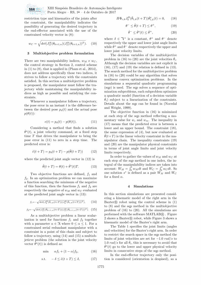
In this section simulations are presented consid-ering a kinematic model of the right arm in theBaxter R© robot using the control scheme in (1)to (8) and the sqp method in the multiobjectiveproblem of (16) to (20). All the simulations areperformed with the software MATLAB R© . Figure2 shows a Baxter R© robot, while Figure 3 shows akinematic model of the Baxter’s right arm.

The Table 1 specifies the joint limits (anglesand velocities) for the Baxter’s right arm. In orderto restrict the search space in the sqp method thelimits of joint velocities are set for −1.0 rad/s to1.0 rad/s for all θi, this is necessary to avoid thatθs(t) go to the lower and upper physical velocitylimits in consecutive steps of the sqp method.

In the end-effector trajectory only the posi-tion is considered (orientation is despised), so a

XIII Simposio Brasileiro de Automacao Inteligente

Porto Alegre – RS, 1o – 4 de Outubro de 2017

1775

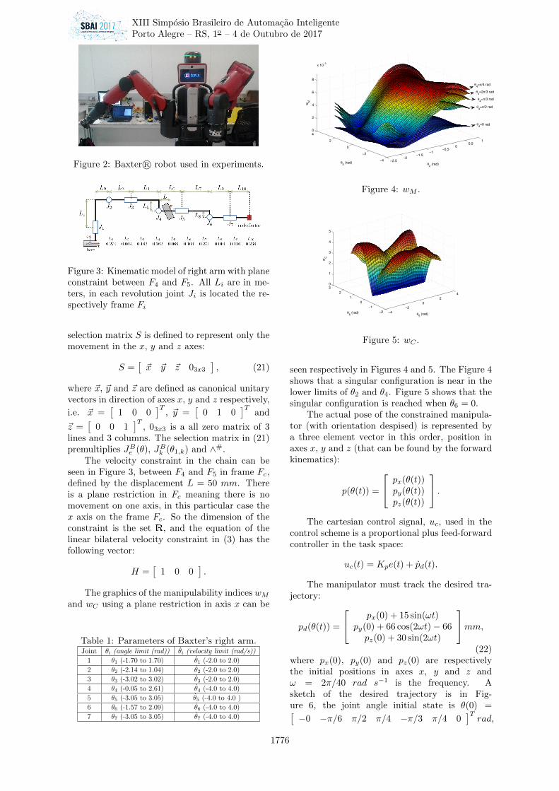
Figure 2: Baxter R© robot used in experiments.

Figure 3: Kinematic model of right arm with planeconstraint between F4 and F5. All Li are in me-ters, in each revolution joint Ji is located the re-spectively frame Fi

selection matrix S is defined to represent only themovement in the x, y and z axes:

S =[~x ~y ~z 03x3

], (21)

where ~x, ~y and ~z are defined as canonical unitaryvectors in direction of axes x, y and z respectively,

i.e. ~x =[

1 0 0]T

, ~y =[

0 1 0]T

and

~z =[

0 0 1]T

, 03x3 is a all zero matrix of 3lines and 3 columns. The selection matrix in (21)premultiplies JBe (θ), JBk (θ1,k) and ∧#.

The velocity constraint in the chain can beseen in Figure 3, between F4 and F5 in frame Fc,defined by the displacement L = 50 mm. Thereis a plane restriction in Fc meaning there is nomovement on one axis, in this particular case thex axis on the frame Fc. So the dimension of theconstraint is the set R, and the equation of thelinear bilateral velocity constraint in (3) has thefollowing vector:

H =[

1 0 0].

The graphics of the manipulability indices wMand wC using a plane restriction in axis x can be

Table 1: Parameters of Baxter’s right arm.Joint θi (angle limit (rad)) θi (velocity limit (rad/s))

1 θ1 (-1.70 to 1.70) θ1 (-2.0 to 2.0)

2 θ2 (-2.14 to 1.04) θ2 (-2.0 to 2.0)

3 θ3 (-3.02 to 3.02) θ3 (-2.0 to 2.0)

4 θ4 (-0.05 to 2.61) θ4 (-4.0 to 4.0)

5 θ5 (-3.05 to 3.05) θ5 (-4.0 to 4.0 )

6 θ6 (-1.57 to 2.09) θ6 (-4.0 to 4.0)

7 θ7 (-3.05 to 3.05) θ7 (-4.0 to 4.0)

−2.5−2

−1.5−1

−0.50

0.51

−4

−2

0

2

40

2

4

6

8

x 10−3

θ2 (rad)θ

3 (rad)

wM

θ4=π/4 rad

θ4=π/3 rad

θ4=π/2 rad

θ4=0 rad

θ4=2π/3 rad

Figure 4: wM .

−4

−2

0

2

4

−2

−1

0

1

2

30

1

2

3

4

5

θ5 (rad)θ

6 (rad)

wC

Figure 5: wC .

seen respectively in Figures 4 and 5. The Figure 4shows that a singular configuration is near in thelower limits of θ2 and θ4. Figure 5 shows that thesingular configuration is reached when θ6 = 0.

The actual pose of the constrained manipula-tor (with orientation despised) is represented bya three element vector in this order, position inaxes x, y and z (that can be found by the forwardkinematics):

p(θ(t)) =

px(θ(t))py(θ(t))pz(θ(t))

.The cartesian control signal, uc, used in the

control scheme is a proportional plus feed-forwardcontroller in the task space:

uc(t) = Kpe(t) + pd(t).

The manipulator must track the desired tra-jectory:

pd(θ(t)) =

px(0) + 15 sin(ωt)py(0) + 66 cos(2ωt)− 66pz(0) + 30 sin(2ωt)

mm,(22)

where px(0), py(0) and pz(0) are respectivelythe initial positions in axes x, y and z andω = 2π/40 rad s−1 is the frequency. Asketch of the desired trajectory is in Fig-ure 6, the joint angle initial state is θ(0) =[−0 −π/6 π/2 π/4 −π/3 π/4 0

]Trad,

XIII Simposio Brasileiro de Automacao Inteligente

Porto Alegre – RS, 1o – 4 de Outubro de 2017

1776

750760

770420

440

460

480

500

520

540

440

450

460

470

480

490

x (mm)

y (mm)

z (

mm

)

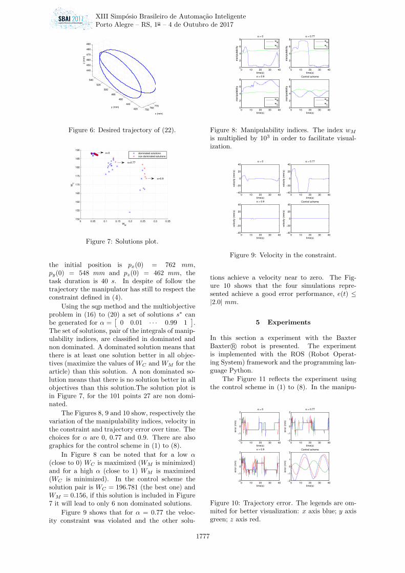
Figure 6: Desired trajectory of (22).

0 0.05 0.1 0.15 0.2 0.25 0.3 0.35150

155

160

165

170

175

180

185

190

WM

WC

dominated solutions

non dominated solutions

α=0

α=0.77

α=0.9

Figure 7: Solutions plot.

the initial position is px(0) = 762 mm,py(0) = 548 mm and pz(0) = 462 mm, thetask duration is 40 s. In despite of follow thetrajectory the manipulator has still to respect theconstraint defined in (4).

Using the sqp method and the multiobjectiveproblem in (16) to (20) a set of solutions s∗ canbe generated for α =

[0 0.01 · · · 0.99 1

].

The set of solutions, pair of the integrals of manip-ulability indices, are classified in dominated andnon dominated. A dominated solution means thatthere is at least one solution better in all objec-tives (maximize the values of WC and WM for thearticle) than this solution. A non dominated so-lution means that there is no solution better in allobjectives than this solution.The solution plot isin Figure 7, for the 101 points 27 are non domi-nated.

The Figures 8, 9 and 10 show, respectively thevariation of the manipulability indices, velocity inthe constraint and trajectory error over time. Thechoices for α are 0, 0.77 and 0.9. There are alsographics for the control scheme in (1) to (8).

In Figure 8 can be noted that for a low α(close to 0) WC is maximized (WM is minimized)and for a high α (close to 1) WM is maximized(WC is minimized). In the control scheme thesolution pair is WC = 196.781 (the best one) andWM = 0.156, if this solution is included in Figure7 it will lead to only 6 non dominated solutions.

Figure 9 shows that for α = 0.77 the veloc-ity constraint was violated and the other solu-

0 10 20 30 400

2

4

6

8

time(s)

ma

nip

ula

bili

ty

α = 0

w

M

wC

0 10 20 30 400

2

4

6

8

time(s)

ma

nip

ula

bili

ty

α = 0.77

w

M

wC

0 10 20 30 400

2

4

6

8

time(s)

ma

nip

ula

bili

ty

α = 0.9

wM

wC

0 10 20 30 400

2

4

6

8

time(s)

ma

nip

ula

bili

ty

Control scheme

wM

wC

Figure 8: Manipulability indices. The index wMis multiplied by 103 in order to facilitate visual-ization.

0 10 20 30 40−40

−20

0

20

40

α = 0

time(s)

ve

locity (

mm

/s)

0 10 20 30 40−40

−20

0

20

40

α = 0.77

time(s)

ve

locity (

mm

/s)

0 10 20 30 40−40

−20

0

20

40

α = 0.9

time(s)

ve

locity (

mm

/s)

0 10 20 30 40−40

−20

0

20

40Control scheme

time(s)

ve

locity (

mm

/s)

Figure 9: Velocity in the constraint.

tions achieve a velocity near to zero. The Fig-ure 10 shows that the four simulations repre-sented achieve a good error performance, e(t) ≤|2.0| mm.

5 Experiments

In this section a experiment with the BaxterBaxter R© robot is presented. The experimentis implemented with the ROS (Robot Operat-ing System) framework and the programming lan-guage Python.

The Figure 11 reflects the experiment usingthe control scheme in (1) to (8). In the manipu-

0 10 20 30 40−2

−1

0

1

2

α = 0

time(s)

err

or

(mm

)

0 10 20 30 40−2

−1

0

1

2

α = 0.77

time(s)

err

or

(mm

)

0 10 20 30 40−2

−1

0

1

2

α = 0.9

time(s)

err

or

(mm

)

0 10 20 30 40−2

−1

0

1

2Control scheme

time(s)

err

or

(mm

)

Figure 10: Trajectory error. The legends are om-mited for better visualization: x axis blue; y axisgreen; z axis red.

XIII Simposio Brasileiro de Automacao Inteligente

Porto Alegre – RS, 1o – 4 de Outubro de 2017

1777

0 5 10 15 20 25 30 35 40−20

−10

0

10

time (s)

err

or

(mm

)

x axis

y axis

z axis

0 5 10 15 20 25 30 35 40−5

0

5

time (s)

ve

locity (

mm

/s)

0 5 10 15 20 25 30 35 400

2

4

6

8

time (s)

ma

nip

ula

bili

ty

wM

wC

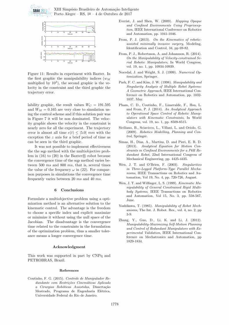
Figure 11: Results in experiment with Baxter. Inthe first graphic the manipulability indices (wMmultiplied by 103), the second graphic is the ve-locity in the constraint and the third graphic thetrajectory error.

lability graphic, the result values WC = 191.595and WM = 0.165 are very close to simulation us-ing the control scheme and if this solution pair wasin Figure 7 it will be non dominated. The veloc-ity graphic shows the velocity in the constraint isnearly zero for all the experiment. The trajectoryerror is almost all time e(t) ≤ |5.0| mm with theexception the z axis for a brief period of time ascan be seen in the third graphic.

It was not possible to implement effectivenessthe the sqp method with the multiobjective prob-lem in (16) to (20) in the Baxter R© robot becausethe convergence time of the sqp method varies be-tween 500 ms and 800 ms, that is, several timesthe value of the frequency ω in (22). For compar-ison purposes in simulations the convergence timefrequently varies between 20 ms and 40 ms.

6 Conclusions

Formulate a multiobjective problem using a opti-mization method is an alternative solution to thekinematic control. The advantage is the freedomto choose a specific index and explicit maximizeor minimize it without using the null space of theJacobian. The disadvantage is the convergencetime related to the constraints in the formulationof the optimization problem, thus a smaller toler-ance means a longer convergence time.

Acknowledgment

This work was supported in part by CNPq andPETROBRAS, Brazil.

References

Coutinho, F. G. (2015). Controle de Manipulador Re-dundante com Restricoes Cinematicas Aplicadoa Cirurgias Roboticas Assistidas, DissertacaoMestrado, Programa de Engenharia Eletrica,Universidade Federal do Rio de Janeiro.

Everist, J. and Shen, W. (2009). Mapping Opaqueand Confined Environments Using Propriocep-tion, IEEE International Conference on Roboticsand Automation, pp. 1041-1046.

From, P. J. (2013). On the Kinematics of robotic-assisted minimally invasive surgery, Modeling,Identification and Control, 34, pp 69-82.

From, P. J., Robertsson, A. and Johansson, R. (2014).On the Manipulability of Velocity-constrained Se-rial Robotic Manipulators, In World Congress,vol. 19, no. 1, pp. 10934-10939.

Nocedal, J. and Wright, S. J. (1999). Numerical Op-timization, Springer.

Park, F. C. and Kim, J. W. (1998). Manipulability andSingularity Analysis of Multiple Robot Systems:A Geometric Approach, IEEE International Con-ference on Robotics and Automation, pp. 1032-1037, May.

Pham, C. D., Coutinho, F., Lizarralde, F., Hsu, L.and From, P. J. (2014). An Analytical Approachto Operational Space Control of Robotic Manip-ulators with Kinematic Constraints, In WorldCongress, vol. 19, no. 1, pp. 8509-8515.

Siciliano, B., Sciavicco, L., Villani, L. and Oriolo, G.(2009). Robotics Modelling, Planning and Con-trol, Springer.

Simas, H., Dias, A., Martins, D. and Pieri, E. R. D.(2013). Analytical Equation for Motion Con-straints in Confined Environments for a P6R Re-dundant Robot, 22nd International Congress ofMechanical Engineering, pp. 4425-4435.

Wen, J. T. and O’Brien, F. (2003). Singularitiesin Three-Legged Platform-Type Parallel Mecha-nisms, IEEE Transactions on Robotics and Au-tomation, Vol 19, No. 4, pp. 720-726, August.

Wen, J. T. and Wilfinger, L. S. (1999). Kinematic Ma-nipulability of General Constrained Rigid Multi-body Systems, IEEE Transactions on Roboticsand Automation, Vol 15, No. 3, pp. 558-567,June.

Yoshikawa, T. (1985). Manipulability of Robot Mech-anisms, The Int. J. Robot. Res., vol. 4, no. 2, pp3-9.

Zhang, Y., Guo, D., Li, K. and Li, J. (2012).Manipulability-Maximizing Self-Motion Planningand Control of Redundant Manipulators with Ex-perimental Validation, IEEE International Con-ference on Mechatronics and Automation, pp1829-1834.

XIII Simposio Brasileiro de Automacao Inteligente

Porto Alegre – RS, 1o – 4 de Outubro de 2017

1778