tre :

Université Toulouse 3 Paul Sabatier (UT3 Paul Sabatier)

Universidade de Brasília (UnB)

ED SDU2E : Hydrologie, Hydrochimie, Sol, Environnement

Raúl Espinoza Villar

vendredi 15 mars 2013

Suivi de la dynamique spatiale et temporelle des flux sédimentaires dans le

bassin de l'Amazone à partir d'images satellite

UMR Géosciences Environnement Toulouse (GET)

Jean-Loup Guyot

Jean-Michel Martinez

José CândidoStevaux

Laerte Guimarães Ferreira

Henrique Llacer Roig

Gustavo Macedo de Mello Baptista

Bruno Lartiges

UNIVERSIDADE DE BRASÍLIA INSTITUTO DE GEOCIÊNCIAS

MONITORAMENTO DAS DINÂMICAS ESPACIAIS E TEMPORAIS DOS FLUXOS SEDIMENTARES NA BACIA

AMAZÔNICA A PARTIR DE IMAGENS DE SATÉLITE

Raúl Espinoza Villar

Tese de Doutorado Nº 08

Brasília-DF

2013

ii

Monitoramento das dinâmicas espaciais e temporais dos

fluxos sedimentares na bacia Amazônica a partir de imagens de satélite

Tese de Doutorado submetida ao Instituto de Geociências da Universidade de Brasília, como parte dos requisitos para obtenção do grau de Doutor em Geociências Aplicada, área de concentração em Geoprocessamento e Análise Ambiental, opção Acadêmica. Apresentada por:

Raúl Espinoza Villar Aprovado por:

______________________________________ Jean-Michel Martinez (IG-UnB) (Orientador) _______________________________________ Paulo Roberto Meneses (Co-Orientador) _______________________________________ Laerte Guimarães Ferreira (Examinador – UnB – DF) _______________________________________ José CândidoStevaux (Suplente – UnB – DF) ______________________________________ Gustavo Macedo de Mello Baptista (Examinador – UnB – DF) ______________________________________ Henrique Llacer Roig (Examinador – UnB – DF)

Brasília-DF

2013

Ficha catalográfica elaborada pela Biblioteca Central da Universidade de Brasília. Acervo 1006773.

V i l l a r , Raú l Arna l do Esp i noza .

V719m Mon i t oramen to das d i nâmi cas espac i a i s e t empora i s dos f l uxos

sed imen tares na Bac i a Amazôn i ca a par t i r de imagens de sa t é l i t e

/ Raú l Arna l do Esp i noza Vi l l ar . - - 2013 .

xx i i i , 226 f . : i l . ; 30 cm.

Tese (dou t orado) - Un i vers i dade de Bras í l i a , I ns t i t u to

de Geoc i ênc i as , Programa de Pós -Graduação em Geoc i ênc i as

Ap l i cadas , 2013 .

I nc l u i b i b l i ogra f i a .

Or i en tação : Jean-Mi che l Mar t i nez ; Coor i en t ação : Pau l o

Rober t o Meneses .

1 . Transpor t e de sed imen t os . 2 . Sensor i amen to remo to .

3 . Fo tograme t r i a aérea - Bac i as h i drográ f i cas . 4 . Amazonas ,

Ri o - Sensor i ament o remo t o . I . Mar t i nez , Jean-Mi che l .

I I . Meneses , Pau l o Rober t o . I I I . T í t u l o .

CDU 528 . 77

iv

Agradecimiento

La presente tesis es el fruto de 4 años de trabajo, no solo mío, sino de todo un equipo

al que quisiera dar mi profundo agradecimiento. Son muchas las instituciones y

personas que colaboraron en sus orígenes y en la realización de esta tesis, en ese

sentido, en primer lugar agradezco a mis orientadores Jean-Michel Martinez, a Jean-

Loup Guyot y Paulo Roberto Meneses que dieron origen a este trabajo y lo

acompañaron y cuidaron hasta el último minuto, y su colaboración dentro y fuera del

ámbito laboral. También quisiera agradecer al Programa de Estudantes-Convênio de

Pós-Graduação (PEC-PG) y a la “Coordenação de Aperfeiçoamento de Pessoal de

Nível Superior” (CAPES) por el financiamiento del Doctorado.

Este trabajo hace parte de un gran proyecto de investigación en la región amazónica,

así quisiera agradecer al equipo HIBAM y a todas las instituciones que hacen parte de

él, especialmente al Instituto de Geociencias de la Universidad de Brasilia (IG-UnB)

por haberme acogido y formado durante estos años, al Institut de recherche pour

le développement (IRD), al laboratorio Géosciences Environnement Toulouse (GET), a

la Agencia Nacional de Aguas (ANA), al Servicio Geológico de Brasil (CPRM), a la

Universidad Nacional Agraria La Molina (UNALM) al Servicio Nacional de Meteorología

e Hidrología del Perú (SENAMHI), al Proyecto CARBAMA y a los integrantes de estas

instituciones por el apoyo, especialmente en las campañas realizadas en la amazonia

en la Amazonia.

Las gracias también a los miembros de mi jurado de tesis y comité de

acompañamiento: José Cândido Stevaux, Laerte Guimarães Ferreira, Henrique Llacer

Roig, Gustavo Macedo de Mello Baptista y Bruno Lartiges por sus muy pertinentes

comentarios y remarcas.

Quisiera agradecer profundamente a mis amigos y compañeros, a los que me

ayudaron tanto en la parte académica y fuera de ella. A la familia de “La Casita Verde”

en especial a Jhan-Carlo Espinoza, Elisa Armijos, Pascal Frazy, Philippe Vauchel, y

William Santini, por estar siempre prestos a ayudar. También los amigos de Brasilia,

en especial a los que me apoyaron desde mi adaptación a la ciudad, a Beatriz

Lamback, Edivaldo Lima, Edinelson Sena, Cristian Rondan, Paulo Henrique Meneses

y a todos los amigos que hicieron mi estadía en Brasilia más agradable y llevadera. A

los amigos de Toulouse, en especial a Tristan Rousseau e Frédéric Satge.

v

Quisiera mencionar también mi agradecimiento a los compañeros de los viajes por los

ríos amazónicos, científicos y a los tripulantes del Yane Jose VI. Por las charlas

enriquecedoras y hacer más placentera las campañas y la colecta de datos.

Por último mi más profundo agradecimiento a mi familia, por su apoyo incondicional y

entender mi ausencia por este periodo, en especial a mis papas Raúl y Nora; a mis

hermanos y sobrinos.

vi

Resumo

A bacia amazônica é a mais importante do mundo em termos de superfície e de vazão

ao oceano, representando uns 15% do volume d’água chegando aos oceanos e

proveniente dos continentes. O fluxo de sedimento do Rio Amazonas foi estimado

entre 600 e 1200 Milliões de toneladas. Na bacia do Amazonas, por causa de seu

tamanho e de difícil acesso, é demasiado complexo e dispendioso o monitoramento

das sub-bacias importantes. Para resolver esses problemas serão exigidos

instrumentos alternativos, como imagens de satélite. A principal desvantagem da

utilização de sensores ópticos nesta região é a grande quantidade de nuvens, mas

este problema pode ser solucionado com a utilização de imagens de alta resolução

temporal. Este trabalho tem como principal objetivo controlar os fluxos de sedimentos

nos grandes rios da Amazônia, e classificar os diferentes tipos de água presente na

bacia, a partir de suas características ópticas.

O sensor MODIS (Moderate Resolution Imaging Spectroradiometer), a bordo dos

satélites TERRA e AQUA, fornecem imagens diárias por cada satélite, fazendo um

total de 2 imagens por dia, com resolução espacial de até 250 m. Nesta pesquisa

serão usadas imagens compostas de 8 dias com resolução espacial de 250 e 500 m

para ambos os satélites, fazendo um total de 4 produtos MODIS (MOD09Q1,

MOD09A1, MYD09Q1 e MYD09A1). Estes produtos fornecem dados de reflectância

com uma correção atmosférica bastante robusta.

A rede de monitoramento ORE-HIBAM vem coletando dados de qualidade de água, a

cada dez dias, desde 2003, em diferentes locais da bacia amazônica. Estas amostras

são para a medição da concentração de matéria em suspensão (MES) de superfície.

Para calibrar estas estações, o projeto HIBAM, em cooperação com entidades

regionais, realiza campanhas para a coleta de amostras d’água e medição de

diferentes parâmetros. Nessas campanhas foram também realizadas medições de

radiometria (reflectância de sensoriamento remoto (Rrs) e coeficiente de atenuação

difusa (Kd)) da água. De maneira simultânea às medições de radiometria foram

coletadas amostras de água.

As medições de Rrs foram relacionados com as concentrações correspondentes de

MES, obtendo um coeficiente de correlação (R2) de 0,89 para 259 amostras. Da

mesma forma foram correlacionados com as medidas de Kd e a concentração de

MES, obtendo R2 de 0,93 para 129 amostras. Ambas as medidas com um intervalo de

concentrações de 2-621.6 mg/l. As medições de radiometria também foram utilizadas

para classificar as águas naturais da Amazônia em 8 classes, dependendo de suas

vii

propriedades ópticas. Com as medidas radiométricas de campo foi possível calcular o

coeficiente de absorção (a) das águas naturais, estimar a absorção do CDOM (aCDOM)

e dos sedimentos (as). Usando estes dados, também foi calculado o coeficiente de

espalhamento (b) e retroespalhamento (bb) para diferentes tipos de água, com

resultados consistentes com a literatura.

A extração da reflectância das imagens MODIS foi realizada de maneira automatizada,

mediante a ferramenta computacional MOD3R. Esta ferramenta extrai a reflectância

dos pixels correspondentes da água, a partir de uma região previamente designada.

Desta forma, pode-se processar e analisar séries históricas a partir de uma grande

quantidade de imagens (mais de 500 imagens por estação).

Com as imagens MODIS foram criadas 6 estações virtuais ao longo do Rio Madeira.

Para esse trabalho foi usada uma razão de bandas (infravermelha / vermelha) e, a

partir dos dados de radiometria de campo e de concentração de MES das campanhas,

os dados MODIS foram calibrados a partir da relação entre dados de MES e o

resultado da razão de bandas. Os dados de MES estimados com as imagens MODIS

foram validados com os dados das estações de Fazenda Vista Alegra e Porto Velho,

da rede ORE-HIBAM obtendo-se um valor de R2 = 0.78. Assim, foram estimados os

valores de MES para cada estação e para um período de 2000 a 2011. Com esses

dados, foi calculado um ano médio (12 médias mensais) para as seis estações. Assim,

observamos os processos de transporte de sedimentos como diluição e precipitação

ao longo do rio Madeira e do comportamento temporal em cada estação e época do

ano, e da influência nos sedimentos do remanso hidráulico causado pelo rio

Amazonas, em alguns meses do ano.

Na confluência dos rios Ucayali e Maranon é formado o rio Amazonas (peruano).

Nessa região existem três estações de amostragem de concentração de sedimentos

de superfície, da rede ORE-HYBAM, nos três rios (Marañón, Ucayali e Amazonas). A

estação do rio Ucayali teve um problema causado pela pluma de um rio afluente,

fazendo com que as amostras nesta estação representem as águas do afluente. O

projeto HIBAM realiza campanhas de amostragem de sedimentos e medição do

caudal sólido e líquido, assim podem se ligar as amostras de sedimentos de superfície

com descarga sólida.

Os dados de reflectância infravermelha MODIS foram relacionados com as

concentrações médias de superfície, medidas durante as campanhas, obtendo-se

boas correlações entre estas duas magnitudes. Usando as relações MES-

Reflectância, foram estimadas series de concentração de sedimentos e posteriormente

viii

foi estimada a descarga sólida em 3 estações. Nas estações dos rios Marañon e

Amazonas, os dados estimados com as imagens de satélite foram validadso com os

dados da rede ORE-HIBAM. Para validar o resultado do rio Ucayali foi realizado um

balanço de massa entre as três estações, de modo que a descarga sólida dos rios

Maranon e Ucayali seja igual à descarga sólida na estação do rio Amazonas. O

equilíbrio foi realizado com dados MODIS estimados, em uma série de imagens entre

os anos 2000 e 2009, fechando o equilíbrio entre as estações tanto a montante quanto

a jusante.

Na presente pesquisa foram estimados dados de MES para um intervalo entre 4 e

1832 mg/l, sem achar saturação na reflectância do canal infravermelho, na razão de

bandas e no Kd. As estimações de MES, a partir dos dados MODIS, realizadas na

presente pesquisa mostraram um erro médio quadrático entre 30 e 40%. Com a

utilização da radiometria de campo, este erro diminui cerca de 23%.

ix

Résumé de la thèse

Le bassin Amazonien est le grand plus réseau hydrographique du monde en termes

d’extension géographique et de débit. Il couvre approximativement 5 % des surfaces

émergées, représente 15 % des apports continentaux en eau douce aux océans

tandis que son débit sédimentaire est de l’ordre de 800 millions de tonnes par an. Le

suivi hydro-sédimentaire des fleuves amazoniens est rendu difficile par la taille du

bassin et la puissance des flux à mesurer pour lesquels les méthodes traditionnelles de

caractérisation sont peu adaptées. Les données de télédétection optique pourraient

représenter une alternative intéressante pour le suivi de paramètres de qualité des

eaux, notamment pour des grands bassins « sous » instrumentés comme l’Amazonie.

Un obstacle important reste cependant le fort ennuagement typique des zones

tropicales humides qui ne peut être dépassé que par l’utilisation d’une très haute

résolution temporelle. L’objectif de la présente thèse est de caractériser les flux

sédimentaires des principaux fleuves amazoniens à partir du suivi par télédétection

des propriétés optiques de leurs eaux.

Les capteurs MODIS (Moderate Resolution Imaging Spectroradiometer) à bord des

satellites Terra et Aqua, fournissent des images journalières sur toute la surface

terrestre. Nous considérons les produits continentaux composites à 8 jours et à 250

mètres de résolution spatiale. Ces images présentent l’avantage d’être calibrées,

corrigées des effets atmosphériques et géoréférencées de manière robuste permettant

un traitement automatisé de longues séries temporelles depuis l’an 2000.

La caractérisation des flux sédimentaires in situ se base sur les données de réseaux

conventionnels de mesure (ORE-HYBAM) et des campagnes de mesure qui ont

permis de mesurer, selon des transects amont-aval, les principales caractéristiques

des flux hydrologiques (débit, variations spatiales et saisonnières), des matières en

suspension (MES) (concentration, minéralogie, granulométrie) et de leurs propriétés

optiques (propriétés optiques apparentes AOP – réflectance télédétectée Rrs et

coefficient d’atténuation diffus vertical descendant Kd).

Un total de 279 mesures de Rrs et 133 de Kd sont analysées afin de déterminer la

variabilité des propriétés optiques des MES au sein du bassin versant de l’Amazone et

durant les différentes périodes du cycle hydrologique. Une classification non

supervisée de Rrs permet de séparer aisément les eaux des plaines d’inondation et les

grands types d’eaux fluviales (eaux noires / claires / blanches). La réflectance est bien

corrélée avec la concentration en MES dans l’infrarouge (r² = 0.81 – 840 < λ < 900 nm)

sur toute la gamme mesurée [2-621 mg/l]. Cependant, Rrs sature rapidement du bleu

x

au rouge dès 100 mg/l. Au contraire, Kd montre une remarquable corrélation avec la

concentration en MES (r² > 0.9), sans saturation et pour une large gamme de longueur

d’ondes du vert (500 nm) à l’infrarouge (850 nm). Les propriétés optiques inhérentes

(IOP) sont aussi étudiées directement (matière organique dissoute colorée – CDOM)

ou déduites à partir des mesures des AOP. La moyenne de l'absorption du CDOM à

440 nm varie en fonction des types d’eaux. Pour les eaux noires, aCDOM est de 7.9

m-1, alors qu’il est de l’ordre de 4.8 m-1, pour les eaux blanches. La relation entre

aNAP (coefficient d’absorption du matériel particulaire) à 550 nm et la MES est très

robuste (r2 =0.91) mais présente une dispersion significative pour les faibles

concentrations. L'absorption spécifique des particules non algales (a*NAP), qui est

définie comme l'absorption par unité de concentration est évaluée à 0.028 m2/g à 555

nm. La variation de aNAP est modélisée par une exponentielle négative dont

l’exposant varie entre 0.006 et 0.015 avec une corrélation négative avec la MES. Le

coefficient de diffusion spécifique des particules non algales b*NAP à 555 nm est en

moyenne de 0.672 ± 0.18 m2.g-1 et montre une variation spectrale du type λ-0.77 avec

la longueur d’onde. Alors que sur l’Amazone et son principal affluent, le Solimões,

aucunes variations saisonnières ne sont détectées, on mesure une variation

saisonnière de b*NAP au sein du fleuve Madeira qui contribue à hauteur de 50% au

débit solide du fleuve Amazone.

L’utilisation des données satellitaires de résolution moyenne (hectométrique) est rendu

difficile par l’étroitesse des cours d’eau vis-à-vis de la taille des pixels. Le phénomène

de mélange spectral peut altérer la réflectance des pixels d’eau en fonction de la

proximité d’éléments possédant des signatures spectrales contrastées (végétation de

berge). Un algorithme a été développé afin d’identifier de manière automatique les

pixels purs d’eaux au sein des scènes MODIS. La réflectance des eaux fluviales

calculées par l’algorithme est validée avec les données radiométriques de terrain

décrites précédemment, avec une bonne précision et avec un biais compatible avec

les études de CAL/VAL précédemment publiées en milieu tropical humide marquée la

présence d’aérosols en grande quantité. L’utilisation de cet algorithme permet un

traitement automatisée des séries temporelles MODIS sur toutes les stations du

réseau HYBAM en Amazonie et sans connaissance a priori des caractéristiques

hydrologiques, météorologiques ou de la géométrie d’acquisition.

Au Brésil, le fleuve Madeira est étudiée de manière systématique avec les données

MODIS Terra et Aqua à partir de la création d’un réseau de stations virtuelles le long

du cours d’eau. L’analyse conjointe des données satellitaires, radiométrique de terrain

et des données de MES à deux stations (Porto Velho et Borba) met en évidence une

xi

hystérésis dans la relation Rrs – concentration en MES. En effet, il apparait que pour

une même concentration en MES, la Rrs est inférieure en période de pic de crue, un

comportement cohérent avec celui détecté pour le coefficient de diffusion spécifique de

la MES comme décrit précédemment. Cette sensibilité est expliquée par une variation

du type de MES qui affecte leur propriétés optique bien qu’il ne soit pas possible de

conclure sur l’origine exacte de cette variation (variabilité granulométrique,

minéralogique ou de la fraction organique). Cependant, l’utilisation d’un ratio

Rrs(Infrarouge) / Rrs(Rouge) permet de s’affranchir de cette sensibilité saisonnière et

permet un suivi précis de la concentration en MES comme l’atteste la validation avec

les données du réseau HYBAM (r = 0.79 – N = 282) pour une large gamme de MES (4

– 1832 mg/ l). L´étude des comportements moyens de la concentration en MES

mesurée par satellite au pas de temps mensuel (estimée par une moyenne

interannuelle entre 2000 et 2011), d’amont en aval, permet le suivi fin des processus

hydro-sédimentaires qui se développent au cours de la traversée du Madeira au sein

de la plaine amazonienne jusqu’à sa confluence avec le fleuve Amazone : dilution,

sédimentation et resuspension. En particulier, la zone de sédimentation induite par le

barrage hydraulique à la confluence Madeira / Amazone est précisément délimitée lors

de la période d’étiage.

Au Pérou, nous étudions la zone de confluence Marañon / Ucayali où se forme le

fleuve Amazone et où l’ORE HYBAM maintient une station hydro-sédimentaire sur

chaque cours d’eau avec le service hydrologique péruvien. La station terrain de

l’Ucayali montre des mesures incohérentes pendant plusieurs années du fait de

l’influence d’un affluent local à l’amont de la station, rendant impossible l’utilisation de

ces données. Pour cette étude, les images MODIS sont calibrées à partir de

campagnes de mesures intensives des MES aux trois stations du réseau HYBAM entre

2007 et 2009. La validation est effectuée de manière indépendante de deux manières.

D’abord en comparant les MES estimées par satellite et les données du réseau

HYBAM (données à 10 jours) aux deux stations montrant des enregistrements valides

(fleuves Amazone et Marañon). Ensuite, les données de MES de surface estimées par

satellite sont utilisées pour calculer une concentration moyenne sur la colonne d’eau

grâce aux données de campagne HYBAM. Les MES moyennes sur la section sont

ensuite multipliées par le débit liquide pour calculer un débit sédimentaire à chaque

station dans la zone de confluence. La comparaison des débits solides déduit par

satellite entre amont (Marañon + Ucayali) et aval (Amazone) montre une excellente

robustesse des estimations satellitaires (RMSE de 18 %, biais de 3 % sur 104 mois de

xii

données) compatible avec une utilisation opérationnelle des données MODIS pour le

suivi des flux sédimentaires au sein du bassin amazonien.

La présente thèse démontre pour la première fois que les propriétés optiques des MES

au sein d’un grand bassin versant hydrologique sont suffisamment stables

spatialement et temporellement afin de permettre un suivi efficace des flux

sédimentaires de surface. Nous avons également démontré que les données MODIS,

grâce au post-traitement que nous présentons, permettent de suivre robustement la

réflectance des eaux de rivières. L’exploitation des images satellitaires permet ainsi de

mettre en évidence les processus hydro-sédimentaires sur de larges périodes de

temps (> 10 ans) et de mesurer les flux sédimentaires en conjonction avec les réseaux

conventionnels de mesure.

xiii

Abstract

The Amazon basin is the largest hydrographical network in terms of geographical

extension and discharge. It covers approximatively 5% of the continental surface,

represents 15% of the fresh water continental contribution to the ocean, while its solid

discharge is of around the 800 millions of ton per year. The hydro-sedimentary

monitoring of the Amazonian rivers is limited by the large extension of the basin and

the magnitude of the fluxes to measure, for which the traditionally characterisation

methods are not well adapted. The optical remote sensing data could represent an

interesting alternative for the monitoring of water quality parameters, particularly for

large under-instrumented basins like the Amazon. However, a main limitation of this

method is the typical nebulosity of the wet tropical regions. This difficulty can only be

resolved by using very high temporal resolution of the data. The objective of this thesis

is to characterize the sedimentary fluxes of the main amazonian rivers, using the

remote sensing monitoring of their water optical properties.

The MODIS sensors (Moderate Resolution Imaging Spectroradiometer) on board of

Terra and Aqua satellites provide daily images on the whole Earth surface. The

continental product composites every 8 days and with 250-m spatial resolution are

used. The advantage of those images is that they are calibrated, the atmospheric

effects are corrected, and they are robustly georeferenced, which make possible an

automatized treatment of large temporal series since 2000.

The in-situ sedimentary fluxes characterization is based on a conventional

measurement network data (ORE-HYBAM) and field campaigns. Those data provided,

via upstream-downstream section, main characteristics of hydrological fluxes

(discharge, spatial and seasonal variabilities), suspended sediment (SS)

(concentration, mineralogy and granulometry) and their optical properties (apparent

optical proprieties AOP – remote sensing reflectance Rrs and downwelling diffuse

attenuation coefficient Kd).

A total of 279 measurements of Rrs and 133 of Kd are analyzed in order to determinate

the variability of optical properties of SS into the Amazon basin and during the distinct

periods of the hydrological cycle. With a classification not supervised of Rrs , the flood

plains water and the main fluvial water types (black water/clear/white) are separated.

The reflectance is well correlated with the SS concentration in the infrared (r² = 0.81 –

840 < � < 900 nm) over all the measured range [2-621 mg/l]. However, Rrs rapidly

saturates from blue to red from 100 mg/l. On the contrary, Kd shows a clear correlation

with the SS concentration (r² > 0.9), without saturation and for a large range of

xiv

wavelength from green (500 nm) to infrared (850 nm). The inherent optical properties

(IOP) are also directly studied (colored dissolved organic matter – CDOM) or deduced

from AOP measurements. The mean absorption of the CDOM at 440 nm differs

according to water types. For black water, aCDOM is 7.9 m-1, while it is of about 4.8

m-1 for white waters. The relation between aNAP (absorption coefficient of the

suspended sediment) at 550 nm and the SS is robust (r2 =0.91) but shows a

significative dispersion for weak concentrations. The specific absorption of the non-

algal particles (a*NAP), which is defined as the absorption per concentration unity is

estimated at 0.028 m2/g à 555 nm. The variation of aNAP is modelized by a negative

exponential with an exponent that varies from 0.006 to 0.015, with a negative

correlation with the SS. The scattering coefficient specific of the non-algal particles

b*NAP at 555 nm is in average of 0.672 ± 0.18 m2.g-1 and shows a spectral variation

of the �-0.77 type with the wavelength. While for the Amazon and its main tributary,

the Solimões, no seasonal variation are detected, a seasonal variation of b*NAP is

measured for the Madeira river, which contribute in around 50% to the solid discharge

of the Amazon mainstream.

The utilization of the medium resolution satellital data (hectometric) is complicated due

to the river narrowness by comparison to the pixel size. The mixing spectral

phenomenon can degrade the reflectance of the water pixels, in relation to the

proximity of the elements having contrasted spectral signatures (riverbank vegetation).

An algorithm was developed in order to automatically identify the pure water pixels into

the MODIS images. The fluvial water reflectance calculated with the algorithm is

validated with the in-situ radiometric data previously described, with a good precision

and a compatible bias with the CAL/VAL studies previously published in humid tropical

environment characterized by the strong quantity of aerosols. This algorithm is used to

automatically treat the MODIS temporal series over all the HYBAM network stations in

the Amazon basin, and without an a priori knowledge of hydrological, meteorological or

acquisition geometry characteritics.

In Brazil, the Madeira River is systematically studied with the MODIS Terra and Aqua

data from the creation of a virtual stations network along the river. The parallel analysis

of the satellital, in-situ radiometric and SS data at two stations (Porto Velho and Borba)

put in evidence an hysterisis in the relation Rrs – SS concentration. Indeed, it seems

that for a similar SS concentration, the Rrs is lower during the highflow period, a

coherent behavior, with regards to the one detected for the SS specific scattering

coefficient, as previously described. This sensibility is explained by a variation of the

SS type, which affect their optical properties, while it is not possible to conclude about

xv

the extract origin of this variation (granulometrical, mineralogical or organic fraction

variability). However, the Rrs(Infrared) / Rrs(Red) ratio is used to avoid the seasonal

sensibility and make possible the precise monitoring of the SS concentration, as the

validation of HYBAM network data has demonstrated (r = 0.79 – N = 282) for a large

SS range (4 – 1832 mg/ l). The study of the mean behaviors of the SS concentration

measured by satellite with a monthly time step (estimated with a interannual mean

between 2000 and 2011), from upstream to downstream, makes possible the precise

monitoring of the hydro-sedimentary processes which develop during the cross section

of the Madeira in the amazon plains, until its confluence with the Amazon River:

dilution, sedimentation and resuspension in particular, the sedimentation zone induced

by the backwater to the Madeira/Amazon confluence is precisely delimited during the

lowflow period.

In Peru, we studied the confluence Marañon / Ucayali zone that is the beginning of the

Amazon River, and where the ORE-HYBAM maintains a hydro-sedimentary station in

each river with the Peruvian hydrological service. The Ucayali in-situ station shows

incoherent measurements during several years, because of the influence of a local

tributary upstream of the station, making impossible the utilization of these data. For

this study the MODIS images are calibrated from the intensive SS measurements field

campaigns in three stations of the HYBAM network between 2007 and 2009. Validation

is achieved using two independent ways. First by comparing the estimated SS from

satellite and HYBAM network data (ten days data) in two stations showing valid

recordings (Amazon and Marañon River ). Second, SS surface satellite data are used

to compute a column water mean concentration with HYBAM field campaigns data.

The comparison of solid discharges deduced from satellite between upstream

(Marañon + Ucayali) and downstream (Amazon) shows a clear robustness of the

satellital estimations (RMSE of 18 %, bias of 3 % over 104 data months) compatible

with an operational utilization of the MODIS data for the monitoring of the sedimentary

fluxes in the Amazon basin.

This thesis demonstrates for the first time that the SS optical properties in a large

hydrological basin are spatially and temporally sufficiently stable to a efficient

monitoring of the surface sedimentary fluxes. In addition, the MODIS data post-

treatment that we describe makes possible the identification of the river water

reflectance. The hydro-sedimentary processes over large temporally periods (>10

years) are characterized by the satellital images utilization and to measure the

sedimentary fluxes in parallel with the measurements conventional networks.

xvi

SUMARIO

1 INTRODUÇÃO 1

1.1 Amazônia. 2

1.1.1 Os recursos hídricos na bacia Amazônica 4

1.1.2 População amazônica. 6

1.2 Problemática. 6

1.2.1 Barragens na bacia Amazônica. 7

1.2.2 Mudança de uso de solo e impacto sobre a hidrologia. 9

1.2.3 Difusão dos metais pesados nos Rios Amazônicos. Exemplo do Mercúrio 14

1.2.4 Estudos de fluxo de Sedimentos na bacia Amazônica. 16

1.3 Sensoriamento Remoto 19

1.3.1 Teledetecção em corpos d’água 21

1.4 Objetivos 23

1.5 Metodologia 24

1.6 Plano da tese 25

2 REVISÃO BIBLIOGRÁFICA 26

2.1 Zona de Estudo 27

2.1.1 Geologia da Amazônia 27

2.1.2 Solo 29

2.1.3 Vegetação 30

2.1.4 Climatologia 30

2.1.5 Hidrologia 32

2.2 Sedimentos nos rios 35

2.2.1 Amostragem de sedimentos 37

2.2.1.1 Amostragem de sedimentos em suspeição 37

xvii

2.2.1.2 Amostragem de fundo. 39

2.2.2 Sedimentos na Bacia Amazônica 39

2.2.2.1 Mineralogia. 40

2.3 Propriedades Ópticas Da Água 41

2.3.1 Grandezas radiométricas 42

2.3.2 Propriedades Ópticas Inerentes 43

2.3.3 Propriedades Ópticas Aparentes e Quase inerentes 45

2.3.3.1 Distribuição da Radiância 46

2.3.3.2 Coeficiente Vertical de Atenuação difuso (K) 46

2.3.3.3 Reflectâncias 47

2.3.4 Relação entre a Reflectância Irradiância Subsuperficial e POI. 47

2.3.5 As POI Espectrais da água 48

3 RESUMO DOS TRABALHOS 53

3.1 Dados 54

3.1.1 Material em suspensão ORE-HIBAM 54

3.1.2 Dados De Campo 55

3.1.2.1 Propriedades dos sedimentos 58

3.1.3 Espectrometria de Campo 61

3.1.3.1 Medição de Reflectância. 62

3.1.3.2 Medições do Coeficiente de atenuação difuso (Kd). 64

3.1.4.1 Produtos MOD09 e MYD09 65

3.1.4 Imagens de Satélite MODIS 65

3.1.4.2 Resolução espacial e Espectrometria Misturada 67

3.1.4.3 Análisis Espectral Sub-Pixel 68

3.1.4.4 Seleção do Endmember 69

3.1.4.5 Extração da reflectância da água. 69

3.2 Influencia das características físicas do MES sobre as propriedades ópticas 73

xviii

3.2.1 Influência do MES sobre Reflectância 73

3.2.2 Influência do MES sobre o coeficiente de atenuação difuso 76

3.2.3 Influência do MES sobre o coeficiente de absorção 76

3.2.4 Influência do MES sobre o coeficiente de retroespalhamento 79

3.3 Relação entre os dados de satélite e a espectrorradiometria de campo 80

3.4 Relação entre a reflectância medida por satélite com a concentração

e tipo de MES 82

3.5 Estimação da vazão Solida nos rios mediante satélite 85

3.6 Monitoramento da dinâmica espacial e temporal dos fluxos de sedimentos. 86

4 Analysis of apparent and inherent optical properties of the

sediment-dominated waters in the Amazon River basin 89

5 Surface water quality monitoring with MODIS data – Application to

the Amazon River 124

6 The integration of field measurements and satellite observations

to determine river solid loads in poorly monitored basins 153

7 A study of sediment transport in the Madeira River, Brazil, using MODIS

remote-sensing images 174

8 Conclusões 206

9 Recomendações 210

10 Referencias Bibliográficas 214

xix

LISTA DE FIGURAS

Figura 1.1. Mapas paleo-geográficos da transição de "cratônica" (A e B) para paisagens de

dominação "Andina" (C a F).

(A) uma vez que a Amazônia se estendeu por grande parte do norte da América do

Sul. Rompimento das placas do Pacífico e os Andes começaram a se formar

(B) Os Andes continuaram emergindo formando a drenagem principal ao noroeste.

(C) Formação de montanhas no Centro e Norte dos Andes, Sistema Pevas.

(D) elevação dos Andes do Norte limitado à "pan-Amazônia"

.(E e F) O mega-Pantanal “Sistema Acre” desapareceu e florestas de terra firme se

expandiram.(F) Quaternário. Note-se que a América do Sul migrou para o norte

durante o curso da Paleogene. Adaptado de Hoorn, et al. 2010 ................................ 3

Figura 1.2. Localização da bacia Amazônica e os principais afluentes .......................................... 5

Figura 1.3. Localização e nível de impacto ecológico das barragens na bacia amazônica.

Adaptada de Finer e Jenkins (2012) ............................................................................ 8

Figura 1.4. Evolução temporal do desmatamento. No ano 1988 a área desmatada era

já de 355000 km². http://www.obt.inpe.br/prodes/prodes_1988_2011.htm. .......................... 10

Figura 1.5. Cobertura vegetal da bacia amazônica, com três classes, terra abrange florestas

tropicais sempre verdes (verde), fechado (bege) e agricultura (amarelo). Mostrado

para vegetação potencial (CTL) como reconstruído por Ramankutty e Foley (1998),

distribuição da vegetação do ano de 2000 (MOD), estimado por Eva et al. (2002), e

dois cenários para o ano de 2050 por Soares-Filho et al. (2006) com forte

governança do desmatamento (GOV) e governação relativamente fraco (BAU).

Fonte Coe et al., 2009 .............................................................................................. 12

Figura 1.6. Mudança relativa da vazão média anual em várias sub bacias, para os cenários

futuros GOV (azul) e BAU (vermelho), respeito a CTL. A vazão é estimada mediante

as simulações IBIS (a) e o modelo integrado CCM3 -IBIS (b)….. ................................ 13

Figura 1.7. Concentração de sedimentos em suspensão de superfície na estação de Óbidos em

função da vazão na mesma estação. Dados do projeto HIBAM coletados a cada 10

dias desde 1995. (adaptado de Martinez et al., 2009) ........................................ …..18

Figure 1.8. Descarga anual de sedimentos em suspensão na estação de Óbidos entre os anos

1996 e 2007. (adaptado de Martinez et al., 2009) ...................................... ……….…19

Figura 1.9. Esquema da metodologia a ser desenvolvido no presente trabalho. ....................... 24

Figura 2.1. Principais elementos tectônicos da América do Sul (fonte CPRM) .......................... .28

Figura 2.2. Variabilidade espacial das chuvas na Bacia Amazônica; todos os gráficos de barras

com as mesmas escalas no eixo Y (precipitação mm) e eixo X (meses do ano

1=janeiro até 12=dezembro). Adaptada de Espinoza et al. (2009b) ..................... ….32

Figura 2.3. Localização das principais sub-bacias e estações hidrológicas da Bacia Amazônica. A

vazão média mensal 1974-2004 (m³/sx10³) é apresentada para cada sub-bacia.

Dados G-L é a soma das estações Gavião e Lábrea. O eixo X são os meses a partir de

1, janeiro a 12, dezembro. Adaptada de Espinoza et al. (2009a)……………………………33

Figura 2.4. Evolução da vazão em Iquitos desde 1970. (Adaptada de Espinoza et al.,

2006)…………………………… ........................................................................................... 35

xx

Figura 2.5. Distribuições de concentração na vertical para materiais de tamanhos variados que

podem ser encontradas num curso d’água (Carvalho, 1994) ................................... 37

Figura 2.6. Interação do raio de luz com o meio aquático. Quando um raio de luz entra no meio

aquatico: uma parte da luz é absorvida pelo meio (Φa), outra é espalhada (Φb) e

outra é transmitida sem variar sua direcção (Φt) ................................................. ….43

Figura 2.7. Variação espectral dos coeficientes de absorção (a) espalhamento (b) e atenuação

(c) da água pura (adaptado de Dekker, 1993).......................... ………………………………49

Figura 2.8. Coeficiente de absorção especifico para a: água pura (aw), e os componentes:

fitoplâncton (aph), matéria orgânica dissolvida (aCDOM) e o material particulado

não orgânico (aTR). (Adaptado de Giardino 2007) ................................................. . 51

Figura 2.9. Variação espectral dos coeficientes de retroespalhamento específicos da água pura

(bbw), do fitoplâncton (bb ph) e do material particulado não orgânico (bb TR).

(Adaptado de Giardino 2007). ........................................................................... ………52

Figura 3.1. Esquema a metodologia a seguir, em parêntesis são indicados os itens onde serão

detalhados .................................................................................. …………………………….54

Figura 3.2. Pontos de coleta de dados nas campanhas realizadas durante a tese. Em círculos

vermelhos, amostras sobre os rios e em estrelas verdes amostras sobre as várzeas

................................................................................................................................... 56

Figura 13.3. Corte transversal do Rio Solimões (medição ADCP) na estação de MAN, os pontos

pretos são os lugares de amostragem. ...................................................... ……………58

Figura 3.4. Amostrador de fundo Callède I, com sonda multiparamétricas e granulômetro lazer

................................................................................................................................... 59

Figura 3.5. Granulometria duas estações no rio Madeira para três temporadas diferentes

........................................................................................................................ …………61

Figura 3.6 Radiômetros TriOS: a) RAMSES-ARC: medição da energia radiante refletida e b)

RAMSES-ACC-VIS: medição da energia incidente ................................................. ….62

Figura 3.7. Esquema da medição da reflectância e a iteração da luz com a superfície e a coluna

de água. Irradiância (Ed), Radiância do céu (Ld) e radiância da água (Ld). θ=30º

................................................................................................................. ………………..63

Figura 3.8. Medições radiométricas de: a) Reflectância e b) Coeficiente de atenuação vertical

difuso da luz descendente (Kd). .............................. ……………………………………………..64

Figura 3.9. Variação da reflectância normalizada com respeito ao ângulo de visada do sensor

radiométrico (Lu) .................................... ……………………………………………………………… 64

Figura 3.10. Medição de Irradiância descendente em diferentes profundidades do corpo de

água, a) para todos os comprimentos de onda a 0,13 m; 0,26 m; 0,45 m; 0,66 m de

profundidade b) para um comprimento de onda (670 nm) em todas as

profundidades ................................................................................ …………………………65

Figura 3.11. Representação da resposta do sensor ao amostrar um alvo misturado. (Adaptado

de: www.envi-sw.com/tut11.htm)............................................................................ 67

Figura 3.12. Representação bidimensional (duas bandas) do conjunto de pixels misturados de

três alvos (A, B, e C), os vértices do triângulo são os endmember de cada alvo e a

área interior do triângulo são os valores da mistura espectral dos três alvos…...... .68

Figura 3.13. Máscara na estação Óbidos no rio Amazonas que pré-seleciona os pixels a serem

analisados……………… .............................................................................. …………………71

xxi

Figura 3.14. Gráfico de espalhamento dos pixels selecionados na máscara, indicando as regiões

teóricas dos endmembers de água, vegetação, alvos de albedo forte e sombra…

................................................................................................................ …………………71

Figura 3.15. Assinaturas espectrais típicas dos diferentes tipos de água dos rios. Madeira,

Amazonas, Tapajos e Negro, e a várzea de Janauacá ........................................... ….74

Figura 3.16. correlação entre a concentração de sedimentos e a reflectância para um

comprimento de onda de 850 nm. ………………………… .............................................. .75

Figura 3.17. variação da correlação de Pearson (R2), entre MES e reflectância, em função do

comprimento de onda…………… ............................................................................ ……75

Figura 3.18. Correlação entre a concentração de sedimentos e o Kd para um comprimento de

onda de 650 nm. …… ............................................................................................. ….76

Figura 3.19. Coeficiente de absorção total para diferentes tipos d’água na Amazônia ………… . 77

Figura 3.20. Coeficiente de absorção do CDOM para diferentes tipos d’água na

amazónia.…………………… .............................................................................. ………….. 78

Figura 3.21. Coeficiente de absorção do material particulado para diferentes concentrações de

MES d’água na amazónia. ……… .......................................................................... …….78

Figura 3.22. Coeficiente de retroespalhamento de diferentes águas amazônicas.…… ........... …79

Figura 3.23. relação entre o coeficiente de retroespalhamento (bb) y material em suspensão

................................................................................................................................ …80

Figura 3.24. Reflectância típica das águas brancas, em linhas pretas a localização das bandas

MODIS e sua distribuição segundo o comprimento de onda ................................... 80

Figura 3.25. Relação da reflectância do sensor MODIS e as medidas de campo com os sensores

TriOS para os diferentes comprimentos de onda do MODIS: a) MODIS a bordo do

satélite TERRA (MOD) e TriOS, b) MODIS a bordo do satélite AQUA e TriOS (MYD) e

c) MODIS a bordo do satélite TERRA e AQUA ......................................................... ..81

Figura 3.26. Relação entre os dados de MES das campanhas e a reflectância de

espectroradiometria nos 851 nm (+) e simulado para a banda infravermelha MODIS

(o), para as águas do rio Solimões/Amazonas ........................................................ ..82

Figura 3.27. Serie temporal de MES da rede ORE-HIBAM e da reflectância infravermelha

MODIS. Na estação de Tamshiyacu… ....................................................................... 83

Figura 3.28. correlação entre MES da rede ORE-HIBAM e da reflectância infravermelha MODIS.

Na estação de Tamshiyacu ................................................................. …………………….83

Figura 3.29. Relação da média dos valores da Reflectância e MES para o período 2000-2011, na

estação de Fazenda Vista Alegre (rio Madeira). As barras de erro mostram o desvio

padrão. A letra indica o MÊS ....................................................................... ……………84

Figura 3.30. Relação da média dos valores de cada MES da razão (IV/V) e MES para o período

2000-2011, na estação de Fazenda Vista Alegre (rio Madeira). As barras de erro

mostram o desvio padrão. A letra indica o MÊS ................................................... ….85

Figura 3.31. Descarga anual de sedimentos (em barras) nas estações de San Regis (SRG) e

Requena (REQ) e vazão média anual .......................................................... ……………86

Figura 3.32. Varicião temporal para um ano médio a o longo do rio Madeira. Sendo Abunã

(ABU), Porto Velho (PV), Humaitá (HUM), Manicoré (MNI), Fazenda Vista Alegre

(FVA) e Foz do Madeira (FOZ). A distância à estação de ABU (km) está ao lado do

código da estação ................................................................... ………………………………..87

xxii

Figura 3.33. Concentração de material em suspensão ao longo do rio Madeira estimada usando

as imagens MODIS, Radiometria de campo e amostras da campanha. Para o MES de

Julho do 2011, considerando a estação de Abuna o km cero

.................................................................................. ………………………………………………88

xxiii

LISTA DE TABELAS

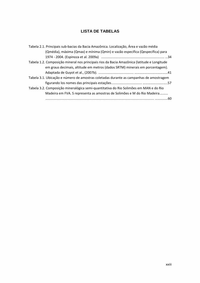
Tabela 2.1. Principais sub-bacias da Bacia Amazônica. Localização, Área e vazão média

(Qmédia), máxima (Qmax) e mínima (Qmin) e vazão específica (Qespecífica) para

1974 - 2004. (Espinoza et al. 2009a) .................................................................... …34

Tabela 1.2. Composição mineral nos principais rios da Bacia Amazônica (latitude e Longitude

em graus decimais, altitude em metros (dados SRTM) minerais em porcentagem).

Adaptada de Guyot et al., (2007b). ...................................... …………………………………41

Tabela 3.1. Ubicação e número de amostras coletadas durante as campanhas de amostragem

figurando los nomes das principais estações ................................. ………………………..57

Tabela 3.2. Composição mineralógica semi-quantitativa do Rio Solimões em MAN e do Rio

Madeira em FVA. S representa as amostras de Solimões e M do Rio Madeira.………

..................................................................................................................... ……………60

1

CAPITULO I

----------------------------------------------------------------------------

Introdução

2

1 INTRODUÇÃO

1.1 Amazônia

A bacia amazônica se estende por mais de 6 x 106 km2, e aporta ao Oceano Atlântico

uma vazão média estimada em 209.000 m3/s (Molinier et al., 1996), representando

15% das águas continentais que chegam aos oceanos. A bacia amazônica atual se

divide em três grandes unidades morfológicas: 44% da superfície pertence aos

escudos Guianês e Brasileiro, 45% à planície amazônica, e 11% aos Andes.

A Amazônia que conhecemos, hoje, fez parte de uma área chamada “Pan –

Amazônia”, região que antes do final do Mioceno, até 10 Milhões de anos (MA) se

estendia pelas atuais bacias dos rios Amazonas, Orinoco, Magdalena e o norte do rio

Paraná (Lundberg et al.,1998). As paisagens dominantes eram rios e ambientes

costeiros, com o mar presente na parte norte do continente. Havia um divisor de

águas, na região leste, fazendo com que a maioria dos rios corresse de leste para

oeste, ao contrário do que ocorre hoje em dia (Figura 1.1A).

A maior parte da história geológica da Amazônia foi centrada no Cráton Amazônico,

onde o núcleo era formado de rocha dura, na parte oriental da América do Sul. Mas

essa situação mudou durante o curso do Cenozóico, causando a ruptura continental

(135 a 100 Ma). Tanto o crescimento do Oceano Atlântico, quanto os ajustes de placas

tectônicas, ao longo da margem do Pacífico, ocasionou a deformação dentro do

Cráton Amazonas. A subducção da placa, ao longo da margem do Pacífico, causou

elevação nos Andes Centrais durante o Paleógeno (65-34 MA). Posteriormente, o

rompimento da placa do Pacífico (~ 23 Ma) e a colisão posterior das novas placas da

América do Sul e do Caribe resultaram na formação de montanhas, intensificando o

crescimento dos Andes do norte (Figura 1.1B).

Os sistemas de drenagem anteriores foram capturados em um rio "invertido" com o

fluxo de oeste ao leste (Mapes 2009), muito diferente do rio Amazonas atual. A divisão

da drenagem situou-se inicialmente no leste da Amazônia, mas em tempos

Paleógenos (~ 65 a 23 MA) a divisão migrou para o oeste (Costa et al., 2001), abrindo

caminho para o precursor do moderno baixo Amazonas, desembocando no Oceano

Atlântico. Perto do final do Paleógeno, a divisão continental localizou-se na Amazônia

Central, separando os rios amazônicos leste e oeste (Figueiredo et al., 2009) (Figura

1.1 B). Durante o Paleógeno, as partes oeste e noroeste das terras baixas pan-

3

amazônicas foram caracterizadas por uma alternância de condições fluviais e

enseadas marinhas (Roddaz et al., 2010).

Figura 1.1. Mapas paleo-geográficos da transição de "cratônica" (A e B) para paisagens de dominação "Andina" (C a F). (A) a Amazônia se estendeu por grande parte do norte da América do Sul. Rompimento das placas do Pacífico e os Andes começaram a se formar (B) Os Andes continuaram emergindo formando a drenagem principal ao noroeste. (C) Formação de montanhas no Centro e Norte dos Andes, Sistema Pevas. (D) Elevação dos Andes do Norte limitado à "pan-Amazônia". (E e F) O mega-Pantanal “Sistema Acre” desapareceu e florestas de terra firme se expandiram. (F) Quaternário. a América do Sul migrou para o norte durante o curso da Paleogene. Adaptado de Hoorn, et al. (2010).

4

Até o final do Mioceno médio (~ 12MA), o crescimento das montanhas andinas foi

mais rápido e mais generalizado (Figura 1.1C). Isso criou um cânion profundo nos

Andes da Venezuela, onde foram desenvolvidos “megafans” aluviais causados pela

erosão nos Andes Central e Norte há ~ 10 Ma, coincidindo com a queda do nível do

mar e resfriamento do clima. As altas taxas de sedimentos andinos atingiram a costa

do Atlântico, através do sistema de drenagem da Amazônia. Finalmente, o rio

Amazonas tornou-se plenamente estabelecido em ~ 7 MA (Figura 1.1D e E). Enquanto

isso, a Amazônia Ocidental passou de um sistema lacustre a um sistema fluvial

(Figura 1.1D) (Hovikoski et al., 2007), que se assemelhava ao Pantanal de hoje no sul

da Amazônia. Esta região foi chamada sistema "Acre". A Amazônia Ocidental, a partir

de então, passou a ter as principais características geográficas da paisagem como a

conhecemos hoje (Figura 1.1E e F), mudando de um sistema inundado com relevo

negativo, para um relevo positivo, cortado por um sistema de rios, cada vez mais

arraigado e com maior carga de sedimentos.

1.1.1 Os recursos hídricos na bacia Amazônica

O rio Amazonas (Figura 1.2) é formado no Peru pelos rios andinos Ucayali e Marañón

e recebe um pouco mais a jusante, o rio Napo vindo do Equador. Ao entrar no Brasil

este rio passa a se chamar Solimões, com fluxo médio é de 46.000 m³/s, ou seja, o

equivalente do rio Congo (o segundo maior rio do mundo em extensão) (Filizola

2003). O rio Solimões passa a se chamar rio Amazonas no Brasil, somente após o

recebimento das águas do rio Negro. Na região de Manaus, a convergência dos rios

Solimões, Negro a 200 kilometros mais a jusante do rio Madeira, aumenta de forma

acentuada a área drenada e os fluxos. Esta concentração de recursos, associada ao

gradiente hidráulico muito baixo, irá gerar perturbações no fluxo destes rios,

agravando a não univocidade das curvas chave (altura-vazão) dos rios, nesta região

(Meade et al., 1991). De Tabatinga, na fronteira entre o Peru e o Brasil, o rio

Amazonas tem cerca de 3.000 km, antes da chegada ao Atlântico, no entanto, apesar

dessa distância, ele possui apenas 60 metros de desnível, o que explica a

peculiaridade da propagação da onda criando uma gigantesca zona de

inundação. Neste percurso o seu volume será multiplicado por 4,5 despejando uma

média de 209.000 m3/s no oceano Atlântico (Molinier et al., 1996).

5

Figura 1.2. Localização da bacia Amazônica e os principais afluentes

Os principais formadores da Bacia Amazônica têm características relacionadas a três

grandes unidades morfológicas: i) A vertente oriental dos Andes, principalmente, com

os Rios Marañón, Ucayali e Madeira que contribuem ao rio Amazonas com águas

carregadas de matéria dissolvida e particulada (Gibbs 1967); ii) Os escudos Guayani e

Brasileiro os quais são caracterizados pela pouca erosão de suas ladeiras (Bordas

1991) que aportam poucos sedimentos ao rio Amazonas; e iii) A Planície Amazônica

onde ficam presas grandes quantidades de sedimentos e podem ser removidas em

diferentes escalas de tempo (Schmidt 1972). Esta planície se estende desde o meio

da bacia, entre os escudos e a região do "piedemonte" andino.

O rio Solimões-Amazonas é um “mega” rio que exibe padrão anastomosado, com dois

ou três braços, grandes ilhas cobertas por vegetação, em formato elipsóidal, e bancos

de areia laterais (Latrubesse, 2008). Seu leito principal é, principalmente, retilíneo ao

longo de seu curso, com um índice de sinuosidade médio, em 100 km de 1,0 a 1,2

(segundo Brice, 1964, o índice de sinuosidade é a razão entre os comprimentos real

do canal e o comprimento vetorial do canal), com exceção do trecho de 350 km a

montante da foz do rio Purus, que apresenta um padrão de multi-canais sinuosos com

meadros duplos ou triplos e a sinuosidade variando de 1,3 a 1,7. Na época de

estiagem, na parte brasileira de 2500 km, a largura média do canal do rio

6

Solimões/Amazonas varia de 2,2 a 6 km enquanto a profundidade média, por seção

transversal, aumenta de 10 a 20 m (Mertes et al., 1996).

A Bacia Amazônica, por seu tamanho e posição equatorial, apresenta vários regimes

hidrológicos, assim como, vazão específica. Muitos trabalhos descrevem tanto a

variabilidade regional como interanual (Richey et al., 1989; Marengo, 1995; Callède et

al., 2004; Espinoza et al., 2009b). Em particular, Callède (2004), Espinoza et al.

(2009b, 2011) e Marengo et al. (2011), reportam um aumento da frequência dos

eventos hidrológicos extremos na bacia amazônica, desde o final da década de 1970.

1.1.2 População amazônica

Calcular a área e a população da Amazônia sempre foram alguns dos maiores

desafios para pesquisadores e planejadores (Oliveira Jr., 2009). Para alguns, a

Amazônia representa uma grande reserva de recursos naturais ou capital natural,

despovoada, que necessita ser ocupada. Para outros, a população já existente na

região está gerando impactos ambientais negativos irreversíveis, sendo preciso,

portanto, controlar ou mesmo frear seu crescimento populacional.

Aragón (2011) apresenta dados dos últimos censos dos países Amazônicos,

considerando os territórios da Guiana, Guiana Francesa e Suriname 100% amazônico,

e usando no Brasil como referência o território da Amazônia Legal (bacia Amazônica

mais as bacias dos rios Tocantins e Maranhão). Ele estima a população dessa área

total em 29 milhões de habitantes. No Brasil, a população é mais de 21 milhões, que

representa 72% dos habitantes da bacia Amazônica. A população amazônica peruana

é de 4,5 milhões (16% da população total do Peru). As principais cidades da Amazônia

são Manaus, Belém, Santa Cruz de la Sierra (Bolivia), Iquitos (Peru), Porto Velho,

Macapá, Rio Branco e Santarem.

1.2 Problemática

O foco desta tese é o monitoramento dos fluxos de sedimentos que é relevante para

uma grande variedade de disciplinas ambientais e para a gestão dos recursos

hídricos. De fato, muitos problemas ambientais estão relacionados com o transporte

de sedimentos pelos rios, tanto os sedimentos de suspensão como os de fundo. Nos

rios, em geral, a turbulência do escoamento mantém os sedimentos finos

permanentemente em suspensão. Os sedimentos em suspensão geralmente são

7

argilas com propriedades coesivas capazes de transportar diversos contaminantes

(metais pesados como o mercúrio, chumbo e outros) além de nutrientes. O fluxo de

sedimento traz uma carga de elementos essencias (nitrogênio, fósforo etc.) para o

crecimento do fitoplâncton nas águas (Alabaster e Lloyd, 1982; Steinman and

McIntire, 1990; Heathwaite,1994) e do zooplâncton (Langer, 1980; Ryder, 1989) e,

consequentemente, influencia toda a biota da bacia. No entanto, em cenários com

menor intensidade de turbulência, como em estuários, reservatórios ou lagos, os

sedimentos encontram condições propícias para a deposição e, de tal modo, o leito

desses ambientes se transformam no último sumidouro dos contaminantes (Gibbs,

1983). Esses processos de assoreamento também podem causar dificuldades de

navegação nos grandes rios e diminuir a vida útil das barragens. Outra problemática

que pode ser entendida com os estudos dos fluxos sedimentares envolve os

processos de erosão e a perda de solos que estão fortemente ligados ao uso das

terras. A quantidade de sedimentos transportados por um rio é proporcional à erosão

causada dentro da bacia. Assim, o monitoramento dos fluxos de sedimentos traz

informações sobre as mudanças na climatologia e no uso dos solos, na escala da

bacia.

Todas as problemáticas descritas acima podem ser observadas no caso da Bacia

Amazônica, o que justifica o interesse e a importância em aprimorar as técnicas de

monitoramento dos fluxos de sedimentos. Detalharemos a seguir as problemáticas

ambientais citadas acima.

1.2.1 Barragens na bacia amazônica

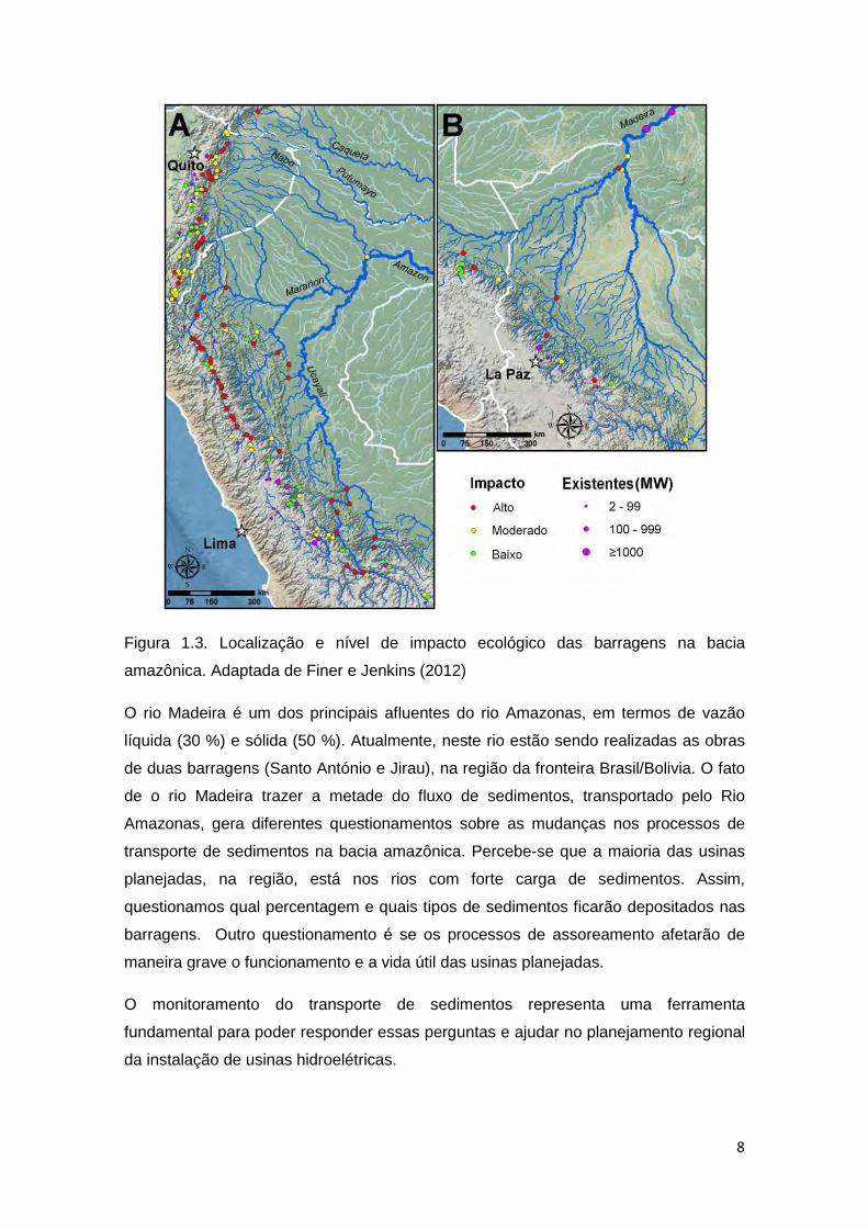
Atualmente, os governos da região estão planejando a construção de 151 barragens

para a geração de energia elétrica (Finer e Jenkins, 2012) em todos os principais

afluentes andinos do rio Amazonas (Caquetá/Japurá, Madeira, Napo, Marañon,

Putumayo/Iça e Ucayali) (Figura 1.3), abrangendo cinco países: Bolívia, Brasil,

Colômbia, Equador e Peru.

Como sabemos, o rio Amazonas está intimamente ligado à cordilheira dos Andes. Os

Andes fornecem a grande maioria dos sedimentos, nutrientes e matéria orgânica para

o curso principal do Amazonas, alimentando um ecossistema de várzea. Finer e

Jenkins (2012) analisaram o impacto causado por estas barragens de maneira global,

no curso da bacia, considerando os impactos no local e os causados, na planície da

bacia. Das 151 barragens projetadas 71 delas são de alto impacto ecológico, 51 delas

de impacto moderado e 29 de baixo impacto ecológico.

8

Figura 1.3. Localização e nível de impacto ecológico das barragens na bacia

amazônica. Adaptada de Finer e Jenkins (2012)

O rio Madeira é um dos principais afluentes do rio Amazonas, em termos de vazão

líquida (30 %) e sólida (50 %). Atualmente, neste rio estão sendo realizadas as obras

de duas barragens (Santo António e Jirau), na região da fronteira Brasil/Bolivia. O fato

de o rio Madeira trazer a metade do fluxo de sedimentos, transportado pelo Rio

Amazonas, gera diferentes questionamentos sobre as mudanças nos processos de

transporte de sedimentos na bacia amazônica. Percebe-se que a maioria das usinas

planejadas, na região, está nos rios com forte carga de sedimentos. Assim,

questionamos qual percentagem e quais tipos de sedimentos ficarão depositados nas

barragens. Outro questionamento é se os processos de assoreamento afetarão de

maneira grave o funcionamento e a vida útil das usinas planejadas.

O monitoramento do transporte de sedimentos representa uma ferramenta

fundamental para poder responder essas perguntas e ajudar no planejamento regional

da instalação de usinas hidroelétricas.

9

1.2.2 Mudança de uso do solo e o impacto sobre a hidrologia

A bacia amazônica é coberta por grandes extensões de florestas densas. O

desmatamento raso é o método mais comum de desenvolvimento que tem sido

utilizado, e, é a principal causa de distúrbios na natureza na região Amazônica, pois

interfere em ciclos naturais, como os da água e do carbono. Essa prática altera,

rapidamente, as características hidrológicas e físicas dos solos e, consequentemente,

pode alterar os processos de transporte de sedimentos nos rios da região.

A erosão e a perda de solo são as consequências mais óbvias do desmatamento,

assim como, a perda da capacidade de infiltração e retenção da água. Isso influi,

diretamente, nas condições hídricas das bacias. As funções da bacia hidrográfica são

alteradas, quando a floresta é desmatada. A precipitação nas áreas desmatadas

escoa rapidamente, formando as cheias, seguidas por períodos de grande redução ou

interrupção do fluxo dos cursos d’água. Os padrões regulares das cheias são

importantes para o funcionamento do ecossistema natural do rio e das regiões

arredores.

No Brasil, a Amazônia Legal vem sendo desmatada a partir da década de 1960. A

fronteira agropecuária, com incentivo do Governo Federal, se expandiu para o oeste

da bacia. Tal expansão continua ocorrendo e resultará em taxas elevadas de

desmatamento, na bacia do rio Amazonas (Achard et al., 2002; Fearnside e Graça,

2006; Kaimowitz et al., 2004). Aproximadamente, 17% da bacia amazônica (excluindo

Tocantins) foram desmatadas até 2007 (INPE, 2011), As principais zonas desmatadas

estão na região leste e sul da bacia (Fearnside, 1993, Nepstad et al., 1999; Skole e

Tucker, 1993). A pecuária é a maior responsável pelo desmatamento na Amazônia,

cobrindo cerca de 75% da área total desflorestada (Faminow, 1998; Margulis, 2003).

No entanto, a produção de soja, principalmente, como ração animal para exportação

para a Europa e China (Nepstad et al., 2006), tornou-se mais importante na última

década, utilizando outras áreas, como o cerrado e bosques, principalmente, no sul da

bacia.

A pecuária, na região, vem crescendo, desde a década de 1970, passando de cerca

de 18,7 milhões de unidades em 1985, para 35 milhões em 1995 e 56 milhões em

2006. Esse crescimento ocorreu, devido à melhoria das condições sanitárias de

produção, permitindo a exportação para outras regiões do país e, também, para os

mercados internacionais (Nepstad et al., 2006).

10

Sobre as rodovias existe certo consenso na literatura de que a abertura ou a

pavimentação, das já existentes, facilitam o acesso dos agentes econômicos (como os

agricultores) à áreas, até então, isoladas, diminuindo, assim, os custos de transporte e

ampliando a área destinada à agropecuária, causando, então, mais desmatamento.

Entre todas as variedades de culturas, a da soja é apontada pelos especialistas como

a grande responsável pelo avanço do desmatamento na região amazônica. O cultivo

da soja na região não é recente. Ele data de meados da década de 1950, quando o,

então, Instituto Agronômico do Norte realizou alguns experimentos com essa cultura

em áreas de várzea em Belém. Em 1982, foi registrada a primeira área para o cultivo

comercial da soja, totalizando 60 hectares no Estado de Rondônia. No ano de 1984, a

Embrapa Soja recomendou o plantio dessa cultura em Rondônia (Homma, 2006). A

partir dessa época, a área ocupada pela soja foi crescente.

A Figura 1.4 mostra a área desmatada na Amazônia Legal no período de 1988 a 2011,

alcançando o pico máximo em 1995 com mais de 29.000 km² desmatados e nos anos

2003 e 2004 com mais de 25.000 km². Depois de 2004 observa-se que a área de

desmatamento, por ano, vai diminuindo, e, no ano de 2011 foi o de menor

desmatamento, sendo de 6.400 km² (INPE 2011). A área desmatada até o 1988 é

estimada em 355.000 km² e a média estimada de desmatamento é de 21.050 km²/ano.

Figura 1.4. evolução temporal do desmatamento. No ano 1988 a área desmatada era já de 355.000 km² Fonte: http://www.obt.inpe.br/prodes/prodes_1988_2011.htm Entre os estados pouco desmatados encontram-se o Acre, Amapá, Amazonas,

Maranhão, Roraima e Tocantins. Esses estados responderam, em média, por

0

5000

10000

15000

20000

25000

30000

35000

1988

1989

1990

1991

1992

1993

1994

1995

1996

1997

1998

1999

2000

2001

2002

2003

2004

2005

2006

2007

2008

2009

2010

2011

De

smat

ame

nto

an

ual

(km

²)

ano

11

aproximadamente 16% de todo o desmatamento na região amazônica. Os estados

desmatados de maneira mais intensa na Amazônia Legal são Mato Grosso, Pará e

Rondônia.

Na Figura 1.5 são mostrados os diferentes cenários da cobertura vegetal da bacia

Amazônica. O primeiro cenário (Control- CTL) mostra a bacia em um estado natural

com suas condições potenciais. O segundo cenário mostra o ambiente “atual” (ano

2000), cenário (Modern- MOD) estimado por Eva et al., (2002) onde a quantidade de

desmatamento é de, aproximadamente, 10% da área total. E dois cenários futuros

(ano 2050) , em um extremo, o cenário “negócio como o habitual” (business-as-usual-

BAU), que assume que: as tendências recentes de desmatamento continuarão; as

rodovias, atualmente, programadas para a pavimentação serão feitas; a legislação que

exige reservas florestais, em terras privadas, permanecerá baixa, e novas Unidades

de Conservação, não serão criadas. O cenário BAU assume que até 40% das florestas

no interior de Unidades de Conservação estão sujeitas ao desmatamento. No outro

extremo, o cenário de "governança" (Governance-GOV) assume que a legislação

ambiental brasileira é implementada, em toda a bacia amazônica, através do

refinamento e multiplicação de experiências atuais. Essas experiências incluem a

aplicação de reservas florestais obrigatórias, em propriedades privadas, através de um

sistema de licenciamento baseado em satélites, zoneamento agroecológico do uso da

terra, e a expansão da rede de Unidades de Conservação.

Para o ano 2050 o desmatamento chegaria a 30%, segundo o cenário GOV, e, de

49% ,segundo a análise BAU.

Coe et al., (2009) usou dois tipos de modelagem com os cenários futuros GOV e BAU

estimando a precipitação e vazão das principais sub-bacias amazônicas. O primeiro é

um modelo hidrológico físico, que integra uma variedade de processos em um modelo

mecânico, basicamente, de balanço de massa e energia (Integrated Biosphere

Simulato -IBIS). O segundo é um modelo hidrológico de circulação atmosférica global,

de grande escala, que considera a retroalimentação causada pela floresta (evapo-

transpiração) (Community Climate Model version 3 -CCM3) que é aplicado no primeiro

modelo. Os resultados dos modelos foram comparados com as modelagens para o

cenário CTL.

12

Figura 1.5. Cobertura vegetal da bacia amazônica, com três classes: florestas tropicais

sempre verdes (verde), Cerrado (bege) e agricultura (amarelo). Cenarios da vegetação

potencial (CTL) como reconstruído por Ramankutty e Foley (1998); distribuição da

vegetação do ano de 2000 (MOD), estimado por Eva et al. (2002); e os cenários para

o ano de 2050 por Soares-Filho et al. (2006) com forte governança do desmatamento

(GOV) e governação relativamente fraca (BAU)

Fonte Coe et al., 2009

A precipitação estimada com o segundo método mostra uma diminuição que varia,

dependendo da região, entre 5 e 15% para o cenário GOV e ente 5 e 20% para o

cenário BAU. Os resultados da vazão estimada mediante o primeiro e segundo modelo

encontram-se na Figura 1.6a e 1.6b respetivamente.

A Figura 1.6a mostra os resultados do modelo IBIS, indicando um incremento da

vazão em todas as sub-bacias, sendo o incremento maior, para o cenário BAU. O

modelo CCM3-IBIS, que considera a dinâmica atmosférica, mostra como resultado,

uma diminuição da vazão em todas as sub-bacias, excluindo as bacias de Tapajós e

Tocantins. Em termos gerais, a diminuição da vazão é mais forte para o cenário BAU.

Observando a Figura 1.6 pode-se notar a importância da vegetação no ciclo

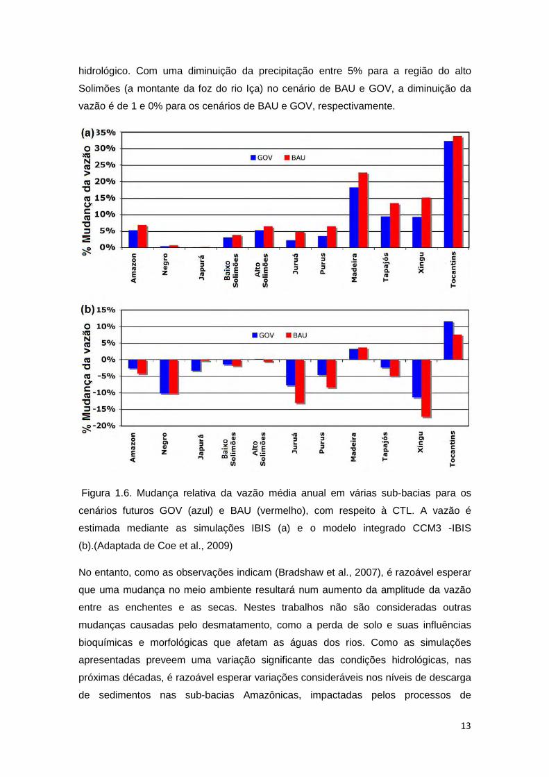
13

hidrológico. Com uma diminuição da precipitação entre 5% para a região do alto

Solimões (a montante da foz do rio Iça) no cenário de BAU e GOV, a diminuição da

vazão é de 1 e 0% para os cenários de BAU e GOV, respectivamente.

Figura 1.6. Mudança relativa da vazão média anual em várias sub-bacias para os

cenários futuros GOV (azul) e BAU (vermelho), com respeito à CTL. A vazão é

estimada mediante as simulações IBIS (a) e o modelo integrado CCM3 -IBIS

(b).(Adaptada de Coe et al., 2009)

No entanto, como as observações indicam (Bradshaw et al., 2007), é razoável esperar

que uma mudança no meio ambiente resultará num aumento da amplitude da vazão

entre as enchentes e as secas. Nestes trabalhos não são consideradas outras

mudanças causadas pelo desmatamento, como a perda de solo e suas influências

bioquímicas e morfológicas que afetam as águas dos rios. Como as simulações

apresentadas preveem uma variação significante das condições hidrológicas, nas

próximas décadas, é razoável esperar variações consideráveis nos níveis de descarga

de sedimentos nas sub-bacias Amazônicas, impactadas pelos processos de

14

desmatamento. Para analisar e compreender esses fenômenos é fundamental contar

com ferramentas adequadas para monitorar a qualidade das águas dos principais rios

da Amazônia e as suas variações, no tempo e no espaço.

1.2.3 Difusão dos metais pesados nos rios Amazônicos. Exemplo do Mercúrio

De modo geral, o monitoramento dos sedimentos tem sido objeto de crescente

interesse, tendo em vista, que os sedimentos constituem um veículo para a difusão

dos contaminantes e dos nutrientes. Os impactos danosos à saúde causados pela

contaminação por metais pesados, tal como mercúrio, são objetos de amplos estudos

ao redor do mundo. Os riscos toxicológicos e ecotoxicológicos deste metal decorrentes

da biodisponibilização no meio ambiente são preocupantes (Hacon e Azevedo, 2006).

Neste quadro, a região Amazônica é considerada uma região de amplo risco e,

consequentemente, tem sido alvo de estudos nas últimas três décadas, uma vez que

se constatou uma elevada descarga de mercúrio proveniente de garimpos.

A descarga de mercúrio na Amazônia, proveniente de atividades garimpeiras que se

estenderam, em maior escala, do final da década de 1970, a meados da década de

1990, foi estimada em mais 2000 toneladas (Malm et al., 1998; Mallas e Benedito,

1986; Cleary, 1990; Lacerda, 1990). Hacon (1991) estimou que, somente, na região

sul da Amazônia brasileira ao norte de Mato Grosso, houve uma utilização superior a

15 toneladas anuais de mercúrio, no pico da atividade garimpeira na década de 1980,

calculando que houve uma descarga superior a 100 toneladas até meados da década

de 1990. Outros autores também exemplificam esta maciça utilização do mercúrio

nesta região na década de 1980. (Mallas e Benedito, 1986; Pfeiffer e Lacerda, 1988,

Pfeiffer et al., 1989, Nriagu et al., 1992).

A lixiviação e a erosão de solos contendo mercúrio são processos que os transferem

para a água e o sedimento, tanto em ambientes marinhos como d’água doce. Este

fluxo envolve o mercúrio inorgânico, mas, grande parte, está associada com matéria

orgânica particulada e dissolvida. Nos corpos d’água, o mercúrio pode ser lançado,

diretamente, através de efluentes líquidos ou ser depositado na forma de particulado

inerte ou reativo (Hg+2). O íon mercúrico (Hg+2) pode estar presente complexado ou

quelado com ligantes, sendo esta, provavelmente, a forma predominante de mercúrio

presente nas águas superficiais (Lindqvist et al., 1991).

Em águas e sedimentos, o Hg+2 dissolvido é convertido em metilmercúrio por

processos químicos e, principalmente, microbiológicos, quando se trata de ambientes

15

aeróbicos e anaeróbicos (D’Itri, 1992). As taxas de metilação parecem variar em

função de alguns parâmetros ambientais, como temperatura, pH, carbono orgânico

dissolvido e particulado, cálcio e concentrações de sulfeto (Compeau e Bartha, 1985;

Bjornberg et al., 1988; Lechler et al., 2000; Miller et al., 2003;). O metil-mercúrio, ao

contrário da forma metálica, é facilmente assimilado pela biota, tem a tendência de se

acumular nos organismos (bioacumulação) e magnificar-se através da cadeia

alimentar (biomagnificação) (Bache et al., 1971, Barak e Mazon 1990, Meili 1997;

Bidone et al., 1997; Barbosa et al., 1995).

Os fatores morfológicos e químicos têm um importante papel na determinação da taxa

de adsorção e sedimentação do mercúrio no sistema aquático. A distribuição do

mercúrio é fortemente correlacionada com conteúdo de carbono orgânico, e

complexos solúveis em água, tais como humatos e fulvatos que podem quelar as

espécies solúveis e insolúveis à água; os últimos precipitam-se diretamente da

solução para o sedimento. Grande quantidade de mercúrio é adsorvido no húmus, em

pH muito baixo (como no rios Negro ou Tapajós). Em valores de pH alto (caso dos rios

descendo dos Andes), maior proporção de mercúrio é adsorvido pela fração mineral.

Os complexos solúveis de mercúrio são adsorvidos pelo material particulado orgânico

e inorgânico, e removidos pela sedimentação, em recursos hídricos aeróbicos.

Enquanto, nos sedimentos anaeróbicos os compostos de mercúrio precipitados

geralmente, são convertidos à sulfeto mercúrio (HgS), o que, pela sua elevada

insolubilidade, reduz a possibilidade de serem reciclados para a coluna d’água (D’Itri,

1992 e Queiroz, 1995).

A matéria fina em suspensão tem grande capacidade de adsorver o mercúrio

dissolvido. Foi detectada concentração de 34 mg de mercúrio por 1 kg de peso seco

de sedimento, ligada ao material particulado. A capacidade de adsorção do mercúrio

é, exponencialmente, proporcional à média da área superficial especifica das

partículas em suspensão, com tamanho menor que 60 µm (Queiroz, 1995). Verifica-se

que a quantidade de mercúrio que pode transportar um rio está diretamente ligada à

quantidade de argilas transportadas por eles (Maurice Bourgoin et al., 2002). Assim, o

monitoramento dos sedimentos nos rios pode servir para quantificar, de forma indireta,

os fluxos de mercúrio nas bacias hidrográficas.

16

1.2.4 Estudos do fluxo de Sedimentos na bacia Amazônica

O transporte de sedimentos na bacia amazônica situa-a na terceira colocação no

mundo, depois do rio Huang- He (rio Amarelo) na China e Ganges-Bamaputra na

India- Bangladesh. (Walling e Webb, 1996; Chakrapani, 2005), depositando 800 x 106

toneladas, por ano, de material em suspensão (MES) (Guyot et al., 2005). A bacia

amazônica mostra altas taxas de erosão, sendo que, a grande maioria dos sedimentos

provém dos Andes. Estes sedimentos são transportados para a planície de inundação

onde podem ser depositados ou arrastrados em diferentes escalas de tempo (Meade

et al., 1985).

Considerando o tamanho da bacia amazônica e sua importância, são relativamente

poucos os trabalhos de pesquisa realizados para o entendimento dos fluxos de

sedimentos nos rios. Estes trabalhos começaram nos anos de 1960: Gibbs (1967) com

74 amostras, coletadas durante duas campanhas, nos períodos de enchente e seca,

estimou uma vazão de sedimentos de 500 x 106 ton/ano (mas não considerou as

variações da concentração com a profundidade). Oltman (1968), durante três

campanhas em enchente, vazante e seca, coletou amostras pontuais em diferentes

profundidades das verticais , na estação de Óbidos, estimando uma descarga de 600 x

106 ton/ano. Meade et al. (1979) estimaram um fluxo sólido de 900 x 106 ton/ano.

Meade (1985) com mais de 300 amostras integrais e pontuais de concentração de

sedimentos, faz uma descrição dos fluxos laterais e estima o fluxo de sedimentos

entre 1.100 e 1.300 x 106 ton/ano. Estas estimações foram calculadas, apenas,

multiplicando a concentração de sedimentos com a descarga líquida do rio, assumindo

uma relação simples, entre a concentração e a vazão.

Richey et al. (1986) dentro do programa CAMREX (Carbon in the Amazon River

Experiment), adicionaram 200 amostras aos dados de Meade (1985) e obteve

resultados parecidos aos anteriores. Bordas et al. (1988) e Bordas (1991), usando

dados das entidades brasileiras, estimaram uma descarga sólida similar àquela

estimada por Meade et al. (1979). Nittrouer et al. (1986 e 1995), usando uma sonda

para medir a concentração em diferentes perfis no estuário do Amazonas, estimaram

uma descarga ao oceano, entre 550 e 1.000 x 106 ton/ano.

No ano 2003 foi formado o Projeto HIBAM (Hidrologia da Bacia Amazônica –www.ore-

HIBAM.org) em colaboração e a participação de instituições de diferentes países

como:

17

França. Institut de recherche pour le développement (IRD), Géosciences

Environnement Toulouse (GET), Institut National Des Sciences De L'univers - Centre

National de la Recherche Scientifique (INSU-CNRS), L’Observatoire Midi Pyrénées

(OMP), Laboratoire d’Etudes en Géophysique et Océanographie Spatiales (LEGOS) e

HydroSciences Montpellier (HSM) e Expertise et spatialisation des connaissances en

environnement (L'UMR ESPACE-DEV)

Brasil. Agência Nacional de Águas (ANA), Universidade de Brasilia (UnB),

Universidade do Estado de Amazonas (UEA), Universidade Federal do Amazonas

(UFAM), Universidade Federal Fluminense (UFF) e a Universidade Federal do Rio de

Janeiro (UFRJ)

Peru. Servicio Nacional de Meteorología e Hidrología (SENAMHI) e Universidad

Nacional Agraria la Molina (UNALM)

Colombia. Instituto de Hidrología, Meteorología y Estudios Ambientales (IDEAM) e a

Universidad Nacional de Colombia (UNC)

Bolivia. Servicio Nacional de Meteorología e Hidrología (SENAMHI) e a Universidad

Mayor de San Andrés (UMSA)

Venezuela. Universidade Central de Venezuela (UCV) e a Universidad Nacional

Experimental de Guayana (UNEG) e,

Equador Instituto Nacional de Meteorología e Hidrología (INAMHI).

Entre essas institiçoes foi criada uma rede de amostragem multitemporal, de coletas a

cada 10 dias, em vários rios da bacia amazônica e em todos os países amazônicos

(Guyot et al.,1996; Filizola 1999 e 2003; Guyot et al., 2005; Filizola e Guyot 2004 e

2009). Usando os dados da rede HIBAM (mais de oito anos de dados) e os dados da

ANA (Agência Nacional de Águas) e outras instituições no Brasil, Guyot et al., 2011

estima um fluxo de sedimentos entre 600 e 900 x 106 ton/ano na estação de Óbidos

(última estação antes do oceano sem influência da maré).

O trabalho da equipe HIBAM se diferencia dos trabalhos anteriores porque coleta

dados, a cada 10 dias, para suas estimativas. Essa resolução temporal permitiu

demostrar, pela primeira vez, a não-unicidade da relação vazão liquida – concentração

em sedimentos como mostra a Figura 1.7 onde ficam exibidas as variações, a cada 10

dias, dos dois parâmetros, por vários ciclos hidrológicos consecutivos (Martinez et al.,

2009). Assim, fica demonstrada a importância de monitorar conjuntamente a

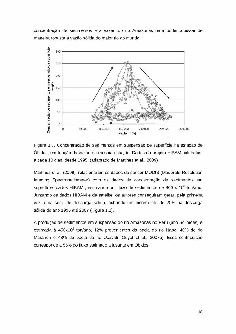
18

concentração de sedimentos e a vazão do rio Amazonas para poder acessar de

maneira robusta a vazão sólida do maior rio do mundo.

Figura 1.7. Concentração de sedimentos em suspensão de superfície na estação de

Óbidos, em função da vazão na mesma estação. Dados do projeto HIBAM coletados,

a cada 10 dias, desde 1995. (adaptado de Martinez et al., 2009)

Martinez et al. (2009), relacionaram os dados do sensor MODIS (Moderate Resolution

Imaging Spectroradiometer) com os dados de concentração de sedimentos em

superfície (dados HIBAM), estimando um fluxo de sedimentos de 800 x 106 ton/ano.

Juntando os dados HIBAM e de satélite, os autores conseguiram gerar, pela primeira

vez, uma série de descarga sólida, achando um incremento de 20% na descarga

sólida do ano 1996 até 2007 (Figura 1.8).

A produção de sedimentos em suspensão do rio Amazonas no Peru (alto Solimões) é

estimada à 450x106 ton/ano, 12% provenientes da bacia do rio Napo, 40% do rio

Marañón e 48% da bacia do rio Ucayali (Guyot et al., 2007a). Essa contribuição

corresponde a 56% do fluxo estimado a jusante em Óbidos.

19

Figure 1.8. Descarga anual de sedimentos em suspensão na estação de Óbidos entre

os anos 1996 e 2007. (adaptado de Martinez et al., 2009)

O rio Madeira é o outro grande transportador de sedimentos, representado 50% dos

sedimentos carregados ao oceano (Guyot et al., 1996) pelo rio Amazonas. Filizola

(2003) com dados de campanhas estima o fluxo de sedimentos do rio Madeira em 371

x 106 ton/ano e com dados da rede ORE-HIBAM estima 406 x106 ton/ano.

Posteriormente, com dados da rede da ANA (Agencia Nacional de Águas) Filizola e

Guyot (2009) estimam um fluxo de 285x106 ton/ano, representando 53% do fluxo

sedimentar estimado na estação de Óbidos.

1.3 Sensoriamento Remoto

Por muito tempo o sensoriamento remoto limitou-se à fotografia aérea e ao seu modo

de exploração à fotointerpretação. Com o aparecimento das plataformas espaciais, e

depois do lançamento do satélite Spoutnik em 4 de outubro de 1957, estimulou-se o

surgimento dos primeiros satélites comerciais no início dos anos 1970 (e.g., Landsat

em 1972). Essa revolução dos meios de observação da Terra fortaleceu a utilização

do sensoriamento remoto, buscando responder as diversas problemáticas ambientais

com as quais o homem é confrontado.

O aprimoramento do sensoriamento remoto, no caso específico da região amazônica,

é fator essencial para superar as inúmeras dificuldades que a região oferece

20

(distâncias, acessibilidade, tamanho, etc.) tanto ao manejo, como à conservação dos

ecossistemas tropicais, lá existentes.

A principal aplicação das técnicas de sensoriamento remoto na bacia amazônica é o

monitoramento do desmatamento. As imagens do satélite Landsat têm sido a principal

fonte de dados para monitorar o avanço do desflorestamento da região (Pereira,

1996), por meio do Programa de Monitoramento do Desmatamento na Amazônia

Legal (Prodes) (www.obt.inpe.br/prodes) que tem estimado a taxa anual de

degradação florestal, na região. Outras imagens de satélite têm também sido usadas

para monitorar o desmatamento em áreas menores da Amazônia (Moran et al., 1994).

Por exemplo, imagens do satélite sino-brasileiro CBERS para acompanhar o

desmatamento em propriedades rurais (Carreiras, e Pereira, 2005). A partir de 2004,

imagens do sensor MODIS (Moderate Resolution Imaging Spectroradiometer) estão

sendo utilizadas pelo INPE em um sistema de detecção de desflorestamento em

tempo real (DETER) www.obt.Inpe.br/deter.

As imagens do satélite Landsat (Anser, 2001, Sousa e Barreto, 2001 e Sousa et al.,

2005) e Spot (Sousa et al., 2003) têm sido usadas, com sucesso, para identificar e

mapear os impactos da exploração madeireira. A dificuldade para monitorar esse tipo

de distúrbio florestal reside no fato de que a exploração madeireira altera,

parcialmente, a floresta com a abertura de pátios de estocagem de madeira, de

clareiras, e de estradas e ramais (Sousa et al., 2003), enquanto no desmatamento

ocorre a remoção completa da floresta.

As técnicas de teledetecção foram testadas, com sucesso, para avaliar a qualidade de

planos de manejo florestal na Amazônia. As queimadas em áreas desmatadas podem

atingir, eventualmente, florestas adjacentes. As queimadas ativas são detectadas em

tempo real por sensores a bordo de satélites meteorológicos, sensíveis à radiação

termal. Dados de radares orbitais também têm grande potencial de aplicação no

monitoramento ambiental da Amazônia, por serem capazes de observar através de

nuvens (Martinez e Le Toan 2007). A viabilidade de monitoramento da cobertura da

terra foi demonstrada com dados de missões experimentais e com satélites

operacionais (Saatchi et al., 1997). Há também o potencial para o monitoramento da

biomassa de florestas secundárias, a partir de dados de radar e, mesmo, de florestas

primárias, através de técnicas de polarimetría e interferometria de dados de radar

(Martinez et al., 2000, Strozzi et al., 2000 e Salas et al., 2002).

21

1.3.1 Teledetecção em corpos d’água

A hidrologia óptica, inicialmente, foi baseada na teledetecção para pesquisas

atmosféricas. O inicio deste ramo da ciência começou com a publicação do livro

“Optical Oceanografy” (Jerov 1968) e, posteriormente, do mesmo autor “Marine Optics”

(1976) e Austin (1974) ”The remote sensing of spectral radiance from below the ocean

surface”. Posteriormente, aprofundando estes conceitos, Preisendorfer (1976) publica

um tratado de seis volumes chamado “Hydrologyc Optics”.

Essas publicações desempenharam um importante papel na formação e consolidação

da óptica Hidrológica como ciência, influenciando toda uma comunidade de

pesquisadores, incorporando novos avanços no conhecimento. Dentre estes,

destacam-se aqui os livros de Kirk (1983), “Light and Photosynthesis in Aquatic

Ecosystems”, e de Mobley (1984), “Light and water: radiative transfer in natural

waters”.O sensoriamento remoto de águas é restrito a uma faixa relativamente estreita

de comprimentos de onda da luz em relação ao sensoriamento remoto de objetos

terrestres. Isto é causado pela baixa radiação solar em comprimentos de onda mais

curtos do que cerca de 400 nm, e por uma combinação de mais baixa energia solar e

a absorção acentuadamente crescente de luz, através da água, para além de 850 nm

(Dekker, 1993). Portanto, a faixa de 400 a 850 nm é, muitas vezes, escolhida para

estimar parâmetros de qualidade da água, na coluna d’água, a partir de dados de

sensoriamento remoto.

A água representa uma mistura complexa de diversos materiais dissolvidos ou

particulados. Esses materiais possuem propriedades ópticas diversas, ou seja,

interagem com a luz, de maneira diferente, em função de sua concentração e

natureza. A presença desses componentes na coluna d’água é responsável por

modificações em sua cor, pois eles absorvem ou espalham seletivamente a luz

incidente.

Por exemplo, a clorofila tem um máximo de absorção no comprimento de onda

vermelho de 676 nm e uma faixa de absorção mínima em 559 nm, o que permite uma

comparação entre os espectros e a concentração do fito-pigmento. O húmus aquático

(consiste principalmente de carbono orgânico dissolvido) pode remover,

eficientemente, a luz azul, em poucos centímetros, de topo da coluna d’água,

conferindo, assim, uma cor amarela. (Dekker, 1993).

22

O sensoriamento remoto da água de superfície tem sido usado principalmente para

investigar os oceanos. Isso contribuiu muito para a descoberta, mapeamento e

compreensão dos processos marinhos de grande escala. Preisendorfer (1976), Jerlov

(1976) e Austin (1974) estabeleceram uma firme base física definindo as propriedades

inerentes e aparente ópticas das águas marinhas. Infelizmente, esses trabalhos

pioneiros não foram aproveitados, no âmbito dos estudos das águas continentais, nem

sistematizados dentro das redes de monitoramento hidrológicos. O principal motivo

adveio da falta de sensores espaciais adequados, que impedia o monitoramento,

suficientemente preciso, em termos de resolução temporal (número de imagens

disponíveis por unidade de tempo) e/ou espacial (tamanho dos rios que poderiam ser

estudados), para propiciar uma relevante rede de monitoramento.

Diferentes estudos realizados no mundo (Kirk 1981, 1991, Mertes et al., 1993; Dekker,

2002; Curran et al., 1987; Curran e Novo 1988), incluindo o Brasil (Novo et al., 1989) a

partir dos anos oitenta e noventa, demonstraram a possibilidade de relacionar o

conteúdo de sedimentos e a “cor” das águas continentais detectada pelos satélites.

Em particular, comprovou-se que as propriedades ópticas das águas são fortemente

influenciadas pelo conteúdo e tipo de sedimento. Estudos realizados por Mertes et al.

(1993) usando técnicas de mistura espectral para imagens Landsat , demonstraram

que os dados de satélite poderiam ser bons estimadores da concentração de

sedimento, apesar da falta de validação.

Nos últimos anos, os sensores de resolução espacial média MODIS foram lançados

pela Agência Espacial Americana (NASA). Esses sensores fornecem imagens diárias

de qualquer ponto do mundo, com resolução espacial de até 250 metros, e são usados

para monitorar os ecossistemas continentais.

Recentes estudos sobre a Amazônia demonstram a possibilidade de usar esse tipo de

dado para mapear a concentração de sedimentos das áreas inundadas e dos rios da

Amazônia. Martinez et al. (2004) confirmou a correlação da concentração de

sedimentos com os dados de reflectância de satélite usando os sensores MERIS e

MODIS, sendo o MODIS uma boa ferramenta para os estudos da variabilidade

temporal da concentração de sedimentos, devido à alta resolução temporal deste

sensor. Martinez et al. (2009) utilizando o sensor MODIS completa uma série histórica

de concentração de sedimentos detectando uma variação temporal.

A facilidade de uso desses dados, cuja distribuição é gratuita pela NASA, e a

qualidade reconhecida da calibração, abriram caminho para o aproveitamento

sistemático das imagens de satélite do tipo MODIS.

23

1.4 Objetivos

A quantificação dos fluxos de sedimentos nos rios é importante para várias disciplinas

ambientais como acabamos de ver. Como foi mencionado no parágrafo 1.2.2, na bacia

amazônica, estão acontecendo grandes mudanças de uso de solo, contaminação das

águas com metais pesados e obras de engenheira que mudarão a hidrologia dos rios

e a quantidade de sedimentos transportados, isso em diferentes escalas de tempo.

Como foi dito anteriormente, no item 1.1.1 por Espinoza et al. (2009b, 2011) e

Marengo et al. (2011), a bacia Amazônica sofre com maior frequência eventos

extremos hidrológicos de enchentes e secas. Martinez et al. (2009) sinaliza um

incremento do fluxo de sedimentos para o período de 1996 ate 2007, o que nos faz

questionar sobre a proveniência deste incremento.

Esta tese busca aprimorar as técnicas de monitoramento dos fluxos de sedimentos,

analisando o uso dos dados espaciais. Martinez et al. (2004 e 2009) relacionaram,

com êxito, os dados do sensor MODIS com a concentração de sedimentos no baixo

Amazonas, onde o rio alcança até 4 km de largura. Tentaremos definir as

possibilidades de utilização destas ferramentas, em outras regiões da bacia

amazônica. Em particular, vamos analisar as propriedades ópticas das águas da bacia

amazônica, de maneira sistemática, para definir robustamente a relação entre a

concentração de sedimentos e as imagens de satélite.

Assim os objetivos desta tese podem ser resumidos da seguinte forma:

OBJETIVO PRINCIPAL

• Quantificar as variabilidades espaciais e temporais dos fluxos sedimentares

a partir do uso sistemático dos dados espaciais.

OBJETIVOS SECUNDÁRIOS

• Caracterizar espectralmente os tipos d’água dos rios da Amazônia

mediante medições in situ das propriedades ópticas

• Quantificar o grau de precisão na determinação do tipo de sedimentos e a

sua concentração, a partir de imagens de satélite, buscando os fatores

que determinam essa precisão.

24

1.5 Metodologia

Para alcançar os objetivos propostos pretende-se usar o fluxograma apresentado na

Figura 1.9. Os dados de entrada são de dois tipos: os de reflectância e os de

características do material em suspensão (MES). Os primeiros dados são as imagens

do sensor MODIS e os dados de espectrorradiometria de campo; e os segundos

dados provêm da rede de monitoramento ORE-HIBAM e das campanhas realizadas

durante a tese, nas quais, foram coletados os dados de concentração de MES,

granulometria, mineralogia e matéria orgânica dissolvida colorida (CDOM).

Figura 1.9. Esquema da metodologia a ser desenvolvido no presente trabalho.

Nesta tese pretende-se compreender como os sedimentos afetam a “cor” das águas

(assinaturas espectrais) dependendo do tipo e concentração do material particulado. A

partir deste conhecimento detalhado das propriedades óticas, poderemos simular a

resposta dos satélites (bandas radiométricas) e determinar a sensibilidade das

imagens de satélite para a medição das características físicas dos sedimentos. Em

particular, tentaremos entender se a reflectância medida pelo satélite está,

primeiramente, relacionada à concentração de sedimentos ou se está influenciada de

maneira significativa por outros parâmetros, como granulometria ou mineralogia.

As estimativas de satélite servirão para criar estações virtuais e/ou completar estações

existentes de medição de sedimentos. Com esta rede poderemos estudar e interpretar

as variações espaciais e temporais dos sedimentos, nos rios da Amazônia, analisando

em prioridade os rios Solimões/Amazonas e Madeira.

25

1.6 Plano da tese

Apresentamos a introdução, e, em seguida uma revisão bibliográfica (Capitulo2)

dispõe o atual estágio das pesquisas, nas diferentes temáticas da tese e os principais

fundamentos relevantes para o entendimento dos trabalhos deste presente estudo. O

capítulo 3 resume os trabalhos realizados, detalhando os diferentes passos e

sintetizando os principais resultados obtidos na tese. A seguir são apresentados os

quatro artigos submetidos e/ou publicados em revistas internacionais. Esses artigos

estão ordenados de maneira a seguir o esquema de metodologia acima indicado:

Artigo A : Analysis of apparent and inherent optical properties of the sediment-

dominated waters in the Amazon River basin – Jean-Michel Martinez, Raul Espinoza-

Villar, Luciane Moreira - Submitted to Journal of Geophysical Research

Artigo B : Surface water quality monitoring with MODIS data – Application to the

Amazon River – J.M. Martinez, R. Espinoza Villar, G. Cochonneau, E. Le Hesran e J.L.

Guyot- Submitted to Remote Sensing of Environment

Artigo C : The integration of field measurements and satellite observations to determine

river solid loads in poorly monitored basins – Raúl Espinoza Villar, Jean-Michel

Martinez, Jean-Loup Guyot, Pascal Fraizy, Elisa Armijos, Alain Crave, Hector Balzan,

Philippe Vauchel, Waldo Lavado. 2012 - Publicado em Journal of Hydrology

Artigo D : A study of sediment transport in the Madeira River, Brazil, using MODIS

remote-sensing images –Raúl Espinoza Villar, Jean-Michel Martinez, Marie Le Texier,

Jean-Loup Guyot, Pascal Fraizy, Paulo Roberto Meneses, Eurides De Oliveira. –

Aceito em Journal of South American Earth Sciences

26

CAPITULO II

----------------------------------------------------------------------------

Revisão Bibliográfica

27

2 REVISÃO BIBLIOGRÁFICA

2.1 Zona de Estudo

A bacia hidrográfica Amazônica é a maior do mundo com uma área de drenagem de

6,1x106 km2 (perto dos 5% das terras emergidas) (Goulding et al., 2003), e uma

descarga média anual estimada em 209.000 m3 /s na foz do rio, representando cerca

de 15% dos aportes hídricos para os oceanos (Molinier et al., 1996). A Amazônia está

situada na zona intertropical, recebendo precipitações médias anuais de 2200 mm

com um desvio padrão de 138 mm (Espinoza et al., 2009b). A bacia do Rio Amazonas

se estende desde 48 ° W (Rio Pará, Brasil) a 79 ° W (Rio Chamaya, Peru), e de 5° N

(Rio Cotingo, Brasil) a 20 ° S (Parapeti Rio, Bolívia). Esta bacia continental abrange

vários países: Brasil (63%), Peru (16%), Bolívia (12%), Colômbia (5,6%), Equador

(2,3%), Venezuela (0,6%) e Guiana (0,2%). Os limites da bacia são: a Norte com o

escudo Guianês, a Oeste a cadeia dos Andes, com seus picos mais altos, atingindo

cerca de 7.000 m (Guyot et al., 2007a), a Sul o escudo brasileiro e a Leste o oceano

Atlântico.

2.1.1 Geologia da Amazônia

A história geológica da bacia sedimentar do Amazonas inicia com a formação do

Supercontinente Gondwana, no final do Pré-Cambriano e caracteriza-se por ser uma

bacia intra-cratônica gerada através da movimentação e colisão de placas tectônicas

compostas pelas atuais placas da América do Sul, África, Madagascar, Índia, Antártica

e Austrália (Scotese & Mckerrow, 1990). O Gondwana sofreu diversos tectonismos

simultâneos ligados a eventos vulcânicos, magmáticos e metamórficos, durante o

Proterozóico superior e início do Fanerozóico, o que ocasionou uma subsidência

tectônica onde se encontrava o Cráton Amazônico, gerando um “protorifteamento” da

bacia. Com o cessar dos esforços tectônicos e o resfriamento das massas plutônicas

no Cambriano-Ordoviciano [500-450 Milhões de anos (MA)], teve início a subsidência

térmica regional e o desenvolvimento da “sinéclise intracontinental” da Bacia do

Amazonas (Montalvão e Bezerra, 1980).

O substrato da bacia é constituído por rochas metamórficas das Províncias de Maroni-

Itacaiúnas e Amazônia Central. (Figura 2.1) A Província Maroni-Itacaiúnas consiste de

uma Faixa Móvel do Proterozóico inferior composta por sequências meta-vulcânicas e

meta-sedimentares intercaladas tectonicamente por lineamentos de direções WNW-

28

ESE bem definidos, deformadas e intrudidas por rochas granitóides do Ciclo

Transamazônico (2.100 a 1.800 Milhões de anos).

Figura 2.1. Principais elementos tectônicos da América do Sul (fonte CPRM, 2003)

29

A província Amazônia Central compreende rochas graníticas e sequências vulcano

sedimentares pouco ou não deformadas, datadas através do método K-Ar como

pertencentes ao Proterozóico inferior a médio, com idades aproximadas entre 1.800 a

1.400 Ma (Cordani et al., 1984). A partir do Proterozóico superior surgem os primeiros

registros de eventos sedimentares da bacia, caracterizando uma sucessão sedimentar

aluvial, fluvial e lacustre, pertencentes ao Grupo Purus.

No Fanerozóico ocorreram quatro sequências sedimentares principais: Ordoviana-

Devoniana, Devoniana-Carbonífera, Permo-Carbonífera e Cretácea-Terciária. Estudos

feitos por Cunha et al. (1994) demonstraram que a sedimentação Paleozóica reflete os

eventos tectono-magmáicos ocorridos nessa Era, que provocaram movimentações

epirogenéticas intraplaca, formando arcos e discordâncias regionais. Além disso,

controlavam as ingressões marinhas, influenciando os ambientes deposicionais. A

sedimentação da sequência Cretácea-Terciária foi extensamente afetada por eventos

vulcânicos relacionados com a abertura do Oceano Atlântico e pela formação da

Cadeia Andina.

Verificam-se na Figura 2.1 os principais elementos tectónicos da América do Sul,

mostrando que a bacia Amazônica é formada principalmente pelas províncias Central,

Ventuari-Tapajós e Maroni-Itacaiúnas e a cobertura sedimentar Fanerozóica e Pre-

Cambriana.

2.1.2 Solo

Segundo Guyot et al. (2007b), apesar da aparente homogeneidade da floresta úmida

os solos da bacia amazônica apresentam certa heterogeneidade. Na parte ocidental

da bacia, os solos são bem drenados, ácidos, de coloração marrom amarelo, friáveis,

porosos e arenosos. Os solos que não apresentam uma boa drenagem encontram-se

na porção oriental da bacia, sendo ácidos e de coloração marrom amarelo. Na porção

norte da bacia observamos solos podzólicos desenvolvidos sobre os sedimentos

arenosos resultantes da erosão do embasamento do escudo das Guianas. Na planície

amazônica, os solos aluviais são mal drenados, e estão associados aos tipos de

sedimentos depositados e à periodicidade local das condições da inundação.

30

2.1.3 Vegetação

A floresta tropical úmida ocupa, aproximadamente, 5 milhões km2, que corresponde a

70% do total da bacia amazônica (Guyot et al., 2007b), estendendo-se também por

toda a planície aluvial, denominada de floresta fluvial alagada, devido à oscilação dos

níveis das águas e os grandes períodos em que suas raízes encontram-se submersas.

A floresta de terra firme é uma floresta aberta com grandes árvores dispersas e

frequentes grupamentos de palmeiras, estando localizada em planaltos pouco

elevados. Essas florestas apresentam um solo extremamente pobre em nutrientes, e

suas raízes adaptam-se às condições do ambiente, através de uma associação

simbiótica com alguns tipos de fungos, passando a decompor rapidamente a matéria

orgânica, depositada no solo, para absorver os nutrientes antes de ser lixiviados

(Schubart, 1983).

A floresta montanhosa andina é uma floresta mais densa, que nunca se alaga e

apresenta uma vegetação arbórea heterogênea (Schubart, 1983). Em meio à floresta

úmida, apresentam-se manchas de savana, pastagens e cerrado, na região da

Bolivia, Mato Groso e na nascente do rio Branco. Salati (1983) relatou que os campos

áridos de savana são resultantes de alterações inter-glaciais e glaciais, durante o

período quaternário, com longa faixa de transição, entre os dois tipos de vegetação. A

pastagem corresponde à substituição da floresta úmida por gramíneas, para a criação

de gado. Ribeiro Neto (2006) descreve o cerrado como um conjunto de árvores e

arbustos retorcidos, cujas folhas são largas e as raízes podem atingir grandes

profundidades, a fim de alcançar a água. No cerrado as árvores encontram-se

esparsamente distribuídas sobre um tapete gramíneo, com intercalações de plantas

arbustivas e áreas campestres.

2.1.4 Climatologia

Devido aos altos valores de energia solar que incidem na superfície da zona

equatorial, o comportamento da temperatura do ar mostra uma pequena variação ao

longo do ano na Amazônia, com exceção da região sul, que sofre a ação de sistemas

frontais (denominados localmente de friagens). A amplitude térmica sazonal é da

ordem de 1-2º C, sendo que os valores médios situam-se entre 24 e 26º C. Belém

(PA), especificamente, apresenta a temperatura média mensal máxima de 26,5º C em

31

novembro e a temperatura mínima de 25,4º C em março. Manaus (AM), por sua vez,

possui seus extremos de temperatura nos meses de setembro (27,9º C) e abril (25,8º

C).

A precipitação é um dos elementos climáticos mais importantes a serem analisados na

região tropical, já que induz as características de outros elementos, tais como

temperatura, umidade relativa e vento.

Como visto, a bacia amazônica é localizada entre 5°N e 20°S, estando, desta maneira,

dentro da zona tropical. A zona tropical é, geograficamente, delimitada pelas latitudes

extremas dos pontos onde o sol alcança o zênite, durante um ano terrestre.

A energia solar é distribuída pela circulação atmosférica e oceânica de grande escala

que permite um fluxo positivo para os polos. Do ponto de vista atmosférico, a principal

fonte de energia para o transporte de menor escala em latitudes médias é a circulação

de Hadley. Esta é composta por um ascenso do ar na forma de convecção de umidade

no Equador, um movimento divergente das massas do ar para os polos sobre a

troposfera, e uma subsidência nas regiões tropicais. A Zona de Convergência Inter-

Tropical (ITCZ) é a região da máxima energia emitida através da convecção úmida, e

desloca-se na latitude, dependendo da época do ano, e, em função da posição do sol.

Este deslocamento é baixo nos oceanos, porque sua inerência térmica é importante e

maior nos continentes.

A bacia amazônica, por ser de tamanho continental e ter área nos dois hemisférios,

tem uma alta variação da climatologia. A distribuição espacial das precipitações anuais

apresenta uma forte heterogeneidade, variando, desde menos de 300 mm/ano, até em

estações que registram 6.000 mm/ano, no este da região andina (Figura 2.2).

Os regimes de chuvas são muito diferentes, observando-se que na zona sul as

precipitações concentram-se entre dezembro e março, e diminuem nos meses de

junho, julho e agosto (Figura 2.2 c,d,e). Na parte norte central pode-se observar o

regime contrário (Figura 2.2 b), com a concentração das precipitações nos meses de

junho, julho e agosto e a seca nos meses de dezembro a março. A zona ocidental

norte mostra a região com mais concentração de chuvas, sendo a zona ocidental sul a

região com menos precipitação.

Os Andes, por sua elevação, representam uma barreira para o fluxo climático da

troposfera, permitindo condições mais secas, do lado oeste, em comparação com a

região úmida amazônica, ao leste. O vapor d’água nesta região vem do oceano

32

Atlântico e da floresta amazônica por meio da evapotranspiração (Salati et al., 1984;

Zhou et al., 1998; Nogués-Peagle et al., 1997; Vera et al., 2006.)

Figura 2.2. Variabilidade espacial das chuvas na Bacia Amazônica; todos os gráficos de barras com as mesmas escalas no eixo Y (precipitação mm) e eixo X (meses do ano 1=janeiro até 12=dezembro). Adaptada de Espinoza et al. (2009b)

2.1.5 Hidrologia

O rio Amazonas é o maior rio do mundo em termos de descarga líquida e área

drenada (Molinier et al., 1996). Sua fonte mais distante é o nevado Mismi (5628 metros

acima do nível do mar), no sul do Peru, percorrendo 6.500 km até sua foz no Atlântico

(Peñaherrera, 1969, Bohumir et al., 2011). Recebe o nome de Amazonas ainda na

confluência dos rios Ucayali e Marañón onde a vazão média já é de 25.000 m³/s

(Espinoza et al., 2006); um pouco mais a jusante, vem o rio Napo do Equador, depois

o rio Javari (na fronteira do Peru com Brasil), onde o curso principal do rio passa a ser

denominado de Solimões, no qual desembocam os rios Iça ou Putumayo, Jutai, Juruá,

Japura ou Caqueta e Purus. Nesta região a vazão média é de 102.600 m³/s (na

estação de Manacapuru) (Espinoza et al., 2009a). O rio Solimões recebe as águas do

rio Negro e tem seu nome alterado para Amazonas, no qual desemboca o rio Madeira

proveniente dos Andes Bolivianos e do sul da bacia. À jusante o rio Amazonas recebe

as águas dos rios Trombetas, Tapajós e Xingu, alcançando uma média de 209.000

m3/s (Molinier et al., 1996) que verte no oceano Atlântico.

33

A Bacia Amazônica, por seu tamanho e posição equatorial, apresenta vários regimes

hidrológicos, assim como vazão específica. Espinoza et al., (2009a), a partir dos dados

da Agência Nacional de Águas (ANA, Brasil), do Servicio Nacional de Meteorología e

Hidrología (SENAMHI do Perú e Bolívia), e do projeto HIBAM; demonstra a

variabilidade de regimes hidrológicos na Bacia Amazônica no período 1974-2004 nas

estações hidrológicas de: Fazenda Vista Alegre (FVA) e Porto Velho (PVE),

Tamshiyacu (TAM) no rio Amazonas peruano, que drena parte dos Andes do Peru e

do Equador;. Santo Antônio de Içá (SAI) no rio Iça, Acanauí (ACA) no rio Japurá na

parte noroeste da Bacia Amazônica, Manacapuru (MAN) que é a ultima estação do

Solimões, Caracaraí (CAR) no rio branco, Serrinha (SER) no rio Negro e finalmente

Óbidos (OBI) no rio Amazonas (Figura 2.3) Os dados das duas estações Gavião, no

Rio Juruá, e Labréa, no rio Purus, no centro-oeste da Amazônia brasileira, são

adicionados, a fim de criar a estação virtual Gavião-Lábrea (G- L), que tem o tamanho

e descarga da mesma ordem de grandeza das outras estações. Na Figura 2.3 se

mostram os regimes hidrológicos de cada região

Figura 2.3. Localização das principais sub-bacias e estações hidrológicas da Bacia Amazônica. A vazão média mensal 1974-2004 (m³/sx10³) é apresentada para cada sub-bacia. Dados G-L é a soma das estações Gavião e Lábrea. O eixo X são os meses a partir de 1, janeiro a 12, dezembro. Adaptada de Espinoza et al. (2009a)

34

O regime sul - tropical (PVE, FVA, G-L, ALT e ITA) apresenta os níveis máximos de

vazão nos meses de Março até Maio e as mínimas em agosto até outubro. E ao

contrário, na zona norte (CAR, SAI e ACA) a vazão máxima ocorre entre Junho e

agosto e as mínimas, de dezembro a março. Em Tamshiyacu, que se estende em

ambos os hemisférios, a vazão máxima acontece em abril ou maio e as vazões

mínimas nos meses de setembro ou outubro. Assim, nas estações MAN e OBI a vazão

máxima ocorre nos meses de maio ou junho e as vazões mínimas nos meses de

outubro ou novembro.

A Tabela 2.1 mostra as principais estações hidrológicas da bacia amazônica em

termos de área drenada, vazão média (Qmédia), máxima (Qmax) e mínima (Qmin). A

tabela mostra a vazão específica (Qespecífica), indicando a quantidade d’água

produzida pela bacia por unidade de área drenada. As estações com vazão específica

mais alta são ACA e SER (que estão localizadas mais ao norte da bacia), seguidas

pelas estações de TAM e SAI da região andina centro e norte da bacia, e MAN que é

influenciada pelas duas anteriores. As estações com vazões específicas menores

encontram-se nos rios que vem do sul (ALT, PVE, FVA, ITA).

Tabela 2.1.- Localização, Área e vazão média (Qmédia), máxima (Qmax) e mínima (Qmin) e vazão específica (Qespecífica) para 1974 – 2004, das principais sub-bacias da bacia amazônica. (Espinoza et al., 2009a).

Na tabela 2.1, pode-se observar que o rio Solimões aporta 60% da vazão em Óbidos

enquanto o rio Madeira contribue em 16%, e o rio Negro contribue em 17%. As

estações que drenam a zona andina (TAM e PVE) contribuem juntas com 29% da

vazão observada em Óbidos.

Area Qmédia Qmáx Qmín Qespecífica

(km2) (m

3/s) (m

3/s) (m

3/s) (m

3/s.km

2)

Altamira ALT Xingu -3,38 -52,14 469100 7800 22300 1000 0,017

Itaituba ITA Tapajós -4,28 -57,58 461100 11700 24500 3000 0,025

Porto Velho PVE Madeira -8,74 -63,92 954400 18300 37900 3900 0,019

Gaviao G Juruá -4,84 -66,85 170400 4900 9100 900 0,029

Lábrea L Purus -7,25 -64,8 230000 5500 11100 2100 0,024

Tamshitacu TAM Amazonas -4,01 -73,16 726400 31700 46700 16400 0,044

Santo Antônio do Içá SAI Solimões -3,08 -67,93 1158600 55800 77550 27100 0,048

Acanaui ACA Japura -1,82 -66,6 251800 14800 22900 5300 0,059

Serrinha SER Negro -0,48 -64,83 291100 16500 28500 5900 0,057

Caracaraí CAR Branco 1,83 -61,38 130600 2900 9600 500 0,022

Fazenda Vista Alegre FVA Madeira -4,68 -60,03 1293600 27700 58300 5100 0,021

Manacapuru MAN Solimões -3,31 -60,61 2242400 81000 139000 58800 0,036

Obidos OBI Amazon -1,93 -55,5 4680000 172400 240000 100200 0,037

Rio Lat LonEstação

35

Callède et al., 2004 analisa a vazão na estação de Óbidos, verificando quebras na

tendência para a vazão media, de cheia e de seca:

• A tendência geral da vazão média é de aumento. Ocorreu um aumento entre os

anos 1940-1954 e depois uma diminuição entre os anos 1954 e 1964. Após um

novo ciclo de aumento / diminuição notamos um crescimento de 1981 até 2003.

• Para as cheias os valores máximos de vazões cresceram entre os anos 1940-

1953 e diminuíram depois até 1966. Essa série mostrou um marcado crescimento

até 1977, mantendo-se estável entre 1977-2003.

• Para as vazões de seca a tendência geral 1940-2003 mostra um ligeiro aumento.

De 1940 a 1965 a tendência é negativa, seguida por um forte aumento de 1965-

1974. De 1974 a 2003 a tendência é de queda.

Figura 2.4. Evolução da vazão em Iquitos desde 1970. Linha tracejada, indica a

tendencia da vazão. (Adaptada de Espinoza et al., 2006)

Na estação hidrológica de Tamshiyacu (TAM), localizada perto da cidade de Iquitos, o

rio Amazonas drena uma área de 726.400 km2 (53% correspondente aos Andes) e

apresenta uma vazão média anual de 31.700 m3/s para o período 1969-2006. A

variabilidade temporal de descarga (Figura 2.4) mostra uma tendência clara de

diminuição no período de observação (Espinoza et al., 2006).

2.2 Sedimentos nos rios

Os processos que regulam o transporte das partículas de sedimentos são

desagregação, erosão, e sedimentação ou deposição (Bordas e Smmelnann, 1997).

36

Segundo Carvalho (1994), a sedimentação provém da erosão. Existem quatro tipos de

erosão: erosão eólica, erosão hídrica superficial, erosão por remoção em massa e a

erosão fluvial. A erosão hídrica superficial pode se dar em forma de erosão pluvial.

Erosão pluvial é a erosão que se dá pelo impacto da gota de chuva sobre a superfície

do solo. O impacto da gota de chuva destaca a partícula de solo, a qual será

transportada pelo escoamento. A erosão depende de muitos fatores e será maior,

quanto mais desprotegida de vegetação for a superfície do solo.

O transporte dos sedimentos erodidos nos rios pode se dar por: carga sólida de

arraste, carga sólida saltante e carga sólida em suspensão. A carga sólida de arraste

são as partículas de sedimentos que rolam e escorregam sobre o leito dos cursos

d’água. A carga sólida saltante são as partículas que pulam devido à colisão umas nas

outras e sob o efeito da correnteza d’água. A carga sólida em suspensão são as

partículas de sedimentos capazes de se manter em suspensão pelo fluxo turbulento,

devido ao seu peso reduzido.

Uma propriedade importante dos sedimentos nos rios é a distribuição do tamanho das

partículas ou granulometria. Uma partícula em suspensão está sujeita à ação de seu

peso, que tende a deslocá-la para baixo e da velocidade e turbulência da corrente que

tendem mantê-la em suspensão. Portanto, a distribuição da granulometria dos

sedimentos ao longo da seção transversal é variável em função da velocidade de

corrente, considerando que as velocidades são menores perto das margens.

Na Figura 2.5 pode-se observar as diferentes distribuições de concentração de

sedimentos, dependendo do tamanho da partícula. As areias apresentam uma

distribuição heterogênea, sendo de alta concentração no fundo e muito baixa na

superfície. Os siltes e as argilas têm uma distribuição mais homogênea. Sabendo-se

que a concentração de sedimentos é mais elevada no fundo do rio, deve se levar em

conta, que a velocidade do fluxo é mais importante perto da superfície e muito fraca no

fundo.

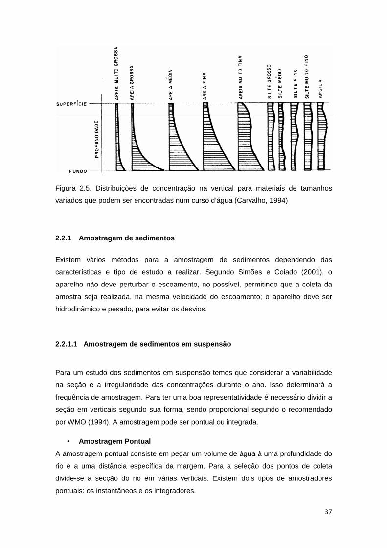
37

Figura 2.5. Distribuições de concentração na vertical para materiais de tamanhos

variados que podem ser encontradas num curso d’água (Carvalho, 1994)

2.2.1 Amostragem de sedimentos

Existem vários métodos para a amostragem de sedimentos dependendo das

características e tipo de estudo a realizar. Segundo Simões e Coiado (2001), o

aparelho não deve perturbar o escoamento, no possível, permitindo que a coleta da

amostra seja realizada, na mesma velocidade do escoamento; o aparelho deve ser

hidrodinâmico e pesado, para evitar os desvios.

2.2.1.1 Amostragem de sedimentos em suspensão

Para um estudo dos sedimentos em suspensão temos que considerar a variabilidade

na seção e a irregularidade das concentrações durante o ano. Isso determinará a

frequência de amostragem. Para ter uma boa representatividade é necessário dividir a

seção em verticais segundo sua forma, sendo proporcional segundo o recomendado

por WMO (1994). A amostragem pode ser pontual ou integrada.

• Amostragem Pontual

A amostragem pontual consiste em pegar um volume de água à uma profundidade do

rio e a uma distância específica da margem. Para a seleção dos pontos de coleta

divide-se a secção do rio em várias verticais. Existem dois tipos de amostradores

pontuais: os instantâneos e os integradores.

38

− Amostragem pontual instantâneo. São usados amostradores do tipo de cilindro

horizontal que é mergulhado com as válvulas laterais abertas, até a

profundidade desejada. Esse tipo de aparelho opera com um mensageiro que

dispara duas válvulas especiais de borracha que fecham o cilindro, nas

extremidades.

− Amostragem pontual integrado. Este amostrador é aberto no local desejado e

coleta a amostra em um determinado tempo (normalmente superior a 10 s)

(Carvalho et al., 2000).

• Amostragem Integrada na vertical

Segundo Carvalho et al. (2000), esse método permite a medição da concentração

média na vertical. A amostra é coletada, em certo tempo, no qual a mistura da água e

sedimentos é acumulada, continuamente, num recipiente. O amostrador move-se,

verticalmente, à velocidade constante entre a superfície e perto do fundo. A velocidade

de entrada da água tem que ser a mesma que a velocidade do fluxo natural do rio.

Esse procedimento é conhecido como IVT, (Igual Velocidade de Trânsito). Para que a

velocidade de entrada da amostra seja igual ou quase igual à velocidade instantânea

da corrente, é necessário que o bico fique na horizontal. Para tanto, atribui-se a cada

bico uma equação para calcular a velocidade de trânsito, trocando o bico, conforme a

velocidade de fluxo.

Nesta amostragem são coletadas amostras em várias verticais da secção do rio.

Segundo Carvalho et al., (2000) essas verticais podem ser definidas de duas

maneiras:

− Amostragem por igual incremento de largura. É o método mais utilizado devido

a sua simplicidade. Neste método a área transversal é dividida em verticais

regularmente espaçadas. Em cada vertical se usa a mesma velocidade de

trânsito, mesmo amostrador, com o mesmo bico do amostrador. Como a

velocidade do fluxo da água não é homogênea e a profundidade do rio varia de

vertical em vertical, o volume amostrado, em cada vertical, será diferente. As

sub-amostras obtidas podem ser combinadas em uma só amostra composta

para determinação da concentração média.

− Amostragem por igual incremento de descarga. Neste método a seção

transversal é dividida lateralmente em segmentos, representando iguais

incrementos de descarga líquida, para que seja feita uma coleta de sub-

amostra, no meio de cada secção. Os bicos e as velocidades de trânsito

39

podem variar dependendo da velocidade do fluxo e da profundidade, mas o

volume coletado, em cada vertical, deve ser o mesmo. As sub-amostras

obtidas podem ser combinadas em uma só amostra composta para

determinação da concentração média.

2.2.1.2 Amostragem de fundo

Segundo Carvalho et al., (2000), a medição direta da descarga sólida do leito é feita

com medidores portáteis ou removíveis, ou estruturas fixas, como poços ou fendas. Os

equipamentos portáteis devem ser aferidos em laboratório para conhecimento da sua

eficiência de amostragem. O equipamento é colocado no leito por alguns minutos, de

tal forma que o recipiente fique no máximo com 50% de sua capacidade com

sedimento do leito. Todas as partículas que entram no recipiente do amostrador

devem ser recolhidas para análises posteriores, no laboratório.

A descarga parcial do leito é o peso seco da amostra, dividida pelo tempo de

amostragem e pela largura do bocal do amostrador, e multiplicada pela largura parcial

do leito. A descarga total do leito é a somatória de todas as descargas parciais do

leito, dividida pelo fator de eficiência do equipamento.

2.2.2 Sedimentos na Bacia Amazônica

A bacia amazônica é a terceira maior do mundo em termos de descarga de

sedimentos (Walling e Webb, 1996; Chakrapani, 2005). Gibbs (1967) determinou que

a geoquímica do rio Amazonas encontra-se controlada, principalmente, pelos aportes

dos ambientes de montanha, particularmente, da Cordilheira dos Andes, nas

nascentes dos rios Solimões e Madeira. Considerando o material sólido em

suspensão, Gibbs (1967) determinou que 84 % dos sedimentos em suspensão são

originados naqueles ambientes, que correspondem a 12 % da área total da bacia

amazônica.

Os primeiros estudos realizados para estudar a vazão solida do rio Amazonas como

Gibbs (1967), Oltman (1968), Meade et al. (1979), Meade (1985), Richey et al. (1986)

e Nittrouer et al. (1986 a 1995), utilizaram dados coletados, durante campanhas, e

estimaram uma vazão entre 600 e 1.300 x106 ton/ano. Mais tarde, no âmbito do

projeto HIBAM (Guyot et al. (1996), Filizola (1999 e 2003), Guyot et al. (2005), Filizola

e Guyot (2004, 2009)), usando dados de uma rede de amostragem de sedimentos em

40

superfície, e, relacionando estes dados com a concentração média na seção (a partir

de dados de campanhas), estimaram uma descarga de sedimentos de 600 a 900 x 106

ton/ano. Mais recentemente, Martinez et al. (2009), usando estimativas de MES do

projeto HIBAM e estimado pelo sensor MODIS, estimaram um fluxo de sedimentos em

média de 800 x 106 ton/ano.

Os principais portadores destes sedimentos são o rio Madeira com aproximadamente

50% da descarga total na estação de Óbidos (Guyot et al., 1996, Filizola 2003, Filizola

e Guyot 2009) e os rios Ucayali e Marañon que aportam 26% e 22%,

respectivamente, do fluxo de sedimentos em Óbidos (Guyot et al., 2007a).

Martinez et al. (2009) observou um aumento na descarga entre os anos de 1999 e

2007 na estação de Óbidos. A descarga média de sedimentos antes do ano 2001 foi

de 688x106 toneladas por ano, com um coeficiente de variação de 4,4% (corroborando

os estudos de Filizola 2003). Depois de 2001, a média aumentou para 801x106

toneladas por ano (coeficiente de variação de 4,0%) incrementando-se em 16%, em

termos de descarga absoluta de sedimentos entre os dois períodos.

Poucas pesquisas reportaram valores de descarga de fundo. Gibbs (1967) reportou

que o rio Amazonas, perto da desembocadura, transporta em torno de 5 % da carga

sólida total como carga de fundo (~68.000 ton/dia). Estimativas realizadas por Milliman

e Meade (1983) em Óbidos, concluíram que ~245.000 ton/dia (~10 % da carga em

suspensão) são transportadas como carga do fundo. Mertes (1985) estimou uma

média de descarga de fundo que varia entre 2.000 e 20.000 ton/dia (0.7 e 7 x 106

ton/dia), podendo variar, no período de seca, de 1.000 a 55.000 ton/dia. Esses valores

representam 1% da vazão sólida em suspensão. Posada e Nordin (1992) utilizando o

método modificado de Einstein, estimaram que o transporte de sedimentos do fundo

varía entre 2 e 15 % da descarga em suspensão, com um valor médio de ~200.000

ton/dia.

2.2.2.1 Mineralogia

Gibbs (1967) determinou que os principais componentes minerais dos sólidos em

suspensão do rio Amazonas são o quartzo, feldspato, montmorillonita, caulinita e mica.

Essa meneralogia foi também verificada por Vinzon (1998) nos sedimentos da

plataforma continental, como se viu anteriormente, sendo os rios provenientes dos

Andes os grandes fornecedores dos sedimentos no fluxo principal do rio Amazonas.

Guyot et al. (2007b) determinou que os sedimentos dos rios andinos apresentam uma

41

assinatura típica com um alto conteúdo de illita + clorita, maior que 50%. Nas planícies

de inundação observa-se um incremento da esmectita proveniente da erosão dos

bancos laterais e da drenagem dos tributários. A Tabela 2.2 apresenta as quantidades,

em percentagem, das argilas, nos principais tributários do rio Amazonas e no percurso

principal do rio Amazonas. Na estação de Óbidos o principal componente dos minerais

é a esmectita com 50%.

Tabela 1.2 - Composição mineral nos principais rios da Bacia Amazônica (latitude e

longitude em graus decimais, altitude em metros (dados SRTM) minerais em

porcentagem). Adaptada de Guyot et al., (2007b)

2.3 Propriedades Ópticas da Água

A hidrologia óptica se refere ao estudo do comportamento da luz no meio aquático.

Cabe distinguir por um lado as propriedades ópticas da água “pura” e pelo outro, das

águas naturais. Evidentemente, as águas naturais são uma mistura de água “pura”

com diferentes compostos em suspensão ou dissolução, que alteram

significativamente as propriedades ópticas. Em geral, devido às variações destes

Estação Rio Lat. Lon. AmostrasPeriodo de

Amostragem Illita ChloritaCamadas

Mixtas Esmectita CaulinitaBorja Maranon -4,470 -77,548 1 Mar/10 39 14 0 17 30

Nauta Maranon -4,502 -73,560 1 Jan/10 26 12 0 38 24

Pucallpa Ucayali -8,380 -74,520 1 Jan/10 27 8 0 52 13

Cfl Maranon Maranon-Ucayali -4,479 -73,426 1 Jan/10 19 11 0 60 10

Iquitos Amazonas -3,599 -73,138 1 Jan/10 28 10 0 44 18

Tabatinga Solimoes -4,255 -69,956 1 Out/95 4 3 0 83 10

Cfl Itaquai Javari -4,331 -70,210 1 Out/95 12 8 7 62 12

Cfl Javari Itaquai -4,346 -70,203 1 Out/95 9 7 10 60 15

São Paulo de O. Solimoes -3,450 -68,905 1 Out/95 15 9 7 59 10

Ipiranga Içá -2,929 -69,695 1 Out/95 10 12 8 61 8

Porto Antunes Jutai -2,879 -66,936 1 Nov/95 16 11 5 49 20

Fonte Boa Soliões -2,492 -66,075 1 Nov/95 16 13 5 54 11

Cfl Jurua -2,634 -65,794 1 Nov/95 8 3 4 79 5

Aruma Purus -4,734 -62,156 4 03/95–10/96 6 2 2 86 5

Jacitara Japura -1,906 -65,279 1 Nov/95 21 18 7 39 16

Tefe Tefe -3,415 -64,869 1 Nov/95 15 10 6 16 54

Coari Coari -4,061 -63,162 1 Nov/95 19 14 5 41 21

Itapeua Solimoes -4,052 -63,027 1 Nov/95 10 7 3 67 13

Aruma Purus -4,734 -62,156 4 03/95–10/96 6 2 2 86 5

Manacapuru Solimoes -3,299 -60,639 2 03/95–11/95 14 9 8 57 13

Pena Amarilla Beni -11,559 -66,677 1 Fev/10 53 7 0 14 25

Miraflores Madre de Dios -11,112 -66,416 4 10/87–10/02 40 14 0 27 19

Cach.Esperanza Beni -10,535 -65,581 3 10/87–10/02 44 14 3 20 19

Guayaramerin Mamore -10,808 -65,346 5 01/87–10/02 46 13 2 14 25

Abuna Madeira -9,673 -65,439 1 Jun/95 38 10 3 30 19

Humaitá Madeira -7,413 -63,025 1 Jun/95 49 10 4 15 22

Manicoré Madeira -5,817 -61,307 1 Jun/95 40 13 2 20 25

F.Vista Alegre Madeira -4,892 -60,028 1 Jul/95 32 13 3 36 16

Cfl Madeira -3,437 -58,794 4 07/95–10/96 31 10 3 38 18

Itacoatiara Amazonas -3,150 -58,466 1 Nov/95 18 8 4 34 35

Obidos Amazonas -1,912 -55,543 3 07/95–10/96 16 7 3 58 16

42

compostos, as propriedades ópticas das águas naturais mostram grandes variações

temporais e espaciais (Bannister 1988). Nas águas puras, o intervalo de energia

eletromagnética que tem uma interação volumétrica, vai de 400 nm até 700 nm, e

dependendo dos elementos presentes em suspensão e dissolução, a luz interage em

outros comprimentos de onda, se estendendo até o infravermelho próximo.

A grande variabilidade das propriedades ópticas das águas naturais é o inconveniente

para aqueles que desejam dados precisos e facilmente tabulados. No entanto, são as

conexões entre as propriedades ópticas e os componentes químicos, biológicos e

geológicos da água natural, no ambiente físico, que definem o papel crítico da óptica

em pesquisa aquática.

As propriedades ópticas da água podem ser classificadas em duas classes: as

Propriedades Ópticas Inerentes (POI) e as Propriedades Ópticas Aparentes (POA). As

POI são aquelas que dependem, unicamente, das características bio-fisicas do corpo

da água. As POI mais importantes são o coeficiente de absorção e o coeficiente de

espalhamento por unidade de volume. Outras são o coeficiente de atenuação e o

albedo de espalhamento simples. As POA são aquelas que dependem, tanto das

características do corpo d’água, como da quantidade e a geometria do campo de luz.

As principais POA são a reflectância, as funções de atenuação (funções K) e as

médias dos cossenos, as quais mostram suficiente estabilidade e regularidade, e

podem ser utilizadas como descritores das propriedades da água. As POI são

facilmente definíveis, mas podem resultar extremamente difíceis de medir. As POA

são geralmente mais fáceis de medir, mas são mas problemáticas para relacionar com

os parâmetros de interesse (material em suspensão, pigmentos fotossintéticos,

matéria orgânica dissolvida colorida).

2.3.1 Grandezas radiométricas As principais grandezas na radiometria são a irradiância e a radiância.

Irradiância (E): É a razão entre o fluxo de radiação irradiante por área em um

elemento de superfície, cuja unidade é W/m2λ. A irradiância pode ser caracterizada de

duas maneiras: a Irradiância descendente Ed (downward irradiance), que representa a

radiação descendente do hemisfério superior, e a irradiância ascendente Eu (upward

irradiance) que representa a radiação ascendente do hemisfério inferior em razão a

uma superfície horizontal. Por exemplo, o Ed medido acima da superfície da água

representa a quantidade de luz proveniente do céu que vai entrar na coluna da água.

43

Radiância (L): É a razão entre a intensidade de radiação que deixa certo elemento de

superfície, em uma determinada direção, e a área da projeção ortogonal deste

elemento em um plano perpendicular à direção da radiação. Sua unidade é W/(m2.λ).

2.3.2 Propriedades Ópticas Inerentes

Considera-se um volume de água infinitésimo ∆V, de espessura ∆r, iluminado por um

raio de luz de comprimento de onda λ, cuja densidade espectral de potência Φ é Φo(λ)

com unidades (W/nm), como mostra a Figura 2.6. A quantidade do raio de luz que é

absorvida no volume da água é denotada como Φa(λ). Outra parte é espalhada com

um ângulo ψ em relação à direção do raio incidente Φb(ψ, λ). Denotaremos Φb(λ) à

quantidade espectral de energia espalhada. A energia restante, denominada Φt(λ), é

aquela que é transmitida através do volume da água, sem sofrer trocas, em sua

direção. Essa teoria assume que a radiação luminosa é monocromática. As

propriedades ópticas e as quantidades eletromagnéticas descritas têm um caráter

espectral, denotando-se sua dependência com o comprimento de onda (λ).

Figura 2.6. Interação do raio de luz com o meio aquático. Quando um raio de luz entra

no meio aquático; uma parte da luz é absorvida pelo meio (Φa), outra é espalhada (Φb)

e outra é transmitida, sem variar sua direção (Φt).

Assim, se tem os coeficientes de absorção a e o coeficiente de espalhamento b que é

composto pelos coeficientes de retroespalhamento bb e de espalhamento frontal bf. Se

um raio de luz incidente é espalhado por uma partícula, o espalhamento da luz se dá

em todas as direções, portanto pode ser dividida em dois componentes: o

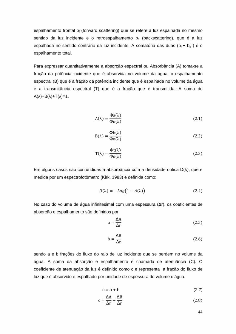
44

espalhamento frontal bf (forward scattering) que se refere à luz espalhada no mesmo

sentido da luz incidente e o retroespalhamento bb (backscattering), que é a luz

espalhada no sentido contrário da luz incidente. A somatória das duas (bf + bb ) é o

espalhamento total.

Para expressar quantitativamente a absorção espectral ou Absorbância (A) toma-se a

fração da potência incidente que é absorvida no volume da água, o espalhamento

espectral (B) que é a fração da potência incidente que é espalhada no volume da água

e a transmitância espectral (T) que é a fração que é transmitida. A soma de

A(λ)+B(λ)+T(λ)=1.

A�λ� = Φa�λ�Φo�λ��2.1�

B�λ� = Φb�λ�Φo�λ��2.2�

T�λ� = Φt�λ�Φo�λ��2.3�

Em alguns casos são confundidas a absorbância com a densidade óptica D(λ), que é

medida por um espectrofotômetro (Kirk, 1983) e definida como:

��λ� = −����1 − ��λ���2.4� No caso do volume de água infinitesimal com uma espessura (∆r), os coeficientes de

absorção e espalhamento são definidos por:

a = ∆A∆r �2.5�

b = ∆B∆r �2.6�

sendo a e b frações do fluxo do raio de luz incidente que se perdem no volume da

água. A soma da absorção e espalhamento é chamada de atenuância (C). O

coeficiente de atenuação da luz é definido como c e representa a fração do fluxo de

luz que é absorvido e espalhado por unidade de espessura do volume d’água.

c = a + b (2.7)

c = ∆A∆r + ∆B∆r �2.8�

45

c = ∆C∆r �2.9�

A determinação do coeficiente de absorção a(λ) das águas naturais é bastante

complicado, por muitas razões, de modo que uma consideração cuidadosa deve ser

feita minimizando, no possível, os efeitos de espalhamento nas medidas de absorção.

Os efeitos do espalhamento podem dominar a atenuação em todos os comprimentos

de onda do visível, especialmente em águas com grande quantidade de material

particulado.

2.3.3 Propriedades Ópticas Aparentes e Quase Inerentes

As propriedades ópticas aparentes (POA) da água são as propriedades que

dependem tanto do meio aquático como da estrutura direcional do campo de luz do

ambiente. (quantidades de luz, inclinação do sol, ângulo de visada, etc.). As POA de

um mesmo alvo podem variar, rapidamente, sem que variem suas POI (características

físicas, biológicas, químicas, etc.). Se uma nuvem passa, se o ângulo de visada muda,

ou se a superfície da água muda de rugosidade, por causa do vento, as POA mudam.

A POA ideal deveria variar apenas, ligeiramente, com as mudanças ambientais

externas, mas deveria variar, suficientemente, a partir de um corpo d’água para o

próximo na caracterização das propriedades ópticas. Note-se que, ao contrário das

POI, as POA não podem ser medidas em amostras d’água, uma vez que dependem

da distribuição da luz ambiental encontrada, no corpo da água em si.

As principais propriedades aparentes são: a distribuição angular, o coeficiente vertical

de atenuação da luz, a reflectância estimada a partir de um sensor remoto e a

reflectância irradiante de superfície.

A irradiância é o fluxo de energia por unidade de área, proveniente de todas as

direções, e a radiância é o fluxo de energia por unidade de área, proveniente de um

determinado lugar no espaço (ângulo solido).

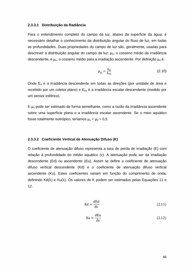
46

2.3.3.1 Distribuição da Radiância

Para o entendimento completo do campo da luz, abaixo da superficie da água, é

necessário detalhar o conhecimento da distribuição angular do fluxo de luz, em todas

as profundidades. Duas propriedades do campo de luz são, geralmente, usadas para

descrever a distribuição angular do campo da luz: µd, o cosseno médio da irradiância

descendente, e µu, o cosseno médio para a irradiação ascendente. Por definição µd é:

µ! = "#"$# (2.10)

Onde Ed é a irradiância descendente em todas as direções (por unidade de área e

recebido por um coletor plano) e E0d é a irradiância escalar descendente (medido por

um sensor esférico).

E µu pode ser estimado de forma semelhante, como a razão da irradiância ascendente

sobre uma superfície plana e a irradiância escalar ascendente. Se o meio aquático

fosse totalmente isotrópico, teríamos µu = µd = 0,5.

2.3.3.2 Coeficiente Vertical de Atenuação Difuso (K)

O coeficiente de atenuação difuso representa a taxa de perda de irradiação (E) com

relação à profundidade do médio aquático (z). A atenuação pode ser da irradiação

descendente (Ed) ou ascendente (Eu). Assim se define o coeficiente de atenuação

difuso vertical descendente (Kd) e o coeficiente de atenuação difuso vertical

ascendente (Ku). Estes coeficientes variam em função do comprimento de onda,

definindo Kd(λ) e Ku(λ). Os valores de K podem ser estimados pelas Equações 11 e

12.

Kd = dEddz �2.11� Ku = dEudz �2.12�

47

2.3.3.3 Reflectância

No sensoriamento remoto a reflectância ou reflectância de sensoriamento remoto, é

definida pela Equação 2.13.

R+, = L.�θ,Φ, λ�E0�λ� �2.13�

Onde Ed é a irradiância descendente que chega à superfície da água, θ e φ são os

ângulos polar e azimutal, respetivamente, λ é o comprimento de onda e Lw é a

radiância espectral emergindo da água na direção θ e φ.

Rrs pode ser escrita como uma função da reflectância volumétrica (R-0), que é definida

como a razão Eu-0/Ed-0, onde Eu-0 e Ed-0 são a irradiância ascendente e descendente

a uma profundidade infinitésima (-0). De acordo com Morel e Gentili, (1993) temos:

R+, = �1 − ρ� ∗ �1 − ρ′� ∗ R23n² ∗ �1 − r′R23� ∗ Q �2.14�

Onde R-0 é a reflectância volumétrica, ou seja, a reflectância do corpo d’água em si, ρ

é a reflectância interna de Fresnel que depende da rugosidade da superfície, do

ângulo zenital solar e da cobertura de nuvens; ρ’ é a reflectância de Fresnel para a

interface água-ar, tipicamente estimada em 4% ou 5%; n, é o índice de refração da

água (n = 1,34); r’, a reflexão da água-ar, da ordem de 0,48; Q é a razão de Eu-0/Lu-0,

que para um campo ideal isotrópico seria π, mas em águas naturais varia entre 3,1 e

5,6 (Morel e Gentili, 1993).

2.3.4 Relação entre a Reflectância Volumetrica e POI

Gordon (1973) relacionou a reflectância irradiância volumétrica R-0 com as

propriedades óticas inerentes POI, qual foi simplificada por Jerlov (1976), tal como se

apresenta na Equação 2.15:

48

R23 = 6′ b7a + b7 �2.15� onde f’ é um coeficiente que varia com as condições de iluminação e tipos de água, e

a e bb são respectivamente, os coeficientes de absorção e retroespalhamento do

corpo de água. Estudos feitos por Kirk (1991); Kirk (1981); Prieur (1976) definiram o

valor do coeficiente f’ para condições específicas de luz e de tipos de água. Froidefond

e Doxaran (2004), assinalaram que a constante varia entre 0,324 (sol ao zenit) e 0,369

(céu coberto uniformemente). Normalmente se adota um valor de 0,33 (Morel e Prieur,

1977).

Kirk (1991), relacionou o Kd e as propriedades ópticas inerentes para um intervalo de

a/b= 0–20, como se mostra na Equação 2.16.

Kd = 8�a9 + Gab��2.16� onde G é uma função que especifica a contribuição relativa do espalhamento na

atenuação vertical da luz. Usualmente, o valor de G é estimado entre 0,233 e 0,264

(Kirk 1994).

Aas (1987), relacionou as POI com as POA encontrando uma equação que define a

absorção a partir da reflectância irradiância, Kd e os cossenos médios (µu e µd).

; = Kd ∗ µd <2=�$>�<?=�$>��µ0/µA� (2.17)

Esse conjunto de equações permitira relacionar as POA que são medidas no campo

com as POI que são diretamente relacionas às propriedades biofisicas das águas.

2.3.5 As POI Espectrais da Água

Diferentemente das POA, as POI tem a vantagem de não ser influenciada pelas

condições de iluminação, como se mencionou anteriormente. Existe outra vantagem

para lidar com estas quantidades: num meio aquático de componentes múltiplos, a

maior parte das POI é obtida através de uma simples adição das contribuições dos

componentes individuais. Essa adição não é efetivamente avalidada para as POA,

especialmente em meios aquáticos, com espalhamento significativo.

49

As POI da Água Pura

A água pura mostra um espectro de absorção (Figura 2.7) com um mínimo no azul,

seguido por um incremento continuo da absorção para comprimentos de onda acima

de 570 nm. Um incremento acentuado aparece em 700 nm. Em 800 nm aw disminue e

aumenta novamente depois dos 820 nm.

O comportamento espectral da água pura é determinado, basicamente, pelo

espalhamento molecular nos comprimentos de onda mais curtos. O coeficiente de

absorção (a) da água pura é mínimo na região compreendida entre 400 nm e 600 nm,

aumentando, rapidamente, na região do infravermelho.

O coeficiente de espalhamento (b) da água pura, ao contrário, é máximo na região do

azul, e decresce exponencialmente em direção ao infravermelho, mas com valores

muito mais baixos. Sendo a absorção muito maior que o valor do espalhamento, o

valor de atenuação da luz (c) da água pura será muito próximo ao valor da absorção,

como se vê na Figura 2.7.

Figura 2.7. Variação espectral dos coeficientes de absorção (a) espalhamento (b) e

atenuação (c) da água pura (adaptado de Dekker, 1993).

Se o espectro de reflexão da água pode ser estimado pela razão (b/a), pode-se

concluir que a energia refletida pela água pura é máxima na região do azul e decresce

em direção ao vermelho. Portanto, pode-se concluir que a água pura, quando

observada a partir de um satélite, tenderá a apresentar a cor azul, principalmente, se a

50

dimensão do corpo da água for suficiente para atenuar os efeitos das margens e do

fundo.

Uma visão detalhada de dados experimentais sobre as características ópticas da água

pura pode ser encontrada e, valores numéricos, em Tam e Patel (1979), Smith e Baker

(1981) e Buiteveld et al. (1994).

Entretanto, em águas naturais, os componentes opticamente ativos presentes na água

passam a ser determinantes na reflectância de corpos de água. Sedimentos em

suspensão (TR), pigmentos fotossintéticos (chf) e matéria orgânica dissolvida colorida

(CDOM) são os componentes responsáveis pelo comportamento espectral das águas

continentais. As regiões de absorção e espalhamento destes constituintes da água é

que vão definir a forma final da curva de reflectância, enquanto sua concentração é

responsável pela magnitude das feições e pela magnitude da energia refletida em

subsuperfície (Kirk, 1994; Mobley, 1994).

As POI das águas naturais.

As POI são influenciadas, diretamente, pelos componentes dos corpos da água. A

absorção é representada pela Equação 2.18 (Sathyendranath e Morel, 1983).

a�λ� = a.�λ� + aBCDE�λ� + aFGH�λ� + aI=�λ��2.18� onde aw é a absorção da água pura, aCDOM é a absorção da matéria orgânica dissolvida

colorida, achf é a absorção dos pigmentos fotossintéticos e atr é a absorção do material

particulado não orgânico.

A presença de matéria orgânica dissolvida (gilvin ou substância amarela) é um dos

componentes responsáveis pelo aumento do coeficiente de absorção da água. A

Figura 2.8 ilustra a absorção específica pela matéria orgânica dissolvida, que é muito

alta nos comprimentos de onda curtos e diminui de maneira exponencial para

comprimentos de onda maiores. O fitoplâncton apresenta uma absorção muito alta no

azul (440 nm), baixa entre 550 nm e 650 nm, apresentando um novo pico de absorção

em torno de 675 nm. Estes máximos estão associados à clorofila a, que tem seus

picos de absorção em 440 nm e 675 nm. A absorção do material inorgânico

particulado é também uma curva exponencial negativa, sendo, muito alta no azul e vai

baixando, quando o comprimento de onda é maior.

51

Figura 2.8. Coeficiente de absorção especifico para a: água pura (aw), e os componentes: fitoplâncton (aph), matéria orgânica dissolvida (aCDOM) e o material particulado não orgânico (aTR). (Adaptado de Giardino 2007)

O retroespalhamento (bb) é afetado pelas moléculas d’água (bbw), sedimentos (bbs) e

partículas fitoplanctônicas (bbph). Equação 2.19.

JK�λ� = JKL�λ� + JKM�λ� + JKNO�λ��2.19� O retroespalhamento pelas moléculas da água apresenta uma forma de exponencial

negativa, muito similar à curva de espalhamento da água pura. O retroespalhamento

do material particulado diminui em função do comprimento de onda, mas de maneira

mais suave (Figura 2.9). O fitoplâncton presenta um retroespalhamento maior no azul

e disminui, à medida, que o comprimento de onda aumenta, apresentando uma zona

de baixo espalhamento entre os 650 nm e 700 nm.

52

Figura 2.9. Variação espectral dos coeficientes de retroespalhamento específicos da

água pura (bbw), do fitoplâncton (bb ph) e do material particulado não orgânico (bb TR).

(Adaptado de Giardino 2007).

O retroespalhamento dos sedimentos (bbs) é modelado usando a teoria de Mie (Van de

Hulst 1957) a qual foi usada por muitas décadas para águas oceânicas. Para um

conjunto de partículas com uma distribuição de tamanhos N(D) e um índice de

refractância relativo ao da água de mar, ms, bbs pode ser definido com a Equação 2.20

JKM�λ� = P QKK��,RMλ�πD94

T U���V��2.20�

onde Qbb é o fator de eficiência de retroespalhamento das partículas que é uma função

de D e ms . ms é o índice de refração de partícula de sedimento, que, supostamente, é

independente de λ. N(D) dD é o tamanho das partículas compreendidas entre D e

D+dD por unidade de volume. Da Equação 2.20 pode-se concluir que o

retroespalhamento depende de três parâmetros: concentração, diâmetro e índice de

refração.

53

CAPITULO III

----------------------------------------------------------------------------

Resumo dos Trabalhos

54

3 RESUMO DOS TRABALHOS

Neste capítulo são resumidos os dados de entrada da tese e as metodologias

utilizadas, tais como, amostragem de sedimentos, espetrorradiometria e

processamento das imagens de satélite. Destacaremos os mais importantes

resultados obtidos durante a tese para introduzir os quatro artigos.

Figura 3.1. Esquema da metodologia utilizada na tese. Entre parêntesis são indicados

os parágrafos, onde serão detalhados os trabalhos

3.1 Dados

3.1.1 Material em suspensão ORE-HIBAM

O ORE-HIBAM (http://www.ore-HIBAM.org) opera desde 2003, respondendo a um

edital do Ministério Francês da Educação Superior e Pesquisa. A finalidade é fornecer

à comunidade científica internacional dados de qualidade, necessários para a

compreensão e modelagem dos processos hidro-geológicos e sua dinâmica em longo

prazo. Liderado por um grupo de pesquisadores do Institut de recherche pour le

développement (IRD) que desenvolve, desde 1995, projetos de pesquisas na bacia

amazônica, o ORE-HIBAM conta também com parceiros locais (agências nacionais e

universidades) para manter a perenidade das observações.

Os dados dos materiais em suspensão (MES) da rede ORE-HIBAM são dados de

amostras, a cada 10 dias (dias 01, 11 e 21 de cada MES). As amostras são coletadas

55

por um observador local, que toma a amostra em uma garrafa de 500 ml, em um

ponto do rio previamente indicado. As amostras são levadas a cada três meses,

aproximadamente, para o laboratório, onde estão filtradas em membranas de celulose

de 0,45 µm, previamente, pesadas. Esses filtros, logo após a filtragem, são secados e

pesados, novamente. A concentração de MES é determinada a partir da diferença dos

pesos dos filtros, dividida pelo volume de água que foi filtrado.

O inconveniente deste tipo de amostragem é a sua fraca representatividade em

relação aos pixels de imagens de satélite do tipo MODIS. Outra limitação é que as

séries são, às vezes, interrompidas por alguns meses.

O aspecto favorável destes dados fica na sua disponibilidade em longas séries

temporais e vários lugares da bacia. Existem 40 estações de coleta de concentração

de sedimentos com séries históricas, algumas delas, desde 1995.

Outra rede disponibilizando dados é a rede da Agência Nacional de Águas do Brasil

(ANA), que conta com uma rede de medição de concentração de sedimentos na bacia

amazónica, com 94 estações sedimentométricas e amostras integradas trimestrais

(SAR/ANA -Banco de Dados Hidro).

3.1.2 Dados de Campo

Os dados de campanhas de amostragem nos diversos rios da Amazônia foram

coletados com barcos e lanchas. Essas campanhas foram realizadas com o apoio de

diferentes entidades e projetos, como o Serviço Geológico do Brasil (CPRM), a ANA

(Agência Nacional de Águas), o Projeto HIBAM (Controles geodinâmico, hidrológico e

biogeoquímico da erosão/alteração e da transferência de matérias na bacia

amazônica), o CNPq (Conselho Nacional de Desenvolvimento Científico e

Tecnológico) dentro do convênio de cooperação bilateral IRD-UnB e o projeto ANR

CARBAMA (ciclo do carbono no rio Amazonas)

Nessas campanhas foram feitas medições de espectrorradiometria, medições de

sedimentos da superfície e de vazão sólida e vazão liquida, nos principais rios da

bacia amazônica. As amostragens foram realizadas, nos diferentes períodos do ciclo

hidrológico, tentando melhorar o entendimento dos processos de transporte de

sedimento, em cada estação, conseguindo uma grande diversidade de concentrações

de sedimentos, nas águas dos rios.

As estações principais de medição e coleta de amostras são: San Regis (SRG),

Requena (REQ), Bellavista (BLL), Tamshiyacu (TAM), Tabatinga (TAB), Santo António

56

do Iça (SAI), Fonte Boa (FBA), Tefé (TEF), Manacapuru (MAN), Itacoatiara (ITA),

Parintins (PAR), Óbidos (OBI), Abuna (ABU), Porto Velho (PVE), Humaitá (HUM),

Manicoré (MNI), Borba (BBA) e Fazenda Vista Alegre (FVA).

Na Figura 3.2 são mostrados os pontos das medições feitas nas campanhas

realizadas durante os três primeiros anos da tese. As estações são descritas na

Tabela 3.1. É um total de 279 medições de reflectância e 133 de Kd. Na Tabela 3.1

podemos observar a grande amplitude de concentração de sedimentos amostrados,

sendo a mínima de 2 mg/l no rio Negro e a máxima de 621 mg/l na foz do rio Madeira.

Figura 3.2. Pontos de coleta de dados nas campanhas realizadas durante a tese. Em

círculos vermelhos amostras sobre os rios e estrelas verdes amostras sobre as

várzeas.

No total foram realizadas 10 campanhas dentro do período da tese, sendo da seguinte

forma: 4 de Manacapuru a Óbidos, 1 de Porto Velho a Manacapuru, 1 de Porto Velho

a Óbidos, 1 Manacapuru a Porto Velho e 2 de San Regis/ Requena a Óbidos

57

Tabela 3.1. Localização e número de amostras coletadas durante as campanhas de

amostragem figurando los nomes das principais estações.

As medições foram feitas também na foz dos principais afluentes, os rios Marañón,

Ucayali, Napo, Javari, Iça, Jutai, Jurua, Japura, Purus, Negro, Trombetas é Tapajós; e

algunas várzeas ao lado dos rios Solimões e Amazonas: lagos Cabaliana, Janauacá,

Miratuba, Canaçari e Curuai. Para completar a análise, amostras anteriormente

coletadas por Jean Michel Martinez nos anos 2007 e 2008 foram adicionadas.

Lat. Long.

Fora da

água

Dentro

da água Min Max

Tamshiyacu (TAM) Amazonas -3,976 -73,236 1 1 238,00 289,00

Tabatinga (TAB) Solimões -4,082 -70,094 1 2 145,00 200,80

São Paulo de Olivença (SPO) Solimões -3,424 -69,005 5 2 145,00 293,00

Santo Antonio do Iça (SAI) Solimões -2,992 -67,867 0 1 244,00 244,00

Fonte Boa (FBA) Solimões -2,582 -66,300 1 2 121,00 154,80

Tefé (TEF) Solimões -3,636 -64,196 2 1 63,00 196,00

Coari Solimões -4,075 -63,098 2 2 77,00 170,80

Codajas Solimões -3,790 -62,224 1 0 88,00 88,00

Manacapuru (MAN) Solimões -3,339 -60,477 10 8 22,40 228,40

Itacoatiara (ITA) Amazonas -3,194 -58,537 10 4 26,80 185,20

Parintins (PAR) Amazonas -2,572 -57,065 2 2 58,00 77,00

Obidos (OBI) Amazonas -1,935 -55,519 14 9 24,30 173,00

San Regis (SRG) Marañon -4,475 -74,098 2 2 120,40 241,60

Requena (REQ) Ucayali -4,940 -73,803 3 2 357,00 432,40

Foz do Napo Napo -3,341 -72,760 2 1 155,60 174,00

Foz do Javari Javari -4,164 -70,491 2 1 58,00 105,40

Foz do Iça Iça -3,002 -68,282 2 2 65,60 21,20

Foz do Jutaí Jutaí -2,888 -66,956 1 2 12,20 37,60

Foz do Juruá Juruá -2,865 -65,845 1 2 166,20 222,00

Foz do Japurá Japurá -2,607 -64,987 2 2 26,40 77,20

Beruri Purus -4,123 -61,577 3 3 5,60 52,00

Paricatuba Negro -2,939 -60,611 4 5 2,00 8,00

Foz do Trombetas Trombetas -1,511 -56,034 0 1 8,50 8,50

Foz do Tapajos Tapajos -2,656 -55,052 2 1 9,60 2,70

Cabaliana Varzea de Cabaliana -2,663 -62,079 4 4 7,60 4,40

Janauaca Varzea de Janauaca -4,098 -60,588 7 7 33,00 2,00

Canaçari Varzea de Canaçari -2,413 -59,274 7 3 14,20 3,00

Miratuba Varzea de Miratuba -4,099 -57,878 7 2 35,90 6,93

Curuai Varzea de Curuai -3,070 -56,206 8 3 81,30 3,20

Abunã (ABU) Madeira -10,001 -65,334 1 1 104,80 97,60

Porto Velho (PVE) Madeira -9,143 -64,350 7 6 401,00 102,40

Humaitá (HUM) Madeira -7,422 -62,970 3 4 418,40 108,40

Manicoré (MNI) Madeira -5,854 -61,316 3 3 418,00 110,00

Borba (BBA) Madeira -4,309 -59,527 4 3 464,00 46,00

Fazenda Vista Alegre (FVA) Madeira -4,779 -59,917 4 2 81,20 48,80

Foz do Madeira Madeira -3,476 -58,804 11 9 621,60 25,20

Amostras MES (mg/l)

Estação

Nome do

Rio/Varzea

Coordenadas

3.1.2.1 Propriedades dos sedimentos

As amostragens da água

profundidades (Figura 3.3), a fim de realizar as estimativas de vazão sólida

estação, e, para calibrar e validar os dados de satélite e de radiometria de campo.

As amostras da superfície são coletadas em uma profundidade de

processadas seguindo o mesmo

determinação da concentração de material

Figura 3.3. Corte transversal do rpontos pretos são os lugares de amostragem.

Para as estimativas de vazão sólida

regularmente espaçadas. Em cada vertical

diferentes profundidades, conforme apresentado na Figura 3.3

realizado com um amostrador de profundidade instantâneo (Figura 3.4).

amostras podem-se relacionar a concentração de MES superficial com a concentração

média da secção do rio.

integrador, devido à dificuldade de uso em

fato de não dar uma estimativa separada

Depois de coletar a amostra, as partículas grossas

uma peneira de 63 µm. O que fica na peneira é colocado em um filtro de celulose, que

logo é secado e pesado. A água que passa pelo tamis é fil

mesmo procedimento das amostras de supe

concentrações pontuais no c

o software HydroMESAD do IRD

Propriedades dos sedimentos

água foram realizadas na superfície, como em diferentes

profundidades (Figura 3.3), a fim de realizar as estimativas de vazão sólida

para calibrar e validar os dados de satélite e de radiometria de campo.

As amostras da superfície são coletadas em uma profundidade de

processadas seguindo o mesmo protocolo das amostras ORE-HIBAM para a

ncentração de material em suspensão.

3.3. Corte transversal do rio Solimões (medição ADCP) na estação de MAN, os pontos pretos são os lugares de amostragem.

Para as estimativas de vazão sólida, a secção transversal é dividida em verticais

das. Em cada vertical coletam-se amostras

diferentes profundidades, conforme apresentado na Figura 3.3. Est

mostrador de profundidade instantâneo (Figura 3.4).

onar a concentração de MES superficial com a concentração

média da secção do rio. Para o presente trabalho não se usou um

dificuldade de uso em grandes profundidades (40 a 60 m

fato de não dar uma estimativa separada da concentração de superficie

a amostra, as partículas grossas são separadas das finas usando

que fica na peneira é colocado em um filtro de celulose, que

logo é secado e pesado. A água que passa pelo tamis é filtrada e secada, usando o

mesmo procedimento das amostras de superfície. Desta maneira,

concentrações pontuais no corte transversal do rio. A vazão sólida é estimada

do IRD (www.ore-HIBAM.org/).

58

como em diferentes

profundidades (Figura 3.3), a fim de realizar as estimativas de vazão sólida, em cada

para calibrar e validar os dados de satélite e de radiometria de campo.

As amostras da superfície são coletadas em uma profundidade de 0 a 20 cm, e

HIBAM para a

io Solimões (medição ADCP) na estação de MAN, os

a secção transversal é dividida em verticais

amostras pontuais em

. Este protocolo é

mostrador de profundidade instantâneo (Figura 3.4). Com estas

onar a concentração de MES superficial com a concentração

ou um amostrador

(40 a 60 m) e pelo

da concentração de superficie.

das finas usando

que fica na peneira é colocado em um filtro de celulose, que

trada e secada, usando o

rfície. Desta maneira, têm-se várias

é estimada usando

59

Figura 3.4. Amostrador de fundo Callède I com sonda multiparamétricas e granulômetro lazer.

Nas campanhas, além das amostras de água são coletados dados com sondas

multiparamétricas de pH, turbidez, temperatura, condutividade, entre outros. As

sondas foram usadas, tanto na superfície dos rios, como em perfis verticais.

Amostras d’água foram também coletadas para análises posteriores no laboratório de

granulometria, com um granulômetro a laser pela CPRM, e para analise de

mineralogia.

Mineralogia

As amostras para o estudo da mineralogia foram coletadas na superfície dos rios,

aproximadamente, a 80 cm de profundidade, e no meio dos rios, nas estações de FVA

e MAN, durante as campanhas de novembro de 2007 a maio de 2008. Estas amostras

foram analisadas pelo professor Jérôme Viers (Laboratório GET – Toulouse, França),

utilizando um difratômetro de raios X. Os resultados obtidos dessas análises são

apresentados na Tabela 3.2.

Na tabela 3.2 pode-se observar que as duas bacias não são significativamente

diferentes com relação ao quartzo e clorita. Mas, as concentrações de esmectita são

bastante diferentes, sendo o rio Solimões mais carregado em esmectitas que o rio

Madeira, com maiores concentrações durante a enchente do afluente. Ao contrário, o

rio Madeira apresenta concentrações maiores em ilita do que o rio Solimões. As

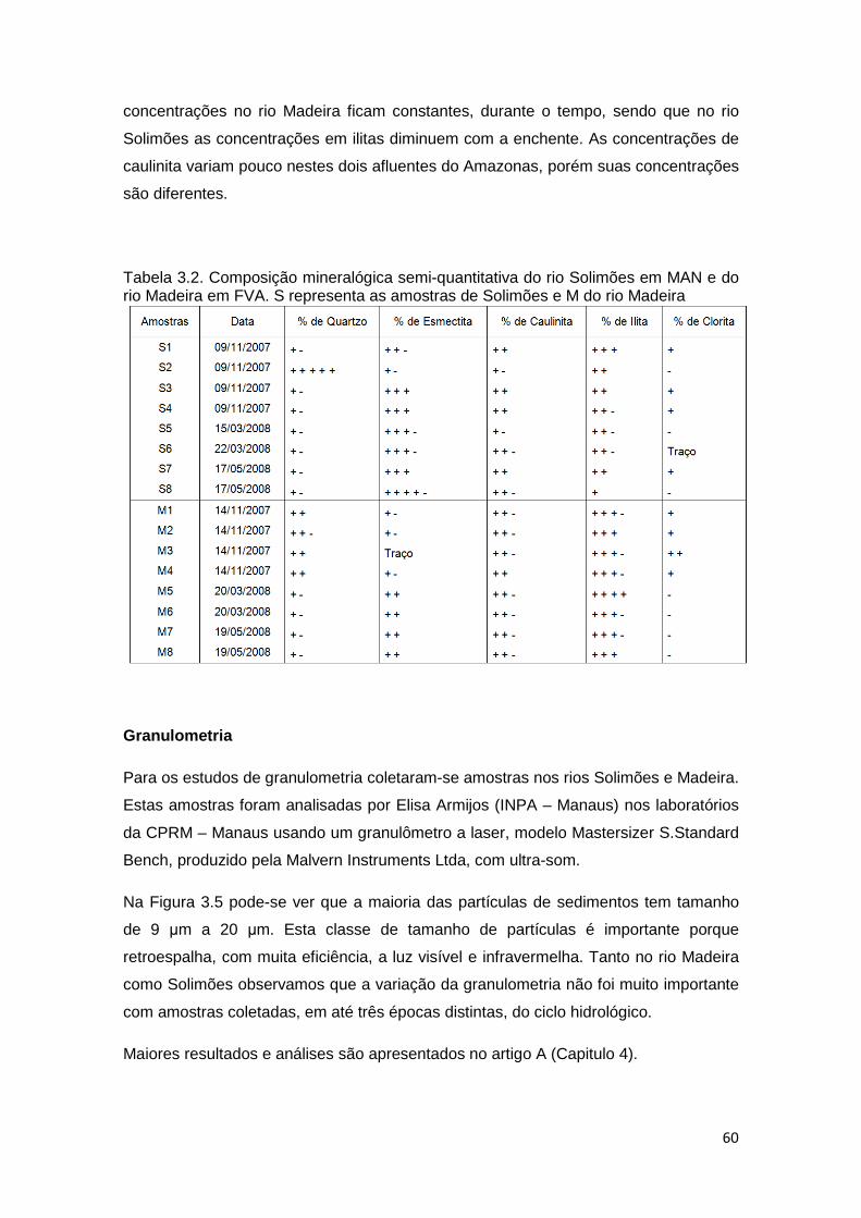
60

concentrações no rio Madeira ficam constantes, durante o tempo, sendo que no rio

Solimões as concentrações em ilitas diminuem com a enchente. As concentrações de

caulinita variam pouco nestes dois afluentes do Amazonas, porém suas concentrações

são diferentes.

Tabela 3.2. Composição mineralógica semi-quantitativa do rio Solimões em MAN e do rio Madeira em FVA. S representa as amostras de Solimões e M do rio Madeira

Granulometria

Para os estudos de granulometria coletaram-se amostras nos rios Solimões e Madeira.

Estas amostras foram analisadas por Elisa Armijos (INPA – Manaus) nos laboratórios

da CPRM – Manaus usando um granulômetro a laser, modelo Mastersizer S.Standard

Bench, produzido pela Malvern Instruments Ltda, com ultra-som.

Na Figura 3.5 pode-se ver que a maioria das partículas de sedimentos tem tamanho

de 9 µm a 20 µm. Esta classe de tamanho de partículas é importante porque

retroespalha, com muita eficiência, a luz visível e infravermelha. Tanto no rio Madeira

como Solimões observamos que a variação da granulometria não foi muito importante

com amostras coletadas, em até três épocas distintas, do ciclo hidrológico.

Maiores resultados e análises são apresentados no artigo A (Capitulo 4).

61

Figura 3.5. Granulometria das partículas em suspensão na superfície em duas

estações no rio Madeira (Porto Velho e Manicoré), para três períodos diferentes

3.1.3 Espectrorradiometria de Campo

A espectrradiometria foi realizada com os espectrorradiômetros TriOS – RAMSES

(Figura 3.6) que operam nas faixas espectrais do ultra violeta, visível e o infravermelho

próximo (320-950 nm), os quais têm as seguintes características:

Óptico

Região do comprimento de onda: 320 - 950 nm

Tipo de detector: 256 fotodiodos de silício

Amostragem espectral: 3,3 nm/pixel

Acurácia espectral: 0,3 nm

Canais usáveis: 190

Campo de visada: 7° (no ar)

As medições de espectrorradiometria foram feitas nas campanhas realizadas nos rios

da Amazônia com a finalidade de comparar os dados radiométricos com os dados de

satélite. Com esses instrumentos registra-se o espectro total. Os principais parâmetros

medidos são: reflectância e coeficiente vertical de atenuação da luz descendente (Kd).

Em seguida, são mostrados alguns resultados das medições de espectrorradiometria e

as propriedades ópticas das águas. Mais resultados e análises são mostrados no

artigo A (Capitulo 4).

0

1

2

3

4

5

6

7

0.1 1 10 100 1000 10000

Volu

men

(%

)

Diâmetro das Partículas (µm)

jul-2011 PV

nov-2009 PV

mar-2010 PV

jul-2011 MNI

nov-2009 MNI

mar-2010 MNI

62

Figura 3.6 Espectrorradiômetros TriOS: a) RAMSES-ARC: medição da energia radiante refletida e b) RAMSES-ACC-VIS: medição da energia incidente

3.1.3.1 Medição de Reflectância

A medição de reflectância da água é complexa. A quantidade de energia

eletromagnética que chega à superfície da água (Ed) é medida pelo sensor de energia

incidente (irradiância) (Figura 3.7). Parte dessa energia é refletida na superficie do

corpo da água e outra parte atravessa a interface ar/água para interagir com a água e

os outros componentes, fazendo com que parte desta energia seja absorvida ou

espalhada.

A energia que é retroespalhada volta para a superfície da água e uma fração emerge

dessa superfície. Essa energia emergente é a radiância da água (Lw). Porém, um

sensor localizado acima da água registra a energia Lu que constitui a somatória de Lw

mais uma fração da energia, que provém do céu Ld (refletida na superficie da água na

direção do sensor). Portanto para o cálculo da reflectância se usa a Equação 3.1.

XYZ = �[ − ρ ∗ �V\V �3.1� Onde ρ é um fator que depende da rugosidade da superfície. Geralmente é usado o

valor de 0,028 como mostram as simulações de Mobley (1999).

Com a finalidade de diminuir o problema da luz refletida pela surperficie da água

(ρ*Ld), as medições de reflectância são realizadas com três aparelhos (dois medidores

de radiância e um sensor de irradiância (Ed)), colocados fora da água, em uma

a) b) b)

63

distribuição geométrica especial, como se mostra na Figura 3.7. O primeiro sensor a

30º off nadir (que “vê” a água) amostra a radiânça saindo da água (Lu). O segundo

sensor, a 30º com o zênite (que “vê” o céu) mede a radiância proveniente do céu, que

é depois refletida pela água (Ld). O sensor colocado verticalmente mede a irradiância

descendente que chega sobre o local (Ed).

Figura 3.7. Esquema da medição da reflectância Rrs e da interação da luz com a

superfície da coluna d’água. Irradiância (Ed), Radiância do céu (Ld) e radiância da

água (Ld). θ=30º.

Para calcular a influência da geometria na sensibilidade das medições, testamos os

ângulos de visada (θ) (Figura 3.8a), calculando a reflectância em diferentes posições

dos sensores. Na Figura 3.9, observamos que se o ângulo do sensor que mede a

radiância da água for mudado para 60° (30° de diferença com a posição requerida),

pode variar até 1,7 vezes, o valor de reflectância para o comprimento de onda de 400

nm. Para os comprimentos entre 500 nm e 750 nm, a variação é menor de 20%, e

para os valores maiores que 750 nm a variação não passa de 20%, sempre para o

ângulo de 60°. Observa-se que para uma pequena variação da geometria (10°), a

variação da reflectância será menor de 10%, em todo o espectro, confirmando a

robustez da configuração.

64

Figura 3.8. Medições radiométricas de: a) Reflectância e b) Coeficiente de atenuação

vertical difuso da luz descendente (Kd)

Figura 3.9. Variação da reflectância normalizada em relação ao ângulo de visada do sensor radiométrico (Lu)

3.1.3.2 Medições do Coeficiente de Atenuação Difuso (Kd).

Para as medições de Kd o sensor de irradiação (RAMSES-ACC-VIS) é submergido na

água. Este aparelho conta com um sensor de profundidade, cujos valores serão

usados para os cálculos. Para essas medições o aparelho é colocado com o sensor de

irradiância para cima (Figura 3.8b), tomando amostras de irradiância em diferentes

0,0

0,5

1,0

1,5

2,0

2,5

3,0

3,5

4,0

400 500 600 700 800 900

Var

iaçã

o n

orm

aliz

ada

resp

eit

o a

30

°

Comprimento de onda (nm)

35°

40°

45°

50°

55°

60°

b) a)

65

profundidades, até que os valores medidos fiquem perto de 1% do valor da superfície.

Exemplos de valores coletados são apresentados na Figura 3.10. O valor de Kd é

calculado com a Equação 3.2, como indica Jerlov, (1976).

(3.2)

Onde Z1 e Z2 são as profundidades e Ed(λ)Z1 e Ed(λ)Z2 são as medições de irradiância,

nas profundidades Z1 e Z2 no comprimento de onda λ.

Na Figura 3.10a pode-se observar que os comprimentos de onda menores que 400

nm e maiores que 900 nm são absorvidos nos primeiros centímetros da coluna d’água.

Para profundidades maiores, os comprimentos de onda do vermelho são os únicos

que se propagam no meio aquático. Na Figura 3.10b pode se apreciar que a

diminuição da energia, segundo a profundidade, é uma exponencial negativa. O valor

de Kd é o expoente positivo da equação; no caso da Figura 3.10, o valor do Kd é de

4,62.

Figura 3.10. Medição de irradiância descendente em diferentes profundidades do

corpo d’água, a) para todos os comprimentos de onda a 0,13 m; 0,26 m; 0,45 m; 0,66

m de profundidade b) para um comprimento de onda (670 nm) em todas as

profundidades.

3.1.4 Imagens de Satélite MODIS

3.1.4.1 Produtos MOD09 e MYD09

Para o presente trabalho foram utilizados os produtos MODIS MOD09 e MYD09 dos

satélites TERRA e AQUA, respectivamente. O nível de processamento destas

Ed(λ) = 1691,8e-4,624(Z)

1

10

100

1000

- 0,20 0,40 0,60 0,80 1,00 1,20 1,40 1,60

Ed (m

W/(

m².

nm

))

Profundidade (m)

0

100

200

300

400

500

600

700

800

900

350 450 550 650 750 850 950

Ed

(m

W/(

m².

nm

))

Comprimento de onda (nm)

0.13 m

0.26 m

0.45 m

0.66 m

a) b)

66

imagens é 3. Elas podem ser de dois tipos: A1 e Q1 de resolução espacial de 500 m

ou 250 m, respectivamente, somando quatro tipos de imagens:

− MODIS/Terra Surface Reflectance 8-Day L3 Global MOD09A1 (500 m),

− MODIS/Terra Surface Reflectance 8-Day L3 Global MOD09Q1 (250 m)

− MODIS/Aqua Surface Reflectance 8-Day L3 Global MYD09 A1 (500 m)

− MODIS/Aqua Surface Reflectance 8-Day L3 Global MYD09Q1 (250 m).

As imagens de 500 m de resolução são compostas por sete bandas. Essas imagens

possuem, também, bandas de qualidade trazendo informações sobre o ângulo zenital

de visada, o ângulo zenital do sol, o azimute relativo, a presença de nuvens ou de

sombra das nuvens e a presença de aerossóis. As bandas eletromagnéticas são:

− Banda 1 – Vermelho: 620 – 670 nm

− Banda 2 – Infravermelho próximo: 841 – 876 nm

− Banda 3 – Azul: 459 – 479 nm

− Banda 4 – Verde: 545 – 565 nm

− Banda 5 – Infravermelho Médio 1: 1230 – 1250 nm

− Banda 6 – Infravermelho Médio 2: 1628 – 1652 nm

− Banda 7 – Infravermelho Médio 3: 2105 – 2155 nm

O produto MODIS de 250 m é composto das bandas 1 e 2 (vermelho e infravermelho),

e de uma banda de qualidade geral, que contém dados básicos de qualidade.

Cada pixel MOD09 ou MYD09 contém a melhor observação diária, durante um período

de 8 dias, selecionado com base no critério da qualidade de observação (ângulo de

visada baixo, ausência de nuvens ou sombras de nuvens, e presença fraca de

aerossóis).

Os produtos MODIS podem ser adquiridos, sem custo, através da internet

(http://reverb.echo.nasa.gov/reverb/). Todos os produtos MODIS têm um

processamento prévio, o qual está indicado no Algoritmal Theoretical Basis Document

(ATBD), que proporciona toda a informação sobre os algoritmos usados para a

geração dos produtos. O ATBD correspondente para estes produtos é MOD-08:

Atmospheric Correction Algorithm Spectral Reflectances.

67

3.1.4.2 Resolução espacial e Espectrometria Misturada

Quando a resolução espacial é baixa, é muito provável que mais de um alvo seja

representado no mesmo pixel (Figura 3.11), contribuindo na reflectância total e

resultando numa radiométria misturada. Se o pixel fosse a resposta de um só alvo,

seria um “pixel puro”. A Figura 3.12 representa um exemplo para um grupo de pixels

com mistura espectral, o qual pode ser mostrado no espaço espectral como os

endmembers (membros finais) definidos pelos vértices da área formada. Um

endmember é um espectro de referência (de pixel puro ou não) que é localizado nos

extremos da área formada na área espectral.

Todos os espectros mistos se localizam dentro do espaço formado pelos

endmembers. Esta ideia pode ser levada para mais dimensões adicionando bandas

espectrais. Esta metodologia também pode ser conduzida de forma inversa: se os

pixels misturados são conhecidos, então os limites da nuvem de pontos são os

endmembers.

Figura 3.11. Representação da resposta do sensor ao amostrar um pixel misturado.

(Adaptado de: www.envi-sw.com/tut11.htm)

68

Figura 3.12. Representação bidimensional (duas bandas) do conjunto de pixels

misturados entre três polos (A, B, e C). Os vértices do triângulo são os endmembers

de cada alvo e a área interior do triângulo são os pixels misturados.

3.1.4.3 Análise Espectral Sub-Pixel

O modelo linear de mistura espectral assume que o espectro total de um pixel é uma

combinação linear dos espectros “puros” dos materiais, ponderada em função da sua

abundância na superfície do pixel. O objetivo da análise sub-pixel é determinar as

dimensões da mistura espectral, ou seja, número de endmembers, e como se viu, o

mais simples é o modelo linear.

Adams et al., (1995) e Roberts et al., (1998) indicaram que o espectro medido pelo

sensor é uma combinação linear do espectro de todos os materiais no mesmo pixel. O

modelo matemático pode ser expressado por:

XK =]^_X`,K + εKa`b<

�3.3� Onde Rb é o valor ou número digital da banda b do pixel que é examinado, Fi é a

fração do endmember i, R,i,b é a reflectância do endmember i na banda b e εb é o erro

residual do modelo com a banda b.

Baseado nesta equação, cada pixel pode ser examinado para determinar a fração de

cada endmember no pixel, e a qualidade do processo pode ser avaliado usando o erro

médio quadrático (RMS)

69

Xcd = e∑ εK9ab<U �3.6� Onde N é o número de bandas usadas.

De acordo com Roberts et al., (1998), o modelo linear é fácil de usar e de entender,

não tem limitação, em relação ao número de bandas ou de alvos misturados no pixel.

Porém, não é eficiente quando alvos apresentam reflectâncias parecidas.

3.1.4.4 Seleção do Endmember

Os endmembers podem ser obtidos mediante dois métodos: o primeiro é selecioná-los

a partir da imagem (usando endmembers conhecidos); e o segundo é derivar os

endmembers usando os dados espectrométricos das imagens, por meio dos gráficos

de dispersão das imagens, como já foi explicado (Johnson et al. 1998). A maneira

mais prática consiste em acessar os endmembers diretamente da imagem. Porém, o

inconveniente no uso de endmembers da imagem é que se limita o número de

extremos ao número de bandas radiométricas que são usadas.

Selecionando os endmembers de uma imagem deve-se garantir que os pixels são de

fato "puros" e não misturados, o que pode ser difícil, quando os pixels são

grandes. Isso, normalmente, significa que se tem de ter os dados do terreno muito

precisos e encontrar a posição exata na imagem do satélite, especialmente se esta

imagem é extremamente heterogênea. Outro fator a considerar é que, se a imagem

contém muitos endmembers e que alguns não são identificados, haverá erros nos

valores das frações (Roberts et al. 1998).

3.1.4.5 Extração da reflectância da água.

A análise dos dados do sensor MODIS mostra que a determinação da reflectância dos

rios é dificultada pela baixa resolução espacial, podendo resultar em pixels d’água

pura ou não, dependendo da largura do rio e da geometria de aquisição. A Figura 3.13

ilustra este fenômeno mostrando grande dispersão dos pixels selecionados, dentro de

uma máscara aplicada a um rio. A análise dessa dispersão faz com que seja possível

avaliar a mistura espectral de cada imagem. Espectralmente, os pixels puros estão

70

nos vértices do polígono ou linha de conexão. Em teoria, se todos os pixels fossem

dentro do polígono ou da linha formada pelos endmembers, o modelo de mistura seria

considerado um modelo linear perfeito.

A delimitação clara na representação dos canais vermelho e infravermelho próximo,

sugere que os espectros de reflectância da imagem MODIS poderiam ser melhor

representados por dois endmember: água e vegetação. Na Figura 3.14, o endmember

da vegetação é claramente separado com uma reflectância alta no infravermelho e

baixa no vermelho. O endmember d’água com sedimentos localiza-se do outro lado do

quadro com valores moderados de reflectância no canal de vermelho e menor no

infravermelho.

Observamos que a mistura espectral pode variar temporalmente por três fatores:

• A hidrologia dos rios: em função do nível d’água, a largura do rio que varia, e

alguns bancos de areia eventualmente cobertos de vegetação podem surgir.

• A geometria de aquisição: a resolução espacial do sensor pode ser degradada,

dependendo do ângulo de visada zenital.

• A atmosfera: presença de alguns resíduos atmosféricos mal corrigidos (borda de

nuvens, aerossóis).

Em outras palavras, é impossível identificar pixels puros d’água a priori.

Consequentemente, é necessário elaborar um procedimento específico para

determinar os endmembers da água do rio. Neste contexto, para o cálculo da

reflectância da água dos rios, com uma grande quantidade de imagens, é necessária a

utilização ou automatização do processo. Para isso foi usado o algoritmo “MODIS

River Reflectance Retrieval” (MOD3R) desenvolvido por Jean-Michel Martinez. A

metodologia para a extração da reflectância do endmember d’água usando o MOD3R

é apresentada a seguir:

• Os dados de entrada são: a série de imagens da zona de interesse é uma

máscara da estação (Figura 3.13);

• O primeiro passo é a extração dos pixels da máscara, identificando os pixels de

melhor qualidade (utilizando a banda de qualidade do produto de 500 metros);

• Os valores de reflectância dos pixels são classificados em grupos homogêneos,

usando estes valores, mediante a metodologia estatística do K-means.

• O endmember de vegetação é automaticamente selecionado com critério, na

diferença máxima entre o infravermelho e o vermelho;

71

• Por último, cada grupo é testado como endmember d’água, e o grupo que

produz o menor erro residual é selecionado, solucionando o modelo linear de

mistura espectral.

Figura 3.13. Máscara na estação Óbidos no rio Amazonas que pré-seleciona os pixels a serem analisados

Figura 3.14. Gráfico de espalhamento dos pixels selecionados na máscara, indicando as regiões teóricas dos endmembers d’água e de vegetação.

A Figura 3.13 mostra a máscara da zona selecionada; unicamente os pixels dentro da

máscara serão processados e a Figura 3.14 mostra os valores dos pixels nas duas

bandas (vermelho e infravermelho) com as localizações dos endmembers.

Este procedimento é centrado na determinação automática do endmember d’água por

testes sucessivos de um grupo de pixels, em cada modelo linear de mistura, para

encontrar o grupo que melhor descreve outros grupos de pixels misturas do rio. A

72

classificação dos pixels em grupos é baseada no algoritmo estatístico K-means ou K-

médias.

O algoritmo K-means é um método de classificação não supervisionado. Basicamente,

este algoritmo busca formar grupos que são representados por K centróides, cada um

identificado pelo valor médio dos pixels que pertencem a esse grupo. Um número de

grupos inicial é selecionado (> 20) para a classificação, que consiste nos seguintes

passos.

1. Primeiro são estimados os K1 valores dos primeiros grupos; estes K1 valores são

as médias dos primeiros grupos formados pelos pixels.

2. Calculam-se as distâncias dos pixels para cada um dos centróides dos

grupos. Os pixels são atribuídos aos grupos cuja distância é mínima em relação

a todos os centróides.

3. Os centróides são atualizados conforme o valor médio de todos os novos pixels

incorporados ou retirados.

4. Repetem-se os passo 2 e 3 até chegar a um determinado critério de

convergência.

No final do processo temos i grupos com 1 ≤ i ≤ K.

Uma vez definidos os grupos, o passo seguinte é selecionar o grupo que representa

melhor o endmember d’água Refágua. Como não conhecemos esse endmember, a

priori, temos que testar cada grupo Gi para entender qual é o que melhor descreve o

processo de mistura espectral em todos os outros grupos Gj.

Para selecionar o grupo adequado se procede de acordo com a Equação 3.7 para

cada banda radiométrica e para cada grupo resultado da segmentação j com 1 ≤ j ≤ K

(derivada da Equação 3.7).

Xg6h,λ = αh ∗ Xg6λ,áijk +βh ∗ Xg6λ,lmimnkção +εh �3.7� Onde:

αj: é a fração do endmember d’água no grupo j.

βj: é a fração do endmember de vegetação no grupo j.

Refλ, vegetação: é a reflectância do endmember de vegetação na banda λ.

73

Refλ,água é a reflectância do endmember d’água na banda λ a ser testada nos grupos

segmentados : Refagua ∈ { G1, G2 , .... Gj, ... GK}.

Ref j,λ,: é reflectância do grupo j na banda λ.

Εj, λ: é o erro residual resultante da resolução da Equação (3.7) para a banda λ e o

grupo j.

Cada grupo “j” resultado da segmentação é testado como um candidato a endmember

d’água Eagua. Assim, a Equação 3.7 apresenta duas incógnitas, as frações αi e βi para

cada grupo “j”. Com duas equações (para a banda vermelha e banda infravermelha)

para cada grupo Gj resolvemos o sistema de equações produzindo estimativas de αi,

βi e εi. Acrescentamos uma condição de positividade das frações (algoritmo NNLS)

para forçar o algoritmo a produzir estimativas realísticas de frações. Este processo é

repetido para cada grupo Gj para guardar no final o resíduo total εt = ΣjΣbεj,b que está

associado ao candidato a endmember d’água. De maneira iterativa vai-se testando

cada grupo como candidato a endmember d’água, e o grupo que produzir o menor

valor de εt será selecionado como o endmember d’água.

Maiores resultados e análises são apresentados no artigo B (Capitulo 5).

3.2 Influência das características físicas do MES sobre as propriedades ópticas

3.2.1 Influência do MES sobre a Reflectância

Como foi mencionada, anteriormente, a reflectância da água depende dos

componentes que se encontram no meio aquático. Assim, na Bacia Amazônica

podem-se encontrar diferentes tipos de águas, mostrando diferentes assinaturas

espectrais, como se observa na Figura 3.15. As águas do rio Madeira, com grande

quantidade de sedimentos, tem forte reflectância no vermelho e no infravermelho

próximo. As águas de rio Amazonas, também carregadas de material particulado,

apresentam alta reflectância no vermelho e um pico menor no infravermelho próximo.

No rio Negro, onde as águas contém grande quantidade de material orgânico

dissolvido, apresenta uma assinatura espectral muito baixa em todos os comprimentos

de onda. As várzeas têm águas com material orgânico dissolvido e baixa quantidade

de material particulado, mas podem apresentar fitoplâncton, em grande concentração.

Isso faz com que tenham assinaturas espectrais, com maior variação no visível, e com

picos no verde e infravermelho (705 nm).

74

Figura 3.15. Assinaturas espectrais típicas dos diferentes tipos de água dos rios (Madeira, Amazonas, Tapajós e Negro) e da várzea de Janauacá.

A reflectância nos comprimentos de onda maiores que 950 nm é muito baixa, devido à

absorção da água nestes comprimentos de onda (como visto na Figura 2.8). Nos

comprimentos de onda menores que 400 nm, Rrs é baixo, devido à absorção de

alguns elementos na água, como o material particulado e CDOM, principalmente.

A Figura 3.16 mostra a correlação entre a reflectância e o MES para todas as

amostras de campo, com 279 amostras. O valor do coeficiente de correlação de

Pearson (R2) é de 0,89 para uma função de potência. A amplitude de concentrações é

de 2 a 622 mg/l, para diferentes tipos de águas (várzeas, águas pretas, águas brancas

e águas claras), o que mostra que a reflectância, neste comprimento de onda, é um

bom estimador da concentração em MÊS, para vários tipos de água.

Para entender o comportamento desta relação, em todos os comprimentos de onda,

foi elaborada a Figura 3.17, onde se mostra uma curva de variação da correlação

entre a reflectância e a concentração de MÊS, em função do comprimento de onda.

75

Figura 3.16. Correlação entre a concentração de sedimentos e a reflectância para um

comprimento de onda de 850 nm.

Figura 3.17. Variação da correlação de Pearson (R2) entre MES e reflectância, em

função do comprimento de onda.

Como se pode ver na Figura 3.17 a correlação vai aumentando, à medida que o

comprimento de onda aumenta, até alcançar o valor máximo em 860 nm. A variação

da correlação, além dos 740 nm, apresenta poucas variações, e isso indica que a

banda 2 do sensor MODIS (Infravermelho próximo) seria um bom estimador da

concentração de MES. Para a banda vermelha do MODIS, a correlação é menor (0,7),

devido à saturação da reflectância acima de 100 mg/l (ver artigo A).

Maiores discussões desses resultados são apresentados no artigo A (Capitulo 4).

Rsr = 0,0003(MES)0,7539

R² = 0,887

0,0001

0,001

0,01

0,1

1

1,00 10,00 100,00 1 000,00

Ref

lect

ân

cia

Concentração de sedimentos (mg/l)

76

3.2.2 Influência do MES sobre o coeficiente de atenuação difuso

As medições do coeficiente de atenuação vertical descendente da luz (Kd) foram feitas

de maneira pontual nos rios. Juntamente com estas medições foram coletadas

amostras d’água para a medição de concentração de MES. Comparando as medições

de Kd e MES podemos notar que o Kd é um estimador mais robusto da concentração

de MES. A Figura 3.18 mostra a correlação entre MES e Kd para 133 amostras

coletadas durante as campanhas na Amazônia, com diferentes tipos d’água e um

intervalo de concentrações de 2 a 621,6 mg/l.

O coeficiente de Pearson é de 0,93 e nota-se que o valor de Kd não satura em função

do MES. Nota-se também que o Kd não mostra muita dispersão mesmo com águas

com baixo conteúdo de MES (< 10 mg/l).

Figura 3.18. Correlação entre a concentração de sedimentos e o Kd para um

comprimento de onda de 650 nm.

3.2.3 Influência do MES sobre o coeficiente de absorção

O coeficiente de absorção é calculado a partir dos dados de Kd e reflectância, medidos durante as campanhas, utilizando a Equação 2.17 (Aas, 1986).

Como foi visto no item 2.3.6, a absorção das águas naturais depende da absorção da

água pura, CDOM, clorofila e material particulado (Equação 2.18). A Figura 3.19

MES = 20,7*Kd - 25,064

R² = 0,935

1

10

100

1,00 10,00 100,00 1 000,00

Coef

icie

nte

de a

tenu

ação

ver

tica

l da

luz

desc

ende

nte

(Kd)

Concentração de sedimentos (mg/l)

77

apresenta a variação espectral do coeficiente de absorção para varias concentrações

de MES.

Figura 3.19. Coeficiente de absorção total para diferentes tipos de água na Amazônia.

Pode-se observar que a absorção é alta na, faixa do azul, dependendo da absorção do

CDOM e do MES. No infravermelho a absorbção é, principalmente, influenciada pela

absorção da água pura.

Coeficiente de absorção do CDOM

Coletamos amostras, durante três campanhas, para medição do coeficiente de

absorção do CDOM, que foram realizadas nos laboratórios Departamento de

Geoquímica da UFF do Rio de Janeiro, por Luciane Moreira. A Figura 3.20 apresenta

os coeficientes de absorção do CDOM para vários afluentes do rio Amazonas e em

várias estações, no curso principal do Amazonas/Solimões. A curva de absorção do

CDOM é uma exponencial negativa. O rio Negro é altamente carregado de matéria

orgânica dissolvida e apresenta valores maiores de absorção às outras águas, seguido

pela várzea de Janauacá. O rio que apresenta a menor absorção é o rio Tapajós, de

águas claras.

0

2

4

6

8

10

12

14

500 550 600 650 700 750 800 850 900

Co

efi

cie

nte

de

ab

sorç

ão

(1

/m)

Comprimento de onda (nm)

Varzea 8 (mg/l)

Amazonas 49 (mg/l)

Madeira 102 (mg/l)

Solimões 293 (mg/l)

Marañón 428 (mg/l)

78

Figura 3.20. Coeficiente de absorção do CDOM para diferentes tipos de água na

Amazônia.

Coeficiente de absorção do material particulado

O cálculo do coeficiente de absorção do material particulado foi realizado de maneira

indireta, subtraindo da absorção total, os valores de absorção dos outros elementos,

como foi indicado na Equação 2.18. Os valores de absorção decrescem,

exponencialmente, em função do comprimento de onda (Figura 3.21). Podemos

observar também que a absorção aumenta, proporcionalmente, à concentração de

MES.

Figura 3.21. Coeficiente de absorção do material particulado para diferentes

concentrações de MES d’água na Amazônia.

0

5

10

15

20

25

30

35

350 400 450 500 550 600

Coef

icie

nte

de a

bsor

ção

(1/m

)

Comprimento de Onda (nm)

Parintins

Fonte Boa

Tefé

Foz do Madeira

Rio Purus

Rio Negro

Rio Tapajós

Varzea Janauacá

-

2

4

6

8

10

12

14

16

500 550 600 650 700

Coef

icie

nte

de a

bsor

ção

(1/m

)

Comprimento de onda (nm)

Amazonas 49 (mg/l)

Madeira 102 (mg/l)

Solimões 293 (mg/l)

Madeira 401 (mg/l)

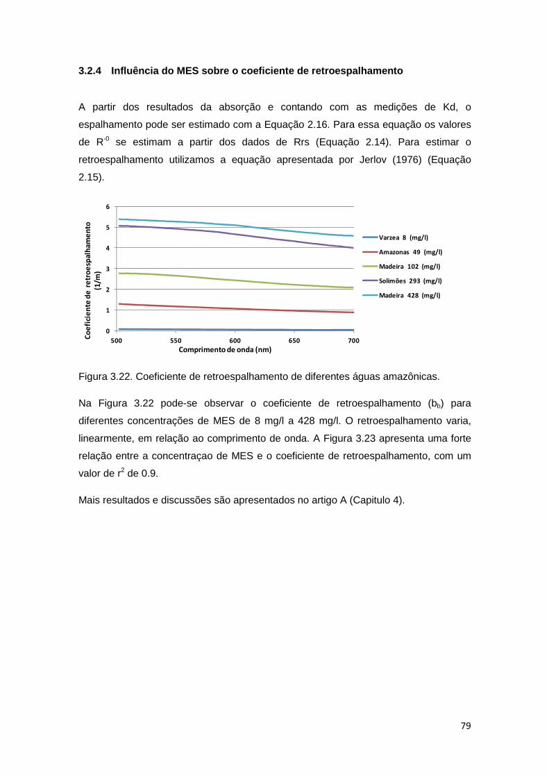
79

3.2.4 Influência do MES sobre o coeficiente de retroespalhamento

A partir dos resultados da absorção e contando com as medições de Kd, o

espalhamento pode ser estimado com a Equação 2.16. Para essa equação os valores

de R-0 se estimam a partir dos dados de Rrs (Equação 2.14). Para estimar o

retroespalhamento utilizamos a equação apresentada por Jerlov (1976) (Equação

2.15).

Figura 3.22. Coeficiente de retroespalhamento de diferentes águas amazônicas.

Na Figura 3.22 pode-se observar o coeficiente de retroespalhamento (bb) para

diferentes concentrações de MES de 8 mg/l a 428 mg/l. O retroespalhamento varia,

linearmente, em relação ao comprimento de onda. A Figura 3.23 apresenta uma forte

relação entre a concentraçao de MES e o coeficiente de retroespalhamento, com um

valor de r2 de 0.9.

Mais resultados e discussões são apresentados no artigo A (Capitulo 4).

0

1

2

3

4

5

6

500 550 600 650 700Co

efi

cie

nte

de

re

tro

esp

alh

ame

nto

(1

/m)

Comprimento de onda (nm)

Varzea 8 (mg/l)

Amazonas 49 (mg/l)

Madeira 102 (mg/l)

Solimões 293 (mg/l)

Madeira 428 (mg/l)

80

Figura 3.23. Relação entre o coeficiente de retroespalhamento (bb) e a concentração

em material em suspensão.

3.3. Relação entre os dados de satélite e a espectrorradiometria de campo

Para conferir a precisão das reflectâncias MODIS extraídas pelo algoritmo proposto

anteriormente, foram comparadas as medições de reflectância realizadas no campo

com as reflectâncias determinadas, a partir dos sensores MODIS, em locais e datas

coincidentes, e para imagens de ótima qualidade (baixa cobertura de nuvens). Para a

comparação das reflectâncias MODIS com as de radiometria de campo, a radiometria

de campo foi simulada para a resposta MODIS. Para isso foi calculada uma média

ponderada, conforme a posição das bandas mostradas na Figura 3.24.

Figura 3.24. Reflectância típica das águas brancas e a posição e largura espectral das

bandas MODIS.

81

Na Figura 3.24 pode-se observar a localização e distribuição das bandas MODIS e os

espectros de reflectância das águas dos rios Madeira e Amazonas.

Nas Figuras 3.25a e 3.25b pode-se observar a relação entre as reflectâncias medidas

pelos sensores MODIS e TriOS nas mesmas datas e área, para as bandas azul,

verde, vermelho e infravermelho. As medidas de reflectância de MODIS são por

unidade de área e as de TriOS, por unidade de ângulo sólido (estereorradiano). Essas

têm que ser multiplicadas pelo valor π para que possam ser comparadas. Nas Figuras

3.25a e 3.25b pode-se notar isso vendo a pendente da linha, que para o satélite

TERRA é de 2,95 e para o satélite AQUA é de 3,14, O R² é igual a 0,66 com 96 dados

para o sensor do satélite TERRA; e R² igual a 0,63 com 68 dados para o sensor do

satélite AQUA. Para conferir os resultados dos sensores MODIS foram comparadas as

respostas dos dois sensores para o mesmo local e data. Esse teste pode ser

observado na Figura 3.25c, dando um R² de 0,98 com 48 imagens coincidentes em

uma linha muito perto de 1:1. Comparações mas detalhadas são também

apresentadas no artigo B.

Figura 3.25. Relação da reflectância do sensor MODIS e as medidas de campo com

os espectrorradiômetros para os diferentes comprimentos de onda do MODIS: a)

MODIS a bordo do satélite TERRA (MOD) e TriOS, b) MODIS a bordo do satélite

AQUA e TriOS (MYD) e c) MODIS a bordo do satélite TERRA e AQUA

A Figura 3.26 compara a relação entre a concentração de MES e: 1) a reflectância de

campo em 851 nm; 2), a reflectância simulada do sensor MODIS a partir dos dados de

espectrorradiometria. Entre as duas séries de pontos observamos uma mínima

diferença. Isso confirma a observação da Figura 3.17, onde vimos que a correlação

82

reflectância / MES não apresentava variações significantes na faixa da banda

infravermelha do MODIS (841 a 876 nm).

Figura 3.26 Relação entre os dados de MES das campanhas e a reflectância de

espectrorradiometria em 851 nm (+) e simulado para a banda infravermelha MODIS

(841 a 876 nm) (o), para as águas do rio Solimões/Amazonas.

3.4 Relação entre a reflectância medida por satélite com a concentração e tipo de MES

Grandes quantidades de imagens podem ser processadas com a ferramenta

computacional MOD3R, analisando séries temporais, desde o ano 2000, o que

significa mais de 500 imagens composta de 8 dias para o satélite TERRA e mais de

400 para o satélite AQUA. Os valores de reflectância de ambos os satélites são

combinados, gerando uma serie única de reflectância, com base nos parâmetros de

qualidade das respectivas imagens.

A Figura 3.27 apresenta na estação de Tamshiyacu as séries temporais de dados de

concentração de MES e de reflectância da banda infravermelha MODIS. Nesta

estação o rio Amazonas tem uma largura de 1200 m e apresenta um intervalo de

dados de concentração entre 36 e 877 mg/l. Apesar da variabilidade temporal média

de 37% entre duas amostras de MES ,consecutivas, a 10 dias (máxima de 300%), a

reflectância do infravermelho é bem correlacionada com a concentração de MES. As

0

0.005

0.01

0.015

0.02

0.025

- 100 200 300 400 500

Re

fle

ctân

cia

Concentração de sedimentos

851 Radiomeria

Infravermelho MODIS Simulado

83

duas séries apresentam um coeficiente de correlação satisfatório, R2=0.62 (Figura

3.28).

Figura 3.27. Série temporal de MES da rede ORE-HIBAM e da reflectância

infravermelha MODIS na estação de Tamshiyacu.

Vale ressaltar que as comparações reflectâmcia / MES são realizadas com os dados

da rede ORE-HIBAM, que representam amostras pontuais de 500 ml e os dados

MODIS, onde cada pixel cobre uma superficie de 250 x 250 m, equivalente a sete

campos de futebol. Essa diferença de escala gera diferenças entre as duas

estimativas.

Maiores detalhes são apresentados no artigo C (Capitulo 6).

Figura 3.28. Correlação entre MES da rede ORE-HIBAM e a reflectância infravermelha

MODIS na estação de Tamshiyacu.

-100

-

100

200

300

400

500

600

700

800

900

0

200

400

600

800

1000

1200

1400

1600

1800

Jan/2003 Jan/2004 Jan/2005 Jan/2006 Jan/2007 Jan/2008 Jan/2009 Jan/2010 Jan/2011

Co

nce

ntr

ação

de

se

dim

en

tos

(mg

/l)

Re

fle

ctân

cia

x10

00

0

Data

Reflectância Infravermelha MODIS

MES ORE-HYBAM

Reflectância = 1.076*(MES) + 413.08

R² = 0.615

0

200

400

600

800

1,000

1,200

1,400

0 100 200 300 400 500 600 700 800

Refle

ctân

cia

x100

00

Concentração de sedimentos (mg/l)

84

No Caso do rio Madeira foi encontrada uma variação sazonal na reflectância. Na

Figura 3.29 pode-se observar esse efeito: nos meses de novembro e abril têm-se

valores de reflectância próximos, mas os valores de MES são muito diferentes. Assim

pode-se observar um “loop” ou laço em sentido anti-horário, com os meses de maior

reflectância e MES em janeiro e fevereiro.

Figura 3.29. Relação da média dos valores da reflectância e MES para o período

2000-2011, na estação de Fazenda Vista Alegre (rio Madeira). As barras de erro

mostram o desvio padrão. A letra indica o mês.

Como foi proposto por diferentes autores (Doxaran et al., 2002; Froidefond et al., 2002;

Topliss et al., 1990) o uso de uma razão das bandas infravermelho (IV) e vermelho (V)

deve permitir reduzir os efeitos de mineralogia e granulometria das partículas. Usando

esta técnica a correlação foi melhorada significativamente e a influência temporal foi

reduzida notavelmente. A Figura 3.30 mostra a relação entre a razão de bandas IV/V e

a concentração de sedimentos na estação de Fazenda Vista Alegre, sendo que o

mesmo efeito foi observado na estação de Porto Velho. O laço e a eficiência do uso de

razão de bandas foram comprovados também com as medições

espectrorradiométricas de campo.

Os resultados e as análises deste trabalho são detalhados e interpretados no artigo de

D (Capitilo 7).

JF

M

A

M

J

JAS

O

N

D

-

200

400

600

800

1,000

1,200

1,400

- 100 200 300 400 500 600 700

Ref

lect

ânci

a x1

0000

MES (mg/l)

85

Figura 3.30. Relação da média mensal dos valores de cada MES da razão (IV/V) e

MES para o período 2000-2011 na estação de Fazenda Vista Alegre (rio Madeira). A

letra ao lado de cada ponto indica o mês.

3.5 Estimativa da vazão sólida nos rios por satélite

Com os dados de MES coletados durante as campanhas é possível determinar uma

relação entre os valores de MES superficial e a MES na secção do rio. Assim com os

dados de MES estimados com o satélite e a vazão do rio no mesmo local, podemos

estimar o fluxo total de sedimentos em suspensão, ou seja, a vazão sólida. A Figura

3.31 mostra a variação temporal da descarga de sedimentos em suspensão estimada

a partir dos dados MODIS e a descarga líquida nos rios Marañon e Ucayali. Podemos

notar que a descarga anual de sedimentos não é correlacionada diretamente à vazão

líquida anual. Observamos que o rio Ucayali é o grande fornecedor de sedimentos ao

rio Amazonas. Para o período estudado no artigo C, a vazão sólida do rio Ucayali

mostra um aumento principalmente nos anos de 2000 a 2003, enquanto a vazão sólida

do rio Marañon estava diminuindo, ligeiramente. Para o período estudado a vazão

sólida foi estimada em 393 x 106, 149 x 106 e 270 x 106 ton/ano nas estações de

Tamshiyacu, San Regis e Requena, respectivamente. Estes dados são coincidentes

com os resultados publicados por Guyot et al. (2007).

Este estudo é apresentado com maiores detalhes no artigo C (capitulo 6).

J FM

A

MJ

JASO

N

D

0

0.2

0.4

0.6

0.8

1

(100) 100 300 500 700 900 1,100 1,300

Ra

zão

de

ban

das

(IV

/V)

MES (mg/l)

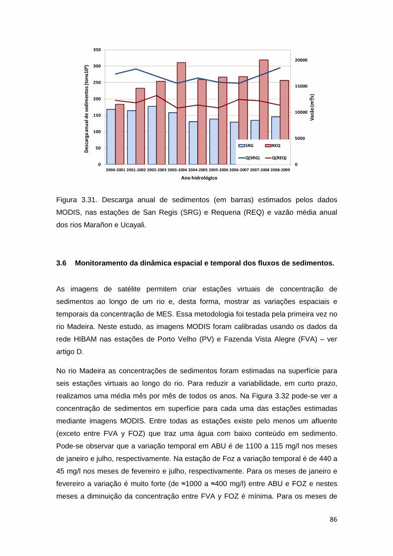
86

Figura 3.31. Descarga anual de sedimentos (em barras) estimados pelos dados

MODIS, nas estações de San Regis (SRG) e Requena (REQ) e vazão média anual

dos rios Marañon e Ucayali.

3.6 Monitoramento da dinâmica espacial e temporal dos fluxos de sedimentos.

As imagens de satélite permitem criar estações virtuais de concentração de

sedimentos ao longo de um rio e, desta forma, mostrar as variações espaciais e

temporais da concentração de MES. Essa metodologia foi testada pela primeira vez no

rio Madeira. Neste estudo, as imagens MODIS foram calibradas usando os dados da

rede HIBAM nas estações de Porto Velho (PV) e Fazenda Vista Alegre (FVA) – ver

artigo D.

No rio Madeira as concentrações de sedimentos foram estimadas na superfície para

seis estações virtuais ao longo do rio. Para reduzir a variabilidade, em curto prazo,

realizamos uma média mês por mês de todos os anos. Na Figura 3.32 pode-se ver a

concentração de sedimentos em superfície para cada uma das estações estimadas

mediante imagens MODIS. Entre todas as estações existe pelo menos um afluente

(exceto entre FVA y FOZ) que traz uma água com baixo conteúdo em sedimento.

Pode-se observar que a variação temporal em ABU é de 1100 a 115 mg/l nos meses

de janeiro e julho, respectivamente. Na estação de Foz a variação temporal é de 440 a

45 mg/l nos meses de fevereiro e julho, respectivamente. Para os meses de janeiro e

fevereiro a variação é muito forte (de ≈1000 a ≈400 mg/l) entre ABU e FOZ e nestes

meses a diminuição da concentração entre FVA y FOZ é mínima. Para os meses de

0

5000

10000

15000

20000

0

50

100

150

200

250

300

350

2000-2001 2001-2002 2002-2003 2003-2004 2004-2005 2005-2006 2006-2007 2007-2008 2008-2009

Vaz

ão (m

³/s)

Des

carg

a an

ual

de

sed

imen

tos

(to

nx1

06 )

Ano hidrológico

SRG REQ

Q(SRG) Q(REQ)

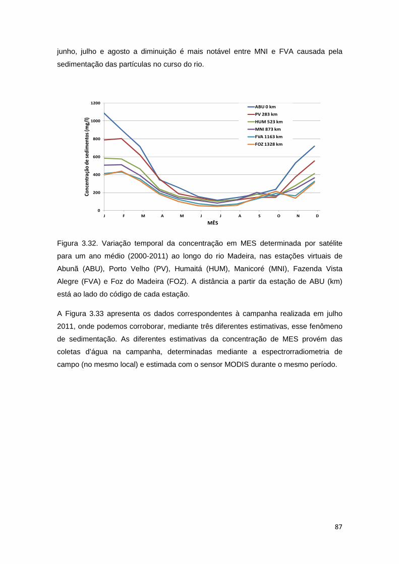
87

junho, julho e agosto a diminuição é mais notável entre MNI e FVA causada pela

sedimentação das partículas no curso do rio.

Figura 3.32. Variação temporal da concentração em MES determinada por satélite

para um ano médio (2000-2011) ao longo do rio Madeira, nas estações virtuais de

Abunã (ABU), Porto Velho (PV), Humaitá (HUM), Manicoré (MNI), Fazenda Vista

Alegre (FVA) e Foz do Madeira (FOZ). A distância a partir da estação de ABU (km)

está ao lado do código de cada estação.

A Figura 3.33 apresenta os dados correspondentes à campanha realizada em julho

2011, onde podemos corroborar, mediante três diferentes estimativas, esse fenômeno

de sedimentação. As diferentes estimativas da concentração de MES provém das

coletas d’água na campanha, determinadas mediante a espectrorradiometria de

campo (no mesmo local) e estimada com o sensor MODIS durante o mesmo período.

0

200

400

600

800

1000

1200

J F M A M J J A S O N D

Conc

entr

ação

de

sedi

men

tos

(mg/

l)

MÊS

ABU 0 km

PV 283 km

HUM 523 km

MNI 873 km

FVA 1163 km

FOZ 1328 km

88

Figura 3.33. Concentração estimada de material em suspensão ao longo do rio

Madeira usando as imagens MODIS, a espectrorradiometria de campo e as amostras

da campanha no mês de Julho de 2011. A estação de Abuna representa o quilômetro

zero e o último ponto a confluência do rio Madeira com o rio Amazonas.

Observamos que a concentração de MES na superfície diminui desde a estação de

MNI (873 km a jusante de ABU), a montante da foz do rio Aripuanã de águas pretas, o

que permite concluir que essa diminuição não é causada pela diluição. A diminuição

de MES mais marcada (> 25%) ocorre entre os quilômetros 873 e 1000. Para

interpretar esse padrão temos que tomar em conta o comportamento do rio Amazonas.

Neste mes de julho o nível do rio Amazonas é muito maior que do rio Madeira, o que

gera um fenômeno de barragem hidráulica, causando a perda da velocidade do fluxo

d’água, e, consequentemente, diminui a capacidade de transporte dos sedimentos em

suspensão pelo rio Madeira. Esse exemplo demonstra como o uso de sensores do

tipo MODIS permite detectar robustamente processos de transporte de sedimentos,

dentro do curso de um rio.

Mais análises deste caso são apresentadas no artigo D (Capitulo 7).

0

20

40

60

80

100

120

140

0 200 400 600 800 1000 1200 1400

MES

(mg

/l)

Distancia (km)

Campanha

Radiomeria

MODIS

89

CAPITULO IV

----------------------------------------------------------------------------

Artigo A

90

Résumé

Cet article étudie les propriétés optiques apparentes et inhérentes des différents types

d'eaux du bassin amazonien en fonction de l’origine et de la concentration du matériel

en suspension (SPM). Les nombreuses études réalisées précédemment sur les eaux

océaniques (Cas 1) et côtières (Cas 2) ont permis de décrire précisément la variabilité

des propriétés optiques des eaux marines. Pour les eaux continentales, la

connaissance des propriétés optiques est loin d’avoir atteint celle acquise sur les eaux

marines ce qui constitue un frein à l’utilisation des données de télédétection “couleur

de l’eau” à l’intérieur des terres. Des études systématiques sont nécessaires pour

documenter les variations de ces propriétés optiques à différentes périodes du cycle

hydrologique et à l’échelle du bassin versant. Ces dernières années, 16 campagnes de

mesure des propriétés optiques ont été réalisées dans le bassin amazonien et

notamment sur les principaux fleuves drainant les SPM provenant de la Cordillère des

Andes tels que le Solimões, le Madeira et l’Amazone. Durant ces campagnes, des

mesures des propriétés optiques apparentes de l'eau ont été réalisées telles que la

réflectance télédétectée (Rrs) et le coefficient d'attenuation diffus vertical descendant

(Kd).

La Rrs a été mesurée avec des capteurs TriOS- RAMSES au dessus de l’eau selon le

protocole de Mobley (1999). Pour la mesure de Kd, les capteurs ont été immmergés

afin de mesurer la variation de l’irradiance descendante en fonction de la profondeur

dans la couche euphotique. Les propriétés optiques inherentes du matériel non algal

(NAP), coefficient d'absorption (aNAP) et de diffusion (bNAP), ont été calculées à partir

des équations mettant en relation ces paramètres avec ceux de réflectance irradiance

(R) et Kd. Les principales caractéristiques des eaux ont été collectées simultanément

aux propriétés optiques : concentration en SPM, granulométrie, minéralogie,

phytoplancton et mesure de la matière organique dissoute colorée (CDOM).

279 mesures de Rrs et 133 de Kd ont été réalisées pour différents types d'eaux et à

différentes périodes hydrologiques. Ces données ont permis de classer les eaux

amazoniennes en 8 types, 3 classes correspondants aux eaux fluviales dominées par

le NAP (eaux “blanches”) avec un important contenu en NAP, 4 classes pour les eaux

de plaines inondées et d'eaux claires avec des concentrations variables de

chlorophylle et de NAP, et une classe pour les eaux noires caractérisées par leur forte

teneur en CDOM. La Rrs est fortement corrélée avec le SPM, saturant autour de 100

g.m-3 du bleu au rouge et permettant de suivre la gamme totale de SPM dans

l’infrarouge de 2 à 620 g.m-3. La corrélation maximale (r² = 0.81) est ainsi trouvée pour

91

la longueur d’onde de 860 nm. Le Kd est très fortement corrélé avec le SPM (r² > 0.9

entre 500 et 850 nm) sans aucune saturation. Les équations de régression entre la Rrs

et le SPM ne montrent pas de différences statistiques significatives entre le fleuve

Madeira et le fleuve Solimoes démontrant que la Rrs peut être un estimateur robuste de

la SPM à l’échelle du bassin versant.

Le jeu de données est séparé en un ensemble de calibration et un ensemble de

validation afin d’évaluer la précision de l’inversion des AOP en fonction de la SPM.

Sans surprise, un modèle en puissance avec Rrs réalise de meilleures performances

du bleu vers l’infrarouge, avec une RMSE relative de l’ordre de 37 %. Pour Kd, un

simple modèle linéaire d’inversion est nécessaire et la précision de l’inversion est de

l’ordre de 18 % entre 500 et 700 nm.

Pour diminuer la sensibilité de Rrs à la taille des particules ou de l’indice de réfraction,

l'utilisation du ratio de Rrs à deux longueurs d’onde est évalué. Le ratio permet d’obtenir

une diminution de la dispersion dans la relation Rrs – SPM, légérement pour le

Solimões (r² = 0.83 vs. 0.73) et très clairement pour le Madeira (r² = 0.62 vs. 0.93).

Les coefficients aNAP et bNAP ont été calculés pour 81 points à partir des équations de

Gershun et de Kirk. La moyenne de l'absorption du CDOM à 440 nm varie en fonction

des types d’eaux. Pour les eaux noires, aCDOM est de 7.9 m-1, pour les plaines

innondées aCDOM de 4.8 m-1, pour les eaux blanches aCDOM est de 3.3 m-1 et pour les

eaux claires aCDOM est de 1.8 m-1. La variation spectrale de aCDOM est modélisée par

une exponentiel négative dont l’exposant varie entre 0.008 et 0.011 nm-1. La relation

entre aNAP à 550 nm et la SPM est très robuste (R2 =0.91) mais présente une

dispersion significative pour les faibles concentrations de SPM. L'absorption spécifique

des particules non algales (a*NAP), qui est définie comme l'absorption par unité de SPM

est évaluée à 0.028 m2/g pour une longueur d'onde de 555 nm. La variation de aNAP est

également modélisée par une exponentielle négative dont l’exposant varie entre 0.006

et 0.015 avec une corrélation négative avec la SPM. Le coefficient spécifique b*NAP est

en moyenne à 555 nm de 0.672 ± 0.18 m2.g-1 et montre une variation spectrale du type

λ-0.77 avec la longueur d’onde. Dans le fleuve Madeira, une variation saisonnière de

b*NAP a été trouvée, avec des valeurs plus fortes pendant les périodes sèches, et des

valeurs plus basses pendant la saison de croissance (Janvier-Avril). Cette variation

explique la dépendance saisonnière trouvée pour le fleuve Madeira qui sera mentionné

dans l’article C.

92

Les courbes spectrales obtenues pour ces eaux coindident avec celles trouvées dans

des travaux précédents confirmant que les propriétés optiques des eaux continentales

sont proches des eaux turbides côtières. Cependant, la teneur en CDOM,

phytoplancton et SPM des eaux continentales oblige à développer de nouveaux

algorithmes d’inversion.

93

Resumo

No presente trabalho são estudadas as propriedades ópticas aparentes e inerentes

para diferentes tipos de águas amazônicas, em função do material particular

suspendido (SPM). São muitos os estudos descrevendo, com sucesso, os parâmetros

ópticos. Para águas continentais ainda não se obteve um conhecimento das

propriedades ópticas como para as águas marinhas, ou seja, faltam estudos

sistemáticos para analisar a variação dessas propriedades durante o ciclo hidrológico.

Este trabalho apresenta, pela primeira vez ,um estudo com o objetivo de documentar,

sistematicamente, as variações espectrais e temporais das propriedades ópticas em

uma grande bacia hidrográfica. Nos últimos anos se realizaram 16 campanhas de

amostragem das propriedades ópticas ,assim como, as características físicas e

mineralógicas de diversas águas na bacia amazônica. Durante as campanhas foram

medidas as propriedades ópticas aparentes da água, reflectância de sensoriamento

remoto (Rrs) e o coeficiente de atenuação vertical difuso (Kd).

A Rrs foi medida com os sensores TriOS-RAMSES posicionados fora da água e em

ângulos precisos para reduzir os efeitos da interface ar- água. Para a medição de Kd

os sensores foram mergulhados na coluna de água realizando medidas sucessivas a

diferentes profundidades. As propriedades ópticas inerentes das partículas não algalis

(NAP), coeficiente de absorção (aNAP) e de espalhamento (bNAP), foram calculados

utilizando as medições de Rrs e Kd, mediante equações que relacionam os parâmetros

de reflectância irradiância (R) e Kd. De forma simultânea com as medições de

radiometria foram realizadas coletas de água para diferentes análises (Concentraçao

de sedimentos, granulometria, mineralogia, e medição de matéria orgânica dissolvida

colorida (CDOM).

Realizaram-se 279 medições de Rrs em diferentes tipos de águas, e, em vários

períodos hidrológicos. Com estes dados pode-se classificar as águas superficiais

amazônicas em 8 tipos: 3 correspondem às águas brancas com alto conteúdo de

sedimentos em suspensão, 4 para águas das várzeas e águas claras, com grande

conteúdo de clorofila e 1 para águas pretas caracterizadas por sua alta concentração

de CDOM.

A relação entre Rrs e a concentração de SPM varia segundo comprimento de onda,

achando-se um valor máximo do coeficiente de correlação Pearson (R2) de 0,81 em

860 nm, para águas brancas. Estes valores demostram que a Rrs é um robusto

94

estimador de SPM. Pode-se achar que a relação entre os valores de Kd e SPM é

bastante robusta entre 495 e 860 nm (R2= 0,90), com uma regressão linear. As

equações de regressão entre Rrs e SPM não presentam diferencias significativas entre

os diferentes rios estudados.

Para diminuir o efeito do tipo de sedimento foi feito uma análise de razão de bandas

(vermelha / infravermelha) em diferentes rios, para pesquisar se o efeito é global ou

varia de um rio para outro. Com o uso da razão de bandas no rio Solimões, a relação

melhorou, levemente, porém, no rio Madeira a relação melhorou, notavelmente,

incrementando o R2 de 0,62 para 0,93. Entre os dados estimados, a partir das

propriedades ópticas e das amostras de SPM, se encontrou um RMSE relativo de

37%, utilizando, unicamente, uma banda. Com a utilização da razão de bandas, o

RMSE, diminuiu cerca de 23%, e, usando o Kd o RMSE relativo foi de 18%.

Foram estimados os valores de aNAP e bNAP para 81 amostras e os coeficientes de

absorção do CDOM e NAP. A média de absorção do CDOM a 440 nm varia

dependendo dos tipos d’água. Para as águas pretas a absorção é de 7,9 m-1 e para as

várzeas é de 4,8 m-1, para as águas brancas diminui a 3,3 m-1 e para as águas claras é

de 1,8 m-1. A relação entre aNAP a 550 nm e SPM é bastante robusta (R2=0,91). A

absorção específica (a*NAP), que é definida como a absorção por unidade de SPM

(em g.m-3), foi estimada em 0,028 m2.g-1, para um comprimento de onda de 555 nm.

O valor de R2 entre o coeficiente de espalhamento a 555 nm e SPM é de 0,87 para 81

dados. O coeficiente de espalhamento específico do NAP (b*NAP em m2.g-1) se calculo

em 0,61 e situa-se dentro dos valores publicados para aguas túrbidas, entre 0,4 e 1

m2.g-1. No rio Madeira foi encontrada uma variação sazonal de b*NAP, sendo maior na

época de seca e menor no período de cheia (janeiro – abril). Esta variação explica a

dependência estacional de Rrs achada neste rio, como será visto no capítulo 7.

As pendentes espectrais (SCDOM e SNAP) obtidas para estas águas amazônicas

coincidem com as achadas em trabalhos anteriores sobre águas dominadas por

sedimentos, nos ambientes costeiros ou continentais como Babin et al. (2003), Ma et

al. (2006 e 2007), Giardino et al. (2007), Doxaran et al. (2009), Loisel et al. (2009).

95

Analysis of the apparent and inherent optical properties of the sediment-dominated waters in the Amazon River basin

Jean-Michel Martinez12, Raul Espinoza-Villar12, Luciane Moreira3, Elisa Armijos4

1 GET, UMR5563, IRD/CNRS/Université Toulouse 3, 14 Avenue Edouard Belin,

31400 Toulouse, France. E-mail : jean-michel.martinez@ird.fr 2 Instituto de Geociências, Universidade de Brasília, Campus Universitário

Darcy Ribeiro, ICC Centro, 70910-900, Brasília, Brazil. 3 Departamento de Geoquímica, Universidade Federal Fluminense (UFF), Niterói,

Brazil. 4 LBA, Instituto Nacional de Pesquisas da Amazônia (INPA)- Universidade do Estado do

Amazonas

(UEA). Av. André Araújo, 2936, Aleixo, CEP 69060-001, Manaus- Brazil

Submitted to Journal of Geophysical Research

ABSTRACT

The inherent optical properties of Amazon basin waters were derived from in situ measurements of the remote sensing reflectance (Rrs - 279 stations) and downwelling diffuse attenuation coefficients (Kd - 133 stations). Measurements of the apparent optical properties, suspended particulate matter (SPM) contents, chlorophyll-a concentrations and colored dissolved organic matter (CDOM) absorption spectra were performed during 16 cruises along the main Amazonian rivers draining the Andes. For comparison, we also collected data in the floodplains and main tributaries.

Overall, both Rrs and Kd were strongly correlated with the SPM, even though strong CDOM absorption limited the use of the blue spectrum. Reflectance saturation was observed from blue to red at approximately 100 g.m-3, whereas the near-infrared (NIR) wavelength enabled the monitoring of the full SPM range [5-620 g.m-3]. In contrast, Kd showed no saturation for SPM from green to NIR, and a linear model was calculated. The use of the reflectance ratio was investigated and shown to improve the retrieval performance.

The CDOM absorption coefficient at 440 nm varied from 1.8 to 7.9 m-1. Over sediment-dominated waters, the range of variation was much more limited, and the spectral slope of CDOM absorption ranged from 0.008 to 0.011 nm-1. The spectral slope of non-algal particle (NAP) absorption varied as a function of the SPM with values ranging from 0.006 to 0.015. The aNAP(440)/SPM ratio averaged 0.072 ± 0.045 m2.g-1 but with a net difference for low SPM and high SPM contents. The NAP-specific scattering coefficient at 550 nm averaged 0.672 ± 0. 18 m2.g-1 and fit a λ-0.77 relationship with the wavelength.

96

1. INTRODUCTION

Monitoring of inland water quality using remote sensing data represents a major challenge for water color researchers due to the complexity of their optical properties relative to oceanic and coastal waters (i.e., Case 1 and 2 waters). In inland waters, absorption and scattering by CDOM and mineral particles can mask the phytoplankton optical properties and show a very weak covariance, thereby invalidating most common retrieval models based on ocean color data that are used over marine waters. The optical properties of mineral particles suspended in water depend on the material concentration, size distribution and refraction index, which, in theory, could demonstrate a site- and/or time-dependent relationship between apparent optical properties (AOP) and inherent optical properties (IOP) with the inorganic particulate material.

Suspended sediment fluxes in rivers are the result of erosion, transport and deposition processes that occur within catchments. The quantification of these fluxes is necessary to monitor and understand the impacts of human activities (e.g., land use and hydraulic infrastructure) and climate change (e.g., extreme events and changes in rainfall patterns) at the catchment scale. However, an accurate calculation of sediment budgets is often difficult due to the poor availability and reliability of sediment flux data in most developed and developing countries [Walling and Fang, 2003]. Water quality monitoring networks are usually based on water sampling in different locations in a watershed (i.e., hydrological stations) to monitor the production, accumulation and transfer of certain elements of interest within the river network. The efficiency of such monitoring is therefore a direct function of the number of sampling locations and sampling frequency. In this manner, the capacity of remote sensing imagery to frequently monitor different locations over a short time span may be efficiently used to complete existing field hydrological station networks. Unfortunately, there is a lack of systematic measurements of the main AOP/IOP in continental waters that may support the operational use of remote sensing imagery for water quality monitoring.

A large number of studies have been conducted to measure the relationship between AOPs, IOPs and parameters of interest (often the pigment concentration), and various syntheses have been published for oceanic waters [Bricaud et al., 1998; Stramski et al., 2001; Morel et al., 2007] and coastal regions [Babin et al., 2003a; Snyder et al., 2008; Doxaran et al., 2009; Neukermans et al., 2012]. These syntheses have paved the way for detailed optical modeling and robust remote sensing monitoring at both the regional and global scales. A significant number of studies have also been published on inland water optical properties [Kirk 1976, Whitlock et al., 1981; Hoogenboom et al., 1998; Ma et al., 2006; Giardino et al., 2007; Gitelson et al., 2008]. However, unlike the progress that has been achieved for marine waters, there is a lack of systematic studies of rivers and lakes documenting the variability of the AOPs/IOPs in these areas to establish the foundation for the remote sensing-based operational monitoring of inland waters. In particular, it is necessary to consider the whole watershed, instead of a specific river/lake, and to determine the variation of AOPs/IOPs as a function of the hydrological cycle.

In recent years, several studies have shown that medium-resolution remote sensing imagery may be efficiently used for the operational monitoring of the suspended

97

sediment discharge in the Amazon River catchment. Martinez et al. [2009] have shown that is it possible to derive robust empirical relationships between the SPM and surface reflectance using corresponding MODIS 250-meter images and field samples collected over 7 years with a significant accuracy (30 %) and an absence of seasonal bias. Using 10 years of MODIS data for the Amazon River in Peru, Espinoza et al. [2012] compared upstream and downstream remote sensing-derived river sediment discharge estimates and demonstrated that satellite assessments are robust (root mean square of error of 18 %). Mangiarotti et al. [2013] analyzed how conventional network data and satellite-derived SPM estimates can be combined to improve sediment budget assessments in the Amazonian plain. Finally, Espinoza et al. [in press] analyzed the variation of the MODIS remote sensing reflectance in a tributary of the Amazon River (the Madeira River) and found good agreement between satellite-derived estimates and those from field samples. However, all of these studies have been based on empirical relationships between Rrs and SPM, which may prevent a generalized use of the reported remote sensing methods. Therefore, it is necessary to investigate the robustness of the link between the optical properties of water and suspended sediment to ensure the robustness of the retrieval.

The objective of this study is to understand how the optical properties of water vary across a large river basin and to determine the significance of this variability based on a large dataset of water sampling and optical measurements. In particular, we assessed the variability of the AOP/IOP for different periods of the hydrological cycle, over floodplain lakes and river mainstreams as well as between different sub-catchments, focusing on the mineral fraction of the suspended particle matter. This study also contributes to the field of bio-optic modeling by extensively documenting the optical properties of the world’s largest watershed.

2. MATERIALS AND METHODS

2.1 The Amazon basin

The Amazon catchment covers 6.2 million sq.km encompassing various soils and lithologies. The Amazon basin is composed of 3 major morpho-structural units : i) the Brazilian and Guyana cratonic shields, ii) the Altiplano, Oriental Cordillera and Subandean zone of the Andes to the west and iii) the lowlands where the main rivers progressively join to form the Amazon River. The cratonic shields cover approximately 44 % of the Amazonian basin area and are composed of strongly weathered and metamorphosed igneous rocks. The Andes account for 11 % of the Amazonian basin area and consist of Paleozoic to Meso-Cenozoic metamorphic, igneous and sedimentary rocks. The Amazonian lowlands cover approximately 45 % of the Amazonian basin and are composed of a very thick layer of Cenozoic sediments.

Interestingly, the first and most common classification used to describe the main Amazonian water types is based on their coarse optical properties, catalogued as white, clear and black [Sioli 1956]. White waters refer to waters loaded with sediment showing strong dissolved organic material, mainly originating from the Andes. Clear waters originate from the cratonic shields and show very low SPM loads but also low levels of organic matter. Black waters are of low biological productivity with near-zero SPM concentrations, have almost no nutrients and are strongly acidic due to the

98

organic material present in the colloidal fraction, which also gives them their dark color. The main black-water rivers drain the northern tributaries, such as the Negro River and the Trombetas River, although black waters can also be found in a large number of smaller sub-catchments in the Amazon lowlands that finally converge in the Amazon River main stem from the piedmont to the Atlantic Ocean. The white waters flow through the Madeira River and Solimões catchments that drain the southern Andes and the central and northern Andes, respectively. Herein, we mainly focus on these sediment-dominated waters along the Madeira River, the Solimões River and the reach of the Amazon River that is formed by the Madeira, Solimões and Negro Rivers.

The Amazon basin extends over 2 hemispheres and experiences contrasting rainfall regimes. Consequently, the hydrological regime shows a distinct high-water period from March to April in the Madeira catchment in the south and from June to July in the Negro catchment in the north. The Amazon/Solimoes River shows an intermediate hydrological cycle as it receives waters from both the north and the south of the catchment. Overall, the hydrological regime becomes more consistent from upstream to downstream. From the Andes piedmont to the lowlands, the flood regime is monomodal with a steadily increasing water level during the rainy season. Consequently, during the majority of the hydrological cycle, the suspended sediment and geochemical characteristics of the surface water change slowly. The HYBAM network data (www.ore-hybam.org) allow for assessments of the suspended sediment cycle throughout the catchment. Variations in SPM concentration are correlated with the river discharge in the Andes, whereas the SPM becomes progressively disconnected with the river discharge through the confluence with other rivers draining the forested catchments that provide almost no SPM to the system. Consequently, there is an overall decrease of the SPM concentration from upstream to downstream due to sedimentation and dilution processes. Several studies have noted that the dissolved organic carbon (DOC) concentrations show a low seasonal difference in the main stem of the river [Ertel et al., 1986; Hedges et al., 1994; Moreira-Turcq et al., 2003] of between 3 and 5 g.m-3, whereas in black waters, the DOC concentrations are typically greater than 10 g.m-3. The proportion of humic acids versus fulvic acids, known to affect the extent of light absorption, has been shown to remain relatively constant seasonally, with a ratio of fulvic to humic acids in the Amazon River at Óbidos of 3.2 ± 0.3 [Ertel et al., 1986]. The Amazon basin is marked by a large floodplain that significantly contributes to the water fluxes and mass transfer. The open floodplain lakes are affected by different processes, such as the mixing of different water masses derived from the local catchments and the rivers, resuspension processes during the low-water period and intense blooms of phytoplankton during the dry season. Such phytoplankton blooms extend over large areas during the period of decreasing water levels from July to September. The phytoplankton composition is dominated by Cyanophyceae with a significant proportion of Bacillariophyceae and Chlorophyceae [Nogueira et al. 2010].

2.2 Calculation of apparent optical properties: Rrs and Kd

Below- and above-water radiometric measurements were performed using TriOs RAMSES radiometers operating in the 350-900 nm spectral range. One radiometer was mounted with a cosine collector for irradiance measurements, and 2 other

99

radiometers were equipped for radiance measurements with a field of view of 7° in air. All of the radiometers were synchronized to simultaneously measure the various optical properties.

For the majority of the locations, radiometric measurements were collected both from the boat deck to calculate the remote sensing reflectance Rrs (λ) and in the water to retrieve downward irradiance Ed(z,λ) profiles. Above-water measurements of the upwelling radiance Lu (λ) preferred to below-water measurements Lw(λ)due to the strong light absorption in the blue and NIR domains by water, which may result in unreliable reflectance assessments at those wavelengths. The remote sensing reflectance was calculated as Rrs (λ):

R+,�λ� = qr�λ�2ρ.qs�λ�"#�λ� (1)

where Ed(λ) is the downwelling irradiance above the water surface, Lu(λ) is the upwelling radiance above the surface water and Ls(λ) is the sky radiance that is used to correct for the skylight reflection effect at the air-water interface. The above-water upwelling radiance Lu is the sum of the upwelling radiance Lw(0+) and the sky radiance directly reflected by the air–water interface Lr. Because only Lu is directly measureable, and Lw(0+) and Lr are not measured, Lr is assessed as Lr = ρ.Ls, where ρ is a proportionality factor. The factor ρ is not an inherent optical property of the surface and is dependent on the sky conditions, wind speed, solar zenith angle and viewing geometry. Mobley [1999] used a radiative transfer code to estimate the variability of ρ as a function of the different forcing factors. These results showed that when Lu is acquired with a viewing direction of 40° from the nadir and 135° from the sun, the variability of ρ is considerably reduced under clear-sky conditions, and a value of 0.028 is acceptable at wind speeds less than 5 m.s-1. Finally, Lw(0+) was assessed by the subtraction of Lu and ρ.Ls. To limit the effects of external factors, all radiometric measurements were acquired within the viewing geometry defined by Mobley and under low-wind conditions (0-4 m.s-1) and clear-sky conditions and for sun zenith angle values ranging from 0 to 30°.

In-water downward irradiance Ed(z,λ) and upward radiance Lu(z,λ) profiles were measured at discrete depths in rapid succession within the euphotic layer that was usually not more than 3 meters in depth. The diffuse attenuation coefficients for downward irradiance Kd(λ) were computed from measurements at 2 depths, z1 and z2, as follows:

Kd(λ) = <tu2tv ln xy�tv,λ�xy�tu,λ� (2)

To retrieve robust estimates of Kd at each station, at least 2 vertical profiles were collected sequentially, and the more stable profile was selected. Irradiance reflectance is an AOP that can be directly related to the main IOPs (absorption and scattering coefficient) and can be calculated from the remote sensing reflectance as follows (Morel and Gentily 1996):

R=z = �<2ρ�.�<2ρ{�=|u�<2+=�} (3)

100

where n (= 1.34) is the refractive index of water, R is the irradiance reflectance, ρ is the internal Fresnel reflectance at normal incidence (0.021), ρ{ is the air–water Fresnel reflection at the interface for the entire downwelling irradiance (set at 5 %), r is the water–air Fresnel reflection for the entire diffuse upwelling irradiance (approximately 0.48) and Q is the ratio of the in-water upwelling irradiance Eu(0

-) to the upwelling radiance Lu(0

-). If the upwelling radiance was isotropic, the Q value would be π. However, modeling calculations and field measurements suggest that Q may vary up to 5. We performed several direct and simultaneous measurements of Eu and Lu to derive a Q value of 3.7 that does not vary significantly with the SPM concentration.

2.3 Calculation of inherent optical properties: a and b

To calculate the water absorption coefficient, we used an equation derived from the Gershun equation that allows for a direct correlation between R, Kd and a [Aas 1987; Kirk 1994; Morel and Maritorena 2001]:

; = ~!�! {{{{ <2�<?��y{{{{/��{{{{ (4)

where µd and µu are the downward and upward cosines, respectively. Kirk [1984] showed that µd, µu and R vary as a function of b/a, thereby allowing for the accurate calculation of the cosines from irradiance reflectance data. Equation (4) demonstrates the advantage of not involving the scattering or backscattering coefficient and allows for the assessment of an IOP from 2 independent measurements, R and Kd.

The water scattering coefficient b is retrieved from Kd and a using an equation based on Monte Carlo modeling [Kirk 1994, Loisel and Morel 2001]:

~! = <µ$ �;9 + ��µ3�;J�</9 (5)

where µ0 is the mean underwater cosine (i.e., the mean value of the cosine of the photon angle relative to vertical) just below the sea surface. We consider vertically incident light (µ0 = 1.0) corresponding to a solar elevation of 0°, which is similar to the mid-day solar elevation at the latitudes of the Amazon basin. Kirk [1994] calculated that for a large range of b/a (i.e., 2-200), G(1.0) varies only from 0.233 to 0.264, suggesting the use of an average value of 0.245.

2.4 Water sampling

In situ water quality data were collected during 16 cruises along the main Amazonian Rivers in Peru and Brazil from 2007 to 2011 in different seasons (see Table 1). This sampling scheme made it possible to register the radiometric variability of the waters in the Amazonian catchment, the river main stems and floodplains and the estuary, representing locations separated by more than 3,000 kilometers. Although the sampling program was focused on the 2 rivers draining the Andes (Amazon and Madeira rivers), samples were acquired from the tributaries and floodplain connected to these 2 streams to document the radiometric variability among the black and white

101

waters. A total of 279 surface reflectance samples and 133 below-surface measurements were used in this study. When possible, the above and in-water measurements were realized sequentially within approximately 15 minutes while the surface water samples were collected during each measurement for water quality assessment.

At each of the stations that were visited, a water sample for SPM concentration determination was collected at the surface either from a small boat or research vessel. It is important to note that for most of the locations, the water depth exceeded 20 meters and reached up to 60 meters at some stations. Water samples were processed onboard the ship immediately after collection. When using small ships, water samples were stored in 2-l polyethylene containers and processed on land no later than 12 hours after sampling. The samples were filtered using 0.45-µm cellulose acetate filters (Millipore) that were previously dried for 24 h at 60 ºC and weighted. After filtration, the filters were dried for 24 h at 60 ºC and weighed again to determine the concentration of suspended matter. Phytoplankton pigment concentrations were measured during 4 cruises by filtering 250 ml of water through GF/F filters, which were then frozen onboard the research vessel. At the laboratory, the pigments were extracted in acetone and analyzed for chlorophyll and phaeopigment concentrations using a calibrated fluorometer. Herein, Chl is defined as the sum of Chl-a and phaeopigments.

Figure 1. Location of the 42 stations for above-water (279 measurements) and below-water (133 measurements) sampling in the Amazon River basin from 2007 to 2011

along the 2 main rivers draining the Andes: the Solimões and Madeira Rivers. Stations are partitioned into 4 subgroups: 1) the Amazon River and its main tributary, the

Solimões River; 2) the Madeira River; 3) other tributaries; and 4) floodplain lakes.

102

Campaign

Time period Water stage

Sampling Location

Number of stations visited

Above In Water Water

1 30/01/07 20/02/07 Rising Obidos to Macapa 2 1

2 21/05/07 25/05/07 High Manacapuru 19 0

3 10/11/07 15/11/07 Low/Risin

g Manacapuru to Borba 34 2

4 15/03/08 20/03/08 Rising/High

Manacapuru to Borba 58 2

5 10/04/08 10/04/08 Rising Amazon estuary 2 0

6 15/05/08 23/05/08 High Manacapuru to

Santarem 9 8

7 05/10/08 13/10/08 Low Manacapuru to

Santarem 14 5

8 20/06/09 06/07/09 High Manacapuru to

Santarem 18 13

9 19/11/09 28/11/09 Rising Porto Velho to Manacapuru

7 11

10 26/03/10 30/04/10 High Manacapuru to Porto

Velho 5 7

11 08/06/10 02/07/10 Recession

/High Requena to Santarem 18 18

12 25/08/10 12/09/10 Recession Manacapuru to

Santarem 31 14

13 26/01/11 02/02/11 Rising Manacapuru to

Santarem 4 5

14 15/02/11 25/02/11 Rising Manacapuru to

Santarem 11 8

15 07/07/11 30/07/11 Recession Abunã to Coari and

Santarem 25 20

16 23/11/11 18/12/11 Low/Risin

g Requena to Santarem 22 19

Total 279 133

Table 1. Location and dates of the 16 sampling campaigns conducted for this study.

Particle-size distribution analyses were performed on 39 5-l water samples collected during 6 cruises. Granulometric data were obtained using a laser grain-size measurement device (Mastersizer 2000 with a sample dispersion unit) at the CPRM Laboratory for Sediment and Water Quality. The results were modeled according to the classical Junge hyperbolic law to assess the variability of the slope coefficient and the range of sizes over which the fit could be performed.

Samples were collected during 3 cruises to assess the variability of the CDOM absorption coefficient for different types of waters and along an upstream to downstream profile of the Solimões and Amazon Rivers. Water was filtered under low vacuum on a 0.45-µm Millipore membrane using an all-glass filtering device. The filtered samples were stored and frozen in dark 10-cl bottles. At the UFF laboratory, a 1-cm quartz cuvette was used to measure the absorbance of the filtered water between 350 and 750 nm at 1-nm increments using a dual-beam spectrophotometer. Milli-Q

103

water was used as a reference. After conversion to absorption coefficients, the CDOM absorption at 440 nm aCDOM(440) was calculated, and an exponential function was fitted by nonlinear regression to the data to assess the exponential slope SCDOM.

We analyzed 33 samples collected during 8 cruises to determine the temporal and spatial variations of the surface suspended sediment mineral assemblage along the Madeira and Amazon rivers. Samples were collected at the river surface in 25-l canisters and evaporated to a final volume of 500 ml. At the laboratory, water samples were prepared by evaporating the aqueous suspensions to dryness on a glass slide. The suspensions were prepared by the ultrasonic dispersion of 10 mg of sample in 2 ml of de-ionized water. The identification of minerals was based on their reactions to commonly used treatments: air-drying, ethyl–glycol solvation and heating to 550 °C. Based on the glycolated sample diffractograms, semi-quantitative estimates of the different clay minerals were performed manually by measuring the characteristic reflection areas.

3 RESULTS AND DISCUSSION

3.1 Variability of the SPM characteristics: concentration, granulometry and mineralogy

The SPM values of the water samples spanned more than 2 orders of magnitude [2-621.6 g.m-3], with a mean value of 140.8 g.m-3. There was a general decrease of the SPM from upstream to downstream areas along the rivers draining the Andes (the Maranon, Ucayali, Napo, Solimões and Madeira rivers). For each location, the highest TSM values were observed during the rising water period, and a decrease occurred during the remainder of the hydrological cycle. Black river waters showed very low SPM levels (i.e., < 10 g.m-3) whereas, in floodplains waters, SPM concentrations show low to intermediate SPM values [0-76 g.m-3] and were generally associated with higher organic contents.

The NAP scattering properties (i.e., the absolute values and spectral dependence) vary with the particle size distribution and may influence the AOP/IOP relationship with the SPM. Suspended sediment granulometry was obtained to assess the variability of the particle size across the different white water rivers, at different locations along the main stems and during different seasons. To characterize the particle size distribution, hydrologists often use the D50 parameter, called the median grain size, which is the grain diameter at which half of the sample is smaller and half is larger. Studies of hydrologic optics use the number size distribution N(D), which represents the number of particles for a given size interval around the mean diameter D. It is often assumed that N(D) follows the Junge distribution as a function of increasing particle size with

N(D) = K. D-j (6)

where K determines the scale and j is the slope of the distribution. Typical values of the factor “j” reported for marine waters (including organic and mineral fractions) vary between 2 and 5 [Mobley, 1994]; although most studies assume a unique value for j of 4, experimental data are very limited. The value of this coefficient has been shown to be determinant because when j < -4, the relative contribution of the small particles to the total particle volume concentration decreases, and therefore, the contribution of small particles to the total light scattering decreases [Babin et al. 2003b]. The

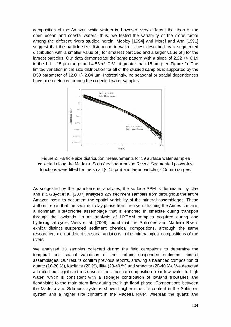
104

composition of the Amazon white waters is, however, very different that than of the open ocean and coastal waters; thus, we tested the variability of the slope factor among the different rivers studied herein. Mobley [1994] and Morel and Ahn [1991] suggest that the particle size distribution in water is best described by a segmented distribution with a smaller value of j for smallest particles and a larger value of j for the largest particles. Our data demonstrate the same pattern with a slope of 2.22 +/- 0.19 in the 1.1 – 15 µm range and 4.56 +/- 0.61 at greater than 15 µm (see Figure 2). The limited variation in the size distribution for all of the studied samples is supported by the D50 parameter of 12.0 +/- 2.84 µm. Interestingly, no seasonal or spatial dependences have been detected among the collected water samples.

Figure 2. Particle size distribution measurements for 39 surface water samples collected along the Madeira, Solimões and Amazon Rivers. Segmented power-law functions were fitted for the small (< 15 µm) and large particle (> 15 µm) ranges.

As suggested by the granulometric analyses, the surface SPM is dominated by clay and silt. Guyot et al. [2007] analyzed 229 sediment samples from throughout the entire Amazon basin to document the spatial variability of the mineral assemblages. These authors report that the sediment clay phase from the rivers draining the Andes contains a dominant illite+chlorite assemblage that is enriched in smectite during transport through the lowlands. In an analysis of HYBAM samples acquired during one hydrological cycle, Viers et al. [2008] found that the Solimões and Madeira Rivers exhibit distinct suspended sediment chemical compositions, although the same researchers did not detect seasonal variations in the mineralogical compositions of the rivers.

We analyzed 33 samples collected during the field campaigns to determine the temporal and spatial variations of the surface suspended sediment mineral assemblages. Our results confirm previous reports, showing a balanced composition of quartz (10-20 %), kaolinite (20 %), illite (20-40 %) and smectite (20-40 %). We detected a limited but significant increase in the smectite composition from low water to high water, which is consistent with a stronger contribution of lowland tributaries and floodplains to the main stem flow during the high flood phase. Comparisons between the Madeira and Solimoes systems showed higher smectite content in the Solimoes system and a higher illite content in the Madeira River, whereas the quartz and

105

kaolinite remained stable. These observations highlight a limited but significant variability in the type of suspended sediment that may be related to the seasonal and/or spatial dependency of the reflectance over time.

3.2 Classification of the Rrs spectra

A cluster analysis was applied to classify the entire set of Rrs spectra into homogeneous groups. For this analysis, we used the k-means unsupervised classification technique, which categorizes the data set into classes based on the natural distribution of the data in multivariate space. In contrast to supervised classification techniques, this approach does not require predefined classes. To define the optimal number of classes, we used a hierarchical cluster method of applying Ward's algorithm to squared Euclidian distances between the spectra [Lubac and Loisel, 2007]. To enhance the spectral shape of the Rrs spectra in the classification, each Rrs spectrum was previously normalized by its integral calculated over the entire spectrum. The initial dataset of 279 spectra was reduced to 171 spectra to avoid the over-representation of the Solimões River and Madeira River samples. The analysis of the hierarchical clustering showed that the partition into 8 classes minimized the within-cluster variances. Figure 3 shows the mean spectrum of each class, and each group is described below.

Figure 3. The mean Rrs spectra obtained for each class as calculated by the Kmeans clustering technique.

Class 1 consists of the Rio Negro black waters (N = 3). This class presents the lowest reflectance values of < 0.003 sr-1, with a slightly increasing reflectance from blue to red wavelengths. This pattern is directly related to the high CDOM concentration associated with low Chl and SPM values. Class 2 includes black- and clear-water stations that mainly occur in the floodplain (N = 4). The class spectrum slowly increases from 400 to 570 nm and then declines gradually toward the higher wavelengths. Chlorophyll-a absorption at approximately 665 nm is clearly apparent, although the other characteristic Chlorophyll-a absorption peak at 440 nm is not detected. This class presents the lowest SPM loads and a high Chl concentration (mean = 34.4 mg.m-3). Class 3 mainly consists of the productive floodplain waters (N = 21) and samples from river confluences. For this class, the reflectance increases sharply from 400 to 575 nm and presents a wide maximum up to 700 nm. The local minimum observed at approximately 675 nm most likely corresponds to the presence

106

of Chlorophyll-a. A second reflectance maximum is detected at 800 nm. This class presents intermediate SPM values (mean = 21.9 g.m-3) and a high Chl concentration (mean =21.5 mg.m-3). Class 4 is also mostly composed of floodplain waters and river confluence stations (N = 28). This class shows a very similar spectral pattern and reflectance values to those of class 3, although the first reflectance maximum is shifted toward larger wavelengths at 585 nm, and the reflectance does not exhibit marked absorption troughs up to 700 nm. Class 4 is associated with intermediate SPM values (mean = 23.4 g.m-3) but lower Chl concentrations (mean = 9.5 mg.m-3) than Class 3.

Class 5 consists of some floodplain waters (N = 6). This class presents 2 distinct maxima of comparable amplitude: one near 550 nm and one near 705 nm. The first peak matches the Chlorophyll-a absorption minimum in the green spectrum, whereas the second peak corresponds to the Chlorophyll-a absorption minimum in the red spectrum. Two local minima detected at 625 and 675 nm correspond to the absorption maximum of phaeopigments and chlorophyll-a pigments, respectively. We note the absence of any pigment-induced absorption pattern in the blue part of the spectrum, which is likely due to the strong absorption by CDOM. Not surprisingly, Class 5 shows the highest Chl concentration (66.9 mg.m-3) among all classes and an intermediate SPM value (mean = 39 g.m-3).

Classes 6, 7 and 8 include river sediment-dominated waters showing strong SPM concentrations. All of these classes show similar spectral patterns with sharply increasing Rrs values from 400 to 580 nm and a much less pronounced increase up to 700 nm. Class 6 (N = 57) presents intermediate SPM values (72 mg.m-3) and a low Chl value of 1.8 mg.m-3. Class 7 (N = 33) shows strong SPM values (187 mg.m-3), and Class 8 (N = 19) shows the highest SPM values (368 mg.m-3) associated with low Chl-a concentrations (< 1 mg.m-3). It is important to note that Classes 7 and 8 can only be discriminated based on the shapes of their NIR spectra, although they show very different SPM values. Interestingly, although the spectra were normalized to enhance the spectral shape in the classification, the Rrs classes represent rather homogeneous classes as a function of SPM or Chl.

3.3. The relationship of Rrs and Kd to SPM: average relationship

Figure 4 shows the variation of the remote sensing reflectance at 670 nm and 850 nm as a function of the SPM for 279 samples collected during the 16 cruises in of all the studied rivers and floodplain lakes. Although the reflectance in the red and NIR channels shows a clear increasing trend as a function of the SPM, we note a strong difference between the channels. Although the red channel shows saturation at approximately 100 g.m-3, we cannot define a saturation point for the NIR channel up to 600 g.m-3, demonstrating a remarkable sensitivity to the SPM concentration over 2 orders of magnitude. The dispersion around the main trend appears to be stronger for lower SPM values, specifically for the floodplain stations. Linear regressions between the natural logarithm of the wavelength and of Rrs for the Madeira River and Solimões River show similar intercepts (p = 0.763) and slopes (p = 0.461). In contrast, the slopes and intercepts for Madeira River and Solimões Rivers are different when compared with the tributary and floodplain samples (p < 0.001). However, the fact that the SPM range for the floodplains (mean SPM = 22.9 g.m-3) is much lower than for the Madeira (mean SPM = 239.3 g.m-3) and Solimões (mean SPM = 128.9 g.m-3) Rivers limits the

107

relevance of this statistical result. The clear correlation between SPM and reflectance for all of the water types and seasons demonstrates that SPM is clearly driving the water optical properties in the majority of the waters of the Amazon Basin. However, whereas the SPM is mainly composed of mineral particles at high concentrations and along the white-water rivers, the composition of the suspended matter may be much more diverse at low SPM values with a much larger organic fraction (living and non-living). Studies have reported that white-water rivers show low particulate organic carbon (POC) contents (1-4 % weight percent relative to the SPM concentration) [Moreira-Turcq et al., 2003]. These relationships have been confirmed for a wide range of riverine environments throughout the world, demonstrating that the POC/SPM ratio decreases with increasing SPM, reaching approximately 1 % for SPM levels of greater than 100 g.m-3 [Coynet et al., 2009; Meybeck 1993]. In the Amazon River, it has been shown that the POC concentrations directly vary with the discharge volume, and higher concentrations occur during high water periods (corresponding to low SPM concentrations). In black and floodplain waters, the POC concentrations are much higher, with weight percentages of up to 25 %. This variability and importance of the organic fraction relative to the inorganic fraction clearly affects the reflectance level at low SPM concentrations (i.e., < 20 g.m-3).

Figure 4. Variation of Rrs(670) (left) and Rrs(850) (right) as a function of the SPM concentration. The collected samples are identified based on their sampling location: the Solimões and Amazon Rivers (triangles), the Madeira River (Black circles), the

floodplain lakes (White circles) and all of the tributaries (squares).

Figure 5 shows the variation of Kd(650) as a function of the SPM for 133 samples collected during the 16 cruises in all of the studied rivers and floodplain lakes. Unlike

108

the Rrs at the red wavelength, saturation is not observed for up to 620 g.m-3. The dispersion is relatively constant across the entire SPM range, and a simple linear function could be fit to model the Kd – SPM relationship. At low SPM levels, Kd(650) appears to be greater than 1, which is indicative of residual CDOM absorption at those wavelengths (see section 3.5.1). This result shows that Kd is a good predictor of SPM for all types of waters in the Amazon basin.

Figure 5. Variation of Kd(670) as a function of the SPM concentration.

We also investigated the spectral dependence of the relationship of Rrs and Kd with SPM, excluding all floodplain and non-white waters. The revised dataset represents 229 stations for Rrs and 109 stations for Kd. To assess the accuracy of the AOPs in predicting SPM concentrations, 2 subsets were formed for each AOP. For Rrs, the calibration dataset included 115 samples (mean SPM = 168.2 g.m-3) and the validation dataset included 114 samples (mean SPM = 166.2 g.m-3). For Kd, the calibration dataset included 56 samples (mean SPM = 128.1 g.m-3) and the validation dataset included 53 samples (mean SPM = 138.9 g.m-3).

Figure 6. Variation of the square of the Pearson correlation coefficient (left axis) and the RMSE of the SPM concentration (right axis) as a function of the wavelength for Kd

and Rrs.

Figure 6 presents the model-fitting and SPM-retrieval performances for Rrs and Kd as a function of the wavelength. For Rrs, there is a clear increasing relationship with SPM from the blue to NIR wavelengths, with a square Pearson correlation factor of greater than 0.75 beyond 730 nm and an optimal range of 840-900 nm (r² of approximately 0.81). A lower correlation in the visible spectrum (400 to 700 nm) is induced by the

109

rapid saturation of the Rrs as a function of the SPM at low concentrations. The least-squares regression shows that a power law model a.Rrs(λ)b provides the best-fit values. The model factors and performance are calculated based on the linear regression between the natural logarithm of the wavelength and of Rrs. The RMSE of the retrieval model decreases as a function of increasing wavelength starting at 114.1 g.m-3 (400 nm) down to 61 g.m-3 (820-900 nm). The optimal wavelength occurs at 860 nm, and the corresponding model is as follows:

d�c = 20.411�X�M�860��<.<��< (7)

For Kd, there is a strong and robust correlation with SPM (see Figure 6) over a wide range of wavelengths in both the visible and NIR spectra from 495 to 860 nm (r² > 0.90). The lower Pearson correlation at short wavelengths and beyond 890 nm may be induced by the strong absorption of light that makes it difficult to accurately assess the downwelling irradiance distant from the water surface. Accordingly, a linear best-fit model between SPM and Kd performs better than for Rrs with an RMSE of better than 30 g.m-3 from 500 to 870 nm.

d�c = 20.51~!�650� − 22.94 (8)

These observations may be related to the link between the AOPs and IOPs (the absorption and scattering coefficients); i.e., whereas Rrs is related to the absorption to scattering ratio, Kd is assumed to vary as the sum of absorption and scattering. With increasing SPM, coefficients a and b will increase, meaning that Kd will increase indefinitely as a function of the suspended sediment concentration, whereas Rrs may reach a saturation point. Not surprisingly, Kd and Rrs are well correlated at 730 nm up to 900 nm (r2 > 0.80). At 850 nm, we observe the following relationship (r2 > 0.85):

~!�850� = 559.17X�M�850� + 3.98

3.4 Improvement of SPM retrieval using the Rrs ratio at 2 wavelengths

It has been shown that the ratio between Rrs at 2 wavelengths may lessen the dependence on the SPM type and thus is more robustly linked to the SPM concentration [Moore et al., 1999; Doxaran et al., 2002]. Irradiance reflectance is generally modeled as R = f . bb / (a +bb), where bb is the backscattering coefficient and f is a factor determined by the incident light field and often assumed to be invariant as a function of the wavelength. Doxaran et al. [2002] analyzed the variation of the bb/(a + bb) ratio for highly turbid waters in the Gironde estuary. These authors showed that when the contributions of pure water, algal pigments and CDOM to light absorption can be neglected, the bb/(a + bb) ratio becomes independent of the SPM concentrations, leading to the saturation phenomenon observed in the Rrs. The total absorption by pure water is high at NIR, and thus, this simple model predicts that saturation will occur for higher SPM concentrations at the visible to infrared wavelengths. Interestingly, the same authors reported that the bb/(a + bb) ratio at 2 wavelengths will be less sensitive to the refraction index and grain size variation than to the SPM concentration at high SPM loads. Indeed, by assuming that the spectral variations of bb are weak [Whitlock et al., 1981; Moore et al., 1999], it can be shown that the ratio is much more dependent

110

on the absorption than on the backscattering, which, in turn, may limit the influence of the refraction indices and granulometry. This simple ratio model will perform better using wavelengths at which SPM absorption shows a strong variation and, together with the pure water absorption, dominates the total absorption. it can be deduced that the Rrs ratio should make use of the red and NIR wavelengths.

We investigated whether the use of the reflectance ratio Rrs (λ1) / Rrs(λ2) improves the SPM – Rrs relationship in the river sediment-dominated waters. To determine the optimal position of λ1, we chose an initial value of λ2 = 670 nm within the range of minimum total absorption in the red spectrum. We performed a regression of the model [Rrs (λ1) / Rrs(670)] vs. SPM for the range of 730 to 900 nm; the RMSE of the SPM estimation showed minimal values over a wide range of λ1 between 760 and 820 nm (see Figure 7A). In the second iteration, we determined λ2 after fixing λ1 at 805 nm and regressing the model [Rrs(805) /Rrs(λ2)] vs. SPM. Again, the RMSE was minimal over a wide range of λ2 between 650 and 700 nm, with the best result obtained at λ2 = 680 (see Figure 7B). Of interest, the ratio model performed significantly better than with the use of a unique wavelength with an RMSE of approximately 38 g.m-3. Interestingly, the spectral bands showing a minimal RMSE at both the red and NIR regions of the spectrum include the spectral bands of commonly used water-color sensors, such as MERIS and MODIS, and future platforms, such as Sentinel-3, NPP/VIIRS and JPSS.

A

B

Figure 7. RMSE of the SPM estimations from Rrs in the validation dataset plotted as a function of the wavelength for λ1 (A) and λ2 (B). Minimal values of RMSE were

observed for λ1 in the range of 760 to 820 nm. For λ2, the range was 660 to 700 nm.

111

We further investigated whether the efficiency of the Rrs ratio is global or may vary from one river to another. For the Solimões River, the use of the ratio when compared to a single wavelength model at NIR increased the model accuracy (r² = 0.83 vs. 0.73, N = 76). For the Madeira River, the use of the ratio showed a strong improvement of the retrieval accuracy (r² = 0.93 vs. 0.62, N = 102) (see Figure 8). However, when the regression lines assessed for both rivers are compared, the data support the hypothesis that the slope (p = 0.108) and intercept (p = 0.225) are equal. From our dataset, we conclude that the use of the Rrs ratio may not show an increased SPM retrieval efficiency globally, but it may be used as a general tool to homogenize a dataset across a watershed.

Figure 8. Variation of Rrs(850) and the reflectance ratio Rrs(805)/Rrs(680) as a function of the SPM concentration for the Madeira River samples

3.5 Inherent optical properties

3.5.1 Absorption coefficient: aCDOM and aNAP

The water absorption is conventionally modeled as the sum of the absorption by pure water, SPM, phytoplankton and CDOM:

;n�λ� = ;L�λ� + ;�T���λ� + ;����λ� +;��λ� (9)

112

where at is the total absorption (m-1), aw is the absorption coefficient for pure water, ap is the absorption coefficient for phytoplankton and aNAP is the absorption coefficient for non-algal particles. For sediment-loaded river waters, absorption by phytoplankton is assumed to be negligible. Values of aw were obtained from Pope and Fry (1997) and corrected for a temperature dependence over the range 745–755 nm with a 0.36 % change per °C at 750 nm (Pegau and Zaneveld 1993).

Figure 9. Spectral variation of aCDOM for different river water types and floodplain lakes.

Figure 9 shows the aCDOM variation for 19 samples collected from black, clear and white waters as well as floodplain lakes. The aCDOM was higher in the black river waters (acdom(440) = 7.9 m-1, N=1) and floodplain lakes (acdom(440) = 4.8 ± 0.8 m-1, N = 2) and lower in white (acdom(440) = 3.3 ± 1.0 m-1, N = 14) and clear waters (acdom(440) = 1.8 ± 0.8 m-1, N = 2). Interestingly, at longer wavelengths, the CDOM absorption in white river waters remained significant (aCDOM (670) = 0.72 ± 0.5 m-1). The spectral slope SCDOM shows small variations (0.013 nm-1 ± 0.0016) from one location to another. The CDOM absorption classes follow the usual water type classification used to describe the main water types in the Amazon (clear/white/black), for which both DOC and POC have been shown to exhibit increasing carbon concentrations. The aCDOM values reported here are much stronger than in any other measurements for the open ocean and can only be compared with coastal waters marked by large freshwater inputs from land. Bowers et al. [2000] monitored a CDOM absorption gradient from the Clyde Sea to an estuary and measured an aCDOM value of 1.6 at zero salinity. The fact that SCDOM does not show a strong variation is in accordance with other studies in which this parameter was assessed in other coastal waters. Babin et al. [2003a] reported a mean SCDOM value of 0.018 ± 0.002 over 345 samples collected from 6 different coastal regions, and Bowers et al. [2000] reported a mean value of 0.018 ± 0.005 for 25 samples. In a previous work, Bricaud et al. [1981] found an SCDOM value of 0.014 ± 0.003, and Kirk [1976], who studied lake waters, observed SCDOM values between 0.013 and 0.016. In an analysis of CDOM in a tidal marsh area, Tzortziou et al. [2008] showed that SCDOM was systematically lower at low tide (0.0149), as dissolved terrestrial material is drained out of the marshes, than during high tide (SCDOM = 0.0168). Our study does not aim to document systematic variations of aCDOM across the watershed, although our observations allow for the quantification of the very strong

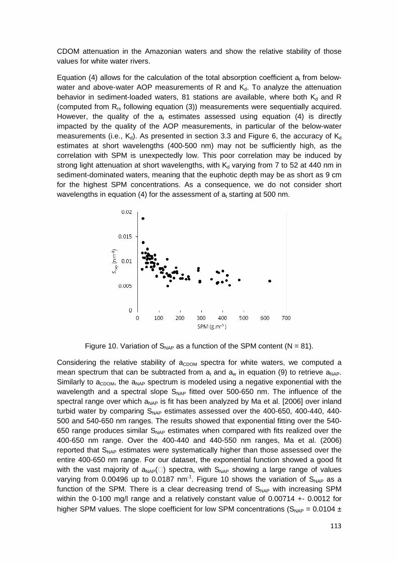
113

CDOM attenuation in the Amazonian waters and show the relative stability of those values for white water rivers.

Equation (4) allows for the calculation of the total absorption coefficient at from below-water and above-water AOP measurements of R and Kd. To analyze the attenuation behavior in sediment-loaded waters, 81 stations are available, where both Kd and R (computed from Rrs following equation (3)) measurements were sequentially acquired. However, the quality of the at estimates assessed using equation (4) is directly impacted by the quality of the AOP measurements, in particular of the below-water measurements (i.e., Kd). As presented in section 3.3 and Figure 6, the accuracy of Kd

estimates at short wavelengths (400-500 nm) may not be sufficiently high, as the correlation with SPM is unexpectedly low. This poor correlation may be induced by strong light attenuation at short wavelengths, with Kd varying from 7 to 52 at 440 nm in sediment-dominated waters, meaning that the euphotic depth may be as short as 9 cm for the highest SPM concentrations. As a consequence, we do not consider short wavelengths in equation (4) for the assessment of at starting at 500 nm.

Figure 10. Variation of SNAP as a function of the SPM content (N = 81).

Considering the relative stability of aCDOM spectra for white waters, we computed a mean spectrum that can be subtracted from at and aw in equation (9) to retrieve aNAP. Similarly to aCDOM, the aNAP spectrum is modeled using a negative exponential with the wavelength and a spectral slope SNAP fitted over 500-650 nm. The influence of the spectral range over which aNAP is fit has been analyzed by Ma et al. [2006] over inland turbid water by comparing SNAP estimates assessed over the 400-650, 400-440, 440-500 and 540-650 nm ranges. The results showed that exponential fitting over the 540-650 range produces similar SNAP estimates when compared with fits realized over the 400-650 nm range. Over the 400-440 and 440-550 nm ranges, Ma et al. (2006) reported that SNAP estimates were systematically higher than those assessed over the entire 400-650 nm range. For our dataset, the exponential function showed a good fit with the vast majority of aNAP(�) spectra, with SNAP showing a large range of values varying from 0.00496 up to 0.0187 nm-1. Figure 10 shows the variation of SNAP as a function of the SPM. There is a clear decreasing trend of SNAP with increasing SPM within the 0-100 mg/l range and a relatively constant value of 0.00714 +- 0.0012 for higher SPM values. The slope coefficient for low SPM concentrations (SNAP = 0.0104 ±

114

0.0021) is similar to that of studies realized over coastal waters [Babin et al. 2003a] that show a SNAP of 0.0123 +- 0.0013. For more turbid coastal waters, Loisel et al. [2009] observed a mean slope of 0.0084, and Ma et al. [2006] reported SNAP values between 0.0088 and 0.0129 for lake waters in China. Our observations are also consistent with the report of Babin et al. [2003a]), showing that SNAP may be related to the relative abundance of mineral organic matter, with low values generally occurring in mineral-dominated waters.

The aNAP(550) shows a good relationship with SPM (r2 = 0.91), even though a significant dispersion is observed for the lowest concentrations at less than 50 g.m-3 (see Figure 11). The aNAP(�):SPM relationship shows a linear fit over the entire spectral range, with r² values of greater than 0.89 from 500 to 720 nm. The mass-specific particulate absorption coefficient �;���∗ �λ�inm9. g2<� is defined as the particulate absorption coefficient per unit of SPM. At 555 nm, ;���∗ = 0.028 ± 0.017 shows values that match those of studies for turbid coastal waters, such as Doxaran et al. [2009] who reported a mean value of 0.026 but with strong variations between different European estuaries. At 715 nm, the relationship ;���∗ �715� = 0.077 ± 0.077 was observed, which is also in the range reported by Doxaran (0.011 ± 0.007). For comparison with the literature, aNAP was extrapolated at 440 nm by assuming negative exponential trend with the SNAP slope assessed over the 540-650 nm range. We observed an aNAP(440)/SPM ratio of 0.072 ± 0.045 m2.g-1 but with a net difference between low SPM conditions (< 100 g.m-3) with aNAP(440)/SPM = 0.105 ± 0.055 m2.g-1 and high SPM conditions (> 100 g.m-3) with aNAP(440)/SPM = 0.050 ± 0.013 m2.g-1. This behavior has been previously reported for highly turbid inland waters of a tropical lake in China [Ma et al. 2006], with aNAP(440)/SPM varying between 0.043 and 0.169 m2.g-1 and a mean of 0.080 ± 0.030 m2.g-1 showing a decreasing ratio with increasing SPM within a the 0-150 g.m-3 range. For an alpine lake, Giardino et al. [2007] reported an aNAP(440)/SPM ratio of 0.08 m2.g-1 and Doxaran et al. [2009] reported a ratio of 0.071 ± 0.038 m2.g-1.

Figure 11. Scatterplot of aNAP(550) as a function of the SPM content (N = 81).

3.5.2 Scattering of non-algal particles

We obtained the water scattering coefficient bt from the Kd and at values using equation (5). We assumed that bNAP = bt considering that the pure water scattering coefficient bw

115

does not contribute significantly to the total scattering at all wavelengths. For the 81 stations, bNAP(555) showed a broad variation from 10.7 up to 362.5 m2.g-1. Figure 12 presents the variation of bNAP as a function of SPM at 555 nm, showing good agreement over the entire SPM range (r² = 0.87). The mass-specific particulate scattering coefficient �J���∗ �λ�inm9. g2<� is defined as the particulate scattering coefficient per unit of SPM. At 555 nm, the relationship J���∗ �555� = 0.672 ± 0.018 is observed, showing significant variation across the dataset. This trend is consistent with the values reported by Loisel et al. [2009], Doxaran et al. [2009] and Babin et al. [2003b] for coastal waters, with J���∗ varying between 0.4 and 1 m2.g-1 and, more specifically, is closer to the lower limit for Case 2 waters. We analyzed the variation of J���∗ for the different sediment-dominated rivers. The Solimões River exhibited a low and stable scattering J���∗ �555� = 0.529 ± 0.051 throughout the hydrological cycle, and the Amazon River showed an intermediate value, with J���∗ �555� = 0.638 ± 0.178. A much stronger variability was observed for the Madeira River, with J���∗ �555� =0.804 ± 0.100 during rising water and J���∗ �555� = 0.814 ± 0.065 during low water. However, during the high-water period, we noted a significant decrease for the Madeira River, with J���∗ �555� = 0.562 ± 0.156.

Figure 12. Scatterplot of bNAP(555) as a function of the SPM content (N = 81).

Figure 13. Spectral variation of the mass-specific scattering coefficient J���∗ .

The spectral variation of bNAP has often been modeled using a λ-n relationship, where n depends on the particle size distribution and is typically 1.0 or less within the range of

116

1.0 to 0.8 [Moore et al. 1999]. Babin et al. [2003] and Gould et al. [1999] stated that a λ-

1 fit is too steep, and a linear or near-linear trend would better fit the spectral variation of the scattering function. For our dataset, the spectral variation is low, and a λ-n relationship shows a better fit with N = 0.78 (see figure 13). The overall bNAP(555) / bNAP(670) ratio is 0.859 (compared to 0.853 reported by Gould et al. [1999]). The bNAP(850)/bNAP(555) is 0.774, whereas the bNAP(850)/bNAP(670) is 0.892.

4. DISCUSION AND CONCLUSIONS

The Amazon basin presents Case 2 waters with an absorption budget dominated by CDOM and SPM in rivers but with a significant contribution from Chl in floodplains. A simple unsupervised classification of Rrs spectra made it possible to discriminate several classes: 1) one class presenting very low Rrs values corresponding to the so-called black waters with strong CDOM absorption and very low SPM concentrations; 2) 4 groups of floodplain lakes and river confluences, where a reduced water velocity phytoplankton at high concentrations; and 3) 3 classes of sediment-dominated waters with relatively high SPM concentrations. Rrs shows a strong saturation, with SPM at approximately 100 g.m-3 in the green and red spectra. However, the use of Rrs makes it possible to monitor the SPM range without saturation. Interestingly, the three main Amazonian rivers having sediment-dominated water (the Madeira, Solimões and Amazon Rivers) showed a similar behavior as a function of SPM, even though the samples were collected at stations that in some cases were separated by more than 3,000 km. Kd proved to be a very robust predictor (r² > 0.9) of SPM through a simple linear relationship for a very wide range of SPM values (up to 622 g.m-3) and wavelengths. We analyzed the behavior of main IOPs for the sediment-loaded waters. Whereas aCDOM and aNAP showed very high absolute values when compared to most studies of water color, the shape factors SCDOM and SNAP exhibited values within the range of coastal or inland waters presenting mineral-dominated waters. However, a dependence of SNAP on the SPM concentrations was detected and should be considered for optical modeling. The spectral variation of bNAP fit a typical λ-n relationship with n = 0.78. It is interesting to note that despite the extreme values recorded for aCDOM, aNAP and bNAP, the spectral shape and specific coefficient of absorption and scattering were within the range of the values reported in most marine studies and sediment-dominated Case-2 waters in particular. The absorption budget derived from our data shows that aNAP represents 22, 74 and 97 % of the total absorption for 10, 100 and 1000 g.m-3, respectively, at 500 nm. At longer wavelengths, our data show that aNAP remains significant for SPM values greater than 100 g.m-3. At 670 nm, aNAP represents 9, 51 and 91 % of the total absorption for 10, 100 and 1000 g.m-3, respectively. At 780 nm, aNAP is 1, 12 and 57 % of the total absorption for 10, 100 and 1000 g.m-3, respectively.

For such sediment-dominated waters, it is expected that the AOP/IOP variations may be strongly impacted by spatial and seasonal changes in sediment type and particle size distribution. However, our results show that at the Amazon catchment scale, Rrs exhibits a relationship with SPM that is sufficiently robust to be used for the accurate monitoring of surface suspended sediment discharge in the largest river of the world. Regarding the particle size distribution, our granulometric results show a relatively consistent grain size distribution among different rivers and hydrological periods. These observations agree with the classical results of sediment transport dynamics in a

117

turbulent flow system that predict a relatively constant distribution of the fine-grain size fraction in the water column in which the coarse-grain size fraction increases from the surface to the river bottom [Rouse 1950], resulting in an almost pure fine sediment composition at the river surface. The segmented grain size distribution shows a more even distribution (2.22) for the 1- to 15-µm diameter range than is usually predicted in optical modeling (approximately 4), which implies that very fine particles (< 1 µm) may not contribute strongly to NAP scattering. Our study does not allow for a detailed assessment of the variability of the mineral particle types but does confirm that results of previous studies in the Amazon Plain showing a relatively consistent pattern of mineral compositions. These results have important implications for AOP/IOP variations as a function of SPM, as we demonstrated that at the scale of a large river basin, the sediment size distribution and type may not sufficiently vary to significantly affect the AOP-SPM relationship.

The use of reflectance ratios has been previously presented as a means to reduce the sensitivity of Rrs to the sediment type or size distribution in sediment-dominated waters [Moore et al., 1999; Doxaran et al., 2002]. In our dataset, we observed that the use of a ratio model does not improve the results uniformly for all of the studied water bodies. For example, although the retrieval model accuracy is slightly improved for the Solimões River when using a reflectance ratio instead of one wavelength, for the Madeira River, the improvement is much stronger. An analysis of the IOPs showed that for the Madeira River, bnap presents a significant seasonal variation that may explain the Rrs sensitivity. NAP scattering is higher at the low water and rising water periods than during the flood peak. This pattern supports the interpretation of the Rrs seasonal variation observed in this study using field measurements and that of a previous study based on satellite data. In an analysis of 11 years of MODIS red and infrared surface reflectance data and of SPM data acquired at 2 hydrological stations along the Madeira River in Brazil, Espinoza et al. [in press] showed that the NIR reflectance does not exhibit a simple relationship with SPM. The authors detected a hysteresis effect in which for the same SPM concentration, the reflectance during rising water is higher than at the flood peak. It is important to note that using the same method, Espinoza et al. (2012) did not detect such a seasonal variation for the Solimões River or its main tributaries (Marañon and Ucayali) in Peru.

The cause of the variations in the AOP-IOP/SPM relationship remain unclear for the Madeira River case because the deviation may originate from variations of the physical properties of the SPM or variation in the organic fraction. Viers et al. [2008] analyzed the variations in the geochemical and physical properties of SPM from the Solimões River and Madeira River during one hydrological cycle. These authors showed that both rivers exhibit distinct suspended sediment chemical compositions but that these characteristics do not vary significantly over time except for in the Madeira River, where the strontium isotopic composition shows clear variations between the high-water period and the remainder of the year. This difference is attributed to increasing physical weathering during the rainy season due to landslides in the upstream catchments and riverbank erosion in the lowlands and connected floodplains. Although this seasonal control of the Sr isotopic composition remains ambiguous, these observations highlight the fact that there is a limited but significant variability in the suspended sediment type in the Madeira River. Unfortunately, data on DOC and POC concentrations were not

118

available for the majority of the measurements acquired on the Madeira River. The variations of J���∗ are consistent with a higher mineral fraction during periods of higher water. This behavior may contradict the global POC/SPM relationship that predicts a decrease in the POC percentage with increasing SPM. However, Moreira-Turcq et al. (2003) reported that the percentage weight of POC in SPM was higher during periods of lower discharge in the Madeira River basin. This variability may be used to explain the seasonal dependency of the reflectance in this sub-catchment and the lower J���∗ and Rrs values observed during high water periods in particular.

This work is one of the first studies to assess the variation of the AOP/IOP of river waters across a large river basin and for all hydrological periods. The SPM retrieval performance assessed based on the AOPs varied from 37 % (Rrs at a single wavelength in the NIR) to 23 % (Rrs ratio at 2 wavelengths) to 18 % (Kd in the visible spectrum) relative RMSE. These performances are consistent with the operational monitoring of suspended sediment in rivers. Uncertainties regarding both the sampling and calculation methods are known to affect the accuracy of in situ SPM concentration assessments in rivers by approximately 10 to 20 % [Cheviron et al. 2011]. In recent years, we have published several studies that used MODIS satellite imagery to retrieve surface SPM values for the Amazon basin using correlations between RRs and SPM data obtained from field samples. Martinez et al. [2009] found a 36 % relative difference when comparing 7 years of MODIS-derived surface SPM estimates and 10-day surface field samples acquired at one station in Brazil. At 2 stations in Peru (Solimões and Marañon Rivers), Espinoza et al. (2012) reported a 27 % and 45 % relative RMSE when comparing 4 years of MODIS-derived surface SPM estimates and 10-day surface field samples. The retrieval accuracy assessed based on the satellite data is consistent with the Rrs-based model performance we analyzed and demonstrates that significant improvement may be achieved using an appropriate reflectance model. The optical properties presented in the present study cannot be extrapolated for global use in continental waters. However, considering the size of the catchment, our results support the notion that remote sensing monitoring may be used efficiently for sediment discharge monitoring in large river basins.

5. ACKNOWLEDGMENTS

This work has been supported by the Brazilian Water Agency (ANA), CNPq, MCT (Ministry of Science and Technologies) and PEC-PG (Program for Graduate Students-Agreement) program in Brazil; IRD, Joint International Laboratory “Environmental Changes Observatory in Amazon Region”, INSU “Reliefs”, INSU “Syster”, ANR “CARBAMA” and CNES/TOSCA programs in France. Our thanks also go to all the HYBAM program partners in Brazil and Peru: the University of Brasilia (UnB), the Amazonas State Federal University (UFAM), the Fluminense State University (UFF), the Brazilian Mineral Resources Research Company (CPRM) and the Peruvian Hydrologic and Meteorology Service (SENAMHI). The authors are grateful to the ship crews who accompanied them during the surveys.

6. BIBLIOGRAPHY

119

Aas, E. (1987), Two-stream irradiance model for deep waters, Applied Optics, Vol. 26, Issue 11, pp. 2095-2101.

Babin, M., D. Stramski, G. M. Ferrari, H. Claustre, A. Bricaud, G. Obolensky, and N. Hoepffner (2003a), Variations in the light absorption coefficients of phytoplankton, nonalgal particles, and dissolved organic matter in coastal waters around Europe, J. Geophys. Res., 108(C7), 3211, doi:10.1029/2001JC000882.

Babin, M., A. Morel, V. Fournier-Sicre, F. Fell and D. Stramski (2003b), Light Scattering Properties of Marine Particles in Coastal and Open Ocean Waters as Related to the Particle Mass Concentration, Limnology and Oceanography, Vol. 48, No. 2, pp. 843-859.

Bowers, D.G., G.E.L. Harker, P.S.D. Smith and P. Tett (2000), Optical Properties of a Region of Freshwater Influence (The Clyde Sea), Estuarine, Coastal and Shelf Science, 50, 717–726, doi:10.1006/ecss.1999.0600.

Bricaud, A., Morel, A. and L. Prieur (1981), Absorption by dissolved organic matter of the sea (yellow substance) in the UV and visible domains, Limnology and Oceanography, 26, 43-53.

Bricaud, A., A. Morel, M. Babin, K. Allali, and H. Claustre (1998), Variations of light absorption by suspended particles with chlorophyll-a concentration in oceanic (case 1) waters: Analysis and implications for bio-optical models, J. Geophys. Res., 103, 31,033–31,044.

Cheviron, B., M. Delmas, O. Cerdan and J.-M. Mouchel (2011), Parameter uncertainty and sensitivity analysis in sediment flux calculation, Hydrol. Earth Syst. Sci. Discuss., 8, 1469–1506, doi:10.5194/hessd-8-1469-2011.

Coynel, A., P. Seyler, H. Etcheber, M. Meybeck, and D. Orange (2005), Spatial and seasonal dynamics of total suspended sediment and organic carbon species in the Congo River, Global Biogeochem. Cycles, 19, GB4019, doi:10.1029/2004GB002335.

Doxaran, D., K. Ruddick, D. McKee, B. Gentili, D. Tailliez, M. Chami and M. Babin (2009) Spectral variations of light scattering by marine particles in coastal waters, from the visible to the near infrared. Limnology and Oceanography, 54 (4). pp. 1257-1271. ISSN 0024-3590.

Doxaran, D., J.-M. Froidefond and P. Castaing (2002), A reflectance band ratio used to estimate suspended matter concentrations in sediment-dominated coastal waters, International Journal of Remote Sensing, Vol. 23, Iss. 23.

Ertel J.R., Hedges J.I., Devol A.H., J.E. Richey and M. Goes Ribeiro (1986), Dissolved Humic Substances of the Amazon River System, Limnology and Oceanography, Vol. 31, No. 4, pp. 739-754.

Espinoza Villar, R., J.M. Martinez, J.L. Guyot, P. Fraizy, E. Armijos, A. Crave, H. Bazán, P. Vauchel and W. Lavado (2012), The integration of field measurements and satellite observations to determine river solid loads in poorly monitored basins, Journal of Hydrology, Volumes 444–445, Pages 221-228, ISSN 0022-1694, 10.1016/j.jhydrol.2012.04.024.

Espinoza Villar, R., J.M. Martinez, M. Le Texier, J.L. Guyot, P. Fraizy, P. R. Meneses, E. de Oliveira (in press), A study of sediment transport in the Madeira River, Brazil,

120

using MODIS remote-sensing images, Journal of South American Earth Sciences, ISSN 0895-9811, 10.1016/j.jsames.2012.11.006.

Giardino, C., V. E. Brando, A.G. Dekker, N. Strömbeck, G. Candiani (2007), Assessment of water quality in Lake Garda (Italy) using Hyperion, Remote Sensing of Environment, Volume 109, Issue 2, Pages 183-195, ISSN 0034-4257, 10.1016/j.rse.2006.12.017.

Gitelson, A.A., G. Dall'Olmo, W. Moses, D.C. Rundquist, T. Barrow, T.R. Fisher, D. Gurlin, J. Holz (2008), A simple semi-analytical model for remote estimation of chlorophyll-a in turbid waters: Validation, Remote Sensing of Environment, Volume 112, Issue 9, Pages 3582-3593, ISSN 0034-4257, 10.1016/j.rse.2008.04.015.

Gould, R., R. Arnone and P. Martinolich (1999), Spectral Dependence of the Scattering Coefficient in Case 1 and Case 2 Waters, Appl. Opt. 38, 2377-2383.

Guyot, J.L., J.M. Jouanneau, L. Soares, G.R. Boaventura, N. Maillet, and C. Lagane (2007), Clay mineral composition of river sediments in the Amazon basin. Catena, 71, 340-356.

Hedges, J.I., G.L. Cowie, J.E. Richey, P.D. Quay, R. Benner, M. Strom and R. Bruce (1994), ForsbergOrigins and Processing of Organic Matter in the Amazon River as Indicated by Carbohydrates and Amino Acids, Limnology and Oceanography, Vol. 39, No. 4, pp. 743-761.

Hoogenboom, H.J., A.G. Dekker, I.A. Althuis (1998), Simulation of AVIRIS Sensitivity for Detecting Chlorophyll over Coastal and Inland Waters, Remote Sensing of Environment, Volume 65, Issue 3, Pages 333-340, ISSN 0034-4257, 10.1016/S0034-4257(98)00042-X.

Kirk, J. T. O. (1976), Yellow substance (Gelbstoff) and its contribution to the attenuation of photosynthetically active radiation in some inland and coastal south-eastern Australian waters. Aust. J.Mar. Freshwater Res. 27: 61-71.

Kirk, J. T. O. (1984), Dependence of relationship between in- herent and apparent optical properties of water on solar altitude. Limnol. Oceanogr. 29: 350-356.

Kirk, J. T. O. (1994),Characteristics of the Light Field in Highly Turbid Waters: A Monte Carlo Study, Limnology and Oceanography, Vol. 39, No. 3, pp. 702-706.

Loisel, H. and A. Morel (2001), Non-isotropy of the upward radiance field in typical coastal (Case 2) waters, International Journal of Remote Sensing, vol. 22, issue 2-3, pp. 275-295.

Loisel, H., X. Mériaux, A. Poteau, L. F. Artigas, B. Lubac, A. Gardel, J. Caillaud, and S. Lesourd (2009), Analyze of the inherent optical properties of French Guiana coastal waters for remote sensing applications. Journal of Coastal Research SI 56, 1532 – 1536.

Lubac, B., and H. Loisel (2007), Variability and classification of remote sensing reflectance spectra in the Eastern English Channel and southern North Sea. Remote Sensing of Environment 110, 45-58.

Ma, R., J. Tang, J. Dai, Y. Zhang, Q. Song (2006), International Journal of Remote Sensing, Volume 27, Number 19, pp. 4277-4304(28).

Mangiarotti, S., J.M. Martinez, M.P. Bonnet, D.C. Buarque, N. Filizola and P. Mazzega (2013), Discharge and suspended sediment flux estimated along the mainstream of the

121

Amazon and the Madeira Rivers (from in situ and MODIS Satellite Data), International Journal of Applied Earth Observation and Geoinformation, Volume 21, Pages 341-355, ISSN 0303-2434, 10.1016/j.jag.2012.07.015.

Martinez, J.M.; J.L. Guyot, N. Filizola and F. Sondag (2009), Increase in suspended sediment discharge of the Amazon River assessed by monitoring network and satellite data, CATENA, Volume 79, Issue 3, Pages 257-264, ISSN 0341-8162, 10.1016/j.catena.2009.05.011.

Meybeck, M. (1993), Riverine transport of atmospheric carbon: Sources, global typology and budget, Water, Air, and Soil Pollution, Volume 70, Issue 1-4, pp 443-463

Mobley, C.D. (1994), Light and Water: Radiative Transfer in Natural Waters, Academic Press.

Mobley, C., (1999), Estimation of the Remote-Sensing Reflectance from Above-Surface Measurements,Appl. Opt. 38, 7442-7455.

Moore,G.F., J. Aiken and S. J. Lavender (1999), The atmospheric correction of water colour and the quantitative retrieval of suspended particulate matter in Case II waters: Application to MERIS, International Journal of Remote Sensing, Vol. 20, Iss. 9.

Moreira-Turcq, P., P. Seyler, J.L. Guyot and H.Etcheber (2003), Exportation of organic carbon from the Amazon River and its main tributaries, Hydrological Processes, vol. 17, Issue 7, pp.1329-1344

Morel, A., S. Maritorena (2001), Bio-optical properties of oceanic waters: A reappraisal, Journal of Geophysical Research, Volume 106, Issue C4, p. 7163-7180

Morel, A., and Y.-H. Ahn (1991), Optics of heterotrophic nanoflagellates and ciliates: A tentative assessment of their scattering role in oceanic waters compared to those of bacterial and algal cells, Journal of Marine Research, 49, 177-202.

Morel A., B. Gentili, H. Claustre, M. Babin, A. Bricaud, J. Ras and F. Tièche (2007),Optical Properties of the "Clearest" Natural Waters, Limnology and Oceanography, Vol. 52, No. 1, pp. 217-229.

Neukermans, G., H. Loisel, X. Mériaux, R. Astoreca and D. McKee (2012). In situ variability of mass-specific beam attenuation and backscattering of marine particles with respect to particle size, density, and composition Limnol. Oceanogr. , 57(1): 124-144. dx.doi.org/10.4319/lo.2011.57.1.0124

Nogueira, I., J.C. Nabout, M. Ibanez and L. Maurice (2010), Determinantes da diversidade beta: a importância relativa de processos ambientais e espaciais na estrutura de comunidades fitoplanctônicas de uma planície de inundação amazônica. Acta Limnol. Bras., vol.22, n.3 [cited 2013-01-07], pp. 247-256

Rouse, H. (1950), Engineering Hydraulics, Wiley: New York.

Sioli, H. (1956), Über Natur und Mensch im brasilianischen Amazonasgebiet, Erdkunde 10(2):89–109.

Stramski, D., A. Bricaud, and A. Morel (2001), Modeling the inherent optical properties of the ocean based on the detailed composition of the planktonic community, Appl. Opt., 40(18), 2929– 2945.

122

Snyder W., R. Arnone, C. Davis, W. Goode, R. Gould, S. Ladner, G. Lamela, W. Rhea, R. Stavn, M. Sydor, and A. Weidemann (2008), "Optical scattering and backscattering by organic and inorganic particulates in U.S. coastal waters," Appl. Opt. 47, 666-677.

Tzortziou, M., P.J. Neale, C.L. Osburn, J.P. Megonigal, N. Maie and R. Jaffé (2008), Tidal Marshes as a Source of Optically and Chemically Distinctive Colored Dissolved Organic Matter in the Chesapeake Bay, Limnology and Oceanography, Vol. 53, No. 1, pp. 148-159.

Viers, J., M. Roddaz, N. Filizola, J.L. Guyot, F. Sondag, P. Brunet, C. Zouiten, C. Boucayrand, F. Martin and G. R. Boaventura (2008), Seasonal and provenance controls on Nd/Sr isotopic compositions of Amazon rivers suspended sediments and implications for Nd and Sr fluxes exported to the Atlantic Ocean, Earth Planet. Sci. Lett., 274, 511–523.

Walling W. and D. Fang (2003), Recent trends in the suspended sediment loads of the world's rivers, Global and Planetary Change, 39(1–2), Pages 111-126, ISSN 0921-8181, 10.1016/S0921-8181(03)00020-1.

Whitlock, C., L. Poole, J. Usry, W. Houghton, W. Witte, W. Morris, and E. Gurganus (1981), Comparison of reflectance with backscatter and absorption parameters for turbid waters, Appl. Opt. 20, 517-522.

LIST OF TABLE AND FIGURE CAPTIONS

Table 1. Location and dates of the 16 sampling campaigns conducted for this study.

Figure 1. Location of the 42 stations for above-water (279 measurements) and below-water (133 measurements) sampling in the Amazon River basin from 2007 to 2011 along the 2 main rivers draining the Andes: the Solimões and Madeira Rivers. Stations are partitioned into 4 subgroups: 1) the Amazon River and its main tributary, the Solimões River; 2) the Madeira River; 3) other tributaries; and 4) floodplain lakes.

Figure 2. Particle size distribution measurements for 39 surface water samples collected along the Madeira, Solimões and Amazon Rivers. Segmented power-law functions were fitted for the small (< 15 µm) and large particle (> 15 µm) ranges.

Figure 3. The mean Rrs spectra obtained for each class as calculated by the Kmeans clustering technique.

Figure 4. Variation of Rrs(670) (left) and Rrs(850) (right) as a function of the SPM concentration. The collected samples are identified based on their sampling location: the Solimões and Amazon Rivers (triangles), the Madeira River (Black circles), the floodplain lakes (White circles) and all of the tributaries (squares).

Figure 5. Variation of Kd(670) as a function of the SPM concentration.

Figure 6. Variation of the square of the Pearson correlation coefficient (left axis) and the RMSE of the SPM concentration (right axis) as a function of the wavelength for Kd and Rrs.

Figure 7. RMSE of the SPM estimations from Rrs in the validation dataset plotted as a function of the wavelength for λ1 (A) and λ2 (B). Minimal values of RMSE were observed for λ1 in the range of 760 to 820 nm. For λ2, the range was 660 to 700 nm.

123

Figure 8. Variation of Rrs(850) and the reflectance ratio Rrs(805)/Rrs(680) as a function of the SPM concentration for the Madeira River samples.

Figure 9. Spectral variation of aCDOM for different river water types and floodplain lakes.

Figure 10. Variation of SNAP as a function of the SPM content (N = 81).

Figure 11. Scatterplot of aNAP(550) as a function of the SPM content (N = 81).

Figure 12. Scatterplot of bNAP(555) as a function of the SPM content (N = 81).

Figure 13. Spectral variation of the mass-specific scattering coefficient J���∗ .

124

CAPITULO V

----------------------------------------------------------------------------

Artigo B

125

Résumé

L'étude de la qualité des eaux continentales à partir d'images satellites s’est

développée depuis de nombreuses années, notamment sur les lacs, mais le manque

de données à des résolutions spatiales et temporelles adéquates a toujours été un

facteur limitant pour le suivi opérationnel des rivières et fleuves. Nous démontrons

dans ce travail que le capteur orbital MODIS est un outil approprié pour le suivi de la

concentration de matières en suspension (MES) dans les grands fleuves. L’artcile

décrit une nouvelle méthodologie d'extraction de la réflectance MODIS au dessus de

plusieurs stations du fleuve Amazone et quantifie la précision de la réflectance estimée

grâce à des données radiométriques acquises in situ.

Les données de MES acquises à 4 stations (N = 1472) par le réseau HYBAM au Pérou

et au Brésil sont utilisées pour vérifier le lien entre matières en suspension et

réflectance satellite. Les stations ont été choisies de manière à offrir des tailles de

section croissante de 300 m (Borja) jusqu’à 4 kilomètres (Obidos). Les produits

MOD09Q1 et MYD09Q1 (composites à 8 jours) des capteurs MODIS correspondants

aux satellites TERRA et AQUA respectivement, sont considérées dans cette étude.

L’utilisation des données satellitaires de résolution moyenne (hectométrique) est

rendue difficile par l’étroitesse des cours d’eau vis-à-vis de la taille des pixels. Le

phénomène de mélange spectral peut altérer la réflectance des pixels d’eau en

fonction de la proximité d’éléments possédant des signatures spectrales contrastées

(végétation de berge). Un algorithme a été développé afin d’identifier de manière

automatique les pixels purs d’eaux au sein des scènes MODIS. La procédure peut se

résumer en 4 étapes : 1) extraction de la réflectance des pixels du fleuve à partir d'un

masque préalablement élaboré et qui constitue l’unique information a priori fourni à

l’algorithme par l’utilisateur, 2) ces pixels sont classés en groupe homogènes à l'aide

de l'algorithme de classification non-supervisée K-means, 3) Les groupes de pixels

ainsi définis sont décris par un modèle linéaire de mélange spectral à deux pôles

(végétation et eau) avec une condition de positivité des fractions d’appartenance; 4) le

groupe de pixels représentant la végétation est sélectionné automatiquement comme

celui présentant la plus grande différence positive Infrarouge – Rouge, alors que

l’identification du cluster « eau » est réalisé par test successifs en résolvant l’équation

de mélange pour tout les groupes de pixels (résolution par moindres carrés). Au final,

le cluster permettant de mieux décrire le mélange spectral au sein des autres groupes

de pixels, c’est à dire celui permettant d’obtenir le plus petit résidu dans l’équation de

mélange est retenu comme le pôle « eau ».

126

La comparaison des mesures radiométriques in situ et satellite est satisfaisante (r² =

0.81 et 0.87 pour Terra et Aqua respectivement) avec un biais (0,007 dans l’infrarouge)

compatible avec les études de CAL/VAL précédemment publiées en milieu tropical

humide marquée la présence d’aérosols en grande quantité dans l’atmosphère.

L’utilisation de cet algorithme de retraitement de la réflectance permet un traitement

automatisée des séries temporelles MODIS sur toutes les stations du réseau HYBAM

en Amazonie et sans connaissance a priori des caractéristiques hydrologiques,

météorologique ou de la géométrie d’acquisition.

La variation de la réflectance avec la MES aux 4 stations du réseau HYBAM

considérées et au pas de temps mensuel montre une bonne corrélation (r² = 0.7) et un

modèle en puissance à partir de la bande infrarouge est proposé. La précision de

l’inversion, estimée par bootstrap, est de 60 % ce qui est satisfaisant étant donné que

toutes les données sont considérées sans aucune segmentation vis à vis de la station

(certianes étant éloignées de plus de 3000 km) ou de la saison. Si la précision finale

peut paraitre faible, l’impact de la différence d’échelles entre mesure ponctuelles

(réseau conventionnel) et sur une grille plus vaste (satellitaire ou simulée par des

prélèvements intensifs) est discuté. La variation d’échelle est clairement fonction des

caractéristiques hydrauliques car la différence entre ces échantillonages de terrain

réalisés aux mêmes dates varient entre 6 et 32 % selon la saison et la station.

La résolution temporelle effective d’acquisition, tenant en compte l’ennuagement,

montre que la résolution presque bi-journalières des acquisitions MODIS permet un

suivi compatible avec un monitoring hydrologique (couverture temporelle > 70 % ).

127

Resumo

O estudo da qualidade das águas mediante imagens de satélite não é novo, mas

sempre foi limitado pela falta de sensores com a resolução espacial e temporal

adequada. Com o lançamento do sensor MODIS se têm uma ferramenta adequada

para o monitoramento da concentração de material particulado. No presente trabalho

se mostra a metodologia para a extração da reflectância dos rios. na bacia do rio

Amazonas, com uma variedade alta de concentração de sedimentos

O projeto HIBAM, em cooperação com instituições locais, vem monitorando os

principais rios amazônicos, com estações de amostragem de concentração de

sedimentos, cada 10 dias.

Os produtos MOD09Q1 e MYD09Q1 do sensor MODIS correspondentes aos satélites

TERRA y AQUA, respetivamente, têm dados de reflectância corregida

atmosfericamente nas bandas vermelha e infravermelha com uma resolução espacial

de 250 m. De outro lado, os produtos MOD09A1 e MYD09A1 (TERRA y AQUA

prospectivamente) são imagens de 6 bandas de reflectância corrigida (azul, verde,

vermelho, e 3 bandas no infravermelho) e uma resolução espacial de 500 m. Todas

estas imagens são compostas por 8 imagens diárias.

A baixa resolução espacial das Imagens MODIS faz que seja quase impossível

encontrar o endmember de água a partir de uma máscara sobre a imagem. Para

solucionar esse problema são utilizadas ferramentas estatísticas. O procedimento

pode ser sintetizado em 4 etapas. 1) Extração da reflectância dos pixels do rio a partir

de uma máscara previamente elaborada, 2) Os pixels são agrupados utilizando o

algoritmo K-means, 3) são identificados os endmembers de vegetação, albedo alto e

muito baixo, a partir da mesma imagem MODIS, 4) O endmember da água é

identificado usando Modelos de Mescla Lineal (LMM), usando os endmenbers

identificados na etapa 3, isso é mediante provas sucessivas de cada grupo de pixels

em cada LMM, para encontrar o grupo que melhor descreve o resto dos grupos. O

endmember que tenha o menor erro residual do LMM será tomado como o

endmember d’água.

A metodologia foi testada em 4 estações da rede de monitoramento do projeto HIBAM.

Desde estações no sopé (com uma largura de aproximadamente 300 m) até estações

da planície amazônica onde a largura supera os 2000 m. Para um total (nas 4

estações) de 387 dados coincidentes, o valor de coeficiente correlação de Pearson

(R2) é de 0,70 entre os dados da rede ORE-HIBAM e reflectância MODIS.

128

Ao relacionar os dados de reflectância MODIS com os dados de reflectância estimada

com radiômetros de campo se encontrou valores de R2 de 0,81 e 0,87 para os satélites

TERRA e AQUA, respectivamente, para a banda do infravermelho. A pendente da

curva é bem próxima de 1:1, demostrando, assim, que a extração da reflectância com

o presente método é bem robusta.

129

Surface water quality monitoring of rivers with MODIS data

Application to the Amazon River

J.M. MARTINEZ12, R. ESPINOZA VILLAR12, G. COCHONNEAU1, E. LE HESRAN1 and

J.L. GUYOT1

1 GET, UMR5563, IRD/CNRS/Université Toulouse 3, 14 Avenue Edouard Belin,

31400 Toulouse, France. E-mail : jean-michel.martinez@ird.fr

2 Instituto de Geociências, Universidade de Brasília, Campus Universitário

Darcy Ribeiro, ICC Centro, 70910-900, Brasília, Brazil.

Submitted to Remote Sensing of Environement

ABSTRACT

Monitoring river water quality with satellite data has been limited by the lack of sensors offering high revisit frequency and suitable spatial and radiometric resolutions. In this paper, it is shown that the moderate resolution sensors makes possible to monitor efficiently large tropical basins characterized by limited field monitoring and strong cloud coverage. Twelve years of MODIS data are reviewed considering the 250-meter (red and near infrared channels) surface reflectance 8-day composite products. Emphasis is placed on monitoring suspended sediment concentration (SSC) at the river surface at 4 different stations, along the Amazon River, presenting increasing river widths from 300 meters up to 4 kilometers. We use a large SSC database (N = 1472) available in Brazil and Peru and field radiometric measurements acquired during 16 cruises to test the accuracy of the satellite-derived estimates. It is shown that MODIS coarse resolution results in significant spectral mixing between river stream pixels and river sides. An automated reflectance retrieval algorithm has been developed to assess the water endmember pixels from a river mask. The algorithm is based on unsupervised clustering technique and linear mixing model between two endmembers : river bank vegetation and water. The retrieved reflectance agrees well with the field radiometric measurements showing low bias and fine correlation at NIR. The MODIS reflectance allows the seasonal cycle of the SSC to be reliably monitored at the four stations. Matchups between satellite reflectance and field SSC measurements show that the MODIS reflectance is a robust predictor of SSC when all the stations are considered (r² = 0.70). The retrieval accuracy using bootstrap resampling technique show that the relative error of the SSC prediction is approximatively 60 % considering the data from all the 4 stations. Satellite image efficiency for SSC monitoring are discussed in relation to its temporal resolution and accuracy.

Keywords : Suspended sediment, remote sensing, MODIS, reflectance, Amazon

130

1. INTRODUCTION

Usually, water quality monitoring in rivers is based on stations in the river streams where frequent samples are needed to characterize the variations in chemical and sediment concentrations that occur during the year, particularly between low and high flows and the different seasons of a year. These samples make it possible to determine reliably the material fluxes (the transport of a mass per unit time expressed as tons / year) by multiplying the concentration of a constituent by the stream discharge. Then, these material fluxes can be compared between stations to assess gains or losses or to compute the amounts of materials delivered to a reservoir or estuary. The ability to determine values such as source, transport, and delivery of constituents allows broad range of scientific and environmental policy issues to be addressed (Hooper 1997).

It is generally accepted that the state of the world’s inland waters has to be better known. Indeed, three quarters of the world cannot afford the full-scale water quality monitoring infrastructure needed and will not be able to get it in the near future (GEMS 2003). The effectiveness and precision of follow-up is directly a function of the volume of measured data (quantity of stations, temporal sampling and number of parameters). However, the huge costs of maintaining and managing networks have had a limiting effect on the number of stations installed. For example, in developed countries, faced with budget constraints, the number of samples collected at stations has diminished as a result of decreased sampling frequency and discontinuation of stations. Moreover, the quality of hydrologic data may vary greatly (e.g. sampling protocol) between watersheds and/or countries. As a result, these data cannot be easily used in studies at the global or regional scale.

Because conventional inland water monitoring techniques cannot catch up with the increasing demand for monitoring the impact of local and global changes, alternative solutions are required. Satellites can provide the synoptic, continuous and long-term global observation needed but owing to the characteristics of river systems specific satellite configuration are required. Hence, river systems exhibit four main specificities : 1) high temporal variability (i.e. the hydrologic regime) requiring a high revisit frequency; 2) a drainage network over large areas demanding a large spatial coverage; 3) narrow streams from a few tenths of meters up to a few kilometers for the largest rivers requiring an adequate spatial resolution; 4) complex optical properties of the inland waters in relation to clear oceanic waters due to organic and inorganic components at high concentrations calling for a fine radiometric resolution (number of bands and bandwidth).

Unfortunately, most past and present satellites are unsuited to water quality monitoring in rivers and lakes because these sensors fail to offer an adequate trade off between spatial resolution / spatial coverage / revisit frequency and radiometric resolution. As a result, the greater part of the works linking remote sensing data and some inland water quality parameters has been reduced to one-shot studies making use of high resolution imagery (A.G. Dekker 2002; Aranuvachapun and Walling 1988; Dekker and Malthus 1991; Doxaran et al. 2002; Mertes et al. 1993; Ritchie et al. 1987) or airborne sensors (Hakvoort et al. 2002; Robinson et al. 1998; Thiemann and Kaufmann 2002). However, some of the last generation spaceborne sensors and future satellite constellations seem promising in terms of inland water monitoring because they offer spatial

131

resolution and spatial coverage which is now compatible with the dimensions of river systems while allowing for fine temporal revisit.

1.2 STUDY OBJECTIVES

Although it exists a significant bibliography on inland water monitoring using optical and infrared data, most of the works have focused on large water bodies such as lakes (Gitelson et al. 2000; Schalles et al. 1998), reservoirs or estuaries (Chen et al. 2007; Doxaran et al. 2002; Hu et al. 2004). Over river streams the challenge is to retrieve the reflectance over an area of water of a few pixel wide which makes that very few studies has been conducted on river quality monitoring from space. The unique references available deal with high resolution imagery and large rivers such as the Amazon (Bradley et al. 1979; Mertes et al. 1993) or the Mississippi (Gomez et al. 1995) where the river width constraint is much less severe.

Bradley (1979) showed that using Landsat MSS images it was possible to discriminate different reflectance values over water that may be related to different SSC concentrations classes in the river and the wetlands but without field measurements to validate these observations. Later, Mertes (1993) demonstrates that the reflectance values extracted from one Landsat MSS and two Landsat TM image is consistent with field measurements acquired over different time periods. More recently, different studies have focused on river-immersed topography and in-stream habitat using airborne very high resolution imagery (Bailly et al. 2010; Feurer et al. 2008).

The primary purpose of this research work was to investigate the feasibility of using Moderate-Resolution Image Spectroradiometer (MODIS) surface reflectance data to identify variations in water color at the river surface on weekly and annual time steps. In particular we intend to determine the robustness of surface reflectance as a predictor for some parameters of the water quality of continental waters. Although MODIS sensors may provide fine revisit frequency, they have never been used for river monitoring, mainly because its spatial resolution may be evaluated as too rough to provide robust reflectance estimate of the surface water. However, previous studies have shown that radiometric calibration of MODIS 250-m data (originally designed for land use) may be sufficiently accurate for SSC (suspended sediment concentration) monitoring over estuarine turbid waters (Chen et al. 2007; Hu et al. 2004; Miller and McKee 2004) provided the SSC concentrations may be sufficiently high enough, of about 80 mg/l (Hu et al. 2004). Thus, emphasis has been placed in this study on several methodological issues including the spectral mixing and the robustness of the reflectance for water quality monitoring. However modeling of the optical properties of the river waters is beyond the scope of this paper.

This research effort focused on monitoring suspended sediment load that is relevant to a wide range of applications from contaminant transport (trace elements, nutrients, and hydrophobic organic compounds) (Martin and Windom 1991; Mayer et al. 1998), to water quality trends, reservoir sedimentation, lake eutrophication and/or soil erosion. The Amazon basin has been selected since it provides a large database of field measurements collected over several years in various stations located several hundreds of kilometers away from one another. Moreover, the Amazonian rivers

132

present a large variety of characteristics in terms of river width (from a few hundred meters to several kilometers) and water types. Hence, the Amazon basin is ideally suited for detailed sensitivity analyses of remote sensing data.

In the study area section, the Amazon River catchment is briefly presented and the main optical properties of the river waters are introduced. MODIS image products are detailed in the Data section. In the same section the measurement network that provided water quality data (SSC) in the Amazon basin is equally presented. In the results section, we present the methodology used to automatically extract the water reflectance over the river stream from a MODIS image. Matchups (i.e. pairing satellite data with field observations) between MODIS retrieved reflectance and field radiometric measurements samples are presented to assess the robustness of the algorithm. The 12-year time series extracted from MODIS images are provided and compared to field SSC measurements acquired at 4 different stations along the Amazon River. In the discussion section, the monitoring accuracy and frequency are discussed in relation to the operational use of MODIS data for inland water quality retrieval.

2. STUDY AREA

The Amazon River is the widest river in the world, with an average discharge estimated at 209.000 m³/s in the estuary (Molinier et al. 1996). The Amazon basin covers an area of about 6.4 millions km², extending between the Guyana Shield to the North and the Brazilian Shield to the South and the Andean and sub-Andean regions to the west. Figure 1 shows the Amazon mainstream that is formed by the Ucayali and Maranõn Rivers in the Peruvian Andes called Solimões River downstream the Brazilian boundary, changing to the Amazon River after its confluence with the Rio Negro. The water of the Amazon River has been classified as “white water” (Sioli 1975) that are turbulent and brown because of the vast amount of nutrient-rich sediment carried from the Andes. At Iquitos, 3600 meters from the Atlantic Ocean, the river level is about 80 meters above the sea and at the confluence with the Negro river (in Manaus outskirts), 1500 km from the sea, it is only 23 meters above the sea level. Two hundred kilometers downstream the Solimões-Negro confluence, the Amazon River receives the Madeira River waters, volumetrically the largest tributary and which contributes for about 50 % of the total solid fluxes of the Amazon River at its mouth in the Atlantic Ocean. Numerous smaller tributaries drain exclusively lowland regions into the river channels or into the floodplain.

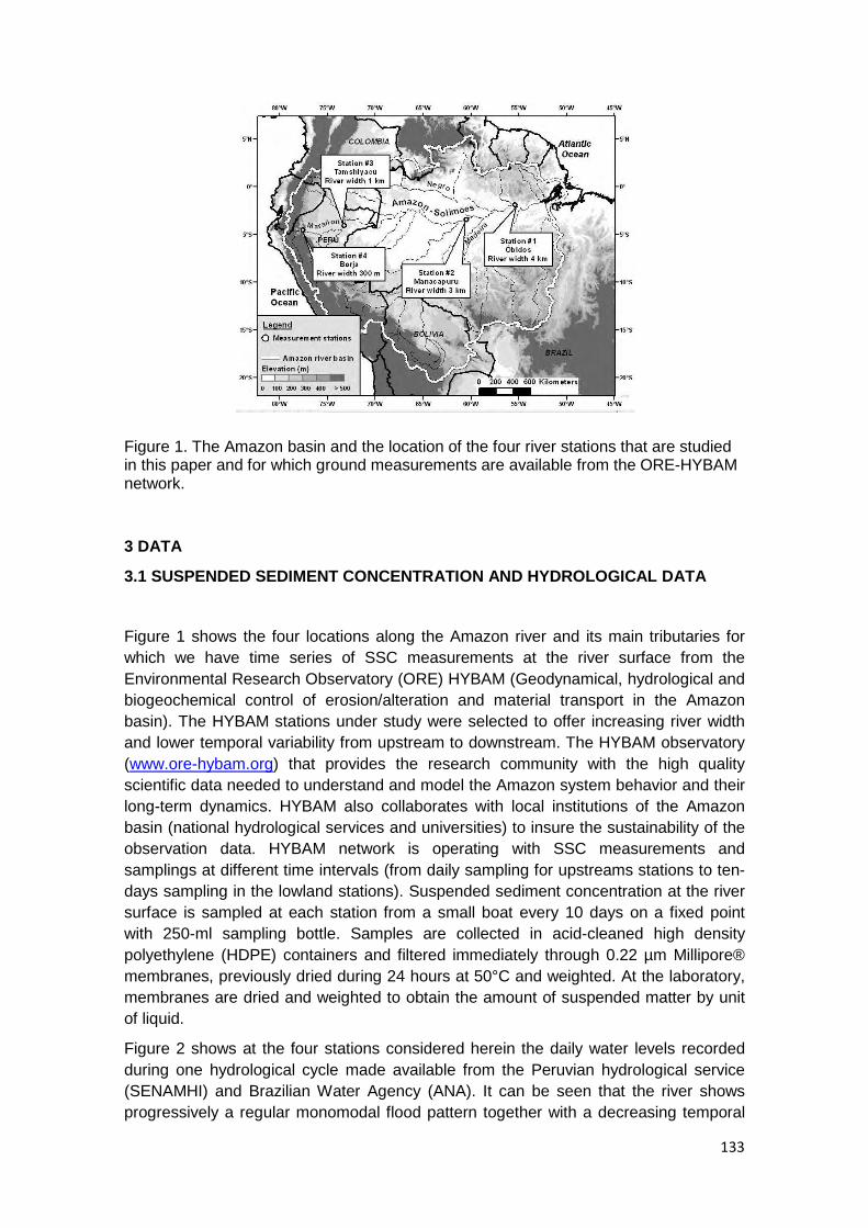
133

Figure 1. The Amazon basin and the location of the four river stations that are studied in this paper and for which ground measurements are available from the ORE-HYBAM network.

3 DATA

3.1 SUSPENDED SEDIMENT CONCENTRATION AND HYDROLOGICAL DATA

Figure 1 shows the four locations along the Amazon river and its main tributaries for which we have time series of SSC measurements at the river surface from the Environmental Research Observatory (ORE) HYBAM (Geodynamical, hydrological and biogeochemical control of erosion/alteration and material transport in the Amazon basin). The HYBAM stations under study were selected to offer increasing river width and lower temporal variability from upstream to downstream. The HYBAM observatory (www.ore-hybam.org) that provides the research community with the high quality scientific data needed to understand and model the Amazon system behavior and their long-term dynamics. HYBAM also collaborates with local institutions of the Amazon basin (national hydrological services and universities) to insure the sustainability of the observation data. HYBAM network is operating with SSC measurements and samplings at different time intervals (from daily sampling for upstreams stations to ten-days sampling in the lowland stations). Suspended sediment concentration at the river surface is sampled at each station from a small boat every 10 days on a fixed point with 250-ml sampling bottle. Samples are collected in acid-cleaned high density polyethylene (HDPE) containers and filtered immediately through 0.22 µm Millipore® membranes, previously dried during 24 hours at 50°C and weighted. At the laboratory, membranes are dried and weighted to obtain the amount of suspended matter by unit of liquid.

Figure 2 shows at the four stations considered herein the daily water levels recorded during one hydrological cycle made available from the Peruvian hydrological service (SENAMHI) and Brazilian Water Agency (ANA). It can be seen that the river shows progressively a regular monomodal flood pattern together with a decreasing temporal

134

variability from upstream to downstream. The SSC is strongly correlated with the runoff upstream but becomes partially decorrelated downstream. The four stations studied are Borja, Tamshiyacu, Manacapuru and Obidos. Borja (station #4) is located in the piedmont of the Andes, after the confluence of the Marañon and Santiago rivers in Peru. The river width varies roughly from 200 to 450 meters in the vicinity of the station. Formally, the union of the Ucayali and the Marañon rivers forms the Rio Amazonas, which changes its name to Solimões on the triple frontier between Peru, Columbia and Brazil, and later changes its name back to the Amazon only after it meets the Rio Negro near Manaus. Tamshiyacu (station #3) is located downstream the confluence of Marañon and Ucayali rivers at an altitude of 65 meters. The Amazon River at Tamshiyacu presents a mean discharge of 43.000 m3/s and the river width is of about 1000 meters. Manacapuru (station #2) is located in the central Amazon plain in Brazil where the Solimões have a discharge of about 100.000 m3/s. The river width at Manacapuru varies between 2000 and 4000 meters. Finally, Obidos (station #1) is located 900-kilometer upstream from the Amazon river mouth with a mean discharge of about 200.000 m3/s and a river width varying between 2000 and 4000 meters.

Figure 2. Variation of daily water levels recorded at the four stations understudy during 2005. For clarity, the water level minimum recorded at each station has been set to 0. Water level range increases downstream to upstream (station #4 to station #2). On the contrary the hydrological variability is much stronger upstream (station #4) in relation to the reduced catchment size while the Amazon River exhibits a well defined monomodal flood downstream (stations #1 and 2).

At station #4, 345 measurements are available from HYBAM database from May 2005 to June 2011 with a mean SSC of 730 ± 616 mg/l. At station #3, 502 measurements are available from January 2004 to December 2011 with a mean SSC of 322 ± 200 mg/l. At station #2, 359 measurements are available from January 2000 to December 2011 with a mean SSC of 103 ± 64 mg/l. At station #1, 266 measurements are available from January 2000 to November 2010 with a mean SSC of 78 ± 58 mg/l.

3.2 SATELLITE IMAGES

The Collection 5 atmospherically-corrected surface reflectance products from Terra and Aqua MODIS sensors are utilized in this study. The MODIS data product

135

MOD09Q1/MYD09Q1 provides calibrated reflectance for two bands measured at 250-meter pixel resolution (http://modis.gsfc.nasa.gov) from the sensor on board Terra satellite. Band 1 is centered at 645 nm and band 2 at 858.5 nm. MODIS surface reflectance 8-day composite data in HDF format was acquired between February 2000 and November 2011 from the NASA Earth Observing System (EOS) data gateway. Two time series of data (250-meter products for both Terra and Aqua MODIS sensors) were chosen to analyze temporal variations of the reflectance through the seasonal cycle. We chose composite images because 1) the 8-day composite is compatible with the SSC sampling frequency (i.e. 10 days) that will be used for validation; 2) it reduces the amount of data to analyze as a large number of daily images cannot be used in view of the persistent cloud cover; 3) it significantly reduces the BRDF and atmospheric artifacts (Wang et al. 2010). Figure 3 shows MODIS 250-meter 8-day composites over the four measurement stations considered here. For pixel quality assessment we made use of the corresponding 500-meter product at a given date (MOD/MYD09A1) that provides detailed information of the image processing (Surface Reflectance Data State Quality Layer). For pixel selection, the following criteria were used: pixel flagged as “clear” (bit 00); no cloud shadow; low or average aerosol quantity; none or small cirrus presence and no adjacent cloud.

Figure 3. MODIS images acquired over the four river stations understudy : #1 Obidos (Brazil, 700 km from the Ocean); #2 Manacapuru (Brazil, 1300 km from the Ocean); #3 Tamshiyacu (Peru, 3200 km from the Ocean) and #4 Borja (Peru, 3800 km from the Ocean).

3.3 RADIOMETRIC MEASUREMENTS

Figure 4 shows surface reflectance measurements carried out using TriOs spectroradiometers during a field campaign along the Amazon River from station #3 to station #1 in Peru and Brazil during the high water period. Technical specifications of the TriOS-RAMSES sensors can be found on www.trios.de. The setup of the instrumentation was standard for above water remote sensing reflectance measurements (Mobley 1999). A cosine irradiance sensor detected the incident daylight, one radiance sensor measured the upwelling radiance from the water column (35° viewing angle - azimuth angle of 135° away from the sun) and another radiance sensor detected the sky radiance that is used to correct for skylight reflection effect at the air-water interface (Mobley 1999). In the article, the results are given as the surface reflectance which is the remote sensing reflectance times pi. Surface reflectance measurements were collected during 16 cruises along the two rivers draining the Andes (Amazon and Madeira rivers) in Peru and Brazil from 2007 to 2011 and for different seasons. A total of 229 measurements were used for validation of MODIS

4 Km 4 Km 4 Km 4 Km

#1 #2 #3 #4

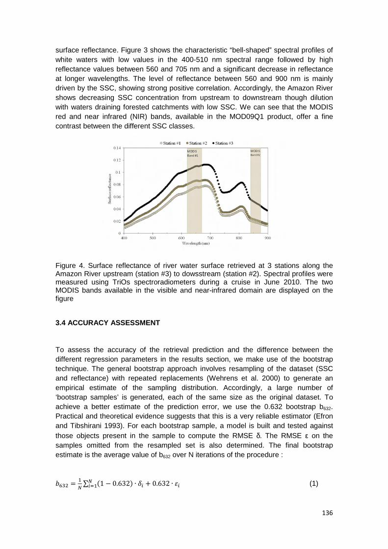
136

surface reflectance. Figure 3 shows the characteristic “bell-shaped” spectral profiles of white waters with low values in the 400-510 nm spectral range followed by high reflectance values between 560 and 705 nm and a significant decrease in reflectance at longer wavelengths. The level of reflectance between 560 and 900 nm is mainly driven by the SSC, showing strong positive correlation. Accordingly, the Amazon River shows decreasing SSC concentration from upstream to downstream though dilution with waters draining forested catchments with low SSC. We can see that the MODIS red and near infrared (NIR) bands, available in the MOD09Q1 product, offer a fine contrast between the different SSC classes.

Figure 4. Surface reflectance of river water surface retrieved at 3 stations along the Amazon River upstream (station #3) to dowsstream (station #2). Spectral profiles were measured using TriOs spectroradiometers during a cruise in June 2010. The two MODIS bands available in the visible and near-infrared domain are displayed on the figure

3.4 ACCURACY ASSESSMENT

To assess the accuracy of the retrieval prediction and the difference between the different regression parameters in the results section, we make use of the bootstrap technique. The general bootstrap approach involves resampling of the dataset (SSC and reflectance) with repeated replacements (Wehrens et al. 2000) to generate an empirical estimate of the sampling distribution. Accordingly, a large number of ‘bootstrap samples’ is generated, each of the same size as the original dataset. To achieve a better estimate of the prediction error, we use the 0.632 bootstrap b632. Practical and theoretical evidence suggests that this is a very reliable estimator (Efron and Tibshirani 1993). For each bootstrap sample, a model is built and tested against those objects present in the sample to compute the RMSE δ. The RMSE ε on the samples omitted from the resampled set is also determined. The final bootstrap estimate is the average value of b632 over N iterations of the procedure :

J��9 = <�∑ �1 − 0.632� ∙ �` + 0.632 ∙ �`�b< (1)

137

The factor 0.632 is used because it corresponds to the probability of getting an observation in a bootstrap sample. Although two hundred bootstrap samples are usually sufficient, two thousand bootstrap samples have been routinely used in this study.

4 RESULTS

4.1 RETRIEVAL OF SURFACE REFLECTANCE OVER RIVER STREAMS

Spectral mixing occurs when materials (e.g. endmembers) presenting distinct spectral properties are present within a certain pixel. Because river stream is only a few pixels wide at MODIS resolution, it may result in spectral mixing between water endmember, riverine vegetation or any element close to the river stream. Accordingly, it is possible that very few (or no) pure (non-mixed) water pixels can be found over the river stream in a MODIS image. In order to assess the impact of the spectral mixing among the river pixels, we take a look at the spectral mixing at red and infrared bands.

Although the spectral resolution offered by the 250-meter mode resolution is limited, i.e. only two bands, it may be sufficient to detect spectral mixing between water and vegetation since those targets present contrasted behaviors at red and NIR wavelengths. Unlike clear waters (such as oceanic waters) that exhibit low and decreasing reflectance values from the blue to the infrared, white water is characterized by strong reflectance values in the red and a lower but significant reflectance in the NIR. Hence, visible and NIR channels have been shown to be a robust estimator of suspended sediment concentration in coastal waters and rivers in various previous studies (Doxaran et al. 2002; Han 1997; Mertes et al. 1993). On the other hand, the strong positive difference between infrared and red bands, i.e. the red edge, is classically used to detect vegetation through the use of vegetation indices.

Because, there is no river mask available from MODIS 250-meter resolution products, we define a river mask from visual interpretation and that will be applied on MODIS images acquired at different dates over station #1 and station #3 (figure 3). Figure 5 displays the feature space representation of the red and infrared bands from two MOD09Q1 images for the pixels extracted from the river mask at stations #1 and #3. Analysis of these feature spaces makes it possible to assess the spectral mixing in each image. Theoretically, spectrally pure pixels are found at the vertices of the polygon or the line that binds the data space. Vegetation endmember is clearly separated in the different feature spaces with a strong NIR reflectance and a low red reflectance. White water endmember appears at the other extreme end with moderate reflectance values in the red and low value at the NIR channels. Most of all the pixels lies along the line connecting the two endmembers confirming that a two-endmember linear mixture model is reasonably good.

138

Figure 5. NIR vs. red scatterplot of cloud free pixels within the river mask at stations #1 (above) and # 3 (below). Almost all the river pixels are bounded by vegetation and water endmembers.

Feature space analysis shows that the retrieval of river stream reflectance using MODIS data is effectively hampered by the low spatial resolution that may result in few pure water pixels depending on river width. Spectral mixing may depend on four different factors : 1) river hydrology (depending on river water level, river width may vary and some sand banks may emerge (eventually covered by vegetation) and greatly affect the resulting spectral signature); 2) the variation of the MODIS effective resolution that is degraded at high view zenith angles because individual observations cover several adjacent grid cells at high view zenith angles (Justice et al. 2002); 3) the presence of some local residual atmospheric effects; 4) residual error in the geolocation and satellite navigation. In other words, it is impossible to retrieve geometrically pure water pixels from pixel-based mask and we need to develop a specific retrieval procedure to assess a posteriori the river water endmember in each image.

We propose a method allowing to retrieve automatically the water endmember within a MODIS scene. The methodology for getting estimates of the river water endmember from MODIS images is organized in four steps. Firstly, pixels are extracted over the river from each image using a pixel-based mask designed for the whole time series. Secondly, the pixels are partitioned into homogeneous clusters using K-means algorithm. Thirdly, vegetation endmember is retrieved using the same MODIS scene. Fourthly, linear mixing model (LMM) is tested. This procedure essentially focuses on

139

the autonomous determination of the water end-member by successive testing of each pixel cluster in the LMM to find the cluster that best describe the remaining groups of mixed water pixels over the river stream. The pixel cluster leading to the lowest residual in the LMM is retained as the water endmember.

The pixel-based river mask is manually outlined for each station and is used for the entire time series. As the algorithm takes into consideration the spectral mixing, it is not necessary that the mask match perfectly the river reach. Furthermore, as the river stream varies with the water level it would be impossible to match the river stream extent. The extent of the river mask along the stream is restricted to the vicinity of the station depending on the hydraulic conditions at each station (river confluence, connection with lakes). The pixels from the river mask are clustered using K-means algorithm, one of the simplest unsupervised learning algorithms. The K-means procedure attempts to find the centers of natural clusters in the data by minimizing total intra-cluster variance. In practice, the algorithm converges rapidly, taking only a few iterations. Yet, the algorithm may not return a global optimum because the quality of the final solution depends largely on the initial set of clusters (both number of clusters and initial centroid position). To overcome this limitation, the Monte Carlo method is used to generate 100 initial sets of centroid position. Then, for each initial set of clusters, we also test increasing numbers of clusters from 6 to 20. The set of clusters that minimizes the total intra-cluster variance at convergence is then selected for the next step.

The LMM equation for each cluster b (1< b < N) is :

X`,K = 6Lknm�. XLknm� +6lmimnkn`oa. Xlmimnkn`oa +�`,K (2)

where Ri,b stands for the cluster b reflectance at band i, fwater and fvegetation are the

fraction of each endmember, XLknm� and Xlmimnkn`oa are the reflectance of water and

vegetation endmembers at band i, and εb is the unmodeled residual. In equation (2), XLknm� and Xlmimnkn`oaare unknown and are selected among the N cluster retrieved using the K-means algorithm. The cluster representing the vegetation endmember is automatically selected as the one presenting the higher Infrared Red positive difference. The fraction of each endmember fi for each cluster is obtained by applying a least squares technique in order to minimize the unmodeled residual for red and infrared channels with an additional nonnegative constraint for each fraction. We successively test each cluster to select the best “river water endmember” candidate that achieves the lowest residual ε = ∑ �ε<,K + ε9,K��< assessed over the entire set of LMM equations corresponding to the N clusters.

Figure 6 shows the algorithm results over a series of 6 scatterplots from February to April 2006 corresponding to the cloud-free pixels within the river mask at station #3. For each date, the K-means cluster centroids are displayed and the water endmember

140

selected from Equation (2) is shown. As commented previously, the spectral mixing is basically described by a two endmember mixture (i.e., vegetation and water). However, we notice that the vegetation endmember reflectance and the dispersion of the reflectance values vary from one image to another as influenced by the cloud coverage, image acquisition geometry and hydrology. In particular, high albedo pixels resulting from unfiltered cloud edges can appear (date 2006 – 081 in Figure 6). Although the spectral mixing show large variability it can be noticed that the procedure succeeds in retrieving a stable water endmember reflectance over the short time series. In the next sections, water endmember reflectance behavior over larger time spans (12 years) will be further analysed.

Figure 6. NIR vs. red scatterplot of cloud-free pixels (white circles) within the river mask at station # 3 at 6 different dates from February to April 2006. Cluster’s centroid positions assessed from K-means unsupervised algorithm appear as black circles. The cluster selected as the water endmember with the automatic procedure appears as a grey star. For each image, satellite viewing angle and water endmember cluster characteristics are listed.

141

The geometry of acquisition is computed to detect sunglint cases where the reflectance increase dramatically. To remove thoses cases, we use the geometric formula proposed by Giglio et al. (2003) :

cosθ� = cosθ� . cosθ, − sinθ� sinθ, cosϕ (3)

Where θv and θs are the view and solar zenith angles, respectively, and φ is the relative azimuth angle. For θg angles lower than 20 degrees we automatically discard the data.

The algorithm presented will always produce an estimate provided there are sufficient cloud-free pixels in the mask. However, the existence of pure water pixels may not be confirmed a priori since it varies as a function of river hydrology and image acquisition geometry. Accordingly, we must define a test based on the spectral shape of the water endmember estimate. Red and NIR channels over turbid waters are strongly correlated and NIR reflectance should show lower values than red reflectance because of increasing absorption of water towards higher wavelengths. On the contrary, mixed pixels showing spectral contribution from vegetation banks or sand banks will show higher or similar reflectance values in the NIR channel than in the red channel. Based on this observation, we reject water endmember estimates that exhibit equal or higher reflectance in the NIR than in the red. If spectral signature is considered invalid, the water endmember estimate is rejected and the processing moves to the next image in the time series.

4.2 SURFACE REFLECTANCE RETRIEVAL ACCURACY

The benefit of water endmember retrieval over the river stream is first evaluated by comparing: 1) the mean reflectance of all pixels extracted from the river mask (the “apparent” river reflectance); 2) water endmember reflectance retrieved with our algorithm (the “effective” river reflectance). Figure 7 shows this comparison for MODIS band #2 (858 nm) of the MOD09Q1 (250-meters) product and for the whole MODIS archive over stations #1 (river width of 4 km) and #3 (river width of 1 km). It can be seen that the “apparent” estimates of the reflectance presents a greater variability and higher values than the post-processed water reflectance. For a narrower river (station #3), the spectral mixing is stronger and the impact of the reflectance extraction procedure is much more pronounced. The spectral mixing biases the apparent river reflectance towards higher values in the near IR because of the vegetation reflectance peak in this part of the spectrum. It is concluded that the water endmember retrieval technique allows the mixed river water pixels to be efficiently filtered out.

142

Figure 7. Comparisons of the MOD09Q1 NIR surface reflectance extracted over the Amazon river and of the water endmember retrieved with our algorithm (see section 4.1) for 2 river reaches : station #1 (river width 4 km) and #3 (river width 1 km).

Figure 8 compares post-processed MODIS surface reflectance (Aqua and Terra 8-day composites) and surface reflectance measurements realized during 16 cruises along the Amazon and Madeira Rivers. Out of the 229 measurements realized along the Amazon and Madeira Rivers, 73 were used for matchups with MODIS-Terra images and 80 were used for matchups with MODIS-Aqua. MODIS data were processed over the river reachs where were acquired the radiometric measurements along the Madeira, Solimoes and Amazon rivers. Although difficult to measure, the variability of the field surface reflectance was estimated from 90 measurements assessed over four grids at two river reaches (Station #2 and Borba station along the Madeira River). From these measurements, we assessed a relative mean standard deviation of surface reflectance across the river reach varying from 4.1 % up to 10.7 % at red band and from 10.9 % up to 19.6 % at NIR band. A total uncertainty of 7 % (red band) and of 15 % (NIR band) was finally considered for the measured surface reflectance. For MODIS surface reflectance, the reflectance at a given point stands for the water endmember

143

estimates from the procedure described in the previous section. Error bars stand for the standard deviation of the water end-member cluster assessed from our algorithm.

Figure 8. Comparison of MODIS 8-day composite surface reflectance with field radiometric measurements realized in the Amazon and Madeira Rivers from 2007 to 2011. Error bars stand for estimated uncertainty on the measured reflectance and for MODIS reflectance standard deviation of the water endmember cluster (see text).

Overall, fine agreement is found between both reflectance datasets at both red and NIR bands. The slope of regression is close to one in the near infrared, and it decreases in the red. It appears that MODIS surface reflectance is slightly higher than the field measurements and that the regression line intercept is positive. These observations agree with Wang et al. (2010) that analyzed MOD09 data over several test sites and showed that the magnitude of biases may vary with locations and is higher in the world regions of biomass burning with higher aerosol optical thickness such as the Amazon basin. Of interest, the post-processing algorithm allows a significant increase in the reflectance accuracy in the NIR as the matchups accuracy increase from 0.18 (no post-processing) to 0.81 (post-processed) for Terra images. At red band, the matchup accuracy increases slightly from 0.67 (no post-processing) to 0.74 (post-processed) for Terra images. This is consistent with the fact that water reflectance is less affected by the environment at red band than at NIR, limiting the improvement bring by the use of the reflectance post-processing.

4.3 SURFACE REFLECTANCE TEMPORAL BEHAVIOUR

We now analyze the temporal behavior of the river water endmember reflectance in relation to ground measurements. In this section, the composites from Terra and Aqua are merged to produce a more complete time series. For each date, both Terra and Aqua 8-day composites are compared and the image with the averaged lowest satellite viewing angle is selected. If both composites were acquired with the same viewing angle, the composite acquired with the lowest cloud coverage is preferred. The extent of the river mask using in the reflectance post-processing along the stream is restricted to the vicinity of the station depending on the hydraulic conditions at each station (river confluence, connection with lakes). The number of pixels outlined varies from one station to another with a minimum of 709 pixels at Borja (where the river width is the

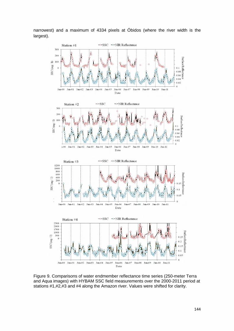
144

narrowest) and a maximum of 4334 pixels at Óbidos (where the river width is the largest).

Figure 9. Comparisons of water endmember reflectance time series (250-meter Terra and Aqua images) with HYBAM SSC field measurements over the 2000-2011 period at stations #1,#2,#3 and #4 along the Amazon river. Values were shifted for clarity.

145

Figure 9 compares the IR surface reflectance time series extracted automatically from MODIS 250m-products with SSC time series for the four field stations. The SSC presents a well-defined annual cycle in relation to the monomodal flood of the main Amazonian rivers with higher concentrations during the increasing water period (the concentration peak always occurs a few weeks before the flood peak) and lower concentrations during the decreasing water period. However, the seasonal cycle is less pronounced upstream and, at station #4, we observe a much stronger variability between SSC consecutive samples. Direct comparisons of field measurements and MODIS data are difficult because spatial and temporal samplings are extremely different. On the one hand, a 1-liter sample is taken on a fixed point. On the other hand, we retrieve the reflectance the MODIS on a much wider area (from hundreds to thousands of pixels) and with a temporal sampling depending on the local meteorology. However, we note that there is a general good agreement between the ground measurements and the reflectance and that the annual cycle is well-monitored by satellite data with correct timing. The automatic retrieval procedure appears to produce robust estimates over twelve consecutive hydrological cycles of the Amazon River.

4.4 SSC RETRIEVAL

Numerous works have studied the sensitivity of remote sensing reflectance to the suspended sediment concentration in oceanic and inland waters. A significant number of researchers have reported a strong positive correlation between SSC and spectral radiance (Bhargava and Mariam 1990, 1991; Doxaran et al. 2002; Hinton 1991; Novo et al. 1989a, b; Ritchie and Cooper 1988; Ritchie et al. 1987) and also noted that the relation may depend on the range of concentration, water types and suspended matter origin. Most studies agree that the best correlation between reflectance and SSC is between 700 and 900 nm in turbid inland waters.

Figure 10 presents the variation of reflectance for the MODIS 250-meter product, band 2, as a function of monthly average SSC concentrations using all the reflectance data and corresponding SSC estimates we had for the four stations. The SSC values present a wide range of values from 18 up to 1772 mg/l (mean = 224.0 mg/l, N = 387). There is a significant positive correlation between field data and surface reflectance. The determination coefficient shows that 70% of the variation of the reflectance is explained by the variation of the SSC. The relationship is more particularly remarkable as data originates from different years (from 2000 to 2011) and has been acquired in different stations located thousands of kilometers away from one another. The accuracy of the relationship between surface reflectance and SSC concentrations has been assessed using the Bootstrap technique. A power law model SSC = a . (RNIR)b shows the best fitting values with a = 41288 ± 21333 (95% confidence interval) and b = 1.93 ± 0.26 computed using 1000 bootstrap samples. The b632 estimate is 131.6 mg/l (60 % relative error).

146

Figure 10. Surface reflectance derived from MODIS 8-day composite (Terra and Aqua Satellite) as a function of the surface SSC. Surface reflectance was extracted over the four stations (see Figure 1). Measurements represent monthly average values and error bars stand for the standard deviation each month

Accuracy of the SSC retrieval is satisfactory given the major spatial scale difference between in-situ measurements and the reflectance data (assessed from buffers containing hundreds of pixels). However, a significant part of the observed dispersion may be related to different other factors such as : 1) site dependence; 2) reflectance variability introduced by miscalibration or adjacency effects; 3) temporal dependency of the reflectance – SSC relationship; 4) reliability of reflectance pre-processing.

5 DISCUSSION

In our study, we chose to assess the water reflectance from a river mask instead of a pointwise estimate. This approach has been considered since the cloud coverage constitutes a severe constraint in tropical humid area such as in the Amazon basin. Despite the excellent revisit frequency of MODIS (near daily coverage for each sensor) there is a high rate of rejection due to high probability of cloud coverage. On the one hand, considering a large number of pixels along the river in a same buffer increases the probability to get cloud-free and sun glint-free pixels for monitoring and matchups purposes. On the other hand, by increasing the number of pixels, the difference in the spatial scale between the river mask and the field pointwise estimates may alter the accuracy of the subsequent calibration and validation tests. Hence, the size of the mask is a result of a trade-off between the number of image available for calibration or SSC retrieval and the necessity to keep homogeneous reflectance estimate. We now discuss the benefits and limits in using such approach.

147

5.1 INFLUENCE OF THE MASK SIZE

To understand the importance of assessing large river mask in tropics, we tested different buffer sizes for the processing of MODIS time series starting from a 9-pixel buffer up to a 5000-pixel buffer that represents a 80-km long mask along the Amazon River at station #1. This station is appropriated for such test provided that the Amazon River discharge vary very slowly in time (see figure 2) and do not receive any large tributary that would change the water quality parameters. We define four classes for a coarse image quality classification taking into consideration cloud coverage and image acquisition geometry : i) class “0” stands for MOD09 composites presenting more than 95 % cloud coverage over the river mask; ii) class “1” include images presenting fine conditions with cloud coverage lower than 90 % over the river mask, viewing angle lower than 45° and θg greater than 25°; iii) class “2” include images presenting cloud coverage between 90 and 95 % or viewing angle larger than 45° or θg varying between 20 and 25° (equation 3); iiii) class “3” stands for sunglint conditions, e.g. θg smaller than 25°. It can be seen that class 1 represents the optimal image quality while class 2 may be flagged as “poor” quality. Processing a 10-year time series of MODIS Terra 8-day composites and considering a 9-pixel buffer, only 30 % of the images match the class 1 criteria. With increasing river mask size, more pixels with good quality are included. Consequently, we note a clear increase of the class 1 scenes from 36 %, 42 %, 56 up to 58 % when using 150, 700, 4000 and 5000 pixel-masks, respectively. In fact, this increase is not homogeneous during the year and the gain is much more pronounced during the rainy season when the cloud coverage is the strongest. When considering the class 1 and 2 scenes together, the production rate increase at 38, 49, 62, 76 and 78 % when considering river masks of 9,150, 700, 4000 and 5000 pixels, respectively. Interestingly, the class 3 scenes, which are affected by sunglint, only appear for 1.2 % relatively to the entire time series.

The percentages presented for Terra sensor are quite similar but slightly better for Aqua (83 % for a 5000-pixel mask). By merging both Terra and Aqua time series, the monitoring capacity is significantly improved: 87 % of the time a water endmember estimate is produced at quality 1 or 2 at station #1 using 250-meter resolution mode images from MODIS Terra and Aqua collections. At station #3, where the river mask is smaller (i.e., 850 pixels) due to the narrower river course, the probability of having class 1 or 2 images is of 54 % and 64 % when considering the Terra sensor and Aqua sensor, respectively. By merging both Terra and Aqua time series, the monitoring capacity is significantly improved: 71 % of the time a water endmember estimate is produced with class 1 or 2 pixels.

The high percentage of valid records using a large river mask makes that MODIS data meet a fundamental requirement for a monitoring system : the availability of a sufficient number of observations allowing for a constant monitoring whatever the period of the hydrologic cycle considered. Accordingly, though the tropical rainforest presents strong cloud coverage, we show that the near-daily coverage provided by MODIS would efficiently support the existing water quality monitoring networks operating in the Amazon basin that operate with a 10-day sampling schedule (HYBAM network) or a quarterly sampling schedule (Brazilian water agency network) in Brazil.

148

5.2 SSC VARIABILITY AT THE RIVER REACH

The ORE-HYBAM data provides unprecedented knowledge of the temporal behavior of SSC concentrations along the Amazon River. However the comparison of field data and MODIS estimates in uneasy provided that both estimates are not assessed over the same area. While MODIS reflectance is assessed on hundreds of pixels, the field data consists of pointwise estimates. Moreover, the ORE-HYBAM data provides SSC estimates but no error bars. When considering large river mask for MODIS processing, it is necessary to understand how relevant is an estimate assessed over areas covering various kilometers and how accurately it may be related to a pointwise estimate.

We conducted field experiments at station #2 and station #1 to link the SSC pointwise estimates to SSC estimates acquired simultaneously on a larger grid across the river reach at the same stations. We also investigated the variability of the pointwise estimate by sampling the vicinity of the ORE HYBAM measurement point at station #2 both temporally and spatially: 15 points were successively measured during one hour at the precise measurement point and 15 points were collected on a regular grid centered on the HYBAM measurement point. At high waters, we measured a mean SSC of 50 ± 5 mg/l, with a coefficient of variation (CV) of 10 %, for the 30 measurements at the HYBAM ORE sampling point. At low waters, we measured a mean SSC of 80 ± 10 mg/l (CV =12.5 %) at the HYBAM ORE sampling point.

We analyzed the variability of the SSC at larger scales by sampling 4 rectangular grids extending across the Amazon River reach at station #1 and station #2. Sample spacing made use of a grid interval of 250 meters by 250 meters with 35 points for the first grid, covering 2 sq.km, (6-km upstream the HYBAM measurement point). For the second grid, the grid interval was of 500 meters by 500 meters with 42 points, covering 5 sq.km (8-km downstream the HYBAM measurement point). For station #1, the first grid included 39 points (grid interval of 250 meters), covering 3.5 sq.km. and was centered on the HYBAM measurement point. The second grid included 25 points (grid interval of 250 meters), covering 2 sq.km and was 6-km downstream from the previous grid.

For station #2, at high waters, we measured a mean SSC value of 74 ± 14 mg/l (CV = 19.0 %) and 75 ± 29 mg/l (CV = 38.7 %) for the first and second grid, respectively. During low waters, we measured a mean SSC value of 128 ± 16 mg/l (CV = 12.5 %) and 101 ± 24 mg/l (CV = 23.7 %) for the first and second grid, respectively. Comparisons between SSC measurements at the ORE HYBAM measurement point and based on the intensive sampling over the 2 grids the same day show a relative difference of 1) 50 % during flood peak; 2) between 25 and 60 % during low water.

For station #1, during high waters, we measured a mean SSC of 64.5 ± 12.3 mg/l (CV = 19.0 %) and of 59.7 ± 6.5 mg/l (CV = 10.0 %) for the first and second grid, respectively. At low water, we measured a mean SSC of 43.7 ± 3.3 mg/l (CV = 7.5 %) and of 42.0 ± 2.5 mg/l (CV = 5.9 %) for the first and second grid, respectively. At this station, comparisons between SSC measurements at the ORE HYBAM measurement

149

point and based on the intensive sampling over the 2 grids show a relative difference of 1) 5.9 % and 10.3 % during flood peak; 2) -27 and -32 % during low water.

Based on these observations, we deduce that the uncertainty of the pointwise SSC estimates may be of 10 % minimum. The spatial heterogeneity of the surface SSC across the Amazon River reaches studied herein is significant but is low enough to ensure that pointwise and grid-based estimates show similar behavior. It remains ambiguous how much the size of the grid influences the SSC retrieval accuracy (either using remote sensing or field sampling), but clearly the hydraulic conditions of the river reach are a dominant factor in affecting the suspended sediment variability. Nonetheless the comparisons presented in this section show that it is unreasonable to expect the SSC retrieval based on MODIS data to outperform a level of about 20-30 % accuracy when compared to pointwise measurements. In this manner, the satellite ability to sense large river reaches may be seen as a complementary technique to the conventional field sampling practices making use of pointwise or transect-based estimates.

6 CONCLUSIONS

The objective of the paper was to investigate the feasibility of using MODIS surface reflectance data to identify variation in water color at the river surface on weekly and annual time frames. Our results suggest that the medium spatial resolution does not preclude the use of sensors such as MODIS for monitoring the world’s largest rivers. In particular, the surface reflectance data appears to be robustly linked with some water quality parameters such as SSC. However it is shown that reflectance retrieval is not easy over rivers because the coarse spatial resolution induces spectral mixing. Furthermore, the spectral mixing is shown to be changing depending on hydrological factors (river width controlled by flood stage, presence of sand banks) and acquisition geometry (depending on MODIS imaging angle). Accordingly, a specific algorithm has been developed for water endmember retrieval among the pixels extracted over the river stream. The core of this procedure lies in the autonomous determination of the water end-member by successively testing each pixel cluster over the river stream with different linear mixing models to find the cluster that can be used to describe at best the remaining groups of mixed water pixels. By using the information present in each image and a priori limited knowledge, the algorithm makes full use of the parameters available in the multitemporal dataset. This procedure has demonstrated its ability to provide robust estimates of the water reflectance over 12 consecutive hydrological cycles and for river reaches along the Amazon River presenting marked differences in terms of SSC range or river width. Hence, our study shows that it is now possible to get water quality parameter over rivers from medium resolution satellite for long term monitoring. By combining an excellent temporal resolution and a fine calibration quality MODIS paves the way for potentially rewarding remote sensing data applications to continental water monitoring. However more studies are needed to fully assess the retrieval accuracy of water quality parameters such as SSC. In particular, more robust inversion retrieval techniques will have to be developed using either statistical models or classical approaches based on the knowledge of water optical properties. The

150

monitoring of the world’s largest rivers will clearly benefit from such technological approach.

ACKNOWLEDGMENTS

This work has been supported by CNPq and MCT (Minister of Science and Technologies) in Brazil; IRD, INSU and French Spatial Agency (CNES) in France. We thank all the HYBAM observatory partners in Brazil and in Peru : the Brazilian Water Agency (ANA), the University of Brasilia (UnB), the Amazonas Federal University (UFAM), the Mineral Resources Research Company (CPRM), the Peruvian Hydrological Service (SENAMHI) and the Agrarian National University La Molina in Lima (UNALM).

BIBLIOGRAPHY

A.G. Dekker, R.J.V., S.W.M. Peters (2002). Analytical algorithms for lake water TSM estimation for retrospective analyses of TM and SPOT sensor data. International journal of remote sensing, 23, 15-35

Aranuvachapun, S., & Walling, D.E. (1988). Landsat-MSS Radiance as a measure of suspended sediment in the lower Yellow River (Hwang Ho). Remote Sensing of Environment, 25, 145-165

Bailly, J.-S., Le Coarer, Y., Languille, P., Stigermark, C.-J., & Allouis, T. (2010). Geostatistical estimations of bathymetric LiDAR errors on rivers. Earth Surface Processes and Landforms, 35, 1199–1210

Bhargava, D.S., & Mariam, D.W. (1990). Spectral refletance relationships to turbidity generated by different clay materials. Photogrammetric Engineering Remote Sensing, 56, 225-229

Bhargava, D.S., & Mariam, D.W. (1991). Effects of suspended particle size and concentration on reflectance measurements. Photogrammetric Engineering Remote Sensing, 57, 519-529

Bradley, J., Eden, M.J., & Rice-Evans, P. (1979). Remote sensing of suspended sediment in Amazonian rivers from Landsat imagery. In J.A. Allen & R. Harris (Eds.), Remote Sensing and National Mapping (pp. 110-116). Reading, UK: The remote sensing society - University of Reading

Chen, Z., Hu, C., & Muller-Karger, F. (2007). Monitoring turbidity in Tampa Bay using MODIS/Aqua 250-m imagery. Remote Sensing of Environment, 109, 207-220

Dekker, G.A., & Malthus, T.J. (1991). Quantitative Modeling of Inland Water Quality for High-Resolution MSS Systems. IEEE Transactions on Geoscience and Remote Sensing, 29, 89-95

Doxaran, D., Froidefond, J.M., Lavender, S., & Castaing, P. (2002). Spectral signature of highly turbid waters. Application with SPOT data to quantify suspended particulate matter concentrations. Remote Sensing of Environment, 81, 149-161

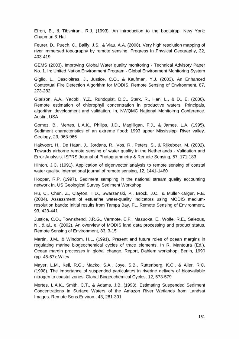
151

Efron, B., & Tibshirani, R.J. (1993). An introduction to the bootstrap. New York: Chapman & Hall

Feurer, D., Puech, C., Bailly, J.S., & Viau, A.A. (2008). Very high resolution mapping of river immersed topography by remote sensing. Progress In Physical Geography, 32, 403-419

GEMS (2003). Improving Global Water quality monitoring - Technical Advisory Paper No. 1. In: United Nation Environment Program - Global Environment Monitoring System

Giglio, L., Descloitres, J., Justice, C.O., & Kaufman, Y.J. (2003). An Enhanced Contextual Fire Detection Algorithm for MODIS. Remote Sensing of Environment, 87, 273-282

Gitelson, A.A., Yacobi, Y.Z., Rundquist, D.C., Stark, R., Han, L., & D., E. (2000). Remote estimation of chlorophyll concentration in productive waters: Principals, algorithm development and validation. In, NWQMC National Monitoirng Conference. Austin, USA

Gomez, B., Mertes, L.A.K., Philips, J.D., Magilligan, F.J., & James, L.A. (1995). Sediment characteristics of an extreme flood: 1993 upper Mississippi River valley. Geology, 23, 963-966

Hakvoort, H., De Haan, J., Jordans, R., Vos, R., Peters, S., & Rijkeboer, M. (2002). Towards airborne remote sensing of water quality in the Netherlands - Validation and Error Analysis. ISPRS Journal of Photogrammetry & Remote Sensing, 57, 171-183

Hinton, J.C. (1991). Application of eigenvector analysis to remote sensing of coastal water quality. International journal of remote sensing, 12, 1441-1460

Hooper, R.P. (1997). Sediment sampling in the national stream quality accounting network In, US Geological Survey Sediment Workshop

Hu, C., Chen, Z., Clayton, T.D., Swarzenski, P., Brock, J.C., & Muller-Karger, F.E. (2004). Assessment of estuarine water-quality indicators using MODIS medium-resolution bands: Initial results from Tampa Bay, FL. Remote Sensing of Environment, 93, 423-441

Justice, C.O., Townshend, J.R.G., Vermote, E.F., Masuoka, E., Wolfe, R.E., Saleous, N., & al., e. (2002). An overview of MODIS land data processing and product status. Remote Sensing of Environment, 83, 3-15

Martin, J.M., & Windom, H.L. (1991). Present and future roles of ocean margins in regulating marine biogeochemical cycles of trace elements. In R. Mantoura (Ed.), Ocean margin processes in global change. Report, Dahlem workshop, Berlin, 1990 (pp. 45-67): Wiley

Mayer, L.M., Keil, R.G., Macko, S.A., Joye, S.B., Ruttenberg, K.C., & Aller, R.C. (1998). The importance of suspended particulates in riverine delivery of bioavailable nitrogen to coastal zones. Global Biogeochemical Cycles, 12, 573-579

Mertes, L.A.K., Smith, C.T., & Adams, J.B. (1993). Estimating Suspended Sediment Concentrations in Surface Waters of the Amazon River Wetlands from Landsat Images. Remote Sens.Environ., 43, 281-301

152

Miller, R.L., & McKee, B.A. (2004). Using MODIS Terra 250 m imagery to map concentrations of total suspended matter in coastal waters. Remote Sensing of Environment, 93, 259-266

Mobley, C. (1999). Estimation of the Remote-Sensing Reflectance from Above-Surface Measurements. Applied Optics, 38, 7442-7455

Molinier, M., Guyot, J.L., Oliveira, E., & Guimaraes, V. (1996). Les regimes hydrologiques de l'Amazone et de ses affluents. In P. Chevallier & B. Pouyaud (Eds.) (pp. 209-222). Paris: AIHS

Novo, E.M.L.M., Hamsom, J.D., & Curran, P.J. (1989a). The effect of sediment type on the relationship between reflectance and suspended sediment concentrations. International journal of remote sensing, 10, 1283-1289

Novo, E.M.L.M., Hamsom, J.D., & Curran, P.J. (1989b). The effect of viewing geometry and wavelength on the relationship between reflectance and suspended sediment concentration. International journal of remote sensing, 10, 1357-1372

Ritchie, J.C., & Cooper, C.M. (1988). Comparison of measured suspended sediment concentrations with suspended sediment concentrations estimated from Landsat MSS data. International journal of remote sensing, 9, 379-387

Ritchie, J.C., Cooper, C.M., & Yongqing, J. (1987). Using Landsat Multispectral Scanner data to estimate suspended sediments in Moon Lake, Mississippi. Remote Sensing of Environment, 23, 65-81

Robinson, M.C., Morris, K.P., & Dyer, K.R. (1998). Deriving fluxes of suspended particulate matter in the Humber estuary, UK, using airborne remote sensing. Marine Pollution Bulletin, 37, 155-163

Schalles, J.F., Gitelson, A., Yacobi, Y.Z., & Kroenke, A.E. (1998). Chlorophyll estimation using whole seasonal, remotely sensed high spectral-resolution data for an eutrophic lake. J. Phycol., 34, 383-390

Sioli, H. (1975). Amazon tributaries and drainage basins. Landscapes of river basins (South America) (pp. 199-213). New York: Springer Verlag

Thiemann, S., & Kaufmann, H. (2002). Lake water quality monitoring using hyperspectral airborne data - a semiempirical multisensor and multitemporal approach for the Mecklenburg Lake District, Germany. Remote Sensing of Environment, 81, 228-237

Wang, Y., Lyapustin, A.I., Privette, J.L., Cook, R.B., SanthanaVannan, S.K., Vermote, E.F., & Schaaf, C.L. (2010). Assessment of biases in MODIS surface reflectance due to Lambertian approximation. Remote Sensing of Environment, 114, 2791-2801

Wehrens, R., Putter, H., & Buydens, L.M.C. (2000). The bootstrap: a tutorial. Chemometrics and Intelligent Laboratory Systems, 54, 35-52

153

CAPITULO VI

----------------------------------------------------------------------------

Artigo C

154

Résumé

Cet article étudie la confluence des fleuves Marañon et Ucayali à partir de laquelle se

forme le fleuve Amazone au Pérou. L’ORE HYBAM y maintient une station hydro-

sédimentaire sur chaque cours d’eau avec le service hydrologique péruvien

(SENAMHI) : San Regis (SRG) sur le fleuve Marañon, Requena (REQ) sur le fleuve

Ucayali, et Tamshiyacu (TAM) sur le fleuve Amazonas (50 km en amont de la ville

d'Iquitos). A chaque station, la concentration en matières en suspension (MES) de

surface est mesurée tous les 10 jours. La station de REQ a enregistré des valeurs de

MES très faibles pendant plusieurs années qui, après comparaison entre les 3 stations,

se sont révélées être des erreurs d'échantillonnage du fait de la présence d’un affluent

local (Tapiche) d'eau noire.

Pour cette étude, les images MODIS sont calibrées à partir des données de MES de

surface issues de campagnes de mesures intensives aux trois stations du réseau

HYBAM réalisées entre 2005 et 2008. Ces données de campagne fournissent 3

estimations de MES de surface à chaque campagne ce qui améliore la robustesse de

la comparaison satellite – terrain. Ainsi, on trouve d’excellentes corrélations (r2) entre la

MES et la réflectance MODIS de 0.99, 0.87 et 0.80 pour les stations de TAM, SRG et

REQ respectivement. Trois équations sont créées mettant en relation la réflectance

infrarouge MODIS avec les données de MES de surface.

La validation est effectuée indépendamment et de deux manières :

1) D’abord en comparant les MES estimées par satellite et les données du réseau

HYBAM (données à 10 jours) aux deux stations montrant des enregistrements valides

(fleuves Amazone et Marañon) pendant deux cycles hydrologiques (2004 et 2005). La

RMSE entre les données prédites par satellite et mesurées in situ (prélèvements

ponctuels décadaires) est de 75 mg/l (RMSE relative de 27 %) à la station de TAM et

de 72 mg/l (RMSE relative de 45 %) à la station de SRG.

2) Ensuite, les données de MES de surface estimées par satellite sont utilisées pour

calculer une concentration moyenne sur la colonne d’eau grâce aux données de

campagne HYBAM. Les MES moyennes sur la section sont ensuite multipliées par le

débit liquide pour calculer un débit sédimentaire à chaque station dans la zone de

confluence. La différence relative de débit solide annuel (satellite vc

HYBAM/SENAMHI) est de -9.9% et 2.7% pour la station de TAM et de -1.58 et +1.43%

pour SRG, pour les deux années hydrologiques considérées. La comparaison des

débits solides déduit par satellite en amont (Marañon + Ucayali) et en aval (Amazone)

155

montre une excellente robustesse des estimations satellitaires (RMSE de 18 %, biais

de 3 % sur 104 mois de données) compatible avec une utilisation opérationnelle des

données MODIS pour le suivi des flux sédimentaires au sein du bassin amazonien.

Le débit sédimentaire annuel moyen estimé par satellite entre 2000 et 2009 est de 392,

150 et 270 millons de tonnes par an pour les stations de TAM, SRG et REQ. Le débit

solide de l’Amazone à la station de TAM est ainsi de l’ordre de 50 % de celui mesuré à

la station d’Obidos près de l’Océan Atlantique.

156

Resumo

No presente trabalho foram utilizadas imagens de satélite para a medição do fluxo de

sedimentos nos rios e a construção de uma serie temporal de dados para uma estação

mal calibrada.

O rio Amazonas (peruano) é formado na confluência dos rios Ucayali e Maranon. O

projeto HIBAM conjuntamente com o SENAMHI instalaram uma rede de

monitoramento da concentração de sedimentos, em suspensão de superfície (SSS),

com amostragens, cada 10 dias. Nestes rios são localizadas 3 estações: San Regis

(SRG) (4,51ºS; 73,91ºW) no rio Marañon, Requena (REQ) (5,03º S; 73,83º W) no rio

Ucayali e Tamshiyacu (TAM) (4,00ºS; 73,16ºW) no rio Amazonas (50 km a montante

da cidade de Iquitos). Na estação REQ foram observados dados muito menores e,

comparando com as outras estações, foi evidente que nesta estação tinha-se um erro

nas medições. A movimentação dos meandros neste rio fez que o ponto de

amostragem fique na pluma de um afluente (Tapiche) com negras, causando o erro.

O HIBAM realiza campanhas periódicas de medição de vazão liquida, conjuntamente,

são realizadas amostragens de concentração de sedimentos, em diferentes

profundidades, e, em várias verticais da secção do rio. Com estas amostras é possível

calcular a concentração média da secção (ASS) da estação e, posteriormente, estimar

a vazão sólida. Assim pode-se relacionar os dados SSS com os dados de ASS para

cada estação de amostragem.

Os produtos do sensor MODIS, MOD09Q1 e MYD09Q1 dos satélites TERRA e AQUA,

são imagens compostas de cada 8 dias com dados de reflectância calibrada e de 2

bandas radiométricas (vermelho e infravermelho). Os dados de reflectância

infravermelha foram relacionados com os valores de SSS das campanhas,

conseguindo valores da correlação de Pearson de 0,99; 0,87 e 0,80 para as estações

de TAM, SRG e REQ, respectivamente. Desta maneira, elaboraram-se 3 equações

que relacionam a reflectância infravermelha do MODIS com os dados de SSS. A

obtenção dos dados de reflectância das imagens foi realizada de jeito automático

utilizando o programa computacional MOD3R.

Na validação destas estimativas, foi estimada a vazão sólida, usando os dados

provenientes de MODIS e usando os dados da rede HIBAM. A diferença relativa de

descarga sólida anual foi de -9,9 e 2,7% para a estação de TAM e de -1,58 y +1,43%

para SRG, para os dois anos hidrológicos coincidentes. Ao não ter dados da rede

HIBAM na estação de REQ, foi realizado um balanço de massas entre as 3 estações.

157

Assim a descarga sólida em TAM deve ser igual à somatória das estações a montante

(SRG e REQ). O cálculo foi realizado com os dados MODIS, para o período entre os

anos 2000 e 2009. O balanço foi cerrado entre as estações a montante e a jusante,

com um erro médio quadrático de 18%.

A descarga anual promedio estimada é de 392, 150 e 270 milhões de ton/ano para as

estaçoes de TAM, SRG e REQ, respectivamente, para o período do ano 2000 a 2009.

158

Integration of Field Measurements and Satellite Observations to Derive River Solid Load in Poorly Gauged Basins

Raúl ESPINOZA VILLAR a1, Jean-Michel MARTINEZ abc, Jean-Loup GUYOT bc, Pascal FRAIZYbc, Elisa ARMIJOSd, Alain CRAVEe, Hector BAZÁNd, Philippe VAUCHELbcdf,

Waldo LAVADOdf.

a Instituto de Geociências, Universidade Nacional de Brasília, Campus Universitário Darcy Ribeiro, ICC Centro, 70910-900, Brasília, Brazil. raulev@unb.br

b LMTG, UMR5563, CNRS/IRD/Université Toulouse 3, 14 Avenue Edouard Belin, 31400 Toulouse, France. jean-michel.martinez@ird.fr

c IRD, UR154-Hybam, CP 7091 Lago Sul, CEP 71635-971, Brasilia, DF, Brazil.

dFacultad de Ingeniería Agrícola, Universidad Nacional Agraria La Molina, Avenida La Molina s/n, Lima 12, Peru

e Géosciences Rennes, UMR 6118, CNRS/Université de Rennes1, Campus de Beaulieu, 35042 Rennes, France

f Servicio Nacional De Meteorologia E Hidrologia Del Peru Jr. Cahuide 785 Jesús María, Lima11 - Peru

Article published: Journal of Hydrology

1 Corresponding author . Tel + 5561 3307-2433 - Fax +5561 3272-4286. Campus Universitário Darcy Ribeiro, ICC Centro, 70910-900, Brasília, Brazil

e-mail address: raulev@unb.br

159

ABSTRACT

The use of satellite imagery to assess river sediment discharge is discussed in the

context of poorly gauged basins. For more than three decades the Peruvian

hydrological service SENAMHI has been maintaining several gauging stations in the

lower part of the Amazon River catchment. This network has been recently

supplemented by the HYBAM program with a water quality monitoring network

distributed over 5 locations and allowing assessment of river discharge and surface

suspended sediment (SSS) concentration. In this paper, the three stations located near

the Marañon and Ucayali rivers confluence that form the Amazon River are more

specifically reviewed. Two stations provide complete time series of 10-day SSS

samples over the period considered. The third station, along the Ucayali River, failed to

provide valid estimates of sediment concentration at the river surface. The objective is

to use satellite data as a substitute for the missing records in order to assess the

Ucayali river sediment discharge that has never been directly assessed before; and to

extend in time the river sediment discharge records over the two other stations. Water

reflectance assessed from time series of MODIS satellite images is calibrated using

field sampling campaigns to provide satellite-based SSS estimates. Validation is

achieved on an independent dataset that is the 10-day SSS samples derived from the

HYBAM network. Over the 2004-2006 period, it is demonstrated that there is a good

agreement, better than 10%, between satellite-derived data and network data and for

two stations offerings complete field records. Making use of satellite-derived SSS

estimates assessed from 2000 to 2009, it is shown that the river sediment balance is

closed between upstream and downstream stations. The use of satellite data and of

their integration with field data in the context of lowly gauged basins is discussed and

different scenarios are proposed.

Keywords: Hydrology, Sediment discharge, Amazon, Remote sensing, MODIS

1. INTRODUCTION

The growing demand for information on water resources either locally or globally as

part of environmental studies and/or monitoring makes it necessary to consider various

methods that enable the collection of monitoring parameters. In hydrology, for example

determination of source, transport and delivery of constituents in a watershed is based

on a network of stations where frequent samples are needed to characterize the

variations in chemical and sediment concentrations that occur during the hydrological

cycle. Hence, the relevance and efficiency of hydrological monitoring is a function of

160

numerous measured parameters, of the sampling frequency and of the spatial

distribution of stations within the catchment area (Hooper, 1997).

It is generally accepted that the state of the world’s inland waters should be better

known. Valuable hydrological monitoring should provide both long term and

uninterrupted observations regardless of political and institutional contingencies that

may arise, as may be the case with multinational catchments. However, facilities and

maintenance costs tend to put a damper on the implementation of a hydrological

monitoring network. Indeed, it has been estimated that three quarters of the world

cannot afford a full-scale water quality monitoring infrastructure and will not be able to

get it in the near future (GEMS, 2003). As conventional inland water monitoring

techniques cannot catch up with the increasing need for monitoring the impact of local

and global changes, alternative solutions are required.

Satellite imagery can provide the synoptic, continuous long-term global observation

needed. It has been show that the optical qualities of water are closely linked to some

quality parameters of interest such as turbidity (A.G. Dekker, 2002; Mertes et al.,

1993), algal pigment (Gohin et al., 2002; Schalles et al., 1998), organic matter

(Vodacek et al., 1995) likewise they offer invaluable information for the detection of oil

spills (Lennon et al., 2006). However, those observations have usually been limited to

one-shot studies owing to the unavailability of spaceborne platforms offering adequate

spatial resolution and time revisit frequency for most continental water bodies. In a

recent study, global monitoring spaceborne sensors such as MODIS have been used

to complete a monitoring network and assess the SSS at the Amazon river surface in

Brazil for several years (Martinez et al., 2009). This opens up new prospects in the

monitoring of surface water quality since MODIS sensors provide global coverage daily

which in turn enables water reflectance to be estimated anywhere in the world.

Monitoring of sediment transport in river systems is a good way of assessing erosion

and sedimentation processes that take place in the river catchment. The

Intergovernmental Council of the International Hydrological Programme (IHP)

emphasized the significant socio-economic and environmental impacts of these

processes in river basin management and the fact that they are still poorly understood

for practical use. A better knowledge of sediment transport becomes critical in areas

were monitoring remains inadequate such as in the largest watersheds of the world

both in boreal and tropical areas which may be the first to suffer from climate change.

In this study, MODIS data is used to complete a monitoring network covering the

Amazon River in Peru. In that area, the Peruvian water agency (SENAMHI) has been

161

monitoring the main river water level for more than 20 years but no information was

available for basic water quality parameters till a few years ago. Since 2004, the

HIBAM program installed with the SENAMHI a monitoring network of 5 stations in

western Peru to assess river SSS concentration as well as other basin water quality

parameters. Making use of ground measurements, satellite data are calibrated and

used to assess the Marañon, Ucayali and Amazon river sediment discharge. Accuracy

of the method will be discussed as well as the integration of classical ground

measurements together with spatial techniques.

2. SITE AND METHODS

2.1. Hydrology

The Amazonian basin drains 76% of Peruvian territory (IIAP, 1998) (977,900 km2) and

accounts for 98% of all Peruvian water resources (DGAS, 1995). At the confluence of

the Ucayali and Marañon rivers the Amazon River is formed. The Marañon River drains

350,000 km², of which 189,000 km² are mountainous areas in the Andes. The Ucayali

River drains 360,000 km2, of which 198,000 km2 represents mountainous areas in the

Andes. While the Marañon River drains the northern and central part of the Peruvian

Andean Cordillera, the Ucayali River drains the southern part. The Amazon plain is

scarcely populated, preventing the setting up of a dense hydrological station network.

Figure 1 shows the locations of the 3 gauging stations considered: San Regis (SRG)

(4.51ºS, 73.91ºW) along the Marañon River, Requena (REQ) (5.03º S, 73.83º W) along

the Ucayali River and Tamshiyacu (TAM) (4.00ºS, 73.16ºW) along the Amazon River.

The Peruvian Service of Meteorology and Hydrology (SENAMHI) has been recorded

river water levels twice a day at these 3 stations since the eighties. Since 2004, thanks

to the HYBAM program (http://www.ore-hybam.org), discharge is also measured by

Acoustic Doppler Current Profilers (ADCP) (Filizola and Guyot, 2004) during field

campaigns conducted three times a year, thereby greatly improving the quality of rating

curves at each station. Figure 2 shows the discharge time series for the three stations.

Hydrological cycle is very similar between SRG and REQ stations, with a flood peak

between March and May and a low water period between August and October. The

Marañon River mean annual discharge is about 16200 m3/s at SRG while the Ucayali

River mean annual discharge is about 11200 m3/s at REQ. As there is no significant

tributaries between the three stations, the river discharge at TAM is simply the sum of

REQ and SRG discharges, leaving measurement errors aside.

162

Figure 1: Location of the three hydrological stations in Peru: San Regis (SRG) along the Marañon River and Requena (REQ) along the Ucayali River, both rivers forming the Amazon River and Tamshiyacu (TAM), 80-kilometers downstream from the river

confluence.

Figure 2: Daily discharges for the Marañon (San Regis), Ucayali (Requena) y Amazonas (Tamshiyacu) rivers in the period 2004- 2008. Grey bars denote the nine

field sampling campaigns used for satellite calibration.

2.2. Monitoring Network

From August 2004 to July 2006, 65, 72 and 72 500-ml SSS samples were collected

respectively in REQ, SRG and TAM stations. SSS concentration at the river surface

has been sampled by local operator in a small boat every 10-days at a fixed point.

Bottles were stored and sent approximately every 3 months for filtering to the UNALM

(University National Agraria La Molina, Lima) laboratory. The samples were filtered

using 0.45µm cellulose acetate filters, previously dried for 24 h at 50 ºC and weigthed.

163

The weight difference before and after filtration allows the amount of suspended matter

to be determined by unit of liquid.

Figure 3 displays the temporal series of SSS concentration at TAM, SRG and REQ

stations. At TAM station, the mean SSS concentration is 317 mg/l, with a maximum of

846 mg/l and a minimum of 36 mg/l over the period considered. At SRG station, the

mean SSS concentration is 169 mg/l, with a maximum of 596 mg/l and a minimum of

31 mg/l. At REQ station, SSS samples yield a much lower value with a mean

concentration of 77 mg/l. After crosschecking SSS data from the 3 stations it becomes

apparent that measurements at REQ station were incorrectly sampled. Misplacement

of the measurement point within the plume of a local tributary draining the local forest,

the Tapiche river, is likely to have caused the error. Owing to its remoteness, sampling

was abandoned, meaning no 10-day SSS data is available for the Ucayali River.

Figure 3: 10-day surface suspended sediment concentration for the Marañon (San Regis), Ucayali (Requena) y Amazonas (Tamshiyacu) rivers in the period 2004- 2006

assessed by the HYBAM program.

2.3. Average Suspended Sediments Concentration.

In every station, sampling campaigns were conducted between 2005 and 2008 (8 in

TAM, 10 in SRG, 9 in REQ) to relate the 10-day surface samples to the average

suspended sediment (ASS) concentration across the whole river reach. The

measurements were defined in order to sample at least twice each period of the

hydrological samples : rising waters, flood peak and low water stage. During these

campaigns, the river discharge was measured with Acoustic Doppler Current Profiles

164

(ADCP). ASS was estimated using nine 500-ml water samples collected at three

verticals and three different depths from the surface to the bottom of the water column.

Each sample was processed using the same protocol as for the 10-day HYBAM

measurement network.

Figure 4 shows the SSS concentration as a function of the ASS concentration for all

campaigns. ASS concentration is strongly correlated with SSS concentration

confirming that the surface estimate is a robust predictor of the average concentration

in the river reach. Although one unique relation may be used for all the three stations

together, we segment the dataset by river, for better accuracy, and we will make use of

the following relationship between ASS and SSS concentration for respectively, TAM,

SRG and REQ stations :

ASSTAM = 1.12 SSSTAM + 34.3 (1)

ASSSRG = 1.00 SSSSRG + 72.5 (2)

ASSREQ = 1.18 SSSREQ + 67.6 (3)

The same equations will be used to derive ASS concentration from SSS concentration

over the whole period either by measurement network (2004-2006) or by satellite data

(2000- 2009).

Figure 4: Average suspended sediment concentration as function of surface suspended sediment concentration assessed during 9 sampling campaigns at REQ,

TAM and SRG stations. Sampling within the water column was based on 9 points samples at 3 different verticals and 3 increasing depths. Errors bars stand for the

standard deviation of all points collected at given campaigns, either at the river surface (3 points) or within the water column (12 points).

165

2.4. Satellite images

The Collection 5 atmospherically-corrected surface reflectance products from the Terra

and Aqua MODIS spaceborne sensors are utilized in this study. The MODIS data

product MOD09Q1 (Terra on-board sensor) and MYD09Q1 (Aqua on-board sensor)

provides calibrated reflectance for two radiometric bands measured at a 250 m pixel

resolution while offering near-daily time coverage over tropical areas

(http://modis.gsfc.nasa.gov). Band 1 is centered at 645 nm and band 2 at 858.5 nm

(infrared). MODIS surface reflectance 8-day composite data were acquired between

March 2000 and October 2009 from the NASA Earth Observing System (EOS) data

gateway. We chose composite images because i) the 8-day composite is compatible

with the 10-day field measurement sampling frequency; ii) it reduces the amount of

data to be analyzed as a large number of daily images cannot be used in view of the

persistent cloud cover and iii) it significantly reduces the directional reflectance effects

and atmospheric artifacts. For each date, the composites from Terra and Aqua are

automatically scanned and the image with the lowest cloud coverage is selected. When

both composites exhibit low cloud coverage, the composite acquired with the lowest

satellite viewing angle is preferred.

Retrieval of river stream reflectance using MODIS data is hampered by the low spatial

resolution that may result in few pure (non-mixed) water pixels, depending on the river

width and image acquisition geometry. Spectral mixing has been described extensively

in the literature and occurs when different materials are present in a same pixel. In the

context of this study, spectral mixing may occur between water, riverine vegetation or

sand banks. Accordingly, specific algorithm has been developed allowing deriving the

water endmember reflectance in each image. Firstly, river pixels are partitioned into

homogeneous clusters using the K-means algorithm (Martinez et al., Submitted;

Martinez et al., 2009). Then, the fraction of each endmember in each cluster is

obtained by applying a least squares technique to minimize the unmodeled residual.

The set of linear equations is then solved by testing every cluster as a possible “pure”

water endmember. The cluster leading to the lowest residual is retained as the water

endmember (Martinez et al., Submitted).

3. RESULTS

We calibrate the reflectance – SSS concentration by comparing the water endmember

reflectance retrieved from the 8-day MODIS composites and SSS measurements

assessed during the sampling campaigns between 2005 and 2008. Figures 5a), 5b)

and 5c) show respectively 8-day composite surface reflectance as a function of river

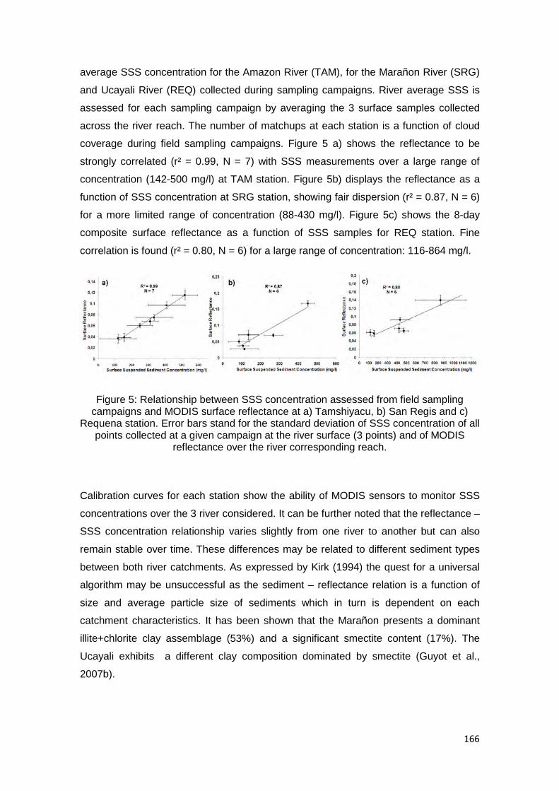
166

average SSS concentration for the Amazon River (TAM), for the Marañon River (SRG)

and Ucayali River (REQ) collected during sampling campaigns. River average SSS is

assessed for each sampling campaign by averaging the 3 surface samples collected

across the river reach. The number of matchups at each station is a function of cloud

coverage during field sampling campaigns. Figure 5 a) shows the reflectance to be

strongly correlated (r² = 0.99, N = 7) with SSS measurements over a large range of

concentration (142-500 mg/l) at TAM station. Figure 5b) displays the reflectance as a

function of SSS concentration at SRG station, showing fair dispersion (r² = 0.87, N = 6)

for a more limited range of concentration (88-430 mg/l). Figure 5c) shows the 8-day

composite surface reflectance as a function of SSS samples for REQ station. Fine

correlation is found (r² = 0.80, N = 6) for a large range of concentration: 116-864 mg/l.

Figure 5: Relationship between SSS concentration assessed from field sampling campaigns and MODIS surface reflectance at a) Tamshiyacu, b) San Regis and c)

Requena station. Error bars stand for the standard deviation of SSS concentration of all points collected at a given campaign at the river surface (3 points) and of MODIS

reflectance over the river corresponding reach.

Calibration curves for each station show the ability of MODIS sensors to monitor SSS

concentrations over the 3 river considered. It can be further noted that the reflectance –

SSS concentration relationship varies slightly from one river to another but can also

remain stable over time. These differences may be related to different sediment types

between both river catchments. As expressed by Kirk (1994) the quest for a universal

algorithm may be unsuccessful as the sediment – reflectance relation is a function of

size and average particle size of sediments which in turn is dependent on each

catchment characteristics. It has been shown that the Marañon presents a dominant

illite+chlorite clay assemblage (53%) and a significant smectite content (17%). The

Ucayali exhibits a different clay composition dominated by smectite (Guyot et al.,

2007b).

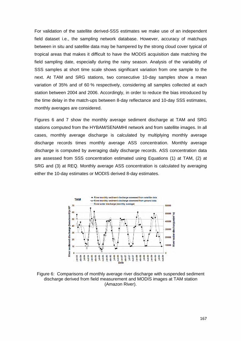
167

For validation of the satellite derived-SSS estimates we make use of an independent

field dataset i.e., the sampling network database. However, accuracy of matchups

between in situ and satellite data may be hampered by the strong cloud cover typical of

tropical areas that makes it difficult to have the MODIS acquisition date matching the

field sampling date, especially during the rainy season. Analysis of the variability of

SSS samples at short time scale shows significant variation from one sample to the

next. At TAM and SRG stations, two consecutive 10-day samples show a mean

variation of 35% and of 60 % respectively, considering all samples collected at each

station between 2004 and 2006. Accordingly, in order to reduce the bias introduced by

the time delay in the match-ups between 8-day reflectance and 10-day SSS estimates,

monthly averages are considered.

Figures 6 and 7 show the monthly average sediment discharge at TAM and SRG

stations computed from the HYBAM/SENAMHI network and from satellite images. In all

cases, monthly average discharge is calculated by multiplying monthly average

discharge records times monthly average ASS concentration. Monthly average

discharge is computed by averaging daily discharge records. ASS concentration data

are assessed from SSS concentration estimated using Equations (1) at TAM, (2) at

SRG and (3) at REQ. Monthly average ASS concentration is calculated by averaging

either the 10-day estimates or MODIS derived 8-day estimates.

Figure 6: Comparisons of monthly average river discharge with suspended sediment discharge derived from field measurement and MODIS images at TAM station

(Amazon River).

168

Figure 7: Comparisons of monthly average river discharge with suspend sediment

discharge derived from measurement and MODIS images at SRG station (Marañon

River).

Sediment discharge estimate is compared during 2 hydrological cycles (from August

2004 to July 2005 and August 2005 to July 2006) for which complete records are

available for both network-derived and satellite-derived SSS concentration. Both

network-derived and satellite-derived estimates of the river sediment discharge agree

closely in time and in quantity. At TAM station, the relative difference between both

annual solid discharge estimates is -9.9 % (sediment discharge of 496.106 tons with

network measurements and 546.106 tons with satellite data) for the 2004-2005

hydrological cycle. The relative difference decreases to -2.7 % for the 2005-2006

hydrological cycle at the same station (sediment discharge of 438.106 tons with field

measurements and 450.106 tons with satellite images). At SRG station the relative

difference is -1.58% (sediment discharge of 190.106 tons with field measurements and

193.106 tons with satellite images) in 2004-2005 hydrological cycles and +1.43% in

2005-2006 hydrological cycles (sediment discharge of 173.106 tons with field

measurements and 170.106 tons with satellite images). In both cases, solid discharge

minimum and maximum are correctly captured by the satellite although some

discrepancies can be found during the flood peak at SRG. The much higher SSS time

variability at SRG station (60%) is likely to introduce some bias in the matchups.

169

Figure 8: Amazon River monthly average sediment discharge (TAM station) as a function of Maranon (SRG station) and Ucayali(REQ station) river monthly average

sediment discharge. Sediment load is calculated for all stations from ASS concentration assessed by satellite data and river discharge is calculated from gauge records for the 2000-2009 hydrological cycles. Ideally, the sediment discharge at TAM

should match the sum of the sediment discharges at SRG and REQ station.

We compare the river sediment discharge at each station calculated from the ASS

concentration assessed by satellite and from the discharge assessed at each gauging

station. Because there is no significant tributary between SRG, REQ and TAM stations,

the sediment discharge at TAM station should be simply the sum of the sediment

discharge assessed at SRG and REQ stations. Figure 8 shows the monthly average

sediment discharge at TAM station as a function of SRG and REQ estimates for the

corresponding months during the 2000 to 2009 hydrological cycles, representing 104

months. The Root Mean Square (RMS) Error, that is the sum of the residuals, is about

6.106 tons/month (18 % relatively to the sample average). Dispersion appears to

increase as a function of sediment discharge causing a slight underestimation of

downstream sediment discharge of about 3%.

4. DISCUSSION

These results demonstrate that in the context of a poorly gauged basin with a reduced

set of monitoring network stations and of sampling campaigns, satellite data may be

used to provide long-term observations of suspended sediment discharge. Thus, this

work demonstrates that satellite information may be used either to 1) supplement

missing records, 2) crosscheck the data quality when field records are available, 3)

extend time series before or after a station has been installed or discontinued, 4)

provide estimates where installation and/or maintenance costs prevent the setting up of

170

a water quality monitoring station. The case of the REQ station along the Ucayali River

falls under options #2 and #4 because that station failed to provide robust data and

then was closed. Application #3 may stand for both SRG and TAM stations that exhibit

short time series starting in 2004 while MODIS data are available from March 2000.

Finally, application #2 may stand for any monitoring station in the context of

consistency checking between stations along the same rivers from upstream to

downstream.

The analysis of our dataset demonstrates that satellite data may be used efficiently to

complement a monitoring network when one or more station fails. In poorly gauged

basins, it may take a few weeks or even months to identify and fix a problem resulting

in a significant loss of data. Once calibrated, we show that satellite data may provide a

constant quality estimate at any station and for several years. MODIS sensors offer

global coverage and frequent observations meaning that the same method/sensor can

be used simultaneously over different locations, separated by hundreds of kilometers.

In this way, one the best application in the field of hydrology for satellite data may be

the assessment of both spatial and temporal heterogeneities at different scales. One

limitation may be the fact that satellite data can only provide estimate for the superficial

water layer (less than one meter in our case due to very strong water turbidity). It is

well known that SSS concentration can be a good predictor of the ASS concentration

for the whole river reach for fine sediments but may be much less robust for coarser

sediments such as sand. Spatial resolution of MODIS data, limits the use of such data

over small and medium size rivers, but hopefully that in a few years, earth-observation

satellites will offer a better spatial resolution combined with an adequate time revisit

frequency.

We have processed MODIS images from 2000 to 2009 to assess the river sediment

balance over the past decade. During that time, the mean annual sediment discharge

of the Marañon River is estimated by satellite data to be 150.106 tons/year showing low

inter-annual variability with a coefficient of variation of 12 %. Very good agreement is

found with the measurement network that assessed 168.106 tons/year over the 2004-

2006 period (Guyot et al. 2007a). Intra-annual variability remains moderate with a

range of variation of 4 to 24.106 tons/month. Between 2000 and 2009, the mean

annual sediment discharge of the Ucayali River is estimated by satellite data to be of

270.106 tons/year, with a coefficient of variation of 9 %. Monthly sediment discharge

shows strong variability from 2.106 tons/month, when occurred the lowest ever water

flow in august 2005, up to 56.106 tons/month,.

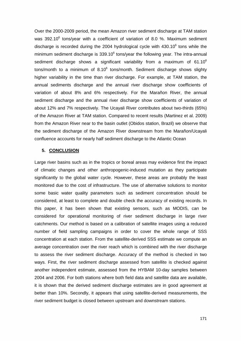
171

Over the 2000-2009 period, the mean Amazon river sediment discharge at TAM station

was 392.106 tons/year with a coefficient of variation of 8.0 %. Maximum sediment

discharge is recorded during the 2004 hydrological cycle with 430.106 tons while the

minimum sediment discharge is 339.106 tons/year the following year. The intra-annual

sediment discharge shows a significant variability from a maximum of 61.106

tons/month to a minimum of 8.106 tons/month. Sediment discharge shows slighty

higher variability in the time than river discharge. For example, at TAM station, the

annual sediments discharge and the annual river discharge show coefficients of

variation of about 8% and 6% respectively. For the Marañon River, the annual

sediment discharge and the annual river discharge show coefficients of variation of

about 12% and 7% respectively. The Ucayali River contributes about two-thirds (65%)

of the Amazon River at TAM station. Compared to recent results (Martinez et al. 2009)

from the Amazon River near to the basin outlet (Obidos station, Brazil) we observe that

the sediment discharge of the Amazon River downstream from the Marañon/Ucayali

confluence accounts for nearly half sediment discharge to the Atlantic Ocean

5. CONCLUSION

Large river basins such as in the tropics or boreal areas may evidence first the impact

of climatic changes and other anthropogenic-induced mutation as they participate

significantly to the global water cycle. However, these areas are probably the least

monitored due to the cost of infrastructure. The use of alternative solutions to monitor

some basic water quality parameters such as sediment concentration should be

considered, at least to complete and double check the accuracy of existing records. In

this paper, it has been shown that existing sensors, such as MODIS, can be

considered for operational monitoring of river sediment discharge in large river

catchments. Our method is based on a calibration of satellite images using a reduced

number of field sampling campaigns in order to cover the whole range of SSS

concentration at each station. From the satellite-derived SSS estimate we compute an

average concentration over the river reach which is combined with the river discharge

to assess the river sediment discharge. Accuracy of the method is checked in two

ways. First, the river sediment discharge assessed from satellite is checked against

another independent estimate, assessed from the HYBAM 10-day samples between

2004 and 2006. For both stations where both field data and satellite data are available,

it is shown that the derived sediment discharge estimates are in good agreement at

better than 10%. Secondly, it appears that using satellite-derived measurements, the

river sediment budget is closed between upstream and downstream stations.

172

6. BIBIOGRAPHY

A.G. Dekker, R.J.V. and S.W.M. Peters. 2002. Analytical algorithms for lake water TSM estimation for retrospective analyses of TM and SPOT sensor data. International journal of remote sensing, 23(1): 15-35.

DGAS (Dirección General de Aguas y Suelos). 1995. Hacia una gestión integrada de los recursos hídricos en el Perú. Ministerio de Agricultura, Perú.

Filizola, N. and Guyot, J.L. 2004. The use of Doppler technology for suspended sediment discharge determination in the River Amazon. Hydrological Sciences Journal, 49(1): 143-153.

GEMS. 2003. Improving Global Water quality monitoring - Technical Advisory Paper No. 1., United Nation Environment Program - Global Environment Monitoring System.

Gohin, F., Druon, J.N. and Lampert, L. 2002. A five channel chlorophyll concentration algorithm applied to SeaWiFS data processed by SeaDas in coastal waters. International journal of remote sensing, 23: 1639-1661.

Guyot, J.L., Bazán, H., Fraizy, P., and Ordoñez, J. 2007a. Suspended sediment yields in the Amazon basin of Peru: a first estimation, Water Quality and Sediment Behaviour of the Future: Predictions for the 21st Century. IAHS Publis., Perugia, pp. 3-10.

Guyot, J.L., Jouanneau, J.M., Soares, L., Boaventura, G.R., Maillet, N., and Lagane, C. 2007b. Clay mineral composition of river sediments in the Amazon basin. Catena, 71, 340-356

Hooper, R.P. 1997. Sediment sampling in the national stream quality accounting network US Geological Survey Sediment Workshop.

IIAP (Instituto de Investigación de la Amazonía Peruana). 1998. Información interna (Unidad de Información geográfica y Teledetección – UIGT), Iquitos, Perú.

Kirk, J. T. O. 1994. Light & Photosynthesis in Aquatic Ecosystems. Cambridge Univ. Press, New York.

Lennon, M., S. Babichenko, N. Thomas, V. Mariette, G. Mercier, and A. Lisin. 2006. Detection and mapping of oil slicks in the sea by combined use of hyperspectral imagery and laser-induced fluorescence, EARSEL, pp. 120-128.

Martinez, J.M., Guyot, J.L., Cochonneau, G., Espinoza Villar, R., Filizola, N., and Seyler, F. Submitted. Surface water quality monitoring of rivers with MODIS data - Application to the Amazon River. Remote Sensing of Environment.

Martinez, J.M., Guyot, J.L., Filizola, N. and Sondag, F., 2009. Increase in suspended sediment discharge of the Amazon River assessed by monitoring network and satellite data. Catena, 79: 257-264.

Mertes, L.A.K., Smith, C.T. and Adams, J.B.. 1993. Estimating Suspended Sediment Concentrations in Surface Waters of the Amazon River Wetlands from Landsat Images. Remote Sens.Environ., 43: 281-301.

173

Schalles, J.F., Gitelson, A., Yacobi, Y.Z. and Kroenke, A.E., 1998. Chlorophyll estimation using whole seasonal, remotely sensed high spectral-resolution data for an eutrophic lake. J. Phycol., 34: 383-390.

Vodacek, A. et al., 1995. The in situ and airborne fluorescence measurements to determine UV absorption coefficients and DOC concentrations in surface waters. Limnology and Oceanography, 40: 411-415.

174

CAPITULO VII

----------------------------------------------------------------------------

Artigo D

175

Résumé

Le fleuve Madeira est le troisième affluent de l’Amazone en terme de débit liquide mais

il représente près de 50 % des apports en matières en suspension (MES). Le fleuve

Madeira est formé par la confluence des fleuves Beni et Mamoré (chacun d'origine

andine), près de la frontière entre le Brésil et la Bolivie, et draine toute la partie Sud de

la Cordillère des Andes et des bassins provenant du bouclier brésiliens (très peu

chargés en MES).

Le long du fleuve Madeira, l’ORE HYBAM maintient 2 stations sédimentologiques avec

l’Agence de l’Eau du Brésil : Porto Velho (PV) et Fazenda Vista Alegre/Borba (FVA).

La concentration MES de surface y est mesurée tous les 10 jours depuis 1995. Depuis

2007, dix campagnes de mesures ont été effectuées, afin de mesurer la variation de la

concentration en MES le long du Madeira au Brésil ainsi que de collecter des

échantillons pour caractériser la granulométrie et la minéralogie du matériel

particulaire. Des mesures spectroradiométriques ont également été réalisées afin de

mesurer la réflectance télédétectée (Rrs) des eaux de surface du fleuve.

Les produits satellite MOD09Q1 et MYD09Q1 du capteur MODIS correspondants aux

satellites TERRA et AQUA respectivement, fournissent des données de réflectance

corrigées dans les bandes rouges et infrarouges et une résolution spatiale de 250m.

Ces images sont post-traitées selon la méthdologie proposée dans l’article B.

L’analyse conjointe des données satellitaires, radiométrique de terrain et des données

de MES à deux stations (Porto Velho et Borba) met en évidence une hystérésis dans la

relation Rrs – concentration en MES. En effet, il apparait que pour une même

concentration en MES, la Rrs est inférieure en période de pic de crue (Janvier – Avril),

un comportement cohérent avec celui détecté pour le coefficient de diffusion spécifique

de la MES comme décrit précédemment (Article A). Une légère variabilité dans la

granulométrie des particules de surface (plus grossières au pic de crue) pourrait

expliquer cette variation mais le jeu de données ne permet pas de conclure

définitivement sur la cause de la variation saisonnière

Cependant, l’utilisation d’un ratio Rrs(Infrarouge) / Rrs(Rouge) permet de s’affranchir de

cette sensibilité saisonnière et permet un suivi précis de la concentration en MES

comme l’atteste la validation des estimations satellites avec les données du réseau

HYBAM (r = 0.79 – N = 282) pour une large gamme de MES (4 – 1832 mg/ l). En

utilisant la même relation de bandes mais sur les données de spectroradiométrie de

terrain, on obtient une meilleure corrélation de 0.95 (N = 40). La différence de précision

entre les deux jeux de données s’explique par les différences d’échelles spatiales et

176

temporelles des mesures satellitaires en relation à des prélèvements ponctuels à 10

jours. Un modèle de régression en puissance dont les paramètres sont calculés par la

technique du bootstrap est proposé.

Les données satellites entre 2000 et 2011 sont moyennées au pas de temps mensuels

d’amont en aval, afin de suivre les processus hydro-sédimentaires qui se développent

au cours de la traversée du Madeira au sein de la plaine amazonienne jusqu’à sa

confluence avec le fleuve Amazone. Six stations virtuelles sont créées depuis Abunã

jusqu’à la confluence de l’Amazone représentant un transect de plus de 1000 km. De

manière générale, on observe une diminution de la concentration en MES d’amont en

aval. Lors du pic de crue, on observe une diminution marquée de la concentration en

MES amont (- 30 % en relation à la concentration à la station d’Abunã) alors que près

de la confluence avec l’Amazone on observe une plus grande stabilité (- 4 % sur les

160 derniers kilomètres). On observe le contraire en étiage lorsque les bassins

versants locaux, eux aussi en étiage, contribuent peu au début du fleuve Madeira. A

cette période, on observe une diminution de 22 % en moyenne sur le derniers 160

kilomètres. Ce processus de sédimentation est expliqué par le barrage hydraulique

formé par le fleuve Amazone à l’aval (qui est encore en crue à cette période).

Les processus de dilution et de sédimentation observés sont analysés en fonction du

débit du fleuve Madeira et de ses affluents. Les résultats obtenus sont d’autant plus

intéréssant que deux barrages hydroélectriques sont en cours construction sur le

fleuve Madeira et pourraient altérer les processus de trasnport sédimentaires naturels.

Les données MODIS pourraient ainsi contribuer à la caractérisation des impacts

environnementaux futurs de telles infrastrutures.

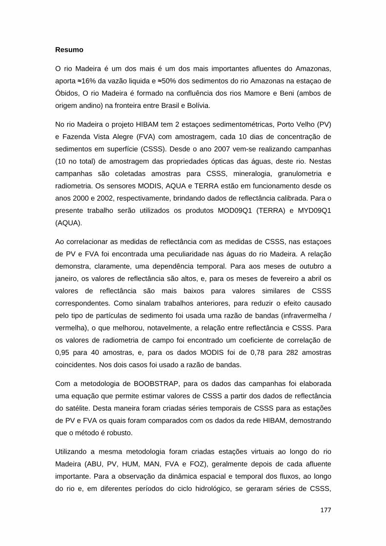
177

Resumo

O rio Madeira é um dos mais é um dos mais importantes afluentes do Amazonas,

aporta ≈16% da vazão liquida e ≈50% dos sedimentos do rio Amazonas na estaçao de

Óbidos, O rio Madeira é formado na confluência dos rios Mamore e Beni (ambos de

origem andino) na fronteira entre Brasil e Bolívia.

No rio Madeira o projeto HIBAM tem 2 estaçoes sedimentométricas, Porto Velho (PV)

e Fazenda Vista Alegre (FVA) com amostragem, cada 10 dias de concentração de

sedimentos em superfície (CSSS). Desde o ano 2007 vem-se realizando campanhas

(10 no total) de amostragem das propriedades ópticas das águas, deste rio. Nestas

campanhas são coletadas amostras para CSSS, mineralogia, granulometria e

radiometria. Os sensores MODIS, AQUA e TERRA estão em funcionamento desde os

anos 2000 e 2002, respectivamente, brindando dados de reflectância calibrada. Para o

presente trabalho serão utilizados os produtos MOD09Q1 (TERRA) e MYD09Q1

(AQUA).

Ao correlacionar as medidas de reflectância com as medidas de CSSS, nas estaçoes

de PV e FVA foi encontrada uma peculiaridade nas águas do rio Madeira. A relação

demonstra, claramente, uma dependência temporal. Para aos meses de outubro a

janeiro, os valores de reflectância são altos, e, para os meses de fevereiro a abril os

valores de reflectância são mais baixos para valores similares de CSSS

correspondentes. Como sinalam trabalhos anteriores, para reduzir o efeito causado

pelo tipo de partículas de sedimento foi usada uma razão de bandas (infravermelha /

vermelha), o que melhorou, notavelmente, a relação entre reflectância e CSSS. Para

os valores de radiometria de campo foi encontrado um coeficiente de correlação de

0,95 para 40 amostras, e, para os dados MODIS foi de 0,78 para 282 amostras

coincidentes. Nos dois casos foi usado a razão de bandas.

Com a metodologia de BOOBSTRAP, para os dados das campanhas foi elaborada

uma equação que permite estimar valores de CSSS a partir dos dados de reflectância

do satélite. Desta maneira foram criadas séries temporais de CSSS para as estações

de PV e FVA os quais foram comparados com os dados da rede HIBAM, demostrando

que o método é robusto.

Utilizando a mesma metodologia foram criadas estações virtuais ao longo do rio

Madeira (ABU, PV, HUM, MAN, FVA e FOZ), geralmente depois de cada afluente

importante. Para a observação da dinâmica espacial e temporal dos fluxos, ao longo

do rio e, em diferentes períodos do ciclo hidrológico, se geraram séries de CSSS,

178

desde o ano 2000 a 2011, para cada estação. Com séries de dados de mais de 11

anos foi estimado o ano médio, com um valor médio para cada mês, de toda a série de

dados e, também, para cada estação. Assim se têm o ano típico e seu comportamento

ao longo do rio de CSSS.

Os resultados foram analisados para 3 períodos hidrológicos: enchente, cheia e seca,

quando, geralmente, a CSSS decresce a jusante. No período de cheia, foi encontrado

uma diminuição mais notável à jusante e, também, mais pronunciado, na parte alta do

rio (≈30%). Já na parte baixa, a diminuição é de ≈4%. O contrário acontece na época

de seca, na qual, a diminuição é na parte baixa do rio. Nos primeiros 1160 km diminui

≈51% e no último trecho, de 160 km, diminui ≈22%. Esta caída da CSSS é ocasionada

pelo efeito do remanso gerado pelo rio Amazonas, neste período.

Com o presente trabalho podem se observar os processos de diluçao e sedimentação

do material particulado ao longo do rio Madeira e em diferentes épocas do ciclo

hidrológico.

Esta técnica é uma nova ferramenta que pode ser utilizada em outros rios para

monitoramento destes processos. Atualmente estão se construindo 2 barragens com

fins hidrelétricos. Com esta ferramenta pode se monitorar o impacto destas obras no

transporte de sedimentos.

179

A study of sediment transport in the Madeira River, Brazil, using MODIS remote-

sensing images

Raúl ESPINOZA VILLARa1, Jean-Michel MARTINEZabce, Marie LE TEXIERcd, Jean-Loup

GUYOTbc, Pascal FRAIZYbc, Paulo Roberto MENESESa, Eurides de OLIVEIRAe

a Instituto de Geociências, Universidade de Brasília, Campus Universitário Darcy Ribeiro, ICC Centro, 70910-900, Brasília, Brazil.

b GET, UMR5563, CNRS/IRD/Université Toulouse 3, 14 Avenue Edouard Belin, 31400 Toulouse, France.

c IRD, UR154-Hybam, CP 7091 Lago Sul, CEP 71635-971, Brasilia, DF, Brazil. d ENSEEIHT, INP-ENSEEIHT 2, rue Charles CAMICHEL - BP 7122 , 31071 TOULOUSE

Cedex 7 e Agência Nacional de Águas - Setor Policial Sul, Área 5, Quadra 3, Bloco L, Sala 112.

Brasília – DF Brazil

Accepted to Special Issue : “Hydrology, geochemistry and dynamic of South

American great river systems”

1 Corresponding author . Tel + 5561 3307-2433 - Fax +5561 3272-4286. Campus

Universitário Darcy Ribeiro, ICC Centro, 70910-900, Brasília, Brazil

e-mail address: raulev@unb.br

180

ABSTRACT

The Madeira River may contribute nearly half of the Amazon River sediment discharge to

the Atlantic Ocean, showing the highest erosion rates in the Amazon Basin. However, few

studies have assessed the Madeira River sediment budget and the transport processes

occurring in the main stem of the river. In this study, MODIS space-borne sensors were

used to analyze the suspended sediment transport processes along the main stem of the

Madeira River. Field measurements of suspended sediment concentration, spectral

radiometry and granulometry were performed during 10 cruises from 2007 to 2011. The

relationship between the spectral reflectance and the surface suspended sediment

concentration (SSSC) was analyzed using both field radiometric measurements and

satellite data. Ten-day SSSC samples acquired by the HYBAM monitoring network were

used to match satellite observations with field measurements performed from 2000 to

2011. Over 900 MODIS images of 6 different locations were processed to monitor the

SSSC dynamics in space and time. Satellite reflectance was found to be significantly

correlated with the SSSC. However, a seasonal dependency was demonstrated, most

likely caused by a variable granulometric distribution along the annual cycle. The ratio

between the red and near-infrared bands was found to be free of the seasonal

dependency (r = 0.79, N = 282), and a SSSC retrieval model was built from the satellite

data using a bootstrap resampling technique. The satellite-retrieved SSSC time series

showed excellent accuracy over the 11-year period and at two different stations located

800 kilometers from each other. The satellite data were averaged to analyze the SSSC

pattern temporally and spatially along the entire Madeira River, which provided evidence

of significant sedimentation and resuspension. The backwater effect caused by the two-to-

three-month lag between peak water in the Madeira and Amazon Rivers was used to

predict local sedimentation near the Madeira River mouth. Our results facilitated a precise

assessment of such sedimentation, which demonstrated an SSSC decrease 400 km

upstream from the Madeira-Amazon confluence.

181

1. Introduction

Sediment transport is of special significance in large tropical basins, which are known to

concentrate approximately 50% of the world’s solid fluxes from continental lands to the

oceans (Latrubesse et al., 2005). Among these basins, the Amazon Basin exhibits high

erosion rates in which most of the sediment is derived from the Andes and from large

floodplains that can store and release sediment on different time scales (Meade, 1994).

The size of the basin and the fact that the basin is moderately affected by anthropogenic

activities make it a valuable case study for understanding erosion and sediment transport

and their relation with past and present geomorphology (Baby et al., 2009) and climate

(Martinez et al., 2009).

Most studies on the sediment budget of the Amazon Basin have focused on the Amazon

River main stem, where the availability of hydrological data is better than in other areas of

the catchment (Filizola and Guyot, 2004; Gibbs, 1967; Martinez et al., 2009; Meade et al.,

1979). The Madeira River Basin drains approximately 25% of the Amazon Basin but may

account for nearly half of the sediment fluxes released to the ocean (Guyot et al., 1996).

The Madeira drainage basin forms the southwestern boundary of the Amazon Basin. It is

limited to the southwest by the Cordillera Oriental, which supplies a large quantity of

sediment to the rest of the basin and to the northeast by the Brazilian craton (Baby et al.,

2009). Sediment yield data show that the upper basin hosts the most elevated erosion

rates in the Amazon Basin, which are approximately 3 200 t x km-2 x year-1 on average,

with large variations ranging from 50 to 50 000 t x km-2 x year-1 (Guyot et al., 1996). The

total mass of suspended sediment exported from the eastern Andes and sub-Andean

drainage basins in Bolivia, excluding the Peruvian Madre de Dios subcatchment, has

been estimated to be approximately 500-600 million t x year-1 (Guyot et al., 1996). Using a

network of sampling stations for river sediment discharge assessment in Bolivia, Guyot et

al. (1996) estimated that the current sedimentation in the Madeira foreland basin may be

approximately 270 million t x year-1.

Sediment transport monitoring is critical in the Madeira River Basin because the

monitoring provides valuable information for economic activity that is dependent on river

flows and sediment discharge, such as ship transport. Interestingly, the construction of

two large hydroelectric power-generation dams in the upper reach of the Madeira River,

upstream of Porto Velho, may affect the natural sediment transport. Concerns about the

impact of these dams and the future behavior of sediment discharge as a function of

regional climate change (Espinoza Villar et al., 2009) require the development of robust

and cost-efficient monitoring methods adapted to large rivers. It has been shown that the

182

optical qualities of water are closely linked to certain quality parameters, such as turbidity

(A.G. Dekker, 2002; Mertes et al., 1993), algal pigment (Gohin et al., 2002; Schalles et al.,

1998) and organic matter (Vodacek et al., 1995). Recent studies on the Amazon Basin

have shown that space-borne global monitoring sensors can be used to efficiently monitor

river sediment discharge along the Amazon River (Martinez et al., 2009) (Espinoza et al.,

2012 ). In this study, we analyzed the optical properties of the Madeira River waters to

develop a surface suspended sediment concentration (SSSC) retrieval algorithm based

on MODIS satellite data. The SSSC estimates acquired over an 11-year period were

analyzed to assess the sediment transport processes along the main stream of the

Madeira River. Special attention was paid to the Madeira River mouth, where backwater

effects originating from the confluence with the Amazon River cause sedimentation.

2. The Study Area

With an area of 6.2 x 106 km2, the Amazon Basin is the world’s largest catchment,

delivering a water discharge of 6 600 km3 x year-1 (Molinier et al., 1996) and a sediment

discharge of 800 million t x year-1 based on measurements at the last gauged station

along the Amazon River that is not disturbed by sea tides (Martinez et al., 2009).

Sediments are transported principally from the Andes, which surround 12% of the Amazon

Basin. One of the most important tributaries is the Madeira River, which contributes 16%

of the Amazon River water budget and approximately 50% of the sediment discharge

(Filizola, 1999). According to the Sioli classification system (1957), the Madeira River is a

white-water river that is rich in dissolved material and suspension solids.

The Madeira River drains an area of approximately 1.4 106 km² and has a mean annual

discharge of 32 000 m3 x s-1 (Molinier et al., 1993). This river is among the ten largest

rivers in the world and was classified as a mega river (Latrubesse 2008). The Madeira

River is formed at the confluence of the Beni and Mamore Rivers near the border between

Brazil and Bolivia. These rivers are of Andean origin and present high sediment loads of

approximately 690 and 280 mg x l-1 at the river surface, respectively (Guyot et al., 1996).

The lower load of the Mamore River results from low sediment load tributaries that drain

the lowlands (e.g., the Guapore River) and strong sedimentation processes in the Andean

Piedmont (Guyot et al., 1996). Downstream from the Beni-Mamore confluence, all of the

tributaries are characterized by low sediment concentrations because they drain the

Amazonian lowlands on the Brazilian Shield (Figure 1). In Brazil, most of the tributaries

from the Abunã River down to the Aripuanã River confluence flow into the Madeira River

from its right bank as the Madeira River nears the Purus River catchment.

Figure 1: A map of the Madeira River and the major tributaries showing the stations along the river main stem maintained by the Brazilian Water Agency. The relief

data were extracted from the SRTM digital elevation model.

The Madeira River sediment budget estimates show significant variations from one study

to another because some studies use sediment discharge

whereas others are based on a network of stations at which the river water was sampled

for particle concentration assessment but with different sampling frequencies or sampling

methods (i.e., integrated versus surface sampling). Based on a limited set of sampling

field campaigns, Gibbs (1967) reported suspended sediment yields of approximately 217

x 106 t x year-1 at the mouth of the Madeira River in the Amazon. Subsequent studies

reevaluated the previous estimates and calculated a yield of 550 million t

et al., 1988; Martinelli et al., 1993). In Bolivia, the results obtained by the Climatological

and Hydrological Program of the Bolivian Amazon basin (PHICAB) for

Basin from 1983 to 1990 showed that the Beni and Mamore Rivers contribute a

suspended sediment yield of 223 million t x year

Roche and Fernandez Jauregui, 1988). Using the quarterly integrated s

sediment concentration data from the Brazilian Water Agency, Guyot et al. (1996)

calculated the sediment discharge at the Porto Velho station to be 320 million t x year

which is significantly higher than the value directly assessed upstream.

years of sampling records from the HYBAM network, Guyot et al. (2010) determined a

sediment discharge of 411 million t

sediment discharge-water discharge relationships they used for the Brazil

be disregarded for the Madeira Basin because the relationships show strong dispersion.

Figure 1: A map of the Madeira River and the major tributaries showing the stations along the river main stem maintained by the Brazilian Water Agency. The relief

data were extracted from the SRTM digital elevation model.

The Madeira River sediment budget estimates show significant variations from one study

r because some studies use sediment discharge-water discharge relationships,

whereas others are based on a network of stations at which the river water was sampled

for particle concentration assessment but with different sampling frequencies or sampling

thods (i.e., integrated versus surface sampling). Based on a limited set of sampling

field campaigns, Gibbs (1967) reported suspended sediment yields of approximately 217

at the mouth of the Madeira River in the Amazon. Subsequent studies

reevaluated the previous estimates and calculated a yield of 550 million t

et al., 1988; Martinelli et al., 1993). In Bolivia, the results obtained by the Climatological

and Hydrological Program of the Bolivian Amazon basin (PHICAB) for

Basin from 1983 to 1990 showed that the Beni and Mamore Rivers contribute a

suspended sediment yield of 223 million t x year-1 to the Madeira River (Guyot et al., 1993;

Roche and Fernandez Jauregui, 1988). Using the quarterly integrated s

sediment concentration data from the Brazilian Water Agency, Guyot et al. (1996)

calculated the sediment discharge at the Porto Velho station to be 320 million t x year

which is significantly higher than the value directly assessed upstream.

years of sampling records from the HYBAM network, Guyot et al. (2010) determined a

sediment discharge of 411 million t x year-1. However, the authors suggest that the

water discharge relationships they used for the Brazil

be disregarded for the Madeira Basin because the relationships show strong dispersion.

183

Figure 1: A map of the Madeira River and the major tributaries showing the water-gauge stations along the river main stem maintained by the Brazilian Water Agency. The relief

data were extracted from the SRTM digital elevation model.

The Madeira River sediment budget estimates show significant variations from one study

water discharge relationships,

whereas others are based on a network of stations at which the river water was sampled

for particle concentration assessment but with different sampling frequencies or sampling

thods (i.e., integrated versus surface sampling). Based on a limited set of sampling

field campaigns, Gibbs (1967) reported suspended sediment yields of approximately 217

at the mouth of the Madeira River in the Amazon. Subsequent studies

reevaluated the previous estimates and calculated a yield of 550 million t x year-1 (Ferreira

et al., 1988; Martinelli et al., 1993). In Bolivia, the results obtained by the Climatological

and Hydrological Program of the Bolivian Amazon basin (PHICAB) for the Upper Madeira

Basin from 1983 to 1990 showed that the Beni and Mamore Rivers contribute a

to the Madeira River (Guyot et al., 1993;

Roche and Fernandez Jauregui, 1988). Using the quarterly integrated suspended

sediment concentration data from the Brazilian Water Agency, Guyot et al. (1996)

calculated the sediment discharge at the Porto Velho station to be 320 million t x year-1,

which is significantly higher than the value directly assessed upstream. Finally, using 10

years of sampling records from the HYBAM network, Guyot et al. (2010) determined a

. However, the authors suggest that the

water discharge relationships they used for the Brazilian data should

be disregarded for the Madeira Basin because the relationships show strong dispersion.

184

3 Data acquisition and method

3.1. General Hydrology

Five water-gauge stations providing river-flow estimates are currently maintained by the

National Water Agency (ANA) along the Madeira River in Brazil. Starting from the Bolivia-

Brazil border, the stations are Abunã (ABU; upstream of the Abunã River confluence),

Porto Velho (PV), Humaita (HUM), Manicore (MAN) and Fazenda Vista Alegre (FVA) (see

www.ana.gov.br/hydroweb). Near-real-time data are available at the PV and FVA stations,

whereas at the other stations, the river water level is measured twice a day. The water

level was calibrated to the water discharge using the mechanical current-meter method at

all of the stations except for the PV and FVA stations, where acoustic doppler current

profiler (ADCP) measurements were also used (Filizola and Guyot, 2004). Figure 2 shows

the Madeira River water discharge time series at the ABU, PV, HUM, MAN and FVA

stations for the studied period. We note well-defined monomodal hydrograph with peaks in

March-April and low water between August and September. At the FVA station, the

maximum water discharge recorded over the period is 60 000 m³ x s-1, the minimum is 3

500 m³ x s-1, and the average discharge is approximately 27 000 m³ x s-1.

The water discharge increase between the ABU and FVA stations is 62% on average with

the inputs of the tributaries. The increase is relatively larger in May, up to 100%, and

smaller between October and December, down to 20%. For the main tributary of the

Madeira River, the ANA data show that the annual mean water discharge is 700, 1 400, 1

000 and 3 300 m³ x s-1 for the Abunã, Ji-Parana, Marmelos and Aripuana Rivers,

respectively. These rivers have similar hydrological cycles with a high water level between

February and April and a low water level in September, similar to the behavior of the main

stem of the Madeira River.

Comparisons of water discharge data from the tributaries and the river main stem show

inconsistencies that may result from insufficiently accurate water level-river discharge

relationships. The main problem occurs at the MAN station, where the flow is much higher

(i.e., 25% from June to December) than measured at the next downstream station on the

Madeira River, FVA.

Figure 2: The monthly water discharges for talong the main stem of the Madeira River recorded during 2000provided by the Brazilian water agency.

The large volume of the Amazon River affects the Madeira River water level in the lower

courses of the tributary, producing what is known as the backwater effect. This effect is

amplified by the two-to-three

Rivers, resulting in a hysteresis effect in the stage

Figure 3 for the FVA station. While the backwater effect in the HUM station records is not

measurable, it can be detected downstream at the MAN station

becomes significant at the FVA station, where the water level varies between 2 and 3

meters for the same discharge amount, depending on the hydrological period.

Figure 3: The relationship between water level and discharge at the FVA water-gauge station maintained by the Brazilian Water Agency before the AmazonMadeira River confluence. The measurements were performed with the mechanical current-meter method or the acoustic Doppler current profiler.

Figure 2: The monthly water discharges for the ABU, PV, HUM, MAN, and FVA stations along the main stem of the Madeira River recorded during 2000-provided by the Brazilian water agency.

The large volume of the Amazon River affects the Madeira River water level in the lower

courses of the tributary, producing what is known as the backwater effect. This effect is

three-month lag between peak water in the Madeira and

Rivers, resulting in a hysteresis effect in the stage-discharge relationship, as shown in

Figure 3 for the FVA station. While the backwater effect in the HUM station records is not

measurable, it can be detected downstream at the MAN station (Meade e

becomes significant at the FVA station, where the water level varies between 2 and 3

meters for the same discharge amount, depending on the hydrological period.

Figure 3: The relationship between water level and discharge at the FVA gauge station maintained by the Brazilian Water Agency before the Amazon

Madeira River confluence. The measurements were performed with the mechanical meter method or the acoustic Doppler current profiler.

185

he ABU, PV, HUM, MAN, and FVA stations -2009, which were

The large volume of the Amazon River affects the Madeira River water level in the lower

courses of the tributary, producing what is known as the backwater effect. This effect is

month lag between peak water in the Madeira and Amazon

discharge relationship, as shown in

Figure 3 for the FVA station. While the backwater effect in the HUM station records is not

(Meade et al., 1991) and

becomes significant at the FVA station, where the water level varies between 2 and 3

meters for the same discharge amount, depending on the hydrological period.

Figure 3: The relationship between water level and discharge at the FVA station, the last gauge station maintained by the Brazilian Water Agency before the Amazon-

Madeira River confluence. The measurements were performed with the mechanical

186

3.2. The suspended sediment from the monitoring networks

The ANA protocol requires quarterly measurements of the suspended sediment

concentration at five stations in its network using the depth integration method (using

integrating USD-49 samplers). However, the data are scarce for the 2000-2010 period.

The HYBAM network maintained by the ANA and the Institut de Recherche pour le

Développement (IRD) at the PV and FVA stations has been providing 10-day samples

from the river surface since 1995. To obtain the HYBAM data (see www.ore-network.org),

a local operator samples the SSSC every 10 days at a fixed point. The sample bottles are

stored and collected every 6 months to be processed at a laboratory at Amazonas State

University in Manaus, Brazil. The samples are filtered using 0.45-µm cellulose acetate

filters (Millipore) which are previously dried for 24 h at 60 ºC and weighed. After filtration,

the filters are dried for 24 h at 60 ºC and weighed again. The suspended matter

concentration is computed as the difference between the weight of the filter after and

before filtration divided by the volume of water collected. In this study, we will use the

HYBAM data, provided that this dataset furnishes surface estimates that match what the

satellite measures (because sunlight penetrates only a thin surface layer of the water

column) and provided that the HYBAM data enable access to SSSC temporal variability at

both intra- and inter-annual scales.

The SSSC time series from the HYBAM database exhibit a behavior similar to that of the

hydrological cycle, with an increase in the SSSC during the rising-water period and

decreasing values down to the low-water period. However, high SSSC values usually

occur from December to February, one or two months prior to the flood peak, highlighting

that a simple sediment discharge-water discharge relationship may not be applicable to

the Madeira River (Filizola and Guyot, 2009). The sediment discharge peak for the

Madeira River at Fazenda Vista Alegre occurs in March, whereas the water discharge

peak occurs between April and May (Filizola and Guyot, 2009). The SSSC exhibits a

strong variation from 1.1 to 1950 mg x l-1 at the PV station and between 4.5 and 823 mg x

l-1 downstream at the FVA station. The SSSC exhibits a downstream decrease. At the PV

and FVA stations, the SSSC averages 440 and 202 mg x l-1, respectively. Similar values

were reported by Guyot et al. (1996), who analyzed ANA data acquired from 1978 to 1994

and found an average concentration of 483 mg x l-1 at PV (23 samples) and 181 mg x l-1 at

FVA (35 samples). Considering the HYBAM data, the mean rate of SSSC decrease

between both stations over one year is 35%. However, this decrease varies with the

season, being higher in July (-51%) and lower in October (-6%).

187

3.3. Field-sampling campaigns

From 2007 to 2011, hyperspectral radiometric measurements were performed using

spectroradiometers during ten cruises that were conducted to acquire field data along the

Madeira River at different hydrological periods. During these cruises, spectral reflectance

data and water samples were collected simultaneously. The suspended sediment

samples were processed using the same protocol as that used for the 10-day HYBAM

measurement network.

The measurements were performed with three TriOS-RAMSES hyperspectral

spectroradiometers, two measuring radiance and one measuring downwelling irradiance.

The instruments were mounted on a steel frame that was fixed to the prow of the ship,

facing forward to minimize ship shadow and reflection. A cosine irradiance sensor

detected the incident daylight. One radiance sensor detected the reflected light from the

upper water column at a nadir angle of 30°, and another measured the diffuse radiance

originating from the region of the sky that reflects into the water-viewing radiance sensor.

The acquisition geometry recommended by Mobley (1999) from numerical modeling was

followed. The results are provided as the remote-sensing reflectance, which is the ratio of

reflected light from the upper water column (upwelling radiance) to incident light from the

sky (downwelling solar irradiance). Field reflectance data were used to simulate the

MODIS surface reflectance in the red and near-infrared (NIR) channels.

3.4 Satellite images

The Collection 5 atmospherically corrected surface reflectance products from the Terra

and Aqua MODIS space-borne sensors were used in this study. The MODIS data

products MOD09Q1 (Terra on-board sensor) and MYD09Q1 (Aqua on-board sensor)

provide calibrated reflectance for two radiometric bands measured at a 250-m pixel

resolution while offering near-daily time coverage over tropical areas

(http://modis.gsfc.nasa.gov). Bands 1 and 2 are centered at 645 and 858.5 nm,

respectively (Figure 5). The MODIS surface reflectance 8-day composite data were

acquired for March 2000 to July 2011 from the NASA Warehouse Inventory Search Tool

(WIST) data gateway. We chose composite images for three reasons: i) the 8-day

composite images are compatible with the 10-day field measurement sampling frequency;

ii) the 8-day composite images reduce the quantity of data to be analyzed because

persistent cloud cover renders a large number of daily images unusable; and iii) the 8-day

composite images significantly reduce the directional reflectance effects and atmospheric

188

artifacts. For each date, the composites from Terra and Aqua are automatically scanned,

and the image with the lowest cloud cover is selected. When both composites exhibit low

cloud cover, the composite acquired with the lowest satellite viewing angle is preferred.

The retrieval of river stream reflectance using the MODIS data is hampered by the low

spatial resolution that may result in few pure (non-mixed) water pixels, depending on the

river width and image acquisition geometry. Spectral mixing has been described

extensively in the literature and occurs when different materials are present in the same

pixel. In the context of this study, spectral mixing may occur between water, riverine

vegetation or sand banks. Accordingly, specific algorithms have been developed that

enable the derivation of the water endmember reflectance in each image. First, river pixels

are partitioned into homogeneous clusters using the K-means algorithm (Martinez et al.,

submitted; Martinez et al., 2009). Next, the fraction of each endmember in each cluster is

obtained by applying a least squares technique to minimize the un-modeled residual. The

testing of every cluster as a possible pure water endmember is performed to solve the set

of linear equations. The cluster leading to the lowest residual is retained as the water

endmember (Martinez et al., submitted).

The MODIS surface reflectance was retrieved for six different locations along the main

stem of the river (Figure 1) to create 11-year time series. For each station, 936 8-day

composites were processed from the MODIS Terra and Aqua sensors. The locations

match the five ANA water-gauge stations. An additional virtual station (i.e., the FOZ

station) was added to analyze the SSSC near the Madeira River mouth at the confluence

with the Amazon River. Data from the PV and FVA stations were used to analyze

reflectance-SSSC matchups with the HYBAM network data, whereas the other stations

enabled the study of the SSSC behavior in space and time.

4. Results

4.1. The SSSC and granulometry

Table 1 summarizes the measurements acquired during the 10 field-sampling campaigns

at each station along the Madeira River. The measurements consisted of the

simultaneous recording of spectroradiometric data and surface-water sampling. Three

field campaigns were conducted to visit most of the stations in the downstream direction

(i.e., the PV station to the FOZ station) in November 2009, March-April 2010 and July

2011. The stations more easily accessible from Manaus (i.e., the FOZ and FVA stations)

were visited more often, namely up to 10 times. At the FVA station, multiple sampling was

performed during 3 campaigns. The 40 SSSC records show a

25 to 622 mg x l-1.

Stations Low Water

ABU 1 PV 2

HUM 2 MAN 1 FVA 4 FOZ 4

Table 1: Field data in Madeira River from 2007 to 2011 and suspended sediment rangue data for three hydrological periods.

Particle-size distribution analyses were performed on 5

samples collected during the 2009 rising

Granulometric data were obtained using a laser grain

Mastersizer 2000 with a sample dispersion unit) at the CPRM Laboratory for Sediment

and Water Quality. Figure 4 shows the grain

stations during the 2009 and 2010 cruises. Fine

samples (99% of the grains are finer than 63

shift toward larger sizes during the flood peak. The med

was 9 µm in April and 5 µm in November at the MAN station, whereas the D50 decreased

from 7 µm in April to 5 µm in November at the HUM station.

Figure 4. The particle volume distribution for surface samples collected MAN stations on two cruises during the rising(April).

performed during 3 campaigns. The 40 SSSC records show a large range of values, from

Sample Number Low Water Peak Water Rising Water Total

1 1 3 6 1 3 1 1 3 3 10 17 2 4 10

1: Field data in Madeira River from 2007 to 2011 and suspended sediment rangue data for three hydrological periods.

size distribution analyses were performed on 5-liter surface-suspended sediment

samples collected during the 2009 rising-water cruise and the 2010 flood

Granulometric data were obtained using a laser grain-size measuring device (a

Mastersizer 2000 with a sample dispersion unit) at the CPRM Laboratory for Sediment

and Water Quality. Figure 4 shows the grain-size distribution at the HUM and MAN

stations during the 2009 and 2010 cruises. Fine-grained silt dominated the surface

samples (99% of the grains are finer than 63 µm). However, the distribution appeared to

shift toward larger sizes during the flood peak. The median particle-size distribution (D50)

m in November at the MAN station, whereas the D50 decreased

m in November at the HUM station.

Figure 4. The particle volume distribution for surface samples collected MAN stations on two cruises during the rising-water stage (November) and flood peak

189

large range of values, from

SSSC Range (mg/l)

105 106-401 110-286 61-418 43-300 25-622

1: Field data in Madeira River from 2007 to 2011 and suspended sediment rangue

suspended sediment

er cruise and the 2010 flood-peak cruise.

size measuring device (a

Mastersizer 2000 with a sample dispersion unit) at the CPRM Laboratory for Sediment

tribution at the HUM and MAN

grained silt dominated the surface

m). However, the distribution appeared to

size distribution (D50)

m in November at the MAN station, whereas the D50 decreased

Figure 4. The particle volume distribution for surface samples collected at the HUM and water stage (November) and flood peak

4.2. The Optical properties of the Madeira River

The analysis of the spectroradiometric measurements enables the registering of the

variations of the Madeira River spectra at different periods during the hydrological cycle.

Figure 5 shows the remote

periods at the PV station. The sediment

reflectance values in the blue

560 and 705 nm and a strong decrease in the reflectance at longer wavelengths. The

reflectance level seems to be directly related to the SSSC, with higher values occurring

during the rising-water period, particularly in the red and infrared parts of the spectra.

Figure 5 shows the location of the MODIS red and NIR bands. The MODIS bands match

the parts of the spectra where the reflectance shows greater sensitivity as a function

the SSSC.

Figure 5: The remote-sensing reflectance of the Madeira River water measured during three field sampling campaigns in November 2009 (rising water), April 2010 (flood peak) and July 2011 (low water). The gray curves denote the spectral MODIS red and near-infrared bands.

The low values in the blue and green parts of the spectra are characteristic of the light

absorption by CDOM and suspended sediment that is known to decrease exponentially

from ultraviolet wavelengths toward higher wavelengths

spectrum, light scattering and absorption are controlled by the concentration of inorganic

suspended matter, and the reflectance reaches its hig

on the TSS load. The contribution of pure water absorption increases rapidly in the near

infrared (NIR) region of the spectrum, which results in a significant decrease in reflectance

4.2. The Optical properties of the Madeira River

The analysis of the spectroradiometric measurements enables the registering of the

the Madeira River spectra at different periods during the hydrological cycle.

Figure 5 shows the remote-sensing reflectance as a function of wavelength at 3 different

periods at the PV station. The sediment-loaded Madeira River waters present low

ce values in the blue-green spectra, followed by high reflectance values between

560 and 705 nm and a strong decrease in the reflectance at longer wavelengths. The

reflectance level seems to be directly related to the SSSC, with higher values occurring

water period, particularly in the red and infrared parts of the spectra.

Figure 5 shows the location of the MODIS red and NIR bands. The MODIS bands match

the parts of the spectra where the reflectance shows greater sensitivity as a function

sensing reflectance of the Madeira River water measured during three field sampling campaigns in November 2009 (rising water), April 2010 (flood peak) and July 2011 (low water). The gray curves denote the spectral response functions of the

infrared bands.

The low values in the blue and green parts of the spectra are characteristic of the light

absorption by CDOM and suspended sediment that is known to decrease exponentially

engths toward higher wavelengths (Kirk, 1994). In the red part of the

spectrum, light scattering and absorption are controlled by the concentration of inorganic

suspended matter, and the reflectance reaches its highest value, which seems to depend

on the TSS load. The contribution of pure water absorption increases rapidly in the near

infrared (NIR) region of the spectrum, which results in a significant decrease in reflectance

190

The analysis of the spectroradiometric measurements enables the registering of the

the Madeira River spectra at different periods during the hydrological cycle.

sensing reflectance as a function of wavelength at 3 different

loaded Madeira River waters present low

green spectra, followed by high reflectance values between

560 and 705 nm and a strong decrease in the reflectance at longer wavelengths. The

reflectance level seems to be directly related to the SSSC, with higher values occurring

water period, particularly in the red and infrared parts of the spectra.

Figure 5 shows the location of the MODIS red and NIR bands. The MODIS bands match

the parts of the spectra where the reflectance shows greater sensitivity as a function of

sensing reflectance of the Madeira River water measured during three field sampling campaigns in November 2009 (rising water), April 2010 (flood peak)

response functions of the

The low values in the blue and green parts of the spectra are characteristic of the light

absorption by CDOM and suspended sediment that is known to decrease exponentially

. In the red part of the

spectrum, light scattering and absorption are controlled by the concentration of inorganic

hest value, which seems to depend

on the TSS load. The contribution of pure water absorption increases rapidly in the near

infrared (NIR) region of the spectrum, which results in a significant decrease in reflectance

191

beyond 705 nm. Although the concentrations in November 2009 and April 2010 were

similar (i.e., a 5% variation), there is a significant difference between both spectra,

indicating a possible seasonal dependence. Additionally, the light attenuation in the water

column was measured by assessing downwelling irradiance as a function of depth in the

euphotic zone. The data show that the light penetration in the water column in the red and

NIR is directly linked to the SSSC, with the euphotic zone varying between 20 cm and 1

meter. This result confirms that the riverbed does not affect the water’s spectral response

because the main channel is on average more than 15 m deep.

4.3. The seasonal control of the SSSC-reflectance relationship

The field spectroradiometric measurements collected along the Madeira River were used

to simulate the MODIS radiometric band behavior as a function of the SSSC using the

MODIS spectral response functions. Figure 6 shows the simulation of the MODIS near-

infrared band as a function of the SSSC, where each point is labeled with the month of

collection. Samples were collected during 10 field sampling cruises that covered a large

range of SSSCs (i.e., 25-622 mg x l-1). Low concentration or reflectance values

correspond to the low-water period (May - October), whereas higher values were found

during the rising-water and flood-peak period (November to April). The SSSC-remote-

sensing reflectance relationship appears to be linear for most of the SSSC range except

during the rising-water period (i.e., the November samples). For similar SSSC levels, the

November samples exhibit a significantly higher reflectance than the flood-peak samples

(principally, the March and April samples). This difference confirms our analysis in the

previous section, where the reflectance in the red and NIR part of the spectrum was much

higher in November than in April for the same range of SSSC. However, the limited

number of field radiometric samples makes a full assessment of this seasonal

dependency difficult.

We now analyze the SSSC-near-infrared reflectance matchups between the MODIS

images and the HYBAM network samples to improve our understanding of the relationship

variation for the entire SSSC range and in all of the periods of the hydrological cycle.

Figure 7 shows the average reflectance derived from MODIS for each month during the

2000-2011 period as a function of the average SSSC over the same period. The error

bars indicate the standard deviation of the reflectance and of the SSSC of all of the

samples collected during each month. The data are plotted for the PV and FVA stations.

The seasonal dependency is obvious, with a stronger reflectance during the rising-water

period (from October to January) than during the flood-peak period (February to April).

The SSSC-reflectance relationship seems to

effect seems to be less pronounced downstream following the sediment dilution by the

sediment-poor waters from the lowland tributaries between the PV and FVA stations.

Separate studies performed on the Amazon

neither upstream in the Peruvian Amazon River tributaries

downstream near the Amazon River mouth at the Obidos station

Figure 6: The NIR MODIS band simulated from field radiometric measurements as a function of the SSSC, which wasdenote the sampling month.

Figure 7: The MODIS surface reflectance in the NIR as a function of the SSSC from the HYBAM monitoring network. The black circles represent the PV station data, and the gray circles represent the FVA station data. The measurements represent monthly average values, and the error bars indicate the standard deviation for each month. The numbers denote the months from January (1) to December (12).

reflectance relationship seems to vary similarly for both stations. However, the

effect seems to be less pronounced downstream following the sediment dilution by the

poor waters from the lowland tributaries between the PV and FVA stations.

Separate studies performed on the Amazon River did not show this seasonal pattern,

neither upstream in the Peruvian Amazon River tributaries (Espinoza et al., 2012)

downstream near the Amazon River mouth at the Obidos station (Martinez et al., 2009)

Figure 6: The NIR MODIS band simulated from field radiometric measurements as a function of the SSSC, which was assessed during 10 sampling campaigns. The numbers denote the sampling month.

Figure 7: The MODIS surface reflectance in the NIR as a function of the SSSC from the HYBAM monitoring network. The black circles represent the PV station data, and the gray circles represent the FVA station data. The measurements represent monthly average values, and the error bars indicate the standard deviation for each month. The numbers denote the months from January (1) to December (12).

192

vary similarly for both stations. However, the

effect seems to be less pronounced downstream following the sediment dilution by the

poor waters from the lowland tributaries between the PV and FVA stations.

River did not show this seasonal pattern,

(Espinoza et al., 2012) nor

(Martinez et al., 2009).

Figure 6: The NIR MODIS band simulated from field radiometric measurements as a assessed during 10 sampling campaigns. The numbers

Figure 7: The MODIS surface reflectance in the NIR as a function of the SSSC from the HYBAM monitoring network. The black circles represent the PV station data, and the gray circles represent the FVA station data. The measurements represent monthly average values, and the error bars indicate the standard deviation for each month. The numbers

193

A significant number of studies have been conducted concerning SSSC and remote-

sensing reflectance, mostly over oceanic and coastal waters. Forget et al. (1999) showed

that the way in which the light is scattered and absorbed by inorganic suspended

sediment is a function of particle concentration, size distribution and the refraction index.

Therefore, for the same SSSC level, a difference in the measured reflectance may

indicate a differential suspended sediment type. Guyot et al. (1999) measured the

suspended sediment grain size from the Andes downstream near the Beni-Mamore

confluence. They showed that, downstream of the Andean Piedmont where strong

sedimentation processes occur for the larger grains, the suspended sediment

granulometric distribution exhibits reduced variability at different flood stages. Our results

suggest the same behavior but with certain slight variations between the hydrological

phases. The silt-dominated suspended sediment exhibited a finer distribution during rising

water than during the flood-peak stage. Analyzing the spectral reflectance from different

soil textures, Han and Rundquist (1996) showed that as SSSC increased, the reflectance

from the finest particles increased faster than that from the coarser soil. Additionally,

mineralogical differences in the suspended sediment may exhibit different reflectance

responses because the river flow may be dominated by several different upstream

sources. Guyot et al. (2007) suggested that the sediment from the Andes is enriched in

smectite as the river flows through the lowlands during the flood peak. Analyzing the

HYBAM samples acquired during one hydrological cycle, Viers et al. (2008) found that the

Solimões and the Madeira Rivers exhibit distinct suspended sediment chemical

compositions, although the same researchers did not detect seasonal variations in the

mineralogical composition of the rivers. Nevertheless, the same authors found significant

strontium isotopic composition variations over time in the suspended sediments, with a

difference between the high-water period and the remainder of the year. This seasonal

variation in the Sr isotopic composition remains unclear and may be caused by increasing

physical weathering during the rainy season, i.e., when landslides and riverbank erosion

may facilitate the input of radiogenic sediments not easily mobilized during periods of low

water. These observations highlight a limited but significant variability in suspended

sediment type and size distribution. This variability may be used to explain the seasonal

dependency of the reflectance over time. However, more research is necessary, using

optical modeling, to fully assess the phenomenon.

194

4.4. The satellite-based SSSC retrieval model

Light scattering by inorganic particles varies little as a function of wavelength. However,

the light absorption decreases exponentially toward higher wavelengths (Kirk, 1994).

Therefore, the optical properties of the suspended sediment may vary from one part of the

spectrum to another. Different authors (Doxaran et al., 2002; Froidefond et al., 2002;

Topliss et al., 1990) have proposed that the use of the ratio of the reflectance in at least

two different channels should reduce the overall sensitivity of the remote-sensing

reflectance to the inorganic particle type. We computed the ratio between the NIR and the

red MODIS bands for the entire dataset. Figure 8 shows the matchups between the

MODIS NIR/red surface reflectance ratios and the HYBAM samples from the PV and FVA

stations. The matchups were selected when the delay between the MODIS acquisitions

and the field samples was less than 4 days. The SSSC exhibited a wide range, from 4 to

1832 mg x l-1 with a mean value of 300 mg x l-1, for 282 field samples. There is a

significant positive relationship (r = 0.79, p < 0.05) between the SSSC and the reflectance

ratio. The determination coefficient shows that 61% of the variation in the reflectance ratio

is explained by the variation in the SSSC. Most of the residual dispersion may be

attributed to the differences in the spatial scale between the remote-sensing data,

averaged over tens of pixels and representing several square kilometers, and the field

samples acquired at the riverside in 250-ml bottles. Additional dispersion may be caused

by the time delay between the sampling and the closest cloud-free satellite image, which

rarely matches the exact day of sampling. Finally, natural SSSC heterogeneity across the

river reach is likely to increase the dispersion in the relationships between the satellite and

field samples. To provide a better view of the impact of these different dispersion factors,

Figure 8 shows the reflectance ratio-SSSC matchups based on the field

spectroradiometric measurements that should be free of most of the scale problems,

provided that the spectroradiometric measurements and water sampling were performed

simultaneously from a boat. For these field spectroradiometric measurements, 40

matchups are available, with an SSSC variation of 25 to 622 mg x l-1 and a mean value of

198 mg x l-1. The correlation factor is 0.96 and 91% of the variation in the field

spectroradiometric measurements are explained by the SSSC variations.

Figure 8: The NIR/red surface reflectance band ratio as a fdots represent matchups between field spectroradiometric measurements and simultaneously acquired water samples (N= 40) from 2007 to 2011. The spectroradiometric measurements were convolved to match the MODIS radiometric bands. The gray dots represent matchups between the MODIS data and the HYBAM SSSC data at the PV and FVA stations during 2000maximum delay criterion (N=282). The model was fitted for satellite data using least squares regression with 1000 bootstrap samples.

The best-fit model was assessed using least squares regression. To assess the variability

in the model parameters, we used the bootstrap resampling technique

2000). This technique proves particularly useful in case

limited. Its main uses are the estimation of accuracy measures and the construction of

confidence sets. Least squares regression shows that a power law model, SSSC = a.

(RNIR / RRed)b, provides the best

and b = 2.94 ± 0.37 computed using 1000 bootstrap samples.

4.5. SSSC time series from satellite data vs. those from conventional networks

The SSSCs were retrieved from the MODI

model defined in the previous section at the PV and FVA stations. Figure 9 compares the

satellite-derived and network SSSC samples at PV and FVA over the 2000

Good agreement was found, which shows t

temporal variability regardless of cloud cover, even when the cloud cover is persistent

during the rainy period. Over the common period of analysis between February 2000 and

March 2009, MODIS 8-day composites

the PV station, representing a 90% time coverage, which is the same percentage that the

HYBAM 10-day network achieved with 296 samples. At the FVA station, the MODIS

Figure 8: The NIR/red surface reflectance band ratio as a function of SSSC. The black dots represent matchups between field spectroradiometric measurements and simultaneously acquired water samples (N= 40) from 2007 to 2011. The spectroradiometric measurements were convolved to match the MODIS radiometric

he gray dots represent matchups between the MODIS data and the HYBAM SSSC data at the PV and FVA stations during 2000-2009 with a 4maximum delay criterion (N=282). The model was fitted for satellite data using least

1000 bootstrap samples.

fit model was assessed using least squares regression. To assess the variability

in the model parameters, we used the bootstrap resampling technique

This technique proves particularly useful in cases where the sample data are

limited. Its main uses are the estimation of accuracy measures and the construction of

Least squares regression shows that a power law model, SSSC = a.

, provides the best-fit values, with a = 1020 ± 150 (95% confidence interval)

0.37 computed using 1000 bootstrap samples.

4.5. SSSC time series from satellite data vs. those from conventional networks

The SSSCs were retrieved from the MODIS 8-day time composite time series using the

model defined in the previous section at the PV and FVA stations. Figure 9 compares the

derived and network SSSC samples at PV and FVA over the 2000

Good agreement was found, which shows that satellite data enable the monitoring of the

temporal variability regardless of cloud cover, even when the cloud cover is persistent

during the rainy period. Over the common period of analysis between February 2000 and

day composites enabled the calculation of 372 SSSC estimates at

the PV station, representing a 90% time coverage, which is the same percentage that the

day network achieved with 296 samples. At the FVA station, the MODIS

195

unction of SSSC. The black dots represent matchups between field spectroradiometric measurements and simultaneously acquired water samples (N= 40) from 2007 to 2011. The spectroradiometric measurements were convolved to match the MODIS radiometric

he gray dots represent matchups between the MODIS data and the HYBAM 2009 with a 4-day acquisition

maximum delay criterion (N=282). The model was fitted for satellite data using least

fit model was assessed using least squares regression. To assess the variability

in the model parameters, we used the bootstrap resampling technique (Wehrens et al.

s where the sample data are

limited. Its main uses are the estimation of accuracy measures and the construction of

Least squares regression shows that a power law model, SSSC = a.

150 (95% confidence interval)

4.5. SSSC time series from satellite data vs. those from conventional networks

day time composite time series using the

model defined in the previous section at the PV and FVA stations. Figure 9 compares the

derived and network SSSC samples at PV and FVA over the 2000-2011 period.

hat satellite data enable the monitoring of the

temporal variability regardless of cloud cover, even when the cloud cover is persistent

during the rainy period. Over the common period of analysis between February 2000 and

of 372 SSSC estimates at

the PV station, representing a 90% time coverage, which is the same percentage that the

day network achieved with 296 samples. At the FVA station, the MODIS

coverage outperformed the HYBAM network

coverage over the 2000-2009 period. These results demonstrate the potential use of

satellite time series to study the spatial and temporal variability in sediment transport. The

PV and FVA stations are located 880 kilomet

temporal behavior. However, we noted a significant SSSC decrease from upstream to

downstream, which we will analyze in the next section.

Figure 9: SSSC time series retrieved from 8and 10-day HYBAM samples during 2000the FVA station (below). The error bars indicate the standard deviation of the satellitederived SSSC estimate.

4.6. An analysis of the SSSC seasonal pattern

MODIS images

The sediment concentration at the virtual stations was calculated using MODIS 8

composites. The SSSC estimates were averaged for each month of the year, enabling

study of the seasonality of sediment transp

2000-2011. Figure 10 shows the variation of the SSSC along the Madeira River from the

ABU station downstream to the Madeira River mouth at the FOZ station in 3 periods:

rising water, flood peak and decreasing wat

from upstream to downstream in all of the periods. However, strong spatial variations

were detected from one part of the seasonal cycle to another. For the rising

(October to January), we noted the fol

as the water level rose and 2) a sharp SSSC decrease from upstream to downstream.

coverage outperformed the HYBAM network by more than 10%, with an 81% time

2009 period. These results demonstrate the potential use of

satellite time series to study the spatial and temporal variability in sediment transport. The

PV and FVA stations are located 880 kilometers from each other but exhibit similar

temporal behavior. However, we noted a significant SSSC decrease from upstream to

downstream, which we will analyze in the next section.

Figure 9: SSSC time series retrieved from 8-day composite MODIS images day HYBAM samples during 2000-2011 (white dots) at the PV station (above) and

the FVA station (below). The error bars indicate the standard deviation of the satellite

4.6. An analysis of the SSSC seasonal pattern along the Madeira River based on

The sediment concentration at the virtual stations was calculated using MODIS 8

composites. The SSSC estimates were averaged for each month of the year, enabling

study of the seasonality of sediment transport along the main stem of the river during

2011. Figure 10 shows the variation of the SSSC along the Madeira River from the

ABU station downstream to the Madeira River mouth at the FOZ station in 3 periods:

rising water, flood peak and decreasing water. The SSSC exhibited a decreasing trend

from upstream to downstream in all of the periods. However, strong spatial variations

were detected from one part of the seasonal cycle to another. For the rising

(October to January), we noted the following: 1) a consistent increase in the SSSC level

as the water level rose and 2) a sharp SSSC decrease from upstream to downstream.

196

by more than 10%, with an 81% time

2009 period. These results demonstrate the potential use of

satellite time series to study the spatial and temporal variability in sediment transport. The

ers from each other but exhibit similar

temporal behavior. However, we noted a significant SSSC decrease from upstream to

day composite MODIS images (black dots) 2011 (white dots) at the PV station (above) and

the FVA station (below). The error bars indicate the standard deviation of the satellite-

along the Madeira River based on

The sediment concentration at the virtual stations was calculated using MODIS 8-day

composites. The SSSC estimates were averaged for each month of the year, enabling

ort along the main stem of the river during

2011. Figure 10 shows the variation of the SSSC along the Madeira River from the

ABU station downstream to the Madeira River mouth at the FOZ station in 3 periods:

er. The SSSC exhibited a decreasing trend

from upstream to downstream in all of the periods. However, strong spatial variations

were detected from one part of the seasonal cycle to another. For the rising-water period

lowing: 1) a consistent increase in the SSSC level

as the water level rose and 2) a sharp SSSC decrease from upstream to downstream.

197

The SSSC decrease was considerable, particularly in the upper reaches (i.e., between the

ABU, PV and HUM stations), with a mean decrease of approximately 30% between ABU

and PV from October to January. Downstream, the SSSC decrease was weak, with a

diminution of 4% between the FVA and FOZ stations in December and January.

During the flood peak, from February to May, the overall SSSC level was lower and the

relative decrease was reduced compared with the rising-water period. The concentration

diminished by approximately 12% between the ABU and PV stations on average from

February to May. The strongest SSSC decrease occurred between the PV and HUM

stations, with a reduction of approximately 26% on average over the same period.

Downstream from the PV-to-HUM reach, the SSSC decrease was lower, with a reduction

of approximately 22% between the HUM and FVA stations. In the last reach, between the

FVA and FOZ stations, the decrease was on average 8%. During the low-water period

(i.e., June to September), the SSSC level was much lower along the entire Madeira River,

and the SSSC variation along the river main stem was reduced upstream. The SSSC

decrease between the ABU and FVA stations was on average 51% between June and

August and 28% in September. However, downstream from the MAN station, the SSSC

decrease was strong; namely, there was a 50% decrease from the MAN to FOZ stations

from June to August. This decrease was the strongest for that reach of the river in all of

the periods; namely, from June to August, the SSSC decrease between the FVA and FOZ

stations was 22%, whereas the decrease was limited to 5% on average from October to

May.

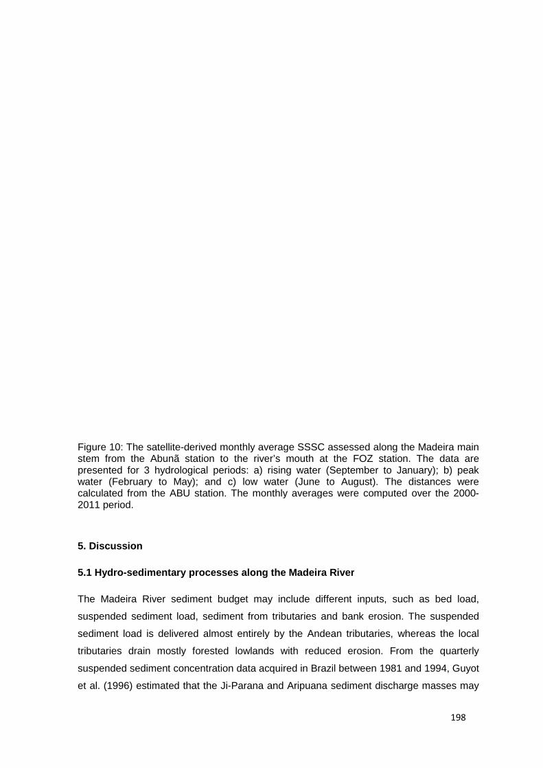
Figure 10: The satellite-derived monthly average SSSC assessed along the Madeira main stem from the Abunã station to the river’s mouth at the FOZ station. The data are presented for 3 hydrological periods: a) rising water (September to January); b) water (February to May); and c) low water (June to August). The distances were calculated from the ABU station. The monthly averages were computed over the 20002011 period.

5. Discussion

5.1 Hydro- sedimentary processes along the Madeira River

The Madeira River sediment budget may include different inputs, such as bed load,

suspended sediment load, sediment from tributaries and bank erosion. The suspended

sediment load is delivered almost entirely by the Andean tributaries, whereas the local

tributaries drain mostly forested lowlands with reduced erosion. From the quarterly

suspended sediment concentration data acquired in Brazil between 1981 and 1994, Guyot

et al. (1996) estimated that the Ji

derived monthly average SSSC assessed along the Madeira main stem from the Abunã station to the river’s mouth at the FOZ station. The data are presented for 3 hydrological periods: a) rising water (September to January); b) water (February to May); and c) low water (June to August). The distances were calculated from the ABU station. The monthly averages were computed over the 2000

sedimentary processes along the Madeira River

The Madeira River sediment budget may include different inputs, such as bed load,

suspended sediment load, sediment from tributaries and bank erosion. The suspended

sediment load is delivered almost entirely by the Andean tributaries, whereas the local

butaries drain mostly forested lowlands with reduced erosion. From the quarterly

suspended sediment concentration data acquired in Brazil between 1981 and 1994, Guyot

et al. (1996) estimated that the Ji-Parana and Aripuana sediment discharge masses may

198

derived monthly average SSSC assessed along the Madeira main stem from the Abunã station to the river’s mouth at the FOZ station. The data are presented for 3 hydrological periods: a) rising water (September to January); b) peak water (February to May); and c) low water (June to August). The distances were calculated from the ABU station. The monthly averages were computed over the 2000-

The Madeira River sediment budget may include different inputs, such as bed load,

suspended sediment load, sediment from tributaries and bank erosion. The suspended

sediment load is delivered almost entirely by the Andean tributaries, whereas the local

butaries drain mostly forested lowlands with reduced erosion. From the quarterly

suspended sediment concentration data acquired in Brazil between 1981 and 1994, Guyot

Parana and Aripuana sediment discharge masses may

199

not exceed 1.2 million and 2.9 million t x year-1, respectively, representing approximately

1% of the Madeira River sediment discharge that the same authors assessed at the PV

station. The measurements performed during our field sampling trips suggest that this

budget may not have changed since then. Few studies have been conducted on riverbed

transport in the Amazon. However, studies on the Amazon River main stem suggest that

this transport varies depending on the season but may not exceed more than 5% of the

total sediment budget of the river (Mertes, 1985; Strasser et al., 2004).

The SSSC decrease assessed by satellite data agrees with our field observations and

with previous results, such as those obtained by Martinelli et al. (1993) during two cruises

from PV to FOZ in January 1986 and April 1984. Although these authors used a depth-

integrating sampler, which prevents the direct comparison of the SSSC levels, the trends

obtained from the satellite data and from these field measurements exhibit similar

behavior. Both datasets demonstrate a much higher SSSC level in January than in April

and a pronounced SSSC decrease from PV to FVA, followed by stabilization downstream

at the FOZ station in January.

In the Madeira catchment, previous studies have shown that the SSSC is closely related

to the average concentration in a river reach (Guyot et al., 1996). Therefore, the SSSC

data can be used as a proxy to detect sedimentation or resuspension along the main stem

of a river. Our satellite-derived SSSC climatology data enable the definition of three

different regions exhibiting distinct sediment transport processes.

1) Upstream, from the ABU station to the PV station, where the water discharge inputs

from the local tributaries are limited, there is a sedimentation zone during the rising-water

period with a 30% SSSC decrease from October to January (Figure 9a), while the

Madeira River discharge exhibits a very low increase (+1% from the ANA data). For the

remainder of the period, the SSSC decrease is consistent with the river-water discharge

increase resulting from the inputs of the low sediment-load tributaries (Abunã, Jaci

parana).

2) Between the PV and FVA stations, dilution and sedimentation appear to occur during

the rising-water period; the SSSC decreases by 53%, whereas the water discharge

increases by 17%. However, resuspension is likely to occur during the flood peak from

February to May; the SSSC decreases by 42%, while the water discharge increases by

59%. In April, when the Madeira River discharge is strongest, approximately 53 000 m3 x

s-1 on average at the FVA station, the SSSC decrease between the PV and FVA stations

is 34%, whereas the river discharge increases by 78% with the inputs of the Marmelos

200

and Aripuanã Rivers. During the period of decreasing water, resuspension continues but

at a slower rate than during other periods.

3) Downstream, the backwater effect caused by the Amazon River water (Meade et al.,

1991) has been predicted to produce temporal sedimentation as the slope of the water

line diminishes near the Madeira-Amazon confluence (Martinelli et al., 1993). The

systematic satellite observations demonstrate the following: 1) the backwater effect is

significant from May to August, with a 22% decrease in the SSSC in the last reach of this

river; and 2) sedimentation affects river reaches far from the confluence, more than 400

km upstream between the MAN and FVA stations, where the SSSC decreases by 36%

during the months of June, July and August. The SSSC increases slightly between the

FVA and FOZ stations in September and October by approximately 12%. This increase

can occur because of the resuspension of recently deposited sediments during the early

stage of a flood, when the Amazon River reaches its low level, generally in October.

To determine a precise budget of the sedimentation and resuspension occurring along a

stream, accurate estimates of each tributary flow near its confluence with the Madeira

River and a vertical distribution model for suspended sediment concentration in the water

column are necessary. However, the number of gauge stations providing river flow

information is reduced along the main stem, with a mean between-station distance along

the stream of approximately 200 km. Furthermore, only three tributaries are gauged for

river flow, and their stations are, in two cases, remote from the Madeira confluence (i.e.,

the Aripuana and Ji-Parana Rivers). Water-flow modeling may enable the gap between

field measurements and satellite observations to be closed. However, this topic remains

beyond the scope of the present study.

5.2 Remote-sensing monitoring

Although there is a limited amount of research on the remote-sensing monitoring of the

Amazon Basin waters, the advantage of using satellite data for such a task has been

foreseen for more than 3 decades. Bradley et al. (1979) reported the first study to

demonstrate the possibility of detecting the main water type in the Amazon Basin from

Landsat imagery. Several years later, Mertes et al. (1993) estimated sediment

concentration using spectral mixture analysis of Landsat images. In that study, spectral

endmembers were calibrated from a set of spectroradiometric laboratory measurements

of Mississippi River water samples. Mertes et al. (1995) proposed a qualitative retrieval

algorithm to identify five types of water depending on the concentration of sediments in

201

three Landsat scenes and at three different locations along the Amazon River but without

quantitative retrieval. More generally, a significant quantity of research exists on the

determination of the optical properties of suspended sediment in oceanic and coastal

waters. Forget et al. (1999) presented an analytical reflectance model showing the

dependency of the optical properties on the granulometry, mineralogy and concentration

of turbid coastal waters. However, such a model cannot be inverted for operational

retrieval because the model depends on a large set of input data that are difficult to

measure in different locations and periods. Instead, the use of empirical or semi-analytical

algorithms derived from the simplification of the radiative transfer theory applied to the

interaction of sunlight and a water column has been proposed (Gordon et al., 1983). Using

SPOT satellite data for the Gironde estuary, Doxaran et al. (2002) used the empirical

relationship between the visible SPOT bands of the near-infrared and red channels to

reduce the effects of sediment type (grain size and refractive index) on reflectance.

Nechad et al. (2010) developed a semi-analytical generic model to retrieve the SSSC in

coastal waters from superspectral ocean color sensors. In contrast to previous studies on

the Amazon Basin, our work uses the latest available satellite data that enables both

global and frequent monitoring. Following the results presented by Martinez et al. (2009)

and Espinoza (2012), the present study confirms that the MODIS time series enables

robust monitoring of the SSSC and facilitates the integration of this information in

conventional monitoring networks.

6 Conclusions

The relationship between optical properties and suspended sediment was investigated

using field spectroradiometric measurements and remote-sensing images. Remote-

sensing reflectance proved to be a robust predictor of SSSC. However, a seasonal control

was detected that most likely resulted from the differential granulometric distribution of the

suspended sediment. Using the red and near-infrared reflectance channels to retrieve

SSSC, a retrieval model was developed that demonstrated precise accuracy with field

spectral radiometry (r = 0.95 – N =40) and satellite data (r = 0.78 – N = 282). Time series

of surface samples from the HYBAM network were compared at two stations and showed

excellent agreement. The 11-year MODIS time series were processed at six different

locations along the Madeira River to analyze the monthly average SSSC at each station.

The statistics enabled the identification of two depositional areas, namely the upper reach

of the Madeira River in Brazil and an area near the Madeira River mouth in a location

influenced by the backwater effect of the confluence with the Amazon River. This study

202

demonstrates the utility and robustness of remote-sensing data for sediment-transport

monitoring. In particular, this new tool may be useful for the monitoring of future changes

resulting from the construction of two large hydroelectric dams along the Madeira River.

7 Acknowledgments

This work was supported by the Brazilian Water Agency (ANA), CNPq, MCT (the Ministry

of Science and Technology), PEC-PG (the Program for Graduate Students Agreement) in

Brazil, IRD, the “Environmental Changes Observatory in the Amazon Region” Joint

International Laboratory, INSU/Relief and CNES/TOSCA programs in France.

Additionally, we extend our appreciation to the HYBAM program partners in Brazil, namely

the University of Brasilia (UnB), the Amazonas State Federal University (UFAM) and the

Mineral Resources Research Company (CPRM). The authors are grateful to the ship

crews who accompanied them during the surveys.

BIBLIOGRAPHY

A.G. Dekker, Voz R.J., Peters S.W.M., 2002. Analytical algorithms for lake water TSM estimation for retrospective analyses of TM and SPOT sensor data. International journal of remote sensing 23, 15-35.

Baby, P., Guyot, J.L., Hérail, G., 2009. Tectonic control of erosion and sedimentation in the Amazon Basin of Bolivia. Hydrological processes 23, 3225–3229.

Bradley, J., Eden, M. J., and Rice-Evans, P. (1979). Remote sensing of suspended sediment in Amazonian rivers from Landsat imagery, in Remote Sensing and National Mapping (J. A. Allen and R. Harris, Eds.), The Remote Sensing Society, University of Reading, Reading, UK, pp. 110-116.

Doxaran, D., Froidefond, J.M., Lavender, S., Castaing, P., 2002. Spectral signature of highly turbid waters. Application with SPOT data to quantify suspended particulate matter concentrations. Remote Sensing of Environment 81, 149-161.

Espinoza, R., Martinez, J.M., Guyot, J.L., Frazy, P., Armijos, E., Crave, A., Bazán, H., Vauchel, P., Lavado, W., 2012. Integration of Field Measurements and Satellite Observations to Derive River Solid Load in Poorly monitored Basins. Journal of Hydrology 444–445, 221–228.

Espinoza Villar, J.C., Ronchail, J., Guyot, J.L., Cochonneau, G., Filizola, N., Lavado, W., De Oliveira, E., Pombosa, R., Vauchel, P., 2009. Spatio-temporal rainfall variability in the Amazon basin countries (Brazil, Peru, Bolivia, Colombia and Ecuador), International journal of climatology. DOI: 10.1002/joc.1791.

Ferreira, J.R., Devol, A.H., Martinelli, L., Forsberg, B.R., Victoria, R., Richey, J.E., Mortatti, J., 1988. Chemical Composition of the Madeira River: Seasonal Trends and Total Transport. Mitt.Geol.-Palaont.Inst.Univ.Hamburg 66, 63-75.

Filizola, N., 1999. O fluxo de sedimentos em suspensão nos rios da Bacia Amazônica brasileira. Publ. ANEEL 63 p.

203

Filizola, N., Guyot, J.L., 2004. The use of Doppler technology for suspended sediment discharge determination in the River Amazon. Hydrological Sciences Journal 49, 143-153.

Filizola, N., Guyot, J.L., 2009. Suspended sediment yields in the Amazon basin: an assessment using the Brazilian national data set. Hydrological Processes 23, 3207–3215

Forget, P., Ouillon, S., Lahet, F., Broche, P., 1999. Inversion of Reflectance Spectra of Nonchlorophyllous Turbid Coastal Waters. Remote Sensing of Environment 68, 264–272.

Froidefond, J.M., Lavender, S., Laborde, P., Herbland, A., Lafon, V., 2002. SeaWiFS data interpretation in a coastal area in the Bay of Biscay. International Journal of Remote Sensing 23, 881–904.

Gibbs, R.J., 1967. Amazon rivers: Environmental factors that control its dissolved and suspended load. Science 156, 1734-1737.

Gordon, H. R., D. K. Clark, J. W. Brown, O. B. Brown, R. H Evans, and W. W. Broenkow. 1983. Phytoplankton pigment concentrations in the Middle Atlantic Bight: Comparison of ship determinations and CZCS estimates. Appl. Opt. 22: 20-36.

Gohin, F., Druon, J.N., Lampert, L., 2002. A five channel chlorophyll concentration algorithm applied to SeaWiFS data processed by SeaDas in coastal waters. International journal of remote sensing 23, 1639-1661.

Guyot, J.L., Filizola, N., Laraque, A., Seyler, P., 1999. La variabilité saisonnière des flux sédimentaires dans le bassin de l'Amazone, Conference on hydrological and geochemical processes in large-scale river basins, Manaus, Brazil.

Guyot, J.L., Filizola, N.P., Quintanilla, J., Cortes, J., 1996. Dissolved solids and suspended sediment yields in the Rio Madeira basin, from the Bolivian Andes to the Amazon, Erosion and sediment yield : Global and Regional Perspectives. IAHS Publications, Exeter, pp. 55-63.

Guyot, J.L., Jouanneau, J.M., Soares, L., Boaventura, G.R., Maillet, N., Lagane, C., 2007. Clay mineral composition of river sediments in the Amazon basin. Catena 71, 340-356.

Guyot, J.L., Quintanilla, J., Calliconde, M., Calle, H., 1993. Distribuci¢n regional de la hidroqu¡mica en la cuenca amazonica de Bolivia, In: Roche, M.A., Bourges, J., Salas, E., Diaz, C. (Eds.). PHICAB, La Paz, pp. 135-144.

Guyot, J.L., Vauchel, P., Cochonneau, G., De Oliveira, E., Filizola, N., Fraizy, P., Fuertes, O., Martinez, J., Molina, J., Noriega, L., Sondag, F., 2010. A new estimation of the suspended sediment yields in the Madeira River basin, from the Andes to the Amazon. AGU Meeting 2010 : The Meeting of the Americas. Foz de Iguaçu Aout 2010.

Han, L., Rundquist, D.C., 1996. Spectral characterization of suspended sediments generated from two texture classes of clay soil. International journal of remote sensing 17, 643-649.

Kirk, J.T.O., 1994. Light and Photosynthesis in Aquatic Ecosystems. Cambridge University Press.

Latrubesse, E.M., Stevaux, J.C., Sinha, R., 2005. Tropicalrivers. Geomorphology 70, 187–206.

Latrubesse, E.M., 2008. Patterns of anabranching channels: The ultimate end-member adjustment of mega rivers. Geomorphology 101, 130–145.

Martinelli, L., Forsberg, B.R., Victoria, R.L., Devol, A.H., Mortatti, J., Ferreira, J.R., Bonassi, J.A., Oliveira, E., 1993. Suspended Sediment Load in the Madeira River. Mitt.Geol.-Palaont.Inst.Univ.Hamburg 74, 41-54.

Martinez, J.M., Guyot, J.L., Cochonneau, G., Espinoza Villar, R., Filizola, N., Seyler, F., Submitted. Surface water quality monitoring of rivers with MODIS data - Application to the Amazon River. Remote Sensing of Environment.

204

Martinez, J.M., Guyot, J.L., Filizola, N., Sondag, F., 2009. Increase in suspended sediment discharge of the Amazon River assessed by monitoring network and satellite data. Catena 79, 257-264.

Meade, R.H., 1994. Suspended sediments of the modern Amazon and Orinoco Rivers. Quaternary International 21, 29-39.

Meade, R.H., Nordin, C.F., Curtis, W.F., Costa Rodrigues, F.M., Do Vale, C.M., Edmond, J.M., 1979. Sediment loads in the Amazon River. Nature 278, 161-163.

Meade, R.H., Rayol, J.M., Concei‡Æo, S.C., Natividade, J.R.G., 1991. Backwater Effects in the Amazon River Basin of Brazil. Envion.Geol.Water Sci. 18, 105-114.

Mertes LAK. 1985. Floodplain development and sediment transport in the Solimoes-Amazon River, Brazil. MSc thesis, University of Washington.108

Mertes L.A.K.,. Daniel D.L., Melack J.M., Nelson B., Martinelli L.A.,. Forsberg B.R., 1995. Spatial patterns of hydrology, geomorphology, and vegetation on the floodplain of the Amazon River in Brazil from a remote sensing perspective. Geomorphology 13 215-232

Mertes, L.A.K., Smith, C.T., Adams, J.B., 1993. Estimating Suspended Sediment Concentrations in Surface Waters of the Amazon River Wetlands from Landsat Images. Remote Sens.Environ. 43, 281-301.

Mobley, C.D., 1999. Estimation of the remote-sensing reflectance from above-surface measurements. Applied Optics 38, 7442–7455.

Molinier, M., Guyot, J.L., Calléde, J., Oliveira, E., GuimarÆes, V., Cudo, K.J., Aquino, M.C., 1993. Hidrologia de la cuenca amazonica brasileira, HiBAM. Primeros resultados sobre la cuenca del rio Madeira, In: Roche, M.A., Bourges, J., Salas, E., Diaz, C. (Eds.). PHICAB, La Paz, pp. 155-164.

Molinier, M., Guyot, J.L., Oliveira, E., Guimaraes, V., 1996. Les regimes hydrologiques de l'Amazone et de ses affluents, In: Chevallier, P., Pouyaud, B. (Eds.). AIHS, Paris, pp. 209-222.

Nechad B, Ruddick K., Park Y., 2010. Calibration and validation of a generic multisensor algorithm for mapping of total suspended matter in turbid Waters.Remote Sens. Environ., 114, 854–866

Roche, M.A., Fernandez Jauregui, C., 1988. Water resources, salinity and salt yields of the rivers of the Bolivian Amazon. Journal of Hydrology 101, 305-331.

Schalles, J.F., Gitelson, A., Yacobi, Y.Z., Kroenke, A.E., 1998. Chlorophyll estimation using whole seasonal, remotely sensed high spectral-resolution data for an eutrophic lake. J. Phycol. 34, 383-390.

Sioli, H., 1957. Sedimentation im Amazonasgebiet. Geologische Runsdchau 45, 608-633. Strasser, M.A., Vinzon, S.B., Borba Mascarenhas, F.C., 2004. Transporte de sedimentos

de arrastre no Rio Amazonas., Third LBA Scientific Conference, Brasilia, Brazil. Topliss, BJ, Almos, CL, and Hill, PR, 1990, Algorithms for remote sensing of high

concentration, inorganic suspended sediment. International Journal of Remote Sensing, 11, 947-966

Viers, J., M. Roddaz, N. Filizola, J.-L. Guyot, F. Sondag, P. Brunet, C. Zouiten, C. Boucayrand, F. Martin, and G. R. Boaventura (2008), Seasonal and provenance controls on Nd-Sr isotopic compositions of Amazon rivers suspended sediments and implications for Nd and Sr fluxes exported to the Atlantic Ocean, Earth Planet. Sci. Lett., 274, 511–523

Vodacek, A., Hoge, F.E., Swift, R.N., Yungel, J.K., Peltzer, E.T., Blough, N.V., 1995. The in situ and airborne fluorescence measurements to determine UV absorption coefficients and DOC concentrations in surface waters. Limnology and Oceanography 40, 411-415.

205

Wehrens R, Putter H, Buydens L. 2000. The bootstrap: A tutorial. Chemom Intell Lab Syst 54:35–52.

206

CAPITULO VIII

----------------------------------------------------------------------------

Conclusões

207

8. Conclusões

Várias mudanças estão acontecendo ou estão prestes a acontecer na bacia

amazônica (usinas hidroelétricas, desmatamento, eventos extremos e mudanças

climáticas). Vimos na introdução que várias problemáticas ambientais podem ser

consideradas através do estudo do transporte sedimentar, nos principais rios da

Amazônia. Na presente pesquisa se tem estudado o rio Amazonas e dois dos seus

maiores tributários, os rios Solimões e Madeira. Estes rios são os principais

fornecedores de sedimentos ao curso principal e representam, aproximadamente ,90%

da descarga sólida do rio Amazonas na estação de Óbidos.

Durante a tese, as características físicas do MES (principalmente a concentração)

foram relacionadas com as POA (reflectância e Kd) e as POI (coeficientes de absorção

total, absorção do MES, espalhamento e retroespalhamento) das águas. Para uma

grande variedade de águas foram medidas a reflectância de teledeteção e o

coeficiente de atenuação da luz vertical difuso e foram calculados os coeficientes de

absorção (total e do material particulado) e de espalhamento (e retroespalhamento).

Essas estimativas foram realizadas para várzeas, afluentes principais, e o canal

principal do rio Amazonas. Com os dados de reflectância foram classificadas as águas

amazónicas em oito classes, sendo três de águas brancas, uma de águas pretas e

quatro, para águas com conteúdo elevado de clorofila (várzeas e águas claras). A forte

ligação das POA com a concentração de sedimentos foi comprovada. Definiu-se o

melhor comprimento de onda para a detecção de sedimentos, a partir da reflectância,

entre os 750 nm e 900 nm, a melhor correlação sendo obtida em 860 nm. A precisão

foi avaliada com o coeficiente de correlação Pearson (r) e mostrou valores acima de

0,81 e um valor de erro quadrático médio relativo (RMSE) de 30%. O uso de razão de

bandas (vermelho/infravermelho) foi testado e melhorou a precisão da inversão AOP-

MES : R2=0,89 e RMSE de 23 %. O coeficiente de atenuação difuso vertical da luz

descendente é também um robusto estimador da concentração de sedimentos. Para

109 dados encontrou-se uma correlação linear com um índice R2 de 0,93 e um RMSE

relativo de 18%.

Uma metodologia de extração automatizada da reflectância de satélite dos rios foi

desenvolvida e testada em vários rios com concentrações variadas de sedimentos.

Com esta metodologia foi realizado com facilidade o cálculo da reflectância para séries

de mais de 500 imagens de rios com concentrações que variam de 2 a mais de 1000

mg/l e em rios menores que 500 m de largura. A reflectância MODIS foi comparada

com a reflectância medida em campo. A correlação entre estes valores é boa,

208

indicando a robustez da qualidade dos dados MODIS. O R2 para a banda vermelha é

0,74 e 0,70 para os satélites TERRA E AQUA, respectivamente. Para a banda

infravermelha é de 0,81 e 0,87 para os dados do satélite TERRA e AQUA,

respectivamente.

A relação entre os dados de reflectância por satélites e os dados de concentração de

MES foi analisada para diferentes estações sedimentométricas da bacia. Para as

estações do rio Madeira a relação entre a reflectância do satélite e os valores de

concentração de MES apresentou um valor de R2 de 0,62 para 282 amostras

coincidentes, e uma variação de concentração entre 4 e 1.832 mg/l. Nas estimativas

realizadas no rio Madeira foi utilizada, com sucesso, uma razão de bandas

(infravermelho/ Vermelho). O RMSE entre os MES da rede ORE-HIBAM (2000-2011) e

os MES estimados com MODIS foi entre 35%, 39% e 27% nas estações de Porto

Velho, Fazenda Vista Alegre e Tamchiyacu, respectivamente. Desta maneira

concluímos que os dados de reflectância MODIS são uma ferramenta robusta para o

monitoramento de fluxos de sedimentos.

No rio Madeira foi detectada uma sazonalidade na relação entre a reflectância e a

concentração de MES. Nos meses de outubro, novembro e dezembro foi encontrada

uma reflectância maior para um valor similar de MES para os meses março, abril e

maio. Como foi visto na Equação 2.20 o retroespalhamento depende da concentração,

diâmetro e índice de refração do material particulado. O fenômeno descrito no rio

Madeira foi interpretado como uma variação do tipo de sedimento. Infelizmente, os

dados adquiridos sobre a granulometria e a mineralogia do sedimento em suspensão

não permitiram definir exatamente a causa da variação sazonal da reflectância.

No trabalho realizado na confluência dos rios Marañón e Ucayali demonstrou-se no

contexto de uma bacia com uma rede de monitoramento reduzida, que os dados de

satélite podem fornecer observações robustas de descarga de sedimentos em

suspensão em longo prazo. Neste estudo, a calibração das imagens foi realizada com

dados provenientes de campanhas de amostragem, e mostram um RMSE entre 30% a

40 % quando comparado aos dados HIBAM, nas mesmas estações. Desta forma, este

trabalho demonstra que as informações de satélite podem ser usadas tanto para: 1)

complementar registros perdidos em rede convencionais de monitoramento, 2) conferir

a qualidade dos dados, quando os registros de campo estão disponíveis, 3) estender

séries de tempo, antes ou depois, de uma estação ter sido instalada ou deixado de

operar, 4) fornecer estimativas onde as dificuldades de manutenção impedem a

instalação de um posto de controle da qualidade da água.

209

Para os rios Amazonas e Marañon observa-se que erro estimado na descarga sólida

do rio, entre os dados da rede ORE-HYBAM e os provenientes dos satélites, foi menor

que 10%. A descarga média anual para estes rios foi estimada em 392, 150 e 270

milhões de toneladas/ano para as estações de Tamshiyacu, San Regis e Requena,

respetivamente. No rio Madeira as variações espaciais e temporais dos fluxos de

sedimentos foram analisadas utilizando séries longas de imagens MODIS. Neste rio

diversos processos do transporte de sedimentos foram detectados tais como diluição,

sedimentação e suspensão.

A precisão no uso de imagens MODIS para estimar o MES nos rios amazônicos

mostrou um RMSE relativo entre 30% e 40% para os rios estudados (Madeira,

Marañon e o Amazonas Peruano). Martinez et al., (2009) encontrou em Óbidos um

RMSE relativo de 36% entre dados da rede ORE-HIBAM e os provenientes do sensor

MODIS. No rio Madeira, comparando com dados de campanha, o RMSE relativo

diminuiu para 23% utilizando a razão de bandas.

As causas dos erros são principalmente duas: 1) a diferença de datas entre a imagem

MODIS (cada 8 dias) e as amostras da rede de monitoramento (cada 10 dias), o que é

acentuado devido à forte variação temporal de concentração de MES e 2) a diferença

de área que representa cada amostra, as imagens representam vários km2 e as

amostras d’água é pontual.

210

CAPITULO IX

----------------------------------------------------------------------------

Recomendações

211

9. Recomendações

Está planejado continuar com as pesquisas que relacionam a utilização de sensores

remotos para o monitoramento da qualidade das águas continentais. Em particular,

pretendemos usar novos sensores, analisar os limites de saturação das propriedades

ópticas, estudar os impactos antrópicos como desmatamento ou construção de

barragens e as mudanças ocasionadas pelas imudanças climáticas.

9.1. Monitoramento dos impactos antrópicos

Os problemas antrópicos como as mudanças de uso de solo, construção de barragens

ou desmatamento causam um efeito no transporte de sedimentos pelos rios, como foi

visto no capítulo 1.

Coe et al., (2009) estudou os impactos em diferentes cenários futuros para a variação

de uso de solo, mostrando mudanças na hidrologia. Para compreender como essas

variações de uso de solo modificariam a perda de solo e seu transporte, é preciso

monitorar as bacias e sub-bacias. As ferramentas desenvolvidas durante a tese podem

ser de grande ajuda para esses tipos de análises, monitorando, sistematicamente,

várias bacias usando séries temporais longas, maiores do que 10 anos.

No rio Madeira a construção de duas barragens hidrelétricas está perto de se concluir

e está planejada a construção de 151 represas dentro da bacia Amazônica (Finer e

Jenkins, 2012). É de suma importância o estudo da influência destas barragens sobre

a carga sedimentar. Neste contexto, o monitoramento com imagens MODIS dos

sedimentos, a montante e a jusante das construções será uma aplicação muito

interessante.

9.2. Impacto das mudanças climáticas no fluxo de sedimentos

Estudos anteriores evidenciaram alguns incrementos nos eventos extremos no canal

central do rio Amazonas, principalmente, associado ao incremento de vazões de cheia

e à diminuição de vazões de seca (Callède et al., 2004). Uma evidência destes

processos são as fortes inundações que aconteceram nos anos de 1999, 2009 e 2012

(Chen et al., 2010; Marengo et al., 2011), além das secas extremas dos anos 2005 e

2010 (e.i. Zeng et al., 2008; Marengo et al., 2008; Espinoza et al., 2011).

Adicionalmente, Espinoza et al, (2009a) mostraram que o incremento dos eventos

212

hidrológicos extremos são, principalmente, associados aos rios andinos (Madeira,

Solimões, Iça), importantes na produção de sedimentos.

Espinoza et al. (2012) encontraram uma relação entre os eventos climáticos extremos

e o incremento da concentração MES no rio Amazonas no Peru. Assim, nos meses

posteriores à seca extrema do 2010, foi observado o evento máximo de concentração

de MES associado às primeiras chuvas do ano hidrológico 2010 – 2011. O trabalho

relaciona a repentina transição da seca (setembro 2010) para uma das cinco maiores

vazões observadas no rio Amazonas, ocorrida em abril de 2011, ao evento “La Niña”

no Pacifico equatorial central.

Com a metodologia desenvolvida na presente pesquisa poderemos monitorar os

efeitos dos impactos climáticos extremos em diferentes bacias amazônicas.

Tentaremos melhorar o entendimento das relações entre as mudanças climáticas e o

transporte de sedimentos de maneira sistemática. Em particular, usaremos as

ferramentas de teledeteção nas regiões de alta intensidade de chuva, visando

relacionar os eventos extremos de precipitação com os fluxos de sedimentos

correspondentes a esses eventos.

9.3. Estudo dos limites de saturação das propriedades ópticas em

relação à concentração de sedimentos.

Na presente pesquisa foi relacionada com sucesso a reflectância de sensoriamento

remoto do canal infravermelho com a concentração de MES. Para os dados das

campanhas o intervalo de concentração de sedimentos foi entre 2 e 622 mg/l; e para

os dados do sensor MODIS versus os dados da rede ORE-HIBAM, o intervalo foi entre

de 4 e 1.832 mg/l para a reflectância. Para estes intervalos de concentração de MES

não se detectou uma saturação da reflectância no canal infravermelho.

É muito interesse, para futuras pesquisas, encontrar o limite máximo de concentração

de sedimentos para as propriedades ópticas, tanto para a reflectância de

sensoriamento remoto como para o Kd. Para resolver este tópico pretende-se

continuar com as pesquisas estudando estações no piedmonte amazônico, onde as

concentrações de MES, às vezes superam os 3000 mg/l, usando radiômetros de

campo e os sensores orbitais.

213

9.4. Utilização de novos sensores

O sensor MODIS foi utilizado com sucesso na presente pesquisa. Atualmente, planeja-

se a utilização de novos sensores como: 1) o sensor Sentinel-3 da ESA com resolução

temporal diária, 6 bandas no espectro óptico e 500 m de resolução espacial e que será

lançado no ano 2013 (Wooster et al., 2012; 2) o sensor VIIRS que foi posto em órbita

em outubro de 2011 pela NASA, que tem características similares ao MODIS, com

resoluções espaciais de 371 m e 742 m, correspondentes aos 250 m e 500 m de

MODIS (Wu e Xiong). A colocação em órbita destes sensores assegura a continuidade

no tempo, das pesquisas de qualidade das águas continentais com imagens de

satélite.

214

CAPITULO X

----------------------------------------------------------------------------

Referencias Bibliográficas

215

10. Referencias Bibliográficas

Aas, E. 1987. Two-stream irradiance model for deep waters. AppliedOptics, 26, 2095 – 2101.

Achard, F., Eva, H., Stibig, H.J., Mayaux, P., Gallego, J., Richards, T. e Malingreau, J.P. 2002.Determination of deforestation rates of the world's humid tropical forests. Science 297: p. 999-1002

Adams, J.B., Sabol, D. E., Kapos, V., Filho, R.A, Roberts, D.A., e Smith, M. O., 1995, Classification of multispectral images based on fractions of endmembers: application to land-cover change in the Brazilian Amazon: Remote Sensing of Environment v. 52, p. 137-154.

Alabaster, J.S., Lloyd, D.S., 1982. Finely divided solids. In: Alabaster, J.S., Lloyd, D.S. (Eds.), Water Quality Criteria for Freshwater Fish. Butterworth, London, pp. 1–20.

Aragon LE. 2011. Introdução ao Estudo da Migração Internacional na Amazônia. Contexto Internacional. 33, n. 1.

Asner, G.P. 2001. Cloud cover in Landsat observations of the Brazilian Amazon. International Journal of Remote Sensing, v.22, p.3855-3862.

Austin, R. W. 1974. The remote sensing of spectral radiance from below the ocean surface, p, 317-344. In N. G. Jerlov e E. Steemann Nielsen [eds.], Optical aspects of oceanography. Academic.

Bache, C.A., Gutenmann, W.H., Lish, D.J., 1971. Residues of total mercury and methylmercuric salts in lake trout as a function of age. Science 172, 951–953

Bannister, T. T., 1988, Estimation of absorption coefficients of scat-tering suspensions using opal glass. Limnology and Oceanography, v. 33, p. 607-615.

Barak, N.A.E., Mason, C.F., 1990. Mercury, cadmium and lead in eels and roach:the effects of size, season and locality on metal concentrations in flesh and liver. Sci. Total Environ. 92, 249–256.

Barbosa, A. C., Boischio, A. A., East, G. A., Ferrari, I., Goncalves, A., Silva, P. R. M., e Cruz, T. M. E., 1995, Mercury contamination in the Brazilian Amazon. Environmental and Occupational Aspects: Water,Air, and Soil Pollution, v. 80, p. 109-121.

Bidone E. D.; Castilhos, Z. C.; Santos, T. J. S.; Souza, T.M.S.; Lacerda, L. D. 1997. Fish contamination and human exposure to mercury in Tartarugalzinho River, Amapá state, Northern Amazon, Brazil. A screening approach. Water, Air and Soil Pollution. p.95.

Bjornberg A., Hakason L., Lundbergh K. 1988. A theory on the mechanisms regulating the bioavailability of mercury in natural waters. Environ. Poll. 49,53-61.

Bohumír Janský, Zbyněk Engel, Jan Kocum, Luděk Šefrna & Julius Česák 2011. The Amazon River headstream area in the Cordillera Chila, Peru: hydrographic, hydrological and glaciological conditions, Hydrological Sciences Journal, 56:1, 138-151

216

Bordas, M. P., 1991, An outline of hydrosedimentological zones in the brazilian Amazon basin, p. 191-203.

Bordas, M., Semmelmann, F. 1997. Elementos de engenharia de sedimentos. In: Tucci, C. 1997. (Organizador).Hidrología, ciencia y aplicación. 2ª. Edición. Ed. UFRGS, P.Alegre. pp.915 -940.

Bordas M.P., Lanna A.E., Semmelmann F.R. 1988. Evaluation des Risques D’érosion et de Sédimentation au Brésil à Partir de Bilans Sédimentologiques Rudimentaires. In: Bordas M.P. & Walling D.E. (eds.) Sediment Budgets. Porto Alegre, IAHS Publ., p. 359-368.

Bradshaw, J.A., Sodhi, N.S., Peh, K.S.-H., Brook, B.W., 2007. Global evidence that deforestation amplifies flood risk and severity in the developing world. Global Change Biology 13, 17.

Brice J. C. 1964. Channel patterns and tenaces of the Loup River in Nebraska. US Geo. Survey Prof. Paper, 422-D.

Buiteveld, H., Hakvoort J. H. M., Donze M.. 1994. The optical properties of pure water. SPIE Ocean Optics XII 2258: 174–183

Callède, J., Guyot, J.L., Ronchail, J., L'Hôte, Y., Niel, H., e DeOliveira, E., 2004, Evolution du débit de l'Amazone à Obidos de 1903 à 1999.: Hydrological Sciences Journal, v. 49, p. 85-97.

Campeau, G. C., e Bartha, R. 1985. Sulfate-reducing bacteria: principal methylators of mercury in anoxic estuarine sediment. Appl. Environ. Mecrobiol. 50:498-502.

Carvalho, N.O. 1994. Hidrossedimentologia Prática. CPRM, ELETROBRÁS. Rio de Janeiro, RJ.

Carvalho, N.O; Filizola J.N.P; Santos, P.M.C.; Lima, J.E.F.W. Guia de práticas sedimentométricas. Brasília: ANEEL. 2000. 154p

Carreiras, J. M. B.; Pereira, J. M. C., 2005. SPOT-4 Vegetation multi-temporal compositing for land cover change studies over tropical regions. International Journal of Remote Sensing, v. 26, n. 7, p. 1323-1346.

Chakrapani, G.J. 2005. Factors controlling variations in river sediment loads. Department of Earth Sciences, Indian Institute of Technology. India. 88 No 4, 25.

Cleary, D. 1990. The anatomy of the gold rush. London, the Macmillan Press. p. 245.

Coe MT., Costa MH., Soares-Filho BS. 2009. The influence of historical and potential future deforestation on the stream flow of the Amazon River – Land surface processes and atmospheric feedbacks. Journal of Hydrology 369. p 165–174

Cordani, U.G., Brito-Neves, B.B., Fuck, R.A., Porto, R., Thomaz Filho, A., Cunha, F.M.B. 1984. Estudo preliminar da integração do pré-Cambriano com os eventos íectônicos das bacias sedimentares brasileiras. Rio de Janeiro, PETROBRÁS/CENPES, 70p. (Série Ciência-Técnica-Petróleo, Seção Explor. Petróleo nº 15).

Costa J. B. S., Léa Bemerguy R., Hasui Y., Da Silva Borges M, 2001. Tectonics and paleogeography along the Amazon river. 2001. Journal of South American Earth Sciences 14(4):335-347.

217

Cunha, P.R.C.; Gonzaga, F.G.; Coutinho, L.F.C.; Feijó, F.J. 1994. Bacia do Amazonas. Boletim de Geociências da PETROBRÁS, V. 8, N. 1, P. 47-55.

Curran, P.J, Hansom J.D, Plumrner SE and Pedley MI. 1987. Multispectral remote sensing of nearshore suspended sediments: a pilot study, International Journal of Remote Sensing, 8:103-112.

Curran, P.J., e Novo, E.M.M., 1988, The relationship between suspended sediment concentration and remotely sensed spectral radiance: a review: Journal of Coastal Research, v. 4, p. 351-368.

Dekker, A.G. Detection of optical water quality parameters for eutrophic waters by high resolution remote sensing. 1993. 222 p. PhD. Thesis. Proefschrift Vrije Universiteit Amsterdam.

D’itri, F.M. 1992. Mercury Pollution and cycling in Aquatic Systems. Environmental Contamination. In: INTERNATIONAL CONFERENCE – Morges, 5, p.64-74.

Dekker, A. G. e Donze, M. 1994. Imaging spectrometry as a research tool for inland water resources analysis. Kluwer, Dordrecht, The Netherlands.

Espinoza J C, Fraizy P, Guyot J-L, Ordoñez J J, Pombosa R, Ronchail J. 2006 La variabilit´e des d´ebits du Rio Amazonas au Perou Proc. 5th FRIEND World Conf.: Climate Variability and Change, Hydrological Impacts (Havana, Cuba, November 2006) (IAHS Publication vol 308) ed S Demuth et al (Wallingford: IAHS) pp 424–9

Espinoza, J.C., Guyot, J.L., Ronchail, J., Cochonneau, G., Filizola, N., Fraizy, P., Labat, D., Noriega, L., Oliveira, D., E., Ordonez, J.J., e Vauchel, P., 2009a, Contrasting regional discharge evolutions in the Amazon basin (1974 – 2004): Journal of Hydrology.

Espinoza, J.C., Ronchail, J., Guyot, J.L., Cochonneau, G., Filizola, N., Lavado, W., Oliveira, D., E., Pombosa, R., e Vauchel, P., 2009b, Spatio-temporal rainfall variability in the Amazon basin countries (Brazil, Peru, Bolivia, Colombia and Ecuador), International journal of climatology. DOI: 10.1002/joc.1791.

Espinoza J C, Ronchail J, Guyot J L, Junquas C, Vauchel P, Lavado W, Drapeau G, Pombosa R 2011. Climate variability and extreme drought in the upper Solimões River (western Amazon Basin): Understanding the exceptional 2010 drought Geophys. Res. Lett. 38 L13406

Espinoza J C., Ronchail J, Guyot JL, Junquas C, Drapeau G, Martinez JM, Santini W, Vauchel P, Lavado W, Ordoñez J, Espinoza R. 2012, From drought to flooding: understanding the abrupt 2010–11 hydrological annual cycle in the Amazonas River and tributaries. Environmental Research Letters, 7 (2012) 024008 (7pp)

Eva, H.D., de Miranda, E.E., De Bella, C.M., Gond, V., Huber, O., Sgrenzaroli, M., Jones, S., Coutinho, A., Dorado, A., Guimarães, M., Achard, F., Belward, A.S., Bartholomé, E., Baraldi, A., DeGrandi, G., Vogt, P., Fritz, S. & Hartley, A., 2002. A Vegetation Map of South America. Official Publications of the European Communities, Luxembourg.

Faminow, M.D. 1998. Cattle, deforestation and development in the Amazon: an economic and environmental perspective. CAB International, Nova York.

218

Fearnside, P.M., 1993. Deforestation in Brazilian Amazonia: the effect of population and land tenure. Ambio 22 (8), 537–545.

Fearnside, P.M., Graça, P.M.L.d.A., 2006. BR-319: Brazil’s Manaus-Porto Velho highway and the potential impact of linking the arc of deforestation to central Amazonia. Environmental Management 38, 705–716.

Figueiredo J., Hoorn C., van der Ven P., Soares E. 2009. Late Miocene onset of the Amazon River and the Amazon deep-sea fan: Evidence from the Foz do Amazonas Basin. Geology, v7, 619-622

Filizola N. 1999. O fluxo de sedimentos em suspensão nos rios da Bacia Amazônica brasileira. Publ. ANEEL, Brasilia, 63 p.

Filizola, N. e Guyot, J.L. 2009. Suspended sediment yields in the Amazon basin: an assessment using the Brazilian national data set. Hydrol. Process. 23, 3207–3215.

Filizola, N. e Guyot, J.L. 2011. Fluxo de sedimentos em suspensão nos rios da Amazônia. Revista Brasileira de Geociências, 41(4): 566-576, dezembro de 2011.

Filizola, N. e Guyot, J.L. 2004. The use of Doppler technology for suspended sediment discharge determination in the River Amazon. Hydrological Sciences Journal, 49(1): 143-153.

Filizola, N., 2003, Transfert sédimentaire actuel par les fleuves amazoniens: Unpub. Ph.D. thesis, Paul Sabatier University 292 p.

Finer M, Jenkins CN (2012) Proliferation of Hydroelectric Dams in the Andean Amazon and Implications for Andes-Amazon Connectivity. PLoS ONE 7(4): e35126. Journal Pone.0035126

Froidefond, D, e Doxaran, D., 2004, Télédétection optique appliquée à l’étude des eaux côtières: Télédétection, v. 4, p. 579–597.

Giardino, C., Brando V.E, Dekker A.G, Strömbeck N., Candiani G. 2007. Assessment of water quality in Lake Garda (Italy) using Hyperion. Remote Sensing of Environment 109. Pp. 183–195

Gibbs, R. J., 1967, Amazon rivers: Environmental factors that control its dissolved and suspended load: Science, v. 156, p. 1734-1737.

Gibbs, RJ., 1983, Effect of natural organic coatings on the coagulation of particles. Environ. Sci. Technol., 17, pp. 237–240

Gordon, H. R., 1973, Simple calculation of the diffuse reflectance of the ocean: Applied Optics, v. 12, p. 2803-2804.

Goulding, M., Barthem, R., e Ferreira, E., 2003, The Smithsonian Atlas of the Amazon: Washington and London, Smithsonian Institution press.

Guyot J.L., Filizola N., Quintanilla J., Cortez J. (1996). Dissolved solids and suspended sediment yields in the Rio Madeira basin, from the Bolivian Andes to the Amazon, 55-63. In Erosion and Sediment yield : Global and Regional Perspectives, Exeter, July 1996. IAHS. 236.

219

Guyot, J.L., Filizola, N., Laraque, A. 2005. Régime et bilan du flux sédimentaire de l’Amazone à Óbidos (Pará, Brésil), de 1995 à 2003. 7th IAHS Scientific Assembly - Sediment Budgets (Walling D.E. and Horowitz A.J., Eds.), Foz de Iguaçu (Brésil), 04/2005. IAHS Publ. 291, 347-356.

Guyot, J.L., Bazan, H., Fraizy, P., Ordonez, J.J., Armijos, E., e Laraque, A., 2007a, Suspended sediment yields in the Amazon basin of Peru: a first estimation: Water Quality and Sediment Behaviour of the Future: Predictions for the 21st Century, p. 3-10.

Guyot, J.L., Jouanneau, J.M., Soares, L., Boaventura, G.R., Maillet, N., e Lagane, C., 2007b, Clay mineral composition of river sediments in the Amazon basin: Catena, v. 71, p. 340-356.

Guyot JL., Armijos, E, Bonnet, M.P, Bourrel, L., Calmant, S. Cochonneau, G., Crave, A. De Oliveira, E., Espinoza, J.C., Espinoza, R., Filizola, N., Fraizy, P., Labat, D., Lagane, C., Laraque, A., Lavado, W., Martinez, J.M., Moquet, J.S., Moreira-Turcq, P., Noriega, L., Pombosa, R., Ronchail, J., Seyler, F., Seyler, P., Sondag, F., Vauchel, P,. 2011. Hydrology and sediment transport in the Amazon basin, from the Andes to the ocean. In: Proceedings of the World's Large Rivers Conference, Vienna, 2011.

Hacon, S.; Azevedo F. 2006 Plano de ação regional para prevenção e controle da contaminação por mercúrio nos Ecossistemas Amazônicos Brasília – DF – OTCA 2006. p 8-46.

Hacon, S. 1991. Mercury Contamination in Brazil with emphasis on human exposure to mercury in the Amazonian Region. A Technical Report. Rio de Janeiro, FINEP. p. 69.

Heathwaite, L., 1994. Eutrophication. Geography Rev. 7 (4), 31–37.

Homma, A. K. O. 2006. Agricultura familiar na Amazônia: a modernização da agricultura itinerante. In: Sousa, I. S. F. (Ed.). Agricultura familiar na dinâmica da pesquisa agropecuária. Brasília: Embrapa Informação Tecnológica, 2006. p. 33-60.

Hoorn C., Wesselingh F. P., ter Steege H., Bermudez M. A., Mora A., Sevink J., Sanmartín I., et al. 2010. Amazonia through time: Andean uplift, climate change, landscape evolution, and biodiversity.Science 330: 927–931.

Hovikoski J., Gingras M., Räsänen M., Rebata L.A., Guerrero J., Ranzi A., Melo J., Romero L., Nuñez del Prado H., Jaimes F., Lopez S. 2007. The nature of Miocene Amazonian epicontinental embayment: high-frequency shifts of the low-gradient coastline: Geological Society of America Bulletin, 119, pp. 1506–1520

Instituto Brasileiro de Geografia e Estatística – IBGE. 2012. Censo Demográfico 2010. (Disponivel em http://www.ibge.gov.br/home/estatistica/populacao/censo2010. Acesso em 26 nov. 2012)

Instituto Nacional De Pesquisas Espaciais – INPE. Monitoramento da floresta amazônica brasileira por satélite: Projeto Prodes. São José dos Campos. 2011 – Estimativa da Taxa de Desmatamento da Amazônia no período 2010-2011

220

(Disponível em: http://www.obt.inpe.br/prodes/prodes_1988_2011.htm. Acesso em: 24 nov. 2012)

Jerlov N.G. 1968. Optical Oceanography, Oceanography Series Elsevier Pub. Co, Amsterdam. 199 p

Jerlov, N. G., 1976, Marine Optics: Elsevier Scientific Pub: Amsterdam, 231 p.

Johnson, R., Bronsdon, R., e Collins, R., 1998, Initial design of a model for Himalayan river sediments, p. 325-332.

Justice, C.O., Townshend, J.R.G., Vermote, E.F., Masuoka, E., Wolfe, R.E., e Saleous, N., 2002, An overview of MODIS land data processing and product status: Remote Sensing of Environment, v. 83, p. 3-15.

Kaimowitz D, Mertens B, Wunder S, Pacheco P. Center for International Forest Research; Bangor, Indonesia: 2004. Hamburger connection fuels Amazon destruction.

Kirk, J. T. O., 1981, A Monte Carlo study of the nature of the underwater light field in, and the relationships between optical properties of, turbid yellow waters: Australian Journal of Marine & Freshwater Research, v. 32, p. 517-532.

Kirk, J.T.O., 1983. Light and photosynthesis in aquatic ecosystems; CSIRO, Canberra, Australia; Cambridge University Press:pp 401.

Kirk, J. T. O., 1991, Volume scattering function, average cosines, and the underwater light field,: Limnology and Oceanography, v. 36, p. 455-467.

Kirk J. T. O. 1994. Characteristics of the Light Field in Highly Turbid Waters: A Monte Carlo Study. Limnology and Oceanography, Vol. 39, No. 3. pp. 702-706.

Lacerda. L. D. Ciclo biogeoquímico do mercúrio na Amazônia. In; Hacon, S.; Lacerda, L. D.; Carvalho, D.; Pfeiffer, W. C. eds. Riscos e Conseqüências do Uso do mercúrio. Rio de Janeiro, FINEP/ CNPq/MS/IBAMA. 1990. p. 80-90.

Langer, O.E., 1980. Effects of sedimentation on salmonid stream life. In: Weagle, K. (Ed.), Report on the Technical Workshop on Suspended Solids and the Aquatic Environment. Whitehorse.

Latrubesse E.M., 2008, Patterns of anabranching channels: the ultimate end member adjustment of mega rivers. Geomorphology 101:130–145

Lechler PJ, Miller JR, Lacerda LD, Vinson D, Bozongo J-C, Lyons WB, Warwick JJ. 2000, Elevated mercury concentrations in soils, sediments, water, and fish of the Madeira River basin, Brazilian Amazon: a function of natural enrichments? Sci. Tot. Environ. 260:87-96.

Lindqvist O., Johansson, K., Aastrup, M., Andersson, A., Bringmark, L., Hovsenius, G., Håkanson, L., Iverfeldt, Å. Meili, M., Timm, B. 1991. Mercury in the swedish environment – recent research on causes, consequences and corrective methods. Water, Air and Soil Pollution 55

Lundberg J.G, Marshall L.G, Guerrero J, Horton B, Malabarba MCSL, Wesselingh F.1998. The stage for Neotropical diversification: a history of tropical South American rivers. IN: Malabarba LR, Reis RE, Vari RP, Lucena ZMS, Lucena

221

CAS. Phylogeny and Classification of Neotropical Fishes. Porto Alegre: EDIPUCRS, 1998. p13-48.

Mallas J. e Benedito, N.; 1986. Mercury and gold mining in the Brazilian Amazon Ambio. V. 15. p. 248-249.

Malm, O., Fonseca, M. De F., Miguel, P. H. (1998). Use epiphyte plants as biomonitors to map atmospheric in a gold trade center city, Amazon, Brazil The Science of the Total Environment 213(1): 57-64.

Mapes R. W. 2009. Past and present provenance of the Amazon River. Doctoral Thesis University of North Carolina at Chapel Hill. 195 p.

Marengo, J. A., 1995, Variations and change in south American streamflow: Climatic Change, v. 31, p. 99-117.

Marengo J, Nobre C, Tomasella J, Oyama M, de Oliveira G, de Oliveira R, Camargo H and Alves L 2008 The drought in Amazonia in 2005 J. Clim. 21 495–516

Marengo J A, Tomasella J, Soares W R, Alves L M and Nobre C., 2011. Extreme climatic events in the Amazon basin Theoretical Appl. Climatol. 107 73–85

Margulis, S. 2003. Causas do desmatamento na Amazônia brasileira. The World Bank, Brasília.

Martinez J M, Beaudoin A, Durand P, Le Toan T, Stach N. 2000. Estimation de la hauteur des peuplements forestiers par diffusiomètre radar. Canadian Journal of

Forest Research, 30(12): 1983-1991

Martinez JM, Le Toan, T.; 2007, Mapping of Food Dymanics and Spatial Distribution of Vegetation in the Amazon Floodplain Using Multitemporal SAR Data. Remote Sensing of Environment, 108 (3), 209-223.

Martinez, J.M., Guyot, J.L., Filizola, N., e Sondag, F., 2009, Increase in suspended sediment discharge of the Amazon River assessed by monitoring network and satellite data: Catena, v. 79, p. 257-264.

Martinez, J.M., Maurice-Bourgoin, L., Moreira-Turcq, P., e Guyot, J. L., 2004, Use of MODIS and MERIS data for the water quality monitoring of Amazonian rivers and floodplain lakes: LBA Third International Conference.

Maurice-Bourgoin, L., Aalto, R., e Guyot, J.L., 2002, Sediment-associated mercury distribution within a major Amazon tributary: centuryscale contamination history and importance of floodplain accumulation, in IAHS, ed., The structure, function and management implications of fluvial sedimentary systems, proceeding of an international symposium held at Alice Springs, Autralia, 276, p. 161-168.

Meade R.H. 1985. Suspended sediment in the Amazon River and its tributaries in Brazil, during 1982-1984. Denver, U.S Geological Survey Open fi le Report, 39 p.

Meade, R.H., Dunne, T., Richey, J.E., Santos, U.M., e Salati, E., 1985, Storage and remobilization of suspended sediment in the lower Amazon river of Brazil: Science, v. 228, p. 488-490.

222

Meade, R.H., Nordin, C.F., Curtis, W.F., Rodrigues, C., F.M., Vale, D., C.M., e Edmond, J.M., 1979, Sediment loads in the Amazon River: Nature, v. 278, p. 161-163.

Meade, R.H., Rayol, J.M., Conceião, S.C., e Natividade, J.R.G., 1991, Backwater Effects in the Amazon River Basin of Brazil: Envion.Geol.Water Sci., v. 18, p. 105-114.

Meili M. 1997. Mercury in lakes and rivers. 22-48 p. En: Mercury and its effects on environmental and biology (Sygel A.S.H. Ed.), Tayloy and Francis Group, New York.

Mertes, L. A. K., 1985, Floodplain development and sediment transport in the Solimões-Amazon River, Brazil [M.S. thesis]: Seattle, University of Washington, 108 p.

Mertes L.A.K., Dunne T., Martinelli L.A.1996, Channel-floodplain geomorphology along the Solimoes-Amazon River, Brazil Geological Society of America Bulletin, 108, pp. 1089–1107

Mertes, L.A.K., Smith, C.T., e Adams, J.B., 1993, Estimating Suspended Sediment Concentrations in Surface Waters of the Amazon River Wetlands from Landsat Images: Remote Sens.Environ., v. 43, p. 281-301.

Miller J. R., Lechler P.J. e Bridge G. 2003. Mercury contamination of alluvial sediments within the Essequibo and Muzaruni RIver Basins, Guyana. Wat. Air and Soil Poll. 148, 139-166.

Milliman, J. D., e Meade, R. H., 1983, World-wide de- livery of river sediment to the oceans: Jour. Geology: v. 91, p. 1-21.

Mobley, C.D. 1994. Light and water: radiative transfer in natural waters. San Diego, Academic Press. 592 p.

Mobley, C. D., 1999, Estimation of the remote-sensing reflectance from above-surface measurements: Applied Optics, v. 38, p. 7442-55.

Molinier, M., Guyot, J.L., Oliveira, E., e Guimarães, V., 1996, Les régimes hydrologiques de l'Amazone et de ses affluents, in Chevallier, P., Pouyaud, and B., eds., L'hydrologie tropicale : géoscience et outil pour le développement: L'hydrologie tropicale: geoscience et outil pour le développement, Paris, AIHS, p. 209-222.

Montalvão, R.M.G. e Bezerra, P.E.L. 1980. Geologia e tectônica da Plataforma (Cráton) Amazônica (parte da Amazônia Legal Brasileira). Rev. Bras. Geoc., 10: 1-27

Moran, E.F., Brondizio, E., Mausel, P., e Wu, Y., 1994, Integrating amazonian vegetation, land-use, and satellite data: BioScience, v. 44, p. 329-338.

Morel A. e Gentili B., 1993. Diffuse reflectance of oceanic waters.II. Bidirectional aspects, Appl. Opt. 32, 6864–6879.

Morel, A. e Prieur, L. 1977. Analysis of variations in ocean color. Limnology and Oceanography, v. 22, n. 4, p. 709.

223

Nepstad, D.; Verissimo, A.; Alencar, A.; Nobre, C.; Lima, E.; Lefebvre, P.; Schlesinger. P.; Potter, C.; Moutinho, P.; Mendoza, E.; Cochrane, M. E Brooks, V.. 1999. Large-scale impoverishment of Amazonian forests by logging and fire. Nature 398: 505-508.

Nepstad, D.C.; Stickler, C. M.; Almeida, O. T. 2006. Globalization of the Amazon soy and beef industries: opportunities for conservation. Conservation Biology, Malden, v. 20, p. 1595-1603, Nogués-Peagle, J., e Mo, C. K., 1997, Alternating wet and dry conditions over South America during summer: Monthly Weather Review, v. 125, p. 279-291.

Nittrouer C.A., Kuehl S.A., DeMaster D.J., Kowsmann R.O. 1986. The deltaic nature of Amazon shelf sedimentation. Geological Society of America Bulletin 97 : 444-458.

Nittrouer, C.A., Kuehl, S.A. Sternberg, R.W. Figueiredo, A.G. e Faria, L.E.C. 1995. An introduction to the geological significance of sediment transport and accumulation on the Amazon continental shelf, Mar. Geol. 125, 177-192

Nogues-Peagle, J. e Mo, K. 1997. Alternating wet and dry conditions over South America during summer. Monthly Weather Review, 125 :279–291..

Novo, E.M.L.M., Hamsom, J.D., e Curran, P.J., 1989, The effect of sediment type on the relationship between reflectance and suspended sediment concentrations: International journal of remote sensing, v. 10, p. 1283-1289.

Nriagu J. O.; Pfeiffer W. C.; Malm O.; Souza C. M. M.; Mierle G. 1992. Mercury Pollution in Brazil. Nature. p. 356, 389.

Oltman R.E. 1968. Reconnaissance investigations of the discharge and water quality of the Amazon. U.S. Geological Survey Circ., 552, 16 p.

Oliveira Jr., Antonio de. Amazônia: a gênese de uma região de planejamento.In: Aragón, L. E.; Oliviera, J. A. De (Org.). Amazônia no cenário Sul-Americano. Manaus: EDUA, 2009. p. 41-77.

Organización Meteorológica Mundial. OMM., 1994, Guía de Prácticas Hidrológicas Adquisición y Proceso de Datos ,Análisis, Predicción, y Otras Aplicaciones, Quinta Edición , OMM–Nº 168.

Peñaherrera, C. 1969. Geografía General del Perú. Tomo I,.Aspectos Físicos. Lima: Editorial Ausonia Talleres Graficos.

Pereira, J. L. G., 1996, Estudos de áreas de florestas em regeneração através de imagens Landsat TM, Instituto Nacional de Pesquisas Espaciais 137 p.

Pfeiffer, W.C.; Lacerda, L.D. 1988. Mercury imputs into the Amazon Region, Brazil. Environment Technology Letter. V. 9. p.325- 330.

Pfeiffer W. C., Lacerda L. D., Malm O., Souza C. M. M. Silveira E. G.; Bastos W. R. 1989. Mercury concentrations in Inland Waters of Gold Mining Areas in Rondonia, Brazil. The Science of the Total

Posada-G, L. and Nordin, C. F. (1993). Total Sediment Loads of Tropical Rivers. Hydraulics Engineering’93, ASCE, Hydraulic Division, Vol. 1, pp. 258-262.

224

Preisendorfer, R.W., 1976. Hydrologic Optics, Vol 1-6. Washington, Dep. of Commerce.

Prieur, L., 1976, Transfert radiatif dans les eaux de mer. Application à la determination de paramètres optiques caractérisant leur teneur en substances dissoutes et leur contenu en particules, Pierre et Marie Curie 243 p.

Queiroz, I. R. 1995. Determinação de metilmercúrio em peixes de região de garimpo, Dissertação de mestrado. – Faculdade de Ciências Farmacêuticas da USP. 109p.

Ramankutty, N., Foley, J.A., 1998. Characterizing patterns of global land use: na analysis of global croplands data. Journal of Geophysical Research 103 (D22) 13.

Ribeiro Neto, A. 2006. Simlação hidrológica na Amazônia: Rio Madeira. Tese de doutorado. Universidade Federal do Rio de Janeiro, Rio de Janeiro, Brasil, 178 p.

Richey J.E., Meade R.H., Salati E., Devol A.H., Nordin C.F., dos Santos U. 1986. Water Discharge and Suspended Sediment Concentrations in the Amazon River. Water Resources Research, 22(5):756-764.

Richey, J.E., Nobre, C.A., e Deser, C., 1989, Amazon River Discharge and Climate Variability: 1903 to 1985: Science, v. 246, p. 101-103.

Ritchie, J.C., Schiebe, F.R., e Cooper, C.M., 1989, Landsat digital data for estimating suspended sediment in inland water, p. 151-158.

Roberts, D.A., Gardner, M., Church, R., Ustin, S., Scheer, G, e Green, R. O., 1998, Mapping chaparral in the Santa Monica mountains using multiple endmember spectral mixture models: Remote Sensing of Environment, v. 65, p. 267-279.

Roddaz, M., Hermoza, W., Mora, A., Baby, P., Parra, M., Christophoul, F., Brusset, S., Espurt, N., 2010. Cenozoic sedimentary evolution of the Amazonian foreland basin system. In: Hoorn, C. Wesselingh, F.P. (Eds.), Amazonia, Landscape and SpeciesEvolution: A Look into the Past. Blackwell-Wiley, Hoboken, 61–88.

Roulet, M., Guimarães, J.R.D., e Lucotte, M., 2001, Methylmercury production and accumulation in sediments and soils of an Amazonian floodplain - Effect of seasonal inundation: Water, Air and Soil Pollution, v. 128, p. 41-60.

Ryder, G.L., 1989. Experimental Studies on the Effects of Fine Sediment on Lotic Invertebrates Cited in Ryan P.A 1991.University of Otago, New Zealand, Otago.

Saatchi, S.S.; Soares, J.V.; Alves, D.S. 1997. Mapping deforestation and land use in amazon rainforest by using SIR-C imagery. Remote Sensing Of Environment,59, 191-202 ,

Salas, W. A.; Ducey, M. J.; Rignot, E.; Skole, D. 2002. Assessment of JERS-1 SAR for monitoring secondary vegetation in Amazonia: I. Spatial and temporal variability in backscatter across a chrono-sequence of secondary vegetation stands in Rondonia, International Journal of Remote Sensing, 23(7), 1357-1379.

225

Salati, E., 1983, O clima atual depende da floresta. IN: SALATI, E. et al., Amazônia: desenvolvimento, integração e ecologia. São Paulo: Brasiliense, (Brasília): Conselho de Desenvolvimento Científico e Tecnológico, p. 15-44.

Salati, E., e Vose, P.B., 1984, Amazon basin: a system in equilibrium: Science, v. 225, p. 129-138.

Sathyendranath, S., e Morel, A., 1983, Light emerging from the sea: Interpretation and uses, in Cracknell, A. P., ed., Remote Sensing Applications in Marine Science and Technology, Dordrecht, Reidel Publishing, p. 323-357.

Schalles, J.F., Gitelson, A., Yacobi, Y.Z. and Kroenke, A.E., 1998. Chlorophyll estimation using whole seasonal, remotely sensed high spectral-resolution data for an eutrophic lake. J. Phycol., 34: 383-390.

Schmidt G.W. 1972. Amonts of suspended solids and dissolved substances in the middle reaches of the Amazon over the course of one year (August, 1969 - July 1970). Amazoniana 3(2) : 208-223.

Schubart, H. O., 1983, “Ecologia e Utilização das florestas”. In: Salati, E. et al., Amazônia: desenvolvimento, integração e ecologia. São Paulo: Brasiliense, (Brasília): Conselho de Desenvolvimento Científico e Tecnológico, p. 102-143.

Scotese C.R. e McKerrow W. S. 1990. Revised World maps and introduction. Geological Society, London, Memoirs January 1, 1990, v. 12, p. 1-21.

Simões, S.J.C. e Coiado; E.M. (2001). Métodos de Estimativa da Produção de Sedimentos em Pequenas Bacias Hidrográficas, in: Hidrologia Aplicada à Gestão de Pequenas Bacias Hidrográficas. Org. por De PAIVA, J.B.D.; De PAIVA, E.M.C.D., Porto Alegre: ABRH, 2001. p. 365-394.

Sioli, H., 1957, Sedimentation im Amazonasgebiet: Geologische Runsdchau, v. 45, p. 608-633.

Smith, R.C. e Baker S. 1981. Optical properties of the clearest natural waters (200-800 nm). Appl. Opt. 20: 177- 84.

Soares-Filho, B.S. et al., 2006. Modelling conservation in the Amazon basin. Nature 440 (7083), 520–523.

Souza Jr., C. M. e Barreto, P. 2001. Sistema de fiscalização, licenciamento e monitoramento de propriedades rurais de Mato Grosso. In : Causas e dinâmicas do desmatamento da Amazônia, MMA (ed) Brasília, p. 307-341.

Souza Jr..C.M, Roberts D.A., Cochrane M.A. 2005. Combining spectral and spatial information to map canopy damage from selective logging and forest fires Remote Sensing of Environment, 98, pp. 329–343

Souza C, Jr, Firestone L, Silva LM, Roberts D. 2003. Mapping forest degradation in the Eastern Amazon from SPOT 4 through spectral mixture models. Remote Sensing of Environment. 87 pp.494–506.

Skole, D.L. e Tucker, C.J., 1993. Tropical deforestation and habitat fragmentation in the Amazon satellite data from 1978 to 1988. Science 260, 1905–1910.

Steinman, A.D., McIntire, C.D., 1990. Recovery of lotic periphyton communities after disturbance. Environ. Manage. 14, 598–604.

226

Strozzi, T., Dammart, P. B. G., Wegmu¨ Ller, U., Martinez, JM., Askne, J., Beaudoin, A., Hallikainen, M. T., 2000, Land use mapping with ERS SAR interferometry. IEEE Transactions on Geoscience and Remote Sensing, 38, 766–775.

Tam, A.C., e. Patel C.K.N. 1979. Optical absorption of light and heavy water by laser optoacoustic spectroscopy. Appl. Opt. 18: 3348-3357.

Van de Hulst, H. C., 1957, Light scattering by small particles, v. 2: New York, Dover, 470 p.

Vera, C., Higgins, W., Amador, J., Ambrizzi, T., Garreaud, R., Gochin, D., Gutzler, D., Lettenmaier, D., Marengo, J., Mechoso, C., J., N.-P., Diaz, S., P-L., e Zhang, C., 2006., Towards a unified view of the American Monsoon System: Journal of Climate, v. 19, p. 4977- 5000.

Vinzon A.W, 1998. A preliminary examination of Amazon shelf sediment dynamics. 168 p Engineer Degree Thesis Univeristy of Florida, Gainesville (1998)

Vodacek, A. et al., 1995. The in situ and airborne fluorescence measurements to determine UV absorption coefficients and DOC concentrations in surface waters. Limnology and Oceanography, 40: 411-415

Walling, D.E. e Webb, B.W. 1996. Erosion and sediment yield: a global overview. In: Walling, D.E., Webb, B.W. (Eds.), Erosion and Sediment Yield: Global and Regional Perspectives. (Proc.Exeter Symposium, July, 1996), IAHS Publication No. 236.IAHS Press, Wallingford, UK, pp. 3– 19.

World Meteorological Organization (WMO). 1994. Guide to hydrological practices. Data Acquisition and Processing, Analysis, Forecasting and Others Aplications. World Meteorological Organization, WMO-nº.168. 5th ed. 735p., Geneva.

Zhou, J., e Lau, K-M., 1998, Does a monsoon climate exist over South America?: Journal of Climate, v. 11, p. 1020–1040.