
Potential of CPV receivers integrating screen-printed ... · A presente dissertação intitulada...
203
Carina Alexandra Rebelo Ramos Licenciatura em Engenharia do Ambiente Potential of CPV receivers integrating screen-printed solar cells Dissertação para obtenção do Grau de Mestre em Energias Renováveis – Conversão Eléctrica e Utilização Sustentável Orientador: Prof. Doutor Stanimir Valtchev Co-orientador: Doutor Luís Pina Júri: Presidente: Prof. Doutor Adolfo Steiger Garção Arguente(s): Prof. Doutor Jorge Pamies Teixeira Vogal(ais): Prof. Doutor Stanimir Valtchev Doutor Luís Pina Dezembro de 2011
Transcript of Potential of CPV receivers integrating screen-printed ... · A presente dissertação intitulada...
Carina Alexandra Rebelo Ramos Licenciatura em Engenharia do Ambiente
Potential of CPV receivers integrating screen-printed solar cells
Dissertação para obtenção do Grau de Mestre em Energias Renováveis – Conversão Eléctrica e Utilização Sustentável
Orientador: Prof. Doutor Stanimir Valtchev Co-orientador: Doutor Luís Pina
Júri:
Presidente: Prof. Doutor Adolfo Steiger Garção Arguente(s): Prof. Doutor Jorge Pamies Teixeira
Vogal(ais): Prof. Doutor Stanimir Valtchev Doutor Luís Pina
Dezembro de 2011

A presente dissertação intitulada “Potential of CPV receivers integrating screen-printed solar cells”,
escrita por mim, Carina Alexandra Rebelo Ramos, tem o seguinte termo de COPYRIGHT:
“A Faculdade de Ciências e Tecnologia e a Universidade Nova de Lisboa tem o direito, perpétuo e
sem limites geográficos, de arquivar e publicar esta dissertação através de exemplares impressos
reproduzidos em papel ou de forma digital, ou por qualquer outro meio conhecido ou que venha a ser
inventado, e de a divulgar através de repositórios científicos e de admitir a sua cópia e distribuição
com objectivos educacionais ou de investigação, não comerciais, desde que seja dado crédito ao autor
e editor.”


To my parents and brother, for believing in me.
To you David, for all patience and dedication.
I know that today they are very happy for me!


“The height of your accomplishments will equal the depth of
your convictions”
William F. Scolavino

xi
Acknowledgements
Becomes essential, a word of thanks to all those who, directly or indirectly, enabled one more of the objectives of my life come truth.
I would like to thank...
... my supervisor Dr. Stanimir Valtchev for creating the conditions and the protocol that enabled me to develop this master thesis on the R&D Department of WS Energia, giving me the opportunity of doing research in a business environment, as I was looking forward to and for the support, interest and availability that always showed throughout the course of this work;
... my co-supervisor, Dr. Luis Pina, for all the support and guidance along this work, and for keeping my work focused on what really matters;
... MSc Filipa Reis for the supervision, advice, patience and also for helping me going through the hurdles of this work, without which there would have been impossible to perform the same;
... all the staff of WS Energia, for their time and warm welcome; … all the FCUL team, for the unconditional help that always offered and by providing all the
equipment that made possible the realization of the experimental part of this thesis. ... my family for the support during the thesis work and through all my master degree. In
particular, my parents and brother, for all the patience and support not only during the writing stage of the thesis, but my entire life; to my cousin Vera Teles, for the help and support that always showed in the right moments;
... all my friends, for understanding my absences and for providing me great and extremely important relaxing times.
And finally, to David, for always being by my side over the years, even when we were apart; for the dedication, love, understanding and patient that always demonstrated. For this, I will always be grateful.
To all, my sincere thanks!

xii
xiii
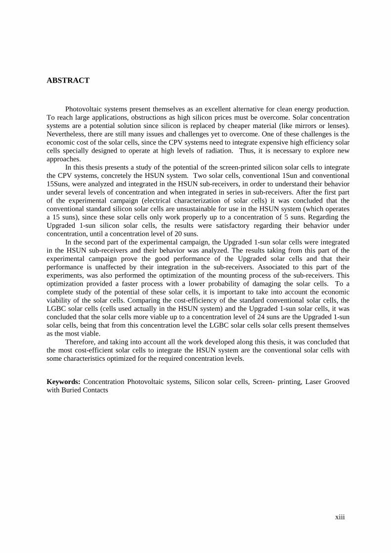
ABSTRACT
Photovoltaic systems present themselves as an excellent alternative for clean energy production. To reach large applications, obstructions as high silicon prices must be overcome. Solar concentration systems are a potential solution since silicon is replaced by cheaper material (like mirrors or lenses). Nevertheless, there are still many issues and challenges yet to overcome. One of these challenges is the economic cost of the solar cells, since the CPV systems need to integrate expensive high efficiency solar cells specially designed to operate at high levels of radiation. Thus, it is necessary to explore new approaches.
In this thesis presents a study of the potential of the screen-printed silicon solar cells to integrate the CPV systems, concretely the HSUN system. Two solar cells, conventional 1Sun and conventional 15Suns, were analyzed and integrated in the HSUN sub-receivers, in order to understand their behavior under several levels of concentration and when integrated in series in sub-receivers. After the first part of the experimental campaign (electrical characterization of solar cells) it was concluded that the conventional standard silicon solar cells are unsustainable for use in the HSUN system (which operates a 15 suns), since these solar cells only work properly up to a concentration of 5 suns. Regarding the Upgraded 1-sun silicon solar cells, the results were satisfactory regarding their behavior under concentration, until a concentration level of 20 suns.
In the second part of the experimental campaign, the Upgraded 1-sun solar cells were integrated in the HSUN sub-receivers and their behavior was analyzed. The results taking from this part of the experimental campaign prove the good performance of the Upgraded solar cells and that their performance is unaffected by their integration in the sub-receivers. Associated to this part of the experiments, was also performed the optimization of the mounting process of the sub-receivers. This optimization provided a faster process with a lower probability of damaging the solar cells. To a complete study of the potential of these solar cells, it is important to take into account the economic viability of the solar cells. Comparing the cost-efficiency of the standard conventional solar cells, the LGBC solar cells (cells used actually in the HSUN system) and the Upgraded 1-sun solar cells, it was concluded that the solar cells more viable up to a concentration level of 24 suns are the Upgraded 1-sun solar cells, being that from this concentration level the LGBC solar cells solar cells present themselves as the most viable.
Therefore, and taking into account all the work developed along this thesis, it was concluded that the most cost-efficient solar cells to integrate the HSUN system are the conventional solar cells with some characteristics optimized for the required concentration levels.
Keywords: Concentration Photovoltaic systems, Silicon solar cells, Screen- printing, Laser Grooved with Buried Contacts

xiv
xv
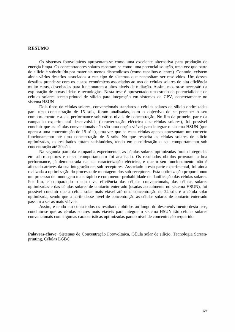
RESUMO
Os sistemas fotovoltaicos apresentam-se como uma excelente alternativa para produção de
energia limpa. Os concentradores solares mostram-se como uma potencial solução, uma vez que parte do silício é substituído por materiais menos dispendiosos (como espelhos e lentes). Contudo, existem ainda vários desafios associados a este tipo de sistemas que necessitam ser resolvidos. Um desses desafios prende-se com os custos económicos associados ao uso de células solares de alta eficiência muito caras, desenhadas para funcionarem a altos níveis de radiação. Assim, mostra-se necessário a exploração de novas ideias e tecnologias. Nesta tese é apresentado um estudo da potencialidade de células solares screen-printed de silício para integração em sistemas de CPV, concretamente no sistema HSUN.
Dois tipos de células solares, convencionais standards e células solares de silício optimizadas para uma concentração de 15 sois, foram analisadas, com o objectivo de se perceber o seu comportamento e a sua performance sob vários níveis de concentração. No fim da primeira parte da campanha experimental desenvolvida (caracterização eléctrica das células solares), foi possível concluir que as células convencionais não são uma opção viável para integrar o sistema HSUN (que opera a uma concentração de 15 sóis), uma vez que as estas células apenas apresentam um correcto funcionamento até uma concentração de 5 sóis. No que respeita as células solares de silício optimizadas, os resultados foram satisfatórios, tendo em consideração o seu comportamento sob concentração até 20 sóis.
Na segunda parte da campanha experimental, as células solares optimizadas foram integradas em sub-receptores e o seu comportamento foi analisado. Os resultados obtidos provaram a boa performance, já demonstrada na sua caracterização eléctrica, e que o seu funcionamento não é afectado através da sua integração em sub-receptores. Associado a esta parte experimental, foi ainda realizada a optimização do processo de montagem dos sub-receptores. Esta optimização proporcionou um processo de montagem mais rápido e com menor probabilidade de danificação das células solares. Por fim, e comparando o custo vs. eficiência das células convencionais, das células solares optimizadas e das células solares de contacto enterrado (usadas actualmente no sistema HSUN), foi possível concluir que a célula solar mais viável até uma concentração de 24 sóis é a célula solar optimizada, sendo que a partir desse nível de concentração as células solares de contacto enterrado passam a ser as mais viáveis.
Assim, e tendo em conta todos os resultados obtidos ao longo do desenvolvimento desta tese, concluiu-se que as células solares mais viáveis para integrar o sistema HSUN são células solares convencionais com algumas características optimizadas para o nível de concentração requerido.
Palavras-chave: Sistemas de Concentração Fotovoltaica, Célula solar de silício, Tecnologia Screen-printing, Células LGBC

xvi

xvii
CONTENTS
Acknowledgements ................................................................................................................................ xi
ABSTRACT ......................................................................................................................................... xiii
RESUMO .............................................................................................................................................. xv
LIST OF TABLES .............................................................................................................................. xxv
List of Abbreviations ......................................................................................................................... xxvii
INTRODUCTION ................................................................................................................................. 1
1.1 Context .................................................................................................................................... 1
1.2 Scope and objectives ............................................................................................................... 2
1.3. Structure of the thesis .............................................................................................................. 3
Concentration Photovoltaic Systems ................................................................................................... 5
2.1. Photovoltaic Solar Energy ....................................................................................................... 5
2.2. Concentration of photovoltaic ................................................................................................. 7
2.2.1. Why Concentration? ........................................................................................................ 7
2.2.2. Fundamentals of CPV systems ........................................................................................ 8
2.2.1.1Optics ........................................................................................................................................ 9
2.2.1.2. Tracking systems................................................................................................................ 11
2.2.1.3.Receiver ................................................................................................................................. 11
Fundamentals of Solar Cells to CPV systems ................................................................................... 13
3.1. Basic principles of photovoltaic solar cells ........................................................................... 13
3.1.1. Equivalent electric circuit of the solar cell .................................................................... 13
3.2. Electrical parameters of a solar cell....................................................................................... 19
3.2.1. Short-circuit current and open-circuit voltage ............................................................... 20
3.2.2. Maximum power point .................................................................................................. 20
3.2.3. Fill Factor ...................................................................................................................... 21
xviii
3.2.4.Conversion efficiency ........................................................................................................... 22
3.3.Influence of temperature and radiation intensity on the characteristic curve .............................. 22
3.4.Overview of Solar Cells for CPV ................................................................................................ 23
3.4.1.Single-crystalline solar cells for CPV applications .............................................................. 25
3.4.1.1.Modified screen-printed solar cells ................................................................................... 26
3.4.1.2.Laser Grooved Buried Contact (LGBC) solar cells ........................................................ 27
3.4.1.3.Back contact cells ................................................................................................................. 29
3.4.1.3.1. Emitters wrap trough (EWT) solar cells .............................................................. 29
3.4.1.3.2. Metallization wrap trough (MWT) solar cells ..................................................... 30
Theorectical characterization of Solartec and KVAZAR solar cells .............................................. 31
4.1.Physical characteristics of the KVAZAR and Solartec solar cells .............................................. 31
4.1.1.KVAZAR solar cells ............................................................................................................ 31
4.1.2.Solartec solar cell .................................................................................................................. 36
4.2.Mathematical model to estimate the behavior of solar cells under concentration ....................... 39
4.3.Theorical behavior of the Solartec and KVAZAR solar cells under concentration .................... 43
Experimental characterization of the Solartec and KVAZAR solar cells ...................................... 47
5.1. Electroluminescence of solar cells ............................................................................................. 47
5.1.1. Electroluminescence ............................................................................................................ 47
5.1.2. Experimental procedure ....................................................................................................... 49
5.1.3. Results ................................................................................................................................. 50
5.1.3.1. KVAZAR solar cells .......................................................................................................... 50
5.1.3.2. Solartec solar cells .............................................................................................................. 54
5.1.4. Main Conclusions ................................................................................................................ 55
5.2. Measurement of electrical parameters of the solar cells............................................................. 56
5.2.1. Electrical parameters ........................................................................................................... 56
5.2.2. Experimental procedure ....................................................................................................... 57
5.2.3. Results ................................................................................................................................. 59
5.2.3.1. KVAZAR solar cells .......................................................................................................... 59
5.2.3.2. Solartec solar cells .............................................................................................................. 64
5.2.4. Main conclusions ................................................................................................................. 66
5.3. Measurement of the Series Resistance ....................................................................................... 68

xix
5.3.1. I-V curves ............................................................................................................................ 68
5.3.1.1. Theoretical Introduction ..................................................................................................... 68
5.3.1.2. Results .................................................................................................................................. 71
5.3.2. Suns Voc method ................................................................................................................. 74
5.3.2.1. Theoretical Introduction ..................................................................................................... 74
5.3.2.2. Results .................................................................................................................................. 75
5.3.3. Conclusions ......................................................................................................................... 75
5.4. Spectral Response and Quantum Efficiency .............................................................................. 79
5.4.1. Theoretical Introduction ...................................................................................................... 79
5.4.2. Experimental procedure ....................................................................................................... 81
5.4.3. Results ................................................................................................................................. 82
5.5. Thermal coefficients of solar cells ............................................................................................. 86
5.5.1. Thermal coefficients concept ............................................................................................... 86
5.5.2. Experimental procedure ....................................................................................................... 87
5.5.3. Results ................................................................................................................................. 88
5.5.4. Main conclusions ................................................................................................................. 90
Integration of the solar cells in the HSUN sub-receivers ................................................................. 91
6.1. Integration of solar cells in the HSUN technology .................................................................... 91
6.2. Mounting process of the receiver and preliminary tests ............................................................. 92
6.2.1. Process ................................................................................................................................. 93
6.2.2. Tests ..................................................................................................................................... 97
6.2.3. Optimization of the mounting process ............................................................................... 116
6.2.3.1. Tests .................................................................................................................................... 118
6.3. Electrical performance ............................................................................................................. 123
6.3.1 Experimental procedure ...................................................................................................... 123
6.3.2. Results ............................................................................................................................... 124
6.3.2.1. Analysis of the results taking into account the incident radiation .............................. 127
6.3.2.2. Analysis of the results taking into account the radiation and cell temperature ........ 129
6.3.2.2.1. Experimental procedure .................................................................................. 129
6.3.2.2.2. Results ............................................................................................................. 129
6.3.2.3. Adjust of the results obtained by the temperature estimated of the solar cells ....... 131
6.3.3. Main conclusions ............................................................................................................... 133

xx
Cost-efficiency analysis of screen-printed solar cells to integrate CPV systems ......................... 135
CONCLUSIONS AND FUTURE WORK....................................................................................... 139
8.1. Conclusions .............................................................................................................................. 139
8.2. Future Work ............................................................................................................................. 140
REFERENCES .................................................................................................................................. 143
ANNEXES .......................................................................................................................................... 147
xxi
LIST OF FIGURES
Figure 2.1 - Adams and Days' Selenium glass tube ............................................................................... 5
Figure 2.2– Vanguard 1 .......................................................................................................................... 6
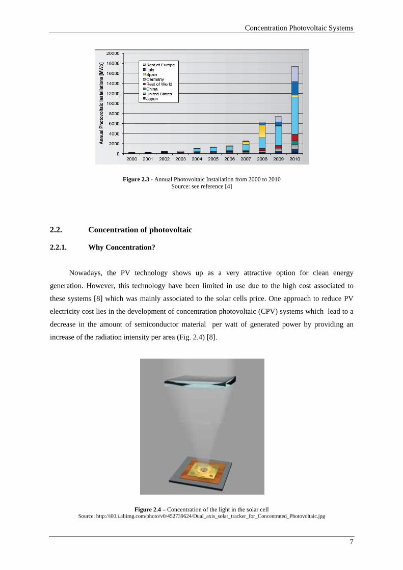
Figure 2.3 - Annual Photovoltaic Installation from 2000 to 2010 .......................................................... 7
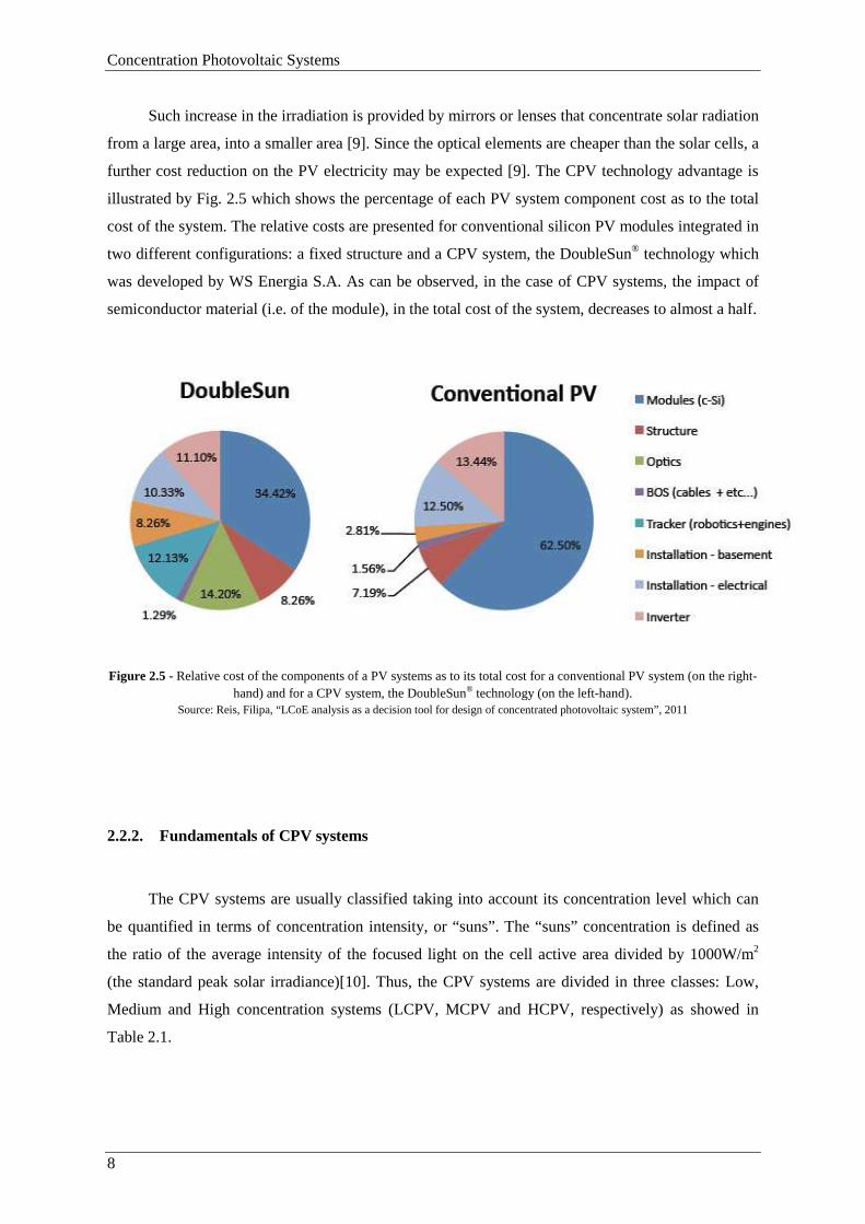
Figure 2.4 – Concentration of the light in the solar cell ......................................................................... 7
Figure 2.5 - Relative cost of the components of a PV systems as to its total cost for a conventional PV
system and for a CPV system. ........................................................................................... 8
Figure 2.6 - Schematic of Linear-Focus Trough PV Concentrator ........................................................ 9
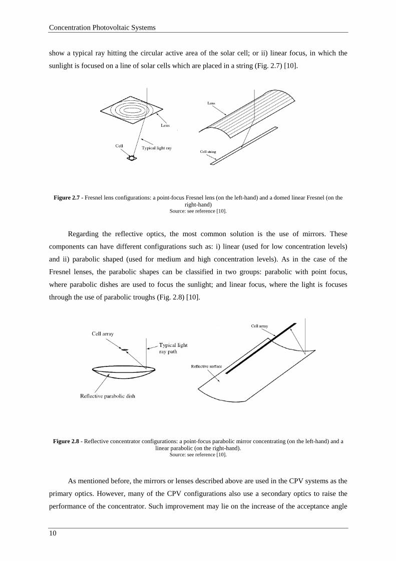
Figure 2.7 - Fresnel lens configurations ............................................................................................... 10
Figure 2.8 - Reflective concentrator configurations. ............................................................................ 10
Figure 2.9 – Types of Tracking systems: (a) 1 axis tracker and (b) 2 axis tracker ............................... 11
Figure 3.1- Principle of operation of a solar cell. ................................................................................. 14
Figure 3.2 - I-V characteristic of a silicon diode .................................................................................. 14
Figure 3.3 - Diagram of equivalent circuit;Characteristic curve of the cell in total darkness .............. 16
Figure 3.4 - Diagram of equivalent circuit, Characteristic curve of the irradiated cell ........................ 17
Figure 3.5 - Representation of the electrical circuit of one real solar cell ............................................ 17
Figure 3.6 - Effect of variation of series resistance in the I-V curve .................................................... 18
Figure 3.7 - Effect of the variation of the parallel or shunt resistance in the I-V curve ....................... 18
Figure 3.8 - I-V and P-V characteristic curve of an silicon cell ........................................................... 19
Figure 3.9 - I-V curve and point of maximum power draw of the CIEMAT’s simulator. ................... 20
Figure 3.10 - Fill Factor of solar cells .................................................................................................. 21
Figure 3.11 - Effect of a) irradiance and b) temperature in the I-V curve ............................................ 23
Figure 3.12 - Historic summary of champion cell efficiencies for various PV technologies. .............. 24
Figure 3.13 - (a) The structure of a MJ solar cell. (b) Graph of spectral irradiance G vs. Wavelength λ
over the AM1.5 solar spectrum. ..................................................................................... 25
Figure 3.14 - Monocrystalline solar cells ............................................................................................. 26
Figure 3.15 - Normalized plot of Efficiency against the concentration ratio of the optimized and
unoptimized grid solar cell. ............................................................................................ 27
Figure 3.16 - Buried contact solar cells ................................................................................................ 28
Figure 3.17 - Buried contact in a silicon solar cell ............................................................................... 28
Figure 3.18 - Emitters wrap trough (EWT) solar cells ......................................................................... 29
Figure 3.19 - Metallization wrap trough (MWT) solar cells ................................................................ 30
Figure 4.1 - Front surface of the KVAZAR solar cell (main cell) ....................................................... 32
Figure 4.2 - Back surface of the KVAZAR solar cells ( main cell) ..................................................... 32
Figure 4.3 - Drawing of the cut (and dimensions) performed in the solar cells ................................... 34
xxii
Figure 4.4 - Reference of the KVAZAR solar cells. ........................................................................... 34
Figure 4.5 – Number given to each cell according to its position at the conventional wafer. .............. 35
Figure 4.6 – KVAZAR solar cell ......................................................................................................... 35
Figure 4.7 - Front surface of the Solartec solar cells ........................................................................... 36
Figure 4.8 - Back surface of the Solartec solar cells ........................................................................... 36
Figure 4.9 –Solartec solar cells with different front grid designs: a) one busbar; b) two busbars ....... 37
Figure 4.10 – Reference of the Solartec solar cells .............................................................................. 38
Figure 4.11 - Calculated values for Voc and Isc as function of concentration level in the a) KVAZAR
solar cells and b)Solartec solar cells ................................................................................. 43
Figure 4.12 - Estimated power loss (Ploss) and efficiency (ε) as a function of the concentration level
of a) Solartec solar cells and b) KVAZAR solar cells ...................................................... 44
Figure 5.1 - Electroluminescence image of a) a monocrystalline and b) poly-crystalline silicon cell. 48
Figure 5.2 – Electroluminescence System. ........................................................................................... 49
Figure 5.3 – Electroluminescence apparatus ........................................................................................ 50
Figure 5.4 - Power and characteristic curves of a solar cell ................................................................. 57
Figure 5.5 – Measurement of the FF from the I-V curve of a solar cell ............................................... 57
Figure 5.6 – Solar Simulation located in the Laboratory of FCUL ...................................................... 58
Figure 5.7 – Detail of the solar cell placed on the sample holder in the solar simulator. ..................... 58
Figure 5.8 – I-V curve of cell nº 6.2 with the I-V tracer ...................................................................... 60
Figure 5.9 – I-V curve of cell nº 6.3 with the I-V tracer ...................................................................... 60
Figure 5.10 – I-V curve of cell nº 6.4 with the I-V tracer .................................................................... 60
Figure 5.11 – I-V curve of cell nº 6.5 with the I-V tracer ................................................................... 60
Figure 5.12 – I-V curve of cell nº 6.6 with the I-V tracer .................................................................... 60
Figure 5.13 – I-V curve of cell nº 6.7 with the I-V tracer .................................................................... 60
Figure 5.14 – I-V curve of cell nº 6.8 with the I-V tracer .................................................................... 61
Figure 5.15 – Values of a) Voc and b) Isc measured from the I-V curves before and after the soldering
process of the KVAZAR solar cells ............................................................................... 61
Figure 5.16 – I-V curves traced with the four-point I-V measurement (green) and the I-V tracer
(violet) of the a)solar cell nº 6.2, b) solar cell nº 6.4, c) solar cell nº 6.7 and d) solar cell
nº 6.8 .............................................................................................................................. 63
Figure 5.17 – I-V curve of cell nº 24.1 before and after the soldering process .................................... 64
Figure 5.18 – I-V curve of cell nº 24.2 before and after the soldering process .................................... 64
Figure 5.19 – I-V curve of cell nº 26.1 before and after the soldering process ................................... 65
Figure 5.20 – I-V curve of cell nº 26.2 before and after the soldering process ................................... 65
Figure 5.21 – I-V curve of cell nº 2BB.1 before and after the soldering process ................................ 65
Figure 5.22 – I-V curve of cell nº 2BB.2 before and after the soldering process ................................. 65
Figure 5.23 - Obtaining the series and shunt resistances from the I-V Curve. ..................................... 69

xxiii
Figure 5.24 - Two I-V curves of the same solar cell under different illumination intensities. ............. 70
Figure 5.25 - I-V curve registered for the a) KVAZAR, b) Solartec and c) NaREC solar cells under 1,
2 and 10 suns. I-V curves are normalized to Isc and Voc. ............................................. 71
Figure 5.26 - Concentration Simulator placed in the FCUL laboratory ............................................... 72
Figure 5.27 – Suns-Voc apparatus placed in the FCUL laboratory. ..................................................... 74
Figure 5.28 - The spectral response of a silicon solar cell under glass ................................................ 79
Figure 5.29 - Quantum Efficiency of a silicon solar cell ...................................................................... 81
Figure 5.30 - System for measuring the spectral response and quantum efficiency ............................ 81
Figure 5.31 - Measurement of the SR in the solar cells: a) reference solar cell, b) KVAZAR or
Solartec solar cell ........................................................................................................... 82
Figure 5.32 - External quantum efficiency of a conventional solar cell (KVZ.40 – 6.8) measured in
different positions on the cell. ........................................................................................ 83
Figure 5.33 - External quantum efficiency of a conventional solar cell (KVZ.40 – 6.7) measured in
different position ............................................................................................................ 83
Figure 5.34 - External quantum efficiency of the Solartec solar cell a) class 24; b) class 26; c) with
two busbar ...................................................................................................................... 84
Figure 5.35 - QE curves obtained for the KVAZAR and the Solartec solar cells. ............................... 85
Figure 5.36 - Measured temperature coefficients for voltage for solar cell with uniform and
nonuniform temperature during testing. ......................................................................... 86
Figure 5.37 – Solar Simulator located in the Laboratory of the WS Energia S.A. ............................... 87
Figure 5.38 - Variation of the Voc and Isc as a function of the temperature of the: a) KVAZAR, b)
SLT.C24, c) SLT.C26 and d) SLT.2BB solar cells. ....................................................... 89
Figure 6.1 – HSUN module mounted on a 2-axes tracking system...................................................... 92
Figure 6.2 – Components and characteristics of the PCB. ................................................................... 93
Figure 6.3 – Sub-receiver. When three of these sub-receivers are connected, a receiver is obtained. . 93
Figure 6.4 –Specific position of the each component on the PCB. ...................................................... 94
Figure 6.5 – Set of six PCBs that are the base for the HSUN sub-receivers. ....................................... 94
Figure 6.6 – Position where the thermal tape and the solder is placed on the PCB ............................. 95
Figure 6.7 – Mounting process of the sub-receivers ............................................................................ 97
Figure 6.8 – Presence of spots in the solar cell of the sub-receiver nº 2. ............................................. 98
Figure 6.9 – Displacement of the ribbon from its specific position. .................................................... 98
Figure 6.10 – Unsoldered ribbon .......................................................................................................... 99
Figure 6.11 – Diode displaced from its position on the PCB. .............................................................. 99
Figure 6.12 – Percentage of sub-receivers that are within a certain range of Pmp. ........................... 113
Figure 6.13 - Values of Pmp before (dark blue) and after (light blue) the re-soldering process. ....... 114
Figure 6.14 – Open-circuit voltage before and after the re-soldering process ................................... 114
Figure 6.15 – Short-circuit current before and after the re-soldering process .................................. 115
xxiv
Figure 6.16 – Maximum power before and after the re-soldering process. ...................................... 116
Figure 6.17 – Short-circuit before and after the re-soldering process. ............................................... 116
Figure 6.18 – Open-circuit voltage before and after the re-soldering process ................................... 116
Figure 6.19 – Pressure Board ............................................................................................................. 117
Figure 6.20 – Pen flux ........................................................................................................................ 118
Figure 6.21 – Presence of spot sand balls of soldering paste on the solar cell busbar. ...................... 119
Figure 6.22 – Percentage of sub-receivers that are within a certain range of Pmp. ........................... 120
Figure 6.23 – Maximum power point before and after the re-soldering process of sub-receivers. .... 121
Figure 6.25 – Open circuit voltage before and after the re-soldering process .................................... 122
Figure 6.25 – Sub-receiver with the output ribbons soldered. ............................................................ 123
Figure 6.27 – Experimental set to measure the I-V curves under outdoor conditions. ...................... 124
Figure 6.28 – Placement of the a) thermocouple at the rear surface of the sub-receiver and b) the
radiation meter apparatus side-by-side with the sub-receiver. ..................................... 124
Figure 6.29 – I-V curves measured to sub-receivers. ......................................................................... 125
Figure 6.30 – Measured values of Pmp of the sub-receiver and the average of the Pmp of the solar
cells. ............................................................................................................................. 126
Figure 6.31 – Estimated values of FF of the sub-receiver .................................................................. 126
Figure 6.32 –Values of a) Isc and b) Voc of each solar cell (different red hue bars) and sub-receiver
(blue bars) normalized at outdoor conditions ............................................................... 127
Figure 6.33 –Values of a) Isc and b) Voc of each solar cell (different red hue bars) and sub-receiver
(blue bars) normalized at outdoor conditions ............................................................... 128
Figure 6.34 - Placement of the Thermocouple in the back rear surface of the solar cell ................... 129
Figure 6.35 - I-V curves measured in the sunlight exposure from the a) SLT.C26-2 and b) SLT.C24-2
sub-receivers. ............................................................................................................... 130
Figure 6.36 – Temperature of the rear surface of the cell and the temperature. ................................. 131
Figure 6.37 – Temperatures of the sub-receivers estimated by two different methods ...................... 132
Figure 6.38 –Values of a) Isc and b) Voc of each solar cell and sub-receiver. .................................. 132
Figure 7.1 – Estimated cost-effectiveness and Pmp of solar cells ...................................................... 137
xxv
LIST OF TABLES
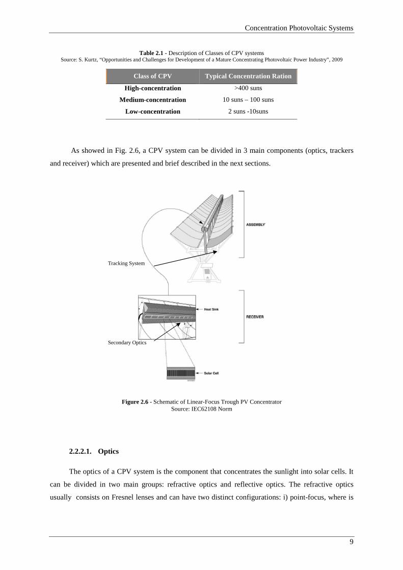
Table 2.1 - Description of Classes of CPV systems ............................................................................... 9
Table 4.1 - Dimensions and materials of KVAZAR solar cells ........................................................... 33
Table 4.2 - Physical characteristics of solar cells ................................................................................. 35
Table 4.3 – Dimensions and materials of Solartec solar cells .............................................................. 37
Table 4.4- Calculated electrical parameters of Solartec and KVAZAR solar cells under different
concentration levels .......................................................................................................... 45
Table 5.1 - Photographs taken with the Electroluminescence method: before and after the cutting
process of KVAZAR solar cells, and after the soldering process. .................................... 53
Table 5.2- Electroluminescent images taken to Solartec solar cells after the soldering process. ......... 54
Table 5.3 - Values of parameters of the solar cells tested before and after the soldering process........ 63
Table 5.4 – Electrical parameters estimated for KVAZAR solar cells at 1 sun. .................................. 64
Table 5.5 - Values of parameters of the solar cells tested before and after the soldering process........ 66
Table 5.6 - Values of electrical parameters of the Solartec and KVAZAR solar cells. ........................ 66
Table 5.7 – Series Resistance estimated by the slope method .............................................................. 72
Table 5.8 – Series Resistance estimated by the multiple light intensities method................................ 73
Table 5.9 - Series Resistance estimated by the Suns Voc setup ........................................................... 75
Table 5.10 – Series Resistance of the KVAZAR, Solartec and NaREC solar cells estimated by the
different methods. ............................................................................................................. 77
Table 5.11 – Thermal coefficients estimated for the Solartec and KVAZAR solar cells ..................... 89
Table 6.1 - Description of the soldering paste configuration used on each sub-receiver .................. 101
Table 6.2 - Description of the soldering paste configuration used on each sub-receiver ................... 102
Table 6.3 - Description of the soldering paste configuration used on each sub-receiver. .................. 103
Table 6.4 - Description of the soldering paste configuration used on each sub-receiver ................... 104
Table 6.5 - Description of the soldering paste configuration used on each sub-receiver ................... 105
Table 6.6 - Description of the soldering paste configuration used on each sub-receiver ................... 106
Table 6.7 - Description of the soldering paste configuration used on each sub-receiver. .................. 107
Table 6.8 - Description of the soldering paste configuration used on each sub-receiver. .................. 108
Table 6.9 – Method used in each of the sub-receiver ......................................................................... 118
Table 7.1 – Technology and prices of the Solartec, NaREC and KVAZAR solar cells. .................... 136


xxvii
List of Abbreviations
Acronyms
CPV – Concentrated photovoltaic
ECT – Equivalent Cell Temperature
EL – Electroluminescence
EWT – Emitters Wrap Trough
FCT-UNL – Faculdade de Ciências e Tecnologia – Universidade Nova de Lisboa
FCUL – Faculdade de Ciências da Universidade de Lisboa
HCPV – High Concentration Photovoltaic
I-V – Current-voltage
LCPV – Low Concentration Photovoltaic LGBC – Laser Grooved Buried Contact
MCPV – Medium Concentration Photovoltaic
MWT – Metallization Wrap Trough
QE – Quantum Efficiency
PCB – Printed Circuit Board
PV – Photovoltaic
RE – Renewable Energy
R&D – Research and Development
SR – Spectral Response

xxviii
Variables
ε – Efficiency
λ – Wavelength
β – Thermal coefficient
Eg –Energy gap
FF – Fill Factor
I0 - Reverse Saturation Current (or leakage current)
IMPP – Current at Maximum Power Point
Isc – Short-circuit current
k – Boltzmann constant
Jsc – Short-circuit current density Ploss – Power losses
Pmp – Maximum power point
q –Electron charge
Rs – Series resistance
Rsh – Shunt resistance
T – Temperature
VMPP – Voltage at maximum power point
Voc – Open circuit voltage
Introduction
1
Chapter 1
INTRODUCTION
1.1 Context
Since 1860, the average surface temperature increased 0.6 °C. Different future scenarios
predict that by 2100, this temperature will increase between 1.5 and 6º C, if the energy choices and
habits of current consumption remain unchanged [1].
The Renewable Energy whose conversion technologies have reached a maturity which allows
commercial and technical perspective the application of economic significance, are forms of energy
that regenerate cyclically in a reduced scale of time. That is, energies that are in constant renewal,
are inexhaustible and can be continuously used [2]. Thus, the renewable energies are pointed out as
one of the solutions to mitigate the energetic problems, as well as a sustainable alternative to fossil
fuels [2]. Among them, solar energy has the biggest developing potential and has proven to be an
efficient and cost-effective energy source for different applications.
The Sun is the most abundant power source and is estimated that the sunlight that reaches the
Earth's surface is enough to provide more energy as it is currently used. On a global average, each
square meter of land is exposed to enough sunlight to produce 1700 kWh of power every year [3].
Photovoltaic (PV) technology involves the generation of energy from the direct conversion of
the sunlight into electricity. Since 2000, total PV production increased almost by two orders of
magnitude, with annual growth rates between 40% and 90%. The most rapid growth in annual
production over the last five years could be observed in Asia, where China and Taiwan together now
account for almost 60% of world-wide production. However, the major barrier towards very large-
scale use of PV systems has been the cost of electricity generation with this type of technology [4].
Concentrated photovoltaic (CPV), by concentrating the sunlight into the solar cells through the
use of mirrors or lenses, decreases the silicon area necessary for the production of the same power,
leading to a decrease of the price of electricity generated by the system. As so, the CPV technology is
considered by some the technology with most potential to reach costs of electricity that can compete
with fossil fuels [5].

Introduction
2
The CPV configurations vary widely according to the concentration ratio, the type of optics
(refractive or reflective) and the geometry, but also by the type of solar cells used. Since the CPV
systems operate under concentration, it’s necessary that the solar cells used in this kind of systems
present several proprieties that lead to a good performance. Thus, the solar cell choice is decisive for
a CPV system to achieve high performance and to be reliable over its entire lifetime [5].
1.2 Scope and objectives
This master thesis was developed within the framework of the HSUN project, a new CPV
system that is being developed in a collaboration between the research and development (R&D)
Wemans and Sorasio Laboratories of WS Energia, the Departamento de Engenharia Electrotécnica
from Faculdade de Ciências e Tecnologia – Universidade Nova de Lisboa (FCT-UNL) and the
Faculdade de Ciências da Universidade de Lisboa (FCUL) and intends to contribute to evolution of
science and technology on photovoltaic systems, and thus increase the penetration of solar energy in
the markets.
The objective of this research was to study the performance of various types of solar cells
under solar concentration and thus, contributing for the development of the HSUN technology. Thus,
taking into account the main objective, the thesis is divided in two distinct parts:
• Laboratorial characterization of the solar cells in study to validate the theoretical
method that was used for predicting the behavior of solar cells under different concentration
levels.
• Improvement of the mounting process of the HSUN receivers. Through the
implementation of this process, the soldering of solar cells has become faster with a lower
probability of damaging the solar cells. It was also performed an experimental campaign to
understand the behavior of the solar cells when integrated into the HSUN sub-receivers.
The objectives were accomplished and are completely integrated in the project: the improved
mounting process of the HSUN receivers is being used to the preparation of new prototypes and the
solar cells studied are already being used in the new HSUN prototype. Some of parts of this work
were presented in the European Photovoltaic Solar Energy Conference in Hamburg and the article
and poster presented can be consulted in the Annex I.
Introduction
3
1.3. Structure of the thesis
This thesis is organized in eight Chapters:
Chapter 1 sets the context, scope and main objectives of the thesis as the necessity of a correct
choice of the solar cell that integrates the CPV system.
Chapter 2 presents the fundamental concepts and state of the art of concentrated photovoltaics
systems
Chapter 3 presents the fundamental concepts of the solar cells and describes the state of the
art of the solar cells that are suitable to integarte the CPV systems. Also in this chapter it is presented
the physical characteristics of the solar cells under study in this thesis.
Chapter 4 covers the estimated behavior of the solar cells under different concentration
levels. A mathematical model to estimate the behavior of solar cells under concentration is explained
and the expected behavior of the solar cells under concentration is presented.
Chapter 5 describes the laboratorial characterization of the solar cells under study, with the
presentation of a full experimental campaign where several experimental procedures were performed
in order to test and analyze the electrical and physical parameters of the solar cells.
Chapter 6 describes the behavior of the solar cells tested integrated in the HSUN sub-
receivers. Also in this chapter is explained the whole soldering process of solar cells developed in the
context of this thesis.
Chapter 7 describes the cost-efficiency analysis of screen-printed solar cells to integrate CPV
systems.
Chapter 8 presents the main conclusions of this work, as well as directions for future
developments related to the solar cells in the HSUN project.

Concentration Photovoltaic Systems
5
Chapter 2
Concentration Photovoltaic Systems
This chapter introduces the fundamental concept and a brief history of Photovoltaic (PV)
technology. Within this area, Concentration photovoltaic (CPV) systems are pointed out as an
interesting technological option to significantly reduce the PV electricity costs. The main areas of
CPV technology are then briefly described.
2.1.Photovoltaic Solar Energy
The photovoltaic (PV) effect consists on the direct conversion of sunlight into electricity. Such
effect, involves the transfer of the photon energy of the incident radiation to the electrons of the
atomic structure of the semiconductor material. This translates into the creation of free charges in the
semiconductor, which are separated inside the device by the electric field of the junction, thus
producing an electric current outside [6].
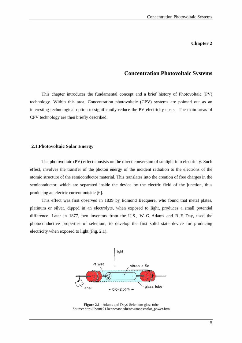
This effect was first observed in 1839 by Edmond Becquerel who found that metal plates,
platinum or silver, dipped in an electrolyte, when exposed to light, produces a small potential
difference. Later in 1877, two inventors from the U.S., W. G. Adams and R. E. Day, used the
photoconductive properties of selenium, to develop the first solid state device for producing
electricity when exposed to light (Fig. 2.1).
Figure 2.1 - Adams and Days' Selenium glass tube Source: http://ihome21.kennesaw.edu/new/mods/solar_power.htm
Concentration Photovoltaic Systems
6
This device consisted on a film of selenium, iron deposited on a substrate and a second film of
gold, semi-transparent, which worked as a front contact. Despite the low conversion efficiency of the
device (about 0.5%) in the late nineteenth century, the German engineer Werner Siemens (founder of
the industrial empire with his name) marketed as selenium cell light meters for cameras [7]. With the
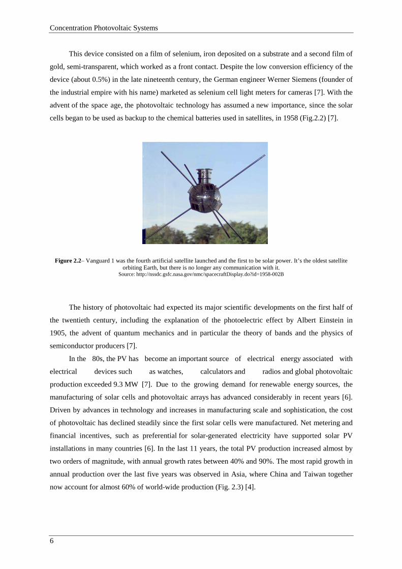
advent of the space age, the photovoltaic technology has assumed a new importance, since the solar
cells began to be used as backup to the chemical batteries used in satellites, in 1958 (Fig.2.2) [7].
Figure 2.2– Vanguard 1 was the fourth artificial satellite launched and the first to be solar power. It’s the oldest satellite
orbiting Earth, but there is no longer any communication with it. Source: http://nssdc.gsfc.nasa.gov/nmc/spacecraftDisplay.do?id=1958-002B
The history of photovoltaic had expected its major scientific developments on the first half of
the twentieth century, including the explanation of the photoelectric effect by Albert Einstein in
1905, the advent of quantum mechanics and in particular the theory of bands and the physics of
semiconductor producers [7].
In the 80s, the PV has become an important source of electrical energy associated with
electrical devices such as watches, calculators and radios and global photovoltaic
production exceeded 9.3 MW [7]. Due to the growing demand for renewable energy sources, the
manufacturing of solar cells and photovoltaic arrays has advanced considerably in recent years [6].
Driven by advances in technology and increases in manufacturing scale and sophistication, the cost
of photovoltaic has declined steadily since the first solar cells were manufactured. Net metering and
financial incentives, such as preferential for solar-generated electricity have supported solar PV
installations in many countries [6]. In the last 11 years, the total PV production increased almost by
two orders of magnitude, with annual growth rates between 40% and 90%. The most rapid growth in
annual production over the last five years was observed in Asia, where China and Taiwan together
now account for almost 60% of world-wide production (Fig. 2.3) [4].
Concentration Photovoltaic Systems
7
Figure 2.3 - Annual Photovoltaic Installation from 2000 to 2010 Source: see reference [4]
2.2. Concentration of photovoltaic
2.2.1. Why Concentration?
Nowadays, the PV technology shows up as a very attractive option for clean energy
generation. However, this technology have been limited in use due to the high cost associated to
these systems [8] which was mainly associated to the solar cells price. One approach to reduce PV
electricity cost lies in the development of concentration photovoltaic (CPV) systems which lead to a
decrease in the amount of semiconductor material per watt of generated power by providing an
increase of the radiation intensity per area (Fig. 2.4) [8].
Figure 2.4 – Concentration of the light in the solar cell Source: http://i00.i.aliimg.com/photo/v0/452739624/Dual_axis_solar_tracker_for_Concentrated_Photovoltaic.jpg
Concentration Photovoltaic Systems
8
Such increase in the irradiation is provided by mirrors or lenses that concentrate solar radiation
from a large area, into a smaller area [9]. Since the optical elements are cheaper than the solar cells, a
further cost reduction on the PV electricity may be expected [9]. The CPV technology advantage is
illustrated by Fig. 2.5 which shows the percentage of each PV system component cost as to the total
cost of the system. The relative costs are presented for conventional silicon PV modules integrated in
two different configurations: a fixed structure and a CPV system, the DoubleSun® technology which
was developed by WS Energia S.A. As can be observed, in the case of CPV systems, the impact of
semiconductor material (i.e. of the module), in the total cost of the system, decreases to almost a half.
Figure 2.5 - Relative cost of the components of a PV systems as to its total cost for a conventional PV system (on the right-
hand) and for a CPV system, the DoubleSun® technology (on the left-hand). Source: Reis, Filipa, “LCoE analysis as a decision tool for design of concentrated photovoltaic system”, 2011
2.2.2. Fundamentals of CPV systems
The CPV systems are usually classified taking into account its concentration level which can
be quantified in terms of concentration intensity, or “suns”. The “suns” concentration is defined as
the ratio of the average intensity of the focused light on the cell active area divided by 1000W/m2
(the standard peak solar irradiance)[10]. Thus, the CPV systems are divided in three classes: Low,
Medium and High concentration systems (LCPV, MCPV and HCPV, respectively) as showed in
Table 2.1.
Concentration Photovoltaic Systems
9
Table 2.1 - Description of Classes of CPV systems Source: S. Kurtz, “Opportunities and Challenges for Development of a Mature Concentrating Photovoltaic Power Industry”, 2009
Class of CPV Typical Concentration Ration
High-concentration >400 suns
Medium-concentration 10 suns – 100 suns
Low-concentration 2 suns -10suns
As showed in Fig. 2.6, a CPV system can be divided in 3 main components (optics, trackers
and receiver) which are presented and brief described in the next sections.
Figure 2.6 - Schematic of Linear-Focus Trough PV Concentrator Source: IEC62108 Norm
2.2.2.1. Optics
The optics of a CPV system is the component that concentrates the sunlight into solar cells. It
can be divided in two main groups: refractive optics and reflective optics. The refractive optics
usually consists on Fresnel lenses and can have two distinct configurations: i) point-focus, where is
Secondary Optics
Tracking System
Concentration Photovoltaic Systems
10
show a typical ray hitting the circular active area of the solar cell; or ii) linear focus, in which the
sunlight is focused on a line of solar cells which are placed in a string (Fig. 2.7) [10].
Figure 2.7 - Fresnel lens configurations: a point-focus Fresnel lens (on the left-hand) and a domed linear Fresnel (on the right-hand)
Source: see reference [10].
Regarding the reflective optics, the most common solution is the use of mirrors. These
components can have different configurations such as: i) linear (used for low concentration levels)
and ii) parabolic shaped (used for medium and high concentration levels). As in the case of the
Fresnel lenses, the parabolic shapes can be classified in two groups: parabolic with point focus,
where parabolic dishes are used to focus the sunlight; and linear focus, where the light is focuses
through the use of parabolic troughs (Fig. 2.8) [10].
Figure 2.8 - Reflective concentrator configurations: a point-focus parabolic mirror concentrating (on the left-hand) and a linear parabolic (on the right-hand).
Source: see reference [10].
As mentioned before, the mirrors or lenses described above are used in the CPV systems as the
primary optics. However, many of the CPV configurations also use a secondary optics to raise the
performance of the concentrator. Such improvement may lie on the increase of the acceptance angle
Concentration Photovoltaic Systems
11
or even on a higher homogeneity of the radiation that falls on the cells. As the primary optics, there
are several configurations for the secondary optics [10].
2.2.2.2. Tracking systems
To correctly concentrate the sunlight on the solar cells, the optics of the CPV systems have to
be aligned with the sun rays, thus demanding for a tracking system which places the CPV system
towards the sun from sunrise until sunset [8].In general, the tracking systems, depending of the optics
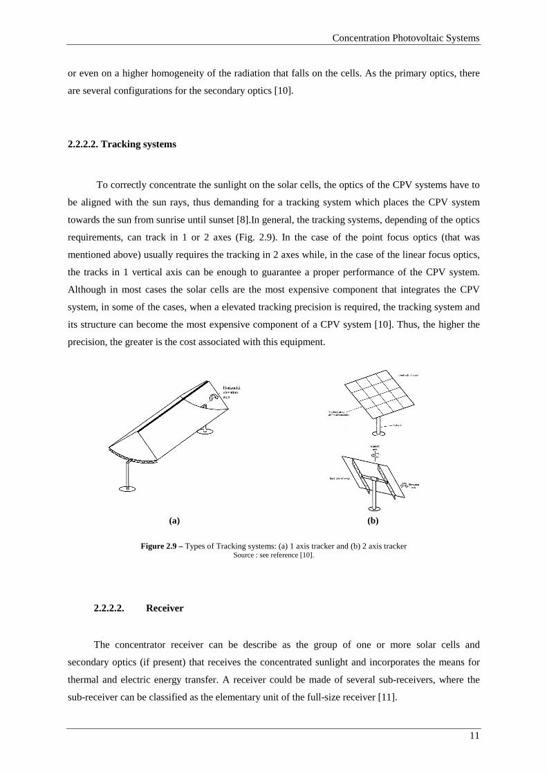
requirements, can track in 1 or 2 axes (Fig. 2.9). In the case of the point focus optics (that was
mentioned above) usually requires the tracking in 2 axes while, in the case of the linear focus optics,
the tracks in 1 vertical axis can be enough to guarantee a proper performance of the CPV system.
Although in most cases the solar cells are the most expensive component that integrates the CPV
system, in some of the cases, when a elevated tracking precision is required, the tracking system and
its structure can become the most expensive component of a CPV system [10]. Thus, the higher the
precision, the greater is the cost associated with this equipment.
(a) (b)
Figure 2.9 – Types of Tracking systems: (a) 1 axis tracker and (b) 2 axis tracker Source : see reference [10].
2.2.2.2. Receiver
The concentrator receiver can be describe as the group of one or more solar cells and
secondary optics (if present) that receives the concentrated sunlight and incorporates the means for
thermal and electric energy transfer. A receiver could be made of several sub-receivers, where the
sub-receiver can be classified as the elementary unit of the full-size receiver [11].
Concentration Photovoltaic Systems
12
The concentration ratios that are reached in a CPV system leads to high temperatures, which
affect the cells performance. Thus, a cooling system may be required. The cooling system can be
classified in two strands: passive, where the cooling of the module is made through by aluminum
fins; and active, where the cooling of the module is made with running water[11].
To a properly function in the CPV systems, the photovoltaic cells demand for specific
requirements of the concentrated light and from the solar cell itself. This aspect will be addressed in
detail in Chapter 3.
Fundamentals of Solar Cells to CPV Systems
13
Chapter 3
Fundamentals of Solar Cells to CPV systems
This Chapter covers the basic principles of PV solar cells by addressing: i) the equivalent
electrical circuit; ii) the main electrical parameters that characterize a solar cell and iii) the influence
of radiation and temperature on solar cells performance. This chapter ends with an overview of the
solar cells that are suitable for CPV applications.
3.1. Basic principles of photovoltaic solar cells
3.1.1. Equivalent electric circuit of the solar cell
Photovoltaic cells are made of semiconductor material, i.e. material with intermediate
characteristics between a conductor and an insulator. Silicon presents itself typically as sand.
However, through the appropriate methods is obtained silicon in a pure form. The crystal of pure
silicon has no free electrons and therefore is a poor electrical conductor [12].
Thus, in order to change this situation, percentages of other elements, as phosphorus and
boron, are added to the silicon. This process is named doping. Through the doping of silicon with
phosphorus, a material with free electrons or materials with negative charge carriers (n-type silicon)
is obtained. By performing the same process, but now added boron instead of phosphorus, is obtained
a material with the opposite characteristics, i.e. lack of electrons or a material with free positively
charges (p-type silicon) [12].
Each solar cell is composed of a thin layer of n-type material and a thick layer of p-type
material. Separately, both layers are electrically neutral. But together, in the p-n region, they form an
electric field due to free electrons from the n-type silicon that occupy the gaps in the structure of the
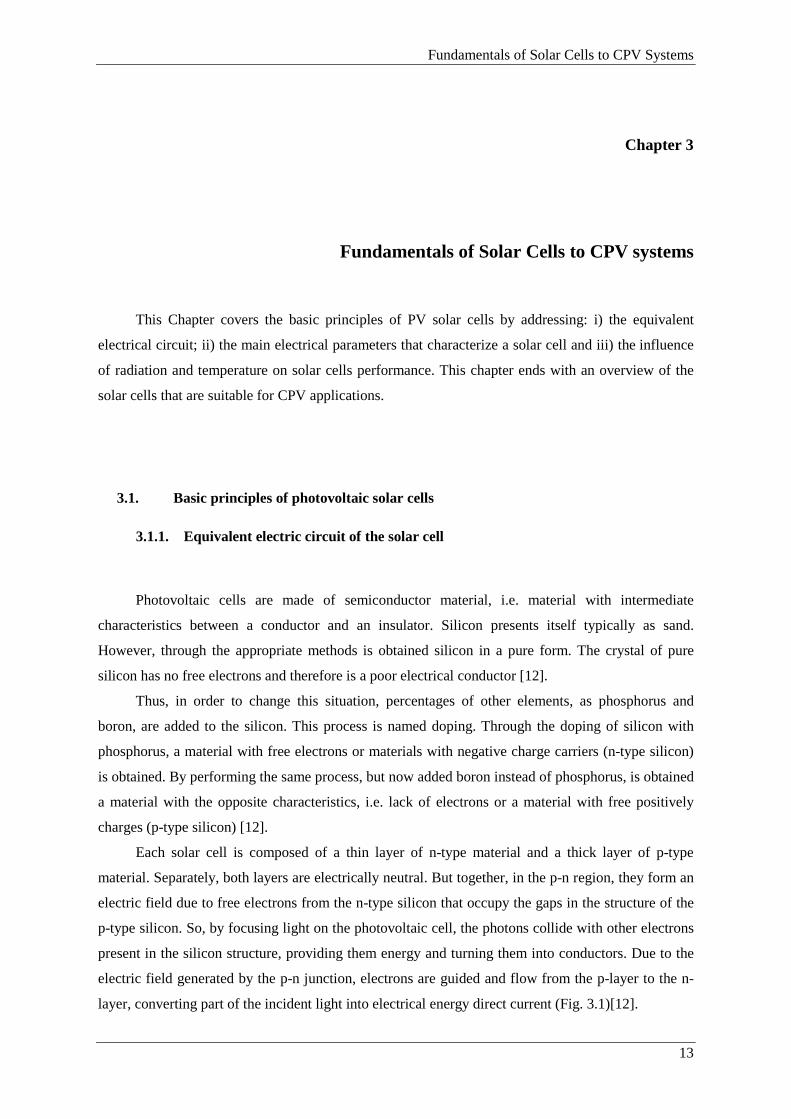
p-type silicon. So, by focusing light on the photovoltaic cell, the photons collide with other electrons
present in the silicon structure, providing them energy and turning them into conductors. Due to the
electric field generated by the p-n junction, electrons are guided and flow from the p-layer to the n-
layer, converting part of the incident light into electrical energy direct current (Fig. 3.1)[12].
Fundamentals of Solar Cells to CPV Systems
14
Figure 10- Principle of operation of a solar cell. Source: http://www.esdalcollege.nl/eos/vakken/na/zonnecel.htm
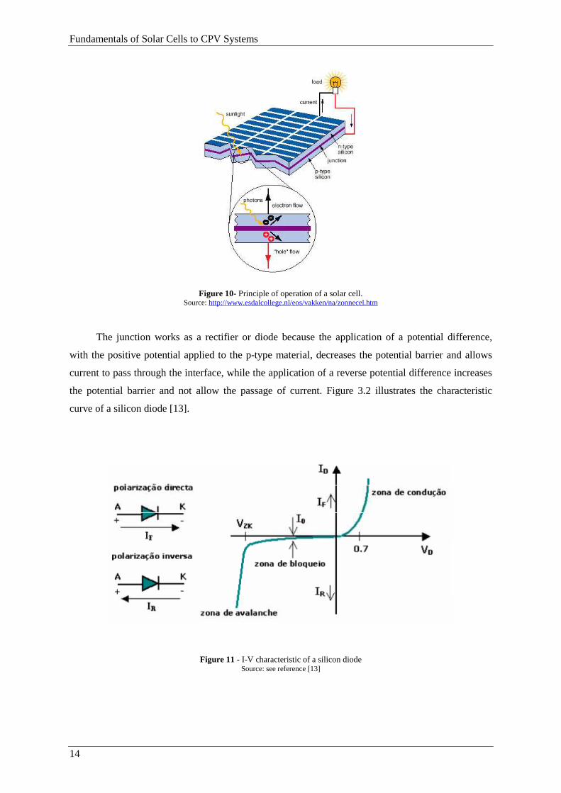
The junction works as a rectifier or diode because the application of a potential difference,
with the positive potential applied to the p-type material, decreases the potential barrier and allows
current to pass through the interface, while the application of a reverse potential difference increases
the potential barrier and not allow the passage of current. Figure 3.2 illustrates the characteristic
curve of a silicon diode [13].
Figure 11 - I-V characteristic of a silicon diode Source: see reference [13]
Fundamentals of Solar Cells to CPV Systems
15
When the diode is connected to a circuit so as that the potential is positive on the anode doped
with impurities of type p, and negative on the cathode doped with impurities of type n, the diode is
directly polarized. In this case its applied the first quadrant of characteristic curves, where, from a
defined voltage (threshold driving voltage in this case is 0.7 V), the current will flow [13].
If the diode is reverse-biased, current is prevented to move in this direction and in this case, it
applies to the third quadrant of the characteristic curve. The diode goes into avalanche or breakdown
region when the reverse voltage exceeds a given threshold value (which may lead to its destruction),
specific for each diode, called rupture strain. It is the "knee" strain of the I-V curve, and it is
designated by VZK. In the region of rupture, the reverse current grows quickly, while the
corresponding increase in voltage drop too low [13].
The expression that gives us the variation of intensity of the diode current (Id ) with a
difference of potential on the terminals is the Shockley equation [13]:
= exp − 1
(1)
where:
I0 - Reverse Saturation Current (or leakage) that passes through the diode;
V - Difference of potential on the terminals of the diode;
m - Ideality factor of the diode (when m = 1, we have a ideal diode; when the m> 1, we have a
real diode);
VT - Thermal Potential that is given by the equation 2
=
(2)
k -Boltzman Constant ( = 1.38 × 10 /);
T - Absolute temperature of the cell (in Kelvin);
q – Electron charge ( = 1.60 × 10 ! /).
Fundamentals of Solar Cells to CPV Systems
16
The current Id is void when V = 0, increases exponentially for positive values of qV and
decreases when qV is negative for a value of saturation negative.
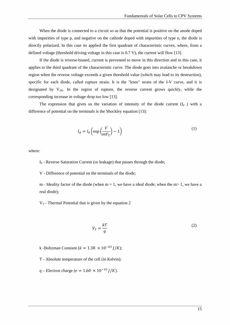
A solar cell that is not exposed to solar radiation is represented by the equivalent circuit of a
diode and the respective I-V curve in Fig. 3.3 [13].
Figure 12 - a) Diagram of equivalent circuit; b) Characteristic curve of the cell in total darkness Source: see reference [13]
The equation that expresses the variation of current vs. voltage for the ideal solar cell is given
by [13]:
= # − $ ⇔ = # − &' − 1 (3)
where IL is the current generated due to exposure to light or solar radiation. Then, it proves that if
does not exist solar radiation, the value of IL is 0, and the equation (3) leads to the equation (1). In the
presence of solar radiation, the characteristic curve of diode is deflected by the peak current IL in the
direction of reverse bias (fourth quadrant in the diagram of I-V curve) (Fig. 3.4) [13]. The current
generated by the solar radiation can be electrically represented by a current source (Fig. 3.4).
a) b)
Fundamentals of Solar Cells to CPV Systems
17
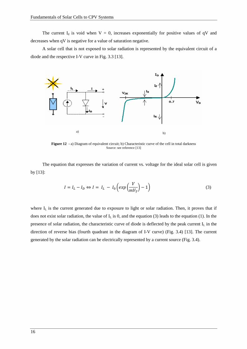
Figure 13 - a) Diagram of equivalent circuit b) Characteristic curve of the irradiated cell Source: see reference [13]
However, contrary to what occurs in the ideal solar cell, in reality the PV cells have associated
to their characteristic parasitic resistances that affect their performance. As such, the equivalent
electric circuit should include two elements, the series (Rs) and shunt or parallel (Rsh) resistance
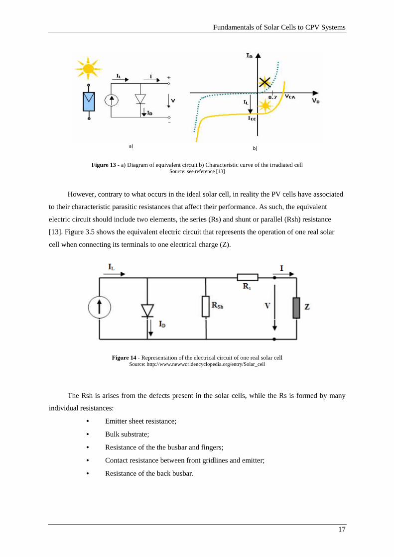
[13]. Figure 3.5 shows the equivalent electric circuit that represents the operation of one real solar
cell when connecting its terminals to one electrical charge (Z).
Figure 14 - Representation of the electrical circuit of one real solar cell Source: http://www.newworldencyclopedia.org/entry/Solar_cell
The Rsh is arises from the defects present in the solar cells, while the Rs is formed by many
individual resistances:
• Emitter sheet resistance;
• Bulk substrate;
• Resistance of the the busbar and fingers;
• Contact resistance between front gridlines and emitter;
• Resistance of the back busbar.
a) b)
Fundamentals of Solar Cells to CPV Systems
18
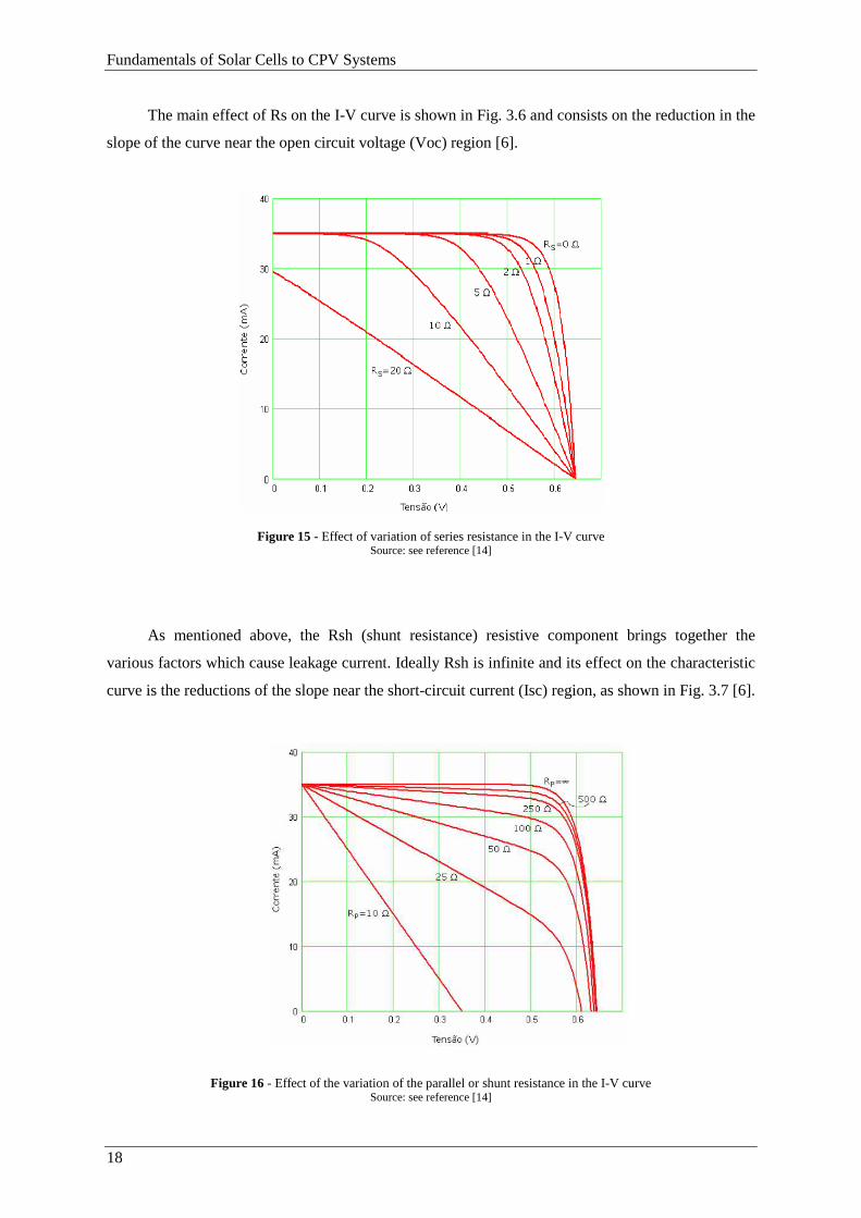
The main effect of Rs on the I-V curve is shown in Fig. 3.6 and consists on the reduction in the
slope of the curve near the open circuit voltage (Voc) region [6].
Figure 15 - Effect of variation of series resistance in the I-V curve
Source: see reference [14]
As mentioned above, the Rsh (shunt resistance) resistive component brings together the
various factors which cause leakage current. Ideally Rsh is infinite and its effect on the characteristic
curve is the reductions of the slope near the short-circuit current (Isc) region, as shown in Fig. 3.7 [6].
Figure 16 - Effect of the variation of the parallel or shunt resistance in the I-V curve Source: see reference [14]
Fundamentals of Solar Cells to CPV Systems
19
Both resistances influence the I-V curve by reducing the cell fill factor. Very high values of
Rsh and very low values of Rs may cause the reduction in short circuit current and in the open circuit
voltage, respectively. In the presence of these resistances, the general equation of the characteristic
curve of the cell is given by [6, 15]:
= # − &' + )* × − 1 − + )* ×
)+, (4)
3.2. Electrical parameters of a solar cell
When through one variable resistance that varies the electrical charge on the terminals of a
photovoltaic module or other photovoltaic device exposed to solar radiation, the photogenerated
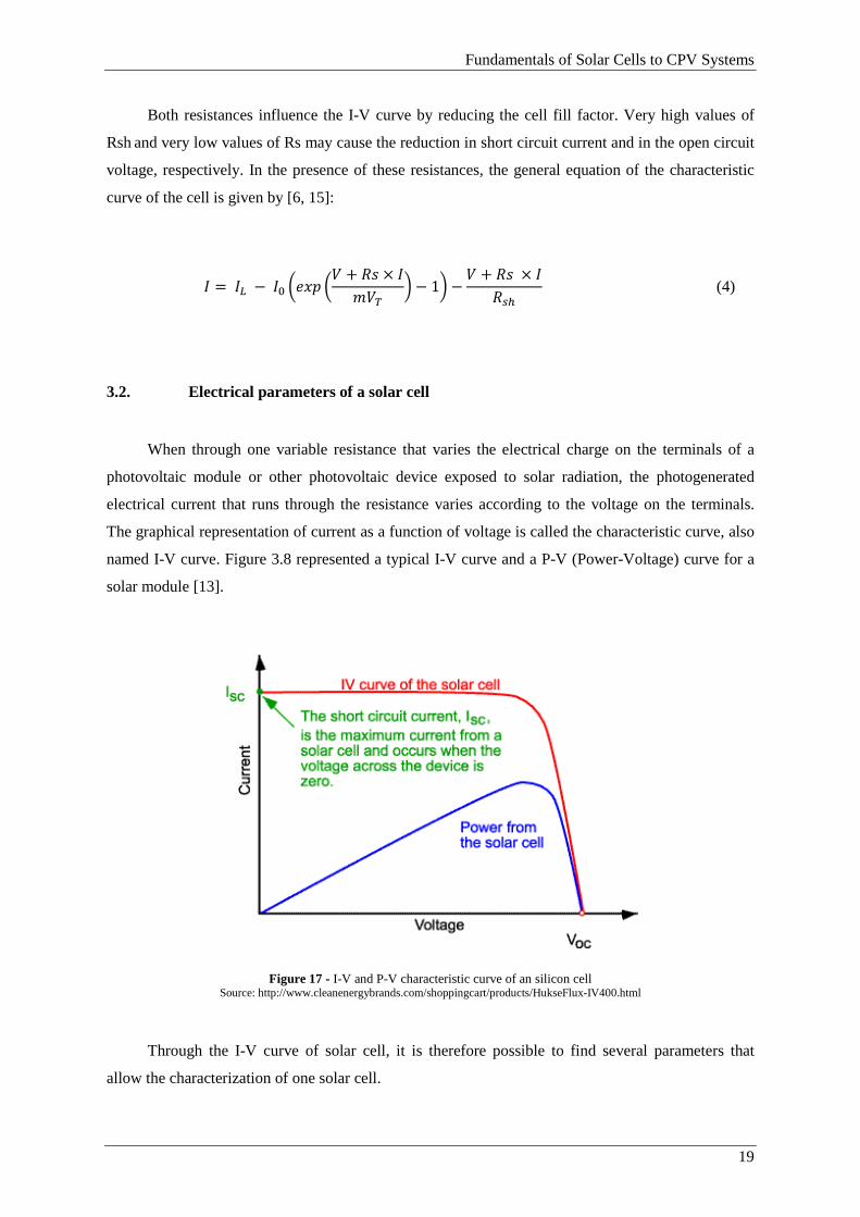
electrical current that runs through the resistance varies according to the voltage on the terminals.
The graphical representation of current as a function of voltage is called the characteristic curve, also
named I-V curve. Figure 3.8 represented a typical I-V curve and a P-V (Power-Voltage) curve for a
solar module [13].
Figure 17 - I-V and P-V characteristic curve of an silicon cell Source: http://www.cleanenergybrands.com/shoppingcart/products/HukseFlux-IV400.html
Through the I-V curve of solar cell, it is therefore possible to find several parameters that
allow the characterization of one solar cell.
Fundamentals of Solar Cells to CPV Systems
20
3.2.1. Short-circuit current and open-circuit voltage
The two parameters obtained from the intercept of the I-V curve with the axis system for a
given radiation and temperature, allow to characterize one solar cell of a given area.
This two parameters are the short-circuit current (Isc (V = 0)) and the maximum voltage on the
terminals of the cell by the open circuit voltage (Voc (I = 0)) [16].
According to equation 5 and 6, the value of ISC and the Voc is given, respectively, by [16]:
*- = # (5)
.- = × × /0102 + 1 3 (6)
3.2.2. Maximum power point
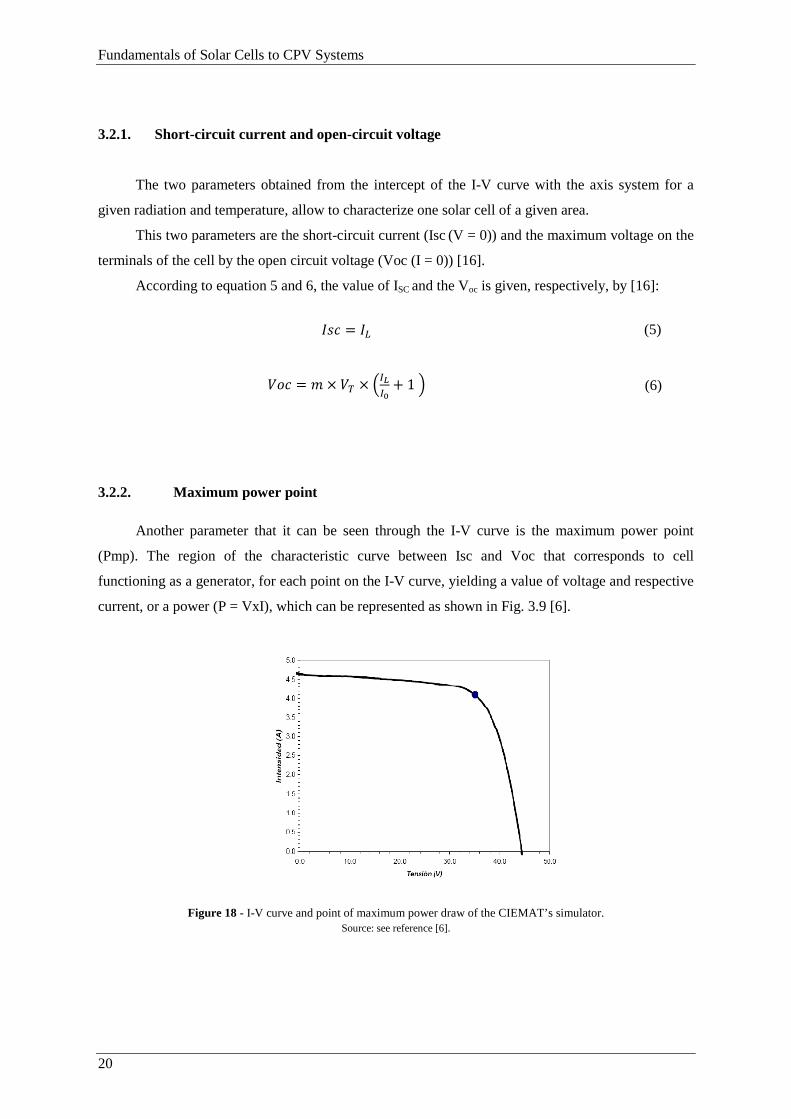
Another parameter that it can be seen through the I-V curve is the maximum power point
(Pmp). The region of the characteristic curve between Isc and Voc that corresponds to cell
functioning as a generator, for each point on the I-V curve, yielding a value of voltage and respective
current, or a power (P = VxI), which can be represented as shown in Fig. 3.9 [6].
Figure 18 - I-V curve and point of maximum power draw of the CIEMAT’s simulator. Source: see reference [6].
Fundamentals of Solar Cells to CPV Systems
21
The power delivered is given by the above product and there will be an operating point (Impp,
Vmpp) at which maximum power is delivered - the point of maximum power.
In a short circuit or in an open circuit the power is zero. The maximum power that emerges
from the cell (Pmp), occurs at the point of the characteristic curve where the product (I x V) is
maximum, ie (05)(5) = (6)
(5) = 0. So, according to equation 7, the value of voltage at the maximum power point is given by [16]:
'' = 78 − × × /0102 + 1 3 (7)
And, according to the equation 8, the value of current at the maximum power is given by [16]:
'' = − 59::5; × &' /59::
5; 3 (8)
The value of maximum power is therefore calculated by the product of the maximum values of
intensity and voltage of the solar cell at the Pmp, as can be seen in the equation 9 [14].
<' = '' × ('') = '' × '' (9)
3.2.3. Fill Factor
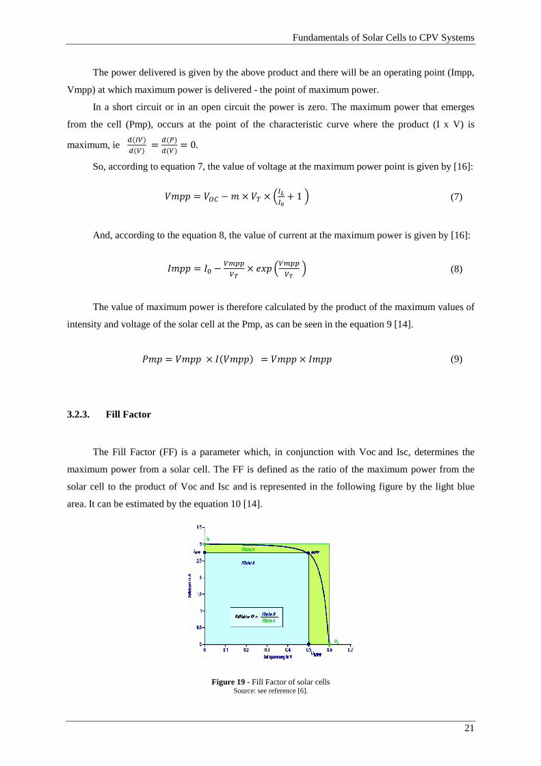
The Fill Factor (FF) is a parameter which, in conjunction with Voc and Isc, determines the
maximum power from a solar cell. The FF is defined as the ratio of the maximum power from the
solar cell to the product of Voc and Isc and is represented in the following figure by the light blue
area. It can be estimated by the equation 10 [14].
Figure 19 - Fill Factor of solar cells Source: see reference [6].
Fundamentals of Solar Cells to CPV Systems
22
== = '' × ''*- × .- (10)
The FF is a parameter of great importance and of great practical use because it is the indicator
of the quality of the cells[6].
Making use of the definition of FF, the Pmp delivered by a cell is given by equation 11 [6].
<' = == × *- × .- (11)
3.2.4. Conversion efficiency
The energy conversion efficiency of a solar cell is defined by the ratio between the Pmp and
the power that falls on the solar cell, G [6].
> = <'?
(12)
Naturally, this efficiency and maximum power is obtained only if the load resistance is
adequate, given by Vmpp / Impp. For example, when one says that a commercial cell has an
efficiency of 15% it means that if we had a cell surface of 1m2 that is illuminated with 100W/m2 of
incident radiation, the maximum output power will be 15W [14].
3.3. Influence of temperature and radiation intensity on the characteristic curve
Factors such as the intensity of solar radiation and temperature directly influence the
performance of a photovoltaic cell, which can easily be observed through its I-V curve, as showed in
Fig. 3.11.
Fundamentals of Solar Cells to CPV Systems
23
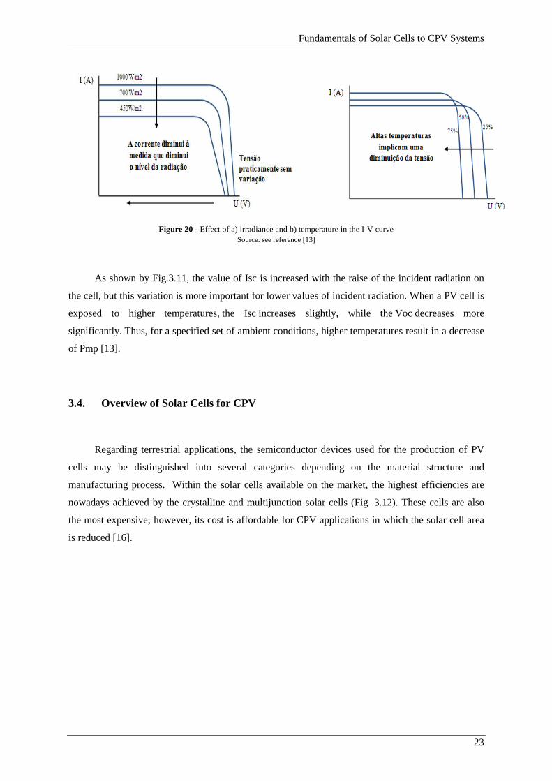
Figure 20 - Effect of a) irradiance and b) temperature in the I-V curve
Source: see reference [13]
As shown by Fig.3.11, the value of Isc is increased with the raise of the incident radiation on
the cell, but this variation is more important for lower values of incident radiation. When a PV cell is
exposed to higher temperatures, the Isc increases slightly, while the Voc decreases more
significantly. Thus, for a specified set of ambient conditions, higher temperatures result in a decrease
of Pmp [13].
3.4. Overview of Solar Cells for CPV
Regarding terrestrial applications, the semiconductor devices used for the production of PV
cells may be distinguished into several categories depending on the material structure and
manufacturing process. Within the solar cells available on the market, the highest efficiencies are
nowadays achieved by the crystalline and multijunction solar cells (Fig .3.12). These cells are also
the most expensive; however, its cost is affordable for CPV applications in which the solar cell area
is reduced [16].
Fundamentals of Solar Cells to CPV Systems
24
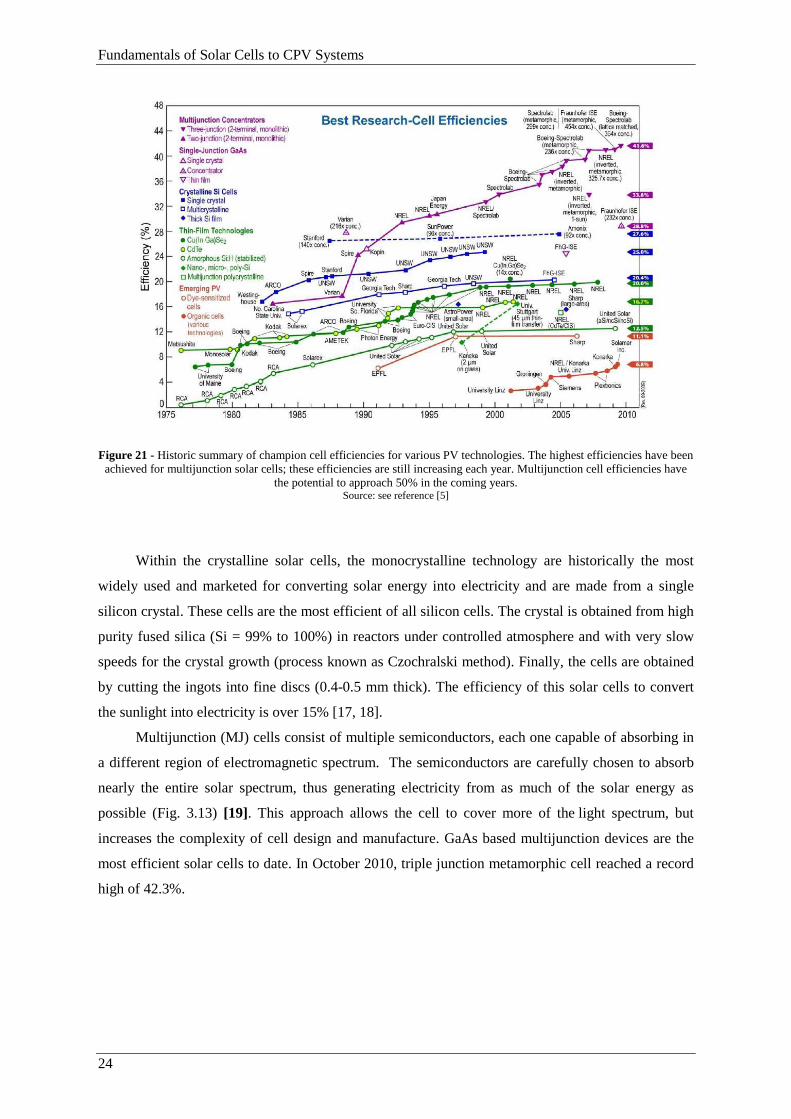
Figure 21 - Historic summary of champion cell efficiencies for various PV technologies. The highest efficiencies have been achieved for multijunction solar cells; these efficiencies are still increasing each year. Multijunction cell efficiencies have
the potential to approach 50% in the coming years. Source: see reference [5]
Within the crystalline solar cells, the monocrystalline technology are historically the most
widely used and marketed for converting solar energy into electricity and are made from a single
silicon crystal. These cells are the most efficient of all silicon cells. The crystal is obtained from high
purity fused silica (Si = 99% to 100%) in reactors under controlled atmosphere and with very slow
speeds for the crystal growth (process known as Czochralski method). Finally, the cells are obtained
by cutting the ingots into fine discs (0.4-0.5 mm thick). The efficiency of this solar cells to convert
the sunlight into electricity is over 15% [17, 18].
Multijunction (MJ) cells consist of multiple semiconductors, each one capable of absorbing in
a different region of electromagnetic spectrum. The semiconductors are carefully chosen to absorb
nearly the entire solar spectrum, thus generating electricity from as much of the solar energy as
possible (Fig. 3.13) [19]. This approach allows the cell to cover more of the light spectrum, but
increases the complexity of cell design and manufacture. GaAs based multijunction devices are the
most efficient solar cells to date. In October 2010, triple junction metamorphic cell reached a record
high of 42.3%.
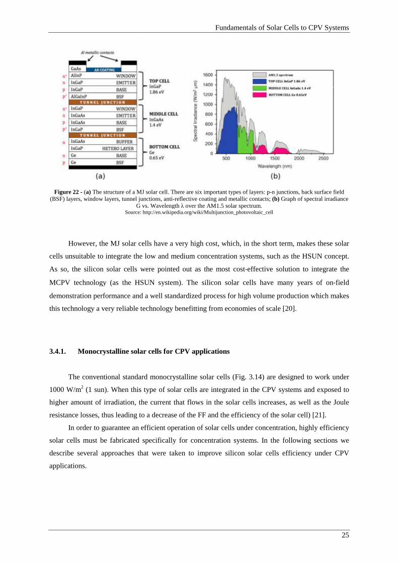
Figure 22 - (a) The structure of a MJ solar cell. There are six important types of layers: p(BSF) layers, window layers, tunnel junctions,
G vs. Wavelength Source: http://en.wikipedia.org/wiki/Multijunction_photovoltaic_cell
However, the MJ solar cells have a very high cost, which, in the short term, makes these solar
cells unsuitable to integrate the low and medium
As so, the silicon solar cells were pointed out as the most cost
MCPV technology (as the HSUN system). The silicon solar cells have many years of on
demonstration performance and a well standardized process for high volume production which makes
this technology a very reliable technology benefitting from economies of scale
3.4.1. Monocrystalline solar cells for CPV applications
The conventional standard mono
1000 W/m2 (1 sun). When this type of solar cells are integrated in the CPV systems and expose
higher amount of irradiation, the current that flows in the solar cells increases, as well as the Joule
resistance losses, thus leading to a decrease of the FF and the
In order to guarantee an efficient operation of solar cells under concentra
solar cells must be fabricated specifically for concentration systems. In the following sections we
describe several approaches that were taken to improve silicon solar cells efficiency under CPV
applications.
Fundamentals of Solar Cells to C
The structure of a MJ solar cell. There are six important types of layers: p-n junctions, back surface field
(BSF) layers, window layers, tunnel junctions, anti-reflective coating and metallic contacts; (b) Graph of spectral irradiance G vs. Wavelength λ over the AM1.5 solar spectrum.
http://en.wikipedia.org/wiki/Multijunction_photovoltaic_cell
However, the MJ solar cells have a very high cost, which, in the short term, makes these solar
cells unsuitable to integrate the low and medium concentration systems, such as the HSUN concept.
As so, the silicon solar cells were pointed out as the most cost‐effective solution to integrate the
MCPV technology (as the HSUN system). The silicon solar cells have many years of on
rformance and a well standardized process for high volume production which makes
this technology a very reliable technology benefitting from economies of scale [20]
crystalline solar cells for CPV applications
he conventional standard monocrystalline solar cells (Fig. 3.14) are design
(1 sun). When this type of solar cells are integrated in the CPV systems and expose
higher amount of irradiation, the current that flows in the solar cells increases, as well as the Joule
resistance losses, thus leading to a decrease of the FF and the efficiency of the solar cell)
In order to guarantee an efficient operation of solar cells under concentration, highly efficiency
solar cells must be fabricated specifically for concentration systems. In the following sections we
describe several approaches that were taken to improve silicon solar cells efficiency under CPV
Fundamentals of Solar Cells to CPV Systems
25
n junctions, back surface field Graph of spectral irradiance
However, the MJ solar cells have a very high cost, which, in the short term, makes these solar
concentration systems, such as the HSUN concept.
effective solution to integrate the
MCPV technology (as the HSUN system). The silicon solar cells have many years of on‐field
rformance and a well standardized process for high volume production which makes
[20].
are designed to work under
(1 sun). When this type of solar cells are integrated in the CPV systems and exposed to
higher amount of irradiation, the current that flows in the solar cells increases, as well as the Joule
efficiency of the solar cell) [21].
tion, highly efficiency
solar cells must be fabricated specifically for concentration systems. In the following sections we
describe several approaches that were taken to improve silicon solar cells efficiency under CPV
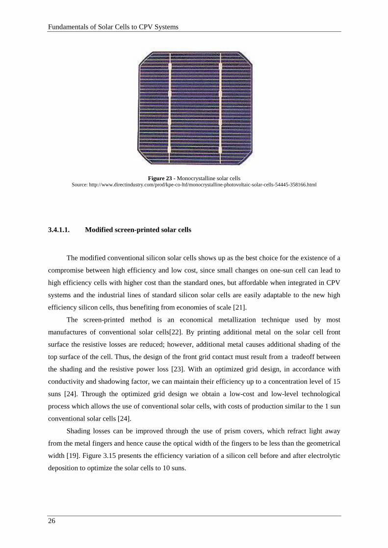
Fundamentals of Solar Cells to CPV Systems
26
Figure 23 - Monocrystalline solar cells Source: http://www.directindustry.com/prod/kpe-co-ltd/monocrystalline-photovoltaic-solar-cells-54445-358166.html
3.4.1.1. Modified screen-printed solar cells
The modified conventional silicon solar cells shows up as the best choice for the existence of a
compromise between high efficiency and low cost, since small changes on one-sun cell can lead to
high efficiency cells with higher cost than the standard ones, but affordable when integrated in CPV
systems and the industrial lines of standard silicon solar cells are easily adaptable to the new high
efficiency silicon cells, thus benefiting from economies of scale [21].
The screen-printed method is an economical metallization technique used by most
manufactures of conventional solar cells[22]. By printing additional metal on the solar cell front
surface the resistive losses are reduced; however, additional metal causes additional shading of the
top surface of the cell. Thus, the design of the front grid contact must result from a tradeoff between
the shading and the resistive power loss [23]. With an optimized grid design, in accordance with
conductivity and shadowing factor, we can maintain their efficiency up to a concentration level of 15
suns [24]. Through the optimized grid design we obtain a low-cost and low-level technological
process which allows the use of conventional solar cells, with costs of production similar to the 1 sun
conventional solar cells [24].
Shading losses can be improved through the use of prism covers, which refract light away
from the metal fingers and hence cause the optical width of the fingers to be less than the geometrical
width [19]. Figure 3.15 presents the efficiency variation of a silicon cell before and after electrolytic
deposition to optimize the solar cells to 10 suns.
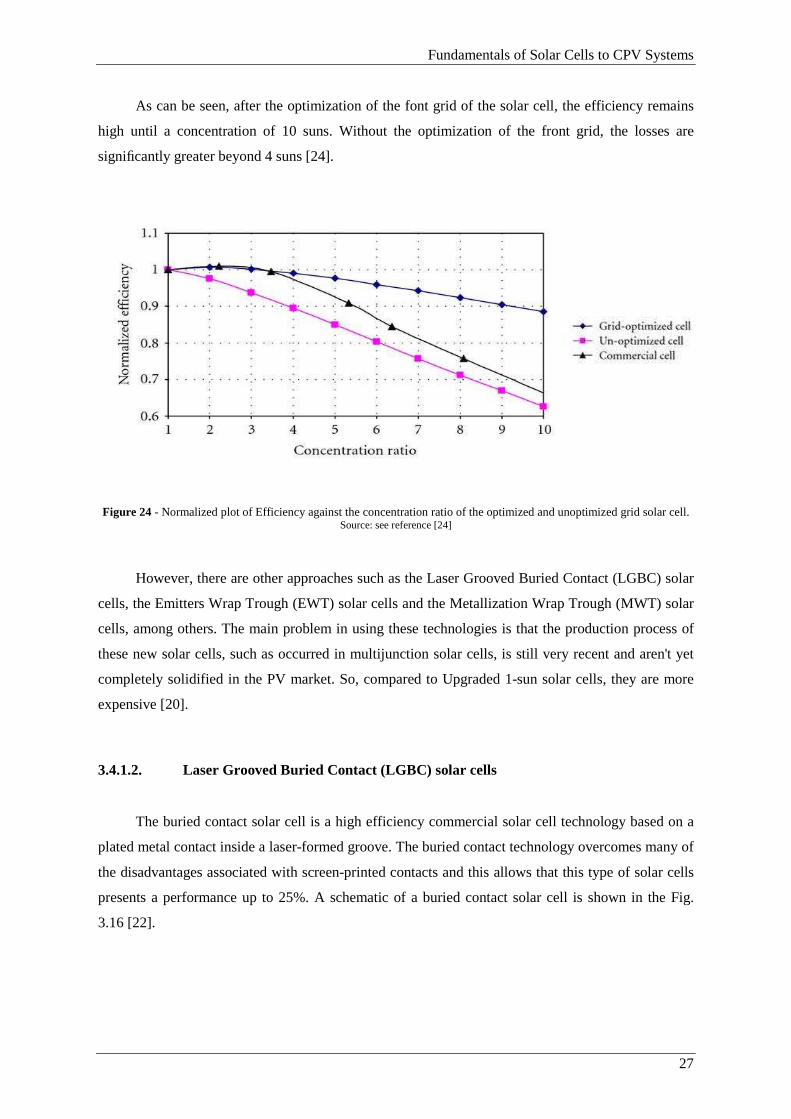
Fundamentals of Solar Cells to CPV Systems
27
As can be seen, after the optimization of the font grid of the solar cell, the efficiency remains
high until a concentration of 10 suns. Without the optimization of the front grid, the losses are
significantly greater beyond 4 suns [24].
Figure 24 - Normalized plot of Efficiency against the concentration ratio of the optimized and unoptimized grid solar cell. Source: see reference [24]
However, there are other approaches such as the Laser Grooved Buried Contact (LGBC) solar
cells, the Emitters Wrap Trough (EWT) solar cells and the Metallization Wrap Trough (MWT) solar
cells, among others. The main problem in using these technologies is that the production process of
these new solar cells, such as occurred in multijunction solar cells, is still very recent and aren't yet
completely solidified in the PV market. So, compared to Upgraded 1-sun solar cells, they are more
expensive [20].
3.4.1.2. Laser Grooved Buried Contact (LGBC) solar cells
The buried contact solar cell is a high efficiency commercial solar cell technology based on a
plated metal contact inside a laser-formed groove. The buried contact technology overcomes many of
the disadvantages associated with screen-printed contacts and this allows that this type of solar cells
presents a performance up to 25%. A schematic of a buried contact solar cell is shown in the Fig.
3.16 [22].
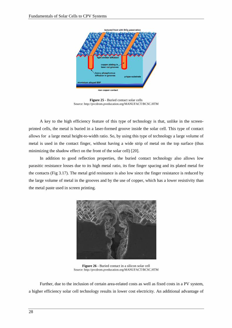
Fundamentals of Solar Cells to CPV Systems
28
Figure 25 - Buried contact solar cells Source: http://pvcdrom.pveducation.org/MANUFACT/BCSC.HTM
A key to the high efficiency feature of this type of technology is that, unlike in the screen-
printed cells, the metal is buried in a laser-formed groove inside the solar cell. This type of contact
allows for a large metal height-to-width ratio. So, by using this type of technology a large volume of
metal is used in the contact finger, without having a wide strip of metal on the top surface (thus
minimizing the shadow effect on the front of the solar cell) [20].
In addition to good reflection properties, the buried contact technology also allows low
parasitic resistance losses due to its high metal ratio, its fine finger spacing and its plated metal for
the contacts (Fig 3.17). The metal grid resistance is also low since the finger resistance is reduced by
the large volume of metal in the grooves and by the use of copper, which has a lower resistivity than
the metal paste used in screen printing.
Figure 26 - Buried contact in a silicon solar cell Source: http://pvcdrom.pveducation.org/MANUFACT/BCSC.HTM
Further, due to the inclusion of certain area-related costs as well as fixed costs in a PV system,
a higher efficiency solar cell technology results in lower cost electricity. An additional advantage of
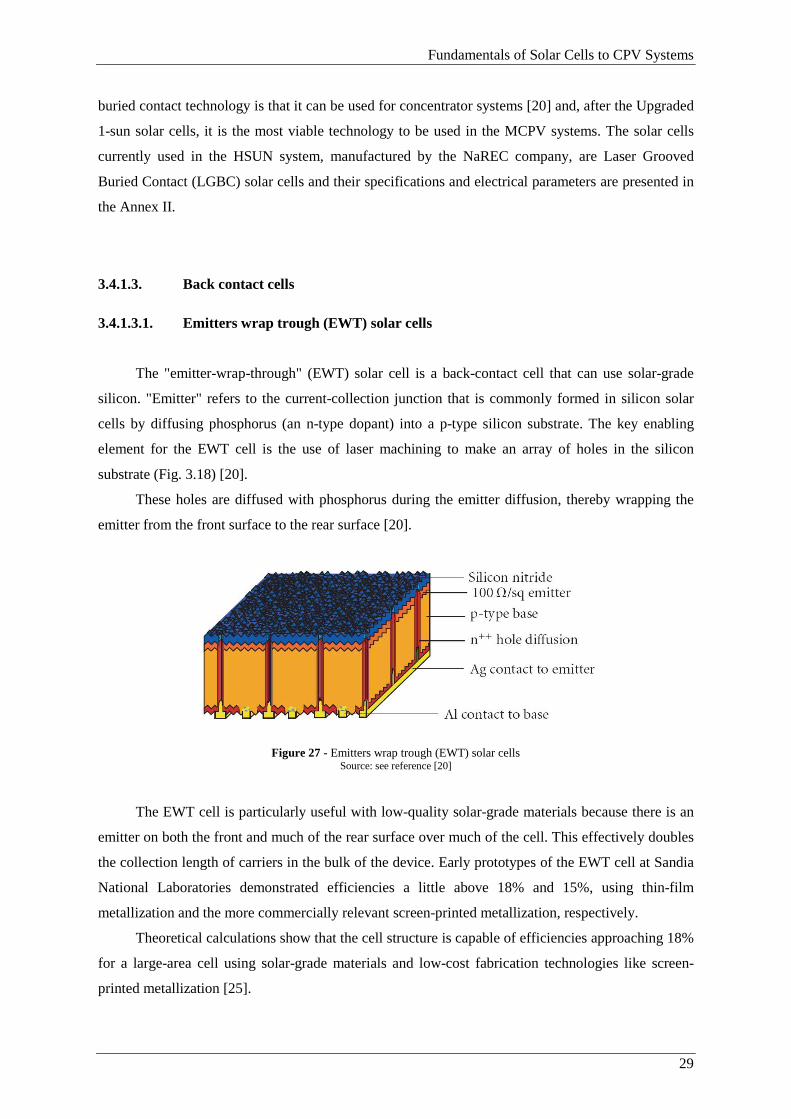
Fundamentals of Solar Cells to CPV Systems
29
buried contact technology is that it can be used for concentrator systems [20] and, after the Upgraded
1-sun solar cells, it is the most viable technology to be used in the MCPV systems. The solar cells
currently used in the HSUN system, manufactured by the NaREC company, are Laser Grooved
Buried Contact (LGBC) solar cells and their specifications and electrical parameters are presented in
the Annex II.
3.4.1.3. Back contact cells
3.4.1.3.1. Emitters wrap trough (EWT) solar cells
The "emitter-wrap-through" (EWT) solar cell is a back-contact cell that can use solar-grade
silicon. "Emitter" refers to the current-collection junction that is commonly formed in silicon solar
cells by diffusing phosphorus (an n-type dopant) into a p-type silicon substrate. The key enabling
element for the EWT cell is the use of laser machining to make an array of holes in the silicon
substrate (Fig. 3.18) [20].
These holes are diffused with phosphorus during the emitter diffusion, thereby wrapping the
emitter from the front surface to the rear surface [20].
Figure 27 - Emitters wrap trough (EWT) solar cells Source: see reference [20]
The EWT cell is particularly useful with low-quality solar-grade materials because there is an
emitter on both the front and much of the rear surface over much of the cell. This effectively doubles
the collection length of carriers in the bulk of the device. Early prototypes of the EWT cell at Sandia
National Laboratories demonstrated efficiencies a little above 18% and 15%, using thin-film
metallization and the more commercially relevant screen-printed metallization, respectively.
Theoretical calculations show that the cell structure is capable of efficiencies approaching 18%
for a large-area cell using solar-grade materials and low-cost fabrication technologies like screen-
printed metallization [25].

Fundamentals of Solar Cells to CPV Systems
30
3.4.1.3.2. Metallization wrap trough (MWT) solar cells
The contact wrap-through or metallization wrap-through (MWT) back-contact cell is the
concept that is most closely linked to the conventional cell structure. In these cells, the emitter is
located near the front surface, but part of the front metallization grid is moved from the front to the
rear surface (the busbar on the front surface of the solar cells are transferred to the rear side of the
cell). In the schematic representation in Fig. 3.19, this is depicted as the busbar moving from one
surface to the other, while the remaining front surface grid is connected to the interconnection pads
on the rear surface by extending it through a number of openings in the wafer [20].
Figure 28 - Metallization wrap trough (MWT) solar cells Source: see reference [20]
The MWT cells requires only a relatively small number of through-holes to direct
photogenerated electrons to the back surface, through the metal electrodes and n-doped emitters, and
produce higher collection photocurrents due to absence of a bus bar (main electrode) on the front
surface (as in conventional cells). A high Jsc of 37.3 mA/ cm–2 and an efficiency of 18.3% were
reported for a recent MWT cell by Kyocera, and the module efficiency for MWT cell modules by
ECN, 16.4%, is the highest reported to date [25].
To understand the real potential single crystalline silicon solar cells integrated in MCPV
systems, different monocrystalline silicon solar cells were studied and the description of these solar
cells are presented in the next chapters.

Fundamentals of Solar Cells to CPV Systems
31
Chapter 4
Theoretical characterization of Solartec and KVAZAR solar cells
This chapter covers the theoretical behavior of the Solartec and KVAZAR solar cells under
concentration. In section 4.1, the physical characteristics of the Solartec and KVAZAR solar cells are
presented; in section 4.2, a description of the mathematical model used for estimate the behavior of
the solar cells is describe and in section 4.3, the theorical results obtained and the consequents
conclusions are presented.
4.1. Physical characteristics of the KVAZAR and Solartec solar cells
In this thesis two types of silicon solar cells were studied: i) the conventional solar cells,
provided by the KVAZAR company and ii) Upgraded 1-sun screen printed silicon solar cells,
provided by the Solartec company. In the next section, the physical characteristics of these solar cells
are explained and the datasheets provided by the suppliers are presented in the Annex III.
4.1.1. KVAZAR solar cells
The KVAZAR conventional solar cells (Fig. 4.1), provided by the KVAZAR company, are
made of monocrystalline silicon and the metallization method is the screen printing.

32
Figure 29
The KVAZAR solar cells
approximately. The active area of these conventional solar cells
by the contacts of the cell) is, approximately, 150 cm
The front of the solar cells is composed by a busbar and fingers
cell) with 1.5 mm and 0.04 mm of width, respectively. The b
two soldering pads with 3mm of width and a back surface field
Figure 30
Theorical Characterization of Solartec and KVAZAR solar cells
29 - Front surface of the KVAZAR solar cell (main cell)
cells (Fig. 4.1) have a total area of 156.25 cm2 and a thickness of 200
approximately. The active area of these conventional solar cells (i.e. total area less the area occupied
by the contacts of the cell) is, approximately, 150 cm2.
The front of the solar cells is composed by a busbar and fingers (negative contact of the solar
cell) with 1.5 mm and 0.04 mm of width, respectively. The back of the solar cells is composed by
two soldering pads with 3mm of width and a back surface field (Fig. 4.2).
30 - Back surface of the KVAZAR solar cells ( main cell)
and KVAZAR solar cells
and a thickness of 200 µm,
(i.e. total area less the area occupied
(negative contact of the solar
ack of the solar cells is composed by
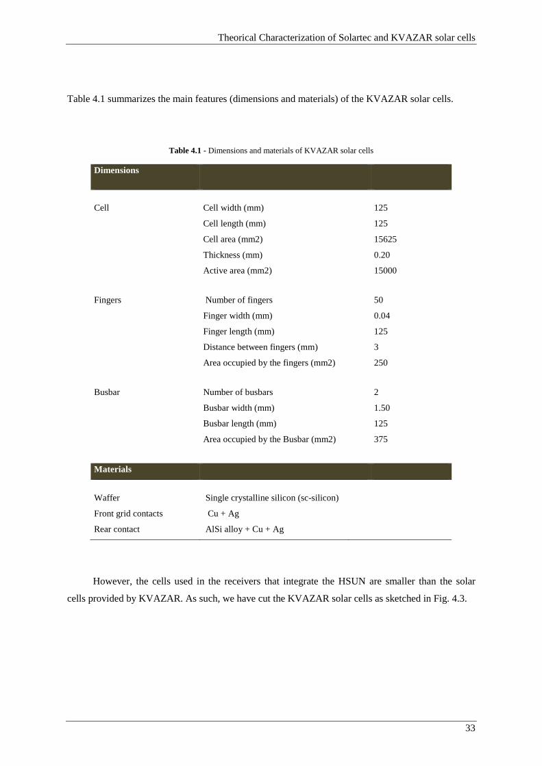
Theorical Characterization of Solartec and KVAZAR solar cells
33
Table 4.1 summarizes the main features (dimensions and materials) of the KVAZAR solar cells.
Table 4.1 - Dimensions and materials of KVAZAR solar cells
Dimensions
Cell Cell width (mm) 125
Cell length (mm) 125
Cell area (mm2) 15625
Thickness (mm) 0.20
Active area (mm2) 15000
Fingers Number of fingers 50
Finger width (mm) 0.04
Finger length (mm) 125
Distance between fingers (mm) 3
Area occupied by the fingers (mm2) 250
Busbar Number of busbars 2
Busbar width (mm) 1.50
Busbar length (mm) 125
Area occupied by the Busbar (mm2) 375
Materials
Waffer Single crystalline silicon (sc-silicon)
Front grid contacts Cu + Ag
Rear contact AlSi alloy + Cu + Ag
However, the cells used in the receivers that integrate the HSUN are smaller than the solar
cells provided by KVAZAR. As such, we have cut the KVAZAR solar cells as sketched in Fig. 4.3.
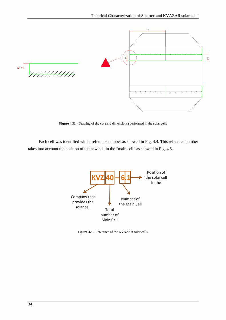
Theorical Characterization of Solartec and KVAZAR solar cells
34
Figure 4.31 - Drawing of the cut (and dimensions) performed in the solar cells
Each cell was identified with a reference number as showed in Fig. 4.4. This reference number
takes into account the position of the new cell in the “main cell” as showed in Fig. 4.5.
Figure 32 - Reference of the KVAZAR solar cells.
KVZ.40 – 6.1
Company that
provides the
solar cell Total
number of
Main Cell
Number of
the Main Cell
Cell
Position of
the solar cell
in the
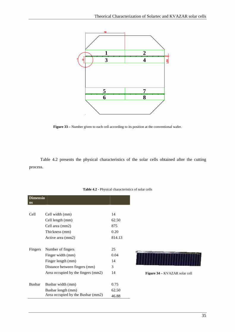
Theorical Characterization of Solartec and KVAZAR solar cells
35
Figure 33 – Number given to each cell according to its position at the conventional wafer.
Table 4.2 presents the physical characteristics of the solar cells obtained after the cutting
process.
Table 4.2 - Physical characteristics of solar cells
Dimensions
Cell Cell width (mm) 14
Cell length (mm) 62.50
Cell area (mm2) 875
Thickness (mm) 0.20
Active area (mm2) 814.13
Fingers Number of fingers 25
Finger width (mm) 0.04
Finger length (mm) 14
Distance between fingers (mm) 3
Area occupied by the fingers (mm2) 14
Busbar Busbar width (mm) 0.75
Busbar length (mm) 62.50 Area occupied by the Busbar (mm2) 46.88
1 2 3 4
5 6
7 8
Figure 34 – KVAZAR solar cell
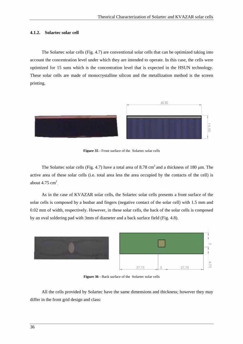
Theorical Characterization of Solartec and KVAZAR solar cells
36
4.1.2. Solartec solar cell
The Solartec solar cells (Fig. 4.7) are conventional solar cells that can be optimized taking into
account the concentration level under which they are intended to operate. In this case, the cells were
optimized for 15 suns which is the concentration level that is expected in the HSUN technology.
These solar cells are made of monocrystalline silicon and the metallization method is the screen
printing.
Figure 35 - Front surface of the Solartec solar cells
The Solartec solar cells (Fig. 4.7) have a total area of 8.78 cm2 and a thickness of 180 µm. The
active area of these solar cells (i.e. total area less the area occupied by the contacts of the cell) is
about 4.75 cm2.
As in the case of KVAZAR solar cells, the Solartec solar cells presents a front surface of the
solar cells is composed by a busbar and fingers (negative contact of the solar cell) with 1.5 mm and
0.02 mm of width, respectively. However, in these solar cells, the back of the solar cells is composed
by an oval soldering pad with 3mm of diameter and a back surface field (Fig. 4.8).
Figure 36 - Back surface of the Solartec solar cells
All the cells provided by Solartec have the same dimensions and thickness; however they may
differ in the front grid design and class:
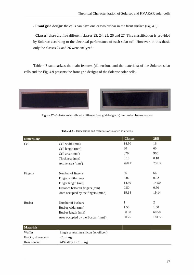
Theorical Characterization of Solartec and KVAZAR solar cells
37
- Front grid design: the cells can have one or two busbar in the front surface (Fig. 4.9).
- Classes: there are five different classes 23, 24, 25, 26 and 27. This classification is provided
by Solartec according to the electrical performance of each solar cell. However, in this thesis
only the classes 24 and 26 were analyzed.
Table 4.3 summarizes the main features (dimensions and the materials) of the Solartec solar
cells and the Fig. 4.9 presents the front grid designs of the Solartec solar cells.
Figure 37 –Solartec solar cells with different front grid designs: a) one busbar; b) two busbars
Table 4.3 – Dimensions and materials of Solartec solar cells
Dimensions Classes 2BB
Cell Cell width (mm) 14.50 16
Cell length (mm) 60 60
Cell area (mm2) 870 960
Thickness (mm) 0.18 0.18
Active area (mm2) 760.11 759.36
Fingers Number of fingers 66 66
Finger width (mm) 0.02 0.02
Finger length (mm) 14.50 14.50
Distance between fingers (mm) 0.50 0.50
Area occupied by the fingers (mm2) 19.14 19.14
Busbar Number of busbars 1 2
Busbar width (mm) 1.50 1.50
Busbar length (mm) 60.50 60.50
Area occupied by the Busbar (mm2) 90.75 181.50
Materials
Waffer Single crystalline silicon (sc-silicon)
Front grid contacts Cu + Ag
Rear contact AlSi alloy + Cu + Ag
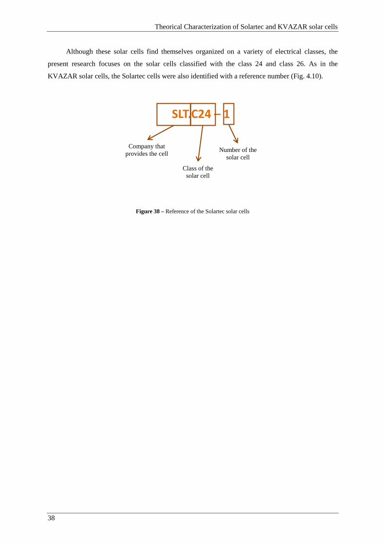
Theorical Characterization of Solartec and KVAZAR solar cells
38
Although these solar cells find themselves organized on a variety of electrical classes, the
present research focuses on the solar cells classified with the class 24 and class 26. As in the
KVAZAR solar cells, the Solartec cells were also identified with a reference number (Fig. 4.10).
Figure 38 – Reference of the Solartec solar cells
SLT.C24 – 1
Company that provides the cell
Class of the solar cell
Number of the solar cell
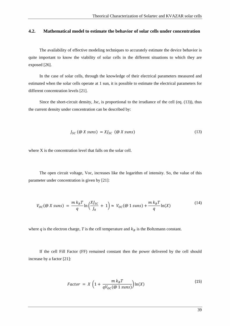
Theorical Characterization of Solartec and KVAZAR solar cells
39
4.2. Mathematical model to estimate the behavior of solar cells under concentration
The availability of effective modeling techniques to accurately estimate the device behavior is
quite important to know the viability of solar cells in the different situations to which they are
exposed [26].
In the case of solar cells, through the knowledge of their electrical parameters measured and
estimated when the solar cells operate at 1 sun, it is possible to estimate the electrical parameters for
different concentration levels [21].
Since the short-circuit density, Jsc, is proportional to the irradiance of the cell (eq. (13)), thus
the current density under concentration can be described by:
@8 (@ B *CD*) = B@8 (@ B *CD*) (13)
where X is the concentration level that falls on the solar cell.
The open circuit voltage, Voc, increases like the logarithm of intensity. So, the value of this
parameter under concentration is given by [21]:
78(@ B *CD*) = E ln B@8 + 1 ≈ 78(@ 1 *CD*) + E
ln(B) (14)
where q is the electron charge, T is the cell temperature and E is the Boltzmann constant.
If the cell Fill Factor (FF) remained constant then the power delivered by the cell should
increase by a factor [21]:
=I-J.K = B 1 + E78(@ 1 *CD*) ln(B)
(15)
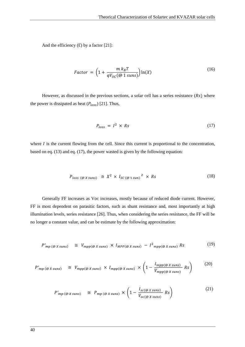
Theorical Characterization of Solartec and KVAZAR solar cells
40
And the efficiency (Ɛ) by a factor [21]:
=I-J.K = 1 + E78(@ 1 *CD*) ln(B)
(16)
However, as discussed in the previous sections, a solar cell has a series resistance ()*) where
the power is dissipated as heat (<LM++) [21]. Thus,
<LM++ = × )* (17)
where is the current flowing from the cell. Since this current is proportional to the concentration,
based on eq. (13) and eq. (17), the power wasted is given by the following equation:
<LM++ (@ N +OP+) ≅ B × @8 (@ +OP) × )* (18)
Generally FF increases as Voc increases, mostly because of reduced diode current. However,
FF is most dependent on parasitic factors, such as shunt resistance and, most importantly at high
illumination levels, series resistance [26]. Thus, when considering the series resistance, the FF will be
no longer a constant value, and can be estimate by the following approximation:
<′9: (@ N +OP+) ≅ 9::(@ N +OP+) × R66(@ N +OP+) − 9::(@ N +OP+) )* (19)
<′9: (@ N +OP+) ≅ 9::(@ N +OP+) × 9::(@ N +OP+) × S1 − 9::(@ N +OP+) 9::(@ N +OP+) )*T (20)
<′9: (@ N +OP+) ≅ <9: (@ N +OP+) × S1 − +U(@ N +OP+) MU(@ N +OP+) )*T (21)
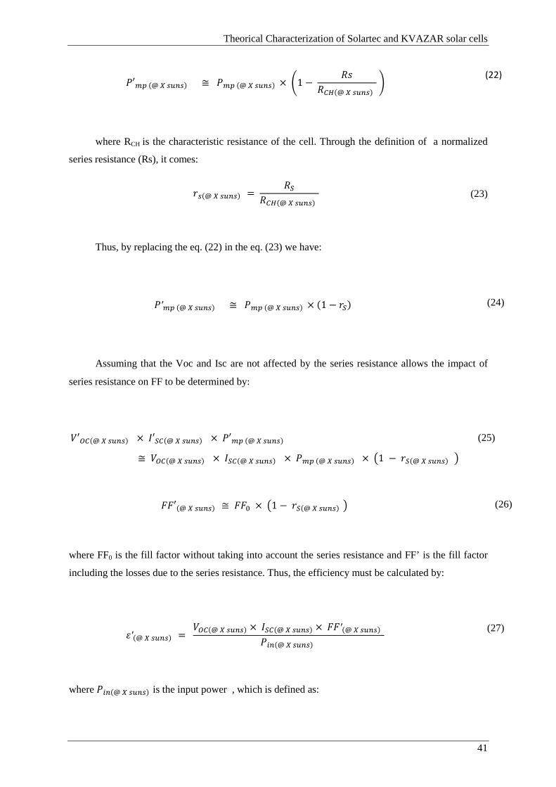
Theorical Characterization of Solartec and KVAZAR solar cells
41
<′9: (@ N +OP+) ≅ <9: (@ N +OP+) × S1 − )*)8W(@ N +OP+) T
(22)
where RCH is the characteristic resistance of the cell. Through the definition of a normalized
series resistance (Rs), it comes:
K+(@ N +OP+) = )@)8W(@ N +OP+) (23)
Thus, by replacing the eq. (22) in the eq. (23) we have:
<′9: (@ N +OP+) ≅ <9: (@ N +OP+) × (1 − K@) (24)
Assuming that the Voc and Isc are not affected by the series resistance allows the impact of
series resistance on FF to be determined by:
′78(@ N +OP+) × ′@8(@ N +OP+) × <′9: (@ N +OP+) ≅ 78(@ N +OP+) × @8(@ N +OP+) × <9: (@ N +OP+) × X1 − K@(@ N +OP+) Y
(25)
==′(@ N +OP+) ≅ == × X1 − K@(@ N +OP+) Y (26)
where FF0 is the fill factor without taking into account the series resistance and FF’ is the fill factor
including the losses due to the series resistance. Thus, the efficiency must be calculated by:
Z′(@ N +OP+) = 78(@ N +OP+) × @8(@ N +OP+) × ==′(@ N +OP+) <[P(@ N +OP+) (27)
where <[P(@ N +OP+) is the input power , which is defined as:
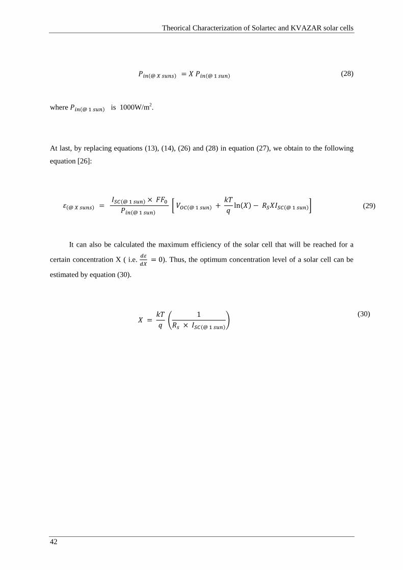
Theorical Characterization of Solartec and KVAZAR solar cells
42
<[P(@ N +OP+) = B <[P(@ +OP) (28)
where <[P(@ +OP) is 1000W/m2.
At last, by replacing equations (13), (14), (26) and (28) in equation (27), we obtain to the following
equation [26]:
Z(@ N +OP+) = @8(@ +OP) × == <[P(@ +OP) \ 78(@ +OP) + ln(B) − )@B@8(@ +OP)] (29)
It can also be calculated the maximum efficiency of the solar cell that will be reached for a
certain concentration X ( i.e. ^N = 0). Thus, the optimum concentration level of a solar cell can be
estimated by equation (30).
B = S 1
)+ × @8(@ +OP)T (30)
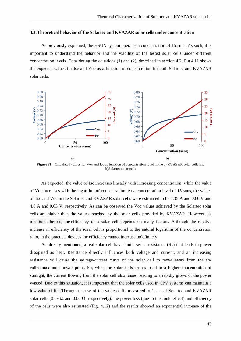
Theorical Characterization of Solartec and KVAZAR solar cells
43
4.3. Theoretical behavior of the Solartec and KVAZAR solar cells under concentration
As previously explained, the HSUN system operates a concentration of 15 suns. As such, it is
important to understand the behavior and the viability of the tested solar cells under different
concentration levels. Considering the equations (1) and (2), described in section 4.2, Fig.4.11 shows
the expected values for Isc and Voc as a function of concentration for both Solartec and KVAZAR
solar cells.
a) b)
Figure 39 - Calculated values for Voc and Isc as function of concentration level in the a) KVAZAR solar cells and b)Solartec solar cells
As expected, the value of Isc increases linearly with increasing concentration, while the value
of Voc increases with the logarithm of concentration. At a concentration level of 15 suns, the values
of Isc and Voc in the Solartec and KVAZAR solar cells were estimated to be 4.35 A and 0.66 V and
4.8 A and 0.63 V, respectively. As can be observed the Voc values achieved by the Solartec solar
cells are higher than the values reached by the solar cells provided by KVAZAR. However, as
mentioned before, the efficiency of a solar cell depends on many factors. Although the relative
increase in efficiency of the ideal cell is proportional to the natural logarithm of the concentration
ratio, in the practical devices the efficiency cannot increase indefinitely.
As already mentioned, a real solar cell has a finite series resistance (Rs) that leads to power
dissipated as heat. Resistance directly influences both voltage and current, and an increasing
resistance will cause the voltage-current curve of the solar cell to move away from the so-
called maximum power point. So, when the solar cells are exposed to a higher concentration of
sunlight, the current flowing from the solar cell also raises, leading to a rapidly grows of the power
wasted. Due to this situation, it is important that the solar cells used in CPV systems can maintain a
low value of Rs. Through the use of the value of Rs measured to 1 sun of Solartec and KVAZAR
solar cells (0.09 Ω and 0.06 Ω, respectively), the power loss (due to the Joule effect) and efficiency
of the cells were also estimated (Fig. 4.12) and the results showed an exponential increase of the
0
5
10
15
20
25
30
35
0.60
0.62
0.64
0.66
0.68
0.70
0.72
0.74
0.76
0.78
0.80
0 50 100
Cur
rent
(A
)
Vol
tage
(V)
Concentration (suns)
Voc
Isc
0
5
10
15
20
25
30
35
0.60
0.62
0.64
0.66
0.68
0.70
0.72
0.74
0.76
0.78
0.80
0 50 100
Cur
rent
(A
)
Vol
tage
(V)
Concentration (suns)
Voc
Isc
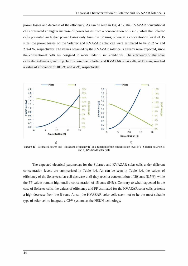
Theorical Characterization of Solartec and KVAZAR solar cells
44
power losses and decrease of the efficiency. As can be seen in Fig. 4.12, the KVAZAR conventional
cells presented an higher increase of power losses from a concentration of 5 suns, while the Solartec
cells presented an higher power losses only from the 12 suns, where at a concentration level of 15
suns, the power losses on the Solartec and KVAZAR solar cell were estimated to be 2.02 W and
2.074 W, respectively. The values obtained by the KVAZAR solar cells already were expected, since
the conventional cells are designed to work under 1 sun conditions. The efficiency of the solar
cells also suffers a great drop. In this case, the Solartec and KVAZAR solar cells, at 15 suns, reached
a value of efficiency of 10.3 % and 4.2%, respectively.
a) b)
Figure 40 - Estimated power loss (Ploss) and efficiency (ε) as a function of the concentration level of a) Solartec solar cells and b) KVAZAR solar cells
The expected electrical parameters for the Solartec and KVAZAR solar cells under different
concentration levels are summarized in Table 4.4. As can be seen in Table 4.4, the values of
efficiency of the Solartec solar cell decrease until they reach a concentration of 20 suns (8.7%), while
the FF values remain high until a concentration of 15 suns (54%). Contrary to what happened in the
case of Solartec cells, the values of efficiency and FF estimated for the KVAZAR solar cells presents
a high decrease from the 5 suns. As so, the KVAZAR solar cells seem not to be the most suitable
type of solar cell to integrate a CPV system, as the HSUN technology.
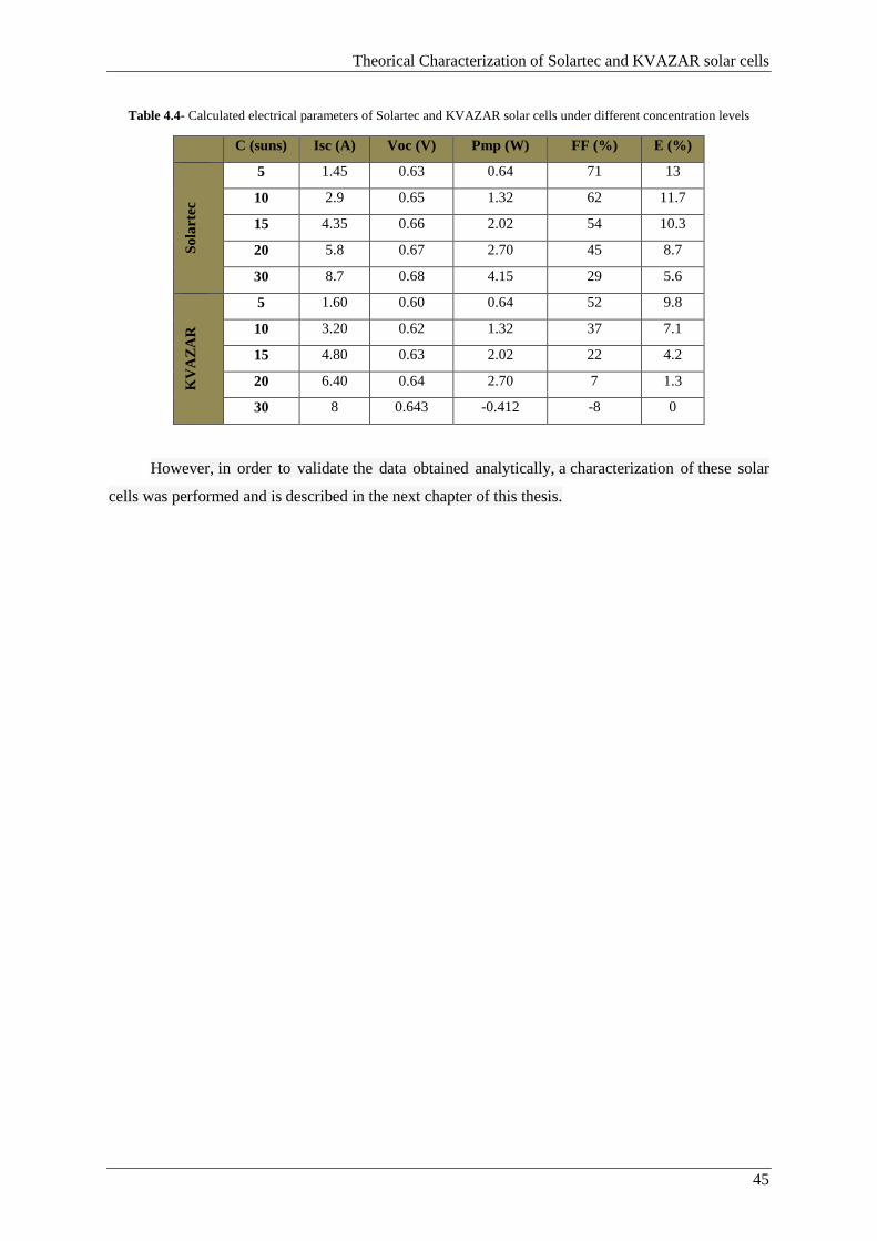
Theorical Characterization of Solartec and KVAZAR solar cells
45
Table 4.4- Calculated electrical parameters of Solartec and KVAZAR solar cells under different concentration levels
C (suns) Isc (A) Voc (V) Pmp (W) FF (%) Ε (%)
Sol
arte
c 5 1.45 0.63 0.64 71 13
10 2.9 0.65 1.32 62 11.7
15 4.35 0.66 2.02 54 10.3
20 5.8 0.67 2.70 45 8.7
30 8.7 0.68 4.15 29 5.6
KV
AZ
AR
5 1.60 0.60 0.64 52 9.8
10 3.20 0.62 1.32 37 7.1
15 4.80 0.63 2.02 22 4.2
20 6.40 0.64 2.70 7 1.3
30 8 0.643 -0.412 -8 0
However, in order to validate the data obtained analytically, a characterization of these solar
cells was performed and is described in the next chapter of this thesis.

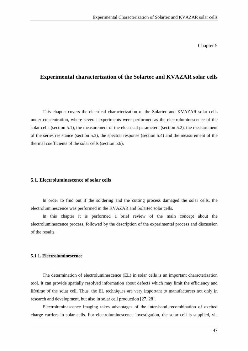
Experimental Characterization of Solartec and KVAZAR solar cells
47
Chapter 5
Experimental characterization of the Solartec and KVAZAR solar cells
This chapter covers the electrical characterization of the Solartec and KVAZAR solar cells
under concentration, where several experiments were performed as the electroluminescence of the
solar cells (section 5.1), the measurement of the electrical parameters (section 5.2), the measurement
of the series resistance (section 5.3), the spectral response (section 5.4) and the measurement of the
thermal coefficients of the solar cells (section 5.6).
5.1. Electroluminescence of solar cells
In order to find out if the soldering and the cutting process damaged the solar cells, the
electroluminescence was performed in the KVAZAR and Solartec solar cells.
In this chapter it is performed a brief review of the main concept about the
electroluminescence process, followed by the description of the experimental process and discussion
of the results.
5.1.1. Electroluminescence
The determination of electroluminescence (EL) in solar cells is an important characterization
tool. It can provide spatially resolved information about defects which may limit the efficiency and
lifetime of the solar cell. Thus, the EL techniques are very important to manufacturers not only in
research and development, but also in solar cell production [27, 28].
Electroluminescence imaging takes advantages of the inter-band recombination of excited
charge carriers in solar cells. For electroluminescence investigation, the solar cell is supplied, via
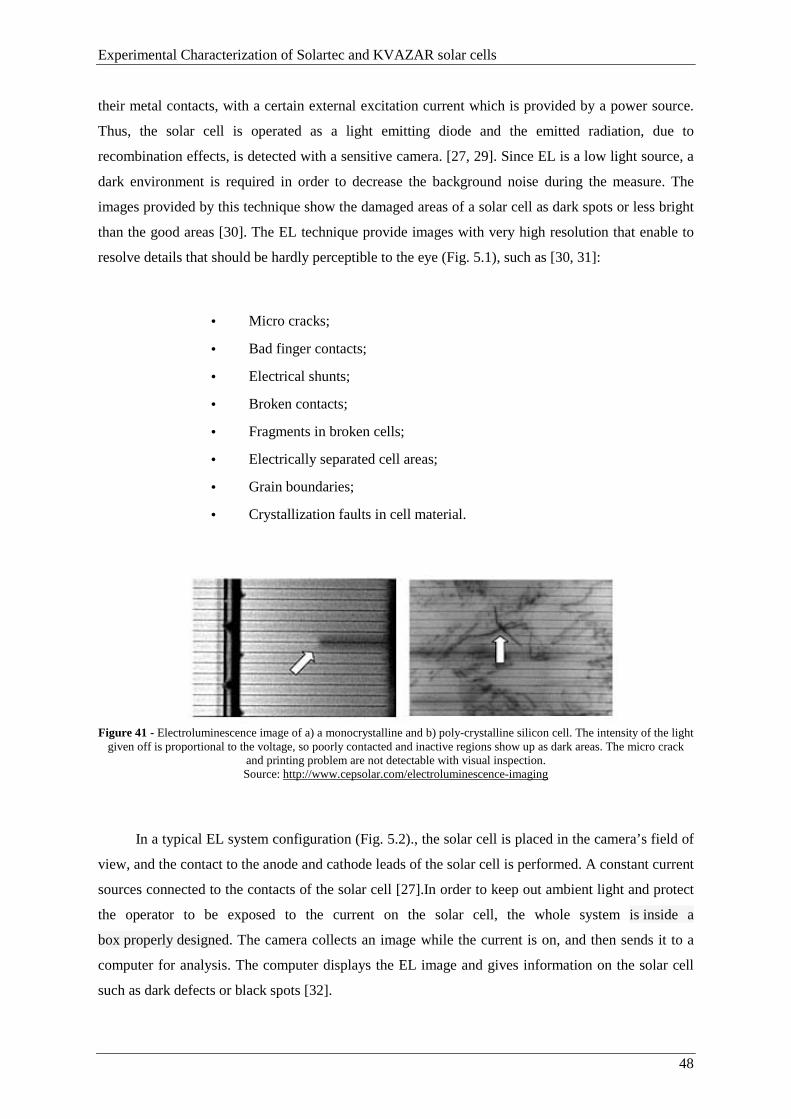
Experimental Characterization of Solartec and KVAZAR solar cells
48
their metal contacts, with a certain external excitation current which is provided by a power source.
Thus, the solar cell is operated as a light emitting diode and the emitted radiation, due to
recombination effects, is detected with a sensitive camera. [27, 29]. Since EL is a low light source, a
dark environment is required in order to decrease the background noise during the measure. The
images provided by this technique show the damaged areas of a solar cell as dark spots or less bright
than the good areas [30]. The EL technique provide images with very high resolution that enable to
resolve details that should be hardly perceptible to the eye (Fig. 5.1), such as [30, 31]:
• Micro cracks;
• Bad finger contacts;
• Electrical shunts;
• Broken contacts;
• Fragments in broken cells;
• Electrically separated cell areas;
• Grain boundaries;
• Crystallization faults in cell material.
Figure 41 - Electroluminescence image of a) a monocrystalline and b) poly-crystalline silicon cell. The intensity of the light
given off is proportional to the voltage, so poorly contacted and inactive regions show up as dark areas. The micro crack and printing problem are not detectable with visual inspection. Source: http://www.cepsolar.com/electroluminescence-imaging
In a typical EL system configuration (Fig. 5.2)., the solar cell is placed in the camera’s field of
view, and the contact to the anode and cathode leads of the solar cell is performed. A constant current
sources connected to the contacts of the solar cell [27].In order to keep out ambient light and protect
the operator to be exposed to the current on the solar cell, the whole system is inside a
box properly designed. The camera collects an image while the current is on, and then sends it to a
computer for analysis. The computer displays the EL image and gives information on the solar cell
such as dark defects or black spots [32].
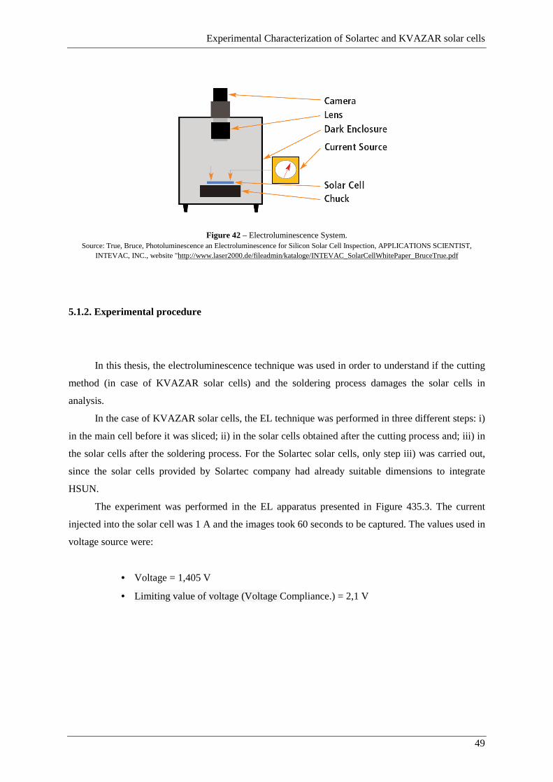
Experimental Characterization of Solartec and KVAZAR solar cells
49
Figure 42 – Electroluminescence System. Source: True, Bruce, Photoluminescence an Electroluminescence for Silicon Solar Cell Inspection, APPLICATIONS SCIENTIST,
INTEVAC, INC., website "http://www.laser2000.de/fileadmin/kataloge/INTEVAC_SolarCellWhitePaper_BruceTrue.pdf
5.1.2. Experimental procedure
In this thesis, the electroluminescence technique was used in order to understand if the cutting
method (in case of KVAZAR solar cells) and the soldering process damages the solar cells in
analysis.
In the case of KVAZAR solar cells, the EL technique was performed in three different steps: i)
in the main cell before it was sliced; ii) in the solar cells obtained after the cutting process and; iii) in
the solar cells after the soldering process. For the Solartec solar cells, only step iii) was carried out,
since the solar cells provided by Solartec company had already suitable dimensions to integrate
HSUN.
The experiment was performed in the EL apparatus presented in Figure 435.3. The current
injected into the solar cell was 1 A and the images took 60 seconds to be captured. The values used in
voltage source were:
• Voltage = 1,405 V
• Limiting value of voltage (Voltage Compliance.) = 2,1 V
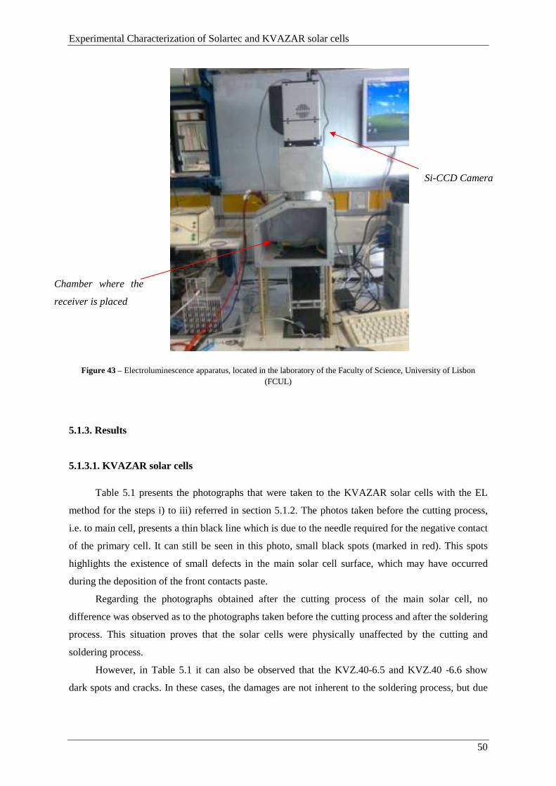
Experimental Characterization of Solartec and KVAZAR solar cells
50
Figure 43 – Electroluminescence apparatus, located in the laboratory of the Faculty of Science, University of Lisbon (FCUL)
5.1.3. Results
5.1.3.1. KVAZAR solar cells
Table 5.1 presents the photographs that were taken to the KVAZAR solar cells with the EL
method for the steps i) to iii) referred in section 5.1.2. The photos taken before the cutting process,
i.e. to main cell, presents a thin black line which is due to the needle required for the negative contact
of the primary cell. It can still be seen in this photo, small black spots (marked in red). This spots
highlights the existence of small defects in the main solar cell surface, which may have occurred
during the deposition of the front contacts paste.
Regarding the photographs obtained after the cutting process of the main solar cell, no
difference was observed as to the photographs taken before the cutting process and after the soldering
process. This situation proves that the solar cells were physically unaffected by the cutting and
soldering process.
However, in Table 5.1 it can also be observed that the KVZ.40-6.5 and KVZ.40 -6.6 show
dark spots and cracks. In these cases, the damages are not inherent to the soldering process, but due
Chamber where the
receiver is placed
Si-CCD Camera
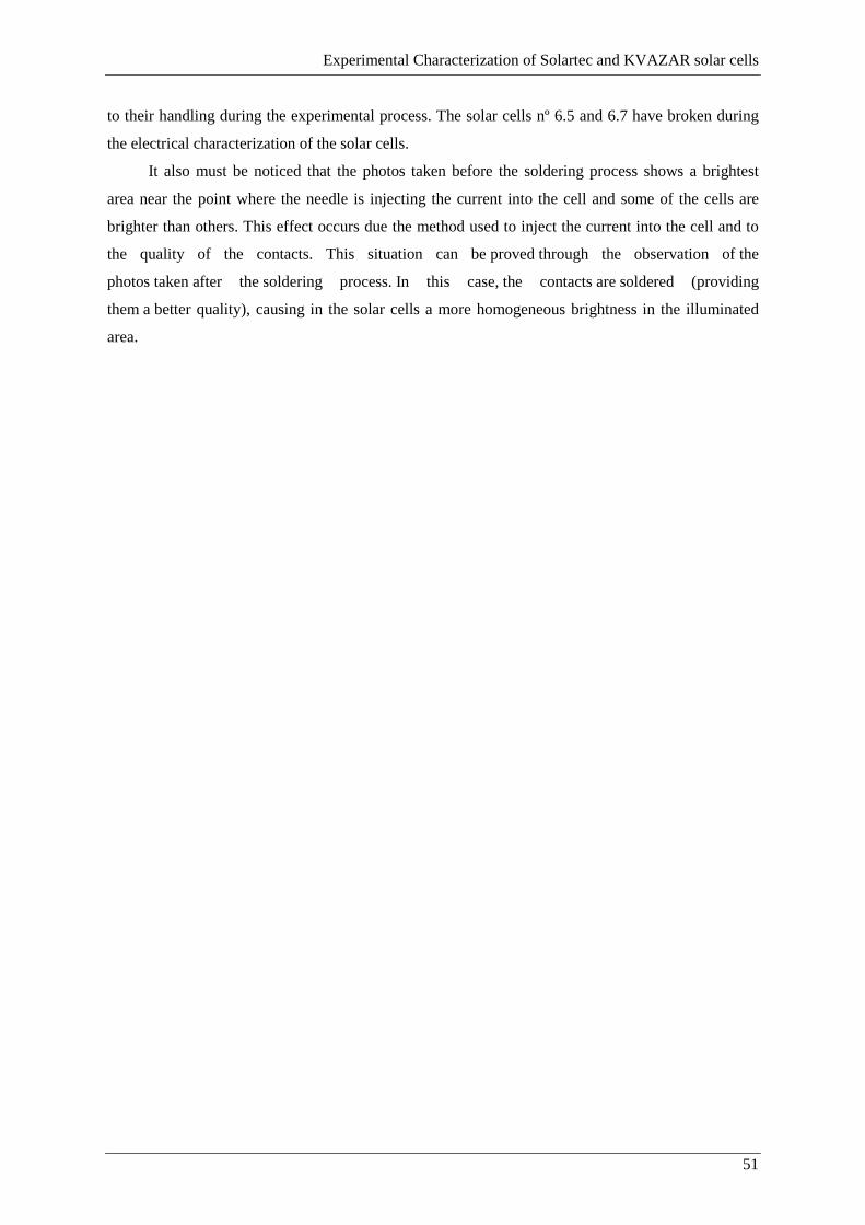
Experimental Characterization of Solartec and KVAZAR solar cells
51
to their handling during the experimental process. The solar cells nº 6.5 and 6.7 have broken during
the electrical characterization of the solar cells.
It also must be noticed that the photos taken before the soldering process shows a brightest
area near the point where the needle is injecting the current into the cell and some of the cells are
brighter than others. This effect occurs due the method used to inject the current into the cell and to
the quality of the contacts. This situation can be proved through the observation of the
photos taken after the soldering process. In this case, the contacts are soldered (providing
them a better quality), causing in the solar cells a more homogeneous brightness in the illuminated
area.


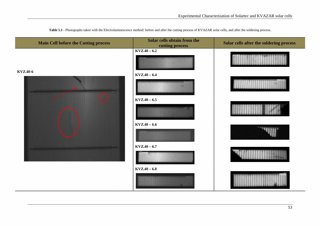
Table 5.1 - Photographs taken with the Electroluminescence method: before and after the cutting process of
Main Cell before the Cutting process
KVZ.40-6
Experimental Characterization of Solartec and KVAZAR solar cells
Photographs taken with the Electroluminescence method: before and after the cutting process of KVAZAR solar cells, and after the soldering process.
Solar cells obtain from the cutting process
Solar cells after the
KVZ.40 – 6.2
KVZ.40 – 6.4
KVZ.40 – 6.5
KVZ.40 – 6.6
KVZ.40 – 6.7
KVZ.40 – 6.8
Experimental Characterization of Solartec and KVAZAR solar cells
53
KVAZAR solar cells, and after the soldering process.
Solar cells after the soldering process
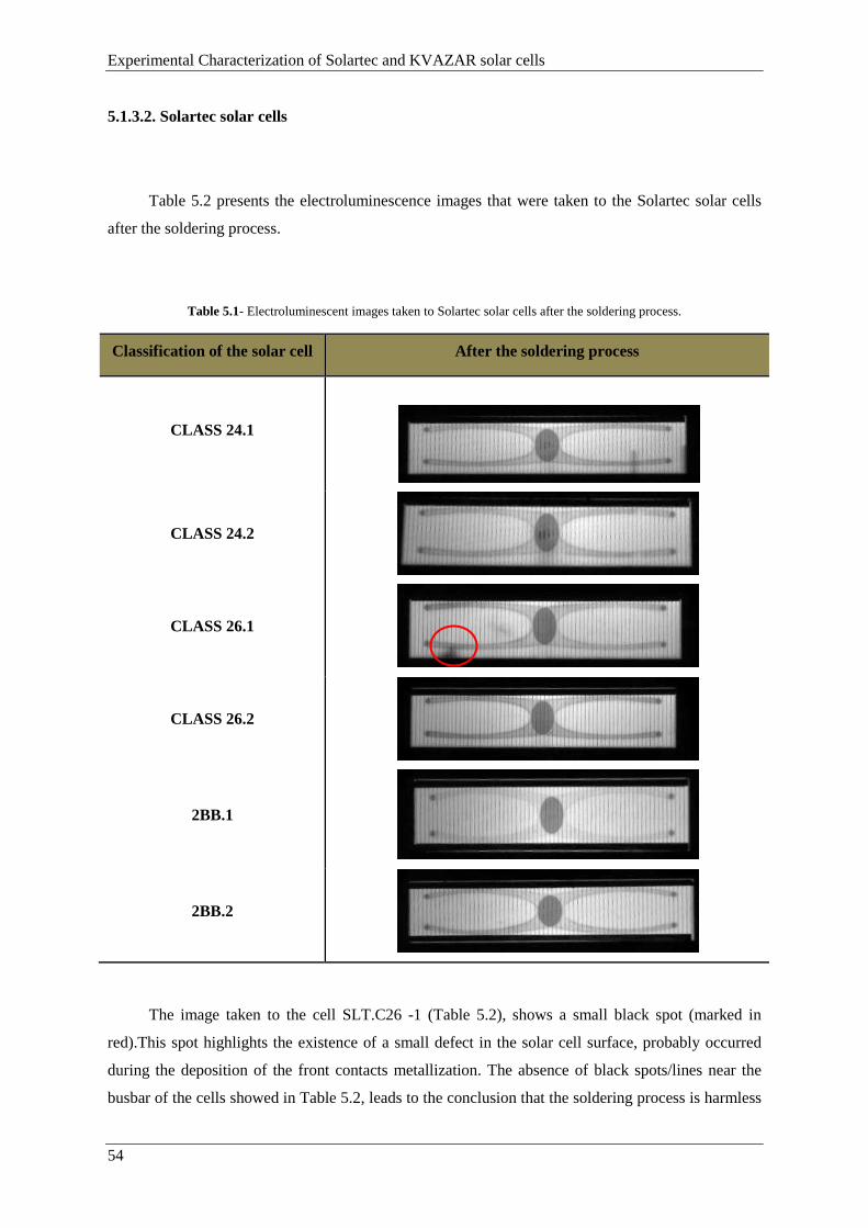
Experimental Characterization of Solartec and KVAZAR solar cells
54
5.1.3.2. Solartec solar cells
Table 5.2 presents the electroluminescence images that were taken to the Solartec solar cells
after the soldering process.
Table 5.1- Electroluminescent images taken to Solartec solar cells after the soldering process.
Classification of the solar cell After the soldering process
CLASS 24.1
CLASS 24.2
CLASS 26.1
CLASS 26.2
2BB.1
2BB.2
The image taken to the cell SLT.C26 -1 (Table 5.2), shows a small black spot (marked in
red).This spot highlights the existence of a small defect in the solar cell surface, probably occurred
during the deposition of the front contacts metallization. The absence of black spots/lines near the
busbar of the cells showed in Table 5.2, leads to the conclusion that the soldering process is harmless
Experimental Characterization of Solartec and KVAZAR solar cells
55
to the cells. This means that the Solartec solar cells, as in the case of KVAZAR solar cells, were
physically unaffected by the soldering process.
5.1.4. Main Conclusions
The main conclusions are:
a) The process used to cut the solar cells was proved to be harmless to the solar cells.
b) In both cell types (KVAZAR and Solartec), the EL photographs taken before and after
the soldering process proved that the solar cells were unaffected by the soldering
process, i.e. the appearance of new black spots after the soldering process was
undetectable.
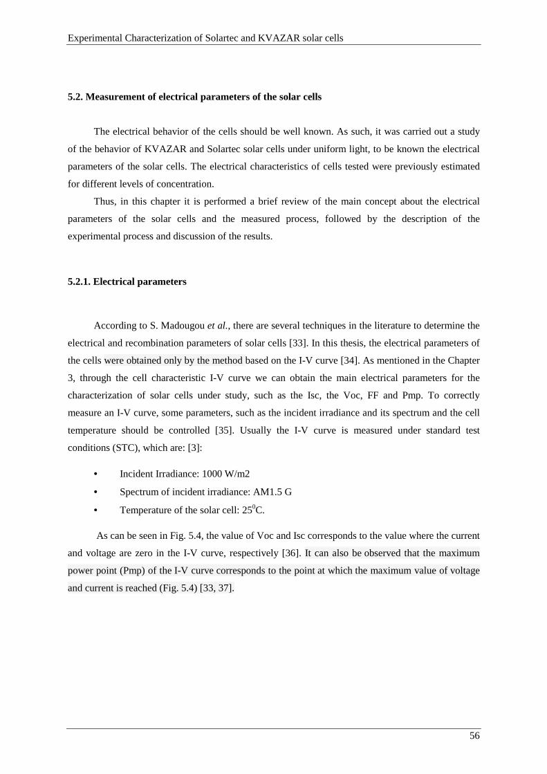
Experimental Characterization of Solartec and KVAZAR solar cells
56
5.2. Measurement of electrical parameters of the solar cells
The electrical behavior of the cells should be well known. As such, it was carried out a study
of the behavior of KVAZAR and Solartec solar cells under uniform light, to be known the electrical
parameters of the solar cells. The electrical characteristics of cells tested were previously estimated
for different levels of concentration.
Thus, in this chapter it is performed a brief review of the main concept about the electrical
parameters of the solar cells and the measured process, followed by the description of the
experimental process and discussion of the results.
5.2.1. Electrical parameters
According to S. Madougou et al., there are several techniques in the literature to determine the
electrical and recombination parameters of solar cells [33]. In this thesis, the electrical parameters of
the cells were obtained only by the method based on the I-V curve [34]. As mentioned in the Chapter
3, through the cell characteristic I-V curve we can obtain the main electrical parameters for the
characterization of solar cells under study, such as the Isc, the Voc, FF and Pmp. To correctly
measure an I-V curve, some parameters, such as the incident irradiance and its spectrum and the cell
temperature should be controlled [35]. Usually the I-V curve is measured under standard test
conditions (STC), which are: [3]:
• Incident Irradiance: 1000 W/m2
• Spectrum of incident irradiance: AM1.5 G
• Temperature of the solar cell: 250C.
As can be seen in Fig. 5.4, the value of Voc and Isc corresponds to the value where the current
and voltage are zero in the I-V curve, respectively [36]. It can also be observed that the maximum
power point (Pmp) of the I-V curve corresponds to the point at which the maximum value of voltage
and current is reached (Fig. 5.4) [33, 37].
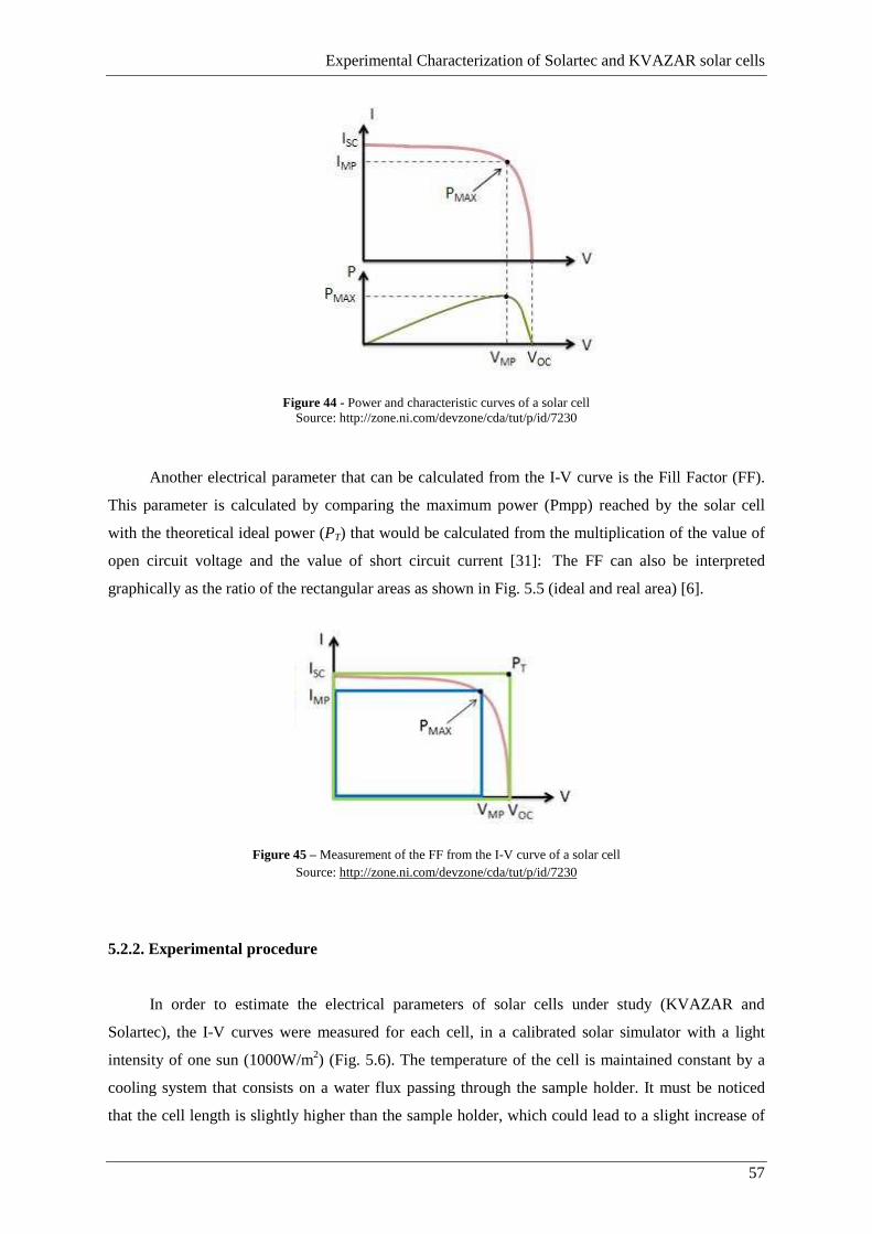
Experimental Characterization of Solartec and KVAZAR solar cells
57
Figure 44 - Power and characteristic curves of a solar cell Source: http://zone.ni.com/devzone/cda/tut/p/id/7230
Another electrical parameter that can be calculated from the I-V curve is the Fill Factor (FF).
This parameter is calculated by comparing the maximum power (Pmpp) reached by the solar cell
with the theoretical ideal power (PT) that would be calculated from the multiplication of the value of
open circuit voltage and the value of short circuit current [31]: The FF can also be interpreted
graphically as the ratio of the rectangular areas as shown in Fig. 5.5 (ideal and real area) [6].
Figure 45 – Measurement of the FF from the I-V curve of a solar cell Source: http://zone.ni.com/devzone/cda/tut/p/id/7230
5.2.2. Experimental procedure
In order to estimate the electrical parameters of solar cells under study (KVAZAR and
Solartec), the I-V curves were measured for each cell, in a calibrated solar simulator with a light
intensity of one sun (1000W/m2) (Fig. 5.6). The temperature of the cell is maintained constant by a
cooling system that consists on a water flux passing through the sample holder. It must be noticed
that the cell length is slightly higher than the sample holder, which could lead to a slight increase of
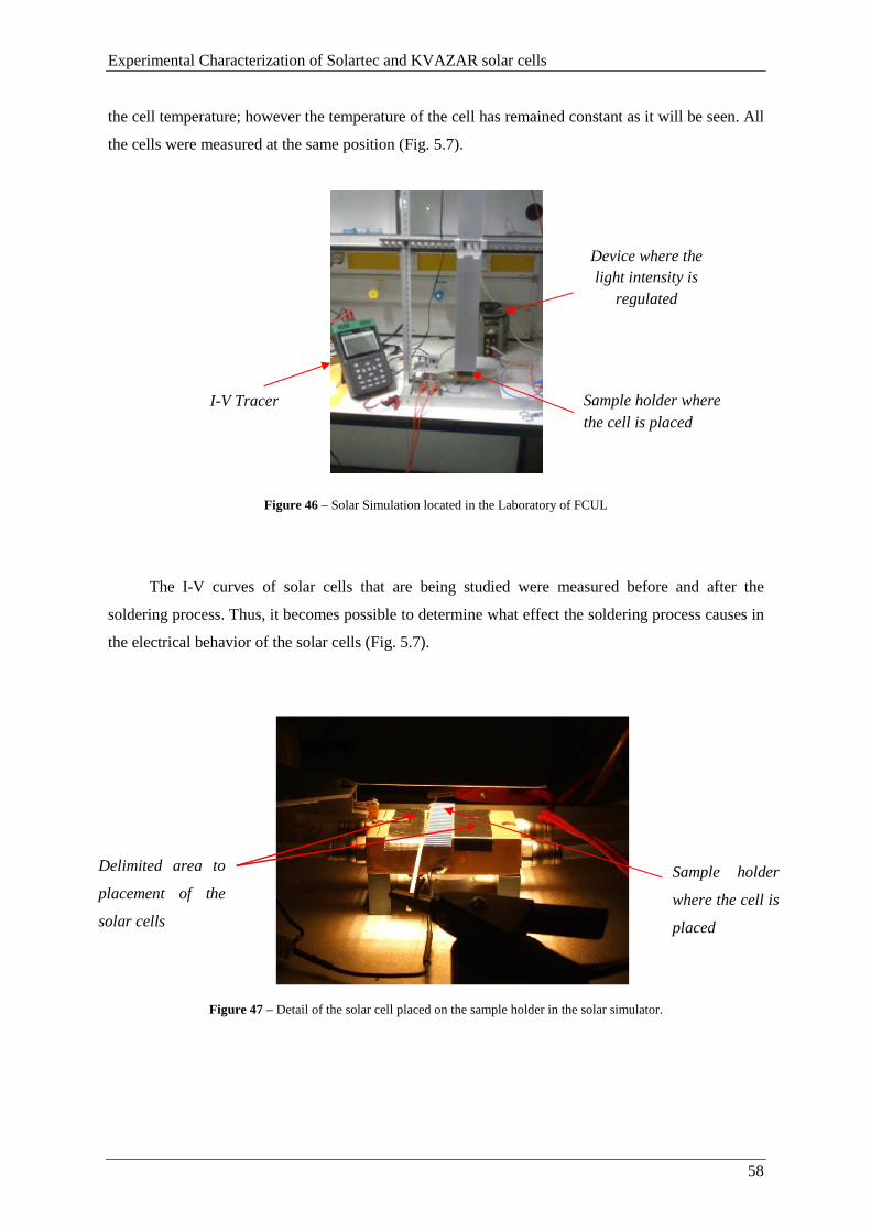
Experimental Characterization of Solartec and KVAZAR solar cells
58
the cell temperature; however the temperature of the cell has remained constant as it will be seen. All
the cells were measured at the same position (Fig. 5.7).
Figure 46 – Solar Simulation located in the Laboratory of FCUL
The I-V curves of solar cells that are being studied were measured before and after the
soldering process. Thus, it becomes possible to determine what effect the soldering process causes in
the electrical behavior of the solar cells (Fig. 5.7).
Figure 47 – Detail of the solar cell placed on the sample holder in the solar simulator.
I-V Tracer
Device where the light intensity is
regulated
Sample holder
where the cell is
placed
Sample holder where the cell is placed
Delimited area to
placement of the
solar cells
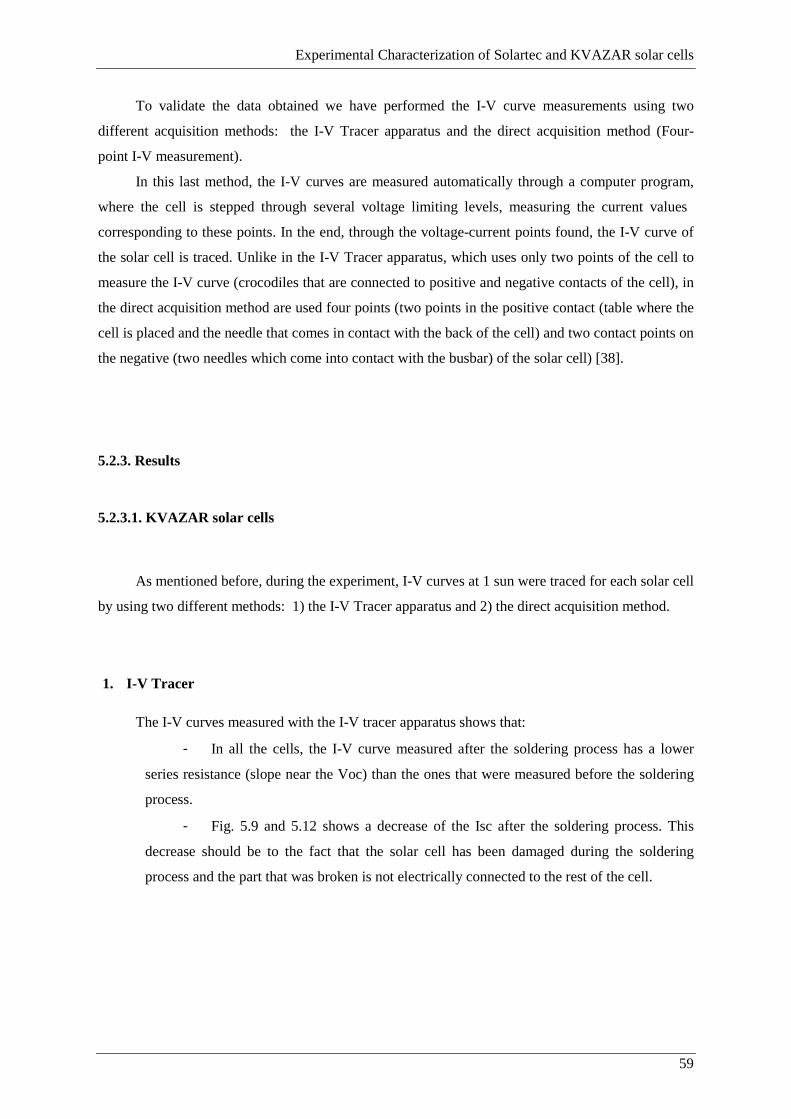
Experimental Characterization of Solartec and KVAZAR solar cells
59
To validate the data obtained we have performed the I-V curve measurements using two
different acquisition methods: the I-V Tracer apparatus and the direct acquisition method (Four-
point I-V measurement).
In this last method, the I-V curves are measured automatically through a computer program,
where the cell is stepped through several voltage limiting levels, measuring the current values
corresponding to these points. In the end, through the voltage-current points found, the I-V curve of
the solar cell is traced. Unlike in the I-V Tracer apparatus, which uses only two points of the cell to
measure the I-V curve (crocodiles that are connected to positive and negative contacts of the cell), in
the direct acquisition method are used four points (two points in the positive contact (table where the
cell is placed and the needle that comes in contact with the back of the cell) and two contact points on
the negative (two needles which come into contact with the busbar) of the solar cell) [38].
5.2.3. Results
5.2.3.1. KVAZAR solar cells
As mentioned before, during the experiment, I-V curves at 1 sun were traced for each solar cell
by using two different methods: 1) the I-V Tracer apparatus and 2) the direct acquisition method.
1. I-V Tracer
The I-V curves measured with the I-V tracer apparatus shows that:
‐ In all the cells, the I-V curve measured after the soldering process has a lower
series resistance (slope near the Voc) than the ones that were measured before the soldering
process.
‐ Fig. 5.9 and 5.12 shows a decrease of the Isc after the soldering process. This
decrease should be to the fact that the solar cell has been damaged during the soldering
process and the part that was broken is not electrically connected to the rest of the cell.

Experimental Characterization of Solartec and KVAZAR solar cells
60
Figure 48 – I-V curve of cell nº 6.2 with the I-V tracer .
Figure 49 – I-V curve of cell nº 6.3 with the I-V tracer
Figure 50 – I-V curve of cell nº 6.4 with the I-V tracer Figure 51 – I-V curve of cell nº 6.5 with the I-V tracer
Figure 52 – I-V curve of cell nº 6.6 with the I-V tracer Figure 53 – I-V curve of cell nº 6.7 with the I-V tracer
0.00
0.05
0.10
0.15
0.20
0.25
0.30
0.35
0 0.2 0.4 0.6
Cu
rre
nt
(A)
Voltage (V)
I‐V Curve before the soldering process
I‐V Curve after the soldering process
0.00
0.05
0.10
0.15
0.20
0.25
0.30
0.35
0 0.2 0.4 0.6
Cu
rre
nt
(A)
Voltage (V)
I‐V Curve after the soldering processI‐V Curve before the soldering process
0.00
0.05
0.10
0.15
0.20
0.25
0.30
0.35
0.40
0 0.2 0.4 0.6
Cu
rre
nt
(A)
Voltage (V)
I‐V Curve before the soldering process
I‐V Curve after the soldering process
0.00
0.05
0.10
0.15
0.20
0.25
0.30
0.35
0.40
0 0.1 0.2 0.3 0.4 0.5 0.6
Cu
rre
nt
(A)
Voltage (V)
I‐V Curveafter the soldering process
I‐V Curve before the soldering process
0.00
0.05
0.10
0.15
0.20
0.25
0.30
0.35
0 0.2 0.4 0.6
Cu
rre
nt
(A)
Voltage (V)
I‐V Curves before the soldering process
I‐V Curves after the soldering process
0.00
0.05
0.10
0.15
0.20
0.25
0.30
0.35
0 0.2 0.4 0.6
Cu
rre
nt
(A)
Voltage (V)
I‐V Curve before the soldering process
I‐V Curve after the soldering process
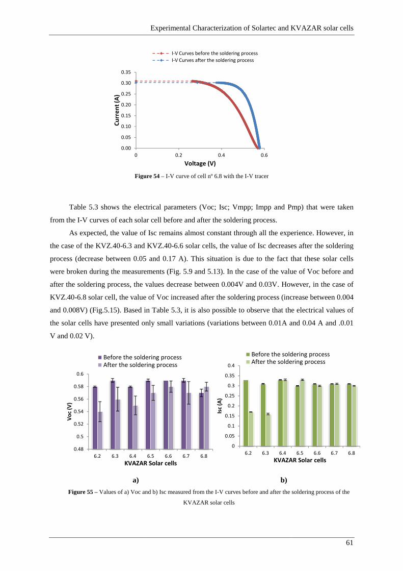
Figure
Table 5.3 shows the electrical parameters (Voc; Isc; Vmpp; Impp
from the I-V curves of each solar cell before and after the soldering process.
As expected, the value of Isc remains almost constant through all the experience. However, in
the case of the KVZ.40-6.3 and KVZ.40
process (decrease between 0.05 and 0.17 A). This situation i
were broken during the measurements (Fig. 5.9 and 5.13
after the soldering process, the values decrease between 0.004V and 0.03V. However, in the case of
KVZ.40-6.8 solar cell, the value of Voc increased after the soldering process (increase between 0.004
and 0.008V) (Fig.5.15). Based in T
the solar cells have presented only small
V and 0.02 V).
a)
Figure 55 – Values of a) Voc and b) Isc measured from the I
0.00
0.05
0.10
0.15
0.20
0.25
0.30
0.35
0
Cu
rre
nt
(A)
0.48
0.5
0.52
0.54
0.56
0.58
0.6
6.2 6.3 6.4
Vo
c (V
)
KVAZAR Solar cells
Before the soldering processAfter the soldering process
Experimental Characterization of Solartec and KVAZAR solar cells
Figure 54 – I-V curve of cell nº 6.8 with the I-V tracer
shows the electrical parameters (Voc; Isc; Vmpp; Impp and Pmp
V curves of each solar cell before and after the soldering process.
As expected, the value of Isc remains almost constant through all the experience. However, in
6.3 and KVZ.40-6.6 solar cells, the value of Isc decreases after the soldering
process (decrease between 0.05 and 0.17 A). This situation is due to the fact that these solar cells
measurements (Fig. 5.9 and 5.13). In the case of the value of Voc before and
after the soldering process, the values decrease between 0.004V and 0.03V. However, in the case of
cell, the value of Voc increased after the soldering process (increase between 0.004
Based in Table 5.3, it is also possible to observe that the electrical values of
have presented only small variations (variations between 0.01A and 0.04 A and
b)
Values of a) Voc and b) Isc measured from the I-V curves before and after the soldering process of the
KVAZAR solar cells
0.2 0.4 0.6
Voltage (V)
I‐V Curves before the soldering process
I‐V Curves after the soldering process
6.5 6.6 6.7 6.8
KVAZAR Solar cells
Before the soldering processAfter the soldering process
0
0.05
0.1
0.15
0.2
0.25
0.3
0.35
0.4
6.2 6.3 6.4
Isc
(A)
KVAZAR Solar cells
Before the soldering processAfter the soldering process
Experimental Characterization of Solartec and KVAZAR solar cells
61
Pmp) that were taken
As expected, the value of Isc remains almost constant through all the experience. However, in
solar cells, the value of Isc decreases after the soldering
s due to the fact that these solar cells
In the case of the value of Voc before and
after the soldering process, the values decrease between 0.004V and 0.03V. However, in the case of
cell, the value of Voc increased after the soldering process (increase between 0.004
, it is also possible to observe that the electrical values of
between 0.01A and 0.04 A and .0.01
V curves before and after the soldering process of the
6.5 6.6 6.7 6.8
KVAZAR Solar cells
Before the soldering processAfter the soldering process

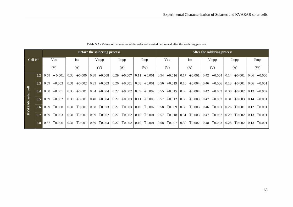
Experimental Characterization of Solartec and KVAZAR solar cells
63
Table 5.2 - Values of parameters of the solar cells tested before and after the soldering process.
Cell Nº
Before the soldering process After the soldering process
Voc Isc Vmpp Impp Pmp Voc Isc Vmpp Impp Pmp
(V) (A) (V) (A) (W) (V) (A) (V) (A) (W)
KV
AZ
AR
sol
ar c
ell
6.2 0.58 ∓ 0.001 0.33 ∓0.000 0.38 ∓0.008 0.29 ∓0.007 0.11 ∓0.001 0.54 ∓0.016 0.17 ∓0.001 0.42 ∓0.004 0.14 ∓0.001 0.06 ∓0.000
6.3 0.59 ∓0.003 0.31 ∓0.002 0.33 ∓0.003 0.26 ∓0.001 0.08 ∓0.001 0.56 ∓0.019 0.16 ∓0.004 0.46 ∓0.006 0.13 ∓0.001 0.06 ∓0.001
6.4 0.58 ∓0.001 0.33 ∓0.001 0.34 ∓0.004 0.27 ∓0.002 0.09 ∓0.002 0.55 ∓0.015 0.33 ∓0.004 0.42 ∓0.003 0.30 ∓0.002 0.13 ∓0.002
6.5 0.59 ∓0.002 0.30 ∓0.001 0.40 ∓0.004 0.27 ∓0.003 0.11 ∓0.000 0.57 ∓0.012 0.33 ∓0.003 0.47 ∓0.002 0.31 ∓0.003 0.14 ∓0.001
6.6 0.59 ∓0.000 0.31 ∓0.001 0.38 ∓0.023 0.27 ∓0.003 0.10 ∓0.007 0.58 ∓0.009 0.30 ∓0.003 0.46 ∓0.001 0.26 ∓0.001 0.12 ∓0.001
6.7 0.59 ∓0.003 0.31 ∓0.001 0.39 ∓0.002 0.27 ∓0.002 0.10 ∓0.001 0.57 ∓0.018 0.31 ∓0.003 0.47 ∓0.002 0.29 ∓0.002 0.13 ∓0.001
6.8 0.57 ∓0.006 0.31 ∓0.001 0.39 ∓0.004 0.27 ∓0.002 0.10 ∓0.001 0.58 ∓0.007 0.30 ∓0.002 0.48 ∓0.003 0.28 ∓0.002 0.13 ∓0.001

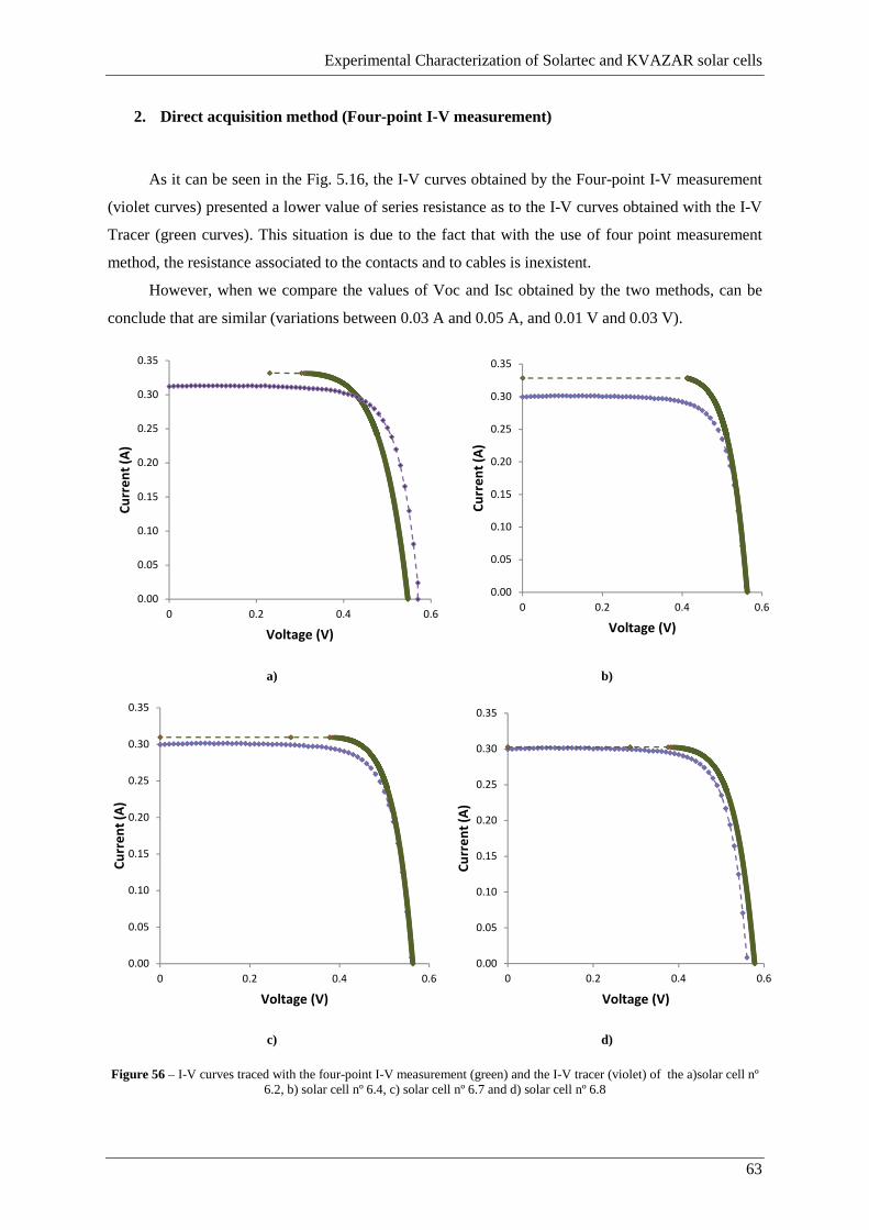
Experimental Characterization of Solartec and KVAZAR solar cells
63
2. Direct acquisition method (Four-point I-V measurement)
As it can be seen in the Fig. 5.16, the I-V curves obtained by the Four-point I-V measurement
(violet curves) presented a lower value of series resistance as to the I-V curves obtained with the I-V
Tracer (green curves). This situation is due to the fact that with the use of four point measurement
method, the resistance associated to the contacts and to cables is inexistent.
However, when we compare the values of Voc and Isc obtained by the two methods, can be
conclude that are similar (variations between 0.03 A and 0.05 A, and 0.01 V and 0.03 V).
a) b)
c) d)
Figure 56 – I-V curves traced with the four-point I-V measurement (green) and the I-V tracer (violet) of the a)solar cell nº 6.2, b) solar cell nº 6.4, c) solar cell nº 6.7 and d) solar cell nº 6.8
0.00
0.05
0.10
0.15
0.20
0.25
0.30
0.35
0 0.2 0.4 0.6
Cu
rre
nt
(A)
Voltage (V)
0.00
0.05
0.10
0.15
0.20
0.25
0.30
0.35
0 0.2 0.4 0.6
Cu
rre
nt
(A)
Voltage (V)
0.00
0.05
0.10
0.15
0.20
0.25
0.30
0.35
0 0.2 0.4 0.6
Cu
rre
nt
(A)
Voltage (V)
0.00
0.05
0.10
0.15
0.20
0.25
0.30
0.35
0 0.2 0.4 0.6
Cu
rre
nt
(A)
Voltage (V)
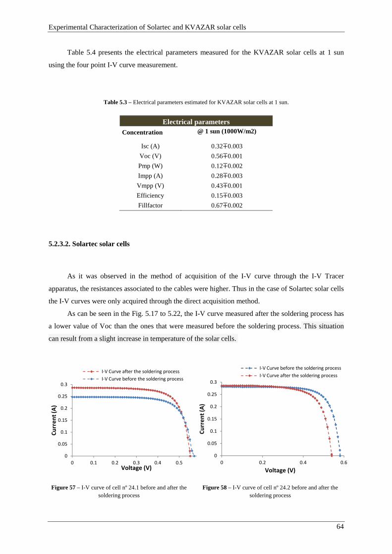
Experimental Characterization of Solartec and KVAZAR solar cells
64
Table 5.4 presents the electrical parameters measured for the KVAZAR solar cells at 1 sun
using the four point I-V curve measurement.
Table 5.3 – Electrical parameters estimated for KVAZAR solar cells at 1 sun.
Electrical parameters Concentration @ 1 sun (1000W/m2)
Isc (A) 0.32∓0.003
Voc (V) 0.56∓0.001
Pmp (W) 0.12∓0.002
Impp (A) 0.28∓0.003
Vmpp (V) 0.43∓0.001
Efficiency 0.15∓0.003
Fillfactor 0.67∓0.002
5.2.3.2. Solartec solar cells
As it was observed in the method of acquisition of the I-V curve through the I-V Tracer
apparatus, the resistances associated to the cables were higher. Thus in the case of Solartec solar cells
the I-V curves were only acquired through the direct acquisition method.
As can be seen in the Fig. 5.17 to 5.22, the I-V curve measured after the soldering process has
a lower value of Voc than the ones that were measured before the soldering process. This situation
can result from a slight increase in temperature of the solar cells.
Figure 57 – I-V curve of cell nº 24.1 before and after the
soldering process
Figure 58 – I-V curve of cell nº 24.2 before and after the
soldering process
0
0.05
0.1
0.15
0.2
0.25
0.3
0 0.1 0.2 0.3 0.4 0.5
Cu
rre
nt
(A)
Voltage (V)
I‐V Curve after the soldering process
I‐V Curve before the soldering process
0
0.05
0.1
0.15
0.2
0.25
0.3
0 0.2 0.4 0.6
Cu
rre
nt
(A)
Voltage (V)
I‐V Curve before the soldering process
I‐V Curve after the soldering process

Experimental Characterization of Solartec and KVAZAR solar cells
65
Figure 59 – I-V curve of cell nº 26.1 before and after the
soldering process Figure 60 – I-V curve of cell nº 26.2 before and after the
soldering process
Figure 61 – I-V curve of cell nº 2BB.1 before and after
the soldering process
Figure 62 – I-V curve of cell nº 2BB.2 before and after the
soldering process
Table 5.5 shows the electrical parameters that were taken from the I-V curves of each solar cell
before and after the soldering process. Analyzing the results presented in Table 5.5 it can be
observed that in the case of cell SLT.C24, the value of Pmp is higher after the soldering process,
while in other tested cells, after the soldering process, the value of Pmp has decreased or remained
equal. As expected, the value of Isc remains almost constant through all the experience (variation
between 0.02 and 0.06A).
In the case of the value of Voc before and after the soldering process, the values decrease
between 0.04V and 0.03V. However, in the case of SLT.C24 solar cell, the value of Voc remains
equal after the soldering process.
0
0.05
0.1
0.15
0.2
0.25
0.3
0 0.2 0.4 0.6
Cu
rre
nt
(A)
Voltage (V)
I‐V Curve before the soldering process
I‐V Curve after the soldering process
0
0.05
0.1
0.15
0.2
0.25
0.3
0 0.2 0.4 0.6
Cu
rre
nt
(A)
Voltage (V)
I‐V Curve before the soldering process
I‐V Curve after the soldering process
0
0.05
0.1
0.15
0.2
0.25
0.3
0 0.2 0.4 0.6
Cu
rre
nt
(A)
Voltage (V)
I‐V Curve before the soldering process
I‐V Curve after the soldering process
0
0.05
0.1
0.15
0.2
0.25
0.3
0 0.2 0.4 0.6
Cu
rre
nt
(A)
Voltage (V)
I‐V Curve before the soldering process
I‐V Curve after the soldering process
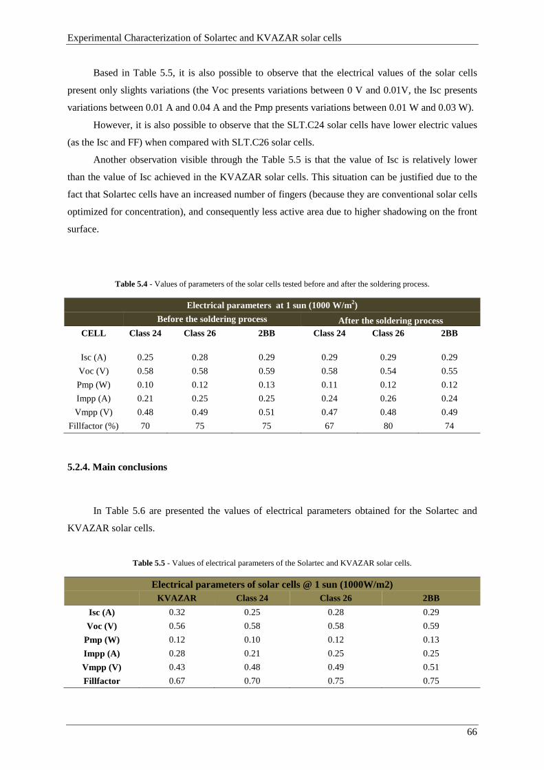
Experimental Characterization of Solartec and KVAZAR solar cells
66
Based in Table 5.5, it is also possible to observe that the electrical values of the solar cells
present only slights variations (the Voc presents variations between 0 V and 0.01V, the Isc presents
variations between 0.01 A and 0.04 A and the Pmp presents variations between 0.01 W and 0.03 W).
However, it is also possible to observe that the SLT.C24 solar cells have lower electric values
(as the Isc and FF) when compared with SLT.C26 solar cells.
Another observation visible through the Table 5.5 is that the value of Isc is relatively lower
than the value of Isc achieved in the KVAZAR solar cells. This situation can be justified due to the
fact that Solartec cells have an increased number of fingers (because they are conventional solar cells
optimized for concentration), and consequently less active area due to higher shadowing on the front
surface.
Table 5.4 - Values of parameters of the solar cells tested before and after the soldering process.
Electrical parameters at 1 sun (1000 W/m2)
Before the soldering process After the soldering process CELL Class 24 Class 26 2BB Class 24 Class 26 2BB
Isc (A) 0.25 0.28 0.29 0.29 0.29 0.29
Voc (V) 0.58 0.58 0.59 0.58 0.54 0.55
Pmp (W) 0.10 0.12 0.13 0.11 0.12 0.12
Impp (A) 0.21 0.25 0.25 0.24 0.26 0.24
Vmpp (V) 0.48 0.49 0.51 0.47 0.48 0.49
Fillfactor (%) 70 75 75 67 80 74
5.2.4. Main conclusions
In Table 5.6 are presented the values of electrical parameters obtained for the Solartec and
KVAZAR solar cells.
Table 5.5 - Values of electrical parameters of the Solartec and KVAZAR solar cells.
Electrical parameters of solar cells @ 1 sun (1000W/m2) KVAZAR Class 24 Class 26 2BB
Isc (A) 0.32 0.25 0.28 0.29
Voc (V) 0.56 0.58 0.58 0.59
Pmp (W) 0.12 0.10 0.12 0.13
Impp (A) 0.28 0.21 0.25 0.25
Vmpp (V) 0.43 0.48 0.49 0.51
Fillfactor 0.67 0.70 0.75 0.75
Experimental Characterization of Solartec and KVAZAR solar cells
67
Through the values presented, it can be concluded that, when compared, the Solartec solar
cells show lower values of Isc at one sun, while the value of Voc is very similar in all solar cells, and
the value of FF and Pmpp is higher in the Solartec solar cells.
On the contrary as occurred with the direct acquisition method, the I-V Tracer apparatus shows
associated values of resistance of cables, since in this method the contacts are made through long and
thin wires and only two points make contact with the solar cell. So, it can be concluded that the direct
acquisition method is more suitable to measure the I-V curves of the solar cells.
After the soldering process, the I-V curves obtained have lower series resistance (slope near
the Voc) than the ones that were measured before the soldering process, since after the soldering
process the contacts presents a better quality.
Experimental Characterization of Solartec and KVAZAR solar cells
68
5.3. Measurement of the Series Resistance
For high current devices, such as solar cells, minimization of the ohmic series resistance losses
is crucial. The analysis of the series resistance (Rs) requires an accurate determined value and should
also give a conclusive proof of its correctness [35]. There are many techniques to measure/estimate
the series resistance of solar cells. In this chapter we present the Rs estimated for the KVAZAR and
Solartec solar cells by using two different methods: i) I-V curve measurement and ii) Suns-Voc. The
concept behind each of the previous methods as well as the experimental procedure and results are
described in the following lines.
5.3.1. I-V curves
5.3.1.1. Theoretical Introduction
A current-voltage (I-V) curve is usually described as the possible combinations of current and
voltage output of a photovoltaic (PV) device. However, to represent a real behavior of the device, it
should be taken into account the presence of parasitic series resistance and shunt conductance as an
integral part of the system [35].
Through the I-V curves, the series resistance can be estimated by two methods: i) The Slope method
at constant light intensity and ii) Multiple light intensity method.
i) Slope method at constant light intensity
As mentioned in the previous chapters, the maximum voltage value is achieved at open circuit
conditions thus being known as the open circuit voltage (Voc). At this point, the series resistance is
infinitely high and there is no current [39].
Thus, in this method, series resistance is estimated by the inverse of the slope of the I-V curve
near the Voc (equation (31)). The Rs parameter is one of the parameters that mainly influence the I-V
curve of a solar cell. As can be seen in Figure 5.23, how much higher is the value of Rs, greater is the
slope of the IV curve near the point I = 0 [32].[40]

Experimental Characterization of Solartec and KVAZAR solar cells
69
)* = −1Slope of the I − V curve near the Voc
(31)
This is the method to calculate the series resistance most commonly used, since it is only
necessary to know the I-V curve of the solar cell under study (Fig. 5.23).
Figure 63 - Obtaining the series and shunt resistances from the I-V Curve.
ii) Multiple light intensity method
In this method the series resistance is calculated through the use of two I-V curves measured at
different light intensities. Such curves have also two different values of Isc (Isc1 and Isc2,
respectively). Then, a value of current below the Isc is picked (δI) and is subtracted from the value of
Isc on both curves (eq. (32) and eq. (33)), originating two new points equally spaced from the point
where V = 0 (Fig. 5.24) [33][34].

Experimental Characterization of Solartec and KVAZAR solar cells
70
Figure 64 - Two I-V curves of the same solar cell under different illumination intensities. Source: See reference [33]
= @8 − δI (32)
= @8 − δI (33)
The values of current obtained from the new points, corresponds the voltage values (V1 and
V2, respectively) to calculate the series resistance [33]. So can be said that the series resistance is
calculated by:
)+ = − − (34)
Thus, replacing the equations (32) and (33) in the equation (34),
)+ = − +U − +U (35)
where V1 and V2 are the voltage that corresponds to I1 and I2, respectively.
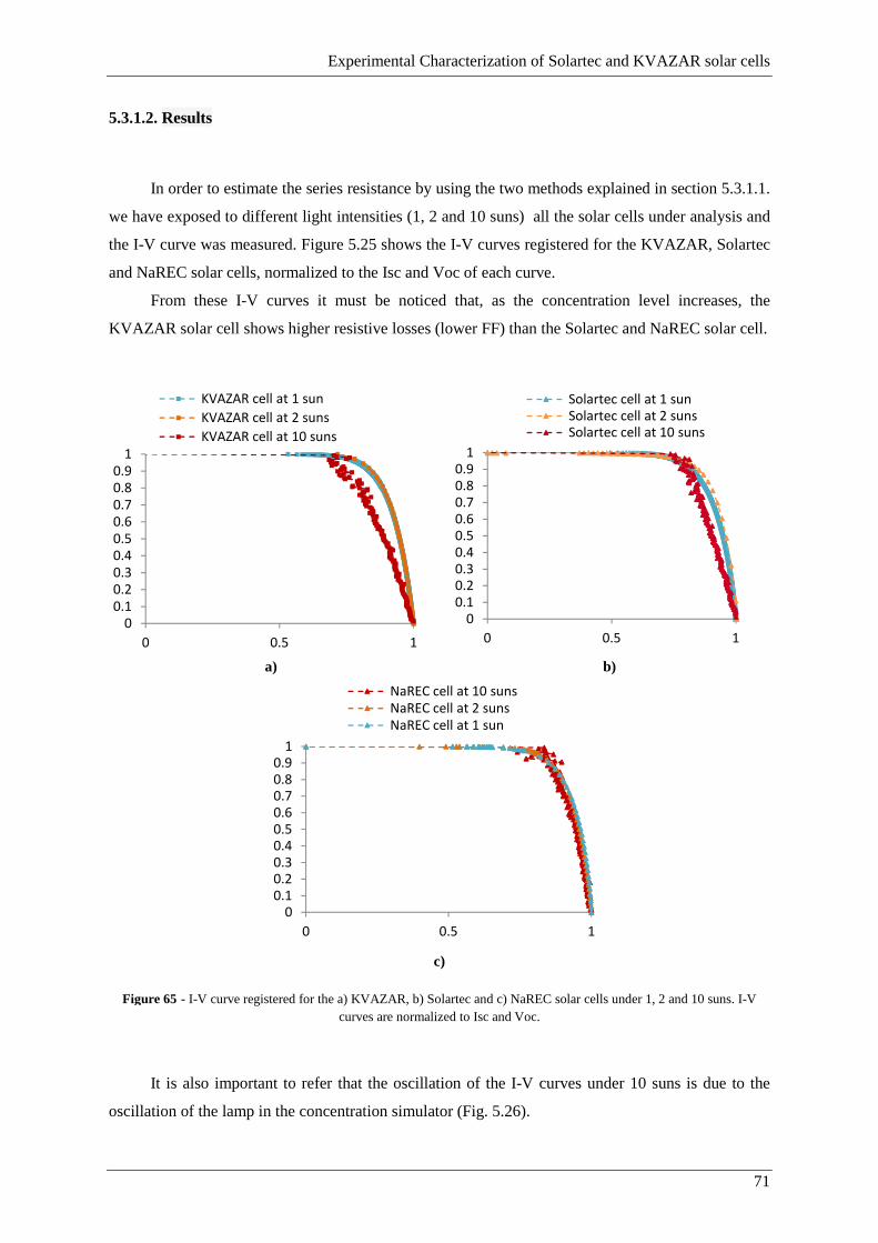
Experimental Characterization of Solartec and KVAZAR solar cells
71
5.3.1.2. Results
In order to estimate the series resistance by using the two methods explained in section 5.3.1.1.
we have exposed to different light intensities (1, 2 and 10 suns) all the solar cells under analysis and
the I-V curve was measured. Figure 5.25 shows the I-V curves registered for the KVAZAR, Solartec
and NaREC solar cells, normalized to the Isc and Voc of each curve.
From these I-V curves it must be noticed that, as the concentration level increases, the
KVAZAR solar cell shows higher resistive losses (lower FF) than the Solartec and NaREC solar cell.
a) b)
c)
Figure 65 - I-V curve registered for the a) KVAZAR, b) Solartec and c) NaREC solar cells under 1, 2 and 10 suns. I-V curves are normalized to Isc and Voc.
It is also important to refer that the oscillation of the I-V curves under 10 suns is due to the
oscillation of the lamp in the concentration simulator (Fig. 5.26).
0
0.1
0.2
0.3
0.4
0.5
0.6
0.7
0.8
0.9
1
0 0.5 1
KVAZAR cell at 1 sun
KVAZAR cell at 2 suns
KVAZAR cell at 10 suns
00.10.20.30.40.50.60.70.80.9
1
0 0.5 1
Solartec cell at 1 sunSolartec cell at 2 sunsSolartec cell at 10 suns
00.10.20.30.40.50.60.70.80.9
1
0 0.5 1
NaREC cell at 10 suns
NaREC cell at 2 suns
NaREC cell at 1 sun
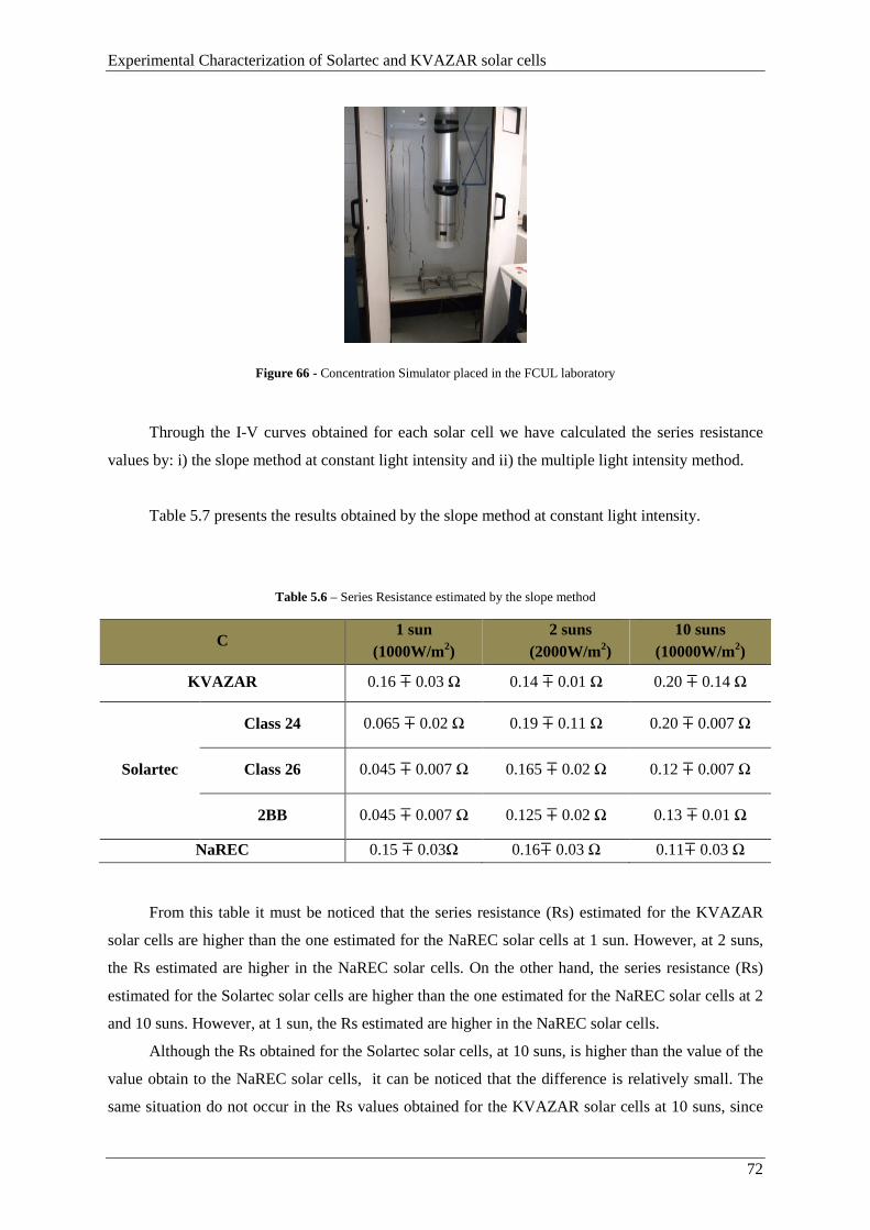
Experimental Characterization of Solartec and KVAZAR solar cells
72
Figure 66 - Concentration Simulator placed in the FCUL laboratory
Through the I-V curves obtained for each solar cell we have calculated the series resistance
values by: i) the slope method at constant light intensity and ii) the multiple light intensity method.
Table 5.7 presents the results obtained by the slope method at constant light intensity.
Table 5.6 – Series Resistance estimated by the slope method
C 1 sun
(1000W/m2) 2 suns
(2000W/m2) 10 suns
(10000W/m2)
KVAZAR 0.16 ∓ 0.03 Ω 0.14 ∓ 0.01 Ω 0.20 ∓ 0.14 Ω
Solartec
Class 24 0.065 ∓ 0.02 Ω 0.19 ∓ 0.11 Ω 0.20 ∓ 0.007 Ω
Class 26 0.045 ∓ 0.007 Ω 0.165 ∓ 0.02 Ω 0.12 ∓ 0.007 Ω
2BB 0.045 ∓ 0.007 Ω 0.125 ∓ 0.02 Ω 0.13 ∓ 0.01 Ω
NaREC 0.15 ∓ 0.03Ω 0.16∓ 0.03 Ω 0.11∓ 0.03 Ω
From this table it must be noticed that the series resistance (Rs) estimated for the KVAZAR
solar cells are higher than the one estimated for the NaREC solar cells at 1 sun. However, at 2 suns,
the Rs estimated are higher in the NaREC solar cells. On the other hand, the series resistance (Rs)
estimated for the Solartec solar cells are higher than the one estimated for the NaREC solar cells at 2
and 10 suns. However, at 1 sun, the Rs estimated are higher in the NaREC solar cells.
Although the Rs obtained for the Solartec solar cells, at 10 suns, is higher than the value of the
value obtain to the NaREC solar cells, it can be noticed that the difference is relatively small. The
same situation do not occur in the Rs values obtained for the KVAZAR solar cells at 10 suns, since
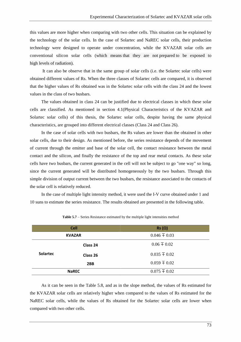
Experimental Characterization of Solartec and KVAZAR solar cells
73
this values are more higher when comparing with two other cells. This situation can be explained by
the technology of the solar cells. In the case of Solartec and NaREC solar cells, their production
technology were designed to operate under concentration, while the KVAZAR solar cells are
conventional silicon solar cells (which means that they are not prepared to be exposed to
high levels of radiation).
It can also be observe that in the same group of solar cells (i.e. the Solartec solar cells) were
obtained different values of Rs. When the three classes of Solartec cells are compared, it is observed
that the higher values of Rs obtained was in the Solartec solar cells with the class 24 and the lowest
values in the class of two busbars.
The values obtained in class 24 can be justified due to electrical classes in which these solar
cells are classified. As mentioned in section 4.1(Physical Characteristics of the KVAZAR and
Solartec solar cells) of this thesis, the Solartec solar cells, despite having the same physical
characteristics, are grouped into different electrical classes (Class 24 and Class 26).
In the case of solar cells with two busbars, the Rs values are lower than the obtained in other
solar cells, due to their design. As mentioned before, the series resistance depends of the movement
of current through the emitter and base of the solar cell, the contact resistance between the metal
contact and the silicon, and finally the resistance of the top and rear metal contacts. As these solar
cells have two busbars, the current generated in the cell will not be subject to go "one way" so long,
since the current generated will be distributed homogeneously by the two busbars. Through this
simple division of output current between the two busbars, the resistance associated to the contacts of
the solar cell is relatively reduced.
In the case of multiple light intensity method, it were used the I-V curve obtained under 1 and
10 suns to estimate the series resistance. The results obtained are presented in the following table.
Table 5.7 – Series Resistance estimated by the multiple light intensities method
As it can be seen in the Table 5.8, and as in the slope method, the values of Rs estimated for
the KVAZAR solar cells are relatively higher when compared to the values of Rs estimated for the
NaREC solar cells, while the values of Rs obtained for the Solartec solar cells are lower when
compared with two other cells.
Cell Rs (Ω)
KVAZAR 0.046 ∓ 0.03
Solartec
Class 24 0.06 ∓ 0.02
Class 26 0.035 ∓ 0.02
2BB 0.059 ∓ 0.02
NaREC 0.075 ∓ 0.02
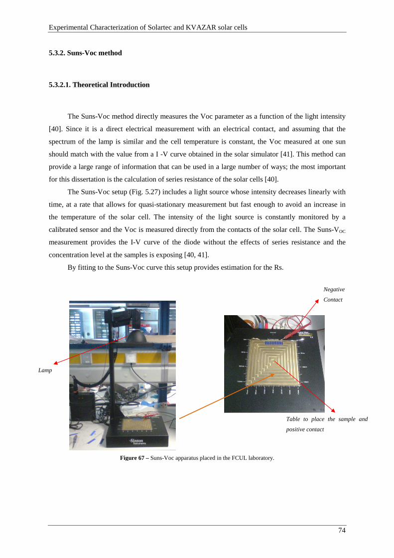
Experimental Characterization of Solartec and KVAZAR solar cells
74
5.3.2. Suns-Voc method
5.3.2.1. Theoretical Introduction
The Suns-Voc method directly measures the Voc parameter as a function of the light intensity
[40]. Since it is a direct electrical measurement with an electrical contact, and assuming that the
spectrum of the lamp is similar and the cell temperature is constant, the Voc measured at one sun
should match with the value from a I -V curve obtained in the solar simulator [41]. This method can
provide a large range of information that can be used in a large number of ways; the most important
for this dissertation is the calculation of series resistance of the solar cells [40].
The Suns-Voc setup (Fig. 5.27) includes a light source whose intensity decreases linearly with
time, at a rate that allows for quasi-stationary measurement but fast enough to avoid an increase in
the temperature of the solar cell. The intensity of the light source is constantly monitored by a
calibrated sensor and the Voc is measured directly from the contacts of the solar cell. The Suns-VOC
measurement provides the I-V curve of the diode without the effects of series resistance and the
concentration level at the samples is exposing [40, 41].
By fitting to the Suns-Voc curve this setup provides estimation for the Rs.
Figure 67 – Suns-Voc apparatus placed in the FCUL laboratory.
Lamp
Negative
Contact
Table to place the sample and
positive contact
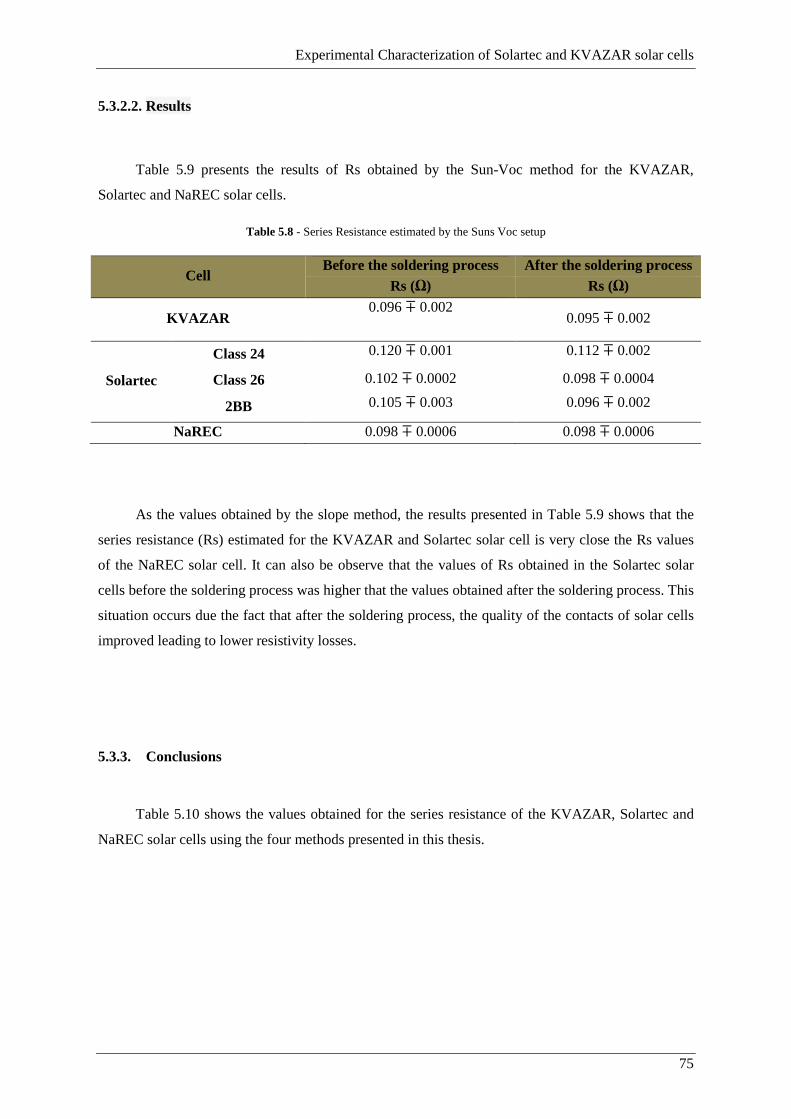
Experimental Characterization of Solartec and KVAZAR solar cells
75
5.3.2.2. Results
Table 5.9 presents the results of Rs obtained by the Sun-Voc method for the KVAZAR,
Solartec and NaREC solar cells.
Table 5.8 - Series Resistance estimated by the Suns Voc setup
As the values obtained by the slope method, the results presented in Table 5.9 shows that the
series resistance (Rs) estimated for the KVAZAR and Solartec solar cell is very close the Rs values
of the NaREC solar cell. It can also be observe that the values of Rs obtained in the Solartec solar
cells before the soldering process was higher that the values obtained after the soldering process. This
situation occurs due the fact that after the soldering process, the quality of the contacts of solar cells
improved leading to lower resistivity losses.
5.3.3. Conclusions
Table 5.10 shows the values obtained for the series resistance of the KVAZAR, Solartec and
NaREC solar cells using the four methods presented in this thesis.
Cell Before the soldering process After the soldering process
Rs (Ω) Rs (Ω)
KVAZAR 0.096 ∓ 0.002
0.095 ∓ 0.002
Solartec
Class 24 0.120 ∓ 0.001 0.112 ∓ 0.002
Class 26 0.102 ∓ 0.0002 0.098 ∓ 0.0004
2BB 0.105 ∓ 0.003 0.096 ∓ 0.002
NaREC 0.098 ∓ 0.0006 0.098 ∓ 0.0006


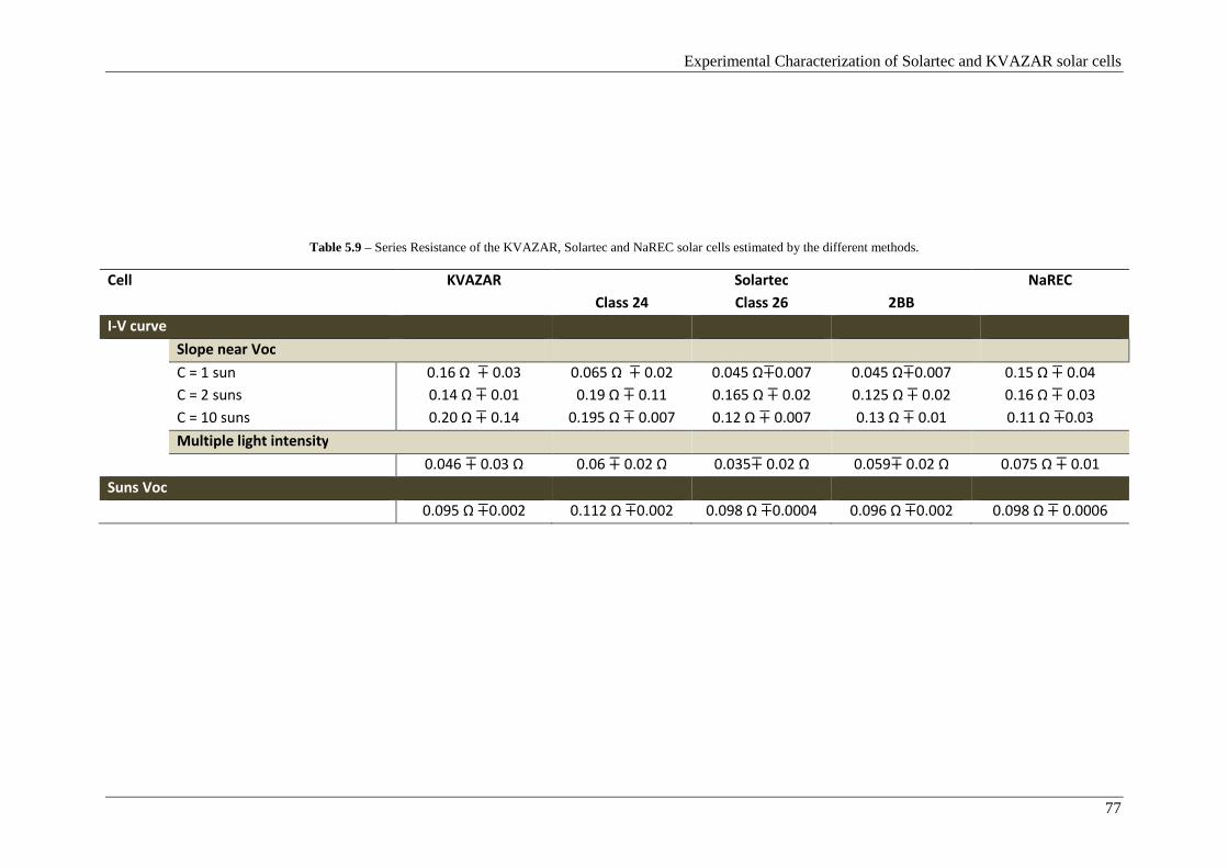
Experimental Characterization of Solartec and KVAZAR solar cells
77
Table 5.9 – Series Resistance of the KVAZAR, Solartec and NaREC solar cells estimated by the different methods.
Cell KVAZAR Solartec NaREC
Class 24 Class 26 2BB
I-V curve
Slope near Voc
C = 1 sun 0.16 Ω ∓ 0.03 0.065 Ω ∓ 0.02 0.045 Ω∓0.007 0.045 Ω∓0.007 0.15 Ω ∓ 0.04
C = 2 suns 0.14 Ω ∓ 0.01 0.19 Ω ∓ 0.11 0.165 Ω ∓ 0.02 0.125 Ω ∓ 0.02 0.16 Ω ∓ 0.03
C = 10 suns 0.20 Ω ∓ 0.14 0.195 Ω ∓ 0.007 0.12 Ω ∓ 0.007 0.13 Ω ∓ 0.01 0.11 Ω ∓0.03
Multiple light intensity
0.046 ∓ 0.03 Ω 0.06 ∓ 0.02 Ω 0.035∓ 0.02 Ω 0.059∓ 0.02 Ω 0.075 Ω ∓ 0.01
Suns Voc
0.095 Ω ∓0.002 0.112 Ω ∓0.002 0.098 Ω ∓0.0004 0.096 Ω ∓0.002 0.098 Ω ∓ 0.0006
Experimental Characterization of Solartec and KVAZAR solar cells
78
The main conclusions are:
a. When expose to 1 or 2 suns, the standard commercial silicon solar cell from
KVAZAR features a series resistance similar to the NaREC solar cell, while the Solartec
solar cells features a series resistance lower to the NaREC solar cell;
b. This difference becomes higher when the solar cells are exposed under
concentrated radiation; while the Rs values of KVAZAR solar cells raise under 10 suns, the
Rs values of NaREC solar cells remain low. However, in the case of the Solartec solar cell,
although the Rs values raises under 10 suns, when compared with the values obtained by
the NaREC solar cells, the values are very similar;
c. When compared the several groups of Solartec cells, the cells classified with the
class 24 are the cells that show higher values of Rs and the solar cells with two busbars
shows the lowers Rs values.
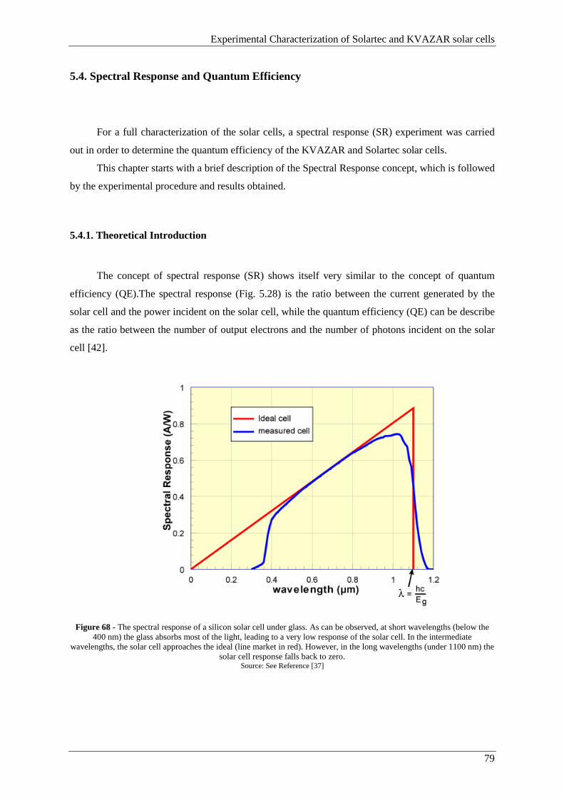
Experimental Characterization of Solartec and KVAZAR solar cells
79
5.4. Spectral Response and Quantum Efficiency
For a full characterization of the solar cells, a spectral response (SR) experiment was carried
out in order to determine the quantum efficiency of the KVAZAR and Solartec solar cells.
This chapter starts with a brief description of the Spectral Response concept, which is followed
by the experimental procedure and results obtained.
5.4.1. Theoretical Introduction
The concept of spectral response (SR) shows itself very similar to the concept of quantum
efficiency (QE).The spectral response (Fig. 5.28) is the ratio between the current generated by the
solar cell and the power incident on the solar cell, while the quantum efficiency (QE) can be describe
as the ratio between the number of output electrons and the number of photons incident on the solar
cell [42].
Figure 68 - The spectral response of a silicon solar cell under glass. As can be observed, at short wavelengths (below the 400 nm) the glass absorbs most of the light, leading to a very low response of the solar cell. In the intermediate
wavelengths, the solar cell approaches the ideal (line market in red). However, in the long wavelengths (under 1100 nm) the solar cell response falls back to zero.
Source: See Reference [37]

Experimental Characterization of Solartec and KVAZAR solar cells
80
The spectral response (SR) of the tested cell (under short-circuit) is obtained using the
relationship shown in equation (36) [42],
m)nop(q) = m)noprns(q) I (q)Irns(q)
(36)
where I (q) is the amplitude of the signal in the cell that we intend to test, Irns(q) is the
amplitude measured in the reference cell and m)noprns(q) is the spectral response of the reference solar
cell.
In the case of an ideal solar cell, the SR and the QE curves are limited in the higher
wavelengths, due the inability of the semiconductor (as in the case of a solar cell) to absorb photons
with energies below the band gap. However, when we observe the SR curve it is possible to see that,
unlike the square shape that QE curves presents along the entire spectrum, the SR curve decreases in
the small photon wavelengths. This situation occurs due the fact that in these kinds of wavelengths,
the photon has a higher energy which consequently leads to a reduced ratio of photons and power.
[42].
The SR is an important parameter since it is the SR that is measured from a solar cell, and
from this the quantum efficiency is calculated. The QE can be determined through the SR by
replacing the power of the light at a particular wavelength with the photon flux for the same
wavelength [43]. So, the QE can be calculated by [44],
tu = ℎ-q m)
(37)
Where c and h are respectively the speed of light and Planck's constant, λ the wavelength and
q represents the electron charge.
Figure 5.29 presents the quantum efficiency of an ideal and a real silicon solar cell [37]. As
can be seen in Fig. 5.29, the QE for photons with energy below the band gap is zero. It can also be
seen that while QE of an ideally solar cell, as mentioned before, has a square shape, the QE for
most of the real solar cells is reduced due to recombination effects, reflections and low diffusion
length.
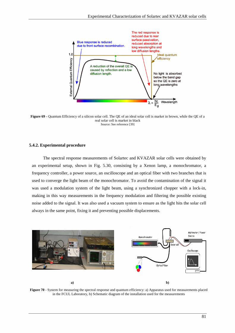
Experimental Characterization of Solartec and KVAZAR solar cells
81
Figure 69 - Quantum Efficiency of a silicon solar cell. The QE of an ideal solar cell is market in brown, while the QE of a real solar cell is market in black
Source: See reference [39]
5.4.2. Experimental procedure
The spectral response measurements of Solartec and KVAZAR solar cells were obtained by
an experimental setup, shown in Fig. 5.30, consisting by a Xenon lamp, a monochromator, a
frequency controller, a power source, an oscilloscope and an optical fiber with two branches that is
used to converge the light beam of the monochromator. To avoid the contamination of the signal it
was used a modulation system of the light beam, using a synchronized chopper with a lock-in,
making in this way measurements in the frequency modulation and filtering the possible existing
noise added to the signal. It was also used a vacuum system to ensure as the light hits the solar cell
always in the same point, fixing it and preventing possible displacements.
a) b)
Figure 70 - System for measuring the spectral response and quantum efficiency: a) Apparatus used for measurements placed in the FCUL Laboratory, b) Schematic diagram of the installation used for the measurements
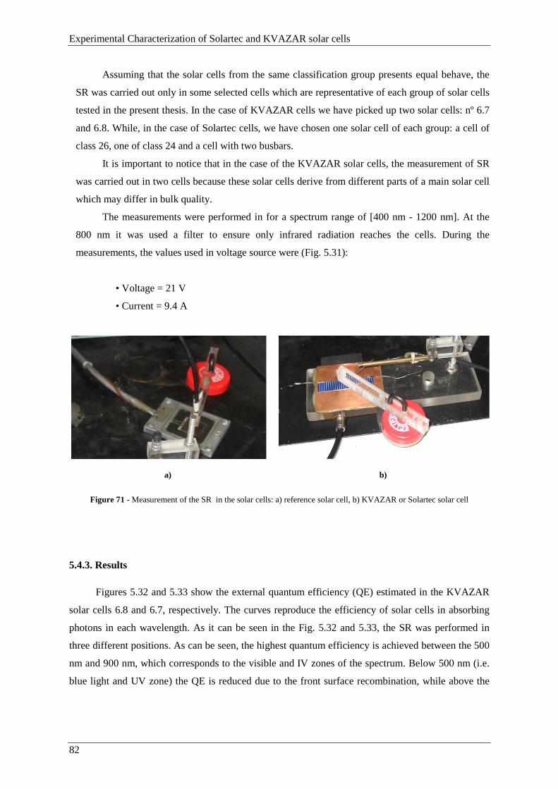
Experimental Characterization of Solartec and KVAZAR solar cells
82
Assuming that the solar cells from the same classification group presents equal behave, the
SR was carried out only in some selected cells which are representative of each group of solar cells
tested in the present thesis. In the case of KVAZAR cells we have picked up two solar cells: nº 6.7
and 6.8. While, in the case of Solartec cells, we have chosen one solar cell of each group: a cell of
class 26, one of class 24 and a cell with two busbars.
It is important to notice that in the case of the KVAZAR solar cells, the measurement of SR
was carried out in two cells because these solar cells derive from different parts of a main solar cell
which may differ in bulk quality.
The measurements were performed in for a spectrum range of [400 nm - 1200 nm]. At the
800 nm it was used a filter to ensure only infrared radiation reaches the cells. During the
measurements, the values used in voltage source were (Fig. 5.31):
• Voltage = 21 V
• Current = 9.4 A
a) b)
Figure 71 - Measurement of the SR in the solar cells: a) reference solar cell, b) KVAZAR or Solartec solar cell
5.4.3. Results
Figures 5.32 and 5.33 show the external quantum efficiency (QE) estimated in the KVAZAR
solar cells 6.8 and 6.7, respectively. The curves reproduce the efficiency of solar cells in absorbing
photons in each wavelength. As it can be seen in the Fig. 5.32 and 5.33, the SR was performed in
three different positions. As can be seen, the highest quantum efficiency is achieved between the 500
nm and 900 nm, which corresponds to the visible and IV zones of the spectrum. Below 500 nm (i.e.
blue light and UV zone) the QE is reduced due to the front surface recombination, while above the
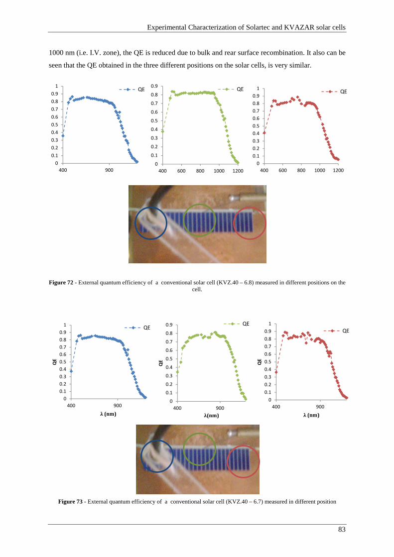
Experimental Characterization of Solartec and KVAZAR solar cells
83
1000 nm (i.e. I.V. zone), the QE is reduced due to bulk and rear surface recombination. It also can be
seen that the QE obtained in the three different positions on the solar cells, is very similar.
Figure 72 - External quantum efficiency of a conventional solar cell (KVZ.40 – 6.8) measured in different positions on the cell.
Figure 73 - External quantum efficiency of a conventional solar cell (KVZ.40 – 6.7) measured in different position
0
0.1
0.2
0.3
0.4
0.5
0.6
0.7
0.8
0.9
1
400 900
QE
0
0.1
0.2
0.3
0.4
0.5
0.6
0.7
0.8
0.9
400 600 800 1000 1200
QE
0
0.1
0.2
0.3
0.4
0.5
0.6
0.7
0.8
0.9
1
400 600 800 1000 1200
QE
0
0.1
0.2
0.3
0.4
0.5
0.6
0.7
0.8
0.9
1
400 900
QE
λ (nm)
QE
0
0.1
0.2
0.3
0.4
0.5
0.6
0.7
0.8
0.9
400 900
QE
λ(nm)
QE
0
0.1
0.2
0.3
0.4
0.5
0.6
0.7
0.8
0.9
1
400 900
QE
λ (nm)
QE
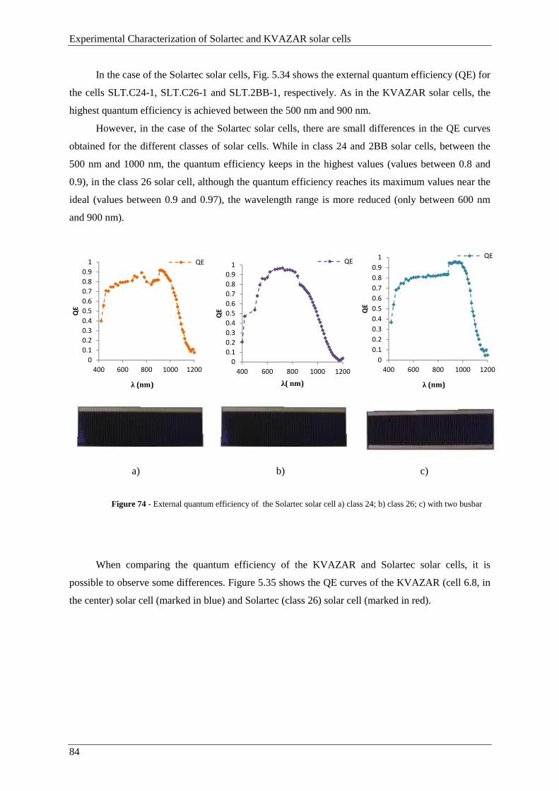
Experimental Characterization of Solartec and KVAZAR solar cells
84
In the case of the Solartec solar cells, Fig. 5.34 shows the external quantum efficiency (QE) for
the cells SLT.C24-1, SLT.C26-1 and SLT.2BB-1, respectively. As in the KVAZAR solar cells, the
highest quantum efficiency is achieved between the 500 nm and 900 nm.
However, in the case of the Solartec solar cells, there are small differences in the QE curves
obtained for the different classes of solar cells. While in class 24 and 2BB solar cells, between the
500 nm and 1000 nm, the quantum efficiency keeps in the highest values (values between 0.8 and
0.9), in the class 26 solar cell, although the quantum efficiency reaches its maximum values near the
ideal (values between 0.9 and 0.97), the wavelength range is more reduced (only between 600 nm
and 900 nm).
a) b) c)
Figure 74 - External quantum efficiency of the Solartec solar cell a) class 24; b) class 26; c) with two busbar
When comparing the quantum efficiency of the KVAZAR and Solartec solar cells, it is
possible to observe some differences. Figure 5.35 shows the QE curves of the KVAZAR (cell 6.8, in
the center) solar cell (marked in blue) and Solartec (class 26) solar cell (marked in red).
0
0.1
0.2
0.3
0.4
0.5
0.6
0.7
0.8
0.9
1
400 600 800 1000 1200
QE
λ (nm)
QE
0
0.1
0.2
0.3
0.4
0.5
0.6
0.7
0.8
0.9
1
400 600 800 1000 1200
QE
λ( nm)
QE
0
0.1
0.2
0.3
0.4
0.5
0.6
0.7
0.8
0.9
1
400 600 800 1000 1200Q
E
λ (nm)
QE
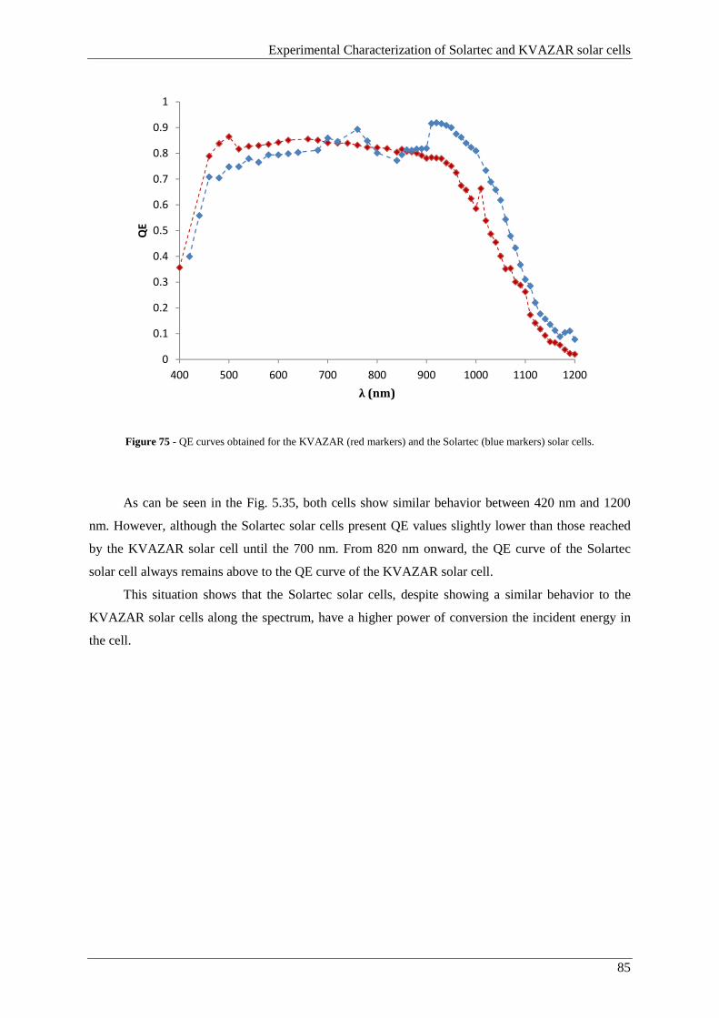
Experimental Characterization of Solartec and KVAZAR solar cells
85
Figure 75 - QE curves obtained for the KVAZAR (red markers) and the Solartec (blue markers) solar cells.
As can be seen in the Fig. 5.35, both cells show similar behavior between 420 nm and 1200
nm. However, although the Solartec solar cells present QE values slightly lower than those reached
by the KVAZAR solar cell until the 700 nm. From 820 nm onward, the QE curve of the Solartec
solar cell always remains above to the QE curve of the KVAZAR solar cell.
This situation shows that the Solartec solar cells, despite showing a similar behavior to the
KVAZAR solar cells along the spectrum, have a higher power of conversion the incident energy in
the cell.
0
0.1
0.2
0.3
0.4
0.5
0.6
0.7
0.8
0.9
1
400 500 600 700 800 900 1000 1100 1200
QE
λ (nm)

Experimental Characterization of Solartec and KVAZAR solar cells
86
5.5. Thermal coefficients of solar cells
As mentioned in the previous chapters, the solar cell temperature is one of the important
factors that affect how much electricity that the solar cells will produce. So, given this situation, the
influence of this characteristic, should not be overlooked. In order to understand the influence of
increase of the temperature in the KVAZAR and Solartec solar cells, through an experimental
campaign, their thermal coefficients were calculated. In this chapter a brief description of the thermal
coefficients concept is performed, passing through the description of the experimental procedure
performed to measure these parameters in the KVAZAR and Solartec solar cells, ending with a
description of the results obtained and the respective conclusions.
5.5.1. Thermal coefficients concept
The temperature of a solar cell is a parameter that highly influences its electrical behavior, being such
variation usually described by thermal coefficients (%/ºC). In the case of Voc and Isc, as the
temperature increases, the first will decrease while the latter will rise. Still, it must be noticed that the
Voc variation is much higher (Fig. 5.36) [45].
Figure 76 - Measured temperature coefficients for voltage for solar cell with uniform and nonuniform temperature during
testing. Source: see reference [45]
According to King et al.[45], the procedures for measuring the thermal coefficient(s) for solar
cells don’t exist yet standardized, and systematic influences are common in the experimental methods
performed to measure them. However, it can be stated that the most common method used to
calculate the thermal coefficient is the Equivalent Cell Temperature method (ECT) [46 Germany

Experimental Characterization of Solartec and KVAZAR solar cells
87
(2001) 156. #139]. According to I. Antón, the thermal coefficient β has a high variation with
concentration level for a silicon solar cell, but when the temperature is lower than 100 ºC, the
thermal coefficients has very little variation, being considered constant at the usual one-sun operating
conditions [45]. Usually, to estimate the thermal coefficients, the solar cell is placed in a solar
simulator being illuminated with a uniform light and remains at constant temperature. The I-V curve
is measured for a range of different temperatures and then the rate of change of the desired parameter
with temperature (i.e. the thermal coefficients) is calculated according with equation (38)[45]:
w = Δ BΔ = B( +OP,) − B( +OP,!z. |) − 298.15
(38)
where B( +OP,) is the value of the electrical parameter registered under a certain temperature
and at 1 sun, B( +OP,!z. |) is the value of the electrical parameter at 1 sun and 25º C and T is the
temperature of the solar cell and CT is the thermal coefficient in study.
5.5.2. Experimental procedure
In order to calculate the thermal coefficients of the KVAZAR and Solartec solar cells, the solar
cells were exposed to a uniform light (equivalent to 1 sun), through the use of a solar simulator (Fig.
5.37). In order to exists a coherence of data, and to check if the radiation incident on cells was
constant, was also carried out a control of the emitted radiation by the lamps of the solar simulator
through the use of a radiation meter apparatus (Fig. 5.37).
Figure 77 – Solar Simulator located in the Laboratory of the WS Energia S.A.
Table where
the solar cell
is placed
Radiation
meter
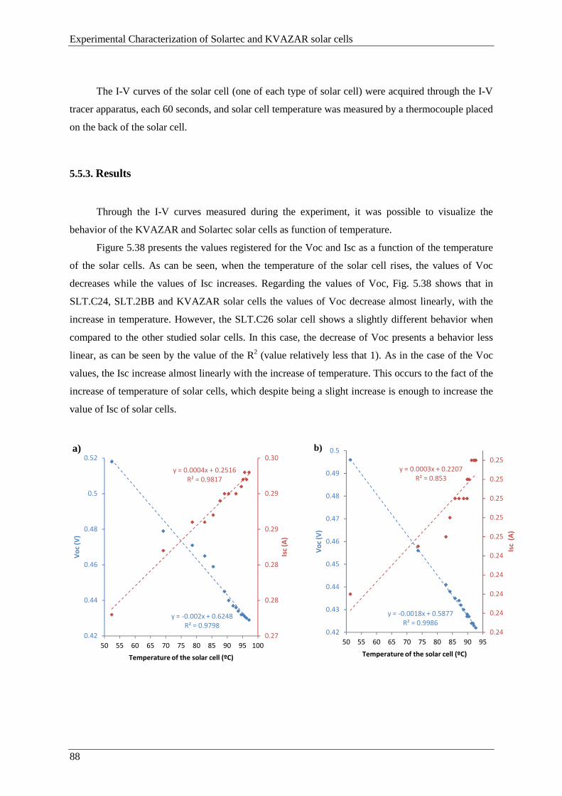
Experimental Characterization of Solartec and KVAZAR solar cells
88
The I-V curves of the solar cell (one of each type of solar cell) were acquired through the I-V
tracer apparatus, each 60 seconds, and solar cell temperature was measured by a thermocouple placed
on the back of the solar cell.
5.5.3. Results
Through the I-V curves measured during the experiment, it was possible to visualize the
behavior of the KVAZAR and Solartec solar cells as function of temperature.
Figure 5.38 presents the values registered for the Voc and Isc as a function of the temperature
of the solar cells. As can be seen, when the temperature of the solar cell rises, the values of Voc
decreases while the values of Isc increases. Regarding the values of Voc, Fig. 5.38 shows that in
SLT.C24, SLT.2BB and KVAZAR solar cells the values of Voc decrease almost linearly, with the
increase in temperature. However, the SLT.C26 solar cell shows a slightly different behavior when
compared to the other studied solar cells. In this case, the decrease of Voc presents a behavior less
linear, as can be seen by the value of the R2 (value relatively less that 1). As in the case of the Voc
values, the Isc increase almost linearly with the increase of temperature. This occurs to the fact of the
increase of temperature of solar cells, which despite being a slight increase is enough to increase the
value of Isc of solar cells.
y = ‐0.002x + 0.6248
R² = 0.9798
y = 0.0004x + 0.2516
R² = 0.9817
0.27
0.28
0.28
0.29
0.29
0.30
0.42
0.44
0.46
0.48
0.5
0.52
50 55 60 65 70 75 80 85 90 95 100
Isc
(A)
Vo
c (V
)
Temperature of the solar cell (ºC)
a)
y = ‐0.0018x + 0.5877
R² = 0.9986
y = 0.0003x + 0.2207
R² = 0.853
0.24
0.24
0.24
0.24
0.24
0.25
0.25
0.25
0.25
0.25
0.42
0.43
0.44
0.45
0.46
0.47
0.48
0.49
0.5
50 55 60 65 70 75 80 85 90 95
Isc
(A
)
Vo
c (V
)
Temperature of the solar cell (ºC)
b)
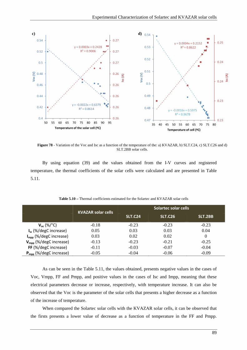
Experimental Characterization of Solartec and KVAZAR solar cells
89
Figure 78 - Variation of the Voc and Isc as a function of the temperature of the: a) KVAZAR, b) SLT.C24, c) SLT.C26 and d)
SLT.2BB solar cells.
By using equation (39) and the values obtained from the I-V curves and registered
temperature, the thermal coefficients of the solar cells were calculated and are presented in Table
5.11.
Table 5.10 – Thermal coefficients estimated for the Solartec and KVAZAR solar cells
KVAZAR solar cells
Solartec solar cells
SLT.C24 SLT.C26 SLT.2BB
Voc (%/°C) -0.18 -0.23 -0.23 -0.23 Isc (%/degC increase) 0.05 0.03 0.03 0.04
Impp (%/degC increase) 0.03 0.02 0.02 0 Vmpp (%/degC increase) -0.13 -0.23 -0.21 -0.25 FF (%/degC increase) -0.11 -0.03 -0.07 -0.04
Pmpp (%/degC increase) -0.05 -0.04 -0.06 -0.09
As can be seen in the Table 5.11, the values obtained, presents negative values in the cases of
Voc, Vmpp, FF and Pmpp, and positive values in the cases of Isc and Impp, meaning that these
electrical parameters decrease or increase, respectively, with temperature increase. It can also be
observed that the Voc is the parameter of the solar cells that presents a higher decrease as a function
of the increase of temperature.
When compared the Solartec solar cells with the KVAZAR solar cells, it can be observed that
the firsts presents a lower value of decrease as a function of temperature in the FF and Pmpp.
y = ‐0.0022x + 0.6379
R² = 0.8614
y = 0.0003x + 0.2428
R² = 0.9006
0.26
0.26
0.26
0.26
0.26
0.27
0.27
0.27
0.4
0.42
0.44
0.46
0.48
0.5
0.52
0.54
50 55 60 65 70 75 80 85 90 95Is
c (A
)
Vo
c (V
)
Temperature of the solar cell (ºC)
c)
y = ‐0.0016x + 0.5975
R² = 0.9678
y = 0.0004x + 0.2152
R² = 0.8622
0.23
0.23
0.24
0.24
0.25
0.47
0.48
0.49
0.5
0.51
0.52
0.53
0.54
35 40 45 50 55 60 65 70 75 80
Isc
(A)
Vo
c (V
)
Temperature of cell (ºC)
d)

Experimental Characterization of Solartec and KVAZAR solar cells
90
However, in the remaining electrical parameters, the KVAZAR solar cells presents lower values of
degradation as a function of the increase of temperature in the solar cell. Regarding the Solartec solar
cells, the SLT.C24 presents the lowest values of thermal coefficients of Voc and Vmpp.
5.5.4. Main conclusions
Despite all the electrical parameters of solar cell being affected by the increase in temperature,
is the Voc that presents a further decrease with the increase of temperature in the solar cell.
Regarding the results obtained for the Solartec solar cells, the SLT.C24 solar cells present
themselves with the lowest values of thermal coefficients, when compared with the remaining
Solartec solar cells.
Another conclusion that can be observed is that in comparison, the KVAZAR and Solartec
solar cells show quite different thermal coefficients. While the Solartec solar cells present lower
thermal coefficients in the case of FF and Pmpp, the KVAZAR solar cells present lower thermal
coefficients in the remaining electrical parameters. So, it can be affirm that the KVAZAR solar cells
seem to be the solar cells with lower decrease of electrical parameters with the increase of
temperature.
The datasheets with the values measured in the experimental campaign are presented in the
Annex IV.
Integration of the solar cells in the HSUN sub-receivers
91
Chapter 6
Integration of the solar cells in the HSUN sub-receivers
In this chapter is presented the behavior of the Solartec solar cells integrated in the HSUN sub-
receivers. In section 6.1 the entire HSUN system is described, while in the section 6.2 the mounting
process of the sub-receivers is explained. In the section 6.3 the behavior of the solar cells integrated
in the sub-receivers was analyzed.
6.1. Integration of solar cells in the HSUN technology
The HSUN technology (Fig. 6.1) is a medium concentration photovoltaic (MCPV) system that
is being developed by WS Energia S.A. It has a total area of 1.68 m2 and 6.3 kg/m2 of weight. This
technology is based on a 20X integrated parabolic trough (primary optics) that focus the light on a
receiver with coupled reflective secondary optics. Each module has 7 successive primary optics (high
reflective aluminum mirrors), being each receiver attached to the backside of the parabolic mirror
that succeed [47]. This configuration is used as a passive cooling integrated system through which
the heat dissipation of the receiver is performed.
Each HSUN receiver is composed by three sub-receivers which have five solar cells each (i.e.
each HSUN receiver integrates a total of 15 solar cells).
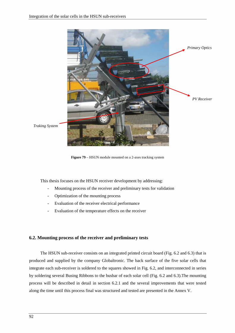
Integration of the solar cells in the HSUN sub-receivers
92
Figure 79 – HSUN module mounted on a 2-axes tracking system
This thesis focuses on the HSUN receiver development by addressing:
- Mounting process of the receiver and preliminary tests for validation
- Optimization of the mounting process
- Evaluation of the receiver electrical performance
- Evaluation of the temperature effects on the receiver
6.2. Mounting process of the receiver and preliminary tests
The HSUN sub-receiver consists on an integrated printed circuit board (Fig. 6.2 and 6.3) that is
produced and supplied by the company Globaltronic. The back surface of the five solar cells that
integrate each sub-receiver is soldered to the squares showed in Fig. 6.2, and interconnected in series
by soldering several Busing Ribbons to the busbar of each solar cell (Fig. 6.2 and 6.3).The mounting
process will be described in detail in section 6.2.1 and the several improvements that were tested
along the time until this process final was structured and tested are presented in the Annex V.
Traking System
PV Receiver
Primary Optics
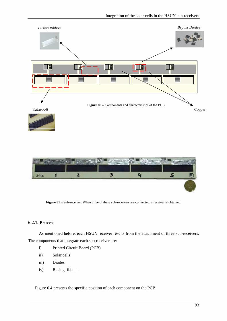
Integration of the solar cells in the HSUN sub-receivers
93
Figure 80 – Components and characteristics of the PCB.
Figure 81 – Sub-receiver. When three of these sub-receivers are connected, a receiver is obtained.
6.2.1. Process
As mentioned before, each HSUN receiver results from the attachment of three sub-receivers.
The components that integrate each sub-receiver are:
i) Printed Circuit Board (PCB)
ii) Solar cells
iii) Diodes
iv) Busing ribbons
Figure 6.4 presents the specific position of each component on the PCB.
Solar cell
Busing Ribbon
Copper
Bypass Diodes
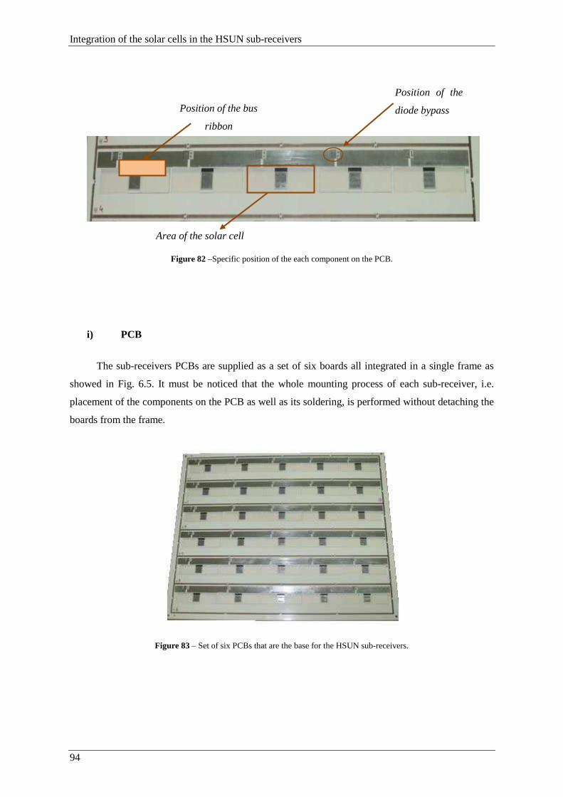
Integration of the solar cells in the HSUN sub-receivers
94
Figure 82 –Specific position of the each component on the PCB.
i) PCB
The sub-receivers PCBs are supplied as a set of six boards all integrated in a single frame as
showed in Fig. 6.5. It must be noticed that the whole mounting process of each sub-receiver, i.e.
placement of the components on the PCB as well as its soldering, is performed without detaching the
boards from the frame.
Figure 83 – Set of six PCBs that are the base for the HSUN sub-receivers.
Position of the bus
ribbon
Position of the
diode bypass
Area of the solar cell

Integration of the solar cells in the HSUN sub-receivers
95
ii) Solar cells
The back surface of the solar cell is only soldered in the central area. Otherwise, if the whole
back surface of the solar cell is soldered to the PCB, the solar cell is unable to support the thermal
expansions and eventually breaks.
In order to promote a better heat dissipation from the solar cell to the PCB, the unsoldered
back surface of the solar cell is filled with thermal tape. Notice that the thermal tape must be placed
on the PCB before the solar cell. The thermal tape should be placed inside the delimited area for the
positioning of the solar cell, as can be visualized in Fig. 6.6.
Figure 84 – Position where the thermal tape and the solder is placed on the PCB
iii) Diodes
In the printed circuit board it is also integrated a bypass diode for each solar cell. This is because,
as the cells are connected in series, if one of the solar cell is damaged, the entire sub-receiver would
crash, leading to high losses of efficiency in the entire system. However, through the application of
these diodes, this situation may be circumvented. For a correct functioning, the bypass diode is
connected in parallel, but with an opposite polarity as to the solar cell. If any of the solar cells is
damaged, the diode of this cell begins to conduct current, allowing the current generated by the solar
cells that stills operate flows by an external circuit [3].
iv) Bussing Ribbon
To connect the five solar cells in series, a Busing Ribbon is soldered on the busbar of
each solar cell and on the superior strip of the PCB, as can be observed in Fig. 6.5.
Filled area with
thermal tape
Area where the
solder is placed
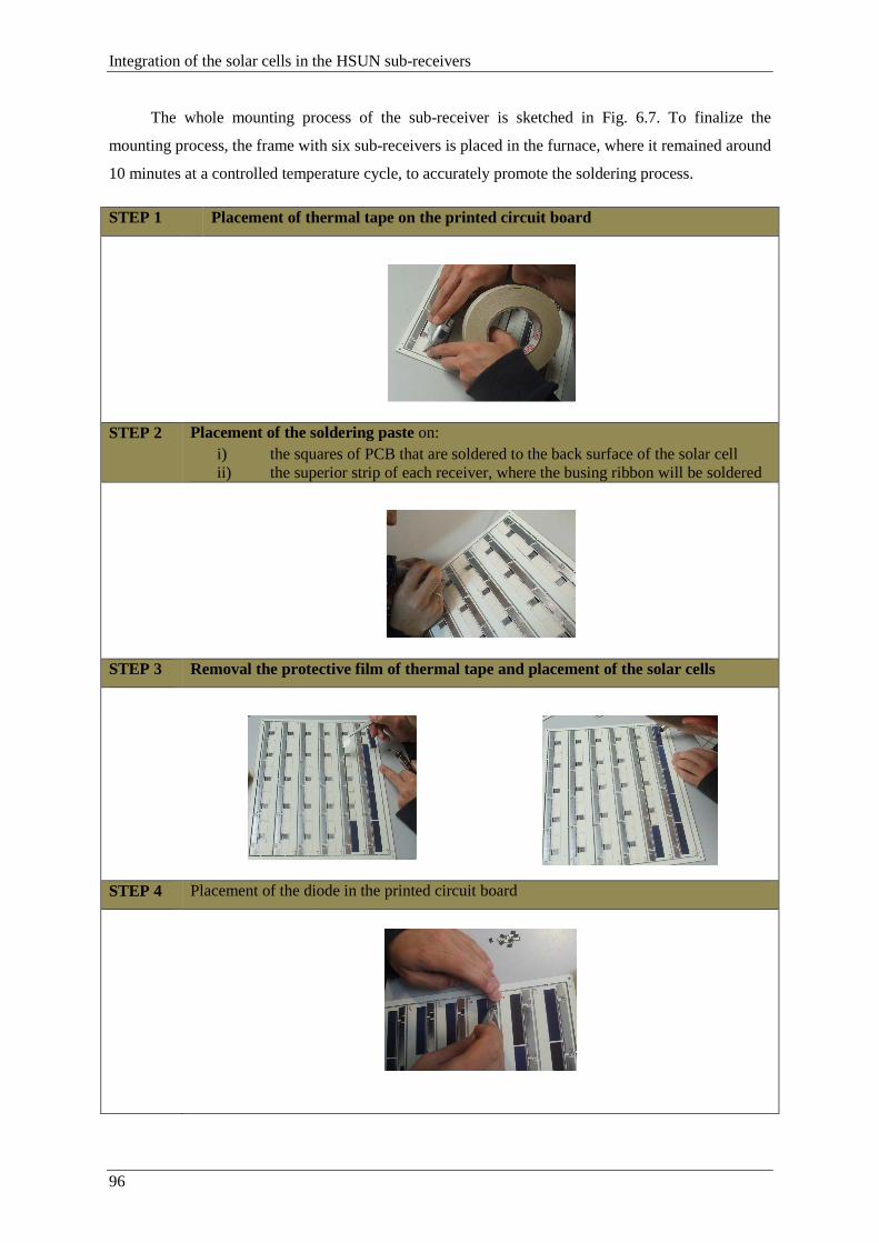
Integration of the solar cells in the HSUN sub-receivers
96
The whole mounting process of the sub-receiver is sketched in Fig. 6.7. To finalize the
mounting process, the frame with six sub-receivers is placed in the furnace, where it remained around
10 minutes at a controlled temperature cycle, to accurately promote the soldering process.
STEP 1 Placement of thermal tape on the printed circuit board
STEP 2 Placement of the soldering paste on: i) the squares of PCB that are soldered to the back surface of the solar cell ii) the superior strip of each receiver, where the busing ribbon will be soldered
STEP 3 Removal the protective film of thermal tape and placement of the solar cells
STEP 4 Placement of the diode in the printed circuit board
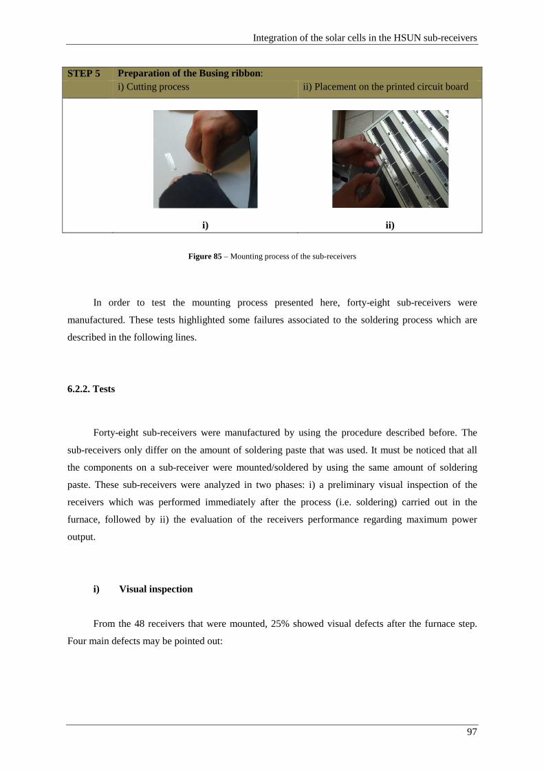
Integration of the solar cells in the HSUN sub-receivers
97
STEP 5 Preparation of the Busing ribbon: i) Cutting process ii) Placement on the printed circuit board
i) ii)
Figure 85 – Mounting process of the sub-receivers
In order to test the mounting process presented here, forty-eight sub-receivers were
manufactured. These tests highlighted some failures associated to the soldering process which are
described in the following lines.
6.2.2. Tests
Forty-eight sub-receivers were manufactured by using the procedure described before. The
sub-receivers only differ on the amount of soldering paste that was used. It must be noticed that all
the components on a sub-receiver were mounted/soldered by using the same amount of soldering
paste. These sub-receivers were analyzed in two phases: i) a preliminary visual inspection of the
receivers which was performed immediately after the process (i.e. soldering) carried out in the
furnace, followed by ii) the evaluation of the receivers performance regarding maximum power
output.
i) Visual inspection
From the 48 receivers that were mounted, 25% showed visual defects after the furnace step.
Four main defects may be pointed out:
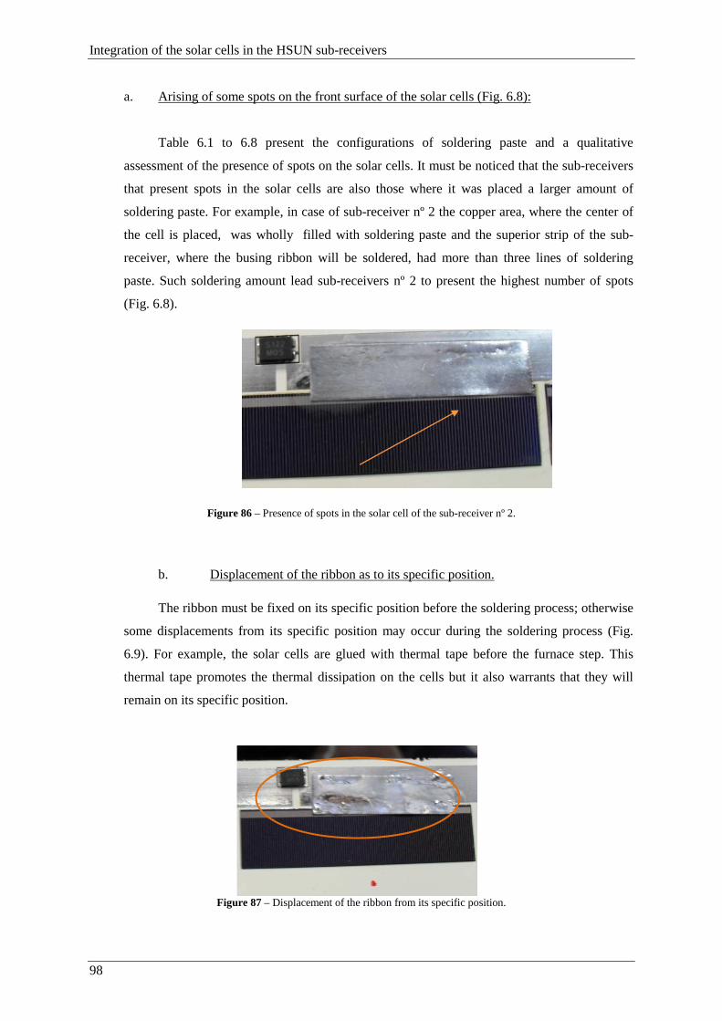
Integration of the solar cells in the HSUN sub-receivers
98
a. Arising of some spots on the front surface of the solar cells (Fig. 6.8):
Table 6.1 to 6.8 present the configurations of soldering paste and a qualitative
assessment of the presence of spots on the solar cells. It must be noticed that the sub-receivers
that present spots in the solar cells are also those where it was placed a larger amount of
soldering paste. For example, in case of sub-receiver nº 2 the copper area, where the center of
the cell is placed, was wholly filled with soldering paste and the superior strip of the sub-
receiver, where the busing ribbon will be soldered, had more than three lines of soldering
paste. Such soldering amount lead sub-receivers nº 2 to present the highest number of spots
(Fig. 6.8).
Figure 86 – Presence of spots in the solar cell of the sub-receiver nº 2.
b. Displacement of the ribbon as to its specific position.
The ribbon must be fixed on its specific position before the soldering process; otherwise
some displacements from its specific position may occur during the soldering process (Fig.
6.9). For example, the solar cells are glued with thermal tape before the furnace step. This
thermal tape promotes the thermal dissipation on the cells but it also warrants that they will
remain on its specific position.
Figure 87 – Displacement of the ribbon from its specific position.
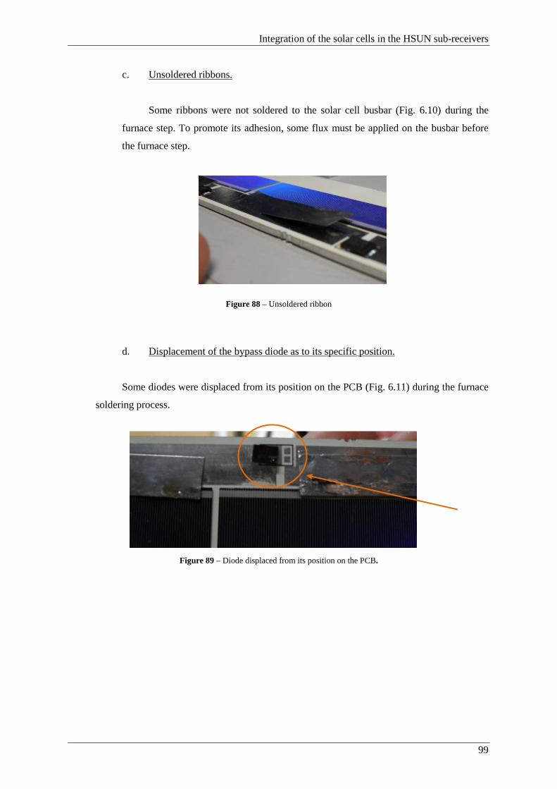
Integration of the solar cells in the HSUN sub-receivers
99
c. Unsoldered ribbons.
Some ribbons were not soldered to the solar cell busbar (Fig. 6.10) during the
furnace step. To promote its adhesion, some flux must be applied on the busbar before
the furnace step.
Figure 88 – Unsoldered ribbon
d. Displacement of the bypass diode as to its specific position.
Some diodes were displaced from its position on the PCB (Fig. 6.11) during the furnace
soldering process.
Figure 89 – Diode displaced from its position on the PCB.


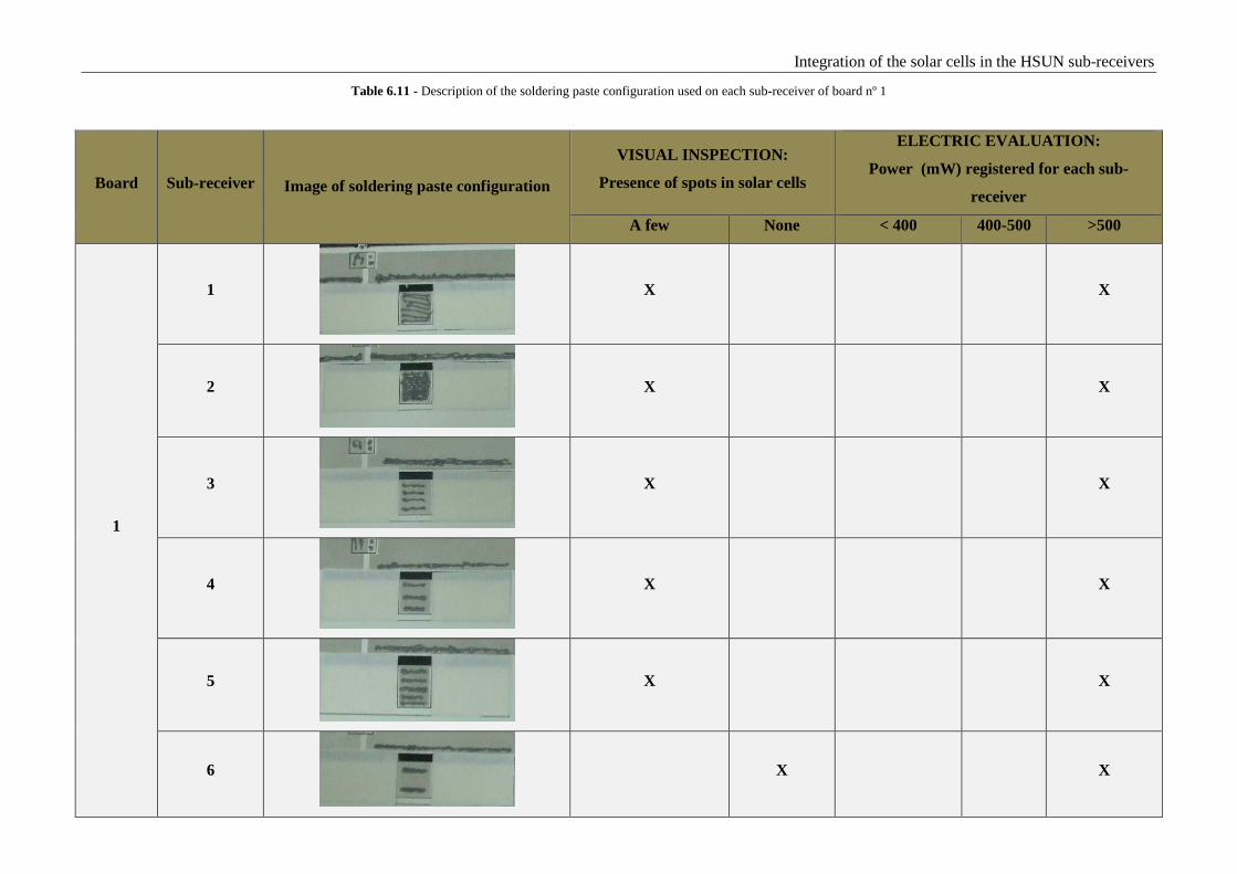
Integration of the solar cells in the HSUN sub-receivers
101
Table 6.11 - Description of the soldering paste configuration used on each sub-receiver of board nº 1
Board Sub-receiver Image of soldering paste configuration
VISUAL INSPECTION:
Presence of spots in solar cells
ELECTRIC EVALUATION:
Power (mW) registered for each sub-
receiver
A few None < 400 400-500 >500
1
1
X X
2
X X
3
X X
4
X X
5
X X
6
X X
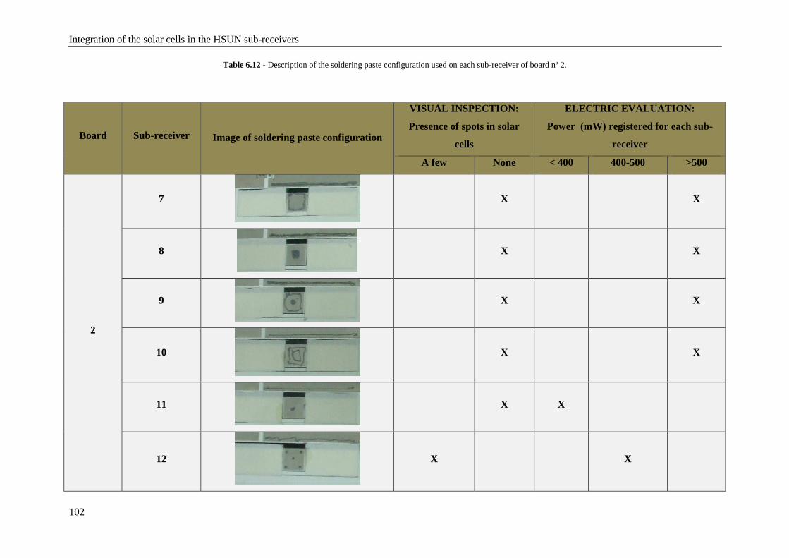
Integration of the solar cells in the HSUN sub-receivers
102
Table 6.12 - Description of the soldering paste configuration used on each sub-receiver of board nº 2.
Board Sub-receiver Image of soldering paste configuration
VISUAL INSPECTION:
Presence of spots in solar
cells
ELECTRIC EVALUATION:
Power (mW) registered for each sub-
receiver
A few None < 400 400-500 >500
2
7
X X
8
X X
9
X X
10
X X
11
X X
12
X X
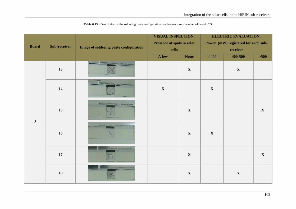
Integration of the solar cells in the HSUN sub-receivers
103
Table 6.13 - Description of the soldering paste configuration used on each sub-receiver of board nº 3.
Board Sub-receiver Image of soldering paste configuration
VISUAL INSPECTION:
Presence of spots in solar
cells
ELECTRIC EVALUATION:
Power (mW) registered for each sub-
receiver
A few None < 400 400-500 >500
3
13
X X
14
X X
15
X X
16
X X
17
X X
18
X X
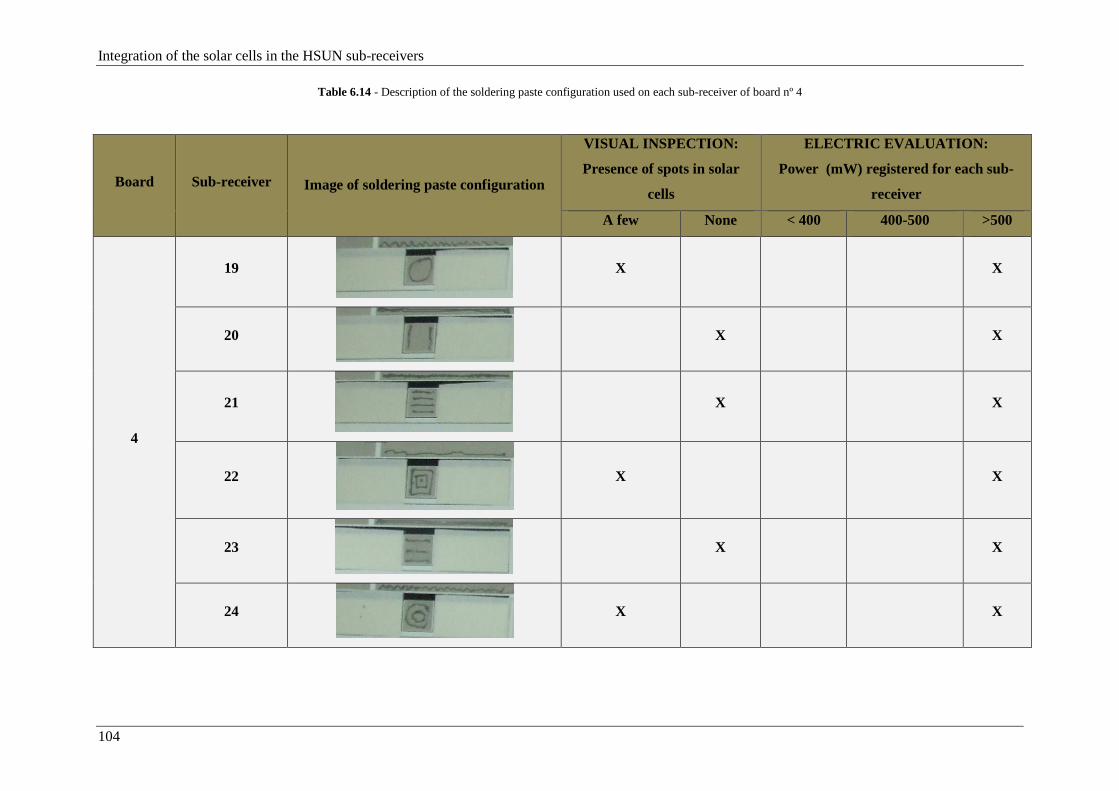
Integration of the solar cells in the HSUN sub-receivers
104
Table 6.14 - Description of the soldering paste configuration used on each sub-receiver of board nº 4
Board Sub-receiver Image of soldering paste configuration
VISUAL INSPECTION:
Presence of spots in solar
cells
ELECTRIC EVALUATION:
Power (mW) registered for each sub-
receiver
A few None < 400 400-500 >500
4
19
X X
20
X X
21
X X
22
X X
23
X X
24
X X

Integration of the solar cells in the HSUN sub-receivers
105
Table 6.15 - Description of the soldering paste configuration used on each sub-receiver of board nº 5.
Board Sub-receiver Image of soldering paste configuration
VISUAL INSPECTION:
Presence of spots in solar cells
ELECTRIC EVALUATION:
Power (mW) registered for each sub-receiver
A few None < 400 400-500 >500
5
25
X X
26
X X
27
X X
28
X X
29
X X
30
X X

Integration of the solar cells in the HSUN sub-receivers
106
Table 6.16 - Description of the soldering paste configuration used on each sub-receiver of board nº 6
Board Sub-receiver Image of soldering paste configuration
VISUAL INSPECTION:
Presence of spots in solar cells
ELECTRIC EVALUATION:
Power (mW) registered for each sub-receiver
A few None < 400 400-500 >500
6
31
32
X X
33
X X
34
X X
35
X X
36
X X
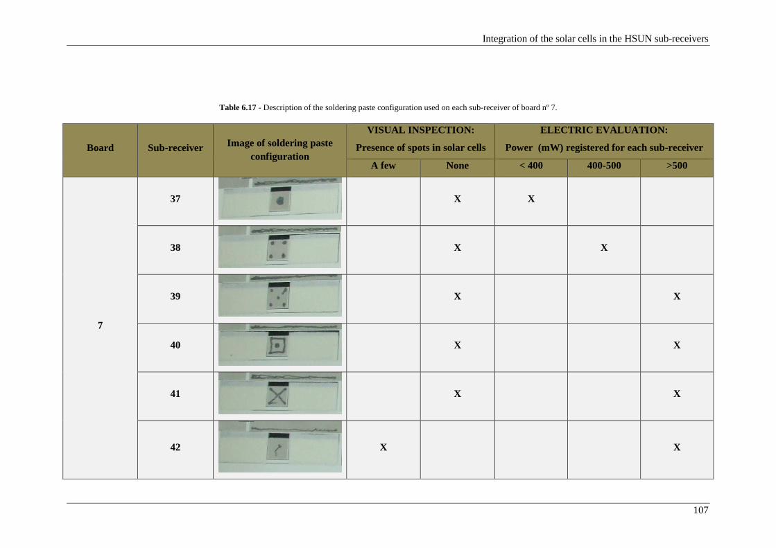
Integration of the solar cells in the HSUN sub-receivers
107
Table 6.17 - Description of the soldering paste configuration used on each sub-receiver of board nº 7.
Board Sub-receiver Image of soldering paste configuration
VISUAL INSPECTION:
Presence of spots in solar cells
ELECTRIC EVALUATION:
Power (mW) registered for each sub-receiver
A few None < 400 400-500 >500
7
37
X X
38
X X
39
X X
40
X X
41
X X
42
X X
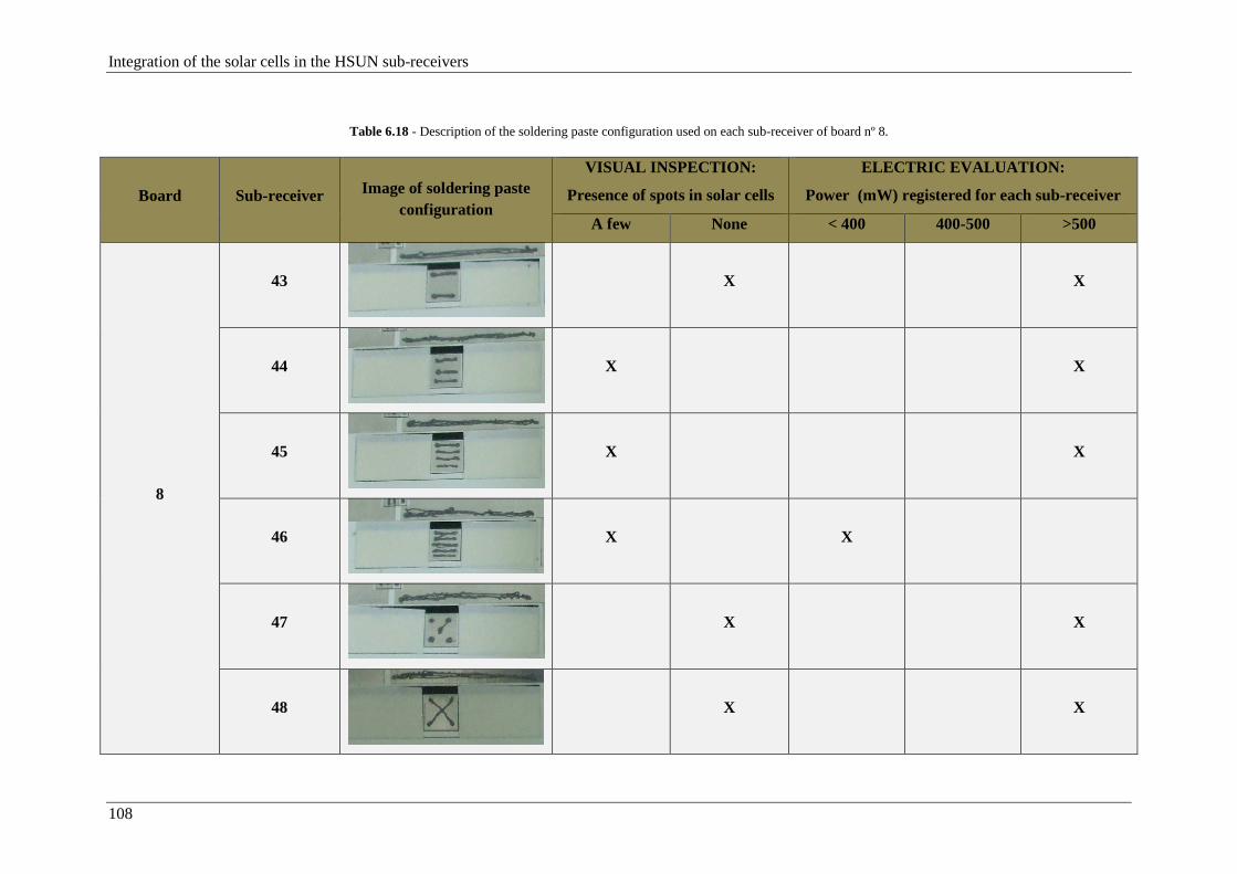
Integration of the solar cells in the HSUN sub-receivers
108
Table 6.18 - Description of the soldering paste configuration used on each sub-receiver of board nº 8.
Board Sub-receiver Image of soldering paste configuration
VISUAL INSPECTION:
Presence of spots in solar cells
ELECTRIC EVALUATION:
Power (mW) registered for each sub-receiver
A few None < 400 400-500 >500
8
43
X X
44
X X
45
X X
46
X X
47
X X
48
X X
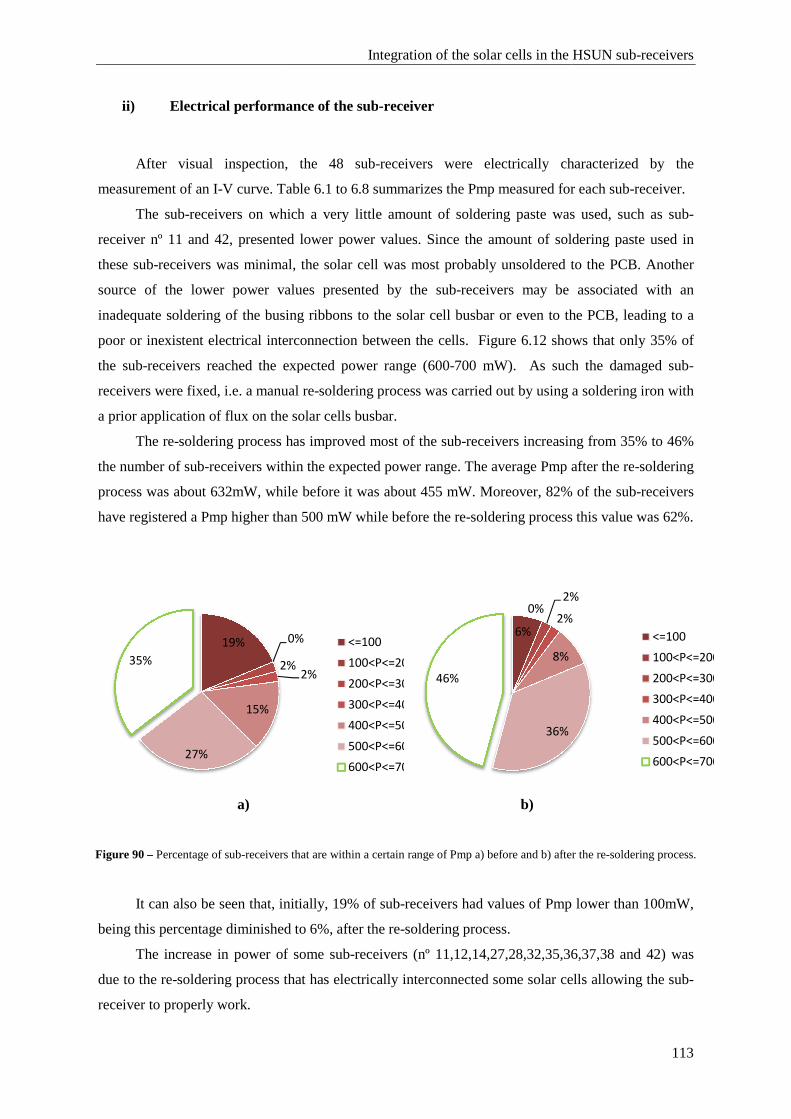
ii) Electrical performance of the sub
After visual inspection, the
measurement of an I-V curve. Table
The sub-receivers on which
receiver nº 11 and 42, presented lower power values
these sub-receivers was minimal
source of the lower power values
inadequate soldering of the busing ribbons to the solar cell busbar or even to the PCB,
poor or inexistent electrical interconnection
the sub-receivers reached the expected
receivers were fixed, i.e. a manual re
a prior application of flux on the
The re-soldering process ha
the number of sub-receivers within the
process was about 632mW, while before it was about
have registered a Pmp higher than 500 mW
Figure 90 – Percentage of sub-receivers that are within a certain range of
It can also be seen that, initially, 19% of sub
being this percentage diminished to 6%, after the re
The increase in power of some sub
due to the re-soldering process that
receiver to properly work.
19%
2%
15%
27%
35%
a)
Integration of the solar cells in the HSUN sub
lectrical performance of the sub-receiver
After visual inspection, the 48 sub-receivers were electrically characterized by the
Table 6.1 to 6.8 summarizes the Pmp measured for each sub
on which a very little amount of soldering paste was used
, presented lower power values. Since the amount of soldering paste used
was minimal, the solar cell was most probably unsoldered to the
lower power values presented by the sub-receivers may be
ing of the busing ribbons to the solar cell busbar or even to the PCB,
or inexistent electrical interconnection between the cells. Figure 6.12 shows that only 35% of
the expected power range (600-700 mW). As such
a manual re-soldering process was carried out by using a soldering iron
the solar cells busbar.
soldering process has improved most of the sub-receivers increasing from 35% to 46%
within the expected power range. The average Pmp after the re
, while before it was about 455 mW. Moreover, 82% of the sub
higher than 500 mW while before the re-soldering process this value was 62%.
receivers that are within a certain range of Pmp a) before and b) after
It can also be seen that, initially, 19% of sub-receivers had values of Pmp
being this percentage diminished to 6%, after the re-soldering process.
The increase in power of some sub-receivers (nº 11,12,14,27,28,32,35,36,37,38
that has electrically interconnected some solar cells
0%
2%2%
<=100
100<P<=200
200<P<=300
300<P<=400
400<P<=500
500<P<=600
600<P<=700
6%
0%2%
2%
8%
36%
46%
b)
in the HSUN sub-receivers
113
receivers were electrically characterized by the
measured for each sub-receiver.
soldering paste was used, such as sub-
soldering paste used in
to the PCB. Another
associated with an
ing of the busing ribbons to the solar cell busbar or even to the PCB, leading to a
shows that only 35% of
700 mW). As such the damaged sub-
using a soldering iron with
increasing from 35% to 46%
Pmp after the re-soldering
. Moreover, 82% of the sub-receivers
soldering process this value was 62%.
after the re-soldering process.
lower than 100mW,
(nº 11,12,14,27,28,32,35,36,37,38 and 42) was
solar cells allowing the sub-
2%
2%
<=100
100<P<=200
200<P<=300
300<P<=400
400<P<=500
500<P<=600
600<P<=700
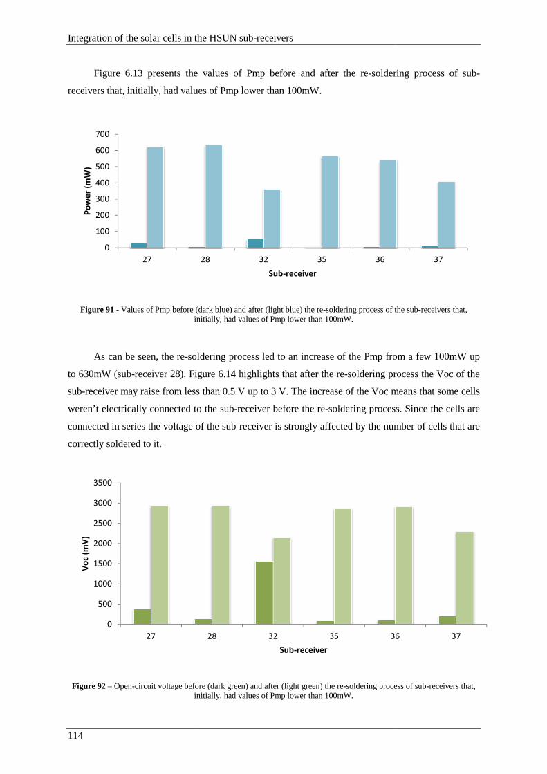
Integration of the solar cells in the HSUN sub
114
Figure 6.13 presents the values of
receivers that, initially, had values of
Figure 91 - Values of Pmp before (dark blue) and after (light blue) the reinitially, had values of Pmp lower than 100mW.
As can be seen, the re-soldering pro
to 630mW (sub-receiver 28). Figure
sub-receiver may raise from less than 0.5 V up to 3 V. The increase of the Voc
weren’t electrically connected to the sub
connected in series the voltage of the sub
correctly soldered to it.
Figure 92 – Open-circuit voltage before (dark initially, had values of Pmp lower than 100mW.
0
100
200
300
400
500
600
700
27
Po
we
r (m
W)
0
500
1000
1500
2000
2500
3000
3500
27
Vo
c (m
V)
Integration of the solar cells in the HSUN sub-receivers
presents the values of Pmp before and after the re-soldering process of sub
receivers that, initially, had values of Pmp lower than 100mW.
Pmp before (dark blue) and after (light blue) the re-soldering process of the subinitially, had values of Pmp lower than 100mW.
soldering process led to an increase of the Pmp from a few 100mW up
Figure 6.14 highlights that after the re-soldering process
receiver may raise from less than 0.5 V up to 3 V. The increase of the Voc means that some cells
electrically connected to the sub-receiver before the re-soldering process. Since the cells are
connected in series the voltage of the sub-receiver is strongly affected by the number of cells that are
circuit voltage before (dark green) and after (light green) the re-soldering process of subinitially, had values of Pmp lower than 100mW.
28 32 35 36
Sub-receiver
28 32 35 36
Sub-receiver
soldering process of sub-
soldering process of the sub-receivers that,
from a few 100mW up
soldering process the Voc of the
means that some cells
soldering process. Since the cells are
receiver is strongly affected by the number of cells that are
soldering process of sub-receivers that,
37
36 37

Contrary to what occurred in the values
increase (Fig. 6.15).
Figure 93 – Short-circuit current before (dark orange) and after (light orange) the reinitially, had values of Pmp lower than 100mW
As can be seen in Fig. 6.15
mA. This occurred since, when solar cells are connected in series, the current has small variations,
and the current generated by a sub
higher value of Isc due to the bypass diodes.
However, even after the re
of the Pmp and, in some of the cases, the value of
receiver was even more damaged with the re
14, 38 and 42 the values of Isc and
while the values of Voc increased slightly (Fig. 6.18
the values of Pmp decreases, the difference between values
process didn't exceed the 8%.
0
50
100
150
200
250
300
350
27
Cu
rre
nt
(mA
)
Integration of the solar cells in the HSUN sub
Contrary to what occurred in the values of Voc, the values of Isc didn't suf
circuit current before (dark orange) and after (light orange) the re-soldering process of subinitially, had values of Pmp lower than 100mW
As can be seen in Fig. 6.15, the value of Isc has been increased only between 32 mA and 100
mA. This occurred since, when solar cells are connected in series, the current has small variations,
and the current generated by a sub-receiver is close to the current generated by the cell that has the
the bypass diodes.
However, even after the re-soldering process, some sub-receivers didn’t show an
and, in some of the cases, the value of Pmp had declined which means that the sub
receiver was even more damaged with the re-soldering process. In the case of sub
of Isc and Pmp decreased after the re-soldering process (Fig. 6.16 and 6.17
c increased slightly (Fig. 6.18). However, it is noted that despite the fact that
decreases, the difference between values obtained before and after the re
28 32 35 36
Sub-receiver
in the HSUN sub-receivers
115
of Voc, the values of Isc didn't suffer the same
soldering process of sub-receivers that,
ly between 32 mA and 100
mA. This occurred since, when solar cells are connected in series, the current has small variations,
receiver is close to the current generated by the cell that has the
receivers didn’t show an improvement
which means that the sub-
In the case of sub-receivers nº 11, 12,
soldering process (Fig. 6.16 and 6.17),
). However, it is noted that despite the fact that
obtained before and after the re-soldering
37
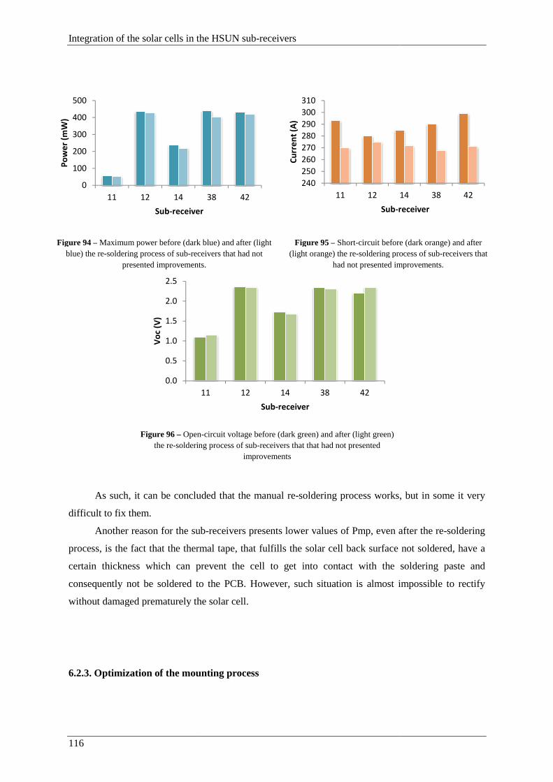
Integration of the solar cells in the HSUN sub
116
Figure 94 – Maximum power before (dark blue)blue) the re-soldering process of sub-receivers that had not
presented improvements
Figure 96 – Openthe re-soldering process of sub
As such, it can be concluded that the manual
difficult to fix them.
Another reason for the sub
process, is the fact that the thermal tape
certain thickness which can prevent the cell to get
consequently not be soldered to the PCB
without damaged prematurely the solar cell.
6.2.3. Optimization of the mounting process
0
100
200
300
400
500
11 12 14
Po
we
r (m
W)
Sub-receiver
0.0
0.5
1.0
1.5
2.0
2.5
Vo
c (V
)
Integration of the solar cells in the HSUN sub-receivers
(dark blue) and after (light
receivers that had not ovements.
Figure 95 – Short-circuit before(light orange) the re-soldering process of sub
had not presented imp
Open-circuit voltage before (dark green) and after (light green)
soldering process of sub-receivers that that had not presented improvements
As such, it can be concluded that the manual re-soldering process works, but
Another reason for the sub-receivers presents lower values of Pmp, even after the re
process, is the fact that the thermal tape, that fulfills the solar cell back surface not soldered,
which can prevent the cell to get into contact with the soldering paste and
consequently not be soldered to the PCB. However, such situation is almost impossible to rectify
thout damaged prematurely the solar cell.
Optimization of the mounting process
38 42
receiver
240
250
260
270
280
290
300
310
11 12 14
Cu
rre
nt
(A)
Sub-receiver
11 12 14 38 42
Sub-receiver
before (dark orange) and after
soldering process of sub-receivers that improvements.
soldering process works, but in some it very
, even after the re-soldering
that fulfills the solar cell back surface not soldered, have a
the soldering paste and
uch situation is almost impossible to rectify
14 38 42
receiver

Integration of the solar cells in the HSUN sub-receivers
117
As described in the previous chapter, several failures were detected on the sub-receiver after
the soldering process. In this section, some solutions are suggested to avoid such failures and
optimize the mounting process.
a) Elimination of the spots
Regarding the spots that appeared on the solar cells, and after studying the various
configurations of soldering paste, it was concluded that: i) the spots on the solar cell only appeared in
the sub-receivers on which a higher quantity of soldering paste was used (see Tables 6.1-6.8, sub-
receivers nº 1,2, 3,4,5,12,14,19,22,24,26,25,42,44,45,46) however, ii) in the sub-receivers on which it
was used only a meager amount of soldering paste (see Table 6.1-6.8, sub-receivers nº
11,12,14,16,27,28,32 and 37), the solar cells were improperly soldered to the PCB. As such, the
soldering process should be optimized by using an intermediate amount of soldering paste, which lies
between 4 to 5 risks of soldering paste on the copper square that is soldered to the solar cell back
surface and 3 lines of soldering paste on the superior strip of copper that is soldered to the busing
ribbon. Moreover, a thinner thermal tape (with the same thickness of the copper square) should
promote the contact between the solar cell back surface and the copper square.
b) Avoid displacement of the busing ribbon
To avoid the displacement of the busing ribbon, before the furnace soldering step, a plate (as
showed in Fig. 6.19) should be used to exert a small pressure on the ribbons, so they remain fixed
and connected to the solar cell during the passage of printed circuit board in the furnace.
Figure 97 – Pressure Board
c) Avoid unsoldered ribbons
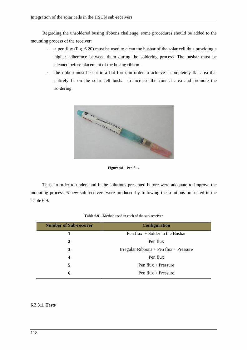
Integration of the solar cells in the HSUN sub-receivers
118
Regarding the unsoldered busing ribbons challenge, some procedures should be added to the
mounting process of the receiver:
- a pen flux (Fig. 6.20) must be used to clean the busbar of the solar cell thus providing a
higher adherence between them during the soldering process. The busbar must be
cleaned before placement of the busing ribbon.
- the ribbon must be cut in a flat form, in order to achieve a completely flat area that
entirely fit on the solar cell busbar to increase the contact area and promote the
soldering.
Figure 98 – Pen flux
Thus, in order to understand if the solutions presented before were adequate to improve the
mounting process, 6 new sub-receivers were produced by following the solutions presented in the
Table 6.9.
Table 6.9 – Method used in each of the sub-receiver
Number of Sub-receiver Configuration
1 Pen flux + Solder in the Busbar
2 Pen flux
3 Irregular Ribbons + Pen flux + Pressure
4 Pen flux
5 Pen flux + Pressure
6 Pen flux + Pressure
6.2.3.1. Tests
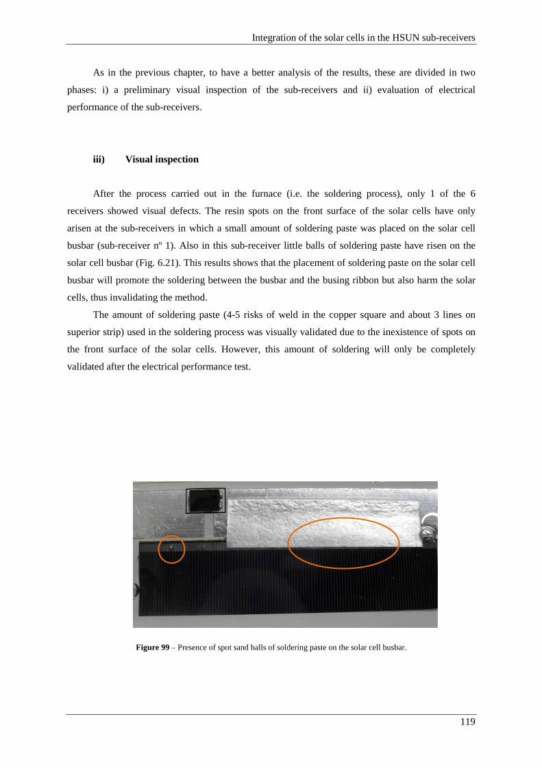
Integration of the solar cells in the HSUN sub-receivers
119
As in the previous chapter, to have a better analysis of the results, these are divided in two
phases: i) a preliminary visual inspection of the sub-receivers and ii) evaluation of electrical
performance of the sub-receivers.
iii) Visual inspection
After the process carried out in the furnace (i.e. the soldering process), only 1 of the 6
receivers showed visual defects. The resin spots on the front surface of the solar cells have only
arisen at the sub-receivers in which a small amount of soldering paste was placed on the solar cell
busbar (sub-receiver nº 1). Also in this sub-receiver little balls of soldering paste have risen on the
solar cell busbar (Fig. 6.21). This results shows that the placement of soldering paste on the solar cell
busbar will promote the soldering between the busbar and the busing ribbon but also harm the solar
cells, thus invalidating the method.
The amount of soldering paste (4-5 risks of weld in the copper square and about 3 lines on
superior strip) used in the soldering process was visually validated due to the inexistence of spots on
the front surface of the solar cells. However, this amount of soldering will only be completely
validated after the electrical performance test.
Figure 99 – Presence of spot sand balls of soldering paste on the solar cell busbar.
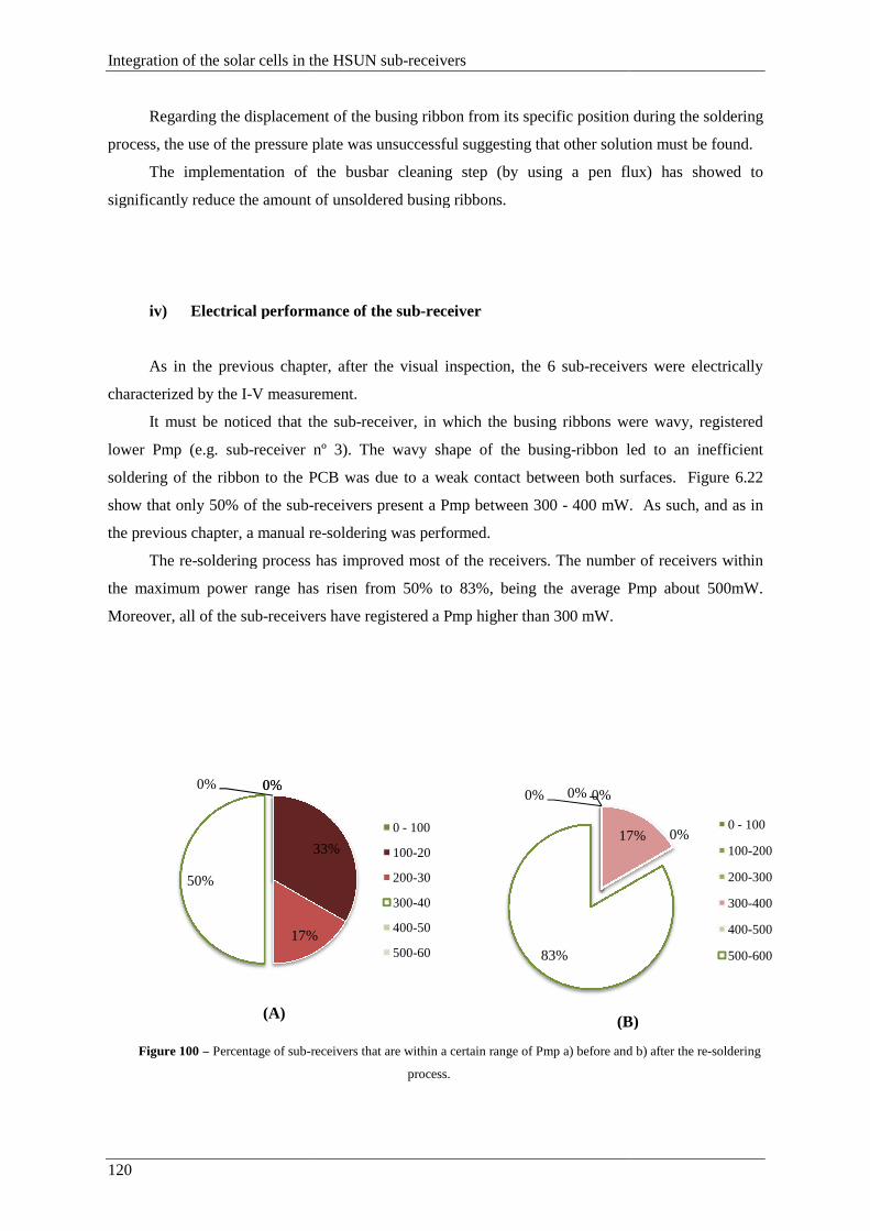
Integration of the solar cells in the HSUN sub
120
Regarding the displacement of the
process, the use of the pressure plate was unsuccessful
The implementation of th
significantly reduce the amount of unsoldered busing ribbons.
iv) Electrical performance of the sub
As in the previous chapter, a
characterized by the I-V measurement.
It must be noticed that the sub
lower Pmp (e.g. sub-receiver nº 3
soldering of the ribbon to the PCB was due to a
show that only 50% of the sub-receivers
the previous chapter, a manual re
The re-soldering process has
the maximum power range has risen from 50% to 83%, being the average
Moreover, all of the sub-receivers have registered a
Figure 100 – Percentage of sub-receivers that ar
0%
33%
17%
50%
0% 0%
(A)
Integration of the solar cells in the HSUN sub-receivers
the displacement of the busing ribbon from its specific position during the soldering
process, the use of the pressure plate was unsuccessful suggesting that other solution must be found
The implementation of the busbar cleaning step (by using a pen flux) has showed to
significantly reduce the amount of unsoldered busing ribbons.
Electrical performance of the sub-receiver
As in the previous chapter, after the visual inspection, the 6 sub-receivers were electrically
measurement.
It must be noticed that the sub-receiver, in which the busing ribbons were wavy,
receiver nº 3). The wavy shape of the busing-ribbon led to an inefficient
soldering of the ribbon to the PCB was due to a weak contact between both surfaces.
receivers present a Pmp between 300 - 400 mW. As such,
a manual re-soldering was performed.
soldering process has improved most of the receivers. The number of receivers within
the maximum power range has risen from 50% to 83%, being the average Pmp
receivers have registered a Pmp higher than 300 mW.
receivers that are within a certain range of Pmp a) before and
process.
33%
17%
0 - 100
100-200
200-300
300-400
400-500
500-600
0% 0% 0%
17%
83%
(B)
its specific position during the soldering
suggesting that other solution must be found.
e busbar cleaning step (by using a pen flux) has showed to
receivers were electrically
the busing ribbons were wavy, registered
ribbon led to an inefficient
between both surfaces. Figure 6.22
400 mW. As such, and as in
roved most of the receivers. The number of receivers within
Pmp about 500mW.
before and b) after the re-soldering
17% 0%0 - 100
100-200
200-300
300-400
400-500
500-600
(B)

It can also be seen that, initially,
being this percentage diminished to 0%, after the re
6 had several disconnected solar cells that when re
Pmp registered for each sub-receiver before and after the soldering process are presented in
Figure 101 – Maximum power point before and after the re
As can be seen, the re-soldering process
10mW and 210 mW). This increase in the
of the sub-receiver, which in turn rises due to the re
well performed before. Figure 6.2
of the sub-receiver rose between 5 mV and 600 mV.
0.00
0.10
0.20
0.30
0.40
0.50
0.60
1
Pm
p (W
)
Integration of the solar cells in the HSUN sub
It can also be seen that, initially, 33% of sub-receivers had values of Pmpp
being this percentage diminished to 0%, after the re-soldering process. The sub-
several disconnected solar cells that when re-soldered began to work properly.
receiver before and after the soldering process are presented in
Maximum power point before and after the re-soldering process of sub
soldering process led to an increase of the f Pmp
This increase in the Pmp is mainly due to a significant increase in the voltage
receiver, which in turn rises due to the re-soldering of some interconnections that were not
well performed before. Figure 6.25 highlights this situation since after re-soldering process the Voc
se between 5 mV and 600 mV.
2 3 4 5
Sub-receiver
Before After
in the HSUN sub-receivers
121
of Pmpp lower than 200mW,
-receivers nº 3, 5 and
soldered began to work properly. The values of
receiver before and after the soldering process are presented in Fig. 6.23.
soldering process of sub-receivers.
led to an increase of the f Pmp (increase between
is mainly due to a significant increase in the voltage
some interconnections that were not
soldering process the Voc
6
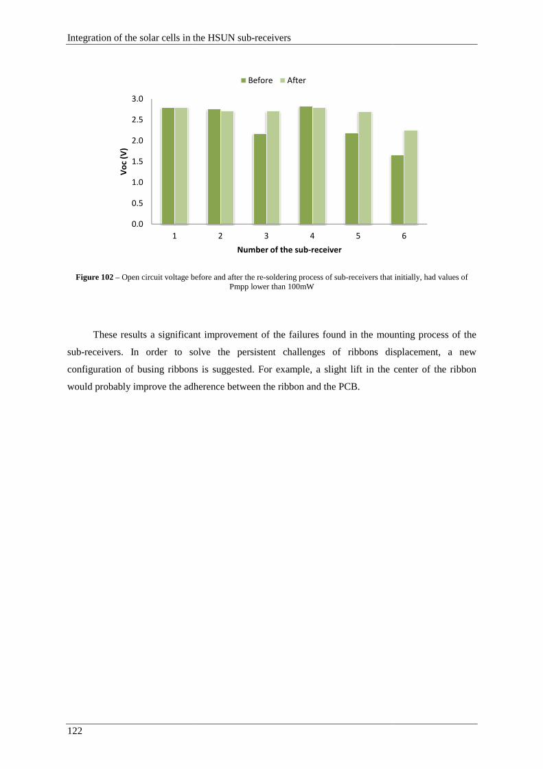
Integration of the solar cells in the HSUN sub
122
Figure 102 – Open circuit voltage befo
These results a significant improvement
sub-receivers. In order to solve the
configuration of busing ribbons
would probably improve the adherence
0.0
0.5
1.0
1.5
2.0
2.5
3.0
1
Vo
c (V
)
Integration of the solar cells in the HSUN sub-receivers
Open circuit voltage before and after the re-soldering process of sub-receivers that initially, had values of Pmpp lower than 100mW
a significant improvement of the failures found in the mounting process of the
n order to solve the persistent challenges of ribbons displacement, a new
ibbons is suggested. For example, a slight lift in the center of the ribbon
adherence between the ribbon and the PCB.
2 3 4 5
Number of the sub-receiver
Before After
receivers that initially, had values of
mounting process of the
displacement, a new
. For example, a slight lift in the center of the ribbon
6
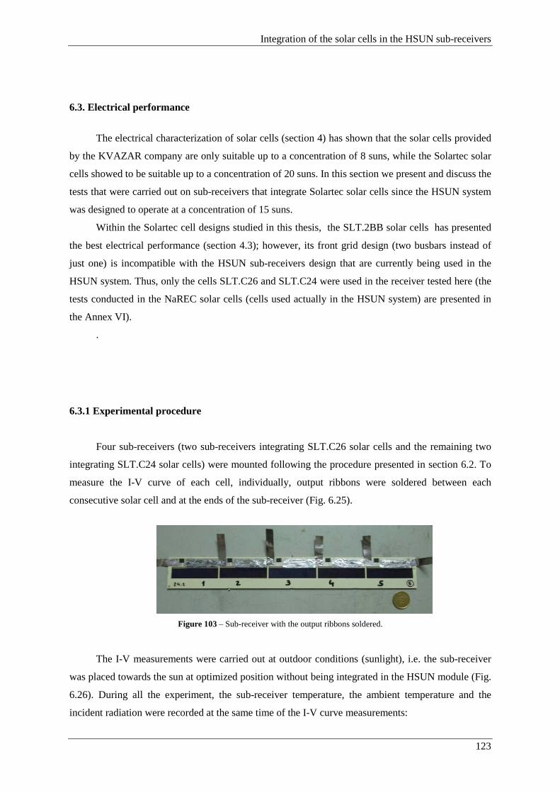
Integration of the solar cells in the HSUN sub-receivers
123
6.3. Electrical performance
The electrical characterization of solar cells (section 4) has shown that the solar cells provided
by the KVAZAR company are only suitable up to a concentration of 8 suns, while the Solartec solar
cells showed to be suitable up to a concentration of 20 suns. In this section we present and discuss the
tests that were carried out on sub-receivers that integrate Solartec solar cells since the HSUN system
was designed to operate at a concentration of 15 suns.
Within the Solartec cell designs studied in this thesis, the SLT.2BB solar cells has presented
the best electrical performance (section 4.3); however, its front grid design (two busbars instead of
just one) is incompatible with the HSUN sub-receivers design that are currently being used in the
HSUN system. Thus, only the cells SLT.C26 and SLT.C24 were used in the receiver tested here (the
tests conducted in the NaREC solar cells (cells used actually in the HSUN system) are presented in
the Annex VI).
.
6.3.1 Experimental procedure
Four sub-receivers (two sub-receivers integrating SLT.C26 solar cells and the remaining two
integrating SLT.C24 solar cells) were mounted following the procedure presented in section 6.2. To
measure the I-V curve of each cell, individually, output ribbons were soldered between each
consecutive solar cell and at the ends of the sub-receiver (Fig. 6.25).
Figure 103 – Sub-receiver with the output ribbons soldered.
The I-V measurements were carried out at outdoor conditions (sunlight), i.e. the sub-receiver
was placed towards the sun at optimized position without being integrated in the HSUN module (Fig.
6.26). During all the experiment, the sub-receiver temperature, the ambient temperature and the
incident radiation were recorded at the same time of the I-V curve measurements:
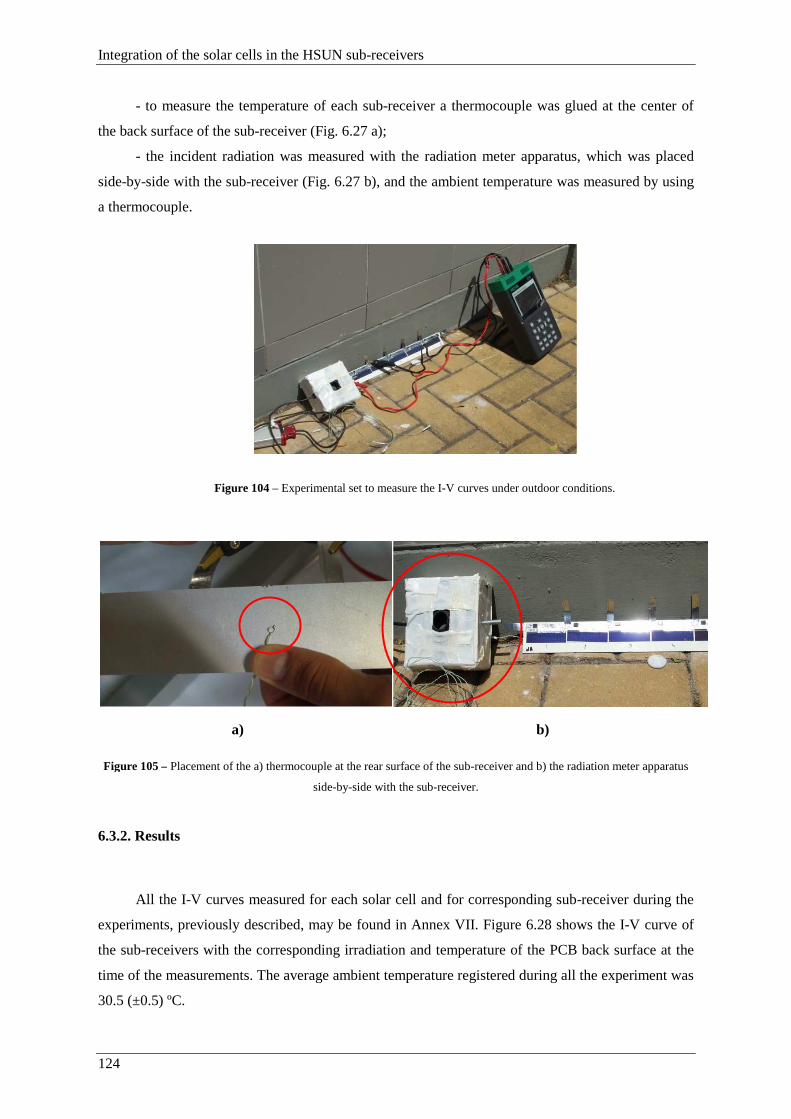
Integration of the solar cells in the HSUN sub-receivers
124
- to measure the temperature of each sub-receiver a thermocouple was glued at the center of
the back surface of the sub-receiver (Fig. 6.27 a);
- the incident radiation was measured with the radiation meter apparatus, which was placed
side-by-side with the sub-receiver (Fig. 6.27 b), and the ambient temperature was measured by using
a thermocouple.
Figure 104 – Experimental set to measure the I-V curves under outdoor conditions.
a) b)
Figure 105 – Placement of the a) thermocouple at the rear surface of the sub-receiver and b) the radiation meter apparatus
side-by-side with the sub-receiver.
6.3.2. Results
All the I-V curves measured for each solar cell and for corresponding sub-receiver during the
experiments, previously described, may be found in Annex VII. Figure 6.28 shows the I-V curve of
the sub-receivers with the corresponding irradiation and temperature of the PCB back surface at the
time of the measurements. The average ambient temperature registered during all the experiment was
30.5 (±0.5) ºC.
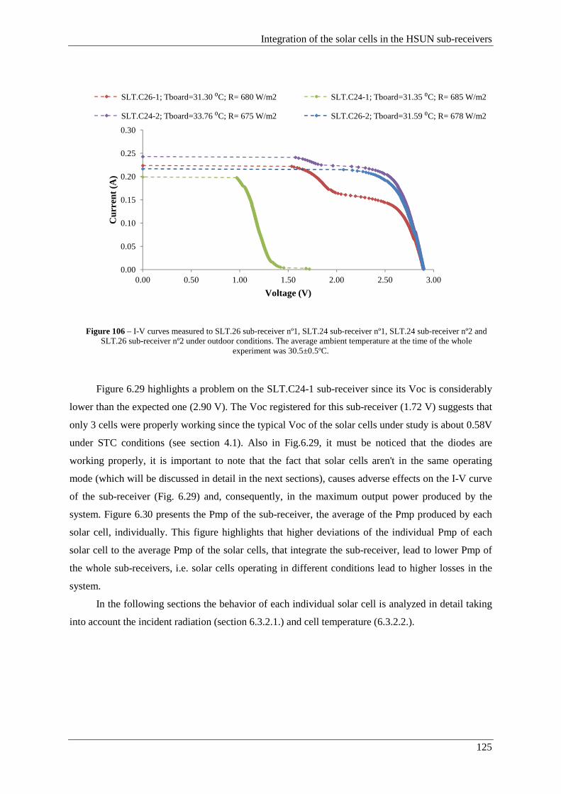
Integration of the solar cells in the HSUN sub-receivers
125
Figure 106 – I-V curves measured to SLT.26 sub-receiver nº1, SLT.24 sub-receiver nº1, SLT.24 sub-receiver nº2 and SLT.26 sub-receiver nº2 under outdoor conditions. The average ambient temperature at the time of the whole
experiment was 30.5±0.5ºC.
Figure 6.29 highlights a problem on the SLT.C24-1 sub-receiver since its Voc is considerably
lower than the expected one (2.90 V). The Voc registered for this sub-receiver (1.72 V) suggests that
only 3 cells were properly working since the typical Voc of the solar cells under study is about 0.58V
under STC conditions (see section 4.1). Also in Fig.6.29, it must be noticed that the diodes are
working properly, it is important to note that the fact that solar cells aren't in the same operating
mode (which will be discussed in detail in the next sections), causes adverse effects on the I-V curve
of the sub-receiver (Fig. 6.29) and, consequently, in the maximum output power produced by the
system. Figure 6.30 presents the Pmp of the sub-receiver, the average of the Pmp produced by each
solar cell, individually. This figure highlights that higher deviations of the individual Pmp of each
solar cell to the average Pmp of the solar cells, that integrate the sub-receiver, lead to lower Pmp of
the whole sub-receivers, i.e. solar cells operating in different conditions lead to higher losses in the
system.
In the following sections the behavior of each individual solar cell is analyzed in detail taking
into account the incident radiation (section 6.3.2.1.) and cell temperature (6.3.2.2.).
0.00
0.05
0.10
0.15
0.20
0.25
0.30
0.00 0.50 1.00 1.50 2.00 2.50 3.00
Cur
rent
(A
)
Voltage (V)
SLT.C26-1; Tboard=31.30 ⁰C; R= 680 W/m2 SLT.C24-1; Tboard=31.35 ⁰C; R= 685 W/m2
SLT.C24-2; Tboard=33.76 ⁰C; R= 675 W/m2 SLT.C26-2; Tboard=31.59 ⁰C; R= 678 W/m2
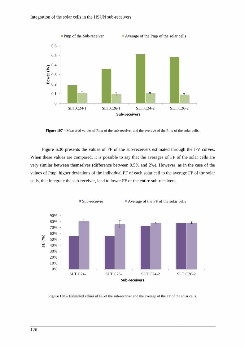
Integration of the solar cells in the HSUN sub
126
Figure 107 – Measured values of Pmp of the sub
Figure 6.30 presents the values of FF of the sub
When these values are compared, it is possible to say that the averages of FF of the solar cells are
very similar between themselves (difference between 0.5% and 2%). However
values of Pmp, higher deviations of the individual FF of each solar cell to the average FF of the solar
cells, that integrate the sub-receiver, lead to lower FF of the entire sub
Figure 108 – Estimated values of
0
0.1
0.2
0.3
0.4
0.5
0.6
SLT.C24-1
Pow
er (
W)
Pmp of the Sub
0%
10%
20%
30%
40%
50%
60%
70%
80%
90%
SLT.C24-1
FF
(%
)
Sub-
Integration of the solar cells in the HSUN sub-receivers
Measured values of Pmp of the sub-receiver and the average of the Pmp of the solar cells
presents the values of FF of the sub-receivers estimated through the I
When these values are compared, it is possible to say that the averages of FF of the solar cells are
very similar between themselves (difference between 0.5% and 2%). However, as in the case of the
values of Pmp, higher deviations of the individual FF of each solar cell to the average FF of the solar
receiver, lead to lower FF of the entire sub-receivers.
values of FF of the sub-receiver and the average of the FF of the solar cells
SLT.C26-1 SLT.C24-2 SLT.C26
Sub-receivers
Pmp of the Sub-receiver Average of the Pmp of the solar cells
SLT.C26-1 SLT.C24-2 SLT.C26
Sub-receivers
-receiver Average of the FF of the solar cells
receiver and the average of the Pmp of the solar cells.
receivers estimated through the I-V curves.
When these values are compared, it is possible to say that the averages of FF of the solar cells are
, as in the case of the
values of Pmp, higher deviations of the individual FF of each solar cell to the average FF of the solar
of the solar cells.
SLT.C26-2
Average of the Pmp of the solar cells
SLT.C26-2
Average of the FF of the solar cells
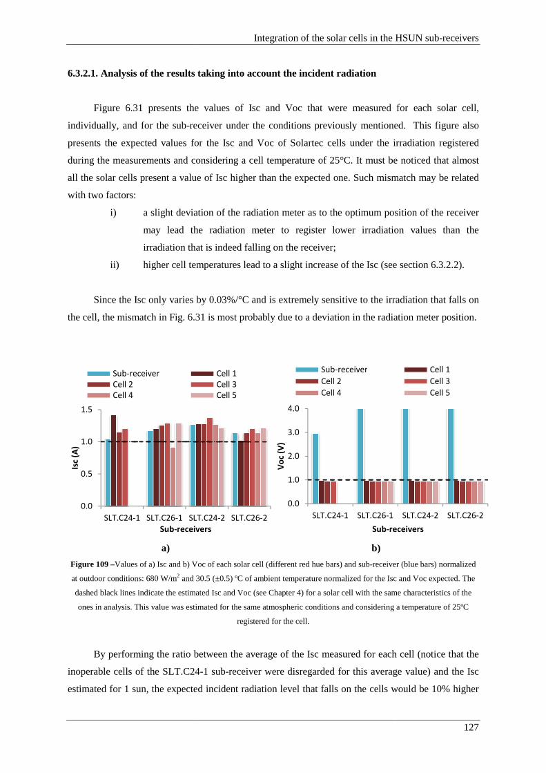
6.3.2.1. Analysis of the results taking into account the incident radiation
Figure 6.31 presents the values of Isc
individually, and for the sub-receiver
presents the expected values for the
during the measurements and considering a cell temperatu
all the solar cells present a value of Isc
with two factors:
i) a slight deviation of the radiation meter as to the optimum position of the receiver
may lead the radiation meter to register lower irradiation values than the
irradiation that is indeed falling on the receiver;
ii) higher cell temperatures lead to a slight increase of the Isc (
Since the Isc only varies by 0.03%/°C and is extrem
the cell, the mismatch in Fig. 6.3
a)
Figure 109 –Values of a) Isc and b) Voc of each solar cell (different red hue bars) and sub
at outdoor conditions: 680 W/m2 and 30.5 (±0.5) ºC of ambient temperature
dashed black lines indicate the estimated Isc and Voc (see Chapter 4
ones in analysis. This value was estimated for the same atmospheric conditions and considering a temperature of 25ºC
By performing the ratio between the average of the Isc measured for each cell (notice that the
inoperable cells of the SLT.C24
estimated for 1 sun, the expected incident radiation level that falls on the cells would be 10% higher
0.0
0.5
1.0
1.5
SLT.C24‐1 SLT.C26‐1 SLT.C24
Isc
(A)
Sub-receivers
Sub‐receiver
Cell 2
Cell 4
Integration of the solar cells in the HSUN sub
6.3.2.1. Analysis of the results taking into account the incident radiation
presents the values of Isc and Voc that were measured for
receiver under the conditions previously mentioned.
values for the Isc and Voc of Solartec cells under the irradiation registered
during the measurements and considering a cell temperature of 25°C. It must be noticed that almost
value of Isc higher than the expected one. Such mismatch may be related
a slight deviation of the radiation meter as to the optimum position of the receiver
the radiation meter to register lower irradiation values than the
irradiation that is indeed falling on the receiver;
higher cell temperatures lead to a slight increase of the Isc (see section 6.3.2.2
Since the Isc only varies by 0.03%/°C and is extremely sensitive to the irradiation that falls on
6.31 is most probably due to a deviation in the radiation meter position.
b)
Values of a) Isc and b) Voc of each solar cell (different red hue bars) and sub-receiver (blue bars)
and 30.5 (±0.5) ºC of ambient temperature normalized for the Isc and Voc expected
mated Isc and Voc (see Chapter 4) for a solar cell with the same characteristics of the
ones in analysis. This value was estimated for the same atmospheric conditions and considering a temperature of 25ºC
registered for the cell.
By performing the ratio between the average of the Isc measured for each cell (notice that the
of the SLT.C24-1 sub-receiver were disregarded for this average value) and the Isc
estimated for 1 sun, the expected incident radiation level that falls on the cells would be 10% higher
SLT.C24‐2 SLT.C26‐2
receivers
Cell 1
Cell 3
Cell 5
0.0
1.0
2.0
3.0
4.0
SLT.C24‐1 SLT.C26‐1
Vo
c (V
)
Sub-receivers
Sub‐receiver
Cell 2
Cell 4
in the HSUN sub-receivers
127
that were measured for each solar cell,
under the conditions previously mentioned. This figure also
Solartec cells under the irradiation registered
It must be noticed that almost
Such mismatch may be related
a slight deviation of the radiation meter as to the optimum position of the receiver
the radiation meter to register lower irradiation values than the
see section 6.3.2.2).
ely sensitive to the irradiation that falls on
is most probably due to a deviation in the radiation meter position.
receiver (blue bars) normalized
normalized for the Isc and Voc expected. The
) for a solar cell with the same characteristics of the
ones in analysis. This value was estimated for the same atmospheric conditions and considering a temperature of 25ºC
By performing the ratio between the average of the Isc measured for each cell (notice that the
receiver were disregarded for this average value) and the Isc
estimated for 1 sun, the expected incident radiation level that falls on the cells would be 10% higher
SLT.C24‐2 SLT.C26‐2
receivers
Cell 1
Cell 3
Cell 5
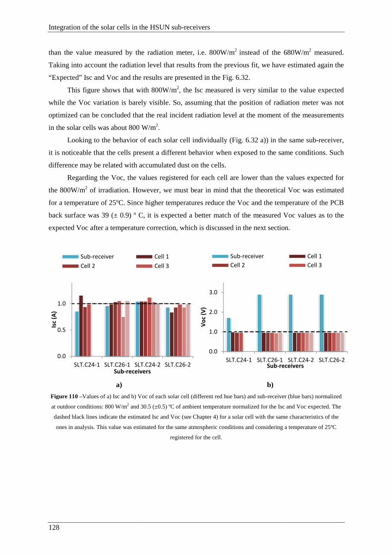
Integration of the solar cells in the HSUN sub
128
than the value measured by the radiation meter, i.e. 800W/m
Taking into account the radiation level that results from the previous fit, we have estimated again the
“Expected” Isc and Voc and the resu
This figure shows that with 800W/m
while the Voc variation is barely visible. So, assuming that the position of radiation meter was not
optimized can be concluded that the real incident radiation level at the moment of the measurements
in the solar cells was about 800 W/m
Looking to the behavior of each solar cell individually
it is noticeable that the cells present a different behavior
difference may be related with accum
Regarding the Voc, the values registered for each cell are lower than the values expected for
the 800W/m2 of irradiation. However,
for a temperature of 25ºC. Since highe
back surface was 39 (± 0.9) º C
expected Voc after a temperature correction, which is discussed in the next section.
a)
Figure 110 –Values of a) Isc and b) Voc of each solar cell (different red hue bars) and sub
at outdoor conditions: 800 W/m2 and 30.5 (±0.5) ºC of ambient temperature
dashed black lines indicate the estimated Isc and Voc (see Chapter
ones in analysis. This value was estimated for the same atmospheric conditions and considering a temperature of 25ºC
0.0
0.5
1.0
SLT.C24‐1 SLT.C26‐1 SLT.C24
Isc
(A)
Sub-receivers
Sub‐receiver
Cell 2
Integration of the solar cells in the HSUN sub-receivers
than the value measured by the radiation meter, i.e. 800W/m2 instead of the 680W/m
Taking into account the radiation level that results from the previous fit, we have estimated again the
Isc and Voc and the results are presented in the Fig. 6.32.
This figure shows that with 800W/m2, the Isc measured is very similar to the value expected
while the Voc variation is barely visible. So, assuming that the position of radiation meter was not
optimized can be concluded that the real incident radiation level at the moment of the measurements
was about 800 W/m2.
the behavior of each solar cell individually (Fig. 6.32 a)) in the same sub
it is noticeable that the cells present a different behavior when exposed to the same conditions
difference may be related with accumulated dust on the cells.
Regarding the Voc, the values registered for each cell are lower than the values expected for
However, we must bear in mind that the theoretical Voc was estimated
for a temperature of 25ºC. Since higher temperatures reduce the Voc and the temperature of the PCB
C, it is expected a better match of the measured Voc values as to the
expected Voc after a temperature correction, which is discussed in the next section.
b)
Values of a) Isc and b) Voc of each solar cell (different red hue bars) and sub-receiver (blue bars)
and 30.5 (±0.5) ºC of ambient temperature normalized for the Isc and Vo
dashed black lines indicate the estimated Isc and Voc (see Chapter 4) for a solar cell with the same characteristics of the
This value was estimated for the same atmospheric conditions and considering a temperature of 25ºC
registered for the cell.
SLT.C24‐2 SLT.C26‐2receivers
Cell 1
Cell 3
0.0
1.0
2.0
3.0
SLT.C24‐1 SLT.C26‐1
Vo
c (V
)
Sub-receivers
Sub‐receiver
Cell 2
of the 680W/m2 measured.
Taking into account the radiation level that results from the previous fit, we have estimated again the
very similar to the value expected
while the Voc variation is barely visible. So, assuming that the position of radiation meter was not
optimized can be concluded that the real incident radiation level at the moment of the measurements
in the same sub-receiver,
the same conditions. Such
Regarding the Voc, the values registered for each cell are lower than the values expected for
we must bear in mind that the theoretical Voc was estimated
r temperatures reduce the Voc and the temperature of the PCB
, it is expected a better match of the measured Voc values as to the
expected Voc after a temperature correction, which is discussed in the next section.
receiver (blue bars) normalized
normalized for the Isc and Voc expected. The
) for a solar cell with the same characteristics of the
This value was estimated for the same atmospheric conditions and considering a temperature of 25ºC
SLT.C24‐2 SLT.C26‐2receivers
Cell 1
Cell 3
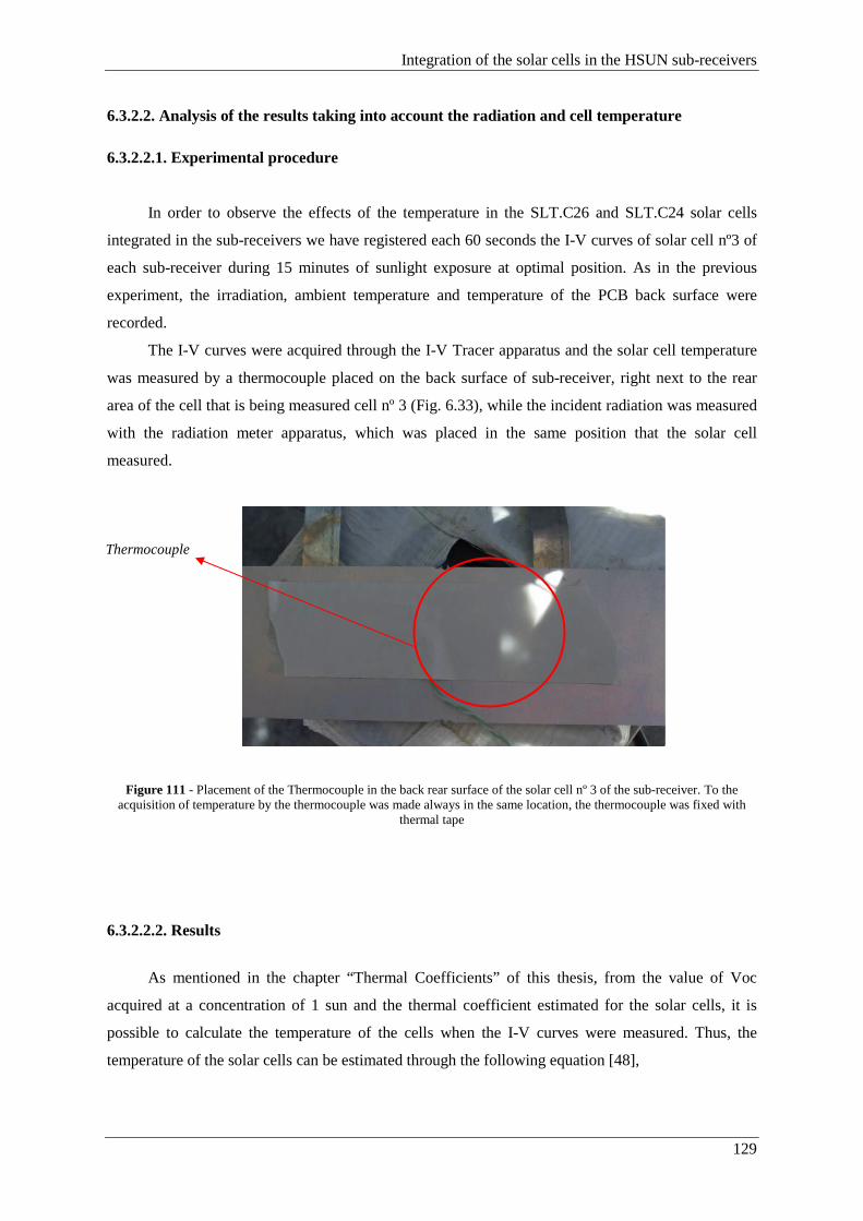
Integration of the solar cells in the HSUN sub-receivers
129
6.3.2.2. Analysis of the results taking into account the radiation and cell temperature
6.3.2.2.1. Experimental procedure
In order to observe the effects of the temperature in the SLT.C26 and SLT.C24 solar cells
integrated in the sub-receivers we have registered each 60 seconds the I-V curves of solar cell nº3 of
each sub-receiver during 15 minutes of sunlight exposure at optimal position. As in the previous
experiment, the irradiation, ambient temperature and temperature of the PCB back surface were
recorded.
The I-V curves were acquired through the I-V Tracer apparatus and the solar cell temperature
was measured by a thermocouple placed on the back surface of sub-receiver, right next to the rear
area of the cell that is being measured cell nº 3 (Fig. 6.33), while the incident radiation was measured
with the radiation meter apparatus, which was placed in the same position that the solar cell
measured.
Figure 111 - Placement of the Thermocouple in the back rear surface of the solar cell nº 3 of the sub-receiver. To the acquisition of temperature by the thermocouple was made always in the same location, the thermocouple was fixed with
thermal tape
6.3.2.2.2. Results
As mentioned in the chapter “Thermal Coefficients” of this thesis, from the value of Voc
acquired at a concentration of 1 sun and the thermal coefficient estimated for the solar cells, it is
possible to calculate the temperature of the cells when the I-V curves were measured. Thus, the
temperature of the solar cells can be estimated through the following equation [48],
Thermocouple
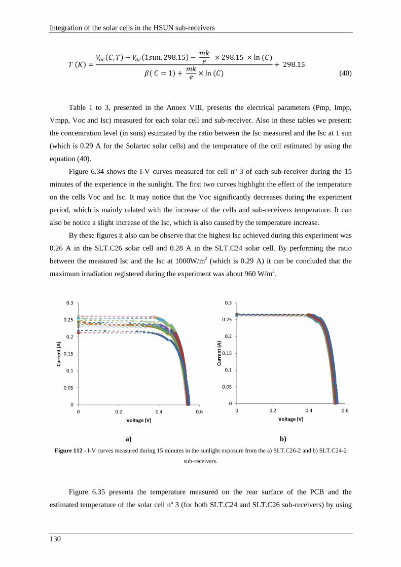
Integration of the solar cells in the HSUN sub-receivers
130
() = MU(w, ) − MU(1*CD, 298.15) − × 298.15 × ln (w)( w = 1) + × ln (w) + 298.15
(40)
Table 1 to 3, presented in the Annex VIII, presents the electrical parameters (Pmp, Impp,
Vmpp, Voc and Isc) measured for each solar cell and sub-receiver. Also in these tables we present:
the concentration level (in suns) estimated by the ratio between the Isc measured and the Isc at 1 sun
(which is 0.29 A for the Solartec solar cells) and the temperature of the cell estimated by using the
equation (40).
Figure 6.34 shows the I-V curves measured for cell nº 3 of each sub-receiver during the 15
minutes of the experience in the sunlight. The first two curves highlight the effect of the temperature
on the cells Voc and Isc. It may notice that the Voc significantly decreases during the experiment
period, which is mainly related with the increase of the cells and sub-receivers temperature. It can
also be notice a slight increase of the Isc, which is also caused by the temperature increase.
By these figures it also can be observe that the highest Isc achieved during this experiment was
0.26 A in the SLT.C26 solar cell and 0.28 A in the SLT.C24 solar cell. By performing the ratio
between the measured Isc and the Isc at 1000W/m2 (which is 0.29 A) it can be concluded that the
maximum irradiation registered during the experiment was about 960 W/m2.
Figure 6.35 presents the temperature measured on the rear surface of the PCB and the
estimated temperature of the solar cell nº 3 (for both SLT.C24 and SLT.C26 sub-receivers) by using
a) b)
Figure 112 - I-V curves measured during 15 minutes in the sunlight exposure from the a) SLT.C26-2 and b) SLT.C24-2
sub-receivers.
0
0.05
0.1
0.15
0.2
0.25
0.3
0 0.2 0.4 0.6
Cu
rre
nt
(A)
Voltage (V)
0
0.05
0.1
0.15
0.2
0.25
0.3
0 0.2 0.4 0.6
Cu
rre
nt
(A)
Voltage (V)
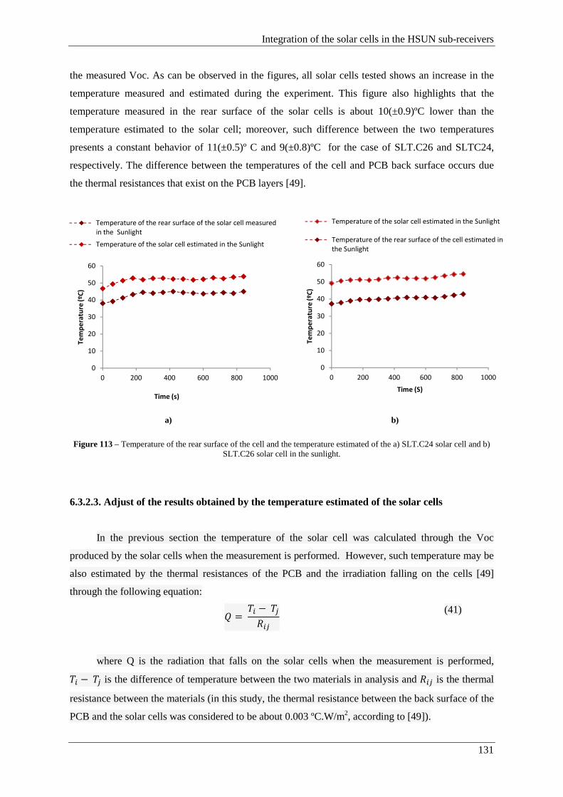
Integration of the solar cells in the HSUN sub-receivers
131
the measured Voc. As can be observed in the figures, all solar cells tested shows an increase in the
temperature measured and estimated during the experiment. This figure also highlights that the
temperature measured in the rear surface of the solar cells is about 10(±0.9)ºC lower than the
temperature estimated to the solar cell; moreover, such difference between the two temperatures
presents a constant behavior of 11(±0.5)º C and 9(±0.8)ºC for the case of SLT.C26 and SLTC24,
respectively. The difference between the temperatures of the cell and PCB back surface occurs due
the thermal resistances that exist on the PCB layers [49].
a) b)
Figure 113 – Temperature of the rear surface of the cell and the temperature estimated of the a) SLT.C24 solar cell and b) SLT.C26 solar cell in the sunlight.
6.3.2.3. Adjust of the results obtained by the temperature estimated of the solar cells
In the previous section the temperature of the solar cell was calculated through the Voc
produced by the solar cells when the measurement is performed. However, such temperature may be
also estimated by the thermal resistances of the PCB and the irradiation falling on the cells [49]
through the following equation:
t = [ − )[ (41)
where Q is the radiation that falls on the solar cells when the measurement is performed,
[ − is the difference of temperature between the two materials in analysis and )[ is the thermal
resistance between the materials (in this study, the thermal resistance between the back surface of the
PCB and the solar cells was considered to be about 0.003 ºC.W/m2, according to [49]).
0
10
20
30
40
50
60
0 200 400 600 800 1000
Te
mp
era
ture
(ºC
)
Time (s)
Temperature of the rear surface of the solar cell measured
in the Sunlight
Temperature of the solar cell estimated in the Sunlight
0
10
20
30
40
50
60
0 200 400 600 800 1000
Te
mp
era
ture
(ºC
)
Time (S)
Temperature of the solar cell estimated in the Sunlight
Temperature of the rear surface of the cell estimated in
the Sunlight
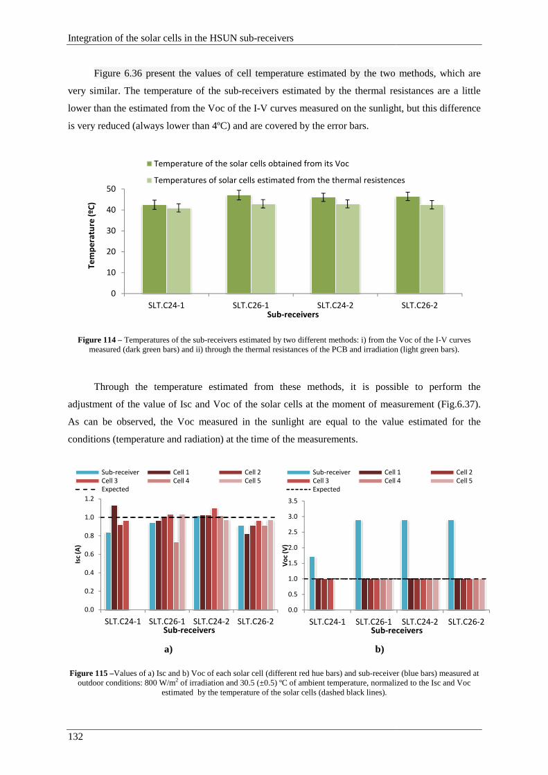
Integration of the solar cells in the HSUN sub
132
Figure 6.36 present the values of
very similar. The temperature of the sub
lower than the estimated from the Voc of the I
is very reduced (always lower than 4ºC) a
Figure 114 – Temperatures of the submeasured (dark green bars) and ii) through the thermal resistances of the P
Through the temperature estimated from these methods, it is possible
adjustment of the value of Isc and Voc of the solar cells at the moment of measurement
As can be observed, the Voc measured in the sunlight are equal to the value estimated for the
conditions (temperature and radiation) at the time of the measurements.
a)
Figure 115 –Values of a) Isc and b) Voc of eachoutdoor conditions: 800 W/m2 of irradiation and 30.5 (±0.5) ºC of ambient temperature, normalized to the Isc and Voc
estimated by the temperature of the solar cells (dashed black lines).
0
10
20
30
40
50
SLT.C24‐1
Te
mp
era
ture
(ºC
)
Temperature of the solar cells obtained from its Voc
Temperatures of solar cells estimated from the thermal resistences
0.0
0.2
0.4
0.6
0.8
1.0
1.2
SLT.C24‐1 SLT.C26‐1 SLT.C24
Isc
(A)
Sub-receivers
Sub‐receiver Cell 1
Cell 3 Cell 4Expected
Integration of the solar cells in the HSUN sub-receivers
present the values of cell temperature estimated by the two methods
very similar. The temperature of the sub-receivers estimated by the thermal resistances are a little
lower than the estimated from the Voc of the I-V curves measured on the sunlight, but this difference
is very reduced (always lower than 4ºC) and are covered by the error bars.
Temperatures of the sub-receivers estimated by two different methods: i) from the Voc of the Imeasured (dark green bars) and ii) through the thermal resistances of the PCB and irradiation (light green bars).
Through the temperature estimated from these methods, it is possible
adjustment of the value of Isc and Voc of the solar cells at the moment of measurement
As can be observed, the Voc measured in the sunlight are equal to the value estimated for the
conditions (temperature and radiation) at the time of the measurements.
b)
Values of a) Isc and b) Voc of each solar cell (different red hue bars) and sub-receiver (blue bars) measured at of irradiation and 30.5 (±0.5) ºC of ambient temperature, normalized to the Isc and Voc
estimated by the temperature of the solar cells (dashed black lines).
SLT.C26‐1 SLT.C24‐2Sub-receivers
Temperature of the solar cells obtained from its Voc
Temperatures of solar cells estimated from the thermal resistences
SLT.C24‐2 SLT.C26‐2receivers
Cell 2
Cell 5
0.0
0.5
1.0
1.5
2.0
2.5
3.0
3.5
SLT.C24‐1 SLT.C26‐1
Vo
c (V
)
Sub-receivers
Sub‐receiver Cell 1
Cell 3 Cell 4
Expected
by the two methods, which are
receivers estimated by the thermal resistances are a little
V curves measured on the sunlight, but this difference
receivers estimated by two different methods: i) from the Voc of the I-V curves CB and irradiation (light green bars).
Through the temperature estimated from these methods, it is possible to perform the
adjustment of the value of Isc and Voc of the solar cells at the moment of measurement (Fig.6.37).
As can be observed, the Voc measured in the sunlight are equal to the value estimated for the
receiver (blue bars) measured at of irradiation and 30.5 (±0.5) ºC of ambient temperature, normalized to the Isc and Voc
SLT.C26‐2
Temperatures of solar cells estimated from the thermal resistences
SLT.C24‐2 SLT.C26‐2receivers
Cell 1 Cell 2
Cell 4 Cell 5
Integration of the solar cells in the HSUN sub-receivers
133
6.3.3. Main conclusions
The values of Isc and Voc estimated for the condition at the moment of the measurement
(radiation level and temperature of the solar cells) prove to be similar to the values obtained by the
measurement. So, it can be concluded that the performance of the solar cells is unaffected by their
integration in the HSUN sub-receivers.


Cost-efficiency analysis of screen-printed solar cells to integrate CPV systems
135
Chapter 7
Cost-efficiency analysis of screen-printed solar cells to integrate CPV
systems
Most CPV systems integrate high efficiency solar cells which are designed to operate under
high levels of radiation. Such cells are more expensive than the standard screen-printed solar cell
technology which is being produced at high volume by a well-standardized industry thus benefitting
from economies of scale. Thus, in this thesis we have been evaluating the potential of such cells to
integrate CPV systems.
The previous sections have focused on the electrical characterization and technological
integration of conventional 1-sun solar cells (such as KVAZAR) and upgraded 1-sun solar cells (such
as Solartec) to operate under different concentration levels. However, to really understand the
potential of a specific solar cell technology, when integrated in a CPV system, we have to analyze the
relation between its cost and power output, i.e. to perform a cost-efficiency analysis. As such, the
cost-efficiency of a solar cell can be estimated by equation (42)[50].
€/IJJ = <K- . Jℎ *.IK - (€)<' . Jℎ - (w)()
(42)
where the <' . Jℎ - (w) is the maximum power of the cell for a concentration C.
In the following lines we perform a comparison of the cost-capacity between:
i) Conventional 1-sun screen-printed solar cells
ii) Upgraded screen-printed solar cells (optimized for 15 suns)
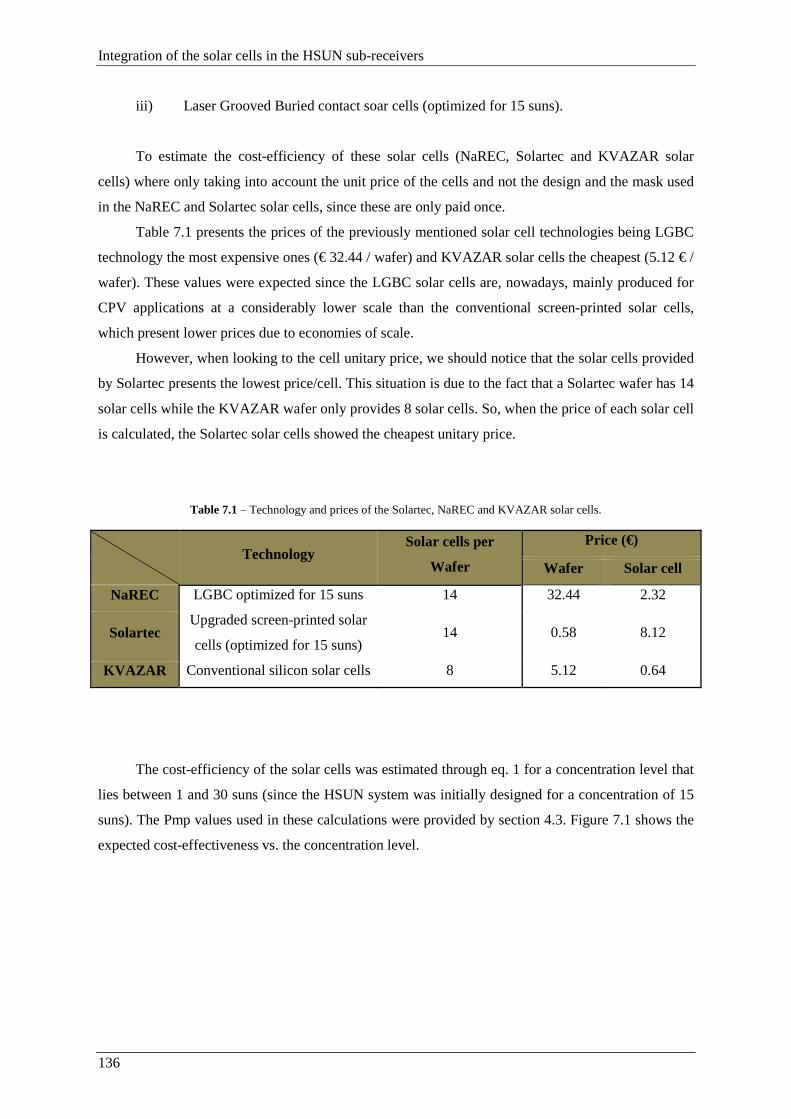
Integration of the solar cells in the HSUN sub-receivers
136
iii) Laser Grooved Buried contact soar cells (optimized for 15 suns).
To estimate the cost-efficiency of these solar cells (NaREC, Solartec and KVAZAR solar
cells) where only taking into account the unit price of the cells and not the design and the mask used
in the NaREC and Solartec solar cells, since these are only paid once.
Table 7.1 presents the prices of the previously mentioned solar cell technologies being LGBC
technology the most expensive ones (€ 32.44 / wafer) and KVAZAR solar cells the cheapest (5.12 € /
wafer). These values were expected since the LGBC solar cells are, nowadays, mainly produced for
CPV applications at a considerably lower scale than the conventional screen-printed solar cells,
which present lower prices due to economies of scale.
However, when looking to the cell unitary price, we should notice that the solar cells provided
by Solartec presents the lowest price/cell. This situation is due to the fact that a Solartec wafer has 14
solar cells while the KVAZAR wafer only provides 8 solar cells. So, when the price of each solar cell
is calculated, the Solartec solar cells showed the cheapest unitary price.
Table 7.1 – Technology and prices of the Solartec, NaREC and KVAZAR solar cells.
Technology Solar cells per
Wafer
Price (€)
Wafer Solar cell
NaREC LGBC optimized for 15 suns 14 32.44 2.32
Solartec Upgraded screen-printed solar
cells (optimized for 15 suns) 14 0.58 8.12
KVAZAR Conventional silicon solar cells 8 5.12 0.64
The cost-efficiency of the solar cells was estimated through eq. 1 for a concentration level that
lies between 1 and 30 suns (since the HSUN system was initially designed for a concentration of 15
suns). The Pmp values used in these calculations were provided by section 4.3. Figure 7.1 shows the
expected cost-effectiveness vs. the concentration level.
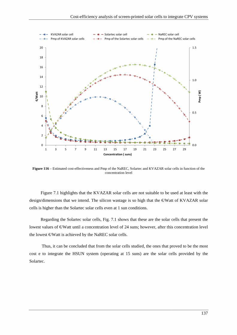
Cost-efficiency analysis of screen
Figure 116 – Estimated cost-effectiveness and Pmp
Figure 7.1 highlights that
design/dimensions that we intend
cells is higher than the Solartec solar cells even at 1 sun conditions.
Regarding the Solartec solar cells, Fig.
lowest values of €/Watt until a conc
the lowest €/Watt is achieved by the NaREC solar cells.
Thus, it can be concluded that from the solar cells studied, the ones that proved to be the most
cost e to integrate the HSUN
Solartec.
0
2
4
6
8
10
12
14
16
18
20
1 3 5 7 9
€/W
att
KVAZAR solar cell
Pmp of KVAZAR solar cells
efficiency analysis of screen-printed solar cells to integrate CPV systems
effectiveness and Pmp of the NaREC, Solartec and KVAZAR solar cellsconcentration level
that the KVAZAR solar cells are not suitable to be used at least with the
intend. The silicon wastage is so high that the €/Watt of KVAZAR solar
cells is higher than the Solartec solar cells even at 1 sun conditions.
Regarding the Solartec solar cells, Fig. 7.1 shows that these are the solar cells that present the
until a concentration level of 24 suns; however, after this concentration level
€/Watt is achieved by the NaREC solar cells.
Thus, it can be concluded that from the solar cells studied, the ones that proved to be the most
system (operating at 15 suns) are the solar cells provided by the
9 11 13 15 17 19 21 23 25
Concentration ( suns)
Solartec solar cell NaREC solar cell
Pmp of the Solartec solar cells Pmp of the NaREC solar cells
printed solar cells to integrate CPV systems
137
of the NaREC, Solartec and KVAZAR solar cells in function of the
used at least with the
€/Watt of KVAZAR solar
shows that these are the solar cells that present the
entration level of 24 suns; however, after this concentration level
Thus, it can be concluded that from the solar cells studied, the ones that proved to be the most
m (operating at 15 suns) are the solar cells provided by the
0.0
0.5
1.0
1.5
27 29
Pm
p (
W)
NaREC solar cell
Pmp of the NaREC solar cells


Conclusions and Future Work
139
Chapter 8
CONCLUSIONS AND FUTURE WORK
8.1. Conclusions
The use of alternative and environmentally friendly energy is a crucial issue in the fight against
waste and proper use of natural resources. Thus, dominate and spreading the processing technology
of photovoltaic energy, as the CPV market, is the primary task for the technological areas.
The HSUN is a concentration photovoltaic (CPV) system concept under development by WS
Energia S.A. It uses crystalline silicon solar cells optimized for a concentration factor of about 15
suns. However, the price of the HSUN PV receiver is strongly conditioned by the expensive high
efficiency solar cells that integrate. Thus, the main purpose of this thesis regards the study of new
approaches of silicon solar cells to use in the HSUN PV receiver.
In a first approach, a theoretical mathematical analysis was made in order to understand what
the behavior of solar cells studied in several levels of concentration. This study, later supported by
the full electrical characterization of the solar cells performed, allowed to conclude that the
conventional cells provided by the KVAZAR company show to be viable only up to a concentration
of 8 suns, while the modified silicon cells for concentration, provided by the Solartec company,
prove to be viable up to a concentration of 20 suns. Thus, since the HSUN system operates at a
concentration of 15 suns, the viability of KVAZAR solar cells proves to be insufficient to integrate
this system.
Thus, for the experimental campaign performed to understand the behavior of the solar cells
integrated in the HSUN sub-receivers were only tested sub-receivers.
Throughout this experimental campaign was possible to compare the results obtained
experimentally with the values estimated by the theorical model. The values appear to be similar and
show that the Solartec solar cells present a good performance (according to the expectative), that is
unaffected, when integrated in the sub-receivers of the HSUN system.
Conclusions and Future Works
140
The best performance of solar cells when integrated into the sub-receivers, in the context of
experimental campaign, was also carried out an improvement of the mounting process of the HSUN
receivers. Through the preliminary tests conducted to validate this process was possible to discover
some issues such unsoldered Ribbons, appearance of spots on solar cells and displacement of
Ribbons. After studying the results obtained in these preliminary tests, solutions were found and
implemented to optimize the process (application flux and straight cut of the ribbons). After the
optimization, this process was again tested and the results showed that the solutions were feasible,
eliminating the problems previously encountered. Much more experimental tests were performed and
were not included in this thesis.
As the main aim of the study of these new approaches is to reduce the cost of the system, it is
important not only to have a good perspective of the solar cell performance when integrated in a CPV
system, but also take into account the economic viability of the solar cells. Thus, to a correct choice
of the most viable solar cell to integrate the HSUN system was taken into account not only the values
of output power produced by the solar cells, but also their cost-efficiency. Through this cost-
efficiency, where the KVAZAR conventional solar cells, the NaREC LGBC solar cells and Solartec
optimized solar cells were compared, it was concluded that the solar cells more viable up to a
concentration level of 24 suns are the Solartec solar cells, being that from this concentration level the
NaREC solar cells present themselves as the most viable solar cells.
Therefore, and taking into account all the work developed along this thesis, it can be concluded
that the most cost-efficient solar cells to integrate the HSUN system are the mono-crystalline silicone
solar cells with optimized screen-printing, such as the Solartec solar cells.
8.2. Future Work
As mentioned throughout the thesis, this work was integrated in the development of a new
photovoltaic concentrator. Therefore, much work still needs to be done. One of the conclusions of the
comparison of the behavior of the solar cells estimated by the mathematical model and the
measurements on field is the confirmation of the values estimated. However, in this thesis, it was
only possible perform measurements at 1, 2, 4 and 10 suns. So, for a complete understanding of the
real behavior and validation of theoretical values of the solar cells under each concentration level,
measurements under other concentration levels should be further performed.
Other development to be made is the upgrade of the design of the PCB plate, so that solar cells
with new settings (as in the case of Solartec solar cells with two busbars) can be integrated and
studied in the HSUN sub-receivers.
Conclusions and Future Work
141
Another important issue, as evidenced in the experiments conducted in this thesis, is the effect
of the inhomogeneous sunlight on the solar cells. This phenomenon shows to be harmful for the
performance of the system. Thus, a study of the effect of inhomogeneous irradiation on solar cells
performance seems to be a good approach to understand the real effect of this phenomenon and the
solutions needed to minimize these effects on the output efficiency of the system.
As regards the soldering of the solar cells, in this thesis was conducted an improvement of the
mounting the sub-receivers components and the soldering method of solar cells. However, in order to
make the whole process ready for the industrialization of the HSUN system, it seems necessary to
automate the entire soldering process (including the mounting of the several components on the
PCB). Thus, a study in the automation of this part of the process seems to be necessary.

143
REFERENCES
[1] B. ROBYNS, "Situação Actual", accessed on 29 August 2011: http://e-lee.ist.utl.pt/realisations/EnergiesRenouvelables/Enjeux/Enjeux/LesEnjeux_PO.pdf, 2008.
[2] M. COLLARES-PEREIRA-PEREIRA, "Energias renováveis. A opção inadiável.," Lisboa, 2000
[3] P. A. and P. J., "PHOTOVOLTAIC SOLAR ENERGY - Development and current research ", Office for Official Publications of the European Union, Bélgica, 2009.
[4] A. Jäger-Waldau, "PV STATUS REPORT 2011," European Commission, DG Joint Research Centre, Institute for Energy, Renewable Energy Unit, Italy, 2011.
[5] K. S., "Opportunities and Challenges for Development of a Mature Concentrating Photovoltaic Power Industry," in Innovation for Our Energy Future, Colorado: National Renewable Energy Laboratory, 2009.
[6] S. H. and A. M., "Energia solar fotovoltaica: Contributo para um roadmapping do seu desenvolvimento tecnológico ", Monte da Caparica: Research Centre on Enterprise and Work Innovation, 2009.
[7] A. M. Vallêra and M. C. Brito, "Meio Século de História Fotovoltaica," ed: Gazeta da Física, 2006.
[8] R. F., "Development of Solar Concentrators for Large Photovoltaic Plants ", Dissertação para obtenção do Grau de Mestre em Engenharia Física Tecnológica, IST, Lisboa, 2008.
[9] S. A. S., "Estimativa de Produção em Centrais Solares de Concentração," Dissertação realizada no âmbito do Mestrado Integrado em Engenharia Electrotécnica e de Computadores, FEUP, Porto, 2010.
[10] A. Luque and S. H., "Handbook of Photovoltaic Science and Engineering," John Willey & Sons, England, 2003
[11] "Concentrator Photovoltaic (CPV) Modules and Assemblies - Design Qualification and Type Approval," IEC 62108: 1bDraft, 2010
[12] C. A. d. Nascimento, "PRINCÍPIO DE FUNCIONAMENTO DA CÉLULA FOTOVOLTAICA", Monografia apresentada ao Departamento de Engenharia da Universidade Federal de Lavras, MINAS GERAIS - BRASIL, 2004
[13] F. M. E. Emanuel, "Módulo fotovoltaico com seguimento da posição solar", Dissertation to obtain a Master Degree in Electrical and Computer Engineering, FCT - UNL, Lisboa, 2008
[14] D. A. D. Afonso, "Modelação e Controlo Analógico de um Sistema de Microgeração a Energia Solar", Dissertation to achive the Master Degree in Electrical and Computer Engineering, FEUP, Porto, 2009
[15] K. Bouzidi, M. Chegaar, and A. Bouhemadou, "Solar cells parameters evaluation considering the series and shunt resistance," Solar Energy Materials and Solar Cells, vol. 91, pp. 1647-1651, Nov 2007.
[16] M. T., "Solar Electricity," s.l. :Wiley, 2000. [17] F. R., "Aplicação Informática para o Estudo da Viabilidade Técnico-económica de uma
habitação sustentável", Dissertação apresentada na Faculdade de Ciências e Tecnologia da Universidade Nova de Lisboa, Lisboa, 2010
[18] S. V. K., C. A., and S. G., "OUTLOOK FOR HIGH EFFICIENCY SOLAR CELLS TO BE USED WITH AND WITHOUT CONCENTRATION," vol. 36, ed. Matera: Energy Convers. Mgmt, 1995, pp. 239-255.
[19] L. A. and A. V., "Concentrator Photovoltaics," vol. 130, ed. Athanta: Springer Series in optical sciences 2007.
[20] D.-H. Neuhaus, A. Munzer, and E, "Review Article: Industrial Silicon Wafer Solar Cells," ed. Hindawi Publishing Corporation, Advances in OptoElectronics: Dissertation to obtain a Master Degree in Electrical and Computer Engineering, 2007, p. doi:10.1155/2007/24521.
144
[21] F. Reis, "Why use NaREC solar cells on the HSUN® receiver?," WS Energia S.A.: Private communication, 2011.
[22] V. M., M. C., A. I., and S. G., "Laser grooved buried contact cells optimised for linear concentration systems," vol. 94, ed. Madrid: Solar EnergyMaterials&SolarCells, 2009, pp. 187–193.
[23] V. A. Chaudhari and C. S. Solanki, "From 1 Sun to 10 Suns c-Si Cells by Optimizing Metal Grid, Metal Resistance, and Junction Depth," International Journal of Photoenergy, 2009.
[24] J. Coello, Castro, A. M., S. G. I., and M. A. Vázquez, " Conversion of commercial si solar cells to keep their efficient performance at 15 suns," Progress in Photovoltaics: Research and Applications, 2004, pp. 12: 323–331. doi: 10.1002/pip.534.
[25] K. E. V. and B. G., "Back-contact Solar Cells: A Review ", Wiley InterScience, 2005, pp. 107–123, Bélgica
[26] A. Cheknane, H. S. Hilal, J. P. Charles, B. Benyoucef, and G. Campet, "Modelling and simulation of InGaP solar cells under solar concentration: Series resistance measurement and prediction," Solid State Sciences, vol. 8, pp. 556-559, 2006
[27] T. Fuyuki and A. Kitiyanan, "Photographic diagnosis of crystalline silicon solar cells utilizing electroluminescence," Applied Physics a-Materials Science & Processing, vol. 96, pp. 189-196, Jul 2009
[28] S. Unlimited, "Aplicação: Inspeção Electroluminescence de energia fotovoltaica com imagem SWIR," Goodrich Corporation, 2011
[29] B. TRUE, "Photoluminescence an Electroluminescence for Silicon Solar Cell Inspection",http://www.laser2000.de/fileadmin/kataloge/INTEVAC_SolarCellWhitePaper_BruceTrue.pdf: , APPLICATIONS SCIENTIST, INTEVAC, INC., consulted in 3rd July, 2011
[30] A. Kitiyanan, A. Ogane, A. Tani, T. Hatayama, H. Yano, Y. Uraoka, and T. Fuyuki, "Comprehensive study of electroluminescence in multicrystalline silicon solar cells," Journal of Applied Physics, vol. 106, Aug 2009.
[31] F. T. and K. A., "Photographic diagnosis of crystalline silicon solar cells utilizing electroluminescence ", ed: Springer-Verlag, 2008, pp. 189–196.
[32] B. O., K. A., A. Y., B. J., W. J.-M., and I. K., "Quantitative evaluation of electroluminescence images of solar cells ", www.pss-rapid.com: WILEY-VCH Verlag GmbH & Co. KGaA, online 30 October 2009
[33] C. L. Garrido-Alzar, "Algorithm for extraction of solar cell parameters from I-V curve using double exponential model," Renewable Energy, vol. 10, pp. 125-128
[34] M. S., K. M., and S. G., "Silicon Solar Cells: Recombination and Electrical Parameters ", ed. Croácia: Solar Energy, 2010, p. 432
[35] A. G. Aberle, S. R. Wenham, M. A. Green, and Ieee, "A NEW METHOD FOR ACCURATE MEASUREMENTS OF THE LUMPED SERIES RESISTANCE OF SOLAR-CELLS," in Conference Record of the Twenty Third Ieee Photovoltaic Specialists Conference - 1993, pp. 133-139
[36] http://pt.scribd.com/doc/56832517/projectofinal, "consulted in 30th August, 2011," [37] C. R., "Energias Renováveis e Produção Descentralizada", Universidade Técnica de Lisboa
Instituto Superior Técnico: DEEC / Área Científica de Energia, 2008. [38] http://www.californiascientific.com/resource/Solar%20Cell.pdf,,consulted in 15th August,
2011 [39] D. Pysch, A. Mette, and S. W. Glunz, "A review and comparison of different methods to
determine the series resistance of solar cells," Solar Energy Materials and Solar Cells, vol. 91, pp. 1698-1706, 2007
[40] B. S. and R. A., "RAPID AND ACCURATE DETERMINATION OF SERIES RESISTANCE AND FILL FACTOR LOSSES IN INDUSTRIAL SILICON SOLAR CELLS ", ed. Atlanta: Georgia Institute of Technology, 2011
[41] H. C. and B. S., "Effect of Light Intensity", PV Education,PV CDROM, 2011. [42] S. Response”, "http://pvcdrom.pveducation.org/CELLOPER/spectral.htm,", consulted in
20th August, 2011.
145
[43] R. E. E. Fotovoltaica, "http://pvcdrom.pveducation.org/CELLOPER/spectral.htm,", consulted in 20th August, 2011
[44] Q. Efficiency”, "http://pvcdrom.pveducation.org/CELLOPER/spectral.htm,", consulted in 20th August, 2011
[45] B. A. J., G. F. P., and K. A., "Análise da medida da Temperatura de módulos fotovoltaicos em ensaios de caracterização eléctrica," vol. 14, Avances en Energías Renovables y Medio Ambiente: Laboratório de Energia Solar – Programa de Pós Graduação em Engenharia Mecânica – Universidade Federal do Rio Grande do Sul (UFRGS) Rua Sarmento Leite, 2010
[46] A. I., S. G., and P. D., "Correction oh the Voc vs. Temperature dependence under Non-uniform concentrates Illumination ", Proceedings of the 17th European Photovoltaic Solar Energy Conference, , Munich, Germany (2001)
[47] M.-L. J., P. L., R. F., C. S., W. J., S. G., and P. N., "On-Field Demonstration Results of Medium Concentration System HSun," Faculty of Sciences of University of Lisbon, Lisboa, 2011
[48] A. I., S. G., and P. D., "Correction of the Voc vs. temperature dependence under non-uniform concentrated illumination," ed. Munich, Germany: Proceedings of the 17th European Photovoltaic Solar Energy Conference, 2001, p. 156
[49] D. P. F. Reis, L. Pina, J. M. Lopes, S. Coelho, J. Wemans, G. Sorasio, M. C. Brito, "Thermal Modeling of a PV Receiver for CPV Applications," ed. Los Angeles: CPV7 Conference, 2011
[50] P. R. C. a. G. A. Taylor, "THE ECONOMIC AND POLICY IMPLICATIONS OF GRID-CONNECTED RESIDENTIAL SOLAR PHOTOVOLTAIC POWER SYSTEMS," M.I.T. ENERGY LABORATORY REPORT - MIT-EL 78-007, DEPARTMENT OF ENERGY, E.U.A., 1978


147
ANNEXES
Annex I – Poster and Article presented in the 26th European Photovoltaic Solar Energy Conference,
in Hamburg
Annex II – Datasheets of the NaREC solar cells
Annex III – Datasheets of Solartec and KVAZAR solar cells provided by the respective companies
Annex IV – Datasheets of Solartec and KVAZAR solar cells with measured values
Annex V – Experiments performed to improve the soldering process of the solar cells
Annex VI– Experiments performed in the NaREC solar cells
Annex VII – I-V curves of the sub-receivers and the each solar cell individually
Annex VIII – Estimated temperatures of the solar cells integrated in the sub-receivers


ANNEX I
Poster and Article presented in the 26th European Photovoltaic Solar Energy
Conference, in Hamburg

ANNEX II
Datasheets of the NaREC solar cells

ANNEX III
Datasheets of Solartec and KVAZAR solar cells
provided by the respective companies

ANNEX IV
Datasheets of Solartec and KVAZAR solar cells with measured values

ANNEX V
Experiments performed to improve the soldering process of the
solar cells

ANNEX VI
Experiments performed in the NaREC solar cells

ANNEX VII
I-V curves of the sub-receivers and the each solar cell individually


ANNEX VIII
Estimated temperatures of the solar cells integrated in the sub-receivers