PROJECT SCHEDULING USING AN EFFICIENT PARALLEL EVOLUTIONARY ALGORITHM

Matías Galnares

Facultad de Ingeniería, Universidad de la República Herrera y Reissig 565, 11300 Montevideo, Uruguay

mgalnares@fing.edu.uy

Sergio Nesmachnow Facultad de Ingeniería, Universidad de la República Herrera y Reissig 565, 11300 Montevideo, Uruguay

sergion@fing.edu.uy

ABSTRACT

The deadline scheduling problem in project management is a NP-hard problem with major relevance in software engineering and scheduling of activities. In this article, we introduce an efficient parallel evolutionary algorithm applied to solve that problem, engineered to compute accurate solutions in reduced execution times. Specific evolutionary operators are proposed to allow solving realistic problem instances, and a master-slave parallel strategy is applied to further improve the computational efficiency and the results quality. The experimental analysis performed on a set standard problem instances shows that accurate solutions are computed. The comparative evaluation demonstrates that the proposed parallel evolutionary algorithm is able to outperform one of the best well-known deterministic techniques for the problem in reduced execution times, especially when facing instances with tight deadline constraints.

KEYWORDS. Evolutionary Algorithms, Parallelism, Project Management, Scheduling, Deadline Problem.

Main areas: Metaheurísticas, Gestão de projetos.

1. Introduction

Project management involves planning and organizing a set of activities in order to generate a product or offer a service in the best possible way (Nicholas and Steyn 2011). In order to shorten the project duration, some activities can be performed faster by employing additional resources, increasing the cost of the entire project. Considering that each activity can be performed by using a set of alternative modes, each one defined by a time-cost pair, a key problem to enable the best project performance consists in finding a schedule that assigns modes to activities, providing a good tradeoff between the duration and cost for each activity. In this article, we tackle the scheduling problem known as Deadline Problem in Project Management (DPPM), which accounts for both precedence between activities and deadline for its execution. In the related literature, the problem is also known as the Discrete Time/Cost Trade-off Problem (DTCTP).

Traditional scheduling problems are NP-hard (Garey and Johnson 1979), thus classic exact methods are only useful for solving problem instances of reduced size. Heuristics and metaheuristics are promising methods for solving scheduling problems, since they are able to get efficient solutions in reasonable time, even for large problem instances. Evolutionary algorithms (EAs) have emerged as flexible and robust metaheuristic methods for solving this kind of complex problems, achieving the high level of accuracy and efficiency also shown in many other application areas (Bäck et al. 1997). Parallel implementations have been proposed to improve both the computational efficiency and search quality of EAs (Alba 2005).

The main contributions of this article are: i) to introduce a highly efficient parallel EA to solve the DPPM, designed to solve realistic instances in reduced execution times, and ii) to efficiently compute accurate schedules, outperforming previous results in literature, for a set of problem instances with tight deadline constraints. Overall, the proposed parallel EA was able to compute 12 new best solutions for the set of 36 problem instances tackled.

The manuscript is structured as follows. Section 2 describes the paradigm of evolutionary computation and parallel EAs. The DPPM formulation is introduced in Section 3. Section 4 reviews previous works applied to solve the DPPM and problem variants. The features of the parallel EA used in the study are described in Section 5. The experimental analysis and the discussion of the results are presented in Section 6, while the conclusions and main lines for future work are formulated in Section 7.

2. Evolutionary algorithms and parallel implementations

EAs are non-deterministic methods that emulate the evolutionary process of species in nature, in order to solve optimization, search, and machine learning problems (Bäck et al. 1997). In the last twenty-five years, EAs have been successfully applied for solving optimization problems underlying many real applications of high complexity.

An EA is an iterative technique (each iteration is called a generation) that applies stochastic operators on a pool of individuals (the population P) in order to improve their fitness, which is a measure related to the objective function. Every individual in the population is the encoded version of a solution for the problem. The initial population is generated by a random method or by using a specific heuristic for the problem. An evaluation function associates a fitness value to every individual, indicating its suitability to the problem. Iteratively, the probabilistic application of variation operators like the recombination of parts from two individuals or random changes (mutations) are guided by a selection-of-the-best technique to tentative solutions of higher quality. The stopping criterion usually involves a fixed number of generations or execution time, a quality threshold on the best fitness value, or the detection of a stagnation situation. Specific policies are used to select the groups of individuals to recombine (the selection method) and to determine which new individuals are inserted in the population in each new generation. The EA returns the best solution ever found, taking into account the fitness function.

Parallel implementations are used to improve the efficiency of EAs. By using several computing elements, parallel EAs allow reaching high quality results in a reasonable execution time even for hard-to-solve optimization problems. Three main paradigms have been proposed in the related literature to design parallel EAs, regarding the criterion used for the organization of the population (Alba and Tomassini2002). In this work, we have applied the master-slave model to design the proposed parallel EA.

The master-slave model follows a functional decomposition of the evolutionary search. A master-slave parallel EA is organized in a hierarchic structure: a master process guides the search, while it controls a group of slave processes which perform the fitness function evaluation and/or the application of the variation operators (when they require large computing times) over different candidate solutions in parallel.

3. Deadline Problem in Project Management

The DPPM formulation considers the following elements: A set of activities with starting times . Some activities may

require the completion of some other activities before they begin, so a precedence function is defined, where is the set of immediate predecessors of activity .

A set of execution modes is defined for each activity ,

where each activity must be assigned to exactly one mode. For each activity and each mode the time/cost pair is defined,

where is the duration and is the cost. For any two modes and

of a

given activity

implies

, which means that in order to

speed up the time of a given activity additional resources are needed, i.e. higher costs are demanded. In addition, implies

for all activities ,

that is, the activity modes are ordered by decreasing order of duration. A deadline for the project duration is established.

The goal of the DPPM is to find a schedule, i.e. a function that assigns modes to the activities, which minimizes the total cost while fulfilling the precedence constraints and subject to that the entire project duration cannot exceed the deadline .

For the DPPM mathematical formulation, let consider two dummy activities, which precedes all those real activities with no predecessors, and , which is performed after all activities having no successors are finished (thus, is the entire project duration), and the binary decision variables , whose values are given by Eq. 1.

So, the DPPM formulation as an optimization problem is presented in Eq. 2.

Minimize

subject to

The DPPM objective is the minimization of the total cost (2.1). The constraints of the problem are: each activity must be assigned to exactly one mode (2.2); an activity cannot start before all its immediate predecessors are completed (2.3); the entire project duration cannot exceed the deadline (2.4); the starting time of the activities must be non-negative (2.5); and the values of are binary (2.6).

4. Related work: heuristics and metaheuristics for the DPPM

This subsection presents a review of previous works that have proposed applying heuristics and metaheuristics to the DPPM and related variants of the problem.

Pioneering works on scheduling proved that for linear time/cost functions, the DPPM can be solved by traditional methods such as Maximum Flow or Cut Search algorithms. Dunne et al. (1997) showed that the DTCTP is NP-hard in the strong sense, but some special structures like pure parallel and pure series are solvable in polynomial times.

Demeulemeester et al. (1998) solved the Time/Cost Curve Problem by applying a horizon-varying approach using iterative solutions of the DPPM, computed with a Branch and Bound (BAB) algorithm using Linear Relaxation based lower bounds (LB). The proposed approach solved small-sized instances up to 30 activities and four modes easily, but failed to solve most of the tackled instances with 40 activities. Deineko et al. (2001) proved that there cannot exist a polynomial time approximation algorithm with a performance guarantee better than 3/2 for any versions of the DTCTP.

Akkan et al. (2005) computed LB for the DPPM using column generation techniques based on a network decomposition approach. The proposed techniques were also applied to construct feasible solutions. The experimental analysis revealed the satisfactory behavior of the algorithm, which obtained solutions with average gap less than 7% in only 6 seconds.

Hafizoglu and Azizoglu (2010) studied algorithms based on linear programming relaxation to solve the DPPM. They defined two LBs on the optimal total cost, namely Naive Bound and LPR-Based LB, which are used in their BAB algorithm to define the branching strategy and to eliminate non-promising partial solutions. BAB solved instances with up to 150 activities and 10 modes in reasonable execution times, showing a satisfactory behavior for loose deadline time constraints. However, when faced with tighter constraints, the execution time of BAB increased considerably, reaching an hour of computing time. Up to our knowledge, the BAB algorithm is one of the best method for solving the DPPM, although it demands a large computing time for instances with tight deadlines.

Anagnostopoulos et al. (2010) developed five variants of a simulated annealing (SA) algorithm for the DPPM, using different parametrizations. The SAs achieve feasible solutions in a few seconds, and solved large-sized instances up to 300 activities with 4 modes. However, the quality of the computed solutions is only evaluated with estimations of the global optimum within a certain confidence interval.

Hazir et al. (2010) proposed an exact algorithm to solve the time minimization version of the DTCTP by a decomposition strategy. A master problem solves a relaxed DTCTP generating a LB for minimization and trial values for the integer variables to be used as fixed values in the subproblem. Instances with 85 to 136 activities, 2 to 10 modes, and tight deadline constraints were solved. The results show that 74% of the instances are solved exactly in 10 minutes, 96% in an hour, and all of them are solved in 90 minutes. Up to our knowledge, this is the best method for the time minimization DTCTP with tight deadlines.

Zhang et al. (2010) extended the DTCTP by considering renewable and non renewable resource-constrains simultaneously. A genetic algorithm was implemented for this problem, which is able to solve an instance with two renewable and two nonrenewable resources and with up to 30 activities and three modes. The computation experiments show that the algorithm solved these instances in no more than four seconds.

Recently, Fallah-Mehdipour et al. (2012) included a new parameter, the quality of the project, to previously considered time and cost parameters. Two multiobjective EAs (NSGA-II and MOPSO) are used to solve the proposed problem. The experimental analysis solved two instances with two objectives and 18 activities, and three objectives and 7 activities, respectively. The results show that both multiobjective EAs are able to achieve feasible solutions, but no computing times are reported.

Up to our knowledge, there are no antecedents of previous works applying parallel metaheuristic to solve the DPPM/DTCTP.

Summarizing, the analysis of the related works shows that solving DPPM/DTCTP instances with tight deadline constraints in reduced execution times is a hard task. For this kind of instances, the best existing approaches demands more than one hour of execution time. Thus, there is still room to contribute in this line of research, by developing efficient and accurate methods to solve the DPPM/DTCTP, able to handle the increasing complexity of realistic instances with tight constraints in reduced execution times.

5. An efficient parallel EA for the DPPM

This section presents the main features of the proposed parallel EA for the DPPM.

5.1. The GAlib library

The algorithm was implemented on GAlib, a library for EAs developed in C/C++ using the object oriented paradigm (Wall 1996). The library includes tools to implement EAs and offers the possibility of developing user-defined representations and operators. Several modifications were needed in order to provide support for the master-slave model applied to the proposed EA, including: i) implementing the thread creation, management, and synchronization, ii) implementing a thread-safe variant for the pseudorandom number generator, and iii) applying mutual exclusion sections for the selection operator, population, and statistical variables.

5.2. Features of the proposed EA

This subsection presents the main features of the proposed parallel EA, designed with two main goals: computing accurate DPPM solutions in reduced time and providing a good exploration pattern by using ad-hoc variation operators.

Solution encoding. A non-traditional encoding is defined to represent solutions, taking into account the precedence relations between activities and the different modes in which each activity can be performed. Each individual in the population is encoded as an

array

where represents the activity , and

denotes the activity in mode . The execution order of activities is from left to right: all of the predecessors of activity are located before—i.e. at the left—of .

Fitness function. Let S be a solution, represented by

.

The fitness function is given by Eq. 3, where is the maximum cost of the project, i.e. the sum of all activity costs assuming that all activities are in the costliest mode.

Feasibility check and repair mechanism. The proposed operators never violate the precedence constrains, but they can generate non-feasible solutions that do not fulfill the deadline constraints. Thus, a feasibility check/repair method is applied to correct non-feasible solutions. The total time of the project cannot exceed the deadline . Therefore, any

individual

must fulfill t

. When this condition is not verified, the feasibility repair mechanism works

by randomly selecting an activity and changing its mode in order to demand a shorter execution time. This procedure is iteratively applied until the deadline constraint is met.

Initialization. An initial population of feasible solutions is generated by applying an ad-hoc randomized construction operator. Starting from

, a new activity in mode is randomly selected. If all the predecessors of activity have been

inserted in the solution, then is inserted in the first available empty location. Otherwise,

another activity is selected. When the whole schedule has been constructed, the feasibility check/repair mechanism is applied in order to meet the deadline constraints.

Selection. The proportional selection method is used. An individual is selected to recombine/mutate with probability given by Eq. 4, where pSize is population size.

Exploitation: recombination. An ad-hoc single point crossover operator is used to recombine solutions, in order to preserve the precedence relations between activities. Two

parents

and

are selected from the population, and an integer is selected randomly from the interval . Then, two offspring and are generated according to :

where

are the elements

in , but using the modes in , and arranged in the order they are in , and

where

are the elements

in , but

using the modes in , and arranged in the order they are in . So, each offspring inherits activities from one parent, half of them with the order and modes they have in the other parent. The crossover operator can generate solutions that exceed the maximum time allowed, so the feasibility check/repair method is used to assure that all constraints are met.

Exploration: mutation. Let

be the individual

that is selected for mutation, where denotes the activity in any (fixed) mode. An

integer is selected at random from the interval . Let activity be the last

predecessor of activity , and let activity be the first successor of activity . An integer is selected randomly from the interval , then:

The mutation operator maintains the precedence relations between activities, but the new mode is randomly selected, so the feasibility check/repair mechanism is applied to guarantee that the deadline constraint is met.

Local search. The local search operator attempts to improve a given solution

by evaluating to change the activities to a mode that

reduces the total cost. Starting on a randomly selected activity , the operator cyclically analyzes all the activities, attempting to change it to mode , assuming that the

activity is assigned to execute in mode . The process is iteratively applied until all activities have been analyzed and no change has been applied, because making such changes will imply to violate the deadline constraint. Thus, a new schedule

is generated. This operator maintains the precedence relations between activities and it also guarantees that the deadline constraint is not violated.

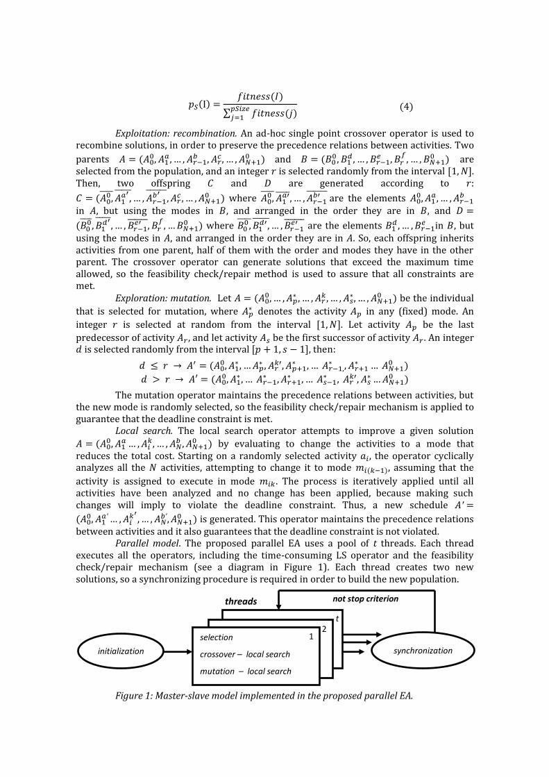
Parallel model. The proposed parallel EA uses a pool of t threads. Each thread executes all the operators, including the time-consuming LS operator and the feasibility check/repair mechanism (see a diagram in Figure 1). Each thread creates two new solutions, so a synchronizing procedure is required in order to build the new population.

Figure 1: Master-slave model implemented in the proposed parallel EA.

not stop criterion

1 2

t

threads

synchronization initialization

selection

crossover – local search

mutation – local search

1 2

t

6. Experimental analysis

This section introduces the set of DPPM instances and the platform used in the experimental evaluation. After that, the parameter setting experiments are commented. The last subsection presents and discusses the numerical results of the proposed parallel EA.

6.1. DPPM instances

Thirty-six complex instances in the benchmark from Akkan et al. (2005) are used to evaluate the proposed EA. The complexity is evaluated regarding two metrics: Coefficient of Network Complexity (CNC), the ratio between number of activities and number of modes, and Complexity Index (CI), that evaluates how close an instance to a series-parallel one is.

In the selected instances, the number of modes and the durations of each activity are selected using a discrete uniform distribution in and , respectively. The minimum cost is uniformly selected in [5,15] for all activity , and is defined

recursively by , where is also taken from a uniform

distribution. The deadline values are defined by being and the shortest and longest project durations respectively, and θ {0.15, 0.30, 0.45}.

6.2. Development and execution platform

The EAs was implemented in C++, using the GAlib library. The experimental analysis was performed on a HP server with an Opteron 6172 Magny Cours (24 cores) processor at 2.26 GHz, with 24 GB RAM, and CentOS Linux 5.2.

6.3. Parameter setting experiments

A study was performed to determine the best values of three EA parameters: pSize, and the crossover and mutation probabilities. The candidate values were: , , and . Thirty executions of the proposed parallel EA were performed for two average-size DPPM instances, with CI=14, CNC=6, N=102, and . The best results were obtained when using the configuration pSize=50, =0.95, =0.01, showing the importance of the crossover operator to compute accurate solutions. No significant improvements were detected when increasing pSize, suggesting that using a larger population is not useful to improve the results quality.

6.4. Validation experiments

In the experimental evaluation, fifty executions of the proposed parallel EA were performed to solve each of the 36 DPPM instances studied, using from one to 24 threads. The parallel EA is compared against LBs for the problem computed using CPLEX and against the BAB method by Hafizoglu and Azizoglu (2010), which is, up to our knowledge, the best method to solve the DPPM, even outperforming the original method by Akkan et al (2005).

We defined two GAP metrics in order to compare the quality of the solutions computed by the proposed parallel EA against BAB and LBs. The GAP metrics are defined in Eq. 5, where bestPEA, bestBAB, and bestLB are the cost of the best solution computed by the proposed parallel EA, BAB and the LB, respectively.

We also evaluated the wall-clock time required by the proposed parallel EA, and report a comparison with the sequential version using only one thread of execution.

Table 1 presents the experimental results obtained by the proposed parallel EA using 24 threads, and a comparison with BAB and LB regarding both the quality of solutions and the execution time. The best, average, and standard deviation results computed in 50 independent executions of the parallel EA are reported. In those cases where the proposed parallel EA found the optimal solution or it outperformed the BAB method—regarding either the cost of the best solution or the execution time—the results are marked in bold.

CI = 13

CNC N Ɵ parallel EA (24 threads) BAB LB

avg tAVG σ best tBEST best tBAB GAPBAB best tLB GAPLB

5 85

0.15 12988.4 18.2 43.4 12951 18,0 12951 2094.7 0.00% 12951 1.9 0.00%

0.30

7838.1 14.5 21.2 7790 14,0

7790 158.7 0.00%

7790 0.4 0.00%

0.45 5072.0 12.0 10.6 5054 12,1 5054 65.5 0.00% 5054 0.5 0.00%

6 102

0.15 15502.6 40.0 49.8 15440 39,3 15555 3600.0 -0.74% 15440 87.8 0.00%

0.30

10585.6 30.1 63.0 10392 31,1

10547 3600.0 -1.47%

10326 190.0 0.64%

0.45 6057.6 24.1 21.7 6010 23,2 6010 294.9 0.00% 6010 3.3 0.00%

7 117

0.15 27624.1 76.8 12.6 27585 75,6 27693 3600.0 -0.39% 27526 2305.2 0.21%

0.30

17578.6 51.8 34.8 17537 51,2

17537 3600.0 0.00%

17537 112.1 0.00%

0.45 11488.2 38.2 48.1 11377 38,0 11389 3600.0 -0.11% 11308 2.0 0.61%

7 119

0.15 23930.9 79.3 21.7 23895 77,4 24406 3600.0 -2.09% 23895 3601.4 0.00%

0.30

14537.4 57.4 39.1 14425 55,1

14425 3600.0 0.00%

14425 32.4 0.00%

0.45 8695.5 35.7 38.2 8625 37,3 8625 398.9 0.00% 8625 1.4 0.00%

8 128

0.15 22048.7 112.1 194.5 21715 117,2 22125 3600.1 -1.85% 21603 260.3 0.52%

0.30

12908.2 80.5 142.4 12733 90,0

13357 3600.0 -4.67%

12696 14.2 0.29%

0.45 7480.9 53.6 22.0 7428 54,4 7428 210.4 0.00% 7428 0.6 0.00%

8 129

0.15 17067.2 81.5 77.1 17005 86,1 17118 3600.0 -0.66% 17005 11.2 0.00%

0.30

11078.3 55.2 2.4 11077 54,7

11077 950.6 0.00%

11077 5.8 0.00%

0.45 7095.4 44.0 6.5 7092 44,4 7092 48.8 0.00% 7092 0.3 0.00%

CI = 14

CNC N Ɵ parallel EA (24 threads) BAB LB

avg tAVG σ best tBEST best tBAB GAPBAB best tLB GAPLB

5 85

0.15 13160,3 13.5 90.9 13057 13.3 13057 247.0 0.00% 13057 0.3 0.00%

0.30

8518,6 11.1 10.2 8481 11.0

8481 157.6 0.00%

8481 0.2 0.00%

0.45 5640,8 9.5 60.2 5573 9.6 5573 10.4 0.00% 5573 0.1 0.00%

6 102

0.15 19020,3 30.3 32.3 18948 29.9 18948 238.7 0.00% 18948 0.9 0.00%

0.30

12585,9 23.6 38.1 12558 23.6

12558 82.4 0.00%

12558 0.5 0.00%

0.45 7656,2 18.9 33.3 7610 18.7 7610 9.5 0.00% 7610 0.1 0.00%

7 116

0.15 19646,4 58.0 65.7 19585 57.2 19585 1891.3 0.00% 19585 9.7 0.00%

0.30

11175,6 46.6 59.5 11123 47.2

11123 127.6 0.00%

11123 0.7 0.00%

0.45 7380,9 32.7 14.2 7364 32.9 7364 57.6 0.00% 7364 0.3 0.00%

7 119

0.15 9747,4 69.8 18.2 9693 70.2 9736 3600.1 -0.44% 9693 482.0 0.00%

0.30

5937,2 47.3 19.7 5884 45.6

5886 3600.0 -0.03%

5884 13.5 0.00%

0.45 3868,4 35.0 10.4 3841 34.3 3834 3.6 0.18% 3834 0.3 0.18%

8 128

0.15 8089,5 90.1 6.6 8082 88.1 8082 3600.1 0.00% 8082 92.3 0.00%

0.30

5330,2 63.4 30.2 5263 63.9

5326 3600.0 -1.18%

5263 11.3 0.00%

0.45 3637,0 42.8 5.5 3607 43.0 3575 160.7 0.90% 3575 0.5 0.90%

8 129

0.15 18757,8 76.4 43.2 18697 78.4 18794 3600.0 -0.52% 18642 96.3 0.30%

0.30

11864,6 59.7 26.3 11808 59.1

11808 1014.1 0.00%

11808 3.6 0.00%

0.45 7858,2 48.0 13.2 7850 47.5 7850 237.5 0.00% 7850 0.8 0.00%

Table1: Experimental results and comparison versus BAB and LB.

The results in Table 1 show that the proposed parallel EA is an accurate method to solve the DPPM. Regarding the solution quality, the parallel EA outperformed BAB in 12 instances, 8 of them for CI = 13. The parallel EA also computed identical results than BAB but requiring significant less execution time in other 21 instances, especially when tight deadlines are imposed. The percentage of improvement in the project cost are slight, mainly due to the excellent results computed by BAB, one of the best existing exact method to solve the problem. However, by taking advantage of the local search operator, a maximum cost improvement of 4.67% over the BAB solution was obtained for an instance with CI = 13, CNC = 8, 128 activities, and = 0.30. The proposed parallel EA required less than one minute of execution time in all but nine of the problem instances tackled. The comparison with LB indicates that the EA was able to compute at least 28 optimal solutions for the problem, and in the remaining eight instances the GAPLB metric was always below 1%.

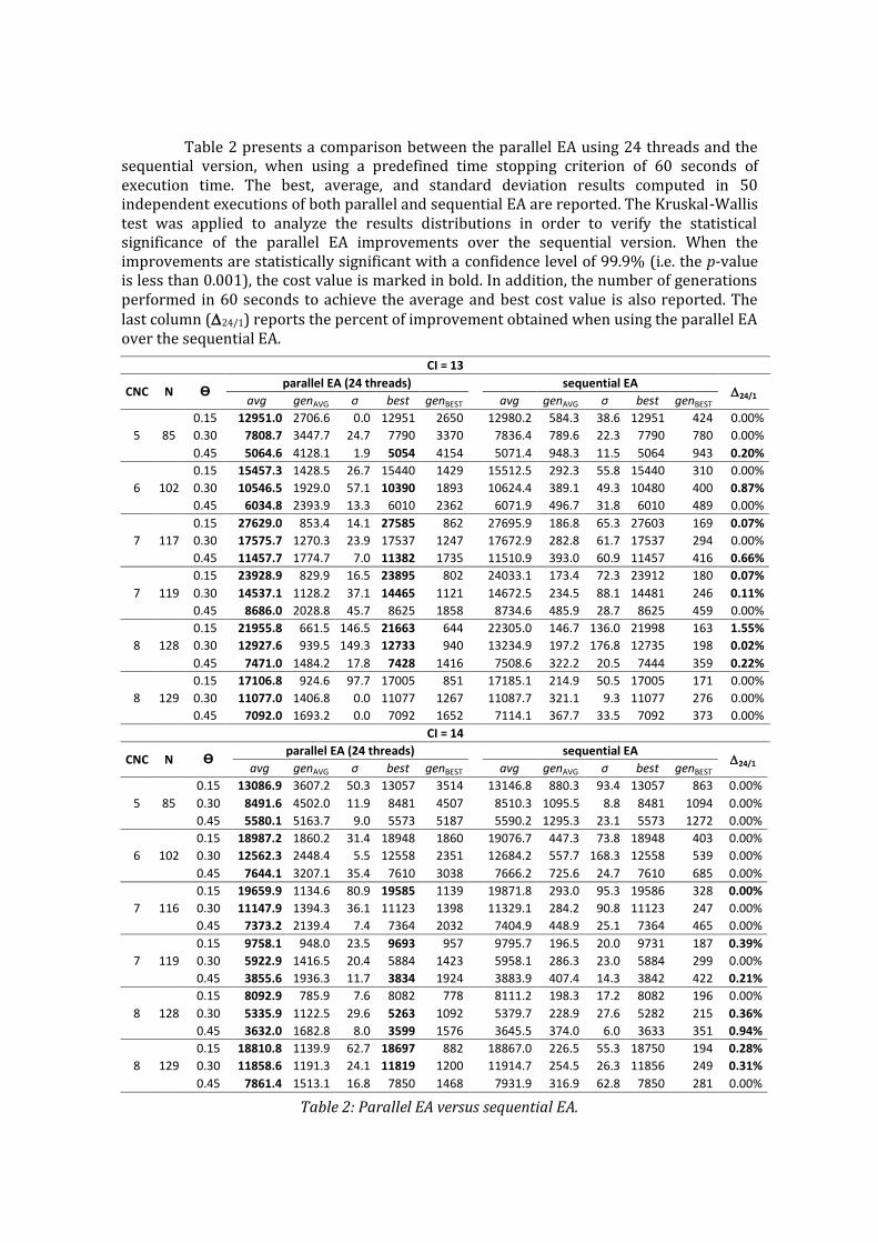
Table 2 presents a comparison between the parallel EA using 24 threads and the sequential version, when using a predefined time stopping criterion of 60 seconds of execution time. The best, average, and standard deviation results computed in 50 independent executions of both parallel and sequential EA are reported. The Kruskal-Wallis test was applied to analyze the results distributions in order to verify the statistical significance of the parallel EA improvements over the sequential version. When the improvements are statistically significant with a confidence level of 99.9% (i.e. the p-value is less than 0.001), the cost value is marked in bold. In addition, the number of generations performed in 60 seconds to achieve the average and best cost value is also reported. The last column (24/1) reports the percent of improvement obtained when using the parallel EA over the sequential EA.

CI = 13

CNC N Ɵ parallel EA (24 threads)

sequential EA

24/1 avg genAVG σ best genBEST avg genAVG σ best genBEST

5 85

0.15 12951.0 2706.6 0.0 12951 2650 12980.2 584.3 38.6 12951 424 0.00%

0.30 7808.7 3447.7 24.7 7790 3370

7836.4 789.6 22.3 7790 780 0.00%

0.45 5064.6 4128.1 1.9 5054 4154 5071.4 948.3 11.5 5064 943 0.20%

6 102

0.15 15457.3 1428.5 26.7 15440 1429 15512.5 292.3 55.8 15440 310 0.00%

0.30 10546.5 1929.0 57.1 10390 1893

10624.4 389.1 49.3 10480 400 0.87%

0.45 6034.8 2393.9 13.3 6010 2362 6071.9 496.7 31.8 6010 489 0.00%

7 117

0.15 27629.0 853.4 14.1 27585 862 27695.9 186.8 65.3 27603 169 0.07%

0.30 17575.7 1270.3 23.9 17537 1247

17672.9 282.8 61.7 17537 294 0.00%

0.45 11457.7 1774.7 7.0 11382 1735 11510.9 393.0 60.9 11457 416 0.66%

7 119

0.15 23928.9 829.9 16.5 23895 802 24033.1 173.4 72.3 23912 180 0.07%

0.30 14537.1 1128.2 37.1 14465 1121

14672.5 234.5 88.1 14481 246 0.11%

0.45 8686.0 2028.8 45.7 8625 1858 8734.6 485.9 28.7 8625 459 0.00%

8 128

0.15 21955.8 661.5 146.5 21663 644 22305.0 146.7 136.0 21998 163 1.55%

0.30 12927.6 939.5 149.3 12733 940

13234.9 197.2 176.8 12735 198 0.02%

0.45 7471.0 1484.2 17.8 7428 1416 7508.6 322.2 20.5 7444 359 0.22%

8 129

0.15 17106.8 924.6 97.7 17005 851

17185.1 214.9 50.5 17005 171 0.00%

0.30 11077.0 1406.8 0.0 11077 1267

11087.7 321.1 9.3 11077 276 0.00%

0.45 7092.0 1693.2 0.0 7092 1652 7114.1 367.7 33.5 7092 373 0.00%

CI = 14

CNC N Ɵ parallel EA (24 threads)

sequential EA

24/1 avg genAVG σ best genBEST avg genAVG σ best genBEST

5 85

0.15 13086.9 3607.2 50.3 13057 3514

13146.8 880.3 93.4 13057 863 0.00%

0.30 8491.6 4502.0 11.9 8481 4507

8510.3 1095.5 8.8 8481 1094 0.00%

0.45 5580.1 5163.7 9.0 5573 5187

5590.2 1295.3 23.1 5573 1272 0.00%

6 102

0.15 18987.2 1860.2 31.4 18948 1860

19076.7 447.3 73.8 18948 403 0.00%

0.30 12562.3 2448.4 5.5 12558 2351

12684.2 557.7 168.3 12558 539 0.00%

0.45 7644.1 3207.1 35.4 7610 3038

7666.2 725.6 24.7 7610 685 0.00%

7 116

0.15 19659.9 1134.6 80.9 19585 1139

19871.8 293.0 95.3 19586 328 0.00%

0.30 11147.9 1394.3 36.1 11123 1398

11329.1 284.2 90.8 11123 247 0.00%

0.45 7373.2 2139.4 7.4 7364 2032

7404.9 448.9 25.1 7364 465 0.00%

7 119

0.15 9758.1 948.0 23.5 9693 957

9795.7 196.5 20.0 9731 187 0.39%

0.30 5922.9 1416.5 20.4 5884 1423

5958.1 286.3 23.0 5884 299 0.00%

0.45 3855.6 1936.3 11.7 3834 1924

3883.9 407.4 14.3 3842 422 0.21%

8 128

0.15 8092.9 785.9 7.6 8082 778

8111.2 198.3 17.2 8082 196 0.00%

0.30 5335.9 1122.5 29.6 5263 1092

5379.7 228.9 27.6 5282 215 0.36%

0.45 3632.0 1682.8 8.0 3599 1576

3645.5 374.0 6.0 3633 351 0.94%

8 129

0.15 18810.8 1139.9 62.7 18697 882

18867.0 226.5 55.3 18750 194 0.28%

0.30 11858.6 1191.3 24.1 11819 1200

11914.7 254.5 26.3 11856 249 0.31%

0.45 7861.4 1513.1 16.8 7850 1468

7931.9 316.9 62.8 7850 281 0.00%

Table 2: Parallel EA versus sequential EA.

The results in Table 2 demonstrate that the parallel model allows computing better solutions than the sequential EA. When using the time stop limit of 60 seconds, the average fitness values computed by the parallel EA outperformed the ones computed by the sequential version in all the instances, and regarding the best values the parallel EA found best solutions in 16 out of 36 instances. The largest solution improvement found by the parallel EA was 1.55% for an instance with CI = 13, CNC = 8, 128 activities, and = 0.15.

A summary of the results quality is presented in Figure 2, reporting the comparative improvements over the BAB algorithm (larger improvements are better), and the GAPs with respect to the LB (smaller GAPs are better).

(a) Improvement over BAB (larger is better) (b) GAP with respect to LB (smaller is better)

Figure 2: Summary of results, parallel EA and sequential EA versus BAB and LB.

The computational efficiency of the parallel version is significantly better than the sequential EA. The values of genAVG and genBEST reported in Table 2 and the values of genAVG summarized in Figure 3 indicate that the parallel EA allows performing more than four times the number of generations performed by the sequential version in 60 seconds. This feature permits the parallel EA to perform a better search and to compute better solutions.

Figure 3: Summary of genAVG for the parallel EA and the sequential EA.

We also performed a scalability analysis of the parallel EA when varying the number of cores used. Figure 4 reports the average execution times required to perform a fixed number of generations (1000) for each value of the parameter. The time results demonstrate that tightest instances ( ) are the most difficult to solve, since both the feasibility check/repair and the local search demand larger computing times. Figure 4 also shows that the execution times reduce when using a larger number of cores. The average ratio between the execution times of the sequential EA (using one core) and the parallel EA using 24 cores is 3.9.

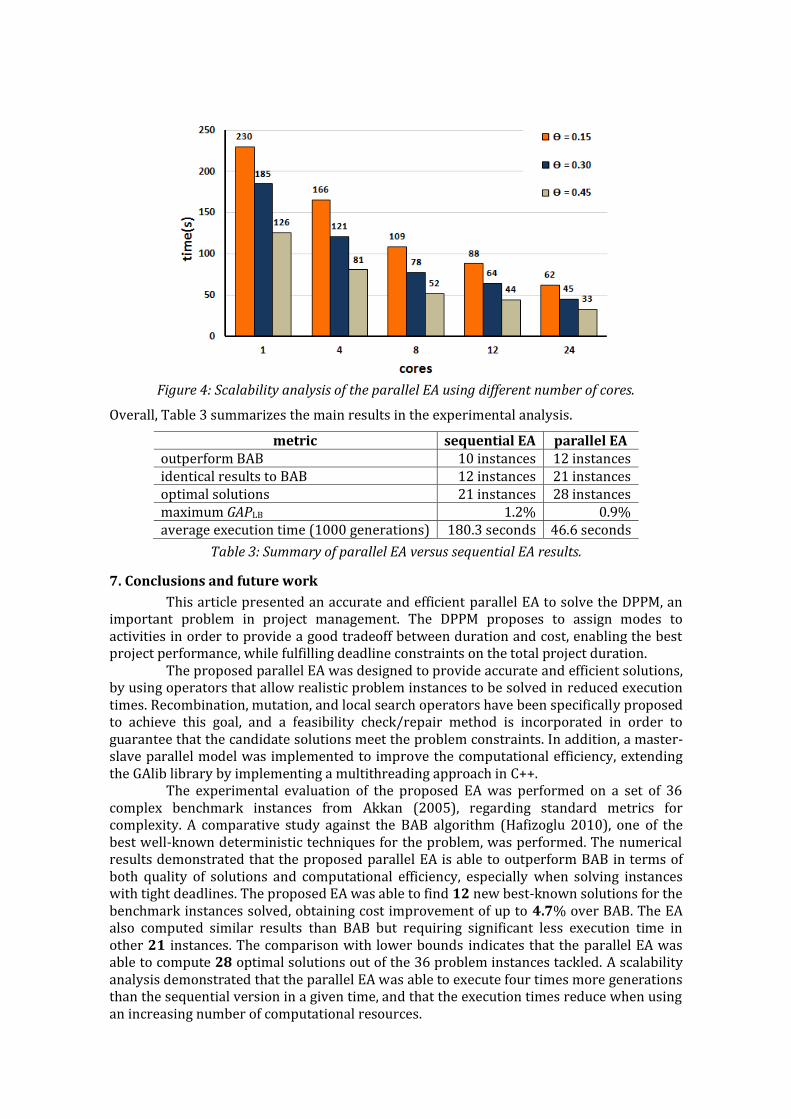
Figure 4: Scalability analysis of the parallel EA using different number of cores.

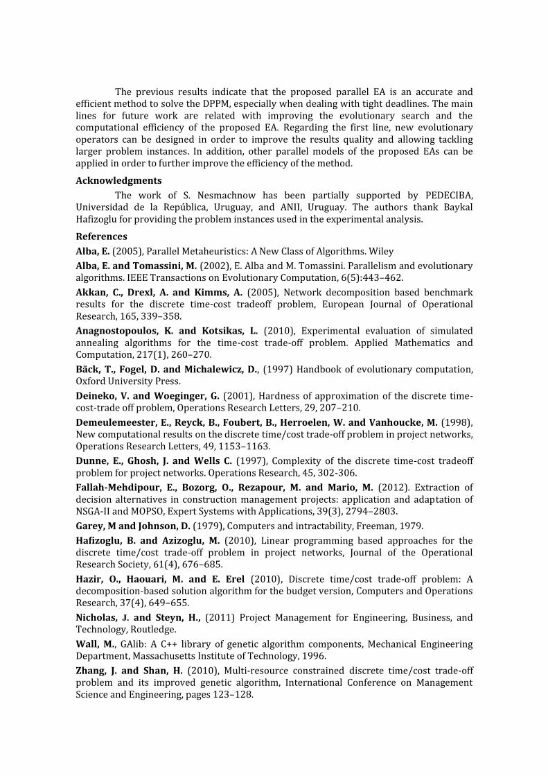
Overall, Table 3 summarizes the main results in the experimental analysis.

metric sequential EA parallel EA outperform BAB 10 instances 12 instances identical results to BAB 12 instances 21 instances optimal solutions 21 instances 28 instances maximum GAPLB 1.2% 0.9% average execution time (1000 generations) 180.3 seconds 46.6 seconds

Table 3: Summary of parallel EA versus sequential EA results.

7. Conclusions and future work

This article presented an accurate and efficient parallel EA to solve the DPPM, an important problem in project management. The DPPM proposes to assign modes to activities in order to provide a good tradeoff between duration and cost, enabling the best project performance, while fulfilling deadline constraints on the total project duration.

The proposed parallel EA was designed to provide accurate and efficient solutions, by using operators that allow realistic problem instances to be solved in reduced execution times. Recombination, mutation, and local search operators have been specifically proposed to achieve this goal, and a feasibility check/repair method is incorporated in order to guarantee that the candidate solutions meet the problem constraints. In addition, a master-slave parallel model was implemented to improve the computational efficiency, extending the GAlib library by implementing a multithreading approach in C++.

The experimental evaluation of the proposed EA was performed on a set of 36 complex benchmark instances from Akkan (2005), regarding standard metrics for complexity. A comparative study against the BAB algorithm (Hafizoglu 2010), one of the best well-known deterministic techniques for the problem, was performed. The numerical results demonstrated that the proposed parallel EA is able to outperform BAB in terms of both quality of solutions and computational efficiency, especially when solving instances with tight deadlines. The proposed EA was able to find 12 new best-known solutions for the benchmark instances solved, obtaining cost improvement of up to 4.7% over BAB. The EA also computed similar results than BAB but requiring significant less execution time in other 21 instances. The comparison with lower bounds indicates that the parallel EA was able to compute 28 optimal solutions out of the 36 problem instances tackled. A scalability analysis demonstrated that the parallel EA was able to execute four times more generations than the sequential version in a given time, and that the execution times reduce when using an increasing number of computational resources.

The previous results indicate that the proposed parallel EA is an accurate and efficient method to solve the DPPM, especially when dealing with tight deadlines. The main lines for future work are related with improving the evolutionary search and the computational efficiency of the proposed EA. Regarding the first line, new evolutionary operators can be designed in order to improve the results quality and allowing tackling larger problem instances. In addition, other parallel models of the proposed EAs can be applied in order to further improve the efficiency of the method.

Acknowledgments

The work of S. Nesmachnow has been partially supported by PEDECIBA, Universidad de la República, Uruguay, and ANII, Uruguay. The authors thank Baykal Hafizoglu for providing the problem instances used in the experimental analysis.

References

Alba, E. (2005), Parallel Metaheuristics: A New Class of Algorithms. Wiley

Alba, E. and Tomassini, M. (2002), E. Alba and M. Tomassini. Parallelism and evolutionary algorithms. IEEE Transactions on Evolutionary Computation, 6(5):443–462.

Akkan, C., Drexl, A. and Kimms, A. (2005), Network decomposition based benchmark results for the discrete time-cost tradeoff problem, European Journal of Operational Research, 165, 339–358.

Anagnostopoulos, K. and Kotsikas, L. (2010), Experimental evaluation of simulated annealing algorithms for the time-cost trade-off problem. Applied Mathematics and Computation, 217(1), 260–270.

Bäck, T., Fogel, D. and Michalewicz, D., (1997) Handbook of evolutionary computation, Oxford University Press.

Deineko, V. and Woeginger, G. (2001), Hardness of approximation of the discrete time-cost-trade off problem, Operations Research Letters, 29, 207–210.

Demeulemeester, E., Reyck, B., Foubert, B., Herroelen, W. and Vanhoucke, M. (1998), New computational results on the discrete time/cost trade-off problem in project networks, Operations Research Letters, 49, 1153–1163.

Dunne, E., Ghosh, J. and Wells C. (1997), Complexity of the discrete time-cost tradeoff problem for project networks. Operations Research, 45, 302-306.

Fallah-Mehdipour, E., Bozorg, O., Rezapour, M. and Mario, M. (2012). Extraction of decision alternatives in construction management projects: application and adaptation of NSGA-II and MOPSO, Expert Systems with Applications, 39(3), 2794–2803.

Garey, M and Johnson, D. (1979), Computers and intractability, Freeman, 1979.

Hafizoglu, B. and Azizoglu, M. (2010), Linear programming based approaches for the discrete time/cost trade-off problem in project networks, Journal of the Operational Research Society, 61(4), 676–685.

Hazir, O., Haouari, M. and E. Erel (2010), Discrete time/cost trade-off problem: A decomposition-based solution algorithm for the budget version, Computers and Operations Research, 37(4), 649–655.

Nicholas, J. and Steyn, H., (2011) Project Management for Engineering, Business, and Technology, Routledge.

Wall, M., GAlib: A C++ library of genetic algorithm components, Mechanical Engineering Department, Massachusetts Institute of Technology, 1996.

Zhang, J. and Shan, H. (2010), Multi-resource constrained discrete time/cost trade-off problem and its improved genetic algorithm, International Conference on Management Science and Engineering, pages 123–128.