arX

iv:1

407.

5034

v2 [

cond

-mat

.mes

-hal

l] 2

9 Ju

l 201

4

Quantitative µPIV Measurements of Velocity Profiles

Bryant, P. W.1,†, Neumann, R. F.1,†, Moura, M. J. B.1,†, Steiner, M.1,Carvalho, M. S.2, and Feger, C.1

1IBM Research – Brazil, Av. Pasteur 138 & 146, Urca, Rio de Janeiro, CEP

22290-240, Brazil2Dept. Mech. Eng., PUC–Rio, R. Marques de Sao Vicente, 225, Gavea, Rio

de Janeiro, Brazil†Equal contribution

July 16, 2018

Abstract

In Microscopic Particle Image Velocimetry (µPIV), velocity fields in microchannelsare sampled over finite volumes within which the velocity fields themselves may varysignificantly. In the past, this has limited measurements often to be only qualitativein nature, blind to velocity magnitudes. In the pursuit of quantitatively useful results,one has treated the effects of the finite volume as errors that must be corrected bymeans of ever more complicated processing techniques. Resulting measurements havelimited robustness and require convoluted efforts to understand measurement uncer-tainties. To increase the simplicity and utility of µPIV measurements, we introduce astraightforward method, based directly on measurement, by which one can determinethe size and shape of the volume over which moving fluids are sampled. By compar-ing measurements with simulation, we verify that this method enables quantitativemeasurement of velocity profiles across entire channels, as well as an understandingof experimental uncertainties. We show how the method permits measurement of anunknown flow rate through a channel of known geometry. We demonstrate the methodto be robust against common sources of experimental uncertainty. We also apply thetheory to model the technique of Scanning µPIV, which is often used to locate the cen-ter of a channel, and we show how and why it can in fact misidentify the center. Theresults have general implications for research and development that requires reliable,quantitative measurement of fluid flow on the micrometer scale and below.

1 Introduction

Microscopic Particle Image Velocimetry (µPIV) has become an invaluable measurementtechnique for probing fluid flow in systems at the micro- and the nano-scale [1, 2, 3, 4]. Well-

1

controlled and understood µPIV experiments performed on increasingly complex systemswill become crucial to maintaining the rapid progress observed in the biomedical and naturalresources industries [5, 6, 7]. When imaging only over a region small compared to the sizeof a microfluidic system, it is sometimes possible optically to restrict the volume over whichthe system is probed. The result is often a quantitative measurement of fluid flow in thatregion [8, 9]. To image simultaneously as many flow features as possible, however, onerequires a field of view of size comparable to the length scales of the system. Unfortunately,this leads inevitably to having also a large depth of field along the optical axis, which is anissue [10, 11, 12] that hinders a straightforward quantification and interpretation of results.For µPIV to reach its full potential as an investigative and design tool, it must providerepeatable and quantitatively useful results. It has been an open question whether or notthis is possible for µPIV with a depth of field of size comparable to that of the microfluidicssystem it measures.

There are two standard approaches to treating the effects of a large depth of field. Thefirst is to limit µPIV to qualitative comparisons of velocity profile shapes, often away fromchannel walls. In such cases, one treats the volumetric flow rate of the fluid as a freeparameter used to match expected profiles to the measured data [10, 11]. In the secondapproach, one treats finite volume effects as measurement errors, particularly near the walls,and attempts to remove as many of these effects as possible via data processing. Thisapproach has, to some extent, enabled the quantitative evaluation of µPIV data [12, 13, 14,15].

A shortcoming of the latter method, however, is the often complicated and convoluteddata processing that limits or even precludes the physical understanding of the fluid flowand its analysis. It bears the risk of over-fitting results to the extent that important flowfeatures are missed, or even misdiagnosing the causes of observed phenomena. An exampleis the spurious, increasing velocity near the channel walls that sometimes appears [13, 15].In most cases noisy or uncertain experimental data are excluded from the measured flowprofile altogether, without physical justification. A related problem is that excessive dataprocessing introduces additional sources of experimental uncertainty in an obscure fashion.

In this article, we investigate the results of a series of experiments performed with alarge depth of field µPIV, in which we image across the entire microchannel and measurethe velocity profile from wall to wall. Rather than use data processing to remove the effectsof finite measurement volumes, we introduce the concept of Sampling Volume (SV) overwhich the velocity field can be averaged to recover the measured velocity profiles. Wethen systematically determine the size and shape of the SV using an error minimizationprocedure. For our experiment, which is described below, we find that measurements nearthe walls reflect in a straightforward manner the non-trivial intersection of the SV with theedges of the microchannel. Consequently, the entire measured profile contains informationuseful for determining the SV, and one should therefore not discard features measured nearchannel walls.

We begin with a discussion of µPIV for large depth of field and a motivation for ourdefinition of the SV. We then describe our experimental setup and how our data are processed

2

and analyzed. We also discuss the expected velocity field in the channel, and its relevantsources of uncertainty. Then we show how averaging the velocity field over a rectangular SVreproduces to within our experimental uncertainty the measured velocity profiles across theentire channel. We also demonstrate how, because of the simplicity of our method and theminimal post-processing of data, µPIV can in some cases be used to infer an unknown velocityfield or flow rate in a channel of known cross section. We close with a series of use cases forour approach, which include robustly measuring velocity profiles in the presence of cameramisalignment and very noisy data that would typically be deemed useless, a demonstrationof how data processing affects the SV, and finally a critical analysis of the procedure knownas “Scanning PIV,” which is often used to place a measurement domain at the center ofmicrochannels [12, 16]. We show why, for finite-sized SV, Scanning PIV does not necessarilylocate the center of a microchannel, and should therefore be used with caution.

2 Particle Image Velocimetry

2.1 General description

Particle Image Velocimetry (PIV) is an optical method for visualizing and measuring flowfields. One seeds a fluid with tracer particles, and if the particles follow the fluid flow withoutdisturbing it significantly, by analyzing their trajectories one can infer the velocity field ofthe moving fluid. To determine the particle displacements one uses consecutive snapshotsof the system taken at times t and t + ∆t, containing several particle images at variouspositions. The snapshots are subdivided into smaller regions called “interrogation windows”and the net particle displacement is calculated for each one of them. Finally, the velocityrepresentative of each window is calculated simply by dividing the respective displacementby the interval, ∆t, between frames.

Analyzing and interpreting a PIV measurement is complicated for the following reasons.First, the velocity obtained from this process is an average in space and time, and its accuracydepends on the flow field itself, as well as on both spatial and temporal resolution of theexperimental setup [17]. Second, tracer particles are susceptible to Brownian motion, and asa consequence their positions in images must be correlated within sub-ensembles to suppressthe effect of random movements and determine net particle displacements. The applicationof cross-correlation techniques ultimately provides a 2D projection of the 3D velocity fieldof the fluid located within the imaged region, as viewed from the camera [4].

In Microscopic PIV (µPIV), see Figure 1(a), fluorescent tracer particles in a fluid channelof arbitrary geometry are observed by means of an optical microscope setup. The size of thetracer particles needs to be chosen carefully such that particles emit a sufficient amount oflight for detection without perturbing the flow. To perform the measurement, one focusesa laser pulse on the fluid channel to excite the tracer particles. The particles then emitlight at a red-shifted fluorescence wavelength that is collected by the same objective lens,alongside with the reflected laser light. The reflected excitation laser light is then filtered outby a dichroic beam splitter while the fluoresced light passes, rendering fluorescence images

3

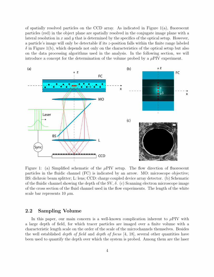
of spatially resolved particles on the CCD array. As indicated in Figure 1(a), fluorescentparticles (red) in the object plane are spatially resolved in the conjugate image plane with alateral resolution in x and y that is determined by the specifics of the optical setup. However,a particle’s image will only be detectable if its z-position falls within the finite range labeledδ in Figure 1(b), which depends not only on the characteristics of the optical setup but alsoon the data processing algorithms used in the analysis. In the following section, we willintroduce a concept for the determination of the volume probed by a µPIV experiment.

Figure 1: (a) Simplified schematic of the µPIV setup. The flow direction of fluorescentparticles in the fluidic channel (FC) is indicated by an arrow. MO: microscope objective;BS: dichroic beam splitter; L: lens; CCD: charge coupled device array detector. (b) Schematicof the fluidic channel showing the depth of the SV, δ. (c) Scanning electron microscope imageof the cross section of the fluid channel used in the flow experiments. The length of the whitescale bar represents 10 µm.

2.2 Sampling Volume

In this paper, our main concern is a well-known complication inherent to µPIV witha large depth of field, for which tracer particles are imaged over a finite volume with acharacteristic length scale on the order of the scale of the microchannels themselves. Besidesthe well established depth of field and depth of focus [4, 18], several other quantities havebeen used to quantify the depth over which the system is probed. Among them are the laser

4

light sheet [4, 10], the depth of measurement [19], and the depth of correlation [11, 12, 20].Although they have various meanings and account for various effects, many of them derivefrom the basic definition of the depth of field.

The term “laser light sheet” [4, 10] was introduced to denote the illuminated region insidethe fluid system. In most µPIV applications the light sheet and the entire fluid system areof comparable sizes. When that is the case, all particles inside the channel are excited bythe laser light and, in general, all fluorescent particles within the (x, y) field of view of theoptical setup and within the depth of field, ∆z, create in-focus images on the CCD detector.The geometrical shape of this volume can be approximated as a parallelepiped, and the focal(x, y)-plane oriented perpendicular to the optical z axis cuts this volume in half.

In standard far-field fluorescence microscopy the total point spread function and, hence,the size of the focal volume is determined by the product of the excitation point spread func-tion and the detection point spread function [18]. In µPIV, however, where image processingis used to determine the particles’ displacements over successive frames, there are additionalcontributions that alter the effective volume that is being probed, such as the application ofthe image pair correlation function [21]. As a consequence, a “depth of correlation” (DOC)was introduced to estimate the depth of the volume that contains those particles contributingsignificantly to the spatial correlation function [11, 12, 20]. The calculated DOC is useful foridentifying the experimental parameters relevant to the probed volume. However, it is basedon an assumed intensity threshold beyond which imaged particles do not “cause a significantbias in the velocity estimate” [15]. It is thus not quantitatively well defined, and has not ledto conclusive results in comparison with experiments [11, 12]. In Section 6.3 we will presenta series of results that indicate the DOC should be used only as an order-of-magnitudeestimate of the probed volume.

Despite significant effort to determine precisely the probed volume, a simultaneouslyintuitive and quantitative definition is lacking. To address this issue, we introduce a quantitywith a straightforward and verifiable interpretation. We call it Sampling Volume (SV), andit is designed to account for the combined effects of illumination scheme, optical depth, andimage processing. The concept, as opposed to previously defined quantities such as the DOC,is strikingly simple: the SV is defined as the volume over which one averages the velocityfield of the fluid in order to recover the measured profile.

We begin with a complete description of our averaging process for one experiment per-formed on a simple, straight channel, for which we will ignore any variation in measuredvelocity down the channel (x direction). We denote the velocity field within the channel by~v(x, y, z). Because of the translational symmetry in x, we take ~v(x, y, z) → ~v(y, z). Thevelocity averaged over the SV, which is compared with measurements, is then

〈~v〉SV (y) =∫ z+(y)

z–(y)dz ~v(y, z)

z+(y)− z–(y), (1)

as a function of y, which is the direction across the channel, as seen below in Figure 3. In (1),

5

the integration bounds for a rectangular SV are defined by

z– ≡ Max

(

c− δ

2, zbot(y)

)

(2)

and

z+ ≡ Min

(

c+δ

2, ztop(y)

)

. (3)

In (2) and (3), Max(·) and Min(·) denote the maximum and minimum values of thearguments. The bottom and top locations of the channel itself are zbot(y) and ztop(y),respectively. The vertical center of the SV, as measured with respect to the channel center,is denoted by c, and the vertical depth, or thickness, of the SV is represented by δ. Theselection of the maximum or minimum values in the integration bounds is necessary to keepfrom continuing the average beyond the channel’s extent, where no fluid exists. In Section 6.4is a demonstration of how failing to cut off the average properly at the edge of the channelcan lead to a calculated velocity of limited applicability. Throughout Sections 4 and 6 areseveral demonstrations of the success of using Equation (1) to explain measurements.

3 Experimental Methods and Data Analysis

3.1 Flow Field Measurements

In this section, we briefly describe the experimental setup used for performing all the fluidflow experiments discussed in this article. Further description of the experimental setup canbe found in Ref. [22]. The experiments were performed using a commercially available µPIVsystem (TSI Inc.), composed of an optical microscope, CCD camera, two lasers, and a laserpulse synchronizer. The system is operated by a data acquisition and management software(Insight 3G, TSI Inc.). The inverted microscope (IX71S1F-3, Olympus) is equipped with a10x/0.30 air objective (UPlanFL N, Olympus). The Peltier-cooled CCD (Sensicam 630166,PowerView) has a resolution of 1376× 1024 pixels (1.4MP) and a 2x projection lens. The twopulsed Nd:YAG lasers (Gemini PIV-15, NEW WAVE) operate at 532 nm and a frequencyof 15 Hz, providing a pulse energy of 50 mJ. From the specifications of the optical setup wecan calculate our depth of field [18] to be approximately 20µm. The laser pulse synchronizer(610034, TSI Inc.) controls the timing sequence of laser pulses and exposure time of theCCD. For each flow experiment, 100 pairs of images were collected with a time interval, ∆t,of 500µs between successive images.

A glass microfluidic device manufactured by Dolomite Centre Ltd, UK was used to per-form the flow experiments. The device has a straight channel with an elliptical cross-section,with a semi-minor axis of 50µm and semi-major axis of 55µm. To visualize the flow we use amix of 14% aqueous solution of fluorescent particles of 1µm in diameter (ex/em 542/612 nm,Thermo Scientific Fluoro-Max Dyed Red Aqueous Fluorescent Particles) and 86% purifiedwater (Thermo Scientific Nalgene Analytical Filter, 0.2µm). This fluid mix is injected in thedevice with the use of a syringe pump (11 Elite syringe pump 704501, Harvard Apparatus).The injection rates ranged from 75µl/h to 100µl/h.

6

3.2 Measurement Uncertainty

The extent to which we can determine the size and shape of our SV depends on our exper-imental uncertainties, as will be demonstrated in Sections 4 and 6. We therefore performedseveral calibration procedures to assess the accuracy and precision of our measurements.

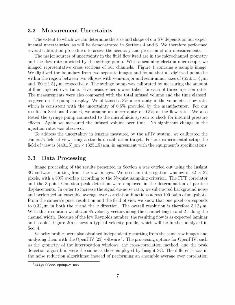
The major sources of uncertainty in the fluid flow itself are in the microchannel geometryand the flow rate provided by the syringe pump. With a scanning electron microscope, weimaged representative cross sections of our channels. Figure 1 contains a sample image.We digitized the boundary from two separate images and found that all digitized points liewithin the region between two ellipses with semi-major and semi-minor axes of (55±1.5)µmand (50± 1.5)µm, respectively. The syringe pump was calibrated by measuring the amountof fluid injected over time. Five measurements were taken for each of three injection rates.The measurements were also compared with the total infused volume and the time elapsed,as given on the pump’s display. We obtained a 3% uncertainty in the volumetric flow rate,which is consistent with the uncertainty of 0.5% provided by the manufacturer. For ourresults in Sections 4 and 6, we assume an uncertainty of 0.5% of the flow rate. We alsotested the syringe pump connected to the microfluidic system to check for internal pressureeffects. Again we measured the infused volume over time. No significant change in theinjection rates was observed.

To address the uncertainty in lengths measured by the µPIV system, we calibrated thecamera’s field of view using a standard calibration target. For our experimental setup thefield of view is (440±5)µm × (325±5)µm, in agreement with the equipment’s specifications.

3.3 Data Processing

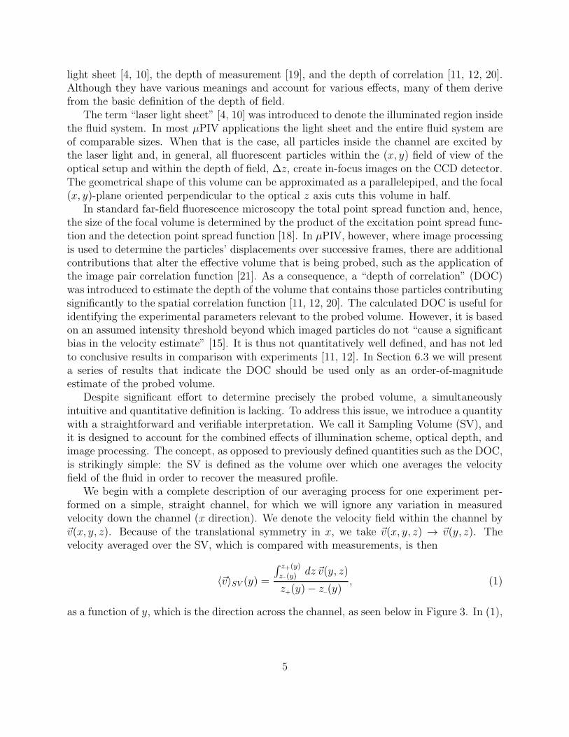
Image processing of the results presented in Section 4 was carried out using the Insight3G software, starting from the raw images. We used an interrogation window of 32 × 32pixels, with a 50% overlap according to the Nyquist sampling criterion. The FFT correlatorand the 3-point Gaussian peak detection were employed in the determination of particledisplacements. In order to increase the signal-to-noise ratio, we subtracted background noiseand performed an ensemble average over correlation functions across 100 pairs of snapshots.From the camera’s pixel resolution and the field of view we know that one pixel correspondsto 0.32µm in both the x and the y direction. The overall resolution is therefore 5.12µm.With this resolution we obtain 85 velocity vectors along the channel length and 21 along thechannel width. Because of the low Reynolds number, the resulting flow is as expected laminarand stable. Figure 2(a) shows a typical velocity profile, which will be further analyzed inSec. 4.

Velocity profiles were also obtained independently starting from the same raw images andanalyzing them with the OpenPIV [23] software 1. The processing options for OpenPIV, suchas the geometry of the interrogation windows, the cross-correlation method, and the peakdetection algorithm, were the same as those employed by Insight 3G. The difference was inthe noise reduction algorithms: instead of performing an ensemble average over correlation

1http://www.openpiv.net

7

functions, we averaged the flow field themselves over the 100 pairs of snapshots, and we didnot perform background noise subtraction. The results of the two processing methods arediscussed in Section 6.3.

(a)

(b)

Figure 2: Quiver plots of the measured velocity field as processed by (a) Insight 3G and (b)OpenPIV.

4 Results

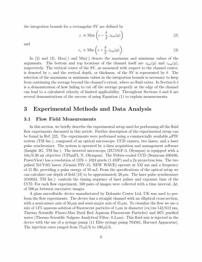
For comparison with theory we averaged the profiles located along the (streamwise) xdirection. The resulting average profile for an injection rate of 100µl/h is pictured in Fig-ure 3(a) as dots with vertical error bars corresponding to one standard deviation. Horizontalerror bars representing the uncertainty in length calibration discussed in Section 3.2 aretoo small to be seen. The large speeds with large error bars beyond the channel walls arenumerical artifacts from data processing.

We used Equation (1) to calculate 〈v〉SV (y) for a given thickness, δ, and position, c, of theSV. To compute the velocity field, ~v(x, y, z), we used the Lattice Boltzmann Method [24], towhich is input the injection rate of the pump, the channel geometry, and the fluid properties.To determine the position, c, and the thickness, δ, of the SV that results in the measuredprofile, we searched for possible fits to the data by varying c and δ while keeping ~v(x, y, z)fixed. In other words, we did not vary the pressure drop or the injection flow rate, andthus the magnitude of the theoretically expected velocity field is not a free parameter. In

8

(a) (b)

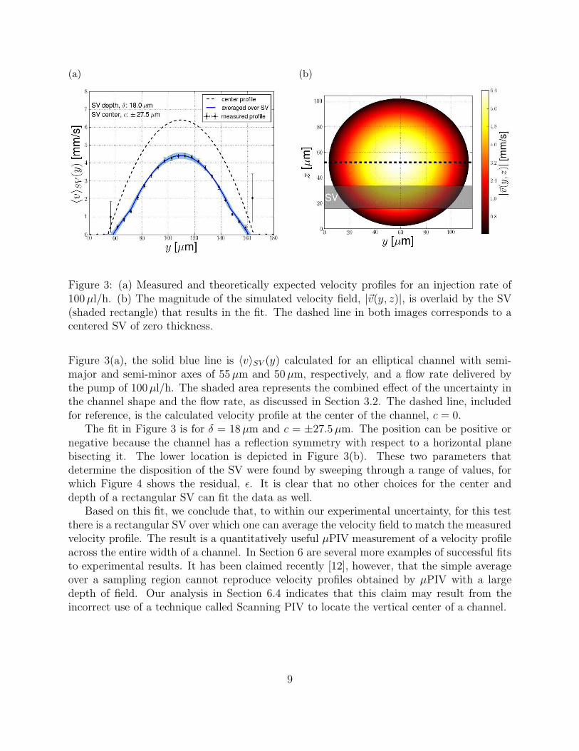
Figure 3: (a) Measured and theoretically expected velocity profiles for an injection rate of100µl/h. (b) The magnitude of the simulated velocity field, |~v(y, z)|, is overlaid by the SV(shaded rectangle) that results in the fit. The dashed line in both images corresponds to acentered SV of zero thickness.

Figure 3(a), the solid blue line is 〈v〉SV (y) calculated for an elliptical channel with semi-major and semi-minor axes of 55µm and 50µm, respectively, and a flow rate delivered bythe pump of 100µl/h. The shaded area represents the combined effect of the uncertainty inthe channel shape and the flow rate, as discussed in Section 3.2. The dashed line, includedfor reference, is the calculated velocity profile at the center of the channel, c = 0.

The fit in Figure 3 is for δ = 18µm and c = ±27.5µm. The position can be positive ornegative because the channel has a reflection symmetry with respect to a horizontal planebisecting it. The lower location is depicted in Figure 3(b). These two parameters thatdetermine the disposition of the SV were found by sweeping through a range of values, forwhich Figure 4 shows the residual, ǫ. It is clear that no other choices for the center anddepth of a rectangular SV can fit the data as well.

Based on this fit, we conclude that, to within our experimental uncertainty, for this testthere is a rectangular SV over which one can average the velocity field to match the measuredvelocity profile. The result is a quantitatively useful µPIV measurement of a velocity profileacross the entire width of a channel. In Section 6 are several more examples of successful fitsto experimental results. It has been claimed recently [12], however, that the simple averageover a sampling region cannot reproduce velocity profiles obtained by µPIV with a largedepth of field. Our analysis in Section 6.4 indicates that this claim may result from theincorrect use of a technique called Scanning PIV to locate the vertical center of a channel.

9

Figure 4: Dependence of the residual, ǫ, with respect to the fit parameters c (the SV center)and δ (the SV thickness). The white spots around the minima depict regions in which ǫ isno more than 20% larger than its lowest value.

5 Inferring Flow Rate, Channel Geometry, or Velocity

Field

In Section 4, we demonstrated how to determine the SV for a system in which the flowrate, channel geometry, and fluid properties are known. An important benefit of minimizingthe post-processing of data and instead working with the SV is that one may be able toreverse the analysis and infer either the flow rate, the velocity field, or the channel geometryin systems where one of them is not known. For example, a common approach when oneuses µPIV to measure the flow rate of, for example, blood in an artery or oil in porousmedia [7], is to measure the velocity profile and then match the maximum velocity to thepeak of the theoretically expected profile, such as the Hagen-Poiseuille profile for cylindricalchannels. As is clear from our analysis of the SV, however, this approach will underestimatethe experimental flow rate.

One can already obtain a better evaluation from the same data by acknowledging thepresence of the SV. If one first calibrates the µPIV apparatus for a well-controlled experimentin which the thickness, δ, of the SV is determined for a given set of optical and processingparameters, as described in Section 4, one can use the knowledge of δ to understand thedegree to which a measured velocity profile will underestimate the actual flow rate.

Perhaps more interestingly, by retaining all measured features, such as the kinks near thewalls in the profiles seen in Figure 3(a), for some channel shapes one can determine with asingle experiment the size and position of the SV, without fitting 〈v〉SV (y) to the measuredprofile. As shown in Figure 5 for our experiment, the y values where the measured profilegoes to zero uniquely determine where the top of the SV intersects the channel’s walls, where

10

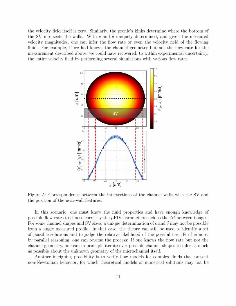
the velocity field itself is zero. Similarly, the profile’s kinks determine where the bottom ofthe SV intersects the walls. With c and δ uniquely determined, and given the measuredvelocity magnitudes, one can infer the flow rate or even the velocity field of the flowingfluid. For example, if we had known the channel geometry but not the flow rate for themeasurement described above, we could have recovered, to within experimental uncertainty,the entire velocity field by performing several simulations with various flow rates.

Figure 5: Correspondence between the intersections of the channel walls with the SV andthe position of the near-wall features.

In this scenario, one must know the fluid properties and have enough knowledge ofpossible flow rates to choose correctly the µPIV parameters such as the ∆t between images.For some channel shapes and SV sizes, a unique determination of c and δ may not be possiblefrom a single measured profile. In that case, the theory can still be used to identify a setof possible solutions and to judge the relative likelihood of the possibilities. Furthermore,by parallel reasoning, one can reverse the process: If one knows the flow rate but not thechannel geometry, one can in principle iterate over possible channel shapes to infer as muchas possible about the unknown geometry of the microchannel itself.

Another intriguing possibility is to verify flow models for complex fluids that presentnon-Newtonian behavior, for which theoretical models or numerical solutions may not be

11

accurate. In this case, one must either determine the SV as in Figure 5, or else by means ofa calibration experiment using known optical parameters and a well-understood fluid, suchas we have described in Section 4. Then one can measure the velocity profile of the complexfluid, and the result will be a µPIV measurement that can provide quantitative insight intothe various theoretical treatments of the complex fluid.

6 Use Cases

Here we describe several use cases for the simple theory of the SV presented in Section 4.These use cases demonstrate its robustness against common sources of experimental errorand against noisy data, its utility for quantifying the effect of processing variables, and howthe theory has led to a deeper understanding of the Scanning PIV technique.

6.1 Robustness Against Camera Misalignment

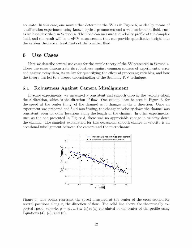
In some experiments, we measured a consistent and smooth drop in the velocity alongthe x direction, which is the direction of flow. One example can be seen in Figure 6, forthe speed at the center (in y) of the channel as it changes in the x direction. Once anexperiment was prepared and fluid was flowing, the change in velocity down the channel wasconsistent, even for other locations along the length of the channel. In other experiments,such as the one presented in Figure 3, there was no appreciable change in velocity downthe channel. The simplest explanation for this occasional smooth change in velocity is anoccasional misalignment between the camera and the microchannel.

Figure 6: The points represent the speed measured at the center of the cross section forseveral positions along x, the direction of flow. The solid line shows the theoretically ex-pected speed, 〈v〉SV (x, y = ycenter) ≡ 〈v〉SV (x) calculated at the center of the profile usingEquations (4), (5), and (6).

12

With our method, one can easily treat a misaligned camera. The translational symmetryof the channel is unaffected, so we continue to use ~v(x, y, z) → ~v(y, z) for the velocity fieldinside the channel. The position and shape of the SV do depend on the optical system,however, so we model a misalignment of the camera by varying in x the position of thecenter of the SV: c → c(x). The result is an expected measured velocity that also varies inx, 〈~v〉SV (x, y), which is calculated as

〈~v〉SV (x, y) =∫ z+(x,y)

z–(x,y)dz ~v(y, z)

z+(x, y)− z–(x, y). (4)

Here the integration bounds must be defined as

z–(x, y) ≡ Max

(

c(x)− δ

2, zbot(y)

)

(5)

and

z+(x, y) ≡ Min

(

c(x) +δ

2, ztop(y)

)

. (6)

For the fit in Figure 6 the thickness of the SV, δ, is a constant 18µm. The center of the SV,c(x), varies linearly from c(x = 6µm) = −21.7µm to c(x = 517µm) = −27µm. The channeldepth is 100µm, so the fit in Figure 6 suggests a camera misalignment of approximately 0.6◦,which is reasonable for our experimental setup. Even though the camera was misaligned, wewere able to verify the flow in the microchannel.

6.2 Robustness Against Noisy Data

In the past, when normalized velocities have been measured in a more qualitative fash-ion [10, 11], interesting features in velocity profiles, such as the kinks highlighted in Figure 5,have typically been ignored. In the more quantitative evaluations [12, 14, 15], one has triedto eliminate any kinks or other features near walls via post-processing meant to reduce theeffects of a finite SV.

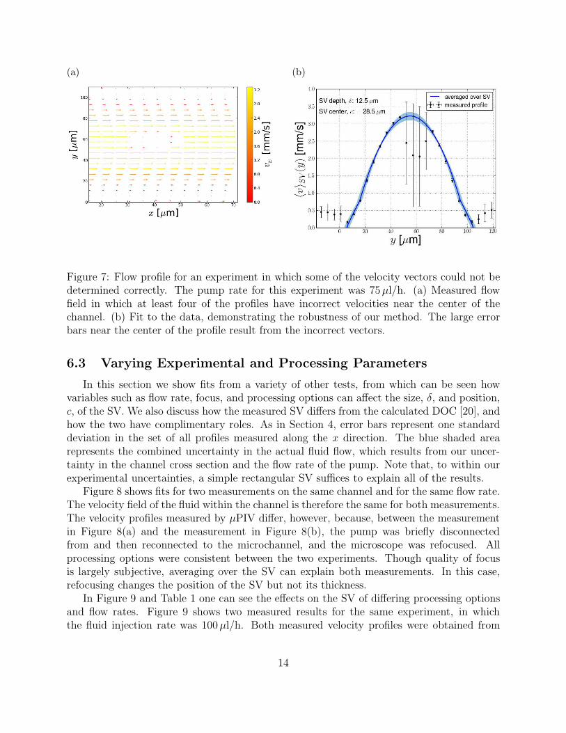
With Figure 7 we demonstrate how maintaining such features can in fact lead to morerobust µPIV measurements, particularly when one has noisy data. In this experiment, rawparticle images included a large, stationary bright spot that resulted, after processing, inthe area with zero velocity shown in Figure 7(a). The average profile, shown in Figure 7(b),has large uncertainty in the center of the channel. Rather than discard the results of theexperiment, by fitting the entire measured speed profile, from wall to wall, we were ableto quantify the flow in the microchannel. Because we fit the entire profile, and therebyincorporate more data that have been minimally processed, we believe that quantitativeevaluation using the SV is significantly more robust and more straightforward than withother methods.

13

(a) (b)

Figure 7: Flow profile for an experiment in which some of the velocity vectors could not bedetermined correctly. The pump rate for this experiment was 75µl/h. (a) Measured flowfield in which at least four of the profiles have incorrect velocities near the center of thechannel. (b) Fit to the data, demonstrating the robustness of our method. The large errorbars near the center of the profile result from the incorrect vectors.

6.3 Varying Experimental and Processing Parameters

In this section we show fits from a variety of other tests, from which can be seen howvariables such as flow rate, focus, and processing options can affect the size, δ, and position,c, of the SV. We also discuss how the measured SV differs from the calculated DOC [20], andhow the two have complimentary roles. As in Section 4, error bars represent one standarddeviation in the set of all profiles measured along the x direction. The blue shaded arearepresents the combined uncertainty in the actual fluid flow, which results from our uncer-tainty in the channel cross section and the flow rate of the pump. Note that, to within ourexperimental uncertainties, a simple rectangular SV suffices to explain all of the results.

Figure 8 shows fits for two measurements on the same channel and for the same flow rate.The velocity field of the fluid within the channel is therefore the same for both measurements.The velocity profiles measured by µPIV differ, however, because, between the measurementin Figure 8(a) and the measurement in Figure 8(b), the pump was briefly disconnectedfrom and then reconnected to the microchannel, and the microscope was refocused. Allprocessing options were consistent between the two experiments. Though quality of focusis largely subjective, averaging over the SV can explain both measurements. In this case,refocusing changes the position of the SV but not its thickness.

In Figure 9 and Table 1 one can see the effects on the SV of differing processing optionsand flow rates. Figure 9 shows two measured results for the same experiment, in whichthe fluid injection rate was 100µl/h. Both measured velocity profiles were obtained from

14

(a) (b)

Figure 8: Fits to the experimental profiles obtained with fluid injection rate of 75µl/h. (a)Before disconnecting from the pump and (b) after reconnecting to the pump and refocusing.

(a) (b)

Figure 9: Flow profile obtained after processing the same set of CCD images with (a)Insight 3G and (b) OpenPIV software. The processing options are detailed in Section 3.3.Figure 9(a) is a reproduction of the fit shown in Figure 3. We have included it again herefor easier comparison.

15

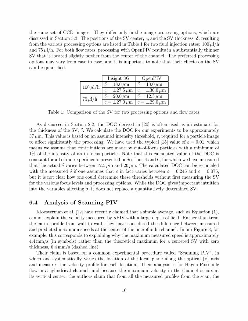
the same set of CCD images. They differ only in the image processing options, which arediscussed in Section 3.3. The positions of the SV center, c, and the SV thickness, δ, resultingfrom the various processing options are listed in Table 1 for two fluid injection rates: 100µl/hand 75µl/h. For both flow rates, processing with OpenPIV results in a substantially thinnerSV that is located slightly farther from the center of the channel. The preferred processingoptions may vary from case to case, and it is important to note that their effects on the SVcan be quantified.

Insight 3G OpenPIV

100µl/hδ = 18.0µm δ = 13.0µmc = ±27.5µm c = ±30.0µm

75µl/hδ = 20.0µm δ = 12.5µmc = ±27.0µm c = ±29.0µm

Table 1: Comparison of the SV for two processing options and flow rates.

As discussed in Section 2.2, the DOC derived in [20] is often used as an estimate forthe thickness of the SV, δ. We calculate the DOC for our experiments to be approximately37µm. This value is based on an assumed intensity threshold, ε, required for a particle imageto affect significantly the processing. We have used the typical [15] value of ε = 0.01, whichmeans we assume that contributions are made by out-of-focus particles with a minimum of1% of the intensity of an in-focus particle. Note that this calculated value of the DOC isconstant for all of our experiments presented in Sections 4 and 6, for which we have measuredthat the actual δ varies between 12.5µm and 20µm. The calculated DOC can be reconciledwith the measured δ if one assumes that ε in fact varies between ε = 0.245 and ε = 0.075,but it is not clear how one could determine these thresholds without first measuring the SVfor the various focus levels and processing options. While the DOC gives important intuitioninto the variables affecting δ, it does not replace a quantitatively determined SV.

6.4 Analysis of Scanning PIV

Kloosterman et al. [12] have recently claimed that a simple average, such as Equation (1),cannot explain the velocity measured by µPIV with a large depth of field. Rather than treatthe entire profile from wall to wall, they have considered the difference between measuredand predicted maximum speeds at the center of the microfluidic channel. In our Figure 3, forexample, this corresponds to explaining why the maximum measured speed is approximately4.4mm/s (in symbols) rather than the theoretical maximum for a centered SV with zerothickness, 6.4mm/s (dashed line).

Their claim is based on a common experimental procedure called “Scanning PIV”, inwhich one systematically varies the location of the focal plane along the optical (z) axisand measures the velocity profile for each location. Their analysis is for Hagen-Poiseuilleflow in a cylindrical channel, and because the maximum velocity in the channel occurs atits vertical center, the authors claim that from all the measured profiles from the scan, the

16

one with the highest peak velocity is the centered profile. Having centered the region overwhich particle images are resolved, then, they find that for large depths of field that coverthe entire channel, the measured velocity is larger than what is predicted from averagingover the entire channel.

Using the average over the SV in Equation (1), however, we can show that this use ofScanning PIV will not find the center of the channel for large SV. To analyze the resultspublished in Ref. [12], we use the Hagen-Poiseuille profile for flow in a cylindrical channel,

vP (r) = v0

(

1− r2

R2

)

, (7)

where v0 is the maximum speed in the channel, r is the radial coordinate, R is the channelradius, and r = 0 at the center of the channel. Let us change to Cartesian coordinateswith z = 0 at the vertical center of the channel, and substitute D = 2R for the channel’sdiameter. In this section we are interested in the maximum speed, which occurs at the fixedy value of the center of the channel, y = ycenter, while the SV changes. We will thereforefix y and emphasize the dependence of the speed on the position, c, and size, δ, of the SV.Let 〈v〉SV (y = ycenter) ≡ 〈v〉SV (c, δ) denote our prediction of the maximum speed. UsingEquation (1) with the Poiseuille profile (7), we find

〈v〉SV (c, δ) = v0

[

1− 4

3

(

z2–+ z–z+ + z2

+

D2

)]

, (8)

where the dependence on c and δ is in the integration bounds z– = Max (c− δ/2,−D/2) andz+ = Min (c + δ/2, D/2), as before.

In terms of the notation in Equation (8), when one uses scanning PIV to find the center ofa channel for a given δ, one varies c until 〈v〉SV (c, δ) is maximized. The principal assumption,then, is that this maximum always occurs at c = 0. To check this assumption, we solve∂∂c〈v〉SV (c, δ) = 0 for c and find multiple solutions. One solution is for a centered SV, with

c = 0, for which the maximum speed is

〈v〉SV (c, δ)∣

∣

∣

c=0=

{

v0

(

1− δ2

3D2

)

0 ≤ δ < D

23v0 δ ≥ D.

(9)

Another is for c = ±(D − 2δ)/4, for which the SV is not centered in the channel, and themaximum speed is

〈v〉SV (c, δ)∣

∣

∣

c=±(D−2δ)/4=

{

v0(9D2+12Dδ−16δ2)

12D2 0 ≤ δ < 34D

34v0 δ ≥ 3

4D.

(10)

Figure 10 is a plot of 〈v〉SV (c, δ) for these two maximizing values of c. The curves cross

at δ =√32D. Because the experimenter selects the value of c that maximizes the measured

speed, for δ >√32D in a cylindrical channel, this scanning PIV method will position the SV

17

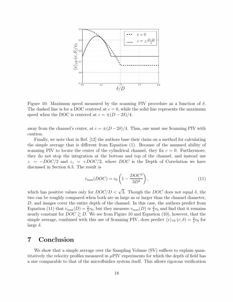
Figure 10: Maximum speed measured by the scanning PIV procedure as a function of δ.The dashed line is for a DOC centered at c = 0, while the solid line represents the maximumspeed when the DOC is centered at c = ±(D − 2δ)/4.

away from the channel’s center, at c = ±(D−2δ)/4. Thus, one must use Scanning PIV withcaution.

Finally, we note that in Ref. [12] the authors base their claim on a method for calculatingthe simple average that is different from Equation (1). Because of the assumed ability ofscanning PIV to locate the center of the cylindrical channel, they fix c = 0. Furthermore,they do not stop the integration at the bottom and top of the channel, and instead usez– = −DOC/2 and z+ = +DOC/2, where DOC is the Depth of Correlation we havediscussed in Section 6.3. The result is

vmax(DOC) = v0

(

1− DOC2

3D2

)

, (11)

which has positive values only for DOC/D <√3. Though the DOC does not equal δ, the

two can be roughly compared when both are as large as or larger than the channel diameter,D, and images cover the entire depth of the channel. In this case, the authors predict fromEquation (11) that vmax(D) = 2

3v0, but they measure vmax(D) ≈ 3

4v0 and find that it remains

nearly constant for DOC & D. We see from Figure 10 and Equation (10), however, that thesimple average, combined with this use of Scanning PIV, does predict 〈v〉SV (c, δ) = 3

4v0 for

large δ.

7 Conclusion

We show that a simple average over the Sampling Volume (SV) suffices to explain quan-titatively the velocity profiles measured in µPIV experiments for which the depth of field hasa size comparable to that of the microfluidics system itself. This allows rigorous verification

18

of the velocity fields of fluids flowing in microchannels. With this simple approach, one caneasily understand and physically interpret the measured features of velocity profiles. In somecases, it allows the complete determination of an unknown flow rate or velocity field basedonly on the µPIV measurement. Furthermore, in a straightforward manner one can deter-mine measurement uncertainty, which is essential for any quantitatively useful experiment.Because of the presence of a finite sampling region, in the past one has either ignored themagnitude of the measured velocity or else treated the effects of the finite volume as errorsto be corrected by complicated processing.

By minimally processing data and retaining all measured features, such as kinks in thevelocity profile, we have developed a method that is especially robust against noise and othercommon sources of measurement error. By comparing the measured velocity profiles to thetheoretical predictions, we are able to quantify the effect on the SV of processing options andfocus. We also provide a critical evaluation of Scanning PIV, which is often used to locatethe center of a microchannel. We show how and why it in fact fails to locate the center forlarge SV. In general, the concept of the SV has implications for quantitative measurementof flow within channels on the micrometer scale and below.

Acknowledgments

We would like to thank Michael Engel from IBM Research – Watson as well as theLABNANO–CBPF for the SEM images, Diney Ether and the LPO–UFRJ for help with thecalibration, Angelo Gobbi at the LMF–LNNano for profilometer measurements, and JoseFlorian at PUC–Rio for help with the µPIV equipment.

References

[1] Stuart J Williams, Choongbae Park, and Steven T Wereley. Advances and applications on microfluidicvelocimetry techniques. Microfluid Nanofluid, 8(6):709–726, 2010.

[2] Ralph Lindken, Massimiliano Rossi, Sebastian Große, and Jerry Westerweel. Micro-particle imagevelocimetry (µPIV): Recent developments, applications, and guidelines. Lab Chip, 9(17):2551–2567,2009.

[3] Steven T Wereley and Carl D Meinhart. Recent advances in micro-particle image velocimetry. Annu.Rev. Fluid Mech., 42:557–576, 2010.

[4] Ronald J Adrian and Jerry Westerweel. Particle image velocimetry, volume 30. Cambridge UniversityPress, 2010.

[5] Eric K Sackmann, Anna L Fulton, and David J Beebe. The present and future role of microfluidics inbiomedical research. Nature, 507(7491):181–189, 2014.

[6] Daniel Mark, Stefan Haeberle, Gunter Roth, Felix von Stetten, and Roland Zengerle. Microfluidic lab-on-a-chip platforms: requirements, characteristics and applications. Chem. Soc. Rev., 39(3):1153–1182,2010.

[7] Naga Siva Kumar Gunda, Bijoyendra Bera, Nikolaos K Karadimitriou, Sushanta K Mitra, and S Ma-jid Hassanizadeh. Reservoir-on-a-Chip (ROC): A new paradigm in reservoir engineering. Lab Chip,11(22):3785–3792, 2011.

19

[8] Pierre Joseph and Patrick Tabeling. Direct measurement of the apparent slip length. Phys. Rev. E,71(3):035303, 2005.

[9] Peichun Tsai, Alisia M Peters, Christophe Pirat, Matthias Wessling, Rob GH Lammertink, and DetlefLohse. Quantifying effective slip length over micropatterned hydrophobic surfaces. Phys. Fluids,21(11):112002, 2009.

[10] Carl D Meinhart, Steve T Wereley, and Juan G Santiago. PIV measurements of a microchannel flow.Exp. Fluids, 27(5):414–419, 1999.

[11] Kristin Sott, Tobias Geback, Maria Pihl, Niklas Loren, Anne-Marie Hermansson, Alexei Heintz, andAnders Rasmuson. µPIV methodology using model systems for flow studies in heterogeneous biopolymergel microstructures. J. Colloid Interf. Sci., 398:262–269, 2013.

[12] A Kloosterman, C Poelma, and J Westerweel. Flow rate estimation in large depth-of-field micro-PIV.Exp. Fluids, 50(6):1587–1599, 2011.

[13] Massimiliano Rossi, Rodrigo Segura, Christian Cierpka, and Christian J Kahler. On the effect ofparticle image intensity and image preprocessing on the depth of correlation in micro-PIV. Exp. Fluids,52(4):1063–1075, 2012.

[14] J Westerweel, PF Geelhoed, and R Lindken. Single-pixel resolution ensemble correlation for micro-PIVapplications. Exp. Fluids, 37(3):375–384, 2004.

[15] C Cierpka and CJ Kahler. Particle imaging techniques for volumetric three-component (3d3c) velocitymeasurements in microfluidics. J. Vis., 15(1):1–31, 2012.

[16] Boris Chayer, Katie L Pitts, Guy Cloutier, and Marianne Fenech. Velocity measurement accuracy inoptical microhemodynamics: experiment and simulation. Physiol. Meas., 33(10):1585, 2012.

[17] J Westerweel. Fundamentals of digital particle image velocimetry. Meas. Sci. Technol., 8(12):1379,1997.

[18] Lukas Novotny and Bert Hecht. Principles of nano-optics. Cambridge university press, 2012.

[19] CD Meinhart, ST Wereley, and MHB Gray. Volume illumination for two-dimensional particle imagevelocimetry. Meas. Sci. Technol., 11(6):809, 2000.

[20] MG Olsen and RJ Adrian. Out-of-focus effects on particle image visibility and correlation in microscopicparticle image velocimetry. Exp. Fluids, 29(1):S166–S174, 2000.

[21] CD Meinhart, AK Prasad, and RJ Adrian. A parallel digital processor system for particle imagevelocimetry. Meas. Sci. Technol., 4(5):619, 1993.

[22] Jose Angel Florian Gutierrez and Marcio S Carvalho. Flow of oil drops through micro-capillaries. In22nd International Congress of Mechanical Engineering (COBEM 2013), pages 6458–6469, 2013.

[23] Zachary J Taylor, Roi Gurka, Gregory A Kopp, and Alex Liberzon. Long-duration time-resolved PIV tostudy unsteady aerodynamics. Instrumentation and Measurement, IEEE Transactions on, 59(12):3262–3269, 2010.

[24] Shiyi Chen and Gary D Doolen. Lattice boltzmann method for fluid flows. Annu. Rev. Fluid Mech.,30(1):329–364, 1998.

20