
rrn FACULDAD DE ECONOMIA E I tf … · economia com entrega incerta é formalmente equivalente ao...
125
Il PORTO r r n FACULDADE DE ECONOMIA I tf UNIVERSIDADE DO PORTO ESSAYS ON GENERAL EQUILIBRIUM WITH ASYMMETRIC INFORMATION João Oliveira Correia da Silva Orientador: Carlos Hervés Beloso TESE DE DOUTORAMENTO EM ECONOMIA PORTO, 2005
Transcript of rrn FACULDAD DE ECONOMIA E I tf … · economia com entrega incerta é formalmente equivalente ao...
I l PORTO r r n FACULDADE DE ECONOMIA I t f UNIVERSIDADE DO PORTO
ESSAYS ON GENERAL EQUILIBRIUM
WITH ASYMMETRIC INFORMATION
João Oliveira Correia da Silva
Orientador: Carlos Hervés Beloso
TESE DE DOUTORAMENTO EM ECONOMIA
PORTO, 2005

Ao Júlio e à Odete

Agradecimentos
Ao meu orientador e amigo, Carlos Hervés Beloso, quero manifestar a minha gratidão.
O seu apoio, confiança e empenho foram constantes ao longo destes anos. Este trabalho
também lhe pertence.
Agradeço a Jean Gabszewicz e Nicholas Yannelis pelos importantes comentários,
sugestões e encorajamento. Estes agradecimentos estendem-se a Álvaro Aguiar,
Gustavo Bergantinos, Jacques Drèze, Guadalupe Fugarolas, Dionysius Glycopantis,
Ani Guerdjikova, Inès Macho-Stadler, Jean-François Mertens, Enrico Minelli, Paulo
Monteiro, Diego Moreno, Emma Moreno-García, Allan Muir, Luca Panaccione, Mário
Páscoa, Mário Patrício Silva, David Pérez-Castrillo e Alexei Savvateev.
Esta investigação foi desenvolvida na Faculdade de Economia do Porto. Agradeço
aos meus acompanhantes internos Manuel Luís Costa e Elvira Silva, e a todos os meus
professores e colegas. Agradeço também às pessoas que trabalham na Biblioteca.
Nas dezenas de visitas que fiz à Universidade de Vigo, fui recebido com muita
hospitalidade. Agradeço a todos, e, em especial, a Margarita Estévez.
Para resolver os problemas informáticos que foram surgindo, pude contar com toda a
disponibilidade dos Serviços de Informática da FEP e de Ramiro Martins.
Agradeço também a Daniel Bessa, que me ensinou as ideias básicas da ciência
económica, e que recomendou a minha candidatura à FEP.
Sem o apoio financeiro da Fundação para a Ciência e Tecnologia, este trabalho não
teria sido possível.
Finalmente, um agradecimento muito especial ao meu pai, e a todos os que estão
sempre comigo.

Do que você precisa, acima de tudo, é de se não lembrar do que eu lhe
disse; nunca pense por mim, pense sempre por você; fique certo de que mais
valem todos os erros se forem cometidos segundo o que pensou e decidiu do
que todos os acertos, se eles forem meus, não seus. Se o criador o tivesse
querido juntar a mim não teríamos talvez dois corpos ou duas cabeças também
distintas. Os meus conselhos devem servir para que você se lhes oponha. É
possível que depois da oposição venha a pensar o mesmo que eu; mas nessa
altura já o pensamento lhe pertence. São meus discípulos, se alguns tenho, os
que estão contra mim; porque esses guardaram no fundo da alma a força que
verdadeiramente me anima e que mais desejaria transmitir-lhes: a de se não
conformarem.
- AGOSTINHO DA SILVA -

Sumário
O ponto de partida para este trabalho é o modelo introduzido por Radner (1968), que
estende a teoria de equilíbrio geral a situações nas quais os agentes têm informação
diferentes sobre o estado da natureza. A ideia por detrás desta extensão consiste em
restringir os agentes a produzir e consumir os mesmos cabazes, era estados da natureza
que não distingam. Isto significa, essencialmente, que os contratos entre dois agentes só
podem ser contingentes à ocorrência de eventos que ambos observam.
Uma propriedade importante de qualquer conceito de solução é a continuidade do
resultado relativamente a variações nos parâmetros do modelo. Pequenas variações nos
parâmetros devem conduzir a pequenas variações do resultado de equilíbrio. Mas, medindo
as variações na informação dos agentes de acordo com as topologias introduzidas por
Boylan (1971) e Cotter (1986), o conceito não cooperativo de Equilíbrio de Expectativas
Walrasianas (Radner, 1968) e o conceito cooperativo de núcleo privado (Yannelis, 1991)
não se comportam de forma contínua.
O problema crucial é que pequenas variações nos campos de informação privada
podem provocar grandes variações no campo da informação comum. Como os contratos
contingentes se baseiam na informação comum, pequenas variações na informação privada
podem abrir ou fechar mercados contingentes, levando a variações significativas do
resultado de equilíbrio.
v

Neste trabalho é introduzida uma topologia sobre a informação (a-algebras finitas
definidas no espaço de estados da natureza) que ultrapassa este problema. Nesta topologia,
dois campos de informação estão próximos se ambos estiverem próximos da informação
comum. Com esta topologia, passa a verificar-se a semicontinuidade superior do núcleo
privado da economia.
Em seguida, procura-se generalizar o modelo de Radner (1968). A restrição que força
os agentes a consumir o mesmo em estados que não distinguem é relaxada. Permite-se
que os agentes façam contratos de entrega incerta. Isto significa que, além de poderem
comprar bens contingentes, como uma "bicicleta" se estiver "sol", os agentes podem
também comprar o direito a receber um dos cabazes que esteja numa lista. Por exemplo,
uma "bicicleta azul ou bicicleta vermelha" se estiver "sol". Deste modo, o espaço de trocas
é alargado, possibilitando melhorias de bem-estar no sentido de Pareto.
No contexto das economias com entrega incerta, estudam-se as expectativas
prudentes/pessimistas. Estas levam os agentes a escolher estratégias minimax. São
apresentadas diversas justificações. Com expectativas prudentes, o modelo da
economia com entrega incerta é formalmente equivalente ao modelo de Arrow-Debreu
(1954). Consequentemente, muitos resultados da teoria de equilíbrio geral se aplicam
imediatamente a este modelo: existência de núcleo e equilíbrio competitivo, convergência
núcleo-equilíbrio, propriedades de continuidade, etc.
vi

Summary
The starting point for this work is the model introduced by Radner (1968), which extends
general equilibrium theory to a setting in which agents have different private information.
The idea underlying this extension is to restrict agents to produce and consume the same
bundles, in states of nature that they do not distinguish. Essentially, this means that
the contracts for contingent trade between two agents can only be contingent upon their
common information.
An important property of any solution concept is the continuity with respect to the
parameters of the model. That is, small changes in the parameters should lead to small
changes in the equilibrium outcome. But measuring changes in the information of the
agents according to the topologies introduced by Boylan (1971) and Cotter (1986), the
non-cooperative Walrasian Expectations Equilibrium (Radner, 1968) and the cooperative
private core (Yannelis, 1991) do not behave continuously.
The crucial problem is that small changes in the private information fields can lead to
big changes in the field of common information. Since contingent contracts are based on
common information, these small changes may open or close some contingent markets,
leading to significant changes in the equilibrium outcome.
In this work is introduced a topology on information (finite a-algebras defined over the
space of states of nature) that overcomes this problem. In this topology, two information
vii
fields are close if both are close to their common information. As a result, we find that the
private core is upper semicontinuous with respect to variations in the information of the
agents.
Afterwards, a generalization of the model of Radner (1968) is sought. The restriction
that forces agents to consume the same in states of nature that they do not distinguish is
alleviated. Agents are allowed to sign contracts for uncertain delivery. This means that,
besides being able to buy state-contingent goods, for example, a "bicycle" if "weather is
sunny", agents are also able to buy the right to receive one of the bundles that are included
in a list. For example, a "blue bicycle or red bicycle" if "weather is sunny". In this way,
the space of possible trades is enlarged, and welfare improvements in the sense of Pareto
become possible.
In the context of uncertain delivery, the case is made for prudent/pessimistic expectations.
These expectations lead agents to select minimax strategies. Several justifications are
presented. With prudent expectations, the model of an economy with uncertain delivery
is formally equivalent to the model of Arrow-Debreu (1954). As a result, many results
in general equilibrium theory also apply in this model: existence of core and competitive
equilibrium, core-convergence, continuity properties, etc.
vm

Ah Love! could thou and I with Fate Conspire
To grasp this sorry Scheme of Things entire,
Would not we shatter it to bits - and then
Re-mould it nearer to the Heart's Desire!
- OMAR KHAYYAM -

Contents
1 Words of caution 2
2 Introduction 9
3 Equilibrium with Perfect Information 15
3.1 Nash equilibrium of an n-player game 15
3.2 Nash equilibrium of an n-player pseudo-game 17
3.3 Competitive equilibrium of an exchange economy 19
3.4 The core of an exchange economy 21
3.5 Exchange economies as pseudo-games 23
3.6 Existence of Nash equilibrium 24
3.7 Existence of competitive equilibrium 26
4 Equilibrium with Asymmetric Information 32
4.1 Modeling information 33
4.2 Terminal acts and informational acts 35
x

CONTENTS
4.3 Arrow-Debreu equilibrium under uncertainty 36
4.4 Radner equilibrium under asymmetric information 39
4.5 Incomplete markets 43
5 Topology of Common Information 45
5.1 Introduction 45
5.2 The Differential Information Economy 48
5.3 The Topology of Common Information 50
5.4 Upper Semicontinuity Results 59
5.5 An Illustrative Example 62
6 Economies with Uncertain Delivery 67
6.1 Introduction 67
6.2 Contracts for uncertain delivery 69
6.3 Examples 72
6.4 Economies with Uncertain Delivery 78
7 Prudent Expectations Equilibrium 83
7.1 Prudent preferences 83
7.1.1 Prudence as a rule-of-thumb 84
7.1.2 Prudence as a result 84
7.1.3 Prudence by construction 86
7.1.4 Prudence as realism 88
xi
CONTENTS
7.2 General Equilibrium with Uncertain Delivery 89
7.3 Characteristics of Equilibrium 92
7.4 Cooperative Solutions: the Prudent Cores 97
7.5 Concluding Remarks 99
A The Expected Utility Hypothesis 101
A.l Von Neumann's Axiomatization 102
A.2 Savage's Axiomatization 103
A.3 The value of information 106
Bibliography 107
Xll

Chapter 1
Words of caution
According to Adam Smith's (1776) idea of the invisible hand, in a market system,
individuals contribute to the welfare of the society by seeking to maximize their well-being.
The economic outcome of a market system is the result of individuals independently trying
to maximize their well-being, a notion known as competitive equilibrium.
A competitive equilibrium is a situation in which:
i) each individual, taking prices as fixed, chooses the quantities of the different goods to
produce and exchange, in order to obtain the most preferred bundle in the budget set;
ii) equality between supply and demand holds, that is, for each good, the sum of the
quantities supplied is equal to the sum of the quantities demanded.
These conditions must hold for all the commodities in an economy. This is what general
equilibrium theory is concerned with: the determination of production, exchange and prices
of all the commodities in an economy. The main contributor to this line of thought was Leon
1

CHAPTER 1. WORDS OF CAUTION
Walras (1874), in spite of the independent contributions of Stanley Jevons (1871) and Carl Menger(1871).1
It is not obvious that such equilibrium situation is possible. Under general conditions,
the existence of competitive equilibria was established by Arrow and Debreu (1954) and
by McKenzie (1954). Their results mean that there exists a price system which induces
individuals to choose quantities to produce and exchange which are consistent with equality
between supply and demand.
Furthermore, Adam Smith's claim about the effectiveness of the invisible handm promoting
the welfare of the society was supported by two famous results. According to the First
Welfare Theorem, a competitive equilibrium allocation is Pareto-optimal. This means that
there isn't any situation that all individuals prefer to a competitive equilibrium. The Second
Welfare Theorem holds that any Pareto-optimal allocation can be attained as a competitive
equilibrium, if a certain redistribution of initial endowments is made.
The impossibility of measuring and comparing the well-being of different individuals could
seem to prevent the measurement of society's welfare. But there are certain accepted criteria
for comparing different economic outcomes, as the criterion of Pareto (1906). An outcome
is designated as Pareto-optimal if there isn't any alternative that everyone prefers.2
If the model of Arrow-Debreu-McKenzie described the economy perfectly, we wouldn't observe any unemployment or price volatility. In fact, some strong hypothesis are imposed.
As early as 1781, A.N. Isnard presented the first general equilibrium model, considering a pure exchange
economy where in which each individual owned a single asset, with all demand functions having unit elasticity
in income and own price.
The criterion of Pareto is criticized for neglecting the question of distribution. Assume that there are 10 units to divide among 2 individuals. If one of them receives 10, and the other receives nothing, the outcome is optima] in the sense of Pareto.
2

CHAPTER 1. WORDS OF CAUTION
It is assumed that the agents have perfect and complete information, and that there exists
a complete set of markets. Let's analyze these and other limitations of classical general
equilibrium theory.
The welfare theorems support the idea that market economies are efficient, but there are
elements that lead to "non-fair" equilibrium prices, such as adverse selection and moral
hazard. In fact, real market economies are almost never efficient, and Adam Smith's
conjecture is not true in general.
For the two welfare results to be obtained, it is fundamental that each agent takes prices as
fixed. This assumption is usually designated as perfect competition. Since there exists a
large number of sellers and buyers in the markets, no one can influence prices.3
Another assumption is that there are markets for all the products. Even for commodities that
will only be delivered in the distant future. These markets serve as a guide to the investment
decisions of the firms. For example, the absence of a market for delivery of buildings in
2100 could prevent agents from optimizing their investment decisions.4 Many decisions are
actually based on bets, but the point is that even if we assume that agents behave rationally,
the efficiency of the market system is not guaranteed in general in the absence of complete
markets.
The conjecture of Coase (1960) focuses the importance of property rights, and the problems
associated with the exploration of common resources. The example of fishing is quite
illustrative, since it is an activity with private benefits which has some costs that are 3For a discussion and critique of the assumption of perfect competition, see Makowsky & Ostroy (2001). 4Suppose that a firm decides to construct a building based on an estimate of the value that it will have in
2015. The problem is that this value depends on the number of buildings that will be built in 2006, 2007, etc.
And these depend on the estimate of the value of the buildings in 2016, 2017, etc. This extends to infinity!
3

CHAPTER 1. WORDS OF CAUTION
supported by the whole society (decrease of the quantity offish in the ecosystem). Consider
a fishing zone shared by 100 firms, and a study that advises the use of 100 boats in order
to maximize the total (present and future) volume of fishing. If each firm decided to use
1 boat, this advice would be followed. But imagine that when the firms weight benefits
against costs, they conclude that it is better to use two boats and catch almost twice as
much fish as with one single boat. Since all firms send two boats, too much fish is caught,
and the ecosystem ends up being depleted.5
There are other strong assumptions in the model of Arrow-Debreu-McKenzie. One is the
assumption of linear prices, that is, independence of prices from the quantities exchanged.
And it is assumed that firms have no profits, otherwise a new competitor would enter the
market (free entry).
Now let's turn to the crucial limitation which constitutes the motivation to our work: the
problems related to information. In general, the agents do not possess all the relevant
information for making economic decisions. There is usually some uncertainty about the
environment, and there are events which only some of the agents can observe.
Our work is in the context of the literature on differential information economies, which
developed from the seminal article of Radner (1968). This literature seeks to extend the
model of general equilibrium to situations in which agents have asymmetric information.
What follows are some questions that the reader should keep in mind.
The complexity associated with the issues related to information is such that it cannot
be captured by any simple model. The market economy is too complicated to be fully
described in simple terms. A realistic goal is to find simple models that give enlightening,
although partial, descriptions. 5Hardin (1968) has a classical article on this problem.
4

CHAPTER 1. WORDS OF CAUTION
Taking into account uncertainty about product quality introduces a lot of complexity. Even
if quality is assumed to be purely objective, buyers should question the truthfulness of
the claims made by sellers. This issue is usually referred to as the problem of incentive
compatibility.
For many commodities, the cost of providing them depends on the behavior of the
purchaser. Moral hazard arises when behavior of the demander that is not easily observed
affects the cost of the supplier. An example is the case of insurance. After buying insurance,
agents may become careless.6
Sometimes several goods are different in the eyes of the consumer, but are sold as if they
were equal. When one side of the market treats certain commodities as different, while the
other side treats them as equal, problems of adverse selection arise. An example occurs
when buyers cannot observe the quality of the product, but sellers can. In this case, the
sellers of high quality products withdraw from the market.
Akerlof (1970) analyzed a market in which the sellers could distinguish the quality level
of a product, while the buyers did not. Initially the buyers may expect an average level of
quality, and think of making a correspondent bid. But the sellers of good quality products
would not be willing to sell them at this average price. So, the potential buyers reason
that only the sellers of "bad" products will be willing to trade in the market. Expecting to
receive a "bad" product, they offer a low price. As a consequence, only "bad" products are
bought or sold, and all products are priced as if they were "bad".7
6Assuming that carefulness is, even if only slightly, costly. 7C. Wilson (1980) studies a variant of the model of Akerlof (1970) in which agents differ on the value
that they attach to cars of the same quality. He finds that the results depend on whether it is an auctioneer, the
buyers or the sellers that set the price.
5

CHAPTER 1. WORDS OF CAUTION
Rothschild & Stiglitz (1976) analyzed an insurance market in which the sellers could not
distinguish the risk level of the customers, which could be high or low. So, they cannot
offer a better contract to the low-risk customers, because all the customers would pretend
to be low-risk to get this contract. As a consequence, there was no competitive equilibrium.
In the model of Arrow-Debreu, supply equals demand when the economy is in equilibrium.
But we observe frequently disparities between supply and demand of certain goods. The
classical example is unemployment, or excess of supply of labor. In fact, problems of
information may render the balance of supply and demand untenable:.
Imagine a situation of full employment in which employers cannot observe perfectly the
effort of the worker. Firing the worker does not work as a punishment, because she can find
another job instantly. The incentives are for workers to shirk!8
Another common situation is of excess demand for credit. The interest rate charged by
a bank influences the risk of the loans that are proposed. The interest rate that an agent
is willing to accept signals its risk-level. A bank which sets a high interest rate will only
attract loans with high risk. Therefore, the optimal interest rate may not be equal to the one
that balances supply and demand.9
The behavior of the agents varies with the interest rate. Higher interest rates diminish the
value of investments, and induce individuals to take more risks (since the worst possible
outcome is a return of zero, which corresponds to bankruptcy). With perfect information,
these issues would be meaningless. But, since the bank cannot control the decisions of the
firms, it is important to analyze the incentives that the loan contracts give to firms. 8This is described in the seminal article of Shapiro & Stiglitz (1984). 9This is analyzed by Stiglitz & Weiss (1981).
6

CHAPTER 1. WORDS OF CAUTION
Spence (1973) studies actions outside the market that generate information which is then
used by the market. In his model of signalling, agents engage in education because their
potential employers see this a sign of good capabilities. If they had poor capabilities,
engaging in education would be irrational. So, signalling is a kind of implicit guarantee. A
situation in which beliefs are stable is a signalling equilibrium}0
Besides assuming that prices are linear, it is also assumed that they are homogeneous, that
is, that all trades are made according to the same price system. Stigler (1961) questions
this hypothesis and analyzes the the problem of search, that is, of buyers seeking costly
information about the prices quoted by the different sellers.
The point of Grossman & Stiglitz (1980) is that if arbitrage is costly and gives no return in
equilibrium, then no agents will engage in this activity. As a consequence, in equilibrium,
the condition of null arbitrage profits should be substituted by one giving an "equilibrium
amount of disequilibrium".
Besides analyzing whether an equilibrium situation exists or not, it is important to study
the way agents reach this situation - the problem of implementation. In the seminal article
of Schmeidler (1980), Walrasian equilibrium is implemented as a Nash equilibrium of a
market game.
According to Hayek (1945), the perfect information model does not capture the
fundamental role of prices and markets in processing and disseminating information. Sixty
years have passed since he warned us that general equilibrium theory does not by itself
solve the economic problem. The theory "only" gives a logical solution to a problem in
which the relevant data is given. I0For a survey on signalling and general issues related to information see Riley (2001).
7

CHAPTER 1. WORDS OF CAUTION
"On certain familiar assumptions the answer is simple enough. If we possess all the
relevant information, if we can start out from a given system of preferences, and if we
command complete knowledge of available means, the problem which remains is purely
one of logic. That is, the answer to the question of what is the best use of the available
means is implicit in out assumptions.'"
But this relevant data is never given to a single mind.
"[...] the economic calculus which we have developed to solve this logical problem,
though an important step toward the solution of the economic problem of society, does not
yet provide an answer to it. The reason for this is that the 'data'from which the economic
calculus Starts are never for the whole society 'given' to a single mind which could work
out the implications, and can never be so given."
After these words of caution, we can start the study of general economic equilibrium with
asymmetric information.
8

Chapter 2
Introduction
The treatment of uncertainty in the theory of general equilibrium is based upon two
foundations: the Expected Utility Theorem of von Neumann and Morgenstern (1944);
and the formulation of the ultimate goods or objects of choice in an uncertain universe
as contingent consumption claims (Arrow, 1953).
The Expected Utility Theorem provides a convenient way to compare risky bundles, by
establishing the existence of an utility function that represents preferences over lotteries.
Under the formulation of objects of choice as contingent consumption bundles, besides
being defined by their physical properties and their location in space and time, commodities
can also be defined by the state in which they are made available. For example, an
"umbrella" that is delivered if the "weather is rainy" and an "umbrella" delivered if the
"weather is sunny" are seen as two different commodities. This formulation allowed Debreu
(1959, chapter 7) to extend the general equilibrium model to a situation of uncertainty.
There were essentially two lines of contribution to equilibrium theory with complete
information: one of Cournot (1838) and Nash (1950), and that of K. J. Arrow & Debreu
9

CHAPTER 2. INTRODUCTION
(1954), and McKenzie (1954). But to take into account the problems of incomplete
information introduces a great deal of complexity. The main advances were made by
Harsanyi (1967), who extended the Cournot-Nash framework, and by Radner (1968), who
did the same to the model of Arrow-Debreu-McKenzie.
The transformation of games with incomplete information into games with imperfect
information, accomplished by Harsanyi (1967) was a giant step. In a game with incomplete
information, agents are uncertain about the payoff functions. The meaning of imperfect
information is that when information is that agents cannot perfectly observe the strategies
chosen by the other players. Considering that there are many possible types of players, it
may be assumed that an unobservable choice of nature at the beginning of the game selects
the actual players from the set of possible types. So, from a problem of knowledge about
payoffs, we move to a problem of knowledge about the type of player selected by nature.
With agents having prior probabilities on the choice of nature, the game with incomplete
information ends up being defined as a game of imperfect information. This type of game
can be analyzed with standard techniques.
To model an economy in which agents have asymmetric information, it is considered that
it extends over two time periods. In the first period, agents know their endowments and
preferences, as a function of the state of nature, and have a partition of information, that
tells them which events they can observe. In this period (ex ante), agents make contracts for
delivery of goods in the second period, which can be contingent upon the state of nature. In
the second period, agents get to know which set of their partition of information includes
the actual state of nature. As a consequence, they are informed on their preferences and
receive the corresponding endowments. Finally, contracts are enforced and consumption
takes place.1
'For a survey on differential information economies, see Allen & Yannelis (2001).
10

CHAPTER 2. INTRODUCTION
This setup allowed Radner (1968) to propose an extension of the model of Arrow-Debreu-
McKenzie to the case of private information. By private information it is meant a situation
in which agents have asymmetric information and do not communicate.
The basic idea is that agents are not willing to pay for delivery that is contingent upon
events that they do not observe. As a result, it is assumed that they will consume the same
in states of nature that they do not distinguish. With this condition, the economy with
private information is formally equivalent to the Arrow-Debreu-McKenzie economy. The
equilibrium of prices and consumption vectors of the economy with private information is
designated as a Walrasian expectations equilibrium (WEE).
The essential modification, with respect to the equilibrium notion without uncertainty, is
this restriction of measurability, that is, of forcing agents to consume the same in states of
nature that they do not distinguish. Formally, the consumption of an agent, as a function of
the state of nature, has to be measurable with respect to the cr-field of its private information.
A corresponding cooperative notion of equilibrium is the it private core. This concept was
introduced by Yannelis (1991), who also proved existence in general conditions. Relatively
to the classical core notion, it has the same measurability restriction: allocations have to be
informationally feasible.
Allowing for communication introduces a lot of complexity. But, actually, the first notions
of a core in an economy with asymmetric information (Wilson, 1978) were based on the
ideas of common information and pooled information. These are the coarse core and the
fine core. If coalitions are only allowed to block allocations by using allocations which
are measurable with respect to the common information among their members, the result
is the coarse core. At the other extreme is the fine core, which is constituted by the
11

CHAPTER 2. INTRODUCTION
informationally feasible allocations which cannot be blocked by any consumption vector
that is measurable with respect to the pooled information of the members of a coalition.2
The notion of incentive compatibility (Hurwicz, 1972) is the focus of a recent survey by
Forges, Minelli, & Vohra (2002) on the core of an exchange economy with asymmetric
information. They consider the restriction of informationally feasibility to be too strong,
and prefer to analyze incentives. The emphasis of their work is on incentive compatibility,
and on convergence of the core to price equilibrium allocations.
In the case in which it is possible to communicate, it is crucial to know if information can
be verified or not. If it can be verified, then we may be able to treat it as a commodity.
This is the crux of the work of Allen (1990), who studied information as if it were an
economic commodity, susceptible of production and exchange. There are non-convexities,
because each partition is only interesting in integer quantities (half partition would be
meaningless). With an infinite number of traders this problem disappears. A problem that
arises if production of information is considered in the economy is that the costs associated
to the production of information are essentially fixed costs.
The private core was shown to have nice properties. Koutsougeras & Yannelis (1993)
proved that it is coalitionally Bayesian incentive compatible (CBIQ. Einy, Moreno, &
Shitovitz (2001) prove an equivalence theorem for the private core. Serrano, Vohra, &
Volij (2001) present counter-examples to the core convergence theorems whenever expected
utilities are interim.
Forges, Heifetz, & Minelli (2001) obtain a Debreu-Scarf analogue for a type-model where
the space of allocations is defined as the set of incentive compatible state-contingent
lotteries over consumption goods. They show that competitive equilibrium allocations
Note that such consumption vector may not be an allocation, since it may not be informationally feasible.
12

CHAPTER 2. INTRODUCTION
exist and are elements of the (ex-ante incentive) core. This core is constituted by the
allocations such that no coalition can propose a feasible incentive compatible allocation
which improves the expected utility of all its members. Any competitive equilibrium is
an element of the core of the n-fold replicated economy. The converse holds with the
assumption of private values - equal preferences in states of nature that the agent does not
distinguish. This is in the lines of Prescott and Townsend (1984a, 1984b), who also impose
a finite "base" for lotteries and private values.
The main idea in Prescott and Townsend (1984a, 1984b) is that individuals trade state-
contingent lotteries over the initial consumption goods. This ensures that the consumption
set is convex. With objects of trade as incentive compatible state-contingent lotteries over
the original goods, competitive equilibria can be defined in the usual way, using expected
feasibility and constructing prices of lotteries as expectations of the prices of original goods.
To provide scope and context to this work, the first chapter was a discussion of the limits of
these models to explain real economies.
In this second chapter, the state of the art of general equilibrium with asymmetric was
presented. Special attention was given to the works on differential information economies.
This is a line of research that follows the seminal work of Radner (1968), where general
equilibrium theory was extended to a setting in which agents have different private
information.
The third and fourth chapter review the theory of general equilibrium. In chapter 3, the
analysis is restricted to perfect information. Chapter 4 extends the theory to the cases
of symmetric uncertainty (Arrow and Debreu, 1954), and to a setting of asymmetric
information (Radner, 1968). The idea underlying Radner's extension is to restrict agents
to produce and consume the same bundles, in states of nature that they do not distinguish.
13

CHAPTER 2. INTRODUCTION
Essentially, this means that the net trades between two agents can only be contingent upon
their common information.
In the fifth chapter, the problem of the continuity of equilibrium with respect to variations in
the private information of the agents is studied. A new topology on finite information fields
is introduced. This topology evaluates the similarity between information fields taking
into account their compatibility, that is, the events that are commonly observed. With this
"topology of common information", the Walrasian expectations equilibrium (Radner, 1968)
and the private core (Yannelis, 1991) are upper semicontinuous.
In chapter 6, the model of Radner (1968) is generalized. Recall that Radner extended
the model of Arrow-Debreu to the case of private information by constraining agents to
consume the same in states of nature that they do not distinguish. But agents may be willing
to buy different goods for delivery in states that they do not distinguish ex ante, if, in any
case, they become better off. This suggests the introduction of contracts for uncertain
delivery.
Finally, in chapter 7, economies with private information and uncertain delivery are studied.
Agents are assumed to be prudent, that is, to follow minimax strategies. Many classical
results still hold: existence of core and equilibrium, core convergence, continuity properties,
etc. In a prudent expectations equilibrium, agents consume bundles with the same utility
in states of nature that they do not distinguish ex ante. Since this restriction is weaker than
equal consumption, efficiency of trade and welfare are improved.
In the appendix, both Von Neumann's and Savage's axiomatizations of expected utility are
presented, and the value of information is defined accordingly.
14

Chapter 3
Equilibrium with Perfect Information
In the literature on differential information economies, two concepts of equilibrium
predominate: one is the cooperative notion of the core; and the other is the non-cooperative
notion of competitive equilibrium. The notion of competitive equilibrium has much in
common with the famous concept of Nash equilibrium. But while Nash equilibrium applies
to games in general, a competitive equilibrium makes sense in the context of a market
economy.
3.1 Nash equilibrium of an n-player game
A game in normal form is defined by the strategies available to each player, and by
the outcomes that correspond to every possible combination of strategies by the players.
A strategy determines every action of a player throughout the game for all possible
contingencies that the player may face. So, given the strategies of the players, it is possible
to determine each player's outcome. We assume that each agent compares the outcomes
15

CHAPTER 3. EQUILIBRIUM WITH PERFECT INFORMATION
according to an agent-specific utility function that assigns a real number to each point in
the strategy space of the players.
Definition 1 (N-PLAYER GAME) A game G = {Xh V^=l in its normal form is defined by:
- the set of strategies available to each player i, Xf,
- the utility function of each player i, V*.
The space of the possible strategies of the game is X = f[ Xt. A possible strategy is
x = {xi,x2,...,xn) ex.
The utility function of each player, Vt : X x X{ -> IR, is such that V^x, x[) is the utility of
agent i playing x[ while the others play Xj, (j ^ i).
The idea of an equilibrium as a situation in which no agent has incentives to deviate,
assuming the actions of the others as given, was first discussed by Augustin Cournot (1838)
in a context of a duopoly. It was rediscovered by John Nash (1950), who proved the
existence of such equilibrium solution for general n-player games. This is probably why
it is referred as Nash equilibrium, although sometimes it is designated as Cournot-Nash
equilibrium.
Definition 2 (NASH EQUILIBRIUM)
n
The strategy x* G X = T\ Xt is a Nash Equilibrium of the game G = (Xi, V5)JLi if and
only if, for every player i, Vi(x*,x*) > K(x*,^) ,V^ € X,. That is, x* = (x^x^ ...,x*n)
is composed by best responses of each agent to x*.
16

CHAPTER 3. EQUILIBRIUM WITH PERFECT INFORMATION
In a Nash equilibrium, each agent's strategy is the best response to the strategies chosen by
the other agents. Existence of Nash equilibrium means that the agents can reach a situation
in which they consider their strategies to be simultaneously optimal.
Consider the illustrative paper-rock-scissors game. In this two-player game, the players
choose among three possible actions: "paper", "rock" or "scissors". The paper beats the
rock by enveloping it, the rock beats the scissors by breaking them, and the scissors beat the
paper by cutting it. It is straightforward that, given the strategy of the opponent, there is a
best response that makes one win every time (play paper against rock, rock against scissors,
and scissors against paper). But then, given this new strategy, the opponent's best response
will be to play differently, in order to be able to win every time. The change of strategy leads
the opponent to choose a new optimizing strategy. From this circularity follows that there
isn't any pair of mutually optimal pure strategies, that is, there isn't a Nash equilibrium of
the game in the space of the pure strategies.
Yet, there exists a Nash equilibrium in the space of mixed strategies. If the players randomly
play paper, rock or scissors with equal probabilities (1/3 each) in each repetition of the
game, their strategies are optimal responses to the strategies of the opponent. As this
example suggests, the famous result of existence of Nash Equilibrium demands a convex
space of possible strategies (X{ convex for all i), otherwise, the theorem of Kakutani cannot
be applied. Convexity can be obtained by allowing the agents to play mixed strategies.
3.2 Nash equilibrium of an n-player pseudo-game
A pseudo-game is a more general concept than that of a game. In a pseudo-game, the
strategies that are available to a player may depend upon the strategies that are selected by
the other players. A game does not allow this kind of interdependence.
17

CHAPTER 3. EQUILIBRIUM WITH PERFECT INFORMATION
Definition 3 (N-PLAYER PSEUDO-GAME)
A pseudo-game in its normal form, PG = (Xu Fit V$ml, is defined by:
- the set of strategies potentially available to each player i, Xit-
- the set of strategies available to each player i, given the strategies chosen by the other
players, F{ : X -* Xh with X = f[ X{;
- the utility or payoff function ofeach player i, Vi : Gr(Fi) -> IR.
In a Nash equilibrium of a pseudo-game, a player may have strategies that would be
preferable, but which are inaccessible due to the choices of the other agents. This cannot
occur in a game.1
When the correspondence Ft is continuous and convex-valued, existence of Nash
equilibrium of a pseudo-game can be proved by direct application of the fixed point theorem
of Kakutani and Berge 's maximum theorem. Nash equilibrium of a game is a corollary of
this for the case in which F; is a constant correspondence.
Definition 4 (NASH EQUILIBRIUM OF A PSEUDO-GAME)
n
A strategy x* € X = T[ X{ is a Nash Equilibrium of PG = (Xi} Fu V^ <=>
a) x* G Fiix*);
Again, the vector of equilibrium strategies, x* = (x\, x\,..., a?*), is composed by optimal
responses of each agent to x*, but only among those in the possibility set Fi(x*).
Pseudo-games are useful in many contexts. For example, to model situations where imitation is excluded, as in the choice of location or in branding.
18

CHAPTER 3. EQUILIBRIUM WITH PERFECT INFORMATION
3.3 Competitive equilibrium of an exchange economy
An exchange economy is a system in which a finite number of agents exchanges an initial
distribution of endowments, without incurring in any transaction cost. Each economic agent
is characterized by: (1) a consumption possibility set; (2) preferences among alternative
plans that are feasible; (3) initial endowments of physical resources. The objective of each
agent is to maximize individual well-being.
The preferences of the agents are usually assumed to be représentante by continuous and
quasi-concave utility functions, in order to guarantee the convexity of the set of desirable
bundles.
In general, each agent's choice of bundles, xit depends on what the other agents choose.
The vector x = (xux2, ...,xn) is designated as an allocation. The interaction between
the agents is mediated by a price-system. With a finite number of commodities, I, the
price vector can be normalized to p G A^ = {p e \Rl+ : £ \ P i = 1} A common
simplification that guarantees existence of competitive equilibrium consists in allowing
only the consumption of non-negative quantities, x 6 \Rl+, and assuming non-negative
prices, pi > 0 (hypothesis of "free disposal").
Definition 5 (EXCHANGE ECONOMY)
An exchange economy is a triple, £ = (Xu Uh e^=1, where, for each agent i:
- the space of possible consumption bundles is X^;
- the utility function is Ui : Xd —*■ IR;
- the initial endowments are es G X .
19

CHAPTER 3. EQUILIBRIUM WITH PERFECT INFORMATION
A Walrasian or competitive equilibrium is an equilibrium in a situation of perfect
competition, as demand exactly matches supply with agents taking prices as fixed. In such
a situation, every agent has an utility maximizing bundle, that is, each agent has the optimal
quantities of each commodity at the prevailing price level. Therefore, each agent faces no
utility-increasing trades.2
Definition 6 (COMPETITIVE EQUILIBRIUM)
(x*,p*) is a Competitive Equilibrium of the economy S = (Xt, Uh e*)^ <=> n n
1) x* = (x\, . . . , < ) is feasible, i.e., x* £ X<, V»; and £ ) x* < £ e*. i= l z=l
2) p* e Al+ is a price system such that for each agent i:
2.1) x* E Bi(p*) = {xeXi;p*-x<p*- m);
2.2) Ui(z) > Ui(x*) ^p* -z<p* -ei(x is Ui-maximal in Bi(p*)).
A competitive equilibrium is, by definition, a state in which every bundle, x[, that an agent
would prefer to x* lies outside its budget set: Ut(xfi > Ui(x*) & p • x\ > p ■ &i. Such
state must of course be feasible, that is, the sum of the quantities allocated cannot be higher
than the sum of the initial endowments: J2ti xi < E L i ei- I I i s a[so necessary that the
cost of an agent's consumption bundle does not exceed the value of its initial endowments:
p- Xi <p- e{. This condition can be interpreted as excluding gains from speculation.
An assumption usually imposed to guarantee existence of competitive equilibrium is the
"hypothesis of survival', which determines that for every price-system there is at least one
bundle in the interior of the budget set: Vp, 3xp G Xt : p ■ xp < p ■ e*.
Existence of equilibrium may be ruled out by indivisibles or rationings, which can prevent some agents from obtaining the bundle that they prefer at the prevailing market prices.
20
CHAPTER 3. EQUILIBRIUM WITH PERFECT INFORMATION
The proof of existence of competitive equilibrium is based on two results: Berge's theorem
of the maximum and Kakutani's fixed point theorem.
The exchange economy is first characterized by two correspondences: one that assigns to
given prices the utility-maximizing bundles of each agent; and another that assigns to given
bundles the prices that maximize the difference between the value of the bundles and that
of the initial endowments, that is, the value of the excess demand. These prices ensure
that the allocations allowed by the agents' budgets are also feasible. By the theorem of
the maximum, both correspondences are upper hemicontinuous, with non-empty compact
values.
The product of these two correspondences, whose image is the product of the images of
the two described correspondences, is a correspondence from the product space of prices
and consumption possibilities into itself. The product correspondence retains the properties
of upper hemicontinuity, and, given the quasi-concavity of the utility functions, has also
convex values. In these conditions, the theorem of Kakutani ensures the existence of a
fixed-point. The fixed point consists of an allocation and a price-system with the following
properties: in this price-system, each agent's bundles is an utility-maximizer; and the prices
are such that ensure that this allocation is feasible. Thus, the fixed point is a competitive
equilibrium of the exchange economy.
3.4 The core of an exchange economy
Another known concept of equilibrium of an exchange economy is that of the core. An
allocation is in the core if no coalition of agents can force a better outcome for themselves.
If some group of agents can reach a better outcome, y, by trading only among them, we say
21

CHAPTER 3. EQUILIBRIUM WITH PERFECT INFORMATION
that the coalition S blocks the allocation x via the feasible allocation y. By better we mean
an outcome that is not worse for any member of the coalition and is better for at least one
of them.
This concept of equilibrium is less restrictive than the competitive equilibrium. A
competitive equilibrium is always in the core, while the converse is not true.
W{£) C N(£)
Since an allocation in the core cannot be blocked by any individual coalition, the core
satisfies the criteria of individual rationality. And, since the coalition of all agents does
not block a core allocation, all the allocations in the core are Pareto-optimal.
W{£) Ç N(£) C IR(£)nOP(£)
According to the old conjecture of Isidro Edgeworth (1881), in conditions of perfect
competition, the core and the set of competitive equilibria coincide. In this context, perfect
competition is modeled by considering an exchange economy with an infinite number of
traders, so that the influence of each agent can be neglected.
This conjecture was proved by Debreu & Scarf (1963) for a market with an infinite number
of traders, but with a finite number of types of traders. By replicating a finite economy they
found that the core converges to the set of competitive equilibrium allocations.
Robert Aumann (1964) obtained a similar result for any infinite number of traders with
different preferences and initial endowments. Instead of a finite number of types of traders,
Aumann demanded neighboring preferences and endowments. With the further assumption
of quasi-ordered preferences, Aumann (1966) also proved that the set of allocations
satisfying the coinciding concepts of core and competitive equilibrium, in a market with
22
CHAPTER 3. EQUILIBRIUM WITH PERFECT INFORMATION
an infinite number of traders, was not empty. A comprehensive study of economies with an
infinite number of traders was provided by Hildenbrand (1970).
3.5 Exchange economies as pseudo-games
An exchange economy, S = {Xh Uu e*)^, can be modeled as a pseudo-game with n + 1
players, PG = (Xit Fu Vfig}. The additional player is the auctioneer, that can also be
designated as market or price-setter.
The space of possible strategies for the auctioneer is compact and convex:
Xn+1 = AÍ, = {pe Rl+ : YJPJ = !}•
This player is not restricted in its choice - Fn+1 is a constant correspondence:
Fn+1 :XxAl+->Al
+
But the possible strategies of each agent are a function of the choice of the market. They
must choose a bundle that belongs to their budget set. In this pseudo-game, the possible
strategies of the agents are:
Fi(x,p) = Bi{p) ^{xiGXi-.p-XiKp- et}.
The utility functions of the agents only change in terms of domain:
Vi : Gr(Fi) -> IR , with Vi[{x,p); x[] = Ufâ).
The objective of the auctioneer is to maximize the cost of the excess demand:
23
CHAPTER 3. EQUILIBRIUM WITH PERFECT INFORMATION
14+i : Gr(Fn+1) = I x A x A ^ I R /with Vn+1[{x,p); q] = £ g ■ fo - e,).
A Nash equilibrium of this pseudo-game is a competitive equilibrium of the original
exchange economy.
Theorem 1 (EQUIVALENCE NASH-WALRAS)
The strategy {x*,p*) is a Nash equilibrium of the pseudo-game PG = (X^F^Vi)^
if and only if (x*,p*) is a competitive equilibrium of the exchange economy £ =
{XhUuei)U
A corollary of this theorem is the existence of competitive equilibrium of the exchange
economy £ = {Xi,Uu e;)™=1, since this pseudo-game is in the conditions of existence of
Nash equilibrium.3
3.6 Existence of Nash equilibrium
Now we want to prove theorems of existence of Nash equilibrium and competitive
equilibrium. To guarantee existence of a Nash Equilibrium, it is enough to assume a
compact and convex space of strategies, and quasi-concave utility functions.
Theorem 2 (EXISTENCE OF NASH EQUILIBRIUM)
Consider a game defined in its normal form: G = {Xh K)?=i- For every i, let X{ be
compact and convex, and V* be continuous and quasi-concave in the second variable.
=> There exists a Nash Equilibrium.
Because J3j(p) is a continuous and convex-valued correspondence.
24

CHAPTER 3. EQUILIBRIUM WITH PERFECT INFORMATION
Proof.
Consider the correspondence of the "best responses":
ipi(x) = argmax Vi(x) = fa G Xi) Vï(x, z{) > ^ foa^NteJ G Xi}.
Since Vi : X x Xi —> IR is continuous, and the constant correspondence Fi : X —> Xj is,
of course, continuous and compact-valued, we can apply the Theorem of the Maximum.
The correspondence of the "best responses" is non-empty and upper hemicontinuous.
Furthermore, ipi(x) is also closed because it is a u.h.c. correspondence with compact
Hausdorff range.
We also need to show that ipi{x) is convex. Since Vi is quasi-concave, for a given pair
zi, z2 € ijfi(x) and any A e (0,1):
Vi[x,Xzx + (1 - X)z2] > minVi(x,zi),Vi(x,z2) = VM.
That is, ipi(x) is convex. The product correspondence retains this prop<îrty. n n
i=l i=l
The product correspondence retains also the properties of upper hemicontinuity (Aliprantis
and Border, 1999, p. 537), and, by Tychonoff's Product Theorem (Aliprantis and Border,
1999, p. 52), ofclosedness.
The correspondence ip : X —» X is upper hemicontinuous and closed, with nonempty
and convex values. Assuming that X is a convex and compact subset of a locally convex
Hausdorff space (in particular, it may be a finite dimensional Euclidean space), we can
apply the fixed point theorem of Kakutani.
25
CHAPTER 3. EQUILIBRIUM WITH PERFECT INFORMATION
This theorem establishes the existence of a fixed point of ip. There exists a Nash
equilibrium, x*, composed by the best responses of each agent to the strategies of the others.
QED
3.7 Existence of competitive equilibrium
First we prove existence of competitive equilibrium assuming a compact and convex space
of possible bundles. Then we extend this result.
Theorem 3 Let S = (Xit Ui: e;)™=1 be such that, for every i:
1) Xi is a compact and convex subset 0/IR+;
2) Ui is continuous and quasi-concave;
3) for each p <G A'+, there exists xp G Xi such that p ■ xp < p ■ a ("hypothesis of
survival").
=> There exists a competitive equilibrium, (x*,p*).
Proof.
For each i, define the utility functions, Vi(p, x, x{) = UÍ(XÍ). These functions are obviously
continuous and quasi-concave as the Ui, but the domain is conveniently modified.
Vi : A _ x X x Xi -» IR.
The budget correspondence is defined by:
26
CHAPTER 3. EQUILIBRIUM WITH PERFECT INFORMATION
Br.Al+xX^ Xi-
Bi{p,x) = {x'ieXi:p-x'i <p-ei}.
By 3), Bi is non-empty. To apply the Maximum Theorem, we also need the correspondence
Bi to be continuous and compact-valued.
To see that Bi is upper hemicontinuous and compact-valued, consider its graph:
Gr(Bi) = {(p,x,x'J eA^xXxXr.x'.e Biip)}.
Now consider an arbitrary sequence in the graph of B^.
{(P, *, xî)}« ! : Vn € IN, (pn, xn, x'J <= Gr{BA.
We have: pn ■ x'm <pn-&i. With l i m ^ , ^ = Poo:
l i mn-oo(Pn • x'in) < l i m ^ o ^ • ef) <£> pTO • lim*-,», x\n < p^ ■ e{.
A point of the adherence is also a point of the graph. The graph of B{ is closed, and,
therefore, closed-valued. It is also compact-valued, because B^p) is a closed subset of the
compact Xi e Rl+. In these conditions, by the closed graph theorem (Aliprantis and Border,
1999, p. 529), Bi is upper hemicontinuous.
To apply the Maximum Theorem, all that is left to prove is that Bt is lower hemicontinuous.
We will show that if some x e B^p) belongs to an open set V, then there is an open ball
around p with radius S such that for every p' e B{p, 5) f| A, there exists some x' e Bi(p') that also belongs to V.
By the hypothesis of survival, there exists xp 6 X{ : p ■ a - p ■ xv > 0. Since Xt is convex, for some Xp G (0,1):
27

CHAPTER 3. EQUILIBRIUM WITH PERFECT INFORMATION
Ap • xp + (1 - Xp) ■ x = x\p e Xi. Of course thatp • e{ - p ■ x\p — r > 0.
Since p' G B(p, 5), the minimum value of the initial endowments is:
p' ■ei=p-ei- ip-p') -d >p-ei-8\\ei\\.
On the other hand, the maximum cost of xXp is:
p' ■ xXv = p ■ xXp + (p1 -p)-xXp<p- xXp + 5\\xXp ||.
As a result, we have:
p' -ei-p' ■xXp>p-ei- 5\\ei\\ - p ■ xXp - ó\\xXp\\ >r- 5{\\ei\\ + \\xXp\\).
So it is enough to choose S = „ ,. ,ru—iï. ° l|et||+||xAp||
The particular case with Xi = \Rl+ and e, > > 0 satisfies 3). Since at least one of the
commodities has a positive price pj > 0, a bundle with xpj = e,/2 and xpk = e (with
k ^ j) satisfies p ■ xp < p ■ e .
The cost of excess demand is: i
K+i : Al+ x X x Al
+-> IR; with Vn+1(p, X,q) = ^21j ' (x ~ ei)-
The objective function of the auctioneer, K+i, is linear and, therefore, continuous.
Define also the constant correspondence:
Bn+l : A'+ x X -* Al+ ; with Bn+1(p, x) = Al
+.
We are in conditions of applying Berge's theorem to Vi and Bi for each i.
tpi : Al+ x X -* Xi , for i = 1,..., n;
28

CHAPTER 3. EQUILIBRIUM WITH PERFECT INFORMATION
^n+l : A ' x I ^ A +•
All ipi, are u.h.c. with compact (closed subsets of the compact X) and convex (from quasi-
concaveness) values.
n+l The product correspondence: ip = TT ipi retains these properties, satisfying the conditions
of Kakutani's theorem.
V> : A1, x X -* A' x X.
Therefore, there exists (p*, a;*) G ^(p*, a;*), which is a competitive equilibrium. In effect,
withp* G Az+ C |RZ
+, we have:
x* G Vi(p*,**) =► í / i « ) > í/i(z),Vz G Biíp*);
that is, Ui(z) > Ui(x*) =>z$ Biif).
n n
The only thing that remains is to be confirmed is that x* is feasible, i.e., that Y^ff* < y^e-i-
i = l 1=1
We know that the equilibrium prices maximize the cost of the excess demand:
p* G ÍJn+i(p\x*) ^,p* ■ J > * -ei)>q- J > * - e,), V9 G A< 4-i = l i = l
Furthermore, we know that:
x* e Biip*) ^ p* ■ {x* - ei) >Q =^ n n
=» 0 >p* • sjtf - e<) > e;- • y^(ar* - c<) = j-coordinate of the sum. i = l 1=1
Each of the coordinates of ] P ( e ; - #*) is not negative, that is, x* is feasible. There exists i = i
a competitive equilibrium of the exchange economy, (x* ,p*). QED
S = (0, . . ,1, . ,0)6AV
29

CHAPTER 3. EQUILIBRIUM WITH PERFECT INFORMATION
Now we extend this result to consumption sets which are not necessarily compact.
Theorem 4 (EXISTENCE OF COMPETITIVE EQUILIBRIUM)
Let 8 = (Xi,Ui, ei)™=1 be such that, for all i:
1) Xi Ç \Rl+ is closed, convex and bounded from below.
2) Ui is continuous and quasi-concave.
3) for each p <E A, there exists xp <G X{ s.t. p ■ xp < p ■ a (hypothesis of survival)
In particular, we have 3) ifei » 0 and X{ = IR
=> There exists a competitive equilibrium.
Proof.
Since Xi is bounded from below, there exists m < X{ , Vi
n n With x* being feasible, we have: Y^ff* < y ^ i -
i= l i= l
Then: m = n-m < ] P x* <Y]ei < ë , V». »=i i= i
Let i? > 0 be such that {x : m < x < e} C 5(0, i?). By the previous theorem, there exists
{x*,p*), a competitive equilibrium of 8 = (X{ f]B(0, R),Ui} e ^ . We want to show that
(x*,p*) is also a competitive equilibrium of 8.
The equilibrium allocation, x*, belongs to the budget set:
x* E Bi(p*) = {Xi e Xi f]B(0, 2R) : p* ■ Xi < p* • e j C {a* G Xt :p*-Xi<p*- *}.
30

CHAPTER 3. EQUILIBRIUM WITH PERFECT INFORMATION
And maximizes utility in the restricted space:
\/z G XiOBiO, 2R) : Ui(z) > Ufà) =» p* ■ z > p* • e*.
Let zeXibe such that Ui(z) > Ui(x*) andp* ■ z < p* ■ e». The existence of such z would
deny that (x*,p*) is an equilibrium in 8.
Consider a convex combination of z with the bundle that verifies the hypothesis of survival:
z5 = Sxp + (1 - 5)z.
For all 5 G (0,1), we know that z5 e Xit and that it is such that p* ■ z$ < p* ■ e{.
The utility functions are continuous, so we can choose a small J G (0,1) such that we also
have Ui(zs) > Ui(x*).
Now consider a convex combination of zs and x*:
zs = Xx* + (1 - 8)zx , with A € (0,1).
Since zs is in the interior of the budget set, zx also is, VA e (0,1):
p* ■ zx < p* ■ Ci.
The utility functions are quasi-concave, so Ui(z\) > Ui(x*).
Now consider a A G (0,1) such that zx G 5(0, R). There exists a small e » 0 such
that z' - zx + e is still in B(Q, R), and also in the budget set. Since preferences have the
property of no satiation: Ui(z') > Ui(zx).
This is a contradiction denying that (x*,p*) is an equilibrium in S. Therefore, such z does
not exist, and (x*,p*)is also an equilibrium in 8. QED
31

Chapter 4
Equilibrium with Asymmetric
Information
In an economic system, we may distinguish between endogenous and exogenous
uncertainty. We deal exclusively with exogenous uncertainty. Only environmental variables
are acceptable as contingencies to be included in the contracts. In this context, uncertainty
can be seen as generated by an unobserved choice of nature between a set of possible states
of nature. Our problem is of "costless exchange at market clearing prices'".
When the relevant type of uncertainty is generated inside the economic system, that is,
if it concerns the decisions of the agents, then the problem becomes one of "market
disequilibrium and price dynamics"}
The economy extends over two time periods. In the first, there is uncertainty about the
environment. Agents make contracts before (ex ante stage) and after they receive their
'For a review on the economics of uncertainty see Hirschleifer & Riley (1979).
32

CHAPTER 4. EQUILIBRIUM WITH ASYMMETRIC INFORMATION
information (interim stage). In the second period, contracts are enforced and consumption
takes place.
4.1 Modeling information
By a state of nature is designated a complete specification (history) of the environmental
variables from the beginning to the end of the economic system. An event is a set of states.
Agents have subjective beliefs about the probabilities of occurrence of the different states
of nature. Each individual can assign to each state of nature a number between 0 and 1, n
with 2 J qJ' = 1. Subjective certainty occurs when a probability of 100% is attributed to a
single state. When the beliefs of the agent give strictly positive probabilities to at least two
different states, we have subjective uncertainty.
The model is simpler when a finite number of possible states is assumed:
n = {u1,...,un}2
Agents have a prior belief regarding the probability of occurrence of each state: a
q C Aj , where An = {q € IRj : ] T qj = 1}. i=i
When an infinite set of states of nature is needed, we consider a compact and measurable
space of states of nature: (Í2, J7). In this case, the prior belief of an agent is represented by
a probability measure on (il, T), with the density function denoted by yu(-). 2Notice that here fl denotes both the set of states and the number of states.
33

CHAPTER 4. EQUILIBRIUM WITH ASYMMETRIC INFORMATION
To illustrate the theory, we borrow an example from Laffont (1986). Assume that Q has
three elements: u1, LU2 and a;3. These states represent, respectively, good, average, and bad
product quality.
The seller knows the actual quality of the product. With the prior beliefs written as
Q == (ç1, Q2, q3) the beliefs of the seller are:
q = (1,0,0) , if the product is good;
< q = (0,1,0) , if the product is average;
q = (0,0,1) , if the product is bad.
The buyer is uncertain about the product quality, having the following prior distribution:
q = (q\q2, q3), with q1 + q2 + q
z = 1.
An information structure without noise consists of a cr-algebra on Q, such that the agent
knows whether the true state of nature belongs or not to each set of the cr-algebra. Dealing
with finite Q, we can also define information as a partition such that the agent cannot
distinguish states of nature that belong to the same element of the partition.
After receiving its information, what the agent knows is which set of the partition includes
the true state of nature. In the example above, the information structure of the seller is
perfect. The seller knows the true state of nature: Ps = {{a;1}, {u2}, {a;3}}. An expert
that never makes a mistake, but who is unable to distinguish good from average quality, has
the partition: PA = {{ul,u2}, {w3}}. Another expert that never makes a mistake, but who
cannot distinguish average from bad quality has the partition: PB = {{w1}, {cu2, a;3}}.
34

CHAPTER 4. EQUILIBRIUM WITH ASYMMETRIC INFORMATION
4.2 Terminal acts and informational acts
While nature chooses among states, individuals choose among acts. Two classes of acts can
be distinguished: terminal and informational. When making terminal actions, individuals
make the best of their existing combination of information and ignorance to maximize their
utility. With informational actions, individuals defer a final decision while waiting or
actively seeking for new evidence which may reduce uncertainty.3
Upon receival of new information, agents adjust their prior beliefs. Higher prior confidence
implies that posterior beliefs are more similar to the prior.4 New information has less
impact, so agents assign less value to their acquisition. A simple way to value new
information is to equate it to the expected gain that results from revising the best action.
The idea of information emerging with time is a possible justification for the fact that real
economic agents give value to flexibility and liquidity. The trade-off is between waiting and
making an irreversible decision.
When thinking about informational acts, some keywords come to mind: dissemination,
evaluation, espionage, monitoring, security, speculation, etc. These phenomena are very
complex. In our study, we deal only with terminal acts, avoiding these more complex
phenomena.
The notion of degree of confidence is fundamental when dealing with informational acts. A higher degree
of confidence implies that a lower value is assigned to the acquisition of new information.
In many models, there are two trading periods: "prior" and "posterior" to receiving message. In complete
market regimes, the price ratios are the same in both periods.
35

CHAPTER 4. EQUILIBRIUM WITH ASYMMETRIC INFORMATION
4.3 Arrow-Debreu equilibrium under uncertainty
Suppose that the state of nature becomes public information in the interim stage. As a
result, agents cannot deceive each other about the state of nature. In this case, assuming
the existence of complete markets for present and future contingent delivery, the model of
Arrow-Debreu-McKenzie can be extended to a context of uncertainty.
The basic idea underlying this extension is to distinguish commodities not only by their
physical characteristics, location, and dates of their availability, but also by the state of
nature in which they are made available.
Existence of separate markets for each of these contingent commodities is assumed. An
elementary contract in these markets consists of the purchase (or sale) of some specified
number of units of a specified commodity to be delivered if and only if a specified state of
nature occurs. Payment is made at the beginning.
Agents make a single choice, the choice of a consumption plan, which specifies
consumption of each commodity in each state of nature.
Let Xi denote the set of feasible consumption plans for agent i, and let Xi(u) denote the
/-dimensional bundle consumed by agent i in state of nature u. The function Xi maps the set
of states of nature into IR', thus, consumption (and also initial endowments) can be written
as a vector in IR+.
The state-dependent utility function of agent i is a real-valued function on IRZ, and the
expected utility of Z; is the expected value (with beliefs &) of it»(a?», u>):
ui (x ) = Ylqi (WJ )U i fr» > ui ) • i=i
36

CHAPTER 4. EQUILIBRIUM WITH ASYMMETRIC INFORMATION
Besides their consumption possibility sets, preferences, and initial endowments, agents are
also characterized by their prior beliefs, q{ e A J, about the probabilities of realization of
the different states of nature.
Definition 7 (EXCHANGE ECONOMY WITH UNCERTAINTY)
An exchange economy with uncertainty, £ = (Xh Uh eh g , ) ^ , is such that, for each
agent i:
- the space of possible consumption bundles is Xiy-
- the utility function is Ui : Xi —► IR;
- the initial endowments are e; G X^;
- the prior beliefs are çá € A".
An equilibrium of the economy is a set of prices, and a set of consumption plans, such that:
each consumer maximizes preferences inside the budget set; and, for each commodity in
each state of nature, total demand equals total supply.
Agents are price-takers, so, there is no uncertainty about the value of the resource
endowments, nor about the present cost of a consumption plan. This means that there is
no uncertainty about a given agent's present net wealth.
Note that since a consumption plan may specify that, for a given commodity, quantity
consumed is to vary according to the event that actually occurs, preferences reflect not only
tastes, but also subjective beliefs about probabilities of different events and attitude towards
risk (Savage, 1954).
37

CHAPTER 4. EQUILIBRIUM WITH ASYMMETRIC INFORMATION
All the assumptions that were necessary to prove existence of equilibrium are preserved.
So, the existence theorem for exchange economies with perfect information still holds in
economies with symmetric information.
This economy is formally equivalent to the exchange economy without uncertainty, so it is
straightforward to establish:
(1) existence of equilibrium;
(2) Pareto-optimality of equilibrium;
(3) that every Pareto-optimum is an equilibrium relative to some price system and some
distribution of resource endowments.
Theorem 5 (EXISTENCE OF COMPETITIVE EQUILIBRIUM)
Let 8 ==(Xi,qi,Ui, e,)"=1 be such that, for all i:
1) Xi C IR™ is closed, convex and bounded from below;
2) the vector q{ e A n represents the subjective prior beliefs;
3) the expected utility, Ui = J ^ q? tiffa), is continuous and quasi-concave;
4) for each p G AQI+, there exists xp € XiS.t. p ■ xp < p- e{ (hypothesis of survival);
In particular, we have 3)ifei»0 and Xi = IR™.
=4> There exists a competitive equilibrium.
The model of Arrow-Debreu-McKenzie was easily extended to a context of uncertainty
(with symmetric information). It was only necessary to expand the consumption space from
a subset of \Rl+ to one of R™, and to represent preferences by an expected utility function.5
5An analysis of the assumptions needed on the preferences of the agents for this representation to be
possible is made in the Appendix.
38
CHAPTER 4. EQUILIBRIUM WITH ASYMMETRIC INFORMATION
4.4 Radner equilibrium under asymmetric information
Real economic agents have limited foresight. Some of them have more information, or
better abilities to discern, than others. To take this into account, in general equilibrium
theory, we talk about an economy with asymmetric information. If the information of the
agents is fixed and purely exogenous, the extension of the model of Arrow-Debreu to this
setting requires only a reinterpretation.
To say that the information of the agents is fixed means that it is independent of their
actions. Introducing the possibility of acquisition of information is problematic, because
this may be like a set-up cost which implies loss of convexity.
We still consider a finite number of possible states of the nature:
Í2 = {a; \ . . . ,u; a}.
Each agent is endowed with a partition of information, P = {P1 , . . . , PT}, with T < Q,
being unable to distinguish states of nature that are in the same set of the partition. What the
agent knows is in which of the sets of the partition is included the actual state of nature. It is
natural to represent the information of agent i by the a-field, Fu generated by the partition
Pi.
The union of the sets P3 of a partition of information is equal to 0, and any intersection of
them is empty:
(i)\Jpj = n-3
(2) Vj^k : u £ Pj =$> to £ Pk.
39

CHAPTER 4. EQUILIBRIUM WITH ASYMMETRIC INFORMATION
Let ei(tu) denote agent i's endowment of commodities if state u occurs. It is natural to
assume the functions e* and m to be measurable with respect to Fj.
Any action that the agent takes at that date must necessarily be the same for all elementary
events in that set. This suggest that an agent should choose the same consumption in states
of nature that she does not distinguish.
An agent would not want to go to the market to buy a commodity whose delivery is
contingent upon the occurrence of an event that the agent cannot observe. To see this,
suppose that the agent faces a seller that promises to deliver some bundle if a result of a toss
of a coin is heads. If only the seller observes the coin toss, what should the agent expect?
Well, the seller will say that the result was tails, and won't deliver anything.
This led Radner (1968) to restrict the consumption space of the agents. They are forced to
make the same trades and consume the same bundles in states of nature that they do not
distinguish. So it is also required that Xi be measurable with respect to Ft-, This restriction
is usually referred to as informational feasibility.
The concept of a measurable function provides a compact way of representing allowable
consumption bundles. A commitment to deliver y units of commodity j if and only if event
E Ç Q occurs, can be regarded as a function defined on the space of states of nature, Ù,
with value y in the set E, and zero elsewhere. Any sum of simple commitments that are
allowable with respect to F< would be a function defined on Q, being constant on elements
of the partition that generates Fiy the information cr-algebra of agent i. Such function has
the property that, for any y and j , the set of elementary events in which the amount of
commodity j that is delivered is y is a set in F;. This is why we say that the function is
measurable with respect to F*.
40

CHAPTER 4. EQUILIBRIUM WITH ASYMMETRIC INFORMATION
Restricting consumption to be measurable with respect to information, we obtain a theory
of existence and optimality of competitive equilibrium relative to a fixed structure of
information.6
An allocation is feasible if each trader's consumption plan belongs to her consumption set
and if total consumption does not exceed total endowments: n n
V^'eO, X><V)<$>(u/) . i= l i= l
This condition implies a kind of "free disposal". Observe that the amount to be disposed
may not be measurable with respect to the information of any agent.
Each trader faces a single budget constraint:
Vi, Xi € Biip) & p ■ Xi < p ■ 6i.
The model of Radner can now be seen as formally equivalent to the Arrow-Debreu
model. A Radner equilibrium allocation maximizes the expected utility of the agents,
is informationally feasible, and is physically feasible in all the states of nature.
Definition 8 (RADNER EQUILIBRIUM)
The pair (x*,p*) is a Radner Equilibrium in the economy £ = {Xi, Pi, <&,«*, e;)™=1, if
and only if:
l)x* = [xl(iv1),...,xl(ojn),x2(uJ1)1...,xn(ujQ)} is such that, for every agent i:
1.1) x* is informationally feasible, that is, uj,ujk G Pm & x*(uj) - x*(uk); n n
1.2) x* is physically feasible, i.e., \fujj 6 fi,])Pa£(a^) < Y^e^o;-7).
6For a complete presentation of this model, see Radner (1982).
41

CHAPTER 4. EQUILIBRIUM WITH ASYMMETRIC INFORMATION
2)p* — (p*(ajl),...,p*(uci)) isanon-zero, non-negative price system, such that, for every
agent i: n
x* = argmax{Ui(x*i)} = a r # m a x { V ç ^ ( z t V ) ) } . Bi(p) Bi{p) *r-i
With the expected utility functions being continuous and concave, we can apply Theorem
4 to establish existence of Radner equilibrium for quasi-concave, weakly monotone, and
continuous expected utility functions. Such conditions are satisfied if the state-dependent
utility functions are concave, weakly monotone, and continuous.
Theorem 6 (EXISTENCE OF RADNER EQUILIBRIUM)
Let £ = (Xi, qi,Ui, e*)^ be such that, for all i:
1) Xi C IR+* is closed, convex and bounded from below.
2) the vector <& 6 A n represents the subjective prior beliefs.
3) the expected utility function, Ui = y^gu' uu(x), is continuous, quasi-concave, and,
for every feasible consumption plan, there is another, also feasible, that is strictly preferred;
4) for each p G A, there exists xp G X{ s.t. p ■ xp < p ■ e* (hypothesis of survival)
In particular, we have 4)ifei»0 and Xi = IR™.
=*> There exists a Radner equilibrium.
42

CHAPTER 4. EQUILIBRIUM WITH ASYMMETRIC INFORMATION
4.5 Incomplete markets
To arrive at the notion of Arrow-Debreu equilibrium under uncertainty (Debreu, 1959,
chapter 7), existence of complete contingent markets (CCM) was implicitly assumed. In
this setting, agents can buy any contingent commodity. As a result, the welfare theorems
hold.
When markets are not complete, the situation is more complicated. In general, there are
some future dates and events for which it is not possible to contract for future contingent
delivery. In this context, several concepts of equilibrium can be analyzed. To begin with,
there are many possible patterns of market incompleteness.
One example is the absence of prior-round markets. Information arrives before any
exchange takes place, preventing some risk sharing. An alternative is the consideration
of numeraire contingent markets (NCM). Only one contingent commodity is available for
each state. K. J. Arrow (1953) showed that equilibrium under CCM is achievable in this
regime. Another possibility is to consider that it is only possible to trade in spot and future
markets (FM).
Each of these possibilities has specific restrictions on the number of active markets. The
CCM regime implies the existence of C x S markets, while NCM only demands C + S
markets, and FM demands C + C.
In a context of emergent information being inconclusive, repeated rounds of trade increase
the effectiveness of FM relatively to CCM and NCM. A more sophisticated notion would
be of a reactive equilibrium. If deviations are followed by reactions, then deviations may
not occur in the first place. A set of offers is a reactive equilibrium if, for any additional
43

CHAPTER 4. EQUILIBRIUM WITH ASYMMETRIC INFORMATION
offer that yields an expected gain to the agent making the offer, there is another that yields a
gain to a second agent and losses to the first. Moreover, no further addition to or withdrawal
from the set of offers generates losses to the second agent.
Suppose that the agents can use equilibrium prices to make inferences about the
environment. An economic agent with a good understanding of the market is able to use
market prices to make inferences about the (non-price) information of the other agents.
These inferences are derived from the agent's model of the relationship between market
prices and the non-price information received by the agents. Individuals successively revise
their models and expectations. An equilibrium Of this system, in which the individual
models are identical with the true model, is called a "rational expectations equilibrium".
The relation between equilibrium and informational acts is a complex one. We should keep
in mind the thoughts of Schumpeter (1911): information generation is a disequilibrium
creating process, while information dissemination is a disequilibrium repairing process.
44

Chapter 5
Topology of Common Information
5.1 Introduction
A classic problem in economic theory is that of the continuity of economic behavior with
respect to variations in the characteristics of the agents. Economies with similar agents
are expected to generate similar outcomes. In the Arrow-Debreu setting, where agents are
characterized by preferences and initial endowments, Kannai (1970) and Hildenbrand &
Mertens (1972) have, respectively, shown upper semicontinuity of the core and Walrasian
equilibrium correspondences. In differential information economies, agents are also
characterized by their private information, so similarity between agents also requires
proximity of private information, evaluated by some topology on the information fields.
Information is modeled as a partition on the states of nature such that an agent distinguishes
states of nature that belong to different sets of the partition. The question to answer is: How
does an economy respond to small changes in the characteristics of the agents, including
45
CHAPTER 5. TOPOLOGY OF COMMON INFORMATION
information? In differential information economies, this problem is not vacuous, since
the Walrasian expectations equilibrium (also known as Radner equilibrium) set and the
private core are not empty. Existence of W.E.E. in differential information economies was
established by Radner (1968), while Yannelis (1991) proved the existence of the private
core, and Glycopantis, Muir, & Yannelis (2001) gave it an extensive form interpretation.
To pursue this inquiry, a precise notion of proximity between information fields is needed.
Boylan (1971) proposed a topology that is analogous to the Hausdorff metric on closed
sets. Allen (1983) studied its properties and proved convergence of consumer demand and
indirect utility with respect to this topology on information. Cotter (1986, 1987) introduced
a weaker topology, based on the pointwise convergence metric, and showed that it retains
the same continuity properties.
The metric of Boylan was used by Einy, Haimanko, Moreno, & Shitovitz (2005)1 to
establish upper semicontinuity of the W.E.E. correspondence. On the other hand, they
present an example showing that the upper semicontinuity of the private core fails.2 This
unpleasant result suggests that small changes in information may have a big impact on the
economy. But it may also be read as a sign of inadequacy of the topologies of Boylan and
Cotter in the context of differential information economies.
A small perturbation in the information of an agent (in the sense of Boylan or Cotter)
may render it incompatible with the information of the others. Thus, it can provoke a
shift from a situation of no trade to one of full trade! These small perturbations that have
significant impacts should actually be seen as big changes. Here is introduced a topology
on information that accomplishes this. In the topology of common information, neighboring
'Referred to as Einy et al. in the rest of the paper. 2 The example is also valid with the weaker topology of Cotter.
46

CHAPTER 5. TOPOLOGY OF COMMON INFORMATION
information fields are compatible, in the sense of allowing the agents to observe essentially
the same events and, therefore, to make essentially the same contingent contracts.
This topology can be used to investigate the continuity properties of the private core
and W.E.E. correspondences in differential information economies with a finite number
of agents, where the private information of each agent is a finite partition of a compact
and metrizable space of states of the world.3 There are interesting positive results in the
literature. Balder & Yannelis (2005) showed upper semicontinuity of the private core when
the agents learn monotonically, and Einy et al. (2005) did this for the cases of convergence
to the complete information economy and of convergence with decreasing information.
The topology of common information allows us to establish upper semicontinuity of the
Walrasian expectations equilibrium and of the private core. Here this is done by recasting
results of Einy et al. (2005). This is enough evidence of the intimate relation between
convergence of equilibrium and convergence of information in the topology of common
information.
The chapter is organized as follows: in section 2 the differential information economy is
defined; in section 3 the topology of common information is introduced and characterized;
in section 4, upper semicontinuity of the W.E.E. and private core correspondences is
established; finally, in section 5 an example is presented as an illustration.
3 As in the negative example of Einy et al. (2005) that excludes u.s.c. of the private core.
47
. CHAPTER 5. TOPOLOGY OF COMMON INFORMATION
5.2 The Differential Information Economy
Our framework is the model of differential information economy with a finite number of
agents. The economy extends over two time periods. In the first, agents make contracts that
may be contingent on the state of nature that occurs in the second period (ex-ante contract
arrangement). Consumption takes place in the second period. In every state of nature, the
commodity space is the positive orthant of IR .
The exogenous uncertainty is described by the probability measure space (Í2, B, //), where:
- Q, compact and metrizable, denotes the possible states of nature;
- B, a <7-algebra of subsets of Q, denotes the set of all events;
- fi, a countably additive probability measure on (O, B), gives the (common) prior of every agent.
In the differential information economy, £ = (e\ u\ P)f=1, for each agent i:
- A finite partition of Q, Pi generates the cr-algebra J* c B, the private information of agent i.
- ul : VL x IR_ -> |R+ is the random utility function of agent i. For all u>, the function
U1(UJ,-) : IR . -> IR+ is continuous, strictly monotone and concave. For every x, u%(-, x) : Q, —> IR+ is continuous.
- é : Q -* Re+, a function in Ll
p representing the random initial endowments of agent
i, is ^'-measurable and strictly positive: é(u) > 0 for all u e Q.
48

CHAPTER 5. TOPOLOGY OF COMMON INFORMATION
Let LXi denote set of all ^-measurable functions in the random consumption set of agent
i, that is: LXi = {xi € Llp : fi -+ \Rl
+) such that xi is .P-measurable}.
The product of these sets, Lx = J J 1 ^ , is the space of allocations. With "free disposal' 2 = 1
an allocation a; 6 Lx is said to be feasible if: n n
2_jx% ^ z2,e% f°r (Ai-)almost every u e O , i= l i= l
The economic agents seek to maximize their ex-ante expected utility, given by:
A coalition S C N privately blocks an allocation x e Lx if there exists (y^ies € IT^x*
such that: ^ yi < J ^ ei and U^f) > U^x1) for every i e 5. é and t/*^*) > [ 7 ^ ) for every % € 5.
The private core of a differential information economy E is the set of all feasible allocations
which are not privately blocked by any coalition. Although coalitions of agents are formed,
information is not shared between them. The redistribution of the initial endowments is
based only on each agent's private information.
A price system is a ^-measurable, non-zero function ir : O -> IR .. Consider bundles in
Llp, with p > 1, and, accordingly, restrict the price functions to the unit-sphere of Ll, with
q > 1 such that - + ± = 1. v q
For a price system ir, the budget set of agent i is given by:
B\-K,é) = jx*" G Lx*, such that f <K{u))x\uj)dn < I\{u)é{u)dÀ.
A pair (7T, x) is a Walrasian expectations equilibrium if n is a price system and x = (x ,... ,xn) G Lx is a feasible allocation such that, for every i, xl maximizes Ui on BHn,é).
49
CHAPTER 5. TOPOLOGY OF COMMON INFORMATION
5.3 The Topology of Common Information
The previous studies on the continuity of economic behavior with respect to information
(Allen (1983) and Einy et al. (2005)) used the topology introduced by Boylan (1971). This
topology is generated by a pseudometric d that assigns a finite distance to any pair of a-
algebras, x and y, contained in B.
d(x, y) = supAex infB€y fi(AAB) + supBey infAex /J,(AAB).4
In this model, the information of each agent is a cr-algebra generated by a finite partition
of O such that the agent can tell in which of the sets of the partition lies the actual state of
nature.
Let X = { x c B ; x is the cr-algebra generated by a finite partition of O }.
Although the possible information of the agents is restricted to this set X, it is useful
to include the cr-algebra of the total information, B, in the topological space. Let
X = Xu{B}.
A stronger topology than Boylan's is constructed, having the particularity of taking into
account the common information to establish similarity. Given two cr-algebras, x, y G X,
the cr-algebra that represents the "common information between x and y" is defined as:
xAy = {A<=x : 3B e y s.t. fx(AAB) - 0}.5
4AAB is the symmetric difference between sets A and B: A&.B = A\B U B\A. 5To see that a: A y is a cr-algebra, consider a countable family of sets {Ai} that belong to x A y. The
difficulty lies in showing that the union of these sets also belongs to x A y. For each Au there exists a 5» € y
50
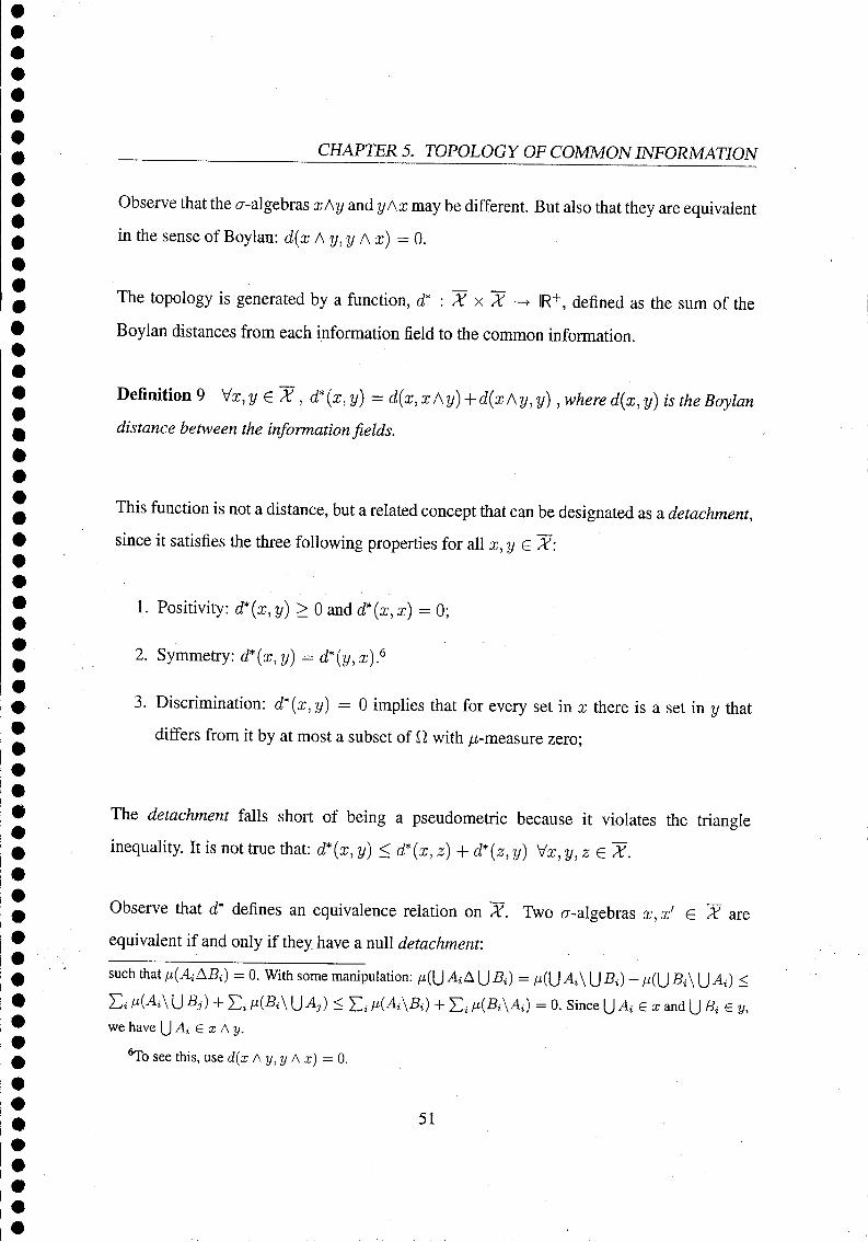
CHAPTER 5. TOPOLOGY OF COMMON INFORMATION
Observe that the a-algebras xAy and y Ax may be different. But also that they are equivalent
in the sense of Boylan: d(x Ay, y Ax) = 0.
The topology is generated by a function, d* : X x X -> IR+, defined as the sum of the
Boylan distances from each information field to the common information.
Definition 9 \/x, y G X , d*(x, y) = d(x,xAy) + d(xAy, y), where d(x, y) is the Boylan distance between the information fields.
This function is not a distance, but a related concept that can be designated as a detachment,
since it satisfies the three following properties for all x, y € X:
1. Positivity: d*(x, y) > 0 and d*{x, x) = 0;
2. Symmetry: d*(x,y) = d*(y,x).6
3. Discrimination: d*(x,y) - 0 implies that for every set in x there is a set in y that
differs from it by at most a subset of fi with / -measure zero;
The detachment falls short of being a pseudometric because it violates the triangle
inequality. It is not true that: d*(x, y) < d*(x, z) + d*{z, y) Vx, y, z € X.
Observe that d* defines an equivalence relation on X. Two cr-algebras x, x' € X are
equivalent if and only if they have a null detachment:
such that fi(AiABi) = 0. With some manipulation: /x((J A{A U 5 0 = M([J ^ \ [j Bt) + fxQJ Bi\ \J Ai) < Ei l*(Ai\ \JBJ) + Zi l*(Bi\ (J Aj) < Ei KA\Bi) + Zi l*(Bi\Ai) = 0. Since |J A{ e x and (JBd e y, we have \jAi £ x Ay.
6To see this, use d(x Ay,y Ax) =0.
51

CHAPTER 5. TOPOLOGY OF COMMON INFORMATION
x ~ x' <£> d* (x, x') = 0 .
Let y = X/ ~ denote the set of equivalence classes of X, that is,y = {[x] : x € X},
where [x] = {y e # : <f (x,y) = 0}. According to Proposition 1, the detachment and
Boylan's pseudometric define the same equivalence classes.
Proposition 1 Var, y £ X , d*(x, y) = 0o d(x, y) = 0.
Proof. Since d is nonnegative and satisfies the triangle inequality, we have: 0 < d(x, y) <
d(x, xAy) + d{xA y, y) = d*(x, y). On the other hand, d(x, y) = 0 implies that for every
set A G x there exists a set B e y such that p{AAB) = 0. This also means that xAy = x.
So, d*(x, y) = d(x, x) + d(x, y) = 0 + 0. QED
Use "open balls", B*(x, e) = {y e X : d*(x, y) < e}, to generate the topology. In the case
of a metric, the triangle inequality ensures that the open balls generate a topology, that is,
that the open sets are arbitrary unions of open balls. In this case, it has to be proved that
the "open balls" produced by d* also generate a topology.7 This is done in three steps,
each of them illustrative of the characteristics of the topology. Proposition 2 shows that in
a small "open ball", all information partitions have more information than the center. And
according to Proposition 4, in a small "open ball" all partitions have the same common
information with a third partition. These two results allow to prove that a kind of local
triangle inequality holds, implying that the "open balls" generated by d* are open sets.
Now it is shown that all the information fields which are very close to a given finite a-
algebra x have more information than x. 7The concept of "ball" was generalized from distances to detachments, but, alternatively, a different
designation can be used, like "open zone" with some "reach" around a center.
52

CHAPTER 5. TOPOLOGY OF COMMON INFORMATION
Proposition 2 Va; G X , 35(x) > 0 such that
d*(x, y) < 5(x) =>• x A y = x.
Proof. For the particular case of x having no information, [x] = [{0, fi}], the proposition
is trivial.
Now consider an arbitrary x G X with some information. Since a; is a finite cr-algebra,
there exists a finite number of a-algebras that are contained in x. Thus:
min d(x, z) = 5(x) > 0. z<Zx
[z&[x]
By definition, d*(x, y) < 5{x) =4> d(x, x A y) < 5(x).
Since ï A i / Ç x ^ [ a ; A j / ] = [x\.
The way in which x A y is defined implies that x Ay = x. QED
The distance of Boylan and the detachment are locally equivalent in the following sense.
Proposition 3 Va; G X , 35 (x) > 0 suc/i í/iaí
d*(x, y) < 5(x) =ï d*(x,y) = d(x,y).
Proof. By definition, d*(x, y) = d(rc, x Ay) + d(x A y, y).
If a; (or y) represents the total information, d and d* are clearly equivalent: d*{x,y) =
d(x,y) + d(y,y) = d(x,y).
With finite cr-algebras, in the small neighborhood as defined by Proposition 2, x A y = x.
So, we have: d*(x, y) = 0 + d(x, y). QED
Observe that 5 defines a cf-ball where this equality holds, not a d-ball. It is not true that
35(x) > 0 such that d(x, y) < 5(x) =*> d*(x, y) = d(x, y).
53

CHAPTER 5. TOPOLOGY OF COMMON INFORMATION
An important corollary is that convergence in the topology generated by d* implies
convergence in the topology of Boylan (defined by d). Note also that Proposition 1 is a
particular case of Proposition 3.
According to the Proposition 4, given two finite information fields, if one of them varies
slightly, the common information remains the same.
Proposition 4 Vx, y <G X , 3ô(x, y) > 0 such that
d*(y,z) < 5(x,y)=^xAy = xAz.
Proof. Consider two arbitrary finite a-algebras x,y G X. In the particular case of
[x] = [y], of course that x A y = x. By Proposition 2, there exists a S(y) such that
d*(y, z) < S(y) implies that y/\z — y. It follows from the definition of common information
that this operation is associative. So, we have xAy —xA{yAz) = {xAy)Az = xAz.
In the general case of [x] ^ [y], and because we deal with finite cr-algebras, there is only a
finite number of subsets of Q, Ax e x and Ay e y. Thus:
min u(AxAAv) = e. »(AxAAy)>0 v y/
Given x and y, consider <%) as in Proposition 2 and let 5(x, y) = min{e, 5(y)}.
From Proposition 2, d*{y, z) < 6(x, y) =4> y - y A z. Thus, xAy = x Ay Az.
Assuming that x Az ^ x Ay Az, then, by the way "common information" was defined, we
are sure that [x Az]^[x Ay A z\. So there exist Az € z and Ax £ x with fi(AzAAx) = 0
such that there isn't any Ay e y with fj,(AzAAy) = 0 or fj,(AxAAy) = 0.
So, min jj,(AzAAy) = minfj,(AxAAy) >e> S(x,y). Ay€y Ayey N
This implies that d*(y, z) > S(x, y). This is a contradiction, sox A z = x Ay Az ^ x Ay. QED
Propositions 2 and 4 can be read together. By the first, in a small neighborhood of an
information set, information does not decrease. According to the second, the possible
54

CHAPTER 5. TOPOLOGY OF COMMON INFORMATION
increase of information has a bound, as the common information with another information
set remains constant.
Theorem 1 is based on a kind of local triangle inequality which implies that all the points
of an "open ball" are "interior points". A point x is "interior to A <> 3e > 0 s.t.
B*(x,e) c A
Use two kinds of "open balls" to define the topology:
(1) the open d* -balls centered on finite cr-algebras with radius that are small enough for
not including the a-algebra of total information, B;
(2) the open d*-balls centered in B.s These "open balls" constitute a base for the topology
r* = {A : A is a union of open balls }.
Theorem 7 Vz G X and 0 < e < d*(x,B) : B*(x,e) = {y G X : d*(x,y) < e}
are open d*-balls (all points are interior). The d*-balls defined by B*(B, e) = {y G X :
d*{&, y) < e} are also open (all points are interior). This collection of open balls (consider
only rational radius) is a base for T* and (X, r*) is a topological space.
Proof. Given an arbitrary ball B*(x, e), we want to show that all points of this ball are
interior points. Equivalently, that given y G B*(x,e), there exists S'(x,y) > 0 such that
B*(y,S'(x,y))cB*(x,e).
Consider first a finite center, x G X. With a 5(x, y) that is small enough for Proposition 4
to hold, and an arbitrary z G B*(y, 5(x, y)):
Considering only finite cr-algebras and using all the open d* -balls we obtain a simpler topological space
55

CHAPTER 5. TOPOLOGY OF COMMON INFORMATION
d*(x, z) = d(x, x A z) + d(x A z, z) = (by Proposition 4)
= d(x, x A y) + d(x Ay,z) <
< d(x, xAy) + d(xA y, y) + d{y, z) <
<d*(x,y) + d(y,z)<
<d*(x,y) + d*(y,z).
Let 5'(x,y) = min{5(x,y),e - d*(x,y)}. For any z <E B*[y,ô'(x, y)], we have:
d*(x,z) < d*(x,y) + d*(y,z) < d*(x,y) + e - d*(x,y) = e.
Thus, the arbitrary y is an interior point. All points in the balls centered in finite cr-algebras
(with small radius to prevent them from containing B) are interior points.
With x = B, and an arbitrary y in B* (x, e), let d*(x, y) = a < e, and let 5(B, y) — e - a. Given an arbitrary z 6 B*(y, S(x, y)):
d*(B, z) = d(B, BAz) + d(BA z, z) =
= d(B, z) + d(z, z) = d{B, z) <
< d{B, y) + d{y, z) = a + d(y, z) < < a + e — a — e.
Thus, all points in the balls that are considered are interior points.
The sets whose points are all interior are open sets (members of the topology), since they
can be obtained by arbitrary unions of the members of the base. To see this, consider an
arbitrary set, A, whose points are all interior.
A = int(A) => Vx € A , 3B*(x, ex)cA^
56
CHAPTER 5. TOPOLOGY OF COMMON INFORMATION
=> UX<ZAB*(X, ex) C A C \JX€AB*{X, ex) => A is a union of open balls.
Of course that all the points inside an open set are interior points. A point in a set that is an
union of open sets is interior to at least one of the open sets, therefore it is also interior to
the union.
For the topology to be well defined, a finite intersection of open sets A must be open. It is
enough to prove that the intersection of two open sets is open. Consider an arbitrary point
a e A = A\ n A2. The point is interior to both open sets, so each of them contains a
ball centered in a. Designate these balls by B*(a, r{) C A\ and B*(a, r2) C A2. Pick the
smallest radius, w.l.o.g., rx. Of course that B*(a,r{) C Ai and B*(a,r{) C A2. This open
ball, B*(a, r{), is contained in the intersection.
QED
The Boylan topology, defined by d, is a Hausdorff topology on the space of equivalence
classes of information a-algebras. The topology of common information is stronger, so it
inherits this property.9 Observe that the topology is first countable, as every point has a
countable neighborhood base.10 Thus, to prove upper semicontinuity of the equilibrium
(or private core) correspondence, it suffices to show that given a convergent sequence of
economies, the limit of a sequence of equilibrium (private core) allocations of the sequence
of economies is an equilibrium (private core) allocation of the limit economy (see Theorem
16.20 of Aliprantis & Border (1999)). 9Given any two distinct points, there are Boylan neighborhoods of each point with null intersections (the
Boylan and Cotter topologies are separated because every topology generated by a metric is separated). And
for every Boylan neighborhood, there is a neighborhood in this topology that is contained in it, because:
Vx £ X, e G R+ : B*(x, e) c B(x, e). This implies that this topology is also separated. 10For every neighborhood of any x, there is an open ball with rational radius centered in x that is contained
in the neighborhood.
57

CHAPTER 5. TOPOLOGY OF COMMON INFORMATION
The following example shows that this detachment does not generate a topology on the
space of the infinite cr-algebras. Let the space of possible states of nature be O = [0,1]
and all the states be "equally probable". Consider the simple information cr-algebra
x = {0, [0, |] ,] J, 1], 0} . An infinite information cr-algebra y that is inside B*(x,e) is
generated by the partition:
VS = {[0, J],]§ + ^FT, \ + £]„«*,] j + 1, l]}.11
Now construct a sequence of information fields that approaches y, but remains outside
B*(x,e).
Letz? = {[0, jã + ãÃThls + j j ^ ' 5 + ;j^']m=n,...,i,]!"'"i> 1]} be the partitions that generate
the elements zn of the sequence of information fields.
Observe that the difference between y and zn is that [0, \ + j fo] is an elementary set in zn,
but appears subdivided in y. Since the set of y that is farther from [0, \ + ^+i] is [0, \], the
Boylan distance between y and zn is ^FT-
So, we have: if (y, zn) = d{y, y A zn) + d(y A zn, zn) = d(y, zn) + d(zn, zn) = e/2n+l.
But, since x and zn have no common information:12
d*(x, zn) = d{x, xAzn)+ d(x A zn, zn) = d(x, 0) + d(0, zn) = l i e e
= _ - j = i i 2 2 2 n + 1 2n + 1
"Note that with some small e, d*(x,y) = d(x,x A y) + d(x A y,y) = d(x,x) + d(x,y) -
suPAey infBgx n(AAB) = e/2. 12With the cr-algebra of "no information" defined as 0 = {0,fi}, to say that x and zn have no common
information means that d(x A zn, 0) = 0.
58

CHAPTER 5. TOPOLOGY OF COMMON INFORMATION
All the zn are outside B*(x, e), while there isn't any open d*-ball with center y that does not
include any zn. Therefore, there isn't any open cf-ball centered in y contained in B*(x, e).
5.4 Upper Semicontinuity Results
In this section, a recasting of three upper semicontinuity results of Einy et al. (2005) is
done. To illustrate the usefulness of the topology, a notion of convergence of economies is
used, which differs from theirs only in what concerns convergence of private information
fields. The use of the topology of common information, instead of the topology of Boylan,
allows to establish the upper semicontinuity of the private core correspondence (Theorem
3).13
Definition 10 Let {Sk}f=l = { ( 4 , 4 , ^ ) ^ } ^ be a sequence of economies with
differential information that converges to £Q = (4>Uo>*o)ïU- Precisely, convergence
means that, for every agent i e N:
i) e\ converges to el0 in the L[-norm;
ii) u\ converges uniformly to u^ on every compact subset o / i l x IR /
Hi) F\ converges to Fj, in (X, r*). 13Allen (1983) showed continuity of consumer demand with respect to information using the topology of
Boylan. Convergence in the topology of common information implies convergence in the Boylan topology:
xn e B(x0, e) => xne B*(x0, e). Therefore, the results obtained by Allen remain valid with this topology.
59

CHAPTER 5. TOPOLOGY OF COMMON INFORMATION
Note that what is needed is convergence of information fields for each agent in separate. The
common information among the agents is not calculated. What is relevant is the common
information between the information that an agent has in an economy of the sequence and
the information that the same agent has in the limit economy.
Since convergence of information fields in the topology of common information implies
convergence in the topology of Boylan, recasting Theorem 1 of Einy et al. (2005)
establishes upper semicontinuity of the W.E.E. correspondence.
Theorem 8 Let {£k}kLi = {(el>uk^l)7=\}h=i be a sequence of economies with
differential information that converges to £Q = (e^, uzQ, Fl
Q) f=1.
Let {{xk, Kk)}kLi be a sequence such that (xk, Kk) G WEE(Sk) for every k, and for every
ieN:
i) x\ converges to XQ in the Lep-norm;
ii) -K\ converges to TTQ in the Leq-norm.
Then(x0,TTQ) G WEE(£0).
From Proposition 2 we know that in a small neighborhood of a finite information field F^,
information fields are more rich,14 in the sense that F^ A F^ — F^, that is, all sets in Fi
have an equivalent set in F^ (that is, [x(AAB) = 0). This does not imply that Fi C F„.
But, replacing all the sets in Fln by their equivalent in F^, is obtained an information field,
14The limit economy differs of those in the sequence because markets for very unlikely contingencies may disappear.
60

CHAPTER 5. TOPOLOGY OF COMMON INFORMATION
F*, such that F^ ~ F*n and F\ C F£. Furthermore, changing the information fields from
FJ, to F£ has no impact on the solutions of the model. So, the sequence F^ can be used
to apply Theorem 2 of Einy et al. (2005), establishing upper semicontinuity of the private
core correspondence for all finite cr-algebras Fj,.
Theorem 9 Let {£k)t=i = {(4>ulFk)ti}k=i be a sequence of economies with
differential information that converges to £Q = (ej, u£, F*0) ?=1, with F^ finite.
If a convergent sequence of allocations in L[, {xk}f=v with lim^oo xk = x0, is such that,
for every k, xk = {x\,x\,..., xnk) is a private core allocation in £k, then the limit of the
sequence, xQ = (XQ, XQ, ..., XQ), is a private core allocation in £0.
The private core correspondence also converges when the information fields of all the agents
converge to the total information consisting of the a-algebra of all Borel sets in Í1 From
Proposition 3, convergence of information fields in the topology of common information
implies convergence in the topology of Boylan. Thus, with B equal to the complete
information field, Theorem 3 of Einy et al. (2005) establishes convergence of the private
core.
Theorem 10 Let {£k}kLi = {(ek>uk,Fk)i=i}kLi be a sequence of economies with
differential information that converges to £B = (elB, vfe, B) "=1, with B defined as the o-
algebra of all Borel sets in O.
If a convergent sequence of allocations in L[, {xk}kLv with limfc-oo xk = x0, is such that,
for every k, xk = {x\,x\,..., xJJ) is a private core allocation in £k, then the limit of the
sequence, XB — {xlB, x%,..., Xg), is a private core allocation in £B.
61
CHAPTER 5. TOPOLOGY OF COMMON INFORMATION
A negative counterpart of this result is given by Krasa & Shafer (2001): if the
complete information is approached by changing priors instead of expanding fields, upper
semicontinuity fails.
Theorem 4 is also related to a result of Balder & Yannelis (2005) that establishes upper
semicontinuity of the private core for sequences of economies with increasing information
(learning), that is, when Fk Ç Fk+1 for every k. It may seem at first that Fk Ç Fk+1
together with \/kFk = Fœ implies that lim d{Fk, F«,) = 0. This would allow us to recast fc—*oo
their result, because in the case of monotonie learning, convergence of information fields in
the topology of Boy Ian is equivalent to convergence in our topology. But, in fact, monotone
convergence in the sense of Balder and Yannelis does not imply convergence in the sense
of Boylan, so the results are complementary.15
5.5 An Illustrative Example
In the introduction, was mentioned an example presented by Einy et al. (2005) which
excluded the upper semicontinuity of the private core. This example is reproduced in
this section to illustrate the problem of the continuity of the private core with respect to
variations in information. The sequence of information fields considered in this example
does not converge in the topology of common information. I5To see this, consider fi = P0 = [0,1] and Pk = {[0, £] , . . . , [£ , i+i],..., [2^1], l}. Observe that the
partition Pk+1 is obtained by dividing each element of Pk in half. It may be shown that d(Fk+i, Fk) = 1/2
by selecting from Fk+l the set A = U J =i ,3 ... 2 * - i [ ^ . ^ r ] . since min fj,(AAB) = 1/2.
62

CHAPTER 5. TOPOLOGY OF COMMON INFORMATION
Consider a sequence of economies, Se, with two agents and one commodity, where only
one of the private information fields varies. The space of possible states of nature is
Í2 = [0,1] U [2,3]. The agents have equal initial endowments, independent of the state of
nature: e-\. The private information of the agents are generated by the finite partitions:
Í Fe1 = [0,l]U[2;2 + e],]2 + e,3];
\ Fe2 = [0,l],[2,3].
Agent 1 only values consumption in [0,1], while agent 2 only values consumption in [2,3]. Their preferences are given by:
u x J x ,ifu/€[0,l]; Í 0 , ifu/e[0,l];
[ 0 ,ifwG[2,3]; ' ' [ x , if u €[2,3].
The economies differ only in the parameter e, which converges to zero. Private allocations are of the form:
x* = {a] ■ X[o,i]u[2,2+e] + a2e ■ X]2+e,3\, b\ ■ X[o,i] + h\ ■ X%z\)-
Feasibility in [0,1], [2,2 + e], and in ]2 + e, 3] implies that:
(al + bl<l;
< a\ + b2e<l;
k a2t+bl<l.
Since xt is a core allocation, a\ > | , or else U^e1) > Ul(x\). For the same reason, b\ > \. So, a\ +b2<l implies that a\ = b\ = \, that b\ < \, and a\ < \.
Therefore, the initial endowments form a (constant) sequence of private core allocations,
converging, of course, to x - e = \. In a limit economy, where F1 = F2 =
63

CHAPTER 5. TOPOLOGY OF COMMON INFORMATION
{[M], [2,3]}16, the only private core allocation is xe = (x[o,i],X[2,3]), corresponding to
a situation in which agent 1 consumes everything in [0,1] and agent 2 consumes everything
in [2,3]. Upper semicontinuity of the private core correspondence fails.
Observe that in the sequence of economies ££, even for a very small e, the common
information of the agents is null. So, agent 1 cannot trade worthless consumption in
[2,3] for consumption in [0,1] (which agent 2 doesn't value). Their information fields
are incompatible, in the sense that they do not allow contingent trade. In the limit economy,
the agents have the same information, so they are able to make contingent trades. This is
the source of the discontinuity.
According to Boylan's topology on information, the fields generated by the partitions
{[0,1] U [2,2 + e],]2 + e, 3]} and {[0,1], [2,3]} are neighbor. Nevertheless, these fields
imply substantially different economic outcomes. The first has no information in common
with agent 2's information field, so it does not allow contingent trade. It is as useless for
agent 1 as would be the null information field {0, Q}. The second is compatible with the
information of agent 2, that is, agents have common information, {0, [0,1], [2,3], fi}, based
on which they are able to make contingent trades.
This means that a very small perturbation can lead to incompatibilities in the information
of the agents, and have a big impact on the economic outcome. This motivates the
introduction of a new topology that can grasp the compatibility of the information of
the agents. According to the topology of common information, if the information fields
become incompatible, the perturbation could not have been a small one. Compatibility of
information fields is preserved under small perturbations. 16Note that the information partitions F1 = {[0,1], [2,3]} and F1' = {[0,1] U {2}, ]2,3]} are equivalent
in the sense of Boylan.
64
_ _ _ _ CHAPTER 5. TOPOLOGY OF COMMON INFORMATION
With this new topology, the example does not show any failure of continuity, because
the sequence of information fields F} = {[0,1] U [2,2 + e], ]2 + e, 3]} does not converge.17
A sequence that would actually converge to F^ = {[0,1], [2,3]} in our topology is, for
example, F}' = {[0,1], [2,2 + e],]2 + e,3]}.18 But, in this case, contingent trades would
also be allowed in the sequence of economies, not just in the limit economy.
In the topology of common information, two information fields that are neighbor may differ
only in events that are very unlikely. Notice that F£ and F}' differ because while ift
observes [2,3], F}' can distinguish the unlikely event [2,2 + e] from ]2 + e,3]. Trades
contingent on realization of [2,3] are allowed. Only trades that are contingent on a very
"unlikely" event, [2, 2 + e], are excluded.
Information fields that are very close in the topology of Boylan may also differ in an
additional way, by distinguishing different but very correlated events. In fact, F& and F}
differ because they allow the observation of very correlated events: [0,1] U [2,2 + e] is
similar to [0,1]; and ]2 + e, 3] is similar to [2,3]. Nevertheless, the common information is
null and so contingent agreements are not allowed.
The differences of the first kind only imply that agreements cannot be contingent on the
very unlikely events that are not commonly observed, and therefore, have a small impact
on economic outcomes. Differences of the second kind may prevent valuable agreements,
contingent on events that are not commonly observed but nevertheless probable, and thus
may imply very different economic outcomes. This second type of differences between
Consider Í2 = [0,2], and a strictly decreasing sequence {en} that converges to zero. The limit of a
sequence of information fields Fn = {0, [0,1 - en], ]1 - en, 2], fi} must include all the sets [0,1 - en] after
some n (or sets that are Boylan-equivalent). Otherwise, there is no common information between Fn and F0,
and therefore d*(Fn,F0) = 1 - e. This means that the limit cannot be a finite information field. ,8Note that Fo1 A F}' = F0\ so á*(F0\ F,1') - d(Fa,F}') - e.
65

CHAPTER 5. TOPOLOGY OF COMMON INFORMATION
information fields that are neighbor is allowed by the topology of Boy Ian but not by the topology of common information.
66

Chapter 6
Economies with Uncertain Delivery
6.1 Introduction
Uncertainty and private information are crucial in modern economies. Agents know that
their decisions can lead to different outcomes, depending on the decisions of others, and
on the state of the environment. The complexity associated with these issues is such that
it cannot be completely captured by any simple model. A realistic goal is to find simple
models that give enlightening, although partial, descriptions.
In general equilibrium theory, several proposals have been made regarding the introduction
of private information. A first one was made by Radner (1968), who restricted agents to
consume the same in states of nature that they did not distinguish. With this condition,
the model of K. J. Arrow & Debreu (1954) could be reinterpreted in a way that took into
account each agent's private information.
After this- first solution, another concept came to dominate the literature: the rational
expectations equilibrium (Muth, 1961). But to assume that agents have rational
67

CHAPTER 6. ECONOMIES WITH UNCERTAIN DELIVERY
expectations and take prices as fixed can be problematic. If, by observing prices, an agent
can infer all the information of the others, then it is useless to have more information ex
ante. Agents do not care about producing and gathering information, therefore, insights on
these economic processes do not arise. Furthermore, this kind of inference also seems to
require agents to have incredible knowledge and cognitive abilities.
Another alternative approach was taken by Prescott and Townsend (1984a, 1984b),
who restricted trade contracts to be incentive compatible. But how can the incentive
compatibility of the contracts be guaranteed? Again, agents would have to know
everything about the whole economy in order to evaluate whether the contracts are incentive
compatible or not.
The objective of this work is not to provide an equilibrium concept that is "better" than
these in all instances. The goal is to present an equilibrium concept that fits a situation in
which agents know only their characteristics (endowments and preferences in each state of
nature) and the prevailing prices. The economy is not assumed to be common information.
Agents do not know the endowments, preferences and private information of the others, and
aren't able to figure them out.
The notion that is propose is a prudent expectations equilibrium. In this model, agents
are allowed to make contracts for uncertain delivery, that is, contracts that may give them
different bundles in states of nature that they do not distinguish ex ante. Agents buy the right
to receive one of these different bundles, and expect to receive the worst of the possibilities
contracted. This leads them to select bundles with the same utility for consumption in states
that they do not distinguish. So, agents actually end up receiving the worst possibility,
which is as good as any of the others.
In sum, economies with incomplete private information are modeled, in which agents are
assumed to follow a simple rule-of-thumb: to be prudent. The model of Arrow-Debreu can
68

CHAPTER 6. ECONOMIES WITH UNCERTAIN DELIVERY
be reinterpreted to cover this situation, therefore, many classical results still hold: existence
of core and equilibrium, core convergence, continuity properties, etc.
In a prudent expectations equilibrium, agents obtain the same utility in states of nature
that they do not distinguish, instead of equal consumption. This is a weaker restriction,
therefore, efficiency of trade and welfare are improved.
The chapter is organized as follows: in section 2, contracts for uncertain delivery are
defined, section 3 includes examples that motivate the model; and, in section 4, an
interpretation of the economy with uncertain delivery is given.
6.2 Contracts for uncertain delivery
The theory of general equilibrium under uncertainty has developed upon the formulation of
objects of choice as contingent consumption claims (Arrow, 1953). Under this formulation,
besides being defined by their physical properties and their location in space and time,
commodities can also be defined by the state of nature in which they are made available.
For example, a "bicycle" in "rainy weather" and a "bicycle" in "sunny weather" are seen
as two different commodities. This incorporation of uncertainty in the commodity space
allows an interpretation of the Walrasian model that covers the case of uncertainty.
The Arrow-Debreu (1954) economy extends over two time periods. In the first period,
agents know their preferences and endowments, which depend on the state of nature. In this
ex ante stage, agents trade state-dependent endowments for state-dependent consumption.
69

CHAPTER 6. ECONOMIES WITH UNCERTAIN DELIVERY
In the second period, the state of nature becomes public information, trade is realized, and
consumption takes place.
Now suppose that the state of nature does not become public information. In this case,
agents have to be careful when trading contingent goods. Consider a seller that offers the
following game:
"/ will toss a coin. If the result is heads, you receive a bicycle; if it is tails, you don't
receive anything."
How much would an agent pay for this contingent good, which can be described as a
"bicycle" if the state of nature is "heads"? If it is common information that the agent
does not observe the coin toss, this contingent good has no value. The seller is able to avoid
delivery. This suggests that agents are only willing to pay for goods which are contingent
upon events that they can observe.
This restriction allowed Radner (1968) to extend the model of Arrow and Debreu to the
case of private information. Agents are constrained to consume the same in states of
nature that they do not distinguish. That is, consumption is measurable with respect to the
private information of each agent. This restriction trivially implies incentive compatibility.
Whatever the state of nature that occurs, agents are always sure about the bundle that will be
delivered to them, so they can never be deceived. On the other hand, incentive compatibility
does not imply measurability, so this restriction may be seen as too strong.1
Relaxing this restriction could allow agents to achieve better outcomes, in the sense of
Pareto. But does it make sense to buy the right to receive different bundles in states of
'For a thorough analysis of the problem of incentive compatibility in exchange economies with private
information, see Forges, Minelli, & Vohra (2002).
70

CHAPTER 6. ECONOMIES WITH UNCERTAIN DELIVERY
nature that the agent does not distinguish? Suppose now that the seller offers a different
game:
"/ will toss a coin. If the result is heads, you receive a blue bicycle; if it is tails, you
receive a red bicycle."
Even if it is common information that the agent does not observe the coin toss, this is a
valuable uncertain contingent good, because the delivery of a "bicycle" is guaranteed. An
agent is probably willing to pay for the right to receive a "blue bicycle or red bicycle".
Here the notion of objects of choice as uncertain consumption bundles is proposed, and
these uncertain bundles are designated as "lists". If the specified contingency occurs, a
contingent list gives an agent the right to receive one of the bundles in the list. Agents
are now allowed to sign "contracts for uncertain delivery", which specify a list of bundles
out of which a single one will be selected for delivery. These contracts can be contingent,
so, in general, agents buy the right to receive one of the bundles in the list if the specified
contingency occurs. The selection of the bundle that is delivered is made by the seller, but
the buyer is certain about receiving one of the bundles in the list.2
Agents are able to sign more general contracts, so allowing contracts for uncertain delivery
may be seen as opening additional markets.3 A supplier may not be able to guarantee the
delivery of neither a "blue bicycle" nor a "red bicycle", while being able to ensure the
delivery of one of the two. In the Radner model, there would be no trade, but contracts for
uncertain delivery allow trade to take place.
2Contracts commonly known as "options" are covered by this definition. 3Obviously, contracts for contingent delivery (Arrow, 1953) can be seen as "contracts for uncertain
delivery" with lists of only one element.
71

CHAPTER 6. ECONOMIES WITH UNCERTAIN DELIVERY
6.3 Examples
Two situations will be presented in which there aren't any commonly observed events. As
a consequence, if agents are constrained to consume the same in states that they do not
distinguish, there will be no trade in equilibrium. Allowing agents to sign contracts for
uncertain delivery leads to welfare improvements in the sense of Pareto. In these two
examples, agents actually reach the full information (first-best) outcome.
Example 1: Perfect substitutes
This economy has two agents and four commodities: "ham sandwiches", "cheese
sandwiches", "orange juices" and "apple juices".
Both agents need to eat and drink. Sandwiches are perfect substitutes, as well as the
juices. Agents want to maximize expected utility, having the same preferences in every
state, described by a Cobb-Douglas utility function:
There are four possible states of nature, Ù = {wi, u2, w3, u4}.
- Inui, agent A is endowed with two "ham sandwiches" and agent B with two "orange
juices": eAM = (2,0,0,0) and eB{ux) = (0,0, 2,0);
- In u2, agent A is endowed with two "ham sandwiches" and agent B with two "apple
juices": eA{u2) = (2,0,0,0) and eB{u2) = (0,0,0,2);
- In o;3, agent A is endowed with two "cheese sandwiches" and agent B with two
"orange juices": eA(oo3) = (0, 2,0,0) and eB(u3) = (0,0, 2,0);
72

CHAPTER 6. ECONOMIES WITH UNCERTAIN DELIVERY
- In co>4, agent A is endowed with two "cheese sandwiches" and agent B with two
"apple juices": eA{cuA) = (0,2,0,0) andeB{cuA) = (0,0,0,2).
Each agent observes only its endowments. Their information partitions are:
PA = {{wi,W2},{w3,W4}}andPs = {{WI,WS},{WÍ,W4}}.
Agents want to guarantee that they will eat and drink in the future. The problem is that
they are unable to buy any specific good for future delivery contingent upon events (sets of
states) that they observe.
For example, agent A wants to buy orange juice. For consumption to be the same across
undistinguished states, the delivery of orange juice must be contingent upon events that A
can observe. The possibilities are: (i) delivery in all states, (ii) delivery in {ui,co2}, (iii)
delivery in {u3,Ui}.
None of these possibilities is feasible, because agent B only has orange juice in the states
wi and u>3. The same reasoning applies to each of the other commodities, so there is no
trade in this economy. From another angle, suppose that agent A consumed some quantity
of "orange juice" in LOX. The same consumption would have to take place in u2, but in u>2
there isn't any "orange juice" in the economy.4
There is no trade if equal consumption in undistinguished states is imposed. Nevertheless, contracts for uncertain delivery allow agents to guarantee future consumption of a sandwich and a juice.
4We can assume strictly positive endowments, substituting every zero for a small e, and reach the same conclusions.
73
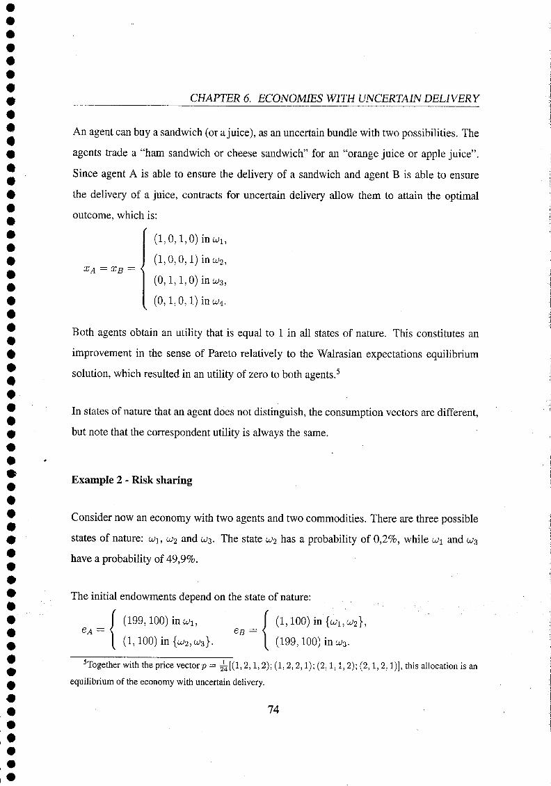
CHAPTER 6. ECONOMIES WITH UNCERTAIN DELIVERY
xA = xB = <
An agent can buy a sandwich (or a juice), as an uncertain bundle with two possibilities. The
agents trade a "ham sandwich or cheese sandwich" for an "orange juice or apple juice".
Since agent A is able to ensure the delivery of a sandwich and agent B is able to ensure
the delivery of a juice, contracts for uncertain delivery allow them to attain the optimal
outcome, which is:
(1,0,1,0) in W l ,
(1,0,0,1) in W2,
(0,1,1,0) in ws,
(0,1,0,1) in w4.
Both agents obtain an utility that is equal to 1 in all states of nature. This constitutes an
improvement in the sense of Pareto relatively to the Walrasian expectations equilibrium
solution, which resulted in an utility of zero to both agents.5
In states of nature that an agent does not distinguish, the consumption vectors are different,
but note that the correspondent utility is always the same.
Example 2 - Risk sharing
Consider now an economy with two agents and two commodities. There are three possible
states of nature: ux, u2 and us. The state u2 has a probability of 0,2%, while uj\ and u;3
have a probability of 49,9%.
The initial endowments depend on the state of nature:
(199,100) in wi, Í (1,100) in {uhu2}, eA = \ eB= <
(1,100) in {ws, us}. (199,100)incu3.
together with the price vectorp = i [ ( l , 2,1,2); (1, 2,2,1); (2,1,1, 2); (2,1,2,1)], this allocation is an equilibrium of the economy with uncertain delivery.
74
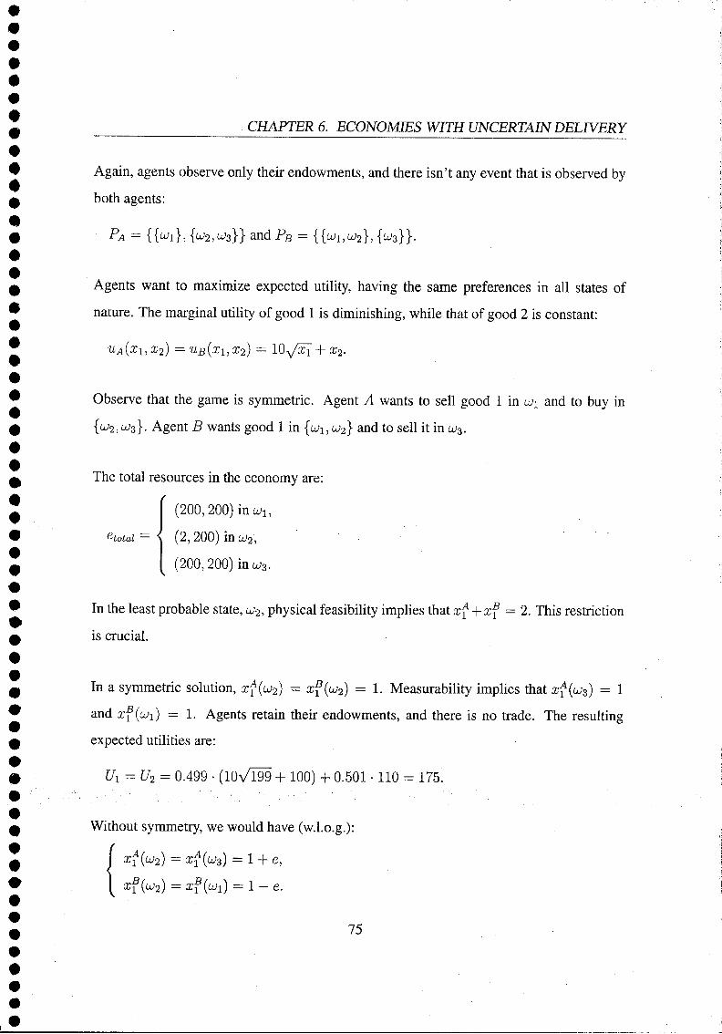
CHAPTER 6. ECONOMIES WITH UNCERTAIN DELIVERY
Again, agents observe only their endowments, and there isn't any event that is observed by
both agents:
PA = {{ivi},{u2>ujz}} and PB = {{wi,W2},{ws}}.
Agents want to maximize expected utility, having the same preferences in all states of
nature. The marginal utility of good 1 is diminishing, while that of good 2 is constant:
uA(xx,x2) -uB(xi,x2) = 10Jxl + x2.
Observe that the game is symmetric. Agent A wants to sell good 1 in ux and to buy in
{U2,UJ3}. Agent B wants good 1 in {u>i,u2} and to sell it in u3.
The total resources in the economy are:
(200,200) in uu
etotai = < (2,200) in u2,
^ (200,200)in u3.
In the least probable state, u2, physical feasibility implies that xf + xf = 2. This restriction
is crucial.
In a symmetric solution, xf(cu2) = xf(u2) = 1. Measurability implies that xf(u3) = 1
and xf (u>i) = 1. Agents retain their endowments, and there is no trade. The resulting
expected utilities are:
UX = U2 = 0.499 • (ÎOV ÏOÏÏ + 100) + 0.501 • 110 = 175.
Without symmetry, we would have (w.l.o.g.):
xf(u2) =xf(u3) = 1 + e,
xf(u2) = xf (wi) = 1 - e.
75
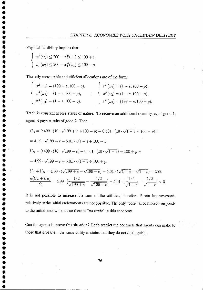
CHAPTER 6. ECONOMIES WITH UNCERTAIN DELIVERY
Physical feasibility implies that:
xfM < 200 - xf (wi) < 199 + e,
xfM < 200 - xf(u3) < 199 - e.
The only measurable and efficient allocations are of the form:
xA(u1) = (199 + e,lQ0-p), f xB(ui) = (1 - e, 100 + p),
xA{cu2) = (l + e,100-p), ; < xB(u2) = (1 - e, 100 +p),
^ xA(u3) = (1 + e, 100 - p). [ z 5 ^ ) = (199 - e, 100 + p).
Trade is constant across states of nature. To receive an additional quantity, e, of good 1,
agent A pays p units of good 2. Then:
UA = 0.499 • (10 • V199 + e + 100 - p) + 0.501 • (10 • v T + ë + 100 - p) =
= 4.99 • Vl99 + e + 5.01 ■ VT+e + 100 - p.
?7S = 0.499 • (10 • V199 - e) + 0.501 • (10 • y/T^e) + 100 + p =
= 4.99 • V199 - e + 5.01 • vT^~e" + 100 + p.
UA + UB = 4.99 • (V199 + e + ^199 - e) + 5.01 • (VTTë + T T ^ ) + 200. WA + UB)^ 1/2 1/2
de V199 + e V199 - eJ ^.[^=-i]<o Vl + e Vl - e
It is not possible to increase the sum of the utilities, therefore Pareto improvements
relatively to the initial endowments are not possible. The only "core" allocation corresponds
to the initial endowments, so there is "no trade" in this economy.
Can the agents improve this situation? Let's restrict the contracts that agents can make to
those that give them the same utility in states that they do not distinguish.
76

CHAPTER 6. ECONOMIES WITH UNCERTAIN DELIVERY
In a symmetric allocation, each agent gets (1,100) in u2. The correspondent utilities are
UA = uB = 110. An allocation with measurable utility for agent A must have the same
utility in LU3:
l O v V M + X$M = HO =* XA(U3) = 110 - 10y/xf((J3).
Thus, XA{UJ3) must be of the form:
xA(u3) = (X, 110 - 10vOf).
Without waste of resources, we have a r 8 ^ ) = (200 - X, 90 + lOVX). By symmetry:
xB{ux) = (X, 110 - WVX) and a r 4 ^ ) = (200 - X, 90 + 10-/ÃT).
The utility of agent A in {UJ2, 103} has to be equal to 110. To arrive at an optimal solution, it
is enough to maximize utility in uj\:
U = 10V200 - X + 90 + Wy/X =s> U' = - 5 • (200 - X)" 1 / 2 + 5 • X"1 /2 .
[/' = 0 => (200 - xyv2 = x-1'2 ^ X = 100.
This gives the following state-contingent and expected utilities:
uA(ui) = 10 • %/ÏOÔ + 90 + IOA/IÕÕ = 290.
UA = UB = 0.499 • 290 + 0.501 • 110 = 200.
The symmetric optimal solution is:
(100,190) in uu
x = , 1 . 290inwi,
, l " 7 (1,100) in w2, u
! 110 in { c ^ , ^ } -(100,10),^.
77

CHAPTER 6. ECONOMIES WITH UNCERTAIN DELIVERY
xB = < (100,10) in uu ,
D 110 in {UJI.UJO}, (1,100) inu2, uB={ x h 2 / '
! 290ino>3. (100,190), w3. k
They can obtain this allocation by signing a contract under which, in every state of
nature, each agent would deliver to the other one of two bundles: (99, -90) or (0,0).
It is straightforward to see that agents would deliver (99, -90) if their endowments are
(199,100), ending up with (100,190) in that state of nature.
This solution can also be achieved as a competitive equilibrium with the prevailing price
vector p = [(1,2); J§(10,2); (1,2)], leading agents to select the non-measurable bundles
xA and xB.
The resulting expected utility is close to 200, higher than the 175 which correspond to the
classical solution. Again, the introduction of contracts for uncertain delivery allowed a
Pareto improvement in the exchange economy.
6.4 Economies with Uncertain Delivery
To clarify the modification that is proposed to the model of the economy, first an economy
that leads to the model of Radner (1968) is described. This economy has separate markets
for each commodity, and extends over two periods. In the first period, agents make
78

CHAPTER 6. ECONOMIES WITH UNCERTAIN DELIVERY
contingent trade agreements in each market. In the second period, agents receive their
information, trade is realized, and consumption takes place.6
In this interpretation of the model, a very demanding notion of information is used. To have
information about an event is actually to be able to prove in a court of law that the event
occurred.7 For the goods to be delivered in the second period, the agent has to be able to
prove that the specified contingency occurred. This has the obvious implication that, in this
economy, contracts for contingent delivery are enforceable.
Agents are not able to buy a "blue bicycle or red bicycle", because the markets are separated.
To see this, suppose that an agent buys a "blue bicycle" if the "coin toss result is heads" and
buys a "red bicycle" if the "coin toss result is tails". The agent ought to receive a "bicycle",
in any case. But notice that the agent cannot neither prove that the state is "heads", nor that
it is "tails". So, the sellers in both markets evade the law, and the agent gets nothing. In this
economy, contracts for uncertain delivery are not enforceable.
As a result, agents only will demand goods contingent on events included in their private
information. This resembles what occurs in the model of Radner (1968).
The modification that is introduced is to lump markets together, so that there is only one
representative of the market dealing with the agent. Thus, an agent can take the "market"
to a court of law, in order to receive a "blue bicycle or red bicycle".
information is received in the second period, but in the first period the agents already know which events they are able to observe.
7Another way to see private information is as allowing agents to "distinguish" between states of nature. So this would be a very demanding notion of "distinguishing" between two states: to be able to prove in a court of law that the state cannot be one of the two.
79
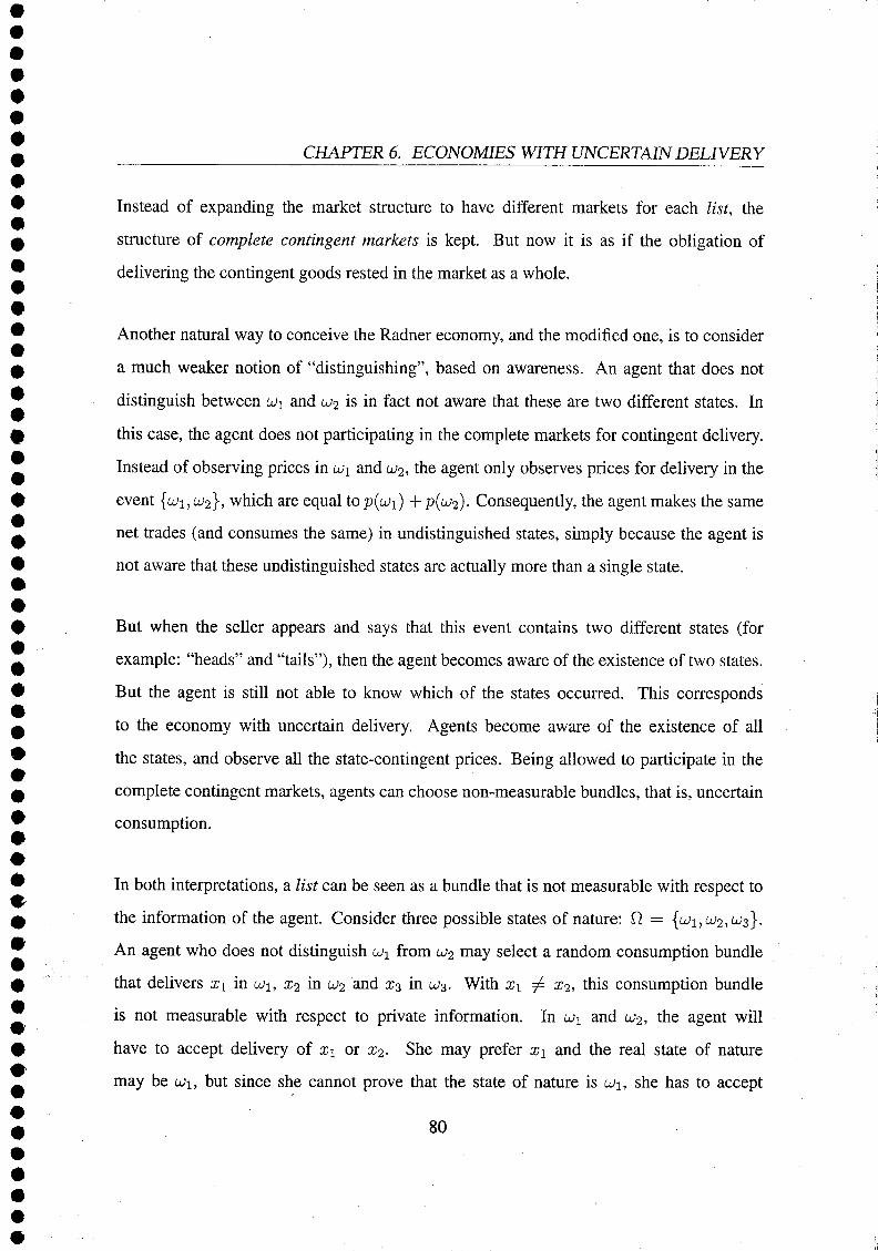
CHAPTER 6. ECONOMIES WITH UNCERTAIN DELIVERY
Instead of expanding the market structure to have different markets for each list, the
structure of complete contingent markets is kept. But now it is as if the obligation of
delivering the contingent goods rested in the market as a whole.
Another natural way to conceive the Radner economy, and the modified one, is to consider
a much weaker notion of "distinguishing", based on awareness. An agent that does not
distinguish between u\ and u2 is in fact not aware that these are two different states. In
this case, the agent does not participating in the complete markets for contingent delivery.
Instead of observing prices in u\ and UJ2, the agent only observes prices for delivery in the
event {ui,ui2}, which are equal top(u\) + p(tu2). Consequently, the agent makes the same
net trades (and consumes the same) in undistinguished states, simply because the agent is
not aware that these undistinguished states are actually more than a single state.
But when the seller appears and says that this event contains two different states (for
example: "heads" and "tails"), then the agent becomes aware of the existence of two states.
But the agent is still not able to know which of the states occurred. This corresponds
to the economy with uncertain delivery. Agents become aware of the existence of all
the states, and observe all the state-contingent prices. Being allowed to participate in the
complete contingent markets, agents can choose non-measurable bundles, that is, uncertain
consumption.
In both interpretations, a list can be seen as a bundle that is not measurable with respect to
the information of the agent. Consider three possible states of nature: fl — {wi, 0*2,^3}.
An agent who does not distinguish u\ from UJ2 may select a random consumption bundle
that delivers X\ in wlt x2 in OJ2 and x3 in u;3. With x\ / x2, this consumption bundle
is not measurable with respect to private information. In u\ and UJ2, the agent will
have to accept delivery oî xx 01 x2. She may prefer x\ and the real state of nature
may be ui\, but since she cannot prove that the state of nature is oj\, she has to accept
80

CHAPTER 6. ECONOMIES WITH UNCERTAIN DELIVERY
x2 if this is the bundle that is delivered. In wi and o>2, she receives "x\ or x2", an
uncertain bundle that is denoted as {xx V i 2 ) . Instead of writing the consumption bundle
as x = (xi, x2, x3), from the perspective of the agent it would be more adequate to use the
notation x - {(x\ V x2), (xi V x2), x3]. Observe that this construction implies measurability
of the vector of contingent lists with respect to the information of the agent. Instead of
contingent bundles, agents are constrained to select contingent lists.
Observe that if consumption is measurable with respect to the information of the agents,
then the contingent bundles may be seen as contingent lists with only one element. Let
the information of an agent be P = {{ui,u2}, {u3}}, and consider the measurable
consumption bundle x = (xi,xi,xz). The correspondent list is x = [(x1 V xi), (xi V
xi),x3] = {xuxi,x3).
In the economy with uncertain delivery, the prices of the lists are restricted to be based
on the prices of the contingent commodities. The intermediaries are prevented from doing
speculation. Their role is simply to offer to the agent a list composed by contingent goods.
Consider the right to receive a "blue bicycle or red bicycle". It is weaker than the right
to receive a "blue bicycle", in the sense that delivery of a "blue bicycle" implies delivery
of a "blue bicycle or red bicycle", while the converse is not true. Thus, uncertain delivery
of a "blue bicycle or red bicycle" should not be more expensive than the delivery of a
"blue bicycle". If it were more expensive, there would be an opportunity for arbitrage. An
intermediary could buy a "blue bicycle" and sell it as a "blue bicycle or red bicycle" with
profit.
To see how prices are assigned to the lists consider an agent with information P =
{{U)1:UJ2}, {^3}}- The agent can obtain the list x = [(xi V x2), {x\ V x2),xs] by buying
any of the following bundles: xa = {xx,xux3), xb = (xux2,x3), xc = (x2,x1,x3), or
81

CHAPTER 6. ECONOMIES WITH UNCERTAIN DELIVERY
Xd = (#2, x2, xs). It only makes sense to buy the cheapest of these bundles, so the price of
a list is actually the price of the cheapest alternative.
82

Chapter 7
Prudent Expectations Equilibrium
This chapter is organized as follows: in section 1, the idea of prudent preferences is justified;
the model of general equilibrium with uncertain delivery is formalized in section 2, and
characterized in section 3; in section 4, concepts of core in economies with uncertain
delivery are introduced and commented; and, finally, in section 5 we conclude the paper
with some remarks.
7.1 Prudent preferences
It is necessary to extend the domain in which preferences are defined, to include the non-
measurable bundles. What is the utility of receiving "x\ or x2"?
83

CHAPTER 7. PRUDENT EXPECTATIONS EQUILIBRIUM
7.1.1 Prudence as a rule-of-thumb
We assume that agents are not able to figure out the true probabilities of getting x1 and x2.
So, they cannot use expected utility. They use a simple rule of thumb, instead. Consider,
for example, a seller which has a "bicycle" to sell. Instead of selling a "bicycle", the seller
could gain by selling a "bicycle or car", and always deliver the "bicycle" and never the car.
In order to defend themselves against being deceived by the sellers, the agents expect the
worst outcome:1
Vxi,...,Xk :u(xi V... Va:*;) = min u{xó). j=l,...,k
This is our proposal: the utility of an uncertain bundle (a list) is equal to the utility of the worst possible outcome.
Contingent bundles which are constant in states that the agent does not distinguish can
be seen as contingent lists with only one element. In this case, prudent utility is equal to
the primitive utility. Now we extend preferences to a domain that include also the non-
measurable bundles (contingent lists), preserving the values in the space of measurable
bundles.
7.1.2 Prudence as a result
The following analysis resembles the work of K. Arrow & Hurwicz (1972) on optimality
criteria for decision under ignorance. By "ignorance" it is meant that the agent has no prior
probabilities on the occurrence of different states, perceiving them as a single state.
'These preferences have some relation with Choquet expected utilities (Schmeidler, 1989), but they are a degenerate case since an infinite weight is placed on the lowest utilities.
84

CHAPTER 7. PRUDENT EXPECTATIONS EQUILIBRIUM
The "prudent behavior" is necessary to generate preferences that have the two following
properties: (1) if x' y x, then substituting x by x' in a list does not decrease the utility of
the list; and (2) indifference between a bundle x\ and a list with the alternatives xx and x2,
where x% > X\.
The first property is a kind of monotonicity:
(PI) Xj t Vj , Vj = 1,..., k =» {xi V ... V a*) £ (yi V ... V yk).
Suppose that an agent is indifferent between receiving a "blue bicycle" and a "red bicycle".
What utility should be assigned to the delivery of a "blue bicycle or red bicycle"? An
"uncertainty averse" agent would prefer to know what will be delivered in the future.
Although she is indifferent between the two bicycles, she wants to know which bicycle
will be delivered. On the other hand, an agent with "taste for uncertainty" may prefer to be
surprised. A corollary of PI is that agents are neutral with respect to uncertainty:
\fxi,...,Xk : xi ~ ... ~ xk => (xi V ... V xk) ~ xi ~ ... ~ xk.
It is easy to see that PI implies that the utility of a list cannot be lower than the utility of the
worst possibility. Assuming that the least preferred bundle is xx:
Xj h xx , Vj = l,...,k => (xi V ... Vxk) h (xi V... Vxi) ~xx.
The second property means that an agent is indifferent between a bundle x\ and a list with
xi and xi + a, where a > 0. The seller complies with the contract by delivering xu so
why would she make the effort to deliver the additional a? The agent realistically expects
to receive always xx, and never x\ + a.
(P2) Vxi,..., xk : xk+1 >xk^ (xi V ... V ^ V xk+1) ~ (Xl V ... V xk).
Assume that preferences satisfy PI and P2. Introducing an alternative such as xk+1 does not
increase the utility of the list, and, by PI, introducing an alternative that is less attractive
85
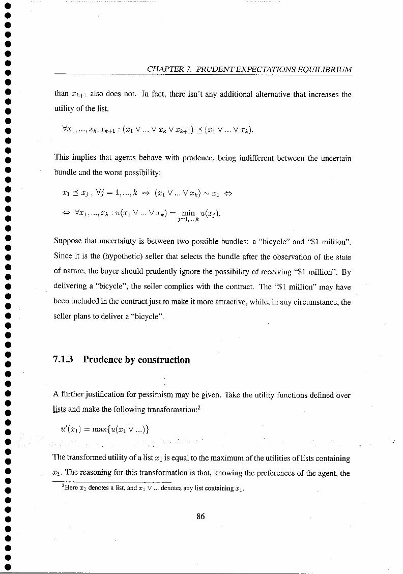
CHAPTER 7. PRUDENT EXPECTATIONS EQUILIBRIUM
than xk+1 also does not. In fact, there isn't any additional alternative that increases the
utility of the list.
\/Xi,...,Xk,xk+i : (xi V... V xkVxk+1) ^ (xi V ... Va*).
This implies that agents behave with prudence, being indifferent between the uncertain
bundle and the worst possibility:
x% ■< Xj , Vj = 1,..., k =4> (xi V ... V xk) ~ xi <=>
■& Vxi, ...,xk : u(x\ V ... V xk) = min uixA. j=i,...,fc
J /
Suppose that uncertainty is between two possible bundles: a "bicycle" and "$1 million".
Since it is the (hypothetic) seller that selects the bundle after the observation of the state
of nature, the buyer should prudently ignore the possibility of receiving "$1 million". By
delivering a "bicycle", the seller complies with the contract. The "$1 million" may have
been included in the contract just to make it more attractive, while, in any circumstance, the
seller plans to deliver a "bicycle".
7.1.3 Prudence by construction
A further justification for pessimism may be given. Take the utility functions defined over
lists and make the following transformation:2
u'(xi) = max{u(xi V ...)}
The transformed utility of a list x\ is equal to the maximum of the utilities of lists containing
X\. The reasoning for this transformation is that, knowing the preferences of the agent, the 2Here x\ denotes a list, and xj V ... denotes any list containing x\.
86

CHAPTER 7. PRUDENT EXPECTATIONS EQUILIBRIUM
seller may sell xx as the most preferred list which contains xx. In any case, xx will be
delivered. So, v! is a kind of virtual utility of xx. Observe that under the assumption of
prudent preferences, we have u' = u.
Under this framework, notice that if the seller has a product to deliver which is (xt V x2),
then this product cannot have more virtual utility to the seller than either xx or x2. The
seller has to sell this product as list containing (xx V x2), which cannot have more virtual
utility than xx or x2:
(A) u'{xi V x2) = max{u(a;i V x2 V ...)} < min{it'(a?i), u'(x2)}.
Assume that, when faced with the possibility of receiving the list xx or the list x2, the agents
do not prefer to receive the worst possibility with certainty.
u(xx V x2) > mm{u(xx),u(x2)}.
Denote by y a list containing both xx and x2 that maximizes utility, that is, such that
u(y) = u'(xi V x2). Similarly, find the list yx such that u(yx) = u'{xx) and the list y2
such that u(y2) = u'(x2). Since y is a maximizer:
u(y) > u(yxVy2) > mm{u(yi),u(y2)} & u'(xxVx2) > mm{u'(xx),u'(x2)}.
Together with (A), this implies that the transformed preferences are prudent:
u'(xx V x2) = mm{u'(xx),u'(x2)}.
So, over the (virtual) preferences u', prudence seems to be a weak restriction. But for
the transformation to be applied in the context of our results, it is necessary that the
transformation from u to u' preserves continuity, weak monotonicity, and concaveness.
Continuity and weak monotonicity should normally be preserved. The assumption of
concaveness is harder to interpret.
87

CHAPTER 7. PRUDENT EXPECTATIONS EQUILIBRIUM
u'(Xxx + (1 - X)x2) > \u'(xx) + (1 - X)u'{x2) <*
ma,x{u(Xxi + (1 - A)z2 V ...)} > Amax{u(a:1 V ...)} + (1 - A) max{u(x2 V ...)}.
Having a the product (lottery) Xxx + (1 - A)a;2, the seller can sell it as one of the elements
of a list with utility u'(Xxi + (1 - X)x2). Alternatively, the product can be sold as a lottery
between two lists. One that gives u'(xx), and other that gives u'(x2). Concaveness means
that the buyer weakly prefers the first "package".
If these hypothesis are accepted, prudence is ensured by construction.
7.1.4 Prudence as realism
It seems pessimistic to consider that the utility of a "blue bicycle or red bicycle" is equal
to the worst possibility. The seller should deliver the bundle that has the lowest (ex post) value. But it is a big step from the lowest value to the lowest utility for the buyer. So, in
some situations, prudence may be seen as overly conservative. But when the interests of
the seller and the buyer are perfectly aligned, then the buyer should reasonably expect the
worst possibility.
If the bundles are actually portfolios that give a money return, and the bicycle is what the
agent buys with this money, then it is perfectly realistic to consider that the minimum is
going to be delivered. Suppose that there is a second round of trade. In this case, agents
should evaluate the utility of bundles (portfolios) by their indirect utility. Sellers do exactly
the same valuation. In this case, the seller always delivers the bundle with the lowest (ex-
post) value, so this worst bundle is what the buyer always receives.
88

CHAPTER 7. PRUDENT EXPECTATIONS EQUILIBRIUM
7.2 General Equilibrium with Uncertain Delivery
The model of the economy with uncertain delivery is actually the model known as a
differential information economy, but now agents are allowed to select non-measurable
consumption bundles. The economy extends over two time periods. In the first, agents
trade their state-contingent endowments for state-contingent bundles. In the second period
agents receive (and consume) one of the bundles that corresponds to a state that the agent
does not distinguish from the actual state of nature. This is equivalent to assume that agents
select measurable lists.
Trade takes place in markets for contingent goods, where agents select bundles which do
not need to be measurable with respect to their information. These bundles are, in turn,
equivalent to lists. For example, suppose that Q, = {ui,u)2,u>3}, and that the agent's
partition of information is Pi = {{ui,u2}, {^3}}- The agent may select a consumption
bundle that is not Pj-measurable, x = (xi,x2,xs). Observing {UJI,UJ2}, the agent has
the right to receive Xi or x2, while the observation of u>3 ensures consumption of x3. So,
from the perspective of the agent, this bundle is seen as the following Pi -measurable list:
x - {{xi Vx2),(xi V x2),x3].
Nothing essential is lost by considering that the choice is between non-measurable bundles
instead of measurable lists. For convenience, restrict lists to a maximum of K alternatives,
and divide each state of nature into K identical sub-states. This transformed economy is
equivalent to the original economy. But now agents can select any consumption list with a
maximum of K alternatives for each original state of nature, simply by selecting different
bundles in the K sub-states.
Consider a finite number of agents, commodities and states of nature. In the economy with
uncertain delivery, £ — (d, Ui, Pi, Çi)™=1, for each agent i:
89

CHAPTER 7. PRUDENT EXPECTATIONS EQUILIBRIUM
- A partition of Cl, Pu represents the private information. Sets that belong to Pi are
denoted A{. The set of states of nature that agent i does not distinguish from uk is
denoted Pi(uk).
- Agents assign subjective probabilities to the different elementary events that they
observe. To each set A\ G Pi corresponds a prior probability q\, with ]T. qf = 1.
- Preferences are the same in undistinguished states, represented by the Von Neumann-
Morgenstern (1944) utility functions u\ : IRf -» IR+, which are assumed to be
continuous, weakly monotone and concave.
- The initial endowments are constant across undistinguished states, and strictly
positive: e{ > 0 for all j .
After receiving information, agent i knows that the state of nature that occurred belongs to
A\, one of the sets of Pit In this interim stage, the agent is sure of receiving one of the
bundles Xi(u) with u € A\. Under prudent expectations, the utility that the agent expects
is the lowest:
vl(xi) = minul (Xi(u)).
The objective function, that may be designated as prudent expected utility, is simply the
expected interim utility:
Ufa) = J2 d vlfa). A{ePi
From the properties of the state-dependent utility functions, u{, it is shown below that the
prudent expected utility function is also concave.
90

CHAPTER 7. PRUDENT EXPECTATIONS EQUILIBRIUM
Ui(\xt + (i - %,) = ]T d vi(^ + (! - A)yO = 4 eft
= J ] Í ram{ul{\Xi{u) + (1 - A ) ^ ) ) } > A Í ^ <***
> J2 «í min.íAtí XiCu;)) + (1 - A ^ f o M ) } >
> J ] gf mm{A^(u / ) )} + V gj min{(l - A)uJ (#(«;))} M** ^ A>ePt ^
= A ^ g > ^ ) + ( l - A ) X)«?«í ( t t ) =
= XUi(Xi) + (1 - A)^(W).
With this property, we can interpret the model of Arrow-Debreu to cover the case of an
economy with uncertain delivery in which agents are prudent. The economy with uncertain
delivery is transformed in the Arrow-Debreu economy, £AD = (et, t/;)?=1, where, for each
agent v?
- The utility function, Ut : IR+ -* IR+, is continuous, weakly monotone and concave.
- The vector of initial endowments, e{ 6 IR+ , is strictly positive.
We impose exact feasibility with free disposal:
5 > < ] T e & Vu:J2x(u)<J2e(u).
We normalize the price functions to the simplex of Rni, that is:
weûk=i,..,,i
3Note that if x is Pt-measurable, then prudent expected utility is equal to classical expected utility. If agents are perfectly informed this obviously occurs. So, with symmetric information, the transformed model is equivalent to the classical model of Arrow and Debreu.
91

CHAPTER 7. PRUDENT EXPECTATIONS EQUILIBRIUM
The "budget set" of agent i is given by:
Bi(p,ei) = < Xi € IRn', such that ^p{uj)xi{uj) < ^p(w)e i(a;) I. I a a )
A pair {jp*, x*) is a competitive equilibrium with prudent expectations if p* is a price system
and x* = (x*,..., x*n) is a feasible allocation such that, for every i, x* e IR+ maximizes Ui
on Bi(p*,ei).
Private information is introduced in the model of Arrow and Debreu by a transformation
of the preferences. This transformation preserves the properties of continuity, weak
monotonicity and concaveness. Everything else in the model remains unchanged.
Therefore, several classical results still hold: existence of core and competitive equilibrium,
core convergence, continuity properties, etc.4
7.3 Characteristics of Equilibrium
On the measurability of utility
In this extended Arrow-Debreu model, competitive equilibrium allocations are characterized by the fact that in states of nature that an agent does not distinguish, the utility of the contingent bundles tends to be the same. Instead of imposing a measurability
4This framework also allows the analysis of continuity properties of equilibrium with respect to
information as a problem of continuity with respect to preferences, which was settled by Hildenbrand &
Mertens (1972).
92

CHAPTER 7. PRUDENT EXPECTATIONS EQUILIBRIUM
restriction on the consumption space, as in Radner (1968) and Yannelis (1991), we see the
weaker restriction of measurable utility arising naturally in our model.
Actually, if equilibrium prices aren't strictly positive, then some equilibrium allocations
may have non-measurable utility. But, removing a free component of excess supply, we can
obtain consumption vectors with measurable utility, which are also equilibrium allocations.
The following results make this precise.
Theorem 11 Let (x*,p*) be a competitive equilibrium with prudent expectations. Then,
for each agent i, x* = y* + z» with y* having measurable utility, and Zi being "free".
Precisely:
y* G IR™ and such that: J G PÎ(LO) =* <(y*(u;)) = uf(y*(u;')).
Zi G IR™ and such that: p* ■ z{ = 0.
Proof. Recall that for any u>' G Pi{u), preferences are equal: v% = uf. Now suppose
that for some u' G P<(w), we have different utilities, that is: uf(x*(u)) > uf(x?(u')).
Then, there exists some 5 < 1 such that uf(5 ■ x*(u)) = v%(x*(u')). Whenever this occurs,
modify the allocation accordingly to obtain y* < x*. This allocation has measurable utility.
If y* belongs to the interior of the budget set, there exists a positive e such that the allocation
(1 + e) • y* belongs to the budget set and has higher utility than x*. In this case, x* would
not be an equilibrium allocation, and we would have a contradiction. Therefore, y* is not
in the interior of the budget set, that is: z{ = x* - y* is such that p* ■ Zi = 0. QED
With utility being measurable with respect to the information of the agents, prudent
expected utility is equal to expected utility, for any prior probabilities over states of nature
consistent with the given prior probabilities over observed events.
93

CHAPTER 7. PRUDENT EXPECTATIONS EQUILIBRIUM
Y^ 4 min u\ (XÍ(U)) = Y^ tf < (Xi(w)). AlePi 1 w e n
The pair (y*,p*) is also a competitive equilibrium with prudent expectations. But, since y*
has measurable utility, the prudent behavior is not shown to have been unjustified. Prudent
expected utility is equivalent to the classical expected utility, so the prudent expectations
were, in a certain sense, self-fulfilled. A natural refinement of the concept of equilibrium
is to demand expectations to be fulfilled, that is, to restrict equilibrium to allocations with
measurable utility.
A pair (y*,p*) is a "prudent expectations equilibrium" if p* is a price system and y* =
(y*,...,y*) is a feasible allocation such that, for every i, y* G IR+ maximizes Ui on
Bi(p*, ei) with Ui(y*) being Pi -measurable.
Corollary 1 Given any competitive equilibrium with prudent expectations, (x*,p*), there
exists a prudent expectations equilibrium, (y*,p*) under the same price system (y* as
defined in Theorem 1).
Proof. The allocation y* has the same prudent expected utilities as the equilibrium
allocation x*: Ui(y*) = Ui(x*), for all i. Under the price system p*, both allocations
cost the same: p* ■ y\ = p* ■ x*, for all i. Thus, y* is also allowed by each agent's budget
restriction, and maximizes utility. Furthermore, since y* < x*, y* is feasible. QED
An important consequence is the existence of equilibrium allocations with measurable
utility. If instead of forcing agents to consume the same in states that they do not distinguish,
as in Radner (1968) and Yannelis (1991), we force them to consume bundles with the same
utility, equilibrium existence is preserved.
Corollary 2 There exists a prudent expectations equilibrium.
94

CHAPTER 7. PRUDENT EXPECTATIONS EQUILIBRIUM
There exists a competitive equilibrium of the Arrow-Debreu economy, so this is an obvious
consequence of Corollary 1.
From Theorem 1, it is straightforward that with strictly positive prices, then z = 0 and
x* = y*. That is, all competitive equilibrium with prudent expectations have measurable
utility. Any conditions that guarantee strict positivity of prices are sufficient to guarantee
that equilibrium allocations are prudent expectations equilibria.
On incentive compatibility
Remember the seller that offered the game:
"/ will toss a coin. If the result is heads, you receive a blue bicycle; if it is tails, you
receive a red bicycle."
If the agent is indifferent between the two colors, the impossibility of observing the state of
nature is not a problem. The agent does not fear being "tricked", because the delivery of a
bicycle is guaranteed.
After receiving private information, the agent can prove that the state of nature belongs to,
for example, A]. Whatever the state in A\, the bundles that are supposed to be delivered
have the same utility. So, agents cannot be deceived to receive consumption bundles with
lower utility. Contracts can be enforced and issues of incentive compatibility do not arise.
In sum, the consideration of contracts for uncertain delivery allows us to relax in a natural
way the measurability assumption, while preserving (trivial) incentive compatibility. This
enlarges the space of allocations, improving the efficiency of exchange, relatively to
economies in which consumption has to be measurable with respect to private information.
95

CHAPTER 7. PRUDENT EXPECTATIONS EQUILIBRIUM
On welfare
Compared with measurable consumption, measurable utility is less restrictive, as it allows
agents to select different consumption bundles in order to take advantage of variations in
prices across states that they do not distinguish.
Theorem 12 Let (x*,p*) be a competitive equilibrium with prudent expectations.
u/ € Piiyi) =* p*(u) ■ x*{u) < p*(u) ■ X*(UJ').
Proof. Suppose that for some u' e Pi(to), we had p*(u) ■ x*(u) > p*(u) • x*(u').
Designate by y{ a modified bundle with y*(u) = x*(ui') being the only difference relatively
to x*. This bundle has the same utility and allows the agent to retain some income. There
exists a positive e such that (1 + e) • y» belongs to the budget set and has higher utility than
X*. Contradiction! QED
In spite of the penalization implied by prudence, in equilibrium, prudent expected utility is
higher in the sense of Pareto than that which is attainable under the classical restriction of
equal consumption in states of nature that are not distinguished.
Theorem 13 Let (x*,p*) be an equilibrium in the sense ofRadner (1968),
There are Pareto optima of the economy with uncertain delivery, z, such that UÍ(ZÍ) >
Ui(x*), for every agent. The improvement may be strict (see section 3).
Proof. The proof is straightforward. If (x*,p*) is an equilibrium in the sense ofRadner
(1968), the allocation x* is still feasible in the economy with prudent expectations. QED
If preferences are strictly concave and relative prices vary across states that at least one
agent does not distinguish, then, in a competitive equilibrium with prudent expectations,
96

CHAPTER 7. PRUDENT EXPECTATIONS EQUILIBRIUM
consumption is not measurable. In these cases, welfare improvements are strict in the sense
of Pareto.
7.4 Cooperative Solutions: the Prudent Cores
Cooperative solutions can be defined in a similar way. Instead of constraining allocations
to be measurable with respect to information, we introduce again the prudent expectations
regarding consumption in undistinguished states.
Remember that the economy with uncertain delivery and prudent expectations was
transformed into an Arrow-Debreu economy. The core of an Arrow-Debreu economy
exists, and we designate it as the "prudent private core".
A coalition S Ç N "privately blocks" an allocation x if there exists (yi)ies such that:
E _—^ Hi < 2_^&% and Ui{yi) > UÍ(XÍ) for every i £ S, where Ui is the prudent expected
ies ies utility of agent i.
The "prudent private core" is the set of all feasible allocations which are not privately
blocked by any coalition. Although coalitions of agents are formed, information is not
shared between them. The prudent expected utility is based only on each agent's private
information.
The prudent private core is very similar to a modified private core where measurable utility
is required instead of measurable consumption. Given an allocation in the prudent private
core, there exists another with the same utility for every agent, which has measurable utility
and requires less resources.
97

CHAPTER 7. PRUDENT EXPECTATIONS EQUILIBRIUM
Theorem 14 LetxePPC{£).
There exists some x' G PPC (S) such that, Vz = 1,..., n:
a) A < Xi,-
b) Uifâ) = Ui(xi);
c) Ui(x[) is Pi-measurable.
Proof. If Uiixi) isn't Pj-measurable, we can multiply the Xi(u) that have higher utilities
in each element of Pi by a factor smaller than 1 to obtain a modified allocation with
measurable utility. These higher utilities are not taken into account in the calculation of
prudent expected utility, because only the worst outcome is considered. Therefore, expected
utility remains unchanged and this allocation satisfies x\ < Xi. QED
Even being penalized by the prudence, allocations in the prudent private core dominate, in
the sense of Pareto, those in the private core (Yannelis, 1991). The latter are always feasible
in the economy with uncertain delivery, while the converse is not true.
The coarse core and the fine core introduced by R. Wilson (1978), also have correspondent
concepts with prudent expectations: the "prudent coarse core" and the "prudent fine core".
To find the prudent coarse core, consider a strong block, in which prudence is based on
common information.
A coalition S Ç N strongly blocks an allocation x if there exists (yi)ies such that:
}Vi <"^2ei ^ d U°s(yi) > Ufs(xi) for every i G S, where Ufs is the "strongly S-ies ies
prudent expected utility" of agent i in the coalition S. The interim utility for agent i in
coalition S is calculated using the minimum utility across states that the coalition cannot
distinguish using only the common information among the members.
98

CHAPTER 7. PRUDENT EXPECTATIONS EQUILIBRIUM
To find the prudent fine core, use a weak notion of block, based on pooled information.
A coalition S Ç N weakly blocks an allocation x if there exists (yi)ies such that:
Y, Vi ^ Yle* a n d Ui!s(Vi) > U?s(xi) for every i G S, where U% is the "weakly S-prudent ies ies expected utility" of agent i in the coalition S. The interim utility for agent i in coalition S is calculated using the minimum utility across states that the coalition cannot distinguish
using the pooled information of its members.
In any case, welfare is improved in the prudent cores.
7.5 Concluding Remarks
We model economies with private information and uncertain delivery, in which agents are
assumed to follow a simple rule-of-thumb: to bo prudent. The model of Arrow-Debreu can
be reinterpreted to cover this situation, therefore, many classical results still hold: existence
of core and equilibrium, core convergence, continuity properties, etc.
The inclusion of contracts for uncertain delivery allows agents to improve their welfare. In
any case, they are better off relatively to allocations with measurable consumption.
Expecting to receive the worst of the possibilities contracted, agents behave prudently by
selecting bundles with the same utility for consumption in states that they do not distinguish.
Instead of consuming the same, as in Radner (1968) and Yannelis (1991), agents consume
bundles with the same utility.
99

CHAPTER 7. PRUDENT EXPECTATIONS EQUILIBRIUM
In certain situations, such prudence may not be appropriate, but there are others in which
it is absolutely justified. For example, if there is a second round of trade, agents should
evaluate portfolios by their indirect utility. In this case, the seller always delivers the bundle
with the lowest value.
While an intuition for the concept of rational expectations equilibrium was the idea that
"agents cannot be fooled'', in the prudent expectations equilibrium it is the market that
cannot be fooled. Agents use a rule of thumb which is related to Murphy's law: "if anything
can go wrong, it will".
An advantage of this concept with respect to the rational expectations equilibrium is that it
is useful to have more information. Markets for information can be studied with two-stage
games: in the first stage, agents trade information; in the second, they maximize prudent
expected utility. This way, economic insights on information production and dissemination
could be obtained.
Real economic agents follow simple rules of decision, instead of making huge amounts of
calculations (Tversky and Kahneman, 1974). This further justifies the study of equilibrium
with agents constructing expectations in a simple way.
100

Appendix A
The Expected Utility Hypothesis
An act is a mapping of a probability space (0,, T, n) into a space of consequences, C. This
may be simply IR, representing utility. Each act induces a probability measure q on (IR, B),
where B is the Borelian a-algebra.
For simplicity, assume a finite number of possible states of nature: Q = {uii,..., WQ}. The
cr-algebra T consists of the subsets of CI.
Under the expected utility hypothesis, there exist functions u(-) that are nondecreasing
and bounded.1 such that it is possible to represent the rational behavior of an agent by the
maximization of: n
'Non-boundedness of u(-) leads to the St. Petersburg paradox, according to which agents are willing to pay an infinite value to play a game that pays 2n units of utility if a head appears for the first time on the nth
toss.
101
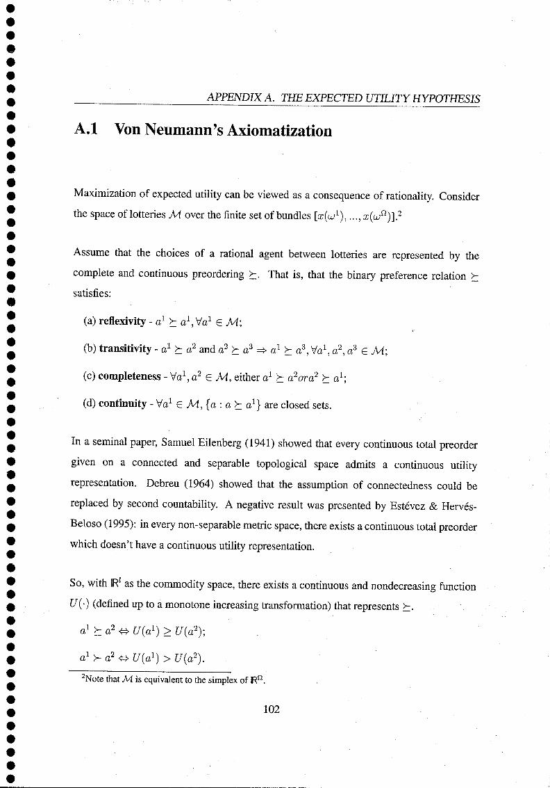
APPENDIX A. THE EXPECTED UTILITY HYPOTHESIS
A.l Von Neumann's Axiomatization
Maximization of expected utility can be viewed as a consequence of rationality. Consider
the space of lotteries M over the finite set of bundles [^(w1),..., x(un)].2
Assume that the choices of a rational agent between lotteries are represented by the
complete and continuous preordering y. That is, that the binary preference relation y
satisfies:
(a) reflexivity - a1 y a1, Va
1 € M;
(b) transitivity - a1 £ a2 and a2 y a
3 =*► a1 y a
3, Va
1, a2
, a3 G M;
(c) completeness - Va1, a2 e M, either a1 y a2ara2 y a1;
(d) continuity - Va1 G A4, {a : a y a1} are closed sets.
In a seminal paper, Samuel Eilenberg (1941) showed that every continuous total preorder
given on a connected and separable topological space admits a continuous utility
representation. Debreu (1964) showed that the assumption of connectedness could be
replaced by second countability. A negative result was presented by Estévez & Hervés-
Beloso (1995): in every non-separable metric space, there exists a continuous total preorder
which doesn't have a continuous utility representation.
So, with IRJ as the commodity space, there exists a continuous and nondecreasing function
£/(■) (defined up to a monotone increasing transformation) that represents K
^ha2^ U{al) > U(a2);
alya2& U(al) > U(a2). 2Note that M is equivalent to the simplex of IRn.
102
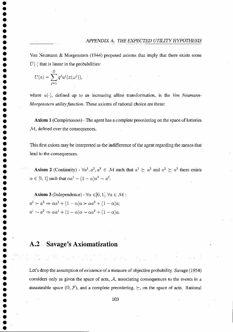
APPENDIX A. THE EXPECTED UTILITY HYPOTHESIS
Von Neumann & Morgenstern (1944) proposed axioms that imply that there exists some
[/(•) that is linear in the probabilities: Q
U{a)=*Tqjuj(x{ujj)),
where u(-), defined up to an increasing affine transformation, is the Von Neumann-
Morgenstern utility function. These axioms of rational choice are three:
Axiom 1 (Completeness) - The agent has a complete preordering on the space of lotteries
M., defined over the consequences.
This first axiom may be interpreted as the indifference of the agent regarding the means that
lead to the consequences.
Axiom 2 (Continuity) - Va1, a2, a3 G M such that a1 y a2 and a2 y a3 there exists
a e [0,1] such that aa1 + (1 - a)a3 ~ a2.
Axiom 3 (Independence) - Va e]0,1[, Va € M :
a1 >- a2 =>■ aa1 + (1 - a)a y aa2 + (1 — a)a;
a1 ~ a2 =» aa1 + (1 — a)a ~ aa2 + (1 — a)a.
A.2 Savage's Axiomatization
Let's drop the assumption of existence of a measure of objective probability. Savage (1954)
considers only as given the space of acts, A, associating consequences to the events in a
measurable space (O, T), and a complete preordering, y, on the space of acts. Rational
103

APPENDIX A. THE EXPECTED UTILITY HYPOTHESIS
behavior under uncertainty is specified by seven axioms on this preordering. From these
axioms, Savage derives a subjective probability distribution and an utility function such that
the preordering is represented by the expected value of this function.
Define first the conditional preferences. Let E e F be an event. Comparison between acts
depends only of the consequences when E occurs:
a h\E a' =*■ ã y ã',
with ueE^ õ(w) = a(u) A ã'(co) = a'(u), and u £ E => ã(u) = ã'{u).
Axiom 1 (Existence) - Conditional preferences exist.
For any x <E C, the constant act ax is defined by: ax = x, \/u e Q.
Axiom 2 (Constant acts) - \fx € C, ax € A.
There may not be such acts, it is sufficient to imagine their existence.
Axiom 3 (Independence) - If E ^ 0, ax t\E a* & x h x'.
Let E,E' e T be two events, and x,x' £ C two consequences with x y x'. Construct acts a, a' € A as follows:
LO G E =*> a(uj) = x and u £ E =4> a(u) = x'
u e E' =>• a'(uj) = a; and u <£ E' =*► a'(a>) = a;'
If a X a', we say that the qualitative probability of E is at least as great as that of E': EhE'.
104

APPENDIX A. THE EXPECTED UTILITY HYPOTHESIS
So it is possible to infer subjective probabilities from the preordering over lotteries. For the
relation y to be well defined, we need:
Axiom 4 (Comparability) - All the events are comparable in qualitative probability.
And we also need some technical axioms.
Axiom 5 (No indifference) - 3a, a' € A such that a y a' V a' y a.
Axiom 6 (Continuity - implies infinite Ù) - If a y a', for any x G C there exists a finite
partition of D, such that if a or a' is modified on an event of the partition so that x becomes
the consequence in this event, the strict preference of a over a' is preserved.
Axiom 7 (Independence II) - Let a £ A. Then:
a' h\E aa(u}) Vui G E implies a' y_\E a;
aa{u) y_\E a' Va; € E implies a >z\E a'.
These seven axioms allowed Savage (1954) to obtain the following result.
Theorem Given axioms 1-7, there exists a unique probability measure \i defined on
(fi, T), and a continuous, nondecreasing and bounded function u(-) defined up to an affine
transformation such that:
aha'^ Jau(a(u}))dfi(u) > fnu(a'(u))dii(uj).
p is such that E"yE-& /i(E') > y.{E), and it is called the agent's subjective probability.
105

APPENDIX A. THE EXPECTED UTILITY HYPOTHESIS
A.3 The value of information
Consider a rational decision maker with imperfect information, seeking to maximize
expected utility:
max / uw(a) <f du. « * Lea
Let a* be the solution of this problem, and let P be the partition of information of the agent.
With the agent revising expectations according to the Theorem of Bayes, after receiving its
information, Pj e P, the (posterior) beliefs are:
Pr{u\Pj) = 0 , ifu<£Pj;
Pr(u\Pj) = £ <t jf u c pj l I ' P i 9" dw g(Pi) ' U U fc ^ •
For each Pj e P, the agent solves the problem:
max / uu(a) Pr(ui\Pj) dw\ aeA Ju>m
Which is equivalent to:
max / u^ia) q" dio = V(Pj).
So, the value of having the information structure P can be estimated, for finite and infinite
partitions, as:
i
or U(P,q,u(A))= [v(Pj)q(pJ)dj. Jj
106

References
Akerlof, G. (1970). The market for 'lemons': Quality, uncertainty and the market
mechanism. Quarterly Journal of Economics, 84, 488-500.
Aliprantis, C , & Border, K. (1999). Infinite dimensional analysis (2 ed.). New York:
Springer.
Allen, B. (1983). Neighboring information and distribution of agent characteristics under
uncertainty. Journal of Mathematical Economics, 12, 63-101.
Allen, B. (1990). Information as an economic commodity. American Economic Review,
80(2), 268-273.
Allen, B., & Yannelis, N. (2001). Differential information economies: Introduction.
Economic Theory, 18, 263-273.
Arrow, K., & Hurwicz, L. (1972). An optimality criterion for decision making under
ignorance. In Uncertainty and expectations in economics. Oxford: Basil Blackwell.
Arrow, K. J. (1953). The role of securities in the optimal allocation of risk-bearing.
Econometrie, 41-48.
Arrow, K. J., & Debreu, G. (1954). Existence of equilibrium for a competitive economy.
Econométrica, 22(3), 265-290.
107

REFERENCES
Aumann, R. (1964). Markets with a continuum of traders. Econométrica, 32, 39-50.
Aumann, R. (1966). Existence of competitive equilibria in markets with a continuum of
traders. Econométrica, 34, 1-17.
Balder, E., & Yannelis, N. (2005). Continuity properties of the private core, forthcoming
in Economic Theory.
Boylan, E. (1971). Equiconvergence of martingales. Annals of Mathematical Statistics, 42,
552-559.
Coase, R. (1960). The problem of social cost. Journal of Law and Economics, III, 1-40.
Cotter, K. (1986). Similarity of information and behavior with pointwise convergence
topology. Journal of Mathematical Economics, 15, 25-38.
Cotter, K. (1987). Convergence of information, random variables and noise. Journal of
Mathematical Economics, 16, 39-51.
Cournot, A. (1838). Recherches sur les principes mathématiques de la théorie des
richesses. Paris: Hachette.
Debreu, G. (1959). Theory of value. New York: Wiley.
Debreu, G. (1964). Continuity properties of paretian utility. International Economie
Review, 5, 285-293.
Debreu, G., & Scarf, H. (1963). A limit theorem on the core of an economy. International
Economic Review, 4, 235-246.
Edgeworth, F. (1881). Mathematical psychics. London: KeganPaul.
Eilenberg, S. (1941). Ordered topological spaces. American Journal of Mathematica, 63,
39-45.
108
REFERENCES
Einy, E., Haimanko, O., Moreno, D., & Shitovitz, B. (2005). On the continuity
of equilibrium and core correspondences in economies with differential information.
Economic Theory, 26(4), 793-812.
Einy, E., Moreno, D., & Shitovitz, B. (2001). Competitive and core allocations in large
economies with differential information. Economic Theory, 18, 321-332.
Estévez, M., & Hervés-Beloso, C. (1995). On the existence of continuous preference
orderings without utility representations. Journal of Mathematical Economics, 24, 305-
309.
Forges, E, Heifetz, A., & Minelli, E. (2001). Incentive compatible core and competitive
equilibria in differential information economies. Economic Theory, 18, 349-365.
Forges, E, Minelli, E., & Vohra, R. (2002). Incentives and the core of an exchange
economy: a survey. Journal of Mathematical Economics, 38, 1-41.
Glycopantis, D., Muir, A., & Yannelis, N. (2001). An extensive form interpretation of the
private core. Economic Theory, 18, 293-319.
Grossman, S., & Stiglitz, J. (1980). On the impossibility of informationally efficient
markets. American Economic Review, 70, 393-408.
Hardin, G. (1968). The tragedy of the commons. Science, 162, 1243-1248.
Harsanyi, J. (1967). Games with incomplete information played by 'bayesian' players
(parts i, ii and iii). Management Science, 14(3, 5 and 7), 159-182, 320-324, 486-502.
Hayek, F. (1945). The use of knowledge in society. American Economic Review, XXXV(4),
519-530.
Hildenbrand, W. (1970). On economies with many agents. Journal of Economic Theory, 2, 161-188.
109

REFERENCES
Hildenbrand, W., & Mertens, J. (1972). Upper hemi-continuity of the equilibrium-set
correspondence for pure exchange economies. Econométrica, 40(1), 99-108.
Hirschleifer, J., & Riley, J. (1979). The analytics of uncertainty and information - an
expository survey. Journal of Economic Literature, VXII, 1375-1421.
Hurwicz, L. (1972). On informationally decentralized systems. In R. Radner & B. McGuire
(Eds.), Decision and organization. Amsterdam: North-Holland.
Isnard, A. (1781). Traité des richesses. London and Lausanne: François Grasset.
Jevons, W. (1871). The theory of political economy. London.
Kannai, Y. (1970). Continuity properties of the core of a market. Econométrica, 38(6),
791-815.
Koutsougeras, L., & Yannelis, N. (1993). Incentive compartibility and information
superiority of the core of an economy with differential information. Economic Theory,
3, 195-216.
Krasa, S., & Shafer, W. (2001). Core concepts in economies where information is almost
complete. Economic Theory, 18,451-471.
Laffont, J.-J. (1986). The economics of uncertainty and information. Cambridge: MIT
Press.
Makowsky, L., & Ostroy, J. (2001). Perfect competition and the creativity of the market.
Journal of Economic Literature, XXXIX(2), 479-535.
McKenzie, L. (1954). On equilibrium in graham's model of world trade and other
competitive systems. Econométrica, 22(2), 147-161.
Menger, C. (1871). Principles of economics. Vienna.
110
REFERENCES
Muth, J. (1961). Rational expectations and the theory of price movements. Econométrica,
29(3), 315-335.
Nash, J. (1950). Equilibirum points in n-person games. Proceedings of NAS, 36, 48-49.
Pareto, V. (1906). Manual of political economy. Milano.
Prescott, E., & Townsend, R. (1984a). Pareto-optima and competitive equilibria with
adverse selection and moral hazard. Econométrica, 52, 21-45.
Prescott, E., & Townsend, R. (1984b). General competitive analysis in an economy with
private information. International Economic Review, 25, 1-20.
Radner, R. (1968). Competitive equilibrium under uncertainty. Econométrica, 36(1), 31-58.
Radner, R. (1982). Equilibrium under uncertainty. In (Vol. II, chap. 21). Amsterdam:
North-Holland.
Riley, J. (2001). Silver signals: Twenty-five years of screening and signalling. Journal of
Economic Literature, XXXIX(2), 432-478.
Rothschild, M., & Stiglitz, J. (1976). Equilibrium in competitive insurance markets: An
essay on the economics of imperfect information. Quarterly Journal of Economics, 90,
629-649.
Savage, L. (1954). The foundations of statistics. New York: Wiley.
Schmeidler, D. (1980). Walrasian analysis via strategic outcome functions. Econométrica,
48(1), 1585-1593.
Schmeidler, D. (1989). Subjective probability and expected utility without additivity.
Econométrica, 57(3), 571-587.
I l l
REFERENCES
Schumpeter, J. (1911). The theory of economic development: An inquiry into profits,
capital, credit, interest and the business cycle. Leipzig: Duncker und Humblot.
Serrano, R., Vohra, R., & Volij, O. (2001). On the failure of core convergence in economies
with asymmetric information. Econométrica, 69, 1685-1696.
Shapiro, C , & Stiglitz, J. (1984). Equilibrium unemployment as a worker discipline device.
American Economic Review, 74(3), 433-444.
Smith, A. (1776). An inquiry into the nature and causes of the wealth of nations. London:
Routledge.
Spence, A. (1973). Job market signalling. Quarterly Journal of Economics, 87, 355-374.
Stigler, G. (1961). The economics of information. Journal of Political Economy, 69,
213-225.
Stiglitz, J., & Weiss, A. (1981). Credit rationing in markets with imperfect information.
American Economic Review, 71(3), 393-410.
Tversky, A., & Kahneman, D. (1974). Judgement under uncertainty: heuristics and biases.
Science, 185, 1124-1131.
Von Neumann, J., & Morgenstern, O. (1944). Theory of games and economic behavior.
Princeton: Princeton University Press.
Walras, L. (1874). Eléments d'économie politique pure, ou théorie de la richesse sociale.
Lausanne: Corbaz.
Wilson, C. (1980). The nature of equilibrium in markets with adverse selection. Bell
Journal of Economics, 11(1), 108-130.
Wilson, R. (1978). Information, efficiency, and the core of an economy. Econométrica, 46,
807-816.
112

REFERENCES
Yannelis, N. (1991). The core of an economy with differential information. Economic
Theory, 1, 183-198.
113


![Modelagem e Simulação de Processossistemas.eel.usp.br/docentes/arquivos/5817066/LOQ4013/Reatores.… · Em Chemical Reactions, clique em (+) e selecione clicando em [Equilibrium].](https://static.fdocumentos.com/doc/165x107/5f357096af289c7e6e12fd4e/modelagem-e-simulao-de-em-chemical-reactions-clique-em-e-selecione-clicando.jpg)