Seleção de Variáveis no Desenvolvimento de Modelos · 25 O artigo a seguir se divide de acordo...

24

Seleção de Variáveis no Desenvolvimento

de Modelos

Variable Selection in Model

Development

Jeffrey S. MorrisonEm artigos ante-

riores, discutimos

diversas questões

relacionadas ao de-

senvolvimento de

modelos de risco

de crédito, entre

elas modelagem de PI (probabilidade de

inadimplência) e de PCI (perda em caso de

inadimplência), validação, testes de des-

gaste, tratamento dado a valores ausentes

e os prós e contras do uso de redes neurais.

Dedicamos pouco tempo ao luxo (e maldi-

ção) com que se deparam muitos analistas

num mundo repleto de sistemas de gestão

de risco da empresa: o excesso de dados.

A maioria dos manuais universitários mal

toca nesse assunto. E isso é compreensível,

já que sua principal preocupação é que o

aluno entenda as propriedades estatísticas

associadas a cada uma das técnicas de mo-

delagem e as importantes premissas em que

se baseiam. Mas, uma vez compreendidas as

questões teóricas, o analista terá que lidar

com questões práticas que podem ser a cha-

ve para o sucesso ou o fracasso de qualquer

projeto. E uma das principais dentre elas é o

desafi o da seleção de variáveis.

In previous ar-ticles, we have discussed various issues related to the development of credit risk mo-dels. Among these

were modeling designs for PD (probabili-ty of default), LGD (loss given default), validation, stress testing, handling mis-sing values, and the pros and cons of using neural networks. Little time was focused on the luxury (and curse) that many analysts face today in a world of enterprise risk management systems — having too much data. Most college text-books give little space in their curriculum for this subject. Understandably so, they are more concerned that the student un-derstands the statistical properties asso-ciated with a particular modeling techni-que and the important assumptions that underlie them. However, after the theore-tical issues are properly understood, the analyst still has to deal with practical is-sues which can make or break the success of any given project. Central among these is the challenge of variable selection.

CAP2_TecCred_57.indd 24CAP2_TecCred_57.indd 24 1/12/2006 10:57:081/12/2006 10:57:08

25

O artigo a seguir se divide de acordo com

seis abordagens comuns freqüentemente as-

sociadas ao problema da seleção de variáveis.

Embora a lista não seja exaustiva, deve dar ao

leitor uma idéia das questões e de alguns dos

prós e contras de cada abordagem.

Métodos de Correlação Um dos métodos mais diretos de reduzir o nú-

mero de preditivas em um problema de regres-

são talvez seja criar alguns critérios de fi ltragem

por regras através de correlações bivariadas e

casadas. Na análise de regressão, é preciso ter

cuidado para não incluir duas ou mais variáveis

preditivas fortemente correlacionadas se qui-

sermos determinar a verdadeira contribuição de

cada uma delas para a variável dependente. Se

as preditivas estiverem por demais relacionadas

entre si, pequenas mudanças dos dados podem

redundar em grandes variações dos coefi cientes

— resultando até mesmo em erros de sinal. Na

literatura estatística isso é chamado de multi-

colinearidade. Uma regra de dedo afi rma que a

multicolinearidade tende a ser um problema se

a correlação aritmética entre duas variáveis for

maior do que a existente entre qualquer uma de-

las e a variável dependente1.

Para usar esse método de redução de variá-

veis, calculamos a correlação de cada variável

preditiva com a outra (correlações casadas) e

com a variável dependente (correlações bivaria-

das). Embora esses cálculos possam ser feitos em

segundos por qualquer pacote de software esta-

tístico e apresentados sob a forma de matriz de

correlação, talvez seja necessário escrever um

programa especial para extrair os membros e fi l-

The following article is divided into a discus-

sion of six common approaches often asso-

ciated with the problem of variable selection.

Although this list is in no way exhaustive, it

should give the reader a fl avor of the issues and

some of the pros and cons for each approach.

Correlation MethodsPerhaps one of the most straightforward ways

of reducing the number of predictors in a regres-

sion problem is to make up some rules-based

screening criteria using bivariate and pairwise

correlations. In regression analysis, you need

to be careful not to include two or more pre-

dictor variables that are highly correlated with

one another if you’re interested in determining

the true contribution of each predictor to your

dependent variable. If predictors have too high

a correlation with one another, slight changes

in the data may result in signifi cant changes

in the coeffi cients – even resulting in incorrect

signs. In the statistical literature, this is kno-

wn as multicollinearity. A rule of thumb states

that multicollinearity is likely to be a problem

if the simple correlation between two variables

is larger than the correlation of either or both

variables with the dependent variable1.

In order to use this method for variable re-

duction, calculate the correlation of each

predictor variable against the other (pairwise

correlations) as well as the correlation of each

with the dependent variable (bivariate corre-

lations). Although these computations can be

done in seconds by almost any statistical sof-

tware package and displayed in the form of a

correlation matrix, it may require a special pro-


26

trá-los por meio de algumas regras pré-estabele-

cidas. Começamos por estabelecer um limite de

correlação casada (digamos, por exemplo, 0,65)

e eliminar todas as variáveis que refl itam infor-

mações duplicadas.

Na Tabela 1, VAR1 e VAR3 são variáveis pre-

ditivas que seriam consideradas por demais

colineares (correlação = 0,72) segundo nossa

regra de correlação de 0,65. Como não quere-

mos incluir as duas variáveis no modelo, es-

colhemos apenas aquela com maior correla-

ção com a variável dependente (DEPV). Nesse

caso, VAR1 vence, com correlação de 0,23 com

a variável dependente (contra a correlação de

-0,21 de VAR3). Usando essa técnica, podemos

eliminar cada vez mais variáveis antes do es-

tágio de regressão, reduzindo o limite de 0,65

para, por exemplo, 0,55 e assim por diante.

Embora esse procedimento possa ser de

fácil implementação, oferece uma visão sim-

plista da seleção de variáveis. Não incorpo-

ra testes de signifi cância estatística e trata

apenas de um par de variáveis por vez. Em

certo ponto é preciso considerar uma abor-

dagem mais multivariada.

Procedimentos de Seleção AutomáticaUma das boas coisas que os computadores

gram to be written to extract its members and

fi lter them through some preset rules. Begin

by setting some pairwise correlation threshold

(say .65, for example) and eliminate those va-

riables that refl ect duplicate information.

In Table 1, VAR1 and VAR3 are predictor va-

riables that would be considered too collinear

(correlation = .72) using our .65 correlation

rule. Since you would not want to include both

as variables in the model, select only the varia-

ble that exhibits the highest correlation with

your dependent variable (DEPV). In this case,

VAR1 is the winner with a correlation with the

dependent variable of .23 (rather than VAR3’s

correlation of -.21). Using this technique,

you could eliminate more and more variables

before the regression stage by lowering this

threshold, say from .65 to .55, etc.

Although this procedure may be easy to im-

plement, it only offers a very simplistic view

of variable selection. It does not incorporate

tests for statistical signifi cance and looks at

only pairs of variables one at a time. At some

point, a more multivariate approach needs to

be considered.

Automatic Selection ProceduresOne of the great things about computers

Matriz de Correlação

Tabela 1

VAR1 VAR2 VAR3 VAR4 DEPV

VAR1 1 0,45 0,72 0,06 0,23

VAR2 - 1 -0,44 0,23 0,12

VAR3 - - 1 -0,23 -0,21

VAR4 - - - 1 0,14

DEPV - - - - 1

Table 1

VAR1 VAR2 VAR3 VAR4 DEPV

VAR1 1 0.45 0.72 0.06 0.23

VAR2 - 1 -0.44 0.23 0.12

VAR3 - - 1 -0.23 -0.21

VAR4 - - - 1 0.14

DEPV - - - - 1

Correlation Matrix


27

nos oferecem é a capacidade de automatizar

muitos procedimentos que tomariam muito

tempo dos analistas. Um desses procedimen-

tos é encontrado na maioria dos pacotes de

regressão estatística: a seleção stepwise. Esse

procedimento — ou conjunto de procedimen-

tos — enfrenta uma das difi culdades do mé-

todo de seleção de variáveis por correlação:

avaliar correlações aritméticas isoladas e não

coletivamente. Na verdade, há muitas varia-

ções desse procedimento — seleção avançada,

retro-seleção e seleção de melhores subcon-

juntos, para indicar apenas algumas.

A técnica de seleção avançada começa sem

quaisquer variáveis no modelo de regressão.

Para cada uma das variáveis preditivas can-

didatas, o método calcula estatísticas F que

refl etem a contribuição que a variável traria

para o modelo se fosse usada. A técnica de

retro-seleção começa calculando as estatís-

ticas F de um modelo com todas as variáveis

preditivas. Em seguida, as variáveis são eli-

minadas uma a uma da regressão, até que to-

das as variáveis remanescentes tenham esta-

tística F superior a um dado limite de corte. O

método stepwise é uma variante da técnica de

seleção adiante, que difere porque as variá-

veis que já se encontram no modelo não per-

manecem nele necessariamente. Como no

método de seleção avançada, as variáveis

são acrescentadas uma a uma com base na

estatística F. Uma vez acrescentada uma va-

riável, o método stepwise avalia as variáveis

presentes no modelo e remove quaisquer que

não atinjam o critério de corte. Na prática,

o analista pode colocar centenas, ou até mi-

is that they automate many procedures

that would take the analyst a long time to

develop otherwise. One of these procedu-

res is found in most statistical regression

software packages — stepwise selection.

This procedure, or collection of procedu-

res, addresses one of the drawbacks of the

correlation method for variable selection:

only evaluating simple correlations one at

a time, not collectively. Actually, there are

a number of variations to this procedure —

forward selection, backward selection, and

best subsets selection just to name a few.

The forward-selection technique begins

with no variables in the regression model.

For each of the candidate predictor varia-

bles, this method calculates F statistics

that refl ect the variable’s contribution to

the model if it were used. The backward eli-

mination technique begins by calculating F

statistics for a model, including all of the

predictor variables. Then the variables are

deleted from the regression one at time un-

til all the variables remaining in the model

have an F statistic at some cutoff threshold.

The stepwise method is a variation of the

forward-selection technique and differs in

that variables already in the model do not

necessarily stay there. As in the forward-

selection method, variables are added one

by one based on the F statistic. Once a va-

riable is added, the stepwise method eva-

luates the variables already included in the

model and removes any that does not make

the threshold criteria. In practice, the

analyst can place hundreds, even thousan-


28

lhares, de variáveis nesses procedimentos de

regressão stepwise, deixando que o software

produza um conjunto mais exíguo de variá-

veis aprovadas.

Embora esses procedimentos existam há dé-

cadas, há um considerável número de oponen-

tes na literatura2. Alguns dos comentários ne-

gativos a respeito dessas técnicas de seleção de

variáveis são:

• Os valores de R2 são artifi cialmente eleva-

dos;

• A seleção de variáveis é fortemente depen-

dente das correlações entre as preditivas;

• Os erros-padrão dos coefi cientes de regres-

são são artifi cialmente baixos;

• Evita a necessidade de teoria fundamental

ou bom entendimento dos dados;

• Quanto maior o número de variáveis can-

didatas, maior a interferência a que o modelo

fi nal pode estar sujeito.

Dentre essas objeções, duas são especialmente

dignas de nota. Em primeiro lugar, um excesso

de correlação entre as variáveis preditivas pode

levar a um conjunto fi nal abaixo do ideal. Assim,

uma solução parcial para esse problema é fazer

uma fi ltragem casada (como vimos anteriormen-

te) das correlações casadas elevadas antes de

usar técnicas de seleção stepwise. Muitas vezes,

usar um limite de corte de 0,75 ou mais ajuda.

Os econometristas, que se concentram na cons-

trução de modelos estatísticos a partir de ten-

dências econômicas, enfatizam a necessidade

de compreender adequadamente os dados e os

comportamentos teóricos em que se apóiam. Por

exemplo, se o preço do produto for uma das va-

ds of variables in these stepwise regression

procedures and the software will produce a

fi nal model with a more condensed set of

variables that end up making the cut.

Although these procedures have been around

for decades, there exist a signifi cant body of

statistical literature that oppose its use2. Some

of the negative comments about these variable

selection techniques include the following…

• R-square values are artifi cially high;

• Variable selection is highly dependent on

the correlations among predictors;

• Standard errors of the regression coeffi -

cients are artifi cially low;

• It avoids the need for underlying theory or

a good understanding of the data;

• The greater the number of candidate va-

riables, the greater the “noise” that can end

up in the fi nal model.

Two of these points are especially no-

teworthy. First, too much correlation

among predictor variables can lead to a

fi nal solution set that may not be optimal.

Therefore, a partial solution to this problem

is to fi rst perform a pairwise screening (as

was mentioned earlier) for high pairwise

correlations before invoking these stepwise

selection techniques. Often, using a cut-off

value of .75 or greater is helpful. Second,

econometricians, whose focus is building

statistical models using economic trends,

stress the need for an adequate understan-

ding of the data as well as the theoretical

behaviors underlying them. For example, if

product price is one of the variables to ex-


29

riáveis explicativa da receita de vendas, então o

sinal do coefi ciente deve ser negativo. Usar um

procedimento de seleção automática pode, fre-

qüentemente, conferir ao analista uma falsa sen-

sação de segurança a respeito da aceitabilidade

do modelo. Mas, bem usadas, essas técnicas po-

dem ajudar o analista a atingir os prazos de seus

projetos.

Principais ComponentesComo vimos, lidar com o problema da corre-

lação entre um enorme número de variáveis

potencialmente preditivas é o principal obstá-

culo à seleção de variáveis. Uma técnica con-

cebida para lidar com essa questão vem sendo

usada há anos por pesquisadores e analistas

dos campos da psicologia e das ciências sociais

— a análise de componentes principais (ACP)3. A

diferença entre essa técnica e a análise de re-

gressão é que a primeira não envolve variável

dependente. A ACP examina apenas as variá-

veis preditivas que pretendemos introduzir no

arcabouço de regressão. O objetivo da análise

de principais componentes é identifi car um

conjunto reduzido de dimensões (fatores) que

melhor explique a estrutura de correlações dos

dados, admitindo que haja sobreposição subs-

tancial. Por exemplo, se tivermos 500 variáveis

em potencial que refl etem dados de diversos

relatórios fi nanceiros, então as dimensões re-

duzidas podem representar um pequeno núme-

ro de fatores, como lucratividade, porte, idade,

setor etc. A idéia é usar essas informações de

duas maneiras: a) como ferramenta explorató-

ria para melhor entender os dados ou b) usar

esses fatores (principais componentes) de al-

plain sales revenue, then the sign of the co-

effi cient should be negative. Using an auto-

matic selection procedure can often give the

analyst a false sense of security about the

model’s acceptability. However, when used

properly, these techniques can substantially

help the analyst meet project deadlines in a

timely fashion.

Principal Components As we have seen, tackling the correlation

problem across a huge number of possibly pre-

dictive variables is the major hurdle in dealing

with variable selection. One technique that is

designed to address this issue has been used

for years by researchers and analysts in the

fi elds of psychology and the social sciences —

principal component analysis (PCA)3. What’s

different about this technique and regression

analysis is that there is no dependent varia-

ble involved. PCA examines only the predictor

variables that you plan to introduce into your

regression framework. The purpose of princi-

pal component analysis is to fi nd a reduced set

of dimensions (factors) that best explain the

correlation structure in your data, assuming

there is substantial overlap. For example, if

you have 500 potential variables refl ecting

data from various corporate fi nancial reports,

then the reduced underlying dimensions mi-

ght end up being a small number of factors

such as profi tability, size, age, industry, etc.

The idea would be to use this information in

possibly two ways — a). as an exploratory tool

to better understand your data or b). to use

these factors (principal components) in some


30

guma maneira direta na regressão.

A análise de principais componentes ana-

lisa as candidatas a variáveis preditivas e as

“descorrelaciona” por meio de uma série de

transformações lineares. O processo cria o

primeiro fator, selecionando um conjunto de

pesos da estrutura de correlação entre todas

as variáveis originais, através de transforma-

ções lineares que expliquem o maior nível de

variação dos dados (espaço preditivo).

Em seguida, é criado um

conjunto de pesos que

explique o segundo maior

nível de variação dos dados

— com a condição de ausên-

cia de correlação com o pri-

meiro conjunto. Assim, se ti-

vermos 100 variáveis originais

a APC criaria 1090 fatores que,

somados, explicariam 100% da

variação do espaço preditivo.

Uma vez concluído o processo,

uma das práticas é abandonar

os fatores de maior ordem,

que contribuem pouco para a

variância explicada em geral

(resultado da colinearidade

ou de duplicidade de informações). Se come-

çarmos com 100 variáveis, não raro desco-

brimos que apenas os primeiros cinco ou dez

fatores (componentes principais) são neces-

sários para explicar 95% do total do conteúdo

informacional dos dados.

Como já vimos, a APC não procura anali-

sar uma variável “dependente”, como se-

ria o caso em uma regressão. Uma maneira

way directly in the regression.

Principal component analysis looks at all the

candidate predictor variables and “de-correla-

tes” them through a series of linear transfor-

mations. The process creates the fi rst factor by

selecting a set of weights from the correlation

structure of all the original variables through

the use of linear transformations that explains

the maximum amount of variation in the data

(predictor space). Next, a se-

cond set of weights are crea-

ted that explains the second

greatest amount of variation

in the data – with the condi-

tion that it has no correla-

tion with the fi rst. Therefo-

re, if you have 100 original

variables, PCA would cre-

ate 100 factors which,

when added up, would

explain 100 percent the

variation in the predictor

space. Once this is com-

pleted, one practice is to

drop the higher order fac-

tors, which contribute little

to the overall explained va-

riance (a result of collinea-

rity or duplicate information). If we start out

with 100 variables, it is not uncommon to fi nd

that only the fi rst fi ve or ten factors (principal

components) are needed to explain 95 percent

of the entire information content in the data.

As we stated earlier, PCA does not attempt

to analyze a “dependent” variable as you

would in regression. One way to provide

A seleção

stepwise

apresenta

muitas

variações.

Stepwise selection

shows many variations.


31

de fornecer esse elo necessário seria usar

os próprios componentes principais (fato-

res) resultantes como variáveis preditivas.

A vantagem dessa abordagem está em que

os componentes principais, por sua própria

natureza, não estão correlacionados. Isso

pode ser feito de duas maneiras. Primeiro,

poderíamos inserir todos os fatores numa re-

gressão stepwise e deixar o algoritmo reduzir

o conjunto de candidatas. Mas ainda haverá

questões estatísticas quanto a essa técnica

de redução de variáveis. Alternativamente,

poderíamos abandonar os fatores que contri-

buem pouco para a variância explicada total,

como já vimos. Nesse caso, acabaríamos com

um conjunto muito menor de fatores poten-

cialmente preditivos. Outra vantagem é que

esse processo pode ser concluído muito ra-

pidamente com softwares como SAS®, SPSS®,

ou muitos outros pacotes estatísticos.

Mas há um problema. Durante o processo de

transformação linear, a variável dependente

não foi considerada. Assim, o processo pode

eliminar involuntariamente dimensões fato-

riais que poderiam trazer uma contribuição

importante para explicar a variável preditiva.

Essa desvantagem, juntamente com o fato de

que é difícil explicar o que signifi cam os valo-

res dos principais componentes, resulta em

que essa técnica não é tão usada no setor de

crédito quando em outros campos.

Agrupamento de VariáveisEmbora a APC tradicional não tenha consegui-

do se fi rmar na área de risco, uma de suas va-

riantes tem ganhado popularidade nos últimos

that necessary linkage would be to use the

resulting principal components (factors) as

predictors themselves in the regression. The

advantage of this approach is that the prin-

cipal components by their very nature are

not correlated with one another. You could

do this in two ways. First, you could enter all

the factors in a stepwise regression and let

the algorithm reduce the candidate set. Ho-

wever, there are still some of the same statis-

tical issues surrounding this variable reduc-

tion technique as before. Alternatively, you

could drop the factors that contributed little

to the overall explained variance as mentio-

ned earlier. In this case, you always end up

with a much smaller candidate set of poten-

tially predictive factors. Another advantage

is that this process can be completed very

quickly with software such as SAS®, SPSS®,

or a host of different statistical packages.

Here’s the drawback. During the linear trans-

formation process, the dependent variable was

never considered. Therefore, the process can

inadvertently clip factor dimensions that might

have otherwise made important contributions

in explaining the prediction variable. This di-

sadvantage, along with the fact that it is diffi -

cult to explain what the values of these princi-

pal components really mean, have resulted in

this technique not being used as heavily in the

credit industry as it is in other fi elds of study.

Variable ClusteringAlthough traditional PCA has not found a

strong foothold in the risk area, a variation

of it has gained popularity in recent ye-


32

anos — o agrupamento de variáveis4. Ao lidar

com centenas ou milhares de variáveis candida-

tas a um modelo de regressão, o agrupamento

de variáveis procura identifi car um conjunto de

agrupamentos de variáveis cujos membros se as-

semelhem aos demais do mesmo agrupamento

e difi ram dos encontrados nos demais agrupa-

mentos (Figura 1).

O software SAS oferece um procedimento

chamado PROC FASTCLUS para realizar esse

tipo de análise5. Com uma enorme variedade

de opções e confi gurações disponíveis para

permitir que o usuário faça o ajuste fi no da

análise, um procedimento de agrupamento

de variáveis pode ser realizado e usado como

ferramenta para recomendar candidatas em

potencial para o modelo de regressão.

Quando temos acesso a muitos dados, podemos

nos ver às voltas com mais de 1.500 variáveis de

crédito. Com tão vasto espaço preditivo, é quase

certo que haja problemas de multicolinearidade.

ars — variable clustering4. In dealing with

hundreds or even thousands of candidate

variables for a regression model, variable

clustering looks to identify a set of varia-

ble clusters whose members look most like

one another within the cluster and least

like those found in the remaining clusters

(Figure 1).

The SAS software offers a procedure cal-

led PROC FASTCLUS to perform this type of

analysis5. With a host of options and default

settings available to allow the user to fi ne

tune the analysis, a variable clustering pro-

cedure can be performed and used as a tool

to recommend potential candidates in your

regression model.

If you have access to a lot of data, you may

be dealing with 1,500 credit variables or

more. With this large of a predictor space, you

are almost guaranteed to have multicollinea-

rity problems. So which variables might make

Figure 1

Agrupamento de Variáveis

Figura 1

Variable Clustering


33

the best candidates for your regression? Gi-

ven the correlation structure of your data, a

variable clustering procedure could give you

1). an educated guess as to the number of

clusters and 2). which variables to choose

from each cluster. Example output using the

SAS software system is given in Figure 2 for

illustrative purposes.

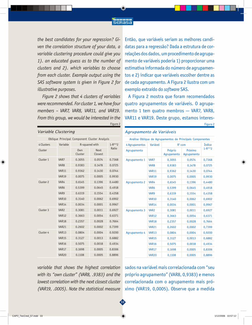
Figure 2 shows that 4 clusters of variables

were recommended. For cluster 1, we have four

members – VAR7, VAR8, VAR11, and VAR19.

From this group, we would be interested in the

variable that shows the highest correlation

with its “own cluster” (VAR8, .9383) and the

lowest correlation with the next closest cluster

(VAR19, .0005). Note the statistical measure

Então, que variáveis seriam as melhores candi-

datas para a regressão? Dada a estrutura de cor-

relações dos dados, um procedimento de agrupa-

mento de variáveis poderia 1) proporcionar uma

estimativa informada do número de agrupamen-

tos e 2) indicar que variáveis escolher dentre as

de cada agrupamento. A Figura 2 ilustra com um

exemplo extraído do software SAS.

A Figura 2 mostra que foram recomendados

quatro agrupamentos de variáveis. O agrupa-

mento 1 tem quatro membros — VAR7, VAR8,

VAR11 e VAR19. Deste grupo, estamos interes-

sados na variável mais correlacionada com “seu

próprio agrupamento” (VAR8, 0,9383) e menos

correlacionada com o agrupamento mais pró-

ximo (VAR19, 0,0005). Observe que a medida

Agrupamento de Variáveis

Figura 2

Análise Oblíqua de Agrupamentos de Principais Componentes

4 Agrupamentos Variável R2 com Índice 1-R**2Agrupamento Próprio

AgrupamentoPróximo

Agrupamento

Agrupamento 1 VAR7 0,3055 0,0574 0,7368

VAR8 0,9383 0,1478 0,0725

VAR11 0,9362 0,1430 0,0744

VAR19 0,0075 0,0005 0,9930

Agrupamento 2 VAR4 0,6145 0,1396 0,4480

VAR6 0,5399 0,0645 0,4918

VAR9 0,6319 0,1554 0,4358

VAR10 0,3140 0,0062 0,6902

VAR14 0,0034 0,0001 0,9967

Agrupamento 3 VAR2 0,3081 0,0011 0,6927

VAR12 0,3663 0,0054 0,6371

VAR18 0,2357 0,0028 0,7664

VAR21 0,2602 0,0002 0,7399

Agrupamento 4 VAR13 0,0804 0,0004 0,9200

VAR15 0,3127 0,0013 0,6882

VAR16 0,5075 0,0018 0,4934

VAR17 0,1698 0,0005 0,8306

VAR20 0,1108 0,0005 0,8896

Figure 2

Variable Clustering

Oblique Principal Component Cluster Analysis

4 Clusters Variable R-squared with 1-R**2RatioCluster Own

ClusterNext

Closest

Cluster 1 VAR7 0.3055 0.0574 0.7368

VAR8 0.9383 0.1478 0.0725

VAR11 0.9362 0.1430 0.0744

VAR19 0.0075 0.0005 0.9930

Cluster 2 VAR4 0.6145 0.1396 0.4480

VAR6 0.5399 0.0645 0.4918

VAR9 0.6319 0.1554 0.4358

VAR10 0.3140 0.0062 0.6902

VAR14 0.0034 0.0001 0.9967

Cluster 3 VAR2 0.3081 0.0011 0.6927

VAR12 0.3663 0.0054 0.6371

VAR18 0.2357 0.0028 0.7664

VAR21 0.2602 0.0002 0.7399

Cluster 4 VAR13 0.0804 0.0004 0.9200

VAR15 0.3127 0.0013 0.6882

VAR16 0.5075 0.0018 0.4934

VAR17 0.1698 0.0005 0.8306

VAR20 0.1108 0.0005 0.8896


34

estatística apresentada na última coluna da Fi-

gura 2, “1-R**2 ratio”, combina essas informa-

ções numa só medida que pode ser usada para

selecionar a melhor candidata de acordo com

os dois critérios. Para os fi ns de regressão, o

analista poderia escolher em cada agrupamen-

to a variável com o menor índice para ser usada

como candidata a variável preditiva no mode-

lo. Nesse exemplo, VAR8, VAR9, VAR12 e VAR16

seriam as recomendadas. Se houver necessida-

de de mais variáveis, o analista poderia tomar

duas variáveis de cada agrupamento — as duas

de menor índice. Mas quaisquer variáveis se-

lecionadas durante o processo que não façam

sentido intuitivo devem ser descartadas.

As vantagens dessa metodologia são:

• Velocidade do cálculo;

• Não há necessidade de interpretação — ou

seja, não são usados os principais componentes

propriamente ditos;

• O número de agrupamentos pode ser deter-

minado automaticamente;

• Questões de elevada correlação são trata-

das automaticamente.

Mínimos Quadrados ParciaisO último dos métodos de cálculo discutidos

nesse artigo é um procedimento matemático

criado por Herman Wold na década de 1960 e

aprimorado por diversas pessoas nos anos 80

e 90, inclusive pelo próprio Wold. Em essência,

o procedimento, conhecido como, mínimos

quadrados parciais (MQP), começa onde ter-

mina a análise de principais componentes,

ao mesmo tempo levando em conta mudanças

da variável dependente e tentando extrair os

shown in the last column of Figure 2, “1-R**2

ratio” combines this information into a single

measure that can be used to select the best

candidate given both criteria. For regression

purposes, the analyst might pick the variable

with the lowest ratio from each cluster as a pre-

dictor candidate in the model. In this example

VAR8, VAR9, VAR12, and VAR16 would be the

recommendations. If more variables were

needed, the analyst could take two variables

from each cluster — the fi rst having the lowest

ratio and the second having the next lowest

ratio. However, any variables that are selected

during this process that do not make intuitive

sense should be discarded.

The advantages in using this method in-

clude:

• Computational speed;

• No interpretation needed — i.e. we

don’t use actual principal components;

• Number of clusters can be chosen auto-

matically;

• High correlation issues are handled au-

tomatically.

Partial Least SquaresThe fi nal computational method discussed in

this paper is a mathematical procedure origina-

ted by Herman Wold in the 1960’s and refi ned

by a number of individuals in the 1980’s and

1990’s, including the original author himself.

This procedure, partial least squares (PLS), es-

sentially picks up where principal components

analysis leaves off by simultaneously accoun-

ting for variations in the dependent variable

while trying to extract those factors represen-


35

fatores que representem a máxima correlação

singular dos atributos preditivos6. Isso é fre-

qüentemente descrito como um procedimento

supervisionado de redução da dimensionalida-

de dos dados por causa da ligação necessária

com a variável dependente. Do ponto de vista

histórico, a técnica tem sido usada em aplica-

ções industriais como análise quimiométrica,

onde o analista muitas vezes

defronta-se com mais atributos

explicatórios do que dados ob-

servados. Com o rápido avanço

do software e da tecnologia

computacional nos últimos 10

anos, esse tipo de análise está

começando a chegar a outros

campos, como o de pesquisa

de mercado7, risco de crédito

e previsão econométrica.

O algoritmo original dos

mínimos quadrados par-

ciais envolvia cálculos que

abrangiam diversas variáveis

dependentes e um sem-nú-

mero de atributos preditivos

em potencial. As contribui-

ções de Jong8 e a implementa-

ção no software SAS (SIMPLS)

aumentaram a efi ciência do método, limitan-

do-o a uma só variável dependente. A Figura 3

mostra como a técnica produz um equilíbrio,

considerando a variação do espaço preditivo

(ver “Efeitos do Modelo”) e da variável visada

(“Variáveis Dependentes”).

A Figura 3 é um exemplo hipotético em que

temos cinco variáveis representadas por cin-

ting the maximum unique correlation in the

predictive attributes6. This is often referred to

as a supervised procedure for reducing the di-

mensionality of the data because of the neces-

sary linkage to the dependent variable. From a

historical perspective, this technique has been

used frequently in industrial applications such

as chemometric analysis where the analyst is

often faced with more potential expla-

natory attributes then

observational data. With

software and computing

technology making rapid

gains in the last 10 years,

this type of analysis is be-

ginning to fi nd its way into

other fi elds such as marke-

ting research7, credit risk, and

econometric forecasting.

The original algorithm for

partial least squares invol-

ved computations covering

multiple dependent varia-

bles as well as a host of po-

tentially predictive attri-

butes. Contributions by de

Jong8 and implemented in the

SAS software system (SIMPLS) have made the

method more effi cient by limiting it to a single

dependent variable. Figure 3 shows how the

technique produces a balance by accounting

for variation in the predictor space (see Model

Effects) as well as the target variable (Depen-

dent Variables).

Figure 3 is a hypothetical example where we

have fi ve variables represented by fi ve factors in

A ACP examina

apenas as

variáveis

preditivas.

PCA examines only the

predictor variables.


36

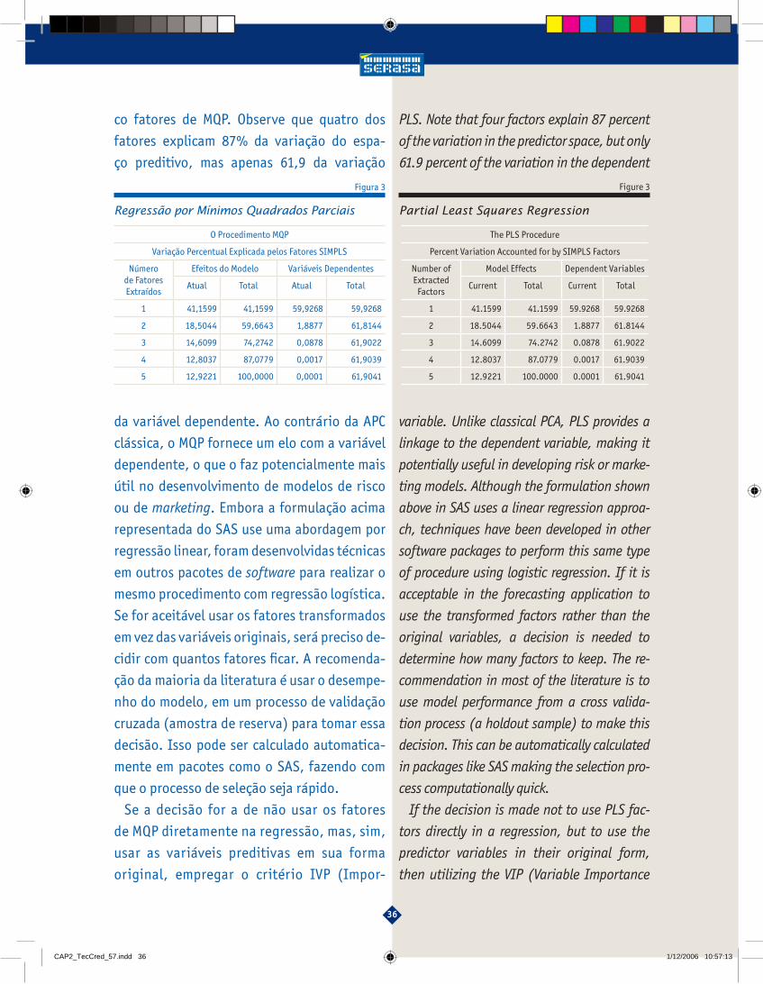
PLS. Note that four factors explain 87 percent

of the variation in the predictor space, but only

61.9 percent of the variation in the dependent

variable. Unlike classical PCA, PLS provides a

linkage to the dependent variable, making it

potentially useful in developing risk or marke-

ting models. Although the formulation shown

above in SAS uses a linear regression approa-

ch, techniques have been developed in other

software packages to perform this same type

of procedure using logistic regression. If it is

acceptable in the forecasting application to

use the transformed factors rather than the

original variables, a decision is needed to

determine how many factors to keep. The re-

commendation in most of the literature is to

use model performance from a cross valida-

tion process (a holdout sample) to make this

decision. This can be automatically calculated

in packages like SAS making the selection pro-

cess computationally quick.

If the decision is made not to use PLS fac-

tors directly in a regression, but to use the

predictor variables in their original form,

then utilizing the VIP (Variable Importance

co fatores de MQP. Observe que quatro dos

fatores explicam 87% da variação do espa-

ço preditivo, mas apenas 61,9 da variação

da variável dependente. Ao contrário da APC

clássica, o MQP fornece um elo com a variável

dependente, o que o faz potencialmente mais

útil no desenvolvimento de modelos de risco

ou de marketing. Embora a formulação acima

representada do SAS use uma abordagem por

regressão linear, foram desenvolvidas técnicas

em outros pacotes de software para realizar o

mesmo procedimento com regressão logística.

Se for aceitável usar os fatores transformados

em vez das variáveis originais, será preciso de-

cidir com quantos fatores fi car. A recomenda-

ção da maioria da literatura é usar o desempe-

nho do modelo, em um processo de validação

cruzada (amostra de reserva) para tomar essa

decisão. Isso pode ser calculado automatica-

mente em pacotes como o SAS, fazendo com

que o processo de seleção seja rápido.

Se a decisão for a de não usar os fatores

de MQP diretamente na regressão, mas, sim,

usar as variáveis preditivas em sua forma

original, empregar o critério IVP (Impor-

Regressão por Mínimos Quadrados Parciais

Figura 3

O Procedimento MQP

Variação Percentual Explicada pelos Fatores SIMPLS

Número de Fatores Extraídos

Efeitos do Modelo Variáveis Dependentes

Atual Total Atual Total

1 41,1599 41,1599 59,9268 59,9268

2 18,5044 59,6643 1,8877 61,8144

3 14,6099 74,2742 0,0878 61,9022

4 12,8037 87,0779 0,0017 61,9039

5 12,9221 100,0000 0,0001 61,9041

Figure 3

Partial Least Squares Regression

The PLS Procedure

Percent Variation Accounted for by SIMPLS Factors

Number of Extracted

Factors

Model Effects Dependent Variables

Current Total Current Total

1 41.1599 41.1599 59.9268 59.9268

2 18.5044 59.6643 1.8877 61.8144

3 14.6099 74.2742 0.0878 61.9022

4 12.8037 87.0779 0.0017 61.9039

5 12.9221 100.0000 0.0001 61.9041


37

tância da Variável para a Projeção) pode ser

um meio promissor de obter recomendações

para seleção de variáveis9. Preditivas com

baixos coefi cientes de regressão de MQP (em

termos absolutos) contribuirão pouco para a

previsão. Enquanto esses coefi cientes repre-

sentam a importância de cada preditiva para

a previsão apenas da variável dependente, a

IVP representa o valor de cada preditiva para

a adequação do modelo de MQP tanto às pre-

ditivas quanto ao resultado. Se uma preditiva

tiver coefi ciente relativamente baixo (em va-

lor absoluto) e baixo valor de IVP, será forte

candidata à eliminação. WOLD (1994) consi-

derou um valor inferior a 0,8 “baixo” para a

IVP. Assim, o analista poderia selecionar um

subconjunto das variáveis originais para a re-

gressão com base no critério de IVP. Partindo

de simulações Monte Carlo, o procedimento

MQP demonstrou resultados promissores,

embora ainda precise de muita pesquisa.

Um resultado surpreendente é o de que a re-

gressão por mínimos quadrados parciais local-

mente ponderada oferece os melhores resultados

médios, com desempenho superior até mesmo

ao da análise fatorial, que, teoricamente, é a

mais atraente das nossas técnicas candidatas10.

Finalmente, surgiram nos últimos anos alguns

trabalhos interessantes com análise de sensibi-

lidade de MQP como alternativa para seleção de

variáveis11. Com a introdução de uma variável

aleatória num procedimento iterado, é possível

estabelecer um processo de fi ltragem que per-

mite selecionar as variáveis que demonstrem

maior sensibilidade relativa. Nesse contexto, a

sensibilidade é defi nida como a variação absolu-

for Projection) criteria may offer a promising

way for recommendations to be made as to

variable selection9. Predictors with small PLS

regression coeffi cients (in absolute value)

make a small contribution to the response

prediction. Whereas, these coeffi cients repre-

sent the importance each predictor has in the

prediction of just the dependent variable, the

VIP represents the value of each predictor in

fi tting the PLS model for both predictors and

response. If a predictor has a relatively small

coeffi cient (in absolute value) and a small

value of VIP, then it is a prime candidate for

deletion. Wold (1994) considered a value less

than 0.8 to be “small” for the VIP. Therefore,

the analyst could select a subset of the ori-

ginal variables for the regression based upon

the VIP criteria. Based upon Monte Carlo si-

mulations, the PLS procedure has showed

promising results, although much research is

yet to be done…

One surprising outcome is that locally

weighted partial least squares regression

offers the best average results, thus ou-

tperforming even factor analysis, the the-

oretically most appealing of our candidate

techniques.10

Finally, some interesting work has been

done in the last few years using PLS sensi-

tivity analysis as a variable selection alter-

native11. By introducing a random variable

in an iterative procedure, a fi ltering process

can be established that allows a selection

to be made for those variables showing re-

latively greater sensitivities. In this context,

sensitivity is defi ned as the absolute maxi-


38

mum change in PLS prediction when each

attribute is varied across its sample range,

all other variables being kept constant at

their mean or median values.

Concluding RemarksWith the advances in modern computing, a

variety of methods are available to the analyst

to select a set of candidate variables from a

very large predictor space for

use in regression analysis.

These methods can be simple

to complex, ranging from the

analysis of basic correlations

to determining the structu-

re of the entire correlation

matrix as a whole. Perhaps

the most frequently used

automatic procedure for

variable selection is ste-

pwise regression. Unfor-

tunately, this technique

is fi lled with pitfalls that

have been repeatedly do-

cumented in the statisti-

cal literature, pitfalls that

could lead to potentially su-

boptimal prediction models.

Other techniques such as variable clustering

offer theoretically pleasing approaches using

a variation of principal component analysis.

More advanced techniques such as partial least

squares combine the advantages of principal

components along with regression analysis

offering the analyst a possible tool to replace

or supplement their current variable selection

ta máxima da previsão de MQP quando cada atri-

buto é variado em relação a sua faixa amostral,

mantidas constantes todas as demais variáveis

em seus valores médios ou medianos.

Últimas Observações Com os recentes avanços da computação, os

analistas contam com diversos métodos de se-

leção de um conjunto de variáveis candidatas a

partir de um espaço preditivo muito gran-

de, para uso numa análise

de regressão. Esses métodos

vão dos simples aos comple-

xos, da análise de correlações

básicas à determinação da es-

trutura da matriz de correlação

como um todo. O procedimen-

to automático de seleção de

variáveis mais freqüentemente

utilizado talvez seja a regressão

stepwise. Infelizmente, essa téc-

nica está cheia de armadilhas

reiteradamente documentadas

na literatura estatística e que

podem levar a modelos prediti-

vos potencialmente inferiores

ao desejável. Outras técnicas,

como o agrupamento de variáveis, oferecem

abordagens agradáveis baseadas em variantes

da análise de principais componentes. Técnicas

mais avançadas como a dos mínimos quadrados

parciais, combinam as vantagens dos principais

componentes com a análise de regressão, ofere-

cendo ao analista uma ferramenta em potencial

para substituir ou complementar seu método

atual de seleção de variáveis. Embora não tenha

O MQP

fornece um

elo com a

variável

dependente.

PLS provides a linkage to

the dependent variable.


39

method. Although not discussed here, a Baye-

sian approach to variable selection may offer

the next step forward in variable selection tech-

nology12, but like PLS, this method, too, needs

to be further developed and implemented in

the proper software framework.

References1.PINDYCK, Robert S. and RUBINFELD, Daniel

L. Econometric Models and Econometric Fore-

casts. 2nd edition, 1981, McGraw-Hill, Inc.2.THOMPSON, B. Signifi cance, effect sizes,

stepwise methods, and other issues: Strong

arguments move the fi eld. Journal of Expe-

rimental Education., 70, 80-93.3.HAIR, Anderson, TATHAM, and BLACK.

Multivariate Data Analysis, Fourth Edition,

Prentice Hall, Inc. 1995.4.SIDDIQI, Nadeem. Credit Risk Scorecards

— Developing and Implementing Intelligent

Credit Scoring. 2006. John Wiley & Sons, Inc.5.NELSON, Bryan D. Variable Reduction for

Modeling Using PROC VARCLUS. Fingerhut

Companies Incorporated, Minnetonka, MN.6.TOBIAS, Randall D. An Introduction to Le-

ast Minimum Squares Regression. SAS Insti-

tute., Cary, NC.7.GRABER, Stephanie, CZELLAR, Sandor,

and DENIS, Jean-Emile. Using Least Mini-

mum Squares Regression in Marketing Rese-

arch. University of Geneva, December 2002.

8.DE JONG, S. An alternative approach to

least minimum squares regression. Chemome-

trics and Intelligent Laboratory Systems, 18,

251-263.9.CHONG, IL-Gyo and JUN, Chi-Hyuck. Perfor-

sido discutida aqui, uma abordagem Bayesiana

à seleção de variáveis pode ser o próximo pas-

so na tecnologia de seleção de variáveis12, mas,

como o MQP, esse método também precisa ser

mais desenvolvido e implementado na estrutura

de software adequada.

Referências1.PINDYCK, Robert S. e RUBINFELD, Daniel L.

Econometric Models and Econometric Forecasts.

2a edição, 1981, McGraw-Hill, Inc.2.THOMPSON, B. Signifi cance, effect sizes, ste-

pwise methods, and other issues: Strong argu-

ments move the fi eld. Journal of Experimental

Education., 70, 80-93.3.HAIR, Anderson, TATHAM e BLACK. Multi-

variate Data Analysis, Quarta Edição, Prentice

Hall, Inc. 1995.4.SIDDIQI, Nadeem. Credit Risk Scorecards — De-

veloping and Implementing Intelligent Credit Sco-

ring. 2006. John Wiley & Sons, Inc.5.NELSON, Bryan D. Variable Reduction for Mo-

deling Using PROC VARCLUS. Fingerhut Companies

Incorporated, Minnetonka, MN.6.TOBIAS, Randall D. An Introduction to Least

Minimum Squares Regression. SAS Institute.,

Cary, NC.7.GRABER, Stephanie, CZELLAR, Sandor e DE-

NIS, Jean-Emile. Using Least Minimum Squares

Regression in Marketing Research. University of

Geneva, Dezembro de 2002.8.DE JONG, S. An alternative approach to least

minimum squares regression. Chemometrics

and Intelligent Laboratory Systems, 18, 251-

263.9.CHONG, IL-Gyo & JUN, Chi-Hyuck. Perfor-


40

mance of Some Variable Selection Methods

When Multicollinearity is Present. December,

2004. Department of Industrial Engineering,

Pohang University of Science and Technology.10.SCHAAL, Stefan, SETHU, Vijayakumar and

ATKESON, Christopher. Local Dimensionality

Reduction. Advances in Neural Information Pro-

cessing Systems 10. Cambridge, MA: MIT Press.11.ARCINIEGAS, Fabio A., and EMBRECHTS,

Mark J. Selecting Regressors with Least Mini-

mum Squares Sensitivity Analysis: An Appli-

cation to Currency Crises’ Real Effects. Latin

American and Caribbean Economic Confe-

rence, October 11, 2002, Madrid, Spain.12.GERLACH, R., BIRD, R., and HALL, A. A

Bayesian Approach to Variable Selection in

Logistic Regression with Application to Pre-

dicting Earnings Directed from Accounting In-

formation. School of Finance and Economics,

University of Technology, Sydney, Australia

SAS is a registered trademark of SAS Ins-

titute Inc. in the USA and other countries.

SPSS is a registered trademark of SPSS Inc.

Jeffrey S. Morrison is currently Senior Manager at TransUnion, LLC in Atlanta, Georgia where he is heading up the Research and Development function for analytics. TransUnion, LLC builds modeling solutions for both credit risk and marketing applications in addition to offering their core credit bureau products. Jeff has published over 25 articles in applied journals over the last 20 years and has spoken at a number of forecasting conferences nationwide. Recently, Jeff won the RMA Journal’s annual award for ‘Best Series’ with his articles on analytics and the New Basel Capital Accord. Contact Morrison at [email protected]

mance of Some Variable Selection Methods When

Multicollinearity is Present. Dezembro de 2004.

Department of Industrial Engineering, Pohang

University of Science and Technology.10.SCHAAL, Stefan, SETHU, Vijayakumar e

ATKESON, Christopher. Local Dimensionality

Reduction. Advances in Neural Information Pro-

cessing Systems 10. Cambridge, MA: MIT Press.11.ARCINIEGAS, Fabio A. e EMBRECHTS, Mark J.

Selecting Regressors with Least Minimum Squares

Sensitivity Analysis: An Application to Currency Cri-

ses’ Real Effects. Latin American and Caribbean

Economic Conference, 11 de Outubro de 2002,

Madri, Espanha.12.GERLACH, R., BIRD, R. e HALL, A. A Bayesian

Approach to Variable Selection in Logistic Regres-

sion with Application to Predicting Earnings Direc-

ted from Accounting Information. School of Fi-

nance and Economics, University of Technology,

Sydney, Austrália.

SAS é marca registrada do SAS Institute Inc.

nos Estados Unidos e outros países.

SPSS é marca registrada da SPSS Inc.

Jeffrey S. Morrison é gerente sênior da TransUnion, LLC em Atlanta, Geórgia, onde lidera a função de Pesquisa e Desenvolvimento de análises. A TransUnion, LLC constrói soluções de modelagem para aplicações de risco de crédito e marketing, além de oferecer seus produtos centrais de credit bureau. Jeffrey publicou mais de 25 artigos em periódicos do setor nos últimos 20 anos e foi palestrante em diversas conferências sobre previsão em todos os Estados Unidos. Jeffrey ganhou recentemente o prêmio de “Melhor Série” do RMA Journal por seus artigos sobre análise e sobre o Novo Acordo de Capital da Basiléia.Os contatos com Morrison podem ser feitos no endereço [email protected]


Seleção de Variáveis no Desenvolvimento de Modelos · 25 O artigo a seguir se divide de acordo...

Documents

Transcript of Seleção de Variáveis no Desenvolvimento de Modelos · 25 O artigo a seguir se divide de acordo...