
The introduction of grabado in Valencian urban art Adriano ...

Stochastic Differential Equation Modelsin Population Dynamics
Marina Filipa Amado Ferreira


Stochastic Differential EquationModels in Population Dynamics
Marina Filipa Amado Ferreira
Dissertação para a obtenção do Grau de Mestre em Matemática
Área de Especialização em Estatística, Otimização e Matemática Financeira
Júri
Presidente: Prof. Dr. Paulo Eduardo Aragão Aleixo e Neves de Oliveira
Orientador: Prof. Dra. Ana Cristina Martins Rosa
Vogais: Prof. Dra. Ercília Cristina da Costa e Sousa
Data: Setembro de 2014


ResumoO cálculo estocástico tem adquirido uma grande dimensão durante
as últimas décadas, tanto do ponto de vista teórico como prático. Emparticular, no ramo da biologia teórica tem contribuído para a deduçãode modelos mais realistas, mas ao mesmo tempo mais complexos. O es-tudo destes modelos reduz-se, por isso, muitas vezes a uma abordagemnumérica. Os principais objetivos desta tese passam por motivar, esta-belecer e analisar modelos estocásticos de dinâmica de populações queresultam de dois tipos diferentes de aleatoriedade: ambiental e demográ-fica. De modo a analisarmos a primeira classe de modelos, assim comoa justificar o procedimento usado para deduzir a segunda classe, é pre-viamente brevemente apresentada a teoria dos processos de difusão edos sistemas de equações diferenciais estocásticas. Adicionalmente, ap-resentamos também um breve estudo numérico dos modelos que é feitorecorrendo ao método de Euler-Maruyama.
Palavras Chave: processos de difusão, sistemas de equações diferenciais estocás-
ticas de Itô, modelos de crescimento populacional, modelo de epidemias
AbstractStochastic calculus has gained a great expansion in the last decades
both from theoretical and practical perspectives. In particular, in thefield of theoretical biology, it has contributing for the deduction of morerealistic but also less tractable models. Due to the complexity of themathematical theory behind stochastic calculus, the approaches followedare often limited to numerical technics. The principal aims of this the-sis are the motivation, establishment and discussion of classic stochasticdifferential equation models in population dynamics, resulting from twodifferent types of randomness: environmental and demographic. In or-der to analyse the first class of models, as well as rigorously justify theprocedure used in the second class, we deal with the theory of diffusionprocesses and Itô stochastic differential systems. Additionally, a numer-ical study by implementing the Euler-Maruyama method is made.
Keywords: diffusion processes, system of Itô stochastic differential equations,
growth population models, epidemic model
i


AgradecimentosI am deeply indebted to my supervisor, Professor Ana Cristina Rosa,
for her scientific guidance, dedication and friendship. I am very thankfulby the mathematical sensibility she transmitted me regarding the com-plex issue of stochastic differential equations, as well as her support in thisexciting adventure through Mathematical Biology, which I appreciatedvery much.
I would like to thank to Filipe Carvalho for the interesting discussionson the biological motivation of the models and to Flávio Cordeiro for thethorough reading.
Finally, I would like to thank my parents by their constant support,encouragement and love.
iii

Contents
1 Introduction 1
2 Diffusion processes and solutions of Stochastic Differential Equa-tions 32.1 Preliminaries . . . . . . . . . . . . . . . . . . . . . . . . . . . . . . . 32.2 Diffusion processes . . . . . . . . . . . . . . . . . . . . . . . . . . . . 62.3 Systems of stochastic differential equations . . . . . . . . . . . . . . . 14
2.3.1 Systems of linear stochastic differential equations . . . . . . . 21
3 Modelling the evolution of populations 233.1 Environmental randomness . . . . . . . . . . . . . . . . . . . . . . . 23
3.1.1 Stochastic Malthusian linear model . . . . . . . . . . . . . . . 233.1.2 Stochastic logistic growth model I . . . . . . . . . . . . . . . 273.1.3 Stochastic predator-prey model I . . . . . . . . . . . . . . . . 30
3.2 Demographic randomness . . . . . . . . . . . . . . . . . . . . . . . . 323.2.1 Stochastic logistic growth model II . . . . . . . . . . . . . . . 353.2.2 Stochastic predator-prey model II . . . . . . . . . . . . . . . . 383.2.3 Stochastic SIR epidemic model . . . . . . . . . . . . . . . . . 39
4 Conclusion 45
Appendix A Matlab code 47A.1 Euler-Maruyama method for stochastic logistic growth model . . . . 47A.2 Euler-Maruyama method for stochastic SIR model . . . . . . . . . . 48
v


Chapter 1
Introduction
The study of Markov processes, and particularly of diffusion processes, marked un-
doubtedly the origin of the research concerning continuous-time stochastic processes.
Besides the contributions of N. Wiener (1923) and Lévy-Khinchin (1937), we may
say that the modern theory of Markov processes was initiated by A. Kolmogorov
(1931), who characterized the transition probability distribution of a diffusion pro-
cess as a solution of a parabolic partial differential equation involving its drift and
diffusion coefficients, extended afterwards by Feller (1936) to the characterization of
a Markov process admitting jumps.
K. Itô (1940) entered in the scene right after this:
"I saw a powerful analytic method to study the transition probabilities of the
process, namely Kolmogorov’s parabolic equation and its extension by Feller. But I
wanted to study the paths of Markov processes (...)".
Itô’s original goal was thus to complement the study of diffusion processes (see
[1] [2]), in order to permit the explicit construction of their trajectories. This goal
led him to conceive a new concept of integral, named stochastic integral, giving rise
to the famous stochastic calculus and stochastic differential equations (SDEs), which
revealed to be a powerful tool for the construction and analysis of mathematical
models. In fact, during the last decades, SDEs gained a remarkable popularity by
finding multiple applications in different areas of science such as finance, chemistry,
physics, engineering, population dynamics and, more generally, in systems biology
(see, for instance, [3], [4], [5], [6], [7], [8] and [9]). They are particularly important in
modelling complicated systems where randomness can not be ignored. On the other
hand, these applications have also motivated theoretical developments conducting to
new kinds of stochastic integrals (see, for example, [1], [5]).
This thesis aims to motivate, establish, compare and analyse, essentially from a
1

Chapter 1 Introduction
numerical point of view, some classic models of stochastic differential equations in
the field of life sciences, supported by a rigorous mathematical justification, as far as
possible. We begin, in Chapter 2, by briefly describing the probabilistic background
needed to understand the models that will be considered and the techniques support-
ing their manipulation. We then proceed by presenting the class of diffusion processes
and the corresponding Kolmogorov’s forward differential equation, in order to estab-
lish the link between SDE solutions and diffusion processes. Later on, in Chapter 3,
two different classes of stochastic models are analised and several examples are given.
In the first class, models are obtained directly from a deterministic ordinary differ-
ential equation (ODE) model, by adding a random perturbation, which pretends
to represent environmental stochasticity. The stochastic Malthusian growth model
(Black-Scholes model), the stochastic logistic growth model as well as the stochastic
Lotka-Volterra model, are then settled and slightly explored. In the second class
of models, the stochasticity arises intrinsically from the underlying phenomena. A
general time-continuous Markov chain model is first constructed, leading to the es-
tablishment of a SDE by diffusion approximation procedures (see [10] [11] [12] [13]).
A few examples are subsequently given, including a second version of the stochastic
logistic growth model, a two species stochastic Lotka-Volterra model and, finally, a
stochastic epidemic model.
In order to gain some insight about the models’ behavior and, consequently,
about the underlying biological phenomenon, the Euler-Maruyama method was im-
plemented for approximating trajectories of SDE solutions. Although there exist
higher order convergence methods (see [3]), this method is computationally simple
and often proposed in the literature. In this way, it was possible to obtain some
sample paths for the solutions of nonlinear models, for which an analytical resolu-
tion procedure is in general not available. As in the scope of PDEs, some analytical
approaches exist and others continue being developed, in order to complement the
numerical study. However, because of the complex mathematical tools they encom-
pass, we opted by not bringing very deeply this analysis to this thesis, instead, we
suggest appropriate references. Since this is yet a quite recent and complex field of
research, when compared to deterministic partial differential equations (PDEs), still
many questions are far from being answered and new techniques must be developed.
Finally, together with the models’ descriptions, we present a short discussion on the
comparison between deterministic and stochastic models.
2

Chapter 2
Diffusion processes and solutionsof Stochastic Differential
Equations
2.1. Preliminaries
In this thesis, we consider the complete1 probability measure space (Ω,A, P ) where
all real random vectors and real vector-valued stochastic processes are defined. The
set of d-dimensional real vectors, as well as any subset of it, is equipped with the
Borel σ-algebra, BC , C ⊆ Rd, d ∈ N. The time interval on which all stochastic
processes are defined is [0, T ], for some T > 0, which may be allowed to be infinite.
Vectors will be written in bold to distinguish from scalars. The Euclidean vector-
norm will be denoted by |.| and the Hilbert-Schmidt norm, ‖.‖, for an m × n real
matrix A = [aij ]i=1,...,m,j=1,...,n, m,n ∈ N, is defined by
‖A‖ =
m∑
i=1
n∑
j=1
a2ij
1/2
.
The Wiener process is a basic tool in stochastic calculus. Among several defini-
tions that can be found in the literature, we consider the following one.( see [14])
Definition 1. (i) Given a complete2 filtration (Gt, t ∈ [0, T ]) of (Ω,A, P ), the
stochastic process W = (Wt, t ∈ [0, T ]) is called a scalar Wiener process
with respect to (Gt, t ∈ [0, T ]) if it satisfies the following properties:
• X0 = 0 a.s.,
• Wt is adapted to Gt, ∀t ∈ [0, T ]
• ∀ t ∈ [0, T ], ∀ h > 0, with 0 ≤ t < t + h ≤ T , Wt+h −Wt ∼ N (0, σ2h),
where σ2 is a real positive constant,1A probability measure space is complete if its σ-algebra is complete. In turn, a σ-algebra, F , is
called complete if for each A ∈ F such that P (A) = 0, one has B ∈ F for any B ⊂ A. The complete
framework is used in this thesis for technical convenience.2Notice that a filtration is complete if all σ-algebras which constitute it are complete.
3
Chapter 2 Diffusion processes and solutions of Stochastic Differential Equations
• ∀t ∈ [0, T ], ∀ h > 0, with 0 ≤ t < t + h ≤ T , Wt+h −Wt is independent
of Gt,
• almost all sample paths of W are continuous functions.
(ii) A d-dimensional Wiener process W is defined by W = (Wt, t ∈ [0, T ]),
where Wt = (W (1)t , ..., W
(d)t ) and (W (i)
t , t ∈ [0, T ]), i = 1, ..., d, d ∈ N, are d
independent scalar Wiener processes.
If σ2 = 1, W is called the standard Wiener process.
We denote by (Ft, t ∈ [0, T ]) the complete filtration of (Ω,A, P ) generated by
the Wiener process W.
For T ∈ (0, T ], we denote by Li([0, T ] × Ω), i = 1, 2, the spaces of functions
f : [0, T ]× Ω → Rd such that
• f is measurable regarding the tensor-product σ-algebra B[0,T ] ⊗A,
• f is adapted to the filtration (Ft, t ∈ [0, T ]),
• ∫ T0 |f |idt < ∞ a.s., i = 1, 2 .
We next present a central tool in stochastic calculus, namely, the famous Itô’s
lemma, which is formulated for a specific class of processes, called Itô processes.
Definition 2. Let W = (Wt, t ∈ [0, T ]) be an m-dimensional Wiener process.
(i) A scalar stochastic process X = (Xt, t ∈ [0, T ]) is called a scalar Itô process
driven by an m-dimensional Wiener process W if
• X0 is F0-measurable,
• X can be expressed in the form
Xt = X0 +∫ t
0Bsds +
m∑
j=1
∫ t
0C(j)
s dW (j)s a.s., t ∈ [0, T ], (2.1)
where (Bt, t ∈ [0, T ]) ∈ L1(Ω × [0, T ]) and (C(j)t , t ∈ [0, T ]) ∈ L2(Ω ×
[0, T ]), j = 1, ...,m.
(ii) An n-dimensional stochastic process X = (Xt, t ∈ [0, T ]), with Xt = (X(1)t , ..., X
(n)t )
is called an Itô process driven by W if, for each i = 1, ..., n, X(i)t is a scalar
Itô process, defined by
X(i)t = X
(i)0 +
∫ t
0B(i)
s ds +m∑
j=1
∫ t
0C(i,j)
s dW (j)s a.s., t ∈ [0, T ] (2.2)
4

2.1 Preliminaries
where (B(i)t , t ∈ [0, T ]) ∈ L1(Ω × [0, T ]) and (C(i,j)
t , t ∈ [0, T ]) ∈ L2(Ω ×[0, T ]), i = 1, ..., n j = 1, ..., m.
Moreover, rewriting (2.2) in the differential form, we obtain the stochastic differ-
ential of X, namely,
dXt = Btdt + CtdWt, t ∈ [0, T ],
with
Ct =
C(1,1)t · · · C
(1,m)t
.... . .
...
C(n,1)t · · · C
(n,m)t
, Bt =
B(1)t
...
B(n)t
.
An Itô process thus results from a linear combination of a Lesbesgue and a
stochastic integral.
The Itô’s lemma for n-dimensional Itô processes is next presented. A proof can
be found in [3].
Lemma 1. Let (Xt, t ∈ [0, T ]) be an n-dimensional Itô process with stochastic dif-
ferential dXt = Btdt + CtdWt, t ∈ [0, T ]. Let also f(t,x), (t,x) ∈ [0, T ] × Rn, be
a continuous real function with continuous partial derivatives ∂f∂t ,
∂f∂xi
and ∂2f∂xixj
, for
i, j = 1, ..., n. Then f(t,Xt) is also an Itô process satisfying the Itô’s formula:
f(t,Xt) = f(0,X0) +∫ t
0
∂f
∂t(s,Xs) +
n∑
i=1
∂f
∂xi(s,Xs)B(i)
s +m∑
k=1
n∑
i,j=1
12
∂2f
∂xixj(s,Xs)C(i,k)
s C(j,k)s
ds +
m∑
k=1
n∑
i=1
∫ t
0
∂f
∂xi(s,Xs)C(i,k)
s dW (k)s a.s.. (2.3)
In the scalar case, the Itô’s formula for f(t,Xt), where X = (Xt, t ∈ [0, T ]) is a
scalar Itô process with stochastic differential dXt = Btdt + CtdWt, takes the form
f(t,Xt) = f(0, X0) +∫ t
0
[∂f
∂t(s,Xs) +
∂f
∂x(s,Xs)Bs +
12
∂2f
∂x2(s,Xs)C2
s
]ds +
∫ t
0
∂f
∂x(s,Xs)CsdWs a.s., t ∈ [0, T ]. (2.4)
Notice that ( 2.4) corresponds to a stochastic chain rule. If f is linear in x,
then ∂2f∂x2 = 0 and the Itô formula reduces to the usual chain rule. Itô’s lemma
is particularly useful in the analytical calculation of the solution of some specific
stochastic differential equations, as we shall see later.
5
Chapter 2 Diffusion processes and solutions of Stochastic Differential Equations
From (2.3) we can deduce the Itô product formula. Consider f(x, y) = xy.
Let X = (Xt, t ∈ [0, T ]) and Y = (Yt, t ∈ [0, T ]) be two scalar Itô processes with
stochastic differentials dXt = Atdt + BtdWt and dYt = Ctdt + DtdWt. Therefore,∂f∂x (x, y) = y, ∂f
∂y (x, y) = x, ∂2f∂xy (x, y) = 1 and ∂2f
∂x2 = ∂2f∂y2 = 0. Applying ( 2.3) to
f(Xt, Yt), we obtain the Itô product formula,
XtYt = X0Y0+∫ t
0(YsAs + XsCs + BsDs) ds+
∫ t
0(YsBs + XsDs) dWs a.s, t ∈ [0, T ]
(2.5)
or, in the differential form,
dXtYt = (YtAt + XtCt + BtDt) dt + (YtBt + XtDt) dWt, t ∈ [0, T ].
2.2. Diffusion processes
In this section we begin by considering real-valued processes. At the end, appropriate
generalizations shall then be made.
In order to develop stochastic models in biology, we first present a brief exposition
on the general concept of Markov processes.
Markov processes constitute a widely studied class of stochastic processes with
the property that future probabilities only depend on the most recent values of the
process, i.e., the process "forgets" the past. The formal definition is presented below.
Definition 3. Let X = (Xt, t ∈ [0, T ]) be a real-valued stochastic process. X is
called a Markov process if the following so-called Markov property is satisfied: for
any 0 ≤ t1 < ... < tn ≤ s ≤ T , the equality
P (Xs ≤ y/Xt1 , ..., Xtn) = P (Xs ≤ y/Xtn) a.s.
holds for all y ∈ R.
We find in the literature (see e.g. [2] and [15]) various equivalent formulations
of the Markov property, from which we highlight the following one: for any 0 ≤ t ≤s ≤ T and B ∈ BR,
P (Xs ∈ B/Gt) = P (Xs ∈ B/Xt) a.s.,
where Gt := σ(Xs, s ∈ [0, t]), i.e., Gt is the σ-algebra generated by the variables Xs.
These processes are used to model random systems that change according to a
transition rule that only depends on the current state. Their finite distributions
6

2.2 Diffusion processes
are, in fact, characterized by the distribution of X0 and the family of transition
probability functions,
P = P (t, x, s, B), 0 ≤ t ≤ s ≤ T, x ∈ R B ∈ BR,
where the function P has the following properties:
(i) for fixed t ≤ s and B ∈ BR, we have
P (t, X, s, B) = P (Xs ∈ /Xt) a.s.,
(ii) for fixed t ≤ s and x ∈ R, P (t, x, s, ·) is a probability on BR,
(iii) for fixed t ≤ s and B ∈ BR P (t, x, s, ·) is adapted to BR,
(iv) for t ≤ u ≤ s and for all B ∈ BR, (with a possible exception of a set A ∈ BRsuch that P (Xt ∈ A) = 0), the so-called Chapman-Kolmogorov equation
P (t, x, s, B) =∫
RP (u, y, s, B)P (t, x, u, dy), (2.6)
(v) for all t ∈ [0, T ] and B ∈ BR P (t, x, t, B) = 1B(x).
We shall use the notation P (t, x, s, B) = P (Xs ∈ B/Xt ∈ x) = Pt,x(s,B).3
For instance, if Xs represents the position of an object at time s, then Pt,x(s, B)
represents the probability that this object, being at x at time t, will be in B at time
s.
If, for all t and s, 0 ≤ t < s ≤ T , and x ∈ R, the transition probability function
Pt,x(s, ·) is absolutely continuous, then it admits a density ft,x(s, ·), which is called
a transition density function of X. In this case, the Chapman-Kolmogorov equation
takes the form,
ft,x(s, y) =∫
Rfu,z(s, y)ft,x(u, z)dz,
for 0 ≤ t < u < s ≤ T .
One classical example of a Markov process is the Wiener process, which describes
the behavior (with friction neglected) of the well-known Brownian motion, the chaotic
motion of a grain of pollen on a water surface, first noticed by the British botanist
Brown in 1826. For further details on the modellation of the Brownian motion using
the Wiener process (see [16]). A first rigorous proof of its (mathematical) existence
was given by Norbert Wiener in 1923 (see [1]).3Note that the number P (Xs ∈ B/Xt = x) is well defined, even though P (Xt = x) = 0.
7
Chapter 2 Diffusion processes and solutions of Stochastic Differential Equations
We introduce now a particular subclass of Markov processes that represents a
form of conditional probabilistic equilibrium, in the sense that the transition proba-
bilities do not depend explicitly on time, they are stationary. Formally speaking, we
have the following definition.
Definition 4. Let X be a Markov process with transition probabilities P = Pt,x, x ∈R, t ∈ [0, T ). X is called time-homogeneous if
Pt+u,x(s + u,B) = Pt,x(s,B),
for all 0 ≤ t ≤ s ≤ T and 0 ≤ t + u ≤ s + u ≤ T .
In this case, P is thus a function of x, s − t and B. Hence, we can write,
Pt,x(s,B) = P0,x(s− t, B), 0 ≤ s− t ≤ T .
In natural systems, homogeneous Markov processes are quite common (see [17]).
Some illustrations will be given in Chapter 3. The Wiener process is an example of
a time-homogeneous Markov process.
In 1931 Kolmogorov found out that there are two types of time-continuous
Markov processes: diffusion and jump processes, which differ on the behavior over
small time intervals. Roughly speaking, suppose that in a small time interval there
is an overwhelming probability that the state will remain unchanged, however if it
changes, the change can be either radical or small, leading to a jump or a diffusion
process, respectively. Kolmogorov then derived the so-called forward and backward
equations for each kind of process referred before.
Our interest will remain on the Kolmogorov forward equation for diffusion pro-
cesses, also known as Fokker-Plank equation, since this equation will be crucial for
the deduction of mathematical models, as we shall see.
We present in the following the definition of diffusion process.
Definition 5. Let X = (Xt, t ∈ [0, T ]) be a real-valued Markov process with al-
most certainly continuous paths. X is said to be a diffusion process if there exist
functions m : [0, T ]× R→ R and Q : [0, T ]× R→ R+, such that4,
(i) P (|Xt+h −Xt| ≥ c/Xt = x) = o(h),
(ii)∫|y−x|<c(y − x)Pt,x(t + h, dy) = m(t, x)h + o(h),
(iii)∫|y−x|<c(y − x)2Pt,x(t + h, dy) = Q(t, x)h + o(h),
4As usually, o denotes a function of h such that limh→0o(h)
h= 0.
8
2.2 Diffusion processes
for all c ∈ R+ and (t, x) ∈ [0, T ]× R .
The functions m and Q are called the drift and diffusion coefficients of the
diffusion process X, respectively.
Remark 1. In the literature, one can find different a more intuitive definition of
diffusion process (see [18]), where the condition (i) is omitted, the following condition
is added:
(i)’ for some δ > 0, E(|Xt+h −Xt|2+δ/Xt = x
)= o(h),
and the truncated moments in conditions (ii) and (iii) are replaced by the non-
truncated moments, namely
(ii)’ E(Xt+h −Xt/Xt = x) = m(t, x)h + o(h),
(iii)’ E((Xt+h −Xt)2/Xt = x
)= Q(t, x)h + o(h).
These conditions are stronger, once they require the process to have finite condicional
moments.
To prove that (i)′, (ii)′ and (iii)′ imply (i), (ii) and (iii) it is enough to show
that ∫
|y−x|≥c|y − x|kPt,x(t + h, dy) = o(h),
for k = 0, 1, 2, which is a consequence of (i)′ and the inequality∫
|y−x|≥c|y − x|kPt,x(t + h, dy) ≤ 1
c2+δ−k
∫
|y−x|≥c|y − x|2+δPt,x(t + h, dy).
Notice that condition (i) says that large displacements are very unlikely in small
time intervals. This fact can be viewed as a formalization of the process sample
paths’ continuity. A diffusion process is thus a Markov process with no instantaneous
jumps. Moreover, the functions m and Q correspond to the infinitesimal mean and
variance of X, respectively, since m represents the instantaneous rate of change in
the conditional mean of the process and Q measures the average size of instantaneous
conditional fluctuations of the diffusion process.
The standard scalar Wiener process and the Ornstein-Uhlenbeck process, defined
by Xt = g(t)Wf(t), t ∈ R+0 , with g(t) = e−αt and f(t) = σ2e2αt
2α , α, σ2 positive
constants, are basic examples of diffusion processes. To prove this, note that W is a
Markov process, as it was referred above, and, consequently, X is a Markov process
too. Furthermore, for all t, t + h ∈ [0, T ], we know that Wt+h −Wt ∼ N (0, h), by
definition, which together with the independence of increments implies that
E(Wt+h −Wt) = 0, E((Wt+h −Wt)2) = h,
9
Chapter 2 Diffusion processes and solutions of Stochastic Differential Equations
showing that W is a diffusion process with drift m(t, x) = 0 and diffusion coefficient
Q(t, x) = 1.
It follows that for the Ornstein-Uhlenbeck process, the conditional distribution is
also gaussian with mean E(Xt+h/Xt = x) = xe−αh and variance V (Xt+h/Xt = x) =(1−e−
2αh
2α
)σ2. Therefore, X is a diffusion process with coefficients m(t, x) = −αx
and Q(t, x) = σ2.
This process arose as an improvement of the Wiener process model for the diffu-
sion phenomenon, which has into account the friction effect inherent to the movement
of the particles of pollen on a water surface.
We are now ready to deduce the Kolmogorov forward equation for diffusion pro-
cesses. As we will see in the next theorem, the term forward is motivated by the fact
that the time variable s moves forward from t, contrarily to the backward equation.
Theorem 1. Let X be a real-valued diffusion process with drift m and diffusion
coefficient Q , such that the limits (in definition 5) are uniform with respect to x.
Moreover, assume that the transition density functions of X, ft,x, (t, x) ∈ [0, T ]×R,exist and that the derivatives
∂ft,x
∂s,
∂(mf)t,x
∂y,
∂(Qft,x)∂y
and∂2(Qft,x)
∂y2
exist and are continuous functions on [0, T ]× R. Then, for each (t, x) ∈ [0, T ]× R,ft,x satisfies the Kolmogorov forward equation:
∂
∂sft,x = − ∂
∂y(mft,x) +
12
∂2
∂y2(Qft,x), (2.7)
evaluated at (s, y) ∈ (t, T ]× R, with the initial condition5
lims→t+ft,x(s, y) = δx(y). (2.8)
Proof. Let t ∈ [0, T ) and x ∈ R be fixed and consider ft,x as a function of s ∈ (t, T ]
and y ∈ R. For any smooth real-valued function6, φ, such that φ has compact
support C, we define the function θ as
θ(s) :=∫
Rφ(z)ft,x(s, z)dz =
∫
Cφ(z)ft,x(s, z)dz, s ∈ (t, T ]. (2.9)
Notice that φ′, φ′′ and φ′′′ vanish outside C. For h ∈ R+, we may write, by the
Chapman-Kolmogorov equation,
ft,x(s + h, z) =∫
Rfs,y(s + h, z)ft,x(s, y)dy,
5δx denotes the Dirac delta function at x.6For example, for any a, b, c ∈ R, with a < b and c > 0, define φ as
φ(z) = (z − a)3(b− z)3e−cz21[a,b](z).
10
2.2 Diffusion processes
which implies, from (2.9), that
θ(s + h)− θ(s)h
=1h
∫
Rφ(z)
[∫
Rfs,y(s + h, z)ft,x(s, y)dy
]dz− 1
h
∫
Rφ(y)ft,x(s, y)dy.
Using Fubini’s theorem and rearranging terms, we obtain
θ(s + h)− θ(s)h
=1h
∫
R
(∫
R(φ(z)− φ(y))fs,y(s + h, z)dz
)ft,x(s, y)dy. (2.10)
For any positive constant c, the integral with respect to the variable z can be written
as a sum of two integrals as follows
∫
|y−z|<c(φ(z)− φ(y))fs,y(s + h, z)dz +
∫
|y−z|≥c(φ(z)− φ(y))fs,y(s + h, z)dz.
Once φ is bounded, from definition 5 the second term of the previous expression
is an o(h) uniformly with respect to y, by hypothesis. Moreover, considering c > 0
sufficiently small, we may use the Taylor expansion of φ at y with Lagrange reminder
to get for the first term
∫
|z−y|<c
(φ′(y)(z − y) +
12φ′′(y)(z − y)2 +
16φ′′′(ξ)(z − y)3
)fs,y(s + h, z)dz, (2.11)
for some real number ξ between y and z. Notice that if we divide ( 2.11) by h, and
take the limit as h approaches zero, we obtain (see definition 5)
φ′(y)m(s, y) +12φ′′(y)Q(s, y) + lim
h→0+
1h
16φ′′′(ξ)
∫
|z−y|<c(z − y)3fs,y(s + h, z)dz.
By the Lebesgue’s dominated convergence theorem, the limit of ( 2.10) as h ap-
proaches zero conduces to the expression
θ′(s) =∫
R
(φ′(y)m(s, y) +
12φ′′(y)Q(s, y)
)ft,x(s, y)dy
+ limh→0+
1h
16
∫
Rφ′′′(ξ)
∫
|z−y|<c(z − y)3fs,y(s + h, z)dzft,x(s, y)dy.
The second term of the previous expression turns out to be an O(c) (recall that φ′′′ is
null outside C), therefore it must be null. Once φ′ and φ′′ have support C, it follows
that
θ′(s) =∫
C
(φ′(y)m(s, y) +
12φ′′(y)Q(s, y)
)ft,x(s, y)dy. (2.12)
The integration by parts leads to
θ′(s) =∫
C
[−φ(y)
∂
∂y(m(s, y)ft,x(s, y)) +
12φ(y)
∂2
∂y2(Q(s, y)ft,x(s, y))
]dy.
11

Chapter 2 Diffusion processes and solutions of Stochastic Differential Equations
On the other hand, from (2.9), θ′(s) is obtained by bringing the derivative inside the
integral
θ′(s) =∫
Cφ(y)
(∂
∂sft,x(s, y)
)dy.
The equality of the last two integrals for all functions φ specified above implies that
the integrand functions are equal too, which ends the proof.
Notice that, whenever the solution is unique, the Kolmogorov forward equation
represents a useful tool to obtain the probabilistic characterization of a diffusion
process X satisfying the conditions of the previous theorem, because it reduces the
probabilistic problem of finding the transition density functions of the diffusion pro-
cess to a deterministic problem of solving a PDE.
The simplest example is again given by the standard scalar Wiener process. Re-
call that the drift and diffusion coefficients of this process are 0 and 1, respectively.
The Kolmogorov forward equation for the transition probability from x at time t to
y at time s of this process is then
∂
∂tft,x(s, y) =
12
∂2
∂y2ft,x(s, y), 0 ≤ t < s ≤ T, y ∈ R (2.13)
lims→t+
ft,x(s, y) = δx(y).
This equation belongs to the class of diffusion equations (also called heat equations)
which consist of well-known deterministic models for describing diffusion phenomena.
In fact, their solutions represent the density of Brownian particles at point y and at
time s, such that all particles were concentrated at a point x at time t. On the other
hand, in the context of SDEs, the solution of this equation represents the probability
of a particle being in a position y at time s, if it was in a position x at time t. In
fact, the solution to (2.13) is given by
ft,x(s, y) =1√
2π(s− t)exp
(−(y − x)2
2(s− t)
), 0 ≤ t < s ≤ T, y ∈ R,
which corresponds to the probability density function of the Gaussian distribution
with mean value x and variance s−t. We now understand why both models are used
to model Brownian motion, following different interpretations, and that the Wiener
process represents a basic example of a diffusion process.
The existence and uniqueness of the solution of ( 2.7)-( 2.8), which is a partial
differential equation of parabolic type, is ensured under certain conditions on the
coefficients m and Q, described in the next theorem.
12

2.3 Systems of stochastic differential equations
Theorem 2. Let m , Q and the partial derivatives ∂m∂x ,
∂Q∂x and ∂2Q
∂x2 be continuous
functions defined on [0, T ] × R and satisfying the Lipschitz and the linear growth
conditions in x, namely, ∃k1, k2 > 0 : ∀t ∈ [0, T ], x, y ∈ R,
Lipschitz condition |m(t, x)−m(t, y)|+ |Q(t, x)−Q(t, y)| ≤ k1|x− y|,
Growth condition |m(t, x)|2 + |Q(t, x)|2 ≤ k2(1 + x2).
Additionally, assume that there exists a positive constant c such that Q ≥ c.Then,
for each x ∈ R and t ∈ [0, T ), (2.7)- (2.8)) has exactly one solution.
A proof of this theorem can be found in [19].
Before proceeding to the introduction of systems of stochastic differential equa-
tions, we need to see how to generalize the previous concepts and results for vector-
valued stochastic processes. Let X = (Xt, t ∈ [0, T ]) be a Rn-valued stochastic
process. The definitions of Markov process, transition probability function and time-
homogeneous Markov process are identical. The definition of diffusion process is sim-
ilar too, but m is now an n-dimensional vector, Q a symmetric and positive definite
n ×m-dimensional matrix, in (iii) and (iii)′ the square is replaced by the product
(Xt+h −Xt)(Xt+h −Xt)T . The Kolmogorov forward equation takes the form
∂
∂sft,x = −
n∑
i=1
∂
∂yi(mift,x) +
12
n∑
i,j=1
∂2
∂yi∂yj(Qijft,x) (2.14)
evaluated at (s,y) ∈ (t, T ]× Rn, with the initial condition
lims→t+
ft,x(s,y) = δx(y). (2.15)
In theorem 2 the inequality for Q takes the form
∀v ∈ Rn, vTQv ≥ c|v|2,
for some positive constant c and the Lipschitz and growth conditions are now given
by
|m(t,x)−m(t,y)|+ ‖Q(t,x)−Q(t,y)‖ ≤ k1|x− y|,
|m(t,x)|2 + ‖Q(t,x)‖2 ≤ k2(1 + |x|2).
respectively.
Finally, we stress that if we consider an unbounded time domain, i.e., if t ∈ [0,∞),
all results remain valid (see [20]) under the following modification in the definition
of the space Li([0,∞)), i = 1, 2: the third condition must be replaced by
∀t ∈ [0,∞)∫ t
0|f |idt < ∞ a.s., i = 1, 2.
13

Chapter 2 Diffusion processes and solutions of Stochastic Differential Equations
2.3. Systems of stochastic differential equations
Stochastic differential equations are becoming increasingly important in mod-
elling biological phenomena, by their capacity of including random aspects, which
are intrinsic to real situations. Population dynamics, oncogenesis, epidemic and ge-
netics are some examples where SDE models can constitute popular generalizations
of ordinary differential equation models (see [17], [5], [4] and [21]).
We shall now briefly introduce stochastic differential equations and, subsequently,
systems of stochastic differential equations, as they will be our main tool for estab-
lishing the models in the next chapter.
Let X = (Xt, t ∈ [0, T ]) be a real-valued stochastic process and ρ and σ be real
functions defined on [0, T ]×R and measurable with respect to B[0,T ]⊗BR. A stochas-
tic differential equation, with initial condition X0 = ξ a.s., F0-measurable, is in fact
an integral equation involving a Lebesgue and a stochastic integral. Symbolically, it
is of the form
dXt = ρ(t,Xt)dt + σ(t,Xt)dWt, t ∈ [0, T ],
which should be interpreted, mathematically, as
Xt = ξ +
t∫
0
ρ(s, Xs)ds +
t∫
0
σ(s,Xs)dWs a.s., t ∈ [0, T ]
where ρ and σ are the coefficients of the equation and must satisfy appropriate
conditions in order to ensure the existence of these integrals. The notation used to
represent SDEs pretends to make the analogy with classic differential calculus.
Likewise, let (W (j)t , t ∈ [0, T ]), j = 1, ..., m, m ∈ N, be m independent Wiener
processes and, for i = 1, ..., n and j = 1, ..., m, let σi,j and ρi be real functions on
[0, T ]×Rn, which we assume to be measurable regarding B[0,T ]⊗BRn . A system of n
stochastic differential equations and n variables with the initial condition X(i)0 = ξ(i)
a.s., i = 1, ..., n, F0-measurable, is naturally given by
dX(i)t = ρi
(t,X
(1)t , . . . , X
(n)t
)dt +
m∑
j=1
σij
(t,X
(1)t , . . . , X
(n)t
)dW
(j)t , 1 ≤ i ≤ n,
which should be interpreted as
X(i)t = ξi+
∫ t
0ρi
(s,X(1)
s , . . . , X(n)s
)ds+
m∑
j=1
∫ t
0σij
(s,X(1)
s , . . . , X(n)s
)dW (j)
s a.s., i = 1, ..., n.
14
2.3 Systems of stochastic differential equations
Using matrix notation, this system can be rewritten as the matrix SDE
dXt = ρ(t,Xt)dt + σ(t,Xt)dWt, t ∈ [0, T ], X0 = ξ a.s. (2.16)
with
Xt =
X(1)t
...
X(n)t
, σ =
σ11 · · · σ1m
.... . .
...
σn1 · · · σnm
, Wt =
W(1)t
...
W(m)t
, ρ =
ρ1
...
ρn
, ξ =
ξ(1)
...
ξ(n)
,
where ρ and σ are the coefficients of the equation and, again, must satisfy appropriate
conditions in order to ensure the existence of these integrals.
If ρ and σ are linear with respect to the second variable, we say (2.16) is a
system of linear stochastic differential equations. It is important to notice that in the
linear regime it is possible to find the exact solution of the system using analytical
procedures (see section 2.3.1). However, in the general setting, there is no way
of solving such equations, except in some particular cases, so that we must resort
to numerical approximations, using the Euler-Maruyama or Mildstein methods, for
instance.(see [22] and [3])
Since we are interested in formulating mathematical models in biology, we want
to ensure certain properties on the system so that our model is consistent with
the reality we want to model, namely, the existence and uniqueness of the solution
and the continuous dependency on initial conditions. A problem satisfying these
three properties is said to be well-posed in the sense of Hadamard. Notice that in
biological models the initial conditions must frequently be estimated or measured
with a certain degree of precision. For this reason, it is important to be sure that
small perturbations on the initial conditions will not lead to very different solutions.
The well-posedness is also important for numerical simulations, as it ensures that
an accurate solution can be found when using a stable algorithm.
Before checking these properties, we shall present the concept of strong solution
of a system of SDEs.
Definition 6. A Rn-valued stochastic process X = (Xt, t ∈ [0, T ]), with Xt =
(X(1)t , ..., X
(n)t ), is called a strong solution to the matrix SDE ( 2.16) if
• almost all sample paths of X are continuous functions,
• X is adapted to the filtration (Ft)t∈[0,T ],
• (ρ(t,Xt), t ∈ [0, T ]) ∈ L1(Ω× [0, T ]),
15
Chapter 2 Diffusion processes and solutions of Stochastic Differential Equations
• (σ(t,Xt), t ∈ [0, T ]) ∈ L2(Ω× [0, T ]),
• X satisfies X0 = ξ a.s. and
Xt = X0 +
t∫
0
ρ(s,Xs)ds +
t∫
0
σ(s,Xs)dWs a.s., t ∈ [0, T ].
The literature refers two types of solutions: strong and weak solutions. In the
later case, the integrator Wiener process is not previously specified, making part of
the solution. A weak solution consists thus in a pair (Xt, t ∈ [0, T ]) and (Wt, t ∈[0, T ]) such that
Xt = X0 +
t∫
0
ρ(s,Xs)ds +
t∫
0
σ(s,Xs)dWs a.s., t ∈ [0, T ].
The next result assures the existence and uniqueness of a strong solution to ( 2.16)
under appropriate conditions. As in the case of deterministic PDE’s (see theorem 2),
we shall require the Lipschitz continuity of the coefficients in x, so that the solution
exists and is unique in a finite time interval, as well as a growing condition, in order
to safeguard the boundedness of the solution for all time t > 0, when we are working
in [0, +∞). A detailed proof can be found in [14], for example.
Theorem 3. Let ξ be a F0-measurable random vector such that E(|ξ|2) < ∞. Let
ρ and σ be functions satisfying the Lipschitz and growth conditions in x. Then, the
stochastic differential equation (2.16) has exactly one strong solution, X.
The solution is unique in the sense of pathwise uniqueness, i.e, if two processes X
and Y solve (2.16) in the conditions of theorem 3, then almost all their sample paths
coincide. In this case, we say that the processes X and Y are indistinguishable.
It is possible to guarantee the existence of a unique solution under weaker hypoth-
esis on the coefficients, such as local Lipschitz continuity, instead of global Lipschitz
continuity (see [23]). By the mean-value theorem, any continuously differentiable
function satisfies this condition. The growing condition is also not essential, but
its absence may allow the unbounded growth of the sample paths within a finite
time interval. Hence, we encounter in this context a similar behaviour as in ODE’s
context.
The strong solution to an SDE, X, satisfies three properties that we shall address
next. The most important property of the strong solution of an SDE states that,
under certain conditions, (Xt, t ∈ [0, T ]) is a Markov process and, moreover, it
is a diffusion process. As a consequence of this result, we can apply the powerful
16

2.3 Systems of stochastic differential equations
analytical tools that have been developed for diffusion processes to the solutions of
stochastic differential equations, which will assume a crucial role in the next chapter.
In order to establish this property, we need the following auxiliary properties.
Lemma 2. Let ρ and σ be functions as described in theorem 3, with Lipschitz
constant k1 and growth constant k2. Let ξ be a F0-measurable random vector, such
that E(|ξ|2n) < ∞, for some positive integer n. Then the solution (Xt, t ∈ [0, T ]) to
the system ( 2.16) satisfies the inequalities:
E(|Xt|2n) ≤ (1 + E(|ξ|2n)
)eat
E(|Xt − ξ|2n) ≤ b(1 + E(|ξ|2n)
)tneat, t ∈ (0, T ] (2.17)
with a = 2n(n + 1)max(k1, k2) and b is a positive constant depending only on k1, k2
and T .
A proof of this lemma can be found in [6].
Lemma 3. Let H be a sub-σ-algebra of A and X and Y Rn−valued random vectors
defined on (Ω,A, P ) such that X is H-measurable and Y is independent of G. Then,for all measurable and limited functions g : Rn × Rn → R, we have
E(g(X,Y/G)) = φ(X) a.s.,
with φ(x) = E[g(x,y)], x ∈ Rn.
Proof. Due to φ(x) =∫R g(x,y)dPY (y), x ∈ Rn, this function is limited and mea-
surable. Hence, for all random variable Z, H-measurable and limited, we have, by
Fubini’s theorem,
E [g(X,Y)Z] =∫
Rn
∫
Rn+1
g(x,y)zdP(X,Z)(x, z)dPY(y)
=∫
Rn+1
(∫
Rn
g(x,y)dPY(y))
zdP(X,Z)(x, z)
=∫
Rn+1
φ(x)zdP(X,Z)(s, z)
= E(φ(X)Z) (2.18)
which, by definition of conditional probability, ends the proof.
Theorem 4. Let ρ and σ be functions as described in theorem 3, and assume that
they are continuous on [0, T ] × Rn. Let ξ be a F0-measurable random vector such
that E(|ξ|4) < ∞. Then the unique solution X to the system
dXt = ρ(t,Xt)dt + σ(t,Xt)dWt, t ∈ [0, T ], X0 = ξ a.s. (2.19)
17

Chapter 2 Diffusion processes and solutions of Stochastic Differential Equations
is a diffusion process with diffusion coefficient Q = σσT and drift m = ρ.
Proof. We begin by noticing that under the conditions of this theorem, the processes
ρ(t,Xt) and σ(t,Xt) satisfy∫ t
0E
(|ρ(u,Xu)|2) du < ∞ (2.20)
and∫ t
0E
(|σ(u,Xu)|2) du < ∞, (2.21)
because the linear growth condition implies∫ t
0E
(|ρ(u,Xu)|2) du ≤∫ t
0E
(|k1(1 + X2u)|) du
and ∫ t
0E
(|σ(u,Xu)|2) du ≤∫ t
0E
(|k1(1 + X2u)|) du
which is finite because ∫ t
0E(|Xu|2)du < ∞,
due to the upper bound of E(|Xt|2) presented in lemma 2.
We proceed to prove that the only solution X to (2.16) is a Markov process with
initial distribution Pξ and transition probabilities given by
∀B ∈ BRn , ∀x ∈ Rn,∀s, t ∈ [0, T ], s ≤ t, P (Xt ∈ B/Xs = x) = P (Xsxt ∈ B),
where (Xsxt , t ∈ [s, T ]) is the solution to the equation
Xsxt = x +
∫ t
sρ(u,Xsx
u )du +∫ t
sσ(u,Xsx
u )dWu a.s., t ∈ [s, T ], (2.22)
with the initial condition Xs = x ∈ Rn a.s..
Let 0 ≤ t1 < ... < tn < t ≤ T be arbitrarily fixed. Since Xti , i = 1, ..., n are
measurable regarding Ftn , we have σ(Xt1 , ...,Xtn) ⊆ Ftn , therefore,
∀B ∈ BRn , P (Xt ∈ B/Xt1 , ...,Xtn) = E(P (Xt ∈ B/Ftn)/Xt1 , ...,Xtn) a.s..
Consequently, the Markov property is valid if
P (Xt ∈ B/Ftn) = P (Xt ∈ B/Xtn)
holds almost surely. To prove this, note that for all t ∈ [tn, T ], Xtnxt is independent
os Ftn since, by virtue of the initial value at time s being constant, this variable
18

2.3 Systems of stochastic differential equations
is measurable with respect to the σ-algebra generated by Wt −Wtn , for t ≥ tn.
Therefore, Xtnxt , for t ∈ [tn, T ], is independent of Fu, 0 ≤ u ≤ tn, by the properties
of the Wiener process. On the other hand, (Xt, t ∈ [0, T ]) also satisfies the equation
Xt = Xtn +∫ t
tn
ρ(u,Xu)du +∫ t
tn
σ(u,Xu)dWu a.s., t ∈ [tn, T ].
Then, by the uniqueness of the solution, it follows that Xt = XtnXtnt , t ∈ [tn, T ] a.s.,
and therefore, 1B
(XtnXtn
t
)= 1B(Xt), t ∈ [tn, T ] a.s.. As Xtn is Ftn-measurable,
lemma 3 allows us to write
E(1B
(XtnXtn
t
)/Ftn
)= φ(Xtn) a.s., t ∈ [tn, T ]
with φ(x) = E(1B
(Xtnx
t
)), x ∈ Rn, by a similar reasoning. Thus, we conclude that
P (Xt ∈ B/Ftn) = P(1B
(XtnXtn
t ∈ B/Ftn
))=
= P(1B
(XtXtn
t ∈ B/Xtn
))= P (Xt ∈ B/Xtn) a.s..
Finally, we stress that
P (Xt ∈ B/Xtn = x) = φ(x) = P(Xtnx
t
),
which shows the the transition probabilities of the process are of the form referred
above. We have thus proved that X is a Markov process.
We shall prove now that X satisfies the conditions (i), (ii) and (iii) in definition
5. Let (Xsxt , t ∈ [s, t]) be the solution to ( 2.22) with the initial condition Xs = x,
a.s.. Then, for any 0 ≤ s < t ≤ T and for x ∈ Rn, we have, by the inequality ( 2.17)
E(|Xt −Xs|4/Xs = x) = E(|Xsxt − x|4)
≤ b(1 + |x|4)(t− s)2ea(t−s) = o(t− s),
where a and b are the constants referred in theorem 2. The condition (iii) in defini-
tion 5 is then verified, with δ = 2.
In order to prove the existence of the drift function, we notice that
Xsxt = x +
t∫
s
ρ(u,Xsxu )du +
t∫
s
σ(u,Xsxu )dWu, a.s., t ∈ (s, T ]. (2.23)
Using the relation ( 2.20) and the fact that the mean value of a stochastic integral
is 0, one gets, by applying Fubbini’s theorem,
E(Xt − x/Xs = x) = E(Xsxt − x)
= E
(∫ t
sρ(u,Xsx
u )du
)
=∫ t
sE(ρ(u,Xsx
u ))du.
19

Chapter 2 Diffusion processes and solutions of Stochastic Differential Equations
Dividing by t− s and taking the limit when t → s+ we obtain the drift coefficient
limt→s+
1t− s
E(Xt − x/Xs = x) = limt→s+
1t− s
∫ t
sE(ρ(u,Xsx
u ))du
= E(ρ(s,Xsxs )) (2.24)
= ρ(s,x)
since ρ is continuous, by assumption, E(ρ(s,Xtxs )) is continuous too and we can use
the fundamental theorem of calculus to justify the step ( 2.24).
In what concerns the existence of the diffusion coefficient, we just need to prove
that
limt→s+
1t− s
E[(
(Xsxt )(i) − xi
)((Xsx
t )(j) − xj
)]= σij(s, x),
for i = 1, ..., n and j = 1, ..., m. We begin by applying the Itô product formula ( 2.5),
limt→s+
1t− s
E((Xsx
t )(i) (Xsxt )(j) − xixj
)
= limt→s+
1t− s
∫ t
sE
[(Xsx
u )(i) ρj(u,Xsxu ) + (Xsx
u )(j) ρi(u,Xsxu ) + σij(u,Xsx
u )]du
= xiρj(u, x) + xjρi(u, x) + σij(u, x).
Then,
limt→s+
1t− s
E[(
(Xsxt )(i) − x
)((Xsx
t )(j) − x)]
= xiρj(s, x) + xjρi(s, x) + σij(s, x)− xi limt→s+
1t− s
E((Xsx
t )(j) − xj
)− xj lim
t→s+
1t− s
E((Xsx
t )(i) − xi
)
= σij(s, x).
Hence, (Xt, t ∈ [0, T ]) is a diffusion process with diffusion coefficient Q = σσT
and drift m = ρ.
Notice that if the coefficients of the system of SDEs do not depend on time, then
the strong solution is an homogeneous Markov process. In this case, we say that the
system of SDEs is autonomous.
It can be proved (see [20]) that if the drift and diffusion coefficients of a diffu-
sion process X satisfy the conditions of theorem 2, then X has transition densities
ft,x, (t,x) ∈ [0, T ]×Rn, which, by theorem 1, satisfy the Kolmogorov forward equa-
tions ( 2.14)-( 2.15) and, by theorem 2, constitute their only solutions.
We can now think on the reverse of this theorem, i.e., if any diffusion process can
constitute a solution to some stochastic differential equation. Let X be a diffusion
20
2.3 Systems of stochastic differential equations
process with coefficients ρ and Q and Y the solution of the SDE with the corre-
sponding coefficients ρ and σ, such that Q = σTσ. If the initial distribution of both
processes is the same and they both satisfy the conditions of theorem 2 then their
transition densities will be the only solutions of the the same Kolmogorov forward
equations, therefore, X and Y are identical in distribution.
Finally, we stress that all results in this section can be generalized for t ∈ [0,∞)
with the additional requirement that in definition 6, for all t > 0, (ρ(t,Xs), s ∈[0, t]) ∈ L1(Ω× [0, t]), and (σ(t,Xs), s ∈ [0, t]) ∈ L2(Ω× [0, t]).
2.3.1. Systems of linear stochastic differential equations
As mentioned in section 2, in the particular case of linear systems of SDEs, it is
possible to find an analytical solution. That solution is unique, because the co-
efficients satisfy the Lipschitz and growth conditions in the second variable. Let
(W (j)t , t ∈ [0, T ]), j = 1, ..., m, m ∈ N, be m independent Wiener processes. The
general form of a system of n linear SDEs and n variables, with the initial condition
X0 = (ξ(1), ..., ξ(n)) a.s., F0-measurable, is given by
dXt = (A(t)Xt+a(t))dt+m∑
j=1
(Bj(t)Xt+bj(t))dW(j)t , t ∈ [0, T ], X0 = ξ a.s., (2.25)
where A(t), B1(t), ..., Bm(t) are n×n-dimensional matrix functions and a(t), b1(t),
..., bm(t) are n-dimensional vector functions. When a(t), b1(t), ..., bm(t) are identi-
cally zero we call it a homogeneous system of SDEs. As in the case of ODEs, the solu-
tion to the general system (2.25) is given in function of the fundamental matrix satis-
fying the homogeneous system, which is obtained by making all a(t), b1(t), ..., bm(t)
identically zero, as follows
dΦt = A(t)Φtdt +m∑
j=1
Bj(t)ΦtdW(j)t , t ∈ [0, T ], Φ0 = I a.s., (2.26)
where I is the identity matrix. Unfortunately, except for the scalar case, an explicit
expression cannot be given in general, even if all the matrices are constant. However,
if they are constant and pairwise commute, then it is possible to obtain the explicit
solution by Itô’s formula (see [24]), which is given by
Φ(t) = exp
A(t)− 1
2
m∑
j=1
B2j (t)
t +
m∑
j=1
Bj(t)W (j)(t)
, t ∈ [0, T ]. (2.27)
21

Chapter 2 Diffusion processes and solutions of Stochastic Differential Equations
The general solution to ( 2.25) can likewise be deduced as in the scalar case (see
[22] [25]). It is given by
Xt = Φ(t)
ξ +
∫ t
0Φ−1(s)
a(s)−
m∑
j=1
Bj(s)bj(s)
ds (2.28)
+
t∫
0
Φ−1(s)m∑
j=1
bj(s)dW (j)(s)
.
An example of a linear SDE is given in the next Chapter. However, in general, it is
not possible to construct the explicit solution to an SDE nor even to the Kolmogorov
forward equation. It may still be possible to obtain invariant distributions, which
do not depend on time, and therefore they must satisfy the Kolmogorov forward
equation after taking out the derivative with respect to time, which is null, i.e.,
0 = −n∑
i=1
∂
∂yi(mift,x) +
12
n∑
i,j=1
∂2
∂yi∂yj(Qijft,x) (2.29)
evaluated at x ∈ Rn. Despite this equation being slightly easier to solve, it does
not tell us whether a given invariant distribution is a stationary distribution or not,
in the sense that its distribution will eventually converge to that distribution, as
t → +∞. For more details, please see [24] and [4].
22

Chapter 3
Modelling the evolution ofpopulations
Biological phenomena may involve frequently one or more different species that in-
teract with each other making all the system to evolve across time; we can think,
for example, in a growing population of cells or animals, the spread of diseases or
the migration of species. The state of the systems may evolve depending just on
the current state and not on the past, thus reflecting the Markovian property of the
system. This assumption is frequently used in this context, either in deterministic
and stochastic models.
In this Chapter we will present and motivate two classes of SDE models in biol-
ogy. The first one arises as a generalization of a deterministic ordinary differential
equation model, considering environmental randomness, which may affect the param-
eters of the model. The second class of models results from the natural demographic
randomness, existing even when the growing rate is constant and the environmental
disturbances are disregarded. As we will see, the models belonging to this latter
class are intrinsically non-linear, for we shall resort to numerical technics, in order
to gain some insight about their behavior.
We stress that the systems arising in the models are autonomous and satisfy
the local Lipschitz condition, therefore, the solution exists and is unique until an
eventual moment of explosion. In case the model being linear, we know already that
the solution exists for all t > 0. In some cases considered in the next section, it is
possible to obtain the explicit expression for the solution.
3.1. Environmental randomness
3.1.1. Stochastic Malthusian linear model
Consider a population of animals or cells growing at a constant rate per capita,
r, in a bounded habitat with no food shortage. If no other aspects are relevant
for the evolution of the population and if the habitat area is big enough, we may
23
Chapter 3 Modelling the evolution of populations
approximately describe the population density, x(t), on each time t ∈ [0, T ], using the
continuous deterministic Malthusian growth model (also called exponential growth
model),
dx
dt(t) = rx(t), t ∈ [0, T ] (3.1)
with the initial condition x(0) = x0, x0 ∈ R+. However, if the growing rate per
capita, r, is affected by small non-negligible random environmental pressures, such
as the temperature, humidity, light or diseases, we should replace the constant r
by a random variable R. As usually, we will consider that r is affected by a time
dependent gaussian noise, i.e., R := r + σWt a.s., σ ∈ R+. This gives rise to the
following linear autonomous stochastic differential equation
dXt = rXtdt + σXtdWt, t ∈ [0, T ], X0 = x0. (3.2)
This model constitutes a stochastic version of the deterministic Malthusian model
and is called the Black-Scholes model1
The Black-Scholes equation has exactly one strong solution X = (Xt, t ∈ [0, T ]),
which is an homogeneous diffusion process with drift m(t, x) = rx and diffusion
coefficient Q(t, x) = σ2x2.
From ( 2.28), the solution X = (Xt, t ∈ [0, T ]) is thus given by
Xt = x0exp
((r − 1
2σ2
)t + σWt
)a.s. t ∈ [0, T ] (3.3)
which is known as the geometric Brownian motion, while the process Z = (Zt, t ∈[0, T ]), defined by Xt = x0exp(Zt), is a Wiener process with drift such that Zt ∼N (
(r − 12σ2)t, σ
√t). Obviously, X is adapted to (Ft)t∈[0,T ] and has continuous
sample paths almost surely, consequently, both integrals∫ t0 r|Xs|ds and
∫ t0 σ2|Xs|2ds,
t > 0, are almost surely finite. In view of definition 6, we conclude that X given in
( 3.3) is in fact the only strong solution of ( 3.2).
The parameter r represents the mean growing rate per capita and σ the intensity
of the random effects on the growing rate. In fact, the mean function E(Xt) =
u(t), t ∈ [0, T ] verifies the ODE
du
dt(t) = ru(t), u(0) = x0 (3.4)
1The Black-Scholes model was first used in the context of finances by Black and Scholes in 1973
(see [26] [1]).
24
3.1 Environmental randomness
We conclude that the solution of the deterministic model corresponds to the mean
function of the solution of the stochastic model. Naturally, the stochastic model
gives more insight about the underlying biological phenomenon, but it needs more
information to be settled because one more parameter must be estimated.
0 0.5 1 1.5 2 2.5 30
2
4
6
8
10
12
14
16
18
t
x
Malthusian growth model
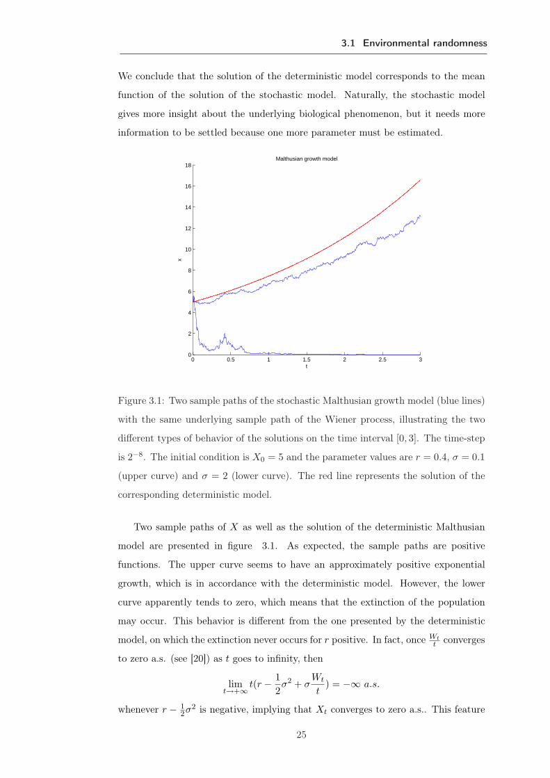
Figure 3.1: Two sample paths of the stochastic Malthusian growth model (blue lines)
with the same underlying sample path of the Wiener process, illustrating the two
different types of behavior of the solutions on the time interval [0, 3]. The time-step
is 2−8. The initial condition is X0 = 5 and the parameter values are r = 0.4, σ = 0.1
(upper curve) and σ = 2 (lower curve). The red line represents the solution of the
corresponding deterministic model.
Two sample paths of X as well as the solution of the deterministic Malthusian
model are presented in figure 3.1. As expected, the sample paths are positive
functions. The upper curve seems to have an approximately positive exponential
growth, which is in accordance with the deterministic model. However, the lower
curve apparently tends to zero, which means that the extinction of the population
may occur. This behavior is different from the one presented by the deterministic
model, on which the extinction never occurs for r positive. In fact, once Wtt converges
to zero a.s. (see [20]) as t goes to infinity, then
limt→+∞ t(r − 1
2σ2 + σ
Wt
t) = −∞ a.s.
whenever r − 12σ2 is negative, implying that Xt converges to zero a.s.. This feature
25
Chapter 3 Modelling the evolution of populations
0 0.5 1 1.5 24
6
8
10
12
14
16
18
20
t
Xt
Stochastic Malthusian growth model
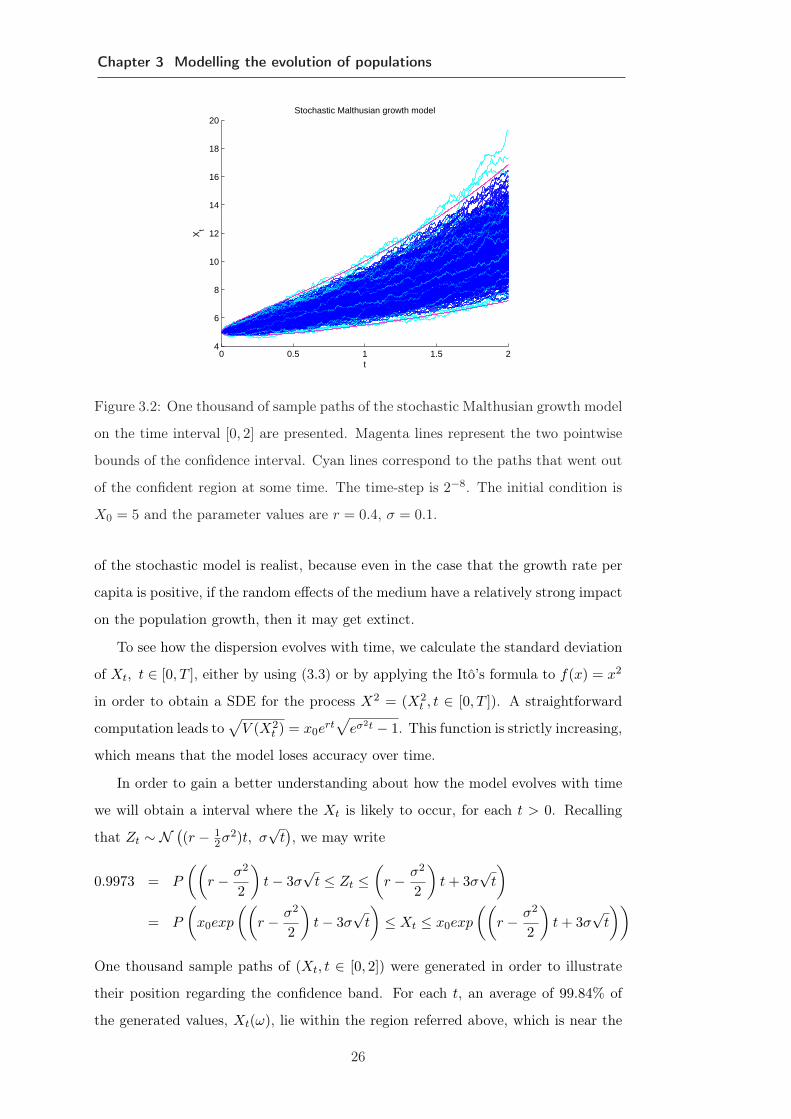
Figure 3.2: One thousand of sample paths of the stochastic Malthusian growth model
on the time interval [0, 2] are presented. Magenta lines represent the two pointwise
bounds of the confidence interval. Cyan lines correspond to the paths that went out
of the confident region at some time. The time-step is 2−8. The initial condition is
X0 = 5 and the parameter values are r = 0.4, σ = 0.1.
of the stochastic model is realist, because even in the case that the growth rate per
capita is positive, if the random effects of the medium have a relatively strong impact
on the population growth, then it may get extinct.
To see how the dispersion evolves with time, we calculate the standard deviation
of Xt, t ∈ [0, T ], either by using (3.3) or by applying the Itô’s formula to f(x) = x2
in order to obtain a SDE for the process X2 = (X2t , t ∈ [0, T ]). A straightforward
computation leads to√
V (X2t ) = x0e
rt√
eσ2t − 1. This function is strictly increasing,
which means that the model loses accuracy over time.
In order to gain a better understanding about how the model evolves with time
we will obtain a interval where the Xt is likely to occur, for each t > 0. Recalling
that Zt ∼ N ((r − 1
2σ2)t, σ√
t), we may write
0.9973 = P
((r − σ2
2
)t− 3σ
√t ≤ Zt ≤
(r − σ2
2
)t + 3σ
√t
)
= P
(x0exp
((r − σ2
2
)t− 3σ
√t
)≤ Xt ≤ x0exp
((r − σ2
2
)t + 3σ
√t
))
One thousand sample paths of (Xt, t ∈ [0, 2]) were generated in order to illustrate
their position regarding the confidence band. For each t, an average of 99.84% of
the generated values, Xt(ω), lie within the region referred above, which is near the
26
3.1 Environmental randomness
theoretical value, as expected. In figure 3.2, we can see the generated sample paths,
as well as the confidence region. Despite being quite simple to calculate the pointwise
confidence band, it would be more worthwhile to obtain a confidence band uniformly
in t. However there is not a closed formula for obtaining that band (see [27]). In
this simulation, only 95.5% of the sample paths presented in figure 3.2 lie entirely
within the considered region. Those are presented in blue, while the remaining 4.5%
are presented in cyan. If we consider a bigger time interval, these percentages get
worse.
3.1.2. Stochastic logistic growth model I
One assumption underlying the previous model is the lack of any limitation of re-
sources, which allows the unbounded growth of the population whenever the growing
rate satisfies a certain condition. This situation is realistic when the size of the pop-
ulation is far bellow the carrying capacity of the habitat. However, as the population
grows, a different dynamic may occur: the system will eventually enter a region in
which negative feedback factors become important. The lack of resources makes the
growing rate to decrease and the size of the population will eventually reach an equi-
librium. A basic model that incorporates these two phenomena is the well-known
deterministic logistic model,
dx
dt(t) = rx(t)
(1− x(t)
K
), x(0) = x0, t ∈ [0, T ],
where x(t) represents the density of the population at time t, r ∈ R+ the growth
rate and K ∈ R+ the carrying capacity. The variation per capita is now given by the
quotient dxdt /x = r1(x) := r
(1− x
K
). Notice that r is now the maximum rate. For
x0 < K, dxdt is positive and as the population increases, r1 decreases until vanishing.
At this moment, the derivative dxdt is null, which means that the population density
reaches an equilibrium with the habitat: limt→∞x(t) = K. On the other hand, if
x0 > K, then dxdt is negative and the population decreases until it reaches again K.
For r > 0, K is then a globally asymptotic stable equilibrium point, while 0 is an
unstable equilibrium point.
As in the study of the Malthusian model, we will introduce a gaussian pertur-
bation on the growth rate per capita, R := r1 + σWt a.s., σ > 0, leading to the
following logistic stochastic differential equation,
dXt = rXt
(1− Xt
K
)dt + σXtdWt, X0 = x0, t ∈ [0, T ]. (3.5)
27

Chapter 3 Modelling the evolution of populations
0 2 4 6 8 10 12 14 16 18 200
1
2
3
4
5
6
7Stochastic logistic growth model I
t
Xt
Figure 3.3: Three sample paths of the stochastic logistic growth model on the time
interval [0, 20], corresponding to three different values for σ: 0.01 (magenta), 0.1
(cyan) and 0.2 (red). The time-step is 2−8, the initial condition is X0 = 1 and the
values of the remaining parameters are r = 1, k = 5. The blue line represents the
solution of the corresponding deterministic model with the same time-step and the
same parameters’ values.
Since the coefficients are not linear, a unique strong solution, X = (Xt, t ∈ [0, T ]),
of (3.5) exists until a time of explosion, which turns out to be infinite (see [7]).
The solution X is a homogeneous diffusion process with drift coefficient m(t, x) =
rx(1− x
K
)and diffusion coefficient Q(t, x) = σ2x2.
The Euler-Maruyama method was implemented (see [6] [22]).2 Some sample
paths are plotted in figures 3.3 and 3.4.
We see that the sample paths are positive. In figure 3.3, the sample paths behave
accordingly to the deterministic solution: they stay in the vicinity of the carrying
capacity, K = 5, which suggests that the solution of the SDE has a stationary distri-
bution with mean value K. This is in fact true and can be formally proved (see [7]).
We also observe that as σ increases, the variance of Xt increases too, as was to be ex-
pected from ( 3.5). In figure 3.4, we see a different behavior: the sample paths differ
from the deterministic model, they apparently do not follow any specific rule, except
the sample path (c), which tends to zero (extinction). This behavior is justified by
the big oscillations due to the value of σ being bigger then one, which causes the
random term to be bigger then Xt. As Xt increases governed by the deterministic
2This model can also be solved analytically by performing an appropriate change of variable (see
[3]).
28

3.1 Environmental randomness
0 5 10 15 200
5
10
15
20
(a) σ = 1.2
0 5 10 15 200
5
10
15
20
25
(b) σ = 1.3
0 5 10 15 200
2
4
6
8
10
(c) σ = 2
Figure 3.4: Three sample paths (cyan) of the stochastic logistic growth model on the
time interval [0, 20]. The time-step is 2−8, the initial condition is X0 = 1 and the
values of the remaining parameters are r = 1, k = 5. The blue line represents the
solution of the corresponding deterministic model with the same time-step and the
same parameters’ values.
part of the equation, the random term increases too, making the sample path to vary
with such a big amplitude that it nearly reaches zero. At this moment, the random
term is small again and Xt remains near zero making small "jumps" only, until it
eventually goes up and we return to the initial situation that may be repeated over
time. This feature of the model is in accordance with population growth mechanisms
observed in real life: if the randomness of the environment is big, then the changes
on the population size are more unpredictable and may result in dramatic changes or
even extinction in a short period of time. We can think, for example, in a population
which is infected by a contagious disease: when the population is small, individuals
do not have so much contact with each other, therefore, the disease does not prop-
agate easily and the growth of the population is approximately logistic. When the
density of the population gets bigger, then two situations may occur: the contacts
do not increase and the size of the population may remain following a logistic growth
or the contacts may increase so that many individuals get infected and may dye. In
this example, the randomness of the environment can be associated to the contacts
between individuals.
We shall next find an approximation for the mean function of the solution by
applying the Monte Carlo method. The mean function was obtained from 10, 100
and 1000 generated sample paths. The resulting estimations were then compared to
the solution, u, of the deterministic logistic growth equation obtained numerically.
29
Chapter 3 Modelling the evolution of populations
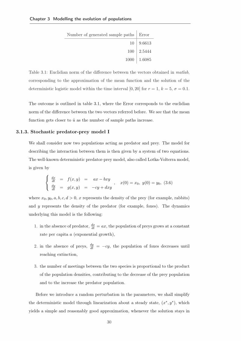
Number of generated sample paths Error
10 9.6613
100 2.5444
1000 1.6085
Table 3.1: Euclidian norm of the difference between the vectors obtained in matlab,
corresponding to the approximation of the mean function and the solution of the
deterministic logistic model within the time interval [0, 20] for r = 1, k = 5, σ = 0.1.
The outcome is outlined in table 3.1, where the Error corresponds to the euclidian
norm of the difference between the two vectors referred before. We see that the mean
function gets closer to u as the number of sample paths increase.
3.1.3. Stochastic predator-prey model I
We shall consider now two populations acting as predator and prey. The model for
describing the interaction between them is then given by a system of two equations.
The well-known deterministic predator-prey model, also called Lotka-Volterra model,
is given by
dxdt = f(x, y) = ax− bxy
dydt = g(x, y) = −cy + dxy
, x(0) = x0, y(0) = y0, (3.6)
where x0, y0, a, b, c, d > 0, x represents the density of the prey (for example, rabbits)
and y represents the density of the predator (for example, foxes). The dynamics
underlying this model is the following:
1. in the absence of predator, dxdt = ax, the population of preys grows at a constant
rate per capita a (exponential growth),
2. in the absence of preys, dydt = −cy, the population of foxes decreases until
reaching extinction,
3. the number of meetings between the two species is proportional to the product
of the population densities, contributing to the decrease of the prey population
and to the increase the predator population.
Before we introduce a random perturbation in the parameters, we shall simplify
the deterministic model through linearization about a steady state, (x∗, y∗), which
yields a simple and reasonably good approximation, whenever the solution stays in
30
3.1 Environmental randomness
the vicinity of (x∗, y∗). The steady states of ( 3.6) are (0, 0) and (c/d, a/b), which
were easily obtained by making f and g equal to zero. On the one hand, a lineariza-
tion around (0, 0) allows us to draw conclusions about the predation phenomenon
when both prey and predator populations have a small number of individuals. On
the other hand, a linearization around (c/d, a/b) gives us insight about the phe-
nomenon when the prey and predator populations have a density about a/b and
c/d, respectively. In the first case, it turns out that the population growth is ex-
ponential for both populations, which conduces us to a Malthusian model already
discussed in the beginning of this section. We will then see what happens in the
second case. By applying the first order Taylor polynomial at (c/d, a/b) we obtain a
linear approximation for f and g, which leads to the following linear system,
dudt = − bc
d v
dvdt = ad
b u, u(0) = u0, v(0) = v0 (3.7)
with u = x − cd , v = y − a
b and u0 and v0 in the vicinity of the steady state
(u∗, v∗) = (0, 0).
Introducing now a gaussian perturbation on the parameters c and a of the form
c + σ1Wt and a + σ2Wt, with σi ∈ R+, i = 1, 2, we obtain the following stochastic
linear system,
dUt = − bcd Vtdt− σ1
bdVtdWt
dVt = adb Utdt + σ2
dbUtdWt,
, U0 = u0, V0 = v0 a.s.
or, in the matrix form,
dZt = AZtdt + BZtdWt,
with Zt = (Ut, Vt),
A =
0 − bc
d
adb 0
, B =
0 −σ1
bd
σ2db 0
.
Suppose that the parameters of the model satisfy ca = σ1
σ2, which may be plausible,
once the parameters responsible for the randomness, σ1 and σ2, do not need to be
very specific, only the order of magnitude of the noise is important. In this case, we
have that A and B are constants and verify AB = BA. We may then obtain an
explicit expression for the solution to this system given in ( 2.28), namely,
Zt = Φ(t)ξ, t ∈ [0, T ],
31

Chapter 3 Modelling the evolution of populations
0 5 10 15 2020
40
60
80
100
120
140
160Linearized stochastic predator−prey growth model I
t
Figure 3.5: Three sample paths of the linearized stochastic Lotka-Volterra I on the
time interval [0, 20], corresponding to n = 4 (cyan), n = 7 (green) and n = 10
(magenta). The time-step is 2−8, the initial condition is Z0 = (20,−10) and the
values of the remaining parameters are a = 1, b = 0.02, c = 1, d = 0.01 . The blue
line represents the solution of the corresponding deterministic linearized model with
the same time-step and the same parameters’ values.
with
Φ(t) = exp
[(A− 1
2B2
)t + BWt
], t ∈ [0, T ]. (3.8)
Three sample paths of Z are presented in figure 3.5.
Finally, notice that the random effect introduced to obtain the models ( 3.2),
(3.5) and ( 3.8) results from environmental randomness and not from demographic
randomness, i.e., the randomness associated to the number of births and deaths,
which exists even when the birth and death rates are constant. This case is considered
in the next section.
3.2. Demographic randomness
The phenomena studied in population dynamics are intrinsically discrete and are
often modeled by Markov chains. However, as the discretization becomes finer,
Markov chains might be well approximated by diffusion processes corresponding to
32

3.2 Demographic randomness
solutions of stochastic differential equations, therefore facilitating the mathematical
analysis (see [3], [10], [12], [13], [11] and [28]).We will then make the assumption that
the biological phenomenon is well described by a vector-valued time-homogeneous
Markov chain X = (X(n)t , t ∈ [0, T ]), with X(n)
t = (X(n)t,1 , ..., X
(n)t,d ), d ∈ N, with state
space 1nZ, where X
(n)t represents its population density at time t, depending on the
parameter n, which represents the order of magnitude of the populationsŠ size or of
the area of the habitat.
The procedure followed for the model deduction comprises the following steps:
• define X(n)0 = x0 and the transition probabilities of the Markov chain X(n),
• for large n, we approximate X(n) by a diffusion process Y(n) with coefficients
ρ and Q,
• Y(n) is a solution of the matrix SDE
dY(n)t = ρ(Y(n), t)dt +
12√
nσ(Y(n), t)dWt, Y(n)
0 = x0
with σσT = Q.
We begin by briefly presenting the discrete model for one population. An heuristic
deduction of the continuous model shall then be described and analysed in order
to draw some conclusions about the underlying biological phenomenon. Consider
one species in a certain habitat at time t > 0. For a small positive constant δt let
∆X(n) := X(n)t+∆t−X
(n)t denote the variation of the density occurring within [t, t+∆t]
and Dn the support of ∆X(n), which is defined by
Dn =
l
n: l ∈ D
,
where D := Z∩E and E is a limited interval. Assume that the transition probabilities
of X(n),
pt,k/n
(t + ∆t,
k + l
n
):= P
(∆X(n) =
l
n/X
(n)t =
k
n
),
take the general form
pt,k/n
(t + ∆t,
k + l
n
)= nβl
(t,
k
n
)∆t + o(∆t), (3.9)
for each l ∈ D \0 and βl : [0, T ]×R→ R+0 , which represents the transition change
rate of the Markov chain. Since pt,k/n is a probability, then for l = 0 the probability
of the variation to be null is naturally given by
pt,k/n
(t + ∆t,
k
n
)= 1− n∆t
∑
l∈D\0βl
(t,
k
n
)+ o(∆t). (3.10)
33

Chapter 3 Modelling the evolution of populations
The Markov chain is, thus, completely determined by the transition probabilities
( 3.9) and ( 3.10) and the distribution of X(n)0 .
The deduction of the diffusion approximation undergoes now through the heuris-
tic construction of a relation involving the transition probability functions pt,x(s, y),
for x, y ∈ 1nZ and 0 ≤ t < s ≤ T , based on the forward Kolmogorov equations.
We begin by writing down the Chapman-Kolmogorov equation for time-continuous
Markov chains,
pt,x(s + ∆s, y) =∑
l∈D
pt,x(s, y − l/n)ps,y−l/n(s + ∆s, y).
with 0 ≤ t < s < s + ∆s ≤ T . Using the expressions in ( 3.9) and ( 3.10), the
previous summation can be rewritten as
pt,x(s + ∆s, y) = pt,x(s, y)
1− n∆s
∑
l∈D\0βl (s, y) + o(∆s)
+ n∆s∑
l∈D\0pt,x(s, y − l/n)βl (s, y − l/n) + o(∆s).
Dividing by ∆s and making ∆s to approach 0 we derive a differential equation
for the transition probability function pt,x. From ( 3.11) we thus obtain,
∂pt,x
∂s(s, y) = −n
∑
l∈D\0pt,x(s, y)βl(s, y) (3.11)
+ n∑
l∈D\0pt,x(s, y − l/n)βl(s, y − l/n)
Furthermore, for l/n sufficiently small, which is easily verified if n is large, we can
find a local approximation for pt,x(s, y− l/n)βl(s, y− l/n), by using the second order
Taylor polynomial at y. Under adequate regularity conditions, it follows from ( 3.12)
that
∂pt,x
∂s≈ −n
∑
l∈D\0pt,xβl + n
∑
l∈D\0
[pt,xβl − l
n
∂(pt,xβl)∂y
+12
l2
n2
∂2(pt,xβl)∂y2
](3.12)
evaluated at (s, y). Finally, simplifying this equation, we conclude that the transition
probability, pt,x, satisfies approximately the second-order partial differential equation
∂ft,x
∂s=
∂(ft,xρ)∂y
+12n
∂2(ft,xQ)∂y2
at (s, y), (3.13)
with
ρ :=∑
l∈D\0lβl and Q :=
∑
l∈D\0l2βl.
34

3.2 Demographic randomness
This gives us an idea about the diffusion process Y (n) we may use as an approximation
for the Markov chain X(n). Whenever ρ and Q satisfy the conditions described in
theorem 2, ( 3.13) coincides with the Kolmogorov forward equation of the diffusion
process with coefficients ρ and Qn , whose the unique solution, ft,x, is a transition
density function of the process Y (n). Indeed, it can be shown that, for n large
enough, Y (n) represents a good approximation of X(n) (see [10]).
We finally arrived to the SDE’s stochastic model for one species given by
dY(n)t = ρ(Y (n)
t , t)dt +1
2√
nσ(Y (n)
t , t)dWt, Y(n)0 = x0 a.s. (3.14)
with√
Q = σ.
The previous deduction can easily be generalized for the case of d interacting
species. In this case, define D := Zd∩E, where E a limited d-dimensional rectangle,
and
ρ :=∑
l∈D\0lβl and Q :=
∑
l∈D\0llT βl,
where βl is a real function defined in Dn The resulting model is given by
dY(n)t = ρ(Y(n)
t , t)dt +1
2√
nσ(Y(n)
t , t)dWt, Y(n)0 = x0 a.s. (3.15)
such that Q = σσT .
3.2.1. Stochastic logistic growth model II
The functions βl can be obtained from the deterministic logistic growth model, which
is given by dydt = y
(r − r y
K
). To establish the stochastic model, we need some
more information related to the population in consideration, namely, for instance,
the birth and death rates, which are represented by the parameters β1 and β−1,
respectively, and must satisfy β1 − β−1 = y(r − r y
K
). In order to present latter
numerical examples we will consider β1(t, y) = ry, β−1(t, y) = r y2
k and rl = 0 for
l 6= −1, 0, 1. Consequently, m(s, y) = y(r − r y
K
)and Q(s, y) = y
(r − r y
K
). A
stochastic logistic growth model for the population density, whose size of the habitat
has a order of magnitude of n, assumed constant, is thus given by the following SDE
dY(n)t =
(rY
(n)t − r
K
(Y
(n)t
)2)
dt +1
2√
n
√∣∣∣∣rY(n)t +
r
K
(Y
(n)t
)2∣∣∣∣dWt.
Some sample paths of the solution are plotted in figure 3.6. Similarly to the stochastic
logistic model I studied in section 3.1.2, we observe that the sample paths remain
in the vicinity of the solution of the deterministic model. Increasing the parameter
35
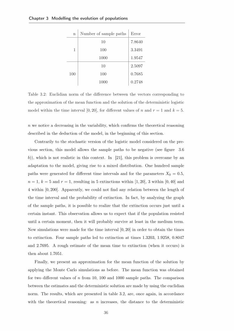
Chapter 3 Modelling the evolution of populations
n Number of sample paths Error
10 7.8640
1 100 3.3491
1000 1.9547
10 2.5097
100 100 0.7685
1000 0.2748
Table 3.2: Euclidian norm of the difference between the vectors corresponding to
the approximation of the mean function and the solution of the deterministic logistic
model within the time interval [0, 20], for different values of n and r = 1 and k = 5.
n we notice a decreasing in the variability, which confirms the theoretical reasoning
described in the deduction of the model, in the beginning of this section.
Contrarily to the stochastic version of the logistic model considered on the pre-
vious section, this model allows the sample paths to be negative (see figure 3.6
b)), which is not realistic in this context. In [21], this problem is overcame by an
adaptation to the model, giving rise to a mixed distribution. One hundred sample
paths were generated for different time intervals and for the parameters X0 = 0.5,
n = 1, k = 5 and r = 1, resulting in 5 extinctions within [1, 20], 3 within [0, 40] and
4 within [0, 200]. Apparently, we could not find any relation between the length of
the time interval and the probability of extinction. In fact, by analyzing the graph
of the sample paths, it is possible to realize that the extinction occurs just until a
certain instant. This observation allows us to expect that if the population resisted
until a certain moment, then it will probably survive at least in the medium term.
New simulations were made for the time interval [0, 20] in order to obtain the times
to extinction. Four sample paths led to extinction at times 1.3203, 1.9258, 0.8047
and 2.7695. A rough estimate of the mean time to extinction (when it occurs) is
then about 1.7051.
Finally, we present an approximation for the mean function of the solution by
applying the Monte Carlo simulations as before. The mean function was obtained
for two different values of n from 10, 100 and 1000 sample paths. The comparison
between the estimates and the deterministic solution are made by using the euclidian
norm. The results, which are presented in table 3.2, are, once again, in accordance
with the theoretical reasoning: as n increases, the distance to the deterministic
36
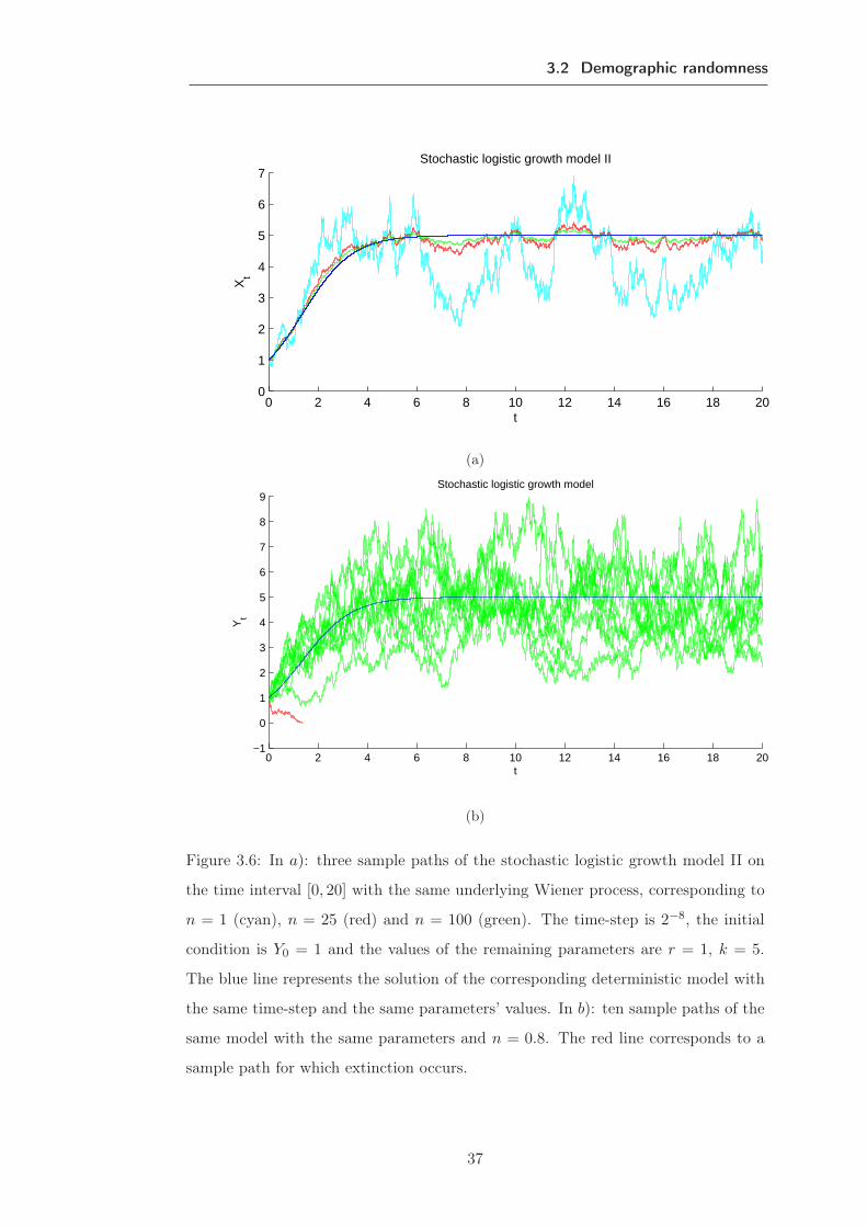
3.2 Demographic randomness
0 2 4 6 8 10 12 14 16 18 200
1
2
3
4
5
6
7Stochastic logistic growth model II
Xt
t
(a)
0 2 4 6 8 10 12 14 16 18 20−1
0
1
2
3
4
5
6
7
8
9
t
Yt
Stochastic logistic growth model
(b)
Figure 3.6: In a): three sample paths of the stochastic logistic growth model II on
the time interval [0, 20] with the same underlying Wiener process, corresponding to
n = 1 (cyan), n = 25 (red) and n = 100 (green). The time-step is 2−8, the initial
condition is Y0 = 1 and the values of the remaining parameters are r = 1, k = 5.
The blue line represents the solution of the corresponding deterministic model with
the same time-step and the same parameters’ values. In b): ten sample paths of the
same model with the same parameters and n = 0.8. The red line corresponds to a
sample path for which extinction occurs.
37

Chapter 3 Modelling the evolution of populations
0 2 4 6 8 10 12 14 16 18 2020
40
60
80
100
120
140
160
t
Yn t
Stochastic Lotka Volterra model
Figure 3.7: Three sample paths of the stochastic Lotka-Volterra model on the time
interval [0, 20] with the same underlying Wiener process, corresponding to n = 1
(cyan), n = 25 (red) and n = 100 (green). The time-step is 2−8, the initial condition
is Z0 = (120, 40) and the values of the remaining parameters are a = 1, b = 0.02, c =
1, d = 0.01. The blue line represents the solution of the corresponding deterministic
model with the same time-step and the same value of the parameters.
model decreases. This fact suggests that the empirical mean function converges to
the solution of the deterministic model.
3.2.2. Stochastic predator-prey model II
Consider the deterministic Lotka-Volterra model ( 3.6). Define z := (x, y) and
D := (0, 0), (1, 0), (−1, 0), (0, 1), (0,−1), where (1, 0) and (−1, 0) represent one
birth and one death, respectively, in the prey population and (0, 1) and (0,−1)
represent one birth and one death in the predator population. The birth and death
rates in each population are given by β(1,0) = ax, β(0,1) = dxy, β(−1,0) = bxy,
β(0,−1) = cy. Consequently, we have
m(t, y) =∑
l∈D
lβl =
ax− bxy
dxy − cy
and
Q(t, y) =∑
l∈D
llT βl =
ax + bxy 0
0 dxy + cy
.
38

3.2 Demographic randomness
Prey
n No. of sample paths Error
10 698.7552
1 100 341.6737
1000 286.4792
10 59.9920
100 100 26.2427
1000 12.2385
Predator
n No. of sample paths Error
10 387.3996
1 100 164.3148
1000 107.8320
10 34.1499
100 100 12.6041
1000 6.0136
Table 3.3: Euclidian norm of the difference between the vectors corresponding to
the approximation of the mean function and the solution of the deterministic logistic
model within the time interval [0, 20], for a = 1, b = 0.02, c = 1, d = 0.01 and for
different values of n.
Once Q is a diagonal matrix, the diffusion matrix is given by
σ(t, y) =
√|ax + bxy| 0
0√|dxy + cy|
.
If the habitat area has a order of magnitude of n, then a stochastic predator-prey
model is given by the system
dXt = (aXt − bXtYt)dt + 12√
n
√|aXt + bXtYt|dW
(1)t
dYt = (dXtYt − cYt)dt + 12√
n
√|dXtYt + cYt|dW
(2)t .
For simplicity, we suppress the index n on the random variables Xt and Yt. Recall
that the Wiener processes (W (1)t , t ∈ [0, T ]) and (W (2)
t , t ∈ [0, T ]) are independent.
Some sample paths are plotted in figure 3.7 corresponding to different values of the
parameter n. We see that the general dynamics of the stochastic model is consistent
with the deterministic model: when the prey population increases (decreases), the
density of the predators increases (decreases) too, with a delay. Once again, as n
increases, the variability decreases and the sample paths get apparently closer to the
solution of the deterministic model. The results outlined in table 3.3 were obtained
through Monte Carlo simulations and they confirm the previous conclusions.
3.2.3. Stochastic SIR epidemic model
An epidemic model pretends to represent the dynamic associated to the transmission
of a disease within a population. In this section, we begin by considering the most
39

Chapter 3 Modelling the evolution of populations
basic deterministic epidemic model, the SIR model, which describes the number
of susceptible (S), infected (I) and recovered (R) individuals of a population. The
following assumptions are made:
1. the recovered individuals are not able to be infected again or to transmit the
infection to any susceptible individual,
2. the size of the population is considered to be fixed, i.e., S(t)+I(t)+R(t) = N ,
3. all individuals of the population have the same probability of contracting the
disease at a rate proportional to the number of meetings between infected and
susceptible, aSI,
4. infected individuals recover at a rate per capita b
Summarizing the above description, the evolution of each class of individuals is gov-
erned by the following rules
S + Ia−→ 2I, I
b−→ R.
By the Law of Mass Action, the deterministic model is then given by
dsdt = −asj
djdt = asj − bj,
,
with s = S/N , j = I/N . Obviously, the percentage of recovered individuals follows
directly from the second assumption: r = R/N = 1−s−j. In the setting of figure 3.8,
at t = 0 the fraction of infected individuals corresponds to 1%, while the remaining
99% are susceptible. The epidemic increases until reaching its maximum 0.1586 at
time t = 6.25. At this time, the susceptible population falls below c = b/a = 0.5, as
we can see in figure 3.8. The parameter c is called basic parameter number and has
a crucial importance in the model, since it determines whether the disease will dye
out (c < 1) or whether it may become epidemic (c > 1). The stochastic model is
capable of giving a more realistic description of this value, as we will see next.
Proceeding as before, we define z := (s, j) and D := (0, 0), (−1, 1), (0,−1),where (−1, 1) represents the infection of one individual and (0,−1) represents one
recovery. The rates of change of each class of individuals is given by β(0,−1) = bj and
β(−1,1) = asj. Consequently, we have
40

3.2 Demographic randomness
0 5 10 15 200
0.1
0.2
0.3
0.4
0.5
0.6
0.7
0.8
0.9
1
X: 6.25Y: 0.5009
t
Deterministic SIR model
Figure 3.8: Evolution of the percentages of susceptible (magenta), infected (blue)
and recovered (green) individuals within the time interval [0, 20] in the deterministic
SIR model ( 3.16). The time-step is 2−8, the initial condition is x0 = (0.99, 0.01, 0)
and the values of the parameters are a = 1.4, b = 0.7.
m(t, z) =
−asj
asj − bj
and Q(t, z) =
asj −asj
−asj asj + bj
. By using the Cholesky
decomposition, we obtain Q = σT σ, with
σ =
√|asj| 0
−√|asj|
√|bj|
.
Notice that the decomposition Q = σT σ is not unique. Another decomposition for
the matrix Q satisfying the previous relation is given by
σ′(t, z) =1d
asj + g −asj
−asj asj + bj + g
,
where g =√
det(Q) and d =√|2asj + bj + 2g|. This ambiguity allows that different
SDE models can be used to construct the same diffusion process, which seems a
contradiction. In fact, once both systems are associated to the same Kolmogorov
forward equation, the solutions of each system have the same distribution. Moreover,
under the conditions of theorem 3, it can be proved that a sample path solution of
one system is also a sample path solution of the other system and vice versa (see
[13]). The systems may be considered as thus equivalent.
41
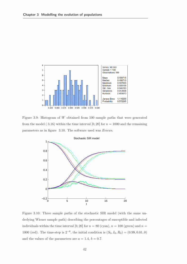
Chapter 3 Modelling the evolution of populations
Figure 3.9: Histogram of W obtained from 100 sample paths that were generated
from the model ( 3.16) within the time interval [0, 20] for n = 1000 and the remaining
parameters as in figure 3.10. The software used was Eviews.
0 5 10 15 20−0.2
0
0.2
0.4
0.6
0.8
1
t
Stochastic SIR model
Figure 3.10: Three sample paths of the stochastic SIR model (with the same un-
derlying Wiener sample path) describing the percentages of susceptible and infected
individuals within the time interval [0, 20] for n = 80 (cyan), n = 100 (green) and n =
1000 (red). The time-step is 2−8, the initial condition is (S0, I0, R0) = (0.99, 0.01, 0)
and the values of the parameters are a = 1.4, b = 0.7.
42

3.2 Demographic randomness
For a big enough population, and considering the matrix σ, a stochastic SIR
model is given by the system
dSt = −aStItdt + 12√
n
√|aStIt|dW
(1)t
dIt = (aStIt − bIt)dt− 12√
n
√|aStIt|dW
(2)t + 1
2√
n
√|bIt|dWt,2
.
For simplicity, we suppress the index n on the random variables It and St. Some
sample paths are plotted in figure 3.10 corresponding to different values of n. Due
to the importance of the parameter c = b/a referred before, we will explore the
behavior of the correspondent random variable C in the stochastic model. From 100
sample paths we obtained the histogram of C presented in figure 3.9 and confirmed
by Jarque-Béra test that C follows a gaussian distribution with mean 0.4997 and
standard deviation 0.0408. It follows that about 99.7% of the values of C drawn
from this model are within three standard deviations from the mean value, i.e.,
[0.3273, 0.5721]. Consequently, in this case, the disease will be eradicated, which is
in accordance with the results illustrated in figure 3.10.
43

Chapter 3 Modelling the evolution of populations
44

Chapter 4
Conclusion
As we could see, from the perspective of modellation, SDEs can provide a rich variety
of models in the context of population dynamics. One can settle different stochastic
models corresponding to the same phenomenon, depending on the assumption and
on the random aspect we want to model. In this thesis, two different random effects
were considered: the environmental and the demographic randomness.
In order to build SDE models, one can add a random ad hoc perturbation in
the classic ODE model, assuming that the dynamics are partly driven by noise, or
consider a diffusion approximation of a continuous-time Markov chain, frequently a
simple birth and death process (see [10], [29] and [30]). The last method seems
more natural as it is based on the relationship between diffusion processes and SDE
solutions, while the first one is more vague, because of the wide variety of different
environmental aspects existing in Nature. A combination of both would naturally
be the best option from the modellation point of view.
In what concerns the analysis of the established models, different technics were
used. When the model was linear, it was possible to find the exact solution. However,
realistic models in population dynamics are usually nonlinear. In this case, two differ-
ent approaches were followed: in the first one, we proceeded to the linearization of the
deterministic model and introduced then the random environmental perturbation,
which led to a linear stochastic differential system for describing the prey-predator
interaction; in the second one, the Euler-Maruyama method was implemented in or-
der to give an approximation for the sample paths solution of the original non-linear
model.
The dynamic of one population following a logistic growth as well as the predator-
prey interaction were analysed in the context of the two construction methods men-
tioned above. It was thus possible to obtain two different stochastic models for the
same phenomenon. Lastly, a stochastic SIR epidemic model was established and the
distribution of the basic parameter number was estimated by Monte-Carlo simula-
45

tions. Curiously, this parameter has apparently a normal distribution.
During the preparation of this thesis, we could realize that stochastic differential
equations constitute a fundamental modelling tool in science and an extensive field
of mathematical research. During the last decades, the subject has been developing
in many exciting ways and in several fields (for instance in image denoising, see [31]),
both theoretical and application specific. In the theoretical framework, we stress the
study of the assymptotic behavior of their solutions and extinction times, which are
particularly important in biology, parameters estimation (see [30] for an introduc-
tion), as well as the properties of numerical approximations of the solutions (see [32])
such as error estimation, consistency, stability and convergence. More recently, we
also find in the literature new and more realistic modeling approaches that comprise
stochastic partial differential equation systems, in order to obtain also a spatial dis-
tribution of the populations, or stochastic differential equations driven by Wiener
and Poisson processes, known as SDEs with jumps, where the jump component can
capture event-driven uncertainties.
46

Appendix A
Matlab code
A.1. Euler-Maruyama method for stochastic logistic growthmodel
1 %Método de Euler−Maruyama
2 %Generating 100 sample paths o f s t o c h a s t i c l o g i s t i c growth
model
3 %dX=mudt+sigmadW
4 c l e a r a l l
5 de l t a=2^(−8) ;
6 T=20;
7 n=T/ de l t a ;
8 X0=1;
9 t0=0;
10 num_trajetorys=100;
11 Y=ze ro s ( num_trajetorys , n ) ;
12 Ye=ze ro s (1 , n) ;
13 Yt=X0 ;
14 Yte=X0 ;
15 meantime=ze ro s (n , 1 0 ) ;
16 e x t i n c t i o n =0;
17 N=0.8;
18 k=5;
19 r=1;
20 hold on
21 f o r i =1: num_trajetorys
22 dW=sqr t ( de l t a ) ∗ randn (1 , n) ;
23 Yt=X0 ;
24 f o r j =1:n
47

Appendix A Matlab code
25 mu=r ∗Yt∗(1−Yt/k ) ;
26 sigma=sq r t ( abs ( r ∗Yt∗(1+Yt/k ) ) ) /(2∗ s q r t (N) ) ;
27 Yt=Yt+mu∗ de l t a+sigma∗dW( j ) ;%random so l u t i o n
28 Y( i , j )=Yt ;
29 end
30 bool=Y( i , : ) >0;
31 i f (sum( bool )==n)
32 p lo t ( [ 0 : d e l t a :T ] , [ X0 ,Y( i , : ) ] , ’ g ’ ) ;
33 e l s e
34 meantime ( : , e x t i n c t i o n+1)=1−bool ;
35 e x t i n c t i o n=ex t i n c t i o n +1;
36 time=f i nd (1−bool , 1 ) ;
37 p lo t ( [ 0 : d e l t a : time∗ de l t a ] , [ X0 ,Y( i , 1 : time ) ] , ’ r ’ ) ;
38 end
39 end
40 f o r j =1:n
41 mu=r ∗Yte∗(1−Yte/k ) ;
42 Yte=Yte+mu∗ de l t a ;
43 Ye( j )=Yte ;%de t e rm i n i s t i c s o l u t i o n
44 end
45 p lo t ( [ 0 : d e l t a :T ] , [ X0 ,Ye ] ) ;
46 hold o f f
47 MeanTimeExtinction=f i nd (meantime ( : , 1 ) , 1 ) ∗ de l t a ;
A.2. Euler-Maruyama method for stochastic SIR model
1 %Euler−Maruyama method f o r systems o f SDEs
2 %Generating 100 sample paths o f s t o c h a s t i c SIR model
3 %dX=mudt+sigmadW
4 c l e a r a l l
5 de l t a=2^(−8) ;
6 T=20;
7 n=T/ de l t a ;
8 X0= [ 0 . 9 9 , 0 . 0 1 ] ’ ;
9 m=length (X0) ;
48

A.2 Euler-Maruyama method for stochastic SIR model
10 t0=0;
11 num_trajetorys=100;
12 Y=ze ro s ( num_trajetorys , n ,m) ;
13 Ye=ze ro s (m, n) ;
14 C=ze ro s (1 , num_trajetorys ) ;
15 Yte=X0 ;
16 a=1.4 ;
17 b=0.7 ;
18 N=1000;
19 hold on
20 f o r i =1: num_trajetorys
21 dW=sqr t ( de l t a ) ∗ randn (m, n) ;
22 Yt=X0 ;
23 f o r j =1:n
24 mu=[−a∗Yt (1) ∗Yt (2) ; a∗Yt (1) ∗Yt (2)−b∗Yt (2) ] ;
25 sigma=[ sq r t ( abs ( a∗Yt (1) ∗Yt (2) ) ) ,0;− s q r t ( abs ( a∗Yt (1) ∗Yt (2) ) ) , s q r t ( abs (b∗Yt (2) ) ) ] ;
26 Yt=Yt+mu∗ de l t a+sigma/ sq r t (N) /2∗dW( : , j ) ;%random
so l u t i o n
27 Y( i , j , 1 )=Yt (1) ;
28 Y( i , j , 2 )=Yt (2) ;
29 end
30 [ maximo , i nd i c e ]=max(Y( i , : , 2 ) ) ;
31 C( i )=Y( i , i nd i c e , 1 ) ;
32 p lo t ( [ 0 : d e l t a :T ] , [ X0(1 ) ,Y( i , : , 1 ) ] , ’ c ’ ) ;%S
33 p lo t ( [ 0 : d e l t a :T ] , [ X0(2 ) ,Y( i , : , 2 ) ] , ’ c ’ ) ;%I
34 p lo t ( [ 0 : d e l t a :T] , [1−X0(1)−X0(2) ,1−Y( i , : , 1 )−Y( i , : , 2 ) ] , ’ c ’
) ;%R
35 end
36 f o r j =1:n
37 mu=[−a∗Yte (1 ) ∗Yte (2 ) ; a∗Yte (1 ) ∗Yte (2 )−b∗Yte (2 ) ] ;
38 Yte=Yte+mu∗ de l t a ;
39 Ye(1 , j )=Yte (1 ) ;%de t e rm i n i s t i c s o l u t i o n
40 Ye(2 , j )=Yte (2 ) ;
49
Chapter 4 Conclusion
41 end
42 p lo t ( [ 0 : d e l t a :T ] , [ X0(1) ,Ye ( 1 , : ) ] ) ;%S
43 p lo t ( [ 0 : d e l t a :T ] , [ X0(2) ,Ye ( 2 , : ) ] ) ;%I
44 p lo t ( [ 0 : d e l t a :T] , [1−X0(1)−X0(2) ,1−Ye ( 2 , : )−Ye ( 1 , : ) ] ) ;%R
45 hold o f f
50
Bibliography
[1] R. Jarrow and P. Protter. A Short History of Stochastic Integration and Math-
ematical Finance the Early Years, 1880-1970. IMS Lecture Notes Monograph,
Vol. 45, 1-17, 2004.
[2] L. Arnold. Stochastic Differential Equations: Theory and Applications. John
Wiley and Sons, Inc., United States of America, 1974.
[3] P. E. Kloeden and E. Platen. Numerical Solution of Stochastic Differential
Equations. Springer-Verlag, Berlin, 1992.
[4] D. Bakstein V. Capasso. An Introduction to Continuous-Time Stochastic Pro-
cesses: Theory, Models and Applications to Finance, Biology and Medicine.
Birkhäser Boston, United States of America, 2nd edition, 2005.
[5] F. C. Klebaner. Introduction to Stochastic Calculus with Applications. Imperial
College Press, Singapore, 2nd edition, 2005.
[6] D. Heath E. Platen. A Benchmark Approach to Quantitative Finance. Springer-
Verlag, Berlin, 2006.
[7] C. A. Braumann. Uma Introdução às Equações Diferenciais Estocásticas e Apli-
cações. Sociedade Portuguesa de Matemática, Lisboa, 2005.
[8] B. Oksendal. Stochastic Differential Equations: an introduction with applica-
tions. Springer-Verlag, Berlin Heidelberg.
[9] M. Grigoriu. Stochastic Calculus: applications in science and engineering.
Springer Science+Business Media, LLC, Birkhiiuser Boston.
[10] S. N. Ethier and T. Kurtz. Markov Processes. John Wiley & Sons, Inc., United
States of America.
51
Chapter 4 Conclusion
[11] P. K. Pollett. Diffusion Approximations for Ecological Models. Proc. Inter-
national Congress on Modelling and Simulation society of Australia and New
Zeland, 843-848, 2000.
[12] E. Allen L. Allen. A comparison of three different stochastic population models
with regard to persistence time. Theoretical Population Biology, Vol. 64, 439-449,
2003.
[13] A. Arciniega E. Allen, L. Allen and P. Greenwood. Construction of Equivalent
Stochastic Differential Equation Models. Stochastic Analisys and Applications,
Vol. 26, pp. 274-297, United States of America, 2008.
[14] H. Kuo. Introduction to Stochastic Integration. Springer, United States of Amer-
ica, 2006.
[15] M. F. Gardner R. B. Ash. Topics in Stochastic Processes. Academic Press, 1975.
[16] Z. Schuss. Theory and Applications of Stochastic Differential Equations. John
Wiley & Sons, New York, 1980.
[17] T. Wai-Yuan. Stochastic Models with Applications to Genetics, AIDS and other
Biomedical Systems. World Scientific Publishing Co. Pte. Ltd., Singapore, 2002.
[18] S. Karlin and H. M. Taylor. A Second Course in Stochastic Processes. Academic
Press, Inc., London, 1981.
[19] A. Friedman. Partial Differential Equations of Parabolic Type. Prentice-Hall,
Inc., United States of America, 1964.
[20] L. B. Koralov and Y. G. Sinai. Theory of Probability and Random Processes.
Springer, Berlin, 2007.
[21] M. Joannides F. Campillo and I. L. Valverde. Estimation of the Param-
eters of a Stochastic Logistic Growth Model. Cornell University Library,
asXiv:1307.2217[math.ST], United States of America, 2013.
[22] D. F. Alves. Uma Introdução à Resolução de Equações Diferenciais Estocásticas:
Soluções Exatas e Aproximações Numéricas. Tese de Mestrado, Universidade de
Coimbra, Coimbra, 2012.
[23] A. Friedman. Stochastic Differential Equations and Applications. Academic
Press, Inc., United Kingdom, 1975.
52
4.2 Demographic randomness
[24] T. Gard. Introduction to Stochastic Diferential Equations. Marcel Dekker, Inc.,
New York and Basel.
[25] T. Mikosch. Elementary Stochastic Calculus with Finance in View. World Sci-
entific Publishing, 1998.
[26] F. Black and M. Scholes. The Pricing of Options and Corporate Liabilities.
The Journal of Political Economy, Vol. 81, No. 3, pp. 637-654, United States of
America, 1973.
[27] J.-M. Marin W. S. Kendall and C. P. Robert. Confidence Bands for Brownian
Motion and Applications to Monte Carlo Simulation. Journal Statistics and
Computing, V.7, No. 1, pp.1-10, United States of America, 2007.
[28] C. Dargatz. A Diffusion Approximation for an Epidemic Model. Technical
report, Ludwig-Maximilian Universität München, 2007.
[29] L. Allen. An Introduction to Stochastic Processes with Applications to Biology.
Taylor and Francis Group, LLC, United States of America, 2nd edition, 2011.
[30] E. Allen. Modeling with Itô Stochastic Differential Equations. Springer, United
States of America, 2007.
[31] E. Zhizhina X. Descombes. Image Denoising using Stochastic Differential Equa-
tions. INRIA, No. 4814, 2003.
[32] D. Higham. An Algorithmic Introduction to Numerical Simulation of Stochas-
tic Differential Equations. SIAM Review, Vol. 43, No.3, 525-546, Birkhiiuser
Boston.
53