Aus der Universitäts-Augenklinik Tübingen Abteilung Augenheilkunde II

Ärztlicher Direktor: Professor Dr. E. Zrenner

Studying the L- and M-cone ratios by the multifocal visual evoked potential

Inaugural-Dissertation zur Erlangung des Doktorgrades

der Medizin

der Medizinische Fakultät der Eberhard-Karls-Universität

zu Tübingen

vorgelegt von

Alice Lap-Ho Yu aus

Hongkong

2005

Dekan: Professor Dr. C. D. Claussen 1. Berichterstatter: Professor Dr. E. Zrenner 2. Berichterstatter: Professor Dr. H. – P. Thier

To my parents

TABLE OF CONTENTS

1 Introduction 1

1.1 Physiology of Color Vision 3 1.1.1 Morphology of Cones 3

1.1.2 Spatial Distribution of Cones 4

1.1.3 Processing of Visual Signals in the Retina 4

1.1.4 Ganglion Cells and the MC and PC Pathways 6

1.1.5 Red-green and Luminance Pathways 8

1.2 Significance of the Relative Number of L- and M-cones 10

1.3 Multifocal Visual Evoked Potential (mfVEP) 12 1.4 Multifocal Stimulation 13 1.5 Silent Substitution Technique 14 1.6 Thesis Goals 15

2 Materials and Methods 16 2.1 Subjects 16 2.2 L- and M-cone Isolation for the mfVEP 17 2.2.1 Calibration of the mfVEP Monitor 17

2.2.2 Cone Fundamentals 18

2.2.3 Silent Substitution 19

2.2.4 L-cone Modulation for the mfVEP 22

I

2.2.4.1 L-cone Quantal Catch in the L-cone Modulation 24

2.2.4.2 M-cone Quantal Catch in the L-cone Modulation 25

2.2.4.3 Cone Contrast for the L-cone Modulation 26

2.2.5 M-cone Modulation for the mfVEP 27

2.2.5.1 M-cone Quantal Catch in the M-cone Modulation 28

2.2.5.2 L-cone Quantal Catch in the M-cone Modulation 29

2.2.5.3 Cone Contrast for the M-cone Modulation 29

2.3 L- and M-cone Isolation for the mfERG 30 2.4 Multifocal Visual Evoked Potential (mfVEP) 31 2.4.1 Hardware and Software 31

2.4.2 Multifocal Stimulation in the mfVEP 33

2.4.3 mfVEP Stimulus Calibration 35

2.4.4 Electrode Placement and Three Channels 35

2.4.5 mfVEP Recording Parameters 36

2.4.6 mfVEP Recording Protocol 36

2.5 Multifocal Electroretinogram (mfERG) 37 2.5.1 Hardware and Software 37

2.5.2 Multifocal Stimulation in the mfERG 38

2.5.3 mfERG Stimulus Calibration 39

2.5.4 mfERG Electrodes 39

2.5.5 mfERG Recording Parameters 40

2.5.6 mfERG Recording Protocol 40

3 Results 42

3.1 Test Studies for the L- and M-cone Modulation Settings 42 3.1.1 Dichromat Data 42

3.1.2 Cone Fundamentals for 2° 42

II

3.2 mfVEP Studies 43 3.2.1 General Features of VEP Responses 43

3.2.2 Displaying the mfVEP Responses 44

3.2.3 Grouping of the mfVEP Responses 47

3.2.4 Comparison of the Central to Middle/Peripheral Groups 48

3.2.5 Root Mean Square (RMS) Ratio 51

3.2.6 Comparison of mfVEP Responses Summed in Six Rings 53

3.2.7 Effects of Contrast 54

3.3 mfERG Studies 58 3.3.1 General Features of ERG Responses 58

3.3.2 Summed mfERG Responses to L- and M-cone Modulation 58

4 Discussion 60 4.1 Method Discussion 60 4.1.1 Reliability of the L- and M-cone Isolating Stimuli 60

4.1.2 Difficulties in the mfVEP Recordings 61

4.1.3 Difficulties in the mfERG Recordings 62

4.2 Discussion of the Results 63 4.2.1 Foveal mfVEP and PC Pathway 63

4.2.2 Peripheral mfVEP and MC Pathway 66

4.2.3 Limitations of the mfVEP for L/M-cone Ratio Estimates 67

4.2.4 Effects of Contrast Changes in the mfVEP 67

4.2.5 Interpretation of the mfERG Results 69

4.3 Discussion of Various Techniques for L/M-cone Ratio Estimates 70 4.3.1 Heterochromatic Flicker Photometry (HFP) 70

4.3.2 Retinal Densitometry 72

III

4.3.3 Flicker-photometric ERG 73

4.3.4 mRNA Analysis 74

4.3.5 Direct High-resolution Imaging of the Retina 74

4.3.6 Microspectrophotometry of Single Cones 75

4.3.7 Monochromatic Light Detection 75

4.3.8 Detection of Unique Yellow 76

4.3.9 Foveal Cone Detection Thresholds 77

4.3.10 Red-green Equiluminance Points 77

4.3.11 Flicker Detection Thresholds and Minimal Flicker Perception 78

4.4 Conclusion 79

5 Summary 80

6 Appendix 82 6.1 Screen Calibration Table 82 6.2 Index of Figures 83 6.3 Index of Tables 84

7 References 85

IV

1 Introduction

„ Now, as it is almost impossible to conceive each sensitive point of the

retina to contain an infinite number of particles, each capable of vibrating

in perfect unison with every possible undulation, it becomes necessary to

suppose the number limited, for instance, to the three principal colours,

red, yellow, and blue, of which the undulations are related in magnitude

nearly as the numbers 8, 7, and 6; and that each of the particles is capable

of being put in motion less or more forcibly by undulations differing less or

more from a perfect unison; for instance the undulations of green light

being nearly in the ratio of 6 1/2, will affect equally the particles in unison

with yellow and blue, and produce the same effect as a light composed of

these two species: and each sensitive filament of the nerve may consist of

three portions, one for each principal colour.“ (Young 1802)

With this observation in 1802, the British physicist Thomas Young suggested

that the retina might be sensitive to only three principal colors, and that the

sensation of different colors might depend on varying degree of excitation of

these three receptors. This model of color perception laid the groundwork for

the trichromatic theory of color vision: Human color vision is initiated by

absorption of light by three different classes of cone receptors, and all colors of

the visible spectrum can be matched by appropriate mixing of three primary

colors. Consequently, trichromacy is not attributable to the spectral composition

of the light but to the biological limitation of the eye. Later on, in 1852, Hermann

von Helmholtz, a German physiologist, stated that our ability of color detection

is based on a comparison of the relative outputs of the three cone types at

some postreceptoral stage:

„Luminous rays of different wavelength and colour distinguish

themselves in their physiological action from tones of different times of

vibration, by the circumstance that every two of the former, acting

1

simultaneously upon the same nervous fibres, give rise to a simple

sensation in which the most practised organ cannot detect the single

composing elements, while two tones, though exciting by their united

action the peculiar sensation of harmony or discord, are nevertheless

always capable of being distinguished singly by the ear. The union of the

impressions of two different colours to a single one is evidently a

physiological phenomenon, which depends solely upon the peculiar

reaction of the visual nerves. In the pure domain of physics such a union

never takes place objectively. Rays of different colours proceed side by

side without any mutual action, and though to the eye they may appear

united, they can always be separated from each other by physical means.“

(von Helmholtz 1852)

Since then, the modern version of the Young-Helmholtz theory of trichromacy

has been based on the premise that there are three classes of cone receptors,

each containing a different photopigment in their outer segments. They are

named L, M, and S (long-, middle- and short-wavelength sensitive, respectively)

according to the part of the visible spectrum to which they are most sensitive.

The spectral sensitivity of each cone type can exactly be measured by the

device of a microspectrophotometry, which reveals that S-cones peak at

approximately 437 nm, M-cones peak at 533 nm and L-cones peak at 564 nm

(Gouras 1984).

Vision is initiated by a transduction process starting in the retina with its

photopigment absorbing a photon. The probability of a photon being absorbed

depends on both the wavelength and the density of the photons incident on the

photoreceptor. Therefore the coding for wavelength, and thus color detection,

arises from comparison of the relative excitatory signals of each cone type at

some postreceptoral sites. The processing of cone signals itself, beginning in

the retina and continuing to the cerebral cortex of the brain, is a very complex

chapter of color vision. In order to understand the physiology of color vision and

to study the interconnections and responses of neurons, it is fundamental to

2

know about the morphology, the spatial distribution and the relative numbers of

cones.

1.1 Physiology of Color Vision

1.1.1 Morphology of Cones In the mammalian retina, photoreceptors can be divided into rods and cones;

rods to detect dim light and cones to mediate color vision. Their names are

derived from their lightmicroscopical structure: Cones are robust conical-shaped

structures with their cell bodies situated in a single row directly below the outer

limiting membrane, and rods are slim rod-shaped structures filling the area

between the larger cones. A photoreceptor consists of four major functional

regions:

• an outer segment filled with stacks of folded double membrane, which

contain the visual pigment molecules (rhodopsins), and where

phototransduction occurs.

• an inner segment containing mitochondria, ribosomes and membranes,

where biosynthesis of opsins occurs (a thin cilium joins the inner and outer

segments of the photoreceptors).

• a cell body containing the nucleus of the photoreceptor cell.

• a synaptic terminal, where neurotransmission to second order neurons

occurs.

The visual pigment molecules, which initiate the phototransduction process,

are embedded in the bilipid membranous discs forming the outer segment. The

visual pigment molecules, namely rhodopsins, consist of the protein opsin and

the light-absorbing chromophore 11-cis retinal. Each molecule of rhodopsin is

made up of seven transmembrane portions surrounding the 11-cis retinal, which

apparently lies horizontally in the membrane and is bound at a lysine residue to

the helix seven.

3

1.1.2 Spatial Distribution of Cones Photoreceptors are organized in a mosaic pattern. In the fovea, L- and M-

cones are randomly distributed in a fairly regular hexagonal mosaic, which is

only distorted by large-diameter S-cones. Thus, cluster of the same type of

cones may occur. Rods are missing in the foveal pit. Their density is highest in

a ring around the fovea at about 4.5 mm or 18 degrees from the foveal pit

(Osterberg 1935). Outside the fovea, the hexagonal packing of the cones is

broken up by the rods. The optic nerve (blind spot) is free of photoreceptors.

The cone density is highest in the foveal pit and falls rapidly outside the fovea

to a fairly even density into the peripheral retina (Curcio et al. 1987). The S-

cones form about 8-12% of the cones in the fovea, with their lowest density at

3-5% of the cones in the foveal pit and their highest density at 15% on the

foveal slope (1 degree from the fovea pit). Outside the fovea, they make up

about 8% of the total cone population, evenly scattered between the hexagonal

packing of the other two cones (Ahnelt et al. 1987). The L- and M-cones form

about 88-92% of the cones in the fovea, and about 92% of the cones outside

the fovea. Their relative numbers are discussed later in this study.

1.1.3 Processing of Visual Signals in the Retina The processing of visual signals begins in the photoreceptors, which absorb

the photons of the light and convert them into electrical energy. On the

biochemical level, the following enzyme cascade occurs: Light activates

rhodopsin, which induces an isomerization of retinal from the 11-cis form to an

all-trans form, which in turn causes a semistable conformation change of opsin

and a release of several intermediaries - among them metarhodopsin II.

Metarhodopsin II stimulates transducin, a G protein, which in turn activates

cGMP phosphodiesterase. Consequently, the cytoplasmic concentration of

cGMP drops, and the cGMP-gated ion channels in the outer segment

membrane of the photoreceptors close. In the dark, a steady current flows into

open cGMP-gated ion channels, allowing an inward current of Na+, and thus

depolarizing the photoreceptor cells. When light stimulates the rhodopsin

molecules and above cascade ensues, the closure of the cGMP-gated ion

4

channels results in a drop of the Na+ inward current, and thus in a

hyperpolarization of the photoreceptor cells and a decrease in the release of the

neurotransmitter glutamate.

The receptive field of a visual neuron is defined as the retinal area, whose

stimulation activates this visual neuron. It is set in a concentrical arrangement,

consisting of a receptive field center and a receptive field surround. The size of

receptive fields increases from the fovea to the periphery, and the receptive

fields of neighbouring neurons overlap each other. The function and size of

receptive fields can be explained by the synaptic signal convergence and

divergence in the neuronal cells of the retina. In the retina, a signal can traverse

directly from the photoreceptors to the bipolar cells and ganglion cells and thus

activates the receptive field center, or it can be transmitted from the

photoreceptors via interneurons, namely horizontal cells and amacrine cells, to

the bipolar cells and ganglion cells and thus activates the receptive field

surround. The activation of the receptive field center can cause depolarization

or hyperpolarization, depending on the synaptic neurotransmitter released

between the cones and the bipolar cells. However, the response to the surround

is always of opposite sign than to the center of the receptive field, achieved via

lateral inhibitions of bipolar cells by horizontal cells (Kaneko 1970). In this way,

this center-surround organization of the receptive field creates simultaneous

contrast, needed for high resolution.

One pattern of the ganglion cell receptive field is the ON-center, OFF-

surround pattern. Light hitting the center of the receptive field depolarizes the

ganglion cell, while light hitting the surround of the receptive field hyperpolarizes

the ganglion cell. OFF-center, ON-surround is the other possible pattern, where

the responses of the ganglion cells are reversed. These two patterns can

already be found at earlier stages of cone signal transmission. Thus, the

processing of cone signals occurs in two parallel channels, which have the

function of mediating successive contrast. They are called ON-center channel -

providing information of brighter than background stimulus - and OFF-center

channel - providing information of darker than background stimulus (Kuffler

1953). Each channel comprises bipolar and ganglion cells, with the ON-center

5

channel excited by an increment of light absorption, and the OFF-center

channel excited by the decrement of light absorption.

The origins of the ON- and OFF-center channels are determined by the

synaptic contacts of bipolar cells with the cone pedicles, since the synapses

between the bipolar and ganglion cells only conduct excitatory signals: On the

one hand, there are the invaginating bipolar cells, which connect with the cone

pedicles via central invaginating dendrites at ribbon synapses in the cone

pedicles. They are related to metabotropic glutamate receptors (mGluR),

selectively sensitive to the glutamate agonist APB (or AP4, 2-amino-4-

phosphonobutryrate), which hyperpolarizes the membrane potentials. Thus, the

invaginating bipolar cells depolarize with lightness and form the start of ON-

center channels. On the other hand, there are the flat bipolar cells, which

contact the cone pedicles by means of semi-invaginating, wide-cleft basal

junctions and carry AMPA-kainate receptors, which are excitatory, ionotropic

glutamate receptors (iGluR). Therefore the flat bipolar cells hyperpolarize with

lightness and thus make up the start of OFF-center channels (Nelson and Kolb

1983). These bipolar responses are transmitted to ganglion cells with dendrites

of anatomically separated sublaminae of the inner plexiform layer (Famiglietti

and Kolb 1976). The invaginating bipolar cells of the ON-center channels

contact ganglion cells with dendrites in the sublamina b (proximal retina),

whereas the flat bipolar cells of the OFF-center channels are connected to

dendrites of ganglion cells within the sublamina a (distal retina). This specificity

of bipolar to ganglion cell contacts, underlying ON-center and OFF-center

ganglion cell responses, was first described in monkeys (Gouras 1971). Later,

this hypothesis was conclusively proved by means of intracellular recordings in

ganglion cells of cat (Nelson et al. 1978).

1.1.4 Ganglion Cells and the MC and PC Pathways

In the human retina, the ganglion cells can be divided into 18 or more

different morphological types. However, there are only three different ganglion

cell types, which are involved in the human color processing system: the midget

ganglion cells, the parasol ganglion cells and the small bistratified ganglion

6

cells. Most of these ganglion cell types project to the Laterale Geniculate

Nucleus (LGN) by the following two distinctive pathways: the MC and PC

pathways.

The concept of the MC and PC pathways is termed according to the laminae

within the primate LGN, in which ganglion cells axons terminate. The LGN is

divided into six separate layers of cells: The four dorsal layers comprise of small

neurons, therefore they are named the parvocellular layers. The two ventral

layers are made up by larger cells and therefore are called the magnocellular

layers. These different types of LGN layers receive input from different types of

ganglion cells. These ganglion cells were first characterized by Polyak (1941),

who named them as parasol ganglion cells and midget ganglion cells. Parasol

ganglion cells are identified as the M cells, projecting to the magnocellular LGN

(Perry et al. 1984). They are fewer in number, but each cell has a large,

branched dendritic field and a large axon. In contrary, the midget ganglion cells

are the anatomical counterpart of the P cells, feeding into the parvocellular LGN

layers (Merigan 1989). They show small compact dendritic fields and smaller

axons.

Neurons in both MC and PC pathways are also mostly different in their

physiological characteristics. Parasol ganglion cells of the retina and the LGN

are highly sensitive to luminance contrast and have a high contrast gain. They

are especially sensitive to low contrast stimuli but saturate already at low

contrast level (10-15%) (Derrington and Lennie 1984; Purpura et al. 1988; Scar

et al. 1990). In addition, the parasol ganglion cells apparently play an important

role in transmitting information about the high temporal and low spatial

frequencies in the stimuli (Derrington and Lennie 1984). Therefore they are

useful for the perception of high frequency flicker (Schiller and Colby 1983; Lee

et al. 1990; Benardete et al. 1992) and motion (Schiller et al. 1991). In contrary,

the midget ganglion cells of the retina and the LGN are mainly responsible for

color detection. They are spectrally opponent and form the red-green axis, by

receiving antagonistic inputs from both L- and M-cones, and the blue-yellow

axis, by opposing the S-cones to a combined signal from L- and M-cones

(Krauskopf et al. 1982). The midget ganglion cells are therefore highly sensitive

7

to chromatic contrast and saturate at a much higher contrast level. However,

their contrast gain is relatively low (Derrington and Lennie 1984; Purpura et al.

1988; Scar et al. 1990). They prefer to detect high spatial but low temporal

frequencies in the stimuli (Derrington and Lennie 1984), which is mostly

important for color, texture and pattern discrimination and high visual acuity

(Derrington et al. 1984; Merigan 1989; Schiller et al. 1991; Lynch et al. 1992).

A distinctive pathway in color vision includes the small bistratified ganglion

cells, which project to intercalated cells between the magnocellular and

parvocellular layers of the LGN (Martin et al. 1997; White et al. 1998). Their

inner dendritic trees synapse with the blue cone bipolar cells, which themselves

are exclusively connected to S-cones (Kouyama and Marshak 1992). Their

outer dendritic trees are stratified in the amacrine cell layer, which in turn

receives input from non-selective L- and M-cones (Dacey and Lee 1994;

Calkins et al. 1998). The small bistratified ganglion cells are reserved to carry

color information. They belong to the short-wavelength system, which is more

sensitive to lower spatial and temporal frequencies than the other two cone

systems.

Besides the MC and PC pathways, there is a third retinogeniculocortical

pathway, the so-called koniocellular (KC) pathway. The KC pathway conveys

information of moving stimuli via the LGN to the cortex. The K cells, feeding into

the KC pathway, are a physiologically heterogeneous group in terms of their

temporal and spatial sensitivities. Though overall, it is assumed that the

response properties of K cells are more similar to those of P cells than those of

M cells (Solomon et al. 1999).

1.1.5 Red-green and Luminance Pathways

Parasol and midget ganglion cells together make up about 90% of the total

retinal ganglion cells, with 10% being parasol and 80% being midget ganglion

cells. Parasol and midget ganglion cells have a characteristic distribution within

the retina: Dacey and Peterson (1992) examined the dendritic field sizes of

parasol and midget ganglion cells by using intracellular staining in an in vitro

preparation of a isolated and intact human retina. In the human fovea, the

8

midget ganglion cells make up about 90%, parasol ganglion cells about 5% and

small bistratified ganglion cells about 1%. Opposed to that, the proportion of the

midget ganglion cells in the peripheral retina lies around 45%, parasol ganglion

cells about 20% and small bistratified ganglion cells about 10%. Thus, unlike

the parasol and small bistratified ganglion cells, the midget ganglion cells are

most densely populated in the parafoveal retina and decrease in number with

eccentricity.

In the parafoveal retina, extending over the central 7-10° eccentricity, the

midget ganglion cells make up special cone pathways, the so-called midget

pathways. In a midget pathway, only one cone connects to one bipolar cell to

one ganglion cell through a private-line, to provide maximal resolution

capabilities and visual acuity (Kolb and Dekorver 1991; Calkins et al. 1994). In

order to ensure high contrast discrimination, also the midget pathway is

organized in two parallel channels: Every cone is connected to two midget

bipolar cells, one bipolar cell of an ON-center type connected to an ON-center

ganglion cell, and one bipolar cell of an OFF-center type connected to an OFF-

center ganglion cell (Kolb 1970). These midget pathways form the substrate for

the circuitry for red-green opponency. As the private-line persists through the

midget-single-cone pathway, the midget system of L- and M-cones carries

sensitivity information of its wavelength in its receptive field center to the brain,

where further processing occurs for final color discrimination.

However, with increasing eccentricities to the periphery, the midget ganglion

cells increase in their dendritic tree dimension (Dacey 1993) and therefore are

connected to an increasing number of multibranching midget bipolar cells

(Milam et al. 1993), which themselves receive input from multiple cones. It is

still questionable if these multibranching midget bipolar cells stay committed to

one spectral class of cone or transmit a mixture of chromatic types. According

to the cone-type mixed hypothesis, L- and M-cones are randomly connected to

the midget receptive field (Lennie et al. 1991; De Valois and De Valois 1993;

Mullen and Kingdom 1996). Therefore cone-type selectivity can only occur,

when cone input to the receptive field center is restricted to one cone and

dominates over a mixed-cone input to a weaker surround. For this reason, the

9

midget pathways in the parafovea account for a strong red-green opponency. In

contrary to that, with increasing dendritic field size of midget ganglion cells in

the retinal periphery, both the receptive field center and surround receive input

from both L- and M-cones, resulting in a non-opponent light response (Dacey

1999).

The parasol ganglion cells, on the other hand, increase in number from the

fovea to the periphery and show no private-line pathways. They have large cell

bodies with a large extension of dendrites, which are connected to diffuse

bipolar cells (Jacoby et al. 1996). Those diffuse bipolar cells converge signals

from multiple cones (Dacey et al. 2000b). Although they are anatomically linked

with the S-cones, S-cone contribution is neglectable. Thus, the parasol ganglion

cells draw indiscriminate inputs from L- and M-cones to both their receptive field

center and surround, similar to the midget ganglion cells in the periphery. Thus,

they carry non-opponent signals, known to create the luminance pathways,

which are driven by both L- and M-cone signals.

1.2 Significance of the Relative Number of L- and M-cones

In the evolution of color vision, two different cone types have evolved, one

best responding to one part and the other to the other part of the visible

spectrum, namely the L-cones and S-cones, so that the brain could compare

both signals to distinguish color. With the emergence of trivariant human color

vision, the long-wavelength system has been split into two similar systems with

similar opsins, which are sensitive to slightly different spectral sensitivities, one

most sensitive to yellow-green and the other to yellow-red. Molecular analysis

has shown that L- and M-cone photopigment gene loci are located in a tandem

array on the X chromosome, and that the amino acid sequences for these two

proteins are nearly identical (Nathans et al. 1986a,b). By this duplication, both

L- and M-cones use the same neural circuitry, compared to the S-cones with

their own neural pathways. Furthermore, S-cones are morphologically distinct

(Ahnelt et al. 1990; Calkins et al. 1998) and spatially form an independent and

10

non-random arrangement across the retina (Curcio et al. 1991). By contrast, the

L- and M-cones cannot be distinguished morphologically (Wikler and Rakic

1990). As L- and M-cones also do not appear to be recognized selectively by

each other (Tsukamoto et al. 1992) or by the bipolar cells, it is essential to know

the spatial arrangement and relative number of L- and M-cones across the

retina in order to understand the pathways for luminance and red-green

opponency. Studying the proportions of cones also provides a better

understanding about how postreceptoral pathways may adjust to the large

variability of cone ratios, and how the variability of cone ratios affects color

perception among individuals. This and more can provide deeper insights into

the visual capacity of the human eye.

It seems to be acknowledged, that the number of L- to M-cones in the human

retina varies widely among individuals. For the foveal L/M-cone ratios,

estimates were obtained by fitting HFP functions with weighted sum of L- and

M-cone fundamentals and yielded an average ratio of 1.5 to 2.0 (Guth et al.

1968; Vos and Walraven 1971; Smith and Pokorny 1975; Stockman and Sharpe

2000). Other psychophysical techniques, like the point-source detection

technique, gave estimates ranging from 1.6:1 to greater than 7:1 (Wesner et al.

1991; Otake and Cicerone 2000). Flicker-photometric ERGs suggested a ratio

between 0.6:1 and 12:1 (Jacobs et al. 1996; Carroll et al. 2000). Recordings by

the multifocal electroretinogram (mfERG) with cone-isolating stimuli brought up

similar data (Kremers et al. 1999; Albrecht et al. 2002), as did the combination

of psychophysical tasks, ERGs and retinal densitometry (Kremers et al. 2000).

Already the sole application of retinal densitometry suggested a large variation

of cone numbers (Rushton and Baker 1964). New approaches with direct retinal

imaging provided convincing results of very diverse L/M-cone ratio of 1.15:1 and

3.79:1 for two color normal subjects (Roorda and Williams 1999). Analysis of

the L/M-cone pigment mRNA revealed ratios between 4.3:1 and 6.7:1

(Hagstrom et al. 2000).

Thus, there seems to be general agreement, that there are more L- than M-

cones in the human retina and there is evidence indicating that the L/M-cone

ratios of individuals may vary from less than 1:1 to more than 10:1. However, it

11

is still unclear, if there are any changes in the L/M-cone ratio with eccentricity.

Examinations of the L/M-cone pigment mRNA in retinal patches of 23 human

donor eyes elicited an average L/M cone ratio of 1.5:1 for the central retina, and

a ratio up to 3:1 for the retinal periphery of approximately 40° eccentricity

(Hagstrom et al. 1998). An accompanying mfERG study (Albrecht et al. 2002)

suggested similar results with a lower L/M cone ratio in the central fovea (5°

diameter) than in the periphery (annular ring centered at 40°). However, here

the resolution of the central foveal region was limited to about 5° in diameter. In

contrast to that, analysis of the L/M cone photopigment mRNA ratio in the whole

retinas of Old World monkeys showed no change in this ratio with eccentricity

up to 9 mm (~45°) (Deeb et al. 2000). The L/M mRNA ratios among these

nonhuman primates, however, were also highly variable between 0.6 to 7.0.

1.3 Multifocal Visual Evoked Potential (mfVEP)

The visual evoked potential (VEP) is a gross electrical potential generated

from activated cells in the primary visual cortex in the occipital lobe. A stimulus,

which is presented to the subject’s vision, produces electrical potentials in the

neuro-optical pathway traveling from the retina to the primary visual cortex.

Electrodes are placed at the scalp directly above the occipital cortex in order to

record the VEPs, which are used to examine the visual pathway from the retina

via the optic nerve, the chiasma, the optic radiation to the area 17. The

techniques most commonly used are the flash and pattern reversal VEP.

Optimal recordings with pattern reversal VEP can only be obtained with correct

refraction. Therefore, pattern reversal VEPs find use in determining objective

refraction (Teping et al. 1981), especially in cases of unknown visual loss with

intact retinal functions. Besides that, the VEP is sensitive to demyelinating or

inflammatory optic nerve diseases, and therefore it is used in the diagnosis of

multiple sclerosis or precisely optic neuritis. It has been shown that

approximately two-third of multiple sclerosis patients present with delayed VEP

implicit times with or without impaired vision (Halliday et al. 1973).

12

1.4 Multifocal Stimulation

The VEP signal comprises inputs from multiple visual areas of the brain and

therefore is a summed response of all these visual representations. To extract

the different components of the neural mechanisms responsible for the total

VEP signal, it is necessary to stimulate specific cortical sources separately. This

has been a complex task, since reducing the size of the stimuli was limited by a

poor signal-to-noise ratio of the VEP responses, and repeated recordings from

many locations required many recording sessions, making a comparison of

signals impossible. Baseler et al. (1994) presented a solution by applying the

multiple-input method to the recording of VEPs, which was firstly developed by

Sutter and Tran (1992) for the study of the field topography of ERG responses.

This multifocal technique allows a simultaneous recording of 60 or more

independently stimulated local VEP responses across the visual field. To

overcome the great variations in gross cortical anatomy among individuals,

stimuli are scaled with eccentricity according to the cortical magnification in

human striate cortex (V1).

The initial conclusion of Baseler et al. (1994), that clinical field testing with the

mfVEP would not be feasible due to its great inter-subject variability, was soon

dismissed by the hypothesis of Klistorner et al. (1998), suggesting a close

correspondence between the mfVEP and the Humphrey visual field defects. A

new approach to overcome the inter-subject variability in the mfVEP responses

was laid down by Hood et al. (2000b), who compared monocular mfVEP

responses from both eyes of the same patient. Since then, clinical use of the

mfVEP has been established. So can local damage to the optic nerve be

detected by decreased VEP amplitudes. In ischemic optic neuropathy, the

reduction in amplitude correlates with the degree of visual field loss, whereas

the implicit time remains unchanged (Hood and Zhang 2000). Changes in the

VEP of optic neuritis patients present differently at the onset and after recovery:

While at the onset amplitude decreases and implicit time is prolonged, the

recovery from optic neuritis is marked by a regain of full amplitude in all regions,

13

while the implicit time in the affected regions of visual field loss during the acute

phase remains prolonged (Hood et al. 2000a).

1.5 Silent Substitution Technique

Estevez and Spekreijse (1982) firstly described a method of silent

substitution, formerly called spectral compensation, in 1974, in which one of the

cones is selectively stimulated, while the other cones are kept from responding

to the stimulus. This method was based on the ‚principle of univariance‘ of

Rushton, saying that for each class of cones the result of light depends upon

the effective quantal catch, but not upon what quanta are caught (Mitchell and

Rushton 1971a,b). Rushton introduced the concept of effective quantal catch,

which is the fraction of the quantal flux from a light source that actually

produces pigment bleaching. Thus, only the amount of bleaching (and not e.g.

the amount of quanta caught in a cone by passive pigments or transition

photoproducts) leads to an intrinsic response of a cone contributing to a real

visual response.

In the principle of trichromacy, any spectral light can be matched by a mixture

of three fixed-color primary lights (‚primaries‘). The match is achieved when the

amount of total quantal catch, which the three primaries produce in each of the

three cone types, equals to the quantal catch produced by the spectral test light.

Similarly, there are spectral test lights, which are equally effective for two

spectrally different lights, meaning that the two lights are color-matched and

metameric in their two mechanisms and cannot be distinguished from each

other by our visual system. Thus, a substitution can be detected for the third

non-metameric light. This is the basic idea behind the silent substitution

method, which uses the linearity of color-matching processes (Grassmann’s

laws) and the trichromacy of color vision to calculate the effective quantal catch

in the cone pigments. The cone-isolating stimulus is a spectral light, which only

modulates a single cone type and is determined by the total effective quantal

catch in the pigments of this cone type.

14

1.6 Thesis Goals

The goals of our study were to examine the underlying mechanisms for cone

signal processing with regard to the L/M-cone ratio in the central fovea and to

compare them with peripheral visual processing. The mfVEP technique

appeared to be a particularly good way to study the central fovea, since the

mfVEP is generated after foveal responses has been cortically magnified.

In the first part of our study, we calculated the stimulus settings for the L-

cone and M-cone-isolating stimuli in accordance with the silent substitution

method. To ensure the reliability of our calculated cone-isolating stimuli, we

adjusted the stimulus settings to the mfVEP recordings from a protanopic and

deuteranopic observer.

In the second part of our study, we conducted mfVEP recordings for 50% L-

cone modulation and 50% M-cone modulation on six color-normal trichromats.

These mfVEP recordings should provide deeper insights into the L/M-cone ratio

in the central 1.2° of visual field and bring up the difference between central and

peripheral visual processing.

In the third part of our study, we examined the effect of contrast reductions in

the mfVEP responses to L- and M-cone modulations, with the aim to see if any

change in the relative strengths of L- and M-cone input was revealed in the

mfVEP responses.

In the fourth part of our study, we compared the mfVEP responses of two

observers with their mfERG data previously obtained in Tübingen, Germany in

order to have a closer look at the cone pathways in the central fovea, where

normalization mechanisms for the L/M-cone ratio were suspected.

15

2 Materials and Methods

2.1 Subjects

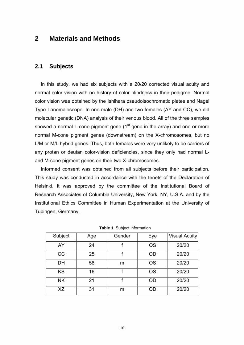
In this study, we had six subjects with a 20/20 corrected visual acuity and

normal color vision with no history of color blindness in their pedigree. Normal

color vision was obtained by the Ishihara pseudoisochromatic plates and Nagel

Type I anomaloscope. In one male (DH) and two females (AY and CC), we did

molecular genetic (DNA) analysis of their venous blood. All of the three samples

showed a normal L-cone pigment gene (1st gene in the array) and one or more

normal M-cone pigment genes (downstream) on the X-chromosomes, but no

L/M or M/L hybrid genes. Thus, both females were very unlikely to be carriers of

any protan or deutan color-vision deficiencies, since they only had normal L-

and M-cone pigment genes on their two X-chromosomes.

Informed consent was obtained from all subjects before their participation.

This study was conducted in accordance with the tenets of the Declaration of

Helsinki. It was approved by the committee of the Institutional Board of

Research Associates of Columbia University, New York, NY, U.S.A. and by the

Institutional Ethics Committee in Human Experimentation at the University of

Tübingen, Germany.

Table 1. Subject information

Subject Age Gender Eye Visual Acuity

AY 24 f OS 20/20

CC 25 f OD 20/20

DH 58 m OS 20/20

KS 16 f OS 20/20

NK 21 f OD 20/20

XZ 31 m OD 20/20

16

2.2 L- and M-cone Isolation for the mfVEP

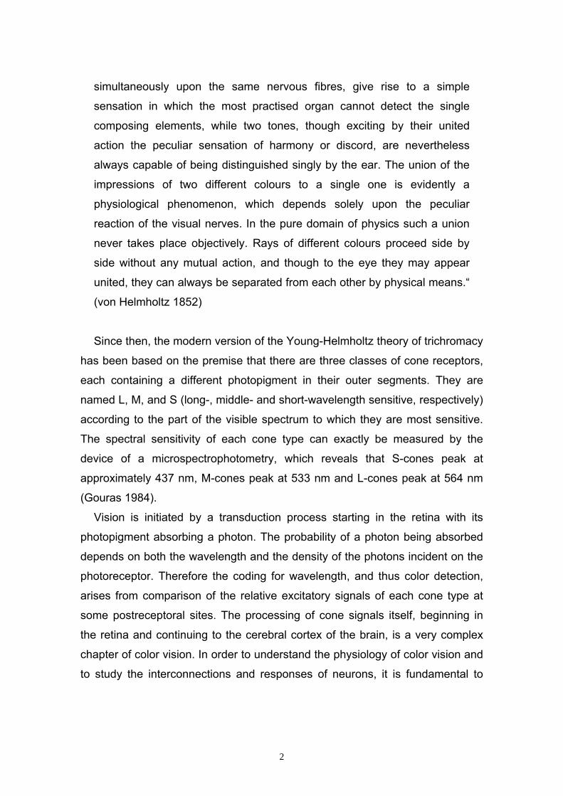
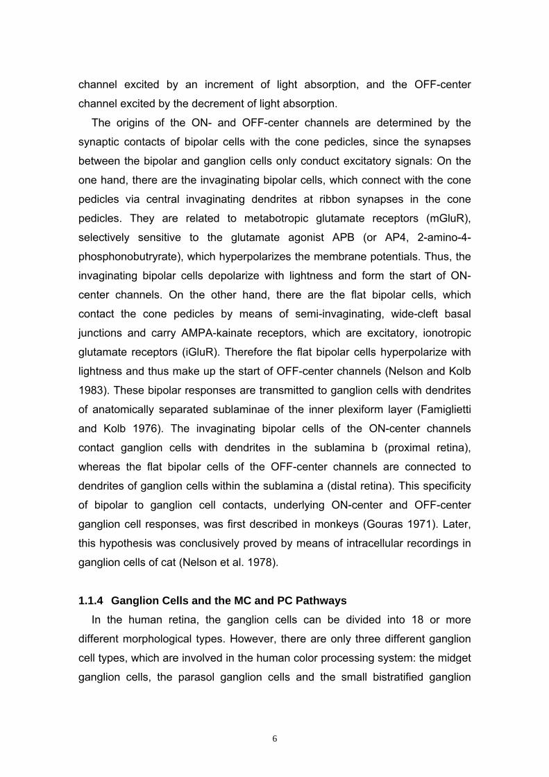
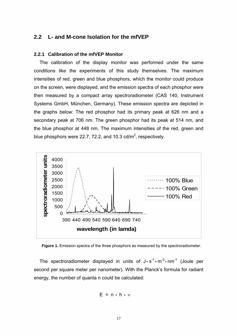
2.2.1 Calibration of the mfVEP Monitor The calibration of the display monitor was performed under the same

conditions like the experiments of this study themselves. The maximum

intensities of red, green and blue phosphors, which the monitor could produce

on the screen, were displayed, and the emission spectra of each phosphor were

then measured by a compact array spectroradiometer (CAS 140, Instrument

Systems GmbH, München, Germany). These emission spectra are depicted in

the graphs below: The red phosphor had its primary peak at 626 nm and a

secondary peak at 706 nm. The green phosphor had its peak at 514 nm, and

the blue phosphor at 448 nm. The maximum intensities of the red, green and

blue phosphors were 22.7, 72.2, and 10.3 cd/m2, respectively.

0500

1000150020002500300035004000

390 440 490 540 590 640 690 740

wavelength (in lamda)

spec

tror

adio

met

er u

nits

100% Blue100% Green100% Red

Figure 1. Emission spectra of the three phosphors as measured by the spectroradiometer.

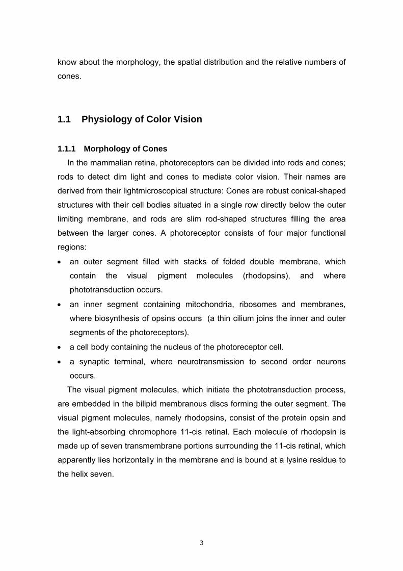
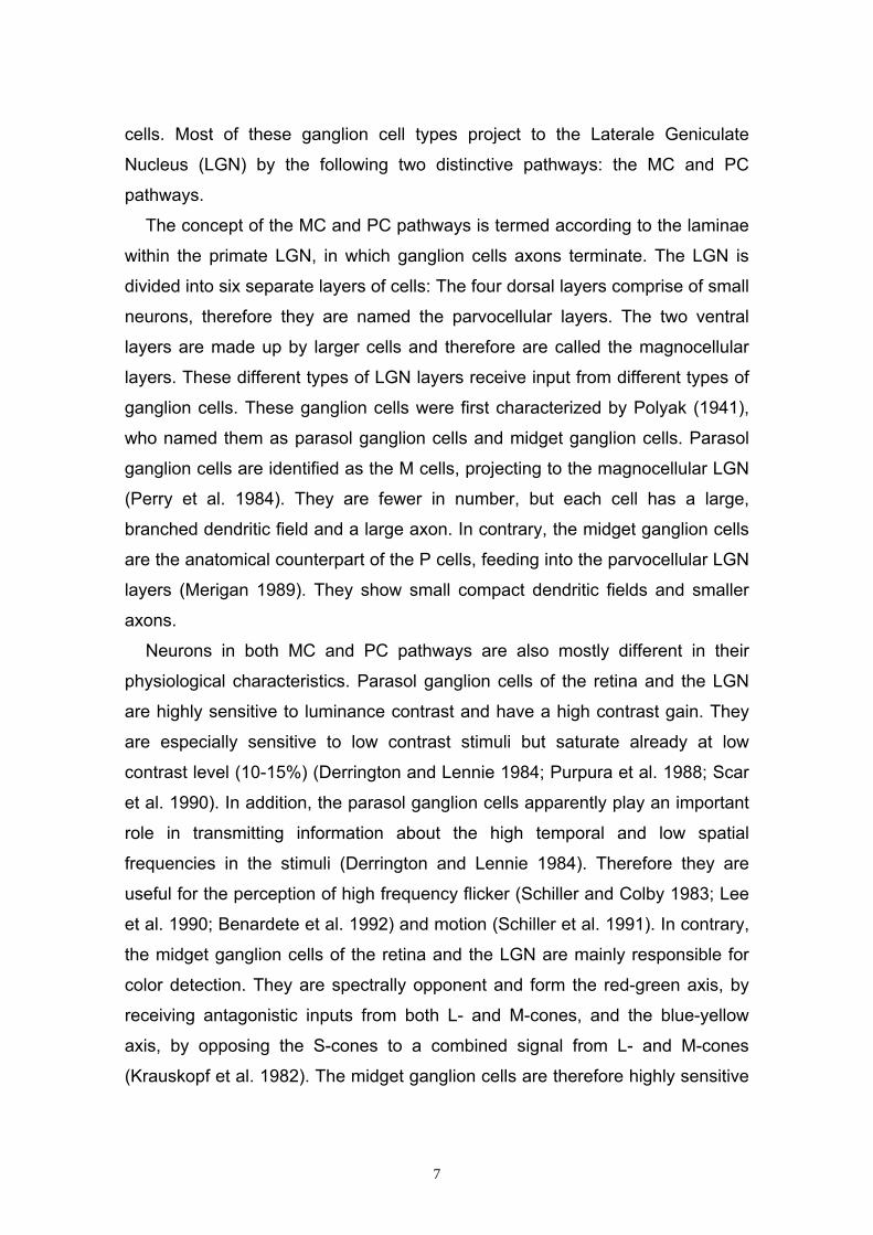
The spectroradiometer displayed in units of J ∗s-1 ∗m-2 ∗nm-1 (Joule per

second per square meter per nanometer). With the Planck’s formula for radiant

energy, the number of quanta n could be calculated:

E = n ∗ h ∗ ν

17

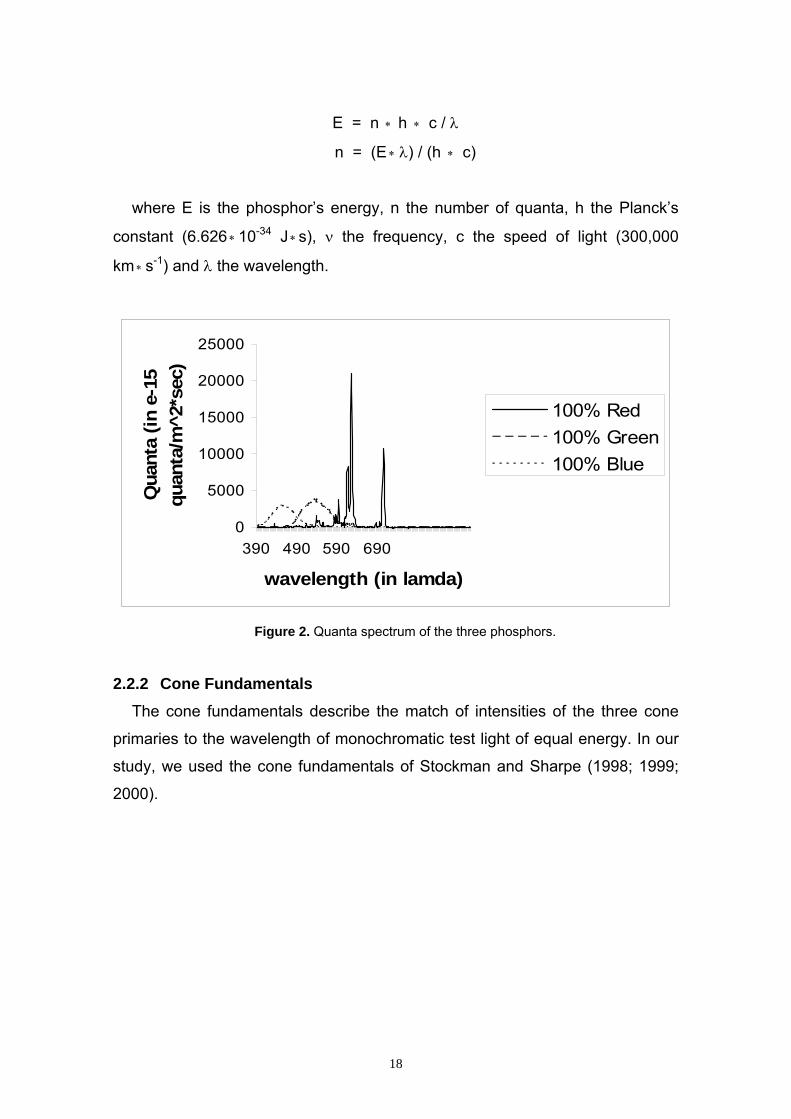
E = n ∗ h ∗ c / λ

n = (E ∗ λ) / (h ∗ c)

where E is the phosphor’s energy, n the number of quanta, h the Planck’s

constant (6.626 10∗ -34 J ∗s), ν the frequency, c the speed of light (300,000

km s∗-1) and λ the wavelength.

0

5000

10000

15000

20000

25000

390 490 590 690

wavelength (in lamda)

Qua

nta

(in e

-15

quan

ta/m

^2*s

ec)

100% Red100% Green100% Blue

Figure 2. Quanta spectrum of the three phosphors.

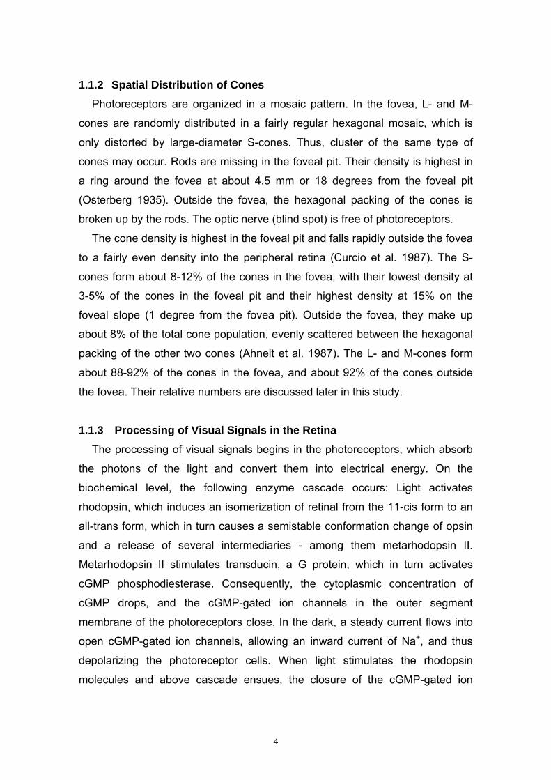
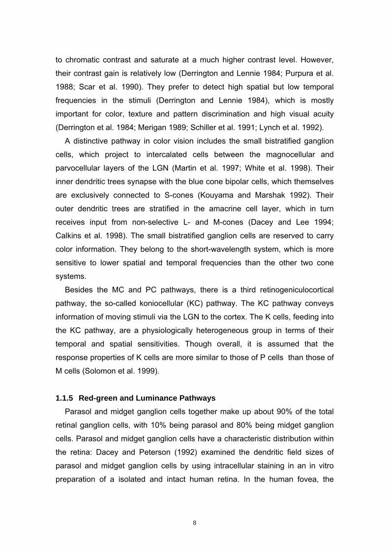
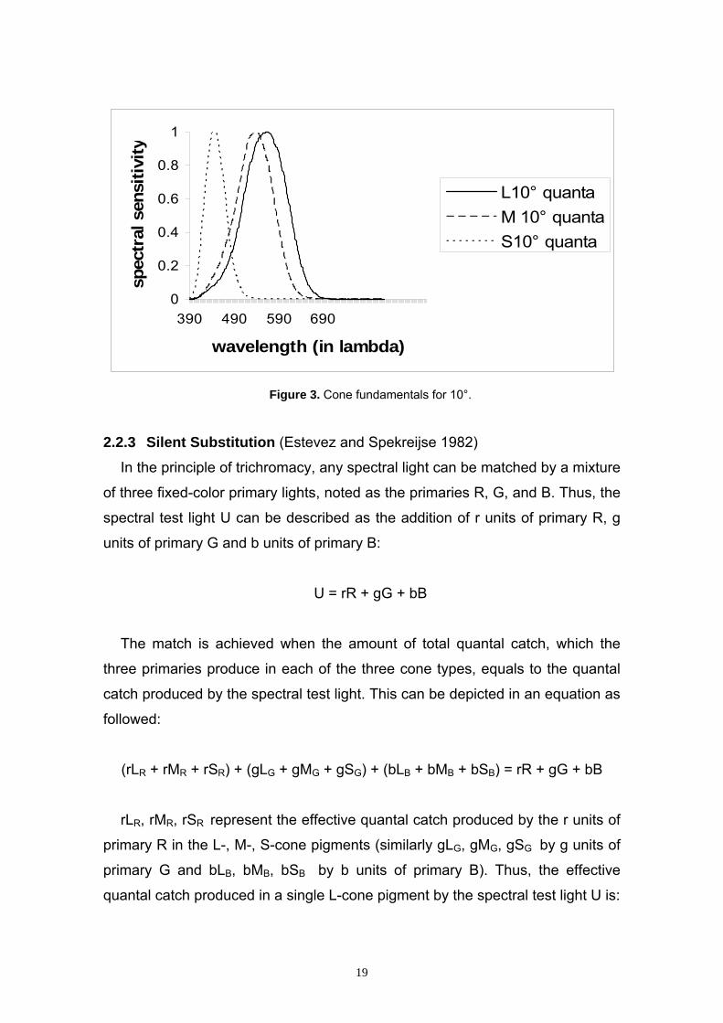
2.2.2 Cone Fundamentals The cone fundamentals describe the match of intensities of the three cone

primaries to the wavelength of monochromatic test light of equal energy. In our

study, we used the cone fundamentals of Stockman and Sharpe (1998; 1999;

2000).

18

0

0.2

0.4

0.6

0.8

1

390 490 590 690

wavelength (in lambda)

spec

tral

sen

sitiv

ity

L10° quantaM 10° quantaS10° quanta

Figure 3. Cone fundamentals for 10°.

2.2.3 Silent Substitution (Estevez and Spekreijse 1982) In the principle of trichromacy, any spectral light can be matched by a mixture

of three fixed-color primary lights, noted as the primaries R, G, and B. Thus, the

spectral test light U can be described as the addition of r units of primary R, g

units of primary G and b units of primary B:

U = rR + gG + bB

The match is achieved when the amount of total quantal catch, which the

three primaries produce in each of the three cone types, equals to the quantal

catch produced by the spectral test light. This can be depicted in an equation as

followed:

(rLR + rMR + rSR) + (gLG + gMG + gSG) + (bLB + bMB + bSB) = rR + gG + bB

rLR, rMR, rSR represent the effective quantal catch produced by the r units of

primary R in the L-, M-, S-cone pigments (similarly gLG, gMG, gSG by g units of

primary G and bLB, bMB, bSB by b units of primary B). Thus, the effective

quantal catch produced in a single L-cone pigment by the spectral test light U is:

19

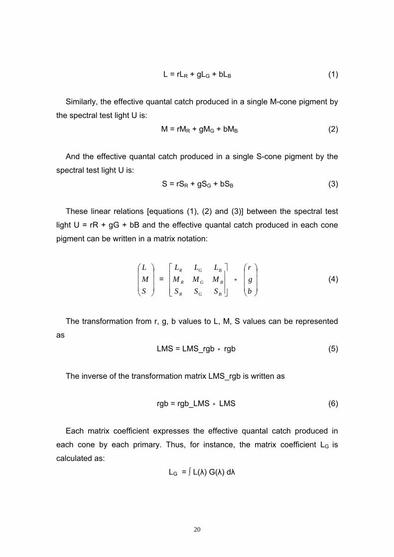
L = rLR + gLG + bLB (1)

Similarly, the effective quantal catch produced in a single M-cone pigment by

the spectral test light U is:

M = rMR + gMG + bMB (2)

And the effective quantal catch produced in a single S-cone pigment by the

spectral test light U is:

S = rSR + gSG + bSB (3)

These linear relations [equations (1), (2) and (3)] between the spectral test

light U = rR + gG + bB and the effective quantal catch produced in each cone

pigment can be written in a matrix notation:

⎟⎟⎟

⎠

⎞

⎜⎜⎜

⎝

⎛

SML

= ⎥⎥⎥

⎦

⎤

⎢⎢⎢

⎣

⎡

BGR

BGR

BGR

SSSMMMLLL

∗ (4) ⎟⎟⎟

⎠

⎞

⎜⎜⎜

⎝

⎛

bgr

The transformation from r, g, b values to L, M, S values can be represented

as

LMS = LMS_rgb ∗ rgb (5)

The inverse of the transformation matrix LMS_rgb is written as

rgb = rgb_LMS ∗ LMS (6)

Each matrix coefficient expresses the effective quantal catch produced in

each cone by each primary. Thus, for instance, the matrix coefficient LG is

calculated as:

LG = ∫ L(λ) G(λ) dλ

20

L(λ) represents the quantal spectral sensitivity of the L-cone pigment and

G(λ) the quantal spectral sensitivity of primary G. For each cone type, a test

stimulus exists, which is equally effective for the other two cone types and thus

only modulates this cone type, the so-called cone-isolating stimulus. The cone-

isolating stimulus is proportional to the total effective quantal catch of its

corresponding cone pigments. The spectral sensitivity functions, which relate

the matching intensities of the three primary lights to the wavelength of this

cone-isolating stimulus, are described in the cone fundamentals. In this study,

each matrix coefficient was calculated by multiplying the Stockman and Sharpe

cone fundamentals, determined for 10 degree and larger viewing conditions,

with the emission spectra of the three phosphors and a constant k, and by

integrating the product over wavelength. The constant k is different for each

cone, depending on τλmax, the product of the ocular media transmissivity and the

absolute absorption coefficients for the wavelength of the maximal absorption

probability for each cone. So kL, kM and kS are derived from the multiplication of

the foveal cone collecting area of 2.92 µm2 with a pupil’s area of 50.26 mm2 and

the factor τλmax of 0.6024, 0.555 and 0.1087 for the L-, M- and S-cones, and

division of this product by 259.21 mm2, since 16.1 mm is the distance between

the nodal point of the lens and the retina (Wyszecki and Stiles 1982, Pugh

1988). Thus, the matrix coefficient allowed an estimate of the excitation of the

cones by the phosphors:

Matrix coefficient = ∫ cone fundamentals ∗ emission spectra ∗ constant k dλ

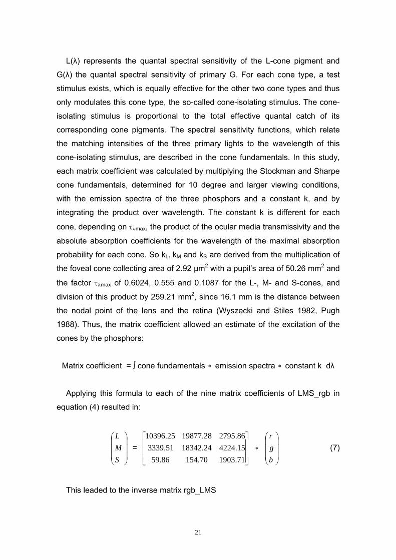
Applying this formula to each of the nine matrix coefficients of LMS_rgb in

equation (4) resulted in:

⎟⎟⎟

⎠

⎞

⎜⎜⎜

⎝

⎛

SML

= ⎥⎥⎥

⎦

⎤

⎢⎢⎢

⎣

⎡

71.190370.15486.5915.422424.1834251.333986.279528.1987725.10396

∗ (7) ⎟⎟⎟

⎠

⎞

⎜⎜⎜

⎝

⎛

bgr

This leaded to the inverse matrix rgb_LMS

21

⎟⎟⎟

⎠

⎞

⎜⎜⎜

⎝

⎛

bgr

= ⎥⎥⎥

⎦

⎤

⎢⎢⎢

⎣

⎡

−−−

−−−

−−−

466

445

444

32.508.114.355.107.130.377.102.285.1

eeeeeeeee

∗ (8) ⎟⎟⎟

⎠

⎞

⎜⎜⎜

⎝

⎛

SML

Each matrix coefficient of LMS_rgb represented the number of absorbed

quanta per cone per second (quanta ∗cone-1 ∗s-1), which an appropriate

maximum phosphor intensity would have created, e.g. 100% red phosphor

produced 10396.25 quanta L-cone∗ -1 ∗s-1, 3339.51 quanta ∗M-cone-1 ∗s-1 and

59.86 quanta ∗S-cone-1 ∗s-1. Each inverse matrix coefficient of rgb_LMS held the

unit of quanta ∗s cone∗ -1 and allowed to calculate the appropriate intensity of the

red, green and blue phosphors for any given quantal absorption in the cones.

2.2.4 L-cone Modulation for the mfVEP

When a stimulus is chosen to change the effective quantal catch produced in

the three cones by ∆L, ∆M, ∆S, equation (6) can be altered as followed in order

to calculate the corresponding values of ∆r, ∆g, ∆b:

⎟⎟⎟

⎠

⎞

⎜⎜⎜

⎝

⎛

∆∆∆

bgr

= rgb_LMS ∗ (9) ⎟⎟⎟

⎠

⎞

⎜⎜⎜

⎝

⎛

∆∆∆

SML

The so-called L-cone modulation is defined as an L-cone-isolating stimulus,

which is equally effective for the M- and S-cones and thus only modulates the L-

cones. In this study, the L-cone-isolating stimulus was a pattern-reversal

stimulus alternating between red and green patches. Thus, for the L-cone

modulation, the red and green patches produced the same quantal catch in the

M-cones (∆M = 0), and similarly the same number of quanta was absorbed in

the S-cones (∆S = 0). A maximal change of quantal catch in the L-cones (∆Lmax)

could be obtained by setting the red phosphor at a maximum intensity of 100%

(∆r = 1.0) [setting the green phosphor at maximum intensity (∆g = 1.0) required

22

∆r > 1.0 in order to meet the conditions ∆Lmax, ∆M = 0 and ∆S = 0; the blue

phosphor is less significant in the stimulation of L-cones].

⎟⎟⎟

⎠

⎞

⎜⎜⎜

⎝

⎛

∆∆

bg0.1

= rgb_LMS ∗ (10) ⎟⎟⎟

⎠

⎞

⎜⎜⎜

⎝

⎛∆

00

maxL

Substitution of rgb_LMS by the inverse matrix coefficients in equation (8)

resulted in:

1.0 = ∆Lmax (1.85e∗ -4) + 0 (2.02e∗ -4) + 0 ∗ (1.77e-4)

∆g = ∆Lmax ∗ (3.30e-5) + 0 ∗ (1.07e-4) + 0 ∗ (1.55e-4) (11)

∆b = ∆Lmax ∗ (3.14e-6) + 0 ∗ (1.08e-6) + 0 ∗ (5.32e-4)

From equation (11), the following values were obtained for ∆Lmax, ∆g and ∆b:

∆Lmax = 1.0/ (1.85e-4) = 5405.41

∆g = 5405.41 ∗ (3.30e-5) = 0.1784

∆b = 5405.41 ∗ (3.14e-6) = 0.0170

∆Lmax = 5405.41 was the change of the quantal absorption, when the stimulus

changed from red to green patch during the L-cone modulation, meaning one L-

cone absorbed 5405.41 more quanta with the red patch than with the green one

per second.

∆r, ∆g, ∆b corresponded to the phosphor’s energy in %. To display colors

accurately on the computer monitor, the input signal to the monitor (the voltage)

had to be "gamma corrected". Most computer monitors have an intensity to

voltage response curve, which is roughly a power function. This means that a

pixel value in voltage sent to the monitor with an intensity of x, will actually be

displayed as a pixel of an intensity equal to xgamma on the monitor. Most

monitors have a gamma between 1.7 and 2.7. Gamma correction is defined by

applying the inverse of this function to the image before display, which can be

23

computed by new_pixel_value = old_pixel_value(1.0/gamma). Here, the conversion

of ∆r, ∆g, ∆b into the Veris phosphor’s energy scale, the scale of the operating

device, reflected the gamma correction for the computer system, so that the

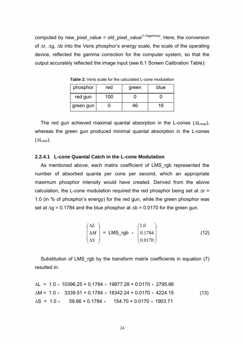
output accurately reflected the image input (see 6.1 Screen Calibration Table):

Table 2. Veris scale for the calculated L-cone modulation

phosphor red green blue

red gun 100 0 0

green gun 0 46 16

The red gun achieved maximal quantal absorption in the L-cones (∆Lmax),

whereas the green gun produced minimal quantal absorption in the L-cones

(∆Lmin).

2.2.4.1 L-cone Quantal Catch in the L-cone Modulation As mentioned above, each matrix coefficient of LMS_rgb represented the

number of absorbed quanta per cone per second, which an appropriate

maximum phosphor intensity would have created. Derived from the above

calculation, the L-cone modulation required the red phosphor being set at ∆r =

1.0 (in % of phosphor’s energy) for the red gun, while the green phosphor was

set at ∆g = 0.1784 and the blue phosphor at ∆b = 0.0170 for the green gun.

⎟⎟⎟

⎠

⎞

⎜⎜⎜

⎝

⎛

∆∆∆

SML

= LMS_rgb ∗ (12) ⎟⎟⎟

⎠

⎞

⎜⎜⎜

⎝

⎛

0170.01784.00.1

Substitution of LMS_rgb by the transform matrix coefficients in equation (7)

resulted in:

∆L = 1.0 10396.25 + 0.1784 ∗ ∗ 19877.28 + 0.0170 ∗ 2795.86

∆M = 1.0 3339.51 + 0.1784 ∗ ∗ 18342.24 + 0.0170 ∗ 4224.15 (13)

∆S = 1.0 59.86 + 0.1784 ∗ ∗ 154.70 + 0.0170 ∗ 1903.71

24

Now, the L-cone quantal catch produced by each phosphor could be

calculated via the first row in equation (13):

L-cone quantal catch produced by the

- red phosphor : 1.0 ∗ 10396.25 = 10396.25 quanta L-cone∗ -1 ∗s-1

- green phosphor: 0.1784 ∗ 19877.28 = 3546.11 quanta L-cone∗ -1 ∗s-1

- blue phosphor : 0.0170 ∗ 2795.86 = 47.53 quanta L-cone∗ -1 ∗s-1

The total L-cone quantal catch in the L-cone modulation summed up to

10396.25 + 3546.11 + 47.53 = 13989.89 quanta L-cone∗ -1 ∗s-1

2.2.4.2 M-cone Quantal Catch in the L-cone Modulation

The red gun with the ∆Lmax condition and the green gun with the ∆Lmin

condition had to generate nearly the same M-cone quantal catch to confirm the

correct calculation for the L-cone modulation. This is shown here through the

calculations for the M-cone quantal catch via the second row of equation (13):

M-cone quantal catch produced by the

- red phosphor: 1.0 ∗ 3339.51 = 3339.51 quanta ∗M-cone-1 ∗s-1

The ∆Lmax condition produced an M-cone quantal catch of 3339.51 quanta M-

cone

∗

-1 ∗s-1.

M-cone quantal catch produced by the

- green phosphor: 0.1784 ∗ 18342.24 = 3272.26 quanta ∗M-cone-1 ∗s-1

- blue phosphor: 0.0170 ∗ 4224.15 = 71.81 quanta M-cone∗ -1 ∗s-1

- green and blue phosphors:

3272.26 + 71.81 = 3344.07 quanta M-cone∗ -1 ∗s-1

The ∆Lmin condition produced an M-cone quantal catch of 3344.07 quanta M-

cone

∗

-1 ∗s-1.

25

2.2.4.3 Cone Contrast for the L-cone Modulation The modulation of the cone excitation could be quantified according to the

cone contrast formula (Michaelson Contrast) with Emax and Emin representing the

maximal and mininal cone excitations:

100% ∗ (Emax – Emin) /(Emax + Emin) (14)

Thus, the calculated L-cone modulation had a maximal cone contrast of

100% [10396.25 - (3546.11 + 47.53)] / [10396.25 + (3546.11 + 47.53)] ∗

= 48.63%

for the L-cones, while the cone contrast for the M-cones and S-cones was

maintained at 0 %.

Our calculations confirmed the nearly equal quantal absorptions in the M-

cones for the ∆Lmax and ∆Lmin conditions. However so far, these calculations

were relied on accurate calibration measurements as a prerequisite. In order to

avoid the influence of calibration errors arose from the susceptibility of the

spectroradiometer to interferences, the L-cone-isolating setting was adjusted in

contrast and intensity to pre-studied calibration series obtained in Tübingen,

Germany (see Albrecht et al. 2002), and to the recordings from a protanope. By

these adjustments, a precise silent substitution was reached by an L-cone-

isolating setting of 50% cone contrast, named L50, which was used in this

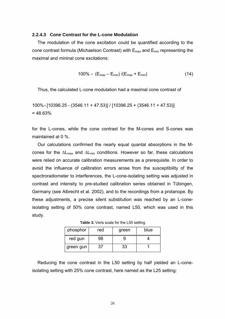
study. Table 3. Veris scale for the L50 setting

phosphor red green blue

red gun 98 9 4

green gun 37 33 1

Reducing the cone contrast in the L50 setting by half yielded an L-cone-

isolating setting with 25% cone contrast, here named as the L25 setting:

26

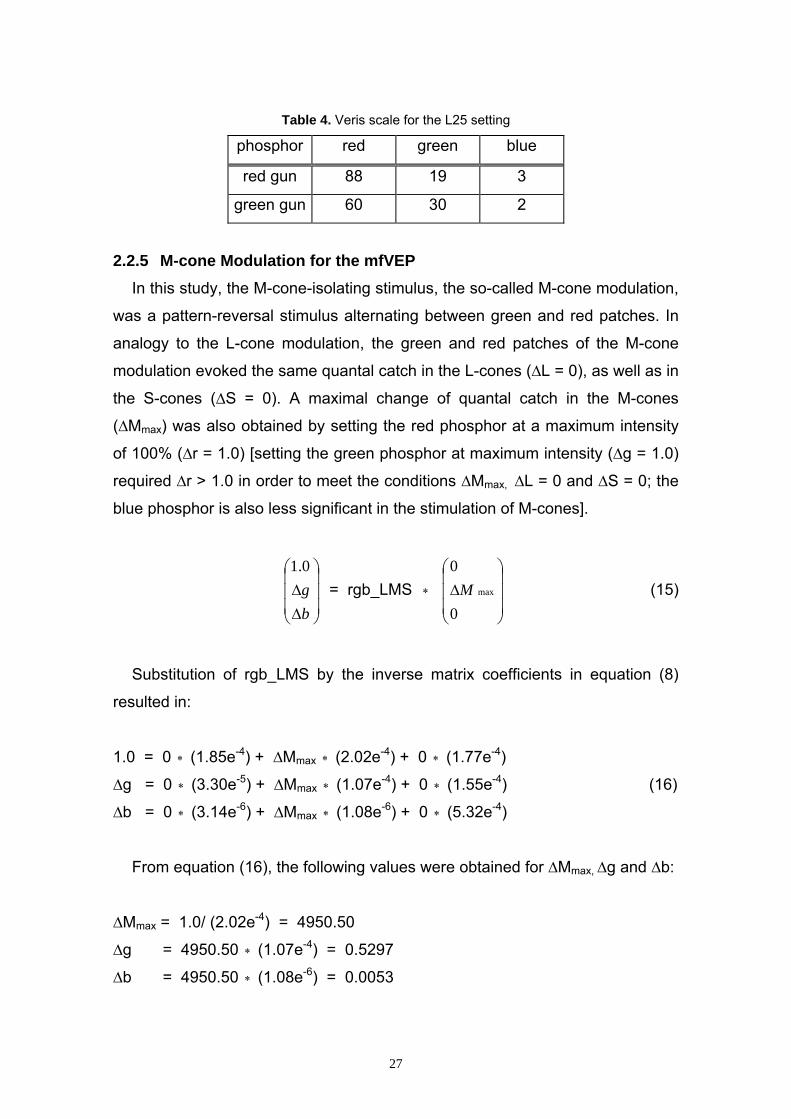
Table 4. Veris scale for the L25 setting

phosphor red green blue

red gun 88 19 3

green gun 60 30 2

2.2.5 M-cone Modulation for the mfVEP In this study, the M-cone-isolating stimulus, the so-called M-cone modulation,

was a pattern-reversal stimulus alternating between green and red patches. In

analogy to the L-cone modulation, the green and red patches of the M-cone

modulation evoked the same quantal catch in the L-cones (∆L = 0), as well as in

the S-cones (∆S = 0). A maximal change of quantal catch in the M-cones

(∆Mmax) was also obtained by setting the red phosphor at a maximum intensity

of 100% (∆r = 1.0) [setting the green phosphor at maximum intensity (∆g = 1.0)

required ∆r > 1.0 in order to meet the conditions ∆Mmax, ∆L = 0 and ∆S = 0; the

blue phosphor is also less significant in the stimulation of M-cones].

⎟⎟⎟

⎠

⎞

⎜⎜⎜

⎝

⎛

∆∆

bg0.1

= rgb_LMS ∗ (15) ⎟⎟⎟

⎠

⎞

⎜⎜⎜

⎝

⎛∆0

0maxM

Substitution of rgb_LMS by the inverse matrix coefficients in equation (8)

resulted in:

1.0 = 0 ∗ (1.85e-4) + ∆Mmax (2.02e∗ -4) + 0 ∗ (1.77e-4)

∆g = 0 (3.30e∗ -5) + ∆Mmax (1.07e∗ -4) + 0 ∗ (1.55e-4) (16)

∆b = 0 (3.14e∗ -6) + ∆Mmax (1.08e∗ -6) + 0 ∗ (5.32e-4)

From equation (16), the following values were obtained for ∆Mmax, ∆g and ∆b:

∆Mmax = 1.0/ (2.02e-4) = 4950.50

∆g = 4950.50 (1.07e∗ -4) = 0.5297

∆b = 4950.50 (1.08e∗ -6) = 0.0053

27

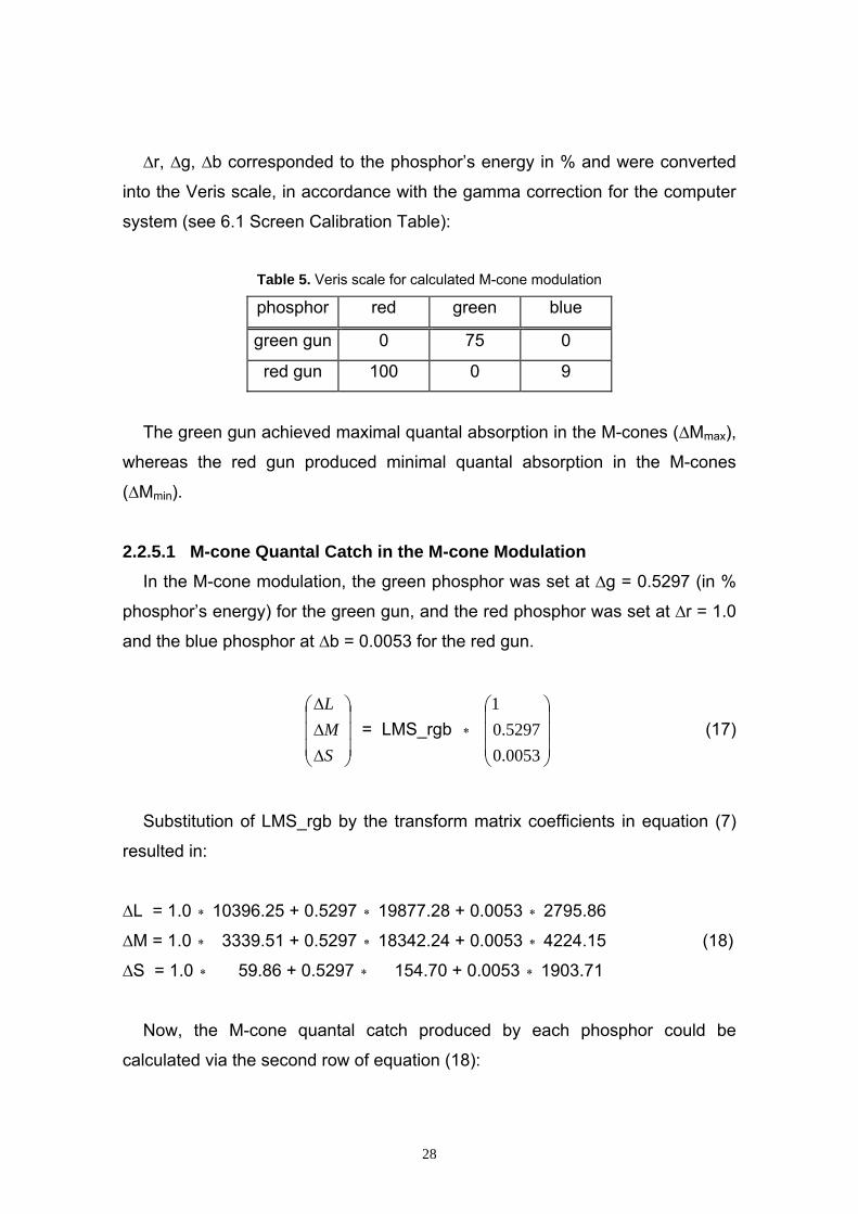
∆r, ∆g, ∆b corresponded to the phosphor’s energy in % and were converted

into the Veris scale, in accordance with the gamma correction for the computer

system (see 6.1 Screen Calibration Table):

Table 5. Veris scale for calculated M-cone modulation

phosphor red green blue

green gun 0 75 0

red gun 100 0 9

The green gun achieved maximal quantal absorption in the M-cones (∆Mmax),

whereas the red gun produced minimal quantal absorption in the M-cones

(∆Mmin).

2.2.5.1 M-cone Quantal Catch in the M-cone Modulation In the M-cone modulation, the green phosphor was set at ∆g = 0.5297 (in %

phosphor’s energy) for the green gun, and the red phosphor was set at ∆r = 1.0

and the blue phosphor at ∆b = 0.0053 for the red gun.

⎟⎟⎟

⎠

⎞

⎜⎜⎜

⎝

⎛

∆∆∆

SML

= LMS_rgb ∗ (17) ⎟⎟⎟

⎠

⎞

⎜⎜⎜

⎝

⎛

0053.05297.0

1

Substitution of LMS_rgb by the transform matrix coefficients in equation (7)

resulted in:

∆L = 1.0 ∗ 10396.25 + 0.5297 ∗ 19877.28 + 0.0053 ∗ 2795.86

∆M = 1.0 ∗ 3339.51 + 0.5297 ∗ 18342.24 + 0.0053 ∗ 4224.15 (18)

∆S = 1.0 59.86 + 0.5297 ∗ ∗ 154.70 + 0.0053 ∗ 1903.71

Now, the M-cone quantal catch produced by each phosphor could be

calculated via the second row of equation (18):

28

M-cone quantal catch produced by the

- green phosphor: 0.5297 ∗ 18342.24 = 9715.88 quanta ∗M-cone-1 ∗s-1

- red phosphor : 1.0 ∗ 3339.51 = 3339.51 quanta ∗M-cone-1 ∗s-1

- blue phosphor : 0.0053 ∗ 4224.15 = 22.39 quanta ∗M-cone-1 ∗s-1

The total M-cone quantal catch in the M-cone modulation summed up to

3339.51 + 9715.88 + 22.39 = 13077.78 quanta M-cone∗ -1 ∗s-1

2.2.5.2 L-cone Quantal Catch in the M-cone Modulation

The green gun with the ∆Mmax condition and the red gun with the ∆Mmin

condition had to generate nearly the same L-cone quantal catch to confirm the

correct calculation for the M-cone modulation. This is shown here through the

calculations of the L-cone quantal catch via the first row of equation (18):

L-cone quantal catch produced by the

- green phosphor: 0.5297 ∗ 19877.28 = 10529.0 quanta ∗L-cone-1 ∗s-1

The ∆Mmax condition produced an L-cone quantal catch of 10529.0 quanta ∗L-

cone-1 ∗s-1.

L-cone quantal catch produced by the

- red phosphor: 1.0 ∗ 10396.25 = 10396.25 quanta ∗L-cone-1 ∗s-1

- blue phosphor: 0.0053 ∗ 2795.86 = 14.82 quanta L-cone∗ -1 ∗s-1

- red and blue phosphors:

10396.25 + 14.82 = 10411.07 quanta ∗L-cone-1 ∗s-1

The ∆Mmin condition produced an L-cone quantal catch of 10411.07 quanta ∗L-

cone-1 ∗s-1.

2.2.5.3 Cone Contrast for the M-cone Modulation According to equation (14), the calculated M-cone modulation should had a

maximal cone contrast of

29

100% [9715.88 - (3339.51 + 22.39)] / [9715.88 + (3339.51 + 22.39)] = 48.59% ∗

for the M-cones, while the cone contrast for the L-cones and S-cones was

maintained at 0 %.

Similarly as described above for the L-cone modulation, the M-cone-isolating

setting was adjusted in contrast and intensity to pre-studied calibration series

obtained in Tübingen, Germany (see Albrecht et al. 2002), and to the recordings

from a deuteranope. By these adjustments, a precise silent substitution was

reached by an M-cone-isolating setting of 50% cone contrast, named M50,

which was used in this study.

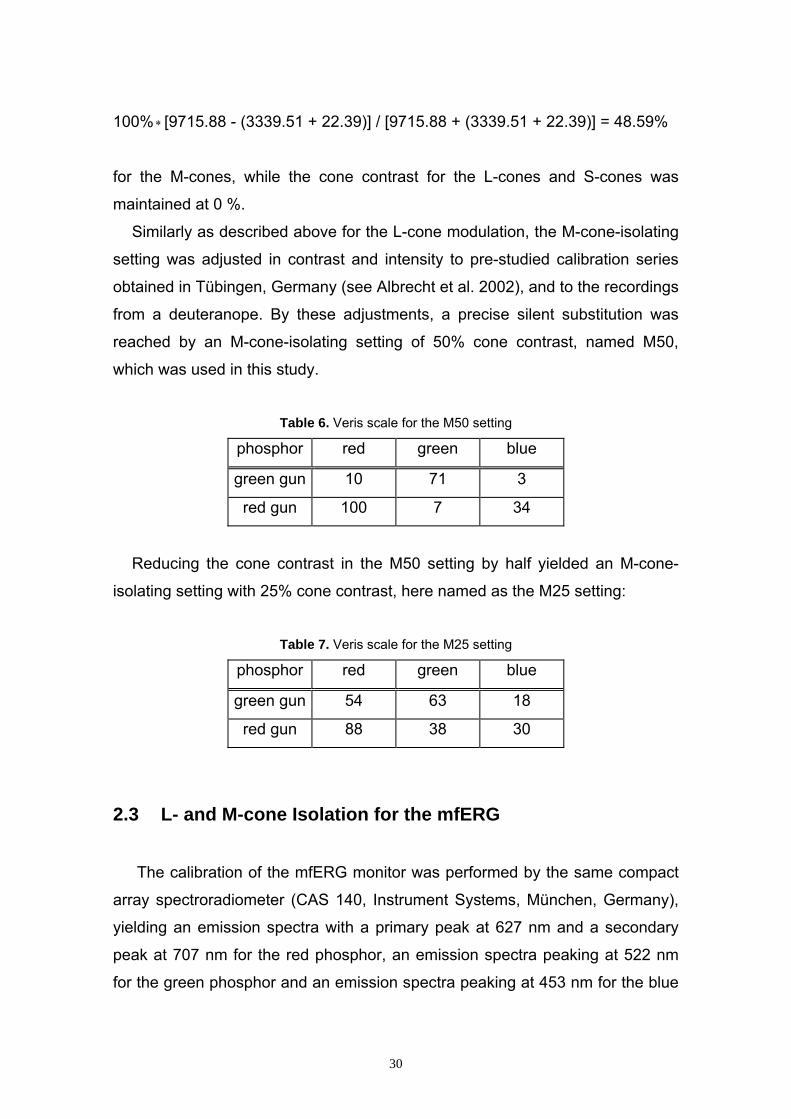
Table 6. Veris scale for the M50 setting

phosphor red green blue

green gun 10 71 3

red gun 100 7 34

Reducing the cone contrast in the M50 setting by half yielded an M-cone-

isolating setting with 25% cone contrast, here named as the M25 setting:

Table 7. Veris scale for the M25 setting

phosphor red green blue

green gun 54 63 18

red gun 88 38 30

2.3 L- and M-cone Isolation for the mfERG

The calibration of the mfERG monitor was performed by the same compact

array spectroradiometer (CAS 140, Instrument Systems, München, Germany),

yielding an emission spectra with a primary peak at 627 nm and a secondary

peak at 707 nm for the red phosphor, an emission spectra peaking at 522 nm

for the green phosphor and an emission spectra peaking at 453 nm for the blue

30

phosphor of the monitor. The maximum intensities of the red, green, and blue

phosphors were 24, 79.3, and 13.8 cd/m2, respectively. The L- and M-cone

isolations used for the mfERG recordings were generated analogous to the L-

and M-cone isolations for the mfVEP as described in 2.2. (for details see

Albrecht et al. 2002).

2.4 Multifocal Visual Evoked Potential (mfVEP) 2.4.1 Hardware and Software

The multifocal visual evoked potentials (mfVEPs) were recorded with the

Visual Evoked Response Imaging System (VERIS) Science 4.2beta915

featured by the EDI (Electro Diagnostic Imaging, Inc., San Mateo, CA) (Sutter

and Tran 1992). The VERIS Science 4.2beta915 is an electrophysiological

recording system, used as a steering device for the integrated management of

information and instruments.

The VERIS software was executed under the Macintosh OS 7.5 (Windows)

Operating System. The stimulus was generated on a 21 inch Apple Studio

Display Monitor (Apple Computer, Inc., Cupertino, CA) driven at a frame rate of

75 Hz. The resolution of the monitor was set at 1024 x 768 pixels, and the

checks inside the smallest sector had an average of approximately 20 pixels.

The specific stimulator parameters were adjusted as followed in the VERIS 4.2

Setting:

31

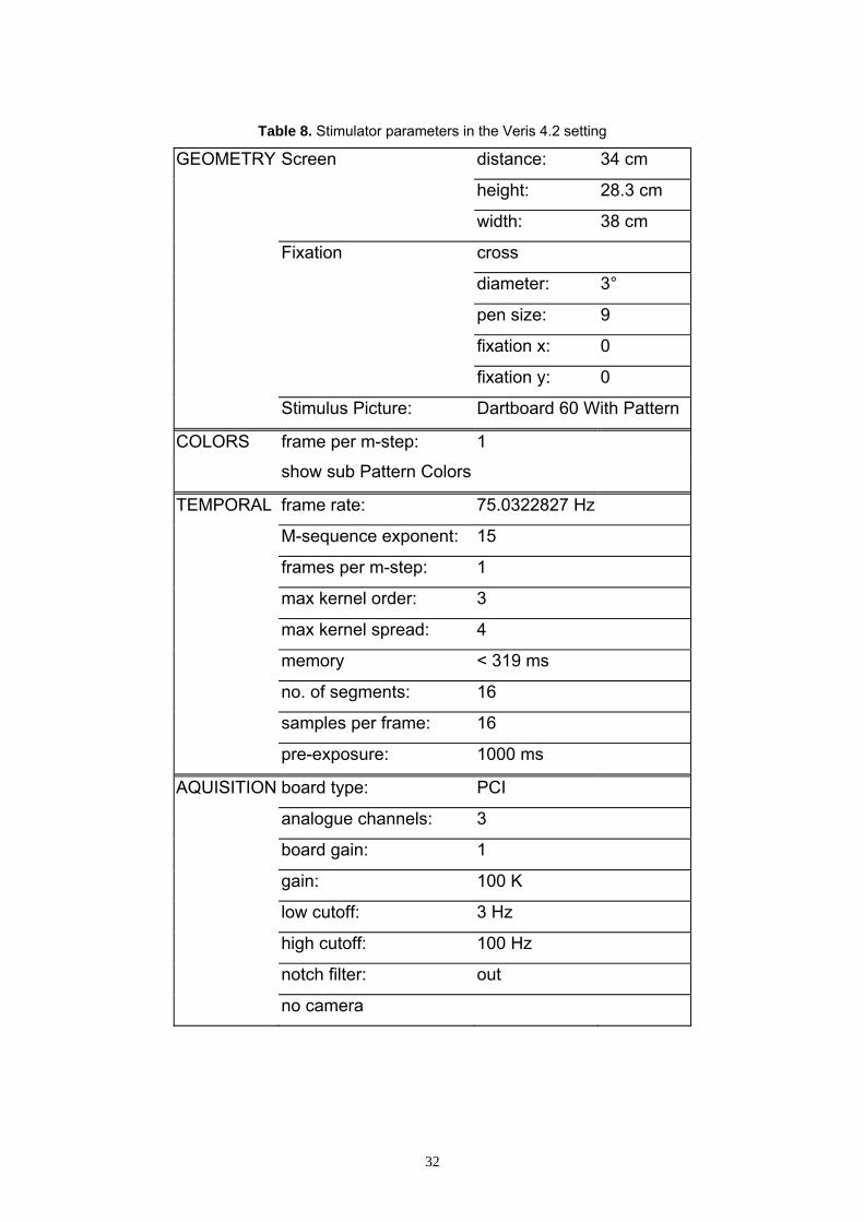
Table 8. Stimulator parameters in the Veris 4.2 setting

GEOMETRY Screen distance: 34 cm

height: 28.3 cm

width: 38 cm

Fixation cross

diameter: 3°

pen size: 9

fixation x: 0

fixation y: 0

Stimulus Picture: Dartboard 60 With Pattern

COLORS frame per m-step: 1

show sub Pattern Colors

TEMPORAL frame rate: 75.0322827 Hz

M-sequence exponent: 15

frames per m-step: 1

max kernel order: 3

max kernel spread: 4

memory < 319 ms

no. of segments: 16

samples per frame: 16

pre-exposure: 1000 ms

AQUISITION board type: PCI

analogue channels: 3

board gain: 1

gain: 100 K

low cutoff: 3 Hz

high cutoff: 100 Hz

notch filter: out

no camera

32

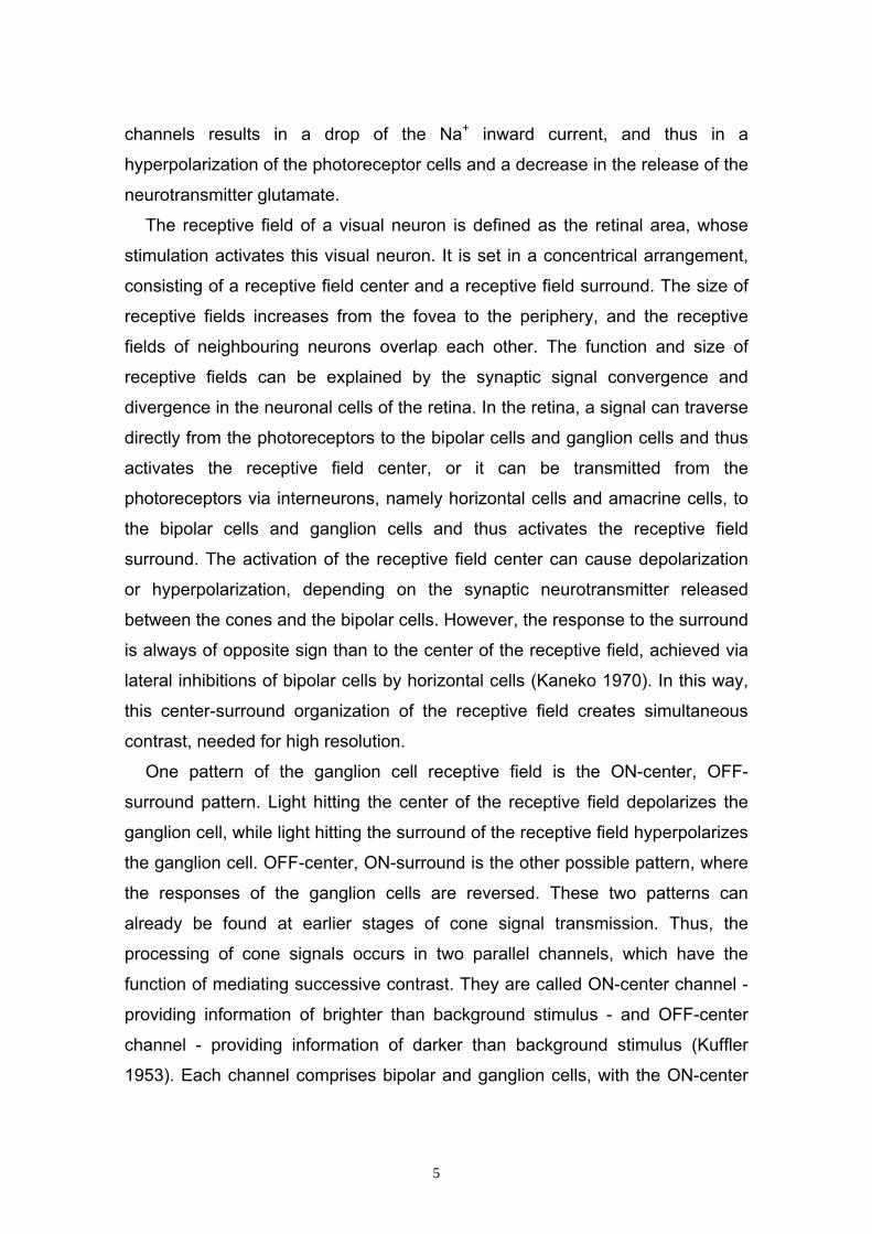
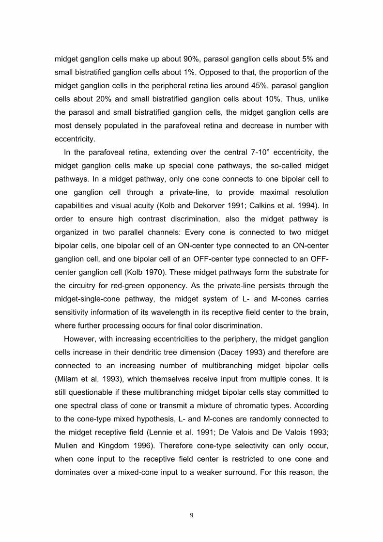
2.4.2 Multifocal Stimulation in the mfVEP The mfVEP stimulus picture was depicted in a dartboard array consisting of

60 sectors (Dart Board 60 With Pattern). Each of the 60 sectors contained a

checkerboard pattern made up by 16 checks, which were displayed in a color-

alternated 4 x 4 arrangement. The entire display spanned a circular central

visual field of 22.2° radius. The visual angle α in (°) for the visual field was

calculated according to the formula

tan α = xdw

2

with w representing the width of the visual field (mm) and d the distance of

pattern from the corneal surface (mm). The central 4 sectors fell within 1.2° (i.e.

a diameter of 2.4°) of the foveal center, the 20 sectors of the next two rings

within 5.8° and the 36 sectors of the next three rings within the 22.2°. A black

fixation cross was displayed at the center of the stimulus picture. The sectors

were scaled with eccentricity according to cortical magnification in human striate

cortex (V1), so that each sector activates nearly equal area of the visual cortex.

Thus, each stimulus produces approximately equal amplitude in focal response

and improves the signal-to-noise ratio at each location. However, since inter-

subject variation in cortical folding are preserved, the sectors may still happen

to activate more than one retinotopic locus of the visual cortex. Therefore even

amplitudes from scaled stimuli can differ due to opposed signal orientation or

ultimately signal cancellation (Baseler et al. 1994).

33

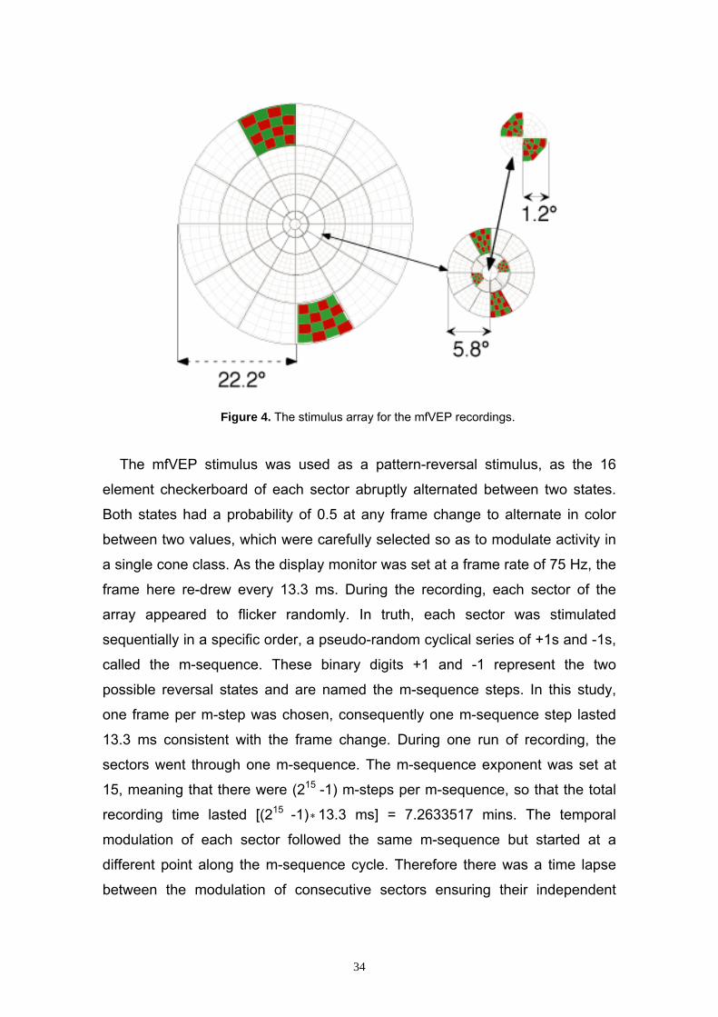
Figure 4. The stimulus array for the mfVEP recordings.

The mfVEP stimulus was used as a pattern-reversal stimulus, as the 16

element checkerboard of each sector abruptly alternated between two states.

Both states had a probability of 0.5 at any frame change to alternate in color

between two values, which were carefully selected so as to modulate activity in

a single cone class. As the display monitor was set at a frame rate of 75 Hz, the

frame here re-drew every 13.3 ms. During the recording, each sector of the

array appeared to flicker randomly. In truth, each sector was stimulated

sequentially in a specific order, a pseudo-random cyclical series of +1s and -1s,

called the m-sequence. These binary digits +1 and -1 represent the two

possible reversal states and are named the m-sequence steps. In this study,

one frame per m-step was chosen, consequently one m-sequence step lasted

13.3 ms consistent with the frame change. During one run of recording, the

sectors went through one m-sequence. The m-sequence exponent was set at

15, meaning that there were (215 -1) m-steps per m-sequence, so that the total

recording time lasted [(215 -1) ∗13.3 ms] = 7.2633517 mins. The temporal

modulation of each sector followed the same m-sequence but started at a

different point along the m-sequence cycle. Therefore there was a time lapse

between the modulation of consecutive sectors ensuring their independent

34

uncorrelated stimulation. This allowed an extraction of the individual

contributions of the 60 locations from a continuous EEG signal, which was

recorded from each bipolar response channel. Thus, the mfVEP final data were

displayed as 60 individual traces spatially arranged according to the stimulus

array. In this study, the first slice of the second order kernel were extracted for

each stimulus patch using Veris Science 4.2beta915 software from EDI. All

other analyses were done with programs written in MATLAB (Mathworks,

Natick, MA).

2.4.3 mfVEP Stimulus Calibration The screen was set at the time average mean luminance, which was 16.8

and 30.6 cd/m2 for the L- and M-cone modulations. The percent contrast was

set at 50% for the L- and M-cone modulations. The percent contrast is defined

by the Michaelson formula:

Michaelson contrast [%] = [(Lmax – Lmin)/( Lmax + Lmin)] x 100

Lmax and Lmin are the maximal and minimal luminances of the pattern

elements. They were measured by a spot photometer.

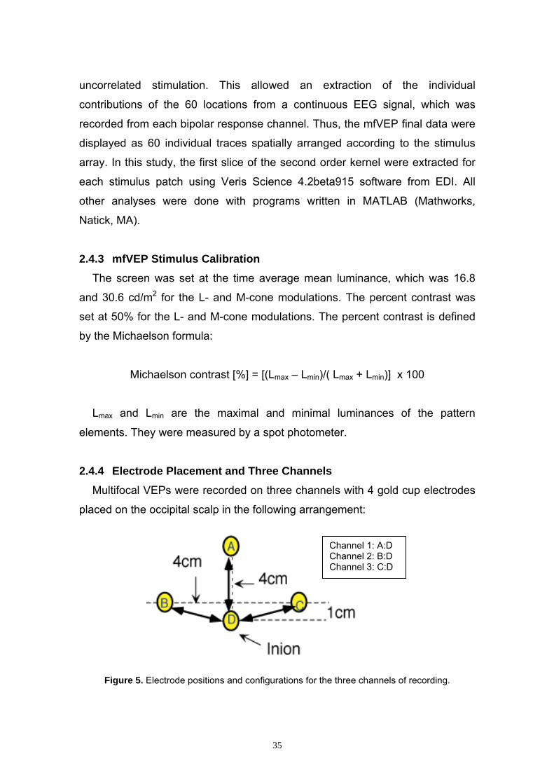
2.4.4 Electrode Placement and Three Channels

Multifocal VEPs were recorded on three channels with 4 gold cup electrodes

placed on the occipital scalp in the following arrangement:

Channel 1: A:D Channel 2: B:D Channel 3: C:D

Figure 5. Electrode positions and configurations for the three channels of recording.

35

Electrode A was placed 4 cm above the inion, electrodes B and C were

placed 1 cm above and 4 cm lateral to the inion on both sides. All three

electrodes A, B, and C were each referenced to electrode D placed at the inion.

The associated differential signals were recorded on three separate channels

as indicated in Figure 5. A forehead electrode served as the ground electrode.

All responses in the figures are displayed with the reference (inion) electrode as

negative. The scalp-electrode impedance was kept below 5 kOhms for all three

channels to achieve recordings as noise-free as possible.

2.4.5 mfVEP Recording Parameters

Analogue low- and high-frequency cutoff filters were set at 3 and 100 Hz (1/2

amplitude; Grass preamplifier P511J, Quincy, Mass.). The notch filter was

turned off. The continuous mfVEP signals were amplified and were sampled at

a rate of 1200 Hz (every 0.83 ms). Three 7-min runs of mfVEP recordings were

performed and then averaged in order to increase the signal-to-noise ratio

between the mfVEP and the background noise.

2.4.6 mfVEP Recording Protocol The mfVEP study was conducted in the Psychology Department of Columbia

University in New York, U.S.A.. Color vision was tested with the

pseudoisochromatic plates and the Nagel anomaloscope. After ensuring a

normal color vision, the subjects were hooked up for the mfVEP recordings in a

relaxing position to minimize muscle and other artifact.

First of all, the inion at the occipital scalp of each subject was found as a

landmark for the electrode placement scheme depicted in Figure 5. All four

electrode sites on scalp were marked with a green pen. The skin areas for

electrode placement on the forehead and on the occipital scalp were cleaned

with single-used electrode skin preparation pads (saturated with 70% Isopropyl

Alcohol and Pumice). To further ensure a low resistance, an abrasive skin

prepping gel (Nuprep®) was lightly rubbed into the cleaned electrode sites on

the scalp. The gold electrodes were submerged with conducting electrode paste

(Genuine Grass EC2 Electrode Cream® by Grass Instrument Division/Astro-

36

med, Inc., W. Warwick, RI 02893) and then applied to the clean electrode sites.

Electrodes were hold in place by self-adherent wrap. After finishing the

electrode placements, the subject was comfortably sat in front of the display

monitor at a distance of 34 cm. None of both eyes were dilated. One eye was

patched up with a light-tight opaque patch in order to conduct monocular mfVEP

recordings. The subject was asked to fixate at the ‘X’ in the center of the

stimulus and to refrain from moving, talking or swallowing during the runs.

All recordings to L- and M-cone modulations for each subject, which are

compared in the result section (see 3.2 mfVEP Studies), were conducted in a

single session, under identical electrode placements and amplification

conditions but with a random assignment of orders. In this single session, each

L- and M-cone modulation for each subject was repeated in three 7-min runs,

e.g. for DH’s results in Figure 13, three runs to 50% L-cone modulation and

three runs to 50% M-cone modulation were recorded in random order in a

single session; for DH’s results in Figure 17, three runs to 25% L-cone

modulation and three runs to 25% M-cone modulation were recorded in random

order in a single session; for DH’s results in Figure 18, three runs to 25% L-

cone modulation and three runs to 50% M-cone modulation were recorded in

random order in a single session; etc. For the ease of the subject, each run was

divided into 16 overlapping segments, each lasting 27.26 s. Each run lasted

approximately 7.26 mins.

2.5 Multifocal Electroretinogram (mfERG)

2.5.1 Hardware and Software

The multifocal electroretinograms (mfERGs) were recorded with the VERIS

system software (Version 3.0.1) from EDI (Sutter and Tran 1992). The stimulus

was generated on a flat-screen SONY Trinitron monitor driven at a frame rate of

75 Hz. The resolution of the monitor was set at 1024 x 768 pixels.

37

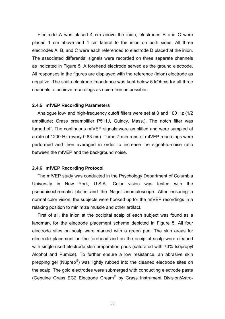
2.5.2 Multifocal Stimulation in the mfERG

The mfERG stimulus picture consisted of 103 hexagonal elements, which

were scaled with eccentricity in accordance with the variations in cone density,

so that approximately equal amplitude was produced for each hexagon. The

stimulus picture spanned a width of 32 cm and a height of 27.5 cm and was

presented at a distance of 18 cm. Thus, the entire display subtended 84° x 75°

of visual angle.

Figure 6. The stimulus array for the mfERG recordings. The numbers indicate the six concentric rings used to analyse the summed signals.

Sutter and Tran (1992) were the first, who used the technique of

simultaneous ERG recordings with an independent uncorrelated stimulation of

small retinal areas in order to obtain ERG response topography maps. They

selected the pseudo-random m-sequence as a sequential temporal modulation

of the individual sectors, which allowed them to assign each response to a

certain timing. By cross-correlation between the m-sequence and the

contiguous response cycle, the local response contributions, identified by its

timing dimension, could be extracted. In this study, the mfERG hexagons were

sequentially reversed in color according to a pseudo-random m-sequence,

38

which included a total of 214 -1 elements. This corresponded to a total recording

time of 3 mins and 38.5 s for each run.

The traces produced by multifocal stimulation were analysed in binary

kernels (Sutter 2000). The first-order kernel is a linear approximation of the total

response, which is calculated by addition of all records following the

presentation of a flash in that patch (e.g. the presentation of a white patch), and

subtraction of all records following a dark frame (equal to a ‚non-presentation‘).

In this way, the flash response to the patch is built up, while all responses,

which do not contribute to the flash response, are eliminated. The second-order

kernel measures the influence of preceding flashes on the flash response to

that patch. The first slice of the second-order kernel measures the effect of an

immediately preceding flash, the second slice of the second-order kernel the

effect of the flash two frames away, and so forth. First-order kernel responses

were taken for analysis with the VERIS system software (Version 3.0.1) from

EDI. For mfERG recordings, the first-order kernel corresponds to the linear

responses in the outer and middle retinal layer including the photoreceptors

(Hood et al. 1997), whereas the second-order kernel reflects the non-linear

activity of the inner retinal layer and thus of the ganglion cells, the so-called

optic nerve head component (ONHC) (Sutter and Bearse 1999; Sutter et al.,

1999).

2.5.3 mfERG Stimulus Calibration

The screen was set at the time average mean luminance, which was 19.2

and 33.8 cd/m2 for the L- and M-cone modulation. The percent contrast was set

at 50% for the L- and M-cone modulation. The ambient room illumination was

maintained at 150 cd/m2 in order to suppress the rod inputs.

2.5.4 mfERG Electrodes

Multifocal ERGs were registered by DTL-electrodes (named by Dawson,

Trick and Litzkow 1979) and applied at the limb of the lower lid of the eye. A

DTL-electrode is made up of 50µm drilled with silver laminated Nylon fibers

coiled round a plug. The free end of the Nylon fibers is attached at the nose,

39

whilst the coiled up end is connected to the amplifier. Since the fibers are very

fine and thus flexible, the DTL-electrodes can adapt to any corneal form, which

also contributes to the patients’ comfort. The fibers are only fixed by adhesion to

the bulbi oculi. In this way, they can potentially be used for several hours

without causing any damages to the eye. To maintain a good registration quality

and for hygienic reasons, the DTL-electrodes are only for one single use.

Compared to contact lenses electrodes, however, the amplitudes registered by

DTL-electrodes are up to 10% smaller as reported by Dawson et al. (1982).

Additionally, they are also less resistant to blinking of the eyes. However, even

a delicate change in the position of the electrode can be noticed at the

oscilloscope and can then immediately be corrected.

2.5.5 mfERG Recording Parameters The continuous mfERG recordings were amplified by 200 K, with the low-

and high-frequency cutoffs set at 10 and 100 Hz for half amplitude (Grass

Instruments), and were sampled at 1200 Hz (every 0.83 ms). Electrode

resistance of the reference electrode was kept below 5 kOhms.

2.5.6 mfERG Recording Protocol For two subjects, AY and DH, mfERG recordings were conducted in the

Division of Experimental Ophthalmology, University Eye Hospital of the

University of Tübingen in Germany.

First of all, the pupil of the tested eye was dilated (around 8 mm) with a

mydriatic (0.5% tropicamide). After maximal dilation of the pupil, the skin areas

for electrode placement were cleaned with single-used alcohol swabs. The

reference electrode was positioned near the orbital rim temporally, whereas the

ground skin electrode was placed on the forehead. The gold skin electrodes

were submerged with electrode paste (Elefix EEG paste® by Nihon Kohden

America, Inc., Foothill Ranch, CA 92610), applied to the clean electrode sites

and attached with some adhesive tape. The subject’s eye was then fitted with a

DTL-fiber electrode and kept light-adapted before and during the mfERG

recordings. After finishing the electrode placement, the subject was comfortably

40

sat in front of the flat-screen monitor at a distance of 18 cm. The subject was

asked to fixate at the center of the stimulus and to refrain from blinking during

the runs.

The L- and M-cone-isolating recordings for each subject were performed in a

single run, under identical electrode placement and amplification conditions but

with a random assignment of orders to make the results comparable. To

improve the subject’s ability to maintain fixation and to prevent blinking during

the recording time, each run was divided into 16 overlapping segments, each

lasting 13.65 s. Therefore each run lasted 3 mins and 38.5 s.

41

3 Results

3.1 Test Studies for the L- and M-cone Modulation Settings

3.1.1 Dichromat Data As mentioned in the method section, the calculated mfVEP settings were

adjusted to pre-studied calibration series obtained in Tübingen, Germany (see

Albrecht et al. 2002) and to the recordings from a protanope and deuteranope.

Precise silent substitution was confirmed by the dichromats’ recordings at the

adjusted L50 and M50 settings, where they showed no residual cone response.

In addition to that, both the intially calculated L- and M-cone modulations and

the adjusted L50 and M50 settings were tested on two subjects (DH and AY).

The calculated setting and the adjusted setting for both the L- and for the M-

cone modulation produced similar mfVEP amplitudes with no significant

differences.

3.1.2 Cone Fundamentals for 2° In another reliability test study, the L- and M-cone modulations were

calculated the same way as described in the method section (see 2.2 L- and M-

cone Isolation for the mfVEP), with the exception that this time the cone

fundamentals for 2° viewing conditions (Stockman and Sharpe 2000) were used

instead of the cone fundamentals for the 10° or larger viewing conditions (see

2.2.2 Cone Fundamentals). Their results showed that an adjustment of the

settings by using the 2° fundamentals would change the cone contrast values

by less than 1.5 %, the phosphor settings by about 1% and the linearized gun

values by about 2%. These minimal changes are insignificant in terms of the

mfVEP amplitudes and their variability, as they lie within the error of

measurement.

42

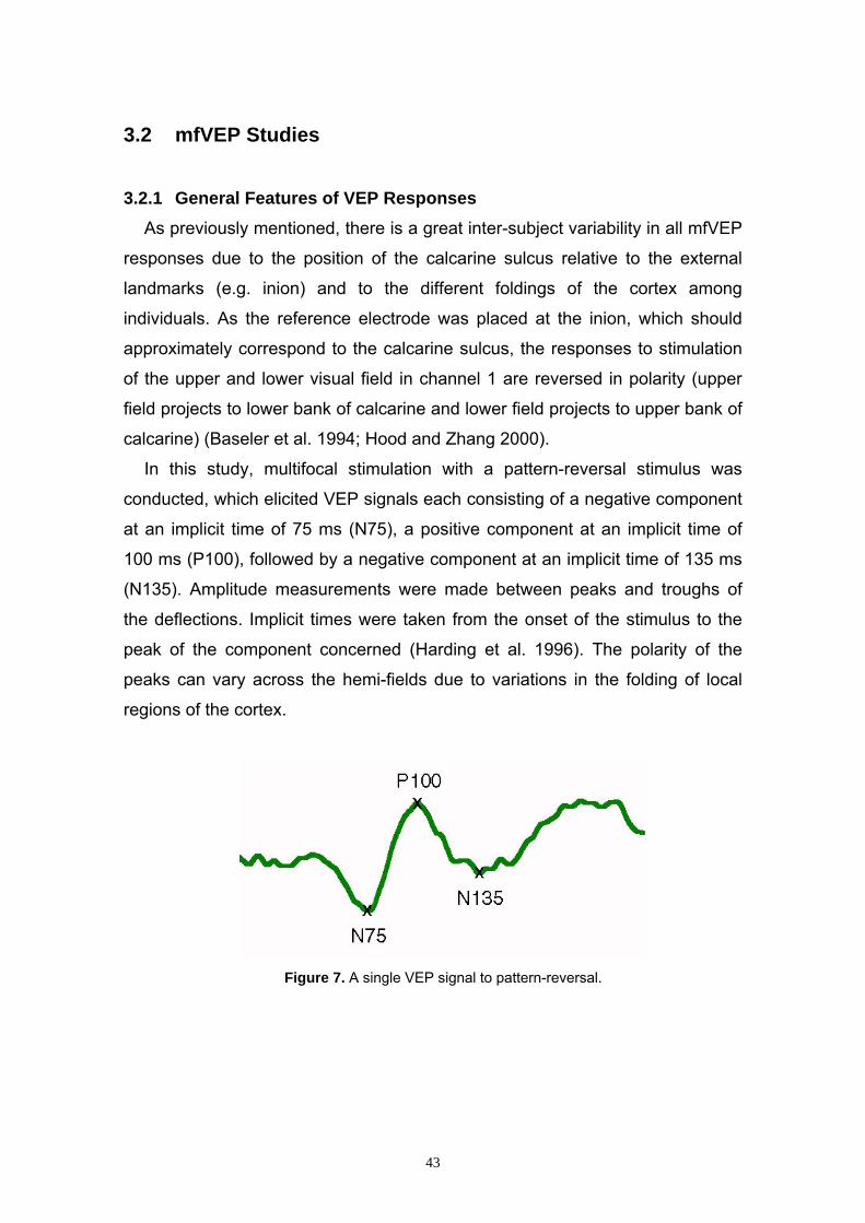
3.2 mfVEP Studies

3.2.1 General Features of VEP Responses As previously mentioned, there is a great inter-subject variability in all mfVEP

responses due to the position of the calcarine sulcus relative to the external

landmarks (e.g. inion) and to the different foldings of the cortex among

individuals. As the reference electrode was placed at the inion, which should

approximately correspond to the calcarine sulcus, the responses to stimulation

of the upper and lower visual field in channel 1 are reversed in polarity (upper

field projects to lower bank of calcarine and lower field projects to upper bank of

calcarine) (Baseler et al. 1994; Hood and Zhang 2000).

In this study, multifocal stimulation with a pattern-reversal stimulus was

conducted, which elicited VEP signals each consisting of a negative component

at an implicit time of 75 ms (N75), a positive component at an implicit time of

100 ms (P100), followed by a negative component at an implicit time of 135 ms

(N135). Amplitude measurements were made between peaks and troughs of

the deflections. Implicit times were taken from the onset of the stimulus to the

peak of the component concerned (Harding et al. 1996). The polarity of the

peaks can vary across the hemi-fields due to variations in the folding of local

regions of the cortex.

Figure 7. A single VEP signal to pattern-reversal.

43

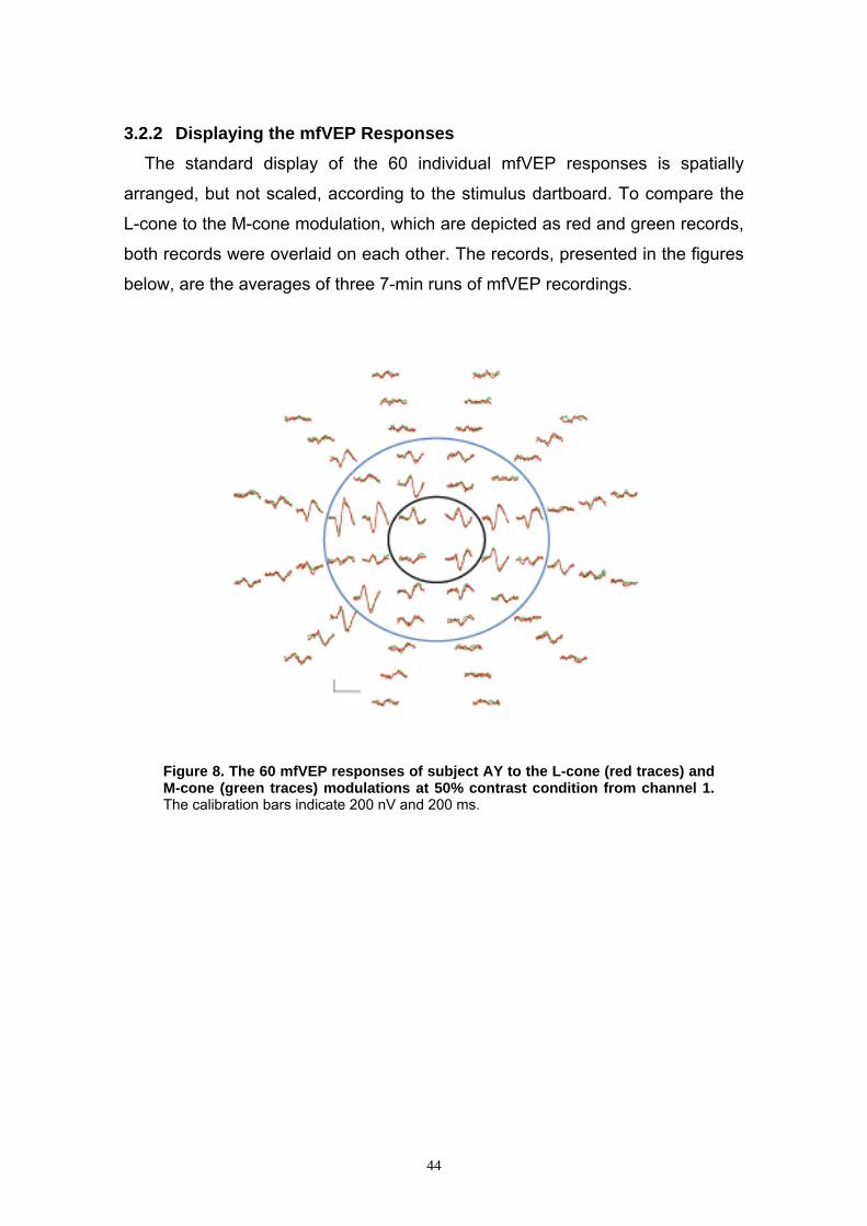
3.2.2 Displaying the mfVEP Responses

The standard display of the 60 individual mfVEP responses is spatially

arranged, but not scaled, according to the stimulus dartboard. To compare the

L-cone to the M-cone modulation, which are depicted as red and green records,

both records were overlaid on each other. The records, presented in the figures

below, are the averages of three 7-min runs of mfVEP recordings.

Figure 8. The 60 mfVEP responses of subject AY to the L-cone (red traces) and M-cone (green traces) modulations at 50% contrast condition from channel 1. The calibration bars indicate 200 nV and 200 ms.

44

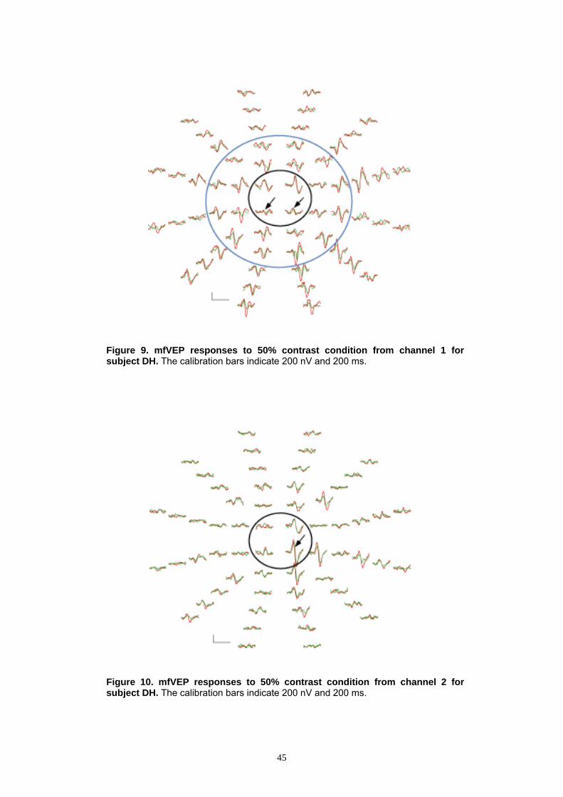
Figure 9. mfVEP responses to 50% contrast condition from channel 1 for subject DH. The calibration bars indicate 200 nV and 200 ms.

Figure 10. mfVEP responses to 50% contrast condition from channel 2 for subject DH. The calibration bars indicate 200 nV and 200 ms.

45

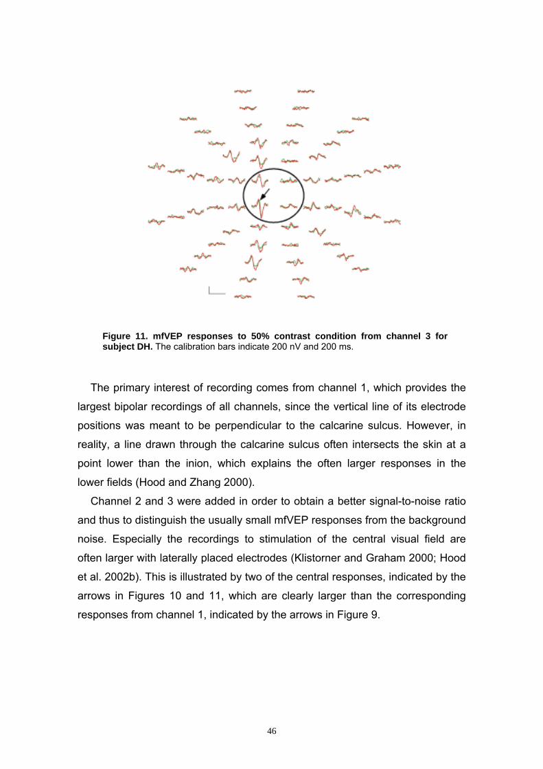
Figure 11. mfVEP responses to 50% contrast condition from channel 3 for subject DH. The calibration bars indicate 200 nV and 200 ms.

The primary interest of recording comes from channel 1, which provides the

largest bipolar recordings of all channels, since the vertical line of its electrode

positions was meant to be perpendicular to the calcarine sulcus. However, in

reality, a line drawn through the calcarine sulcus often intersects the skin at a

point lower than the inion, which explains the often larger responses in the

lower fields (Hood and Zhang 2000).

Channel 2 and 3 were added in order to obtain a better signal-to-noise ratio

and thus to distinguish the usually small mfVEP responses from the background

noise. Especially the recordings to stimulation of the central visual field are

often larger with laterally placed electrodes (Klistorner and Graham 2000; Hood

et al. 2002b). This is illustrated by two of the central responses, indicated by the

arrows in Figures 10 and 11, which are clearly larger than the corresponding

responses from channel 1, indicated by the arrows in Figure 9.

46

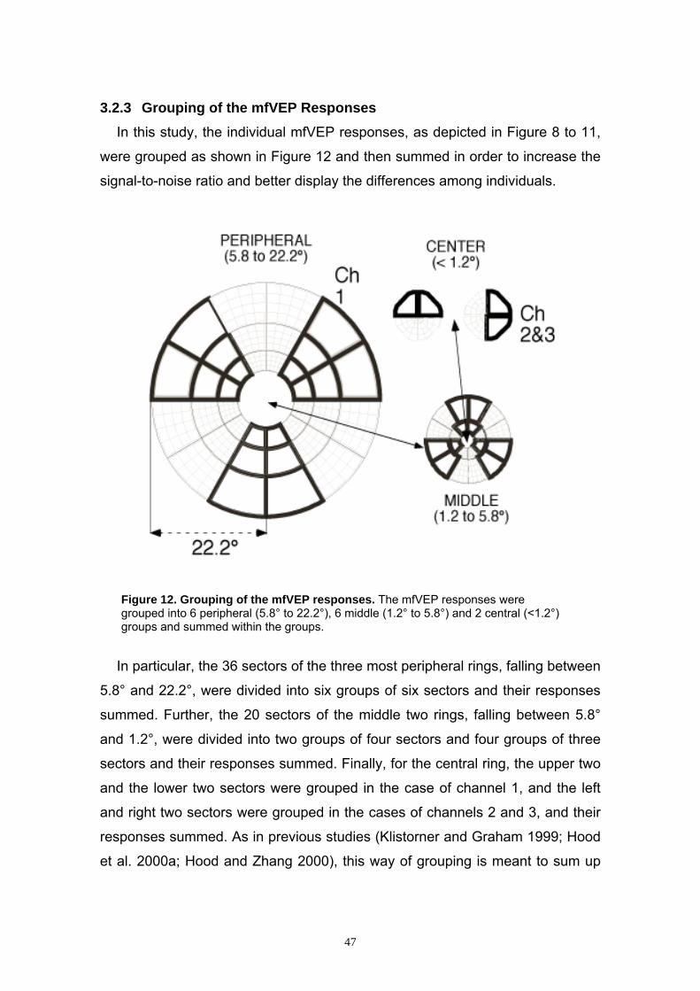
3.2.3 Grouping of the mfVEP Responses

In this study, the individual mfVEP responses, as depicted in Figure 8 to 11,

were grouped as shown in Figure 12 and then summed in order to increase the

signal-to-noise ratio and better display the differences among individuals.

Figure 12. Grouping of the mfVEP responses. The mfVEP responses were grouped into 6 peripheral (5.8° to 22.2°), 6 middle (1.2° to 5.8°) and 2 central (<1.2°) groups and summed within the groups.

In particular, the 36 sectors of the three most peripheral rings, falling between

5.8° and 22.2°, were divided into six groups of six sectors and their responses

summed. Further, the 20 sectors of the middle two rings, falling between 5.8°

and 1.2°, were divided into two groups of four sectors and four groups of three

sectors and their responses summed. Finally, for the central ring, the upper two

and the lower two sectors were grouped in the case of channel 1, and the left

and right two sectors were grouped in the cases of channels 2 and 3, and their

responses summed. As in previous studies (Klistorner and Graham 1999; Hood

et al. 2000a; Hood and Zhang 2000), this way of grouping is meant to sum up

47

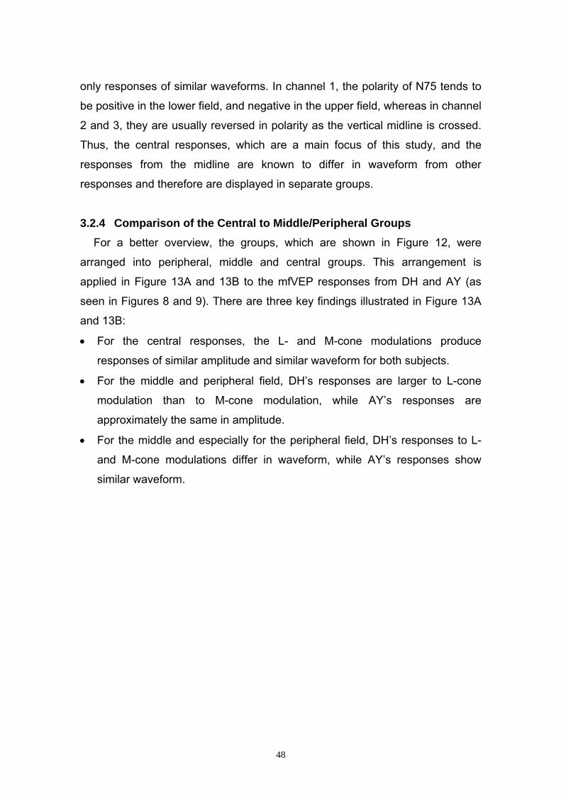
only responses of similar waveforms. In channel 1, the polarity of N75 tends to

be positive in the lower field, and negative in the upper field, whereas in channel

2 and 3, they are usually reversed in polarity as the vertical midline is crossed.

Thus, the central responses, which are a main focus of this study, and the

responses from the midline are known to differ in waveform from other

responses and therefore are displayed in separate groups.

3.2.4 Comparison of the Central to Middle/Peripheral Groups For a better overview, the groups, which are shown in Figure 12, were

arranged into peripheral, middle and central groups. This arrangement is

applied in Figure 13A and 13B to the mfVEP responses from DH and AY (as

seen in Figures 8 and 9). There are three key findings illustrated in Figure 13A

and 13B:

• For the central responses, the L- and M-cone modulations produce

responses of similar amplitude and similar waveform for both subjects.

• For the middle and peripheral field, DH’s responses are larger to L-cone

modulation than to M-cone modulation, while AY’s responses are

approximately the same in amplitude.

• For the middle and especially for the peripheral field, DH’s responses to L-

and M-cone modulations differ in waveform, while AY’s responses show

similar waveform.

48

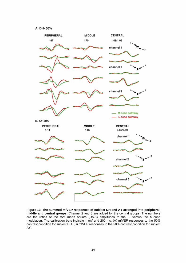
Figure 13. The summed mfVEP responses of subject DH and AY arranged into peripheral, middle and central groups. Channel 2 and 3 are added for the central groups. The numbers are the ratios of the root mean square (RMS) amplitudes to the L- versus the M-cone modulation. The calibration bars indicate 1 mV and 200 ms. (A) mfVEP responses to the 50% contrast condition for subject DH. (B) mfVEP responses to the 50% contrast condition for subject AY.

49

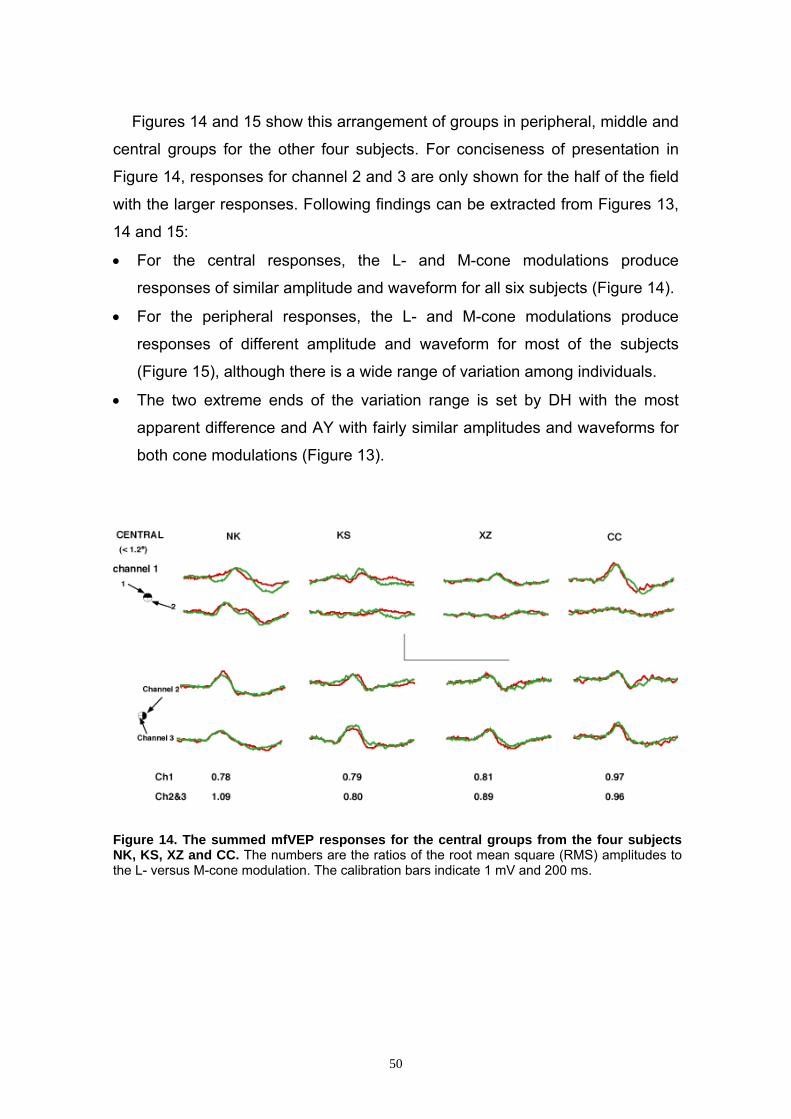
Figures 14 and 15 show this arrangement of groups in peripheral, middle and

central groups for the other four subjects. For conciseness of presentation in

Figure 14, responses for channel 2 and 3 are only shown for the half of the field

with the larger responses. Following findings can be extracted from Figures 13,

14 and 15:

• For the central responses, the L- and M-cone modulations produce

responses of similar amplitude and waveform for all six subjects (Figure 14).

• For the peripheral responses, the L- and M-cone modulations produce

responses of different amplitude and waveform for most of the subjects

(Figure 15), although there is a wide range of variation among individuals.

• The two extreme ends of the variation range is set by DH with the most

apparent difference and AY with fairly similar amplitudes and waveforms for

both cone modulations (Figure 13).

Figure 14. The summed mfVEP responses for the central groups from the four subjects NK, KS, XZ and CC. The numbers are the ratios of the root mean square (RMS) amplitudes to the L- versus M-cone modulation. The calibration bars indicate 1 mV and 200 ms.

50

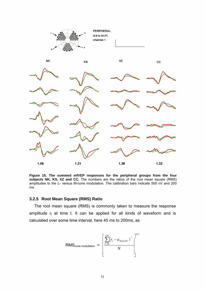
Figure 15. The summed mfVEP responses for the peripheral groups from the four subjects NK, KS, XZ and CC. The numbers are the ratios of the root mean square (RMS) amplitudes to the L- versus M-cone modulation. The calibration bars indicate 500 nV and 200 ms.

3.2.5 Root Mean Square (RMS) Ratio The root mean square (RMS) is commonly taken to measure the response

amplitude rt at time t. It can be applied for all kinds of waveform and is

calculated over some time interval, here 45 ms to 200ms, as

RMScone modulation = [ ]

5.0120

4512045

2

⎥⎥⎥⎥

⎦

⎤

⎢⎢⎢⎢

⎣

⎡−∑

=

N

urt

tot

51

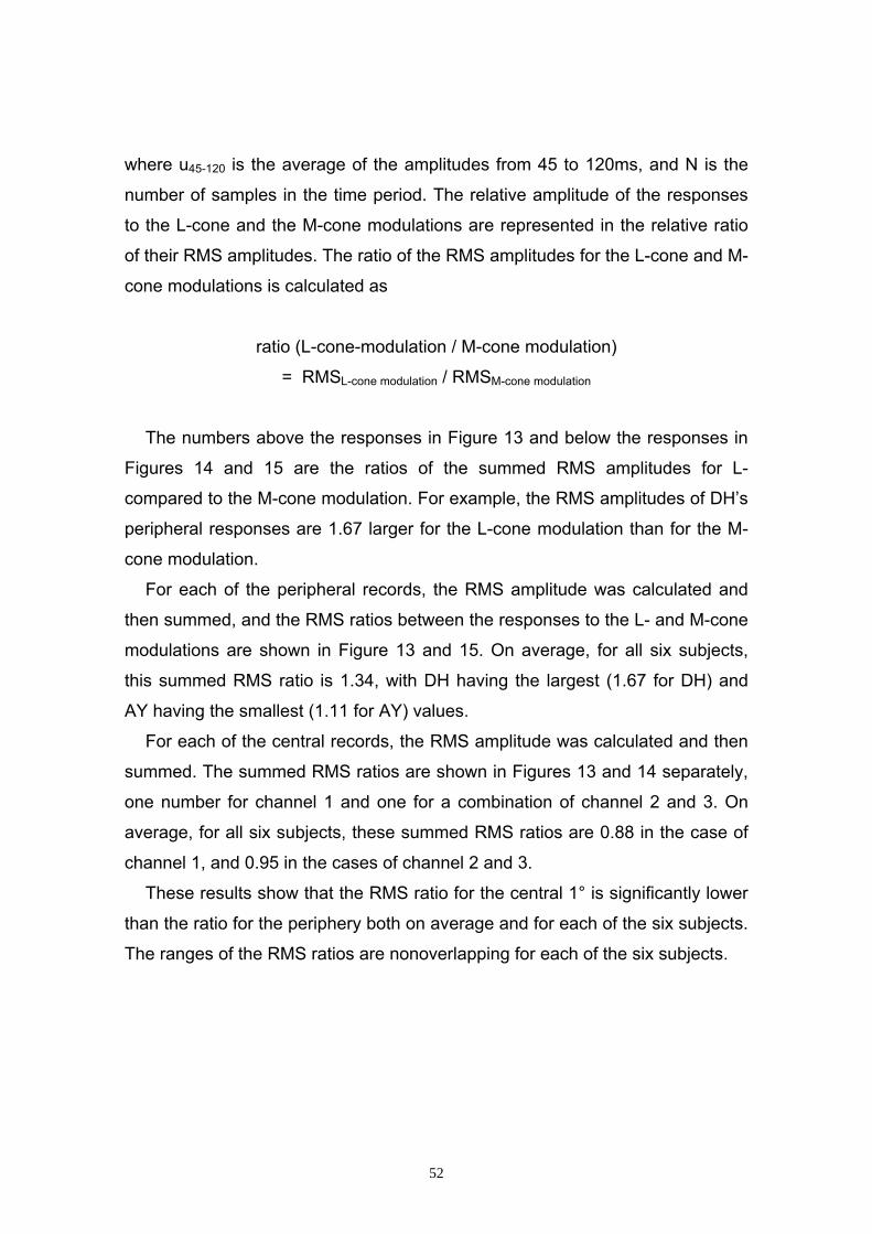
where u45-120 is the average of the amplitudes from 45 to 120ms, and N is the

number of samples in the time period. The relative amplitude of the responses

to the L-cone and the M-cone modulations are represented in the relative ratio

of their RMS amplitudes. The ratio of the RMS amplitudes for the L-cone and M-

cone modulations is calculated as

ratio (L-cone-modulation / M-cone modulation)

= RMSL-cone modulation / RMSM-cone modulation

The numbers above the responses in Figure 13 and below the responses in

Figures 14 and 15 are the ratios of the summed RMS amplitudes for L-

compared to the M-cone modulation. For example, the RMS amplitudes of DH’s

peripheral responses are 1.67 larger for the L-cone modulation than for the M-

cone modulation.

For each of the peripheral records, the RMS amplitude was calculated and

then summed, and the RMS ratios between the responses to the L- and M-cone

modulations are shown in Figure 13 and 15. On average, for all six subjects,

this summed RMS ratio is 1.34, with DH having the largest (1.67 for DH) and

AY having the smallest (1.11 for AY) values.

For each of the central records, the RMS amplitude was calculated and then

summed. The summed RMS ratios are shown in Figures 13 and 14 separately,

one number for channel 1 and one for a combination of channel 2 and 3. On

average, for all six subjects, these summed RMS ratios are 0.88 in the case of

channel 1, and 0.95 in the cases of channel 2 and 3.

These results show that the RMS ratio for the central 1° is significantly lower

than the ratio for the periphery both on average and for each of the six subjects.

The ranges of the RMS ratios are nonoverlapping for each of the six subjects.

52

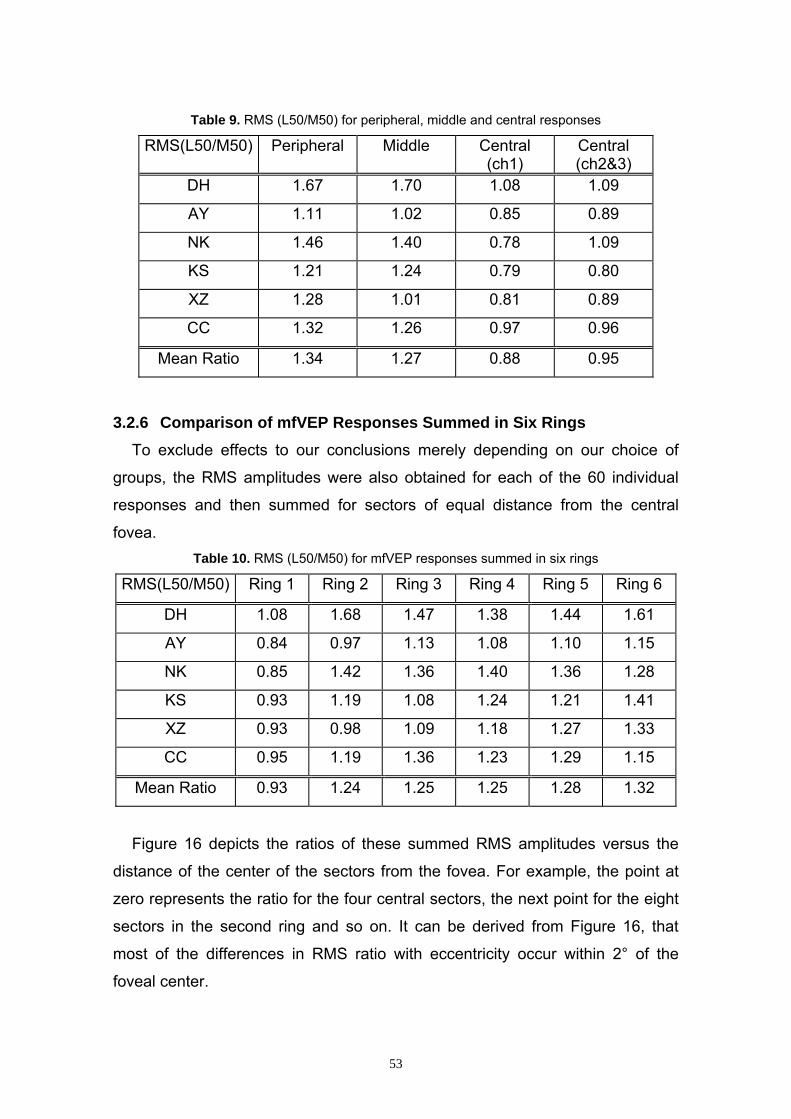
Table 9. RMS (L50/M50) for peripheral, middle and central responses

RMS(L50/M50) Peripheral Middle Central (ch1)

Central (ch2&3)

DH 1.67 1.70 1.08 1.09

AY 1.11 1.02 0.85 0.89

NK 1.46 1.40 0.78 1.09

KS 1.21 1.24 0.79 0.80

XZ 1.28 1.01 0.81 0.89

CC 1.32 1.26 0.97 0.96

Mean Ratio 1.34 1.27 0.88 0.95

3.2.6 Comparison of mfVEP Responses Summed in Six Rings

To exclude effects to our conclusions merely depending on our choice of

groups, the RMS amplitudes were also obtained for each of the 60 individual

responses and then summed for sectors of equal distance from the central

fovea. Table 10. RMS (L50/M50) for mfVEP responses summed in six rings

RMS(L50/M50) Ring 1 Ring 2 Ring 3 Ring 4 Ring 5 Ring 6

DH 1.08 1.68 1.47 1.38 1.44 1.61

AY 0.84 0.97 1.13 1.08 1.10 1.15

NK 0.85 1.42 1.36 1.40 1.36 1.28

KS 0.93 1.19 1.08 1.24 1.21 1.41

XZ 0.93 0.98 1.09 1.18 1.27 1.33

CC 0.95 1.19 1.36 1.23 1.29 1.15

Mean Ratio 0.93 1.24 1.25 1.25 1.28 1.32

Figure 16 depicts the ratios of these summed RMS amplitudes versus the

distance of the center of the sectors from the fovea. For example, the point at

zero represents the ratio for the four central sectors, the next point for the eight

sectors in the second ring and so on. It can be derived from Figure 16, that

most of the differences in RMS ratio with eccentricity occur within 2° of the

foveal center.

53

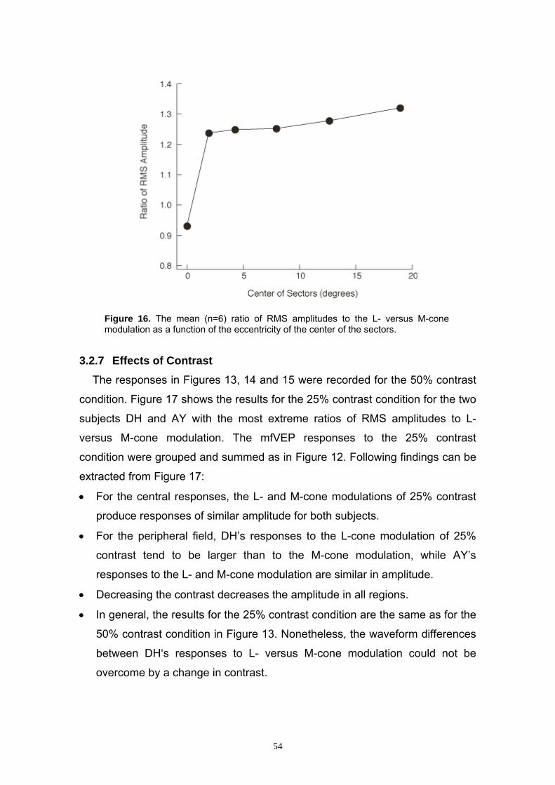
Figure 16. The mean (n=6) ratio of RMS amplitudes to the L- versus M-cone modulation as a function of the eccentricity of the center of the sectors.

3.2.7 Effects of Contrast The responses in Figures 13, 14 and 15 were recorded for the 50% contrast

condition. Figure 17 shows the results for the 25% contrast condition for the two

subjects DH and AY with the most extreme ratios of RMS amplitudes to L-

versus M-cone modulation. The mfVEP responses to the 25% contrast

condition were grouped and summed as in Figure 12. Following findings can be

extracted from Figure 17:

• For the central responses, the L- and M-cone modulations of 25% contrast

produce responses of similar amplitude for both subjects.

• For the peripheral field, DH’s responses to the L-cone modulation of 25%

contrast tend to be larger than to the M-cone modulation, while AY’s

responses to the L- and M-cone modulation are similar in amplitude.

• Decreasing the contrast decreases the amplitude in all regions.

• In general, the results for the 25% contrast condition are the same as for the

50% contrast condition in Figure 13. Nonetheless, the waveform differences

between DH‘s responses to L- versus M-cone modulation could not be

overcome by a change in contrast.

54

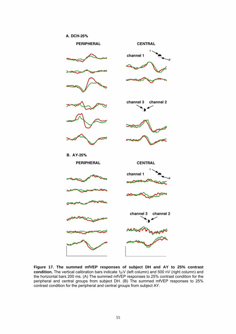
Figure 17. The summed mfVEP responses of subject DH and AY to 25% contrast condition. The vertical calibration bars indicate 1µV (left column) and 500 nV (right column) and the horizontal bars 200 ms. (A) The summed mfVEP responses to 25% contrast condition for the peripheral and central groups from subject DH. (B) The summed mfVEP responses to 25% contrast condition for the peripheral and central groups from subject AY.

55

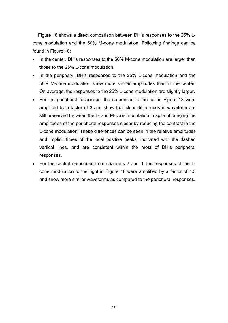
Figure 18 shows a direct comparison between DH’s responses to the 25% L-

cone modulation and the 50% M-cone modulation. Following findings can be

found in Figure 18:

• In the center, DH’s responses to the 50% M-cone modulation are larger than

those to the 25% L-cone modulation.

• In the periphery, DH‘s responses to the 25% L-cone modulation and the

50% M-cone modulation show more similar amplitudes than in the center.

On average, the responses to the 25% L-cone modulation are slightly larger.

• For the peripheral responses, the responses to the left in Figure 18 were

amplified by a factor of 3 and show that clear differences in waveform are

still preserved between the L- and M-cone modulation in spite of bringing the

amplitudes of the peripheral responses closer by reducing the contrast in the

L-cone modulation. These differences can be seen in the relative amplitudes

and implicit times of the local positive peaks, indicated with the dashed

vertical lines, and are consistent within the most of DH’s peripheral

responses.

• For the central responses from channels 2 and 3, the responses of the L-

cone modulation to the right in Figure 18 were amplified by a factor of 1.5

and show more similar waveforms as compared to the peripheral responses.

56

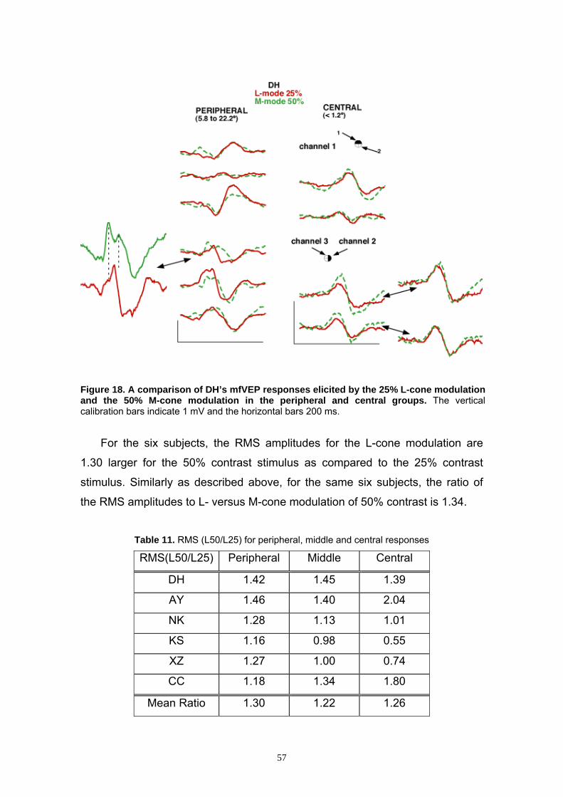
Figure 18. A comparison of DH’s mfVEP responses elicited by the 25% L-cone modulation and the 50% M-cone modulation in the peripheral and central groups. The vertical calibration bars indicate 1 mV and the horizontal bars 200 ms.

For the six subjects, the RMS amplitudes for the L-cone modulation are

1.30 larger for the 50% contrast stimulus as compared to the 25% contrast

stimulus. Similarly as described above, for the same six subjects, the ratio of

the RMS amplitudes to L- versus M-cone modulation of 50% contrast is 1.34.

Table 11. RMS (L50/L25) for peripheral, middle and central responses

RMS(L50/L25) Peripheral Middle Central

DH 1.42 1.45 1.39

AY 1.46 1.40 2.04

NK 1.28 1.13 1.01

KS 1.16 0.98 0.55

XZ 1.27 1.00 0.74

CC 1.18 1.34 1.80

Mean Ratio 1.30 1.22 1.26

57

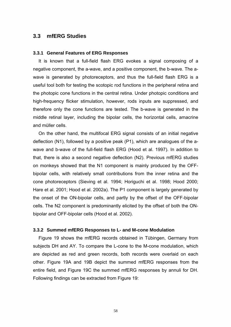
3.3 mfERG Studies

3.3.1 General Features of ERG Responses It is known that a full-field flash ERG evokes a signal composing of a

negative component, the a-wave, and a positive component, the b-wave. The a-

wave is generated by photoreceptors, and thus the full-field flash ERG is a

useful tool both for testing the scotopic rod functions in the peripheral retina and

the photopic cone functions in the central retina. Under photopic conditions and

high-frequency flicker stimulation, however, rods inputs are suppressed, and

therefore only the cone functions are tested. The b-wave is generated in the

middle retinal layer, including the bipolar cells, the horizontal cells, amacrine

and müller cells.

On the other hand, the multifocal ERG signal consists of an initial negative

deflection (N1), followed by a positive peak (P1), which are analogues of the a-

wave and b-wave of the full-field flash ERG (Hood et al. 1997). In addition to

that, there is also a second negative deflection (N2). Previous mfERG studies

on monkeys showed that the N1 component is mainly produced by the OFF-

bipolar cells, with relatively small contributions from the inner retina and the

cone photoreceptors (Sieving et al. 1994; Horiguchi et al. 1998; Hood 2000;

Hare et al. 2001; Hood et al. 2002a). The P1 component is largely generated by

the onset of the ON-bipolar cells, and partly by the offset of the OFF-bipolar

cells. The N2 component is predominantly elicited by the offset of both the ON-

bipolar and OFF-bipolar cells (Hood et al. 2002).

3.3.2 Summed mfERG Responses to L- and M-cone Modulation

Figure 19 shows the mfERG records obtained in Tübingen, Germany from

subjects DH and AY. To compare the L-cone to the M-cone modulation, which

are depicted as red and green records, both records were overlaid on each

other. Figure 19A and 19B depict the summed mfERG responses from the

entire field, and Figure 19C the summed mfERG responses by annuli for DH.

Following findings can be extracted from Figure 19:

58

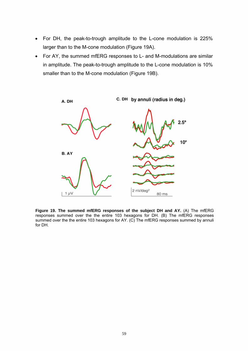
• For DH, the peak-to-trough amplitude to the L-cone modulation is 225%

larger than to the M-cone modulation (Figure 19A).

• For AY, the summed mfERG responses to L- and M-modulations are similar

in amplitude. The peak-to-trough amplitude to the L-cone modulation is 10%

smaller than to the M-cone modulation (Figure 19B).

Figure 19. The summed mfERG responses of the subject DH and AY. (A) The mfERG responses summed over the the entire 103 hexagons for DH. (B) The mfERG responses summed over the the entire 103 hexagons for AY. (C) The mfERG responses summed by annuli for DH.

59

4 Discussion

4.1 Method Discussion

4.1.1 Reliability of the L- and M-cone-Isolating Stimuli For the calibration of the monitor, the emission spectra of the phosphors of

the monitor were only measured once at the maximum intensities of each

phosphor, meaning at 100% red, 100% green and 100% blue phosphor. This

had the advantage of reducing the systematic error, which could be caused by

many measurements. It has to be noted that a spectroradiometer can be

susceptible to interferences, especially to temperature fluctuations. Thus, plenty

subsequent measurements during a longer time can be interfered by

temperature changes (e.g. through repeated touch of the spectroradiometer),

causing a systematic error.

In this study, the cone fundamentals of Stockman and Sharpe (1998; 1999;

2000), which were adjusted to trichromats and dichromats spectral sensitivities,

were used. Those cone fundamentals were already chosen in previous studies

by Kremers et al. (1999) and Kremers et al. (2000), who also calculated the L-

and M-cone-isolating stimuli according to the silent substitution technique

described by Estevez and Spekreijse (1982). In one of those studies (Kremers

et al. 1999), the cone excitations by cone-isolating stimuli were recalculated by

using another set of cone fundamentals, which resulted in only minor difference

in the stimulus settings. Similarly, the recalculation, here in this study, with the

cone fundamentals for 2° viewing conditions (Stockman and Sharpe 2000) in

the reliability test showed only minor changes in the stimulus settings,

insignificant for the evaluation of the mfVEP amplitudes.

To exclude any stimulation of cones other than the L-cones in the L-cone

modulation and the M-cones in the M-cone modulation, the stimulus settings

were adjusted to pre-studied calibration series obtained in Tübingen, Germany

(see Albrecht et al. 2002). They yielded similar settings as the adjustment to the

mfVEP data from a protanope and a deuteranope, when they showed no

60

residual cone response. These reliability tests were performed in order to

confirm the precise silent substitution of the cone-isolating stimuli.

4.1.2 Difficulties in the mfVEP Recordings The mfVEP recordings took place in an established setting in Donald C.

Hood’s laboratory, Psychology Department of Columbia University in New York,

U.S.A., and were obtained in accordance with previous studies conducted in

this laboratory [see (Hood et al. 2000a; Hood and Zhang 2000; Hood et al.

2000b)]. The major difference in this study was the display of cone-isolating

stimuli instead of black-white dartboard arrays. The difficulty to generate

responses from cone-isolating stimuli is largely due to the lower contrast

between the red and green patches, in comparison to black versus white

patches of the pattern-reversal dartboard. Therefore, in this study, cone contrast

did not drop below 25%, since pre-study contrast series with e.g. only 12.5%

cone contrast had shown to be too noise-overlapped. For this reason, the

contrast settings were set at their maximal level to increase signal-to-noise

ratio. Despite lifting the contrast to a maximum of 50% for the cone-isolating

stimuli, their mfVEP responses were still smaller in amplitude than the

responses to black-white pattern arrays. Given these conditions, it was of

highest priority to reduce the noise to its lowest possible level in cone-isolating

stimulus settings.

The most obvious prerequisite to reduce noise is a proper and clean

electrode placement. The scalp-electrode impedances were checked before

each recording, with the aim to achieve approximately 2 kOhms. High

impedance was corrected by cleaning the scalp once again and replacing the

electrodes. Furthermore, the positions of the scalp-electrodes are also of great

importance. It has been shown that mfVEP recordings with multiple electrodes

achieve higher signal-to-noise ratios (Hood et al. 2002b). Especially electrodes

placed lateral to the midline seem to be beneficial for the central amplitudes

(Klistorner and Graham 2000; Hood et al. 2002b). The disadvantages are

mainly of practical nature: So does the placement of multiple electrodes require

longer set-up time and higher costs, and also the data analysis and its

61

interpretation are more time-consuming and complex. Another source of noise

is surrounding electronic instruments near the mfVEP equipments. Therefore all

electronic instruments, which were not in use for the mfVEP recordings, were

removed from the recording room. Lastly, the subject itself can generate a great

amount of noise, for instance, by muscle artifacts or alpha-waves. However, this

could be overcome by an awaken subject in a relaxing position.

The mfVEPs are known to be highly variable among individuals due to the

variance in cortical anatomy and the orientation of the primary visual area in the

cortex. However, the mfVEP data presents high reproducibility, when mfVEP

responses of the same subject on different days are compared. This requires an

accurate replacement of the electrodes according to an established

arrangement of electrode positions as described in Figure 5. Against this

background, the mfVEP has shown to be a useful clinical tool for detecting local

damage to the optic nerve (Hood et al. 2000a; Hood and Zhang 2000; Hood et

al. 2000b).

4.1.3 Difficulties in the mfERG Recordings By the same line of arguments as for the mfVEP recordings, reducing noise

and artifact are extremely important for mfERG recordings as well. In this study,

the main source of noise during mfERG recordings came from the direct contact

of the Nylon fibers of the DTL-electrodes to the subject’s conjunctiva. Therefore

anesthetic eye drops were offered to the subjects, who were sensitive to the

Nylon fibers placed at the limb of the lower lid of their eye, in order to increase

the subject’s comfort and thus reduce blinking and muscle artifact.

62

4.1 Discussion of the Results

4.2.1 Foveal mfVEP and PC Pathway

The amplitudes and waveforms of the central responses to the L- and M-

cone modulations appear to be similar for all six subjects, while they seem to

differ in the peripheral responses.

It is known that there are two pathways, which receive major inputs from L-

and M-cones, namely the MC and PC pathways. They can be tracked up to the

human primary visual cortex surrounding the calcarine sulcus, the source of the

mfVEPs, where stimuli are inverted and mapped on the contralateral

hemisphere (Slotnick et al. 1999). Morphological studies with intracellular

staining and recording have shown, that 95% of the total ganglion cells in the

central retina between 2 and 6 mm eccentricity (equivalent to 0.34° and 1.01°)

are midget ganglion cells projecting to the PC pathway (Dacey 1993). For this

reason, it can be assumed that most mfVEP responses from the central 1.2°

were recorded from the PC pathway. The similarity of the central mfVEP

responses in waveform is also suggestive for the activation of a single pathway.

Furthermore, midget ganglion cells were likely to be stimulated by the central

segments of the mfVEP pattern, given their spectral opponency and their high

sensitivities to chromatic contrast and high spatial frequency. At this point, the

question arises why the central mfVEP responses produce similar amplitudes to

L- and M-cone modulations.

There are two diverging hypotheses to this question, which are attributed to

two different locations in the PC pathway. One hypothesis is based on a

difference in the relative numbers of cones between the central and peripheral

retina and particularly suggests an L/M cone ratio of approximately 1:1 in the

retinal fovea (Krauskopf 2000). In contrary to that, the other hypothesis

assumes a cone-type specific adjustment in the gain of the input to the PC

pathway at or before the striate cortex, where the mfVEP is generated (Pokorny

et al. 1991; Kremers et al. 2000; Otake and Cicerone 2000).

The hypothesis believing in an L/M cone ratio close to 1:1 in the central fovea

is mainly defended by Krauskopf (2000). His flicker photometry studies with

63

foveal light of 2° diameter have shown that at high temporal frequencies (~30

Hz) the modulation sensitivity of L-cones is approximately twice of the

modulation sensitivity of the M-cones, whereas low temporal frequencies (~2

Hz) trigger similar modulation sensitivities for both L- and M-cones. Krauskopf

discussed two explanations: One interpretation assumed an L/M cone ratio of

2:1, given that the MC pathway gives equal weight to L- and M-cones and the

PC pathway gives twice as much weight to the M-cones than to the L-cones.

The other interpretation was based on an L/M cone ratio of 1:1, and that the MC

pathway gives more weight to the L-cones than to the M-cones at higher

temporal frequencies, while the PC pathway gives equal weight to both types of

cones at low temporal frequencies. To further examine these contradictory

interpretations, Krauskopf assembled and statistically analysed color

appearance studies of small, brief, monochromatic lights, with the result that

flashes are called red twice as often as green at approximately 600 nm.

However, this was surprising given an L/M cone ratio of 2:1, since the observers

were expected to locate the wavelength, at which they call twice as many

flashes red as green, at approximately 570 nm, the wavelength where L- and M-

cones are equally sensitive [according to the cone fundamentals of Smith and

Pokorny (1975) and the field sensitivities of Stiles (1978)]. The comparison of

the spectral sensitivities, as derived from these color-naming methods, with

increment thresholds of the field sensitivities of L- and M-cones, measured on

the same observers, showed close agreement. As the field sensitivities are

assumed to be independent of the number of cone types, it was concluded that

the L/M cone ratio is close to 1:1 in the central fovea and may not be so variable

among individuals. However, it should be noted that this conclusion was derived

from flicker photometry studies with a relatively larger fovea light of 2° diameter,

whose low temporal frequencies were supposed to tap into the PC pathway.

Thus, given that the midget ganglion cells are most highly concentrated in the

central retina between 2 and 6 mm eccentricity, equivalent to 0.34° and 1.01°

(Dacey 1993), it cannot be excluded that more than just the PC pathway was

stimulated.

64

Until now, most estimates of L/M cone ratios for the central 2° or so come

from behavioral data such as spectral sensitivity functions, HFPs or two-point

detections. Their results diverge, though most researchers agree to an L/M

cone ratio greater than 1.0 in the central fovea, but propose adjustment

mechanisms in the central cone pathways. So did detection studies with small

monochromatic lights imply stable, though inter-individual varying L/M cone

ratios from fovea to midperiphery (± 28 deg nasotemporal) (Otake and Cicerone

2000). Consistent with the stability of the L/M cone ratio, the wavelength chosen

as uniquely yellow remained unvarying over the same range of eccentricities,

indicating a maintenance of red-green color appearance. However, findings

saying that observers with different L/M cone ratios select similar wavelengths

for unique yellow, appear to be suggestive for the existence of mechanisms in

the cone pathways, which may achieve a standardization of color appearance.

In another study, a combination of three different psychophysical tasks, namely

detection thresholds for cone-isolating stimuli at different temporal frequencies,

HFPs and cone contrast ratios at minimal flicker perception, as well as flicker

ERG and retinal densitometry were applied in order to tap into the MC and PC

pathways separately (Kremers et al. 2000). According to the sensitivity of the

parasol ganglion cells, psychophysical tasks with high temporal frequencies as

well as flicker ERGs and retinal densitometry yielded large inter-individual

variations in L/M cone ratio. Opposed to that, psychophysical tasks with low

temporal frequencies, similar to the sensitivity of midget ganglion cells,

produced L/M cone ratios close to 1:1. These results imply a gain adjustment to

compensate for the differences in L- and M-cone signal strength in the PC

pathway, but not in the MC pathway, which may reflect the relative ratios of the

cones. Lastly, a new approach as the direct visual imaging of the retina was

combined with flicker ERG and the detection of unique yellow (Brainard et al.

2000). Again, the flicker ERG data yielded a stable variation in L/M cone ratio,

whereas the small variation in the wavelength of unique yellow in the same two

observers was assumed to be attributed to neural factors.

Convincing evidence is provided by Roorda and Williams (1999). Their

technique achieved direct imaging of retinal patches within 1° of the foveal

65

center and confirmed large inter-individual variations in L/M cone ratio in the

central retina. In addition to that, examinations of the L/M cone pigment mRNA

in retinal patches of 23 human donor eyes elicited an L/M cone ratio of 1.5:1 in

the central retina, which increased to 3:1 in the periphery of about 40°

eccentricity (Hagstrom et al. 1998).

In face of these evidences, it is unlikely that the central 2° has a ratio close to

1:1 in all subjects. While DH’s mfVEP responses from the central 1.2° are

similar in amplitude, his mfERG responses from the central 2.5° are clearly

larger for the L-cone modulation. These results indicate a gain adjustment in the

PC pathway, after the mfERG is generated and before the mfVEP is elicited. As

it is known that the mfERG, like the photopic full-field ERG, mainly represents

bipolar responses (Sieving et al. 1994; Hood 2000; Hood et al. 2002a), it can be

assumed that this gain adjustment occurs in the PC pathway after the bipolar

cells respond, but before the cells in area 17 are activated, most likely in the

inner plexiform layer before the ganglion cells are stimulated.

4.2.2 Peripheral mfVEP and MC Pathway

In the periphery, all subjects have different waveforms and larger amplitudes

in their mfVEP responses to the L-cone modulation as compared to the M-cone

modulation, except AY, whose responses to both cone modulations are similar

in amplitude and waveform.

The peripheral mfVEP responses are considered as being some combined

signals from the MC and PC pathways, evolving from receptive fields of the

parasol and midget ganglion cells, which are large enough to receive the same

L/M cone ratio of cones. Recordings with light-evoked voltage responses of H1

horizontal cells in the primate’s retina showed that the L- and the M-cone inputs

to the H1 horizontal cells reflect the L/M cone ratio in the H1 cell’s receptive

field (Dacey et al. 2000a). This leads to the assumption that this proportion may

also be preserved in postreceptoral stages of the MC and PC pathways, which

are the source of the mfVEP in the peripheral retina. To explain the qualitative

differences in waveforms seen in most observers, the different features of MC

and PC pathways need to be taken into consideration. The MC pathway is more

66

nonlinear and/or saturates at lower contrast than does the PC pathway.

Therefore the cone contrast in this study is likely to evoke maximal responses in

the MC pathway for both cone modulations, so that different L/M cone ratios

achieve similar MC pathway activity. In contrary to that, the PC pathway is

highly sensitive to chromatic contrast and saturates at a much higher contrast

level. Thus, larger number of L-cones produces a larger PC pathway activity

than do fewer M-cones, as the PC pathway has not reached its saturation level

yet. Furthermore, according to the work of Baseler and Sutter (1997), MC and

PC pathway show different waveforms in mfVEP recordings. Derived from these

evidences, the responses to the L-cone modulation are larger due to a larger

PC pathway contribution at high contrast. The waveforms to L-cone compared

to M-cone modulation are different due to the different activities of MC and PC

pathways in the periphery. The exception is seen in AY. AY‘s mfERG data

implies an L/M cone ratio estimate of approximately 1:1. Thus, AY‘s responses

are similar in amplitude and waveform, as the same number of L- and M-cones

produces the same proportion of MC and PC pathway activities in the periphery.

4.2.3 Limitation of the mfVEP for L/M-cone Ratio Estimates

The mfVEP is not a particularly good way to estimate the variablity in L/M

cone ratio across the retina. The results of this study suggest that in the central

fovea, a gain adjustment in the cone pathway has taken place before the

mfVEP is generated. In the periphery, the mfVEP is considered as a

combination of the MC and PC pathways. However, since at high contrast the

MC pathway is already saturated to its maximal level independent of the cone

numbers, a combined response from the MC and PC pathways is not linear to

the numerosity of cones. Furthermore, the positive and negative portions of the

MC and PC responses can both reinforce or cancel parts of the waveform.

Other techniques for L/M cone ratio estimates are discussed below in 4.3.

4.2.4 Effects of Contrast Changes in the mfVEP

As in Figure 17, reducing the contrast to 25% in both cone modulations

generates central responses of equal amplitude for DH and AY, and larger

67

peripheral responses for DH. This goes along with the above argument, that in

the foveal center, the PC pathway activity dominates and undertakes a gain

adjustment before the cells of area 17 are stimulated. As mentioned above as

well, the peripheral responses are larger due to a larger PC contribution for the

L-cone modulation. The MC pathway is thought to saturate around 10-15%

contrast, and therefore still receive maximal saturation at a contrast of 25%.

Reducing the contrast decreases the amplitude in all regions, as the height of

the amplitudes in both the center and the periphery are mainly dependent on

the PC pathway activity, given that the MC pathway in the periphery is already

saturated at contrast levels above 10-15%.

As in Figure 18, the responses to 50% M-cone modulation are larger in the

center compared to the responses to the 25% L-cone modulation for DH, since

the central responses reflect the activity of the PC pathway, which is highly

sensitive to chromatic contrast. However, both modulation show more similar

amplitudes in the periphery with slightly larger responses to the 25% L-cone

modulation. This observation is probably due to a balance between the effect of

cone contrasts and cone inputs into the PC pathway. So is the 50% M-cone

modulation assumed to elicit a high PC pathway activity due to higher chromatic

contrast, but low PC pathway contribution due to the fewer M-cones in DH.

Contrarily, the 25% L-cone modulation probably produces low PC pathway

activity due to low contrast levels, but achieves high PC pathway contribution

due to larger numbers of L-cones in the same subject. Decreasing contrast to

bring the amplitudes of the peripheral responses closer, did not dissolve the

difference in waveform for the L- and M-cone modulations. This is consistent

with the assumption that the peripheral mfVEP responses are sums of MC and

PC pathways, with their different contributions attributing to the different

waveforms (Baseler and Sutter 1997). On the other hand, central mfVEP

responses are likely to be generated by the sole PC pathway and thus have

similar waveforms for both cone modulations.

Decreasing the contrast by half, the average RMS amplitude ratio for the

50% L-cone modulation to the 25% L-cone modulation is approximately 1.30,

similar to the average RMS amplitude ratio of approximately 1.34 for the 50% L-

68

cone to the 50% M-cone modulation. Thus, the relative effectiveness of the L-

and M-cone modulations is approximately equivalent to halving the contrast of

the L-cone modulation. It is surprising that the average results are consistent

with a linear summation of cone receptor signals, as it is typically assumed, and

a L/M ratio of about 2. It is unclear if this is just a coincidence or if there are

other mechanisms subserving cone contrast changes. Similarly to the H1

horizontal cells, it is worthwhile to ask if the L- and M-cone inputs are summed

in proportion to the stimulus cone contrast in the MC and PC pathways as well

(Dacey et al. 2000a). As for H1 horizontal cells, these L- and M-cone contrast

gains are highly variable, since they are thought to reflect the mosaic of the L-

and M-cones in their receptive fields.

4.2.5 Interpretation of the mfERG Results The mfERG recordings were conducted in Lindsay T. Sharpe’s laboratory,

Division of Experimental Ophthalmology, University Eye Hospital, Tübingen,

Germany, for DH and AY, the two subjects with the most extreme RMS

amplitude ratios for the L- and M-cone modulations. For DH, the peak-to trough

amplitudes of the summed mfERG responses are 225% larger to the L-cone

modulation than to the M-cone modulation. For AY, the mfERG responses are

similar in amplitude.

In Albrecht et al. (2002), the L- and M-cone driven amplitude ratios of the

summed inner 20° mfERG responses were compared with the L/M cone ratio

estimates derived from HFP measurements for a 2° diameter. Especially the

N1P1 component of the mfERG responses showed close correlation to the 2°

HFP data for the same observers. This leads to the conclusion that the L/M

cone ratios both in the central fovea and in the periphery vary among

individuals, and that the L/M cone ratio for the central fovea highly correlates

with the L/M cone ratio in the periphery within an individual. These results make

it unlikely to believe in an abrupt L/M cone ratio change between the central

fovea and the periphery. For DH, the mfERG responses in the central 2.5° show

larger peak-to-trough-amplitudes for the L-cone than for the M-cone modulation,

69

suggesting larger L-cone than M-cone inputs to the central cone pathways at

the bipolar level.

The mfERG is probably a less useful tool to examine the central responses,

as the central mfERG responses are more noise-sensitive. Furthermore, there

is evidence that a gain change of L- and M-cone signals may take place

between the cone receptors and the bipolar cells depending on the eccentricity,

since L- and M-cone driven mfERG amplitude ratios differ between central and

peripheral retina (Albrecht et al. 2002).

4.3 Discussion of Various Techniques for L/M-cone Ratio Estimates Since our understanding of postreceptoral color processing is still very vague,

many different techniques have been developed and studied in order to

estimate the variation in L/M-cone ratio across the retina and to learn more

about the effect of the variation of cone ratios on postreceptoral pathways.

4.3.1 Heterochromatic Flicker Photometry (HFP) The Heterochromatic Flicker Photometry (HFP) is a psychophysical method

to obtain the spectral luminous efficiency function (LEF). The LEF, denoted V(λ)

function, describes the human spectral sensitivity to light within the visible

spectrum under photopic daylight conditions. For the HFP, firstly a pre-

procedural test is conducted, in which the subject determines the mean flicker

threshold of a 2° reference light (~560nm), which flickers with a frequency of

~25Hz. After that, the 2° reference light is presented in counterphase-alternation

with a test light at high flicker frequency (~25Hz). The subject then has to adjust

the intensity of the flickering test light to a minimal subjective flicker perception.

This procedure is repeated along nanometer wavelength-increments of the test

light over the spectral range of 400 to 700 nm. Finally, the testing results can be

depicted in an HFP function, which plots the overall spectral sensitivity of the

subject, named as the LEF, against the tested wavelengths.

70

The LEF is only recruited by L- and M-cone spectral sensitivities, since

appropriate filters in the background suppress the S-cones and high flicker rate

(25Hz) saturates the rods. According to the CIE, L- and M-cone spectral

sensitivities are described in cone fundamentals, which relate matching

intensities of three cone primaries to the wavelength of monochromatic test light

of equal energy. So did Smith and Pokorny (1975) fit cone primaries to the

luminosity functions, determined by HFP procedures on protanopes and

deuteranopes. It was De Vries (1946), who firstly suggested that the individual

differences in the weighted sum of the L- and M-cone fundamentals could be

mediated by the different proportions of L- and M-cones among individuals. His

hypothesis was supported by Rushton and Baker (1964), who conducted HFP

and retinal densitometry measurements on the same observers. Both methods

yielded large inter-individual variations of L/M-cone ratios, but confirmed the

same cone ratio for the same observer. In more recent approaches (Kremers et

al. 2000), HFP functions were taken to provide an estimate of the L/M-cone

ratio over the entire visible spectrum. HFP functions were fitted with weighted

sum of the L- and the M-cone fundamentals of Stockman and Sharpe (1999;

2000), in which L/M-cone ratios were reflected by their relative weighting

factors.

Although the HFP has become the most widely used method for estimating

L/M-cone ratios, its application has been criticized by its accuracy and reliability.

As light is firstly filtered by ocular media and inert macular pigments before

transmitted to the photoreceptors, preretinal absorption may interfere with the

measurements of the HFP. Other factors constraining the HFP accuracy include

the different λmax of the photopigments’ spectral sensitivities and the different

optical densities of photopigments in each individual. To exclude these effects,

the variable properties of photopigments were examined (Bieber et al. 1998).

An algorithm-based model was used, where shifts in the λmax of photopigments

were fitted to the L- and M-cone fundamentals of Smith and Pokorny (1975),

and different optical densities of photopigments were simulated in order to

generate LEFs. Deriving from this modelling experiment, it was concluded that

both λmax shifts, especially variations in the L-cone sensitivity, and different

71

optical densities of photopigments can attribute to deviations in L/M-cone ratio

estimates by HFPs. Another critical point for its accuracy is the logarithmic

distortion of L/M-cone ratio estimates by HFPs (Carroll et al. 2000): Since the

change in the relative quantity of cone numbers does not cause a proportional

but a logarithmic change in spectral luminosity, a large change of cone ratio

from e.g. 2:1 to 3:1 only produces a tiny change in the LEF by 0.05 log units,

which is smaller than the usual error in HFP measurements.

4.3.2 Retinal Densitometry The method of the retinal densitometry goes along with Rushton’s principle of

univariance: Regarding that each system only has one dimension of output, the

intrinsic response of a photoreceptor to light is only determined by the effective

quantal catch in the photopigment which produces pigment bleaching.

Therefore photopigments do not recognize the wavelength property of light but

only differ in their spectral sensitivities of quantal absorption. Based on this

principle, Rushton and Baker (1964) were the first using the retinal densitometry

according to the following procedure: A measuring light consisting of two

beams, one beam of deep red (700 µm) unabsorbed by any visual pigment and

serving as a control and another beam with 610 or 535 µm, is sent into the

dilated eye through a 2° centered aperture. The light’s quantal energy is

partially absorbed by the photopigments, whereas the non-absorbed part of the

light’s energy is reflected from the fundus oculi. A photometric wedge in the 700

µm beam sets both beams to the same luminance. The measuring light is

rapidly alternated to a bleaching light at about 10 times per second in order to

obtain equilibrium conditions of bleaching. Gradual increase of the bleaching

lights causes changes in the luminance registered by the photometric wedge,

which reflects the change in density of the cone pigments.

Kremers et al. (2000) applied the method of retinal densitometry of Rushton

and Baker to generate four different reflectance measurements: They measured

the reflection spectra for the red and green photopigments both in light- and

dark-adapted conditions. The four reflection spectra obtained in each subject

were then analysed with a model for fundus reflectance, which considered the

72

absorption and reflection of different retinal layers as well as of the spectral

extinction spectra (van de Kraats et al. 1996). A simultaneously fitting of the four

measured spectra yielded an estimate of the optical pigment densities and thus

an estimate of the L/M-cone ratios.

4.3.3 Flicker-Photometric ERG Another method to measure the spectral luminosity function is the flicker-

photometric electroretinogram (ERG), which is recorded by a three-channel

Maxwellian-view optical system consisting of one test beam, one reference

beam and one adaptation beam. A monochromatic test light is created by an

electronically tunable computer-controlled liquid-crystal filter. It interferes with

an achromatic reference light from a second beam. The test light and the

reference light are rapidly alternated (~30Hz) with interposed off period phases.

A circular neutral-density wedge helps to adjust the intensity of the test light to a

value, until it produces an ERG amplitude comparable to that produced by the

reference light. Thus, during the overall test session a null response of the ERG

monitors equal intensity levels of the test and the reference lights. The spectral

luminosity function of the tested individuals can be measured by increasing the

wavelength of the test light at nanometer increments over a range of up to 400-

700 nm.

To exclude the error of variable λmax, Carroll et al. (2000) extracted

photopigment gene sequences from each subject’s DNA samples in order to

obtain the individual λmax. The individual λmax could then be matched to

individual L- or M-cone fundamentals by using a wavelength-shiftable visual

pigment template curve. Lastly, the L/M-cone ratios were estimated by finding

the weighted sum of L- and M-cone fundamentals required for the best fit of the

spectral sensitivity data. In contrary to the HFP, the flicker-photometric ERG is

regarded of being more objective, as the intensity of the test light depends on

the electrophysiological ERG amplitude. Additionally, it is also viewed as a more

accurate method: While variations in the macular pigment is mostly concerned

for recordings in the fovea, the stimulus of the flicker-photometric ERG

illuminates a vast retinal area, subtended up to 70°. Thus, the ERG signal is

73

mainly created by peripheral cones with short cone outer segments, which

ensures a more consistent optical density of photopigments.

4.3.4 mRNA Analysis There is a rich variety of the number and arrangement of cone pigment

genes on the X- chromosome including spectrally distinct subtypes of L and M

pigment genes, which allows expression of more than three spectrally distinct

cone pigment genes. To assess which genes are expressed, Hagstrom et al.

(2000) examined photopigment messenger RNAs (mRNAs) from retinal

homogenates derived from human donor eyes. They collected single cones

from midperipheral retinal regions in approximately 10° to 20° eccentricities.

The mRNA was then amplified by polymerase chain reaction (PCR), cleaved

with restriction endonuclease and finally visualized by either a phosphor

imaging or fluorescence method. For midperipheral patches of retina, their

results suggested that the relative L/M mRNA levels are consistent with the

counting of single L and M cells in the same cadaver eyes, although inter-

individual variation exists. Previous studies of the relative amount of L- to M-

cone opsin gene expression were conducted on 23 human donor eyes for

different retinal locations (Hagstrom et al. 1998). For the central retina, the

average L/M mRNA ratio was about 1.5:1 and increased to 3:1 for the far

periphery of approximately 40° eccentricity. The L/M mRNA ratios differed

largely among individuals up to a factor of more than 3 for central retinal

patches. This method for quantification of differences in mRNA has its

limitations in errors during the isolation and sequence analysis of the mRNA.

Contaminations by mRNA of lysed cells or incomplete enzyme digestions are

examples of such errors.

4.3.5 Direct High-Resolution Imaging of the Retina Direct imaging of the living human retina provided the first images of the

arrangement of L-, M- and S-cones. This progressive method of combining

direct retinal imaging with retinal densitometry was firstly applied by Roorda and

Williams (1999). They developed a scanning laser ophthalmoscope with

74

adaptive optics, a system of segmented mirrors similar to those used in ground-

based telescopes, which helps to refocus stray photons to a point and thus

improves the lens’s resolution by fourfold, enough to image single retinal cells.

Repeated pictures of the same small patch of retina (about 30-40 arc min in

diameter) were taken in a dark-adapted state. Afterwards, they were compared

to fully bleached images in order to detect S-cones, then compared to images

taken after a 650 nm light had selectively bleached the L pigments, and to

images taken after a 470 nm light had selectively bleached the M pigments.

Finally absorption images from those images showed the distribution of the

classified cones and allowed estimates of the L/M-cone ratio. These

measurements were conducted on two retinal patches for each of two male

subjects with normal color vision, one at a retinal eccentricity of one degree

nasal and one at a retinal eccentricity of one degree temporal of the foveal

centre. Their results directly confirmed large individual differences in the L-/M-

cone ratio in the central retina. Convincing as this results have been, direct

retinal imaging is still regarded as a very demanding technique at the forefront

of its development. Not until the size and the costs for the apparatus are

reduced, it will remain hard to establish its broad use as a representative counts

from humans.

4.3.6 Microspectrophotometry of Single Cones The microspectrophotometry is a method to obtain the absorbance spectra of

the outer segment of cones. For this purpose, a measuring beam transversely

passes through isolated outer segments of cones and thus yields the mean

absorbance spectra of all three cones with their different λmax, which appear to

reflect the spectral sensitivities of the cones (Bowmaker and Dartnall 1980;

Dartnall et al. 1983).

4.3.7 Monochromatic Light Detection The probability of detecting a point-source stimulus of a particular intensity is

highly dependent on the sample of cones that it affects. Detection occurs when

any of the illuminated cones absorbs the required number of quanta. Cicerone

75

and Nerger (1989) presented small, brief, monochromatic test lights of 1 min

visual angle in the fovea centralis. Yes-no detection reports were gathered for

the spectral range between 520 nm and 660 nm. To the observers, the color of

the tiny test lights appeared to be either red or green varying from individual to

individual. This was attributed to the relative number of effective cone type

activation. As the stimulus was so small, only few cones were illuminated. Thus,

the number of the activated cone type affected the probability of the detection

function. Detection functions were measured on six color normal observers and

yielded L/M-cone ratio estimates ranging between 1.46:1 and 2.36:1. Similarly,

Otake and Cicerone (2000) used a standard three-channel Maxwellian-view

apparatus to study the relative number of L- to M-cones from the fovea to the

midperipheral retina. One channel presented a monochromatic test light

stepwise along the horizontal meridian from the fovea up to the 28° eccentricity

for both the nasal and temporal retina. The stimulus sizes were chosen so that

they illuminated the same amount of cones at each eccentricity. The two other

channels were responsible for the 7° background field. Rods were bleached by

a white light and by carefully selected adapting background fields, to allow L-

and M-cones being tested separately: The monochromatic test light was set at

640 nm on a 500 nm background field to favor L-cone detection, and at 520 nm

on a background field, composed of a mixture of 460 nm and 640 nm lights, to

favor M-cone detection. The intensity of the test light was then logarithmically

increased for each eccentricity. The observer was asked to determine the

degree of certainty that the test light was seen. The psychometric function of

detection yielded the relative numerosity of the L- and M-cones, which were

stable from the fovea to the midperipheral retina for each observer.

4.3.8 Detection of Unique Yellow

Otake and Cicerone (2000) applied the same study design like in the

monochromatic light detection experiment on the same observers, however, this

time they changed the test light to unique yellow. Unique yellow is considered

as the wavelength, which is created by a balanced contributions of the L- and

M-cones to the opponent red-green channel. A force-choice experiment

76

determined the wavelength of the unique yellow, by adjusting the intensity of the

test light until the observers declared it being neither reddish nor greenish.

These results showed that the unique yellow wavelengths were invariant from

fovea to midperiphery ( 28° nasotemporal) and were consistent with the

stability in red-green color appearance and the stability in the relative number of

the L- to M-cones over this range of eccentricities.

±

4.3.9 Foveal Cone Detection Thresholds

Extensive studies on the foveal cone detection threshold were conducted by

Wesner et al. (1991). One or two brief (0.5 ms) point sources of light with a

visual angle of 1 min were simultaneously presented at randomly different

foveal locations. As the two points were only separated by 17 mins, the

observers were asked to report seeing either 0, 1 or 2 flashes of lights. By

incrementally increasing the radiance level, the one-to-two flash detections

conjured up a psychometric function, usable to estimate the foveal L/M-cone

proportions.

4.3.10 Red-Green Equiluminance Points As described above, the luminous efficiency function constitutes the weighted

sum of the L- and M-cone fundamentals, referring to a weighted sum of L- and

M-cone excitations. It can be derived from this model of human spectral

sensitivity that two lights at equiluminance must have the same weighted sum of

L- and M-cone excitations. In a study of Dobkins et al. (2000), the subjects were

asked to adjust the red-green luminance contrast of a moving heterochromatic

grating to minimal moving perception, which yielded the red-green

equiluminance points. The L- and M-cone excitations were then depicted as

spectral functions of the red and green peaks of the gratings at the average

equiluminance point. By cross-multiplication of the spectral functions with the L-

and M-cone fundamentals of Stockman et al. (1993), an estimate of the relative

numerosity of L- and M-cones could be calculated.

77

4.3.11 Flicker Detection Thresholds and Minimal Flicker Perception There is evidence that flicker sensitivities to L- and M-cone modulations

vary with changes in the temporal frequencies of the stimuli. In a study of

Kremers et al. (2000), sinusoidally modulated L- or M-cone-isolating stimuli with

a stimulus field of 4° diameter were presented at different temporal frequencies.

The cone contrasts were modulated in order to determine the flicker detection

thresholds for different temporal frequencies. Finally, the L- and M-cone

contrast sensitivities could be used to calculate the proportions of L- to M-

cones. In another experiment of the same study, the subjects were asked to

adjust the cone contrast ratio for sine-wave stimuli to a minimal flicker

perception. Direct estimates of L/M-cone ratios were then derived from the

change of the modulation depths of the red and green phosphors. Both

experiments resulted in a greater L- to M-cone proportion for high temporal

frequency testing, whereas testing conducted at low temporal frequencies

revealed similar L- and M-cone proportions. Similarly, in a study of Krauskopf

(2000), the temporal modulation sensitivities of L- and M-cones were measured

with an odd-symmetric temporal Gabor stimuli spanning a circle area of 2°

diameter, which varied the inputs of either only the L- or only the M-cones. Their

results showed that the modulation sensitivity of L-cones was approximately

twice that of M-cones at higher temporal frequencies, but similar at lower

frequencies. Thus, they concluded that equal numbers of L- and M-cones may

exist, and that it may have been the MC and PC pathways, which assigned

different weights to both types of cone at different temporal frequency levels.

78

4.4 Conclusion

The variation in the relative RMS amplitude ratio and the waveform of mfVEP

responses to L- and M-cone modulations are likely to be due to the differences

in the ratio of the L/M cone input to both the MC and PC pathways. The

similarities in amplitude and waveform of the central responses for all subjects

can be attributed to an L/M cone ratio close to 1.0 in the central 1° and/or a gain

adjustment of the L- versus M-cone contributions to the central PC pathway.

Evidence from other techniques, as well as the mfERG results from Albrecht et

al. (2002), suggest the latter. The central mfVEP responses mainly tap into the

PC pathway, which is also reflected in the similarity of their waveforms. For one

observer, mfERG records from the central 2.5° were obtained, which show

clearly larger responses to the L-cone than to the M-cone modulation, whilst the

mfVEP responses from the central 1.2° from the same observer remain similar

in amplitude. These results support a gain adjustment of the L- versus the M-

cone contributions in the central PC pathway after the bipolar cells respond, but

before the cells in area 17 are activated, most likely in the inner plexiform layer.

This gain adjustment in the central PC pathway may be considered for

optimizing foveal hue discrimination in the red-green region of the spectrum

among observers.

The mfVEP is not a particularly good way to estimate the variation in L/M

cone ratio across the retina, while other techniques still leave room for

improvement. To sum up, the mfVEP is useful to examine the implications of

L/M cone ratio in the PC and MC pathways by bridging between the physiology

and anatomy of primates including humans and behavioural data from the

humans.

79

5 Summary

We conducted mfVEP recordings to L- and M-cone-isolating stimuli on six

color-normal trichromats. The relative RMS amplitudes of the mfVEP responses

to the L- and M-cone modulations of equal cone contrast seemed to differ

between the central fovea and the periphery. In the central 1.2° of visual field,

the RMS amplitude ratios of the mfVEP responses to the L- and M-cone

modulations showed only small variations between 0.8 and 1.1 among

individuals, with an average ratio of approximately 0.9. On the other hand, in the

more peripheral responses outside the central 5.8° radius, the RMS amplitude

ratios varied between 1.1 and 1.7, with an average ratio of approximately 1.34.

Furthermore, there were differences in waveform of the mfVEP responses in the

fovea compared to those in the periphery as well. The central responses to the

L- and M-cone modulations were similar in waveform for all subjects. In

contrary, the waveforms of the peripheral responses to L- and M-cone

modulations differed for most subjects. The clear exception was AY, the

subject, whose mfERG records suggested an approximately equal number of L-

and M-cones. Her mfVEP responses to L- and M-cone modulations were similar

in waveform for both the central fovea and the periphery.

Reducing the contrast for both the L- and M-cone modulation did not seem to

bring the waveforms for both cone modulations closer. Interestingly, the RMS

amplitude for the 50% L-cone modulation was 1.30 larger than for the 25% L-

cone modulation, similar to the average RMS amplitude ratio of approximately

1.34 for the 50% L-cone to the 50% M-cone modulation. Thus, the relative

effectiveness of the L- and M-cone modulations is approximately equivalent to

halving the contrast of the L-cone modulation.

The substantially lower ratio for the central responses is consistent with an

L/M cone ratio close to 1.0 in the central 1° and/or a gain adjustment of the L-

versus M-cone contributions to the central PC pathways. Evidence from other

techniques, as well as the mfERG results from two observers support the latter.

It appears that a gain adjustment of the L- versus the M-cone contribution in the

80

central PC pathway takes place after the bipolar cells respond, but before the

cells in area 17 are activated, most likely in the inner plexiform layer.

81

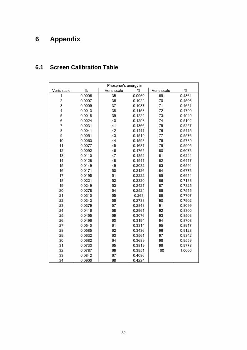
6 Appendix

6.1 Screen Calibration Table

Phosphor's energy in Veris scale % Veris scale % Veris scale %

1 0.0006 35 0.0960 69 0.4364 2 0.0007 36 0.1022 70 0.4506 3 0.0009 37 0.1087 71 0.4651 4 0.0013 38 0.1153 72 0.4799 5 0.0018 39 0.1222 73 0.4949 6 0.0024 40 0.1293 74 0.5102 7 0.0031 41 0.1366 75 0.5257 8 0.0041 42 0.1441 76 0.5415 9 0.0051 43 0.1519 77 0.5576 10 0.0063 44 0.1598 78 0.5739 11 0.0077 45 0.1681 79 0.5905 12 0.0092 46 0.1765 80 0.6073 13 0.0110 47 0.1852 81 0.6244 14 0.0128 48 0.1941 82 0.6417 15 0.0149 49 0.2032 83 0.6594 16 0.0171 50 0.2126 84 0.6773 17 0.0195 51 0.2222 85 0.6954 18 0.0221 52 0.2320 86 0.7138 19 0.0249 53 0.2421 87 0.7325 20 0.0278 54 0.2524 88 0.7515 21 0.0310 55 0.263 89 0.7707 22 0.0343 56 0.2738 90 0.7902 23 0.0379 57 0.2848 91 0.8099 24 0.0416 58 0.2961 92 0.8300 25 0.0455 59 0.3076 93 0.8503 26 0.0496 60 0.3194 94 0.8708 27 0.0540 61 0.3314 95 0.8917 28 0.0585 62 0.3436 96 0.9128 29 0.0632 63 0.3561 97 0.9342 30 0.0682 64 0.3689 98 0.9559 31 0.0733 65 0.3819 99 0.9778 32 0.0787 66 0.3951 100 1.0000 33 0.0842 67 0.4086 34 0.0900 68 0.4224

82

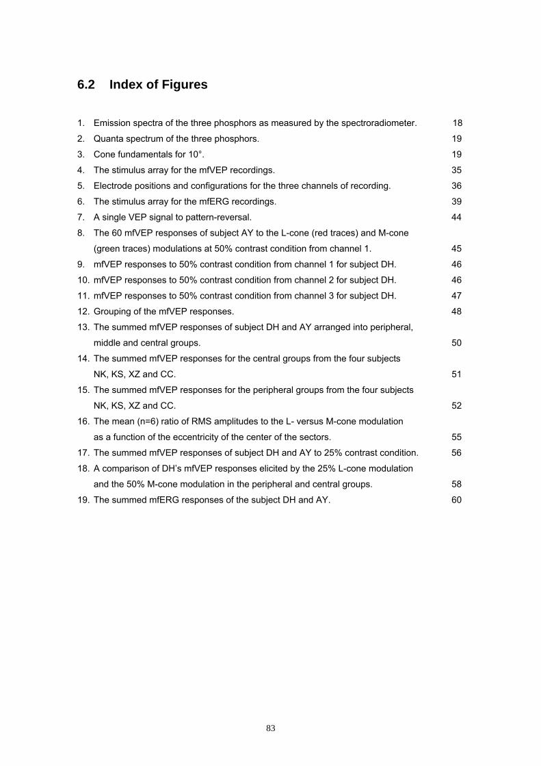
6.2 Index of Figures 1. Emission spectra of the three phosphors as measured by the spectroradiometer. 18

2. Quanta spectrum of the three phosphors. 19

3. Cone fundamentals for 10°. 19

4. The stimulus array for the mfVEP recordings. 35

5. Electrode positions and configurations for the three channels of recording. 36

6. The stimulus array for the mfERG recordings. 39

7. A single VEP signal to pattern-reversal. 44

8. The 60 mfVEP responses of subject AY to the L-cone (red traces) and M-cone

(green traces) modulations at 50% contrast condition from channel 1. 45

9. mfVEP responses to 50% contrast condition from channel 1 for subject DH. 46

10. mfVEP responses to 50% contrast condition from channel 2 for subject DH. 46

11. mfVEP responses to 50% contrast condition from channel 3 for subject DH. 47

12. Grouping of the mfVEP responses. 48

13. The summed mfVEP responses of subject DH and AY arranged into peripheral,

middle and central groups. 50

14. The summed mfVEP responses for the central groups from the four subjects

NK, KS, XZ and CC. 51

15. The summed mfVEP responses for the peripheral groups from the four subjects

NK, KS, XZ and CC. 52

16. The mean (n=6) ratio of RMS amplitudes to the L- versus M-cone modulation

as a function of the eccentricity of the center of the sectors. 55

17. The summed mfVEP responses of subject DH and AY to 25% contrast condition. 56

18. A comparison of DH’s mfVEP responses elicited by the 25% L-cone modulation

and the 50% M-cone modulation in the peripheral and central groups. 58

19. The summed mfERG responses of the subject DH and AY. 60

83

6.3 Index of Tables 1. Subject information 16

2. Veris scale for the calculated L-cone modulation 24

3. Veris scale for the L50 setting 27

4. Veris scale for the L25 setting 27

5. Veris scale for the calculated M-cone modulation 28

6. Veris scale for the M50 setting 31

7. Veris scale for the M25 setting 31

8. Stimulator parameters in the Veris 4.2 setting 33

9. RMS (L50/M50) for peripheral, middle and central responses 54

10. RMS (L50/M50) for mfVEP responses summed in six rings 54

11. RMS (L50/L25) for peripheral, middle and central responses 58

84

7 References

Ahnelt, P. K., Kolb, H., Pflug, R. (1987) Identification of a subtype of cone photoreceptor, likely to be blue sensitive, in the human retina. Journal of Comparative Neurology 255: 18-34.

Ahnelt, P., Keri, C., Kolb, H. (1990) Identification of pedicles of putative blue-sensitive cones in the human retina. Journal of Comparative Neurology 293: 39-53.

Albrecht, J., Jägle, H., Hood, D. C., Sharpe, L. T. (2002) The multifocal electroretinogram (mfERG) and cone isolating stimuli: Variation in L- and M-cone driven signals across the retina. Journal of Vision 2(2): 543-558.

Baseler, H. A., Sutter, E. E., Klein, S. A., Carney, T. (1994) The topography of visual evoked response properties across the visual field. Electroencephalography and Clinical Neurophysiology 90(1): 65-81.

Baseler, H. A., Sutter, E. E. (1997)

M and P components of the VEP and their visual field distribution. Vision Research 37(6): 675-690.

Benardete, E. A., Kaplan, E., Knight, B. W. (1992)

Contrast gain control in the primate retina: P cells are not X-like, some M cells are. Visual Neuroscience 8: 483-486.

Bieber, M. L., Kraft, J. M., Werner, J. S. (1998)

Effects of known variations in photopigments on L/M cone ratios estimated from luminous efficiency functions. Vision Research 38(13): 1961-1966.

Bowmaker, J. K., Dartnall, H. J. (1980)

Visual pigments of rods and cones in a human retina. Journal of Physiology 298: 501-511.

Brainard, D. H., Roorda, A., Yamauchi, Y., Calderone, J. B., Metha, A., Neitz,

M., Neitz, J., Williams, D. R., Jacobs, G.H. (2000) Functional consequences of the relative numbers of L and M cones. Journal of the Optical Society of America. A, Optics, Image Science, and Vision 17(3): 607-614.

85

Calkins, D. J., Schein, S. J., Tsukamoto, Y., Sterling, P. (1994) M and L cones in macaque fovea connect to midget ganglion cells by different numbers of excitatory synapses. Nature 371(6492): 70-72.

Calkins, D. J., Tsukamoto, Y., Sterling, P. (1998)

Microcircuitry and mosaic of a blue-yellow ganglion cell in the primate retina. Journal of Neuroscience 18: 3373-3385.

Carroll, J., McMahon, C., Neitz, M., Neitz, J. (2000)

Flicker-photometric electroretinogram estimates of L:M cone photoreceptor ratio in men with photopigment spectra derived from genetics. Journal of the Optical Society of America. A, Optics, Image Science, and Vision 17(3): 499-509.

Cicerone, C. M., Nerger, J. L. (1989)

The relative numbers of long-wavelength-sensitive to middle-wavelength- sensitive cones in the human fovea centralis. Vision Research 29(1): 115-128.

Curcio, C. A., Sloan, K. R., Packer, O., Hendrickson, A. E., Kalina, R. E. (1987).

Distribution of cones in human and monkey retina: individual variability and radial asymmetry. Science 236: 579-582.

Curcio, C. A., Allen, K. A., Sloan, K. R., Lerea, C. L., Hurley, J. B., Klock, I. B.,

Milam, A. H. (1991) Distribution and morphology of human cone photoreceptors stained with anti-blue opsin. Journal of Comparative Neurology 312: 610-624.

Dacey, D. M., Petersen, M. R. (1992)

Dendritic field size and morphology of midget and parasol ganglion cells of the human retina. Proceedings of the National Academy of Sciences of the United States of America 89(20): 9666-9670.

Dacey, D. M. (1993)

The mosaic of midget ganglion cells in the human retina. Journal of Neuroscience 13(12): 5334-5355.

Dacey, D. M., Lee, B. B. (1994)

The blue-ON opponent pathway in primate retina originates from a distinct bistratified ganglion cell type. Nature 367: 731-735.

86

Dacey, D. M. (1999) Primate retina: cell types, circuits and color opponency. Progress in Retinal Research 18(6): 737-763.

Dacey, D. M., Diller, L. C., Verweij, J., Williams, D. R. (2000a)

Physiology of L- and M-cone inputs to H1 horizontal cells in the primate retina. Journal of the Optical Society of America. A, Optics, Image Science, and Vision 17(3): 589-596.

Dacey, D. M, Packer, O. S., Diller, L. C., Brainard D. H., Peterson, B. B., Lee, B.

B. (2000b). Center-surround receptive field structure of cone bipolar cells in primate retina. Vision Research 40(14): 1801-1811.

Dartnall, H. J., Bowmaker, J. K., Mollon, J. D. (1983)

Human visual pigments: microspectrophotometric results from the eyes of seven persons. Proceedings of the Royal Society of London. Series B, Biological Sciences 220(1218): 115-130.

Dawson, W. W., Trick, G. L., Litzkow, C. A. (1979)

Improved electrode for electroretinography. Investigative Ophthalmology and Visual Science 18: 988-991.

Dawson, W. W., Trick, G. L., Maida, T. M. (1982)

Evaluation of the DTL-corneal electrode. Documenta Ophthalmologica 31: 81-88.

Deeb, S. S., Diller, L. C., Williams, D. R., Dacey, D. M. (2000)

Interindividual and topographical variation of L:M cone ratios in monkey retinas. Journal of the Optical Society of America. A, Optics, Image Science, and Vision 17(3): 538-544.

Derrington, A. M., Krauskopf, J., Lennie, P. (1984)

Chromatic mechanisms in lateral geniculate nucleus of macaque. Journal of Physiology 357: 241-265.

Derrington, A. M., Lennie, P. (1984)

Spatial and temporal contrast sensitivities of neurons in lateral geniculate nucleus of macaque. Journal of Physiology 357: 219-240.

De Valois, R. L., De Valois, K. K. (1993)

A multi-stage color model. Vision Research 33(8): 1053-1065.

87

De Vries (1946) Luminosity curves of trichromats. Nature 157: 736-737.

Dobkins, K. R., Thiele, A., Albright, T. D. (2000)

Comparison of red-green equiluminance points in humans and macaques: evidence for different L:M cone ratios between species. Journal of the Optical Society of America. A, Optics, Image Science, and Vision 17(3): 545-556.

Estevez, O., Spekreijse, H. (1982)

The "silent substitution" method in visual research. Vision Research 22(6): 681-691.

Famiglietti, E. V., Jr., Kolb, H. (1976)

Structural basis for ON-and OFF-center responses in retinal ganglion cells. Science 194(4261): 193-195.

Gouras, P. (1971)

The function of the midget cell system in primate color vision. Vision Research Supplement 3: 397-410.

Gouras, P. (1984)

Color Vision. Progress in Retinal Research 3: 227-261.

Guth, S. L., Alexander, J. V., Chumbly, J. I., Gillman, C. B., Patterson, M. M.

(1968) Factors affecting luminance additivity at threshold among normal and color-blind subjects and elaborations of a trichromatic-opponent colors theory. Vision Research 8(7): 913-928.

Hagstrom, S. A., Neitz, J., Neitz, M. (1998)

Variations in cone populations for red-green color vision examined by analysis of mRNA. Neuroreport 9(9): 1963-1967.

Hagstrom, S. A., Neitz, M., Neitz, J. (2000)

Cone pigment gene expression in individual photoreceptors and the chromatic topography of the retina. Journal of the Optical Society of America. A, Optics, Image Science, and Vision 17(3): 527-537.

Halliday, A. M., McDonald, W. I., Mushin, J. (1973)

Visual evoked response in diagnosis of multiple sclerosis. British Medical Journal 4(5893): 661-664.

88

Harding, G. F., Odom, J. V., Spileers, W., Spekreijse, H. (1996) Standard for visual evoked potentials 1995. The International Society for Clinical Electrophysiology of Vision. Vision Research 36(21): 3567-3572.

Hare, W. A., Ton, H., Ruiz, G., Feldmann, B., Wijono, M., WoldeMussie, E.

(2001) Characterization of retinal injury using ERG measures obtained with both conventional and multifocal methods in chronic ocular hypertensive primates. Investigative Ophthalmology and Visual Science 42(1): 127-136.

Hood, D. C., Seiple, W., Holopigian, K., Greenstein, V. (1997)

A comparison of the components of the multifocal and full-field ERGs. Visual Neuroscience 14(3): 533-544.

Hood, D. C. (2000)

Assessing retinal function with the multifocal technique. Progress in Retinal Research 19(5): 607-646.

Hood, D. C., Odel, J. G., Zhang, X. (2000a)

Tracking the recovery of local optic nerve function after optic neuritis: a multifocal VEP study. Investigative Ophthalmology and Visual Science 41(12): 4032-4038.

Hood, D. C., Zhang, X. (2000)

Multifocal ERG and VEP responses and visual fields: comparing disease- related changes. Documenta Ophthalmologica 100(2-3): 115-137.

Hood, D. C., Zhang, X., Greenstein, V. C., Kangovi, S., Odel, J. G., Liebmann,

J. M., Ritch, R. (2000b) An interocular comparison of the multifocal VEP: a possible technique for detecting local damage to the optic nerve. Investigative Ophthalmology and Visual Science 41(6): 1580-1587.

Hood, D. C., Frishman, L. J., Saszik, S., Viswanathan, S. (2002a)

Retinal origins of the primate multifocal ERG: implications for the human response. Investigative Ophthalmology and Visual Science 43(5): 1673-1685.

Hood, D. C., Zhang, X., Hong, J. E., Chen, C.S. (2002b)

Quantifying the benefits of additional channels of multifocal VEP recording. Documenta Ophthalmologica 104(3): 303-320.

89

Hood, D. C., Yu, A. L., Zhang, X., Albrecht, J., Jägle, H., Sharpe, L. T. (2002c) The multifocal visual evoked potential and cone-isolating stimuli: Implications for L- to M-cone ratios and normalization. Journal of Vision 2(2): 178-189.

Horiguchi, M., Suzuki, S., Kondo, M., Tanikawa, A., Miyake, Y. (1998)

Effect of glutamate analogues and inhibitory neurotransmitters on the electroretinograms elicited by random sequence stimuli in rabbits. Investigative Ophthalmology and Visual Science 39(11): 2171-2176.

Jacobs, G. H., Neitz, J., Krogh, K. (1996)

Electroretinogram flicker photometry and its applications. Journal of the Optical Society of America. A, Optics, Image Science, and Vision 13(3): 641-648.

Jacoby, R., Stafford, D., Kouyama, N., Marshak, D. (1996)

Synaptic inputs to ON parasol ganglion cells in the primate retina. Journal of Neuroscience 16: 8041-8056.

Kaneko, A. (1970)

Physiological and morphological identification of horizontal, bipolar and amacrine cells in goldfish retina. Journal of Physiology, London 207: 623-633.

Klistorner, A. I., Graham, S. L., Grigg, J. R., Billson, F. A. (1998)

Multifocal topographic visual evoked potential: improving objective detection of local visual field defects. Investigative Ophthalmology and Visual Science 39(6): 937-950.

Klistorner, A. I., Graham, S. L. (1999)

Multifocal pattern VEP perimetry: analysis of sectoral waveforms. Documenta Ophthalmologica 98(2): 183-196.

Klistorner, A., Graham, S. L. (2000)

Objective perimetry in glaucoma. Ophthalmology 107(12): 2283-2299.

Kolb, H. (1970)

Organization of the outer plexiform layer of the primate retina: electron microscopy of Golgi-impregnated cells. Philosophical Transactions of the Royal Society of London. Series B 258: 261-283.

Kolb, H., Dekorver, L. (1991)

Midget ganglion cells of the parafovea of the human retina: a study by electron microscopy and serial section reconstructions. Journal of Comparative Neurology 303(4): 617-636.

90

Kouyama, N., Marshak, D. W. (1992) Bipolar cells specific for blue cones in the macaque retina. Journal of Neuroscience 12: 1233-1252.

Krauskopf, J., Williams, D. R., Heeley, D. W. (1982)

Cardinal directions of color space. Vision Research 22:1123-1131.

Krauskopf, J. (2000)

Relative number of long- and middle-wavelength-sensitive cones in the human fovea. Journal of the Optical Society of America. A, Optics, Image Science, and Vision 17(3): 510-516.

Kremers, J., Usui, T., Scholl, H. P., Sharpe, L. T. (1999)

Cone signal contributions to electroretinograms [correction of electrograms] in dichromats and trichromats. Investigative Ophthalmology and Visual Science 40(5): 920-930.

Kremers, J., Scholl, H. P., Knau, H., Berendschot, T. T., Usui, T., Sharpe, L.T.

(2000) L/M cone ratios in human trichromats assessed by psychophysics, electroretinography, and retinal densitometry. Journal of the Optical Society of America. A, Optics, Image Science, and Vision 17(3): 517-526.

Kuffler, S. W. (1953)

Discharge patterns and functional organization of mammalian retina. Journal of Neurophysiology 16: 37-68.

Lee, B. B., Pokorny, J., Smith, V. C., Martin, P. R., Valberg, A. (1990)

Luminance and chromatic modulation sensitivity of macaque ganglion cells and human observers. Journal of the Optical Society of America. A, Optics, Image Science, and Vision 7(12): 2223-2236.

Lennie, P., Haake, P. W., Williams, D. R. (1991)

The design of chromatically opponent receptive fields. In: Landy, M. S., Movshon, J. A. (eds.): Computational Models of Visual Processing, pp. 71-82. MIT Press, Cambridge, MA.

Lynch, J. J., Silveira, L. C. L., Perry, V. H., Merigan, W. H. (1992)

Visual effects of damage to P ganglion cells in macaques. Visual Neuroscience 8: 575-583.

91

Martin, P. R., White, A. J. R., Goodchild, A. K., Wilder, H. D., Sefton, A. E. (1997) Evidence that blue-ON cells are part of the third geniculocortical pathway in primates. European Journal of Neuroscience 9: 1536-1541.

Merigan, W. (1989)

Chromatic and achromatic vision of macaques: role of the P pathway. Journal of Neuroscience 9: 776-783.

Milam A. H., Dacey, D. M., Dizhoor, A. M. (1993)

Recoverin immunoreactivity in mammalian cone bipolar cells. Visual Neuroscience 10: 1-12.

Mitchell, D. E., Rushton, W. A. H. (1971a)

Visual pigments in dichromats. Vision Research 11: 1033-1043.

Mitchell, D. E., Rushton, W. A. H. (1971b)

The red/green pigments of normal vision. Vision Research 11: 1045-1056.

Mullen, K. T., Kingdom, F. A. (1996)

Losses in peripheral colour sensitivity predicted from "hit and miss" post-receptoral cone connections. Vision Research 36(13): 1995-2000.

Nathans, J., Piantanida, T. P., Eddy, R. L., Shows, T. B. (1986a)

Molecular genetics of inherited variation in human color vision. Science 232: 203-210.

Nathans, J., Thomas, D., Hogness, D. S. (1986b)

Molecular genetics of human color vision: the genes encoding blue, green, and red pigments. Science 232: 193-202.

Nelson, R., Famiglietti, E. V., Jr., Kolb, H. (1978)

Intracellular staining reveals different levels of stratification for on- and off-center ganglion cells in cat retina. Journal of Neurophysiology 41(2): 472-483.

Nelson, R., Kolb, H. (1983)

Synaptic patterns and response properties of bipolar and ganglion cells in the cat retina. Vision Research 23: 1183-1195.

92

Osterberg, G. (1935) Topography of the layer of rods and cones in the human retina. Acta Ophthalmologica (suppl.) 6: 1-103.

Otake, S., Cicerone, C. M. (2000)

L and M cone relative numerosity and red-green opponency from fovea to midperiphery in the human retina. Journal of the Optical Society of America. A, Optics, Image Science, and Vision 17(3): 615-627.

Perry, V. H., Oehler, R., Cowey, A. (1984)

Retinal ganglion cells that project to the dorsal lateral geniculate nucleus in the macaque monkey. Neuroscience 12: 1101-1123.

Pokorny, J., Smith, V. C., Wesner, M. F. (1991) Variability in cone populations and implications.

In: Valberg, A., Lee B. B. (eds.): From pigments to perception: Advances in understanding visual processes, pp.1-9. Plenum Press, New York.

Polyak, S. L. (1941) In: The Retina. University of Chicago Press, Chicago. Pugh E. N. (1988)

Physics and retinal physiology. In: Atkinson R. C. (ed.): Stevens Handbook of Experimental Psychology. Wiley, New York.

Purpura, K., Kaplan, E., Shapley, R. M. (1988)

Background light and the contrast gain of primate P and M retinal ganglion cells. Proceedings of the National Academy of Sciences of the United States of America 85: 4534-4537.

Roorda, A., Williams, D. R. (1999)

The arrangement of the three cone classes in the living human eye. Nature 397(6719): 520-522.

Rushton, W. A., Baker, H. D. (1964)

Red-green sensitivity in normal vision. Vision Research 4(1): 75-85.

Scar, G., Maunsell, J. H. R., Lennie, P. (1990)

Coding of image contrast in central visual pathways of the macaque monkey. Vision Research 30: 1-10.

93

Schiller, P. H., Colby, C.L. (1983) The responses of single cells in the lateral geniculate nucleus of the rhesus monkey to color and luminance contrast. Vision Research 23: 1631-1641.

Schiller, P. H., Logothetis, N. K., Charles, E. R. (1991)

Parallel pathways in the visual system: their role in perception at isoluminance. Neuropsychologia 29: 433-441.

Sieving, P. A., Murayama, K., Naarendorp, F. (1994) Push-pull model of the primate photopic electroretinogram: a role for hyperpolarizing neurons in shaping the b-wave. Visual Neuroscience 11(3): 519-532.

Slotnick, S. D., Klein, S. A., Carney, T., Sutter, E., Dastmalchi, S. (1999)

Using multi-stimulus VEP source localization to obtain a retinotopic map of human primary visual cortex. Clinical Neurophysiology 110(10): 1793-1800.

Smith, V. C., Pokorny, J. (1975)

Spectral sensitivity of the foveal cone photopigments between 400 and 500 nm. Vision Research 15(2): 161-171.

Solomon, S. G., White A. J., Martin P. R. (1999)

Temporal contrast sensitivity in the lateral geniculate nucleus of a New World monkey, the marmoset Callithrix jacchus. Journal of Physiology 517(3): 907-917.

Stiles, W.S. (1978)

Further studies of visual mechanisms by the two-colour threshold method. In: Colloquio sobre Problemas Opticos de la Vision (n.p., Madrid, 1953), Vol. 1, pp.65-103; reprinted in W. S. Stiles, Mechanisms of Colour Vision (Academic, New York, 1978).

Stockman, A., MacLeod, D. I. A., DePriest, D. D. (1991)

The temporal properties of the human short-wave photoreceptors and their associated pathways. Vision Research 31: 189-208.

Stockman, A., MacLeod, D. I., Johnson, N. E. (1993)

Spectral sensitivities of the human cones. Journal of the Optical Society of America. A, Optics, Image Science, and Vision 10(12): 2491-2521.

94

Stockman, A., Sharpe, L. T. (1998) Human cone spectral sensitivities: a progress report. Vision Research 38(21): 3193-3206.

Stockman, A., Sharpe, L. T. (1999)

Cone spectral sensitivities and color matching. In: Gegenfurtner, K., Sharpe, L. T. (eds.): Color Vision: From Genes to Perception, pp. 53-88. Cambridge U. Press, Cambridge, UK.

Stockman, A., Sharpe, L. T. (2000)

The spectral sensitivities of the middle- and long-wavelength-sensitive cones derived from measurements in observers of known genotype. Vision Research 40(13): 1711-1737.

Sutter, E. E., Tran, D. (1992)

The field topography of ERG components in man--I. The photopic luminance response. Vision Research 32(3): 433-446.

Sutter, E. E., Bearse, M. A., Jr. (1999)

The optic nerve head component of the human ERG. Vision Research 39(3): 419-436.

Sutter, E. E., Shimada, Y., Li, Y., Bears, M. A. (1999)

Mapping inner retinal function through enhancement of adapative component in the mERG. In: Vision Science and its Applications, OSA Tech Dig Ser 1 (Optical Society of America, Washington DC), pp: 52-55.

Sutter, E. E. (2000)

The interpretation of multifocal binary kernels. Documenta Ophthalmologica 100 (2/3): 49-75.

Teping, C. (1981)

Visusbestimmung mit Hilfe des visuell evozierten kortikalen Potentials (VECP). Klinische Monatsblätter fuer Augenheilkunde: 179-169.

Tsukamoto, Y., Masarachia, P., Schein, S. J., Sterling, P. (1992)

Gap junctions between the pedicles of macaque foveal cones. Vision Research 32: 1809-1815.

van de Kraats, J., Berendschot, T. T., van Norren, D. (1996)

The pathways of light measured in funds reflectometry. Vision Research 36(15): 2229-2247.

95

von Helmholtz, H. (1852) On the theory of compound colours. Philosophical Magazine, Serial 4, 4: 519-535.

Vos, J. J., Walraven, P. L. (1971)

On the derivation of the foveal receptor primaries. Vision Research 11(8): 799-818.

Wesner, M. F., Pokorny, J., Shevell, S. K., Smith, V. C. (1991)

Foveal cone detection statistics in color-normals and dichromats. Vision Research 31(6): 1021-1037.

White, A. J. R., Wilder, H. D., Goodchild, A. K., Sefton, A. J., Martin, P. R. (1998) Segregation of receptive field properties in the lateral geniculate nucleus of a new-world monkey, the marmoset Callithrix jacchus. Journal of Neurophysiology 80: 2063-2076.

Wikler, K. C., Rakic, P. (1990)

Distribution of photoreceptor subtypes in the retina of diurnal and nocturnal primates. Journal of Neuroscience 10: 3390-3401.

Wyszecki, G., Stiles, W. S. (1982)

Color science: Concepts and methods, quantitative data and formulae. Wiley, New York, Chichester, Brisbane, Toronto, Singapore.

Young, T. (1802)

On the theory of light and colors. Philosophical Transactions of the Royal Society 91:12-49.

96

Acknowledgments

I would like to acknowledge my great indebtness to Professor Dr. E. Zrenner for

leaving the topic of this doctoral thesis with me and enabling me to spend a

sojourn at Columbia University, New York, NY, U.S.A..

I owe an equally great debt to Professor Dr. D. C. Hood, with whom I conducted

the majority of the experiments, and who was invaluable in providing support at

all stages of this work. I especially would like to thank him for his intensive

personal assistance and for being such an excellent mentor.

I am immensely grateful to Professor Dr. Lindsay T. Sharpe for his scientific and

strategic advices during this work and for his help and encouragement to apply

for this sojourn.

I give gratitude to Dr. H. Jägle for his patience to look through my manuscripts

and making the proper corrections, without which this thesis could not be

completed.

Special thanks goes to J. Albrecht and X. Zhang for introducing me into the

silent substitution method and into their programming work and for providing me

with their many advices and technical support.

I am also indebted to all the participants of this study for their time and efforts,

which only made this study possible.

Thank you very much also to the Deutsche Akademische Auslandsdienst

(DAAD), which provided me with a stipend for this sojourn.

And lastly, I would like to thank my parents for their perpetual encouragement

and their financial support.

Curriculum Vitae

Name: Yu, Alice Lap-Ho

Date and Place of Birth: 07th October 1976 in Hongkong

Marital Status: single

Parents: Ping-Pok Yu, M.D.; Kin-Fan Ku, M.D.

School: 1983 – 1987 Kasteneckschule in Freiberg a.N. (elementary school)

1987 – 1996 Oscar-Paret-Schule in Freiberg a.N. (‚Gymnasium’),

graduating with ‚Abitur’

Medical Studies: 04/97 Start of medical studies at the Eberhard-Karls-Universität

Tübingen

03/99 Ärztliche Vorprüfung (preclinical exam)

03/00 1. Abschnitt der Ärztlichen Prüfung (1st clinical exam)

09/00 – 04/01 Research scholar at Columbia University, New York, NY,

U.S.A.

04/01 Continued medical studies at the Ludwig-Maximilians-

Universität München

03/02 2. Abschnitt der Ärztlichen Prüfung (2nd clinical exam)

04/02 – 08/02 1. PJ-Tertial (1st clinical clerkship) at Harvard Medical

School, Boston, MA, U.S.A.

08/02 – 11/02 2. PJ-Tertial (2nd clinical clerkship) at Universitäts-

Augenklinik – Innenstadt, München

12/02 – 03/03 3. PJ-Tertial (3rd clinical clerkship) at Chirurgische Klinik

und Poliklinik, Großhadern, München

04th June 2003 3. Abschnitt der Ärztlichen Prüfung (3rd clinical exam)