Tesseroids: forward modeling gravitational elds in ...Tesseroids: forward modeling gravitational...
29
Tesseroids: forward modeling gravitational fields in spherical coordinates Leonardo Uieda 12 , Val´ eria C. F. Barbosa 2 , and Carla Braitenberg 3 Peer-reviewed code related to this article can be found at http://software.seg.org/2016/0004. 1 Universidade do Estado do Rio de Janeiro, Rio de Janeiro, Brazil. email: [email protected] 2 Observat´orio Nacional, Rio de Janeiro, Brazil. email: [email protected] 3 Department of Mathematics and Geosciences, University of Trieste, Trieste, Italy (May 10, 2016) GEO-2015-0204 Running head: Tesseroids: modeling in spherical coordinates ABSTRACT We present the open-source software Tesseroids, a set of command-line programs to per- form the forward modeling of gravitational fields in spherical coordinates. The software is implemented in the C programming language and uses tesseroids (spherical prisms) for the discretization of the subsurface mass distribution. The gravitational fields of tesseroids are calculated numerically using the Gauss-Legendre Quadrature (GLQ). We have improved upon an adaptive discretization algorithm to guarantee the accuracy of the GLQ integra- tion. Our implementation of adaptive discretization uses a “stack” based algorithm instead of recursion to achieve more control over execution errors and corner cases. The algorithm is controlled by a scalar value called the distance-size ratio (D) that determines the accu- 1
Transcript of Tesseroids: forward modeling gravitational elds in ...Tesseroids: forward modeling gravitational...
Tesseroids: forward modeling gravitational fields in spherical
coordinates
Leonardo Uieda12, Valeria C. F. Barbosa2, and Carla Braitenberg3
Peer-reviewed code related to this article can be found at
http://software.seg.org/2016/0004.
1Universidade do Estado do Rio de Janeiro, Rio de Janeiro, Brazil. email:
2Observatorio Nacional, Rio de Janeiro, Brazil. email: [email protected]
3Department of Mathematics and Geosciences, University of Trieste, Trieste, Italy
(May 10, 2016)
GEO-2015-0204
Running head: Tesseroids: modeling in spherical coordinates
ABSTRACT
We present the open-source software Tesseroids, a set of command-line programs to per-
form the forward modeling of gravitational fields in spherical coordinates. The software is
implemented in the C programming language and uses tesseroids (spherical prisms) for the
discretization of the subsurface mass distribution. The gravitational fields of tesseroids are
calculated numerically using the Gauss-Legendre Quadrature (GLQ). We have improved
upon an adaptive discretization algorithm to guarantee the accuracy of the GLQ integra-
tion. Our implementation of adaptive discretization uses a “stack” based algorithm instead
of recursion to achieve more control over execution errors and corner cases. The algorithm
is controlled by a scalar value called the distance-size ratio (D) that determines the accu-
1
racy of the integration as well as the computation time. We determined optimal values of
D for the gravitational potential, gravitational acceleration, and gravity gradient tensor by
comparing the computed tesseroids effects with those of a homogeneous spherical shell. The
values required for a maximum relative error of 0.1% of the shell effects are D = 1 for the
gravitational potential, D = 1.5 for the gravitational acceleration, and D = 8 for the grav-
ity gradients. Contrary to previous assumptions, our results show that the potential and
its first and second derivatives require different values of D to achieve the same accuracy.
These values were incorporated as defaults in the software.
2
INTRODUCTION
Satellite missions dedicated to measuring the Earth’s gravity field (like CHAMP, GRACE,
and GOCE) have provided geophysicists with almost uniform and global data coverage.
These new data have enabled interpretations on regional and global scales (e.g. Reguzzoni
et al., 2013; Braitenberg, 2015). Modeling at such scales requires taking into account the
curvature of the Earth and calculating gravity gradients as well as the traditional gravi-
tational acceleration. A common approach to achieve this is to discretize the Earth into
tesseroids (Figure 1) instead of rectangular prisms. An analytical solution exists when the
computation point is along the polar axis and the tesseroid is extended into a spherical
cap (LaFehr, 1991; Mikuska et al., 2006; Grombein et al., 2013). For more general cases,
the integral formula for the gravitational effects of a tesseroid must be solved numerically.
Approaches to this numerical integration include Taylor series expansion (Heck and Seitz,
2007; Grombein et al., 2013) and the Gauss-Legendre Quadrature (Asgharzadeh et al.,
2007). Taylor series expansion produces accurate results at low latitudes but presents a
decrease in accuracy towards the polar regions. This is attributed to tesseroids degenerat-
ing into an approximately triangular shape at the poles. The Gauss-Legendre Quadrature
(GLQ) integration consists in approximating the volume integral by a weighted sum of the
effect of point masses. An advantage of the GLQ approach is that it can be controlled by the
number of point masses used. The larger the number of point masses, the better the accu-
racy of GLQ integration. A disadvantage is the increased computation time as the number
of point masses increases. Thus, there is a trade-off between accuracy and computation
time. This is a common theme in numerical methods. Wild-Pfeiffer (2008) investigated the
use of different mass elements, including tesseroids, to compute the gravitational effects of
topographic masses. The author concludes that using tesseroids with GLQ integration gives
3
the best results for near-zone computations. However, the question of how to determine the
optimal parameters for GLQ integration remained open.
Previous work by Ku (1977) investigated the use of the GLQ in gravity forward modeling.
Ku (1977) numerically integrated the vertical component of the gravitational acceleration
of right rectangular prisms. The author suggested that the accuracy of the GLQ integration
depends on the ratio between distance to the computation point and the distance between
adjacent point masses. Based on this, Ku (1977) proposed an empirical criterion that the
distance between point masses should be greater than the distance to the computation point.
Asgharzadeh et al. (2007) used this criterion for the GLQ integration of the gravity gradient
tensor of tesseroids. To our knowledge, an analysis of how well this ad hoc criteria of Ku
(1977) works for gravity gradient components or for tesseroids has never been done before.
There has also been no attempt to quantify the error committed in the GLQ integration
when applying the criteria of Ku (1977).
Li et al. (2011) devised an algorithm to automatically enforce the criteria of Ku (1977).
Their algorithm divides the tesseroid into smaller ones instead of increasing the number of
point masses per tesseroid. A tesseroid is divided if the minimum distance to the computa-
tion point is smaller than the largest dimension of the tesseroid. This division is repeated
recursively until all tesseroids obey the criterion. Then, GLQ integration is performed for
each of the smaller tesseroids using the specified number of point masses. The advantage
of this adaptive discretization over increasing the number of points masses is that the total
distribution of point masses will be greater only close to the computation point. This makes
the adaptive discretization more computationally efficient.
Grombein et al. (2013) developed optimized formula for the gravitational fields of
4
tesseroids using Cartesian integral kernels. These formulas are faster to compute and do
not have singularities at the poles like their spherical counterparts. The Cartesian formulae
are numerically integrated using a Taylor series expansion as per Heck and Seitz (2007).
Grombein et al. (2013) use a near-zone separation to mitigate the increased error at high
latitudes. In the so called “near-zone” of the computation point they use a finer discretiza-
tion composed by smaller tesseroids. This is accomplished by dividing the tesseroids along
their horizontal dimensions. However, the determination of an optimal size of the near-zone
remains an open question (Grombein et al., 2013).
We have implemented a modified version of the adaptive discretion of Li et al. (2011)
into the open-source software package Tesseroids. The software uses the Cartesian formula
of Grombein et al. (2013) for improved performance and robustness. Previous versions of
the software have been used by, e.g., Alvarez et al. (2012); Bouman et al. (2013a,b); Mariani
et al. (2013); Braitenberg et al. (2013, 2011); Fullea et al. (2014).
This article describes the software design and the implementation of our modified adap-
tive discretization algorithm. We also present a numerical investigation of the error com-
mitted in the computations. These results allow us to calibrate the adaptive discretization
algorithm separately for the gravitational potential, gravitational acceleration, as well as
the gravity gradient tensor components.
THEORY
A tesseroid is a mass element defined in geocentric spherical coordinates (Figure 1). It
is bounded by two meridians, two parallels, and two concentric circles. The gravitational
fields of a tesseroid at a point P = (r, φ, λ) are determined with respect to the local North-
5
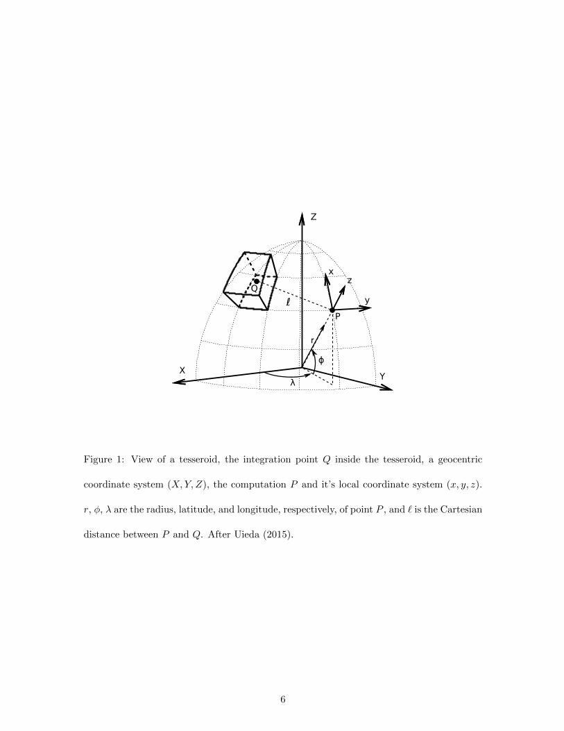
Figure 1: View of a tesseroid, the integration point Q inside the tesseroid, a geocentric
coordinate system (X,Y, Z), the computation P and it’s local coordinate system (x, y, z).
r, φ, λ are the radius, latitude, and longitude, respectively, of point P , and ` is the Cartesian
distance between P and Q. After Uieda (2015).
6
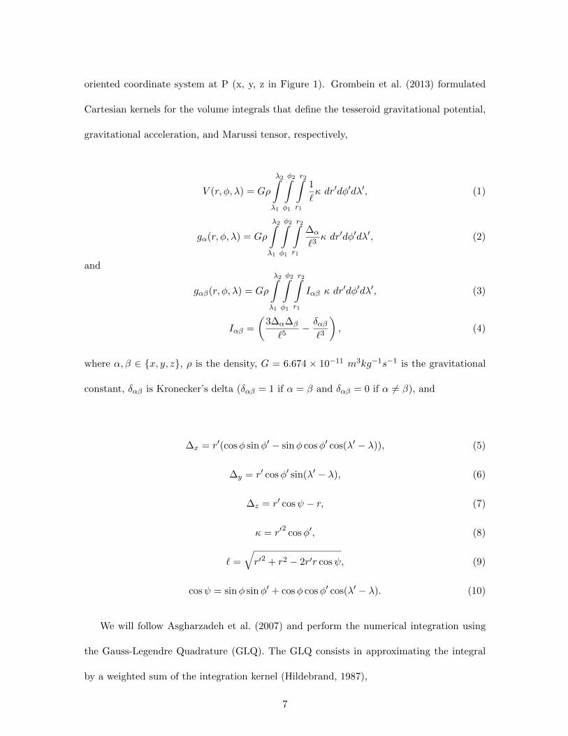
oriented coordinate system at P (x, y, z in Figure 1). Grombein et al. (2013) formulated
Cartesian kernels for the volume integrals that define the tesseroid gravitational potential,
gravitational acceleration, and Marussi tensor, respectively,
V (r, φ, λ) = Gρ
λ2∫λ1
φ2∫φ1
r2∫r1
1
`κ dr′dφ′dλ′, (1)
gα(r, φ, λ) = Gρ
λ2∫λ1
φ2∫φ1
r2∫r1
∆α
`3κ dr′dφ′dλ′, (2)
and
gαβ(r, φ, λ) = Gρ
λ2∫λ1
φ2∫φ1
r2∫r1
Iαβ κ dr′dφ′dλ′, (3)
Iαβ =
(3∆α∆β
`5− δαβ
`3
), (4)
where α, β ∈ x, y, z, ρ is the density, G = 6.674 × 10⁻¹¹ m3kg−1s−1 is the gravitational
constant, δαβ is Kronecker’s delta (δαβ = 1 if α = β and δαβ = 0 if α 6= β), and
∆x = r′(cosφ sinφ′ − sinφ cosφ′ cos(λ′ − λ)), (5)
∆y = r′ cosφ′ sin(λ′ − λ), (6)
∆z = r′ cosψ − r, (7)
κ = r′2
cosφ′, (8)
` =
√r′2 + r2 − 2r′r cosψ, (9)
cosψ = sinφ sinφ′ + cosφ cosφ′ cos(λ′ − λ). (10)
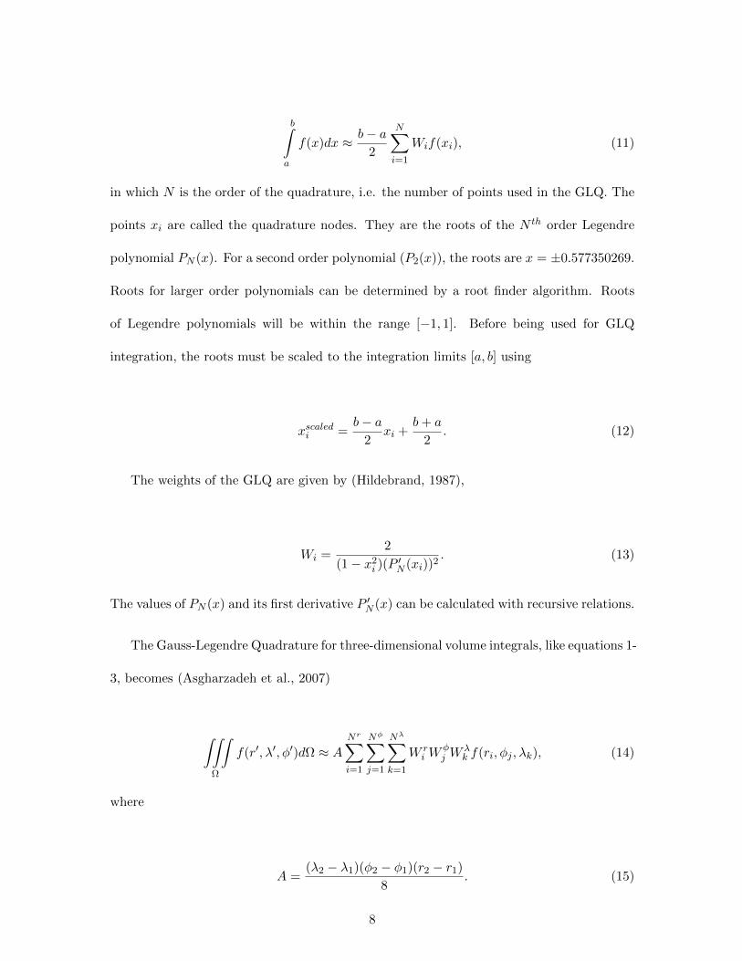
We will follow Asgharzadeh et al. (2007) and perform the numerical integration using
the Gauss-Legendre Quadrature (GLQ). The GLQ consists in approximating the integral
by a weighted sum of the integration kernel (Hildebrand, 1987),
7
b∫a
f(x)dx ≈ b− a2
N∑i=1
Wif(xi), (11)
in which N is the order of the quadrature, i.e. the number of points used in the GLQ. The
points xi are called the quadrature nodes. They are the roots of the N th order Legendre
polynomial PN (x). For a second order polynomial (P2(x)), the roots are x = ±0.577350269.
Roots for larger order polynomials can be determined by a root finder algorithm. Roots
of Legendre polynomials will be within the range [−1, 1]. Before being used for GLQ
integration, the roots must be scaled to the integration limits [a, b] using
xscaledi =b− a
2xi +
b+ a
2. (12)
The weights of the GLQ are given by (Hildebrand, 1987),
Wi =2
(1− x2i )(P
′N (xi))2
. (13)
The values of PN (x) and its first derivative P ′N (x) can be calculated with recursive relations.
The Gauss-Legendre Quadrature for three-dimensional volume integrals, like equations 1-
3, becomes (Asgharzadeh et al., 2007)
∫∫∫Ω
f(r′, λ′, φ′)dΩ ≈ ANr∑i=1
Nφ∑j=1
Nλ∑k=1
W ri W
φj W
λk f(ri, φj , λk), (14)
where
A =(λ2 − λ1)(φ2 − φ1)(r2 − r1)
8. (15)
8
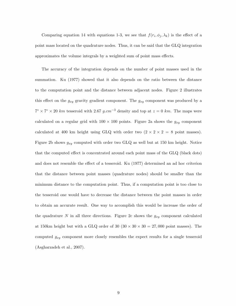
Comparing equation 14 with equations 1-3, we see that f(ri, φj , λk) is the effect of a
point mass located on the quadrature nodes. Thus, it can be said that the GLQ integration
approximates the volume integrals by a weighted sum of point mass effects.
The accuracy of the integration depends on the number of point masses used in the
summation. Ku (1977) showed that it also depends on the ratio between the distance
to the computation point and the distance between adjacent nodes. Figure 2 illustrates
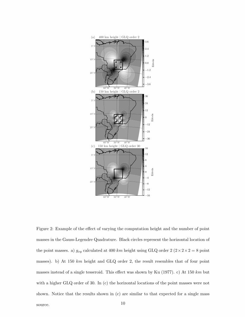
this effect on the gxy gravity gradient component. The gxy component was produced by a
7 × 7 × 20 km tesseroid with 2.67 g.cm−3 density and top at z = 0 km. The maps were
calculated on a regular grid with 100 × 100 points. Figure 2a shows the gxy component
calculated at 400 km height using GLQ with order two (2 × 2 × 2 = 8 point masses).
Figure 2b shows gxy computed with order two GLQ as well but at 150 km height. Notice
that the computed effect is concentrated around each point mass of the GLQ (black dots)
and does not resemble the effect of a tesseroid. Ku (1977) determined an ad hoc criterion
that the distance between point masses (quadrature nodes) should be smaller than the
minimum distance to the computation point. Thus, if a computation point is too close to
the tesseroid one would have to decrease the distance between the point masses in order
to obtain an accurate result. One way to accomplish this would be increase the order of
the quadrature N in all three directions. Figure 2c shows the gxy component calculated
at 150km height but with a GLQ order of 30 (30 × 30 × 30 = 27, 000 point masses). The
computed gxy component more closely resembles the expect results for a single tesseroid
(Asgharzadeh et al., 2007).
9
(a)
25S
15S
5S
60W 50W 40W
400 km height | GLQ order 2
(b)
25S
15S
5S
60W 50W 40W
150 km height | GLQ order 2
(c)
25S
15S
5S
60W 50W 40W
150 km height | GLQ order 30
−3.6
−2.4
−1.2
0.0
1.2
2.4
3.6
Eotvos
−36
−24
−12
0
12
24
36
Eotvos
−16
−12
−8
−4
0
4
8
12
16
Eotvos
Figure 2: Example of the effect of varying the computation height and the number of point
masses in the Gauss-Legendre Quadrature. Black circles represent the horizontal location of
the point masses. a) gxy calculated at 400 km height using GLQ order 2 (2×2×2 = 8 point
masses). b) At 150 km height and GLQ order 2, the result resembles that of four point
masses instead of a single tesseroid. This effect was shown by Ku (1977). c) At 150 km but
with a higher GLQ order of 30. In (c) the horizontal locations of the point masses were not
shown. Notice that the results shown in (c) are similar to that expected for a single mass
source. 10
Adaptive discretization
Li et al. (2011) proposed an alternative method for decreasing the distance between point
masses on the quadrature nodes aiming at achieving an accurate integration. Instead of
increasing the GLQ order, they keep it fixed to a given number and divide the tesseroid into
smaller volumes. The sum of the effects of the smaller tesseroids is equal to the gravitational
effect of the larger tesseroid. This division effectively decreases the distance between nodes
because of the smaller size of the tesseroids. The criterion for dividing a tesseroid is that
the distance to the computation point should be smaller than a constant times the size of
the tesseroid. This is analogous to the criterion proposed by Ku (1977) because the size of
the tesseroid serves as a proxy for the distance between point masses. This procedure is
repeated recursively until all tesseroids are within the acceptable ratio of distance and size
or a minimum size is achieved.
The advantage of this adaptive discretization is that the number of point masses is only
increased in parts of the tesseroid that are closer to the computation point. Notice that the
alternative approach of simply increasing the order of the GLQ would increase the number
of point masses evenly throughout the whole tesseroid.
IMPLEMENTATION
We have implemented the calculation of the tesseroid gravitational fields with adaptive
discretization in version 1.2 of the open-source package Tesseroids. It is freely available
online12 under the BSD 3-clause open-source license. An archived version of the source
code is also available as part of this article.
1http://tesseroids.leouieda.com2http://dx.doi.org/10.5281/zenodo.16033
11
Tesseroids consists of command-line programs written in the C programming language.
The package includes programs to calculate the gravitational fields of tesseroids and rect-
angular prisms (in both Cartesian and spherical coordinates). All programs receive input
through command-line arguments and the standard input channel (“STDIN”) and output
the results through the standard output channel (“STDOUT”). For example, the command
to generate a regular grid with NLON ×NLAT points, calculate gz and gzz caused by the
tesseroids in a file “MODELFILE”, and save the results to a file called “OUTPUT” is:
tessgrd -rW/E/S/N -bNLON/NLAT -zHEIGHT | \
tessgz MODELFILE | \
tessgzz MODELFILE > OUTPUT
The src folder of the source code archive contains the C files that build the command-
line programs (e.g., tessgz.c). The src/lib folder contains the source files that implement the
numerical computations. We will not describe here the implementation of the input/output
parsing and other miscellanea. Instead, we will focus on the details of the Gauss-Legendre
Quadrature integration of equations 1-3 and the adaptive discretization of tesseroids.
Numerical integration
The source file src/lib/glq.c contains the code necessary to perform a Gauss-Legendre
Quadrature integration. The first step in the GLQ is to compute the locations of the
discretization points (i.e., the point masses). These points are roots of Legendre polynomi-
als. Precomputed values are available for low order polynomials, typically up to order five.
For flexibility and to compute higher order roots, we use the multiple root-finder algorithm
of Barrera-Figueroa et al. (2006). The additional computational load is minimal because
12
the root-finder algorithm must be run only once per program execution. The root-finder is
implemented in functions glq nodes and glq next root. The computed roots will be in the
range [−1, 1] and must be scaled to the integration limits (the physical boundaries of the
tesseroid) using function glq set limits (see equation 12).
The GLQ weights (equation 13) are computed by function glq weights. Both the com-
puted roots and weights are stored in a data structure (a C struct) called GLQ. Function
glq new handles memory allocation, calculates the roots and weights, and returns the com-
plete GLQ structure.
The numerical integration of the tesseroid gravitational fields is performed by the func-
tions in module src/lib/grav tess.c. Functions tess pot, tess gx, tess gy, and so on, com-
pute the gravitational fields of a single tesseroid on a single computation point. These
functions require three GLQ structures, each containing the roots and weights for GLQ
integration in the three dimensions. The roots must be scaled to the integration limits
[λ1, λ2], [φ1, φ2], [r1, r2] (see equations 1-3). The integration consists of three loops that sum
the weighted kernel functions evaluated at each GLQ point mass (the scaled roots).
The biggest bottlenecks for the numerical integration are the number of point masses
used and the evaluation of the trigonometric functions in equations 1-3 inside the inner
loops. Better performance is achieved by pre-computing the sine and cosine of latitudes
and moving some trigonometric function evaluations to the outer loops.
Implementation of adaptive discretization
Our implementation of the adaptive discretization algorithm differs in a few ways from the
one proposed by Li et al. (2011). In Li et al. (2011), a tesseroid will be divided when the
13
smallest distance between it and the computation point is smaller than a constant times
the largest dimension of the tesseroid. Instead of the smallest distance, we use the easier to
calculate distance between the computation point (r, λ, φ) and the geometric center of the
tesseroid (rt, λt, φt)
d =[r2 + r2
t − 2rrt cosψt] 12 , (16)
cosψt = sinφ sinφt + cosφ cosφt cos(λ− λt). (17)
Our definition of the dimensions of the tesseroid (the “side lengths” of Li et al. (2011))
along longitude, latitude, and radius, respectively, are (Figure 3a)
Lλ = r2 arccos(sin2 φt + cos2 φt cos(λ2 − λ1)), (18)
Lφ = r2 arccos(sinφ2 sinφ1 + cosφ2 cosφ1), (19)
Lr = r2 − r1. (20)
Lλ and Lφ are arc-distances measured along the top surface of the tesseroid (Figure 3a).
Specifically, Lλ is measured long the middle latitude of the tesseroid (φt).
To determine if a tesseroid must be divided, we check if
d
Li≥ D, (21)
for each i ∈ (λ, φ, r). D is a positive scalar hereafter referred to as the “distance-size ratio”.
If the inequality holds for all three dimensions, the tesseroid is not divided. Thus, the
distance-size ratio determines how close the computation point can be before we must divide
14
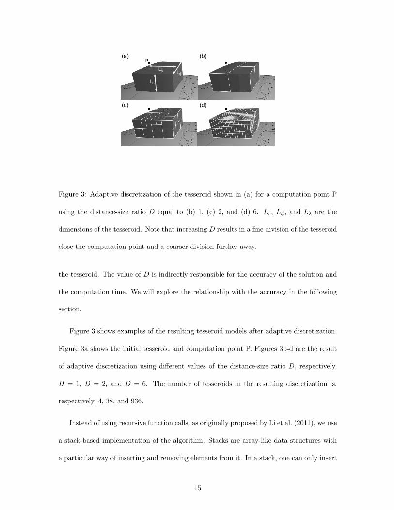
Figure 3: Adaptive discretization of the tesseroid shown in (a) for a computation point P
using the distance-size ratio D equal to (b) 1, (c) 2, and (d) 6. Lr, Lφ, and Lλ are the
dimensions of the tesseroid. Note that increasing D results in a fine division of the tesseroid
close the computation point and a coarser division further away.
the tesseroid. The value of D is indirectly responsible for the accuracy of the solution and
the computation time. We will explore the relationship with the accuracy in the following
section.
Figure 3 shows examples of the resulting tesseroid models after adaptive discretization.
Figure 3a shows the initial tesseroid and computation point P. Figures 3b-d are the result
of adaptive discretization using different values of the distance-size ratio D, respectively,
D = 1, D = 2, and D = 6. The number of tesseroids in the resulting discretization is,
respectively, 4, 38, and 936.
Instead of using recursive function calls, as originally proposed by Li et al. (2011), we use
a stack-based implementation of the algorithm. Stacks are array-like data structures with
a particular way of inserting and removing elements from it. In a stack, one can only insert
15
elements to the top of the stack (the last empty position). Likewise, one can only remove
the last element of the stack (commonly referred to as “popping” the stack). Because of
these restrictions, stacks are also known as “Last-In-First-Out” (LIFO) data structures.
The discretization algorithm is implemented in function calc tess model adapt of the
file src/lib/grav tess.c. This function calculates the effect of a single tesseroid on a single
computation point. The stack of tesseroids is represented by the stack variable, an array of
TESSEROID structures. We must define a maximum size for the stack to allocate memory
for it. Defining a maximum size allows us to avoid an infinite loop in case the computation
point is on (or sufficiently close to) the surface of the tesseroid. We use the integer stktop
to keep track of the index of the last element in the stack (the top of the stack).
Below, we describe the algorithm to calculate the effect of a single tesseroid from the
input model on a single computation point. The algorithm starts by creating an empty stack
of tesseroids. Then, the stack is initialized with the single input tesseroid. The initialization
is done by copying the tesseroid into the stack and setting stktop to zero (the first element).
It is important to note that the stack is not the input tesseroid model. Instead, it is a buffer
used to temporarily store each stage of the discretization algorithm.
Once the stack is initialized, the steps of the algorithm are:
1. “Pop” the stack (i.e., take the last tesseroid from it). This will cause stktop to be
reduced by one. This tesseroid is the one that will be evaluated in the following steps.
2. Compute the distance d (equation 16) between the geometric center of the tesseroid
and the computation point.
3. Compute the dimensions of the tesseroid Lλ, Lφ, and Lr using equations 18-20.
16
4. Check the condition in equation 21 for each dimension of the tesseroid.
5. If all dimensions hold the inequality 21, the tesseroid is not divided and its gravita-
tional effect is computed using the Gauss-Legendre Quadrature (equations 1-3 and 14).
We use a GLQ order of two for all three dimensions (2× 2× 2 = 8 point masses) by
default. This value can be changed using a command-line argument of the modeling
programs.
6. If any of the dimensions fail the condition:
(a) Divide the tesseroid in half along each dimension that failed the condition.
(b) Check if there is room in the stack for the new tesseroids (i.e.,the number of
new elements plus stktop is smaller than the maximum stack size). If there isn’t,
warn the user of a “stack overflow” and compute the effect of the tesseroid, as in
step 5. If there is room in the stack, place the smaller tesseroids into the stack.
7. Repeat the above steps until the stack is empty (stktop is equal to -1).
The algorithm above is repeated for every tesseroid of the input model and the results
are summed. This will yield the gravitational effect of the input tesseroid model on a single
point. Thus, the computations must be repeated for every computation point. The whole
algorithm can be summarized in the following pseudo-code.
Initialize the output array with zeros.
for tesseroid in model:
for point in grid:
Initialize the stack with tesseroid.
stktop = 0
17
while stktop >= 0:
Perform steps 1-6 of the algorithm.
Sum the calculated value to the output.
This stack-based implementation has some advantages over the original recursive im-
plementation, namely: (1) It gives the developer more control over the recursion step. (2)
In general, it is faster because it bypasses the overhead of function calls. In recursive
implementations, the developer has no control over the maximum number of consecutive
recursive calls (i.e., the “recursion depth”). This limit may vary with programming lan-
guage, compiler, and operating system. Overflowing the maximum recursion depth may
result in program crashes, typically with cryptic or inexistent error messages. In the stack-
based implementation, the developer has complete control. Overflowing of the stack can be
handled gracefully with an error message or even performing a suitable approximation of
the result.
Code for figures and error analysis
The error analysis and all figures in this article were produced in IPython notebooks (Perez
and Granger, 2007). The notebook files combine source code in various programming lan-
guages, program execution, text, equations, and the figures generated by the code into a
single document. We used the following Python language libraries to perform the error
analysis and generate figures: pandas by McKinney (2010), matplotlib by Hunter (2007) for
2D figures and maps, and Mayavi by Ramachandran and Varoquaux (2011) for 3D figures.
The IPython notebooks and the data generated for the error analysis, as well as in-
structions for installing the software and running the programs, are also included in the
18
source code archive that accompanies this article. Alternatively, all accompanying material
is available in an online repository3.
EVALUATION OF THE ACCURACY
The key controlling point of the adaptive discretization algorithm is the distance-size ratio
D (equation 21). The specific value chosen for D determines how many divisions will be
made (Figure 3). Thus, D indirectly controls both the accuracy of the integration and the
computation time. In this section, we investigate the relationship between the distance-size
ratio and the integration error. We perform the analysis for the gravitational potential,
acceleration, and gradient tensor components to evaluate if the same value of D yields
compatible error levels for different fields.
The reference against which we compare the computed tesseroid fields is a homoge-
neous spherical shell. The shell has analytical solutions along the polar axis (LaFehr, 1991;
Mikuska et al., 2006; Grombein et al., 2013) and can be perfectly discretized into tesseroids.
We chose a spherical shell with a thickness of 1 km, density of 2670 kg.m−3, bottom at
height 0 km above the reference sphere, and top at 1 km height. We produced tesseroid
models of the shell by discretizing it along the horizontal dimensions into a regular mesh.
Figure 2 shows that the largest errors are spread over on top of the tesseroid. Thus,
calculating the tesseroid fields at a single point might not capture the point of largest error.
Instead, we calculate the effect of the tesseroid model on a regular grid of 10× 10 points at
different geographic locations (see Table 1). Fortunately, the symmetry of the shell allows
us to consider the computation point at any geocentric coordinate. Therefore, the effect of
3https://github.com/pinga-lab/paper-tesseroids
19
the shell will be same along the entire grid. We compute the differences between the effects
of the shell and the tesseroid model on the grid. However, we will consider only the largest
error in our analysis.
We placed the grid on top of a particular tesseroid to increase the chances of capturing
the true largest integration error. We calculate the errors for values of the distance-size
ratio D varying from 0 (i.e., no divisions) to 10 in 0.5 intervals. Furthermore, we repeated
the error analysis in four different numerical experiments, each with computation grids at
different locations and different tesseroid model sizes. Table 1 describes the different numer-
ical experiments and the corresponding parameters of the computation grid and tesseroid
model.
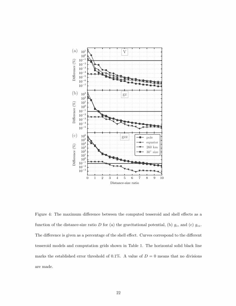
Figure 4 shows the maximum difference between the shell and tesseroid fields as a
function of D for the four experiments. The differences are given as a percentage of the shell
value. We established a maximum tolerated error of 0.1%, represented by the horizontal
solid lines in Figure 4. Only results for the gravitational potential, gz, and gzz are shown.
The results for the other diagonal components of the gravity gradient tensor are similar to
gzz. Figures for these components can be found in the supplementary material (see section
”Reproducing the analysis and results”).
For the potential V , a distance-size ratio D = 1 guarantees that the curves for all
experiments are below the 0.1% error threshold. For gz, the same is achieved with D = 1.5.
Conversely, gzz requires a value ofD = 8 to achieve an error level of 0.1%. For a computation
height of 260 km, the error curve for gzz intercepts the error threshold line at D = 2.5. This
behavior suggests that the error curves for gzz might depend on the computation height.
To test this hypothesis, we computed the error curves for gzz at heights 2, 10, 50, 150, and
20
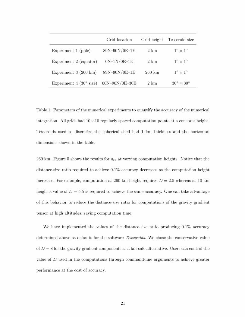
Grid location Grid height Tesseroid size
Experiment 1 (pole) 89N–90N/0E–1E 2 km 1 × 1
Experiment 2 (equator) 0N–1N/0E–1E 2 km 1 × 1
Experiment 3 (260 km) 89N–90N/0E–1E 260 km 1 × 1
Experiment 4 (30 size) 60N–90N/0E–30E 2 km 30 × 30
Table 1: Parameters of the numerical experiments to quantify the accuracy of the numerical
integration. All grids had 10×10 regularly spaced computation points at a constant height.
Tesseroids used to discretize the spherical shell had 1 km thickness and the horizontal
dimensions shown in the table.
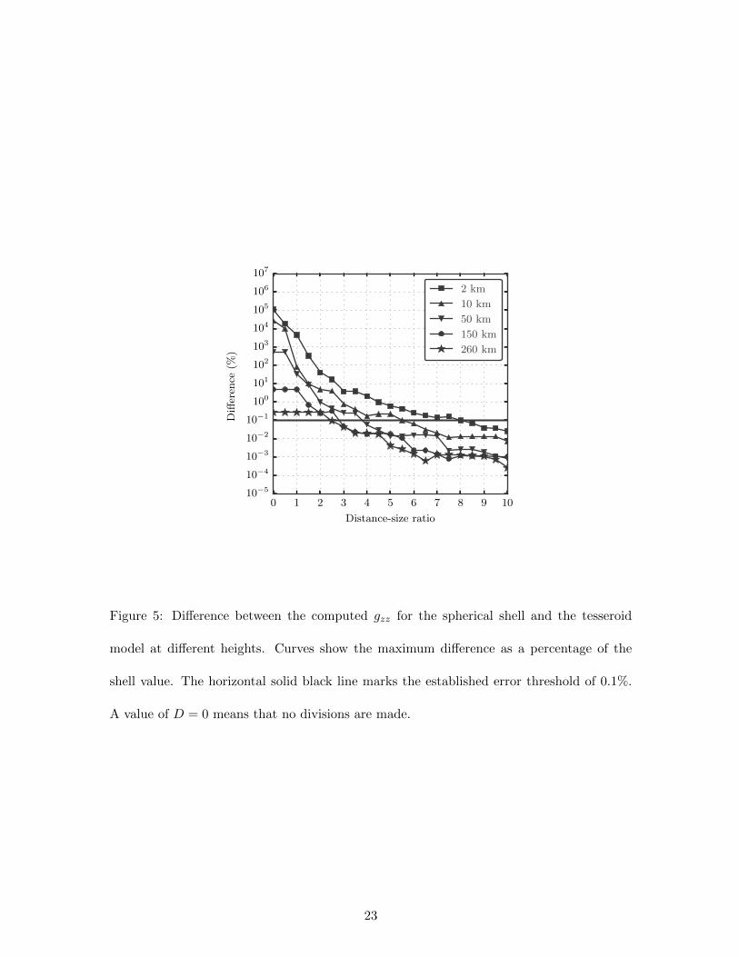
260 km. Figure 5 shows the results for gzz at varying computation heights. Notice that the
distance-size ratio required to achieve 0.1% accuracy decreases as the computation height
increases. For example, computation at 260 km height requires D = 2.5 whereas at 10 km
height a value of D = 5.5 is required to achieve the same accuracy. One can take advantage
of this behavior to reduce the distance-size ratio for computations of the gravity gradient
tensor at high altitudes, saving computation time.
We have implemented the values of the distance-size ratio producing 0.1% accuracy
determined above as defaults for the software Tesseroids. We chose the conservative value
of D = 8 for the gravity gradient components as a fail-safe alternative. Users can control the
value of D used in the computations through command-line arguments to achieve greater
performance at the cost of accuracy.
21
10−710−610−510−410−310−210−1100101
Differen
ce(%
)
(a) V
10−510−410−310−210−1100101102103
Differen
ce(%
)
(b) gz
0 1 2 3 4 5 6 7 8 9 10
Distance-size ratio
10−310−210−1100101102103104105106
Differen
ce(%
)
(c) gzz pole
equator
260 km
30 size
Figure 4: The maximum difference between the computed tesseroid and shell effects as a
function of the distance-size ratio D for (a) the gravitational potential, (b) gz, and (c) gzz.
The difference is given as a percentage of the shell effect. Curves correspond to the different
tesseroid models and computation grids shown in Table 1. The horizontal solid black line
marks the established error threshold of 0.1%. A value of D = 0 means that no divisions
are made.
22
0 1 2 3 4 5 6 7 8 9 10
Distance-size ratio
10−5
10−4
10−3
10−2
10−1
100
101
102
103
104
105
106
107
Differen
ce(%
)
2 km
10 km
50 km
150 km
260 km
Figure 5: Difference between the computed gzz for the spherical shell and the tesseroid
model at different heights. Curves show the maximum difference as a percentage of the
shell value. The horizontal solid black line marks the established error threshold of 0.1%.
A value of D = 0 means that no divisions are made.
23
CONCLUSIONS
We have presented the open-source software Tesseroids. It consists of command-line pro-
grams, written in the C programming language, to perform the forward modeling of gravita-
tional fields in spherical coordinates. The fields are calculated from a mass model composed
of spherical prisms, the so-called tesseroids. The volume integrals of the gravitational fields
of a tesseroid are solved numerically using the Gauss-Legendre Quadrature (GLQ). The
GLQ approximates the volume integrals by weighted sums of point mass effects. The error
of the GLQ integration increases as the computation point gets closer to the tesseroid. To
counter this effect, the accuracy of the GLQ integration can be increased by using more
point masses or by dividing each tesseroid into smaller ones.
We have implemented and improved upon an adaptive discretization algorithm to achieve
an optimal division of tesseroids. Tesseroids are divided into more parts closer to the com-
putation point, where more point masses are needed. Our implementation of the adaptive
discretization uses a “stack” data structure in place of the originally proposed recursive
implementation. As a rule of thumb in procedural languages (like C), stack-base imple-
mentations are computationally faster than the equivalent code using function recursion.
Furthermore, the stack-based algorithm allows more control over errors when too many
divisions are necessary. The adaptive discretization is controlled by a scalar called the
distance-size ratio (D). The algorithm ensures that all tesseroids will have dimensions
smaller than D times the distance to the computation point. The value of D indirectly
controls the accuracy of the integration as well as the computation time.
We performed an error analysis to determine the optimal value of D required to achieve
a target accuracy. We used a spherical shell as a reference to calculate the computation
24
error of our algorithm for different values of D. Our results show that the values of D
required to achieve a maximum error of 0.1% of the shell values are 1 for the gravitational
potential, 1.5 for the gravitational acceleration, and 8 for the gravity gradients. Previous
assumptions in the literature were that accurate results are guaranteed if the distance to the
tesseroid is larger than the distance between point masses. This condition was previously
applied indiscriminately to both the gravitational acceleration and the gravity gradients.
That assumption is equivalent to using D = 1.5 for all fields. Our results show that this
is valid for the gravitational acceleration and results in a 0.1% computation error. This is
expected because the original study that determined the above condition was performed on
the vertical component of gravitational acceleration. However, applying the same condition
to the gravity gradients produces an error of the order of 102%.
For the gravity gradients in particular, the distance-size ratio required for 0.1% error
decreases with height. We believe this is because the decay factor for the gravity gradient
components is d−3, whereas the discretization algorithm uses d/Li. As the computation
point becomes closer to the tesseroid, the field increases more rapidly than the algorithm
increases the amount of discretization. Hence, a higher value of D (i.e., more discretization)
is required.
The values of the distance-size ratio determined above were incorporated as defaults in
the software Tesseroids. We chose the value D = 8 for the gravity gradients as a conservative
default. If the user desires, the value of D used can be controlled by a command-line
argument.
In situations that require many tesseroid divisions, the stack used in the algorithm will
overflow and further divisions become impossible. The current implementation warns the
25
user that the overflow occurred and proceeds with the GLQ integration without division.
Future improvements to the algorithm include a better way to handle such situations as
they arise. An alternative would be to replace the tesseroid by an equivalent right rectan-
gular prism and compute its effects instead. This would allow accurate computations at
smaller distances. Furthermore, the computation time increases drastically as the compu-
tation point gets closer to the tesseroid. This effect can be prohibitive for computing the
gravity gradients at relatively low heights (e.g., for terrain corrections of ground or airborne
surveys). Further investigation of different criteria for dividing the tesseroids could yield
better performance through a reduced number of divisions.
ACKNOWLEDGMENTS
We are indebted to the developers and maintainers of the open-source software without
which this work would not have been possible. The authors thank associate editor Joe
Dellinger, reviewer Roman Pasteka, and four anonymous reviewers for their hard work and
helpful comments. The authors were supported in this research by a fellowship (VCFB) from
Conselho Nacional de Desenvolvimento Cientıfico e Tecnologico (CNPq) and a scholarship
(LU) from Coordenacao de Aperfeicoamento de Pessoal de Nıvel Superior (CAPES), Brazil.
Additional support for the authors was provided by the Brazilian agency FAPERJ (grant
E-26/103.175/2011) and by the GOCE-Italy project (ASI).
26
REFERENCES
Alvarez, O., M. Gimenez, C. Braitenberg, and A. Folguera, 2012, GOCE satellite derived
gravity and gravity gradient corrected for topographic effect in the south central andes
region: GOCE derivatives in the south central andes: Geophysical Journal International,
190, 941–959.
Asgharzadeh, M. F., R. R. B. von Frese, H. R. Kim, T. E. Leftwich, and J. W. Kim, 2007,
Spherical prism gravity effects by Gauss-legendre quadrature integration: Geophysical
Journal International, 169, 1–11.
Barrera-Figueroa, V., J. Sosa-Pedroza, and J. Lopez-Bonilla, 2006, Multiple root finder
algorithm for legendre and Chebyshev polynomials via Newton’s method: Annales Math-
ematicae et Informaticae, 3–13.
Bouman, J., J. Ebbing, and M. Fuchs, 2013a, Reference frame transformation of satellite
gravity gradients and topographic mass reduction: Journal of Geophysical Research: Solid
Earth, 118, 759–774.
Bouman, J., J. Ebbing, S. Meekes, R. Abdul Fattah, M. Fuchs, S. Gradmann, R. Haagmans,
V. Lieb, M. Schmidt, D. Dettmering, and W. Bosch, 2013b, GOCE gravity gradient
data for lithospheric modeling: International Journal of Applied Earth Observation and
Geoinformation, 35, 16–30.
Braitenberg, C., 2015, Exploration of tectonic structures with GOCE in Africa and across-
continents: International Journal of Applied Earth Observation and Geoinformation, 35,
88–95.
Braitenberg, C., P. Mariani, and A. De Min, 2013, The European alps and nearby orogenic
belts sensed by GOCE: Bollettino di Geofisica Teorica e Applicata, 54, 321–334.
Braitenberg, C., P. Mariani, J. Ebbing, and M. Sprlak, 2011, The enigmatic Chad lineament
27
revisited with global gravity and gravity-gradient fields: Geological Society, London,
Special Publications, 357, 329–341.
Fullea, J., J. Rodrıguez-Gonzalez, M. Charco, Z. Martinec, A. Negredo, and A. Villasenor,
2014, Perturbing effects of sub-lithospheric mass anomalies in GOCE gravity gradient and
other gravity data modelling: Application to the atlantic-mediterranean transition zone:
International Journal of Applied Earth Observation and Geoinformation, 35, 54–69.
Grombein, T., K. Seitz, and B. Heck, 2013, Optimized formulas for the gravitational field
of a tesseroid: Journal of Geodesy, 87, 645–660.
Heck, B., and K. Seitz, 2007, A comparison of the tesseroid, prism and point-mass ap-
proaches for mass reductions in gravity field modelling: Journal of Geodesy, 81, 121–136.
Hildebrand, F. B., 1987, Introduction to numerical analysis: Dover Publications.
Hunter, J. D., 2007, Matplotlib: A 2d graphics environment: Computing in Science &
Engineering, 9, 90–95.
Ku, C. C., 1977, A direct computation of gravity and magnetic anomalies caused by 2-and 3-
dimensional bodies of arbitrary shape and arbitrary magnetic polarization by equivalent-
point method and a simplified cubic spline: Geophysics, 42, 610–622.
LaFehr, T., 1991, An exact solution for the gravity curvature (Bullard B) correction: GEO-
PHYSICS, 56, 1179–1184.
Li, Z., T. Hao, Y. Xu, and Y. Xu, 2011, An efficient and adaptive approach for modeling
gravity effects in spherical coordinates: Journal of Applied Geophysics, 73, 221–231.
Mariani, P., C. Braitenberg, and N. Ussami, 2013, Explaining the thick crust in parana
basin, Brazil, with satellite GOCE gravity observations: Journal of South American
Earth Sciences, 45, 209–223.
McKinney, W., 2010, Data structures for statistical computing in python: Proceedings of
28
the 9th Python in Science Conference, 51 – 56.
Mikuska, J., R. Pasteka, and I. Marusiak, 2006, Estimation of distant relief effect in gravime-
try: GEOPHYSICS, 71, J59–J69.
Perez, F., and B. E. Granger, 2007, IPython: a system for interactive scientific computing:
Computing in Science and Engineering, 9, 21–29.
Ramachandran, P., and G. Varoquaux, 2011, Mayavi: 3d visualization of scientific data:
Computing in Science & Engineering, 13, 40–51.
Reguzzoni, M., D. Sampietro, and F. Sanso, 2013, Global Moho from the combination of
the CRUST2.0 model and GOCE data: Geophysical Journal International, 195, 222–237.
Uieda, L., 2015, A tesserioid (spherical prism) in a geocentric coordinate sys-
tem with a local-North-oriented coordinate system: figshare, available from:
http://dx.doi.org/10.6084/m9.figshare.1495525. (Accessed May 2016).
Wild-Pfeiffer, F., 2008, A comparison of different mass elements for use in gravity gradiom-
etry: Journal of Geodesy, 82, 637–653.
29