Universidade de Lisboa Faculdade de Ciências Departamento...
95
Universidade de Lisboa Faculdade de Ciências Departamento de Engenharia Geográfica, Geofísica e Energia Cumulus Boundary Layers in the Atmosphere: High Resolution Models and Satellite Observations João Paulo Afonso Martins Doutoramento em Ciências Geofísicas e da Geoinformação (Meteorologia) 2011
Transcript of Universidade de Lisboa Faculdade de Ciências Departamento...

Universidade de Lisboa
Faculdade de Ciências
Departamento de Engenharia Geográfica, Geofísica e Energia
Cumulus Boundary Layers in the Atmosphere: High
Resolution Models and Satellite Observations
João Paulo Afonso Martins
Doutoramento em Ciências Geofísicas e da Geoinformação
(Meteorologia)
2011

Universidade de Lisboa
Faculdade de Ciências
Departamento de Engenharia Geográfica, Geofísica e Energia
Cumulus Boundary Layers in the Atmosphere: High
Resolution Models and Satellite Observations
João Paulo Afonso Martins
Doutoramento em Ciências Geofísicas e da Geoinformação
(Meteorologia)
Tese Orientada por:
Prof. Pedro M. A. Miranda
Dr. João Teixeira
2011

i
Contents
Acknowlegements ........................................................................................................... iii
Abstract ............................................................................................................................ iv
Resumo ............................................................................................................................. v
List of acronyms and abbreviations ............................................................................... viii
List of Symbols ................................................................................................................. x
1. Introduction .................................................................................................................. 1
1.1 Motivation .............................................................................................................. 1
1.2 Thesis outlook ........................................................................................................ 2
2. PBL processes, Clouds and Climate ............................................................................. 4
2.1 The Planetary Boundary Layer ............................................................................... 4
2.2 Large Scale Tropical Circulations and Clouds ....................................................... 7
2.3 Low Stratiform clouds ............................................................................................ 8
2.4 Trade Wind Shallow Cumulus ............................................................................. 12
2.5 Deep convection ................................................................................................... 14
2.6 The GCSS/WGNE Pacific Cross-section Intercomparison (GPCI) ..................... 16
3. Evolution of cloud structures in the transition from shallow to deep convection over
land ................................................................................................................................. 23
3.1 Introduction .......................................................................................................... 24
3.2 Model and simulations ......................................................................................... 26
3.3 Evolution of mean properties ............................................................................... 28
3.4 Evolution of dominant length scales .................................................................... 33
3.5 Evolution of cloud structures ................................................................................ 36
3.6 Conclusions .......................................................................................................... 37
ii
4. Infrared Sounding of the Trade-wind Boundary Layer: AIRS and the RICO
Experiment ..................................................................................................................... 41
4.1 Introduction .......................................................................................................... 42
4.2 Data and methods ................................................................................................. 43
4.3 Results .................................................................................................................. 45
4.3.1 Thermodynamic profiles and error statistics ................................................. 45
4.3.2 Possible error sources .................................................................................... 47
4.3.3 Boundary layer height ................................................................................... 49
4.4 Conclusions .......................................................................................................... 51
5. A climatology of Planetary Boundary Layer Height over the ocean from the
Atmospheric Infrared Sounder ....................................................................................... 53
5.1 Introduction .......................................................................................................... 54
5.2 Data and Methods ................................................................................................. 56
5.3 Global PBL Heights ............................................................................................. 57
5.4 The East Pacific Cross-Section............................................................................. 65
5.4.1 Mean values and variability ........................................................................... 65
5.4.2 Sensitivity to cloud fraction ........................................................................... 67
5.5 Conclusions .......................................................................................................... 69
6. Conclusions ................................................................................................................ 72
7. References .................................................................................................................. 76

iii
Acknowlegements
I would like to thank my two advisors, Prof. Pedro Miranda and Dr. João Teixeira not
only for their scientific guidance, friendship and motivation, but also for the opportunity
of working in three fantastic teams, one at Lisbon at Instituto Dom Luiz, and the other
two in Los Angeles, California. In the first two years of this project I had the
opportunity to meet amazing people from the Department of Atmospheric and Oceanic
Sciences of the University of California at Los Angeles. In the last two years I have
spent 6 months at NASA‟s Jet Propulsion Laboratory in Pasadena where I have met
some of the smartest, funniest and competent people I have ever worked with. I will
definitely never forget the time I have spent working there. I would like to thank in
particular to those that I have met on those places who gave their support to make this
thesis a reality. From my time at UCLA, Louise, Sergio, Katy, Greg, Celestino and
Sambingo; from my time at JPL: Johannes, Jenny, Brian, Kay, Mathias, Qing, George,
Daniel, Eric, Evan, Bill and Van. The discussions we had definitely improved the
content of this work.
Of course I cannot forget home. My institute gave me all the tools, the knowledge and
the support I needed. I cannot stress enough how grateful I am to Pedro Soares for
dealing with my bad humor, successes, frustrations, distractions, (bad) jokes and
deadlines… Thank you Pedro, I really enjoyed working with you for the past 4 years
and I hope we can keep doing it for a long time. This acknowledgement has to be
evidently extended to Ricardo and Emanuel, as they had to deal with all this on a daily
basis as well for the whole course of this project. A big thanks to my other colleagues
and friends, that in one way or the other helped me reaching my goals. I would also like
to thank to the people outside the academic world, my family and friends for their
constant support, friendship and love.
I acknowledge the funding I received from the Portuguese Science Foundation (FCT),
under the doctoral grant SFRH/BD/37800/2007. I also acknowledge the funding I
received from Fundação Calouste Gulbenkian by the “Programa Gulbenkian de
Estímulo à Investigação” which helped in some of the expenses and also for funding
from the FCT projects REWRITE (PTDC/CLI/73814/2006). IDL is funded by the FCT
under the project PEST-OE/CTE/LA0019/2011/2012.

iv
Abstract
This project intends to explore some of the challenges on the representation of the
Planetary Boundary Layer (PBL) using both high resolution models and state of the art
observations. Some of the issues related the different types of boundary layers are
highlighted in the context of a model intercomparison at a transect in the northeast
Pacific that served as a benchmark for studying cloud regimes and transitions between
them. Several model biases were detected and even reanalysis products do not show
reasonable comparisons against observations in terms of low-cloud related variables.
The transition from shallow to deep convection over land is a key process in the diurnal
cycle of convection over land. High resolution simulations were analyzed the ability of
the model to reproduce observed precipitation characteristics and its sensitivity to
horizontal resolution and to the evaporation of precipitation. The latter physical process
influences the development of new convection by increasing the thermodynamic
heterogeneities at the PBL through the formation of cold pools which result from
convective downdrafts. At the later stages of the transition these features dominate the
PBL behavior, as the turbulent length scales increase up to several times the size of the
PBL height. Results are however quite sensitive to model resolution. At the
observational perspective, the Atmospheric Infrared Sounder was used to characterize
the PBL properties in a variety of situations. An algorithm for PBL height determination
was developed and validated against radiosondes launched at the Rain in Cumulus over
the Ocean campaign. The encouraging results of the validation led to the calculation of
a PBL height climatology over the tropical, subtropical and midlatitude oceans. Results
were then compared to similar estimates from collocated profiles from ERA-Interim,
revealing similar geographical distribution and seasonal variations. Diurnal variability is
much different between both datasets which warrants further investigations.

v
Resumo
A camada limite planetária (CLP) apresenta desafios tanto em termos observacionais
como em termos da sua modelação numérica. O seu papel no sistema climático traduz-
se na mediação das interacções entre a superfície e a troposfera livre, através de fluxos
turbulentos de calor, humidade , momento e outros constituintes químicos e aerossóis. A
estrutura da CLP encontra-se profundamente relacionada com as condições climatéricas
de uma dada região, em particular com tipo de nuvens predominantes. A
intercomparação de modelos realizada sobre uma secção no Pacífico nordeste pretendeu
avaliar a capacidade dos modelos de representar os diversos processos associados aos
diversos regimes de nuvens presentes na região. A secção mostrou-se indicada para este
exercício, pois além de amostrar as características principais das células de Walker e
Hadley, é também representativa das transições que ocorrem entre nuvens estratiformes
que ocorrem ao largo da costa da California, nuvens tipo cumulus pouco profundos na
região dos Alíseos e nuvens tipo cumulonimbos que ocorrem preferencialmente na Zona
Intertropical de Convergência (ITCZ). Os resultados da comparação evidenciaram as
enormes discrepâncias que existem entre modelos em termos da representação dos
processos associados às nuvens. Além dos modelos, a própria reanálise ERA-40
mostrou diferenças significativas quando comparada com observações de detecção
remota dedicadas a esses processos.
A transição de entre convecção pouco profunda para convecção profunda é o processo
que domina a fase matinal do ciclo diurno da convecção sobre terra nos trópicos, e a sua
representação na maioria dos modelos de larga escala apresenta graves deficiências,
com o pico da precipitação a ocorrer no período na manhã, enquanto as observações
mostram que o mesmo ocorre a meio da tarde. Os modelos tendem a usar um fecho para
a parameterização da convecção baseado no conceito de energia potencial disponível
para a convecção (CAPE), que activa a convecção profunda demasiado cedo, sendo que
as simulações de alta resolução têm mostrado que o processo é bastante mais gradual:
inicia-se com a formação de uma camada limite bem misturada, seguida da formação de
cumulus pouco profundos que humidificam as camadas inferiores da troposfera, para
então se dar a transição para convecção profunda. Neste projecto realizaram-se
simulações de alta resolução deste processo usando o modelo MesoNH, por forma a
estudar a capacidade do modelo de reproduzir as características da precipitação e a
sensibilidade dos resultados à resolução do modelo e à evaporação da precipitação. Este

vi
último processo físico desempenha um papel fundamental no estabelecimento da fase
madura do regime de convecção profunda. Isto porque ao evaporar, a precipitação
arrefece o ar, causando fortes correntes descendentes que ao atingir a superfície se
espraiam sob a forma de correntes gravíticas. Nos limites destas correntes, fortes
gradientes termodinâmicos forçam o ar da CLP a subir, originando novas térmicas que
eventualmente formam novas células convectivas. Nas fases finais da transição, estas
perturbações dominam o comportamento da CLP, tal como indicam os diagnósticos
espectrais das escalas de comprimento dominantes. Esta análise mostra que o tamanho
dos turbilhões na CLP varia desde a dimensão típica da altura da CLP na fase de
convecção pouco profunda até dimensões que superam várias vezes essa escala típica na
fase de convecção profunda. Esse comportamento é totalmente distinto na simulação
sem evaporação de precipitação, com os turbilhões a manterem dimensões associadas à
altura da CLP durante todo o processo. Os resultados revelam contudo uma grande
sensibilidade à resolução do modelo, com evoluções bastante distintas no alcance
vertical da convecção nas simulações com diferentes resoluções. As diferenças são
atribuidas à diferente representação dos processos turbulentos por parte do modelo de
turbulência de subescala, mas os resultados são ainda inconclusivos.
A observação da CLP por métodos de detecção remota apresenta também desafios
próprios. Neste projecto, a base de dados do Atmospheric Infrared Sounder (AIRS) V5
L2 Support Product foi usada para estimar parâmetros da camada limite. Este produto
apresenta um espaçamento de grelha vertical superior ao dos produtos AIRS
convencionais, o que o torna mais indicado para estudar a CLP. Um algoritmo para
determinação da altura da CLP foi desenvolvido e validado contra dados das sondagens
lançadas no contexto da campanha Rain in Cumulus over the Ocean, ocorrida nas
Caraíbas no Inverno de 2004-2005. Essa área é dominada nessa altura do ano por
convecção pouco profunda embebida nos ventos alíseos, o que a torna ideal para a
validação dos perfis obtidos com o AIRS, dado que o sensor utiliza radiâncias da banda
do infravermelho, fortemente atenuadas pela presença de nuvens. Os perfis utilizados
foram comparados com os das radiossondagens e revelaram a sua capacidade de ilustrar
as principais características da CLP, com margens de erro dentro do aceitável de acordo
com as características desejáveis para o instrumento. Os resultados mostraram-se
insensíveis a diversos factores como a fracção de nuvens e de píxeis terrestes no campo
de visão, radiação de longo comprimento de onda no topo da atmosfera e distância entre

vii
a radiossonda e o pixel do satélite. As alturas da CLP são determinadas a partir de perfis
de temperatura potencial e humidade relativa, a partir da localização do nível com
maiores gradientes verticais dessas propriedades. Os métodos utilizados na
determinação da altura da CLP são ainda objecto de debate e dependem da base de
dados utilizada; este foi o método escolhido por ser o mais simples, mais adequado aos
dados disponíveis e com maior aplicabilidade em diferentes regiões do globo. A
comparação entre as estimativas dos dados de satélite e das radiossondas revela erros
médios quadráticos da ordem de 50 hPa, o que mostra que o produto é capaz de
caracterizar de forma aceitável a altura da CLP.
Uma climatologia da altura da CLP foi calculada usando toda a base de dados do AIRS
(2003-2010) ao longo dos oceanos das regiões tropicais, subtropicais e das latitudes
médias. Essa climatologia foi comparada com estimativas semelhantes obtidas a partir
de perfis da reanálise ERA-Interim extraídos da localização mais próxima e da hora
mais próxima da hora de passagem do satélite. Ambas as estimativas revelaram
distribuições realísticas da altura da CLP, com valores mínimos a coincidir com as áreas
dominadas por nuvens estratiformes ao largo da costa oeste dos continentes subtropicais
e valores mais altos nas zonas dominadas por convecção profunda. As variações
sazonais são também realistas em ambos as bases de dados, com características como a
migração da ITCZ ao longo do ano e o estabelecimento das características típicas de
monções sazonais em determinadas regiões do globo. Contudo, o ciclo diurno aparece
representado nas duas bases de dados de forma bastante distinta: enquanto o AIRS
mostra variações realísticas da altura da CLP ao longo do ciclo diurno, a ERA-Interim
não apresenta variações diurnas significativas, o que indica a presença de algumas
deficiências na representação de processos de camada limite sobre o oceano nessa base
de dados. Os dados foram analisados em particular sobre a secção no Pacífico nordeste
com objectivo de explicar alguns dos desvios encontrados. Essa análise evidenciou a
tendência do instrumento para amostrar principalmente pixeis com características de céu
limpo ou com nebulosidade reduzida, pois ao aplicar amostragem condicional aos dados
ERA-Interim de modo a isolar os perfis característicos de baixas coberturas nebulosas,
mostra-se que existe uma correspondência bastante melhor entre as duas bases de dados.
Neste trabalho mostra-se que tanto modelos como observações da CLP sofrem dos seus
problemas e que avanços significativos no conhecimento desta camada tão importante
da atmosfera só podem ser atingidos combinando eficazmente ambas as estratégias.

viii
List of acronyms and abbreviations
AIRS Atmospheric InfraRed Sounder
BOMEX Barbados Oceanographic and Meteorological Experiment
CALIOP Cloud-Aerosol Lidar with Orthogonal Polarization
CAM Community Atmosphere Model
CAPE Convective Available Potential Energy (m2s
-2)
CBL Convective Boundary Layer
CIN Convective Inhibition
CMIP Coupled Model Intercomparison Project
CONTROL Control Experiment (chapter 3)
CPR Cloud Profiling Radar
CRM Cloud Resolving Model
DJF December-January-February
ECMWF European Centre for Medium-Range Weather Forecasts
CLP Camada Limite Planetária
EDMF Eddy-Diffusivity/Mass-Flux
EIS Estimated Inversion Strength (K)
EPIC East Pacific Investigation of Climate
ERA-40 ECMWF 40-year reanalysis
ERA-I ECMWF Interim reanalysis
EUMETSAT European Organization for the Exploitation of Meteorological
Satellites
EUROCS European Union Project on Cloud Systems
GCM Global Circulation Model
GCSS GEWEX Cloud System Studies
GEWEX Global Energy and Water Cycle Experiment
GFDL Geophysical Fluid Dynamics Laboratory
GMAO Global Modeling and Assimilation Office
GPCI GCSS Pacific Cross-Section Intercomparison
GPS RO Global Positioning System Radio Occultation
IASI Infrared Atmospheric Sounding Interferometer
IPCC Intergovernmental Panel on Climate Change
ISCCP International Satellite Cloud Climatology Project
ITCZ Inter-Tropical Convergence Zone
JJA June-July-August
JPL Jet Propulsion Laboratory
L2 Level 2
LBA Large-Scale Biosphere-Atmosphere Experiment in Amazonia
LCL Lifting Condensation Level (m)
LES Large Eddy Simulation
LFC Level of Free Convection (m)
LOWRES Low resolution simulation (chapter 3)
LT Local Time

ix
LTS Low Tropospheric Stability (K)
MAM March-April-May
MesoNH Mesoscale No-Hydrostatic Model
MISR Multi-angle Imaging SpectroRadiometer
MODIS Moderate Resolution Imaging Spectroradiometer
NASA National Aeronautics and Space Administration
NCAR G&M NCAR Global Forecast System and Modular Ocean Model
NCAR National Centers for Atmospheric Research
NCEP National Centers for Environmental Prediction
NOEVAP Simulation with evaporation of precipitation turned off (chapter 3)
NSF National Science Foundation
NWP Numerical Weather Prediction
OLR Outgoing Longwave Radiation
OpenMPI Open Source Message Passing Interface
PBL Planetary Boundary Layer
PDF Probability Distribution Function
RH Relative Humidity
RICO Rain in Cumulus over the Ocean
RMSE Root Mean Square Error
SBL Stable Boundary Layer
SCM Single Column Model
SON September-October-November
SSM/I Special Sensor Microwave Imager
SST Sea Surface Temperature (K)
TCC Total Cloud Cover
TKE Turbulent Kinetic Energy (m2 s
-2)
TRMM Tropical Rainfall Measurement Mission
UCLA University of California at Los Angeles
UTC Coordinated Universal Time
V5 Version 5
VAMOS Variability of the American Monsoon Systems
VOCALS VAMOS Ocean-Cloud-Atmosphere-Land Study
VOCALS-Rex VOCALS Regional Experiment
WGNE Working Group on Numerical Experimentation
WMO World Meteorological Organization
WRF Weather Research and Forecast

x
List of Symbols
b Slope of the linear regression line
CF Cloud Fraction
CAPE Convective Available Potential Energy (m2
s-2
)
CIN Convective Inhibition (m2
s-2
)
Cloud Length Scale (m)
Estimated Inversion Strength (K)
Wavenumber. Radial component of the wavenumber in a
cylindrical coordinate system (m-1
)
Wavenumber along the -axis (m-1
)
Wavenumber along the -axis (m-1
)
Nyquist wavenumber (m-1
)
Lifting Condensation Level (m)
LF Land Fraction
Low Tropospheric Stability (K)
Number of cloudy grid points
OLR Outgoing Longwave Radiation (W m-2
)
Specific humidity (kg kg-1
)
Coefficient of determination
RH Relative Humidity (%)
Spectral density of variable
Temperature (K)
TCC Total Cloud Cover
TKE Turbulent Kinetic Energy (m2 s
-2)
w Vertical velocity (m s-1
)
Height (m)
PBL height (m)
Height of the 700 hPa pressure level (m)
Tangential wavenumber in a cylindrical coordinate system (m-1
)
Model resolution along the -axis (m)
Model resolution along the -axis (m)
Lapse rate at the 700 hPa pressure level (K m-1
)

xi
Lapse rate of the decoupled layer (K m-1
)
Free tropospheric lapse rate (K m-1
)
Dominant length scale of variable
Generic 3D variable
Variance
Shallow convection adjustment time scale (s)
Potential Temperature (K)
Potential Temperature at the 700 hPa level (K)
Potential Temperature at the surface (K)
Virtual potential temperature (K)
1
1. Introduction
1.1 Motivation
The Planetary Boundary Layer (PBL) is a key component of the Climate System and its
effects must be represented in a satisfactory way in numerical weather forecast and
climate models. The PBL has rather unique characteristics: it is relatively shallow, it is
characterized by large spatial and temporal variability, and the processes that govern its
behavior depend on strong interactions with many features of the models such as
radiation, surface, microphysics and also large scale dynamics.
The goal of this project was to improve the understanding of cloudy PBLs, through the
use of model and observational techniques. The GPCI (GCSS Pacific Cross-section
Intercomparison) initiative (Teixeira et al 2011), organized to assess the quality of
Global Circulation Models (GCMs) in the representation of ocean tropical convection,
highlighted a number of difficulties in the representation of cloud processes in large
scale models, with an emphasis on processes governing the transition from shallow to
deep convection regimes. Other intercomparison exercises (Bechtold et al., 2004;
Guichard et al., 2004), looking at the representation of tropical convection over land,
also found relevant discrepancies in the behavior of numerical models with systematic
biases in essential and well-established characteristics of the precipitation fields, also
most probably related with the transition into deep convection. However, at the other
end of the modeling spectrum, numerical experiments with high-resolution cloud-
resolving and large eddy simulation models (Grabowski et al., 2006; Khairoutdinov and
Randall, 2006), have been able to reproduce the main features of deep convection,
although with large spread of results.
High resolution cloud resolving models are very expensive, but they are able to resolve
larger turbulent eddies, while still relying on subgrid scale parameterization schemes to
represent unresolved turbulence. In these models, the effects of resolved turbulence can
be explicitly diagnosed and used in the development of subgrid-scale parameterization
schemes in larger scale models. Such approach is used in the present study, with a set of
simulations of deep convection over land, with a state-of-the-art model.

2
An understanding of the processes governing the cloudy PBL is not possible without a
joint use of modeling and observational techniques. At the global scale, and especially
over the oceans, satellite remote sensing provides the major source of information. A
new set of sensors, and new way of operating multiple platforms with cooperative
sensors, has been offered as a way to get a new tridimensional view of the Earth.
Infrared Sounders like AIRS (Atmospheric InfraRed Sounder, onboard NASA‟s Aqua
platform) and IASI (Infrared Atmospheric Sounding Interferometer, onboard
EUMETSAT‟s MetOp platform) produce continuous, global and three dimensional
datasets of temperature, water vapor mixing ratio and other constituents. A new, high
vertical resolution, version of the AIRS product is here used to verify the ability of this
instrument to represent the structure and variability of oceanic boundary layers. A
validation of results against in-situ data from the RICO field experiment, in the
Caribbean, is produced, followed by a global climatology of the oceanic PBL.
1.2 Thesis outlook
This thesis is organized in six main chapters (plus introduction and conclusions), which
reflect the lines of research that were pursued during the course of this work. Chapter 2
introduces basic concepts and addresses some of the issues that remain unsolved in the
general problem of representing the PBL and its interaction with shallow and deep
convection in numerical weather and climate models. The general problem of the
transition from shallow stratocumulus to trade wind cumulus and to deep cumulus in the
tropical oceans is discussed. There is a brief reference to the paper from Teixeira et al.
(2011) published in Journal of Climate. The paper analyzes the transition using a
variety of information coming not only from remote sensing platforms but also global
reanalysis and models that participated in a model intercomparison project.
Chapter 3 describes a set of Large Eddy Simulations (LES) of the transition from
shallow to deep convection over land. This important mechanism is not well resolved in
the majority of current state-of-the-art numerical weather prediction (NWP) models,
mainly due to the interactions between different scales of turbulence and convection that
has proven difficult to model. This motivated the development of a technique for
studying the evolution of the dominant length scales throughout the transition. The
results show the importance of the turbulent small scales in the initial stage of the

3
process and of the larger convective/mesoscale features such as deep convective
structures, convection organization and cold pools towards the later stages.
In Chapter 4 an extended version of the study that was published in Geophysical
Research Letters is presented, in which a comparison of a high-vertical resolution
version of the AIRS dataset against a set of radiosondes launched during the Rain in
Cumulus over the Ocean (RICO) campaign was performed. Due to the compact format
of the submitted paper, some of the results were omitted therein, and they are presented
here. The quality of the support product of the AIRS dataset is assessed and it is shown
that this product presents characteristics that are within the pre-launch requirements of
the instrument. A methodology for the determination of the PBL height is developed
and applied to both AIRS and RICO sondes and it is shown that AIRS has the potential
to provide useful PBL height information.
A global climatology of PBL height is presented and compared to ERA-Interim
estimates in Chapter 5. This is the best comparison that can be made, due to the global
nature of the used datasets and the limited capacity of launching radiosondes in the open
ocean. This reanalysis is arguably the best source of global data, as it assimilates data
from a huge variety of sources and combines them with a state of the art model first
guess. It is shown that there is some sensitivity to the PBL height determination method
that is used, and also to the cloud regime that dominates each region. PBL height is a
variable that is planned for public release in the upcoming new version of the retrieval
algorithm for AIRS products.
The main conclusions and future lines of work are presented in the last chapter.

4
2. PBL processes, Clouds and Climate
Note: Parts of the text included in section 2.6 are taken from Teixeira et al. (2011),
published in Journal of Climate. The author of the present thesis is a co-author of that
manuscript. Only the main results (with focus on those of which the author was directly
involved) are presented here. For further information, the reader may want to consult
the paper itself.
2.1 The Planetary Boundary Layer
The Planetary Boundary Layer (PBL) may be defined as the part of the troposphere that
is directly influenced by the presence of the Earth‟s surface, and responds to surface
forcings with a timescale of about an hour or less (Stull, 1988). At the same time, this
atmospheric layer mediates the exchanges of energy, momentum, water, other chemical
constituents and aerosol between the surface (land, water and ice) and the free
troposphere aloft. Its thickness ranges from a few tenths of meters to a few kilometers,
varying considerably in space and time. The PBL top is generally marked by strong
gradients in the thermodynamic properties, allowing its identification in radiosonde
temperature and humidity profiles. The most noticeable feature is the presence of a
relatively thin layer where temperature increases with height: the PBL top inversion.
Knowledge of PBL processes is important not only for meteorology but also for areas
such as air quality monitoring, wind energy planning, agrometeorology, aviation and
climate modeling, as the intensity of turbulence affects the way the air is mixed at the
lower levels of the atmosphere. Pollutants and aerosols are dispersed quicker if there are
many wind gusts; wind farms have to be planned to resist a certain expected level of
turbulence; environmental studies for airport construction take into account expected
turbulent structures that may be hazardous for air traffic. In short, it is the atmospheric
layer that affects human lives the most.
Apart from this range of applications, PBL processes influence the atmospheric
circulation in many different ways. Air masses originate as PBLs that form over
different surfaces and conserve their thermodynamic properties as they travel to a
different geographical setting. When neighboring air masses “collide”, they cause
baroclinicity that is responsible for the formation of extra-tropical cyclones that affect
5
the weather in mid-latitudes. The presence of a statically stable capping temperature
inversion (at the PBL top) not only traps heat and moisture in the PBL, which may fuel
convective clouds, but also may inhibit the formation of thunderstorm clouds allowing
for the buildup of Convective Available Potential Energy (CAPE) in the free
atmosphere. The dissipation of kinetic energy in the PBL slows down large scale
weather systems. Surface heterogeneities also cause important PBL circulations such as
sea and mountain breezes or at a larger scale, monsoon systems.
The PBL structure is strongly affected by static stability. Stable PBLs often form over
relatively cold surfaces that absorb heat from the atmosphere, making the PBL air
colder than the air aloft. These occur frequently at night time, over land and whenever
there is a very cold surface, such as ice or snow. Usually they are not associated with
any specific cloud type, although fog may form due to the radiative cooling close to the
surface. Dry/shallow cumulus boundary layers often form by heating from the ground
and are associated to organized thermals that may be topped by fair weather cumulus
clouds if the thermal reaches the Lifting Condensation Level (LCL). They are
associated to the presence of an unstable surface layer, where potential temperature ( )
decreases with height. Stratocumulus boundary layers generally have neutral stability,
and form over humid and relatively colder environments, such as the eastern parts of the
subtropical oceans. Stratocumulus clouds help maintaining their structure as the
evaporative cooling at the cloud top forces convection from upside down.
The main focus of this thesis is on convective PBLs. The typical convective PBL is
formed by eddies of many different sizes, ranging from the microscale to those of the
size of the PBL, but some structures may even have larger horizontal scales (e.g. cold
pools – see chapter 3). The interaction of these different scales has been a major
challenge to the numerical modeling community. On one hand, small scale eddies are
reasonably represented as diffusion processes. However, the convective organized
structures, when present, provide an alternative and efficient way of mixing the
thermodynamic properties of the PBL, and they are usually modeled with mass-flux
approaches. A recent concept was proposed to describe the mixing induced by the
variety of eddies that form convective PBLs: the Eddy-Diffusivity/Mass-Flux approach
(Soares et al., 2004; Siebesma et al., 2007; Rio and Hourdin, 2008; Neggers et al., 2009;
Köhler et al., 2011; Witek et al., 2011). This theory divides the turbulent fluxes in the
PBL in two parts: 1) the local transport, which is modeled using the aforementioned

6
diffusion theory, and 2) the non-local (convective) transport, done by the organized
eddies (updrafts and downdrafts) which is represented using the mass-flux approach,
typical of convection schemes. The improvements this theory has allowed in NWP
show that the description of the different turbulent scales is a key issue to successfully
describe the PBL.
One of the emerging issues in climate modeling is the understanding of the feedbacks
between low clouds and climate, which have recently been recognized as the main
source of uncertainty in climate sensitivity studies (Bony and Dufresne, 2005; Wyant et
al., 2006). Figure 1 shows the diversity of responses across different models to 4 types
of forced climate runs: a SST spatially uniform increase of 2K, a decrease of 2K, a
spatially and monthly varying SST perturbation (ΔCMIP), and a perturbed case with
doubled CO2 concentrations.
Figure 1 – Changes in two key PBL cloud variables (cloud fraction and total water path), normalized by the
tropical mean surface change for each perturbation types (see legend). Data from three major US climate
models: CAM 3.0, GFDL 2.12b and GMAO (version NSIPP-2). From (Wyant et al., 2006).
Results from that intercomparison show distinct model responses to the same
perturbations: while the Community Atmosphere Model (CAM; Collins et al., 2004)
gets more low clouds with more water content in a warmer climate, the same is not true
for the Geophysical Fluid Dynamics Laboratory model (GFDL; Andersson and team,
2004) or for the NASA Global Modeling and Assimilation Office (GMAO) NSIPP-2
model (Bacmeister et al., 2006), which curiously show a decrease in clouds both for
negative and positive SST perturbations. This is a critical feedback mechanism, as low
clouds affect the overall climate state through their interactions with radiation,
precipitation and surface properties.
Teixeira et al. (2008) a number of unresolved issues regarding the representation of PBL
processes in climate models: 1) The need to better represent the sub-grid vertical
turbulent fluxes; 2) The need to better represent cloud fraction and cloud water content;
7
3) The need to solve the equations that model these processes in a computationally
efficient way; and 4) The need to parameterize different boundary layers using unified
schemes, such as EDMF. These authors also stress some of the particular processes that
still require some improvement in their representation, such as boundary layer clouds
(not only in the oceanic subtropics but also in polar and continental regions), stable
boundary layers, interaction with ocean and land surfaces, as well as with deep
convection. Some of these issues will be tackled in the remaining of this work.
2.2 Large Scale Tropical Circulations and Clouds
Oceanic tropical large scale circulations are often idealized as a combination of the
effects of the Walker and Hadley circulation cells. The first controls the mechanisms
that regulate the trade wind belts and is mainly caused by the large scale pressure
gradient between the Western and Eastern parts of the Equatorial oceans, as well as by
the large differential land-sea heating contrasts. In the low pressure areas, such as the
Pacific Warm Pool, warmer SSTs cause atmospheric instability and frequent and strong
deep convection occurs. The latent heat release fuels the upper level westerlies, which
upon cooling will subside in the opposite side of the oceanic basin (e.g. the eastern
Pacific). The circulation is closed by the surface Easterlies (the Trades), that are forced
by the zonal pressure gradient. Variations in the strength of this large scale circulation
cell are the cause of the El Niño/Southern Oscillation phenomenon, which affects the
climate at a truly global scale, changing weather patterns everywhere, with stronger
impacts in the tropical belt itself.
The Hadley cell is a meridional circulation which is also fueled by deep convection at
the ITCZ, and pumps air towards the polar regions through the upper troposphere.
Heavy precipitation at the ITCZ will make the air relatively warm and dry. This air will
subside in the subtropics, causing the prevalent high pressure centers that characterize
those latitudes. The circulation is closed near the surface by the trade winds.
The joint effect of these two similar mechanisms creates regions with very different
climatic characteristics, with particular emphasis on the predominant cloud types.
Stevens (2005) discussed the variety of moist convection regimes that dominate the
tropical and subtropical oceans. Figure 2 shows an idealized view of what happens in
the North Pacific Ocean, which may easily be translated to what happens in the other
oceanic basins. There are three main convection regimes in this region: Stratiform

8
Convection, Shallow Cumulus Convection and Deep Cumulus Convection. They occur
in each region for different reasons. Near the Equator, convergence, higher SSTs and
strong static instability favor deep convection. In the subtropical eastern oceans,
relatively strong subsidence induces high static stability and lowers the PBL. In
between, intermediate environmental conditions (mainly SST and large-scale
subsidence) lead to the formation of shallow cumulus. These form in response to
increasing SSTs towards the Equator, which helps increasing turbulent transport at the
PBL that progressively deepens. Due to the presence of the temperature inversion
caused by the subsiding air, these clouds are confined to the PBL, but they are
extremely important in maintaining the overall circulation, as discussed in some detail
in section 2.4.
Figure 2 – Idealized picture of the location of predominant cloud regimes across the Hadley/Walker
circulation. Dashed lines denote the PBL top. (from Stevens, 2005).
2.3 Low Stratiform clouds
In the eastern borders of the subtropical oceans, coastal upwelling occurs due to the
action of the anticyclonic highs and land-sea circulations. Colder SSTs help keeping the
PBL very shallow and moist. At its top, saturation occurs over wide areas, and large
Stratocumulus decks form. Convection is then maintained from the top, through
evaporative cooling at the cloud top, which further enhances mixing across the PBL. A
strong temperature inversion usually caps the PBL (i.e. a very stable layer where
temperature increases with height). It forms at the interface between the relatively dry
and warm (in terms of potential temperature) air from the subsiding free troposphere
and the moist and relatively cold air from the PBL.
9
The presence of large stratiform low cloud decks has been shown to be strongly
correlated to Low Tropospheric Stability (LTS) (Slingo, 1987; Klein and Hartmann,
1993; Wood and Hartmann, 2006), which is usually defined as the difference of the
potential temperature at 700 hPa and the surface:
(1)
The 700 hPa level is chosen because it corresponds to the pressure at which an inversion
is usually found as the air flows to the Equator from the subtropics. This bulk measure
of the inversion strength has been used in different parameterization schemes for low
level clouds, as high values of this parameter are usually associated to higher low cloud
fractions. A recent work by Wood and Bretherton (2006) proposes an alternative
measure that relates low cloud fraction to a more refined estimate of the inversion
strength, which they termed Estimated Inversion Strength (EIS). This new estimate
depends not only on the bulk LTS but it takes into account the detailed vertical structure
of the lower tropospheric potential temperature profile (Figure 3).
The inversion at the PBL top is located a certain height with a strength , which
normally ranges from 1-10 K. The PBL may be vertically well mixed or decoupled into
multiple turbulent layers. This decoupling is usually modeled using a bulk scheme that
breaks the PBL into a surface mixed layer, that extends from the surface up to the LCL
and has constant ; and a decoupled layer that extends from the LCL up to the inversion
level, where increases linearly with height at a rate . Above the inversion (in the
free troposphere), also increases linearly with height, at a rate . It is
straightforward to relate the inversion strength to the LTS and these lapse rates:
( ) ( ) ( ) (2)
where is the height of the 700 hPa pressure level. This would perfectly correlate
with the LTS (the first term on the rhs), provided that all the other terms are constant.
However, it can be shown that they actually vary as a function of . In the Tropics
the temperature profile is close to a moist adiabat, which is supported by the idea that
due to the relatively weak Coriolis force, large horizontal temperature gradients are very
unlikely (Wood and Bretherton, 2006), so the temperature profile is largely determined
by the regions of deep convection at the ITCZ. Moreover, it was shown that is
positively correlated to , which shows that the LTS alone cannot be the only

10
responsible for . On the other hand, the decoupled layer also shows some degree of
dependency on surface properties, as its temperature profile is usually is approximated
by the shape of moist adiabat that crosses the LCL (which may be determined as a
function of surface properties alone). If it is assumed that the decoupled layer is usually
much shallower than the free tropospheric layer below 700 hPa, and that , the
EIS may then be computed as:
( ) (3)
The latter relationship holds not only in tropical and subtropical regions (which were
already satisfactorily explained by the LTS relationship) but also at the midlatitudes, as
shown in Figure 4. Regions marked with “At” (North Atlantic) and “Pa” (North
Pacific), collapse into the regression line using EIS which did not happen with the LTS
relationship, that only holds in tropical and subtropical regions.
Figure 3 – Typical vertical structure of the potential temperature profile in a situation of undisturbed flow
with moderate tropospheric subsidence. The gray lines are moist adiabats. From (Wood and Bretherton,
2006).
Global remote sensing observations of these parameters are possible using multi-sensor
approaches, such as the one proposed by Yue et al. (2011). They used thirteen months
of observations of temperature and water vapor from the Atmospheric InfraRed Sounder
(AIRS) onboard Aqua, cloud profiles from the Cloud Profiling Radar (CPR) onboard

11
Cloudsat and Cloud-Aerosol Lidar with Orthogonal Polarization (CALIOP) onboard
CALIPSO, which are part of NASA‟s A-Train (Stephens et al., 2002), a constellation of
polar-orbiting satellites with orbits minutes apart from each other that provide
complementary views of the same ground scene. These datasets were collocated with
European Center for Medium-Range Forecasts (ECMWF) model analysis (non-
collocated National Centers for Environmental Prediction (NCEP) National Centers for
Atmospheric Research (NCAR) reanalysis data was also used for comparison). The
authors focused on the characterization of stratocumulus decks, namely in the global
estimation of parameters such as LTS and EIS. As expected, higher values of EIS are
related to the presence of low clouds, as diagnosed by CloudSat. The comparison
between both reanalyses revealed large discrepancies that were attributed to differences
in model physics as well as to different temporal and spatial sampling. The use of
CALIOP allowed the confirmation of the results shown in Figure 4 (on which a linear
relationship between LTS/EIS and cloud fraction is derived), using global remote
sensing data, and not only surface based cloud observations, as done by Wood and
Bretherton (2006).
Figure 4 – Relationship between Low Cloud Fraction a) LTS and b) EIS using data from regions where low
stratiform clouds are predominant according to Klein and Hartmann (1993). See text for details. From Wood
and Bretherton (2006).
The structure of the stratiform cloud decks is not homogeneous, as shown by the results
from VOCALS-Rex (Bretherton et al., 2010). In the particular case of the Peruvian
stratus deck, the clouds tend to be shallower close to land and the air above the
inversion tends to be more humid, an effect of the ventilation caused by mountain
breezes originating in the Andes. Offshore, the PBL is usually deeper and decoupled
(e.g. Zuidema et al., 2009) and drizzle often occurs. The horizontal structure is also
characterized by the presence of pockets of open cells. The transition between these two
regimes is not well understood. Some studies suggest that LTS alone is not a suitable

12
indicator of the presence of low clouds out of the core of the stratocumulus regions, near
the transition to the shallow cumulus region. Instead, cold advection seems to be more
important (Klein, 1997), which suggests that the local cloud amount may be determined
by the upstream conditions. This conclusion is supported by Pincus et al. (1997) who
used satellite data to demonstrate the existence of significant correlations between
images separated up to 24h in different locations of the Lagrangian trajectory the clouds
perform on their way towards the tropics. The way these clouds later evolve to shallow
cumuli is still a matter of debate. The traditional explanations rely on the fact that the
LTS is reduced as SST increases, increasing turbulence and favoring the cloud top
instability, which favors entrainment of free tropospheric air into the PBL, breaking the
cloud decks.
2.4 Trade Wind Shallow Cumulus
Shallow cumulus may form everywhere on Earth, and are particularly common over the
ocean, and over land in fair weather conditions. The trade wind belts are areas where
this type of convection is favored due to their light subsidence rates and warm SSTs
(when compared to the SSTs in the stratocumulus regions). Their importance in
maintaining the overall tropical circulation has been recognized for a long time (e.g.
Riehl et al., 1951). In these regions, a temperature inversion caps the PBL and inhibits
further vertical development of the PBL clouds. It is generally weaker than the
inversions found over stratocumulus decks.
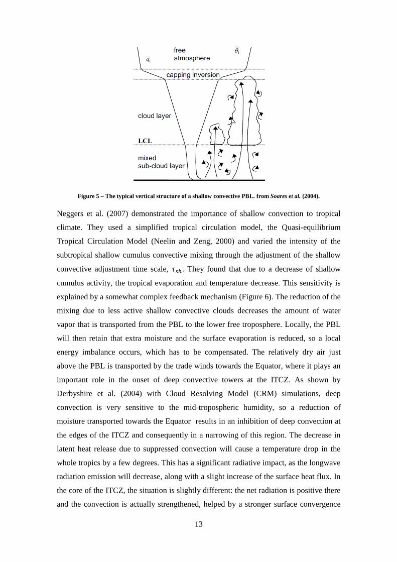
The typical structure of the PBL under shallow convection is depicted in Figure 5. The
region closer to the ground is slightly unstable due to the underlying warming, favoring
vertical updrafts. Some of them are strong enough to reach the LCL and form a cloud.
Clouds usually occupy less than 10% of the horizontal area. The traditional view of the
vertical transport in a shallow cumulus cloud layer employs the notion that there cloudy
updrafts that occupy a relatively small area which are compensated by a slowly
subsiding environment. There are recent studies using LES that show that a large part of
the downward vertical transport is actually done by narrow subsiding shells around the
cumulus clouds, that form when cloudy air detrains from the cloud and evaporates,
becoming negatively buoyant (Heus and Jonker, 2008; Jonker et al., 2008). At the top of
the turbulent layer, there is an inversion which may extend up to a few hundred meters
above the cloud top.
13
Figure 5 – The typical vertical structure of a shallow convective PBL. from Soares et al. (2004).
Neggers et al. (2007) demonstrated the importance of shallow convection to tropical
climate. They used a simplified tropical circulation model, the Quasi-equilibrium
Tropical Circulation Model (Neelin and Zeng, 2000) and varied the intensity of the
subtropical shallow cumulus convective mixing through the adjustment of the shallow
convective adjustment time scale, . They found that due to a decrease of shallow
cumulus activity, the tropical evaporation and temperature decrease. This sensitivity is
explained by a somewhat complex feedback mechanism (Figure 6). The reduction of the
mixing due to less active shallow convective clouds decreases the amount of water
vapor that is transported from the PBL to the lower free troposphere. Locally, the PBL
will then retain that extra moisture and the surface evaporation is reduced, so a local
energy imbalance occurs, which has to be compensated. The relatively dry air just
above the PBL is transported by the trade winds towards the Equator, where it plays an
important role in the onset of deep convective towers at the ITCZ. As shown by
Derbyshire et al. (2004) with Cloud Resolving Model (CRM) simulations, deep
convection is very sensitive to the mid-tropospheric humidity, so a reduction of
moisture transported towards the Equator results in an inhibition of deep convection at
the edges of the ITCZ and consequently in a narrowing of this region. The decrease in
latent heat release due to suppressed convection will cause a temperature drop in the
whole tropics by a few degrees. This has a significant radiative impact, as the longwave
radiation emission will decrease, along with a slight increase of the surface heat flux. In
the core of the ITCZ, the situation is slightly different: the net radiation is positive there
and the convection is actually strengthened, helped by a stronger surface convergence

14
(associated to the equatorial convergence of the trade wind belts), increasing
precipitation and surface evaporation.
Figure 6 – Illustration of the mechanisms leading to the sensitivity of the strength of the tropical general
circulation to the evaporation caused by trade wind shallow cumulus. From Neggers et al. (2007).
2.5 Deep convection
Near the Equator, the Sun zenithal angle is minimum, so the amount of direct radiation
that reaches the top of the atmosphere is greater there than in any other region in the
planet. The impacts of the solar radiation on the atmosphere are indirect and depend on
the surface characteristics. Ocean areas store heat more efficiently than land areas, not
only due to the larger heat capacity of water, when compared to heat capacities of land
surfaces, but also due to the mixing on the oceanic boundary layer. The surface re-emits
the energy it receives from the Sun in the form of surface turbulent fluxes of heat and
moisture. The partition between both is different depending on surface type and affects
the way convection develops during the diurnal cycle.
The ocean areas where deep convection occurs are characterized by high SSTs
(generally warmer than 27-28ºC), convergent surface winds and high relative humidity
(e.g. Bretherton et al., 2004; Derbyshire et al., 2004). The atmosphere in these regions is
also characterized by high values of CAPE (Riemann-Campe et al., 2009). This concept
has been used as a closure for the majority of the cumulus convection parameterization
schemes (e.g., Arakawa, 2004 and references therin). It is defined as the vertical integral
15
of the positive departure of the temperature profile with respect to the temperature
profile that a rising air parcel would have if it was lifted through a moist adiabatic
process from the surface (Emanuel, 1994). Deep convection occurs as PBL air parcels
become able to overcome the Convective Inhibition (CIN) – the amount of energy
needed by an air parcel to reach the Level of Free Convection (LFC), i.e. the height
where the temperature of the moist adiabatic process becomes greater than the
environmental profile. Only a few plumes have enough energy to overcome this layer,
so the more turbulence there is in the PBL, the more turbulent plumes are likely to
become deep cumulus clouds. The local effects of deep convection are twofold: it dries
and warms the atmosphere where it occurs. The drying happens more intensely below
the freezing level (at about 5km), whereas the warming occurs at upper levels. This is
consistent with the co-existence of two modes of convection in these areas: shallow
non-precipitating and deep precipitating. In fact, convective towers tend to self-organize
in cloud clusters and sometimes into rather large mesoscale convective systems. The
surroundings of these systems are usually characterized by the presence of shallow
cumuli (that may later develop into congestus) or regions of stratiform clouds - which
may also produce large amounts of precipitation, or even no clouds at all, such as in the
case of what happens in the cold pools produced by the evaporation of precipitation
from the convective towers (Khairoutdinov and Randall, 2006). Precipitation comes
from these deep convective clouds, but also from the stratiform regions in equal parts,
despite the fact that the intensity of individual showers is much larger (by a factor of
four or greater; Schumacher and Houze, 2003).
Nesbitt and Zipser (2003) discussed some of the differences of the deep convection
diurnal cycle over land and over the ocean. Its amplitude is much larger over land
surfaces, with maximum rainfall in the afternoon due to stronger solar irradiation and
boundary layer destabilization. There are certain regions where local convection is
reinforced by sea-breeze and complex terrain circulations or even by the occurrence of
mesoscale convective systems, leading to maximum rainfall a few hours later during the
night. Over the oceans, there are a few studies pointing to the strong influence of remote
forcing from nearby land regions through gravity waves or coastline effects (Rahn and
Garreaud, 2010). In regions that are not close enough to land masses, there is some
degree of debate on the causes of the observed diurnal cycle. Possible mechanisms
include 1) the differential radiative heating between convective and the surrounding
16
cloud-free region producing a daily variation in the horizontal divergence field that
modulates convection; 2) the minimum in the morning precipitation may be related to
the absorption of shortwave radiation by the upper portions of the cloud anvils, which
increases static stability and inhibits vertical motions; conversely, in the night longwave
cooling in clouds decreases stability and increases the strength of the convection; 3) the
increase in relative humidity at night due to longwave cooling reduces the effects of
entrainment and enhances cloud development; 4) more complex and debatable
mechanisms such as the occurrence of a maximum in ocean skin temperature in late
afternoon, consequent enhanced convection during the night and reduction in the
morning due to depletion of moist static energy in the wakes produced by convection
and shading of the ocean by deeper clouds. These mechanisms may act altogether, since
it is very difficult to isolate their individual action in currently available datasets
(Nesbitt and Zipser, 2003). The representation of the diurnal cycle of deep convection
has been a major challenge in the numerical weather prediction and climate modeling
communities and will be further discussed in chapter 3.
2.6 The GCSS/WGNE Pacific Cross-section Intercomparison
(GPCI)
The need to better understand the physics and dynamics of clouds and to improve the
parameterizations of clouds and cloud-related processes in weather and climate
prediction models led to the creation of the Global Energy and Water Cycle Experiment
(GEWEX) Cloud Systems Study (GCSS) in the early 1990s (Browning et al. 1993;
Randall et al. 2003). Research efforts in GCSS have been divided into different cloud
types: boundary layer clouds, cirrus, frontal clouds, deep convection, and polar clouds.
The GCSS community has extensively used LES and CRMs to assess those models‟
ability to describe clouds, through the development and evaluation of parameterizations
for single column models (SCM), which are one-dimensional versions of weather and
climate prediction models.
The traditional GCSS strategy can be divided in the following steps: (i) create a case
study using observations; (ii) evaluate CRM/LES models for the case study; (iii) use
SCMs to evaluate the parameterizations; and (iv) use the statistics from CRM/LES to
develop and improve parameterizations. This strategy has been quite successful in
improving CRM/LES models, in helping to define and understand fundamental cloud

17
regimes (e.g. Bretherton et al., 1999; Bechtold et al., 2000; Redelsperger et al., 2000;
Duynkerke and Teixeira, 2001; Stevens et al., 2001; Randall et al., 2003) and in
developing new parameterizations for clouds and the cloudy boundary layer (e.g.
Cuijpers and Bechtold, 1995; Lock et al., 2000; Golaz et al., 2002; Teixeira and Hogan,
2002; Cheinet and Teixeira, 2003; Lenderink et al., 2004; McCaa and Bretherton, 2004;
Soares et al., 2004; Bretherton and Park, 2009).
The convection regimes described above predominantly occur in certain regions where
the environmental characteristics favor their maintenance. In the East Pacific Ocean the
large scale circulation advects air masses that form off the west coast of California
towards the Equator along the trade wind streamlines. In their trajectory, the
environmental conditions change quite dramatically: SST changes from 290 K off the
coast of California to 302K in the Equator – see Figure 10, and the subsidence rates also
change rather severely. As a consequence, transitions between convection regimes
occur. Stratocumulus decks turn into broken stratocumulus, which then evolve to
shallow cumulus and finally deep cumulus convection occurs at the ITCZ. Teixeira et
al. (2011) reviewed some of the deficiencies in the representation of these transitions by
comparing the results from 20 models from different climate and weather prediction
centers, satellite observations and ECMWF reanalysis in an transection in the East
Pacific, designed to coincide with the trade wind streamlines and to be representative of
the large scale circulation and of the transition between the different convection
regimes. The transect consists of 13 locations ranging from (35ºN, 125ºW) in the
northeast to (1ºS, 173ºW) in the southwest, with steps of 4º longitude and 3º latitude
(Figure 7). Preliminary studies using a similar cross section across the Pacific Ocean
were performed in the context of a European Union Project on Cloud Systems
(EUROCS). While important, the EUROCS results (Siebesma et al., 2004) were limited
due to coarse temporal resolution (only monthly mean values at four different times per
day were available) and the absence of some critical observational data sources for the
evaluation of the model results, such as information about the tropospheric temperature
and humidity structure. In the course of the work discussed here, three-hourly model
output from the simulations of the periods of June-August 1998 and 2003 over the
GPCI transect were compiled, as well as two-dimensional fields of certain variables for
completeness. This temporal frequency allows a better characterization of diurnal
variability. One of the questions that the use of such an idealized framework raises is
18
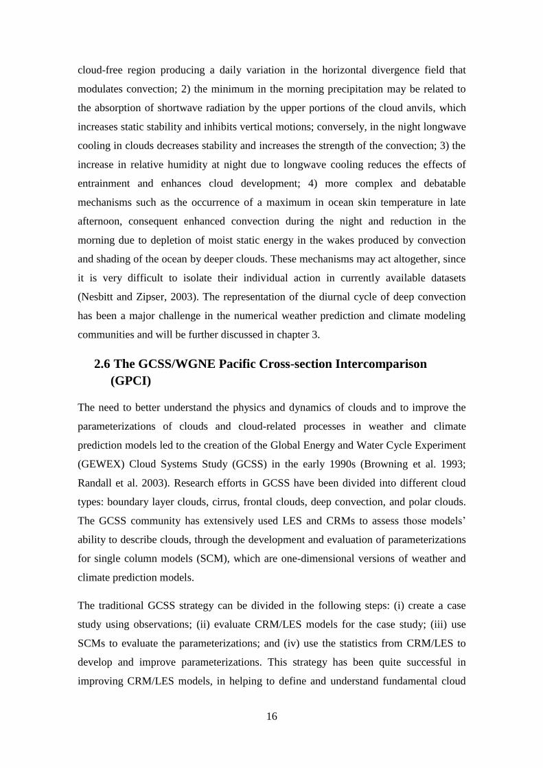
how representative is the GPCI transect of the processes that characterize the convection
regimes and transitions between them. It is assumed that there is an alignment between
the transect orientation and the trajectories described by the air masses. Mean boundary
layer wind directions from ERA-40, for June-August 1998 are shown to roughly
coincide with the orientation of the transect (see Figures 2 and 3 of Teixeira et al.,
2011). That may not necessarily be the case for some of the models used in the
intercomparison, but it is shown that they indeed exhibit bulk Hadley circulation
characteristics using alternative diagnostics.
Figure 7 – Location of the GPCI transect, overlayed on contours of International Satellite Cloud Climatology
Project (ISCCP) low cloud fraction (adapted from Karlsson et al., 2010).
The 2D dataset mentioned above is used to investigate the representativity of the
transect. Histograms of variables, like total cloud cover (TCC) and precipitation, along
the GPCI transect are compared to longitudinally adjacent points (5 degrees to the east
and to the west). Figure 8 shows the histograms of precipitation for one GPCI point
(5ºN, 195ºE) and the two adjacent points from the GFDL, and NCAR models for the
period of JJA 1998. Figure 9 shows a similar plot but for the TCC and another GPCI
point - 20ºN, 215ºE. It is clear from these figures that the histograms for both TCC and
precipitation are quite similar between adjacent points for the same model and quite
different between models. Similar results are obtained for different points along the
GPCI transect as well as for different models (not shown). Overall, these results support
the idea that GPCI is sufficiently representative for the purposes of this study of the
main model physical processes of the subtropics in this region.

19
Figure 8 – Histogram of precipitation (mm day-1) from the National Centers for Atmospheric Research
(NCAR) and Geophysical Fluid Dynamics Laboratory (GFDL) models for one GPCI point (5ºN, 195ºE) and
two adjacent (5º to the east and west along the same latitude) points for JJA 1998. From Teixeira et al. (2010).
Figure 9 – Histogram of total cloud cover (TCC) (%) from the NCAR and GFDL models for one GPCI point
(20ºN, 215ºE) and two adjacent (5º to the east and west along the same latitude) points for JJA 1998. From
Teixeira et al. (2010).
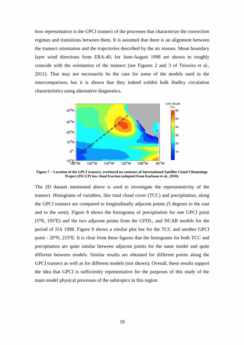
The models, observations and reanalysis were compared using several diagnostics along
the transect, which included SSTs (shown in Figure 10), total column water vapor,
outgoing longwave radiation, as well as vertical cross-sections of subsidence, relative

20
humidity, cloud fractions and cloud liquid water content. In general, the results showed
large spreads in the representation of clouds and cloud-related processes. Even
reanalysis such as ERA-40 show strong inconsistencies with observations. In the case of
SSTs (Figure 10), all models except NCAR G&M (National Centers for Atmospheric
Research – Global Forecast System and Modular Ocean Model version 3, the only
atmosphere and ocean coupled model used in the comparison) show similar
distributions along the GPCI transect. The differences between the uncoupled models
are mainly explained by the use of different implementations for describing the SSTs,
such as the use of different analysis. The differences in the representation of the other
atmospheric variables are mostly related to the differences in the physical
parameterizations used in each model to represent subgrid scale processes. Even ERA-
40 suffers from serious biases in some of those variables: it was shown that when
compared to International Satellite Cloud Climatology Project (ISCCP) observations,
ERA-40 cloud cover is negatively biased in the stratocumulus regions. This is partially
explained by the fact that it does not directly assimilate cloud-related variables from
observations. Those biases have been recently improved in ERA-Interim by the
inclusion of an eddy-diffusivity mass-flux approach, adapted to represent stratocumulus
regimes (Köhler et al., 2011). The bias is also present in the majority of the models in
terms of liquid water path (when compared to SSM/I observations), which in turn is
reflected in positive shortwave radiation biases at the surface and at the top of the
atmosphere. In the deep tropics, ERA-40 (in particular) overestimates cloud cover,
liquid water path, precipitation and, as a consequence, underestimates the outgoing
longwave radiation.
21
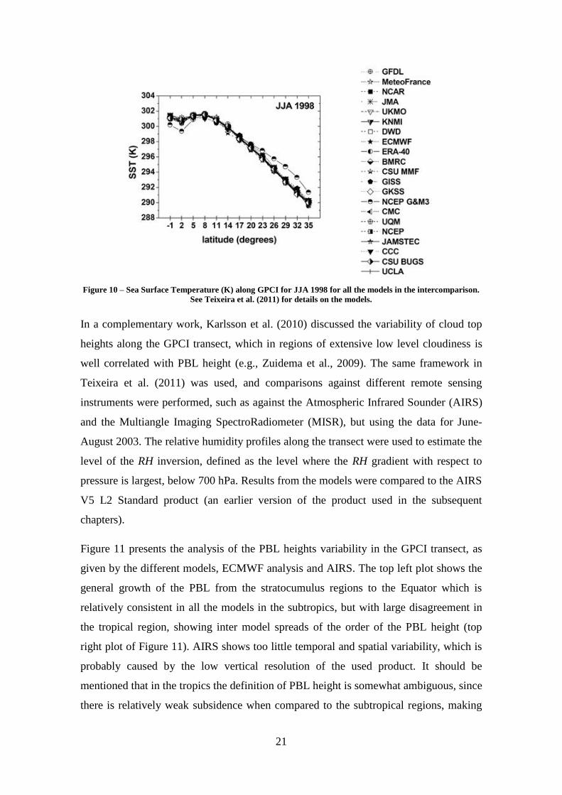
Figure 10 – Sea Surface Temperature (K) along GPCI for JJA 1998 for all the models in the intercomparison.
See Teixeira et al. (2011) for details on the models.
In a complementary work, Karlsson et al. (2010) discussed the variability of cloud top
heights along the GPCI transect, which in regions of extensive low level cloudiness is
well correlated with PBL height (e.g., Zuidema et al., 2009). The same framework in
Teixeira et al. (2011) was used, and comparisons against different remote sensing
instruments were performed, such as against the Atmospheric Infrared Sounder (AIRS)
and the Multiangle Imaging SpectroRadiometer (MISR), but using the data for June-
August 2003. The relative humidity profiles along the transect were used to estimate the
level of the RH inversion, defined as the level where the RH gradient with respect to
pressure is largest, below 700 hPa. Results from the models were compared to the AIRS
V5 L2 Standard product (an earlier version of the product used in the subsequent
chapters).
Figure 11 presents the analysis of the PBL heights variability in the GPCI transect, as
given by the different models, ECMWF analysis and AIRS. The top left plot shows the
general growth of the PBL from the stratocumulus regions to the Equator which is
relatively consistent in all the models in the subtropics, but with large disagreement in
the tropical region, showing inter model spreads of the order of the PBL height (top
right plot of Figure 11). AIRS shows too little temporal and spatial variability, which is
probably caused by the low vertical resolution of the used product. It should be
mentioned that in the tropics the definition of PBL height is somewhat ambiguous, since
there is relatively weak subsidence when compared to the subtropical regions, making

22
the inversions very weak, if they exist, and difficult to detect. ECMWF analysis always
overestimates PBL heights when compared to AIRS, but the values are almost always
within the interquartile range. A follow-up of these results will be presented in chapter
5, since new products have become available since this study was produced.
Figure 11 - JJA 2003 PBL height estimate based on the pressure at the main RH inversion (below 700 hPa) as
a function of latitude. (a) Mean values: the solid dark-gray line represents the median-model ensemble value,
the light-gray envelope is the interquartile model range, and the dark-gray envelope represents the full range
of the model values. (b) Mean values: individual models. (c) Temporal variability: 1 standard deviation. AIRS
and the ECMWF analysis are represented by a triangle-marked solid black line and a diamond-marked black
dashed line, respectively. From Karlsson et al. (2010).

23
3. Evolution of cloud structures in the transition from
shallow to deep convection over land
Abstract
The transition from shallow to deep convection is a crucial process in the
life cycle of convection over land. The process is of paramount importance
in tropical forest climate, where intense rain is produced on a daily basis
during the rainy season, with very well established timings. However, its
representation is deficient in the majority of GCMs, which tend to simulate
maxima of precipitation too early in the morning, when compared to
observations. In this work, high resolution cloud-resolving simulations of
the onset of Amazonian deep convection are analyzed to assess the ability of
the model to reproduce observed precipitation characteristics and its
sensitivity to horizontal resolution and to the evaporation of precipitation. It
is shown that simulations running at different resolutions produce
significantly different results, with the higher resolution experiments
experiencing a significantly slower build-up of deep convection and
precipitation, implying that these simulations to not attain peak values in the
given simulation time. Because of the previous result, the impact of
evaporation and cold-pool dynamics is still tentative, although it is clearly
present in some diagnostics. Finally, an analysis of length scales is proposed
using separate algorithms to analyze turbulent length scales and cloud sizes
in the three simulations.
24
3.1 Introduction
Tropical convection is very important in numerical weather and climate prediction.
Equatorial deep convection is the main engine of the Hadley and Walker circulations,
which are two of the most important features of the atmospheric general circulation
(Stevens, 2005). However, several aspects of deep convection still constitute big
challenges to numerical modelers, such as the correct representation of diurnal cycles,
the geographical and temporal transition between convection regimes, the location and
structure of the ITCZ and of the monsoon systems, the Madden-Julian Oscillation,
among others.
Observational studies showed that the diurnal cycle of precipitation associated with
tropical deep convection is very different for maritime or continental regions, with the
maximum of precipitation over the oceans occurring during the morning, but in the
early afternoon over land (Dias et al., 2002: Yang and Slingo, 2001). Such behavior is
not well captured by the majority of current numerical models. Betts and Jakob (2002a)
compared the results from the ECMWF operational model with observations made
during the TRMM-LBA (Tropical Rainfall Measuring Mission - Large Scale Biosphere-
Atmosphere Experiment in Amazonia) Wet Season Campaign (Dias et al., 2002)
verifying that this diurnal cycle had a strong bias, with the maximum of precipitation
being forecasted too early compared to observations. These authors also found that the
model diurnal cycle peaks twice (one peak in the early morning and another in the late
afternoon), while the observed cycle only shows one stronger peak, around mid-
afternoon. In another study (Betts and Jakob, 2002b) it was shown that this bias was
associated with the parameterization of convective processes.
Subsequent model intercomparison studies (Guichard et al., 2004; Grabowski et al.,
2006) showed that the majority of current GCMs have troubles in the representation of
tropical convection. The most common problems found across the analyzed models
seem to be related to the triggering of convection, which is too insensitive to boundary-
layer turbulence and surface heterogeneities, to a poor representation of the entrainment
and to a large insensitivity to large-scale fields such as relative humidity.
Khairoutdinov and Randall (2006) used a cloud resolving model to investigate the
TRMM-LBA case-study at a very high-resolution and in a huge domain, leading to the
computation of statistically significant PDFs of cloud properties. More importantly,

25
they showed that it is possible to explicitly simulate the transition from shallow to deep
convection with high-resolution models, in agreement with observations. Recently Rio
et al. (2009) were able to alleviate the bias in the diurnal cycle of precipitation on a
EUROCS case over the Southern Great Plains (USA) at the Atmospheric Radiation
Measurement site. This was made possible thanks to a combined approach between an
Eddy-Diffusivity/Mass-Flux (EDMF) shallow convection scheme (Soares et al., 2004;
Siebesma et al., 2007; Rio and Hourdin, 2008), and an improved Emanuel (1991)
scheme with modified triggering and closure functions, that allow a better coupling to
sub-cloud processes and to a parameterization of the effects of cold pools (Grandpeix
and Lafore, 2009; Hohenegger and Bretherton, 2011).
The difficulties found in the parameterization of deep convection are just one aspect of a
still notorious lack of knowledge of many cloud processes, probably the main source of
uncertainty in climate modeling (Bony and Dufresne, 2005; Teixeira et al., 2008;
Teixeira et al., 2011). Available parameterizations in GCMs make use of different
approaches for shallow and deep convection, with and without clouds, requiring the
estimation of too many tunable parameters, generally impossible to verify in an
independent way. A key feature of such parameterizations is the specification of length
scales characterizing convective and cloud structures and which, however, may vary
throughout non-stationary processes. In this study we use cloud resolving simulations to
investigate the evolution of those structures during the transition from shallow to deep
convection. Length scales may be estimated using spectral methods. Such approaches
have been used to study a diversity of processes. Jonker et al. (1999) studied the
evolution of length scales using LES data of the development of a convective boundary
layer (CBL). Cuxart et al. (2000) developed a parameterization for the convective
boundary layer and tested it in several common benchmark cases. These authors also
computed the evolution of length-scales for those cases and pointed that they are very
useful in deriving formulations for the mixing length, a key parameter in several
turbulence parameterizations. The role of mesoscale fluctuations on the evolution of
length-scales was discussed by de Roode et al. (2004). These authors also discussed the
methodology that is often used to compute length-scales on LES domains by means of
spectral analysis. Other authors have used this kind of methodology for example to
study the distortion of turbulence near boundaries (Teixeira and Belcher, 2000) or to

26
study the evolution of length scales on the evening transition of the convective to a
stable boundary layer (Pino et al., 2006).
3.2 Model and simulations
The non-hydrostatic model MesoNH (Lafore et al., 1998), can be used either in LES or
in mesoscale mode, incorporating a full state of the art physics package, terrain
following coordinates and a number of very accurate numerical options. The model
solves an anelastic system of equations (Lipps and Hemler, 1982) with a stretched
vertical coordinate (Galchen and Somerville, 1975). The spatial discretization uses a
staggered Arakawa-C grid. Time integration is performed with an explicit leapfrog
scheme with a time filter (Asselin, 1972). In LES mode, subgrid-scale turbulence is
parameterized with a full 3D scheme with a prognostic equation for TKE (Cuxart et al.,
2000) and microphysics is parameterized using a bulk scheme with 6 water species
(vapor, cloud, rain, ice, snow and graupel), referred to as „ICE3‟ (Lafore et al., 1998).
Two advection schemes were used: for dynamical variables a 4th
order centered on
space and time scheme; for the scalar meteorological variables a positive definite
monotonic version of the Piecewise Parabolic Method (Colella and Woodward, 1984).
To prevent spurious reflection from the model top boundary, a Rayleigh damping layer
is applied above 17 km. The model runs in an OpenMPI parallel environment for which
it was optimized.
As in Grabowski et al. (2006), the simulations were designed to assess the most critical
period of the diurnal cycle of tropical precipitation over land, characterized by the
growth of a well-mixed boundary layer with the formation of shallow cumulus followed
by a smooth transition from shallow to deep convection during the morning. Figure 12
shows the forcings applied to the model, which include an idealized early morning
sounding, and the time evolution of idealized latent and sensible turbulent fluxes and
also radiative cooling profiles (used instead of radiation and soil schemes, to focus the
analysis on the atmospheric processes). To force turbulence to develop, an initial
random noise is applied to the potential temperature field below 1 km. The simulation is
then run from 0730LT to 1330 LT. These were the specifications of the Case 4 of the
Global Energy and Water Cycle Experiment (GEWEX) Cloud System Study (GCSS)
Working Group 4 (Precipitating Convective Cloud Systems).

27
A control simulation with a domain size of 51.2 × 51.2 km2 and a horizontal resolution
of 100 m was performed (CONTROL). A second simulation with a lower resolution of
200 m and the same domain size was performed in order to test the sensitivity of the
results to the model resolution (LOWRES). Finally, the evaporation of precipitation is
switched off in order to evaluate the role of this process in the evolution of the typical
length scales, and a simulation with the same geometry of CONTROL (NOEVAP) is
done. All simulations had 128 vertical levels in a stretched grid in order to increase
resolution within the boundary-layer (from 50m near the ground and to about 500m at
the model top, located at 24.4 km). All simulations use cyclic horizontal boundary
conditions and a time-step of 2 s for CONTROL and NOEVAP and 4 s for LOWRES.

28
Figure 12 - (a) Initial sounding, with Temperature (black), Dew-Point Temperature (blue), and wind (wind-
barbs on the right), plotted in a skew-T diagram. The area between the black and red curves represents the
amount of CAPE. (b) Imposed radiative cooling profiles in K/day. Time is LT. (c) Surface sensible and latent
heat fluxes.
3.3 Evolution of mean properties
The evolution of low-level thermodynamic profiles in CONTROL is shown in Figure
13, starting from a very stable profile with zero initial surface fluxes (Figure 1c). Two
hours into the simulation (blue curves at Figure 13), a mixed layer is well developed
and the moistening and heating of the atmosphere is confined to this layer. As the
convection develops into its deep stage the mixed layer deepens and the moistening and
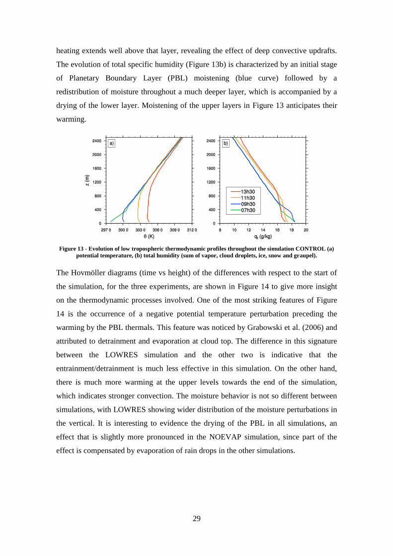
29
heating extends well above that layer, revealing the effect of deep convective updrafts.
The evolution of total specific humidity (Figure 13b) is characterized by an initial stage
of Planetary Boundary Layer (PBL) moistening (blue curve) followed by a
redistribution of moisture throughout a much deeper layer, which is accompanied by a
drying of the lower layer. Moistening of the upper layers in Figure 13 anticipates their
warming.
Figure 13 - Evolution of low tropospheric thermodynamic profiles throughout the simulation CONTROL (a)
potential temperature, (b) total humidity (sum of vapor, cloud droplets, ice, snow and graupel).
The Hovmöller diagrams (time vs height) of the differences with respect to the start of
the simulation, for the three experiments, are shown in Figure 14 to give more insight
on the thermodynamic processes involved. One of the most striking features of Figure
14 is the occurrence of a negative potential temperature perturbation preceding the
warming by the PBL thermals. This feature was noticed by Grabowski et al. (2006) and
attributed to detrainment and evaporation at cloud top. The difference in this signature
between the LOWRES simulation and the other two is indicative that the
entrainment/detrainment is much less effective in this simulation. On the other hand,
there is much more warming at the upper levels towards the end of the simulation,
which indicates stronger convection. The moisture behavior is not so different between
simulations, with LOWRES showing wider distribution of the moisture perturbations in
the vertical. It is interesting to evidence the drying of the PBL in all simulations, an
effect that is slightly more pronounced in the NOEVAP simulation, since part of the
effect is compensated by evaporation of rain drops in the other simulations.

30
Figure 14 – Anomaly (with respect to the initial profiles) of the potential temperature and total specific
humidity for the three simulations.
The evolution of the mean precipitation rate, mean PBL height, maximum cloud top
height in the domain, and height of the center of mass of the cloud field are plotted in
Figure 15. PBL height is diagnosed from the potential temperature profiles, through the
determination of its maximum vertical gradient below 3 km. All the simulations behave
quite similarly in terms of this variable, growing from about 200 m at the beginning to
reach about 2200 m at the end. The PBL is generally a bit higher in the LOWRES
simulation, indicating stronger turbulence at the PBL. The beginning of precipitation
occurs at around 10h in all simulations. Precipitation rates are always higher in
NOEVAP and LOWRES, attaining 12 mm day-1
whereas the CONTROL simulation
only reaches about 9 mm day-1
at 13:30, but without indication of having reached its
peak. These values are slightly smaller than those obtained by Khairoutdinov and
Randall (2006) for the same time frame, but they are still reasonable when compared
with the model intercomparison results discussed by Grabowski et al. (2006). As shown
in Figure 15c, the first shallow clouds appear around 8h45, but a little later in the
LOWRES simulation. However, the highest cloud top, representative of the deeper
updrafts, increases faster in LOWRES. Cloud tops reach almost 10 km towards the end
of the simulation in CONTROL and NOEVAP, and nearly 12 km in LOWRES right
after 1230LT. The center of mass of the clouds (Figure 15d) grows linearly in
CONTROL and NOEVAP, but increases abruptly in LOWRES around 1030LT. The
differences between CONTROL and LOWRES experiments may be explained by a less
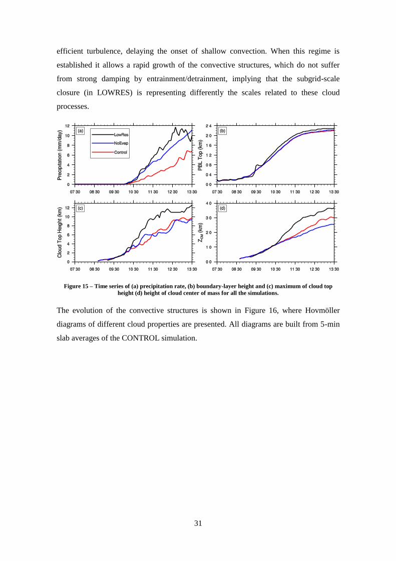
31
efficient turbulence, delaying the onset of shallow convection. When this regime is
established it allows a rapid growth of the convective structures, which do not suffer
from strong damping by entrainment/detrainment, implying that the subgrid-scale
closure (in LOWRES) is representing differently the scales related to these cloud
processes.
Figure 15 – Time series of (a) precipitation rate, (b) boundary-layer height and (c) maximum of cloud top
height (d) height of cloud center of mass for all the simulations.
The evolution of the convective structures is shown in Figure 16, where Hovmöller
diagrams of different cloud properties are presented. All diagrams are built from 5-min
slab averages of the CONTROL simulation.

32
Figure 16 – Evolution of cloud fraction, total precipitation, cloud condensate and variance of vertical velocity
for CONTROL.
As the boundary layer grows, deep convection is triggered, cloud structures become
larger and entrain less, thus being able to reach higher altitudes. At the same time, the
evaporation of precipitation originates convective downdrafts that will cause the
boundary layer moisture to drop, as discussed above. Cloud fraction shows a maximum
just above the LCL in the shallow convection phase. Towards the deep phase, cloud
fraction shows two peaks, one less pronounced at the LCL and a second at about 5 km.
Precipitation starts at 10h30 in result of the larger shallow convective clouds, extends
vertically with the appearance of deep convective clouds. The precipitation mixing ratio
is larger at the freezing level, where the most important microphysical processes occur.
The total cloud condensate shows a similar distribution to cloud fraction. However, at 2-
3 km the condensate shows high values, which indicates that clouds are occupying a
small area but they have high liquid water content. The vertical velocity variance has a
maximum within the PBL, where turbulent eddies induce large variability in this field.
The variance has a minimum at the PBL top and increase again in the cloud layer due to
the increasing intensity of the updrafts and downdrafts.
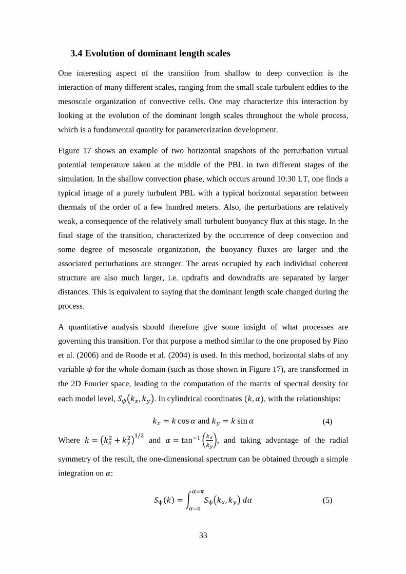
33
3.4 Evolution of dominant length scales
One interesting aspect of the transition from shallow to deep convection is the
interaction of many different scales, ranging from the small scale turbulent eddies to the
mesoscale organization of convective cells. One may characterize this interaction by
looking at the evolution of the dominant length scales throughout the whole process,
which is a fundamental quantity for parameterization development.
Figure 17 shows an example of two horizontal snapshots of the perturbation virtual
potential temperature taken at the middle of the PBL in two different stages of the
simulation. In the shallow convection phase, which occurs around 10:30 LT, one finds a
typical image of a purely turbulent PBL with a typical horizontal separation between
thermals of the order of a few hundred meters. Also, the perturbations are relatively
weak, a consequence of the relatively small turbulent buoyancy flux at this stage. In the
final stage of the transition, characterized by the occurrence of deep convection and
some degree of mesoscale organization, the buoyancy fluxes are larger and the
associated perturbations are stronger. The areas occupied by each individual coherent
structure are also much larger, i.e. updrafts and downdrafts are separated by larger
distances. This is equivalent to saying that the dominant length scale changed during the
process.
A quantitative analysis should therefore give some insight of what processes are
governing this transition. For that purpose a method similar to the one proposed by Pino
et al. (2006) and de Roode et al. (2004) is used. In this method, horizontal slabs of any
variable for the whole domain (such as those shown in Figure 17), are transformed in
the 2D Fourier space, leading to the computation of the matrix of spectral density for
each model level, ( ). In cylindrical coordinates ( ), with the relationships:
and (4)
Where (
)
and (
), and taking advantage of the radial
symmetry of the result, the one-dimensional spectrum can be obtained through a simple
integration on :
( ) ∫ ( )
(5)

34
Figure 17 - Horizontal slabs of the perturbation virtual potential temperature in the middle of the boundary
layer, for CONTROL. The snapshots coincide to two different stages of the simulation, the shallow convection
phase and deep convection with mesoscale organization phase.
As the variance of the variable at that particular level is equal to the integral of this
spectrum over all wavenumbers, i.e.:
∫ ( )
(6)
( ), being the model resolution) one can interpret each ( ) as the
fractional contribution of the length scale to the total variance. However, if
one defines the dominant length scale as the spectral peak, it often returns erratic values
as it is very sensitive to spectral noise. Therefore, an integral quantity is preferred. As
we are interested in scales of the order of the PBL height or greater, a power of k that
puts more weight on those scales is desirable (Pope, 2000; Jonker and Vilà-Guerau de
Arellano, 2005; Pino et al., 2006). Hence, the dominant length scale is defined here as:
∫ ( )
)
∫ ( )
(7)
Vertical profiles of the length scales of virtual potential temperature θv are presented on
Figure 18. There are interesting differences between the three experiments, and also
between convection stages. In the CONTROL simulation, there is a tendency for the
length scale to grow on time and with height. This is especially true within the boundary
layer (z/zi<1), where the length scale almost triples its value towards the end of the
transition. This increase has no correspondence in the free troposphere, indicating that
some boundary layer phenomenon is strongly affecting the spatial distribution of
coherent structures in this region. The second plot corresponds to the NOEVAP

35
simulation, in which length scales generally decrease in time. More importantly, we do
not see any difference in the behavior of the length scale within the PBL and in the free
troposphere. This shows that the length scale is strongly affected by the presence of the
large regions of colder air within the PBL (the cold pools) which result from the surface
divergence of the air coming from the downdrafts caused by the evaporation of
precipitation. The LOWRES simulation revealed qualitatively similar results to those in
the control simulation. However, its absolute value is generally about twice the value in
CONTROL (the resolution being half of the CONTROL simulation), which indicates a
strong model dependency on its resolution. However, one must stress the model
resolution (100-200m) is in all cases more than sufficient to represent the dominant
structures (>2km), suggesting that the resolution dependence is related with the explicit
or subgrid representation of small scale processes.
The results for the vertical velocity length scale are much different (Figure 9). In the
initial stages, length scales are larger and grow with height above the boundary layer.
Once moist ascending air starts to develop, the length scale becomes almost constant
right until the maximum height reached by updrafts, as this height increases with time.
The two high-resolution experiments (with and without evaporation of precipitation)
show similar w length scales growing from in the boundary to about aloft. In
the low resolution simulation, the length scales increase by a factor of 1.5 to 2.
Figure 18 - Vertical profiles of normalized length-scales of virtual potential temperature as a function of
normalized height and time, for the different simulations.

36
Figure 19 - Vertical profiles of normalized length-scales of vertical velocity as a function of normalized height
and time, for the different simulations.
3.5 Evolution of cloud structures
To estimate a cloud length scale, the previously described spectral method is not
suitable since clouds are not continuous features like the potential temperature
perturbations at the lower levels, analyzed in the previous section. Instead, they are
relatively small, localized, features and their location is quite random. The algorithm
used here identified cloudy areas as groups of at least 4 contiguous cloudy grid points in
each horizontal slab. Each cloud receives its unique identifier and all cloud properties
may be computed individually. Each cloud size is then computed as:
√
(8)
where is the number of cloud grid points, is the horizontal grid spacing. A
grid point is here defined as cloudy if the sum of the cloud droplets, cloud ice and snow
mixing ratios, is greater than 1 × 10⁻³
g/kg. These are the water species with relatively
slow fall speeds and thus are considered as cloud particles. Figure 20 shows the
estimates of the mean cloud horizontal size. The top left plot shows the results for the
shallow/congestus phase of the control simulation. At that stage, clouds reach 1.5 km,
just above the Lifting Condensation Level, with mean sizes of about 500 m. In the deep
stage (top right plot), the largest clouds are located at about 5 km (near the freezing
level), with a few of them reaching more than 4 km in horizontal length scale. The mean
and median of the distributions are however much lower, close to 1 km, and they
become slightly larger above the freezing level. These results are comparable to those of
NOEVAP, with the most noticeable difference being the absence of clouds within the
PBL in the case of NOEVAP, which shows they are produced by evaporation of rain.
Also, in the NOEVAP experiment the largest mid-level cloud sizes are narrower.

37
Surprisingly, the LOWRES simulation provides results which are comparable to similar
statistics obtained by Khairoutdinov and Randall (2006), with clouds being able to
penetrate higher, with maximum horizontal sizes (about 4 km) observed near the
tropopause, where deep convective anvils are often formed.
Figure 20 – Mean, median (P50), the 95 percentile (P95) and the maximum (Max) of the distributions of cloud
length scales for each level, for the shallow/congestus phase of CONTROL, and for the mature deep convection
phase of CONTROL, LOWRES and NOEVAP.
Because of the fact that the CONTROL simulation did not attain peak precipitation
within the simulation time, final conclusions from these simulations require significant
extra computations which were not possible in the present study. Indeed, results from
the CONTROL run compare worse with Khairoutdinov and Randall (2006) than the
LOWRES case, but it is unclear if the reason is in the subgrid-scale turbulence scheme
(one major difference between MesoNH and their model) or in other model
characteristics, or in the fact that the CONTROL run needs more time to fully develop
the deep cloud systems, as suggested by observations.
3.6 Conclusions
Convection over land is triggered too early by the majority of the parameterization
schemes used in GCMs. The most critical phase of the diurnal cycle of convection over
land is simulated here using a model with resolution typical of LES. This approach is
necessary since typical cloud resolving simulations, with resolutions of 1km or less, fail
0
2
4
6
8
10
12
14
0 1 2 3 4 5 6 7 80
2
4
6
8
10
12
14
0 1 2 3 4 5 6 7 8
0
2
4
6
8
10
12
14
0 1 2 3 4 5 6 7 80
2
4
6
8
10
12
14
0 1 2 3 4 5 6 7 8
Control - 1130LT
D (km)
z (
km
)
Control - 1330LT
D (km)
z (
km
)
LOWRES - 1330LT
D (km)
z (
km
)
NOEVAP - 1330LT
D (km)
z (
km
)
Mean
P50
P95
Max

38
to explicitly resolve the smallest scales that characterize turbulent transport. These are
key in the transition from shallow to deep convection, a typical feature of the diurnal
cycle of convection over land in its morning stage. An adequate description of the
effects of turbulence is necessary not only to properly characterize the mixing in the
PBL and its heterogeneities but also to understand entrainment/detrainment at the cloud
edges.
Overall the three simulations performed compare reasonably with previous studies
(Grabowski et al., 2006). The different simulations were designed in order to study the
sensitivity to model resolution and to the evaporation of precipitation, one of the most
important physical aspects that control the transition (Khairoutdinov and Randall,
2006). When compared to the results presented in those studies, the control simulation
shows a later onset of deep convection, with less penetrating clouds and consequently
less precipitation until 13:30. One of the major differences relative to the model used by
Khairoutdinov and Randall (2006) is the subgrid turbulence scheme: the model used by
these authors had a simple Smagorinsky-type closure for the subgrid scale turbulent
fluxes, whereas MesoNH in the present study uses a more complex 3D scheme with a
prognostic equation for TKE (Cuxart et al., 2000). The low resolution simulation relies
on the subgrid scheme to represent eddies that are explicitly represented in the high
resolution simulation due to the finer grid size. If the 3D scheme happens to be more
efficient in mixing, clouds entrain more and have much more difficulties in reaching the
tropopause. This does not seem to be the case in the low resolution simulation, on which
clouds do reach the tropopause and form anvils, and precipitation is closer to the
reported precipitation of previous studies.
The shape of the curve of the cloud center of mass in the low resolution simulation also
seems to show a more defined transition from shallow to deep convection as defined by
Wu et al. (2009), which is marked by a sudden increase in the slope of the curve around
1030LT (Figure 15d – black curve).
The sensitivity simulation to the evaporation of precipitation follows the suggestion of
some authors (Khairoutdinov and Randall, 2006; Grandpeix and Lafore, 2009) that it
has an impact on the development of secondary convection. When rain evaporates, it
cools the air causing strong downdrafts which spread horizontally when they reach the
ground, forming cold pools. At the gust front, PBL air is forced to rise since the air of

39
the cold pool is denser, reinforcing convection, as this mechanism acts as an extra
power source for the development of new convective plumes. The results of the
sensitivity experiment performed here partially confirm these assumptions. On one
hand, clouds do not reach as high as in the case of the low resolution experiment (Figure
15c and d), but precipitation in NOEVAP is higher than in CONTROL, both at the same
resolution. However, it should be kept in mind that at least part of this behavior is
explained by the fact that precipitation efficiency is much higher, since the rain drops
are not allowed to re-evaporate, and not because there are stronger convective cells.
This behavior might also be conditioned by the subgrid scale parameterization, since it
might be entraining too much, partially cancelling the effects of the otherwise stronger
secondary convection.
The length scale analysis revealed the importance of the cold pools in terms of
dominant processes at the PBL. When the evaporation of precipitation is suppressed, the
spectral behavior of the thermodynamic variables is much different from the control
simulation. The latter shows a clear signature of the presence of the cold pools, which
are structures that reach horizontal sizes of the order of six times the PBL height. They
are confined to the PBL, in the sense that the dominant length scale drops just above the
PBL top, to a length that is typical of the thermals (of the order of zi). This shows the
importance of these structures in terms of parameterization. Not only they favor the
development of new convection at their edges, but they also suppress it in the areas of
negative potential temperature perturbation.
The cloud length scale analysis showed that clouds grow with height and their behavior
is different for each simulation. In the higher resolution simulations, clouds seem to
struggle to ascend past the freezing level (at about 5 km) at least until 13:30, which
leads to stronger detrainment at those levels and to the formation of wider (stratiform)
clouds. In the lower resolution simulation, that is not the case, with the mean cloud size
increasing around those levels which is followed by a steady increase towards the
tropopause.
In short, the results are sensitive to changes in the resolution of the LES and more
simulations are necessary to assess the causes of this sensitivity: switching to a simpler
subgrid scale scheme with the same model resolutions and increasing resolution even
further are unavoidable tasks in order to answer this question, and would provide a

40
better degree of convergence in the turbulent length scale analysis. The comparison
against simpler methods for the determination of the dominant length scales
(Khairoutdinov and Randall, 2006; Kahn and Teixeira, 2009) would also provide further
insight on the interpretation of the determined length scales. Moreover, establishing
relationships between the diagnostics that were made and quantities usable for
parameterization is also one of the goals for future work. These tasks will be pursued in
the future.

41
4. Infrared Sounding of the Trade-wind Boundary Layer:
AIRS and the RICO Experiment*
Abstract
The new generation of remote sensors on board NASA's A-Train
constellation offers the possibility of observing the atmospheric boundary
layer in different regimes, with or without clouds. In this study we use data
from the Atmospheric InfraRed Sounder (AIRS) and of the Rain In
Cumulus over the Ocean (RICO) campaign, to verify the accuracy and
precision of the AIRS Version 5 Level 2 support product. This AIRS
product has an improved vertical sampling that is necessary for the
estimation of boundary layer properties. Good agreement is found between
AIRS and RICO data, in a regime of oceanic shallow cumulus that is known
to be difficult to analyze with other remote sensing data, and also shows a
low sensitivity to cloud or land fraction. This suggests that AIRS data may
be used for global boundary layer studies to support parameterization
development in regions of difficult in-situ observation.
* João P. A. Martins
(1,2), João Teixeira
(2), Pedro M. M. Soares
(1), Pedro M. A. Miranda
(1), Brian H. Kahn
(2),
Van T. Dang(2)
, Frederick W. Irion(2)
, Eric J. Fetzer(2)
, Evan Fishbein(2)
(2010): Infrared sounding of the
trade-wind boundary layer: AIRS and the RICO experiment, Geophys. Res. Lett., 37, L24806,
doi:10.1029/2010GL045902
(1) University of Lisbon, Instituto Dom Luiz, Lisbon, Portugal
(2) Jet Propulsion Laboratory, California Institute of Technology, Pasadena, CA, USA

42
4.1 Introduction
The planetary boundary layer (PBL) plays a key role in climate by mediating the
interactions between the free troposphere and the land-ocean-ice surface. In spite of its
importance, parameterizations of PBL physics in climate and weather prediction models
are still not realistic enough for accurate predictions of these interactions (e.g., Teixeira
et al., 2008). Shallow convective boundary layers are the most common type of PBL
over the subtropical oceans, and their role is essential to understand the tropical general
circulation (e.g., Riehl et al., 1951; Stevens, 2005). Trade wind boundary layer clouds
are also believed to play an essential role in climate change, as several studies suggest
that differences in model climate sensitivities can largely be explained by the models‟
differences in representation of PBL clouds (Bony and Dufresne, 2005; Wyant et al.,
2006).
The height of the boundary layer, typically marked by sharp temperature and humidity
vertical gradients, is an important integrated measure of the PBL properties and is often
a key parameter in turbulence parameterizations. Given its characteristics, the cloudy
PBL is remarkably difficult to observe with space-borne instruments. Only a few
studies have examined the ability of remote sensing instruments to measure PBL
properties, largely because of poor vertical resolution and cloud opacity in the infrared
(e.g., von Engeln et al., 2005). Techniques that rely on cloud opacity to the infrared
have been used to estimate cloud top heights, and they provide a good indirect estimate
for PBL height in regions dominated by low clouds (Wood and Bretherton, 2004;
Zuidema et al., 2009). While these estimates assume a simple mean thermodynamical
profile that can account for a mean decoupling between cloudy and dry layers,
variability in the coupling is not accounted for. Perhaps more importantly, the retrievals
are restricted to completely overcast, opaque footprints. In contrast, techniques relying
on the full knowledge of the cloud-cleared thermodynamical profiles allow direct
estimations of PBL height, since it maybe defined as the level where their gradients are
largest (e.g., Fetzer et al., 2004). Recent studies show that even in the presence of
significant cloudiness, biases in temperature and water vapor are not significantly
increased (Wu, 2009; Susskind et al., 2011), despite the reduced sampling frequency
(Fetzer et al., 2006).

43
In this work, lower tropospheric profiles from a less often used Atmospheric InfraRed
Sounder (AIRS) dataset (Aumann et al., 2003), referred to as the Level 2 (L2) Support
product, is compared to observations from the Rain in Cumulus over the Ocean (RICO)
campaign (Rauber et al., 2007). The former consists of 100-levels atmospheric retrievals
with a nominal grid spacing of about 25 hPa in the PBL, whereas the more commonly
used 28 level standard product has only 4 levels below 700 hPa (Susskind et al., 2006);
neither product has been extensively validated over the global oceans. The main goal of
this study is to quantify the ability of AIRS to reproduce the main thermodynamic
properties of the PBL in trade wind regions. This is the type of low cloud fraction
regime where the AIRS observations and retrieval algorithm are designed to have
optimal sampling frequency and low retrieval biases, since it relies on cloud free pixels
(Fetzer et al., 2004). Also, the presence of temperature gradients increases the reliability
of the measurements (Maddy and Barnet, 2008; Liang et al., 2010), so that the
information content derived from the radiances should be larger near the PBL top. There
is evidence that the averaging kernels from the Version 5 (V5) AIRS retrievals may be
too broad for T and q (temperature and water vapor mixing ratio, respectively)
(Pougatchev, 2008; N. Pougatchev, 2010, personal communication). In fact, AIRS may
resolve more finely vertical variations within the PBL than currently reported (Maddy
and Barnet, 2008), which further motivates comparisons to correlative in situ
observations such as those from RICO.
4.2 Data and methods
The RICO campaign took place near the Caribbean Islands of Antigua and Barbuda,
within the western Atlantic trade wind region, between 24 November 2004 and 25
January 2005. The main goal of the campaign was to assess the importance of
precipitation on the genesis of trade wind clouds and its role on the global circulation of
the atmosphere (Nuijens et al., 2009; Snodgrass et al., 2009). This study uses data from
the rawinsondes launched from Spanish Point (Barbuda) and from the Research Vessel
Seward Johnson, and dropsondes from the National Science Foundation (NSF) –
National Center for Atmospheric Research (NCAR) C130 aircraft, as they provide a
high resolution sample of lower tropospheric profiles of temperature and moisture.
The RICO data was interpolated to the AIRS L2 Support pressure levels using a moving
average filter with a length corresponding to the 25 hPa grid spacing, and all AIRS
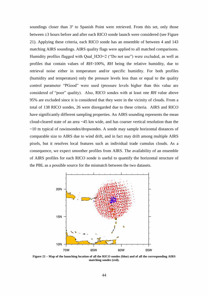
44
soundings closer than 3º to Spanish Point were retrieved. From this set, only those
between 3 hours before and after each RICO sonde launch were considered (see Figure
21). Applying these criteria, each RICO sonde has an ensemble of between 4 and 143
matching AIRS soundings. AIRS quality flags were applied to all matched comparisons.
Humidity profiles flagged with Qual_H2O=2 (“Do not use”) were excluded, as well as
profiles that contain values of RH>100%, RH being the relative humidity, due to
retrieval noise either in temperature and/or specific humidity. For both profiles
(humidity and temperature) only the pressure levels less than or equal to the quality
control parameter “PGood” were used (pressure levels higher than this value are
considered of “poor” quality). Also, RICO sondes with at least one RH value above
95% are excluded since it is considered that they were in the vicinity of clouds. From a
total of 138 RICO sondes, 26 were disregarded due to these criteria. AIRS and RICO
have significantly different sampling properties. An AIRS sounding represents the mean
cloud-cleared state of an area ~45 km wide, and has coarser vertical resolution than the
~10 m typical of rawinsondes/dropsondes. A sonde may sample horizontal distances of
comparable size to AIRS due to wind drift, and in fact may drift among multiple AIRS
pixels, but it resolves local features such as individual trade cumulus clouds. As a
consequence, we expect smoother profiles from AIRS. The availability of an ensemble
of AIRS profiles for each RICO sonde is useful to quantify the horizontal structure of
the PBL as a possible source for the mismatch between the two datasets.
Figure 21 – Map of the launching location of all the RICO sondes (blue) and of all the corresponding AIRS
matching sondes (red).

45
4.3 Results
4.3.1 Thermodynamic profiles and error statistics
Figure 22 shows three examples of AIRS retrievals of lower-tropospheric profiles of
potential temperature , q, and RH together with its corresponding RICO sonde profiles,
along with the AIRS matchup (ensemble). The AIRS profiles are generally smoother
than those from the sondes, as expected. However, despite some localized features, the
sonde measurements are well reproduced by the AIRS ensemble (the individual RICO
profile is mostly contained within the envelope of the AIRS ensemble data), and in
particular, by the geographically closest AIRS retrieval. Most importantly, and most
strikingly in the RH figure, AIRS is capable of reproducing the key features of the
cloudy PBL, namely the correct height of the PBL inversion separating the two distinct
layers of the troposphere, and the moist nature of the cloudy PBL. Note that the trade
wind inversion is not as pronounced in RICO as it appeared in previous campaigns like
BOMEX (Siebesma et al., 2003). The spread of the AIRS retrievals, represented by the
shaded areas in Figure 22, also indicates that the AIRS system is capable of observing
significant spatial variability within the selected area, indicating that the profiles are not
just a by-product of a first guess taken from a monthly mean climatology. Details of the
AIRS algorithms are described in (Susskind et al., 2011).
The overall agreement between AIRS and RICO sondes may be characterized by its
coefficients of determination (defined as 2222 / AIRSAIRSRICORICObR kk ,
where b is the slope of the linear regression between AIRS and RICO [Wilks, 1995]),
with computed values of 0.973 in the case of T, 0.823 for q, and 0.599 for RH. To
characterize the height-dependence of the errors of the AIRS retrievals for all matched
AIRS-RICO comparisons, two error estimates are shown in Figure 23: bias (AIRS –
RICO) and root mean square error (RMSE). In the case of T, a negative AIRS bias of
around -0.5 K is observed throughout the column except just above the PBL top around
700 hPa. It is reassuring that the PBL T bias is similar to the bias in the sub-tropical free
troposphere where AIRS is expected to be particularly reliable (e.g., Susskind et al.,
2011). The AIRS T RMSE is between 1.0-1.5 K with a minimum near 700 hPa that
coincides with a minimum in the AIRS bias just above the shallow cumulus cloud tops.
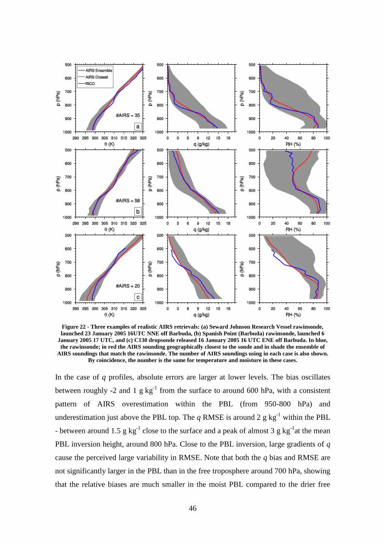
46
Figure 22 - Three examples of realistic AIRS retrievals: (a) Seward Johnson Research Vessel rawinsonde,
launched 23 January 2005 16UTC NNE off Barbuda, (b) Spanish Point (Barbuda) rawinsonde, launched 6
January 2005 17 UTC, and (c) C130 dropsonde released 16 January 2005 16 UTC ENE off Barbuda. In blue,
the rawinsonde; in red the AIRS sounding geographically closest to the sonde and in shade the ensemble of
AIRS soundings that match the rawinsonde. The number of AIRS soundings using in each case is also shown.
By coincidence, the number is the same for temperature and moisture in these cases.
In the case of q profiles, absolute errors are larger at lower levels. The bias oscillates
between roughly -2 and 1 g kg-1
from the surface to around 600 hPa, with a consistent
pattern of AIRS overestimation within the PBL (from 950-800 hPa) and
underestimation just above the PBL top. The q RMSE is around 2 g kg-1
within the PBL
- between around 1.5 g kg-1
close to the surface and a peak of almost 3 g kg-1
at the mean
PBL inversion height, around 800 hPa. Close to the PBL inversion, large gradients of q
cause the perceived large variability in RMSE. Note that both the q bias and RMSE are
not significantly larger in the PBL than in the free troposphere around 700 hPa, showing
that the relative biases are much smaller in the moist PBL compared to the drier free
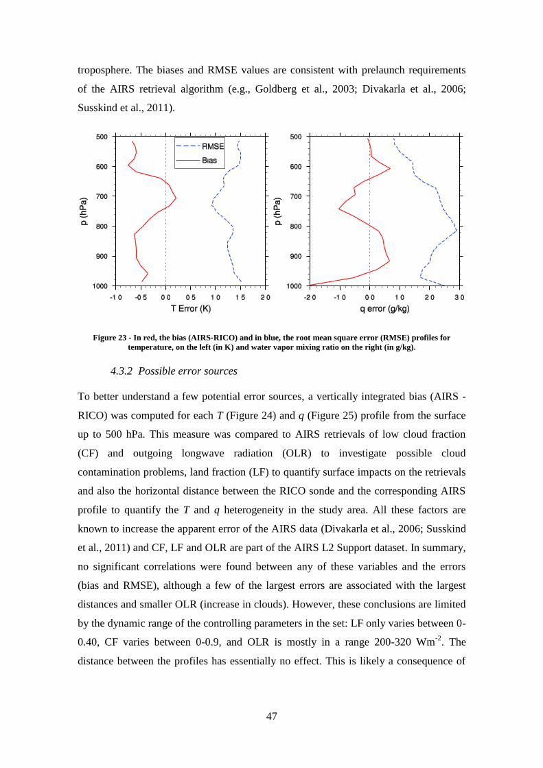
47
troposphere. The biases and RMSE values are consistent with prelaunch requirements
of the AIRS retrieval algorithm (e.g., Goldberg et al., 2003; Divakarla et al., 2006;
Susskind et al., 2011).
Figure 23 - In red, the bias (AIRS‐RICO) and in blue, the root mean square error (RMSE) profiles for
temperature, on the left (in K) and water vapor mixing ratio on the right (in g/kg).
4.3.2 Possible error sources
To better understand a few potential error sources, a vertically integrated bias (AIRS -
RICO) was computed for each T (Figure 24) and q (Figure 25) profile from the surface
up to 500 hPa. This measure was compared to AIRS retrievals of low cloud fraction
(CF) and outgoing longwave radiation (OLR) to investigate possible cloud
contamination problems, land fraction (LF) to quantify surface impacts on the retrievals
and also the horizontal distance between the RICO sonde and the corresponding AIRS
profile to quantify the T and q heterogeneity in the study area. All these factors are
known to increase the apparent error of the AIRS data (Divakarla et al., 2006; Susskind
et al., 2011) and CF, LF and OLR are part of the AIRS L2 Support dataset. In summary,
no significant correlations were found between any of these variables and the errors
(bias and RMSE), although a few of the largest errors are associated with the largest
distances and smaller OLR (increase in clouds). However, these conclusions are limited
by the dynamic range of the controlling parameters in the set: LF only varies between 0-
0.40, CF varies between 0-0.9, and OLR is mostly in a range 200-320 Wm-2
. The
distance between the profiles has essentially no effect. This is likely a consequence of
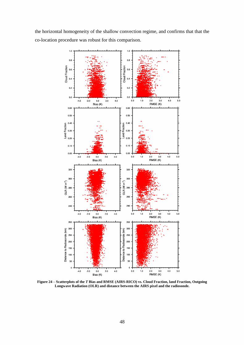
48
the horizontal homogeneity of the shallow convection regime, and confirms that that the
co-location procedure was robust for this comparison.
Figure 24 – Scatterplots of the T Bias and RMSE (AIRS-RICO) vs. Cloud Fraction, land Fraction, Outgoing
Longwave Radiation (OLR) and distance between the AIRS pixel and the radiosonde.

49
4.3.3 Boundary layer height
The main advantage of using the AIRS L2 Support product is the increase in detail in
the representation of the vertical structure of the atmosphere. For typical convective
boundary layers over the ocean, the PBL height can be defined as the height of strong
gradients in both θ and RH. The algorithm developed here locates the first occurrence of
Figure 25 – Same as Figure 24, but for specific humidity errors.

50
a gradient, ascending from the surface, that exceeds a given threshold (-0.06 K hPa-1
for
θ and 0.4 % hPa-1
for RH). Sometimes such a gradient does not exist; in which case the
largest gradient is assumed to coincide with the PBL height. Only levels between 925
and 700 hPa are considered. Histograms for the PBL depth as determined by all the
available AIRS and RICO sondes are presented in Figure 26. The histograms for AIRS
PBL height using both and RH in Figure 26 are qualitatively similar to each other.
Also, the mean value of PBL height from the AIRS retrievals (around 800 hPa) is close
to the climatological value of PBL height in the trade-wind regions in Rauber et al.
(2007). The standard deviation of the PBL height as determined by the AIRS soundings
is about 33 hPa, which is similar to the vertical gridding of the L2 Support product. The
distributions of the AIRS estimates of PBL height show a mean bias of around -6 hPa
and an RMSE of around 53 hPa using profiles, and a bias of 8 hPa and an RMSE of
56 hPa using RH profiles. Furthermore, the PBL gradients as given by the filtered RICO
sondes are also reasonably well reproduced by AIRS, and have typical mean values
close to the thresholds used in the PBL determination algorithm (not shown). The
skewness of the distributions is however much different in the two datasets, and it
reveals that AIRS is not able to reproduce the largest gradients revealed by RICO,
which may explain the broadness of the AIRS PBL height histograms. Still, given the
capabilities of the AIRS suite, these results are promising and this analysis should be
extended to future in situ field campaigns to characterize both similar and dissimilar
cloud regimes.
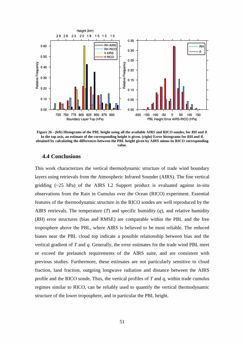
51
Figure 26 - (left) Histograms of the PBL height using all the available AIRS and RICO sondes, for RH and .
In the top axis, an estimate of the corresponding height is given. (right) Error histograms for RH and ,
obtained by calculating the differences between the PBL height given by AIRS minus its RICO corresponding
value.
4.4 Conclusions
This work characterizes the vertical thermodynamic structure of trade wind boundary
layers using retrievals from the Atmospheric Infrared Sounder (AIRS). The fine vertical
gridding (~25 hPa) of the AIRS L2 Support product is evaluated against in-situ
observations from the Rain in Cumulus over the Ocean (RICO) experiment. Essential
features of the thermodynamic structure in the RICO sondes are well reproduced by the
AIRS retrievals. The temperature (T) and specific humidity (q), and relative humidity
(RH) error structures (bias and RMSE) are comparable within the PBL and the free
troposphere above the PBL, where AIRS is believed to be most reliable. The reduced
biases near the PBL cloud top indicate a possible relationship between bias and the
vertical gradient of T and q. Generally, the error estimates for the trade wind PBL meet
or exceed the prelaunch requirements of the AIRS suite, and are consistent with
previous studies. Furthermore, these estimates are not particularly sensitive to cloud
fraction, land fraction, outgoing longwave radiation and distance between the AIRS
profile and the RICO sonde. Thus, the vertical profiles of T and q, within trade cumulus
regimes similar to RICO, can be reliably used to quantify the vertical thermodynamic
structure of the lower troposphere, and in particular the PBL height.

52
A recent study by Karlsson et al. (2010) compared results from Multiangle Imaging
Spectroradiometer (MISR), the AIRS standard product against model and reanalysis
results in a transect across the Eastern Pacific. Good agreement between all the
estimates was found in regions dominated by stratiform low clouds, whereas in the trade
region the variability of cloud top heights increases the uncertainty of MISR
estimations. AIRS should be able to produce reliable profiles in regions with little cloud
cover such as the trades. AIRS also has the advantage of relatively good balance
between temporal and spatial coverage and spatial resolution, in contrast to the high
vertical resolution but poor horizontal resolution of the Global Positioning System
Radio Occultation (GPS RO) (von Engeln et al., 2005) or overall coverage of space-
bourne lidar or MISR.
However, a shortcoming of the AIRS vertical resolution is related to the ability of
detecting the local variability of PBL height, since its value is close to the vertical
resolution of the instrument. For this purpose, a dataset with higher resolution,
especially within the PBL, would be desirable. Nevertheless, this study still suggests
that this AIRS dataset has the potential to provide reliable PBL height information also
beyond the trade-wind regions, as it contains global observations of the PBL structure
that are useful for both spatial and seasonal variability studies, and for climate and
numerical weather prediction model evaluations.

53
5. A climatology of Planetary Boundary Layer Height over
the ocean from the Atmospheric Infrared Sounder†
Abstract
The capability to characterize the Planetary Boundary Layer (PBL) with the
Atmospheric Infrared Sounder (AIRS) suite onboard NASA‟s Aqua satellite
has received attention because of its relatively high spectral resolution, daily
and global spatial coverage, and a nearly continuous temporal record since
September 2002. In this work, the AIRS Version 5 Level 2 Support product
temperature and moisture profiles are used to determine the PBL height by a
method that exploits changes in their vertical gradients. The results are
compared to ERA-Interim PBL heights, which were estimated from
collocated profiles over the global oceans. AIRS and ERA-Interim both
show similar geographic distributions, and signs and amplitudes of the
seasonal cycle. However, the diurnal behavior is much different between the
data sets. AIRS shows realistic diurnal variations determined from
differences between day and night time overpasses, while ERA-Interim
shows no significant diurnal cycle over the global oceans, even near
continental land masses where they are expected to be largest. Results along
a cross-section in the northeast Pacific Ocean that captures the
stratocumulus to trade wind cumulus transition are explored in detail,
showing that these results are sensitive to the presence of high values of
cloud fraction. The differences between both data sets are reduced as
temperature and moisture profiles in the presence of high cloud fraction
values are excluded. These results confirm that AIRS provides a valuable
observational and global benchmark of the PBL height climatology that can
be used to evaluate climate models.
† João P. A. Martins
(1,2); Pedro M. M. Soares
(1); Johannes Karlsson
(2,3); João Teixeira, Pedro M.A.
Miranda and Brian H. Kahn (2011): A climatology of Planetary Boundary Layer Height over the ocean
from the Atmospheric Infrared Sounder. Submitted.
(1) University of Lisbon, Instituto Dom Luiz, Lisbon, Portugal
(2) Stockholm University, Stockholm, Sweden
(3) Jet Propulsion Laboratory, California Institute of Technology, Pasadena, CA, USA

54
5.1 Introduction
Planetary Boundary Layer (PBL) processes have received considerable attention
because they are crucial for understanding the mechanisms regulating feedbacks
between low-level clouds, radiation and surface temperature (Randall et al., 2007;
Teixeira et al., 2011). The necessity of a global observational data set of PBL height has
been recognized in a variety of studies and several approaches have been tried to date.
Medeiros et al. (2005) used an idealized Global Circulation Model (GCM) to study the
PBL height at the global scale. The main causes for its variability were identified,
namely, the land-sea contrast and seasonal variations in the surface turbulent fluxes.
On the observational side, field campaigns have provided high temporal and spatial
resolution data sets of radiosondes, lidars, sodars, ceilometers and radars, which are
typically used for regional studies. These data sets provided valuable information that
facilitated the development of many increasingly sophisticated PBL parameterizations
used in numerical models. Liu and Liang (2010) used data from several major field
campaigns to determine the variability of PBL heights in regions characterized by
certain convection regimes. Examples included the trade-wind cumulus convection
region that was recently studied in the Rain in Cumulus over the Ocean (RICO; Rauber
et al., 2007) and the Barbados Oceanographic and Meteorological Experiment
(BOMEX; Siebesma et al., 2003). The South American stratocumulus cloud deck was
investigated by the Variability of American Monsoon Systems (VAMOS) Ocean–
Cloud–Atmosphere–Land Study (VOCALS; Bretherton et al., 2010) and the East
Pacific Investigation of Climate (EPIC; Raymond et al., 2004) (the full list may be
found in Liu and Liang (2010)). These authors reported that the diurnal cycle of PBL
height shows, both over land and ocean, strong diurnal cycles with peaks at 1500 and
1200 LT, respectively. The main driver of the diurnal cycle over stratocumulus regions
is the diurnal variability of emitted and reflected radiation. At night, longwave cooling
at the cloud top results in a well-mixed stratocumulus topped PBL. During the daytime,
shortwave absorption in the cloud layer causes decoupling with the cloud layer
becoming stably stratified with respect to the sub-cloud layer. This inhibits transport
from the sub-cloud layer to the cloud layer, and as the cloud top continues to entrain dry
and warm tropospheric air, the cloud eventually dissipates (Wood et al., 2002;
Duynkerke et al., 2004). However, local circulations may modulate the phase and
intensity of the diurnal cycle at some locations. Rahn and Garreaud (2010) used the
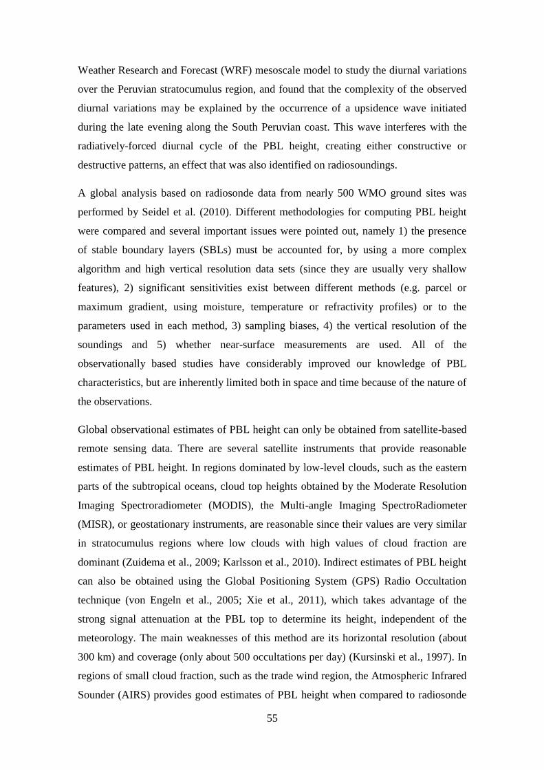
55
Weather Research and Forecast (WRF) mesoscale model to study the diurnal variations
over the Peruvian stratocumulus region, and found that the complexity of the observed
diurnal variations may be explained by the occurrence of a upsidence wave initiated
during the late evening along the South Peruvian coast. This wave interferes with the
radiatively-forced diurnal cycle of the PBL height, creating either constructive or
destructive patterns, an effect that was also identified on radiosoundings.
A global analysis based on radiosonde data from nearly 500 WMO ground sites was
performed by Seidel et al. (2010). Different methodologies for computing PBL height
were compared and several important issues were pointed out, namely 1) the presence
of stable boundary layers (SBLs) must be accounted for, by using a more complex
algorithm and high vertical resolution data sets (since they are usually very shallow
features), 2) significant sensitivities exist between different methods (e.g. parcel or
maximum gradient, using moisture, temperature or refractivity profiles) or to the
parameters used in each method, 3) sampling biases, 4) the vertical resolution of the
soundings and 5) whether near-surface measurements are used. All of the
observationally based studies have considerably improved our knowledge of PBL
characteristics, but are inherently limited both in space and time because of the nature of
the observations.
Global observational estimates of PBL height can only be obtained from satellite-based
remote sensing data. There are several satellite instruments that provide reasonable
estimates of PBL height. In regions dominated by low-level clouds, such as the eastern
parts of the subtropical oceans, cloud top heights obtained by the Moderate Resolution
Imaging Spectroradiometer (MODIS), the Multi-angle Imaging SpectroRadiometer
(MISR), or geostationary instruments, are reasonable since their values are very similar
in stratocumulus regions where low clouds with high values of cloud fraction are
dominant (Zuidema et al., 2009; Karlsson et al., 2010). Indirect estimates of PBL height
can also be obtained using the Global Positioning System (GPS) Radio Occultation
technique (von Engeln et al., 2005; Xie et al., 2011), which takes advantage of the
strong signal attenuation at the PBL top to determine its height, independent of the
meteorology. The main weaknesses of this method are its horizontal resolution (about
300 km) and coverage (only about 500 occultations per day) (Kursinski et al., 1997). In
regions of small cloud fraction, such as the trade wind region, the Atmospheric Infrared
Sounder (AIRS) provides good estimates of PBL height when compared to radiosonde

56
estimates from the RICO campaign (Martins et al., 2010). However, previous
investigations (e.g. Fetzer et al., 2004; Wu, 2009) have recognized that AIRS also
provides thermodynamic profiles that are usable even in cloudy pixels.
This study addresses the cloud fraction dependence of the PBL height applying a similar
methodology to the one developed by Martins et al. (2010) to the full AIRS V5 Level 2
Support data set over tropical, subtropical and mid-latitude oceans. A global PBL height
climatology is presented, along with the seasonal and diurnal variability, using both
potential temperature () and relative humidity (RH) profiles. The results are then
compared to ERA-Interim (ERA-I) reanalysis estimates (Dee et al., 2011). The latter
data set has been analyzed by (von Engeln and Teixeira, 2011) who compared it against
radiosonde data using several methods to determine the PBL height.
The comparison to be shown is not intended to be a true independent validation of
AIRS-observed PBL height, because the radiances from AIRS are regularly assimilated
by the ECMWF system, thus part of the information of both data sets is redundant.
However, ECMWF directly assimilates AIRS Level 1b radiances, and mixes them with
other data sources plus a model first guess, to provide their analysis. This model first
guess is known to be a major source of information in regions where there is less
available data (Dee et al., 2011), such as the cloud-covered open oceans. The AIRS V5
L2 products are retrieved independent of an a priori climatology or the ECMWF
assimilation system. Therefore, significant differences between both data sets exist and
differences in the PBL height are expected.
5.2 Data and Methods
In this study, the AIRS V5 L2 Support product (Liang et al., 2010; Martins et al., 2010;
Susskind et al., 2011; Yue et al., 2011) and RH profiles are used to determine the PBL
height over oceans. The AIRS instrument is onboard the Aqua platform that crosses the
Equator at around 13:30 LT during daytime and at 01:30 LT at nighttime. The AIRS
data set (hereafter AIRS) samples the atmosphere with approximately 45-km horizontal
resolution at nadir, and 100 vertical levels with approximately 25 hPa grid spacing in
the lower troposphere, although the true resolution of the AIRS instrument is still a
matter of debate (Maddy and Barnet, 2008). Retrievals from December 2002 to
November 2010 were used to compute the PBL height climatology.

57
The boundary layer height estimates are defined as the level of maximum vertical
gradient of θ and RH below 3 km, since the PBL inversion is characterized by strong
vertical θ and RH gradients that do not necessarily coincide with each other in all
conditions. The quality control for AIRS is limited to profiles that contain values of
“PGood” ≥ 900 hPa (Yue et al., 2011). The retrieved values are converted to meters
using the hypsometric equation and the AIRS surface pressure estimate, since the
original data set is reported on pressure coordinates. The value is then re-gridded to a 1
× 1º longitude-latitude regular grid. At each grid point, a PDF of the PBL height is
assembled. This procedure ensures the conservation of the statistical properties of the
distribution and allows a better characterization of the local variability across a variety
of space and time scales. The bins of the distribution are 300 m apart, which
approximate the original AIRS data set vertical resolution. PDFs of the θ and RH
gradient strength at the PBL top are computed in a similar fashion.
The same time period was used to compute similar diagnostics for ERA-I. The data set
used in this work has 60 vertical hybrid levels and 1 × 1º horizontal resolution in a
regular horizontal grid. The vertical resolutions of AIRS and ERA-I within the PBL are
much different, since the ECMWF system uses a stretched hybrid grid, which allows
higher resolution throughout the PBL to better resolve important processes occurring in
this layer.
5.3 Global PBL Heights
A quantitative benchmark of the global distribution of PBL height, its mean
climatology, seasonal variability and diurnal cycle, is still lacking and is needed for
GCM evaluation (Medeiros et al., 2005; Seidel et al., 2010). In this work, the focus is
on the convective PBLs. Stable and neutral PBLs are not separately emphasized in part
because the AIRS sounder does not have the necessary vertical resolution as these PBLs
are often very shallow and difficult to observe, even with traditional instruments such as
radiosondes. Also, the gradient method will often detect the height that corresponds to
the residual layer, rather than the PBL that is generated at the time of sampling.
Therefore, the analysis is limited to global oceans between 60S and 60N because (1)
SBLs are more likely outside of this oceanic region, especially over land surfaces
during nighttime, and (2) AIRS retrievals are increasingly problematic over strongly
mineralized terrain and other surfaces with uncertain surface emissivity (e.g. Hulley et
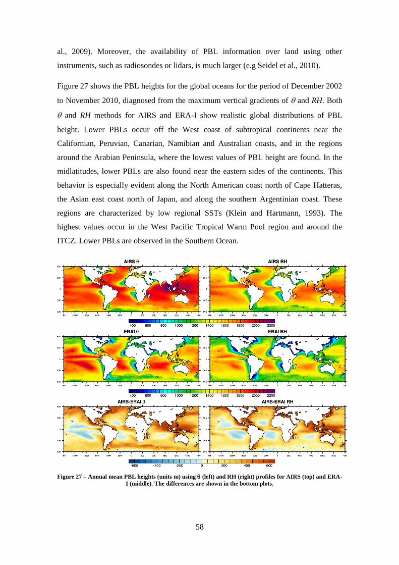
58
al., 2009). Moreover, the availability of PBL information over land using other
instruments, such as radiosondes or lidars, is much larger (e.g Seidel et al., 2010).
Figure 27 shows the PBL heights for the global oceans for the period of December 2002
to November 2010, diagnosed from the maximum vertical gradients of and RH. Both
and RH methods for AIRS and ERA-I show realistic global distributions of PBL
height. Lower PBLs occur off the West coast of subtropical continents near the
Californian, Peruvian, Canarian, Namibian and Australian coasts, and in the regions
around the Arabian Peninsula, where the lowest values of PBL height are found. In the
midlatitudes, lower PBLs are also found near the eastern sides of the continents. This
behavior is especially evident along the North American coast north of Cape Hatteras,
the Asian east coast north of Japan, and along the southern Argentinian coast. These
regions are characterized by low regional SSTs (Klein and Hartmann, 1993). The
highest values occur in the West Pacific Tropical Warm Pool region and around the
ITCZ. Lower PBLs are observed in the Southern Ocean.
Figure 27 – Annual mean PBL heights (units m) using (left) and RH (right) profiles for AIRS (top) and ERA-
I (middle). The differences are shown in the bottom plots.
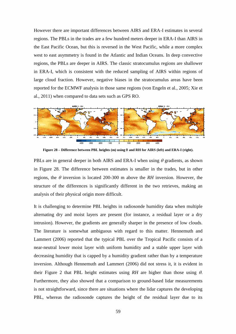
59
However there are important differences between AIRS and ERA-I estimates in several
regions. The PBLs in the trades are a few hundred meters deeper in ERA-I than AIRS in
the East Pacific Ocean, but this is reversed in the West Pacific, while a more complex
west to east asymmetry is found in the Atlantic and Indian Oceans. In deep convective
regions, the PBLs are deeper in AIRS. The classic stratocumulus regions are shallower
in ERA-I, which is consistent with the reduced sampling of AIRS within regions of
large cloud fraction. However, negative biases in the stratocumulus areas have been
reported for the ECMWF analysis in those same regions (von Engeln et al., 2005; Xie et
al., 2011) when compared to data sets such as GPS RO.
Figure 28 – Difference between PBL heights (m) using and RH for AIRS (left) and ERA-I (right).
PBLs are in general deeper in both AIRS and ERA-I when using gradients, as shown
in Figure 28. The difference between estimates is smaller in the trades, but in other
regions, the inversion is located 200-300 m above the RH inversion. However, the
structure of the differences is significantly different in the two retrieves, making an
analysis of their physical origin more difficult.
It is challenging to determine PBL heights in radiosonde humidity data when multiple
alternating dry and moist layers are present (for instance, a residual layer or a dry
intrusion). However, the gradients are generally sharper in the presence of low clouds.
The literature is somewhat ambiguous with regard to this matter. Hennemuth and
Lammert (2006) reported that the typical PBL over the Tropical Pacific consists of a
near-neutral lower moist layer with uniform humidity and a stable upper layer with
decreasing humidity that is capped by a humidity gradient rather than by a temperature
inversion. Although Hennemuth and Lammert (2006) did not stress it, it is evident in
their Figure 2 that PBL height estimates using RH are higher than those using .
Furthermore, they also showed that a comparison to ground-based lidar measurements
is not straightforward, since there are situations where the lidar captures the developing
PBL, whereas the radiosonde captures the height of the residual layer due to its

60
relatively strong humidity gradient. Seidel et al. (2010) also reports higher PBLs using
RH profiles, but their results are restricted to land. The study by von Engeln and
Teixeira (2011) reports lower values using RH over the GEWEX Cloud System Study
(GCSS) Pacific Cross-section Intercomparison (GPCI) transect using ERA-40 and
ERA-I data. Therefore, the general problem of PBL height determination from different
methods (e.g., RH or gradients) remains unresolved due to the large spatial and
temporal variability of the differences between the results using distinct methodologies.
Figure 29 shows the seasonal AIRS PBL heights using RH profiles. A strong seasonal
modulation of PBL height is observed, especially in the subtropical stratocumulus
regions. The seasonal variations are consistent with Klein and Hartmann (1993),
because the lower PBL heights are associated with a low cloud fraction. The Californian
and Canarian regions have minimum PBL heights in JJA, which is associated with
higher low tropospheric stability (LTS, given by the difference between 700 hPa and
the surface), since at the PBL top is larger in in JJA than any other season. This is
caused by greater subsidence warming from the relatively strong summer Walker
circulation. In the Namibian and Peruvian regions, the seasonal variation in the LTS is a
stronger function of the seasonal variation in SST rather than at the PBL top. Near the
Namibian coast, the minimum PBL height occurs in SON, while the Peruvian minimum
occurs in JJA, although SON is very similar, consistent with Klein and Hartmann
(1993). In the mid-latitude western ocean basins, the PBL height also has a minimum in
the summer, possibly due to enhanced subsidence caused by monsoon-like circulations
due to differential heating of the continental and oceanic regions, and/or seasonal
changes in the mean position of the surrounding subtropical center of high pressure.
Higher PBLs associated with deep convective regions track the seasonal changes in the
position of these semi-permanent features. The ITCZ moves northward in the boreal
summer, and PBL heights are higher at the onset of the major monsoon systems (e.g.,
observe the differences in the Bay of Bengal between MAM and JJA).

61
Figure 29 – Mean PBL height (m) using AIRS RH profiles.
Figure 30 shows average maps of the difference between day and night Aqua passes and
the corresponding maps for ERA-I. As AIRS crosses the Equator at around 13:30 LT
(01:30 LT) in the daytime (nighttime) pass, a relatively good estimate of the amplitude
of the diurnal cycle of PBL height can be obtained by AIRS. However, there are some
mechanisms that might cause diurnal variations with a lagged response relative to the
orbital crossing times, thus these behaviors might be missed by the AIRS estimate of the
diurnal cycle presented here. Furthermore, the amplitude of the diurnal cycle in PBL
height and other properties is much larger over land as it is primarily driven by surface
heat fluxes that respond much faster to solar input on land surfaces when compared to
the ocean.
Figure 30 – Annual mean difference of PBL height (m) between daytime and nighttime passes, using θ and RH
profiles, for AIRS and ERA-I.
PBLs are slightly shallower in daytime in regions characterized by monsoon-like
circulations, such as the Gulf of Guinea. As the air rises over land and descends over the

62
ocean, lower PBLs result over the ocean during daytime. Some regions have an opposite
diurnal difference such as the stratocumulus near the Peruvian, Californian and
Namibian coasts. As discussed in the introduction, this behavior is explained not only
by the radiative-driven decoupling process in the daytime, but in certain regions land-
ocean effects may interfere with the diurnal modulation (Rahn and Garreaud, 2010).
The diurnal signal is stronger in than in RH, but the overall features are similar with
the exception of the tropical regions. The larger positive amplitude of -estimated PBL
height in the tropics is related to the relatively higher frequency of shallow convective
regimes in daytime, whereas in the evening deep convective clouds are favored. The
explanation of this diurnal variation in the intensity of convection is still under debate
(Liu and Moncrieff, 1998; Nesbitt and Zipser, 2003; Pereira and Rutledge, 2006), but
there is evidence that convective activity is favored at night due to a combination of
longwave cooling (and increase in RH) in the upper troposphere, and as a consequence a
decrease of the effects of entrainment on convective plumes (e.g. Derbyshire et al.,
2004). The PBL height algorithm is designed to detect the sharpest feature that roughly
corresponds to the mean Lifting Condensation Level (LCL) of the pixel. This feature
has a degree of seasonality, especially in the estimate, shown in Figure 31. The RH
signal exhibits less sharp features, but at the same locations (not shown). There are
diurnal differences of about 300m in the periods of maximum stratocumulus activity
identified above, and the diurnal cycle is virtually absent in those seasons when low
cloud fraction is reduced. The North Atlantic and Pacific stratus regions also show
strong seasonality in the intensity (and sign) of the diurnal cycle. The anomaly is
positive in JJA and negative in DJF, which may be interpreted as a manifestation of the
seasonality of the monsoon-like systems. In stark contrast, no sign of the diurnal cycle
is observed in ERA-I for either or RH. We speculate that the lack of a diurnal cycle
arises because of a misrepresentation of the observed features by the assimilation
system in ERA-I that strongly depends on a model first guess in regions where limited
observations exist. Also, in the production of their analysis, daily maps of SST are
assimilated (i.e. with no diurnal variations) (Dee et al., 2011). Nonetheless, it is
encouraging that the seasonal and spatial patterns of the AIRS diurnal cycle of PBL
height are consistent with expectations.

63
Figure 31 – Seasonal cycle of the diurnal amplitude of the PBL height (m) as given by AIRS estimate.
Some of the seasonal and diurnal features have to be interpreted in light of the sampling
characteristics of AIRS. Given the effects of clouds in the infrared, the PBL
characteristics are not as representative in regions characterized by large cloud fractions
(Yue et al., 2011). However, the limits of AIRS are not well established and some
studies suggest it provides useful information even in regions with significant cloud
fraction (Fetzer et al., 2004; Wu, 2009). Biases are expected in regions dominated by
stratiform clouds, since samples are only drawn from pixels with broken stratocumulus
or clear sky that may have different thermodynamic characteristics, perhaps closer to
those found in trade wind cumulus (i.e. higher PBL heights with weaker gradients at
PBL top). However, these shallow cloud regimes and the transitions that exist between
them are still presently a challenge to current NWP and climate models. It is entirely
possible that ERA-I is lacking a realistic picture of certain shallow PBL features. In
areas of frequent deep convection, AIRS poorly samples the geophysical state because
these regions are dominated by large cloud fractions. In these cases, the PBL height
algorithm may detect a small variation of thermodynamic properties at a particular level
associated with the LCL, or perhaps a variation not directly related to PBL processes. A
possible way to avoid noisy profile features that can contaminate the results would be to
use a minimum threshold for the gradient strength (e.g., Martins et al., 2010). However,
different regions have different characteristic inversion magnitudes, thus it would be
difficult to adopt a sufficiently general algorithm that could be used globally.
Figure 32 shows the frequency that each AIRS pixel contained a “good” quality
retrieval to the surface, which we call “yield”. The yield maps agree well with Yue et al.
(2011) who limited their analysis to shallow clouds identified by CloudSat and

64
CALIPSO. Regions with larger low cloud fractions contain smaller AIRS yield, thus the
results must be interpreted with caution. The regions where AIRS provides the most
representative soundings are in the anticyclonic gyres and the trades, those characterized
by lower cloud fractions, and consistent with the findings of Fetzer et al. (2004) and
Yue et al. (2011).
Figure 32 – Seasonal variation of the daytime yields, as given by the number of good profiles divided by the
number of times each gridbox is scanned by the satellite.
To further explore this issue, the mean differences between AIRS and ERA-I are
calculated, and only pixels above a certain yield (as shown in Figure 32) are used. By
varying the minimum yield, it is possible to infer if the error is coming from poorly
sampled areas such as those frequently contaminated by clouds. Since the results that
include the full range of latitude (60 S to 60 N) did not show a clear signal, we chose to
limit the latitude range to the subtropical and tropical areas (30 S to 30 N) in order to
exclude the effect of mid-latitude weather systems.
Figure 33 – Mean difference between monthly PBL height (AIRS - ERA-I) as a function of the AIRS yield
threshold. Only points with yields above the value on the x-axis are used when computing the error estimates.
In the bottom, the number of points used to compute each mean is shown.
65
The results are presented in Figure 33 and show that when the more thoroughly sampled
regions are retained (i.e. regions with lower cloud fractions), the difference in PBL
height between AIRS and ERA-I decreases. Above yields of 0.85, a slight increase is
observed. However, the number of points used to compute the difference (bottom row
of Figure 33) is then very low, so the general conclusion holds. An interesting feature is
the seasonality of the bias. The lowest values in the mean difference are observed in
JJA, while for RH, the difference is lowest in DJF. The rest of the seasons are ordered
similarly between RH and . This sensitivity test suggests that the AIRS data set
provides more reliable PBL information in pixels that are less contaminated by clouds,
but value is still added in characterizing the PBL when areas with lower yield are
included in the analysis.
5.4 The East Pacific Cross-Section
5.4.1 Mean values and variability
The Hadley and Walker circulations redistribute energy and moisture in the tropics and
subtropics. Over the northern Pacific Ocean, air rises over the warmer waters in the
tropical warm pool region and along the ITCZ and subsides in a geographically broad
area outside of these regions, including the region off the west coast of North America.
These atmospheric circulations cause significant differences in the cloud organization
between these regions. Warm waters enhance surface sensible and latent heat fluxes,
allowing the formation of deep convective clouds within rising air. Large amounts of
stratiform clouds are found below subsiding air and above relatively cold sea surface
temperatures associated with the prevailing anticyclonic highs. Trade wind shallow
convective clouds are found in between these two regimes and dominate the spatial
coverage of the tropics and subtropics (Norris, 1998; Medeiros et al., 2010). The
transition between different regimes is often abrupt (Teixeira et al., 2011) and the
mechanisms responsible for them are not yet fully understood. An idealized transect
across this cloud regime transition has been used in order to better understand these
processes, and spans from near the coast of California, past Hawaii, and to the Equator.
This transect consists of a set of 13 grid boxes with center points starting at (35ºN,
235ºE) and ending at (1º S, 187.5ºE), with each point separated from the next one by 4º
longitude and 3º latitude steps (Siebesma et al., 2004; Teixeira et al., 2011).

66
Figure 34 shows a comparison between the JJA 2003 PBL height estimates determined
from the ERA-I reanalysis and AIRS data sets using RH and . Each transect point
represents the average over a 3 × 3 degree latitude and longitude box. AIRS and ERA-I
profiles were collocated in time such that so they were at most 3h apart. The AIRS
profiles were interpolated to the transect using a nearest neighbor technique.
Figure 34 – Mean PBL height (m) at the GPCI transect, for JJA 2003. Estimates from AIRS and ERA-Interim
are shown, both using RH and θ profiles. The vertical bars represent the variability (+/- standard deviation)
These results show the expected growth of the PBL height towards the Equator for all
four types of estimates. The AIRS and ERA-I RH estimates agree within ± 100–200 m
over the entire GPCI cross-section. The ERA-I estimate is consistently higher than
AIRS from 0–20N while the reverse is true from 25-35N. In the subtropical regions,
there is a tight agreement between AIRS and ERA-I except for the AIRS estimate,
which places the PBL height by 100–200 m over the other estimates. With respect to the
other curves, this difference is well within the AIRS vertical grid spacing. Another
prominent difference between both data sets is the amount of local (temporal)
variability. In the subtropics (20-35N), ERA-I has a much lower variability than AIRS,
and the and RH methods are consistent with each other. In the tropics (0-20N), the
variability is reversed, with ERA-I much larger than AIRS. Furthermore, the AIRS RH
and estimates show improved agreement equator-ward while the ERA-I RH and
estimates diverge in the same direction.

67
Figure 35 shows the gradients of RH and at the inversion level. The red and blue
curves (“all-sky”) represent the results with no conditional sampling. Both data sets
identify the strongest gradients within the stratocumulus regions, with a gradual
decrease towards the ITCZ (located at around 9º N in JJA). There is a large difference
between both data sets regarding the absolute strength of the gradients. Due to its
limited vertical resolution (Maddy and Barnet, 2008), AIRS underestimates the vertical
gradient magnitudes. The variability increases towards the stratocumulus regions in
both the ERA-I and AIRS , but the effect is larger in the ERA-I estimates. This is
consistent with the reduced sampling of AIRS profiles within stratocumulus clouds with
high values of cloud fraction which tend to have the sharpest inversions (e.g., Klein and
Hartmann, 1993). Interestingly, a corresponding latitudinal trend in AIRS RH variability
is not observed.
Figure 35 – Gradients at the PBL top, as given by the value of the vertical derivative at the inversion level.
Also shown, the same results conditionally sampled for cloud fractions (CF) lower or equal to 0.3.
5.4.2 Sensitivity to cloud fraction
To gain further insight of the previous results and their sensitivity to cloudiness, the
calculations were repeated multiple times using profiles with different reductions in
cloud fraction. The cloud fraction dependence was estimated using ERA-I fields, which
have a larger dynamic range of cloud fraction because they are available for all
geophysical scenes. The cloud fraction from AIRS is inherently tied to the quality
control associated with the retrieval algorithm. Hence, the available profiles with good
quality will necessarily have lower cloud fractions (e.g., Susskind et al., 2006; Yue et
al., 2011).
68
As an example, the results were constrained in order to exclude profiles with cloud
fractions above 0.3 (green and black curves on Figure 35). As expected, the AIRS
values change little when compared to the “all-sky” case, which shows that the larger
cloud fractions that contain the largest vertical gradients are absent. With the cloud
fraction filtering, the ERA-I distributions are much closer to AIRS values especially in
the subtropics. Moreover, a local minimum around 30N arises that corresponds to the
transect region where the cloud fraction is highest. This may be explained by the fact
that few cases of shallow cumulus or broken stratocumulus occur in this region of
persistent stratocumulus that corresponds to weaker vertical gradients.
The vertical cross-section of normalized PBL height PDFs are shown in Figure 36 for
RH data (results using are similar and are not shown). In the “all-sky” case (no cloud
filtering), there are major differences between the PDFs using AIRS and ERA-I. The
AIRS data shows a relatively flat PDF across the transect and only becomes bimodal
north of 25N, with two peaks centered around 1600 m and 400 m. the ERA-I data set
shows a smooth transition between this lower peak (around 400 m) near 35N to a higher
peak near the ITCZ of about 2000 m. ERA-I also contains a second peak near and south
of the ITCZ near 400 m, which is not present in AIRS. However, when cloud fraction
thresholds are applied to ERA-I for successively lower values, the shape of the PDFs
appears to show better resemblance with AIRS, which is nearly unchanged as a function
of the cloud fraction threshold. In particular, the increase in PBL depth with decreasing
latitude is reduced in scenes with low cloud fraction. This suggests AIRS‟ behavior is
somewhat realistic for the sample of broken cloud conditions for which it samples.
Figure 34 reveals a consistent match between the average PBL heights of AIRS and
ERA-I in the stratocumulus region, which arises from the bimodal distribution found in
AIRS (Figure 36) not present in ERA-I. This bimodal structure does not depend on the
cloud fraction and suggests that AIRS is sampling very low PBL heights which are
associated with coastal influences (since they only appear near the coast) and higher
PBL heights related to the presence of broken shallow cumulus convection. These
arguments appear to be reinforced when the ERA-I PBL dependency with the cloud
fraction is analyzed. When all-sky cases are taken into account, the PDF clearly shows
the peak associated with stratocumulus near 800m, while for the lower cloud fraction
threshold, the PDF reveals a less sharp peak near 400m, and a more vertically
distributed PDF, indicating the increasing contribution of shallow cumulus convection.

69
Unlike AIRS, ERA-I shows a bimodal distribution of PBL height in the tropics using
RH. AIRS is only able to sample around opaque convective clouds in the more benign
environment, and not within the opaque clouds. However, in the case of ERA-I, the
PBL height method tracks the deep convective cloud bases at lower levels, while the
higher PBLs are related to the convective environment.
Figure 36 – Normalized PDFs of the PBL height using RH across the GPCI transect. On the top, AIRS PDFs
are shown and in the bottom the corresponding ERA-I. From left to right, less restrictive sampling is applied –
only pixels with less or equal than 0.3, 0.5, 0.7 and 1.0 (all sky) ERA-I cloud fraction (0-1) are used.
5.5 Conclusions
The availability of a nearly 10-year record of lower tropospheric thermodynamic
structure from the Atmospheric Infrared Sounder (AIRS) with unprecedented quality
and spectral resolution has facilitated the improvement of global observational
benchmarks of the atmosphere and surface (Chahine et al., 2006). NASA‟s A-Train
constellation has contributed to improvements in numerical model simulations. The
global numerical models critically depend on the best possible characterization of the
initial state of the atmosphere. The length and maturity of the AIRS mission and
operational retrieval algorithm allows the calculation of basic climatologies such as
planetary boundary layer (PBL) height. Further improvements are anticipated with the
release of Version 6 (V6) Level 2 (L2). The AIRS Version 5 (V5) L2 Support product
data set is shown to be useful for characterizing the PBL in a variety of geophysical
scenarios.
70
Despite the difficulties in observing the PBL in cloudy conditions with an infrared
sounder, AIRS is able to faithfully characterize their mean properties within different
cloud regimes. The local variability and magnitude of the vertical gradients of potential
temperature () and relative humidity (RH) at the PBL top are affected by its sensitivity
to cloud fraction, and the nominal vertical resolution of 2–3 km (Maddy and Barnet,
2008). Despite the three-fold increase in the grid spacing used in the L2 Support product
compared to the Standard version, the gridding is still insufficient for deriving
parameters like inversion strength.
Despite these inherent limitations, AIRS is able to provide climatological information of
the depth of the PBL. The approach identifies changes in the vertical gradients of and
RH associated with the top of the PBL. The seasonal cycle is well represented by AIRS
and compares well to ERA-I and previous investigations (Klein and Hartmann, 1993;
Karlsson et al., 2010). Further investigation is warranted in areas where both data sets
compare less well, such as within stratocumulus and regions of deep convection. There
are several AIRS-related factors that may cause differences between AIRS and ERA-I:
1) reduced AIRS yield in pixels with high values of cloud fraction, 2) the simplicity of
the gradient algorithm that determines PBL height, and 3) deficiencies of the AIRS
retrieval algorithm. However, it is also possible that there is a misrepresentation of
certain physical properties by ERA-I that warrants further investigation. As for the
diurnal cycle, AIRS shows a realistic sign and magnitude of the diurnal cycle and
contains a robust spatial coherency that is easily explained with simple physical
arguments. ERA-I shows no sign of a diurnal variation in PBL height. A main factor
that could influence this lack of diurnal variability is the fact that only daily SST values
are assimilated in the ECMWF system. However, further comparisons with in situ
observations, and further evaluation with other model analyses and free-running climate
models is necessary.
Future challenges include the extension of this work over land areas and high latitudes.
Initial investigations of AIRS data in the Arctic show some promise with detecting
inversions (Devasthale et al., 2010; Devasthale et al., 2011). Also, inter-annual
variations in free tropospheric humidity were shown to be correlated to systematic
changes in clouds because of changes in the atmospheric circulation, which led to
accelerated sea ice loss in 2007 (Kay et al., 2008). Further improvements in AIRS
surface emissivity in V6 may also lead to improvements in the characterization of the
71
PBL over land. In these regions, the algorithm must be modified to detect stable PBLs
or surface-based inversions, which have different characteristics than the convective
PBLs. Furthermore, in areas where AIRS thermodynamic sampling is poor, synergies
with other instruments may be used. PBL height is strongly correlated with cloud top
height products from MODIS, MISR or CloudSat, so they can complement the
information provided here. Another approach that is under active development is the
determination of PBL height through GPS radio occultation.
In the future, we speculate that increases in the vertical and horizontal spatial resolution,
as well as spectral resolution of infrared sounder instruments, would be beneficial to
PBL observations because it would capture important small-scale variations that
characterize the inversion within and just above the PBL.

72
6. Conclusions
The Planetary Boundary Layer (PBL) still presents serious challenges both to numerical
modeling and observations. In this project both perspectives were addressed using state
of the art data sets and techniques to improve knowledge about certain processes
governing the PBL. Each type of boundary layer is associated with its own problems.
The observational campaigns that have been done were usually focused on a certain
boundary layer type and in specific phenomena. Those campaigns were usually
followed by modeling exercises which typically led to the identification of large scale
model deficiencies. These exercises included high resolution simulations (with LES or
CRM models) that complement the observations by providing detailed statistical
information about sub grid scale phenomena that NWP and GCM models are not able to
resolve. Despite these high resolution models having problems of their own, they still
are the best tools available to develop new parameterization schemes.
The GPCI effort contributed to bring light to the representation of the cloud transitions
that characterize the Northeast Pacific Ocean. Output from over 20 state of the art
models over the Pacific Cross Section was used to study the transition from the
extensive stratocumulus decks (with high cloud fractions) to situations where cumulus
convection (with much lower cloud fractions) are dominant. It is extremely important
that this transition is properly simulated by climate models, since it affects complex
feedback mechanisms between clouds and climate. The presence of large low cloud
decks affects the radiative balance of a given region in the sense that these clouds are
very efficient in reflecting shortwave radiation coming from the Sun. They also emit
longwave radiation which prevents further cooling of the surface. For these reasons, it is
worrying to find out that there are large spreads in the way different models represent
these transitions. All the analyzed models were able to reproduce a Hadley-like
circulation in terms of vertical velocity and relative humidity. However, some of them
show strong negative biases of cloud cover, liquid water path and consequently positive
biases of shortwave radiation at the surface and at the top of the atmosphere. Even state
of the art reanalyses products show significant differences against observations, not
only in cloud related variables but also in more dynamic aspects such as the preferential
location of the transitions.
73
The representation of the diurnal cycle of convection over the tropical continents has
been studied using LES simulations. This problem is characterized by the interaction
between different scales that range from the small turbulent eddies to the deep
convective updrafts and to the horizontally spread cold pools produced by the
evaporation of precipitation. At the edges of these cold pools, strong horizontal
gradients in the thermodynamic properties often trigger secondary convection, a
mechanism that has been shown to be a key energy source for convection triggering
(Tompkins, 2001; Khairoutdinov and Randall, 2006) and several parameterization
schemes have already been developed in order to take these effects into account
(Grandpeix and Lafore, 2009; Rio et al., 2009; Hohenegger and Bretherton, 2011). A
common parameter in the schemes that describe the effects of turbulence and
convection in numerical models is a typical length scale that controls how effective the
turbulent mixing is. In LES and CRM simulations this parameter is often a function of
the model grid size, in order to assure a degree of dependency on model resolution,
necessary to clearly distinguish between resolved and unresolved fluxes. In large scale
models, the length scale parameters are commonly tuned to provide the best results in
specific pre-operational model runs, which emphasizes the importance of physically
constraining these parameters and make the scheme more robust. Diagnostics of typical
length scales were provided here for the case of the Tropical Rainfall Measurement
Mission - Large Scale Biosphere-Atmosphere Experiment (TRMM-LBA) case study.
Spectral analysis showed that the more energetic wavelengths in the PBL come from the
heterogeneities caused by the cold pools. The results were however limited by a strong
dependency on the LES resolution, demonstrating that even in such high resolutions, the
subgrid model is failing to provide the appropriate mixing. Further simulations with
even higher resolution are needed to study the limits of the model. Simpler alternative
methods for determining the dominant length scales may still be used (e.g.,
Khairoutdinov and Randall, 2006; Kahn and Teixeira, 2009) so that the obtained results
can be properly interpreted. Future work include the extension to 3D of the calculations
of Wu et al.(2009), who studied the sensitivity of the processes governing the transition
to the initial thermodynamic profiles. These tasks are computationally very expensive
and unfortunately they did not fit in the time frame of this project.
Relevant progress in the observation of the PBL using remote sensing techniques have
been accomplished with the introduction of the new generation of polar orbiting

74
satellites. The new available sensors are allowing for increasing detail of the
characterization of the global distribution of low clouds, and they include observations
on several bands of the electromagnetic spectrum and using different technologies,
completing the information from each other. Synergistic approaches between sensors
are becoming increasingly common (e.g., Kahn et al., 2008; Liang et al., 2010;
Medeiros et al., 2010; Yue et al., 2011). In this project, the AIRS V5 L2 Support dataset
was used to characterize the PBL. This product has the advantage of providing higher
sampling at the PBL, when compared to the other AIRS products. Vertical profiles of
temperature and water vapor were compared with those obtained using radiosondes and
dropsondes launched during the RICO campaign which took place in the Caribbean in
winter, when the trade wind cumulus convection regime is dominant. It was shown that
most of the essential features of the PBL were well observed by the remote sensor with
special emphasis on the PBL height, an important integral measure of the amount of
turbulence therein. Some excessive smoothing caused by the limitations of the retrieval
algorithm compromises the proper characterization of small scale features such as the
inversion strength. However, that estimate has been successfully derived from the same
dataset using the LTS and EIS relationships, defined in chapter 2 (Yue et al., 2011).
These encouraging results, together with the lack of sensitivity of the results to factors
such as cloud fraction, suggested that the aforementioned AIRS product could be used
in a variety of meteorological conditions. To assess that possibility, a climatology of
PBL height over the global tropical, subtropical and midlatitude oceans was calculated
and compared to estimates from the ERA-Interim reanalysis. The major challenge in the
evaluation of the proposed dataset was the lack a real “truth”, since the best global
dataset to compare these results with is indeed ERA-Interim, but it has its own problems
in representing PBL processes in some regions such as the stratocumulus decks (cf.
section 2.6). Nevertheless, the majority of the known features and seasonal variations of
the global distribution of PBL height were recovered, regardless of the simplicity of the
retrieval algorithm and of the reported lack of effective resolution of the instrument.
Also, the analysis of the AIRS dataset revealed a realistic diurnal cycle on the PBL
height which is completely missed by the ERA-Interim reanalysis. The PBL height was
proposed to be distributed together with the other L2 products of new AIRS V6, using
the algorithm developed and tested in this project. Despite the encouraging results, the
algorithm still needs refinement in order to distinguish between different PBL types and

75
properly characterize them. It also needs to be evaluated over land and in high latitudes,
but that step has to wait until a better surface emissivity determination algorithm
becomes operational, since there are still large uncertainties on that parameter in
strongly mineralized surfaces. Over the oceans, the areas of greater concern are those
that are more frequently contaminated by opaque clouds, such as the stratocumulus
decks off the west coast of subtropical oceans. In these areas, synergistic approaches
may be used to determine PBL height, as a way to complement the information AIRS is
able to provide.
Despite the limitations of some of results of chapter 3, it already provides useful insight
on some of the difficulties that arise when modeling a complex process like the
transition from shallow to deep convection over land. Even LES, often used as the
“subgrid-truth” for parameterization development, may be strongly influenced by
misrepresentations of subgrid scales or by numeric details and options. This is why
parameterization development must also rely on the state of the art global remote
sensing and local in situ observations, such as those previously analyzed. Since both
suffer from problems of their own, the only way to improve knowledge that will lead to
the development of better large scale models is to rely on a combination of model
results and observations.

76
7. References
Andersson, J., and G. d. team, 2004: The New GFDL Global Atmosphere and Land Model
AM2–LM2: Evaluation with Prescribed SST Simulations. Journal of Climate, 17, 4641-
4673.
Arakawa, A., 2004: The Cumulus Parameterization Problem: Past, Present, and Future. Journal
of Climate, 17, 2493-2525.
Asselin, R., 1972: Frequency Filter for Time Integrations. Monthly Weather Review, 100, 487-
490.
Aumann, H. H., and Coauthors, 2003: AIRS/AMSU/HSB on the aqua mission: Design, science
objectives, data products, and processing systems. IEEE Transactions on Geoscience
and Remote Sensing, 41, 253-264.
Bacmeister, J. T., M. J. Suarez, and F. R. Robertson, 2006: Rain Reevaporation, Boundary
Layer–Convection Interactions, and Pacific Rainfall Patterns in an AGCM. Journal of
the Atmospheric Sciences, 63, 3383-3403.
Bechtold, P., J. P. Chaboureau, A. Beljaars, A. K. Betts, M. Köhler, M. Miller, and J. L.
Redelsperger, 2004: The simulation of the diurnal cycle of convective precipitation over
land in a global model. Quarterly Journal of the Royal Meteorological Society, 130,
3119-3137.
Bechtold, P., and Coauthors, 2000: A GCSS model intercomparison for a tropical squall line
observed during toga-coare. II: Intercomparison of single-column models and a cloud-
resolving model. Quarterly Journal of the Royal Meteorological Society, 126, 865-888.
Betts, A. K., and C. Jakob, 2002a: Evaluation of the diurnal cycle of precipitation, surface
thermodynamics, and surface fluxes in the ECMWF model using LBA data. Journal of
Geophysical Research-Atmospheres, 107.
Betts, A. K., and C. Jakob, 2002b: Study of diurnal cycle of convective precipitation over
Amazonia using a single column model. Journal of Geophysical Research-
Atmospheres, 107.
Bony, S., and J. L. Dufresne, 2005: Marine boundary layer clouds at the heart of tropical cloud
feedback uncertainties in climate models. Geophysical Research Letters, 32, -.
Bretherton, C. S., and S. Park, 2009: A New Moist Turbulence Parameterization in the
Community Atmosphere Model. Journal of Climate, 22, 3422-3448.
Bretherton, C. S., M. E. Peters, and L. E. Back, 2004: Relationships between Water Vapor Path
and Precipitation over the Tropical Oceans. Journal of Climate, 17, 1517-1528.
Bretherton, C. S., R. Wood, R. C. George, D. Leon, G. Allen, and X. Zheng, 2010: Southeast
Pacific stratocumulus clouds, precipitation and boundary layer structure sampled along
20° S during VOCALS-REx. Atmospheric Chemistry and Physics, 10, 10639-10654.
Bretherton, C. S., S. K. Krueger, M. C. Wyant, P. Bechtold, E. Van Meijgaard, B. Stevens, and
J. Teixeira, 1999: A GCSS Boundary-Layer Cloud Model Intercomparison Study Of
The First Astex Lagrangian Experiment. Boundary-Layer Meteorology, 93, 341-380.
Chahine, M. T., and Coauthors, 2006: AIRS: Improving Weather Forecasting and Providing
New Data on Greenhouse Gases. Bulletin of the American Meteorological Society, 87,
911-926.

77
Cheinet, S., and J. Teixeira, 2003: A simple formulation for the eddy-diffusivity
parameterization of cloud-topped boundary layers. Geophysical Research Letters, 30, -.
Colella, P., and P. R. Woodward, 1984: The Piecewise Parabolic Method (Ppm) for Gas-
Dynamical Simulations. Journal of Computational Physics, 54, 174-201.
Collins, W., and Coauthors, 2004: Description of the NCAR Community Atmosphere Model
(CAM 3.0). NCAR Technical Note, 226 pp.
Cuijpers, J. W. M., and P. Bechtold, 1995: A Simple Parameterization of Cloud Water Related
Variables for Use in Boundary Layer Models. Journal of the Atmospheric Sciences, 52,
2486-2490.
Cuxart, J., P. Bougeault, and J. L. Redelsperger, 2000: A turbulence scheme allowing for
mesoscale and large-eddy simulations. Quarterly Journal of the Royal Meteorological
Society, 126, 1-30.
de Roode, S. R., P. G. Duynkerke, and H. J. J. Jonker, 2004: Large-eddy simulation: How large
is large enough? Journal of the Atmospheric Sciences, 61, 403-421.
Dee, D. P., and Coauthors, 2011: The ERA-Interim reanalysis: configuration and performance
of the data assimilation system. Quarterly Journal of the Royal Meteorological Society,
137, 553-597.
Derbyshire, S. H., I. Beau, P. Bechtold, J. Y. Grandpeix, J. M. Piriou, J. L. Redelsperger, and P.
M. M. Soares, 2004: Sensitivity of moist convection to environmental humidity.
Quarterly Journal of the Royal Meteorological Society, 130, 3055-3079.
Devasthale, A., J. Sedlar, and M. Tjernström, 2011: Characteristics of water-vapour inversions
observed over the Arctic by Atmospheric Infrared Sounder (AIRS) and radiosondes.
Atmospheric Chemistry and Physics, 11, 9813-9823.
Devasthale, A., U. Willén, K. G. Karlsson, and C. G. Jones, 2010: Quantifying the clear-sky
temperature inversion frequency and strength over the Arctic Ocean during summer and
winter seasons from AIRS profiles. Atmospheric Chemistry and Physics, 10, 5565-
5572.
Dias, M., and Coauthors, 2002: Cloud and rain processes in a biosphere-atmosphere interaction
context in the Amazon Region. Journal of Geophysical Research-Atmospheres, 107.
Divakarla, M. G., and Coauthors, 2006: Validation of Atmospheric Infrared Sounder
temperature and water vapor retrievals with matched radiosonde measurements and
forecasts. Journal of Geophysical Research - Atmospheres, 111.
Duynkerke, P. G., and J. Teixeira, 2001: Comparison of the ECMWF Reanalysis with FIRE I
Observations: Diurnal Variation of Marine Stratocumulus. Journal of Climate, 14,
1466-1478.
Duynkerke, P. G., and Coauthors, 2004: Observations and numerical simulations of the diurnal
cycle of the EUROCS stratocumulus case. Quarterly Journal of the Royal
Meteorological Society, 130, 3269-3296.
Emanuel, K. A., 1991: A Scheme for Representing Cumulus Convection in Large-Scale
Models. Journal of the Atmospheric Sciences, 48, 2313-2329.
Emanuel, K. A., 1994: Atmospheric convection. Oxford University Press, x, 580 p. pp.
Fetzer, E. J., J. Teixeira, E. T. Olsen, and E. F. Fishbein, 2004: Satellite remote sounding of
atmospheric boundary layer temperature inversions over the subtropical eastern Pacific.
Geophysical Research Letters, 31, -.
Fetzer, E. J., B. H. Lambrigtsen, A. Eldering, H. H. Aumann, and M. T. Chahine, 2006: Biases
in total precipitable water vapor climatologies from Atmospheric Infrared Sounder and
Advanced Microwave Scanning Radiometer. Journal of Geophysical Research, 111.
78
Galchen, T., and R. C. J. Somerville, 1975: Use of a Coordinate Transformation for Solution of
Navier-Stokes Equations. Journal of Computational Physics, 17, 209-228.
Golaz, J.-C., V. E. Larson, and W. R. Cotton, 2002: A PDF-Based Model for Boundary Layer
Clouds. Part I: Method and Model Description. Journal of the Atmospheric Sciences,
59, 3540-3551.
Goldberg, M. D., Y. N. Qu, L. M. McMillin, W. Wolf, L. H. Zhou, and M. Divakarla, 2003:
AIRS near-real-time products and algorithms in support of operational numerical
weather prediction. IEEE Transactions on Geoscience and Remote Sensing, 41, 379-
389.
Grabowski, W. W., and Coauthors, 2006: Daytime convective development over land: A model
intercomparison based on LBA observations. Quarterly Journal of the Royal
Meteorological Society, 132, 317-344.
Grandpeix, J.-Y., and J.-P. Lafore, 2009: A Density Current Parameterization Coupled with
Emanuel‟s Convection Scheme. Part I: The Models. Journal of the Atmospheric
Sciences, 67, 881-897.
Guichard, F., and Coauthors, 2004: Modelling the diurnal cycle of deep precipitating convection
over land with cloud-resolving models and single-column models. Quarterly Journal of
the Royal Meteorological Society, 130, 3139-3172.
Hennemuth, B., and A. Lammert, 2006: Determination of the Atmospheric Boundary Layer
Height from Radiosonde and Lidar Backscatter. Boundary-Layer Meteorology, 120,
181-200.
Heus, T., and H. J. J. Jonker, 2008: Subsiding Shells around Shallow Cumulus Clouds. Journal
of the Atmospheric Sciences, 65, 1003-1018.
Hohenegger, C., and C. S. Bretherton, 2011: Simulating deep convection with a shallow
convection scheme. Atmospheric Chemistry and Physics, 11, 10389-10406.
Hulley, G. C., S. J. Hook, E. Manning, S.-Y. Lee, and E. Fetzer, 2009: Validation of the
Atmospheric Infrared Sounder (AIRS) version 5 land surface emissivity product over
the Namib and Kalahari deserts. Journal of Geophysical Research - Atmospheres, 114,
D19104.
Jonker, H., and J. Vilà-Guerau de Arellano, 2005: The influence of chemistry on the length
scales of reactive species in convective atmospheric boundary layers. Khimicheskaya
Fizika, 24, 105-114.
Jonker, H. J. J., P. G. Duynkerke, and J. W. M. Cuijpers, 1999: Mesoscale Fluctuations in
Scalars Generated by Boundary Layer Convection. Journal of the Atmospheric
Sciences, 56, 801-808.
Jonker, H. J. J., T. Heus, and P. P. Sullivan, 2008: A refined view of vertical mass transport by
cumulus convection. Geophysical Research Letters, 35.
Kahn, B. H., and J. Teixeira, 2009: A Global Climatology of Temperature and Water Vapor
Variance Scaling from the Atmospheric Infrared Sounder. Journal of Climate, 22, 5558-
5576.
Kahn, B. H., and Coauthors, 2008: Cloud type comparisons of AIRS, CloudSat, and CALIPSO
cloud height and amount. Atmospheric Chemistry and Physics, 8, 1231-1248.
Karlsson, J., G. Svensson, S. Cardoso, J. Teixeira, and S. Paradise, 2010: Subtropical Cloud-
Regime Transitions: Boundary Layer Depth and Cloud-Top Height Evolution in Models
and Observations. Journal of Applied Meteorology and Climatology, 49, 1845-1858.

79
Kay, J. E., T. L'Ecuyer, A. Gettelman, G. Stephens, and C. O'Dell, 2008: The contribution of
cloud and radiation anomalies to the 2007 Arctic sea ice extent minimum. Geophysical
Research Letters, 35, L08503.
Khairoutdinov, M., and D. Randall, 2006: High-resolution simulation of shallow-to-deep
convection transition over land. Journal of the Atmospheric Sciences, 63, 3421-3436.
Klein, S. A., 1997: Synoptic Variability of Low-Cloud Properties and Meteorological
Parameters in the Subtropical Trade Wind Boundary Layer. Journal of Climate, 10,
2018-2039.
Klein, S. A., and D. L. Hartmann, 1993: The Seasonal Cycle of Low Stratiform Clouds. Journal
of Climate, 6, 1587-1606.
Köhler, M., M. Ahlgrimm, and A. Beljaars, 2011: Unified treatment of dry convective and
stratocumulus-topped boundary layers in the ECMWF model. Quarterly Journal of the
Royal Meteorological Society, 137, 43-57.
Kursinski, E. R., G. A. Hajj, J. T. Schofield, R. P. Linfield, and K. R. Hardy, 1997: Observing
Earth's atmosphere with radio occultation measurements using the Global Positioning
System. Journal of Geophysical Research-Atmospheres, 102, 23429-23465.
Lafore, J. P., and Coauthors, 1998: The Meso-NH atmospheric simulation system. Part I:
adiabatic formulation and control simulations. Annales Geophysicae-Atmospheres
Hydrospheres and Space Sciences, 16, 90-109.
Lenderink, G., and Coauthors, 2004: The diurnal cycle of shallow cumulus clouds over land: A
single-column model intercomparison study. Quarterly Journal of the Royal
Meteorological Society, 130, 3339-3364.
Liang, C. K., A. Eldering, F. W. Irion, W. G. Read, E. J. Fetzer, B. H. Kahn, and K.-N. Liou,
2010: Characterization of merged AIRS and MLS water vapor sensitivity through
integration of averaging kernels and retrievals. Atmospheric Measurement Techniques
Discussions, 3, 2833-2859.
Lipps, F. B., and R. S. Hemler, 1982: A Scale Analysis of Deep Moist Convection and Some
Related Numerical-Calculations. Journal of the Atmospheric Sciences, 39, 2192-2210.
Liu, C., and M. W. Moncrieff, 1998: A Numerical Study of the Diurnal Cycle of Tropical
Oceanic Convection. Journal of the Atmospheric Sciences, 55, 2329-2344.
Liu, S., and X.-Z. Liang, 2010: Observed Diurnal Cycle Climatology of Planetary Boundary
Layer Height. Journal of Climate, 23, 5790-5809.
Lock, A. P., A. R. Brown, M. R. Bush, G. M. Martin, and R. N. B. Smith, 2000: A New
Boundary Layer Mixing Scheme. Part I: Scheme Description and Single-Column Model
Tests. Monthly Weather Review, 128, 3187-3199.
Maddy, E. S., and C. D. Barnet, 2008: Vertical resolution estimates in version 5 of AIRS
operational retrievals. IEEE Transactions on Geoscience and Remote Sensing, 46, 2375-
2384.
Martins, J. P. A., and Coauthors, 2010: Infrared sounding of the trade-wind boundary layer:
AIRS and the RICO experiment. Geophysical Research Letters, 37.
McCaa, J. R., and C. S. Bretherton, 2004: A New Parameterization for Shallow Cumulus
Convection and Its Application to Marine Subtropical Cloud-Topped Boundary Layers.
Part II: Regional Simulations of Marine Boundary Layer Clouds. Monthly Weather
Review, 132, 883-896.
Medeiros, B., A. Hall, and B. Stevens, 2005: What Controls the Mean Depth of the PBL?
Journal of Climate, 18, 3157-3172.

80
Medeiros, B., L. Nuijens, C. Antoniazzi, and B. Stevens, 2010: Low-latitude boundary layer
clouds as seen by CALIPSO. Journal of Geophysical Research - Atmospheres, 115,
D23207.
Neggers, R. A. J., J. D. Neelin, and B. Stevens, 2007: Impact Mechanisms of Shallow Cumulus
Convection on Tropical Climate Dynamics. Journal of Climate, 20, 2623-2642.
Neggers, R. A. J., M. Köhler, and A. C. M. Beljaars, 2009: A Dual Mass Flux Framework for
Boundary Layer Convection. Part I: Transport. Journal of the Atmospheric Sciences, 66,
1465-1487.
Nesbitt, S. W., and E. J. Zipser, 2003: The Diurnal Cycle of Rainfall and Convective Intensity
according to Three Years of TRMM Measurements. Journal of Climate, 16, 1456-1475.
Norris, J. R., 1998: Low Cloud Type over the Ocean from Surface Observations. Part II:
Geographical and Seasonal Variations. Journal of Climate, 11, 383-403.
Nuijens, L., B. Stevens, and A. P. Siebesma, 2009: The Environment of Precipitating Shallow
Cumulus Convection. Journal of the Atmospheric Sciences, 66, 1962-1979.
Pereira, L. G., and S. A. Rutledge, 2006: Diurnal Cycle of Shallow and Deep Convection for a
Tropical Land and an Ocean Environment and Its Relationship to Synoptic Wind
Regimes. Monthly Weather Review, 134, 2688-2701.
Pincus, R., M. B. Baker, and C. S. Bretherton, 1997: What Controls Stratocumulus Radiative
Properties? Lagrangian Observations of Cloud Evolution. Journal of the Atmospheric
Sciences, 54, 2215-2236.
Pino, D., H. Jonker, J. Arellano, and A. Dosio, 2006: Role of Shear and the Inversion Strength
During Sunset Turbulence Over Land: Characteristic Length Scales. Boundary-Layer
Meteorology, 121, 537-556.
Pope, S., 2000: Turbulent flows. Cambridge Univ Pr, XXXIV, 771 pp.
Pougatchev, N., 2008: Validation of atmospheric sounders by correlative measurements.
Applied Optics, 47, 4739-4748.
Rahn, D. A., and R. Garreaud, 2010: Marine boundary layer over the subtropical southeast
Pacific during VOCALS-REx – Part 1: Mean structure and diurnal cycle. Atmospheric
Chemistry and Physics, 10, 4491-4506.
Randall, D., and Coauthors, 2003: Confronting Models with Data: The GEWEX Cloud Systems
Study. Bulletin of the American Meteorological Society, 84, 455-469.
Randall, D. A., and Coauthors, 2007: Climate Change 2007: The Physical Science Basis.
Contribution of Working Group I to the Fourth Assessment Report of the
Intergovernmental Panel on Climate Change.
Rauber, R. M., and Coauthors, 2007: Rain in shallow cumulus over the ocean - The RICO
campaign. Bulletin of the American Meteorological Society, 88, 1912-+.
Raymond, D. J., and Coauthors, 2004: EPIC2001 and the Coupled Ocean–Atmosphere System
of the Tropical East Pacific. Bulletin of the American Meteorological Society, 85, 1341-
1354.
Redelsperger, J. L., and Coauthors, 2000: A gcss model intercomparison for a tropical squall
line observed during toga-coare. I: Cloud-resolving models. Quarterly Journal of the
Royal Meteorological Society, 126, 823-863.
Riehl, H., T. C. Yeh, J. S. Malkus, and N. E. la Seur, 1951: The north-east trade of the Pacific
Ocean. Quarterly Journal of the Royal Meteorological Society, 77, 598-626.

81
Riemann-Campe, K., K. Fraedrich, and F. Lunkeit, 2009: Global climatology of Convective
Available Potential Energy (CAPE) and Convective Inhibition (CIN) in ERA-40
reanalysis. Atmospheric Research, 93, 534-545.
Rio, C., and F. Hourdin, 2008: A thermal plume model for the convective boundary layer:
Representation of cumulus clouds. Journal of the Atmospheric Sciences, 65, 407-425.
Rio, C., F. Hourdin, J. Grandpeix, and J. Lafore, 2009: Shifting the diurnal cycle of
parameterized deep convection over land. Geophysical Research Letters, 36.
Schumacher, C., and R. A. Houze, 2003: Stratiform Rain in the Tropics as Seen by the TRMM
Precipitation Radar. Journal of Climate, 16, 1739-1756.
Seidel, D. J., C. O. Ao, and K. Li, 2010: Estimating climatological planetary boundary layer
heights from radiosonde observations: Comparison of methods and uncertainty analysis.
Journal of Geophysical Research, 115.
Siebesma, A., P. Soares, and J. Teixeira, 2007: A combined eddy-diffusivity mass-flux
approach for the convective boundary layer. Journal of the Atmospheric Sciences, 64,
1230-1248.
Siebesma, A. P., and Coauthors, 2003: A large eddy simulation intercomparison study of
shallow cumulus convection. Journal of the Atmospheric Sciences, 60, 1201-1219.
Siebesma, A. P., and Coauthors, 2004: Cloud representation in general-circulation models over
the northern Pacific Ocean: A EUROCS intercomparison study. Quarterly Journal of
the Royal Meteorological Society, 130, 3245-3267.
Slingo, J. M., 1987: The Development and Verification of A Cloud Prediction Scheme For the
Ecmwf Model. Quarterly Journal of the Royal Meteorological Society, 113, 899-927.
Snodgrass, E. R., L. Di Girolamo, and R. M. Rauber, 2009: Precipitation Characteristics of
Trade Wind Clouds during RICO Derived from Radar, Satellite, and Aircraft
Measurements. Journal of Applied Meteorology and Climatology, 48, 464-483.
Soares, P. M. M., P. M. A. Miranda, A. P. Siebesma, and J. Teixeira, 2004: An eddy-
diffusivity/mass-flux parametrization for dry and shallow cumulus convection.
Quarterly Journal of the Royal Meteorological Society, 130, 3365-3383.
Stephens, G. L., and Coauthors, 2002: The CloudSat Mission and the A-Train. Bulletin of the
American Meteorological Society, 83, 1771-1790.
Stevens, B., 2005: Atmospheric moist convection. Annual Review of Earth and Planetary
Sciences, 33, 605-643.
Stevens, B., and Coauthors, 2001: Simulations of Trade Wind Cumuli under a Strong Inversion.
Journal of the Atmospheric Sciences, 58, 1870-1891.
Stull, R. B., 1988: An introduction to boundary layer meteorology. Kluwer Academic, XII, 670
p pp.
Susskind, J., J. M. Blaisdell, L. Iredell, and F. Keita, 2011: Improved Temperature Sounding
and Quality Control Methodology Using AIRS/AMSU Data: The AIRS Science Team
Version 5 Retrieval Algorithm. IEEE Transactions on Geoscience and Remote Sensing,
49, 883-907.
Susskind, J., and Coauthors, 2006: Accuracy of geophysical parameters derived from
Atmospheric Infrared Sounder/Advanced Microwave Sounding Unit as a function of
fractional cloud cover. Journal of Geophysical Research, 111.
Teixeira, J., and T. F. Hogan, 2002: Boundary Layer Clouds in a Global Atmospheric Model:
Simple Cloud Cover Parameterizations. Journal of Climate, 15, 1261-1276.
82
Teixeira, J., and Coauthors, 2008: Parameterization of the Atmospheric Boundary Layer: A
View from Just Above the Inversion. Bulletin of the American Meteorological Society,
89, 453-458.
Teixeira, J., and Coauthors, 2011: Tropical and sub-tropical cloud transitions in weather and
climate prediction models: the GCSS/WGNE Pacific Cross-section Intercomparison
(GPCI). Journal of Climate.
Teixeira, M. A. C., and S. E. Belcher, 2000: Dissipation of shear-free turbulence near
boundaries. Journal of Fluid Mechanics, 422, 167-191.
Tompkins, A. M., 2001: Organization of Tropical Convection in Low Vertical Wind Shears:
The Role of Cold Pools. Journal of the Atmospheric Sciences, 58, 1650-1672.
von Engeln, A., and J. Teixeira, 2011: A Planetary Boundary Layer Height Climatology derived
from ECMWF RE-analysis data. submitted.
von Engeln, A., J. Teixeira, J. Wickert, and S. A. Buehler, 2005: Using CHAMP radio
occultation data to determine the top altitude of the Planetary Boundary Layer.
Geophysical Research Letters, 32, -.
Witek, M. L., J. Teixeira, and G. Matheou, 2011: An Integrated TKE-Based Eddy
Diffusivity/Mass Flux Boundary Layer Closure for the Dry Convective Boundary
Layer. Journal of the Atmospheric Sciences, 68, 1526-1540.
Wood, R., and C. S. Bretherton, 2004: Boundary layer depth, entrainment, and decoupling in
the cloud-capped subtropical and tropical marine boundary layer. Journal of Climate,
17, 3576-3588.
Wood, R., and C. S. Bretherton, 2006: On the Relationship between Stratiform Low Cloud
Cover and Lower-Tropospheric Stability. Journal of Climate, 19, 6425-6432.
Wood, R., and D. L. Hartmann, 2006: Spatial Variability of Liquid Water Path in Marine Low
Cloud: The Importance of Mesoscale Cellular Convection. Journal of Climate, 19,
1748-1764.
Wood, R., C. S. Bretherton, and D. L. Hartmann, 2002: Diurnal cycle of liquid water path over
the subtropical and tropical oceans. Geophysical Research Letters, 29, 2092.
Wu, C.-M., B. Stevens, and A. Arakawa, 2009: What Controls the Transition from Shallow to
Deep Convection? Journal of the Atmospheric Sciences, 66, 1793-1806.
Wu, L., 2009: Comparison of atmospheric infrared sounder temperature and relative humidity
profiles with NASA African Monsoon Multidisciplinary Analyses (NAMMA)
dropsonde observations. Journal of Geophysical Research - Atmospheres, 114, D19205.
Wyant, M., and Coauthors, 2006: A comparison of low-latitude cloud properties and their
response to climate change in three AGCMs sorted into regimes using mid-tropospheric
vertical velocity. Climate Dynamics, 27, 261-279.
Xie, F., D. L. Wu, C. O. Ao, A. J. Mannucci, and E. R. Kursinski, 2011: Advances and
limitations of atmospheric boundary layer observations with GPS occultation over
Southeast Pacific Ocean. Atmospheric Chemistry and Physics Discussions, 11, 22857-
22891.
Yue, Q., B. H. Kahn, E. J. Fetzer, and J. Teixeira, 2011: Relationship between marine boundary
layer clouds and lower tropospheric stability observed by AIRS, CloudSat, and
CALIOP. Journal of Geophysical Research - Atmospheres, 116, D18212.
Zuidema, P., D. Painemal, S. de Szoeke, and C. Fairall, 2009: Stratocumulus Cloud-Top Height
Estimates and Their Climatic Implications. Journal of Climate, 22, 4652-4666.