UNIVERSITY OF SÃO PAULO

SÃO CARLOS SCHOOL OF ENGINEERING

BEATRIZ SELAN

The peer effects in asset price models: evidences from emerging and developed

countries

São Carlos

2019

UNIVERSIDADE DE SÃO PAULO

ESCOLA DE ENGENHARIA DE SÃO CARLOS

BEATRIZ SELAN

Os efeitos dos pares nos modelos de precificação de ativos: evidências de países

emergentes e desenvolvidos

São Carlos

2019

BEATRIZ SELAN

The peer effects in asset price models: evidences from emerging and developed countries

Corrected Version

Ph.D. Thesis presented to the Postgraduate

Program in Production Engineering of São

Carlos School of Engineering, University of

São Paulo, to obtain the degree of Doctor of

Science.

Concentration area: Economics, Organizations

and Knowledge Management.

Advisor: Associate Professor Aquiles Elie

Guimarães Kalatzis.

São Carlos

2019

BEATRIZ SELAN

Os efeitos dos pares nos modelos de precificação de ativos: evidências de países

emergentes e desenvolvidos

Versão Corrigida

Tese apresentada ao Programa de Pós-

Graduação em Engenharia de Produção da

Escola de Engenharia de São Carlos,

Universidade de São Paulo, para obtenção do

título de Doutor em Ciências.

Área de Concentração: Economia,

Organizações e Gestão do Conhecimento.

Orientador: Professor Associado Aquiles Elie

Guimarães Kalatzis.

São Carlos

2019

AUTORIZO A REPRODUÇÃO TOTAL OU PARCIAL DESTE TRABALHO, POR QUALQUER MEIO CONVENCIONAL OU ELETRÔNICO, PARA FINS DE ESTUDO E PESQUISA, DESDE QUE CITADA A FONTE.

Ficha catalográfica elaborada pela Biblioteca Prof. Dr. Sérgio Rodrigues Fontes da EESC/USP com os dados inseridos pelo(a) autor(a).

Eduardo Graziosi Silva - CRB - 8/8907

Selan, Beatriz

S464t The peer effects in asset price models: evidences

from emerging and developed countries / Beatriz Selan;

orientador Aquiles Elie Guimarães Kalatzis. São Carlos,

2019.

Tese (Doutorado) - Programa de Pós-Graduação em

Engenharia de Produção e Área de Concentração em

Economia, Organizações e Gestão Conhecimento -- Escola

de Engenharia de São Carlos da Universidade de São

Paulo, 2019.

1. Peer effects. 2. Co-movement. 3. Endogeneity

problem. 4. Emerging economy. 5. Developed economy. I.

Título.

To my family.

ACKNOWLEDGMENTS

First, I thank God for giving me the daily ability to learn new things and to have the curiosity

to always seek new subjects and knowledges.

I can’t thank my family enough for all the understanding and support throughout these years

when I needed to study some more and couldn’t always be with them. Mom and Dad, my life

is better when I have you guys with me!

My sister Barbara always supported me to keep going and to never give up through my

academic life. This journey was possible because of you. Thanks, sis!

I thank professor Aquiles Elie Guimarães Kalatzis for Ph.D. opportunity and for all

contributions.

I thank professors Luiz Ricardo Kabbach de Castro and Márcio Poletti Laurini for all the

important contributions in my qualification exam.

Also, I thank all employees of Postgraduate Program in Production Engineering of São Carlos

School of Engineering, especially Jessyca Aparecida Duarte de Francisco for the support

throughout these years.

ABSTRACT

SELAN, B. The peer effects in asset price models: evidences from emerging and developed

countries. 2019. 100 p. Thesis (Ph.D. degree) − São Carlos School of Engineering, University

of São Paulo, São Carlos, 2019.

This study investigates the peer effect in the asset pricing models in the international stock

market. The peer effect theory proposes a dependence between individual decisions due to

interactions that create a social network structure. The idea is that we need to understand the

correlation between outcomes of individuals that interact in an environment and which could

lead to a homogenous pattern of movement especially on asset pricing models. We use a sample

of almost 7,000 companies listed on fourteen countries from 2006 to 2016 and arrange them in

four peer groups. Since the peer effect has a reflection problem, we divide our empirical models

in two aspects. First, we analyze the relationship between stock return from the firm, its

financial aspects and the financial aspects for the peer group using a fixed effect regressor.

Then, we try to understand the relationship between stock return from a firm, the stock return

from the peer firms, the financial aspects from the firm and the financial aspects for the peer

group by estimating a 2SLS model with an instrumental variable. Our findings show the

existence of peer effects on stock return for all the peer groups. Also, the effects are always

positive regardless if we select emerging or developed markets. Moreover, there is exogenous

peer effect from the characteristics of the peer firms in the stock return that depends on the

indicator and the peer group. Market-to-book ratio of the peers presents a positive relationship

with the stock return. As a robustness test, we re-estimate the models for two subsamples and

find that the results are consistent to the previous ones.

Keywords: Stock return. Peer effects. Emerging markets. Developed economies.

RESUMO

SELAN, B. Os efeitos dos pares nos modelos de precificação de ativos: evidências de países

emergentes e desenvolvidos. 2019. 100 p. Tese (Doutorado) – Escola de Engenharia de São

Carlos, Universidade de São Paulo, São Carlos, 2019.

Este estudo investiga o efeito dos pares nos modelos de precificação de ativos no mercado

acionário internacional. A teoria do efeito de pares propõe uma dependência entre decisões

individuais devido a interações que criam uma estrutura de rede social. A ideia é entender a

correlação entre os resultados de indivíduos que interagem em um ambiente e que podem levar

a um padrão de movimento homogêneo, especialmente em modelos de precificação de ativos.

Utiliza-se uma amostra de quase 7.000 empresas de capital aberto em catorze países de 2006 a

2016 considerando quatro grupos de referência. Como o efeito par tem o conhecido problema

de reflexão, divide-se os modelos empíricos em dois aspectos. Primeiro, analisa-se a relação

entre o retorno das ações, os aspectos financeiros da firma e os aspectos financeiros do grupo

de referência utilizando um modelo de efeito fixo em painel. Em seguida, busca-se entender a

relação entre o retorno das ações de uma empresa, o retorno das ações das empresas pares, os

aspectos financeiros de ambas, estimando um modelo 2SLS com uma variável instrumental. Os

resultados mostram a existência de comovimento no retorno das ações para todos os grupos de

referência. Os efeitos do retorno das ações dos pares são positivos e mais intensos para a

indústria e país independentemente se se escolhe mercados emergentes ou desenvolvidos. Além

disso, existe um efeito de pares exógeno a partir das características das empresas pares,

principalmente para razão market-to-book, que depende do indicador financeiro e do grupo de

referência. Como teste de robustez, reestimou-se os modelos para duas subamostras que

mostraram resultados consistentes com os anteriores.

Palavras-chave: Retorno de ações. Efeitos pares. Mercados emergentes. Economias

desenvolvidas.

LIST OF TABLES

Table 1 – The description of the peer groups for 2006-2016 _________________________ 33

Table 2 – Summary statistics for the emerging and develop countries _________________ 41

Table 3 – Stock return and the firm-specific factors using fixed effect models ___________ 44

Table 4 – Estimated fixed effect models for stock return using Country and Industry as peer

groups (2006-2016) ________________________________________________________ 45

Table 5 – Estimated fixed effect models for stock market and financial characteristic using trade

openness and stock market size as the peer groups – 2006 to 2016 ____________________ 48

Table 6 – Estimations of the IV models for stock return and the peer factors for emerging and

developed countries using Country and Industry as the peer groups – 2006 to 2016 ______ 52

Table 7 – Estimations of the IV models for stock return and the peer factors for emerging and

developed countries using Trade openness and Stock Market Size as the peer groups – 2006 to

2016 ____________________________________________________________________ 54

Table 11 – Estimations of the determinants of the stock return with IV models for peer effects

from Country and Industry – from 2006 to 2016 (10 countries sample) ________________ 58

Table 12 – Estimations of the determinants of the stock return with IV models for peer effects

from Trade openness and stock market size – from 2006 to 2016 (10 countries sample) ___ 60

Table 13 – Estimations of the determinants of the stock return with IV models for peer effects

from all peer groups – from 2006 to 2016 (4 countries sample) ______________________ 61

Table A.1 – Average stock return (%) by Country and Year _________________________ 71

Table A.2 – Average stock return for the industry peer group (%) by Country and Year ___ 72

Table A.3 – GDP growth (%) for the countries from 2006 to 2016 ____________________ 73

Table A.6 – Estimated fixed effect models with financial constraint variable and the peer groups

– KZ index _______________________________________________________________ 74

Table A.7 – Estimated fixed effect models with financial constraint and the peer groups – WW

index ____________________________________________________________________ 76

Table A.8 – Estimated fixed effect models with financial constraint and the peer groups – SA

index ____________________________________________________________________ 78

Table A.9 – Instrumental variables models with financial constraint and the peer groups – KZ

index ____________________________________________________________________ 80

Table A.10 – Instrumental variables models with financial constraint and the peer groups – WW

index ____________________________________________________________________ 82

Table A.11 – Instrumental variables models with financial constraint and the peer groups – SA

index ____________________________________________________________________ 84

Table B.1 – Instrumental tests for the estimated models for stock return for all the peer groups

from tables 3 and 4 – 2006 to 2016. ____________________________________________ 86

SUMMARY

1 INTRODUCTION ................................................................................................................. 9

2 LITERATURE REVIEW ................................................................................................... 13

2.1 The asset price literature ................................................................................................. 13

2.2 The peer effects literature and its applications on financial literature ............................ 16

2.3 The co-movement studies as a peer effect ...................................................................... 22

2.4 The peer groups in international stock market ................................................................ 25

3 DATA AND METHODOLOGICAL PROCEDURE ....................................................... 29

3.1 Sample............................................................................................................................. 29

3.2 Measuring the stock return and the variables of the study .............................................. 29

3.3 Peer effect strategy and the peer groups ......................................................................... 31

3.4 Empirical models and econometric strategy ................................................................... 34

4 PEER EFFECTS IN STOCK RETURN: RESULTS....................................................... 39

4.1 Peer effects and the sample analysis ............................................................................... 39

4.2 Peer effects from the financial characteristics and the traditional econometrics ............ 43

4.3 Peer effects from the stock returns and the instrumental variable estimation ................ 50

4.4 Robustness test for the determinants of the stock return with peer effects ..................... 56

5. FINAL REMARKS ............................................................................................................ 63

REFERENCES ....................................................................................................................... 66

APPENDIX A − Descriptive statistics and estimated models for stock returns ............... 71

APPENDIX B – Instrumental tests for stock returns using the peer groups ................... 86

9

1 INTRODUCTION

Changes in economic structure always create incentives to individuals invest in

unexplored areas especially in periods of economic crisis and political instabilities. The investor

is one of them and the economic literature has extensively explored this subject to understand

the asset prices. Stock return prediction, investors behavior throughout uncertainty, the

influence of some factors on stock return and so many other subjects were discussed by several

scholars (FAMA, 2014; CAMPBELL, 2014; LEARY; ROBERTS, 2014; CAMPBELL;

SHILLER, 1988; FAMA; FRENCH, 1992, 1993, 2015).

In this context, using the modern portfolio theory, the asset price models state that the

explanation of returns of individual assets is driven by general factors, like market movements,

and other industry-, country-, firm-specific components. Finance theory offers, as illustrate by

Campbell (2014), additional information for asset price models and their prediction by

incorporating a larger group of variables to measure the assets’ co-movement. Barberis et al.

(2005) define this co-movement as a high covariance of asset prices since there is a correlation

among stock returns through covariance of fundamentals. Also, Phan et al. (2015) identify a

correlation between stock returns and industry characteristics like size and book-to-market

ratios, as well as trade volume and book-to-market ratio from other firms (peer firms)1. The

dependence of information of peer firms lead Leary and Roberts (2014) to apply the peer effect

theory in the companies’ capital structure choice by using the stock return of the peer firms as

an instrument of the firms’ dependence. They understand a peer firm as a group of competitors

or allies for a company in an industry that can impact decision process.

This approach is primarily used on labor- and classroom-economic models that associate

the achievement of a worker or a student to the interactions with their cohorts (co-workers or

classmates). The motivation is to understand the correlation between outcomes of individuals

that interact together in an environment, differentiating the influence of exogenous peer

characteristics to the ones from the peer outcomes. This is known as the reflection problem and

is an important factor for the peer effects analysis. Manski (1993) was a pioneer in studying

this subject and is responsible for forging the term. The reflection problem “arises when a

researcher observing the distribution of behaviour in a population tries to infer whether the

1 Firms that are in the same industry are known as peer firms and not necessarily compete each other (FOUCAULT;

FRESARD, 2014). They may also be companies exposed to either common demand shocks (suppliers/consumers)

or because their products are complementary.

average behaviour in some group influences the behaviour of the individuals that comprise the

group” (MANSKI, 1993, p.532).

Since the researcher cannot distinguish between an endogenous effect from a response

of the behavior of the group and an exogenous effect from the response of the exogenous

characteristics of the group, the reflection problem is an important issue for the peer effect

models (MANSKI, 1993, 2000; ACEMOGLU; AUTOR, 2011; ANGRIST, 2014; LEARY;

ROBERTS, 2014). This problem illustrates the importance of finding variables that can help

understand the dependence between companies as well as the effect of characteristics and

decisions’ changes in the stock return. Chen et al. (2016, p. 624) suggest “there is growing

evidence that prices move together for reasons that are seemingly unrelated to fundamentals”.

In this context, we use the spillover effect and co-movement subjects to the peer effect

literature in asset price model. For our purpose, the peer effect on stock returns happens among

companies and their baseline groups (peer firms) because of institutional and fundamentals

similarities. With this outlook, the natural question is, do firms and their peers have any

relationship when analyzing stock returns? That is, what is the effect of a peer firms’ stock

return on the stock return of company? Our motivation is to understand the co-movement on

stock returns and the presence of peer effects on characteristics and the stock returns for the

company within the same baseline group.

We select a sample of emerging and developed financial markets which corresponds to

more than 70% of the world GDP from 2016 and has higher stock market capitalization to GDP

countries according the data from World Bank (2018). Our sample has almost 7,000 companies

listed on fourteen countries from 2006 to 2016 and we arrange the companies in four reference

groups as our peer groups: country, industry, trade openness and stock market size. To

understand this co-movement between the stock return markets, we focus this paper on the peer

effect literature for the asset pricing models considering the macro and microeconomic

influences on the stock market2.

Since there is the endogenous effect from the reflection problem, many authors apply

the instrumental variable in empirical models of peer effect in the stock return analysis.

Following this approach, we divide our analysis in two steps: (i) the fixed effect models for the

stock return and some of the peers’ financial features as the exogenous effect from the reflection

problem; and (ii) the use of the instrumental variable to estimate the 2SLS for panel data for the

2 From now on, the term peer effects refer to ‘social norms’, ‘peer influences’, ‘neighborhood effects’, ‘contagion’,

‘social interaction’, ‘peer groups’, ‘herd behavior’, ‘peer agents’, and many others for different disciplines

(MANSKI, 1993).

11

peer effect in stock returns. For the second step, we follow Leary and Roberts (2014), Chen and

Ma (2017), and Adhikari and Agrawal (2018) and construct the instrumental variable as the

idiosyncratic return from the CAPM augmented to include the peer factor.

Our findings show that there is a positive peer effect on previous stock return for all the

peer groups. This means that as the stock return of the peers rises in the previous year, there is

an increase in the current stock return of the company for either emerging or developed

countries. In emerging ones, the impact is higher than in developed ones for all peer groups

which leads us to believe that the co-movement in stock return depends on the macroeconomic

environment and the period.

Leary and Roberts (2014), Chen and Ma (2017) and Adhikari and Agrawal (2018) focus

their peer effect analysis in the industry similarity and find evidences of peer effect for either

the capital structure of the firm or the investment and dividend decision. Here, we also find

evidences that the industry is an important link between the firms for the stock return models.

As a determinant of the stock return, the past stock return experience of the peer firms enhances

the current stock return by up to 1.15% in emerging markets. Therefore, by knowing the

behavior of the stock return of a reference group, the investor can achieve better earnings if

decides to invest in a firm of the same peer group.

Conversely, the market-to-book ratio is an important financial characteristic that always

seems to impact the stock return. This is relevant because an investor can use the information

of financial characteristics of the firm or of the peers to identify future opportunities for the

firm and to gain better stock return. For all peer groups, this is the indicator that shows a positive

externality effect. Perhaps, newer investment opportunities for the peer firms indicate the same

opportunities to firm i and better future stock returns especially in emerging markets.

To test for robustness, we re-estimate the models by excluding four countries that

aggregated more companies than the other countries to verify if the results are consistent with

the previous one. Our results suggest that, by excluding Japan, USA, China and India, the peer

effect in stock return is smaller for all peer groups, but we still find that investors and firms

from emerging markets must observe the decisions of the peers more frequently to obtain higher

gains. Therefore, the peer effect result is persistent even though China, India, USA and Japan

are important markets. For the four excluded countries, we re-estimate the models for the

industry peer group and identify a positive effect of the past stock return of the peer firms,

especially in the Japan and the US companies, followed by China.

Besides this introduction, this work is divided as follows: the next section presents a

brief financial literature review for the peer effects analysis and the co-movement in stock

return. Section 3 describes the data and the methodology for the peer effect approach for panel

data. Section 4 presents our results and the robustness tests estimated. Lastly, we make some

final remarks.

13

2 LITERATURE REVIEW

In this chapter, we present a brief financial literature review about the asset price models,

their empirical studies, as well as the peer effects theory, its application in finance theory, the

co-movement approach and a report of the peer groups.

2.1 The asset price literature

Nobel prizes and researchers have already delved into the financial market earnings,

portfolio selection and stock return prediction. Samuelson (1969) and Merton (1969), for

example, show that the investors will rearrange its optimal investment portfolio and will choose

the same allocation if the equity return does not depend on previous ones. Thus, if an investor

understands the relationship between stock return and all the factors that can affect it, one will

improve the stock return prediction and will have better results. Moreover, Chen and Ma (2017,

p. 172) assert that, “in a developed stock market, a firm’s stock price provides useful

information such as growth opportunities, the state of the economy, the position of competitors

and consumer demand”.

Therefore, this important subject has driven many researchers to better understand the

risk-return relationship. This relationship is a promising area for studies, mainly since the asset

pricing models’ advent such as CAPM (Capital Asset Price Model) and APT (Arbitrage Pricing

Theory). Sharpe (1964) and Lintner (1965) propose the CAPM model as a tool to identify the

risk-return relationship from efficient markets. They believe there is a direct relationship

between stock return and the market risk premium, besides a risk-free rate. Applying the

portfolio choice model from Markowitz (1952), Sharpe (1964) and Lintner (1965) consider that

investors choose a mean-variance-efficient portfolio when they seek to minimize the risk and

maximize the expected return. Nevertheless, the very restrictive assumptions underlying the

CAPM have been lifted by recent contributions like the existence of transaction costs and taxes.

Also, a critical concept in CAPM is the risk aggregation exclusively in the market risk factor.

However, Ross (1976) accepts as true the existence of other factors that affect stock

returns, like industrial-, fundamental- and macroeconomic-factors. This is the reason Ross

(1976) propose a multifactor theory with the arbitrage pricing theory (APT). The model’s main

purpose is to help predict asset’s returns by using a linear relationship between expected return

and any common risk factor. These types of models are extensively studied by economic and

financial literature, especially after Fama and French (1993) seminal work of a three factors

model: risk premium factor, size (or market capitalization) factor and value or future

opportunities factor. The same authors, in their previous work of 1992, evaluate the joint roles

of market risk premium, size, earnings-price ratio, leverage and book-to-market equity in cross-

section stock returns from 1962 to 1990.

Fama and French (1992) affirm that size and book-to-market equity are related to cross-

section average returns and that there is no evidence of the deterioration through time for the

book-to-market equity explaining average stock return. These two fundamentals are important

factors for the determination of stock return and must be more explored academically.

Complementing their work, Fama and French (1993) use monthly stock return data from 1963

to 1990 of US listed companies from the Center for Research in Securities Prices and the

COMPUSTAT and verify the importance of financial attributes to explain stock return. Their

results indicate that the CAPM have more applications for capital asset pricing explanations

previously 1969 since there is an exclusive relationship with market risk premium, while for

recently years this assumption is inaccurate.

The most important point in Fama and French (1993)’s work is that their paper relates

stock return, size, book-to-market equity and market risk premium by using time-series

regressions for the 25 stock portfolios. These financial and economic variables help identify the

company’s exposure and its economic risks by the size and the book-to-market ratio. They

follow the model in equation (1)

𝑅(𝑡) − 𝑅𝐹(𝑡) = 𝛼 + 𝛽𝑀[𝑅𝑀(𝑡) − 𝑅𝐹(𝑡)] + 𝛽𝑆𝑀𝐵𝑆𝑀𝐵(𝑡) + 𝛽𝐻𝑀𝐿𝐻𝑀𝐿(𝑡) + 𝑒(𝑡) (1)

in which, the R(t) is the return of asset for month t, RF(t) is the risk-free rate, RM(t) is the

market return, SMB(t) is the stock returns differences on portfolios with small and big stocks,

and HML(t) is also the stock returns differences on portfolios with high book-to-market (value)

stocks and low book-to-market(growth) stocks.

For them, size and book-to-market equity are the probable proxy for the sensitivity to

common risk factors in returns if the assets are priced rationally. This happens because their

stock portfolios are constructed “to mimic risk factors related to size and BE/ME capture strong

common variation in returns, no matter what else is in the time-series regressions” (FAMA;

FRENCH, 1993, p.5). Thus, they conclude that their model does a better job by separating the

components that are firm-specific in stock price event studies. Moreover,

15

the fact that small firms can suffer a long earnings depression that bypasses big firms

suggests that size is associated with a common risk factor that might explain the

negative relation between size and average return. Similarly, the relation between

book-to-market equity and earnings suggests that relative profitability is the source of

a common risk factor in returns that might explain the positive relation between

BE/ME and average return (FAMA; FRENCH, 1993, p.8).

In 2015, the same authors improved their initial model and test a five-factor model

which include, in addition to the previous three factors, profitability and investment. They also

order the portfolios in these five factors and determine different combinations for the stock’s

exposure by building the profitability and investment factors the same way as the traditional

risk factors3. Considering monthly data from July 1963 to December 2013, Fama and French

(2015) suggest that value, profitability and investment factors are negatively related to market

and size risk premium. For their sample and this period, the book-to-market ratio is redundant

with the inclusion of profitability and investment. But they caution that these results apply to

this specific sample and can be different for other countries. They recommend the use of a four-

(excluding book-to-market ratio) or five-factor model depending the propose of the researcher

and its sample.

In Fama and French (2017), the authors compare their three- and five-factor models to

test the patterns of international returns by using factors from the same region. They collect

international stock returns and accounting data for 23 developed markets from 1990 to 2015

and apply the same approach from their previous works. Their results indicate “low average

returns in Europe and Asia Pacific for small stocks with factor loadings like those of

unprofitable firms that invest a lot” (FAMA; FRENCH, 2017, p. 443). For them, either the five-

or the three-factor model capture patterns in average stock returns, suggesting a common effect

that can occur in lower intensity for small stocks with similar returns to firms with higher

investment despite their lower profitability.

We understand the importance of the asset pricing models, but “asset pricing models are

simplified propositions about expected returns that are rejected in tests with power” (FAMA;

FRENCH, 2015, p.10). For this same reason, these authors would prefer a

theoretical model that captures the salient features of expected returns. The experience

of the last 50 years says, however, that the task is difficult and the wait for a successful

model is likely to be long. In the meantime, [...] there is value in searching for a small

set of RHS (Right Hand Side) portfolios that span the Markowitz (1952) mean-

variance-efficient set and so capture expected returns on all assets (FAMA; FRENCH,

2017, p. 458).

3 These new risk factors are built as the difference between robust and weak profitability as well as the difference

among low (conservative) and high (aggressive) investment firms, respectively.

Thus, we see a broad academic effort to identify financial and economic variables to

help predict stock returns (AVRAMOV, 2004; MUSSO; SCHIAVO, 2008; PETTENUZZO et

al., 2014). Dividend yield, price-earnings and book-to-market ratios are some fundamental

variables already used as determinants to predict stock returns or to explain the cross-section of

average stock returns (FAMA; FRENCH, 1992; ANG; BEKAERT, 2007; CROCHANE, 2011;

PHAN et al., 2015). In addition, company’s attributes and their impacts on the stock returns

have attracted the interest of scholars in the search for sophisticated methods to solve problems

in asset price theory.

Some authors relate the changes in the stock returns to certain components of the peer

companies or the economic distance between international stock markets (PHAN et al., 2015;

SUCHECKA; LASZKIEWICZ, 2011; ASGHARIAN et al., 2013). As Fama and French (2015,

p.10) affirm, “we want to identify the model that is the best (but imperfect) story for average

returns on portfolio formed in different ways”. Thus, the next section provides a new literature

that can influence the stock returns and it is not overly used in capital asset pricing models: the

peer effects theory.

2.2 The peer effects literature and its applications on financial literature

Many studies focus their methodological strategy in the portfolio creation, the main

factors to influence stock returns and the relationship between idiosyncratic and systematic risk.

We propose a distinct approach by using an economic branch that intensify its findings in the

dependence analysis of economic agents and similar behaviors of their markets: the peer agents.

The peer effect literature study the influence of peer agents on product pricing decisions

(BERTRAND, 1883), social interactions in labor market productivity (MAS; MORETTI, 2009;

ACEMOGLU; AUTOR, 2011; ANGRIST, 2014), analysts’ recommendations for financial

investment (CESPEDES; PARRA, 2016), domestic and international capital structure decisions

(LEARY; ROBERTS, 2014; FRANCIS et al., 2016), corporate investment decision (CHEN;

MA, 2017), payout policies (ADHIKARI; AGRAWAL, 2018) among others. Kaustia and

Rantala (2015, p. 653) affirm that “peer influence is interesting as it can create social multiplier

effects, whereby a small initial shock can lead to larger changes as individuals are directly

influenced by each other’s actions”.

This type of analysis elucidates the externality effects and the dependence among

economic agents in the decision-making. For the companies, one can verify that the group of

leading companies from a certain industry determines their strategies based on their internal

17

knowledge and on the market particularities, while the followers make their decisions based on

the leading ones. This behavior from the followers indicates a certain concern for risk reduction

in the decisions plans by pursuing an already tested strategy. For Lieberman and Asaba (2006,

p. 366), “firms may imitate to avoid falling behind their rivals, or because they believe that

others’ actions convey information”. In a competitive environment, imitation can preserve the

status quo among competitors since reduces the uncertainty of the outcomes’ likelihood

(LIEBERMAN; ASABA, 2006).

The peer effects theory is largely used in school achievement, labor studies,

participation in retirement plans and any other study that analyzes social or neighborhood

effects (MANSKI, 1993; ANGRIST, 2014; MAS; MORETTI, 2009). This theory proposes that

individuals interact in groups and are affected by all the others in their group4 creating a social

network structure with interdependency ties like friendship, alliances or values. Since this

technique is mostly affected by the endogeneity social effects, Manski (1993) analyzes the

reflection problem that arises when researchers try to infer the direction of the effect of the

groups’ interactions on the individual outcomes. He shows that the peer influence can occurs

in three channels through which an individual can be affected by its group:

i. an endogenous effect in which the behavior of the individual varies with the

behavior of the group – we identify this effect as the direct peer influence;

ii. an exogenous effect in which the individual behaves accordingly to the

exogenous characteristics of the group – we understand this effect as the

feedback influence of the group; and

iii. correlated effects in which “the individuals in the same group tend to behave

similarly because they have similar individual characteristics or face similar

institutional environment” (MANSKI, 1993, p.533).

The reflection problem proposed by Manski (1993) occurs when the researcher uses a

linear model to estimate the mean of an outcome from an individual using the same outcome of

an individual’s reference group as an explanatory variable. In this case, the endogeneity

problem arises because “the researchers do not know how individuals form reference groups

and perceive reference-group outcomes” (MANSKI, 1993, p.536). Manski (2000) complements

4 We define the peer groups as the reference group of individuals (firms or people) who have similar characteristics

or interests. In stock markets, peer group refers to firms that are in the same industry or belong to the same category

the investor proposed.

this analysis by indicating that the source of the peer effect is the preference interactions that

arises from individuals caring about other's outcomes or caring about other's choices.

Thus, being a type of externality in microeconomic studies, this approach inspired

researchers to test the technique in corporate finance and some stock market analysts’ studies.

The motivation for the financial data and peer effects analysis is the identification of the

interdependency among capital structure’s decisions, dividend and investment policies, as well

as a person’s financial decisions for the purchases of an asset and the cross-country (LEARY;

ROBERTS, 2014; FRANCIS et al., 2016; ADHIKARI; AGRAWAL, 2018; CHEN; MA, 2017;

BURSZTYN et al.; 2014).

The seminal work of Leary and Roberts (2014) in corporate finance literature propose a

new approach to understand capital structure’s decision for a company by incorporating the

externality of the peer’s decision as a shock that affect all the other firms in the reference group.

“Peer effects in capital structure occur when the actions or characteristics of peer firms

explicitly enter a firms’ financing objective function” (LEARY; ROBERTS, 2014, p. 140). As

an example of peer effects or peer influence, consider the effects of a profitability shock from

company A in its baseline group consisting of competitors, suppliers and business allies. The

changes of the baseline group’s financial policy can feed back to company A’ financial decision

and so on as a continuous dependence effect (LEARY; ROBERTS, 2014).

With this idea, they analyze 9,126 unique firms from Center for Research in Security

Prices (CRSP)-Compustat database from 1965 to 2008 by applying an instrument for the peer

effects of capital structure. They define the peer groups as the three-digit SIC industry and

construct the average leverage for the peers using as a proxy the idiosyncratic residual of the

regression of a modified CAPM that includes the stock return of the peers. We detail this

approach in the methodological section since we follow the same pattern.

With the average for the peer group minus the company analyzed, Leary and Roberts

(2014) also reveal the presence of endogeneity problems and their impact on identifying the

appropriate characteristics of the group on individual decisions like Manski (1993) had already

identified. According to them, selection bias and/or omitted common factor can cause

endogeneity problem, with the selection bias surfacing when firms belong to the same

institutional environment and have similar features correlated to financial policy, characteristics

and the actions of the baseline group. Alternatively, the omitted common factor arises when

changes in the company’s characteristics from the baseline group can produce a feedback effect

on capital structure decisions of a firm.

19

Leary and Roberts (2014) show evidences of a company’s dependence to peers’

decisions for capital structure’s choice. Some of their conclusions are that, in industries with

fewer companies, the spillover effects of changes in the peers’ characteristics can either increase

or decrease the effects of exogenous variables in financial policies. The imitation behavior

indicates that financial policies from bellwether firms are insensible to shocks from followers

returns (LEARY; ROBERTS, 2014).

For stock return, the idea is that, adapting the corollary of Foucault and Fresard (2014),

since two or more firms belong to the same peer group, they will have similar information about

each other and the stock price of one firm will covary with the stock price of the peer firms.

Thus, if any investor has information about one company that can change its stock prices and

affect the stock price of a peer firm, the investor will have a better understanding of the co-

moment in the stock market. Figure 1 illustrates our understanding for the peer effect and the

co-movement of stock returns for these two firms. Thus, if the firms belong to the same peer

groups, there is a feedback effect on the financial and economic decisions from one to the other

which could lead to a dependence on stock return from each firm.

Figure 1 – The co-movement and the peer effect in stock return

Considering how a person decides to purchase an asset in the stock market, Bursztyn et

al. (2014) study channels in which the peer effects in financial data work to create a linkage

among individual financial decisions and the “keeping up with the Joneses” effect. They apply

a field experiment (a type of lottery considering information about a group of stocks) in a large

financial brokerage in Brazil to identify a learning from peers’ choices in a person's financial

Investor’s

portfolio

Firm A Firm B

Stock return of

firm A

Stock return of

firm B

Peer groups:

Country

Industry

Stock market openness

Trade openness

Co-movement

Idiosyncratic risk

+ Market risk +

Peer stock return

Idiosyncratic risk

+ Market risk +

Peer stock return

decisions5. It is well known that people do not want to perform less well than their peers,

especially if they are family or friends. The authors observe a dependence from the peer’s

revealed preference if the peer has a greater financial sophistication, indicating a social learning

channel for the unsophisticated investor. Also, there usually is a need to obtain the same

financial return as the peers which leads the individual investor to mimic its peers’ behavior.

Thus, “social learning from peers matters for financial decisions, especially for unsophisticated

investors” (BURSZTYN et al., 2014, p. 1297).

Cespedes and Parra (2016), on the other hand, analyze the security analysts’ accuracy

comparing to its peer for the same social networks and the same industry analysis. With an

annual sample that covers 1990-2014, they analyze the accuracy of an analyst and the effect of

the accuracy of its group formed by all analysts covering the same industries but in a different

brokerage house. They also treat the peer reflection problem and conclude that the main

motivation for peer effects is the learning channel in which the peers’ analysts follow fewer

industries. There are evidences that “a one standard deviation increases in peers’ earnings

forecast accuracy increases analyst’s accuracy by 25.7%” (CESPEDES; PARRA, 2016, p.18).

Also, the internet and other popular technologies after the 2000’s intensify the effects for the

learning process.

This analysis is also applied in Chen and Ma (2017) for the corporate investment

decisions from Chinese companies listed from 1999 to 2013, using the same methodology

applied by Leary and Roberts (2014). They provide a large literature linking stock return to

investment decisions as well as the peer effects in investment decisions in developed and

emerging countries. For them, the similar characteristics used to choose the peer firms is

important and influence the firm’s investment policies since it responds to their peers’

characteristics.

“Firms actively learn from peers’ decisions as they have imperfect information on

decision-making and they believe that peers’ actions convey some useful information to guide

their real decisions” (CHEN; MA, 2017, p.181). Therefore, it seems that imitating a rival can

reduce the risk of any financial decision and, incentive the mimicking of investment decisions.

This could be applied to stock returns and the influence the financial characteristics of the peers

have in asset pricing models.

Adhikari and Agrawal (2018) also use the peer approach to analyze the mimicking

behavior in payout policy and share repurchases. They use a large sample of US non-financial

5 The social connection is a member of the same family and/or a friend that is a client from the same brokerage.

21

firms from 1965 to 2010 and find that the dividend policy is significantly influenced by their

industry peers. To them, the peer effect is higher the more similar in size and age the companies

and their peers are. Using the stock return to construct the peer average idiosyncratic equity

shocks and the idiosyncratic volatilities to predict the peers, they find that a dividend paying

peer firm increases in 26% the chances of a firm to pay dividends. Robustness tests indicate the

consistency of the rivalry-based theory of imitation as the more likely one to dividend policies

in industry peers.

In a cross-country perspective, Francis et al. (2016) increment the analysis of Leary and

Roberts (2014) using 47 countries and 87 different industries from 1990 to 2011 but apply the

same methodological approach to identify the peer effect in financial policy decisions. They

find evidences that the increase in the market or book leverage of a peer company positively

impact the average leverage of a company. They also test in subsamples if the peer effects

matter more if there are investor protection and/or creditor rights laws because the equity and

debt markets are noticeably different.

In weak investor protection countries, the peer effects are higher and matters more

because the companies must build a reputation that they are as well as their peers. For the

creditor rights laws, Francis et al. (2016, p.378) find that “peer effects are more pronounced

when creditors are better protected, and they have more power in times of distress”, although

not persistent unless the firm must always indicate their quality.

Thus, in develop capital markets, stock prices reflect information about firms’ financial

policies, investment decisions, competitive strategies and the effects of firms’ characteristics

(EDMANS et al., 2012; BOND et al., 2012). Hence, the peer effect approach helps identify

externalities in the financial markets as well as the dependence among financial aspects and

stock return (LEARY; ROBERTS, 2014; FERNANDEZ, 2011; WENG. GONG, 2016).

As the peer effect is possible in many areas, the conclusions about peer influence and

their ramifications on stock returns should not focus only on interactions with macroeconomic

environments and companies’ characteristics, since it is possible to have a co-movement from

stock returns. Some authors have sought to understand the intricate features of co-movement

from stock returns, financial policies or economic dependence. Since we understand this co-

movement as a peer effect, next section discusses briefly this co-movement effect for the stock

return.

2.3 The co-movement studies as a peer effect

Usually, the financial studies indicate the existence of common movements on stock

returns with economic news, industry and fundamental characteristics, and peer firms. The idea

of co-movement emerged when some researchers identified a homogenous pattern of

movement on asset returns. Understanding this subject favors the decisions of financial analysts

and investors, as well as being a broad field for academics. The main theorical point for co-

movement is the existence of changes in fundamentals that reflect in the price movements of

some stocks. This traditional view of co-movement, the fundamentals, suggests the asset returns

are affected by cash flow’s news from companies in the same category. The co-movement in

prices, thus, reflect a co-movement in fundamentals and happens with rational investors

(BARBERIS et al, 2005; LIU et al, 2015; CHEN et al, 2016).

Barberis et al (2005), in their classic paper, indicate that there are some other factors for

the co-movement completely unrelated to fundamentals like economic frictions and investors

trading patterns. They separate the friction- and sentiment-based co-movements in three views:

category, habitat and information diffusion. The first one, category view, is the most similar to

our approach as well as some other papers since the co-movement is linked to groups of stocks

separated in categories that are unrelated to fundamentals of the firms. This category view

propose that investors first arrange the assets in categories like small-capitalization stocks or

industry and then allocate funds in these categories. This is similar to our approach since we

separate the stock returns in four classes: countries, industries, trade openness and stock market

size.

The habitat view focus on the fact the investors trade only a subset of all securities,

possibly because of transaction costs, lack of information or any type of trading restriction that

they can identify. Thus, securities that are held and trade by individual investors, for example,

can have a common factor in their returns since these investors’ risk aversion can change even

when the firms’ fundamentals do not shift. To better understand, contemplate the following

situation: consider an individual investor that follows the stock index definitions and organizes

its assets in small-cap stocks and value stocks. If there is a redefinition on the stock index with

the down-weighting of a small-cap stock of the index, this investor can reduce its holdings and

buy more of those included in the index. If other investors have the same behavior, it can be a

co-movement in the stock returns for this situation that has nothing to do with fundamentals

information. Lastly, the information diffusion view indicates a quicker incorporation of the

market frictions into prices of some stocks rather than others (BARBERIS et al., 2005).

23

The authors test this co-movement idea considering the inclusions in the S&P 500 index

between September 22, 1976 and December 31, 2000 and deletions between January 22, 1979

and December 31, 2000. They estimate univariate and bivariate regressions between the stock

return and the contemporaneous return on the S&P 500 index (and the contemporaneous return

on the firms not in the S&P 500 index). They find evidences of stock co-movement based in

friction or sentiment views either in the univariate or the bivariate regressions. For the

univariate regressions, the friction- or sentiment-based stock co-movement is higher between

1988 and 2000. Their most important contribution occurs in the bivariate regressions when they

“provide evidence of friction- or sentiment-based comovement altogether stronger than that

uncovered by the univariate tests” (BARBERIS et al., 2005, p. 286).

Chen et al. (2016) revisit the co-movement proposed by Barberis et al. (2005) by

expanding the period and including the analysis of stock splits. They found the co-movement

is due, firstly, to fundamentals dependence, except for the 1988-2000 subperiod. They indicate

that the stocks in the S&P500 index move more with all stocks. After this fundamental

dependence, the beta changes for the winner stocks along the stock market index when not

controlling for changes in the winner’s betas. Chen et al. (2016) also use univariate and bivariate

regressors to identify co-movement in two different events: the entry in the S&P500 index and

stock splits. They divide the companies in two groups, non-S&P500 group and S&P500 index

group, to analyze the co-movement in stock return using a difference-in-difference/matching

approach. In general, these robustness test results indicate that the changes across the two

univariate regressions are statistically identical for the sample and control stocks. Thus, it seems

that the co-movement is related to changes on the fundamental component of returns.

For Lo and MacKinlay (1990), by splitting the firms among small and large

capitalizations, they find that returns for smaller firms are influenced by common information

initially represented by the prices of larger ones. This means that, although they do not explicitly

apply the co-movement theory for stock return, there seems to be a covariation of firms’

characteristics between groups of firms.

Diversely, Hameed et al. (2015, p.3154) examine the role of the analysts for

understanding the stocks co-movement and have found that some analysts follow “stocks whose

fundamentals are more correlated with the fundamentals of many other firms” as a strategy to

have better compensations. Using all common stocks from different datasets as well as analysts’

coverage data from the Institutional Brokers’ Estimate System, their sample covers almost

5,000 firms per year from 1984 to 2011. They propose that bellwether firms (the ones that are

followed by analysts and with fundamentals related to price prediction of other firms) must

comove in stock returns because their analysts’ forecasts are similar. Stocks “more broadly

followed exhibit more comovement precisely because they are more information-laden, letting

investors use them to value many other less heavily followed stocks” (HAMEED et al., 2015,

p.3183).

Moreover,

comovement in stock returns and in the liquidity of individual stocks is an important

aspect of market stability and risk. Comovement in returns determines the benefits of

cross-sectional diversification, the level of systematic risk, and therefore can affect

companies’ cost of capital. Comovement or “commonality” in liquidity similarly

attracts a return premium because investors dislike stocks that become illiquid when

the market becomes illiquid. Comovement also affects the way shocks are trans-

mitted and thus the level of systemic risk (MALCENIECE; MALCENIEKS;

PUTNIŅŠ, 2019).

Therefore, by understanding the co-movement in stock returns, the investor and the firm

can comprehend the dynamic influence of the stock market. Other studies identify the co-

movement between stocks considering some fundamental variable in common. Daniel and

Titman (1997), for example, find that high book-to-market stocks covary with other high book-

to-market stocks, reflecting institutional aspects like the same industries, the same line of

businesses.

The three-factor model of Fama and French (1993) seems to identify some co-

movement since the jointly varying stock return among firms with similar characteristics create

patterns. We can interpret this fact as evidence of observed cross-level differences in average

stock returns as well as due to differences in systematic risk exposure. Also, the set of firms

with more growth opportunities pays lower risk premiums and their stock returns should mimic

the returns from similar firms. Therefore, it must have a co-movement among stocks

accordingly the theory.

Another example of co-movement happens with financial constrained firms that have

their stock returns moving with the stock returns of the baseline group, indicating the presence

of some common financial constrained factor on stock returns (CHAN et al, 2010; WHITED;

WU, 2006; LAMONT et al., 2001; KAPLAN; ZINGALES, 1997). Lamont et al. (2001)

interpret the use of the financial constraint index as a co-movement of stocks. Using the KZ

index, they determine that if the constraint factor is negative, it is possible that the investors are

irrational, cannot adequately estimate the risk of the stock or an anomaly of unexpected shocks

in the cash flow. Lamont et al. (2001) find a co-movement of stock returns over time which

indicates the financial constraint may be affected by a common shock for firms’ stock returns.

25

In addition, Whited and Wu (2006, p. 557) indicate that “stock returns on constrained firms

positively covary with the returns of other constrained firms”, which is a type of co-movement.

Lastly, Kogan and Papanikolaou (2013) also suggest there is co-movement on stock

returns of firms with similar characteristics, even in different industries. They relate the growth

opportunities of the firm to financial characteristics and suggest that “exposure to the same

common risk factor accounts for a substantial fraction of co-movement among all characteristic-

sorted portfolios” (KOGAN; PAPANIKOLAOU, 2013, p. 2724). Moreover, they propose a

relationship between stock of growth opportunities and the investment by a firm that could lead

to a co-movement in stock returns.

These co-movements in stock return are seen as responses for peer effects. Evidences

suggest that the co-movement and the peer effects seems like a mutual learning of different

individuals into the same group. If stock returns can co-move among firms, how do we separate

the effects of one company from another? Some authors understood the importance of peer

effects mechanism and the co-movement from the financial markets. The next section explores

this relationship empirically and presents some points for our peer groups.

2.4 The peer groups in international stock market

The country and a wide range of attributes may influence the performance of a firm and

its stock return, since economic factors like internal commerce, internal financing and the

investors’ preference for shares are related to different national institutional environments.

Aghabozorgi and Teh (2014, p.1302) affirm that “assessment of the stock market co-movement

between companies in a stock market can be very helpful for predicting the stock price, based

on the similarity of a company to other companies in the same cluster”.

Fan et al. (2012) suggest that knowing the country in which a firm is located helps

identify the changes in financial decisions because the legal environment and market conditions

are similar in the same country. Following this understanding, Francis et al. (2016, p.366)

propose that “firms from countries with larger equity markets are more likely to follow their

peers, since they can gain access to lower cost financing if they learn and build reputation”.

In this context, firms from the same country can face similar institutional environments,

political instabilities and investment opportunities and can be sensible to macroeconomic

decisions that can interfere in the stock market. Gong and Weng (2016), using spatial

econometrics’ analysis in the Chinese market, affirm that firms located in the same country tend

to have similar behavior because they are exposed to the same institutional, economic and social

conditions.

Moreover, an individual investor does not know how to reduce the stock risk through

international diversification and, thus, focus on a home-bias because national factors impact on

security returns in a similar way. This means that some individual investors may have limited

knowledge about the stock market and, therefore, companies listed on the domestic stock

exchange are the better option for them since local information for local companies is easier to

find (FRENCH; POTERBA, 1991; BENA, et al., 2017). Moreover, “portfolio choice is driven

by a logic of diversification but due to the presence of frictions, holding a portfolio biased

towards domestic equities is optimal” (COEURDACIER; GUIBAUD, 2011).

For Bekaert et al (2017), most investors’ equity portfolios are home-country related (or

a home-bias phenomenon, as they refer to it) which imply that investors forfeit the international

diversification benefits for the safety of investing in the same their home country. To invest in

the equity market of other countries, the investor must consider transaction costs, real exchange

rate risks, stock market development and the lack of familiarity, complicating the international

diversification for individual investors. Similarly, Grinblatt and Keloharju (2001) and

Huberman (2001) suggest the investors’ preference for local and familiar companies which can

indicate a preference for home-bias phenomenon. Hence, the choice of this group is important

and can provide insights about the preference of the investors in stock markets.

Following this macroeconomic context, some authors propose that, in the globalized

world, the trade openness of an economy helps understand the degree to which a domestic

economy is exposed to external shocks. Many international trade theories seek a combination

of comparative advantages and the application of economies of scale and consumer preference6.

Since countries rely on bilateral trade, there is a potential to transfer financial instability through

import and export behavior (JING et al., 2017; FUJI, 2017). Ashraf (2018) provides some

examples of studies that relate the trade openness to financial development since these two

aspects "bring in foreign competition and reduce the power of incumbent groups who oppose

financial development. An economy should open to both trade and capital flows simultaneously

because one without the other would not give the desired results. Trade openness without

financial openness is likely to result in more loan subsidies and financial repression" (ASHRAF,

2018, p. 435).

6 For a brief discussion of these theories, consult Bernard et al. (2007), Feenstra (2015) and Helpman and Krugman

(1985).

27

Moreover, Jing et al. (2017) affirm that the linkage across countries can transfer

financial turbulences because, through bilateral trade, any devaluation of a country's currency

can impact on a reduction of exports of a competitor country which, in turn, can lead to

recession. Also, Baltagi et al. (2009) test the importance of trade and financial openness to

explain the pace of financial development and its variation across countries. They use four

different panel datasets from 1980 to 2003 to identify the effects in two dependent variables for

the financial development: private credit and stock market capitalization. With a dynamic

Generalized Method of Moments (GMM), they find that “while closed economies can benefit

most by opening up both their trade and capital accounts, we do not find any evidence to suggest

that opening up one without the other could have a negative impact on financial sector

development” (BALTAGI et al., 2009, p. 286). Thus, we expect a positive effect from this

group in the stock return.

The financial development is essential to an economy since the asymmetric information

and transaction costs may affect the economic growth. Its development can reduce information

and transaction costs as well as increase the allocation of resources which enhances economic

growth. A well-developed stock market can enhance the economic and investment growths for

some countries. In Diebold and Yilmaz (2015, p.101)’s book, they describe the macroeconomic

connectedness and the importance for the stock market by indicating that “as the stock markets

become more interdependent/interconnected, we would expect them to transmit more of the

shocks to other markets”.

The same authors also indicate that knowing the connectiveness of firms across

countries may be an important factor for the investors and the policymakers since systemic risk

is a great measure to worst-case scenario planning. Also, it is important to mention that stock

returns within each market reflects either the individual condition (specifically to a business)

or the environment effect (economy as a whole). Therefore, the stock prices are closely linked

to expected cash flow which is related to economic activity (DIEBOLD; YILMAZ, 2015).

Thus, the stock market size can be a measure of the co-movement of stock returns among firms.

For the micro level aspect, an important topic for the asset pricing theory is the

relationship between industries and stock returns. It is possible that the investors select firms

from the same industry because they have similar economic environment. Hou (2007) agrees

with the existence of the industries effect for co-movement, diffusing from the larger to the

smaller firms possibly because the larger ones must have more insights in the market

competition.

Chen and Ma (2017, p. 168) affirm that “the more similarities a firm has with its peers,

the more likely it is to mimic their investment decisions to reduce the potential failure risk”.

Their idea is that each firm in a peer group will follow the investment action from all the other

peers, especially if the firm does not know its market well. This should also be true for the stock

return since financial decisions can influence the investor’s decision to buy or to sell a share

when considering its fundamentals. Thus, firms with similar characteristics have comparable

behavior within the same industries.

In summary, the empirical literature provides evidences of cross-section determinants

of the stock return, different approaches to validate the importance of this subject as well as

new insights and applications of techniques that can be employed to comprehend the asset

pricing models and the financial theory. To the best of our knowledge, it is growing the

empirical literature on peer effects in corporate finance, but it is not a common use for the asset

pricing models. Therefore, the next chapter presents the data and method procedure, as well as

the empirical models we estimate in this work.

29

3 DATA AND METHODOLOGICAL PROCEDURE

In this chapter, we present the data and the method of the study. Section 3.1 disclosures

the sample-selection procedure and the data sources while section 3.2 explains the construction

of the variables. Section 3.3 describes the peer effect approach for our analysis and discusses

endogeneity concerns. Finally, in Section 3.4, we propose the empirical models, the 2SLS for

panel data estimator and the fixed effect panel data.

3.1 Sample

Our sample comprises 6,989 unique publicly trade companies with valid data over the

2006 to 2016 period from fourteen countries. This sample concentrates more than 70% of the

world GDP from 2016 accordingly the World Bank database. We use the Morgan Stanley

Capital International (MSCI) classification for market development to divide the countries in

emerging and developed economies as listed on appendix. Mainly we collect data from the

annual Orbis database from the Bureau van Dijk for the companies’ financial characteristics

and stock return information. Our macroeconomic data is from the World Bank Dataset and

helps create the peer groups and the variables correlated to stock return like trade openness,

Gross Domestic Product (GDP) growth, stock market capitalization to GDP and real interest

rate.

For each year, we require at least 30 observations per country and at least two firms per

industry following Francis et al. (2016). We exclude financial and insurance companies. Firms

with missing information for any variable of the study are also dropped. To avoid the effects of

outliers, we winsorize the 1% top and bottom of all variables. Also, to follow the peer effects

literature, we opt to use four macroeconomic variables as our reference group. We select

country, industry per country, stock market capitalization to GDP (stock market size) and trade

openness as our peer groups. The approach for the construction of our variables is presented in

the next section as well as the variables of the study.

3.2 Measuring the stock return and the variables of the study

Our dependent variable is the annual stock return measure as the geometrical mean of

the monthly stock returns of the companies as proposed by Adhikari and Agrawal (2018). We

adopt this approach by considering that the investor will buy and hold the stocks due to

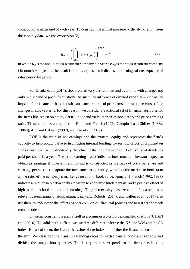
compounding at the end of each year. To construct the annual measure of the stock return from

the monthly data, we use expression (2)

𝑅it = (∏(1 + 𝑟𝑖,𝑚𝑡)

𝑁

𝑚,𝑡

)

1/12

− 1 (2)

in which Rit is the annual stock return for company i in year t, ri,mt is the stock return for company

i in month m in year t. The result from this expression indicates the earnings of the sequence of

rates period by period.

For Gharbi et al. (2014), stock returns vary across firms and over time with changes not

only in dividend or profit fluctuations. As such, the influence of omitted variables – such as the

impact of the financial characteristics and stock returns of peer firms – must be the cause of the

changes in stock returns. For this reason, we consider a traditional set of financial attributes for

the firms like return on equity (ROE), dividend yield, market-to-book ratio and price earnings

ratio. These variables are applied in Fama and French (1992), Campbell and Shiller (1988a,

1988b), Ang and Bekaert (2007), and Fan et al. (2012).

ROE is the ratio of net earnings and the owners’ equity and represents the firm’s

capacity to incorporate value to itself using internal funding. To test the effect of dividend on

stock return, we use the dividend yield which is the ratio between the dollar value of dividends

paid per share in a year. The price-earnings ratio indicates how much an investor expect to

obtain in earnings if invests in a firm and is constructed as the ratio of price per share and

earnings per share. To capture the investment opportunity, we select the market-to-book ratio

as the ratio of the company’s market value and its book value. Fama and French (1992, 1993)

indicate a relationship between this measure to economic fundamentals, and a positive effect of

high market-to-book ratio in high earnings. They also employ these economic fundamentals as

relevant determinants of stock return. Leary and Roberts (2014), and Cullen et al. (2014) also

use them to understand the effects of peer companies’ financial policies and to test for the stock

return models.

Financial constraint presents itself as a common factor influencing stock returns (CHAN

et al, 2010). To validate this effect, we use three different indexes: the KZ, the WW and the SA

index. For all of them, the higher the value of the index, the higher the financial constraint of

the firm. We classified the firms in ascending order for each financial constraint variable and

divided the sample into quantiles. The last quantile corresponds to the firms classified as

31

financial constrained, while the first one has the financial unconstrained ones. Lamont et al.

(2001) implement the KZ index following equation (3)

𝐾𝑍 = −1,00191 (𝐶𝐹

𝐾𝑡−1)

it

+ 0,28264𝑄 + 3,1392 (𝐷𝑒𝑏𝑡

𝑇𝐶)

it− 39,3678 (

𝐷𝑖𝑣

𝐾𝑡−1)

it

− 1,31476 (𝐶𝑎𝑠ℎ

𝐾𝑡−1)

it

(3)

where i is the firm and t is the year; CF is the cash flow; K is the fixed assets; Q is the Tobin’s

Q; Debt is the debt variable; TC is the total capital defined as the sum of debt and stockholders’

equity; Div is the dividends and Cash is the cash, defined as cash plus short-term investments.

The second financial constraints measure is the WW index from Whited and Wu (2006).

Its equation follows (4)

WWit = −0.091 (CF

TA)

it− 0.062Divit + 0.021 (

LTD

TA)

it− 0.044Sizeit + 0.102ISGit

− 0.035SGit

(4)

where i is the firm and t is the year; CF is the cash flow; TA is the total assets; Div is a dummy

for the dividend payment; LTD is the long-term debt; Size is the logarithm of the firm’s total

assets; ISG is the three-digit industry’s sales growth and SG is firm’s sales growth.

The third financial constraint index is the SA index (size and age) from Hadlock and

Pierce (2010) which is firm-specific and follows equation (5)

𝑆𝐴𝑖𝑡 = −0,737𝑆𝑖𝑧𝑒𝑖𝑡 + 0,043𝑆𝑖𝑧𝑒𝑖𝑡2 − 0,040𝐴𝑔𝑒𝑖𝑡 (5)

where Size is the logarithm of book assets and Age is the number of years in activity.

The next section provides the peer effect strategy we apply in this study and the

description of the peer groups considered here.

3.3 Peer effect strategy and the peer groups

The peer theory proposes the influence of characteristics and behavior of peers in the

performance of a person. For our purpose, we consider two companies as peers if they are from

the same peer group such as country, industry, stock market size and trade openness. Companies

in the same country undergo the same institutional condition as demand shocks, exchange rate

changes, purchasing power, interest rate and their spread to equity market. Arranging the

companies by country can provide evidences to recognize, for example, differences between

being in Brazilian’ stock market or being in the Japanese’ stock market since they present

contrasting economic and institutional fundamentals. Also, in emerging markets, the country

portfolio is an effect of the imperfect diversification problem since the investor does not have

the knowledge to choose the international diversification as a risk reduction strategy.

We also follow Chen and Ma (2017), Leary and Roberts (2014), and Adhikari and

Agrawal (2018) by considering the same industry as a socio-economic network measure. Since

we require at least two firms per industry, we use the two-digit NAICS (North American

Industry Classification System) classification to create the peer group for the industry. As

discussed before, industry can affect the results of the companies and their stock returns, and it

can also be used by individual investors as a reference group.

Also, as discussed in the literature chapter, trade linkage can transfer financial

disturbances among firms. Heathcote and Perri (2013) show that openness to trade increases

diversification for stock returns which indicates that countries relatively closed have a large

negative covariance between relative earnings and relative dividends. Moreover, they suggest

that, “if domestic stocks pay a relatively high return in states of the world in which domestic

goods are expensive, then since domestic residents may prefer to hold mostly domestic stocks”

(HEATHCOTE; PERRI, 2013, p. 1127).

Consequently, we consider the trade openness as a trade linkage and we create the

average ratio of total export and import to GDP per country from 2006 to 2016. Then, we divide

this average ratio in quantiles to separate the countries. The first group has countries with lower

trade openness like Brazil, Japan and United States while the higher trade openness group has

Canada, Germany, Mexico and United Kingdom. Note that these groups are not formed only

by emerging or developed markets.

Moreover, we select a proxy of the stock market size to identify the impact of the peer

firms from similar financial markets. The stock market capitalization to GDP is the ratio of the

stock market capitalization to the economic income for each year. We collect the data in the

World Bank Database and, to stablish a point of comparation for the peer groups, we construct

the average stock market size per country and separate the countries in quantiles. The smallest

average size has also the biggest number of countries for stock markets as well as it has either

developed or emerging countries like Brazil, China, Germany, Indonesia, Italy, Mexico,

33

Russian Federation and Turkey. On the other hand, the biggest stock markets’ size group has

firms from Canada and United States, two developed countries.

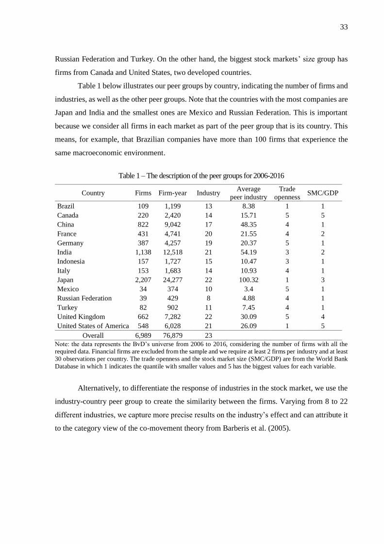
Table 1 below illustrates our peer groups by country, indicating the number of firms and

industries, as well as the other peer groups. Note that the countries with the most companies are

Japan and India and the smallest ones are Mexico and Russian Federation. This is important

because we consider all firms in each market as part of the peer group that is its country. This

means, for example, that Brazilian companies have more than 100 firms that experience the

same macroeconomic environment.

Table 1 – The description of the peer groups for 2006-2016

Country Firms Firm-year Industry Average

peer industry

Trade

openness SMC/GDP

Brazil 109 1,199 13 8.38 1 1

Canada 220 2,420 14 15.71 5 5

China 822 9,042 17 48.35 4 1

France 431 4,741 20 21.55 4 2

Germany 387 4,257 19 20.37 5 1

India 1,138 12,518 21 54.19 3 2

Indonesia 157 1,727 15 10.47 3 1

Italy 153 1,683 14 10.93 4 1

Japan 2,207 24,277 22 100.32 1 3

Mexico 34 374 10 3.4 5 1

Russian Federation 39 429 8 4.88 4 1

Turkey 82 902 11 7.45 4 1

United Kingdom 662 7,282 22 30.09 5 4

United States of America 548 6,028 21 26.09 1 5

Overall 6,989 76,879 23

Note: the data represents the BvD’s universe from 2006 to 2016, considering the number of firms with all the

required data. Financial firms are excluded from the sample and we require at least 2 firms per industry and at least

30 observations per country. The trade openness and the stock market size (SMC/GDP) are from the World Bank

Database in which 1 indicates the quantile with smaller values and 5 has the biggest values for each variable.

Alternatively, to differentiate the response of industries in the stock market, we use the

industry-country peer group to create the similarity between the firms. Varying from 8 to 22

different industries, we capture more precise results on the industry’s effect and can attribute it

to the category view of the co-movement theory from Barberis et al. (2005).

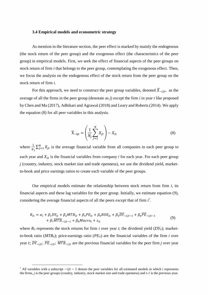
3.4 Empirical models and econometric strategy

As mention in the literature section, the peer effect is marked by mainly the endogenous

(the stock return of the peer group) and the exogenous effect (the characteristics of the peer

group) in empirical models. First, we seek the effect of financial aspects of the peer groups on

stock return of firm i that belongs to the peer group, contemplating the exogenous effect. Then,

we focus the analysis on the endogenous effect of the stock return from the peer group on the

stock return of firm i.

For this approach, we need to construct the peer group variables, denoted �̅�−𝑖𝑗𝑡, as the

average of all the firms in the peer group (denotate as j) except the firm i in year t like proposed

by Chen and Ma (2017), Adhikari and Agrawal (2018) and Leary and Roberts (2014). We apply

the equation (8) for all peer variables in this analysis.

X̅−ijt = (1

𝑁𝑗∑ 𝑋𝑗𝑡

𝑁

𝑗=1

) − 𝑋𝑖𝑡 (8)

where 1

𝑁𝑗∑ 𝑋𝑗𝑡

𝑁𝑗=1 is the average financial variable from all companies in each peer group to

each year and 𝑋𝑖𝑡 is the financial variables from company i for each year. For each peer group

j (country, industry, stock market size and trade openness), we use the dividend yield, market-

to-book and price earnings ratios to create each variable of the peer groups.

Our empirical models estimate the relationship between stock return from firm i, its

financial aspects and these lag variables for the peer group. Initially, we estimate equation (9),

considering the average financial aspects of all the peers except that of firm i7.

𝑅𝑖𝑡 = 𝛼𝑖 + 𝛽1𝐷𝑌𝑖𝑡 + 𝛽2𝑀𝑇𝐵𝑖𝑡 + 𝛽3𝑃𝐸𝑖𝑡 + 𝛽4𝑅𝑂𝐸𝑖𝑡 + 𝛽5𝐷𝑌̅̅ ̅̅−𝑖𝑗𝑡−1 + 𝛽6𝑃𝐸̅̅ ̅̅

−𝑖𝑗𝑡−1

+ 𝛽7𝑀𝑇𝐵̅̅ ̅̅ ̅̅ ̅−𝑖𝑗𝑡−1 + 𝛽8𝑀𝑎𝑐𝑟𝑜𝑡 + 𝜀𝑖𝑡

(9)

where Rit represents the stock returns for firm i over year t; the dividend yield (DYit); market-

to-book ratio (MTBit); price-earnings ratio (PEit) are the financial variables of the firm i over

year 𝑡; 𝐷𝑌̅̅ ̅̅−𝑖𝑗𝑡; 𝑃𝐸̅̅ ̅̅

−𝑖𝑗𝑡; 𝑀𝑇𝐵̅̅ ̅̅ ̅̅ ̅−𝑖𝑗𝑡 are the previous financial variables for the peer firm j over year

7 All variables with a subscript −𝑖𝑗𝑡 − 1 denote the peer variables for all estimated models in which i represents

the firms, j is the peer groups (country, industry, stock market size and trade openness) and t-1 is the previous year.

35

𝑡 − 1; 𝑀𝑎𝑐𝑟𝑜𝑡 are the variables dealing with macroeconomic aspects like GDP growth (GDPt)

and real interest rate (RIRt) over year t.

We follow this path because we believe that if a peer group has an increase in the

investment opportunity, for example, it can convey information for a firm’ stock return. Also,

some individual investors do not have all the information in the stock market and end up

comparing it with peer-to-peer information. Chen and Ma (2017) use the rival-based theory to

indicate that if a firm imitates others, it can alleviate the competitive pressure and reflect in its

stock return. Thus, if there is a change in a financial characteristic of a peer firm that impacts

on the same financial characteristic of the firm i, it can feedback in the stock return of the firm.

Lieberman and Asaba (2006) also suggest that this imitation preserve the status quo in

competition as an additional information.

For this part of the analysis, we apply fixed effects models which helps us understand

the effects from financial characteristics from firm i and its peers on stock return of firm i. We

also include each financial constraint index (KZ, WW, and SA indexes) and report them in

appendix. We separate the results in developed and emerging countries and select models using

the AIC information criteria.

The second part of our estimations focus on the relationship between stock return from

firm i and the stock return from the peer firm j over year t-1. This is the main point of our

analysis of peer effects and co-movement in stock return, also known as the endogenous effect

in the reflection problem. As pointed by Manski (1993), Leary and Roberts (2014) and many

other authors, if we simply apply equation (8) to construct the stock return of the peers, we will

create an endogeneity bias for the stock return.

One could believe that the reflection problem is not applied to asset pricing models since

it depends on the market interactions and any financial and economic news from firms and their

countries. However, since the stock return from the peer firm is, by construction, dependent

from the stock return of firm i, the endogenous problem must be considered in the regression

models. When there is an endogenous variable, the parameters estimate by fixed effect are

inconsistent, and the instrumental variable approach from the two-stage least square (2SLS) is

the appropriate tool after the seminal work of Leary and Roberts (2014).

For the IV model, consider equation (10) which allows for both endogenous peer effect

(due to stock return of the peer group) as well as exogenous peer effect (due to characteristics

of the peers) (CAMERON; TRIVEDI, 2005; WOOLDRIDGE, 2010; LEARY; ROBERTS,

2014; CHEN; MA, 2017). The stock return of peer firms’ parameter is 𝛽8 and measures the

influence of peer firms’ actions on the stock return. Notwithstanding, the parameters 𝛽5, 𝛽6, 𝛽7

correspond to the characteristics of the peer groups that indirectly provides a mechanism to

identify the feedback effect in the firms’ characteristics and the stock return.

𝑅𝑖𝑡 = 𝛼 + 𝛽1

𝐷𝑌𝑖𝑡 + 𝛽2

𝑀𝑇𝐵𝑖𝑡 + 𝛽3

𝑃𝐸𝑖𝑡 + 𝛽4

𝑅𝑂𝐸𝑖𝑡 + 𝛽5

𝐷𝑌̅̅ ̅̅ −𝑖𝑗𝑡−1 + 𝛽6

𝑃𝐸̅̅̅̅ −𝑖𝑗𝑡−1

+ 𝛽7

𝑀𝑇𝐵̅̅ ̅̅ ̅̅ −𝑖𝑗𝑡−1 + 𝛽8�̅�−𝑖𝑗𝑡−1 + 𝜀𝑖𝑡 (10)

where Rit represents the stock returns for firm i over year t; the dividend yield (DYit); market-

to-book ratio (MTBit); price-earnings ratio (PEit) are the fundamentals of the firm i;

𝐷𝑌̅̅ ̅̅−𝑖𝑗𝑡; 𝑃𝐸̅̅ ̅̅

−𝑖𝑗𝑡; 𝑀𝑇𝐵̅̅ ̅̅ ̅̅ ̅−𝑖𝑗𝑡 are the fundamentals for the peer firm j over year 𝑡 − 1; 𝑀𝑎𝑐𝑟𝑜𝑡 are

the variables dealing with macroeconomic aspects like GDP growth (GDPt) and real interest

rate (RIRt) in year t; and �̅�−𝑖𝑗𝑡−1 is the stock return for the peer firm j over year 𝑡 − 1.

Our identification problem lies in the fact that �̅�−𝑖𝑗𝑡−1, the stock return of the peer firms,

depends on the stock return of a firm. Manski (1993, 2000) and Leary and Roberts (2014)

describe the identification problem for all parameters in which there is an instantaneous

feedback from Rit and, therefore, jointly dependence among Rit and �̅�−𝑖𝑗𝑡−1. Thus, the structural

parameters on equation (10) are not identified because of the simultaneity problem. The solution

we find is to follow Leary and Roberts (2014) and any other author that applied the peer effect

theory in financial data.

With an augmented asset pricing model like Leary and Roberts (2014), we compute the

idiosyncratic return of this model as our instrumental variable for the stock return of the peer

groups. To construct the instrumental variable for the annual stock return of peer firms, our first

stage consists in using monthly stock prices from 2006 to 2016 to compute the idiosyncratic

stock return from equation (11) for each firm on a rolling annual basis.

�̂�𝑖𝑗𝑡 = �̂�𝑖𝑗𝑡 + �̂�𝑖𝑗𝑡𝑃𝑒𝑒𝑟(�̅�−𝑖𝑗𝑡 − 𝑅𝑓𝑡) + �̂�𝑖𝑗𝑡

𝑀 (𝑅𝑚𝑡 − 𝑅𝑓𝑡)

�̂�𝑖𝑗𝑡 = 𝑅𝑖𝑗𝑡 − �̂�𝑖𝑗𝑡 (11)

where �̂�𝑖𝑗𝑡 is the expected return from firm i in peer group j from month t; (𝑅𝑚𝑡 − 𝑅𝑓𝑡) is the

excess market return and (�̅�−𝑖𝑗𝑡 − 𝑅𝑓𝑡) is the excess return on an industry portfolio excluding

firm i’s return; �̂�𝑖𝑗𝑡 is the idiosyncratic return from firm i in peer group j from month t.

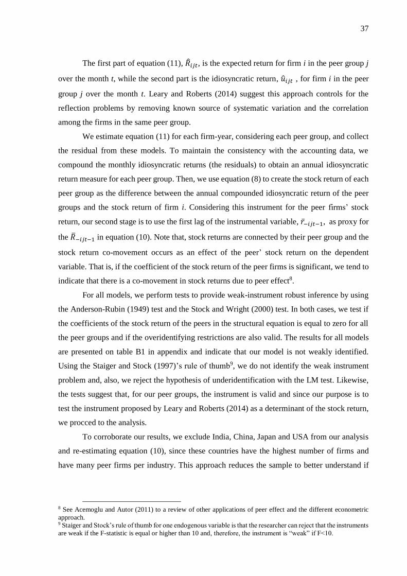
37

The first part of equation (11), �̂�𝑖𝑗𝑡, is the expected return for firm i in the peer group j

over the month t, while the second part is the idiosyncratic return, �̂�𝑖𝑗𝑡 , for firm i in the peer

group j over the month t. Leary and Roberts (2014) suggest this approach controls for the

reflection problems by removing known source of systematic variation and the correlation

among the firms in the same peer group.

We estimate equation (11) for each firm-year, considering each peer group, and collect

the residual from these models. To maintain the consistency with the accounting data, we

compound the monthly idiosyncratic returns (the residuals) to obtain an annual idiosyncratic

return measure for each peer group. Then, we use equation (8) to create the stock return of each

peer group as the difference between the annual compounded idiosyncratic return of the peer

groups and the stock return of firm i. Considering this instrument for the peer firms’ stock

return, our second stage is to use the first lag of the instrumental variable, �̅�−𝑖𝑗𝑡−1, as proxy for

the �̅�−𝑖𝑗𝑡−1 in equation (10). Note that, stock returns are connected by their peer group and the

stock return co-movement occurs as an effect of the peer’ stock return on the dependent

variable. That is, if the coefficient of the stock return of the peer firms is significant, we tend to

indicate that there is a co-movement in stock returns due to peer effect8.

For all models, we perform tests to provide weak-instrument robust inference by using

the Anderson-Rubin (1949) test and the Stock and Wright (2000) test. In both cases, we test if

the coefficients of the stock return of the peers in the structural equation is equal to zero for all

the peer groups and if the overidentifying restrictions are also valid. The results for all models

are presented on table B1 in appendix and indicate that our model is not weakly identified.

Using the Staiger and Stock (1997)’s rule of thumb9, we do not identify the weak instrument

problem and, also, we reject the hypothesis of underidentification with the LM test. Likewise,

the tests suggest that, for our peer groups, the instrument is valid and since our purpose is to

test the instrument proposed by Leary and Roberts (2014) as a determinant of the stock return,

we procced to the analysis.

To corroborate our results, we exclude India, China, Japan and USA from our analysis

and re-estimating equation (10), since these countries have the highest number of firms and

have many peer firms per industry. This approach reduces the sample to better understand if

8 See Acemoglu and Autor (2011) to a review of other applications of peer effect and the different econometric

approach. 9 Staiger and Stock’s rule of thumb for one endogenous variable is that the researcher can reject that the instruments

are weak if the F-statistic is equal or higher than 10 and, therefore, the instrument is “weak” if F<10.

the results are related to these countries. Secondly, we explore the importance of these four

countries for the determinants of the asset price models with peer effect from the industry group.

The next chapter summarizes the empirical results of the peer effects of the stock returns

models considering the reflection problem. We describe the mainly effects and related them to

the stock return theory and the peer effect theory. Also, we test for robustness in the next

chapter.

39

4 PEER EFFECTS IN STOCK RETURN: RESULTS

This chapter presents the empirical evidences for the peer effects in stock return. In

Section 4.1, we analyze the descriptive statistics and estimate the peer effects from the financial

characteristics and the stock return from firm i in Section 4.2. After that, section 4.3 checks the

relationship between the stock return of firm i and the stock return from the peer firm,

identifying the reflection problem and the instrumental variable. In Section 4.4, we provide the

results of the robustness tests.

4.1 Peer effects and the sample analysis

The use of peer effect theory in corporate finance is recent and, to the best of our

knowledge, there is no paper that analyze the peer effect on asset pricing models. In this section,

we present the sample analysis separating it in developed and emerging economies.

Initially, graph 1 below illustrates the firms’ average stock returns for the emerging and

developed countries from 2006 to 2016 using data from Work Bank (2018). There is a clear

difference between them since the developed countries present stock returns with smoothly

peaks and valleys compared to the emerging ones. Before the Great Recession of 2008, the

average stock returns in emerging markets offer more than seven times the returns in the

developed ones, but the financial crisis brought their stock returns closer to a new lower level

after 2010. Considering the Brazilian economy as an example for the emerging countries, it is

interesting that, up until 2013, the Brazilian average stock returns had a similar behavior to the

emerging markets. However, the political instability and subsequent economic crisis in Brazil

from 2014 forward seems to have negatively impacted its stock market performance.

Source: World Bank (2018)

Graph 1 – Average stock return from 2006 to 2016

In this context, table 2 presents summary statistics from all the variables in three panels.

Panel A outlines the average firm-specific characteristics, while panel B cover the average peer

firm-specific attributes for all the peer groups. The average peer firm-specific attributes are

constructed as the average of all firms in a peer group except for the firm i as illustrated in the

previous chapter. Panel C focus on the two macroeconomic variables, real interest rate and GDP

growth.

In general, the average firm-specific characteristics are higher in emerging markets

compared to developed countries. This happens primarily in the positive annual stock returns

in the emerging markets which corroborates the findings from graph 1: developed countries

have smoothly and lower stock returns while the emerging markets have almost four times

greater stock returns. The average stock return for the emerging economies is 0,45%, while the

developed countries have a negative one (-0,23%).

Traditionally, the researchers use the market-to-book (MTB), the price-earnings (P/E)

ratios and the dividend yield (DY) as determinants for the valuation of stock returns (FAMA;

FRENCH, 1992, 2015; AVRAMOV, 2004). The MTB ratio shows the market’s perception of

the stock’s value, the P/E ratio reflects the expected earnings growth and the DY expresses the

dividend-only return of a stock. The typical emerging stock market has higher average ratios

than the developed ones possibly for the prospect of diversification in international markets.

41

Table 2 – Summary statistics for the emerging and develop countries

Emerging Developed

Obs. Mean Std. Dev. Obs. Mean Std. Dev.

Panel A: Firm-specific characteristics

Stock return (%) 24,804 0.450 5.728 49,396 -0.231 3.904

MTB ratio 23,020 2.132 3.314 41,006 1.705 2.782

PE ratio 16,259 38.014 68.895 28,346 25.815 43.115

Dividend Yield (%) 11,723 3.479 4.779 27,597 2.839 2.735

ROE 19,368 4.919 28.567 38,802 0.155 35.005

Financial constraint (KZ) 16,005 0.538 0.498 30,163 0.558 0.497

Financial constraint (WW) 8,597 0.292 0.455 21,537 0.295 0.456

Financial constraint (SA) 14,103 0.271 0.444 33,156 0.163 0.369

Panel B: Peer-firm characteristics

Peer: Country

MTB ratio 26,118 0.324 2.546 50,688 0.320 2.002

PE ratio 21,429 9.184 50.800 41,472 8.199 31.874

DY 25,688 1.866 2.925 50,468 1.658 2.456

Stock return (%) 24,804 -0.443 5.728 49,396 0.232 3.903

Peer: Industry

MTB ratio 25,359 0.296 2.535 49,278 0.353 2.057

PE ratio 21,335 9.224 50.536 41,410 9.390 32.229

DY 24,248 1.692 2.917 47,390 1.425 2.360

Stock return (%) 24,804 -0.478 5.720 49,396 0.185 3.886

Peer: Trade openness

MTB ratio 26,191 0.162 2.527 50,688 0.376 1.990

PE ratio 21,429 5.906 51.191 41,472 10.342 32.851

DY 26,191 1.699 2.760 50,688 1.745 2.275

Stock return (%) 26,059 -0.150 5.401 50,402 0.428 3.845

Peer: SMC

MTB ratio 26,191 0.183 2.489 50,688 0.342 1.990

PE ratio 21,429 6.778 51.671 41,472 9.845 32.647

DY 26,191 2.113 2.764 50,688 1.584 2.407

Stock return (%) 24,804 -0.468 5.717 49,396 0.195 3.888

Panel C: Macroeconomic Variables

Real interest rate (%) 25,289 4.764 6.896 49,364 2.232 1.876

GDP growth (%) 26,191 7.536 2.956 50,688 0.922 2.143

Note: all the peer variables for company i are the mean of the financial characteristics of the peer group except for

the firm i observation. Financial firms are excluded from the sample and we require at least 2 firms per industry

and at least 30 observations per country.

In panel B, we identify the peer-specific characteristics for four peer groups and to help

understand the summary statistics, some insights are provided. First, the country peer group

aggregates the institutional environment and the macroeconomic factors like mentioned by Fan

et al. (2012), and Francis et al. (2016). Also, it is a simple aggregation point for the individual

investor that does not understand the benefits of the international diversification portfolios. On

the other hand, there is a potential of financial contagion through international trade which is

the motivation for the trade openness’ peer group (JING et al., 2017; FUJI, 2017) when

considering that investors will opt for diversified portfolios. Moreover, the stock markets can

transmit shocks from different financial markets depending on its size (DIEBOLD; YILMAZ,

2015). Notwithstanding these relevant situations, Leary and Roberts (2014) and Hou (2007)

argue that the industry has an important on diffusion of market information, leading to clear

insights in the market competition.

Considering this information and the construction of these variables, we interpret the

presence of a positive average variable as a higher value for the peer group, while the negative

average indicates that, on average, the results of the considered variable is higher in the

company i than the peer group. We find similar average financial characteristics for country

and industry peer groups in emerging markets, except for stock returns. That is, on average, the

stock return for the peer groups is negative for emerging market but positive for developed

ones.

Thus, the peer groups have higher average stock returns in emerging markets, while the

opposite result occurs in developed countries. Moreover, the stock return of the peer firms is

almost three times higher in the industry peer group and double in the country peer group. For

all other variables, the mean values are similar for these peer groups. Alternatively, the trade

openness and stock market size have higher market-to-book and P/E ratio for the developed

economies as well as opposite average stock returns10.

In panel C, we report the summary statistics for GDP growth and real interest rate. The

average real interest rates in emerging economies are double the rates applied in developed

countries as the first ones are riskier and, therefore, need to adequately remunerate their

investors. In emerging countries, the GDP growth rate is more than eight times higher than the

ones from the developed markets, especially led by the average GDP growth of China, India

and Indonesia reported in table A.3 in appendix.

10 Note that the average stock return of the peers shows, for example, the stock return of the companies that are in

the same industry, except for one firm. By separating this variable in emerging and developed countries, the

average stock return of the peers denotes that, on average, the companies in the same industry of an emerging

market have a -0.48% stock return for the period.

43

4.2 Peer effects from the financial characteristics and the traditional econometrics

In the peer effects literature, the reflection problem has two different important effects:

(i) the exogenous peer effect due to peer characteristics, and (ii) the endogenous peer effect due

to stock return from peer firms. In this section, we present the results for the exogenous peer

effect due to characteristics of the peer groups. We use fixed-effect models of stock return from

firm i, the financial characteristics of the firm and their peers.

Here, the stock return of the firm is driven by a response to their peers’ characteristics

rather than stock return behavior since changes in the characteristics of their peers influence the

imitation behavior of them. Lieberman and Asaba (2006) find evidences that firms use the

imitation channel as useful information from the peers and, thus, create a spillover effect in the

decision process of other. For all models in this section, we apply equation (9) for the four peer

groups reproduced here

𝑅𝑖𝑡 = 𝛼𝑖 + 𝛽1𝐷𝑌𝑖𝑡 + 𝛽2𝑀𝑇𝐵𝑖𝑡 + 𝛽3𝑃𝐸𝑖𝑡 + 𝛽4𝑅𝑂𝐸𝑖𝑡 + 𝛽5𝐷𝑌̅̅ ̅̅−𝑖𝑗𝑡−1 + 𝛽6𝑃𝐸̅̅ ̅̅

−𝑖𝑗𝑡−1

+ 𝛽7𝑀𝑇𝐵̅̅ ̅̅ ̅̅ ̅−𝑖𝑗𝑡−1 + 𝛽8𝑀𝑎𝑐𝑟𝑜𝑡 + 𝜀𝑖𝑡

(9)

We use the lagged financial peer variables and the contemporaneous financial variables

for the firm i to address the imitation concern and the possible effect that changes in the lagged

peers’ characteristics have in the contemporaneous firm-specific variables. Note that each peer

variable is the average from all the firms in the peer groups minus the information from firm i

per year. It is important to emphasize that the idea is to verify if changes in the characteristics

of the peers can affect the stock return of company i, which could lead to an imitation strategy

between firms in the same peer group.

Initially, table 3 presents the results for the stock return and the firm-specific

characteristics regression using fixed effect models, without the peer groups. In general, we

find a positive and statistically significance effect from market-to-book (MTB) ratio, price-

earning (P/E) ratio and the return on equity (ROE). The difference between emerging and

developed countries is the magnitude of the effect that is greater for the former markets. Fama

and French (1988, 1992, 2017), Leary and Roberts (2014) and Phan et al. (2015) argue that

there are evidences of the importance of these financial ratios for the prediction of stock returns

because they have information content that is useful in the stock market. Maio and Santa-Clara

(2015) also agree that these financial ratios can help predict stock return and it cannot occur

exclusively with one financial ratio. Moreover, we find a weakly and negatively correlation

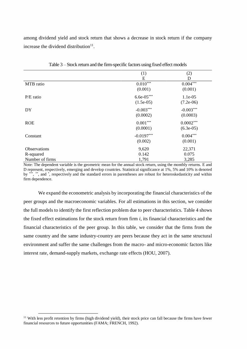
among dividend yield and stock return that shows a decrease in stock return if the company

increase the dividend distribution11.

Table 3 – Stock return and the firm-specific factors using fixed effect models

(1) (2) E D

MTB ratio 0.010*** 0.004***

(0.001) (0.001)

P/E ratio 6.6e-05*** 1.1e-05

(1.5e-05) (7.2e-06)

DY -0.003*** -0.003***

(0.0002) (0.0003)

ROE 0.001*** 0.0002***

(0.0001) (6.3e-05)

Constant -0.0197*** 0.004***

(0.002) (0.001)

Observations 9,620 22,371

R-squared 0.142 0.075

Number of firms 1,791 3,285 Note: The dependent variable is the geometric mean for the annual stock return, using the monthly returns. E and

D represent, respectively, emerging and develop countries. Statistical significance at 1%, 5% and 10% is denoted

by ***, **, and *, respectively and the standard errors in parentheses are robust for heteroskedasticity and within

firm dependence.

We expand the econometric analysis by incorporating the financial characteristics of the

peer groups and the macroeconomic variables. For all estimations in this section, we consider

the full models to identify the first reflection problem due to peer characteristics. Table 4 shows

the fixed effect estimations for the stock return from firm i, its financial characteristics and the

financial characteristics of the peer group. In this table, we consider that the firms from the

same country and the same industry-country are peers because they act in the same structural

environment and suffer the same challenges from the macro- and micro-economic factors like

interest rate, demand-supply markets, exchange rate effects (HOU, 2007).

11 With less profit retention by firms (high dividend yield), their stock price can fall because the firms have fewer

financial resources to future opportunities (FAMA; FRENCH, 1992).

45

Table 4 – Estimated fixed effect models for stock return using Country and Industry as peer groups

(2006-2016)

(1) (2) (3) (4)

E D E D

Firm-specific factors

MTB ratio 0.007*** 0.006*** 0.007*** 0.005***

(0.0007) (0.009) (0.0007) (0.0007)

P/E ratio 3.3e-05** 1.9e-05*** 3.9e-05*** 1.6e-05**

(1.3e-05) (7.2e-06) (1.3e-05) (7.3e-06)

DY -0.0007*** -0.002*** -0.0007*** -0.002***

(0.0002) (0.0003) (0.0002) (0.0003)

ROE 0.0014*** 0.0008*** 0.0014*** 0.0007***

(0.0001) (6.7e-05) (0.0001) (6.5e-05)

Real interest 0.724*** 0.25*** 0.725*** 0.23***

(0.023) (0.013) (0.022) (0.013)

GDP growth 0.763*** -0.058*** 0.79*** -0.06***

(0.04) (0.009) (0.04) (0.009)

Peer factors

Coun MTBt-1 0.01*** 0.008***

(0.0007) (0.0009)

Coun PE t-1 -9.5e-06 -3.6e-06

(1.4e-05) (7.3e-06)

Coun DY t-1 9.7e-05 -0.0004*

(0.0002) (0.0002)

Ind: MTB t-1 0.01*** 0.006***

(0.0007) (0.0007)

Ind: PE t-1 -7.5e-06 1.9e-06

(1.4e-05) (7.3e-06)

Ind: DY t-1 0.0002 -0.0002

(0.0002) (0.0002)

Constant -0.11*** -0.008*** -0.106*** -0.006***

(0.004) (0.002) (0.004) (0.002)

Obs. 8,392 19,802 8,373 19,788

R-squared 0.342 0.122 0.333 0.099

N. firms 1,727 3,229 1,723 3,227

AIC -33395 -97453 -33214 -96877 Note: the dependent variable is the geometric mean for the annual stock return, using the monthly returns. All the

peer variables for company i are the mean of all the financial characteristics of the reference group except for the

firm i. Financial firms are excluded from the sample and we require at least 2 firms per industry and at least 30

observations per country. Statistical significance at 1%, 5% and 10% is denoted by ***, **, and *, respectively and

the standard errors in parentheses are robust for heteroskedasticity and within industry-country dependence.

Models (1) and (2) show the relationship between stock return of firm i and the financial

variables for the peers in the same country for emerging and developed countries, respectively.

In general, the models provide a small positive impact of these variables in stock return for

emerging and developed countries. To illustrate, an increase in the market-to-book ratio from

the peers that are in the same industry will increase the stock return from firm i in 1% and 0.6%,

respectively for emerging and developed countries. For the companies in the same country, we

can say that if the investment opportunity increases in one point, the stock return of company i

is 1% higher for the emerging markets and 0.8% higher for the developed countries. Thus, for

either emerging or developed economies, only the investment opportunity is statistically

significant for the analysis of the country and industry peer groups.

By analyzing the firm-specific factors for these two peer groups, we find the impact of

the firm’s own characteristics and imitation of the peers’ attributes on stock return from firm i.

Despite the small coefficients, in emerging markets, we find similar effects of firms’ own future

opportunities (MTB ratio, 0.7% higher) on the stock return for emerging and developed

countries. That is, if the opportunities for a specific industry increase, all the companies in it

will benefit if they imitate the industry by reduce the uncertainty of their environment

(LIEBERMAN; ASABA, 2006). This imitation can increase the stock return of a firm and can

suggest a co-movement of the characteristics that can lead to a spillover from the peer firms to

the stock return of the firm i as proposed by Leary and Roberts (2014) and Gong and Weng

(2016)12.

We assume that characteristics of the peers are observable and will prompt the decisions

of firm i since the firms extract information from the observation of the chosen characteristics

of peer firms. Moreover, these results indicate that firms pay attention to their peers’ financial

characteristics to reduce the decision’s risk and to increase their stock return (CHEN; MA,

2017). Contrarily, the listed companies of the emerging economies have a negative correlation

with their own dividend yield (-0.07%) which suggests that a change in the dividend policy can

indicate to the market that, overall, the firm will have lower future returns through the decline

in existing investment resources. For the developed economies, this dividend yield effect is

higher (-0.2%), indicating that this variable has different effects in stock return.

Lastly, for the real interest rate and the GPD growth, the results show that firms with

better investment opportunities in the past influence the increase of the stock return of company

i in the same country as well as the same industry. In summary, real interest rate and GPD

growth present a strongly positive effect on stock return from firm i when in emerging

economies which can relate to the impact of institutional environment on financial indicators

and the stock return.

12 Also, the stock returns within each market reflect the individual condition (business) or an economic effect.

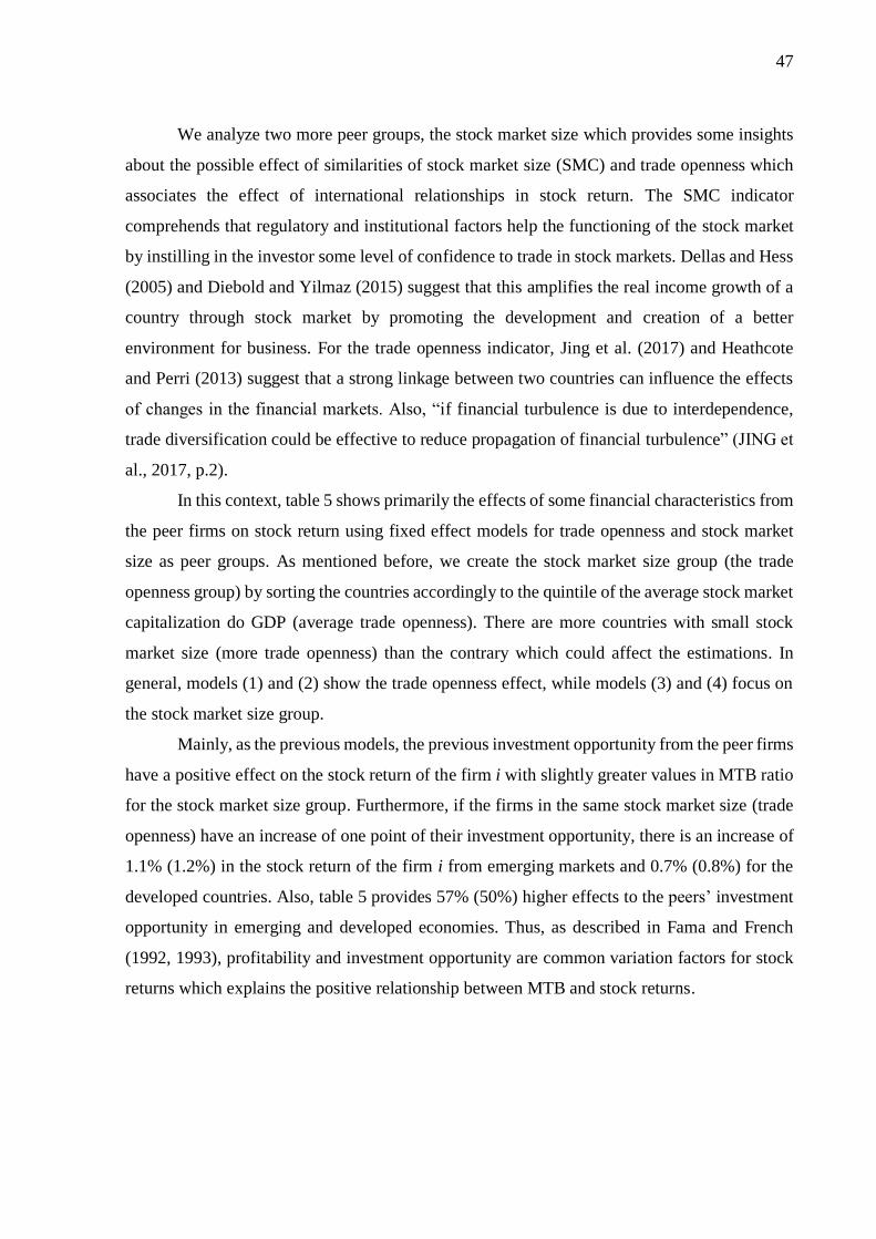
47

We analyze two more peer groups, the stock market size which provides some insights

about the possible effect of similarities of stock market size (SMC) and trade openness which

associates the effect of international relationships in stock return. The SMC indicator

comprehends that regulatory and institutional factors help the functioning of the stock market

by instilling in the investor some level of confidence to trade in stock markets. Dellas and Hess

(2005) and Diebold and Yilmaz (2015) suggest that this amplifies the real income growth of a

country through stock market by promoting the development and creation of a better

environment for business. For the trade openness indicator, Jing et al. (2017) and Heathcote

and Perri (2013) suggest that a strong linkage between two countries can influence the effects

of changes in the financial markets. Also, “if financial turbulence is due to interdependence,

trade diversification could be effective to reduce propagation of financial turbulence” (JING et

al., 2017, p.2).

In this context, table 5 shows primarily the effects of some financial characteristics from

the peer firms on stock return using fixed effect models for trade openness and stock market

size as peer groups. As mentioned before, we create the stock market size group (the trade

openness group) by sorting the countries accordingly to the quintile of the average stock market

capitalization do GDP (average trade openness). There are more countries with small stock

market size (more trade openness) than the contrary which could affect the estimations. In

general, models (1) and (2) show the trade openness effect, while models (3) and (4) focus on

the stock market size group.

Mainly, as the previous models, the previous investment opportunity from the peer firms

have a positive effect on the stock return of the firm i with slightly greater values in MTB ratio

for the stock market size group. Furthermore, if the firms in the same stock market size (trade

openness) have an increase of one point of their investment opportunity, there is an increase of

1.1% (1.2%) in the stock return of the firm i from emerging markets and 0.7% (0.8%) for the

developed countries. Also, table 5 provides 57% (50%) higher effects to the peers’ investment

opportunity in emerging and developed economies. Thus, as described in Fama and French

(1992, 1993), profitability and investment opportunity are common variation factors for stock

returns which explains the positive relationship between MTB and stock returns.

Table 5 – Estimated fixed effect models for stock market and financial characteristic using trade

openness and stock market size as the peer groups – 2006 to 2016

(1) (2) (3) (4)

E D E D

Firm-specific factors

MTB ratio 0.008*** 0.006*** 0.008*** 0.006***

(0.0007) (0.0008) (0.0007) (0.0008)

P/E ratio 3.2e-05** 1.8e-05** 3.0e-05** 1.8e-05**

(1.3e-05) (7.3e-06) (1.3e-05) (7.2e-06)

DY -0.0007*** -0.002*** -0.0007*** -0.002***

(0.0002) (0.0003) (0.0002) (0.0003)

ROE 0.0014*** 0.0008*** 0.0014*** 0.0008***

(0.0001) (6.6e-05) (0.0001) (6.7e-05)

Real interest 0.694*** 0.237*** 0.679*** 0.249***

(0.021) (0.0128) (0.022) (0.013)

GDP growth 0.78*** -0.065*** 0.749*** -0.067***

(0.04) (0.009) (0.039) (0.009)

Peer factors

Trade: MTBt-1 0.011*** 0.007***

(0.0008) (0.0009)

Trade: PE t-1 -2.2e-06 -4.3e-06

(1.4e-05) (7.2e-06)

Trade: DY t-1 -5.9e-05 -0.00034

(0.0002) (0.0002)

SMC: MTBt-1 0.012*** 0.008***

(0.0007) (0.0009)

SMC: PE t-1 -1.1e-05 -4.7e-07

(1.4e-05) (7.2e-06)

SMC: DY t-1 -1.8e-05 -0.0005**

(0.0002) (0.0002)

Constant -0.104*** -0.008*** -0.102*** -0.008***

(0.003) (0.002) (0.004) (0.002)

Obs. 8,392 19,802 8,392 19,802

R-squared 0.367 0.112 0.367 0.118

N. firms 1,727 3,229 1,727 3,229

AIC -33720 -97220 -33723 -97344 Note: the dependent variable is the geometric mean for the annual stock return, using the monthly returns. All the

peer variables for company i are the mean of all the financial characteristics of the reference group except for the

firm i. Financial firms are excluded from the sample and we require at least 2 firms per industry and at least 30

observations per country. Statistical significance at 1%, 5% and 10% is denoted by ***, **, and *, respectively and

the standard errors in parentheses are robust for heteroskedasticity and within industry-country dependence.

Note that the firm-specific factors maintain the same structure as the industry and

country peers with a positive future opportunity to invest, while the dividend yield is negative

correlated to stock returns. It should also be noted that the values of the firm-specific

characteristics in table 5 are like those found in table 4, for both emerging and developed

49

countries. In this case, knowing the size of the stock market (or the trade openness) is a tool for

deciding which stocks should compose an international portfolio based on stock market size (or

real international interaction). We believe that the stock market size allows investors to

understand that smaller markets can grow faster although the larger markets bring more stability

to the investor (AGHION et al., 2004).

Depending on the stock market, the investor must consider the peer effects of the

financial characteristics on the stock return to increase its gains by a spillover effect. A spillover

effect shows the importance of the co-movement in characteristics to the stock return as

Barberis et al. (2005) suggest for the categorization of the equities. By separating the peers in

stock market size, the investor follows the category view of Barberis et al. (2005) since it does

not have a relationship with fundamentals information of the peers. Thus, since the size of the

stock market does not relate to the individual characteristics of the firms, it can lead to a

mimicking strategy to have better gains in the stock market. Moreover, for stock market size,

we find that the individual characteristics have an important role as a determinant of the stock

return. Additionally, since “trade can transfer financial turbulence through competition and

bilateral trade”, we suggest that this is an important linkage between countries and can easily

be made by the individual investors (JING et al., 2017, p.4). Incorporating the macroeconomic

factors do not bristly change the effects already provided by the country and industry peer

groups.

Lastly, we also test for all the financial constraint indexes to see if there is a difference

between the firms with problems obtaining external resources in emerging markets and

developed countries. In appendix A, we report tables A.3, A.4 and A.5 with the results for the

fixed effect models with the peer characteristics considering the KZ index, the WW index and

the SA index, respectively. For these tables, we show the full model for all the peer groups and

the results do not deviate from the previous ones. It seems the estimations are consistent for

financial constrained firms and a co-movement between stock returns and financial

characteristics. Moreover, there is a negative effect from the KZ and the SA indexes and a

positive one from the WW index in emerging markets.

In summary, we identify the exogenous effect for the investment opportunity from the

peer firms, mainly for the emerging markets. Thus, it is important to understand the nuances of

the peer firms in order to achieve better stock returns and to also determine if the imitation of

the peer’s characteristics improves the quality of the firms. In the next section, we describe the

endogenous peer effect from the stock return of the peers by using an instrumented 2SLS

estimation to surpass the reflection problem.

4.3 Peer effects from the stock returns and the instrumental variable estimation

The motivation for this section is to analyze the second part of the reflection problem:

the peer effect due to endogenous variable (the stock return of the peer firms). Since the peer

stock return is the average of the stock return of the peer group minus the stock return from

firm i, by construction, our model has an endogenous variable. This was discussed extensively

by Manski (1993, 2000) as well as Leary and Roberts (2014), Francis et al. (2016), Chen and

Ma (2017), Adhikari and Agrawal (2018). For our estimation purpose, the instrumental variable

provides a general solution by requiring a relationship between the instrument and the

endogenous variable (WOOLDRIGDE, 2010; CAMERON; TRIVEDI, 2005).

Clearly, the endogeneity problem arises from use of the average stock return from the

peers except for the firm i as an explanatory variable (the 𝛽8�̅�−𝑖𝑗𝑡) in the equation (10)

reproduced again here

𝑅𝑖𝑡 = 𝛽1

𝐷𝑌𝑖𝑡 + 𝛽2

𝑀𝑇𝐵𝑖𝑡 + 𝛽3

𝑃𝐸𝑖𝑡 + 𝛽4

𝑅𝑂𝐸𝑖𝑡 + 𝛽5

𝐷𝑌̅̅ ̅̅ −𝑖𝑗𝑡−1 + 𝛽6

𝑃𝐸̅̅̅̅ −𝑖𝑗𝑡−1

+ 𝛽7

𝑀𝑇𝐵̅̅ ̅̅ ̅̅ −𝑖𝑗𝑡−1 + 𝛽8�̅�−𝑖𝑗𝑡−1 + 𝜀𝑖𝑡 (10)

For each firm in a peer group, the stock return of firm i depends on the stock return of

the peer firms, creating a simultaneity problem that requires this instrumental variable approach.

To follow the pattern in literature, we apply the procedure from Leary and Roberts (2014) to

our analysis and estimate the 2SLS version of the peer stock return model. The construction of

the instrumental variable is described in the methodological chapter. As Leary and Roberts

(2014), we require a non-zero average peer firm stock return from the equation (11).

Our main goal is to examine if the interaction among firms and their peers has any

impact on the stock return since valuing the stock price of peer firms can capture useful

information that can reduce the uncertainty for the investor. Examining a peer group involves

the inclusion of firms with similar characteristics that will behave in the same manner within

their markets. Moreover, the peer effect theory advises that the peer group creates a linkage

among individual financial decisions that can lead to a “keeping up with the Joneses” effect as

Bursztyn et al. (2014) proposed. Therefore, this section differentiates from the former by

incorporating the endogeneity problem from not know how the stock return of the peer groups

will affect the outcome of the firm (MANSKI, 1993).

The endogeneity due to the stock return of the peer firms can shed some light in the

imitation behavior as a strategy to reduce uncertainties for the investor and the firm. We follow

51

the same approach as the section before by using the first lag of the instrumental variable for

the stock return of the peers. Maintaining the pattern in the previous section, we analyze country

and industry first and then trade openness and stock market size as the peer groups.

Table 6 presents the estimated 2SLS models for stock return from firm i with the country

and industry as the peer groups. These models offer evidences of both reflection problems: the

endogenous and the exogenous effects. Initially, the financial characteristics of the firms in the

same country or industry has an important role in the stock return of the emerging markets’

companies, especially for the lagged market-to-book ratio of the peers which enhances between

0.2% to 0.6% the stock return. For the dividend yield, the results indicate that emerging and

developed countries have the same impact for the two peer groups. This variable is frequently

used as an instrument for price- and time-risk since many applications in asset pricing assume

that the dividend yield represents the expected stock returns and is linked to stock return

predictability like proposed by Maio and Santa-Clara (2015), Campbell and Shiller (1988a, b),

Cochrane (2011).

Also, we identify that MTB and P/E ratios in emerging markets have the same sign from,

but higher values than, its counterparts from the firm specific variables for developed

economies. Apparently, knowing the characteristics of the industry in these countries offers

useful information for the firm’s decisions and can help identify if mimicking the characteristics

will reduce the firm’s risk like proposed by Chen and Ma (2017). Also, it seems that the MTB

ratio can reflect an institutional aspect for the firms and the co-movement of characteristics like

Daniel and Titman (1997) proposed which can be related to the firms in the same country.

Similarly, since the MTB ratio allows identifying the future perspectives for the industry

or the country, it is not surprisingly that an increase of one point in it can lead to an increase

that varies from 0.5% to 0.8% on the stock return. In this aspect, the firm specific MTB ratio

has an even higher effect on the stock return than the peers’ counterpart especially for the

emerging markets.

Moreover, when analyzing the peer factors and their effects on the stock return, we find

some interesting facts. First, the stock return of the peer firms from the same industry has a

positive and significant effect in emerging and developed economies. Note that the peer effect

of the stock return in emerging markets (1.15%) are triple the developed countries (0.41%).

Firms in the same industry have a significantly influential to stock return, especially in

emerging markets.

Table 6 – Estimations of the IV models for stock return and the peer factors for emerging and developed

countries using Country and Industry as the peer groups – 2006 to 2016

(1) (2) (3) (4)

E D E D

Firm-specific factor

MTB ratio 0.008*** 0.006*** 0.007*** 0.005***

(0.0006) (0.0007) (0.0007) (0.0006)

P/E ratio 3.9e-05*** 1.4e-05** 4.6e-05*** 1.3e-05*

(1.4e-05) (7.0e-06) (1.6e-05) (7.1e-06)

DY -0.001*** -0.002*** -0.001*** -0.002***

(0.0002) (0.0002) (0.0002) (0.0002)

ROE 0.002*** 0.001*** 0.002*** 0.00094***

(0.0001) (6.2e-05) (0.0002) (6.1e-05)

Real interest 0.685*** 0.28*** 0.695*** 0.256***

(0.02) (0.014) (0.025) (0.013)

GDP growth 0.83*** -0.091*** 0.764*** -0.087***

(0.04) (0.008) (0.046) (0.008)

Peer factors

Coun SRt-1 0.954*** 0.369***

(0.03) (0.012)

Coun MTB t-1 0.003*** 0.006***

(0.0007) (0.0007)

Coun PE t-1 -4.1e-06 -1.1e-05

(1.6e-05) (6.9e-06)

Coun DY t-1 0.0008*** 0.0007***

(0.0002) (0.0002)

Ind: SRt-1 1.153*** 0.413***

(0.04) (0.013)

Ind: MTB t-1 0.0018** 0.004***

(0.0008) (0.0005)

Ind: PE t-1 -1.6e-06 -5.8e-06

(1.8e-05) (6.9e-06)

Ind: DY t-1 0.0011*** 0.0008***

(0.0002) (0.0002)

Obs. 8,230 19,646 8,211 19,630

R-squared 0.123 0.131 -0.036 0.102

N. firms 1,566 3,074 1,562 3,070

AIC -30229 -96718 -28798 -95997 Note: the dependent variable is the geometric mean for the annual stock return, using the monthly returns. All the

peer variables for company i are the mean of all the financial characteristics of the reference group except for the

firm i. Financial firms are excluded from the sample and we require at least 2 firms per industry and at least 30

observations per country. Statistical significance at 1%, 5% and 10% is denoted by ***, **, and *, respectively and

the standard errors in parentheses are robust for heteroskedasticity and within industry-country dependence.

53

These results demonstrate the fact that the peer’ stock return act as a critical factor to

one's asset pricing model. Thus, as Leary and Roberts (2014) and Chen and Ma (2017)

suggested, the changes in the financial outcome of the peers positively spill over the outcomes

of a firm. By identifying the changes in stock returns of a peer firm, the investor can choose

how to proceed to benefit from the co-movement of the returns in the stock market. Therefore,

the results show that the applications from Leary and Roberts (2014), Francis et al. (2016) and

Chen and Ma (2017) also find evidences for the asset pricing model with peer effect.

This effect also happens for the country group but is smaller than the industry one for

either economies. This indicates that the investors can use this peer group to create the portfolio

with shares focused on the same country and gain higher returns. These results are in line with

Leary and Roberts (2014)’s consideration about the primary channel of influence from the peer

firms is via policy choices – in our case, the stock return of the peer firms.

Hence, the peer firms’ stock return as well as its financial status take on a significant

role in the stock return of firm i and the possible changes it may suffer. Leary and Roberts

(2014), Francis et al. (2016) and Park et al. (2017) suggest that the imitation behavior from the

peer’s decision has an impact on the firm’s financial decision. Our results seem to align with

these results, and, in contrast, we believe this is also the result of the co-movement as suggested

by Barberis et al. (2005), since the dependence can be originated by an investor arranging the

stocks into categories based on characteristics.

The other peer groups are the stock market size that is a proxy for financial development

like proposed by Durham (2004) and the trade openness that provides insights in the real and

the financial economies. Since efficient financial markets can stimulate higher economic

growth, we seek to identify if the stock return of firm i can change accordingly to the size of

the stock market and the trade openness. Table 7 displays these results for the instrumented

2SLS regressor.

Some authors explain the interaction between financial sector and economy growth

(SOUMARÉ; TCHANA, 2015; BOWMAN, LONDONO; SAPRIZA, 2014) and we find this

an important point to our analysis. Valickova et al. (2015) suggest that financial development

have different impacts on economic growth due to the region, time and economic stage of the

countries. A developed financial sector is critical to support the development in emerging

economies since provides access to financial services as well as new sources of financing. In

developed countries, the financial sector efficiently intervenes in the capital’ supply and

demand which eventually leads to economic growth and the useful information for the market.

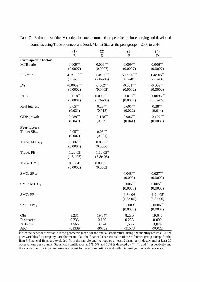
Table 7 – Estimations of the IV models for stock return and the peer factors for emerging and developed

countries using Trade openness and Stock Market Size as the peer groups – 2006 to 2016

(1) (2) (3) (4)

E D E D

Firm-specific factor

MTB ratio 0.009*** 0.006*** 0.009*** 0.006***

(0.0007) (0.0007) (0.0007) (0.0007)

P/E ratio 4.7e-05*** 1.4e-05** 5.1e-05*** 1.4e-05**

(1.3e-05) (7.0e-06) (1.3e-05) (7.0e-06)

DY -0.0009*** -0.002*** -0.001*** -0.002***

(0.0002) (0.0002) (0.0002) (0.0002)

ROE 0.0018*** 0.0009*** 0.0018*** 0.00095***

(0.0001) (6.3e-05) (0.0001) (6.3e-05)

Real interest 0.65*** 0.23*** 0.601*** 0.28***

(0.021) (0.013) (0.022) (0.014)

GDP growth 0.989*** -0.128*** 0.906*** -0.107***

(0.041) (0.009) (0.041) (0.0085)

Peer factors

Trade: SRt-1 0.05*** 0.03***

(0.002) (0.001)

Trade: MTB t-1 0.006*** 0.005***

(0.0007) (0.0006)

Trade: PE t-1 1.2e-05 -1.6e-05**

(1.6e-05) (6.8e-06)

Trade: DY t-1 0.0004* 0.0005***

(0.0002) (0.0002)

SMC: SRt-1 0.048*** 0.027***

(0.002) (0.0009)

SMC: MTB t-1 0.006*** 0.005***

(0.0007) (0.0006)

SMC: PE t-1 1.8e-06 -1.2e-05*

(1.5e-05) (6.8e-06)

SMC: DY t-1 0.0003* 0.0006***

(0.0002) (0.0002)

Obs. 8,231 19,647 8,230 19,646

R-squared 0.233 0.130 0.255 0.099

N. firms 1,566 3,074 1,566 3,074

AIC -31339 -96702 -31573 -96022

Note: the dependent variable is the geometric mean for the annual stock return, using the monthly returns. All the

peer variables for company i are the mean of all the financial characteristics of the reference group except for the

firm i. Financial firms are excluded from the sample and we require at least 2 firms per industry and at least 30

observations per country. Statistical significance at 1%, 5% and 10% is denoted by ***, **, and *, respectively and

the standard errors in parentheses are robust for heteroskedasticity and within industry-country dependence.

55

Thus, the stock return of the peer group differs from the industry and the country peer

groups in magnitude with smaller effects. In general, there still is a positive effect of the stock

return of the peers in the emerging and developed markets, whereas the former has a stronger

effect on the stock return of firm i. The effect of all the peer firm factors is smaller than before,

which could be related to the way we construct the stock market size variable. As stock market

size aggregates different countries into five subgroups, countries with different economic

development paths, but with similar equity markets size, are considered as reference groups and

affect the magnitude of the coefficients for the peers.

For example, Brazil, China, Germany, Indonesia, Italy, Mexico, Russia, and Turkey are

aggregated in the group with the smaller stock market (SMC) size. Note that this group includes

both developed countries – like Germany that is a highly developed economy in Europe – as

countries experiencing political and social instability like Brazil and Turkey. Thus, the

concentration of countries in the smaller SMC size may be one of the reasons that explains, in

part, the different magnitudes of the coefficients. Another explanation may be that the investor

does not choose one country over another simplify for the size of its stock market but pondering

the country's macroeconomic conditions and the possible diversification benefits of this choice.

This seems to happen in trade openness peer group since nine countries have the highest trade

openness and seem to explore the benefits from more trading. Note that opening a country up

to both international trade and financial flow can promote financial development.

Therefore, our results suggest that an increase in 1% in the stock return of the peer firms

for either these peer groups enhances the stock return in 5% in emerging markets, whereas in

developed ones the increase is of 3% in the stock return of firm i. In a way, we can say that the

investors must analyze the country’s financial sector development to identify co-movements on

stock returns of peer firms, as well as understand the impact on the portfolio selection.

The same principal is applied to trade openness since companies in countries more open

to trade undergo the effects of economic fluctuations from foreign markets. Dellas and Hess

(2005) suggest that the development of financial sector is an important determinant to the stock

return performance since the financial system operation and their effects on macroeconomic

fundamentals can lead to economic growth and less volatility on stock returns. Although the

peer firms’ stock returns are higher for industry/country than for the stock market size,

investment opportunity and dividend yield of the peers can influence these financial features

for the firm i and lead to imitation behavior that can impact on its stock return.

Lastly, as mentioned in the methodological chapter, we perform weak instrument tests

for these models and do not find evidences of the presence of the weak problem. Since our

purpose is to test Leary and Roberts (2014), we proceed our analysis but caution the reader to

understand that these evidences are specifically for this sample. Table B1 presents the results

for the tests and reject the null hypothesis of the structural equation is weakly identified as well

as the weak-instrument-robust inference.

In summary, the results show an important role of the peer effects on the stock return of

a firm which can help the investor in the diversification process in the international stock

market. Comparing these four peer groups, the effect of industry and country for emerging

markets are more intense than stock market’ size and trade openness, indicating that investors

can have better gains from these two groups when they do not understand the financial market

diversification principal. In next section, we re-estimate the models using two samples as a

robustness test.

4.4 Robustness test for the determinants of the stock return with peer effects

As a robustness test, we re-estimate the models from section 4.3 for two subsamples. In

the first one, we exclude companies from China, India, Japan and US because they comprise

almost 70% of the firms in our analysis. We aim to verify if the results are the same or if the

number of companies from these countries can influence the previous results. Secondly, we re-

estimate the models for only these four countries to capture any potential difference

contemplating only the industry as a peer group.

The first subsample has 2,274 companies for each year (25,014 firm-year) separated

into emerging (421 firms) and developed countries (1,853 firms). Note that China and India are

important players in our study and, by excluding them, our sample of companies in emerging

markets drastically reduces from more than two thousand companies to little over four hundred

firms per year. Table 11 shows the results for this sample considering country and industry as

the peer groups. Initially, the most striking differences are the effects of the macroeconomic

characteristics on the stock return. Comparing to the complete sample, by excluding China and

India, the economic growth has a negative influence in stock return, contrary to the effect of

full models. This tend to indicate that these two countries may be responsible for the positive

effect of economic growth in the stock return. Conversely, the results for the macroeconomic

variables for the developed countries are the same as before, only differentiating in the

magnitude.

By considering the peer firm factors, there still is a positive effect between the stock

return of the peer firms from the same country, as well as the investment opportunity and

57

dividend yield but in different magnitudes from the previous ones. In these estimations, the

return of companies that belong to the same country is 32% lower than the results of the full

sample for emerging countries and 42% lower for the developed countries. Therefore, China,

India, USA and Japan are important markets for the peer effect theory, mainly because of their

size.

For a smaller sample, a 1% increase in the stock return of the peer group enhances a

0.65% in the stock return of the firm from emerging markets (0.95% previously). In developed

countries, the peer effect of the stock return of companies in the same country increase in 0.21%

the stock return of the firm. Companies in the same industry have a 0.87% increase in their

stock return if there is a 1% increase in the return of the peers which, compared to the earlier

results, corresponds to a 24% lower impact in emerging markets and a 41% lower effect for

developed ones.

Therefore, by identifying the dependence between firms as peer effect or co-movement

in stock returns, the investor can earn higher returns. Foucault and Fresard (2014) suggest the

best course of action for an investor that wants to increase its earnings is to interpret the

information conveyed in the peer stock prices. Moreover, this results also indicates a

homogenous pattern of movement on asset returns like proposed by Barberis et al. (2005)

considering either the category or the habitat view. Furthermore, the arguments of Chen and

Ma (2017) and many authors of peer effect are also applied to asset pricing models since there

is a learning process from the peers’ decisions and their performance in the stock market. Also,

even with the sample reduction, the peer-return proxy maintains the co-movement between

stock returns even to a lesser extent.

Table 11 – Estimations of the determinants of the stock return with IV models for peer effects from

Country and Industry – from 2006 to 2016 (10 countries sample)

(1) (2) (3) (4)

E D E D

Firm-specific factors

MTB ratio 0.011*** 0.0042*** 0.006** 0.004***

(0.003) (0.0007) (0.003) (0.0007)

P/E ratio -0.00001 0.00003* 0.00006 0.00002

(0.0001) (0.00002) (0.0001) (0.00002)

DY -0.002*** -0.002*** -0.0013** -0.002***

(0.0006) (0.0003) (0.0006) (0.0003)

ROE 0.002*** 0.001*** 0.0018*** 0.0006***

(0.0004) (0.0001) (0.0004) (0.0001)

Macro factors

Real int. rate -0.002 0.162*** 0.028 0.098*

(0.037) (0.055) (0.043) (0.056)

GDP growth -0.334*** -0.461*** -0.269*** -0.47***

(0.070) (0.020) (0.079) (0.021)

Peer factor: country

SRt-1 0.648*** 0.213***

(0.082) (0.026)

MTBt-1 0.019*** 0.005***

(0.002) (0.001)

PEt-1 -0.0001 0.00002

(0.0001) (0.00001)

DYt-1 0.003*** -0.0002

(0.0007) (0.0002)

Peer factor: industry

SRt-1 0.872*** 0.245***

(0.117) (0.028)

MTBt-1 0.011*** 0.003***

(0.002) (0.0006)

PEt-1 0.0001 0.00002

(0.0001) (0.00001)

DYt-1 0.003*** 0.0001

(0.0007) (0.0002)

Observations 859 5,216 842 5,201

R-squared 0.241 0.239 0.05 0.225

N. firms 193 945 189 941

AIC -3260 -25388 -3010 -25221 Note: the dependent variable is the geometric mean for the annual stock return, using the monthly returns. All the

peer variables for company i are the mean of all the financial characteristics of the reference group except for the

firm i. Financial firms are excluded from the sample and we require at least 2 firms per industry and at least 30

observations per country. We apply the 2SLS panel data estimator and the standard errors in parentheses are robust

for heteroskedasticity and within industry-country dependence. Statistical significance at 1%, 5% and 10% is

denoted by ***, **, and *, respectively.

59

We also re-estimate the models for the sample without China, India, Japan and US using

the trade openness and the stock market size as the peer groups, reporting the results in table

12. Initially, there is no change in the direction of the peer effects for trade openness and stock

market size groups compared to the earlier results, but their intensity tends to reduce in the

smaller sample. There still is a co-movement between stock returns of firms and their peers, but

robustness estimations are 58% lower for emerging markets with the trade openness as peer

group and 56% lower for developed countries in the same level of financial development.

Thus, increases in stock returns as a result of co-movement from these peer groups range from

0.01% to 0.05%, and in emerging countries the intensity of the peer returns is always greater

than that of developed markets. Here, Babenko, Boguth and Tserlukevich’s (2016) explanation

holds it seems that the profitability shocks have a bearing on determining stock returns. With

respect to these same effects for the industry and country groups, one can say that the co-

movement is surprisingly smaller for a sample with just over 2,000 companies per year.

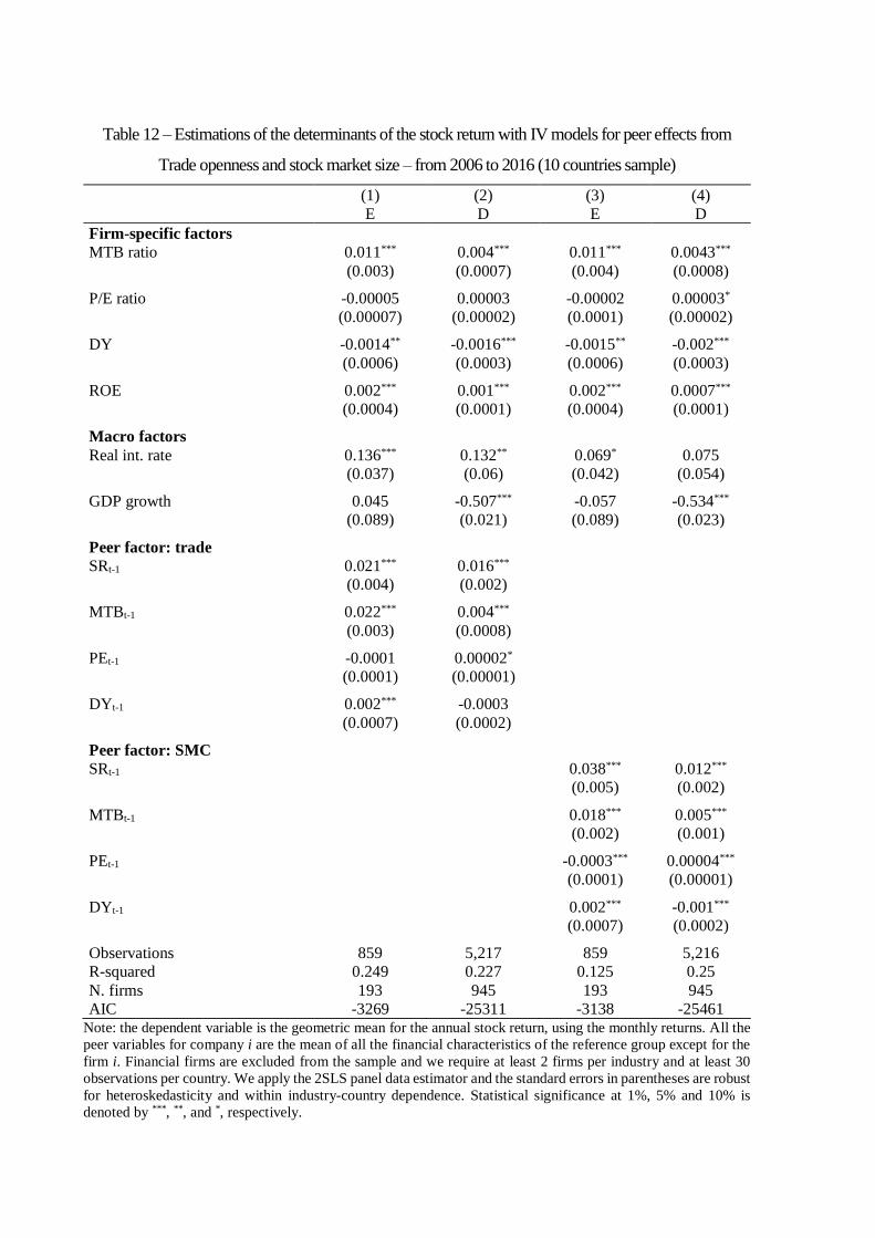
Table 12 – Estimations of the determinants of the stock return with IV models for peer effects from

Trade openness and stock market size – from 2006 to 2016 (10 countries sample)

(1) (2) (3) (4)

E D E D

Firm-specific factors

MTB ratio 0.011*** 0.004*** 0.011*** 0.0043***

(0.003) (0.0007) (0.004) (0.0008)

P/E ratio -0.00005 0.00003 -0.00002 0.00003*

(0.00007) (0.00002) (0.0001) (0.00002)

DY -0.0014** -0.0016*** -0.0015** -0.002***

(0.0006) (0.0003) (0.0006) (0.0003)

ROE 0.002*** 0.001*** 0.002*** 0.0007***

(0.0004) (0.0001) (0.0004) (0.0001)

Macro factors

Real int. rate 0.136*** 0.132** 0.069* 0.075

(0.037) (0.06) (0.042) (0.054)

GDP growth 0.045 -0.507*** -0.057 -0.534***

(0.089) (0.021) (0.089) (0.023)

Peer factor: trade

SRt-1 0.021*** 0.016***

(0.004) (0.002)

MTBt-1 0.022*** 0.004***

(0.003) (0.0008)

PEt-1 -0.0001 0.00002*

(0.0001) (0.00001)

DYt-1 0.002*** -0.0003

(0.0007) (0.0002)

Peer factor: SMC

SRt-1 0.038*** 0.012***

(0.005) (0.002)

MTBt-1 0.018*** 0.005***

(0.002) (0.001)

PEt-1 -0.0003*** 0.00004***

(0.0001) (0.00001)

DYt-1 0.002*** -0.001***

(0.0007) (0.0002)

Observations 859 5,217 859 5,216

R-squared 0.249 0.227 0.125 0.25

N. firms 193 945 193 945

AIC -3269 -25311 -3138 -25461 Note: the dependent variable is the geometric mean for the annual stock return, using the monthly returns. All the

peer variables for company i are the mean of all the financial characteristics of the reference group except for the

firm i. Financial firms are excluded from the sample and we require at least 2 firms per industry and at least 30

observations per country. We apply the 2SLS panel data estimator and the standard errors in parentheses are robust

for heteroskedasticity and within industry-country dependence. Statistical significance at 1%, 5% and 10% is

denoted by ***, **, and *, respectively.

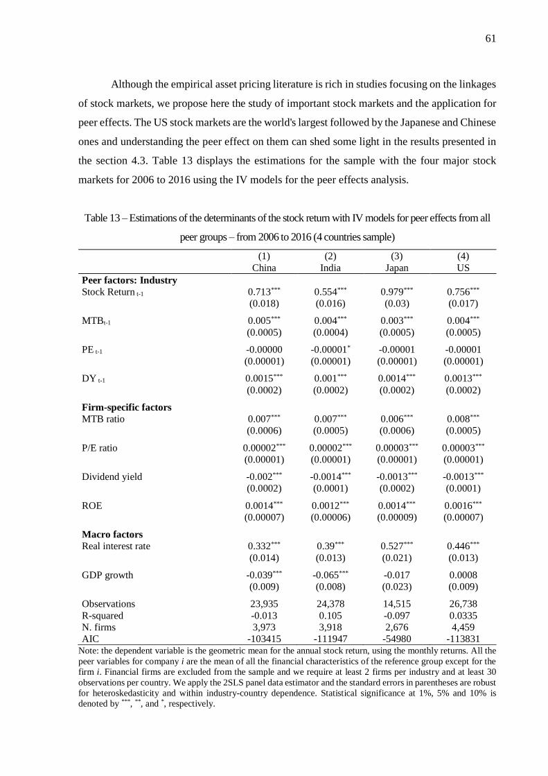
61

Although the empirical asset pricing literature is rich in studies focusing on the linkages

of stock markets, we propose here the study of important stock markets and the application for

peer effects. The US stock markets are the world's largest followed by the Japanese and Chinese

ones and understanding the peer effect on them can shed some light in the results presented in

the section 4.3. Table 13 displays the estimations for the sample with the four major stock

markets for 2006 to 2016 using the IV models for the peer effects analysis.

Table 13 – Estimations of the determinants of the stock return with IV models for peer effects from all

peer groups – from 2006 to 2016 (4 countries sample)

(1) (2) (3) (4)

China India Japan US

Peer factors: Industry

Stock Return t-1 0.713*** 0.554*** 0.979*** 0.756***

(0.018) (0.016) (0.03) (0.017)

MTBt-1 0.005*** 0.004*** 0.003*** 0.004***

(0.0005) (0.0004) (0.0005) (0.0005)

PE t-1 -0.00000 -0.00001* -0.00001 -0.00001

(0.00001) (0.00001) (0.00001) (0.00001)

DY t-1 0.0015*** 0.001*** 0.0014*** 0.0013***

(0.0002) (0.0002) (0.0002) (0.0002)

Firm-specific factors

MTB ratio 0.007*** 0.007*** 0.006*** 0.008***

(0.0006) (0.0005) (0.0006) (0.0005)

P/E ratio 0.00002*** 0.00002*** 0.00003*** 0.00003***

(0.00001) (0.00001) (0.00001) (0.00001)

Dividend yield -0.002*** -0.0014*** -0.0013*** -0.0013***

(0.0002) (0.0001) (0.0002) (0.0001)

ROE 0.0014*** 0.0012*** 0.0014*** 0.0016***

(0.00007) (0.00006) (0.00009) (0.00007)

Macro factors

Real interest rate 0.332*** 0.39*** 0.527*** 0.446***

(0.014) (0.013) (0.021) (0.013)

GDP growth -0.039*** -0.065*** -0.017 0.0008

(0.009) (0.008) (0.023) (0.009)

Observations 23,935 24,378 14,515 26,738

R-squared -0.013 0.105 -0.097 0.0335

N. firms 3,973 3,918 2,676 4,459

AIC -103415 -111947 -54980 -113831 Note: the dependent variable is the geometric mean for the annual stock return, using the monthly returns. All the

peer variables for company i are the mean of all the financial characteristics of the reference group except for the

firm i. Financial firms are excluded from the sample and we require at least 2 firms per industry and at least 30

observations per country. We apply the 2SLS panel data estimator and the standard errors in parentheses are robust

for heteroskedasticity and within industry-country dependence. Statistical significance at 1%, 5% and 10% is

denoted by ***, **, and *, respectively.

The results indicate a positive and significant co-movement of the stock return for the

firms and their peers for all the countries. Although the Japanese stock market is the second

largest, the co-movement with the peers' stock return is the largest of all these countries which

leads us to believe that the companies and their industries are more aligned and dependent of

each other than in other countries. An increase of the stock return of the industry in 1% enhances

the stock return of the firm in approximately 1% for the Japanese stock market, while the largest

stock market (the two US stock markets) has the second higher co-movement of the peer firms

(0.8%).

Conversely, the Chinese stock market is the third largest stock market of the world with

more than 2,400 firms listed and traded in the exchanges. In our models, these stock market

responds to the following higher co-movement for the peer firms (0.71%) as well as the higher

impact of the previous investment opportunity of the peers in the same industry (0.5% for each

increase in one point for the peers’ opportunity). Researches with the Indian stock market

indicates that “the listed companies are mostly family controlled with majority holdings in

shares and board positions” (SRIRAM, 2018, p.3) and this could be the reason for the smaller

co-movement with the peer firms comparing to the other countries. In this context, we can

suggest that the results are consistent with the findings of the models estimated with the

complete sample.

63

5. FINAL REMARKS

We apply the peer effect and co-movement approach in stock returns for almost 7,000

listed companies of the top emerging and developed countries from 2006 to 2016. The peer

effect theory is usually focused in the labor and education economy studies, as well as in

situations that incorporate the social network as the main relation between the subjects. Leary

and Roberts (2014) initiate the use of peer effects technique in corporate finance by

understanding the effects on capital structure decisions of companies in the CRSP database

from 1965 to 2008. Francis et al. (2016), Chen and Ma (2017), and Adhikari and Agrawal

(2018) also use the peer effect to analyze corporate finance.

Some researchers apply the spatial econometrics procedures proposed by Jean H.P.

Paelinck in the book with Leo H. Klaasen from 1979 to identify peer effects on stock return

(ANSELIN, 1988). Fernandez (2011) and Gong and Weng (2016) are some examples of this

application since they consider that stock returns experience effects of their own companies’

characteristics as size, book-to-market ratio and trade volume, but also of the relative values of

these factors in their industries and in their geographic regions13. They group companies

accordingly social and economic distances and find the dependence between different

companies from the same baseline group associated with the peer effect and the co-movement

of the variables. For them, if an investor understands the dependence structure between

companies, the choice for an adequately portfolio is more accurate due to the spillovers effects

when there is a strong integration among companies.

We also group companies according to our references as many authors did. However,

to the best of our knowledge, the peer effect theory is not directly applied to asset pricing models

disregarding the investor or the analyst studies (BURSZTYN et al., 2014; FOUCAULT;

FRESARD, 2014; CESPEDES; PARRA, 2016). To fill this gap, we analyze the peer effect in

stock returns given two parts of the reflection problem from Manski (1993): the exogenous peer

effect between the stock return from firm i and the financial indicators of the peer firms; and

the endogenous peer effect between the stock return from firm i and the spillover effect from

the stock return from the peer firms.

For the first part, we estimate fixed effect models with robust errors considering some

financial characteristics as a catalyst of an imitation or spillover effect. For the second approach,

the main problem is endogeneity that Manski (1993, 2000) and other authors discussed. Leary

13 Asgharian, Hess and Liu (2013), Weng and Gong (2016) and Gong and Weng (2016) also apply a spatial

procedure to identify peer effects and co-movement in financial markets.

and Roberts (2014) and Francis et al. (2016) argue the importance of the 2SLS estimator as an

approach to estimate a model with endogenous variable. In the peer effect aspect, we follow

Leary and Roberts (2014) and use the idiosyncratic return from the CAPM regression with the

stock return of the peers as our instrumental variable.

In general, we provide evidences that the peer effects are important to international asset

pricing models and that exists peer effects in the financial indicators and the stock return. To

the best of our knowledge, this is the first attempt to find out when peer effects drive stock

returns using international stock markets. There is strong exogenous peer effect from financial

characteristics for the emerging markets like market-to-book ratio, while the develop ones have

a lesser magnitude of this effect. In this context, Leary and Roberts (2014) suggest that this

characteristic of the peer firm likely captures relevant changes in the firm’ structure and it seems

that our results are aligned with them. It is worth mentioning that these results are amplified in

the emerging markets.

An alternative explanation is the lack of reliable information of the characteristics of

firm i for the decision-process which would imply in the search for information of companies

of the same branch. The information theory applied by Chen and Ma (2017) indicates that firms

learn from peers’ decisions because same firms capture information otherwise difficult to

obtain. This also happens because firms do not want to fall behind peer firms and therefore

choose to imitate each other (CHEN; MA, 2017).

For the co-movement of stock return of the peer groups, emerging and developed

economies display positive and significant peer effects of the changes in the past stock return

of the peers, attesting the co-movement between stock returns in the models. The stock returns

are strongly higher in emerging countries which leads us to believe that, although these

countries offer a high-risk, high-reward investment opportunity, they are rapidly growing but

still have high political and currency risks.

Thus, understanding the co-movement of the stock return in the peer effect analysis is

essential not only to help the investor achieve higher returns, but also to improve economic

growth and reduce volatility. Dellas and Hess (2005) suggest that the development of financial

sector is an important determinant to the stock return performance since the financial system

operation and their effects on macroeconomic fundamentals can lead to economic growth and

less volatility on stock returns.

The stock return of the peers reveals, then, the behavior of the local or international

environment experienced by the firm and its investors. It is important to note that the emerging

stock markets are smaller than the develop ones and, since these countries are dependable on

65

each other, they suffer rapidly the effects of international economic crisis, it is not a surprise

that there is a positive co-movement between the stock prices.

Nevertheless, the co-movement of stock return occurs in emerging markets, especially

for the industry and country peer groups. For the former, the stock return of the peers tends to

increase between 0.41% to 1.15% respectively for developed and emerging economies, while

the latter varies from 0.37% to 0.95%. Since trade openness and stock market size mix different

countries in their groups, the results are smaller for both emerging and developed countries if

compared to the previous ones, and the co-movement for the developed ones is half the

emerging ones. We attribute this effect to the mix of countries in these variables that cannot

explicitly indicate a better integration of real economy and the financial/stock market in the

developed countries. When comparing trade and stock market size, an increase of 1% in the

stock return of the peers create an increase of 0.05% for emerging countries and 0.03% for

developed markets.

To test the robustness of our results, we analyze the effects of China, India, Japan and

USA in the models. The first subsample does not consider these four countries and has 2,274

companies for each year. The main difference is the effects of the macroeconomic

characteristics with a negative economic growth influence in stock return. For stock return of

the peers, the effect is smaller for all peer groups, but we still find that investors and firms from

emerging markets observe the decisions of the peers to obtain higher gains. Therefore, the peer

effect result is persistent even though China, India, USA and Japan are important markets for

this theory applied to stock markets, mainly because of their size. As Foucault and Fresard

(2014) suggest that the investor must interpret the information conveyed in the peer stock

prices. Also, when analyzing the second subsample that consists of companies in China, India,

Japan and USA, we find evidences that an increase of 1% in stock return of peer firms create

increases in the stock return varying from 0.55% (India) to 1% (Japan), which suggests that

these two developed markets have evidences of peer effects on stock return.

We emphasize that the results obtained here are applied to this sample and may present

distinct results in other situations. The main limitation of this work is, besides the computational

dedication that the individual regressions for the instrumental variable, the selection of a

restricted set of listed companies for fourteen countries. Therefore, this is an academic field that

can be better explored by researchers, including the asset pricing analysis as the expanding

corporate finance one. The next step for the peer effects in asset pricing models is to ascertain

what drives the peer effects, whether they occur especially in emerging or developed countries

and if there are mechanism that intensify the peer effects during instability periods.

REFERENCES

ACEMOGLU, D.; AUTOR, D. Lectures in labor economics. Available in

https://economics.mit.edu/files/4689. 2011.

ADHIKARI, B.K.; AGRAWAL, A. Peer influence on payout policies. Journal of Corporate

Finance, 48: 615-637, 2018.

AGHABOZORGI, S.; TEH, Y.W. Stock market co-movement assessment using a three-phase

clustering method. Expert Systems with Applications, 41: 1301–1314, 2014.

AGHION, P.; et al.. Financial Development and The Instability of Open Economies. NBER

Working Paper Series 10246, 2004.

ANDERSON, T.W.; RUBIN, H. Estimation of the parameters of a single equation in a complete

system of stochastic equations. Annals of Mathematical Statistics, 20: 46-63, 1949.

ANGRIST, J.D. The perils of peer effects. Labour Economics, 30: 98-108, 2014.

ANG, A.; BEKAERT, G. Stock Return Predictability: Is it There? The Review of Financial

Studies, 20 (3): 651-707, 2007.

ANSELIN, L. Spatial Econometrics: methods and models. Boston: Kluwer Academic, 1988

ASHRAF, B.N. Do trade and financial openness matter for financial development? Bank-level

evidence from emerging market economies. Research in International Business and

Finance, 44: 434–458, 2018.

ARNOLD, M.; et al. Modelling different kinds of spatial dependence in stock return. Empirical

Economics, 44 (2): 761-774, 2013.

ASGHARIAN, H.; et al. A spatial analysis of international stock market linkages. Journal of

Banking & Finance, 37 (12): 4738–4754, 2013.

ASGHARIAN, H.; LIU, L. Stock return dependence and product market linkages. In 2018

ASSA Annual Meeting, 2018.

AVRAMOV, D. Stock return predictability and asset pricing models. The Review of Financial

Studies, 17 (3): 699-738, 2004.

BABENKO, I.; et al. Idiosyncratic cash flows and Systematic Risk. The Journal of Finance.

71 (1): 425-456, 2016

BALTAGI, B.H.; et al. Financial development and openness: evidence from panel data.

Journal of Development Economics, 89 (2): 285-296, 2009.

BARBERIS, N.; et al. Comovement. Journal of Financial Economics, 75: 283-317, 2005.

BAUMÖHL, E.; et al. Networks of volatility spillovers among stock markets. Physica A, 490:

1555-1574, 2018.

BEKAERT, G.; el al. International stock return comovements. Working paper series n. 931,

European Central Bank, 2008.

BEKAERT, G.; et al. Who is internationally diversified? Evidence from the 401(k) plans of

296 firms. Journal of Financial Economics, 124 (1): 86–112, 2017.

BENA, J.; et al. Are foreign investors locusts? The long-term effects of foreign institutional

ownership. Journal of Financial Economics, 126: 122–146, 2017.

67

BERNARD, A.B.; et al. Firms in International Trade. Journal of Economic Perspectives. 21

(3): 105–130, 2007.

BOND, P.; et al. Real effects of financial markets. Annual Review of Financial Economics.

4 (1): 339–360, 2012.

BOWMAN, D.; et al. U.S. Unconventional Monetary Policy and Transmission to Emerging

Market Economies. International Finance Discussion Papers Number 1109. Federal Reserve

System, 2014.

BURSZTYN, L.; et al. Understanding Mechanisms Underlying Peer Effects: Evidence from a

Field Experiment on Financial Decisions. Econometrica, 82 (4): 1273–1301, 2014.

CAMPBELL, J.Y.; et al. The Econometrics of Financial Markets. Princeton University

Press. 611p, 1997.

CAMPBELL, J.Y.; SHILLER, R.J. The dividend-price ratio and expectations of future

dividends and discount factors. Review of Financial Studies. 1 (3): 195-228, 1988a.

______________. Stock prices, earnings, and expected dividends. The Journal of Finance. 43

(3): 661-676, 1988b.

CAMPELLO, M.; GRAHAM, J.R. Do stock prices influence corporate decisions? Evidence

from the technology bubble. Journal of Financial Economics, 107: 89–110, 2013.

CESPEDES, J.; PARRA, C. Peer Effects across Firms: Evidence from Security Analysts. 2016.

2017 ASSA Annual Meeting of American Economic Association. Avaliable in

<http://www.sole-jole.org/17230.pdf>. Access in Dec., 2017.

CHAN, H.; et al. Financial constraints and stock returns: evidence from Australia. Pacific-

Basin Finance Journal, 18: 306-318, 2010.

CHEN, H.; et al. Comovement revisited. Journal of Financial Economics, 121: 624-644,

2016.

CHEN, S.; MA, H. Peer effects in decision-making: evidence from corporate investment.

China Journal of Accounting Research, 10: 167-188, 2017.

CHEN, S.-S.; WANG, Y. Financial constraints and share repurchases. Journal of Financial

Economics, 105: 311–331, 2012.

CHOWDHURY, E.K. Functioning of Fama-French Three Factor Model in Emerging Stock

Markets: An Empirical Study on Chittagong Stock Exchange, Bangladesh. Journal of

Financial Risk Management, 6: 352-363, 2017.

CLAEYS, P.; et al. Debt, interest rate, and integration of financial markets. Economic

Modelling, 29: 48-59, 2012.

COCHRANE, J.H. Presidential address: discount rates. The Journal of Finance. 66 (4): 1047-

1108, 2011.

COEURDACIER, N.; GUIBAUD, S. International portfolio diversification is better than you

think. Journal of International Money and Finance, 30: 289–308, 2011.

CULLEN, G.; et al. R&D expenditure volatility and stock return: Earnings management,

adjustment costs or overinvestment? SSRN Discussion Paper 2482827. Disponível em <

http://ssrn.com/abstract=2482827>. Aug., 2014.

DANIEL, K.; TITMAN, S. Evidence on Characteristics of Cross-Sectional Variation in Stock

Returns. The Journal of Finance, 52 (1): 1-33, 1997.

DELLAS, H.; HESS, M. Financial development and stock returns: A cross-country analysis.

Journal of International Money and Finance. 24: 891-912, 2005.

DIEBOLD, F.X.; YILMAZ, K. Financial and Macroeconomic connectedness: a network

approach to measurement and monitoring. Oxford University Press, 2015.

DURHAM, J.B. Absorptive capacity and the effects of foreign direct investment and equity

foreign portfolio investment on economic growth. European Economic Review, 48, 285-306,

2004.

EDMANS, A., et al. The real effects of financial markets: the impact of prices on takeovers.

The Journal of Finance. 67 (3), 933–971, 2012.

ENGELBERG, J. et al. Know Thy Neighbor: Industry Clusters, Information Spillovers, and

Market Efficiency. Journal of Financial and Quantitative Analysis. 53 (5): 1937-1961, 2018.

FAMA, E.F.; FRENCH, K.R. The cross-section of expected stock returns. The Journal of

Finance, 47 (2): 427-465, 1992.

___________. Common risk factors in the returns on stocks and bonds. Journal of Financial

Economics, 33: 3-56, 1993.

___________. Size, Value, and Momentum in International Stock Returns. Journal of

Financial Economics. 105: 457–472, 2012.

___________. A five-factor asset pricing model. Journal of Financial Economics, 116: 1-22,

2015.

___________. International tests of a five-factor asset pricing model. Journal of Financial

Economics, 123: 441-463, 2017.

FAN, J.P.H.; et al. An International Comparison of Capital Structure and Debt Maturity

Choices. The Journal of Financial and Quantitative Analysis, 47 (1): 23-56, 2012.

FEENSTRA, R.C. Advanced International Trade: Theory and Evidence. Princeton

University Press, Second Edition. 496 pages, 2015.

FERNANDEZ, V. Spatial linkages in international financial markets. Quantitative Finance,

11 (2): 237-245, 2011.

FERNÁNDEZ-AVILÉS, G.; MONTERO, J.M. Spatio-temporal modeling of financial maps

from the joint multidimensional scaling-geostatistical perspective. Expert Systems with

Applications, 60: 280-293, 2016.

FOUCAULT, T.; FRESARD, L. Learning from peers’ stock prices and corporate investment.

Journal of Financial Economics, v. 111, pp. 554-577, 2014.

FRANCIS, B.B.; et al. When do peers matter?: A cross-country perspective. Journal of

International Money and Finance, 69: 363-389, 2016.

FRENCH, K.R.; POTERBA, J.M. Investor diversification and international equity markets.

NBER Working Papers series. Working paper n. 3609, 1991.

FUJII, E. What does trade openness measure? CESifo Working Paper n. 6656. Disponível em

http://www.cesifo-group.de/DocDL/cesifo1_wp6656.pdf. Acesso em jan. 2018.

GHARBI, S.; et al. R&D investments and high-tech firms' stock return volatility.

Technological Forecasting & Social Change. 88: 306–312, 2014.

GOLEZ, B. (2014). Expected Returns and Dividend Growth Rates Implied by Derivative

Markets. The Review of Financial Studies. 27 (3): 790-822.

69

GONG, P. WENG, Y. Value-at-Risk forecasts by a spatiotemporal model in Chinese stock

market. Physica A, 441: 173-191, 2016.

HADLOCK, C.J.; PIERCE, J.R. New Evidence on Measuring Financial Constraints: Moving

Beyond the KZ Index. The Review of Financial Studies, 23 (5): 1909-1940, 2010.

HAMEED, A.; MIAN, G.M. Industries and Stock Return Reversals. Journal of Financial and

Quantitative Analysis. 50 (1-2): 89-117, 2015.

HEATHCOTE, J.; PERRI, F. The International Diversification Puzzle Is Not as Bad as You

Think. Journal of Political Economy, 121 (6): 1108-1159, 2013.

HELPMAN, E.; KRUGMAN, P.R. Market Structure and Foreign Trade: Increasing

Returns, Imperfect Competition, and the International Economy. Cambridge: MIT Press, 1985.

JING, Z. et al. The propagation of financial turbulence: interdependence, spillovers, and direct

and indirect effects. Empirical Economics, pp.1-24, < https://doi.org/10.1007/s00181-017-

1249-y>, 2017.

KAPLAN, S., ZINGALES, L. Do investment-cash flow sensitivities provide useful measures

of financing constraints? Quarterly Journal of Economics, 122:169–215, 1997.

KAUSTIA, M.; RANTALA, V. Social learning and corporate peer effects. Journal of Financial

Economics. 117: 653–669, 2015.

KOGAN, L.; PAPANILOLAOU, D. Firm characteristics and stock returns: the role of

investment-specific shocks. The Review of Financial Studies, 26 (11): 2718-2759, 2013.

LAMONT, O.; et al. Financial Constraints and Stock Returns. The Review of Financial

Studies, 14 (2): 529-554, 2001.

LEARY, M.T.; ROBERTS, M.R. Do peer firms affect corporate financial policy? The Journal

of Finance, v. LXIX, n.1, pp. 139-178, 2014.

LI, D. Financial Constraints, R&D Investment, and Stock Returns. The Review of Financial

Studies. 24 (9): 2974-3007, 2011.

LIEBERMAN, M.B.; ASABA, S. Why do firms imitate each other? Academy of Management

Review, 31 (2): 366-385, 2006.

LIN, Y-M., et al. The information content of unexpected stock returns: evidence from

intellectual capital. International Review of Economics and Finance,

<http://dx.doi.org/10.1016/j.iref.2014.11.024>, 2014.

LINTNER, J. The Valuation of Risk Assets and the Selection of Risky Investments in Stock

Portfolios and Capital Budgets. The Review of Economics and Statistics, 47(1): 13–37, 1965.

LIU et al. A social-media-based approach to predicting stock comovement. Expert Systems

with Applications, 42 (8): 3893-3901, 2015.

LO, A.; MACKINLAY, C. When are contrarian profits due to stock market overreaction?

Review of Financial Studies 3:175–205, 1990.

MAIO, P.; SANTA-CLARA, P. Dividend Yields, Dividend Growth, and Return Predictability

in the Cross Section of Stocks. Journal of Financial and Quantitative Analysis. 50 (1/2): 33–

60, 2015.

MALCENIECE, L.; MALCENIEKS, K.; PUTNIŅŠ, T.J. High frequency trading and

comovement in financial markets. Journal of Financial Economics, In Press. Available in

https://doi.org/10.1016/j.jfineco.2018.02.015, 2019.

MANSKI, C.F. Identification of Endogenous Social Effects: The Reflection Problem. The

Review of Economic Studies, 60 (3):531-542, 1993.

___________. Economic Analysis of Social Interactions. The Journal of Economic

Perspective, 14 (3): 115-136, 2000.

MARKOWITZ, H.M. Portfolio Selection. The Journal of Finance. 7 (1):77-91, 1952.

MAS, A.; MORETTI, E. Peers at Work. American Economic Review, 99 (1), 112–145, 2009.

MERTON, R.C. Lifetime Portfolio Selection under Uncertainty: The Continuous-Time Case,

The Review of Economics and Statistics. 51, 247–257, 1969.

MILLER, M., MODIGLIANI, F. Dividend policy, growth, and the valuation of shares. Journal

of Business, 34: 411–432, 1961.

MUSSO, P.; SCHIAVO, S. The impact of financial constraints on firm survival and growth.

Journal of Evolutionary Economics. 18:135–149, 2008.

PARK, K.; et al. The peer-firm effect on firm’s investment decisions. North American

Journal of Economics and Finance. 40: 178-199, 2017.

PETTENUZZO, D.; TIMMERMANN, A.; VALKANOV, R. Forecasting stock returns under

economic constraints. Journal of Financial Economics, 114: 517–553, 2014.

PHAN, D.H.B.; et al. Stock return forecasting: some new evidence. International Review of

Financial Analysis, 40: 38-51, 2015.

ROSS, S.A. The arbitrage theory of capital asset pricing. Journal of Economic Theory. 13

(3): 341-360, 1976.

SAMUELSON, P.A. Lifetime Portfolio Selection by Dynamic Stochastic Programming. The

Review of Economics and Statistics. 51(3): 239–246, 1969.

SHARPE, W. Capital Asset Prices: A Theory of Market Equilibrium Under Conditions of Risk.

The Journal of Finance, 19 (3): 425–442, 1964.

SOUMARÉ, I.; TCHANA, F.T. Causality between FDI and Financial Market Development:

Evidence from Emerging Markets. The World Bank Economic Review, 29 (Supplement):

S205–S216, 2015.

STOCK, J.H.; WRIGHT, J.H. GMM with weak identification. Econometrica, 68: 1055-1096,

2000.

SRIRAM, M. Do firm specific characteristics and industry classification corroborate voluntary

disclosure of financial ratios: an empirical investigation of S&P CNX 500 companies. Journal

of Management and Governance. Available in https://doi.org/10.1007/s10997-018-9414-z,

2018.

VALICKOVA, P.; et al. Financial Development and economic growth. Journal of Economic

Surveys, 29 (3): 506–526, 2015.

WENG, Y.; GONG, P. Modeling spatial and temporal dependencies among global stock

markets. Expert Systems with applications. 43: 175-185, 2016.

WHITED, T., WU, G. Financial Constraints Risk. The Review of Financial Studies, 19: 531–

59, 2006.

WIED, D. CUSUM-type testing for changing parameters in a spatial autoregressive model for

stock returns. Journal of Time Series Analysis, 34: 221–229, 2013.

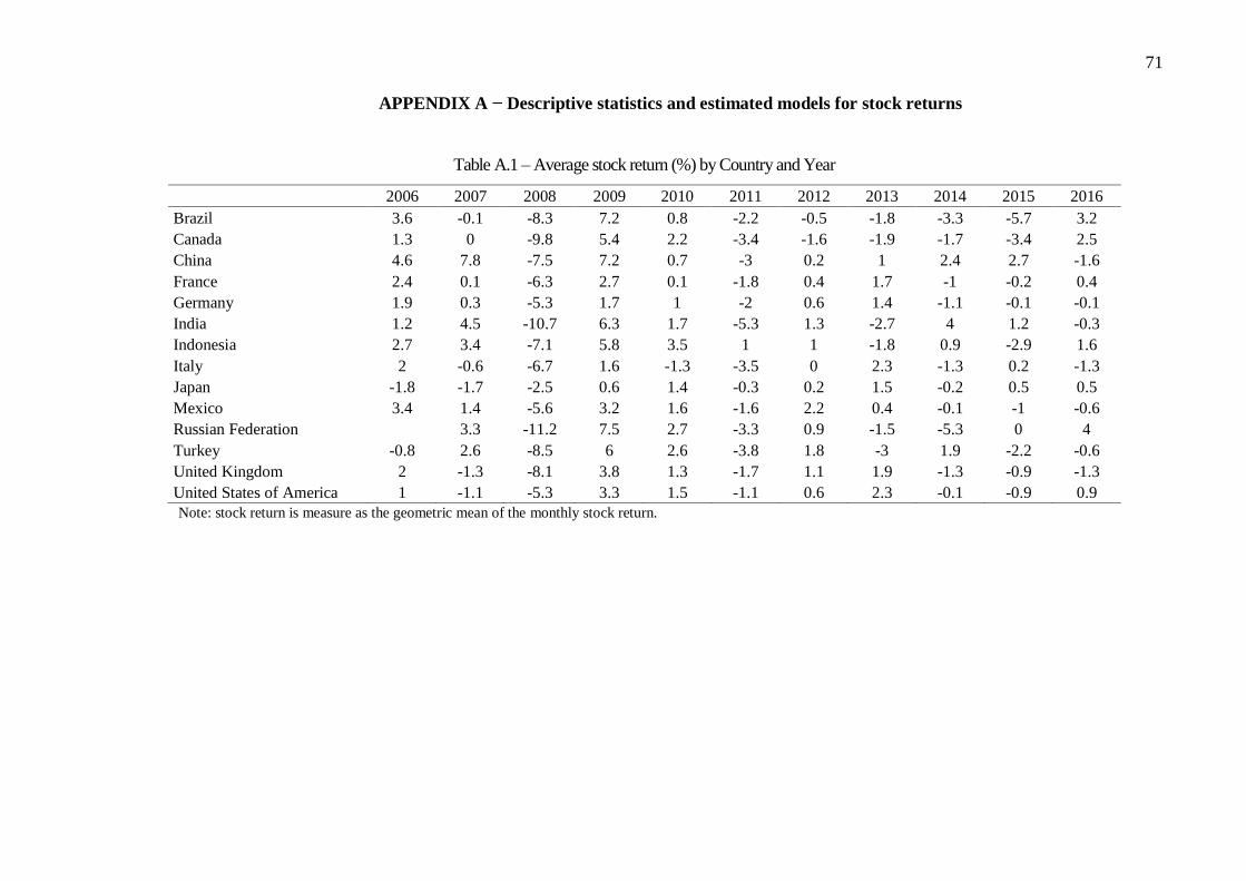
71

APPENDIX A − Descriptive statistics and estimated models for stock returns

Table A.1 – Average stock return (%) by Country and Year

2006 2007 2008 2009 2010 2011 2012 2013 2014 2015 2016

Brazil 3.6 -0.1 -8.3 7.2 0.8 -2.2 -0.5 -1.8 -3.3 -5.7 3.2

Canada 1.3 0 -9.8 5.4 2.2 -3.4 -1.6 -1.9 -1.7 -3.4 2.5

China 4.6 7.8 -7.5 7.2 0.7 -3 0.2 1 2.4 2.7 -1.6

France 2.4 0.1 -6.3 2.7 0.1 -1.8 0.4 1.7 -1 -0.2 0.4

Germany 1.9 0.3 -5.3 1.7 1 -2 0.6 1.4 -1.1 -0.1 -0.1

India 1.2 4.5 -10.7 6.3 1.7 -5.3 1.3 -2.7 4 1.2 -0.3

Indonesia 2.7 3.4 -7.1 5.8 3.5 1 1 -1.8 0.9 -2.9 1.6

Italy 2 -0.6 -6.7 1.6 -1.3 -3.5 0 2.3 -1.3 0.2 -1.3

Japan -1.8 -1.7 -2.5 0.6 1.4 -0.3 0.2 1.5 -0.2 0.5 0.5

Mexico 3.4 1.4 -5.6 3.2 1.6 -1.6 2.2 0.4 -0.1 -1 -0.6

Russian Federation 3.3 -11.2 7.5 2.7 -3.3 0.9 -1.5 -5.3 0 4

Turkey -0.8 2.6 -8.5 6 2.6 -3.8 1.8 -3 1.9 -2.2 -0.6

United Kingdom 2 -1.3 -8.1 3.8 1.3 -1.7 1.1 1.9 -1.3 -0.9 -1.3

United States of America 1 -1.1 -5.3 3.3 1.5 -1.1 0.6 2.3 -0.1 -0.9 0.9

Note: stock return is measure as the geometric mean of the monthly stock return.

Table A.2 – Average stock return for the industry peer group (%) by Country and Year

2006 2007 2008 2009 2010 2011 2012 2013 2014 2015 2016

Brazil -0.08 -0.13 -0.09 -0.11 -0.07 -0.14 -0.06 -0.04 -0.06 -0.09 -0.1

Canada -0.06 -0.05 -0.08 -0.09 -0.05 -0.04 -0.06 -0.08 -0.05 -0.05 -0.05

China -0.03 -0.04 -0.02 -0.02 -0.02 -0.02 -0.01 -0.02 -0.02 -0.03 -0.01

France -0.02 -0.08 -0.03 -0.03 -0.01 -0.02 -0.06 -0.01 -0.02 -0.02 -0.01

Germany -0.02 -0.02 -0.03 -0.04 -0.05 -0.04 -0.03 -0.03 -0.02 -0.02 -0.02

India -0.04 -0.04 -0.02 -0.03 -0.02 -0.01 -0.02 -0.02 -0.03 -0.02 -0.02

Indonesia -0.09 -0.1 -0.1 -0.1 -0.07 -0.05 -0.07 -0.07 -0.05 -0.03 -0.06

Italy -0.02 -0.02 -0.05 -0.04 -0.02 -0.03 -0.05 -0.03 -0.04 -0.03 -0.03

Japan -0.01 -0.07 -0.21 -0.03 -0.01 -0.02 -0.01 -0.03 -0.01 -0.01 -0.01

Mexico -0.12 -0.07 -0.15 -0.14 -0.07 -0.06 -0.05 -0.07 -0.04 -0.04 -0.07

Russian Federation 0 -0.06 -0.24 -0.19 -0.1 -0.05 -0.05 -0.05 -0.1 -0.09 -0.08

Turkey -0.07 -0.17 -0.08 -0.17 -0.08 -0.05 -0.04 -0.03 -0.04 -0.05 -0.06

United Kingdom -0.02 -0.02 -0.05 -0.07 -0.02 -0.02 -0.01 -0.02 -0.02 -0.02 -0.24

United States of America -0.02 -0.02 -0.29 -0.15 -0.14 -0.14 -0.09 -0.04 -0.06 -0.06 -0.09

Note: stock return of the peer group is measure as the geometric mean of the monthly stock return except for the firm i.

73

Table A.3 – GDP growth (%) for the countries from 2006 to 2016

2006 2007 2008 2009 2010 2011 2012 2013 2014 2015 2016 Mean

Brazil 3.96 6.07 5.09 -0.13 7.53 3.97 1.92 3 0.5 -3.77 -3.59 2.23

Canada 2.62 2.06 1 -2.95 3.08 3.14 1.75 2.48 2.57 0.94 1.47 1.65

China 12.72 14.23 9.65 9.4 10.64 9.54 7.86 7.76 7.3 6.9 6.7 9.34

France 2.37 2.36 0.2 -2.94 1.97 2.08 0.18 0.58 0.95 1.07 1.19 0.91

Germany 3.7 3.26 1.08 -5.62 4.08 3.66 0.49 0.49 1.6 1.72 1.87 1.48

India 9.26 9.8 3.89 8.48 10.26 6.64 5.46 6.39 7.51 8.01 7.11 7.53

Indonesia 5.5 6.35 6.01 4.63 6.22 6.17 6.03 5.56 5.01 4.88 5.02 5.58

Italy 2.01 1.47 -1.05 -5.48 1.69 0.58 -2.82 -1.73 0.11 0.78 0.88 -0.32

Japan 1.42 1.65 -1.09 -5.42 4.19 -0.12 1.5 2 0.34 1.22 1 0.61

Mexico 4.94 3.2 1.4 -4.7 5.11 4.04 4.02 1.36 2.27 2.63 2.3 2.42

Russian Federation 8.15 8.54 5.25 -7.82 4.5 4.26 3.52 1.28 0.73 -2.83 -0.22 2.31

Turkey 7.11 5.03 0.85 -4.7 8.49 11.11 4.79 8.49 5.17 6.06 2.88 5.03

United Kingdom 2.5 2.56 -0.63 -4.33 1.92 1.51 1.31 1.91 3.07 2.19 1.81 1.26

United States of America 2.67 1.78 -0.29 -2.78 2.53 1.6 2.22 1.68 2.37 2.6 1.62 1.45

Source: World Bank (2018).

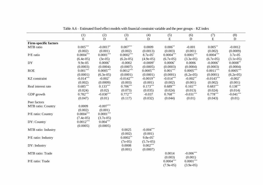
Table A.6 – Estimated fixed effect models with financial constraint variable and the peer groups – KZ index

(1) (2) (3) (4) (5) (6) (7) (8)

E D E D E D E D

Firm-specific factors

MTB ratio 0.005*** -0.0017* 0.007*** 0.0009 0.006** -0.001 0.005** -0.0012

(0.002) (0.001) (0.002) (0.0013) (0.003) (0.001) (0.002) (0.0009)

P/E ratio 0.0004*** 0.0001*** 0.0002*** 8.7e-05* 0.0004*** 0.0001*** 0.0004*** 3.7e-05

(6.4e-05) (3e-05) (6.2e-05) (4.9e-05) (6.7e-05) (3.3e-05) (6.7e-05) (3.1e-05)

DY 9.9e-05 0.0006* -0.0002 -0.0009* 0.0006* 0.0006 -0.0006* 0.0008**

(0.0003) (0.0004) (0.0007) (0.0005) (0.0003) (0.0004) (0.0003) (0.0004)

ROE 0.001*** 0.0005*** 0.0012*** 0.0005*** 0.001*** 0.0005*** 0.0011*** 0.0005***

(0.0001) (6.3e-05) (0.0001) (0.0001) (0.0001) (6.2e-05) (0.0001) (6.2e-05)

KZ constraint -0.014*** -0.002* -0.0142*** -0.0019** -0.014*** -0.002** -0.0143*** -0.002*

(0.002) (0.0009) (0.003) (0.001) (0.002) (0.001) (0.002) (0.001)

Real interest rate 0.685*** 0.133*** 0.706*** 0.173*** 0.689*** 0.165*** 0.683*** 0.138***

(0.024) (0.02) (0.073) (0.035) (0.024) (0.013) (0.024) (0.014)

GDP growth 0.782*** -0.030*** 0.772*** -0.037 0.768*** -0.031*** 0.778*** -0.041***

(0.047) (0.01) (0.117) (0.032) (0.044) (0.01) (0.043) (0.01)

Peer factors

MTB ratio: Country 0.0009 -0.007***

(0.002) (0.001)

P/E ratio: Country 0.0004*** 0.0001***

(7.4e-05) (3.7e-05)

DY: Country 0.0012*** 0.004***

(0.0005) (0.0005)

MTB ratio: Industry 0.0025 -0.004***

(0.002) (0.001)

P/E ratio: Industry 0.0002** 9.8e-05*

(7e-05) (5.7e-05)

DY: Industry 0.0008 0.002***

(0.001) (0.0007)

MTB ratio: Trade 0.0014 -0.006***

(0.003) (0.001)

P/E ratio: Trade 0.0004*** 0.0001***

(7.9e-05) (3.9e-05)

75

DY: Trade 0.002*** 0.004***

(0.0005) (0.0005)

MTB ratio: SMC 0.0002 -0.006***

(0.003) (0.001)

P/E ratio: SMC 0.0005*** 3.3e-05

(7.9e-05) (3.7e-05)

DY: SMC 1.0e-05 0.005***

(0.0005) (0.0005)

Constant -0.108*** -0.001 -0.103*** -0.00135 -0.108*** -0.002 -0.104*** -0.0007

(0.005) (0.002) (0.012) (0.004) (0.005) (0.003) (0.005) (0.002)

Observations 8,148 19,135 8,148 19,135 8,148 19,135 8,148 19,135

R-squared 0.304 0.081 0.302 0.073 0.304 0.078 0.304 0.081

Number of firms 1,694 3,145 1,694 3,145 1,694 3,145 1,694 3,145 Note: the dependent variable is the geometric mean for the annual stock return, using the monthly returns. All the peer variables for company i are the mean of all the financial

characteristics of the reference group except for the firm i. Financial firms are excluded from the sample and we require at least 2 firms per industry and at least 30 observations

per country. We apply the fixed effect model for panel data using the traditional estimator and the standard errors in parentheses are robust for heteroskedasticity and within

industry-country dependence. Statistical significance at 1%, 5% and 10% is denoted by ***, **, and *, respectively.

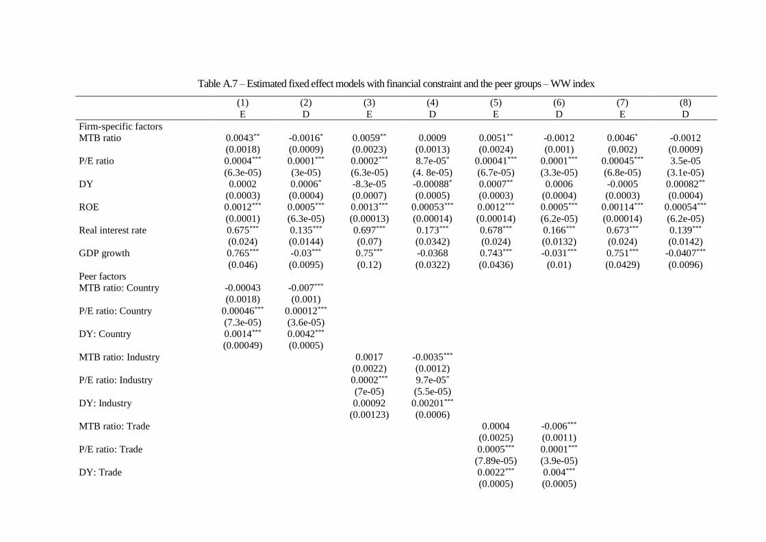
Table A.7 – Estimated fixed effect models with financial constraint and the peer groups – WW index

(1) (2) (3) (4) (5) (6) (7) (8)

E D E D E D E D

Firm-specific factors

MTB ratio 0.0043** -0.0016* 0.0059** 0.0009 0.0051** -0.0012 0.0046* -0.0012

(0.0018) (0.0009) (0.0023) (0.0013) (0.0024) (0.001) (0.002) (0.0009)

P/E ratio 0.0004*** 0.0001*** 0.0002*** 8.7e-05* 0.00041*** 0.0001*** 0.00045*** 3.5e-05

(6.3e-05) (3e-05) (6.3e-05) (4. 8e-05) (6.7e-05) (3.3e-05) (6.8e-05) (3.1e-05)

DY 0.0002 0.0006* -8.3e-05 -0.00088* 0.0007** 0.0006 -0.0005 0.00082**

(0.0003) (0.0004) (0.0007) (0.0005) (0.0003) (0.0004) (0.0003) (0.0004)

ROE 0.0012*** 0.0005*** 0.0013*** 0.00053*** 0.0012*** 0.0005*** 0.00114*** 0.00054***

(0.0001) (6.3e-05) (0.00013) (0.00014) (0.00014) (6.2e-05) (0.00014) (6.2e-05)

Real interest rate 0.675*** 0.135*** 0.697*** 0.173*** 0.678*** 0.166*** 0.673*** 0.139***

(0.024) (0.0144) (0.07) (0.0342) (0.024) (0.0132) (0.024) (0.0142)

GDP growth 0.765*** -0.03*** 0.75*** -0.0368 0.743*** -0.031*** 0.751*** -0.0407***

(0.046) (0.0095) (0.12) (0.0322) (0.0436) (0.01) (0.0429) (0.0096)

Peer factors

MTB ratio: Country -0.00043 -0.007***

(0.0018) (0.001)

P/E ratio: Country 0.00046*** 0.00012***

(7.3e-05) (3.6e-05)

DY: Country 0.0014*** 0.0042***

(0.00049) (0.0005)

MTB ratio: Industry 0.0017 -0.0035***

(0.0022) (0.0012)

P/E ratio: Industry 0.0002*** 9.7e-05*

(7e-05) (5.5e-05)

DY: Industry 0.00092 0.00201***

(0.00123) (0.0006)

MTB ratio: Trade 0.0004 -0.006***

(0.0025) (0.0011)

P/E ratio: Trade 0.0005*** 0.0001***

(7.89e-05) (3.9e-05)

DY: Trade 0.0022*** 0.004***

(0.0005) (0.0005)

77

MTB ratio: SMC -0.0005 -0.006***

(0.003) (0.001)

P/E ratio: SMC 0.0005*** 3e-05

(8e-05) (3.7e-05)

DY: SMC 0.0002 0.005***

(0.0005) (0.0005)

WW constraint 0.026*** 0.001 0.026*** 0.0009 0.026*** 0.0012 0.0255*** 0.001

(0.003) (0.002) (0.004) (0.002) (0.003) (0.002) (0.003) (0.002)

Constant -0.121*** -0.002 -0.114*** -0.002 -0.120*** -0.003 -0.116*** -0.002

(0.004) (0.002) (0.01) (0.004) (0.005) (0.003) (0.005) (0.002)

Observations 8,194 19,221 8,194 19,221 8,194 19,221 8,194 19,221

R-squared 0.302 0.081 0.298 0.073 0.302 0.078 0.301 0.080

Number of firms 1,703 3,145 1,703 3,145 1,703 3,145 1,703 3,145 Note: the dependent variable is the geometric mean for the annual stock return, using the monthly returns. All the peer variables for company i are the mean of all the financial

characteristics of the reference group except for the firm i. Financial firms are excluded from the sample and we require at least 2 firms per industry and at least 30 observations

per country. We apply the fixed effect model for panel data using the traditional estimator and the standard errors in parentheses are robust for heteroskedasticity and within

industry-country dependence. Statistical significance at 1%, 5% and 10% is denoted by ***, **, and *, respectively.

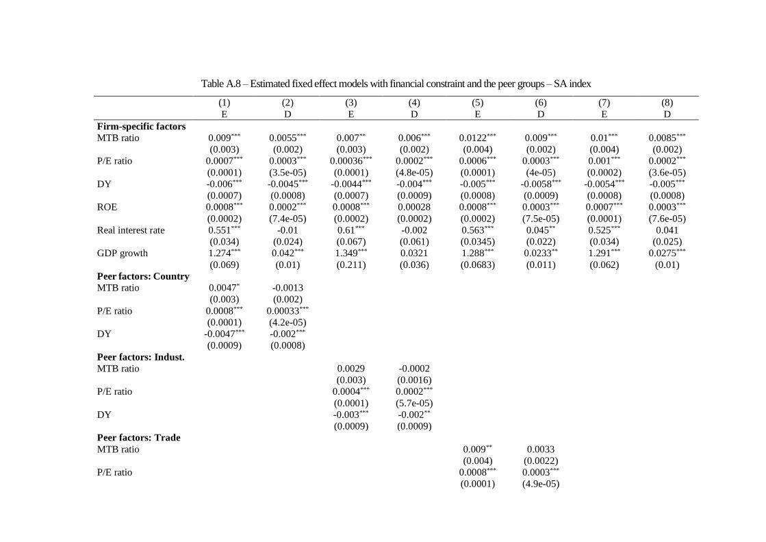
Table A.8 – Estimated fixed effect models with financial constraint and the peer groups – SA index

(1) (2) (3) (4) (5) (6) (7) (8)

E D E D E D E D

Firm-specific factors

MTB ratio 0.009*** 0.0055*** 0.007** 0.006*** 0.0122*** 0.009*** 0.01*** 0.0085***

(0.003) (0.002) (0.003) (0.002) (0.004) (0.002) (0.004) (0.002)

P/E ratio 0.0007*** 0.0003*** 0.00036*** 0.0002*** 0.0006*** 0.0003*** 0.001*** 0.0002***

(0.0001) (3.5e-05) (0.0001) (4.8e-05) (0.0001) (4e-05) (0.0002) (3.6e-05)

DY -0.006*** -0.0045*** -0.0044*** -0.004*** -0.005*** -0.0058*** -0.0054*** -0.005***

(0.0007) (0.0008) (0.0007) (0.0009) (0.0008) (0.0009) (0.0008) (0.0008)

ROE 0.0008*** 0.0002*** 0.0008*** 0.00028 0.0008*** 0.0003*** 0.0007*** 0.0003***

(0.0002) (7.4e-05) (0.0002) (0.0002) (0.0002) (7.5e-05) (0.0001) (7.6e-05)

Real interest rate 0.551*** -0.01 0.61*** -0.002 0.563*** 0.045** 0.525*** 0.041

(0.034) (0.024) (0.067) (0.061) (0.0345) (0.022) (0.034) (0.025)

GDP growth 1.274*** 0.042*** 1.349*** 0.0321 1.288*** 0.0233** 1.291*** 0.0275***

(0.069) (0.01) (0.211) (0.036) (0.0683) (0.011) (0.062) (0.01)

Peer factors: Country

MTB ratio 0.0047* -0.0013

(0.003) (0.002)

P/E ratio 0.0008*** 0.00033***

(0.0001) (4.2e-05)

DY -0.0047*** -0.002***

(0.0009) (0.0008)

Peer factors: Indust.

MTB ratio 0.0029 -0.0002

(0.003) (0.0016)

P/E ratio 0.0004*** 0.0002***

(0.0001) (5.7e-05)

DY -0.003*** -0.002**

(0.0009) (0.0009)

Peer factors: Trade

MTB ratio 0.009** 0.0033

(0.004) (0.0022)

P/E ratio 0.0008*** 0.0003***

(0.0001) (4.9e-05)

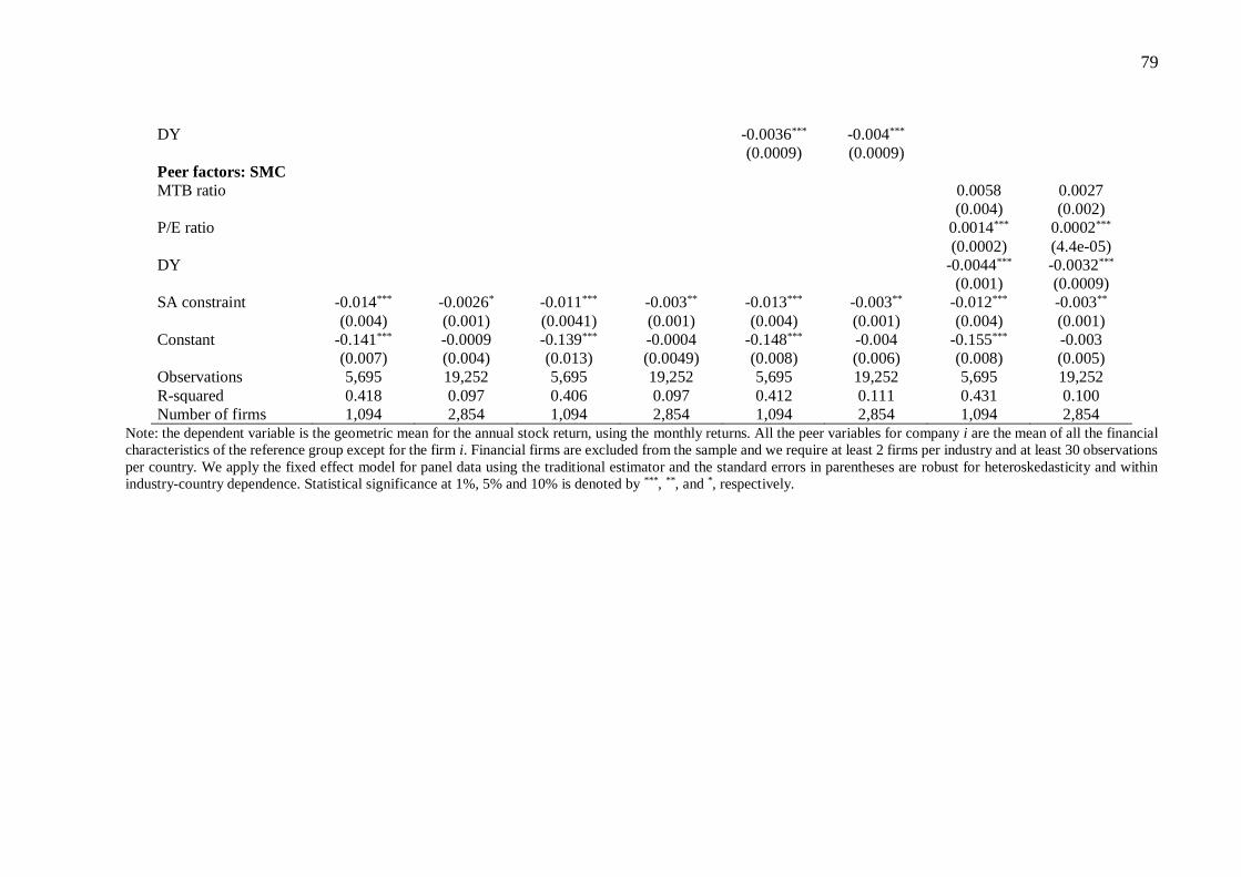
79

DY -0.0036*** -0.004***

(0.0009) (0.0009)

Peer factors: SMC

MTB ratio 0.0058 0.0027

(0.004) (0.002)

P/E ratio 0.0014*** 0.0002***

(0.0002) (4.4e-05)

DY -0.0044*** -0.0032***

(0.001) (0.0009)

SA constraint -0.014*** -0.0026* -0.011*** -0.003** -0.013*** -0.003** -0.012*** -0.003**

(0.004) (0.001) (0.0041) (0.001) (0.004) (0.001) (0.004) (0.001)

Constant -0.141*** -0.0009 -0.139*** -0.0004 -0.148*** -0.004 -0.155*** -0.003

(0.007) (0.004) (0.013) (0.0049) (0.008) (0.006) (0.008) (0.005)

Observations 5,695 19,252 5,695 19,252 5,695 19,252 5,695 19,252

R-squared 0.418 0.097 0.406 0.097 0.412 0.111 0.431 0.100

Number of firms 1,094 2,854 1,094 2,854 1,094 2,854 1,094 2,854 Note: the dependent variable is the geometric mean for the annual stock return, using the monthly returns. All the peer variables for company i are the mean of all the financial

characteristics of the reference group except for the firm i. Financial firms are excluded from the sample and we require at least 2 firms per industry and at least 30 observations

per country. We apply the fixed effect model for panel data using the traditional estimator and the standard errors in parentheses are robust for heteroskedasticity and within

industry-country dependence. Statistical significance at 1%, 5% and 10% is denoted by ***, **, and *, respectively.

Table A.9 – Instrumental variables models with financial constraint and the peer groups – KZ index

(1) (2) (3) (4) (5) (6) (7) (8)

E D E D E D E D

Firm-specific factors

MTB 0.008*** 0.006*** 0.008*** 0.005*** 0.009*** 0.006*** 0.009*** 0.006***

(0.0006) (0.0007) (0.0007) (0.0006) (0.0007) (0.0007) (0.0007) (0.0007)

PE raio 3.8e-05*** 1.7e-05** 4.5e-05*** 1.6e-05** 4.7e-05*** 1.6e-05** 5.0e-05*** 1.6e-05**

(1.4e-05) (7.3e-06) (1.56e-05) (7.4e-06) (1.3e-05) (7.3e-06) (1.3e-05) (7.3e-06)

DY -0.001*** -0.002*** -0.0009*** -0.002*** -0.0009*** -0.002*** -0.001*** -0.002***

(0.0002) (0.0002) (0.0002) (0.0002) (0.0002) (0.0002) (0.0002) (0.0002)

ROE 0.002*** 0.001*** 0.002*** 0.001*** 0.002*** 0.0009*** 0.0017*** 0.001***

(0.0001) (6.4e-05) (0.0002) (6.3e-05) (0.0001) (6.5e-05) (0.0001) (6.5e-05)

KZ constrained -0.015*** -0.002** -0.016*** -0.002** -0.013*** -0.002* -0.014*** -0.002*

(0.002) (0.0009) (0.002) (0.0009) (0.002) (0.0009) (0.002) (0.0009)

Real interest 0.690*** 0.283*** 0.7*** 0.259*** 0.654*** 0.233*** 0.61*** 0.284***

(0.02) (0.014) (0.03) (0.014) (0.02) (0.014) (0.022) (0.014)

GDP growth 0.813*** -0.09*** 0.745*** -0.087*** 0.964*** -0.129*** 0.88*** -0.108***

(0.04) (0.008) (0.046) (0.008) (0.04) (0.009) (0.04) (0.009)

Peer factors

Country: SRt-1 0.947*** 0.368***

(0.03) (0.012)

Country: MTBt-1 0.003*** 0.007***

(0.0007) (0.0007)

Country: PEt-1 -4.3e-06 -8.7e-06

(1.7e-05) (7.1e-06)

Country: DYt-1 0.0008*** 0.0007***

(0.0002) (0.0002)

Ind.: SRt-1 1.142*** 0.413***

(0.04) (0.013)

Ind.: MTBt-1 0.002*** 0.004***

(0.0007) (0.0006)

Ind.: PEt-1 -2.1e-06 -2.6e-06

(1.8e-05) (7.1e-06)

Ind.: DYt-1 0.001*** 0.0009***

(0.0002) (0.0002)

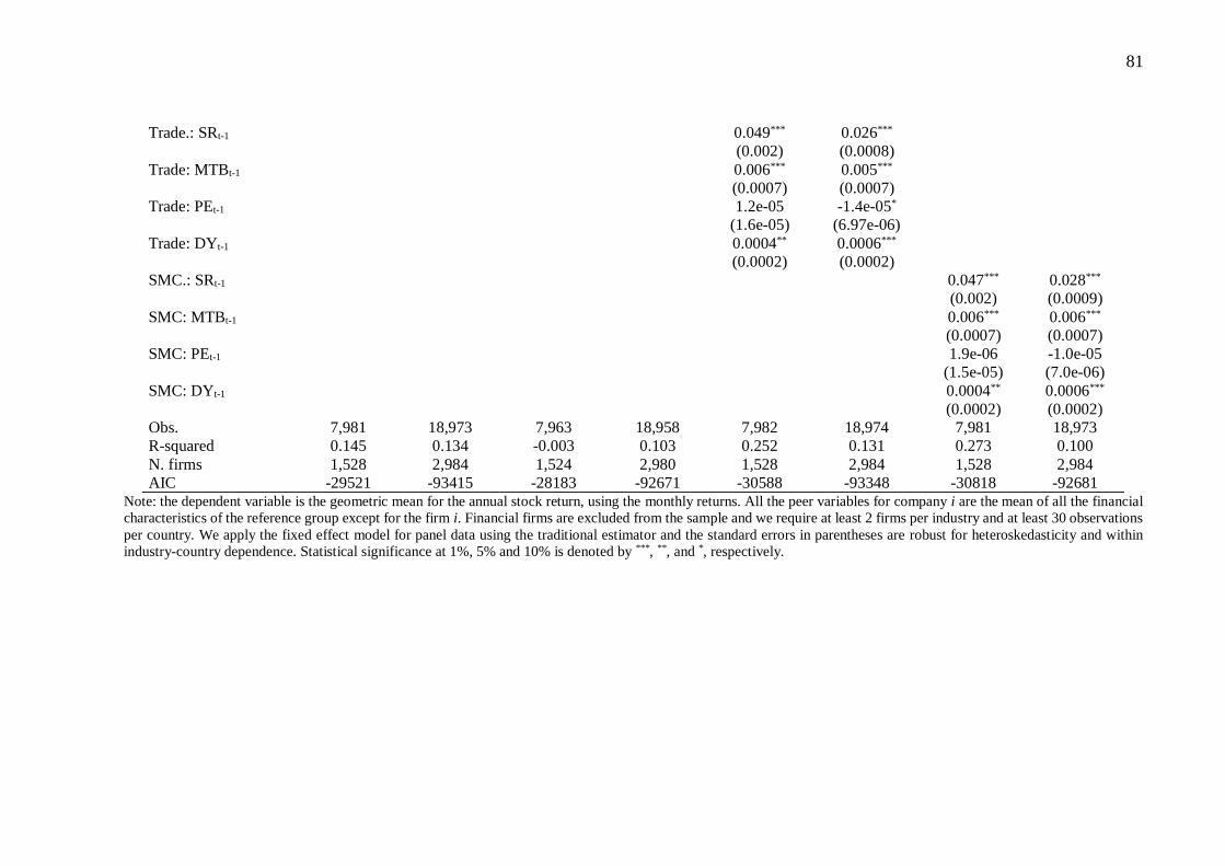
81

Trade.: SRt-1 0.049*** 0.026***

(0.002) (0.0008)

Trade: MTBt-1 0.006*** 0.005***

(0.0007) (0.0007)

Trade: PEt-1 1.2e-05 -1.4e-05*

(1.6e-05) (6.97e-06)

Trade: DYt-1 0.0004** 0.0006***

(0.0002) (0.0002)

SMC.: SRt-1 0.047*** 0.028***

(0.002) (0.0009)

SMC: MTBt-1 0.006*** 0.006***

(0.0007) (0.0007)

SMC: PEt-1 1.9e-06 -1.0e-05

(1.5e-05) (7.0e-06)

SMC: DYt-1 0.0004** 0.0006***

(0.0002) (0.0002)

Obs. 7,981 18,973 7,963 18,958 7,982 18,974 7,981 18,973

R-squared 0.145 0.134 -0.003 0.103 0.252 0.131 0.273 0.100

N. firms 1,528 2,984 1,524 2,980 1,528 2,984 1,528 2,984

AIC -29521 -93415 -28183 -92671 -30588 -93348 -30818 -92681 Note: the dependent variable is the geometric mean for the annual stock return, using the monthly returns. All the peer variables for company i are the mean of all the financial

characteristics of the reference group except for the firm i. Financial firms are excluded from the sample and we require at least 2 firms per industry and at least 30 observations

per country. We apply the fixed effect model for panel data using the traditional estimator and the standard errors in parentheses are robust for heteroskedasticity and within

industry-country dependence. Statistical significance at 1%, 5% and 10% is denoted by ***, **, and *, respectively.

Table A.10 – Instrumental variables models with financial constraint and the peer groups – WW index

(1) (2) (3) (4) (5) (6) (7) (8)

E D E D E D E D

Firm-specific factors

MTB 0.008*** 0.006*** 0.007*** 0.005*** 0.009*** 0.006*** 0.009*** 0.006***

(0.0007) (0.0007) (0.0007) (0.0006) (0.0007) (0.0007) (0.0007) (0.0007)

PE raio 3.8e-05*** 1.6e-05** 4.6e-05*** 1.6e-05** 4.6e-05*** 1.6e-05** 5.0e-05*** 1.6e-05**

(1.4e-05) (7.3e-06) (1.5e-05) (7.4e-06) (1. 3e-05) (7.3e-06) (1.3e-05) (7.3e-06)

DY -0.0009*** -0.002*** -0.0009*** -0.002*** -0.0009*** -0.002*** -0.001*** -0.002***

(0.0002) (0.0002) (0.0002) (0.0002) (0.0002) (0.0002) (0.0002) (0.0002)

ROE 0.002*** 0.001*** 0.002*** 0.0009*** 0.002*** 0.0009*** 0.0018*** 0.001***

(0.0001) (6.4e-05) (0.0001) (6.2e-05) (0.0001) (6.4e-05) (0.0001) (6.5e-05)

WW constrained 0.017*** -0.0005 0.018*** -0.0003 0.015*** -0.002 0.014*** -0.002

(0.003) (0.001) (0.0037) (0.001) (0.003) (0.001) (0.003) (0.001)

Real interest 0.685*** 0.284*** 0.693*** 0.259*** 0.65*** 0.232*** 0.602*** 0.283***

(0.02) (0.01) (0.02) (0.014) (0.02) (0.014) (0.022) (0.014)

GDP growth 0.804*** -0.091*** 0.737*** -0.087*** 0.956*** -0.129*** 0.875*** -0.108***

(0.04) (0.008) (0.05) (0.008) (0.04) (0.009) (0.042) (0.009)

Peer factors

Country: SRt-1 0.93*** 0.369***

(0.03) (0.012)

Country: MTBt-1 0.003*** 0.006***

(0.0007) (0.0007)

Country: PEt-1 -2.6e-06 -7.96e-06

(1.6e-05) (7.1e-06)

Country: DYt-1 0.0008*** 0.0007***

(0.0002) (0.0002)

Ind.: SRt-1 1.118*** 0.415***

(0.04) (0.013)

Ind.: MTBt-1 0.0016** 0.004***

(0.0007) (0.0006)

Ind.: PEt-1 4.9e-07 -2.0e-06

(1.7e-05) (7.1e-06)

Ind.: DYt-1 0.001*** 0.0009***

(0.0002) (0.0002)

83

Trade.: SRt-1 0.048*** 0.026***

(0.002) (0.0008)

Trade: MTBt-1 0.006*** 0.005***

(0.0007) (0.0007)

Trade: PEt-1 1.2e-05 -1.3e-05*

(1.6e-05) (7.0e-06)

Trade: DYt-1 0.0004** 0.0006***

(0.0002) (0.0002)

SMC.: SRt-1 0.047*** 0.028***

(0.002) (0.0009)

SMC: MTBt-1 0.006*** 0.0054***

(0.0007) (0.0007)

SMC: PEt-1 2.6e-06 -9.5e-06

(1.5e-05) (7.0e-06)

SMC: DYt-1 0.0004* 0.0006***

(0.0002) (0.0002)

Obs. 8,027 19,068 8,009 19,053 8,028 19,069 8,027 19,068

R-squared 0.145 0.133 0.003 0.103 0.244 0.131 0.264 0.100

N. firms 1,537 2,993 1,533 2,989 1,537 2,993 1,537 2,993

AIC -29727 -93878 -28435 -93157 -30726 -93835 -30938 -93162 Note: the dependent variable is the geometric mean for the annual stock return, using the monthly returns. All the peer variables for company i are the mean of all the financial

characteristics of the reference group except for the firm i. Financial firms are excluded from the sample and we require at least 2 firms per industry and at least 30 observations

per country. We apply the fixed effect model for panel data using the traditional estimator and the standard errors in parentheses are robust for heteroskedasticity and within

industry-country dependence. Statistical significance at 1%, 5% and 10% is denoted by ***, **, and *, respectively.

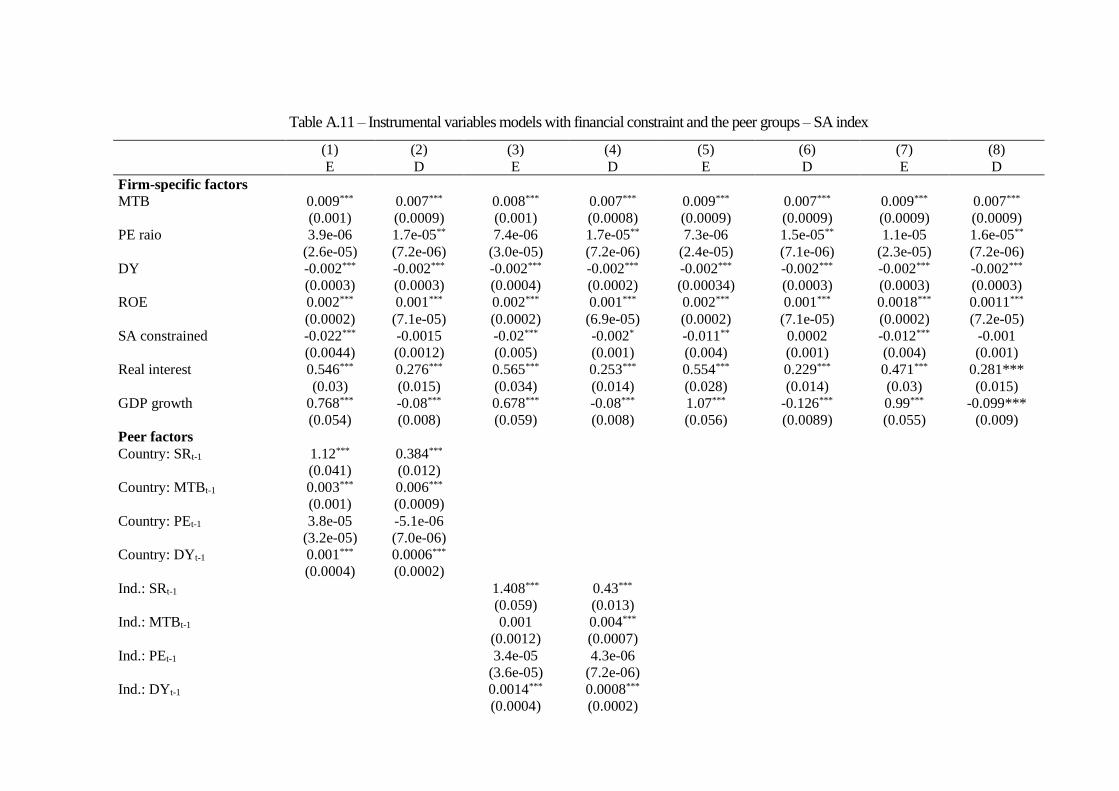
Table A.11 – Instrumental variables models with financial constraint and the peer groups – SA index

(1) (2) (3) (4) (5) (6) (7) (8)

E D E D E D E D

Firm-specific factors

MTB 0.009*** 0.007*** 0.008*** 0.007*** 0.009*** 0.007*** 0.009*** 0.007***

(0.001) (0.0009) (0.001) (0.0008) (0.0009) (0.0009) (0.0009) (0.0009)

PE raio 3.9e-06 1.7e-05** 7.4e-06 1.7e-05** 7.3e-06 1.5e-05** 1.1e-05 1.6e-05**

(2.6e-05) (7.2e-06) (3.0e-05) (7.2e-06) (2.4e-05) (7.1e-06) (2.3e-05) (7.2e-06)

DY -0.002*** -0.002*** -0.002*** -0.002*** -0.002*** -0.002*** -0.002*** -0.002***

(0.0003) (0.0003) (0.0004) (0.0002) (0.00034) (0.0003) (0.0003) (0.0003)

ROE 0.002*** 0.001*** 0.002*** 0.001*** 0.002*** 0.001*** 0.0018*** 0.0011***

(0.0002) (7.1e-05) (0.0002) (6.9e-05) (0.0002) (7.1e-05) (0.0002) (7.2e-05)

SA constrained -0.022*** -0.0015 -0.02*** -0.002* -0.011** 0.0002 -0.012*** -0.001

(0.0044) (0.0012) (0.005) (0.001) (0.004) (0.001) (0.004) (0.001)

Real interest 0.546*** 0.276*** 0.565*** 0.253*** 0.554*** 0.229*** 0.471*** 0.281***

(0.03) (0.015) (0.034) (0.014) (0.028) (0.014) (0.03) (0.015)

GDP growth 0.768*** -0.08*** 0.678*** -0.08*** 1.07*** -0.126*** 0.99*** -0.099***

(0.054) (0.008) (0.059) (0.008) (0.056) (0.0089) (0.055) (0.009)

Peer factors

Country: SRt-1 1.12*** 0.384***

(0.041) (0.012)

Country: MTBt-1 0.003*** 0.006***

(0.001) (0.0009)

Country: PEt-1 3.8e-05 -5.1e-06

(3.2e-05) (7.0e-06)

Country: DYt-1 0.001*** 0.0006***

(0.0004) (0.0002)

Ind.: SRt-1 1.408*** 0.43***

(0.059) (0.013)

Ind.: MTBt-1 0.001 0.004***

(0.0012) (0.0007)

Ind.: PEt-1 3.4e-05 4.3e-06

(3.6e-05) (7.2e-06)

Ind.: DYt-1 0.0014*** 0.0008***

(0.0004) (0.0002)

85

Trade.: SRt-1 0.064*** 0.028***

(0.002) (0.0009)

Trade: MTBt-1 0.0045*** 0.004***

(0.0009) (0.0008)

Trade: PEt-1 7.4e-05** -1.2e-05*

(2.95e-05) (6.95e-06)

Trade: DYt-1 0.0003 0.0005**

(0.0003) (0.0002)

SMC.: SRt-1 0.061*** 0.029***

(0.002) (0.001)

SMC: MTBt-1 0.0047*** 0.0045***

(0.0009) (0.0008)

SMC: PEt-1 4.4e-05 -7.6e-06

(2.8e-05) (7.0e-06)

SMC: DYt-1 0.0003 0.0005**

(0.0003) (0.0002)

Obs. 4,828 17,308 4,813 17,300 4,829 17,309 4,828 17,308

R-squared 0.001 0.144 -0.295 0.114 0.081 0.134 0.140 0.100

N. firms 964 2,696 961 2,694 964 2,696 964 2,696

AIC -16449 -85931 -15150 -85311 -16854 -85741 -17174 -85075 Note: the dependent variable is the geometric mean for the annual stock return, using the monthly returns. All the peer variables for company i are the mean of all the financial

characteristics of the reference group except for the firm i. Financial firms are excluded from the sample and we require at least 2 firms per industry and at least 30 observations

per country. We apply the fixed effect model for panel data using the traditional estimator and the standard errors in parentheses are robust for heteroskedasticity and within

industry-country dependence. Statistical significance at 1%, 5% and 10% is denoted by ***, **, and *, respectively.

APPENDIX B – Instrumental tests for stock returns using the peer groups

Table B.1 – Instrumental tests for the estimated models for stock return for all the peer groups from tables 3 and 4 – 2006 to 2016.

Ind.SRt-1 Coun.SR t-1 Trade SR t-1 SMC SR t-1

E. D. E. D. E. D. E. D.

Shea's Partial R2 0.2416 0.5869 0.313 0.6421 0.4044 0.6978 0.4405 0.5498

Underidentification test 869.15*** 2393.16*** 1033.15*** 2547.31*** 1219.33*** 2576.97*** 1301.19*** 2103.14***

Weak identification test 1812.55 10576.63 2689.4 13248.63 3067.93 11442.04 3403.91 8448.89

Weak instrument? No No No No No No No No

Weak-instrument-robust inference 878.46*** 808.46*** 862.51*** 775.25*** 809.42*** 837.19*** 819.9*** 788.7***

Stock-Yogo weak ID test critical values: 10% maximal IV size 16.38 15% maximal IV size 8.96 20% maximal IV size 6.66 25% maximal IV size 5.53

Note: These are the results for the weak instrument tests for the models in tables 6 and 7. The Shea’s Partial R2 is reported because the models contain an endogenous regressors.

The underidentification test is the Kleibergen-Paap rk LM statistic in which the null hypothesis is that matrix of reduced form coefficients is underidentified, and the weak

instrument test is a Kleibergen-Paap Wald F statistic. The main results indicate that this instrument is a weak one, except for developed countries. We denote *** as the p-value

= 0.000.