Verb Sense Classification

Gonçalo André Rodrigues Suissas

Thesis to obtain the Master of Science Degree in

Information Systems and Computer Engineering

Examination Committee

Supervisor: Doutor Nuno João Neves MamedeCo-supervisor: Doutor Jorge Manuel Evangelista Baptista

October 2014

ii

Dedicated to my parents and to my sister

iii

iv

Acknowledgments

First, I would like to thank my supervisor, Prof. Nuno Mamede, for guiding me through the course of this

thesis. His experience and advice were very important to make this work possible.

I would also like to thank my co-supervisor, Prof. Jorge Baptista, who discuss and give his insight on

several topics addressed in this dissertation. His will to push me to improve this work proved to be of

great value.

I must also mention Claude Roux, from Xerox Research Labs, who provided helpful information on

some issues regarding the KiF language, used in the Naive Bayes implementation.

Finally, I cannot thank enough Tiago Travanca from the L2F group at INESC-ID Lisboa for his avail-

ability, cooperation and will to help. With his help, it made much easier to understand how the modules

developed in his work were integrated in the STRING system.

v

vi

Resumo

Esta dissertacao aborda o problema da desambiguacao de sentido de verbos em Portugues Europeu.

Trata-se de um sub-problema de desambiguacao sematica de palavras, na qual se pretende a partir de

um conjunto de diferentes significados escolher o mais adequado.

Este documento apresenta diversos metodos de aprendizagem supervisionada que podem ser adp-

tados a este tema, onde sao discustidos os problemas encontrados. Serao apresentados um conjunto

de metodos de aprendizagem automatica a serem incorporados no sistema STRING.

Estes metodos, foram testados em diversos cenarios, de modo a perceber o impacto de diferentes

conjuntos de propriedades (features). A exactidao definida (accuracy) de 63.86% a para o limiar de

referencia (baseline), resulta da abordagem do sentido mais frequente para esse lema (most frequent

sense) para um conjunto de 24 verbos. Entre as abordagens de aprendizagem automatica, o metodo

que obteve melhores resultados foi o algoritmo naive bayes que atingiu uma exactidao de 67.71%, um

ganho de 3.85% acima do valor de referencia.

Palavras-chave: Processamento de Lingua Natural, Classificacao de Sentidos de Verbos,

Aprendizagem Automatica, Desambiguacao Semantica

vii

viii

Abstract

This dissertation addresses the verb sense disambiguation (VSD) problem, a sub-problem of word sense

disambiguation (WSD), for European Portuguese. It aims at developing a set of modules of an existing

Natural Language Processing (NLP) system, which will enable it to choose adequately the precise sense

that a verb features in a given sentence from among other potential different meanings.

This paper presents various methods used in supervised classification that can be adopted on VSD,

and it discusses the main problems found for this task, briefly describing the techniques previously used

to address it, as well as the new Machine Learning (ML) techniques that will be integrated in the STRING

system.

These ML techniques were tested in several scenarios to determine the impact of different features.

The baseline accuracy of 63.86% results from the most frequent sense (MFS) for each verb lemma in

a set of 24 verbs. Among the ML techniques tested, the best method was the Naive Bayes algorithm,

which achieved an accuracy of 67.71%, a gain of 3.85% above the baseline.

Keywords: Natural Language Processing, Verb Sense Classification, Machine Learning, Se-

mantic Disambiguation

ix

x

Contents

Acknowledgments . . . . . . . . . . . . . . . . . . . . . . . . . . . . . . . . . . . . . . . . . . . v

Resumo . . . . . . . . . . . . . . . . . . . . . . . . . . . . . . . . . . . . . . . . . . . . . . . . . vii

Abstract . . . . . . . . . . . . . . . . . . . . . . . . . . . . . . . . . . . . . . . . . . . . . . . . . ix

List of Tables . . . . . . . . . . . . . . . . . . . . . . . . . . . . . . . . . . . . . . . . . . . . . . xiii

List of Figures . . . . . . . . . . . . . . . . . . . . . . . . . . . . . . . . . . . . . . . . . . . . . xvi

Acronyms . . . . . . . . . . . . . . . . . . . . . . . . . . . . . . . . . . . . . . . . . . . . . . . . xvii

1 Introduction 1

2 State of the Art 3

2.1 WordNet . . . . . . . . . . . . . . . . . . . . . . . . . . . . . . . . . . . . . . . . . . . . . . 3

2.2 ViPEr . . . . . . . . . . . . . . . . . . . . . . . . . . . . . . . . . . . . . . . . . . . . . . . 5

2.3 Previous works on VSD . . . . . . . . . . . . . . . . . . . . . . . . . . . . . . . . . . . . . 6

2.4 The STRING system . . . . . . . . . . . . . . . . . . . . . . . . . . . . . . . . . . . . . . . 7

2.5 XIP Features . . . . . . . . . . . . . . . . . . . . . . . . . . . . . . . . . . . . . . . . . . . 8

2.6 Rule-generation module . . . . . . . . . . . . . . . . . . . . . . . . . . . . . . . . . . . . . 8

2.7 Machine Learning Disambiguation . . . . . . . . . . . . . . . . . . . . . . . . . . . . . . . 9

2.7.1 Architecture . . . . . . . . . . . . . . . . . . . . . . . . . . . . . . . . . . . . . . . . 9

2.8 Previous Results . . . . . . . . . . . . . . . . . . . . . . . . . . . . . . . . . . . . . . . . . 11

2.8.1 Rule-based disambiguation . . . . . . . . . . . . . . . . . . . . . . . . . . . . . . . 11

2.8.2 Standard rules . . . . . . . . . . . . . . . . . . . . . . . . . . . . . . . . . . . . . . 11

2.8.3 Other methods . . . . . . . . . . . . . . . . . . . . . . . . . . . . . . . . . . . . . . 12

2.8.4 Rules + MFS . . . . . . . . . . . . . . . . . . . . . . . . . . . . . . . . . . . . . . . 12

2.9 Machine Learning . . . . . . . . . . . . . . . . . . . . . . . . . . . . . . . . . . . . . . . . 13

2.9.1 Training Instances . . . . . . . . . . . . . . . . . . . . . . . . . . . . . . . . . . . . 13

2.9.2 Semantic Features and Window Size . . . . . . . . . . . . . . . . . . . . . . . . . . 13

2.9.3 Bias . . . . . . . . . . . . . . . . . . . . . . . . . . . . . . . . . . . . . . . . . . . . 14

2.9.4 Comparison . . . . . . . . . . . . . . . . . . . . . . . . . . . . . . . . . . . . . . . . 14

2.9.5 Rules + ML . . . . . . . . . . . . . . . . . . . . . . . . . . . . . . . . . . . . . . . . 15

2.10 Supervised Classification Methods . . . . . . . . . . . . . . . . . . . . . . . . . . . . . . . 16

2.10.1 Decision Trees . . . . . . . . . . . . . . . . . . . . . . . . . . . . . . . . . . . . . . 16

xi

2.10.2 Decision Tree algorithms . . . . . . . . . . . . . . . . . . . . . . . . . . . . . . . . 16

2.10.3 ID3 algorithm . . . . . . . . . . . . . . . . . . . . . . . . . . . . . . . . . . . . . . . 16

2.10.4 CART Method . . . . . . . . . . . . . . . . . . . . . . . . . . . . . . . . . . . . . . 18

2.10.5 Support Vector Machines . . . . . . . . . . . . . . . . . . . . . . . . . . . . . . . . 18

2.10.6 Conditional Random Fields . . . . . . . . . . . . . . . . . . . . . . . . . . . . . . . 19

3 Corpora 21

3.1 Training corpus . . . . . . . . . . . . . . . . . . . . . . . . . . . . . . . . . . . . . . . . . . 21

3.2 Evaluation Corpus . . . . . . . . . . . . . . . . . . . . . . . . . . . . . . . . . . . . . . . . 28

4 Architecture 31

4.1 Building and annotating a corpus of verb senses for ML . . . . . . . . . . . . . . . . . . . 31

4.2 Weka experiments . . . . . . . . . . . . . . . . . . . . . . . . . . . . . . . . . . . . . . . . 32

4.3 Naive Bayes implementation . . . . . . . . . . . . . . . . . . . . . . . . . . . . . . . . . . 37

5 Evaluation 39

5.1 Measures . . . . . . . . . . . . . . . . . . . . . . . . . . . . . . . . . . . . . . . . . . . . . 39

5.2 Baseline . . . . . . . . . . . . . . . . . . . . . . . . . . . . . . . . . . . . . . . . . . . . . . 40

5.3 Comparison with previous results . . . . . . . . . . . . . . . . . . . . . . . . . . . . . . . . 42

5.4 Naive Bayes experiments . . . . . . . . . . . . . . . . . . . . . . . . . . . . . . . . . . . . 43

5.5 Comparison . . . . . . . . . . . . . . . . . . . . . . . . . . . . . . . . . . . . . . . . . . . . 43

5.6 Performance evaluation . . . . . . . . . . . . . . . . . . . . . . . . . . . . . . . . . . . . . 47

6 Conclusions and Future work 49

6.1 Conclusions . . . . . . . . . . . . . . . . . . . . . . . . . . . . . . . . . . . . . . . . . . . . 49

6.2 Future Work . . . . . . . . . . . . . . . . . . . . . . . . . . . . . . . . . . . . . . . . . . . . 50

Bibliography 55

xii

List of Tables

2.1 Semantic Relations in WordNet (from (Miller, 1995)) . . . . . . . . . . . . . . . . . . . . . 4

3.1 The training corpus used, the number of instances and the number of classes per verb. . 22

3.2 Evaluation Corpus Verb Occurrences. . . . . . . . . . . . . . . . . . . . . . . . . . . . . . 28

3.3 Processed Corpus Distribution. . . . . . . . . . . . . . . . . . . . . . . . . . . . . . . . . . 28

3.4 Corpus Processing Results. . . . . . . . . . . . . . . . . . . . . . . . . . . . . . . . . . . . 29

3.5 The Evaluation corpus used. . . . . . . . . . . . . . . . . . . . . . . . . . . . . . . . . . . 29

3.6 The different MFS in the corpora used. . . . . . . . . . . . . . . . . . . . . . . . . . . . . . 30

4.1 The supervised methods available in Weka chosen for evaluation . . . . . . . . . . . . . 34

4.2 The training corpus used, the number of instances and the number of classes per verb. . 36

5.1 The MFS accuracy for each verb in the training phase. . . . . . . . . . . . . . . . . . . . . 40

5.2 The MFS accuracy for each verb used in the evaluation. . . . . . . . . . . . . . . . . . . . 41

5.3 STRING performance after modules integration and its difference to the baseline. . . . . . 48

xiii

xiv

List of Figures

2.1 Hierarchies used in the disambiguation of brake with context words {horn, man, second}

from (Buscaldi et al., 2004) . . . . . . . . . . . . . . . . . . . . . . . . . . . . . . . . . . . 5

2.2 STRING Architecture with the Rule Generation Module from (Travanca, 2013) . . . . . . . 7

2.3 The Rule-generation Module Architecture from (Travanca, 2013) . . . . . . . . . . . . . . 8

2.4 The Machine Learning Architecture from (Travanca, 2013) . . . . . . . . . . . . . . . . . . 10

2.5 The Supervised Machine Learning Architecture for VSD using STRING from (Travanca,

2013) . . . . . . . . . . . . . . . . . . . . . . . . . . . . . . . . . . . . . . . . . . . . . . . 10

2.6 The results of Standard Rules from (Travanca, 2013) . . . . . . . . . . . . . . . . . . . . . 11

2.7 The results of using the verb meaning filter from (Travanca, 2013) . . . . . . . . . . . . . . 12

2.8 The results of using rules and MFS from (Travanca, 2013) . . . . . . . . . . . . . . . . . . 12

2.9 ML Scenario 1: Verifying the impact of varying the number of training instances from

(Travanca, 2013) . . . . . . . . . . . . . . . . . . . . . . . . . . . . . . . . . . . . . . . . . 13

2.10 The results of semantic features from (Travanca, 2013) . . . . . . . . . . . . . . . . . . . . 14

2.11 The results of using Bias from (Travanca, 2013) . . . . . . . . . . . . . . . . . . . . . . . . 14

2.12 The comparison of the different ML methods from (Travanca, 2013) . . . . . . . . . . . . . 15

2.13 The results of using Machine learning from (Travanca, 2013) . . . . . . . . . . . . . . . . 15

2.14 A example of a decision tree from (Travanca, 2013) . . . . . . . . . . . . . . . . . . . . . . 16

3.1 The initial screen of the interface . . . . . . . . . . . . . . . . . . . . . . . . . . . . . . . . 23

3.2 Parametrization file of the lemma abandonar . . . . . . . . . . . . . . . . . . . . . . . . . 24

3.3 The annotation screen of the interface . . . . . . . . . . . . . . . . . . . . . . . . . . . . . 25

3.4 The edit feature in the interface. . . . . . . . . . . . . . . . . . . . . . . . . . . . . . . . . . 25

3.5 The annotation screen of the interface . . . . . . . . . . . . . . . . . . . . . . . . . . . . . 26

3.6 The annotation screen of the second interface . . . . . . . . . . . . . . . . . . . . . . . . . 27

4.1 Example of a ARFF file used in the Weka experiments . . . . . . . . . . . . . . . . . . . . 33

4.2 Comparison between ML experiments using Weka. . . . . . . . . . . . . . . . . . . . . . . 35

4.3 The results obtain using the weka software package. . . . . . . . . . . . . . . . . . . . . . 37

5.1 Comparison using the rules-disambiguation system. . . . . . . . . . . . . . . . . . . . . . 42

5.2 Comparison between ML methods used in (Travanca, 2013). . . . . . . . . . . . . . . . . 43

5.3 Comparison between naive bayes experiments. . . . . . . . . . . . . . . . . . . . . . . . . 44

xv

5.4 Comparison between naive bayes and maximum entropy methods. . . . . . . . . . . . . . 45

5.5 Comparison between all methods per verb lemma. . . . . . . . . . . . . . . . . . . . . . . 46

5.6 Comparison between average results of all methods integrated in STRING. . . . . . . . . 47

xvi

Acronyms

ARFF Attribute-Relation File Format

CSV Comma Separated Values

MFS Most Frequent Sense

ML Machine Learning

NLP Natural Language Processing

POS Part Of Speech

SVMS Support Vector Machines

ViPEr Verb for European Portuguese

VSD Verb Sense Disambiguation

WSD Word Sense Disambiguation

xvii

xviii

Chapter 1

Introduction

Nowadays, there are many applications that make use Natural Language Processing (NLP): search

engines that use voice recognition, automated speech recognition, automated summarization, spelling

checkers and grammar correctors, among others. But there is a major concern in NLP which needs

to be addressed: ambiguity. Ambiguity is the term used to describe that a certain word, expression

or a sentence in a text could be interpreted in more than one way. Ambiguity is present at several

stages of processing a sentence or a text. One type of ambiguity concerns word tagging. This type of

ambiguity (morphological or morphosyntactic ambiguity) happens when a word can belong to more than

one grammatical class. For example the word rio (river/laugh) could be classified as a verb or a noun as

show in the (1.1 a) and (1.1 b):

(1.1 a)Agora estou a passar pelo rio. (Now I’m going across the river)

(1.1 b)Eu rio tanto deste video. (I laugh so much from this video)

Processing each word individually, most of the times, is not enough to determine correctly which tag

should be assigned. Processing the rest of the sentence enables to determine which part-of-speech

(POS) tag should be correctly assigned to a given word in that context. Once words have been tagged,

the syntactical parsing starts. This task consists in determining and formalizing the syntactical relations

(or dependencies) between words presented in the sentence. But even at this stage ambiguity needs to

be addressed. Given an ambiguous sentence, there can be more than one syntactical representation,

each corresponding to a different meaning. Consider the following examples:

(1.2a) O Pedro mandou-me um postal dos Acores

(i) (Peter sent me a postcard from Azores )

SUBJ(mandou,Pedro); CDIR(mandou,postal); CINDIR(mandou,me);MOD(mandou,Acores)

(ii) (Peter send me a postcard of Azores)

SUBJ(mandou,Peter);CDIR(mandou,postal);CINDIR(mandou,me)MOD(postal,Acores)

1

While the sentence is easy to interpret, the syntactical parsing is likely to produce two potential

outputs for the prepositional phrase (PP) dos Acores(from/of Azores): in (i) it is a complement of the

verb mandou with a semantic role of locative; while in (ii) it is a complement of the noun postal, with a

semantic role of topic.

After the syntactic parsing is finished, there is another type of ambiguity to be solved, which is

semantic ambiguity. This tends to be the hardest type of ambiguity to be resolved. In this type of

ambiguity, the syntactic analysis (syntactical tree) obtained from the syntactical parsing maybe is unique

and can even be correct; however, when semantic analysis is applied, some words could feature more

than one meaning for the grammatical categories each word was tagged with during the syntactical

parsing. Consider the following examples:

(1.3a) O Pedro conta as moedas para comprar um cafe. (Peter counts the coins to buy coffee.)

(1.3b) O Joao conta contigo para a pintura da casa. (John counts on you to paint the house.)

Both sentences use the verb contar (to count) used in the same position. However, the verb in

the first sentence means to enumerate something, while on the second it stands for to rely on. The

most salient difference between these two sentences is the choice of the preposition introducing the

complement: there is no preposition (the verb selects direct object) in the construction of (1.3a), while

the preposition com (with) in (1.3b).

An example of the importance of word sense disambiguation, let us consider the case of machine

translation. When trying to translate a sentence, the system has to capture the sentence’s correct

meaning, in order to do a correct translation. For example, consider the following two sentences:

(1.4 a) O Pedro arranjou o computador do irmao. (Peter repaired his brother’s computer.)

(1.4 b) O Pedro arranjou o livro que procuravas. (Peter found the book that you are looking for.)

Both sentences use the Portuguese verb arranjar. However, when translated to English, each sen-

tence feature different verbs, corresponding to the verb’s different meanings. Notice that this could

also be the case in examples (1.3a-b). The fact that contar can be translated by count in both cases

is just a coincidence. The verb to rely which is a good translation of (1.3b) is totally inadequate for (1.3a).

This dissertation addresses the verb sense disambiguation (VSD) problem, a sub-problem of word

sense disambiguation (WSD), for European Portuguese. It aims at developing a set of modules of a NLP

system that will enable it to choose adequately the precise sense using a set of verb features in a given

sentence, from among potential, different meanings. These modules will consist of supervised learning

methods, where it will be compared with the previous work made from (Travanca, 2013), in order to view

which combinations of methods obtain the better overall results.

2

Chapter 2

State of the Art

When trying to disambiguate word senses using a external tool with sense inventories, the success or

failure of the method used is greatly influenced by the type of information that is available about words

in those databases, and how that information is represented.

The following sections will describe briefly how information about words is represented in WordNet

and ViPEr. It will also present previous works on European Portuguese word disambiguation, giving

special emphasis to the verb category, which is the main focus of this dissertation.

2.1 WordNet

WordNet is an online database developed at Princeton University. At first, it was only available for English

but later other WordNet’s were developed for languages such as Turkish (Bilgin et al., 2004), Romanian

(Tufi et al., 2004), French (Sagot and Fiser, 2008) and Portuguese (Marrafa et al., 2011)1.

WordNet is a database of words and collocations that is organized around synsets. A synset is a

grouping of synonymous words and pointers that describe the relations between this synset and other

synsets.

Some of the relations, among others, are synonymy, antonymy, hyperonymy/hyponymy, meronymy,

troponymy and entailment, each of them used with different categories of words (Miller, 1995).

Synonymy is the most basic of WordNet relations, since everything in the database is built around

synsets. According to WordNet’s definition (Miller et al., 1990), two expressions are synonymous in a

linguistic context C if the substitution of one for the other in C does not alter the truth value of the context.

If the concepts/meanings are represented by synsets and words in that synset must be interchangeable,

then words with different syntactical categories can not be synonyms because they cannot be inter-

changeable and form synsets. This definition of word interchangeability requires that WordNet is divided

according to the major part-of-speech tags, namely: nouns, verbs, adjectives and adverbs. Many words

belong to more than one synset and the same word form may appear in more than one part-of-speech

(fixed, the verb and fixed the adjective)

1Portuguese WordNet is developed by the University of Lisbon in partnership with Instituto Camoes, but is not available to use,only to search via the website www.clul.ul.pt/clg/wordnetpt.

3

Antonymy is the relation between two words that corresponds to the reverse of the synonymy relation,

Hyperonymy/hyponymy is the equivalent to the is-a relation used in ontologies and frame systems that

allows a hierarchical organization of concepts. For example, consider the concepts sardine, fish, animal.

Is possible to infer that a sardine is-a fish and that a fish is-a animal, in order to build a hierarchy

containing sardine-fish-animal.

Meronymy is equivalent to the is-a-part-of relation used in ontologies, which enables composition of

complex concepts/objects from parts of simpler concepts/objects. This concept is applied in WordNet to

detachable objects, like a hand, which is a part of the body, or to collective nouns (soldier-army ).

Troponymy is the relation between verbs that describes the different manners of doing an action. For

example, the verbs speak, whisper and shout. The last two (whisper and shout) denote a particular way

of speaking, therefore they are connected to the verb speak (the more general concept) through this

troponymy relation.

Entailment is also a relation between verbs and has the same meaning it has in logic. This relation is

also applied in logic, where for the antecedent to be true, then the consequent must also be true, such

as the case of the relation between divorce and marry, where, for a couple to divorce, they have to been

married in the first place.

All these relations are present in WordNet as pointers between word forms or between synsets which

are the basis for the organization of WordNet categories.

Table 2.1 summarizes with examples the different WordNet relations described above:

Semantic Relation Semantic Category ExamplesSynonymy N,V,Adj,Adv pipe, tube

rise, ascendsad, unhappyrapidly, speedily

Antonymy Adj,Adv,(N,V) wet, drypowerful, powerlessfriendly, unfriendlyrapidly, slowly

Hyperonymy/hyponymy N sugar, mapplemapple, treetree, plantrapidly, speedily

Meronymy N brim, hatgin, martiniship, fleet

Troponymy V march, walkwhisper, speak

Entailment V ride, drivemarry, divorce

Table 2.1: Semantic Relations in WordNet (from (Miller, 1995))

Other online sources such as PAPEL2 (Oliveira et al., 2007), ONTO-PT (Oliveira, 2013) for European

Portuguese and TeP (da Silva et al., 2000) for Brazilian Portuguese also apply some of the relations and

lexical ontologies described above.2http://www.linguateca.pt/PAPEL/

4

WordNet has several applications in the context of NLP, namely in some WSD tasks. One example,

is the noun disambiguation system described in (Buscaldi et al., 2004), where it makes use of the

WordNet noun hierarchy, based on the hyponym/hypernym relations described above, to assign a noun

to a synset, which can also be considered as assigning specific a meaning to that noun. For example,

given a noun to disambiguate (target) and some context words, the system first will look into which

synsets that can be assigned to the target noun; then for each of those synsets, it will check how many

of the context words fall under the sub-hierarchy defined by that synset. Figure 2.1 shows an example

originally presented in the paper (Buscaldi et al., 2004).

Figure 2.1: Hierarchies used in the disambiguation of brake with context words {horn, man, second}from (Buscaldi et al., 2004)

However, this system is more complex than what was described above, as it takes into account

parameters like the height of the sub-hierarchy. Also, another aspect is the fact that some senses are

more frequent than others, so to take frequency in to account, more weight is given to the most frequent

senses.

2.2 ViPEr

ViPEr (Baptista, 2012) is a lexical resource that describes several syntactic and semantic informa-

tion about the European Portuguese verbs. Unlike WordNet, verbs are the only grammatical category

present in ViPEr and it is available only for European Portuguese.

5

This resource is dedicated to full distributional or lexical verbs, i.e., verbs whose meaning allows for

an intensive definition of their respective construction and the semantic constraints on their argument

positions. A total of 6,224 verb senses have been described so far confiding to verbs appearing with

frequency 10 or higher in the CETEMPublico3 (Rocha and Santos, 2000) corpus. The description of the

remainder verbs is still on going.

As described in (Baptista, 2012), the classification of each verb sense in ViPEr is done using a syn-

tactic frame with the basic sentence constituents for Portuguese. This frame is composed of: N0, prep1,

N1, prep2, N2, prep3, N3. The components N0 − N3 describe the verb’s arguments, for a particular

sense, with N0 corresponding to the sentence’s subject, and N1, N2 and N3 to the verb’s comple-

ments.

Each argument can be constrained in terms of the values it can take. An example of such restrictions

are: Hum or Nnhum to denote the trait human and non-human, respectively; Npl for plural nouns; QueF

for completive sentences, among others.

For the arguments of certain verb senses, specific semantic features such as<instrumento>,<divin-

dade>, <instituicao>, <data>or <jogo>(<instrument>, <divinity>, <institution>, <date>, <game>,

respectively).

However, it is not the number of arguments and their distributional restrictions alone that define a

verb sense. Prepositions introducing these arguments also play a very important role, and so, they are

explicitly encoded in the description of verb senses.

Intrinsically reflexive verbs, i.e. verbs that are only used with reflexive pronouns (queixar-se , for

example) are marked by a feature vse and the pronoun is not considered an autonomous noun phrase

(NP). Consider the following examples:

a) O Joao queixou-se disto ao Pedro. (John complained to Peter about that)

b) O Joao queixou disso ao Pedro (John complained to Peter about that)

c) O Joao queixou o Ze/-o disso ao Pedro (John complained it to Peter about that)

d) O Joao queixou ao Ze/lhe disso ao Pedro. (John complained him to Peter about that)

In the examples, a) illustrates the construction of the intrinsically reflexive verb queixar-se (complain),

this verb cannot be employed without the reflexive pronoun (example b), nor does it accept any NP or

PP with a noun of the same distributional type but not correferent to the sentence’s subject (examples c

and d).

2.3 Previous works on VSD

Many methods have been developed for VSD, however very few were tested for European Portuguese.

3http://www.linguateca.pt/cetempublico/

6

The main focus of this dissertation is to improve the results of the work previously done by (Travanca,

2013), who used different combinations of both a rule-based and machine learning algorithms in order

to disambiguate the meaning of some verbs specifically selected for the task.

Before describing the rule-based disambiguation it is necessary to describe the STRING system

(Mamede et al., 2012), which was used as a base system, and also to describe how the problem was

modelled in the Xerox Incremental Parser (XIP) (Ait-Mokhtar et al., 2002), one of STRING’s modules, as

well as the Rule Generation Module developed by (Travanca, 2013).

2.4 The STRING system

The STRING system (Mamede et al., 2012) serves as the base system for the development of this

dissertation project. It already provides a functional NLP system, capable of executing the major NLP

tasks. Figure 2.2 shows the system’s architecture at the time this work was developed.

Figure 2.2: STRING Architecture with the Rule Generation Module from (Travanca, 2013)

Firstly, the lexical analyzer, LexMan (Vicente, 2013), splits the input text into sentences and these

into tokens (words, numbers, punctuation, symbols,etc.) and labels them with all their potential part-

of-speech (POS) tag, as well as with other appropriate morphosyntactic features such as the gender,

number and tense. LexMan is able to identify, among other, simple and compound words, abbreviations,

emails, URLs, punctuation and other symbols.

Then, RuDriCo (Diniz, 2010), a rule-based converter, executes a series of rules to solve contractions,

and it also identifies some compounds words and joins them as a single token.

After that, a statistical POS disambiguator (MARv) (Ribeiro, 2003) is applied, choosing the most

likely POS tag for each word. The classification model used by MARv is trained on a 250,000 words

Portuguese corpus. This corpus contains texts from books, journals, magazines, among other, making

it quite heterogeneous. The optimal revision of MARv has been recently improved (MARv4), and its

results are significantly better (Precision ' 98%).

XIP (Ait-Mokhtar et al., 2002) is the module responsible for the syntactical parsing. Originally de-

veloped at Xerox (Ait-Mokhtar et al., 2002), and whose Portuguese grammars have been developed by

L2F in collaboration with Xerox (Mamede et al., 2012). The XIP grammar uses a set of lexicon files to

7

add syntactic and semantic features to the output of the previous modules. It parses the result of the

lexical analysis and POS disambiguation, from the previous modules, and divides the sentences into el-

ementary phrase constituents or chunks: NP (noun phrase), PP (prepositional phrase), etc. identifying

respective heads, in order to extract the syntactical relations (or dependencies) between the sentence’s

constituents. These dependency rules extract syntactic relations such as subject (SUBJ) or direct com-

plement (CDIR), but they can also be used to create n-ary dependencies representing named entities

or time expressions, or to identify semantic roles and events.

Finally, after XIP, the post-processing modules are executed to perform specific tasks, such as

anaphora resolution (Marques, 2013), time expressions, identification and normalization (Maurıcio, 2011)

and slot filling (Carapinha, 2013).

2.5 XIP Features

XIP uses features to represent some syntactic and semantic properties of words and nodes. For exam-

ple, a word tagged with a POS tag of noun will have the corresponding feature in its node; or a person

name will have the semantic trait human. In most cases, feature’s are binary, however some features

can take multiple values, such as the lemma feature, which takes the lemma of the word as its value.

VSD is perform in STRING in a hybrid way: a rule-base VSD relies on a Rule-generation module,

and a machine-learning module complements the first one. In the next section (2.7), the rule-generation

module is presented.

2.6 Rule-generation module

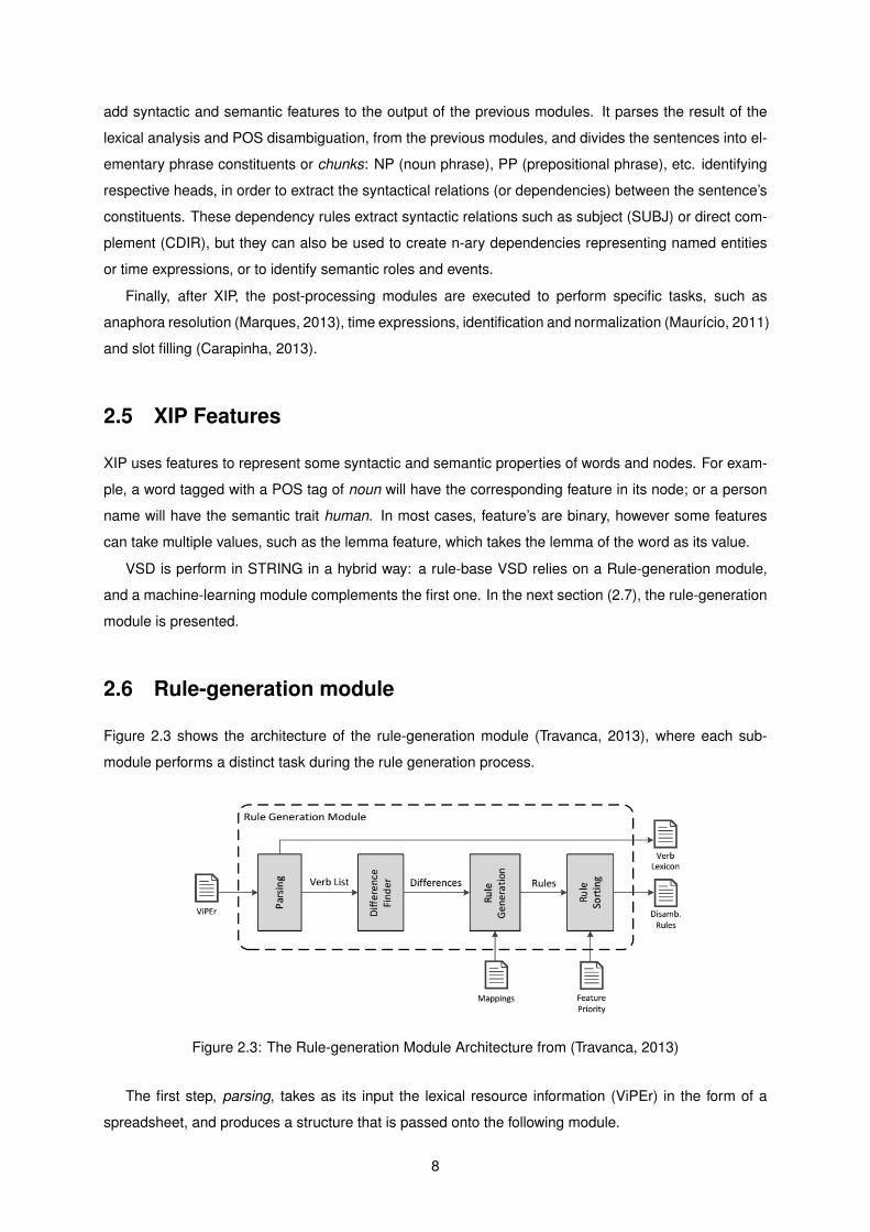
Figure 2.3 shows the architecture of the rule-generation module (Travanca, 2013), where each sub-

module performs a distinct task during the rule generation process.

Figure 2.3: The Rule-generation Module Architecture from (Travanca, 2013)

The first step, parsing, takes as its input the lexical resource information (ViPEr) in the form of a

spreadsheet, and produces a structure that is passed onto the following module.

8

In this module, each meaning is represented as a collection of features, described in ViPEr, and

their possible values. The attributes considered as features during the parsing step correspond to the

different arguments a verb can select, noted in ViPEr as N0 to N3 and their corresponding prepositions,

Prep1 to Prep3, as well as other information, like distributional and transformational constraints.

Second in the processing chain comes the difference finder module. This module is responsible

for taking the result of the parsing step and comparing the features associated to each meaning of

a polysemic verb. As a result, it produces a structure that represents the differences between those

meanings.

The next step, the rule generation, takes the differences produced by the previous step and trans-

forms them into rules. In this step, from every difference found usually two different rules are generated,

one for each meaning encapsulated in that difference. For each possible value regrading to the verb ar-

guments, prepositions are introduced, where additional information about their respective prepositions

are added to the rule. This information was added because the verb argument will map onto XIP de-

pendency MOD, which is a very generic dependency. Further increasing the problem is the fact that

one ViPEr value can map onto multiple XIP features, and each XIP feature can be a dependency or

node feature type. To solve this problem, an additional configuration file was added: mappings, where

the correspondences of the lexical resource properties and the NLP system features were added in a

declarative way.

In the last step, the rules are ordered and the disambiguation rules are printed out. However, there is

a need of a new processing step in order to resolve the issue directly related to the mapping of the nHum

feature, where incorrect elimination of ViPEr class may occur. An additional configuration file (Feature

Priority was added to solve this issue, where a higher priority is given to the semantic features and a

lower one to the nHum property, so the system would then be able to guess the correct class.

The disambiguation rules and the lexicon are then added to the XIP Portuguese grammar and used

by the STRING system.

2.7 Machine Learning Disambiguation

This section will explain how the machine learning disambiguation module was implemented in (Tra-

vanca, 2013), followed by a description of the training corpus. Finally, the features used to describe the

instances will also be presented.

2.7.1 Architecture

A typical supervised classification is divided in two steps: training and prediction; and it is composed of

three major modules: feature extraction, the machine learning algorithm and the classification module.

Figure 2.4 describes this architecture.

9

Figure 2.4: The Machine Learning Architecture from (Travanca, 2013)

In the training phase (1), the feature extraction module is responsible for transforming the raw data

into a set of features used to describe that data, which are then passed onto the machine learning

algorithm, alongside their labels, to build a model.

In the prediction phase (2), the same feature extraction module is executed in order to extract the

features on unlabelled data. These features are then passed to the classifier, which gives a label to the

new instances using the model previously obtained.

The machine learning algorithm module was not implemented from scratch, but an existing package,

MegaM (Daume, 2004), based on Maximum Entropy Models (Berger et al., 1996), was used. The

architecture of the implemented supervised classification approach is presented in Figure 2.5.

Figure 2.5: The Supervised Machine Learning Architecture for VSD using STRING from (Travanca,2013)

For the training corpus, the lemmas chosen to be disambiguated by the machine learning technique

were: explicar (explain), falar (talk ), ler (read), pensar (think ), resolver (solve), saber (know) and ver

10

(see). The main reason for choosing these verbs over the rest was the higher number of instances left

to disambiguate that these lemmas exhibited after the rule-based testing.

The instances collected consist mainly from journal articles from the CETEMPublico (Rocha and

Santos, 2000) corpus.

The number of instances collected per lemma varied a lot depending on the verb frequency, however,

all of the verbs had at least around 7,500 instances combined that were collected for the training corpus.

After that, from the collected instances, some sentences had to be filtered out: sentences containing

more than one word form of the same verb lemma were discarded, to facilitate the training step. The

average number of instances filtered corresponded to about 10% of the total instances collected. After

filtering the instances, they were split into partitions of 50 examples, each encompassing all word forms

found for that lemma. These sets were then handed to a team of linguists, who manually annotated 500

examples for each lemma (10 partitions).

2.8 Previous Results

2.8.1 Rule-based disambiguation

Using the rule-based disambiguation approach, different scenarios were experimented. Each scenario

was aimed at testing the impact of certain features used by the rule generation module. These ex-

periments were done iteratively and incrementally, which means that every change resulting from an

experiment was included in the subsequent tests. In these experiments, the number of processed in-

stances was a smaller set than what was initially intended, because the version of STRING used at the

time did not include the most recent developments.

2.8.2 Standard rules

The first testing scenario use only the verbal selectional restrictions on their arguments as conditions in

the disambiguation rules, which corresponds to the first set of features considered by the rule generation

module during its development. Standard Rules results are presented in Table 2.6.

Figure 2.6: The results of Standard Rules from (Travanca, 2013)

In this scenario the generated rules addressed almost half the instances of the corpus (49.02%), with

the majority (37.74%) being fully disambiguated just by this method.

11

2.8.3 Other methods

Most of the methods chosen only slightly improve or reduce the number of rules generated, while pro-

ducing a similar effect in the number of instances fully disambiguated by the standard rule’s method,

although one of them (Verb Meaning Filtering) had improved greatly the results (11 %) achieved by the

previous methods. This later method consisted in discarding the lexicon verb senses that rarely occur in

texts. The results obtained reached almost 50% fully disambiguated instances, that is, just by applying

the rules generated from the rule-generation module, as shown in Table 2.7.

Figure 2.7: The results of using the verb meaning filter from (Travanca, 2013)

This method consists of some deeper analysis, in which considering that the system’s purpose is to

process real texts was concluded that a simplification of the task could be of some advantage. A low

occurrence filter was built, and a new set of rules was generated. Because the low occurrence filter, a

smaller number of rules was generated. The error rate has also dropped from 18.78% to 15.51% due to

the reduction on the number of verb senses being considered.

2.8.4 Rules + MFS

In this method, a combination of both the rule-based disambiguation system and a Most Frequent Sense

(MFS) classifier was tested. The MFS classifier was the baseline considered in this evaluation, where

in the training step, the system counts the occurrences of each sense for every lemma. Then, in the

prediction step, it assigns the most frequent sense to every instance of that lemma. The results ob-

tained reveal that this combination performed worse than just applying the MFS technique. However,

the rules+MFS combination performed better that just MFS alone for verbs that had a higher number of

senses. The MFS classifier was applied after the rule-based module to the remaining non-fully disam-

biguated instances. In other words, the MFS classifier was used so it can decide the verb sense of the

remaining classes accorded to the verb instances still left ambiguous by the rule-based approach. The

result are presented in Table 2.8.

Figure 2.8: The results of using rules and MFS from (Travanca, 2013)

12

2.9 Machine Learning

In this section, the different scenarios used in the Machine Learning method and their results will be

described

2.9.1 Training Instances

This first scenario was aimed to test the impact of the size of the training corpus in the results of the ML

approach. The results are presented in Figure 2.9.

Figure 2.9: ML Scenario 1: Verifying the impact of varying the number of training instances from (Tra-vanca, 2013)

In this scenario, it was concluded that whenever the ML system performs better than the MFS(resolver

and ver ), it is due an increase in the number of training instances, which leads to an increase in the ac-

curacy for that lemma. On the other hand, if the ML module performs worse than the MFS, providing

more training instances leads to even worse results.

2.9.2 Semantic Features and Window Size

In this testing scenario, semantic information was added to the feature set about the tokens in the context

of the target verb. These semantic features were extracted for the head words of the nodes that had a

direct relation with the verb, as these act mostly as selectional restrictions for verb arguments. Figure

2.10 presents the effects of using this added semantic information on the results of the ML method.

13

Figure 2.10: The results of semantic features from (Travanca, 2013)

Adding semantic information to the context tokens provided inconclusive results, as the accuracy

improved for some verbs while it decreased for others, and the number of instances does not seem to

have any significant impact on the results.

2.9.3 Bias

The final modification tested for the ML module was the inclusion of the special feature bias, automati-

cally calculated by the system during the training step. This feature, as the name suggests, indicates the

deviation of the model towards each class. Figure 2.11 represents the impact of the bias on prediction

phase.

Figure 2.11: The results of using Bias from (Travanca, 2013)

Adding the bias feature to the classification step in the prediction phase increased the accuracy of

the system for verbs that have a high MFS. However, the MFS was never surpassed when using the

bias feature.

2.9.4 Comparison

Figure 2.12 compares all the methods described above.

14

Figure 2.12: The comparison of the different ML methods from (Travanca, 2013)

Comparing this technique with all the previously presented methods it is possible to conclude that,

whenever a verb has a high MFS, it is difficult for another approach to surpass it. However, verbs with

low MFS were outperformed by the combination of rules and MFS.

2.9.5 Rules + ML

This scenario tested how the ML performed as a complementary technique to the rule-based disam-

biguation. It is similar to the scenario that combined rules and MFS, previously described.

Globally, adding ML as a complementary technique to rules proved to be worse than just using

ML for the majority of the verbs studied. Although, for the majority of the verbs this combination of

rules+MFS performed worse, some verbs still showed some improvement when compared to the ML

scenario, even through the difference was minimal. In the cases where Rules+ML surpasses ML alone,

other approaches provide better results. In none of the cases the new accuracy values surpassed the

previous best.

Figure 2.13 compares all the methods used with machine learning

Figure 2.13: The results of using Machine learning from (Travanca, 2013)

15

2.10 Supervised Classification Methods

In this section, other methods of classification used in NLP will be briefly presented; namely decisions

trees with the ID3 and CART algorithms, Support Vector Machine (SVM) and Conditional Random Fields

methods.

2.10.1 Decision Trees

Decision trees are often used in supervised classification. This structure represents data in the form

of a tree containing all the rules extracted from a training set. In this structure, each node corresponds

to a test of the value of an attribute, each branch corresponds to the possible value’s of that attribute

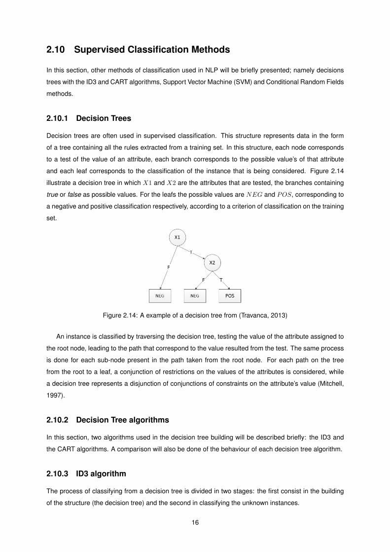
and each leaf corresponds to the classification of the instance that is being considered. Figure 2.14

illustrate a decision tree in which X1 and X2 are the attributes that are tested, the branches containing

true or false as possible values. For the leafs the possible values are NEG and POS, corresponding to

a negative and positive classification respectively, according to a criterion of classification on the training

set.

Figure 2.14: A example of a decision tree from (Travanca, 2013)

An instance is classified by traversing the decision tree, testing the value of the attribute assigned to

the root node, leading to the path that correspond to the value resulted from the test. The same process

is done for each sub-node present in the path taken from the root node. For each path on the tree

from the root to a leaf, a conjunction of restrictions on the values of the attributes is considered, while

a decision tree represents a disjunction of conjunctions of constraints on the attribute’s value (Mitchell,

1997).

2.10.2 Decision Tree algorithms

In this section, two algorithms used in the decision tree building will be described briefly: the ID3 and

the CART algorithms. A comparison will also be done of the behaviour of each decision tree algorithm.

2.10.3 ID3 algorithm

The process of classifying from a decision tree is divided in two stages: the first consist in the building

of the structure (the decision tree) and the second in classifying the unknown instances.

16

Since the model is based on a training set, each model contains a important portion of information.

The main objective of the decision tree building methods is to build the decision tree that best fits the

problem, in other words, that can best classify the instances of the domain that is being considered.

The first algorithm that has been applied in the building of decision trees was the ID3 algorithm

(Quinlan, 1986). The algorithm begins by choosing the attribute that better discriminates the various

classes of the instances, creating a node for that attribute. For each possible value in which the attribute

can be assigned, a branch is created and then the algorithm is executed again. However this time only

a subset of the instances that satisfies the restriction of the branch value is used.

Following the principle of the Occam’s razor, the smallest models should be privileged. This principle

is essential to correctly obtain the attribute that better discriminates the various classes of the instances.

The measure used in the ID3 algorithm is the information gain, based on the concept of entropy.

This concept was first introduced in Information Theory, proposed by Shannon (Shannon, 1948) in or-

der to define mathematically the problem of communication. Entropy can be defined as a measure of

unpredictability or information content, by which it is possible to determine the minimal capacity (in bits)

for sending a message (information). In this context, another form of defining the concept of entropy is

to understand the median quantity of information necessary to identify the class in which an instance

belong to a given set. The following expression refers to the calculation of the value of the entropy:

E(S) =∑ci=1

#{x∈Ci}#{x∈S} × log2

#{x∈Ci}#{x∈S} <= log2(C)

where x corresponds to a particular instance of the set an Ci to all possible classes that could be

assigned to x. In the context of classification problems, the entropy of a set, E(S), is the measure of

impurity of that set, S, in other words, it is the measure of disarray of the set according to the class

attribute.

The information gain of an attribute, A, measures the value of entropy when the training set is ordered

by the values of the attribute A. The value returned is obtained by the difference of the initial entropy of

the set and the entropy associated with the sets ordered by the attribute A.

G(S,A) = E(S)−∑i∈Dom(A)

#{x∈S:x.A=vi}#{x∈S} × E({x ∈ S : x.A = vi})

where G(S,A) corresponds to the information gain of the attribute A in the set S, x is a particular

instance in the set and vi corresponds to each different value in the domain value(Dom(A)) that A could

be assigned.

Therefore, the information gain increases with the increasing of the purity of each subset generated

by the values of the attribute, and the best attribute is the one with the most information gain. The

concept of information gain privileges the attributes for which their domains have a larger number of

values. Therefore, the larger the number of subsets generated, also the larger the purity of that subset

will be. The choice of such attributes not only increases the size of the decision tree, but also increases

the likelihood of the tree being over-adjusted to the training set, reducing the predictability. This problem

is usually known as the problem of over-learning or overfitting.

17

2.10.4 CART Method

The CART algorithm (Breiman et al., 1984) is currently the most used technique for building decision

trees (Witten et al., 2011).

A strong advantage of this method consist in the fact that it can process data that has not been pre-

processed yet, where the missing values are also processed, and by being able to handle efficiently both

categorical and numerical values. Another feature of this method consists in the fact that it generates

a large amount of decision trees and not only a single one. The generated trees are necessary binary

trees, in which every node obeys to a condition xi ¡= C, where xi is the attribute in a set of values xi ∈

{v1, ..., vi} with C as a categorical value and vj the domain value of xi.

After the trees are generated, a pruning method is applied, eliminating the tree that least contributes

to the classifier’s overall results.

Unlike the ID3 algorithm, which uses the entropy criteria to determine the best attribute for the root

node of the decision tree, the determination of the best attribute is found under the criterion of the gini

index. This criterion measures the impurity of the set of values according to the following expression:

gini(D) =∑nj=1 p

2j

In this expression, D corresponds to a set of values distributed by n classes, which are all the possible

values that could be assigned to that attribute; pj gives the relative frequency of the class j in D. On the

other hand, the partition to which each gini index is associated in the value set is given by the following

expression, in which N is the total number instances present in D and Ni are the instances of each

subset Di.

ginisplit(D) =∑mi=1

NiN gini(Di)

From these two expressions, it is possible to calculate which is the best attribute of the set of values,

in other words, which attribute has the lesser value of gini split associated to the partition.

2.10.5 Support Vector Machines

Another method of classifying instances, that has given promising results is support vector machines

(SVM) (Witten et al., 2011). First proposed by Vapnik (Vapnik, 1995), SVM are based in the learning

theory of Vapnik, developed years earlier in collaboration with Chervonenkis (Vapnik and Chervonenkis,

1971).

At first, all instances are mapped to numerical values. This means for each instance x that belongs

to the training set characterized by n attributes, that instance is mapped to a point in Rn. From this,

is possible to infer that the value classes are linearly separable, possibly in a dimension bigger than

the dimension of the instances space. With this idea, the classification problem is reduced to a linear

classification problem; i. e. there is a hyperplane that can separate the instances of the several classes.

Despite being a complex problem, the hyperplane can be described has a reduced amount of points,

hence the word ’support vectors’. In this way in mind, the training set is used to identify the support

vectors of the hyperplane that separates the instances which are then used to classify new instances.

18

By relaying on a strong mathematical theory, this method guaranties a good capacity of general-

ization, which means a low probability of overfitting. The main utility of support vector machines is the

determination of the optimal hyperplane that separates the instances of the training set. In general, the

hyperplane is described by the following expression, with n being the number of instances of the training

set, and x, w and b ∈ R.

f(−→x ) = (−→w .−→x ) + b =∑ni=1(wixi) + b

where w is the weight associated with each instance x and b represents the distance between the

hyperplane and the instances, where b = 0 gives the an equidistant hyperplane from its instance and

b > 0 or b < 0 places the hyperplane nearer to the instances of an class of the training set. The optimal

separation hyperplane is the hyperplane that is equidistant to the instances of all classes, also called

the maximum margin hyperplane.

2.10.6 Conditional Random Fields

Another method of classification is the use of Conditional Random Fields (CRF). Conditional random

fields is a framework for building probabilistic models to segment and label sequence data, offering

several advantages over Hidden Markov Models and stochastic grammars. One of the advantages

relies on the fact that conditional random fields avoid the limitation of the Maximum Entropy Markov

Models (MEMM), where these models are heavily restricted by the training set and, therefore cannot

be expanded over the unseen observations. For testing purposes, this problem can be fixed using a

smoothing method. MEMMs are conditional probabilistic sequence models, where each source state

has a exponential model that takes the observation features as input, and outputs a distribution over

possible next states. These exponential models are trained by an appropriate iterative scaling method in

the maximum entropy framework. However, MEMMs and other non-generative finite-state models based

on next-state classifiers, such as Discriminative Markov Models (Bottou, 1991), share a weakness called

the label bias problem, where transitions leaving a given state compete only against each other, rather

than against the transitions from the other states in the model.

Given X, a random variable over the data sequence to be labeled, and Y is a random variable of

the corresponding label sequence; each Yi in Y is a possible label tag that could be assigned, where

a conditional random field (X,Y) when conditioned on X, the random variables Yv obey to the Markov

property with respect to the graph:

p(Yv|X,Yw, w 6= v) = p(Yv|X,Yw, w ∼ v)

where w ∼ v means that w and v are neighbours in the model. The parameter estimation problem is to

determine the parameters θ = (λ1, λ2, ...;µ1, µ2, ...) from the training data that maximize the log-likelihood

objective function O(θ). In other words, the most probable label sequence given a certain sentence:

O(θ) =∑Ni=1 logpθ(y

(i)|x(i))

19

Although CRF encompass HMM-like models, they are much more expressive, because they allow arbi-

trary dependencies on the observation sequence.

For each position i in the observation sequence x and Y , a |Y | × |Y | matrix random variable is

defined, in which:

Mi(y′, y|x) =

∑k λkfk(ei, Y |ei = (y′, y), x) +

∑k µkgk(vi, Y |vi = y, x)

where y′ is each state possible to achieve by y, and λk and µk are the weights assigned to the state

transition function and the probability function of a particular element in the sequence x, fk and gk

respectively; ei is the edge with labels (y’, y) and vi the state with label y. However, in contrast to

generative models, conditional models like CRFs do not enumerate all possible observation sequences.

Therefore, these matrices are computed directly as needed from a given training or test observation

sequence x. From that, it is possible that a normalization function Zθ(x) could be written in the form of:

Zθ(x) =M1(x)M2(x), ...,Mn+1(x)

This method can be applied to various problems as well as the problem of WSD. Applications on

WSD of CRF as well as other supervised methods, include part-of-speech (POS) tagging, information

extraction and syntactical disambiguation, where it possible to consider x as a sequence of natural

language sequences and y the set of possible part-of-speech tags to be assigned (Lafferty et al., 2001).

Since the only machine learning method integrated in STRING is maximum entropy models, which

were used in (Travanca, 2013), different types of supervised learning methods and the addition of dif-

ferent types of verbs will be experimented to view its impact on the system overall results and in the

problem in hand.

20

Chapter 3

Corpora

In this chapter, the corpora used in this dissertation will be presented. It will be described the training

corpus used to obtain the models of the chosen supervised methods used in this dissertation. Then we

present evaluation corpus.

3.1 Training corpus

This section presents the training corpus, which will also be used for the evaluation of the each super-

vised learning method.

The corpus was collected from the CETEMPublico1 corpus (Rocha and Santos, 2000), and it con-

tains from 1000 to 2500 sentences for each verb lemma. Around 100 of verbs were chosen for this

purpose. The instances set for each verb contained 500 sentences divided in two partitions of 250 sen-

tences each, where it had been manually annotated from a group of students of the Natural Language

course at Instituto Superior Tecnico. Since the annotation process is very complex, it required a team of

linguists with knowledge relating to the grammar subsequent to ViPEr, therefore the annotated instances

were then reviewed by the team of linguists in the L2F laboratory. The corpus contains in total around

13,000 instances, where the number of words is around 437,000.

1http://www.linguateca.pt/cetempublico/

21

Table 3.1 presents the verbs selected, their number of instances and the number of classes for each

verb in the experiments:

Verb Number of instances Number of Classes

abandonar 471 4

aceitar 248 2

acreditar 497 3

aprender 488 4

assinalar 494 3

atirar 247 7

avancar 492 6

chamar 495 4

comprometer 494 3

concordar 497 4

confrontar 485 5

contornar 496 2

convencer 498 5

destacar 418 4

esconder 433 3

explicar 287 3

falar 215 3

ler 388 4

mostrar 480 3

pensar 105 4

preparar 499 4

resolver 508 2

saber 342 2

ver 351 2

Table 3.1: The training corpus used, the number of instances and the number of classes per verb.

The annotation process consisted in attributing to the target verb in each sentence its corresponding

ViPEr class, which is approximately the same as to determine the verb’s sense. To simplify the annota-

tion process, a graphical interface was developed, where it consisted in choosing the respective training

data and parametrization file for each verb lemma. Once loaded the first parametrization file, it was not

necessary to loaded it for each verb lemma, since it automatically searches for the parametrization file

every time a new training data file is chosen.

Figure 3.1 presents the initial screen of the interface, where it displays filters for the instances that

are marketed as doubts with ?, the instances with errors marketed with # and the sentence where are

present 2 or more instances.

22

Figure 3.1: The initial screen of the interface

During the annotation process, a parametrization file was created along with the each annotated

lemma.

The parametrization file consists of 3 lines (Figure 3.2) :

• The verb lemma;

• The conventional codes including the verb’s ViPEr; besides these codes all verbs given the possi-

bility to be classified as:

– VOP, an operator verb (Baptista et al., 2004) (e.g. O Pedro com esta notıcia deixou a Maria

muito preocupada.)

– VSUP, a support verb (Baptista et al., 2004) (e.g. O Pedro abandonou toda a esperanca de

vir a casa com a Maria.)

– FIXED, that is, as an element of a fixed or idiomatic expression (Baptista, 2005) (e.g. Aban-

donar a sua sorte.

• Finally a list of inflected forms associated with that lemma, this allows the interface to highlight (in

bold) the instance of the verb

23

Figure 3.2 presents a parametrization file for the lemma abandonar

abandonar32C 38L1 FIXED VSUP VOPabandona abandona abandonada abandonadas abandonado abandonadosabandonaiabandonais abandonam abandonamo abandonamos abandonamos abandonandoabandonar abandonara abandonara abandonaram abandonaramo abandonaramosabandonarao abandonaras abandonaras abandonardes abandonareiabandona r e iabandonareis abandona r e i s abandonarem abandonaremos abandonaresabandonaria abandonariam abandonar ı amos abandonarias abandonar ı e i sabandonarmo abandonarmos abandonas abandonasse abandona sse isabandonassemabandonassemos abandonasses abandonaste abandonastes abandonavaabandonavam abandonavamo abandonavamos abandonavas abandona ve iabandona ve is abandone abandonei abandoneis abandonem abandonemoabandonemos abandones abandono abandonou

Figure 3.2: Parametrization file of the lemma abandonar

When annotating the training data, all the possible classes for the lemma are displayed. A ViPEr

class must be chosen in order to view the next instance, however it is always possible to view the

previous annotated instances, since all annotations are saved in memory. Additionally, filters to mark

the instance as a doubt or with errors are displayed, where each of them can be applied independently

of the verb sense chosen (Figure 3.3).

The interface allows to save the progress at any point, by clicking the button Guardar Progresso

(Save Progress), to a file named by the user, as well as, to load the saved progress in at a later moment

in order to continue the annotation of the training data.

An edit feature was added to interface, where it enable to correct the sentences that have errors or

multiple instances of the processed lemma. The feature can be accessible only if the value of a system

property is assigned to true, when launching the interface. When applied, it splits the area where the

sentence is displayed on the screen. In the upper area, the sentence is displayed as found on the file

with the progress stored, where in the bottom area, the user can manually write the correct instance for

the training data, replacing the incorrect one once the progress is saved (Figure 3.4).

When multiple annotators process the same training data, and in order to build an integrated golden

standard, it was necessary to compare the differences between each annotator. For this purpose,

another interface was developed, which takes as input the two files provided by the annotators and the

parametrization file (Figure 3.5).

The interface allows the user to define the starting point of his/her task, in order to continue from

a previously saved point of progress. The interface also calculates the Cohen’s kappa interannotator

agreement coefficient (Carletta, 1996). This is given by the following expression:

K = Pr(a)−Pr(e)1−Pr(e)

where Pr(a) is the relative observed agreement among annotators, and Pr(e) is the hypothetical prob-

24

Figure 3.3: The annotation screen of the interface

Figure 3.4: The edit feature in the interface.

25

Figure 3.5: The annotation screen of the interface

26

Figure 3.6: The annotation screen of the second interface

ability of chance agreement, using the observed data to calculate the probabilities of each observer

randomly saying each category. If the annotators are in complete agreement then k is equal to 1.

When during the reviewing process, only the instances where the annotations differ are displayed.

For each instance, the default verb sense is the one chosen from the annotator that is considered correct

for the most times (Figure 3.6).

Each time the user selects one of the annotations, it is viewed which annotator chooses that verb

sense and then the interface counts the amount of annotations that are considered correct for each

source.

27

3.2 Evaluation Corpus

In this section the corpus used for comparison of the methods described above will be presented.

The corpus chosen for evaluation was the Parole corpus (do Nascimento et al., 1998) which contains

around 250 thousand words. Each verb on the corpus had been manually annotated and then reviewed

by linguists. The corpus is composed of texts from a very diverse nature (genre and topic) and its made

of full texts. In this respect it is different from the training corpus, which is composed solely of journalistic

text, and instead of full texts, it features extracts of one to a few sentences.

Although the corpus contained around 38,702 verbs, only 21,289 (about 55%) of those verbs cor-

respond to full verbs, as showed in Table 3.2. The full verbs distribution according to their number of

meanings is presented in Table 3.3.

Total Full Verbs Auxiliary Verbs

Count 38,702 21,289 17,413

% 100 55.01 44.99

Table 3.2: Evaluation Corpus Verb Occurrences.

Meanings Count %

2 6030 48.74

3 3126 25.27

4 1474 11.91

5 940 7.60

6 219 1.77

7 116 0.94

8 179 1.45

10 114 0.92

11 174 1.40

Total 12,372 100

Table 3.3: Processed Corpus Distribution.

Before evaluation, to determine the amount of errors on ambiguous verbs a preliminary processing

was performed, which were consequence of previous modules. Table 3.4 presents the number of errors

found, divided by their type. The number of verb instances wrongly tagged by the POS tagger were

189 (1.42%) and 20 (0.15%) incorrectly assigned of the lemmas, while the not recognized as full verb

constructions 745 (5.59%) instances, resulting in a total of 954 (7.16%) of the instances not being

classified by any of the methods presented.

28

Total Processed Wrong POS Wrong Lemma Not identified as a full verb

Count 13,326 12,372 189 20 745

% 100 92.84 1.42 0.15 5.59

Table 3.4: Corpus Processing Results.

This corpus already undergone extensive annotation for POS tagging and it has also been enriched

with other linguistic information, including the verb class of ViPEr for full verbs, the auxiliary types (modal,

temporal and aspectual) for auxiliary verbs, the verbs entering into verbal idiomatic expressions, several

support and operator verbs (these later two types are still being classified).

Figure 3.5 presents the corpus used for evaluation.

Lemma Number of instances Number of Classes

abandonar 22 4

aceitar 64 2

acreditar 59 3

aprender 56 4

assinalar 13 3

atirar 12 7

avancar 43 6

chamar 91 4

comprometer 14 3

concordar 40 4

confrontar 13 5

contornar 2 2

convencer 24 3

destacar 16 4

esconder 19 3

explicar 134 3

falar 206 3

ler 82 4

mostrar 63 3

pensar 166 4

preparar 48 4

resolver 95 2

saber 480 2

ver 450 2

Table 3.5: The Evaluation corpus used.

The instance set for the evaluation corpus is much smaller than in training corpus, where only around

2200 are used for evaluation as instead of around 10,000 instances used for training the models.

29

It is therefore natural that the distribution of verb senses differ from the training corpus, since the

samples collected for each corpus were not identical.

Table 3.6 shows some cases were the most frequent sense is different in each corpus.

Training Corpus Evaluation Corpus

Lemma MFS Number of instances Accuracy MFS Number of instances Accuracy

abandonar 32C 471 57.54% 38L1 22 54.17%

assinalar 32C 494 71.05% 06 13 50.00%

avancar 35R 492 64.63% 35LD 43 46.51%

comprometer 32C 494 53.04% 07 14 71.43%

concordar 35R 497 57.14% 42S 40 72.50%

esconder 10 433 52.75% 38LD 19 60.87%

mostrar 09 480 58.12% 36DT 63 55.56%

preparar 32A 499 52.91% 32C 48 43.14%

Table 3.6: The different MFS in the corpora used.

The differences in the corpora implies that using the MFS as a solution for VSD is not the most

reliable, since different samples collected for training corpus can lead to different overall results for the

system.

30

Chapter 4

Architecture

In this chapter, the building and annotation of the corpus used in this dissertation will be presented. We

also present the experiments made using the Weka software package and the implementation Naive

Bayes algorithm.

4.1 Building and annotating a corpus of verb senses for ML

The main focus of this dissertation will be the implementation and comparison of different ML methods

in order to improve the results of the verb sense disambiguation in the STRING system. The methods to

be applied are the following; Decision Trees, Support Vector Machines and Conditional Random Fields,

none of them having been implemented so far in this NLP system. It is also our goal to expand the

number of verbs to disambiguate.

For this purpose, a corpus was collected for each verb that will be integrated in the system, taken from

the CETEMPublico1 corpus (Rocha and Santos, 2000), and containing from 1000 to 2500 sentences for

each verb lemma. Around 100 of verbs from the most ambiguous verbs in Portuguese were chosen

for this purpose. A script was developed in order to pre-process the data so it could be manually

annotated, choosing the correct verb class as described in ViPEr, where it splits the collected sentences

in partitions. The instances set for each verb contains 500 sentences divided in two partitions of 250

sentences each and it has been manually annotated by the team of linguists in the L2F laboratory 2.

However, before the team of linguists annotated the instances, a groups of students from the Nat-

ural Language course have manually annotated most of the sentences given and because of that the

instances set needed to be reviewed before giving to the linguists. For each instance given, it was de-

cided the students label the most probable verb sense after in instance of the verb lemma by separating

with a slash.

To review the sentences a script was developed that moves all the ViPEr tags annotated in each

sentence to the beginning of each sentence that is being processed. If there is more than one ViPEr tag1http://www.linguateca.pt/cetempublico/2In fact, the corpus was firstly annotated by students of NLP course at IST and their work was revised by the linguists experts.

In this way, we intended to obtain a large sample of annotated data in a relativity fast and at a small individual cost as possible. Asthe revision process demonstrated, this is not an easy task, and cannot be given to untrained linguists

31

in a sentence, then a question mark is inserted at the beginning of that sentence, in order to be reviewed

by a linguist. The same is applied to a sentence without any annotation or with unknown tags annotated.

However, if there is more than one tag in a instance, it is necessary to report to a linguist to decide what

should be done to that particular instance, which could be to split the two or more sentences in that

instance or even a removal that instance from the training set. The problem regrading the that particular

instance, is since that instance has more than one sentence, if a split of these sentences is made, their

contexts will be lost which is a concern if discourse analysis will be addressed for future work.

A graphical interface was developed in order to facilitate the reviewing process. In this interface, each

instance is shown, where the verb instance is marked in bold. Each possible tag that could be assigned

to the verb lemma is also shown in order to allow the reviewer to change the assigned tag. A filter was

also created to show only the instances that are signalled with a question mark.

With verbs annotated from different sources, another graphical interface was developed, where it

only shows the instances where the assigned tag is different in both sources and the reviewer chooses

between those tags.

When the filtering process is complete, the training set will be moved to each of the classifiers de-

scribed in Section 2.11, in order to know which method obtain the better results for each verb. The main

objective is to compare machine learning techniques described in Section 2.11 and evaluate the results

obtained from each one of them. Also, there is the need to compare to the previous methods imple-

mented in the previous works in VSD, such as the rule-generation disambiguation, described in Section

2.7, and observe what combination or combinations of techniques yield the most promising results.

All these techniques will be integrated in the XIP module, as a part of the STRING system.

4.2 Weka experiments

In this section the different experiments using the Weka software will be presented. Weka is a collection

of machine learning algorithms for data mining tasks. The algorithms can either be applied directly to a

dataset or used in other developed Java code. Using the Weka software, it was able to view the impacts

of different supervised methods on the VSD problems, based on a training corpus.

For each supervised method chosen, a set of experiments was carried out, in order to view what

where the best combinations of extracted features that produced the better overall results.

The features extracted for these methods can be organized in tree groups, as fellow:

• Local features, describe the information around the target word (the verb). In the system, the

context words are extracted in a window of size 3 around the target verb, that is, a total of 6 tokens

are used, with their respective indexes (-3, -2, -1, +1, +2, +3). The information collected about

each of the tokens was the POS tag and lemma.

• Syntactic features, regarding the constituents directly depending on the verb were also used, that

is, constituents that had a direct relation (i.e. XIP dependency relation) with the verb. The POS

tag and the lemma of the head word of each node in these relations were extracted, together with

32

the respective dependency name. Several other dependencies/relations are implemented in the

XIP grammar, only those of SUBJ (subject), CDIR (direct complement) and MOD (modifier) were

considered for each ML system.

• Semantic features were extracted for the head words of the nodes that had a direct relation with

the verb, as these act mostly as selectional restrictions for verb arguments. The semantic features

considered by the system are those that are also present in ViPEr, for example, human, location,

body-part, animal, plant, currency, among others.

In order to use the weka software package, it was necessary to transform the training data into an

ARFF file. ARFF files have two distinct sections. The first section is the Header information, which is

followed the Data information. The Header of the ARFF file contains the name of the relation, a list of the

attributes (the columns in the data), and their types. The other section describes the raw data observed

in the training data, in this case, the features extracted from XIP and the class in ViPEr relating to a verb

sense. Missing values are represented by ? when the respective POS tag and lemma of an context

token is missing from the sentence currently being processed.

@RELATION v iperC lass

@at t r ibu te TOK−3−pos {ART,NP,NOUN,PUNCT,VERB}@at t r ibu te TOK−2−pos {NOUN, VF,PUNCT,ART,CONJ}@at t r ibu te TOK−1−pos {ADV,PREP,CONJ,NOUN,REL,PUNCT,VCOP,VMOD,ADJ}@at t r ibu te DEP−SUBJ {NOUN,ART,REL,PRON, ADJ,NUM,VERB}@at t r ibu te c lass {32C,38L1}

@DATAART,NOUN,ADV,ART,32CART,NOUN, ADJ,ART,38L1

Figure 4.1: Example of a ARFF file used in the Weka experiments

To generate the ARFF file, a converter was implemented in order to write the features extracted from

the STRING system in the required form.

Although every possible combination of extracted features was considered, some combinations were

discarded because the results were not being close of those of the others experiments or the data

needed to be pre-processed.

The algorithms chosen for these experiments are the following:

• ID3 algorithm (Quinlan, 1986) which is an algorithm used to generate a decision tree from a

dataset. ID3 is typically used in the machine learning and natural language processing domains.

• Support Vector Machines (Vapnik, 1995), which is a classification method that finds the maximal

margin hyperplane that best separates the positive from the negative examples. In the particular

case of WSD, this has to be slightly tuned for multiple class classification.

33

• CART algorithm (Breiman et al., 1984) is currently the most used technique for building decision

trees (Witten et al., 2011). A strong advantage of this method consist in the fact that it can pro-

cess data that has not been pre-processed yet, and in which the missing values, which are also

processed, and also by being able to handle efficiently both categorical and numerical values.

• Naive Bayes algorithm (Manning et al., 2008), which estimates the most probable sense for a given

word based on the prior probability of each sense and the conditional probability for each of the

features in that context.

• Bayes Network is a probabilistic model that represents a set of random variables and their con-

ditional dependencies via a directed acyclic graph (DAG). It is very useful to infer unobserved

variables.

• AdaBoost, (Freund and Schapire, 1999) is a machine learning meta-algorithm. It can be used in

conjunction with many other types of learning algorithms to improve their performance. The output

of the other learning algorithms is combined into a weighted sum that represents the final output

of the boosted classifier, where subsequent weak learners are tweaked in favour of instances

misclassified by previous classifiers. For this experiment, it was used a decision stump algorithm

as weak learner, where it is a machine learning model consisting of a one-level decision tree (Iba

and Langley, 1992).

• Decision table is a precise method to model complicated logic. Decision tables, like flowcharts and

if-then-else statements, associate conditions with actions to perform. The approach used in this

method was the Best-first search, which is greedy algorithm which explores a graph by expanding

the most promising node chosen according to a specified rule (Pearl, 1984).

• Maximum Entropy is used for predicting the outcome of a categorical dependent variable (i.e., a

class label) based on one or more predictor variables (features). That is, it is used to measure the

relationship between a categorical dependent variable and one or more independent variables, by

using probability scores as the predicted values of the dependent variable.

Table 4.1 presents the methods chosen for this evaluation and the experiments carried out with them.

Method Experiments

ID3 Lemmas removed; Lemmas and semantic features removed

SVMS None removed; Lemmas removed

CART Lemmas removed; Lemmas and semantic features removed

Naive Bayes None removed; Lemmas removed

Bayes Network None removed; Lemmas removed

Ada Boost None removed; Lemmas removed

Decision table None removed; Lemmas removed

Maximum entropy None removed; Lemmas removed

Table 4.1: The supervised methods available in Weka chosen for evaluation

34

For each experiment made, another test was applied, where for each experiment made it was eval-

uated using preprocessed data and without using it. It was applied a filter available in Weka software

package were it replaces all the missing values for nominal and numeric attributes in a dataset with the

modes and means from the training data.

In most of the algorithms chosen, the results obtained without pre-processing were better, however in

the ID3 and Maximum Entropy algorithms was only applied the experiments with preprocessed data. In

the case of the ID3 algorithm it can only be tested with preprocessed data because the algorithm cannot

handle missing values, where in the case of the maximum entropy it was chosen due performance

issues with the implementation available in the Weka software package, with the amount of time using

preprocessed data being considerably less than with the training data unchanged.

Figure 4.2 presents the mean results for each experiment used.

Figure 4.2: Comparison between ML experiments using Weka.

In order to execute these experiments, a program was developed that automatically executes the

tests proposed, calling the Weka software package with the given experiments and the respective ARFF

files of the training set. The result of the experiments are stored in a CSV file, where the method chosen

for evaluation consisted in a cross-validation with 10 folds applied to each experiment. The corpus used

for this is evaluation was the corpus presented in (section 3.1), where the addition of more instances,

does not lead to a significant change in the overall results. (i.e. the difference in the overall results for

35

each method is very small)

Table 4.2 presents the corpus chosen for these experiments:

Verb Number of instances Number of Classes

abandonar 471 4

aceitar 248 2

acreditar 497 3

aprender 488 4

assinalar 494 3

atirar 247 7

avancar 492 6

chamar 495 4

comprometer 494 3

concordar 497 4

confrontar 485 5

contornar 496 2

convencer 498 5

destacar 418 4

esconder 433 3

explicar 287 3

falar 215 3

ler 388 4

mostrar 480 3

pensar 105 4

preparar 499 4

resolver 508 2

saber 342 2

ver 351 2

Table 4.2: The training corpus used, the number of instances and the number of classes per verb.

Figure 4.3 presents the results of the experiments using the Machine learning algorithms mentioned

above with the Weka software package.

From the results, the Maximum Entropy (78.65%) and Naive Bayes (79.52%) obtain the better overall

results. However, the difference between these methods and the remainder (except ID3) is small. Since

the difference between these algorithms was minimal, a implementation of the Naive Bayes was decided,

in order to view the its impact on the STRING system.

The following section will describe the implementation of the Naive Bayes algorithm in the STRING

system.

36

Figure 4.3: The results obtain using the weka software package.

4.3 Naive Bayes implementation

In this section the implementation of the Naive Bayes algorithm and its integration in STRING system

will be described.

The Naive Bayes algorithm is based on the Bayes theorem, where every feature is assumed to be

independent from the other features. The following expression presents how Naive Bayes determinates

a class according to the observed features.

P (C|F1...Fn) = P (C)∏ni=1 P (Fi|C)

where C is the class to be determined, and F1...Fn the features in the instance that is processed. The

probability P (Fi|C) is simple to calculate, since it is the count of times the feature Fi appears when the

class is C in the training set; as well as, P (C), which is the number of instances that are labelled as C.

The machine learning algorithm was implemented using the KiF language, developed by Xerox, in

order to integrate with the STRING system, using a similar approach used in the existing package,

MegaM (Daume, 2004), based on Maximum Entropy Models (Berger et al., 1996).

The training phase of the model consists of for each instance it extracts the same features extracted

from MegaM, however a tab separates the label from the features extracted. From then, each feature

is separated from the others, where in each line on the training data has only one feature and the class

labelled in that instance, separated with a tab.

When the model is created, each feature in the training data is stored in a hash table, where the key

is the feature extracted and the value stored is an array containing the number of appearances of that

feature for each class.

In prediction phase, the algorithm accesses the model, which contains the counts for each class of

all features presented and calculates the probability for each class, according to the features seen. The

most probable class returned from the algorithm is provided by the following expression:

37

C = argmaxP (C)∏ni=1 P (Fi|C)

where C is the class to be determined, and Fi each of the features in the instance that is processed. For

features that are not present in the training data, a smoothing method was implemented. The method

chosen for this implementation was the additive smoothing, which for each missing feature in the model,

the probability assigned is very low. Without having an smoothing method, the probability of an missing

feature would be zero, since this feature would not be included in the model. The impact caused could

leave to a greater number of incorrectly classified instances as oppose to when a smoothing method is

applied.

The following expression presents the additive smoothing used in this implementation:

P (Fi|C) = Fi+1F (C)+|F |

where F (C) is the number of features counted in the class C and |F | the number of features present

in the model. This method allows to process the missing features without the algorithm returning zero,

whenever such event occurs, giving the possibility to not include more training instances every time a

missing feature is found.

38

Chapter 5

Evaluation

This chapter will be present the results for each supervised learning method previously described.

The corpus chosen for this evaluation is the corpus Parole presented in section 3.2. The evaluation

will consist of cross-validation method with 10 folds, for all methods and a comparison with the results

obtained in (Travanca, 2013) will be made.

5.1 Measures

The goal of this evaluation is to view the adequacy of each supervised method used, where it was

counted the number of instances that are considered correct by the system, among the number of

instances present in the training set. This fits the definition of accuracy.

The following formula describe the definition of accuracy, where nc is the number of instances cor-

rectly classified and N is the number of instances in the training set.

accuracy = nc

N

39

5.2 Baseline

Generally, a baseline is a starting point for comparison of a system’s performance. For the evaluation, it

was decided that the baseline for this evaluation would be the results of the most frequent sense (MFS)

to decide the correct verb sense. This approach counts for every verb, the verb sense that is more

assigned to the training instances, which can be viewed as a simple classifier.

Table 5.1 presents the MFS for each verb used in the training phase:

Verb lemma Number of instances Number of Classes MFS Class

abandonar 471 4 57.54% 32C

aceitar 248 2 73.79% 38TD

acreditar 497 3 55.94% 06

aprender 488 4 69.26% 06

assinalar 494 3 71.05% 32C

atirar 247 7 55.06% 38LD

avancar 492 6 64.63% 35R

chamar 495 4 49.90% 39

comprometer 494 3 53.04% 32C

concordar 497 4 57.14% 35R

confrontar 485 5 80.20% 36R

contornar 496 2 73.79% 32C

convencer 498 5 54.82% 12

destacar 418 4 46.41% 36R

esconder 433 3 52.75% 10

explicar 287 3 81.18% 09

falar 215 3 93.02% 41

ler 388 4 78.04% 32C

mostrar 480 3 58.12% 09

pensar 105 4 59.05% 06

preparar 499 4 52.91% 32A

resolver 508 2 75.00% 32C

saber 342 2 91.14% 06

ver 351 2 64.96% 32C

Table 5.1: The MFS accuracy for each verb in the training phase.

From the training corpus, it is possible to view that on every lemma there is a verb sense with a high

percentage independently of its number number of classes.

Table 5.2 presents the MFS for each verb used in the evaluation:

40

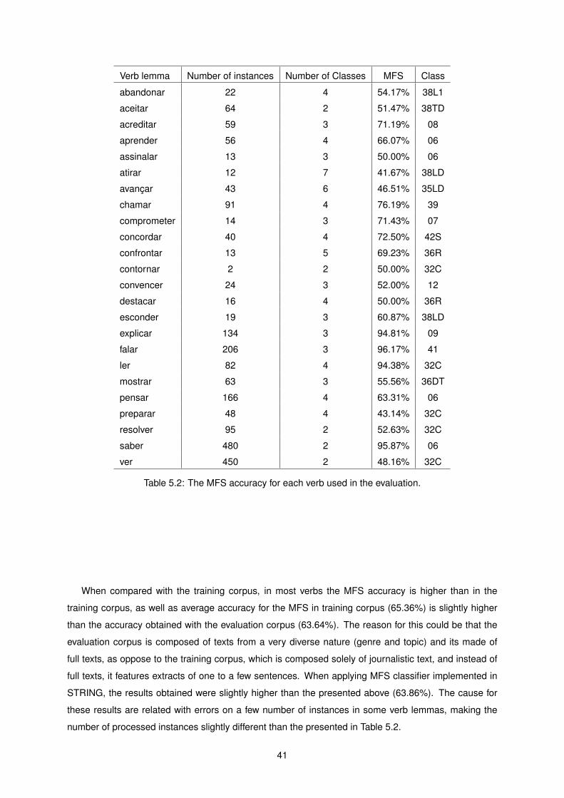
Verb lemma Number of instances Number of Classes MFS Class

abandonar 22 4 54.17% 38L1

aceitar 64 2 51.47% 38TD

acreditar 59 3 71.19% 08

aprender 56 4 66.07% 06

assinalar 13 3 50.00% 06

atirar 12 7 41.67% 38LD

avancar 43 6 46.51% 35LD

chamar 91 4 76.19% 39

comprometer 14 3 71.43% 07

concordar 40 4 72.50% 42S

confrontar 13 5 69.23% 36R

contornar 2 2 50.00% 32C

convencer 24 3 52.00% 12

destacar 16 4 50.00% 36R

esconder 19 3 60.87% 38LD

explicar 134 3 94.81% 09

falar 206 3 96.17% 41

ler 82 4 94.38% 32C

mostrar 63 3 55.56% 36DT

pensar 166 4 63.31% 06

preparar 48 4 43.14% 32C

resolver 95 2 52.63% 32C

saber 480 2 95.87% 06

ver 450 2 48.16% 32C

Table 5.2: The MFS accuracy for each verb used in the evaluation.

When compared with the training corpus, in most verbs the MFS accuracy is higher than in the

training corpus, as well as average accuracy for the MFS in training corpus (65.36%) is slightly higher

than the accuracy obtained with the evaluation corpus (63.64%). The reason for this could be that the

evaluation corpus is composed of texts from a very diverse nature (genre and topic) and its made of

full texts, as oppose to the training corpus, which is composed solely of journalistic text, and instead of

full texts, it features extracts of one to a few sentences. When applying MFS classifier implemented in

STRING, the results obtained were slightly higher than the presented above (63.86%). The cause for

these results are related with errors on a few number of instances in some verb lemmas, making the

number of processed instances slightly different than the presented in Table 5.2.

41

5.3 Comparison with previous results

In this section the results between the verbs processed in (Travanca, 2013) and with the training data

used for this dissertation will be presented. This comparison is aimed to view if the changes in both the

training data and the corpus would led an impact on the system’s overall results.

These changes include the addition of more instances, the correction of some of the verbs classified

and grammatical compounds, which did not leave an large impact on the system’s overall results.

Figure 5.1 presents a comparison between the results obtained from the rule-disambiguation system

with the training data used for this dissertation and the results obtained from (Travanca, 2013).

Figure 5.1: Comparison using the rules-disambiguation system.

The difference between the results is minimal for most of the verbs lemmas used in (Travanca, 2013).

However, the verb lemma resolver was where the difference was considerable. The results using the

rule-disambiguation system and the MFS classifier provided inconclusive results, as the accuracy im-

proved for some verbs while decreased for others.

Another comparison made between the results of (Travanca, 2013) was in the supervised learning

methods used in that work. For this comparison it will be used the bias feature both enabled and disabled

while evaluating the machine learning method integrated in STRING. The bias feature is calculated

during the training step, which indicates the deviation of the model towards each class.

Figure 5.2 presents the results obtained with the bias feature both enabled and disabled.

Although changes were made in the corpus, the difference achieved in the results is minimal. The

results are similar to the previous obtained by (Travanca, 2013), where ler was the only verb lemma with

a considerable difference in the accuracy of the Maximum Entropy algorithm without the bias feature.

42

Figure 5.2: Comparison between ML methods used in (Travanca, 2013).

5.4 Naive Bayes experiments

In this section a comparison between the experiments made in the Naive Bayes algorithm will be pre-

sented.

In this algorithm, it was tested the impact of the dependencies between nodes extracted from XIP

when building the features of the processed sentence during the prediction phase. A comparison of

storing or not these dependencies was made in order to view which had the better overall results.

Figure 5.3 presents a comparison between the experiments made in the Naive Bayes algorithm.

As seen in this Figure, storing these dependencies give the better overall results. However when not

storing these dependencies, in some verbs (aprender, assinalar, confrontar and ver ) it was achieved

the same or slightly higher accuracy than storing the dependencies between nodes extracted from XIP.

When applying this experiment on maximum entropy models, the results did not improve and proved to

be worse than using the dependencies extracted from XIP.

Figure 5.4 presents the comparison between the models obtained by naive bayes and maximum

entropy algorithms.

From the results obtained, the maximum entropy algorithm with the bias feature enabled proved to

be the worst approach. The naive bayes algorithm with the XIP dependencies stored and the maximum

entropy algorithm without the bias feature achieved similar results, however it is not clear from this Figure

which of these achieved the better overall results, since the best approach considered for each lemma

varies for most of the verbs.

5.5 Comparison

In this section a comparison between every method available in the STRING system is presented.

Figure 5.5 presents a comparison between all methods integrated in STRING.

From this figure it is very difficult to view which method gave the better overall results, since for most

verbs all the methods compared achieve similar results for each verb lemma. However, for some lemmas

43

Figure 5.3: Comparison between naive bayes experiments.

44

Figure 5.4: Comparison between naive bayes and maximum entropy methods.

45

Figure 5.5: Comparison between all methods per verb lemma.

46

there is a method that achieved better results and in other verb lemmas, the same method is surpassed

by another machine learning algorithm. This allows to not take any conclusions viewing only the results

from Figure 5.5.

To understand better the impact of each method on the evaluation corpus, we must view the average

accuracy for all verbs lemmas tested, in order to view which achieved the better overall results.

Figure 5.6 presents the average of the results previously presented.

Figure 5.6: Comparison between average results of all methods integrated in STRING.

Comparing these results the naive bayes algorithm with XIP dependencies stored (67.71%) achieved

a slightly better result than the maximum entropy without the bias feature (67.01%). However if the verb

contornar that contains only 2 instances on the evaluation corpus, where the maximum entropy disam-

biguated correctly all instances as oppose to the naive bayes which disambiguate half, was excluded

form the experiments then the difference between these algorithms will be increased. This would give

an increase in accuracy on the naive bayes algorithm with XIP dependencies stored (68.48%) and a

decrease from the maximum entropy (65.57%), which would be surpassed slightly by the naive bayes

algorithm without the XIP dependencies stored (65.59%).

5.6 Performance evaluation

Another experiment made in order to evaluate each method integrated in the STRING system, consisted

in measuring the performance of the methods available in the system.

In this experiment, the training corpus was used for each combination of methods tested, which

contains around 437,000 words collected from CETEMPublico corpus (Rocha and Santos, 2000).

Table 5.3 shows the performance impact results from the addition of the modules.

47

Modules Integrated Execution time (s) Difference (s)

MFS 1372,893

Rules + MFS 1376,520 3,627

Maximum Entropy 2569,149 1196,256

Rules + Maximum Entropy 2614,249 1241,356

NaiveBayes 1805,140 432,247

Rules + Naive Bayes 1938,022 565,129

Table 5.3: STRING performance after modules integration and its difference to the baseline.

From this table, it is possible to view that MFS the with the addition of rule-based disambiguation

provided an increase around 3.6 seconds. For the ML approaches, the naive bayes algorithm obtained

better overall results than the maximum entropy algorithm. In the case of the naive bayes, the addition

of rule-based disambiguation provided an increase around 132.9 seconds which is larger than the dif-

ference obtained when used in the maximum entropy algorithm (45.1 seconds). When comparing the

naive bayes algorithm with the maximum entropy algorithm, the difference between these two algorithms

is around 676.1 seconds using the rule-based disambiguation system and 764.0 seconds without this

addition.

48

Chapter 6

Conclusions and Future work

6.1 Conclusions

In this dissertation the problem of Verb Sense Disambiguation was addressed, that is, the task of select-

ing the most appropriate sense of a verb in a given sentence.

Using a training corpus, a set of supervised learning methods, available in the Weka software pack-

age, were evaluated in order to view which obtained the better overall results, where the naive bayes and

maximum entropy obtained the most promising results, however all approaches except the ID3 algorithm

achieved similar results.

A different approach was made to the machine learning disambiguation, where the naive bayes

algorithm was implemented in to XIP, a component of the STRING system, since the maximum entropy

was already implemented in the system. For this approach, the same extracted features in the maximum

entropy algorithm were used and additive smoothing was implemented in order to process missing

features in the model obtained. The number of verbs used for evaluation was increased from (Travanca,

2013) to 24 verbs are used for training corpus in both the naive bayes and maximum entropy algorithms.

A baseline was established, based on the Most Frequent Sense (MFS), and several scenarios were

considered to test both machine learning modules. The results obtained from the baseline (63,86%)

were slightly above from the its theoretical value, due to not processed instances for some verb lemmas.

Globally, using rule-based disambiguation prior to MFS proved to obtain better results than just using

the MFS, where an improvement of 2,74% above the baseline was achieved. Using the maximum

entropy algorithm, different results were obtained according to usage of the bias feature, achieving an

improvement of 3,15% when not using this feature. However using this feature, proved to be worse than

using the MFS (-13,45%). When applying the naive bayes algorithm, an improvement of 3,85% above

the baseline was achieved with storing the dependencies in XIP during the prediction phase. Although,

the results were worse without these dependencies stored, it still offered an improvement of 1,08%

above the baseline, which the difference between these two experiments is 2,7%.

From the 24 verbs used in this dissertation, the difference between the two machine learning ap-

proaches is 0,6%, however if a verb which contained only 2 instances in the evaluation corpus was

49

removed, the difference increased to 2,9% with the naive bayes algorithm achieving the higher accu-

racy.

In general, the usage of both modules yielded better results and the system was able to achieve a

final score of 67,7% accuracy, an improvement of 3,85% above the baseline.

This work also contributed in building and annotating a corpus of verb senses for ML, where graphical

interfaces were developed in order to facilitate the annotation and reviewing processes. These interfaces

also allow to compare the same training data labelled by multiple annotators.

The API used to create an ARFF file in order to be used in weka, was created based on the features

extracted from STRING in order to study different machine learning approaches in order to view in

advance its impact when integrated in the STRING system.

Finally, the API to execute experiments in the Weka software package was also created to facilitate

the evaluation of subsequent modules to be integrated in the STRING system and all the experiments

realized in this thesis were made using this API, which produced the results in section 4.2.

6.2 Future Work

In this thesis, the approaches here presented still have much room for improvement. In the following,

some possible extensions and future directions for the word described in this dissertation are presented.

Regarding ML, a suggestion of future work would be to incorporate texts from diverse nature (genre

and topic). When applying the training data as evaluation corpus in the evaluation using the Weka

software package, the ML approaches with the models obtained from the same training data achieved

higher accuracy than using the evaluation corpus, presented in section 3.2 Since the training corpus

for this thesis is solely composed of journalistic text, it would be interesting to use a different approach

regrading the training data, to check if there is an improvement in the system’s overall results.

Another suggestion regarding the ML approach is to try out and possibly include a meta-classifier.

This classifier would use each method integrated in STRING as weak classifiers, where each one these

classifiers would be weighted, since each one of the approaches still have room for improvements. For

weak classifiers, it would be considered both naive bayes and maximum entropy algorithms, as well as

the rule-based disambiguation system.

Including other methods of supervised learning such as SVMS or Bayes Net, since these algorithms

achieved high accuracy in the evaluation using the Weka software package. The inclusion of these

methods could enhance the meta-classifier’s overall results, since there would be a larger number of

weak classifiers with similar accuracy.

Finally, the feature set here used by the learning algorithm could be expanded and/or modified.

Considering more context tokens and the dependencies involving elements at a certain distance from

the target verb. With the addition of the APIs developed in this dissertation, it would be possible to view

in advance how the addition of these features would impact the results on the ML approaches used in

section 4.2.

50

Bibliography

Ait-Mokhtar, S., J. Chanod, and C. Roux (2002). Robustness beyond shallowness: incremental depen-

dency parsing. Natural Language Engineering 8(2/3), pp. 121–144.

Baptista, J. (2005). Sintaxe dos Nomes Predicativos com verbo-suporte. SER DE. Lisboa: Fundacao

para a Ciencia e a Tecnologia/Fundacao Calouste Gulbenkian.

Baptista, J. (2012, September). ViPEr: A Lexicon-Grammar of European Portuguese Verbs. 31st Inter-

national Conference on Lexis and Grammar, Nove Hrady, Czech Republic, pp. 10-16.

Baptista, J., A. Correia, and G. Fernandes (2004). Frozen Sentences of Portuguese: Formal Descrip-

tions for NLP. Workshop on Multiword Expressions: Integrating Processing, International Conference

of the European Chapter of the Association for Computational Linguistics, Barcelona (Spain), July 26,

2004. ACL: Barcelona, pp. 72-79.

Berger, A. L., S. A. D. Pietra, and V. J. D. Pietra (1996). A Maximum Entropy approach to Natural

Language Processing. Computational Linguistics 22, pp. 39–71.

Bilgin, O., Ozlem Cetino Glu, and K. Oflazer (2004). Building a WordNet for Turkish. Romanian Journal

of Information Science and Technology 7, pp. 163–172.

Bottou, L. (1991). Une approche theorique de l’apprentissage connexionniste: Applications a la recon-

naissance de la parole. Doctoral dissertation, Universite de Paris XI.

Breiman, L., J. H. Friedman, R. A. O. shen, and C. J. Stone (1984). Classification and Regression Trees.

Wadsworth, Belmont.

Buscaldi, D., P. Rosso, and F. Masulli (2004). The upv-unige-CIAOSENSO WSD system. In R. Mihalcea

and P. Edmonds (Eds.), Senseval-3: Third International Workshop on the Evaluation of Systems for

the Semantic Analysis of Text, Barcelona, Spain, pp. 77–82. Association for Computational Linguistics.

Carapinha, F. (2013). Extracao Automatica de Conteudos Documentais. Master’s thesis, Instituto Supe-

rior Tecnico, Universidade de Lisboa.

Carletta, J. (1996). Assessing agreement on classification tasks: The kappa statistic. Computational

Linguistics, 22(2), pp. 249–254.

51

da Silva, B. C. D., H. Moraes, M. F. Oliveira, R. Hasegawa, D. Amorim, C. Paschoalino, and A. C. Nasci-

mento (2000). Construcao de um thesaurus eletronico para o portugues do Brasil. Processamento

Computacional do Portugues Escrito e Falado (PROPOR), Vol. 4, pp. 1-10.

Daume, H. (2004). Notes on CG and LM-BFGS Optimization of Logistic Regression. Paper available at

http://pub.hal3.name#daume04cg-bfgs, implementation available at http://hal3.name/megam/.

Diniz, C. F. P. (2010). Um conversor baseado em regras de transformacao declarativas. Master’s thesis,

Instituto Superior Tecnico, Universidade de Lisboa.

do Nascimento, M. F. B., P. Marrafa, L. A. S. Pereira, R. Ribeiro, R. Veloso, and L. Wittmann (1998). LE-

PAROLE - Do corpus a modelizacao da informacao lexical num sistema-multifuncao. XIII Encontro

Nacional da Associacao Portuguesa de Linguıstica pp. 115-134.

Freund, Y. and R. E. Schapire (1999). A Short Introduction to Boosting. Journal of Japanese Society for

Artificial Intelligence, 14(5), pp. 771-780.

Iba, W. and P. Langley (1992). Induction of One-Level Decision Trees. ML92: Proceedings of the Ninth

International Conference on Machine Learning, Aberdeen, Scotland, 1–3 July 1992, San Francisco,

CA: Morgan Kaufmann, pp. 233–240.

Lafferty, J., A. McCallum, and F. Pereira (2001). Conditional Random Fields: Probabilistic Models for

Segmenting and Labeling Sequence Data. Proc. 18th International Conf. on Machine Learning. Mor-

gan Kaufmann. pp. 282–289.

Mamede, N. J., J. Baptista, C. Diniz, and V. Cabarrao (2012). STRING: An Hybrid Statistical and Rule-

Based Natural Language Processing Chain for Portuguese. In International Conference on Computa-

tional Processing of Portuguese (PROPOR 2012), Volume Demo Session.

Manning, C. D., P. Raghavan, and H. Schutze (2008). Introduction to Information Retrieval. New York,

NY, USA: Cambridge University Press.

Marques, J. (2013). Resolucao de Expressoes Anaforicas. Master’s thesis, Instituto Superior Tecnico,

Universidade de Lisboa.

Marrafa, P., R. Amaro, and S. Mendes (2011). WordNet.PT global: extending WordNet.PT to Por-

tuguese varieties. In Proceedings of the First Workshop on Algorithms and Resources for Modelling

of Dialects and Language Varieties, DIALECTS ’11, Stroudsburg, PA, USA, pp. 70–74. Association for

Computational Linguistics.

Maurıcio, A. S. B. (2011). Identificacao, Classificacao e Normalizacao de Expressoes Temporais. Mas-

ter’s thesis, Instituto Superior Tecnico, Universidade de Lisboa.

Miller, G. A. (1995). WordNet: A Lexical Database for English. Communications of the ACM 38, pp.

39–41.

52

Miller, G. A., R. Beckwith, D. G. C. Fellbaum, and K. Miller (1990). WordNet: An On-line Lexical

Database. International Journal of Lexicography 3, pp. 235–244.

Mitchell, T. (1997). Machine Learning. McGrawHill.

Oliveira, H. G. (2013). Onto.PT: Towards the Automatic Construction of a Lexical Ontology for Por-

tuguese. PhD thesis, University of Coimbra, 2013.

Oliveira, H. G., P. Gomes, and D. Santos (2007). PAPEL - Trabalho relacionado e relacoes semanticas

em recursos semelhantes. Departamento de Engenharia Informatica, FCTUC, CISUC. Dezembro de

2007. Relatorio do PAPEL num. 1.

Pearl, J. (1984). Heuristics: Intelligent Search Strategies for Computer Problem Solving. Addison-

Wesley, 1984. pp. 48.

Quinlan, J. (1986). Induction of Decision Trees. Machine Learning, vol. 1 (pp. 81- 106). Kluwer Academic

Publishers.

Ribeiro, R. (2003). Anotacao Morfossintactica Desambiguada do Portugues. Master’s thesis, Instituto

Superior Tecnico, Universidade de Lisboa.

Rocha, P. and D. Santos (2000). CETEMPublico: Um corpus de grandes dimensoes de linguagem

jornalıstica portuguesa. in Maria das Gracas Volpe Nunes (ed.), Actas do V Encontro para o proces-

samento computacional da lıngua portuguesa escrita e falada (PROPOR’2000) (Atibaia, Sao Paulo,

Brasil, 19 a 22 de Novembro de 2000), pp. 131-140.

Sagot, B. and D. Fiser (2008). Building a free French wordnet from multilingual resources. In OntoLex,

Marrakech, Maroc.

Shannon, C. (1948). A Mathematical Theory of Communication. The Bell System Technical Journal,

vol. 27, pp. 379–423.

Travanca, T. (2013). Verb Sense Disambiguation. Master’s thesis, Instituto Superior Tecnico, Universi-

dade de Lisboa.

Tufi, D., E. Barbu, V. B. Mititelu, R. Ion, and L. Bozianu (2004). The Romanian Wordnet. Romanian

Journal of Information Science and Technology, pp. 107–124.

Vapnik, V. (1995). The Nature of Statistical Learning Theory. Springer.

Vapnik, V. and A. Chervonenkis (1971). On the uniform convergence of relative frequencies of events to

their probabilities. Theory of Probability and its Applications, nr 16, vol. 2, pp. 264–280.

Vicente, A. (2013). LexMan: um Segmentador e Analisador Morfologico com transdutores. Master’s

thesis, Instituto Superior Tecnico, Universidade de Lisboa.

Witten, I. H., E. Frank, and M. A. Hall (2011). Data Mining: Practical Machine Learning Tools and

Techniques (3 ed.). Amsterdam: Morgan Kaufmann.

53

54