VISION-BASED LANDMARK IDENTIFICATION FOR AUTONOMOUS...

UNIVERSIDADE ESTADUAL DE CAMPINASFaculdade de Engenharia Mecânica

Marcelo Eduardo Pederiva

VISION-BASED LANDMARK IDENTIFICATION FORAUTONOMOUS NAVIGATION

IDENTIFICAÇÃO DE PONTOS DE REFERÊNCIABASEADA EM VISÃO PARA NAVEGAÇÃO AUTÔNOMA

Campinas2020

Marcelo Eduardo Pederiva



Master Dissertation presented to the Faculty of Me-chanical Engineering of the University of Camp-inas in partial fulfillment of the requirements forthe degree of Master of Mechanical Engineering, inMechatronics field.

Dissertação de Mestrado apresentada à Faculdadede Engenharia Mecânica da Universidade Estadualde Campinas como parte dos requisitos exigidospara a obtenção do título de Mestre em EngenhariaMecânica, na Área de Mecatrônica.

Orientador: Prof. Dr. Ely Carneiro de Paiva

Este trabalho corresponde à versão final da Dis-sertação defendida pelo aluno Marcelo EduardoPederiva e orientada pelo Prof. Dr. Ely Carneirode Paiva.

Campinas2020

Ficha catalográficaUniversidade Estadual de Campinas

Biblioteca da Área de Engenharia e ArquiteturaLuciana Pietrosanto Milla - CRB 8/8129

Pederiva, Marcelo Eduardo, 1991- P341v PedVision-based landmark identification for autonomous navigation / Marcelo

Eduardo Pederiva. – Campinas, SP : [s.n.], 2020.

PedOrientador: Ely Carneiro de Paiva. PedDissertação (mestrado) – Universidade Estadual de Campinas, Faculdade

de Engenharia Mecânica.

Ped1. Aprendizado de máquina. 2. Aprendizagem supervisionada

(Aprendizado do computador). 3. Veículos autônomos. 4. Redes neurais(Computação). 5. Visão por computador. I. Paiva, Ely Carneiro de, 1965-. II.Universidade Estadual de Campinas. Faculdade de Engenharia Mecânica. III.Título.

Informações para Biblioteca Digital

Título em outro idioma: Identificação de pontos de referência baseada em visão paranavegação autônomaPalavras-chave em inglês:Machine learnigSupervised learning (Machine learning)Autonomous vehiclesNeural networks (Computer)Computer visionÁrea de concentração: MecatrônicaTitulação: Mestre em Engenharia MecânicaBanca examinadora:Ely Carneiro de Paiva [Orientador]Denis Gustavo FantinatoNiederauer MastelariData de defesa: 28-02-2020Programa de Pós-Graduação: Engenharia Mecânica

Identificação e informações acadêmicas do(a) aluno(a)- ORCID do autor: https://orcid.org/0000-0002-2481-4506- Currículo Lattes do autor: http://lattes.cnpq.br/3882076800161828

Powered by TCPDF (www.tcpdf.org)

UNIVERSIDADE ESTADUAL DE CAMPINASFACULDADE DE ENGENHARIA MECÂNICA

DISSERTAÇÃO DE MESTRADO ACADÊMICO



Autor: Marcelo Eduardo Pederiva

Orientador: Ely Carneiro de Paiva

A Banca Examinadora composta pelos membros abaixo aprovou esta Dissertação:

Prof. Dr. Ely Carneiro de Paiva, PresidenteUniversidade Estadual de Campinas

Prof. Dr. Denis Gustavo FantinadoUniversidade Federal do ABC

Prof. Dr. Niederauer MastelariUniversidade Estadual de Campinas

A Ata de Defesa com as respectivas assinaturas dos membros encontra-se no SIGA/Sistema deFluxo de Dissertação e na Secretaria do Programa da Unidade.

Campinas, 28 de fevereiro de 2020

Acknowledgments

I would like to express my gratitude to my supervisor Ely Carneiro de Paiva for the usefulcomments, remarks and engagement through the learning process of this master dissertation.Furthermore, I would like to thank the Coordenação de Aperfeiçoamento de Pessoal de Nível

Superior – Brasil (CAPES) – Finance Code 001 for financial support during these two yearsof researching (Process nº 88882.435232/2019-01) ("Eu gostaria de agradecer a Coordenaçãode Aperfeiçoamento de Pessoal de Nível Superior – Brasil (CAPES) – Finance Code 001 pelosuporte financeiro durante esses dois anos de pesquisa (Processo nº 88882.435232/2019-01) ").

I would also like to thank my mother and father, Nilda and Robson, for their encouragementand advice throughout the development of this work, without their help none of this would bepossible.

I thank my girlfriend, Elisa, for the support, work, help, encouragement and understandingthroughout the elaboration of this work.

Finally, I take this opportunity to express my gratitude to my friends, for conversations andmoments of distraction. Especially, I would like to thank Renan and Sergio for the advice, helpat work and relaxed conversations during this phase of my life.

"We live in a society exquisitely

dependent on science and

technology, in which anyone knows

anything about science and

technology."

Carl Segan

Resumo

O tema deste projeto é a localização dos limites de uma estrada off-road através de visão. Otrabalho consiste em duas técnicas diferentes para detectar a representação dos limites da pista. Aprimeira técnica usa processamento de imagem para detectar faixas brancas e representa-las emduas equações de segundo grau. Além disso, essa técnica foi implementada no projeto VERDE(Veículo Elétrico Robótico com Diferencial Eletrônico), uma plataforma robótica. A segundatécnica é na área de Aprendizado de Máquina, com a comparação de 3 modelos de Detecção deObjetos, detectando uma referência que representa os limites da pista. A escolha desses modelosde detecção foi feita entre um modelo preciso (Faster R-CNN), um modelo rápido (FastYOLOv2)e um modelo intermediário (SSD300).

Palavras chave: Aprendizado de máquina; Aprendizagem supervisionada (Aprendizado docomputador); Veículos autônomos; Redes neurais (Computação); Visão por computador.

Abstract

The theme of this project is the localization of the track boundary from a vehicle view in anoff-road environment. The work consists of two different techniques to detect a representation ofthe road limits. The first technique uses image processing to detect white lanes and representthem in two second degree equations. Furthermore, this technique was implemented in theVERDE project ("Veículo Elétrico Robótico com Diferencial Eletrônico", in Portuguese), arobotic platform. The second technique is in Machine Learning field with a comparison of threeObject Detection models, detecting a reference that represents the track boundary. The choiceof detection models was made between a precise model (Faster R-CNN), a fast model (FastYOLOv2) and an intermediary model (SSD300).

Keywords: Machine learnig; Supervised learning (Machine learning); Autonomous vehicles;Neural networks (Computer); Computer vision.

List of Figures

1.1 SAE Levels of Automation. . . . . . . . . . . . . . . . . . . . . . . . . . . . . . . 151.2 Vehicle of VERDE Project. . . . . . . . . . . . . . . . . . . . . . . . . . . . . . . 16

2.1 The distortion correction. . . . . . . . . . . . . . . . . . . . . . . . . . . . . . . . 192.2 Correction of camera distortion. . . . . . . . . . . . . . . . . . . . . . . . . . . . 202.3 HLS channels of the Image Example. . . . . . . . . . . . . . . . . . . . . . . . . . 212.4 HLS channels of the experiment in a coffee trail. . . . . . . . . . . . . . . . . . . . 212.5 Sobel Operator . . . . . . . . . . . . . . . . . . . . . . . . . . . . . . . . . . . . 222.6 Image binary with features in white. . . . . . . . . . . . . . . . . . . . . . . . . . 232.7 Warped image. . . . . . . . . . . . . . . . . . . . . . . . . . . . . . . . . . . . . 232.8 Lane detection process. . . . . . . . . . . . . . . . . . . . . . . . . . . . . . . . . 242.9 Final image. . . . . . . . . . . . . . . . . . . . . . . . . . . . . . . . . . . . . . . 262.10 Lane Detection flowchart. . . . . . . . . . . . . . . . . . . . . . . . . . . . . . . . 26

3.1 Illustration of a Deep Neural Network. . . . . . . . . . . . . . . . . . . . . . . . . 293.2 Graph of underfitting vs overfitting. . . . . . . . . . . . . . . . . . . . . . . . . . . 293.3 Example of a Convolutional Neural Network [1]. . . . . . . . . . . . . . . . . . . 303.4 Convolutional Layer with the input image and the Filter(Kernel) representation [2]. 303.5 Common Filters and each results. . . . . . . . . . . . . . . . . . . . . . . . . . . . 313.6 Stride of 2 pixels. . . . . . . . . . . . . . . . . . . . . . . . . . . . . . . . . . . . 313.7 Max Pooling representation. . . . . . . . . . . . . . . . . . . . . . . . . . . . . . 323.8 Flatten process. . . . . . . . . . . . . . . . . . . . . . . . . . . . . . . . . . . . . 333.9 Fully Connected Layer. . . . . . . . . . . . . . . . . . . . . . . . . . . . . . . . . 343.10 Comparative of models. It was used the Pascal 2007+2012 images to train and

compare [3]. . . . . . . . . . . . . . . . . . . . . . . . . . . . . . . . . . . . . . . 353.11 Sample images from Pascal VOC dataset. . . . . . . . . . . . . . . . . . . . . . . 363.12 Intersection over Union. . . . . . . . . . . . . . . . . . . . . . . . . . . . . . . . . 373.13 Intersection over Union (The green and red box represent the ground truth and

prediction box, respectively). . . . . . . . . . . . . . . . . . . . . . . . . . . . . . 38

3.14 R-CNN architecture [4]. . . . . . . . . . . . . . . . . . . . . . . . . . . . . . . . . 403.15 Fast R-CNN architecture[5]. . . . . . . . . . . . . . . . . . . . . . . . . . . . . . 413.16 Faster R-CNN [6]. . . . . . . . . . . . . . . . . . . . . . . . . . . . . . . . . . . . 413.17 Anchors. . . . . . . . . . . . . . . . . . . . . . . . . . . . . . . . . . . . . . . . . 423.18 Example of the Region of Interest(RoI) process. . . . . . . . . . . . . . . . . . . . 423.19 Example of the Fast R-CNN Classification process. . . . . . . . . . . . . . . . . . 423.20 The representation of the two YOLO steps, identifying the objects and defining the

probabilities of the classes in each grid [7]. . . . . . . . . . . . . . . . . . . . . . . 453.21 The output from YOLO. . . . . . . . . . . . . . . . . . . . . . . . . . . . . . . . 453.22 YOLO architecture [7]. . . . . . . . . . . . . . . . . . . . . . . . . . . . . . . . . 463.23 Fast YOLO architecture[8]. . . . . . . . . . . . . . . . . . . . . . . . . . . . . . . 463.24 Accuracy improvements of YOLOv2 compare with YOLO [3] . . . . . . . . . . . 463.25 VGG architecture. . . . . . . . . . . . . . . . . . . . . . . . . . . . . . . . . . . . 483.26 SSD architecture [9]. . . . . . . . . . . . . . . . . . . . . . . . . . . . . . . . . . 483.27 Comparison of the principals networks [10]. . . . . . . . . . . . . . . . . . . . . . 493.28 Performance on ImageNet, comparison for different networks [11]. MAdds repre-

sents the counting of total number of Multiply-Adds. . . . . . . . . . . . . . . . . 493.29 MobileNetv2 - SSD architecture [12]. . . . . . . . . . . . . . . . . . . . . . . . . 493.30 SSD Framework [9]. . . . . . . . . . . . . . . . . . . . . . . . . . . . . . . . . . 503.31 Comparative of SSD models [9]. . . . . . . . . . . . . . . . . . . . . . . . . . . . 50

4.1 Coffee trail with white lanes. . . . . . . . . . . . . . . . . . . . . . . . . . . . . . 524.2 Lane Detection in a coffee trail. . . . . . . . . . . . . . . . . . . . . . . . . . . . . 534.3 6 Frames of the detection in the video. . . . . . . . . . . . . . . . . . . . . . . . . 534.4 Control Process. . . . . . . . . . . . . . . . . . . . . . . . . . . . . . . . . . . . . 544.5 Illustration of the track and the VERDE trajectory. The "X" in the illustration

represents where the vehicle stopped. . . . . . . . . . . . . . . . . . . . . . . . . . 544.6 Laboratory color thresholding calibration. . . . . . . . . . . . . . . . . . . . . . . 554.7 Training process. . . . . . . . . . . . . . . . . . . . . . . . . . . . . . . . . . . . 564.8 Comparative of 3 Detections Methods. . . . . . . . . . . . . . . . . . . . . . . . . 574.9 Comparative of the number of detections in a sequence of 50 video frames. . . . . 584.10 Comparative of 3 Detections Methods in a different environment. . . . . . . . . . . 60

Contents

Acknowledgments v

Resumo vii

Abstract viii

List of Figures ix

1 Introduction 131.1 Overview . . . . . . . . . . . . . . . . . . . . . . . . . . . . . . . . . . . . . 131.2 Autonomous Navigation . . . . . . . . . . . . . . . . . . . . . . . . . . . . . 141.3 Objectives . . . . . . . . . . . . . . . . . . . . . . . . . . . . . . . . . . . . . 151.4 VERDE Project . . . . . . . . . . . . . . . . . . . . . . . . . . . . . . . . . . 151.5 Results and Organization . . . . . . . . . . . . . . . . . . . . . . . . . . . . . 16

2 Lane Detection 182.1 Methodology . . . . . . . . . . . . . . . . . . . . . . . . . . . . . . . . . . . 19

2.1.1 Calibration . . . . . . . . . . . . . . . . . . . . . . . . . . . . . . . . 192.1.2 Color Thresholding . . . . . . . . . . . . . . . . . . . . . . . . . . . . 202.1.3 Bird Eye View . . . . . . . . . . . . . . . . . . . . . . . . . . . . . . 232.1.4 Lane Detection . . . . . . . . . . . . . . . . . . . . . . . . . . . . . . 24

3 Object Detection 273.1 Machine Learning . . . . . . . . . . . . . . . . . . . . . . . . . . . . . . . . . 28

3.1.1 Underfitting and Overfitting . . . . . . . . . . . . . . . . . . . . . . . 293.2 Convolutional Neural Network . . . . . . . . . . . . . . . . . . . . . . . . . . 30

3.2.1 Convolutional Layer . . . . . . . . . . . . . . . . . . . . . . . . . . . 303.2.2 Pooling Layer . . . . . . . . . . . . . . . . . . . . . . . . . . . . . . . 323.2.3 Flatten Layer . . . . . . . . . . . . . . . . . . . . . . . . . . . . . . . 333.2.4 Fully-Connected Layer . . . . . . . . . . . . . . . . . . . . . . . . . . 33

3.3 Object Detection Models . . . . . . . . . . . . . . . . . . . . . . . . . . . . . 343.3.1 Pascal VOC Challenge . . . . . . . . . . . . . . . . . . . . . . . . . . 363.3.2 Intersection over Union (IoU) . . . . . . . . . . . . . . . . . . . . . . 373.3.3 Transfer Learning . . . . . . . . . . . . . . . . . . . . . . . . . . . . . 393.3.4 Loss . . . . . . . . . . . . . . . . . . . . . . . . . . . . . . . . . . . . 39

3.4 Models . . . . . . . . . . . . . . . . . . . . . . . . . . . . . . . . . . . . . . . 403.4.1 Faster R-CNN (Faster Region-based Convolutional Neural Network ) . 403.4.2 YOLO (You Only Look Once) . . . . . . . . . . . . . . . . . . . . . . 443.4.3 SSD (Single Shot Detection) . . . . . . . . . . . . . . . . . . . . . . . 48

4 Results 524.1 Lane Detection . . . . . . . . . . . . . . . . . . . . . . . . . . . . . . . . . . 52

4.1.1 Experiment 1 . . . . . . . . . . . . . . . . . . . . . . . . . . . . . . . 524.1.2 Experiment 2 . . . . . . . . . . . . . . . . . . . . . . . . . . . . . . . 53

4.2 Object Detection . . . . . . . . . . . . . . . . . . . . . . . . . . . . . . . . . 554.2.1 Training Stage . . . . . . . . . . . . . . . . . . . . . . . . . . . . . . . 554.2.2 Experiment 1 . . . . . . . . . . . . . . . . . . . . . . . . . . . . . . . 574.2.3 Experiment 2 . . . . . . . . . . . . . . . . . . . . . . . . . . . . . . . 60

5 Final Conclusion and Perspectives 625.1 Lane Detection . . . . . . . . . . . . . . . . . . . . . . . . . . . . . . . . . . 625.2 Object Detection . . . . . . . . . . . . . . . . . . . . . . . . . . . . . . . . . 635.3 Perspectives . . . . . . . . . . . . . . . . . . . . . . . . . . . . . . . . . . . . 64

5.3.1 Lane Detection . . . . . . . . . . . . . . . . . . . . . . . . . . . . . . 645.3.2 Object Detection . . . . . . . . . . . . . . . . . . . . . . . . . . . . . 64

References 66

13

Chapter 1

Introduction

The autonomous drive in signposted roads is a problem that uses different sensors to map andidentify traffic signs, traffic lights, obstacles, pedestrians and cars on the street. Nowadays, thisquestion has many solutions and strategies to provide the right information and actions to makea robot drive like a human. However, off-road environments still have details that need attention.In the absence of lane lines and traffic signs, an imperfect ground and the presence of animals,off-road environments result in careful driving that requires different approaches to extract theinformation of the road and take the right decisions.

The main issue of this work is the search for a solution to vehicle localization in off-roadenvironments using a low cost sensor. It deals with different vision-based techniques to identifylandmarks on the track.

1.1 Overview

The problem to identify the track boundary of a street is that it cannot be detected usinglaser or radar sensors. The best choice to detect it is using cameras, a cheap sensor thatextracts information of lane lines, traffic lights, traffic signs, pedestrian and many other details.Nowadays, cameras can estimate some distances with a high resolution, comparable to othersensors. Furthermore, cameras represent the eyes of a human driver, the main sensor that we useto drive for many years.

The development of perception techniques using cameras allows the mapping of urban areas:from detecting lanes on the road [13, 14], until the identification of people crossing the street [15].Despite the urban methods provide detailed information based in signposted roads, the absenceof signs and structures in off-road environment make the autonomous driving a challenge.

The main feature of autonomous navigation is to locate the vehicle globally and locally. Withthis information, it can be stipulated the beginning and the end of the route and keep the vehicleinside the track. In general, the global localization extract the measurements of the sensors tolocate the vehicle in a global view. On that way, it is used the sensor fusion to measure the global

14

localization of the vehicle. With Global sensors (GPS) and velocity sensors (Odometry andIMU), the application of Kalman Filters (Extended Kalman Filter and Unscented Kalman Filter)allows to determine the localization of the vehicle in the world with a great precision [16].

The accuracy of global localization do not provide a secure navigation to keep the vehiclein its lane, once that the measurements errors cannot distinguish if the vehicle is in one lane oranother.

To avoid this problem, it is necessary to measure the locally localization of the vehicle on thestreet. For this, it is used a different approach. There are some works that use laser and radarsensors to measure the localization in indoor and outdoor places with lateral obstructions [17].However, these sensors do not work in off-road environments without walls reference. In thiscase, computer vision presents itself as the most effective and low-cost way to identify lanes andlandmarks to locate the vehicle in the extensions of the road.

1.2 Autonomous Navigation

Autonomous vehicle is defined as a vehicle that can drive without any human intervention bysensing the local environment, detecting objects, classifying them and identifying navigationpaths with information, while obeying transportation rules. The field of autonomous driving wasoriginated in the 1980s and 1990s, where it was demonstrated the viability of building cars thatcan control their own motion in urban streets [18, 19].

With the advance in autonomous technology, The Society of Automotive Engineers (SAE)proposed a categorization for "levels of automation" in vehicular automation [20]. The SAEJ3016 defines six levels of automation for cars, where Level 0 represents no automation, Levels 1to 3 are such that the driver has primary control over the vehicle and automation is partially used,and finally, Levels 4 and 5 are met when the vehicle can be controlled autonomously (Figure1.1).

This work aims methods of autonomous localization of vehicles to be applied in levels 4and 5. However, for safety drive with a driver, the work can be applied as a safety system of thevehicle, taking a second control over the vehicle in levels 1 to 3.

15

Figure 1.1: SAE Levels of Automation.

Automation is not a new concept in off-road environment. Since 1994, the study of rangefinder sensors already proposes applications in autonomous driving field [21]. Later on, theadvance of sensor resolution and techniques allowed D. Coombs, in 2000, to provide a vehicle todrive autonomously up to 35km/h avoiding obstacles [22].

The fusion of sensors and the application of Machine Learning, provided an exponentialadvance in autonomous driving, with better results and a fast response. These improvementsallowed Yunpeng Pan et al., in 2017, to present an agile off-road autonomous driving, analgorithm that uses imitation learning system to drive fast (≈ 120km/h ) in an off-road circlecircuit [23].

1.3 Objectives

In this context, the main objectives of this work are the development of low-cost techniquesbased on computer vision to detect references in off-road environments and seek methods toapply in real autonomous driving situations.

Specific objectives include:

• Implementation and evaluation of the Lane Detection method in off-road places.

• The application of the Lane Detection technique in a vehicle, making it drives using onlythe vision measurements and image processing.

• Train Object Detection models using Deep Learning and analyze these methods to anoff-road application according with their accuracy, robustness and processing speed.

1.4 VERDE Project

In this work, it was used an electric vehicle to test one of the detection methods (4.1.2). This ve-hicle named as VERDE ("Veículo Elétrico Robótico com Diferencial Eletrônico", in Portuguese)

16

is an electric robotic vehicle with electrical differential that aims to use sensors (encoders, laser,radar, GPS and camera) to develop methodologies for autonomous navigation in off-road envi-ronments (Figure 1.2). The VERDE project is a cooperation between FEM-UNICAMP and theInformation Technology Center Renato Archer (CTI-Campinas).

Figure 1.2: Vehicle of VERDE Project.

The vehicle presents an actuator composed of three electric motors, where two motorscontrol each rear wheel independently. This configuration allows the implementation of anelectronic differential to distribute different torques and velocities in each wheel. Furthermore,the computing subsystem is composed of an Intense PC with an Intel Core-i7 processor and aUbuntu 16.04 operational system.

The Laboratory of Studies of Robotic Outdoor Vehicles, LEVE ("Laboratório de Estudos em

Veículos roboticos de Exterior", in Portuguese) seeks to use VERDE as a way to find scientificsolutions for autonomous vehicles in non-urban situations, with poor road structures, as aconsequence making the vehicle subject to slip or pass in bumpy terrains [24].

1.5 Results and Organization

In this section, it will be presented a short description about the methods and the respective results,which will determine the organization of the dissertation. The related literature is referencedalong with the respective chapters.

• Lane Identification: This method uses a sequence of image processing to extract andidentify white lanes in the image. The result of this technique is a robust system to

17

identify two lanes on the road and stipulate a second-degree equation to represent eachone. The experiment was performed in trails between coffee rows and implemented inthe VERDE project, which used the detection to navigate autonomously in a route. Thelanes identification presented good results, however, the process had a delay of 2 secondsto identify and send action to the vehicle. This item is shown in Chapter 2 and the resultsare in Section 4.1.

• Object Detection: In the Machine Learning field, this approach uses an object as a referenceto train a machine to detect it in other input images. It was used three different objectdetection techniques, Faster R-CNN, Fast YOLOv2 and SSD300, to compare their results.With around 300 training images of white cones in an off-road, spaced at 3 meters betweenthem, the Faster R-CNN showed a good performance in the identification of the references,spending almost 3.2 seconds in the detection process. On the other hand, Fast YOLOv2had a worse accuracy to detect the cones, but spent 0.07 seconds to process each image, areal-time detection. Finally, the SSD300 model showed itself the intermediary techniquebetween these 3 evaluated algorithms, with a similar accuracy of Faster R-CNN and aprocess time of 1.4 seconds. This topic is shown in Chapter 3 and the results are in Section4.2.

18

Chapter 2

Lane Detection

People can find lane lines on the road fairly easily, even in severe weather conditions, in themorning or at night. While some pilots use all the length of the speedway to be faster, peoplewithout any drive experience can see and understand the lane lines of a road. Computers, on theother hand, need to process the image to distinguish the lane line from the rest of the view. Fromthis perspective, the lane detection technique uses a sequence of image processing to detect alane of a road.

A large amount of research has effectively addressed the lane detection problem for highwaydriving. However, suburban roads present a different situation. While the highway consists oftypically straight roads, the outskirts is designed with tight curves and surfaces badly identifiable[25].

There are many operators that can be used to filter the desired information of an imageto detect lanes on the road, such as Canny, Sobel Operator, Magnitude of the Gradient andColor Thresholding. This Lane Detection model can use any of these operators for differentapplications. For example, while the Canny and Sobel Operators give a satisfactory result in theidentification of lanes in urban streets [14], in off-road trails, this work observed that the ColorThreshold operator was highlighted as the best technique for identifying lanes on a trail.

Searching for a different technique to detect lanes, Shehan Fernando et al., in 2014, promoteda novel lane boundary detection algorithm by integration of two visual cues. First, based onstripe-like features found on lane lines extracted using a two-dimentional symmetric Gabor filter[26]. The second visual cue is based on a texture characteristic determined using the entropymeasure of the predefined neighborhood around a lane boundary line. As a result, the workdemonstrated that this algorithm is capable of extracting lanes boundaries from a 640× 48 imagein less than 90ms [27].

Nowadays, the use of Machine Learning methods presents the best choice for detectinglanes in a fast way using only cameras. For this reason, Davy Neven et al., in 2018, presentedan End-to-End method that uses Semantic Segmentation to detect the lanes and return a 3rdorder polynomial. Their method proposes a fast lane detection, running at 50 frames per second,

19

handling a variable number of lanes [28].Different from the Davy Neven article, this work approximated the lanes to a second-degree

equation, this result well describes the curves present in the experiments.This dissertation presents a method that use Color Thresholding Operator to filter the lines and

after a perspective transform to identify them. This detection method brings an approximation ofeach lane (right and left lanes) for a two second-degree equation. That allows to calculate theradius of the curve and the distance of the vehicle from one of the lanes.

2.1 Methodology

The application of the method was done by Python programming using OpenCV and Numpy

packages.

2.1.1 Calibration

Real cameras use curved lenses to form an image, these lenses create an effect that distortsthe edges of images, so the lines and objects appear different than they actually are. To cor-rect these distortions it uses a chessboard as reference (Fig. 2.1). Using OpenCV functions(cv2.findChessboardCorners() and cv2.calibrateCamera()) the camera image (1240× 720) wascalibrated (Fig. 2.2). As can be observed the example image presents a slight distortion.

Figure 2.1: The distortion correction.

20

(a) Initial image. (b) Undistorted image.

Figure 2.2: Correction of camera distortion.

2.1.2 Color Thresholding

With an image without distortion, the lane pixels of it are then filtered. For this, it is applied TheColor Threshold Operator. This step needs to be calibrated based on the environment that thecamera will be present.

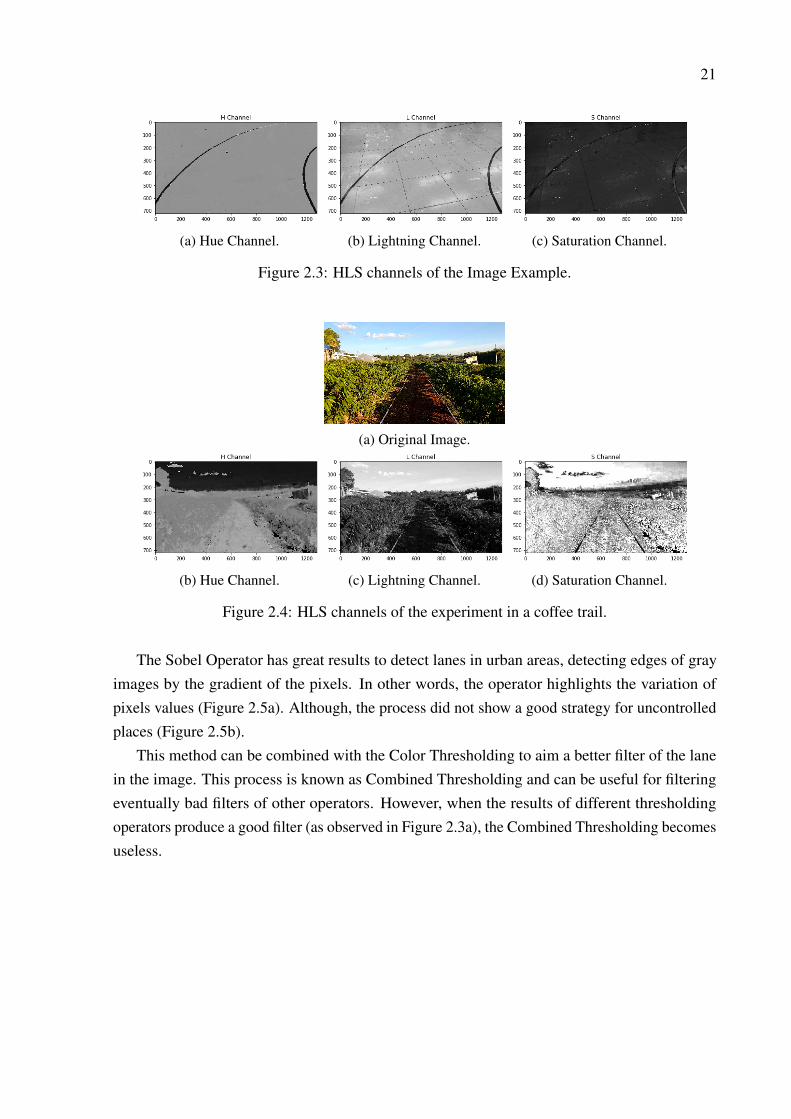
It is possible to use any different operators to extract the best information about the lanepixels. Canny, Sobel Operator or different color channels thresholding. In the Image example(Fig. 2.2a), despite the RBG channels show the lane as different pixel from the background,the texture of the ground pass by this filter, producing noise in the final image. Therefore,it was used a cv2 function (cv2.cvtColor()) to transform the RGB channels of image. Thistransformation can be done from RGB to GRAY, YCrCb, HSV and HLS channels. Each channelextract different information from the image. As the Figure 2.3 showed below, the transformationof the RGB(Red, Green and Blue Channels) to HLS (Hue, Lightning and Saturation) provide aclean detection of the lanes in the Hue Channel. Each application provides a better result with aspecific transformation, highlighting the lanes or interest points of the image.

For this project, the HLS was found as the best choice for filtering the lanes of the image.First, it can be observed in the example image of a laboratory experiment (Section 4.1.2) that theground texture disappears in the Hue channel (Figure 2.3a). Similarly, in a different experiment(Section 4.1.1), the HLS transform provides a better filter of the lanes in a coffee trail. However,in this case, the Saturation channel (Figure 2.4d) provides a better filter to highlight the whitelanes of the original image (Figure 2.4a).

21

(a) Hue Channel. (b) Lightning Channel. (c) Saturation Channel.

Figure 2.3: HLS channels of the Image Example.

(a) Original Image.

(b) Hue Channel. (c) Lightning Channel. (d) Saturation Channel.

Figure 2.4: HLS channels of the experiment in a coffee trail.

The Sobel Operator has great results to detect lanes in urban areas, detecting edges of grayimages by the gradient of the pixels. In other words, the operator highlights the variation ofpixels values (Figure 2.5a). Although, the process did not show a good strategy for uncontrolledplaces (Figure 2.5b).

This method can be combined with the Color Thresholding to aim a better filter of the lanein the image. This process is known as Combined Thresholding and can be useful for filteringeventually bad filters of other operators. However, when the results of different thresholdingoperators produce a good filter (as observed in Figure 2.3a), the Combined Thresholding becomesuseless.

22

(a) Sobel Operator from the Image Exam-ple.

(b) Sobel Operator from the Coffee TrailExperiment.

Figure 2.5: Sobel Operator

23

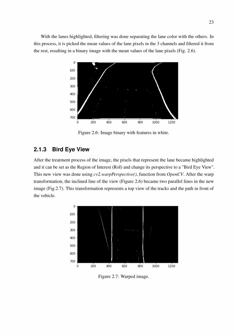
With the lanes highlighted, filtering was done separating the lane color with the others. Inthis process, it is picked the mean values of the lane pixels in the 3 channels and filtered it fromthe rest, resulting in a binary image with the mean values of the lane pixels (Fig. 2.6).

Figure 2.6: Image binary with features in white.

2.1.3 Bird Eye View

After the treatment process of the image, the pixels that represent the lane became highlightedand it can be set as the Region of Interest (RoI) and change its perspective to a "Bird Eye View".This new view was done using cv2.warpPerspective(), function from OpenCV. After the warptransformation, the inclined line of the view (Figure 2.6) became two parallel lines in the newimage (Fig.2.7). This transformation represents a top view of the tracks and the path in front ofthe vehicle.

Figure 2.7: Warped image.

24

2.1.4 Lane Detection

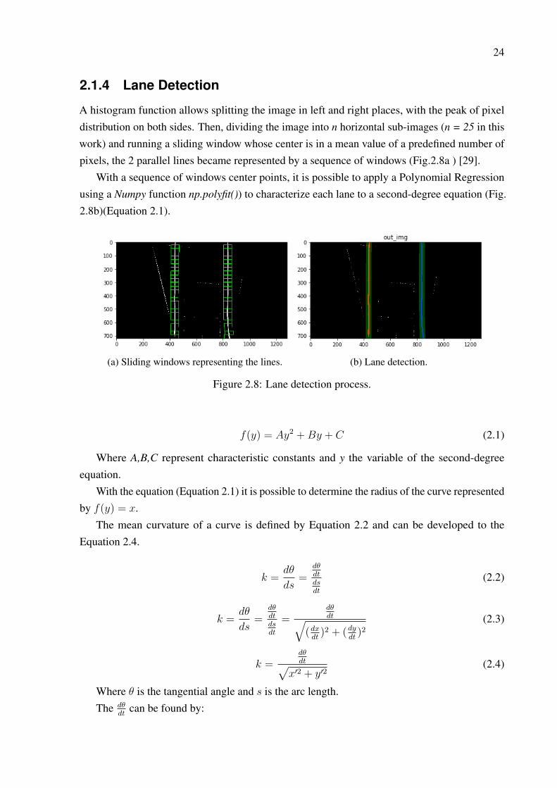
A histogram function allows splitting the image in left and right places, with the peak of pixeldistribution on both sides. Then, dividing the image into n horizontal sub-images (n = 25 in thiswork) and running a sliding window whose center is in a mean value of a predefined number ofpixels, the 2 parallel lines became represented by a sequence of windows (Fig.2.8a ) [29].

With a sequence of windows center points, it is possible to apply a Polynomial Regressionusing a Numpy function np.polyfit()) to characterize each lane to a second-degree equation (Fig.2.8b)(Equation 2.1).

(a) Sliding windows representing the lines. (b) Lane detection.

Figure 2.8: Lane detection process.

f(y) = Ay2 +By + C (2.1)

Where A,B,C represent characteristic constants and y the variable of the second-degreeequation.

With the equation (Equation 2.1) it is possible to determine the radius of the curve representedby f(y) = x.

The mean curvature of a curve is defined by Equation 2.2 and can be developed to theEquation 2.4.

k =dθ

ds=

dθdtdsdt

(2.2)

k =dθ

ds=

dθdtdsdt

=dθdt√

(dxdt)2 + (dy

dt)2

(2.3)

k =dθdt√

x′2 + y′2(2.4)

Where θ is the tangential angle and s is the arc length.The dθ

dtcan be found by:

25

tan θ =dy

dx=y′

x′(2.5)

With the derivative of tan θ

d(tan θ)

dt= sec2 θ

dθ

dt(2.6)

dθ

dt=

d(tan θ)dt

sec2 θ(2.7)

Thus by the derivative of Eq. 2.5,

dθ

dt=

1

sec2 θ

x′y′′ − y′x′′

x′2(2.8)

=1

1 + tan2 θ

x′y′′ − y′x′′

x′2(2.9)

=1

1 + y′2

x′2

x′y′′ − y′x′′

x′2(2.10)

=x′y′′ − y′x′′

x′2 + y′2(2.11)

With the Eq. 2.11 in Eq.2.4, we have,

k =x′y′′ − y′x′′3/2√x′2 + y′2

(2.12)

The Radius of curvature is given by the module of k in the equation

R =1

|k|(2.13)

Then,

R =(x′2 + y′2)

32

|x′y′′ − y′x′′|(2.14)

With the characteristic equation of the curve (Eq. 2.1) it is founded the radius of the curvatureby,

Rcurve =

[1 +

(dxdy

2)] 3

2∣∣∣d2xdy2

∣∣∣ (2.15)

Finally, by the inverse perspective of the warp process (Section 2.1.3) it can be observedthe result of the Lane Detection in the initial image (Fig. 2.9), where the red area of the imagerepresents the safety place for the vehicle ride. The Lane Detection flowchart is presented inFigure 2.10.

26

Figure 2.9: Final image.

Figure 2.10: Lane Detection flowchart.

27

Chapter 3

Object Detection

There are many methods and techniques to identify and represent the limits of a road. In theprevious chapter, it was shown one of these techniques, detecting white lanes in an off-roadenvironment. In a search of a different approach of the problem, the machine learning showeditself the best choice for these detection.

Nowadays, the use of Deep Learning in Autonomous Vehicles is essential, and become thestate-of-the-art approach for a host of problems in perception area, such as image classificationand semantic segmentation [30]. Based on how humans accelerate, brake, identify the signs andthe limits of the road, the machine can learn and respond in the same fashion. Some articlesaddress different ways to train the machine on how to detect the line lanes [31] or the road itself[32, 33]. Other projects with a focus in off-road places used Semantic Segmentation to identifytracks in the middle of a forest [34, 35, 36].

The Semantic Segmentation method presents a perfect choice to train a robot how to drivein an off-road track, once the method do not use any kind of line or reference on the road. Thetechnique uses a mask as a reference to train the machine for identifying each place or objectin the scene [37]. Nowadays, there are some techniques that can achieve more than 70% ofaccuracy processing more than 70 frames per second [38, 39]. However, it requires a powerfulGPU (e.g. Nvidia GTX 1080ti) to train the machine. Consequently, this work used a differentapproach for reference detection.

Object Detection is a fast method to train a robot to detect specific objects (car, dog, cat,person, etc.). Many models, with different architectures, compete to be the fastest and mostaccurate method [40]. The evolution of object detection allows the use of these models to trainand identify specific objects, increasing its application in autonomous systems.

In the next sections, it will be explained the principle of Machine Learning, ConvolutionNeural Network and the Detection Models that were applied in this work.

28

3.1 Machine Learning

Artificial Intelligence (AI) has found important applications in the world, such as the widespreaddeployment of practical speech recognition, machine translation and autonomous vehicles. Withthe advance of CPU’s and GPU’s, the AI aims to become a system that thinks and acts rationally,like or better than humans [41].

Machine Learning (ML) is a subset of Artificial Intelligence. In this area, there are two maintypes of tasks: supervised and unsupervised. The main difference between the types is thatthe supervised learning is done using a ground truth in the training step. In other words, thetrainer says what is the right output. Therefore, the goal of Supervised learning is, with a givensample data and desired output, learn a function that best approximates the input data and output.Unsupervised learning, on the other hand, does not have labeled or classified output, allowingthe algorithm to act on the input data without guidance.

Supervised Learning is classified into two categories of tasks. Classification, where thealgorithm means to group the output inside a category (e.g. "Red" or "Blue") and the Regression

problem occurs when the method search to map the input to a continuous output, seeking to findhow one variable behaves as other variable oscillates.

On the other side, Unsupervised learning has the Clustering as the most common task. Itmainly deals with finding a structure or pattern in a collection of uncategorized data. Clustering

algorithms will process the input data and are intent to find natural clusters (groups) if they existin the dataset.

In Supervised or Unsupervised learning, the ML builds a mathematical model based onsample data (Training data) to predict the expected output. For example, in pattern recognition,ML algorithms have made it possible to train computer systems to be more accurate and morecapable than those that we can manually program [42].

To design an algorithm to make the computer ’learn’ from a dataset, it needs to be imple-mented by fitting models. There are many types of models that can be used in Machine Learning.One of these models is called Artificial Neural Networks (ANN), an information processingstructure that is inspired by the way that the biological nervous system process the information.It is composed of a large number of interconnected processing elements (neurons) workingtogether to solve a specific problem.

When the ANN uses multiple layers between the input and output layers (hidden layers,represented by the column of neurons in Figure 3.1) it is called Deep Neural Network (DNN)[43] (Figure 3.1). The types of DNNs can be made by each architecture of layers and itsfunction, each structure characterizes a different Neural Network. For example, Recurrent NeuralNetwork (RNN), Restricted Boltzmann Machines (RBMs), Autoencoders and ConvolutionalNeural Network (CNN), represents DNN for different applications. For instance, RNN isused for applications that the historical data influence the next predicted output (applied inlanguage modeling, market price, weather change, etc), while CNN is used in computer vision

29

by characterizing signs [44], identifying objects in an image and reconstruct images [45].

Figure 3.1: Illustration of a Deep Neural Network.

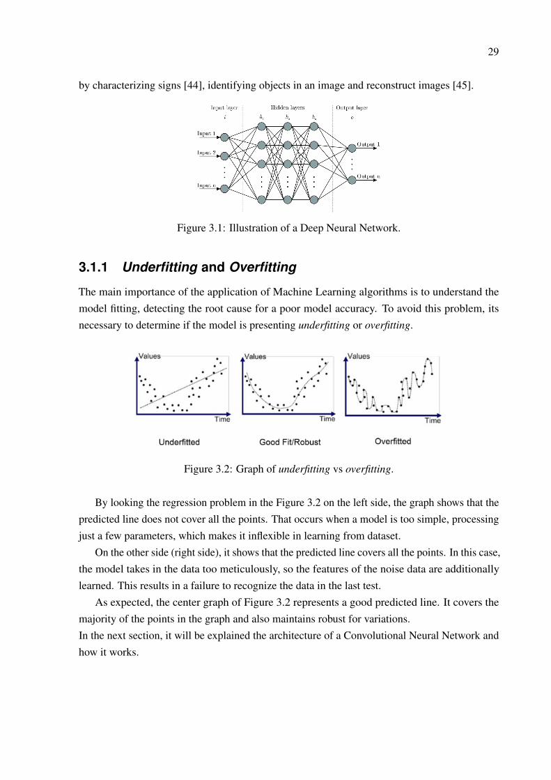
3.1.1 Underfitting and Overfitting

The main importance of the application of Machine Learning algorithms is to understand themodel fitting, detecting the root cause for a poor model accuracy. To avoid this problem, itsnecessary to determine if the model is presenting underfitting or overfitting.

Figure 3.2: Graph of underfitting vs overfitting.

By looking the regression problem in the Figure 3.2 on the left side, the graph shows that thepredicted line does not cover all the points. That occurs when a model is too simple, processingjust a few parameters, which makes it inflexible in learning from dataset.

On the other side (right side), it shows that the predicted line covers all the points. In this case,the model takes in the data too meticulously, so the features of the noise data are additionallylearned. This results in a failure to recognize the data in the last test.

As expected, the center graph of Figure 3.2 represents a good predicted line. It covers themajority of the points in the graph and also maintains robust for variations.In the next section, it will be explained the architecture of a Convolutional Neural Network andhow it works.

30

3.2 Convolutional Neural Network

Convolutional Neural Network (ConvNets or CNN) represents a category of Deep Learning thatis one of the main categories for images and face recognition, image classification, detection ofobjects, and so on. The structure of CNN consists of an input and output layers, with multiplehidden layers between them. The hidden layers are composed of a series of Convolutional layers(where the name of the network comes from), Pooling layers, and a Fully-connected layer in theend.

The structure of a CNN are divided into two steps, the Feature Learning step, with a series ofConvolutional and Pooling layers and the Classification step, where Flatten and Fully ConnectedLayers use the weights of the previous steps to classify the input image (Fig. 3.3).

Figure 3.3: Example of a Convolutional Neural Network [1].

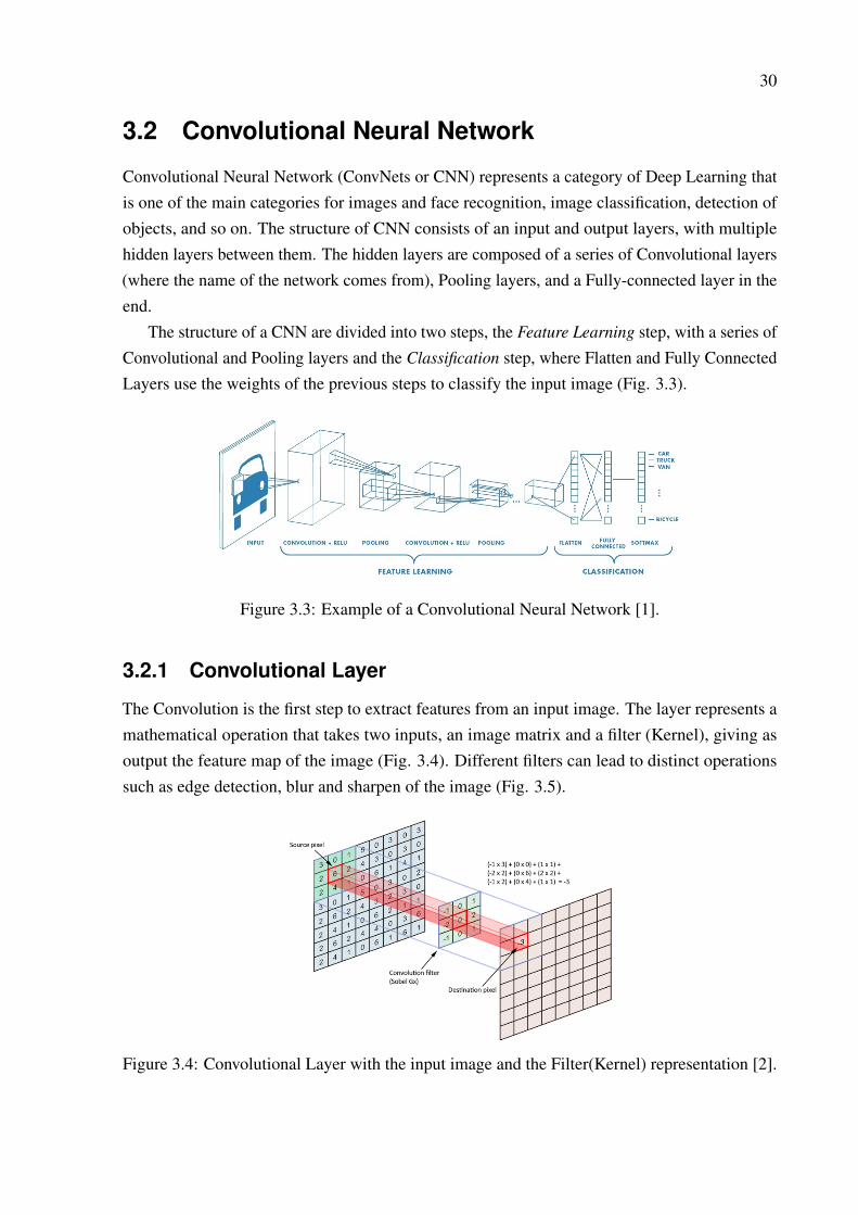
3.2.1 Convolutional Layer

The Convolution is the first step to extract features from an input image. The layer represents amathematical operation that takes two inputs, an image matrix and a filter (Kernel), giving asoutput the feature map of the image (Fig. 3.4). Different filters can lead to distinct operationssuch as edge detection, blur and sharpen of the image (Fig. 3.5).

Figure 3.4: Convolutional Layer with the input image and the Filter(Kernel) representation [2].

31

Figure 3.5: Common Filters and each results.

There are some parameters in the convolution method that can be changed for a betterperformance of the layer operation. The Stride value represents the number of pixels that thefilter moves over the input matrix (Fig. 3.6). Additionally, the Padding variable is important whenthe filter does not fit perfectly in the input image and it is defined by 2 options. Zero-Padding, topad the input matrix with zeros around the border, so that it can be applied the filter to borderingelements of the input and Valid-Padding, where the convolution drop the part of the image wherethe filter did not fit.

Figure 3.6: Stride of 2 pixels.

The Convolutional Layer can be described as the Equation 3.1.

G[m,n] =∑j

∑k

h[j, k]f [m− j, n− k] (3.1)

32

Where f represents the matrix of the input image and h the matrix of the Kernel. The indexesof rows and columns of the result matrix are marked with m and n respectively.

To complete the Convolutional Layer, the result of the convolution method goes to anactivation function, such as ReLU, ELU, Sigmoid, tanh, etc. The ReLU function, RectifiedLinear Unit, is the most used activation in neural networks (P. Ramachandran et al. presented acomparison between the activation functions [46]). The importance of this activation occurs inorder to introduce non-linearity in CNN and to return a non-negative values f(x) = max(0, x).

3.2.2 Pooling Layer

The Pooling Layer is common to be periodically inserted in-between successive convolutionallayers in ConvNet. It is a function to reduce the number of parameters of large images andhence to control overfitting. Spatial pooling reduces the dimension of the image, although ideallyretains the important information. Furthermore, this layer reduces the detachment sensitivity anddifferent distortion changes, making the convolution invariant to translation, rotation and shifting[47].

It can be done by different types: Max Pooling, taking the largest number from the filter size(In 2010, Sherer et al. suggests that max-pooling provides stronger task performances [48]);Average Pooling, taking the average of all pixels in map size; Sum Pooling, summing of allelements in the feature map (Fig. 3.7).

Figure 3.7: Max Pooling representation.

33

3.2.3 Flatten Layer

Once the pooled feature map is obtained by the previous layers, the next step is to classify theresult of the Feature Learning step (Figure 3.3). The Classification step is started with a Flattenlayer, as the name says, flat the input map. It involves transforming the entire feature map matrixinto a single column.

Figure 3.8: Flatten process.

3.2.4 Fully-Connected Layer

The Fully-Connected (FC) Layer is commonly the last layer of a CNN, this is the main stepto classify images. It is a traditional Multi-Layer Perceptron (MLP), a class of artificial neuralnetwork (ANN) that consists at least of an input layer, a hidden layer and an output layer. Thehidden layer usually have as activation function Tanh (Equation 3.2) or Sigmoid (Equation 3.3)function while the output layer is a Softmax (Equation 3.4) layer that use the previous resultsto classify the output as the labels (e.g. cat, dog, car, chair, etc.) [49].

The MLP uses a technique called backpropagation for training [50]. This method computesthe gradient of the loss function with respect to the weights of the network. It has this namebecause the process starts from the output layer and propagates backwards, updating weightsand biases for each layer.

The fully connected layer goes through its backpropagation process to determine the mostaccurate weights. Each neuron receives the correction values of the weights that prioritize theappropriate classification. In other words, the FC layer looks at what high level features moststrongly correlate to a particular class.

Finally, the best probability, from the softmax function, results in the category decision (Fig.3.9b).

34

(a) MLP with one hidden layer [49]. (b) Fully-Connected Layer representation.

Figure 3.9: Fully Connected Layer.

Activation functions used in FC layer:

TanH f(x) = tanh(x) =ex − e−x

ex + e−x(3.2)

Sigmoid f(x) = σ(x) =1

1 + e−x(3.3)

Softmax fi(~x) =exi∑Jj=1 e

xjfor i = 1, ..., J (3.4)

3.3 Object Detection Models

A human eye can look, for a second, identify all the objects around and make decisions. Thesedecisions can be made by sensors, lasers and wave radars systems. However, these sensors havesome disadvantages, for example, the high price and limited information that can be extractedfrom them. In contrast, cameras, with a low-cost can simulate the eye view and with a system itsinterprets the information as humans do.

When it comes to Autonomous vehicles, the fast identification of a lane line or a traffic signbecomes essential for a safe drive. Consequently, Object Detection is the best choice to simulatethe eye view and extract the necessary information.

The concept of detecting patterns by images has been studied along many years, detectingfaces, people and simple objects [51]. Nowadays, with the advantage of CPU’s and GPU’s, thecomplexity of artificial intelligence allows us to train a machine to detect and classify any patternwith a predetermined data set. Furthermore, new techniques, such as transfer learning (Section3.3.3), allow us to use a small amount of data to achieve great results.

Many algorithms have been developed to increase the performance and speed of detection.In 2015, Ross Girshick presented the Fast Region-based Convolutional Neural Network (Fast

35

R-CNN)[5], a method that shows itself faster and more accurate among the latest techniques,which process images in 0.3s and has a mean average precision (mAP) of 66% on PASCALVOC 2012[40].

At the same year Joseph Redmon, presented the YOLO (You Only Look Once)[7], analgorithm that promised to be much faster than Fast R-CNN with a great mAP. In this paper, J.Redmon shows that YOLO has a 63.4% mAP at 45 frames per second (FPS), number of imagesprocessed in one second, and Fast(Tiny) YOLO has 52.7% mAP at 155 FPS, compared to theFast R-CNN that achieved 70% mAP at 0.5 FPS in the same conditions. Fast YOLO shows itselfthe fastest detector on the Pascal VOC detection [52] and YOLO presents at least 10 mAP higherthan this technique while still above the real-time speed.

In the beginning of 2016, Shaoqing Ren showed a new version of the Fast R-CNN, the FasterR-CNN. This change worked in the time-process of the last technique without compromiseits precision. Furthermore, this model achieved state-of-the-art object detection accuracy onPASCAL VOC 2007, 2012 and MS COCO datasets [6].

At the end of 2016, two models became highlighted. Redmon introduced the sequence ofYOLO, the YOLO version 2 (YOLOv2). An algorithm that increases the achievements of the firstversion with detection of over 9000 object categories [3]. On the other hand, Wei Liu presented anew object detection, called Single Shot Multibox Detector (SSD), a model with an architecturethat provides better results compared to the YOLO and Faster R-CNN. The Redmon article[3]provides a comparison of the results between the methods (Fig. 3.10).

Figure 3.10: Comparative of models. It was used the Pascal 2007+2012 images to train andcompare [3].

The fast detection framework of SSD model was combined with a state-of-art classifier(Residual-101)[53] and then it was designed the Deconvolutional Single Shot Detector(DSSD).This model, presented in 2017 by Cheng-Yang Fu, showed a small increase in accuracy andslower detection time, compared to the SSD model on Pascal VOC2007 [54].

Finally, in 2018, Redmon showed the third version of YOLO [55], a Linux applicationmethod with better accuracy than the other versions. Elseways, it had a small decrease in the

36

time process of each image. Based on DarkNet (platform of YOLO), the Fast(Tiny) YOLOv3processes at 220 FPS and Fast(Tiny) YOLOv2 at 244 FPS [56].

3.3.1 Pascal VOC Challenge

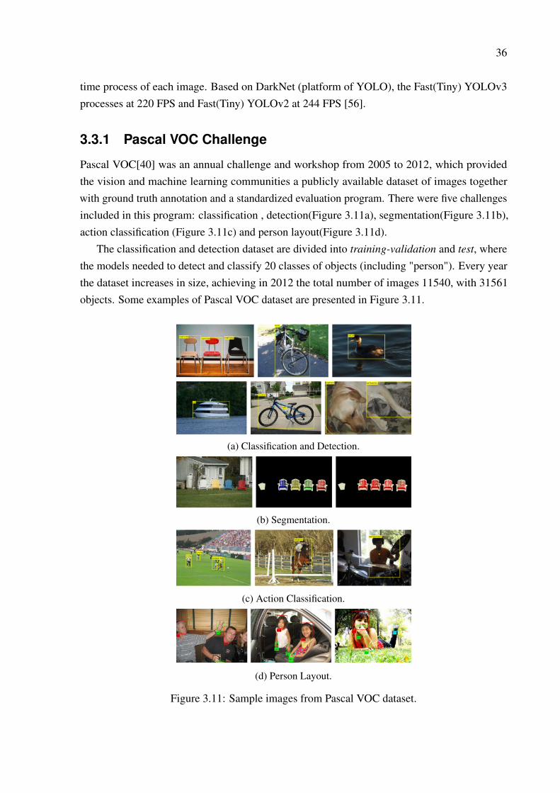
Pascal VOC[40] was an annual challenge and workshop from 2005 to 2012, which providedthe vision and machine learning communities a publicly available dataset of images togetherwith ground truth annotation and a standardized evaluation program. There were five challengesincluded in this program: classification , detection(Figure 3.11a), segmentation(Figure 3.11b),action classification (Figure 3.11c) and person layout(Figure 3.11d).

The classification and detection dataset are divided into training-validation and test, wherethe models needed to detect and classify 20 classes of objects (including "person"). Every yearthe dataset increases in size, achieving in 2012 the total number of images 11540, with 31561objects. Some examples of Pascal VOC dataset are presented in Figure 3.11.

(a) Classification and Detection.

(b) Segmentation.

(c) Action Classification.

(d) Person Layout.

Figure 3.11: Sample images from Pascal VOC dataset.

37

The dataset and evaluation process of Pascal VOC is still used to compare the ObjectDetection models. The different techniques use the dataset of one year (e.g. Pascal VOC 2007)or a dataset combination of more years (e.g. Pascal VOC 2007 trainval+test and Pascal VOC2012 trainval). The use of more dataset allows the models to have better training and, therefore,achieving better results.

3.3.2 Intersection over Union (IoU)

Intersection over Union (IoU)(sometimes referred to as Jaccard index) is an evaluation metricused to measure the accuracy of an object detector on a particular dataset. This evaluationmetric is used in object detection challenges such as the previous topic Pascal VOC Challenge.Therefore, any algorithm that provides predicted bounding boxes as output, can be evaluatedusing IoU.

The Deep Learning models predict a bounding box around the object and compare theprediction to the ground truth bounding box (Figure 3.12a).

(a) Boundary Box Representation (b) Area of Intersection and Area of Union

Figure 3.12: Intersection over Union.

IoU can be computed as Area of Intersection divided over Area of Union (Equation 3.5).

IoU =Area of Intersection

Area of Union(3.5)

In Multibox, system with multiple detection, researchers created the anchors (Faster R-CNNterminology (Section 3.4.1)), which fixed size bounding boxes that closely match the distributionof the original ground truth boxes. Those anchors are selected when their IoU values are greaterthan 0.5. Those value represent a "good" prediction (Figure 3.13b), however, for accuracydetection, those values can be used only for a starting point. This avoids the model to startthe prediction with random coordinates. Figure 3.13 shows the IoU values of different boxpredictions.

38

(a) Poor prediction (b) Good Prediction (c) Excellent Prediction

Figure 3.13: Intersection over Union (The green and red box represent the ground truth andprediction box, respectively).

39

3.3.3 Transfer Learning

Transfer learning is a popular method in computer vision because it allows building accuratemodels in a timesaving way. With transfer learning, instead of starting the learning process fromscratch, it is started from patterns that have been learned when solving different problems.

In computer vision, transfer learning is usually expressed through the use of pre-trainedmodels. Pre-trained models are neural networks that were trained on a large dataset to provideaccurate outputs. These pre-trained models can help a new training that has insufficient data togain a lot of features definitions. For example, training with 1000 images of horses can be startedfrom a pre-trained model such as ResNet, that was trained with more than 1 million images, andobtain a fast learning process in the horse characterization.

It’s observed that a several state-of-art results in image classification based on transferlearning solutions such as presented by Alex Krizhevsky et al. with the ImageNet [30](Used inmany Object detection models), VGG-16 showed by Karen Simonyan et al [57] and the ResNetpresented in 2015 by Kaiming He et al. [58].

3.3.4 Loss

These models present a math operation that determines the error between the output values of itsalgorithm and the given target value, named Loss. The loss function expresses how far off thepredictions are to the ground truth. Therefore, this value will be used to compare the accuracyof each model. The models present different loss functions to measure the error value and, inSection 3.4, it will be presented the characteristic loss equation of each one.

In the next section (Section 3.4) it will be explained the architecture and loss function of 3methods, Faster R-CNN, Fast(Tiny) YOLOv2 and SSD300. In addition, this work will comparethe accuracy and speed of their detection with a new image on an off-road street (Section 4.2).

40

3.4 Models

3.4.1 Faster R-CNN (Faster Region-based Convolutional NeuralNetwork )

Architecture

In 2014 Ross Girshick proposed a simple and scalable detection algorithm, an approach thatcombines the high-capacity of convolutional neural networks and proposes regions to localizeand segment objects [4]. The model called R-CNN(Regions with CNNs features) receives theinput image and extracts around 2000 region proposals. Each region is warped to a fixed-sizeand computed by a large CNN, where it is classified by label probabilities (Fig. 3.14).

Figure 3.14: R-CNN architecture [4].

The R-CNN method presents some problems in real-time implementation. It takes a hugeamount of time to train the network by classifying 2000 region proposals per image, takingaround 47 seconds for each image. So, in 2015 Girshick presented the Fast R-CNN, a modelbuilt on previous work to be faster and more accurate.

The approach of Fast R-CNN is similar to the R-CNN algorithm, however, instead of feedingthe region proposals to the CNN, it inputs the image into the CNN to generate a convolutionalfeature map. From this map, it is identified the regions of proposals and they are warped intobounding boxes. Using a region of interest (RoI) pooling layer the regions are reshaped intoa fixed size to be fed into a sequence of fully connected (FC) layers. These FC layers have2 outputs. The first is a sofmax classification layer, where it decides which object class wasfounded in the prediction. The second is the Bounding Box Regressor (BBox Regressor), apopular technique to refine or predict localization boxes in recent object detection approaches.This technique is trained to regress from either region proposals(or anchors) to nearby boundingboxes [59]. In other words, the BBox Regressor output the bounding box coordinates for eachobject class (Fig. 3.15) [5].

41

Figure 3.15: Fast R-CNN architecture[5].

Both algorithms (R-CNN and Fast R-CNN ) use Selective Search. This involves sliding awindow over the image to generate region proposals, areas where objects could possibly be found[60]. However, this method is a slow and time-consuming process that affects the performanceof the network. For this reason, in 2017 Shaoqing Ren et al. came up with a different objectdetection design, called Faster R-CNN, that eliminates the selective search algorithm and lets anetwork learn the regions proposals [6].

Faster R-CNN is composed of two modules. First, a deep fully convolutional neural networkthat proposes regions, the Region Proposal Network (RPN), and second, a network that usesthese proposals of RPN to detect an objects (Fig. 3.16). The second module works with the samedetector used in Fast R-CNN.

Figure 3.16: Faster R-CNN [6].

The Region proposal Network takes an image of any size, inputs to a Convolutional NeuralNetwork (VGG-16 used in Ren paper [6]) and by the feature map returned from the CNN, theRPN proposes a set of region boxes (Anchors) with an "objectness" score, probability of thecontaining box is an object class or a background. To generate these regions, a n× n windowis slid over the feature map (Figure 3.17a). Each sliding-window location its simultaneously

42

predicts multiple region proposals (Anchors), which the number of maximum possible regions isdenoted by k (k = 9 [6]) (Figure 3.17b).

(a) Sliding-window generating k(k = 9) Anchors.

(b) 800× 600 Image with 9 anchorsat the position (320,320).

Figure 3.17: Anchors.

As a final point, the model unifies the RPN with the Fast R-CNN detector, where the algorithmapplies a Region of Interest (RoI), to reduce all anchors (Figure 3.18) to the same size and foreach region proposal, the model flattens the input, passing it through two fully-connected layers(FC) with ReLU activation and then with two different FC it generates the prediction of the classand the box of each object (Figure 3.19).

Figure 3.18: Example of the Region of Interest(RoI) process.

Figure 3.19: Example of the Fast R-CNN Classification process.

43

Loss

Faster R-CNN presents a combination of localization loss (Lloc) and classification loss (Lcls).The loss function sums up the cost of classification and bounding box prediction (Equation 3.6 ).

L =1

Ncls

∑i

Lcls(pi, p∗i ) + λ

1

Nreg

p∗iLloc (3.6)

Lcls = −p∗i log pi − (1− p∗i ) log(1− pi) (3.7)

Lloc =∑

i∈{x,y,w,h}

Lsmooth1 (ti − t∗i ) (3.8)

in which

Lsmooth1 (x) =

0.5x2 if |x| < 1

|x| − 0.5 otherwise(3.9)

where,pi: Predicted probability of anchor i being an object.p∗i : Ground truth label of whether anchor i is an object.Ncls: Mini-batch size (Ncls = 256 [6]).Nreg: Number of anchor localizations (Nreg ∼ 2400 [6] ).λ: Balancing parameter (λ = 10 [6])ti: Predicted four parameterized coordinates (x, y, w, h).t∗i : Ground truth coordinates.

tx =(x− xa)wa

ty =(y − ya)ha

tw = log(w

wa), th = log(

h

ha)

t∗x =(x∗ − xa)

wat∗y =

(y∗ − ya)ha

t∗w = log(w∗

wa), t∗h = log(

h∗

ha)

Where x, y, w and h represents the box’s center coordinates and its width and height,respectively. Variables x, xa and x∗ are for predicted box,anchor box and ground truth boxrespectively (likewise for y, w, h).

44

3.4.2 YOLO (You Only Look Once)

Architecture

YOLO architecture, different from Faster R-CNN, has no RPN, it uses a single feed-forwardconvolutional network to predict classes and bounding boxes.

The YOLO system divides the input image into a S × S grid, each grid cell is responsiblefor detecting the object in its area. Each one predicts B bounding boxes and it scores theconfidence to be an object or not. The confidence score reflects the probability of the predictedbox containing an object Pr(Object), as well as how accurate is the predicted box by evaluatingits Intersection over Union IoU truth

pred . In this sense, the confidence score becomes the Equation3.10.

Confidence Score = Pr(Obj) ∗ IoU truthpred (3.10)

Pr =

1 If object exist

0 Otherwise(3.11)

Each bounding box consist of 5 values, 4 representing its coordinates (x,y,w,h) and one withthe confidence score.

Looking to the grid cell, each one also predicts number of C conditional class probabilities,which C represents the number of classes and the Conditional Class Probabilities represent thechance of an object be long to class i (Equation 3.12).

Conditional Class Probabilities = Pr(Classi|Object) (3.12)

At the test time, the model multiplies the Conditional Class Probabilities and the individualbox Confidence score (Equation 3.13).

Pr(Classi|Object) ∗ Pr(Obj) ∗ IoU truthpred = Pr(Classi) ∗ IoU truth

pred (3.13)

Consequently, the result of Equation 3.13 gives the score of the probability of the classappearing in the box and how the predicted box fits the object (Fig. 3.20)[7].

45

Figure 3.20: The representation of the two YOLO steps, identifying the objects and defining theprobabilities of the classes in each grid [7].

Figure 3.21: The output from YOLO.

The predictions results into a S × S × (B ∗ 5 + C) tensor. For example, in the figure 3.22it takes S = 7, B = 2 and C = 20, that results in a (7, 7, 2 ∗ 5 + 20)→ (7, 7, 30) tensor. Thistensor provides the information about the Bounding Boxes and each class probabilities.

YOLO has basically two model types: Regular YOLO and Fast(Tiny) YOLO. The Regularmodel consists of 24 convolutional layers followed by 2 fully connected layers (Fig. 3.22). Onthe other side, the Tiny model has 11 layers, 9 convolutional and 2 fully connected (Fig. 3.23).As this architecture is much smaller compared to other detecting methods, it presents a fastresponse in object predictions, allowing the detection in real-time speed.

46

Figure 3.22: YOLO architecture [7].

Figure 3.23: Fast YOLO architecture[8].

The YOLOv2 represents the second version of YOLO with the objective of improving theaccuracy while making it faster. To achieve these characteristics, the second model opted foradding new ideas to improve the previous model performance. Among them, there are the addingof batch normalization (BN) in convolution layers, the high resolution classifier, convolutionalwith anchors boxes, dimension clusters, direct location prediction, fine-grained features and amulti-scale training.

As can be observed in the Figure 3.24 [3], each step added improve the accuracy of theprevious step.

Figure 3.24: Accuracy improvements of YOLOv2 compare with YOLO [3]

47

Loss

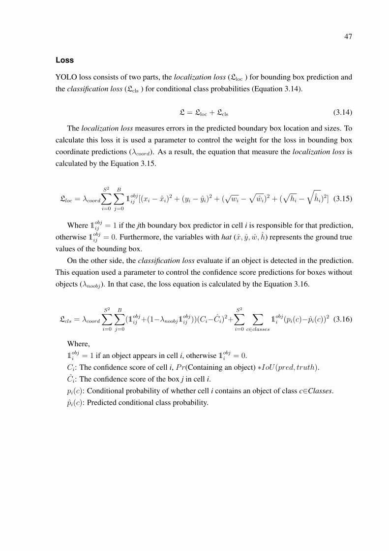
YOLO loss consists of two parts, the localization loss (Lloc ) for bounding box prediction andthe classification loss (Lcls ) for conditional class probabilities (Equation 3.14).

L = Lloc + Lcls (3.14)

The localization loss measures errors in the predicted boundary box location and sizes. Tocalculate this loss it is used a parameter to control the weight for the loss in bounding boxcoordinate predictions (λcoord). As a result, the equation that measure the localization loss iscalculated by the Equation 3.15.

Lloc = λcoord

S2∑i=0

B∑j=0

1objij [(xi − xi)2 + (yi − yi)2 + (

√wi −

√wi)

2 + (√hi −

√hi)

2] (3.15)

Where 1objij = 1 if the jth boundary box predictor in cell i is responsible for that prediction,otherwise 1objij = 0. Furthermore, the variables with hat (x, y, w, h) represents the ground truevalues of the bounding box.

On the other side, the classification loss evaluate if an object is detected in the prediction.This equation used a parameter to control the confidence score predictions for boxes withoutobjects (λnoobj). In that case, the loss equation is calculated by the Equation 3.16.

Lcls = λcoord

S2∑i=0

B∑j=0

(1objij +(1−λnoobj1objij ))(Ci−Ci)2+S2∑i=0

∑c∈classes

1obji (pi(c)−pi(c))2 (3.16)

Where,1obji = 1 if an object appears in cell i, otherwise 1obji = 0.Ci: The confidence score of cell i, Pr(Containing an object) ∗IoU(pred, truth).Ci: The confidence score of the box j in cell i.pi(c): Conditional probability of whether cell i contains an object of class c∈Classes.pi(c): Predicted conditional class probability.

48

3.4.3 SSD (Single Shot Detection)

Architecture

Single Shot Detector, like YOLO, takes only one shot to detect multiple objects present in animage using multibox. Furthermore, similar to Faster R-CNN, SSD model is build on a networkarchitecture, e.g. the VGG-16 architecture [57](Fig. 3.25), a high quality image classificationmodel, without the final classification layers (fully connected layers). Instead of that, a set ofconvolutional layers are added, decreasing the size of the input to each subsequent layer enablingto extract features at multiple scales.Thus, predictions for bounding boxes and confidence fordifferent objects is done by multiple feature maps of different sizes (Fig. 3.26).

Figure 3.25: VGG architecture.

Figure 3.26: SSD architecture [9].

The main Single Shot Detection uses VGG-16 network to extract features of images. How-ever, different bases (GoogleNet, MobileNet, AlexNet, Inception, etc.) can be used for betterperformance. In this work, searching for a high speed detection, it was used the second versionof MobileNet. The first MobileNet, presented by Howard in 2017, shows itself as a networkfaster and nearly as accurate as VGG-16 network [10](Fig. 3.27) and in 2018 the second versionof MobileNet has shown to be faster and more accurate than the last network [11](Fig. 3.28).Figure 3.29 shows the architecture off MobileNetv2 - SSD.

49

Figure 3.27: Comparison of the principals networks [10].

Figure 3.28: Performance on ImageNet, comparison for different networks [11]. MAddsrepresents the counting of total number of Multiply-Adds.

Figure 3.29: MobileNetv2 - SSD architecture [12].

In the training process of SSD model, each added feature layer produce a detection predictionusing convolutional filters (see "Extra Feature Layers" in Figure 3.26). For a layer of size m× n(number of locations) with p channels, the element for predicting is a 3 × 3 × p kernel thatproduces a score for a category. For each location, the element for predicting got k boundingboxes. These boxes have different sizes (e.g. a 4 size box as in Figure 3.30). Furthermore, foreach bounding box, it will be computed c class score and 4 offsets relative to the original defaultbox shape. At the training time, it is matched these default boxes to the ground truth boxes, theboxes that matched with the expected are treated as positives and the remaining as negatives.In that way, it results in a (c+ 4)k filters that are applied around each location in feature map,resulting in a (c+4)kmn outputs for a m× n map. Using the Figure 3.26 as example, its resultsin a 8732 bounding boxes.

50

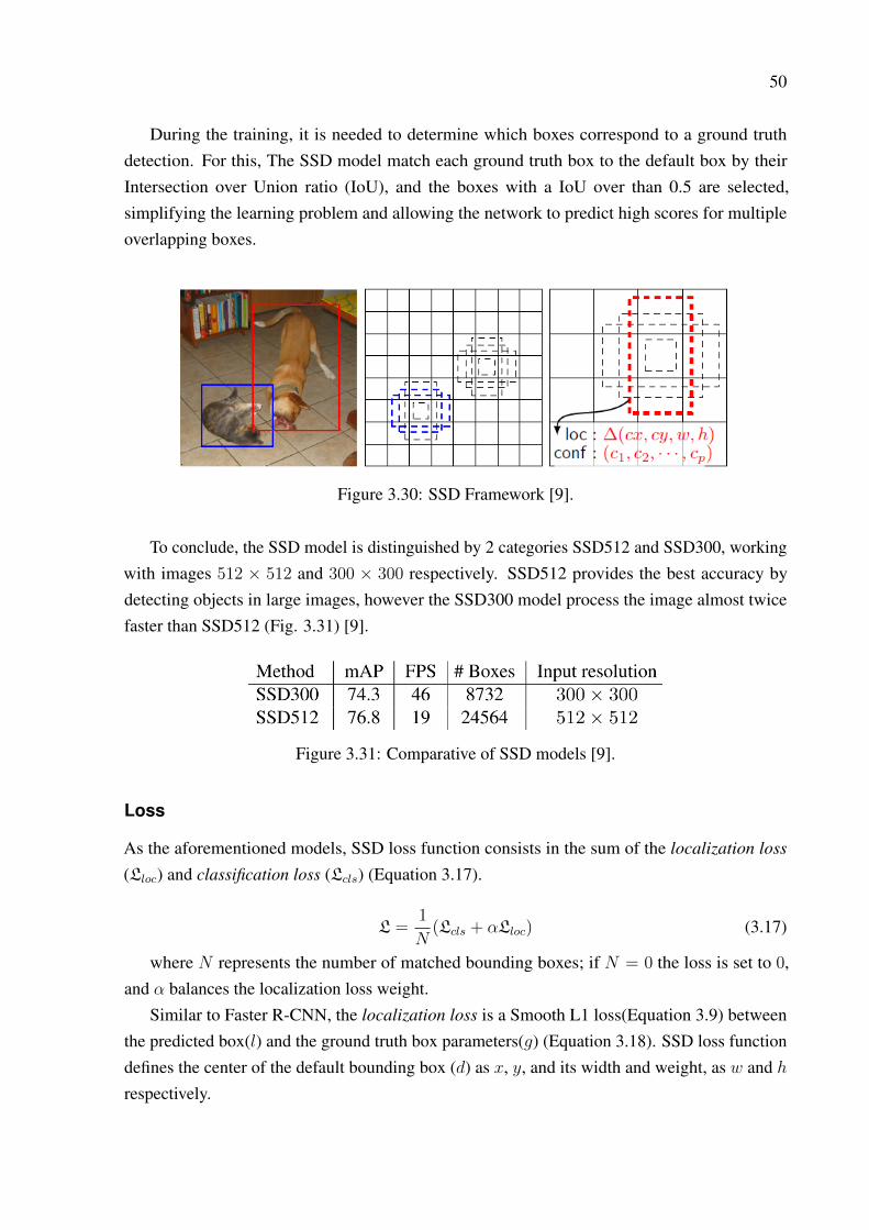
During the training, it is needed to determine which boxes correspond to a ground truthdetection. For this, The SSD model match each ground truth box to the default box by theirIntersection over Union ratio (IoU), and the boxes with a IoU over than 0.5 are selected,simplifying the learning problem and allowing the network to predict high scores for multipleoverlapping boxes.

Figure 3.30: SSD Framework [9].

To conclude, the SSD model is distinguished by 2 categories SSD512 and SSD300, workingwith images 512 × 512 and 300 × 300 respectively. SSD512 provides the best accuracy bydetecting objects in large images, however the SSD300 model process the image almost twicefaster than SSD512 (Fig. 3.31) [9].

Figure 3.31: Comparative of SSD models [9].

Loss

As the aforementioned models, SSD loss function consists in the sum of the localization loss

(Lloc) and classification loss (Lcls) (Equation 3.17).

L =1

N(Lcls + αLloc) (3.17)

where N represents the number of matched bounding boxes; if N = 0 the loss is set to 0,and α balances the localization loss weight.

Similar to Faster R-CNN, the localization loss is a Smooth L1 loss(Equation 3.9) betweenthe predicted box(l) and the ground truth box parameters(g) (Equation 3.18). SSD loss functiondefines the center of the default bounding box (d) as x, y, and its width and weight, as w and hrespectively.

51

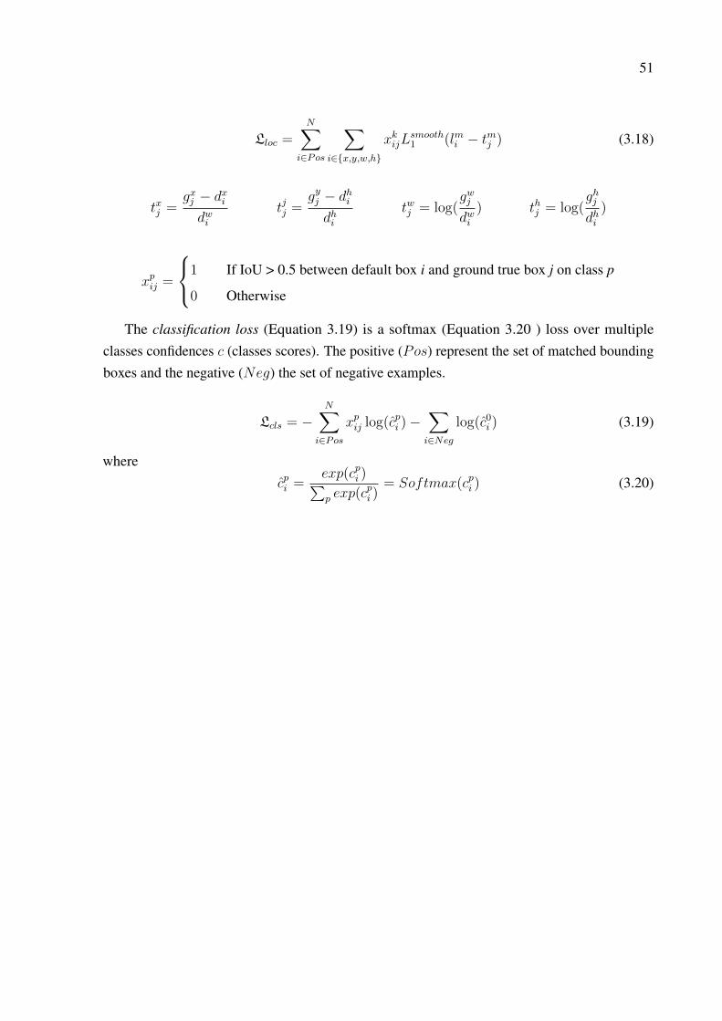
Lloc =N∑

i∈Pos

∑i∈{x,y,w,h}

xkijLsmooth1 (lmi − tmj ) (3.18)

txj =gxj − dxidwi

tjj =gyj − dhidhi

twj = log(gwjdwi

) thj = log(ghjdhi

)

xpij =

1 If IoU > 0.5 between default box i and ground true box j on class p

0 Otherwise

The classification loss (Equation 3.19) is a softmax (Equation 3.20 ) loss over multipleclasses confidences c (classes scores). The positive (Pos) represent the set of matched boundingboxes and the negative (Neg) the set of negative examples.

Lcls = −N∑

i∈Pos

xpij log(cpi )−

∑i∈Neg

log(c0i ) (3.19)

wherecpi =

exp(cpi )∑p exp(c

pi )

= Softmax(cpi ) (3.20)

52

Chapter 4

Results

4.1 Lane Detection

To validate the method, it was tested in two experiments. The First test was done by a manualvideo to observe the robustness of detection and in the second test, the model was applied in anelectric vehicle to control the steering using only the detection measurements.

4.1.1 Experiment 1

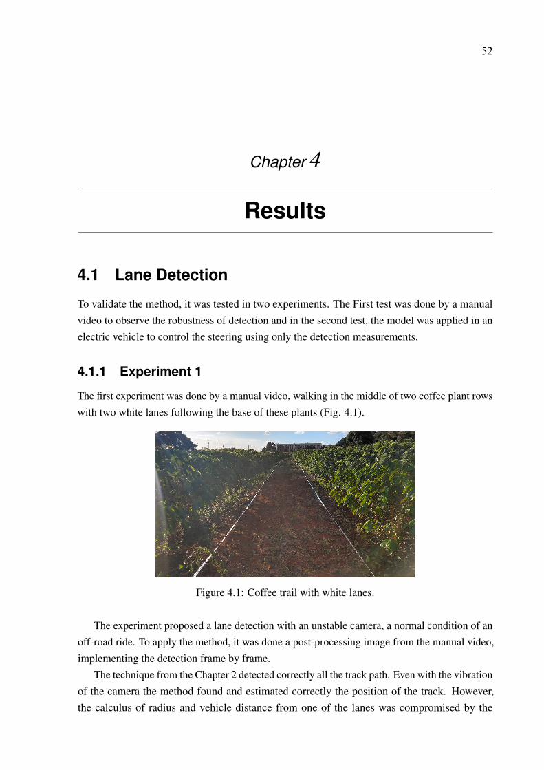
The first experiment was done by a manual video, walking in the middle of two coffee plant rowswith two white lanes following the base of these plants (Fig. 4.1).

Figure 4.1: Coffee trail with white lanes.

The experiment proposed a lane detection with an unstable camera, a normal condition of anoff-road ride. To apply the method, it was done a post-processing image from the manual video,implementing the detection frame by frame.

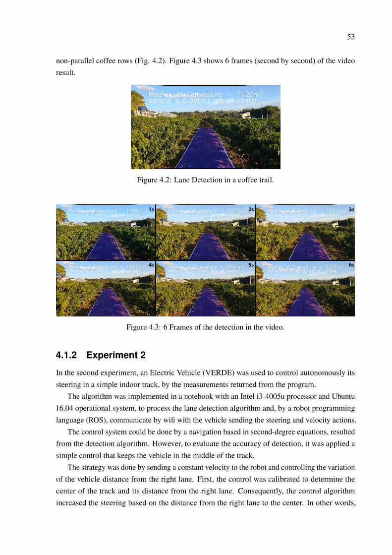
The technique from the Chapter 2 detected correctly all the track path. Even with the vibrationof the camera the method found and estimated correctly the position of the track. However,the calculus of radius and vehicle distance from one of the lanes was compromised by the

53

non-parallel coffee rows (Fig. 4.2). Figure 4.3 shows 6 frames (second by second) of the videoresult.

Figure 4.2: Lane Detection in a coffee trail.

Figure 4.3: 6 Frames of the detection in the video.

4.1.2 Experiment 2

In the second experiment, an Electric Vehicle (VERDE) was used to control autonomously itssteering in a simple indoor track, by the measurements returned from the program.

The algorithm was implemented in a notebook with an Intel i3-4005u processor and Ubuntu16.04 operational system, to process the lane detection algorithm and, by a robot programminglanguage (ROS), communicate by wifi with the vehicle sending the steering and velocity actions.

The control system could be done by a navigation based in second-degree equations, resultedfrom the detection algorithm. However, to evaluate the accuracy of detection, it was applied asimple control that keeps the vehicle in the middle of the track.

The strategy was done by sending a constant velocity to the robot and controlling the variationof the vehicle distance from the right lane. First, the control was calibrated to determine thecenter of the track and its distance from the right lane. Consequently, the control algorithmincreased the steering based on the distance from the right lane to the center. In other words,

54

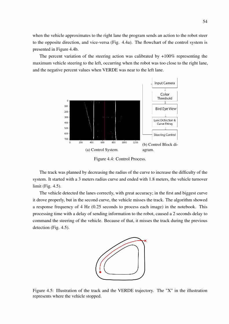
when the vehicle approximates to the right lane the program sends an action to the robot steerto the opposite direction, and vice-versa (Fig. 4.4a). The flowchart of the control system ispresented in Figure 4.4b.

The percent variation of the steering action was calibrated by +100% representing themaximum vehicle steering to the left, occurring when the robot was too close to the right lane,and the negative percent values when VERDE was near to the left lane.

(a) Control System.(b) Control Block di-agram.

Figure 4.4: Control Process.

The track was planned by decreasing the radius of the curve to increase the difficulty of thesystem. It started with a 3 meters radius curve and ended with 1.8 meters, the vehicle turnoverlimit (Fig. 4.5).

The vehicle detected the lanes correctly, with great accuracy; in the first and biggest curveit drove properly, but in the second curve, the vehicle misses the track. The algorithm showeda response frequency of 4 Hz (0.25 seconds to process each image) in the notebook. Thisprocessing time with a delay of sending information to the robot, caused a 2 seconds delay tocommand the steering of the vehicle. Because of that, it misses the track during the previousdetection (Fig. 4.5).

Figure 4.5: Illustration of the track and the VERDE trajectory. The "X" in the illustrationrepresents where the vehicle stopped.

55

The experiment showed that the delay of this lane detection algorithm cannot be implementedin tracks that need fast responses. If the robot was adjusted to take a brief linear velocity whenit detects the lane and after that stopped, the vehicle probably would not had lost the track.However, different from a laboratory test, for an autonomous vehicle application in off-roadenvironments this lane detection algorithm showed not useful.

The lane detection technique showed a great method in controlled places that do not needfast actions. On the other hand, the method needs a calibration by the environment that thecamera is presented (as showed in Section 2.1.2), and a change of the ambient color couldresult in a bad lane identification. For example, a simple weather change is capable to producewrong measurements. As shown in Figure 4.6, the Coffee trail view using a Laboratory colorthresholding calibration results in a polluted image, where the white pixels should represent thelane (Figure 4.6b). Consequently, the program would not identify the track boundary.

(a) Laboratory view. (b) Coffee Trail view.

Figure 4.6: Laboratory color thresholding calibration.

4.2 Object Detection

The training and detection process was done with a GPU Nvidia Geforce 1060 3GB and CPUIntel i5 8500u on Windows 10 operational system.

4.2.1 Training Stage

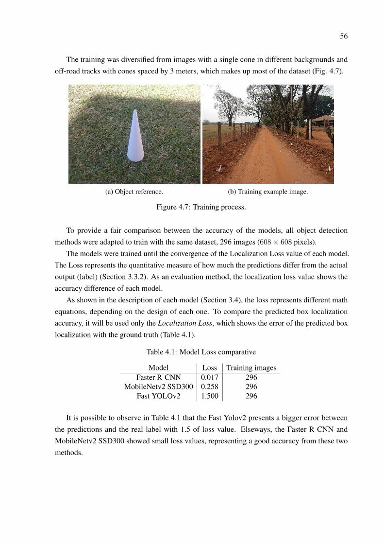
To start the training process, it was chosen a white cone as a reference detection to representthe limits of the road (Fig. 4.7a). The training of this object was presented in Dhall work (June2019), a monocular camera was used to detect and estimate the localization of a traffic cone in3D world coordinates [61].

As the work is aimed to use any reference for the application, the models were trained andtested to detect a new object. This work was done by using transfer learning from existingmodels configurations (Faster R-CNN, Fast YOLOv2 and SSD300) to train the detection of areference.

56

The training was diversified from images with a single cone in different backgrounds andoff-road tracks with cones spaced by 3 meters, which makes up most of the dataset (Fig. 4.7).

(a) Object reference. (b) Training example image.

Figure 4.7: Training process.

To provide a fair comparison between the accuracy of the models, all object detectionmethods were adapted to train with the same dataset, 296 images (608× 608 pixels).

The models were trained until the convergence of the Localization Loss value of each model.The Loss represents the quantitative measure of how much the predictions differ from the actualoutput (label) (Section 3.3.2). As an evaluation method, the localization loss value shows theaccuracy difference of each model.

As shown in the description of each model (Section 3.4), the loss represents different mathequations, depending on the design of each one. To compare the predicted box localizationaccuracy, it will be used only the Localization Loss, which shows the error of the predicted boxlocalization with the ground truth (Table 4.1).

Table 4.1: Model Loss comparative

Model Loss Training imagesFaster R-CNN 0.017 296

MobileNetv2 SSD300 0.258 296Fast YOLOv2 1.500 296

It is possible to observe in Table 4.1 that the Fast Yolov2 presents a bigger error betweenthe predictions and the real label with 1.5 of loss value. Elseways, the Faster R-CNN andMobileNetv2 SSD300 showed small loss values, representing a good accuracy from these twomethods.

57

4.2.2 Experiment 1

The first experiment was done by post-processing of an off-road ride video with similar char-acteristics of the dataset training. The experiment resulted in object detection to all models inany frame of the video. In that way, to compare the results of each model, it was chosen videoframes of the off-road ride (Fig. 4.8).

(a) Faster R-CNN Model. (b) SSD300 Model. (c) Fast YOLOv2 Model.

Figure 4.8: Comparative of 3 Detections Methods.

58

Figure 4.9: Comparative of the number of detections in a sequence of 50 video frames.

As can be observed in Figure 4.8 and Figure 4.9, the Faster R-CNN model and the SSD300presented comparable detections. The Faster R-CNN presents an advantage in accuracy, de-tecting the reference 12 meters distance of the car (Figure 4.8a), while the SSD300 keeps theidentification around 9 meters from the car (Figure 4.8b).

On the other hand, the Fast YOLOv2, which presented the biggest Localization loss value,showed itself the worst detector accuracy among the three models. The model resulted in amaximum detection of ∼ 4 meters distance from the car during all trajectory, failing sometimesto detect near references (Figure 4.8c and Figure 4.9).

Looking at the accuracy of each model, the Faster R-CNN showed itself the best choice foran autonomous driving application in off-road environments. However, besides a high precisionin its detection, it is necessary a fast response of the reference identification. To estimate this itwas tested 10 images, with different angles of the reference on the off-road street, and calculatedthe Mean Time Process (MTP) of each method (Table 4.2). Normally, the object detectionmodels estimate the processing speed by the number of images that the model detects in 1 second(Frames per Second (FPS)).

Table 4.2: Comparative of models. MTP: Mean Time Processing; FPS: Frames per Second

Model Loss Training images MTP (seconds) FPSFaster R-CNN 0.017 296 3.14 00.3

MobileNetv2 SSD300 0.258 296 1.41 00.7Fast YOLOv2 1.500 296 0.07 14.3

59

By the result, it is possible to observe that the Faster R-CNN proved to be the slowest detector.Even with the highest accuracy, it takes around 3 seconds to process each image, resulting inan unfeasible application for autonomous driving. On the other hand, the Fast YOLOv2, whichdemonstrated a low precision in the detection, identified the references in less than 0.1 seconds.For this reason, it showed a good detector for prevention moments, detecting nearby warnings,like animals or holes, or tight curves.

Finally, The MobileNetv2 SSD300 had an intermediary MTP. It detects all references in animage at around 1.4 seconds. The advantage of this model it that its accuracy was near to theFaster R-CNN, though SSD processes the image twice faster. For Autonomous application, 1.4seconds to detect the limits of a road in a curve presumably resulted in a car off the track. Incontrast, in a straight road, that fast steer corrections are not required, then the model can beuseful.

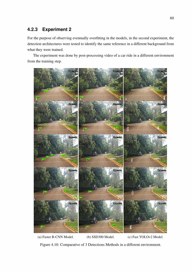
60

4.2.3 Experiment 2

For the purpose of observing eventually overfitting in the models, in the second experiment, thedetection architectures were tested to identify the same reference in a different background fromwhat they were trained.

The experiment was done by post-processing video of a car ride in a different environmentfrom the training step.

(a) Faster R-CNN Model. (b) SSD300 Model. (c) Fast YOLOv2 Model.

Figure 4.10: Comparative of 3 Detections Methods in a different environment.

61

The experiment presented a decrease in the accuracy of the Faster R-CNN and SSD300detection, where the models presented some failures in some near detection. However, even witha small number of training images (296) from a different background, the methods presented thecorrect detection of the cones.

The Fast YOLOv2 had the smallest accuracy decrease. As the first experiment, the modelcould only detect near references, failing sometimes to recognize them.

It was used 10 images of the new background to observe the change in time detection.However, the models provided the same time process that was found in the first experiment.

62

Chapter 5

Final Conclusion and Perspectives

This work covered different techniques to detect the road boundary for a localization of an au-tonomous vehicle. The main contribution of the work was to test existing object detection modelsfor a new reference, training the models with a few images and comparing the results. Anothercontribution occurs in the implementation of lane detection in off-road areas. Furthermore, theidentification allows an estimation of the lane by a second-degree equation.

5.1 Lane Detection

In Chapter 2, it was introduced a method to identify white lanes by image processing. Not only,but also an estimation of a second-degree equation of lanes based in the front view perspectiveof the vehicle. The technique was tested in a coffee tree trail with a non-regular lane line andwith an unstable camera. As result, it was shown very robust and precise in identifying thelanes. In addition, an experiment using the detection system was implemented in an electricrobot vehicle (VERDE) to make it drive in a track autonomously using only the vision to keepitself between the lanes. This experiment showed a response frequency of 4 Hz and with anon-embedded system it had a 2 seconds delay of the real-time image and the vehicle action,what as consequence, made the robot lose itself on the tight curves of the track.

The method spent a lot of time filtering the correct lane pixels and estimating the second-degree equation, resulting in a slower alternative for a real autonomous driving application.Another problem found was the necessity of a low variance of the lane color. When the methodis calibrated to find the lanes by filtering the color of the pixels, even if a small color change ofthese pixels would result in the wrong filtering of the image. For example, weather changes,different locations and illuminations of the lane, result in different calibrations to find the lane.In short, the method needs to be re-calibrated every time that a different illumination representsthe lane.

It was found that this approach to identify the limits of an off-road is not useful. Althoughthe technique had great and stable results in controlled places, closed places with constant

63

illumination and outdoor places during a few hours of the day, when the program is used to findlanes during all day or running in different places it becomes ineffective.

5.2 Object Detection

In Chapter 3, it was shown the introduction of Machine Learning to solve the detection problem.This approach uses the Object Detection models to identify references on a road, representingthe limits of a track. The technique was done by training three existing Object Detection modelswith transfer learning, to identify a new object as a reference and comparing their results, FasterR-CNN, Fast YOLOv2 and MobileNetv2 SSD300.

While Faster R-CNN and SSD300 showed similar accuracy, detecting references in close andlong distances, Fast YOLOv2 model did not detect references when it was more than 4 metersaway. Despite the precision of Fast YOLOv2, it processes the detection in less than 0.1 seconds,providing itself the faster detection among the three models.

As long as the Fast YOLOv2 presented a fast detection, the Faster R-CNN showed theslowest detector. It spent more than 3 seconds to detect the references in each image. On theother hand, the SSD300 with an accuracy similar to the Faster R-CNN process the image twicefaster, detecting objects in around 1.5 seconds.

Each model presented a particularity in accuracy and speed that is necessary for autonomouscars to drive safely on a road without line lanes. The Faster R-CNN presented the best accuracyof all, though it is considerably slow for an autonomous drive application. The SSD300 with asimilar precision was proven to be a good model to identify the limits on straight roads. With alow process time to detect references, the model only analyses and determines the action to keepthe vehicle in the middle of the road in every 1.5 seconds.

Elseways, the Fast YOLOv2 only detected near references what can be useful for fastdetections, e.g. tight curves or emergency situations, allowing the machine to make fast decisionson a drive.

For an autonomous driving application, that uses a powerful GPU and CPU, the implementa-tion of SSD and Fast YOLOv2 models results in a safe drive. The first on detecting the mainlimits of the road and the second as a warning system for fast actions.

64

5.3 Perspectives

This work studied the precision and the speed of different methods for implementation in realautonomous navigation. First, a Lane Detection and second an Object Detection. Besides that,there are some questions to be investigated in future works in each field:

5.3.1 Lane Detection

• The Kalman Filters can be used to predict the position of the lane in the next frame,resulting in an stable method without "bad curves".

• The implementation of a Convolutional Neural Network to classify the lanes of the imageinto the parameters of a second-degree equation.

• With the combination of the vision sensor with the kinematic and dynamic measurementsof the vehicle, it is possible to achieve an improvement in the accuracy at a long distance.

• The implementation of an End-to-End Lane Detection, using a Semantic Segmentationmodel to detect each lane line. With a differentiable least-squares fitting module, it ispossible to find the parameters for the best-fitting curve.

• The application of a Deep Imitation Learning based in the second-degree equations of theLane Detector method, aiming to drive the VERDE vehicle in a track.

5.3.2 Object Detection

• In a search of a track identification without references or traffic signs. The SemanticSegmentation provides the training of the image based in mask locations. However, thehigh GPU memory dependence makes the method not easily accessible to train new tracks.

• The application of new Object Detection models. With the decreasing costs and develop-ment of the GPUs, it’s possible to achieve great accuracy in a fast speed process to achievebetter results in the identification.

• The training of Object Detection models to identify natural references on an off-road street.That will allow the vehicle to ride in non-urban streets that do not have any kind of trackboundary sign.

• The application of the Object Detection method in the VERDE project, providing anautonomous ride using only the references detected to keep the vehicle in the middle ofthe track.

• The implementation of the Perspective n-Point algorithm allows an estimate of the objectdistance using an image as a reference. This system mixed with the Object Detector model

65

should result in a Simultaneous Location and Mapping (SLAM) process of the vehicleusing only computer vision.

66

References

[1] A Comprehensive Guide to Convolutional Neural Networks.https://towardsdatascience.com/a-comprehensive-guide-to-convolutional-neural-networks-the-eli5-way-3bd2b1164a53.

[2] Understanding the Structure of a CNN. https://mc.ai/understanding-the-structure-of-a-cnn/.

[3] Joseph Redmon and Ali Farhadi. YOLO9000: Better, faster, stronger. Proceedings -

30th IEEE Conference on Computer Vision and Pattern Recognition, CVPR 2017, 2017-January:6517–6525, 2017.

[4] Ross Girshick, Jeff Donahue, Trevor Darrell, and Jitendra Malik. Rich feature hierarchiesfor accurate object detection and semantic segmentation. Proceedings of the IEEE Computer

Society Conference on Computer Vision and Pattern Recognition, pages 580–587, 2014.

[5] Ross Girshick. Fast R-CNN. Proceedings of the IEEE International Conference on

Computer Vision, 2015 Inter:1440–1448, 2015.

[6] Shaoqing Ren, Kaiming He, Ross Girshick, and Jian Sun. Faster R-CNN: Towards Real-Time Object Detection with Region Proposal Networks. IEEE Transactions on Pattern

Analysis and Machine Intelligence, 39(6):1137–1149, 2017.

[7] Joseph; Santosh Divvala; Ross Girshick; Ali Farhadi Redmon. (YOLO) You Only LookOnce. Cvpr, 2016.

[8] Qazi Saad. Realization and Optimization of Deep Learning Algorithm for Object Detectionand Classification on FPGA Realization and Optimization of Deep Learning Algorithm forObject Detection and Classification on FPGA Master Thesis Submitted in Fulfilment of theRe. (December 2016), 2018.

[9] Wei Liu, Dragomir Anguelov, Dumitru Erhan, Christian Szegedy, Scott Reed, Cheng YangFu, and Alexander C. Berg. SSD: Single shot multibox detector. Lecture Notes in Computer

Science (including subseries Lecture Notes in Artificial Intelligence and Lecture Notes in

Bioinformatics), 9905 LNCS:21–37, 2016.

67

[10] Andrew G. Howard, Menglong Zhu, Bo Chen, Dmitry Kalenichenko, Weijun Wang, TobiasWeyand, Marco Andreetto, and Hartwig Adam. MobileNets: Efficient ConvolutionalNeural Networks for Mobile Vision Applications. 2017.

[11] Mark Sandler, Andrew Howard, Menglong Zhu, Andrey Zhmoginov, and Liang ChiehChen. MobileNetV2: Inverted Residuals and Linear Bottlenecks. Proceedings of the

IEEE Computer Society Conference on Computer Vision and Pattern Recognition, pages4510–4520, 2018.

[12] Yundong Zhang, Haomin Peng, and Pan Hu. CS341 Final Report: Towards Real-timeDetection and Camera Triggering. 2017.

[13] Joel C. McCall and Mohan M. Trivedi. An integrated, robust approach to lane markingdetection and lane tracking. IEEE Intelligent Vehicles Symposium, Proceedings, pages533–537, 2004.

[14] Abdulhakam A.M. Assidiq, Othman O. Khalifa, Md Rafiqul Islam, and Sheroz Khan. Realtime lane detection for autonomous vehicles. Proceedings of the International Conference

on Computer and Communication Engineering 2008, ICCCE08: Global Links for Human

Development, pages 82–88, 2008.

[15] Daniel Konig, Michael Adam, Christian Jarvers, Georg Layher, Heiko Neumann, andMichael Teutsch. Fully Convolutional Region Proposal Networks for Multispectral PersonDetection. IEEE Computer Society Conference on Computer Vision and Pattern Recognition

Workshops, 2017-July:243–250, 2017.

[16] Renato José. Explorando redundâncias e restrições entre odometrias e sensores absolutosem localização robótica terrestre. 2013.

[17] Randerson A de Lemos, Gabriel Sobral, LG Mirisola, Renato Martins, Mauro F Koyama,Ely C de Paiva, Samuel S Bueno, and Inria Sophia Antipolis-Méditerranée. Estratégia denavegaçao autônoma entre fileiras de cultivares baseada em laser. XIII Simpósio Brasileiro

de Automaçao Inteligente, 2017.

[18] E. D. Dickmanns. The development of machine vision for road vehicles in the last decade.IEEE Intelligent Vehicles Symposium, Proceedings, 1:268–281, 2003.

[19] C. Thorpe, M. H. Hebert, T. Kanade, and S. A. Shafer. Vision and navigation for thecarnegie-mellon navlab. IEEE Transactions on Pattern Analysis and Machine Intelligence,10(3):362–373, May 1988.

[20] Taxonomy and Definitions for Terms Related to Driving Automation Systems for On-RoadMotor Vehicles; J3016 201806. https://www.sae.org/standards/content/j3016_201806/.

https://www.sae.org/standards/content/j3016_201806/

https://www.sae.org/standards/content/j3016_201806/

68

[21] M. Hebert. Pixel-based range processing for autonomous driving. In Proceedings of the

1994 IEEE International Conference on Robotics and Automation, pages 3362–3367 vol.4,May 1994.

[22] D. Coombs, K. Murphy, A. Lacaze, and S. Legowik. Driving autonomously offroad up to35 km/h. IEEE Intelligent Vehicles Symposium, Proceedings, (Mi):186–191, 2000.

[23] Yunpeng Pan, Ching-an Cheng, Kamil Saigol, Keuntaek Lee, and Xinyan Yan. AgileAutonomous Driving using End-to-End Deep Imitation Learning. (April 2018), 2017.

[24] Lucas A. C. de O. Nogueira, Mauro F. Koyama, Rafael Alves Cordeiro, A. M. Ribeiro,Samuel Siqueira Bueno, and Ely Carneiro de Paiva. A miniaturized four-wheel roboticvehicle for autonomous driving research in off-road scenarios. 2018.

[25] Mohamed Aly. Real time detection of lane markers in urban streets. 2014.

[26] P. Kruizinga, N. Petkov, and S.E. Grigorescu. Comparison of texture features basedon gabor filters. In Proceedings 10th International Conference on Image Analysis and

Processing. IEEE Comput. Soc.

[27] Shehan Fernando, Lanka Udawatta, Ben Horan, and Pubudu Pathirana. Real-time lane de-tection on suburban streets using visual cue integration. International Journal of Advanced

Robotic Systems, 11(4):61, April 2014.

[28] Davy Neven, Bert De Brabandere, Stamatios Georgoulis, Marc Proesmans, and Luc VanGool. Towards end-to-end lane detection: an instance segmentation approach, 2018.

[29] Pasquale Cataldi, Marco Grangetto, Tammam Tillo, Enrico Magli, and Gabriella Olmo.Sliding-Window raptor codes for efficient scalable wireless video broadcasting with unequalloss protection. IEEE Transactions on Image Processing, 19(6):1491–1503, 2010.

[30] Alex Krizhevsky, Ilya Sutskever, and Geoffrey Hinton. Imagenet classification with deepconvolutional neural networks. Neural Information Processing Systems, 25, 01 2012.

[31] Seokju Lee, Junsik Kim, Jae Shin Yoon, Seunghak Shin, Oleksandr Bailo, Namil Kim,Tae Hee Lee, Hyun Seok Hong, Seung Hoon Han, and In So Kweon. VPGNet: VanishingPoint Guided Network for Lane and Road Marking Detection and Recognition. Proceedings

of the IEEE International Conference on Computer Vision, 2017-Octob:1965–1973, 2017.

[32] German Ros, Laura Sellart, Joanna Materzynska, David Vazquez, and Antonio M. Lopez.The synthia dataset: A large collection of synthetic images for semantic segmentationof urban scenes. In The IEEE Conference on Computer Vision and Pattern Recognition

(CVPR), June 2016.

69

[33] Jose M. Alvarez, Yann LeCun, Theo Gevers, and Antonio M. Lopez. Semantic roadsegmentation via multi-scale ensembles of learned features. In Computer Vision – ECCV

2012. Workshops and Demonstrations, pages 586–595. Springer Berlin Heidelberg, 2012.

[34] Toby P Breckon. From On-Road to Off : Transfer Learning within a Deep ConvolutionalNeural Network for Segmentation and Classification of Off-Road Scenes. pages 1–14.

[35] Accurate Natural, Trail Detection, and Dynamic Programming. Accurate Natural TrailDetection Using.

[36] Claudio Caraffi, Stefano Cattani, and Paolo Grisleri. Off-road path and obstacle detectionusing decision networks and stereo vision. IEEE Transactions on Intelligent Transportation

Systems, 8(4):607–618, 2007.

[37] German Ros, Laura Sellart, Joanna Materzynska, David Vazquez, and Antonio M. Lopez.The SYNTHIA Dataset: A Large Collection of Synthetic Images for Semantic Segmentationof Urban Scenes. Proceedings of the IEEE Computer Society Conference on Computer

Vision and Pattern Recognition, 2016-Decem(600388):3234–3243, 2016.

[38] Ping Chao, Chao-Yang Kao, Yu-Shan Ruan, Chien-Hsiang Huang, and Youn-Long Lin.HarDNet: A Low Memory Traffic Network. 2019.

[39] Wuyang Chen, Xinyu Gong, Xianming Liu, Qian Zhang, Yuan Li, and Zhangyang Wang.Fasterseg: Searching for faster real-time semantic segmentation, 2019.

[40] Mark Everingham, Luc Van Gool, Christopher K.I. Williams, John Winn, and AndrewZisserman. The pascal visual object classes (VOC) challenge. International Journal of

Computer Vision, 88(2):303–338, 2010.

[41] Stuart Russell and Peter Norvig. Artificial Intelligience: a modern approach, 2016.

[42] Erik Brynjolfsson and Tom Mitchell. What can machine learning do? workforce implica-tions. Science, 358(6370):1530–1534, December 2017.

[43] Dan Ciresan, Ueli Meier, Jonathan Masci, and Jürgen Schmidhuber. Multi-column deepneural network for traffic sign classification. Neural Networks, 32:333–338, August 2012.

[44] Hee Seok Lee and Kang Kim. Simultaneous Traffic Sign Detection and Boundary Estima-tion Using Convolutional Neural Network. IEEE Transactions on Intelligent Transportation

Systems, 19(5):1652–1663, 2018.

[45] Zhi Jin, Muhammad Zafar Iqbal, Dmytro Bobkov, Wenbin Zou, Xia Li, and EckehardSteinbach. A flexible deep CNN framework for image restoration. IEEE Transactions on

Multimedia, pages 1–1, 2019.

70

[46] Prajit Ramachandran, Barret Zoph, and Quoc V. Le. Searching for activation functions,2017.

[47] Richard Zhang. Making convolutional networks shift-invariant again, 2019.

[48] Dominik Scherer, Andreas Müller, and Sven Behnke. Evaluation of pooling operations inconvolutional architectures for object recognition. In Artificial Neural Networks – ICANN

2010, pages 92–101. Springer Berlin Heidelberg, 2010.

[49] Neural Network Models Supervised. https://scikit-learn.org/stable/

modules/neural_networks_supervised.html.

[50] David E. Rumelhart, Geoffrey E. Hinton, and Ronald J. Williams. Learning representationsby back-propagating errors. Nature, 323(6088):533–536, October 1986.

[51] Constantine Papageorgiou and Tomaso Poggio. Trainable system for object detection.International Journal of Computer Vision, 38(1):15–33, 2000.

[52] Mark Everingham, S. M.Ali Eslami, Luc Van Gool, Christopher K.I. Williams, John Winn,and Andrew Zisserman. The Pascal Visual Object Classes Challenge: A Retrospective.International Journal of Computer Vision, 111(1):98–136, 2014.

[53] Jong Won Yun. Deep Residual Learning for Image Recognition arXiv:1512.03385v1.Enzyme and Microbial Technology, 19(2):107–117, 1996.

[54] Cheng-Yang Fu, Wei Liu, Ananth Ranga, Ambrish Tyagi, and Alexander C. Berg. DSSD :Deconvolutional Single Shot Detector. 2017.

[55] Joseph Redmon and Ali Farhadi. YOLOv3: An Incremental Improvement. 2018.

[56] Darknet site. https://pjreddie.com/darknet/yolo/.

[57] Karen Simonyan and Andrew Zisserman. Very Deep Convolutional Networks for Large-Scale Image Recognition. pages 1–14, 2014.

[58] Kaiming He, Xiangyu Zhang, Shaoqing Ren, and Jian Sun. Deep residual learning forimage recognition, 2015.

[59] Seungkwan Lee, Suha Kwak, and Minsu Cho. Universal bounding box regression and itsapplications, 2019.

[60] Jasper RR Uijlings, Koen EA Van De Sande, Theo Gevers, and Arnold WM Smeul-ders. Selective search for object recognition. International journal of computer vision,104(2):154–171, 2013.

[61] Ankit Dhall, Dengxin Dai, and Luc Van Gool. Real-time 3D Traffic Cone Detection forAutonomous Driving. pages 494–501, 2019.

https://scikit-learn.org/stable/modules/neural_networks_supervised.html

https://scikit-learn.org/stable/modules/neural_networks_supervised.html

VISION-BASED LANDMARK IDENTIFICATION FOR AUTONOMOUS...

Documents

Transcript of VISION-BASED LANDMARK IDENTIFICATION FOR AUTONOMOUS...