TEXTO PARA DISCUSSÃO N°°°° 154

EXTERNAL DEBT SUSTAINABILITY:EMPIRICAL EVIDENCE IN BRAZIL

Frederico G. Jayme Jr

Junho de 2001

2

Ficha catalográfica

339.5(81)J42e2001

Jayme Jr., Frederico Gonzaga External debt sustainability: empirical evidence in Brazil./ por Frederico Gonzaga Jayme Jr. Belo Horizonte:UFMG/Cedeplar, 2001.

41p. (Texto para discussão ; 154)

1. Brasil - Relações econômicas internacionais. 2. Dívidaexterna – Brasil. I. Universidade Federal de Minas Gerais.Centro de Desenvolvimento e Planejamento Regional. II.Título. III. Série.

3

UNIVERSIDADE FEDERAL DE MINAS GERAISFACULDADE DE CIÊNCIAS ECONÔMICAS

CENTRO DE DESENVOLVIMENTO E PLANEJAMENTO REGIONAL

EXTERNAL DEBT SUSTAINABILITY:EMPIRICAL EVIDENCE IN BRAZIL

JEL: F300, F340

Frederico G. Jayme, JrCedeplar – Centro de Desenvolvimento e Planejamento Regional

Economics DepartmentUniversidade Federal de Minas Gerais, Brazil

E-mail: gonzaga@cedeplar.ufmg.Address: Rua Curitiba 832/904

Belo Horizonte – MG 30170-120 - BrazilPhone: ++ 55 31 3279-9154

I would like to thank Adalmir Marquetti, Viviane Luporini,and Alfredo Saad-Filho for helpful comments.

CEDEPLAR/FACE/UFMG2001

4

5

SUMÁRIO

1. INTRODUCTION ............................................................................................................................... 9

2. ESSENTIALS OF BALANCE OF PAYMENTS IN BRAZIL ........................................................ 102.1. Balance of Payments and Capital Flows ................................................................................... 102.2. External Accounts and Capital Flows to Brazil ........................................................................ 12

3. EMPIRICAL LITERATURE ABOUT DEBT SUSTAINABILITY ................................................ 20

4. THE ANALYTICAL FRAMEWORK OF CRITICAL DEBT AND DEBT DYNAMICS ............. 21

5. DATA SOURCE AND EMPIRICAL RESULTS ............................................................................ 26

6. CONCLUSIONS .............................................................................................................................. 36

7. REFERENCES .................................................................................................................................. 38

6

7

8. ABSTRACT

The purpose of this paper is to investigate the sustainability of the external debt in Brazil, or, in otherwords, to analyze if Brazilian economy in consideration of its external debt repayments keeps solvent.Tests show that, for different periods and using different models and variables, external debt and currentaccount deficits are not sustainable in the long run, confirming other studies that tested sustainability ofthe current account and external debt in Brazil.

8

9

1. INTRODUCTION

In the 1990s Brazil experienced growing deficits in its current account of the balance ofpayments, mainly after the exchange rate based stabilization plan in 1994, which poses again thequestion whether the current account deficits are sustainable in the long run1. Despite the success of itsanti-inflationary plan, the external passive has been growing fast. Once the financial structure ofdeveloping countries depends on external capital, their capital supply also depends on the internationalenvironment in order to warrant a sustainable path to external debt. This sustainable path is one of theaspects that can be used to prevent balance of payments crises in developing economies. The history of1980s and the end of 1990s is traumatic to Latin American countries, and especially for heavily indebtedcountries like Brazil, Argentina and Mexico. Indeed, the relationship among current account deficits,external debt stock, and external interest rates can lead to an unstable path of the external debt in thelong run, which can lead to currency crises. The purpose of this paper is to investigate the sustainabilityof the external debt in Brazil, or, in other words, to analyze if Brazilian economy in consideration of itsexternal debt repayments keeps solvent.

By building models in which external debt, current account, trade balance, and Gross DomesticProduct (GDP) are confronted, it is possible to investigate the financial fragility of sustaining capitalaccount surplus, or if capital account is under a Ponzi finance situation. The results can help to analyzeeconomic policy implications of financial liberalization. As a matter of fact, although capital inflows canavoid short-run impediments to growth, as well as guarantee macroeconomic stabilization, a calibrationof these inflows is difficult and leads to a knife-edge path, especially for developing economies. Whilemacroeconomic management of capital inflows is central to succeed short-run macroeconomic policy,financing the external debt and dealing with profit transfers abroad are crucial questions, since it is notclear that external savings are perpetual. Therefore, this study contributes to the empirical literatureregarding debt sustainability in developing countries.

After triggering a typical exchange rate based stabilization program, there is evidence tosuppose that the short-run benefits to financial liberalization in capital dependent countries like Brazil isbasically to help the macroeconomic stabilization. In the long run, however, increasing external debt anddenationalization of domestic enterprises (by means of mergers and acquisitions, and privatization) canlead to balance of payments difficulties through the effects of net transfer to profits abroad.

This question is extremely important not only due to the features of capital inflows to Brazil inthe 1990s (high volume of short-term capital), but also because the balance of payments crisis in thebeginning of 1999 confirmed the significance of avoiding speculative capital flows and systematiccurrent account deficits.

Several techniques can be employed to calculate debt sustainability. One procedure is toestimate cointegration regressions among exports, imports, GDP, and interest rates in the fashion of

1 The first time this issue worried policy makers in Brazil was after the debt crisis in early 1980s.

10

Hamilton and Flavin (1986), Sawada (1994). Other procedure is to test for unit root or stationary of thediscounted debt (Greiner and Semmler, 1999). Studies employing those methodologies for the Brazilianeconomy are found in Luporini (2000) for internal debt, Ponta (1996), Rocha and Bender (2000), andCarneiro (1997) for external debt and current account. All of them show that external debt in Brazil isunsustainable in the long run.

This study departs from the seminal work of Hyman Minsky (1986) concerning economy’sunstable financial positions, as well as the work of McCombie and Thirlwall (1994, 1999) about Balanceof payments constraints economic growth in developing countries. I will employ three different methodsto test the sustainability of the external debt in Brazil. After testing series for unit roots, the first methodis to test cointegration regression between exports of good and services and imports plus interest rates.The other one is to test cointegration regression between trade balance and net external debt. The thirdmethod is to test whether the discounted net external debt is stationary. The results show that in eachmethod Brazilian external debt is not sustainable in the long run.

The outline of this paper is as follows. In section 2 I will investigate the Brazilian economy inthe 1990s regarding its external features, as this is the basic stimulus for this essay. Section 3 presentsthe empirical literature about debt sustainability. Section 4 deals with the analytical framework to treatintertemporal budget constraint in an open economy in order to get a statistical testable measurement ofsolvency. Section 5 deals with the empirical results about the sustainability of capital account in Brazil.Finally the last section includes conclusions.

2. ESSENTIALS OF BALANCE OF PAYMENTS IN BRAZIL

2.1. Balance of Payments and Capital Flows

During the 1990s, Brazil and other Latin American countries experienced a rush in capitalinflows after almost ten years without access to international capital markets. This wave of capitalinflows was remarkable different from those ones in 1960s and 1970s2. As usual, they brought aboutexternal savings and accumulation of reserves that helped not only the short-run growth in GDP, butalso the possibility to some countries like Brazil or Argentina of triggering exchange rate basedstabilization programs. The positive aspects of capital flows can be, however, opposed to the negativeones. Some of them are related to an increase of stock of external debt, the rapid denationalization ofenterprises, and the low impact of Foreign Direct Investment (FDI) over export-industries.3

2 See Blecker (1999b) and Cardoso and Goldfjan (1998) regarding the features of capital inflows in 1990s and their

differences from the wave of capital flows in 1960s and 1970s.3 Laplane and Sarti (1999) showed that most of the Foreign Direct Investment in Brazil has been used for mergers,

acquisitions and privatization, so little effect has been felt over export-industries. Further, the increaseddenationalization has brought about problems in Current account management due to the increase in non-reinvested profits.

11

Theoretically, capital flows affect production and macroeconomic management and are relatedto economy’s productive capacity. FDI adds capital stock and thus potentially increases welfare.Further, it can adjoin to competition or improving technology.

On the macroeconomic front, capital flows can bring about several management problems, suchas real appreciation of the local currency, as well money sterilization of these flows. Indeed, sterilizationof foreign currency calls for high domestic interest rates in order to avoid inflationary pressure.Nonetheless, high domestic interest rates stimulate capital inflows, leading to a vicious circle.Furthermore, high domestic interest rates and current account imbalances create fiscal costs and it alsosigns a balance of payments crisis. The combination of expected reduced depreciation with highdomestic interest rates in relation to interest rates in the United States attracts capital inflows. Realappreciation of the exchange rate leads to current account deterioration.

Under these circumstances, capital control becomes one of the alternative policies to avoid notonly currency crises, but also intertemporal non-sustainability of the external debt. As a matter of fact,Cardoso and Goldfajn (1998) showed that countries calibrate their control over capital flows dependingon the combination of external vulnerability and internal costs of capital inflows. Even under thesecircumstances, currency crises could not be avoided. Mexico in 1995, Asia in 1997 and Brazil in 1999are some important evidence of this vulnerability.

From that, it is possible to divide the factors that encourage or inhibit capital flows into internaland external ones. World interest rates are the most important external factor. On the internal side,factors that attract capital flows include sound monetary and fiscal policies and market-oriented reforms,such as trade and capital market liberalization4. Stabilization, in turn, reduces risks and stimulates capitalinflows. Falling interest rates in advanced economies have played a role in driving capital to developingcountries and those flows have not been restricted to countries, which showed good reform records.Finally, there are contagious effects. Capital flows to a couple of countries in a region generateexternalities to neighboring countries and an external crisis in one country may spread to others. Usingan OLS regression method to investigate what determines capital inflows to Brazil, Cardoso andGoldjfan (1998) found that external interest rates play an important role to capital inflows, whereas thecoefficient for domestic interest rates was positive. In the 1980s, however, none of the above conditionshold for Latin American countries, so it was impossible for them to have access to international capitalmarkets.

Although the above-mentioned reasons to attract capital flows can reveal some importantresults, it is not clear whether this is valid for some countries. Indeed, Brazil is a good example thatstabilization programs and market-friendly reforms were carried out only after the wave of capital flowsto that country. Besides, the Real Plan in Brazil has been successful in the short-run due to theaccumulation of foreign currency that allowed stabilization of the local currency. In this case, it seems

4 See Blecker (1999), chapter 2 for critics of these conditions to stimulate capital inflows in developing economies.

12

much more plausible that capital inflows to Brazil and other Latin American countries were a result ofthe external environment, and not the cause of liberal reforms.

Once there is credit availability in international capital markets, which warrant capital inflows,the important feature is to manage not only their macroeconomic consequences, such as current accountdeficits and monetary policy, but also the intertemporal equilibrium of the current account. In fact, highstocks of debt can conduct to the impossibility to finance their flows in the fashion of Minsky (1986)approach. In fact, as long as current account deficits are financed by capital inflows, there is an increasein external debt. In order to avoid speculative and ponzi situation, flows need to be related to the growthrate of GNP, foreign interest rates and current account balance. As Carneiro (1997) emphasized, theproblem of the debt appears only when there is a sudden scarcity of resources, as it is common indeveloping countries and great debtors like Brazil.

2.2. External Accounts and Capital Flows To Brazil

Ponta (1996) tested, using cointegration, the sustainability of the external debt from 1970 to1992 (the year that the new wave of external foreign resources started in Brazil). Her conclusionsdemonstrated the unsustainable intertemporal path of the external debt. The empirical evidence is clear:current account imbalances became impossible to manage in the long run. After 1991, however, capitalinflows to Brazil increased dramatically. Capital account surplus rose from US$ 4,148 million in 1991 toUS$ 29,820 million in 1995, whereas short-term capital increased from US$ 2,9 million negative to US$17,554 million between 1991 and 1995, leading to a fast and dangerous accumulation of external debt.5

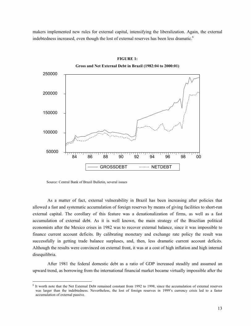
As Sampaio Jr (2000) has pointed out, after spending the 1980s trying to pay the external debt,in 1990 the net external debt in Brazil was US$ 123 billion, or 26% of GDP. In the end of 1999 thisamount reached US$ 237 billion, or more than 40% of the GDP. Furthermore, from 1990 to 1999 Brazilsent US$ 117 billion only as of interest payments. Figure 1 shows the pattern of the gross and netexternal debt in Brazil. While until 1992 its trajectory was stable, after 1992 there is a shift in its level,followed by a change in the slope of the curve after 1998. Indeed, the behavior of the indebtedness after1992 is closely related to the deepened in financial liberalization carried out by the structural reformsunder Fernando Collor’s Government (1990-1992). The mainly feature of those reforms is that theyincreased trade and financial liberalization, by means of decrease average imports tariffs, as well asbreaking the barriers to short-run and speculative capital flows. As a result, capital inflows allowed afast accumulation of foreign reserves, but at a cost of increasing the external passive. Therefore, the netexternal indebtedness remained almost constant until the Asian crisis in 1998, when Brazilian policy

5 Cardoso and Goldjfan (1998).

13

makers implemented new rules for external capital, intensifying the liberalization. Again, the externalindebtedness increased, even though the lost of external reserves has been less dramatic.6

FIGURE 1:

Gross and Net External Debt in Brazil (1982:04 to 2000:01)

50000

100000

150000

200000

250000

84 86 88 90 92 94 96 98 00

GROSSDEBT NETDEBT

Source: Central Bank of Brazil Bulletin, several issues

As a matter of fact, external vulnerability in Brazil has been increasing after policies thatallowed a fast and systematic accumulation of foreign reserves by means of giving facilities to short-runexternal capital. The corollary of this feature was a denationalization of firms, as well as a fastaccumulation of external debt. As it is well known, the main strategy of the Brazilian politicaleconomists after the Mexico crises in 1982 was to recover external balance, since it was impossible tofinance current account deficits. By calibrating monetary and exchange rate policy the result wassuccessfully in getting trade balance surpluses, and, then, less dramatic current account deficits.Although the results were convinced on external front, it was at a cost of high inflation and high internaldisequilibria.

After 1981 the federal domestic debt as a ratio of GDP increased steadily and assumed anupward trend, as borrowing from the international financial market became virtually impossible after the

6 It worth note that the Net External Debt remained constant from 1992 to 1998, since the accumulation of external reserves

was larger than the indebtedness. Nevertheless, the lost of foreign reserves in 1999’s currency crisis led to a fasteraccumulation of external passive.

14

Mexico’s crash in September 1982. The Central Government’s borrowing requirements increased from4.8% of GDP in 1983 to 12.5% in 1985, 26.6% in 1988, and 48.3% in 1989.7 These unique deficits werestrictly correlated with the indexation process in the Brazilian economy and the difficult in financing theinternal debt.8 Indeed, Brazil started an indexation process in its economy after 1965. If, on the one handthe indexation avoided lost to debtors and gains to creditors when inflation is moderated, as well asavoided a classical hyperinflation as occurred in German 1922 or even in Argentina in the end of 1980s,on the other hand turned out more difficult to control the high inflation process. Inflation rates soaredduring the 1980s with the annual rate ranging from 110% in 1981 to 2740% in 1990. There is fewdoubts that the source of the problems in 1980s are strong related to the external crisis and theimpossibility to finance the investment by means of external debt, such as occurred in 1970s.

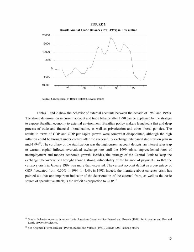
As already said above, the successfully external adjustment was carried out basically by thebehavior of exports that allowed getting vast trade surpluses. Exports increased sharply after anexchange rate maxi devaluation in 1983 and imports keep almost constant which allowed theaccumulation of trade surpluses until 1994 (Figure 2). This fact was the most important aspect thatallowed the success in external front after 1983. By looking at the behavior of the trade surpluses duringthe 1980s it is easy to see a close relationship between exchange-rate policies and trade balances. Afterthe financial liberalization in 1992 and the explicit aim to let Brazilian currency over valuate after 1994,trade surpluses brought down. There were intense debates in economic policy in Brazil during the 1980sabout these surpluses and it is possible to suppose that the import substitution policies in 1970s, after thefirst oil shock, permitted productivity gains for some industries, allowing them to compete in betterconditions in the international market. Those gains of productivity in export competing industriesallowed to get impressive export performance in earlier 1980s. On the other hand, short-run exchangerate policies, wage policies, as well as monetary and fiscal policies were organized jointly to get theexternal equilibrium. The huge decreased in internal absorption by means of recession were the otherside of these policies.9

7 See Luporini (2000) regarding this point.8 Oliveira (1988)9 See Castro and Souza (1985) for this debate.

15

FIGURE 2:

Brazil: Annual Trade Balance (1971-1999) in US$ million

10000

-5000

0

5000

10000

15000

20000

75 80 85 90 95

Source: Central Bank of Brazil Bulletin, several issues

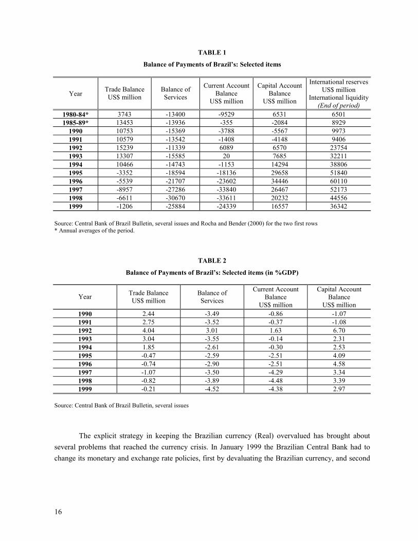
Tables 1 and 2 show the behavior of external accounts between the decade of 1980 and 1990s.The strong deterioration in current account and trade balance after 1990 can be explained by the strategyto expose Brazilian economy to external environment. Brazilian policy makers launched a fast and deepprocess of trade and financial liberalization, as well as privatization and other liberal policies. Theresults in terms of GDP and GDP per capita growth were somewhat disappointed, although the highinflation could be brought under control after the successfully exchange rate based stabilization plan inmid-199410. The corollary of the stabilization was the high current account deficits, an interest rates trapto warrant capital inflows, overvalued exchange rate until the 1999 crisis, unprecedented rates ofunemployment and modest economic growth. Besides, the strategy of the Central Bank to keep theexchange rate overvalued brought about a strong vulnerability of the balance of payments, so that thecurrency crisis in January 1999 was more than expected. The current account deficit as a percentage ofGDP fluctuated from -0.30% in 1994 to -4.4% in 1998. Indeed, the literature about currency crisis haspointed out that one important indicator of the deterioration of the external front, as well as the basicsource of speculative attack, is the deficit as proportion to GDP.11

10 Similar behavior occurred in others Latin American Countries. See Frenkel and Rozada (1999) for Argentina and Ros and

Lustig (1999) for Mexico.11 See Krugman (1999), Blecker (1999b), Rodrik and Velasco (1999), Curado (2001) among others.

16

TABLE 1

Balance of Payments of Brazil’s: Selected items

Year Trade BalanceUS$ million

Balance ofServices

Current AccountBalance

US$ million

Capital AccountBalance

US$ million

International reservesUS$ million

International liquidity(End of period)

1980-84* 3743 -13400 -9529 6531 65011985-89* 13453 -13936 -355 -2084 8929

1990 10753 -15369 -3788 -5567 99731991 10579 -13542 -1408 -4148 94061992 15239 -11339 6089 6570 237541993 13307 -15585 20 7685 322111994 10466 -14743 -1153 14294 388061995 -3352 -18594 -18136 29658 518401996 -5539 -21707 -23602 34446 601101997 -8957 -27286 -33840 26467 521731998 -6611 -30670 -33611 20232 445561999 -1206 -25884 -24339 16557 36342

Source: Central Bank of Brazil Bulletin, several issues and Rocha and Bender (2000) for the two first rows* Annual averages of the period.

TABLE 2

Balance of Payments of Brazil’s: Selected items (in %GDP)

Year Trade BalanceUS$ million

Balance ofServices

Current AccountBalance

US$ million

Capital AccountBalance

US$ million1990 2.44 -3.49 -0.86 -1.071991 2.75 -3.52 -0.37 -1.081992 4.04 3.01 1.63 6.701993 3.04 -3.55 -0.14 2.311994 1.85 -2.61 -0.30 2.531995 -0.47 -2.59 -2.51 4.091996 -0.74 -2.90 -2.51 4.581997 -1.07 -3.50 -4.29 3.341998 -0.82 -3.89 -4.48 3.391999 -0.21 -4.52 -4.38 2.97

Source: Central Bank of Brazil Bulletin, several issues

The explicit strategy in keeping the Brazilian currency (Real) overvalued has brought aboutseveral problems that reached the currency crisis. In January 1999 the Brazilian Central Bank had tochange its monetary and exchange rate policies, first by devaluating the Brazilian currency, and second

17

letting the currency float.12 Bonomo and Terra (1999) showed an historical relationship betweenpolitical cycles and exchange rate. It seems reasonable to suppose that the strategy in keeping the Realovervalued has had the explicit purpose to warrant the reelection of President Cardoso in November1998.13

There are several ways to verify the path of Current account and its possibility to lead to anunsustainable path in the long run. One important measure is the current account deficit as a proportionof GDP. Others are the exchange rate dynamic, the contagious effect and the excess of short-run capitalflows. All of these indicators seemed to hold after the exchange rate based stabilization program inBrazil. As Rocha and Bender (2000) revealed, it is possible to evaluate the effect over current accountimbalance by means of a simple indicator that can be compared with the actual data.

From the identity of the external debt, we get:

Dt+1 = (1+rt)Dt – TBt (1)

Where Dt is the external debt, r is the interest rate, and TB is the trade balance. Dividingeverything by Yt, the nominal GDP, we have:

ttt

t tbdY

rdt −

+=+1

1 (2)

Where the small letters represent a proportion to GDP. Taking g as the growth rate of GDP((Yt+1 – Yt) /Yt), from (2) we get:

(1+ g)dt+1 = (1+rt)dt – tbt (3)

If we assume a stable debt/GDP ratio (dt+1= dt), we have:

tbtR = (rt - g)dt (4)

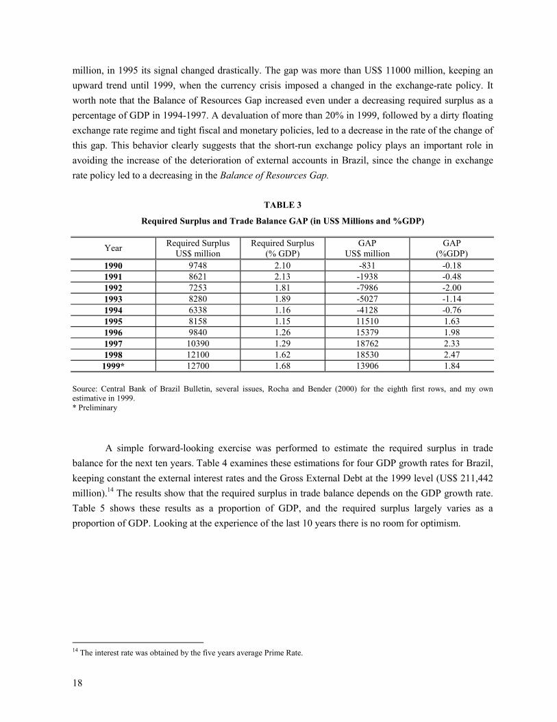
The trade surplus that solved equation (4) is the Required Trade Surplus, which represents thetrade surplus compatible with a stable debt/GDP ratio over time. The difference between the RequiredTrade Surplus and the observed trade balance is the Balance of Resources Gap. Table 3 shows thisbalance for the Brazilian economy from 1990 to 1999 and shows how this gap enlarged after 1994,when the trade balance changed its signal. Indeed, while in 1994 the gap was negative in US$ 4128

12 After an unsuccessful experience of controlling the exchange rate in January and February 1999, the Central Bank imposed a

dirty flexible exchange rate regime.13 Bonomo and Terra (1999) demonstrated the effects over government popularity in keeping the currency overvalued, since

real wages, in an open economy, tend to be higher than real wages under the equilibrium exchange rate.

18

million, in 1995 its signal changed drastically. The gap was more than US$ 11000 million, keeping anupward trend until 1999, when the currency crisis imposed a changed in the exchange-rate policy. Itworth note that the Balance of Resources Gap increased even under a decreasing required surplus as apercentage of GDP in 1994-1997. A devaluation of more than 20% in 1999, followed by a dirty floatingexchange rate regime and tight fiscal and monetary policies, led to a decrease in the rate of the change ofthis gap. This behavior clearly suggests that the short-run exchange policy plays an important role inavoiding the increase of the deterioration of external accounts in Brazil, since the change in exchangerate policy led to a decreasing in the Balance of Resources Gap.

TABLE 3

Required Surplus and Trade Balance GAP (in US$ Millions and %GDP)

Year Required SurplusUS$ million

Required Surplus(% GDP)

GAPUS$ million

GAP(%GDP)

1990 9748 2.10 -831 -0.181991 8621 2.13 -1938 -0.481992 7253 1.81 -7986 -2.001993 8280 1.89 -5027 -1.141994 6338 1.16 -4128 -0.761995 8158 1.15 11510 1.631996 9840 1.26 15379 1.981997 10390 1.29 18762 2.331998 12100 1.62 18530 2.471999* 12700 1.68 13906 1.84

Source: Central Bank of Brazil Bulletin, several issues, Rocha and Bender (2000) for the eighth first rows, and my ownestimative in 1999.* Preliminary

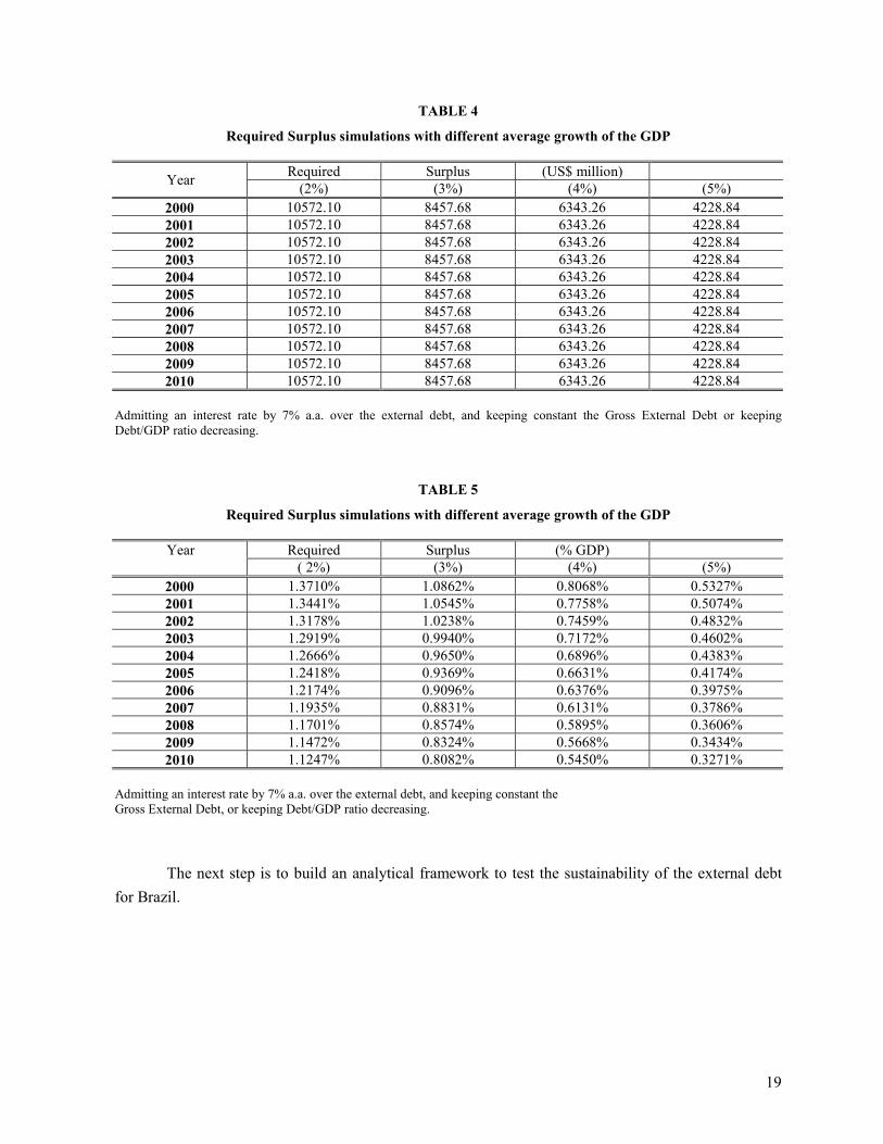
A simple forward-looking exercise was performed to estimate the required surplus in tradebalance for the next ten years. Table 4 examines these estimations for four GDP growth rates for Brazil,keeping constant the external interest rates and the Gross External Debt at the 1999 level (US$ 211,442million).14 The results show that the required surplus in trade balance depends on the GDP growth rate.Table 5 shows these results as a proportion of GDP, and the required surplus largely varies as aproportion of GDP. Looking at the experience of the last 10 years there is no room for optimism.

14 The interest rate was obtained by the five years average Prime Rate.

19

TABLE 4

Required Surplus simulations with different average growth of the GDP

Required Surplus (US$ million)Year (2%) (3%) (4%) (5%)2000 10572.10 8457.68 6343.26 4228.842001 10572.10 8457.68 6343.26 4228.842002 10572.10 8457.68 6343.26 4228.842003 10572.10 8457.68 6343.26 4228.842004 10572.10 8457.68 6343.26 4228.842005 10572.10 8457.68 6343.26 4228.842006 10572.10 8457.68 6343.26 4228.842007 10572.10 8457.68 6343.26 4228.842008 10572.10 8457.68 6343.26 4228.842009 10572.10 8457.68 6343.26 4228.842010 10572.10 8457.68 6343.26 4228.84

Admitting an interest rate by 7% a.a. over the external debt, and keeping constant the Gross External Debt or keepingDebt/GDP ratio decreasing.

TABLE 5

Required Surplus simulations with different average growth of the GDP

Required Surplus (% GDP)Year( 2%) (3%) (4%) (5%)

2000 1.3710% 1.0862% 0.8068% 0.5327%2001 1.3441% 1.0545% 0.7758% 0.5074%2002 1.3178% 1.0238% 0.7459% 0.4832%2003 1.2919% 0.9940% 0.7172% 0.4602%2004 1.2666% 0.9650% 0.6896% 0.4383%2005 1.2418% 0.9369% 0.6631% 0.4174%2006 1.2174% 0.9096% 0.6376% 0.3975%2007 1.1935% 0.8831% 0.6131% 0.3786%2008 1.1701% 0.8574% 0.5895% 0.3606%2009 1.1472% 0.8324% 0.5668% 0.3434%2010 1.1247% 0.8082% 0.5450% 0.3271%

Admitting an interest rate by 7% a.a. over the external debt, and keeping constant theGross External Debt, or keeping Debt/GDP ratio decreasing.

The next step is to build an analytical framework to test the sustainability of the external debtfor Brazil.

20

3. EMPIRICAL LITERATURE ABOUT DEBT SUSTAINABILITY

Studies involving sustainability of public debt became an important issue in economic policymainly after the 1980s, stimulated by the increasing US fiscal deficits as well as the debt crisis thataffect Latin American countries. Recently this subject has come up again for Europe after the unificationand for heavily indebted developing countries. For the latter, not only the external debt, but also theinternal debt have stimulated applied macroeconomic studies.

The first concept of sustainable fiscal policy is due to the work of Harrod and Domar. Minsky(1986) first pointed out the importance of taking care the financial sustainability of fiscal policy in orderto avoid reaching a no sustainable structure coming from a Hedge position to Ponzi finance. Eisner andPieper (1984) also pointed out the importance in analyzing the question of the Federal debt and its longrun sustainability for the United States.

From the work of Hamilton and Flavin (1986) several tests of sustainability were carried out byusing similar methodology of them, or by including other tests. Hamilton and Flavin (1986) employstests of stationarity over the discounted debt factor using Dickey-Fuller tests for unit roots as well asrestricted and generalized Flood-Garber tests for stationarity15. The basic idea is that any debt will besustainable in the long run if its discounted factor is stationary. Applying these methodologies to the USdata from 1960 to 1981, these authors have found that the US Budget balance presented a long runsustainable path, despite its systematic budget deficits.

Wilcox (1989) extended the work of Hamilton and Flavin (1986) in order to allow for stochasticreal interest rates and for nonstationarity in the no interest surplus. His work has power againststochastic violations of the borrowing constraint, whereas at least two of the tests of Hamilton andFlavin assumed that any violation of the borrowing constraint would be stochastic.

Greiner and Semmler (1999) tested the sustainability of the public debt for Germany in order tofind if the unification has caused any violation of the long run path of the public debt. Indeed, theunification has risen the debt to GDP ratio from 44% to 58% in 1995 and this behavior could bring someproblems to the European Union (EU), since one important aspect of the EU was exactly warrant abalance fiscal policy. Their conclusions suggest that the public debt in Germany does not meet therequirements to warrant a sustainable fiscal policy in the long run.

These authors have taken annual data from 1955 to 1994 and used both Flood-Garber test, andADF tests for unit root in the series of discounted net debt, showing that internal debt series werenonstationary. The restricted Flood-Garber tests confirm that outcome. After also testing thesustainability before and after the unification of the Germany the results suggest an unsustainable pathstarted in 1989.

Sawada (1994) explored the case of external debt sustainability of heavily indebted countriesusing a different approach to that one used by Hamilton and Flavin (1986), and Greiner and Semmler

15 See Hamilton and Flavin (1986) to an explanation of the methodology employed.

21

(1999). While the latter have employed the discounted debt to test, the former tests use current accountbalance. Indeed, the methodology employed by Sawada (1994) does not need to make a discounted debt.If the series employed have a unit root, the solvency condition is met whether the series are cointegrated.His results demonstrated that only the Asian countries (Korea, Indonesia, Malaysia and Thailand) havebeen solvent for the period 1955 to 1990. All of Latin American countries did not meet the solvencycondition for the same period. Ponta (1996) using quarterly data from 1970 to 1992 has also found theunsustainability of the external debt in Brazil. Rocha and Bender (2000) made similar exercise testingBrazilian current account sustainability using annual data from 1947 to 1997 and also concluded that thecurrent account deficits in Brazil do not meet the requirements to warrant a sustainable path in the longrun. Both authors used cointegration. They have also performed unit root tests in the presence ofstructural break, although the equations they used were slightly different from each other. Ponta (1996)tested cointegration between net external debt and trade balance whereas Rocha and Bender (2000) usedexports and imports of goods and services including net interest.

By working in a different way, Carneiro (1997) did not find a sustainable path. Luporini (2000)has performed test of sustainability of the fiscal policy using the discounted debt and found that thefiscal policy in Brazil was sustainable before 1980 and unsustainable after that period.

4. THE ANALYTICAL FRAMEWORK OF CRITICAL DEBT AND DEBT DYNAMICS

The intertemporal budget constraint has already been largely discussed in theoretical andempirical literature (Minsky, 1986, Eisner and Pieper, 1984, Hamilton and Flavin, 1986, Trehan andWalsh, 1991, Wilcox, 1989, Hakkio and Rush, 1991, Greiner and Semmler, 1999, and Greiner andSemmler, 2000). Similar work analyzing the Brazilian case can be seen in Simonsen (1985), andLuporini (2000). For the sustainability in an open economy see Sawada (1994), Carneiro (1997), Ponta(1996), and Rocha and Bender (2000).

This paper presents three analytical approaches to get a testable equation in order to confirm theresults. The first one departs from Sawada (1994), Wilcox, (1989), and Hamilton and Flavin, (1986).The second one departs from the net external debt and it shows only simple differential equations to geta basic framework to test sustainability. The third one also departs from Hamilton and Flavin (1986),and it gets a testable equation by using the discounted debt (Greiner and Semmler, 1999).

Model 1

The first useful model to get a feasible empirical estimation equation comes from the work ofSawada (1994), Wilcox (1989) and Hamilton and Flavin (1986). It departs from the basic accountidentity for an open economy during a period t:

Yt + (Dt – Dt-1) + TRt = At + rDt-1 + ∆REt (5)

22

Where Y is the GDP, D is the net external debt (gross external debt minus international reserves), TR isthe net transfer receipts, A is the domestic absorption, r is the nominal interest rate and ∆REt is thechange in foreign reserves.16 As usual in accounting identities, the left side hand of equation (5)represents the economy’s aggregate income whereas the right hand side is the total expenditure.From the income identity in an open economy we get:

Xt - Mt = Yt - At (6)

Where Xt are the nominal exports of goods and services and Mt are the nominal imports of goods andservices at time t. From (5) we can get the trade balance of this economy:

TBt = Xt - Mt = rDt-1 - (Dt – Dt-1) - TRt + ∆REt (7)

The evolution of the external debt is:

(Dt – Dt-1) = rDt-1 - [TBt + TRt -∆REt] (8)

Letting St = [TBt + TRt -∆REt], we can translate this identity as the net external surplus that can be usedto meet the external debt repayments. Since (8) is a differential equation we can solve it recursively toget the forward-looking solution in terms of the net external debt (Dt):

∑∏∏

∞

+=−

=

−

=∞→ ++ +

++

=1

11)1()1(

limtj

tj

i

j

tN

j

N

Nt

itjt rS

rDD (9)

Taking expectation operator in both right hand equations we can determine that the solvency conditionis satisfied when:

∑∏

∞

+=−

=++

=1

1)1(tj

tj

i

jt

itrSED

Or, if

0)1(

1

lim =+

=∏ −

=∞→ +

tN

j

N

Nt

jtrDED (10)

This is the no Ponzi condition, in which external debt repayments are sustainable, or that the amount acountry borrows (lends) in international market equals the present value of future trade surpluses. If

16 Sawada (1994) admits that there is an interest rate over reserves, so ∆REt is [REt – (1+i) REt-1], where i is the interest rate on

this reserves. The results do not present differences if we skip the interest rates over external reserves.

23

equation (10) is greater than zero, the country is paying the old maturity debt by issuing new debt, whichreveals that external debt is not sustainable in the long run.17

Assuming that the interest rate is stationary, with a unconditional mean equal to r, we cansubtract rDt-1 from equation (8) to get:

Et + (1+ r)Dt-1 = EXt + Dt (11)

Where EXt = Xt + TRt + REt-1, IMt = Mt + REt, and Et = IMt + (rt – r) Dt-1. Taking the first difference,we have:

∆Dt = ∆Et + (1+ r) ∆Dt-1 - ∆EXt (12)

Solving this equation forward to get:

∑∞

+=−

+

∞→ +∆−∆+

+∆+=

1

1

)1()1(limtj

tj

jj

i

t

itt

rEEX

rDEXMM (13)

Where MMt is defined as (Mt+rDt-1).From the assumption that EXt and MMt follow a random walk with drift, or in other words, both seriesare non-stationary and have an intercept, we can obtain an empirical testable equation. This equationfollows:

EXt = a + bMMt + ut (14)

If MM and EX are nonstationary process, then the null hypothesis to be tested is that MM andEX are cointegrated, and that b=1.18 Therefore, MM and EX have to be cointegrated in order to reach thenecessary condition for the country to be solvent.

Basically, two values are said to be cointegrated when each variable taken separately isnonstationary, I(1) process, while a linear combination of them is stationary. There may be a number, b,such that EXt - a - bMMt = ut is stationary. After checking whether EXt and MMt each have a unit root, itwill be employed the Johansen testing procedure to estimate the cointegration regression (14).

17 This is the case in which a country is bubble financing its external debt. (Sawada, 1994).18 See for this condition Hakkio and Rush (1991). See, also, Rocha and Bender (2000) regarding the need in supposing that b

should be equal to 1 in order to meet the requirements for sustainability when both variables are cointegrated. AlthoughHakkio and Rush (1991) point out that b could be less than one, this requirement is not sufficient to meet the sustainabilitycondition in case of the external debt is positive.

24

Model 2

An alternative methodology to treat debt sustainability departs from this basic equation

dDY

= (15)

Where D is the stock of external indebtedness of the country and Y is the GNP. Taking time derivativeswe can get:

YY

DD

dd

•••

−= (16)

We know thatCA = -B +rDWhere CA is the Current Account deficit, B is Current Account surplus excluding net interest paymentsand r is the interest rates paid on external debt. From that we have:

D B rD•

= − +

DD

B rDD

•

=− +

dd

BD

r g•

= − + −

Where g is the growth rate of GNP.

dd

r gBD

•

= − −( ) (17)

Of course if r = g, it follows that

dd

BD

•

=−

(18)

If r = g external indebtedness will be growing relative to GNP when the non-interest current account isin deficit. On the other hand, if r exceed g and, for an external debtor, external debt will be risingrelative to GNP when the non-interest current account is not in sufficiently large surplus relative to the

25

stock of external debt. Therefore, the sustainable path is what the ratio of external debt to GNP is

0=•

dd .

If 0=•d , 0=

•dd . Therefore

)( grDB −−=−

Once YDd = , we can reach that

dgrDB

YD )( −=⋅

dB Yr g

* ( )=−

(19)

If r > g, it is not possible to find the sustainable deficit in current account compatible with the stock ofthe external debt, foreign interest rates, and growth of GNP. Therefore, it is necessary a trade surplus ford* > 0.

One way to find the sustainable path of the external debt in Brazil is by means of simulationswith Brazilian data using equation (19) in the fashion of Carneiro (1997). However, unit root andcointegration tests have provided useful tools in gaining insight into the long-run implications of agovernment’s fiscal and the financial policy in a given time-horizon. This method, therefore, will beemployed to test the sustainability of the external debt.

Model 3: Discounted debt

From Model 1 we can redefine the discounted factor that appears in the denominator of equation (9) and(10) in order to get a testable equation using the discounted debt.From equation (9) we get:

Dt = (1+rt)Dt-1 - St (20)

Assuming that ∏ +−

=

−= 1

0

1)1(t

j jt rQ ; Q0 = 1, we can multiplying (20) by the discounted factor:

Dt Qt= Qt-1Dt-1 - QtSt

Using small letters:

dt= dt-1 - st (21)

26

Recursive substitution leads to:

∑=

++ +=N

jNtjtt dsd

1

Assuming dn going to zero, we get:

∑=

+=N

jjtt sEd

1(21’)

Which determines the discounted equation to be tested.

5. DATA SOURCE AND EMPIRICAL RESULTS

As stated in the last item, I will test the sustainability of the external debt and current account inBrazil taking into consideration three models. The aim is to get as much as possible accurate result.

The data set was obtained from the Brazilian Central Bank Monthly Bulletin and consists ofquarterly observations for Gross External Debt, Foreign Reserves, Current account, Exports of goodsand services, Imports of goods and services, External Interest Rates (Prime Rate), and Trade Balance.All data, except Gross External Debt and External Interest rates are quarterly basis from 1969 to 2000.Regarding to gross external debt, the model that use this variable will be performed from 1982 to 2000,while for that one which work with Prime Rate, I will perform the tests from the first quarter of 1970.All tests will be performed with nominal and non-seasonally adjusted data.19

Model 1

As it has already presented in the last section, the following equation will be tested:

EXt = a + bMMt + ut (14)

The necessary and sufficient condition to the Current Account be sustainable is that the series inequation (14) are cointegrated and b = 1. Therefore, as usual, the first step is to perform tests forstationarity of the variables. Dickey and Fuller (1979) suggested that the following equation is estimatedby OLS to test for the presence of a unit root in any xt series:

tit

p

iitt xxx εββ +∆+=∆ −

=− ∑

110

19 In fact, the Imports plus interest rates variable presents seasonal pattern after 1990. The tests applied with the series without

seasonality do not presented substantial change in the results.

27

The Augmented Dickey-Fuller (ADF) test for unit root consists of testing whether thecoefficient on xt-1 is zero. The inclusion of higher-order autoregressive terms in the regression controlsfor serial correlation of the disturbance term. Under the null H 0 1 0:β = , the series xt contains a unit

root and therefore is nonstationary. Under the alternative H1 1 0:β < , the series is stationary.

The Akaike criterion places a penalty on extra coefficients, so one has to be careful when selectthe lag length of the variables. The Phillips-Perron test (PP) was also performed. This unit root test,developed by Phillips and Perron (1988), corrects the statistics for serial correlated and possiblyheteroskedastic error terms.

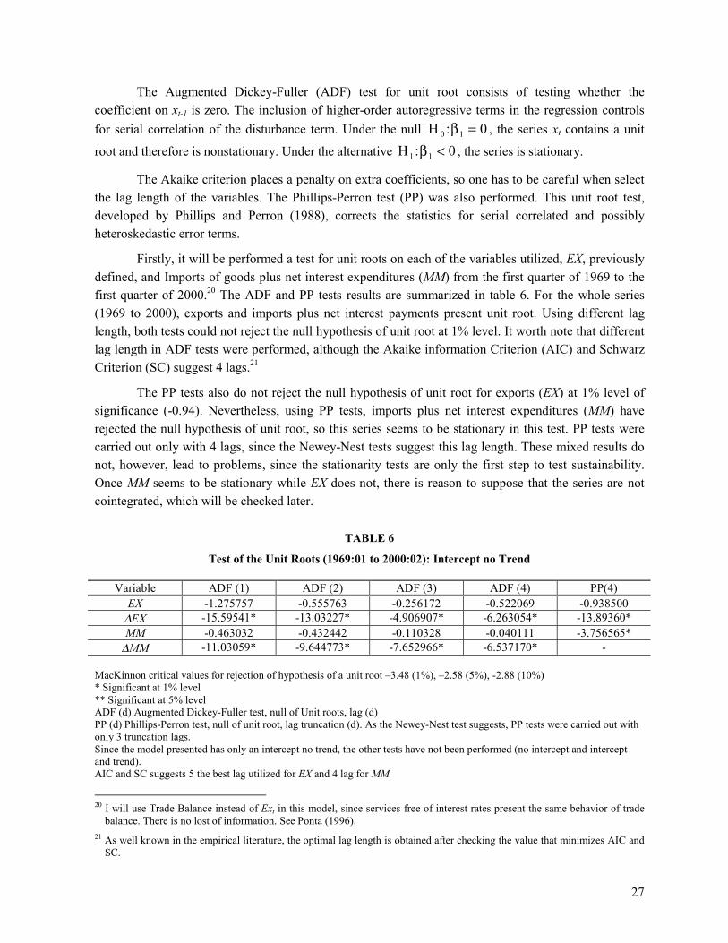
Firstly, it will be performed a test for unit roots on each of the variables utilized, EX, previouslydefined, and Imports of goods plus net interest expenditures (MM) from the first quarter of 1969 to thefirst quarter of 2000.20 The ADF and PP tests results are summarized in table 6. For the whole series(1969 to 2000), exports and imports plus net interest payments present unit root. Using different laglength, both tests could not reject the null hypothesis of unit root at 1% level. It worth note that differentlag length in ADF tests were performed, although the Akaike information Criterion (AIC) and SchwarzCriterion (SC) suggest 4 lags.21

The PP tests also do not reject the null hypothesis of unit root for exports (EX) at 1% level ofsignificance (-0.94). Nevertheless, using PP tests, imports plus net interest expenditures (MM) haverejected the null hypothesis of unit root, so this series seems to be stationary in this test. PP tests werecarried out only with 4 lags, since the Newey-Nest tests suggest this lag length. These mixed results donot, however, lead to problems, since the stationarity tests are only the first step to test sustainability.Once MM seems to be stationary while EX does not, there is reason to suppose that the series are notcointegrated, which will be checked later.

TABLE 6

Test of the Unit Roots (1969:01 to 2000:02): Intercept no Trend

Variable ADF (1) ADF (2) ADF (3) ADF (4) PP(4)EX -1.275757 -0.555763 -0.256172 -0.522069 -0.938500

∆EX -15.59541* -13.03227* -4.906907* -6.263054* -13.89360*MM -0.463032 -0.432442 -0.110328 -0.040111 -3.756565*

∆MM -11.03059* -9.644773* -7.652966* -6.537170* -

MacKinnon critical values for rejection of hypothesis of a unit root –3.48 (1%), –2.58 (5%), -2.88 (10%)* Significant at 1% level** Significant at 5% levelADF (d) Augmented Dickey-Fuller test, null of Unit roots, lag (d)PP (d) Phillips-Perron test, null of unit root, lag truncation (d). As the Newey-Nest test suggests, PP tests were carried out withonly 3 truncation lags.Since the model presented has only an intercept no trend, the other tests have not been performed (no intercept and interceptand trend).AIC and SC suggests 5 the best lag utilized for EX and 4 lag for MM

20 I will use Trade Balance instead of Ext in this model, since services free of interest rates present the same behavior of trade

balance. There is no lost of information. See Ponta (1996).21 As well known in the empirical literature, the optimal lag length is obtained after checking the value that minimizes AIC and

SC.

28

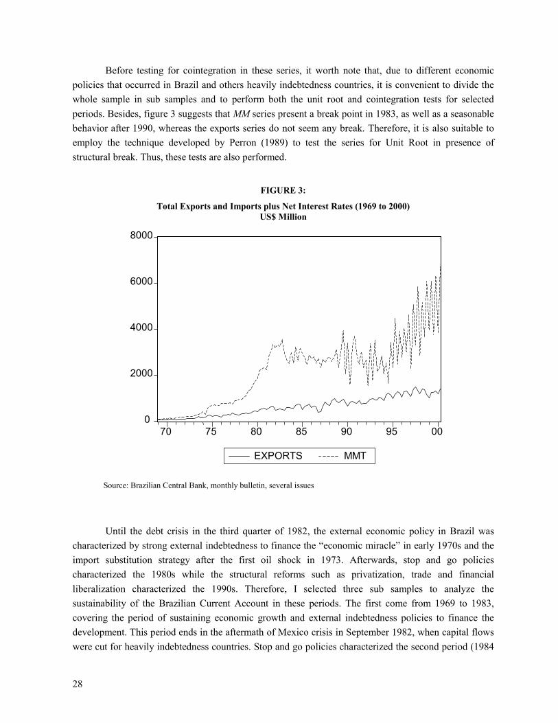
Before testing for cointegration in these series, it worth note that, due to different economicpolicies that occurred in Brazil and others heavily indebtedness countries, it is convenient to divide thewhole sample in sub samples and to perform both the unit root and cointegration tests for selectedperiods. Besides, figure 3 suggests that MM series present a break point in 1983, as well as a seasonablebehavior after 1990, whereas the exports series do not seem any break. Therefore, it is also suitable toemploy the technique developed by Perron (1989) to test the series for Unit Root in presence ofstructural break. Thus, these tests are also performed.

FIGURE 3:

Total Exports and Imports plus Net Interest Rates (1969 to 2000)US$ Million

0

2000

4000

6000

8000

70 75 80 85 90 95 00

EXPORTS MMT

Source: Brazilian Central Bank, monthly bulletin, several issues

Until the debt crisis in the third quarter of 1982, the external economic policy in Brazil wascharacterized by strong external indebtedness to finance the “economic miracle” in early 1970s and theimport substitution strategy after the first oil shock in 1973. Afterwards, stop and go policiescharacterized the 1980s while the structural reforms such as privatization, trade and financialliberalization characterized the 1990s. Therefore, I selected three sub samples to analyze thesustainability of the Brazilian Current Account in these periods. The first come from 1969 to 1983,covering the period of sustaining economic growth and external indebtedness policies to finance thedevelopment. This period ends in the aftermath of Mexico crisis in September 1982, when capital flowswere cut for heavily indebtedness countries. Stop and go policies characterized the second period (1984

29

to 2000). Finally, the last sub sample covers the period after the structural reforms in Brazil (1990 to2000), in which privatizations, trade and financial liberalization took place. This stage also presented therecovery of capital inflows to Latin America countries after a decade without them voluntarily.

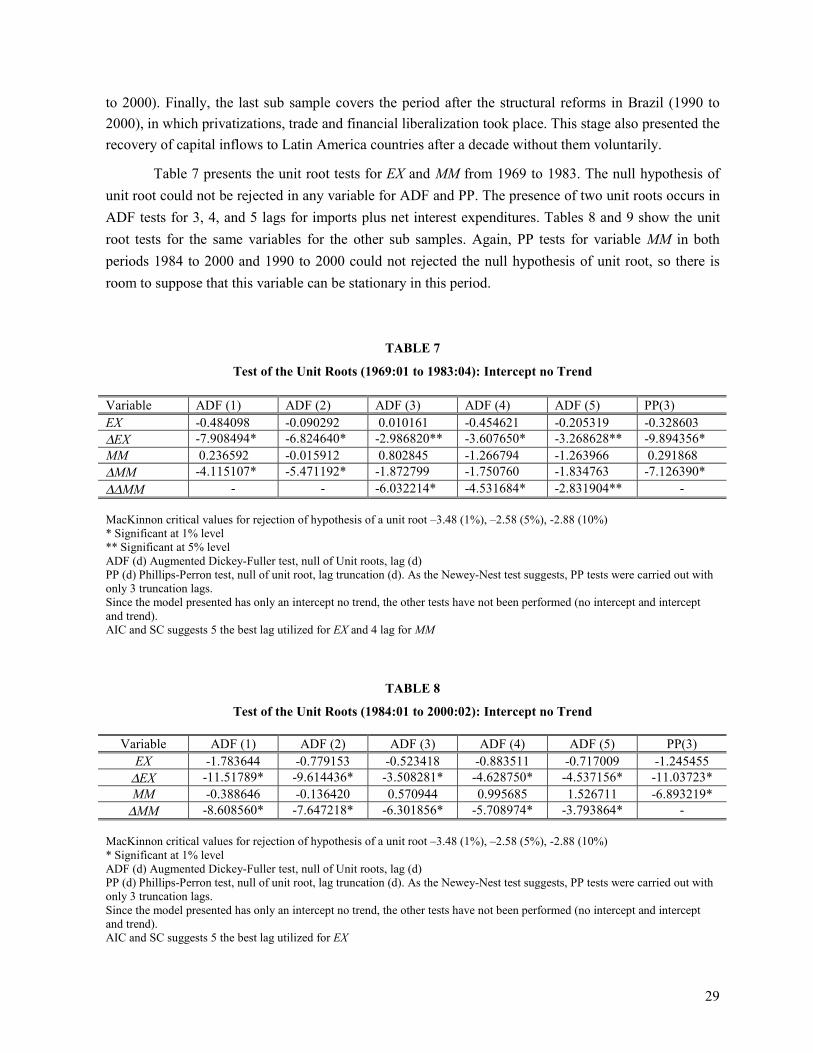
Table 7 presents the unit root tests for EX and MM from 1969 to 1983. The null hypothesis ofunit root could not be rejected in any variable for ADF and PP. The presence of two unit roots occurs inADF tests for 3, 4, and 5 lags for imports plus net interest expenditures. Tables 8 and 9 show the unitroot tests for the same variables for the other sub samples. Again, PP tests for variable MM in bothperiods 1984 to 2000 and 1990 to 2000 could not rejected the null hypothesis of unit root, so there isroom to suppose that this variable can be stationary in this period.

TABLE 7

Test of the Unit Roots (1969:01 to 1983:04): Intercept no Trend

Variable ADF (1) ADF (2) ADF (3) ADF (4) ADF (5) PP(3)EX -0.484098 -0.090292 0.010161 -0.454621 -0.205319 -0.328603∆EX -7.908494* -6.824640* -2.986820** -3.607650* -3.268628** -9.894356*MM 0.236592 -0.015912 0.802845 -1.266794 -1.263966 0.291868∆MM -4.115107* -5.471192* -1.872799 -1.750760 -1.834763 -7.126390*∆∆MM - - -6.032214* -4.531684* -2.831904** -

MacKinnon critical values for rejection of hypothesis of a unit root –3.48 (1%), –2.58 (5%), -2.88 (10%)* Significant at 1% level** Significant at 5% levelADF (d) Augmented Dickey-Fuller test, null of Unit roots, lag (d)PP (d) Phillips-Perron test, null of unit root, lag truncation (d). As the Newey-Nest test suggests, PP tests were carried out withonly 3 truncation lags.Since the model presented has only an intercept no trend, the other tests have not been performed (no intercept and interceptand trend).AIC and SC suggests 5 the best lag utilized for EX and 4 lag for MM

TABLE 8

Test of the Unit Roots (1984:01 to 2000:02): Intercept no Trend

Variable ADF (1) ADF (2) ADF (3) ADF (4) ADF (5) PP(3)EX -1.783644 -0.779153 -0.523418 -0.883511 -0.717009 -1.245455

∆EX -11.51789* -9.614436* -3.508281* -4.628750* -4.537156* -11.03723*MM -0.388646 -0.136420 0.570944 0.995685 1.526711 -6.893219*

∆MM -8.608560* -7.647218* -6.301856* -5.708974* -3.793864* -

MacKinnon critical values for rejection of hypothesis of a unit root –3.48 (1%), –2.58 (5%), -2.88 (10%)* Significant at 1% levelADF (d) Augmented Dickey-Fuller test, null of Unit roots, lag (d)PP (d) Phillips-Perron test, null of unit root, lag truncation (d). As the Newey-Nest test suggests, PP tests were carried out withonly 3 truncation lags.Since the model presented has only an intercept no trend, the other tests have not been performed (no intercept and interceptand trend).AIC and SC suggests 5 the best lag utilized for EX

30

TABLE 9

Test of the Unit Roots (1990:01 to 2000:02): Intercept no Trend

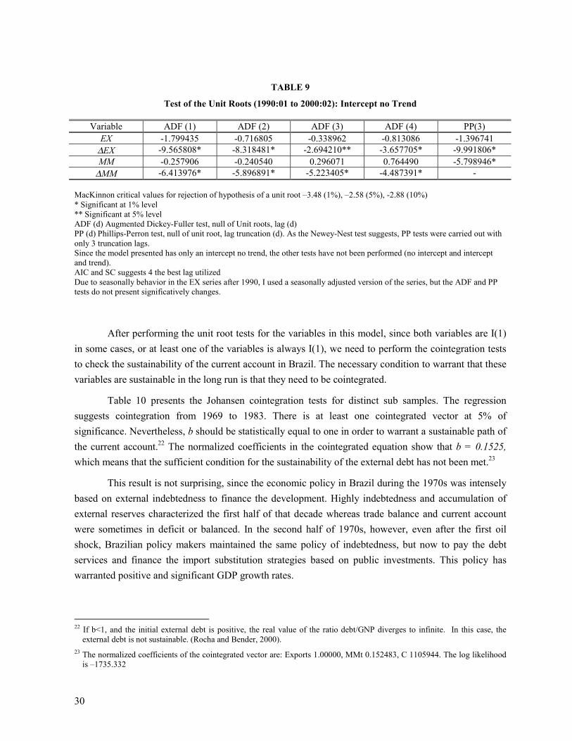
Variable ADF (1) ADF (2) ADF (3) ADF (4) PP(3)EX -1.799435 -0.716805 -0.338962 -0.813086 -1.396741

∆EX -9.565808* -8.318481* -2.694210** -3.657705* -9.991806*MM -0.257906 -0.240540 0.296071 0.764490 -5.798946*

∆MM -6.413976* -5.896891* -5.223405* -4.487391* -

MacKinnon critical values for rejection of hypothesis of a unit root –3.48 (1%), –2.58 (5%), -2.88 (10%)* Significant at 1% level** Significant at 5% levelADF (d) Augmented Dickey-Fuller test, null of Unit roots, lag (d)PP (d) Phillips-Perron test, null of unit root, lag truncation (d). As the Newey-Nest test suggests, PP tests were carried out withonly 3 truncation lags.Since the model presented has only an intercept no trend, the other tests have not been performed (no intercept and interceptand trend).AIC and SC suggests 4 the best lag utilizedDue to seasonally behavior in the EX series after 1990, I used a seasonally adjusted version of the series, but the ADF and PPtests do not present significatively changes.

After performing the unit root tests for the variables in this model, since both variables are I(1)in some cases, or at least one of the variables is always I(1), we need to perform the cointegration teststo check the sustainability of the current account in Brazil. The necessary condition to warrant that thesevariables are sustainable in the long run is that they need to be cointegrated.

Table 10 presents the Johansen cointegration tests for distinct sub samples. The regressionsuggests cointegration from 1969 to 1983. There is at least one cointegrated vector at 5% ofsignificance. Nevertheless, b should be statistically equal to one in order to warrant a sustainable path ofthe current account.22 The normalized coefficients in the cointegrated equation show that b = 0.1525,which means that the sufficient condition for the sustainability of the external debt has not been met.23

This result is not surprising, since the economic policy in Brazil during the 1970s was intenselybased on external indebtedness to finance the development. Highly indebtedness and accumulation ofexternal reserves characterized the first half of that decade whereas trade balance and current accountwere sometimes in deficit or balanced. In the second half of 1970s, however, even after the first oilshock, Brazilian policy makers maintained the same policy of indebtedness, but now to pay the debtservices and finance the import substitution strategies based on public investments. This policy haswarranted positive and significant GDP growth rates.

22 If b<1, and the initial external debt is positive, the real value of the ratio debt/GNP diverges to infinite. In this case, the

external debt is not sustainable. (Rocha and Bender, 2000).23 The normalized coefficients of the cointegrated vector are: Exports 1.00000, MMt 0.152483, C 1105944. The log likelihood

is –1735.332

31

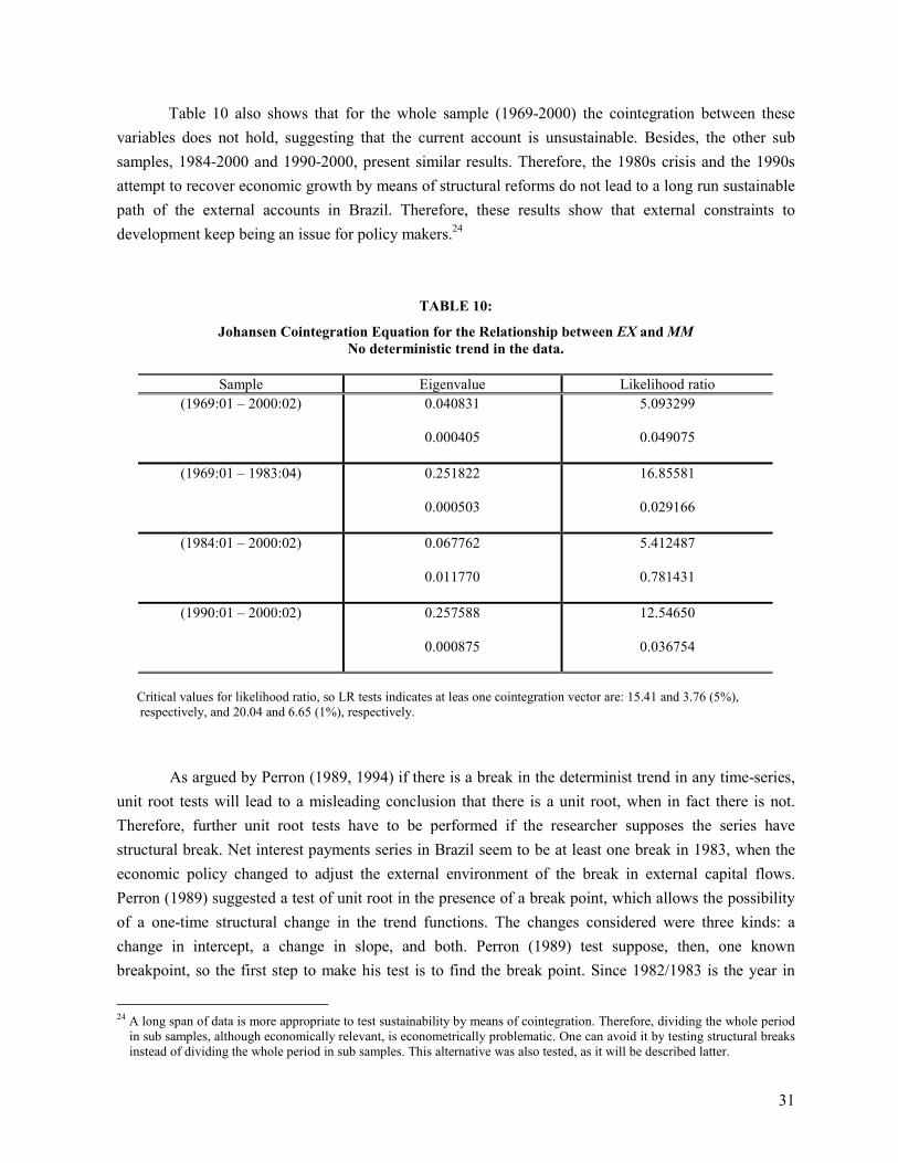
Table 10 also shows that for the whole sample (1969-2000) the cointegration between thesevariables does not hold, suggesting that the current account is unsustainable. Besides, the other subsamples, 1984-2000 and 1990-2000, present similar results. Therefore, the 1980s crisis and the 1990sattempt to recover economic growth by means of structural reforms do not lead to a long run sustainablepath of the external accounts in Brazil. Therefore, these results show that external constraints todevelopment keep being an issue for policy makers.24

TABLE 10:

Johansen Cointegration Equation for the Relationship between EX and MMNo deterministic trend in the data.

Sample Eigenvalue Likelihood ratio(1969:01 – 2000:02) 0.040831

0.000405

5.093299

0.049075

(1969:01 – 1983:04) 0.251822

0.000503

16.85581

0.029166

(1984:01 – 2000:02) 0.067762

0.011770

5.412487

0.781431

(1990:01 – 2000:02) 0.257588

0.000875

12.54650

0.036754

Critical values for likelihood ratio, so LR tests indicates at leas one cointegration vector are: 15.41 and 3.76 (5%), respectively, and 20.04 and 6.65 (1%), respectively.

As argued by Perron (1989, 1994) if there is a break in the determinist trend in any time-series,unit root tests will lead to a misleading conclusion that there is a unit root, when in fact there is not.Therefore, further unit root tests have to be performed if the researcher supposes the series havestructural break. Net interest payments series in Brazil seem to be at least one break in 1983, when theeconomic policy changed to adjust the external environment of the break in external capital flows.Perron (1989) suggested a test of unit root in the presence of a break point, which allows the possibilityof a one-time structural change in the trend functions. The changes considered were three kinds: achange in intercept, a change in slope, and both. Perron (1989) test suppose, then, one knownbreakpoint, so the first step to make his test is to find the break point. Since 1982/1983 is the year in

24 A long span of data is more appropriate to test sustainability by means of cointegration. Therefore, dividing the whole period

in sub samples, although economically relevant, is econometrically problematic. One can avoid it by testing structural breaksinstead of dividing the whole period in sub samples. This alternative was also tested, as it will be described latter.

32

which the Mexico crisis imposes several constraints to Latin American countries, as well as whenBrazilian policy makers elected the external equilibrium as the political economy’s target, it seemsreasonable to test whether there was a break point in both series in this period.

The usual test to find a known break point is the Chow test, in which the break is tested againstthe alternative hypothesis of no break point. Chow breakpoint test (not reported) suggests 1983:02 as thebreak point for MM series, whereas for EX series there is no break point.25 Therefore, it is important totest for unit root the series MM under the presence of a known break point. Furthermore, it was carriedout cointegration tests in the presence of structural break.26

The additive outlier model can be employed in the series after knowing the break point. Thesemodels are specified for each of the three specifications of the types of change occurring at the breakdate (Tb) as follows:

Equation 1: Yt = µ1 + βt + (µ2 - µ1)DUt + νt

Equation 2: Yt = µ1 + β2t + (µ2 - µ1)DUt + (β2 - β1)DTt + νt

Equation 3: Yt = µ + β1t + (β2 - β1)DTt + νt

Where DUt = 1, DTt = t – Tb if t > Tb and 0 otherwise. The noise component νt is in the form A(L) andB(L) pth and qth order polynomials, respectively of the lag operator L. The innovation series {νt} is takento be of the ARMA(p,q) type with the orders p and q possibly unknown. This postulate allows for a series{yt} to represent quite general processes. The null hypothesis specifies that a unit root of theautoregressive polynomial is one, i.e. that we can write A(L) = (1-L)A*(L) where the roots of A*(L) areoutside the unit circle.

Equation 1, then, allows for a change in intercept, whereas equation 2 describes a change in theslope, and equation 3 both changes. These models were then tested to additive outlier model. The test isprocedure in two steps. In the first step, the trend function of the series is estimated and removed fromthe original series via regressions presented in equations 1, 2, and 3 above. For equation 1 and 2, theprocedure is based on the value of the t-statistic for testing that the sum of the autogressive coefficientsis equal to 1 (α = 1) in the following autoregression applied to the estimated noise component νt:27

∑ ∑= =

−− +∆++−=k

j

k

ittijtbjt atDdt

0 1

1)(1 ενανν (22)

For equation 3 the second step regression is in the form:

25 Chow breakpoint test was carried out by E-views 3.0.26 See Mandala and Kim (1998), especially part IV, for a discussion about tests for break in time-series. They also point out the

limitations of Perron (1989) model, as well as models, which work with exogenous break point.27 Perron (1994).

33

t

k

iititt av εναν +∆+= ∑

=−−

11 (23)

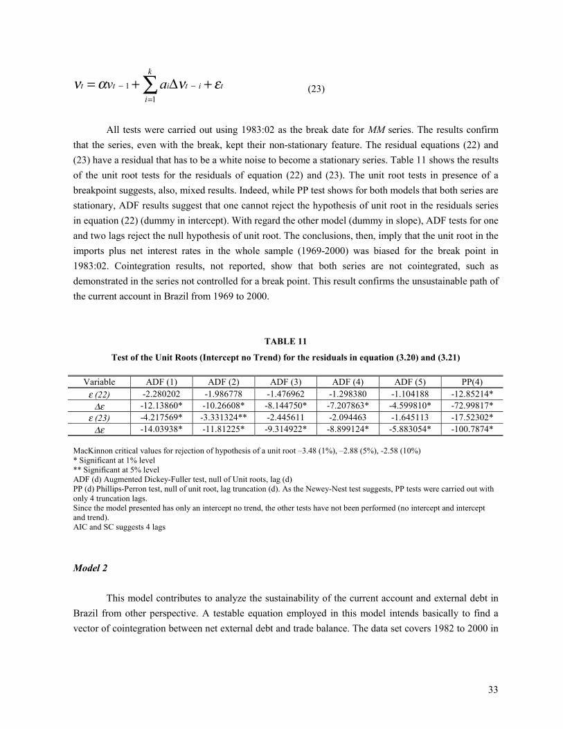
All tests were carried out using 1983:02 as the break date for MM series. The results confirmthat the series, even with the break, kept their non-stationary feature. The residual equations (22) and(23) have a residual that has to be a white noise to become a stationary series. Table 11 shows the resultsof the unit root tests for the residuals of equation (22) and (23). The unit root tests in presence of abreakpoint suggests, also, mixed results. Indeed, while PP test shows for both models that both series arestationary, ADF results suggest that one cannot reject the hypothesis of unit root in the residuals seriesin equation (22) (dummy in intercept). With regard the other model (dummy in slope), ADF tests for oneand two lags reject the null hypothesis of unit root. The conclusions, then, imply that the unit root in theimports plus net interest rates in the whole sample (1969-2000) was biased for the break point in1983:02. Cointegration results, not reported, show that both series are not cointegrated, such asdemonstrated in the series not controlled for a break point. This result confirms the unsustainable path ofthe current account in Brazil from 1969 to 2000.

TABLE 11

Test of the Unit Roots (Intercept no Trend) for the residuals in equation (3.20) and (3.21)

Variable ADF (1) ADF (2) ADF (3) ADF (4) ADF (5) PP(4)ε (22) -2.280202 -1.986778 -1.476962 -1.298380 -1.104188 -12.85214*

∆ε -12.13860* -10.26608* -8.144750* -7.207863* -4.599810* -72.99817*ε (23) -4.217569* -3.331324** -2.445611 -2.094463 -1.645113 -17.52302*

∆ε -14.03938* -11.81225* -9.314922* -8.899124* -5.883054* -100.7874*

MacKinnon critical values for rejection of hypothesis of a unit root –3.48 (1%), –2.88 (5%), -2.58 (10%)* Significant at 1% level** Significant at 5% levelADF (d) Augmented Dickey-Fuller test, null of Unit roots, lag (d)PP (d) Phillips-Perron test, null of unit root, lag truncation (d). As the Newey-Nest test suggests, PP tests were carried out withonly 4 truncation lags.Since the model presented has only an intercept no trend, the other tests have not been performed (no intercept and interceptand trend).AIC and SC suggests 4 lags

Model 2

This model contributes to analyze the sustainability of the current account and external debt inBrazil from other perspective. A testable equation employed in this model intends basically to find avector of cointegration between net external debt and trade balance. The data set covers 1982 to 2000 in

34

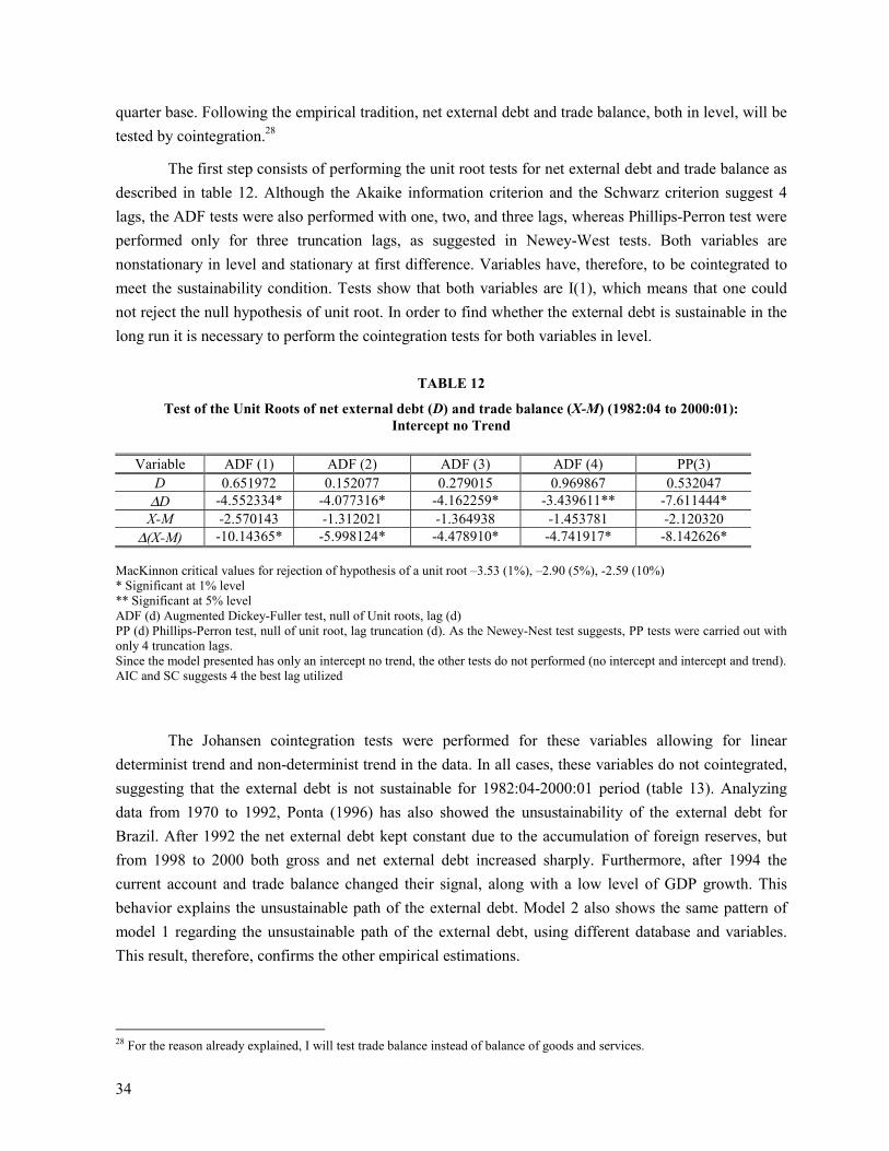
quarter base. Following the empirical tradition, net external debt and trade balance, both in level, will betested by cointegration.28

The first step consists of performing the unit root tests for net external debt and trade balance asdescribed in table 12. Although the Akaike information criterion and the Schwarz criterion suggest 4lags, the ADF tests were also performed with one, two, and three lags, whereas Phillips-Perron test wereperformed only for three truncation lags, as suggested in Newey-West tests. Both variables arenonstationary in level and stationary at first difference. Variables have, therefore, to be cointegrated tomeet the sustainability condition. Tests show that both variables are I(1), which means that one couldnot reject the null hypothesis of unit root. In order to find whether the external debt is sustainable in thelong run it is necessary to perform the cointegration tests for both variables in level.

TABLE 12

Test of the Unit Roots of net external debt (D) and trade balance (X-M) (1982:04 to 2000:01):Intercept no Trend

Variable ADF (1) ADF (2) ADF (3) ADF (4) PP(3)D 0.651972 0.152077 0.279015 0.969867 0.532047

∆D -4.552334* -4.077316* -4.162259* -3.439611** -7.611444*X-M -2.570143 -1.312021 -1.364938 -1.453781 -2.120320

∆(X-M) -10.14365* -5.998124* -4.478910* -4.741917* -8.142626*

MacKinnon critical values for rejection of hypothesis of a unit root –3.53 (1%), –2.90 (5%), -2.59 (10%)* Significant at 1% level** Significant at 5% levelADF (d) Augmented Dickey-Fuller test, null of Unit roots, lag (d)PP (d) Phillips-Perron test, null of unit root, lag truncation (d). As the Newey-Nest test suggests, PP tests were carried out withonly 4 truncation lags.Since the model presented has only an intercept no trend, the other tests do not performed (no intercept and intercept and trend).AIC and SC suggests 4 the best lag utilized

The Johansen cointegration tests were performed for these variables allowing for lineardeterminist trend and non-determinist trend in the data. In all cases, these variables do not cointegrated,suggesting that the external debt is not sustainable for 1982:04-2000:01 period (table 13). Analyzingdata from 1970 to 1992, Ponta (1996) has also showed the unsustainability of the external debt forBrazil. After 1992 the net external debt kept constant due to the accumulation of foreign reserves, butfrom 1998 to 2000 both gross and net external debt increased sharply. Furthermore, after 1994 thecurrent account and trade balance changed their signal, along with a low level of GDP growth. Thisbehavior explains the unsustainable path of the external debt. Model 2 also shows the same pattern ofmodel 1 regarding the unsustainable path of the external debt, using different database and variables.This result, therefore, confirms the other empirical estimations.

28 For the reason already explained, I will test trade balance instead of balance of goods and services.

35

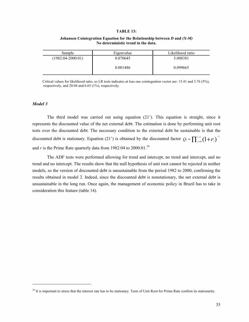
TABLE 13:

Johansen Cointegration Equation for the Relationship between D and (X-M)No deterministic trend in the data.

Sample Eigenvalue Likelihood ratio(1982:04-2000:01) 0.070645

0.001486

5.008381

0.099665

Critical values for likelihood ratio, so LR tests indicates at leas one cointegration vector are: 15.41 and 3.76 (5%), respectively, and 20.04 and 6.65 (1%), respectively.

Model 3

The third model was carried out using equation (21’). This equation is straight, since itrepresents the discounted value of the net external debt. The estimation is done by performing unit roottests over the discounted debt. The necessary condition to the external debt be sustainable is that the

discounted debt is stationary. Equation (21’) is obtained by the discounted factor ∏ +−

=

−= 1

0

1)1(t

j jt rQ

and r is the Prime Rate quarterly data from 1982:04 to 2000:01.29

The ADF tests were performed allowing for trend and intercept, no trend and intercept, and notrend and no intercept. The results show that the null hypothesis of unit root cannot be rejected in neithermodels, so the version of discounted debt is unsustainable from the period 1982 to 2000, confirming theresults obtained in model 2. Indeed, since the discounted debt is nonstationary, the net external debt isunsustainable in the long run. Once again, the management of economic policy in Brazil has to take inconsideration this feature (table 14).

29 It is important to stress that the interest rate has to be stationary. Tests of Unit Root for Prime Rate confirm its stationarity.

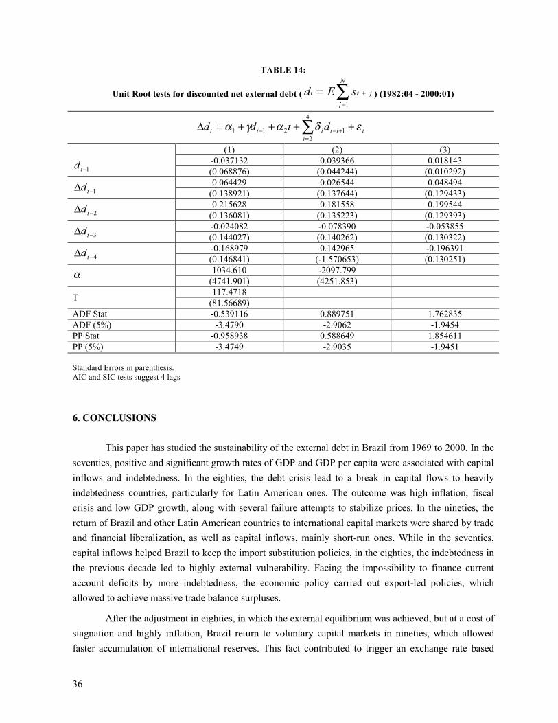
36

TABLE 14:

Unit Root tests for discounted net external debt ( ∑=

+=N

jjtt sEd

1) (1982:04 - 2000:01)

titi

itt dtdd εδαγα ++++=∆ +−=

− ∑ 1

4

2211

(1) (2) (3)-0.037132 0.039366 0.018143

1−td (0.068876) (0.044244) (0.010292)0.064429 0.026544 0.048494

1−∆ td (0.138921) (0.137644) (0.129433)0.215628 0.181558 0.199544

2−∆ td (0.136081) (0.135223) (0.129393)-0.024082 -0.078390 -0.053855

3−∆ td (0.144027) (0.140262) (0.130322)-0.168979 0.142965 -0.196391

4−∆ td (0.146841) (-1.570653) (0.130251)1034.610 -2097.799α

(4741.901) (4251.853)117.4718T (81.56689)

ADF Stat -0.539116 0.889751 1.762835ADF (5%) -3.4790 -2.9062 -1.9454PP Stat -0.958938 0.588649 1.854611PP (5%) -3.4749 -2.9035 -1.9451

Standard Errors in parenthesis.AIC and SIC tests suggest 4 lags

6. CONCLUSIONS

This paper has studied the sustainability of the external debt in Brazil from 1969 to 2000. In theseventies, positive and significant growth rates of GDP and GDP per capita were associated with capitalinflows and indebtedness. In the eighties, the debt crisis lead to a break in capital flows to heavilyindebtedness countries, particularly for Latin American ones. The outcome was high inflation, fiscalcrisis and low GDP growth, along with several failure attempts to stabilize prices. In the nineties, thereturn of Brazil and other Latin American countries to international capital markets were shared by tradeand financial liberalization, as well as capital inflows, mainly short-run ones. While in the seventies,capital inflows helped Brazil to keep the import substitution policies, in the eighties, the indebtedness inthe previous decade led to highly external vulnerability. Facing the impossibility to finance currentaccount deficits by more indebtedness, the economic policy carried out export-led policies, whichallowed to achieve massive trade balance surpluses.

After the adjustment in eighties, in which the external equilibrium was achieved, but at a cost ofstagnation and highly inflation, Brazil return to voluntary capital markets in nineties, which allowedfaster accumulation of international reserves. This fact contributed to trigger an exchange rate based

37

stabilization plan in 1994. Although capital inflows have had important role in short-run management ofmacroeconomic policy, basically allowing exchange rate to be used as the main policy variable, theindebtedness poses the problem of repayments of debt in the long run. The currency crisis in January1999 illustrated the problems related to systematic current account deficits and overvaluated exchangerates. The external front, therefore, keeps being a concern for economic development in Brazil.

Sustainability tests showed that, for different periods and using different models and variables,external debt and current account deficits are not sustainable in the long run. By dividing the wholeperiod in sub samples, it has showed that even from 1969 to 1983, when the necessary condition forsustainability was accomplished, the sufficient condition did no meet. The crisis in early 1980s wasclosely related to the external vulnerability presents in indebtedness policy. The high stock of externaldebt facing the interest rates shock and the break in capital inflows impose a difficult management ofcurrent account deficits, and the impossibility to make external debt repayments.

38

7. REFERENCES

Blecker, R. 1992. Structural Roots of U.S. trade problems: income elasticities, secular trends andhysteresis. Journal of Post Keynesian Economics, 13(3): 321-46.

Blecker, R. 1999a. The fallacy of composition and the limits of Export-Led Growth. New School forSocial Research, Unpublished manuscript.

Blecker, R. 1999b. Taming Global Finance. Washington, D.C. Economic Policy Institute.

Bonomo, M. and C. Terra. 1999. The Political Economy of Exchange Rate Policy in Brazil: 1964-1997.Working Paper, FGV, Brazil (www.fgv.br).

Calvo, G. 1987. Balance of Payments Crisis in a Cash Advance Economy. Journal of Money, Credit andBanking. 19(1): 19-32.

Calvo, G. and C. Vegh. 1999. Inflation stabilization and balance of payments crises in developingcountries. NBER Working papers n.6925, Cambridge, Massachusetts, February.

Cardoso, E. and Ilan Goldfajn. 1998. Capital flows to Brazil: The Endogeneity of Capital Controls. IMFStaff papers. (45)1: 161-202.

Carneiro, D.D. 1997. A sustentabilidade dos déficits externos. Revista Anpec.1(3):11-28. Rio de Janeiro.

Castro, A.B. & F.E Souza. 1985. A Economia Brasileira em marcha forçada. Rio de Janeiro, Paz eTerra.

Conjuntura Economica, FGV, Rio de Janeiro, several issues.

Curado, Marcelo. 2001. Rigidez Comercial, Movimentos de Capitais e Crise Cambial. UnpublishedDoctor dissertation. Unicamp, Campinas, São Paulo.

Dickey, D. and W. Fuller. 1979. Distribution of the Estimators for Autogressive Time Series with a UnitRoot. Journal of American Statistical Association, 74, 427-431.

Dollar, D. 1992. Outward-oriented Developing Economies Really do Growth more Rapidly: Evidencefrom 95 LDCs, 1976-85. Economic Development and Cultural Change, 1992, 523-544.

Eisner, Robert and Paul J.Pieper. 1984. A new view of the Federal Debt and Budget Deficits. AmericanEconomic Review, 74(1): 11-29.

Engle, R. & Cliver W. J. Granger. 1987. Co-integration and Error Correction: Representation,Estimation, and testing. Econometrica, 55(2): 251-76

Fargerberg, J. 1996. Technology and Competitiveness. Oxford Review of Economic Policy. 12(3):.

Franco, G. 1996. A inserção Externa e o desenvolvimento. Brasília, Unpublished Manuscript.

Frenkel, Roberto. 1998. Capital Market Liberalization and Economic Performance in Latin America.Working papers Series III, n.1. Cepa, New School.

39

Frenkel, Roberto and Martin Rozada. 1999. Balance of Payments liberalization: effects on growth andemployment in Argentina. Paper prepared for Cepa, New School Conference on Globalization andSocial Policy. January.

Godley, W. 1999. Seven Unsustainable Processes. Special Report. Jerome Levy Institute.

Granger, C. 1986. Developments in the study of cointegrated economic variables. Oxford Bulletin ofEconomics and Statistics. 48(3): 213-228.

Greene, W.H. 1997. Econometrics Analysis. Prentice hall, New Jersey, Third edition.

Greiner, Alfred and Willi Semmler. 1999. An Inquiry Into The Sustainability Of German Fiscal Policy:Some Time-Series Tests. Public Finance Review, 27(2): 220-36.

Hakkio, C.J. and M. Rush. 1991. Is the Budget Deficit too large? Economic Inquiry, p. 429-45

Hamilton, J.D. and M.A. Flavin.1986. On The Limitations Of Government Borrowing: A FrameworkFor Empirical Testing. American Economic Review. 76(2), pp. 353-73.

Hamilton, W. 1994. Time Series Analysis. Princeton, New York.

Holden D, and R. Perman. 1994. Unit roots and cointegration for the economist. In Rao, B. B. (1994).Cointegration for the applied economist. Saint Martin Press, New York.

Kaldor, N. 1970. The Case for Regional Policies. Scottish Journal of Political Economy. November.

Krugman, P. 1989 Differences in Income Elasticities and Trends in Real Exchange Rates. EuropeanEconomic Review. 33(5): 1031-46.

Laplane, M. And Sarti, F. 1999. Investimento Externo estrangeiro e o impacto na Balança Comercialnos anos 90. Texto para Discussão N. 629 Ipea: Rio de Janeiro. Fevereiro.

Luporini, V. 2000. Sustainability of the Brazilian Fiscal Policy And Central Bank Independence. RevistaBrasileira De Economia. 54(2): 201-26.

Maddala, G.S. and In-Moo Kim. 1998. Unit Roots, Cointegration, and Structural Change. Cambridge,Cambridge University Press.

McCombie, J. 1989. Thirlwal’s Law and balance of payments constrained growth - a comment ondebate. Applied Economics, 21(5): 611-29.

McCombie, J. 1992. Thirlwal’s Law and balance of payments constrained growth - more on the debate.Applied Economics, 24(5): 493-512.

McCombie, J. 1993. Economic Growth, Trade linkages, and The Balance of Payments Constraint.Journal of Post Keynesian Economics, 15(4): 471-505.

McCombie, J. 1997. On The Empirics Of The Balance-Of-Payments-Constrained Growth. Journal ofPost Keynesian Economics, 9(3): 345-75.

McCombie, J. and Thirlwall, A. 1994. Economic Growth and the Balance of Payments constraint.London, St. Martins.

40

McCombie, J. and Thirlwall, A. 1997. The dynamic Harrod Foreign Trade Multiplier and the Demand-oriented Approach to Economic Growth: an evaluation. International Journal of Applied Economics,11(1): 5-26.

McCombie, J. and Thirlwall, A. 1999. “Growth in an international context: a Post Keynesian view”. In:Deprez, J. and John Harvey. Foundations of International Economics: Post Keynesian Perspectives.London, Routledge.

McKinnon. 1991. Critical values for cointegration tests in Engle, R.F. and Granger, C.W.J. (eds). Long-Run Economic Relationships. Readings in Cointegration. Oxford: Oxford University Press.

Maddala, G.S. and In-Moo Kim. 1998. Unit Roots, Cointegration and Structural Change. Cambridge,Cambridge University Press.

Maddison, A. 1995. Monitoring the World Economy: 1820-1992. OECD, Paris.

Mehra, Y. P. 1994. Wage growth and the inflation process: an empirical approach. In Rao, B. B. 1994.Cointegration for the applied economist. Saint Martin Press, New York.

Milesi-Ferreti, G.M. & Razin, A. 1996. Current Account Sustainability: Selected East Asian and LatinAmerican Experiences. NBER Working Papers n.5791. Cambridge, Massachusetts.

Minsky, H. 1986. Stabilizing an Unstable Economy. New Haven, CT: Yale University Press.

Moreno-Brid, J.C. 1998b. On Capital flows and the Balance-of-payments Constrained Growth Model.Journal of Post Keynesian Economics, forthcoming.

Ocampo, Jose Antonio. 1997. `Trade Policy and Productivity,’ Ministry of Finance, Bogota.

Ocampo, J.A. & Taylor, L. 1998. Trade Liberalization in Developing Countries: Modest benefits butProblems with Productivity Growth, Macro Policies, and Income Distribution. Working papersSeries I, n.8. Cepa, New School.

Oliveira, F.A. at alii. 1988. Déficit e Endividamento do Setor Público. São Paulo, IESP/FUNDAP(Relatório de Pesquisa).

Perron, P. 1989. The Great Crash, the Oil Price Shock and the Unit Root Hypothesis. Econometrica,57(4): 1361-1401.

Perron, P.1994. Trend, Unit Root and Structural Change in Macroeconomic Time Series. In Rao, B. B.1994. Cointegration for the applied economist. Saint Martin Press, New York.

Phillips, P.C.B. and Perron, P. 1988. Testing for a Unit Root in Time Series Regression. Biometrika,75(3): 335-346.

Ponta, A.F. 1996. A sustentabilidade da endividamento externo no Brasil: uma análise de co-integração.Pesquisa e Planejamento Econômico. 26(3): 399-416. Rio de Janeiro.

Rao, B. B. 1994. Cointegration for the applied economist. Saint Martin Press, New York.

Rocha, Fabiana and Sigfried Bender.2000. Present Value Tests of the Brazilian Current Account.Revista de Economia Aplicada São Paulo.

41

Rodrik, Dani. 1994. `The Rush to Free Trade in the Developing World: Why so Late? Why Now? Willit Last?' in Stephan Haggard and Steven B. Webb (eds.) Voting for Reform, New York: OxfordUniversity Press.

Rodrik, Dani. 1995. `Trade and Industrial Policy Reform.' in Jere R. Behrman and T. N. Srinivasan(eds.) Handbook of Development Economics, vol. 3B, Amsterdam; North-Holland.

Rodrik, Dani. 1999. The New Global Economy and Developing Countries: Making Openness Work.Washington, DC. Overseas Development Council.

Rodrik, Dani and André Velasco. 1999. Short-term capital flows. NBER Working Papers n.7364.Cambridge, Massachusetts. September.

Rodríguez, F. and Rodrik, D. 1999. Trade policy and Economic Growth: a Skeptic’s guide to the Cross-National evidence. NBER Working Papers n.5791. Cambridge, Massachussets. April.

Ros, Jaime and Nora Lustig. 1999. Trade and financial liberalization with volatile capital inflows:Macroeconomic consequences and Social impacts in Mexico during the 1990s. Paper prepared forCepa, New School Conference on Globalization and Social Policy. January.

Sampaio Jr, Plínio A. 2000. A Armadilha das Dívidas Eternas. Folha de São Paulo, 09/11/200.

Sawada, Y. 1994. Are The Heavily Indebted Countries Solvent? Tests Of Intertemporal BorrowingConstraints. Journal of Development Economics. 45(2): 325-37.

Semmler, Willi and Malte Sieveking. 1999. Growth, Credit Risk And Sustainable Debt: A Model AndEstimations For Euroland. Unpublished manuscript.

Semmler, Willi and Malte Sieveking. 2000. Critical Debt Dynamics. Journal Of Economics DynamicAnd Control. 24(4): 1121-1144.

Simonsen, M. 1985. The Developing Country Debt Problems, in: Smith, G.W. and J. Cudding.International Debt and Developing Countries, World Bank, Washington, DC.

Taylor, L. 1994. `Gap Models,' Journal of Development Economics, 45(1): 17-34.

Taylor, L. 1997. `The Revival of the Liberal Creed – The IMF and the World Bank in a GlobalizedEconomy,' World Development, 25(2): 145-52.

Thirlwall, A. 1979. Balance of Payments constraint as an Explanation of International Growth Ratedifferences. Banca Nazionale del Lavoro Quarterly Review. 128(1): 45-53.

Thirlwall, A. 1991. Professor Krugman 45-degree rule. Journal of Post Keynesian Economics, 14(1):23-28.

Trehan, B. and C.E. Walsh. 1988. Common Trends, Intertemporal Budget Balance, And RevenueSmoothing. Journal Of Economics Dynamic And Control. June, 425-44.

Wilcox, David W. 1989. The Sustainability Of Government Deficits: Implications Of The Present-ValueBorrowing Constraints. Journal Of Money, Credit, And Banking. 21(3): 291-306.