


Línguas
Páginas
Legal

Improving Air Quality Forecasting through Incremental Reduction of Input Uncertainties
– focus on episodic fire emissions
Daewon W. Byun1* Dae-Gyun Lee*, Hyun-Cheol Kim1*, Fantine Ngan1*, Hsin-Mu Lin1,
Daniel Tong1, Tianfeng Chai1, Ariel Stein1, Roland Draxler1, Brad Pierce4, Shobha Kondragunta4, Pius Lee1, Rick Saylor1, Jeff McQueen2,
Youhua Tang2, Jianping Huang2, Marina Tsidulko2, Rohit Mathur5, George Pouliot5, Ivanka Stajner3, and Paula Davison3
1NOAA/Air Resources Laboratory 2NOAA/NCEP, 3NOAA/OST, 4NOAA/NESDIS
5EPA/Atmospheric and Modeling & Analysis Division *previous affiliation: University of Houston
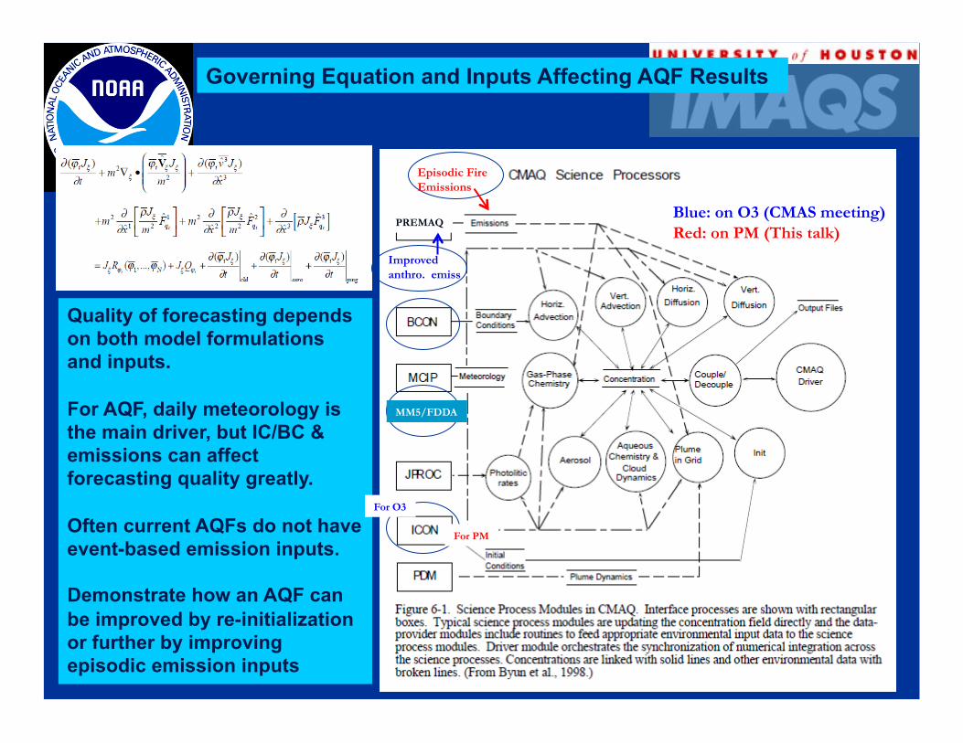
Governing Equation and Inputs Affecting AQF Results
Quality of forecasting depends on both model formulations and inputs.
For AQF, daily meteorology is the main driver, but IC/BC & emissions can affect forecasting quality greatly.
Often current AQFs do not have event-based emission inputs.
Demonstrate how an AQF can be improved by re-initialization or further by improving episodic emission inputs
Improved anthro. emiss
PREMAQ
MM5/FDDA
For PM
For O3
Episodic Fire Emissions
Blue: on O3 (CMAS meeting) Red: on PM (This talk)
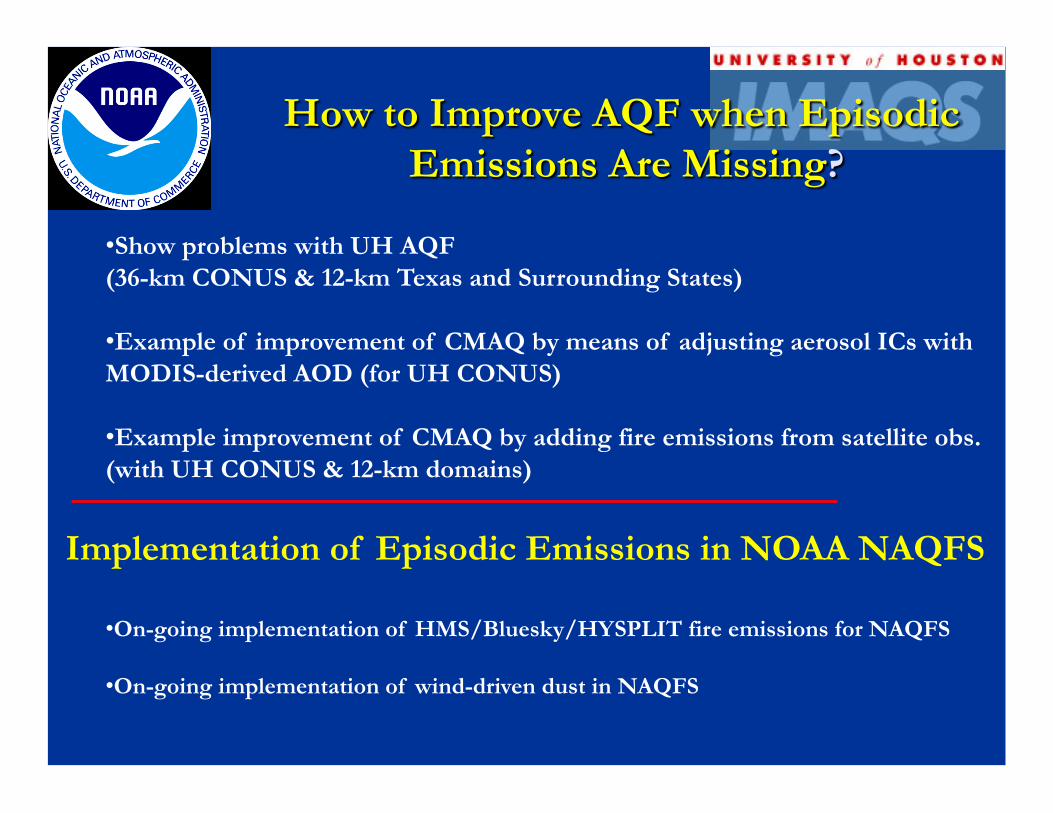
• Show problems with UH AQF (36-km CONUS & 12-km Texas and Surrounding States)
• Example of improvement of CMAQ by means of adjusting aerosol ICs with MODIS-derived AOD (for UH CONUS)
• Example improvement of CMAQ by adding fire emissions from satellite obs. (with UH CONUS & 12-km domains)
• On-going implementation of HMS/Bluesky/HYSPLIT fire emissions for NAQFS
• On-going implementation of wind-driven dust in NAQFS
Implementation of Episodic Emissions in NOAA NAQFS
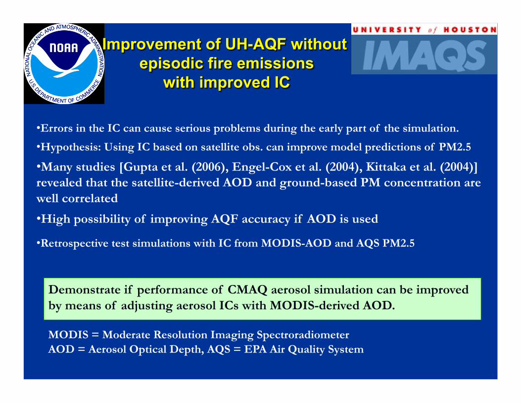
• Errors in the IC can cause serious problems during the early part of the simulation.
• Hypothesis: Using IC based on satellite obs. can improve model predictions of PM2.5
• Many studies [Gupta et al. (2006), Engel-Cox et al. (2004), Kittaka et al. (2004)] revealed that the satellite-derived AOD and ground-based PM concentration are well correlated
• High possibility of improving AQF accuracy if AOD is used
• Retrospective test simulations with IC from MODIS-AOD and AQS PM2.5
Demonstrate if performance of CMAQ aerosol simulation can be improved by means of adjusting aerosol ICs with MODIS-derived AOD.
MODIS = Moderate Resolution Imaging Spectroradiometer AOD = Aerosol Optical Depth, AQS = EPA Air Quality System
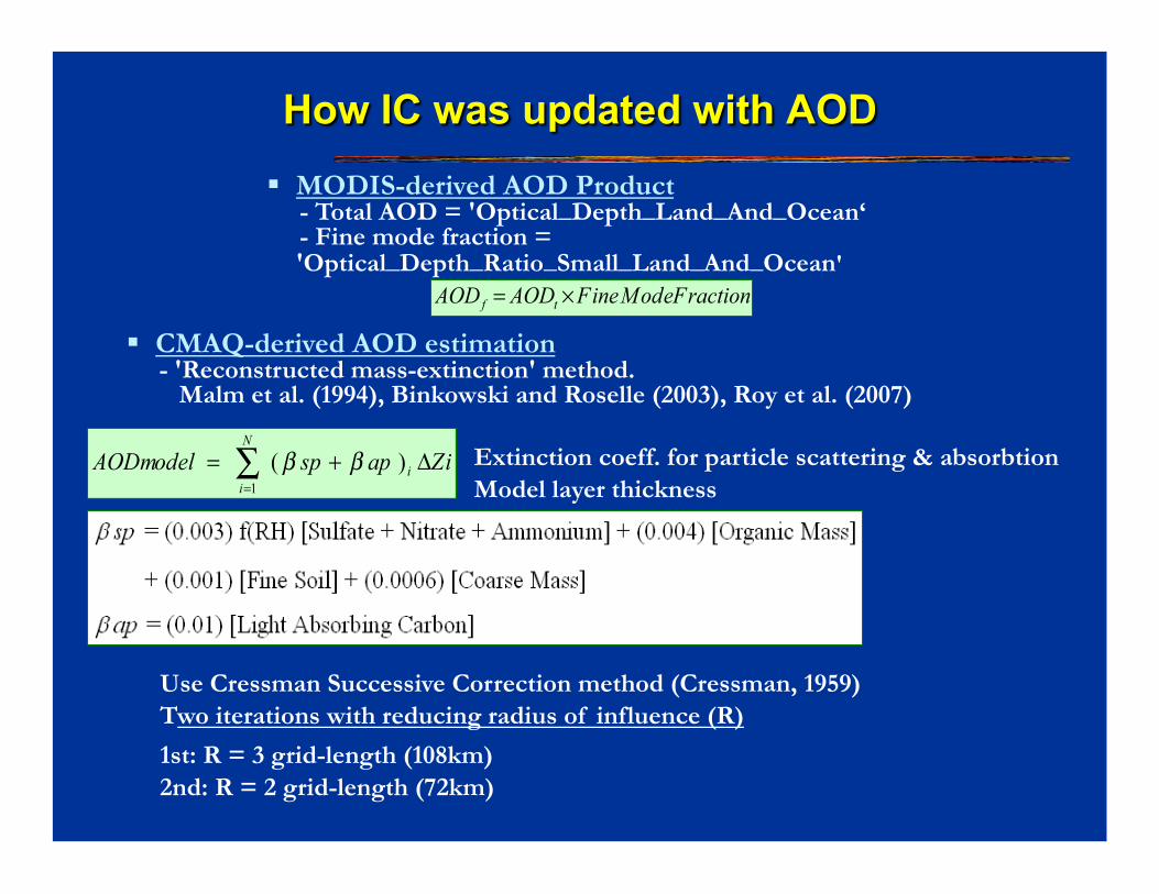
MODIS-derived AOD Product - Total AOD = 'Optical_Depth_Land_And_Ocean‘ - Fine mode fraction =
'Optical_Depth_Ratio_Small_Land_And_Ocean'
Extinction coeff. for particle scattering & absorbtion Model layer thickness
CMAQ-derived AOD estimation - 'Reconstructed mass-extinction' method. Malm et al. (1994), Binkowski and Roselle (2003), Roy et al. (2007)
Use Cressman Successive Correction method (Cressman, 1959) Two iterations with reducing radius of influence (R)
1st: R = 3 grid-length (108km) 2nd: R = 2 grid-length (72km)
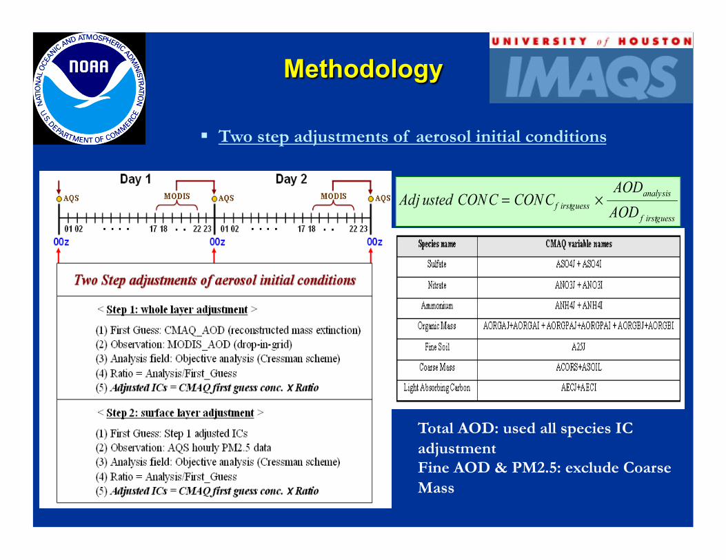
Two step adjustments of aerosol initial conditions
Total AOD: used all species IC adjustment Fine AOD & PM2.5: exclude Coarse Mass
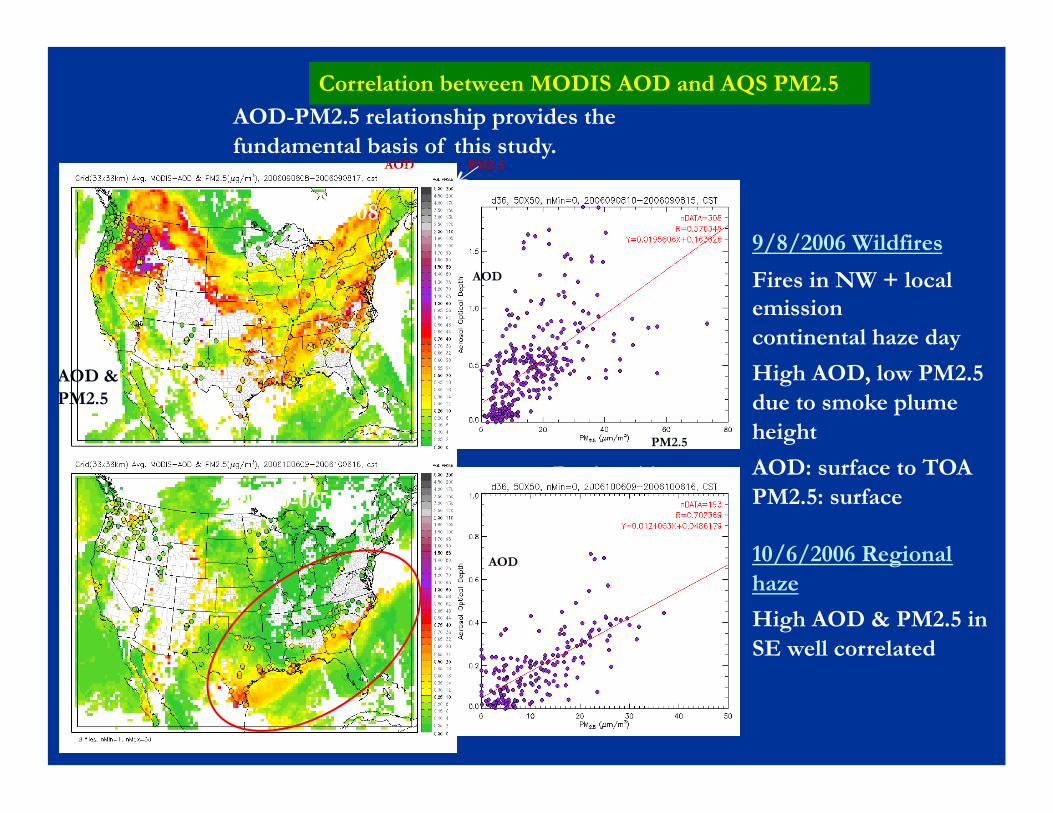
Correlation between MODIS AOD and AQS PM2.5
< Wildfires >
< Regional haze >
9/8/2006 Wildfires
Fires in NW + local emission continental haze day
High AOD, low PM2.5 due to smoke plume height
AOD: surface to TOA PM2.5: surface
10/6/2006 Regional haze
High AOD & PM2.5 in SE well correlated
AOD-PM2.5 relationship provides the fundamental basis of this study.
AOD
AOD & PM2.5
PM2.5
AOD
PM2.5
AOD
2009-09-08
2009-10-06
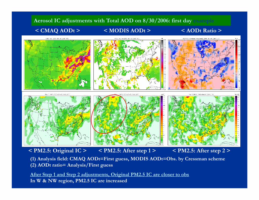
Aerosol IC adjustments with Total AOD on 8/30/2006: first day example
< CMAQ AODt > < MODIS AODt > < AODt Ratio >
< PM2.5: Original IC > < PM2.5: After step 1 > < PM2.5: After step 2 > (1) Analysis field: CMAQ AODt=First guess, MODIS AODt=Obs. by Cressman scheme (2) AODt ratio= Analysis/First guess
After Step 1 and Step 2 adjustments, Original PM2.5 IC are closer to obs In W & NW region, PM2.5 IC are increased
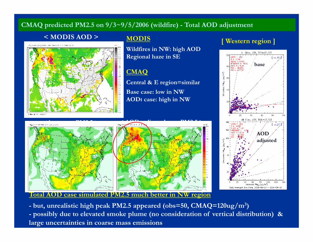
CMAQ predicted PM2.5 on 9/3~9/5/2006 (wildfire) - Total AOD adjustment
< MODIS AOD >
< base case PM2.5 > < AODt adjusted case PM2.5 >
MODIS Wildfires in NW: high AOD Regional haze in SE
CMAQ Central & E region=similar
Base case: low in NW AODt case: high in NW
[ Western region ]
R=0.67
Total AOD case simulated PM2.5 much better in NW region
- but, unrealistic high peak PM2.5 appeared (obs=50, CMAQ=120ug/m3) - possibly due to elevated smoke plume (no consideration of vertical distribution) & large uncertainties in coarse mass emissions
base
AOD adjusted
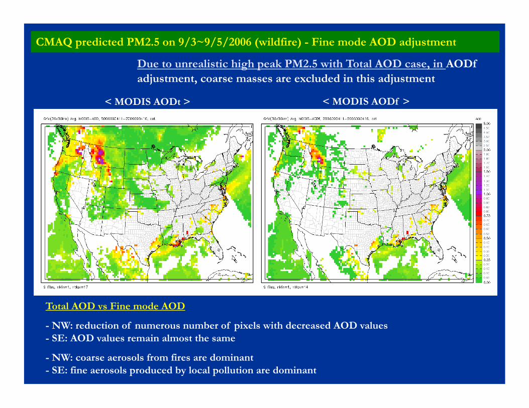
CMAQ predicted PM2.5 on 9/3~9/5/2006 (wildfire) - Fine mode AOD adjustment
< MODIS AODt > < MODIS AODf >
Total AOD vs Fine mode AOD
- NW: reduction of numerous number of pixels with decreased AOD values - SE: AOD values remain almost the same
- NW: coarse aerosols from fires are dominant - SE: fine aerosols produced by local pollution are dominant
Due to unrealistic high peak PM2.5 with Total AOD case, in AODf adjustment, coarse masses are excluded in this adjustment
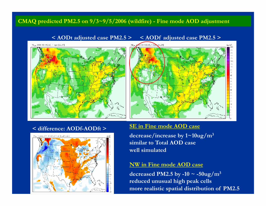
CMAQ predicted PM2.5 on 9/3~9/5/2006 (wildfire) - Fine mode AOD adjustment
< difference: AODf-AODft >
< AODf adjusted case PM2.5 > < AODt adjusted case PM2.5 >
SE in Fine mode AOD case
decrease/increase by 1~10ug/m3
similar to Total AOD case well simulated
NW in Fine mode AOD case
decreased PM2.5 by -10 ~ -50ug/m3
reduced unusual high peak cells more realistic spatial distribution of PM2.5
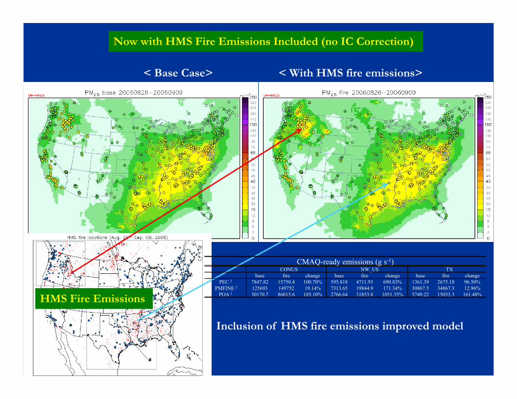
Now with HMS Fire Emissions Included (no IC Correction)
< With HMS fire emissions> < Base Case>
Inclusion of HMS fire emissions improved model
HMS Fire Emissions
PEC 2 7847.82 15750.4 100.70% 595.818 4711.93 690.83% 1361.39 2675.18 96.50% PMFINE 2 125693 149752 19.14% 7313.65 19844.9 171.34% 30867.5 34867.3 12.96%
POA 2 30170.7 86015.6 185.10% 2766.64 31853.8 1051.35% 5749.22 15033.3 161.48%
CMAQ-ready emissions (g s-1) CONUS NW_US TX
base fire change base fire change base fire change
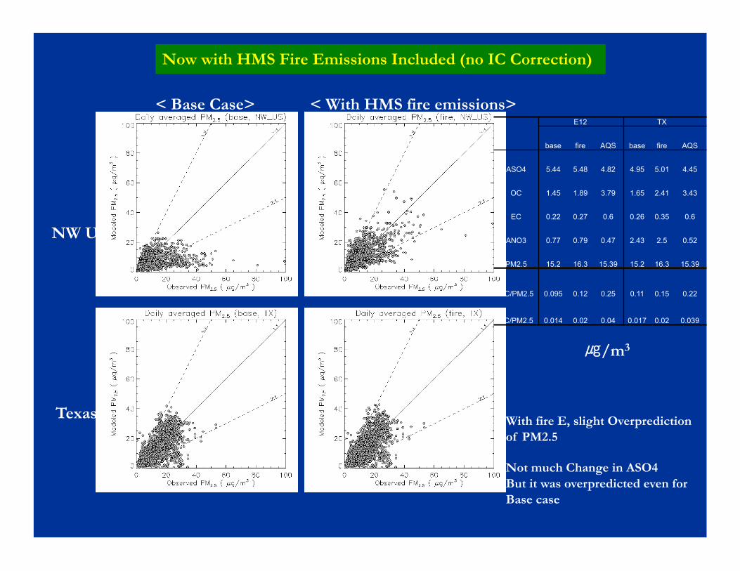
Now with HMS Fire Emissions Included (no IC Correction)
< With HMS fire emissions> < Base Case>
NW US
Texas With fire E, slight Overprediction of PM2.5
Not much Change in ASO4 But it was overpredicted even for Base case
E12 TX
base fire AQS base fire AQS
ASO4 5.44 5.48 4.82 4.95 5.01 4.45
OC 1.45 1.89 3.79 1.65 2.41 3.43
EC 0.22 0.27 0.6 0.26 0.35 0.6
ANO3 0.77 0.79 0.47 2.43 2.5 0.52
PM2.5 15.2 16.3 15.39 15.2 16.3 15.39
OC/PM2.5 0.095 0.12 0.25 0.11 0.15 0.22
EC/PM2.5 0.014 0.02 0.04 0.017 0.02 0.039
㎍/m3
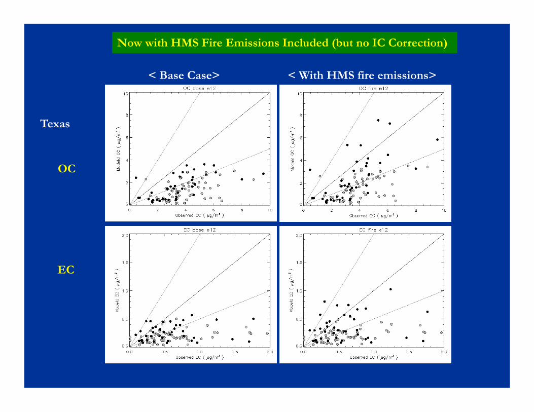
Now with HMS Fire Emissions Included (but no IC Correction)
< With HMS fire emissions> < Base Case>
Texas
OC
EC
Interim Summary for Improving AQF
In order to improve CMAQ aerosol predictions, the aerosol IC are adjusted at the simulation start time-step utilizing the MODIS-derived AOD and AQS PM2.5 observations.
In case of aerosol events such as wildfires - impacts of IC adjustments could be significantly big - due to lack of episodic fire emission inputs, CMAQ could not simulate the event - such deficiencies can be mitigated by improved IC with MODIS-AOD & AQS
Wildfire case with total AOD adjustment, - CMAQ could simulate high PM2.5, but unrealistic high peak values appeared, due to uncertainties in coarse mass emissions and elevated smoke plume
Wildfire case with fine mode AOD adjustment, - Helped reducing unrealistic high peak PM2.5 concentrations
Wildfire case with HMS fire emissions, - Improves simulation of PM2.5 (in particular for EC and OC)
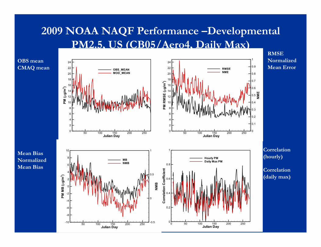
2009 NOAA NAQF Performance –Developmental PM2.5, US (CB05/Aero4, Daily Max)
OBS mean CMAQ mean
Mean Bias Normalized Mean Bias
RMSE Normalized Mean Error
Correlation (hourly)
Correlation (daily max)
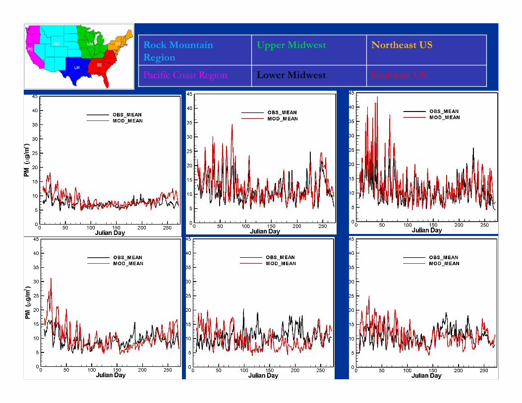
Rock Mountain Region
Upper Midwest Northeast US
Pacific Coast Region Lower Midwest Southeast US
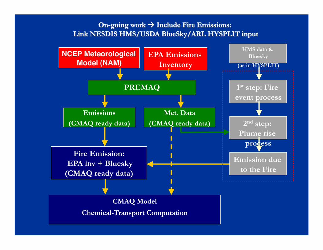
CMAQ Model
Chemical-Transport Computation
NCEP Meteorological Model (NAM)
PREMAQ
EPA Emissions Inventory
HMS data & Bluesky
(as in HYSPLIT)
Fire Emission: EPA inv + Bluesky (CMAQ ready data)
Emissions (CMAQ ready data)
Met. Data (CMAQ ready data)
1st step: Fire event process
2nd step: Plume rise
process
Emission due to the Fire
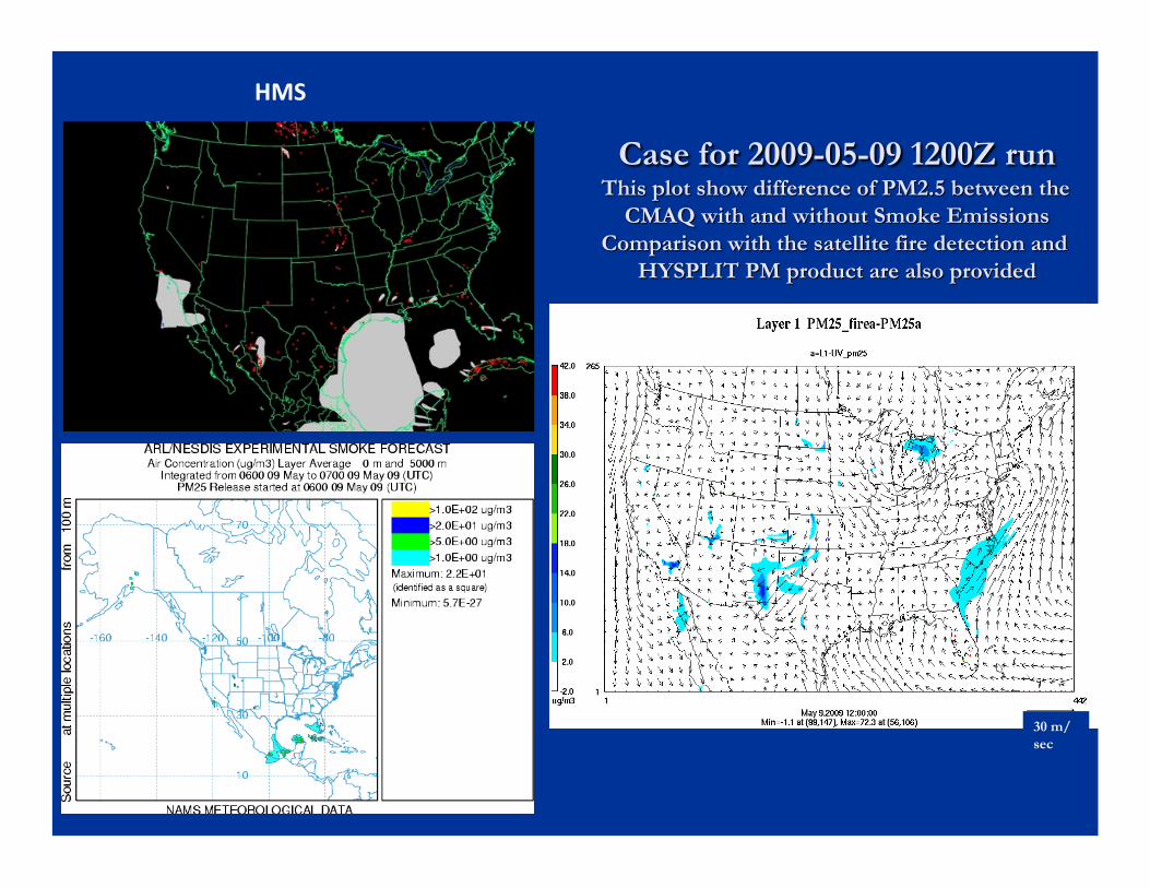
HMS
30 m/sec
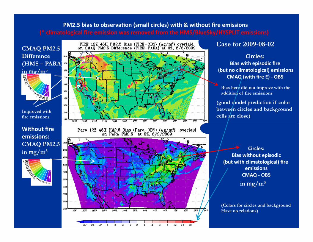
Circles: Bias with episodic fire
(but no climatological) emissions CMAQ (with fire E) ‐ OBS
Circles: Bias without episodic
(but with climatological) fire emissions
CMAQ ‐ OBS
PM2.5 bias to observaGon (small circles) with & without fire emissions (* climatological fire emission was removed from the HMS/BlueSky/HYSPLIT emissions)
CMAQ PM2.5 Difference (HMS – PARA) in mg/m3
Without fire emissions: CMAQ PM2.5 in mg/m3
in mg/m3
Bias here did not improve with the addition of fire emissions
(Colors for circles and background Have no relations)
Improved with fire emissions
Case for 2009-08-02
(good model prediction if color between circles and background cells are close)
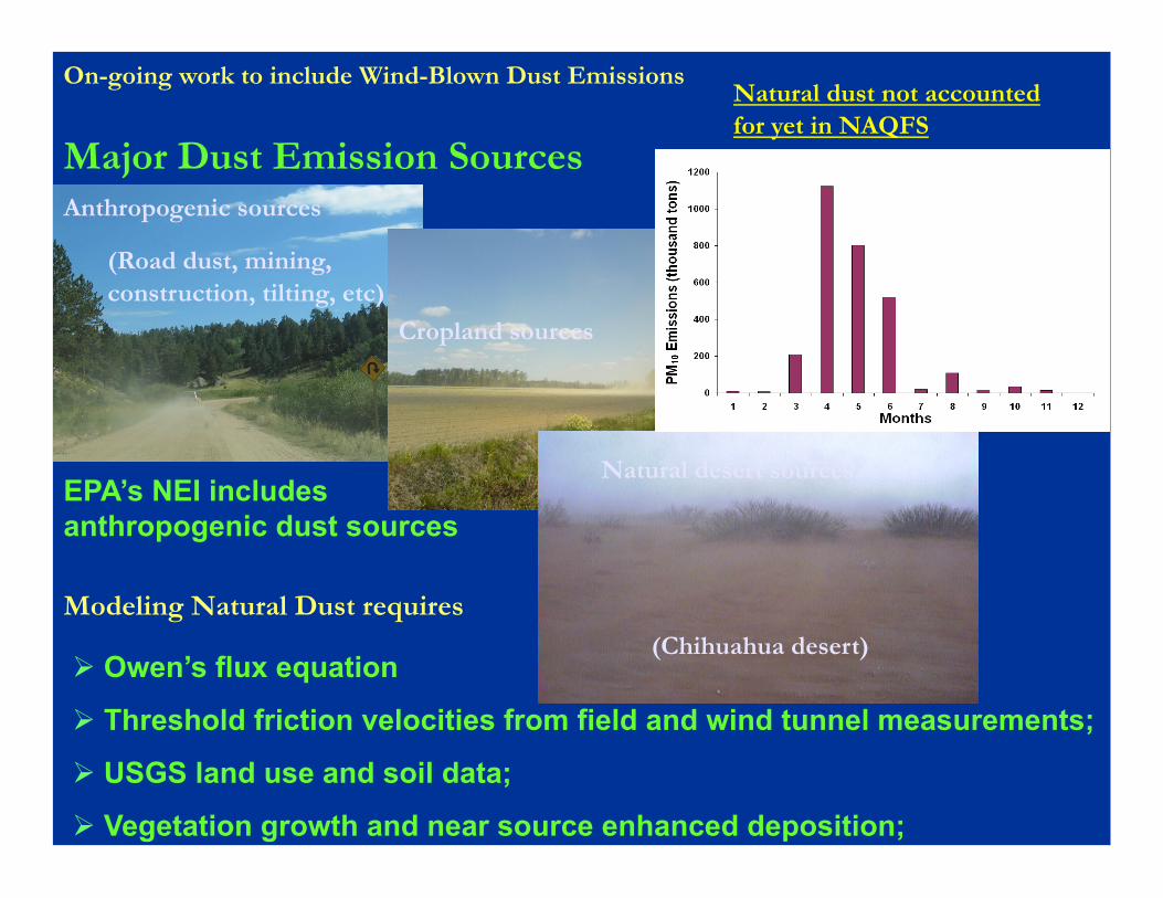
Major Dust Emission Sources
EPA’s NEI includes anthropogenic dust sources
(Road dust, mining, construction, tilting, etc)
Anthropogenic sources
Cropland sources
(Chihuahua desert)
Natural desert sources
Natural dust not accounted for yet in NAQFS
Owen’s flux equation
Threshold friction velocities from field and wind tunnel measurements;
USGS land use and soil data;
Vegetation growth and near source enhanced deposition;
Modeling Natural Dust requires
On-going work to include Wind-Blown Dust Emissions
Dust emissions most active in Spring
Annual Emissions
~ 3 Tg/yr
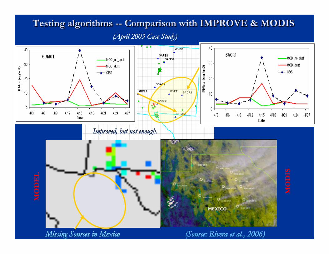
(April 2003 Case Study)
Improved, but not enough.
(Source: Rivera et al., 2006) Missing Sources in Mexico
MO
DIS
MO
DE
L
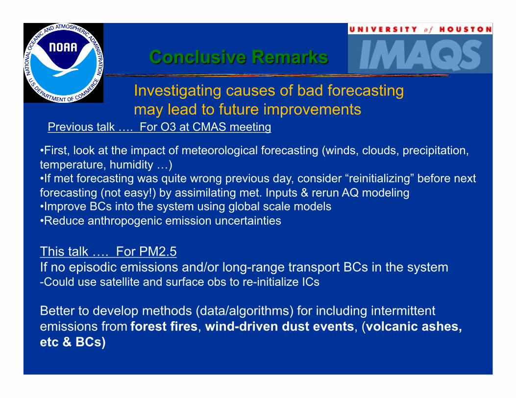
• First, look at the impact of meteorological forecasting (winds, clouds, precipitation, temperature, humidity …) • If met forecasting was quite wrong previous day, consider “reinitializing” before next forecasting (not easy!) by assimilating met. Inputs & rerun AQ modeling • Improve BCs into the system using global scale models • Reduce anthropogenic emission uncertainties
This talk …. For PM2.5 If no episodic emissions and/or long-range transport BCs in the system - Could use satellite and surface obs to re-initialize ICs
Better to develop methods (data/algorithms) for including intermittent emissions from forest fires, wind-driven dust events, (volcanic ashes, etc & BCs)
Investigating causes of bad forecasting may lead to future improvements
Previous talk …. For O3 at CMAS meeting
Top Related