
AnaBeatrizRactPousada ... · Allrightsreserved AnaBeatrizRactPousada Graduated in Economics at...
58
Ana Beatriz Ract Pousada Public Sector and the Allocation of Skills in the Labor Market Dissertação de Mestrado Dissertation presented to the Programa de Pós–graduação em Economia of the Departamento de Economia, Centro de Ciências Sociais, PUC-Rio as partial fulfillment of the requirements for the degree of Mestre em Economia. Advisor: Prof. Gabriel Lopes de Ulyssea Rio de Janeiro April 2017
Transcript of AnaBeatrizRactPousada ... · Allrightsreserved AnaBeatrizRactPousada Graduated in Economics at...

Ana Beatriz Ract Pousada
Public Sector and the Allocation of Skills inthe Labor Market
Dissertação de Mestrado
Dissertation presented to the Programa de Pós–graduação emEconomia of the Departamento de Economia, Centro de CiênciasSociais, PUC-Rio as partial fulfillment of the requirements for thedegree of Mestre em Economia.
Advisor: Prof. Gabriel Lopes de Ulyssea
Rio de JaneiroApril 2017

Ana Beatriz Ract Pousada
Public Sector and the Allocation of Skills inthe Labor Market
Dissertation presented to the Programa de Pós–graduação emEconomia of the Departamento de Economia, Centro de CiênciasSociais, PUC-Rio as partial fulfillment of the requirements for thedegree of Mestre em Economia. Approved by the undersignedExamination Committee.
Prof. Gabriel Lopes de UlysseaAdvisor
Departamento de Economia – PUC-Rio
Prof. Claudio Abramovay Ferraz do AmaralDepartamento de Economia – PUC-Rio
Prof. Cecilia MachadoEscola de Pós-Graduação em Economia – FGV-Rio
Prof. Monica HerzVice Dean of Graduate Studies
Centro de Ciências Sociais – PUC-Rio
Rio de Janeiro, April 29th, 2017

All rights reserved
Ana Beatriz Ract Pousada
Graduated in Economics at University of São Paulo (USP,São Paulo, Brazil) in 2013.
Bibligraphic dataPousada, Ana Beatriz Ract
Public Sector and the Allocation of Skills in the LaborMarket / Ana Beatriz Ract Pousada; advisor: Gabriel Lopesde Ulyssea. – 2017.
v., 58 f: il. color. ; 30 cm
Dissertação (mestrado) - Pontifícia Universidade Católicado Rio de Janeiro, Departamento de Economia.
Inclui bibliografia
1. Economia – Dissertação. 2. Economia do Trabalho –Dissertação. 3. Emprego Público;. 4. Alocação de Trabalha-dores;. 5. Tarefas.. I. Ulyssea, Gabriel Lopes de. II. PontifíciaUniversidade Católica do Rio de Janeiro. Departamento deEconomia. III. Título.
CDD: 330

Acknowledgements
First of all, I want to thank my advisor Prof. Gabriel Ulyssea, for all hisguidance and support. I am also grateful for the useful comments from Prof.Cecilia Machado and Prof. Claudio Ferraz that helped enhance this finalversion.
I am thankful to my other professors from PUC-Rio that helped me developthe concepts applied in this work and gave useful suggestions through theproccess.
I appreciate the help and support of my colleagues from PUC-Rio, with whomI had very productive discussions about research. I am also grateful to theadministrative staff, who were always present to solve my questions.
Finally, I want to thank my family and friends from São Paulo who encouragedme during the past two years. I am specially thankful to my parents, AnaCristina and Marcilio, and my sisters, Marina and Isabela, for being alwayspresent and supportive.

Resumo
Pousada, Ana Beatriz Ract; Ulyssea, Gabriel Lopes de. Efeitosdo Emprego Público Sobre a Alocação de Habilidades noMercado de Trabalho. Rio de Janeiro, 2017. 58p. Dissertação deMestrado – Departamento de Economia, Pontifícia UniversidadeCatólica do Rio de Janeiro.
Esse artigo investiga como o emprego público afeta a alocação de ha-bilidades na economia. Construímos um modelo de Roy onde trabalhadoresse selecionam entre os setores público e privado baseados nas suas produti-vidades e aversões ao risco. O setor privado é caracterizado por pareamentopositivos entre habilidades e tarefas, mas tem retornos incertos, o que podecriar um trade-off para os trabalhadores. Estimamos esse modelo para oBrazil usando dados no nível do trabalhadores para os anos de 2011-2014e fazemos um exercício contra-factual. Resultados mostram que reduzir otamanho do setor público aumento a produtividade média do setor privadoe reduz o prêmio por fazer ensino superior, mas aumenta a desigualdadesalarial.
Palavras-chaveEmprego Público; Alocação de Trabalhadores; Tarefas.

Abstract
Pousada, Ana Beatriz Ract; Ulyssea, Gabriel Lopes de (Advisor).Public Sector and the Allocation of Skills in the LaborMarket. Rio de Janeiro, 2017. 58p. Dissertação de Mestrado –Departamento de Economia, Pontifícia Universidade Católica doRio de Janeiro.
This paper investigates how public sector employment affects theallocation of skills in the economy. We develop a Roy model where workersself-select into either public or private sectors based on their productivityand risk aversion. The private sector is characterized by positive assortativematching between skills and tasks, but it has uncertain returns, whichpotentially creates a trade-off for workers. We estimate the model usingBrazilian worker level data for the years of 2011-2014 and use it to performcounter-factual exercises. We show that reducing the size of the public sectorincreases private sector average productivity, decreases the college wagepremium, but increases wage inequality.
KeywordsPublic Employment; Worker Allocation; Tasks.

Contents
1 Introduction 8
2 Data and Background 132.1 Data 132.2 Facts About the Public Sector 14
3 The Model 223.1 Set Up 223.2 Labor Supply 243.3 Labor Demand 253.4 Equilibrium 28
4 Estimation and Identification 294.1 Functional Forms 294.2 Estimation Method 304.2.1 First Stage 304.2.2 Second Stage 314.3 Identification 33
5 Results 345.1 Estimation Results 345.2 Model Fit 38
6 Counter-Factual Exercises 426.1 Effects on the Distribution of Wages 426.2 Allocation and Productivity Effects 48
7 Conclusion 52
A Participation Decision 57
B Public Good 58

1Introduction
There is a large literature that studies resource allocation and its conse-quences to productivity. For instance, (1) and (2) develop theoretical modelsof talent allocation between productive and unproductive (rent-seeking) acti-vities and find important effects on growth. Moreover, (3) study the allocationof talent in occupations with frictions specific to each gender and color group,and find that the resulting mis-allocation of workers had high consequences forlabor productivity. Considering this, the public sector is an interesting case toanalyze the allocation of skills because it is not only a large part of the labormarket in many countries1, but it also has distinct features that distort skillreturns. Indeed, (5) finds a positive public wage premium in many Europeancountries. Furthermore, (6) argues that the public sector offers non-pecuniaryreturns such as life-time tenure and pensions. Therefore, given its magnitudeand distinguishing characteristics, the public sector is likely to have first ordereffects on the allocation of skills in the economy.
To investigate how the public sector affects the allocation of skillsin the economy we develop an equilibrium Roy model where individualsare heterogeneous in two dimensions, skill and risk aversion. Workers selectthemselves into public or private sectors based on their risk aversion and sectorspecific wages. Consequently, it distorts the distribution of skills available tothe private sector. Labor demand and wages at the private sector are a functionof skills and determined endogenously based on its supply of each skill. Privatesector production allocates workers on tasks based on their skills comparativeadvantage to perform each task. Thus, private sector labor supply of eachskill influences productivity and overall inequality, through skill allocation. Inaddition, they are subject to a productivity shock that makes wages uncertain.
On the other hand, public sector labor demand and wages are exogenous,deterministic and a function of observed characteristics such as education andexperience that are correlated with skills. The idea is to capture three of themain differences in public sector personnel practices that influence worker’s
1For most European countries more than 10% of the labor force is employed in the publicsector (21.47% in the UK; 17.9% in France; 16.03% in Italy and 12.67% in Spain in 2013according to (4)). This is also true in some Latin American countries, such as Brazil, Mexicoand Chile where public sector employees are more than 10% of the labor force.

Chapter 1. Introduction 9
sector selection. First, most public sector hiring and career paths are highlybased on individuals observed characteristics.2 Second, public sector wages arerigid and do not respond to the supply of workers3. Third, the public sector isable to make long term promises to its employees, such as good pensions andjob security, what makes public sector wages more certain than private sectorones4.
We estimate this model for the Brazilian labor market using a nationalhousehold survey (PNAD) for the years of 2011-2014, which is a representativesurvey of the whole Brazilian population. Estimation has two stages. In thefirst stage we estimate the distribution of skills in the private sector throughmaximum likelihood. We suppose the distribution of wages in the privatesector is a finite mixture of normal distributions and estimate average wagesfor each skill and the probabilities of each individual belonging to each skill.In the second stage we use a minimum distance estimator to approximatethose moments estimated in the first stage to their model counterparts. Inother words, we match wages and the distribution of skills and observedcharacteristics in both sectors with wages and labor demand predicted by themodel.
With the estimated model we perform a counter-factual exercise reducingthe size of the public sector and analyze the effects on wages and productivitythrough the allocation of skills. Brazil is an interesting case for two reasons.First, there was a sharp increase in public hiring from 2005 to 2014, we use thesize of the public sector in 2005 as benchmark to interpret our effects. Second,there are significant wage differences between Brazilians’ public and privatesectors that vary across skills and demographic characteristics. Therefore,Brazil’s public sector has a potential to have first order effects on the allocationof skills between sectors.
What distinguishes this paper from the literature is the inclusion oftwo dimensions of unobserved heterogeneity combined with observed charac-teristics. The two dimensions of unobserved heterogeneity creates a trade-offbetween risk and return for individuals when choosing which sector they aregoing to work at, that is specific for each demographic characteristic group.Furthermore, the inclusion of observable characteristics allows us to analyzethe effects on productivity and wages of increasing public sector employment
2In Brazil public sector hiring is done by job specific exams and civil service career pathsare clearly set, this is also true for some European countries such as Italy.
3Public sector size and wages must be on that year’s budget, that must be approved bycongress. Furthermore, public hiring is made through competitive exams that take a whileto set up.
4Several countries offer lifetime tenure to public employees, such as, Brazil, Germany andSpain.

Chapter 1. Introduction 10
in specific educational groups. In addition, we provide a new framework toestimate models of factor allocation with unobserved skills, that can be adap-ted to other contexts besides public and private sector selection. We estimatethis model for Brazil, however, it can be easily applied to other countries withsimilar public employment institutions, such as many European countries.
We show that the distribution of risk aversion in the economy is highlyconcentrated around risk neutrality. However, it has a high dispersion withsome individuals being very risk averse5. Moreover, the public sector has ahigher proportion of high skill workers than low skill ones, thus it is moreattractive for high-skill workers. Consequently, private sector distribution ofskills is more concentrated around low skill workers. As a result, more than halfof private sector tasks are performed by low skill individuals, and a reductionin public sector increases the amount of tasks performed by high-skill workers.Hence, reducing the size of the public sector increases private sector averageproductivity as a result of a more balanced allocation of skills to tasks.
Furthermore, the public average wage premium is greater for those withhigher education than for those with no College degree, in line with otherempirical estimations of Brazilian public-private pay differences6. Our counter-factual exercise shows that a reduction on the size of the public sector increasesthe public average wage premium for those with no College and decreases forthose with some College. This happens because the increase in the proportionof high-skill workers at the private sector is mostly of individuals with noCollege degree. As a consequence, average private sector wages for workerswith no College degree increases and we observe a sharp reduction in theCollege wage premium. However, a reduction in public employment increasesoverall wage inequality. This happens because the rise in the proportion ofhigh-skill individuals that work for the private sector is not accompanied by asame size reduction in high skill wages.
This paper is related to the literature on the implications of the allocationof talent for productivity. (2, 1) discuss the effect of the allocation of talentbetween productive or unproductive (rent seeking) activities. In my model, thepublic sector is an unproductive activity, and it distorts the allocation of skillsbetween sectors in the economy7. There is also a large literature that analyzes
5(7) estimates the distribution of risk aversion using insurance choices and also find thatindividuals are concentrated near risk neutrality and their risk aversion distribution also hasheavy tails.
6See for example (8).7It is also possible to include the public sector as a productive activity. One way of doing
so is assuming that the public good increases private sector productivity. Another way isassuming that the public sector makes a lump sum transfer to workers, thus affecting workerswell-fare, but not production.

Chapter 1. Introduction 11
macroeconomic consequences of talent mis-allocation, for example (9) studyoccupation decision based on the return for talent and occupational frictionsspecific to each gender and color group. We use the differences between publicand private sectors to analyze skill mis-allocation. In our model, private sectorproduction, is based on models that draw a clear distinction between skillsand tasks, such as (10, 11, 12). We apply their framework to a two sectoreconomy (public and private), where individuals are heterogeneous in twodimensions (skills and risk aversion). In this framework, the two dimensionsof heterogeneity are relevant, creating a trade-off between risk and return onsector selection.
There are a few articles discussing effects of public employment in theeconomy. (13, 14) calibrate a general equilibrium model for Brazil to estimateaggregate effects of public employment and find that there are welfare gainsreducing the size of public employment in Brazil. With a model estimatedfor the European economy (15) find that public employment can increaseunemployment in response to an increase in economic turbulence and (16)estimate a search model for the British economy. Differently from these paperswe are able to assess the effects of public employment on the distribution ofskills available to the private sector, labor productivity and wage inequality.Applying a framework that draws a clear distinction between skills and taskswe are able to see how changes in the supply of specific skills affect privatesector wages and production. Moreover, those articles do not account forthe different hiring practices that makes public sector labor demand morecorrelated with observed characteristics than unobserved ones, what createsunique interdependencies between public and private labor markets.
This article is also related to the literature that investigates the effectsof public sector motivation on the allocation of workers in the public sector.(17, 18, 19, 20) show that choosing civil servants with public sector motivationincreases productivity in the public sector which has positive effects on theprivate sector. However, in my model the public sector is an unproductiveactivity, therefore public sector production has no effect on private sectorproductivity or workers well-fare. On the other hand, this paper focus on theeffect of public sector employment on the allocation of workers in the privatesector. We chose not to account for public sector motivation for simplicity andbecause it is not relevant for private sector production, although the modelcan be easily extended to include it.
This article is organized as follows: section 2 presents the data anddiscusses some key facts about public employment that motivates our modelingchoices; section 3 presents the model; section 4 discusses the identification

Chapter 1. Introduction 12
and estimation of the model; section 5 shows the estimated parameters andmodel fit; section 6 present a counter-factual exercise; section ?? shows someextensions of the model followed by a conclusion.
2Data and Background
This section presents our data and some facts about the public sectoraround the world and in Brazil with the objective of rationalizing the mainchoices we made when constructing the model. We show how public sectorinstitutions differ from private sector ones around the world and analyzeBrazil’s case.
2.1Data
We use data from a National household survey conducted by the BrazilianNational Bureau of Statistics (PNAD - IBGE) for the years of 2011 to2014. This household survey consists in a series of repeated cross sectionsrepresentative at the National level. The sample is restricted to individualsbetween 18 and 40 years old, to focus on the age workers usually still transitionbetween sectors. We do not model schooling decisions, thus we use onlyindividuals that have finished their education. In addition we use hourly wagesto account for the fact that on average public sector workers work less hoursper week than private sector workers. We also exclude rural workers andindividuals not economically active. The final estimation sample consists of269,147 observations divided into 4 years.
We separate workers into 10 groups of observable characteristics, 5education groups: (1) High-School drop-outs or less; (2) Finished High-School;(3) College drop-outs; (4) College and (5) Grad-School; and 2 age groups:(1) younger than 30 years old and (2) older than 30 years old, as a proxyfor experience. We choose education and age to separate the sample intodemographic groups because both are highly correlated with skill acquisition.Moreover, they are also the main characteristics taken into consideration forpublic sector hiring and promotion. Table 2.1 shows some statistics on keyvariables for these groups. The first two columns shows the distribution ofthese groups in the population and their public sector participation. Publicworkers are more concentrated between College educated and those that owna Graduate Degree, indicating that public sector may attract more high-skilledworkers than low-skilled ones. Moreover public sector participation in the work

Chapter 2. Data and Background 14
Table 2.1: Descriptive Statistics
Distribution log-wages - Pub. log-wages - Pri.ALL % Pub. mean var. mean var.
YoungHS drop-outs 0.156 0.005 1.403 0.142 1.300 0.379HS 0.226 0.024 1.731 0.414 1.481 0.352College drop-outs 0.012 0.046 1.993 0.314 1.814 0.420College 0.061 0.130 2.474 0.530 2.253 0.546Grad-School 0.002 0.200 2.820 0.862 2.783 0.628OldHS drop-outs 0.219 0.013 1.492 0.195 1.438 0.469HS 0.204 0.060 1.848 0.407 1.716 0.477College drop-outs 0.013 0.085 2.313 0.495 2.150 0.620College 0.102 0.239 2.620 0.529 2.571 0.671Grad-School 0.006 0.320 3.174 0.496 3.143 0.760
Notes: the two first columns show the distribution of education levels in the population (firstcolumn) and participation of public employment in each education level (second column).The last four columns show average wages and their variances by sector. Data from PNAD-IBGE 2011-4, only individuals between 18 and 40 years old that are not in school.
force is also higher between older people.One of our main assumptions in the model is that public sector wages are
more rigid and certain than private sector ones. The last four columns of Table2.1 show evidence that is compatible with this assumption, it presents averagelog-wages for public and private sector with their variances. Notice that wagesincrease with educational level and public sector variances are smaller thanprivate sector ones. With the exception of individuals younger than 30 yearsold with graduate school, who have public sector log-wage variances higherthan private sector ones. Furthermore, notice that public sector wages arealways higher than private sector ones, suggesting that wage differentials mayplay an important role regarding sector decision for some skills.
2.2Facts About the Public Sector
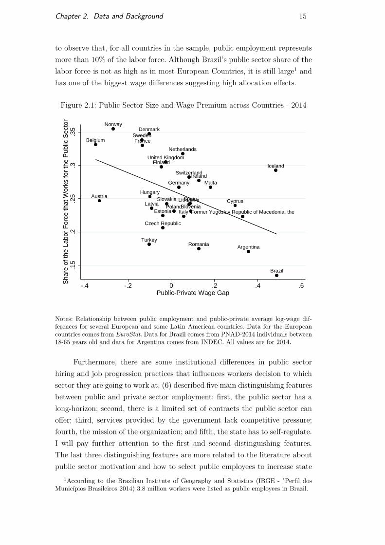
Public sector workers are a large part of the labor market in mostcountries, but public-private wage differences vary a lot between them. Figure2.1 presents public sector employment as a share of the labor market andaverage log-wage differences for a number of European and Latin Americancountries in 2014. The data for the European countries was collected atEuroStat, for Brazil at PNAD and for Argentina at INDEC. It is possible
Chapter 2. Data and Background 15
to observe that, for all countries in the sample, public employment representsmore than 10% of the labor force. Although Brazil’s public sector share of thelabor force is not as high as in most European Countries, it is still large1 andhas one of the biggest wage differences suggesting high allocation effects.
Figure 2.1: Public Sector Size and Wage Premium across Countries - 2014
Brazil
Belgium
Czech Republic
Denmark
Germany
Estonia
Ireland
Spain
France
Italy
CyprusLatviaLithuania
Hungary
Malta
Netherlands
Austria
Poland
Romania
SloveniaSlovakia
Finland
Sweden
United Kingdom
Iceland
Norway
Switzerland
Former Yugoslav Republic of Macedonia, the
TurkeyArgentina
.15
.2.2
5.3
.35
Sha
re o
f the
Lab
or F
orce
that
Wor
ks fo
r th
e P
ublic
Sec
tor
-.4 -.2 0 .2 .4 .6Public-Private Wage Gap
Notes: Relationship between public employment and public-private average log-wage dif-ferences for several European and some Latin American countries. Data for the Europeancountries comes from EuroStat. Data for Brazil comes from PNAD-2014 individuals between18-65 years old and data for Argentina comes from INDEC. All values are for 2014.
Furthermore, there are some institutional differences in public sectorhiring and job progression practices that influences workers decision to whichsector they are going to work at. (6) described five main distinguishing featuresbetween public and private sector employment: first, the public sector has along-horizon; second, there is a limited set of contracts the public sector canoffer; third, services provided by the government lack competitive pressure;fourth, the mission of the organization; and fifth, the state has to self-regulate.I will pay further attention to the first and second distinguishing features.The last three distinguishing features are more related to the literature aboutpublic sector motivation and how to select public employees to increase state
1According to the Brazilian Institute of Geography and Statistics (IBGE - "Perfil dosMunicípios Brasileiros 2014) 3.8 million workers were listed as public employees in Brazil.

Chapter 2. Data and Background 16
efficiency2. The focus of this article is on how these distinguishing featuresaffect workers sector decision influencing the allocation of skills in the privatesector.
First, the public sector has a long horizon, which means that it can makelong term promises to its employees. This is why, in most countries, publicworkers have good pensions and job security. For instance, several Europeancountries offer life-time tenure for public employees, such as Germany, France,Italy and Spain3. This is also the case for Brazilian public sector workers.This countries also have preferential pensions schemes for public employeesthat guarantees much better retirements than for private sector workers. Inaddition, in most of this countries public sector workers follow clear careerpaths once they enter the public sector. The combination of all of theseinstitutions makes public sector wages much more certain than private sectorones.
To illustrate this point, figure 2.2 shows current job tenure in years (yearsworking at the current job) by age and sector. Public sector (dashed line)workers are working longer at the same job than private sector (solid line) ones.This is consistent with the fact that public sector workers have job securityand, therefore, the older they are the longer they are working at the publicsector. On the other hand, if a private sector firm faces an economic shock inthe private sector it can adjust wages and labor demand accordingly.
One consequence of this feature is that there is little transition betweensectors. Since, PNAD is a series of cross-sections we could not use this datato calculate the transition matrix between sectors. For this statistic we usedPNAD-contínua (2012-4), which is also a representative sample of the Brazilianpopulation that follows a household for three quarters and then performsanother follow-up interview four quarters after the third quarter. Similarly,we restricted the sample to individuals between 18 and 40 years old that arecurrently working and not in school. Table 2.2 shows the transition matrixbetween sectors using this data. It is possible to observe that more than 78%of public sector workers younger than 30 years old do not change sectors in thenext period. Furthermore, for workers older than 30 years this probability islarger than 85%. Indicating that most of public sector workers once that havechosen to work at the public sector stay there permanently.
The second main difference between public and private sectors is thatthere is a limited set of contracts that the public sector can offer to its em-
2For more on public sector motivation and the allocation of workers inside the publicsector see (17) and (19)
3Most of the information about public sector institutions in European countries is from(5)

Chapter 2. Data and Background 17
Figure 2.2: Job Tenure by Sector - Smoothed
05
10A
vera
ge Y
ears
At J
ob
20 25 30 35 40Age
Private Public
Notes: Current job tenure by age and sector smoothed. Data is from PNAD-IBGE (2014),only individuals between 18 and 40 years old that are currently working.
Table 2.2: Public - Private Transition Matrix
Sector in t-1Public Private
Public Sector in tYounger than 30 0.781 0.012
(0.002) (0.000)Older than 30 0.856 0.015
(0.001) (0.000)
Notes: Proportion of workers that worker at the public sector by age and which sector theycome from. Data is from PNAD-contínua 2012-2014, only individuals between 18 and 40years old that are not currently in school.
ployees. To detach public hiring, firing and promotion decisions from the po-litical process, countries have rigid public employment rules. For instance, inmany countries public sector hiring is made through open exams which arehighly correlated with formal education, this is the case for France, Italy andSpain and also for Brazil. Moreover, in those countries the government setsclear career paths that determine employee’s promotion based on education

Chapter 2. Data and Background 18
and experience. This makes public sector wages mostly determined by educa-tion and experience.
Figure 2.3 shows the fit, represented by the R2, of a Mincerian regressionof log-hourly-wages on a dummy if the person is male, a dummy if the personis white, dummies for each year of age and dummies for each year of education,by year and sector. Wages at the public sector (dashed line) are more explainedby observable variables than at the private sector (solid line). This illustratesthe point that public sector wages are more correlated with education andexperience than private sector ones.
Figure 2.3: Fit of a Mincerian Regression by Sector
.25
.3.3
5.4
Sta
ndar
d D
evia
tion
Min
ceria
n R
esid
uals
2006 2008 2010 2012 2014Year
Private Public
Notes: R2 of a Mincerian regression of log-hourly-wages on a dummy if the person is male,a dummy if the person is white, dummies for each year of age and dummies for each yearof education, by year and sector. Data is from PNAD-IBGE (2002-2014), only individualsbetween 18 and 40 years old that are currently working.
Furthermore, this rigidity in public sector employment decision allows itlittle flexibility to respond to fluctuations of labor supply. If the governmentwants to hire more public employees it has to open a public hiring exam,announce it in the Official State Newspaper with months in advance. Moreover,it has to be on that year’s government budget which is approved by Congress.All of this process can take months or even years, that’s why we will supposethat public labor demand is determined exogenously. This is also true for public

Chapter 2. Data and Background 19
sector wages, increases in public employees wages must also be approved byCongress in a process that could take months. Therefore, public sector wagesdo not adjust to promote market clearing at the public sector labor market.
Since public sector wages are exogenously determined, they do not followthe one price rule, in other words, similar individuals may face different wagesin each sector. This, in combination with public sector wages being morecorrelated with observable variables than unobservable ones, creates interestingpublic-private wage differentials that may influence individuals sector decision.To estimate how the public-private wage differences varies along the wagedistribution, we estimated the following quantile regression, with Qw(τ |x, pub)being the τth quantile of the wage distribution conditional in a set of controls(x) and a dummy if the person works for the public sector (pub):
Qw(τ |x, p) = α(τ) + β(τ)pub+ θ(τ)x (2-1)
Figure 2.4 shows the β(τ) coefficient of this quantile regression for eachquantile. We use as controls a dummy if the person is male, a dummy if theperson is white, dummies for each year of age and dummies for each year ofeducation. It shows the large heterogeneity of public-private wage differentialsacross the wage distribution.
This figure does not show the relative wages individuals actually face,because it does not include a series of unobserved characteristics such as skillsand risk aversion. Nevertheless, it still provides suggestive evidence of thetrade-offs some individuals face when deciding which sector to work for. Firstnotice that individuals without College degree (dashed line) face a greaterheterogeneity of wage differentials across the wage distribution than individualswith a College degree (solid line). This can be explained by the fact that publicsector wages are more correlated with education than private ones. In privatesector firms, individuals with no College degree, but high skills, may get highwages. However, in the public sector even high-skills individuals do not gethigh-wages without a College degree. Therefore, the public-private wage gapis very high at the beginning of the wage distribution, but it becomes negativeat the end of the wage distribution, for individuals without College.
Wage differentials for workers with a College degree follow a similarpattern, decreasing on the quantiles, but with a smaller inclination. Moreover,for most quantiles, the public-private wage gap is greater for workers withCollege than for workers without College. This suggests that the trade-offsindividuals face when choosing a sector are also correlated with education andunobserved skills. Nevertheless, this estimation does not account for individualsspecific risk aversion. Some individuals may work at the public sector even

Chapter 2. Data and Background 20
Figure 2.4: Public-Private Wage Gap Using Quantile Regression
-.2
-.1
0.1
.2.3
Pub
lic-P
rivat
e W
age
Gap
0 20 40 60 80 100Quantiles
College No College
Notes: Coefficient of a dummy if an individual works at the public sector of a quantileregression of log-hourly-wages on a dummy if the person is male, a dummy if the person iswhite, dummies for each year of age and dummies for each year of education, by educationand sector. Data is from PNAD-IBGE (2014), only individuals between 18 and 40 years oldthat are currently working.
with a negative public-private wage gap, because public sector wages are morecertain than private sector ones. Therefore, to consistently estimate the public-private wage premium we would need to account for this two unobservedvariables, skills and risk aversion.
There is a large literature studying the public private wage gap for severalcountries, but most of the evidence is not causal. (21) study the public-privatewage gap in France using quantile regression in a panel dataset with individualfixed effects and find a positive wage premium in the beginning of the wagedistribution, and a negative for the end of the distribution, both for men andwomen. (22) do a similar study for Brazil, but not using worker fixed effects,and find a positive public-private wage gap at low percentiles of the distributionand negative at the high percentiles. (23) also uses quantile decomposition,this time for several European countries4 and find similar results with positivepremium at the mean for all countries and decreasing premium along quantiles.Overall, those articles show evidence in line with our estimations shown in
4Austria, Belgium, Germany, Spain, France, Greece, Ireland, Italy, Portugal and Slovenia.

Chapter 2. Data and Background 21
figure 2.4, even after controlling for unobserved heterogeneity using fixedeffects.
Furthermore, there are some papers that estimate the average publicwage premium and across education and experience groups. (5) studies thepublic-private premium for several Europeans countries5, but this time ac-counting for lifetime earnings and find a positive premium for all countries.For Brazil, (24) studies the public wage premium by education in 2005 andfind a public-private wage gap decreasing with years of schooling. However,(8) estimates the public wage premium for Brazil using the privatization ofsome State owned companies at the end of the 1990’s as an exogenous shockand find it positive and increasing with years of schooling. Their estimationscontrol for both observed and unobserved heterogeneity, because they are ableto observe the same individual before and after the privatization.
5Germany, Netherlands, France, Italy and Spain.

3The Model
3.1Set Up
The model is a two-sector equilibrium static Roy model, where individu-als must choose between public and private sector jobs. Besides demographiccharacteristics, which are observed by the econometrician, workers are hete-rogeneous in two unobserved variables their skills and risk aversion. Publicsector wages are certain and a function of these demographic characteristics,while private sector wages are uncertain and a function of skills. Therefore,each individual faces different trade-offs when deciding which sector to workat, depending on their skills, demographic characteristics and risk aversion.The private sector labor demand makes a clear distinction between skills andtasks. Changes in the public sector may affect the distribution of skills availa-ble to the private sector through workers sector decision. The skill distributionavailable to the private sector affects the matching function between skills andtasks having consequences on wages and productivity.
There is a continuum of workers of size one, with a finite discrete setof skills s = 1, ..., S and a continuous and unbounded set of risk aversionsβ ∈ [0,+∞). Skills and risk aversion are independent and known by the workerand private sector firms, but not observed by the econometrician and thepublic sector. There is a set of discrete and finite characteristics e = 1, ..., E,such as education, that are jointly distributed with skills by P (s, e)1, suchcharacteristics are common knowledge. Because the public sector has rigidhiring and promotion rules, public sector wages and labor demand depend onthese observable characteristics (e). On the other hand, private sector wagesand labor demand are a function of skills (s).
We can interpret e as a proxy for skills. Education decisions here aretaken as exogenous to simplify the analysis. However, those with higher skillsmay self-select into higher education. To control for this factor we allow for anon parametric specification of the joint distribution of skills and demographic
1One possible extension is to set skills as continuous, in this case each e will have adifferent skill distribution. In the model developed by (12) skills are continuous.

Chapter 3. The Model 23
characteristics. Therefore, in this case skill can be something that is acquiredthrough education and it is not necessarily an intrinsic characteristic, but someindividuals may also never be able to reach some skill types. Another issue withtaking education decisions as exogenous is that individuals may choose to staymore years in school with the objective of applying to a public job. Althoughthis may be true, when an individual decides to earn another degree she doesnot know what will be the size and wages of the public sector when she finishesit. Since the individual can not predict public sector wages and employmentat their graduation, they do not influence education decision.
Even though dynamics is an important factor on an individuals’ decisionto work at the public sector, the model is static for simplicity. Our objectiveis to model skill allocation and its effects on productivity and inequality, notnecessarily to examine dynamic choices. There are two possible interpretationsof the model that explains its static nature. First, that when the individualchooses sector she makes a permanent decision taking into account her lifetimeearnings in each sector. Second, that each period the worker chooses whichsector she is going to work for, taking into account wages at both sectors atthis period.
The model does not account for the extensive margin, in other words,individuals cannot choose if they will participate in the labor market. Oneinterpretation is that individuals must work and cannot choose to stay outof the labor market. Another interpretation is that we are modeling thedecisions of the subpopulation that have already chosen to participate in thelabor market. However, this is an issue if the decision to participate dependson individuals skill and observable characteristic through public or privatereturns. Appendix A discusses a model extension that includes the decision toparticipate in the labor market and its consequences to our results.
We do not account for public sector production, since our objectiveis to analyze the effects on private sector production. To rationalize it thepublic sector can be seen as an unproductive or rent-seeking activity. Anotherpossibility is that public workers produces a public good that is a lump-sumtransfer to workers. Therefore, this public good does not influence workerssector decision, but increases their welfare. In this interpretation a reductionon the size of the public sector reduces workers welfare through the publicgood. Appendix B discusses a possible extension that includes this lump-sumtransfer.
3.2

Chapter 3. The Model 24
Labor Supply
We assume that individuals consume everything they earn, therefore,their utility depends only on wages. Bernoulli utility is u(w|β), where β is therisk aversion parameter which is specific to each individual and distributedaccording to G(β). Individuals know their risk aversion parameter, but theeconometrician does not observe it. We assume that everyone is risk averse,but they differ in their intensities (β ≥ 0)2.
Wages in the public sector are a function of observable characteristicse, while wages in the private sector are a function of skills s. This capturesthe fact, discussed earlier, that wages at the public sector are more rigid tobe exempt from political influence, thus public sector hiring is made throughexams that are highly correlated with formal education and promotion is duemostly to experience and education. On the other hand, the private sector canhave a more flexible hiring and promotion process being able to identify theskill of the worker. In other words, the public sector knows only observablecharacteristics of the worker (e), while the private sector can observe skills(s). Public sector wages are certain, because the public sector can make long-term promises to its employees such as job security and clear career paths.Private sector wages are uncertain, since private sector firms are subject toproductivity shocks and can adjust wages and/or employment accordingly.The determination of private sector wages will be explained in subsection 3.3,but it is influenced mostly by the distribution of skills available to the privatesector.
Since public sector labor demand and wages are exogenous, there maybe more people applying to public jobs than there are job openings. Therefore,there must exist a selection rule that chooses which of the workers that appliedwill be hired. Once an individual chooses to work in the public sector there isa probability b(e)τs that she will be accepted to work there. With probability(1− b(e)τs) she is not accepted and her wage is zero. This probability dependson how many individuals with the same observable characteristics are applying,through b(e), but also accounts for the fact that individuals with higher skillhave a higher probability of being accepted (τs′ > τs ⇔ s′ > s). For instance,Brazilian public sector selection uses exams, in this case τs represents the factthat individuals with higher skill do better on these exams.
If we interpret sector decision as a lifetime decision, this probability canbe seen as a cost of entering after choosing the public sector. In Brazil’s case,this cost could be rationalized as the number of months that the worker will
2This hypothesis is not necessary to close the model and can be relaxed, but it is herefor computational purposes.

Chapter 3. The Model 25
be without wage, due to exam preparations. On the other hand, if the decisionis made every period it is the probability that the worker will get a publicservice position if she chooses the public sector this period, in the case she doesnot get hired her wage will be zero for this period. Notice that this attachessome uncertainty to the public sector choice, but this uncertainty depends onindividuals’ skill level. To sum up, the utility of a worker who chooses thepublic or private sector is respectively:
Ub(s, e) = b(e)τsu(wb(e)|β) (3-1)
Ur(s) = E[u(wr(s)|β)|s, β] (3-2)
The proportion of workers with skill s and observable characteristic e whochoose the private sector is:
Pr(s, e) = P [Ub(s, e) < Ur(s)|s, e] (3-3)
In other words, this is the probability that if we select a worker at randomin the population her private sector expected utility (Ur(s)) is higher than herpublic sector one (Ub(s, e)). Notice that workers, when deciding which sectorto work, must account not only for average wages for her skill level, but alsofor uncertain private sector wages and the probability of being selected to workfor the public sector.
3.3Labor Demand
Private sector labor demand is based on the models developed by (12) and(11), which draw a clear distinction between skills and tasks. The private sectorproduces one final good using a continuum of tasks of size one (t ∈ [0, 1]). Theidea is that tasks produce output and workers are hired to perform such tasksand specific worker’s skills have comparative advantage to perform specifictasks. Firm’s problem in the private sector yields a matching function fromskills to tasks.
The private sector is subject to a productivity shock v, that is distributedaccording to F (v) with E(v) = 0. This productivity shock creates uncertaintyin private sector wages. Since the model is static, this productivity shock can beinterpreted as the effect of many shocks that will happen throughout worker’slifetime, if we interpret sector decision as a permanent decision made whenyoung. Another explanation, is that the worker may face a transitory shock ifshe chooses the private sector in that period. The production function of thefinal good is a C.E.S. aggregation of the different tasks (y(t)), where A is a

Chapter 3. The Model 26
productivity increasing parameter.
Y = A · v ·[∫ 1
0y(t)
η−1η dt
] ηη−1
(3-4)The production of each task uses only labor and different skills are
perfect substitutes in the production of tasks. However, each skill has its ownproductivity in producing each task, represented by the function B(s, t). Thedemand for skill s to produce task t is L(s, t) and determined endogenously inthe model.
y(t) =S∑s=1
B(s, t)L(s, t) (3-5)
The final good firm, which is a representative firm, chooses the demandfor tasks and the task producers choose labor demand for their specific task.In this case, p(t) is the task price and wr(s) are the equilibrium wages. Theproblems of the final good producer and the task producer are respectively thefollowing:
Maxy(t)
A · v ·[∫ 1
0y(t)
η−1η dt
] ηη−1−∫ 1
0p(t)y(t)dt (3-6)
Max{L(s,t)}s
p(t) ·S∑s=1
B(s, t)L(s, t)−S∑s=1
wr(s)L(s, t) (3-7)
We can interpret tasks as intermediate goods, that are aggregated toproduce the final good. However, another, more general interpretation is tosee tasks as a work activity that produces output3. Under this interpretationtasks are not necessarily intermediate goods, but what workers actually doto produce the final good. For instance, some workers are hired to clean thefirm, others are hired to operate machines while some are hired to develop theline of production. The main advantage of this framework is that workers withdifferent skills can produce all tasks and the mapping between skills and tasksdepends on market conditions. Therefore, if the supply of high skill workersdecreases the firm will hire some middle skill workers to develop the line ofproduction, but this middle skill workers will be less productive to do thistask than high-skill workers. The framework where labor demand for each skillappears directly in the production function of the final good producer is aspecial case of this model in which there is a one-to-one mapping betweenskills and tasks.
Notice that wages can only vary across skills, but not tasks, because ofthe law of one price. If the same skill has two possible wages everyone wouldchoose to do the task with the higher wage and in equilibrium the wages will bethe same. Skill specific productivity function B(s, t) resumes the comparative
3This interpretation comes from (11).

Chapter 3. The Model 27
advantage each skill has to produce specific tasks. Task skill intensity growswith t, hence tasks defined by smaller t are less skill intense than tasks definedby higher t. We assume workers with low skill have comparative advantage todo less intensive tasks, and vice-versa, which is the same as saying that B(s, t)is log-supermodular:
Assumption 3.1 B(s′, t′)B(s′, t) ≥ B(s, t′)B(s, t), ∀ s′ > s and t′ > t.
Which implicates that there is positive assortative matching between skillsand tasks in equilibrium. Under this assumption private sector labor demandis determined by the following lemma4:
Lemma 3.2 ∃{Ts}Ss=0 | Ts ∈ [0, 1] ∀s , TS = 1 e T0 = 0, such that,∀t ∈ [Th−1, Th], L(h, t) > 0 e L(s, t) = 0 ∀s 6= h
In other words, there is a sequence of thresholds {Ts}Ss=0 that determinewhich tasks each skill is going to be demanded to perform. This sequence ofthresholds is a matching function that links skills to tasks, which represents theallocation of skills to tasks. It is determined by market clearing and dependson the skill distribution available to the private sector.
To close the model it is necessary to assume that, at the thresholds, bothskill types are equally profitable, given the market wages and prices.
p(Ts) ·B(s, Ts) · L(s, Ts)− wr(s) · L(s, Ts) =
p(Ts) ·B(s+ 1, Ts) · L(s+ 1, Ts)− wr(s+ 1) · L(s+ 1, Ts)(3-8)
Which implies that:
L(s, Ts)L(s+ 1, Ts)
= wr(s+ 1)wr(s)
= B(s+ 1, Ts)B(s, Ts)
(3-9)
Therefore market clearing wages must be equal to the ratio of compa-rative advantage at the thresholds to exist an equilibrium. The first ordercondition of the final good producer is:
y(t) = Y · (A · v)η−1
p(t)η ⇒∫ 1
0p(t)1−ηdt = (A · v)1−η (3-10)
Wages are equal to the marginal productivity of labor, wr(s) = p(t) · B(s, t).Combining this with the arbitrage condition 3-9 and the first order conditionof the final good 3-10 we can calculate wages as a function of the thresholds.The labor demand for each skill is:
lr(s) =∫ Ts
Ts−1L(s, t)dt with L(s, t) = H · (A · v)ηB(s, t)η−1
wr(s)η(3-11)
4demonstration follows (11).
Chapter 3. The Model 28
Where H =[∫ 1
0 y(t)η−1η dt
] ηη−1
is the average product of the private sectordiscounting the effects of productivity parameter A.
Public sector demands workers exogenously based on observable charac-teristics, where lb(e) ∈ [0, 1] is the public sector labor demand for worker cha-racteristic e and wb(e) is the public sector wage also determined exogenously.This captures the fact that variations on public labor demand and wages hasto go through bureaucratic issues that does not allow them to respond imme-diately to market movements.
3.4Equilibrium
Public sector labor demand depends on observable characteristics (e)and private sector labor demand depends on skills (s). Therefore, we definethe public and private labor supply as:
Pb(e) =S∑s=1
(1− Pr(s, e)) · P (s, e) (3-12)
Pr(s) =E∑e=1
Pr(s, e)P (s, e) (3-13)
In equilibrium public and private labor markets clear, Pb(e) = lb(e),∀e =1, ..., E and Pr(s) = lr(s),∀s = 1, ..., S. Notice that while private sector marketclearing depends on skills public sector depends on observable characteristics.This generates different public-private wage gaps for individuals with the sameobservable characteristic. Lastly, equilibrium can be defined as:
Definition 3.3 (Equilibrium) Equilibrium is a sequence of thresholds{Ts}Ss=0, a private sector average product H and a vector of probabilities ofbeing accepted to work at the public sector b(e) such that private sector andpublic sector labor markets clear (Pb(e) = lb(e) and Pr(s) = lr(s)).
Since private sector wages depend on skills, even individuals with thesame demographic characteristics face different trade-offs when choosing asector. Therefore changes in public employment for specific demographicgroups have different effects on the private sector distribution of skills and,hence, on productivity and wages. Even aggregate changes in public hiring havedifferent consequences for each demographic group. This generates interestinginterdependencies between skills and observable characteristics that will befurther explored when we conduct counter-factual exercises.
4Estimation and Identification
4.1Functional Forms
In order to be able to estimate the model we are going to assume somefunctional forms. The functions described in the model that need parametricassumptions are: the Bernoulli utility u(w|β); the distribution of risk aversionG(β); the distribution of the productivity shock F (v); and the function thatdefines the skill comparative advantage B(s, t)1.
First we assume that Bernoulli utility has a C.R.R.A. form u(w|β) =w1−β, thus the individuals with high risk-aversion have higher β. Which me-ans that individuals have decreasing absolute risk aversion, in other words,with this utility function workers accept more risk if the premium is higher. Inaddition, we assume that the distribution of risk aversion follows a Weibull dis-tribution with shape parameter k and scale parameter λ (β ∼Weibull(k, λ)).The main reason for choosing this distribution is that it is very flexible.
Finally, we assume that the distribution of the productivity shock is log-normal (v ∼ lognormal(0, σ2)). This implies that the distribution of wages foreach skill is also log-normal, as it is consensus in the literature. Furthermore,we assume that skill comparative advantage is exponential B(s, t) = exp(δst),which implies that wages for each skill has also an exponential form. Theparameter δs resumes the comparative advantage and assumption 3.1 impliesthat δs′ > δs, ∀s′ > s.
The parameters of the model to be estimated are the skill specificcomparative advantage (δs), public selection advantage (τs), the elasticity ofthe private sector C.E.S. production function (η), the productivity parameter(A), the variance of the economic shock (σ2), the parameters that define thedistribution of risk aversion (k, λ) and skill distribution (P (s|e)). Moreover,the endogenous variables are the probabilities of being selected to work atthe public sector (b(e)), the task thresholds (Ts) and the average productdiscounting the effect of the productivity parameter (H).
1Some of these functional hypotheses can be relaxed in further versions.

Chapter 4. Estimation and Identification 30
4.2Estimation Method
We use a two stage estimator. First, we estimate private sector supplyand average wages for each skill. In the first stage we also estimate the jointdistribution of skills and observable characteristics in the private sector, thedistribution of observable characteristics in the public sector and public sectoraverage wages for each demographic characteristic. Then, in the second stage,we use those moments to estimate the parameters of the model.
4.2.1First Stage
First, notice that the model implies that the distribution of wages in theprivate sector (f(log(w)|r)) is a finite mixture of normal distributions withsame variance.
f(log(wi)|r) =S∑s=1
P (s|r)φ(
log(w)− log(ωr(s))σ2
),
with log(ωr(s)) = E[log(wr(s))|s](4-1)
Using maximum likelihood we can estimate the private sector distribution ofskills P (s|r), the variance of the productivity shock σ2 and average wages ofeach skill log(ωr(s)). To maximize the likelihood function we use the E.M.algorithm as it is described in (25), chapter 2. The E.M. algorithm formulatesthe finite mixture estimation as a missing variable problem, in other words, weobserve wages but we do not observe which skill each individual belongs to.Furthermore, the E.M. algorithm has two steps: the E-Step and the M-Step.The E-Step takes an initial guess of parameters (P0(s|r), σ2
0, log(ωr(s)0)) andestimates for each observation the posterior probability that this observationis of skill s:
P0(i ∈ s) =P0(s|r)φ
(log(wi)−log(ωr(s)0)
σ20
)∑Sh=1 P0(h|r)φ
(log(wi)−log(ωr(h)0)
σ20
) (4-2)
Then the M-Step maximizes the following function obtaining a new set ofguesses:
(σ21, log(ωr(s)1)) = argmax
σ2,log(ωr(s))
n∑i=1
S∑s=1
P0(i ∈ s)φ(
log(w)− log(ωr(s))σ2
)
P1(s|r) =n∑i=1
P0(i ∈ s)(4-3)
The algorithm iterates the E-Step and then the M-Step until the likelihoodfunction converges.

Chapter 4. Estimation and Identification 31
To estimate the number of skills (S), we maximize the likelihood functionfor all the possible number of skills (S) where the model is still identified - inthe next subsection we will describe this set - and choose the one with thelowest B.I.C. information criterion. In addition, the application of the E.M.estimator gives us the optimal posterior probability that each observation isof skill s (P∞(i ∈ s)). Taking the averages of this posterior probabilities allowsus to estimate P (s|e, r). Therefore, using the E.M. estimator to maximize thelikelihood function of the private sector distribution of wages, we estimatethe distribution of skills in the private sector P (s|r) and across demographicgroups P (s|r, e), the number of skills S, average private sector wages for eachskill log(ωr(s)) and the variance of the productivity shock σ2.
Furthermore, in the first stage we also estimate moments that define thelabor market in the public sector. In particular, we estimate the proportionof individuals of each demographic characteristic in the public sector (P (e|b))and the proportion of individuals that choose the private sector and belongsto skill s, given observed characteristic e (P (s, r|e) = P (s|e, r) ∗ P (r|e)). Inaddition, we estimate the proportion of workers that choose the private sectorand belongs to skill s (P (s, r) = P (s|r)∗P (r)). We also estimate average publicsector wages for each demographic characteristic (wb(e)) and the distributionof observable characteristics (P (e)) that are exogenous variables of the model.
4.2.2Second Stage
In the second stage we use the moments estimated in the first stageto calculate parameters and endogenous variables of the model. In otherwords, we have a vector of moments estimated in the first stage (m) andtheir model counterparts (m(θ, y)) that are a function of the parameters(θ) and endogenous variables (y). We use a minimum distance estimator toapproximate those vectors, solving the following problem2:
(θ, y) = argminθ,y
(m−m(θ, y))′W (m−m(θ, y)) (4-4)
Where,m = ( ˆP (s, r), log(ωr(s)), ˆP (s, r|e), ˆP (e|b)) (4-5)
We assume that the data represents an equilibrium. Furthermore, marketclearing for public and private labor markets is a linear transformation of vectorm. First, in the private sector we use the market clearing condition to directlyas a moment P (s, r) = lr(s). Then, in the public sector, market clearing is a
2In this version we assume that W is an identity matrix, but in later versions we willestimate using a more efficient weight matrix.

Chapter 4. Estimation and Identification 32
linear combination of P (s, r|e) and the exogenous variable P (e):
P (b, e) =[1−
S∑s=1
P (s, r|e)]P (e) = lb(e) (4-6)
Thus, because market clearing conditions are used during the estimationprocedure, we are able to estimate both the parameters and endogenousvariables of the model.
The vector of model counterparts is:
m(θ, y) = (lr(s), log(ωr(s)), P (r|s, e), lb(e)/P (b)) (4-7)
First, in the labor demand side lr(s) and log(ωr(s)) are the following functions:
lr(s) = H
ωr(s)η∫ Ts
Ts−1exp(δst(η − 1))dt ,∀ s = 1, ..., S (4-8)
log(ωr(s))− log(ωr(1)) =s∑
h=2(δh − δh−1)Th−1 ,∀ s = 2, ..., S (4-9)
ωr(1) = A
S∑s=1
exp(
s∑h=2
(δh − δh−1)Th−1
)1−η ∫ Ts
Ts−1exp(δst)η−1dt
1η−1
(4-10)
To allow identification we will calibrate the CES parameter of the privatesector production function η = 1.4 and will set δ1 = 1. The elasticity ofsubstitution of the private sector production function (η) follows the consensuson the literature of wage inequality and skill premium (see for example (26) and(27))3. The interpretation of the comparative advantage parameter (δs) is nowalways relative to the first skill. This allows us to estimate all the parameters ofthe private sector labor demand δ2, ..., δS and A, and the endogenous variablesof the labor demand side T1, ..., TS−1 and H.
On the supply side of the model, P (r|s, e) = F (τs, b(e), k, λ|wb(e), ωr(s), σ2)where k and λ are, respectively, the shape and scale parameters of the Weibulldistribution. Furthermore,
P (e|b) =
[1−∑S
s=1 P (r|s, e)P (s|e)]P (e)∑E
e=1
[1−∑S
s=1 P (r|s, e)P (s|e)]P (e)
= P (e, b)P (b) (4-11)
In other words, to estimate the distribution of skills along with the parametersof the labor supply, we are using the distribution of observable characteristicsinside the public sector and workers sector decision. Therefore, we are able toestimate the parameters of the supply side of the model (τs, k, θ and P (s|e))and the endogenous variables (b(e)).
Notice that the model counter-parts used in the labor demand and labor3Next versions will include robustness checks with other values of the C.E.S. parameter
of the private sector production(η).

Chapter 4. Estimation and Identification 33
supply sides are independent of each other. As a consequence, we can estimatethe parameters and endogenous variables of the labor demand side separatelyfrom the labor supply side. To estimate standard-errors of all parameters andendogenous variables we use non-parametric bootstrap. The bootstrap includesboth estimation stages and uses the same number of skills for all bootstrapsamples. To calculate standard errors we draw 50 bootstrap samples of thedata.
4.3Identification
In the first stage, identification of the distribution of skills in the privatesector comes primarily from parametric assumptions on the distribution ofprivate sector wages. In other words, we are able to identify the distributionof skills in the private sector because we assume that it is a finite mixtureof normal distributions with the same variance. In the second stage, thedistinction between labor demand and labor supply comes from the fact thatwe estimate private sector labor demand, depending only on skill, while onthe supply side we estimate public sector labor supply that needs a set ofobservable characteristics.
On the labor demand side we need to estimate 2S + 2 parameters andvariables (δ1, ..., δS, η, A, T1, ..., TS−1, H), with 2S equations (lr(1), ...,lr(S), log(ωr(1)), ..., log(ωr(S))). Therefore, the labor demand side is identifiedbecause we calibrate the C.E.S. parameter of the private sector production andwe set the comparative advantage parameter of the first skill equal to one. Onthe other hand, in the labor supply side we have SE+E equations (P (s, e, r),P (e|b)) to estimate SE + S + 2 parameters and endogenous variables (P (s|e),τs, b(e), k, λ). Therefore, we need E ≥ S + 2 to identify the supply sideof the model. It is the set of observable characteristics, combined with theestimation of the distribution of skills and observable characteristics at theprivate sector that allows the estimation of a non-parametric distribution ofskills and observable characteristics.

5Results
5.1Estimation Results
The estimated parameters, with bootstrap standard errors, are shown intable 5.1. First and second rows show private sector comparative advantagein production (δs) and access to public jobs advantage (τs) for each skill,respectively.
Table 5.1: Estimated Parameters - Skills
s=1 s=2 s=3 s=4 s=5 s=6 s=7δs 1.000 16.660 16.662 16.666 16.678 18.185 20.234
- (0.177) (0.177) (0.177) (0.176) (0.178) (0.186)
τs 116.89 183.83 242.35 259.67 303.62 541.24 545.32( 2.986) ( 8.409) ( 8.481) ( 8.738) (23.448) (18.138) (96.184)
Notes: Bootstraped standard erros in parenthesis.
Individuals with the lowest skill (s = 1) have a very strong comparativedisadvantage in private sector production relative to other skills. Moreover,skills 2 through 5 comparative advantage is very close in magnitude, andtheir differences is not statistically significant. However, the difference betweenskills five, six and seven is significant. Therefore, skills can be divided intofour groups regarding their comparative advantage parameter in private sectorproduction (δs): the first one composed only of skill one, a second group withskills 2 through 5, the third and forth groups composed of skills six and sevenrespectively1.
Even though private sector production comparative advantage is verysimilar from skill 2 to 5, access to public jobs advantage is quite different.Only the difference between skills four and five and the difference betweenskills six and seven are not statistically significant. Moreover, skills 6 and 7
1Albeit the private sector production comparative advantage parameter can be dividedinto four statistically different groups, the number of skills was optimally estimated.

Chapter 5. Results 35
have a very strong advantage when compared to other skills. Similar with theprivate sector production comparative advantage parameter, skill 1 has a verystrong comparative disadvantage in access to public jobs. This pattern of accessto public jobs advantage strongly favors high-skill individuals, and generatesa high proportion of skills six and seven working for the public sector.
Table 5.2: Estimated Parameters - Distributions
k λ σ2
0.389 18.10 0.221(0.1060) (0.297) (0.002)
Notes: Bootstraped standard erros in parenthesis.
Table 5.2 shows the parameters of the distribution os risk aversion (k, λ)and the variance of the economic shock (σ2). The parameters that define thedistribution of risk aversion imply that most of the population is concentratedat a risk aversion parameter (β) close to one, which would imply a log utility.However, since the shape parameter is very small, the distribution has heavytails with some individuals having a very high risk aversion. Figure 5.1 showsthe estimated distribution of risk aversion and illustrates this point. Thevertical lines represent the median and the 90th percentile respectively. Theseresults are consistent with the literature that estimates risk aversion based oninsurance choices and find that the distribution of risk aversion is concentratednear risk neutrality, but has a high dispersion2
Figure 5.1: Distribution of Risk Aversion
0.00
0.02
0.04
0 50 100 150 200
beta
Den
sity
Notes: Estimated distribution of risk aversion p.d.f.. Vertical lines indicate the median andthe 90th percentile.
2See for example (7) and (28).

Chapter 5. Results 36
The variance of the economic shock (σ2) is 0.22 which is smaller than theobserved variance of log-hourly-wages for all demographic groups (accordingto table 2.1). Moreover, it is higher than what was estimated previously in theliterature, (29, 30, 31) estimate a variance of the transitory shock on incomesmaller than 0.1 for the U.S.. However, those papers are able to consistentlyseparate the transitory and the permanent component of income shocks. Sinceour data is series of repeated cross-sections, we are not able to separate thosecomponents of income shocks.
Table 5.3: Distribution of Skills Conditional on Observed Characteristics
s=1 s=2 s=3 s=4 s=5 s=6 s=7younger than 30 yearsHS 0.033 0.220 0.250 0.246 0.210 0.034 0.008drop-outs (0.002) (0.018) (0.019) (0.019) (0.029) (0.078) (0.013)HS 0.013 0.215 0.244 0.241 0.206 0.069 0.011
(0.002) (0.011) (0.011) (0.011) (0.020) (0.044) (0.015)College 0.002 0.187 0.213 0.211 0.183 0.191 0.013drop-outs (0.000) (0.016) (0.015) (0.018) (0.019) (0.070) (0.016)College 0.001 0.127 0.164 0.169 0.156 0.361 0.023
(0.000) (0.004) (0.004) (0.004) (0.005) (0.017) (0.000)Grad- 0.000 0.077 0.094 0.094 0.085 0.589 0.060School (0.000) (0.005) (0.005) (0.005) (0.005) (0.026) (0.026)
older than 30 yearsHS 0.027 0.211 0.240 0.237 0.203 0.071 0.011drop-outs (0.002) (0.019) (0.020) (0.020) (0.033) (0.080) (0.018)HS 0.010 0.190 0.217 0.214 0.186 0.167 0.016
(0.000) (0.007) (0.009) (0.009) (0.000) (0.129) (0.132)College 0.003 0.145 0.165 0.164 0.162 0.330 0.032drop-outs (0.000) (0.006) (0.007) (0.007) (0.007) (0.026) (0.000)College 0.001 0.098 0.119 0.120 0.108 0.505 0.049
(0.000) (0.000) (0.000) (0.000) (0.000) (0.000) (0.000)Grad- 0.001 0.039 0.046 0.046 0.041 0.709 0.119School (0.000) (0.002) (0.002) (0.002) (0.003) (0.035) (0.038)
Notes: Bootstrap standard erros in parenthesis.
Table 5.3 shows the distribution of skills conditional on observed cha-racteristics for the whole population with standard errors in parenthesis. Asexpected, higher skills are concentrated between those with higher educationallevels. Even in the highest educational levels (graduate degree) the proportionof individuals with skill 7 is still very small and most of the individuals of thatgroup are concentrated on skill 6. In addition, even at the highest educational

Chapter 5. Results 37
levels there are still some individuals of skills 1 and 2. This indicates that, eventhough skill here is something that can be acquired through education, thereare still some people that will never be high skill types. Furthermore, workerswith high skill (6 and 7) are also more prevalent among those older than 30years old, which is also the group with a higher share of public employment.This suggests that skill can be something learned through experience.
Table 5.4: Skill types in the private sector
s=1 s=2 s=3 s=4 s=5 s=6 s=7Ts 0.108 0.689 0.801 0.864 0.903 0.970 1.000
(0.000) (0.003) (0.002) (0.002) (0.002) (0.001) (0.000)log(ωr(s)) −0.255 1.436 1.438 1.441 1.451 2.812 4.800
(0.021) (0.002) (0.001) (0.001) (0.001) (0.008) (0.031)P(s|r) 0.016 0.200 0.227 0.224 0.190 0.128 0.011
(0.000) (0.000) (0.000) (0.000) (0.000) (0.000) (0.000)
Notes: Ts are the thresholds that represent factor allocation; log(ωr(s)) are average privatesector log-wages; and P (s|r) is the skill distribution in the private sector. Bootstrap standarderrors in parenthesis.
The variables that define the equilibrium for the private sector areshown in table 5.4. The tasks thresholds Ts indicate a convex matchingfunction of tasks to skills, implicating a very high dispersion of wages. Theskill distribution at the private sector is concentrated on skills 3 and 4,which, combined with the comparative advantage parameter, implicates a highdemand for tasks with middle intensity.
Table 5.5: Probability of Being Accepted to Work at the Public Sector (b(e))
HS drop-outs HS College drop-outs College Grad-Schoolyounger 0.000 0.001 0.001 0.002 0.002
(0.001) (0.001) (0.113) (0.012) (0.012)older 0.000 0.002 0.002 0.002 0.003
(0.001) (0.124) (0.021) (0.004) (0.003)
Notes: b(e) is the probability of being accepted in the public sector, bootstrap standarderrors in parenthesis. First line shows the probability for those younger than 30 years oldand second line for those older than 30.
Table 5.5 shows the probability of being accepted to work at the publicsector for each demographic group. These probabilities are quite small andmost of them are not statistically significant, indicating that the major

Chapter 5. Results 38
factor affecting the probability of being accepted in public employment is theindividuals’ skill level. Table 5.6 shows the skill distribution in the population(row 1), in the private sector (row 2) and in the public sector (row 3) andillustrates this point. The strong comparative advantage in access to publicjobs for skills 6 and 7 generates a skill distribution in the public sector highlyconcentrated among high-skill workers. More than half of public employees areof skills 6 and 7, while those skill types are less than 20% of the workers inthe population. Therefore, the public sector attracts mostly high-skill workersand shifts the distribution of skills in the private sector in the direction of lowskill workers.
Table 5.6: Skill Distribution
s=1 s=2 s=3 s=4 s=5 s=6 s=7P (s) 0.016 0.190 0.218 0.216 0.187 0.156 0.017P (s|r) 0.016 0.200 0.228 0.225 0.191 0.129 0.011P (s|b) 0.012 0.028 0.065 0.073 0.122 0.587 0.112
Notes: Bootstrap standard errors in parenthesis. P (s) is the skill distribution in the wholepopulation, P (s|r) is the skill distribution for private sector workers and P (s|b) is the skilldistribution for public sector workers.
5.2Model Fit
Figures 5.2 and 5.3 show the distribution of private sector wages in thedata and calculated by the model for individuals younger than 30 years oldand older than 30 years old respectively. The model fits well the distributionof wages for the whole population. Notice that to estimate the distribution ofskills we use the distribution of wages in the whole population, not dividing itin demographic groups. These non-targeted moments will be used to evaluatemodel fit. The model fits well the distribution of wages for High-School drop-outs and high-school graduates for both age groups. The fit remains good forCollege drop-outs and College graduates for those younger than 30 years old.However, the fit is not that good for those with graduate school at both skilllevels and for college drop-outs and graduates older than 30 years old.
Table 5.7 shows public sector employment for each observed characteristicin the data and predicted by the model. To guarantee public sector equilibriumthese two variables need to be equal, as is shown in the table. Table 5.8 showsprivate sector log-wages for each demographic group in the data and estimatedby the model and brings similar conclusions to that of figures 5.2 and 5.3.

Chapter 5. Results 39
Figure 5.2: Distribution of wages in the Private Sector - younger than 30 yearsold
All Sample
0.0
0.2
0.4
0.6
−5 0 5
HS drop outs
0.0
0.3
0.6
0.9
−6 −3 0 3 6
HS
0.00
0.25
0.50
0.75
1.00
−4 0 4
College drop outs
0.0
0.2
0.4
0.6
−3 0 3 6
College
0.0
0.2
0.4
0.6
−5 0 5
Grad-School
0.0
0.2
0.4
0.6
−3 0 3 6
Notes: Distribution of wages in the private sector according to PNAD 2011-4 (bars) andestimated private sector distribution of wages (lines) by education.
Table 5.7: Proportion of public sector workers for each observed characteristic
younger than 30 years older than 30 yearsData Model Data Model
HS drop-outs 0.001 0.001 0.003 0.003HS 0.005 0.005 0.012 0.015College drop-outs 0.001 0.001 0.001 0.001College 0.008 0.008 0.024 0.024Grad-School 0.000 0.000 0.002 0.002
Notes: Proportion of public sector workers for each age and education group in the data andestimated by the model. Data from PNAD 2011-4 individuals between 18-40 years old notin school.

Chapter 5. Results 40
Figure 5.3: Distribution of wages in the Private Sector - older than 30 yearsold
All Sample
0.0
0.2
0.4
0.6
−5 0 5
HS drop outs
0.0
0.2
0.4
0.6
0.8
−4 0 4 8
HS
0.0
0.2
0.4
0.6
0.8
−4 0 4 8
College drop outs
0.0
0.2
0.4
0.6
−5.0 −2.5 0.0 2.5 5.0
College
0.0
0.2
0.4
−5 0 5
Grad-School
0.0
0.2
0.4
−5 0 5
Notes: Distribution of wages in the private sector according to PNAD 2011-4 (bars) andestimated private sector distribution of wages (lines) by education.
The model fits better the data for those with less than 30 years and lowereducational levels.
Table 5.9 presents the public-private wage premium calculated by theestimated model (log(wb(e))−
∑Ss=1 log(ωr(s))P (s|e)). The public-private wage
gap increases with education, with the exception of individuals with graduatedegree and younger than 30 years old. This results are consistent with previousestimations of the public-private wage gap. Particularly, (8) estimates thepublic wage premium using the privatization of some state owned companiesas an exogenous shock. Similar to our results, they find that the public wagepremium is bigger for higher educational levels. Nonetheless, their estimationsare slightly bigger than ours, they find that those with College education havea public-private wage gap of 0.544 and those in high-school have a public wagepremium of 0.491.
Chapter 5. Results 41
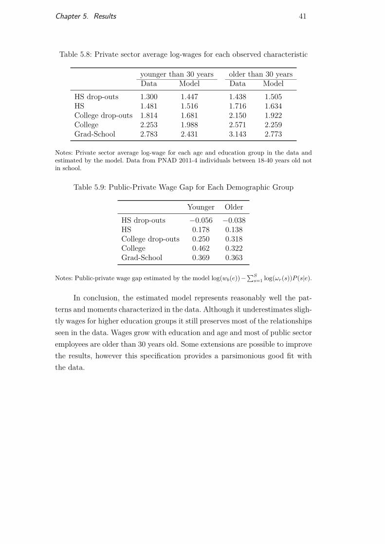
Table 5.8: Private sector average log-wages for each observed characteristic
younger than 30 years older than 30 yearsData Model Data Model
HS drop-outs 1.300 1.447 1.438 1.505HS 1.481 1.516 1.716 1.634College drop-outs 1.814 1.681 2.150 1.922College 2.253 1.988 2.571 2.259Grad-School 2.783 2.431 3.143 2.773
Notes: Private sector average log-wage for each age and education group in the data andestimated by the model. Data from PNAD 2011-4 individuals between 18-40 years old notin school.
Table 5.9: Public-Private Wage Gap for Each Demographic Group
Younger OlderHS drop-outs −0.056 −0.038HS 0.178 0.138College drop-outs 0.250 0.318College 0.462 0.322Grad-School 0.369 0.363
Notes: Public-private wage gap estimated by the model log(wb(e))−∑S
s=1 log(ωr(s))P (s|e).
In conclusion, the estimated model represents reasonably well the pat-terns and moments characterized in the data. Although it underestimates sligh-tly wages for higher education groups it still preserves most of the relationshipsseen in the data. Wages grow with education and age and most of public sectoremployees are older than 30 years old. Some extensions are possible to improvethe results, however this specification provides a parsimonious good fit withthe data.
6Counter-Factual Exercises
This section shows the effects of a reduction in the size of the publicsector, which means reducing the public sector labor demand by the samepercentage for each demographic group1. In our sample the public sectoraccounts for 5.88% of the labor force, if we reduce in 10% the size of thepublic sector it will employ 5.29% of the labor force. Brazil experienced alarge increase in public sector hiring from 2005 until 2014, going back to2005 represents a decrease of 15.64% in the number of public employees.Furthermore, a reduction of 11.30% in the number of public employees wouldmean going back to the size of the public sector in 2007. We will show resultsof a reduction in public sector using this trend observed in the last decade as abenchmark. First we present the effect of reducing the size of the public sectoron the distribution of wages and then on productivity and skill allocation.
6.1Effects on the Distribution of Wages
Figure 6.1 shows the growth in the public-private wage gap. For thoseyounger than 30 years old, a reduction in public labor demand increasesthe public premium for lower education levels (High-School drop-outs andcompleted) and decreases for higher education levels (College drop-outs andcompleted), while for graduate students we do not see any change. Differently,for those older than 30 years old, it is possible to observe a sharp decline in thepublic-private wage differentials for those who completed High-School and arise for High-School drop-outs. Similarly, the wage premium for College drop-outs and individuals who completed College older than 30 years old declinesand nothing happens for grad-students.
Since the only variable in the public sector wage premium that changesis the private sector average wage for each skill, it summarizes the changesin wages for each demographic group not accounting for the change in theskill distribution available to the private sector. On the other hand, figure6.2 shows the growth in average private sector log-wages for each observable
1This exercise will be made for the different demographic groups separately in nextversions.

Chapter 6. Counter-Factual Exercises 43
Figure 6.1: Public Sector Wage Premium
Younger than 30 years old
●
●
●
●
●
●
●
●
●
●
●
●
●
●
●
●
●
●
●●●●●●
●●●●●●
200520052005200520052005200520052005200520052005200520052005200520052005200520052005200520052005200520052005200520052005200720072007200720072007200720072007200720072007200720072007200720072007200720072007200720072007200720072007200720072007200820082008200820082008200820082008200820082008200820082008200820082008200820082008200820082008200820082008200820082008
0.95
1.00
1.05
Baseline 0.9*lb 0.8*lb 0.7*lb 0.6*lb 0.5*lb
● ● ● ● ●HS drop−outs HS College drop−outs College Grad−Schoool
Older than 30 years old●
●●
●●
●
●
●
●
●
●
●
●●●●●● ●●●●●●
●●●●●●
200520052005200520052005200520052005200520052005200520052005200520052005200520052005200520052005200520052005200520052005200720072007200720072007200720072007200720072007200720072007200720072007200720072007200720072007200720072007200720072007200820082008200820082008200820082008200820082008200820082008200820082008200820082008200820082008200820082008200820082008
0.7
0.8
0.9
1.0
Baseline 0.9*lb 0.8*lb 0.7*lb 0.6*lb 0.5*lb
● ● ● ● ●HS drop−outs HS College drop−outs College Grad−Schoool
Notes: Effects of a reduction on the size of the public sector on the public-private wage gaplog(wb(e))−
∑Ss=1 log(ωr(s))P (s|e), for each demographic group in relation to the baseline.
Vertical lines represent the size of the public sector in 2008, 2007 and 2005 respectively inBrazil for our sample.

Chapter 6. Counter-Factual Exercises 44
characteristic taking into account the change in the skill distribution availableto the private sector (∑S
s=1 P (s|r, e)log(ωr(s))). For both age groups High-School drop-outs, those who completed High-School and College drop-outsaverage private sector wages increases, while individuals with a College degreeand Grad-School wages decline or show no movement. This is the opposite ofwhat was observed in the public-sector wage premium. The rise in the public-private wage gap for High-School drop-outs and those who completed High-School would indicate a decline in private sector wages, on the contrary ofwhat we observe. Therefore, changes in the skill distribution available to theprivate sector play a big role on the determination of average wages.
As a result, the effects of a decrease in public sector labor demand onaverage wages for each demographic group are very similar to the proportionof high skill workers in the private sector, in this case we define high skill thoseindividuals with skills 5, 6 and 7. Figure 6.3 shows the proportion of high skillworkers in the private sector for each demographic group. It is similar to logaverage wages in the private sector, with High-School drop-outs, High-Schooland College drop-outs increasing with a reduction on the size of the publicsector. Table 6.1 shows a summary of what happens to wages by demographicgroup after a 10% reduction on the size of the public sector.
Table 6.1: Effects of a 10% Reduction on the Size of the Public Sector
Public Sector Private SectorWage Premium Average Log Wages
Younger than 30 years oldHS drop-outs 1.45% 0.79%HS 3.21% 0.85%College drop-outs -1.87% 2.56%College -0.23% -6.64%Grad-School 0.20% -2.42%Older than 30 years oldHS drop-outs 2.33% 0.75%HS -11.29% 1.19%College drop-outs -0.43% -0.79%College 0.07% -0.91%Grad-School 0.46% 1.21%
Notes: Percent growth in the public sector wage premium and private sector average log-wages after a 10% reduction on the size of the public sector, by demographic group.
Since the increase in private sector average log wages was higher for thosewithout a College degree in both age groups, the College wage premium mustdecline. Figure 6.4 shows the effects of a reduction in public employment on

Chapter 6. Counter-Factual Exercises 45
Figure 6.2: Private Sector Average Log-Wages
Younger than 30 years old
●●●
●●
●
●
●
●
●
●
●
●
●●
●
●
●
●●●
●
●
●
●●
●
●●
●
200520052005200520052005200520052005200520052005200520052005200520052005200520052005200520052005200520052005200520052005200720072007200720072007200720072007200720072007200720072007200720072007200720072007200720072007200720072007200720072007200820082008200820082008200820082008200820082008200820082008200820082008200820082008200820082008200820082008200820082008
−0.075
−0.050
−0.025
0.000
0.025
0.050
Baseline 0.9*lb 0.8*lb 0.7*lb 0.6*lb 0.5*lb
Del
ta in
log
wag
es
● ● ● ● ●HS drop−outs HS College drop−outs College Grad−Schoool
Older than 30 years old
●
●
●
●
●
●
●
●
●
●
●
●
●
●
●
●
●
●
●
●●
●
●
● ●●
●
●
●
●
200520052005200520052005200520052005200520052005200520052005200520052005200520052005200520052005200520052005200520052005200720072007200720072007200720072007200720072007200720072007200720072007200720072007200720072007200720072007200720072007
200820082008200820082008200820082008200820082008200820082008200820082008200820082008200820082008200820082008200820082008
−0.01
0.00
0.01
0.02
0.03
0.04
Baseline 0.9*lb 0.8*lb 0.7*lb 0.6*lb 0.5*lb
Del
ta in
log
wag
es
● ● ● ● ●HS drop−outs HS College drop−outs College Grad−Schoool
Notes: Percent growth in private sector average wages for each demographic group, aftera reduction on the size of the public sector. Vertical lines represent the size of the publicsector in 2008, 2007 and 2005 respectively in Brazil for our sample.
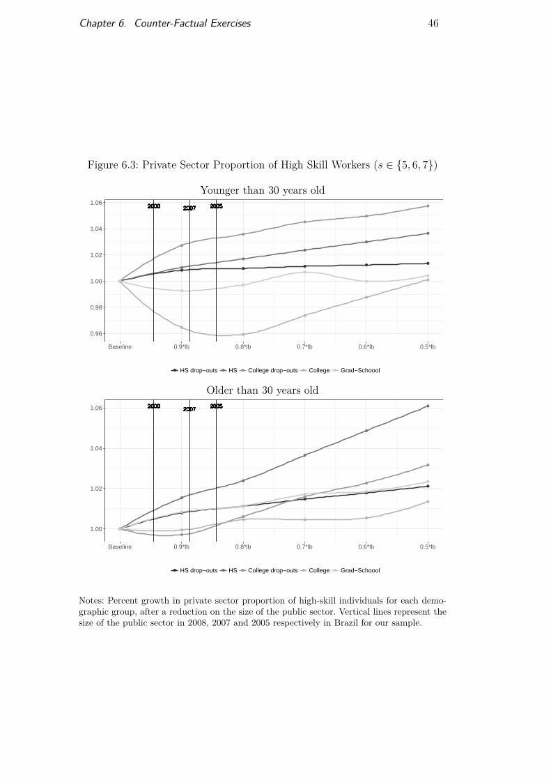
Chapter 6. Counter-Factual Exercises 46
Figure 6.3: Private Sector Proportion of High Skill Workers (s ∈ {5, 6, 7})
Younger than 30 years old
●●
●●
●
●
●
●
●
●
●
●
●
●
●
●
●
● ●
●
●
●
●
●
●
●
●
●
●
●
200520052005200520052005200520052005200520052005200520052005200520052005200520052005200520052005200520052005200520052005200720072007200720072007200720072007200720072007200720072007200720072007200720072007200720072007200720072007200720072007200820082008200820082008200820082008200820082008200820082008200820082008200820082008200820082008200820082008200820082008
0.96
0.98
1.00
1.02
1.04
1.06
Baseline 0.9*lb 0.8*lb 0.7*lb 0.6*lb 0.5*lb
● ● ● ● ●HS drop−outs HS College drop−outs College Grad−Schoool
Older than 30 years old
●
●
●
●
●
●
●
●
●
●
●
●
●
●
●
●
●
●
●
●●●
●●
●
●●
●
●
●
200520052005200520052005200520052005200520052005200520052005200520052005200520052005200520052005200520052005200520052005200720072007200720072007200720072007200720072007200720072007200720072007200720072007200720072007200720072007200720072007200820082008200820082008200820082008200820082008200820082008200820082008200820082008200820082008200820082008200820082008
1.00
1.02
1.04
1.06
Baseline 0.9*lb 0.8*lb 0.7*lb 0.6*lb 0.5*lb
● ● ● ● ●HS drop−outs HS College drop−outs College Grad−Schoool
Notes: Percent growth in private sector proportion of high-skill individuals for each demo-graphic group, after a reduction on the size of the public sector. Vertical lines represent thesize of the public sector in 2008, 2007 and 2005 respectively in Brazil for our sample.

Chapter 6. Counter-Factual Exercises 47
Figure 6.4: College Wage Premium in the Private Sector
●
●
●
●●
● 200520052005200520052005200720072007200720072007
200820082008200820082008
0.62
0.63
0.64
0.65
0.66
Baseline 0.9*lb 0.8*lb 0.7*lb 0.6*lb 0.5*lb
Notes: Effects of a reduction in public employment on the College wage premium in theprivate sector. Vertical lines represent the size of the public sector in 2008, 2007 and 2005respectively in Brazil for our sample.
the private sector College wage premium. As expected a decline on the size ofthe public sector reduces the College wage premium. More specifically a 10%reduction on public labor demand implies on a 5.81% decline on the Collegewage premium, this is due primarily to an increase on the proportion of high-skill for those with no College degree.
Because the public sector does not set wages based on skills, but basedon observable characteristics, high-skill individuals with low educational levelprefer mostly the private sector. On the other hand, low-skill individuals withhigh educational levels prefer the public sector, because the public sectorpays based on their education and not on their skill. Therefore, we wouldexpect that a reduction on the size of the public sector would increase theproportion of high-skill individuals for low-education groups and decrease thesame proportion for high-education groups. This generates the observed effecton the College wage premium.
Nonetheless, a decline on the size of the public sector generates anincrease in inequality. Figure 6.5 shows the growth on the ratios p90/p10,p90/p50 and p50/p10 of the log wage distribution at the private sector. Itis possible to see that a reduction on the size of the public sector increaseswage inequality measured by those ratios. More specifically, a 10% reductionin public labor demand increases the ratios p90/p10, p90/p50 and p50/p10 by1.52%, 2.24% and 0.40% respectively. This happens mainly because the public

Chapter 6. Counter-Factual Exercises 48
Figure 6.5: Private Sector Wage Inequality
●
●
●
●
●
●
●
●
●
●
●
●
●
●
●
●
●
●
200520052005200520052005200720072007200720072007
200820082008200820082008
1.00
1.02
1.04
1.06
Baseline 0.9*lb 0.8*lb 0.7*lb 0.6*lb 0.5*lb
●●●
●●●
●●●
p50p10p90p10p90p50
Notes: Percent growth in p90/p10, p90/p50 and p50/p10 wage ratios during a reduction inpublic employment. Vertical lines represent the size of the public sector in 2008, 2007 and2005 respectively in Brazil for our sample.
sector employs mostly high-skill workers.For instance, figure 6.6 shows the growth in the probability of belonging
to skill s given that the worker chose the private sector (P (s|r)). It is possibleto see that the proportion of individuals of skills 6 and 7 on the private sectorrises a lot, while the same proportion declines for the other skills. Therefore,there is an increase in the supply of high-skill workers in the private sector.This increase in supply generates a slight decrease in wages for those skills,as can be seen in figure 6.7 that shows average wages for each skill in theprivate sector. However, this decrease in wages was not enough to suppress theincrease in the proportion of high skill individuals that rose wage inequality.
6.2Allocation and Productivity Effects
From table 5.4 it is possible to see that the allocation of skills to tasksimply that more than 60% of tasks are performed by skills 1 and 2. In otherwords, the matching function of tasks to skills is convex, as can be seen infigure 6.8. It shows the matching function of tasks to skills first in our baseline(blue) and reducing the public sector (red). It is also possible to see that as theproportion of high skill individuals increases with the reduction in the size ofthe public sector, the private sector goes to a more balanced matching betweenskills and tasks. In other words, the reduction in the size of the public sector
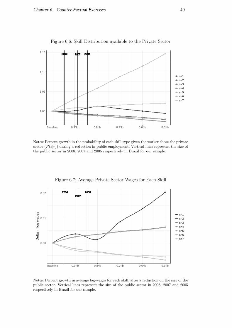
Chapter 6. Counter-Factual Exercises 49
Figure 6.6: Skill Distribution available to the Private Sector
●
●
●
●
●●
●
●●
●
●
●
●
●
●
●
●
●
●
●
●
●●
●
●●
●●
●
●
●
●
●
●
●
●
●●
●●
●
●
200520052005200520052005200520052005200520052005200520052005200520052005200520052005200520052005200520052005200520052005200520052005200520052005200520052005200520052005200720072007200720072007200720072007200720072007200720072007200720072007200720072007200720072007200720072007200720072007200720072007200720072007200720072007200720072007200820082008200820082008200820082008200820082008200820082008200820082008200820082008200820082008200820082008200820082008200820082008200820082008200820082008200820082008
1.00
1.05
1.10
1.15
Baseline 0.9*lb 0.8*lb 0.7*lb 0.6*lb 0.5*lb
●
●
●
●
●
●
●
s=1s=2s=3s=4s=5s=6s=7
Notes: Percent growth in the probability of each skill type given the worker chose the privatesector (P (s|r)) during a reduction in public employment. Vertical lines represent the size ofthe public sector in 2008, 2007 and 2005 respectively in Brazil for our sample.
Figure 6.7: Average Private Sector Wages for Each Skill
●
●
●
●
●
●
●
●
●
●
●
●
●
●
●
●
●
●
●
●
●
●
●
●
●
●
●
●
●
●
●
●
●
●
●
●
●
●●
●
●
●
200520052005200520052005200520052005200520052005200520052005200520052005200520052005200520052005200520052005200520052005200520052005200520052005200520052005200520052005
200720072007200720072007200720072007200720072007200720072007200720072007200720072007200720072007200720072007200720072007200720072007200720072007200720072007200720072007
200820082008200820082008200820082008200820082008200820082008200820082008200820082008200820082008200820082008200820082008200820082008200820082008200820082008200820082008
0.00
0.01
0.02
Baseline 0.9*lb 0.8*lb 0.7*lb 0.6*lb 0.5*lb
Del
ta in
log
wag
es ●
●
●
●
●
●
●
s=1s=2s=3s=4s=5s=6s=7
Notes: Percent growth in average log-wages for each skill, after a reduction on the size of thepublic sector. Vertical lines represent the size of the public sector in 2008, 2007 and 2005respectively in Brazil for our sample.
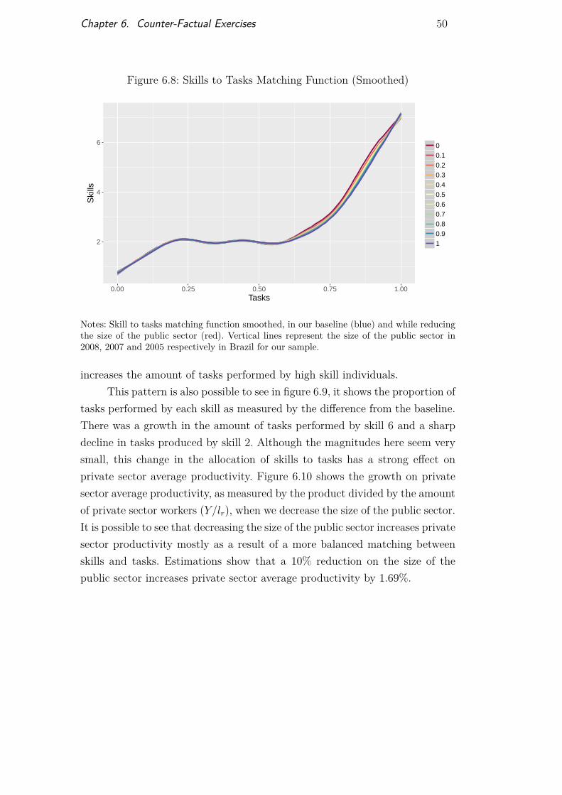
Chapter 6. Counter-Factual Exercises 50
Figure 6.8: Skills to Tasks Matching Function (Smoothed)
2
4
6
0.00 0.25 0.50 0.75 1.00Tasks
Ski
lls
00.10.20.30.40.50.60.70.80.91
Notes: Skill to tasks matching function smoothed, in our baseline (blue) and while reducingthe size of the public sector (red). Vertical lines represent the size of the public sector in2008, 2007 and 2005 respectively in Brazil for our sample.
increases the amount of tasks performed by high skill individuals.This pattern is also possible to see in figure 6.9, it shows the proportion of
tasks performed by each skill as measured by the difference from the baseline.There was a growth in the amount of tasks performed by skill 6 and a sharpdecline in tasks produced by skill 2. Although the magnitudes here seem verysmall, this change in the allocation of skills to tasks has a strong effect onprivate sector average productivity. Figure 6.10 shows the growth on privatesector average productivity, as measured by the product divided by the amountof private sector workers (Y/lr), when we decrease the size of the public sector.It is possible to see that decreasing the size of the public sector increases privatesector productivity mostly as a result of a more balanced matching betweenskills and tasks. Estimations show that a 10% reduction on the size of thepublic sector increases private sector average productivity by 1.69%.

Chapter 6. Counter-Factual Exercises 51
Figure 6.9: Private Sector Skill Thresholds
●●
●●
●●
●
●
●
●
●
● ●●●
●●● ●●●●●●
●●●●●●
●
●
●
●
●
●
●●
●●●
●
200520052005200520052005200520052005200520052005200520052005200520052005200520052005200520052005200520052005200520052005200520052005200520052005200520052005200520052005
200720072007200720072007200720072007200720072007200720072007200720072007200720072007200720072007200720072007200720072007200720072007200720072007200720072007200720072007
200820082008200820082008200820082008200820082008200820082008200820082008200820082008200820082008200820082008200820082008200820082008200820082008200820082008200820082008
−0.005
0.000
0.005
0.010
Baseline 0.9*lb 0.8*lb 0.7*lb 0.6*lb 0.5*lb
Del
ta in
the
Thr
esho
lds
●
●
●
●
●
●
●
T1 − 0T2 − T1T3 − T2T4 − T3T5 − T4T6 − T5T7 − T6
Notes: Difference from the baseline in the delta of skill thresholds (Ts − Ts−1), after areduction in the size of the public sector. Vertical lines represent the size of the public sectorin 2008, 2007 and 2005 respectively in Brazil for our sample.
Figure 6.10: Average Private Sector Productivity
●
●
●
●
●
●
200520052005200520052005200720072007200720072007
200820082008200820082008
1.00
1.01
1.02
1.03
1.04
Baseline 0.9*lb 0.8*lb 0.7*lb 0.6*lb 0.5*lb
Notes: Growth in average productivity (Y/lr) if we decrease the size of the public sector.Vertical lines represent the size of the public sector in 2008, 2007 and 2005 respectively inBrazil for our sample.

7Conclusion
We construct a static Roy model to assess if public sector employmentnegatively affects productivity and wage inequality in the economy throughskill allocation. In the model individuals are heterogeneous in their skills andrisk aversion, private sector demands endogenously based on skills and publicsector demands exogenously based on education which is correlated with skills.Public sector wages are certain while private sector wages are uncertain. Thecombination of different public-private wage gaps for each skill and uncertaintymakes the size of the public sector labor market influence the skill distributionavailable to the private sector. Changes in the skill distribution available tothe private sector affects productivity and wages through skill allocation.
We estimate this model for the Brazilian labor market using PNAD 2011-4. Results show that a reduction in public labor demand increases privatesector productivity, because it raises the proportion of tasks carried out byhigh skill individuals. In addition, the same decrease on the size of the publicsector reduces the College wage premium and increases private sector wageinequality. Although the hike in the supply of high skill workers reduced highskill wages, it was not enough to overcome the rise in the proportion of highskill workers that contributed to increase wage inequality. However, the risein the proportion of high-skill individuals was stronger for those without aCollege degree generating a reduction on the College wage premium.
Furthermore, there are some interesting counter-factual exercises that weintend to perform in future versions. First, changing employment and wagesat the public sector for specific education groups. In addition, it would beinteresting to analyze what would happen if we make public sector wagesuncertain, and see how changes in this uncertainty affects individuals sectordecision. Moreover, this is an interesting model to analyze the effects of therise of the proportion of public workers in the labor force of the last decade,and its consequence on the allocation of skills in the economy.
Although the model is of general equilibrium, it assumes that the publicsector is an unproductive sector. However, a reduction in the size of the publicsector would also implicate a reduction in the amount of public goods suppliedto the consumers and firms. Therefore, our counter-factual exercises must be

Chapter 7. Conclusion 53
interpreted taking into account this limitation. Further contributions shouldanalyze the impacts of public employment institutions on the allocation ofskills both in public and private sectors and its implications to the supply ofpublic and private goods and, consequently, welfare.

Bibliography
[1] MURPHY, K. M.; SHLEIFER, A.; VISHNY, R. W. The allocation of talent:Implications for growth. The Quarterly Journal of Economics, v. 106, n. 2,p. 503–530, 1991.
[2] ACEMOGLU, D. Reward structures and the allocation of talent. EuropeanEconomic Review, v. 39, n. 1, p. 17–33, 1995.
[3] HSIEH, C.-T.; HURST, E.; JONES, C. I.; KLENOW, P. J. The allocationof talent and us economic growth. Technical report, National Bureau ofEconomic Research, 2013.
[4] OECD. “employment in the public sector”. Paris: OECD Publishing, 2015.
[5] DICKSON, M.; POSTEL-VINAY, F.; TURON, H. The lifetime earningspremium in the public sector: The view from europe. Labour Economics,v. 31, p. 141–161, 2014.
[6] FINAN, F.; OLKEN, B. A.; PANDE, R. The personnel economics of the state.Technical report, National Bureau of Economic Research, 2015.
[7] COHEN, A.; EINAV, L. Estimating risk preferences from deductible choice.The American economic review, v. 97, n. 3, p. 745–788, 2007.
[8] FIRPO, S.; GONZAGA, G. Going private: public sector rents and privatizationin brazil. Anais do Encontro Brasileiro de Econometria, v. 32, 2010.
[9] HSIEH, C.-T.; HURST, E.; JONES, C. I.; KLENOW, P. J. The allocationof talent and us economic growth. NBER Working Paper Series, p. 18693,2013.
[10] ACEMOGLU, D.; ZILIBOTTI, F. Productivity differences. Technical report,National Bureau of Economic Research, 1999.
[11] ACEMOGLU, D.; AUTOR, D. Skills, tasks and technologies: Implications foremployment and earnings. Handbook of labor economics, v. 4, p. 1043–1171,2011.
[12] COSTINOT, A.; VOGEL, J. Matching and inequality in the world economy.Journal of Political Economy, v. 118, n. 4, 2010.

Bibliography 55
[13] DOS REIS, A. C.; MODAL, B.; ZILBERMAN, E. On the optimal size ofpublic employment. Technical report, 2013.
[14] SANTOS, M. D.; CAVALCANTI, T. (mis) allocation effects of an overpaidpublic sector. Technical report, Society for Economic Dynamics, 2015.
[15] HÖRNER, J.; NGAI, L. R.; OLIVETTI, C. Public enterprises and labor marketperformance*. International Economic Review, v. 48, n. 2, p. 363–384, 2007.
[16] BRADLEY, J.; POSTEL-VINAY, F.; TURON, H. et al. Public sectorwage policy and labor market equilibrium: a structural model. Unpublishedmanuscript, v. 2, p. 14, 2013.
[17] BESLEY, T.; GHATAK, M. Competition and incentives with motivatedagents. The American economic review, v. 95, n. 3, p. 616–636, 2005.
[18] FRANCOIS, P. ‘public service motivation’as an argument for governmentprovision. Journal of Public Economics, v. 78, n. 3, p. 275–299, 2000.
[19] MACCHIAVELLO, R. Public sector motivation and development failures.Journal of Development Economics, v. 86, n. 1, p. 201–213, 2008.
[20] PRENDERGAST, C. The motivation and bias of bureaucrats. The AmericanEconomic Review, v. 97, n. 1, p. 180–196, 2007.
[21] BARGAIN, O.; MELLY, B. Public sector pay gap in france: new evidenceusing panel data. Available at SSRN 1136232, 2008.
[22] BELLUZZO, W.; ANUATTI-NETO, F.; PAZELLO, E. T. Distribuição de sa-lários e o diferencial público-privado no brasil. Revista brasileira de economia,v. 59, n. 4, p. 511–533, 2005.
[23] DEPALO, D.; GIORDANO, R.; PAPAPETROU, E. Public–private wagedifferentials in euro-area countries: evidence from quantile decompositionanalysis. Empirical Economics, v. 49, n. 3, p. 985–1015, 2015.
[24] BRAGA, B. G.; FIRPO, S.; GONZAGA, G. Escolaridade e diferencial derendimentos entre o setor privado e o setor público no brasil. 2009.
[25] MCLACHLAN, G.; PEEL, D. Finite mixture models. John Wiley & Sons,2004.
[26] KATZ, L. F.; MURPHY, K. M. Changes in relative wages, 1963–1987: supplyand demand factors. The quarterly journal of economics, v. 107, n. 1, p. 35–78, 1992.

Bibliography 56
[27] LEVY, F.; MURNANE, R. J. et al. The skill content of recent technologicalchange: An empirical exploration. The Quarterly journal of economics, v. 118,n. 4, p. 1279–1333, 2003.
[28] BARSEGHYAN, L.; MOLINARI, F.; O’DONOGHUE, T.; TEITELBAUM,J. C. The nature of risk preferences: Evidence from insurance choices. TheAmerican Economic Review, v. 103, n. 6, p. 2499–2529, 2013.
[29] GUVENEN, F. Learning your earning: Are labor income shocks really verypersistent? The American economic review, v. 97, n. 3, p. 687–712, 2007.
[30] GUVENEN, F. An empirical investigation of labor income processes. Reviewof Economic dynamics, v. 12, n. 1, p. 58–79, 2009.
[31] GUVENEN, F.; SMITH JR, A. A. Inferring labor income risk and partialinsurance from economic choices. Econometrica, p. 2085–2129, 2014.

AParticipation Decision
This section will describe a possible extension to the model that modelsthe extensive margin of the labor market. Workers can choose which sectorthey will work for and if they will enter the labor market, so they have threechoices. If they choose not to participate in the labor market their utility willbe a reservation utility of U , which is observed by the worker, but not bythe econometrician. Workers are heterogeneous in their reservation utilitiesand this heterogeneity follows a normal distribution U ∼ N(µ, σ2
U). Therefore,workers choose to work for the private sector if Ur > Ub and Ur > U , publicsector if Ub > Ur and Ub > U and to stay at home if U > Ub and U > Ur.Which implies that the probabilities that a worker with skill s and demographiccharacteristic e chooses the private sector, the public sector or not to work is:
Pr(s, e) = P (Ub < Ur ∩ U ≤ Ur|s, e) (A-1)
Pb(s, e) = P (Ub ≥ Ur ∩ U ≤ Ub|s, e) (A-2)
Pn(s, e) = P (Ub < U ∩ Ur < U |s, e) (A-3)
A reduction on the size of the public sector decreases Ub through areduction in b(e), it becomes harder to be accepted to work at the publicsector. Workers may respond to it choosing to work at the private sector or tostay out of the labor market. Notice that with this formulation the proportionof workers that choose to stay out of the labor market depends on the skill andon the observed characteristic (e). Therefore, it may influence the distributionof skills available to the private sector, thus, average productivity and wageinequality.
Since we have data on individuals that choose to stay out of the labormarket it is possible to estimate the model including this extension. To do it weneed to include E more moments in the second stage that are the proportionof individuals that choose to stay out the labor market for each demographiccharacteristic. Consequently we will be able to identify all the parameters ofthe model and the parameters of the distribution of the reservation utility(µ, σ2
U).

BPublic Good
Even though we interpret the public sector as a unproductive sector, themodel also allows to interpret that the public sector produces a public good.The production of the public good depends on the labor demand for each skillat the public sector (lb(s)) and a productivity parameter D:
G = D
[S∑s=1
lb(s)γ−1γ
] γγ−1
(B-1)
This public good enters as a lump sum transfer in the workers utility, thus notaffecting workers sector decision. In this framework, reducing the size of thepublic sector increases private sector productivity and, consequently, wages,but reduces the public good. Therefore, it is not clear its impact on welfare.However, since we don’t observe individuals utility or the provision of publicgoods we can not estimate its production function. For this reason, we can notdiscuss welfare effects of reducing the size of the public sector.


![Master in Business Economics [PÓS-GRADUAÇÃO FGV]](https://static.fdocumentos.com/doc/165x107/55cf96aa550346d0338cfcf3/master-in-business-economics-pos-graduacao-fgv.jpg)