Dezembro de 2010

Tese de DoutoramentoEngenharia Civil

Trabalho efectuado sob a orientação deDr. José Manuel Pereira VieiraDr. José Luís da Silva Pinho

Cláudia Lindim Fontes

Modelling of Water Quality in the AlquevaReservoir, Portugal

Universidade do MinhoEscola de Engenharia

DECLARAÇÃO

Nome : Cláudia Lindim Fontes

Endereço electrónico: midnil@gmail.com Telefone: +351 253604100 #5723

Número do Cartão de cidadão: 8885663

Título da tese: Modelling of water quality in the Alqueva reservoir, Portugal

Orientadores:

Dr. José Manuel Pereira Vieira

Dr. José Luis Silva Pinho

Ano de conclusão: 2010

Doutoramento em Engenharia Civil

É AUTORIZADA A REPRODUÇÃO PARCIAL DESTA TESE APENAS PARA EFEITOS DE INVESTIGAÇÃO, MEDIANTE DECLARAÇÃO ESCRITA DO INTERESSADO, QUE A TAL SE COMPROMETE.

Universidade do Minho, de Dezembro de 2010

iii

ACKNOWLEDGEMENTS

FCT (Fundação para a Ciência e Tecnologia, Portugal) PhD grant

SFRH/BD/28491/2006 for providing economic support for the current work.

The civil engineering department at the school of engineering of the

University of Minho (Portugal) for being the hosting institution for the current

work.

Dr. José Luis Silva Pinho and Dr. José Manuel Pereira Vieira, both from the

University of Minho, for being my PhD advisors.

The Empresa de desenvolvimento e infraestruturas do Alqueva - EDIA

(Portugal) for making available monitoring data for the Alqueva reservoir,

Portugal.

Luiz Saldanha/Ken Tenore 2009 award from FLAD (Fundação Luso-

Americana para o Desenvolvimento) and IMAR (Instituto do Mar) for providing

invaluable funding for my stay in the USA.

USACE (United States Army Corps of Engineers) for being the hosting

institution for my work in the USA.

Clemson University (SC, USA), the civil engineering department of Clemson

University and the department chair Professor Nadim Aziz for providing research

facilities during my work in the USA.

My work colleagues at University of Minho: M. Eng. Rui Pinho, M. Eng. José

Araújo and MSc. Diogo Neves.

M. Eng. João P. Rodrigues for advanced VB macros hints.

Dr. M. Ruiz Villareal (IEO, Spain) for discussions on turbulence issues.

iv

Dr. E. Pereira (DF, U. Minho, Portugal) for rewarding discussions on theory

of stochastic methods and lending me books on this subject.

Dr. F. Andrade (DBA, FCUL, Portugal) for lending monitoring

instrumentation, for measurements cooperation and for fruitful discussions on

water biology issues and data analysis.

Dr. Earl J. Hayter (USACE and Clemson University, USA) for supervising

my work during my stay in the USA; For providing access to fast computational

resources and scientific software, namely Matlab and up-to-date processing

software SMS v. 10. Dr. Hayter advice was particularly useful for solving

hydrodynamic and transport modelling issues. Dr. Hayter guidance and

encouragement were always present.

Dr. Ian P. King (University of New South Wales, Australia) for all issues

related to RMA models and for making available at no cost up-to-date versions of

the RMA suite. Professor Ian King high professional profile, long years of

experience and infinite kindness gives a new meaning to the word Mentor. The

inspirational Professor King was instrumental to solve many issues with RMA

models and RMA processing tools and I am very much in debt with him and

heartily thankful.

My family for enduring 3.274 long years of neglect.

Chopin piano works and Bose noise cancelling headphones for providing

quietness and peace over morons permanently making phone calls outside my

office, Braga city devoted fireworks fans, yearly “Enterro da Gata” soundwaves,

yelling neighborhood kids and frustrated housewives, busy airports and noisy café

terraces.

v

This work is dedicated to three generations of people instrumental in my life

My maternal grandfather António Rodrigues Jr., my dearest husband E. and my lovely

daughter J.

“All models are wrong . Some are useful.” - George E.P. Box

“We are continually faced with a series of great opportunities brilliantly disguised as insoluble problems.” - John W. Gardner

vi

vii

MODELLING OF WATER QUALITY IN THE ALQUEVA RESERVOIR, PORTUGAL ABSTRACT Eutrophication is a serious environmental problem in lakes and reservoirs worldwide. The eutrophic Alqueva reservoir (Portugal) is the largest western European reservoir and constitutes a vital regional water resource. The river Guadiana, which is the main tributary to the Alqueva reservoir, imports large nutrient loads leading to eutrophication being an issue in this waterbody. But despite its importance and problems, few scientific studies concerning the Alqueva exist. This work aims at contributing to foster the understanding of water ecology in the Alqueva reservoir through the use of data analysis techniques and numerical modelling. The results contained herein can be used to assist management decisions in this waterbody and the modelling effort can be used to obtain forecasts in this and other reservoirs and improve understanding of ecological behavior there. Data analysis methods, namely time series analysis, were applied to monitoring data collected between 2003-2009 at several locations and depths in the Alqueva reservoir in order to infer possible spatial and temporal patterns. The monitoring data comprised climatology, hydrology and water quality data from different sources. Data analysis showed that the Alqueva behavior presents high interannual variability. This is mainly a consequence of the high variability of precipitation, nutrient loads and Guadiana hydrological regimen. It was found that the system is P-limited and that nutrients input is mostly dependent on the main tributary input loads. Therefore management schemes aimed at improving the trophic level in the Alqueva should focus on reducing phosphorus in the Guadiana inflow. Numerical modelling main goals were to develop and apply tools to simulate the main ecological traits in the Alqueva reservoir. A new numerical model to simulate eutrophication processes in lakes and reservoirs based on a hybrid deterministic-stochastic approach was developed. A plain methodology to estimate nutrient loads in a basin was also developed. These tools were used together with the finite element based hydrodynamic model RMA-10 to perform simulations of currents, thermal structure and eutrophication in the Alqueva reservoir. The models were successfully calibrated and validated in both two-dimensional and three-dimensional versions. Model performance was assessed by comparing simulation results with in situ measured data. It was found that the models reproduced Alqueva thermal structure quite accurately and eutrophication related trends reasonably well. The performance of the eutrophication tool was constrained by the availability and quality of input and forcing data. It was shown that the particular geomorphological and hydrological characteristics of the reservoir together with local climate features are responsible for the existence of two distinct ecological regions within the reservoir whose boundary can be placed at a transect south of monitoring station 3:

The upper part of the reservoir is a shallow channel like region with riverine characteristics that is interrupted by a few scattered deeper pools. This area receives

viii

the major nutrients input and is eutrophic. Hydrodynamic in this area is governed by hydraulically induced currents from the Guadiana.

The lower part of the reservoir is a deep lacustrine area that presents stable thermal and oxygen stratification in summer (April – October). In this region, wind induced currents and thermal stratification are the dominant hydrodynamic traits. Wind is dominant over hydraulic flow during all year and affects mostly the surface circulation.

Model results indicate that the velocities in the reservoir are always smaller than 0.25 m/s, with the higher values occurring in the upper reservoir area. The Alqueva was found to present a monomictic behavior with a seasonal summer stratification that is responsible for generating anoxic bottom waters during dry season. An autumnal overturn leads to a fully mixed water column in winter season. Model findings, corroborated by data, indicate that phytoplankton in the Alqueva peaks in spring and in autumn with productivity in the upper reservoir area presenting values much higher than in the lower part. Dry season ecology seems to be ruled by stratification while wet season ecology main driving force appears to be the nutrients load through the main tributary. The Alqueva was build to boost economic development in the region and provide irrigation water for agriculture activities. It can be inferred from the results of the present work that the major problem it may face is the impacts of the poor water quality coming from the Guadiana. The Guadiana river carries wastewater with a high level of nutrients from a large Spanish population, from industries and from agriculture activities. The development of effective water quality management in this reservoir should therefore focus on nutrient containment strategies for the Guadiana river inflow. Keywords: Alqueva reservoir, Modeling, Eutrophication, Thermal stratification, Hydrodynamic.

ix

MODELAÇÃO DA QUALIDADE DA ÁGUA NA ALBUFEIRA DE ALQUEVA, PORTUGAL RESUMO A eutrofização constitui um sério problema ambiental em lagos e albufeiras. A albufeira de Alqueva (Portugal) é a maior albufeira da Europa ocidental e constitui um importante recurso aquático regional. O principal afluente de Alqueva, o rio Guadiana, introduz elevadas cargas de nutrientes na albufeira fazendo com que a eutrofização seja motivo de preocupação nesta albufeira. Apesar da sua importância e problemas, existem poucos estudos científicos sobre a albufeira de Alqueva. Este trabalho tem como objectivo contribuir para o conhecimento e compreensão da ecologia aquática na albufeira de Alqueva através do uso de análise de dados e modelação matemática. Os resultados obtidos podem ser utilizados na tomada de decisões de gestão nesta albufeira e o trabalho de modelação pode ser utilizado para efectuar previsões nesta ou noutras albufeiras ou lagos. Foram aplicados métodos de análise de dados, nomeadamente métodos de análise de séries temporais, a dados de campanhas de monitorização recolhidos no período 2003-2009 em diferentes pontos da albufeira de Alqueva para inferir da existência de padrões espaciais e temporais. Os dados de monitorização são oriundos de diferentes fontes e abrangem climatologia, hidrologia e qualidade da água A análise de dados permitiu concluir que a ecologia do Alqueva tem uma elevada variabilidade interanual que é consequência da elevada variabilidade da precipitação, cargas de nutrientes e regime hidrológico. Concluiu-se que o nutriente limitante é o fósforo e que a entrada de nutrientes no sistema depende sobretudo das cargas que entram pelo afluente principal. Donde resulta que uma gestão eficiente da melhoria do estado trófico da albufeira deve centrar-se na redução do fósforo nas afluências do Guadiana. Os principais objectivos da modelação foram desenvolver e aplicar ferramentas para simular as principais características ecológicas da albufeira de Alqueva. Desenvolveu-se um novo modelo matemático para simular a eutrofização em lagos e albufeiras baseado numa abordagem híbrida determinística-estocástica. Desenvolveu-se também uma metodologia simples para estimar cargas de nutrientes em bacias hidrográficas. Estes instrumentos foram utilizados em conjunto com o modelo hidrodinâmico RMA10, baseado no método dos elementos finitos, para simular correntes, estrutura térmica e eutrofização na albufeira de Alqueva. Os modelos foram calibrados e validados com sucesso nas versões tridimensional e bidimensional integrada lateralmente. O desempenho dos modelos foi avaliado por comparação entre os resultados de simulações e medidas experimentais realizadas in situ. Verificou-se que os modelos reproduzem com grande exactidão a estrutura térmica da albugeira de Alqueva e razoavelmente bem as variações relacionadas com a eutrofização. O desempenho do modelo de eutrofização foi condicionado pela disponibilidade e qualidade dos dados de entrada e de forçamento. Mostrou-se que as características geomorfológicas e hidrológicas particulares da albufeira, em conjunto com características climáticas locais, são responsáveis pela existência de duas zonas ecológicas distintas na albufeira, cuja fronteira se localiza a sul da estação de amostragem 3:

x

A parte superior da albufeira é uma região de leito linear com águas pouco profundas, interrompida a espaços por lagoas mais profundas, que tem características fluviais. Esta zona é muito eutrófica e por ela entram a maior parte dos nutrientes do sistema. A hidrodinâmica nesta área é governada por correntes induzidas pelo fluxo do Guadiana.

A parte inferior da albufeira é uma região lacustre profunda que apresenta estratificações térmica e de oxigénio estáveis durante o verão (Abril - Outubro). Nesta zona as características hidrodinâmicas dominantes são as correntes induzidas pelo vento e a estratificação térmica. O vento é dominante sobre o fluxo hidráulico durante todo o ano e afecta sobretudo a circulação à superfície.

Os resultados da modelação indicam que as velocidades na albufeira são sempre inferiores a 0.25 m/s, com os maiores valores a ocorrer na parte superior da albufeira. Concluiu-se que a albufeira de Alqueva apresenta um comportamento monomíctico com uma estratificação sazonal de verão que é responsável pela geração de camadas de água anóxica no fundo da albufeira durante a estação seca. A circulação convectiva outonal dá origem a uma coluna de água completamente misturada na estação do inverno. Os resultados de modelação, corroborados por dados de campo, indicam que o fitoplâncton no Alqueva apresenta picos primaveris e outonais, com a produtividade na parte superior da albufeira a apresentar sempre valores muito superiores à da parte inferior. A ecologia da estação seca parece ser governada pela estratificação ao passo que a força motriz da ecologia da estação húmida aparenta ser a carga de nutrientes que entra através do afluente principal. A barragem de Alqueva foi construída para fomentar o desenvolvimento económico regional e fornecer água de irrigação para actividades agrícolas. Dos resultados obtidos neste trabalho pode-se concluir que o maior problema com que a albufeira se depara é os impactos da água de baixa qualidade que é trazida pelo rio Guadiana. O Guadiana transporta efluentes com um elevado nível de nutrientes provenientes de uma vasta população espanhola, de indústrias e de actividades agrícolas. Consequentemente, o desenvolvimento de uma gestão de qualidade da água eficaz nesta albufeira deve centrar-se em estratégias de remediação/contenção do fósforo trazido pelo Guadiana. Palavras-chave: Albufeira de Alqueva, Modelação, Eutrofizacão, Estratificação Térmica, Hidrodinâmica.

xi

CONTENTS ACKNOWLEDGEMENTS _____________________________________________iii

ABSTRACT _______________________________________________________ vii

CONTENTS ________________________________________________________xi

NOTATION, ABBREVIATIONS AND SYMBOLS __________________________xiii

CHAPTER 1 - BACKGROUND _________________________________________ 1

1.1 Research motivation and contributions_______________________________________ 1

1.2 Dissertation outline and organization ________________________________________ 2

CHAPTER 2 - INTRODUCTION ________________________________________ 4

2.1 Limnology of reservoirs and eutrophication related phenomena __________________ 4

2.2 Numerical models for simulation of eutrophication - A review __________________ 16

References for Chapter 2 ____________________________________________________ 29

CHAPTER 3 - DESCRIPTION OF MODELLING TOOLS ____________________ 32

3.1 Hydrodynamic model ____________________________________________________ 33

3.2 Eutrophication model____________________________________________________ 38 3.2.1 Temperature dependencies _________________________________________________41 3.2.2 Algae growth and limitation ________________________________________________42 3.2.3 Dissolved oxygen (O2) ____________________________________________________45 3.2.4 Ultimate biological oxygen demand (BOD) ____________________________________46 3.2.5 Phosphate (PO4) _________________________________________________________48 3.2.6 Nitrite and nitrate (NO3) ___________________________________________________48 3.2.7 Ammonia (NH3) _________________________________________________________50 3.2.8 Phytoplankton (PHY) _____________________________________________________50 3.2.9 Zooplankton (Zoo) _______________________________________________________51 3.2.10 Organic nitrogen (ON) ___________________________________________________52 3.2.11 Organic Phosphorus (OP) _________________________________________________52 3.2.12 Parameters_____________________________________________________________53 3.2.13 Eutrophication model implementation _______________________________________55 3.2.14 Calibration methodology for the eutrophication model __________________________55

3.3 Heat transport model ____________________________________________________ 61 3.3.1 Short-wave radiation (HSN) _________________________________________________62 3.3.2 Long-wave radiation (HAN)_________________________________________________63 3.3.3 Evaporation (HE)_________________________________________________________63 3.3.4 Conduction (HC) _________________________________________________________64 3.3.5 Back radiation (HB)_______________________________________________________64

3.4 Data noise reduction methodology and implementation _______________________ 64

References for Chapter 3 ____________________________________________________ 65

CHAPTER 4 - STUDY SITE AND DATA ANALYSIS _______________________ 67

4.1 Climatology ____________________________________________________________ 72 4.1.1 Solar radiation___________________________________________________________73 4.1.2 Air Temperature _________________________________________________________75 4.1.3 Evapotranspiration and rainfall______________________________________________76 4.1.4 Wind __________________________________________________________________79

4.2 Hydrology _____________________________________________________________ 82

xii

4.3 Water quality ___________________________________________________________ 84 4.3.1 Water temperature________________________________________________________85 4.3.2 Dissolved Oxygen________________________________________________________91 4.3.3 Nutrients _______________________________________________________________96 4.3.4 Nutrients limitation analysis _______________________________________________102 4.3.5 Chlorophyll-a __________________________________________________________104

4.4 Methodology developed for estimation of nutrient loads ______________________ 108

References for Chapter 4 ___________________________________________________ 112

CHAPTER 5 - APPLICATION OF MODELS TO THE ALQUEVA RESERVOIR _ 114

5.1 Spatial discretization and computational mesh ______________________________ 115

5.2 Forcing, boundary and initial conditions ___________________________________ 125 5.2.1 Hydrodynamic simulations ________________________________________________126 5.2.2 Thermal simulations _____________________________________________________126

5.3 Models Parameterization and Calibration __________________________________ 127 5.3.1 Hydrodynamic calibration_________________________________________________129 5.3.2 Thermal calibration______________________________________________________130 5.3.3 Eutrophication calibration_________________________________________________134

5.4 Model results and discussion_____________________________________________ 137 5.4.1 Velocities and circulation patterns __________________________________________138 5.4.2 Stratification and water temperature trends____________________________________141 5.4.3 Eutrophication dynamics__________________________________________________144

5.5 Models verification/validation____________________________________________ 150 5.5.1 Hydrodynamic validation _________________________________________________150 5.5.2 Thermal validation ______________________________________________________151 5.5.3 Eutrophication validation _________________________________________________153

5.6 Uncertainty analysis ____________________________________________________ 156 5.6.1 Guadiana inflow scenarios ________________________________________________157 5.6.2 Wind scenarios _________________________________________________________162

References for Chapter 5 ___________________________________________________ 164

CHAPTER 6 – CONCLUSIONS AND FUTURE WORK ____________________ 166

References for Chapter 6 ___________________________________________________ 171

xiii

NOTATION, ABBREVIATIONS AND SYMBOLS [BOD] - biological oxygen demand (mass concentration) [CHLa] - mass concentration of chlorophyll-a [NH3] - mass concentration of ammonia [NO3] - available mass concentration of nitrate plus nitrite [O2] - dissolved oxygen mass concentration [ON] - organic nitrogen mass concentration [OP] – organic phosphorus mass concentration [PHY] - phytoplankton carbon mass concentration [PO4] - available phosphate mass concentration [Zoo] - zooplankton carbon mass concentration 1D - one dimensional 2D - two dimensional 2DL - two dimensional laterally averaged 3D - three dimensional a - fixed bed level in model C - cloud cover Chl-a - chlorophyll-a Cp - specific heat of water CSAT - dissolved oxygen saturation D - eddy diffusion coefficients dkBOD - half-saturation constant for oxygen limitation in BOD decay dkO2 - half-saturation constant for oxygen limitation in nitrification fb - mass stoichiometry ratio in nitrification g - acceleration of gravity h - time varying water surface H0 - incoming solar short wave radiation to earth’s atmosphere HAN - long wave radiation flux HB - back radiation from water surface HC - heat conduction flux

HE - evaporation flux HN - net energy flux at interface air-water HS (z) - short wave radiation at depth z HSN - Short-wave radiation flux i, j, k - generic cartesian coordinates I - intensity of light Io - intensity of light at water surface Isat - optimal light intensity Iz - intensity of light at depth z k - generic kinetic rate at 20ºC k1 - generical kinetic rate at temperature T1 k2 - generical kinetic rate at temperature T2

kd - decay rate for BOD Kd - diffuse attenuation coefficient

kdenit - denitrification rate kdn - decay rate of organic nitrogen to inorganic nitrogen forms kdp - decay rate of organic phosphorus to phosphate kg - zooplankton ingestion rate k - diffusion coefficient

xiv

Kn - half-saturation constant for N limitation kn - nitrification rate kO2 - oxygen inhibition constant in denitrification Kp - half-saturation constant for P limitation kr - respiration rate for phytoplankton ks - surface transfer coefficient for oxygen kt - generic kinetic rate at temperature T kz - half-saturation constant for phytoplankton limitation in zooplankton growth L - latent heat of vaporization Llim - growth limitation by light N:P- total nitrogen to total phosphorus mass ratio nf - mass fraction of nitrogen in phytoplankton or zooplankton NH3 - ammonia Nlim - growth limitation by nitrogen NO3 - nitrate p - water pressure Pa - atmospheric pressure Pdead - non predatory mortality of phytoplankton pf - mass fraction of phosphorus in phytoplankton Plim - growth limitation by phosphorus PO4 - phosphate prodO2 - oxygen mass production per unit of carbon mass in phytoplankton q - inflow per unit volume Q10 - temperature coeffcient qsn - top water column radiation qst - measured solar radiation at water surface R - albedo r - fixed reference vertical location (set at mean reservoir level) R’- percent of radiation useful for photosynthesis respO2 - oxygen mass consumed per unit of carbon mass in phytoplankton for respiration S - wind speed Selfs - self-shading coefficient t - time T - water temperature Ta - air temperature tf - final model run time to - initial model run time Ts - water surface temperature u, v, w - velocity components in the cartesian directions Vset - settling velocity Vsetp - settling velocity for phytoplankton and organic non living material x, y, z - cartesian coordinates along x, y and z-axis z - vertical coordinate Z - water depth z’ - transformed vertical coordinate Zdead1 - non predatory mortality of zooplankton Zdead2 - predatory mortality for zooplankton Zsecchi - Sechi disk depth

xv

Acronyms BfG - Federal institute of hidrology (Germany) BOD - Biological oxygen demand CCDR - Comissão de coordenação e desenvolvimento regional CV - Coefficient of variation DHI - Danish hydraulic institute DIN - Dissolved inorganic nitrogen DO - Dissolved oxygen DON - Dissolved organic nitrogen DOP - Dissolved organic phosphorus DSS - Decision support systems EDF - Electricité de France EDIA - Empresa de desenvolvimento e infraestruturas do Alqueva EFMA - Empreendimento de fins múltiplos do Alqueva EPA - Environmental protection agency (USA) EU - European Union FDM - Finite diference method FEM - Finite element method FVM - Finite volume method GIS - Geographic information system INAG - Instituto nacional da água (Portugal) INE - Instituto nacional de estatística (Portugal) INSAAR - Inventário nacional de sistemas de abastecimento de água e de águas residuais (Portugal) IST - Instituto superior técnico (Portugal) JRC - Joint research center (EU) N - Nitrogen NASA - National aeronautics and space administration (USA) NOAA - National oceanic and atmospheric administration (USA) P - Phosphorus PAR - Photosyntetically active radiation PDE - Partial differential equation PON - Particulate organic nitrogen PP - Particulate phosphorus RE - Relative error RMSE - Root mean square error SAIH - Sistema automático de información hidrológica (Spain) SHMI - Swedish meteorological and hydrological institute SNIRH - Serviço Nacional de informação de recursos hídricos (Portugal) SOD - Sediment oxygen demand SPAWAR - Space and naval warfare (USA) TN - Total nitrogen TP - Total phosphorus UN - United Nations UNESCO - United Nations education, scientific and cultural organization (UN) USA - United States of America USACE - United States army corps of engineers USGS - United States geological survey VIMS - Virginia institute of marine sciences (USA) WES - Waterways experiment station (USA)

xvi

Greek notation - ammonia to nitrate fraction - turbulent eddy coefficients ' - specific weight of water - light extinction coefficient o - light extinction coefficient for all particles except algae - temperature adjustment coefficient s - source/sink for the transported variable - algae growth rate max - algae maximum growth rate temperature corrected - external tractions operating on the boundaries or on the interior; (combined Coriolis, wind and bed friction effects) - density of water o - reference density Stefan-Boltzmann constant, 2.0412x10-7 kJ/(hKm2) 1 - fraction of phosphorus respired material that is organic phosphorus 2 - fraction of nitrogen respired material that is organic nitrogen

1

CHAPTER 1 - BACKGROUND

1.1 Research motivation and contributions

The motivation behind this work was to answer several questions:

- Is it possible to predict eutrophication in reservoirs?

- What is the uncertainty associated with those forecasts?

- What are the key processes controlling eutrophication in reservoirs?

- What are reservoir responses to changes in natural and non-natural conditions?

- What management strategies can be applied to minimize or solve water quality

problems in reservoirs?

With that aims in mind, modelling tools were developed and applied together with

existent well established models to a pre-chosen system: the Alqueva reservoir.

The Alqueva is currently the most important Portuguese reservoir and the largest western

European reservoir1. It is part of a multipurpose hydraulic system interconnecting several

reservoirs designed to provide water for irrigation, drinking and recreational purposes in

the arid Alentejo region. Regardless of that, less than ten scientific publications

concerning the Alqueva reservoir can be found in peer reviewed publications since the

reservoir was filled in 2003. This noteworthy fact was an additional motivation to give

my contribution to improve the current knowledge about this particular reservoir.

Thus, the current work focuses on eutrophication modeling in the Alqueva reservoir,

Portugal.

The objectives of the current work were:

- The development of new and improved modelling tools for eutrophication

simulation in reservoirs.

- The use of numerical models to aftcast and forecast eutrophication and related

traits in the Alqueva reservoir.

1 The Alqueva is the biggest Western Europe reservoir in terms of water volume (4.15 km3). The Lokka

reservoir in Finland can be considered the biggest one in terms of surface area with 417 km2 against just

250 km2 of the Alqueva. The shallow Lokka has a volume of only 2.1 km3. Contrary to a common spread

idea the equally shallow Ijsselmeer (5.4 km3; 1100 km2) in the Netherlands is not technically a reservoir but

a man-made enclosed coastal bay.

2

- The use of model results and data analysis techniques to characterize the Alqueva

ecosystem. Employ that knowledge to contribute to the resolution of ecological

problems in the Alqueva reservoir.

In the pursuit of the first listed objective an innovative approach was chosen. The

developed eutrophication model combines deterministic and stochastic features. The

model takes advantage of the best in both methodologies while avoiding their unwanted

characteristics.

1.2 Dissertation outline and organization

The outline of this dissertation is as follows.

Chapter 1 describes generically the subject and scope of the present work. It also points

out the main motivations and objectives of this work. This is followed by a dissertation

outline and information about the organization of the manuscript.

Chapter 2 is an introductory chapter with two main parts. The first part will highlight the

specificities of reservoirs and the natural and anthropogenic processes taking place there

with emphasis in eutrophication, its causes and effects. The second part contains a

review and state-of-the-art of surface water modelling with a strong emphasis in

eutrophication simulation able tools.

Chapter 3 describes the modelling tools developed and used in the current work

including their theoretical background, numerical details and implementation

information.

Chapter 4 starts by describing the study site – the Alqueva reservoir. This is followed by

a data analysis section used to characterize the study site and to serve as basis for models

implementation. Data analysis for the Alqueva was done for climatology, hydrology and

water quality. A final section presents a methodology developed for estimating nutrient

loads and its application for the Alqueva.

Chapter 5 regards the application of the modelling tools to the study site. This chapter

presents model parameterization details, modelling results and their discussion.

Calibration and validation of models is also included in this chapter.

Chapter 6 presents the general conclusions for this work.

3

References cited in the text are organized by chapter and appear listed at the end of their

respective chapter. Lists of references are organized by alphabetical order of first author,

followed by year order whenever the first author is the same.

4

CHAPTER 2 - INTRODUCTION

This chapter contains a brief introduction that will place the present work in context.

The chapter is divided in two main parts. The first one concerns the current scientific

knowledge about eutrophication and related phenomena. The second part concerns

numerical modelling of aquatic environments. A brief review covering the major

historical advances and the state-of-the-art of eutrophication modelling highlights the

most important research done on this subject.

2.1 Limnology of reservoirs and eutrophication related phenomena

An in-depth look into limnology can be found in the reference books by Horne et al.

(1994), Wetzel (2001), Scheffer (1998), Kalff (2002), Cole (1994), Lampert et al. (1997),

and Welch et al. (2004). Herein only concepts fundamental to understand the current

work will be presented and briefly discussed.

Eutrophication (Figure 2.1) is the process of accelerated nutrient enrichment of a

waterbody. This process is accompanied by an excessive growth of primary producers

and a progressive reduction in secondary producers. The increased mass of

phytoplankton formed is usually constituted by bloom forming species which may differ

from the natural occurring species in that particular waterbody. Although eutrophication

is a natural process, it is usually caused or accelerated by anthropogenic causes. Excessive

nutrient input will unbalance the waterbody ecosystem and will stimulate blooms of algae

with a considerable impact in water quality. Apart from the visual nuisance and the

economic impacts of water treatment processes needed to solve the problem, algae

blooms are accompanied by a depletion of dissolved oxygen levels, an increase in organic

suspended solids and if blue green algae are present, toxins. When the algae die and

accumulate at the bottom they are decomposed by bacteria. In the decomposition

process bacteria use dissolved oxygen (DO). Dissolved oxygen concentration in the

bottom water layers is then depleted to levels that can cause death to fish and shellfish

due to the large algae biomass bacteria have to decompose. If eutrophication persists or

is very intense there will be changes in communities composition and biodiversity losses.

5

Figure 2.1 - Eutrophication and related processes in a reservoir. (Source: Hans Hillewaert

under a Creative Commons license).

Figure 2.2 summarizes causes, effects and solutions for eutrophication. Remediation and

reservoir management techniques used to solve eutrophication problems include acting

on the system inputs or acting on the system itself. Acting on the system inputs by

diverting the nutrients from point sources or by using ponds or constructed wetlands to

remove nutrients from diffuse sources. Acting on the system itself by using forced

reaeration to increase oxygenation; by adding modifying agents like aluminum to obtain

inactive phosphorus; by manipulating the food web or by using dilution (Cooke et al.,

2005).

Of all types of water bodies, lakes and reservoirs are particularly sensitive to

eutrophication due to its enclosed nature and large drainage basins. Large enclosed areas

tend to present stagnant waters and longer residence times than streams. Both these

factors favor the accumulation of nutrients, persistence of density stratification situations

and low oxygenation of water. Most often eutrophication is caused by agricultural runoff

sources and untreated effluents from urban and industrial sources. There is a high

probability of having high concentrations of diffuse source pollutants whenever the basin

has large areas of agriculture, livestock or manure activities.

In deep reservoirs, thermal stratification, a process that can contribute to intensify the

eutrophication problems, may occur during part of the year. Since most reservoirs have

6

only one stream source as the main inflow, it may contribute significantly to alter the

natural trophic state of the reservoir if carrying heavy loads of pollutants.

Figure 2.2 - Eutrophication causes, effects and remediation.

Reservoirs and lakes can be classified according to their trophic state. This classification

can be used to describe the biological condition or “health” of a waterbody. Carlson’s

index is one of the most widespread used trophic classification indexes (Carlson, 1977).

But criteria for this classification are not consensual in the scientific community. Since

2002 the trophic state criteria applicable in Portugal is based on the European Union

water framework directive (directive 2000/60/EC) and uses the ranges of three measured

parameters as presented in table 2.1. The worst case among the three measured

parameters is chosen for the trophic classification.

Table 2.1 - Portuguese trophic level classification for reservoirs and lakes.

Total phosphorus(mg P m-3)

Chlorophyll- a(mg m-3)

Dissolved Oxygen (Saturation %)

Oligotrophic <10 <2.5 - Mesotrophic 10-35 2.5-10 - Eutrophic >35 >10 <40

The pelagic area of a reservoir is traditionally conceptually described by dividing

horizontally the water column into three main areas of different depths. Yet the location,

extension and naming of those three areas will differ according to the field of study.

Biologists and chemists will tend to call the layers epilimnion, metalimnion and

hypolimnion, a classification based on vertical density stratification due to temperature

(see Figure 2.3). Physicists and hydrologists may refer to another altogether different

three layers by the names surface boundary layer, density stratified layer and benthic

boundary layer (these are not synonymous with the former biologists terminology) when

7

the subject is mass, heat or momentum transport. The thickness of these layers depends

on atmospheric conditions and waterbody intrinsic conditions and it may vary over time

and location for a given waterbody.

For temperate lakes, the epilimnion is the warmer, more oxygenated top layer able to

exchange material with the atmosphere. The epilimnion absorbs the major part of the

light reaching the surface. It is usually well mixed by wind action and therefore presents a

uniform temperature over depth. It contains the warmer and less dense water of a

reservoir or lake.

The middle layer is the metalimnion or thermocline, characterized by a quick variation of

temperature with depth. By definition, a decrease of at least 1ºC/m according to

Jorgensen et al. (2000) characterizes a thermocline. Thermoclines can be temporary (due

to daily cycle of radiative heat/cooling), more permanent (seasonal) or be absent. In

temperate lakes, thermoclines are formed during summer when less dense warm water

stays at the surface while more dense cool water will sink to the bottom. Little mixing

will occur if currents and winds are weak. One of the implications of this is that bellow

the thermocline there is a depletion of oxygen by living organisms respiration and there is

no renewal possibility since no mixing occurs. Dissolved oxygen will only enter the water

column via reaeration through the atmosphere-water interface and will stay at the top

mixed layer. The atmospheric oxygen diffuses slowly from atmosphere. Turbulent mixing

transfers oxygen more efficiently from atmosphere and is usually the mechanism

responsible for the oxygen saturation levels found at top water layers. Furthermore,

oxygen production by photosynthesis will only occur at the top layers where there is

enough light. Since oxygen solubility varies inversely with temperature, the hotter the

epilimnion water the lower the oxygen concentration that can be found for the same

mixing conditions. Thus, hot season vertical thermal stratification is accompanied by

dissolved oxygen vertical stratification. Figure 2.3 (top) shows these processes in detail.

The hypolimnion is the bottom layer adjacent to the sediment where temperature

remains constant during thermal stratification periods. In temperate reservoirs, it

contains the denser and colder water during hot season. It is usually depleted of oxygen

during hot season since oxygen demand in the hypolimnion is not balanced with

photosynthetic production or transported DO. The hypolimnion in summer will present

hypoxic conditions (less than 2 mg/L O2) or even anoxic conditions (completely

anaerobic). In shallow oligotrophic lakes if the water is clear enough to allow

photosynthesis in the hypolimnion then some production of oxygen may occur.

8

When summer ends, temperature of the top water will drop since heat losses by

evaporation and sensible heat exceed solar radiation inputs. Whenever density of the top

water becomes that of deeper water, overturn will occur, and the different vertical water

layers will mix. Circulation will then allow oxygen levels to increase. During winter,

vertical uniform water temperature and oxygen concentrations are achieved due to this

vertical mixing. Water oxygen levels will also be higher since low temperatures will favor

a higher solubility and because oxygen consumption by oxidation is then low.

Non-temperate lakes and reservoirs may develop a winter stratification if the water

surface develops an ice layer. In this case, two overturn periods per year will occur.

Figure 2.3 (bottom) exemplifies the evolution of the water column vertical mixing

processes over a yearly cycle for a non-temperate lake with ice cover. Less frequent are

lakes and reservoirs where mixing never occurs or those where mixing occurs more than

twice a year. Portuguese reservoirs are temperate reservoirs that fall in the category of

monomictic waterbodies, that is, they have only one stratification and one mixing period

per year.

A daily variation cycle for the levels of oxygen can sometimes be observed in the water

column of lakes and reservoirs. While there is daylight, the photosynthetic activity will

increase oxygen levels. During the night in the absence of light, respiration will decrease

the levels of oxygen. This will make oxygen levels fluctuate regularly over daily periods.

9

Figure 2.3 - Top: Summer thermal and dissolved oxygen vertical stratification in a

temperate eutrophic reservoir. Bottom: overturn and stratification processes onset during

a yearly cycle in a dimictic lake. (Source: Adapted from Davis et al. (2003)).

The surface boundary layer is responsible for the exchanges with the atmosphere.

Interfacial processes include heat, momentum and mass transfer mostly driven by wind

and the heat flux. In fact, since reservoirs have almost no flowing waters their

hydrodynamic is usually governed by wind. Variations of atmospheric pressure,

horizontal density currents and inflows/outflows of water to/from the reservoir are

other forces responsible for producing currents. The velocity of wind driven currents is

roughly 2% of wind speed according to Wetzel (2001). Wind blowing over the surface

mixes the surface waters and transfers heat and momentum down through the water

column by turbulent diffusion. The turbulent mixing in a reservoir has a layered vertical

structure and is largely restricted to the top of the water column for deep waterbodies. In

shallow reservoirs wind induced turbulence can reach the bottom, resuspend sediments

10

and enhance nutrient transfer from the bed to the pelagic compartment. Turbulence is of

major importance to reservoirs productivity, since water movements influence

distribution of nutrients and plankton. When layers of water of different density flow

along each other, a frictional shearing stress develops between them and instabilities

build up at their interface. When instabilities are amplified, vortices will form and mixing

between fluid layers of different density will occur.

The density stratified layer is the middle layer characterized by stratification and the lack

of active mixing. Usually, only small scale turbulence exists. Local diffusivities are small

and can be compared to molecular diffusivities (Imberger et al., 2001).

The bottom benthic boundary layer is where the exchanges with the bottom occur. Key

processes occurring there are the turbulent dissipation of energy from currents and

waves and mass transfer processes via solute and particles transfer between sediment and

water column. Important processes that influence strongly the pelagic compartment such

as removal of nitrogen by denitrification, release of phosphorus and resuspension of

sediments take place there. In the absence of currents, exchange is mostly done through

molecular diffusion and bioturbation. Slow convective thermal currents induced by heat

flowing from the sediments occur during winter in most reservoirs. This heat was

accumulated in sediments during the previous hot season. During fall overturn, strong

vertical convection can be observed due to density instabilities.

Transport and mixing processes dynamics have a strong influence on the distribution of

nutrients and oxygen on the water column. As such, they are partially responsible for

eutrophication control. But water temperature and the availability of nutrients and light

are the main factors regulating the eutrophication process. Temperature controls kinetics

of all reactions involved in phytoplankton growth, whilst the availability of light is

mandatory for photosynthesis and nutrients are required for cell development.

Nutrients can come from external sources (either point or diffuse sources) or from

internal sources (bed loading). Internal sources nutrients arise from sediment fluxes by

resuspension/settling cycles, diffusion or groundwater seepage. Internal sources may be

significant in deep reservoirs during stratification periods when decomposing bed organic

material will trigger nutrient release from the sediment to the bottom water. Nitrogen

(N), phosphorus (P) and silica are regarded as essential macronutrients since growth of

living organisms depends on them. Silica is only important for diatoms as it is used for

structural purposes in these organisms.

11

Nutrients coexist in several forms in natural waters. Not all of these forms are

bioavailable. The different forms of phosphorus and nitrogen are usually referred to after

measuring/analysis techniques as either organic/inorganic or particulate/dissolved. All

nutrients undergo constant recycling between organic and inorganic forms. Figures 2.4

and 2.5 present the forms of phosphorus and nitrogen found in natural waters and their

cyclic relationships.

Phosphorus is usually the limiting nutrient for algae growth in lakes and reservoirs

because it is less naturally abundant on earth than the other macronutrients. P is a low

solubility very reactive element and easily adsorbs to particles that will settle to the

bottom. The main P forms in aquatic systems are:

- Organic P- mainly consists of living plants, animals and bacteria. It constitutes

95% of P in the water (Wetzel, 2001) and is mostly in particulate form. After

decomposition can be converted to orthophosphate.

- Orthophosphate- also known as soluble reactive phosphorus (SRP) or soluble

inorganic P. Is readily bioavailable but adsorbs and forms colloidal particles

easily.

- Other inorganic P- mostly insoluble phosphate minerals.

Orthophosphate is the only form readily available for algae uptake. The sedimentation of

particulates represents a constant loss of P from the water column. Organic P in dead

organisms settles to the bottom and is mineralized by bacteria to orthophosphates.

Sediments are therefore a source of phosphates. Exchange of P across the sediment–

water interface is done by redox reactions dependent on oxygen availability, sorption

mechanisms and turbulence. When oxygen levels are low, reduced forms of P, like

phosphate, migrate by diffusion from the sediment to the water column. Soluble P

released from the sediment can accumulate in the hypolimnion. The internal loading

process can represent up to 30% of the total loading (Wetzel, 2001) in shallow waters

with high turbulence, large littoral areas and anaerobic hypolimnions. P absorption by

algae depends on pH and light conditions as well as the type of plankton.

12

Figure 2.4 - Cycle of phosphorus in water. (Source: adapted from Davis et al. (2003)).

Primary forms of nitrogen in natural waters are:

- Organic N- nitrogen in organic compounds.

- Ammonium/Ammonia- a dissolved inorganic bioavailable form of N. It is

present both in the ionized form NH4+ and in the non-ionized one NH3.

- Nitrate and nitrite- bioavailable forms of N. Nitrite is an unstable species with a

small half-life.

- Gaseous nitrogen.

Ammonia is often the main source of N used in algae growth. Although ammonia is the

preferred source of N, algae can also use nitrate (Scheffer, 1998). The organic N from

dead cells is mineralized to ammonia in a process called ammonification. Under aerobic

conditions nitrification occurs, that is, ammonia is oxidized to nitrate (plus nitrite) by

bacteria. Under anaerobic conditions, nitrate undergoes denitrification to give gaseous

nitrogen that is released to the water column and eventually to the atmosphere. N forms

do not sorb strongly to particulates as P does so denitrification is a way of returning N

from sediments to the water column. Therefore the sediments do not act as a source of

N as they do for P.

Some organisms can fix directly gaseous nitrogen converting it to organic N, namely

blue-green algae. This is a reason why controlling N sources is usually more difficult than

controlling P sources, since the latter have mostly human activity origin while N fixable

forms exist freely in the atmosphere.

13

Figure 2.5 - Cycle of nitrogen in water. (Source: adapted from Davis et al. (2003)).

The subject of light in aquatic systems and its relation to photosynthesis is extensively

covered by Kirk (1994). The amount of sunlight reaching the surface of the water

column depends on several factors that influence the incidence angle of the light rays

impinging on the water, namely location of the waterbody (latitude), time of the day and

season of the year. Atmospheric transparency plays a role in light absorption in the

atmosphere. The existence of smog and clouds will reduce light and solar radiation

reaching the water surface.

Once reaching the water surface, light will suffer reflection and backscattering. The

extent of these two phenomena is strongly dependent on the angle of incidence of light

and to a lesser extent on atmospheric conditions and the surrounding topography

(Wetzel, 2001).

Figure 2.6 is a schematical representation of what happens to light after penetration in

the water column. Light is then dispersed by scattering and absorbed. This is known as

light attenuation. Both particulates and dissolved substances are responsible for light

attenuation. Particulate materials are the main contributors to scattering of light. The

amount of light scattering can be up to one quarter of the light absorbed by water

according to Kirk (1994). Light entering a water column is absorbed exponentially.

14

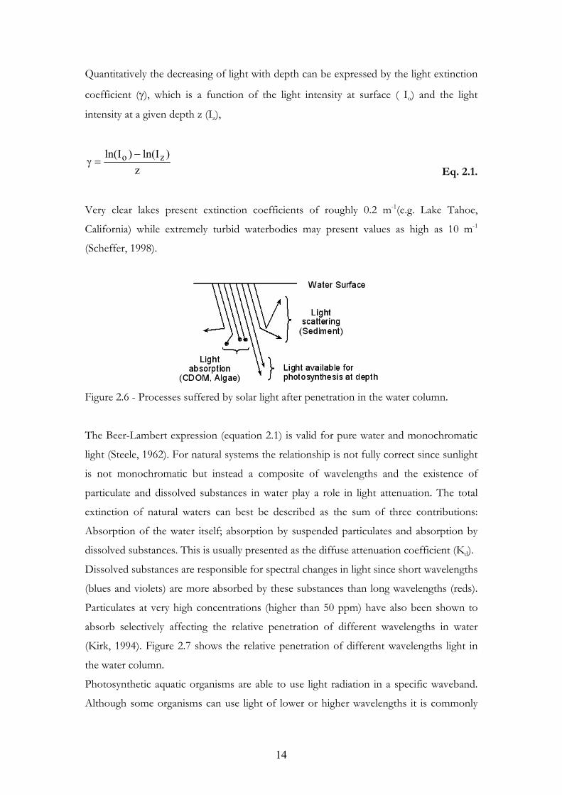
Quantitatively the decreasing of light with depth can be expressed by the light extinction

coefficient (), which is a function of the light intensity at surface ( Io) and the light

intensity at a given depth z (Iz),

z

)Iln()Iln( zo

Eq. 2.1.

Very clear lakes present extinction coefficients of roughly 0.2 m-1(e.g. Lake Tahoe,

California) while extremely turbid waterbodies may present values as high as 10 m-1

(Scheffer, 1998).

Figure 2.6 - Processes suffered by solar light after penetration in the water column.

The Beer-Lambert expression (equation 2.1) is valid for pure water and monochromatic

light (Steele, 1962). For natural systems the relationship is not fully correct since sunlight

is not monochromatic but instead a composite of wavelengths and the existence of

particulate and dissolved substances in water play a role in light attenuation. The total

extinction of natural waters can best be described as the sum of three contributions:

Absorption of the water itself; absorption by suspended particulates and absorption by

dissolved substances. This is usually presented as the diffuse attenuation coefficient (Kd).

Dissolved substances are responsible for spectral changes in light since short wavelengths

(blues and violets) are more absorbed by these substances than long wavelengths (reds).

Particulates at very high concentrations (higher than 50 ppm) have also been shown to

absorb selectively affecting the relative penetration of different wavelengths in water

(Kirk, 1994). Figure 2.7 shows the relative penetration of different wavelengths light in

the water column.

Photosynthetic aquatic organisms are able to use light radiation in a specific waveband.

Although some organisms can use light of lower or higher wavelengths it is commonly

15

considered that that waveband is 400-700 nm. This range is known as the

photossyntetically active radiation (PAR).

Figure 2.7 - Spectral absorption of visible light in water. (Source: NASA).

The euphotic zone is the top water layer from surface until the depth where 99% of the

incident surface light disappears. The intensity of light at this level is the compensation

light intensity at which photosynthesis balances plant respiration.

In situ evaluation of water transparency is most commonly done using a Secchi disk.

However, Secchi disk measurements have considerable errors as noted by several authors

(Hutchinson, 1957; Cole, 1994) since they are a function of light reflection at the disk

surface. Nevertheless, Secchi disk measurements generally correlate well with the

transmission of light. The following empirical relationship between Secchi disk depth (Zs)

and the extinction coefficient,

sz

7.1

Eq. 2.2.

developed by Poole et al. (1929) has been shown to be correct for most inland waters.

Most phytoplankton species tend to present specific tolerance ranges to light, turbidity

and temperature. Their maximum growth will occur within that range. This interval may

vary widely among species, with some more sensitive and other more resilient to stress

conditions.

16

2.2 Numerical models for simulation of eutrophication - A review

The use of highly specialized tools and techniques is currently mandatory for water

resources management and planning. Among them is the use of simulation models for

monitoring and control of environmental problems in waterbodies which became

generalised same decades ago. Models allow us to quickly answer a variety of questions

without the economic/temporal burden of an extensive survey. The use of models has

several advantages, namely enabling comprehensive evaluation of large or complex

waterbodies and the possibility of future previsions.

A wide range of models for simulating eutrophication has been developed over the years.

From crude basic models to highly sophisticated numerical applications. Some simulate

several phenomena and have broad application, others are highly specialized tools

designed to excel in only one area.

This review is not intended to encompass all existent eutrophication models for aquatic

systems developed to date. It will focus on widespread models with a past history of

published applications in the literature that can serve the purposes of the current work.

Ward et al. (1999), Shoemaker et al. (2005) and Shoemaker et al. (1997) present extensive

listings of models for aquatic systems. Irvine at al. (2004) presents a more up-to-date

review and Arheimer et al. (2003) report is more centred in applications used in

European countries. Shoemaker et al. (2005) presents detailed analysis of USA developed

models capabilities. Furthermore, EPA-CEAM, USGS and REM1 internet sites provide

extensive detailed information about numerous models.

Water quality and eutrophication modelling are important fields of water science studies

since the 1960’s (Reichert et al., 2001), although attempts to use mathematical

formulations in water quality studies can be traced back to the work of Streeter and

Phelps in 1925 (Streeter et al., 1925). Then, the attempt to simulate eutrophication in

lakes and reservoirs arose from the need to make predictions concerning non-point

source pollutants. Initially water quality models were deterministic mathematical models

preying on the booming development of computational fluid dynamics. They tended to

1 REM - Register of ecological models http://eco.wiz.uni-kassel.de/ecobas.html

EPA - Environmental protection agency http://www.epa.gov/ceampubl/products.htm

USGS - United States geological survey http://www.usgs.gov/pubprod/software.html

17

include a representation of some sort for hydrology and a detailed representation of

chemical and biological processes regarding nutrients and algae. Hydrodynamics were at

the time not considered important to simulate eutrophication. The inclusion of advective

flow regime and turbulent diffusion influence in water quality models was probably

pioneered by the work of DiToro et al. (1971).

The increase in sophistication of numerical techniques, the development of much faster

processors and the lowering of computational costs during the 1970’s and 80’s

popularized the development of fully three-dimensional models and the addition of new

levels of complexity to eutrophication models.

Coupling models for different types of processes (hydrology, hydrodynamics, sediment

transport, water quality) or media (air, water, land/soil or sediment) became

commonplace in the 90’s decade as evidence of the importance of the interactions

between different environmental compartments and between phenomena from different

scientific fields grew. Alternatively to coupling, the modular approach, in which a single

model with simulation capabilities for multiple media or processes is employed, was also

used. WASP 5.0 (Ambrose et al., 1993) and CE-QUAL-W2 (Cole et al., 1995) are

examples of the modular approach. At this time, temporal and spatial scale integration

became a major issue in modelling.

These large models, once very time consuming, took advantage of the advent of parallel

computing and ever faster processors to be numerically more effective. Sophisticated

models like these imply multidisciplinarity and are usually build and used by a team of

advanced experts. Most of them currently tend to include pre and post processing tools

to help generate meshes, manipulate data and handle graphical display of results.

Improved numerical capacities also allowed the development of applications at a larger

geographical scale – Basin or regional scale (Schultz et al., 2006; Leon et al., 2003).

The high volume of field data required to simulate eutrophication is not always available

and monitoring campaigns tend to be very expensive. Currently, a common approach to

overcome this problem is the use of remote sensing techniques to acquire data and a

GIS2 to store/display the data which are used together with the eutrophication models

(Versace et al., 2008; Srinivasan et al., 1994).

In the last decade, eutrophication models also started to focus strongly on the end users.

With the end user shifting from advanced modelling experts to water managers and

decisors or a stakeholder of some sort. This means that a current trend in eutrophication

2 geographic information system.

18

modelling is its integration in DSS3’s, also known as integrated decision systems, in order

to accomplish the knowledge transfer (Jakeman et al., 2008). This shift to a wider range

of end users, possibly with less training in the field, implies adapting models to be more

user friendly or have improved interfaces. This is frequently achieved at the expenses of a

loss in control over model parameters or conditions by the user.

Portability over different platforms and the lack of common standards when integrating

modelling tools is currently a concern in the development of DSS’s and models

encapsulated in DSS’s (A. Voinov - Univ. of Twente, pers. comm., 2009). In Europe, the

focus is in the development of harmonized modeling tools or platforms to support EU4

water framework directive. The OpenMI5 platform (Gregensen et al., 2007) and the

OASIS/PALM6 are the more visible European efforts so far.

When a mathematical model for eutrophication is build different approaches can be

used: Deterministic, stochastic or hybrid. Almost all widespread models are deterministic,

that is, a model in which every set of state variables values is uniquely determined by

parameters in the model. A deterministic model will always produce the same result for

the same input. Stochastic models on the other hand will always produce a different

result for the same input while maintaining the same statistical properties for the result,

since they output a probability distribution. Stochastic models use available data to infer

statistical patterns to simulate phenomena. They usually do not contain any detailed

knowledge of the physical phenomena. They are therefore not useful for sparse or noisy

datasets. Additionally, they cannot be used to simulate possible scenarios because their

application implies the use of existent data. Those are the main reasons why the majority

of widespread eutrophication models are deterministic. A deterministic model can be

used to simulate scenarios and applied when datasets are imperfect. Nevertheless,

deterministic models have non-quantified amounts of randomness and uncertainty

embedded in their parameters and structure. Their main limitation is not considering

uncertainty in the variables.

3 decision support system.

4 European Union.

5 http://www.openmi.org/reloaded/

6 http://www.cerfacs.fr/globc/PALM_WEB/index.html

19

Classical methodological approaches to implement deterministic models can be

categorized according to the numerical technique used to find approximate solutions for

PDEs7:

Finite difference method (FDM) - Based on a local Taylor series expansion to

approximate the PDE. The spatial discretization lacks versatility meaning it is not

suitable to complex geometries. The other two methods were developed to

overcome the spatial limitations of this one and both make use of the integral

form of the PDE which is mesh independent.

Finite volume method (FVM) – Makes use of a control volume. Calculates the

values of the conserved variables averaged across the volume. Does not require a

structured mesh like finite difference method does.

Finite element method (FEM) - The integral equation is solved by assuming a

piecewise continuous function over the domain. Main differences between FEM

and FVM are the use of alternative versions of the discretization method. In

particular the derivation of the discretized equations. FEM is typically considered

a superior method for complex domain problems ( Zienkiewicz et al., 2005).

All the classical methods described above require the use of a spatial mesh or grid.

Attempts to use meshless methodologies for fluid simulations are currently under

development but not well established yet (Belytschko et al., 2007). Meshless methods rely

on the use of single non-connected nodes distributed in space.

As mentioned in section 2.1 transport and mixing processes influence strongly the

dynamics of eutrophication. Hence, the simulation of eutrophication would be

incomplete without the use of a simulation tool for the hydrodynamic of the system to

be studied. Since this is not the main subject of this work, a pre-existent tool was chosen

to accomplish the task of modelling hydrodynamic and hydrologic features. The

mandatory conditions that the chosen hydrodynamic model should fulfill were:

Suitable for reservoirs.

Open source or available code with comprehensive manuals available in order to

allow code alterations or adaptations needed.

Widespread application with recognized scientific quality – existence of several

references with applications in peer reviewed literature by different authors.

7 Partial differential equation.

20

Dimensional/spatial versatility.

Table 2.2 includes a general description of each hydrodynamic model reviewed and major

literature references describing the models technicalities. A brief review of pre-existent

eutrophication simulation able models with a consistent past story of applications

supported by peer reviewed literature was also done. The reviewed eutrophication

models are included in table 2.2, under the entries Water Quality or Several (for

eutrophication tools that are integrated in more generic modelling tools). The term

“water quality” can be viewed as having a broader scope than the term “eutrophication”

since water quality models usually encompass eutrophication plus other processes (e.g.

organic pollutants or heavy metals modelling) simulation abilities. The reviewed models

were classified firstly according to the type of processes they can simulate.

Regarding the reviewed models with hydrodynamic simulation capabilities, it was found

that:

The following models are not open source or their code is not available: CH3D-

WES, DELFT3D, MIKE21, TELEMAC3D.

The following models have insufficient documented applications in peer

reviewed literature: TRIM, TRIVAST, MOHID.

The following models do not have dimensional versatility: DYRESM, CE-

QUAL-W2, DYNHYD (flow model included in WASP).

These above models will therefore not be further analyzed here. A brief description of

the remaining ones follows.

The Princeton Ocean Model (POM8) developed and maintained at the Princeton

University (Blumberg et al., 1987) was developed as an ocean modeling code but is able

to simulate circulation and mixing processes in all types of water bodies. POM is a sigma

coordinate, free surface ocean model with embedded turbulence and wave sub-models.

Despite its widespread use among oceanic researchers, POM appears to seldom be used

for simulation in reservoirs and lakes. In a review of literature, only two applications of

POM in lakes where found and none in reservoirs: Lake Erie (O’Connor et al., 1999) and

Lake Michigan (Chen et al., 2002).

The environmental fluid dynamics code (EFDC) is an integrated system of models with

the advantage of being public domain. EFDC is a 3D finite difference hydrodynamic and

sediment transport model. EFDC is currently supported by EPA9 and is available for 8 http://www.aos.princeton.edu

9 http://www.epa.gov/athens/wwqtsc/html/efdc.html

21

download. The model has been applied to numerous waterbodies and has very complete

user manuals available online. EFDC uses orthogonal curvilinear coordinates

(horizontal), which are more flexible than rectangular grids and a sigma coordinate

(vertical). Numerically, hydrodynamic in EFDC is similar to POM. Both use the Mellor–

Yamada turbulence closure scheme for eddy viscosity and diffusivity; both use mode

splitting and the numerical methods in the two models are alike. However, in EFDC the

boundary specifications are more general than in POM. For instance, EFDC allows

wetting/drying in boundary cells a useful feature for reservoirs, wetlands and marshes

simulation.

22

Table 2.2 - Classification of models according to type of processes simulated.

Processes Simulated Model General Description Main Reference Institution/Company

POM 3D ocean and coastal circulation model. Blumberg et al., 1987 Princeton Univ., USA. CH3D-WES 3D hydrodynamic model. Johnson et al., 1991 USACE WES, USA. Hydrodynamic

TRIM 2D/3D

2D/3D models for simulation of flow and transport in free surfaces. Casulli et al. , 1992

USGS SPAWAR, USA. Trento Univ., Italy

EFDC-HEM3D 3D hydrodynamic and water quality model. Hamrick, 1996. Park et al., 1995 VIMS, USA

TRIVAST 3D hydrodynamic and water quality model. Falconer et al., 1997 Wales Univ., UK RMA suite 2D/3D hydrodynamic and water quality model. King, 1993 Davis Univ. /USACE, USA. DELFT3D 3D hydrodynamic and water quality model. Commercial user manual Delft hydraulics, Netherlands MIKE21 2D hydrodynamic and water quality model. Commercial user manual DHI, Denmark

MOHID 3D hydrodynamic and water quality model. Neves, 1985. Santos, 1995. Portela, 1996 IST, Portugal

TELEMAC 3D 3D hydrodynamic and water quality model. Hervouet et al., 2000 EDF-DRD, France WASP 3D water quality and toxics model. Ambrose et al., 1993 EPA, USA DYRESM-CAEDYM 1D for vertical distribution simulation in lakes.

DYRESM Manual, 2006. CAEDYM Manual, 2006 Univ. Western Australia

Several (Integrated Systems)

CE-QUAL-W2

2D laterally averaged hydrodynamic and water quality model. Cole et al., 1995 EPA/ Tetratech, USA.

QSIM 1D model for water quality simulation in rivers. Kirchesch et al., 2002 BGF, Germany

CE-QUAL-ICM 3D water quality model. Cerco et al., 1995 USACE WES, USA. Water Quality ECOLAB water quality model. Commercial user manual DHI, Denmark

USGS- United States Geological Survey. EPA- Environmental Protection Agency. EDF- Electricité de France. IST- Instituto Superior Técnico. VIMS- Virginia Institute of Marine Sciences. WES- Waterways Experiment Station. USACE- United States Army Corps of Engineers. SPAWAR- Space and Naval Warfare. DHI- Danish Hydraulic Institute. BGF- Federal Institute of Hidrology. SHMI-Swedish Meteorological and Hydrological Institute.

23

The RMA models family is a finite element suite of models comprising RMA2, RMA4,

RMA10 and RMA11. It was firstly developed at Davis University by King et al. (1973).

Commercial formats for the 2D are available from Aquaveo. USACE owns a different

version of the RMA family with limited capabilities called TABS10. RMA2 and RMA4 are

both 2D depth averaged models thus not suitable for modelling vertically stratified

waterbodies. RMA10 is a 3D hydrodynamic model and RMA11 its correspondent transport

and water quality model. This family of models has a consistent history of documented

applications worldwide for hydrodynamic but not for water quality.

After reviewing the hydrodynamic models, their history of application to reservoirs and their

suitability to the task, the best candidates for simulating hydrodynamic in reservoirs were:

RMA suite and EFDC. RMA10 presents higher mesh versatility than EFDC since the

former is a finite element model and the latter a finite difference based model. Given that

previous research was done in the hydraulics research group of Minho university using the

bidimensional RMA2 (Pinho et al., 2004), RMA10 was chosen for simulating hydrodynamic

in the current work. Details about the model are given in chapter 3.

A brief description of the reviewed tools for eutrophication simulation follows. The main

purpose of analyzing existent models with eutrophication simulation capabilities is to make

an assessment of the state-of–the-art in order to use that knowledge to develop the tool to

be used in this work. Tables 2.3 to 2.5 contain detailed features for the analyzed

eutrophication models. Of the models in table 2.2, models for which source code is not

available, no detailed manuals exist or for which documented applications in peer reviewed

literature are but few were not further analyzed.

QSIM is a riverine water quality model developed and used by the federal institute of

hydrology of Germany. Currently in its 10.0 version has been widely applied in German

locations but unfortunately most of the published applications are in grey literature and

written in German. This model is not public domain.

WASP is a very flexible and customizable model able to run as standalone or together with

hydrodynamic models and/or watershed models. Recently it was used coupled to other types

of models by several authors (Kao et al, 1998; Umgiesser et. al, 2003; Zou et al, 2006).

10 http://chl.erdc.usace.army.mil/rma4

24

WASP can work either as a simple model or as a data intensive complex model since the

level of complexity is chosen by the user based on the needed accuracy. WASP is widely

used and has numerous documented applications.

CAEDYM11 is a finite difference model able to run independently or coupled to 1D

DYRESM and more recently to 3D ELCOM (Zhao et al., 2009) hydrodynamic models.

CAEDYM simulates primary and secondary production, nutrients and oxygen dynamics. Of

all the analyzed models, it is the only one able to simulate secondary production. The model

can use up to seven classes of phytoplankton, up to five classes of zooplankton and up to

three of fish. Version 3.1 includes an expansion of the sediment biology module. This model

is supported by the University of Western Australia. This model lacks the versatility of other

analyzed tools (e.g. WASP) regarding the possibility to change the level of complexity of

simulations, given that most of the modules and state variables must always be included in

simulations.

11 http://www.cwr.uwa.edu.au/software1/models1.php?mdid=3

25

Table 2.3 - Detailed features of eutrophication models for reservoirs I.

Model Inputs Outputs Limitations

WASP

Waterbody Segments Nutrient Loads Boundary conditions Initial conditions Parameters Forcing functions

Time variable concentrations of constituents and process rates at each computational segment

No zooplankton simulation Potential instability or numerical dispersion in user defined computational segments

CE-QUAL-W2 CE-QUAL-ICM

Domain geometric data Initial conditions Boundary conditions Parameters

Velocity fields, temperature and water surface elevation Time variable concentrations of constituents

No zooplankton nor macrophytes simulation Only one algae type

EFDC-HEM3D

Boundary conditions Initial conditions Bathymetry Parameters

Velocity fields, temperature salinity and water surface elevation Time variable concentrations of constituents Heavy input data requirements

CAEDYM

Initial conditions Boundary conditions Parameters Time series of state variables

Heavy input data requirements Fixed complexity level High computational costs (Herzfeld, 1997)

26

Table 2.4 - Detailed features of eutrophication models for reservoirs II.

Water Quality State-Variables Model

Source Code BOD DO S PHY ZOO T PO4 TP Org P Org C TN Org N Inorg N NO3 NH3 Si Chla

WASP FORTRAN AVAILABLE Y Y Y Y N N Y Y Y N Y Y N Y Y N Y CE-QUAL-ICM FORTRAN AVAILABLE Y Y Y Y Y N Y Y Y Y Y N N Y Y Y Y EFDC-HEM3D FORTRAN AVAILABLE Y Y Y Y N Y Y Y Y Y Y Y N Y Y Y Y CAEDYM FORTRAN AVAILABLE Y Y Y Y Y N Y N N N N N N Y Y Y Y

BOD- Biological Oxygen Demand. DO- Dissolved Oxygen. S- Transparency, Secchi disk or suspended sediments. PHY- Phytoplankton. ZOO-Zooplankton. T- Temperature. PO4-Phosphate. TP- Total Phosphorus. Org P- Organic Phosphorus. Org C- Organic Carbon. TN- Total Nitrogen. Org N- Organic N. Inorg N- Inorganic N. NO3- Nitrate. NH3- Ammonia. Si- Silicates. Chla- Chlorophyll-a.

Table 2.5 - Detailed features of eutrophication models for reservoirs III.

Complexity level Model Waterbody Spatial scale Temporal scale

Numerical solution

Pre and post- processing Documentation

Validation/ Applications

WASP L E R C 1, 2 or 3D Dynamical FDM Y CE-QUAL-ICM L E R C 1, 2 or 3D Dynamical FVM N EFDC-HEM3D L E R C 1, 2 or 3D Dynamical FDM Y CAEDYM L E R C 1, 2 or 3D Dynamical FDM N

L- Lakes/Reservoirs, R-Rivers/Channels, E-Estuaries, C-Coastlines. FDM- Finite Difference. FVM- Finite Volume. - Inexistent/insufficient, - Medium. - Good. Documentation- up to date user manual available. Number of applications- Sufficient history of published applications by independent groups of researchers (no inbreed) in international peer reviewed literature. Validation by several independent researchers (no inbreed). A minimum number of 20 publications were considered for classifying as good, 10 for medium.

27

The family of CE-QUAL models (CE-QUAL-ICM, CE-QUAL-R1, CE-QUAL-RIV1

and CE-QUAL-W2) has been developed to address environmental problems in USA

watercourses. CE-QUAL-R1 simulates 1D vertical profiles for water quality and is not

anymore supported nor was further developed after 1986. CE-QUAL-RIV1 is a 1D

longitudinal water quality model for rivers and streams and is also not supported

anymore. CE-QUAL-W2 is a 2D laterally averaged model with hydrodynamic and water

quality simulation capabilities. The water quality module code is similar to the one

contained in the initial CE-QUAL-ICM model. The CE-QUAL-ICM is a fully 3D able

model that includes benthic interactions in the computation of water quality variables.

CE-QUAL-ICM does not have pre and post processing tools. CE-QUAL-W2 current

version (3.6) already includes those features. CE-QUAL-W2 was conceptualized as a 2D

model with horizontal segments and vertical layers (laterally averaged). It is not applicable

in waterbodies were lateral gradients are important. The model branching algorithm

permits the simulation of complex geometries, dendritic domains and multiple reservoirs

with the same grid. Recently it was used to simulate dendritic reservoirs in several Asian

locations (Kuo et al, 2006; Kim et al, 2006). In CE-QUAL-W2, the hydrodynamic and

the water quality routines cannot be used as stand alone. The water quality routines

include the major eutrophication processes, including silica and iron modelling and only

one type of algal compartment. A single bottom sediment layer handles interfacial fluxes

calculation. Although organic N and organic P are not state variables they can be

calculated and present in the output of the model. This model sediment oxygen demand

rational is simplistic. Varies according to temperature only and is not coupled to the

water column, lacking a complete sediment diagenesis model. But it includes labile and

refractory organic matter. The water quality model included in EFDC, HEM3D was

developed by Park et al. (1995). HEM3D is a later development of the CE-QUAL-ICM

code. In particular, sediment diagenesis was extended.

RMA11 and RMA4 accept velocity inputs from the hydrodynamic models RMA10 or

RMA2 or input ASCII files. RMA11 and RMA4 compute the advection-diffusion

transport solution for up to 15 constituents plus the possibility of adding up to more 5

non-conservative constituents defined by the user. The RMA family of models is finite

element based which is better for domain definition but more time consuming for

calculations. These two water quality models have few documented applications and the

user manuals are not detailed.

28

All the reviewed tools for eutrophication simulation are deterministic tools that require a

manual calibration. The calibration in models of this type becomes harder as the number

or model parameters increases. And models with a high level of complexity tend to use

many parameters. This is the main reason for not using a pre-existent tool for simulating

eutrophication in the present work. All the well established eutrophication models use

manual trial and error calibration. As noted by Arhonditsis et al. (2007) this is very

inefficient and unreliable. For the purpose of this work, an eutrophication model with a

hybrid approach, integrating both deterministic and stochastic features and taking

advantage of the potential of both methodologies is developed. The developed tool is

described in detail in chapter 3. Although this mixed approach has been pointed out as

ideal for water models (Gupta et al., 1998) it is seldom seen implemented. The model will

be conceptually deterministic in what concerns eutrophication calculations and will

include a stochastically based automatic calibration method. The automatic calibration

has the ability to locate global optima and help achieve numerical stability. The

implemented optimization criteria uses a probabilistic Monte-Carlo method to identify

the “best parameters set” for calibration of the eutrophication model. The automatic

calibration process is done by minimizing a chosen objective function through numerical

optimization.

29

References for Chapter 2

Ambrose RB, Wool TA, Martin JL. 1993. The water quality analysis simulation program, WASP. EPA,

Athens, USA. Arheimer B, Olsson J. 2003. Integration and coupling of hydrological models with water quality models

applications in Europe. SMHI report. Sweden. Arhonditsis GB, Qian SS, Stow CA, Lamon CE, Reckhow KH. 2007. Eutrophication risk assessment using

Bayesian calibration of process-based models: application to a mesotrophic lake. Ecol. Model. 28:215–229.

Belytschko T, Chen JS. 2007. Meshfree and particle methods. John Wiley and Sons. Blumberg AF, Mellor GL. 1987. A description of a three-dimensional coastal ocean circulation model. In:

Three-dimensional coastal ocean models (N. Heaps, editor). Coastal and Estuarine Science, 4, American Geophysical Union.

CAEDYM user manual. 2006. Center for water research, University of Western Australia. Australia. Carlson RE. 1977. A trophic state index for lakes. Limnol. Oceanogr. 22:361-369. Casulli V, Cheng RT. 1992. Semi-implicit finite difference methods for three dimensional shallow water

flow. Internat. J. Numer. Methods Fluids 15:629-648. Cerco CF, Cole T. 1995: User's guide to the CE-QUAL-ICM three-dimensional eutrophication model,

release version 1.0. Technical report EL-95-15.USACE WES, Vicksburg, USA. Chen CS, Ji RB, Schwab D, Beletsky D, Fahnenstiel GL, Jiang MS, Johengen TH, Vanderploeg H, Eadie B,

Budd JW, Bundy MH, Gardner W, Cotner J, Lavrentyev PJ. 2002. A model study of the coupled biological and physical dynamics in Lake Michigan. Ecol. Model. 152 :145-168.

Cole GA. 1994. Textbook of limnology. 4th ed. Waveland Pr. Inc. Cole RW, Buchak EM. 1995. CE-QUAL-W2: A two-dimensional, laterally averaged, hydrodynamic and

water quality model. V.2.0. USACE WES, Vicksburg, USA. Cooke GD, Welch EB, Peterson SA, Nichols SA. 2005. Restoration and management of lakes and

reservoirs. Taylor and Francis CRC press. Davis ML, Masten SJ. 2003. Principles of environmental engineering and science. McGraw-Hill. DiToro DM, O'Connor DJ, Thomann RV. 1971. A dynamic model of the phytoplankton population in the

Sacramento - San Joaquin Delta. In: Nonequilibrium systems in natural water chemistry (RF Gould, editor). Wash. DC, American Chemical Society. 131-180.

DYRESM science manual. 2006. Center for water research, University of Western Australia. Australia. Falconer RA, Lin B. 1997. Three-dimensional modelling of water quality in the Humber estuary. Water

Res. 31:1092-1102. Gregersen JB, Gijsbers PJA, Westen SJP. 2007. OpenMI: Open Modelling Interface. J. Hydroinf. 9:175-

191. Gupta HV, Sorooshian S, Yapo PO. 1998. towards improved calibration of hydrologic models: multiple

and incommensurable measures of information. Water Resour. Res. 34:751–763. Hamrick JM. 1996. User's manual for the environmental fluid dynamics computer code. Special Report

No. 331 in Applied Marine Science and Ocean Engineering. School of Marine Science, Virginia Institute of Marine Science, The College of William and Mary, Goucester Point, USA.

Hervouet JM, Bates P. 2000. The TELEMAC modelling system. Hydrol. Process. 14:2207-2208. Herzfeld M, Hamilton DP. 1997. A computational aquatic ecosystem dynamics model of the Swan River,

Western Australia. MODSIM'97 International Congress on Modelling and Simulation Proceedings. 663-668.

Horne A, Goldman C.1994. Limnology. McGraw-Hill. Hutchinson GE. 1957. A treatise on limnology, Vol. I. geography, physics and chemistry. John Wiley &

Sons. Imberger A, Imberger J. 2001. Anatomy of turbulence in thermally stratified lakes. Limnol. Oceanogr. 46:

1158-1170. Irvine K, Mills P, Bruen M, Walley W, Hartnett M, Black A, Tynan S, Duck RW, Bragg O, Rowan J,

Wilson JG, Johnston P, O'Toole C. 2004. An assessment of the role of mathematical modelling in the implementation of the Water Framework Directive in Ireland. Final Report to the Irish Environmental Protection Agency. Ireland.

Jakeman A, Voinov A, Rizzoli A, Chen S (Editors). 2008. Environmental Modelling, Software and Decision Support, Volume 3: State of the art and new perspective (Developments in Integrated Environmental Assessment). Elsevier.

Johnson B, Heath RE, Hsieh KW, Kim KW, Butler HL. 1991. User’s guide for a three-dimensional numerical hydrodynamic, salinity and temperature model of Chesapeake Bay. USACE WES, Vicksburg, USA:

30

Jorgensen SE, Vollenweider RA (Editors). 2000. Diretrizes para o gerenciamento de lagos vol. 1. United Nations environment programme.

Kalff J. 2002. Limnology. 2nd ed. Prentice Hall. Kao JJ, Lin WL, Tsai CH. 1998. Dynamic spatial modelling approach for estimation of internal

phosphorus load Source. Water res. 32:47-56. Kim Y, Kim B. 2006. Application of a 2-dimensional water quality model (CE-QUAL-W2) to the turbidity

interflow in a deep reservoir (Lake Soyang, Korea). Lake Reservoir Manage. 22: 213-222. King IP, Norton WR, Orlob GT. 1973. A finite element solution for two-dimensional density stratified

flow. Report prepared by Water Resources Engineers, Walnut Creek CA, for the US Department of the Interior, Office of Water Resources Research, USA.

King IP.1993. A two dimensional finite element model for flow in estuaries and streams, v. 4.4. University of California, Davis, USA.

Kirchesch V, Schöl A. 2002. Das gewässergütemodell QSIM - ein instrument zur simulation und prognose des stoffhaushalts und der planktondynamik von Fließgewässern. Hydrologie und Wasserbewirtschaftung 43:302-308.

Kirk JTO. 1994. Light and photosynthesis in aquatic ecosystems. 2nd ed. Cambridge university press. Kuo JT, Lung WS, Yang CP, Liu WC, Yang MD, Tang TS. 2006. Eutrophication modelling of reservoirs in

Taiwan. Environ. Model. & software. 21: 829-844. Lampert W, Sommer U. 1997. Limnoecology: The ecology of lakes and streams. Oxford university press. Leon LF, Lam DC, McCrimmon C, Swayne DA. 2003. Model integration for watershed management: a

case study for lake Malawi/Nyasa/Niassa. Environ. Model. & Software.18: 531-539. Neves RJJ. 1985. Étude experimentale et modelisation mathematique des circulations de maree et residuelle

dans l´estuaire du Sado. PhD dissertation. University of Liège. Belgium. (In French). O’Connor WP, Schwab DJ, Lang GA.1999. Forecast verification for Eta model winds using lake Erie

storm surge water levels. Weather and Forecasting. 14:119-133. Park K, Kuo AY, Shen J, Hamrick, J. 1995. A three-dimensional hydrodynamic-eutrophication model

(HEM3D): Description of water quality and sediment process submodels. Special Report No. 327 in Applied Marine Science and Ocean Engineering, School of Marine Science, Virginia Institute of Marine Science, The College of William and Mary, Goucester Point, USA.

Pinho JLS, Vieira JMP, Carmo JSA. 2004. Mathematical modelling of oil spills in the Atlantic Iberian coastal waters. 4th International Conference on hydrocarbon spills, modelling, analysis & control Proceedings ( Brebbia CA, Saval Perez JM, Garcia Andion L, Villacampa Y, editors). 337-347.

Poole HH, Atkins WR. 1929. Photo-electric measurements of submarine illumination throughout the year. J. Mar. Biol. Assoc. U.K. 16: 297-324.

Portela LIF. 1996. Modelação matemática de processos hidrodinâmicos e de qualidade da água no estuário do Tejo. PhD dissertation in environmental engineering. Instituto Superior Técnico. Portugal. (In Portuguese).

Reichert P, Borchardt D, Henze M. 2001 River water quality model No.1. Scientific & technical report. IWA Publishing.

Santos AJ.1995. 3D hydrodynamic model for estuarine and oceanic circulation. PhD dissertation in mechanical engineering. Instituto Superior Técnico. Portugal. (In Portuguese).

Scheffer M. 1998. Ecology of shallow lakes. Kluwer academic press. Schultz MT, Small MJ, Fischbeck PS, Farrow RS. 2006. Evaluating response surface designs for uncertainty

analysis and prescriptive applications of a large-scale water quality model. Environ. Model. Assessm. 11:345-359.

Shoemaker L, Lahlou M, Breyer M, Kumar D, Kratt K. 1997. Compendium of tools for watershed assessment and TDML development. EPA, Office of Water, USA.

Shoemaker L, Dai T, Koenig J. 2005. TDML evaluation and research needs. EPA, National Risk Management Research Laboratory, USA.

Srinivasan R, Arnold JG. 1994. Integration of a basin-scale water quality model with GIS. J. Am. Water Res. Ass. 30: 453-462.

Steele JH. 1962. Environmental control of photosynthesis in the sea. Limnol. Oceanogr. 7:137–150. Streeter HW, Phelps EB. 1925. A study on pollution and natural purification of the Ohio River: III.

Factors conserved in the phenomena of oxidation and regeneration. Publ. Health Bull. 146. Umgiesser G, Canu DM, Solidoro C, Ambrose R. 2003. A finite element ecological model: a first

application to the Venice Lagoon. Environ. Model. & Software. 18:131-145. Versace VL, Ierodiaconou D, Stagnitti F, Hamilton AJ, Walter MT, Mitchell B, Boland AM. 2008.

Regional-scale models for relating land cover to basin surface-water quality using remotely sensed data in a GIS. Environ. Monitor. Assessm. 142:171-184.

Ward GW, Benaman J. 1999. Models for TMDL application in Texas watercourses: screening and model review. Report CRWR-99-7. Center for Research in Water Resources, the University of Texas at Austin. USA.

31

Welch EB, Jacoby JM. 2004. Pollutant effects in freshwater: applied limnology. 3rd ed. Spon press. Wetzel RG. 2001. Limnology. Lake and river ecosystems. 3rd ed. Academic press. Zienkiewicz OC, Taylor RL, Zhu JZ. 2005. The finite element method: Its basis and fundamentals. 6th ed.

Butterworth-Heinemann. Zhao Y, Jones ML, Shuter BJ, Roseman EF. 2009. A biophysical model of lake Erie walleye (Sander

Vitreus) explains interannual variations in recruitment. Can. J. Fish. Aquat. Sci.66:114-125. Zou R, Carter S, Shoemaker L, Parker A, Henry T. 2006. Integrated hydrodynamic and water quality

modeling system to support nutrient total maximum daily load development for Wissahickon Creek, Pennsylvania. J. Environ. Eng. ASCE. 132: 555-566.

32

CHAPTER 3 - DESCRIPTION OF MODELLING TOOLS

The current chapter includes descriptions of the modelling tools used and developed in

this work together with their theoretical background and implementation details. Model

application, including details on spatial and temporal discretization, initial and boundary

conditions and calibration are presented in chapter 5.

As mentioned in chapter 2.2, three main methods are widely used in computational fluid

dynamics: Finite element (FEM), finite volume (FVM) and finite difference (FDM). All

of the three methods represent and evaluate PDE’s in the form of algebraic equations.

In the finite difference method the differential equations are approximated by an

algebraic solution at discrete points in space (the grid points). The solution is therefore

only known in a set of discrete points in the domain. Finite difference discretization is

done by applying finite difference operators to the derivatives, term by term.

In the finite volume method the domain is divided into cells. The dependent variables

will take constant values inside each cell (that is, they are known in all domain) and will

present discontinuities at cell faces. Like in FDM, the calculation of the solution is done

in discrete points in the domain. But in FVM surface integrals are used to calculated

fluxes across the cells faces which will in turn be used to approximate the integral

balances of the transported properties while FDM uses finite difference equations to

approximate the derivatives.

While in FDM the variables evolution between the domain points is unknown, in FEM

the variables are approximated by continuous functions all over the domain.

FDM is very easy to implement but its application is limited to simple geometries. FVM,

although more versatile in handling geometries also gives solutions only at discrete points

of the domain and the computational costs associated with calculating geometric

parameters for the cells can sometimes become too high. The FEM easily handles

complicated geometries and boundaries plus gives continuous solutions allover the

domain. The FEM requires more computational time since the system matrix is sparse

(tridiagonal matrices cannot be obtained in FEM).

The models used and developed in the current work are FEM based.

The hydrodynamic model used in the present work was the three dimensional finite

element RMA10 (King, 1993a) version 8.0. This model also included heat transport

capabilities. A model for eutrophication was developed and coupled to RMA10. The

33

eutrophication model uses the spatial discretization of RMA10 and has the possibility of

using a different time step.

The pre and post-processing tools used were RMAGEN (Resource Modelling

Associates, 2008), RMAPLT (Resource modelling associates, 2010), SMS 7.0 (Aquaveo,

2002) and MATLAB 6.5 (Mathworks, 2004).

3.1 Hydrodynamic model

As noted in chapter 2, the model version used is the one developed and maintained by

King (1988, 1993a) and not the USACE1 version called TABS and previously named

RMA10-WES.

The main references describing the model and improvements over time are:

King (1982, 1985a, 1985b, 1988, 1993a) and King et al. (1995). King (1990) and

DeGeorge et al. (1993) focus on the use of mixed dimensions spatial meshes with

RMA10. King (1985a) focus on changes done by King on the sigma coordinate in order

to map the water surface on a horizontal surface while preserving the bottom profile.

Detailed applications of the model can be found in King (1993b), King et al. (1978,

1995), Fossati et al. (2008), Rueda (2002), Rueda et al. (2002) and Cook et al. (2002). A

comprehensive list of references with applications of the RMA suite of models can be

found online at: http://www.rmanet.com/Projects/SFBay-Delta/References.htm.

The model is a three dimensional finite element hydrodynamic model that uses the

Newton-Raphson iterative approach together with a standard Galerkin weighted

residuals to solve a system of non-linear equations based on the 3D Navier-Stokes

equations. RMA10 uses both the hydrostatic and the Boussinesq assumptions.

The resulting governing equations for momentum (Reynolds averaged form of Navier-

Stokes), an advection-diffusion equation for transport of active scalar fields (salinity

and/or heat), the continuity equation and the equation of state for density in RMA10 are

1 United States Army Corps of Engineers.

34

- Equations for the conservation of momentum

0x

p)

z

u(

z)

y

u(

y)

x

u(

xz

uw

y

uv

x

uu

t

uxxzxyxx

Eq.3.1

0y

p)

z

v(

z)

y

v(

y)

x

v(

xz

vw

y

vv

x

vu

t

vyyzyyyx

Eq.3.2

0gz

p)

z

w(

z)

y

w(

y)

x

w(

xz

ww

y

wv

x

wu

t

wzzzzyzx

Eq.3.3

x, y, z - Cartesian coordinates

u, v, w - velocity components in the Cartesian directions

- density of water

g - acceleration of gravity

p - water pressure

ij- turbulent eddy coefficients; index ij denotes Cartesian coordinates

i- external tractions operating on the boundaries or on the interior (combined Coriolis,

wind and bed friction effects); index i denotes Cartesian coordinates

t - time

The hydrostatic assumption (it is assumed that the waterbody is sufficiently shallow

relative to the length dimensions that vertical accelerations are negligible and may be

neglected) is used allowing a simplification of the momentum equation for the vertical

coordinate

0gz

p

Eq. 3. 4

- Equation of state for density (freshwater)

)T(f Eq. 3. 5

states that local density is a function of temperature.

35

- Equation for transport of heat and/or salinity (heat is used here as example)

0)z

Tk(

z)

y

Tk(

y)

x

Tk(

xz

Tw

y

Tv

x

Tu

t

Tszyx

Eq. 3. 6

T - water temperature

s- source/sink for the transported variable

ki- diffusion coefficient; index i denotes Cartesian coordinate

- Equation for the conservation of mass (continuity equation)

where the fluid was assumed to be incompressible

0z

w

y

v

x

u

Eq. 3. 7

Figure 3.1 - z coordinate transformation used in the RMA10 model.

The vertical coordinate in RMA10 was transformed (King, 1985a) to allow nodes to be

located at the time varying water and bed surfaces and have variable vertical node

spacing. That is to obtain a domain of fixed geometry despite water elevation changes

over time, as depicted in Figure 3.1. The transformation is

ahar

az'z

Eq. 3. 8

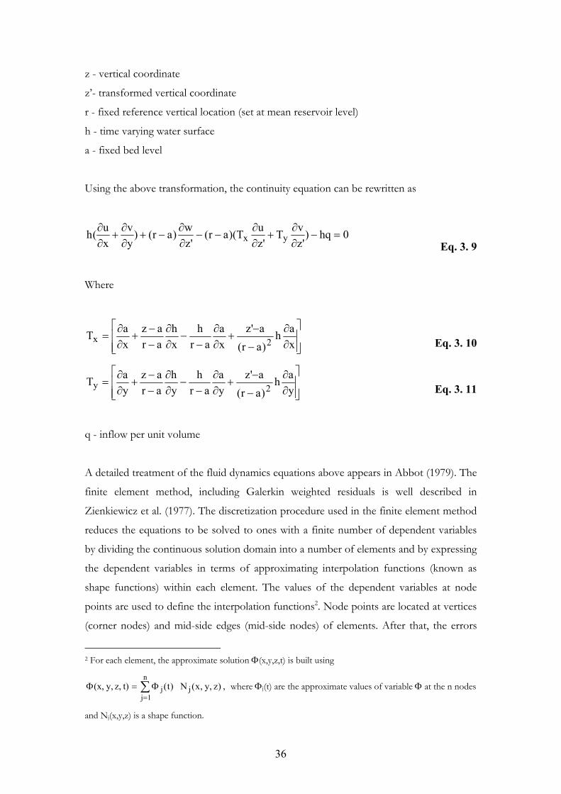
36

z - vertical coordinate

z’- transformed vertical coordinate

r - fixed reference vertical location (set at mean reservoir level)

h - time varying water surface

a - fixed bed level

Using the above transformation, the continuity equation can be rewritten as

0hq)'z

vT

'z

uT)(ar(

'z

w)ar()

y

v

x

u(h yx

Eq. 3. 9

Where

x

ah

)ar(

a'z

x

a

ar

h

x

h

ar

az

x

aT

2x Eq. 3. 10

y

ah

)ar(

a'z

y

a

ar

h

y

h

ar

az

y

aT

2y Eq. 3. 11

q - inflow per unit volume

A detailed treatment of the fluid dynamics equations above appears in Abbot (1979). The

finite element method, including Galerkin weighted residuals is well described in

Zienkiewicz et al. (1977). The discretization procedure used in the finite element method

reduces the equations to be solved to ones with a finite number of dependent variables

by dividing the continuous solution domain into a number of elements and by expressing

the dependent variables in terms of approximating interpolation functions (known as

shape functions) within each element. The values of the dependent variables at node

points are used to define the interpolation functions2. Node points are located at vertices

(corner nodes) and mid-side edges (mid-side nodes) of elements. After that, the errors

2 For each element, the approximate solution (x,y,z,t) is built using

n

1jjj )z,y,x(N)t(t)z,y,(x, wherej(t) are the approximate values of variable at the n nodes

and Nj(x,y,z) is a shape function.

37

which result from using the approximate dependent variables are minimized. This

procedure results in a set of simultaneous equations which are solved for the unknown

nodal dependent variables at the next time step.

RMA10 uses a quadratic interpolation in space (using corner nodes and mid-side nodes)

for the solution of the hydrodynamic and advection-diffusion equations for active scalar

concentrations and for velocities. Unsteady terms are discretized according to a weighted

finite difference scheme (Zienkiewicz et al., 1977). Water surface elevation is interpolated

linearly between corner nodes. FEM integrals are evaluated using Gaussian quadrature.

Temporal discretization uses the following semi-implicit non-centered weighted scheme

t

uu)

t

u()1()

t

u( of

of

Eq. 3. 12

u - variable evaluated over time

uf - variable u evaluated at final time f

uo - variable u evaluated at initial time 0

t= tf - to, time step

=1.8 (King, 1993b)

Note that if =1.0 we would have a fully implicit scheme, while if =2.0 we would have

Crank-Nicolson scheme. The RMA10 scheme allows the use of longer time steps, thus

reducing computational costs (King, 1993). Once discretized the set of non-linear

equations is solved using the Newton-Raphson method.

It should also be noted that in RMA10 each element has a trapezoidal section that varies

linearly between the corner nodes. This section is defined by a bottom width and side

slopes.

The governing equation for three dimensional transport of a generic constituent C in

RMA10 (using the z coordinate transformation from equation 3.8) is

38

0)'z

C

h

)ar(D(

'z)ar(

)'z

C)TDTD(

h

)ar((

'zT)ar()

y

CD

x

CD(

'zT)ar(

)'z

CTDTD(

h

)ar((

yh)

y

CD

x

CD(

yh

)'z

C)TDTD(

h

)ar((

'zT)ar()

y

CD

x

CD(

'zT)ar(

)'z

C)TDTD(

h

)ar((

xh)

y

CD

x

CD(

xh

'z

C

t

h)a'z(

'z

)vC(T)ar(

'z

)uC(T)ar(

'z

)wC()ar()

y

)vC(h

x

)uC(h

t

Ch

s'z

yyxxyyyxyy

)yyxxyyxy

yxyxxxxyxx

yxyxxxyx

yx

Eq. 3. 13

Dij - eddy diffusion coefficient; index ij denotes Cartesian coordinates

The sources and sinks term of the transport equation is the object of the eutrophication

model.

3.2 Eutrophication model

The eutrophication model developed is a pelagic model meant for freshwater lakes and

reservoirs. Interaction at air-water and water-sediment interfaces is included but benthic

and air compartments are not explicitly simulated. The model was implemented with a

modular structure for ease of coupling with hydrodynamic or transport models. The

structure is flexible in order to allow the inclusion of new processes or disabling part of

the existent ones. The model structure is shown in Figure 3.2.

The eutrophication model simulates the pelagic dynamics of phytoplankton and nutrients

cycles using nine state variables (dissolved oxygen, biochemical oxygen demand, nitrate,

ammonia, phytoplankton carbon, zooplankton carbon, organic nitrogen, organic

phosphorus and phosphate). The model was developed to predict eutrophication

situations and evaluate the trophic level of reservoirs or lakes.

The principle of parsimony was used to develop the model rational. Particularly, when it

was envisioned that an increase in complexity would lead to an increase in model

uncertainty the choice was for the lower level of complexity. This was the case for the

benthic compartment, for refractory vs. labile material (or several refractory levels) and

39

for the use of more than one group of phytoplankton none of which were included in

the model. The main reason was the fact that data sources for those variables would be

very difficult to obtain and could hinder model calibration and validation. Data from

sediment cores or sediment/water measured fluxes are usually not available or are sparse.

The implementation of an expansion of phytoplankton groups in the model is

straightforward if needed. Existing state variables can easily be expanded into vectors

with different C:N:P ratios, thus emulating different classes of algae. Organic phosphorus

and nitrogen compounds were not divided in dissolved and particulate compartments or

assigned different lability levels. Instead, a single pool for organic phosphorus and

another one for organic nitrogen were implemented. For each of them a single kinetic

process recycles the pool material to nutrients. This process lumps together the

mineralization of organic forms (giving rise to inorganic forms) and the hydrolysis

process that transforms particulates into dissolved material.

The model core consists of a series of coupled differential equations, one for each state

variable, describing the relationships presented in Figure 3.2.

The model is coupled to RMA10 and shares the same computational mesh. The two

models can use different temporal resolutions. The eutrophication model uses the

velocity components and temperature calculated by RMA10 as input.

The following generic references were used in the development and implementation of

the model: Bowie et al. (1985), EPA (1992), EPA (2000), McCutcheon (1989); Chapra

(1997), Thomann et al. (1987), Wetzel (2001), Jorgensen (2001), Jorgensen et al. (1989)

and Stumm et al. (1996).

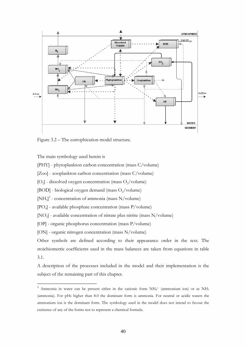
40

Figure 3.2 – The eutrophication model structure.

The main symbology used herein is

[PHY] - phytoplankton carbon concentration (mass C/volume)

[Zoo] - zooplankton carbon concentration (mass C/volume)

[O2] - dissolved oxygen concentration (mass O2/volume)

[BOD] - biological oxygen demand (mass O2/volume)

[NH3]3 - concentration of ammonia (mass N/volume)

[PO4] - available phosphate concentration (mass P/volume)

[NO3] - available concentration of nitrate plus nitrite (mass N/volume)

[OP] - organic phosphorus concentration (mass P/volume)

[ON] - organic nitrogen concentration (mass N/volume)

Other symbols are defined according to their appearance order in the text. The

stoichiometric coefficients used in the mass balances are taken from equations in table

3.1.

A description of the processes included in the model and their implementation is the

subject of the remaining part of this chapter.

3 Ammonia in water can be present either in the cationic form NH4+ (ammonium ion) or as NH3

(ammonia). For pHs higher than 8.0 the dominant form is ammonia. For neutral or acidic waters the

ammonium ion is the dominant form. The symbology used in the model does not intend to favour the

existence of any of the forms nor to represent a chemical formula.

41

Table 3.1 – Main chemical reactions considered in the eutrophication model.

Reaction name (source)

Reaction

Nitrification (Stumm et al., 1996)

H2OHNOO2NH 2324

Eq. 3. 14

Denitrification (Bowie et al., 1985) OH 7 2N CO 5 4HNO 4 OCH 5 222

-32

Eq. 3. 15

Respiration (Stumm et al., 1996) OH6CO6O6OHC 2226126

Eq. 3. 16

3.2.1 Temperature dependencies

All reaction rate parameters in the model are temperature dependent. The temperature

correction is done using an Arrhenius type exponential function

)20T(t kk

Eq. 3. 17

kt - generic kinetic rate at temperature T (1/time)

k - generic kinetic rate at 20ºC (1/time)

- temperature adjustment coefficient

T - water temperature (ºC)

used for BOD decay is 1.047 (Fair et. al, 1968), applicable for temperatures in the range

10-30 ºC. used for denitrification is 1.045 (EPA, 2000). for algae growth and

zooplankton temperature correction was 1.072 which corresponds to doubling the

growth rate for every 10ºC raise (EPA, 2000). used for other kinetic temperature

adjustments not mentioned above was 1.08 (EPA, 2000). Rates presented subsequently in

all the balance equations in this chapter are already temperature corrected.

42

3.2.2 Algae growth and limitation

Phytoplankton growth (μ) is considered to be limited by light and nutrients availability

following a minimum formulation similar to Liebig’s law of the minimum

)L,P,N(min limlimlimmax

Eq. 3. 18

max - algae maximum growth rate (1/time)

- algae growth rate (1/time)

Nlim - growth limitation by nitrogen

Plim - growth limitation by phosphorus

Llim - growth limitation by light

Liebig’s law of minimum considers the limiting factor to be the one with the lowest value

among all the possible limiting factors, that is, the most severely limiting factor of all.

Both phosphorus and nitrogen were assumed to be the possible limiting nutrients

(carbon was not considered as a possible limiting nutrient and silica is not simulated.

Micronutrients are also not included).

The nutrient growth limiting functions used are

33N

33lim NHNOk

NHNON

Eq. 3. 19

4P

4lim POk

POP

Eq. 3. 20

Kp - half-saturation constant for P limitation (mass P/volume)

KN - half-saturation constant for N limitation (mass N/volume)

The light limitation factor in the model has two contributions: The attenuation of light

over depth and the biological effect of the resulting light on algae growth. The light

limitation factor is well described by Steele’s (Steele, 1962) photoinibition formulation

43

)I

I1(

satlim

sateI

IL

Eq. 3. 21

I - intensity of light

Isat - optimal light intensity (saturation situation)

Where the intensity of light, I, for a given depth, can be calculated using the Beer-

Lambert law as mentioned in chapter 2.2

zoz eII

Eq. 3. 22

Iz - intensity of light at a given depth z

Io - intensity of light at water surface

- light extinction coefficient

The light extinction coefficient is a function of turbidity and has two contribution terms:

a base extinction coefficient, o, that includes all the effects of suspended particles except

algae and a contribution term accounting for the temporal variations of turbidity which is

a function of phytoplankton concentration. Phytoplankton is considered responsible for

most of the turbidity fluctuations. This second term constitutes what is called the self-

shading effect. The light extinction coefficient is thus

PHYSelfs0 Eq. 3. 23

0 - light extinction coefficient for all particles except algae (1/ length)

Selfs - self-shading coefficient (volume/ (length mass))

The incident solar shortwave radiation (broad range measurements) is equivalent to the

surface light intensity. Then, the light intensity at the top of the water column can be

calculated as

44

qst R)R-(1qsn ' Eq. 3. 24

qsn - top water column radiation (energy/ (area day))

qst - measured solar radiation at water surface (energy/ (area day))

R - water reflectivity

R’ - percent of radiation useful for photosynthesis

Where R accounts for the water surface reflectivity (albedo4) and R’ is a parameter that

empirically “filters” the radiation useful for photosynthesis (visible radiation in range

400-700 nm) that is not absorbed in the first meter below the water surface. The

reflectivity is expressed in a 0-1 range scale, with 1 for highly reflecting surfaces and 0 for

a completely non-reflecting surface. Lake and reservoir water surfaces absorb more than

reflect the radiation. Their average measured albedo usually lies in the interval 0.02-0.05

(See Figure 3.3). The model uses 0.5 for R’ (Bowie et al., 1985).

Figure 3.3 - Water surface albedo as function of incident solar radiation angle. Data for

steady water surface at 20ºC. (source: Kondratiev, 1969).

Substituting in the equation for the intensity of light

zz eqst'R)R1(I Eq. 3. 25

4 Reflectivity is given by the ratio between reflected radiation and incident radiation at a surface. The

albedo is defined as a reflectivity where the incident radiation source is the solar radiation.

45

3.2.3 Dissolved oxygen (O2)

For oxygen, salinity and pressure dependencies are not considered in the model, only

temperature corrections. Algae photosynthesis produces oxygen, while respiration

consumes it. Reaeration increases water oxygen levels while the oxidation of organic

matter (BOD and SOD5 contributions) as well as nitrification decreases it. Reaeration

and SOD terms are only calculated at the air-water and bed-water interfaces, respectively.

The oxygen rate of change in the model is

SODreaerationdecayionnitrificatnrespiratioproduction

changeofrateO2

Eq. 3. 26

That is

H

SOD)OC(ks

OdkBOD

OBODkd

OdkO

ONHknfbPHYkrrespOPHYprodO

t

O

2sat

2

2

22

232

22

Eq. 3. 27

prodO2 - oxygen mass production per unit of carbon mass in phytoplankton (mass

O2/mass C phytoplankton). That is, 32/12=2.(6)

respO2 - oxygen mass consumed per unit of carbon mass in phytoplankton for

respiration (mass O2/mass C phytoplankton). That is, 32/12=2.(6)

kr - respiration rate for phytoplankton (1/time)

fb - mass stoichiometry ratio in nitrification. That is, 64/14= 4.57

kn - nitrification rate (1/time)

dkO2 - half-saturation constant for oxygen limitation in nitrification (mass O2/volume)

kd - decay rate for BOD (1/time)

dkBOD - half-saturation constant for oxygen limitation in BOD decay (mass

O2/volume)

ks - surface transfer coefficient for oxygen. A function of local velocity and depth

(1/time)

5 Sediment oxygen demand.

46

CSAT - dissolved oxygen saturation (function of temperature) (mass O2/volume)

H – water depth (length)

SOD - sediment oxygen demand (mass O2/area/time)

Oxygen saturation is calculated according to the Elmore relation (Elmore et al., 1960)

that is valid for salinity zero and one atmosphere pressure

CSAT = 14.652 - 0.41022 T + 0.007991 T2 - 7.7774X10-5 T3 Eq. 3. 28

Reaeration, the exchange of oxygen through the water-atmosphere interface is modeled

by calculating the flux of dissolved oxygen across the water surface. The surface transfer

coefficient for oxygen (ks) is calculated using the O’ Connor-Dobbins (O’Connor et al.,

1958) relation which is valid for slow moving waters deeper than one meter. For a given

depth z

5.1

5.0

z

v9.12ks

Eq. 3. 29

Where v is the velocity

For shallower areas the Owens et al. (1964) formula is used

85.1

67.0

z

v35.5ks

Eq. 3. 30

Extensive reviews of existent relationships for calculating surface transfer coefficients for

oxygen can be found at Bowie et al. (1985) and Moog et al. (1995).

3.2.4 Ultimate biological oxygen demand (BOD)

Ultimate biological oxygen demand (BOD) is the use of oxygen by the microbial chain to

completely metabolize organic matter and oxidize reduced chemical species. Highly

organic contaminated water will show a high BOD, giving rise to low levels of dissolved

oxygen which is a sign of low health of a waterbody. Any organic matter load is a source

47

of BOD, either autochthonous or anthropogenic. These include point and non-point

source loads, faecal pellet, exudates and any dead organisms present in the water. In lakes

and reservoirs it is expected that autochthonous matter play the most important role in

BOD, since the carbon fixed by algae is probably the predominant BOD source.

BOD sinks comprise microbial degradation and sedimentation in the water column with

subsequent adsorption or absorption by benthic biota. The model focuses on water

column processes; therefore sediment oxygen demand (SOD) is not simulated, nor

benthic nitrification or resuspension contributions. The carbonaceous BOD (CBOD) is

simulated using first order rates and Michaelis-Menten kinetics. Nitrogenous BOD

(NBOD) is not simulated.

CBOD contributions are the water column deoxygenation caused by microbial

degradation (decay), denitrification, settling and death of phytoplankton and

zooplankton. Denitrification is a sink for BOD when dissolved oxygen levels are low.

Settling was considered because the particulate fraction of BOD can settle and thus

reduce carbonaceous deoxygenation. Phytoplankton and zooplankton death provides

oxidizable organic carbon. BOD balance is

settlingdecayationdenitrificmortalitychangeofrateBOD

Eq. 3. 31

that is

BOD

z

V

OdkBOD

OBODkd

Ok

kNOk

12

48

14

12

4

5)ZOOZPHY)Pkr((

12

32

t

BOD

set

2

2

2O

O3denit1deaddead

2

2

Eq. 3. 32

Pdead - non-predatory mortality of phytoplankton (1/time)

Zdead1 - non-predatory mortality of zooplankton (1/time)

kdenit - denitrification rate (1/time)

kO2 - oxygen inhibition constant in denitrification (mass O2/volume)

Vset - settling velocity (length/time)

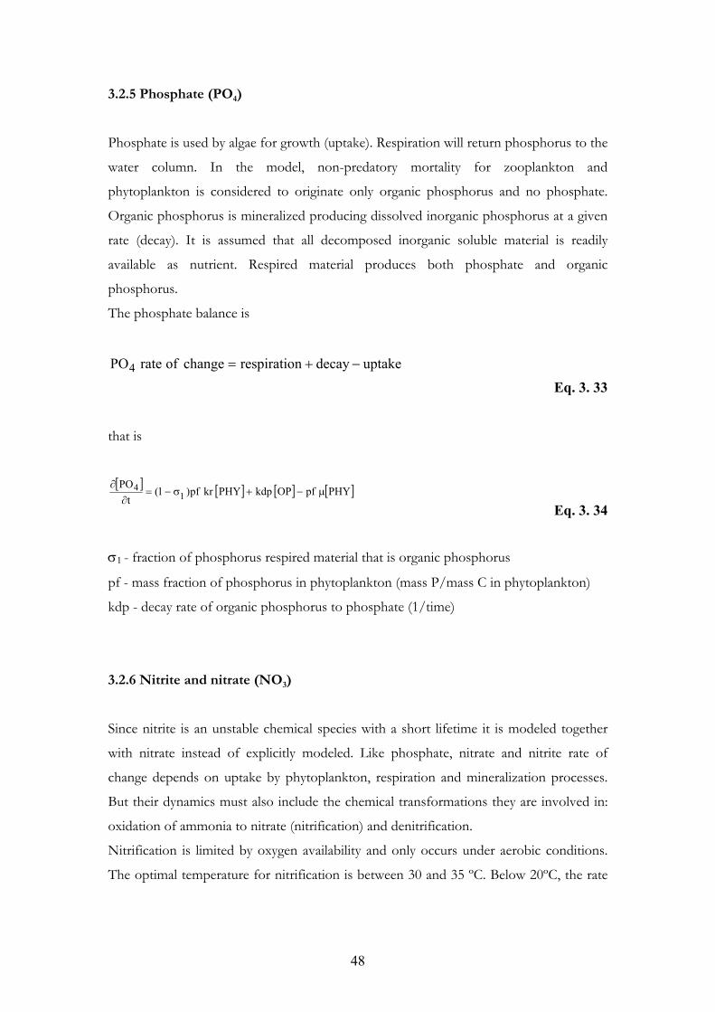
48

3.2.5 Phosphate (PO4)

Phosphate is used by algae for growth (uptake). Respiration will return phosphorus to the

water column. In the model, non-predatory mortality for zooplankton and

phytoplankton is considered to originate only organic phosphorus and no phosphate.

Organic phosphorus is mineralized producing dissolved inorganic phosphorus at a given

rate (decay). It is assumed that all decomposed inorganic soluble material is readily

available as nutrient. Respired material produces both phosphate and organic

phosphorus.

The phosphate balance is

uptakedecaynrespiratiochangeofratePO4

Eq. 3. 33

that is

PHYpfOPkdpPHYkrpf)1(t

PO1

4

Eq. 3. 34

1 - fraction of phosphorus respired material that is organic phosphorus

pf - mass fraction of phosphorus in phytoplankton (mass P/mass C in phytoplankton)

kdp - decay rate of organic phosphorus to phosphate (1/time)

3.2.6 Nitrite and nitrate (NO3)

Since nitrite is an unstable chemical species with a short lifetime it is modeled together

with nitrate instead of explicitly modeled. Like phosphate, nitrate and nitrite rate of

change depends on uptake by phytoplankton, respiration and mineralization processes.

But their dynamics must also include the chemical transformations they are involved in:

oxidation of ammonia to nitrate (nitrification) and denitrification.

Nitrification is limited by oxygen availability and only occurs under aerobic conditions.

The optimal temperature for nitrification is between 30 and 35 ºC. Below 20ºC, the rate

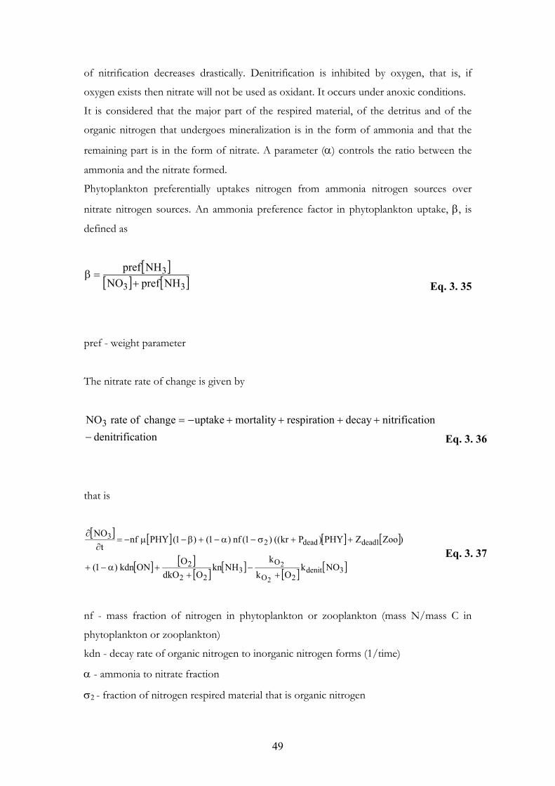
49

of nitrification decreases drastically. Denitrification is inhibited by oxygen, that is, if

oxygen exists then nitrate will not be used as oxidant. It occurs under anoxic conditions.

It is considered that the major part of the respired material, of the detritus and of the

organic nitrogen that undergoes mineralization is in the form of ammonia and that the

remaining part is in the form of nitrate. A parameter () controls the ratio between the

ammonia and the nitrate formed.

Phytoplankton preferentially uptakes nitrogen from ammonia nitrogen sources over

nitrate nitrogen sources. An ammonia preference factor in phytoplankton uptake, , is

defined as

33

3

NHprefNO

NHpref

Eq. 3. 35

pref - weight parameter

The nitrate rate of change is given by

ationdenitrific

ionnitrificatdecaynrespiratiomortalityuptakechangeofrateNO3

Eq. 3. 36

that is

3denit

2O

O3

22

2

1deaddead23

NOkOk

kNHkn

OdkO

OONkdn)1(

)ZooZPHY)Pkr(()1(nf)1()1(PHYnft

NO

2

2

Eq. 3. 37

nf - mass fraction of nitrogen in phytoplankton or zooplankton (mass N/mass C in

phytoplankton or zooplankton)

kdn - decay rate of organic nitrogen to inorganic nitrogen forms (1/time)

- ammonia to nitrate fraction

2 - fraction of nitrogen respired material that is organic nitrogen

50

3.2.7 Ammonia (NH3)

Ammonia nitrogen is consumed in nitrification and in uptake by phytoplankton growth.

Ammonia production occurs through mineralization of the organic nitrogen pool

(decay), dead and respired material. Adsorption of ammonia to particulates is not

considered in the model. The ammonia rate of change is

ionnitrificat

decaynrespiratiomortalityuptakechangeofrateNH3

Eq. 3. 38

that is

3

22

2

1deaddead23

NHOdkO

OknONkdn

)ZooZPHY)Pkr)((1(nfPHYnft

NH

Eq. 3. 39

3.2.8 Phytoplankton (PHY)

The model approach uses aggregates of algae in one single group but can easily be

expanded in more algae classes. No distinction between diatoms, cyanobacteria and other

groups of algae was made. The contributions considered were production, mortality

(non-predatory plus grazing by zooplankton), settling and respiration. Respiration

process was lumped together with excretion. Zooplankton feeding efficiency was

considered to be 100% (that is one gram of ingested phytoplankton leads to one gram of

zooplankton). The algae dynamics is simulated according to

settlinggrazing

nrespiratiomortalitypredatorynonproductionchangeofratePHY

Eq. 3. 40

that is

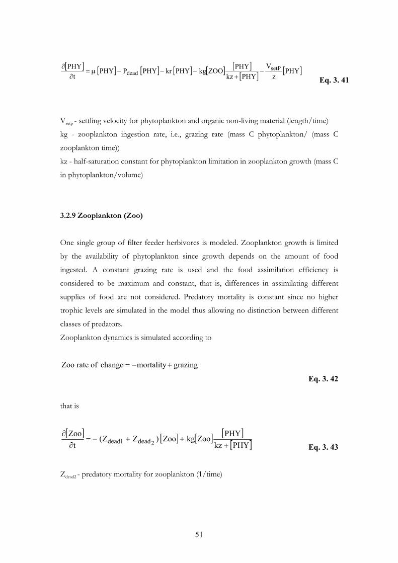
51

PHY

z

V

PHYkz

PHYZOOkgPHYkrPHYPPHY

t

PHY setPdead

Eq. 3. 41

Vsetp - settling velocity for phytoplankton and organic non-living material (length/time)

kg - zooplankton ingestion rate, i.e., grazing rate (mass C phytoplankton/ (mass C

zooplankton time))

kz - half-saturation constant for phytoplankton limitation in zooplankton growth (mass C

in phytoplankton/volume)

3.2.9 Zooplankton (Zoo)

One single group of filter feeder herbivores is modeled. Zooplankton growth is limited

by the availability of phytoplankton since growth depends on the amount of food

ingested. A constant grazing rate is used and the food assimilation efficiency is

considered to be maximum and constant, that is, differences in assimilating different

supplies of food are not considered. Predatory mortality is constant since no higher

trophic levels are simulated in the model thus allowing no distinction between different

classes of predators.

Zooplankton dynamics is simulated according to

grazingmortalitychangeofrateZoo

Eq. 3. 42

that is

PHYkz

PHYZookgZoo)ZZ(

t

Zoo2dead1dead

Eq. 3. 43

Zdead2 - predatory mortality for zooplankton (1/time)

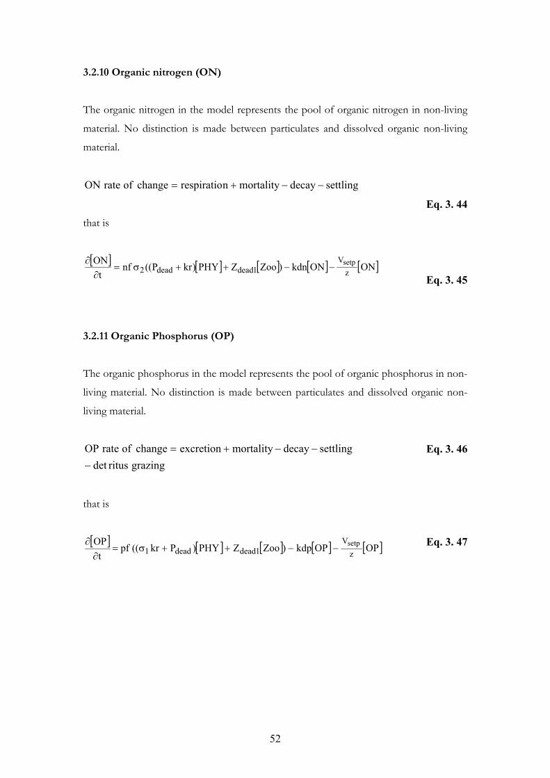
52

3.2.10 Organic nitrogen (ON)

The organic nitrogen in the model represents the pool of organic nitrogen in non-living

material. No distinction is made between particulates and dissolved organic non-living

material.

settlingdecaymortalitynrespiratiochangeofrateON

Eq. 3. 44

that is

ONONkdn)ZooZPHY)krP((nft

ONz

V1deaddead2

setp

Eq. 3. 45

3.2.11 Organic Phosphorus (OP)

The organic phosphorus in the model represents the pool of organic phosphorus in non-

living material. No distinction is made between particulates and dissolved organic non-

living material.

grazingritusdet

settlingdecaymortalityexcretionchangeofrateOP

Eq. 3. 46

that is

OPOPkdp)ZooZPHY)Pkr((pft

OPz

V1deaddead1

setp

Eq. 3. 47

53

3.2.12 Parameters

A descriptive list of parameters and ranges used in the model is presented in table 3.2

together with their source references. The light extinction coefficient, and the ratios nf

and pf (obtainable from the mass relationship C:N:P in phytoplankton) are site specific

parameters whose values can be inferred from monitoring data without the need to use

literature references. A parameter relating carbon mass with chlorophyll-a mass in

phytoplankton which is also site specific was included in the model. This parameter was

also obtained from experimental data.

Table 3.2 – Eutrophication model parameters ranges and literature references.

Parameter Units Reference Range/ Value

Isat optimal light intensity range used in model [200-500]

Ly/day (3) (9) (14)

200-350 225-500 350

Selfs self shading coefficient range used in model [0.0017-0.054]

m-1 (4) (9)

0.0017 0.054

KP half-saturation constant for P limitation uptake range used in model [0.001-0.2]

mg P/L

(1) (2) (6) (3) (9)

1E-3-5E-3 5E-3-8E-3 2E-3-0.2 3E-3-0.05 1E-3

KN half-saturation constant for N limitation uptake range used in model [0.01-0.3]

mg N/L

(1) (2) (6) (9)

0.01-0.02 0.03-0.3 0.01-0.2 0.025

Kz half-saturation constant for phytoplankton limitation in zooplankton growth range used in model [0.2-2.0]

mg C/L (1) (3)

0.6-0.9 0.2-2.0

max Algae maximum growth rate at 20ºC range used in model [0.5-3.0]

day-1 (1),(10) (2) (5) (6) (3) (11),(12),(14)

1.5-2.5 0.8-1.3 3.5 0.5-2.5 1-3 2.0

kr Respiration rate at 20ºC range used in model [0.01-0.25]

day-1 (1) (2),(11) (6) (7) (3) (9)

0.05-0.25 0.14 0.01-0.25 0.01-0.13 0.05-0.15 0.075

Pdead phytoplankton non-predatory mortality rate at 20ºC range used in model [0.01-0.1]

day-1 (1) (2) (7) (3) (10)

0.1 0.09 0.01-0.09 0.02-0.03 0.02-0.1

Zdead1

zooplankton non-predatory mortality at 20ºC range used in model [0.005-0.07]

day-1 (1) (6) (3) (13)

0.02 5e-3-95e-3

5E-3-0.07 0.01

54

Parameter Units Reference Range/ Value

Zdead2 Zooplankton predatory mortality rate at 20 ºC range used in model [0.005-0.1]

day-1 (1) (3)

0.1 5e-3-0.02

kg Ingestion rate for zooplankton at 20 ºC range used in model [0.5-1.5]

mass C algae/(mass C zoo day)

(3) (5) (7)

0.7-1.4 0.8 0.5

pref Weight factor in ammonia preference factor range used in model [1-2]

- (11) 1.5

fraction of phosphorus respired material that is organic phosphorus range used in model [0.0-0.5]

- - -

fraction of nitrogen respired material that is organic nitrogen [0.0-0.5]

- -

Ammonia to nitrate fraction range used in model [0.5-1.0]

- - -

kdp decay rate of organic phosphorus to inorganic P at 20 ºC range used in model [0.03-0.8]

day-1 (1) (7),(10) (8) (3) (9)

0.03-1.0 0.1-0.4 0.07-0.8 0.03-0.14 0.03

kdn decay rate of organic nitrogen to inorganic N at 20 ºC range used in model [0.02-0.5]

day-1 (1) (7) (8) (3) (10)

0.1-0.5 0.02-0.05 0.03-0.3 0.02-0.04 0.02-0.2

kdenit Denitrification rate range used in model [0.09-0.1]

day-1 (1) (9), (14)

0.09 0.1

kn Nitrification rate range used in model [0.01-0.3]

day-1 (1) (2),(14) (7) (3) (10)

0.05 0.02 0.01-0.02 0.1-0.3 0.05-0.15

kO2 oxygen inhibition constant in denitrification range used in model [0.1-0.5]

mg O2/L

(1) (2) (9)

0.1 0.5 0.1

dkO2 half-saturation constant for oxygen limitation in nitrification value used in model 2.0

mg O2/L

(1),(2), (9) 2

kd Decay rate of CBOD at 20ºC range used in model [0.1-0.5]

day-1 (1) (3) (10)

0.1-0.5 0.1-0.2 0.1-0.3

dkBOD half-saturation constant for oxygen limitation in BOD decay value used in model 0.5

mg O2/L

(1),(10),(7) 0.5

Vset Settling velocity for BOD value used in model 0.2

m/day (1) (2), (14) (9) (11)

0.3 0.1 0.1-0.2 0.15

Vsetp settling velocity for phytoplankton and particulates value used in model 0.25

m/day (2) (3) (10) (12)

0.05-0.01 0.02-0.5 0-0.5 0.1-1.0

SOD Sediment oxygen demand range used in model [100-5800]

mg/(m2 day) (15) 100-5800

(1)Chau et al. (1998). (2) Romero et al. (2004). (3) Bowie et al. (1985). (4) Hydroqual (2005). (5) Komatsu et al. (2006). (6) Bonnet et al. (2004). (7) Hamilton et al. (1997a). (8) Hamilton et al. (1997b). (9) Di Toro et al. (1980). (10) Tufford et al. (1999). (11) Deas et al. (1999). (12) Park et al. (2005). (13) Komatsu et al. (2006). (14) Kuo et al. (2006). (15)Cole et al. (2003).

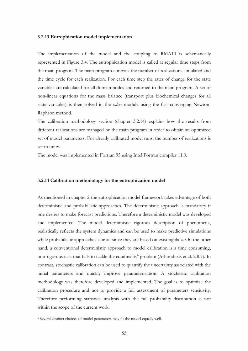
55

3.2.13 Eutrophication model implementation

The implementation of the model and the coupling to RMA10 is schematically

represented in Figure 3.4. The eutrophication model is called at regular time steps from

the main program. The main program controls the number of realizations simulated and

the time cycle for each realization. For each time step the rates of change for the state

variables are calculated for all domain nodes and returned to the main program. A set of

non-linear equations for the mass balance (transport plus biochemical changes for all

state variables) is then solved in the solver module using the fast converging Newton-

Raphson method.

The calibration methodology section (chapter 3.2.14) explains how the results from

different realizations are managed by the main program in order to obtain an optimized

set of model parameters. For already calibrated model runs, the number of realizations is

set to unity.

The model was implemented in Fortran 95 using Intel Fortran compiler 11.0.

3.2.14 Calibration methodology for the eutrophication model

As mentioned in chapter 2 the eutrophication model framework takes advantage of both

deterministic and probabilistic approaches. The deterministic approach is mandatory if

one desires to make forecast predictions. Therefore a deterministic model was developed

and implemented. The model deterministic rigorous description of phenomena,

realistically reflects the system dynamics and can be used to make predictive simulations

while probabilistic approaches cannot since they are based on existing data. On the other

hand, a conventional deterministic approach to model calibration is a time consuming,

non-rigorous task that fails to tackle the equifinality6 problem (Arhonditsis et al. 2007). In

contrast, stochastic calibration can be used to quantify the uncertainty associated with the

initial parameters and quickly improve parameterization. A stochastic calibration

methodology was therefore developed and implemented. The goal is to optimize the

calibration procedure and not to provide a full assessment of parameters sensitivity.

Therefore performing statistical analysis with the full probability distribution is not

within the scope of the current work. 6 Several distinct choices of model parameters may fit the model equally well.

56

The initial model parameters ranges were inferred from literature information (see table

3.2). Subsequently Monte-Carlo simulations provided an adequate way to approximate

the parameter distributions.

Monte-Carlo methods approximate solutions of mathematical problems using statistical

sampling experiments. The term describes not a single method but a large class of

methods whose common characteristic is the use of sequences of random numbers to

perform a statistical simulation. Monte-Carlo methods are useful to study systems with a

large number of coupled degrees of freedom such as fluids and are particularly suitable

for simulating phenomena with significant uncertainty in inputs (Kalos et al., 2008). The

process involves performing many simulations (a.k.a. realizations) using generated

random numbers in order to get an approximation to the answer to the problem. The

higher the number of realizations the more accurate the answer is, since the

approximation error becomes smaller (Kalos et al., 2008). The convergence of Monte-

Carlo estimative is slow. Generally, it is proportional to N/1 , with N the number of

realizations. However, the level of accuracy is also dependent of the suitability of the

method used for solving a given problem.

In many applications of Monte-Carlo methods physical processes are not simulated

directly, that is, no discretizing of differential equations and solving sets of algebraic

equations is involved. Instead a description of the system based on probability density

functions is used for random sampling and simulation. After that, probability is used to

set the approximation to the answer of the problem. In the current work, a Monte-Carlo

method is used to solve a non-linear inverse problem – given observed data, the values

of the most probable model parameters must be obtained. A large collection of random

generated numbers is used as model parameters. Results for the simulations done with

the parameters are compared with the data distribution and their relative likelihood is

analyzed. Minimization and rejection criteria are used to analyze the approximation error.

The random generator implemented was ran2 (Press et al., 1992) which is based on the

Minimal Standard generator (Park et al., 1988) with additional output shuffles to remove

any serial correlations.

57

Figure 3.4 - Flowchart for implemented eutrophication model.

58

The eutrophication model parameters to be calibrated are the parameters presented in

table 3.2 that have an initialization range in the model. Those ranges are presented in the

second column of the table 3.2. The initialization range can be represented by a generic

interval [Minj-Maxj], where j=1,…, n and n is the number of model parameters to be

calibrated.

Given i=1,…, N with N the number of random samples of the eutrophication model

parameters, the random generator implemented generates random numbers, ri, that lie in

the interval [0-1]. The uniformly distributed random model parameters (xji) are built

according to

jjjiji Min)Min-(Maxrx Eq. 3. 48

Each set of random parameters, Xi, built according to

)x...,x,x(X nii2i1i Eq. 3. 49

is used as input for an eutrophication model simulation. Each of these simulations is a

realization of the system.

For each realization, an evaluation of the mass balance of the state variables over domain

space and time is performed, that is a simulation with the random sampling is performed.

Each model realization will output an f ’k(t,Xi) which is an approximation to the real

solution fk(t,X) given by in situ measurements, with k=1,…, m where m is the number of

simulated state variables.

For each realization of the model, the accuracy of the model result is evaluated by

calculating the difference between f ’k(t,Xi) and fk(t,X) using multiple NRMSE7 as criteria

np

)X,t(f)X,t(f

)X,t(f

1NRMSE

2i

'kk

t

tt

kkpi

f

0

for k=1,…,5 Eq. 3. 50

7 Normalized root mean squared error.

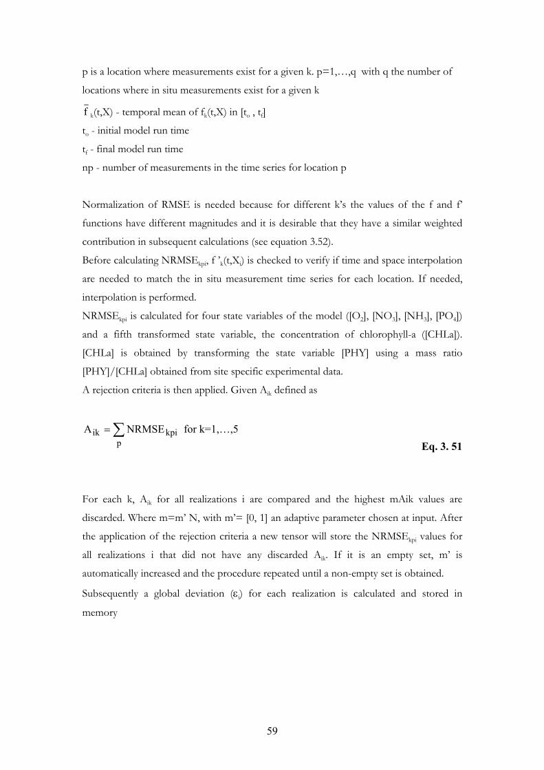
59

p is a location where measurements exist for a given k. p=1,…,q with q the number of

locations where in situ measurements exist for a given k

f k(t,X) - temporal mean of fk(t,X) in [to , tf]

to - initial model run time

tf - final model run time

np - number of measurements in the time series for location p

Normalization of RMSE is needed because for different k’s the values of the f and f’

functions have different magnitudes and it is desirable that they have a similar weighted

contribution in subsequent calculations (see equation 3.52).

Before calculating NRMSEkpi, f ’k(t,Xi) is checked to verify if time and space interpolation

are needed to match the in situ measurement time series for each location. If needed,

interpolation is performed.

NRMSEkpi is calculated for four state variables of the model ([O2], [NO3], [NH3], [PO4])

and a fifth transformed state variable, the concentration of chlorophyll-a ([CHLa]).

[CHLa] is obtained by transforming the state variable [PHY] using a mass ratio

[PHY]/[CHLa] obtained from site specific experimental data.

A rejection criteria is then applied. Given Aik defined as

p

kpiik NRMSEA for k=1,…,5

Eq. 3. 51

For each k, Aik for all realizations i are compared and the highest mAik values are

discarded. Where m=m’ N, with m’= [0, 1] an adaptive parameter chosen at input. After

the application of the rejection criteria a new tensor will store the NRMSEkpi values for

all realizations i that did not have any discarded Aik. If it is an empty set, m’ is

automatically increased and the procedure repeated until a non-empty set is obtained.

Subsequently a global deviation (i) for each realization is calculated and stored in

memory

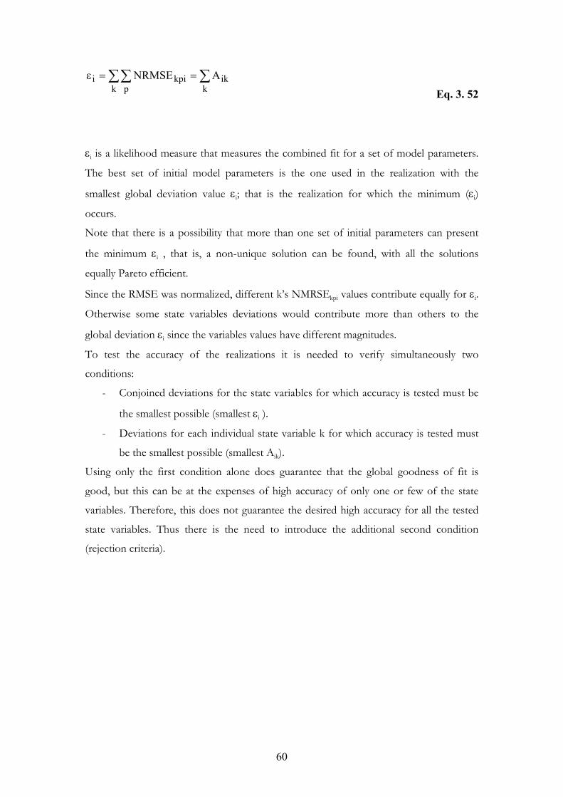
60

k

ikk p

kpii ANRMSE

Eq. 3. 52

i is a likelihood measure that measures the combined fit for a set of model parameters.

The best set of initial model parameters is the one used in the realization with the

smallest global deviation value i; that is the realization for which the minimum (i)

occurs.

Note that there is a possibility that more than one set of initial parameters can present

the minimum i , that is, a non-unique solution can be found, with all the solutions

equally Pareto efficient.

Since the RMSE was normalized, different k’s NMRSEkpi values contribute equally for i.

Otherwise some state variables deviations would contribute more than others to the

global deviation i since the variables values have different magnitudes.

To test the accuracy of the realizations it is needed to verify simultaneously two

conditions:

- Conjoined deviations for the state variables for which accuracy is tested must be

the smallest possible (smallest i ).

- Deviations for each individual state variable k for which accuracy is tested must

be the smallest possible (smallest Aik).

Using only the first condition alone does guarantee that the global goodness of fit is

good, but this can be at the expenses of high accuracy of only one or few of the state

variables. Therefore, this does not guarantee the desired high accuracy for all the tested

state variables. Thus there is the need to introduce the additional second condition

(rejection criteria).

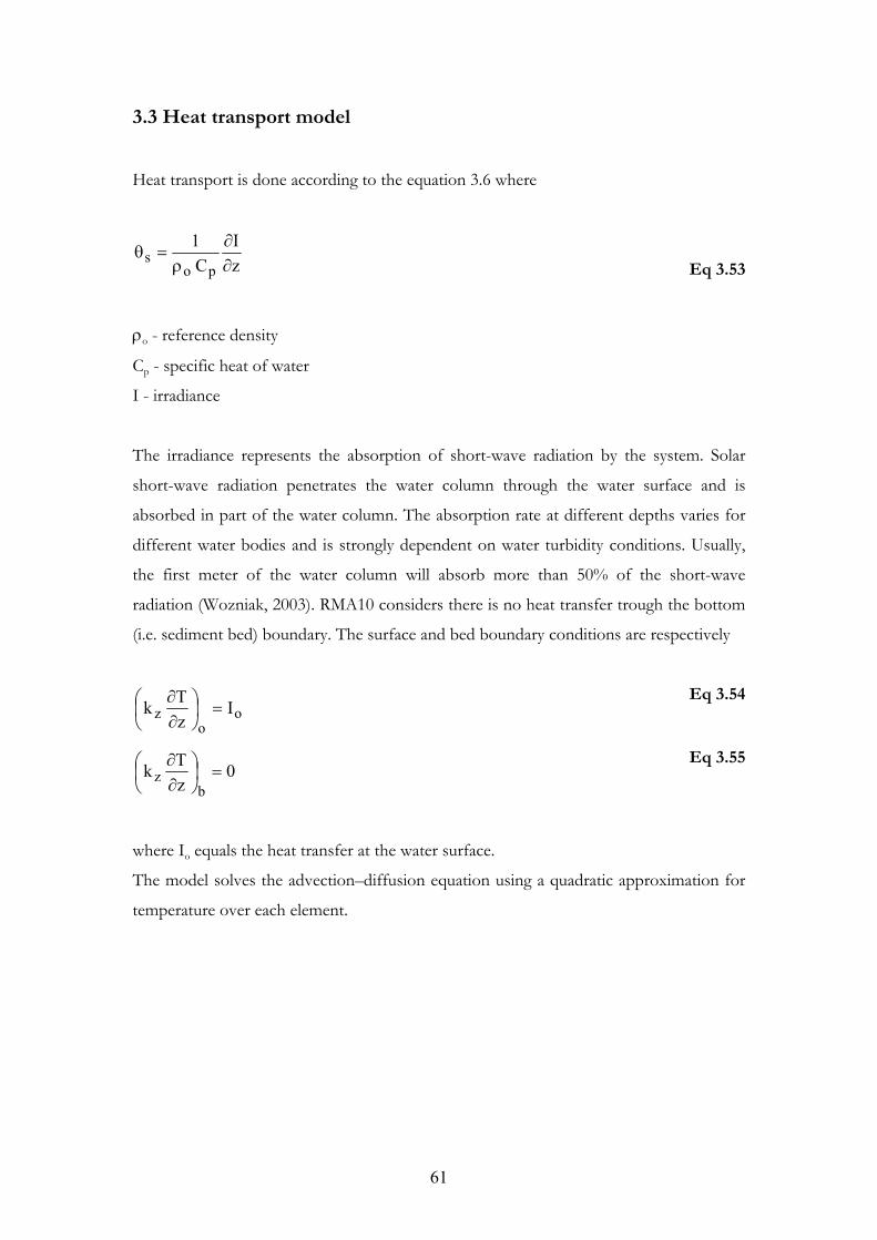
61

3.3 Heat transport model

Heat transport is done according to the equation 3.6 where

z

I

C

1

pos

Eq 3.53

o - reference density

Cp - specific heat of water

I - irradiance

The irradiance represents the absorption of short-wave radiation by the system. Solar

short-wave radiation penetrates the water column through the water surface and is

absorbed in part of the water column. The absorption rate at different depths varies for

different water bodies and is strongly dependent on water turbidity conditions. Usually,

the first meter of the water column will absorb more than 50% of the short-wave

radiation (Wozniak, 2003). RMA10 considers there is no heat transfer trough the bottom

(i.e. sediment bed) boundary. The surface and bed boundary conditions are respectively

oo

z Iz

Tk

Eq 3.54

0z

Tk

bz

Eq 3.55

where Io equals the heat transfer at the water surface.

The model solves the advection–diffusion equation using a quadratic approximation for

temperature over each element.

62

3.3.1 Short-wave radiation (HSN)

In the model, the flux of solar radiation penetrating the water surface (HSN) is given by

the insolation reaching the water surface reduced by the albedo and corrected for cloud

cover and atmospheric transmissivity attenuation. The flux of solar radiation penetrating

the water surface is calculated after Henderson-Sellers (1986) as

)C65.01)(r1(RHH 20SN Eq 3.56

H0 - incoming solar short-wave radiation to earth’s atmosphere

R - albedo

r - water surface parameter

C - cloud cover (expressed as fraction [0-1])

The penetration of the short-wave radiation in the water column is affected by

absorption and scattering phenomena causing an exponential decay over depth. To

calculate the radiation penetration and its attenuation a modified form of the Beer-

Lambert law (see equation 2.1) is used

zSNS eH)z(H Eq 3.57

HS(z) - short-wave radiation at depth z

Besides short-wave radiation, the other heat transfer processes (evaporation, long-wave

radiation, conduction and back radiation) included in RMA10 are considered to be

exclusively surface heat transfer phenomena. As such, they do not occur through the

water column but only at the water surface interface with the atmosphere. For the

computation of net heat flux at the surface given by

)HHH(HHH CEBANSNN Eq 3.58

HN - net energy flux at interface air-water

63

HAN - long-wave radiation flux

HB - back radiation from water surface

HE - evaporation flux

HC - heat conduction flux

the expressions in the sections 3.3.2 through 3.3.5 are used.

3.3.2 Long-wave radiation (HAN)

Long-wave radiation flux at the water atmosphere interface is dependent on water and air

emissivity, cloud cover and reflectivity. The model uses the Swinbank (1963) empirical

expression to calculate the contribution of long-wave radiation as

)R1)(C17.01(T06E37.9H 26aAN Eq 3.59

- Stefan-Boltzmann constant (2.0412x10-7 kJ/(hKm2))

Ta - temperature (K)

3.3.3 Evaporation (HE)

The evaporative heat loss is a function of wind, temperature and humidity. The

evaporative flux in the model is expressed as a function of wind speed and the difference

between saturation vapour pressure at the water surface (es) and the atmospheric vapour

pressure (ea), after Henderson-Sellers (1986)

)ee)(Sba(L'H asE Eq 3.60

‘ - density of water (Kg/m3)

L - latent heat of vaporization (kJ/Kg)

S - wind speed (m/s)

Coefficients a and b are taken from Roesner (1969).

64

3.3.4 Conduction (HC)

Surface heat conduction accounts for heat transfer at the interface due to temperature

differentials not associated with water vapour exchange. It is related to the evaporative

flux by a proportionality constant known as Bowen’s ratio (Edinger, 1974)

)TT(25.1013

P)Sba(L6096.0H as

aC

Eq 3.61

Pa - atmospheric pressure (Pa)

Ts - water surface temperature (K)

3.3.5 Back radiation (HB)

The back radiation is the radiation emitted by the body of water

4sB T97.0H Eq 3.62

3.4 Data noise reduction methodology and implementation

Data smoothing to reduce noise was performed using the Savitzky-Golay filter (Savitzky

et al., 1964). The implementation followed was according to Press et al. (1992) which

allows for optimization of polynomial order and number of neighbor points considered

for smoothing. The Savitzky-Golay method performs a local polynomial regression of

chosen degree on an equally spaced data series in order to smooth the data series.

Specifically, a least-squares fit of a polynomial is done within a moving window around

each data point with a pre-chosen fixed number of neighbors. Savitzky-Golay performs

better than classical methods for noise reduction like moving averages, because it

preserves most of the intrinsical characteristics of the data series like local minima and

maxima, peak widths and skewness. Noise reduction was used to smooth time series of

solar radiation and wind used as model forcing.

65

References for Chapter 3

Abbott MB. 1979. Computational hydraulics: elements of the theory of free surface flows. Pitman, London.

Arhonditsis GB, Qian SS, Stow CA, Lamon EC, Reckhow KH. 2007. Eutrophication risk assessment using Bayesian calibration of process- based models: Application to a mesotrophic lake. Ecol. Model. 208:215–229.

Aquaveo. 2002. SMS Surface-water modeling system reference manual, Version 7.0. Brigham Young University, Environmental Modeling Research Laboratory, USA.

Bonnet MP, Poulin M. 2004. DYLEM-1D: a 1D physical and biochemical model for planktonic succession, nutrients and dissolved oxygen cycling: Application to a hyper-eutrophic reservoir. Ecol. Model. 180:317–344.

Bowie GL, Mills WB, Porcella DB, Campbell CL, Pagenkopf JR, Rupp GL, Johnson KM, Chan PWH, Gherini SA, Chamberlin CE. 1985. Rates, constants, and kinetics formulations in surface water quality modeling. Report EPA/600/3-85/040. 2nd ed. EPA, Athens, USA.

Chapra SC. 1997. Surface water quality modeling. McGraw-Hill, New York. Chau KW, Jin H. 1998. Eutrophication model for a coastal bay in Hong Kong. J. Env. Eng. 124:628-638. Cole TM, Wells SA. 2003. CE-QUAL-W2: A two-dimensional, laterally averaged, hydrodynamic and water

quality model, version 3.1. Instruction report EL-03-1, USACE ERDC, Vicksburg, USA. Cook CB, Orlob GT, Huston DW. 2002. Simulation of wind-driven circulation in the Salton Sea:

implications for indigenous ecosystems. Hydrobiol. 473: 59-75. Deas ML, Orlob GT. 1999. Klamath river modeling project. Report 99-04. University of California, Davis,

USA. DeGeorge JF, King IP. 1993. A multi-dimensional transport model utilizing a characteristic-Galerkin

approach. 3rd International Conference on Estuarine and Coastal Modeling ASCE proceedings. 407-421.

Di Toro DM, Connolly JP.1980. Mathematical models of water quality in large lakes part 2: lake Erie. Report EPA/600/3-80/065. EPA, USA.

Edinger JE, Brady DK, Geyer JC.1974. Heat exchange and transport in the environment. Report 14, Research Project RP-49. Electric Power Research Institute, CA, USA.

Elmore HL, Hayes TW. 1960. Solubility of atmospheric oxygen in water. J. San. Eng. Div. ASCE 86, SA4:41-53.

EPA. 1992. WASP5.x: a hydrodynamic and water quality model: model theory, user’s manual and programmer's guide. Environmental Research Laboratory, EPA, Athens, USA.

EPA. 2000. Nutrient criteria technical guidance manual lakes and reservoirs. EPA, Athens, USA. Fair GM, Geyer JC, Okun DA. 1968. Water and waste-water engineering. Vol. 2. Water purification and

waste-water treatment and disposal. John Wiley & Sons. Fossati M, Piedra-Cueva I.2008. Numerical modelling of residual flow and salinity in the Río de la Plata.

Appl. Math. Model. 32:1066-1086. Hamilton DP, Schladow SG. 1997a. Prediction of water quality in lakes and reservoirs: Part I: Model

description. Ecol. Model 96:91-110. Hamilton DP, Schladow SG. 1997b. Prediction of water quality in lakes and reservoirs: Part II: Model

calibration. Ecol. Model 96:111-123. Henderson-Sellers B. 1986. Calculating the surface energy balance for lake and reservoir modeling: A

review. Rev. Geophys. 24:625–649. Hydroqual. 2005. St Jones river watershed TMDL model development. Report DNRE0060 Delaware

department of natural resources and environmental control, USA. Jorgensen SE. 2001. Fundamentals of ecological modelling, 3rd Edition, Elsevier science. Jorgensen SE, Wollenweider RA. 1989. Princípios para o gerenciamento de lagos: Vol. 1. International lake

environment committee foundation, Otsu, Japan. (In Portuguese). Kalos MH, Whitlock PA. 2008. Monte Carlo Methods. 2nd edition. Wiley-VGH. King IP, Norton WR. 1978. Recent applications of RMA's finite element models for two dimensional

hydrodynamics and water quality. 2nd international conference on finite elements in water resources proceedings. Imperial college, London, UK.

King IP. 1982. A three dimensional finite element model for stratified flow. 4th International conference on finite elements in water resources proceedings. Holz KP (Editor). Springer-Verlag Germany.

King IP. 1985a. Strategies for finite element modelling of three dimensional hydrodynamic systems. Adv. Water Resour.8:69-76.

King IP. 1985b. Finite element modelling of stratified flow in estuaries and reservoirs. Internat. J. Numer. Meth. Fluids. 5: 943-955.

66

King IP. 1988. A model for three dimensional density stratified flow. Report prepared by Resource Management Associates for USACE, Vicksburg, USA.

King IP.1990. Modelling of flow in estuaries using combination of one and two dimensional finite elements. Hydrosoft. 3:108-119.

King IP. 1993a. RMA10: A finite element model for three-dimensional density-stratified flow. Resource Management Associates, Lafayette, USA.

King IP. 1993b. Sydney deepwater outfalls environmental monitoring programme post-commissioning phase: RMA-10, a finite element model for three dimensional stratified flow. AWACS Report. 93[01]04.

King IP, DeGeorge JF. 1995. Multidimensional modeling of water quality using the finite element method. ASCE estuarine and coastal modeling conference proceedings. San Diego, USA. 340-354.

Komatsu E, Fukushima T, Shiraishi H. 2006. Modeling of P-dynamics and algal growth in a stratified reservoir: mechanisms of P-cycle in water and interaction between overlying water and sediment. Ecol. Model. 197:331-349.

Kondratiev KY. 1969. Radiation in the atmosphere. In: International geophysics series, Vol.12. Pp.291. Academic press, USA.

Kuo JT, Lung WS, Yang CP, Liu WC, Yang MD, Tang TS. 2006. Eutrophication modelling of reservoirs in Taiwan. Environ. Model. & Software 21:829-844.

MathWorks. 2004. Matlab version 6.5, USA. McCutcheon SC. 1989. Water quality modeling. Vol. 1, CRC Press, USA. Moog DB, Jirka GH. 1995. Analysis of reaeration equations using mean multiplicative error. In: Jahne B,

Monahan EC (Editors). Air-water transfer, ASCE, NY, 101-111. O’Connor DJ, Dobbins WE. 1958. Mechanism of reaeration in natural streams. ASCE transactions,

2934:641-684. Owens M, Edwards RW, Gibbs JW. 1964. Some reaeration studies in streams. Int. J. Air Wat. Poll. 8:469-

486. Park K, Jung HS, Kim HS, Ahn SM. 2005. Three-dimensional hydrodynamic-eutrophication model (HEM-

3D): application to Kwang-Yang Bay, Korea. Marine Environ. Res. 60:171–193. Park SK, Miller KW.1988. Communications of the ACM. 31:1192-1201. Press WH, Teukolsky SA, Vetterling WT, Flannery BP. 1992. Numerical recipes in FORTRAN: The art of

scientific computing. 2nd edition. New York: Cambridge University Press. Press WH, Teukolsky SA, Vetterling WT, Flannery BP. 1996. Numerical recipes in FORTRAN 90: The art

of parallel scientific computing, Vol. 2. 2nd edition. New York: Cambridge University Press. Resource modelling associates. 2004. RMAGEN: A program for generation of finite element networks –

user instructions. Sydney, Australia. Resource modeling associates. 2010. RMAPLT: A program for displaying results from RMA finite element

programs – user instructions V8, Sydney, Australia. Roesner LA, Norton WR, Orlob G. T.1969. Mathematical models for the prediction of thermal energy

changes in impoundments. Water Resources Engineers, Inc. Water pollution control research series. 16130EXT12/69, EPA, USA.

Romero JR, Antenucci JP, Imberger J. 2004. One- and three-dimensional biogeochemical simulations of two differing reservoirs. Ecol. Model. 174:143-160.

Rueda FJ, Schladow SG. 2002. Quantitative comparison of models for barotropic response of homogeneous basins. J. Hydr. Engr. 128:201-213.

Rueda FJ. 2001. A three dimensional hydrodynamic and transport model for lake environments. PhD dissertation in civil an environmental engineering. University of California, Davis, USA.

Savitzky A, Golay MJE. 1964. Smoothing and differentiation of data by simplified least squares procedures. Anal. Chem. 36(8):1627-1639.

Steele JH. 1962. Environmental control of photosynthesis in the sea. Limnol. Oceanogr. 7:137-150. Stumm W, Morgan JJ.1996. Aquatic chemistry. 3rd edition. John Wiley. Swinbank WC. 1963. Long wave radiation from clear skies. Q. J. Roy. Meteor. Soc. 89: 339-348. Tirok K, Gaedke U. 2007. The effect of irradiance, vertical mixing and temperature on spring

phytoplankton dynamics under climate change: long-term observations and model analysis. Oecologia 150: 625-642.

Thomann RV, Mueller JA. 1987. Principles of surface water quality modeling and control. HarperCollins, NY.

Tufford DL, McKellar HN. 1999. Spatial and temporal hydrodynamic and water quality modeling analysis of a large reservoir on the South Carolina (USA) coastal plain. Ecol. Model. 114:137–173.

Wetzel RG. 2001. Limnology- lake and river ecosystems. 3rd edition, Academic press. Wozniak B, Dera J, Ficek D, Majchrowski R. 2003. Modeling light and photosynthesis in the marine

environment. Oceanologia 45(2):171-245. Zienkiewicz OC, Taylor RL. 2000. The finite element method in engineering science. Vol. 3: fluid

dynamics. 5th edition. Butterworth-Heinemann, Oxford.

67

CHAPTER 4 - STUDY SITE AND DATA ANALYSIS

The study site is the Alqueva reservoir, a component of the EFMA1.

The EFMA, depicted in detail in Figure 4.1 is a system of interconnected reservoirs

whose major components are:

The Alqueva reservoir and dam.

16 smaller reservoirs.

Adduction channels between reservoirs. Detailed connections are shown in

Figure 4.1.

An Irrigation and water supply network with roughly 5000 km.

The EFMA is divided in 3 smaller connected systems: Alqueva, Pedrogão and Ardila, all

shown in Figure 4.1. The primary objectives of the system are irrigation, drinking water

supply and energy production. The main idea behind this project was to tackle climate

change in a drought area and at the same time develop economy in a region facing

human desertification.

Construction of the Alqueva dam itself began in 1997 and ended in 2001. The reservoir

started to be filled in February 2002. The construction of the global irrigation system and

the connections between Alqueva and Alvito reservoirs began in 2000 and are scheduled

to resume by 2025.

The system is located in the southeast of Portugal, in the Alentejo region, bordering

Spain at east. This rural region is characterized by low demography2 with small

communities scattered through the region. Topography is mainly plane and vegetation

sparse (Figure 4.2). The region has a Mediterranean climate, i.e., temperate climate with

dry, hot and long summers and is vulnerable to drought and desertification. Hydrological

regimens in the Guadiana basin are characterized by frequent low levels in rainfall (500-

600 L/ (m2 y) according to Potes, 2008). But rainfall presents huge variations from year

to year (Miranda et al., 1995). Within one year, seasonal water flows typically present

large variations (CCDR, 2000-2007).

The EFMA extends over two basins: The Guadiana basin and to a minor extend the

Sado basin. The Guadiana basin has a drainage area of roughly 66800 km2 of which only

17% are in Portuguese territory, with the remaining area located in Spain.

1 Empreendimento de Fins Múltiplos do Alqueva.

2 Population density in 2001 was 24.0 inhab/km2 (INE, 2001).

68

Figure 4.1-The EFMA subsystems- Alqueva (Large picture), Pedrogão (small picture left)

and Ardila (small picture right).

69

Figure 4.2 - Common land cover and topography in the EFMA area. (SOURCE:

BingMaps 3D).

The Alqueva dam itself is responsible for the creation of the largest reservoir in Western

Europe with a surface area of 250 km2 and a maximum storage capacity of 4150 hm3. A

summary of information for the Alqueva reservoir is presented in table 4.1. The Alqueva

reservoir primary inflow is the river Guadiana which flows North-South in Portuguese

territory. Guadiana flow has strong seasonal variations. Typical wet season flow can

reach 500 m3/s or more, whereas dry season flow usually drops to values below 20 m3/s

(see Figure 4.13). Smaller water input contributions to the Alqueva reservoir come from

other tributaries: Degebe, Alamo, Azevel, Lucefecit and Asseca rivers along the reservoir

west margin and the Zebro and Alcarrache rivers along the east margin. For these smaller

tributaries flow may be absent during part of the year. The Alqueva dam is located at the

southmost part of the lake, controlling the outflow of the Guadiana.

70

Table 4.1 - Alqueva reservoir main characteristics.

Alqueva reservoir Maximum storage capacity 4150 hm3 Usable capacity 3150 hm3 Power station 2 X 120 MVAMaximum area 250 km2 Maximum level 152 m Reservoir extension 83 km

Long residence times together with the fact that the Guadiana imports large nutrient

loads leads to eutrophication being a concerning issue in the reservoir (Lindim et al.,

2010). Diffuse sources from agriculture and animal breeding also contribute to the inputs

in this waterbody (Diogo et al., 2008). Controlling surface water quality problems that

can arise in the Alqueva reservoir is therefore mandatory.

The reservoirs in the EFMA system are all monitored for compliance with water quality

binding directives. But most of them do not have fixed or automated water quality

monitoring stations. Among the reservoirs having fixed monitoring stations, either

automated or not, the majority has only one single station. When that is the case, very

sparse sets of monitoring data exist. This scarcity of data may jeopardize the possible

application of numerical modelling to those waterbodies since models depend strongly

on the quality and availability of data for the system to be studied. Alvito, Odivelas,

Monte Novo and Roxo reservoirs all have one single non automated fixed station. The

Pedrogão reservoir has one single automated monitoring station. The Alqueva reservoir

has several automated monitoring stations. The Alqueva reservoir also has hydrometric

monitoring stations and several meteorological stations can be found in the vicinity of

the reservoir. Currently, the remaining reservoirs in EFMA do not have fixed water

quality monitoring stations.

Monitoring stations measuring meteorological, hydrological and water quality data in the

EFMA area are operated by several different entities, namely INAG3 and EDIA4, in a

somewhat confusing overlap of duties. Those entities sometimes operate stations or

equipment at the very same geographical location. Figure 4.3 presents the locations for

the main monitoring stations in the EFMA.

An analysis of climatology, hydrology and water quality for the Alqueva reservoir is

presented in the remaining sections of this chapter. The period analyzed starts in 2003,

3 INAG - Instituto nacional da àgua.

4 EDIA - Empresa de desenvolvimento e infra-estruturas do Alqueva SA.

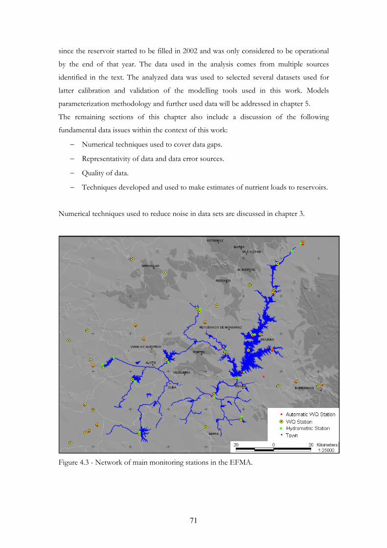
71

since the reservoir started to be filled in 2002 and was only considered to be operational

by the end of that year. The data used in the analysis comes from multiple sources

identified in the text. The analyzed data was used to selected several datasets used for

latter calibration and validation of the modelling tools used in this work. Models

parameterization methodology and further used data will be addressed in chapter 5.

The remaining sections of this chapter also include a discussion of the following

fundamental data issues within the context of this work:

Numerical techniques used to cover data gaps.

Representativity of data and data error sources.

Quality of data.

Techniques developed and used to make estimates of nutrient loads to reservoirs.

Numerical techniques used to reduce noise in data sets are discussed in chapter 3.

Figure 4.3 - Network of main monitoring stations in the EFMA.

72

4.1 Climatology

The works’ of Potes (2008) and Miranda (1995) cover the climatology of the EFMA

region for the period 1960-1990. Hydrology synthesized information for 2000-2007 is

included in CCDR5 Alentejo reports (CCDR, 2000-2007) which are available online at

www.ccdr-a.gov.pt/ (consulted in 2007). Although several entities make measurements in

the area, e.g. Évora University and the national meteorology institute (IM), raw data or

long series of data are not readily available and are difficult to obtain.

In the Alqueva reservoir there are five monitoring stations measuring climatological data.

Information about those stations is summarized in table 4.2. Other meteorological

monitoring stations exist in the EFMA area or nearby, namely a large number of

udometric stations.

In the text monitoring stations will be addressed by name in italic. All climatological data

was retrieved through the SNIRH6 interface or is courtesy of EDIA.

Table 4.2 - Climatology monitoring stations in the Alqueva reservoir.

Station name Code Location Elevation (m) Explored by Caia ** 20O/02UG 38º 53’ N

-7º 05’ W 201 CCDR Alentejo (non automatic)

INAG (automatic) Juromenha** 21N/01UG 38º 44’ N

-7º 13’ W 198 CCDR Alentejo (non automatic)

INAG (automatic) Alqueva (Mourão) 22M/05F 38º 23’ N

-7º 23’ W 103 INAG

Alqueva (Ilha) 24L/03C 38º 12’ N -7º 30’ W

- EDIA*

Alqueva 24L/02F 38º 13’ N -7º 27’ W

79 INAG

* Operating since mid 2006. ** Two stations coexist at the same location. CCDR non automatic stations are exclusively udometric stations.

5 CCDR - Comissão de coordenação e desenvolvimento regional.

6 SNIRH - Sistema nacional de informação de recursos hídricos. Online at www.snirh.pt

73

4.1.1 Solar radiation

Figure 4.4 presents daily solar irradiation7 measured at Alqueva, Alqueva (Ilha) and Alqueva

(Mourão). Both Alqueva and Alqueva (Mourão) presented data gaps for some time periods.

To cover small data gaps spline interpolation was used to complete the data series. For

large data gaps the following technique was used:

Data series were compared against each other to measure their similarity. This allows on

one hand to assess precision in measurements since solar radiation for such close latitude

locations is not expected to present significant differences and on the other hand to

create the possibility of using data from one of the series to fill data gaps in another one

if their degree of similarity is high enough.

The coefficient of variation (CV8) expressed as a percent was used to infer the degree of

similarity between data series. Calculated CVs are shown in table 4.3. CV is a normalized

measure of the dispersion of the data series against each other. The datasets for Alqueva

and Alqueva (Mourão) show little dispersion relative to each other (CV= 2.57%).

Therefore it was considered that data from one of the series can freely be used to fill data

gaps in the other one. The Alqueva (Ilha) dataset has measured values that globally are not

in the close vicinity of the correspondent measured values in the other datasets.

Therefore this data set was not used to fill data gaps.

Table 4.3 - Coefficient of variation for solar irradiation data.

CV Alqueva Alqueva (Mourão) Alqueva (Ilha) Alqueva - Alqueva (Mourão) 2.57% - Alqueva (Ilha) 29.07% 18.29% -

7 Irradiation should not be confused with irradiance. Pyranometers measure radiation per unit of area

(W/m2), that is, irradiance. They can also calculate the integral of irradiance over a time period, that is,

irradiation. Irradiation units of Wh/(m2day) mean that hourly integrated measurements were used to

calculate irradiation for daily periods. The daily value is obtained averaging the hourly data.

8 N

)x(

XandN

)xy(

RMSEwith100X

RMSECV

N

i

N2

ii

74

0

2000

4000

6000

8000

10000

Jul-02 Jul-03 Jul-04 Jul-05 Jul-06 Jul-07 Jul-08 Jul-09 Jul-10

So

lar

Irra

dia

tio

n (

Wh

/(m

2 da

y))

AlquevaAlqueva(Mourão)Alqueva (Ilha)

Figure 4.4 - Daily solar irradiation (Wh/ (m2day)) for 2003-2009 at Alqueva reservoir.

The final data set used in model simulations was obtained by calculating the average

between Alqueva and Alqueva (Mourão) data series after each of the individual series had all

the data gaps covered. Alqueva (Ilha) data was discarded given that only contains data

from 2006 on and data differs significantly from the other data series, hinting that lack of

precision in measurements may exist. For simulations hourly data was used.

Final solar irradiation data series was compared with satellite data corrected for ground

level for 2003-2008 (see Figure 4.5). Satellite data for 2009 was not available. Meteosat

data from the Helioclim databases HC-1 and HC-3 processed using Heliosat-2 method

(Lefèvre et al. 2007) was used. Data resolution was 20 km and 24 h for the period before

2005 and 5 km and 15 min after 2005. Satellite data source was SODA service

(http://www.soda-is.com/). Data from monitoring stations and from satellite present the

same seasonal trends and values have the same magnitude. However, either the

monitoring stations are undermeasuring radiation or satellite data is overmeasuring it.

Satellite data consistently presents higher values of irradiation than in situ monitoring

data through the all period 2003-2008. The error associated with either the satellite or the

monitoring measurements is unknown. Therefore no further conclusions can be made.

Solar irradiation seasonal trends for the analyzed period are similar within each year.

Interannual trends are also similar. Minimum values were found for the months of

75

December and January (absolute minimum was 376 Wh/(m2day) and maximum radiation

levels are reached for June and July months (absolute maximum was 8224 Wh/(m2day),

close to Summer solstice.

0

2000

4000

6000

8000

10000

Jul-02 Jul-03 Jul-04 Jul-05 Jul-06 Jul-07 Jul-08 Jul-09 Jul-10

So

lar

Irra

dia

tio

n (

Wh

/(m

2 da

y))

Alqueva Satellite data

Figure 4.5 - Daily solar irradiation (Wh/ (m2 day)) from monitoring stations vs. satellite

data for 2003-2008.

4.1.2 Air Temperature

Air temperature is measured at Alqueva, Alqueva (Mourão) and Alqueva (Ilha). Measured

averaged daily temperature for the three stations is shown in Figure 4.6. For modelling

purposes hourly air temperature data was used. For readability purposes data in Figure

4.6 was averaged for 24 hours periods. Data gaps were filled using the same strategy as

for solar irradiation data using the hourly measured datasets. Measured temperatures for

the three stations did not differ significantly (see table 4.4). Final data set used in

simulations was obtained by averaging the datasets for the three stations.

Absolute maximum and minimum air temperatures were 34.0 ºC and 2.7 ºC respectively.

Minimum temperatures occurred in January and maximum in July and August. Inter and

intrannual variations in temperature presented regular patterns for the analyzed period.

76

0

5

10

15

20

25

30

35

40

Jul-02 Jul-03 Jul-04 Jul-05 Jul-06 Jul-07 Jul-08 Jul-09 Jul-10

Da

ily T

em

pe

ratu

re (

ºC)

AlquevaAlqueva(Mourão)Alqueva (Ilha)

Figure 4.6 - Daily averaged air temperature (ºC) for 2003-2009 at Alqueva reservoir.

Table 4.4 - Coefficient of variation for hourly air temperature data.

CV Alqueva Alqueva (Mourão) Alqueva (Ilha) Alqueva - Alqueva (Mourão) 2.77% - Alqueva (Ilha) 2.72% 4.25% -

4.1.3 Evapotranspiration and rainfall

Potential evapotranspiration9 is only measured at two stations: Alqueva and Alqueva (Ilha).

In both stations data gaps are extensive. Existent daily data is presented in Figure 4.7.

The inset shows all measured values while the main picture focuses on the visible trends

in evapotranspiration.

The experimental method used to measure evapotranspiration is the pan evaporation. In

this indirect method a correction must be applied to the measured values if one intends

9 Potential evapotranspiration is the total amount of water that could be evaporated if there were sufficient

water available. The effects of surface and air temperatures, humidity, insolation and wind are included in

the measurements, but vegetation and built structures shading effects are not.

77

to estimate a reservoir potential evapotranspiration, since waterbodies do not have metal

walls that get hot with solar radiation but the pan does. The method used for correcting

the pan values for the stations is undocumented and therefore unknown. Some measured

values are significatively different from the values measured in neighbor days, namely the

very high values that can be seen in Figure 4.7 inset. Those values are probably due to

experimental error and where therefore discarded.

Given the extensive gaps in data, it was needed to use other data sources. Monthly data

obtained from Spanish authorities (Ministerio de médio ambiente y medio rural y marino)

for the Guadiana lower basin is depicted in Figure 4.8. The monthly evapotranspiration

data in Figure 4.8 were used as input in simulations.

Comparing Figures 4.5 and 4.8 allows inferring that evapotranspiration and solar

irradiation maxima and minima occur simultaneously in time.

0

5

10

15

20

25

30

35

40

45

50

Jul-02 Jul-03 Jul-04 Jul-05 Jul-06 Jul-07 Jul-08 Jul-09 Jul-10

Dai

ly P

ote

nti

al E

vap

otr

ansp

irat

ion

(m

m)

Alqueva

Alqueva (Ilha)

0

50

100

150

Jul-02 Jul-04 Jul-06 Jul-08 Jul-10

Figure 4.7 - Daily potential evapotranspiration (mm) for 2003 and 2007-2009 in Alqueva

reservoir.

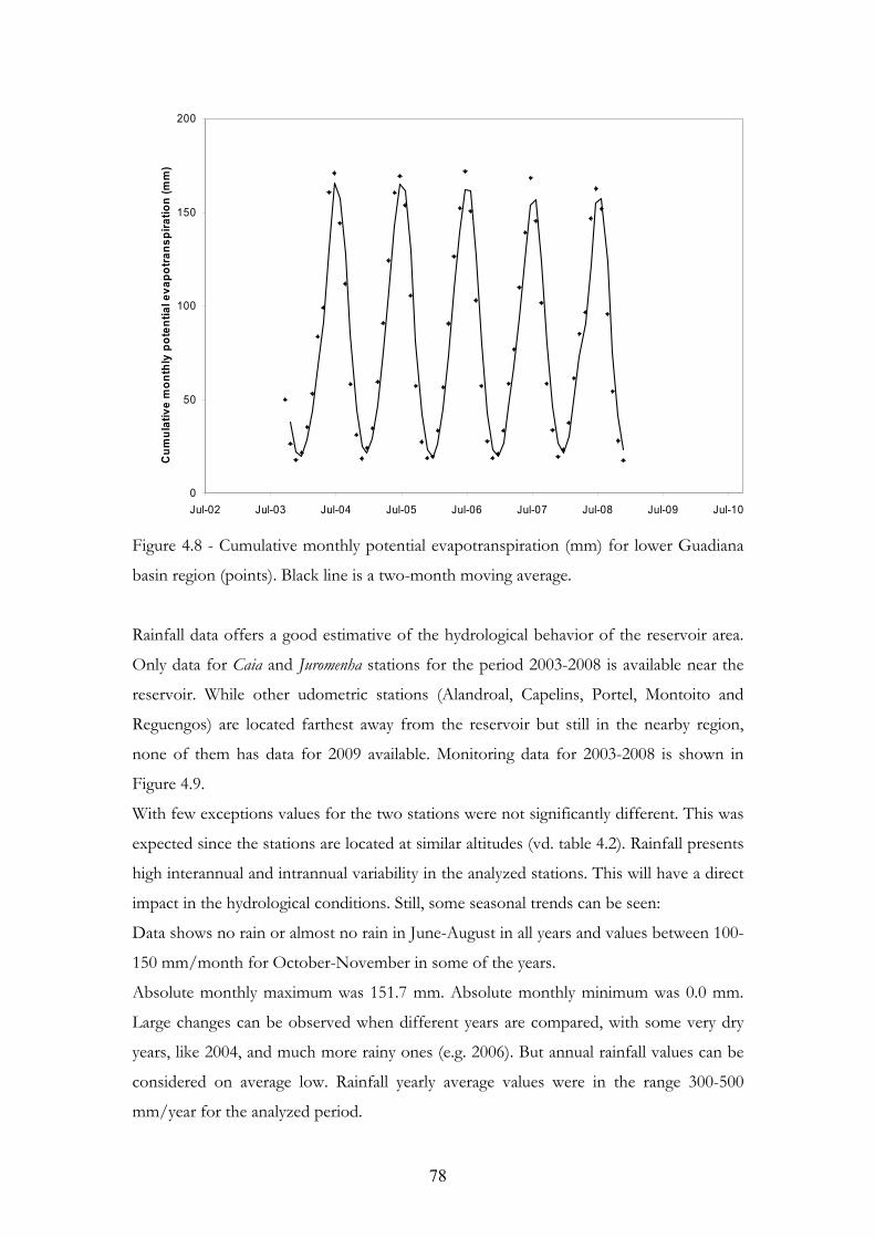
78

0

50

100

150

200

Jul-02 Jul-03 Jul-04 Jul-05 Jul-06 Jul-07 Jul-08 Jul-09 Jul-10

Cu

mu

lati

ve

mo

nth

ly p

ote

nti

al e

va

po

tra

ns

pir

ati

on

(m

m)

Figure 4.8 - Cumulative monthly potential evapotranspiration (mm) for lower Guadiana

basin region (points). Black line is a two-month moving average.

Rainfall data offers a good estimative of the hydrological behavior of the reservoir area.

Only data for Caia and Juromenha stations for the period 2003-2008 is available near the

reservoir. While other udometric stations (Alandroal, Capelins, Portel, Montoito and

Reguengos) are located farthest away from the reservoir but still in the nearby region,

none of them has data for 2009 available. Monitoring data for 2003-2008 is shown in

Figure 4.9.

With few exceptions values for the two stations were not significantly different. This was

expected since the stations are located at similar altitudes (vd. table 4.2). Rainfall presents

high interannual and intrannual variability in the analyzed stations. This will have a direct

impact in the hydrological conditions. Still, some seasonal trends can be seen:

Data shows no rain or almost no rain in June-August in all years and values between 100-

150 mm/month for October-November in some of the years.

Absolute monthly maximum was 151.7 mm. Absolute monthly minimum was 0.0 mm.

Large changes can be observed when different years are compared, with some very dry

years, like 2004, and much more rainy ones (e.g. 2006). But annual rainfall values can be

considered on average low. Rainfall yearly average values were in the range 300-500

mm/year for the analyzed period.

79

0

25

50

75

100

125

150

175

200

Jan-03 Jul-03 Jan-04 Jul-04 Jan-05 Jul-05 Jan-06 Jul-06 Jan-07 Jul-07 Jan-08 Jul-08 Jan-09

Mo

nth

ly a

ve

rag

e r

ain

fall

(mm

)

Caia

Juromenha

Figure 4.9 - Monthly average rainfall for 2003-2008 in Alqueva reservoir.

4.1.4 Wind

Wind speed and direction is measured at all the stations in table 4.2. Non-land based

wind sensors are mounted at 5 m above the reservoir surface. Daily averaged wind speed

data for 2003-2009 is presented in Figure 4.10. In numerical simulations local wind speed

data measured hourly or alternatively a wind distribution were used. Methodology to fill

data gaps in wind speed hourly data was similar to the one used for air temperature

described previously. For readability purposes data in Figure 4.10 was averaged for daily

periods.

Wind speed magnitude is similar in all stations with Caia and Juromenha presenting on

average lower speeds (absolute average is 1.6 m/s) than the other stations (absolute

average is 2.8 m/s). Wind speed absolute maximum value was 11.1 m/s. The majority of

daily averaged wind speeds lie in the range [0-6] m/s, i.e., [0-21.6] km/h. Absolute

minimum value was 0.1 m/s.

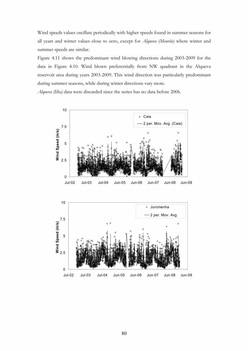
80

Wind speeds values oscillate periodically with higher speeds found in summer seasons for

all years and winter values close to zero, except for Alqueva (Mourão) where winter and

summer speeds are similar.

Figure 4.11 shows the predominant wind blowing directions during 2003-2009 for the

data in Figure 4.10. Wind blown preferentially from NW quadrant in the Alqueva

reservoir area during years 2003-2009. This wind direction was particularly predominant

during summer seasons, while during winter directions vary more.

Alqueva (Ilha) data were discarded since the series has no data before 2006.

0

2.5

5

7.5

10

Jul-02 Jul-03 Jul-04 Jun-05 Jun-06 Jun-07 Jun-08 Jun-09

Win

d S

pe

ed (

m/s

)

Caia

2 per. Mov. Avg. (Caia)

0

2.5

5

7.5

10

Jul-02 Jul-03 Jul-04 Jun-05 Jun-06 Jun-07 Jun-08 Jun-09

Win

d S

pee

d (

m/s

)

Juromenha

2 per. Mov. Avg.

81

0

2.5

5

7.5

10

12.5

15

Jul-02 Jul-03 Jul-04 Jun-05 Jun-06 Jun-07 Jun-08 Jun-09 Jun-10

Win

d S

pe

ed

(m

/s)

Alqueva(Mourão)2 per. Mov. Avg. (Alqueva(Mourão))

0

2.5

5

7.5

10

12.5

15

Jul-02 Jul-03 Jul-04 Jun-05 Jun-06 Jun-07 Jun-08 Jun-09 Jun-10

Win

d S

pee

d (

m/s

)

Alqueva 2 per. Mov. Avg. (Alqueva)

0

2.5

5

7.5

10

Jul-02 Jul-03 Jul-04 Jul-05 Jul-06 Jul-07 Jul-08 Jul-09 Jul-10

Win

d S

pee

d (

m/s

)

Alqueva(Ilha)

Figure 4.10 - Daily averaged wind speed (m/s) for 2003-2009 in the Alqueva reservoir.

Black line is a two-day running average.

82

0

25

50N

E

S

W

Caia

Juromenha

Alqueva

Alqueva(Mourão)

Figure 4.11 - Frequency (%) of daily wind direction for 2003-2009 in the Alqueva

reservoir.

4.2 Hydrology

The river Guadiana is the main tributary of the Alqueva reservoir.

Guadiana flow rate at the border between Spain and Portugal is measured by two

hydrometric stations: A Spanish automatic station of SAIH10 Guadiana (station number

cr2-49) and a Portuguese SNIRH automatic station (station number 21O/07h). The

Spanish station is measuring since September 2003 and is located at Badajoz entrance on

the Ponte Real bridge shown in Figure 4.12. The Portuguese station is located slightly

downriver at the border point Caia (38º 50’ N; -7º 04’ W). The instrumentation was

intercalibrated in 2007.

Daily flow rate data from the two stations is show in Figure 4.13. The figure inset focus

on the measurement differences between Portuguese and Spanish instrumentation. This

information was used to verify data quality.

The Guadiana river has an irregular hydrological regime with strong seasonal variations,

ranging from a 10-20 m3/s low flow in summer to values tenfold or hundredfold higher

during the wet season. The river flow also presents high variability from year to year.

10 Sistema automático de información hidrológica.

83

Figure 4.12 - Portugal-Spain Guadiana border hydrometric stations location (38º50’22’’;

7º4’3’’) (Source: Google Earth).

0

250

500

750

1000

1250

Jul-02 Jul-03 Jul-04 Jul-05 Jul-06 Jul-07 Jul-08 Jul-09 Jul-10

Gu

ad

ian

a d

aily

flo

w r

ate

(m

3/s

)

PortugalSpain

0

40

80

120

160

200

Jul-06 Jun-07 Jun-08 Jun-09 Jun-10

Figure 4.13 - Daily flow rate (m3/s) of river Guadiana at Spain-Portugal border for 2003-

2009. Black points - Portuguese SNIRH station measurements. Grey Points - Spanish

SAIH station measurements.

84

Rainfall intensity in a catchment has a direct impact in the discharge of rivers

(Montgomery et al., 1997). This relationship was used to assess data quality for rainfall

and flow measurements. To infer if rainfall and Guadiana river flow data are related the

Pearson correlation coefficient (r)11 between the two was calculated. Pearson coefficient

measures the extend to which two variables are linearly dependent of each other. The

correlation between monthly rainfall data for Caia and monthly averaged flow rate for

Guadiana (Portuguese station data) was +0.45. Therefore rainfall and discharge are not

independent of each other and have an increasing relationship, as expected. However, it

should be noted that Guadiana flow rates are not natural, since discharges upriver are

controlled.

No data is available regarding flow for smaller tributaries. An estimation of their

contributions was made from 2004 annual data (CCDR, 2004): in that year Degebe

contributed with 7% of the total inflow, Alcarrache and Caia tributaries with 3% each

and Lucefecit with 2%. Guadiana flow contributed 80% for the total flow in that year

4.3 Water quality

Water quality parameters are measured at several stations shown on table 4.5. Stations

operated by different entities exist at the same geographical location. Non automated

stations operated by CCDR Alentejo where closed down in 2003 and 2004 and

substituted by automated stations operated by INAG. EDIA stations are sampling

locations, i.e., no permanent equipment exists in place. EDIA data is sampled monthly.

The stations Guadiana/Táliga and Alcarrache confluência have very limited data, missing

several full years of measurements. These data were therefore not analyzed, except for

cases where comprehensive sets of data existed.

Only Juromenha and Alqueva (Mourão) water quality stations are located in the same place

as their homonymous meteorological stations. The remaining stations, even if sharing the

same name, are not located in the same place.

11 2

i

N

1

2i

N

1

N

1ii

)yy()xx(

)yy)(xx(

r

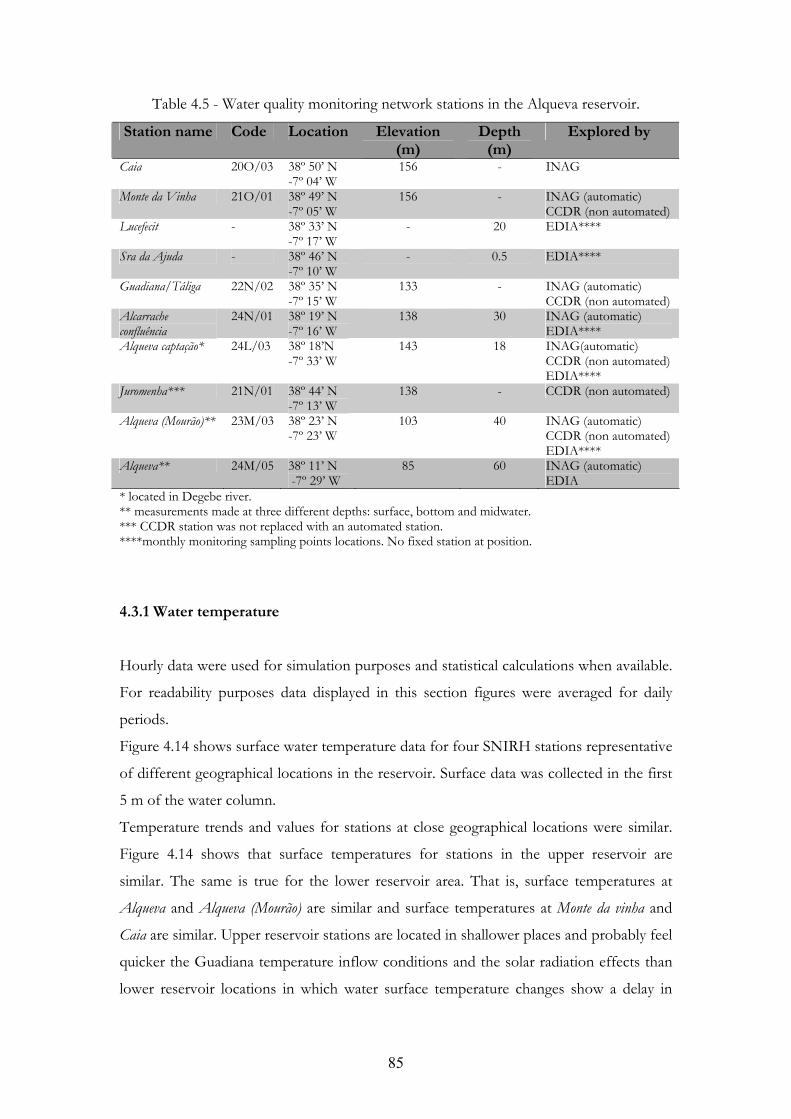
85

Table 4.5 - Water quality monitoring network stations in the Alqueva reservoir.

Station name Code Location Elevation (m)

Depth (m)

Explored by

Caia 20O/03 38º 50’ N -7º 04’ W

156 - INAG

Monte da Vinha 21O/01 38º 49’ N -7º 05’ W

156 - INAG (automatic) CCDR (non automated)

Lucefecit - 38º 33’ N -7º 17’ W

- 20 EDIA****

Sra da Ajuda - 38º 46’ N -7º 10’ W

- 0.5 EDIA****

Guadiana/Táliga 22N/02 38º 35’ N -7º 15’ W

133 - INAG (automatic) CCDR (non automated)

Alcarrache confluência

24N/01 38º 19’ N -7º 16’ W

138 30 INAG (automatic) EDIA****

Alqueva captação* 24L/03 38º 18’N -7º 33’ W

143 18 INAG(automatic) CCDR (non automated) EDIA****

Juromenha*** 21N/01 38º 44’ N -7º 13’ W

138 - CCDR (non automated)

Alqueva (Mourão)** 23M/03 38º 23’ N -7º 23’ W

103 40 INAG (automatic) CCDR (non automated) EDIA****

Alqueva** 24M/05 38º 11’ N -7º 29’ W

85 60 INAG (automatic) EDIA

* located in Degebe river. ** measurements made at three different depths: surface, bottom and midwater. *** CCDR station was not replaced with an automated station. ****monthly monitoring sampling points locations. No fixed station at position.

4.3.1 Water temperature

Hourly data were used for simulation purposes and statistical calculations when available.

For readability purposes data displayed in this section figures were averaged for daily

periods.

Figure 4.14 shows surface water temperature data for four SNIRH stations representative

of different geographical locations in the reservoir. Surface data was collected in the first

5 m of the water column.

Temperature trends and values for stations at close geographical locations were similar.

Figure 4.14 shows that surface temperatures for stations in the upper reservoir are

similar. The same is true for the lower reservoir area. That is, surface temperatures at

Alqueva and Alqueva (Mourão) are similar and surface temperatures at Monte da vinha and

Caia are similar. Upper reservoir stations are located in shallower places and probably feel

quicker the Guadiana temperature inflow conditions and the solar radiation effects than

lower reservoir locations in which water surface temperature changes show a delay in

86

time when compared to values for upper reservoir stations. Another feature related to

geographical location and time delay is the higher surface water temperature amplitudes

observed for upper reservoir stations when compared with lower reservoir ones. The

former feel more directly the climatic and hydrologic regimen changes while in the latter

those conditions are attenuated. A summary of statistics for hourly surface water

temperature is presented in table 4.6.

Table 4.6 - Statistical summary for surface water temperature hourly data from SNIRH.

Temperature (ºC) Absolute maximum

Absolute minimum

Average

Upper reservoir stations 34.7 5.0 17.6 Lower reservoir stations 33.1 6.3 18.6

5

10

15

20

25

30

35

Jul-02 Jul-03 Jul-04 Jul-05 Jul-06 Jul-07 Jul-08 Jul-09 Jul-10

Wa

ter

Te

mp

era

ture

(ºC

)

Caia Monte da Vinha Alqueva Mourão

Figure 4.14 - Daily averaged surface water temperature (ºC) for 2003-2009 at the Alqueva

reservoir.

Regular seasonal and annual water temperature trends can clearly be seen in Figure 4.14.

Data gaps were filled using the method described earlier. CV (table 4.7) for hourly

datasets was calculated grouping upper and lower reservoir stations. Given the CV values

obtained Caia and Monte da Vinha data were used to fill data gaps in each other data

series. The same was done for Alqueva and Alqueva (Mourão) data.

87

Table 4.7 - Coefficient of variation for surface water temperature hourly data from

SNIRH.

CV Caia Monte da Vinha Alqueva Alqueva (Mourão) Caia - Monte da Vinha 9.06% - Alqueva - - - Alqueva (Mourão) - - 4.69% -

A quantitative assessment of data quality was done by verifying how strongly correlated

the surface water temperature data were to the air temperature data measured at the same

locations (coincident location data exists only for Alqueva and Alqueva (Mourão)). Table

4.8 presents the Pearson coefficient results. Data shows a strong positive linear

relationship.

Water temperature at EDIA monitoring locations is measured monthly at three different

depths: Surface, midwater and bottom, except for Sra da Ajuda which is to shallow (see

table 4.5). Figure 4.15 depict the aforementioned data. Two-month moving averages

were calculated for each data series in order to emphasize temporal trends. Data shows

that once a year during Summer, thermal stratification occurs. A vertical stratification

develops in late Mars-April and remains stable until overturn occurs in late October or

the beginning of November for all years analyzed.

Table 4.8 - Correlation between air and water surface temperature data.

Pearson Alqueva 0.923 Alqueva (Mourão) 0.939

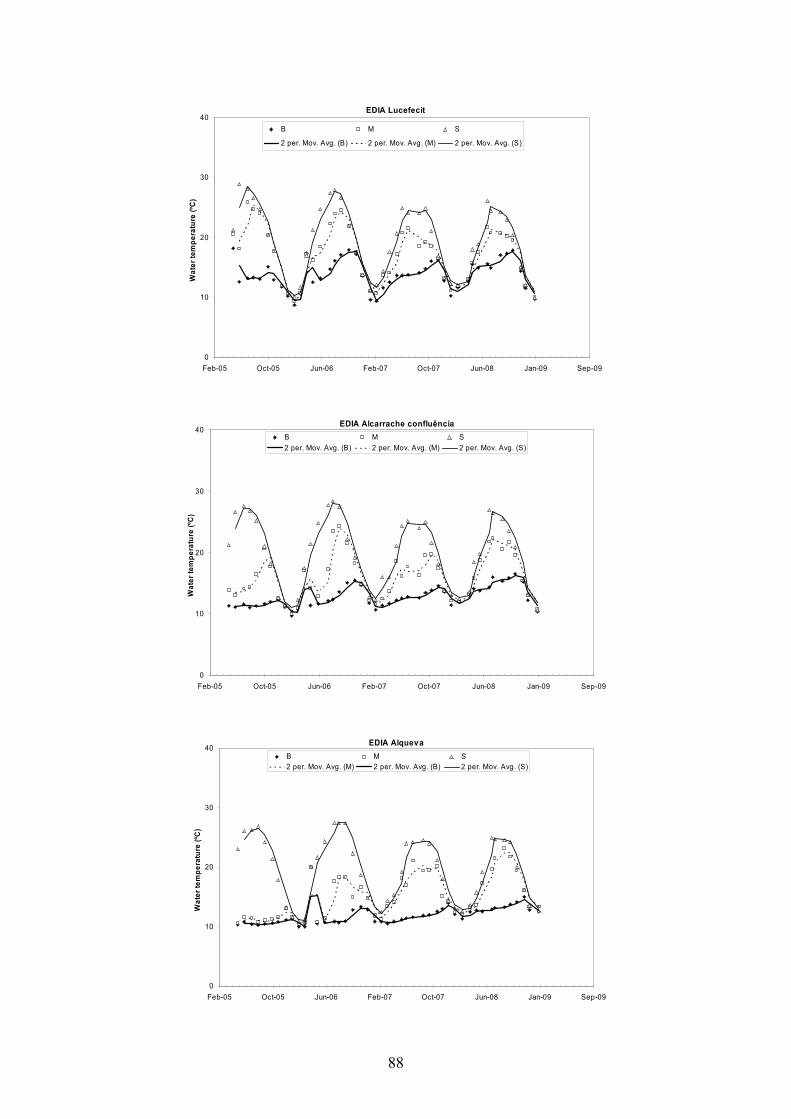
88

EDIA Lucefecit

0

10

20

30

40

Feb-05 Oct-05 Jun-06 Feb-07 Oct-07 Jun-08 Jan-09 Sep-09

Wa

ter

tem

pe

ratu

re (

ºC)

B M S

2 per. Mov. Avg. (B) 2 per. Mov. Avg. (M) 2 per. Mov. Avg. (S)

EDIA Alcarrache confluência

0

10

20

30

40

Feb-05 Oct-05 Jun-06 Feb-07 Oct-07 Jun-08 Jan-09 Sep-09

Wa

ter

tem

pe

ratu

re (

ºC)

B M S

2 per. Mov. Avg. (B) 2 per. Mov. Avg. (M) 2 per. Mov. Avg. (S)

EDIA Alqueva

0

10

20

30

40

Feb-05 Oct-05 Jun-06 Feb-07 Oct-07 Jun-08 Jan-09 Sep-09

Wa

ter

tem

pe

ratu

re (

ºC)

B M S2 per. Mov. Avg. (M) 2 per. Mov. Avg. (B) 2 per. Mov. Avg. (S)

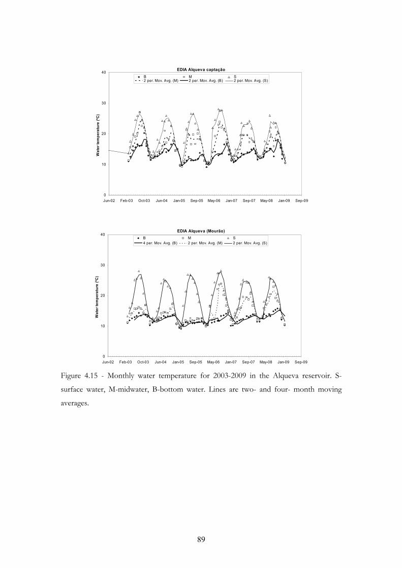
89

EDIA Alqueva captação

0

10

20

30

40

Jun-02 Feb-03 Oct-03 Jun-04 Jan-05 Sep-05 May-06 Jan-07 Sep-07 May-08 Jan-09 Sep-09

Wa

ter

tem

pe

ratu

re (

ºC)

B M S2 per. Mov. Avg. (M) 2 per. Mov. Avg. (B) 2 per. Mov. Avg. (S)

EDIA Alqueva (Mourão)

0

10

20

30

40

Jun-02 Feb-03 Oct-03 Jun-04 Jan-05 Sep-05 May-06 Jan-07 Sep-07 May-08 Jan-09 Sep-09

Wa

ter

tem

pe

ratu

re (

ºC)

B M S4 per. Mov. Avg. (B) 2 per. Mov. Avg. (M) 2 per. Mov. Avg. (S)

Figure 4.15 - Monthly water temperature for 2003-2009 in the Alqueva reservoir. S-

surface water, M-midwater, B-bottom water. Lines are two- and four- month moving

averages.

90

Bottom water data quality was assessed by comparing data series measured by SNIRH

against EDIA data for the same location for the available data. Data comparison is

presented in Figure 4.16. Deviations were not calculated since data from the two sources

was collected at different days and time intervals. Qualitatively, there is a relative good

agreement of the data from the two different sources for the first years (2004-2006), but

deviations seem to grow progressively in time and by the last year (2008) the two sets of

data diverge a lot.

0

5

10

15

20

25

Dec-04 Dec-05 Dec-06 Dec-07 Dec-08 Dec-09

Wa

ter

tem

pe

ratu

re (

ºC)

B Alqueva B EDIA Alqueva

0

5

10

15

20

25

Dec-04 Dec-05 Dec-06 Dec-07 Dec-08 Dec-09

Wa

ter

tem

pe

ratu

re (

ºC)

B Alqueva (Mourão) B EDIA Alqueva (Mourão)

Figure 4.16 - Bottom water temperature (ºC) for 2005-2009 in the Alqueva reservoir. B-

bottom water. (Data Sources: EDIA and SNIRH).

91

4.3.2 Dissolved Oxygen

In most reservoirs dissolved oxygen (DO) is usually below saturation levels due to

oxidation requirements of organic matter in decay (i.e. the carbonaceous oxygen

demand). Bacterial oxidation of ammonia to nitrate, i.e. the nitrogenous oxygen demand,

also requires oxygen.

A concentration of dissolved oxygen below 5 mg/L will affect negatively aquatic

communities while levels below 2 mg/L will kill most fish species (UNESCO, 1996). The

ideal minimum level should be above 7 mg/L.

For 1 atm and temperatures of 10-20 ºC in fresh waters, 10 mg/L is a good estimative of

100% saturation level. If oxygen saturation is below 60% or a supersaturation above

120% exists then the conditions for aquatic life are poor. Dissolved oxygen higher than

100% occurs mainly because of oxygen production by photosynthetic organisms.

Another reason is the existence of a non-ideal equilibration of DO in water and in the air

layer above it. This may occur if temperature changes are fast.

Figure 4.17 shows dissolved oxygen levels in surface water at the Alqueva reservoir

SNIRH stations. A thirty-day moving average was added in order to emphasize trends.

Black horizontal lines at 60% and 120% were added to help identify the threshold limits

for ideal aquatic life conditions.

Dissolved oxygen levels for upper reservoir area stations (Caia and Monte da Vinha) are

very low during Summer, approaching zero for some years. Some supersaturation

situations can also be seen mostly at upper reservoir stations but also for the year 2003 in

all stations. This indicates a possible high level of water pollution. Abrupt changes in DO

levels in lakes are usually associated with changes in the trophic conditions.

Figure 4.18 presents DO monthly levels for different water depths at EDIA stations.

During winter period it is visible that DO levels are more similar for different depths,

which is due to the vertical well mixed water column. In summer, thermal stratification

will hinder the transport of oxygen to lower water layers. Therefore the DO levels drop

over depth which can clearly be seen in Figure 4.18. Sharp drops usually occur at the

thermocline depth.

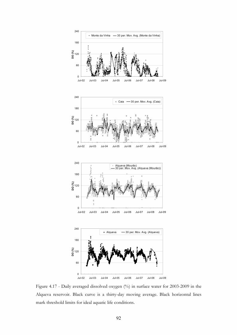
92

0

60

120

180

240

Jul-02 Jul-03 Jul-04 Jul-05 Jul-06 Jul-07 Jul-08 Jul-09

DO

(%

)

Monte da Vinha 30 per. Mov. Avg. (Monte da Vinha)

0

60

120

180

240

Jul-02 Jul-03 Jul-04 Jul-05 Jul-06 Jul-07 Jul-08 Jul-09

DO

(%

)

Caia 30 per. Mov. Avg. (Caia)

0

60

120

180

240

Jul-02 Jul-03 Jul-04 Jul-05 Jul-06 Jul-07 Jul-08 Jul-09

DO

(%

)

Alqueva (Mourão)30 per. Mov. Avg. (Alqueva (Mourão))

0

60

120

180

240

Jul-02 Jul-03 Jul-04 Jul-05 Jul-06 Jul-07 Jul-08 Jul-09

DO

(%

)

Alqueva 30 per. Mov. Avg. (Alqueva)

Figure 4.17 - Daily averaged dissolved oxygen (%) in surface water for 2003-2009 in the

Alqueva reservoir. Black curve is a thirty-day moving average. Black horizontal lines

mark threshold limits for ideal aquatic life conditions.

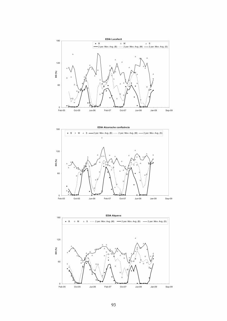
93

EDIA Lucefecit

0

60

120

180

Feb-05 Oct-05 Jun-06 Feb-07 Oct-07 Jun-08 Jan-09 Sep-09

DO

(%

)

B M S

2 per. Mov. Avg. (B) 2 per. Mov. Avg. (M) 2 per. Mov. Avg. (S)

EDIA Alcarrache confluência

0

60

120

180

Feb-05 Oct-05 Jun-06 Feb-07 Oct-07 Jun-08 Jan-09 Sep-09

DO

(%

)

B M S 2 per. Mov. Avg. (B) 2 per. Mov. Avg. (M) 2 per. Mov. Avg. (S)

EDIA Alqueva

0

60

120

180

Feb-05 Oct-05 Jun-06 Feb-07 Oct-07 Jun-08 Jan-09 Sep-09

DO

(%

)

B M S 2 per. Mov. Avg. (M) 2 per. Mov. Avg. (B) 2 per. Mov. Avg. (S)

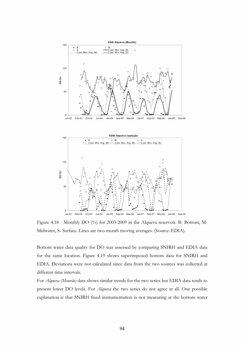
94

EDIA Alqueva (Mourão)

0

60

120

180

Jun-02 Feb-03 Oct-03 Jun-04 Jan-05 Sep-05 May-06 Jan-07 Sep-07 May-08 Jan-09 Sep-09

DO

(%

)

B MS 4 per. Mov. Avg. (B)2 per. Mov. Avg. (M) 2 per. Mov. Avg. (S)

EDIA Alqueva captação

0

60

120

180

Jun-02 Feb-03 Oct-03 Jun-04 Jan-05 Sep-05 May-06 Jan-07 Sep-07 May-08 Jan-09 Sep-09

DO

(%

)

B M S2 per. Mov. Avg. (M) 2 per. Mov. Avg. (B) 2 per. Mov. Avg. (S)

Figure 4.18 - Monthly DO (%) for 2003-2009 in the Alqueva reservoir. B- Bottom, M-

Midwater, S- Surface. Lines are two-month moving averages. (Source: EDIA).

Bottom water data quality for DO was assessed by comparing SNIRH and EDIA data

for the same location. Figure 4.19 shows superimposed bottom data for SNIRH and

EDIA. Deviations were not calculated since data from the two sources was collected at

different time intervals.

For Alqueva (Mourão) data shows similar trends for the two series but EDIA data tends to

present lower DO levels. For Alqueva the two series do not agree at all. One possible

explanation is that SNIRH fixed instrumentation is not measuring at the bottom water

95

but instead at a smaller depth, since their summer DO values seem to be too high for

such a deep water column. SNIRH bottom data series for DO at Alqueva was discarded.

Correlation coefficients between water temperature and DO were calculated to evaluate

DO data quality. Of particular interest was to further investigate the differences between

measurements from EDIA and SNIRH for Alqueva station at bottom water. Given that

the variation of oxygen solubility with temperature in water is almost inversely linear for

the underwater pressures found in the Alqueva12 (see Figure 4.20) the Pearson coefficient

was used.

For SNIRH and EDIA measurements (all depth and stations) correlation coefficients

obtained all had absolute values lower than 0.4, indicating low correlation between the

two DO measurements. The obtained low correlations imply that at least part of the data

has low quality and is probably not accurate. Further use of these DO datasets was done

with great care, particularly in model simulations.

0

60

120

Dec-04 Dec-05 Dec-06 Dec-07 Dec-08 Dec-09

DO

(%

)

B Alqueva EDIA B Alqueva (Mourão) EDIA B Alqueva B Alqueva (Mourão)2 per. Mov. Avg. (B Alqueva EDIA) 2 per. Mov. Avg. (B Alqueva (Mourão) EDIA)

Figure 4.19 - Dissolved oxygen (%) at bottom water (B) for 2003-2009 in the Alqueva

reservoir. Lines are two-month moving averages for EDIA monthly data. (Data sources:

SNIRH and EDIA).

12 Roughly for each 10 m of depth pressure will increase 1 bar. At 4 bar, a linear regression between

temperature and oxygen solubility will give an R2 of 0.94.

96

0

10

20

30

40

50

60

0 5 10 15 20 25 30 35 40 45 50Temperature (ºC)

Ox

yg

en

so

lub

ility

(m

g/L

)

1 bar 2 bar 4 bar

Figure 4.20 - Relationship between oxygen solubility, water temperature and

atmospheric pressure in freshwater.

4.3.3 Nutrients

SNIRH stations do not measure nitrogen and phosphorus species concentrations. Non

automatic CCDR stations have scarce data for 2003. EDIA stations have monthly non-

evenly spaced data covering 2003-2009 that will be used herein. EDIA data used did not

had information regarding analytical methods used, their detection levels and

measurements errors.

Symbology used here will be PO4 for phosphate, NO3 for nitrate, NH3 for ammonia,

TP for total phosphorus, N:P for total nitrogen to total phosphorus mass ratio and TN

for total nitrogen. Concentration units are mg/L for all species.

Data series gaps for nutrients were covered using the techniques described earlier (see

section 4.1.1).

Data series seasonal and annual analysis was performed using autocorrelations13 with

different time lags, ranging from 1 to 12 months. The aforementioned autocorrelations

were calculated at all stations surface measurements for phosphate, nitrate, ammonia,

13

N

1i

2i

kN

1ikii

k

)YY(

)YY)(YY(

r , N is the number of measurements, Yi the measurement at time xi , k is the

lag.

97

total phosphorus and total nitrogen. A temporal trend was considered to exist if the

autocorrelations were strong (|r|>0.5) and noise was absent over several consecutive

lags, that is, slowness in decay existed.

The only meaningful autocorrelations found were for PO4 in Alqueva (Mourão) and for

NO3 in Alqueva, whose results are shown in Figure 4.21. The other variables showed no

seasonal variations. This was expectable only for upper reservoir stations since Guadiana

inflow is highly variable over time and strongly affects ecology dynamics. Therefore no

strong autocorrelations should exist for upper reservoir stations.

Major problems were that the data were not evenly spaced and that the frequency of

measurements is very low (monthly). This may possibly have jeopardized the data

analysis. Good results for time series analysis using lagged autocorrelations for ecological

measurements are usually obtainable with measurements at hourly intervals or less (J.

Rozemeijer - Utrecht University/Deltares, pers. comm., 2010). For that reason a clear

conclusion stating that no temporal trends exist in nutrient data cannot be made although

the existent data and the analysis done hints in that way.

0.0

0.2

0.4

0.6

0.8

1.0

1 2 3 4 5 6 7 8 9 10 11 12Lag (Months)

r

PO4 at Alqueva (Mourão) NO3 at Alqueva

Figure 4.21 - Lagged autocorrelation coefficient variation for different lags in the

Alqueva reservoir. NO3 data for Alqueva and PO4 data for Alqueva (Mourão).

98

An attempt to establish relationships between variables was done using lagged and non

lagged cross correlations14 with variables of interest. Monthly lags ranging from 1 to 12

were used. The methodology was applied to all stations data.

Lag 1 was of particular interest since there is a slight time delay between nutrients

entrance in a waterbody and phytoplankton response. Besides correlations of nutrient

species with Chl-a and with other nutrients species, of particular interest were

correlations of N and P species with:

- Guadiana inflow for upper reservoir stations.

- Rainfall for surface measurements (allows evaluating the weight of rainfall in the

system total loads).

- Water temperature.

- Dissolved oxygen.

Then again, major problems were the fact that parts of the data were not evenly spaced

in time and that the frequency of measurement was in some cases very low (monthly).

Another issue was that some of the data for different variables was not collected at the

same time intervals (interpolation was done). These issues may have influenced the

results obtained.

Total phosphorus (data displayed on Figure 4.22) showed no correlation with other

variables at all stations.

In phosphate correlations, particular attention was paid to any increase in PO4 at bottom

water that could be related to high bottom water temperatures and anoxic conditions

(which usually trigger bed release of phosphorus). But nor bottom DO nor bottom water

temperatures correlated well with PO4 data. Iron in sediments is known to regulate the

release of phosphorus from sediments but sediment iron concentrations in the Alqueva

are unknown. So is the amount of ressuspend material over time that would allow

identifying resuspension episodes.

14

1N

0i

2ki

1N

0i

2i

1N

0ikii

k

)XX()YY(

))XX)(YY((

r , N is the number of measurements, Yi and Xi the

measurements for different variables at time ti and k is the lag.

99

PO4 positively correlated well with lagged Chl-a data for long delays (lags 4 and 10) at

Alqueva (Mourão) and with ammonia and nitrate at Alcarrache for lag 8, which probably is

meaningless.

Like the cross correlations for phosphorus species, the cross correlations for nitrogen

species seldom allowed to infer any relationships between variables. Of particular interest

was the relationship between ammonia and DO. Whenever large quantities of organic

matter enter the system it is expected that DO is depleted due to increased oxidation, so

a lagged inverse relationship was expected, but was not verified in any station. Few good

correlations were attained. Positive strong correlations were found only at Alcarrache

station between NH3 and PO4 with 8 months lag; between NO3 and PO4, TN and DO

(lag 8 also).

Attempts to correlate nitrogen species with Guadiana inflow at upper reservoir stations

were also unsuccessful. Furthermore no correlations were found between rainfall data

and other variables. TN data for different stations and depths in the Alqueva reservoir

are displayed in Figure 4.23.

100

Sra da Ajuda

0.0

0.5

1.0

1.5

2.0

2.5

3.0

3.5

4.0

4.5

Jun-02 Feb-03 Oct-03 Jun-04 Jan-05 Sep-05 May-06 Jan-07 Sep-07 May-08 Jan-09 Sep-09

TP

(mg

/L)

S 2 per. Mov. Avg. (S)

EDIA Lucefecit

0.0

0.5

1.0

1.5

Feb-05 Oct-05 Jun-06 Feb-07 Oct-07 Jun-08 Jan-09 Sep-09

TP

(mg

/L)

B M S

2 per. Mov. Avg. (B) 2 per. Mov. Avg. (M) 2 per. Mov. Avg. (S)

EDIA Alqueva captação

0.0

0.5

1.0

1.5

Jun-02 Feb-03 Oct-03 Jun-04 Jan-05 Sep-05 May-06 Jan-07 Sep-07 May-08 Jan-09 Sep-09

TP

(mg

/L)

B M S 2 per. Mov. Avg. (M) 2 per. Mov. Avg. (B) 2 per. Mov. Avg. (S)

EDIA Alcarrache confluência

0.0

0.5

1.0

1.5

Feb-05 Oct-05 Jun-06 Feb-07 Oct-07 Jun-08 Jan-09 Sep-09

TP

(mg

/L)

B M S 2 per. Mov. Avg. (B) 2 per. Mov. Avg. (M) 2 per. Mov. Avg. (S)

EDIA Alqueva (Mourão)

0.0

0.5

1.0

1.5

Jun-02 Feb-03 Oct-03 Jun-04 Jan-05 Sep-05 May-06 Jan-07 Sep-07 May-08 Jan-09 Sep-09

TP

(mg

/L)

B M S 4 per. Mov. Avg. (B) 2 per. Mov. Avg. (M) 2 per. Mov. Avg. (S)

EDIA Alqueva

0.0

0.5

1.0

1.5

Feb-05 Oct-05 Jun-06 Feb-07 Oct-07 Jun-08 Jan-09 Sep-09

TP

(mg

/L)

B M S 2 per. Mov. Avg. (M) 2 per. Mov. Avg. (S) 2 per. Mov. Avg. (B)

Figure 4.22 - TP (mg/L) for 2003-2008 in the Alqueva reservoir. B- Bottom, M-

Midwater, S- Surface. Lines are two-month moving averages.

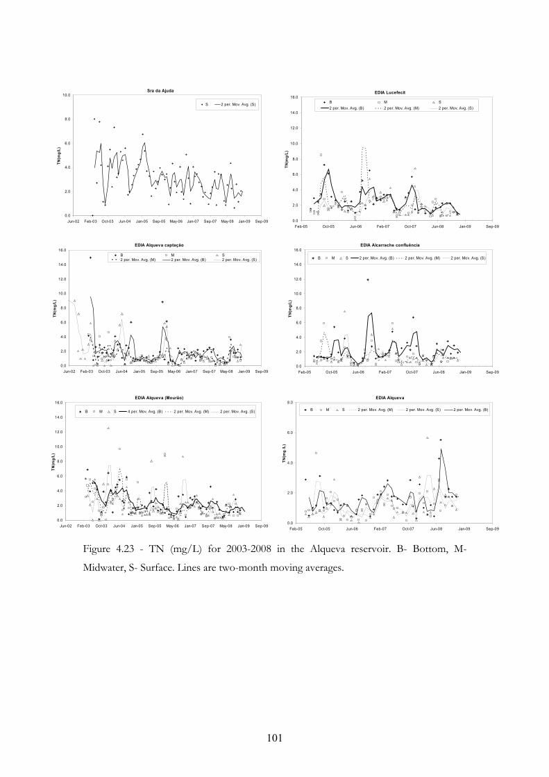
101

Sra da Ajuda

0.0

2.0

4.0

6.0

8.0

10.0

Jun-02 Feb-03 Oct-03 Jun-04 Jan-05 Sep-05 May-06 Jan-07 Sep-07 May-08 Jan-09 Sep-09

TN

(mg

/L)

S 2 per. Mov. Avg. (S)

EDIA Lucefecit

0.0

2.0

4.0

6.0

8.0

10.0

12.0

14.0

16.0

Feb-05 Oct-05 Jun-06 Feb-07 Oct-07 Jun-08 Jan-09 Sep-09

TN

(mg

/L)

B M S

2 per. Mov. Avg. (B) 2 per. Mov. Avg. (M) 2 per. Mov. Avg. (S)

EDIA Alqueva captação

0.0

2.0

4.0

6.0

8.0

10.0

12.0

14.0

16.0

Jun-02 Feb-03 Oct-03 Jun-04 Jan-05 Sep-05 May-06 Jan-07 Sep-07 May-08 Jan-09 Sep-09

TN

(mg

/L)

B M S2 per. Mov. Avg. (M) 2 per. Mov. Avg. (B) 2 per. Mov. Avg. (S)

EDIA Alcarrache confluência

0.0

2.0

4.0

6.0

8.0

10.0

12.0

14.0

16.0

Feb-05 Oct-05 Jun-06 Feb-07 Oct-07 Jun-08 Jan-09 Sep-09

TN

(mg

/L)

B M S 2 per. Mov. Avg. (B) 2 per. Mov. Avg. (M) 2 per. Mov. Avg. (S)

EDIA Alqueva (Mourão)

0.0

2.0

4.0

6.0

8.0

10.0

12.0

14.0

16.0

Jun-02 Feb-03 Oct-03 Jun-04 Jan-05 Sep-05 May-06 Jan-07 Sep-07 May-08 Jan-09 Sep-09

TN

(mg

/L)

B M S 4 per. Mov. Avg. (B) 2 per. Mov. Avg. (M) 2 per. Mov. Avg. (S)

EDIA Alqueva

0.0

2.0

4.0

6.0

8.0

Feb-05 Oct-05 Jun-06 Feb-07 Oct-07 Jun-08 Jan-09 Sep-09

TN

(mg

/L)

B M S 2 per. Mov. Avg. (M) 2 per. Mov. Avg. (S) 2 per. Mov. Avg. (B)

Figure 4.23 - TN (mg/L) for 2003-2008 in the Alqueva reservoir. B- Bottom, M-

Midwater, S- Surface. Lines are two-month moving averages.

102

4.3.4 Nutrients limitation analysis

Conclusions can be reached regarding the limiting nutrient in a waterbody based on the

relative abundance of phosphorus and nitrogen in water and nutrients requirements

stoichiometry analysis. Phosphorus is usually considered to be the limiting nutrient in

lakes and reservoirs. But it is the relationship between supply and demand of nutrients

that will determine which one is the limiting nutrient.

Although stoichiometry requirements vary for different algae species, the phytoplankton

as a whole in lakes and reservoirs has an N:P mass ratio that is on average between 5:1

(Smith, 2001) and 7:1 (Downing et al., 1992). Therefore when N:P ratios in water present

high values, phosphorus will become the limiting nutrient. The most frequent threshold

ratio value assumed to be indicative of phosphorus limitation found in the literature

according to Smith (2001) is 10:1.

N:P ratios were used to find out which nutrient is limiting algae growth in the Alqueva.

High ratios are indicative of phosphorus limitation and the opposite is a sign of nitrogen

limitation. The mass rate 10:1 was used as a threshold value. Monthly N:P mass ratios

were calculated using TN and TP EDIA data for surface water and are presented in

Figure 4.24. Continuous lines were used to connect monthly points in order to

emphasize temporal trends but do not mean that a linear trend between two points exist.

Values were generally well above 10, reaching maxima of 471 at Alcarrache station during

2003. No seasonal trends were found but some years present on average very high N:P

ratios (2006-2007) in all stations while others have lower values during all year (2008). No

particular spatial trends seem to exist. The frequency of values lower than 10 at each

station is presented in table 4.9. The results allow us to conclude that most of the times

the Alqueva is phosphorus limited and there is a minority of situations when it is

nitrogen limited.

N:P ratios vary with a reservoir trophic condition. For worsening trophic conditions the

ratio will decline because eutrophication increases denitrification and therefore causes a

shift to nitrogen limitation situations (Wetzel, 2001). An eutrophic reservoir will usually

present an N:P lower than 10, while oligotrophic ones will usually have an N:P higher

than 100 (Schindler, 1977). Figure 4.25 presents the occurrence over time of N:P ratios

lower than 10 in the Alqueva. Circle areas are proportional to the frequencies presented

in table 4.9.

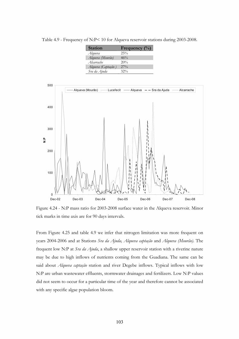
103

Table 4.9 - Frequency of N:P< 10 for Alqueva reservoir stations during 2003-2008.

Station Frequency (%)Alqueva 25% Alqueva (Mourão) 46% Alcarrache 20% Alqueva (Captação ) 27% Sra da Ajuda 32%

0

100

200

300

400

500

Dec-02 Dec-03 Dec-04 Dec-05 Dec-06 Dec-07 Dec-08

N:P

Alqueva (Mourão) Lucefecit Alqueva Sra da Ajuda Alcarrache

Figure 4.24 - N:P mass ratio for 2003-2008 surface water in the Alqueva reservoir. Minor

tick marks in time axis are for 90 days intervals.

From Figure 4.25 and table 4.9 we infer that nitrogen limitation was more frequent on

years 2004-2006 and at Stations Sra da Ajuda, Alqueva captação and Alqueva (Mourão). The

frequent low N:P at Sra da Ajuda, a shallow upper reservoir station with a riverine nature

may be due to high inflows of nutrients coming from the Guadiana. The same can be

said about Alqueva captação station and river Degebe inflows. Typical inflows with low

N:P are urban wastewater effluents, stormwater drainages and fertilizers. Low N:P values

did not seem to occur for a particular time of the year and therefore cannot be associated

with any specific algae population bloom.

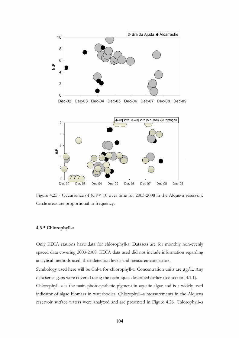
104

0

2

4

6

8

10

Dec-02 Dec-03 Dec-04 Dec-05 Dec-06 Dec-07 Dec-08 Dec-09

N:P

Sra da Ajuda Alcarrache

Figure 4.25 - Occurrence of N:P< 10 over time for 2003-2008 in the Alqueva reservoir.

Circle areas are proportional to frequency.

4.3.5 Chlorophyll-a

Only EDIA stations have data for chlorophyll-a. Datasets are for monthly non-evenly

spaced data covering 2003-2008. EDIA data used did not include information regarding

analytical methods used, their detection levels and measurements errors.

Symbology used here will be Chl-a for chlorophyll-a. Concentration units are g/L. Any

data series gaps were covered using the techniques described earlier (see section 4.1.1).

Chlorophyll–a is the main photosynthetic pigment in aquatic algae and is a widely used

indicator of algae biomass in waterbodies. Chlorophyll–a measurements in the Alqueva

reservoir surface waters were analyzed and are presented in Figure 4.26. Chlorophyll–a

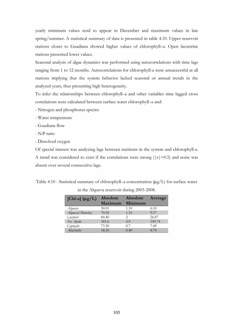
105

yearly minimum values tend to appear in December and maximum values in late

spring/summer. A statistical summary of data is presented in table 4.10. Upper reservoir

stations closer to Guadiana showed higher values of chlorophyll–a. Open lacustrine

stations presented lower values.

Seasonal analysis of algae dynamics was performed using autocorrelations with time lags

ranging from 1 to 12 months. Autocorrelations for chlorophyll-a were unsuccessful at all

stations implying that the system behavior lacked seasonal or annual trends in the

analyzed years, thus presenting high heterogeneity.

To infer the relationships between chlorophyll–a and other variables time lagged cross

correlations were calculated between surface water chlorophyll–a and:

- Nitrogen and phosphorus species

- Water temperature

- Guadiana flow

- N:P ratio

- Dissolved oxygen

Of special interest was analyzing lags between nutrients in the system and chlorophyll-a.

A trend was considered to exist if the correlations were strong (|r|>0.5) and noise was

absent over several consecutive lags.

Table 4.10 - Statistical summary of chlorophyll–a concentration (g/L) for surface water

in the Alqueva reservoir during 2003-2008.

[Chl-a] (g/L) Absolute Maximum

Absolute Minimum

Average

Alqueva 30.01 1.10 6.10 Alqueva( Mourão) 70.50 1.10 9.57 Lucefecit 84.40 2 26.87 Sra Ajuda 365.6 0.9 109.74 Captação 73.30 0.7 7.49 Alcarrache 34.10 0.40 8.74

106

0

20

40

60

80

Dec-02 Dec-03 Dec-04 Dec-05 Dec-06 Dec-07 Dec-08 Dec-09

Ch

loro

ph

yll-

a (

g

/L)

Alqueva (Mourão) AlquevaCaptação 2 per. Mov. Avg. (Alqueva)2 per. Mov. Avg. (Alqueva (Mourão)) 2 per. Mov. Avg. (Captação)

0

100

200

300

400

500

Dec-02 Dec-03 Dec-04 Dec-05 Dec-06 Dec-07 Dec-08 Dec-09

Ch

loro

ph

yll-

a (

g

/L)

Sra da AjudaLucefecitAlcarrache2 per. Mov. Avg. (Lucefecit)2 per. Mov. Avg. (Sra da Ajuda)2 per. Mov. Avg. (Alcarrache)

0

20

40

60

80

100

Dec-02 Dec-03 Dec-04 Dec-05 Dec-06 Dec-07 Dec-08 Dec-09

Ch

loro

ph

yll-

a (

g/L

)

Lucefecit Alcarrache2 per. Mov. Avg. (Lucefecit) 2 per. Mov. Avg. (Alcarrache)

Figure 4.26 - Chlorophyll-a concentration (g/L) at surface water for 2003-2008 in the

Alqueva reservoir. Lines are two-month moving averages. The inset shows the measured

concentrations for Lucefecit and Alcarrache stations.

107

Meaningful cross correlations were only found between water temperature and

chlorophyll-a at station Lucefecit (lag 5) and between phosphate and chlorophyll-a at

station Alqueva (Mourão) (lag 10). Figure 4.27 displays the correspondent lagged

correlation coefficients variation for those two cases. Overall, nor nutrients nor other

variables were able to explain chlorophyll-a variations in the Alqueva.

As mentioned earlier (see section 4.3.3) the use of unevenly spaced data and the low

frequency of measurements creates problems for time series analysis and may have

hampered the analysis of chlorophyll-a dynamics in the Alqueva.

Apart from these data issues, an additional explanation for the absence of strong

correlations between variables is that several variables may contribute strongly to the

dynamics of the system and do that alternately in short periods of time or simultaneously.

This presence of covariates has been shown to confound relationship analysis (Virginia

water resources research center, 2004). But despite the existence of covariates many

authors present results for several waterbodies where strong linear relationships between

nutrients and chlorophyll-a were found (Schindler, 1978, Dillon et al., 1974). On the

other hand, Canfield et al. (1981) analyzed over 1300 natural and manmade

impoundments in the USA and found that for reservoirs chlorophyll-a relationships with

other variables are less frequent than for natural lakes.

Yet, a further possible explanation is that the existent data may not include all the factors

needed to understand the system dynamics and still would not even if sampling where

much more frequent in time. For instance no information is available on the different

phytoplankton communities dominating at different seasons. Since different

phytoplankton communities incorporate nitrogen and phosphorus at different rates this

will affect the system behavior. Also no information on turbidity is available. It is known

that turbidity can limit the development of phytoplankton (Quiros, 1988). Therefore it

would be important to be able to quantify the influence of turbidity in algae development

in the Alqueva.

Recent results by Palma et al. (2009) point to the existence of several different variables

responsible for variability in the Alqueva. The authors used principal component analysis

and cluster analysis to study one year (Feb 2006- May 2007) data collected at different

Alqueva locations and concluded that several factors highly influenced simultaneously

the system dynamics. However, the authors were not analyzing ecology dynamics in the

Alqueva but pollutants behavior (mostly heavy metals and organic pollutants but also

coliforms). Although they included temperature, dissolved oxygen and nutrients in their

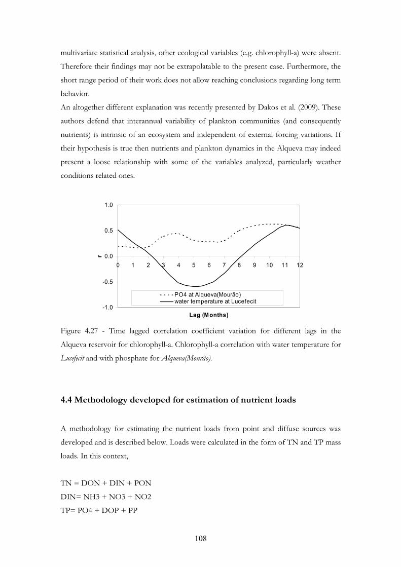
108

multivariate statistical analysis, other ecological variables (e.g. chlorophyll-a) were absent.

Therefore their findings may not be extrapolatable to the present case. Furthermore, the

short range period of their work does not allow reaching conclusions regarding long term

behavior.

An altogether different explanation was recently presented by Dakos et al. (2009). These

authors defend that interannual variability of plankton communities (and consequently

nutrients) is intrinsic of an ecosystem and independent of external forcing variations. If

their hypothesis is true then nutrients and plankton dynamics in the Alqueva may indeed

present a loose relationship with some of the variables analyzed, particularly weather

conditions related ones.

-1.0

-0.5

0.0

0.5

1.0

0 1 2 3 4 5 6 7 8 9 10 11 12

Lag (Months)

r

PO4 at Alqueva(Mourão)water temperature at Lucefecit

Figure 4.27 - Time lagged correlation coefficient variation for different lags in the

Alqueva reservoir for chlorophyll-a. Chlorophyll-a correlation with water temperature for

Lucefecit and with phosphate for Alqueva(Mourão).

4.4 Methodology developed for estimation of nutrient loads

A methodology for estimating the nutrient loads from point and diffuse sources was

developed and is described below. Loads were calculated in the form of TN and TP mass

loads. In this context,

TN = DON + DIN + PON

DIN= NH3 + NO3 + NO2

TP= PO4 + DOP + PP

109

Where DON is dissolved organic nitrogen, DIN is dissolved inorganic nitrogen, PON is

particulate organic nitrogen, DOP is dissolved organic phosphorus and PP is particulate

phosphorus.

In the present case it is not possible to use an advanced land model, like for instance,

MONERIS (Behrendt et al., 2002) or SWAT (Neitsch et al, 2001), to calculate the loads

in the Alqueva since processes information and local data are very scarce. The objective

of the loads estimation was to be able to allocate adequately loads to the different

subbasins and tributaries contributing to the Alqueva. The developed methodology is

plain but still adequate and can be used in cases where detailed information is not

available. The estimated loads were later used as input for model simulations. For

simulations loads variation over time were calculated using a ratio between the annual

estimated loads and the tributaries flow rate.

The Guadiana basin covers 55000 km2 in Spain and just 11700 km2 in Portugal. The

Portuguese area has a low population density but agriculture and animal livestock

production activities in the region are significant. These non-point sources are

accountable for nutrient export to soil and groundwater which in turn increase nutrient

loads from shorelines and watersheds, stimulating the Alqueva reservoir productivity.

According to Rodrigues et al. (1998) the main load sources from the Portuguese area of

the basin are animal production (39%), urban (33%) and agriculture (21%).

The Spanish area of the basin is more densely populated and has a higher industrial and

agricultural production than the Portuguese counterpart. The majority of the nutrient

loads are coming from Spanish territory and the input to the Alqueva is done mainly

through the river Guadiana itself (Rodriguez et al., 2006). The Degebe subbasin is the

second most significant anthropogenic input to the reservoir.

Internal loading was not regarded as important since the reservoir is young (build in

2002).

For point sources loads, statistical data on population from the National institute of

statistics (INE, 2001)and location and discharged volumes of waste water treatment

plants (data from the national assessment of urban water systems- INSAAR15 (INSAAR,

2006)) for the region was used together with specific nutrient loads values (3 g/ (inh.day)

for P and 10 g/ (ihn. day) for N) (Stalnacke et al., 2001) to calculate total point sources

15 INSAAR- Inventário nacional de sistemas de abastecimento de água e de águas residuais.

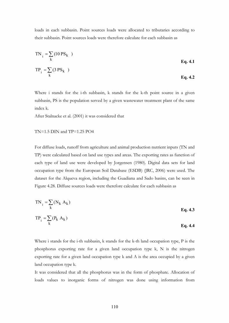
110

loads in each subbasin. Point sources loads were allocated to tributaries according to

their subbasin. Point sources loads were therefore calculate for each subbasin as

k

k )PS10(TNi

Eq. 4.1

k

k )PS3(TPi

Eq. 4.2

Where i stands for the i-th subbasin, k stands for the k-th point source in a given

subbasin, PS is the population served by a given wastewater treatment plant of the same

index k.

After Stalnacke et al. (2001) it was considered that

TN=1.5 DIN and TP=1.25 PO4

For diffuse loads, runoff from agriculture and animal production nutrient inputs (TN and

TP) were calculated based on land use types and areas. The exporting rates as function of

each type of land use were developed by Jorgensen (1980). Digital data sets for land

occupation type from the European Soil Database (ESDB) (JRC, 2006) were used. The

dataset for the Alqueva region, including the Guadiana and Sado basins, can be seen in

Figure 4.28. Diffuse sources loads were therefore calculate for each subbasin as

k

kk )AN(TNi

Eq. 4.3

k

kk )AP(TPi

Eq. 4.4

Where i stands for the i-th subbasin, k stands for the k-th land occupation type, P is the

phosphorus exporting rate for a given land occupation type k, N is the nitrogen

exporting rate for a given land occupation type k and A is the area occupied by a given

land occupation type k.

It was considered that all the phosphorus was in the form of phosphate. Allocation of

loads values to inorganic forms of nitrogen was done using information from

111

concentration measurements in the tributaries (for both diffuse and point sources

estimated loads).

Figure 4.28 - Land occupation type in the Guadiana and Sado basins. (Source: JRC,

2006).

Table 4.11 shows the estimated yearly loads. The estimated values differ from estimatives

done by other authors using different methodologies and source data (Diogo et al.

(2008), Estrela et al. (2009)). However, the magnitude of the values is the same. Given

the general lack of data for both point and diffuse sources a lot of uncertainty was

expected.

Table 4.11 - Estimated loads for Alqueva reservoir allocated to main tributaries.

Tributary TN (ton/y) TP (ton/y)Degebe 52.36 8.75 Guadiana 598.40 100.00 Alcarrache 22.44 3.75

112

References for Chapter 4

Behrendt H, Dannowski R, Deumlich D, Dolezal F, Kajewski I, Kornmilch M, Korol R, Mioduszewski W, Opitz D, Steidl J, Stronska M. 2002. Nutrient and heavy metal emissions into the river system of Odra - results and comparison of models. Schriftenreihe des Institutes für Abfallwirtschaft und Altlasten, Technische Universität Dresden, 28:213-221.

Canfield D, Bachmann R. 1981. Prediction of total phosphorus concentrations, chlorophyll-a and Secchi depths in natural and artificial lakes. Can. J. Fish. Aquat. Sci. 38: 414-423.

CCDR. 2000. Anuário de recursos hídricos do Alentejo. Ano hidrológico 1999-2000. (In Portuguese). CCDR. 2001. Anuário de recursos hídricos do Alentejo. Ano hidrológico 2000-2001. (In Portuguese). CCDR. 2002. Anuário de recursos hídricos do Alentejo. Ano hidrológico 2001-2002. (In Portuguese). CCDR. 2003. Anuário de recursos hídricos do Alentejo. Ano hidrológico 2002-2003. (In Portuguese). CCDR. 2004. Anuário de recursos hídricos do Alentejo. Ano hidrológico 2003-2004. (In Portuguese). CCDR. 2005. Anuário de recursos hídricos do Alentejo. Ano hidrológico 2004-2005. (In Portuguese). CCDR. 2006. Anuário de recursos hídricos do Alentejo. Ano hidrológico 2005-2006. (In Portuguese). CCDR. 2007. Anuário de recursos hídricos do Alentejo. Ano hidrológico 2006-2007. (In Portuguese). Dakos V, Benincà E, van Nes EH, Philippart CJM, Scheffer M, Huisman J. 2009. Interannual variability in

species composition explained as seasonally entrained chaos. Proc. R. Soc. B. 276:2871-2880. Dillon PJ, Rigler FH. 1974. The phosphorus-chlorophyll relationship in lakes. Limnol. Oceanogr. 19:767-

773. Diogo PA, Fonseca M, Coelho PS, Mateus NS, Almeida MC, Rodrigues AC. 2008. Reservoir phosphorous

sources evaluation and water quality modeling in a transboundary watershed. Desalination. 226: 200-214. Downing JA, McCauley E. 1992. The Nitrogen:Phosphorus relationship in lakes. Limnol. Oceanogr.

37:936-945. Estrela M, Silva E. 2009. Guadiana basin. Water quality and the development of the Alqueva region.

NeWater project report, FP6 global change and ecosystems. ISQ, Portugal. INAG. 2000. Implementação das redes de monitorização de recursos hidrícos - Bacias hidrográficas a sul

do Tejo. (In Portuguese). INE. 2001. Censos 2001. Online data at www.ine.pt. (In Portuguese). INSAAR. 2006. Online data at www.insaar.inag.pt. (In Portuguese). Jorgensen SE. 1980. Lake management. Pergamon press (Oxford). JRC. 2006. European soil database (ESDB). Joint research center (JRC), Land management natural hazards

unit, European Union. Online data at http://eusoils.jrc.ec.europa.eu/ESDB_Archive/ESDB/index.htm. Lefèvre M, Wald L, Diabaté L. 2007. Using reduced data sets ISCCP-B2 from the Meteosat satellites to

assess surface solar irradiance. Sol. Energ. 81:240-253. Lindim C, Pinho JL, Vieira JMP. 2010. Analysis of spatial and temporal patterns in a large reservoir using

water quality and hydrodynamic modeling. Ecol. Model. (In press). doi:10.1016/j.ecolmodel.2010.07.019 Miranda PMA, Abreu F, Salgado R. 1995. Estudo de impacte ambiental do Alqueva. Final report of

CLIMA project. ICAT, Faculdade de ciências da universidade de Lisboa, Portugal. (In Portuguese). Montgomery DR, Dietrich WE, Torres R, Anderson SP, Heffner JT, Loague K. 1997. Hydrologic response

of a steep, unchanneled valley to natural and applied rainfall. Water Resour. Res. 33:91-109. Neitsch SL, Arnold JG, Kiniry JR, Williams JR. 2001. Soil and water assessment tool - Theoretical

documentation - Version 2000. Blackland research center, agricultural research service, Texas, USA. Palma P, Alvarenga P, Palma VL, Fernandes RM, Soares AMVM, Barbosa IR. 2009. Assessment of

anthropogenic sources of water pollution using multivariate statistical techniques: a case study of the Alqueva’s reservoir, Portugal. Environ. Monit. Assess. 165:539–552.

Potes MJF. 2008. Climatologia e qualidade da água da bacia hidrográfica do Guadiana. Dissertação de mestrado, Universidade de Èvora. (In Portuguese).

Press WH, Teukolsky SA, Vetterling WT, Flannery BP. 1996. Numerical Recipes in FORTRAN 90, Vol. 2. 2nd ed. Cambridge Univ. Press

Quiros R. 1988. Relationships between air temperature, depth nutrients, and chlorophyll in 103 Argentinean lakes. Verh. Internat. Verein. Limnol. 23:647-658.

Rodrigues AC, Quadrado F, Gomes F. 1998. A qualidade da água no âmbito das bacias internacionais: A bacia do Guadiana. 4th APRH water conference proceedings. Lisbon, Portugal. (In Portuguese).

Rodriguez BZ, Alonso JBH. 2006. Calidad y aprovechamiento de las aguas del Guadiana transfronterizo extremeño-alentejano. R. Estud. Extrem. 62:(3):1189-1244. (In Spanish).

Schindler DW. 1977. Evolution of P limitation in lakes. Science. 195: 260-262. Schindler DW. 1978. Factors regulating phytoplankton production and standing crop in the world’s

freshwaters. Limnol. Oceanogr. 23:478-486. Smith VH. 2001. Blue-green algae in eutrophic fresh waters. LakeLine. 21:34-36.

113

Stålnacke P, Sults Ü, Vasiliev A, Skakalsky B, Botina A, Roll G, Pachel K, Maltsman T. 2001. Nutrient loads to lake Peipsi. Jordforsk report.4/01. Jordforsk. Ås. Finland.

UNESCO. 1996. Water quality assessments: A guide to the use of biota, sediments and water in environmental modeling. United Nations education, scientific and cultural organization(UNESCO). Chapman & Hall, London. Online at http://www.who.int/water_sanitation_health/resourcesquality/wqa/en/index.html

Virginia water resources research center. 2004. Report of the academic advisory committee to Virginia department of environmental quality – freshwater nutrient criteria. Division of water quality programs. Virginia department of environmental quality.

Wetzel RG. 2001. Limnology. Lake and river ecosystems. 3rd ed. Academic press.

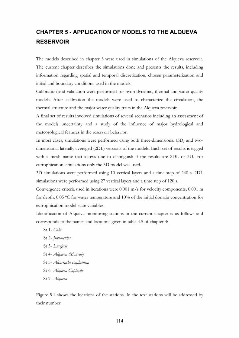
114

CHAPTER 5 - APPLICATION OF MODELS TO THE ALQUEVA

RESERVOIR

The models described in chapter 3 were used in simulations of the Alqueva reservoir.

The current chapter describes the simulations done and presents the results, including

information regarding spatial and temporal discretization, chosen parameterization and

initial and boundary conditions used in the models.

Calibration and validation were performed for hydrodynamic, thermal and water quality

models. After calibration the models were used to characterize the circulation, the

thermal structure and the major water quality traits in the Alqueva reservoir.

A final set of results involved simulations of several scenarios including an assessment of

the models uncertainty and a study of the influence of major hydrological and

meteorological features in the reservoir behavior.

In most cases, simulations were performed using both three-dimensional (3D) and two-

dimensional laterally averaged (2DL) versions of the models. Each set of results is tagged

with a mesh name that allows one to distinguish if the results are 2DL or 3D. For

eutrophication simulations only the 3D model was used.

3D simulations were performed using 10 vertical layers and a time step of 240 s. 2DL

simulations were performed using 27 vertical layers and a time step of 120 s.

Convergence criteria used in iterations were 0.001 m/s for velocity components, 0.001 m

for depth, 0.05 ºC for water temperature and 10% of the initial domain concentration for

eutrophication model state variables.

Identification of Alqueva monitoring stations in the current chapter is as follows and

corresponds to the names and locations given in table 4.5 of chapter 4:

St 1- Caia

St 2- Juromenha

St 3- Lucefecit

St 4- Alqueva (Mourão)

St 5- Alcarrache confluência

St 6- Alqueva Captação

St 7- Alqueva

Figure 5.1 shows the locations of the stations. In the text stations will be addressed by

their number.

115

5.1 Spatial discretization and computational mesh

Mesh resolution is of paramount importance in the simulations. A coarse resolution can

lead to numerical diffusion1 problems (Oberhuber, 1993). When simulating stratified

flows, vertical spatial discretization achieves major significance. Among the most

common vertical coordinate types in models are: sigma (after POM (Blumberg et al.,

1987)), z-level (after MOM (Cox, 1984)) and isopycnic (after MICOM (Bleck et al.,

1992)). Although widespread, the mentioned coordinate types are not exempt from flaws

and can be inadequate in a number of situations. For that reason many recent versions of

models include different types of coordinates (Mellor et al., 2000) or allow the use of

combinations of coordinate types ( Bleck et al, 1981) for a given system simulation.

Z-level are Cartesian coordinates that simply divide the domain in horizontal layers of

varying depth. They are almost exclusively used for open ocean models since there is a

high loss of resolution in shallow areas. Additionally, free surface elevation is difficult to

represent.

Isopycnic coordinates follow lines of constant density. This coordinates are adequate for

simulating stratified systems since flow is in line with the layers and vertical fluxes are

small. This will avoid numerical diffusion problems (numerical diffusion will arise

whenever velocity fields are oblique to the mesh). However, these coordinates lack

versatility and will be inadequate for non-stratified situations (where no isopycnic layers

exist) and for shallow areas with irregular bathymetries.

Sigma coordinates follow terrain topography and therefore are adequate for shallow and

complex areas provided the area does not have highly irregular bathymetry and vertical

densities do not change a lot. For sharp slopes and marked vertical density changes

(stable stratification) the flow will occur preferentially along isopycnic lines and will be

oblique to the mesh vertical layers leading to numerical diffusion issues. Double sigma

coordinates are sometimes used to try to go around the limitations sigma coordinates

have. The double sigma coordinates divide the domain in the area where density changes

are higher creating two different mesh areas. But this method does not reflect any real

physical characteristic of the domain.

1 Numerical diffusion can roughly be defined as an artificial mixing caused by transport of gradients across

the model discrete calculation units.

116

In RMA10 the domain representation is merely a collection of simpler domains called

elements (FEM uses unstructured grids). Bidimensional elements can be either triangular

or quadrilateral in shape (6 or 8 nodes) while three-dimensional elements can be solids

with 10, 13, 15 or 20 quadratic elements. In the current work triangular bidimensional

elements and 15 nodes tridimensional solids were used. The varying computational

domain that results from the variation over time of the water surface elevation implies

the use of a vertical coordinate. For vertical discretization RMA10 uses the transformed

coordinate described in chapter 3. The transformation differs from the classical sigma

coordinate because it preserves the original bottom profile and it only transforms the

water surface to constant elevation (King, 1985).

Bathymetric data for the Alqueva reservoir was obtained from EDIA. The bathymetry of

the reservoir is shown in Figure 5.1. The upper riverine area and the margins are shallow

(less than 10 meters, with river Guadiana entrance less than 5 meters deep). Most of the

reservoir area is shallower than 30 meters, with only the central areas of the wide open

lacustrine regions and the dam area having higher depths. The reservoir presents abrupt

changes in both depth and surface area in several locations that can create simulation

problems if not adequately addressed when generating the mesh.

Computational meshes were generated based on bathymetric data and geotagged

digitized maps of the area using SMS 7.0 (Aquaveo, 2002) for bidimensional meshes and

RMAGEN (Resource modelling associates, 2008) for three-dimensional meshes using an

already generated bidimensional mesh as starting point. Additionally, mixed dimensions

meshes were created using RMAGEN. The geotagged digitized maps were used to define

the domain contours. Water depths at each mesh node were interpolated from the

bathymetric data.

Several meshes with different resolution were created and tested. The mesh generation

process should guarantee that there is enough resolution in order to obtain representative

simulation results and at the same time that simulations are computationally cost-

efficient. Solution oscillations can be eliminated by reducing the time step and by

increasing mesh resolution.

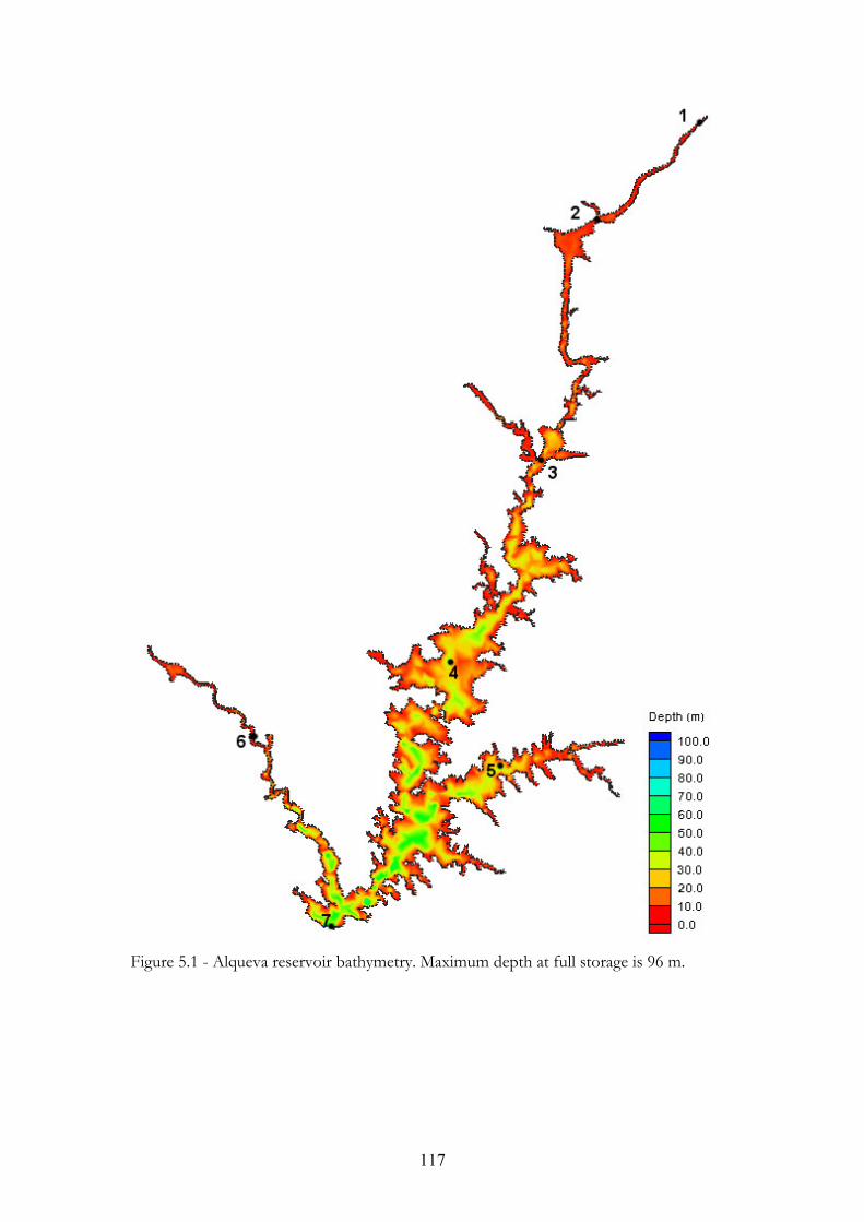
117

Figure 5.1 - Alqueva reservoir bathymetry. Maximum depth at full storage is 96 m.

118

As a rule of thumb elements were constructed following the line of the bathymetry and

the expected direction of flow. Particular attention was paid to internal angles of the

elements and any rapid change of slope. Internal angles were corrected whenever they

were out of the interval 20-130 º. Variations of slope bigger than 0.2 and variations of

area larger than 2.5 between neighbor elements were corrected. Areas where large

variations in either depth or velocities existed or were to be expected had more mesh

detail. Expected fast velocity areas like the river Guadiana entrance and areas of interest

like the dam area also had more mesh detail. Mesh was not as dense in open lacustrine

areas where flow is expected to have stable characteristics. Three final three-dimensional

meshes were chosen to be tested against each other on model test runs:

- A refined very high resolution mesh (M1) (Figure 5.2) was used as reference for

tests. The mesh has 15661 elements and 40712 nodes.

- A medium resolution mesh (M2) with 3986 elements and 10460 nodes (Figure

5.3).

- A lower resolution mesh (M3) with 2727 elements and 7534 nodes (Figure 5.4).

The meshes were tested in 8 day runs, using a time step of 60 s, with different forcings

by water surface level at dam and Guadiana inflows. Results were compared at 6 different

mesh points. The objective was to verify that the solution obtained is independent of the

mesh we use (up to 15% average variation in nodal velocities was considered acceptable).

It was concluded that the lowest resolution mesh (M3) did not comply with the above

condition and this mesh was not subsequently used. M1 and M2 meshes did comply and

were subsequently used. Generally, M2 mesh was used to do initial runs and in fine

tuning models after which M1 mesh was then used to get final results.

A two-dimensional laterally averaged mesh (2DL) and a mixed dimensions mesh (MD)

were also developed and are presented in Figures 5.5 and 5.6.

119

120

Figure 5.2 - High definition mesh M1 for Alqueva. Top: Upper part of mesh showing

Guadiana entrance. Bottom: Lower part of mesh showing dam and southern area.

Distance between nodes: 358 m (Maxima); 169 m (Average).

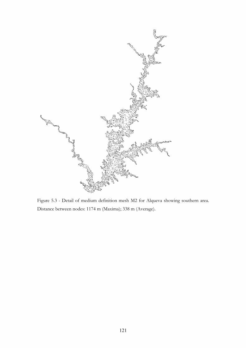
121

Figure 5.3 - Detail of medium definition mesh M2 for Alqueva showing southern area.

Distance between nodes: 1174 m (Maxima); 338 m (Average).

122

Figure 5.4 - Detail of medium definition mesh M3 for Alqueva showing southern area.

Distance between nodes: 1427 m (Maxima); 506 m (Average).

123

Figure 5.5 - Bidimensional mesh 2DL used in Alqueva reservoir simulations. Left image -

Mesh. Black represents longitudinal elements. Grey represents lateral domain dimension.

Right image - Same mesh as left image but superimposed on Alqueva reservoir satellite

image. Mesh has 217 longitudinal elements.

124

Figure 5.6 - Mixed 2D and 1D dimensions mesh MD developed for Alqueva reservoir.

Mesh has 3480 elements.

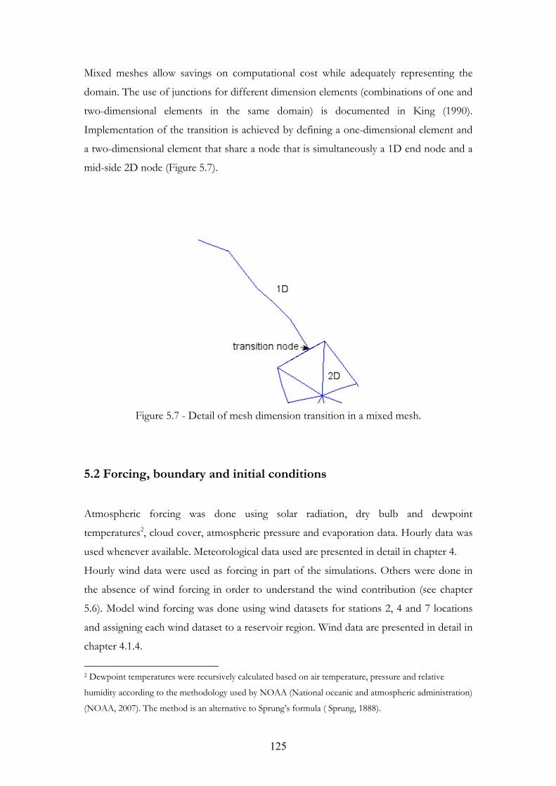
125

Mixed meshes allow savings on computational cost while adequately representing the

domain. The use of junctions for different dimension elements (combinations of one and

two-dimensional elements in the same domain) is documented in King (1990).

Implementation of the transition is achieved by defining a one-dimensional element and

a two-dimensional element that share a node that is simultaneously a 1D end node and a

mid-side 2D node (Figure 5.7).

Figure 5.7 - Detail of mesh dimension transition in a mixed mesh.

5.2 Forcing, boundary and initial conditions

Atmospheric forcing was done using solar radiation, dry bulb and dewpoint

temperatures2, cloud cover, atmospheric pressure and evaporation data. Hourly data was

used whenever available. Meteorological data used are presented in detail in chapter 4.

Hourly wind data were used as forcing in part of the simulations. Others were done in

the absence of wind forcing in order to understand the wind contribution (see chapter

5.6). Model wind forcing was done using wind datasets for stations 2, 4 and 7 locations

and assigning each wind dataset to a reservoir region. Wind data are presented in detail in

chapter 4.1.4.

2 Dewpoint temperatures were recursively calculated based on air temperature, pressure and relative

humidity according to the methodology used by NOAA (National oceanic and atmospheric administration)

(NOAA, 2007). The method is an alternative to Sprung’s formula ( Sprung, 1888).

126

5.2.1 Hydrodynamic simulations

Open boundary conditions used were hourly water surface elevation data at the dam and

daily Guadiana inflow. Figure 5.8 presents water surface elevation data used in the

simulations. Data for river inflow are presented in detail in chapter 4 section 2.

Except for solar radiation and wind action at the free surface, fluxes at the free surface

and bottom are zero. Bottom friction uses Manning coefficient.

The simulations performed were cold starts (initial velocities were set to zero) where the

model was allowed a spin up time of three days in order for the flow field to become

adjusted to the applied meteorological and hydraulic forcings.

120

130

140

150

160

Dec-02 Dec-03 Dec-04 Dec-05 Dec-06 Dec-07 Dec-08 Dec-09

Wat

er S

urfa

ce E

leva

tion

(m)

Figure 5.8 - Daily averaged water surface elevation at Alqueva reservoir dam. (Data

source: SNIRH)

5.2.2 Thermal simulations

Initial conditions used were water temperatures homogeneous over domain based on

averaged in situ measured data. Water temperatures over time were imposed at both river

and dam boundaries. Temperature fluxes at free surface and bottom are zero, but a

source term exists for the transport of heat at the free surface (see model rational in

chapter 3).

127

5.2.3 Eutrophication simulations

Initial conditions used were homogeneous concentrations for the state variables over the

domain based on in situ measured data. Boundary conditions were given for the state

variables as mass loads over time calculated by the nutrients loads estimation (see

methodology description and estimated values in chapter 4.4) and monitoring knowledge

about concentrations over time in tributaries inflow. The yearly loads in table 4.11 were

used for the reference year 2006. For other years, yearly value was corrected using the

ratio of Guadiana average flows for simulation year and reference year.

Results from the hydrodynamic simulation in the form of velocity fields and from the

thermal simulation in the form of water temperatures in the domain over time were used

to feed the eutrophication model.

5.3 Models Parameterization and Calibration

Hydrodynamic and temperature simulations calibrations were based on three parameters:

the bottom friction, the vertical eddy coefficient and the solar extinction coefficient. The

automated calibration process for the eutrophication model is described in chapter 3.

Models’ calibration was done with data from the year 2006. Validation of models was

done with data from 2008.

Since no current meters data were available for the Alqueva, the hydrodynamic model

calibration for 3D simulations proceeded by changing the inflows until a reasonable

agreement with measured and simulated reservoir volume was achieved. The calibration

level of accuracy was assessed using a normalized RMSE for the volume. Normalization

was done using the difference between maximum and minimum observed volume values.

For 2D simulations, calibration with volume was not possible since the domain network

does not encompass all the reservoir. Instead the inflow data series used as input was the

same as in the calibrated 3D model. This procedure should also guarantee that mass

balances are correct. In his doctoral thesis, Rueda (2000) ran a series of benchmark tests

on RMA10 and concluded that RMA10 ability to conserve mass has an error of O(10-7).

Thus, RMA10 adequately conserves mass.

A temperature calibration assessment was done by comparison of model simulation

results with measured vertical temperature profiles and with measured temperature time

128

series at different depths. Water temperature was considered to be calibrated when

RMSE values were small enough to have a minimal effect on the system kinetic rates.

Kinetic rates show an Arrhenius dependency of temperature and for natural systems they

roughly double for every 10 ºC increase. Equation 5.1 returns the rate of change in a

kinetic rate as a function of water temperature variations

1

212 k

klnKTT

Eq. 5.1

Where k2 is a generic kinetic rate at temperature T2, k1 is the correspondent rate at

temperature T1 and K is a constant, with K= 0.1 ln Q10. The temperature coefficient

(Q10) for natural systems is generally between 1.5 and 2.5.

For the purpose of this work and based on equation 5.1 it was considered that a

temperature variation smaller than 3ºC would have a minimal impact in kinetic rates.

Thus, model deviations smaller than 3ºC were considered acceptable.

Eutrophication calibration assessment was done by comparison of model simulation

results with measured data for concentrations of state variables over time for different

locations and depths as described in chapter 3.2.14.

Bottom roughness (Bottom friction coefficient) parameterization

The characteristics of bottom sediment and benthic vegetation, together with the type of

flow, affect the choice of the model coefficients values used to describe the bottom

friction. The Manning roughness coefficient is used in the model to represent the bed

resistance to flow. For the Alqueva, there is neither experimental information about the

type of sediments nor any granulometric data. The bottom of the Alqueva reservoir was

considered as an homogeneous material in the model. Therefore a single value for the

Manning roughness coefficient was applied to all domain elements in the simulations.

Manning coefficients tested were based on tabulated values given by Arcement et al.

(1989). The final Manning coefficient chosen was 0.050.

Eddy viscosity and diffusivity parameterization

RMA10 has different options for turbulence closure methods. The Smagorinsky closure

scheme (Smagorinsky, 1963) was used in the horizontal. For the vertical the original

RMA10 formulation was used. In this formulation the vertical eddy viscosity coefficients

129

vary with depth and are given by a quadratic distribution over the water column. A mid-

depth maximum value is determined during the calibration process.

After calibration the vertical turbulent diffusion coefficient was set to 1x10-6 m2/s which

is roughly the kinematic viscosity of water at 20ºC (therefore adequate for a waterbody

like the Alqueva where vertical mixing is minimal).

Solar extinction coefficient parameterization

The calibrated value for solar extinction coefficient was 0.5 m-1.This value can be

considered adequate for the Alqueva given the turbidity conditions of this waterbody.

Secchi disk measurements3 made in situ ranged from 1.5 m in the turbid riverine upper

part to 6 m in the open lacustrine areas downstream. Based on measurements from 2003-

2009, the average Secchi disk depth for the whole Alqueva is 3 m. A range of values for

the extinction coefficient was tested in the model. The value 0.5 gave the best results.

5.3.1 Hydrodynamic calibration

Figure 5.9 presents simulated vs. measured total reservoir volume over time for mesh

M1. The normalized RMSE was 4.20%.

2.0E+09

2.5E+09

3.0E+09

3.5E+09

4.0E+09

0 50 100 150 200 250 300 350 400 450

Julian day

Vo

lum

e (

m3)

measured

s imulated

Figure 5.9 - Simulated and measured reservoir total volume (m3). Mesh M1. ( Data

source: EDIA)

3 The empirical relationship,

sZC , with C=1.7, developed by Poole et al.(1929) is widely use to quickly

obtain an approximate value of the coefficient of extinction given a Secchi disk measurement. Other

authors (Sverdrup et al. (1947), Beeton (1958)) obtained similar relationships but with 1.7<C< 1.9.

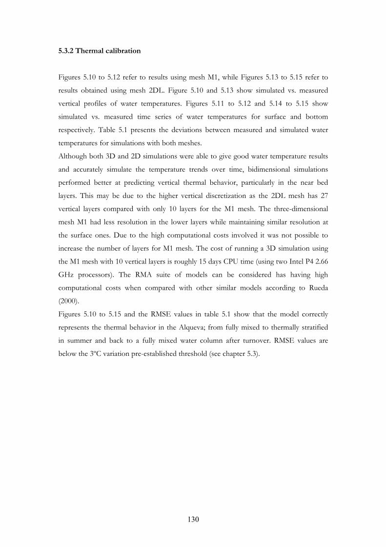
130

5.3.2 Thermal calibration

Figures 5.10 to 5.12 refer to results using mesh M1, while Figures 5.13 to 5.15 refer to

results obtained using mesh 2DL. Figure 5.10 and 5.13 show simulated vs. measured

vertical profiles of water temperatures. Figures 5.11 to 5.12 and 5.14 to 5.15 show

simulated vs. measured time series of water temperatures for surface and bottom

respectively. Table 5.1 presents the deviations between measured and simulated water

temperatures for simulations with both meshes.

Although both 3D and 2D simulations were able to give good water temperature results

and accurately simulate the temperature trends over time, bidimensional simulations

performed better at predicting vertical thermal behavior, particularly in the near bed

layers. This may be due to the higher vertical discretization as the 2DL mesh has 27

vertical layers compared with only 10 layers for the M1 mesh. The three-dimensional

mesh M1 had less resolution in the lower layers while maintaining similar resolution at

the surface ones. Due to the high computational costs involved it was not possible to

increase the number of layers for M1 mesh. The cost of running a 3D simulation using

the M1 mesh with 10 vertical layers is roughly 15 days CPU time (using two Intel P4 2.66

GHz processors). The RMA suite of models can be considered has having high

computational costs when compared with other similar models according to Rueda

(2000).

Figures 5.10 to 5.15 and the RMSE values in table 5.1 show that the model correctly

represents the thermal behavior in the Alqueva; from fully mixed to thermally stratified

in summer and back to a fully mixed water column after turnover. RMSE values are

below the 3ºC variation pre-established threshold (see chapter 5.3).

131

Figure 5.10 - Vertical temperature profiles measured (points) and modeled (line) for

stations 3, 4, 5 and 7 for Julian day 220. Mesh M1.

Figure 5.11 - Simulated (black) and measured (grey) surface water temperatures in the

Alqueva at the indicated locations (Sts 2, 4 and 7). Mesh M1.

132

Figure 5.12 - Simulated (black) and measured (grey) bottom water temperatures in the

Alqueva at the indicated locations (Sts 4 and 7). Mesh M1.

Figure 5.13 - Vertical temperature profiles measured (points) and modeled (line) for

stations 3, 4 and 7 for Julian day 220. Mesh 2DL.

133

Figure 5.14 - Simulated (black) and measured (grey) surface water temperatures in the

Alqueva at the indicated locations (Sts 2, 4 and 7). Mesh 2DL.

Figure 5.15 - Simulated (black) and measured (grey) bottom water temperatures in the

Alqueva at the indicated locations (Sts 4 and 7). Mesh 2DL.

Table 5.1 - Root mean square deviations between measured and simulated water

temperatures in Figures 5.11 to 5.12 and 5.14 to 5.15.

Location and layer M1 RMSE 2DL RMSE Station 2 2.51 2.46 Station 4 surface 1.60 1.97 Station 7 surface 1.38 1.69 Station 7 bottom 1.01 0.33 Station 4 bottom 0.91 0.40 Average deviation 1.48 1.37

134

5.3.3 Eutrophication calibration

Calibration of the eutrophication model was done by comparing model simulation results

with in situ measured data on different temporal and spatial scales as described in chapter

3.2.14. Figure 5.16 presents the calibration results and table 5.2 summarizes the error

statistics and presents the model parameters obtained in calibration. The minimum global

deviation i (see equation 3.52) found was 11.2.

Since no monitoring data exists for OP, ON and zooplankton those state variables are

not represented in the figures. The same holds true for BOD. Monitored BOD cannot

be compared with simulated BOD, since model BOD is for complete oxidation while

measured BOD is BOD5.

Calibration results show that the model is generally able to adequately simulate the

patterns of oxygen, chlorophyll-a and nutrients dynamics at different points of the

reservoir representative of its spatial heterogeneity over time as well as most seasonal

trends.

Ammonia is the poorest predicted state variable (see table 5.2). Some major differences

between the simulated and the measured ammonia exist in the southern area of the

reservoir in winter and spring (see Figure 5.16), with the model overpredicting the

measurements of ammonia. Nevertheless, predicted chlorophyll-a seasonal cycle agrees

reasonably well with measurements and the onset and conclusion of hypoxic/anoxic

conditions in the hypolimnion are well captured by the model for lacustrine locations.

The absence of full vertical profile measurements for DO prevented the calibration of

DO chemocline depths.

Table 5.2 presents an assessment of the goodness-of-fit for the eutrophication model.

Deviations in each table column entry were calculated by averaging the deviations for all

stations and depths. In many cases the high deviations found were mainly caused by what

seems to be isolated anomalous monitoring data points, that is, outliers (e.g. see PO4

data at station 4 surface in Figure 5.16). No outliers were discarded when calculating

deviations. In chapter 4, monitoring data were analyzed and some data problems were

highlighted, namely, the absence of measurements error and of analytical methods

detection limits plus the non-agreement of measured values between different data

sources (EDIA and SNIRH) for some state variables. Since a single monthly

measurement may have a high associated error, it would be better if data collection had a

135

higher periodicity in order to allow averaging over time to be performed which would

most likely help eliminate error sources.

The highest deviations between model results and measurements were found for stations

4 and 7 both located in the lower part of the Alqueva. This can clearly be seen by

comparing the results in the left column in Figure 5.16 with the two other columns

results. These discrepancies between the model results and the data show that the model

may not be sufficiently generic to reflect the full spatial diversity of the reservoir. Since

the upstream portion of the lake behaves like a riverine area with high input of nutrients

while the downstream area of the reservoir is representative of a deep stratified lake, fine-

tuning the model becomes difficult because rates and parameters in the model are fixed

values, thus reducing the model’s ability to simulate such different ecological

environments.

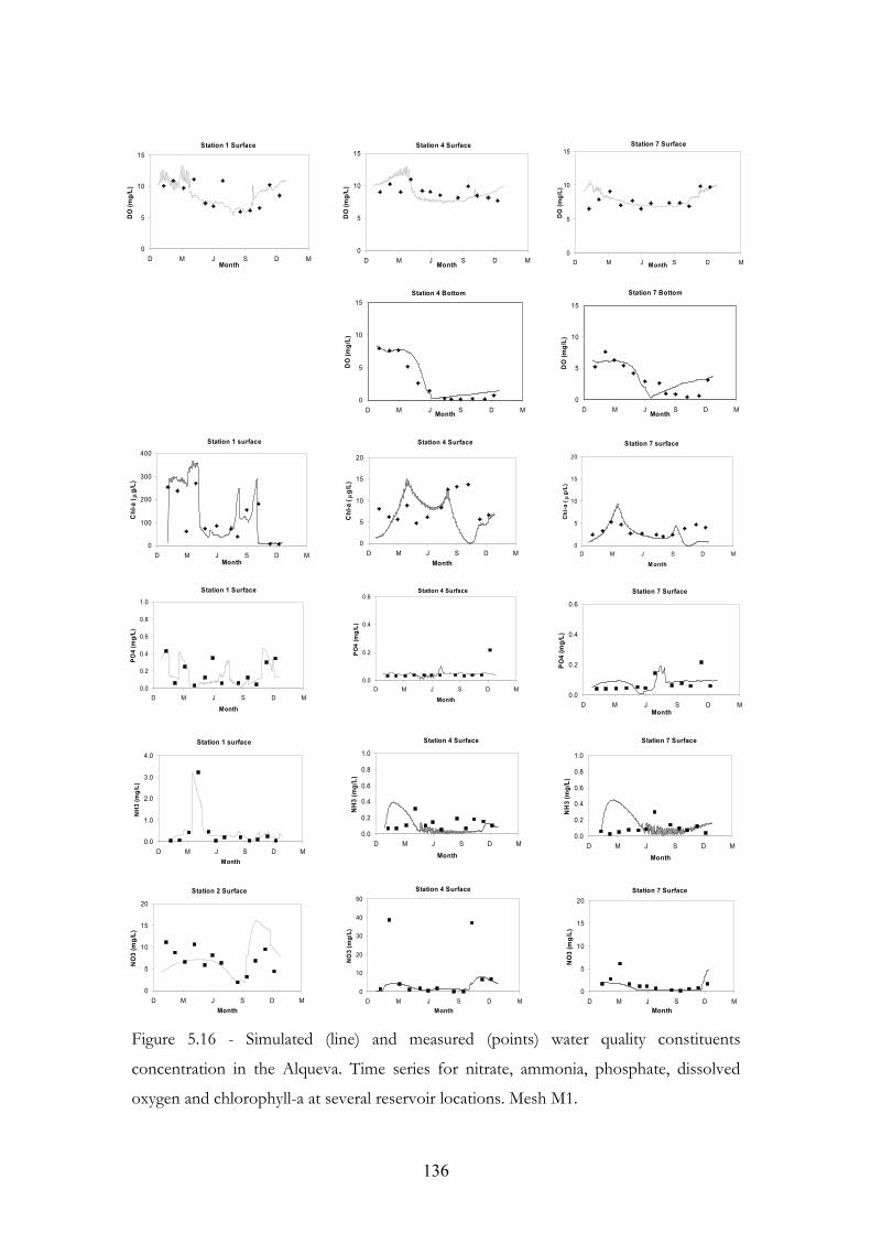
136

Station 1 Surface

0

5

10

15

D M J S D MMonth

DO

(mg

/L)

Station 4 Surface

0

5

10

15

D M J S D MMonth

DO

(mg

/L)

Station 7 Surface

0

5

10

15

D M J S D MMonth

DO

(m

g/L

)

Station 4 Bottom

0

5

10

15

D M J S D MMonth

DO

(mg

/L)

Station 7 Bottom

0

5

10

15

D M J S D MMonth

DO

(m

g/L

)

Station 1 surface

0

100

200

300

400

D M J S D MMonth

Ch

l-a (

g/L

)

Station 4 Surface

0

5

10

15

20

D M J S D M

Month

Ch

l-a

( g

/L)

Station 7 surface

0

5

10

15

20

D M J S D M

M onthC

hl-

a (

g/L

)

Station 1 Surface

0.0

0.2

0.4

0.6

0.8

1.0

D M J S D M

Month

PO

4 (m

g/L

)

Station 4 Surface

0.0

0.2

0.4

0.6

D M J S D M

Month

PO

4 (m

g/L

)

Station 7 Surface

0.0

0.2

0.4

0.6

D M J S D MMonth

PO

4 (m

g/L

)

Station 1 surface

0.0

1.0

2.0

3.0

4.0

D M J S D M

Month

NH

3 (m

g/L

)

Station 4 Surface

0.0

0.2

0.4

0.6

0.8

1.0

D M J S D M

Month

NH

3 (

mg

/L)

Station 7 Surface

0.0

0.2

0.4

0.6

0.8

1.0

D M J S D M

Month

NH

3 (m

g/L

)

Station 2 Surface

0

5

10

15

20

D M J S D M

Month

NO

3 (

mg

/L)

Station 4 Surface

0

10

20

30

40

50

D M J S D M

Month

NO

3 (m

g/L

)

Station 7 Surface

0

5

10

15

20

D M J S D MMonth

NO

3 (m

g/L

)

Figure 5.16 - Simulated (line) and measured (points) water quality constituents

concentration in the Alqueva. Time series for nitrate, ammonia, phosphate, dissolved

oxygen and chlorophyll-a at several reservoir locations. Mesh M1.

137

Table 5.2 - Calibrated model parameters and error statistics in eutrophication model

calibration. Deviations were averaged for all monitored stations and water depths.

Parameter Value Isat optimal light intensity 376 Ly/day Selfs self shading coefficient 0.008 m-1 KP half-saturation constant for P limitation uptake 0.08 mg P/L KN half-saturation constant for N limitation uptake 0.026 mg N/L Kz half-saturation constant for phytoplankton limitation in zooplankton growth 0.6 mg C/L max Algae maximum growth rate at 20ºC 2.0 day-1 kr Respiration rate at 20ºC 0.1 day-1 Pdead phytoplankton non-predatory mortality rate at 20ºC 0.06 day-1 Zdead1 zooplankton non-predatory mortality at 20ºC 0.01 day-1 Zdead2 Zooplankton predatory mortality rate at 20 ºC 0.02 day-1 kg Ingestion rate for zooplankton at 20 ºC

0.9 mg C algae/ (mg C zoo day)

pref Weight factor in ammonia preference factor 1.4 fraction of phosphorus respired material that is organic phosphorus 0.28 fraction of nitrogen respired material that is organic nitrogen 0.34

Ammonia to nitrate fraction 0.98

kdp decay rate of organic phosphorus to inorganic P at 20 ºC 0.03 day-1 kdn decay rate of organic nitrogen to inorganic N at 20 ºC 0.02 day-1 kdenit Denitrification rate 0.1 day-1 kn Nitrification rate 0.1 day-1 kO2 Oxygen inhibition constant in denitrification 0.1 mg O2/L kd Decay rate of BOD at 20ºC 0.2 day-1 SOD Sediment oxygen demand at 20ºC 1957 mg O2 m-2 day-1

Error statistics Chl-a

(g/L) DO

(mg/L) PO4

(mg/L) NO3

(mg/L) NH3

(mg/L) RE 37% 15% 44% 53% 80%

RMSE 25.5 1.1 0.06 5.7 0.22

5.4 Model results and discussion

After calibration the models were used to investigate hydrodynamic, thermal and

eutrophication processes in the Alqueva reservoir. The results obtained and a discussion

are included in the current section.

Text references to “upper” and “lower” reservoir areas refer to a qualitatively division of

the reservoir in two main areas of different behavior. The boundary between the two

regions can be considered as a transect located downstream from station 3 (see Figure

5.1). An explanation for this division is presented in chapter 5.4.1.

138

5.4.1 Velocities and circulation patterns

Figure 5.17 - Simulated surface velocities in the Alqueva at the indicated locations (Sts 2,

4, 7 and a generic point p10). Mesh M1.

Figures 5.17 to 5.19 present circulation results for a three-dimensional simulation using

mesh M1.

Figure 5.17 shows time series plots of surface currents at different reservoir points.

Velocities in the Alqueva reservoir are always smaller than 0.25 m/s for the whole year.

Station 2 is clearly affected by Guadiana inflow rates (see inflow data in chapter 4.2),

since velocity changes over time at this location directly reflect Guadiana inflow rate

variations. Lower reservoir locations (stations 4, 7 and point p10) do not seem to be

directly influenced by the Guadiana inflow. Instead wind forces appear to dominate the

circulation there. The higher velocities obtained for days 28, 95 and 328 correspond to

the maximum registered winds of the year at the lower reservoir areas (see wind data in

chapter 4.1.4).

Year wind speed maxima at station 7 was registered on day 28 (9.3 m/s), with the other

lower reservoir stations also experiencing high wind speeds for that day (7.7 m/s at

station 4). Upper reservoir wind speed for that day was lower (3.2 m/s at station 1).

Figure 5.18 (left) shows a reservoir contour of simulated surface velocities for day 28

(high wind speed) while Figure 5.18 (right) shows a low wind speed situation (day 300). It

is seen that wind affects the surface velocities in the reservoir.

139

For day 300, average registered wind speed for all meteorological stations was 3.3 m/s,

with station 1 presenting 2.2 m/s. Besides representing a weak wind situation, Figure

5.18 (right) also corresponds to a situation of high Guadiana inflow, while Figure 5.18

(left) shows a situation where Guadiana inflow is roughly 10 times smaller than in Figure

5.18 (right). Comparing Figures 5.18 (left) and 5.18 (right), both with weak winds at

upper reservoir but with very different Guadiana inflows, it can be inferred that the

Guadiana inflow rate affects the currents in the upper part of the reservoir. The results

seem to point that the Guadiana inflow area of influence extends to the majority of the

reservoir upper part, an area that has a more riverine character and several shallow

channel like sections. Velocities appear to be influenced by the river inflow until just

south of the station 3 location. Based on the hydrodynamic simulation results and on the

morphological features of the reservoir a boundary between a lotic and a lentic area can

be established at a transect at this location.

Figure 5.19 presents contours of simulated bed velocities for the same situations and

conditions presented in Figure 5.18. For the upstream shallow riverine areas it is seen

that bed velocities are similar to surface ones. This is observable for the upper reservoir

locations between stations 1 and 3. In fact, one can say that a distinction between bed

and surface at locations that shallow cannot be made and we are therefore looking at the

same velocities.

For a low wind situation (Figures 5.18 and 5.19, right) bed and surface velocities are

similar downstream from station 3 whereas for high wind situations (Figures 5.18 and

5.19, left) bed velocities are typically one order of magnitude lower than surface

velocities.

A surface velocity distribution is presented in Figure 5.20. Velocities were time averaged

using the simulation results for the full year to generate the distribution. The figure

allows seeing the dominant time–averaged circulation patterns in the Alqueva. The upper

reservoir region shows clear flow downstream patterns, while lower and wider areas of

the Alqueva present some local eddies, probably due to the reservoir

morphology/geometry and wind effects. In these lower areas flow followed wind

direction when wind speed was high. For low wind or when wind direction changes

occurred gyres tended to be formed.

Unfortunately, findings for velocities and circulation patterns could not be corroborated

since there are no current meter measurements available.

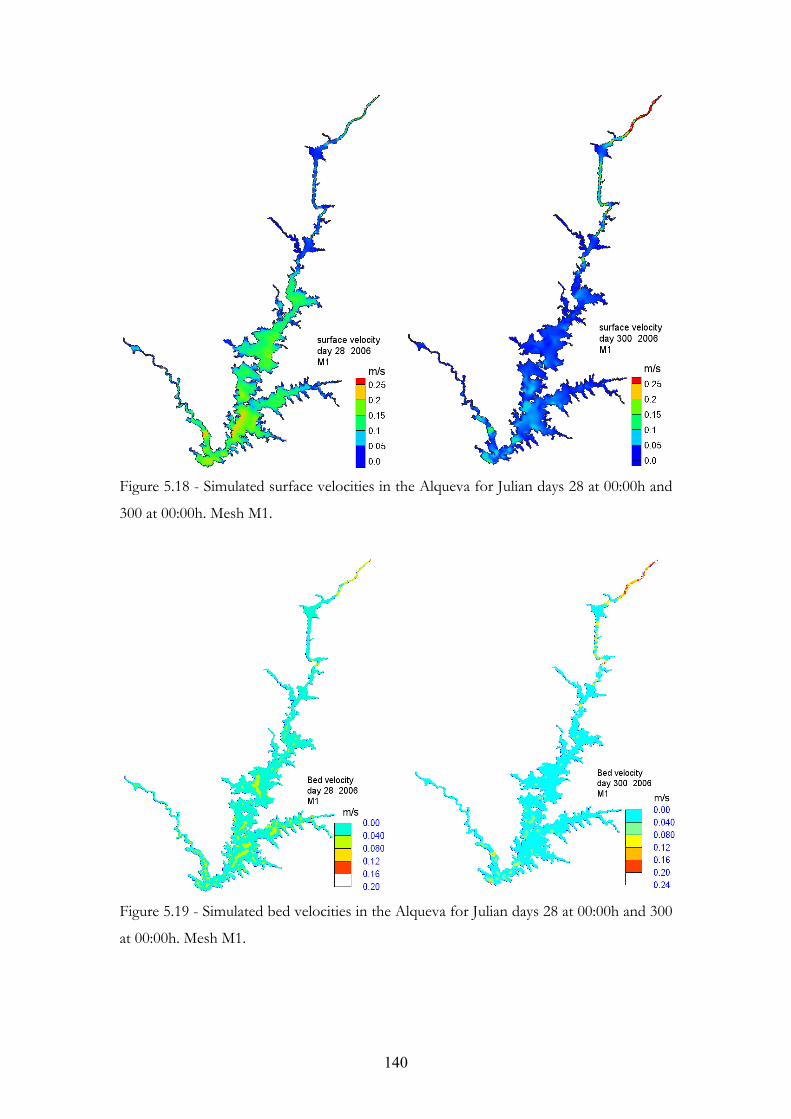
140

Figure 5.18 - Simulated surface velocities in the Alqueva for Julian days 28 at 00:00h and

300 at 00:00h. Mesh M1.

Figure 5.19 - Simulated bed velocities in the Alqueva for Julian days 28 at 00:00h and 300

at 00:00h. Mesh M1.

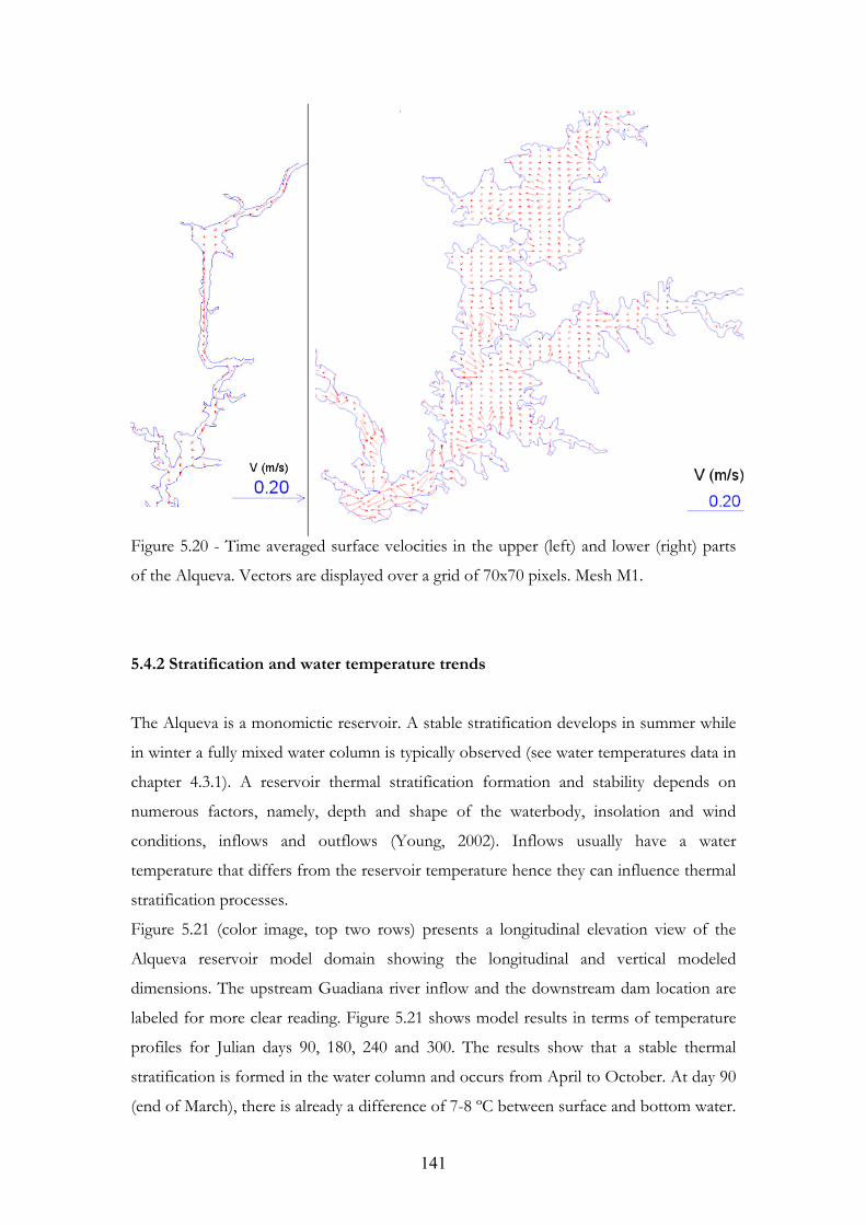
141

Figure 5.20 - Time averaged surface velocities in the upper (left) and lower (right) parts

of the Alqueva. Vectors are displayed over a grid of 70x70 pixels. Mesh M1.

5.4.2 Stratification and water temperature trends

The Alqueva is a monomictic reservoir. A stable stratification develops in summer while

in winter a fully mixed water column is typically observed (see water temperatures data in

chapter 4.3.1). A reservoir thermal stratification formation and stability depends on

numerous factors, namely, depth and shape of the waterbody, insolation and wind

conditions, inflows and outflows (Young, 2002). Inflows usually have a water

temperature that differs from the reservoir temperature hence they can influence thermal

stratification processes.

Figure 5.21 (color image, top two rows) presents a longitudinal elevation view of the

Alqueva reservoir model domain showing the longitudinal and vertical modeled

dimensions. The upstream Guadiana river inflow and the downstream dam location are

labeled for more clear reading. Figure 5.21 shows model results in terms of temperature

profiles for Julian days 90, 180, 240 and 300. The results show that a stable thermal

stratification is formed in the water column and occurs from April to October. At day 90

(end of March), there is already a difference of 7-8 ºC between surface and bottom water.

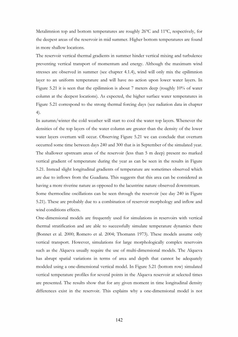
142

Metalimnion top and bottom temperatures are roughly 26ºC and 11ºC, respectively, for

the deepest areas of the reservoir in mid summer. Higher bottom temperatures are found

in more shallow locations.

The reservoir vertical thermal gradients in summer hinder vertical mixing and turbulence

preventing vertical transport of momentum and energy. Although the maximum wind

stresses are observed in summer (see chapter 4.1.4), wind will only mix the epilimnion

layer to an uniform temperature and will have no action upon lower water layers. In

Figure 5.21 it is seen that the epilimnion is about 7 meters deep (roughly 10% of water

column at the deepest locations). As expected, the higher surface water temperatures in

Figure 5.21 correspond to the strong thermal forcing days (see radiation data in chapter

4).

In autumn/winter the cold weather will start to cool the water top layers. Whenever the

densities of the top layers of the water column are greater than the density of the lower

water layers overturn will occur. Observing Figure 5.21 we can conclude that overturn

occurred some time between days 240 and 300 that is in September of the simulated year.

The shallower upstream areas of the reservoir (less than 5 m deep) present no marked

vertical gradient of temperature during the year as can be seen in the results in Figure

5.21. Instead slight longitudinal gradients of temperature are sometimes observed which

are due to inflows from the Guadiana. This suggests that this area can be considered as

having a more riverine nature as opposed to the lacustrine nature observed downstream.

Some thermocline oscillations can be seen through the reservoir (see day 240 in Figure

5.21). These are probably due to a combination of reservoir morphology and inflow and

wind conditions effects.

One-dimensional models are frequently used for simulations in reservoirs with vertical

thermal stratification and are able to successfully simulate temperature dynamics there

(Bonnet et al. 2000; Romero et al. 2004; Thomann 1973). These models assume only

vertical transport. However, simulations for large morphologically complex reservoirs

such as the Alqueva usually require the use of multi-dimensional models. The Alqueva

has abrupt spatial variations in terms of area and depth that cannot be adequately

modeled using a one-dimensional vertical model. In Figure 5.21 (bottom row) simulated

vertical temperature profiles for several points in the Alqueva reservoir at selected times

are presented. The results show that for any given moment in time longitudinal density

differences exist in the reservoir. This explains why a one-dimensional model is not

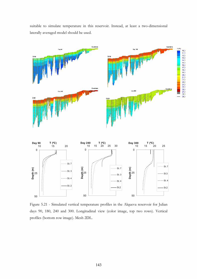
143

suitable to simulate temperature in this reservoir. Instead, at least a two-dimensional

laterally averaged model should be used.

Day 90

0

25

50

10 15 20T (ºC)

De

pth

(m

)

St. 7

St. 3

St. 4

St. 2

Day 240

0

25

50

10 15 20 25 30T (ºC)

De

pth

(m

)

St. 7

St. 3

St. 4

St.2

Day 300

0

25

50

10 15 20 25T (ºC)

De

pth

(m

) St. 7

St.3

St. 4

St.2

Figure 5.21 - Simulated vertical temperature profiles in the Alqueva reservoir for Julian

days 90, 180, 240 and 300. Longitudinal view (color image, top two rows). Vertical

profiles (bottom row image). Mesh 2DL.

144

5.4.3 Eutrophication dynamics

Figure 5.22 presents simulated spatial distributions of surface chlorophyll-a concentration

in the Alqueva for different seasons of the year. Those types of seasonal spatial patterns

are observed in both dry and rainy years, although the magnitude of chlorophyll-a

concentration can differ for different years. Figure 5.23 shows simulated dissolved

oxygen contour plots for a full year at different reservoir deep locations. Figure 5.24

shows simulated spatial distributions of surface nutrient concentration in the Alqueva

reservoir for different seasons of the year.

Winter conditions in the Alqueva, namely low solar radiation (see chapter 4.1.1.) and a

fully mixed water column (see chapter 5.4.2), are responsible for a light limitation

situation in the deep lower reservoir areas. As a result, phytoplankton growth in that

region is hindered as we can see in Figure 5.16. The shallower riverine upper part is not

affected by these light limitation issues and winter productivity there is ten to twenty fold

higher than in the lower reservoir region. Chlorophyll-a concentration in winter is less

than 5 g/L in the reservoir lower area and more than 100 g/L in the upper area (see

Figure 5.22). The higher winter availability of nutrients in the upper part of the reservoir

(see Figures 5.16 and 5.24) should also play a role in these spatial differences in

productivity.

During spring, the increase of light availability (see data on chapter 4.1.1), i.e., the longer

hours of light during the day, is responsible for triggering a seasonal peak of algae in

April (see Figure 5.16). Phosphate concentration at the lower reservoir region remains

relatively constant during winter and spring. Therefore, algae spring growth in this area is

most likely controlled by light and not by nutrients.

The summer period is characterized by an algae concentration decline in all reservoir

areas with particular emphasis in the upper half of the water body (see results in Figures

5.16 and 5.22). Summer phosphate concentration at surface also shows a decrease in the

upper reservoir area (see Figure 5.24), probably due to phytoplankton consumption

accompanied by minimal nutrients renewal since loads in summer are low. For the lower

reservoir area, nutrients remain relatively low all year with only slight changes from

season to season (see Figure 5.24). In fact, in situ measurements for phosphate at lower

reservoir stations areas present values so low that they quite possibly are bellow the

detection level of the analytical method used (see Figure 5.16). On average, nutrient

145

concentration is always lower in summer than in the other seasons, which was expected

since loads during wet seasons4 are higher.

During autumn, increases in the Guadiana flow that contain heavy loads plus vertical and

horizontal mixing will transport nutrients through the reservoir. This will trigger a peak

of phytoplankton which is stronger for locations close to the Guadiana river entrance

(see Figure 5.22).

A longitudinal look at the reservoir along a main central axis shows that chlorophyll-a

concentrations present a longitudinal gradient with maxima at the northern point, that is,

Guadiana entrance and minima in the southern area near the dam, during all year (see

Figure 5.22). The same type of spatial trend is observed for the nutrients, particularly in

spring and autumn (see Figure 5.24). Note that ammonia model results for spring do not

show that trend but experimental data does. In this case a large deviation between data

and model results exists (see table 5.2). The higher nutrient concentrations always occur

in upper reservoir locations and a north-south gradient is observed. Monitoring data for

different years (see chapter 4) also shows this pattern, therefore corroborating the

assumption made in the current work that the majority of nutrient loads enter the system

through the Guadiana river.

According to Morais et al. (2007) winter-spring dominant species in the Alqueva are a

mix of cryptophytes, bacillariophytes (diatoms) and chlorophytes (green algae) while in

summer and autumn cyanobacteria dominate. This constitutes a typical reservoir

planktonic succession in the Portuguese regions of Algarve and Alentejo (Galvão et al.,

2008). Some cyanobacteria can assimilate nitrogen in the form of N2 and many have high

temperature optima (Grover et al., 2006). Therefore, they tend to dominate planktonic

communities when there is low nutrient availability and high temperatures, as is usual

during summer in the Alqueva (see data in chapter 4). Diatoms have low nutrient

requirements and low temperature optima (Reynolds, 1986) that justify their dominance

in winter.

4 Wet season for the Alqueva can be considered to occur between September/October and May.

146

Figure 5.22 - Simulated spatial and temporal distributions of surface chlorophyll-a

concentration (g/L) for the Alqueva in 2006. Notice scale differs. Mesh M1.

147

After the maximum algae growth during the spring months, algae mortality increases and

dead algae sink to the bottom where bacteria will decompose them and consume DO in

the process. Consequently, DO in bottom layers decreases drastically reaching anoxic

levels in summer months, while maintaining near saturation levels at the surface all year

(see DO variations in Figure 5.16). In the Alqueva, there is a defined vertical DO and

thermal stratification starting in April and resuming by the end of the year (see Figures

5.21 and 5.23). Figure 5.23 clearly shows the onset and turnover time of oxygen

stratification in the Alqueva reservoir. During this period water density differences

reduce vertical mixing and turbulence in the water column. Note that since the reservoir

is very young release of PO4 from the sediments under anoxic conditions is not expected

and therefore this internal loading process was not included in the model. The absence of

significant phosphorus release from sediments is corroborated by the in situ

measurements. Thus, anoxic hypolimnion is here not synonymous with PO4 sediment

release as is usual in many reservoirs (Redshaw et al., 1990; Nowlin et al., 2005). An

increase of hypolimnion ammonium under anoxic conditions due to sediment release

also does not currently occur in the Alqueva.

In autumn, surface water temperature decreases (see data in chapter 4.3 and model

results in Figure 5.21) and triggers vertical mixing, which greatly increases the vertical

transport in the water column. Figure 5.23 shows that this results in an increase of DO

concentration in the lower water layers. The increase in DO levels in late autumn is

probably also due to oxygen production by the increasing algae.

Figure 5.23 - Contour plots of simulated dissolved oxygen concentration (mg/L) for the

Alqueva reservoir in 2006.

148

Many authors point out that after a new reservoir is filled with water; nutrient loading

and phytoplankton biomass usually increase (Ostrofsky et al., 1980; Thornton et al.,

1990; Kennedy at al., 1990; Peterson et al., 1997; Perrin et al., 2006). The rise is indicated

to be caused by nutrients that are leached and mineralized after being released from the

recently submerged soil and vegetation. This seems clearly not to be the case in the

young Alqueva (see Figures 4.22, 4.23 and 4.26). The same authors mention that this

increase in productivity is followed by a gradual decline when the waterbody ceases to be

“young” and eventually the reservoir will latter reach some kind of stable state. The term

“young” is used to designate a time period that ranges between 10-20 years depending on

the authors and reservoirs studied.

It is possible, but could not be inferred from the modelling results, that the production

of electricity in the Alqueva has an effect in lowering the trophic level in the region near

the dam. By letting large volumes of water flow downstream through the dam, nutrients

are exported out of the reservoir. Indeed, Guadiana monitoring stations located after the

reservoir5 indicate levels of phytoplankton and nutrients higher than those in the

reservoir near dam area but it is not possible to conclude that this is caused by nutrients

flushed from the reservoir since other non-quantifiable local loads play a role in feeding

the river in the area downstream from the dam.

Based on the simulated seasonal variations and supported by the analysis of ecological

data in chapter 4 it can be concluded that:

The upper reservoir area is much more productive than the lower area, which is

easily explained by the fact that the upper reservoir receives almost all nutrient

loads.

For the main body of the reservoir, a decreasing north-south longitudinal

gradient of nutrients and algae concentration can be observed.

Algae peak twice a year, in spring and autumn.

Spring algae growth in the lower reservoir region is probably controlled by light.

Thermal and oxygen stratification occur in the summer months.

5 SNIRH station Açude de Pedrogão (25L/O2H).

149

Figure 5.24 - Simulated spatial and temporal distributions of surface nutrient

concentration (mg/L) for the Alqueva reservoir in 2006. Mesh M1.

150

5.5 Models verification/validation

The calibration and validation procedures guarantee that the models are able to correctly

reproduce the behavior of the reservoir. In particular, the validation procedure is

performed to ensure that the models can successfully characterize the reservoir behavior

over a range of different environmental conditions. Therefore the experimental data used

in validation should present conditions that differ from those used in calibration. For

calibration, the year 2006, a particularly rainy year, was used. For validation purposes,

simulations for the year 2008, a dry year, were performed. The year 2008 also presented

lower Guadiana inflow than 2006. RMSE was used to statistically evaluate the models

performance.

Figures 5.25 to 5.28 present the comparisons between model results and measured data

for the validation year. The figures show that model results match experimental data.

The validation and calibration results prove that the models are able to predict flow,

water temperatures and eutrophication dynamics in the Alqueva when environmental

and/or operational conditions change.

5.5.1 Hydrodynamic validation

Model validation for the hydrodynamic model was performed in a similar way as the

calibration procedure. Figure 5.25 presents the simulated vs. measured volume for the

reservoir for the year 2008. The normalized RMSE for the volume was 6.82%.

3.0E+09

3.2E+09

3.4E+09

0 100 200 300 400Julian day

Vo

lum

e (

m3 )

measured

simulated

Figure 5.25 - Simulated and measured reservoir total volume (m3) for 2008. Mesh M1.

(Data source: EDIA).

151

5.5.2 Thermal validation

Figures 5.26 and 5.27 present simulated vs. measured time series of water temperature

for different depths and locations of the Alqueva for year 2008. The absence of

comprehensive SNIRH 2008 data for surface water temperature at station 7 implied the

use of EDIA monthly data for model validation in that station.

Figure 5.26 has 3D model results and Figure 5.27 has model results for 2DL simulation.

These results were used to do a thermal model verification using RMSE to quantify the

goodness-of-fit. Calculated RMSE values are presented in table 5.3. Thermal stratification

in the reservoir is clearly reproduced and the simulation results reproduce well the trends

in data. RMSE values imply that the 2DL simulation has better water temperature results

than the 3D simulation for the bottom layers, although in this case the differences are

small. The higher accuracy of the 2DL simulation compared to the 3D is due to the

higher mesh vertical definition as mentioned before. Nevertheless, temperature results

for both 2DL and 3D were within the pre-established deviation interval of +/-3ºC.

Figure 5.26 - Simulated (black) and measured (grey line and data points) water

temperatures in the Alqueva. Time series at the pointed locations (Sts 2, 4 and 7) for the

year 2008. Mesh M1. Note that the data source for measurements at station 7 surface

waters is EDIA and the periodicity of that data is monthly.

152

Figure 5.27 - Simulated (black) and measured (grey line and data points) water

temperatures in the Alqueva. Time series at the pointed locations (Sts 2, 4 and 7) for the

year 2008. Mesh 2DL. Note that the data source for measurements at station 7 surface

waters is EDIA and the periodicity of that data is monthly.

Table 5.3 - Root mean square deviations between measured and simulated water

temperatures in model verification.

Location and layer M1 RMSE 2DL RMSEStation 2 2.1 2.2 Station 4 surface 1.99 2.02 Station 7 surface* 2.0 1.55 Station 7 bottom 1.78 1.78 Station 4 bottom 2.3 1.67 Average deviation 1.96 1.83

* calculated with monthly EDIA data.

153

5.5.3 Eutrophication validation

The verification process for the eutrophication model was similar to the calibration

procedure. Figure 5.28 presents the validation results and table 5.4 summarizes the error

statistics in terms of average RMSE and RE (%) for the different state variables. No data

outliers were excluded in the calculation of deviations presented in table 5.4.

Validation results show that the model simulates reasonably well the dynamics of the

state variables over time and space (see Figure 5.28). Most seasonal variations are

adequately replicated by the eutrophication model.

The fit between model and data was best for DO (see table 5.4), with the model

mimicking well the DO concentrations over time. Model trends related to the onset of

bottom anoxia were similar to the ones in measured data. The poorest predicted variable

was ammonia (see table 5.4).

For chlorophyll-a, model results were only moderately in agreement with monitoring data

(see Figure 5.28). Chlorophyll-a temporal trends were reasonably accurate but the

simulated values had bloom magnitudes that disagreed with the measurements.

As mentioned previously (see chapter 5.3.3), the upper area of the reservoir is much

more productive and has much higher nutrient levels than the lower part, which gives

rise to a large spatial heterogeneity. This heterogeneity implies a higher difficulty to

obtain good eutrophication modelling results for this reservoir.

As pointed out in the calibration section (chapter 5.3.3), monitoring data were collected

at monthly intervals and only a single measurement was made at each station. This is

insufficient to discard any possible errors associated with the data. The low frequency of

sampling and the absence of methodologies to assess accuracy and precision of

measurements translates into deficient data. This, together with the crude loads

estimation can be responsible for large deviations between model results and in situ

collected data.

Concerning chlorophyll-a results, it is possible that the simulation results could be

improved if more than one group of algae was included in the model. Different

planktonic communities are dominant over time/season in the Alqueva (Morais et al.,

2007). These different algae groups possess distinct behavior regarding light and nutrient

needs, responses to hydrodynamic effects and, in general, different biological interactions

(Scavia et al., 1987; Chen et al., 2002). When this diversity is lumped together in a single

model algae group, part of the results resolution will be lost. The non-availability of

154

quantitative data for the different planktonic communities in the Alqueva, made it

impossible to use more than a single algae group in the model since parameterization for

different algae groups could not be made.

Table 5.4 - Error statistics in eutrophication model validation. Deviations were averaged

for all monitored stations and water depths.

Chl-a (g/L)

DO (mg/L)

PO4 (mg/L)

NO3 (mg/L)

NH3 (mg/L)

RE 47% 30% 60% 38% 74% RMSE 22.9 1.8 0.13 0.83 0.18

155

Station 1 Surface

0

5

10

15

20

D M J S D M

Month

DO

(m

g/L

)

Station 4 Surface

0

5

10

15

D M J S D MMonth

DO

(m

g/L

)

Station 7 Surface

0

5

10

15

D M J S D MMonth

DO

(m

g/L

)

Station 4 Bottom

0

5

10

15

D M J S D MMonth

DO

(m

g/L

)

Station 7 Bottom

0

5

10

15

D M J S D MMonth

DO

(m

g/L

)

Station 1 surface

0

250

500

D M J S D MMonth

Ch

l-a

( g

/L)

Station 4 Surface

0

10

20

30

D M J S D MMonth

Ch

l-a (

g/L

)

Station 7 surface

0

10

20

30

D M J S D MMonth

Ch

l-a (

g/L

)

Station 1 Surface

0.0

0.5

1.0

1.5

D M J S D M

Month

PO

4 (m

g/L

)

Station 4 Surface

0.00

0.25

0.50

D M J S D M

Month

PO

4 (m

g/L

)

Station 7 Surface

0.00

0.25

0.50

0.75

1.00

D M J S D M

Month

PO

4 (m

g/L

)

Station 1 Surface

0.0

0.5

1.0

1.5

D M J S D MMonth

NH

3 (m

g/L

)

Station 4 Surface

0.0

0.5

1.0

1.5

D M J S D M

Month

NH

3 (m

g/L

)

Station 7 Surface

0.0

0.5

1.0

1.5

D M J S D M

Month

NH

3 (m

g/L

)

Station 1 Surface

0

10

20

30

40

50

D M J S D M

Month

NO

3 (m

g/L

)

Station 4 Surface

0.0

2.5

5.0

D M J S D M

Month

NO

3 (m

g/L

)

Station 7 Surface

0

5

10

15

20

D M J S D M

Month

NO

3 (m

g/L

)

Figure 5.28 - Simulated (line) and measured (points) water quality constituents

concentration in the Alqueva. Time series for nitrate, ammonia, phosphate, dissolved

oxygen and chlorophyll-a at several reservoir locations. Mesh M1.

156

5.6 Uncertainty analysis

The models were used to study ecosystem changes induced by changes in natural

conditions. The scenarios investigated involved inflow variations and wind variations.

These scenarios can also be viewed as a model uncertainty study6, in this case, for

uncertainties contained in the input and output data (uncertainty intrinsically embedded

in the model was not addressed). Preliminary tests were used to determine which natural

conditions of interest would have bigger impacts on the ecology of the Alqueva when

perturbed. Subsequently, the chosen natural conditions were used to design scenarios for

simulations. In the scenarios all conditions, inputs and parameters were maintained

constant except for the variable to be studied. The model run used as base for

comparisons was the 2006 run.

6 “Uncertainty analysis” and “sensitivity analysis” are not to be confused. Sensitivity analysis is used to obtain

information regarding the most sensitive model parameters, that is, the ones where small changes in the

parameter value will most impact the model results. Uncertainty analysis refers to model previsions as a range

of expected values and is used to account for uncertainties contained in parameters, input and output data.

Figure 5.29 summarizes the use of the two in water surface models.

Figure 5.29 - Schematic procedures for analysis of sensitivity and analysis of uncertainty in surface water

numerical models.

157

Of major interest would be to investigate variations in anthropogenic stress in the

Alqueva. However, because crude assumptions were already made to estimate loads (see

chapter 4) and the evolution of loads over time in the Alqueva is not known it is

challenging to design scenarios that are realistic. It is not known if the loads in the

reservoir have been increasing or decreasing over the years and the evolution of loads

composition over time is also unknown, that is, relative contribution from different

sources over time is unknown. Relationships between loads and other variables (e.g.

hydrology, precipitation, phytoplankton concentration) could not be inferred to help

characterize loads evolution. Thus, any guidance for nutrient loads reduction or

eutrophication management strategies devised using model results obtained in this way

would be highly hypothetical and the results would contain great uncertainty. Although

model sensitivity tests showed that the eutrophication model is sensitive to changes in

nutrient load conditions, which seem to be responsible for a large part of the algae

variability in the reservoir, no load scenarios were simulated for the reasons presented

above. Furthermore, testing for this type of scenario usually requires model runs of at

least a decade to allow definitive conclusions to be reached (Cole et al., 1999).

5.6.1 Guadiana inflow scenarios

Guadiana inflow variation scenarios were used to investigate:

The extension of the Guadiana hydraulic influence.

Ecological impact of inflow changes.

The potential significance of density currents arising from cold inflows.

The effects of changes to other smaller tributaries inflows were not studied since no up-

to-date flow data exist for them. Nevertheless, the estimation of their flow made in

chapter 4.2 indicates that their relative contributions are very small (Guadiana itself

contributes with an estimated 80% of the total reservoir inflow). Morais et al. (2007)

present qualitative data that imply that the Alcarrache branch contributes with water that

is less mineralized than the main reservoir water and that the Degebe branch contributes

with water with higher BOD than the main waterbody water.

Understanding the effects that variations in the Guadiana inflow can have on the

reservoir is rather important. The river is the main source of nutrients to the reservoir.

Particularly, it is the main source of phosphorus, the reservoir limiting nutrient. Inflow

158

from the river is also responsible for generating hydrodynamically driven currents in the

reservoir upstream area.

The temperature of the surface water layer of the reservoir closely follows air

temperature conditions (see Table 4.8). Variations in air temperature are therefore quickly

reflected in the reservoir surface water temperature. During the dry season the river

Guadiana inflow is small and has water temperatures similar to the air temperature, but

during the wet season the inflow is usually colder than the reservoir waters and the air

temperature. Therefore, during the wet season river water and reservoir water have

different temperatures and densities when they mix. Water temperature variations are

likely to affect oxygen water solubility and kinetic biogeochemical rates in a reservoir and

consequently affect biological behavior (Kim et al., 2006).

A simulation was done using Guadiana daily inflow values that were increased and

decreased fivefold from the 2006 flows. Although 2006 was a rainy year, in terms of

Guadiana inflow it can be considered an average year. Fivefold was chosen based on

variations observed in the hydrological regime (see chapter 4.2). Fivefold increases and

decreases can be considered as very extreme scenarios. Water inflow temperatures were

set to be the same as those in the 2006 daily dataset. Results were then compared with

the 2006 normal flow by calculating the temperature difference T defined as

flowchangedflownormal TTT Eq. 5.2

Where T is the simulated water temperature (ºC). Figures 5.30 ( flow increase) and 5.31

(flow decrease) present T results for some noteworthy time steps.

159

Figure 5.30 - Simulated temperature differences in the Alqueva reservoir for dry season

(top image, Julian day 222) and wet season (bottom three images). Plot represents water

temperature difference between normal inflow and fivefold the inflow situation for

Guadiana river. Mesh 2DL.

160

Figure 5.31 - Simulated temperature differences in the Alqueva reservoir for dry season

(top image, Julian day 222) and wet season (bottom three images). Plot represents water

temperature difference between normal inflow and a fivefold inflow decrease situation

for Guadiana river. Mesh 2DL.

161

Results suggest that no major alterations in water thermal profiles will occur during the

dry season (see Figures 5.30 and 5.31 top image). A stable stratification is still observed

during the same period and similar characteristics for the metalimnion are found. In

contrast, for the wet season flow variations will affect the upper part of the reservoir (see

Figures 5.30 and 5.31) and the higher the flow rate, the longer the reach of the reservoir

that is affected. In the wet season the colder water from the river will sink to the

reservoir lower layers since it is denser. This underflow effect can clearly be seen in the

results for days 321 and 326 in Figure 5.30 (red and orange colors). The introduction of

water with a different temperature into the reservoir also leads to the development of

longitudinal temperature gradients that travel downstream with the flow (see Figures 5.30

and 5.31, three bottom images). When the inflow increases the extent of the reservoir

that is affected by the cold stream increases as well. With a fivefold increase in the flow

the influence area of the colder stream will ultimately extend downstream of station 4

(see Figure 5.30 for Julian day 326) in the bidimensional simulation performed. The water

temperature in the affected area is up to 4.0 ºC lower due to the increase in flow.

Thus, inflow rate variations will have an impact in water temperature, nutrients and

constituents distributions and concentrations in the reservoir during the wet season,

although this influence does not seem to extend beyond station 4 even for a worst case

scenario of intense flow. Fluctuations in temperature and flow rate of the inflow may

therefore shift in time and location the appearance and disappearance of algae

populations.

Although it is clear that changes in Guadiana inflow will have an impact in water

temperature and the spatial transport of chemical species and algae, no relationship

between river inflow variations and constituents concentration exists (see chapter 4.3). In

chapter 4.3 no correlations were found between river flow and nutrients concentration

(TP, TN, PO4, NO3 and NH3) nor between river flow and chlorophyll-a concentration.

This means that a low river inflow is not synonymous of low amount of nutrients and

vice-versa. Nutrients concentration can be high when river inflow is low or the opposite

may occur. The dominant component of load in the Alqueva is therefore the nutrients

concentration and not the river flow. It should be noted that this may just result from the

fact that the river flow is controlled and not a natural regimen.

162

5.6.2 Wind scenarios

Wind variation scenarios were used to investigate the effect of wind induced mixing vs.

hydraulic induced mixing and their spatial influence in the Alqueva reservoir. Simulations

in the absence and the presence of wind were performed and the results compared. Wind

forced simulations used hourly wind datasets for stations 2, 4 and 7 locations with each

wind dataset assigned to a domain region.

Alqueva thermal structure measurements and model results (see chapter 4 and 5.4.2)

indicate that wind is not strong enough to disrupt the summer stratification in this

reservoir. Nevertheless wind induced shear is an important mechanism that explains

velocities and mixing at the water surface layer of the reservoir.

Surface layer turbulence induced by local wind is responsible for surface horizontal and

vertical distribution of planktonic communities in reservoirs (Reynolds, 1987; George et

al., 1976) and is pointed out as determinant for phytoplankton and zooplankton

transport and accumulation in reservoirs were wind induced water movement dominates

over hydrodynamic currents (MacKenzie et al., 1993). While Margalef (1978) findings

suggest that turbulence plays a role in determining phytoplankton cell size in different

hydrodynamic environments, MacKenzie et al. (1993) indicate that wind induced

turbulence in lakes affects food web structures and rates of production for higher trophic

levels. These findings imply that wind has an impact in plankton ecology.

Figure 5.32 presents results for simulated surface velocities in the Alqueva in the

presence and absence of wind. Table 5.5 presents further information regarding wind and

Guadiana inflow strengths for the situations in Figure 5.32.

Table 5.5 - Registered daily averaged wind velocities (m/s) and Guadiana qualitative

inflow information at different Alqueva stations for days 28, 300 and 328 in 2006.

day St 2 St 3 St 4 St 7 Guadiana 28 3.2 3 7.7 9.3 Low inflow

300 2.2 - 3.5 3.8 High inflow

328 5.8 6 8.8 7.8 High inflow

163

Figure 5.32 - Simulated surface velocities in the Alqueva for Julian days 28 at 00:00h, 300

at 0:00h and 328 at 00:00h in the presence (top images) and absence (bottom images) of

wind. Mesh M1.

As seen in chapter 5.4 wind affects surface velocities in the reservoir and is the dominant

factor for driving the surface currents in the lower reservoir area.

In Figure 5.32, day 28 is a situation of year wind maxima at the lower reservoir stations

while day 328 is a situation of year wind maxima at the upper reservoir stations. Day 300

is a situation of wind minima for the whole reservoir. By comparing results from the

simulation with and without wind forcing (Figure 5.32 top and bottom rows) it can be

concluded that the surface velocities are affected by the wind stress. Even for weak wind

164

situations (day 300), the surface circulation is influenced by wind action. Wind speed

affects mostly the lower reservoir area which is also where higher wind stresses are

registered. Results for a situation with high Guadiana inflow and the highest registered

winds of the year at station 2 (day 328) indicate that some wind action can be seen in the

deep pools of the riverine area upstream but the hydraulic flow of the river dominate the

circulation in the riverine area.

A general conclusion is that wind action dominates the surface circulation in the lower

area of the reservoir and river hydraulic flow dominates the surface circulation in the

upper part of the reservoir. Upper reservoir planktonic communities and nutrients are

therefore probably distributed and transported along a longitudinal axis that follows the

river path while lower reservoir plankton is most likely spread horizontally.

References for Chapter 5

Arcement GJ, Schneider VR. 1989. Guide for selecting manning's roughness coefficients for natural channels and flood plains. USGS Water Supply Paper 2339. USA.

Aquaveo. 2002. SMS Surface-water modeling system reference manual, Version 7.0. Environmental Modeling Research Laboratory. Brigham Young University. USA.

Beeton AM. 1958. Relationship between Secchi disk readings and light penetration in Lake Huron. Trans. Am. Fish. Soc. 87: 73–79.

Bleck R, Rooth C, Hu D, Smith LT. 1992. Salinity-driven thermocline transients in a wind- and thermohaline-forced isopycnic coordinate model of the north Atlantic. J. Phys. Oceanogr. 22:1486-1505.

Bleck R, Boudra D. 1981. Initial testing of a numerical ocean circulation model using a hybrid (quasi-isopycnic) vertical coordinate. J. Phys. Oceanogr. 11:755-770.

Blumberg AG, Mellor L. 1987. A description of a three-dimensional coastal ocean circulation model. In three-dimensional coastal ocean models. N. Heaps (editor). American Geophysical Union, Washington, USA. 1-16.

Bonnet MP, Poulin M, Devaux J. 2000. Numerical modeling of thermal stratification in a lake reservoir. Methodology and case study. Aquat. Sci. 62: 105–124.

Chen C, Ji R, Schwab DJ, Beletsky D, Fahnenstiel GL, Jiang M, Johengen TH, Vanderploeg H, Eadie B, Budd JW, Bundy MH, Gardner W, Cotner J, Lavrentyev PJ. 2002. A model study of the coupled biological and physical dynamics in Lake Michigan. Ecol. Model. 152:145–168.

Cole TM, Tillman DH. 1999. Water quality modeling of Lake Monroe using CE-QUAL-W2. Report EL-99-1. USACE WES, USA.

Cox MD. 1984. A primitive equation, 3-dimensional model of the ocean. Technical report nr 1. Ocean group, geophysical fluid dynamics laboratory, Princeton, USA.

Galvão HM, Reis MP, Valério E, Domingues RB, Costa C, Lourenço D, Condinho S, Miguel R, Barbosa A, Gago C, Faria N, Paulino S, Pereira P. 2008. Cyanobacteria blooms in natural waters in Southern Portugal - a water management perspective. Aquat Microb. Ecol 53: 129-140, 2008.

George DG, Edwards RW. 1976. The effect of wind on the distribution of chlorophyll a and crustacean plankton in a shallow eutrophic reservoir. J. Appl. Ecol. 13: 667-690.

Grover JP, Chrzanowski TH. 2006. Seasonal dynamics of phytoplankton in two warm temperate reservoirs: association of taxonomic composition with temperature. J. Plankton Res. 28:1-17.

Kennedy RH, Walker WW. 1990. Reservoir nutrient dynamics. In: Reservoir limnology: ecological perspectives. (Thornton KW, Kimmel BL, Payne FE, Editors). John Wiley and Sons, NY.

Kim, Y, Kim B. 2006. Application of a 2-dimensional water quality model (CE-QUAL-W2) to the turbidity interflow in a deep reservoir (Lake Soyang, Korea). Lake Reserv. Manag. 22:213-222.

165

King IP. 1985. Strategies of finite element modeling of three dimensional hydrodynamic systems. Adv. Water Resour. 8:69–76.

King IP. 1990. Modeling of flow in estuaries using combination of one and two dimensional finite elements. Hydrosoft. 3:108-119.

MacKenzie BR, Leygett WC. 1993. Wind- based models of turbulent energy dissipation. Mar. Ecol. Prog. Ser. 94:207-216.

Margalef R. 1978. Life-forms of phytoplankton as survival alternatives in an unstable environment. Oceanol. Acta 1: 493-509.

Mellor GL, Hakkinen S, Ezer T, Patchen R. 2000. A generalization of a sigma coordinate ocean model and an intercomparison of model vertical grids. In: Ocean forecasting: theory and practice. N. Pinardi (editor). Springer-Verlag.

Morais M, Serafim AM, Pinto P, Ilhéu A, Ruivo, M. 2007. Monitoring the water quality in Alqueva reservoir, Guadiana river, southern Portugal. In: Gunkel G, Sobral M, editors. Reservoir and river basin management: exchange of experiences from Brazil, Portugal and Germany. 96-112.

NOOA. 2007. Document retrieved on 2007. Online at: http://www.srh.noaa.gov/images/epz/wxcalc/rhTdFromWetBulb.pdf

Nowlin WH, Evarts JL, Vanni MJ. 2005. Release rates and potential fates of nitrogen and phosphorus from sediments in a eutrophic reservoir. Freshwat. Biol. 50:301–322

Oberhuber JM. 1993. Simulation of the Atlantic circulation with a coupled sea ice-mixer layer-isopycnal general circulation model. Part II: model experiment. J. Phys. Oceanogr. 23:830-845.

Ostrofsky ML, Duthie HC. 1980. Trophic upsurge and the relationship between phytoplankton biomass and productivity in Smallwood Reservoir, Canada. Can. J. Bot. 58:1174-1180.

Paterson MJ, Findlay D, Beaty K, Findlay W, Schindler EU, Stainton M, McCulloughG. 1997. Changes in the planktonic food web of a new experimental reservoir. Can. J. Fish. Aquat. Sci. 54:1088-1102.

Perrin CJ, Harris S. 2006. Trophic state of Elsie lake reservoir. Report by Limnotek research and development Inc. Vancouver, Canada.

Poole HH, Atkins WR. 1929. Photo-electric measurements of submarine illumination throughout the year. J. Mar. Biol. Assoc. UK. 16: 297-324.

Redshaw CJ, Mason CR, Hayes CR, Roberts RD. 1990. Factors influencing phosphate exchange across the sediment-water interface in eutrophic reservoirs. Hydrobiol. 192:233–245.

Resource modelling associates. 2008. RMAGEN: A program for generation of finite element networks –user instructions. Resource modeling associates, Sydney, Australia.

Reynolds CS. 1986. The ecology of freshwater phytoplankton. Cambridge Univ. Press. Reynolds CS, Oliver RL, Walsby AE. 1987. Cyanobacterial dominance: The role of buoyancy regulation in

dynamic lake environments. N.Z. J. Mar. Freshwater Res. 21: 379-390. Romero JR, Antenucci JP, Imberger J. 2004. One- and three-dimensional biogeochemical simulations of

two differing reservoirs. Ecol. Model. 174:143-160. Rueda FJV. 2001. A three-dimensional hydrodynamic and transport model for lake environments. PhD

dissertation in civil and environmental enginnering, university of California, Davis, USA. Scavia D, Fahnenstiel G L. 1987. Dynamics of Lake Michigan phytoplankton: mechanisms controlling

epilimnetic communities. J. Great Lakes Res.13:103–120. Smagorinsky J. 1963. General circulation experiment with the primitive equations. Monthly Weather Rev.

91: 99-164. Sprung A. 1888. Uber die Bestimmung der Luftfeuchtigkeit mit Hilfe des Assmannschen

Aspirationspsychrometers. Z.Angew. Merteorol. Das Weter. 5:105-108. Sverdrup HV, Munk WH. 1947. Wind, sea and swell: Theory of relations for forecasting. Publication No.

601. US Navy Hydrogr. Office, USA. Thomann RV. 1973. Effects of longitudinal dispersion on dynamic water quality response of streams and

rivers. Water Resour. Res. 9:355-366. Thornton KW, Kimmel BL, Payne FE. 1990. Reservoir limnology: ecological perspectives. John Wiley and

Sons, NY. Young DLF. 2002. In: Environmental fluid mechanics: Theories and applications. (Shen HH, Cheng

AHD, Wang K, Teng MH, Lui CCk editors), ASCE editions.

166

CHAPTER 6 – CONCLUSIONS AND FUTURE WORK

Although the Guadiana estuary has been intensively studied by several researchers

(Chícharo et al., 2006a, 2006b; Barbosa et al., 2010; Wolanski et al., 2006) the upper part

of the river Guadiana in Portuguese territory is seldom the subject of scientific studies.

Despite being the largest western European reservoir, there is an enormous scarcity of

scientific results regarding the Alqueva reservoir.

Palma et al. (2009); Palma et al. (2010) and Perez et al. (2009) study the Alqueva water

quality from a point of view of ecotoxicology. Their work concerns mostly

contamination with pesticides and heavy metals whose assessment is done using different

analytical techniques.

Serafim et al. (2006) and Morais et al. (2007) present results from water quality

monitoring campaigns in the Alqueva for the period 2003-2006. These authors approach

is based on water quality legal standards abiding. They analyze trophic state indicators

and characterize the ecological evolution of the ecosystem over time using their

measurements.

The work of Rodriguez et al. (2006) focuses on water quality indicators in the Guadiana

and transboundary watersheds of the Guadiana basin during 2005-2006.

For the Alqueva reservoir, except for Lindim et al. (2009); Lindim et al. (2010) and

Lindim et al. (2010a), there is only a single published scientific study that includes

modelling: Diogo et al. (2008) used CE-QUAL-W2 model to investigate phosphorus

management scenarios in the reservoir in order to help develop nutrient control

strategies. The authors concluded that even a 100% reduction of loads with origin in

Portuguese territory would not be enough for the Alqueva to present water quality

satisfactory levels according to Portuguese law.

Overall, less than 10 scientific papers can be found concerning the Alqueva reservoir

since the reservoir was filled in 2003. Some of them were not published in peer reviewed

journals. The current work is therefore a major contribution to the study of the Alqueva

reservoir. The results contained herein can be used to assist management decisions in this

waterbody and the modelling effort can be used to obtain forecasts in this and other

reservoirs and improve understanding of ecological behavior there.

The current work presents also an important contribution to the field of numerical

modelling of eutrophication by introducing an innovative reasoning for model

calibration. Most well established eutrophication models, like CE-QUAL-W2 (Cole and

167

Buchak, 1995) or WASP (Wool et al., 2003), use a trial and error calibration process

(Schladow et al., 1997). As noted by Arhonditsis et al. (2007) this is highly inefficient and

not reliable. The current work eliminates that problem by using a deterministic

eutrophication model with a stochastic autocalibration. Although this mixed approach

has been pointed out before as ideal for water models (Gupta et al., 1998) it is seldom

implemented. Arhonditsis et al. (2007) and more recently Missaghi et al. (2010) are

among the very few examples found in literature of deterministic models that use a

stochastic method for automating calibration.

Among the major findings of the present work are:

It was found that the Alqueva reservoir behavior presents high interannual

variability. Data analysis in chapter 4 points this as a current major characteristic

of the reservoir. This is mainly a consequence of the high variability of

precipitation, loads and Guadiana hydrological regimen. Data were statistically

examined for homogeneity across information sources, homogeneity across

locations, dispersion and stability and trends across time. It is possible that after

long term data series are gathered, some interannual trends start to emerge but

with the currently available data no particular interannual trend is observable.

According to the national trophic state classification (see chapter 2, Table 2.1) the

Alqueva reservoir trophic status ranges from mesotrophic to eutrophic. The

evaluated parameter responsible for this classification is always the average

annual TP. Any management scheme aimed at improving the trophic level in the

Alqueva should therefore focus on phosphorus.

It was found that the system is P-limited (see chapter 4) and that nutrients input

and eutrophication conditions are mostly dependent on the main tributary (river

Guadiana) input loads. Therefore management schemes should focus on

reducing phosphorus in the main tributary inflow.

It was proved that the models developed and used were able to replicate very well

thermal dynamics in the Alqueva reservoir and reasonably well eutrophication

dynamics. Simulation results showed that the models were robust enough to

capture the Alqueva ecosystem spatial and temporal variations. Eutrophication

modeling results sometimes failed to capture the high heterogeneity of this large

and morphologically complex reservoir. This can be explained by the high

variability over space and time in the domain, by the crude estimation of loads

168

due to scarcity of data, by monitoring data quality/quantity issues and the

resulting error propagation. In particular, given the limited data existent in some

cases, the eutrophication model results obtained can be considered quite

acceptable1.

It was also the inexistence of current meter measurements in the Alqueva that

blocked the possibility of confirmation for the results obtained with the

hydrodynamic model. On the other end, the availability of comprehensive

meteorological and water temperature datasets was decisive for the success of the

thermal structure simulations, with the model capturing even short-term

variations very well. This asserts what was said in chapters 3 and 4 regarding the

necessity of high quality and exhaustive datasets in order to obtain superior

reliable results with models.

It was shown that the particular geomorphological and hydrological

characteristics of the reservoir together with local climate features are responsible

for the existence of distinct ecological regions within the reservoir:

- The upper part of the reservoir is a shallow channel like region with

riverine characteristics that is interrupted by a few scattered deeper pools.

This area receives the major nutrients input and is eutrophic.

Hydrodynamic in this area is governed by hydraulically induced currents

from the Guadiana (see chapter 5.4.1).

- The lower part of the reservoir is a deep lacustrine area that presents

stable thermal and DO stratification in summer (April – October). In this

region wind induced currents and thermal stratification are the dominant

hydrodynamic traits. Wind is dominant over hydraulic flow during all year

and affects mostly the surface circulation (see chapter 5.4.1).

The boundary between these two areas can be placed south of monitoring station

3.

In fact, this upper reservoir area should better not be considered as part of a reservoir

given its distinct morphology and riverine characteristics and instead should be classified

as river.

1 Although there are no fixed standards to quantify model performance, reported state variables relative

errors higher than 30% have been presented as quite satisfactory by several different authors (Cerco et al.,

2004; Arhonditsis et al., 2005; Tetratech, 1999; Kwun et al., 2007) for water quality models.

169

The model results show that the Guadiana river inflow dynamics has an impact in

the ecology of the reservoir. Inflow rate variations affect water temperatures and

induce density currents. Consequently, the distributions of dissolved oxygen and

nutrients in the Alqueva are also affected. Thus, Guadiana inflow changes can

shift in time and location algae populations and to some extend control

phytoplankton dynamics by controlling transport. For an extreme flow case

tested with the 2D model the river hydraulic influence could still be felt near

station 4.

Dry season ecology is ruled by thermal stratification. During that period vertical

mass and heat exchanges are hampered in the water column and the hypolimnion

becomes anoxic. Dry season winds in lower reservoir area are not strong enough

to mix significantly the stratified water column but play a role in surface

circulation. Wet season ecology governing feature is the nutrients load through

the main tributary. Guadiana flow is responsible for transporting the nutrients

downstream leading to the appearance of a decreasing north-south gradient of

nutrients and algae concentrations.

The results presented in the current work reveal fragilities in the way monitoring is

performed in the Alqueva reservoir: There are entities with overlapping responsibilities,

inaccuracy of measurements and little international cooperation with the Spanish

authorities/researchers. The current monitoring network does not account for spatial

and temporal representativity of data. It seems to have been designed to assess hydrology

and water quality of inflows and outflows to the reservoir, while neglecting the reservoir

main water mass in itself.

The Alqueva reservoir was build to boost economic development in the region and

provide irrigation water for agriculture activities. As we can infer from the results of the

present work, one of the major problems it may face is the impacts of the poor water

quality coming from the Guadiana inflow. The Guadiana carries treated urban

wastewater from a large Spanish population and a mix of treated and untreated water

from industries and agriculture activities with a high level of nutrients. The development

of effective water quality management in this reservoir should therefore focus on

nutrient containment strategies for the Guadiana river inflow. The findings of Diogo et

al. (2008) seem to corroborate this. The authors studied nutrient control strategies in the

Alqueva by simulating different P load scenarios that included inflow contributions from

170

Guadiana, Alcarrache and Degebe branches. They concluded that reducing nutrient loads

with strict origin in the Portuguese territory would not improve water quality in the

Alqueva. EPA eutrophication control recommendations suggests 0.05 mg P/L as a

threshold value for a stream at the point it enters a lake or reservoir and 0.1 mg P/L as

the limit in streams not discharging directly into the lake or reservoir (Mueller et al.,

1999). These values could be used as general guidelines for the Alqueva case.

The changes in water flow and sediment volume felt downstream from the dam are also

possible problems (Chícharo et al., 2006a, 2006b) that will need mitigation actions. If

there is retention of sediments by the dam then a consequent loss of sediments

downstream may be responsible in the future for accelerating coastal erosion in the

estuary of the Guadiana River. This could be even further rushed up if due to the dam

construction a lower freshwater flow reaches the coastal area.

Serafim et al. (2006) points out that the changes in river flow downstream of the dam

seem to be responsible for plankton communities changes. According to the authors,

before the Alqueva dam was built, phytoplankton had a diatom biomass peak in spring

and a summer cyanobacteria bloom. After the dam was built, cyanobacteria started to

dominate the phytoplankton community in summer and also in autumn and winter.

Given that many species of cyanobacteria can produce toxins that are able to affect

animal and human health this situation should be monitored and controlled.

Further efforts and future improvements for the current work may include:

Implementation of sediment processes and the expansion of the number of algae

groups in the eutrophication model, provided that the application sites have

biogeochemical data and algae speciation information available.

Further tests and simulations involving mixed meshes. Mixed meshes are

computational cost efficient and highly adequate to simulate a reservoir like the

Alqueva whose stagnant lateral arms can be treated as one-dimensional.

Changes in the eutrophication model automated calibration implementation in

order to produce broader parameter sensitivity analysis with the possibility of

presenting results in the form of probability distributions or confidence intervals,

provided adequate computational capacity is available.

171

References for Chapter 6

Arhonditsis GB, Brett MT. 2005. Eutrophication model for Lake Washington (USA). Part II. Model calibration and system dynamics analysis. Ecol. Model. 187:179–200.

Arhonditsis GB, Qian SS, Stow CA, Lamon CE, Reckhow KH. 2007. Eutrophication risk assessment using Bayesian calibration of process-based models: application to a mesotrophic lake. Ecol. Model. 28:215–229.

Barbosa A, Domingues R, Galvão H. 2010. Environmental forcing of phytoplankton in a Mediterranean estuary (Guadiana estuary, south-western Iberia): A decadal study of anthropogenic and climatic influences. Estuar. Coast. 33:324-341.

Cerco CF, Noel MR, Kim SC. 2004. Three-dimensional eutrophication model of lake Washington, Washington State. Report ERDC/EL TR-04-12. USACE, Vicksburg, USA.

Chícharo MA, Chícharo L, Morais P, 2006a. Inter-annual differences of ichthyofauna structure of the Guadiana estuary and adjacent coastal area (SE Portugal/SW Spain): before and after Alqueva dam construction. Estuar. Coast. Shelf Sci. 70:39– 51.

Chícharo L, Chícharo MA, Ben-Hamadou R. 2006b. Use of a hydrotechnical infrastructure (Alqueva dam) to regulate planktonic assemblages in the Guadiana estuary: basis for the sustainable water and ecosystem services management. Estuar. Coast. Shelf Sci. 70:3-18.

Cole TM, Buchak EM. 1995. CE-QUAL-W2: A two-dimensional, laterally averaged hydrodynamic and water quality model, version 2.0, user Manual. Instruction report EL-95-1. USACE-WES, Vicksburg, USA.

Diogo PA, Fonseca M, Coelho PS, Mateus NS, Almeida MC, Rodrigues AC. 2008. Reservoir phosphorous sources evaluation and water quality modeling in a transboundary watershed. Desalination. 226:200-214.

Gupta HV, Sorooshian S, Yapo PO. 1998. Towards improved calibration of hydrologic models: multiple and incommensurable measures of information. Water Resour. Res. 34:751–763.

Kwun S, Park B, Kim S. 2007. Pollution control via a dredged pool at the inlet of a reservoir. Paddy Water Environ. 5:49–56.

Lindim C, Pinho JLS, Vieira JMP. 2009. Water quality modeling and loads estimation in a large reservoir. In: Proceedings of International symposium on environmental software systems, Venice, Italy.

Lindim C, Pinho JLS, Vieira JMP. 2010. Analysis of spatial and temporal patterns in a large reservoir using water quality and hydrodynamic modeling. Ecol. Model. (In press). doi:10.1016/j.ecolmodel.2010.07.019

Lindim C, Hayter EJ, Pinho JLS, Vieira JMP. 2010a. Modeling thermal structure variations in a stratified reservoir. In: Proceedings of international congress on environmental modelling and software, Ottawa, Canada. (D. A. Swayne, W. Yang, A. A. Voinov, A. Rizzoli, T. Filatova, editors.)

Missaghi S, Hondzo M. 2010. Evaluation and application of a three-dimensional water quality model in a shallow lake with complex morphometry. Ecol. Model. 221:512–1525.

Morais M, Serafim AM, Pinto P, Ilhéu A, Ruivo, M. 2007. Monitoring the water quality in Alqueva reservoir, Guadiana river, southern Portugal. In: Reservoir and river basin management: exchange of experiences from Brazil, Portugal and Germany. (G. Gunkel, M. Sobral, editors). 96-112.

Mueller DK, Helsel DR. 1996. Nutrients in the nation’s waters: Too much of a good thing? USGS. circular 1131. Denver, USA.

Palma P, Kuster M, Alvarenga P, Palma VL, Fernandes RM, Soares AM, López de Alda MJ, Barceló D, Barbosa IR. 2009. Risk assessment of representative and priority pesticides, in surface water of the Alqueva reservoir (South of Portugal) using on-line solid phase extraction-liquid chromatography-tandem mass spectrometry. Environ. Int. 35: 545-551.

Palma P, Alvarenga P, Palma VL, Fernandes RM, Amadeu MVM, Soares AM, Barbosa IR. 2010. Assessment of anthropogenic sources of water pollution using multivariate statistical techniques: a case study of the Alqueva’s reservoir, Portugal. Environ. Monit. Assess. 165: 539-552.

Pérez JR, Loureiro S, Menezes S, Palma P, Fernandes RM, Barbosa IR, Soares AM. 2010. Assessment of water quality in the Alqueva Reservoir (Portugal) using bioassays. Environ. Sci. Pollut. Res. 17: 688-702.

Rodriguez BZ, Alonso JBH. 2006. Calidad y aprovechamiento de las aguas del Guadiana transfronterizo extremeño-alentejano. R. Estud. Extrem. 62:1189-1244. (In Spanish).

Rueda FJV. 2001. A three-dimensional hydrodynamic and transport model for lake environments. PhD dissertation in civil and environmental engineering, university of California, Davis, USA.

Schladow SG, Hamilton DP. 1997. Prediction of water quality in lakes and reservoirs. Part II. Model calibration, sensitivity analysis and application. Ecol. Model. 96:111–123.

Serafim A, Morais M, Guilherme P, Sarmento P, Ruivo M, Magriço A. 2006. Spatial and temporal heterogeneity in the Alqueva reservoir, Guadiana river, Portugal. Limnetica 25: 161-176.

172

Tetra Tech. 1999. Hydrodynamic and water quality model of Christina river basin. Report for EPA, USA. Wolanski E, Chícharo L, Chícharo MA, Morais P. 2006. An ecohydrology model of the Guadiana Estuary

(South Portugal). Estuar. Coast. Shelf Sci. 70:132-143. Wool TA, Ambrose RB, Martin JL, Comer EA. 2003. Water quality analysis and simulation program

(WASP), version 6.0. Draft user’s manual. EPA, USA. Zhang H. 2006. Ecological modeling of the lower trophic levels of lake Erie. PhD dissertation in evolution,

ecology and organismal biology. Ohio state university. USA.