Cláudia Andreia Teixeira dos Santos
174
Transcript of Cláudia Andreia Teixeira dos Santos


Cláudia Andreia Teixeira dos Santos
Development of new methodologies based on
vibrational spectroscopy and chemometrics for
wine characterization and classification
Tese do 3º Ciclo de Estudos Conducente ao Grau de Doutoramento em Ciências
Farmacêuticas na Especialidade de Química Analítica
Trabalho realizado sob a orientação do Professor Doutor João Pedro Martins de Almeida
Lopes e co-orientação do Professor Doutor José Luís Fontes da Costa Lima e Doutor
Ricardo Nuno Mendes de Jorge Páscoa
Outubro de 2017


v
É autorizada a reprodução integral desta tese apenas para efeitos de investigação,
mediante declaração escrita do interessado, que a tal se compromete.

vii
Aos que não conseguem ver os meus defeitos:
a minha mãe,
a minha Inês,
o meu Óscar.

ix
Agradecimentos:
É muito difícil atribuir sorrisos e cobrar lágrimas sem o peso da injustiça. Prometo fazer o
meu melhor.
Obrigada ao Professor Costa Lima pelo acolhimento carinhoso no “seu” departamento e
pelo privilégio de ter feito parte da sua equipa.
Obrigada ao Professor João Lopes por me ter selecionado para este desafio (espero que
não se tenha arrependido). Obrigada pela liberdade que me soube dar: ensinou-me a
aprender. Obrigada pelo apoio, que por ter sido à distância, entendo ter sido muito
complicado.
Obrigada à unidade que tão bem me acolheu.
- Obrigada Ricardo Páscoa! Muito obrigada! Pela tua co-ORIENTAÇÃO. Pela tua
paciência. Pelas palavras encorajadoras. Por acreditares em mim mais do que eu consigo.
Pela tua amizade. Pelo teu tempo. Por me teres ensinado muito mais do que quimiometria
e espectroscopia. Muito obrigada pela tua humildade (já não se vê muito disso por aí). Foi
uma honra ter sido co-orientada por ti.
- Obrigada Miguel Lopo! Obrigada por teres dividido o campo de batalha comigo.
- Obrigada ao Jorge e Mafalda Sarraguça! Obrigada pela vossa disponibilidade. Pelas
muitas dúvidas esclarecidas. Jorge, entre outras coisas, obrigada por me teres
apresentado ao Matlab. Mafalda, obrigada pela solidariedade feminina.
Serei eternamente grata ao trio que alegrou os meus dias:
- À Sofia Rodrigues (agora Aguiar). A minha AMIGA de todas as circunstâncias para todas
as ocasiões. A minha irmã escolhida. O melhor presente e a melhor presença desta
aventura. Partilhamos tantas coisas: as sobrinhas Inês, as irmãs Ana, os quistos na tiroide,
a alergia à penicilina e até os sopros no coração. Tantas coincidências, devem ter algum
significado. Obrigada pelas injeções de alegria e otimismo. Obrigada por me teres
arrastado até aqui (teria ficado pelo caminho). Quanto mais te conheço, mais reconheço a
minha sorte por te ter na minha vida. Do fundo do coração: Obrigada amiguinha!
- Ao David Ribeiro (Dávi). Foram montanhas e montanhas de disparates. Saíram de um
subconsciente que eu nem sabia que tinha. Assaltavam-me o cérebro e saíam disparadas.
E ri-me. Ri-me muito. Ganhei um amigo. Um grande amigo. Desses com quem se pode
falar de tudo e de nada (do assunto mais sério ao mais ridículo). Não podia pedir melhor.
Obrigada por tudo amiguinho!
- Ao Professor João Santos. Muito obrigada por “ter posto mais lenha nas fogueiras”. Por
ter alimentado as brincadeiras. Por me ter feito rir ao rir-se connosco. Por me ter deixado
ser um “outlier” no seu grupo.
x
Obrigada Edite Cunha! Obrigada por me ouvires. Obrigada pela tua simplicidade e
humildade. Sabes? Eu achava que já não existiam pessoas como tu. Obrigada por me
mostrares que sim. Obrigada por seres tão tímida e insegura como eu, (faz-me sentir
normal). Obrigada amiguinha. Muito obrigada!
Obrigada Estrelinha (Susana Costa)! Pela companhia e amizade ao longo deste percurso.
Por seres um exemplo de persistência! Continuo a achar que o teu dia tem mais de vinte e
quatro horas. Obrigada pelo teu exemplo.
Obrigada à Juci! Muito obrigada pela alegria contagiante que me trouxeste do Brasil, na
altura certa.
Estou grata de uma forma geral a todas as pessoas que me sorriram e cumprimentaram
no corredor deste departamento.
Obrigada à Comissão de Viticultura da Região dos Vinhos Verdes. Um agradecimento
especial à Patrícia Porto por toda a disponibilidade e esforço que sempre me dedicou.
Obrigada à Estación Enológica de Haro. Obrigada a Montserrat Iñiguez pela sua
amabilidade. Espero que me perdoe a insistência.
Obrigada à Professora Consuelo Pizarro e ao Professor José Maria González Sáiz, pelo
acolhimento carinhoso na Universidad de La Rioja. Muito obrigada à Nuria Pérez del
Notario. Gracias Nurita por tu amistad. Gracias por hacerme sentir que te conozco de toda
la vida.
Obrigada aos meus amigos de sempre Hélder Monteiro e Jorge Estrela. Obrigada às
minhas amigas para sempre: Ana Filipa Nunes, Rita Ribeiro, Cláudia Gonçalves, Juliana
Dias.
Obrigada à minha família. Aos meus irmãos Pedro e Ana Santos. Ao meu padrinho António
Teixeira. Aos meus tios. À minha prima Susana Pereira. Às minhas famílias emprestadas
de Haro e de Jerez de la Frontera.
Obrigada à minha Mãe. Eu sei como a vida te tem calejado. Obrigada porque, apesar de
tudo, consegues sempre abrir um espaço onde ainda cabem as minhas lamúrias. Se calhar
nunca te disse, mas admiro-te muito. Admiro-te pela força que tu não reconheces ter.
Admiro-te porque entendes e reconheces os meus esforços e dificuldades, numa realidade
que é tão diferente da tua. E isso torna-te tão especial. Tão inteligente. Tão MÃE.
Obrigada à minha Inês, tu és tão pequenina e não imaginas o impacto do teu sorriso. Não
imaginas como fazes tudo valer a pena. Se soubesses como sabem os teus bracinhos à
volta do meu pescoço. Se soubesses como soa a tua voz quando chamas por mim. Se
soubesses como enches o meu coração e os meus planos. Obrigada minha princesinha.
Obrigada pelo que fazes sem saber!
xi
Obrigada ao meu Óscar! Obrigada por me compreenderes quando eu não me compreendo.
Por veres em mim um lado bom, quando eu não vejo mais que o lado mau. Por me
escutares quando eu não quero falar. Por me ouvires quando eu falo demais. Por esperares
e superares as minhas crises (ou hormonas). Por sentires a minha falta tanto quanto eu
sinto a tua. Por me encontrares quando eu estou tão perdida. Pelas lágrimas que secam
no teu peito. Pela mão que tão bem encaixa na minha. Pelos sorrisos que só tu sabes
provocar e pelos que provocas sem saber. Por me amares (mesmo quando eu me odeio).
Por esses olhos que me admiram. Por seres a minha melhor metade! Te quiero!
E agora deixem-me pedir perdão e reconhecer as minhas culpas.
Perdoem-me as desilusões que causei. O que devia ter sido e não fui, e o que fui e não
devia ter sido. Perdoem-me a ausência. Perdoem-me ter sido menos filha, menos irmã,
menos tia, sobrinha ou neta e menos amiga. Perdoem-me o tempo que vos devo. Perdoem-
me a imodéstia, e deixem-me agradecer um bocadinho a mim mesma.

xiii
Contents
Contents xiii
List of tables xvii
List of figures xix
List of abbreviations xxi
Abstract xxiii
Resumo xxv
Aims and scope xxix
Structure xxxi
CHAPTER 1 - Vibrational spectroscopy in the wine industry 1
1.1. Wine 3
1.2. Vibrational spectroscopy 3
1.2.1. Mid infrared spectroscopy 4
1.2.2. Near infrared spectroscopy 6
1.2.3. Raman spectroscopy 7
1.2.4. The role of chemometrics 8
1.3. Application of vibrational spectroscopy in the wine industry 9
1.3.1. Grapes’ growth and maturation 9
1.3.1.1. Soils 9
1.3.1.2. Grapevine leaves and other tissues 10
1.3.1.3. Grapes 10
1.3.1.4. Grape diseases 13
1.3.2. The winemaking process 14
1.3.2.1. Fermentation 14
1.3.2.2. Yeast characterization and classification 15
1.3.3. The compositional profile of wine 16
1.3.3.1. Quality and safety indicators 16
xiv
1.3.3.2. Sensory analysis 17
1.3.3.3. Geographic origin 18
1.3.3.4. Authentication 19
1.3.3.5. In bottle measurements 20
1.3.4. Other wine related measurements 20
1.4. Critical aspects and limitations of vibrational spectroscopy 43
1.5. Conclusions and future trends 44
CHAPTER 2 - Chemometric methods 47
2.1. Chemometrics 49
2.2. Pre-processing 49
2.2.1. Scatter corrections 49
2.2.1.1. Multiplicative scatter correction 50
2.2.1.2. Standard normal variate 50
2.2.2. Spectral derivatives 51
2.3. Multivariate calibration and classification 52
2.3.1. Principal component analysis 53
2.3.2. Partial least squares regression 54
2.3.2.2. Partial least squares – discriminant analysis 55
2.3.2.3. Multiblock partial least squares 56
2.3.2.4. Evaluation of PLS models' performance (figures-of-merit) 57
2.3.2.5. Selection of latent variables 61
2.3.3. Outlier detection 61
CHAPTER 3 - Determination of chloride and sulfate in wines by MIR
spectroscopy 63
3.1. Introduction 65
3.2. Materials and methods 65
3.2.1. Data set 65
3.2.2. Reference analyses 66
3.2.3. MIR analyses 67

xv
3.2.4. Data processing 67
3.2.5. Multivariate data analysis 68
3.3. Results and discussion 69
3.3.1. Calibration procedures and statistics 69
3.3.2. Spectral interpretation 71
3.4. Conclusion 72
CHAPTER 4 - Determination of wine spoilage indicators by MIR
spectroscopy 75
4.1. Introduction 77
4.2. Materials and methods 78
4.2.1. Samples’ preparation 78
4.2.2. MIR analyses 800
4.2.3. Data processing 800
4.2.4. Multivariate data analysis 81
4.3. Results and discussion 82
4.3.1. Calibration procedure and statistics 82
4.3.2. Models’ interpretation 85
4.3.3. Methods’ evaluation 87
4.4. Conclusions 87
CHAPTER 5 - Raman spectroscopy for wine analysis: a comparison with NIR
and MIR spectroscopy 89
5.1. Introduction 91
5.2. Material and methods 92
5.2.1. Sample set 92
5.2.2. Analytical determinations 92
5.2.3. Spectroscopic measurements 93
5.2.3.1. Raman spectroscopy 93
5.2.3.2. MIR spectroscopy 93
5.2.3.3. NIR spectroscopy 93
xvi
5.2.4. Data processing 93
5.2.5. Multivariate data analysis 96
5.3. Results and discussion 96
5.3.1. Spectral analyses 96
5.3.1.1. Raman spectroscopy 96
5.3.1.2. MIR spectroscopy 101
5.3.1.3. NIR spectroscopy 101
5.3.2. PLS models’ development 101
5.1.1. Methods’ evaluation 106
5.2. Conclusions 108
CHAPTER 6 - Merging vibrational spectroscopic data for wine classification
according to the geographic origin 109
6.1. Introduction 111
6.2. Material and methods 112
6.2.1. Sample set 112
6.2.2. Spectroscopic measurements 112
6.2.2.1. Raman spectroscopy 112
6.2.2.2. NIR spectroscopy 112
6.2.2.3. MIR spectroscopy 113
6.2.3. Data processing and multivariate data analysis 113
6.3. Results and discussion 116
6.3.1. Classification models 117
6.3.2. Joint use of NIR, MIR and Raman spectral information 120
6.4. Conclusions 122
CHAPTER 7 – Concluding remarks and future perspectives 123

xvii
List of tables
Table 1.1: Main applications of vibrational spectroscopy to soil, grapevine leaves
and other tissues, and grape samples (both intact and homogenized). 22
Table1.2: Main applications of vibrational spectroscopy to fermenting juice and
yeast. 31
Table1.3: Main applications of vibrational spectroscopy to wine samples. 33
Table 2.1: Guidelines for the interpretation of R2 and RER, according to Williams
and Norris (2001). 59
Table 3.1: Summary of the samples produced in this work for developing the MIR
spectroscopic methodology for quantification of sulfate and chloride in wines. 67
Table 3.2: Summary of the properties of the MIR spectroscopy based PLS
regression models for the quantification of sulfate and chloride in wines. 69
Table 4.1: List of the compounds under investigation, responsible for some of the
most common off-odors in wine. Chemical formula and associated odor
description. 78
Table 4.2: Description of the samples produced in this work including
concentration range, number of produced samples, and odor threshold according
to Guth (1997), and Ferreira (2000). 80
Table 4.3: Summary of the developed PLS models’ statistics. 83
Table 5.1: Statistics for the chemical parameters of wine samples. 92
Table 5.2: Summary of the developed PLS models for Raman spectroscopy. 102
Table 5.3: Summary of the developed PLS models for MIR spectroscopy. 103
Table 5.4: Summary of the developed PLS models for NIR spectroscopy. 104
Table 6.1: Division of the NIR, MIR and Raman spectra in spectral regions. 113
Table 6.2: PLS-DA models for the classification of wine samples according to
geographic origin. The optimal number of latent variables was previously
established by leave-one-out cross-validation. The percentage of correct
predictions correspond to models tested with independent data sets. 118
Table 6.3: Confusion matrices of the best PLS-DA models developed for the
discrimination of wine samples, using Raman spectra. 119
Table 6.4: Confusion matrices of the best PLS-DA models developed for the
discrimination of wine samples, using MIR spectra. 119
Table 6.5: Confusion matrices of the best PLS-DA models developed for the
discrimination of wine samples, using NIR spectra. 119
xviii
Table 6.6: PLS-DA models based on the combination of Raman, MIR, and NIR
spectral data. The optimal number of latent variables was previously established
by leave-one-out cross-validation. The percentage of correct predictions was
obtained by testing the models with independent data sets. The pre-processing
techniques and spectral regions selected for Raman, NIR, and MIR data sets are
described in Table 6.2.
120
Table 6.7: Description of the MB-PLS model developed for the classification of
wine samples from Vinhos Verdes and Lisboa wine regions. 121
xix
List of figures
Figure 1.1: Typical MIR spectrum of wine. 5
Figure 1.2: Typical NIR spectrum of wine. 6
Figure 1.3: Typical Raman spectrum of wine. 8
Figure 3.1: Raw MIR spectra of wine samples. 68
Figure 3.2: Comparison of experimentally determined sulfate and chloride with
MIR spectroscopy based PLS regression models for cross-validation (●) and
prediction (■) sets. 71
Figure 3.3: Regression coefficients for the developed MIR spectroscopy based
PLS regressions for chloride and sulfate in wines. 72
Figure 4.1: MIR raw spectra of all wine samples used in this work. 81
Figure 4.2: PLS regression models for cross-validation (●) and test sets (□) for
isoamyl alcohol, isobutanol, 1-hexanol, butyric acid, isobutyric acid, decanoic
acid, ethyl acetate, furfural and acetoin. 84
Figure 4.3: Regression coefficients’ vectors for all PLS-1 models. 86
Figure 5.1: Raw spectra of wine samples obtained by a) Raman, b) MIR and c)
NIR spectroscopy, and correspondent wavelength division. 95
Figure 5.2: Raman spectroscopy regression coefficients, for the developed PLS
models of a) alcoholic strength; b) total sugars; c) total acidity; d) volatile acidity;
e) pH and f) density, based on Raman spectroscopy. 98
Figure 5.3: Raman spectroscopy PLS regression models for cross-validation (■)
and test sets ( ) for a) alcoholic strength; b) total sugars; c) total acidity; d)
volatile acidity; e) pH and f) density. 99
Figure 5.4: Comparison of the range error ratio (RER) values obtained from
NIR, MIR and Raman based calibration models for alcoholic strength, total
sugars, total acidity, volatile acidity, pH and density. 107
Figure 6.1: Raw spectra of wine samples obtained by a) Raman, b) MIR and c)
NIR spectroscopy, and corresponding division in spectral regions. 115
Figure 6.2: Weight of each data block (Raman, NIR, and MIR) in the latent
variables included in the MB-PLS model. 121


xxi
List of abbreviations
AAE Ascorbic acid equivalents
AAS Atomic absorption spectroscopy
ANN Artificial neural networks
AOTF Acousto-optical tunable filter
ATR Attenuated total reflectance
AU Arbitrary units
CE Catechin equivalents
DA Discriminant analysis
DPPH 1,1-diphenyl-2-picrylhydrazyl
DW Dry weight
FRAP Ferric reducing antioxidant power
FT Fourier-transform
FTIR Fourier-transform infrared spectroscopy
GAE Gallic acid equivalents
GLC Gas-liquid chromatography
HPLC High performance liquid chromatography
IR Infrared
KMW Klosterneuburger Mostwaage
LPP Large polymeric pigments
LV Latent variable
LOD Limit of detection
MB-PLS Multiblock partial least squares
MIR Mid infrared
MS Mass spectrometry
MS-eNose Mass spectrometry based electronic nose
NIR Near infrared
OIV International Organization of Vine and Wine
OSC Orthogonal signal correction
PC Principal component
PCA Principal component analysis
PLS Partial least squares
PLS-DA Partial least squares discriminant analysis
r Correlation coefficient
R2 Coefficient of determination
xxii
R2P Coefficient of determination of prediction
RER Range error ratio
RMSEC Root mean square error of calibration
RMSECV Root mean square error of cross-validation
RMSEP Root mean square error of prediction
SD Standard deviation
SEC Standard error of calibration
SECV Standard error of cross-validation
SG Savitzky-Golay
SEL Selectivity
SEN Sensitivity
SEP Standard error of prediction
SPP Small polymeric pigments
SVR Support vector regression
TEAC Trolox equivalent antioxidative capacity
TSS Total soluble solids
Vis-NIR Visible/near infrared

xxiii
Abstract
Wine is the final result of a long process of physical, chemical, and biological
transformations, predetermined by several interrelated backgrounds. Monitoring the wine
production chain is nowadays an indispensable tool to achieve high standard wines,
simultaneously meeting consumers’ demands and legal requirements. Several methods
have been developed over the time to analytically follow the winemaking processes in every
stage of wine production. In the last decades, vibrational spectroscopic techniques (near-
infrared, mid-infrared and Raman spectroscopies), associated with chemometric methods,
have been proposed as an alternative to the expensive, time-consuming, laborious, and
destructive methods, traditionally used. Although the applicability of these vibrational
techniques have been demonstrated on a wide range of applications, their potential has not
been fully exhausted in the wine industry. Therefore, the main purpose of this thesis was to
further explore the potential of vibrational spectroscopy and chemometrics, and to evaluate
their combination for the development of new methodologies for wine characterization and
classification. The thesis was conducted in order to cooperate with the wine industry sector,
by expanding the applications of MIR spectroscopy (chapters 3 and 4), by introducing the
potential of Raman spectroscopy for routine wine analysis (chapter 5), and by comparing
the performance of the vibrational spectroscopic techniques for both characterization and
classification purposes (chapter 5 and 6).
In the Chapter 3, mid infrared (MIR) spectroscopy and partial least squares (PLS)
regression, were combined for the development of novel analytical methods for chloride
and sulfate determination in wines. The concentration of these parameters must comply
with legal requirements, and is usually assessed by slow and complicated analytical
procedures. MIR spectroscopy is currently used in many oenological laboratories for the
routine analysis of wines. However, so far this technique did not cover the determination of
chloride and sulfate in wines. Therefore, the aim of this chapter was to evaluate the
suitability of MIR spectroscopy for the quantitative assessment of these parameters in wine
samples. A careful selection of different types of wine was performed to produce different
matrices and ensure the robustness of the methods. The resulting calibration models
yielded enough accuracy to allow the quantitative determination of sulfate (R2P,sulfate = 0.98
and RMSEPsulfate = 0.11 g/L), and the semi-quantitative prediction of chloride (R2P,chloride =
0.83 and RMSEPchloride = 0.18 g/L) in wines.
The suitability of MIR spectroscopy, as a fast and easy methodology, for the early detection
of some of the most common off-odors in wines, was explored in the Chapter 4. PLS
regression models were built for the simultaneous measurement of isoamyl alcohol,
isobutanol, 1-hexanol, butyric acid, isobutyric acid, decanoic acid, ethyl acetate, furfural and
xxiv
acetoin. The precision and accuracy of developed models (R2P>0.91 and range error
ratio>10.1), proved the ability of the proposed methodology for the quantification of the
aforementioned compounds.
Raman spectroscopy has been much less explored within the wine industry than near
infrared (NIR) or mid infrared (MIR) spectroscopy (whose potential has already been proved
by several studies that revealed their ability for the determination of several wine
parameters with high levels of precision and accuracy). In Chapter 5, the ability of Raman
spectroscopy for routine wine analysis was evaluated and compared to NIR and MIR
spectroscopy. Several models were developed aiming at the quantitative assessment of
alcoholic strength, density, total acidity, volatile acidity, total sugars and pH in white wines.
For this purpose, partial least squares (PLS) regression was employed, enabling the
correlation between reference results and spectral information obtained by NIR, MIR and
Raman spectroscopy. Results revealed the superior performance of MIR spectroscopy for
alcoholic strength (R2P=0.99, RMSEP=0.081%vol.), total acidity (R2
P=0.99, RMSEP=0.10
g/L), volatile acidity (R2P=0.88, RMSEP=0.042 g/L), total sugars (R2
P=0.97, RMSEP=0.66
g/L) and density (R2P=0.99, RMSEP=2.9 x 10⁻⁴ g/mL). For the pH determination, Raman
based models provided slightly better results (R2P=0.90, RMSEP=0.035).
The classification ability of vibrational spectroscopic techniques was also contemplated in
this thesis. Classification methods are valuable tools in the wine industry, since they may
provide a direct measurement of authenticity. The use of NIR, MIR and Raman
spectroscopy for tracing the origin of wine samples, has been reported with different levels
of success. Wine origin tracing was explored in Chapter 6 where the performance of the
vibrational spectroscopy techniques, as well as their joint use, was evaluated in terms of
the potential for geographic origin classification. NIR, MIR and Raman spectra of wine
samples belonging to four Portuguese wine regions (Vinhos Verdes, Lisboa, Açores and
Távora-Varosa) were analysed by partial least squares discriminant analysis (PLS-DA).
Results revealed the better suitability of MIR spectroscopy (87.7% of correct predictions)
over NIR (60.4%) and Raman (60.8%). The joint use of spectral sets did not improve the
predictive ability of the models. The development of a multiblock partial least squares (MB-
PLS) model demonstrated the superiority of MIR spectroscopy for the classification of wines
according to its origin. Simultaneously, this method revealed that Raman information is
clearly more powerful than NIR, for this objective.
Keywords: Wine; MIR spectroscopy; NIR spectroscopy; Raman spectroscopy;
chemometrics.
xxv
Resumo
O vinho é o resultado final de um longo processo de transformações físicas, químicas e
biológicas, predeterminadas por vários fatores interrelacionados. A monitorização do
processo de produção do vinho é atualmente uma ferramenta indispensável para a
obtenção de vinhos de elevada qualidade, respondendo simultaneamente às exigências
dos consumidores e aos requisitos legais. Vários métodos foram desenvolvidos ao longo
do tempo para seguir analiticamente o processo de vinificação em todas as suas etapas.
Nas últimas décadas, a associação entre técnicas espectroscópicas vibracionais
(espectroscopias de infravermelho médio, infravermelho próximo e Raman) e ferramentas
quimiométricas, tem sido proposta como uma alternativa aos métodos de análise lentos,
caros, laboriosos e destrutivos, tradicionalmente usados. Embora a capacidade destas
técnicas vibracionais já tenha sido amplamente reportada através de inúmeras aplicações,
o seu potencial ainda não está completamente esgotado na indústria vitivinícola. O principal
objetivo dos trabalhos descritos nesta tese consistiu em explorar o potencial da
espectroscopia vibracional e da quimiometrica, e utilizar essa conjugação no
desenvolvimento de novos métodos de caracterização e classificação de vinhos. A tese foi
conduzida com o objetivo de cooperar com o setor vitivinícola: ampliando as aplicações da
espectroscopia de infravermelho médio (capítulos 3 e 4), introduzindo o potencial da
espectroscopia de Raman para análises de rotina de vinhos (capítulo 5) e comparando o
desempenho das técnicas espectroscópicas vibracionais na caracterização e classificação
de vinhos (capítulos 5 e 6).
No primeiro trabalho (descrito no Capítulo 3), a espectroscopia de infravermelho médio
com transformada de Fourier foi combinada com a regressão por mínimos quadrados
parciais, para o desenvolvimento de um novo método analítico, capaz de determinar a
concentração dos iões cloreto e sulfato em vinhos. A concentração destes parâmetros deve
obedecer a requisitos legais, e é normalmente determinada através de processos analíticos
complicados e morosos. A espectroscopia de infravermelho médio é correntemente
utilizada em muitos laboratórios enológicos. No entanto, até ao momento esta técnica não
foi aplicada na determinação dos iões cloreto e sulfato em vinhos. Consequentemente, este
capítulo teve como objetivo avaliar o desempenho da espectroscopia de infravermelho
médio na determinação quantitativa destes parâmetros em vinhos. De modo a assegurar
a robustez dos métodos, as amostras foram cuidadosamente selecionadas de forma a
incluir diferentes tipos de vinhos. A análise dos modelos de calibração obtidos, revelou a
sua capacidade para a determinação quantitativa de sulfato (R2P,sulfato = 0.98 and
RMSEPsulfato = 0.11 g/L), e para a determinação semi-quantitativa de cloreto (R2P,cloreto =
0.83 and RMSEPcloreto = 0.18 g/L) em vinhos.

xxvi
O Capítulo 4 foi dedicado à deteção antecipada de compostos responsáveis por maus
odores em vinhos através da espectroscopia de infravermelho médio. Esta técnica
espectroscópica, associada à regressão por mínimos quadrados parciais, foi usada para a
determinação simultânea de álcool isoamílico, isobutanol, 1-hexanol, ácido butírico, ácido
isobutírico, ácido decanóico, acetato de etilo, furfural e acetoína. A precisão dos modelos
desenvolvidos, comprovaram a capacidade da metodologia proposta para a quantificação
dos compostos mencionados (R2P >0.91 e RER >10.1).
A espectroscopia de Raman tem sido muito menos explorada na indústria do vinho do que
a espectroscopia de infravermelho. No Capítulo 5 foram desenvolvidos modelos baseados
na espectroscopia de Raman para a análise de parâmetros de rotina em vinhos, e
comparados com modelos baseados na espectroscopia de infravermelho próximo e médio.
Os resultados obtidos através de métodos analíticos de referência (para o teor alcoólico,
densidade, acidez total, acidez volátil, pH e açúcares totais) foram correlacionados com as
informações espectrais através da regressão por mínimos quadrados parciais. A avaliação
dos modelos revelou a superioridade da espectroscopia de infravermelho médio para a
determinação do teor alcoólico (R2P=0.99, RMSEP=0.081%vol.), acidez total (R2
P =0.99,
RMSEP=0.10 g/L), acidez volátil (R2P =0.88, RMSEP=0.042 g/L), açúcares totais (R2
P
=0.97, RMSEP=0.66 g/L) e densidade (R2P =0.99, RMSEP=2.9 x 10⁻⁴ g/mL). No entanto, o
melhor modelo de calibração obtido para a determinação do pH foi obtido utilizando a
espectroscopia de Raman (R2P =0.90, RMSEP=0.035).
A capacidade de classificação das técnicas espectroscópicas vibracionais foi também
contemplada nesta tese. Os métodos de classificação são instrumentos valiosos na
indústria vitivinícola, uma vez que podem proporcionar uma medição direta da
autenticidade. O uso da espectroscopia de infravermelho próximo, infravermelho médio e
Raman, para a classificação de vinhos de acordo com a sua origem, tem sido relatado com
diferentes níveis de sucesso. Este tipo de classificação foi explorado no Capítulo 6,
permitindo a avaliação do desempenho das três técnicas espectroscópicas vibracionais, e
do seu uso combinado, quando aplicadas na classificação de vinhos provenientes de
quatro regiões vitivinícolas portuguesas (Vinhos Verdes, Lisboa, Açores e Távora-Varosa).
Os espectros destas amostras, obtidos através das três técnicas vibracionais, foram
submetidos à análise discriminante por mínimos quadrados parciais, cujos resultados
revelaram o melhor desempenho da espectroscopia de infravermelho médio (87,7% de
previsões corretas) em relação às espectroscopias de infravermelho próximo (60,4%) e
Raman (60,8%). A utilização conjunta dos dados espectrais não melhorou a capacidade
de previsão dos modelos. Foi aplicada aos dados uma regressão por mínimos quadrados
parciais combinada com uma estratégia multi-bloco que permitiu combinar os três blocos
xxvii
de dados, e demonstrou a maior contribuição da espectroscopia de infravermelho médio
para a classificação de vinhos de acordo com sua origem geográfica. Simultaneamente,
este método revelou que a informação obtida por espectroscopia de Raman é claramente
mais poderosa do que a obtida por infravermelho próximo, neste tipo de classificação.
Palavras –chave: Vinho; espectroscopia de infravermelho médio; espectroscopia de
infravermelho próximo; espectroscopia de Raman; quimiometria.

xxix
Aims and scope
It is well recognized the impact of the wine industry worldwide. The influence it has on
cultural, economic and health issues persists over the time, and has motivated the search
for more quantity with better quality. Science plays a crucial role in the advancements of
this industry, by developing analytical tools capable of assisting winemaking decisions, and
consequently facilitating the control of the desired quantity and quality. Vibrational
spectroscopy represents a new step towards the fast, automated, real time, and in-situ
monitoring of quality throughout the winemaking procedure. Despite the many studies,
reporting the applications of vibrational spectroscopy in the wine industry, there are still
many gaps that need to be filled in order to ensure the proper use of vibrational
spectroscopic techniques and to extract their maximum potential.
Hence, this thesis was conducted in order to cooperate with the wine industry sector by:
i) expanding the applications of MIR spectroscopy (chapters 3 and 4);
ii) exploring the potential of Raman spectroscopy (chapter 5) and
iii) exposing the performance of the vibrational spectroscopic techniques in wine
characterization and classification (chapter 5 and 6).
In many oenological laboratories, MIR spectroscopy is already used in routine wine
analyses. Its ability to simultaneously analyse various parameters, from a small amount of
sample with high levels of accuracy, is intensely recognized. However, this technique still
does not cover all wine industry demands. There are several quality indicators that still rely
on slow and complicated analytical procedures. Chapters 3 and 4 have been developed to
address some of these lacks. In chapter 3, it is proposed the application of MIR
spectroscopy for the analysis of chloride and sulfate in wines. These compounds may be
important indicators of fraudulent practices and their presence in wines must comply with
legal requirements. In chapter 4, the versatility of MIR spectroscopy is suggested for the
prevention of wine faults. At high concentrations, compounds like isoamyl alcohol,
isobutanol, 1-hexanol, butyric acid, isobutyric acid, decanoic acid, ethyl acetate, furfural and
acetoin, are responsible for unpleasant odors in wines. Therefore, the main goal in this
chapter, was to develop MIR based calibration models, suitable for the early detection of
these compounds in wines.
Raman spectroscopy is still in its infancy, in what concerns its application in the wine
industry. Only recently, has this technique been suggested as a valuable tool for wine
analysis. In chapter 5 it is discussed the suitability of Raman spectroscopy for routine wine
analysis. This technique was proposed for the assessment of the alcoholic strength, density,
total acidity, volatile acidity, total sugars, and pH, (usually considered important indicators
of wine quality standards). Additionally, the performance of Raman spectroscopy was

xxx
compared to the one obtained by NIR and MIR spectroscopy, in order to establish the most
suitable technique among the three.
Chapter 6 discusses the performance of vibrational techniques with regard to their
classification ability. Wines present unique features, inherently associated with their origin.
Geographical classification systems are currently established in order to preserve the
individuality and originality of wines, whose characteristics are inextricably linked to a
particular region. Attesting the origin and authenticity of wines, is an intricate procedure,
relying on complicated analysis of wine compositional profile or on the dubious character of
sensory analysis. Vibrational spectroscopy is, therefore, a valuable solution for attesting
wine authenticity. In chapter 6, NIR, MIR and Raman spectroscopy are employed for wine
classification according to geographic origin. The main aim of this chapter was to compare
the classification ability of the three techniques, and to develop better predictive models by
merging the generated spectral data.
xxxi
Structure
This thesis is organized in seven main chapters:
Chapter 1. Introduction
Provides a simple theoretical background about vibrational spectroscopy, redirected to its
application within the wine industry. The state of the art is carefully exposed, demonstrating
the extensive application of NIR, MIR and Raman spectroscopy in a wide assortment of
subjects throughout the wine production chain: from the soil to the bottle. The limitations
associated to this technique are also considered in this chapter.
The following publications were prepared under the scope of this revision:
Teixeira dos Santos CA, Páscoa RN, Lopo M, Lopes JA. Applications of Portable
Near-infrared Spectrometers. Encyclopedia of Analytical Chemistry: John Wiley &
Sons, Ltd; 2015. p. 1-27.
dos Santos CAT, Lopo M, Pascoa R, Lopes JA. A Review on the Applications of
Portable Near-Infrared Spectrometers in the Agro-Food Industry. Appl Spectrosc.
2013;67(11):1215-33
Teixeira dos Santos CA, Páscoa RN, Lopes JA. Applications of FTIR Spectroscopy
in the Wine Industry. In: Moore E, editor. Fourier Transform Infrared Spectroscopy
(FTIR): Methods, Analysis and Research Insights. New York: Nova Science
Publishers, Inc.; 2017. p. 79-119.
dos Santos CAT, Páscoa RN, Lopes JA. A review on the application of vibrational
spectroscopy in the wine industry: from soil to bottle. TRAC-Trend Anal Chem.
2017;88:100-18
Chapter 2. Chemometric methods
Provides a general overview of the chemometric methods used throughout the work.
Chapter 3-6 Progress beyond the state of the art
These chapters describe the pioneering research carried out under the scope of the thesis.
The obtained results, are condensed in four original manuscripts (one of which is already
published):
Chapter 3 - dos Santos CAT, Páscoa RN, Porto PA, Cerdeira AL, Lopes JA.
Application of Fourier-transform infrared spectroscopy for the determination of
chloride and sulfate in wines. LWT - Food Sci Techno. 2016;67:181-6.
xxxii
Chapter 4 – Application of Fourier-transform infrared spectroscopy for the
assessment of wine spoilage indicators: a feasibility study. (Submitted for
publication)
Chapter 5 – Raman spectroscopy for wine analyses: a comparison with near and
mid infrared spectroscopy. (Submitted for publication)
Chapter 6 - Merging vibrational spectroscopic data for wine classification according
to the geographic origin. (Submitted for publication)
Chapter 7 Concluding remarks and future perspectives
Presents the main conclusions, as well as the perspectives that emerged throughout the
development of this thesis.
CHAPTER 1 - Vibrational spectroscopy in the wine industry
“A bottle of wine contains more philosophy than all the books in the world.”
– Louis Pasteur
CHAPTER 1
VIBRATIONAL SPECTROSCOPY IN THE
WINE INDUSTRY

3
1.1. Wine
Wine is probably the most complex alcoholic beverage in the world. Its attributes were
recognized thousands of years ago, and have been related to religious and historical
events, social and economic factors, as well as medicinal and cultural issues. Enjoyed by
its sensorial attributes or appreciated by its antiseptic properties, inspiring gods and poets
or defying scientists, wine has probably triggered more research than any other beverage
or food in the world [1]. However, thousands of years of existence were still not enough to
ensure the complete knowledge of its composition, properties and behaviour. This so
appreciated beverage is the final result of a long process of physical, chemical and
biological transformations. Its organoleptic properties are defined by the combination of
several hundreds of chemical compounds, and are the main indicators of its character and
quality. Every step involved in the wine production has major contributions in its final
sensory characteristics. Therefore, the whole process is commonly monitored, as a tool to
achieve high standard wines, simultaneously meeting consumers’ demands and legal
requirements. Several analytical methods have been developed and reported over the time,
to support winemaking decisions during all stages of wine production (from the soil to the
bottle). In addition, the International Organisation of Vine and Wine (OIV) established a list
of analytical methods and procedures for wine and must analysis, aiming its standardisation
for scientific, legal and practical interests [2]. Although recognized by the international
community as robust and precise, most of these reported methodologies are slow,
expensive, time-consuming, laborious, destructive and toxic waste generators, limiting their
application to a restricted number of parameters and making them inappropriate to fulfil all
the winemaking industry demands. In the last decades, additional interest has been devoted
to the development of new methodologies capable of overcoming the described limitations,
simultaneously assuring a high level of robustness and precision. Vibrational spectroscopy
emerged as a possible solution, and has been successfully applied for a wide range of
purposes within the wine industry, enhancing its ability to analytically follow all the
winemaking process, from the soil to the bottle.
1.2. Vibrational spectroscopy
In the last decades, vibrational spectroscopy based methodologies have been widely
recognized by the several advantages they offer. These non-destructive and environmental
friendly techniques, enable the estimation of several properties from a single measurement
in a short period of time (few seconds), requiring minimal or no sample preparation.
Additionally, constant developments in instrumentation, mathematics and computational
areas, as well as progresses in chemometric analyses, expanded the versatility of
4
vibrational techniques, enabling in-situ and on-line analysis of several types of samples. All
these features aroused an increasing interest in the development and application of such
techniques for research and routine analysis in the agro-food sector [3], as a solution to the
laborious, expensive, destructive, and time-consuming analytical procedures, classically
employed. Vibrational spectroscopy is a general term used to describe two analytical
techniques: infrared (which includes near, mid, and far) and Raman spectroscopy. Although
these techniques are very different in several aspects, their basic physical principle is the
same: they generate unique and specific spectra for each sample as a consequence of
molecular vibrations [4]. The vibrational modes of a molecule (i.e. the number of ways that
the atoms in a molecule can vibrate) result from transitions between quantized vibrational
energy states. Several factors determine the specificity of those transitions, (such as the
shape of the molecules, the mass of the constituent atoms, the inter-atomic distances, the
stiffness of the bonds, and the periods of vibrational coupling), resulting in spectral signals
with specific position and intensity, unique for the functional group in which the motion is
centred [5]. Thus, the observation of spectral features in a certain region of the spectrum
indicates the presence of a specific functional group. Nevertheless, the frequency of
vibration of a determined functional group, varies from one molecule to another, depending
on its physical state, crystalline structure, configuration, and conformation, meaning that
each molecule has slightly different vibrational modes. Thus the vibrational spectrum of a
given molecule is unique and can be used to identify the concerning molecule and not only
the functional group itself [4, 5].
Three main vibrational spectroscopic techniques have been highlighted in the wine industry:
near infrared (NIR), mid infrared (MIR), and Raman spectroscopies.
1.2.1. Mid infrared spectroscopy
MIR spectroscopy relies on the interpretation of the vibrational behaviour of molecules,
when these are exposed to the electromagnetic radiation lying in the spectral range
between 4000 and 400 cm-1. When MIR light interacts with a molecule, the radiation at
defined frequencies (matching characteristic vibrations of particular functional groups), is
absorbed whereas the remaining will be transmitted or reflected . Therefore the biochemical
components of a sample determine the amount and frequency of absorbed, transmitted or
reflected light, which can be used to infer the chemical composition of the concerning
sample [6]. The vibrations under consideration in MIR are mostly fundamentals (from the
ground vibrational state to the first excited vibrational state. However, the interaction of IR
radiation with a vibrating molecule is only possible if its intrinsic dipole moment changes
with the molecular vibration, making MIR spectroscopy especially sensitive to polar
5
functionalities [5]. The MIR spectrum is typically divided in two distinct regions: the
functional group region (from 4000 to 1500 cm-1) and fingerprint region (from 1500 to 500
cm-1). Most of the relevant information that is used to interpret MIR spectra is extracted from
the functional group region, since it includes signals that are representative of functional
groups such as C─H, N─H, O─H, and S─H stretching (4000 -2500 cm-1), triple bond (2500-
2000 cm-1), and double bond (2000-1500 cm-1) signals. Absorptions in the fingerprint region
are mainly caused by bending and skeletal vibrations, ensuring different and unique
absorption patterns for each compound in this region [3, 5, 7].
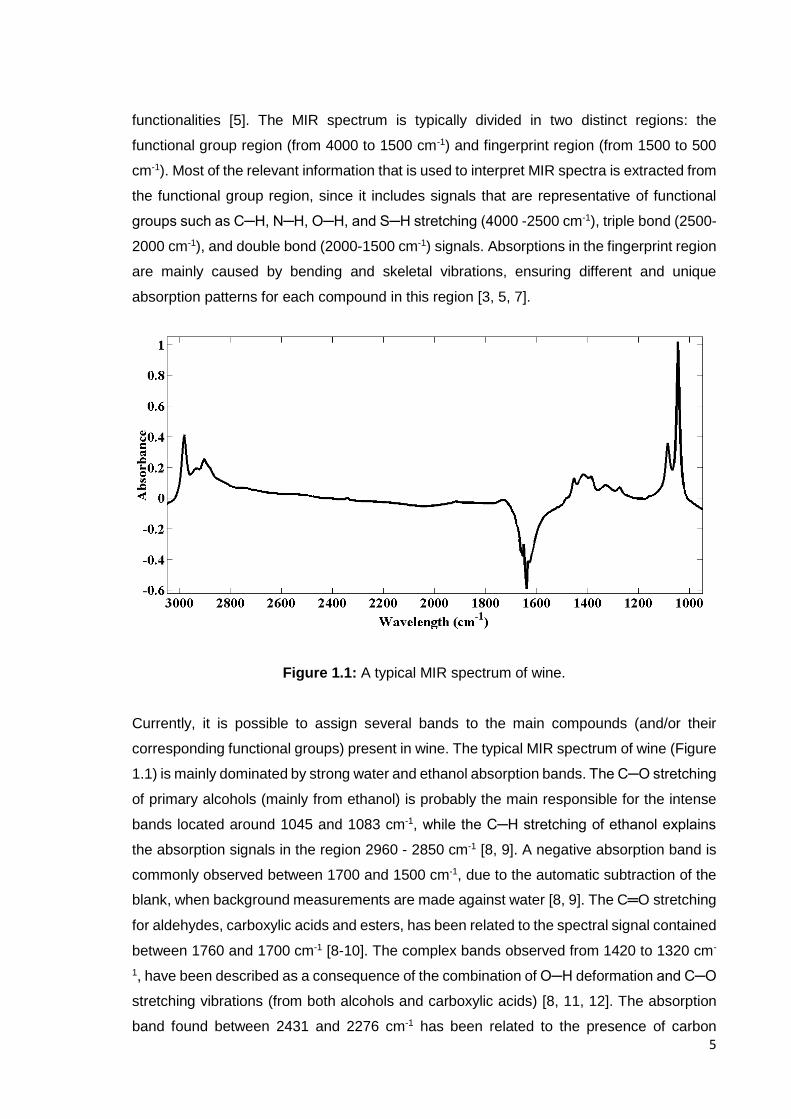
Figure 1.1: A typical MIR spectrum of wine.
Currently, it is possible to assign several bands to the main compounds (and/or their
corresponding functional groups) present in wine. The typical MIR spectrum of wine (Figure
1.1) is mainly dominated by strong water and ethanol absorption bands. The C─O stretching
of primary alcohols (mainly from ethanol) is probably the main responsible for the intense
bands located around 1045 and 1083 cm-1, while the C─H stretching of ethanol explains
the absorption signals in the region 2960 - 2850 cm-1 [8, 9]. A negative absorption band is
commonly observed between 1700 and 1500 cm-1, due to the automatic subtraction of the
blank, when background measurements are made against water [8, 9]. The C═O stretching
for aldehydes, carboxylic acids and esters, has been related to the spectral signal contained
between 1760 and 1700 cm-1 [8-10]. The complex bands observed from 1420 to 1320 cm-
1, have been described as a consequence of the combination of O─H deformation and C─O
stretching vibrations (from both alcohols and carboxylic acids) [8, 11, 12]. The absorption
band found between 2431 and 2276 cm-1 has been related to the presence of carbon
6
dioxide [9]. The spectral region beyond 3000 cm-1 reproduces the O─H stretching vibrations
through intense overlapped absorption bands. The strong presence of compounds
containing the hydroxi group (mainly water and ethanol), leads to signal saturation in this
region. As a consequence, this section of the spectra is not considered during wine analysis
[13-16]. The same happens with the MIR region under 900 cm-1. In this spectral range the
saturation problems are caused by the C─H deformation and C─C skeletal vibrations [17].
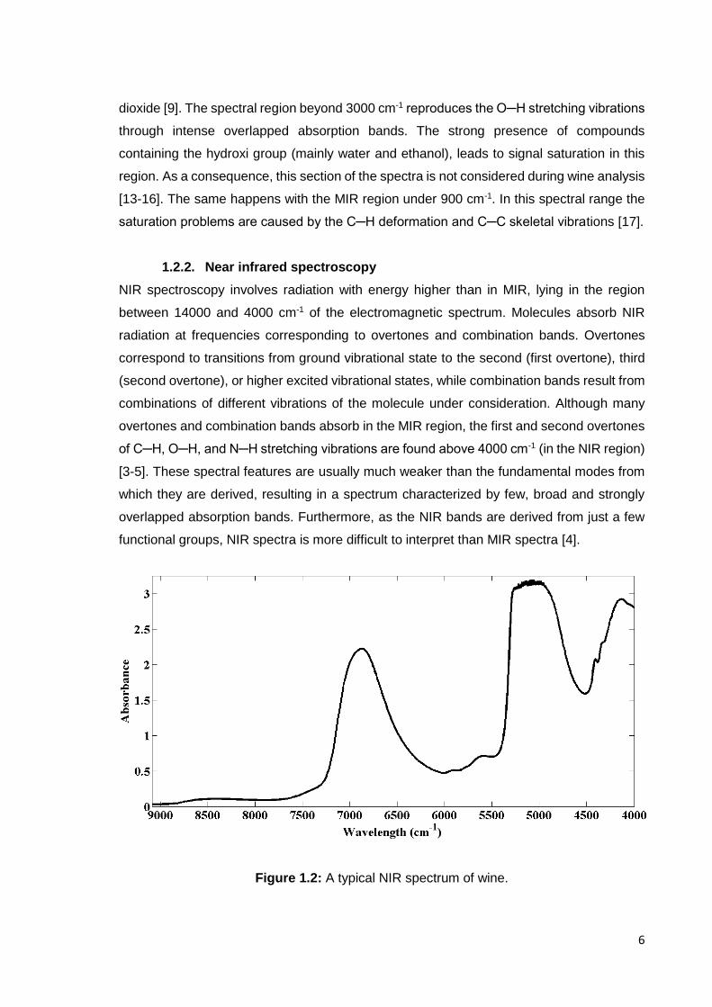
1.2.2. Near infrared spectroscopy
NIR spectroscopy involves radiation with energy higher than in MIR, lying in the region
between 14000 and 4000 cm-1 of the electromagnetic spectrum. Molecules absorb NIR
radiation at frequencies corresponding to overtones and combination bands. Overtones
correspond to transitions from ground vibrational state to the second (first overtone), third
(second overtone), or higher excited vibrational states, while combination bands result from
combinations of different vibrations of the molecule under consideration. Although many
overtones and combination bands absorb in the MIR region, the first and second overtones
of C─H, O─H, and N─H stretching vibrations are found above 4000 cm-1 (in the NIR region)
[3-5]. These spectral features are usually much weaker than the fundamental modes from
which they are derived, resulting in a spectrum characterized by few, broad and strongly
overlapped absorption bands. Furthermore, as the NIR bands are derived from just a few
functional groups, NIR spectra is more difficult to interpret than MIR spectra [4].
Figure 1.2: A typical NIR spectrum of wine.

7
The typical NIR spectra of wine (Figure1.2) is characterized by two main absorption bands
associated with the dominant presence of water and ethanol. One of the bands appears
near 5260 cm-1, and represents a combination of the fundamental O─H stretching and
deformation vibrations. The other one usually occurs around 6900 cm-1 and represents the
O─H stretching first overtone [18-21]. The second overtone of the O─H stretching also
causes the appearance of a relatively intense band around 10310 cm-1 [21]. The small
bands located near 5920 cm-1 and 5710 cm-1 are commonly attributed to the first overtones
of CH3 CH2 and CH groups (caused by the C─H stretching, mainly occurring in ethanol and
sugars) [22, 23].
1.2.3. Raman spectroscopy
In contrast to the two other techniques, Raman spectroscopy involves a scattering process.
In Raman spectroscopy, the sample is illuminated with a monochromatic beam of radiation
(typically from some type of laser) whose frequency may vary from the visible to the NIR
region. The incident light interacts with molecules causing their excitation to a virtual energy
state above the vibrational energy levels. From the excited energy level, most molecules
return to the ground vibrational state (through the emission of a photon of the same
wavelength as that of the incident photon), causing an elastic scattering known as Rayleigh
scattering. As the state of the molecule remains unchanged, the Rayleigh scattering does
not contain information in terms of molecular vibrations and the signal is useless for the
purpose of molecular characterization. However, a small fraction of the incident photons
drop to the first excited vibrational state, causing an inelastic scattering process known as
Stokes Raman scattering. In this process, the emitted photon has lower frequency than the
incident one, and corresponds to the energy of the fundamental transitions (that can be
observed as an MIR absorption band). If the molecules are already in an excited vibrational
state, they may undergo Rayleigh scattering (if they return to their starting vibrational state)
or anti-Stokes scattering in the case they drop to the ground vibrational state. According to
the Maxwell-Boltzmann law, only a small portion of the molecules will occupy an excited
vibrational energy state at room temperature. Therefore, the Raman Stokes scattering
bands are more intense than bands resulting from anti-Stoke scattering, and are the ones
used for practical Raman spectroscopy [5]. The intensity of bands in the Raman spectrum
is determined by the polarizability change occurring during the vibration, and unlike IR
spectroscopy it is not limited to the detection of polar bonds. Therefore, the two techniques
are commonly considered as complementary techniques, since many bands that are weak
in the IR spectrum are among the strongest bands in the Raman spectrum [5, 24]

8
Figure 1.3: A typical Raman spectrum of wine.
Despite the potential of Raman spectroscopy, only a few reports can be found in the
literature concerning the use of this technique for the analysis of wines or other beverages
[24]. The Raman spectra of wine is characterized by several well defined bands, less
intense than the ones observed in the NIR and MIR spectra (Figure 1.3). A broad band near
450 cm-1, is assigned to the C─C─O bending mode (commonly related to the vibration of
glucose rings) [25-27]. The strong band located around 880 cm-1 reproduces the C─C
stretching vibration, mainly due to ethanol molecules [25-28]. The two consecutive bands
around 1050 and 1080 cm-1 are usually assigned to the C─O stretching and CH3 rocking
modes (both attributed to ethanol) [25, 29, 30]. The spectral features near 1300 and 1450
cm-1 have been previously described as a consequence of the C─O─H and CH2 bending
modes, respectively [25, 27, 28]. The strong broad bands situated around 1640 and 3200
cm-1, correspond to the O─H stretching vibration of water [28]. The C─H stretching
vibrations (from ─CH2 and ─CH3 groups) of ethanol have been pointed out as the main
responsible for the appearance of three consecutive bands near 2885, 2935, and 2980 cm-
1 [27, 28]. Although a very intense band appears around 70 cm-1, no information was found
correlating it with any specific compound.
1.2.4. The role of chemometrics
Although vibrational spectroscopy is considered a fingerprinting technique, capable of
providing valuable information about several properties of a sample, that information is often
hidden in complex spectra, characterized by weak and overlapping signals. Besides the

9
sample nature, other sources of variability contribute to the complexity of a spectrum, such
as: sample heterogeneities, instrumental noise, scattering and environmental effects.
Therefore, to extract useful information, (whether for quantitative or qualitative purposes) it
is necessary to use proper chemometric procedures. Principal component analysis (PCA)
and partial least squares (PLS) regression are the most commonly used multivariate
analytical techniques. During the development of calibration models, pre-processing tools
are usually applied to enhance spectral features and remove unwanted sources of variation.
Furthermore, the structure of the sample set is usually inspected using PCA, in order to
detect eventual outliers. After the calibration process is concluded, the accuracy and
robustness of the model should be tested with an independent sample set (validation set)
[6]. The predictive ability of multivariate models is usually assessed by calculating the
uncertainty of their estimations. The approach currently adopted for this purpose is the
determination of the root mean square error of prediction (RMSEP) and/or the standard
error of prediction (SEP) (indicators of the accuracy and precision of the predictions,
respectively).
Further details about these procedures are described in Chapter 2.
1.3. Application of vibrational spectroscopy in the wine industry
Over the past two decades, vibrational spectroscopic techniques, mainly near and mid
infrared spectroscopy, have proved their potential in the wine industry. Hundreds of studies
were published, covering all the production chain and answering a wide range of
purposes.The following sections are devoted to the diversified application of vibrational
spectroscopy in the wine industry: from the soil to the bottle.
1.3.1. Grapes’ growth and maturation
1.3.1.1. Soils
Soils represent the first support for the healthy development of the vineyard and the
consequent achievement of top quality grapes. Thus, it is considered of great importance
to determine and control its characteristic properties and subsequent cultivation practices.
Cozzolino et al. (2013) explored the potential of NIR spectroscopy as a tool toward
sustainable vineyard management, by applying this technique in-situ for the assessment of
soil chemical composition. Results showed the possibility to measure soil chemical
properties directly in the vineyard (SECV values around 14% of the reference ranges)
(Table 1.1), proving the suitability of portable NIR spectroscopy for the rapid and low cost
monitoring of soil fertility [31]. Furthermore, this monitoring approach also revealed to be an
excellent tool for the support of a vineyard's micro-zoning process [32].

10
1.3.1.2. Grapevine leaves and other tissues
The monitoring of grapevine physiology is an important tool to assure its balanced growth,
and is usually assessed through the analysis of the grapevine tissues. NIR spectroscopy
was applied on grapevine leaves and stems, directly in the field, demonstrating its ability for
a fast and reasonable assessment of grapevine water potential, as a response to irrigation
practices [33]. Although the results obtained for the Shiraz variety were good (R2 around
0.85, both in leaves and stems), further studies should be performed including more
grapevine varieties and an independent test set, in order to attest the versatility and
predictive ability of this technique. Other parameters were investigated from the NIR spectra
of leaves [34] (Table 1.1). Grapevine varietal classification was performed by in-field leaf
spectroscopy, allowing a fast and effective discrimination of twenty grapevine varieties (87%
of correct predictions) [35]. NIR hyperspectral imaging of leaves combined with PLS
regression, was also successful in the classification of 3 different grapevine varieties
(Tempranillo, Grenache and Cabernet Sauvignon) [36]. Although the percentage of correct
predictions for all the grapevine varieties was high (around 93%), it would be interesting to
increase the number of grapevine varieties. Ciraolo et al. (2012) used a NIR multispectral
camera in the vineyard crop as an attempt to map the evapotranspiration, demonstrating
the feasibility of the proposed technique for agro-hydrological and precision farming
purposes [37]. The grapevine varieties included in these works and the leaf surface in which
the spectra was collected, were pointed out as the major causes of variability among the
results [38]. MIR spectroscopy was employed in the analysis of grapevine petioles, roots
and wood samples. Results demonstrated the ability of this technique for the quantitative
determination of several inorganic ions in grapevine petioles [39], and for the rapid
monitoring of nitrogen and starch content in roots and wood samples (R2>0.95) [40].
1.3.1.3. Grapes
The compositional profile of grapes has been widely explored by vibrational spectroscopy
in what concerns quality and maturation parameters. The first applications of vibrational
spectroscopy in grape analyses were extracted from the spectra of homogenized grape
samples and grape juices or musts. The determination of compositional parameters and
maturity indicators, such as: total soluble solids (TSS), anthocyanins, minerals (Fe, Mn, Ca,
Mg, K, P), dry matter, condensed tannins, reducing sugars, electric conductivity, pH, and
glycosylated aroma compounds was attempted by both NIR or MIR spectroscopy
techniques [8, 38, 41-46]. Overall, results suggest that NIR spectroscopy is a promising
technique for predicting reducing sugar content and total soluble solids in grape
homogenates [47, 48]. Nevertheless the determination of other parameters seemed to be

11
strongly influenced by the sample presentation mode [48]. MIR spectroscopy displayed an
excellent performance in the construction of calibration models for the assessment of pH,
total soluble solids and ammonia concentration in commercial grape juice (Table 1.1) [49].
Some NIR applications were not so successful when considering the determination of low
concentration compounds. Indeed, poor results were obtained from the measurement of
glycosylated aroma compounds (terpenes, phenols, C6 alcohols and norisoprenoids),
independently of the sample presentation mode (grape juice or homogenized grapes). The
sensitivity of NIR spectroscopy makes this technique inappropriate for the measurement of
low concentration components in complex matrices such as wine [50]. The same problem
occurred in the assessment of anthocyanins through MIR spectroscopy, revealing the
unsuitability of this technique for its determination in red grape musts [51].
The analysis of grape juice, also allowed the classification of grapes, according to their
variety and the irrigation practices to which they were exposed [52]. To increase the
robustness and precision of the calibrations, some researchers evaluated the effects of
microwaving and freezing grape homogenates, the speed and time of homogenization, and
the type of homogenizer [38, 41].
Technological advances in the vibrational spectroscopy area enabled the scanning of
samples in other presentation modes, such as intact grape berries and whole grape
bunches, both in the laboratory and in-field. The prediction of TSS, pH, total acidity and
anthocyanins in fresh berries, by NIR spectroscopy, was reported as a tool for ripening
control and even for the differentiation of soil management practices by understanding its
influence on grapevine growth and berry quality [53]. Good results were obtained for the
measurement of pH, total acidity and anthocyanins content. Nevertheless, it is worth
mentioning that only two grape varieties were included in the calibration models, and their
predictive ability was not tested with independent sample sets. Several other parameters
were estimated through the application of NIR spectroscopy in grapes directly in the
vineyard, whether for the assessment of chemical composition or physical properties [41].
Good results were achieved using a portable NIR-AOTF instrument for the monitoring of
ripening evolution in whole grape berries. However, regression models were constructed
based on reference data obtained from MIR spectroscopy (instead of the recommended
analytical methodologies) [54]. A Vis/NIR device was tested for the prediction of ripening
parameters in both red and white grape samples. The results obtained are encouraging (R2
around 0.75 for TSS, titratable acidity, potential alcoholic degree and extractable
anthocyanins), considering the difficulties that arouse from the use of these tools directly in
the field [55]. Whole grape bunches were analysed using a portable NIR spectrometer,
aiming at the development of accurate and robust models for the prediction of internal

12
quality parameters during on-vine ripening and on arrival at the winery. The determination
of reducing sugars and soluble solids content yielded the best results (R2 higher than 0.94).
Other sample presentation modes, (like individual berries and must), were investigated,
revealing some variability among the results (mainly for pH and potassium content) [48].
After optimizing the process, the authors concluded that NIR spectroscopy is a well suited
technology for the non-destructive evaluation of chemical changes (related to sugar content
and acidity) occurring during the ripening process [56].
NIR hyperspectral imaging systems also seemed to provide valuable information for the
assessment of quality and maturity indicators in intact grapes. Recently, this technique has
been applied for the fast and inexpensive screening of anthocyanins, °Brix, pH and sugar
content. Results were very promising, mainly the ones obtained for the determination of
anthocyanin content (R2=0.95) [57]. Furthermore, those applications worked as a starting
point for the development of frameworks, suitable for the sorting of berries according to their
maturity stages [57-59].
It is important to note, that for the development of the above mentioned calibrations, several
external factors were simultaneously considered and incorporated. Special attention was
given to the variety, year, and geographic origin of the included sample sets. Additionally,
the spatial orientation of the samples and its presentation mode, the instrument availability
and cost, the desired level of accuracy, the spectral range selection, and the application of
mathematical treatments, were also subject of discussion [38, 41].
The vibrational scanning of grape seeds and skins was also performed aiming several
purposes. NIR and MIR spectra of intact grape seeds were used to predict the extractable
content of phenolic compounds, enabling the monitoring of seed phenolic maturity (R2P
around 0.98 for total phenolics and condensed tannins). However, only two red grape
varieties were included [60, 61].
The extension of these spectra to the ultraviolet and visible regions, allowed the
discrimination of grape seeds from different grape varieties. NIR spectroscopy revealed as
well considerable potential for the determination of different sensory parameters (sourness,
astringency, tannic intensity, dryness, hardness, visual colour and olfactory intensity, and
type of aroma) in grape seeds and skins, supporting decisions concerning the optimal
harvest time. The best results were obtained for the prediction of hardness and colour in
grape seeds [62]. Additionally, NIR spectroscopy was successfully applied to winemaking
residues (grape pomace), to estimate total phenolics content and total antioxidant capacity
(R2 higher than 0.95), representing a non-destructive and eco-friendly technique to foster
added value of grape pomace residues [63].
13
NIR hyperspectral imaging has also been explored in the characterization of grape seeds,
skins and stems. This technique proved to be a reliable methodology for the prediction of
maturity stages and for the classification of grapes according to variety or type of soil (100%
of correct predictions when using the entire spectrum) [64]. Results revealed the suitability
of this technique for the quantitative measurement of anthocyanins [65], and some phenolic
compounds (proanthocyanidins, catechin, epicatechin, low molecular weight flavanols and
procyanidin B1) [66].
Spectral acquisitions of seed extracts in the mid infrared region were used for the evaluation
of the degree of polymerization of procyanidins. The calibration model developed, yielded
an R2 of 0.91 and an RMSEP of 2.58 (which corresponds to 29% of the reference range)
[67]. Therefore, additional studies are needed in order to improve the accuracy of these
models.
1.3.1.4. Grape diseases
Grape diseases are probably the main concern of winemakers and producers, since
contaminated grapes contribute negatively to the sensorial attributes of the wine. Therefore,
the early detection of diseases is crucial to properly correct the problem and assure the
healthy growth of grape bunches.
NIR spectroscopy was applied in Chardonnay grape homogenates, contaminated with
powdery mildew, revealing the potential of this technique to classify several degrees of the
infection in grapes [68]. It would be interesting to extend the applicability of this technique,
by including other grape varieties in the construction of the calibration models. Grape mash
samples, of naturally infected grapes, were screened by NIR spectroscopy for the
quantification of several parameters, including ergosterol, which is an indicator of rotness
in grapes. Results revealed RMSEP values of 4.05 mg/kg (corresponding to 8.2% of the
reference range), proving the suitability of this technique for industrial process integration
by allowing on-line measurements in real time [69]. MIR spectroscopy was applied in grape
juice for the determination of gluconic acid (R2=0.98) and glycerol (R2=0.96), commonly
used as chemical markers of grape infection. Results pointed out the possibility of using this
procedure as an alternative to the conventional visual inspection of Botrytized grapes.
However, further research including selected sample sets was suggested, as Botrytis
infection can depend on the grape variety [70]. NIR and MIR spectroscopy, were combined
for the quantification of Botrytis bunch rot in white wine grapes. The best results were
obtained when using the NIR spectra comprised between 1260 and 1370 nm. To increase
the accuracy of the model, additional calibrations (including samples with lower amounts of
Botrytis), should be developed [71].
14
1.3.2. The winemaking process
1.3.2.1. Fermentation
Wine fermentation represents a crucial step in the development of wine sensorial attributes.
The fast and reliable character of vibrational spectroscopy, simultaneously capable of real
time and on-line measurements, made this technique suitable for the monitoring of this
winemaking step.
Infrared spectroscopy, both in the near and mid infrared regions, has been applied in the
fermentation process control. Several quality indicators (glucose, fructose, ethanol,
glycerol, phenolic compounds, anthocyanins, volumic mass and acetic acid, among others)
(Table 1.2) were successfully determined through these vibrational techniques.
Measurements were carried out in large-scale batches, micro-fermentation trials, and even
in model solutions [72-77]. Changes in the wine matrix, occurring during the fermentation
process, represent the main limitation for the development of proper calibration models,
making them unsuitable to be extended to the overall wine fermentations.
Micro-fermentation trials were used by some researchers to predict compositional changes
during alcoholic fermentation of red wines, using NIR and MIR spectroscopy. Both
techniques originated correlation coefficients higher than 0.90 for ethanol, glycerol, fructose,
glucose, total phenolics, total anthocyanins, and total flavonoids, demonstrating their ability
for on-line measurements [78]. NIR spectroscopy was combined with the ultraviolet and
visible spectral regions for the determination of total polyphenol index and colour intensity
during red wine alcoholic fermentation over two vintages and using two grapes varieties
(Cabernet Sauvignon and Shiraz). Results were strongly influenced by the year and variety
of samples (Table 1.2), enhancing the specificity of these parameters. Therefore proper
calibration models should be developed in accordance with such external factors [20, 79].
Other instruments and techniques, such as FT-MIR-ATR, Vis-NIR spectroscopy and Raman
spectroscopy, were still applied in the monitoring of the chemical evolution during the
fermentation time course. The works using FT-MIR-ATR and Vis-NIR spectroscopy showed
that there is a correlation between fermentation changes and spectral features over the
time, highlighting the potential of these techniques to monitor the fermentation process on-
line and at real-time [80, 81].
Regarding the work using Raman spectroscopy, excellent results were obtained for sugar,
ethanol and glycerol contents, with prediction errors of 0.22 g/L, 0.03 % (v/v) and 0.2 %
(v/v) respectively. Hence, this study revealed the suitability of Raman spectroscopy for the
real time monitoring of multiple components in wine fermentation. As this work considered
only two micro-fermentation trials, further research should be carried out, to support these
results and highlight the potential of this technique [28]. New methods were also studied
15
and reported, as an attempt to maintain the online robustness of multivariate calibrations
against unknown influence factors (whether, chemical, physical or environmental). The
development of those methods was based on spectral adjustments whenever disturbances
were detected [82].
Malolactic fermentations were also evaluated by infrared spectroscopy, in near and mid
regions, to detect the beginning of this fermentative stage in a model wine. Absorption
bands were related to molecular modifications occurring during the L-malic acid
transformation, allowing the discrimination of samples according to its fermentative stage.
The results of this preliminary approach lead to the conclusion that this technique could be
used to support the conventional chemical and microbiological analysis to detect the start
of malolactic fermentation and the autolysis of lactic acid bacteria [83].
1.3.2.2. Yeast characterization and classification
Yeasts are the precursors of the fermentation process and consequently responsible for its
products and by-products. Therefore, researchers found useful the application of vibrational
spectroscopy and chemometrics to the characterization and classification of wine yeasts
[73, 74, 84].
In fact, both NIR and MIR spectroscopic techniques, were investigated as potential tools to
discriminate and identify different yeast strains with particular metabolic profiles, and to
assess their physiological state (Table 1.2) [68]. FT-MIR micro-spectroscopy was applied
for the study of yeast cells’ (Saccharomyces cerevisiae) autolysis, working as an accurate
tool to detect major biochemical changes associated with the autolytic process [85].
Additional research was carried out, demonstrating the ability of this technique for the
efficient selection of yeast strains based on their autolytic capacity [86]. NIR spectroscopy
was combined with the visible region of the electromagnetic spectrum, to discriminate
different Saccharomyces cerevisiae yeast strains, coming from a collection data bank. By
correlating spectral features with metabolic profiles, it was possible to differentiate and
classify similar yeast strains [87]. Similar results were obtained from the application of MIR
spectroscopy, which allowed the identification of Saccharomyces cerevisiae and
Saccharomyces bayanus, at the strain level, through a single measurement [88]. The
fermentation profiles of Saccharomyces cerevisiae strains were also evaluated by MIR
spectroscopy, through the quantification of volatile acidity, ethanol, reducing sugar and
glycerol, in fermenting juices and synthetic musts [89].
Raman spectroscopy was also applied for the identification and strain discrimination of wine
spoilage yeasts: Saccharomyces cerevisiae, Zygosaccharomyces bailii and Brettanomyces
bruxellensis. This work achieved an overall accuracy of 82% of correct predictions [90].
16
1.3.3. The compositional profile of wine
1.3.3.1. Quality and safety indicators
After the end of fermentation, wine is still submitted to several procedures. The assessment
of wine composition is essential to support decisions related to those winemaking practices.
Furthermore, it simultaneously enables the meeting of legal requirements and consumers´
satisfaction. Vibrational spectroscopy has been widely developed and employed in the
analysis of wine samples. Nowadays, it is possible to find NIR and MIR based analytical
instruments, implemented as routine methodologies in certified wine laboratories [41, 91-
93].
Ethanol has been the most studied parameter, however, the use of vibrational spectroscopy
was extended to the measurement of many other wine properties, (commonly included in
routine wine analysis) such as: volatile acidity, total acidity, reducing sugars, glycerol, pH,
sulfur dioxide and organic acids, among others (Table 1.3) [10, 13-16, 94-103]. A
comparative study was developed in order to evaluate the performances of NIR and MIR
spectroscopy, as well as their joint use, in the measurement of the alcoholic degree, volumic
mass, total acidity, glycerol, total polyphenol index, lactic acid and free sulfur dioxide in
wine. Overall, both NIR and MIR spectroscopy originated good results, with similar levels
of accuracy (Table 1.3). The alcoholic degree was the best predicted parameter, while poor
calibrations were obtained for the assessment of free sulfur dioxide. Only the determination
of glycerol was considerably favoured by the combination of the two techniques [104].
The sharp and specific absorption bands present in the MIR spectra of wine, made this
technique very attractive, allowing the assignment of specific bands to the corresponding
compositional parameters of wines.
Total antioxidant capacity was determined by MIR spectroscopy in red wines. The prediction
errors obtained from the PLS regression, were acceptable when compared with the ones
obtained from the reference method [105, 106]. The feasibility of infrared spectroscopy was
investigated for the prediction of haze formation in white wines. Results revealed the better
performance of short-wavelength NIR (SW-NIR) over FT-NIR and FT-MIR techniques in the
assessment of colloidal stability [107]. The effect of barrel aging was investigated by NIR
spectroscopy. The authors reported its ability to determinate oak volatile compounds in
barrel aged red wines, simultaneously considering the storage time and oak barrel types
[108]. The results obtained were good (R2 around 0.8) when considering wines with 18
years. However, the prediction errors obtained, are above the sensory threshold values
reported for these compounds, making these calibrations inappropriate.
Several other enological parameters and properties (Table 1.3) were subject of research
works. The samples selected for these works were usually represented by sets of wines

17
from different types, varieties and origins, aiming to develop robust calibrations and prove
the ability of these vibrational techniques for this type of analysis, in a wide diversity of
samples [41, 72, 73, 84].
The strong water absorbance signals in the IR spectra, lead to the development of some
studies reporting the use of dry extracts as samples. The analysis of this type of samples
was proposed for the measurement of polysaccharides and polymeric mannose contents,
for the determination of geographic origin, and for the assessment of total phenols and
sugar concentrations in fortified wines [41, 109-112]. Nevertheless, the quantification of the
main families of polysaccharides was complicated by their low concentration and the strong
collinearity between them [109]. The partial least squares (PLS) regression, developed for
the quantification of polymeric mannose, displayed poor results (RMSECV= 36.2% of the
reference range values used for calibration), which have been considerably improved by
the application of orthogonal signal correction (OSC) (RMSECV= 11.4 %) [110]. Moreover,
it is important to note that, the use of this type of samples requires laborious and time-
consuming extraction steps, preventing its application in-situ.
Raman spectroscopy was combined with multivariate analytical techniques for the
determination of ethanol in wines. Results demonstrated the excellent performance of the
proposed method (r=0.99), for the quantitative measurement of ethanol in commercial wine
samples [113]. Raman spectroscopy was also employed in the measurement of phenolic
compounds in red wines. Promising results were obtained for the quantification of
polyphenols, anthocyanins and tannins (R2 higher than 0.82) [114]. Although Raman
spectroscopy is still in its beginning (concerning its application in the wine industry), the
results obtained suggest the potential use of this technique for further applications.
Investigations in this field also concerned the selection of appropriate spectral regions, the
management of spectroscopic interferences, and the effects of pre-processing methods and
temperature, in the determination of wine parameters [11, 115-119]. The knowledge
obtained from these works had great contribution in the improvement of calibration
techniques.
1.3.3.2. Sensory analysis
Sensory properties of wines may proceed from different stages and sources during the
winemaking process. Grapes, yeasts’ metabolism, winemaking practices, storage and
aging conditions are primarily responsible for the wine sensory character. The evaluation of
these properties is usually performed by experienced winemakers, wine competition judges
or wine tasting panellists. However, the subjective character of this type of analysis has
triggered efforts in order to develop instrumental methodologies, capable of estimate wine

18
sensory attributes. The application of vibrational spectroscopy to this field, found a major
limitation: the concentrations of the compounds responsible for flavour and odour in wine
are often present in concentrations under the detection limit of these instruments [7, 74, 84,
120]. Consequently, several researchers focused on the interpretation of spectral data,
looking for its correlation with compounds affecting wine sensory properties [7, 72]. Thus,
NIR and MIR spectroscopic methods were proposed to indirectly explain variations in
sensory attributes, simultaneously working as screening tools for determination of quality
levels.
Some sensory-linked characteristics of wine were assessed by Vis-NIR spectroscopy,
which proved its ability in the prediction of wine quality, according to commercial rankings
and sensory scores, previously assigned [7, 41, 72, 121].
MIR spectroscopy was applied in the evaluation of wine samples’ bitterness, (by relating
spectral information with bitterness intensity), previously assigned by a trained sensory
panel. The same procedure was applied using a FT-MIR based electronic tongue, for the
determination of tannin amount in red wines (r=0.92) [122] and gelatin index (R2=0.89 and
R2=0.87 for rose and red wines respectively), [123] according to the gustative mouthfeel
sensation. NIR spectroscopy was tested in the prediction of volatile aroma compounds and
sensory descriptors from different aroma categories, in two Australian white wine varieties
(Chardonnay and Riesling) [124, 125]. Good calibration models were obtained for the
prediction of monoterpene alcohols (R2=0.90). Although the predictive ability of the models
has been tested by cross-validation techniques, it would be interesting to evaluate those
models with independent data sets [125]. The models developed for the prediction of aroma
descriptors, presented poor results (with correlation coefficients comprised between 0.12
and 0.78), suggesting that further work needs to be carried out, in order to improve its
usefulness [124].
1.3.3.3. Geographic origin
The geographic origin of wines, may strongly determine its characteristics and properties.
Consequently, the appellation of origin emerged as a geographical indication, used to
designate wines with specific qualities or characteristics that are essentially due to the
geographical environment in which it is produced. Infrared spectroscopy seemed to be a
valuable tool in the classification of wine samples, according to its country or appellation of
origin, and to discriminate wines made from different grape varieties (Table 1.3). Scientific
researches have been published, highlighting NIR spectroscopy as a powerful tool for the
traceability of wine geographic origin and variety, in several countries around the world [126,
127]. MIR spectroscopy was also applied to Gamay wine extracts from three different

19
origins, allowing the correct classification of 71%, 90% and 97% of samples from for Gaillac,
Beaujolais and Touraine regions, respectively. Moreover, a proper analysis of the main
spectral regions used for the models’ development, revealed the importance of phenolic
compounds in the discrimination of samples, according to its geographic origin and
production year [128].
1.3.3.4. Authentication
Vibrational spectroscopy also found potential application for the authentication and fraud
detection of wines. Throughout the years, the evolution of wine adulteration forms, triggered
the search for accurate techniques, capable of routine inspections of wine quality and
authenticity. Some of the works concerning these purposes were already described in the
previous section (section 3.3.3). In fact, establishing real origins, both in terms of variety or
geographic region, is a way of ensuring wine authenticity.
The combination of spectroscopic and chemometric analysis, was reported as a useful tool
to establish the authenticity and uniqueness of wines from protected designations of origin
[129].
The adulteration of red wines by the addition of industrial grade glycerol was assessed by
combining single bounce micro ATR-MIR with multivariate data analysis. This technique
was able to predict the presence of industrial glycerol with an accuracy level ranging
between 94 and 98%. Suitable models were also developed for the quantitative analysis,
yielding low predictive errors (SEP values below 2.25 % w/w) within the studied
concentration range [130]. However, it should be mentioned that these models were
developed using fortified samples and the errors obtained are higher than the glycerol
values commonly found in wines.
Different wine aging conditions were evaluated using MIR and NIR spectral data, allowing
the discrimination of wines aged in oak barrels, in stainless steel tanks, and in steel tanks
with addition of oak chips. The recognition accuracy of the proposed techniques, varied
between 86% and 98% according to the discriminant method and vibrational technique
used. Nevertheless, best results were obtained by merging NIR and MIR spectral data
[131]. The joint use of these techniques, was also applied in the distinction of red and white
wines, resulting from malolactic fermentations carried out with different strains of
Oenococcus oeni. Correct classifications, ranging between 67% and 100% (depending on
the strain), showed that IR spectroscopy can be used as a rapid and effective screening
tool [132].
FT-MIR spectroscopy demonstrated high potential to check wine integrity during
transportation, by comparing the spectra obtained in the dispatch and receival places [9].
20
NIR spectroscopy enabled the discrimination of wine samples containing anthocyanins from
black rice, with minimum sample preparation. Nonetheless, the results obtained were not
the expected ones (70% of correct predictions). The authors justified these results with the
matrix effect and low sensitivity of NIR technique [23]. The mid infrared spectra of a model
wine were combined with sensory analysis, to attempt its classification according to the
origin of added tannins (grape seed or grape skin tannins). The level of accuracy varied
according to the chemometric method employed [133]. Additionally, the same technique
allowed the identification of spoiled wines, discriminating them from samples of fresh wine.
Once again, the classification power of the models depended on the chemometric technique
used [134]. Raman spectroscopy was recently used for the detection of six illegal
sweeteners in commercial liquor and wine. The results showed the high repeatability and
sensitivity of the proposed method, simultaneously enhancing its fast, simple and cost-
effective character [135]. The suitability of vibrational spectroscopy and chemometric
methods for the assessment of wine authenticity, was extensively demonstrated. However,
some authors suggest that its reliability needs to be further improved [72, 73, 136].
1.3.3.5. In bottle measurements
The possibility of determining wine chemical composition directly from the bottle represents
an ideal methodology for the wine industry. Vibrational spectroscopy could provide fast,
non-destructive and non-invasive measurements, capable of detecting compositional
changes and unwanted problems in bottled wine, before it reaches the market. NIR
spectroscopy was proposed for this type of measurements. Although calibration models
developed for the estimation of alcohol content (SECV=0.48%), total sulfur (SECV=4.01
mg/L), free sulfur (SECV=28.6 mg/L) and pH (SECV=0.15) have showed low accuracy, they
were considered acceptable for screening purposes [137].
1.3.4. Other wine related measurements
Throughout the wine making process, it is possible to find several materials that may have
a strong influence in the wine quality. Vibrational spectroscopy was extended to the analysis
of such materials and it is possible to find a number of works related to cork and oak
analysis. A fiber optic probe in the Vis-NIR range was used for the screening of cork planks
and cork stoppers, aiming to identify their geographical origins (Portugal, Morocco and
Spain). Results demonstrated the potential of Vis-NIR spectroscopy to accurately predict
the origins of cork samples from the world’s most representative cork producing areas (90%
of correct predictions) [138]. The same technique was explored to estimate chemical,
physical and mechanical properties of cork stoppers. Natural untreated cork stoppers were
21
analysed for the assessment of waxes, low and high-molecular-weight polyphenols, total
polyphenols, extractives, suberin, insoluble lignin, density, compression force, extraction
force, diametrical recovery and moisture content. However, poor calibrations were obtained,
except for the moisture content (R2=0.85) [139].
The determination of 2,4,6-trichloroanisols (TCA) in cork planks was also tested using MIR-
ATR spectroscopy. The absence of this compound suggested the possible acceptance of
cork planks for cork stoppers production. The TCA was artificially added to cork samples
and the results indicated that this technology could work as a screening technique.
However, no references are given about the amount of TCA added to each sample and so,
additional studies are needed [140]. Additionally, this technique was applied for the
characterization of paraffin and silicone-based surface treatments of cork stoppers. The
authors reported a total of 92% of correct predictions [141]. NIR spectroscopic applications
included as well oak analysis. The use of NIR reflectance spectroscopy was reported for
the identification of oak shavings origin (correct classification rates of 83 and 87 % were
obtained for samples sourced from USA and France respectively). Additionally, NIR spectra
provided useful information about the toasted treatment of the oak used for wine aging (100
% of correct classifications) [142].
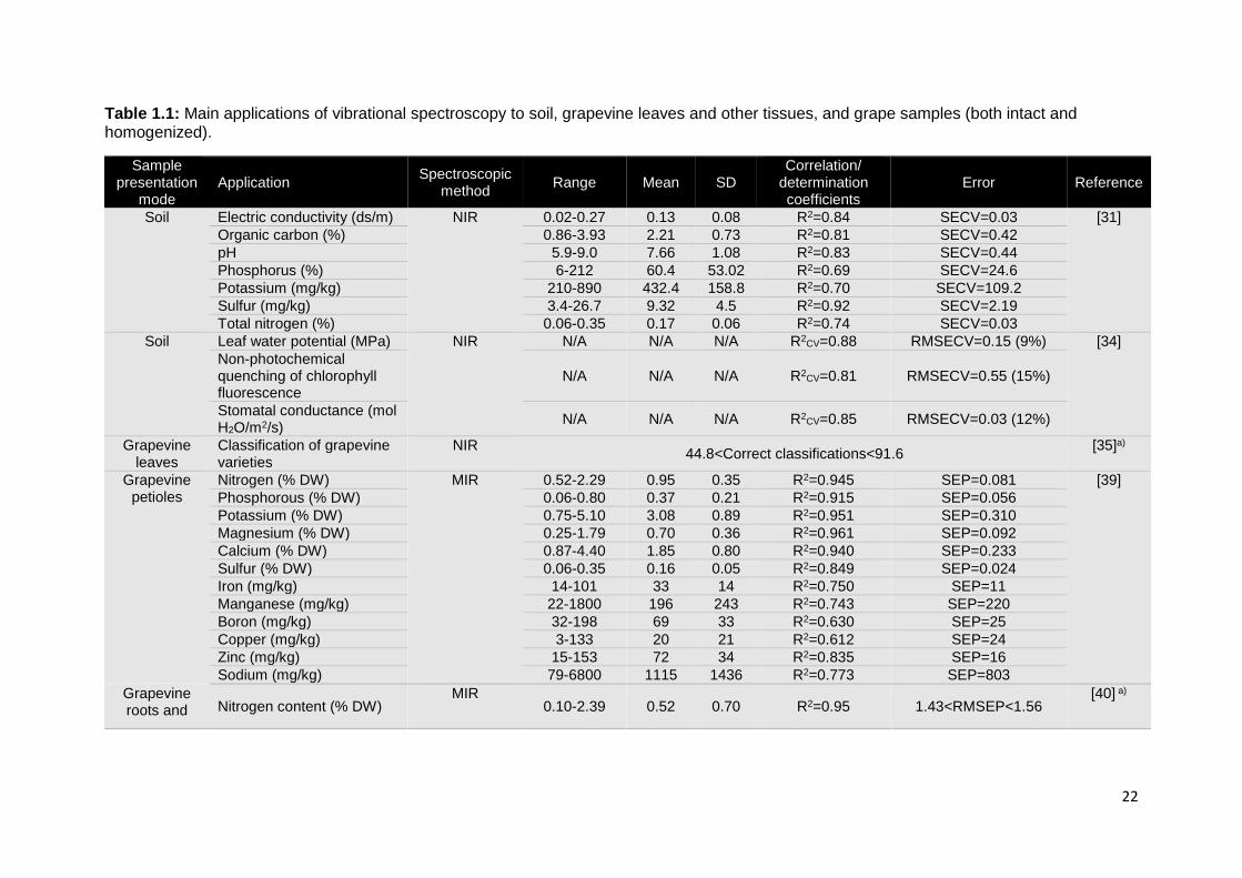
22
Table 1.1: Main applications of vibrational spectroscopy to soil, grapevine leaves and other tissues, and grape samples (both intact and homogenized).
Sample presentation
mode Application
Spectroscopic method
Range Mean SD Correlation/
determination coefficients
Error Reference
Soil Electric conductivity (ds/m) NIR 0.02-0.27 0.13 0.08 R2=0.84 SECV=0.03 [31]
Organic carbon (%) 0.86-3.93 2.21 0.73 R2=0.81 SECV=0.42
pH 5.9-9.0 7.66 1.08 R2=0.83 SECV=0.44
Phosphorus (%) 6-212 60.4 53.02 R2=0.69 SECV=24.6
Potassium (mg/kg) 210-890 432.4 158.8 R2=0.70 SECV=109.2
Sulfur (mg/kg) 3.4-26.7 9.32 4.5 R2=0.92 SECV=2.19
Total nitrogen (%) 0.06-0.35 0.17 0.06 R2=0.74 SECV=0.03
Soil Leaf water potential (MPa) NIR N/A N/A N/A R2CV=0.88 RMSECV=0.15 (9%) [34]
Non-photochemical quenching of chlorophyll fluorescence
N/A N/A N/A R2CV=0.81 RMSECV=0.55 (15%)
Stomatal conductance (mol H2O/m2/s)
N/A N/A N/A R2CV=0.85 RMSECV=0.03 (12%)
Grapevine leaves
Classification of grapevine varieties
NIR 44.8<Correct classifications<91.6
[35]a)
Grapevine petioles
Nitrogen (% DW) MIR 0.52-2.29 0.95 0.35 R2=0.945 SEP=0.081 [39]
Phosphorous (% DW) 0.06-0.80 0.37 0.21 R2=0.915 SEP=0.056
Potassium (% DW) 0.75-5.10 3.08 0.89 R2=0.951 SEP=0.310
Magnesium (% DW) 0.25-1.79 0.70 0.36 R2=0.961 SEP=0.092
Calcium (% DW) 0.87-4.40 1.85 0.80 R2=0.940 SEP=0.233
Sulfur (% DW) 0.06-0.35 0.16 0.05 R2=0.849 SEP=0.024
Iron (mg/kg) 14-101 33 14 R2=0.750 SEP=11
Manganese (mg/kg) 22-1800 196 243 R2=0.743 SEP=220
Boron (mg/kg) 32-198 69 33 R2=0.630 SEP=25
Copper (mg/kg) 3-133 20 21 R2=0.612 SEP=24
Zinc (mg/kg) 15-153 72 34 R2=0.835 SEP=16
Sodium (mg/kg) 79-6800 1115 1436 R2=0.773 SEP=803
Grapevine roots and Nitrogen content (% DW)
MIR 0.10-2.39 0.52 0.70 R2=0.95 1.43<RMSEP<1.56
[40] a)
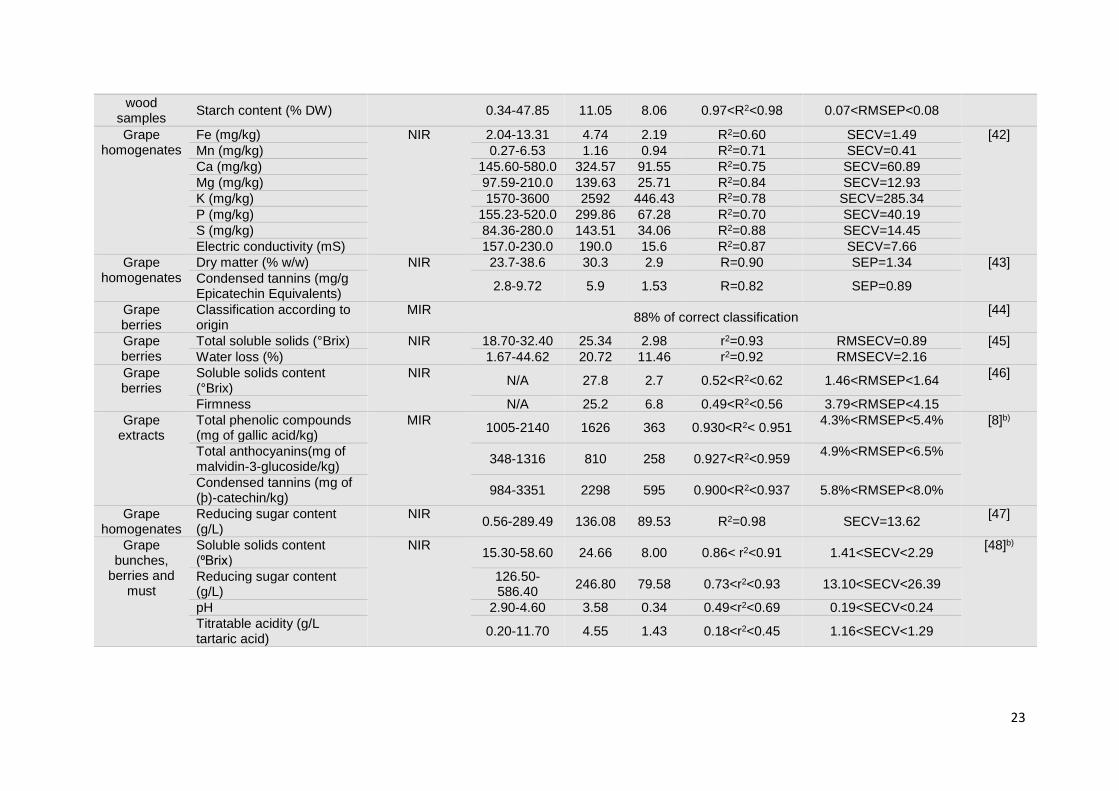
23
wood samples
Starch content (% DW) 0.34-47.85 11.05 8.06 0.97<R2<0.98 0.07<RMSEP<0.08
Grape homogenates
Fe (mg/kg) NIR 2.04-13.31 4.74 2.19 R2=0.60 SECV=1.49 [42]
Mn (mg/kg) 0.27-6.53 1.16 0.94 R2=0.71 SECV=0.41
Ca (mg/kg) 145.60-580.0 324.57 91.55 R2=0.75 SECV=60.89
Mg (mg/kg) 97.59-210.0 139.63 25.71 R2=0.84 SECV=12.93
K (mg/kg) 1570-3600 2592 446.43 R2=0.78 SECV=285.34
P (mg/kg) 155.23-520.0 299.86 67.28 R2=0.70 SECV=40.19
S (mg/kg) 84.36-280.0 143.51 34.06 R2=0.88 SECV=14.45
Electric conductivity (mS) 157.0-230.0 190.0 15.6 R2=0.87 SECV=7.66
Grape homogenates
Dry matter (% w/w) NIR 23.7-38.6 30.3 2.9 R=0.90 SEP=1.34 [43]
Condensed tannins (mg/g Epicatechin Equivalents)
2.8-9.72 5.9 1.53 R=0.82 SEP=0.89
Grape berries
Classification according to origin
MIR 88% of correct classification
[44]
Grape berries
Total soluble solids (°Brix) NIR 18.70-32.40 25.34 2.98 r2=0.93 RMSECV=0.89 [45]
Water loss (%) 1.67-44.62 20.72 11.46 r2=0.92 RMSECV=2.16
Grape berries
Soluble solids content (°Brix)
NIR N/A 27.8 2.7 0.52<R2<0.62 1.46<RMSEP<1.64
[46]
Firmness N/A 25.2 6.8 0.49<R2<0.56 3.79<RMSEP<4.15
Grape extracts
Total phenolic compounds (mg of gallic acid/kg)
MIR 1005-2140 1626 363 0.930<R2< 0.951
4.3%<RMSEP<5.4%
[8]b)
Total anthocyanins(mg of malvidin-3-glucoside/kg)
348-1316 810 258 0.927<R2<0.959 4.9%<RMSEP<6.5%
Condensed tannins (mg of (þ)-catechin/kg)
984-3351 2298 595 0.900<R2<0.937 5.8%<RMSEP<8.0%
Grape homogenates
Reducing sugar content (g/L)
NIR 0.56-289.49 136.08 89.53 R2=0.98 SECV=13.62
[47]
Grape bunches,
berries and must
Soluble solids content (⁰Brix)
NIR 15.30-58.60 24.66 8.00 0.86< r2<0.91 1.41<SECV<2.29
[48]b)
Reducing sugar content (g/L)
126.50-586.40
246.80 79.58 0.73<r2<0.93 13.10<SECV<26.39
pH 2.90-4.60 3.58 0.34 0.49<r2<0.69 0.19<SECV<0.24
Titratable acidity (g/L tartaric acid)
0.20-11.70 4.55 1.43 0.18<r2<0.45 1.16<SECV<1.29

24
Table 1.1 (Continued)
Sample presentation
mode Application
Spectroscopic method
Range Mean SD Correlation/
determination coefficients
Error Reference
Tartaric acid (g/L tartaric acid)
4.90-15.50 7.39 1.62 0.01<r2<0.49 1.20<SECV<1.39
Malic acid (g/L malic acid) 0.10-7.20 0.85 1.04 0.21<r2<0.49 0.68<SECV<0.85 Commercial grape juice
Total soluble solids (⁰Brix) MIR N/A 20.83 1.68 R2=0.98 SECV=0.20 [49]
pH N/A 3.11 0.23 R2=0.86 SECV=0.07
Total phenolics (AU) N/A 9.8 1.80 R2=0.53 SECV=1.01
Ammonia (mg/L) N/A 34.3 30.5 R2=0.92 SECV=14.8
Free amino nitrogen (mg/L) N/A 71.2 59.1 R2=0.79 SECV=28.3
Yeast assimilable nitrogen (mg/L)
N/A 99.4 76.9 R2=0.80 SECV=36.9
Grape homogenates
and juice
C6 alcohols NIR [50]
1-Hexanol (g/L) 16.31-290.77 85.83 42.87 R2=0.5230 (GH) R2=0.5156 (GJ)
SECV= 30.6 (GH) SECV=27.4 (GJ)
(Z)-3-Hexen-1-ol (g/L) 4.19-85.92 24.63 12.36 R2=0.2151 (GH) R2= 0.4683 (GJ)
SECV=9.8 (GH) SECV=9.6 (GJ)
(Z)-2-Hexen-1-ol (g/L) 1.84-124.94 12.99 14.38 R2=0.2402 (GH) R2=0.2668 (GJ)
SECV=5.5 (GH) SECV=5.0 (GJ)
Terpenes
trans-Linalool oxide
(furanoid) (g/L) 0.63-37.14 18.17 8.22
R2=0.4653 (GH) R2=0.7089 (GJ)
SECV=7.9 (GH) SECV=7.3 (GJ)
cis-Linalool oxide (furanoid)
(g/L) 7.65-548.00 33.08 53.87
R2=0.6695 (GH) R2=0.5342 (GJ)
SECV=9.9 (GH) SECV=9.4 (GJ)
trans-Linalool oxide
(pyranoid) (g/L) 7.38-102.49 32.97 16.95 R2=0.4476 (GH) SECV=16.4 (GH)
cis-Linalool oxide
(pyranoid) (g/L) 20.22-191.25 65.23 29.16
R2=0.4622 (GH) R2=0.5105 (GJ)
SECV=28 (GH) SECV=25 (GJ)
α-Terpineol (g/L) 0-36.17 13.59 7.69 R2=0.2990 (GH) R2=0.4973 (GJ)
SECV=7.68 (GH) SECV=7.3 (GJ)
Nerol (g/L) 0-50.81 20.78 11.36 R2=0.6017 (GH) R2=0.5147 (GJ)
SECV=10.2 (GH) SECV=10.9 (GJ)
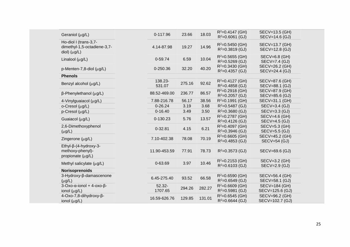
25
Geraniol (g/L) 0-117.96 23.66 18.03 R2=0.4147 (GH) R2=0.6061 (GJ)
SECV=13.5 (GH) SECV=14.6 (GJ)
Ho-diol I (trans-3,7-dimethyl-1,5-octadiene-3,7-
diol) (g/L)
4.14-87.98 19.27 14.96 R2=0.5450 (GH) R2=0.3819 (GJ)
SECV=13.7 (GH) SECV=12.8 (GJ)
Linalool (g/L) 0-59.74 6.59 10.04 R2=0.5655 (GH) R2=0.5269 (GJ)
SECV=6.8 (GH) SECV=7.4 (GJ)
p-Menten-7,8-diol (g/L) 0-250.36 32.20 40.20 R2=0.3430 (GH) R2=0.4357 (GJ)
SECV=26.2 (GH) SECV=24.4 (GJ)
Phenols
Benzyl alcohol (g/L) 138.23-531.07
275.16 92.62 R2=0.4127 (GH) R2=0.4858 (GJ)
SECV=87.6 (GH) SECV=88.1 (GJ)
β-Phenylethanol (g/L) 88.52-469.00 236.77 86.57 R2=0.2918 (GH) R2=0.2057 (GJ)
SECV=87.9 (GH) SECV=85.6 (GJ)
4-Vinylguaiacol (g/L) 7.88-216.78 56.17 38.56 R2=0.1991 (GH) SECV=31.1 (GH)
o-Cresol (g/L) 0-26.24 3.19 3.68 R2=0.5487 (GJ) SECV=3.4 (GJ)
p-Cresol (g/L) 0-16.40 3.49 3.50 R2=0.3680 (GJ) SECV=3.3 (GJ)
Guaiacol (g/L) 0-130.23 5.76 13.57 R2=0.2787 (GH) R2=0.4126 (GJ)
SECV=4.6 (GH) SECV=4.5 (GJ)
2,6-Dimethoxyphenol
(g/L) 0-32.81 4.15 6.21
R2=0.4097 (GH) R2=0.3946 (GJ)
SECV=5.3 (GH) SECV=5.5 (GJ)
Zingerone (g/L) 7.10-402.38 78.08 70.19 R2=0.6605 (GH) R2=0.4853 (GJ)
SECV=45.2 (GH) SECV=54 (GJ)
Ethyl-β-(4-hydroxy-3-methoxy-phenyl)-
propionate (g/L)
11.90-453.59 77.91 78.73 R2=0.3573 (GJ) SECV=69.6 (GJ)
Methyl salicylate (g/L) 0-63.69 3.97 10.46 R2=0.2153 (GH) R2=0.6103 (GJ)
SECV=3.2 (GH) SECV=2.9 (GJ)
Norisoprenoids
3-Hydroxy-β-damascenone
(g/L) 6.45-275.40 93.52 66.58
R2=0.6590 (GH) R2=0.6549 (GJ)
SECV=56.4 (GH) SECV=58.1 (GJ)
3-Oxo-α-ionol + 4-oxo-β-
ionol (g/L)
52.32-1707.65
294.26 282.27 R2=0.6609 (GH) R2=0.5981 (GJ)
SECV=184 (GH) SECV=125.6 (GJ)
4-Oxo-7,8-dihydroxy-β-
ionol (g/L) 16.59-626.76 129.85 131.01
R2=0.6545 (GH) R2=0.6644 (GJ)
SECV=96.2 (GH) SECV=102.7 (GJ)
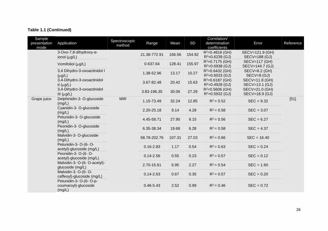
26
Table 1.1 (Continued)
Sample presentation
mode Application
Spectroscopic method
Range Mean SD Correlation/
determination coefficients
Error Reference
3-Oxo-7,8-dihydroxy-α-
ionol (g/L)
21.38-772.91 166.56 154.92
R2=0.4818 (GH) R2=0.6239 (GJ)
SECV=121.9 (GH) SECV=188 (GJ)
Vomifoliol (g/L) 0-637.64 128.41 155.97 R2=0.7175 (GH) R2=0.6938 (GJ)
SECV=117 (GH) SECV=144.7 (GJ)
3,4 Dihydro-3-oxoactinidol I
(g/L) 1.38-52.96 13.17 10.27
R2=0.6432 (GH) R2=0.6033 (GJ)
SECV=8.2 (GH) SECV=8 (GJ)
3,4-Dihydro-3-oxoactinidol
II (g/L) 3.67-82.48 20.42 15.63
R2=0.6187 (GH) R2=0.4928 (GJ)
SECV=11.8 (GH) SECV=13.1 (GJ)
3,4-Dihydro-3-oxoactinidol
III (g/L) 3.83-196.35 30.06 27.29
R2=0.5606 (GH) R2=0.5932 (GJ)
SECV=21.0 (GH) SECV=18.9 (GJ)
Grape juice Delphinidin-3- O-glucoside (mg/L)
MIR 1.15-73.49 32.24 12.85 R2 = 0.52 SEC = 9.32
[51]
Cyanidin-3- O-glucoside (mg/L)
2.20-25.18 9.14 4.28 R2 = 0.58 SEC = 3.07
Petunidin-3- O-glucoside (mg/L)
4.45-58.71 27.90 9.15 R2 = 0.56 SEC = 6.27
Peonidin-3- O-glucoside (mg/L)
6.35-38.34 19.68 6.28 R2 = 0.58 SEC = 4.37
Malvidin-3- O-glucoside (mg/L)
58.78-202.76 107.31 27.03 R2 = 0.66 SEC = 16.40
Petunidin-3- O-(6- O-acetyl)-glucoside (mg/L)
0.16-2.83 1.17 0.54 R2 = 0.63 SEC = 0.24
Peonidin-3- O-(6- O-acetyl)-glucoside (mg/L)
0.14-2.56 0.55 0.23 R2 = 0.57 SEC = 0.12
Malvidin-3- O-(6- O-acetyl)-glucoside (mg/L)
2.70-15.61 6.95 2.27 R2 = 0.54 SEC = 1.60
Malvidin-3- O-(6- O-caffeoyl)-glucoside (mg/L)
0.14-2.63 0.67 0.35 R2 = 0.57 SEC = 0.20
Petunidin-3- O-(6- O-p-coumaroyl)-glucoside (mg/L)
0.46-5.43 2.52 0.99 R2 = 0.46 SEC = 0.72
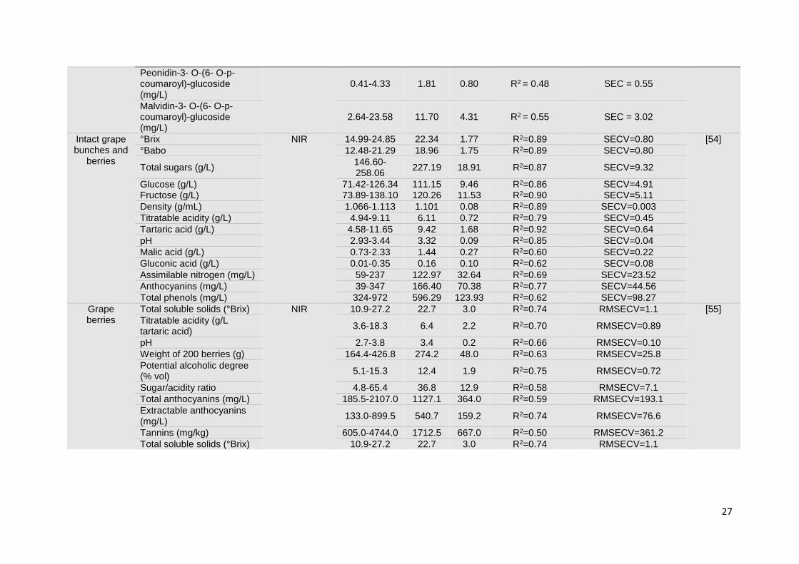
27
Peonidin-3- O-(6- O-p-coumaroyl)-glucoside (mg/L)
0.41-4.33 1.81 0.80 R2 = 0.48 SEC = 0.55
Malvidin-3- O-(6- O-p-coumaroyl)-glucoside (mg/L)
2.64-23.58 11.70 4.31 R2 = 0.55 SEC = 3.02
Intact grape bunches and
berries
°Brix NIR 14.99-24.85 22.34 1.77 R2=0.89 SECV=0.80 [54]
°Babo 12.48-21.29 18.96 1.75 R2=0.89 SECV=0.80
Total sugars (g/L) 146.60-258.06
227.19 18.91 R2=0.87 SECV=9.32
Glucose (g/L) 71.42-126.34 111.15 9.46 R2=0.86 SECV=4.91 Fructose (g/L) 73.89-138.10 120.26 11.53 R2=0.90 SECV=5.11
Density (g/mL) 1.066-1.113 1.101 0.08 R2=0.89 SECV=0.003
Titratable acidity (g/L) 4.94-9.11 6.11 0.72 R2=0.79 SECV=0.45
Tartaric acid (g/L) 4.58-11.65 9.42 1.68 R2=0.92 SECV=0.64
pH 2.93-3.44 3.32 0.09 R2=0.85 SECV=0.04
Malic acid (g/L) 0.73-2.33 1.44 0.27 R2=0.60 SECV=0.22
Gluconic acid (g/L) 0.01-0.35 0.16 0.10 R2=0.62 SECV=0.08
Assimilable nitrogen (mg/L) 59-237 122.97 32.64 R2=0.69 SECV=23.52
Anthocyanins (mg/L) 39-347 166.40 70.38 R2=0.77 SECV=44.56
Total phenols (mg/L) 324-972 596.29 123.93 R2=0.62 SECV=98.27
Grape berries
Total soluble solids (°Brix) NIR 10.9-27.2 22.7 3.0 R2=0.74 RMSECV=1.1 [55]
Titratable acidity (g/L tartaric acid)
3.6-18.3 6.4 2.2 R2=0.70 RMSECV=0.89
pH 2.7-3.8 3.4 0.2 R2=0.66 RMSECV=0.10
Weight of 200 berries (g) 164.4-426.8 274.2 48.0 R2=0.63 RMSECV=25.8
Potential alcoholic degree (% vol)
5.1-15.3 12.4 1.9 R2=0.75 RMSECV=0.72
Sugar/acidity ratio 4.8-65.4 36.8 12.9 R2=0.58 RMSECV=7.1
Total anthocyanins (mg/L) 185.5-2107.0 1127.1 364.0 R2=0.59 RMSECV=193.1
Extractable anthocyanins (mg/L)
133.0-899.5 540.7 159.2 R2=0.74 RMSECV=76.6
Tannins (mg/kg) 605.0-4744.0 1712.5 667.0 R2=0.50 RMSECV=361.2
Total soluble solids (°Brix) 10.9-27.2 22.7 3.0 R2=0.74 RMSECV=1.1

28
Table 1.1 (Continued)
Sample presentation
mode Application
Spectroscopic method
Range Mean SD Correlation/
determination coefficients
Error Reference
Titratable acidity (g/L tartaric acid)
3.6-18.3 6.4 2.2 R2=0.70 RMSECV=0.89
Grape bunches
Soluble solids content (°Brix)
NIR 10.60-58.60 20.49 5.84 0.96<R2<0.97 0.96<SECV<1.00
[56]b)
Reducing sugars (g/L) 81.50-586.40 198.39 64.95 0.94<R2<0.96 13.63<SECV<15.36
pH 2.48-4.60 3.35 0.34 0.65<R2<0.91 0.12<SECV<0.21
Titratable acidity (g/L tartaric acid)
0.20-20.50 6.72 3.52 0.86<R2<0.89 1.07<SECV<1.11
Tartaric acid (g/L tartaric acid)
4.90-18.60 9.48 2.80 0.74<R2<0.81 1.18<SECV<1.28
Malic acid (g/L) 0.10-14.50 2.33 2.32 0.82<R2<0.87 0.74<SECV<0.81
K (mg/L) 841.00-2737.00
1692.28 401.12 0.42<R2<0.65 242.26<SECV<258.94
Grape berries
Total anthocyanins (mg/grape)
NIR 0-5.37 N/A 0.96 N/A SECV=0.78
[59]
Non-acylated anthocyanins (mg/grape)
0-4.63 N/A 0.85 N/A SECV=0.70
Grape seed extracts
Total phenolics (mg gallic acid/g dried weight)
MIR 117.6-169.3 N/A N/A R2=0.97 RMSEP=6.49
[61]
Condensed tannins (mg catechin/g dried weight) (Methylcellulose assay)
37.5-183.3 N/A N/A R2=0.99 RMSEP=10.13
Condensed tannins (mg catechin/g dried weight) (BSA assay)
37.0-83.0 N/A N/A R2=0.99 RMSEP=3.97
Grape seeds Astringency NIR 1.83-3.73 2.59 0.47 N/A SEP=0.245 [62]
Colour 1.00-3.09 2.17 0.47 N/A SEP=0.242
Hardness 1.50-3.82 2.89 0.65 N/A SEP=0.224
Tannic intensity 2.00-3.50 2.68 0.45 N/A SEP=0.320
Grape skins Sourness 1.10-3.00 1.97 0.55 N/A SEP=0.200
Astringency 1.00-1.83 1.33 0.25 N/A SEP=0.239

29
Dryness 1.00-2.73 1.54 0.52 N/A SEP=0.170
Hardness 1.00-1.91 1.46 0.28 N/A SEP=0.303
Tannic intensity 1.00-2.18 1.44 0.34 N/A SEP=0.155
Aroma intensity 1.00-4.40 2.83 0.76 N/A SEP=0.338
Type of aroma 1.50-3.00 2.26 0.38 N/A SEP=0.391
Seeds, skins and stems
Catechin (mg/100g dry mass)
NIR 11.33-104.11 53.86 N/A R2=0.80 RMSECV=14.00
[66]
Epicatechin (mg/100g dry mass)
3.90-66.56 23.17 N/A R2=0.96 RMSECV=4.72
Proanthocyanidin B1 (mg/100g dry mass)
13.89-130.88 48.81 N/A R2=0.65 RMSECV=20.53
Proanthocyanidin B2 (mg/100g dry mass)
3.80-15.10 8.99 N/A R2=0.75 RMSECV=1.86
Proanthocyanidin B3 (mg/100g dry mass)
8.51-32.40 16.83 N/A R2=0.50 RMSECV=3.43
Proanthocyanidin B4 (mg/100g dry mass)
6.69-24.05 12.94 N/A R2=0.63 RMSECV=3.01
Proanthocyanidin trimer 1 (mg/100g dry mass)
2.72-23.95 11.16 N/A R2=0.65 RMSECV=3.12
Proanthocyanidin trimer 2 (mg/100g dry mass)
2.72-58.60 22.39 N/A R2=0.86 RMSECV=7.68
Proanthocyanidin tetramer 1 (mg/100g dry mass)
13.73-84.01 36.71 N/A R2=0.65 RMSECV=11.62
Proanthocyanidin tetramer 2 (mg/100g dry mass)
5.14-17.30 10.57 N/A R2=0.53 RMSECV=2.66
Proanthcyanidin B2-3-O-gallate (mg/100g dry mass)
8.59-63.99 31.76 N/A R2=0.89 RMSECV=6.29
Galloyl proanthocyanidin (mg/100g dry mass)
3.91-42.73 13.59 N/A R2=0.58 RMSECV=7.27
Total flavanols (mg/100g dry mass)
109.55-498.63
285.05 N/A R2=0.78 RMSECV=66.63
Gallic acid (mg/100g dry mass)
2.57-37.32 15.27 N/A R2=0.75 RMSECV=5.58
Protocatechuic acid (mg/100g dry mass)
0.58-19.59 4.91 N/A R2=0.82 RMSECV=2.70
Caffeic acid 0.74-4.19 2.27 N/A R2=0.92 RMSECV=0.36

30
Table 1.1 (Continued)
Sample presentation
mode Application
Spectroscopic method
Range Mean SD Correlation/
determination coefficients
Error Reference
Caftaric acid 0.85-25.91 6.76 N/A R2=0.91 RMSECV=2.56
cis-Coutaric acid 0.54-2.77 1.31 N/A R2=0.95 RMSECV=0.19
trans-Coutaric acid 0.49-1.39 0.82 N/A R2=0.83 RMSECV=0.15
Total phenolic acids 13.57-98.93 41.46 N/A R2=0.87 RMSECV=9.61
Quercetin 3-O-rutinoside 0.33-9.62 3.18 N/A R2=0.63 RMSECV=1.82
Quercetin 3-O-glucuronide 0.86-26.90 9.66 N/A R2=0.81 RMSECV=4.36
Quercetin 3-O-glucoside 0.93-29.15 12.64 N/A R2=0.64 RMSECV=5.95
Quercetin pentoside 1.26-1.39 1.28 N/A R2=0.15 RMSECV=0.04
Kaempferol 3-O-galactoside
1.35-3.78 2.18 N/A R2=0.98 RMSECV=0.11
Kaempferol 3-O-glucuronide
1.31-2.10 1.76 N/A R2=0.93 RMSECV=0.07
Kaempferol 3-O-glucoside 2.02-11.62 5.26 N/A R2=0.98 RMSECV=0.41
Quercetin 1.45-2.84 1.92 N/A R2=0.72 RMSECV=0.19
Kaempferol 1.34-1.64 1.50 N/A R2=0.97 RMSECV=0.02
Total flavonols 3.73-83.65 30.83 N/A R2=0.70 RMSECV=14.27 Grape seed
extracts Estimation of the average degree of polymerization (DPn) of the procyanidins (%)
MIR
N/A N/A N/A R2 = 0.91 RMSEP = 2.58
[67]
Grape mash Relative density
NIR 1.0462-1.1643
1.0871 0.0184 R2=0.891 RMSECV=0.0061 [69]
Fructose (g/kg) 40.89-126.70 81.18 16.00 R2=0.783 RMSECV=7.45
Glucose (g/kg) 45.80-111.95 76.49 13.82 R2=0.711 RMSECV=7.44
Glycerol (g/kg) 0.01-15.17 1.79 2.50 R2=0.774 RMSECV=1.19
Gluconic acid (g/kg) 0.03-19.92 2.23 2.86 R2=0.343 RMSECV=2.32
Ethanol (g/kg) 0.06-7.32 1.20 1.34 R2=0.612 RMSECV=0.84
Acetic acid (g/kg) Non
detectable -14.89
1.01 2.26 R2=0.602 RMSECV=1.43
Titratable acidity (g/kg) 4.36-29.45 9.17 3.68 R2=0.349 RMSECV=2.97

31
pH 2.88-4.08 3.48 0.25 R2=0.308 RMSECV=0.21
Tartaric acid (g/kg) 4.83-11.51 6.72 0.98 R2=0.210 RMSECV=0.87
Malic acid (g/kg) 1.16-9.57 3.52 1.64 R2=0.586 RMSECV=1.06
Laccase activity (units/mL) Non
detectable -75.12
5.32 12.87 R2=0.200 RMSECV=11.51
Ergosterol (mg/kg) 0.07-49.24 8.20 9.82 R2=0.841 RMSECV=3.91
Handpicked and
mechanically harvested
grapes
Grape infection MIR
N/A N/A N/A 0.100<R2 <0.777 N/A <RMSEP<0.39% [70]c)
Gluconic acid (g/L) N/A N/A N/A 0.670<R2 <0.979 15%<RMSEP<31%
Glycerol (g/L) N/A N/A N/A 0.840<R2 <0.959 11%<RMSEP<19%
AU (arbitrary units); DW (dry weight); GH (homogenized grapes); GJ (grape juice); N/A (information not available); PLS (partial least squares); RMSECV (root
mean square error of cross-validation); RMSEP (root mean square error of prediction); SD (standard deviation); SEC (standard error of calibration); SECV
(standard error of cross-validation); SEP (standard error of prediction); SVR (support vector regression).
a) Results vary according to the number of varieties included and/or chemometric techniques employed;
b) Results vary according to the sample presentation mode (bunch berry or must), mathematical treatment and/or spectral range selected;
c) Results vary according to the sample picking mode (hand-picked from vineyard or mechanically sampled from truck);

32
Table1.2: Main applications of vibrational spectroscopy to fermenting juice and yeast.
Sample presentation
mode Application
Spectroscopic method
Range Mean SD Correlation/
determination coefficients
Error Reference
Fermenting juice
Glucose (g/L) MIR 0-125 N/A N/A r2=0.994 SECV=3.4 [75]
Fructose (g/L) 0-133 N/A N/A r2=0.994 SECV=4.9
Alcoholic degree [% (v/v)] 0-15.4 N/A N/A r2=0.990 SECV=1.1
Glycerol (g/L) 0-11 N/A N/A r2=0.988 SECV=0.66
Malic acid (g/L) 0-4.57 N/A N/A r2=0.985 SECV=0.32
Tartaric acid (g/L) 0-2.62 N/A N/A r2=0.987 SECV=0.24
Succinic acid (g/L) 0-10.97 N/A N/A r2=0.982 SECV=0.67
Citric acid (g/L) 0-0.85 N/A N/A r2=0.985 SECV=0.08
Lactic acid (g/L) 0-1.03 N/A N/A r2=0.989 SECV=0.12
Acetic acid (g/L) 0-2.3 N/A N/A r2=0.988 SECV=0.18
Volumic mass (g/L) NIR 986.00-1108.00 1035.21 36.02 r=0.99 SECV=4.22 [76]
Reducing sugars (g/L) 0.91-264.70 97.58 79.23 r=0.99 SECV=10.44
Synthetic must
Glycerol (g/L) MIR N/A N/A N/A r2=0.99 SECV=1.60 [77]
Succinic acid (g/L) N/A N/A N/A r2=0.99 SECV=0.60
Acetic acid (g/L) N/A N/A N/A r2=0.99 SECV=0.51
Fermenting juice
Glycerol (g/L) N/A N/A N/A r2=0.83 SECV=7.3
Succinic acid (g/L) N/A N/A N/A r2=0.99 SECV=0.000290
Acetic acid (g/L) N/A N/A N/A r2=0.99 SECV=0.00260
Ethyl octanoate (mg/L) NIR N/A N/A N/A r=0.99 RMSECV=1.32 [78]
Ethyl decanoate (mg/L) N/A N/A N/A r=0.99 RMSECV=5.19
Ethyl 2-phenylacetate (mg/L) N/A N/A N/A r=0.99 RMSECV=2.04
Diethyl succinate (mg/L) N/A N/A N/A r=0.99 RMSECV=0.44
Diethyl glutarate (mg/L) N/A N/A N/A r=0.97 RMSECV=229
2-Phenylethyl acetate (mg/L) N/A N/A N/A r=0.93 RMSECV=27.5
2-Phenylethanol (mg/L) N/A N/A N/A r=0.96 RMSECV=224
Hexanoic acid (mg/L) MIR N/A N/A N/A r=0.99 RMSECV=1.95
Octanoic acid (mg/L) N/A N/A N/A r=0.99 RMSECV=1.85
Ethanol (g/L) N/A N/A N/A r=0.99 RMSECV=2.13
Glycerol (g/L) N/A N/A N/A r=0.99 RMSECV=0.42
Total phenolics (mg/L) N/A N/A N/A r=0.97 RMSECV=245

33
Total anthocyanins (mg/L) N/A N/A N/A r=0.91 RMSECV=32.2
Total flavonoids (mg/L) N/A N/A N/A r=0.96 RMSECV=228
Total polyphenol index NIR 9.31-73.20 40.55 15.55 0.21<r2<0.98 2.29<SECV<14.91 [79]a)
Colour intensity 1.28-15.96 8.22 2.84 0.56<r2<0.98 1.88<SECV<0.43
Volumic mass (g/L) 992.00-1095.00 1026.80 38.58 0.31<r2<0.94 8.71<SECV<30.20
Malvidin-3-glucoside (M3G) (mg/L)
NIR 13.9-427 183 99.5 N/A 17.5<SECV<31.5 [20]b)
Pigmented polymers, as M3G (mg/L)
4-103 21.4 18.5 N/A 3.2<SECV<26.8
Tannins, as catechin hydrate (mg/L)
12.3-991 319 275 N/A 49.1<SECV<131.2
Sugar (g/L) Raman N/A N/A 3.90 R2=0.995 RMSEP=0.22 [28]
Ethanol (% v/v) N/A N/A 1.03 R2=0.9999 RMSEP=0.03
Glycerol (% v/v) N/A N/A 0.12 R2=0.98 RMSEP=0.2
Volatile acidity (g/L) MIR N/A N/A N/A N/A SEP = 0.07 [89]
Ethanol (% v/v) N/A N/A N/A N/A SEP = 0.32
Reducing sugar (g/l) N/A N/A N/A N/A SEP = 0.56
Glycerol (g/L) 3.43-20.65 12.77 5.86 N/A SEP = 0.38
Synthetic must
Volatile acidity (g/L) N/A N/A N/A N/A SEP = 0.08
Ethanol (% v/v) N/A N/A N/A N/A SEP = 0.31
Reducing sugar (g/l) N/A N/A N/A N/A SEP = 0.39
Glycerol (g/L) 4.12-9.87 6.16 2.57 N/A SEP = 0.32
N/A (information not available); RMSECV (root mean square error of cross-validation); RMSEP (root mean square error of prediction); SD (standard
deviation); SEC (standard error of calibration); SECV (standard error of cross-validation); SEP (standard error of prediction).
a) Results vary according to the mathematical treatment and/or spectral range selected.
b) Results vary according to the year and variety of the sample

34
Table1.3: Main applications of vibrational spectroscopy to wine samples.
Application Spectroscopic
method Range Mean SD
Correlation/ determination coefficients
Error Reference
Minerals
Ca (mg/L) NIR
24.0-107.0 59.13 15.08 R2=0.90 SEP=11.9 [94]
Mg (mg/L) 69.0-210.0 121.56 28.91 R2=0.71 SEP=18.29
Na (mg/L) 4.6-117.0 41.3 24.2 R2=0.55 SEP=9.88
K (mg/L) 300.0-1360.1 874.43 248.5 R2=0.81 SEP=152.0
P (mg/L) 87.0-500.0 207.6 65.9 R2=0.40 SEP=39.5
S (mg/L) 82.0-260.1 160.6 38.9 R2=0.78 SEP=27.5
Fe (mg/L) 0.19-4.0 1.64 0.85 R2=0.72 SEP=0.55
Mn (mg/L) 0.50-3.5 1.63 0.68 N/A SEP=0.58
B (mg/L) 1.8-11.1 6.59 2.5 N/A SEP=1.65
Alcoholic degree (%, v/v) NIR 9.58-15.15 12.4 1.24 r2=0.978 SEP=0.24 [95]
Volumic mass (kg/L) 989.5-999.3 992.9 2.1 r2=0.917 SEP=0.54
Total acidity (meq/L) 3.55-8.72 5.42 0.92 r2=0.812 SEP=0.48
pH 3.26-4.04 3.65 0.15 r2=0.819 SEP=0.07
Volatile acidity (g/L) 0.14-0.87 0.42 0.15 r2=0.345 SEP=0.14
Glycerol (g/L) 1.95-12.38 6.29 2.47 r2=0.845 SEP=0.72
Total polyphenol index 5.0-131.0 35.3 25.4 r2=0.919 SEP=6.70
Reducing sugars (g/L) 0.65-9.78 2.19 1.24 r2=0.712 SEP=0.33
Lactic acid (g/L) 0.06-5.32 1.36 1.10 r2=0.814 SEP=0.41
Malic acid (g/L) 0.03-1.83 0.77 0.49 r2=0.441 SEP=0.36
Tartaric acid (g/L) 1.54-4.64 2.59 0.44 r2=0.428 SEP=0.39
Gluconic acid (g/L) 0.06-1.80 0.63 0.48 r2=0.498 SEP=0.38
Colour (only red wines) 3.80-21.40 10.59 3.77 r2=0.705 SEP=1.83
Tonality (only red wines) 0.440-0.950 0.627 0.120 r2=0.729 SEP=0.06
Total sulphur dioxide (mg/L) 16.0-149.0 59.9 35.4 r2=0.569 SEP=23.5
Free sulphur dioxide (mg/L) 8.0-24.0 16.45 4.7 N/A -
Carbohydrates (KMW) NIR 13.1-19.8 N/A N/A R2=0.99 SEP=0.11 [96]
Total acid (g/L) 5.0-11.0 N/A N/A R2=0.85 SEP=0.61
Tartaric acid (g/L) 3.1-6.7 N/A N/A R2=0.87 SEP=0.54
Malic acid (g/L) 2.9-7.0 N/A N/A R2=0.80 SEP=0.55
pH 3.09-3.74 N/A N/A R2=0.89 SEP=0.06

35
trans-Resveratrol NIR 0.37-11.05 4.01 2.23 N/A 0.21<RMSECV<0.54 [97]a)
Quercetin 0.00-1.50 0.42 0.33 N/A 0.40<RMSECV<0.61
Catechin 62.43-1152.82 560.12 237.90 N/A 0.14<RMSECV<0.66
Malvin 7.32-284.23 97.13 71.63 N/A 0.24<RMSECV<0.55
Epicatechin 46.89-293.07 136.66 65.18 N/A 0.27<RMSECV<0.73
Oenin 281.31-1531.18 876.70 359.95 N/A 0.62<RMSECV<0.88
Syringic acid 25.71-197.55 98.13 39.76 N/A 0.36<RMSECV<0.66
Alcohol [% (v/v)] MIR
7.4-14.0 N/A N/A R2 = 0.9819 RMSEP = 0.16 [14]
Alcohol (g/L) 58.7-110.7 N/A N/A R2 = 0.9753 RMSEP = 1.4
Relative density (20/20) 0.9908-1.0940 N/A N/A R2 = 0.9992 RMSEP = 0.00038
Extract (g/L) 19.8-238.1 N/A N/A R2 = 0.9987 RMSEP = 0.99
Sugar-free extract (g/L) 14.7-55.6 N/A N/A R2 = 0.8590 RMSEP = 1.4
Conductivity (S/cm) 1150-3230 N/A N/A R2 = 0.9478 RMSEP = 96
Glycerol (g/L) 5.20-27.80 N/A N/A R2 = 0.9831 RMSEP = 0.47
Total phenol (mg/L) 134-2260 N/A N/A R2 = 0.9594 RMSEP = 126
TEAC (mmol/L) 2.5-30.9 N/A N/A R2 = 0.9204 RMSEP = 1.7
Fructose (g/L) 0.0-165.7 N/A N/A R2 = 0.9983 RMSEP = 1.1
Glucose (g/L) 0.2-63.5 N/A N/A R2 = 0.9957 RMSEP = 0.7
Sugar before inversion (g/L) 1.5-220.8 N/A N/A R2 = 0.9978 RMSEP = 1.7
Sugar after inversion (g/L) 1.5-234.7 N/A N/A R2 = 0.9983 RMSEP = 1.3
Total acid (g/L) 3.72-14.10 N/A N/A R2 = 0.9734 RMSEP = 0.25
pH 2.49-3.99 N/A N/A R2 = 0.8344 RMSEP = 0.12
Volatile acid (g/L) 0.14-1.41 N/A N/A R2 = 0.7680 RMSEP = 0.09
Tartaric acid (g/L) 0.8-3.3 N/A N/A R2 = 0.4228 RMSEP = 0.47
Malic acid (g/L) 0.0-6.6 N/A N/A R2 = 0.8110 RMSEP = 0.63
Citric acid (g/L) 0.0-2.3 N/A N/A R2 = 0.4875 RMSEP = 0.26
Total SO2 (mg/L) (Tanner–Brunner) 32-588 N/A N/A R2 = 0.7029 RMSEP = 41
Total SO2 (mg/L) (Automated photometry) 7-415 N/A N/A R2 = 0.8431 RMSEP = 33
Free SO2 (mg/L) 0-58 N/A N/A R2 = 0.1196 RMSEP = 12
Total phenol (mg/L) MIR N/A N/A N/A R2 = 0.95 RMSEP = 312.43 [98]
Anthocyanin (mg/L) N/A N/A N/A R2 = 0.90 RMSEP = 8.39
Brix (%) N/A N/A N/A R2 = 0.88 RMSEP = 0.39
Titratable acidity (g/L) N/A N/A N/A R2 = 0.73 RMSEP = 0.32
pH N/A N/A N/A R2 = 0.89 RMSEP = 0.09
Colour intensity N/A N/A N/A R2 = 0.92 RMSEP = 1.63

36
Table 1.3 (Continued)
Application Spectroscopic
method Range Mean SD
Correlation/ determination coefficients
Error Reference
Tint N/A N/A N/A R2 = 0.54 RMSEP = 1.41
Yellow % N/A N/A N/A R2 = 0.73 RMSEP = 0.10
Red % N/A N/A N/A R2 = 0.67 RMSEP = 0.09
Blue% N/A N/A N/A R2 = 0.84 RMSEP = 0.02
Total acidity (g/L) MIR N/A N/A N/A N/A RMSEP = 1.12 [99]
Volatile acidity (g/L) N/A N/A N/A N/A RMSEP = 0.020
Alcohol [% (v/v)] MIR 10.1-16.0 13.5 1.1 R2 = 0.96 SECV = 0.21 [100]
Specific gravity 0.98-1.0 0.99 0.003 R2 = 0.90 SECV = 0.0001
pH 3.01-3.7 3.47 0.16 R2 = 0.94 SECV = 0.04
Titratable acidity (g/L) 4.5-8.2 5.8 0.58 R2 = 0.96 SECV = 0.28
Glucose plus fructose (g/L) 0.23-27.9 3.87 4.5 R2 = 0.86 SECV = 1.4
Volatile acidity (g/L) 0.13-0.85 0.4 0.14 R2 = 0.85 SECV = 0.05
Glycerol (g/L) (dry wines) MIR 4.74-14.00 8.71 N/A r=0.96 SEP=0.40 [13]
Glycerol (g/L) (sweet wines) 4.74-14.00 8.71 N/A N/A SECV=0.65
Tartaric acid (g/L) MIR 0.3-3.97 N/A N/A R2 = 0.90 SEP = 0.15 [10]
Malic acid (g/L) 0.2-4.0 N/A N/A R2 = 0.95 SEP = 0.19
Lactic acid (g/L) 0.2-3.23 N/A N/A R2 = 0.94 SEP = 0.20
Succinic acid (g/L) 0.20-2.0 N/A N/A R2 = 0.94 SEP = 0.13
Citric acid (g/L) 0.19-2.09 N/A N/A R2 = 0.95 SEP = 0.04
Acetic acid (g/L) 0.07-3.58 N/A N/A R2 = 0.92 SEP = 0.035
Total phenolic content (mg GAE/L) MIR N/A 1090 409 r = 0.763 RMSECV = 265 [15]
Total flavonoid content (mg CE/L) N/A 227 123 r = 0.811 RMSECV = 72
DPPH inhibition (%) N/A 72 11 r = 0.606 RMSECV = 9
FRAP (mg TEAC/L) N/A 2957 1141 r = 0.619 RMSECV = 929
Delphinidin-3-glucoside (mg/L) MIR 0.5-53.8 16.8 N/A R2 = 0.90 SEC = 4.2 [101]
Cyanidin-3-glucoside (mg/L) 0.1-4.5 1.5 N/A R2 = 0.87 SEC = 0.4
Petunidin-3-glucoside (mg/L) 0.4-57.2 18.5 N/A R2 = 0.91 SEC = 4.4
Peonidin-3-glucoside (mg/L) 0.1-19.9 5.1 N/A R2 = 0.85 SEC = 1.7
Malvidin-3-glucoside (mg/L) 1.6-234.5 76.2 N/A R2 = 0.92 SEC = 17.9
Petunidin-3-(6-O-acetyl)-glucoside (mg/L) 0.1-3.3 1.0 N/A R2 = 0.87 SEC = 0.3

37
Peonidin-3-(6-O-acetyl)-glucoside (mg/L) 0.1-2.5 0.5 N/A R2 = 0.64 SEC = 0.2
Malvidin-3-(6-O-acetyl)-glucoside (mg/L) 0.1-20.5 4.0 N/A R2 = 0.81 SEC = 1.5
Malvidin-3-(6-O-caffeoyl)-glucoside (mg/L) 0.1-2.9 0.6 N/A R2 = 0.80 SEC = 0.3
Petunidin-3-(6-O-p-coumaroyl)-glucoside (mg/L)
0.1-7.0 2.0 N/A R2 = 0.90 SEC = 0.6
Peonidin-3-(6-O-p-coumaroyl)-glucoside (mg/L)
0.1-4.2 1.2 N/A R2 = 0.87 SEC = 0.4
Malvidin-3-(6-O-p-coumaroyl)-glucoside (mg/L)
0.1-28.4 8.8 N/A R2 = 0.92 SEC = 2.1
∑Anthocyanins non-acylated (mg/L) 2.7-359.8 118.1 N/A R2 = 0.93 SEC = 25.7
∑Anthocyanins acetylated (mg/L) 0.2-26.3 5.5 N/A R2 = 0.84 SEC = 1.9
∑Anthocyanins coumaroylated (mg/L) 0.7-38.2 12.1 N/A R2 = 0.92 SEC = 2.9
Delphinidin-3-glucoside (mg/L) MIR N/A 15.51 10.37 r2 = 0.834 SEC = 4.27 [102]
Cyanidin-3-glucoside (mg/L) N/A 1.58 1.79 r2 = 0.768 SEC = 0.34
Petunidin-3-glucoside (mg/L) N/A 17.70 9.53 r2 = 0.834 SEC = 4.81
Peonidin-3-glucoside (mg/L) N/A 18.94 24.79 r2 = 0.931 SEC = 7.41
Malvidin-3-glucoside (mg/L) N/A 128.09 59.38 r2 = 0.816 SEC = 19.72
Delphinidin-3-glucoside-acetate (mg/L) N/A 1.96 1.18 r2 = 0.844 SEC = 0.37
Cyanidin-3-glucoside-acetate (mg/L) N/A 1.01 0.95 r2 = 0.903 SEC = 0.30
Petunidin-3-glucoside-acetate (mg/L) N/A 1.56 1.15 r2 = 0.725 SEC = 0.51
Peonidin-3-glucoside-acetate (mg/L) N/A 2.61 2.34 r2 = 0.865 SEC = 0.75
Malvidin-3-glucoside-acetate and delphinidin-3-glucoside-p-coumarate (mg/L)
N/A 21.78 21.21 r2 = 0.834 SEC = 4.98
Total acetates (mg/L) N/A 29.09 19.91 r2 = 0.863 SEC = 6.89
Cyanidin-3-glucoside-p-coumarate (mg/L) N/A 1.39 1.01 r2 = 0.840 SEC = 0.39
Petunidin-3-glucoside-p-coumarate (mg/L) N/A 0.75 0.55 r2 = 0.812 SEC = 0.15
Peonidin-3-glucoside-p-coumarate (mg/L) N/A 3.81 4.53 r2 = 0.860 SEC = 1.44
Malvidin-3-glucoside-p-coumarate (mg/L) N/A 14.83 7.57 r2 = 0.706 SEC = 3.26
Total p-coumarates (mg/L) N/A 20.44 10.63 r2 = 0.805 SEC = 4.29
Total anthocyanins (mg/L) N/A 222.13 96.51 r2 = 0.929 SEC = 23.79
Total wine color (AU 520 nm) MIR 1.85-12.1 5.07 1.95 R2 = 0.82 RMSEP = 0.9 [103]
Total anthocyanins (AU 520 nm) 0.77-8.48 3.00 1.50 R2 = 0.83 RMSEP = 0.7
Polymeric pigments (AU 520 nm) 0.43-4.42 2.07 0.84 R2 = 0.66 RMSEP = 0.6
Copigmentation index (AU 520 nm) 0.00-2.49 0.66 0.58 R2 = 0.59 RMSEP = 0.4

38
Table 1.3 (Continued)
Application Spectroscopic
method Range Mean SD
Correlation/ determination coefficients
Error Reference
Tannins (mg/L) (Protein precipitation assay used as reference method)
MIR 85-900 397 189 r = 0.981 RMSEP = 53.7
[16]
Tannins (mg/L) (Phloroglucinolysis used as reference method)
117-514 312 81 r = 0.995 RMSEP = 29.9
Mean Degree of Polymerization (mDP) (Phloroglucinolysis used as reference method)
2.2-6.3 3.90 0.91 r = 0.958 RMSEP = 0.405
Alcoholic degree (% v/v) NIR
9.58–15.15 12.14 1.24
R2=0.978 SEP=0.24 [104]
MIR R2=0.961 SEP=0.29
NIR + MIR R2=0.953 SEP=0.35
Volumic mass (kg/L) NIR
989.5–999.3 992.9 2.1
R2=0.917 SEP=0.54
MIR R2=0.912 SEP=0.60
NIR + MIR R2=0.901 SEP=0.63
Total acidity (meq/L) NIR
3.55–8.72 5.42 0.92
R2=0.812 SEP=0.48
MIR R2=0.795 SEP=0.54
NIR + MIR R2=0.814 SEP=0.49
Glycerol (g/L) NIR
1.95–12.38 6.29 2.47
R2=0.845 SEP=0.72
MIR R2=0.813 SEP=0.68
NIR + MIR R2=0.926 SEP=0.57
Total polyphenol index NIR
5.0–131.0 35.3 25.4
R2=0.919 SEP=6.70
MIR R2=0.892 SEP=7.13
NIR + MIR R2=0.890 SEP=7.24
Lactic acid (g/L) NIR
0.06–5.32 1.36 1.10
R2=0.814 SEP=0.41
MIR R2=0.790 SEP=0.55
NIR + MIR R2=0.811 SEP=0.52
Free sulphur dioxide (mg/L) NIR
8.0–24.0 16.45 4.7
R2=0.569 SEP=23.5
MIR R2=0.520 SEP=27.0
NIR + MIR R2=0.670 SEP=22.7
Total antioxidante capacity (mmol Fe2+/L) (FRAP assay)
MIR N/A 36.9 9.5 r = 0.85 RMSECV = 4.7
[105]
Total phenolic compounds (mg/L GAE) MIR N/A N/A N/A 0.09<R<0.94 16.7<RMSEP<59.1 [106]b)

39
Total antioxidante activity (mmol/L AAE) N/A N/A N/A 0.80<R<0.93 0.4<RMSEP<0.6
Haze prediction based on ethanol stability test (NTU)
Short NIR
20.3-140
N/A N/A R2=0.80 RMSEP=10.12 [107]
NIR N/A N/A R2=0.22 RMSEP=35.12
MIR N/A N/A R2=0.31 RMSEP=30.22
2,4,6-Trichloroanisole (TCA) (ng/L) NIR 0.00-546.61 5.37 36.47 N/A SEP=18.42 [108]
2,3,4,6-Tetrachloroanisole (TeCA) (ng/L) 0.00-774.15 7.16 52.22 N/A SEP=27.17
2,3,4,5,6-Pentachloroanisole (PCA) (ng/L) 0.00-454.33 2.55 24.87 N/A SEP=11.66
2,4,6-Trichlorophenol (TCP) (ng/L) 0.00-521.22 5.07 41.78 N/A SEP=16.34
2,4,6-Tribromoanisole (TBA) (ng/L) 0.00-847.35 5.87 56.62 N/A SEP=29.81
Mannose (%) MIR N/A N/A N/A 0.763<R2 < 0.975 11.4<RMSECV<36.2 [110]c)
Classification of wines according to geographical origin
MIR 97% correctly classified samples
[112]
Polyphenols (mg/L) Raman N/A N/A N/A R2=0.829 RMSEP=5.55 [114]
Anthocyanins (mg/L) N/A N/A N/A R2=0.844 RMSEP=38.5
Tannins (mg/L) N/A N/A N/A R2=0.895 RMSEP=5.65
SPP (AU520 nm) MIR 0.01-0.99 N/A N/A R2 = 0.977 RMSECV = 0.043 [115]
LPP (AU520 nm) 0.-0.87 N/A N/A R2 = 0.955 RMSECV = 0.056
Copigmentation (AU520 nm) 0.14-1.98 N/A N/A R2 = 0.989 RMSECV = 0.060
Total anthocyanin (AU520 nm) 0-3.37 N/A N/A R2 = 0.988 RMSECV = 0.105
Total color (AU520 nm) 0.03-10.61 N/A N/A R2 = 0.990 RMSECV = 0.319
Tannin (mg/L) 0-1.655 N/A N/A R2 = 0.979 RMSECV = 63
Alcohol (% ) NIR 12.49-14.15 13.29 0.52 N/A 0.059<SECV<0.30 [117]
pH 3.43-3.63 3.50 0.10 N/A 0.013<SECV<0.08
Titratable acidity (g/L) 6.04-7.78 6.84 0.58 N/A 0.071<SECV<0.24
Glucose plus fructose (g/L) 0.2-4.6 1.34 1.64 N/A 0.18<SECV<2.58
Tannins (CE/L) MIR 92-1060 456 181 r = 0.94 RMSEP = 69 [118]
Classification according to type of wine MIR 10% <Classification error < 20% [119]c)
Classification according to grape variety Classification error = 9%
Classification according to aging process Classification error = 5%
Classification according to procedence Classification error = 22%
Ethyl octanoate (mg/L) NIR 0.74-6.26 2.42 0.83 R2=0.9931 SEP=0.07 [120]
Ethyl decanoate (mg/L) 0.10-2.93 0.95 0.39 R2=0.9911 SEP=0.04
Ethyl 2-phenylacetate (mg/L) 0.01-0.16 0.04 0.03 R2=0.9927 SEP=0.002
Diethyl succinate (mg/L) 7.75-63.98 22.36 7.16 R2=0.9886 SEP=0.80
Diethyl glutarate (mg/L) 0.03-0.27 0.11 0.05 R2=0.9955 SEP=0.003
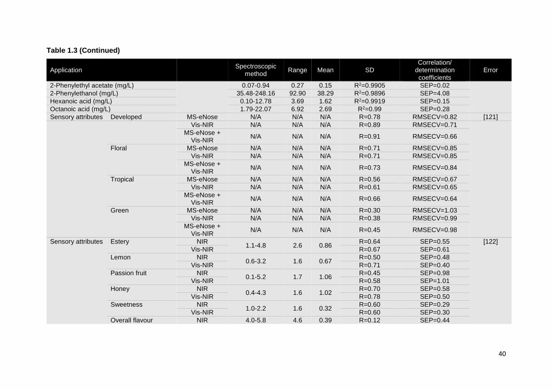
40
Table 1.3 (Continued)
Application Spectroscopic
method Range Mean SD
Correlation/ determination coefficients
Error
2-Phenylethyl acetate (mg/L) 0.07-0.94 0.27 0.15 R2=0.9905 SEP=0.02
2-Phenylethanol (mg/L) 35.48-248.16 92.90 38.29 R2=0.9896 SEP=4.08
Hexanoic acid (mg/L) 0.10-12.78 3.69 1.62 R2=0.9919 SEP=0.15
Octanoic acid (mg/L) 1.79-22.07 6.92 2.69 R2=0.99 SEP=0.28
Sensory attributes Developed MS-eNose N/A N/A N/A R=0.78 RMSECV=0.82 [121]
Vis-NIR N/A N/A N/A R=0.89 RMSECV=0.71
MS-eNose + Vis-NIR
N/A N/A N/A R=0.91 RMSECV=0.66
Floral MS-eNose N/A N/A N/A R=0.71 RMSECV=0.85
Vis-NIR N/A N/A N/A R=0.71 RMSECV=0.85
MS-eNose + Vis-NIR
N/A N/A N/A R=0.73 RMSECV=0.84
Tropical MS-eNose N/A N/A N/A R=0.56 RMSECV=0.67
Vis-NIR N/A N/A N/A R=0.61 RMSECV=0.65
MS-eNose + Vis-NIR
N/A N/A N/A R=0.66 RMSECV=0.64
Green MS-eNose N/A N/A N/A R=0.30 RMSECV=1.03
Vis-NIR N/A N/A N/A R=0.38 RMSECV=0.99
MS-eNose + Vis-NIR
N/A N/A N/A R=0.45 RMSECV=0.98
Sensory attributes Estery NIR 1.1-4.8 2.6 0.86
R=0.64 SEP=0.55 [122]
Vis-NIR R=0.67 SEP=0.61
Lemon NIR 0.6-3.2 1.6 0.67
R=0.50 SEP=0.48
Vis-NIR R=0.71 SEP=0.40
Passion fruit NIR 0.1-5.2 1.7 1.06
R=0.45 SEP=0.98
Vis-NIR R=0.58 SEP=1.01
Honey NIR 0.4-4.3 1.6 1.02
R=0.70 SEP=0.58
Vis-NIR R=0.78 SEP=0.50
Sweetness NIR 1.0-2.2 1.6 0.32
R=0.60 SEP=0.29
Vis-NIR R=0.60 SEP=0.30
Overall flavour NIR 4.0-5.8 4.6 0.39 R=0.12 SEP=0.44

41
Vis-NIR R=0.77 SEP=0.30
Fatty acid esters (g/L) NIR 2103-4483 3284 584 R2=0.74 SECV=314 [125]
Monoterpene alcohols (g/L) 0.01-246 61.3 63 R2=0.90 SECV=21
Short chain fatty acids (g/L) 14780-24900 19420 2235 R2=0.80 SECV=1658
Classification of samples from designation of origin Rías Baixas according to its sub region
Condado UV/VIS/NIR 93.33% <Correct classification< 100% [127]c)
VIS/NIR 93.33% <Correct classification< 100%
NIR 93.33% <Correct classification< 100%
Rosal UV/VIS/NIR 50% <Correct classification< 87.5%
VIS/NIR 12.5% <Correct classification< 100%
NIR 0% <Correct classification< 95.83%
Salnés UV/VIS/NIR 0% <Correct classification< 90%
VIS/NIR 10% <Correct classification< 96.67%
NIR 0% <Correct classification< 96.67%
Ribeira do Ulla UV/VIS/NIR 60% <Correct classification< 73.33%
VIS/NIR 40% <Correct classification< 46.67%
NIR 0% <Correct classification< 46.67%
Total classification UV/VIS/NIR 55.83% <Correct classification< 86.04%
VIS/NIR 40.63% <Correct classification< 82.29%
NIR 25.00% <Correct classification< 84.79%
Classifications, according to the year MIR 92% of the test correctly classified samples [128]
Classification of Commandaria MIR 87.1% <Correct recognition < 100% [129]c)
Classification of commercial Commandaria
0% <Correct recognition < 71.4%
Classification of other sweet wines 74.1% <Correct recognition < 96.2%
Classification of wine samples adulterated with industrial grade glycerol
MIR 93% <Classification accuracy = 100%
[130]c)
Classification of wine according To tannin origin (grape seeds or grape skins)
MIR 60% < correctly classified samples <97%
[133]c)
Discrimination of spoiled wines from fresh samples
MIR 94%< Recognition rate = 100%
[134]c)

42
Table 1.3 (Continued)
AAE (ascorbic acid equivalents); CE (Catechin equivalents); DPPH (1,1-diphenyl-2-picrylhydrazyl); FRAP (ferric reducing antioxidant power); GAE (gallic acid
equivalents); KMW (Klosterneuburger Mostwaage); LPP (large polymeric pigments); MS-eNose (mass spectrometry based electronic nose); N/A (information
not available); NFM (natural fermenting must); PLS (partial least squares); RMSECV (root mean square error of cross-validation); RMSEP (root mean square
error of prediction); SPP (small polymeric pigments); SD (standard deviation); SEC (standard error of calibration); SECV (standard error of cross-validation);
SEP (standard error of prediction); SM (synthetic must); TEAC (Trolox equivalent antioxidative capacity).
a) Results vary according to mathematical treatment and geographic origin;
b) Results vary according to the wine type (red, white or rose);
c) Results vary according to the chemometric techniques employed
Application Spectroscopic
method Range Mean SD
Correlation/ determination coefficients
Error
Ethanol (% v/v) (Bottled wine)
9.1-15.3 13.23 0.85 N/A SECV=0.48 [137]
Free SO2 (mg/L) (Bottled wine) 5.0-47.0 22.78 8.75 N/A SECV=4.01
Total SO2 (mg/L) (Bottled wine) 0.0-248.0 9.18 47.4 N/A SECV=28.6
pH (Bottled wine) 2.9-3.8 3.4 0.18 N/A SECV=0.15

43
1.4. Critical aspects and limitations of vibrational spectroscopy
The advantages of vibrational spectroscopic techniques have been enhanced in a large
amount of publications. Their fast, automated, cost-effective, non-destructive and
environmental-friendly character, capable of simultaneously provide a high level of
reproducibility and accuracy, has found numerous applications in several fields.
NIR, MIR and Raman spectroscopies have their own individual strengths and drawbacks.
MIR spectroscopy is apparently more suitable for wine analysis, since organic functional
groups have characteristic and well defined absorption bands in this spectral region,
consequently enabling its identification and characterization. However, most compounds
strongly absorb in this region, forcing the use of sample holders with extremely short
effective pathlength. In NIR spectroscopy, the sample holders do not need to fulfil this
demand, (the combination of low molar absorptivity and high pathlength enable the
measurement of larger sample volumes). Nevertheless, calibration procedures for
quantitative determinations are more complex and laborious, since they are extracted from
weak overtones and combination bands.
Raman spectroscopy offers a main advantage over NIR and MIR techniques in what
concerns wine analysis: as water is a weak scatterer, aqueous solutions can be analysed
without or with minimal interference from water. However, the laser source may cause the
fluorescence of some compounds, consequently affecting the signal-to-noise ratio and
reducing the sensitivity of this technique. Additionally, the sample heating caused by intense
laser radiation can destroy the sample and conceal the resulting spectrum [3].
Different equipment’s have been developed for infrared (IR) and Raman measurements,
aiming to reduce its limitations and/or increase its applicability, sensitivity and robustness.
Infrared spectrometers currently available, whether benchtop or portable devices, are
equipped with different wavelength selectors (such as diffraction grating, Fourier transform
(FT), and acousto-optical tunable filter (AOTF)), and different sampling techniques (such as
KBr pellet or attenuated total reflectance (ATR)). For Raman spectroscopy, it may also be
found a variety of instruments, mostly relying on resonance, surface-enhanced and
microscopy methods. Both IR and Raman techniques can be used for hyperspectral
imaging [4, 5].
For the proper development of robust calibration models, every step involved in the process
should be rationally analysed. Instrument specifications (such as wavelength scanning
range, wavelength data point interval, noise, stability and measurement type) should be
considered before measurements. Nonetheless, in most situations the instrument selection
is done according to its availability.

44
The sample presentation mode should be taken into account due to the effects it may have
on the resulting spectra. Some authors reported differences among the spectra of grape
berries, grape bunches, and leaves’ surface according to its presentation mode or spatial
orientation. However, this effect is commonly neglected during calibrations’ development.
Additionally, vibrational techniques are still not suitable for the assessment of some sample
presentation modes, as happens with bottled wine.
Other factors, such as grape variety and origin as well as the harvest season, must be
considered in order to increase samples’ representativeness, consequently ensuring robust
calibrations. Sampling conditions should also be contemplated when dealing with
vibrational spectroscopy, due to its sensitivity to temperature and moisture. A high number
of samples need to be included to obtain a robust calibration model. Furthermore, most
reports do not consider the error of the reference methods, nor the validation of the models
with independent data sets. Overoptimistic results are commonly reported, with no
reference to spectral interpretation, loadings, coefficients of regression and correlation
among variables [38]. Common drawbacks associated with infrared spectroscopy are
particularly enhanced when applied to wine samples. The presence of water and ethanol,
which dominate the infrared region, interferes with the determination of other minor
compounds. Additionally, the complexity of the wine matrix (containing hundreds of
chemical compounds), and the chemical similarity between wine major compounds
(resulting in similar infrared absorption features), further complicate the extraction of useful
information.
Other limitations may be associated with vibrational spectroscopic techniques: the relatively
high cost of commercially available instruments (preventing many producers to adopt this
equipment for process control), the low sensitivity of these techniques for the measurement
of minor compounds, the requirement of intensive calibration procedures, and the
dependence on specific scientific knowledge to carry out this task [24, 72-74, 84].
1.5. Conclusions and future trends
In the last decades, the application of vibrational spectroscopy in the wine industry has
considerably increased. Numerous studies reported the successful use of NIR, MIR and
Raman spectroscopies in a wide range of purposes: supporting vineyard management
practices, assuring a healthy growth of vineyard and grapes, assessing grape maturity
stages, monitoring wine fermentations, measuring wine quality parameters and sensory
attributes, and determining wine origin and authenticity. Although the use of Raman
spectroscopy, in the wine industry, is considerably lower than that of NIR and MIR
spectroscopies, the number of publications concerning this technique, has been increasing

45
in the last few years. The results achieved revealed the potential of this underexplored
technique, and suggest its suitability for further demands of the wine industry.
The successful results and the continuous improvements in hardware and software designs,
suggest that in the near future, vibrational techniques may answer effectively to any demand
of wine production chain (directly in-situ and at real-time), being implemented as routine
methods for monitoring and process control.
Wine is a very complex matrix, triggering several types of research around the world.
Consequently, the potential of vibrational spectroscopy has not been fully exhausted in this
area.


CHAPTER 2 - Chemometric methods
“Wine cheers the sad, revives the old, inspires the young, makes weariness forget his toil.”
– Lord Byron
CHAPTER 2
CHEMOMETRIC METHODS


49
2.1. Chemometrics
Spectroscopic instruments provide a huge amount of analytical information (variables) for
a large number of samples (objects), in short periods of time. The resulting multivariate data
matrices require the use of chemometric tools (mathematical and statistic procedures) in
order to effectively extract the maximum useful information and allow its proper
interpretation [143].
The application of chemometric methods for the analysis of vibrational data is commonly
divided into two main procedures:
i) Pre-processing – application of mathematical pre-treatments to facilitate the
search for useful information and decrease the influence of side information
contained in the spectra.
ii) Multivariate calibration and/or classification – development of calibration models
for quantitative analysis (through the use of regression methods capable of
linking the spectral data to quantifiable properties of the samples) and/or
classification of samples according to their spectral features [8].
2.2. Pre-processing
Vibrational spectroscopy is often affected by undesired effects that further increase the
complexity of its resulting spectra. Scattering effects (due to sample heterogeneities),
environmental conditions (for example temperature and moisture fluctuations) and
instrumental noise are the main sources of unwanted variability during spectroscopic
measurements. To attenuate or even remove those inconvenient effects, spectra are pre-
processed through the use of different mathematical treatments (which may be employed
individually or in combination depending on the intended purpose). The application of pre-
processing techniques aims to reduce unwanted variability in the data in order to enhance
the spectral features directly related with the properties of interest [144]. The selection of
the most suitable pre-processing techniques is not always easy. Applying the wrong type
could mean the removal of valuable information.
The most widely used pre-processing techniques in the NIR, MIR and Raman spectra of
wines can be divided into two different categories: scattering correction methods and
spectral derivatives.
2.2.1. Scatter corrections
The scatter correction techniques are designed to reduce the variability due to scatter
effects caused by sample heterogeneities. Two main techniques are usually considered:
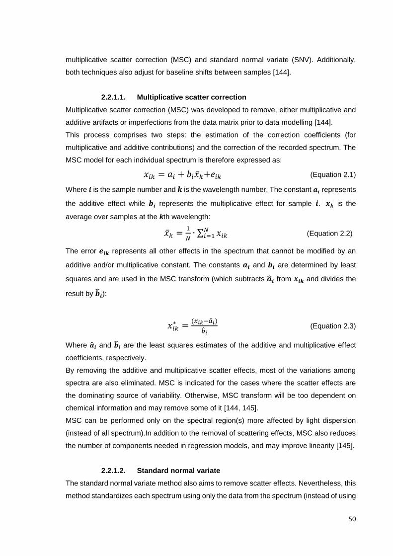
50
multiplicative scatter correction (MSC) and standard normal variate (SNV). Additionally,
both techniques also adjust for baseline shifts between samples [144].
2.2.1.1. Multiplicative scatter correction
Multiplicative scatter correction (MSC) was developed to remove, either multiplicative and
additive artifacts or imperfections from the data matrix prior to data modelling [144].
This process comprises two steps: the estimation of the correction coefficients (for
multiplicative and additive contributions) and the correction of the recorded spectrum. The
MSC model for each individual spectrum is therefore expressed as:
𝑥𝑖𝑘 = 𝑎𝑖 + 𝑏𝑖�̅�𝑘+𝑒𝑖𝑘 (Equation 2.1)
Where 𝒊 is the sample number and 𝒌 is the wavelength number. The constant 𝒂𝒊 represents
the additive effect while 𝒃𝒊 represents the multiplicative effect for sample 𝒊. �̅�𝒌 is the
average over samples at the kth wavelength:
�̅�𝑘 =1
𝑁∙ ∑ 𝑥𝑖𝑘
𝑁𝑖=1 (Equation 2.2)
The error 𝒆𝒊𝒌 represents all other effects in the spectrum that cannot be modified by an
additive and/or multiplicative constant. The constants 𝒂𝒊 and 𝒃𝒊 are determined by least
squares and are used in the MSC transform (which subtracts �̂�𝒊 from 𝒙𝒊𝒌 and divides the
result by �̂�𝒊):
𝑥𝑖𝑘∗ =
(𝑥𝑖𝑘−�̂�𝑖)
�̂�𝑖 (Equation 2.3)
Where �̂�𝒊 and �̂�𝒊 are the least squares estimates of the additive and multiplicative effect
coefficients, respectively.
By removing the additive and multiplicative scatter effects, most of the variations among
spectra are also eliminated. MSC is indicated for the cases where the scatter effects are
the dominating source of variability. Otherwise, MSC transform will be too dependent on
chemical information and may remove some of it [144, 145].
MSC can be performed only on the spectral region(s) more affected by light dispersion
(instead of all spectrum).In addition to the removal of scattering effects, MSC also reduces
the number of components needed in regression models, and may improve linearity [145].
2.2.1.2. Standard normal variate
The standard normal variate method also aims to remove scatter effects. Nevertheless, this
method standardizes each spectrum using only the data from the spectrum (instead of using

51
the mean spectrum of the spectral set, like happens with MSC). In this situation equation
2.3 becomes:
𝑥𝑖𝑘∗ =
(𝑥𝑖𝑘−𝑚𝑖)
𝑠𝑖 (Equation 2.4)
Where 𝒙𝒊𝒌 is the spectral measurement at the kth wavelength for the ith sample (as in
MSC), 𝒎𝒊 is the mean of the 𝒌 spectral measurements for sample 𝒊, and 𝒔𝒊 is the standard
deviation of the same 𝒌 measurements.
Therefore, after SNV transformation, each spectrum in centred on zero, varying roughly
from −2 to+2, on the vertical scale. The selection between the two techniques (MSC or
SNV) is usually dependent on the users’ preference or software availability [145, 146].
2.2.2. Spectral derivatives
Derivatives are commonly employed in the pre-treatment of vibrational spectra aiming to
remove additive and multiplicative effects related with base line differences. Taking the first
derivative spectrum removes an additive baseline (by calculating the slope at each point of
the original spectrum). The second derivative spectrum is the slope of the first derivative
and besides the baseline it also removes the linear trend [144, 145].However, the measured
spectrum is not a continuous curve but a series of measurements at equally-spaced discrete
points. For such data, the easiest way to calculate derivatives is to use differences between
the values at the adjacent points. Therefore, the first derivative is calculated using the
differences between adjacent points of the original spectrum and the second derivative is
performed calculating the differences between the adjacent points of the first derivative.
Although this is the simplest approach, considering the difference between values
decreases the signal-to-noise ratio. To overcome this situation, it is necessary to
incorporate some kind of smoothing in the calculation. This may be performed by basing
the previously described derivatives on the calculation of the averages over several points.
Savitzky and Golay (1964) introduced an approach that allows the calculation of the
derivatives associated with a smoothing function. The Savitzky-Golay (SG) algorithm,
defines a narrow window centred on the point of interest and performs a low-order
polynomial fit on those data points, using least-squares. This procedure is applied to all
points of the spectra moving the defined window from one point to the next one. Besides
the order of the derivative (first or second), two other parameters should be defined when
performing a SG derivative: the window size and the order of the polynomial fit. The window
size determines the number of points used in the smoothing. The choice of the window size
requires a careful balance between the reduction of the noise (better with large windows)
and distortion of the curve, (if the window is too wide). Hence, the selection of the window
52
size depends on the spectral features of the data being used. It is usually suggested to start
with three points size window (the smallest possible) and increasing its size until the noise
is not visible. The order of the polynomial fit should also be selected in accordance with the
spectral characteristics. A second order polynomial is commonly the most used. However
a third order can also be employed (and it is more flexible), it needs a wider window to
achieve the same amount of noise reduction [145].
The use of derivatives changes the form of the original spectrum, which is probably its main
disadvantage. Although in second derivatives, the peaks appear in similar locations to the
ones in the original spectrum (with opposite sign), it usually presents more features than
the original, further increasing its complexity and making difficult its interpretation [145].
2.3. Multivariate calibration and classification
Multivariate data analysis is defined as the application of mathematical or statistical
methods to chemical data, considering multiple variables simultaneously. It is, therefore,
the most suitable tool for the proper treatment of the multivariate matrices generated by
spectroscopic measurements. The application of multivariate analysis, can mathematically
describe the covariance (degree of association) between variables, or find a mathematical
function (regression model) to calculate the values of the dependent variables from values
of measured (independent) variables [147-150].
After defining the problem as clearly as possible, the next step for a proper multivariate
analysis should be the sample selection. Besides the number of samples, it is also important
to take into account the representativeness and the variability included in the sample set, in
order to improve the predictive ability of the multivariate models.
As soon as samples are selected, spectral measurements and reference analysis should
be done. The multivariate matrices generated by the spectroscopic measurements are rich
sources of information and represent a situation where several predictor variables used in
combination can give dramatically better results than any of the individual predictors used
alone. Furthermore, this type of spectral data usually presents a selectivity problem: they
are characterized by overlapped bands/signals and it is not usually possible to use
absorbance at a single wavelength to predict any property of a sample. It is, therefore,
advantageous to combine information from several, or even all, spectral variables, which is
commonly performed through the application of multivariate techniques. Due to a number
of problems, namely collinearity (the number of available samples is often smaller than the
number of variables, leading to exact linear relationship, so called exact multicollinearity,
among the variables in the data matrix) and the presence of outliers, sophisticated
approaches of these techniques are usually to be preferred.

53
Data compression based methodologies use all the information contained in spectral data,
compressing the information into a reduced number variables, and thus avoiding the
collinearity, variable selection and outlier detection problems [145].
There are currently several mathematical alternatives to reduce the number of variables.
Principal component analysis (PCA) and partial least squares (PLS) regression are among
the most commonly employed multivariate data analysis techniques based on data
compression, and will be addressed in the following sections [147, 151, 152].
2.3.1. Principal component analysis
Principal component analysis (PCA) is an exploratory technique commonly used to reveal
hidden patterns in complex data. This multivariate technique is a method of data
compression (or data reduction), since it reduces a set of possibly correlated variables into
a new set of noncorrelated variables, called principal components (PCs). PCs are linear
combinations of the original variables defined by weight vectors of unit length and
orthogonal to each other. The first PC captures as much variability as possible (it is
computed to represent the maximum variance amongst all the linear combinations). The
second PC accounts for as much of the remaining variance as possible, and the same
happens with all the successive PCs. Thus, PCA describes the main variability of
multivariate data through a modest number of variables (PCs), eliminating the redundant
information and variability due to noise.
Briefly, the mathematical procedure of PCA can be described through a set of main steps.
Let’s consider a spectral matrix X, composed by m rows (number of spectra) and n columns
(variables corresponding to the number of wavelengths at which measurements were
taken). After mean-centring the data (each variable is corrected for its average, so that it
has average equal to zero), it is determined the covariance matrix (covariance among each
pair of variables) and its corresponding eigenvectors and eigenvalues. If the original data
matrix is auto-scaled (each variable is adjusted to have an average equal to zero and unit
variance by dividing each column by its standard deviation) instead of mean-centred, it is
obtained the correlation matrix instead of the covariance matrix. Eigenvectors then become
the weight vectors for the construction of PCs and the eigenvalues are indicators of the
amount of variance captured in each PC. Eigenvectors are then ordered according to the
decreasing order of eigenvalues, such that the first PC is the one explaining the highest
amount of variability.
The selection of the appropriate number of PCs depends on the purpose of the analysis.
For exploratory studies, there is no quantitatively well-defined purpose, thus the number of
PCs is not necessarily fixed, since the interest is looking at the main variation among

54
variables, which is by definition well provided by the first PCs [153]. If PCA is used for the
detection of outliers, it is important to establish the proper number of components to use.
The outlier detection will be further discussed later in this chapter [153].
PCA is usually described in matrix notation as:
𝑿 = 𝑻𝑷𝑻 + 𝑬 (Equation 2.5)
Where X is the original data matrix, T is the scores matrix and P is the loadings matrix.
Matrix E contains the residuals and represents the noise or irrelevant variability in X. The
scores T are the linear combinations of the original variables (PCs). The loadings P are
estimated by regressing X onto T, and the residual matrix E is calculated by subtracting the
estimates of TPT from X [145]. The composition of PCs may be attributed to both scores
and loadings, since these are closely related. Nevertheless, scores represent the PCs’
composition obtained from samples, while loadings describe the information obtained from
variables [153].
Geometrically, PCA may be described as a rearrangement of axes, representing the
samples through a new system of coordinates, lower in number than the original one. Under
this point of view, the main goal of PCA is to find the directions that better explain the
maximum variability among samples, and use them as new coordinate axes. The
dimensionality of the space previously defined by n variables is reduced, maintaining the
relevant information. The orthogonality imposed between each successive PC enables its
use as coordinates. The construction of new axes is defined by the loadings (cosines of the
angles formed between the new axes and the original ones), while the scores represent the
coordinates of samples, according to the new axes. Scores are commonly represented
through scatter plots, whose axes are defined by the first PCs. This representation, enables
the easier visualization of grouping features and the consequent classification and/or outlier
detection.
2.3.2. Partial least squares regression
Partial least squares (PLS) regression is a multivariate statistical technique used to develop
regression models for the quantitative analysis of unknown samples.
PLS discards irrelevant and unstable information, using only the most relevant part of data
variability for regression purposes. This process is performed by finding a few linear
combinations (PLS components or latent variables) of the original prediction variables (like
in PCA) and use them in the regression equation [145, 154, 155]. This data compression
technique solves the multicollinearity problem, leading to more stable regression equations
and consequent predictions.
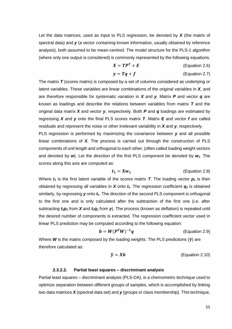
55
Let the data matrices, used as input to PLS regression, be denoted by X (the matrix of
spectral data) and y (a vector containing known information, usually obtained by reference
analysis), both assumed to be mean-centred. The model structure for the PLS-1 algorithm
(where only one output is considered) is commonly represented by the following equations.
𝑿 = 𝑻𝑷𝑻 + 𝑬 (Equation 2.6)
𝒚 = 𝑻𝒒 + 𝒇 (Equation 2.7)
The matrix T (scores matrix) is composed by a set of columns considered as underlying or
latent variables. These variables are linear combinations of the original variables in X, and
are therefore responsible for systematic variation in X and y. Matrix P and vector q are
known as loadings and describe the relations between variables from matrix T and the
original data matrix X and vector y, respectively. Both P and q loadings are estimated by
regressing X and y onto the final PLS scores matrix T. Matrix E and vector f are called
residuals and represent the noise or other irrelevant variability in X and y, respectively.
PLS regression is performed by maximizing the covariance between y and all possible
linear combinations of X. The process is carried out through the construction of PLS
components of unit length and orthogonal to each other, (often called loading weight vectors
and denoted by w). Let the direction of the first PLS component be denoted by w1. The
scores along this axis are computed as:
𝒕𝟏 = 𝑿𝒘𝟏 (Equation 2.8)
Where t1 is the first latent variable of the scores matrix T. The loading vector p1 is then
obtained by regressing all variables in X onto t1. The regression coefficient q1 is obtained
similarly, by regressing y onto t1. The direction of the second PLS component is orthogonal
to the first one and is only calculated after the subtraction of the first one (i.e. after
subtracting t1p1 from X and t1q1 from y). The process (known as deflation) is repeated until
the desired number of components is extracted. The regression coefficient vector used in
linear PLS prediction may be computed according to the following equation:
𝒃 = 𝑾(𝑷𝑻𝑾)−𝟏𝒒 (Equation 2.9)
Where W is the matrix composed by the loading weights. The PLS predictions (�̂�) are
therefore calculated as:
�̂� = 𝑿𝒃 (Equation 2.10)
2.3.2.2. Partial least squares – discriminant analysis
Partial least squares – discriminant analysis (PLS-DA), is a chemometric technique used to
optimize separation between different groups of samples, which is accomplished by linking
two data matrices X (spectral data set) and y (groups or class membership). This technique,
56
also known as PLS-2, is an extension of the PLS regression (PLS-1), capable of handling
multiple dependent categorical variables [151, 156, 157].
PLS-DA maximizes the covariance between variables from X and y-classes of highly
multidimensional data, to find a linear subspace of explanatory variables. Thus, the
prediction of the y is based on a reduced number of PLS components (LVs) that span the
subspace onto which the X variables are projected. The resulting statistical parameters,
such as loading weights, variable importance on projection, and regression coefficients, can
be used to identify the most important variables [157-159]. Additionally, this technique
enables the easy interpretation of complex data sets through low-dimensional scores plot.
Despite the successfully reported applications, PLS-DA carries out some limitations mainly
associated with the identification and selection of a small number of LVS and consequent
overoptimistic solutions [157, 160].
Overall, the PLS-DA procedure is the same of PLS regression. The main difference is that
PLS enables the quantitative analysis of samples, while PLS-DA is used for sample
classification.
2.3.2.3. Multiblock partial least squares
Multiblock partial least squares (MB-PLS) is an extension of the PLS method, that enables
the development of PLS calibration models considering simultaneously different data blocks
(i.e. sets of predictor variables). This is achieved by the development of super levels,
containing the information of scores from each individual block. The PLS Equations 2.6
and 2.7 are normally applied, however, in the MB-PLS the matrix T is a super scores matrix
(obtained by computing the block scores). The super scores matrix enables the tracking of
each individual block during analysis, and reveals each one’s contribution (or importance)
in the calibration equation [161, 162].
The MB-PLS predictions �̂� are calculated according to the method described for PLS
(Equation 2.10), after merging the data blocks into a single matrix X. (Usually, these data
blocks have the same dimension in what refers the number of objects, although they can
differ in the number of variables).
The deflation process in this situation, may be performed using the block scores or the super
scores. It is recommended to follow the super scores deflation approach in MB-PLS. The
block scores leads to inferior predictions, since some of the X information may be lost during
the deflation step [163, 164].
It is important to analyse the variance of each block individually, prior to MB-PLS calibration.
If one block has a much higher variance than the others, it will dominate the results. Hence,

57
it is necessary to give each block equal weight, which may be achieved through
normalization procedures [165].
2.3.2.4. Evaluation of PLS models' performance (figures-of-merit)
After the development of a calibration equation it is necessary to determine its ability to
predict unknown y-values. It is particularly important to decide about the suitability of the
proposed calibration model, and the inherent number of components (or latent variables)
that should be used.
Root mean square error of calibration
The root mean square error of calibration (RMSEC) is an empirical estimate of the
calibration error, defined by:
𝑹𝑴𝑺𝑬𝑪 = √∑ (�̂�𝒊−𝒚𝒊)𝟐𝑵
𝒊=𝟏
(𝑵−𝑨−𝟏) (Equation 2.11)
Where 𝒚𝒊represents the measurement results obtained for sample i, �̂�𝒊 is the result
predicted by the model for that sample, N is the number of samples and A corresponds to
the number of latent variables used for calibration.
This error estimate does not take into account the regression coefficients, which may lead
to over-optimistic estimations of the predictive ability. Essentially, RMSEC is an estimate of
the model error, rather than a prediction error. Other approaches have been suggested as
more reliable for estimating the predictive ability of the regression models, based on
validation techniques, such as cross- validation, and external validation tests.
Root mean square error of cross-validation
Cross-validation technique uses the calibration data set for calibration and validation
purposes. Samples are consecutively excluded from the calibration set. The calibration
process is performed on the remaining samples, while the excluded ones are used to test
the model. The process is repeated until all the samples have been used for testing the
calibration model. Different methods may be employed for the data split, like contiguous
blocks, random subsets, venetian blinds, and leave-one-out cross-validation. The last one,
also called full cross-validation, is one of the most commonly used. Through this technique,
each sample is individually excluded from the calibration set and posteriorly used to test the
model. The performance of the calibration model is evaluated through the root mean square
error of cross-validation (RMSECV), as defined by the following equation:
𝑹𝑴𝑺𝑬𝑪𝑽 = √∑ (�̂�𝑪𝑽,𝒊−𝒚𝒊)𝟐𝑵𝒊=𝟏
𝑵 (Equation 2.12)
58
Here �̂�𝑪𝑽,𝒊 is the estimated value for 𝒚𝒊 obtained by excluding sample i from the calibration
equation. It is important to note that RMSECV is not an estimate of an actual prediction
error, since it is not obtained from computed regression coefficients. It is rather an estimate
of the average prediction error of calibration equations based on N-1 samples.
Nevertheless, cross-validation is a useful tool for the selection of an appropriate number of
latent variables, as will be discussed later in this chapter.
Root mean square error of prediction
To ensure a truly objective evaluation of the calibration models, it is necessary to test these
models with independent data sets (not used for model calibration). It is common practice
to perform a prediction test by splitting the data set into two subsets: one for calibration and
the other for testing procedures. Usually 70% of the original sample set is used for
calibration and the remaining 30% are used for testing the developed calibration model. The
prediction ability of the models is now evaluated through the root mean square error of
prediction (RMSEP), defined as:
𝑹𝑴𝑺𝑬𝑷 = √∑ (�̂�𝒊−𝒚𝒊)𝟐𝑵𝑷
𝒊=𝟏
𝑵𝑷 (Equation 2.13)
The number of samples, included in the test set, is here represented by NP. The predicted
and measured reference values obtained for the test set correspond to �̂�𝒊 and 𝒚𝒊,
respectively.
The plot of 𝒚 versus �̂� is commonly used for a rapid evaluation of the calibration model.
Observations falling close to a 45° straight line are indicative of good calibration models.
Furthermore, it can also be used to detect the least squares effect, identifying regions with
different levels of accuracy, responsible for underestimation or overestimation problems.
Although the predictive ability of multivariate models is usually assessed by calculating the
RMSEP, it is important to note that, this rather standard procedure, has serious
weaknesses. It does not effectively include the errors associated with reference methods.
Its calculation is based on mathematical models, which does not account for the
propagation of errors associated with the reference measurements (assuming that these
are sufficiently negligible when compared with the true prediction uncertainty, which is not
always true). Thus, the resulting RMSEP value is a constant measure, generalized for all
the predictions, rather than a specific uncertainty for each individual prediction,
consequently yielding unrealistic prediction intervals [7]. Despite the abovementioned
limitations, the RMSEP calculations are still the most common way to assess the uncertainty
of regression models.
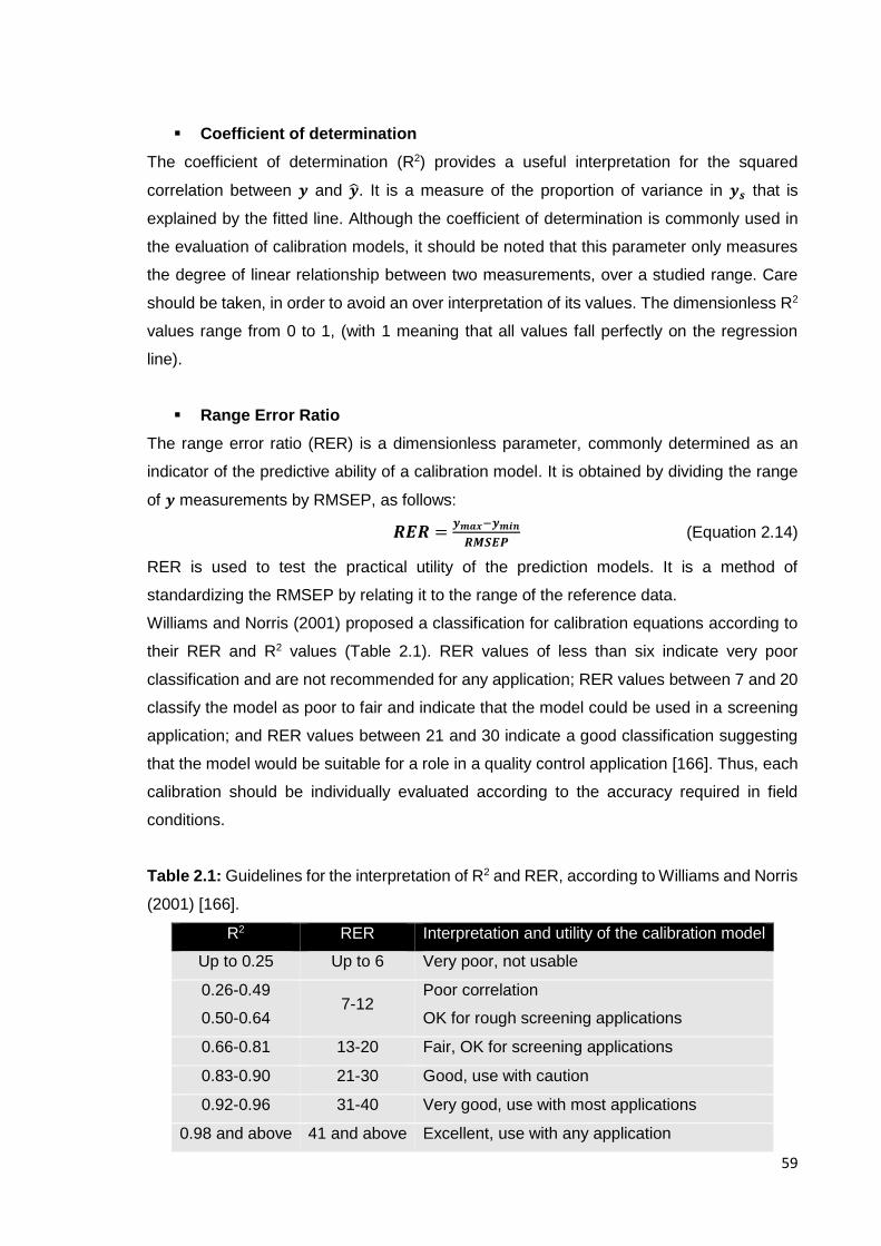
59
Coefficient of determination
The coefficient of determination (R2) provides a useful interpretation for the squared
correlation between 𝒚 and �̂�. It is a measure of the proportion of variance in 𝒚𝒔 that is
explained by the fitted line. Although the coefficient of determination is commonly used in
the evaluation of calibration models, it should be noted that this parameter only measures
the degree of linear relationship between two measurements, over a studied range. Care
should be taken, in order to avoid an over interpretation of its values. The dimensionless R2
values range from 0 to 1, (with 1 meaning that all values fall perfectly on the regression
line).
Range Error Ratio
The range error ratio (RER) is a dimensionless parameter, commonly determined as an
indicator of the predictive ability of a calibration model. It is obtained by dividing the range
of 𝒚 measurements by RMSEP, as follows:
𝑹𝑬𝑹 =𝒚𝒎𝒂𝒙−𝒚𝒎𝒊𝒏
𝑹𝑴𝑺𝑬𝑷 (Equation 2.14)
RER is used to test the practical utility of the prediction models. It is a method of
standardizing the RMSEP by relating it to the range of the reference data.
Williams and Norris (2001) proposed a classification for calibration equations according to
their RER and R2 values (Table 2.1). RER values of less than six indicate very poor
classification and are not recommended for any application; RER values between 7 and 20
classify the model as poor to fair and indicate that the model could be used in a screening
application; and RER values between 21 and 30 indicate a good classification suggesting
that the model would be suitable for a role in a quality control application [166]. Thus, each
calibration should be individually evaluated according to the accuracy required in field
conditions.
Table 2.1: Guidelines for the interpretation of R2 and RER, according to Williams and Norris
(2001) [166].
R2 RER Interpretation and utility of the calibration model
Up to 0.25 Up to 6 Very poor, not usable
0.26-0.49
0.50-0.64 7-12
Poor correlation
OK for rough screening applications
0.66-0.81 13-20 Fair, OK for screening applications
0.83-0.90 21-30 Good, use with caution
0.92-0.96 31-40 Very good, use with most applications
0.98 and above 41 and above Excellent, use with any application
60
Sometimes, in addition to RER, it is estimated the RMSEP in percentage, aiming to compare
the suitability of a calibration model for the measurement of different y-parameters. RMSEP
(%) is calculated as:
𝑹𝑴𝑺𝑬𝑷(%) =𝑹𝑴𝑺𝑬𝑷
𝒚𝒎𝒂𝒙−𝒚𝒎𝒊𝒏𝟏𝟎𝟎 (Equation 2.15)
Limit of detection
The determination of limit of detection (LOD) in multivariate calibrations is an intricate issue.
Several methods have been proposed for its calculation, based on different approaches
(net analyte signal, confidence intervals for concentration, error propagation, non-
parametric test, and univariate transformation) [167]. A reasonable estimation of this
parameter can be done by assuming that the prediction uncertainties are approximately
constant. Hence, LOD value may be calculated as three times the RMSEP value, as
described in the following equation:
𝑳𝑶𝑫 = 𝟑𝑹𝑴𝑺𝑬𝑷 (Equation 2.16)
Selectivity and Sensitivity
To complete the evaluation of the calibration model, it is important to calculate figures-of-
merit such as limit of detection, sensitivity, and selectivity. To estimate these parameters in
multivariate analytical systems, it is usually employed the net analyte signal (NAS) theory.
NAS can be mathematically defined as the vector orthogonal to the space spanned by the
interferences. Let’s represent the NAS vector of the ith sample as ri*. The sensitivity vector
s*, can be calculated as:
𝒔∗ =𝒓𝒊
∗
�̂�𝒊 (Equation 2.17)
Where to �̂�𝒊 is the value of any y-parameter, predicted by the PLS model, using a previously
defined number of LVs. The sensitivity vector is the same for all samples, even when the
measured parameters are affected by systematic and/or random errors [168]. Sensitivity
(SEN) is, therefore, defined as the NAS vector generated by an analyte of unit
concentration, and can be seen as the slope of the calibration curve [169]. Consequently, it
may be defined as the norm of NAS:
𝑺𝑬𝑵 = ‖𝒔∗‖ (Equation 2.18)
Under a practical point of view, the sensitivity characterizes the extent of signal variation,
as a function of the analyte concentration.
Selectivity is also an important figure-of-merit, commonly used to characterize the
calibration curve. It is defined as the part of measured signal unique to the analyte of

61
interest. The calculation of selectivity (SEL) is also based on the NAS theory, and may be
expressed as the ratio between the norm of r* (NAS vector), and the norm of spectra r:
𝑺𝑬𝑳 =‖𝒓∗‖
‖𝒓‖ (Equation 2.19)
Different selectivity values are obtained for each sample. In order to easily characterize the
calibration model, it is usual to calculate the average of SEL over all samples and display
that unique value as percentage.
2.3.2.5. Selection of latent variables
The selection of the appropriate number of PLS latent variables (LVs) is an essential step
in the development of robust PLS calibration models. If too many LVs are used, there is the
risk of including too much of the redundancy present in the variables. The calibration
equation will be, therefore, too data dependent leading to overfitting solutions and
consequently poor prediction results. Using too few components results in underfitting
problems, meaning that the model in not large enough to capture the important variability in
the data. Hence it is necessary to determine the predictive significance of each LV, before
its exclusion or inclusion in the calibration model. Cross-validation is a valuable tool for the
determination of the model structure. Plotting RMSECV values against the number of LVs
illustrates the behavior of the predictive ability of the model, as LVs are added. When using
this type of plot, it is common to search for the smallest value of RMSECV. However, if
increasing the number of LVs does not significantly reduce the cross-validation errors, in
this situation the lowest possible number of LVs should be selected.
2.3.3. Outlier detection
When an observation differs from the remaining data set for some reason, it may be pointed
out as an outlier. Several reasons may explain the anomalous behaviour of such
observations, as an adulterated sample, an instrumental problem, or errors caused by
failures in reference methods. An outlier is not necessarily an erroneous observation, it is
rather an observation that is different from the rest of the population, and that may strongly
influence the calibration models.
Detecting and defining an outlier within a multivariate data matrix, may be a difficult process.
The PCA model may provide useful information in this field, mainly through the analysis of
scores and residuals’ matrices. Although looking at scores plot, enables the rapid and easy
visualization of anomalous samples, it only allows its visualization for a few principal
components at a time. Additionally, it is important to look at how important the component
is, before deciding on what to do with an anomalous sample. The Hotelling’s T2 test is an
extension of the t-test that can be applied to the scores of a PCA model for the detection of
62
outliers. This technique enables the determination of 95 % confidence limits, assuming that
the scores are normally distributed. Consequently, the samples whose scores fall outside
the 95% confidence interval may be considered outliers.
The analysis of residuals may also contribute for the detection of outliers and its eventual
exclusion from the sample matrix. For that purpose it is common to use the sum of the
squared residuals (often called Q- statistics) of each sample, to look for samples that are
not well described by the PCA model. The plot of Q against T2 is known as the influence
plot, and it is a valuable tool to simultaneously analyse the contribution of scores and
residuals in the anomalous behaviour of any sample. As both Q and T2 are influenced by
the number of principal components included in the models, this number should be well
defined before the outlier analysis.
CHAPTER 3 - Determination of chloride and sulfate in wines by MIR spectroscopy
“Age is just a number. It’s totally irrelevant unless, of course, you happen to be a bottle of
wine.”
– Joan Collins
CHAPTER 3
DETERMINATION OF CHLORIDE AND SULFATE
IN WINES BY MIR SPECTROSCOPY


65
3.1. Introduction
The quality of a wine can be achieved by a perfect balance of its analytical properties and
consequent organoleptic characteristics. Therefore, from the grape constitution to the
vinification process, results a particular combination of components that will determine the
wine character [99]. Mainly composed by water, ethanol and sugars, wine also presents
several other chemical elements [170]. Among them are chloride and sulfate anions, which
are as well, important indicators in the quality assessment of wine, and like other
parameters, their concentration must obey to legal requirements. Chloride anion is naturally
present in wines, and its concentration is related to its geographical origin and
corresponding geological and climatic conditions. The frequently low chloride concentration
in wines increases when they come from vineyards located near the coast. Moreover, high
levels of chloride may also point out some fraudulent practices of filtration, stabilization
[171], clarification and organoleptic correction of wines [172].
The sulfate anion (SO42-) is also part of the natural composition of wine, but several factors
influence its concentration, like the soil composition were vines grow, the phytotreatments
to which they were exposed and enological treatments. High levels of sulfate may increase
wine astringency and protein haze formation, but it may also be an indicator of the addition
of certain compounds like copper sulfate, ammonium sulfate and sulfuric acid, aiming the
improvement of wine quality, but in some cases considered as fraudulent practices [173,
174].
Aiming to guarantee consumers’ satisfaction as well as their health protection, several
analytical procedures were developed for the assessment of wine safety and quality, in all
stages of its production, (covering also the determination of chloride and sulfate anions in
wine samples) [173, 175, 176]. However, over the time has emerged the need to develop
faster, automated and cost effective procedures, keeping at the same time a high level of
reproducibility, and accuracy. MIR spectroscopy combined with intensive calibration
procedures appears as a possible solution complying with these requirements. Despite the
large number of studies already performed, and even their implementation for routine
analysis, the potential of MIR spectroscopy has not been fully exhausted. Therefore the aim
of this work was to evaluate MIR suitability in the determination of chloride and sulfate
concentrations in wine.
3.2. Materials and methods
3.2.1. Data set
A total of 45 different wine matrices were provided by the “Vinhos Verdes” Wine Comission
in Portugal, to be the basis of the produced samples and experimental design [177]. Aiming
66
at the representativeness of a wide diversity of wines and to increase the method’s
robustness, samples were selected to include several types (white, red, rosé, sparkling),
and varieties of young wines (2012 and 2013 harvest) from different wineries, located in
different Portuguese wine regions (Douro, Dão, Vinhos Verdes).
The low concentration and variability of the parameters, increases the difficulty of
calibrations’ development. Consequently, for chloride and sulfate determination, it was
necessary to expand the original concentration ranges. For this purpose, the 45
representative wine matrices were divided in two sets of 20 and 25 samples and submitted
to controlled fortifications of chloride and sulfate respectively. For each wine matrix, five
concentration levels were selected and tested in order to respect the detection limits of the
reference methodology and the maximum values allowed by law. From the experimental
plan design, sets of 100 and 125 samples for chloride and sulfate parameters respectively,
were produced. These sets encompass enough variability for the proper construction of
predictive models and were simultaneously wide enough to include the limits established
by legal regulations (1g/L and 2 g/L for chloride and sulfate respectively) [178].
The preparation of highly concentrated standard solutions of sodium chloride (Sigma-
Aldrich, St. Louis MO, USA) and potassium sulfate (Sigma-Aldrich, St. Louis MO, USA),
ensured a minimal addition of these solutions to the original samples, thus keeping the
original matrix effects unchanged.
Despite commercial wines were used and sample pre-treatments were considered
unnecessary, to avoid the possible presence of particles and to remove CO2, all samples
were filtered and degassed prior to measurements.
3.2.2. Reference analyses
The analytical reference results, used for sulfate and chloride calibrations, were obtained
according to internal methodologies, based on segmented flow analyses and
spectrophotometric detection with uncertainties of 15% and 17% respectively. The
determination of sulfate is based in a colorimetric reaction, in which the colour intensity is
directly proportional to the increase in the analyte. After dilution in a solution of barium
chloride, the sulfate ions present in the sample, react with the barium leading to the
formation of barium sulfate precipitate. The excess of barium resulting from the reaction is
dialyzed together with the colouring reagent. The colour decrease is measured on a UV/Vis
spectrophotometer at 630 nm. Chloride determination is also based on a colorimetric
reaction. However, in this case, the sample is diluted in a solution of mercury thiocyanate,
which leads to the formation of mercury chloride and to the release of the thiocyanate ion.
In the presence of the ferric ion, the thiocyanate forms a red complex, whose colour intensity

67
is measured on a UV/Vis spectrophotometer at 490 nm. The number of samples and
measurements, as well as some details are summarised in Table 3.1.
Table 3.1: Summary of the samples produced in this work for developing the MIR
spectroscopic methodology for quantification of sulfate and chloride in wines.
Parameter Sulfate (g/L) Chloride (g/L)
Reference method Continuous flow analyses and spectrophotometric detection
Number of samples 125a) 100a)
Range 0.34 - 2.91 0.194 - 1.779
Mean 1.49 0.86
Standard deviation 0.69 0.43
a) These samples resulted from the fortification of 25 and 20 original wine matrices, for
sulfate and chloride respectively.
3.2.3. MIR analyses
MIR spectral acquisition was performed on previously filtered and degassed samples, using
a Multispec IRTF UV/Visible (CETIM, France) spectrometer and an Avatar 370 (Thermo
Nicolet Corporation, Madison, Wisconsin, USA) detector equipped with a Bacchus
Acquisition / Quantification (CETIM, France) software.
Measurements were carried out in absorbance mode from 3050 to 1000 cm-1, with a
spectral resolution of 16 cm-1, being each spectra the average result of 22 scans.
Spectra were collected through the use of a CaF2 cuvette, with an optical pathlength of 0.1
mm. Sampling was conducted with an auto-sampler, using about 10 mL of sample for a
double measurement, including preflushing of the system, at 25ºC (adjusted by a Peltier
system). Background measurements were taken against distilled water before every
session of measurements. In order to avoid errors, due to chemical modifications, minimal
periods of time elapsed between reference analyses and MIR spectra acquisition.
3.2.4. Data processing
Spectra were collected between 3050 and 1000 cm-1 (Figure 3.1). Its visual analysis
prompts for exclusion of the region between 1700 and 1570 cm-1 due to signal saturation.
In fact, other authors reported similar spectral behaviours nearly the above referred regions,
due to strong water and ethanol absorptions [10, 98, 99, 179].
The resulting spectra (comprised between 1570-1000 and 3050-1700 cm-1), was therefore
subdivided into four spectral regions in agreement with the peaks and/or weak bands
according to their disposition along the spectral wavelength. The four regions, as well as all

68
their possible combinations, were evaluated for the construction of multivariate regression
models. Several spectral pre-processing methods (SNV, MSC, and Savitzky-Golay first and
second order derivatives) were tested, whether individually or combined, to process raw
spectra aiming at removing unwanted spectral variations caused by baseline drifts, light
scattering effects and temperature variations. However, models seemed to work better
without any spectral pre-processing.
Principal Component Analysis (PCA) was applied to the mean-centred MIR spectra, in order
to detect eventual anomalous spectral behaviour. Results showed the absence of sample
grouping (indicating that no wine matrix effect is visible) consequently ensuring the diversity
of the selected samples. Identification of outliers was attempted with the Q residuals and
Hotelling’s T2 statistics, but no sample was found to be atypical [145].
Figure 3.1: Raw MIR spectra of wine samples.
3.2.5. Multivariate data analysis
Calibration models were developed for each of the proposed parameters, aiming at their
quantitative determination in wine. The calibration equations were based on the application
of Partial Least Squares (PLS) regression, whose foundation is based on the correlation of
69
spectral data with the corresponding concentration values obtained by reference methods.
The PLS-1 algorithm was used [180].
Models predictive ability was tested with independent sample sets. Each set of samples
was randomly divided in two subsets: a calibration set (composed by 70% of the original
sample set) and an independent test set (composed by the remaining 30%). This division
was made randomly but ensuring that all types of wine matrices were included in both
calibration and test sets, consequently avoiding unbalanced wine matrices in both sets. The
calibration set was composed by 70 and 87 samples while the test set included 30 and 38
samples for chloride and sulfate models, respectively. For each model, the selection of the
optimal number of latent variables (LV) was established, using the leave-one-out cross-
validation method (based only on the calibration set) [181]. The independent set was
projected onto the developed models yielding the prediction set results.
The calibration models’ accuracy was evaluated using the root mean square error of cross
validation (RMSECV). After models’ optimisation the test sets were projected and the root
mean square error of prediction (RMSEP) and coefficient of determination of prediction
(R2P) were obtained [98]. The figures-of-merit such as limit of detection (LOD), sensitivity
(SEN) and selectivity (SEL) were calculated for modeled parameters according to the net
analyte signal (NAS) theory [169, 182]. The dimensionless parameter range error ratio
(RER) was applied as a tool for evaluating the predictive ability of the PLS models.
All calculations were carried out using Matlab version 8.3 (MathWorks, Natick, MA, USA).
3.3. Results and discussion
3.3.1. Calibration procedures and statistics
As previously referred, spectra were divided in four spectral regions (as shown in Figure
3.1): region 1 (1120-1000 cm-1), region 2 (1570-1120 cm-1), region 3 (2800-1700 cm-1), and
region 4 (3050-2800 cm-1).
The PLS models’ optimisation (spectral regions and number of LVs) was performed
considering exclusively the calibration dataset and the root mean square error of cross-
validation (leave-one-out) (RMSECV) as a measure of model performance. This procedure
enabled the identification of the best regions and pre-processing techniques and the
consequent selection of the best models’ performances for each parameter. Great part of
the spectral region was considered for the calibration of both chloride and sulfate
parameters. Best performances were achieved when no pre-processing technique was
applied, after mean-centring the spectral data.

70
Table 3.2: Summary of the properties of the MIR spectroscopy based PLS regression
models for the quantification of sulfate and chloride in wines.
Regression model statistics Sulfate (g/L) Chloride (g/L)
Calibration
Spectral region (cm-1) 1000-1570,
1700-2800
1120-1570,
1700-3050
RMSEC 0.34 0.18
RMSECV 0.38 0.26
LVs 6 9
Prediction
RMSEP 0.11 0.18
R2P 0.98 0.83
RER 22.3 7.9
Figures of merit
Selectivity (%) 13.5 1.9
Sensitivitya 0.035 0.0065
LOD 0.33 0.53
a) Sensitivity values are expressed as spectral units/concentration units; LOD (limit of
detection); LVs (latent variables); RER (range error ratio); RMSEC (root mean square error
of calibration); RMSECV (root mean square error of cross validation); RMSEP (root mean
square error of prediction); R2P (coefficient of determination of prediction).
Models’ accuracy were then tested in terms of coefficient of determination (R2P) and
prediction errors (RMSEP) using the independent test sets.The accuracy of the predicting
models was classified according to the criteria proposed by Williams and Norris (2001), who
consider as good predictions those with RER values higher than 21 and R2 higher than 0.83
(see Table 2.1) [166]. According to this criteria, the model developed for the sulfate
parameter, combining the regions 1, 2 and 3, (R2P = 0.98, RMSEP=0.11 g/L, and
RER=22.3), may be considered very good in what concerns its predictive ability, making it
remarkably capable of quantitative determinations of sulfate in wines. For the chloride
parameter, the model developed considering regions 2, 3 and 4, presented the best
performance (R2P = 0.83, RMSEP=0.18 g/L, RER=7.9). These results show the suitability
of the model for screening purposes or semi-quantitative determinations of this parameter
in wines. This may provide a valuable solution when the goal is to determine if the parameter
is under the limits established by law. The PLS regression models for both parameters are
represented in Figure 3.2.
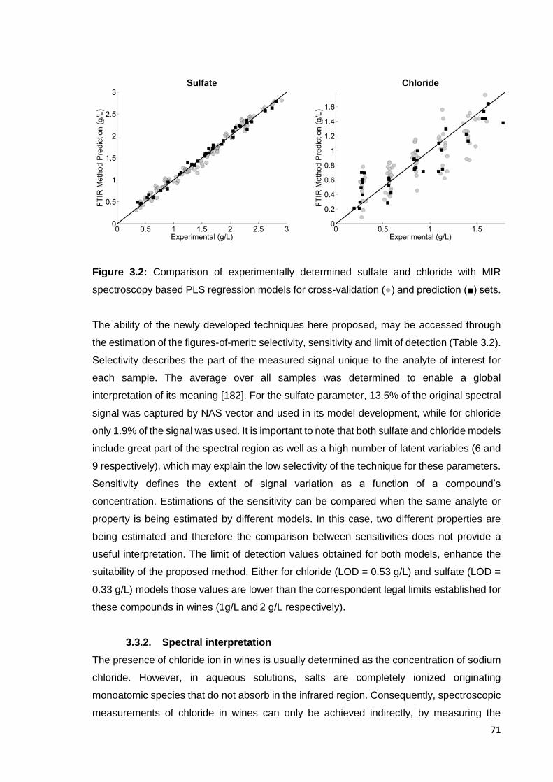
71
Figure 3.2: Comparison of experimentally determined sulfate and chloride with MIR
spectroscopy based PLS regression models for cross-validation (●) and prediction (■) sets.
The ability of the newly developed techniques here proposed, may be accessed through
the estimation of the figures-of-merit: selectivity, sensitivity and limit of detection (Table 3.2).
Selectivity describes the part of the measured signal unique to the analyte of interest for
each sample. The average over all samples was determined to enable a global
interpretation of its meaning [182]. For the sulfate parameter, 13.5% of the original spectral
signal was captured by NAS vector and used in its model development, while for chloride
only 1.9% of the signal was used. It is important to note that both sulfate and chloride models
include great part of the spectral region as well as a high number of latent variables (6 and
9 respectively), which may explain the low selectivity of the technique for these parameters.
Sensitivity defines the extent of signal variation as a function of a compound’s
concentration. Estimations of the sensitivity can be compared when the same analyte or
property is being estimated by different models. In this case, two different properties are
being estimated and therefore the comparison between sensitivities does not provide a
useful interpretation. The limit of detection values obtained for both models, enhance the
suitability of the proposed method. Either for chloride (LOD = 0.53 g/L) and sulfate (LOD =
0.33 g/L) models those values are lower than the correspondent legal limits established for
these compounds in wines (1g/L and 2 g/L respectively).
3.3.2. Spectral interpretation
The presence of chloride ion in wines is usually determined as the concentration of sodium
chloride. However, in aqueous solutions, salts are completely ionized originating
monoatomic species that do not absorb in the infrared region. Consequently, spectroscopic
measurements of chloride in wines can only be achieved indirectly, by measuring the
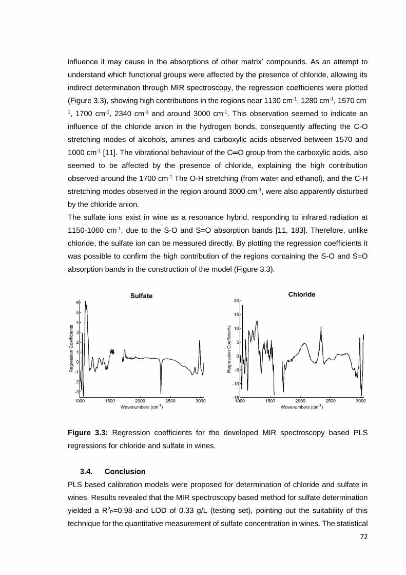
72
influence it may cause in the absorptions of other matrix’ compounds. As an attempt to
understand which functional groups were affected by the presence of chloride, allowing its
indirect determination through MIR spectroscopy, the regression coefficients were plotted
(Figure 3.3), showing high contributions in the regions near 1130 cm-1, 1280 cm-1, 1570 cm-
1, 1700 cm-1, 2340 cm-1 and around 3000 cm-1. This observation seemed to indicate an
influence of the chloride anion in the hydrogen bonds, consequently affecting the C-O
stretching modes of alcohols, amines and carboxylic acids observed between 1570 and
1000 cm-1 [11]. The vibrational behaviour of the C═O group from the carboxylic acids, also
seemed to be affected by the presence of chloride, explaining the high contribution
observed around the 1700 cm-1 The O-H stretching (from water and ethanol), and the C-H
stretching modes observed in the region around 3000 cm-1, were also apparently disturbed
by the chloride anion.
The sulfate ions exist in wine as a resonance hybrid, responding to infrared radiation at
1150-1060 cm-1, due to the S-O and S=O absorption bands [11, 183]. Therefore, unlike
chloride, the sulfate ion can be measured directly. By plotting the regression coefficients it
was possible to confirm the high contribution of the regions containing the S-O and S=O
absorption bands in the construction of the model (Figure 3.3).
Figure 3.3: Regression coefficients for the developed MIR spectroscopy based PLS
regressions for chloride and sulfate in wines.
3.4. Conclusion
PLS based calibration models were proposed for determination of chloride and sulfate in
wines. Results revealed that the MIR spectroscopy based method for sulfate determination
yielded a R2P=0.98 and LOD of 0.33 g/L (testing set), pointing out the suitability of this
technique for the quantitative measurement of sulfate concentration in wines. The statistical

73
results obtained for MIR spectroscopy based method for chloride determination, proved the
ability of the model (R2P=0.83) to ensure semi-quantitative determinations in wine.
Therefore, these calibrations emerge as a rapid, easy and low-cost solutions to support or
even replace the commonly employed reference analysis.
The power of combining MIR spectroscopy with chemometric techniques for determination
of control wine parameters was once again demonstrated in this work. Besides the ability
to provide quantitative chemical information, the MIR spectroscopy technique is also multi-
parametric meaning that multiple compounds can be estimated from a single measurement.


CHAPTER 4 - Determination of wine spoilage indicators by MIR spectroscopy
“The discovery of a wine is of greater moment than the discovery of a constellation. The
universe is too full of stars.”
– Benjamin Franklin
CHAPTER 4
DETERMINATION OF WINE SPOILAGE
INDICATORS BY MIR SPECTROSCOPY


77
4.1. Introduction
Wine is one of the most complex alcoholic beverages. Several hundreds of chemical
compounds define its character and quality. Chemical and organoleptic analyses are
usually performed to assess wine quality. Within these analyses, wine aroma seems to be
the most used and explored quality indicator. In fact, wine aroma is the result of a complex
blend of volatile molecules with their origin in the most diverse and interrelated
backgrounds: grape variety and associated terroir, microbiological pathways followed
during alcoholic and malolactic fermentations, vinification process and ageing/storage
conditions [184-186]. Therefore, besides the assessment of wine quality, the volatile
composition of wine may also provide useful information in the characterization of wines
and in the optimization of viticultural and winemaking practices.
In the last years, several studies reported an extensive number of volatile compounds
present in wine aroma, such as alcohols, acids, esters, phenols, aldehydes, thiols,
monoterpenes and ketones among others [185, 187]. Their contribution to the wine aroma
is determined by their concentration and perception threshold. Thus, only some of them are
considered as impact odorants [185, 187, 188].
At high concentrations, compounds like higher alcohols, volatile fatty acids, ethyl acetate,
acetoin and furfural are related to unpleasant sensorial characteristics in wines. These
odorants (commonly assigned as off-odors), are usually produced by yeasts or bacteria due
to unfavorable conditions during alcoholic and malolactic fermentations. Thus, it is crucial
to measure and control these aromas before they reach their odor thresholds in wine.
Higher alcohols are usually associated to the fruity character of wines. However, at high
concentrations isoamyl and isobutyl alcohols introduce strong and pungent odors, while 1-
hexanol imparts an herbaceous scent, overlapping the global aroma of wine. Volatile fatty
acids, namely butyric, isobutyric and decanoic acids, at concentrations above their odor
threshold are related to fatty, cheesy and sweaty aromas in wine. They could also present
fermentation inhibitory effects to some extent. Ethyl acetate is usually pointed out as the
most significant ester in wines, which is mainly due to its off-odor generally described as
glue or acetone-like. Acetoin (among the ketones) is considered to have flavor significance
in wine. Its presence in high concentration, contributes to the global aroma of wine by adding
a buttery smell. Furfural is an aldehyde whose presence in wine may add toasty, almond
and caramel-like tones, contributing to the baked character of wines [186, 189-192].
Thus, it is important to develop an analytical method capable of determine all these
compounds, whether individually or simultaneously, in wines. The reference procedures
used for their determination, usually require extraction techniques (such as liquid-liquid
extraction, simultaneous distillation/extraction, dynamic and static headspace sampling

78
methods and solid phase micro extraction), followed by slow, expensive and complicated
analytical procedures (gas chromatography coupled to flame ionization detector, gas
chromatography coupled to mass spectrometry and capillary gas chromatography) [193].
Additionally, the sensorial analysis commonly employed in these situations, are dependent
on a highly trained panel of sensory assessors, which can also be time-consuming and
expensive. In the worst scenario, the above mentioned compounds are only detected when
their presence in wine represents already a defect.
Therefore, the aim of this work is to develop a fast and easy method (combining MIR
spectroscopy and chemometrics) capable of measuring some of the most common off-
odors (Table 4.1) usually related with wine defects. The lower sensitivity of the MIR
technique triggered the selection of compounds with higher odor threshold values.
Consequently, isoamyl alcohol, isobutanol, 1-hexanol, butyric acid, isobutyric acid,
decanoic acid, ethyl acetate, acetoin and furfural were chosen. To the best of our knowledge
this is the first time such methods are developed for the quantitative determination of these
compounds in wine through the use of MIR spectroscopy.
Table 4.1: List of the compounds under investigation, responsible for some of the most
common off-odors in wine. Chemical formula and associated odor description [194-196].
Compound Chemical formula Odor description
Isoamyl alcohol C5H12O Cheese, burnt alcohol
Isobutanol C4H10O Fusel, alcohol, nail polish, oily, bitter, Green
1-Hexanol C6H14O Herbaceous, green, grass
Butyric acid C4H8O2 Rancid, cheese, sweat
Isobutyric acid C4H8O2 Fatty, rancid, butter, cheese
Decanoic acid C10H20O2 Fatty, rancid
Ethyl acetate C4H8O2 Fruity, solvent, balsamic
Acetoin C4H8O2 Buttery cream, flowery, wet
Furfural C5H4O2 Pungent
4.2. Materials and methods
4.2.1. Samples’ preparation
A young red wine from the Spanish DO La Rioja, was selected for the development of this
study. The wine, from the 2013 harvest, was kindly donated by Bodegas Riojanas winery
(in the north of Spain), where all the vinification process was developed and carried on. The
sample was taken directly from the cellar (in June 2015) and stored at 14ºC until analysis.

79
It was our purpose to evaluate the suitability of MIR spectroscopy to determine the
compounds under investigation: isoamyl alcohol, isobutanol, 1-hexanol, butyric acid,
isobutyric acid, decanoic acid, ethyl acetate, acetoin and furfural in wine. As a first approach,
a single wine sample was considered to avoid possible interferences related with the wine
compositional matrix. The sensory analyzes of this wine sample was performed in Bodegas
Riojanas winery and no faults were detected.
For the proper development of calibration models, each parameter’s concentration was
increased by submitting wine to controlled additions (spiking). Standard solutions of isoamyl
alcohol, isobutanol, 1-hexanol, butyric acid, isobutyric acid, decanoic acid and furfural (all
supplied by Sigma-Aldrich), ethyl acetate (supplied by Scharlau) and acetoin (supplied by
Fluka) were prepared in methanol (supplied by Sigma-Aldrich). The high concentrations of
these solutions ensured minimal additions, avoiding significant changes in the original
matrix. Previous calculations assured that added volumes always represented less than 5%
of the whole sample volume.
Wine was centrifuged at 11000 rotations per minute, during 10 minutes at a temperature
set at 10⁰C (Eppendorf centrifuge 5403 – N.Y., U.S.A.), prior to additions (spiking) and
respective MIR measurements. To ensure the reliability of this procedure, every single
volume of standard solution added to the sample was weighted.
The concentration intervals selected for each compound’s calibration, were based on their
odor threshold values. Sensory thresholds are commonly determined by adding known
concentrations of the pure compound to a model solution (usually mixtures of water,
ethanol, glycerin and tartaric acid). The resulting solutions are evaluated by trained
panelists through the triangle test. Odor threshold values established by Guth (1997) or
Ferreira (2000) are listed in Table 4.2 for each compound [197, 198].
As a first approach, and having in mind the relatively low sensitivity of MIR instruments,
concentration limits were established between one fifth of the odor threshold value and 200
mg/L for each compound. A total of 125 assays were executed. However, a first calibration
attempt of the resulting data, revealed the unsuitability of the selected interval for the
calibration of eight over the nine compounds. With the exception of isobutyric acid, for all
the other compounds it was necessary to expand the concentrations’ interval. Therefore,
new experimental designs were executed and upper concentration levels were
reestablished as 250 mg/L (for ethyl acetate and furfural), 300 mg/L (for butyric acid) and
500 mg/L (for isoamyl alcohol, isobutanol, 1-hexanol, decanoic acid and acetoin), which
resulted in the addition of 98 new measurements/samples for each compound. The
concentration ranges used for each parameter calibration as well as the respective odor
threshold and number of samples is described in Table 4.2.
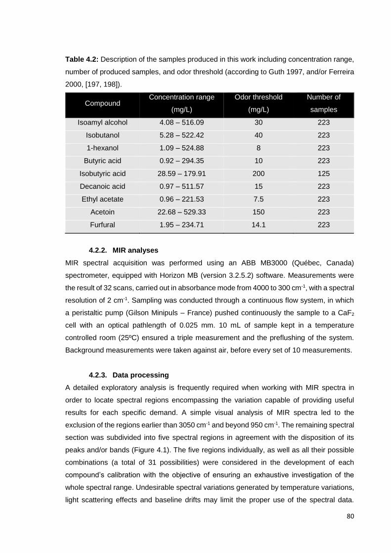
80
Table 4.2: Description of the samples produced in this work including concentration range,
number of produced samples, and odor threshold (according to Guth 1997, and/or Ferreira
2000, [197, 198]).
Compound Concentration range
(mg/L)
Odor threshold
(mg/L)
Number of
samples
Isoamyl alcohol 4.08 – 516.09 30 223
Isobutanol 5.28 – 522.42 40 223
1-hexanol 1.09 – 524.88 8 223
Butyric acid 0.92 – 294.35 10 223
Isobutyric acid 28.59 – 179.91 200 125
Decanoic acid 0.97 – 511.57 15 223
Ethyl acetate 0.96 – 221.53 7.5 223
Acetoin 22.68 – 529.33 150 223
Furfural 1.95 – 234.71 14.1 223
4.2.2. MIR analyses
MIR spectral acquisition was performed using an ABB MB3000 (Québec, Canada)
spectrometer, equipped with Horizon MB (version 3.2.5.2) software. Measurements were
the result of 32 scans, carried out in absorbance mode from 4000 to 300 cm-1, with a spectral
resolution of 2 cm-1. Sampling was conducted through a continuous flow system, in which
a peristaltic pump (Gilson Minipuls – France) pushed continuously the sample to a CaF2
cell with an optical pathlength of 0.025 mm. 10 mL of sample kept in a temperature
controlled room (25ºC) ensured a triple measurement and the preflushing of the system.
Background measurements were taken against air, before every set of 10 measurements.
4.2.3. Data processing
A detailed exploratory analysis is frequently required when working with MIR spectra in
order to locate spectral regions encompassing the variation capable of providing useful
results for each specific demand. A simple visual analysis of MIR spectra led to the
exclusion of the regions earlier than 3050 cm-1 and beyond 950 cm-1. The remaining spectral
section was subdivided into five spectral regions in agreement with the disposition of its
peaks and/or bands (Figure 4.1). The five regions individually, as well as all their possible
combinations (a total of 31 possibilities) were considered in the development of each
compound’s calibration with the objective of ensuring an exhaustive investigation of the
whole spectral range. Undesirable spectral variations generated by temperature variations,
light scattering effects and baseline drifts may limit the proper use of the spectral data.
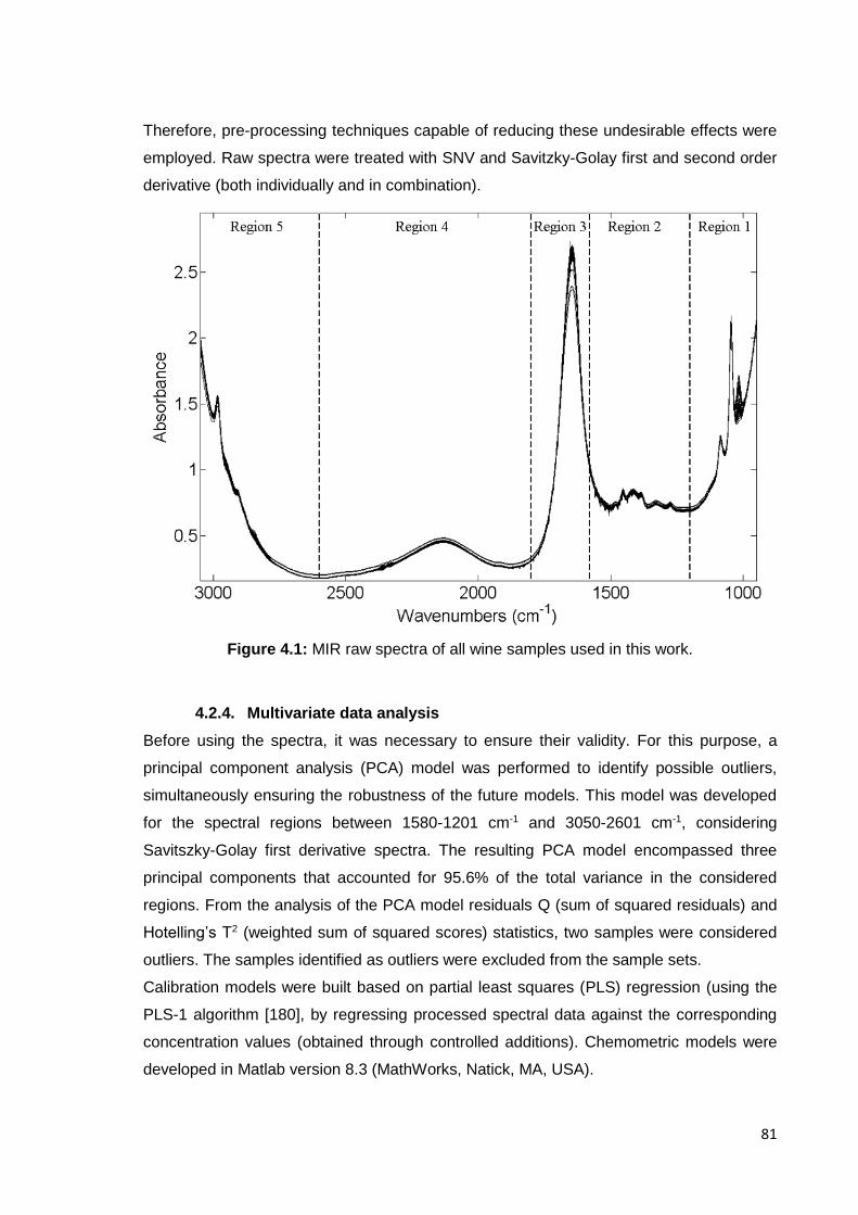
81
Therefore, pre-processing techniques capable of reducing these undesirable effects were
employed. Raw spectra were treated with SNV and Savitzky-Golay first and second order
derivative (both individually and in combination).
Figure 4.1: MIR raw spectra of all wine samples used in this work.
4.2.4. Multivariate data analysis
Before using the spectra, it was necessary to ensure their validity. For this purpose, a
principal component analysis (PCA) model was performed to identify possible outliers,
simultaneously ensuring the robustness of the future models. This model was developed
for the spectral regions between 1580-1201 cm-1 and 3050-2601 cm-1, considering
Savitszky-Golay first derivative spectra. The resulting PCA model encompassed three
principal components that accounted for 95.6% of the total variance in the considered
regions. From the analysis of the PCA model residuals Q (sum of squared residuals) and
Hotelling’s T2 (weighted sum of squared scores) statistics, two samples were considered
outliers. The samples identified as outliers were excluded from the sample sets.
Calibration models were built based on partial least squares (PLS) regression (using the
PLS-1 algorithm [180], by regressing processed spectral data against the corresponding
concentration values (obtained through controlled additions). Chemometric models were
developed in Matlab version 8.3 (MathWorks, Natick, MA, USA).
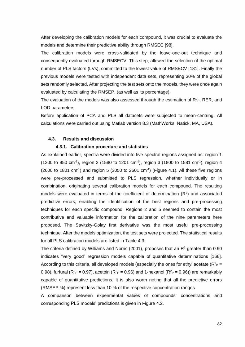
82
After developing the calibration models for each compound, it was crucial to evaluate the
models and determine their predictive ability through RMSEC [98].
The calibration models were cross-validated by the leave-one-out technique and
consequently evaluated through RMSECV. This step, allowed the selection of the optimal
number of PLS factors (LVs), committed to the lowest value of RMSECV [181]. Finally the
previous models were tested with independent data sets, representing 30% of the global
sets randomly selected. After projecting the test sets onto the models, they were once again
evaluated by calculating the RMSEP, (as well as its percentage).
The evaluation of the models was also assessed through the estimation of R2P, RER, and
LOD parameters.
Before application of PCA and PLS all datasets were subjected to mean-centring. All
calculations were carried out using Matlab version 8.3 (MathWorks, Natick, MA, USA).
4.3. Results and discussion
4.3.1. Calibration procedure and statistics
As explained earlier, spectra were divided into five spectral regions assigned as: region 1
(1200 to 950 cm-1), region 2 (1580 to 1201 cm-1), region 3 (1800 to 1581 cm-1), region 4
(2600 to 1801 cm-1) and region 5 (3050 to 2601 cm-1) (Figure 4.1). All these five regions
were pre-processed and submitted to PLS regression, whether individually or in
combination, originating several calibration models for each compound. The resulting
models were evaluated in terms of the coefficient of determination (R2) and associated
predictive errors, enabling the identification of the best regions and pre-processing
techniques for each specific compound. Regions 2 and 5 seemed to contain the most
contributive and valuable information for the calibration of the nine parameters here
proposed. The Savitzky-Golay first derivative was the most useful pre-processing
technique. After the models optimization, the test sets were projected. The statistical results
for all PLS calibration models are listed in Table 4.3.
The criteria defined by Williams and Norris (2001), proposes that an R2 greater than 0.90
indicates “very good” regression models capable of quantitative determinations [166].
According to this criteria, all developed models (especially the ones for ethyl acetate (R2P =
0.98), furfural (R2P = 0.97), acetoin (R2
P = 0.96) and 1-hexanol (R2P = 0.96)) are remarkably
capable of quantitative predictions. It is also worth noting that all the predictive errors
(RMSEP %) represent less than 10 % of the respective concentration ranges.
A comparison between experimental values of compounds’ concentrations and
corresponding PLS models’ predictions is given in Figure 4.2.

83
Table 4.3: Summary of the developed PLS models’ statistics.
Calibration Prediction
Compound Spectral region
(cm-1)
RMSEC
(mg/L)
RMSECV
(mg/L) LVs
RMSEP
(mg/L)
RMSEP
(%) R2
P RER LOD
(mg/L)
Isoamyl alcohol 1580 – 1201 48.37 50.57 3 40.35 7.9 0.92 12.2 121.1
Isobutanol 3050 – 2601 37.30 45.44 6 34.05 6.6 0.95 14.7 102.2
1-hexanol 3050 – 2601 35.76 46.03 9 31.61 6.0 0.96 16.2 94.8
Butyric acid 1580 – 1201 23.30 30.95 7 28.90 9.8 0.91 10.1 86.7
Isobutyric acid 1580 – 1201 12.85 16.69 6 12.30 8.1 0.95 12.2 36.9
Decanoic acid 1580 – 1201 49.60 52.92 4 35.78 7.0 0.94 13.8 107.4
Ethyl acetate 1580 – 1201 10.03 14.04 7 10.42 4.7 0.98 20.5 31.3
Acetoin 1580 – 1201 25.58 37.36 8 30.91 6.1 0.96 16.4 92.7
Furfural 1580 – 1201 15.92 18.80 6 12.11 5.2 0.97 19.0 36.3
LOD (limit of detection); LVs (latent variables); RER (range error ratio); RMSEC (root mean square error of calibration); RMSECV (root mean
square error of cross validation); RMSEP (root mean square error of prediction); R2P (coefficient of determination of prediction).

84
Figure 4.2: PLS regression models for cross-validation (●) and test sets (□) for isoamyl alcohol, isobutanol, 1-hexanol, butyric acid, isobutyric
acid, decanoic acid, ethyl acetate, furfural and acetoin.
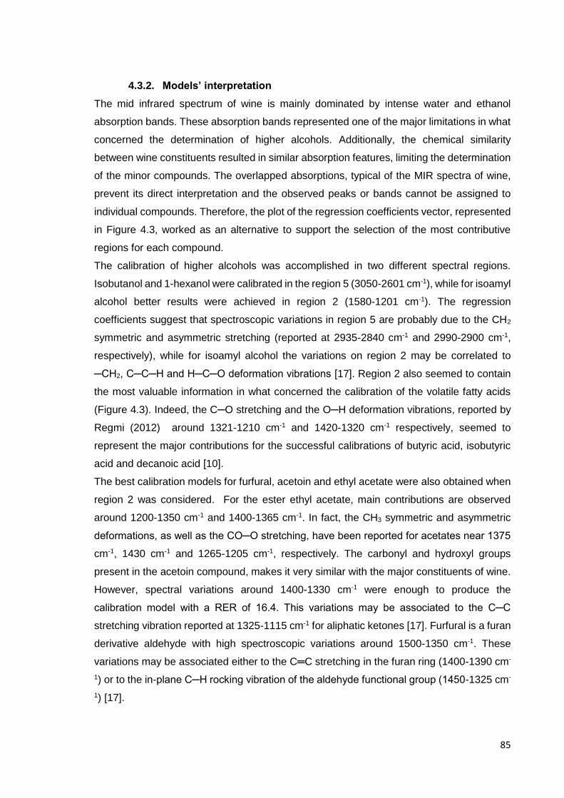
85
4.3.2. Models’ interpretation
The mid infrared spectrum of wine is mainly dominated by intense water and ethanol
absorption bands. These absorption bands represented one of the major limitations in what
concerned the determination of higher alcohols. Additionally, the chemical similarity
between wine constituents resulted in similar absorption features, limiting the determination
of the minor compounds. The overlapped absorptions, typical of the MIR spectra of wine,
prevent its direct interpretation and the observed peaks or bands cannot be assigned to
individual compounds. Therefore, the plot of the regression coefficients vector, represented
in Figure 4.3, worked as an alternative to support the selection of the most contributive
regions for each compound.
The calibration of higher alcohols was accomplished in two different spectral regions.
Isobutanol and 1-hexanol were calibrated in the region 5 (3050-2601 cm-1), while for isoamyl
alcohol better results were achieved in region 2 (1580-1201 cm-1). The regression
coefficients suggest that spectroscopic variations in region 5 are probably due to the CH2
symmetric and asymmetric stretching (reported at 2935-2840 cm-1 and 2990-2900 cm-1,
respectively), while for isoamyl alcohol the variations on region 2 may be correlated to
─CH2, C─C─H and H─C─O deformation vibrations [17]. Region 2 also seemed to contain
the most valuable information in what concerned the calibration of the volatile fatty acids
(Figure 4.3). Indeed, the C─O stretching and the O─H deformation vibrations, reported by
Regmi (2012) around 1321-1210 cm-1 and 1420-1320 cm-1 respectively, seemed to
represent the major contributions for the successful calibrations of butyric acid, isobutyric
acid and decanoic acid [10].
The best calibration models for furfural, acetoin and ethyl acetate were also obtained when
region 2 was considered. For the ester ethyl acetate, main contributions are observed
around 1200-1350 cm-1 and 1400-1365 cm-1. In fact, the CH3 symmetric and asymmetric
deformations, as well as the CO─O stretching, have been reported for acetates near 1375
cm-1, 1430 cm-1 and 1265-1205 cm-1, respectively. The carbonyl and hydroxyl groups
present in the acetoin compound, makes it very similar with the major constituents of wine.
However, spectral variations around 1400-1330 cm-1 were enough to produce the
calibration model with a RER of 16.4. This variations may be associated to the C─C
stretching vibration reported at 1325-1115 cm-1 for aliphatic ketones [17]. Furfural is a furan
derivative aldehyde with high spectroscopic variations around 1500-1350 cm-1. These
variations may be associated either to the C═C stretching in the furan ring (1400-1390 cm-
1) or to the in-plane C─H rocking vibration of the aldehyde functional group (1450-1325 cm-
1) [17].

86
Figure 4.3: Regression coefficients’ vectors for all PLS-1 models.
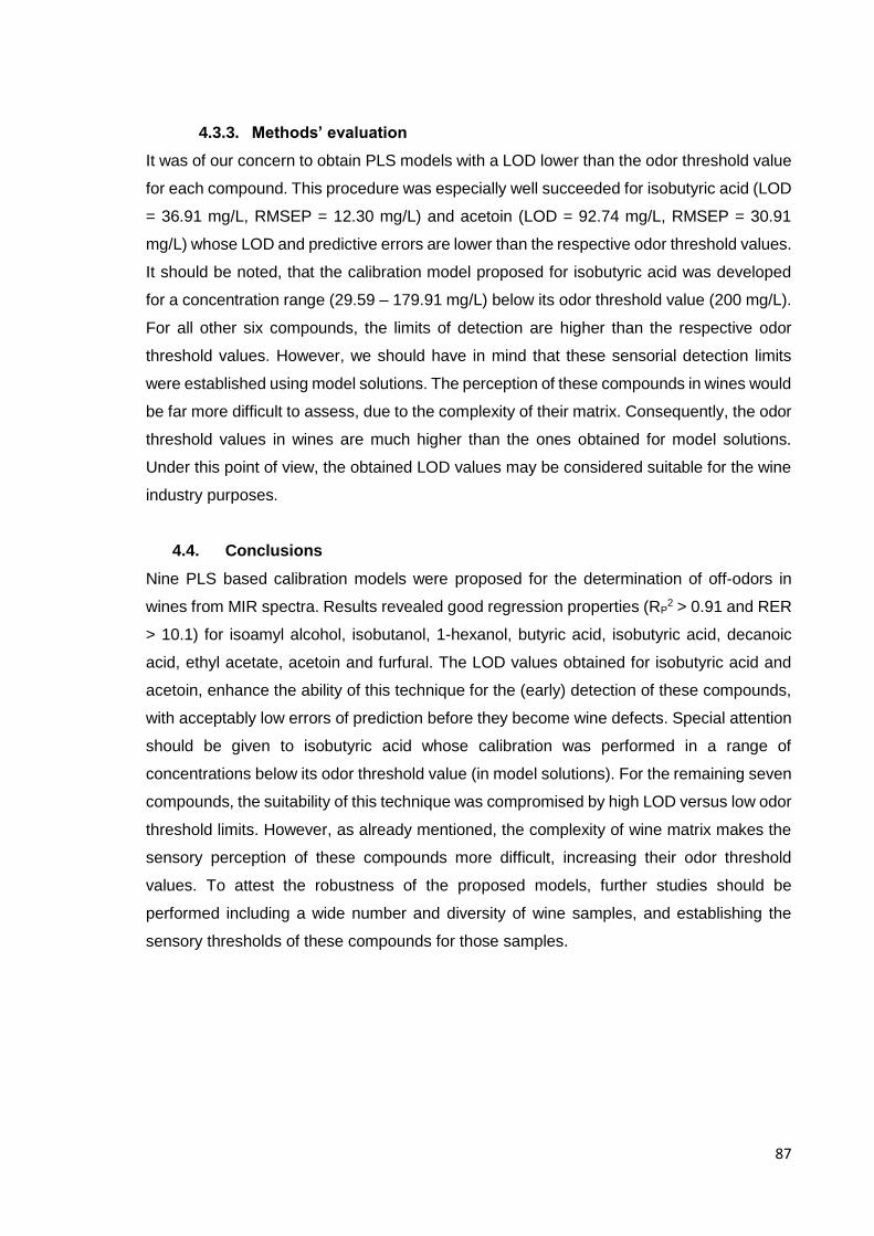
87
4.3.3. Methods’ evaluation
It was of our concern to obtain PLS models with a LOD lower than the odor threshold value
for each compound. This procedure was especially well succeeded for isobutyric acid (LOD
= 36.91 mg/L, RMSEP = 12.30 mg/L) and acetoin (LOD = 92.74 mg/L, RMSEP = 30.91
mg/L) whose LOD and predictive errors are lower than the respective odor threshold values.
It should be noted, that the calibration model proposed for isobutyric acid was developed
for a concentration range (29.59 – 179.91 mg/L) below its odor threshold value (200 mg/L).
For all other six compounds, the limits of detection are higher than the respective odor
threshold values. However, we should have in mind that these sensorial detection limits
were established using model solutions. The perception of these compounds in wines would
be far more difficult to assess, due to the complexity of their matrix. Consequently, the odor
threshold values in wines are much higher than the ones obtained for model solutions.
Under this point of view, the obtained LOD values may be considered suitable for the wine
industry purposes.
4.4. Conclusions
Nine PLS based calibration models were proposed for the determination of off-odors in
wines from MIR spectra. Results revealed good regression properties (RP2 > 0.91 and RER
> 10.1) for isoamyl alcohol, isobutanol, 1-hexanol, butyric acid, isobutyric acid, decanoic
acid, ethyl acetate, acetoin and furfural. The LOD values obtained for isobutyric acid and
acetoin, enhance the ability of this technique for the (early) detection of these compounds,
with acceptably low errors of prediction before they become wine defects. Special attention
should be given to isobutyric acid whose calibration was performed in a range of
concentrations below its odor threshold value (in model solutions). For the remaining seven
compounds, the suitability of this technique was compromised by high LOD versus low odor
threshold limits. However, as already mentioned, the complexity of wine matrix makes the
sensory perception of these compounds more difficult, increasing their odor threshold
values. To attest the robustness of the proposed models, further studies should be
performed including a wide number and diversity of wine samples, and establishing the
sensory thresholds of these compounds for those samples.

88

CHAPTER 5 - Raman spectroscopy for wine analysis: a comparison with NIR and
MIR spectroscopy
“Give me wine to wash me clean of the weather-stains of cares.”
– Ralph Waldo Emerson
CHAPTER 5
RAMAN SPECTROSCOPY FOR WINE ANALYSIS:
A COMPARISON WITH NIR AND MIR
SPECTROSCOPY

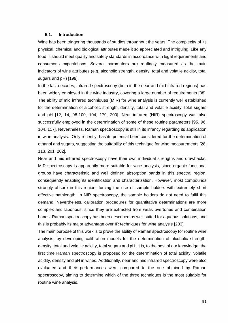
91
5.1. Introduction
Wine has been triggering thousands of studies throughout the years. The complexity of its
physical, chemical and biological attributes made it so appreciated and intriguing. Like any
food, it should meet quality and safety standards in accordance with legal requirements and
consumer’s expectations. Several parameters are routinely measured as the main
indicators of wine attributes (e.g. alcoholic strength, density, total and volatile acidity, total
sugars and pH) [199].
In the last decades, infrared spectroscopy (both in the near and mid infrared regions) has
been widely employed in the wine industry, covering a large number of requirements [38].
The ability of mid infrared techniques (MIR) for wine analysis is currently well established
for the determination of alcoholic strength, density, total and volatile acidity, total sugars
and pH [12, 14, 98-100, 104, 179, 200]. Near infrared (NIR) spectroscopy was also
successfully employed in the determination of some of these routine parameters [95, 96,
104, 117]. Nevertheless, Raman spectroscopy is still in its infancy regarding its application
in wine analysis. Only recently, has its potential been considered for the determination of
ethanol and sugars, suggesting the suitability of this technique for wine measurements [28,
113, 201, 202].
Near and mid infrared spectroscopy have their own individual strengths and drawbacks.
MIR spectroscopy is apparently more suitable for wine analysis, since organic functional
groups have characteristic and well defined absorption bands in this spectral region,
consequently enabling its identification and characterization. However, most compounds
strongly absorb in this region, forcing the use of sample holders with extremely short
effective pathlength. In NIR spectroscopy, the sample holders do not need to fulfil this
demand. Nevertheless, calibration procedures for quantitative determinations are more
complex and laborious, since they are extracted from weak overtones and combination
bands. Raman spectroscopy has been described as well suited for aqueous solutions, and
this is probably its major advantage over IR techniques for wine analysis [203].
The main purpose of this work is to prove the ability of Raman spectroscopy for routine wine
analysis, by developing calibration models for the determination of alcoholic strength,
density, total and volatile acidity, total sugars and pH. It is, to the best of our knowledge, the
first time Raman spectroscopy is proposed for the determination of total acidity, volatile
acidity, density and pH in wines. Additionally, near and mid infrared spectroscopy were also
evaluated and their performances were compared to the one obtained by Raman
spectroscopy, aiming to determine which of the three techniques is the most suitable for
routine wine analysis.
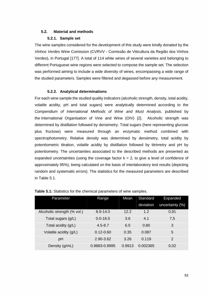
92
5.2. Material and methods
5.2.1. Sample set
The wine samples considered for the development of this study were kindly donated by the
Vinhos Verdes Wine Comission (CVRVV - Comissão de Viticultura da Região dos Vinhos
Verdes), in Portugal [177]. A total of 114 white wines of several varieties and belonging to
different Portuguese wine regions were selected to compose the sample set. The selection
was performed aiming to include a wide diversity of wines, encompassing a wide range of
the studied parameters. Samples were filtered and degassed before any measurement.
5.2.2. Analytical determinations
For each wine sample the studied quality indicators (alcoholic strength, density, total acidity,
volatile acidity, pH and total sugars) were analytically determined according to the
Compendium of International Methods of Wine and Must Analysis, published by
the International Organisation of Vine and Wine (OIV) [2]. Alcoholic strength was
determined by distillation followed by densimetry. Total sugars (here representing glucose
plus fructose) were measured through an enzymatic method combined with
spectrophotometry. Relative density was determined by densimetry, total acidity by
potentiometric titration, volatile acidity by distillation followed by titrimetry and pH by
potentiometry. The uncertainties associated to the described methods are presented as
expanded uncertainties (using the coverage factor k = 2, to give a level of confidence of
approximately 95%), being calculated on the basis of interlaboratory test results (depicting
random and systematic errors). The statistics for the measured parameters are described
in Table 5.1.
Table 5.1: Statistics for the chemical parameters of wine samples.
Parameter Range Mean Standard
deviation
Expanded
uncertainty (%)
Alcoholic strength (% vol.) 8.9-14.0 12.2 1.2 0,91
Total sugars (g/L) 0.0-16.5 3.6 4.1 7,5
Total acidity (g/L) 4.5-8.7 6.5 0.80 3
Volatile acidity (g/L) 0.12-0.60 0.35 0.087 5
pH 2.90-3.62 3.26 0.119 2
Density (g/mL) 0.9883-0.9995 0.9913 0.002365 0,02

93
5.2.3. Spectroscopic measurements
5.2.3.1. Raman spectroscopy
Raman spectral measurements were carried out using a Bruker MultiRAM Fourier transform
spectrometer (Bremen, Germany), equipped with a Ge detector cooled by a liquid nitrogen
tank, and with a 1064 nm laser source. The OPUS software package provided by Bruker
Optics (Bremen. Germany) was used for spectral acquisition. Sampling was performed
through a continuous flow system, employing a flow cell with an optical pathlength of 5 mm.
Triple measurements were performed for each sample, with the laser power set to 1000
mW, covering the wavelength range from 3500 to 50 cm-1 at a spectral resolution of 8 cm-1,
over a five minute period (corresponding to an average of 310 scans).
5.2.3.2. MIR spectroscopy
Mid infrared spectra were acquired using a Multispec IRTF UV/Visible spectrometer
(CETIM, France), coupled with an Avatar 370 detector (Thermo Nicolet Corporation,
Madison, Wisconsin, USA) and recorded through the Bacchus Acquisition/ Quantification
software (CETIM, France). The spectra of filtered and degassed samples were the result of
22 scans measured in the absorbance mode from 3010 to 950 cm-1, with a spectral
resolution of 16 cm-1. Triple measurements were performed in a CaF2 cuvette with an optical
pathlength of 0.1 mm. Sampling was made at 25 ⁰C, through an auto-sampler module
equipped with a Peltier system. Background measurements were taken against distilled
water before every session of measurements.
5.2.3.3. NIR spectroscopy
Near infrared (NIR) spectral acquisition was performed using a NIRSystems 5000
spectrophotometer, equipped with a Vision 2.22 software (Foss NIRSystems, Silver Spring,
Maryland, USA). Measurements resulted from 32 scans carried out in the absorbance mode
from 1100 to 2498 nm (9091 – 4003 cm-1) with 2 nm intervals over the wavelength range.
Sampling was carried out in a liquid analyser module through a continuous flow system
including a flow cell with 2 mm optical pathlength. To assure the reproducibility of the
spectra, three replicates were performed for each sample, and temperature was carefully
controlled and maintained at approximately 28 ⁰C. Background was taken automatically
before each measurement.
5.2.4. Data processing
The complexity of the wine matrix prevents the direct correlation between any individual
wine component and specific absorption bands, for both IR and Raman spectroscopies.

94
Therefore, the obtained spectra were explored in detail to find the spectral regions
containing useful information for the proper calibration of each specific parameter. A visual
inspection of the NIR and MIR spectra lead to the exclusion of spectral regions affected by
low signal/noise ratio and signal saturation problems, which are mainly due to the strong
water and ethanol absorptions [10, 99, 204]. Therefore, the spectral regions from 4309 to
4003 cm-1 and 5434 to 4546 cm-1 were not considered for NIR calibration purposes, and the
one comprised between 1700 and 1500 cm-1 was excluded from the MIR spectra. As
Raman spectroscopy is not affected by the presence of water, no saturation problems were
visualized, thus the whole spectrum was considered for the development of calibration
models.
After calculating each average spectrum (resulting from each set of three replicates), a
principal component analysis (PCA) was performed for NIR, MIR, and Raman spectra, in
order to detect and identify eventual outliers. In the PCA model developed for Raman
spectra, three principal components captured 97.73 % of the total variance. According to Q
residuals and Hotelling’s T2 statistics, two samples were considered outliers and removed
from the sample set. Two principal components accounted for 98.05 % of the total variance
captured from NIR spectra. Q residuals and Hotelling’s T2 statistics enabled the exclusion
of two outliers. For MIR spectra, 95.11 % of the total variance was explained by two principal
components and two samples were eliminated in accordance with the Q residuals and
Hotelling’s T2 statistics.
After the exclusion of the six samples considered as outliers, the resulting sample set
(composed by 108 samples for NIR, MIR and Raman measurements) was randomly divided
in two subsets: a calibration set and a test set. Therefore, 70% of the samples were used
in the construction of the calibration models, and the remaining 30% were employed for
testing the model’s performance.
Aiming to find the spectral region more suitable for the calibration of each parameter, NIR,
MIR and Raman spectra were divided in four spectral regions, as represented in Figure 5.1.
For each spectroscopic technique, the four individual regions, as well as all their possible
combinations (a total of 15 possibilities), were considered for calibration procedures.
Unwanted spectral variations, were corrected by applying pre-processing techniques.
Savitzky-Golay first and second order derivatives, and SNV were tested (whether
individually or combined), in each of the three spectral sets (NIR, MIR and Raman). The
pre-processing techniques and spectral regions that originated the models with the lowest
cross-validation errors are described in Table 5.2 for each parameter and for each
spectroscopic technique.

95
Figure 5.1: Raw spectra of wine samples obtained by a) Raman, b) MIR and c) NIR
spectroscopy, and correspondent wavelength division.

96
5.2.5. Multivariate data analysis
The correlation between spectral data and the results obtained by reference analysis was
performed through the application of PLS regression, using the PLS-1 algorithm [180]. The
number of latent variables (LVs) was evaluated by cross-validation (leave-one-out), and
through the minimization of the RMSECV. This procedure was carried out through a
commitment between the RMSECV and the number of latent variables. Finally, these
models were tested by projecting the test set. The RMSEP and the coefficient of
determination of prediction (R2P) were subsequently determined, being considered the best
indicators of the model’s predictive ability. Additionally, the range error ratio (RER) was also
estimated. This dimensionless parameter enabled an easier and direct comparison of NIR,
MIR and Raman performances. The performance of the three proposed techniques was
also evaluated for each parameter through the estimation of figures-of-merit such as limit
of detection (LOD), sensitivity (SEN) and selectivity (SEL). LOD was defined as three times
the RMSEP. SEN and SEL were calculated using the net analyte signal (NAS) theory [169,
182].
All calculations were carried out using Matlab version 8.3 (MathWorks, Natick, MA, USA)
and the PLS Toolbox version 5.5.1 (Eigenvector Research, Inc., WA, USA).
5.3. Results and discussion
5.3.1. Spectral analyses
As previously referred, several spectral regions (Figure 5.1) and pre-processing techniques
were combined and tested, resulting in the development of 90 calibration models for each
compositional parameter and technique (NIR, MIR and Raman). The evaluation of these
models was performed through the estimation of RMSECV, which enabled the identification
of the best spectral regions and pre-processing techniques (Tables 5.2, 5.3, and 5.4).
5.3.1.1. Raman spectroscopy
For Raman spectroscopy based models, better calibrations were achieved in the regions
3501-2803 and 1796-57 cm-1, and apparently these are the ones containing more
information. Combining these regions, originated the best calibration models for alcoholic
strength. Different vibrational modes, related to the ─CH2 and ─CH3 groups of ethanol, have
already been reported, such as C─H stretching vibrations (originating bands around 2885,
2934 and 2980 cm-1) and H─C─H bending modes (responsible for the band near 1455 cm-
1) [27, 28]. The bands at 1087 and 1048 cm-1 (mainly caused by the C─O stretching, and
─CH3 rocking vibrations) have also been associated with the presence of ethanol [27, 28].
However, the most characteristic band of ethanol is usually assigned to the C─C stretching
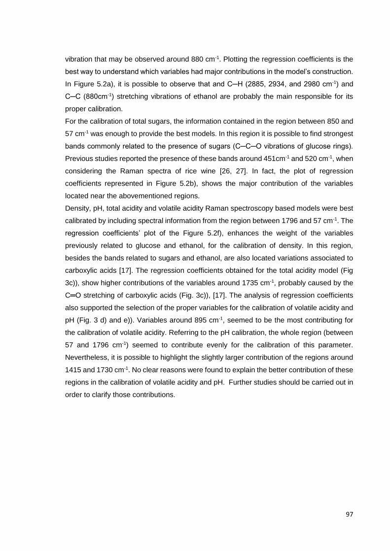
97
vibration that may be observed around 880 cm-1. Plotting the regression coefficients is the
best way to understand which variables had major contributions in the model’s construction.
In Figure 5.2a), it is possible to observe that and C─H (2885, 2934, and 2980 cm-1) and
C─C (880cm-1) stretching vibrations of ethanol are probably the main responsible for its
proper calibration.
For the calibration of total sugars, the information contained in the region between 850 and
57 cm-1 was enough to provide the best models. In this region it is possible to find strongest
bands commonly related to the presence of sugars (C─C─O vibrations of glucose rings).
Previous studies reported the presence of these bands around 451cm-1 and 520 cm-1, when
considering the Raman spectra of rice wine [26, 27]. In fact, the plot of regression
coefficients represented in Figure 5.2b), shows the major contribution of the variables
located near the abovementioned regions.
Density, pH, total acidity and volatile acidity Raman spectroscopy based models were best
calibrated by including spectral information from the region between 1796 and 57 cm-1. The
regression coefficients’ plot of the Figure 5.2f), enhances the weight of the variables
previously related to glucose and ethanol, for the calibration of density. In this region,
besides the bands related to sugars and ethanol, are also located variations associated to
carboxylic acids [17]. The regression coefficients obtained for the total acidity model (Fig
3c)), show higher contributions of the variables around 1735 cm-1, probably caused by the
C═O stretching of carboxylic acids (Fig. 3c)), [17]. The analysis of regression coefficients
also supported the selection of the proper variables for the calibration of volatile acidity and
pH (Fig. 3 d) and e)). Variables around 895 cm-1, seemed to be the most contributing for
the calibration of volatile acidity. Referring to the pH calibration, the whole region (between
57 and 1796 cm-1) seemed to contribute evenly for the calibration of this parameter.
Nevertheless, it is possible to highlight the slightly larger contribution of the regions around
1415 and 1730 cm-1. No clear reasons were found to explain the better contribution of these
regions in the calibration of volatile acidity and pH. Further studies should be carried out in
order to clarify those contributions.

98
Figure 5.2: Raman spectroscopy regression coefficients, for the developed PLS models of a) alcoholic strength; b) total sugars; c) total acidity;
d) volatile acidity; e) pH and f) density, based on Raman spectroscopy.
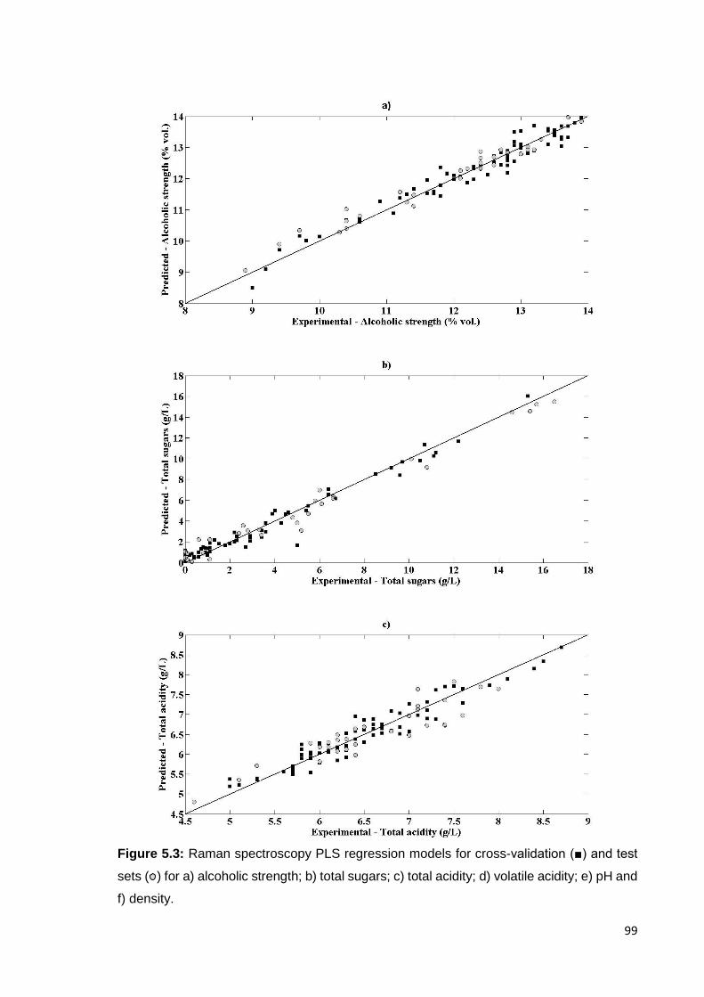
99
Figure 5.3: Raman spectroscopy PLS regression models for cross-validation (■) and test
sets ( ) for a) alcoholic strength; b) total sugars; c) total acidity; d) volatile acidity; e) pH and
f) density.

100
Figure 5.3 (continued): Raman spectroscopy PLS regression models for cross-validation
(■) and test sets ( ) for a) alcoholic strength; b) total sugars; c) total acidity; d) volatile
acidity; e) pH and f) density.
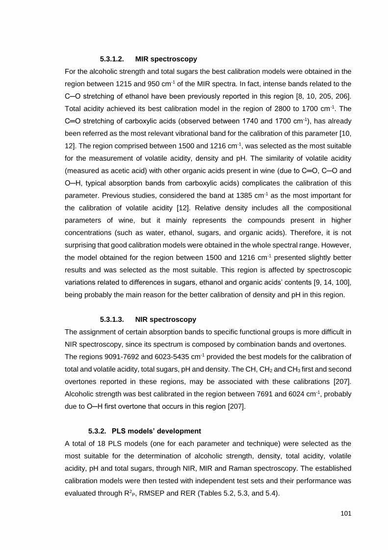
101
5.3.1.2. MIR spectroscopy
For the alcoholic strength and total sugars the best calibration models were obtained in the
region between 1215 and 950 cm-1 of the MIR spectra. In fact, intense bands related to the
C─O stretching of ethanol have been previously reported in this region [8, 10, 205, 206].
Total acidity achieved its best calibration model in the region of 2800 to 1700 cm-1. The
C═O stretching of carboxylic acids (observed between 1740 and 1700 cm-1), has already
been referred as the most relevant vibrational band for the calibration of this parameter [10,
12]. The region comprised between 1500 and 1216 cm-1, was selected as the most suitable
for the measurement of volatile acidity, density and pH. The similarity of volatile acidity
(measured as acetic acid) with other organic acids present in wine (due to C═O, C─O and
O─H, typical absorption bands from carboxylic acids) complicates the calibration of this
parameter. Previous studies, considered the band at 1385 cm-1 as the most important for
the calibration of volatile acidity [12]. Relative density includes all the compositional
parameters of wine, but it mainly represents the compounds present in higher
concentrations (such as water, ethanol, sugars, and organic acids). Therefore, it is not
surprising that good calibration models were obtained in the whole spectral range. However,
the model obtained for the region between 1500 and 1216 cm-1 presented slightly better
results and was selected as the most suitable. This region is affected by spectroscopic
variations related to differences in sugars, ethanol and organic acids’ contents [9, 14, 100],
being probably the main reason for the better calibration of density and pH in this region.
5.3.1.3. NIR spectroscopy
The assignment of certain absorption bands to specific functional groups is more difficult in
NIR spectroscopy, since its spectrum is composed by combination bands and overtones.
The regions 9091-7692 and 6023-5435 cm-1 provided the best models for the calibration of
total and volatile acidity, total sugars, pH and density. The CH, CH2 and CH3 first and second
overtones reported in these regions, may be associated with these calibrations [207].
Alcoholic strength was best calibrated in the region between 7691 and 6024 cm-1, probably
due to O─H first overtone that occurs in this region [207].
5.3.2. PLS models’ development
A total of 18 PLS models (one for each parameter and technique) were selected as the
most suitable for the determination of alcoholic strength, density, total acidity, volatile
acidity, pH and total sugars, through NIR, MIR and Raman spectroscopy. The established
calibration models were then tested with independent test sets and their performance was
evaluated through R2P, RMSEP and RER (Tables 5.2, 5.3, and 5.4).

102
Table 5.2: Summary of the developed PLS models for Raman spectroscopy.
Alcoholic
strength (% vol.)
Total sugars
(g/L)
Total acidity
(g/L)
Volatile acidity
(g/L) pH
Density
(g/mL)
Spectral region (cm-1) 3501-2803;
1796-57 847-57 1796-57 1796-851 1796-57 1796-57
Pre-processing None None None None None None
RMSEC 0.263 0.710 0.216 0.0476 0.0378 0.000410
RMSECV 0.304 0.912 0.330 0.0934 0.0581 0.000507
LVs 4 5 7 7 7 5
RMSEP 0.255 0.845 0.320 0.0746 0.0354 0.000529
RMSEP (%) 5.01 5.12 7.62 15.6 4.92 4.72
R2P 0.956 0.967 0.901 0.592 0.902 0.964
RER 20.0 19.5 13.1 6.43 20.3 21.2
LOD 0.766 2.53 0.960 0.224 0.106 0.00159
SENa) 0.00268 0.000356 0.000916 0.00309 0.00506 1.45
SEL (%) 22.6 10.3 3.28 1.68 2.53 11.7
a) Sensitivity values are expressed as spectral units/concentration units; LOD (limit of detection); LVs (latent variables); RER (range error ratio);
RMSEC (root mean square error of calibration); RMSECV (root mean square error of cross validation); RMSEP (root mean square error of
prediction); R2P (coefficient of determination of prediction); SEL (selectivity); SEN (sensitivity).

103
Table 5.3: Summary of the developed PLS models for MIR spectroscopy.
Alcoholic
strength (% vol.)
Total sugars
(g/L)
Total acidity
(g/L)
Volatile acidity
(g/L) pH
Density
(g/mL)
Spectral region (cm-1) 1215-950 1215-950 2800-1700 1500-1216 1500-1216 1500-1216
Pre-processing None None None None None None
RMSEC 0.069 0.684 0.0964 0.0234 0.0295 0.000228
RMSECV 0.0862 0.817 0.107 0.0326 0.0331 0.000288
LVs 5 4 4 10 4 5
RMSEP 0.0809 0.661 0.101 0.0422 0.0446 0.000289
RMSEP (%) 1.59 4.01 2.42 8.78 6.20 2.58
R2P 0.997 0.974 0.985 0.879 0.915 0.989
RER 63.1 24.9 41.4 11.4 16.1 38.8
LOD 0.243 1.98 0.304 0.126 0.134 0.000866
SENa) 0.0274 0.00760 0.0201 0.00842 0.0544 3.00
SEL (%) 20.2 16.72 21.6 1.65 11.8 11.6
a) Sensitivity values are expressed as spectral units/concentration units; LOD (limit of detection); LVs (latent variables); RER (range error ratio);
RMSEC (root mean square error of calibration); RMSECV (root mean square error of cross validation); RMSEP (root mean square error of
prediction); R2P (coefficient of determination of prediction); SEL (selectivity); SEN (sensitivity).
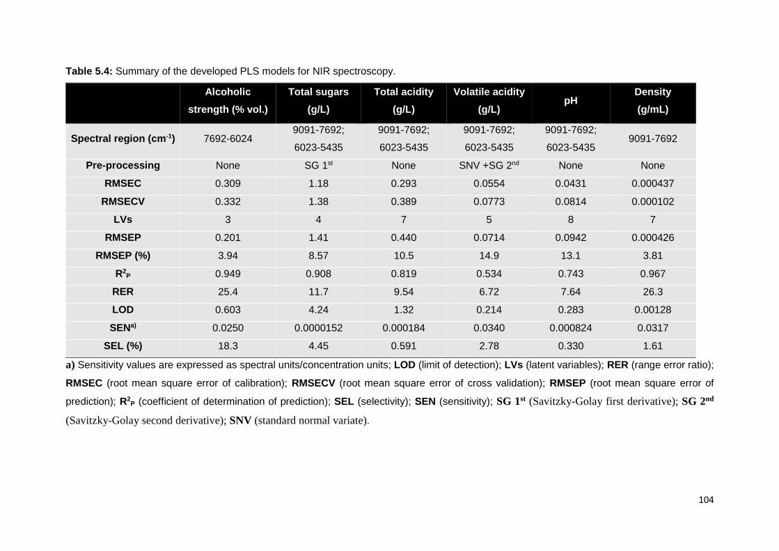
104
Table 5.4: Summary of the developed PLS models for NIR spectroscopy.
Alcoholic
strength (% vol.)
Total sugars
(g/L)
Total acidity
(g/L)
Volatile acidity
(g/L) pH
Density
(g/mL)
Spectral region (cm-1) 7692-6024 9091-7692;
6023-5435
9091-7692;
6023-5435
9091-7692;
6023-5435
9091-7692;
6023-5435 9091-7692
Pre-processing None SG 1st None SNV +SG 2nd None None
RMSEC 0.309 1.18 0.293 0.0554 0.0431 0.000437
RMSECV 0.332 1.38 0.389 0.0773 0.0814 0.000102
LVs 3 4 7 5 8 7
RMSEP 0.201 1.41 0.440 0.0714 0.0942 0.000426
RMSEP (%) 3.94 8.57 10.5 14.9 13.1 3.81
R2P 0.949 0.908 0.819 0.534 0.743 0.967
RER 25.4 11.7 9.54 6.72 7.64 26.3
LOD 0.603 4.24 1.32 0.214 0.283 0.00128
SENa) 0.0250 0.0000152 0.000184 0.0340 0.000824 0.0317
SEL (%) 18.3 4.45 0.591 2.78 0.330 1.61
a) Sensitivity values are expressed as spectral units/concentration units; LOD (limit of detection); LVs (latent variables); RER (range error ratio);
RMSEC (root mean square error of calibration); RMSECV (root mean square error of cross validation); RMSEP (root mean square error of
prediction); R2P (coefficient of determination of prediction); SEL (selectivity); SEN (sensitivity); SG 1st (Savitzky-Golay first derivative); SG 2nd
(Savitzky-Golay second derivative); SNV (standard normal variate).

105
Raman spectroscopy is here proposed for the first time for the determination of total acidity,
volatile acidity, density and pH in wines. Considering the lower intensity of its absorption
bands, (when compared to NIR or MIR spectroscopy), good results were achieved for all
parameters except for volatile acidity. Following the criteria proposed by Williams and Norris
(2001), very good results were obtained for alcoholic strength, sugars, and density (R2P >
0.95). This observation was supported by the range error ratios (RER > 20.00), and
predictive errors (RMSEP < 7.62%). Poor models were obtained for volatile acidity, leading
to the conclusion that this method is not suitable for the quantitative prediction of this
parameter in wine. The PLS regression models developed using Raman spectroscopy are
represented in Figure 5.3.
Overall, the uncertainties associated with the reference methods (Table 5.1), are lower than
the prediction errors (RMSEP %) obtained by PLS calibrations (Tables 5.2, 5.3, and 5.4).
However, the predictive errors resulting from MIR based PLS models developed for total
acidity and total sugars (RMSEP = 2.42 and 4.01%, respectively) are lower than the
uncertainties associated with the respective reference methods (3% and 7.5%). The same
happens with the Raman based PLS model developed for total sugars. The RMSEP %
value obtained for this parameter (RMSEP = 5.12%) is lower than the uncertainty of the
reference method (7.5%).
MIR spectroscopy originated good predictive models for all the compositional parameters.
This technique proved to be remarkably suitable for the quantitative determination of total
acidity, total sugars, alcoholic strength and density (R2P > 0.97, RMSEP < 4.01% and RER
> 24.95). The worst predictive results were obtained for volatile acidity and pH.
Nevertheless, in both situations the predictive errors (RMSEP) are lower than 10% of the
reference range, and the coefficients of determination close to 0.90. Overall, results
demonstrate the accuracy of this vibrational technique, pointing out its excellent
performance for wine analysis.
As expected, the calibration procedures involving NIR spectra were complicated by the
strong water absorption features and by the weak overtones and combination bands.
Consequently, the performance of NIR spectroscopy was lower than the one obtained by
MIR. Still, this technique demonstrated high ability for the quantitative assessment of
alcoholic strength and density (R2P > 0.95, RMSEP<3.94% and RER>25.39), as well as for
the determination of total sugars (R2P = 0.91, RMSEP = 8.57% and RER = 11.67). Results
pointed out the unsuitability of NIR spectroscopy for the measurement of total acidity,
volatile acidity and pH (R2P < 0.74, RMSEP > 10.48% and RER < 9.54).
The three spectroscopic techniques employed in this work originated better results for the
alcoholic strength, total sugars and density calibrations, as it may be observed through the
106
plot of RER values represented in Figure 5.4. In fact, these parameters refer to compounds
present in higher concentrations in wines. Consequently, the major contributions of those
compounds to the spectral information favors the correlation between reference and
spectral data. Volatile acidity (measured as acetic acid concentration) was the parameter
with the poorest results achieved, by the three techniques. Its relatively low concentration
in wines and its chemical similarity with other major compounds make this parameter very
difficult to correlate with the spectral data.
Although the models obtained from MIR spectroscopy presented better results for all the
studied parameters, Raman spectroscopy provided surprisingly good results. The RMSEP
values achieved for total acidity, total sugars and pH models through Raman spectroscopy,
are considerably lower than the ones obtained by NIR spectroscopy. Moreover, it must be
noted that the Raman spectroscopy based model developed for pH determination provided
the lowest prediction error, even when compared to MIR spectroscopy (RMSEP = 0.0354,
0.0446 and 0.0942 for Raman, MIR and NIR spectroscopy, respectively).
Although Raman spectroscopy may be considered as the less sensitive technique among
the others, it offers the advantage of being less sensitive to the presence of water in wine
samples. As strong water and ethanol absorption bands commonly dominate the IR spectra
of wine, (complicating the determination of other compounds), Raman spectroscopy is a
good alternative to avoid the interference of these wine major components.
5.1.1. Methods’ evaluation
The estimation of figures of merit such as limit of detection, sensitivity and selectivity,
supported the evaluation and comparison of the three spectroscopic techniques evaluated
in this work. The results obtained for these parameters are listed in Tables 5.2, 5.3, and
5.4.The MIR based models presented the lowest limits of detection for all parameters,
except for pH. As previously discussed, Raman based models seem to be the most
indicated for accurate determinations of pH in wine. The sensitivity values indicate the
extent of signal variation as a response to any change in a compound’s concentration. This
means that high sensitivity values correspond to more sensitive techniques. MIR based
models presented the highest values of sensitivity for almost all parameters. However,
those values rely on the conditions of each models' development (particularly on the number
of LV), consequently, direct comparisons between techniques should not be done.
Selectivity, usually represents the amount of signal that is uniquely devoted to the modelling
of a given parameter. Although selectivity values were determined for each wine sample
individually, the values here presented are an average over all samples (displayed as
percentage). The regions included between 1796 and 57 cm-1 were the ones selected for

107
the calibration of all the proposed parameters by Raman spectroscopy. Much of the signal
contained in this range was used in the calibration of alcoholic strength (SEL = 22.6%).
Total sugars and density models also used significant amounts of signal (around 10 and
12%, respectively). The calibration of the remaining compounds received only between 1.7
and 3.3% of the signal. For MIR based models, total acidity received the major contribution
of the signal (SEL = 22 %), being the only parameter calibrated in the region between 2800
and 1700 cm-1. Similar amounts of signal were used for the development of density and pH
models (SEL =11.6 and 11.8 respectively) in the region comprised between 1500 and 1216
cm-1. Only 1.6% of the signal in this region was dedicated to the calibration of volatile acidity,
enhancing the lower selectivity of this technique for the measurement of this parameter.
Total sugars and alcoholic strength were modelled using 16.7 and 20.2 % of the signal
included in the region 1215-950 cm-1, respectively. For NIR spectroscopy, alcoholic strength
(the only parameter calibrated in the region 7691-6024 cm-1), received 18.3 % of the signal
contained in this region. Small percentages of the signal contained in the regions 9091-
7692 and 6023-5435 cm-1 were used for the calibration of total and volatile acidity, total
sugars, pH and density (SEL = 0.59, 2.8, 4.4, 0.33 and 1.6% respectively).
Figure 5.4: Comparison of the range error ratio (RER) values obtained from NIR, MIR and
Raman based calibration models for alcoholic strength, total sugars, total acidity, volatile
acidity, pH and density.
0
10
20
30
40
50
60
70
Alcoholic
strength
Total sugars Total acidity Volatile acidity pH Density
RE
R
NIR
MIR
Raman

108
5.2. Conclusions
Raman spectroscopy based methodologies were here proposed for the first time for the
quantitative determination of several parameters, usually considered indicators of wine
quality. This technique originated good results for the quantitative assessment of alcoholic
strength, total acidity, density, pH and total sugars, (with RMSEP values below 7.62 % and
R2P above 0.901 for all parameters). Poor models were obtained for the determination of
volatile acidity, indicating that this method is not suitable for the quantitative prediction of
this parameter in wine. The comparison of this newly proposed technique with NIR and MIR
spectroscopy, demonstrated the best performance of MIR spectroscopy over NIR and
Raman. Nevertheless, the Raman based model developed for pH showed the lowest
prediction error (RMSEP = 0.0354, 0.0446 and 0.0942 for Raman, MIR and NIR
spectroscopy, respectively), suggesting this technique as the most suitable for accurate
predictions of this parameter in wines.
Raman spectroscopy is still underexplored in the wine industry when compared with the
other studied techniques. However, this work proved the suitability and potential of this
technique to accurately determine several parameters in wine through a single
measurement.

CHAPTER 6 - Merging vibrational spectroscopic data for wine classification
acording to the geographic origin
“There are thousands of wines that can take over our minds. Don't think all ecstasies are the
same!”
– Jalaluddin Rumi
CHAPTER 6
MERGING VIBRATIONAL SPECTROSCOPIC
DATA FOR WINE CLASSIFICATION ACCORDING
TO THE GEOGRAPHIC ORIGIN

111
6.1. Introduction
Wine is a complex mixture of hundreds of chemical compounds, present at several levels
of concentrations. There are several factors responsible for the composition of this so
appreciated beverage, namely: the geographical origin, the selection of grape varieties and
harvesting timing, the fermentation process (inherently associated with the presence of
specific yeasts and bacterial strains), storage and aging conditions, as well as the overall
winemaking procedures [208]. Currently, most of these factors can be carefully controlled
in order to increase or decrease the presence of certain chemical compounds, consequently
reinforcing the organoleptic qualities of wine. Still, wines present unique characteristics that
are essentially due to its geographical origin and its associated terroir. Geographical
classification systems emerged as an indicator of wine authenticity, and are currently
established in most wine producing countries [22]. The denomination of Origin (DO) is the
classification form commonly used to identify wines whose individuality and originality are
inextricably linked to a particular region. To benefit from this designation, the entire
production process is regulated by strict guidelines imposed by official authorities.
Moreover, to attest the origin and authenticity of wines, their compositional profile is usually
evaluated through sensory and chemical analysis [209]. Several physicochemical
parameters have been considered indicators of wines’ origin. These parameters, are mainly
associated with the presence of phenolic compounds [210-212], amino acids and biogenic
amines [210, 213], minerals and trace elements [214-217], and with the volatile composition
of the wines [218-220]. High-performance liquid chromatography (HPLC), mass
spectrometry (MS), gas-liquid chromatography (GLC), and atomic absorption spectroscopy
(AAS), are the most commonly used techniques to assess wines’ geographical origin [209].
However, these methods have significant limitations: they are time-consuming, expensive
and laborious. Thus, the possibility of being replaced by fast, non-destructive, easy
operated and environmental friendly procedures is welcomed. Vibrational spectroscopic
techniques, such as near infrared (NIR), mid infrared (MIR) and Raman spectroscopy, have
been increasingly used over the last decades, since they enable the direct measurement of
wine samples with minimum or no sample preparation [3].
Indeed, in the last decades, vibrational spectroscopy and chemometrics have been applied
for the classification of wines according to their geographical origins [221]. Several works
were published, highlighting near infrared (NIR) and mid infrared (MIR) spectroscopy as
powerful tools for the discrimination of wine samples from different geographical indications
[112, 127, 128, 136, 209, 222-225]. Although the classification ability of Raman
spectroscopy has been recently reported [226], the potential of this technique has not yet
been deeply explored.

112
The aim of this study was to evaluate and compare the potential of vibrational spectroscopic
techniques (NIR, MIR and Raman), used individually or in combination, for the classification
of wines according to their geographic origin. Tests were performed on samples from four
different Portuguese wine regions through the application of partial least squares
discriminant analysis (PLS-DA).
6.2. Material and methods
6.2.1. Sample set
A total of 97 white wine samples were kindly donated by the Vinhos Verdes Wine Comission
(CVRVV - Comissão de Viticultura da Região dos Vinhos Verdes), located in the north of
Portugal [227]. All samples come from the 2015 harvest and belong to four different
Portuguese wine regions: 33 samples from Vinhos Verdes, 49 samples from Lisboa, 5
samples from Távora-Varosa and 10 samples from Açores. All samples were filtered and
degassed before spectroscopic measurements.
The number of samples per group is not properly balanced. The Távora-Varosa and Açores
groups are considerably smaller than the other two groups, and are not sufficient to include
adequate variability or to ensure the representativeness of the groups in question. However,
the number of samples was inevitably limited by their availability. Therefore, the work was
developed under a feasibility point of view.
6.2.2. Spectroscopic measurements
6.2.2.1. Raman spectroscopy
Raman spectra were acquired using a Bruker MultiRAM Fourier transform spectrometer
(Bremen, Germany), equipped with a Ge detector cooled by a liquid nitrogen tank, and
controlled by the OPUS software package (Bruker Optics, Bremen, Germany). A laser
source of 1064 nm power with 1000 mW was used. For each wine, three measurements
were obtained using a spectral resolution of 8 cm-1, in the wavelength range from 3500 to
50 cm-1. Each spectrum is the average of 310 scans (each measurement took
approximately five minutes). Sampling was conducted through a continuous flow system,
using a flow cell with 5 mm optical pathlength.
6.2.2.2. NIR spectroscopy
A NIRSystems 5000 spectrophotometer, controlled by the Vision 2.22 software (Foss
NIRSystems, Silver Spring, Maryland, USA), was used for the acquisition of near infrared
(NIR) data. Measurements were carried out in transmittance mode from 1100 to 2500 nm
(9091 – 4000 cm-1), with 2 cm-1 intervals over the wavelength range, being each spectra the

113
average result of 32 scans. A liquid analyzer module, coupled to the spectrophotometer,
and equipped with a 2 mm optical pathlength flow cell was used for sampling wines.
Measurements were performed ensuring a continuous flow system of the sample system.
The reproducibility of the spectral information was assured by triple measurements for each
sample and by controlling the measurement temperature maintaining it to approximately
28⁰C. Background measurements were taken, with the empty cell, automatically before
each measurement.
6.2.2.3. MIR spectroscopy
Mid infrared spectral measurements were carried out using a Multispec IRTF UV/Visible
spectrometer (CETIM, France), coupled with an Avatar 370 detector (Thermo Nicolet
Corporation, Madison, Wisconsin, USA) controlled by the Bacchus Acquisition/
Quantification software (CETIM, France). Each spectrum was the average of 22 scans,
collected in transmittance mode, from 3050 to 950 cm-1, with a spectral resolution of 16 cm-
1. An auto-sampler module, equipped with a Peltier system, ensured that sampling was
conducted at 25 ⁰C. For each sample, three replicates were measured, using a CaF2 cuvette
with an optical pathlength of 0.1 mm. Backgrounds were recorded against distilled water.
Table 6.1: Division of the NIR, MIR and Raman spectra in spectral regions.
Spectral regions (cm-1)
Raman NIR MIR
R1 303-57 9091-7704 3009-2800
R2 847-307 7692-6031 2796-2152
R3 1796-851 6024-5721 2148-1697
R4 2799-1800 5714-5441 1500-1219
R5 3501-2803 4550-4310 1215-953
Excluded regions None 5435-4554
4307-4003 1693-1504
6.2.3. Data processing and multivariate data analysis
The spectral data was analysed with Matlab version 8.3 (MathWorks, Natick, MA, USA) and
with the PLS Toolbox version 5.5.1 (Eigenvector Research, Inc., WA, USA).
The replicate measurements (taken with NIR, MIR, and Raman for each sample) were
reduced to the average spectrum.
Light scattering effects, baseline shifts, background noise and temperature oscillations are
usually responsible for unwanted spectral variations [127]. Baseline correction and light

114
scattering effects were minimized applying Savitzky-Golay first and second order
derivatives [228] and standard normal variate (SNV) normalization [229], both individually
and in combination. The spectral sets were mean centered, before multivariate data
analysis.
To better explore the spectral features associated with each spectroscopic technique, the
spectral ranges were divided into five spectral regions according to Table 6.1 (see Figure
6.1). The five spectral regions, as well as all their possible combinations, were evaluated.
The spectral areas affected by signal saturation problems (mainly caused by the high
concentrations of water and ethanol) and low signal-to-noise ratio were not considered for
classification purposes (Table 6.1).
An exploratory analysis was performed through the application of principal component
analysis (PCA) [145], aiming at the detection of possible outliers and clusters. The
agglomeration of samples according to geographical origin has not been verified in any of
the three sets of spectra (NIR, MIR and Raman). The exploratory analysis of NIR spectra
included the spectral regions from 9091 to 5441 cm-1 and 4550 to 4310 cm-1, resulting in
99.8% of the total variance captured by seven principal components (PC). Three samples
were considered outliers according to the Q residuals and Hotteling’s T2 statistics. For MIR
spectra, the PCA was applied in the spectral range from 3009 to 1697 cm-1 and 1500 to 953
cm-1. In this situation, two principal components accounted for 95.7% of the total variance.
According to Q residuals and Hotteling’s T2 statistics, three samples exhibited an abnormal
behaviour and were pointed out as outliers. The PCA of the Raman spectra comprised the
spectral range between 3501 and 57 cm-1, and three principal components explained 97.8%
of the total variance. Q residuals and Hotteling’s T2 statistics lead to the exclusion of three
samples.
Classification models were based on PLS-DA, using the PLS-2 algorithm [156]. PLS-DA is
a supervised classification method that aims to correlate the spectral data with a set of
known responses (geographic origins) [230].For the development of PLS-DA models, 70%
of the samples were used for calibration and the remaining 30% were used for testing the
models. Although the division of the samples was made randomly, it was ensured that the
proportion of samples from each class was evenly distributed among the calibration and
test groups.
An exhaustive evaluation of the five spectral regions, as well as all their possible
combinations (31 different possibilities) was performed. Simultaneously, six possible
combinations of the pre-processing techniques above mentioned were applied to each of
the 31 spectral ranges. Therefore, for each set of spectra (NIR, MIR and Raman), 186 PLS-
DA classification models were developed and evaluated, enabling the optimization of the
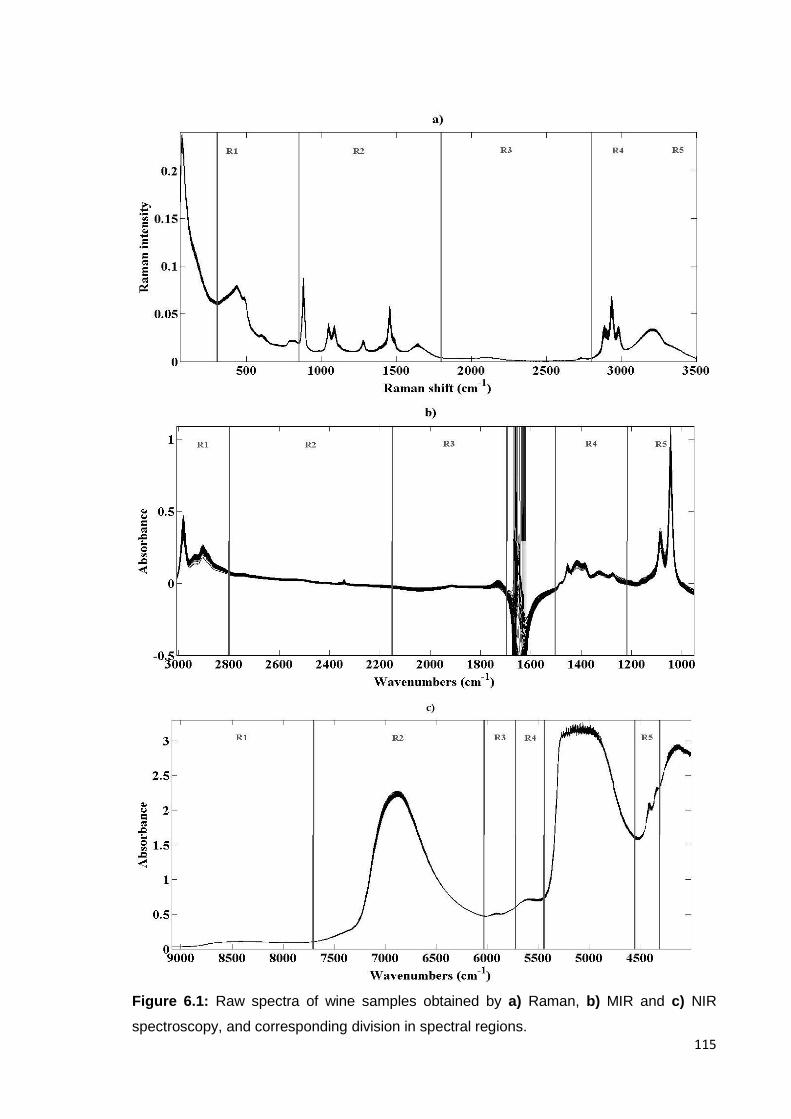
115
Figure 6.1: Raw spectra of wine samples obtained by a) Raman, b) MIR and c) NIR
spectroscopy, and corresponding division in spectral regions.
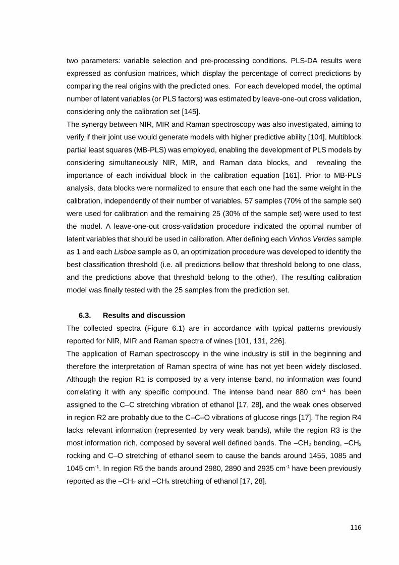
116
two parameters: variable selection and pre-processing conditions. PLS-DA results were
expressed as confusion matrices, which display the percentage of correct predictions by
comparing the real origins with the predicted ones. For each developed model, the optimal
number of latent variables (or PLS factors) was estimated by leave-one-out cross validation,
considering only the calibration set [145].
The synergy between NIR, MIR and Raman spectroscopy was also investigated, aiming to
verify if their joint use would generate models with higher predictive ability [104]. Multiblock
partial least squares (MB-PLS) was employed, enabling the development of PLS models by
considering simultaneously NIR, MIR, and Raman data blocks, and revealing the
importance of each individual block in the calibration equation [161]. Prior to MB-PLS
analysis, data blocks were normalized to ensure that each one had the same weight in the
calibration, independently of their number of variables. 57 samples (70% of the sample set)
were used for calibration and the remaining 25 (30% of the sample set) were used to test
the model. A leave-one-out cross-validation procedure indicated the optimal number of
latent variables that should be used in calibration. After defining each Vinhos Verdes sample
as 1 and each Lisboa sample as 0, an optimization procedure was developed to identify the
best classification threshold (i.e. all predictions bellow that threshold belong to one class,
and the predictions above that threshold belong to the other). The resulting calibration
model was finally tested with the 25 samples from the prediction set.
6.3. Results and discussion
The collected spectra (Figure 6.1) are in accordance with typical patterns previously
reported for NIR, MIR and Raman spectra of wines [101, 131, 226].
The application of Raman spectroscopy in the wine industry is still in the beginning and
therefore the interpretation of Raman spectra of wine has not yet been widely disclosed.
Although the region R1 is composed by a very intense band, no information was found
correlating it with any specific compound. The intense band near 880 cm-1 has been
assigned to the C–C stretching vibration of ethanol [17, 28], and the weak ones observed
in region R2 are probably due to the C–C–O vibrations of glucose rings [17]. The region R4
lacks relevant information (represented by very weak bands), while the region R3 is the
most information rich, composed by several well defined bands. The –CH2 bending, –CH3
rocking and C–O stretching of ethanol seem to cause the bands around 1455, 1085 and
1045 cm-1. In region R5 the bands around 2980, 2890 and 2935 cm-1 have been previously
reported as the –CH2 and –CH3 stretching of ethanol [17, 28].
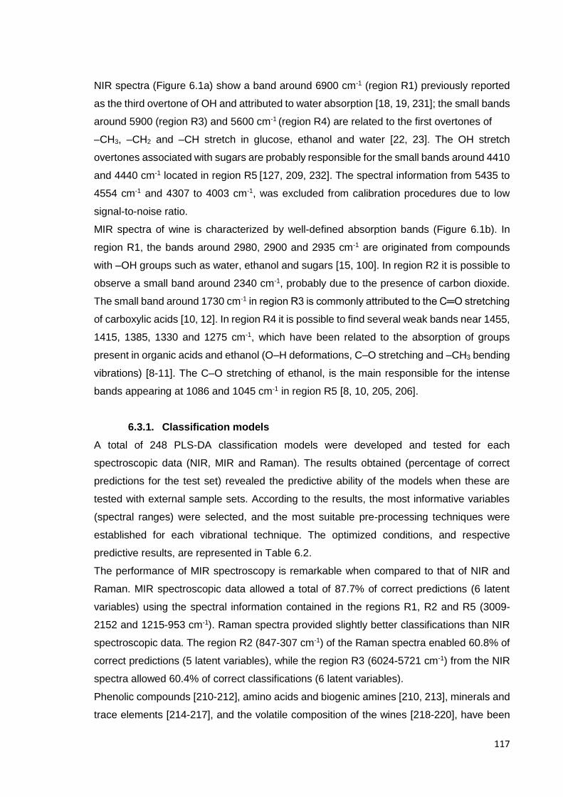
117
NIR spectra (Figure 6.1a) show a band around 6900 cm-1 (region R1) previously reported
as the third overtone of OH and attributed to water absorption [18, 19, 231]; the small bands
around 5900 (region R3) and 5600 cm-1 (region R4) are related to the first overtones of
–CH3, –CH2 and –CH stretch in glucose, ethanol and water [22, 23]. The OH stretch
overtones associated with sugars are probably responsible for the small bands around 4410
and 4440 cm-1 located in region R5 [127, 209, 232]. The spectral information from 5435 to
4554 cm-1 and 4307 to 4003 cm-1, was excluded from calibration procedures due to low
signal-to-noise ratio.
MIR spectra of wine is characterized by well-defined absorption bands (Figure 6.1b). In
region R1, the bands around 2980, 2900 and 2935 cm-1 are originated from compounds
with –OH groups such as water, ethanol and sugars [15, 100]. In region R2 it is possible to
observe a small band around 2340 cm-1, probably due to the presence of carbon dioxide.
The small band around 1730 cm-1 in region R3 is commonly attributed to the C═O stretching
of carboxylic acids [10, 12]. In region R4 it is possible to find several weak bands near 1455,
1415, 1385, 1330 and 1275 cm-1, which have been related to the absorption of groups
present in organic acids and ethanol (O–H deformations, C–O stretching and –CH3 bending
vibrations) [8-11]. The C–O stretching of ethanol, is the main responsible for the intense
bands appearing at 1086 and 1045 cm-1 in region R5 [8, 10, 205, 206].
6.3.1. Classification models
A total of 248 PLS-DA classification models were developed and tested for each
spectroscopic data (NIR, MIR and Raman). The results obtained (percentage of correct
predictions for the test set) revealed the predictive ability of the models when these are
tested with external sample sets. According to the results, the most informative variables
(spectral ranges) were selected, and the most suitable pre-processing techniques were
established for each vibrational technique. The optimized conditions, and respective
predictive results, are represented in Table 6.2.
The performance of MIR spectroscopy is remarkable when compared to that of NIR and
Raman. MIR spectroscopic data allowed a total of 87.7% of correct predictions (6 latent
variables) using the spectral information contained in the regions R1, R2 and R5 (3009-
2152 and 1215-953 cm-1). Raman spectra provided slightly better classifications than NIR
spectroscopic data. The region R2 (847-307 cm-1) of the Raman spectra enabled 60.8% of
correct predictions (5 latent variables), while the region R3 (6024-5721 cm-1) from the NIR
spectra allowed 60.4% of correct classifications (6 latent variables).
Phenolic compounds [210-212], amino acids and biogenic amines [210, 213], minerals and
trace elements [214-217], and the volatile composition of the wines [218-220], have been

118
considered the indicators of wines’ origin. In fact, it has been previously linked the presence
of phenolic compounds with spectral signals in the region from 1680 to 900 cm-1 of the MIR
spectra [15], which matches the region R5 selected for the development of the MIR
classification model. Nevertheless, the main spectral regions selected as the most suitable
for the development of the classification models are apparently the ones caused by
vibrations in ethanol and sugars.
Table 6.2: PLS-DA models for the classification of wine samples according to geographic
origin. The optimal number of latent variables was previously established by leave-one-out
cross-validation. The percentage of correct predictions correspond to models tested with
independent data sets.
Classification of samples from: Açores, Lisboa, Távora-Varosa, and Vinhos Verdes
Spectroscopic
technique
Spectral
region
Pre-processing
technique LVs
Correct predictions
(%)
Raman R2 SNV 5 60.8
NIR R3 SNV 6 60.4
MIR R1 + R2 + R5 SG 2nd + SNV 6 87.7
Classification of samples from: Lisboa and Vinhos Verdes
Raman R3 + R4 + R5 SNV + SG 1st 4 76.6
NIR R3 + R4 SNV 5 78.0
MIR R1 + R2 + R5 SG 2nd + SNV 5 91.1
LVs (latent variables); SG 1st (Savitzky-Golay first derivative); SG 2nd (Savitzky-Golay
second derivative); SNV (standard normal variate).
The confusion matrices corresponding to the NIR, MIR and Raman PLS-DA models
previously described, are summarized in Tables 6.3, 6.4, and 6.5. The sum of the diagonal
elements of the confusion matrices correspond to the overall percentage of correct
predictions. The percentage of each sample type in the global sample group can be
obtained by adding the elements of each line. Through the analysis of the diagonal elements
it is possible to conclude that the information provided by MIR spectroscopy is the most
suitable for the classification of the four origins. The information obtained by Raman
spectroscopy, did not provide a clear separation between wines from Vinhos Verdes and
Lisboa. Additionally, most of the Távora-Varosa wines were misclassified (being predicted
as Lisboa wines). Same evidence was found for NIR based models, which led to the poor
classification of a great percentage of Lisboa samples (wrongly classified as being from
Vinhos Verdes, Açores and Távora-Varosa regions).
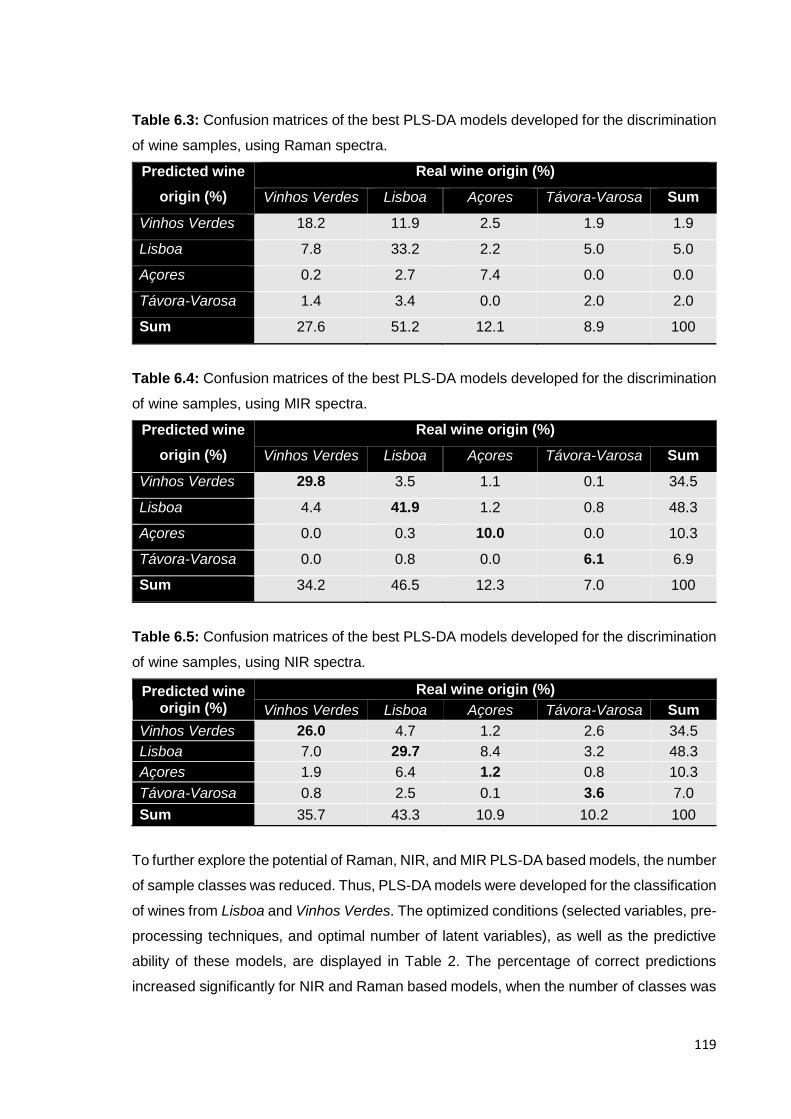
119
Table 6.3: Confusion matrices of the best PLS-DA models developed for the discrimination
of wine samples, using Raman spectra.
Predicted wine
origin (%)
Real wine origin (%)
Vinhos Verdes Lisboa Açores Távora-Varosa Sum
Vinhos Verdes 18.2 11.9 2.5 1.9 1.9
Lisboa 7.8 33.2 2.2 5.0 5.0
Açores 0.2 2.7 7.4 0.0 0.0
Távora-Varosa 1.4 3.4 0.0 2.0 2.0
Sum 27.6 51.2 12.1 8.9 100
Table 6.4: Confusion matrices of the best PLS-DA models developed for the discrimination
of wine samples, using MIR spectra.
Predicted wine
origin (%)
Real wine origin (%)
Vinhos Verdes Lisboa Açores Távora-Varosa Sum
Vinhos Verdes 29.8 3.5 1.1 0.1 34.5
Lisboa 4.4 41.9 1.2 0.8 48.3
Açores 0.0 0.3 10.0 0.0 10.3
Távora-Varosa 0.0 0.8 0.0 6.1 6.9
Sum 34.2 46.5 12.3 7.0 100
Table 6.5: Confusion matrices of the best PLS-DA models developed for the discrimination
of wine samples, using NIR spectra.
Predicted wine origin (%)
Real wine origin (%)
Vinhos Verdes Lisboa Açores Távora-Varosa Sum
Vinhos Verdes 26.0 4.7 1.2 2.6 34.5
Lisboa 7.0 29.7 8.4 3.2 48.3
Açores 1.9 6.4 1.2 0.8 10.3
Távora-Varosa 0.8 2.5 0.1 3.6 7.0
Sum 35.7 43.3 10.9 10.2 100
To further explore the potential of Raman, NIR, and MIR PLS-DA based models, the number
of sample classes was reduced. Thus, PLS-DA models were developed for the classification
of wines from Lisboa and Vinhos Verdes. The optimized conditions (selected variables, pre-
processing techniques, and optimal number of latent variables), as well as the predictive
ability of these models, are displayed in Table 2. The percentage of correct predictions
increased significantly for NIR and Raman based models, when the number of classes was
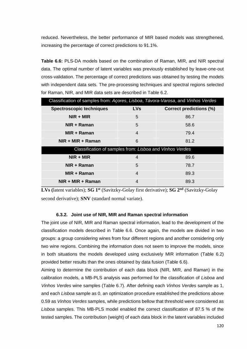
120
reduced. Nevertheless, the better performance of MIR based models was strengthened,
increasing the percentage of correct predictions to 91.1%.
Table 6.6: PLS-DA models based on the combination of Raman, MIR, and NIR spectral
data. The optimal number of latent variables was previously established by leave-one-out
cross-validation. The percentage of correct predictions was obtained by testing the models
with independent data sets. The pre-processing techniques and spectral regions selected
for Raman, NIR, and MIR data sets are described in Table 6.2.
Classification of samples from: Açores, Lisboa, Távora-Varosa, and Vinhos Verdes
Spectroscopic techniques LVs Correct predictions (%)
NIR + MIR 5 86.7
NIR + Raman 5 58.6
MIR + Raman 4 79.4
NIR + MIR + Raman 6 81.2
Classification of samples from: Lisboa and Vinhos Verdes
NIR + MIR 4 89.6
NIR + Raman 5 78.7
MIR + Raman 4 89.3
NIR + MIR + Raman 4 89.3
LVs (latent variables); SG 1st (Savitzky-Golay first derivative); SG 2nd (Savitzky-Golay
second derivative); SNV (standard normal variate).
6.3.2. Joint use of NIR, MIR and Raman spectral information
The joint use of NIR, MIR and Raman spectral information, lead to the development of the
classification models described in Table 6.6. Once again, the models are divided in two
groups: a group considering wines from four different regions and another considering only
two wine regions. Combining the information does not seem to improve the models, since
in both situations the models developed using exclusively MIR information (Table 6.2)
provided better results than the ones obtained by data fusion (Table 6.6).
Aiming to determine the contribution of each data block (NIR, MIR, and Raman) in the
calibration models, a MB-PLS analysis was performed for the classification of Lisboa and
Vinhos Verdes wine samples (Table 6.7). After defining each Vinhos Verdes sample as 1,
and each Lisboa sample as 0, an optimization procedure established the predictions above
0.59 as Vinhos Verdes samples, while predictions bellow that threshold were considered as
Lisboa samples. This MB-PLS model enabled the correct classification of 87.5 % of the
tested samples. The contribution (weight) of each data block in the latent variables included
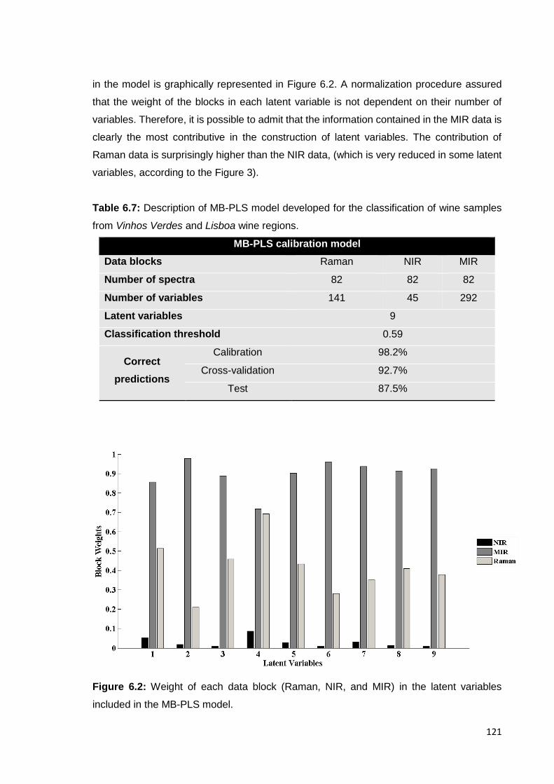
121
in the model is graphically represented in Figure 6.2. A normalization procedure assured
that the weight of the blocks in each latent variable is not dependent on their number of
variables. Therefore, it is possible to admit that the information contained in the MIR data is
clearly the most contributive in the construction of latent variables. The contribution of
Raman data is surprisingly higher than the NIR data, (which is very reduced in some latent
variables, according to the Figure 3).
Table 6.7: Description of MB-PLS model developed for the classification of wine samples
from Vinhos Verdes and Lisboa wine regions.
MB-PLS calibration model
Data blocks Raman NIR MIR
Number of spectra 82 82 82
Number of variables 141 45 292
Latent variables 9
Classification threshold 0.59
Correct
predictions
Calibration 98.2%
Cross-validation 92.7%
Test 87.5%
Figure 6.2: Weight of each data block (Raman, NIR, and MIR) in the latent variables
included in the MB-PLS model.

122
6.4. Conclusions
In this work, NIR, MIR and Raman spectroscopy were combined with PLS-DA and proposed
as classification methodologies for the discrimination of wines from four Portuguese
geographic origins. The suitability of MIR spectroscopy was demonstrated, allowing the
correct prediction of 87.7% of the wines. NIR and Raman spectroscopy presented inferior
responses (60.4% and 60.8% of correct predictions for NIR and Raman, respectively). After
investigating the synergy between the three spectroscopic techniques, it was possible to
conclude that the combination of these techniques was not superior to the single use of MIR
spectroscopy. The development of a MB-PLS calibration model, considering simultaneously
normalized NIR, MIR, and Raman data blocks, indicated the main contribution of MIR
spectroscopic data in the construction of the model. Results also revealed that the Raman
data block is considerably more informative than the NIR data in the classification of wines
according to its origin. For the consolidation of robust calibration models, capable of
discriminating wines from different locations, it will be necessary to include a larger number
of samples, representatively identifying their origins.
CHAPTER 7 – Concluding remarks and future perspectives
“Wine improves with age. The older I get, the better I like it.”
– Anonymous
CHAPTER 7
CONCLUDING REMARKS AND FUTURE
PERSPECTIVES


125
The advantages of vibrational spectroscopic techniques have been widely enhanced in the
last decades. Their fast, automated, cost-effective, non-destructive and environmental-
friendly character, was welcomed by the wine industry. Numerous studies reported the
successful use of NIR, MIR, and Raman spectroscopies for a wide range of purposes:
supporting vineyard management practices, assuring a healthy growth of the vineyard and
grapes, assessing grape maturity stages, monitoring wine fermentations, measuring wine
quality parameters and sensory attributes, determining wine origin and establishing its
authenticity.
It was the aim of this project to further explore the potential of vibrational spectroscopy, and
expand its suitability for wine analysis, cooperating with some of the wine industry demands.
The advantages of vibrational spectroscopy are, so far, well known. However, it is important
to mention that the implementation of this technique as a routine analytical method, requires
a series of procedures that must be carefully performed. The sampling is the first of those
procedures, requiring special attention. To achieve robust calibration models, it is necessary
to include a high number of samples encompassing enough variability to properly describe
the represented population. This is particularly difficult for wine samples. Wines are complex
matrices, strongly dependent on cultivation practices, climatic conditions, winemaking
procedures, fermentation conditions, as well as aging and storage processes. It is not
surprising that there are so different wine classification systems, categorising wines
according to its vintage year, colour, sugar concentration, grape variety, geographical origin,
and aging processes, among others. In these circumstances, calibration models must be
developed to specific wine categories, in order to reduce the weight of undesired sources
of variability. Still, the calibration models should be frequently subjected to recalibration
procedures.
The selection of the appropriate vibrational spectroscopic technique, is also another
important step that should be considered, prior to calibration development. NIR, MIR and
Raman spectroscopy have their own individual strengths and drawbacks. MIR spectroscopy
is apparently more suitable for wine analysis, since organic functional groups have
characteristic and well defined absorption bands in this spectral region. However, as most
compounds strongly absorb in this region, this technique requires the use of sample holders
with extremely short effective pathlength. In NIR spectroscopy, the sample holders do not
need to fulfil this demand, but the calibration procedures are strongly complicated by weak
overtones and combination bands. Raman spectroscopy has only recently been suggested
as a potential tool for wine analysis. In fact, it offers a main advantage over NIR and MIR
techniques: it is not affected by water interferences. However, the laser source may cause
the fluorescence of some compounds, or even destroy the sample, leading to concealed

126
spectra. The results described throughout this thesis, clearly demonstrate the suitability of
MIR spectroscopy for wine measurements. This observation is particularly enhanced in
chapters 5 and 6, where the performance of the three techniques is compared for both
quantification and classification purposes.
Two main limitations are still attributed to vibrational spectroscopic techniques: the relatively
high cost of commercially available instruments, and the low sensitivity of these techniques
for the measurement of minor compounds. However, continuous improvements in
chemometrics and instrumentation promise to increase their applicability, sensitivity and
robustness, consequently reducing these limitations.
Through an overall perspective, it seems that the advantages of vibrational spectroscopy
compensate for its limitations, and it is expected that in the near future, vibrational
techniques may answer effectively to any demand of wine production chain (directly in-situ
and at real-time), being implemented as routine methods for monitoring and process control
in the wine industry.
As overall conclusion, it can be highlighted that the work performed under the scope of this
thesis confirmed the great versatility and analytical applicability arising from combining
vibrational spectroscopy and chemometrics.
127
References
[1] P. Ribéreau-Gayon, D. Dubourdieu, A. Lonvaud, Handbook of Enology, The microbiology of wine and vinifications, John Wiley & Sons2006. [2] International Organisation of Vine and Wine (OIV), Compendium of International Methods of Wine and Must Analysis. Available online at: http://www.oiv.int/public/medias/4231/compendium-2016-en-vol1.pdf (accessed 02 February 2017) Paris, 2016. [3] S. Lohumi, S. Lee, H. Lee, B.-K. Cho, A review of vibrational spectroscopic techniques for the detection of food authenticity and adulteration, Trends in Food Science & Technology, 46 (2015) 85-98. [4] D.A. Burns, E.W. Ciurczak, Handbook of near-infrared analysis, Third Edition ed., CRC Press - Taylor & Francis Group, Boca Raton, Florida, USA, 2007. [5] J.M. Chalmers, P.R. Griffiths, Handbook of vibrational spectroscopy, J. Wiley, Chichester, UK, 2002. [6] D. Cozzolino, Infrared spectroscopy: theory, developments and applications, Nova Science Publishers2014. [7] H. Smyth, D. Cozzolino, Instrumental methods (Spectroscopy, Electronic Nose, and Tongue) as tools to predict taste and aroma in beverages: Advantages and limitations, Chem. Rev., 113 (2013) 1429-1440. [8] S. Fragoso, L. Acena, J. Guasch, O. Busto, M. Mestres, Application of FT-MIR Spectroscopy for Fast Control of Red Grape Phenolic Ripening, J. Agric. Food Chem., 59 (2011) 2175-2183. [9] C.J. Bevin, A.J. Fergusson, W.B. Perry, L.J. Janik, D. Cozzolino, Development of a rapid "fingerprinting" system for wine authenticity by mid-infrared spectroscopy, J. Agric. Food Chem., 54 (2006) 9713-9718. [10] U. Regmi, M. Palma, C.G. Barroso, Direct determination of organic acids in wine and wine-derived products by Fourier transform infrared (FT-IR) spectroscopy and chemometric techniques, Anal. Chim. Acta, 732 (2012) 137-144. [11] J.L.s. Moreira, L. Santos, Spectroscopic interferences in Fourier transform infrared wine analysis, Anal. Chim. Acta, 513 (2004) 263-268. [12] J.L. Moreira, L. Santos, Analysis of organic acids in wines by Fourier-transform infrared spectroscopy, Anal. Bioanal. Chem., 382 (2005) 421-425. [13] H.H. Nieuwoudt, B.A. Prior, I.S. Pretorius, M. Manley, F.F. Bauer, Principal component analysis applied to Fourier transform infrared spectroscopy for the design of calibration sets for glycerol prediction models in wine and for the detection and classification of outlier samples, J. Agric. Food Chem., 52 (2004) 3726-3735. [14] C.D. Patz, A. Blieke, R. Ristow, H. Dietrich, Application of FT-MIR spectrometry in wine analysis, Anal. Chim. Acta, 513 (2004) 81-89. [15] S.D. Silva, R.P. Feliciano, L.V. Boas, M.R. Bronze, Application of FTIR-ATR to Moscatel dessert wines for prediction of total phenolic and flavonoid contents and antioxidant capacity, Food Chem., 150 (2014) 489-493. [16] K. Fernandez, E. Agosin, Quantitative analysis of red wine tannins using Fourier-transform mid-infrared spectrometry, J. Agric. Food Chem., 55 (2007) 7294-7300. [17] G. Socrates, Infrared and Raman characteristic group frequencies: tables and charts, Third ed. ed., John Wiley & Sons, Chichester, UK, 2004. [18] I. Murray, The NIR spectra of homologous series of organic compounds, Proceedings of the international NIR/NIT conference, Akademiai Kiado: Budapest, Hungary, 1986, pp. 13-28. [19] V.A. McGlone, S. Kawano, Firmness, dry-matter and soluble-solids assessment of postharvest kiwifruit by NIR spectroscopy, Postharvest Biol. Tec., 13 (1998) 131-141. [20] D. Cozzolino, M.J. Kwiatkowski, M. Parker, W.U. Cynkar, R.G. Dambergs, M. Gishen, M.J. Herderich, Prediction of phenolic compounds in red wine fermentations by visible and near infrared spectroscopy, Anal. Chim. Acta, 513 (2004) 73-80.
128
[21] M.A. Czarnecki, Y. Ozaki, The temperature-induced changes in hydrogen bonding of decan-1-ol in the pure liquid phase studied by two-dimensional Fourier transform near-infrared correlation spectroscopy, PCCP, 1 (1999) 797-800. [22] L. Liu, D. Cozzolino, W. Cynkar, R. Dambergs, L. Janik, B. O’neill, C. Colby, M. Gishen, Preliminary study on the application of visible–near infrared spectroscopy and chemometrics to classify Riesling wines from different countries, Food Chem., 106 (2008) 781-786. [23] E. Ferrari, G. Foca, M. Vignali, L. Tassi, A. Ulrici, Adulteration of the anthocyanin content of red wines: perspectives for authentication by Fourier transform-near infrared and 1 H NMR spectroscopies, Anal. Chim. Acta, 701 (2011) 139-151. [24] D. Cozzolino, Sample presentation, sources of error and future perspectives on the application of vibrational spectroscopy in the wine industry, J. Sci. Food Agr., 95 (2015) 861-868. [25] C. Martin, J.-L. Bruneel, F. Castet, A. Fritsch, P.-L. Teissedre, M. Jourdes, F. Guillaume, Spectroscopic and theoretical investigations of phenolic acids in white wines, Food Chem., 221 (2017) 568-575. [26] P. Vasko, J. Blackwell, J. Koenig, Infrared and raman spectroscopy of carbohydrates.: Part II: Normal coordinate analysis of α-D-glucose, Carbohydrate Research, 23 (1972) 407-416. [27] Z. Wu, E. Xu, J. Long, F. Wang, X. Xu, Z. Jin, A. Jiao, Measurement of fermentation parameters of Chinese rice wine using Raman spectroscopy combined with linear and non-linear regression methods, Food Control, 56 (2015) 95-102. [28] Q. Wang, Z. Li, Z. Ma, L. Liang, Real time monitoring of multiple components in wine fermentation using an on-line auto-calibration Raman spectroscopy, Sensor. Actuat. B: Chem., 202 (2014) 426-432. [29] A. Picard, I. Daniel, G. Montagnac, P. Oger, In situ monitoring by quantitative Raman spectroscopy of alcoholic fermentation by Saccharomyces cerevisiae under high pressure, Extremophiles, 11 (2007) 445-452. [30] R.S. Uysal, E.A. Soykut, I.H. Boyaci, A. Topcu, Monitoring multiple components in vinegar fermentation using Raman spectroscopy, Food Chem., 141 (2013) 4333-4343. [31] D. Cozzolino, W. Cynkar, R. Dambergs, N. Shah, P. Smith, In situ measurement of soil chemical composition by near-infrared spectroscopy: A tool toward sustainable vineyard management, Commun. Soil Sci. Plan., 44 (2013) 1610-1619. [32] M. Lopo, C.A.T.d. Santos, R.N.M.J. Páscoa, A.R. Graça, J.A. Lopes, Non-invasive real-time monitoring of vineyard soils, berries and leaves with FT-NIR spectroscopy, BIO Web of Conferences, 5 (2015) 01003. [33] R. De Bei, D. Cozzolino, W. Sullivan, W. Cynkar, S. Fuentes, R. Dambergs, J. Pech,
S. Tyerman, Non‐destructive measurement of grapevine water potential using near infrared spectroscopy, Aust. J. Grape Wine R., 17 (2011) 62-71. [34] T. Rapaport, U. Hochberg, M. Shoshany, A. Karnieli, S. Rachmilevitch, Combining leaf physiology, hyperspectral imaging and partial least squares-regression (PLS-R) for grapevine water status assessment, ISPRS Journal of Photogrammetry and Remote Sensing, 109 (2015) 88-97. [35] S. Gutiérrez, J. Tardaguila, J. Fernández-Novales, M.P. Diago, Support Vector Machine and Artificial Neural Network Models for the Classification of Grapevine Varieties Using a Portable NIR Spectrophotometer, PLoS ONE, 10 (2015) e0143197. [36] M.P. Diago, A. Fernandes, B. Millan, J. Tardaguila, P. Melo-Pinto, Identification of grapevine varieties using leaf spectroscopy and partial least squares, Comput. Electron. Agric., 99 (2013) 7-13. [37] G. Ciraolo, F. Capodici, G. D'Urso, G. Loggia, A. Maltese, Mapping evapotranspiration on vineyards: The Sentinel-2 potentiality, ESA SP, 707 (2012). [38] R. Dambergs, M. Gishen, D. Cozzolino, A Review of the State of the Art, Limitations, and Perspectives of Infrared Spectroscopy for the Analysis of Wine Grapes, Must, and Grapevine Tissue, Appl. Spectrosc. Rev., 50 (2015) 261-278.
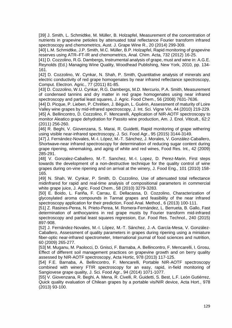
129
[39] J. Smith, L. Schmidtke, M. Müller, B. Holzapfel, Measurement of the concentration of nutrients in grapevine petioles by attenuated total reflectance Fourier transform infrared spectroscopy and chemometrics, Aust. J. Grape Wine R., 20 (2014) 299-309. [40] L.M. Schmidtke, J.P. Smith, M.C. Müller, B.P. Holzapfel, Rapid monitoring of grapevine reserves using ATR–FT-IR and chemometrics, Anal. Chim. Acta, 732 (2012) 16-25. [41] D. Cozzolino, R.G. Dambergs, Instrumental analysis of grape, must and wine in: A.G.E. Reynolds (Ed.) Managing Wine Quality, Woodhead Publishing, New York, 2010, pp. 134-161. [42] D. Cozzolino, W. Cynkar, N. Shah, P. Smith, Quantitative analysis of minerals and electric conductivity of red grape homogenates by near infrared reflectance spectroscopy, Comput. Electron. Agric., 77 (2011) 81-85. [43] D. Cozzolino, W.U. Cynkar, R.G. Dambergs, M.D. Mercurio, P.A. Smith, Measurement of condensed tannins and dry matter in red grape homogenates using near infrared spectroscopy and partial least squares, J. Agric. Food Chem., 56 (2008) 7631-7636. [44] D. Picque, P. Lieben, P. Chrétien, J. Béguin, L. Guérin, Assessment of maturity of Loire Valley wine grapes by mid-infrared spectroscopy, J. Int. Sci. Vigne Vin, 44 (2010) 219-229. [45] A. Bellincontro, D. Cozzolino, F. Mencarelli, Application of NIR-AOTF spectroscopy to monitor Aleatico grape dehydration for Passito wine production, Am. J. Enol. Viticult., 62:2 (2011) 256-260. [46] R. Beghi, V. Giovenzana, S. Marai, R. Guidetti, Rapid monitoring of grape withering
using visible near‐infrared spectroscopy, J. Sci. Food Agr., 95 (2015) 3144-3149. [47] J. Fernández-Novales, M.-I. López, M.-T. Sánchez, J. Morales, V. González-Caballero, Shortwave-near infrared spectroscopy for determination of reducing sugar content during grape ripening, winemaking, and aging of white and red wines, Food Res. Int., 42 (2009) 285-291. [48] V. Gonzalez-Caballero, M.-T. Sanchez, M.-I. Lopez, D. Perez-Marin, First steps towards the development of a non-destructive technique for the quality control of wine grapes during on-vine ripening and on arrival at the winery, J. Food Eng., 101 (2010) 158-165. [49] N. Shah, W. Cynkar, P. Smith, D. Cozzolino, Use of attenuated total reflectance midinfrared for rapid and real-time analysis of compositional parameters in commercial white grape juice, J. Agric. Food Chem., 58 (2010) 3279-3283. [50] E. Boido, L. Fariña, F. Carrau, E. Dellacassa, D. Cozzolino, Characterization of glycosylated aroma compounds in Tannat grapes and feasibility of the near infrared spectroscopy application for their prediction, Food Anal. Method., 6 (2013) 100-111. [51] Z. Rasines-Perea, N. Prieto-Perea, M. Romera-Fernández, L. Berrueta, B. Gallo, Fast determination of anthocyanins in red grape musts by Fourier transform mid-infrared spectroscopy and partial least squares regression, Eur. Food Res. Technol., 240 (2015) 897-908. [52] J. Fernández-Novales, M.-I. López, M.-T. Sánchez, J.-A. García-Mesa, V. González-Caballero, Assessment of quality parameters in grapes during ripening using a miniature fiber-optic near-infrared spectrometer, International journal of food sciences and nutrition, 60 (2009) 265-277. [53] M. Muganu, M. Paolocci, D. Gnisci, F. Barnaba, A. Bellincontro, F. Mencarelli, I. Grosu, Effect of different soil management practices on grapevine growth and on berry quality assessed by NIR-AOTF spectroscopy, Acta Hortic, 978 (2013) 117-125.
[54] F.E. Barnaba, A. Bellincontro, F. Mencarelli, Portable NIR‐AOTF spectroscopy combined with winery FTIR spectroscopy for an easy, rapid, in‐field monitoring of Sangiovese grape quality, J. Sci. Food Agr., 94 (2014) 1071-1077. [55] V. Giovenzana, R. Beghi, A. Mena, R. Civelli, R. Guidetti, S. Best, L.F. Leòn Gutiérrez, Quick quality evaluation of Chilean grapes by a portable vis/NIR device, Acta Hort., 978 (2013) 93-100.

130
[56] V. González-Caballero, D. Pérez-Marín, M.-I. López, M.-T. Sánchez, Optimization of NIR spectral data management for quality control of grape bunches during on-vine ripening, Sensors, 11 (2011) 6109-6124. [57] A.M. Fernandes, C. Franco, A. Mendes-Ferreira, A. Mendes-Faia, P.L. da Costa, P. Melo-Pinto, Brix, pH and anthocyanin content determination in whole Port wine grape berries by hyperspectral imaging and neural networks, Comput. Electron. Agric., 115 (2015) 88-96. [58] V.M. Gomes, A.M. Fernandes, A. Faia, P. Melo-Pinto, Determination of sugar content in whole Port Wine grape berries combining hyperspectral imaging with neural networks methodologies, Computational Intelligence for Engineering Solutions (CIES), 2014 IEEE Symposium on, IEEE, 2014, pp. 188-193. [59] J.R. Martínez-Sandoval, J. Nogales-Bueno, F.J. Rodríguez-Pulido, J.M. Hernández-Hierro, M.A. Segovia-Quintero, M.E. Martínez-Rosas, F.J. Heredia, Screening of anthocyanins in single red grapes using a non-destructive method based on the near infrared hyperspectral technology and chemometrics, J. Sci. Food Agr., 96 (2016) 1643-1647. [60] L. Rolle, F. Torchio, B. Lorrain, S. Giacosa, S. Río Segade, E. Cagnasso, V. Gerbi, P.-L. Teissedre, Rapid methods for the evaluation of total phenol content and extractability in intact grape seeds of Cabernet-Sauvignon: Instrumental mechanical properties and FT-NIR spectrum, J. Int. Sci. Vigne Vin, 46 (2012) 29-40. [61] M. Kyraleou, C. Pappas, E. Voskidi, Y. Kotseridis, M. Basalekou, P.A. Tarantilis, S. Kallithraka, Diffuse reflectance Fourier transform infrared spectroscopy for simultaneous quantification of total phenolics and condensed tannins contained in grape seeds, Ind. Crops Prod., 74 (2015) 784-791. [62] R. Ferrer-Gallego, J.M. Hernández-Hierro, J.C. Rivas-Gonzalo, M.T. Escribano-Bailón, Evaluation of sensory parameters of grapes using near infrared spectroscopy, J. Food Eng., 118 (2013) 333-339. [63] R.N. Páscoa, S. Machado, L.M. Magalhães, J.A. Lopes, Value adding to red grape pomace exploiting eco-friendly FT-NIR spectroscopy technique, Food and Bioprocess Technology, 8 (2015) 865-874. [64] F.J. Rodríguez-Pulido, D.F. Barbin, D.-W. Sun, B. Gordillo, M.L. González-Miret, F.J. Heredia, Grape seed characterization by NIR hyperspectral imaging, Postharvest Biol. Tec., 76 (2013) 74-82. [65] S. Chen, F. Zhang, J. Ning, X. Liu, Z. Zhang, S. Yang, Predicting the anthocyanin content of wine grapes by NIR hyperspectral imaging, Food Chem., 172 (2015) 788-793. [66] M. Jara‐Palacios, F. Rodríguez‐Pulido, D. Hernanz, M. Escudero‐Gilete, F. Heredia, Determination of phenolic substances of seeds, skins and stems from white grape marc by
near‐infrared hyperspectral imaging, Aust. J. Grape Wine R., DOI (2015). [67] C.P. Passos, S.M. Cardoso, A.S. Barros, C.M. Silva, M.A. Coimbra, Application of Fourier transform infrared spectroscopy and orthogonal projections to latent structures/partial least squares regression for estimation of procyanidins average degree of polymerisation, Anal. Chim. Acta, 661 (2010) 143-149. [68] D. Cozzolino, R.G. Dambergs, L. Janik, W.U. Cynkar, M. Gishen, Analysis of grapes and wine by near infrared spectroscopy, J. Near Infrared Spec., 14 (2006) 279-289. [69] J.U. Porep, M.E. Erdmann, A. Koerzendoerfer, D.R. Kammerer, R. Carle, Rapid determination of ergosterol in grape mashes for grape rot indication and further quality assessment by means of an industrial near infrared/visible (NIR/VIS) spectrometer - A feasibility study, Food Control, 43 (2014) 142-149. [70] A. Versari, G.P. Parpinello, A.U. Mattioli, S. Galassi, Determination of grape quality at harvest using Fourier-transform mid-infrared spectroscopy and multivariate analysis, American Journal of Enology and Viticulture, 59 (2008) 317-322. [71] G. Hill, K. Evans, R. Beresford, R. Dambergs, Near and mid-infrared spectroscopy for the quantification of botrytis bunch rot in white wine grapes, J. Near Infrared Spec., 21 (2014) 467-475.
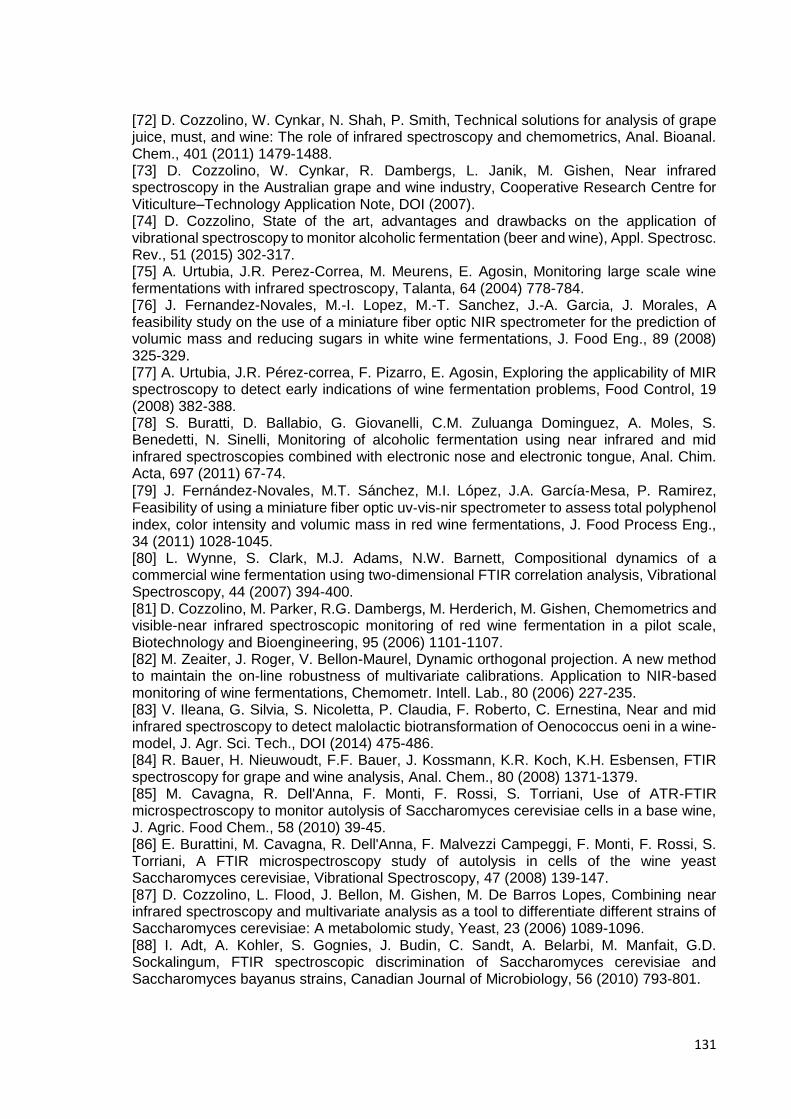
131
[72] D. Cozzolino, W. Cynkar, N. Shah, P. Smith, Technical solutions for analysis of grape juice, must, and wine: The role of infrared spectroscopy and chemometrics, Anal. Bioanal. Chem., 401 (2011) 1479-1488. [73] D. Cozzolino, W. Cynkar, R. Dambergs, L. Janik, M. Gishen, Near infrared spectroscopy in the Australian grape and wine industry, Cooperative Research Centre for Viticulture–Technology Application Note, DOI (2007). [74] D. Cozzolino, State of the art, advantages and drawbacks on the application of vibrational spectroscopy to monitor alcoholic fermentation (beer and wine), Appl. Spectrosc. Rev., 51 (2015) 302-317. [75] A. Urtubia, J.R. Perez-Correa, M. Meurens, E. Agosin, Monitoring large scale wine fermentations with infrared spectroscopy, Talanta, 64 (2004) 778-784. [76] J. Fernandez-Novales, M.-I. Lopez, M.-T. Sanchez, J.-A. Garcia, J. Morales, A feasibility study on the use of a miniature fiber optic NIR spectrometer for the prediction of volumic mass and reducing sugars in white wine fermentations, J. Food Eng., 89 (2008) 325-329. [77] A. Urtubia, J.R. Pérez-correa, F. Pizarro, E. Agosin, Exploring the applicability of MIR spectroscopy to detect early indications of wine fermentation problems, Food Control, 19 (2008) 382-388. [78] S. Buratti, D. Ballabio, G. Giovanelli, C.M. Zuluanga Dominguez, A. Moles, S. Benedetti, N. Sinelli, Monitoring of alcoholic fermentation using near infrared and mid infrared spectroscopies combined with electronic nose and electronic tongue, Anal. Chim. Acta, 697 (2011) 67-74.
[79] J. Fernández‐Novales, M.T. Sánchez, M.I. López, J.A. García‐Mesa, P. Ramirez, Feasibility of using a miniature fiber optic uv‐vis‐nir spectrometer to assess total polyphenol index, color intensity and volumic mass in red wine fermentations, J. Food Process Eng., 34 (2011) 1028-1045. [80] L. Wynne, S. Clark, M.J. Adams, N.W. Barnett, Compositional dynamics of a commercial wine fermentation using two-dimensional FTIR correlation analysis, Vibrational Spectroscopy, 44 (2007) 394-400. [81] D. Cozzolino, M. Parker, R.G. Dambergs, M. Herderich, M. Gishen, Chemometrics and visible-near infrared spectroscopic monitoring of red wine fermentation in a pilot scale, Biotechnology and Bioengineering, 95 (2006) 1101-1107. [82] M. Zeaiter, J. Roger, V. Bellon-Maurel, Dynamic orthogonal projection. A new method to maintain the on-line robustness of multivariate calibrations. Application to NIR-based monitoring of wine fermentations, Chemometr. Intell. Lab., 80 (2006) 227-235. [83] V. Ileana, G. Silvia, S. Nicoletta, P. Claudia, F. Roberto, C. Ernestina, Near and mid infrared spectroscopy to detect malolactic biotransformation of Oenococcus oeni in a wine-model, J. Agr. Sci. Tech., DOI (2014) 475-486. [84] R. Bauer, H. Nieuwoudt, F.F. Bauer, J. Kossmann, K.R. Koch, K.H. Esbensen, FTIR spectroscopy for grape and wine analysis, Anal. Chem., 80 (2008) 1371-1379. [85] M. Cavagna, R. Dell'Anna, F. Monti, F. Rossi, S. Torriani, Use of ATR-FTIR microspectroscopy to monitor autolysis of Saccharomyces cerevisiae cells in a base wine, J. Agric. Food Chem., 58 (2010) 39-45. [86] E. Burattini, M. Cavagna, R. Dell'Anna, F. Malvezzi Campeggi, F. Monti, F. Rossi, S. Torriani, A FTIR microspectroscopy study of autolysis in cells of the wine yeast Saccharomyces cerevisiae, Vibrational Spectroscopy, 47 (2008) 139-147. [87] D. Cozzolino, L. Flood, J. Bellon, M. Gishen, M. De Barros Lopes, Combining near infrared spectroscopy and multivariate analysis as a tool to differentiate different strains of Saccharomyces cerevisiae: A metabolomic study, Yeast, 23 (2006) 1089-1096. [88] I. Adt, A. Kohler, S. Gognies, J. Budin, C. Sandt, A. Belarbi, M. Manfait, G.D. Sockalingum, FTIR spectroscopic discrimination of Saccharomyces cerevisiae and Saccharomyces bayanus strains, Canadian Journal of Microbiology, 56 (2010) 793-801.
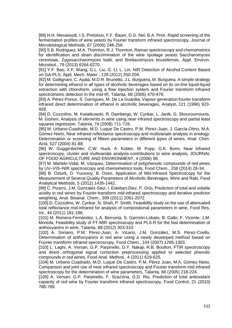
132
[89] H.H. Nieuwoudt, I.S. Pretorius, F.F. Bauer, D.G. Nel, B.A. Prior, Rapid screening of the fermentation profiles of wine yeasts by Fourier transform infrared spectroscopy, Journal of Microbiological Methods, 67 (2006) 248-256. [90] S.B. Rodriguez, M.A. Thornton, R.J. Thornton, Raman spectroscopy and chemometrics for identification and strain discrimination of the wine spoilage yeasts Saccharomyces cerevisiae, Zygosaccharomyces bailii, and Brettanomyces bruxellensis, Appl. Environ. Microbiol., 79 (2013) 6264-6270. [91] Y.F. Bao, X.F. Wang, G.L. Liu, G. Li, L. Lin, NIR Detection of Alcohol Content Based on GA-PLS, Appl. Mech. Mater., 128 (2012) 200-204. [92] M. Gallignani, C. Ayala, M.D.R. Brunetto, J.L. Burguera, M. Burguera, A simple strategy for determining ethanol in all types of alcoholic beverages based on its on-line liquid-liquid extraction with chloroform, using a flow injection system and Fourier transform infrared spectrometric detection in the mid-IR, Talanta, 68 (2005) 470-479. [93] A. Pérez-Ponce, S. Garrigues, M. De La Guardia, Vapour generation-fourier transform infrared direct determination of ethanol in alcoholic beverages, Analyst, 121 (1996) 923-928. [94] D. Cozzolino, M. Kwiatkowski, R. Dambergs, W. Cynkar, L. Janik, G. Skouroumounis, M. Gishen, Analysis of elements in wine using near infrared spectroscopy and partial least squares regression, Talanta, 74 (2008) 711-716. [95] M. Urbano-Cuadrado, M.D. Luque De Castro, P.M. Pérez-Juan, J. García-Olmo, M.A. Gómez-Nieto, Near infrared reflectance spectroscopy and multivariate analysis in enology: Determination or screening of fifteen parameters in different types of wines, Anal. Chim. Acta, 527 (2004) 81-88. [96] W. Guggenbichler, C.W. Huck, A. Kobler, M. Popp, G.K. Bonn, Near infrared spectroscopy, cluster and multivariate analysis-contributions to wine analysis, JOURNAL OF FOOD AGRICULTURE AND ENVIRONMENT, 4 (2006) 98. [97] M. Martelo-Vidal, M. Vázquez, Determination of polyphenolic compounds of red wines by UV–VIS–NIR spectroscopy and chemometrics tools, Food Chem., 158 (2014) 28-34. [98] B. Ozturk, D. Yucesoy, B. Ozen, Application of Mid-infrared Spectroscopy for the Measurement of Several Quality Parameters of Alcoholic Beverages, Wine and Raki, Food Analytical Methods, 5 (2012) 1435-1442. [99] C. Pizarro, J.M. Gonzalez-Saiz, I. Esteban-Diez, P. Orio, Prediction of total and volatile acidity in red wines by Fourier-transform mid-infrared spectroscopy and iterative predictor weighting, Anal. Bioanal. Chem., 399 (2011) 2061-2072. [100] D. Cozzolino, W. Cynkar, N. Shah, P. Smith, Feasibility study on the use of attenuated total reflectance mid-infrared for analysis of compositional parameters in wine, Food Res. Int., 44 (2011) 181-186. [101] M. Romera-Fernández, L.A. Berrueta, S. Garmón-Lobato, B. Gallo, F. Vicente, J.M. Moreda, Feasibility study of FT-MIR spectroscopy and PLS-R for the fast determination of anthocyanins in wine, Talanta, 88 (2012) 303-310. [102] A. Soriano, P.M. Pérez-Juan, A. Vicario, J.M. González, M.S. Pérez-Coello, Determination of anthocyanins in red wine using a newly developed method based on Fourier transform infrared spectroscopy, Food Chem., 104 (2007) 1295-1303. [103] L. Laghi, A. Versari, G.P. Parpinello, D.Y. Nakaji, R.B. Boulton, FTIR spectroscopy and direct orthogonal signal correction preprocessing applied to selected phenolic compounds in red wines, Food Anal. Method., 4 (2011) 619-625. [104] M. Urbano Cuadrado, M.D. Luque De Castro, P.M. Pérez Juan, M.A. Gómez-Nieto, Comparison and joint use of near infrared spectroscopy and Fourier transform mid infrared spectroscopy for the determination of wine parameters, Talanta, 66 (2005) 218-224. [105] A. Versari, G.P. Parpinello, F. Scazzina, D.D. Rio, Prediction of total antioxidant capacity of red wine by Fourier transform infrared spectroscopy, Food Control, 21 (2010) 786-789.

133
[106] J. Preserova, V. Ranc, D. Milde, V. Kubistova, J. Stavek, Study of phenolic profile and antioxidant activity in selected Moravian wines during winemaking process by FT-IR spectroscopy, J. Food Sci. Tech., 52 (2015) 6405-6414. [107] A. Versari, L. Laghi, J.H. Thorngate, R.B. Bulton, Prediction of colloidal stability in white wines using infrared spectroscopy, J. Food Eng., 104 (2011) 239-245. [108] T. Garde-Cerdán, C. Lorenzo, A. Zalacain, G. Alonso, M. Salinas, Using near infrared spectroscopy to determine haloanisoles and halophenols in barrel aged red wines, LWT - Food Sci. Techno., 46 (2012) 401-405. [109] J.C. Boulet, P. Williams, T. Doco, A Fourier transform infrared spectroscopy study of wine polysaccharides, Carbohyd. Polym., 69 (2007) 79-85. [110] M.A. Coimbra, A.S. Barros, E. Coelho, F. Gonçalves, S.M. Rocha, I. Delgadillo, Quantification of polymeric mannose in wine extracts by FT-IR spectroscopy and OSC-PLS1 regression, Carbohyd. Polym., 61 (2005) 434-440. [111] M.A. Coimbra, F. Goncalves, A.S. Barros, I. Delgadillo, Fourier transform infrared spectroscopy and chemometric analysis of white wine polysaccharide extracts, J. Agric. Food Chem., 50 (2002) 3405-3411. [112] D. Picque, T. Cattenoz, G. Corrieu, Classification of red wines analysed by middle infrared spectroscopy of dry extract according to their geographical origin, Journal International Des Sciences De La Vigne Et Du Vin, 35 (2001) 165-170. [113] Y.-x. Huang, C. Wang, Normalization Methods for Ethanol Raman Spectra Quantitative Analysis, Spectroscopy and Spectral Analysis, 30 (2010) 971-974. [114] Á.L. Gallego, A.R. Guesalaga, E. Bordeu, Á.S. González, Rapid measurement of phenolics compounds in red wine using raman spectroscopy, IEEE Transactions on Instrumentation and Measurement, 60 (2011) 507-512. [115] A. Versari, R. Boulton, G. Parpinello, Effect of spectral pre-processing methods on the evaluation of the color components of red wines using Fourier-transform infrared spectrometry, Ital. J. Food Sci., 18 (2006) 423-431. [116] R. Lletí, E. Meléndez, M. Ortiz, L. Sarabia, M. Sánchez, Outliers in partial least squares regression: Application to calibration of wine grade with mean infrared data, Anal. Chim. Acta, 544 (2005) 60-70. [117] D. Cozzolino, L. Liu, W. Cynkar, R. Dambergs, L. Janik, C. Colby, M. Gishen, Effect of temperature variation on the visible and near infrared spectra of wine and the consequences on the partial least square calibrations developed to measure chemical composition, Anal. Chim. Acta, 588 (2007) 224-230. [118] J.S. Jensen, M. Egebo, A.S. Meyer, Identification of spectral regions for the quantification of red wine tannins with Fourier transform mid-infrared spectroscopy, J. Agric. Food Chem., 56 (2008) 3493-3499. [119] M.U. Cuadrado, M.L. de Castro, M. Gomez-Nieto, Study of spectral analytical data using fingerprints and scaled similarity measurements, Anal. Bioanal. Chem., 381 (2005) 953-963. [120] C. Lorenzo, T. Garde-Cerdan, M.A. Pedroza, G.L. Alonso, M. Rosario Salinas, Determination of fermentative volatile compounds in aged red wines by near infrared spectroscopy, Food Res. Int., 42 (2009) 1281-1286. [121] D. Cozzolino, H.E. Smyth, K.A. Lattey, W. Cynkar, L. Janik, R.G. Dambergs, I.L. Francis, M. Gishen, Combining mass spectrometry based electronic nose, visible-near infrared spectroscopy and chemometrics to assess the sensory properties of Australian Riesling wines, Anal. Chim. Acta, 563 (2006) 319-324. [122] L. Vera, L. Aceña, R. Boqué, J. Guasch, M. Mestres, O. Busto, Application of an electronic tongue based on FT-MIR to emulate the gustative mouthfeel "tannin amount" in red wines, Anal. Bioanal. Chem., 397 (2010) 3043-3049. [123] A.M.S. Costa, M.M.C. Sobral, I. Delgadillo, A. Cerdeira, A. Rudnitskaya, Astringency quantification in wine: comparison of the electronic tongue and FT-MIR spectroscopy, Sensor. Actuat. B: Chem., 207 (2015) 1095-1103.

134
[124] D. Cozzolino, H.E. Smyth, K.A. Lattey, W. Cynkar, L. Janik, R.G. Dambergs, I.L. Francis, M. Gishen, Relationship between sensory analysis and near infrared spectroscopy in Australian Riesling and Chardonnay wines, Anal. Chim. Acta, 539 (2005) 341-348. [125] H.E. Smyth, D. Cozzolino, W.U. Cynkar, R.G. Dambergs, M. Sefton, M. Gishen, Near infrared spectroscopy as a rapid tool to measure volatile aroma compounds in Riesling wine: possibilities and limits, Anal. Bioanal. Chem., 390 (2008) 1911-1916. [126] C. Daniel, H. Smyth, Analytical and chemometric-based methods to monitor and evaluate wine protected designation, Comprehensive Analytical Chemistry, 2013, pp. 385-408. [127] M.J. Martelo-Vidal, F. Domínguez-Agis, M. Vázquez, Ultraviolet/visible/near-infrared spectral analysis and chemometric tools for the discrimination of wines between subzones inside a controlled designation of origin: A case study of Rías Baixas, Aust. J. Grape Wine R., 19 (2013) 62-67. [128] D. Picque, T. Cattenoz, G. Corrieu, J.L. Berger, Discrimination of red wines according to their geographical origin and vintage year by the use of mid-infrared spectroscopy, Sci. Aliment., 25 (2005) 207-220. [129] E. Ioannou-Papayianni, R.I. Kokkinofta, C.R. Theocharis, Authenticity of Cypriot Sweet Wine Commandaria Using FT-IR and Chemometrics, Journal of Food Science, 76 (2011) C420-C427. [130] V. Dixit, J.C. Tewari, B.K. Cho, J.M.K. Irudayaraj, Identification and quantification of industrial grade glycerol adulteration in red wine with Fourier transform infrared spectroscopy using chemometrics and artificial neural networks, Applied Spectroscopy, 59 (2005) 1553-1561. [131] S. Tao, J. Li, J. Li, J. Tang, J. Mi, L. Zhao, Discriminant analysis of red wines from different aging ways by information fusion of NIR and MIR spectra, Computer and Computing Technologies in Agriculture V, Springer2011, pp. 478-483. [132] D. Cozzolino, J. McCarthy, E. Bartowsky, Comparison of near infrared and mid infrared spectroscopy to discriminate between wines produced by different Oenococcus Oeni strains after malolactic fermentation: A feasibility study, Food Control, 26 (2012) 81-87. [133] K. Fernández, X. Labarca, E. Bordeu, A. Guesalaga, E. Agosin, Comparative study of wine tannin classification using fourier transform mid-infrared spectrometry and sensory analysis, Applied Spectroscopy, 61 (2007) 1163-1167. [134] X.D. Zhao, D.M. Dong, W.G. Zheng, L.Z. Jiao, Y. Lang, Application of Fourier transform infrared spectroscopy in identification of wine spoilage, Guang Pu Xue Yu Guang Pu Fen Xi/Spectroscopy and Spectral Analysis, 34 (2014) 2667-2672. [135] D.Y. Fu, D. Yuan, X.F. Zhang, X. Zhao, Fast Detection of Illegal Sweeteners in Liquor and Wine by Laser Raman Spectroscopy, Adv. Mat. Res., 960 (2014) 32-38. [136] A. Versari, V. Felipe Laurie, A. Ricci, L. Laghi, G.P. Parpinello, Progress in authentication, typification and traceability of grapes and wines by chemometric approaches, Food Res. Int., 60 (2014) 2-18. [137] D. Cozzolino, M. Kwiatkowski, E. Waters, M. Gishen, A feasibility study on the use of visible and short wavelengths in the near-infrared region for the non-destructive measurement of wine composition, Anal. Bioanal. Chem., 387 (2007) 2289-2295. [138] C. Prades, I. Gómez-Sánchez, J. García-Olmo, J.R. González-Adrados, Discriminant analysis of geographical origin of cork planks and stoppers by near infrared spectroscopy, Journal of Wood Chemistry and Technology, 32 (2012) 54-70. [139] C. Prades, I. Gómez-Sánchez, J. García-Olmo, F. González-Hernández, J.R. González-Adrados, Application of VIS/NIR spectroscopy for estimating chemical, physical and mechanical properties of cork stoppers, Wood Sci. Technol., 48 (2014) 811-830. [140] A.R. Garcia, L.F. Lopes, R.B.d. Barros, L.M. Ilharco, The Problem of 2, 4, 6-Trichloroanisole in Cork Planks Studied by Attenuated Total Reflection Infrared Spectroscopy: Proof of Concept, J. Agric. Food. Chem., 63 (2014) 128-135.
135
[141] C. Ortega-Fernández, J.R. González-Adrados, M.C. García-Vallejo, R. Calvo-Haro, M.J. Cáceres-Esteban, Characterization of surface treatments of cork stoppers by FTIR-ATR, J. Agric. Food Chem., 54 (2006) 4932-4936. [142] S. Li, K.L. Wilkinson, D. Cozzolino, The use of near infrared reflectance spectroscopy to identify the origin of oak shavings used in wine aging, Sens. Instrum. Food Qual. Saf., 8 (2014) 356-361. [143] L.A. Berrueta, R.M. Alonso-Salces, K. Héberger, Supervised pattern recognition in food analysis, Journal of Chromatography A, 1158 (2007) 196-214. [144] Ǻ. Rinnan, F.v.d. Berg, S.B. Engelsen, Review of the most common pre-processing techniques for near-infrared spectra, Anal. Chem., 28 (2009) 1201-1222. [145] T. Naes, T. Isaksson, T. Fearn, T. Davies, A user friendly guide to multivariate calibration and classification, NIR publications, Chichester, UK, 2002. [146] I.S. Helland, T. Næs, T. Isaksson, Related versions of the multiplicative scatter correction method for preprocessing spectroscopic data, Chemometr. Intell. Lab., 29 (1995) 233-241. [147] D. Cozzolino, W. Cynkar, N. Shah, R. Dambergs, P. Smith, A brief introduction to multivariate methods in grape and wine analysis, International Journal of Wine Research, 1 (2009) 123-130. [148] P. Geladi, Chemometrics in spectroscopy. Part 1. Classical chemometrics, Spectrochimica Acta Part B: Atomic Spectroscopy, 58 (2003) 767-782. [149] S. Wold, Chemometrics; what do we mean with it, and what do we want from it?, Chemometr. Intell. Lab., 30 (1995) 109-115. [150] B.M. Wise, N.B. Gallagher, The process chemometrics approach to process monitoring and fault detection, Journal of Process Control, 6 (1996) 329-348. [151] S. Wold, M. Sjöström, L. Eriksson, PLS-regression: A basic tool of chemometrics, Chemometr. Intell. Lab., 58 (2001) 109-130. [152] R.G. Brereton, Introduction to multivariate calibration in analytical chemistry, Analyst, 125 (2000) 2125-2154. [153] R. Bro, A.K. Smilde, Principal component analysis, Analytical Methods, 6 (2014) 2812-2831. [154] S. Wold, H. Martens, H. Wold, The multivariate calibration problem in chemistry solved by the PLS method, Matrix pencils, DOI (1983) 286-293. [155] H. Martens, T. Naes, Multivariate calibration, John Wiley & Sons1992. [156] M. Barker, W. Rayens, Partial least squares for discrimination, J. Chemom., 17 (2003) 166-173. [157] P.S. Gromski, H. Muhamadali, D.I. Ellis, Y. Xu, E. Correa, M.L. Turner, R. Goodacre, A tutorial review: Metabolomics and partial least squares-discriminant analysis–a marriage of convenience or a shotgun wedding, Anal. Chim. Acta, 879 (2015) 10-23. [158] T. Mehmood, K.H. Liland, L. Snipen, S. Sæbø, A review of variable selection methods in partial least squares regression, Chemometr. Intell. Lab., 118 (2012) 62-69. [159] T. Mehmood, H. Martens, S. Sæbø, J. Warringer, L. Snipen, A partial least squares based algorithm for parsimonious variable selection, Algorithms for Molecular Biology, 6 (2011) 27. [160] J.A. Westerhuis, H.C. Hoefsloot, S. Smit, D.J. Vis, A.K. Smilde, E.J. van Velzen, J.P. van Duijnhoven, F.A. van Dorsten, Assessment of PLSDA cross validation, Metabolomics, 4 (2008) 81-89. [161] L.g.P. Brás, S.A. Bernardino, J.A. Lopes, J.C. Menezes, Multiblock PLS as an approach to compare and combine NIR and MIR spectra in calibrations of soybean flour, Chemometr. Intell. Lab., 75 (2005) 91-99. [162] C.C. Felício, L.P. Brás, J.A. Lopes, L. Cabrita, J.C. Menezes, Comparison of PLS algorithms in gasoline and gas oil parameter monitoring with MIR and NIR, Chemometr. Intell. Lab., 78 (2005) 74-80. [163] J.A. Westerhuis, T. Kourti, J.F. MacGregor, Analysis of multiblock and hierarchical PCA and PLS models, Journal of chemometrics, 12 (1998) 301-321.

136
[164] J.A. Westerhuis, A.K. Smilde, Deflation in multiblock PLS, Journal of chemometrics, 15 (2001) 485-493. [165] S. Wold, N. Kettaneh, K. Tjessem, Hierarchical multiblock PLS and PC models for easier model interpretation and as an alternative to variable selection, Journal of chemometrics, 10 (1996) 463-482. [166] P. Williams, K. Norris, Near-Infrared Technology in the Agricultural and Food Industries, Second ed. ed., American Association of Cereal Chemists Inc, St Paul, MN, USA, 2001. [167] R. Boqué, F. Rius, Multivariate detection limits estimators, Chemometr. Intell. Lab., 32 (1996) 11-23. [168] J. Ferré, S.D. Brown, F.X. Rius, Improved calculation of the net analyte signal in inverse multivariate calibration, Journal of chemometrics, 15 (2001) 537-553. [169] A.C. Olivieri, N.K.M. Faber, J. Ferre, R. Boque, J.H. Kalivas, H. Mark, Uncertainty estimation and figures of merit for multivariate calibration, Pure and Applied Chemistry, 78 (2006) 633-661. [170] D. Cozzolino, R. Dambergs, L. Janik, W. Cynkar, M. Gishen, Analysis of grapes and wine by near infrared spectroscopy, J. Near Infrared Spectrosc, 14 (2006) 279-289. [171] J.L.F.C. Lima, A.O.S.S. Rangel, Chloride pseudotitration in wines by FIA with a Ag2S/Ag tubular electrode as detector, Journal of Food Composition and Analysis, 2 (1989) 356-363. [172] P. Leske, A. Sas, A. Coulter, C. Stockley, T. Lee, The composition of Australian grape juice: chloride, sodium and sulfate ions, Aust. J. Grape Wine R., 3 (1997) 26-30. [173] G. Dugo, L. La Pera, T.M. Pellicanó, G. Di Bella, M. D’Imperio, Determination of some inorganic anions and heavy metals in DOC Golden and Amber Marsala wines: statistical study of the influence of ageing period, colour and sugar content, Food Chem., 91 (2005) 355-363. [174] G. Tamasi, D. Pagni, C. Carapelli, N.B. Justice, R. Cini, Investigation on possible relationships between the content of sulfate and selected metals in Chianti wines, Journal of food composition and analysis, 23 (2010) 333-339. [175] X. Jun, J. Lima, M. Montenegro, Simultaneous determination of inorganic anions and carboxylic acids in wine using isocratic separation on a permanently coated reversed-phase column and UV indirect detection, Anal. Chim. Acta, 321 (1996) 263-271. [176] C. Mongay, A. Pastor, C. Olmos, Determination of carboxylic acids and inorganic anions in wines by ion-exchange chromatography, Journal of Chromatography A, 736 (1996) 351-357. [177] CVRVV (Comissão de Viticultura da Região dos Vinhos Verdes), 2015. [178] Diário da República - I Série-B, 2015. [179] S. Fragoso, L. Aceña, J. Guasch, O. Busto, M. Mestres, Application of FT-MIR spectroscopy for fast control of red grape phenolic ripening, J. Agric. Food Chem., 59 (2011) 2175-2183. [180] P. Geladi, B.R. Kowalski, Partial least-squares regression: a tutorial, Anal. Chim. Acta, 185 (1986) 1-17. [181] K.H. Esbensen, D. Guyot, F. Westad, L.P. Houmoller, Multivariate data analysis: in practice: an introduction to multivariate data analysis and experimental design, fifth ed., Multivariate Data Analysis, Oslo, Norway, 2002. [182] M.C. Sarraguça, J.A. Lopes, The use of net analyte signal (NAS) in near infrared spectroscopy pharmaceutical applications: Interpretability and figures of merit, Anal. Chim. Acta, 642 (2009) 179-185. [183] R.M. Silverstein, G.C. Bassler, Spectrometric identification of organic compounds, Journal of Chemical Education, 39 (1962) 546. [184] M. Gil, J.M. Cabellos, T. Arroyo, M. Prodanov, Characterization of the volatile fraction of young wines from the Denomination of Origin “Vinos de Madrid”(Spain), Anal. Chim. Acta, 563 (2006) 145-153.

137
[185] H. Li, Y.-S. Tao, H. Wang, L. Zhang, Impact odorants of Chardonnay dry white wine from Changli County (China), Eur. Food Res. Technol., 227 (2008) 287-292. [186] J. Swiegers, E. Bartowsky, P. Henschke, I. Pretorius, Yeast and bacterial modulation of wine aroma and flavour, Aust. J. Grape Wine R., 11 (2005) 139-173. [187] R. Perestrelo, A. Fernandes, F. Albuquerque, J.C. Marques, J.d.S. Câmara, Analytical characterization of the aroma of Tinta Negra Mole red wine: Identification of the main odorants compounds, Anal. Chim. Acta, 563 (2006) 154-164. [188] M. Vilanova, C. Martínez, First study of determination of aromatic compounds of red wine from Vitis vinifera cv. Castanal grown in Galicia (NW Spain), Eur. Food Res. Technol., 224 (2007) 431-436. [189] J. Bakker, R.J. Clarke, Wine: flavour chemistry, John Wiley & Sons, Chichester, UK, 2011. [190] R.S. Jackson, Wine tasting: a professional handbook, Academic Press, London, UK, 2009. [191] A.M. Molina, J.H. Swiegers, C. Varela, I.S. Pretorius, E. Agosin, Influence of wine fermentation temperature on the synthesis of yeast-derived volatile aroma compounds, Applied Microbiology and Biotechnology, 77 (2007) 675-687. [192] M.V. Moreno-Arribas, M.C. Polo, Wine chemistry and biochemistry, Springer, New York, USA, 2009. [193] J. Torrens, M. Riu-Aumatell, E. López-Tamames, S. Buxaderas, Volatile compounds of red and white wines by headspace-solid-phase microextraction using different fibers, Journal of chromatographic science, 42 (2004) 310-316. [194] B. Jiang, Z. Zhang, Volatile compounds of young wines from Cabernet Sauvignon, Cabernet Gernischet and Chardonnay varieties grown in the Loess Plateau Region of China, Molecules, 15 (2010) 9184-9196. [195] R.A. Peinado, J. Moreno, J.E. Bueno, J.A. Moreno, J.C. Mauricio, Comparative study of aromatic compounds in two young white wines subjected to pre-fermentative cryomaceration, Food Chem., 84 (2004) 585-590. [196] E. Sánchez-Palomo, E.G. García-Carpintero, M.Á.G. Gallego, M.Á.G. Viñas, The Aroma of Rojal Red Wines from La Mancha Region–Determination of Key Odorants, Gas Chromatography in Plant Science, Wine Technology, Toxicology and Some Specific Applications, DOI (2012) 147. [197] H. Guth, Quantitation and sensory studies of character impact odorants of different white wine varieties, J. Agric. Food Chem., 45 (1997) 3027-3032. [198] V. Ferreira, R. López, J.F. Cacho, Quantitative determination of the odorants of young red wines from different grape varieties, Journal of the Science of Food and Agriculture, 80 (2000) 1659-1667. [199] A. de Villiers, P. Alberts, A.G. Tredoux, H.H. Nieuwoudt, Analytical techniques for wine analysis: An African perspective; a review, Anal. Chim. Acta, 730 (2012) 2-23. [200] M. Friedel, C.D. Patz, H. Dietrich, Comparison of different measurement techniques and variable selection methods for FT-MIR in wine analysis, Food Chem., 141 (2013) 4200-4207. [201] Q. Wang, Z. Li, Z. Ma, G. Si, Quantitative Analysis of Multiple Components in Wine Fermentation using Raman Spectroscopy, Adv. J. Food Sci. Technol., 9 (2015) 13-18. [202] C. Meneghini, S. Caron, A.C.J. Poulin, A. Proulx, F. Emond, P. Paradis, C. Pare, A. Fougeres, Determination of ethanol concentration by Raman spectroscopy in liquid-core microstructured optical fiber, IEEE Sensors Journal, 8 (2008) 1250-1255. [203] E. Li-Chan, J. Chalmers, P. Griffiths, Applications of vibrational spectroscopy in food science, John Wiley & Sons, Chichester, UK, 2011. [204] M. Sáiz-Abajo, J. González-Sáiz, C. Pizarro, Prediction of organic acids and other quality parameters of wine vinegar by near-infrared spectroscopy. A feasibility study, Food Chem., 99 (2006) 615-621.
138
[205] A. Edelmann, J. Diewok, K.C. Schuster, B. Lendl, Rapid method for the discrimination of red wine cultivars based on mid-infrared spectroscopy of phenolic wine extracts, J. Agric. Food Chem., 49 (2001) 1139-1145. [206] G. Mazarevica, J. Diewok, J.R. Baena, E. Rosenberg, B. Lendl, On-line fermentation monitoring by mid-infrared spectroscopy, Applied Spectroscopy, 58 (2004) 804-810. [207] J. Workman Jr, L. Weyer, Practical Guide to Interpretive Near-Infrared Spectroscopy, CRC Press, Sound Parkway, NW, 2007. [208] V. Cotea, C. Luchian, N. Bilba, M. Niculaua, Mesoporous silica SBA-15, a new adsorbent for bioactive polyphenols from red wine, Anal. Chim. Acta, 732 (2012) 180-185. [209] D. Cozzolino, H.E. Smyth, M. Gishen, Feasibility study on the use of visible and near-infrared Spectroscopy together with chemometrics to discriminate between commercial white wines of different varietal origins, J. Agric. Food Chem., 51 (2003) 7703-7708. [210] I. Arvanitoyannis, M. Katsota, E. Psarra, E. Soufleros, S. Kallithraka, Application of quality control methods for assessing wine authenticity: Use of multivariate analysis (chemometrics), Trends in Food Science & Technology, 10 (1999) 321-336. [211] A. Pena-Neira, T. Hernández, C. García-Vallejo, I. Estrella, J.A. Suarez, A survey of phenolic compounds in Spanish wines of different geographical origin, Eur. Food Res. Technol., 210 (2000) 445-448. [212] A. De Villiers, P. Majek, F. Lynen, A. Crouch, H. Lauer, P. Sandra, Classification of South African red and white wines according to grape variety based on the non-coloured phenolic content, Eur. Food Res. Technol., 221 (2005) 520-528. [213] K. Héberger, E. Csomós, L. Simon-Sarkadi, Principal component and linear discriminant analyses of free amino acids and biogenic amines in Hungarian wines, J. Agric. Food. Chem., 51 (2003) 8055-8060. [214] M.J. Baxter, H.M. Crews, M.J. Dennis, I. Goodall, D. Anderson, The determination of the authenticity of wine from its trace element composition, Food Chem., 60 (1997) 443-450. [215] M.d.M. Castiñeira, I. Feldmann, N. Jakubowski, J.T. Andersson, Classification of German white wines with certified brand of origin by multielement quantitation and pattern recognition techniques, J. Agric. Food. Chem., 52 (2004) 2962-2974. [216] S. Frı́as, J.E. Conde, J.J. Rodrı́guez-Bencomo, F. Garcı́a-Montelongo, J.P. Pérez-Trujillo, Classification of commercial wines from the Canary Islands (Spain) by chemometric techniques using metallic contents, Talanta, 59 (2003) 335-344. [217] M.J. Latorre, C. Garcia-Jares, B. Medina, C. Herrero, Pattern recognition analysis applied to classification of wines from Galicia (Northwestern Spain) with certified brand of origin, J. Agric. Food. Chem., 42 (1994) 1451-1455. [218] C. Garcia-Jares, S. Garcia-Martin, R. Cela-Torrijos, Analysis of some highly volatile compounds of wine by means of purge and cold trapping injector capillary gas chromatography. Application to the differentiation of Rias Baixas Spanish white wines, J. Agric. Food. Chem., 43 (1995) 764-768. [219] U. Fischer, D. Roth, M. Christmann, The impact of geographic origin, vintage and wine estate on sensory properties of Vitis vinifera cv. Riesling wines, Food Quality and Preference, 10 (1999) 281-288. [220] J.L. Aleixandre, V. Lizama, I. Alvarez, M.J. García, Varietal differentiation of red wines in the Valencian region (Spain), J. Agric. Food. Chem., 50 (2002) 751-755. [221] L. Liu, D. Cozzolino, W.U. Cynkar, M. Gishen, C.B. Colby, Geographic classification of Spanish and Australian tempranillo red wines by visible and near-infrared spectroscopy combined with multivariate analysis, J. Agric. Food Chem., 54 (2006) 6754-6759. [222] A. Mignani, L. Ciaccheri, B. Gordillo, A.A. Mencaglia, M. González-Miret, F. Heredia, A. Cichelli, Near-infrared spectroscopy and pattern-recognition processing for classifying wines of two Italian provinces, SPIE Sensing Technology+ Applications, International Society for Optics and Photonics, 2014, pp. 91060G-91060G-91066.
139
[223] M.J.M. Vidal, M.V. Vázquez, Classification of red wines from controlled designation of origin by ultraviolet-visible and near-infrared spectral analysis, Ciência e técnica vitivinícola, 29 (2014) 35-43. [224] M.J. Martelo-Vidal, M. Vazquez, Rapid authentication of white wines. Part 1: Classification by designation of origin, Agro FOOD Industry Hi Tech, 25 (2014) 5. [225] C. Daniel, H. Smyth, Chapter 15 - Analytical and Chemometric-Based Methods to Monitor and Evaluate Wine Protected Designation, in: G. Miguel de la, G. Ana (Eds.) Comprehensive Analytical Chemistry, Elsevier 2013, pp. 385-408. [226] L. Mandrile, G. Zeppa, A.M. Giovannozzi, A.M. Rossi, Controlling protected designation of origin of wine by Raman spectroscopy, Food Chem., 211 (2016) 260-267. [227] Comissão de Viticultura da Região dos Vinhos Verdes (CVRVV). Available online at: http://www.vinhoverde.pt/ (accessed 02 February 2017) [228] A. Savitzky, M.J.E. Golay, Smoothing and differentiation of data by simplified least squares procedures, Anal. Chem., 36 (1964) 1627-1639. [229] R.J. Barnes, M.S. Dhanoa, S.J. Lister, Standard normal variate transformation and de-trending of near-infrared diffuse reflectance spectra, Appl. Spectrosc., 43 (1989) 772-777. [230] P.S. Gromski, H. Muhamadali, D.I. Ellis, Y. Xu, E. Correa, M.L. Turner, R. Goodacre, A tutorial review: Metabolomics and partial least squares-discriminant analysis - a marriage of convenience or a shotgun wedding, Anal. Chim. Acta, 879 (2015) 10-23. [231] P.C. Williams, Implementation of near-infrared technology, Near-infrared technology in the agricultural and food industries, 2 (2001) 143. [232] P.A. da Costa Filho, Rapid determination of sucrose in chocolate mass using near infrared spectroscopy, Anal. Chim. Acta, 631 (2009) 206-211.