Generalizations of harmonic functions in Rm

Daniel Alfonso Santiesteban; Yudier Pena Perez;Ricardo Abreu Blaya

Facultad de Matematicas, Universidad Autonoma de Guerrero, Mexico.Emails: danielalfonso950105@gmail.com, ypenap88@gmail.com, rabreublaya@yahoo.es

Abstract

In recent works, arbitrary structural sets in the non-commutative Clifford analysiscontext have been used to introduce non-trivial generalizations of harmonic Cliffordalgebra valued functions in Rm. Being defined as the solutions of elliptic (generallynon-strongly elliptic) partial differential equations, (ϕ,ψ)-inframonogenic and (ϕ,ψ)-harmonic functions do not share the good structure and properties of the harmonicones. The aim of this paper it to show and clarified the relationship between theseclasses of functions.

Keywords. Clifford analysis, harmonic functions, structural sets.Mathematics Subject Classification (2021). 30G35.

1 Introduction

In recent works [2, 13] the authors used the so called structural sets to define two subclasses of bi-harmonic functions in Rm, which may be interpreted as somewhat exotic generalizations of classicalharmonic functions.

A structural set can be though as an orthonormal basis ψ = ψ1, ψ2, . . . , ψm of Rm, whosevectors being subjected to the multiplication rules

ψiψj + ψjψi = −2δij (i, j = 1, 2, . . . ,m)

generate the real Clifford algebra R0,m.The conventional notion of Clifford monogenicity [4] refers to the R0,m-valued solutions of the

Dirac equation ∂f = 0, where

∂ = e1∂

∂x1+ e2

∂

∂x2+ · · ·+ em

∂

∂xm

stands for the orthogonal Dirac operator in Rm constructed with the standard basis e1, e2, . . . , em.More generally, the notion of ψ-hyperholomorphic functions [5,6,14] ties up the above mentioned

monogenicity with arbitrary structural sets. In this way, for a fixed arbitrary structural set ψ, anR0,m-valued function f is said to be (left or right respectively) ψ-hyperholomorphic if it belongs toker[ψ∂(·)] or ker[(·)ψ∂], where

ψ∂ := ψ1 ∂

∂x1+ ψ2 ∂

∂x2+ · · ·+ ψm

∂

∂xm.

1

arX

iv:2

109.

0821

2v1

[m

ath.

AP]

16

Sep

2021

As is easily seen, ψ∂ factorizes the Laplace operator in the sense that

ψ∂2

= ψ∂ψ∂ = −∆.

Having in mind this factorization, the Laplace equation ∆f = 0 may be written as ψ∂ψ∂[f ] = 0. Theconsideration of arbitrary and distinct structural sets ϕ, ψ, will give us the flexibility to deal withthe second order partial differential equation ϕ∂ψ∂[f ] = 0 whose solutions have been referred to as(ϕ,ψ)-harmonic functions (see [13]). In a more general context we refer to [3], where higher orderequations associated to a finite number of different structural sets has been studied. At the sametime the non-commutativity of the product in R0,m gives rise to the sandwich equation ϕ∂[f ]ψ∂ = 0.The solutions of this last equation represent a natural generalization of the so-called inframonogenicfunctions studied in [7–11], which explains the name of (ϕ,ψ)-inframonogenic functions adopted forthem in [2].

In the sequel, when speaking of domains, they will always be assumed to be open and connectedsets of Rm. We will use the Greek capital letter Ω to denote a generic domain. To avoid needlessrepetition, we specify at once that we use the symbols H(Ω), Hϕ,ψ(Ω) and Iϕ,ψ(Ω) to denote theclass of harmonic, (ϕ,ψ)-harmonic and (ϕ,ψ)-inframonogenic functions in Ω, respectively.

Of course, since ψ∂2

= ϕ∂2 = −∆, one may conclude that the above three sets are propersubspaces of the space of R0,m-valued biharmonic functions in Ω. The relative positions of thesefunction subspaces are illustrated in Figure 1.

Figure 1: The subspaces H(Ω), Hϕ,ψ(Ω) and Iϕ,ψ(Ω)

The following concrete examples help us to give a more complete picture of Figure 1 whenΩ = R3 and ϕ = e1, e2, e3, ψ = e3, e2, e1.

The R0,3-valued polynomial (x22 − x21)e2 − 2x1x2e3 − x1e1e2 + x3e2e3, being (left and right)ψ-hyperholomorphic in R3, obviously belongs to

H(R3) ∩Hϕ,ψ(R3) ∩ Iϕ,ψ(R3). (1)

Direct computations however confirm that the 2-th degree polynomial 2x1x3e1−x2e2− (x21−x23)e3is indeed in the above intersection without being ψ-hyperholomorphic in R3.

On the other hand, the polynomial 2x2x3e1 − (x21 + x22)e2 belongs to Hϕ,ψ(R3) ∩ Iϕ,ψ(R3) \H(R3), meanwhile x1x3e1 + x2e2 and (x1x2 + x2x3)e2 belong to H(R3) ∩ Iϕ,ψ(R3) \ Hϕ,ψ(R3) andH(R3)∩Hϕ,ψ(R3)\Iϕ,ψ(R3), respectively. Similarly, one can easily construct examples of functionswhich belong to only one of the subspaces appearing in (1).

2

In this paper, we introduce a generalization of the operator

Ψ(a) =m∑j=1

ejaej ,

which has been extensively used in [1,12]. This generalization aids us in finding several relationshipsbetween the subspaces H(Ω), Hϕ,ψ(Ω) and Iϕ,ψ(Ω).

2 Preliminaries and auxiliary results

We begin by recalling that any Clifford number a ∈ R0,m may be written as a =∑m

k=0[a]k where

[a]k is the projection of a onto the subspace of k-grade multivectors R(k)0,m defined by

R(k)0,m =

a ∈ R0,m : a =∑|A|=k

aAeA, aA ∈ R

.

Here A = j1, . . . , jk ⊂ 1, . . . ,m (j1 < · · · < jk) and eA = ej1 · · · ejk .The real Clifford algebra R0,m can be split up into two subspaces R+

0,m and R−0,m containing

respectively the even and odd multivectors, namely R0,m = R+0,m ⊕ R−0,m.

In this way, any Clifford number a admits also the unique splitting

a = a+ + a−, a± ∈ R±0,m,

where a+ (a−) are referred to as the even (odd) part of a.We shall use of the following anti-automorphisms in R0,m: the conjugation a 7→ a defined by

ei = −ei, and the reversion a 7→ a defined by ei = ei, i = 1, . . . ,m.Let ϕ and ψ be two arbitrary structural sets in Rm. For k = 1, . . . ,m, we introduce the operators

ϕ,ψΨk : R0,m → R0,m given byϕ,ψΨk(a) :=

∑|A|=k

ϕAaψA,

where ϕA = ϕj1 · · ·ϕjk , ψA = ψj1 · · ·ψjk .For k = 0 we adopt the convention ϕ,ψΨ0 := I, being the identity operator.In particular, if we take ϕ = ψ = e1, . . . , em and k = 1 we get

ϕ,ψΨ1(a) =m∑j=1

ejaej ,

which is the above-mentioned operator Ψ introduced in [1]. As proved in [12], when restricting toodd dimension m, the operator Ψ becomes a bijection. We will see now that this is a characteristicproperty of the generalized operators ϕ,ψΨ1, a fact that can be regarded a special case of thefollowing general reasoning.

Let j1, . . . , jk ⊂ 1, . . . ,m and consider the sub-collections ϕj1 , . . . , ϕjk and ψj1 , . . . , ψjkof ϕ and ψ, respectively. Now we formulate

Proposition 2.1. If k is odd, then the operator

ϕ,ψΨj1,...,jk1 : a 7→

k∑i=1

ϕjiaψji ,

is a real linear bijection on R0,m.

3

Proof.We are reduced to prove that

ker

[ϕ,ψΨ

j1,...,jk1

]= 0.

We proceed by complete induction on k. For k = 1 the conclusion is immediate, since ϕj1 and ψj1

are both invertible R(1)0,m-valued constants.

Let us assume thatϕ,ψΨ

j1,...,jk+21 (a) = 0. (2)

If we multiply (2) on the left by ϕji , on the right by ψji and use the identities ϕjiϕji = −1,ψjiψji = −1, we see that

a+ ϕj1ϕj2aψj2ψj1 + · · ·+ ϕj1ϕjk+2aψjk+2ψj1 = 0a+ ϕj2ϕj1aψj1ψj2 + · · ·+ ϕj2ϕjk+2aψjk+2ψj2 = 0

......

...a+ ϕjk+2ϕj1aψj1ψjk+2 + · · ·+ ϕjk+2ϕjk+1aψjk+1ψjk+2 = 0.

Subtracting the first equation from the others in the above system, one obtainsϕ,ψΨ

j3,...,jk+21 (ϕj1aψj1) = ϕ,ψΨ

j3,...,jk+21 (ϕj2aψj2)

ϕ,ψΨj2,j4,...,jk+21 (ϕj1aψj1) = ϕ,ψΨ

j2,j4,...,jk+21 (ϕj3aψj3)

......

...ϕ,ψΨ

j2,...,jk+11 (ϕj1aψj1) = ϕ,ψΨ

j2,...,jk+11 (ϕjk+2aψjk+2).

Hence, by the induction hypothesis we have

ϕj1aψj1 = ϕjiaψji ∀i ∈ 2, k + 2,

which together with (2) implies that a = 0.

Corollary 2.1. Let ϕ and ψ be two arbitrary structural sets and suppose that m is odd. Then ϕ,ψΨ1

is a bijective R-linear mapping on R0,m.

Some interesting and explicit relations arise when we consider the particular case ϕ = ψ. Indeedwe have

Proposition 2.2. Let be ak ∈ R(k)0,m, then

ϕ,ϕΨj(ak) = (−1)j(k+1)

minj,k∑i=max0,j+k−m

(m− kj − i

)(k

i

)(−1)iak. (3)

Proof.The proof relies on a direct computation and will be omitted.

Remark 2.1. Formula (3) generalizes the one derived in [8] (see also [11, Lema 2.1-(4)]) and itcan be rewritten using the well-known Gaussian hypergeometric function 2F1 as follows

ϕ,ϕΨj(ak) =

(−1)j(k+1)

(m−kj

)2F1(−j,−k, 1− j − k +m,−1)ak, j + k −m ≤ 0,

(−1)k(j+1)+m(

km−j

)2F1(j −m, k −m, 1 + j + k −m,−1)ak, j + k −m > 0.

4

The following relations are straightforward consequences of the above proposition.

Corollary 2.2. If m is odd, then for a given a ∈ R0,m we have

ϕ,ϕΨj(a) = −ϕ,ϕΨm−j(a), j = 0, . . . ,m.

On the contrary if m is even, then we have

ϕ,ϕΨj([a]k) =

ϕ,ϕΨm−j([a]k) if k is even,−ϕ,ϕΨm−j([a]k) if k is odd.

For further use we introduce the natural notations

ϕ,ψΨ+(a) =∑

k−even

ϕ,ψΨk(a), ϕ,ψΨ−(a) =∑k−odd

ϕ,ψΨk(a).

Returning to Corollary 2.2 it is noticed that, when m is odd and ϕ = ψ, we have

ϕ,ϕΨ+(a) = −ϕ,ϕΨ−(a).

More generally, we have the following

Proposition 2.3. If m is odd, then

ϕ,ϕΨ+(a) = −ϕ,ϕΨ−(a) = 2m−1([a]0 + [a]m).

On the other hand, if m is even, we have

ϕ,ϕΨ+(a) = 2m−1([a]0 + [a]m),ϕ,ϕΨ−(a) = 2m−1([a]m − [a]0).

Proof.The proof consists in the convenient use of the identity

ϕj [ϕ,ϕΨ+(a)]ϕj = ϕ,ϕΨ−(a), j = 1, . . . ,m.

3 Main results

In this section we state and prove our main results. Generally we will consider functions definedon subsets of Rm and taking values in R0,m. Those functions might be written as f =

∑A fAeA,

where fA are R-valued functions. The notions of continuity, differentiability and integrability of anR0,m-valued function have the usual component-wise meaning.

Before going further, one interesting remark is in order. As indicated in [2, Remark 1], the niceproperty

(f ∈ Iϕ,ϕ(Ω))⇐⇒ ([f ]k ∈ Iϕ,ϕ(Ω), k = 0,m)

is no longer true when ϕ 6= ψ, and the same disadvantage attaches to (ϕ,ψ)-harmonic functions.However, all is not lost, the odd and even parts of f enable us to obtain a weaker version of it.

5

Proposition 3.1. Let f = f+ + f− be a C2-smooth function in Ω, then

(f ∈ Iϕ,ψ(Ω))⇐⇒ (f± ∈ Iϕ,ψ(Ω)),

(f ∈ Hϕ,ψ(Ω))⇐⇒ (f± ∈ Hϕ,ψ(Ω)).

Proof.The proof follows after a direct checking of the commutation relations:

[ϕ∂fψ∂]± = ϕ∂[f±]ψ∂, [ϕ∂ψ∂f ]± = ϕ∂ψ∂[f±].

We continue with a proposition, which involves the Dirac operators ψ∂, ϕ∂ and the operatorϕ,ψΨ1 introduced in the previous section. We tacitly assume that any required differentiations arewell defined.

Proposition 3.2. Let be f : Rm → R0,m, then

(i) ϕ∂[ϕ,ψΨ1(f)] = −2[f ]ψ∂ − ϕ,ψΨ1(ϕ∂[f ]), [ϕ,ψΨ1(f)]ψ∂ = −2ϕ∂[f ]− ϕ,ψΨ1([f ]ψ∂),

(ii) ϕ∂[ϕ,ψΨ1(f)]ψ∂ = ϕ,ψΨ1(ϕ∂[f ]ψ∂), ∆[ϕ,ψΨ1(f)] = ϕ,ψΨ1(∆f),

(iii) ϕ,ψΨ1(ϕ∂ψ∂[f ]) = −2ψ∂[f ]ψ∂ − ϕ∂[ϕ,ψΨ1(

ψ∂[f ])].

Proof.We shall prove the first statements in (i) and (ii), the second identities may be proved in a quiteanalogous way.

Proof of (i):

ϕ∂[ϕ,ψΨ1(f)] =∑

1≤i,j≤m

ϕiϕj(∂f

∂xi)ψj

=∑i=j

1≤i,j≤m

ϕiϕj(∂f

∂xi)ψj +

∑i6=j

1≤i,j≤m

ϕiϕj(∂f

∂xi)ψj

= −m∑i=1

(∂f

∂xi)ψi −

∑i6=j

1≤i,j≤m

ϕjϕi(∂f

∂xi)ψj

= −m∑i=1

(∂f

∂xi)ψi −

∑i,j

ϕjϕi(∂f

∂xi)ψj +

m∑i=1

(∂f

∂xi)ψi

= −2

m∑i=1

(∂f

∂xi)ψi −

∑i,j

ϕjϕi(∂f

∂xi)ψj

= −2[f ]ψ∂ − ϕ,ψΨ1(ϕ∂[f ]).

Proof of (ii): By (i) we have

ϕ∂[ϕ,ψΨ1(f)]ψ∂ = −2[f ]ψ∂ψ∂ − [ϕ,ψΨ1(ϕ∂[f ])]ψ∂

= −2[f ]ψ∂ψ∂ − −2ϕ∂ϕ∂[f ]− ϕ,ψΨ1(ϕ∂[f ]ψ∂)

= ϕ,ψΨ1(ϕ∂[f ]ψ∂).

Proof of (iii): The proof is straightforward from (i).

6

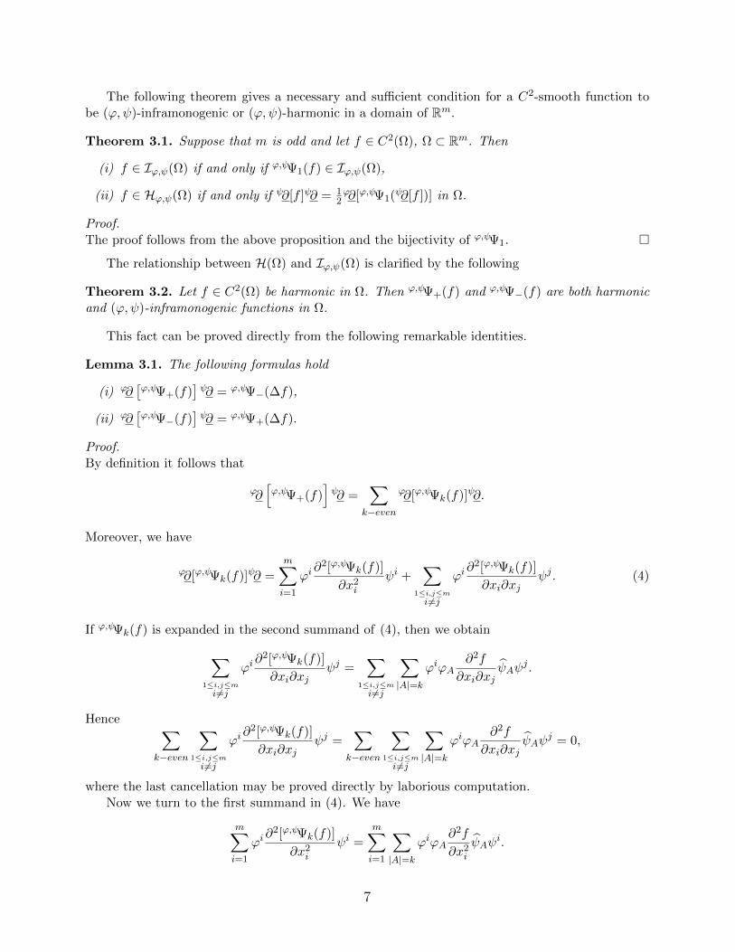
The following theorem gives a necessary and sufficient condition for a C2-smooth function tobe (ϕ,ψ)-inframonogenic or (ϕ,ψ)-harmonic in a domain of Rm.

Theorem 3.1. Suppose that m is odd and let f ∈ C2(Ω), Ω ⊂ Rm. Then

(i) f ∈ Iϕ,ψ(Ω) if and only if ϕ,ψΨ1(f) ∈ Iϕ,ψ(Ω),

(ii) f ∈ Hϕ,ψ(Ω) if and only if ψ∂[f ]ψ∂ = 12ϕ∂[ϕ,ψΨ1(

ψ∂[f ])] in Ω.

Proof.The proof follows from the above proposition and the bijectivity of ϕ,ψΨ1.

The relationship between H(Ω) and Iϕ,ψ(Ω) is clarified by the following

Theorem 3.2. Let f ∈ C2(Ω) be harmonic in Ω. Then ϕ,ψΨ+(f) and ϕ,ψΨ−(f) are both harmonicand (ϕ,ψ)-inframonogenic functions in Ω.

This fact can be proved directly from the following remarkable identities.

Lemma 3.1. The following formulas hold

(i) ϕ∂[ϕ,ψΨ+(f)

]ψ∂ = ϕ,ψΨ−(∆f),

(ii) ϕ∂[ϕ,ψΨ−(f)

]ψ∂ = ϕ,ψΨ+(∆f).

Proof.By definition it follows that

ϕ∂[ϕ,ψΨ+(f)

]ψ∂ =

∑k−even

ϕ∂[ϕ,ψΨk(f)]ψ∂.

Moreover, we have

ϕ∂[ϕ,ψΨk(f)]ψ∂ =m∑i=1

ϕi∂2[ϕ,ψΨk(f)]

∂x2iψi +

∑1≤i,j≤m

i 6=j

ϕi∂2[ϕ,ψΨk(f)]

∂xi∂xjψj . (4)

If ϕ,ψΨk(f) is expanded in the second summand of (4), then we obtain

∑1≤i,j≤m

i 6=j

ϕi∂2[ϕ,ψΨk(f)]

∂xi∂xjψj =

∑1≤i,j≤m

i 6=j

∑|A|=k

ϕiϕA∂2f

∂xi∂xjψAψ

j .

Hence ∑k−even

∑1≤i,j≤m

i 6=j

ϕi∂2[ϕ,ψΨk(f)]

∂xi∂xjψj =

∑k−even

∑1≤i,j≤m

i 6=j

∑|A|=k

ϕiϕA∂2f

∂xi∂xjψAψ

j = 0,

where the last cancellation may be proved directly by laborious computation.Now we turn to the first summand in (4). We have

m∑i=1

ϕi∂2[ϕ,ψΨk(f)]

∂x2iψi =

m∑i=1

∑|A|=k

ϕiϕA∂2f

∂x2iψAψ

i.

7

Observe that for all i = 1, . . . ,m:∑|A|=k

ϕiϕA∂2f

∂x2iψAψ

i =∑|A|=k

A3i

ϕiϕA∂2f

∂x2iψAψ

i +∑|A|=k

A 63i

ϕiϕA∂2f

∂x2iψAψ

i

=∑|A|=k

A3i

ϕA\i∂2f

∂x2iψA\i +

∑|A|=k

A 63i

ϕA∪i∂2f

∂x2iψA∪i.

On the other hand, for k ≥ 2∑|A|=k

ϕiϕA∂2f

∂x2iψAψ

i +∑

|A|=k−2

ϕiϕA∂2f

∂x2iψAψ

i

=∑|A|=k

A3i

ϕA\i∂2f

∂x2iψA\i +

∑|A|=k

A 63i

ϕA∪i∂2f

∂x2iψA∪i

+∑|A|=k−2

A3i

ϕA\i∂2f

∂x2iψA\i +

∑|A|=k−2

A 63i

ϕA∪i∂2f

∂x2iψA∪i

=∑|A|=k−2

A3i

ϕA\i∂2f

∂x2iψA\i +

∑|A|=k−1

ϕA∂2f

∂x2iψA +

∑|A|=k

A 63i

ϕA∪i∂2f

∂x2iψA∪i,

where use has been made of the obvious equality∑|A|=k

A3i

ϕA\i∂2f

∂x2iψA\i +

∑|A|=k−2

A 63i

ϕA∪i∂2f

∂x2iψA∪i =

∑|A|=k−1

ϕA∂2f

∂x2iψA.

A repeated use of the above argument leads to∑k−even

∑|A|=k

ϕiϕA∂2f

∂x2iψAψ

i =∑κ−odd

∑|A|=κ

ϕA∂2f

∂x2iψA.

Therefore

ϕ∂[ϕ,ψΨ+(f)

]ψ∂ =

m∑i=1

∑k−even

∑|A|=k

ϕiϕA∂2f

∂x2iψAψ

i =∑κ−odd

∑|A|=κ

m∑i=1

ϕA∂2f

∂x2iψA

=∑κ−odd

∑|A|=κ

ϕA[∆f ]ψA = ϕ,ψΨ−(∆f).

The second identity may be proved in a quite analogous way.

Proof of Theorem 3.2. If f is harmonic, then the harmonicity of ϕ,ψΨ+(f) follows directlyfrom the obvious identity ∆[ϕ,ψΨ+(f)] = ϕ,ψΨ+(∆f). That the function ϕ,ψΨ+(f) is also (ϕ,ψ)-inframonogenic is clear from Lemma 3.1-(i). In a similar fashion, the function ϕ,ψΨ−(f) is dealtwith.

As we shall now see, the conclusion of Theorem 3.2 remains true if “harmonic” is replaced by“(ϕ,ψ)-inframonogenic”. More precisely:

8

Theorem 3.3. Let f be (ϕ,ψ)-inframonogenic in Ω. Then ϕ,ψΨ+(f) and ϕ,ψΨ−(f) are both har-monic and (ϕ,ψ)-inframonogenic functions in Ω.

Proof.The proof is obtained as a combination of Proposition 3.2-(ii), Lemma 3.1 and the following recur-sive rule

(m− k + 1)ϕ,ψΨk−1(f) + (k + 1)ϕ,ψΨk+1(f) = ϕ,ψΨ1(ϕ,ψΨk(f)), k = 1, . . . ,m− 1, (5)

which may be verified by direct checking.Indeed, if f ∈ Iϕ,ψ(Ω) then by Proposition 3.2-(ii) one has ϕ,ψΨ1(f) ∈ Iϕ,ψ(Ω). This last fact

and (5) together say that ϕ,ψΨ2(f) ∈ Iϕ,ψ(Ω). Thus, this argument may be applied repeatedly toobtain that ϕ,ψΨk(f) (k = 1, . . . ,m) and so ϕ,ψΨ±(f) are (φ, ψ)-inframonogenic functions in Ω aswell. With this in hand, the harmonicity of ϕ,ψΨ±(f) is a straightforward consequence of Lemma3.1.

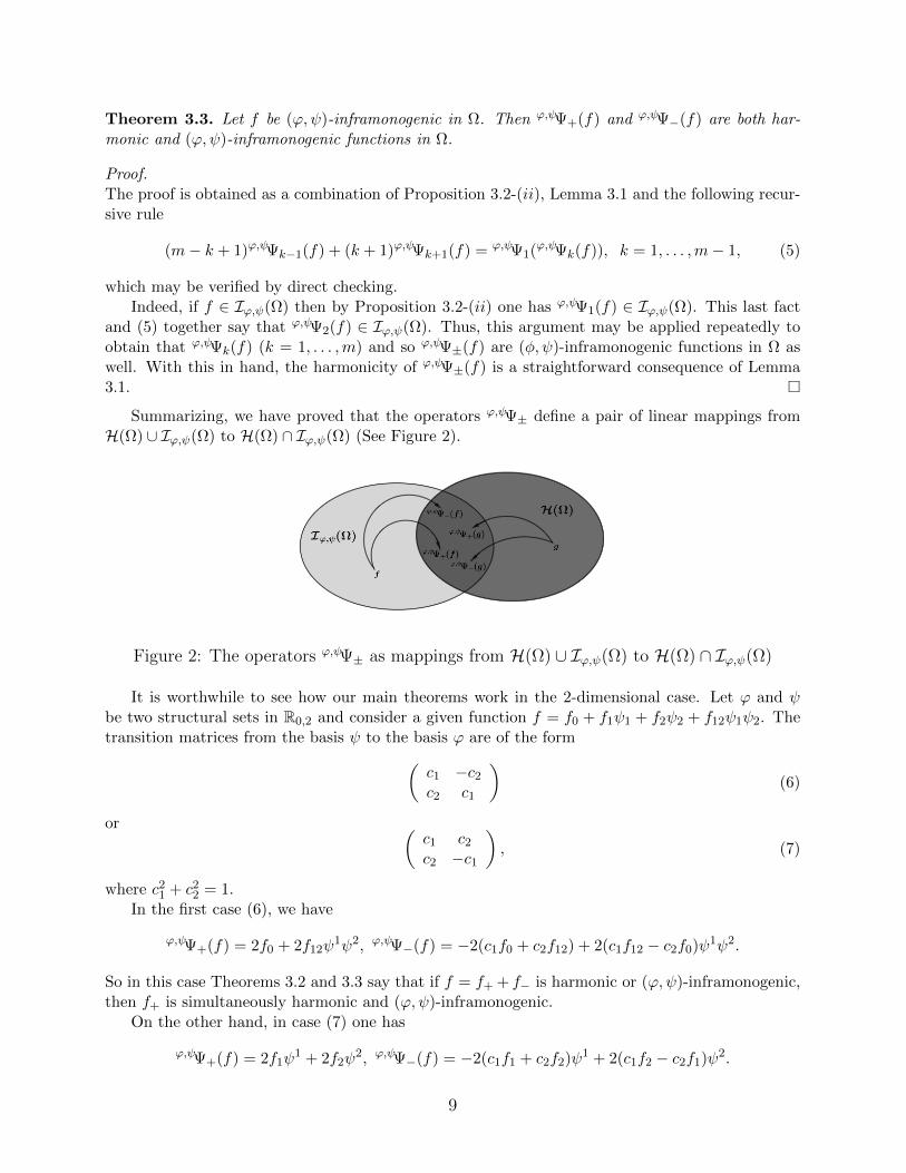
Summarizing, we have proved that the operators ϕ,ψΨ± define a pair of linear mappings fromH(Ω) ∪ Iϕ,ψ(Ω) to H(Ω) ∩ Iϕ,ψ(Ω) (See Figure 2).

Figure 2: The operators ϕ,ψΨ± as mappings from H(Ω) ∪ Iϕ,ψ(Ω) to H(Ω) ∩ Iϕ,ψ(Ω)

It is worthwhile to see how our main theorems work in the 2-dimensional case. Let ϕ and ψbe two structural sets in R0,2 and consider a given function f = f0 + f1ψ1 + f2ψ2 + f12ψ1ψ2. Thetransition matrices from the basis ψ to the basis ϕ are of the form(

c1 −c2c2 c1

)(6)

or (c1 c2c2 −c1

), (7)

where c21 + c22 = 1.In the first case (6), we have

ϕ,ψΨ+(f) = 2f0 + 2f12ψ1ψ2, ϕ,ψΨ−(f) = −2(c1f0 + c2f12) + 2(c1f12 − c2f0)ψ1ψ2.

So in this case Theorems 3.2 and 3.3 say that if f = f+ + f− is harmonic or (ϕ,ψ)-inframonogenic,then f+ is simultaneously harmonic and (ϕ,ψ)-inframonogenic.

On the other hand, in case (7) one has

ϕ,ψΨ+(f) = 2f1ψ1 + 2f2ψ

2, ϕ,ψΨ−(f) = −2(c1f1 + c2f2)ψ1 + 2(c1f2 − c2f1)ψ2.

9

Therefore, in this situation, our theorems ensure that if f = f+ + f− is harmonic or (ϕ,ψ)-inframonogenic, then f− is simultaneously harmonic and (ϕ,ψ)-inframonogenic.

Of course, the two-dimensional case is very special. In general such a nice interpretation of ourtheorems is no longer available.

Finally we mention that the converse of the above theorems is not true. As is easily seen fromProposition 2.3, a general C2-smooth function f (neither harmonic nor (ϕ,ϕ)-inframonogenic)can be constructed in such a way that [f ]0 and [f ]m, hence ϕ,ϕΨ+(f), be harmonic and (ϕ,ϕ)-inframonogenic, simultaneously.

References

[1] Abreu Blaya, R., Bory Reyes, J., Moreno Garcıa, A., Moreno Garcıa, T. A Cauchy IntegralFormula for Infrapolymonogenic Functions in Clifford Analysis. Adv. Appl. Clifford Algebras30, 21 (2020). https://doi.org/10.1007/s00006-020-1049-x.

[2] Alfonso Santiesteban, D., Abreu Blaya, R., Arciga Alejandre, M. On (φ, ψ)-InframonogenicFunctions in Clifford Analysis. Bull Braz Math Soc, New Series (2021). https://doi.org/10.1007/s00574-021-00273-6.

[3] Bory Reyes, J.; De Schepper, H., Guzman Adan, A., Sommen, F. Higher order Borel-Pompeiurepresentations in Clifford analysis. Math. Methods Appl. Sci. 39 , no. 16, 4787–4796, 2016.

[4] Brackx, F., Delanghe, R., Sommen, F. Clifford analysis. Research Notes in Mathematics, 76,Pitman (Advanced Publishing Program), Boston, 1982.

[5] Gurlebeck, K., Nguyen, H. M. ψ-Hyperholomorphic functions and an application to elasticityproblems, AIP Conference Proceedings, 1648 (1), 440005, 2015.

[6] Gurlebeck, K., Nguyen, H. M. On ψ-hyperholomorphic Functions and a Decomposition ofHarmonics. Hyper complex Analysis: New Perspectives and Applications. Trends in Mathe-matics, 181-189, 2014.

[7] Malonek, H., Pena-Pena, D., Sommen, F. A Cauchy-Kowalevski Theorem for InframonogenicFunctions. Math. J. Okayama Univ. 53, 167–172, 2011.

[8] Malonek, H., Pena-Pena, D., Sommen, F. Fischer decomposition by inframonogenic functions.CUBO A Mathematical Journal. Vol.12, No 02, (189–197), 2010.

[9] Moreno Garcıa, A., Moreno Garcıa, T., Abreu Blaya, R., Bory Reyes, J. A Cauchy integralformula for inframonogenic functions in Clifford analysis. Adv. Appl. Clifford Algebras 27,no.2, 1147-1159, 2017.

[10] Moreno Garcıa, A., Moreno Garcıa, T., Abreu Blaya, R., Bory Reyes, J. Decomposition ofinframonogenic functions with applications in elasticity theory. Math Meth Appl Sci. 2020;43:1915–1924.

[11] Moreno Garcıa, A., Moreno Garcıa, T., Abreu Blaya, R., Bory Reyes, J. Inframonogenicfunctions and their applications in three dimensional elasticity theory. Math. Methods Appl.Sci. 41, no.10, 3622-3631, 2018.

10

[12] Moreno Garcıa, A., Moreno Garcıa, T, Abreu Blaya, R. Comparing harmonic and inframono-genic functions in Clifford analysis, to appear in Mediterranean Journal of Mathematics,2021.

[13] Serrano Ricardo, J. L., Bory Reyes, J., Abreu Blaya, R. Singular integral operators and a ∂-problem for (ϕ,ψ)-harmonic functions. Anal.Math.Phys. 11, 155 (2021). https://doi.org/10.1007/s13324-021-00590-5.

[14] Shapiro, M. V., Vasilevski, N. L. Quaternionic ψ-hyperholomorphic functions, singular inte-gral operators and boundary value problems. I. ψ-hyperholomorphic function theory, ComplexVariables, 27, 17–46, 1995.

11