Universidade de Sao PauloInstituto de Fısica

Estudo do comportamento da entropia embilhares

Gabriel Dıaz Iturry

Orientador(a): Prof. Dr. Edson Denis Leonel

Coorientador(a): Prof. Dr. Ibere Luiz Caldas

Tese de doutorado apresentada ao Instituto de Fısicada Universidade de Sao Paulo, como requisito parcialpara a obtencao do tıtulo de Doutor em Ciencias.

Banca Examinadora:Prof. Dr. Edson Denis Leonel - Orientador (UNESP/IFUSP)Prof. Dr. Mario Jose de Oliveira (IFUSP)Prof. Dr. Antonio Marcos Batista (UEPG)Prof. Dr. Luiz Antonio Barreiro (UNESP)Prof. Dr. Ricardo Luiz Viana (UFPR)

Sao Paulo2020

FICHA CATALOGRÁFICAPreparada pelo Serviço de Biblioteca e Informaçãodo Instituto de Física da Universidade de São Paulo

Díaz Iturry, Gabriel

Estudo do comportamento da entropia em bilhares. São Paulo,2021.

Tese (Doutorado) – Universidade de São Paulo. Instituto de Física. Depto. de Física Aplicada

Orientador: Prof. Edson Denis Leonel

Área de Concentração: Física

Unitermos: 1. Caos (Sistemas dinâmicos); 2. Bilhares; 3. Entropia.

USP/IF/SBI-007/2021

University of Sao PauloPhysics Institute

Study of entropy behaviour in billiard systems

Gabriel Dıaz Iturry

Supervisor: Prof. Dr. Edson Denis LeonelCo-supervisor: Prof. Dr. Ibere Luiz Caldas

Thesis submitted to the Physics Institute of the Uni-versity of Sao Paulo in partial fulfillment of the re-quirements for the degree of Doctor of Science.

Examining Committee:Prof. Dr. Edson Denis Leonel - Orientador (UNESP/IFUSP)Prof. Dr. Mario Jose de Oliveira (IFUSP)Prof. Dr. Antonio Marcos Batista (UEPG)Prof. Dr. Luiz Antonio Barreiro (UNESP)Prof. Dr. Ricardo Luiz Viana (UFPR)

Sao Paulo2020

A quienes quiero.

Ustedes saben quienes son.

Agradecimentos

Agradezco a mi familia por su paciencia y por el tiempo propio que vivimos; a

mi orientador Prof. Edson Denis Leonel y coorientador Prof. Ibere Luiz Caldas por

brindarme la oportunidad de desarrolar este trabajo, a Matheus Palmero por sus agu-

das observaciones. A las amistades, antiguas y nuevas, que estan ahı por el mundo.

Agradezco tambien a la agencia CNPq y al Instituto de Fısica de USP-Sao Paulo.

A los que ayudaron en esto.

Resumo

Neste trabalho estudamos como usar o comportamento da entropia para medir oexpoente de difusao de um conjunto de condicoes iniciais em sistemas do tipo bilhar.Os modelos considerados sao o Modelo Fermi Ulam Simplificado, o Mapa Padrao e oBilhar Ovoide. Nos preocupamos com a difusao perto da ilha principal no espaco defases, onde existe o fenomeno de aprisionamento temporario. Calculamos o expoentede difusao para diversos valores do parametro de controle do Mapa Padrao e o BilharOvoide, onde para cada valor a ilha principal tinha uma forma diferente, e mostramosque as mudancas de comportamento no expoente estao relacionadas com mudancas naarea da ilha principal. Particularmente, mostramos que toda vez que a area da ilhaprincipal se reduzia abruptamente, devido a destruicao de toros invariantes e a criacaode pontos fixos hiperbolicos e elıpticos, o expoente de difusao cresce. Para investigarmelhor a conexao entre o expoente de difusao e a criacao de pontos fixos hiperbolicose elıpticos, desenvolvemos um esquema de controle apropriado no Mapa Padrao, com oqual mostramos que fechando os caminhos de fuga das proximidades da ilha o expoentede difusao tornou-se menor. Em seguida, relacionamos os caminhos de fuga com avariedade instavel dos pontos hiperbolicos.

Palavras Chaves: Caos, Bilhares, Difusao.

Abstract

In this work we studied how to use the behaviour of the entropy to measure thediffusion exponent of a set of initial conditions in Billiard like systems. The consid-ered models are the Simplified Fermi Ulam Model, Standard Map and the Oval Billiard.We care about the diffusion near the main island in the phase space, where exists thestickiness phenomenon. We calculated the diffusion exponent for many values of thenonlinear parameter of the Standard Map and the Oval Billiard, where for each valuethe main island has a different shape, then we show that the changes of behaviour in thediffusion exponent are related to changes in the area of the main island. Particularly, weshow when the main island’s area is abruptly reduced, due to the destruction of invarianttori and consequently creation of hyperbolic and elliptic fixed points, the diffusion ex-ponent grows. To further investigate the connection between the diffusion exponent andthe creation of hyperbolic and elliptic fixed points, we developed an appropriate controlscheme in the Standard Map, with which we showed that closing paths of escape fromthe island shore the diffusion exponent became smaller. Then we related the paths ofescape with the unstable manifold of the hyperbolic points.

Key Words: Chaos, Billiards, Diffusion.

CONTENTS

1 Introduction 91.1 A brief history of nonlinear dynamics, the beginning . . . . . . . . . . 91.2 Objectives and some preliminary concepts . . . . . . . . . . . . . . . . 101.3 Organization of the text . . . . . . . . . . . . . . . . . . . . . . . . . . 13

2 Dynamical models 142.1 Standard Map, the typical first example . . . . . . . . . . . . . . . . . 142.2 Billiard systems, hardly pool games . . . . . . . . . . . . . . . . . . . 19

3 Diffusion, an entropy approach 233.1 Diffusion . . . . . . . . . . . . . . . . . . . . . . . . . . . . . . . . . 23

3.1.1 Examples of Diffusion in Maps . . . . . . . . . . . . . . . . . 243.1.2 Diffusion Entropy Analysis . . . . . . . . . . . . . . . . . . . 273.1.3 Entropy approach in the Simplified Fermi Ulam Model . . . . . 29

4 Results 324.1 Navigating through the chaotic sea . . . . . . . . . . . . . . . . . . . . 324.2 The shore of the main island . . . . . . . . . . . . . . . . . . . . . . . 344.3 Diffusion exponent and Area . . . . . . . . . . . . . . . . . . . . . . . 384.4 Controlling escape, a targeting algorithm . . . . . . . . . . . . . . . . . 424.5 The manifold effect . . . . . . . . . . . . . . . . . . . . . . . . . . . . 46

5 Conclusions 51

6 Perspectives 53

7

A For those about to map 54A.1 Standard Map . . . . . . . . . . . . . . . . . . . . . . . . . . . . . . . 54A.2 Simplified Fermi Ulam Model . . . . . . . . . . . . . . . . . . . . . . 56A.3 Oval Billiard . . . . . . . . . . . . . . . . . . . . . . . . . . . . . . . 58

B Oval Billiard, an algorithm to solve it 61

C A little more on diffusion 64C.1 Anomalous Diffusion . . . . . . . . . . . . . . . . . . . . . . . . . . . 64C.2 Validity of the scaling relation on our mappings . . . . . . . . . . . . . 71

D Entropy and time irreversibility, some comments 77D.1 Entropy conservation . . . . . . . . . . . . . . . . . . . . . . . . . . . 77D.2 Entropy growth . . . . . . . . . . . . . . . . . . . . . . . . . . . . . . 79D.3 Time reversibility and time irreversibility . . . . . . . . . . . . . . . . 79

Chapter 1

Introduction

1.1 A brief history of nonlinear dynamics, the beginning

In the second half of 17th century Newton was able to mathematically describethe planetary motion of two bodies [1], which until then was known by the empiricalKepler’s laws.

New generation of mathematicians and physicists tried to solve the gravitationalproblem of three bodies without success. At the end of 19th century Poincare broughta new insight to the problem [2]. Instead of wondering about quantitative aspects, heasked about qualitative description of the problem, as the stability of the motion. Withthis in mind he developed geometric approximations to analyze the problem. Eventhough the three body problem was not solvable by looking for first integrals of motion,at the end of 20th century Sundman found an analytic series approximation of the solu-tion to the gravitational problem of three bodies for almost all admissible initial condi-tions [3], later, in 1990, Wang resolved the problem of n bodies [4], again in an analyticseries approximation. Both solutions showed up to be of less interest than Poincare’sgeometric approach for qualitative aspects, since physically they do not brought newinsights to the problem in hands, even more, both series converge very slowly, so noteven presented numerical improvement [5].

In the second half of the 20th century the studies in dynamics focused in nonlinearoscillators and applications of those in physics and engineering, applications such asradio, laser, radar among many others. In the theoretical counterpart new methods of

9

10

analysis, based on Poincare’s geometric approach, were developed. The use of the com-puters to perform the calculations allowed to study and experiment with new equationsin ways that were impossible before. This kind of experiments yields Lorenz, whilestudying atmospheric models, to the discovery of chaotic movement in strange attrac-tors [6]. Lorenz found that solutions to the equations he was studying could oscillatein a strange and unpredictable way, even more, starting from close initial conditions thebehaviour of the trajectories could be very different.

After Lorenz’s discovery many more similar results were found in sciences whilestudying nonlinear systems. In the 70’s Feigenbaum realized there are universal lawsgoverning transition between regular and chaotic behaviour [7]. He proved that twocompletely different systems can become chaotic in the same way. Besides chaos, non-linear dynamics also growth due the works done in fractals and synchronization [8].

An important area of research in nonlinear dynamics is in systems described by aHamiltonian [9]. The system’s dynamical variables are canonical conjugate pair of vari-ables, position and momentum. If in the dynamics exist conserved quantities, integralsof movement, it is possible to reduce the number of variables that describe the system. Ifa Hamiltonian system has as many integrals of movement as position-momentum pairs,it is called of integrable. In many cases, an integrable Hamiltonian system under anarbitrary perturbation leads to chaotic dynamics.

1.2 Objectives and some preliminary concepts

The diffusion problem in phase space for low dimensional classical Hamiltoniansystems is very important nowadays from a theoretical point of view [10, 11]. Thepresence of regular and chaotic trajectories produces different kinds of diffusion fordensities of trajectories. Depending on the region in the phase space the diffusion maybe normal or anomalous. From a physical point of view, diffusion in phase space ispresent in many problems, such as the unlimited growth of energy, 1[12, 13, 14], or thestudy of transport properties from one region of phase space to another region [15, 16],and plasma dynamics [17, 18], among others.

Usually the diffusion is studied as the growth over time of the standard deviation

1This phenomenon is some times called Fermi Acceleration, the diffusion is along the energy axis.

11

of a generalized momentum variable [10, 19, 20, 21], in those studies it is consideredthat the diffusion along the generalized position, angle like variable, is fast. The growthover time (t) of the standard deviation (σ = Ct∆) is characterized by two variables,a diffusion coefficient (C) and a diffusion exponent (∆), the most important being theexponent since it allows us to distinguish between anomalous diffusion, when the expo-nent is different from 1/2, and normal diffusion, when the exponent is 1/2. Even thoughthis method gives good results in some cases, like in an almost completely chaotic sea[22, 23], it fails in some other cases, since it is difficult to find the appropriate general-ized momentum that it is better suited to describe a specific behaviour in phase space[24, 25]. A particular physical scenario where the momentum method fails, is when ex-ists coexistence of dynamics, regions of regular trajectories arranged in complex struc-tures called Kolmogorov-Arnold-Moser (KAM) islands [26, 27, 28], surrounded by asea of chaotic trajectories. This complex scenario is described by the KAM Theorem,which states that quasiperiodic motion persists under small perturbations on integrableHamiltonian systems. Due to the action of the perturbation some invariant curves, tori,are deformed and some are broken becoming pairs of unstable/stable fixed points. Sta-ble fixed points are surrounded by invariant curves forming stability islands, and the setof broken tori form a complex pattern, the Cantori [26, 27, 28, 29].

A method that overcomes the standard-deviation problem was proposed by Scafettaand Grigolini to characterize superdiffusive dynamics. This method, called DiffusionEntropy Analysis (DEA), is known to serve in common diffusion models [30], it is basedon the use of entropy behaviour rather than the standard deviation’s behaviour. For ourpurposes, study diffusion in Hamiltonian systems, we adapt this method. Consideringthe fact that the entropy is invariant under a certain type of variable transformations,as changing from one set of canonical variables to another, we expect that the methodworks fine in the physical scenarios where finding momentum variables is not feasible.

In this work we will focus in two points:

1. Use measurement of Entropy to study Diffusion process in Billiard Systems.

2. Give empirical explanation of the diffusion regimes encountered.

We will use the Shannon Entropy [31]. This entropy quantifies the unevenness of a

probability distribution [32]. Some valid remarks about Shannon entropy in the problemat hands are:

12

• It is in natural units.

• It is not the Thermodynamical entropy, the system is deterministic and not inequilibrium.

The idea of diffusion that we use in this work is the movement of particles from

region of higher concentration to region of lower concentration. Particularly we willconsider trajectories of an ensemble of non-interacting particles, our dynamical modelswill be deterministic then the ensemble behaviour is completely determined from theinitial conditions of its components.

A billiard system is a class of Hamiltonian system. It consists in free particle moving

a N-dimensional closed region suffering collisions with a border. This system showsthe complexity of general low dimensional Hamiltonian systems with simple dynamicallaws.

We will specifically focus in using the entropy behaviour to characterize the diffu-sion around KAM islands; we particularly focus in the subdiffusive behaviour producedby the Cantori.

13

1.3 Organization of the text

The text is organized as follows:In chapter 2 we present the dynamical models that will be our working place where

we will study the diffusion process. The models are the Standard Map [33, 34] andthe Oval Billiard [35]. We give a detailed discussion about the mappings variables andcontrol parameters. We also describe the different kinds of dynamics that they present,i. e. regular, quasiregular and chaotic. We particularly care about showing the KAMislands and in describing the mappings in canonical variables, this last point is importantin order to measure the entropy.

Chapter 3 shows how to use the Diffusion Entropy Analysis approach in a Hamilto-nian map that we know it presents normal diffusion process, with this we can establish

a methodology to characterize the diffusion exponent in other scenarios, i. e. aroundKAM islands. The main result from this chapter is a relation between the diffusion

range of our variables, the fluctuation size that ensemble suffers under the dynamics,and the number of grid divisions needed to measure the entropy by an histogram.

Having the results from chapter 3 we proceed to study the diffusion around the

KAM islands, this is done in chapter 4. We proceed to calculate the diffusion exponentfor many values of the control parameter both for the Standard Map as for the OvalBilliard, and show there is a correlation between the main island’s area and the diffusionexponent. Particularly we find that when the main island’s area is abruptly reduced, duethe destruction of invariant tori and creation of hyperbolic and elliptic fixed points, the

diffusion exponent grows. Then, we relate this behaviour with the influence of invariant

manifolds associated to the hyperbolic fixed points.

In chapter 5 we drawn conclusions and discuss our results.Finally, in chapter 6 we present our perspectives for future research.

Chapter 2

Dynamical models

In this chapter we present a brief description of the dynamical models that we usealong the text: The Standard Map and the Oval Billiard. A more complete descriptionand demonstration of the maps is shown in Appendix A and Appendix B.

2.1 Standard Map, the typical first example

Dynamical systems provide mathematical models that help to comprehend differentphenomena [36, 37, 9, 38]. In Physics several dynamical systems can be described bya Hamiltonian. Among a variety of possible physical phenomena, the ones describedby low dimensional Hamiltonians have a special property, they may present chaoticbehaviour even though the deterministic dynamics is simple.

To describe and understand dynamical systems is common to use a Poincare’s sec-

tion. This description gives information about the dynamics in a resumed way, it ex-ploits the existence of symmetries or some geometrical characteristics of the dynamicalsystem, see figure 2.1.

14

15

Figure 2.1: Diagrammatic explanation of a Poincare section in a fictitious system.

In figure 2.1 we show a diagrammatic explanation of a Poincare section. The tra-jectory in phase space1 is described by the red line. Assuming that the trajectory willalways cross the gray plane we only care about the points where the red line crosses theplane in a given direction, this gives the map xn+1 = F (xn). A condensed descriptionof the dynamics, the Poincare section, is achieved by the mapping sequence xn, xn+1,....

In Classical Mechanics, the dynamics of a system can be described by a Hamilto-nian. The system’s phase space is given by canonical conjugate pair of variables, gen-eralized position and momentum. Trajectories in phase space do not cross each other,even more, if in the dynamics exist conserved quantities, integrals of movement, it is

1Phase space is a space in which all possible states of a system are represented, it has one dimensionfor each variable that describes the system.

16

possible to reduce the dimensions in the representation. If a Hamiltonian system hasas many integrals of movement as position-momentum pairs, it is called of integrable.In many cases, an integrable Hamiltonian system under an arbitrary perturbation leadsto chaotic dynamics. In this kind of systems is usual to use a Poincare section, sincewe can reduce one dimension in the representation of the trajectory, given us a muchsimpler image of the problem at hands. Since this representation is discretized, i. e. wehave a sequence xn, xn+1, ..., we call it a Poincare map representation.

A typical example of a Poincare map of a low dimensional Hamiltonian is givenby Chirikov’s Standard Map [33, 34]. The unperturbed Hamiltonian describes the freemotion of a particle constrained to move in a ring:

H0 (q, p) =p2

2, (2.1)

this is an integrable Hamiltonian system, we have only one pair [q, p] and one conservedquantity, the energy. To this system we add a periodic time dependent perturbation,giving the following Hamiltonian:

H (q, p, t) =p2

2+ k cos (q)

∞∑n=−∞

δ (t− n) , (2.2)

the second term in the right hand side represents the particle being kicked periodicallyby an external q dependent field, the magnitude of this field is given by the parameter k.If it’s value is different from zero, the energy is not longer a constant of movement, thus,this is a nonintegrable Hamiltonian system, characterized by the nonlinearity parameterk. A Poincare map can be constructed considering the position-momentum pair aftereach kick, this is the Chirikov’s Standard Map, derived in Appendix A:

pn+1 = pn + k sin (qn) ,

qn+1 = qn + pn+1, (2.3)

where qn and pn are positions in phase space at iteration n, k is the parameter thatcontrols the nonlinearity, the equation (2.3) gives at each iteration a new position inphase space. In Appendix A is shown that this is an area preserving map. A common2

2Unless stated otherwise, this will be the case in this Thesis.

17

procedure is to actually care of qn and pn modulo 2π.A important set of trajectories possibles in the mapping (2.3) are the fixed points,

periodic orbits3 [8]. Since the map is area preserving there are two possible types offixed points: i) The elliptic ones, who have neutral stability in all directions aroundthem, and ii) the hyperbolic fixed points, who have directions of stability and unstability[8, 39]. From these directions of stability/unstability, are born the invariant manifolds4,both the stable5 as the unstable6. These invariant manifolds have important properties,i) At each iteration a point in a manifold is mapped to another point in the manifold, ii)they influence the dynamics around them, trajectories tend to align along the unstablemanifold, iii) their action is all over the phase space.

Figure 2.2: Phase space portrait of Standard Map for k = 0.1.

3The fixed points of period m are the set of solutions that have property x0 = Fm(x0).4A manifold is a topological space that locally resembles Euclidian space near each point.5Stable manifold is the invariant set of points that goes to the fixed point when the number of iterations

goes to infinity. For a mapping f : X → X the stable manifold of a fixed point x0 = f(x0) is the invariantset defined by W s(f, x0) = {x ∈ X : fn(x)→ x0 as n→∞}.

6Unstable manifold is the invariant set of points that goes to the fixed point when the number ofiterations of the inverse mapping goes to infinity. For a mapping f : X → X the unstable manifold of afixed point x0 = f(x0) is the invariant set defined byWu(f, x0) = {x ∈ X : f−n(x)→ x0 as n→∞},where f−1 is the inverse of f .

18

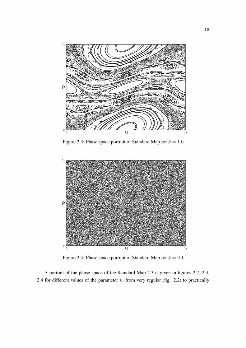
Figure 2.3: Phase space portrait of Standard Map for k = 1.0

Figure 2.4: Phase space portrait of Standard Map for k = 9.1

A portrait of the phase space of the Standard Map 2.3 is given in figures 2.2, 2.3,2.4 for different values of the parameter k, from very regular (fig. 2.2) to practically

19

completely chaotic (fig. 2.4), passing by coexistent dynamics7 (fig. 2.3). For a givenset of initial conditions in phase space we applied many times the mapping (2.3) to gofrom on position in phase space to another position, those positions are drawn as pointsin the phase space portrait. For values of k where there is coexistence of dynamics,the regions of regular motion are generally formed by invariant curves8 arranged incomplex structures called Kolmogorov-Arnold-Moser (KAM) islands9.

2.2 Billiard systems, hardly pool games

Among many Hamiltonian systems ones of special interest are the billiard systems[40, 41]. They evolve by simple dynamical rules but show all the complexity of generallow dimensional Hamiltonian dynamics, they can be integrable, as the circular billiard,ergodic, as the Sinai billiard, or of mixed phase space, as the Oval billiard, see ref [41].Even more, billiard systems can be used to model some phenomena with direct physicalinterpretation, as thermometric efficiency, nuclear collisions, transport and others [42].The most simple one consists of a free particle moving in a N-dimensional closed regionsuffering collisions with a border. We can also add some special dynamics both in theoriginal free moving particle region as in the collision zone, for example, the movementof the particle can be influenced by external field forces, and the border, also knownas wall, can be moving in a known way, besides that, the collisions can be elastic orinelastic.

The notion of billiard is known since Birkhoff proposed the problem of a sphericalparticle moving in many directions colliding with a border [43]. Later on, due the workof Sinai in mathematical properties of billiards of dispersing wall [44], and also Krylov’sexhaustive work in the same systems [45], a new period of billiard analysis begun.

The oval billiard, introduced M. Berry in [35], is nowadays a common billiard sys-

7Mixed dynamics in the sense that chaotic, periodic and quasi periodic dynamics coexist.8Invariant under the action of the map, i. e. a set of points that is over an invariant curve will always

be over it when we iterate our mapping. The motion of these points is quasiperiodic so they draw a curvein the phase space portrait. They are also known as invariant tori.

9KAM Theorem states that quasiperiodic motion persist under small perturbations on integrableHamiltonian systems. Due the action of the perturbation some invariant curves, tori, are deformed andsome are broken becoming pairs of unstable/stable fixed points. Stable fixed points are surrounded byinvariant curves forming stability islands, and the set of broken tori form a complex pattern, the Cantori[26, 27, 28, 29].

20

tem well studied. The radius of the boundary, in polar coordinates, is given by

R (θ, ε, p) = 1 + ε cos (pθ) . (2.4)

The parameter ε ∈ [0, 1) controls the deformation of the circle, the non linearity, pis an integer number and θ ∈ [0, 2π) is the polar angle. A trajectory is shown in figure2.5.

Figure 2.5: Trajectory of a particle inside an oval billiard with p = 1 and ε = 0.3

In figure 2.5 we show an example of a particle’s trajectory inside the oval billiard,we consider elastic collisions, then, the velocity component tangent to the boundary isconserved while the normal component changes sign. Between collisions the particlemoves in straight lines, free moving particle. A Poincare section of this trajectory canbe constructed if we collect data at each collision of the particle with the wall. In thiscase we care about two variables, the angle θ of collision, and the angle α that makesthe trajectory with the tangent to the boundary. This set of variables give a resumeddescription of the trajectory.

In Appendix B we describe an algorithm used to perform the simulation of the par-ticle’s movement. Starting from the coordinates (θn, αn) we find the particles position,xn = R (θn, ε, p) cos(θn), yn = R (θn, ε, p) sin(θn), and velocity, vx,n = cos(αn + φn)

21

vy,n = sin(αn+φn). With this information we calculate the time tn to the next collisionbetween the particle and the border, for this we consider a free particle movement, oncewe have the time tn, we calculate the position of the collision, xn+1, yn+1, and the newvelocity after the collision, vx,n+1, vy,n+1, considering elastic collisions. With this wefind the new coordinates (θn, αn).

Figure 2.6: Portrait of the Poincare section of oval billiard with parameters p = 1 andε = 0.3.

Figure 2.6 shows the Poincare section portrait of the oval billiard for the parametersp = 1 and ε = 0.3. Our Poincare section is described by the variables θ and α shown infigure 2.5. For a given set of initial conditions we follow the trajectories and write thevariables α, θ after each collision with the billiard’s wall. We see it has similar structuresas those shown in figure 2.3 of the Standard Map, i. e., a chaotic sea surrounding KAMislands. In this case the main island belongs to a periodic orbit, we care about the islandcentered in α = π

2and θ = 0.

The pair (θn, αn) is not set of canonical conjugate variables, then, its mapping is notarea preserving. We have to transform to Poincare-Birkhoff coordinates [43] to have anarea preserving map, these are given by the arc-length, sn, and the tangential velocity,vn, to the impact point at the nth collision.

22

The tangential velocity, vn in the nth collision is given by:

vn+1 = cos(αn+1). (2.5)

The arc-lenght sn at the nth iteration can be found by the integral:

sn =

∫ θn

0

√R(θ)2 +

(dR(θ)

dθ

)2

dθ, (2.6)

where the radius R(θ) is parameterized by the angle θ, Eq. (2.4). Considering p = 1

and doing some algebra we arrive to

sn =2

1 + ε

∫ θn2

0

√1− 4ε

(1 + ε)2sin2(u)du, (2.7)

which can be written in terms of the incomplete elliptic integral of second type,E (φ, k),[48], the numerical value can be computed efficiently using the subroutines provided by[49]. The new mapping (sn, vn) to (sn+1, vn+1) it is given by:

sn+1 =2

1 + εE

(θn+1

2,

2√ε

1 + ε

),

vn+1 = cos(αn+1). (2.8)

In Appendix A we show that this is an area preserving mapping.These models, Standard Map and Oval Billiard, will be used in the subsequent Chap-

ters as examples of mappings that present anomalous diffusion. We will study their dif-fusion processes, characterize the diffusion exponent, and describe the physical scenariothat leads to such class of anomalous diffusion.

Chapter 3

Diffusion, an entropy approach

In this chapter we present the Diffusion Entropy Analysis approach, developed in[30]. We show how to make this approach suitable to our mappings, then we apply thisadaptation to a known normal diffusion process. With this we establish an importantrelation, eq. (3.8), and a methodology to measure the diffusion exponent, which will beused in other diffusive scenarios in chapter 4.

3.1 Diffusion

The diffusion problem in phase space for low dimensional classical Hamiltoniansystems is very important nowadays from a theoretical point of view [10, 11]. Thepresence of regular and chaotic trajectories produces different kinds of diffusion fordensities of trajectories. Depending on the region in the phase space the diffusion maybe normal or anomalous. The diffusion in phase space can be used in many problems,such as the unlimited growth of energy, 1[12, 13, 14], or the study of transport propertiesfrom one region of phase space to another region [15, 16].

Usually the diffusion is studied as the growth over time of the standard deviationof a generalized momentum variable [10, 19, 20, 21]. In those studies it is consideredthat the diffusion along the generalized position, angle like variable, is fast. The growthover time, t, of the standard deviation, σ, is characterized by two variables, a diffusion

1This phenomenon is some times called Fermi Acceleration, the diffusion is along the energy axis.

23

24

coefficient D and a diffusion exponent ∆:

σ = Dt∆. (3.1)

The important variable is the diffusion exponent since it allow us to distinguishbetween normal diffusion, when the exponent is 1/2, subdiffusion, when the exponentis less than 1/2 and superdiffusion, when the exponent is higher than 1/2.

Even though characterize the diffusion exponent via eq. (3.1) gives good results insome cases, like in an almost completely chaotic sea, see figure 3.1, it fails in someother cases, since it is difficult to find the appropriate generalized momentum that itis better suited to describe a particular behaviour in phase space2 [24, 25], like aroundKAM islands, see figure 3.2.

3.1.1 Examples of Diffusion in Maps

Normal diffusion in Hamiltonian systems can be exemplified by the SimplifiedFermi-Ulam Model [37, 13], the mapping is:

φn+1 =

[φn +

2

Vn

]mod (2π) ,

Vn+1 = ‖Vn − 2ε sin (φn+1)‖ . (3.2)

This model consists of a classical particle of unit mass, suffering successive elasticcollisions in a confined region of one unit of longitude bounded by two walls, one fixedand the other capable of exchange energy with the particle, affecting the particle’s ve-locity V , this depending on which phase φ it is the wall. The term 2

Vnis the time between

collisions and −2ε sin (φn+1) gives the gain or loss of the particle’s velocity/energy ineach collision. The absolute value in the velocity is to reinject the particle in the correctdirection after each collision, i. e. towards the fixed wall. Although this map is not writ-ten in position-momentum variables it is area preserving. A detailed explanation of howto obtain the mapping (3.2) and the proof that is area preserving is given in AppendixA.

2The canonical transformation might not be obvious and only reachable after an iterative numericalprocedure.

25

For a given value of the control parameter ε, we apply the mapping (3.2) to a setof 1 × 106 points, these points correspond to initial conditions that approach an initialprobability density, indicated by a small circular red area in the bottom of the mapshown in figure 3.1a. After iterating the map, the new positions of the points give us anapproach of the new probability density indicated in figure 3.1b, with this we can studythe time evolution of the probability density, see figure 3.1.

(a) n = 0 (b) n = 1

(c) n = 10 (d) n = 100

Figure 3.1: Plot of the behaviour of the diffusion process, measured by the probabilitydensity, in a chaotic region of phase space for the Simplified Fermi-Ulam Model ε =0.001, for different numbers of iterations n. The orange-white color scale represents thedensity of points in phase space. The subplots (a) to (d) shows the diffusion process.

We see in figure 3.1 that the initial distribution (n = 0 in figure 3.1a) is centeredaround a point, and after only one iteration it spreads out totally along the φ axis (n = 1

in figure 3.1b). In the next iterations the points diffuse along the V axis while remainingalmost spread along φ axis (n = 10 and n = 100 in figure 3.1c and 3.1d).

To show an anomalous diffusion process we will use a variant of the Standard Map

26

given by:

pn+1 = pn + k sin (qn) ,

qn+1 = qn + pn+1 + π. (3.3)

This map is the same as the typical Standard Map (2.3) just with a translation in thep variable in order to have the main island at the middle of the phase space, near thisisland there is anomalous diffusion as shown in figure 3.2.

Again we apply the mapping to a set of 1 × 106 points and look at the evolution ofthe probability density, see figure 3.2.

(a) n = 0 (b) n = 1

(c) n = 10 (d) n = 100

Figure 3.2: Plot of the behaviour of the diffusion process, measured by the probabilitydensity, in a chaotic region of phase space for the Standard Map k = 2.3, for differentnumbers of iterations n. The orange-white color scale represents the density of pointsin phase space. The subplots (a) to (d) shows the diffusion process.

It is possible to see in figure 3.2 that the probability distribution spreads along theshore of the KAM islands and then diffuses outwards. We can observe that the diffusion

27

process is not homogeneous, there are preferred channels along which the trajectoriesleak to the chaotic sea. Even more, this leaking is slow so we are seeing a subdiffusionprocess.

Find the appropriate canonical variables for this problem is not an easy task, theaction/angle variables must be related to the island’s invariant curves, i. e. the anglevariable tells the position over the invariant curve and the action variable says whichinvariant curve we are in, see [24, 25]. Since the Shannon entropy is invariant undercanonical coordinate transformations, in the next section, we will use it to characterizethe diffusion exponent by means of the analysis proposed by Scafetta and Grigolini in[30].

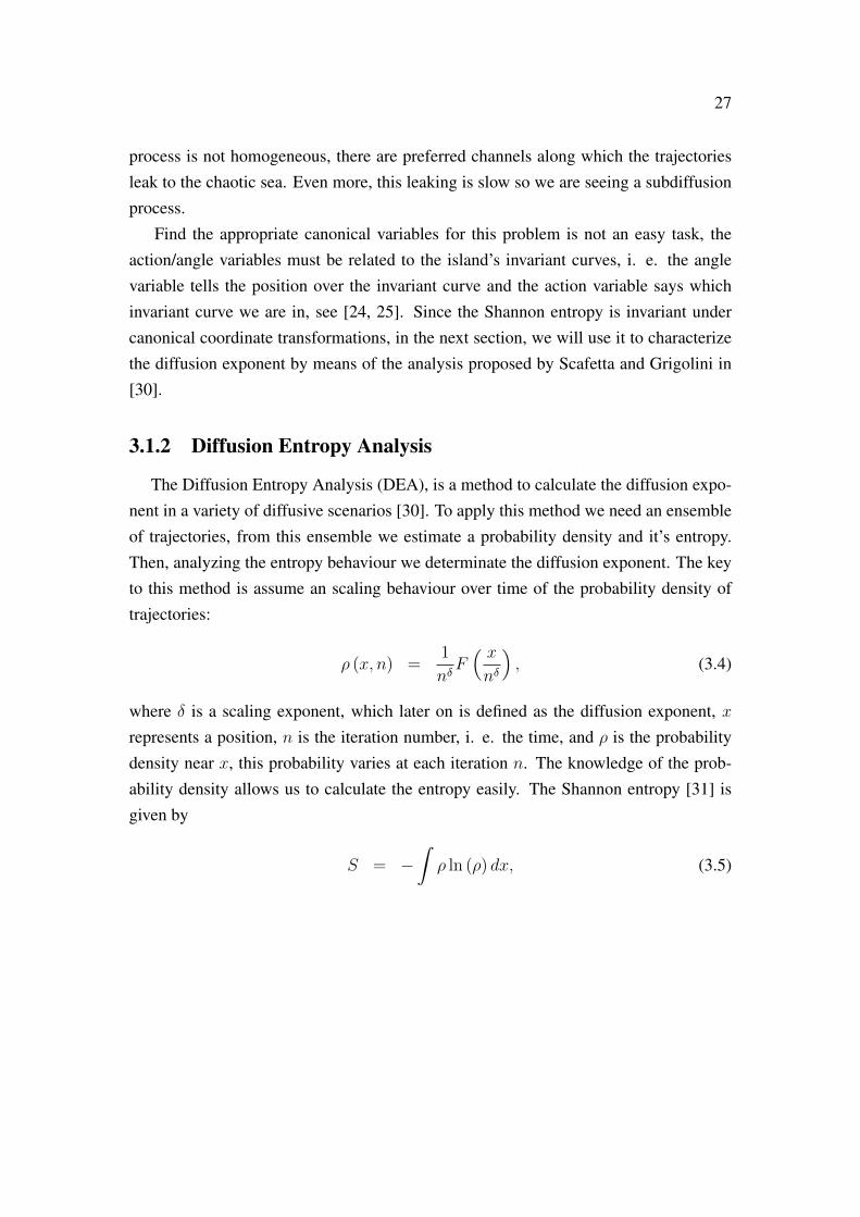
3.1.2 Diffusion Entropy Analysis

The Diffusion Entropy Analysis (DEA), is a method to calculate the diffusion expo-nent in a variety of diffusive scenarios [30]. To apply this method we need an ensembleof trajectories, from this ensemble we estimate a probability density and it’s entropy.Then, analyzing the entropy behaviour we determinate the diffusion exponent. The keyto this method is assume an scaling behaviour over time of the probability density oftrajectories:

ρ (x, n) =1

nδF( xnδ

), (3.4)

where δ is a scaling exponent, which later on is defined as the diffusion exponent, xrepresents a position, n is the iteration number, i. e. the time, and ρ is the probabilitydensity near x, this probability varies at each iteration n. The knowledge of the prob-ability density allows us to calculate the entropy easily. The Shannon entropy [31] isgiven by

S = −∫ρ ln (ρ) dx, (3.5)

28

applying eq. (3.4) to last equation we find the relation between entropy and number ofiteration3:

S = A+ δ ln (n) , (3.6)

According to the work of Scafetta and Grigolini, ref [30], the diffusion exponent canbe defined by equation (3.6), instead of equation (3.1) for the standard deviation. Theydemonstrated that their definition and method gives better results than standard devia-tion methods, particularly in some cases of superdiffusion where the standard deviationis not even mathematically defined 4 [30].

To actually use equation (3.5) in our numerical experiments we have to discretizethe phase space. In all this work we choose to use a regular I × J two dimensionalgrid. After each iteration of a given mapping, we count how many points are insideeach box of the grid and construct an histogram, this is our discretized approximation ofthe probability density. The integral over space in the definition of the Shannon entropy,eq. (3.5), is numerically given by:

S = −I∑i=1

J∑j=1

hij ln (hij) , (3.7)

were the histogram is described by the variables hij of each box in the grid, with thenormalization condition that the sum of all the [hij] must be one.

In [30] they also give a recipe to select the grid box size, they deal with randomwalks, where each particle changes position at each time, the fluctuation in the positionis given by

ξi = xi,n − xi,n−1,

where xi,n is the position of the ith particle at time n. According to [30], the grid boxsize must be a fraction of the standard deviation of the fluctuations5 ξ.

3In Appendix C we show a detailed demonstration of this passage.4This happens when the probability distribution does not have a first or second moment.5Whose value is independent of time in random walk models [30].

29

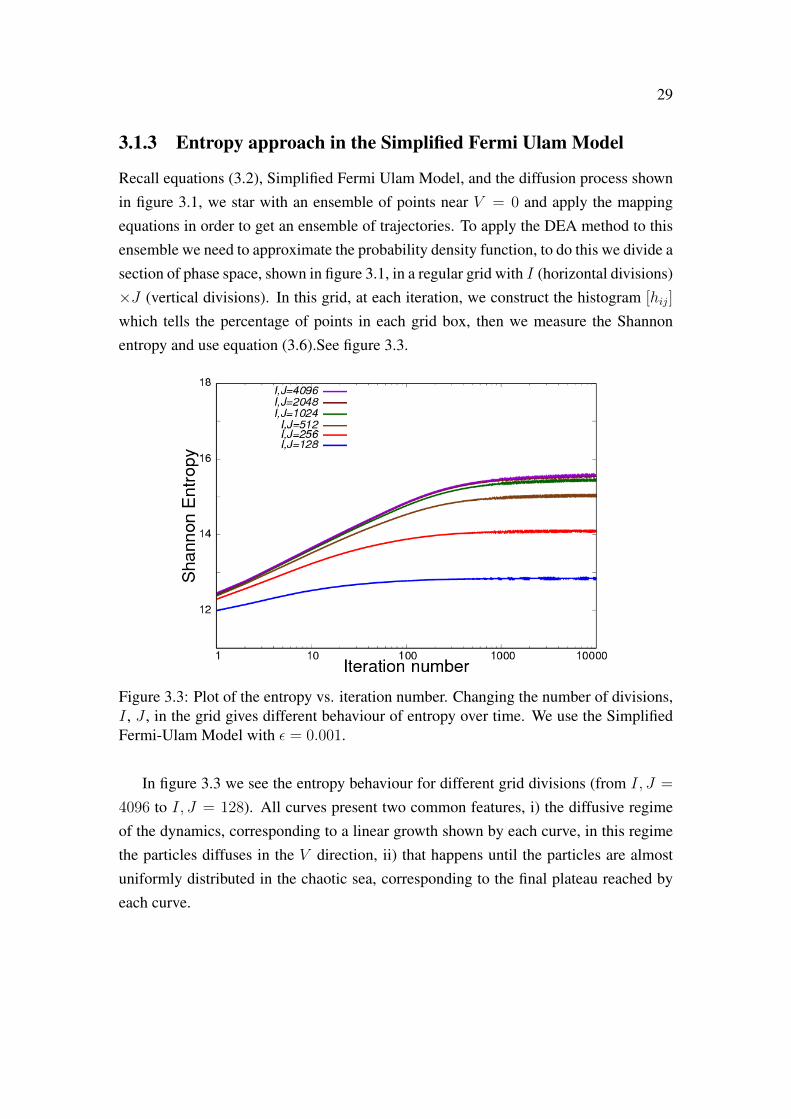
3.1.3 Entropy approach in the Simplified Fermi Ulam Model

Recall equations (3.2), Simplified Fermi Ulam Model, and the diffusion process shownin figure 3.1, we star with an ensemble of points near V = 0 and apply the mappingequations in order to get an ensemble of trajectories. To apply the DEA method to thisensemble we need to approximate the probability density function, to do this we divide asection of phase space, shown in figure 3.1, in a regular grid with I (horizontal divisions)×J (vertical divisions). In this grid, at each iteration, we construct the histogram [hij]

which tells the percentage of points in each grid box, then we measure the Shannonentropy and use equation (3.6).See figure 3.3.

Figure 3.3: Plot of the entropy vs. iteration number. Changing the number of divisions,I , J , in the grid gives different behaviour of entropy over time. We use the SimplifiedFermi-Ulam Model with ε = 0.001.

In figure 3.3 we see the entropy behaviour for different grid divisions (from I, J =

4096 to I, J = 128). All curves present two common features, i) the diffusive regimeof the dynamics, corresponding to a linear growth shown by each curve, in this regimethe particles diffuses in the V direction, ii) that happens until the particles are almostuniformly distributed in the chaotic sea, corresponding to the final plateau reached byeach curve.

30

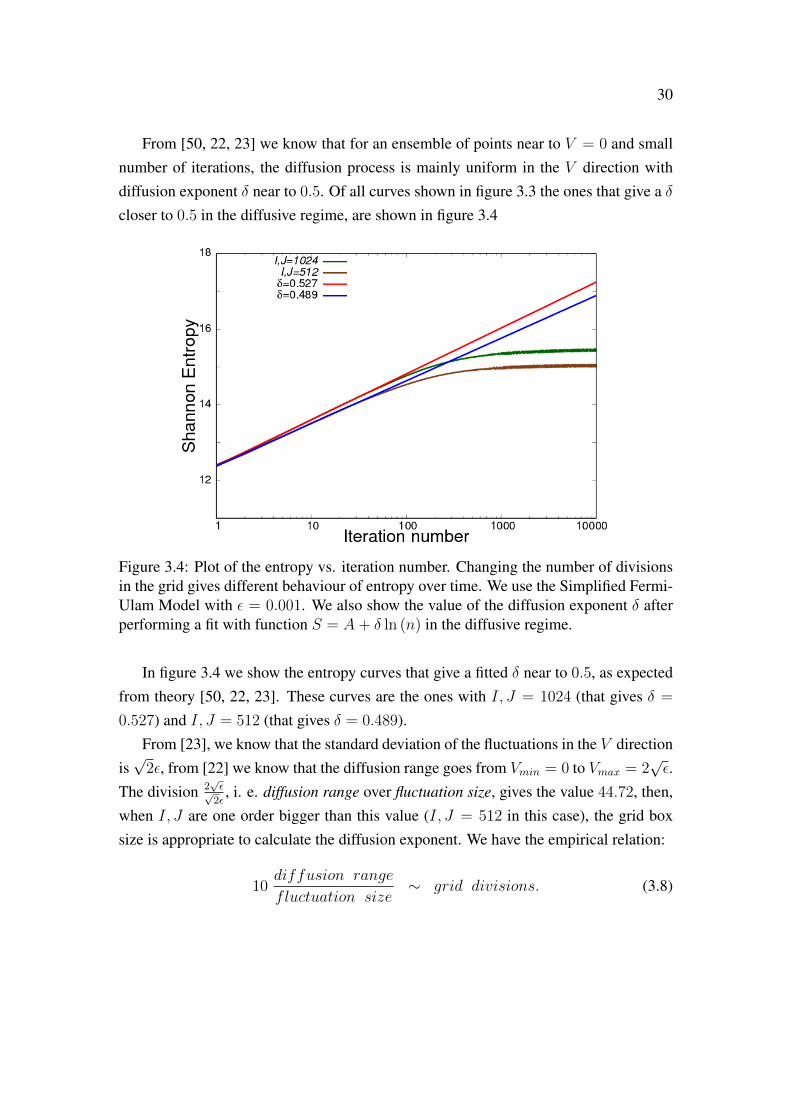
From [50, 22, 23] we know that for an ensemble of points near to V = 0 and smallnumber of iterations, the diffusion process is mainly uniform in the V direction withdiffusion exponent δ near to 0.5. Of all curves shown in figure 3.3 the ones that give a δcloser to 0.5 in the diffusive regime, are shown in figure 3.4

Figure 3.4: Plot of the entropy vs. iteration number. Changing the number of divisionsin the grid gives different behaviour of entropy over time. We use the Simplified Fermi-Ulam Model with ε = 0.001. We also show the value of the diffusion exponent δ afterperforming a fit with function S = A+ δ ln (n) in the diffusive regime.

In figure 3.4 we show the entropy curves that give a fitted δ near to 0.5, as expectedfrom theory [50, 22, 23]. These curves are the ones with I, J = 1024 (that gives δ =

0.527) and I, J = 512 (that gives δ = 0.489).From [23], we know that the standard deviation of the fluctuations in the V direction

is√

2ε, from [22] we know that the diffusion range goes from Vmin = 0 to Vmax = 2√ε.

The division 2√ε√

2ε, i. e. diffusion range over fluctuation size, gives the value 44.72, then,

when I, J are one order bigger than this value (I, J = 512 in this case), the grid boxsize is appropriate to calculate the diffusion exponent. We have the empirical relation:

10diffusion range

fluctuation size∼ grid divisions. (3.8)

31

A detailed description of the scaling (3.4) and its relation with anomalous diffusionit is shown in Appendix C. Demonstration of equation (3.6) and a discussion of itsvalidity in our models is also given in the same appendix. A short review of the physicalreasons of the entropy growth and its relation with the time irreversibility is given inAppendix D.

Chapter 4

Results

In this chapter we show some results obtained while studying the entropy behaviourin the standard map. We focus on the diffusion exponent near the main island, and itspossible relation with the island’s area. Let us remember that the map under study is thefollowing one:

pn+1 = pn + k sin (qn) ,

qn+1 = qn + pn+1 + π. (4.1)

Since we are interested in studying the diffusion behaviour near the islands, anoma-lous diffusion, we first have to find the main island shore, then pick many initial condi-tions along it, initial probability distribution, after that we have to iterate the mapping forall the conditions, calculating the entropy at each iteration, and finally, find the diffusionexponent by relation (3.6), as done in figure 3.3.

4.1 Navigating through the chaotic sea

We use the following procedure to get near the main island. We know there is anhyperbolic fixed point at coordinates q = 0, p = π. Near this point exist chaos, choosingmany initial conditions in this region we know they will expand all over the chaotic seaafter many iterations of the mapping (4.1). Then we separate the regions visited by thepoints and the regions that were not visited, see figure 4.1.

32

33

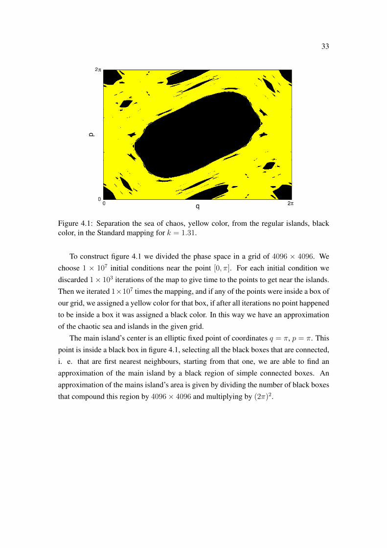
Figure 4.1: Separation the sea of chaos, yellow color, from the regular islands, blackcolor, in the Standard mapping for k = 1.31.

To construct figure 4.1 we divided the phase space in a grid of 4096 × 4096. Wechoose 1 × 107 initial conditions near the point [0, π]. For each initial condition wediscarded 1× 103 iterations of the map to give time to the points to get near the islands.Then we iterated 1×107 times the mapping, and if any of the points were inside a box ofour grid, we assigned a yellow color for that box, if after all iterations no point happenedto be inside a box it was assigned a black color. In this way we have an approximationof the chaotic sea and islands in the given grid.

The main island’s center is an elliptic fixed point of coordinates q = π, p = π. Thispoint is inside a black box in figure 4.1, selecting all the black boxes that are connected,i. e. that are first nearest neighbours, starting from that one, we are able to find anapproximation of the main island by a black region of simple connected boxes. Anapproximation of the mains island’s area is given by dividing the number of black boxesthat compound this region by 4096× 4096 and multiplying by (2π)2.

34

4.2 The shore of the main island

After navigating the chaotic sea we are near the shore of the main island, now wewant to get closer, to do this we will investigate the rotation number of a set of orbits.

We consider the elliptic fixed point of coordinates q = π, p = π, center of the mainisland, as our reference point and the ray q > π, p = π as our polar axis and calculate,after each iteration n, the angle θn that an orbit has with the polar axis. The rotationnumber is defined as:

r = limN→∞

∑Nn=0 θnN

. (4.2)

In practice we pick N = 1000, but we calculate the rotation number for the sameorbit for 1 × 106 iterations, i. e., we have 1000 rotation numbers for the same orbit, ifthis is a quasiperiodic orbit these rotation numbers must be almost equal, then we expectthat for a single quasiperiodic orbit these rotation numbers have a Gaussian distributionwith small standard deviation , σ, and small range between the maximal and the minimalrotation numbers found for the same orbit, rrange. On the other hand, if the orbit ischaotic we expect that the standard deviation and the range to be big because r does notconverge.

To find the shore of the main island first we take the coordinate qi of the first yellowbox that has q > π and p = π in figure 4.1. Then we choose initial conditions withp0 = π and different values of q0 around qi, we take care that the minimal q0 is actuallyinside the island, this will be of use later on. For each one of this initial conditions weanalyze the rotation number statistics as described in the last paragraph. The results areshown in figure 4.2.

35

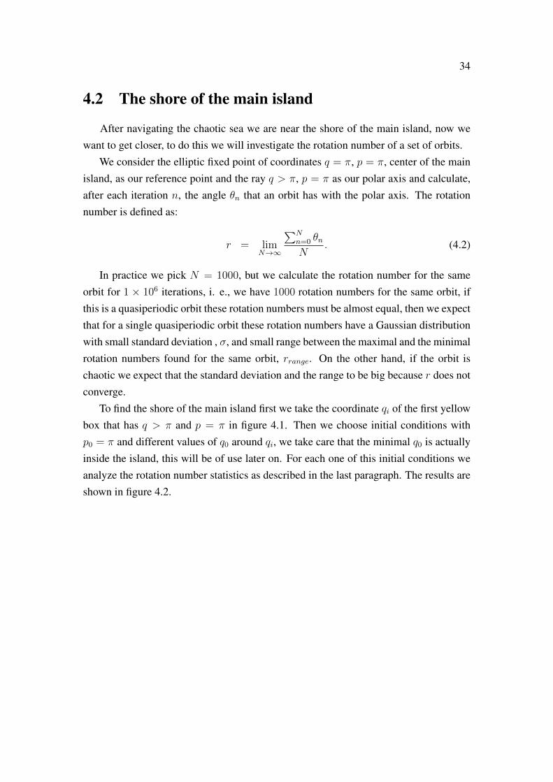
Figure 4.2: The horizontal axis gives the orbit initial q0 coordinate, p0 is always π. Foreach initial condition we calculate the rotation number 1000 times at intervals of 1000iterations and analyze its distribution. The vertical axis shows the standard deviationσ and rotation number range rrange of those distributions, we also show the horizontalcuts σ = 1× 10−2 and rrange = 1× 10−1. The model under study is the Standard Mapwith k = 1.31

In figure 4.2 we show the rotation number statistical behaviour for different initialconditions. The horizontal axis gives the orbit initial q0 coordinate, p0 is always π.For each initial condition we iterate the Standard map 1 × 106 times and calculate therotation number by means of equation (4.2) considering N = 1000, obtaining 1000

rotation numbers for each initial condition. Then we analyze the distribution of those1000 rotation numbers, the vertical axis shows the standard deviation and the rangebetween the maximal and the minimal rotation numbers. To separate quasiperiodic andchaotic behaviours we perform the cuts in σ = 1 × 10−2 and rrange = 1 × 10−11,meaning that any orbit that has both statistical measures above the cuts is consideredchaotic, otherwise is considered quasiperiodic.

From these results we care about the chaotic orbit that has the minimum q0 for the1The value of these cuts were chosen empirically from observing trajectories in phase space, there is

not additional significance in these numbers.

36

interval considered, we call this value q0c2. Once we have this coordinate we save the

first 1000 iterations of the map starting from [q0c, π], then we add a small perturbationto each one of those 1000 iterations until we have an array of 1× 106 points, this arrayof coordinates will be our initial conditions that approach our initial distribution, theywill spread in the phase space and we will use them to calculate the diffusion exponentby means of equations (3.6) and (3.7), see figure 4.3.

Figure 4.3: Phase space portrait of Standard Map for k = 1.31. The red points arethe initial coordinates that will spread in phase space and will be used to calculate thediffusion exponent.

Figure 4.3 shows in red the initial condition to be used with equations (3.6) and (3.7)to find the diffusion exponent δ, we observe that they are close to the islands shore anddistributed around it, but not uniformly, we need to perform some iterations until theyspread along the island, see figure 4.4.

The next step to be taken before been able to measure the diffusion exponent is todefine the grid box size, we will use the relation (3.8). We know that the diffusion range

is 2π for both q as p. To estimate the value of fluctuation size we need to know how muchdoes our distribution changes in one iteration, this can be done in the following way; i)

2We know that we always will be able to find it since the minimal of all q0 is quasiperiodic and alsoqf marks a yellow box, i. e., chaotic region.

37

Perform a map iteration on our initial conditions. Even if the ith point jumps far awayfrom its starting position after one iteration, say xi,n → xi,n+1, some other point, say thejth, will land near the starting position of the ith point, xj,n+1 ∼ xi,n; ii) For each one ofour initial points [xi,n=0] we search for the xj,n=1 points such that xj,n=1 ∼ xi,n=0, thenwe iii) define the fluctuation at the n = 1 iteration as ξi,n=1 = xj,n=1 − xi,n=0, if we dothe same a couple more of iterations, ten iterations in our case, we can iv) approximatethe fluctuation size as the standard deviation of the [ξi,n] fluctuations. Observe that thisapproximation is valid for orbits that are near the main island as our initial distributionis around its shore. In our case we find that 10 diffusion range

fluctuation size= 4856.2, then we divide

our space in I×J = 4096×4096 boxes of equal size. With this grid choice we calculatethe Shannon Entropy as shown in figure 4.4.

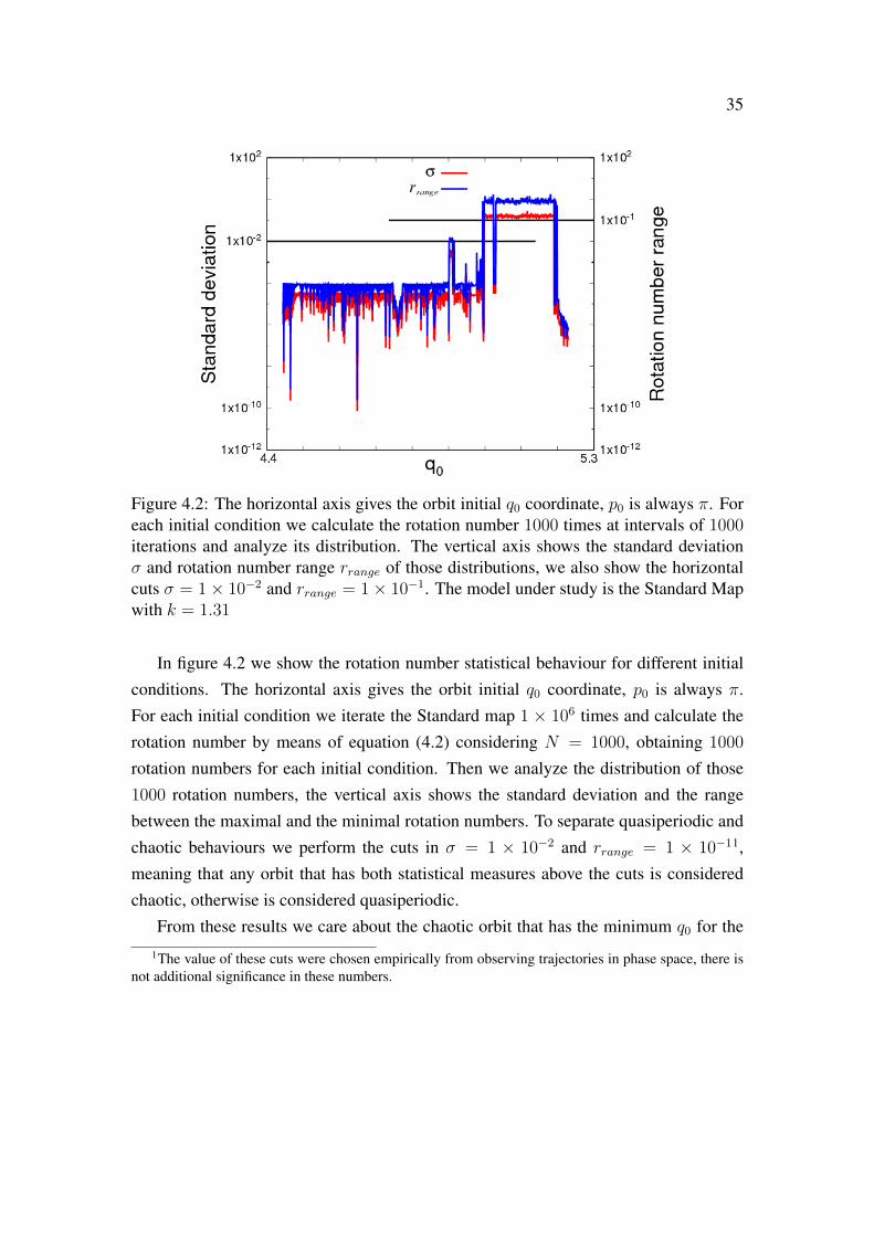
Figure 4.4: Plot of the entropy vs. iteration number for k = 1.31. In subfigure (a)we can see that the entropy has three growth regimes, i) in the first 100 iterations thedistribution spreads along the main island, subfigure (b), ii) then for 3000 iterationsslowly leaks out through the Cantori, subfigure (c), iii) finally more of the distributionis outside the Cantori and rapidly spreads in the chaotic sea.

We show in figure 4.4a the entropy behaviour as the time passes. We can recognizethree growth regimes: i) First the distribution quickly spreads along the shore of themain island, this is a fast process equivalent to the spreading in the phase direction in

38

the SFMU, shown in the transition from figure 3.1a to figure 3.1b. We can appreciatethis in the sub-figure 4.4b, that shows how is distributed our ensemble of trajectoriesafter n = 100 iterations. ii) The second regime is a slow one, the distribution leaksthrough the Cantori, see sub-figure 4.4c, this is a regime of subdiffusion, the one wherewe measure the diffusion exponent, the numerical fit is shown in a blue line, the valueof δ is 0.2344. iii) In the third regime more of the distribution is outside the Cantori andrapidly spreads in the chaotic sea. A fourth regime, not shown in figure 4.4, exists, whenthe ensemble of trajectories is almost uniformly distributed in the chaotic sea, similar tofigure 3.4, the entropy reaches a plateau.

4.3 Diffusion exponent and Area

Now that we know how to measure the diffusion exponent δ in the subdiffusive regimefor a given parameter k, we want to understand how does δ depends on the value of k.To do this we measure the diffusion exponent for 101 different values of the parameterequally spaced from k = 1.31 to k = 2.31, see figure 4.5

Figure 4.5: Plot of the Diffusion exponent vs. parameter k of Standard Map. The blackline represents the numerical data obtained after the power law fitting and the red line isan quintic spline smoothing approximation to the numerical data.

39

In figure 4.5 we see the behaviour of the diffusion exponent when the parameter kchanges. Since this behaviour is very noisy, in part due the election of initial probabilitydistribution, we perform a quintic spline smoothing approximation to the data [51].With this is possible to appreciate more easily the tendency of the data, i. e. growth anddecay of δ. Next we will try to relate the diffusion exponent to some characteristic ofthe main island, we choose to measure the area3 of it for all the given values of k, seefigure 4.6.

Figure 4.6: Plot of the diffusion exponent, red line, and normalized area of the mainisland, blue line vs. parameter k of Standard Map. The normalized area is the area ofthe main island divided by the area of the entire phase space.

It is possible to see in figure 4.6 that every time the area decreases abruptly thediffusion exponent increases. Then the area grows, while the exponent decreases, untila critical value when the area abruptly decreases once more, with its correspondingincrease in the diffusion exponent. We mark two values of k figure 4.6, at this intervalhappens the biggest decrements in the area, for the values of k considered, and we showin figure 4.7 what is happening with the main island at this particular values of k.

3The area is measured by the number of black boxes that compound it times (2π)2 divided by 4096×4096.

40

(a) k = 1.45 (b) k = 1.46

Figure 4.7: Separation the sea of chaos, yellow color, from the regular islands, blackcolor, in the Standard mapping for two values of the nonlinear parameter. Smaller is-lands are ejected from the main island when we change the parameter value

We see in figure 4.7 the transition marked in figure 4.6. When passing from k = 1.45

to k = 1.46 the main island ejects a resonance of smaller islands, this reduces the areaof the main island, but also each ejected island has an elliptic periodic point in themiddle, and by the Poincare Birkhoff theorem [52, 53] there exists their correspondinghyperbolic fixed points pair. The action of the stable and unstable manifolds of these hy-perbolic points is responsible for the changes in diffusion behaviour since they providebig channels to escape from the main island [54, 55, 56].

Even with a more complicated mapping, the Oval Billiard, eq. (2.8), shows similarresults, see figures 4.8 and 4.9. With these results we observe that changes of behaviourin the diffusion exponent are related with changes in the area of the main island. Particu-larly, we find that when the main island’s area is abruptly reduced, due the destruction ofinvariant tori and creation of hyperbolic and elliptic fixed points, the diffusion exponentgrows.

41

Figure 4.8: Plot of the Diffusion exponent vs. parameter ε of Oval Billiard. The blackline represents the numerical data obtained after the power law fitting and the red line isan quintic spline smoothing approximation to the numerical data.

Figure 4.9: Plot of the diffusion exponent, red line, and normalized area of the mainisland, blue line vs. parameter ε of Oval Billiard. The normalized area is the area of themain island divided by the the area of the entire phase space.

42

4.4 Controlling escape, a targeting algorithm

To study the influence of the hyperbolic fixed point in the diffusion dynamic, weperform an appropriate control scheme in the Standard Map. The idea is target to initialconditions that do not escape of the island’s shore by a given control area, and charac-terize they diffusion behaviour, with this we can evaluate the importance of the controlarea in the escape of trajectories. The targeting algorithm consists in the following steps:

1. Choose a two dimensional I (horizontal divisions) ×J (vertical divisions) gridwith help of the relation 10× diffusion range

fluctuation size∼ grid divisions, Eq (3.8).

2. Set an ensemble of initial conditions around the KAM island to apply the map-ping.

3. Choose a control area in phase space 4.

4. Apply the mapping (4.1) to the ensemble of orbits. At each iteration construct anhistogram [hij] counting how many points are inside each grid box. Then measurethe entropy by means of the equation S = −

∑Ii=1

∑Ij=1 hij ln (hij), Eq. (3.7).

5. At every iteration for each element of the ensemble of orbits ask if the orbit hasentered in the control area. If it does it, re-initiate the orbit choosing a new initialcondition randomly from our ensemble of orbits at n = 0, i. e. we target to initialconditions that do not pass in the control area.

6. After some iterations search of a interval in time where the entropy grows linearly5

with ln (n).

7. Use the equation S = A + δ ln (n), Eq. (3.6), to calculate the diffusion exponentδ.

For a given value of k in the SM, Eq. (4.1), we search the hyperbolic points, asso-ciated to the smaller islands ejected, and control a circular area around them when wecalculate the diffusion exponent. Then we change the control’s area, and position. With

4In our case an circular ball of some radius.5In this region is possible to consider the scaling hypothesis of [30].

43

this we can observe the influence of the given fixed hyperbolic point in the diffusiondynamic.

k Period δ (with control) δ (no control)1.46 6 0.143± 0.001 0.247± 0.0011.47 6 0.2448± 0.0009 0.3218± 0.00091.48 6 0.152± 0.003 0.288± 0.0031.96 10 0.201± 0.009 0.221± 0.0091.97 10 0.25± 0.01 0.275± 0.0091.98 10 0.179± 0.007 0.189± 0.007

Table 4.1: Table showing changes in the diffusion exponent when controlling an smallcircular area around hyperbolic points, (ball radius r = 0.001) .

In table 4.1 we show the effect of the control scheme in the standard map. The firstcolumn is the value of the Standard Map’s parameter k. Second column gives the periodof the hyperbolic fixed point analyzed. Third and fourth column show the values of thediffusion exponent with and without control respectively. We can appreciate the changein diffusion exponent when an area around the hyperbolic points is controlled. Fordifferent values of the parameter k we have different periods in the resonance islands,but in every case the diffusion exponent becomes smaller than without the control. Thevalues of k were chosen near two decays in the normalized area from figure 4.6.

We examine now the effect of the control area, we change the radius of the circularball around the hyperbolic fixed points and see how does the diffusion exponent changes,see figure 4.10.

44

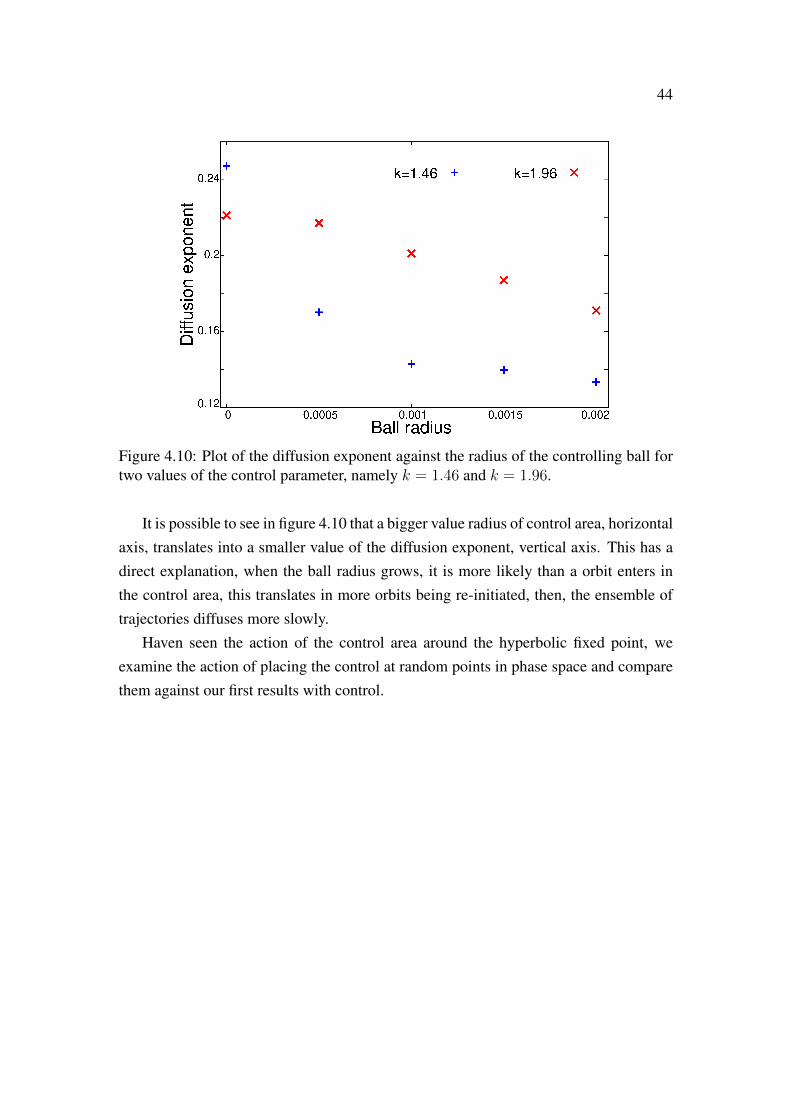
Figure 4.10: Plot of the diffusion exponent against the radius of the controlling ball fortwo values of the control parameter, namely k = 1.46 and k = 1.96.

It is possible to see in figure 4.10 that a bigger value radius of control area, horizontalaxis, translates into a smaller value of the diffusion exponent, vertical axis. This has adirect explanation, when the ball radius grows, it is more likely than a orbit enters inthe control area, this translates in more orbits being re-initiated, then, the ensemble oftrajectories diffuses more slowly.

Haven seen the action of the control area around the hyperbolic fixed point, weexamine the action of placing the control at random points in phase space and comparethem against our first results with control.

45

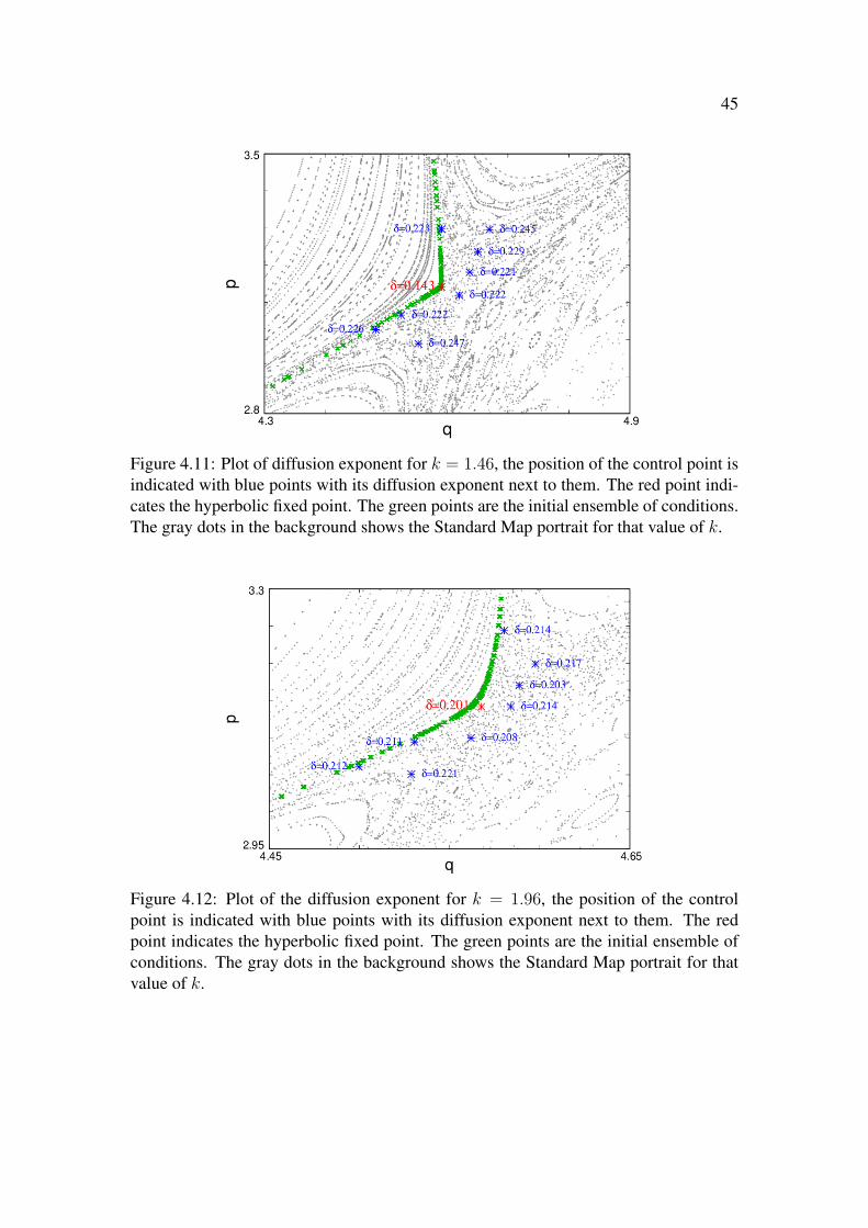
Figure 4.11: Plot of diffusion exponent for k = 1.46, the position of the control point isindicated with blue points with its diffusion exponent next to them. The red point indi-cates the hyperbolic fixed point. The green points are the initial ensemble of conditions.The gray dots in the background shows the Standard Map portrait for that value of k.

Figure 4.12: Plot of the diffusion exponent for k = 1.96, the position of the controlpoint is indicated with blue points with its diffusion exponent next to them. The redpoint indicates the hyperbolic fixed point. The green points are the initial ensemble ofconditions. The gray dots in the background shows the Standard Map portrait for thatvalue of k.

46

When we change the position of the control area, the diffusion exponent also changes,as can be seen in figures 4.11 and 4.12. We notice the diffusion exponent seems to bemore affected when the control area is around an hyperbolic point (red point) than whenis around another random point (blue points).

4.5 The manifold effect

From the hyperbolic fixed point we change the focus of our attention to the unstablemanifold, and study its effect in the diffusion dynamic.

Figure 4.13: Phase space portrait of Standard Map for k = 1.46. The green points arethe unstable manifold associated to the hyperbolic fixed point of period 6, red point.

In figure 4.13 we show the unstable manifold, green points, for the period 6 hyper-bolic fixed point, red point, the mapping is the SM with k = 1.46. It is possible toappreciate that near the fixed point the manifold has a lot o zig-zags. Since trajecto-ries tend to align along the unstable manifold, we expect that regions near it have a lotvisitations from an ensemble of trajectories.

For the initial ensemble of conditions, green points shown in figure 4.11, we cal-culate the number of times any of them enters a small box of a grid when we perform

47

iterations of the SM. According to the number of times any point entered, a box isassigned with a given color, see figure 4.14.

Figure 4.14: Recurrence plot for the initial ensemble of orbits (green points). Every boxin the grid has a color assigned depending on the number of points visited them, see thecolor box.

It is possible to see in figure 4.14 that the manifolds zig-zag is still visible in the re-currence plot, meaning that indeed regions near the unstable manifold are highly visited.Since trajectories are common to be found in this regions we expect them to be goodplaces to perform the control in the SM iterations, method discussed in last section. Seefigure 4.15

48

Figure 4.15: Diffusion exponent for the initial ensemble of orbits (green points). Everybox in the grid has a color assigned depending on the value of the diffusion exponentwhen the control area is in the grid box.

In figure 4.15 wee see a color grid with the value of the diffusion exponent when thecontrol area is in each grid box. We notice the diffusion exponent near the hyperbolicpoint is smaller than in other regions. Even more, this figure shows similar zig-zagstructure as seen in figures 4.14 and 4.15. This means that the unstable manifold createssmall channels were the control is better than away from those channels.

Further on our study of the manifold effect, we care about the entropy growth be-haviour. We perform several simulations. For each simulation we start with a givennumber of points over the unstable manifold, see table 4.2, then, we add noise to thesepoints until we have an ensemble of 1 × 108 initial conditions, using this ensemble westart iterating the SM and study the ensemble’s entropy growth.

49

Points in manifoldSimulation 1 1720594Simulation 2 0Simulation 3 720594Simulation 4 20594

Table 4.2: Table showing the number of starting points in the unstable manifold foreach simulation. The rest of the points are noise added in the manifold until we reachan ensemble of 1× 108 initial conditions .

Figure 4.16: Entropy growth for different number of initial conditions over the unstablemanifold. Simulation 1, brown line, and Simulation 2, blue line, are described in Table4.2.

Figure 4.16 shows the entropy growth for Simulation 1, whose initial ensemble hasseveral points over the manifold, and Simulation 2, whose initial ensemble are noisyrandom points near the manifold. We observe that for small number of iterations Simu-lation 2 is over Simulation 1, this is expected due the initial noise, until some iterationwhen Simulation 1 surpass Simulation 2, this due the fact that, having more points overthe unstable manifold, they escape more rapidly to other regions. We can also observethat Simulation 2 is aligning to Simulation 1.

50

Figure 4.17: Entropy growth for different number of initial conditions over the unstablemanifold. Simulation 1, brown line, and Simulation 3, light green line, and Simulation4, green line, are described in Table 4.2.We see that all converge to the same entropybehaviour after some number of iterations.

In figure 4.17 we can see the entropy growth for Simulations 1, 3 and 4. It is clearthat initially each one has its own entropy. Simulation 1 having the biggest initial en-tropy since their 1720594 initial points are distributed over a bigger number of gridboxes, Simulation 4 has the lower entropy, zero, since initially all its points are in justone grid box, and Simulation 2 a medium entropy value. When the iterations start,we can see that Simulation 4 grows very rapidly until it aligns with Simulation 1, thismeans that in the first iterations the points of Simulation 4 go through a superdiffusivebehaviour until the ensemble is distributed on phase space almost as Simulation 1. Fromthere both Simulations behave similarly. Same happens with Simulation 3. From thisbehaviour we conjecture that there exists a biggest entropy growth curve given whenall the ensemble points over the unstable manifold, even more, this entropy curve is thelimit behaviour of all the other possible entropy growth for ensembles running awayfrom the sticky effect of the main island plus resonances.

Chapter 5

Conclusions

We showed that the use of Shannon Entropy permits us to characterize the diffusionexponent in low dimensional Hamiltonian systems described by maps. The methodol-ogy proposed allowed us to calculate the diffusion exponent both in regions where thediffusion is normal, as in regions where the stickiness phenomenon is present, producingan anomalous diffusion.

We calculated the diffusion exponent for many values of the nonlinear parameterof the Standard Map and the Oval Billiard, where for each value the main island had adifferent shape, then we showed that the changes of behaviour in the diffusion exponentwere related with changes in the area of the main island. Particularly, we found thatwhen the main island’s area is abruptly reduced, due the destruction of invariant toriand creation of hyperbolic and elliptic fixed points, the diffusion exponent grew.

To investigate the dependence of the diffusion exponent with the creation of reso-nance islands, we developed an appropriate control scheme in the Standard Map. Then,for different values of the nonlinear parameter k, where resonance islands were cre-ated, we showed that when considering an small control area, around hyperbolic pointsassociated to the resonances, it is possible to change the diffusion exponent making itsmaller. This is mainly due to the fact that the control action closes paths to escapefrom the main island. We also showed that the bigger the control area the smaller thediffusion exponent, since it is more probable that an orbit will enter the control area.

We showed that changing the position of the control point the diffusion exponentchanges, for random control points this diffusion exponent is not much affected as when

51

52

we consider the hyperbolic point. Then, by performing a detailed analysis in phasespace of the relation position of control point Vs Diffusion exponent, and comparingthis with the portrait of the unstable manifold, we showed that this manifold providessmall channels for the escape of trajectories from the main island.

Finally, observing the entropy’s behaviour of different ensembles of trajectories, andwatching the alignment tendency of the entropy curves, we conjectured that there existsa biggest entropy growth curve given when all the ensemble points are over the unstablemanifold, even more, this entropy curve is the limit behaviour of all the other possibleentropy growths for ensembles running away from the sticky effect of the main islandplus resonances.

Chapter 6

Perspectives

Even though the Standard Map is a prototypical example for Hamiltonian Sys-tems, it would be interesting to explore and confirm the results in other systems, in thiswork we expanded some results to the Oval Billiard and showed that behave similarlyas in the Standard Map, this encourages to extend the methodology to other Hamil-tonian Systems. In the case of higher dimensional Hamiltonian Systems the invariantstructures presented in phase space are different, in principle is possible to extend theDEA method to these systems, although constructing frequency histograms for high di-mensional spaces becomes more challenging, so a possible way to overcome this couldbe to project to lower dimensional spaces and use cumulative probability distributionfunctions, and see if it is possible to calculate diffusion exponents.

Another point of interest is the manifold’s effect of other resonance islands, herewe had our focus in the first resonance island, although it is known that the hyperbolicpoint’s manifolds extend all over phase space, meaning that is not a localized effect, it isalso known that other hyperbolic point’s manifolds also exist and affect the dynamics.So, it would be interesting to study what happens with the entropy behaviour for en-sembles near the crossing points of the manifolds, it can be expected that these regionspresent interesting dynamics since they go easily from one resonance to another, thiscould facilitate the diffusion, or on the contrary, make the trajectories enter even morein sticky regions.

53

Appendix A

For those about to map

In this appendix we describe the maps used in this thesis.

A.1 Standard Map

The Standard Map is constructed by a Poincare section of the kicked rotator, whichdescribes the motion of a particle constrained to move in a ring. The particle is kickedperiodically by an external field. The model is described by the Hamiltonian

H (q, p, t) =p2

2mr2+K cos (q)

∞∑n=−∞

δ (t/T − n) , (A.1)

where δ is the Dirac delta function, q is the angular coordinate and p is its conjugatemomentum. It is worth remarking that we can consider that the particle’s mass m, thering’s radius r and the period of kicks T are equal to one, this due the fact that we havethree unit dimensions, length, time and energy (or mass). For now we will leave theadditional parameters until the final steps.

Now we make use of Hamilton’s equations of motion

p = −∂H∂q

= K sin (q)∞∑

n=−∞

δ (t/T − n) ,

q =∂H

∂p=

p

mr2. (A.2)

54

55

We will analyze the movement in the interval of time just before the kick at t = 0 andthe kick at t = T , i. e. t ∈ [−ε, T − ε]. For other intervals of time the analysis wouldbe similar due the periodicity of the kicks.

From Hamilton’s equations A.2 we can see that the instant of the kick in t = 0 themomentum has an abrupt change and then remains constant∫ T−ε

−εp dt =

∫ T−ε

−εK sin (q)

∞∑n=−∞

δ (t/T − n) dt,

p− p0 = KT sin (q) . (A.3)

After the kick at t = 0 the movement is uniform so the change in coordinate is givenby: ∫ T−ε

−εq dt =

∫ T−ε

−ε

p

mr2dt,

q − q0 =p

mr2T . (A.4)

Finally, rescaling the momentum pTmr2→ p, and generalizing for any kick, we arrive to:

pn+1 = pn +KT 2

mr2sin (qn) ,

qn+1 = qn + pn+1. (A.5)

Which is the Standard Map if we consider k = KT 2

mr2l. This map is area preserving, the

Jacobian of the transformation (qn+1, pn+1) = M (qn, pn) is given by

∂ (qn+1, pn+1)

∂ (qn, pn)=

(∂qn+1

∂qn

∂qn+1

∂pn∂pn+1

∂qn

∂pn+1

∂pn

)=

(1 + k cos (qn) 1

k cos (qn) 1

), (A.6)

and it’s determinant is 1:∥∥∥∥∂ (qn+1, pn+1)

∂ (qn, pn)

∥∥∥∥ =

∥∥∥∥∥ 1 + k cos (qn) 1

k cos (qn) 1

∥∥∥∥∥ = 1, (A.7)

56

This means that the mapping is area preserving since:

dqndpn =

∣∣∣∣∣(∥∥∥∥∂ (qn+1, pn+1)

∂ (qn, pn)

∥∥∥∥)−1∣∣∣∣∣ dqn+1dpn+1 = dqn+1dpn+1. (A.8)

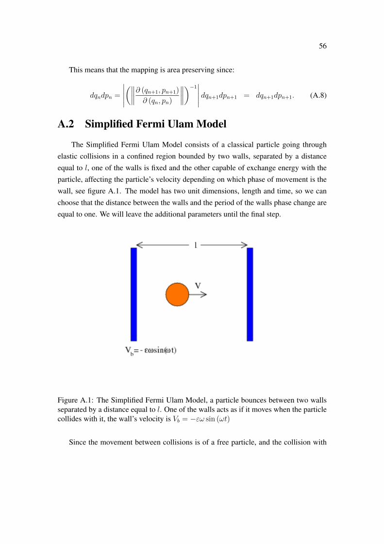
A.2 Simplified Fermi Ulam Model

The Simplified Fermi Ulam Model consists of a classical particle going throughelastic collisions in a confined region bounded by two walls, separated by a distanceequal to l, one of the walls is fixed and the other capable of exchange energy with theparticle, affecting the particle’s velocity depending on which phase of movement is thewall, see figure A.1. The model has two unit dimensions, length and time, so we canchoose that the distance between the walls and the period of the walls phase change areequal to one. We will leave the additional parameters until the final step.

Figure A.1: The Simplified Fermi Ulam Model, a particle bounces between two wallsseparated by a distance equal to l. One of the walls acts as if it moves when the particlecollides with it, the wall’s velocity is Vb = −εω sin (ωt)

Since the movement between collisions is of a free particle, and the collision with

57

the right wall is elastic and the wall is not moving, we will care about collision with theleft wall. The time between the nth collision and the next one is given by:

tn+1 − tn =2l

Vn. (A.9)

where we considered that the particle’s velocity after the nth collision is Vn. Whichis the same magnitude, but different direction, as the particle’s velocity just before thenext collision. For the collision we consider the left wall as if it were moving, withvelocity −εω sin (ωtn+1), then the particle’s velocity, relative to the wall, just beforethe collision, V ′n, is the same as the particle’s velocity, relative to the wall, just afterthe the collision, V ′n+1, but with different sign, elastic collision. We have the followingequations:

V ′n = −Vn + εω sin (ωtn+1) , (A.10)

V ′n+1 = Vn+1 + εω sin (ωtn+1) , (A.11)

V ′n = −V ′n+1. (A.12)

Finally, making the following change of variables ωt → φ, Vεω→ V and ε

l→ ε we

arrive to the Simplified Fermi Ulam Model:

φn+1 =

[φn +

2

Vn

]mod (2π) ,

Vn+1 = ‖Vn − 2ε sin (φn+1)‖ . (A.13)

Note that in this case the Jacobian of the transformation is:

∂ (φn+1, Vn+1)

∂ (φn, Vn)=

1 − 2

V 2n

−2ε cos (φn+1) sgn (Vn+1)

(1 + 2ε cos (φn+1)

2

V 2n

)sgn (Vn+1)

,(A.14)

where sgn (Vn+1) is the sign function, takes the value 1 if Vn+1 > 0 and−1 if Vn+1 < 0.It’s determinant is: ∥∥∥∥∂ (φn+1, Vn+1)

∂ (φn, Vn)

∥∥∥∥ = sgn (Vn+1) . (A.15)

58

Then this map is area preserving:

dφndVn = dφn+1dVn+1. (A.16)

A.3 Oval Billiard

The Oval Billiard consists in a free moving particle; whose position is given by:

x− x0 = vx0t ,

y − y0 = vy0t , (A.17)

inside a closed region whose boundary radius1 is written as:

R (θ, ε, p) = 1 + ε cos (pθ) , (A.18)

where the parameter ε ∈ [0, 1) controls the deformation of the circle, the non linearity,p is an integer number and θ ∈ [0, 2π) is the polar angle. Every time that the particlereaches the border suffers from a elastic collision, see figure A.2.

1Using polar coordinates.

59

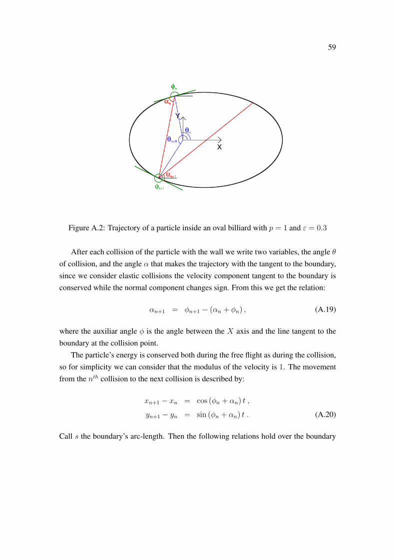
Figure A.2: Trajectory of a particle inside an oval billiard with p = 1 and ε = 0.3

After each collision of the particle with the wall we write two variables, the angle θof collision, and the angle α that makes the trajectory with the tangent to the boundary,since we consider elastic collisions the velocity component tangent to the boundary isconserved while the normal component changes sign. From this we get the relation:

αn+1 = φn+1 − (αn + φn) , (A.19)

where the auxiliar angle φ is the angle between the X axis and the line tangent to theboundary at the collision point.

The particle’s energy is conserved both during the free flight as during the collision,so for simplicity we can consider that the modulus of the velocity is 1. The movementfrom the nth collision to the next collision is described by:

xn+1 − xn = cos (φn + αn) t ,

yn+1 − yn = sin (φn + αn) t . (A.20)

Call s the boundary’s arc-length. Then the following relations hold over the boundary

60

[41]:

dx = cos (φ) ds , (A.21)

dy = sin (φ) ds , (A.22)

dφ = −κds , (A.23)

where κ is the boundary’s curvature. Differentiating eqs. (A.19) and (A.20) we get:

dαn+1 + κn+1dsn+1 = κndsn − dαn ,

cos (φn+1) dsn+1 − cos (φn) dsn = cos (φn + αn) dt− t sin (φn + αn) (dφn + dαn) ,

sin (φn+1) dsn+1 − sin (φn) dsn = sin (φn + αn) dt+ t cos (φn + αn) (dφn + dαn) .(A.24)

After some algebraic manipulations we find:

∂ (sn+1, αn+1)

∂ (sn, αn)=

1

sin (αn+1)

(sin (αn) + tκn −t

κn sin (αn+1)− κn+1 sin (αn)− tκnκn+1 tκn+1 − sin (αn+1)

).(A.25)

The determinant is: ∥∥∥∥∂ (sn+1, αn+1)

∂ (sn, αn)

∥∥∥∥ = − sin (αn)

sin (αn+1). (A.26)

Then this map preserves the area:

dsn d cos (αn) = dsn+1 d cos (αn+1) , (A.27)

where we recognize the tangential velocity vn = cos (αn). Thus the Oval Billiard isarea preserving considering the Poincare-Birkhoff coordinates, i. e. arch-length andtangential velocity.

Appendix B

Oval Billiard, an algorithm to solve it

In the oval billiard the radius of the boundary, in polar coordinates, is given by:

Rb (θ) = 1 + ε cos (pθ) . (B.1)

If we know the position (x0, y0) and velocity (vx0, vy0) of the particle immediatelyafter a collision, iteration 0, we want to know the position (x1, y1) and the velocity(vx1, vy1) of the particle after the next collision, iteration 1.

For the case of p = 1 a very simple algorithm exist to find exact solution. Let usrewrite the boundary radius in the following way:

Rb = 1 + εx1

Rb

, (B.2)

where Rb is the radius of the boundary in collision 1. Since the particle moves freelybetween collisions we know that x1 = x0+vx0t, t is the time from collision 0 to collision1. After doing some algebra with equation (B.2) we arrive to:

R2b =

(R2b − ε (x0 + vx0t)

)2. (B.3)

Then we use the following auxiliar variables A = x20 + y2

0 , B = 2 (x0vx0 + y0vy0)

and C = v2x0 + v2

y0 and the fact that R2b = (x2

0 + vx0t)2

+ (y20 + vy0t)

2 in equation (B.3)

61

62

to find:

(−A+ A2 − 2Aεx0 + ε2x2

0

)+(−B + 2AB − 2Bεx0 − 2εAvx0 + 2ε2x0vx0

)t

+(B2 − C + 2AC − 2Cεx0 + ε2vx0 − 2εBvx0

)t2

+ (2BC − 2εCvx0) t3 + Ct4 = 0. (B.4)

The first term is zero since the initial position is in the boundary, then we have tosolve a third degree polynomial, which has exact solution [47]. We use the algorithmwritten by Skowron and Gould [46] to find the roots of the polynomial, then we pick thesmallest real root bigger than zero, this is our time between collision 0 and 1. With thiswe can find the collision angle θ1.

Figure B.1: Trajectory of a particle inside a oval billiard with p = 1 and ε = 0.3

We are interested now in the angle αn+1, by means of figure B.1 we find the relation:

αn+1 = φn+1 − (αn + φn) , (B.5)

where the auxiliar angle φ is related to the tangent line to the boundary at the point of

63

collision, is the angle between the X axis and the tangent line, so it is given by:

φ = arctan

(dYbdXb

), (B.6)

using the chain rule and the parametric description of the boundary given by θ, wefinally find that φ is:

φn = arctan

(−pε sin (pθn) sin (θn) +R (θn) cos (θn)

−pε sin (pθn) cos (θn)−R (θn) sin (θn)

). (B.7)

Appendix C

A little more on diffusion

In this appendix we comment on anomalous diffusion, the reasons behind the scalingrelation1:

ρ (x, t) =1

tδF( xtδ

), (C.1)

and its validity in our mappings.

C.1 Anomalous Diffusion

A diffusion process is characterized by the behaviour of the Mean Squared Displace-ment (MSD) [59], contrary to normal diffusion, in an anomalous diffusion process, theMSD does not grow linearly in time:

〈x2 (t)〉 ∝ tα; α 6= 1 (C.2)

where 〈·〉 means ensemble average and we use the variable α instead of δ = α2

forreasons that will become apparent later on. A subdiffusive process has α < 1 and asuperdiffusive one has α > 1. Observe that in this equation two things are assumed,i) all the trajectories in the ensemble start in the position x (0) = 0, ii) the diffusionprocess happens in an infinity space.

1Equation (3.4) in the main text

64

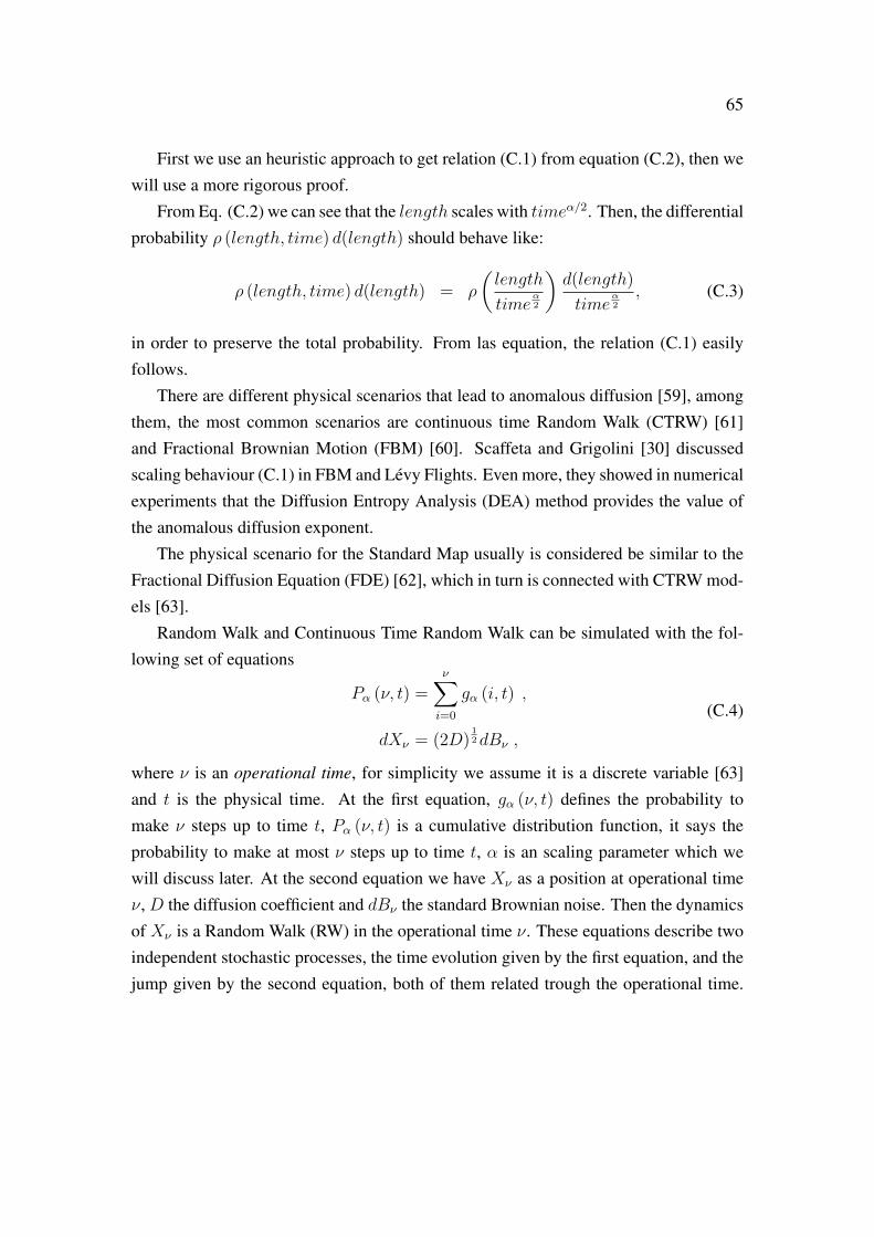
65

First we use an heuristic approach to get relation (C.1) from equation (C.2), then wewill use a more rigorous proof.

From Eq. (C.2) we can see that the length scales with timeα/2. Then, the differentialprobability ρ (length, time) d(length) should behave like:

ρ (length, time) d(length) = ρ

(length

timeα2

)d(length)

timeα2

, (C.3)

in order to preserve the total probability. From las equation, the relation (C.1) easilyfollows.

There are different physical scenarios that lead to anomalous diffusion [59], amongthem, the most common scenarios are continuous time Random Walk (CTRW) [61]and Fractional Brownian Motion (FBM) [60]. Scaffeta and Grigolini [30] discussedscaling behaviour (C.1) in FBM and Levy Flights. Even more, they showed in numericalexperiments that the Diffusion Entropy Analysis (DEA) method provides the value ofthe anomalous diffusion exponent.

The physical scenario for the Standard Map usually is considered be similar to theFractional Diffusion Equation (FDE) [62], which in turn is connected with CTRW mod-els [63].

Random Walk and Continuous Time Random Walk can be simulated with the fol-lowing set of equations

Pα (ν, t) =ν∑i=0

gα (i, t) ,

dXν = (2D)12dBν ,

(C.4)

where ν is an operational time, for simplicity we assume it is a discrete variable [63]and t is the physical time. At the first equation, gα (ν, t) defines the probability tomake ν steps up to time t, Pα (ν, t) is a cumulative distribution function, it says theprobability to make at most ν steps up to time t, α is an scaling parameter which wewill discuss later. At the second equation we have Xν as a position at operational timeν, D the diffusion coefficient and dBν the standard Brownian noise. Then the dynamicsof Xν is a Random Walk (RW) in the operational time ν. These equations describe twoindependent stochastic processes, the time evolution given by the first equation, and thejump given by the second equation, both of them related trough the operational time.

66

The trajectoryX (t), that arises from both processes of Eq. (C.4) is itself a subordinatedstochastic process.

The scaling parameter α ∈ (0, 1] enters in the relation

ν ∝ tα , (C.5)

allowing a sub-linear dependence of ν with t. Since long time t can go with a smalloperational time ν, this behavior is responsible for sub-diffusive dynamics. In terms ofEq. (C.4) it means that we can wait long time, trap-time, t until a jump is taken by Xν .This scenario is the so called Continuous Time Random Walk (CTRW) model.

The behavior of an ensemble of trajectories that follows RW can be described by aprobability density function ρν (x) and, its evolution in the operational time is given by[64]:

ρν+1 (x) =

∫ ∞−∞

dx′f (x− x′) ρν (x′) , (C.6)

meaning that the probability ρν+1 (x) to be at x at time ν + 1 is given by the probabilityf (x− x′) to jump from x′ to x, times the probability ρν (x′) of being at x′ at time ν,summed over all the possible values of x′.

Given that we have a Brownian noise model in Eq. (C.4), our jump-probability-

function f (x− x′) is given by:

f (x− x′) =1√

4πDe−

(x−x′)2

4D . (C.7)

Considering now the analysis of a given function F in a Fourier space, F (k) =

F{F (x) ; k} =∫∞−∞ e

−ikxF (x) dx. Setting F as wish, Eq. (C.6) can be rewritten as

ρv+1 (k) = f (k) ρv (k) . (C.8)

One can notice that Eq. (C.8) is a recurrence relation that can be solved if the initialdistribution ρ0 (k) is known. Considering the following points:

i) An initial distribution ρ0 (x) = δ (x);

ii) The Fourier transform of Eq. (C.7) is f (k) = e−Dk2 ;

67

iii) Assuming ν a continuous variable.

We have that:

ρ (k, ν) = e−Dk2ν . (C.9)

Now, to be able to change from the operational to the physical time we use

ρ (x, t) =

∫ ∞0

dν ρ (x, ν) g (ν, t) . (C.10)

Eq. (C.10) means that the probability ρ (x, t) to be at x at time t is given by theprobability g (ν, t) to take ν steps up to time t, times the probability ρ (x, ν) to be at xafter ν steps, summed over all the possible number of steps ν. Moreover, if the relationbetween the operational time and the physical time is given by g (ν, t) = δ (t− ν),which reasonably means α = 1 in the relation (C.5), then, using Eqs. (C.9), (C.10) andthe Laplace transform F (s) = L{F (t) ; s} =

∫∞0e−stF (t) dt, we get:

ˆρ (k, s) =1

s+Dk2. (C.11)

Remembering the initial condition ρ (x, 0) we can invert the Fourier-Laplace transformand finally arrive on:

∂ρ (x, t)

∂t= D

∂2ρ (x, t)

∂x2, (C.12)

which is the Diffusion Equation. Meaning that an ensemble of trajectories followinga RW behaves like a probability distribution function from the diffusion equation, asexpected.

Continuous Time Random Walk enters in play when we want to address the anoma-lous diffusion case, α ∈ (0, 1). Magdziarz proposed in [65] to use an inverse α-stable subordinator for gα (ν, t). Setting uα (t, ν), as the probability distribution function(PDF) for a completely skewed α stable process, by the following Laplace transform:

uα (s, ν) = e−νsα

, (C.13)

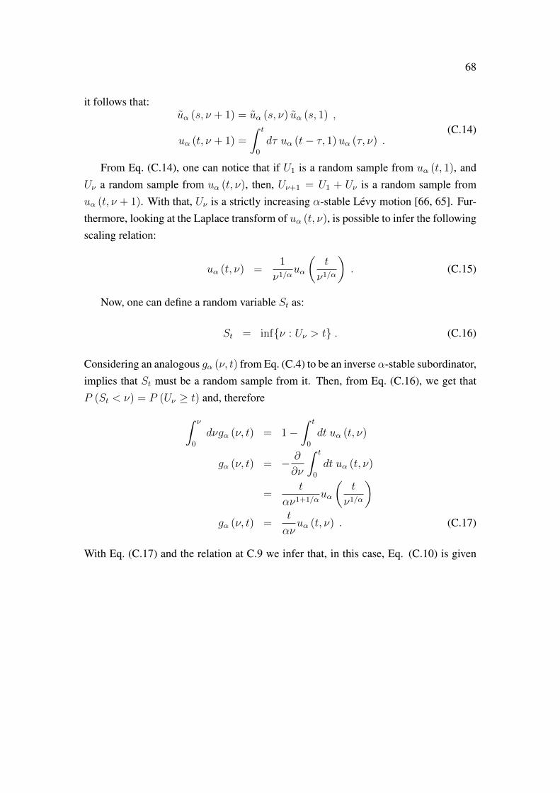
68

it follows that:uα (s, ν + 1) = uα (s, ν) uα (s, 1) ,

uα (t, ν + 1) =

∫ t

0

dτ uα (t− τ, 1)uα (τ, ν) .(C.14)

From Eq. (C.14), one can notice that if U1 is a random sample from uα (t, 1), andUν a random sample from uα (t, ν), then, Uν+1 = U1 + Uν is a random sample fromuα (t, ν + 1). With that, Uν is a strictly increasing α-stable Levy motion [66, 65]. Fur-thermore, looking at the Laplace transform of uα (t, ν), is possible to infer the followingscaling relation:

uα (t, ν) =1

ν1/αuα

(t

ν1/α

). (C.15)

Now, one can define a random variable St as:

St = inf{ν : Uν > t} . (C.16)

Considering an analogous gα (ν, t) from Eq. (C.4) to be an inverse α-stable subordinator,implies that St must be a random sample from it. Then, from Eq. (C.16), we get thatP (St < ν) = P (Uν ≥ t) and, therefore∫ ν

0

dνgα (ν, t) = 1−∫ t

0

dt uα (t, ν)

gα (ν, t) = − ∂

∂ν

∫ t

0

dt uα (t, ν)

=t

αν1+1/αuα

(t

ν1/α

)gα (ν, t) =

t

ανuα (t, ν) . (C.17)

With Eq. (C.17) and the relation at C.9 we infer that, in this case, Eq. (C.10) is given

69

by:

ρ (k, t) =

∫ ∞0

dν e−Dk2ν t

αν1+1/αuα

(t

ν1/α

)ˆρ (k, s) =

∫ ∞0

dν e−Dk2νsα−1e−νs

α

ˆρ (k, s) =sα−1

sα +Dk2. (C.18)

Finally, inverting the Fourier-Laplace transform, we arrive on:

∂αρ (x, t)

∂tα= D

∂2ρ (x, t)

∂x2, (C.19)

which is the Fractional Diffusion Equation.A couple of remarks are noted:

1. ˆρ (0, s) = 1s, then ρ (0, t) = 1, and the probability is conserved;

2. −[∂2

∂k2ˆρ (k, s)

]k=0

= 2Dsα+1 , then 〈x2 (t)〉 = 2Dtα

Γ(1+α), recovering the expected mean

square displacement behavior.

3. See that ρ (k, t) = Eα (−Dtαk2), whereEα (z) is the Mittag Leffler function [67].Thus, recalling the scaling property of the Fourier Transform F−1{F (ak) ;x} =

1‖a‖F

(x‖a‖

)we have the result ρ (x, t) = 1√

Dtαφ(

x√Dtα

), which recovers the

scaling relation (C.1).

4. If the initial distribution is given by ρ0(x) = δ(x − x0) we only have to changethe location x→ x− x0 and all the demonstrations still hold.

It is important to mind that the analysis made from Eq. (C.13) to the FDE presentedin Eq. (C.19) means that, an ensemble of trajectories following a CTRW-like model,behaves as a probability distribution function from the solution of the FDE.

Considering this analytical background of either normal and anomalous diffusionprocess, connected respectively to RW and CTRW, we use the set of equations in Eq.(C.4) and follow the numerical method proposed by Magdziarz in [65] to simulate thedynamics of a RW process, setting α = 1 and the CTRW process, setting α = 0.6

70

(relatively not so long trap-time) and α = 0.3 (relatively long trap-time). In figure C.1we show examples of simulated trajectories of these three different dynamic scenarios.

Figure C.1: Examples of trajectories for a RW process (α = 1) in black. Also, for twodistinct CRTW processes considering a relatively not so long trap-time (α = 0.6) inred, and a long trap-time (α = 0.3) in green. The time-axis was chosen to be linear toproperly show the different trap-times that arrive from the relation (C.5).

From figure C.1 we can appreciate that the diffusive behaviour in CTRW is due thetrap-times that the particle goes trough. The case of diffusion in the SM is analogous,a particle tend to follow an unstable manifold, but suddenly it can reach a place thatis near the action of an stable manifold. This makes the particle enter the vicinity ofa resonance islands and stay trapped there an unpredictable amount of time, due thenature of chaotic dynamics. After some iterations, the particle either escapes from theeffect of that resonance island or enters in the effect of another smaller resonance island.This trapping/releasing dynamics of the many manifolds, that are born in the Cantori,makes the particle follow a CTRW-like dynamics.

71

C.2 Validity of the scaling relation on our mappings

The Shannon entropy is given by:

S = −∫ b

a

ρ (x, t) ln (ρ (x, t)) dx, (C.20)

let us consider an scaling relation (C.1) located around the point x0, i. e.:

ρ (x, t) =1

tδF

(x− x0

tδ

), (C.21)

using this scaling in eq. (C.20) we find:

S = −∫ b

a

1

tδF

(x− x0

tδ

)ln

(1

tδF

(x− x0

tδ

))dx

= −∫ b

a

F

(x− x0

tδ

)ln

(F

(x− x0

tδ

))dx

tδ−∫ b

a

F

(x− x0

tδ

)ln

(1

tδ

)dx

tδ.

Making the change of variable u = x−x0tδ

we get:

S = −∫ ub

ua

F (u) ln (F (u)) du+ δ ln (n)

∫ ub

ua

F (u) du,

where ua = a−x0tδ

and ub = b−x0tδ

. Note that∫ ubuaF (u) du = 1 since F (u) it is an

unknown normalized probability distribution. With this in mind we get the entropy-time relation:

S = δ ln (t) + A, (C.22)

where the second term in the r.h.s. is

A = −∫ ub

ua

F (u) ln (F (u)) du (C.23)

whose value in principle has a time dependence trough ua and ub. Nevertheless, thistime dependence can be dropped out if a = x0 and b→∞.

We give the following remarks

72

• Our demonstration of equation (C.22) considers that the diffusion is in one di-mension.

• The entropy grows with the logarithm of the time if the diffusion is in the range[x0,∞), where x0 is the location parameter of the scaling (C.21).

Remember the diffusion process for the Simplified Fermi Ulam Model shown infigure C.2.

(a) n = 0 (b) n = 1

(c) n = 10 (d) n = 100

Figure C.2: Plot of the behaviour of the diffusion process, measured by the probabilitydensity, in a chaotic region of phase space for the Simplified Fermi-Ulam Model ε =0.001, for different numbers of iterations n. The orange-white color scale represents thedensity of points in phase space. The subplots (a) to (d) shows the diffusion process.

We see in figure C.2 that the initial distribution (n = 0 in figure C.2a) is centeredaround a point, and after only one iteration it spreads out totally along the φ axis (n = 1

in figure C.2b). In the next iterations the points diffuse along the V axis while remainingalmost spread along φ axis (n = 10 and n = 100 in figure C.2c and C.2d). We can

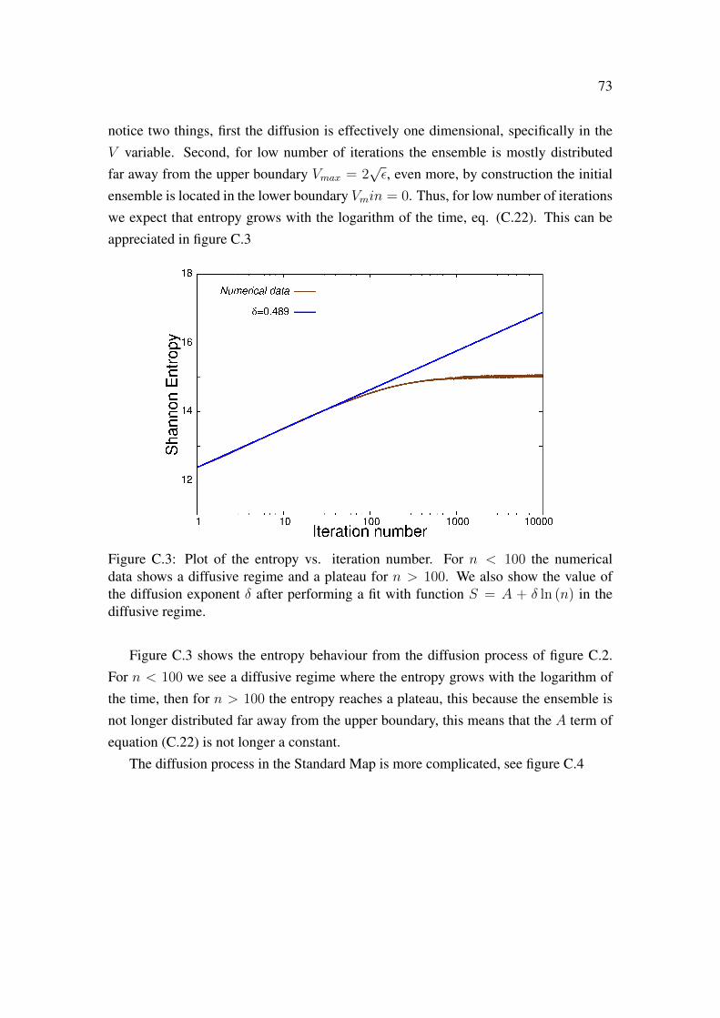
73

notice two things, first the diffusion is effectively one dimensional, specifically in theV variable. Second, for low number of iterations the ensemble is mostly distributedfar away from the upper boundary Vmax = 2

√ε, even more, by construction the initial

ensemble is located in the lower boundary Vmin = 0. Thus, for low number of iterationswe expect that entropy grows with the logarithm of the time, eq. (C.22). This can beappreciated in figure C.3

Figure C.3: Plot of the entropy vs. iteration number. For n < 100 the numericaldata shows a diffusive regime and a plateau for n > 100. We also show the value ofthe diffusion exponent δ after performing a fit with function S = A + δ ln (n) in thediffusive regime.

Figure C.3 shows the entropy behaviour from the diffusion process of figure C.2.For n < 100 we see a diffusive regime where the entropy grows with the logarithm ofthe time, then for n > 100 the entropy reaches a plateau, this because the ensemble isnot longer distributed far away from the upper boundary, this means that the A term ofequation (C.22) is not longer a constant.

The diffusion process in the Standard Map is more complicated, see figure C.4

74

(a) n = 0 (b) n = 1

(c) n = 10 (d) n = 100

Figure C.4: Plot of the behaviour of the diffusion process, measured by the probabilitydensity, in a chaotic region of phase space for the Standard Map k = 2.3, for differentnumbers of iterations n. The orange-white color scale represents the density of pointsin phase space. The subplots (a) to (d) shows the diffusion process.

It is possible to see in figure C.4 that the probability distribution first spreads alongthe shore of the KAM islands and then diffuses outwards. Let us assume that thereis a set of canonical variables x, y such that the spreading along the island is roughlydescribed by a diffusion along the variable y, and the diffusion outwards the islandis roughly described by a diffusion along the variable x. If there exist such a set ofvariables, then the entropy growth should allow us to determinate the diffusion exponentif we are studying an appropriate ensemble. Note the entropy does not depend on thevariables, it can be measured using q and p with out any change, but the entropy growthof equation C.22 depends on the ensemble. Thus, is rather more important to establishthe appropriate ensemble than the canonical variables.

Inside the island we have the presence of invariant curves, a natural way to choosethe canonical variables in this case is to label each invariant curve with an action an-

75

gle variable x, and every point of the invariant curve corresponds to a different anglevariable y, this canonical variables can be extrapolated to outside the island, in [24, 25]show a numerical method to achieve this. Observe that inside the island an ensembleof particles along the same invariant curve will spread in the y variable, while its xcoordinate will not change. An ensemble of particles in the shore of the main islandwill behave in similar way for a small number of iterations. For this reason we choosean ensemble of particles along the shore of the main island. After a small number ofiterations they will spread in the whole shore, y coordinate. For the following iterations,our dynamic is reduced effectively to just one dimension, diffusion in the x coordinate.Even more, the initially the ensemble is located in the border of the island, and consid-ering that for small number of iterations does not leaks to much outside the island, wehave have established the conditions in which we have the appropriate ensemble to useequation (C.22). This description of the dynamics can be seen in figure C.5.

Figure C.5: Plot of the entropy vs. iteration number for k = 1.31. The entropy has threegrowth regimes, i) in the first 100 iterations the distribution spreads along the mainisland, ii) then for 3000 iterations slowly leaks out through the Cantori, iii) finally moreof the distribution is outside the Cantori and rapidly spreads in the chaotic sea.

We show in figure C.5a the entropy behaviour as the time passes. We can recognizethree growth regimes: i) First the distribution quickly spreads along the shore of the

76

main island, y coordinate. This is a fast process equivalent to the spreading in the phasedirection in the SFMU, shown in the transition from figure C.2a to figure C.2b. Wecan appreciate this in the sub-figure 4.4b, that shows how is distributed our ensembleof trajectories after n = 100 iterations. ii) The second regime is a slow one, the dis-tribution leaks through the Cantori, x coordinate, see sub-figure C.5c, this is a regimeof subdiffusion where we have the conditions to use eq. (C.22). Here we measure thediffusion exponent δ, the numerical fit is shown in a blue line. iii) In the third regimemore of the distribution is outside the Cantori and rapidly spreads in the chaotic sea. Afourth regime, not shown in figure C.5, exists, when the ensemble of trajectories is al-most uniformly distributed in the chaotic sea, similar to figure C.3, the entropy reachesa plateau.

Appendix D

Entropy and time irreversibility, somecomments

D.1 Entropy conservation

Recall Hamilton’s equation of motion

q =∂H

∂p,

p = −∂H∂q

, (D.1)

H is the Hamiltonian, q and p are the canonical conjugate variables. Define V as:

V = (q, p) , (D.2)

i. e. the phase space velocity of the representative point1 X = (q, p). If we have anensemble of systems, following the same set of equations (D.1), the phase space densityρ of representative points around X behaves like:

∂ρ

∂t+∇ · (V ρ) = 0 . (D.3)

1X represents a system following the dynamics of Hamilton’s equations, in our case the trajectory ofa particle in phase space.

77

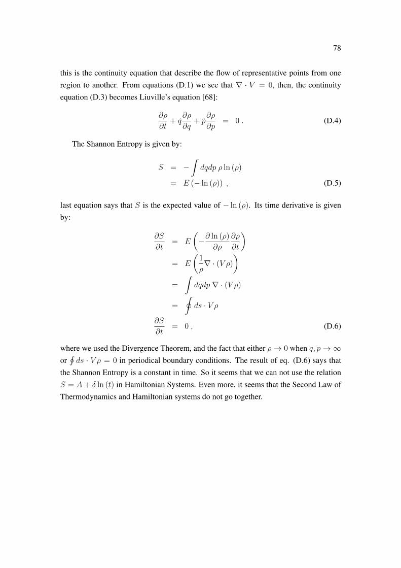
78

this is the continuity equation that describe the flow of representative points from oneregion to another. From equations (D.1) we see that ∇ · V = 0, then, the continuityequation (D.3) becomes Liuville’s equation [68]:

∂ρ

∂t+ q

∂ρ

∂q+ p

∂ρ

∂p= 0 . (D.4)

The Shannon Entropy is given by:

S = −∫dqdp ρ ln (ρ)

= E (− ln (ρ)) , (D.5)

last equation says that S is the expected value of − ln (ρ). Its time derivative is givenby:

∂S

∂t= E

(−∂ ln (ρ)

∂ρ

∂ρ

∂t

)= E

(1

ρ∇ · (V ρ)

)=

∫dqdp∇ · (V ρ)

=

∮ds · V ρ

∂S

∂t= 0 , (D.6)

where we used the Divergence Theorem, and the fact that either ρ→ 0 when q, p→∞or∮ds · V ρ = 0 in periodical boundary conditions. The result of eq. (D.6) says that

the Shannon Entropy is a constant in time. So it seems that we can not use the relationS = A + δ ln (t) in Hamiltonian Systems. Even more, it seems that the Second Law ofThermodynamics and Hamiltonian systems do not go together.

79

D.2 Entropy growth

The usual approach to overcome the problem form last section is to study the effectsof the coarse grained entropy. Define the function s (ρ) as:

s = −ρ ln (ρ) , (D.7)

see that ∂2s∂ρ2≤ 0, then s is a concave function and, by definition of concave functions,

the following relation holds:

xs (ρ1) + (1− x) s (ρ2) ≤ s (xρ1 + (1− x) ρ2) , (D.8)

interpreting 0 ≤ x ≤ 1 as a weight last equation becomes:

s (ρ) ≤ s (ρ) , (D.9)

which means that the average of s is less or equal than taking s of the averaged ρ. Then,when considering all contributions of s, and averaging at each time step, we have thefollowing equation for the coarse grained entropy S:

dS

dt≥ 0 , (D.10)

this means that the entropy growth, in Hamiltonian Systems, is due the fact that the prob-ability density is being coarse grained. This averaging is natural to happen in chaoticsystems due the stable/unstable manifold’s squeezing/expanding action.

D.3 Time reversibility and time irreversibility

Hamiltonian systems at particles level are time reversible, even more, since the equa-tions of motion preserve the phase space area, the entropy of an ensemble of particles,representation points, must be conserved. The averaging process in last section is timeirreversibility and this produced an entropy growth. although from a practical point ofview this averaging process is paussible, specially due the manifold’s dynamics, is stillcontroversial from a physical point of view, since, in principle, we do not know how to

80

interpret the entropy growth. To understand more this behaviour, we focus in studyingthe evolution of the probability density rather than representative points.

Without loss of generality let us consider the discrete mapping xn = F (xn−1), then,the evolution of the point x0 after one iteration can be described in terms of Dirac deltafunction as:

δ (x− F (x0)) =

∫dx′ δ (x− F (x′)) δ (x′ − x0) , (D.11)

since by superposition we have ρ (x, n) =∫dx0 δ (x− x0) ρ (x0, n), we obtain terms

of Dirac delta function as:

ρ (x, n+ 1) =

∫dx′ δ (x− F (x′)) ρ (x′, n)

= Uρ (x, n) , (D.12)

which defines the operator U , Perron Frobenius operator2, that evolves densities. Ifthe mapping xn+1 = F (xn) preserves some measure and is time reversible, then U

is unitary in Hilbert Space [71], which means that in this space its eigenvalues are ofmodulus one. In this case the density behaves like:

ρ (x, n) =∞∑k=0

akeiwknψk (x) , (D.13)

where eiwk , ψk (x), are the eigenvalues, eigenvectors, of the Perron-Frobenius operator,ak are constants related to the initial value ρ (x, 0). In this solution apparently thereis no decay to an equilibrium density, nevertheless, in chaotic systems, we know thatdensities in the chaotic sea decay to an equilibrium density that fills the whole chaoticsea. For this observation is necessary to use the Resolvent of the Perron Frobeniusoperator [69, 70], which will bring us to other functional spaces rather than HilbertSpace [71]. For more on the mathematical method and application to hyperbolic mapssee refs [71, 73], although for non hyperbolic maps there is no mathematical justificationto use the Resolvent, in ref [72] show that finite approximations of the Perron-Frobeniusoperator give interesting results when studying correlations in chaotic non hyperbolic

2This is the analogous of Liuville’s operator for general systems

81

maps.We highlight some physical relevant results of the bibliography:

1. The functional spaces of U appropriate for forward time evolution and backwardtime evolution, are different, meaning that there is an asymmetry in the time evo-lution [71, 73].

2. For some systems, trajectories are not possible to recover from the spectral de-composition of U , this because trajectories correspond to non-differentiable pointdensities. Thus, by considering a representation of the system were we care aboutdensities rather than trajectories, the dynamical laws include time irreversibility,which do not contradict the time reversibility at trajectory level. Then, since therepresentation that breaks time symmetry is in accordance with or experience ofnature it might be that trajectories must be seen as stochastic realizations of themore fundamental probability densities, [71].

Since entropy is related to probability densities and not trajectories, it is expectedthat it grows in a time irreversible dynamic.

Bibliography

[1] I. Newton, Philosophiae Natvralis Principia Mathematica. London, 1687.

[2] H. Poincare. Les methodes nouvelles de la mecanique celeste. Gauthier-Villars itfils, 1892-1899.

[3] K. F. Sundman, “Memoire sur le probleme des trois corps”. Acta Mathematica,vol. 36, pp. 105, 1913.

[4] W. Qiu-Dong, “The global soltion of the n-body problem”. Celestial Mechanicsand Dynamical Astronomy, vol. 50, pp. 73, 1990.

[5] F. Dicau, “The solution of the n-body problem”. The Mathematical Intelligencer,vol. 18, pp. 66, 1996.

[6] E. N. Lorenz “Deterministic nonperiodic flow”. Journal of the atmospheric sci-ences, vol.20, pp. 130, 1963.

[7] M. J. Feigenbaum “The universal metric properties of nonlinear transformations”.Journal of Statistical Physics, vol. 21, pp. 669, 1979.

[8] S. H. Strogatz, Nonlinear dynamics and chaos: with applications to physics, biol-

ogy, chemistry and engineering. Westviez press, 2014.

[9] G. M. Zaslavsky, Physics of Chaos in Hamiltonian Systens, Imperial College Press,New York, 2007.

[10] M. F. Shlesinger, G. M. Zaslavsky and J. Klafter, “Strange Kinetics”. Nature, vol.363, pp. 31, 1993.

82

83

[11] C. P. Dettmann, “Diffusion in the Lorentz gas”. Commun. in Theoretical Physicsvol. 62, No. 4, pp. 521, 2014.

[12] E. Fermi, “On the Origin of the Cosmic Radiation”. Phys. Rev., vol. 75, No. 8, pp.1169, 1949.

[13] A. J. Litchenberg, M. A. Lieberman and R. H. Cohen, “Fermi acceleration re-visted”. Physica D, vol. 1, pp. 291, 1980.

[14] S. O. Kamphorst, E. D. Leonel and J.K.L. Da Silva, “The presence and lack ofFermi acceleration in nointegrable billiards”. Journal of Physics A, vol 40, p. F887,2007.

[15] R. S. MacKay, J. D. Meiss, I. C. Percival, “Transport in Hamiltonian systems”.Physica D, vol. 13, pp. 55, 1984.

[16] N. B. de Faria, D. S. Tavares, W. C. de Paula, E. D. Leonel and D. G. Ladeira,“Transport of chaotic trajectories from regions distant from or near to structures ofregular motion of the Fermi-Ulam model”. Physical Review E, vol. 94, pp. 042208,2016.

[17] M. Roberto, E. C. Silva, I. L. Caldas and R. L. Viana, “Magnetic trapping causedby resonant perturbations in tokamaks with reversed magnetic shear”, Phys. Plas-mas vol. 11, pp. 214, 2004.

[18] C. G. L Martins, M. Roberto and I. L. Caldas, “Magnetic field line stickiness intokamaks”, IEEE TRANSACTIONS ON PLASMA SCIENCE, vol. 42, pp. 2764,2014.

[19] D. F. Oliveira, M. R. Silva and E. D. Leonel, “A symmetry break in energy dis-tribution and a biased random walk behavior causing unlimited diffusion in a twodimensional mapping”. Physica A, vol. 436, pp. 909, 2015.

[20] A. L. P. Livorati, T. Kroetz, C. P. Dettmann, I. L. Caldas e E. D. Leonel, “Stickinessin a Bouncer model: a slowing mechanism for Fermi acceleration”, Phys. Rev. E,vol. 86, pp. 036204, 2012.

84

[21] G. M. Zaslavsky, “Chaos, fractional kinetics, and anomalous transport”. PhysRep., vol. 371, pp. 461, 2002.

[22] E. D. Leonel, J. A. De Oliveira and F. Saif, “Critical exponents for a transition fromintegrability to non-integrability via localization of invariant tori in the Hamilto-nian system”. Journal of Physics A, vol. 44, pp. 302001, 2011.

[23] M. S. Palmero, G. I. Dıaz, P. V. McClintock and E. D. Leonel, “Diffusion Phe-nomena in a Mixed Phase Space”. 2019.

[24] A. Backer, R. Ketzmerick and S. Lock, “Direct regular-to-chaotic tunneling ratesusing the fictitious-integrable-system approach”. Physical Review E, vol. 82, pp.05608, 2010.

[25] C. Lobner, S. Lock, A. Backer and R. Ketzmerick “Integrable approximation ofregular islands: The iterative canonical transformation method”. Physicial ReviewE, vol. 88, pp. 062901, 2013.

[26] A. N. Kolmogorov “On the Conservation of Conditionally Periodic Motions underSmall Perturbation of the Hamiltonian”. Dokl. Akad. Nauk. SSR., vol. 98, pp 2,1954.

[27] J. Moser, “On invariant curves of area-preserving mappings of an annulus”. Nachr.Akad. Wiss. II, pp. 1, 1962.

[28] V. I. Arnold, “Proof of a theorem of A. N. Kolmogorov on the preservation ofconditionally periodic motions under a small perturbation of the Hamiltonian”.Uspekhi Mat. Nauk, vol. 18, 1963 (English transl. ¿ Russ. Math. Surv, vol. 18).

[29] I. C. Percival, “A variational principle for invariant tori of fixed frequency”. Journalof Physics A: Mathematical and General, vol. 12, 1979.

[30] N. Scafetta and P. Grigolini, “Scaling detection in time series: diffusion entropyanalysis”. Physical Review E, vol. 66, pp. 036130, 2002.

[31] C. E. Shannon, “A mathematical theory of communication”. Bell System technicalJournal, vol. 27, pp. 379, 1948.

85

[32] A.Lesne, “Shannon entropy: A rigorous notion at the crossroads between probabil-ity, information theory, dynamical systems and statistical physics”. MathematicalStructures in Computer Science, vol. 24, 2014.

[33] B. V. Chirikov, “Research concerning the theory of nonlinear resonance andstochasticity”. Preprint N 267, Institute of Nuclear Physics, Novosibirsk, 1969,(Engl. Trans., CERN Trans. 71-40 1971).

[34] B. V. Chirikov, “A universal instability of many-dimensional oscillator systems”.Phys. Rep. vol. 52, pp. 263, 1979.

[35] M. V. Berry, “Regularity and chaos in classical mechanics, illustrated by threedeformations of a circular billiard”. Eur. J. Phys. vol. 2, pp. 91-102, 1981.

[36] R. C. Hilborn, Chaos and Nonlinear Dynamics: An Introduction for Scientists and

Engineers. Oxford University Press, New York, 1994.

[37] A. J. Lichtenberg, M.A. Lieberman, Regular and Chaotic Dynamics. Appl. Math.Sci. 38, Springer Verlag, New York, 1992.

[38] G. M. Zaslavsky, Hamiltonian Chaos and Fractional Dynamics, Oxford UniversityPress, New York, 2008.

[39] D. Ciro, I. L. Caldas, R. L. Viana and T. E. Evans, “Efficient manifold tracing forplanar maps” Chaos: An Interdisciplinary Journal of Nonlinear Science vol. 28,pp. 093106, 2018.

[40] L. A. Bunimovich, “On Ergodic Properties of Certain Billiards”. Funct. Anal.Appl., vol. 8, pp. 254, 1974.

[41] N. Chernov and R. Markarian, Chaotic Billiards. American Mathematical Society,Vol. 127, 2006.

[42] C. P. Dettmann, “Recent advances in open billiards with some open problems”.Frontiers in the study of chaotic dynamical systems with open problems, pp. 195,2011.

86

[43] G. D. Birkhoff, “On the periodic motions of dynamical systems”, Acta Mathemat-ica, vol. 50, pp. 359, 1927.

[44] Y. G. Sinai,“Dynamical systems with elastic reflections”. Russ. Math. Surveys.,vol. 25, pp. 137, 1970.

[45] N. Krylov, Works on the Foundations of Statistical Physics Princeton Univ. Press,Princeton, NJ, 1979.

[46] J. Skowron, A. Gould, “General complex polynomial root solver and its futheroptimizarion for binary microlenses”. arXiv preprint arXiv:1203.1034, 2012

[47] J. L. Lagrange, “Reflexions sur la resolution algebrique des equations”. CEuvresde Lagrange, III, Gauthier-Villars, pp. 205, 1869.

[48] F. W. J. Olver, A. B. Olde Daalhuis, D. W. Lozier, B. I. Schneider, R. F. Boisvert, C.W. Clark, B. R. Miller, and B. V. Saunders, eds., “Digital Library of MathematicalFunctions”. http://dlmf.nist.gov/, Realese 1.0.22 of 2019-03-15.

[49] F. T. Krogh, C. L. Lawson, and W. Van Snyder, eds., “MATH77 and mathc90,Realese 6.0. Libraries of Mathematical Subprograms in Fortran 77 and C”. Cali-fornia Institute of Technology, 1998.

[50] E. D. Leonel, P. V. McClintock and J. K. L. da Silva, “Fermi-Ulam acceleratorundes scaling analysis”. Physical Review Letters, vol. 93, pp. 014101, 2004.

[51] P. Dierckx, “Curve and surface fitting with splines”. Oxford University Press,1995.

[52] S. Lange, M. Richter, F. Onken, A. Backer, R. Ketzmerick, “Global structure ofregular tori in a generic 4D sympletic map”. Chaos: An Interdisciplinary Journalof Nonlinear Science, vol. 24, pp. 024409, 2014.

[53] G. D. Birkhoff, “An extension of Poincare’s last geometric theorem”. Acta. Math.,vol. 47, pp. 297, 1925.

[54] Y. S. Sun, L. Zhou and J. L. Zhou, “The role of hyperbolic invariant sets in sticki-ness effects”, in A Comparison of the Dynamical Evolution of Planetary Systems,Springer, Dordrecht, 2005.

87

[55] T. S. Kruger, P. P. Galuzio, T. D. L. Prado, R. L. Viana, J. D. Jr. Szezech and S. R.Lopes, “Mechanism for stickiness suppression during extreme events in Hamilto-nian systems”. Physical Review E, vol.91, pp. 062903, 2015.

[56] G. Contopoulos and M. Harsoula, “Stickiness effects in chaos”. Celestial Mechan-ics and Dynamical Astronomy, vol. 107, pp. 77, 2010.

[57] S. Tomsovic, “Tunneling and Chaos”. Physica Scripta, no. T90 pp. 162, 2001.

[58] M. J. Davis and E. J. Heller, “Quantum dynamical tunneling in bound states”. TheJournal of Chemical Physics, no. 1, pp. 246, 1981.

[59] Y. Meroz, and I. Sokolov, “A toolbox for determining subdiffusive mechanisms”.Physics Reports, vol. 573, pp. 1, 2015.

[60] B. B. Mandelbrot, and J. W. Van Ness, “Fractional Brownian motions, fractionalnoises and applications”. SIAM review, vol. 10, no. 4, pp. 422, 1968.

[61] H. Scher, and E. W. Montroll, “Anomalous transit-time dispersion in amorphoussolids”. Physical Review B, vol. 12, no. 6, pp. 2455, 1975.

[62] G. M. Zaslavsky, M. Edelman, and B. A. Niyazov, “Self-similarity, renormaliza-tion, and phase space nonuniformity of Hamiltonian chaotic dynamics”. Chaos:An Interdisciplinary Journal of Nonlinear Science, vol. 7, no. 1, pp. 159, 1997.

[63] I. M. Sokolov, and J. Klafter, “From diffusion to anomalous diffusion: a centuryafter Einstein’s Brownian motion”. Chaos: An Interdisciplinary Journal of Non-linear Science vol. 15, pp. 026103, 2005.

[64] R. Balescu, Statistical Dynamics: Matter Out of Equilibrium, Imperial CollegePress, 1997.

[65] M. Magdziarz, A. Weron, and K. Weron,“Fractional Fokker-Planck dynamics:Stochastic representation and computer simulation”. Physical Review E, vol. 75,pp. 016708, 2007.

[66] A. Janicki, A. Weron, Simulation and chaotic behaviour of α-stable stochastic

processes, CRCPress, 1993.

88

[67] H. J. Haubol, A. M. Mathai, and R. K. Saxena, “Mittag-Leffler functions and theirapplications”. Journal of Applied Mathematics, vol. 2011, pp. 298628, 2011.

[68] H. Goldstein, C. Poole, and J. Safko, Classical mechanics, 2002.

[69] M. Pollicott, “On the rate of mixing of Axiom A flows”. Inventiones mathemati-cae, vol. 81, no. 3, pp. 413, 1985.

[70] D. Ruelle, “Resonances of chaotic dynamical systems”. Physical review letters,vol. 56, no. 5, pp. 405, 1986.

[71] D. J. Driebe, Fully chaotic maps and broken time symmetry. Springer Science andBusiness Media, 1999.

[72] S. Fishman, and S. Rahav, “Relaxation and noise in chaotic systems”. In Dynamics

of Dissipation, Springer, Berlin, Heidelberg, pp. 165, 2002.

[73] S. Tasaki, “Irreversibility in reversible multibaker maps-Transport and fractal dis-tributions”. Advances in Chemical Physics, vol. 122, pp. 77, 2002.