![[Habilitações Académicas] Hybrid System of Distributed ... · [Engenharia Informática] [Habilitações Académicas] [Habilitações Académicas] [Habilitações Académicas] Hybrid](https://static.fdocumentos.com/doc/165x107/5e11ed0be14dd447f151a808/habilitaes-acadmicas-hybrid-system-of-distributed-engenharia-informtica.jpg)
FACULDADE DE ENGENHARIA DA UNIVERSIDADE … · FACULDADE DE ENGENHARIA DA UNIVERSIDADE DO PORTO...
111
FACULDADE DE ENGENHARIA DA UNIVERSIDADE DO PORTO Simulation of Intelligent Active Distributed Networks Implementation of Storage Voltage Control Daniel Burnier de Castro Licenciado em Engenharia Electrotécnica e de Computadores pela Faculdade de Engenharia da Universidade do Estado do Rio de Janeiro Dissertação submetida para satisfação parcial dos requisitos do grau de mestre em Engenharia Electrotécnica e de Computadores (Área de especialização de Energias Renováveis) Dissertação realizada no OFPZ Arsenal Ges.m.b.H, localizado em Viena, Áustria sob a supervisão do professor João Abel Peças Lopes do Departamento de Engenharia Electrotécnica e de Computadores da Faculdade de Engenharia da Universidade do Porto e co-supervisão dos engenheiros Helfried Brunner e Benoît Bletterie, pesquisadores do OFPZ Arsenal Ges.m.b.H Porto, Setembro de 2008
-
Upload
dinhkhuong -
Category
Documents
-
view
214 -
download
0
Transcript of FACULDADE DE ENGENHARIA DA UNIVERSIDADE … · FACULDADE DE ENGENHARIA DA UNIVERSIDADE DO PORTO...

FACULDADE DE ENGENHARIA DA UNIVERSIDADE DO PORTO
Simulation of Intelligent Active Distributed Networks
Implementation of Storage Voltage Control
Daniel Burnier de Castro
Licenciado em Engenharia Electrotécnica e de Computadores pela Faculdade de Engenharia da Universidade do Estado do Rio de Janeiro
Dissertação submetida para satisfação parcial dos
requisitos do grau de mestre em
Engenharia Electrotécnica e de Computadores (Área de especialização de Energias Renováveis)
Dissertação realizada no OFPZ Arsenal Ges.m.b.H, localizado em Viena, Áustria
sob a supervisão do professor João Abel Peças Lopes
do Departamento de Engenharia Electrotécnica e de Computadores
da Faculdade de Engenharia da Universidade do Porto
e co-supervisão dos engenheiros Helfried Brunner e Benoît Bletterie,
pesquisadores do OFPZ Arsenal Ges.m.b.H
Porto, Setembro de 2008

2
Abstract
While distributed generation (DG) from renewable energy resources is seen as a key element
of future energy supply, current electricity grids are not designed to integrate a steadily
increasing share of distributed generators. The hierarchical network topology was designed
for unidirectional power flows and passive operation. In order to avoid excessively expensive
grid reinforcements, new solutions for active grid operation are necessary. In the context of
the Austrian national research project DG DemoNet, different methods for an active
distribution network with a high penetration of distributed generation were developed,
especially regarding the voltage control in these networks. These methods were simulated for
existing Austrian net sections, in the medium voltage systems. This work analysis the
possibility to broaden these methods by the application of storage technologies and its
integration into the already existing voltage control methods, especially into the coordinated
voltage control, which comprises tap changing of the on-load tap changer of the transformer,
the production of reactive power and the curtailment of the active power of the power plants.
The work explains the changes performed in the algorithm of the coordinated voltage control
to admit the integration of storage systems, including the definition of the storage variable and
the behavior of the storage system in different voltage scenarios. Simulations were performed
to discover the required power and capacity of a theoretical storage device to keep the voltage
within the desired limits, with and without other voltage control methods. Several different
storage technologies were analyzed, taking into account their characteristics, principal
advantages and disadvantages. These technologies were then compared aiming to find those
more suitable for the application to the coordinated voltage control method. The simulation
results and storage technologies comparison can be used for the modeling of different storage
systems, as long as the required variables and parameters are well defined and validated for
the application to the voltage control methods.

3
Resumo
Embora a geração distribuída a partir de recursos energéticos renováveis seja vista como
elemento-chave do futuro abastecimento energético, as actuais redes eléctricas não são
concebidas para integrar um constante aumento da quota de geração distribuída. A topologia
de rede hierarquizada foi concebida para um fluxo de potência unidirecional e operação
passiva. A fim de evitar reforços na rede, que são excessivamente caros, novas soluções para
uma rede activa são necessários. No contexto do projecto de investigação nacional austríaco
DG DemoNet, diferentes métodos para uma rede activa de distribuição com uma elevada taxa
de penetração de geração distribuída foram desenvolvidas, especialmente no que diz respeito
ao controlo da tensão destas redes. Estes métodos foram simulados para secções da rede
austríaca, em sistemas de média tensão. Este trabalho analiza a possibilidade de expandir estes
métodos através da aplicação de tecnologias de armazenamento e sua integração aos métodos
de controlo de tensão já existentes, especialmente para o método de controlo coordenado de
tensão, que inclui transformadores de passo, produção de potência reativa e o corte de
potência activa das centrais eléctricas. Este trabalho explica as mudanças realizadas no
algoritmo do controlo coordenado de tensão com o fim de permitir a integração dos sistemas
de armazenamento, incluindo a definição da variável de armazenamento e o comportamento
do sistema de armazenamento para diferentes cenários de tensão. Foram realizadas
simulações para descobrir a potência e capacidade necessários de um dispositivo teórico de
armazenamento para manter a tensão dentro dos limites desejados, com e sem outros métodos
de controle de tensão. Várias tecnologias de armazenamento diferentes foram analisadas,
levando em conta as suas principais características, vantagens e desvantagens. Estas
tecnologias foram, então, comparadas com o objetivo de encontrar as mais adequadas para a
aplicação ao método de controlo coordenado de tensão. Os resultados da simulação e
comparação das tecnologias de armazenamento podem ser utilizados para a modelagem de
diferentes sistemas de armazenamento, desde que as variáveis e os parâmetros exigidos sejam
bem definidos e validados para a aplicação aos métodos de controlo de tensão.
4
Preface
The voltage control method presented in this work is an extension to the coordinated voltage
control in the ambit of the DG DemoNet project. In this project different techniques are
applied to solve the voltage problems that can occur on networks with a high share of
distributed generation. Since some of these techniques involve the curtailment of active
power, some alternative solutions need to be investigated as the power curtailment leads to
serious economical issues. One of the alternatives is the application of storage devices that
can be used to charge in cases of overvoltage and discharge in cases of undervoltage, keeping
the voltage between expected operational limits. However, the modelling of appropriate
storage systems for this application requires the knowledge of technical requirements and
available technologies that fulfil these requirements.
Simulations were carried out with the objective to dimension the storage systems
for voltage control, within the coordinated voltage control algorithm. With this dimensioning
it was possible to investigate some technologies and find those more suitable to be applied to
these systems.
My main difficulty in this work was to find an accurate correlation between the
simulated storage system (concerning mainly their capacity and power) and the available
technologies, since many of the time constants of the diverse network components and the
precise and complete description of some storage technologies were not available. Another
difficult I faced was to understand the behaviour of the algorithm of the coordinated voltage
control, which was written in MATLAB® and simulated with DIgSILENT Power Factory®.
The interface between the two softwares doesn’t permit debugging, what made the process of
changing the algorithm and testing it very complex and time consuming.
This work was accomplished at OFPZ Arsenal Ges.m.b.H (or simply “arsenal
research”) in Vienna, Austria and could not be done without the help of Helfried Brunner and
Benoît Bletterie, employees of this research institute. They helped me in every way, providing
me with useful references and with their experience and time. I learnt a lot during this year at
arsenal research and I am glad I had this opportunity to work with them. I would also like to
thank to my advisor, Professor Peças Lopes, who deposited his confidence in me and arsenal
research and was ready to help when necessary.

5
Index
1 Introduction ......................................................................................................................10 1.1 Objectives and Motivation........................................................................................10 1.2 Chapters Overview ...................................................................................................11
2 Distributed Generation .....................................................................................................13 2.1 Reasons for Distributed Generation .........................................................................13 2.2 Technical Challenges of Integration of DG into Distribution Networks..................16
2.2.1 Network Voltage Changes................................................................................17 2.2.2 Increase in Network Fault Levels .....................................................................19 2.2.3 Power Quality ...................................................................................................19 2.2.4 Protection Schemes...........................................................................................20 2.2.5 Stability.............................................................................................................22 2.2.6 Grid Losses .......................................................................................................22 2.2.7 Network Operation ...........................................................................................22
3 DG DemoNet Project........................................................................................................24 3.1 Current Situation in Austria......................................................................................24 3.2 The Voltage Rise Problem........................................................................................26 3.3 Active Voltage Control: The Step Model.................................................................29
3.3.1 Current Practice ................................................................................................29 3.3.2 Local Voltage Control ......................................................................................30 3.3.3 “Decoupling Solution” .....................................................................................30 3.3.4 Distributed Voltage Control .............................................................................30 3.3.5 Coordinated Voltage Control............................................................................30
3.4 Algorithm for Coordinated Voltage Control ............................................................32 4 Energy Storage Systems, Status and Potential .................................................................37
4.1 Storage Systems: History..........................................................................................37 4.2 Storage Systems: Applications and Technologies....................................................39
4.2.1 Supercapacitors.................................................................................................41 4.2.2 Superconducting Magnetic Energy Storage (SMES) .......................................43 4.2.3 Pumped Hydro Storage.....................................................................................45 4.2.4 Compressed Air Energy Storage (CAES) ........................................................47 4.2.5 Flywheels..........................................................................................................48 4.2.6 Batteries ............................................................................................................51 4.2.7 Redox-Flow Batteries .......................................................................................58 4.2.8 Hydrogen Storage .............................................................................................63 4.2.9 Other Systems Storing Primary Energy............................................................64
4.3 Storage Systems: Technologies Comparison ...........................................................65 4.4 Integration of Storage Systems to the Coordinated Voltage Control .......................68
5 Study Case: Vorarlberg, Austria.......................................................................................77 5.1 DIgSILENT PowerFactory® Software Overview....................................................77 5.2 Study Case Network Analysis ..................................................................................81 5.3 Simulations and Results............................................................................................85
5.3.1 Storage Model 1 – Standalone Storage System................................................89 5.3.2 Storage Model 2 – Integrated Storage System .................................................98
6 Conclusions and Next Steps ...........................................................................................103 References ..............................................................................................................................109
6
Index of Figures
Figure 2.1 – Scheme of a centralized power plant ..................................................................14 Figure 2.2 – Scheme of distributed generation........................................................................15 Figure 2.3 – Conventional distribution system........................................................................16 Figure 2.4 – Distribution system with DG ..............................................................................17 Figure 2.5 – Voltage drop in a conventional distribution network..........................................18 Figure 2.6 – Voltage rise in a distribution network with DG penetration ...............................18 Figure 2.7 – Illustration of the islanding issue ........................................................................21 Figure 2.8 – Grid losses related to the penetration of DG (VAN GERWENT, 2006) ............22 Figure 3.1 – Dispersion of the installed DG power per m², Energie AG OÖ Netz GmbH
(LUGMAIER et al., 2007) ...............................................................................................25 Figure 3.2 – Simple distribution network with DG ..................................................................26 Figure 3.3 – Step Model “DG Integration” – Step model sequence.........................................31 Figure 3.4 – Basic representation of the CVC algorithm (BRUNNER et al., 2007) ...............32 Figure 3.5 – Voltage conflicts – in situations (a) and (b), tap change operation is not possible.
In this case, DG units are actively controlled ...................................................................33 Figure 3.6 – Priority Matrix (BRUNNER et al., 2007)............................................................34 Figure 3.7 – Priority Matrix Decoupling (BRUNNER et al., 2007) ........................................34 Figure 3.8 – DG Unit Control Scheme (BRUNNER et al., 2007) ...........................................35 Figure 3.9 – Calculation of the active and reactive power management in the CVC algorithm
..........................................................................................................................................35 Figure 3.10 – Flow chart algorithm of the CVC......................................................................36 Figure 4.1 – Electricity storage spectrum.................................................................................40 Figure 4.2 – Setup of a Supercapacitor (SELS et al., Sep. 2001).............................................42 Figure 4.3 – Basic setup of a SMES unit (SELS et al., Oct. 2001) ..........................................44 Figure 4.4 – Pumped Hydro storage scheme (ERBEN, 2008) .................................................46 Figure 4.5 – Scheme of a CAES system (BLAABJERG et al., 2007).....................................47 Figure 4.6 – Block diagram of a Flywheel for grid connected applications. (BLAABJERG et
al., 2007)...........................................................................................................................49 Figure 4.7 – Lead-Acid storage system in Chino, California (ESA, 2007/2008).....................53 Figure 4.8 – NaS cell scheme (ESA, 2007/2008).....................................................................54 Figure 4.9 –Working principle of a Li-Ion battery...................................................................56 Figure 4.10 – Metal-Air Battery scheme (ESA, 2007/2008)....................................................57 Figure 4.11 – Schematic diagram of a Redox flow battery (SELS et al., Oct. 2001) ..............59 Figure 4.12 – Principle of the hydrogen storage system (BODACH, 2006)............................63 Figure 4.13 – Biogas storage system in Burgenland, Austria ..................................................64 Figure 4.14 – Volume and weight energy densities for different storage technologies (ESA,
2007/2008)........................................................................................................................65 Figure 4.15 – Efficiency and life cycles for different storage technologies (ESA, 2007/2008)
..........................................................................................................................................66 Figure 4.16 – Discharge time at rated power (ESA, 2007/2008) .............................................67 Figure 4.17 – Storage device definition added to the CVC algorithm .....................................69 Figure 4.18 – Storage device model added to the CVC, showing the control action in different
cases..................................................................................................................................70 Figure 4.19 – Storage Model 1 – Standalone Storage System .................................................71 Figure 4.20 – Storage Model 2 – Integrated Storage System...................................................72 Figure 4.21 – Flow chart algorithm of the CVC with the addition of the SD Control .............73 Figure 4.22 – Basic representation of the CVC algorithm with SD control.............................74 Figure 4.23 – Active Power Priority Matrix with Storage Control ..........................................75

7
Figure 5.1 – Graphical windowing environment in DIgSILENT PowerFactory® simulation software. ...........................................................................................................................78
Figure 5.2 – User written models within a graphical environment. .........................................79 Figure 5.3 – MATLAB® integration through *.m file.............................................................80 Figure 5.4 – Study case network – Vorarlberg, Austria ...........................................................81 Figure 5.5 – Yearly voltage profile (p.u.) for the eleven nodes ...............................................82 Figure 5.6 – SDs connected to the selected critical nodes – Storage Model 1 .........................83 Figure 5.7 – Generator DEA_DG10_W – Storage Model 2 ....................................................84 Figure 5.8 – Coordinated voltage control at overvoltage nodes...............................................86 Figure 5.9 – Active and reactive power at DEA_DG9_W .......................................................86 Figure 5.10 – Active and reactive power at DEA_DG13_V2_2MW.......................................86 Figure 5.11 – CVC: Overvoltage..............................................................................................87 Figure 5.12 – CVC: Undervoltage............................................................................................87 Figure 5.13 – Active and reactive power at DEA_DG9_W .....................................................88 Figure 5.14 – Active and reactive power at DEA_DG13_V2_2MW.......................................88 Figure 5.15 – Tap positions of the transformer 61.810_UM2..................................................88 Figure 5.16 – SD definition for SD_83902 ..............................................................................89 Figure 5.17 – SD definition for SD_62905-SS1.......................................................................89 Figure 5.18 – Storage power – SD_83902 ...............................................................................90 Figure 5.19 – Storage power – SD_62905_SS1 .......................................................................90 Figure 5.20 – Application of the CVC with SD (Storage Model 1) to overvoltage nodes.......91 Figure 5.21 – Application of the CVC with SD (Storage Model 1) to undervoltage nodes.....92 Figure 5.22 – Application of the CVC with SD (Storage Model 1) to overvoltage nodes –
SD_83902 contributes to the voltages at the nodes 83902 and 183. ................................93 Figure 5.23 – Storage power – SD_83902 (contributes to the voltages at the nodes 83902 and
183)...................................................................................................................................93 Figure 5.24 – Storage power – SD_83902 (limited power) .....................................................94 Figure 5.25 – Active and reactive power – DEA–DG9_W......................................................94 Figure 5.26 – Active and reactive power – DEA–DG13_V2_2MW .......................................95 Figure 5.27 – Application of the CVC with SD (Storage Model 1) to overvoltage nodes.......95 Figure 5.28 – Active and reactive power – DEA–DG9_W......................................................96 Figure 5.29 – Active and reactive power – DEA–DG13_V2_2MW .......................................96 Figure 5.30 – Application of the CVC with SD to overvoltage nodes .....................................97 Figure 5.31 – Application of the CVC with SD to undervoltage nodes ...................................97 Figure 5.32 – Active and Reactive Power at DEA_DG10_W (Model 2) ................................98 Figure 5.33 – Voltage profile at node 83902 – SD Model 2 control (No Q nor PQ control)...99 Figure 5.34 – Voltage profile at node 83902 – Storage Model 2 (Q control, but no PQ control)
..........................................................................................................................................99 Figure 5.35 – Active and reactive power at DEA–DG10_W (Storage Model 2)...................100 Figure 5.36 – Voltage profile at node 83902 – Storage Model 2 (with Q and PQ control) ...100 Figure 5.37 – Active and reactive power at DEA_DG10_W (Storage Model 2)...................101 Figure 5.38 – Active and reactive power at DEA_DG9_W ...................................................101 Figure 6.1 – Voltage control with DSM – load in kW (a) and voltage at the point of common
coupling (b).....................................................................................................................107

8
Index of Tables
Table 3.1 – Share of generation in distribution grids (LUGMAIER et al., 2007) ...................25 Table 3.2 – Step Model “DG Integration” – Voltage control tools used for each step of the
model ................................................................................................................................29 Table 3.3 – Step Model “DG Integration” – Important advantages / drawbacks .....................31 Table 4.1 – Application category specifications for storage systems (SCHOENUNG et al.,
2003).................................................................................................................................40 Table 4.2 – Summary of the investigated storage technologies ...............................................41 Table 4.3 – Overall characteristics of supercapacitors .............................................................42 Table 4.4 – Advantages and drawbacks of Supercapacitors (ERBEN, 2008)..........................43 Table 4.5 – Advantages and drawbacks of SMES systems (ERBEN, 2008) ...........................44 Table 4.6 – Parameters and costs for SMES systems (SCHOENUNG et al., 2003) ...............45 Table 4.7 – Parameters and costs for Pumped Hydro storage systems (SCHOENUNG et al.,
2003).................................................................................................................................46 Table 4.8 – Advantages and drawbacks of Pumped Hydro storage systems (ERBEN, 2008).46 Table 4.9 – Advantages and drawbacks of CAES systems ......................................................48 Table 4.10 – Parameters and costs for a CAES system (SCHOENUNG et al., 2003) ............48 Table 4.11 – Characteristics of Flywheels (current and expected)...........................................50 Table 4.12 – Parameters and costs for Flywheel systems (SCHOENUNG et al., 2003) .........50 Table 4.13 – Advantages and drawbacks of Flywheels (SCHOENUNG et al., 2003) ............51 Table 4.14 – Advantages and drawbacks of Lead-acid batteries .............................................53 Table 4.15 – Parameters and costs for Lead-acid battery systems (SCHOENUNG et al., 2003)
..........................................................................................................................................54 Table 4.16 – Parameters and costs for NaS systems (SCHOENUNG et al., 2003) .................55 Table 4.17 – Parameters and costs for Li-Ion systems (SCHOENUNG et al., 2003)..............57 Table 4.18 – Advantages and drawbacks of Metal-Air batteries .............................................58 Table 4.19 – Parameters and costs for a VRB system (SCHOENUNG et al., 2003) ..............60 Table 4.20 – Parameters and costs for a ZnBr system (SCHOENUNG et al., 2003) ..............61 Table 4.21 – Parameters and costs for a PSB (Regenesys®) system (SCHOENUNG et al.,
2003).................................................................................................................................62 Table 4.22 – Comparison between different technologies of flow batteries (BLAABJERG et
al., 2007)...........................................................................................................................62 Table 4.23 – Advantages and drawbacks of hydrogen storage ................................................63 Table 4.24 – Parameters and costs for a hydrogen fuel cell system (SCHOENUNG et al.,
2003).................................................................................................................................64 Table 4.25 – Storage applications in the energy supply field (BODACH, 2006) ....................67 Table 4.26 – Application of different storage system technologies (ESA, 2007/2008) ...........68 Table 4.27 – Storage parameters ..............................................................................................69 Table 5.1 – Priority Matrix for Q Control – Storage Model 1..................................................83 Table 5.2 – Priority Matrix for PQ Control – Storage Model 1 ...............................................84 Table 5.3 – Priority Matrix for Q Control – Model 2...............................................................84 Table 5.4 – Priority Matrix for PQ Control – Model 2.............................................................85 Table 5.5 – Priority matrix for PQ control (SD_83902 contributes also to the voltage at the
node 183) ..........................................................................................................................92 Table 5.6 – Storage Models 1 and 2 – Results summary .......................................................102
9
Abbreviations List
CAES Compressed Air Energy Storage
CHP Combined Heat and Power
CN Critical Nodes
CVC Coordinated Voltage Control
DEA Dezentrale Erzeugungsanlage (Distributed Generator)
DG Distributed Generation
DNO Distribution Network Operators
DSM Demand Side Management
EC Electrochemical Capacitors
Li-Ion Lithium-Ion Battery
MV Medium Voltage
MOC Multiple Overvoltage Control
NaS Sodium-Sulfur Battery
P Active Power
PM Priority Matrix
PQ Power Quality
PSB Polysulfide Bromide Battery
Q Reactive Power
RE Renewable Energies
RES Renewable Energy Systems
RFB Redox Flow Battery
SMES Superconducting Magnetic Energy Storage
VRB Vanadium Redox Flow Battery
VRLA Valve-regulated lead-acid batteries
ZnBr Zinc Bromine Flow Battery

10
1 Introduction
In recent years, distributed generation (DG) and its integration into distribution networks has
been the subject of growing interest as it is now projected that the penetration of renewable
DG is likely to increase significantly in the upcoming years. The international community,
faced with the environmental challenge and the increasing energy demand worldwide,
accepted the fact that the future energy strategy should be based on a “clean” energy supply.
As the conventional power generation technologies that use fossil fuels represent major
sources of CO2 emissions, distributed and renewable energy technologies have, in the long
term, the potential to make a large contribution to the world energy supply, achieving the
security of supply and environmental sustainability.
The DG main targets are to decrease the cost of electricity and fuel supplies to
competitive levels developing highly efficient concepts and achieving major cost reductions
in the entire production chain, as well as to improve reliability, safety, availability, system
efficiency and durability with long maintenance intervals of electricity supply.
Therefore all renewable energy technologies and their integration into the network
require further research and development to reduce costs, optimize performance and to
improve reliability. These aspects will not only contribute to a modern and clean electrical
system, but will also make it economically feasible.
1.1 Objectives and Motivation
In the context of the austrian national research project DG DemoNet, different methods for an
active distribution network with a high penetration of distributed generation were developed.
These methods were implemented in the net simulation environment
DIgSILENT PowerFactory under integration with MATLAB into existing austrian net
sections, in the medium voltage systems. Active networks define networks where the
distributed generators and consumers actively contribute to keep the voltage between
tolerance limits.
The research performed during the period visiting arsenal research was focusing
mainly on the project DG DemoNet Project and the possibility to improve and broaden it, by
application of storage technologies for the voltage control and its integration with the already
existing voltage control methods.
These existing methods are based on the intelligent usage of the distribution
network elements, like transformers and generators, to improve the voltage profiles and keep

11
them between expected limits. The application of the storage systems has the objective to
provide an alternative solution for these existing voltage regulation methods and this work has
the objective to serve as reference in a future implementation of these solutions to real
distribution networks
In a broaden sense, the energy storage technologies can enhance DGs stability and
permit DGs to run at a constant and stable output, providing energy to ride-through
instantaneous lacks of primary energy and permitting DGs to operate as dispatchable units.
This work’s application is, however, focused on the voltage control capabilities of the storage
systems.
1.2 Chapters Overview
This work is divided in six chapters. The first chapter is this introduction. The second chapter
“Distributed Generation” gives an overview about the differences between the traditional
centralized generation and the new decentralized generation schemes. It also explains the
main goals behind this new electrical generation paradigm and what are the technical
challenges due to the integration of this generation to the distribution networks.
The third chapter “DG DemoNet Project” explains briefly the current situation of
the distribution networks in Austria and how the DG DemoNet Project deals with the issue of
the integration of DG to these networks. It explains the technical aspects of this integration
and focuses on the step model, which consists of different approaches for voltage control in
distributed networks with high DG penetration. Special attention is given to the coordinated
voltage control, which is the most elaborated among the step models. The algorithm of the
coordinated voltage control is explained, especially referring to the innovative generation
share concept.
The fourth chapter “Energy Storage Systems, Status and Potential” presents a
brief history of the storage and presents an overview of many storage technologies used
especially for the integration in distributed generation with presence of DG. The application
of each of these technologies, their characteristics and their advantages and drawbacks are
commented. In the end of the chapter a comparison of these technologies is presented and also
how the storage principle was integrated to the coordinated voltage control algorithm,
highlighting the changes performed in this algorithm.
The fifth chapter “Study Case: Vorarlberg, Austria” presents a study case used as
an example to show the results of the integration of the storage principle to the coordinated
12
voltage control algorithm. This chapter also shows the basic characteristics of the software
used for the simulations and a comprehensive list of results of the performed simulations, for
the considered storage model systems.
The sixth and last chapter presents a brief discussion about the results obtained
and the main difficulties faced during the elaboration of this work. It includes also a
discussion about the new improvements to the coordinated voltage control that are currently
being implemented. Finally, the possibility to use Demand Side Management together with
the analyzed solutions is considered.
13
2 Distributed Generation
Power systems were designed to generated electricity in large generating stations. These
stations produce and transmit electricity through high-voltage transmission systems then, at
reduced voltage, transmit it through local distribution systems to consumers.
DG is another power paradigm, where electricity is not generated by some large
power stations, but by many small energy sources. This new paradigm introduces many
advantages, like reducing the energy losses in transmission, reducing the number of
transmission lines and also reducing the need to operate power stations burning fossil fuels
such as coal and gas. DG conducts, however, to some technical issues like voltage changes in
the networks, the need to special protections and controls.
There is no universally accepted terms for distributed generation, since each
author has a definition that can vary somehow in comparison with the others. It can be
defined, for example, as (HI-ENERGY, 2008):
“A distributed generation system involves small amounts of generation located on a utility's
distribution system for the purpose of meeting local (substation level) peak loads and/or
displacing the need to build additional (or upgrade) local distribution lines.”
Besides this definition, there are many other which can be considered equivalent
or synonyms to distributed generation, like embedded generation or dispersed generation. In
fact, many of these definitions try to establish a clear difference to the traditional and
centralized generation concept. In this text only the term “distributed generation”, and
alternatively its abbreviation “DG” will be used, although all of these terms are considered
equivalent and interchangeable.
In this chapter, the most important characteristics of the DG are commented, in
special regarding its effects on the integration into distribution networks.
2.1 Reasons for Distributed Generation
The conventional arrangement of a modern large power system (Figure 2.1) offers a number
of advantages. Large generating units can be made efficient and operated with only a
relatively small number of personnel. The interconnected high voltage transmission network
allows generator reserve requirements to be minimized and the most efficient generating plant
to be dispatched at any time, and bulk power can be transported large distances with limited

14
electrical losses. The distribution networks can be designed for unidirectional flows of power
and sized to accommodate customer loads only. However, a number of influences started to
play a role over the last few years encouraging DG. Some of these influences are the rational
use of energy, the deregulation policy, the diversification of energy sources and specially the
need of reduction the gaseous emissions, mainly CO2.
Figure 2.1 – Scheme of a centralized power plant
Environmental impact is a major factor in the consideration of any electrical
power scheme, and there is a generally accepted concern over gaseous emissions from fossil-
fuelled plants. As part of the Kyoto Protocol, especially the European Union has to reduce
substantially the CO2 emissions, in order to help counter climate changes. Hence most
governments have programs to support the exploitation of so-called new renewable energy
resources, which include wind power, micro-hydro, solar photovoltaic, landfill gas, energy
from waste and biomass generation. Renewable energy sources have much lower energy
density than fossil fuels and so the generation plants are smaller and geographically widely
spread (Figure 2.2). For example, wind farms must be located in windy areas, while biomass
plants, typically of less than 50 MW in capacity, are then connected into the distributed
system. In many countries the new renewable generation plants are not planned by the utility
but are developed by entrepreneurs and are not centrally dispatched but generate whenever the
energy source is available (JENKINS et al., 2000).

15
Figure 2.2 – Scheme of distributed generation
Cogeneration or Combined Heat and Power (CHP) schemes, for example, make
use of waste heat of thermal generating plants for either industrial processes or space heating
and are a well established way of increasing overall energy efficiency. Transporting the low
temperature waste heat from thermal generation plants over long distances is not economical
and so it is necessary to locate the CHP plant close to the heat load. This again leads to
relatively small generation units, geographically distributed and with their electrical
connection made to the distribution network. Although CHP units can, in principal, be
centrally dispatched, they tend to be operated in response to the requirements of the heat load
or the electrical load of the host installation rather than the needs of the public electricity
supply.
The commercial structure of the electricity supply industry is also playing an
important role in the development of DG. In general a deregulated environment and open
access to the distribution network is likely to provide greater opportunities for DG.
The benefits of the DG to the power system depend on its location, but normally it
reduces the amount of energy lost in transmitting electricity because the electricity is
generated very near where it is used, perhaps even in the same building. This also reduces the
size and number of power lines that must be built and increases the quality of supply, which
leads to a distribution network infrastructure cost deferral. Other benefits include additional
energy-related benefits like improved security of supply, avoidance of overcapacity and peak
load reduction.

16
Finally, in some countries the fuel diversity offered by DG is considered to be
valuable while in some developing countries the shortage of power is so acute that any
generation is to be welcome.
At present, DG is seen almost exclusively as producing energy (kWh) and making
no contribution to other functions of the power system (e.g. voltage control, network
reliability, generation reserve capacity, etc). Although this is partly due to the technical
characteristics of the DG, this restricted the role of the DG is predominantly caused by the
administrative and commercial arrangements under which it presently operates.
Looking further into the future, the increased use of fuel cells, micro CHP using
novel turbines or Stirling engines and photovoltaic devices integrated into the fabric of
buildings may all be anticipated as possible sources of power for DG. If these technologies
become cost-effective then their widespread implementation will have very considerable
consequences for existing power systems (JENKINS et al., 2000).
2.2 Technical Challenges of Integration of DG into Distribution
Networks
Modern distribution systems were designed to accept bulk power at the bulk supply
transformers and to distribute it to customers. Thus the flow of both active power (P) and
reactive power (Q) was always from the higher to the lower voltage levels (Figure 2.3). Even
with interconnected distribution systems, the behavior of the network is well understood and
the procedures for both design and operation long established.
Figure 2.3 – Conventional distribution system

17
However, with significant penetration of DG the power flows may become
reversed and the distribution network is no longer a passive circuit supplying loads but an
active system with power flows and voltages determined by the generation as well by the
loads (Figure 2.4). For example, the CHP scheme with the synchronous generator (S) will
export active power when the electrical load of the premises falls below the output of the
generator, but may absorb or export reactive power depending on the setting of the excitation
system of the generator. The wind turbine will export active power but is likely to absorb
reactive power as its asynchronous generator (A) requires a source of reactive power to
operate. The voltage source converter of the photovoltaic (pv) system will allow export of
active power at a set power factor but may introduce harmonic currents, as indicated in
Figure 2.5. Thus the power flows through the circuits may be in either direction depending on
the relative magnitudes of the active and reactive network loads compared to the generator
outputs and any losses in the network.
Figure 2.4 – Distribution system with DG
The changes in P and Q flows caused by DG have important technical and
economic implications for the power system. The most important technical issues of DG on
the distribution system are listed on the next topics.
2.2.1 Network Voltage Changes
Every distribution utility has an obligation to supply its costumers at a voltage within
specified limits. This requirement often determines the design and expense of the distribution

18
circuits and so, over the years, techniques have been developed to make the maximum use of
distribution circuits to supply costumers within the required voltages.
In a conventional distribution system the voltage drops along network (Figure
2.5); with the connection of DG the voltage may rise (Figure 2.6). If system studies are
undertaken to investigate the effect of DG on the network voltage, then these can either
consider the impact on the voltage received by customers or may be based on permissible
voltage variations of some intermediate section of the distribution network (JENKINS et al.,
2000).
Figure 2.5 – Voltage drop in a conventional distribution network
Figure 2.6 – Voltage rise in a distribution network with DG penetration
DG will generally increase voltage at its connection point, which may cause overvoltage
during low loading conditions. Different techniques can be used to counteract the voltage rise
due to the DG:
• Reinforcement of the network (upgrade the conductor, transformer…);
• Constrain generation;
• Generator reactive power management;
U
I
R+jX R+jX R+jX R+jX I
Voltage Limits
Loads
U
I
R+jX R+jX R+jX R+jX I
Voltage Limits
Loads
~
Generation

19
• Controlling the primary substation voltage with the OLTC (on load tap changer)
transformer;
• Installing auto transformers or voltage regulators along the critical line;
• Demand side management.
2.2.2 Increase in Network Fault Levels
Most of the DG plants use rotating machines and these will contribute to the network fault
levels, by reducing the combined source impedance. Both induction and synchronous
generators will increase the fault level of the distribution system although their behavior under
sustained fault conditions differs.
In urban areas where the existing fault level approaches the rating of the
switchgear, the increase in fault level can be a serious impediment to the development of DG.
The fault level contribution of a DG may be reduced by introducing an impedance
between the generator of the network by a transformer or a reactor but at the expense of
increasing the losses and wider voltage variations at the generator.
2.2.3 Power Quality
Two aspects of power quality are usually considered to be important: (i) transient voltage
variations and (ii) harmonic distortion of the network voltage. Depending on the particular
circumstance, DG plant can either decrease or increase the quality of the voltage received by
other users of the distribution network.
DG plant can cause transient voltage variations on the network if relatively large
current changes during connection and disconnection of the generator are allowed. The
magnitude of the current transients can, to a large extent, be eliminated by careful design of
the DG plant, although for single generators connected to weak systems, the transient voltage
variations caused may be the limitation on their use, rather than steady-state voltage rise.
Synchronous generators can be connected to the network with negligible disturbance if
synchronized correctly, and anti-parallel soft-start units can be used to limit the magnetizing
inrush of induction generators to less than rated current. However, disconnection of the
generators when operating at full load may lead to significant, if infrequent, voltage drops.
Also, some forms of prime-mover (e.g. fixed speed wind turbines) may cause cyclic
variations in the generator output current which can lead to so-called “flicker” nuisance if not
adequately controlled. Conversely, however, the addition of DG plant acts to raise the
20
distribution generation fault level. Once the generation is connected any disturbances caused
by other customer’s loads, or even remote faults, will result in smaller voltage variations and
hence improved power quality. It is interesting to note that one conventional approach to
improving the power quality of sensitive high value manufacturing plants is to install local
generation.
Similarly, incorrectly designed or specified DG plants, with power electronic
interfaces to the network, may inject harmonic currents which can lead to unacceptable
network voltage distortion. However, directly connected generators can also lower the
harmonic impedance of the distribution network and so reduce the network harmonic voltage
at the expense of increased harmonic currents in the generation plant and possible problems
due to harmonic resonances. This is of particular importance if power factor correction
capacitors are used to compensate induction generators (JENKINS et al., 2000).
2.2.4 Protection Schemes
A number of different aspects of DG protection can be identified:
• Protection of the generation equipment from internal faults;
• Protection of the faulted distribution network from fault currents supplied by the
generator;
• Anti-Islanding protection;
• Impact of DG on existing distribution system protection.
Protecting the generator from internal faults is usually fairly straightforward.
Fault current flowing from the distribution network is used to detect the fault, and techniques
used to protect any large motor are generally adequate.
Protection of the faulted distribution network from fault current from the
generators is often more difficult. Induction generators cannot supply sustained fault current
to a three-phase close-up fault and their sustained contribution to asymmetrical fault is
limited. Small synchronous generators require sophisticated exciters and field forcing circuits
if they are to provide sustained fault current significantly above their full load current. Thus,
for some installations it is necessary to rely on the distribution protection to clear any
distribution circuit fault and hence isolate the DG plant which is then tripped on
over/undervoltage, over/under frequency protection or anti-islanding protection. This
21
technique of sequential tripping is unusual but necessary, given the inability of some
generators to provide adequate fault current for more conventional protection schemes.
“Islanding” protection is a particular issue in a number of countries, particularly
where autoreclose is used on the distribution circuits. For a variety of reasons, both technical
and administrative, the prolonged operation of a power island fed from the generator, but not
connected to the main distribution network is generally considered to be unacceptable.
However, intentional islanding can be used, following certain procedures, in order to improve
the reliability of distribution networks with high DG penetration. Planned islanding can be
applied to avoid loss of load for predictable situations such as maintenance or repair in the
upstream grids (PEÇAS LOPES et al., 2005).
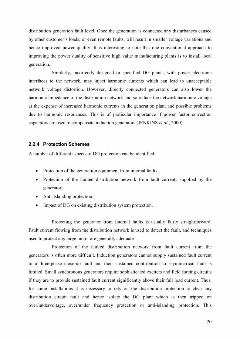
The islanding issue is shown in Figure 2.7. If circuit breaker A opens, perhaps on
a transient fault, there may be insufficient fault current to operate the circuit breaker B. In this
case the generator may be able to continue to supply the load. If the output of the generator is
able to match the active and reactive power demand of the load precisely, then there will be
no change in either the frequency or voltage of the islanded section of the network. Thus it is
very difficult to detect reliably that circuit breaker A has opened using only local
measurements at B. In the limit, if there is no current flowing through A (the generator is
supplying the entire load) then the network conditions at B are unaffected whether A is open
or closed. It may also be seen that since the load is being fed through the delta winding of the
transformer then there is no neutral earth on that section of the network.
Figure 2.7 – Illustration of the islanding issue
Finally, DG may affect the operation of existing distribution networks by
providing flows of fault current which were not expected when the protection was originally
designed. The fault contribution from a DG generator can support the network voltage and
lead to relays under-reaching.
22
2.2.5 Stability
For DG schemes, whose object is to generate kWh from new renewable energy sources,
considerations of generator transient stability tend not to be of great significance. If a fault
occurs somewhere on the distribution network to depress the network voltage and the DG
generator trips, then all that is lost is a short period of generation. In contrast, if a DG
generator is viewed as providing support for the power system, then its transient stability
becomes of considerable importance. Both voltage and/or angle stability may be significant
depending on the circumstances.
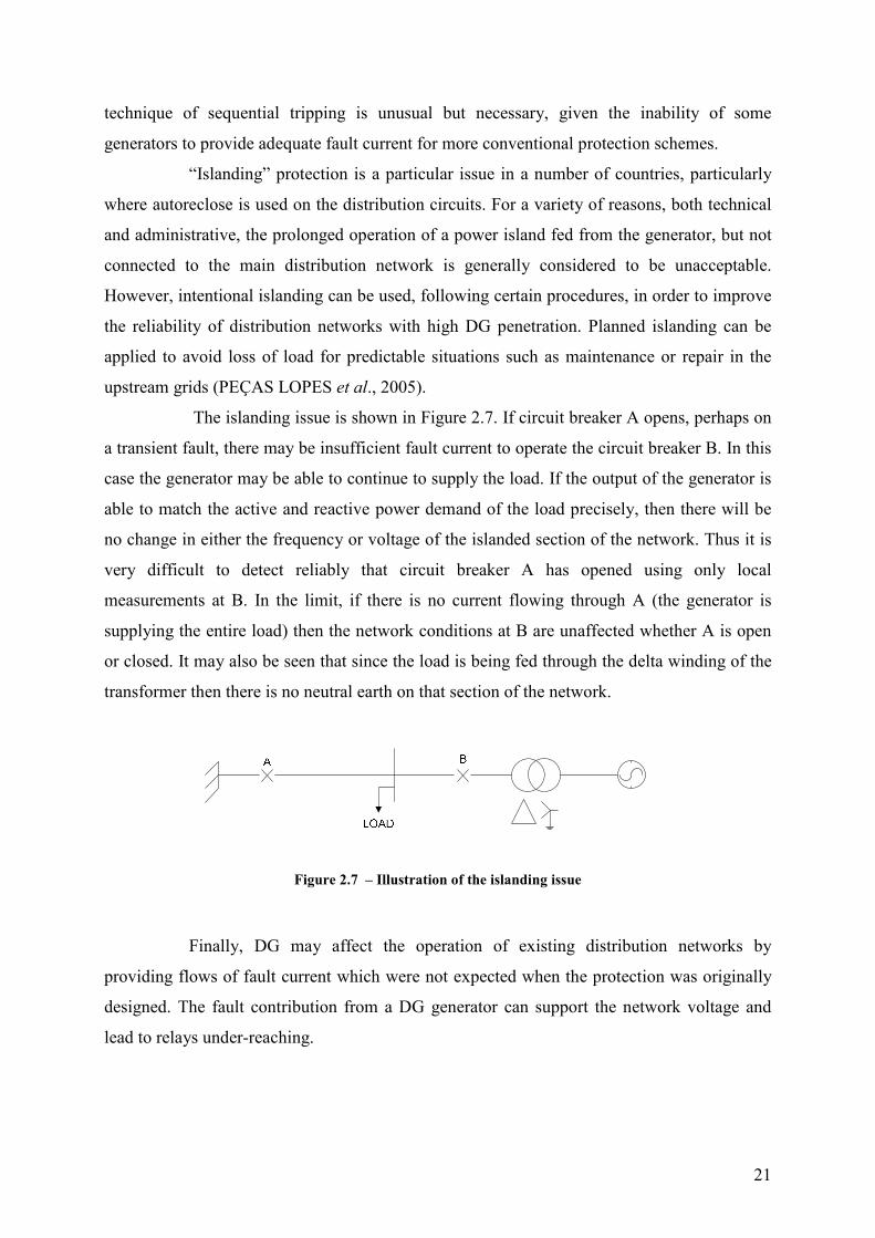
2.2.6 Grid Losses
Connecting the DG in distribution networks also influences the losses in the network. Small
penetrations of distributed generators tend to reduce network power flows and consequently
network losses. When the penetrations increases the distributed generators will export power
to the grid and may cause increase in network losses, as shown in Figure 2.8.
Figure 2.8 – Grid losses related to the penetration of DG (VAN GERWENT, 2006)
2.2.7 Network Operation
DG also has important consequences for operation of the distribution network in that circuits
can now be energized from a number of points. This has implications for policies of isolation
and earthing for safety before work is undertaken. There may also be more difficulty in
obtaining outages for planned maintenance and so reduced flexibility for work on a network
with DG connected to it.
To date, most attention has been paid to the immediate technical issues of
connecting and operating generation on a distribution system, and most countries have
23
developed standards and practiced to deal with these. In general, the approach adopted has
been to ensure that any DG does not reduce the quality of supply offered to other costumers
and to consider the generator as “negative load”. Some economic consequences and
opportunities of DG are only now being considered, and it is likely that these will become
apparent most quickly in electricity supply industries which are deregulated and there is a
clear distinction between electricity supply (i.e. provision of kWh) and electricity distribution
(i.e. provision of distributed network service).
In order to minimize the negative effects of DG, network operators prefer to
connect DG to higher voltages where their impact to voltage profile is minimal
(STRBAC et al., 2002). However, the commercial viability of DG projects is sensitive to
connection costs. These costs increase considerably with the voltage level at which the DG is
connected. Generally the higher the voltage or sparser the network, the higher the connection
cost. The developers of DG therefore generally prefer to connect at lower voltages.
Due to the afore-mentioned technical challenges, distribution networks with high
DG penetration need an active approach in sense of operation, control, communication and
protection. Therefore research and development (R&D) is necessary to overcome barriers and
make further use of the benefits of DG. The R&D should be focused on modern information
and communication technologies, storage technologies, new protection schemes, new network
planning tools, interconnection standards, control and management systems, cost reduction,
improvement of efficiency, availability and reliability of DG devices (e.g. with new
forecasting methods) and reducing the environmental impact (SCHWAEGERL, 2004).

24
3 DG DemoNet Project
As was described in the previous chapter, a higher penetration of DG changes the former
purely passive distribution system to active, and the unidirectional flow changes to a
bidirectional load flow. However, this development is usually not reflected when it comes to
network operation, since in most cases DG is simply seen as a negative load. Real active
operation means that generation, the network and consumption (loads) within the distribution
system actively interact and adapt each other according to the actual load flow situation. The
austrian project DG DemoNet-Concept represents new strategies in the field of DG where
currently passive distribution networks become active networks, able to accommodate a
significant penetration from DG. The conversion from passive to active operation introduces
many challenges considering DG network integration, power quality, concepts and strategies
for network planning, control and supervision as well as information and communication
technologies. As the research work in the field of active networks is mainly focusing on the
theoretical part of the problem, the goal of the DG Demo-Net project is the practical
realization of the demonstration network where active network approach should be
implemented with the least investment costs.
3.1 Current Situation in Austria
Innovative distribution network operators (DNOs) are already taking part in research and
demonstration projects. Those operators intend to learn how to deal with the change towards a
more and more decentralized electricity system. The DG DemoNet-Concept is being
performed by three austrian DNOs and its main objectives are to choose representative parts
of networks in Austria for practical realization of demonstration networks with a high
penetration of DG, and to analyze within these low and/or medium voltage grid selections, the
possibilities for implementing different model systems (Step Model “DG Integration”) and
plan the technical, organizational and economical realization.
The share of DG in the networks of the three DNOs is shown in Table 3.1. In two
cases the installed capacity of distributed generation is close to the maximum load in the
network. The dominating primary energy carriers are hydro power and photovoltaic (with a
high number of units but small installed power). In addition, the DG units are not
homogeneously distributed in the networks (Figure 3.1).

25
Table 3.1 – Share of generation in distribution grids (LUGMAIER et al., 2007)
DNO1
(NL4 4-7)
DNO1
(NL4 3–
7)
DNO2
(NL4 3-7)
DNO3
(NL4 4-7)
GWhgen/GWhdem1 0,11 0,41 0,54 0,11
MW inst/MWgridmin2 0,72 2,37 2,76 0,58
MW inst/MWgridmax3 0,22 0,90 0,94 0,17
1 – Ratio of energy delivered by DG and energy demand in the network (annually)
2 – Ratio of installed DG capacity and minimum load in the network
3 – Ratio of installed DG capacity and maximum load in the network
4 – Network level (level 3 is equivalent to 110 kV, level 7 to 0,4 kV)
Figure 3.1 – Dispersion of the installed DG power per m², Energie AG OÖ Netz GmbH
(LUGMAIER et al., 2007)
The experiences of the DNOs show that, if in the distribution networks the
dispersion of DG units is almost like the dispersion of the loads, a DG share (different DG
types) of approximate 60% (installed power of DG) of the maximum load in the network
seems to be possible without voltage problems, estimated over all. This value will decrease if
the units are concentrated at unique nodes, especially in case of peripheral nodes.

26
The key barrier for generation in distribution networks is the voltage rise effect
(overvoltage) due to the power injection, as explained in the section 2.2. If it is not possible to
connect the desired power, currently there are two approaches used. The first one is to find a
point of common coupling with a higher short circuit power or to reinforce the network. The
second possibility is to reduce the feed in power when voltage is exceeding the upper limits.
Demand side management (DSM) and remote control of DG units are, in general,
not yet used in respect to voltage level and there are only few measurement data in the
peripheral distribution network available. Because of limited share of DG neither the DSM
nor measurement data and remote control of DG were required before
(LUGMAIER et al., 2007).
3.2 The Voltage Rise Problem
Keeping the voltage between the limits is becoming a primary concern of the DNOs.
Increasing levels of DG penetration cause the voltage to rise above the limits, presenting a
risk to the customers. As the present DNOs voltage control equipment is only able to handle a
limited amount of DG, the modification, replacement and installation of different equipment
are necessary to increase the DG penetration in the distribution networks
(KUPZOG et al., 2007).
Loads, line impedances, power exported by the DG and the distance of the DG
from the primary substation are the most important factors causing the changes in the voltage
profile. The voltage profile change in the distribution network with DG can be illustrated on a
simple network model, shown in Figure 3.2.
Figure 3.2 – Simple distribution network with DG
PDG and QDG are the active and reactive power output of the generator
respectively, QC is the reactive power compensation at the DG site, PL and QL are the load
active and reactive power respectively, R and X are the line resistance and reactance
27
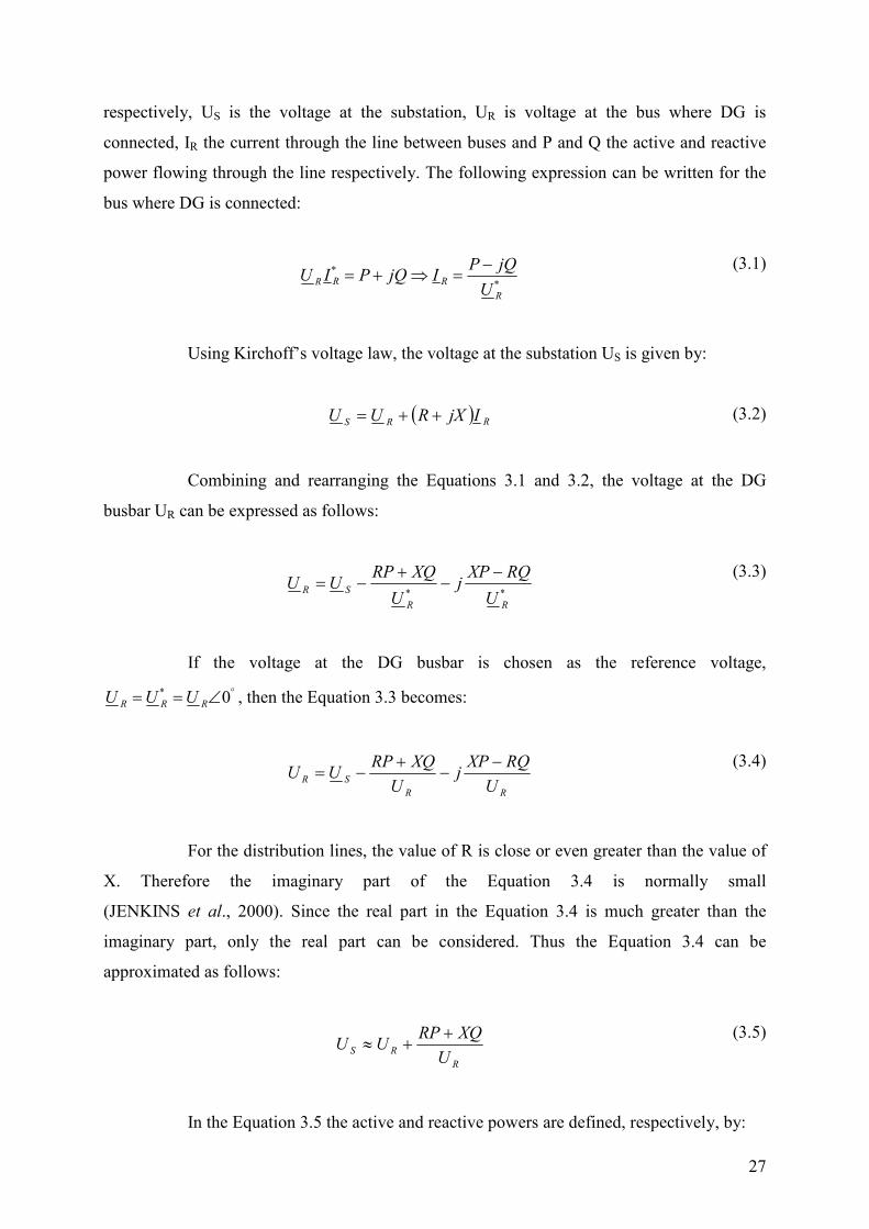
respectively, US is the voltage at the substation, UR is voltage at the bus where DG is
connected, IR the current through the line between buses and P and Q the active and reactive
power flowing through the line respectively. The following expression can be written for the
bus where DG is connected:
∗
∗ −=⇒+=
R
RRRU
jQPIjQPIU
(3.1)
Using Kirchoff’s voltage law, the voltage at the substation US is given by:
( ) RRS IjXRUU ++= (3.2)
Combining and rearranging the Equations 3.1 and 3.2, the voltage at the DG
busbar UR can be expressed as follows:
∗∗
−−
+−=
RR
SRU
RQXPj
U
XQRPUU
(3.3)
If the voltage at the DG busbar is chosen as the reference voltage,
°∗∠== 0RRR UUU , then the Equation 3.3 becomes:
RR
SRU
RQXPj
U
XQRPUU
−−
+−=
(3.4)
For the distribution lines, the value of R is close or even greater than the value of
X. Therefore the imaginary part of the Equation 3.4 is normally small
(JENKINS et al., 2000). Since the real part in the Equation 3.4 is much greater than the
imaginary part, only the real part can be considered. Thus the Equation 3.4 can be
approximated as follows:
R
RSU
XQRPUU
++≈
(3.5)
In the Equation 3.5 the active and reactive powers are defined, respectively, by:

28
DGL PPP −= (3.6)
LCDG QQQQ +±±= (3.7)
As the common practice for DNOs is to require distributed generators to operate
at unity power factor, no reactive power is injected to or absorbed from the network by the
DG.
0≈±± CDG QQ (3.8)
Regardless to the Equation 3.8 and considering the worst case scenario, which is
based on extreme conditions of a minimum load (PL=0 and QL=0) and the maximum
generation, voltage at the substation US becomes:
R
DG
RSU
RPUU −≈
(3.9)
The voltage at the DG busbar UR can be written as follows:
R
DG
SRU
RPUU +≈
(3.10)
It can be seen from Equation 3.10 that the voltage at the DG busbar UR is higher
than the voltage at the substation US due to DG active power injected into the line. The
voltage at the DG busbar depends mainly on the resistance of the line, the amount of injected
active power from the DG and the voltage at the substation. Maximum injected power from
the DG can be therefore obtained by reducing the voltage at the substation (with the OLTC).
However, the voltage at the substation should be controlled, in a way that voltage at the DG
busbar is kept between the DG operation limits. Therefore, in order to effectively control the
voltage at substation and to allow or increase the active power injection from the DG, it is
necessary to measure the remote voltages on the network.

29
3.3 Active Voltage Control: The Step Model
According to what was said before, an intelligent approach for integration of a rising share of
DG would start, where necessary, with local solutions for each generation unit or sensible
network areas. Furthermore, with growing share of DG, an intelligent approach would request
a step by step implementation of local measuring and controlling units as well as
communication channels and coordinating central systems.
In the framework of the DG DemoNet Project, a set of such innovative
approaches for voltage control has been developed. These tools actively use network assets
(e.g. On-Load Tap changers, OLTC), distributed generators and even loads to perform voltage
control. These tools have been theoretically developed and then implemented into a
simulation environment for validation and improvement. For this purpose, the simulation
software DIgSILENT PowerFactory has been used and adapted to allow performing
realistic simulations. Validations have been made on exemplary MV networks provided by
DNOs. The proposed five steps are shown in Table 3.2 and described in the next topics
(LUGMAIER et al., 2007).
Table 3.2 – Step Model “DG Integration” – Voltage control tools used for each step of the model
Step OLTC DG Loads Decoupling
assets
Current practice
Fix set-point
- - -
Local voltage control
Fix set-point
� � �
“Decoupling solution”
Fix set-point
- - �
Distributed voltage control
Variable set-point
- - �
Coordinated voltage control
Variable set-point
� � �
3.3.1 Current Practice
This first step corresponds to the current approach, i.e. passive operation of the distribution
network mainly based on the On-Load Tap Changer, OLTC. In case of voltage limit violation
due to the connection of distributed generation, the network must be reinforced, also to avoid
an automatic disconnection of the DG units because of overvoltage.
30
3.3.2 Local Voltage Control
In this approach, the OLTC is further controlled traditionally (fix set-point), but some selected
generators and/or loads perform local voltage control with reactive and active power
management. Due to higher R/X ratios in distribution networks compared to the transmission
networks, the use of reactive power management for voltage control may not be always
sufficient. If required, active power must be curtailed (regulatory and economical frameworks
will be considered in the next steps of the projects). The selection of the generators which
perform voltage control must be done on the basis of detailed analysis through offline studies.
3.3.3 “Decoupling Solution”
This approach considers the use of additional assets (e.g. voltage regulators) to “decouple” the
voltage in parts of the network for which the voltage situation is different. This solution has
been considered at the initial stage of the study, from a theoretical point of view. Like the
other solutions, it needs to be economically assessed.
3.3.4 Distributed Voltage Control
In this step, the OLTC is controlled according to real-time voltage measurements at critical
nodes of the network. In case the voltage exceeds the operational limits at one of the
monitored nodes, the OLTC performs a tap changing. The critical nodes have to be selected
on the basis of offline studies in order to ensure that compliance with the voltage limits at
these nodes imply compliance in the whole network. Of course, the effectiveness of this
control is limited by the network characteristic (e.g. different load flow characteristic of MV
branches). This solution supposes a communication infrastructure with limited requirements
between selected nodes and the OLTC controller.
3.3.5 Coordinated Voltage Control
This step represents the most sophisticated and complex control (coordinated use of local
voltage control and distributed voltage control). A control unit controls the OLTC and the
generators and/or loads participating to local control on the basis of the measurements
received for the critical nodes. The use of coordinated local control allows solving the conflict
appearing in the previous approach (OLTC not able to maintain the voltage within the limits
in the whole network). Like in the previous steps, the critical nodes and the controlled

31
generators have to be suitably selected (selection criteria are currently developed). For this
control, the requirements on the communication infrastructure are higher.
Table 3.3 summarizes the most important advantages and drawbacks of the step
model from the technical point of view and Figure 3.3 illustrates the sequence of these steps.
Table 3.3 – Step Model “DG Integration” – Important advantages / drawbacks
Operation approach
Advantages Drawbacks
Current practice � Approved standard solution � limited DG amount
Local control
� easy to implement, � P & Q control usually
available on most DGs � extendable/scalable
� complex selection of controlled DGs
� not coordinated
“Decoupling solution”
� isolate a problematic area � partly inflexible, difficult to scale
Distributed control
� simple � extendable/scalable
� communication infrastructure needed
� effectiveness depending on the network structure
Coordinated control
� coordinated � high effectiveness � effective use of all the
resources � extendable/scalable
� complexity � high engineering efforts
(selection of critical nodes and controlled DGs)
Figure 3.3 – Step Model “DG Integration” – Step model sequence
32
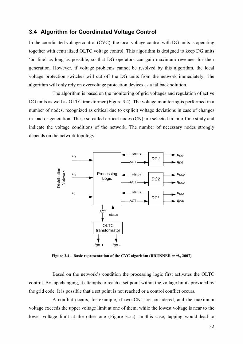
3.4 Algorithm for Coordinated Voltage Control
In the coordinated voltage control (CVC), the local voltage control with DG units is operating
together with centralized OLTC voltage control. This algorithm is designed to keep DG units
‘on line’ as long as possible, so that DG operators can gain maximum revenues for their
generation. However, if voltage problems cannot be resolved by this algorithm, the local
voltage protection switches will cut off the DG units from the network immediately. The
algorithm will only rely on overvoltage protection devices as a fallback solution.
The algorithm is based on the monitoring of grid voltages and regulation of active
DG units as well as OLTC transformer (Figure 3.4). The voltage monitoring is performed in a
number of nodes, recognized as critical due to explicit voltage deviations in case of changes
in load or generation. These so-called critical nodes (CN) are selected in an offline study and
indicate the voltage conditions of the network. The number of necessary nodes strongly
depends on the network topology.
Figure 3.4 – Basic representation of the CVC algorithm (BRUNNER et al., 2007)
Based on the network’s condition the processing logic first activates the OLTC
control. By tap changing, it attempts to reach a set point within the voltage limits provided by
the grid code. It is possible that a set point is not reached or a control conflict occurs.
A conflict occurs, for example, if two CNs are considered, and the maximum
voltage exceeds the upper voltage limit at one of them, while the lowest voltage is near to the
lower voltage limit at the other one (Figure 3.5a). In this case, tapping would lead to
ACT
status
ACT
ACT
status
status
ACT status
tap + tap -
u1
u2
ui
pDG1
pDG2
pDGi
qDG1
qDG2
qDGi
Dis
trib
ution
Netw
ork
Processing Logic
OLTC transformator
DG1
DG2
DGi

33
undervoltage at the second node. Alternatively, if the minimum voltage exceeds the lower
voltage limit at one of the nodes and the highest voltage is near to the upper voltage limit at
the other one (Figure 3.5b), tapping would lead to overvoltage at the second node.
Figure 3.5 – Voltage conflicts – in situations (a) and (b), tap change operation is not possible. In this case,
DG units are actively controlled
In case of voltage conflict, local voltage control with DG is activated. Only DG
units that allow the voltage controlling are included into the algorithm. A ranking order of DG
units is introduced for optimal operation. This ranking is based on the injection share of the
DG units and their stochastic nature of energy production. This concept is called the “Power
Share Injection Concept”.
This concept makes use of the ranking concept to control voltage at monitored
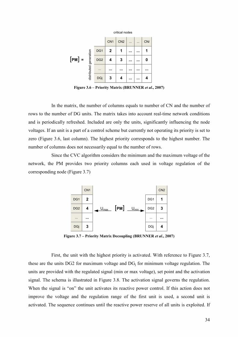
points and introduces the Priority Matrix (PM). This matrix comprises information about
active DG units and their role in voltage control. It consists of numbers in a successive order,
indicating the intensity of power injection measured at a CN. The structure of the PM is
illustrated in the Figure 3.6.
The priority level of each DG unit is determined in a process, in which intentional
voltage deviations are generated by rapid changes in the DG unit generation at constant
network loading. By measurement of voltage variations caused by the changes, the unit’s
influence is recognized and ranked accordingly. The more intense the variations are the more
effect has the DG injection on the voltage profile of the monitored node.
34
critical nodes
CN1 CN2 ... ... CNi
DG1 2 1 ... ... 1
DG2 4 3 ... ... 0
... ... ... ... ... ...
[PM] =
dis
trib
ute
d g
enera
tion
DGj 3 4 ... ... 4
Figure 3.6 – Priority Matrix (BRUNNER et al., 2007)
In the matrix, the number of columns equals to number of CN and the number of
rows to the number of DG units. The matrix takes into account real-time network conditions
and is periodically refreshed. Included are only the units, significantly influencing the node
voltages. If an unit is a part of a control scheme but currently not operating its priority is set to
zero (Figure 3.6, last column). The highest priority corresponds to the highest number. The
number of columns does not necessarily equal to the number of rows.
Since the CVC algorithm considers the minimum and the maximum voltage of the
network, the PM provides two priority columns each used in voltage regulation of the
corresponding node (Figure 3.7)
CN1
CN2
DG1 2
DG1 1
DG2 4 Umax [PM] Umin
DG2 3
... ...
... ...
DGj 3
DGj 4
Figure 3.7 – Priority Matrix Decoupling (BRUNNER et al., 2007)
First, the unit with the highest priority is activated. With reference to Figure 3.7,
these are the units DG2 for maximum voltage and DGj for minimum voltage regulation. The
units are provided with the regulated signal (min or max voltage), set point and the activation
signal. The schema is illustrated in Figure 3.8. The activation signal governs the regulation.
When the signal is “on” the unit activates its reactive power control. If this action does not
improve the voltage and the regulation range of the first unit is used, a second unit is
activated. The sequence continues until the reactive power reserve of all units is exploited. If

35
the sequence of these actions still does not improve the voltage, the active power control
activation follows in the same manner. The sequence continues until the voltage of regulated
nodes meets the criteria, which means bringing the voltage back within the specified
regulation band, or all units are put in operation. The deactivation process is performed in the
inverse order.
Figure 3.8 – DG Unit Control Scheme (BRUNNER et al., 2007)
Both P and Q management are calculated according to the control mechanism
present in the CVC algorithm. Q and P controls are based in the usage of a PI control, which
receives the voltage values and voltage limits as inputs and calculates ∆Q and ∆PQ, as shown
in Figure 3.9.
Figure 3.9 – Calculation of the active and reactive power management in the CVC algorithm
It is important to note that, while ∆Q is calculated independently of P, ∆P
influences the reactive power, and therefore, is called ∆PQ.
The complete flow chart algorithm of CVC algorithm is presented in Figure 3.10.
This flow chart includes the OLTC tapping and the local voltage control.
Simulations accomplished at arsenal research show that while the passively
operated grid suffers from overvoltage conditions already at 50 % DG of maximum load, the
CVC approach is still able to keep voltages in the limits at 150 % installed DG of maximum

36
load. To be able to integrate more than 150 % of the maximum demand DG power into the
example network, the network should be reinforced (KUPZOG et al., 2007).
In order to evaluate the performance of the power injection share concept, a test
was conducted, whose aim was to demonstrate network conditions in case of installation of
additional DG units to it. The results show that without the scheme, the integration of these
additional units was not possible due to numerous tap changer conflict situations; however, by
using the power injection share concept, the integration of the additional DG units is possible
without any voltage limit violation (BRUNNER et al., 2007).
Determination of min and max network voltage from measurements
at critical points in the network
Umax > Uup_lim Yes
Time Delayskip short voltage variations
No
Uup_lim Umin < Ulow_lim
Ulow_lim
Umin < Ulow_lim
Yes
No
Time Delayskip short voltage variations
Umin < Ulow_lim Umax > Uup_lim No
No
Is it possible and valid to tap?
No
Yes
Yes
Change the tap position
Yes
No
Voltage input
P,Q ControlUset=Uup_lim – Utap
or
Uset=Ulow_lim
Is it possible and valid to tap?
NoP,Q Control
Uset=Uup_lim
or
Uset=Ulow_lim
Yes
Yes
Ranking and decision system
LOCAL CONTROL
Figure 3.10 – Flow chart algorithm of the CVC

37
4 Energy Storage Systems, Status and Potential
One of the major issues surrounding the various replacements for carbon-based fuels is the
ability to store the energy until the demand is present, as most renewable sources are
intermittent in nature. While oil can be stored in large tanks and coal can be stored in a pile, a
shift to intermittent sources of energy requires some sort of electricity storage system
analogous to a storage tank so that power can be dispatched when needed. Therefore, to keep
from losing this energy, the electricity must be converted into a different kind of energy until
consumer demands rise. Although many different ideas for this storage exist, an efficient
universal way to solve this problem has yet to materialize (WALKER, 2007). In this chapter,
a brief history of the storage systems is presented and the different technologies are analyzed,
regarding their status and potential, specially referring to storage systems that could be used
for integration to the voltage control methods in the framework of the DG DemoNet-Concept.
4.1 Storage Systems: History
Energy storage as a natural process is as old as the universe itself - the energy present at the
initial creation of the universe has been stored in stars such as the Sun, and is now being used
by humans directly (e.g. through solar heating), or indirectly (e.g. by growing crops or
conversion into electricity in solar cells).
As a purposeful activity, energy storage has existed since pre-history, though it
was often not explicitly recognized as such. An example of deliberate mechanical energy
storage is the use of logs or boulders as defensive measures in ancient strongholds - the logs
or boulders were collected at the top of a hill or wall, and the energy thus stored used to attack
invaders who came within range.
One of the oldest forms of energy storage involves harvesting ice from lakes and
rivers, which was stored in well insulated warehouses and sold or used throughout the year for
almost everything for what mechanical refrigeration is used today, including preserving food,
cooling drinks, and air conditioning. The Hungarian Parliament Building in Budapest is still
air conditioned with ice harvested from Lake Balaton in the winter.
A more recent application is the control of waterways to drive water mills for
processing grain or powering machinery. Complex systems of reservoirs and dams were
constructed to store and release water (and the potential energy it contained) when required.
Energy storage became a dominant factor in economic development with the
widespread introduction of electricity and refined chemical fuels, such as gasoline, kerosene
and natural gas in the late 1800s. Unlike other common energy storage used in prior use, such

38
as wood or coal, electricity must be used as it is generated and cannot be stored on anything
other than a minor scale. Electricity is transmitted in a closed circuit, and for essentially any
practical purpose cannot be stored as electrical energy. This meant that changes in demand
could not be accommodated without either cutting supplies (e.g. via brownouts or blackouts)
or arranging for a storage technique.
An early solution to the problem of storing energy for electrical purposes was the
development of the battery, an electrochemical storage device. It has been of limited use in
electric power systems due to small capacity and high cost. A similar possible solution with
the same type of problems is the capacitor.
Chemical fuels have become the dominant form of energy storage, both in
electrical generation and energy transportation. Chemical fuels commonly uses processed
coal, gasoline, diesel fuel, natural gas, liquefied petroleum gas (LPG), propane, butane,
ethanol, biodiesel and hydrogen. All of these chemicals are readily converted to mechanical
energy and then to electrical energy using heat engines (turbines or other internal combustion
engines, or boilers or other external combustion engines) used for electrical power generation.
Heat engine powered generators are nearly universal, ranging from small engines producing
only a few kW to utility-scale generators with ratings up to 800 MW.
Electrochemical devices called fuel cells were invented about the same time as the
battery. However, for many reasons, fuel cells were not well developed until the advent of
manned spaceflight (the Gemini Program) when lightweight, non-thermal, sources of
electricity were required in spacecraft. Fuel cell development has increased in recent years to
an attempt to increase conversion efficiency of chemical energy stored in hydrocarbon or
hydrogen fuels into electricity.
At this time, liquid hydrocarbon fuels are the dominant forms of energy storage
for use in transportation. Unfortunately, these produce greenhouse gases when used to power
cars, trucks, trains, ships and aircraft. Carbon-free energy carriers, such as hydrogen, or
carbon-neutral energy carriers, such as some forms of ethanol or biodiesel, are being sought in
response to concerns about the consequences of greenhouse gas emissions.
In some areas of the world (Washington and Oregon in the USA, Wales in the
United Kingdom and western Austria are examples) enjoying particular geographical
conditions, large quantities of water can be stored in elevated reservoirs, using excess
electricity at times of low demand to pump water up to the reservoirs, then letting the water
fall through turbine generators to retrieve the energy when demand peaks.
39
Energy storage has been closely associated with solar installations, including both
solar heating and photovoltaic (PV) applications. Today it can be found several different
storage technologies, depending on the application. Some more recent technologies have also
been investigated, such as flywheels or compressed air storage in underground caverns, but to
date no widely available solution to the challenge of mass energy storage has been deployed
commercially. However, many utilities provide incentives for energy storage applications,
while time-of-day rates and stiff demand charges also entice customers to consider these
opportunities (DISTRICT ENERGY, 2008).
4.2 Storage Systems: Applications and Technologies
Energy storage systems play the important role of unifying, distributing and enhancing the
capabilities of alternative and renewable energy-distributed generating systems, namely by:
Enhancing the Power Quality
Energy storage can provide "ride-through" for momentary outages, and extended protection
from longer outages. Coupled with advanced power electronics, storage systems can reduce
harmonic distortions, and eliminate voltage sags and surges.
Providing Renewables Support
In combination with renewable resources, energy storage can increase the value of
photovoltaic (PV) and wind-generated electricity, making supply coincident with periods of
peak consumer demand, permitting DG to operate as a dispatchable unit.
Providing Utility Support
Energy storage systems can be used to follow load, stabilize voltage & frequency, manage
peak loads, improve power quality, defer upgrade investments, and support renewables.
Large-scale electricity storage technologies cover a wide spectrum of
applications, ranging from fast power quality applications to improve reliability all the way to
slow energy management applications to improve profitability. These applications require
energy discharges from a fraction of a second in high power applications to hours in high
energy applications (Figure 4.1).
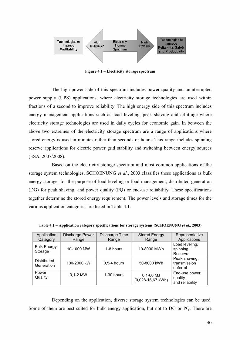
40
Figure 4.1 – Electricity storage spectrum
The high power side of this spectrum includes power quality and uninterrupted
power supply (UPS) applications, where electricity storage technologies are used within
fractions of a second to improve reliability. The high energy side of this spectrum includes
energy management applications such as load leveling, peak shaving and arbitrage where
electricity storage technologies are used in daily cycles for economic gain. In between the
above two extremes of the electricity storage spectrum are a range of applications where
stored energy is used in minutes rather than seconds or hours. This range includes spinning
reserve applications for electric power grid stability and switching between energy sources
(ESA, 2007/2008).
Based on the electricity storage spectrum and most common applications of the
storage system technologies, SCHOENUNG et al., 2003 classifies these applications as bulk
energy storage, for the purpose of load-leveling or load management, distributed generation
(DG) for peak shaving, and power quality (PQ) or end-use reliability. These specifications
together determine the stored energy requirement. The power levels and storage times for the
various application categories are listed in Table 4.1.
Table 4.1 – Application category specifications for storage systems (SCHOENUNG et al., 2003)
Application Category
Discharge Power Range
Discharge Time Range
Stored Energy Range
Representative Applications
Bulk Energy Storage
10-1000 MW 1-8 hours 10-8000 MWh Load leveling, spinning Reserve
Distributed Generation
100-2000 kW 0,5-4 hours 50-8000 kWh Peak shaving, transmission deferral
Power Quality
0,1-2 MW
1-30 hours
0,1-60 MJ
(0,028-16,67 kWh)
End-use power quality and reliability
Depending on the application, diverse storage system technologies can be used.
Some of them are best suited for bulk energy application, but not to DG or PQ. There are

41
others, however, that are suitable for DG and bulk storage or DG and PQ. In general, the
information for DG storage is similar to that in the section for bulk energy storage. However,
these systems are much smaller in size and are expected to be placed in an existing facility,
which reduces the balance of plant cost.
The following topics present a variety of storage technologies, with their technical
characteristics, vantages, drawbacks and the most common applications. In the next topic
these technologies are compared, in order to figure out what are the best suited for the
implementation to the voltage control scheme in the ambit of this work. Table 4.2 presents a
summary of the analyzed technologies.
Table 4.2 – Summary of the investigated storage technologies
Direct Storage Indirect Storage
Electrical Mechanical Chemical
• Supercapacitor
• SMES
• Pumped Hydro Storage
• CAES
• Flywheel
• Batteries
• Redox-Flow Batteries
• Hydrogen Storage
On the table 4.2, “Direct Storage” consists of those technologies that store
electricity without converting it into any other form or energy, while “Indirect Storage”
consists of technologies that store electricity converting it into one (or more) different forms
of energy.
4.2.1 Supercapacitors
Electrochemical capacitors (EC) have components related to both a battery and a capacitor.
They store electrical energy in the two series capacitors of the electric double layer, which is
formed between each of the electrodes and the electrolyte ions. The distance over which the
charge separation occurs is just a few angstroms. The capacitance and energy density of these
devices are thousands of times larger than electrolytic capacitors. The electrodes are often
made with porous carbon material. The electrolyte is either aqueous or organic. The aqueous
capacitors have a lower energy density due to a lower cell voltage but are less expensive and
work in a wider temperature range. The asymmetrical capacitors that use metal for one of the
electrodes have a significantly larger energy density than the symmetric ones and have lower
leakage current. Figure 4.2 shows the basic setup of a Supercapacitor system.
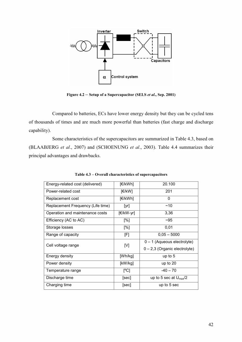
42
Figure 4.2 – Setup of a Supercapacitor (SELS et al., Sep. 2001)
Compared to batteries, ECs have lower energy density but they can be cycled tens
of thousands of times and are much more powerful than batteries (fast charge and discharge
capability).
Some characteristics of the supercapacitors are summarized in Table 4.3, based on
(BLAABJERG et al., 2007) and (SCHOENUNG et al., 2003). Table 4.4 summarizes their
principal advantages and drawbacks.
Table 4.3 – Overall characteristics of supercapacitors
Energy-related cost (delivered) [€/kWh] 20.100
Power-related cost [€/kW] 201
Replacement cost [€/kWh] 0
Replacement Frequency (Life time) [yr] ~10
Operation and maintenance costs [€/kW-yr] 3,36
Efficiency (AC to AC) [%] ~95
Storage losses [%] 0,01
Range of capacity [F] 0,05 – 5000
Cell voltage range [V] 0 – 1 (Aqueous electrolyte)
0 – 2,3 (Organic electrolyte)
Energy density [Wh/kg] up to 5
Power density [kW/kg] up to 20
Temperature range [ºC] -40 – 70
Discharge time [sec] up to 5 sec at Umax/2
Charging time [sec] up to 5 sec

43
Table 4.4 – Advantages and drawbacks of Supercapacitors (ERBEN, 2008)
Advantages Drawbacks
• Very high capacity (many kF)
• High power density
• Very high cycling lifetime
• Minor inner resistance
• Fast loading capacity
• Deep discharging stability
• High costs
• Low energy density
• High self-discharging rate (insignificant
if used as short time storage system)
• Additional electronic is necessary due
to the variable voltage
Supercapacitors are ideal devices for PQ and short-term energy storage. For some
capacitor systems, this is less than one second, whereas for others it can be as long as a few
minutes. Individual units store a limited amount of energy, however depending on design; a
great deal of it can be removed in a second or so.
There is an increasing interest in developing high cycle life, high-energy
supercapacitors, that could be used on high energy applications (NAMISNYK, 2003).
Presently, very small super capacitors in the range of seven to ten watts are widely available
commercially for consumer power quality applications and are commonly found in household
electrical devices. Development of large scale capacitors has been focused on electric
vehicles. Currently, small scale power quality (< 250 kW) is considered to be the most
promising utility use for advanced capacitors.
4.2.2 Superconducting Magnetic Energy Storage (SMES)
SMES systems store energy in the magnetic field created by the flow of direct current in a
superconducting coil which has been cryogenically cooled to a temperature below its
superconducting critical temperature. A typical SMES system includes three parts:
superconducting coil, power conditioning system and cryogenically cooled refrigerator.
Figure 4.3 shows the basic setup of a SMES unit.
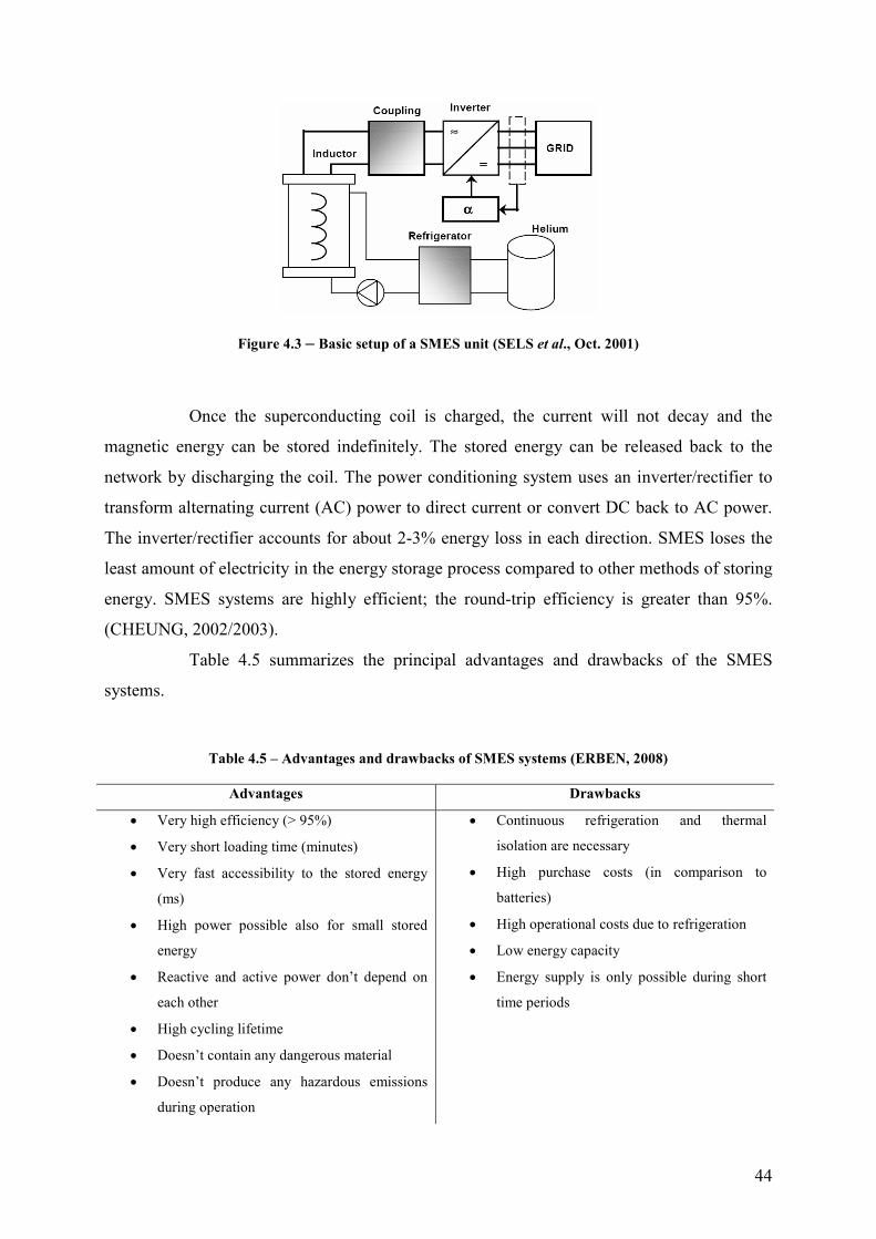
44
Figure 4.3 – Basic setup of a SMES unit (SELS et al., Oct. 2001)
Once the superconducting coil is charged, the current will not decay and the
magnetic energy can be stored indefinitely. The stored energy can be released back to the
network by discharging the coil. The power conditioning system uses an inverter/rectifier to
transform alternating current (AC) power to direct current or convert DC back to AC power.
The inverter/rectifier accounts for about 2-3% energy loss in each direction. SMES loses the
least amount of electricity in the energy storage process compared to other methods of storing
energy. SMES systems are highly efficient; the round-trip efficiency is greater than 95%.
(CHEUNG, 2002/2003).
Table 4.5 summarizes the principal advantages and drawbacks of the SMES
systems.
Table 4.5 – Advantages and drawbacks of SMES systems (ERBEN, 2008)
Advantages Drawbacks
• Very high efficiency (> 95%)
• Very short loading time (minutes)
• Very fast accessibility to the stored energy
(ms)
• High power possible also for small stored
energy
• Reactive and active power don’t depend on
each other
• High cycling lifetime
• Doesn’t contain any dangerous material
• Doesn’t produce any hazardous emissions
during operation
• Continuous refrigeration and thermal
isolation are necessary
• High purchase costs (in comparison to
batteries)
• High operational costs due to refrigeration
• Low energy capacity
• Energy supply is only possible during short
time periods
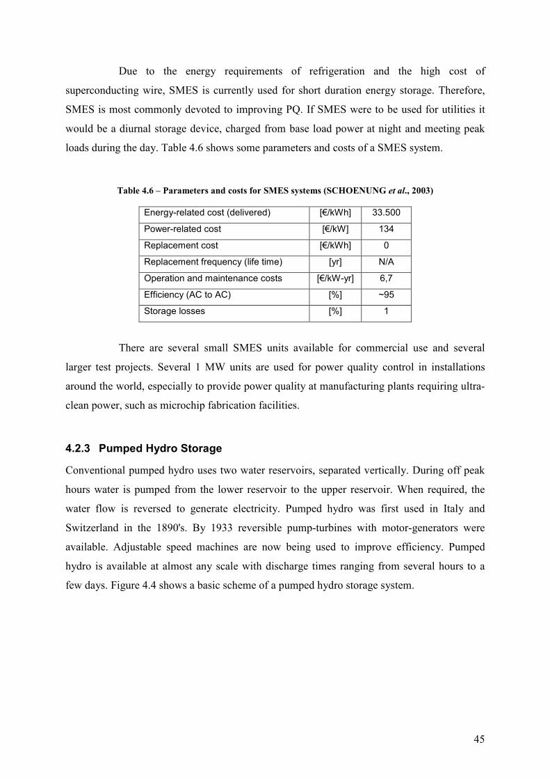
45
Due to the energy requirements of refrigeration and the high cost of
superconducting wire, SMES is currently used for short duration energy storage. Therefore,
SMES is most commonly devoted to improving PQ. If SMES were to be used for utilities it
would be a diurnal storage device, charged from base load power at night and meeting peak
loads during the day. Table 4.6 shows some parameters and costs of a SMES system.
Table 4.6 – Parameters and costs for SMES systems (SCHOENUNG et al., 2003)
Energy-related cost (delivered) [€/kWh] 33.500
Power-related cost [€/kW] 134
Replacement cost [€/kWh] 0
Replacement frequency (life time) [yr] N/A
Operation and maintenance costs [€/kW-yr] 6,7
Efficiency (AC to AC) [%] ~95
Storage losses [%] 1
There are several small SMES units available for commercial use and several
larger test projects. Several 1 MW units are used for power quality control in installations
around the world, especially to provide power quality at manufacturing plants requiring ultra-
clean power, such as microchip fabrication facilities.
4.2.3 Pumped Hydro Storage
Conventional pumped hydro uses two water reservoirs, separated vertically. During off peak
hours water is pumped from the lower reservoir to the upper reservoir. When required, the
water flow is reversed to generate electricity. Pumped hydro was first used in Italy and
Switzerland in the 1890's. By 1933 reversible pump-turbines with motor-generators were
available. Adjustable speed machines are now being used to improve efficiency. Pumped
hydro is available at almost any scale with discharge times ranging from several hours to a
few days. Figure 4.4 shows a basic scheme of a pumped hydro storage system.
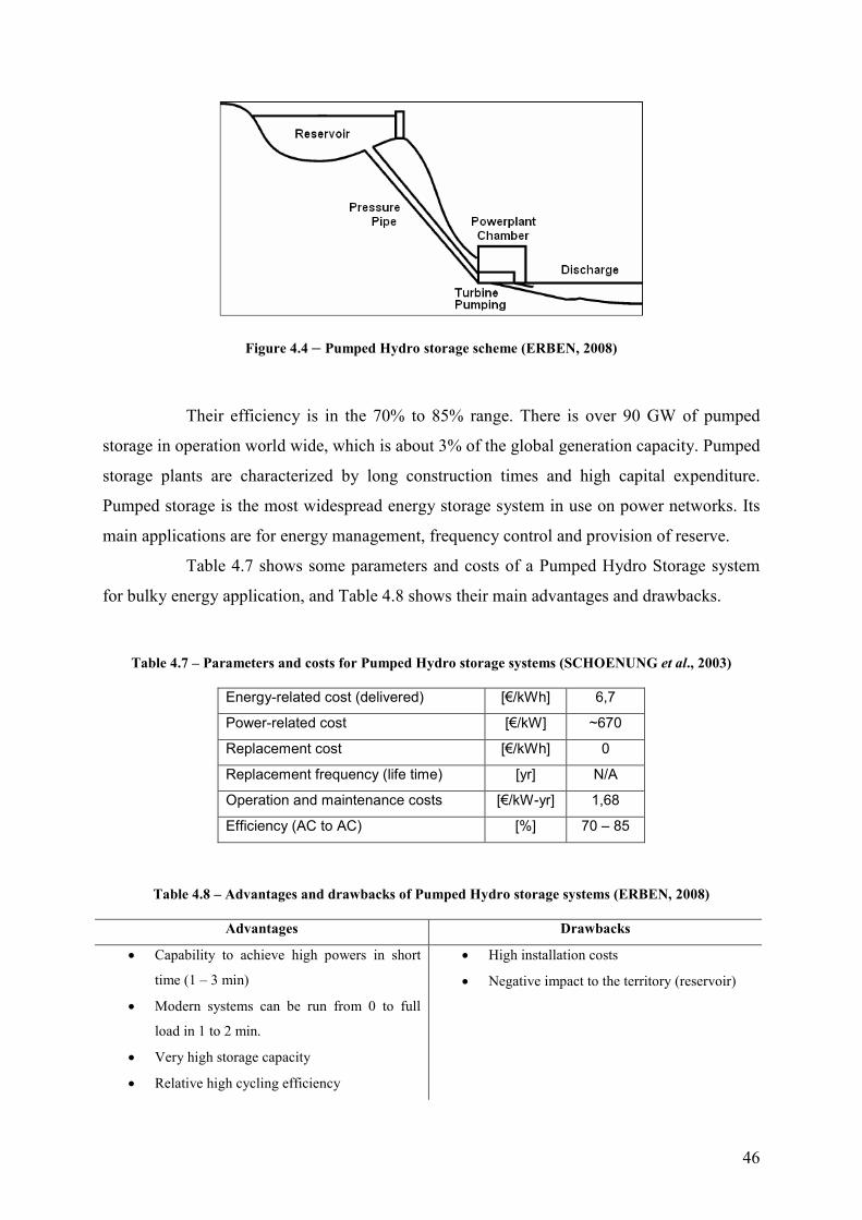
46
Figure 4.4 – Pumped Hydro storage scheme (ERBEN, 2008)
Their efficiency is in the 70% to 85% range. There is over 90 GW of pumped
storage in operation world wide, which is about 3% of the global generation capacity. Pumped
storage plants are characterized by long construction times and high capital expenditure.
Pumped storage is the most widespread energy storage system in use on power networks. Its
main applications are for energy management, frequency control and provision of reserve.
Table 4.7 shows some parameters and costs of a Pumped Hydro Storage system
for bulky energy application, and Table 4.8 shows their main advantages and drawbacks.
Table 4.7 – Parameters and costs for Pumped Hydro storage systems (SCHOENUNG et al., 2003)
Energy-related cost (delivered) [€/kWh] 6,7
Power-related cost [€/kW] ~670
Replacement cost [€/kWh] 0
Replacement frequency (life time) [yr] N/A
Operation and maintenance costs [€/kW-yr] 1,68
Efficiency (AC to AC) [%] 70 – 85
Table 4.8 – Advantages and drawbacks of Pumped Hydro storage systems (ERBEN, 2008)
Advantages Drawbacks
• Capability to achieve high powers in short
time (1 – 3 min)
• Modern systems can be run from 0 to full
load in 1 to 2 min.
• Very high storage capacity
• Relative high cycling efficiency
• High installation costs
• Negative impact to the territory (reservoir)
47
4.2.4 Compressed Air Energy Storage (CAES)
CAES plants use off-peak energy to compress and store air in an air-tight underground
storage cavern. Upon demand, stored air is released from the cavern, heated and expanded
through a combustion turbine to create electrical energy. Figure 4.5 shows the scheme of a
CAES system.
Figure 4.5 – Scheme of a CAES system (BLAABJERG et al., 2007)
The sitting of CAES plant requires favorable geology for the storage reservoir as
well as a suitable location near transmission lines and fuel supplies. Potential sites for
underground storage are grouped into three categories:
• Rock caverns created by excavating comparatively hard and impervious rock
formations;
• Salt caverns created by solution or dry mining of salt formations;
• Porous media reservoirs made by water bearing aquifers or depleted gas or oil fields
e.g., sandstone, fissured limestone.
Table 4.9 summarizes the principal advantages and drawbacks of the CAES
systems and Table 4.10 shows some parameters and costs of these systems applied to bulky
energy storage.

48
Table 4.9 – Advantages and drawbacks of CAES systems
Advantages Drawbacks
• Air is unlimited and freely available
• Production and usage of compressed air
involves well known technologies
• Can achieve very high efficiency
• No emissions
• The storage period is longer than other
storage methods (very small losses)
• Necessity of favorable geology for the
underground installation
• It takes about 1,5 to 2 years to create caverns
by dissolving salt
Table 4.10 – Parameters and costs for a CAES system (SCHOENUNG et al., 2003)
Energy-related cost (delivered) [€/kWh] 2,02
Power-related cost [€/kW] 284
Replacement cost [€/kWh] 0
Replacement frequency (life time) [yr] N/A
Operation and maintenance costs [€/kW-yr] 1,68
Efficiency (AC to AC) [%] 73
The largest commercial CAES is a 2700 MW plant that is planned for
construction in Norton, Ohio. This 9-units plant will compress air to 1500 psi (pounds per
square inch) in an existing limestone mine some 670 meters under ground. This project has
been started in 2001, but in early 2007 construction had not actually begun.
Besides the CAES systems for bulky storage systems, small compressed air
energy storage systems (CAES-surface) have been proposed for DG applications. In this
technology, the compressed air is stored at high pressure in steel pipes that are typically used
for natural gas transmission. These pipes are relatively inexpensive and are generally
available. They can be placed on the surface or buried at a modest depth for safety. Units
between 50 kW and 50 MW are possible. Because there are no installed examples, the
projected cost estimates are quite uncertain (SCHOENUNG et al., 2003).
4.2.5 Flywheels
Flywheels are electromechanical storage systems in which energy is stored as kinetic energy
of a rotating mass. The progresses in the power electronics, composite materials,
manufacturing quality control as well as a system approach in development of these devices
has made possible the realization of “mechanical batteries” able to cover a wide range of

49
applications. Nowadays, the flywheel energy storage systems are considered the enabling
technology for applications such as space satellites, power quality and integration of
renewable energies.
A flywheel storage device consists of a massive rotating cylinder (comprised of a
rim attached to a shaft) that spins at a very high velocity and an integrated electrical apparatus
that can operate either as a motor to turn the flywheel and store energy or as a generator to
produce electrical power on demand using the energy stored in the flywheel. The use of
magnetic bearings and a vacuum chamber helps to reduce energy losses. Figure 4.6 shows the
block diagram of a Flywheel for grid connected applications.
Figure 4.6 – Block diagram of a Flywheel for grid connected applications. (BLAABJERG et al., 2007)
The motor/generator can be an induction machine or a permanent magnet
synchronous machine. The electrical machine can also be integrated with the flywheel. In
order to increase the effective capacity a mechanical gearbox is used to connect the electrical
machine to the flywheel.
Usually, the power electronic interface consists of a back-to-back power
converter. However, in some configuration an additional DC/DC conversion stage can be
inserted in the DC-link circuit.
In motoring mode the flywheel stores mechanical energy speeding up as it
accumulates energy and slowing down as the flywheel delivers energy to the AC network.
Flywheels systems are divided into two main categories: low speed systems
which are commercially available and the high speed ones which are in development and are
just becoming available.
The low speed flywheels have steel rotors, conventional bearings and operating
speeds up to 6.000 rpm, while the high speed ones can operate up to 50.000 rpm due to the
advanced composite materials for the rotor combined with magnetic bearings. Prototypes

50
addressed to automotive and spacecraft applications which can run up to 110.000 rpm are
reported in some publications.
Some parameters of the flywheels are summarized in Table 4.11, based on
(BODACH, 2006). These parameters take into account the current technology status and the
development target of the technology.
Table 4.11 – Characteristics of Flywheels (current and expected)
Technology Status Development Target
Revolutions [min] 2.000 – 3.000 To 100.000
Energy density [kWs/kg] 15 – 200 150-500
Power [MW] < 15 < 50
Cycling lifetime -- 1.000.000 1.000.000
Efficiency [%] 85 – 90 90 – 95
Self discharging [%/h] 3 – 20 1 – 10
Table 4.12 shows some parameters and costs of a Flywheel system, for both DG
(high speed flywheels) and PQ (high/low speed flywheels) and Table 4.13 presents a resume
of the principal advantages and drawbacks of this technology.
Table 4.12 – Parameters and costs for Flywheel systems (SCHOENUNG et al., 2003)
DG PQ
Energy-related cost (delivered) [€/kWh] 670 670 – 33.500
Power-related cost [€/kW] 201 201 – 223
Replacement cost [€/kWh] 0 0
Replacement frequency (life time) [yr] N/A N/A
Operation and maintenance costs [€/kW-yr] 670/yr 3,35
Efficiency (AC to AC) [%] 95 90-95
Storage losses [%] 0,05 0,05 – 0,2

51
Table 4.13 – Advantages and drawbacks of Flywheels (SCHOENUNG et al., 2003)
Advantages Drawbacks
• Long life time
• Compact
• High power density (quickly chargeable and
dischargeable)
• High energy density (4 to 5 times greater
than conventional batteries)
• High Efficiency (to 80%)
• Minor maintenance needs
• Immune to temperature fluctuations
• Environment friendly (exhaust-free and no
chemical agents)
• Relatively immune to bad operation
conditions (e.g. deep discharge has no effect
on the life time)
• High costs (due to the life time, but small
when compared to batteries)
• Security aspects concerning the rotor
• If a part of the system doesn’t work, the
complete system must be turned off
• cannot deliver its rated power at very low
speeds
While high-power flywheels are developed and deployed for aerospace and UPS
applications, there is an effort, pioneered by Beacon Power, to optimize high-energy, low cost
commercial flywheel designs for long duration operation (up to several hours).
4.2.6 Batteries
The most established way of storing electricity is in the form of chemical energy in batteries.
A battery comprises of one or more electrochemical cells and each cell consists of a liquid,
paste, or solid electrolyte together with a positive electrode and a negative electrode.
During discharge, electrochemical reactions occur at the two electrodes
generating a flow of electrons through an external circuit. The reactions are reversible,
allowing the battery to be recharged by applying an external voltage across the electrodes.
Battery systems range from mature and reliable technologies, such as lead acid,
which have been proven and developed over many years, to various newer designs which are
at different stages of development. Sections 4.2.6.1 to 4.2.6.4 provide some information and
characteristics of some battery technologies.

52
4.2.6.1 Lead-Acid Battery
Lead-acid is one of the oldest and most developed battery technologies. The batteries used in
renewable energy systems are classified in two major technologies based on the electrolyte:
• Flooded lead acid batteries – represent the “classical” technology with the electrodes
and the separators immersed in the liquid electrolyte. Water electrolysis and gas
release lead to water loss during overcharging. Therefore, regular maintenance is
needed.
• Valve-regulated lead-acid batteries (VRLA) are characterized by the immobilized
electrolyte and, therefore, considerably less maintenance is necessary.
Basically, flooded lead-acid battery technology for renewable energy storage
systems is the large-scale application of a technology similar to that found in automobile
batteries. Flooded lead-acid batteries are manufactured in large numbers for many uses and
their operating characteristics and technology are well understood by manufacturers.
VRLAs use the same basic electrochemical technology as flooded lead-acid
batteries, but these batteries are closed with a pressure regulating valve, so that they are
essentially sealed. In addition, the acid electrolyte is immobilized. This eliminates the need to
add water to the cells to keep the electrolyte functioning properly, or to mix the electrolyte to
prevent stratification. The oxygen recombination and the valves of VRLAs prevent the
venting of hydrogen and oxygen gases and the ingress of air into the cells. The battery
subsystem may need to be replaced more frequently than with the flooded lead-acid battery,
increasing the cost of the system.
These batteries are used in renewable energy applications providing stand-by
energy or working on regular basis in hybrid systems. Some advantages and drawbacks of
these batteries are given in Table 4.14.

53
Table 4.14 – Advantages and drawbacks of Lead-acid batteries
Advantages Drawbacks
• Good efficiency
• Low maintenance level
• Easy to install
• Effective recycling
• Low investment price
• Low system cost over battery life
• Reduced life-cycle compared with renewable
energy conversion systems especially wind
and PV
• Sensible to extreme operating conditions
such as extreme temperature and extreme
depth-of-discharge
• Sensible to overcharge and extreme range of
charging currents
These batteries are commonly installed in uninterruptible power supply (UPS)
systems as well as in renewable and distributed power systems. The largest one installed is a
40 MWh system in Chino, California (Figure 4.7).
Figure 4.7 – Lead-Acid storage system in Chino, California (ESA, 2007/2008)
Table 4.15 presents some parameters and costs of this time of battery for bulky
storage, DG and PQ applications.

54
Table 4.15 – Parameters and costs for Lead-acid battery systems (SCHOENUNG et al., 2003)
Bulky DG PQ
Energy-related cost (delivered) [€/kWh] 100,5 – 134 100,5 – 134 201
Power-related cost [€/kW] 83,7 117,3 167,5
Replacement cost [€/kWh] 100,5 – 134 100,5 – 134 201
Replacement frequency (life time) [yr] 5 – 6 5 – 6 10
Operation and maintenance costs [€/kW-yr] 3,35 – 10 3,35 – 10 6,7
Efficiency (AC to AC) [%] 75 75 75
Storage losses [%] N/A 0,1 0,2
4.2.6.2 Sodium Sulfur Battery (NaS)
The NaS battery consists of liquid (molten) sulfur at the positive electrode and liquid (molten)
sodium at the negative electrode as active materials separated by a solid beta alumina ceramic
electrolyte. The electrolyte allows only the positive sodium ions to go through it and combine
with the sulfur to form sodium polysulfides. During discharge, positive Na+ ions flow
through the electrolyte and electrons flow in the external circuit of the battery producing
about 2 volts. This process is reversible as charging causes sodium polysulfides to release the
positive sodium ions back through the electrolyte to recombine as elemental sodium. The
battery is kept at about 300 ºC to allow this process. Figure 4.8 shows a scheme of the NaS
cell.
Figure 4.8 – NaS cell scheme (ESA, 2007/2008)

55
NaS battery cells have a pulse power capability over six times their continuous
rating (for 30 seconds). This attribute enables the NaS battery to be economically used in
combined power quality and peak shaving applications. Table 4.16 shows the parameters and
costs of NaS battery systems for bulky storage and DG.
Table 4.16 – Parameters and costs for NaS systems (SCHOENUNG et al., 2003)
Bulky DG
Energy-related cost (delivered) [€/kWh] 167,5 167,5
Power-related cost [€/kW] 100,5 100,5
Replacement cost [€/kWh] 154 154
Replacement frequency (life time) [yr] 10 15
Operation and maintenance costs [€/kW-yr] 13,4 13,4
Efficiency (AC to AC) [%] 70 70
Storage losses [%] N/A 0,05
NaS battery technology has been demonstrated at over 30 sites in Japan totaling
more than 20 MW with stored energy suitable for 8 hours daily peak shaving. The largest NaS
installation is a 6MW, 8h unit for Tokyo Electric Power Company.
4.2.6.3 Lithium Ion Battery (Li-Ion)
Li-ion batteries have a high power densities (kW/m3), energy densities (J/m3), specific powers
(kW/kg) and specific energies (kW/kg) when compared to the batteries discussed above. They
have also a long life cycle (3.000 cycles at 80% depth of discharge). The cathode in these
batteries is a lithiated metal oxide (LiCoO2, LiMO2, etc.) and the anode is made of graphitic
carbon with a layer structure. The electrolyte is made up of lithium salts (such as LiPF6)
dissolved in organic carbonates. When the battery is being charged, the Lithium atoms in the
cathode become ions and migrate through the electrolyte toward the carbon anode where they
combine with external electrons and are deposited between carbon layers as lithium atoms.
This process is reversed during discharge. Figure 4.9 shows the working principle of a Li-Ion
battery.

56
Figure 4.9 –Working principle of a Li-Ion battery
While Li-ion batteries took over 50% of small portable market in a few years (like
mobile phones and laptop batteries), there are some challenges for making large-scale Li-ion
batteries. The main hurdle is the high cost (above €400/kWh) due to special packaging and
internal overcharge protection circuits. Several companies are working to reduce the
manufacturing cost of Li-ion batteries to capture large energy markets.
Another drawback of this battery is that its life span is dependent upon aging from
time of manufacturing (shelf life) regardless of whether it was charged, and not just on the
number of charge/discharge cycles. So an older battery will not last as long as a new battery
due solely to its age, unlike other batteries.
Table 4.17 shows some parameters and costs of a Li-Ion battery for both DG and
PQ applications.
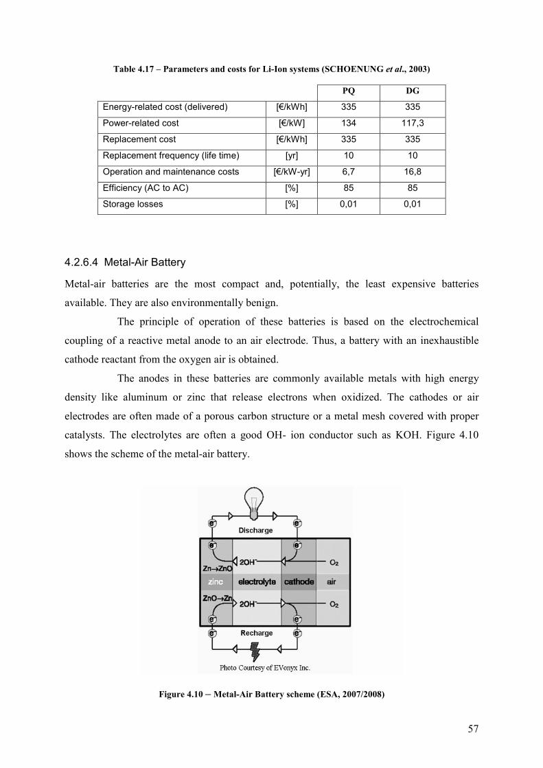
57
Table 4.17 – Parameters and costs for Li-Ion systems (SCHOENUNG et al., 2003)
PQ DG
Energy-related cost (delivered) [€/kWh] 335 335
Power-related cost [€/kW] 134 117,3
Replacement cost [€/kWh] 335 335
Replacement frequency (life time) [yr] 10 10
Operation and maintenance costs [€/kW-yr] 6,7 16,8
Efficiency (AC to AC) [%] 85 85
Storage losses [%] 0,01 0,01
4.2.6.4 Metal-Air Battery
Metal-air batteries are the most compact and, potentially, the least expensive batteries
available. They are also environmentally benign.
The principle of operation of these batteries is based on the electrochemical
coupling of a reactive metal anode to an air electrode. Thus, a battery with an inexhaustible
cathode reactant from the oxygen air is obtained.
The anodes in these batteries are commonly available metals with high energy
density like aluminum or zinc that release electrons when oxidized. The cathodes or air
electrodes are often made of a porous carbon structure or a metal mesh covered with proper
catalysts. The electrolytes are often a good OH- ion conductor such as KOH. Figure 4.10
shows the scheme of the metal-air battery.
Figure 4.10 – Metal-Air Battery scheme (ESA, 2007/2008)
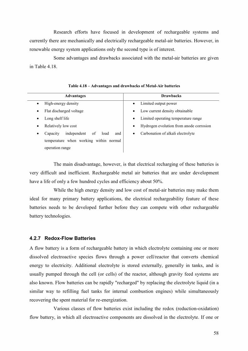
58
Research efforts have focused in development of rechargeable systems and
currently there are mechanically and electrically rechargeable metal-air batteries. However, in
renewable energy system applications only the second type is of interest.
Some advantages and drawbacks associated with the metal-air batteries are given
in Table 4.18.
Table 4.18 – Advantages and drawbacks of Metal-Air batteries
Advantages Drawbacks
• High-energy density
• Flat discharged voltage
• Long shelf life
• Relatively low cost
• Capacity independent of load and
temperature when working within normal
operation range
• Limited output power
• Low current density obtainable
• Limited operating temperature range
• Hydrogen evolution from anode corrosion
• Carbonation of alkali electrolyte
The main disadvantage, however, is that electrical recharging of these batteries is
very difficult and inefficient. Rechargeable metal air batteries that are under development
have a life of only a few hundred cycles and efficiency about 50%.
While the high energy density and low cost of metal-air batteries may make them
ideal for many primary battery applications, the electrical rechargeability feature of these
batteries needs to be developed further before they can compete with other rechargeable
battery technologies.
4.2.7 Redox-Flow Batteries
A flow battery is a form of rechargeable battery in which electrolyte containing one or more
dissolved electroactive species flows through a power cell/reactor that converts chemical
energy to electricity. Additional electrolyte is stored externally, generally in tanks, and is
usually pumped through the cell (or cells) of the reactor, although gravity feed systems are
also known. Flow batteries can be rapidly "recharged" by replacing the electrolyte liquid (in a
similar way to refilling fuel tanks for internal combustion engines) while simultaneously
recovering the spent material for re-energization.
Various classes of flow batteries exist including the redox (reduction-oxidation)
flow battery, in which all electroactive components are dissolved in the electrolyte. If one or

59
more electroactive component is deposited as a solid layer, the system is known as a hybrid
flow battery. The main difference between these two types of flow battery is that the energy
of the redox flow battery can be determined fully independently of the battery power, because
the energy is related to the electrolyte volume (tank size) and the power to the reactor size.
The hybrid flow battery, similarly to a conventional battery, is limited in energy
to the amount of solid material that can be accommodated within the reactor. In practical
terms this means that the discharge time of a redox flow battery (RFB) at full power can be
varied, as required, from several minutes to many days, whereas a hybrid flow battery may be
typically varied from several minutes to a few hours. Figure 4.11 shows the schematic
diagram of a RFB.
Figure 4.11 – Schematic diagram of a Redox flow battery (SELS et al., Oct. 2001)
Besides the fact that the storage capacity of a RFB is independent of the battery
power, while only depending on the concentration of the electrolyte, the RFB have other
advantages when compared to ordinary batteries. They are very cheap and can withstand
overloading and totally discharging without any risk of damage. One of the major
disadvantages is the use of aggressive chemical solutions, which can have a major impact on
the environment. Since the 1990s, the “Regenesys Energy Storage System” project is doing
intensive research to the usability of RFB for large power ratings in the United Kingdom.
Sections 4.2.7.1 to 4.2.7.3 provide some information and characteristics of some
flow battery technologies.

60
4.2.7.1 Vanadium Redox Flow Battery (VRB)
VRB stores energy by employing vanadium redox couples (V2+/V3+ in the negative and
V4+/V5+ in the positive half-cells). These are stored in mild sulfuric acid solutions
(electrolytes). During the charge/discharge cycles, H+ ions are exchanged between the two
electrolyte tanks through the hydrogen-ion permeable polymer membrane. The cell voltage is
1,4 - 1,6 volts.
The main advantages of the vanadium redox battery is that it can offer almost
unlimited capacity simply by using larger and larger storage tanks, it can be left completely
discharged for long periods with no ill effects, it can be recharged simply by replacing the
electrolyte if no power source is available to charge it, and if the electrolytes are accidentally
mixed the battery suffers no permanent damage.
The main disadvantages with vanadium redox technology are a relatively poor
energy-to-volume ratio, and the system complexity in comparison with standard storage
batteries. Table 4.19 shows some parameters and costs of a VRB for DG applications.
Table 4.19 – Parameters and costs for a VRB system (SCHOENUNG et al., 2003)
Energy-related cost (delivered) [€/kWh] 402
Power-related cost [€/kW] 117,3
Replacement cost [€/kWh] 402
Replacement frequency (life time) [yr] 10
Operation and maintenance costs [€/kW-yr] 13,4
Efficiency (AC to AC) [%] 70
Storage losses [%] 0,2
Currently installed vanadium batteries include a 1,5 MW UPS system in a
semiconductor fabrication plant in Japan and a 250 kW, 2MWh load leveler in use at Castle
Valley, Utah.
4.2.7.2 Zinc Bromine Flow Battery (ZnBr)
The zinc-bromine flow battery is a type of hybrid flow battery. In each cell of a ZnBr battery,
two different electrolytes flow past carbon-plastic composite electrodes in two compartments
separated by a microporous polyolefin membrane. During discharge, Zn and Br combine into
zinc bromide, generating 1,8 volts across each cell. This will increase the Zn2+ and Br- ion
density in both electrolyte tanks. During charge, metallic zinc will be deposited as a thin film
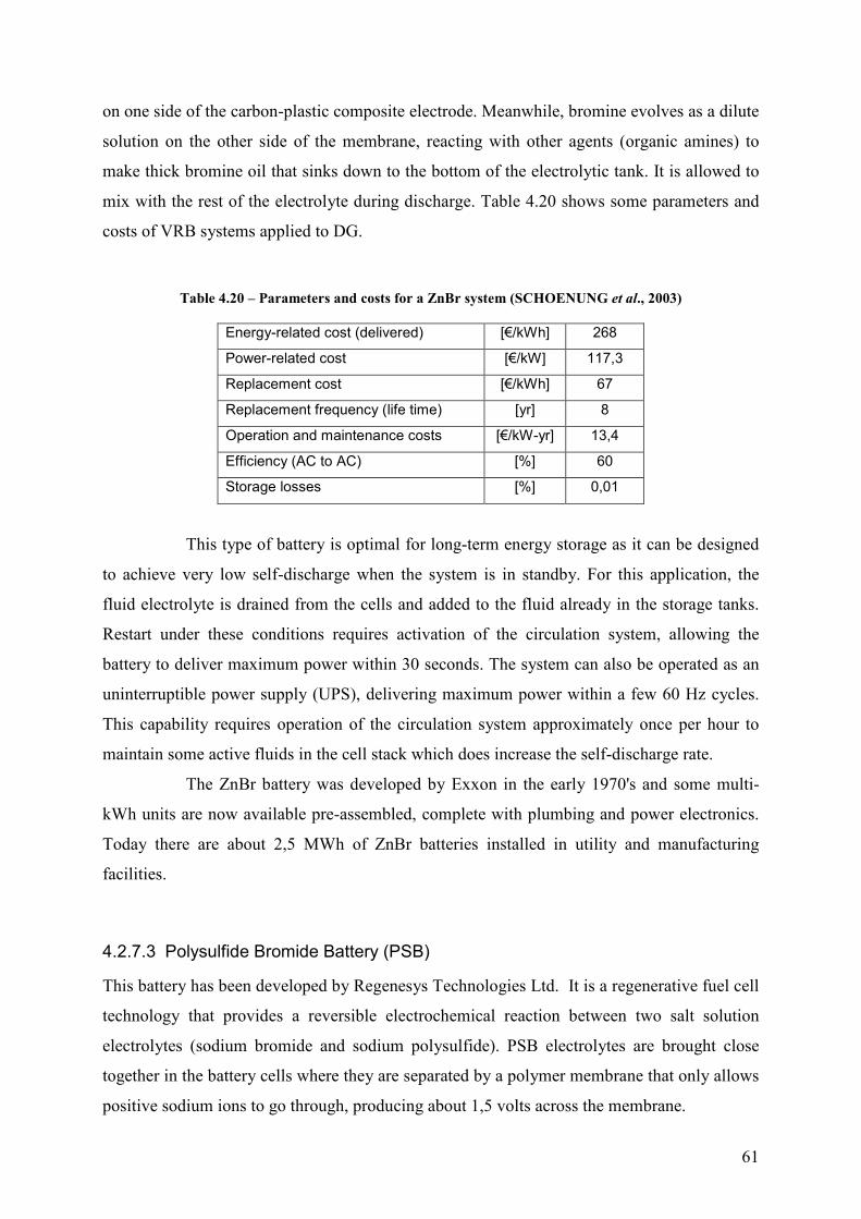
61
on one side of the carbon-plastic composite electrode. Meanwhile, bromine evolves as a dilute
solution on the other side of the membrane, reacting with other agents (organic amines) to
make thick bromine oil that sinks down to the bottom of the electrolytic tank. It is allowed to
mix with the rest of the electrolyte during discharge. Table 4.20 shows some parameters and
costs of VRB systems applied to DG.
Table 4.20 – Parameters and costs for a ZnBr system (SCHOENUNG et al., 2003)
Energy-related cost (delivered) [€/kWh] 268
Power-related cost [€/kW] 117,3
Replacement cost [€/kWh] 67
Replacement frequency (life time) [yr] 8
Operation and maintenance costs [€/kW-yr] 13,4
Efficiency (AC to AC) [%] 60
Storage losses [%] 0,01
This type of battery is optimal for long-term energy storage as it can be designed
to achieve very low self-discharge when the system is in standby. For this application, the
fluid electrolyte is drained from the cells and added to the fluid already in the storage tanks.
Restart under these conditions requires activation of the circulation system, allowing the
battery to deliver maximum power within 30 seconds. The system can also be operated as an
uninterruptible power supply (UPS), delivering maximum power within a few 60 Hz cycles.
This capability requires operation of the circulation system approximately once per hour to
maintain some active fluids in the cell stack which does increase the self-discharge rate.
The ZnBr battery was developed by Exxon in the early 1970's and some multi-
kWh units are now available pre-assembled, complete with plumbing and power electronics.
Today there are about 2,5 MWh of ZnBr batteries installed in utility and manufacturing
facilities.
4.2.7.3 Polysulfide Bromide Battery (PSB)
This battery has been developed by Regenesys Technologies Ltd. It is a regenerative fuel cell
technology that provides a reversible electrochemical reaction between two salt solution
electrolytes (sodium bromide and sodium polysulfide). PSB electrolytes are brought close
together in the battery cells where they are separated by a polymer membrane that only allows
positive sodium ions to go through, producing about 1,5 volts across the membrane.
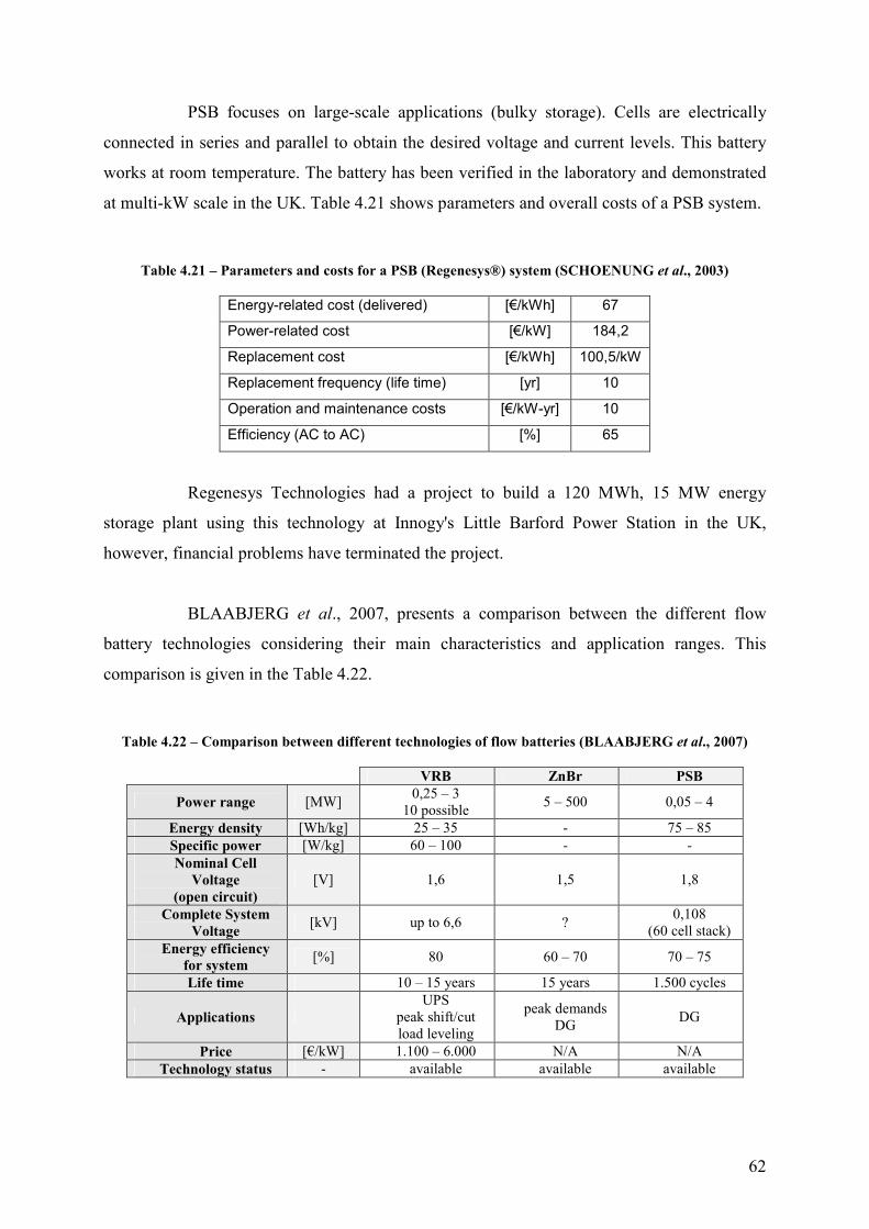
62
PSB focuses on large-scale applications (bulky storage). Cells are electrically
connected in series and parallel to obtain the desired voltage and current levels. This battery
works at room temperature. The battery has been verified in the laboratory and demonstrated
at multi-kW scale in the UK. Table 4.21 shows parameters and overall costs of a PSB system.
Table 4.21 – Parameters and costs for a PSB (Regenesys®) system (SCHOENUNG et al., 2003)
Energy-related cost (delivered) [€/kWh] 67
Power-related cost [€/kW] 184,2
Replacement cost [€/kWh] 100,5/kW
Replacement frequency (life time) [yr] 10
Operation and maintenance costs [€/kW-yr] 10
Efficiency (AC to AC) [%] 65
Regenesys Technologies had a project to build a 120 MWh, 15 MW energy
storage plant using this technology at Innogy's Little Barford Power Station in the UK,
however, financial problems have terminated the project.
BLAABJERG et al., 2007, presents a comparison between the different flow
battery technologies considering their main characteristics and application ranges. This
comparison is given in the Table 4.22.
Table 4.22 – Comparison between different technologies of flow batteries (BLAABJERG et al., 2007)
VRB ZnBr PSB
Power range [MW] 0,25 – 3
10 possible 5 – 500 0,05 – 4
Energy density [Wh/kg] 25 – 35 - 75 – 85 Specific power [W/kg] 60 – 100 - - Nominal Cell
Voltage (open circuit)
[V] 1,6 1,5 1,8
Complete System Voltage
[kV] up to 6,6 ? 0,108
(60 cell stack) Energy efficiency
for system [%] 80 60 – 70 70 – 75
Life time 10 – 15 years 15 years 1.500 cycles
Applications UPS
peak shift/cut load leveling
peak demands DG
DG
Price [€/kW] 1.100 – 6.000 N/A N/A Technology status - available available available
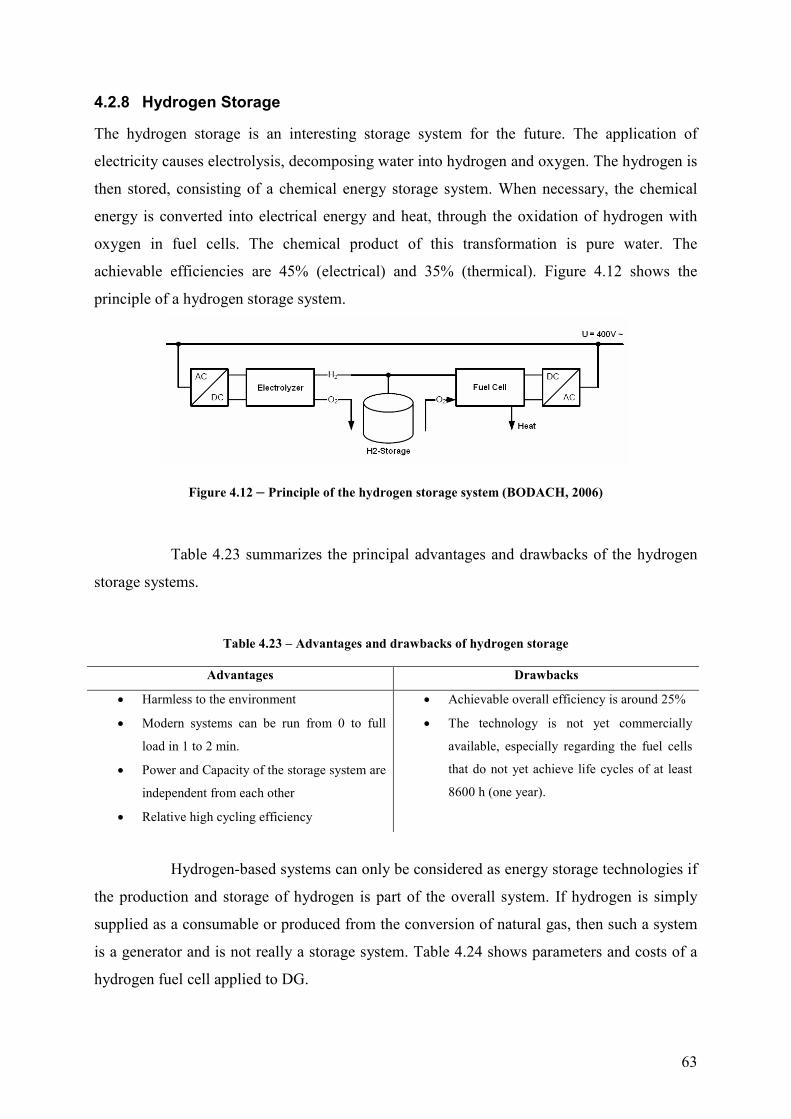
63
4.2.8 Hydrogen Storage
The hydrogen storage is an interesting storage system for the future. The application of
electricity causes electrolysis, decomposing water into hydrogen and oxygen. The hydrogen is
then stored, consisting of a chemical energy storage system. When necessary, the chemical
energy is converted into electrical energy and heat, through the oxidation of hydrogen with
oxygen in fuel cells. The chemical product of this transformation is pure water. The
achievable efficiencies are 45% (electrical) and 35% (thermical). Figure 4.12 shows the
principle of a hydrogen storage system.
Figure 4.12 – Principle of the hydrogen storage system (BODACH, 2006)
Table 4.23 summarizes the principal advantages and drawbacks of the hydrogen
storage systems.
Table 4.23 – Advantages and drawbacks of hydrogen storage
Advantages Drawbacks
• Harmless to the environment
• Modern systems can be run from 0 to full
load in 1 to 2 min.
• Power and Capacity of the storage system are
independent from each other
• Relative high cycling efficiency
• Achievable overall efficiency is around 25%
• The technology is not yet commercially
available, especially regarding the fuel cells
that do not yet achieve life cycles of at least
8600 h (one year).
Hydrogen-based systems can only be considered as energy storage technologies if
the production and storage of hydrogen is part of the overall system. If hydrogen is simply
supplied as a consumable or produced from the conversion of natural gas, then such a system
is a generator and is not really a storage system. Table 4.24 shows parameters and costs of a
hydrogen fuel cell applied to DG.
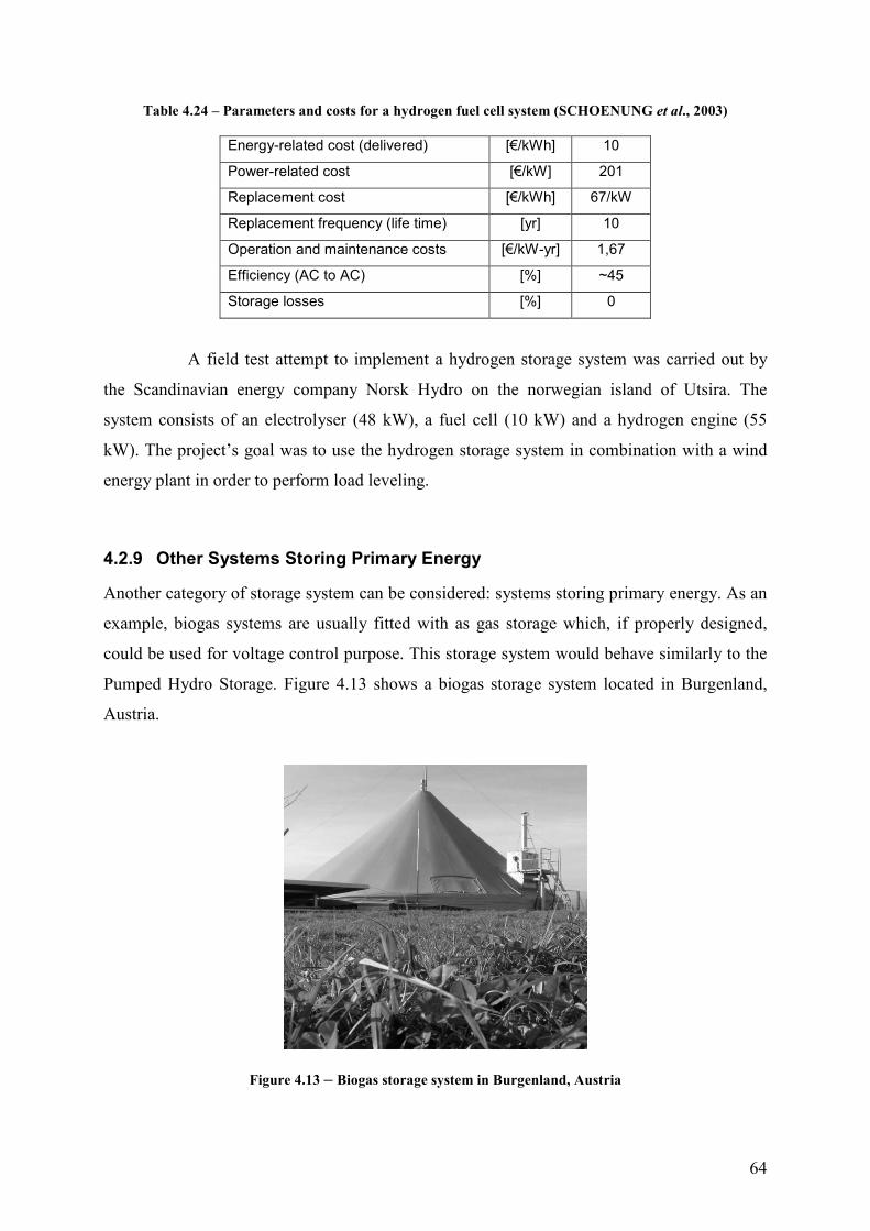
64
Table 4.24 – Parameters and costs for a hydrogen fuel cell system (SCHOENUNG et al., 2003)
Energy-related cost (delivered) [€/kWh] 10
Power-related cost [€/kW] 201
Replacement cost [€/kWh] 67/kW
Replacement frequency (life time) [yr] 10
Operation and maintenance costs [€/kW-yr] 1,67
Efficiency (AC to AC) [%] ~45
Storage losses [%] 0
A field test attempt to implement a hydrogen storage system was carried out by
the Scandinavian energy company Norsk Hydro on the norwegian island of Utsira. The
system consists of an electrolyser (48 kW), a fuel cell (10 kW) and a hydrogen engine (55
kW). The project’s goal was to use the hydrogen storage system in combination with a wind
energy plant in order to perform load leveling.
4.2.9 Other Systems Storing Primary Energy
Another category of storage system can be considered: systems storing primary energy. As an
example, biogas systems are usually fitted with as gas storage which, if properly designed,
could be used for voltage control purpose. This storage system would behave similarly to the
Pumped Hydro Storage. Figure 4.13 shows a biogas storage system located in Burgenland,
Austria.
Figure 4.13 – Biogas storage system in Burgenland, Austria
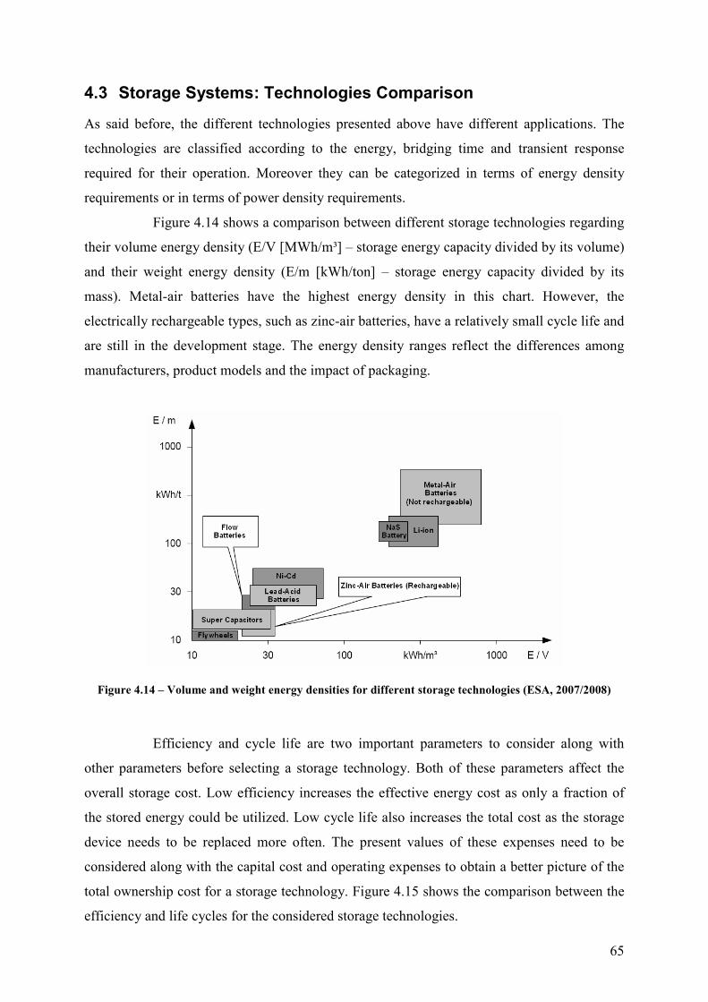
65
4.3 Storage Systems: Technologies Comparison
As said before, the different technologies presented above have different applications. The
technologies are classified according to the energy, bridging time and transient response
required for their operation. Moreover they can be categorized in terms of energy density
requirements or in terms of power density requirements.
Figure 4.14 shows a comparison between different storage technologies regarding
their volume energy density (E/V [MWh/m³] – storage energy capacity divided by its volume)
and their weight energy density (E/m [kWh/ton] – storage energy capacity divided by its
mass). Metal-air batteries have the highest energy density in this chart. However, the
electrically rechargeable types, such as zinc-air batteries, have a relatively small cycle life and
are still in the development stage. The energy density ranges reflect the differences among
manufacturers, product models and the impact of packaging.
Figure 4.14 – Volume and weight energy densities for different storage technologies (ESA, 2007/2008)
Efficiency and cycle life are two important parameters to consider along with
other parameters before selecting a storage technology. Both of these parameters affect the
overall storage cost. Low efficiency increases the effective energy cost as only a fraction of
the stored energy could be utilized. Low cycle life also increases the total cost as the storage
device needs to be replaced more often. The present values of these expenses need to be
considered along with the capital cost and operating expenses to obtain a better picture of the
total ownership cost for a storage technology. Figure 4.15 shows the comparison between the
efficiency and life cycles for the considered storage technologies.

66
Figure 4.15 – Efficiency and life cycles for different storage technologies (ESA, 2007/2008)
In the previous figure it is clear that the supercapacitors have high cycle stability,
what is very important for the fluctuating energy fraction of a network with a high DG
penetration. By the observation of both diagrams (Figures 4.14 and 4.15), it is clear that, for a
global DG storage solution, the combination of different technologies is the best option, as the
necessary energy fraction can be stored in the batteries and the fluctuating energy fraction in
supercapacitors.
The final and most comprehensive comparison takes into account the electricity
storage spectrum explained in the last topic. The electric energy storage systems are divided
in three major functional categories, shown in Figure 4.16.
These categories can be considered equivalent to the PQ, DG and bulky storage
applications. The Power Quality & UPS refers to applications where the stored energy is only
applied for seconds or less, as needed, to assure continuity of quality power. In the Bridging
Power applications, the stored energy is used for seconds to minutes to assure continuity of
service when switching from one source of energy generation to another. Finally, in the
Energy Management applications, the stored energy is used to decouple the timing of
generation and consumption of electric energy, like load leveling (the charging of storage
when energy cost is low and utilization as needed).

67
Figure 4.16 – Discharge time at rated power (ESA, 2007/2008)
It can be seen from the figure above that Pumped Hydro Storage and Compressed
Air Energy Storage can not be integrated to low voltage networks due to their nominal power
(Pnom >> 10MW). The other technologies cover a broader power range and can be, therefore,
used in such networks (BODACH, 2006).
Alternatively, some of the storage technologies can also be allocated according to
their energy supply time, which is shown in Table 4.25. According to (BODACH, 2006), the
storage systems supply times up to 20 min are classified as short-period, those over one week
as long-period, and the rest of them as average-period.
Table 4.25 – Storage applications in the energy supply field (BODACH, 2006)
Energy Transfer
(full load) Class
Hyd
roge
n
CA
ES
Pum
ped
Hyd
ro S
tora
ge
Red
ox F
low
B
atte
ries
Oth
er
Bat
teri
es
Fly
whe
els
SM
ES
Sup
er
Cap
acit
or
4 months X
3 weeks Long period X
3 days X X X X
8 hours X X X X X
2 hours
Average period
X X X X X
20 min X X X X X X X
3 min X X X X X X
20 sec
Short Period
X X X X X

68
ESA® presents another comparison table, based on the aforementioned spectrum
of applications presented in Figure 4.1. This classification is shown on Table 4.26.
Table 4.26 – Application of different storage system technologies (ESA, 2007/2008)
Storage Technologies Power
Application
Energy
Application
Pumped Storage CAES Flow Batteries (VRB, ZnBr, PSB) Metal-Air NaS Li-ion Other Advanced Batteries Lead-Acid Flywheels SMES Super Capacitors
Fully capable and reasonable
Reasonable for this application
Feasible but not quite practical or economical
NONE Not feasible or economical
The analysis of all the comparisons among technologies helps to identify those
more suitable to be applied to the CVC in the framework of the DG DemoNet-Concept. But
first it is necessary to consider how the storage systems were integrated to the CVC. The next
topic explains this integration and presents a discussion about what technologies, among those
analyzed, are best suitable to be used.
4.4 Integration of Storage Systems to the Coordinated Voltage
Control
For the integration of the Storage Devices (SD) into the CVC, some changes in its algorithm
were proposed. These changes take into account the characteristics defining the storage
systems applied to the voltage control in DG networks.
The new CVC algorithm is also based on the power injection share concept and
considers the installation of SD at some of the critical nodes of the network, which are
detected in an offline study, as explained in the chapter 3.
Many changes were conducted in order to incorporate the SD to the CVC
algorithm. First of all, the SD itself was defined as a generator/load device. It means that,
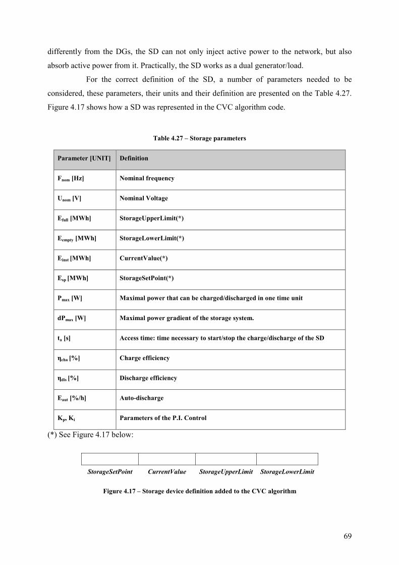
69
differently from the DGs, the SD can not only inject active power to the network, but also
absorb active power from it. Practically, the SD works as a dual generator/load.
For the correct definition of the SD, a number of parameters needed to be
considered, these parameters, their units and their definition are presented on the Table 4.27.
Figure 4.17 shows how a SD was represented in the CVC algorithm code.
Table 4.27 – Storage parameters
Parameter [UNIT] Definition
Fnom [Hz] Nominal frequency
Unom [V] Nominal Voltage
Efull [MWh] StorageUpperLimit(*)
Eempty [MWh] StorageLowerLimit(*)
Einst [MWh] CurrentValue(*)
Esp [MWh] StorageSetPoint(*)
Pmax [W] Maximal power that can be charged/discharged in one time unit
dPmax [W] Maximal power gradient of the storage system.
ta [s] Access time: time necessary to start/stop the charge/discharge of the SD
ηcha [%] Charge efficiency
ηdis [%] Discharge efficiency
Eaut [%/h] Auto-discharge
Kp, Ki Parameters of the P.I. Control
(*) See Figure 4.17 below:
StorageSetPoint CurrentValue StorageUpperLimit StorageLowerLimit
Figure 4.17 – Storage device definition added to the CVC algorithm

70
The CurrentValue represents the current amount of energy (MWh) stored in the
SD at a certain point in time (sum of all three phases). The StorageUpperLimit denotes the
size, or maximal capacity, of the SD. When the CurrentValue is equal to StorageUpperLimit,
it means that the SD can not absorb any power from the network; or, from the voltage control
perspective, it is at its limit. The same occurs if the CurrentValue is equal to
StorageLowerLimit, which represents the minimal amount of energy that can be stored in the
SD; in this work, this value is considered to be zero.
The StorageSetPoint represents the set point to be achieved when the SD does not
need to contribute to the voltage control. In the case the SD is connected to an overvoltage
node, for example, this value is set to the StorageLowerLimit, so the SD can discharge
(generator) when no voltage control is needed, optimizing its contribution in case of a future
overvoltage. On the other hand, when connected to an undervoltage node, the StorageSetPoint
is set to StorageUpperLimit, so the SD can charge (load) when no voltage control is needed,
also optimizing it’s voltage control capacity in case of future undervoltage. Of course this
StorageSetPoint adjust can lead to overvoltage and undervoltage, respectively, however, the
whole CVC is prepared to deal with these situations. Figure 4.18 shows the action performed
by the SD control in the cases where the voltage is outside the upper and lower limits and
when the voltage is ok, but the CurrentValue and StorageSetPoint have different values.
Figure 4.18 – Storage device model added to the CVC, showing the control action in different cases
In the CVC algorithm, both Eaut and ta were considered to be zero. The first one,
the battery auto-discharge value, was not considered because it is much smaller when
compared with the charge/discharge rates for this application, making it have a minor
UMAX
UMIN
Overvoltage (SD is charged)
Undervoltage (SD is discharged)
StorageSetPoint < CurrentValue (SD is discharged)
StorageSetPoint > CurrentValue (SD is charged)

71
relevance in the simulations. ta, however, though important, was not considered since many
time constants of the network still need to be investigated and validated. Of course this affects
the simulations, as explained later and it is expected to be improved in the near future, since a
time constants investigation is being currently carried out (See chapter 6).
For a better modeling of the SD in the CVC algorithm to broaden its applicability
to different storage technologies, they were divided in two different models, depending on
their physical and operation characteristics. The Storage Model 1 (Figure 4.19) considers a
SD connected to the same bus the generator is connected. In this model, Pout is the sum of the
SD output and the generator output, which are independent from each other. If the generator is
at its maximal output value, the storage system can still discharge. It is important to note, that
the value PSD shown in the figure can not be greater than the PMAX (Table 4.27).
Figure 4.19 – Storage Model 1 – Standalone Storage System
The Storage Model 2 (Figure 4.20) considers that Pout is equal to the generator
output, which is a sum of the required generation and the storage output. In this model, if the
generator is at its maximal output value, the storage system can not discharge, as they are
dependent from each other. In this case, POUT can not be greater than PMAX (Table 4.27).
G SD
Pout (PG + PSD)
-PSD_LIM < PSD < + PSD_LIM PG_MIN < PG < + PG_MAX
PG ≥ 0

72
Figure 4.20 – Storage Model 2 – Integrated Storage System
The original local voltage control part of the CVC algorithm considers that active
power voltage control is introduced in the case of reactive power management reaches its
limit. With the introduction of the Storage Model 1, the active power voltage is introduced
only after the SD reaches its limit. Therefore, this new voltage control acts between the
reactive and active power voltage control. Figure 4.21 shows the change in the flow chart
algorithm of the CVC.
For the Storage Model 2, the storage control is also performed after the Q control
and before the PQ control, but in this case the storage control is nothing more a PQ control
performed by a generator that is not part of the original PQ control scheme. It means that,
after the Q control is exploited, the generator that incorporates the storage control is activated
and when its control’s capacity is also exploited, the PQ control, through the priority matrix is
activated.
G SD
Pout (PG + PSD)
-PSD_LIM < PSD < + PSD_LIM PG_MIN < PG + PSD < + PG_MAX
PG ≥ 0

73
Determination of min and max network voltage from
measurements at critical points in the network
Umax > Uup_lim Yes
Time Delayskip short voltage variations
No
Uup_lim Umin < Ulow_lim
Ulow_lim
Umin < Ulow_lim
Yes
No
Time Delayskip short voltage variations
Umin < Ulow_lim Umax > Uup_lim No
No
No
Yes
Change the tap
position
Voltage input
Q, SD and P
ControlUset=Uup_lim
or
Uset=Ulow_lim
Is it possible and valid to tap?
No
Ranking and
decision system
LOCAL CONTROL
Yes
Yes
Yes
Figure 4.21 – Flow chart algorithm of the CVC with the addition of the SD Control
The SD also participates in the power injection share concept, as it works as a
generator when discharging. When charging, however, the Storage Model 1 works as a load;
this improves the capacity of the device in controlling also undervoltage. As an example, in a
situation where there is overvoltage, but it is not possible to activate the centralized OLTC
voltage control due to the possibility of undervoltage in another node, the SD could discharge,
rising the overall voltage and, making it possible to tap the transformer. It is not necessary to
have different voltage setpoints for conflict conditions anymore, in comparison with the flow
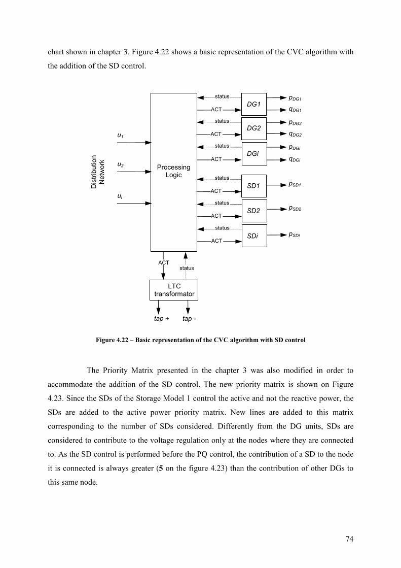
74
chart shown in chapter 3. Figure 4.22 shows a basic representation of the CVC algorithm with
the addition of the SD control.
Figure 4.22 – Basic representation of the CVC algorithm with SD control
The Priority Matrix presented in the chapter 3 was also modified in order to
accommodate the addition of the SD control. The new priority matrix is shown on Figure
4.23. Since the SDs of the Storage Model 1 control the active and not the reactive power, the
SDs are added to the active power priority matrix. New lines are added to this matrix
corresponding to the number of SDs considered. Differently from the DG units, SDs are
considered to contribute to the voltage regulation only at the nodes where they are connected
to. As the SD control is performed before the PQ control, the contribution of a SD to the node
it is connected is always greater (5 on the figure 4.23) than the contribution of other DGs to
this same node.
ACT
status
ACT
ACT
status
status
tap + tap -
u1
u2
ui
pDG1
pDG2
pDGi
qDG1
qDG2
qDGi
Dis
trib
ution
Netw
ork
Processing Logic
ACT status
LTC transformator
DG1
DG2
DGi
ACT
status
SD1
ACT
status
SD2
ACT
status
SDi
pSD1
pSD2
pSDi
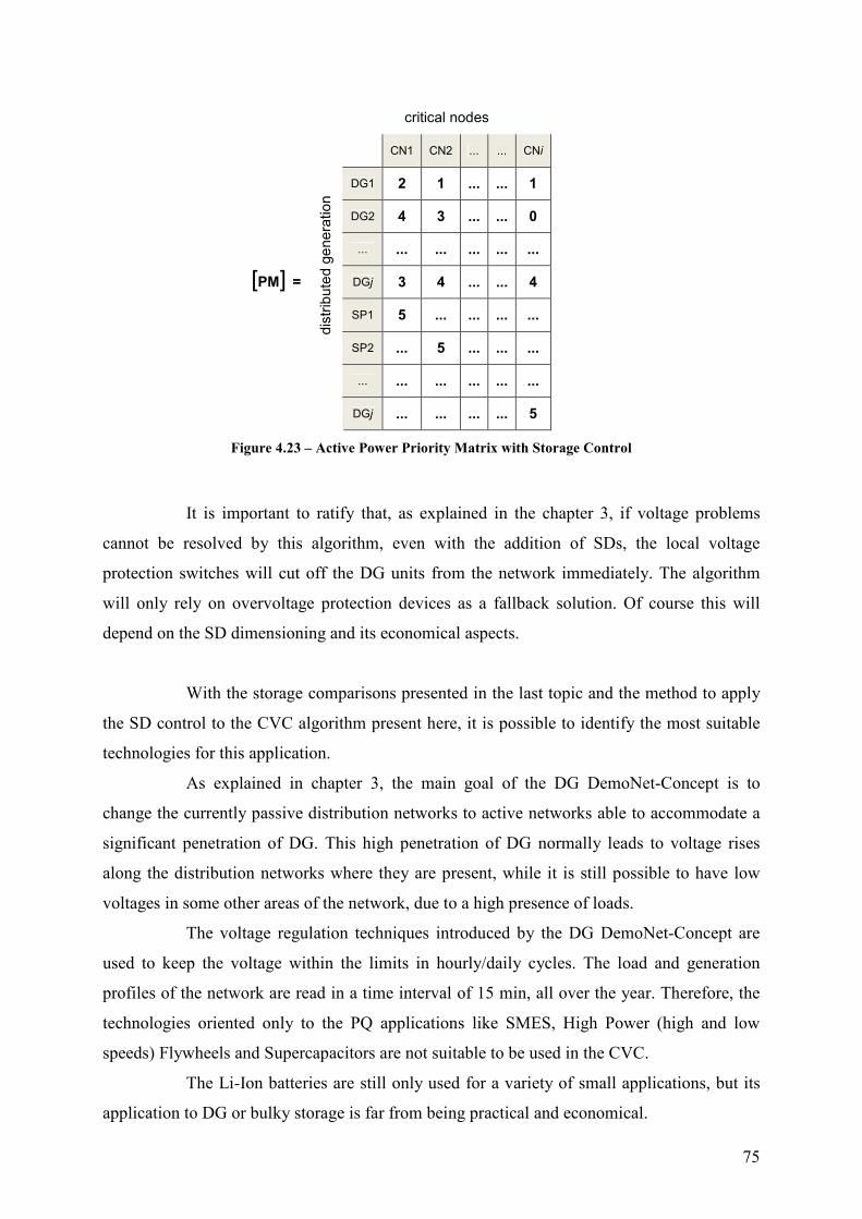
75
critical nodes
CN1 CN2 ... ... CNi
DG1 2 1 ... ... 1
DG2 4 3 ... ... 0
... ... ... ... ... ...
DGj 3 4 ... ... 4
SP1 5 ... ... ... ...
SP2 ... 5 ... ... ...
... ... ... ... ... ...
[PM] =
dis
trib
ute
d g
enera
tio
n
DGj ... ... ... ... 5
Figure 4.23 – Active Power Priority Matrix with Storage Control
It is important to ratify that, as explained in the chapter 3, if voltage problems
cannot be resolved by this algorithm, even with the addition of SDs, the local voltage
protection switches will cut off the DG units from the network immediately. The algorithm
will only rely on overvoltage protection devices as a fallback solution. Of course this will
depend on the SD dimensioning and its economical aspects.
With the storage comparisons presented in the last topic and the method to apply
the SD control to the CVC algorithm present here, it is possible to identify the most suitable
technologies for this application.
As explained in chapter 3, the main goal of the DG DemoNet-Concept is to
change the currently passive distribution networks to active networks able to accommodate a
significant penetration of DG. This high penetration of DG normally leads to voltage rises
along the distribution networks where they are present, while it is still possible to have low
voltages in some other areas of the network, due to a high presence of loads.
The voltage regulation techniques introduced by the DG DemoNet-Concept are
used to keep the voltage within the limits in hourly/daily cycles. The load and generation
profiles of the network are read in a time interval of 15 min, all over the year. Therefore, the
technologies oriented only to the PQ applications like SMES, High Power (high and low
speeds) Flywheels and Supercapacitors are not suitable to be used in the CVC.
The Li-Ion batteries are still only used for a variety of small applications, but its
application to DG or bulky storage is far from being practical and economical.

76
Some other technologies could be suitable for the integration to the CVC, like the
Hydrogen Storage, High Energy Flywheels and High Energy Supercapacitors, but they are at
an early development status and it is not clear if they will be available in the next years and if
it will be possible to use them in high energy applications.
The Metal-Air Battery is also not a good option, due to its recharging issue, since
the expected storage system needs to charge, discharge in daily cycles and this cannot be
constrained by a poor recharging performance. The rechargeable types are still being
researched and can be a good option in the future.
The Lead-Acid Batteries have a reduced lifecycle and are sensible to extreme
depth of discharge, what is a critical constraint for the storage systems needed for the
integration to the CVC, since the systems need to have the capacity be fully charged or
discharged in daily cycles without major changes in their efficiencies and operation.
The other evaluated technologies, namely Flow Batteries (VRB, ZnBr and PSB),
Sodium Sulfur Battery (NaS), Compressed Air Energy Storage (CAES) and Pumped Hydro
Storage can be considered as possible solutions for the integration of storage devices into the
CVC. The flow batteries and the NaS battery can be modelled by the Storage Model 1 and the
Pumped Hydro Storage, as well as the Biogas Storage, by the Storage Model 2, due to their
physical characteristics and operation parameters.
77
5 Study Case: Vorarlberg, Austria
In this chapter a study case is considered in order to evaluate the results obtained by adding
SDs to the CVC. Simulations were carried out using the software
DIgSILENT PowerFactory and MATLAB, as explained in the next topic, and had the
main objectives to integrate storage systems into the coordinated voltage control and provide
rules for the dimensioning of the SD and for the comparison with the original CVC system.
Due to the length of the simulations, year simulations, which would be useful for economical
considerations, could not be performed.
5.1 DIgSILENT PowerFactory® Software Overview
The calculation software PowerFactory, as written by DIgSILENT, is a computer aided
engineering tool for the analysis of industrial, utility and commercial electrical power
systems. It is designed as an advanced integrated and interactive software package dedicated
to electrical power system and control analysis in order to achieve the main objectives of
planning and operation optimization. The name DIgSILENT stands for Digital SimuLation
and Electrical NeTwork calculation program.
DIgSILENT PowerFactory software incorporates a list of simulation
functionalities including load flow and fault analysis of complete AC/DC network
representation, low voltage network analysis, distribution network optimization, harmonic
analysis, interface SCADA, power electronic device modeling, among others.
The software performs within a fully graphical windowing environment as shown
in Figure 5.1. Separate windows are available for output display, single line graphics and
substation drawings, data base editing and calculation functions. Additionally, multiple
windows in each window class may be open simultaneously to show for example different
aspects of the same substation graphic, or to highlight different hierarchies in a network single
line graphic.

78
Figure 5.1 – Graphical windowing environment in DIgSILENT PowerFactory® simulation software.
DIgSILENT PowerFactory also provides a fully integrated graphical editing
environment, which enables the user to draw and modify electrical grids, operate several
windows with different layers and grid sections simultaneously, display calculation results
immediately in result boxes within the single line diagram, among other functionalities.
The software also features definition of user written models within a fully
graphical environment (block diagrams – Figure 5.2). The integrated graphical editor provides
the needed flexibility to implement the most complex models also supporting unlimited model
nested. Connectivity checks are permanently active ensuring proper “wiring” of all frame
signals and model connections.
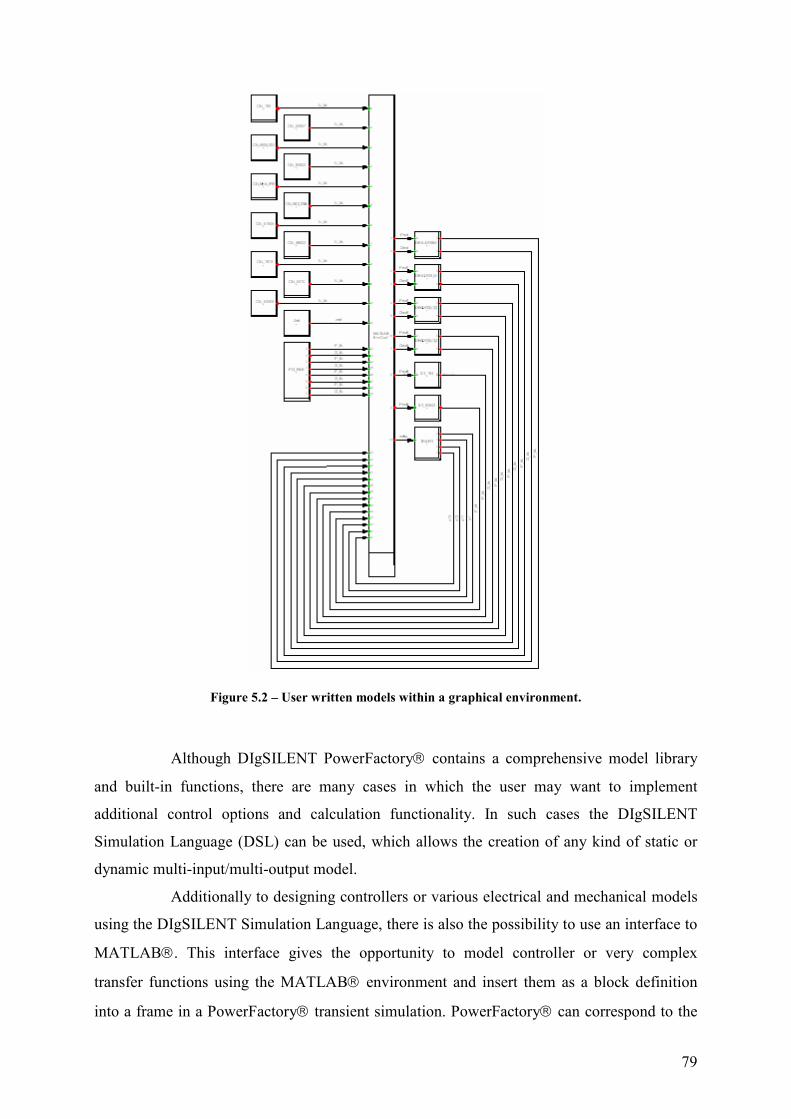
79
Figure 5.2 – User written models within a graphical environment.
Although DIgSILENT PowerFactory contains a comprehensive model library
and built-in functions, there are many cases in which the user may want to implement
additional control options and calculation functionality. In such cases the DIgSILENT
Simulation Language (DSL) can be used, which allows the creation of any kind of static or
dynamic multi-input/multi-output model.
Additionally to designing controllers or various electrical and mechanical models
using the DIgSILENT Simulation Language, there is also the possibility to use an interface to
MATLAB. This interface gives the opportunity to model controller or very complex
transfer functions using the MATLAB environment and insert them as a block definition
into a frame in a PowerFactory transient simulation. PowerFactory can correspond to the

80
MATLAB program during the simulation. It transfers the input values of a block to
MATLAB for every time step, which will then simulate a specified *.m file in its own
environment and gives back the results as the outputs of the block.
In this work the interface between DIgSILENT PowerFactory® and MATLAB
was used, since the local, centralized and coordinated voltage control were implemented as
*.m files in MATLAB. The main reason for this was the possibility to use the flexibility of
the matrix-oriented MATLAB language. Figure 5.3 shows how the MATLAB integration
is done in the DIgSILENT environment.
Figure 5.3 – MATLAB® integration through *.m file
In the figure above, the variables y01, y02, y03… are the MATLAB® outputs to
the PowerFactory® environment, while the variables U_Ist1, U_Ist2… are the inputs to
MATLAB®. On Figure 5.2, MATLAB® is represented by the central and elongated block,
while the arrows represent its inputs and outputs.

81
5.2 Study Case Network Analysis
In order to evaluate the performance of the presented control scheme, a test case was
conducted. The test network is a part of the distribution network operated by VKW
Vorarlberg, Austria (Figure 5.4). The network is represented by 81 km of cable and overhead
lines, one transmission network interconnection, 116 nodes, 75 loads and 31 distributed
generators. In the network model wind (pink), photovoltaic (yellow), hydro (blue) and
biomass (brown) generators are represented by simplified models (negative loads) and
equipped with adequate control systems. An exponential dependence on the bus voltages was
assumed to represent the nonlinear loads.
In simulation, real load and generation profiles were considered. The profiles
included 15 minutes measurements of energy consumption (production) on feeders of active
elements and are available for one year. For the test, a time step of 0,1 second and a
simulation interval of one day (1440 minutes) were adopted. One second of the simulation
time is equivalent to one minute in real time; therefore, one day has 1440 seconds in the
simulation time.
Planning and operation rules were provided by the distribution network operator.
Although strict restrictions on grid voltages are included, due to high DG penetration, in
current praxis small-scale voltage deviations are tolerated. In the tests, the targeted voltage
was considered to be between 0,98 p.u. and 1,03 p.u. or -2 % and +3 % of the nominal
voltage. The undervoltage limit was chosen to be 0,94 instead of 0,98 since no monitored
node had voltages under 0,94 and, therefore, the undervoltage analysis could not be
performed if the original undervoltage limit was used.
Figure 5.4 – Study case network – Vorarlberg, Austria

82
In the network the green and red nodes represent overvoltage and undervoltage
nodes, respectively. In the simulation, eleven critical nodes were taken into account: 183,
62907, 62905_SS1, 83902, DEA_8781, 61810_SSB, 61905, 48902, 1812, 6310, 63/9/9.
Figure 5.5 shows the voltage profile for these nodes during the whole year. These critical
nodes were identified based on the offline studies explained in chapter 3. The results show
that the nodes DEA_8781, 61810_SSB, 61905, 48902, 1812, 63/9/9 remain between the
tolerated voltage limits during all the year, ranging from 0,985 to 1,015 p.u.. These nodes
were therefore not considered on the tests (light grey color on the figure). The nodes 62907
and 62905_SS1 present undervoltage (dark grey color on the figure); their voltages range
from 0,959 to 0,983 p.u.. Both nodes have almost the same voltage profile during all year, due
to their physical proximity, therefore, only the node 62905_SS1 was considered out of these
two. The nodes 183, 83902 and 6310 present overvoltage (black color on the figure); their
voltages range from 0,992 to 1,066 and they were all considered for the simulations.
Figure 5.5 – Yearly voltage profile (p.u.) for the eleven nodes
The test was performed for both storage models presented in chapter 4. Four DG
units and an existing transformer (61.810_UM2) with the OLTC option were included. The
tap changer reaction time was 20s.
For the Storage Model 1 (standalone storage system), the voltage regulation
scheme was composed also of storage devices connected to the node 83902, which is the
more critical node among the overvoltage nodes, and to the node 62905_SS1, which is an

83
undervoltage node. These elements were named in DIgSILENT as SD_83902 and
SD_62905_SS1 respectively. Figure 5.6 shows the connection of both SDs to their respective
nodes.
Figure 5.6 – SDs connected to the selected critical nodes – Storage Model 1
To illustrate the integration of the SDs into the CVC using the voltage share
concept, the priority matrixes for Q and PQ control are presented. Four DGs were considered
on the tests due to their contributions to the voltage regulation at the selected critical nodes;
these DGs are DEA_DG8_W, DEA_DG9_W, DEA_DG13_V2_2MW and
DEA_DG13_V3_2MW. Two new rows were added to both priority matrixes, each line
referring to one of the two SDs. Since the SDs in the Storage Model 1 don’t manage reactive
power, they don’t contribute to the Q control, as shown in Table 5.1. No DG contributed to
the voltage at node 62905_SS1.
Table 5.1 – Priority Matrix for Q Control – Storage Model 1
Critical Nodes
62905-SS1
183 83902 6310
X X X 1 DEA_DG8_W
X X 4 4 DEA_DG9_W
X 4 3 3 DEA_DG13_V2_2MW
X 3 X 2 DEA_DG13_V3_2MW
DG
X X X X SD_83902
X X X X SD_62905_SS1 SD
Even though the SD control is performed before the PQ control, the SDs were
added to the PQ priority matrix (Table 5.2), as they also contribute to the active power
regulation. They have of course higher priority when compared to DGs, but their contribution
to the voltage control is locally limited, as explained in chapter 4. Even though no DG
contributes to the voltage at node 62905_SS1, the SD can contribute to this node, because of
its capacity to absorb power from system by charging.
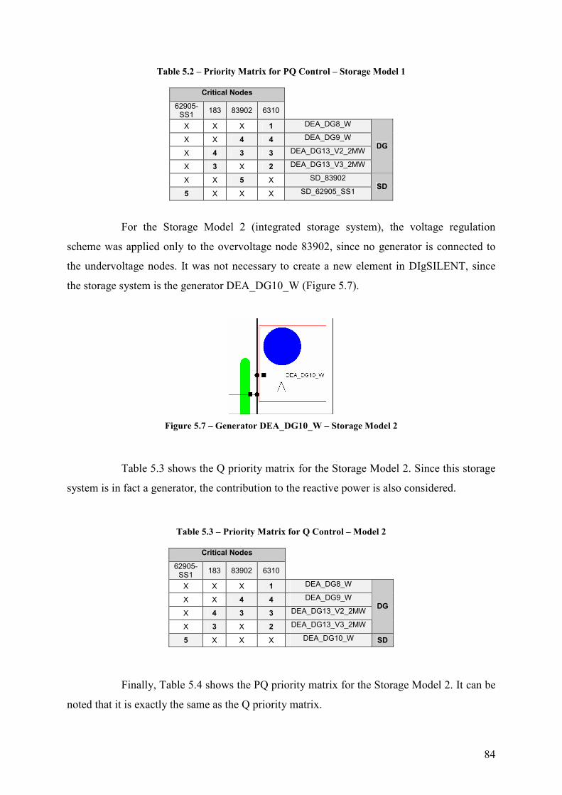
84
Table 5.2 – Priority Matrix for PQ Control – Storage Model 1
Critical Nodes
62905-SS1
183 83902 6310
X X X 1 DEA_DG8_W
X X 4 4 DEA_DG9_W
X 4 3 3 DEA_DG13_V2_2MW
X 3 X 2 DEA_DG13_V3_2MW
DG
X X 5 X SD_83902
5 X X X SD_62905_SS1 SD
For the Storage Model 2 (integrated storage system), the voltage regulation
scheme was applied only to the overvoltage node 83902, since no generator is connected to
the undervoltage nodes. It was not necessary to create a new element in DIgSILENT, since
the storage system is the generator DEA_DG10_W (Figure 5.7).
Figure 5.7 – Generator DEA_DG10_W – Storage Model 2
Table 5.3 shows the Q priority matrix for the Storage Model 2. Since this storage
system is in fact a generator, the contribution to the reactive power is also considered.
Table 5.3 – Priority Matrix for Q Control – Model 2
Critical Nodes
62905-SS1
183 83902 6310
X X X 1 DEA_DG8_W
X X 4 4 DEA_DG9_W
X 4 3 3 DEA_DG13_V2_2MW
X 3 X 2 DEA_DG13_V3_2MW
DG
5 X X X DEA_DG10_W SD
Finally, Table 5.4 shows the PQ priority matrix for the Storage Model 2. It can be
noted that it is exactly the same as the Q priority matrix.
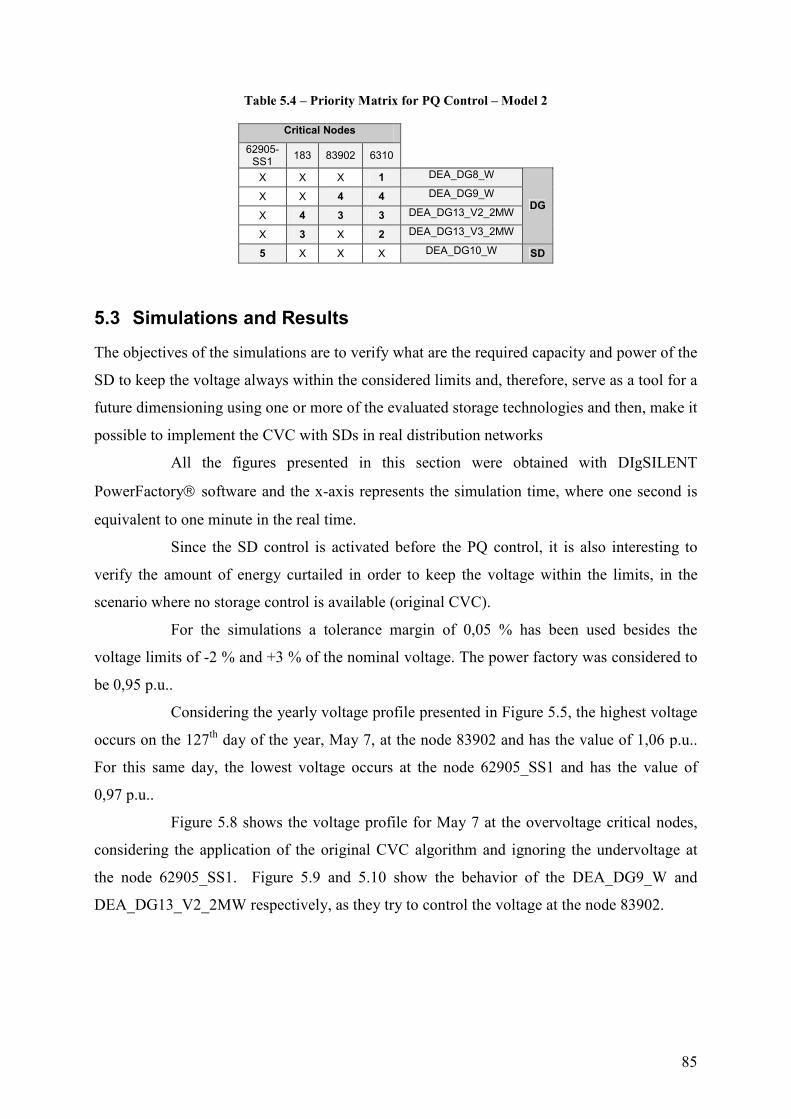
85
Table 5.4 – Priority Matrix for PQ Control – Model 2
Critical Nodes
62905-SS1
183 83902 6310
X X X 1 DEA_DG8_W
X X 4 4 DEA_DG9_W
X 4 3 3 DEA_DG13_V2_2MW
X 3 X 2 DEA_DG13_V3_2MW
DG
5 X X X DEA_DG10_W SD
5.3 Simulations and Results
The objectives of the simulations are to verify what are the required capacity and power of the
SD to keep the voltage always within the considered limits and, therefore, serve as a tool for a
future dimensioning using one or more of the evaluated storage technologies and then, make it
possible to implement the CVC with SDs in real distribution networks
All the figures presented in this section were obtained with DIgSILENT
PowerFactory software and the x-axis represents the simulation time, where one second is
equivalent to one minute in the real time.
Since the SD control is activated before the PQ control, it is also interesting to
verify the amount of energy curtailed in order to keep the voltage within the limits, in the
scenario where no storage control is available (original CVC).
For the simulations a tolerance margin of 0,05 % has been used besides the
voltage limits of -2 % and +3 % of the nominal voltage. The power factory was considered to
be 0,95 p.u..
Considering the yearly voltage profile presented in Figure 5.5, the highest voltage
occurs on the 127th day of the year, May 7, at the node 83902 and has the value of 1,06 p.u..
For this same day, the lowest voltage occurs at the node 62905_SS1 and has the value of
0,97 p.u..
Figure 5.8 shows the voltage profile for May 7 at the overvoltage critical nodes,
considering the application of the original CVC algorithm and ignoring the undervoltage at
the node 62905_SS1. Figure 5.9 and 5.10 show the behavior of the DEA_DG9_W and
DEA_DG13_V2_2MW respectively, as they try to control the voltage at the node 83902.

86
Figure 5.8 – Coordinated voltage control at overvoltage nodes
Figure 5.9 – Active and reactive power at DEA_DG9_W
Figure 5.10 – Active and reactive power at DEA_DG13_V2_2MW
Even though only one node (83902) is being controlled, it can be seen the
influence of the voltage of this node on the voltage of the other nodes.
After the transformer is at its limit (cannot tap anymore) and after the reactive
powers reach their limits, the PQ contributions of DEA_DG9_W and DEA_DG13_V2_2MW

87
to the voltage at the node 83902 are necessary, curtailing the power. They also reach their
limit (Power ≈ 0) for some time during the simulation, however, that is not enough to keep the
voltage within the limits during all the considered period.
The same test was carried out, but this time taking the undervoltage into account.
Figures 5.11 and 5.12 show the voltage profiles for over- and undervoltage. Figures 5.13 and
5.14 show the power at DEA_DG9_W and DEA_DG13_V2_2MW and Figure 5.15 shows the
transformer tap positions during the voltage control.
Figure 5.11 – CVC: Overvoltage
Figure 5.12 – CVC: Undervoltage

88
Figure 5.13 – Active and reactive power at DEA_DG9_W
Figure 5.14 – Active and reactive power at DEA_DG13_V2_2MW
Figure 5.15 – Tap positions of the transformer 61.810_UM2
When the control “jumps” from the node 83902 to the node 62.905_SS1, and vice
versa, the control is turned off and starts again at the new node. This causes instability in this
control scheme, as shown on the figures above.

89
In this situation, the coordinated voltage control cannot control both overvoltage
and undervoltage. After the transformer reaches its limit, it cannot be tapped anymore and
nothing can be done to keep the voltage at the node 62905_SS1 between the limits.
The application of the SDs to the CVC was accomplished separately for each of
the two storage system models presented in the chapter 4. Furthermore, many cases were
considered, especially to evaluate the requirements for the storage control in the presence or
not of the other voltage control methods.
5.3.1 Storage Model 1 – Standalone Storage System
The tests were accomplished to figure out what were the minimum storage parameters to keep
the voltage within the limits, taking into account also the other control methods of the
coordinated voltage control. The storage device definitions for both SDs on this model are
represented in Figures 5.16 and 5.17, respectively.
0 0 SD_Size (83902)
0
StorageSetPoint CurrentValue StorageUpperLimit StorageLowerLimit
Figure 5.16 – SD definition for SD_83902
SD_Size (62905-SS1)
SD_Size (62905-SS1)
SD_Size (62905-SS1)
0
StorageSetPoint CurrentValue StorageUpperLimit StorageLowerLimit
Figure 5.17 – SD definition for SD_62905-SS1
As explained in chapter 4, the SD definition depends on its usage for either
overvoltage or undervoltage control. SD_83902 is connected to an overvoltage node, thus
both the initial value (CurrentValue) and the StorageSetPoint for this SD are set to zero in
order to optimize its capacity to absorb energy from the network and, therefore, control the
overvoltage. On the other hand, SD_62905_SS1 is connected to an undervoltage node and,
therefore, is defined as having both CurrentValue and StorageSetPoint equal to
StorageUpperLimit, in order to inject as much energy as possible into the network to raise the
voltage, when necessary. The value of SD_Size was calculated using the Equation 5.1.
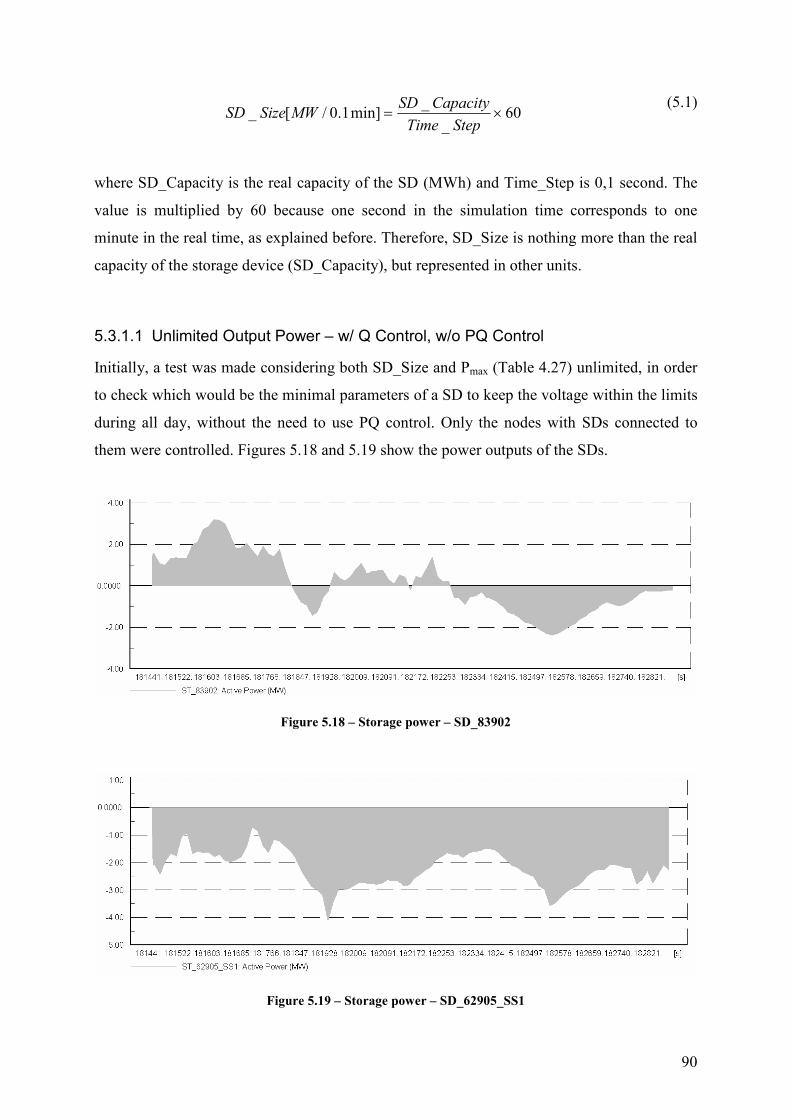
90
60_
_min]1.0/[_ ×=
StepTime
CapacitySDMWSizeSD
(5.1)
where SD_Capacity is the real capacity of the SD (MWh) and Time_Step is 0,1 second. The
value is multiplied by 60 because one second in the simulation time corresponds to one
minute in the real time, as explained before. Therefore, SD_Size is nothing more than the real
capacity of the storage device (SD_Capacity), but represented in other units.
5.3.1.1 Unlimited Output Power – w/ Q Control, w/o PQ Control
Initially, a test was made considering both SD_Size and Pmax (Table 4.27) unlimited, in order
to check which would be the minimal parameters of a SD to keep the voltage within the limits
during all day, without the need to use PQ control. Only the nodes with SDs connected to
them were controlled. Figures 5.18 and 5.19 show the power outputs of the SDs.
Figure 5.18 – Storage power – SD_83902
Figure 5.19 – Storage power – SD_62905_SS1
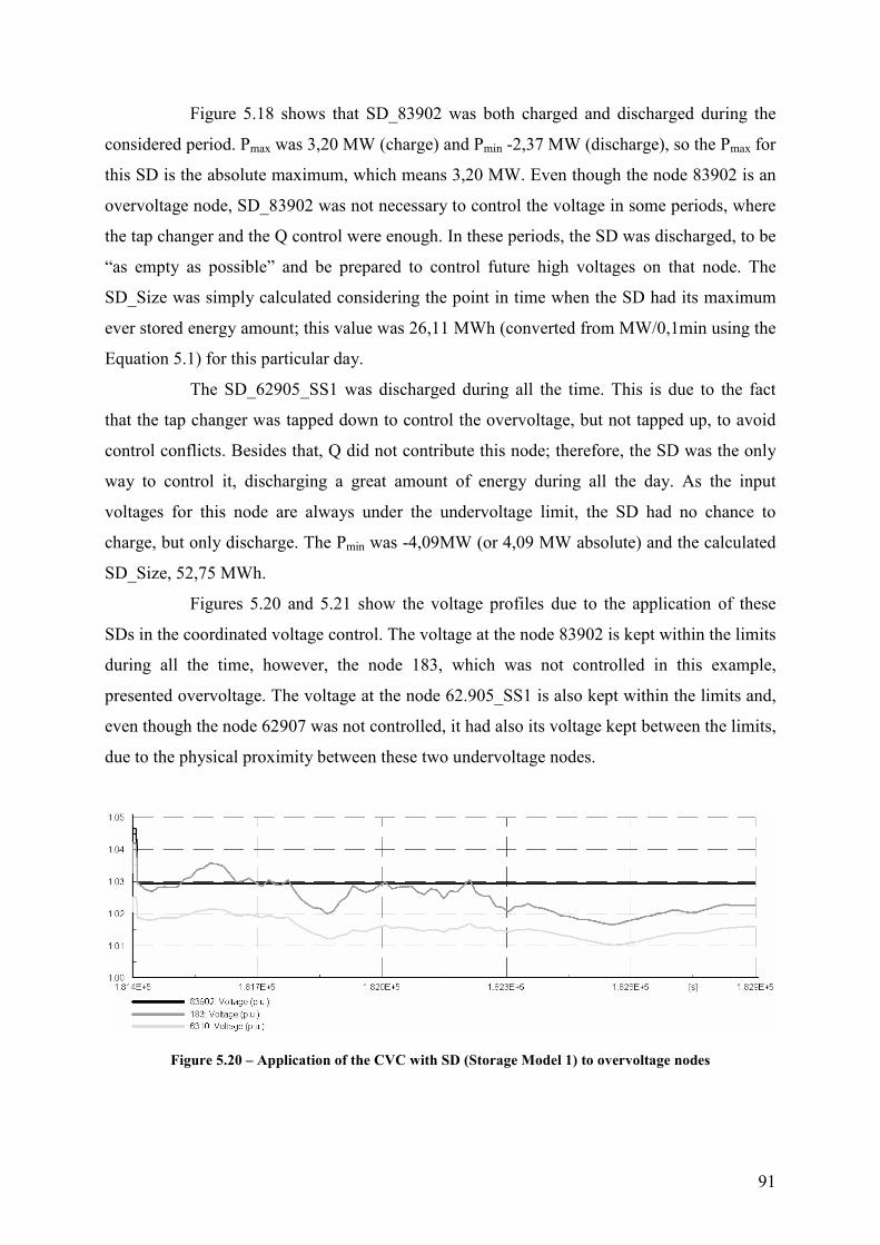
91
Figure 5.18 shows that SD_83902 was both charged and discharged during the
considered period. Pmax was 3,20 MW (charge) and Pmin -2,37 MW (discharge), so the Pmax for
this SD is the absolute maximum, which means 3,20 MW. Even though the node 83902 is an
overvoltage node, SD_83902 was not necessary to control the voltage in some periods, where
the tap changer and the Q control were enough. In these periods, the SD was discharged, to be
“as empty as possible” and be prepared to control future high voltages on that node. The
SD_Size was simply calculated considering the point in time when the SD had its maximum
ever stored energy amount; this value was 26,11 MWh (converted from MW/0,1min using the
Equation 5.1) for this particular day.
The SD_62905_SS1 was discharged during all the time. This is due to the fact
that the tap changer was tapped down to control the overvoltage, but not tapped up, to avoid
control conflicts. Besides that, Q did not contribute this node; therefore, the SD was the only
way to control it, discharging a great amount of energy during all the day. As the input
voltages for this node are always under the undervoltage limit, the SD had no chance to
charge, but only discharge. The Pmin was -4,09MW (or 4,09 MW absolute) and the calculated
SD_Size, 52,75 MWh.
Figures 5.20 and 5.21 show the voltage profiles due to the application of these
SDs in the coordinated voltage control. The voltage at the node 83902 is kept within the limits
during all the time, however, the node 183, which was not controlled in this example,
presented overvoltage. The voltage at the node 62.905_SS1 is also kept within the limits and,
even though the node 62907 was not controlled, it had also its voltage kept between the limits,
due to the physical proximity between these two undervoltage nodes.
Figure 5.20 – Application of the CVC with SD (Storage Model 1) to overvoltage nodes

92
Figure 5.21 – Application of the CVC with SD (Storage Model 1) to undervoltage nodes
5.3.1.2 Unlimited Output Power – w/ Q Control, w/o PQ Control (MOC)
Another test was carried out, but this time with the possibility to control all the overvoltage
nodes simultaneously (“MOC” – Multiple Overvoltage Control). SD_83902 was permitted to
control also the voltage at the node 183. With this modification, the new PQ priority matrix
would be as shown on table 5.5.
Table 5.5 – Priority matrix for PQ control (SD_83902 contributes also to the voltage at the node 183)
Critical Nodes
62905-SS1
183 83902 6310
X X X 1 DEA_DG8_W
X X 4 4 DEA_DG9_W
X 4 3 3 DEA_DG13_V2_2MW
X 3 X 2 DEA_DG13_V3_2MW
DG
X 5 5 X SD_83902
5 X X X SD_62905_SS1 SD
Figures 5.22 and 5.23 show the voltage profiles for the overvoltage nodes and the
SD_83902 power output, respectively.

93
Figure 5.22 – Application of the CVC with SD (Storage Model 1) to overvoltage nodes – SD_83902
contributes to the voltages at the nodes 83902 and 183.
Figure 5.23 – Storage power – SD_83902 (contributes to the voltages at the nodes 83902 and 183)
In this case, the highest Pmax was 4,45MW and the lowest was again -2,37 MW.
Pmax is the maximum absolute (4,45 MW). There are again periods when the SD is
discharged. The SD_Size was calculated this time as 29,92 MWh.
At the undervoltage node 62.905_SS1, Pmax (4,09 MW) and SD_Size (52,93
MWh) are almost the same as the values obtained for the last case. This was already expected
as the contribution of SD_62.905_SS1 on the PQ priority matrix was not altered.
5.3.1.3 Limited Power Output – w/ Q and PQ Control
The next test considers that Pmax of SD_83902 is limited and is only enough to keep the
voltage within the limits if the PQ control is also considered. Pmax for this test was found,
empirically, to be 0,65 MW, for charge and discharge. Figure 5.24 shows the power output of
the SD. The value of SD_Size was also calculated and is 8,45 MWh, which is smaller than the
value obtained without storage limits.
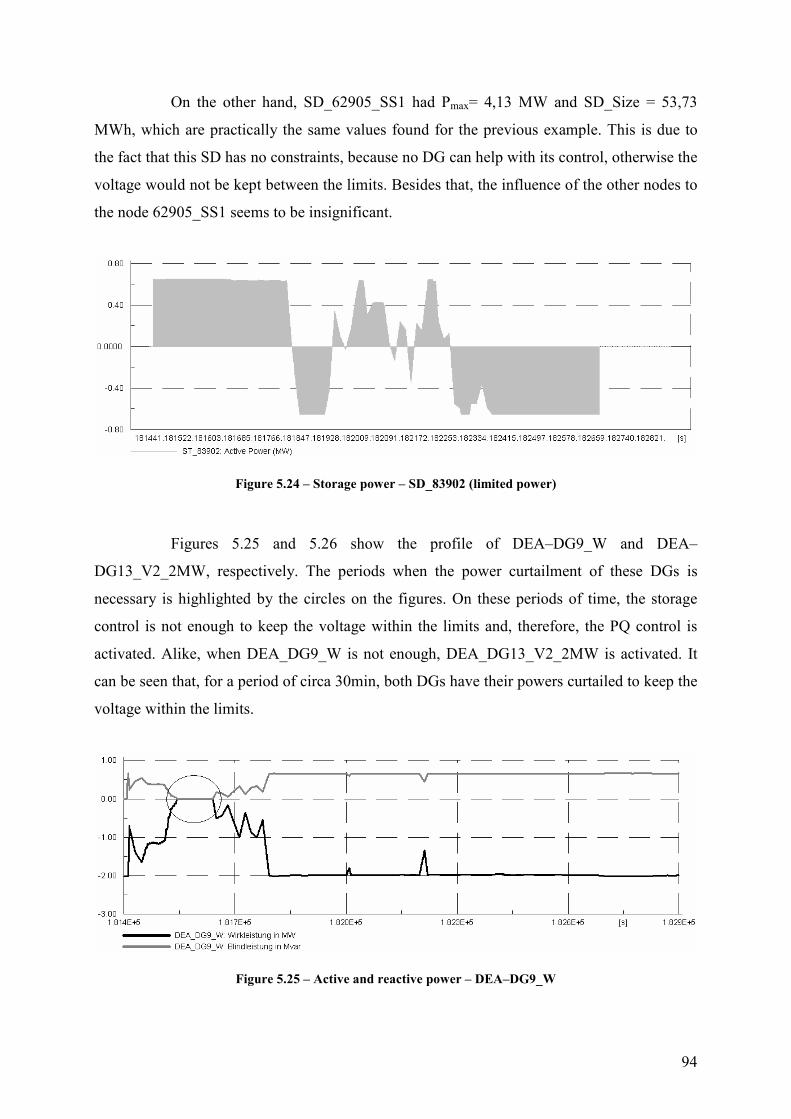
94
On the other hand, SD_62905_SS1 had Pmax= 4,13 MW and SD_Size = 53,73
MWh, which are practically the same values found for the previous example. This is due to
the fact that this SD has no constraints, because no DG can help with its control, otherwise the
voltage would not be kept between the limits. Besides that, the influence of the other nodes to
the node 62905_SS1 seems to be insignificant.
Figure 5.24 – Storage power – SD_83902 (limited power)
Figures 5.25 and 5.26 show the profile of DEA–DG9_W and DEA–
DG13_V2_2MW, respectively. The periods when the power curtailment of these DGs is
necessary is highlighted by the circles on the figures. On these periods of time, the storage
control is not enough to keep the voltage within the limits and, therefore, the PQ control is
activated. Alike, when DEA_DG9_W is not enough, DEA_DG13_V2_2MW is activated. It
can be seen that, for a period of circa 30min, both DGs have their powers curtailed to keep the
voltage within the limits.
Figure 5.25 – Active and reactive power – DEA–DG9_W

95
Figure 5.26 – Active and reactive power – DEA–DG13_V2_2MW
Figure 5.27 shows the voltage profile for the overvoltage nodes. While the voltage
at node 83902 is kept within the limits, the node 183 presents light overvoltage for a period of
time, as only the first one was controlled on this example.
Figure 5.27 – Application of the CVC with SD (Storage Model 1) to overvoltage nodes
An interesting comparison can be made considering the necessary DGs curtailed
energy to control the voltage. In this case it is necessary to subtract the PQ control output
powers from the DG generation profile. For May 7th, 10,65 MWh were curtailed in order to
control the voltage. The sum of all the storage positive outputs (charges) gives how much
energy was not necessary to be curtailed by the DGs to control the voltage. This value was
10,61 MWh. If the SD control was not used, the DGs curtailment would be 21,26 MWh. This
means that almost 50% of the energy that would be curtailed by the DGs to control the
voltage was compensated by the SD control.
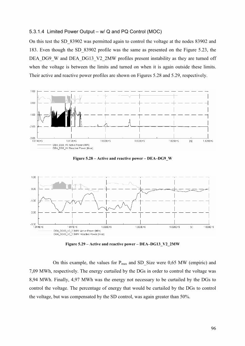
96
5.3.1.4 Limited Power Output – w/ Q and PQ Control (MOC)
On this test the SD_83902 was permitted again to control the voltage at the nodes 83902 and
183. Even though the SD_83902 profile was the same as presented on the Figure 5.23, the
DEA_DG9_W and DEA_DG13_V2_2MW profiles present instability as they are turned off
when the voltage is between the limits and turned on when it is again outside these limits.
Their active and reactive power profiles are shown on Figures 5.28 and 5.29, respectively.
Figure 5.28 – Active and reactive power – DEA–DG9_W
Figure 5.29 – Active and reactive power – DEA–DG13_V2_2MW
On this example, the values for Pmax and SD_Size were 0,65 MW (empiric) and
7,09 MWh, respectively. The energy curtailed by the DGs in order to control the voltage was
8,94 MWh. Finally, 4,97 MWh was the energy not necessary to be curtailed by the DGs to
control the voltage. The percentage of energy that would be curtailed by the DGs to control
the voltage, but was compensated by the SD control, was again greater than 50%.

97
Figures 5.30 and 5.31 show the voltage profile at the overvoltage and
undervoltage nodes respectively. Especially for the overvoltage nodes, the control instability
causes the voltage to present incongruities.
The SD power and capacity should be greater than on the last case, due to the fact
that two nodes are being controlled instead of one; however, they are smaller due to the
aforementioned control instability.
Figure 5.30 – Application of the CVC with SD to overvoltage nodes
Figure 5.31 – Application of the CVC with SD to undervoltage nodes
It is important to highlight that the SDs don’t contribute to these control
instabilities as they are always active and are never turned off. When they are not necessary to
keep the voltage within the limits, they charge or discharge in order to reach the storage
setpoint and, therefore, maximize their control capacity
New methods to control multiple nodes simultaneously with PQ control are being
developed and are discussed in chapter 6.

98
5.3.2 Storage Model 2 – Integrated Storage System
The generator DEA_DG10_W, connected to the node 83902, can be modeled according to the
Storage Model 2 presented in chapter 4. In this case, the SD_83902 is disconnected and the
storage is the DEA_DG10_W itself. As no generator is connected to the 62905_SS1, it can
not be modeled according to the second Storage Model.
Since the Storage Model 2 considers the SD as the generator itself, Pout is equal
to the generator output, which is a sum of the required generation and the storage output, but
cannot be greater than the maximum production of the generator (See Figure 4.20).
5.3.2.1 Generator Limited Output – w/o Q/PQ Control
The first test considers that no Q or PQ controls are activated. The voltage at the node 83902
is controlled only by the transformer’s tapping and the SD control. Figure 5.32 shows the
profile at the DEA_DG10_W. It can be seen that the reactive and active power regulation are
at their limit, for some hours, but it was not sufficient to keep the voltage within the limits
during all the time, as seen on Figure 5.33.
Figure 5.32 – Active and Reactive Power at DEA_DG10_W (Model 2)

99
Figure 5.33 – Voltage profile at node 83902 – SD Model 2 control (No Q nor PQ control)
Pmax was limited by the generator’s nominal power (≈1 MW) and the SD_Size
was calculated as 11,43 MWh. The amount of energy not curtailed, and stored, was
11,36 MWh.
5.3.2.2 Generator Limited Output – w/ Q Control and w/o PQ Control
Considering also the Q control, the voltage is kept between the limits for a longer time, as can
be seen on Figure 5.34. However, there are again periods when the control is not enough to
keep the voltage within the limits. Figure 5.35 shows the active and reactive power of the
DEA_DG10_W, while trying to control the voltage.
Figure 5.34 – Voltage profile at node 83902 – Storage Model 2 (Q control, but no PQ control)

100
Figure 5.35 – Active and reactive power at DEA–DG10_W (Storage Model 2)
Pmax is again ≈ 1 MW and the SD_Size was calculated as 8,09 MWh. The amount
of energy not generated in order to control the voltage was 8,03 MWh. This energy was again
stored and not thrown away.
5.3.2.3 Generator Limited Output – w/ Q and PQ Control
Considering also the PQ control, it was possible to keep the voltage between the limits during
all the day, as presented on Figure 5.36. The Figure shows some instabilities around the
overvoltage limit, which are caused by turning the controllers on and off.
Figure 5.36 – Voltage profile at node 83902 – Storage Model 2 (with Q and PQ control)
Figure 5.37 shows the active and reactive power of the DEA_DG10_W, while
controlling the voltage at the node 83902. These powers are at their limit for some period of
time.

101
Figure 5.37 – Active and reactive power at DEA_DG10_W (Storage Model 2)
Figure 5.38 shows the active and reactive power profile at DEA_DG9_W, which
is also necessary to keep the voltage between the limits. This generator is also at its limit for a
short period, marked with a small circle on the figure.
Figure 5.38 – Active and reactive power at DEA_DG9_W
DEA_DG13_V2_2MW was not necessary to control the voltage and could
generate according to its normal profile.
The storage parameters were Pmax ≈ 1 MW and SD_Size = 4,50 MWh. The
amount of energy not generated, and stored, in order to control the voltage was 4,38 MWh.
The table below groups the results obtained for both Storage Models 1 and 2 and
the tested control variations. The “SD Control Contribution” and “DG Control Contribution”
can be considered as the same for the Storage Model 2, as the storage system is, in fact, the
generator itself, with the difference that it stores the energy, instead of curtailing it.

102
Table 5.6 – Storage Models 1 and 2 – Results summary
OVERVOLTAGE UNDERVOLTAGE
Pmax
(MW) SD_Size (MWh)
SD Control Contribution
(MWh)
DG Control Contribution
(MWh)
Pmax
(MW) SD_Size (MWh)
1 Unlimited Power Q Control
3,20 26,11 28,84 X 4,09 52,75
2 Unlimited Power Q Control (MOC)
4,45 29,92 32,65 X 4,09 52,93
3 Limited Power Q / PQ Control
0,65 8,45 10,61 10,65 4,13 53,73
ST
OR
AG
E
MO
DE
L 1
4 Limited Power Q / PQ Control (MOC)
0,65 7,09 8,94 4,07 4,04 53,00
1 No Q nor PQ ≈1 11,43 11,36 X X
2 Q, no PQ ≈1 8,09 8,03 X X
ST
OR
AG
E
MO
DE
L 2
3 Q and PQ ≈1 4,50 4,38 X X
The voltage is kept between the limits for all the four cases of the Storage
Model 1. For the Storage Model 2, the voltage is kept between the limits only in the third
case. The values in italic for the fourth case in the Storage Model 1 are approximated due to
the control instabilities. These values should be in fact greater than those of the third case,
since the multiple overvoltage control (MOC) is active.

103
6 Conclusions and Next Steps
In this work, the application of the storage to control the voltage in distribution networks was
presented. This application was based on the coordinated voltage control in the framework of
the project DG-DemoNet. The results show that this approach can be a good alternative, but
is, of course, strongly dependant on the applied technology.
Some technologies, like the hydrogen storage, are not yet fully developed, but can
be in the future a good option for the desired application, or even better than the technologies
that were selected. It is also necessary to investigate what would be the requirements of the
DNO for the integration of these technologies to the distribution networks.
Obtaining detailed technical information and costs for some of the technologies,
particularly those under development, is extremely difficult. As a result, some of the costs
may change as the technologies reach full development or as competition with other
technologies drives prices down.
The flow batteries are of extreme interest because their capacity and output power
are independent from each other. This is very important as there can be a critical node where
the voltage is always too high (or too low) but not far from the voltage limit. It means this
node needs constant charge/discharge action but not high output power is required. On the
other hand, there can be a node where the storage voltage control action is not often required,
but it needs a high power to bring the voltage between the limits.
Batteries (of one type or another) can address all application areas, although they
are not always the least expensive option. The replacement costs factor is significant into the
life-cycle costs of batteries, much more so than other technologies. The batteries connected to
nodes that need intensive storage voltage control need to be selected by a rigorous life-cycle
criterion.
The CAES technology is very cost-effective for bulk energy storage and can be
applied at nodes that need high capacity storage devices.
In almost all applications, particularly for large scale systems, the installations are
composed of multiple units or cells that are combined in series and/or parallel arrangements to
achieve the system rating for power and stored energy. For example, battery systems almost
always have cells in series to form a string with an appropriate operating voltage and multiple
strings in parallel to achieve the total stored energy. Similarly, pumped hydro systems have
multiple turbines, each of which operates most effectively at a specific power output level.
Regarding the results obtained in chapter 5, the normally accepted undervoltage
limit is 0,94, however, there was no voltages under 0,94 during all the year, the undervoltage

104
limit was set to 0,98. This caused the undervoltage nodes, namely 62907 and 62905_SS1 to
present undervoltage during all the selected day. Therefore the SD for undervoltage control
needed to discharge during twenty four hours leading to the very high storage capacity
requirements obtained for undervoltage control.
Another important aspect in this work is the lack of time constants for the
simulations presented in this work. Not only the reaction time of the diverse storage
technologies should be taken in account, but also all the time constants related to all the
distribution network elements, like generators, transformers and loads. A new graduation
thesis will start on September, 2008 at arsenal research with the objective to determine the
time constants for the voltage regulation concepts in medium voltage networks. This work
will take into account the voltage dynamics, transformer switching, determination of time
constants for generators and loads (dynamic P and Q). The obtained values will be used to
improve the coordinated voltage regulation algorithm to reflect the real response of the system
to the active voltage control.
One of the main difficulties in this work was to embed the storage control to the
CVC, trying always not to change drastically the behavior of the already existing control.
Both the original code and the new code have some issues that need to be solved in order to
provide more accurate and efficient simulation results.
Some important modifications are being currently accomplished in order to
develop a more readable and clean algorithm, but also with the objective to improve and
broader the control concept. These changes can be highlighted as:
• Simultaneous optimization of multiple critical nodes, avoiding undesired effects like
those evidenced in chapter 5, caused by the fact that the voltage control is currently
performed sequentially. This multiple optimization could be performed by the
application of simultaneously control loops. One of the difficulties associated to this
solution is that the voltage control in one of the critical nodes can have influences on
others and, therefore, the multiple voltage control loops need to be coupled;
• Improvement of the precision of the priority matrix: Unlike the currently qualitative
classification of the contribution of DEAs and SDs to critical nodes (only sequential),
the new classification will be quantitative; illustrating clearly how important is the
contribution of these elements to the voltage at a specific node;

105
• Improvement of the transition between normal operation and voltage control. In the
present coordinated control algorithm, the control is abruptly turned off when the
voltage is within the limits, causing control instabilities around these limits. This could
be implemented by the coordinated application of open and closed control loops
through a states machine. With the system dynamics and the usage of a states machine
it will be possible to define the states and temporally activated transitions;
• Development of a simulations environment to test and debug the algorithmic routines.
This is important from the developer’s point of view, since the integration between
MATLAB® and DIgSILENT PowerFactory® doesn’t allow any debugging.
Therefore, a simulation environment is being already created; using a MATLAB®
based toolbox called PSAT®. The idea is to test and validate the routines using
PSAT®, and then simulate them with DIgSILENT. It is important to assure that the
target network is the same and has the same parameters in both PSAT® and
DIgSILENT and to assure a minimal cost for this porting between the two systems.
Still regarding the priority matrix, the selection of the generators which perform
voltage control must be done on the basis of detailed analysis through offline studies. The
critical nodes have to be selected on the basis of offline studies in order to ensure that
compliance with the voltage limits at these nodes imply compliance in the whole network. Of
course, the effectiveness of this control is limited by the network characteristic (e.g. different
load flow characteristic of medium voltage branches). This solution also supposes a
communication infrastructure with limited requirements between selected nodes and the
OLTC controller.
Also interesting is the evaluation of the effectiveness of a specific voltage control
method in scenarios with different DG penetration rates, or in other words, to what DG
penetration rate a method is still valid.
The most critical point of the future integration of the validated CVC to a real
network is the communication infrastructure of the network. The control needs to obtain all
the necessary inputs to perform the calculations and provide its results. If, however, one of the
inputs takes longer than the estimated time to be read, it can delay the control. Therefore,
there is also the need to determine the time constants of the communication devices and to
figure out how they can be configured and integrated. Depending on the chosen
communication technology, a varying delay on these lines has to be expected

106
Another future investigation can be the application of Demand Side Management
(DSM) in addition to the CVC and storage technologies. The following lines give a brief
overview about the DSM and how it could be used in addition to the voltage control methods
present in this work.
Demand side management can be understood as the planning and implementation
of utility activities designed to influence customer use of electricity in ways that will produce
desired changes in the utility’s load shape, i.e., changes in the pattern and magnitude of a
utility’s load. Demand-side management encompasses the entire range of management
functions associated with directing demand-side activities. Opportunities for demand-side
management can be found in all customer classes, including residential, commercial,
industrial, and wholesale (DELGADO, 1985).
The DSM can reduce the demand peaks, shift the loads between times of day or
even seasons, fill the demand valleys to better utilize existing power resources, reduce overall
demand (strategic saving) in the context of delivering the required energy services by use of
less energy (and not a reduction in services) and provide strategic growth especially to shift
between one type of supply to another with more favorable characteristics, for example, in
terms of the environment.
DSM can also have some positive effect in grids with high share of DG. As the
voltage problem presents the main power quality problem in networks with DG, it was
identified that DSM techniques can be used to mitigate a voltage rise effect caused by DG and
can be also used as a complementary technique in conjunction with a conventional technique
to minimize voltage rise effects on distributions networks. The advantages of using DSM are
as follows:
• DSM may be able to mitigate voltage rise problems with minimum network
reinforcement;
• It may be able to mitigate voltage rise problems on a low voltage network integrated
with DG;
• DSM may be able to avoid any voltage rise problems with minimum generation
constraint;
• DSM provides a more robust solution to voltage rise problems than a voltage regulator
due to the system having no single point of failure and a certain level of redundancy.

107
Figure 6.1 shows an example of the application of DSM to the voltage control. In (a) two load
switching profiles can be seen. A controlled load and a PV unit are connected to the same
node. To keep the voltage between the required ±10 % limits (Figure 6.1 (b)) the load is
increased by 50 % of its normal value (normal value is represented with dotted red curve in
Figure 6.1 (a)). When the voltage reaches the lower voltage limit the load reduces by 50 % of
its normal value. It can be seen from Figure 6.1 (b) that DSM can help to keep the voltage
between the required limits.
Figure 6.1 – Voltage control with DSM – load in kW (a) and voltage at the point of common coupling (b)
Another specific further approach would be the usage of storage technologies to
fulfill the goals of the load management on distribution level. Load management can be
understood as the utility activities designed to influence the timing and magnitude of customer
use of electricity. To many people, the traditional load shape objectives of load management
include peak clipping, valley filling, and load shifting.
In the case of fast changing load flow patterns or changes in the distribution of the
loads or power plants among the grid, the risk of voltage instability increases. One of the
solutions could be the injection of an amount of power into the grid, stored earlier during the
time that there was no need for peak power, to maintain the voltage. Two possibilities using
SMES and Redox Flow Batteries are presented in (SELS et al., Sep. 2001) and the results
promise an increased overall efficiency of the power plant and on the other hand an increased
stability of the electrical distribution grid. Both solutions can act very quickly on peak
demands or transients in the load pattern and have stabilizing effects. This will introduce new
perspectives for load managing on distribution level.
In any case, if DSM would be used together with the CVC and SDs, a priority
order between local voltage control with DG units, SD control and DSM should be

108
introduced, and, for the real application of the DSM concepts, an evaluation of the
quantitative potential of DSM would be necessary, both for habitations and for the industry.
Finally, it is important to reinforce that the method developed in this work was
intended to determine the most suitable technologies for the application to the voltage control
and, despite this is a difficult choice, it is expected that all the improvements currently carried
out will help to refine this method and adequate it to play an important role in the voltage
control schemes of distribution networks with a high penetration of distributed generation.

109
References
BLAABJERG, F., IOV, F., “Advanced Power Converters for Universal and Flexible Power
Management in Future Electricity Network”, Deliverable No. D2.1, 20 Feb. 2007.
BODACH, M., "Energiespeicher im Niederspannungsnetz zur Integration dezentraler,
fluktuierender Energiequellen", Dissertation, Chemnitz, 30 Jun. 2006.
BRUNNER, H., KERIN, U., BLETTERIE, B., LUGMAIER, A., PAPIC, I., “Distribution
Network Voltage Control Based on Distributed Generation Power Injection Share”, ERK, 24 -
26 Sep. 2007.
CHEUNG K.Y.C, CHEUNG S.T.H, NAVIN DE SILVIA R.G, JUVONEN M.P.T, SINGH R,
WOO J.J., “Large-Scale Energy Storage Systems”, Imperial College London: ISE2,
2002/2003
DELGADO, R.M., “Demand-side management alternatives”, Proceedings of the IEEE, Oct.
1985: 1471- 1488
DIgSILENT PowerFactory® Version 13.1 User Manual, Nov. 2005.
DISTRICT ENERGY – Energy Storage, http://www.energy.rochester.edu/storage/, accessed
on 11/05/2008.
ERBEN, S., “Wirtschaftlicher und ökologischer Vergleich verschiedener Technologien zur
Speicherung von Elektrizität”, Diplomarbeit, 2008.
ESA (Electricity Storage Association), http://www.electricitystorage.org/, accessed many
times between November/2007 and August/2008.
HI-ENERGY – Renewable Energy in the Highlands & Islands, Glossary of Renewable
Energy, http://www.hi-energy.org.uk/glossary.html, accessed on 12/01/2008.

110
JENKINS, N., ALLAN, R., CROSSLEY, P., KIRSCHEN, D. and STRBAC, G., Embedded
Generation. London: IEE, 2000.
KUPZOG, F., BRUNNER, H., PRUGGLER, W., PFAJFAR, T., LUGMAIER, A., “DG
DemoNet-Concept - A new Algorithm for active Distribution Grid Operation facilitating high
DG penetration”, 5th IEEE International Conference on Industrial Informatics, 23-27 June
2007: 1197 – 1202.
LUGMAIER A., BRUNNER H., BLETTERIE B., KUPZOG F., ABART A., “Intelligent
Distribution Grids in Respect of a Growing Share of Distributed Generation”, CIRED - 19th
International Conference on Electricity Distribution, 21-24 May 2007.
NAMISNYK, A., “A survey of electromechanical Supercapacitor technology“, University of
Technology, Sydney Faculty of Engineering, 23 June 2003.
PEÇAS LOPES, J.A., SECA, L., “Intentional islanding for reliability improvement in
distribution networks with high DG penetration”, 2005 International Conference on Future
Power Systems, 16-18 Nov. 2005: 1 - 5.
SCHOENUNG, S.M., W.V. HASSENZAHL, “Long- vs. Short-Term Energy Storage
Technologies Analysis A Life-Cycle Cost Study”, in Sandia Report, Aug. 2003.
SCHWAEGERL, C., “Recommendations for further R&D needs”, ENIRGnet project, WP7.2,
D23, 5 Nov. 2004.
SELS, T., DRAGU, C., VAN CRAENENBROECK, T., BELMANS, R., “Electrical energy
storage systems: Existing systems versus newest systems - an overview”, International
Conference Power Generation and Sustainable Development (AIM), Liège, Belgium, 8 – 9
Oct. 2001
SELS, T., DRAGU, C., VAN CRAENENBROECK, T., BELMANS, R., “New energy
storage devices for an improved load managing on distribution level”, IEEE Porto Power
Tech Proceedings, 10 - 13 Sep. 2001.
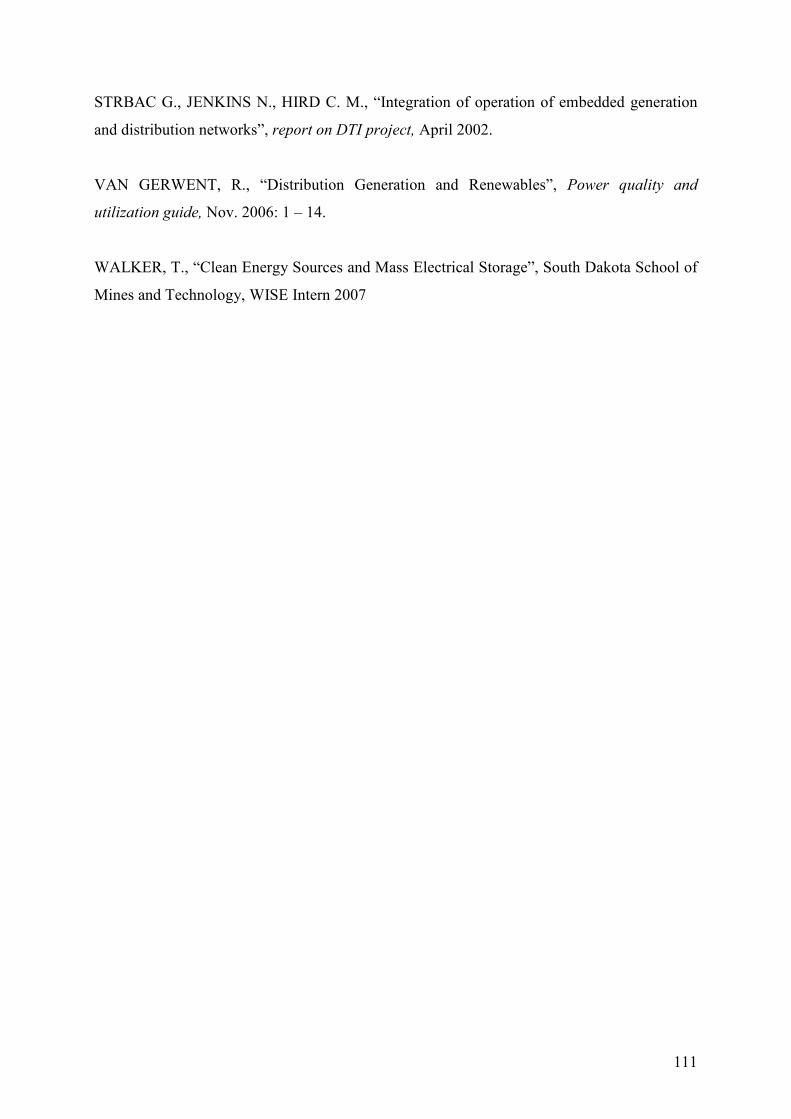
111
STRBAC G., JENKINS N., HIRD C. M., “Integration of operation of embedded generation
and distribution networks”, report on DTI project, April 2002.
VAN GERWENT, R., “Distribution Generation and Renewables”, Power quality and
utilization guide, Nov. 2006: 1 – 14.
WALKER, T., “Clean Energy Sources and Mass Electrical Storage”, South Dakota School of
Mines and Technology, WISE Intern 2007


![[SPO][PT-BR] Ficha de Matricula ALEGRIA SOCIAL v1.5 Distributed](https://static.fdocumentos.com/doc/165x107/577c84c61a28abe054ba49f6/spopt-br-ficha-de-matricula-alegria-social-v15-distributed.jpg)