
Modelling and Optimization of Large-Scale Processes ... · DEPARTAMENTO DE ENGENHARIA QUIMICA...
350
DEPARTAMENTO DE ENGENHARIA QUIMICA FACULDADE DE CIENCIAS E TECNOLOGIA UNIVERSIDADE DE COIMBRA Modelling and Optimization of Large-Scale Processes — Application to the liquid-phase aniline production Dissertação apresentada à Faculdade de Ciências e Tecnologia da Uni- versidade de Coimbra, para obtenção do grau de Doutor em Engenharia Química, na especialidade de Processos Químicos. Filipe José Marques Neves PORTUGAL 2007
Transcript of Modelling and Optimization of Large-Scale Processes ... · DEPARTAMENTO DE ENGENHARIA QUIMICA...
DEPARTAMENTO DE ENGENHARIA QUIMICA
FACULDADE DE CIENCIAS E TECNOLOGIA
UNIVERSIDADE DE COIMBRA
Modelling and Optimization ofLarge-Scale Processes — Application to
the liquid-phase aniline production
Dissertação apresentada à Faculdade de Ciências e Tecnologia da Uni-versidade de Coimbra, para obtenção do grau de Doutor em EngenhariaQuímica, na especialidade de Processos Químicos.
Filipe José Marques Neves
PORTUGAL 2007

Work financially supported by
under the program Bolsas de Doutoramento em Empresas(BDE/15512/2004).

Dedico este trabalho aos meus pais:José Neves e Maria Licínia.
Obrigado por tudo aquilo que não pode ser expresso por palavras.
iii

Agradecimentos
A realização deste trabalho não teria sido possível sem a contribuição de diversas pessoase entidades, não só a um nível técnico / logístico, mas também num plano pessoal. Assim,e porque o todo de um trabalho resulta sempre do somatório de várias partes, aqui deixoos meus sentidos agradecimentos:
• ao Nuno Oliveira, meu orientador académico, pela sua excelência técnica (umareferência para o meu futuro) e pelo seu contínuo esforço em me tentar transmitirque, para além de aprender a pensar, também é importante aprender a aprender.Agradeço-lhe ainda a amizade, honestidade e integridade que sempre pautaram assuas acções e que contribuíram, marcadamente, para tornar todo este trabalho numaexperiência produtiva, agradável e pessoalmente valorizante. Resta-me assim es-perar pelo privilégio de poder contar com a sua parceria em novas “aventuras”, aolongo do trajecto profissional que se estende à minha frente. Por fim, uma palavrade apreço pelo seu esforço e contribuição para a elaboração deste documento final.
• ao Fernando Mendes, coordenador deste trabalho na empresa, por tão bem me tertransmitido que “existe vida para além da teoria”. A partilha dos seus vastos con-hecimentos, especialmente no que respeita à ligação de aspectos de cálculo com asua implementação prática, constituiu (e, felizmente, ainda constitui) uma das ex-periências mais enriquecedoras e valiosas da minha vida profissional. Agradeço-lheainda a amizade que tantas vezes demonstra, e o apoio que sempre assegurou nasactividades desenvolvidas em conjunto.
• à CUF — Químicos Industriais, S.A., na pessoa dos Eng. Mário Jorge e João Fu-gas, por ter acreditado no plano de trabalhos desta Tese, e nas minhas própriascapacidades em o executar, viabilizando assim o presente momento. Para além doimplícito apoio financeiro, agradeço ainda à CUF–QI a criação de condições detrabalho óptimas, sem as quais muitos dos objectivos deste documento não teriamsido alcançados. Ao Eng. Vilela de Matos, o meu agradecimento também pelo seuespírito pioneiro na criação destas oportunidades de desenvolvimento.
• à FCT — Fundação para a Ciência e Tecnologia, pela concessão de apoio financeiroao abrigo do programa de Bolsas de Doutoramento em Empresa (BDE/15512/2004).
• à FCTUC — Faculdade de Ciências e Tecnologia da Universidade de Coimbra, pela
v

vi
oportunidade de desenvolver e defender esta Tese, sob a sua filiação académica.
• ao DEQ — Departamento de Engenharia Química da FCTUC, pelas infra-estruturasde apoio disponibilizadas. Agradeço a alguns dos seus docentes, nomeadamenteaos Professores Lino Santos, Cristina Gaudêncio, Jorge Rocha, Hermínio Sousa,Helena Gil, Margarida Figueiredo, Pedro Simões e Abel Ferreira, pela sua simpatia,prestabilidade e incentivo. Um palavra de especial apreço à Mafalda Fernandes eao Adamo Caetano, pelas inúmeras ocasiões em que me auxiliaram de forma tãodecisiva.
• ao Paulo Araújo, o meu primeiro coordenador em ambiente empresarial, ainda antesde iniciar o presente Doutoramento. A ele lhe agradeço a orientação e o apoionaquela que foi a minha primeira experiência na indústria, um momento marcantedo qual só guardo boas recordações, e que contribuiu decisivamente para uma cas-cata de acontecimentos que culminaram nesta Tese. Agradeço-lhe ainda a seu pre-cioso auxílio logístico para o términus do processo de escrita deste documento; sema sua compreensão, toda esta etapa final teria sido bastante mais difícil e penosa.
• à Dulce Silva por, ao longo de todos estes anos, ter sido uma colega de trabalhoinexcedível. Agradeço-lhe a boa vontade e prontidão com que sempre se disponi-bilizou para me ajudar, e que tão importante foi na fase inicial deste Doutoramento.Uma palavra de apreço também pela partilha dos seus conhecimentos em LATEX,que permitiu acelerar, de forma drástica, todo o processo de escrita desta Tese.
• ao Jorge Coelho, meu grande amigo, pelo seu constante incentivo e apoio ao longode todos estes anos, pelo sempre pronto “sim” em resposta a qualquer pedido deauxílio, pelos muitos conselhos que teve a bondade de partilhar comigo. Por maiori-tária influência dele optei por escrever esta Tese em Inglês, facto este que hoje muitome apraz e que lhe irei sempre agradecer.
Por último, não por serem menos importantes mas, ao invés, porque merecem um lugar dedestaque, gostaria de agradecer a todos aqueles que constituem a minha mais íntima esferaprivada. Aos meus pais, José Neves e Maria Licínia, que por mais Teses que lhes dediquee por mais palavras que gaste, nunca conseguirei expressar a gratidão e orgulho que sintoenquanto seu filho; são a mais importante referência da minha vida, e nunca o deixarão deser. Ao meu irmão, Luis Neves, à minha cunhada, Carla Susana, e às minhas sobrinhas,Catarina e Patrícia, por serem a melhor família que alguém pode desejar; obrigado peloconstante apoio, por um sorriso sempre pronto, por todo o carinho e ajuda a que mehabituaram. Finalmente, um agradecimento especial à Yolanda Assunção, por partilharcomigo todas as tristezas, felicidades e sonhos, dividindo as primeiras, multiplicando assegundas, e fazendo dos últimos algo pelo qual vale a pena lutar.

Resumo
Motivações
A progressiva diminuição das margens de lucro, fruto de uma concorrência internacional,obriga as empresas a assumir como objectivo crucial, mais do que nunca, o contínuodesenvolvimento dos seus processos produtivos. Neste sentido, gerar um conjunto demétodos e ferramentas, capaz de responder às necessidades específicas de cada indústria,deverá ser uma tarefa assumida pela Engenharia de Sistemas e Processos (ESP), abrindouma importante janela de oportunidades, e criando em simultâneo um vasto conjunto dedesafios.
Caso de estudo
A instalação em estudo, propriedade da CUF — Químicos Industriais, S.A., assegurauma produção anual de 120 kton/ano de anilina, via hidrogenação do nitrobenzeno emfase líquida. O processo pode ser decomposto em duas secções principais: reacção eseparação. A primeira secção, onde grande parte do consumo de utilidades frias ocorre,é constituída por várias unidades trifásicas, onde finas partículas suspensas asseguramuma catálise heterogénea. A segunda secção, grande consumidora de utilidades quentes,compreende um complexo arranjo de 7 colunas de destilação e 5 separadores de fase,onde 10 compostos (a maioria em composições vestigiais) exibem equilíbrios complexos.
Objectivos gerais
Os objectivos gerais deste trabalho consistem na construção de modelos matemáticos ca-pazes de descreverem globalmente este processo, e na sua utilização para a simulação eoptimização do mesmo.
Deste modo, numa perspectiva Académica, os esforços foram concentrados em lidar, deforma eficiente, com um conjunto significativo de dificuldades, através da melhoria e /ou desenvolvimento de estratégias de ESP; nesta vertente, construir modelos matemáticosrepresentativos, ultrapassar problemas numéricos durante a sua solução e evitar resultados
vii

viii
de baixa qualidade aquando da sua optimização, constituíram os desafios mais comuns.Numa perspectiva Industrial, a melhoria da performance do processo (e.g., produtividadee eficiência energética), e a capacidade de previsão do seu comportamento global (e.g.,para antecipação dos efeitos de novas medidas) foram, na prática, os principais objectivosperseguidos.
Trabalho desenvolvido
Devido à complexa natureza do processo em estudo, vários problemas, caracterizados pordiferentes escalas, foram considerados:
• Micro-escala: relacionada com a modelação de fenómenos intrínsecos; esta incluiua descrição mecanística de etapas de transferência de massa e reacção, bem comoa previsão de equilíbrios LL e LV através da contribuição de grupos funcionais.Diversas estratégias de modelação, caracterizadas por diferentes níveis de detalhe(e.g., modelos de parâmetros distribuídos versus descrições macroscópicas), foramdesenvolvidas com vista a avaliar os compromissos entre precisão e dificuldade desolução, e assim obter representações matemáticas tão simples quanto possível.
• Meso-escala: respeitante à solução individual dos modelos das unidades. Numaperspectiva Industrial, visou-se prever / optimizar a performance de cada reactor dehidrogenação, coluna de destilação e separador de fases envolvido. Sob o pontode vista Académico, a atenção recaiu na solução de sistemas algébrico-diferenciais,onde procedimentos de inicialização e normalização se revelaram cruciais, e na con-vergência de modelos baseados em estágios de equilíbrio onde, para além de umafase de pré-processamento, foi desenvolvida uma nova estratégia de optimizaçãocontínua.
• Macro-escala: envolvendo a solução de arranjos de unidades. Neste caso, a topolo-gia da instalação poderá deixar de ser considerada fixa, dependendo dos objec-tivos. Neste tipo de estudos, as super-estruturas envolvidas representam o principaldesafio, devido à sua elevada dimensão e não-linearidade. No que respeita à suasimulação, duas estratégias de flowsheeting foram desenvolvidas (uma sequencial-modular e outra orientada por equações), com diferentes campos de aplicação. Asíntese de redes óptimas de reacção e separação (nesta última, contemplando aspec-tos de integração energética) foi também conduzida, mais uma vez através de novasestratégias baseadas, principalmente, em programação não-linear (NLP).
Conclusões
Diversos ganhos podem ser apontados, com impacto directo a nível Industrial: um melhorentendimento das unidades de reacção através de estudos de sensibilidade detalhados, a

ix
optimização de várias unidade de destilação contemplando custos operatórios e de inves-timento, a síntese de novas redes de reacção com potencial para estender a produtividadeglobal, a identificação de esquemas de integração energéticas que permitem a poupançade aproximadamente 300 kAC/ano (já implementados) e o projecto de um novo núcleo depurificação capaz de assegurar um produto final de melhor qualidade com um menor con-sumo de utilidades. Estes resultados foram alcançados por intermédio de vários estudossistemáticos, onde os aspectos chave para assegurar implementações eficientes recaíram,de um modo geral, na substituição de estratégias discretas não-lineares por formulaçõescontínuas, e na utilização de fases robustas de pre-processamento numérico.

Abstract
Motivations
The natural decrease of the profit margins, as a consequence of strong international com-petition, will force enterprises, more than ever, to assume as primary target the continuousdevelopment of their manufacturing processes. In this sense, providing the methods andtools that allow industry to meet these needs is a compelling aspect of Process System En-gineering (PSE). This opens a window of significant economical benefits but also requiresa number of difficult challenges to be overcome.
Case-study
The plant under study, owned by CUF — Químicos Industriais, S.A., currently assuresa production of approximately 120 kton/year of aniline, via the liquid phase hydrogena-tion of nitrobenzene. The process can be decomposed into two main sections: reactionand purification. The first section, a large consumer of cold utilities, is composed by anumber of triphasic units, where finely suspended particles are employed to promote anheterogeneous catalytic reaction. The second section, a large consumer of hot utilities,comprehends a complex arrangement of 7 distillation columns and 5 phase separators,where 10 components (most of them reaction byproducts, in vestigial compositions) ex-hibit complex equilibria.
Main objectives
The main objectives of this work are the construction of mathematical models capable ofaccurately and globally describing this process, and their effective use for simulation andoptimization.
From an Academical perspective, efforts were concentrated in dealing efficiently with aset of typical difficulties, through the improvement and / or development of PSE formula-tions. Here, constructing representative models, overcoming numerical problems duringtheir solution and avoiding results of poor quality during their optimization, constituted
xi
xii
the most representative challenges. From an Industrial point of view, improving the pro-cess performance (e.g., productivity and energy efficiency, among other indicators) andbeing capable of predicting its global behavior (e.g., to anticipate the impact of futurechanges) were the main pursued goals.
Work developed
Due to the complex nature of the process under study, several problems, characterized bydifferent scales, were considered:
• Micro-scale: related to the modelling of intrinsic fundamental phenomena. Thisincluded the mechanistic description of mass-transfer and reaction steps, as well asthe prediction of LL and VL equilibria at a functional group level. Several mod-elling approaches, characterized by different degrees of detail (e.g., lumped modelsversus macroscopic descriptions), were developed to evaluate possible trade-offsbetween model accuracy and solution difficulty and, therefore, obtain mathematicalrepresentations as complex as strictly required.
• Meso-scale: relative to the individual solution of units models. Here, from anIndustrial point of view, the stand-alone performance of the hydrogenation reac-tors, distillation columns and phase-separators was predicted and / or optimized.From an Academical perspective, emphasis was given to the solution of algebraic-differential systems, where initialization and scaling procedures revealed to be cru-cial, and to the convergence of staged equilibrium models where, additionally to anew pre-processing phase, a continuous optimization strategy was also developed.
• Macro-scale: involving the solution of arrangements of units. In this case, the planttopology may no longer be considered fixed, depending on the type of study. Here,handling the required superstructures was the main challenge, due to their largedimension and high non-linearity. For simulation, two flowsheeting strategies weredeveloped (a sequential-modular and an equation-oriented), with different rangesof application. The synthesis of optimal networks was also considered, both for thereaction and separation steps (in this last case, also considering heat integration)where new strategies, relying mostly on nonlinear programming (NLP), were againsuccessfully employed.
Conclusions
From an Industrial point of view, several gains can be pointed out: a better understandingof the reaction units through detailed sensitivity studies, the optimization of several dis-tillation units considering both operational and investment costs, the synthesis of a newreaction network capable of extending the overall productivity, the identification of heat

xiii
integration schemes that enable savings of approximately 300 kAC/year (already imple-mented), and the design of a new purification core with better product quality and lowerutility requirements. These were accomplished through the application of a number ofsystematic PSE strategies, where one of the key aspects to assure efficient implementa-tions relied on the replacement of discrete nonlinear strategies by continuous formula-tions, and on the use of robust numerical pre-processing phases.


Contents
1 Introduction 11.1 Motivation . . . . . . . . . . . . . . . . . . . . . . . . . . . . . . . . . . 11.2 The aniline global market . . . . . . . . . . . . . . . . . . . . . . . . . . 21.3 Aniline manufacturing . . . . . . . . . . . . . . . . . . . . . . . . . . . 41.4 The CUF aniline plant . . . . . . . . . . . . . . . . . . . . . . . . . . . 71.5 Thesis Outline . . . . . . . . . . . . . . . . . . . . . . . . . . . . . . . . 9
1.5.1 Objectives and Scope . . . . . . . . . . . . . . . . . . . . . . . . 91.5.2 Structure and Organization . . . . . . . . . . . . . . . . . . . . . 10
Bibliography . . . . . . . . . . . . . . . . . . . . . . . . . . . . . . . . . . . 15
I Reaction Step 17
2 Modelling and Simulation of Heterogeneous Catalytic Reaction Systems 212.1 Catalytic reaction processes . . . . . . . . . . . . . . . . . . . . . . . . . 21
2.1.1 Simplified modelling approaches . . . . . . . . . . . . . . . . . . 232.2 Multiphasic units . . . . . . . . . . . . . . . . . . . . . . . . . . . . . . 25
2.2.1 Modelling aspects . . . . . . . . . . . . . . . . . . . . . . . . . 272.3 Industrial case-study . . . . . . . . . . . . . . . . . . . . . . . . . . . . 30
2.3.1 System description . . . . . . . . . . . . . . . . . . . . . . . . . 302.3.2 Modelling objectives . . . . . . . . . . . . . . . . . . . . . . . . 312.3.3 Prediction of fundamental phenomena . . . . . . . . . . . . . . . 342.3.4 Modelling and solution . . . . . . . . . . . . . . . . . . . . . . . 422.3.5 Main results . . . . . . . . . . . . . . . . . . . . . . . . . . . . . 462.3.6 Sensitivity analysis . . . . . . . . . . . . . . . . . . . . . . . . . 50
3 Optimization of Reaction Units and Networks 613.1 Optimization of reaction units . . . . . . . . . . . . . . . . . . . . . . . 613.2 Optimization of reaction networks . . . . . . . . . . . . . . . . . . . . . 64
3.2.1 Optimization based on general superstructures . . . . . . . . . . 653.2.2 Optimization based on the use of sequential modules . . . . . . . 663.2.3 Cases of higher complexity . . . . . . . . . . . . . . . . . . . . . 66
3.3 Analogy with other “hard” problems . . . . . . . . . . . . . . . . . . . . 68
xv

xvi Contents
3.3.1 The pooling problem . . . . . . . . . . . . . . . . . . . . . . . . 683.3.2 Solution strategies for the pooling problem . . . . . . . . . . . . 70
3.4 Developed strategy . . . . . . . . . . . . . . . . . . . . . . . . . . . . . 723.4.1 Scope and motivations . . . . . . . . . . . . . . . . . . . . . . . 733.4.2 Key-ideas of the methodology . . . . . . . . . . . . . . . . . . . 733.4.3 Formulation aspects . . . . . . . . . . . . . . . . . . . . . . . . 793.4.4 Objective function . . . . . . . . . . . . . . . . . . . . . . . . . 873.4.5 Model simplification . . . . . . . . . . . . . . . . . . . . . . . . 91
3.5 Industrial case-study . . . . . . . . . . . . . . . . . . . . . . . . . . . . 933.5.1 Problem description . . . . . . . . . . . . . . . . . . . . . . . . 933.5.2 Application aspects . . . . . . . . . . . . . . . . . . . . . . . . . 953.5.3 Case-studies considered . . . . . . . . . . . . . . . . . . . . . . 1003.5.4 Results . . . . . . . . . . . . . . . . . . . . . . . . . . . . . . . 101
Final notes 107Conclusions and Future Work . . . . . . . . . . . . . . . . . . . . . . . . . . . 107Nomenclature . . . . . . . . . . . . . . . . . . . . . . . . . . . . . . . . . . . 110Bibliography . . . . . . . . . . . . . . . . . . . . . . . . . . . . . . . . . . . 113
A Physical property estimation 119
II Separation Step 123
4 Modelling and Simulation of Separation Blocks 1274.1 Separation phases in chemical processes . . . . . . . . . . . . . . . . . . 1274.2 Gathering and treatment of experimental data . . . . . . . . . . . . . . . 129
4.2.1 Developed procedure: a pragmatic approach . . . . . . . . . . . . 1304.2.2 Industrial case-study . . . . . . . . . . . . . . . . . . . . . . . . 134
4.3 Model Validation and Solution . . . . . . . . . . . . . . . . . . . . . . . 1384.3.1 Liquid-Liquid separation . . . . . . . . . . . . . . . . . . . . . . 1384.3.2 Vapour-Liquid separation . . . . . . . . . . . . . . . . . . . . . . 1394.3.3 Solution of equilibrium-staged operations . . . . . . . . . . . . . 1424.3.4 Industrial case-study . . . . . . . . . . . . . . . . . . . . . . . . 146
4.4 Convergence of large-scale flowsheets . . . . . . . . . . . . . . . . . . . 1554.4.1 Types of classical approaches . . . . . . . . . . . . . . . . . . . 1564.4.2 Developed flowsheeting strategies . . . . . . . . . . . . . . . . . 1584.4.3 Industrial case-study . . . . . . . . . . . . . . . . . . . . . . . . 164
5 Optimization of Distillation Units 1795.1 Design of separation units . . . . . . . . . . . . . . . . . . . . . . . . . 179
5.1.1 Typical challenges involved . . . . . . . . . . . . . . . . . . . . 1805.1.2 Classical objective functions . . . . . . . . . . . . . . . . . . . . 180

Contents xvii
5.2 Overview of available strategies . . . . . . . . . . . . . . . . . . . . . . 1815.2.1 Tray elimination schemes . . . . . . . . . . . . . . . . . . . . . 1815.2.2 Mathematical formulations . . . . . . . . . . . . . . . . . . . . . 1835.2.3 Implementation details . . . . . . . . . . . . . . . . . . . . . . . 1875.2.4 Problem pre-processing . . . . . . . . . . . . . . . . . . . . . . 192
5.3 Developed methodology . . . . . . . . . . . . . . . . . . . . . . . . . . 1945.3.1 Key aspects . . . . . . . . . . . . . . . . . . . . . . . . . . . . . 1945.3.2 Main advantages . . . . . . . . . . . . . . . . . . . . . . . . . . 200
5.4 Benchmark study . . . . . . . . . . . . . . . . . . . . . . . . . . . . . . 2065.4.1 Tested formulations and numerical schemes . . . . . . . . . . . . 2065.4.2 Examples and Results . . . . . . . . . . . . . . . . . . . . . . . 2105.4.3 Main indications . . . . . . . . . . . . . . . . . . . . . . . . . . 228
5.5 Industrial case-studies . . . . . . . . . . . . . . . . . . . . . . . . . . . . 2315.5.1 Optimization of existing units . . . . . . . . . . . . . . . . . . . 2315.5.2 Root design of new units . . . . . . . . . . . . . . . . . . . . . . 235
6 Optimization of Distillation Networks 2436.1 Optimization of blocks of separation units . . . . . . . . . . . . . . . . . 243
6.1.1 Reaction versus separation . . . . . . . . . . . . . . . . . . . . . 2436.1.2 Sequencing aspects . . . . . . . . . . . . . . . . . . . . . . . . . 2456.1.3 Integration aspects . . . . . . . . . . . . . . . . . . . . . . . . . 251
6.2 Synthesis of integrated sequences . . . . . . . . . . . . . . . . . . . . . 2596.2.1 Methodologies based on MILP . . . . . . . . . . . . . . . . . . . 2596.2.2 Methodologies based on MINLP . . . . . . . . . . . . . . . . . . 2616.2.3 Methodologies based on GDP . . . . . . . . . . . . . . . . . . . 264
6.3 Complex large-scale processes . . . . . . . . . . . . . . . . . . . . . . . 2666.3.1 Limitations of the classical formulations . . . . . . . . . . . . . . 2666.3.2 Developed strategy . . . . . . . . . . . . . . . . . . . . . . . . . 268
6.4 Industrial case-studies . . . . . . . . . . . . . . . . . . . . . . . . . . . . 2756.4.1 Objective function . . . . . . . . . . . . . . . . . . . . . . . . . 2756.4.2 Optimization of the current configuration . . . . . . . . . . . . . 2786.4.3 Synthesis of a new configuration . . . . . . . . . . . . . . . . . . 283
Final notes 303Conclusions and Future Work . . . . . . . . . . . . . . . . . . . . . . . . . . . 303Nomenclature . . . . . . . . . . . . . . . . . . . . . . . . . . . . . . . . . . . 307Bibliography . . . . . . . . . . . . . . . . . . . . . . . . . . . . . . . . . . . 309
B Complements 317B.1 Prediction of physical properties . . . . . . . . . . . . . . . . . . . . . . 317

List of Figures
1.1 Global aniline market by sector. . . . . . . . . . . . . . . . . . . . . . . 21.2 Aniline capacity by regions and manufacturers. . . . . . . . . . . . . . . 41.3 Existing industrial chemical routes for aniline production. . . . . . . . . . 41.4 Nitrobenzene vapor-phase hydrogenation. . . . . . . . . . . . . . . . . . 61.5 Nitrobenzene liquid-phase hydrogenation. . . . . . . . . . . . . . . . . . 71.6 Overview of the chemical cluster in Estarreja. . . . . . . . . . . . . . . . 81.7 Overview of the CUF–QI’s organics production site. . . . . . . . . . . . 91.8 Overview of the CUF–QI’s aniline production process. . . . . . . . . . . 91.9 Main objectives: Industrial and Academic perspectives. . . . . . . . . . . 101.10 Thesis scope: physical scales involved in the developed work. . . . . . . 111.11 Thesis structure: division of subjects per Part. . . . . . . . . . . . . . . . 121.12 Thesis organization: data flow along the chapters. . . . . . . . . . . . . . 13
2.1 Microscopic modelling of the solid phase in heterogeneous systems. . . . 232.2 Simplified modelling of the solid phase in heterogeneous systems. . . . . 242.3 Main types of multiphasic (3-phase) reaction units. . . . . . . . . . . . . 262.4 Dispersion regime as a battery of CSTR regimes . . . . . . . . . . . . . . 292.5 Schematic representation of the pilot reaction system. . . . . . . . . . . . 302.6 Products of nitrobenzene hydrogenation in CUF–QI. . . . . . . . . . . . 312.7 Main goals during the simulation of the reaction units. . . . . . . . . . . 322.8 Milling effect in slurry hydrogenation units. . . . . . . . . . . . . . . . . 332.9 Binodal distribution of catalyst diameters in CUF–QI units. . . . . . . . . 332.10 Reduction of the catalyst BET areas in CUF–QI units. . . . . . . . . . . 332.11 Schematic representation of the main phenomena under study. . . . . . . 342.12 GL mass transfer coefficient: correlation of Yagi-Yoshida. . . . . . . . . . 352.13 GL mass transfer coefficient: experimental results. . . . . . . . . . . . . 362.14 LS mass transfer coefficient: Boon-Long correlation. . . . . . . . . . . . 372.15 Hydrogenation mechanism of nitrobenzene. . . . . . . . . . . . . . . . . 392.16 Dependence of MNB conversion on temperature. . . . . . . . . . . . . . 402.17 Dependence of MNB conversion on H2 pressure. . . . . . . . . . . . . . 402.18 Reactants concentration profiles: microscopic model. . . . . . . . . . . . 492.19 Temperature and product concentration profiles: microscopic model. . . . 49
xix

xx List of Figures
2.20 Influence of temperature on the MNB liquid phase concentration. . . . . . 512.21 Influence of temperature on the MNB solid phase concentration. . . . . . 522.22 Influence of the particle diameter on mass transfer parameters. . . . . . . 532.23 Influence of the particle diameter on the MNB liquid phase concentration. 532.24 Influence of particle diameter on the MNB solid phase concentration. . . 542.25 Influence of the catalyst charge on mass transfer parameters. . . . . . . . 552.26 Influence of the catalyst charge on the MNB liquid phase concentration. . 552.27 Influence of the catalyst charge on the MNB solid phase concentration. . . 562.28 Influence of stirring speed on mass transfer parameters. . . . . . . . . . . 562.29 Influence of the stirring speed on the MNB liquid phase concentration. . . 572.30 Influence of the pressure on the MNB liquid phase concentration. . . . . . 582.31 Dependence of the reaction rate on the MNB solid phase concentration. . 582.32 Influence of the feed flowrate on the MNB liquid phase concentration. . . 592.33 Influence of the feed flowrate on the MNB solid phase concentration. . . . 592.34 Influence of the feed flowrate on the reaction conversion. . . . . . . . . . 60
3.1 Optimization of feed and side-streams locations in tubular reactors. . . . . 623.2 Representation of a tubular reactor for continuous optimization. . . . . . 633.3 Representation of a tubular reactor for discrete formulations. . . . . . . . 643.4 Generic representation of superstructure based formulations. . . . . . . . 653.5 Generic representation of sequential modules based formulations. . . . . 663.6 Possible superstructure for non-isothermal reactors optimization. . . . . . 673.7 Schematic representation of the generalized pooling problem. . . . . . . . 693.8 Convergence characteristics of interior point methods . . . . . . . . . . . 723.9 Solution of a heterogeneous reactor through different representations. . . 763.10 Network synthesis through the use of discrete stream selection. . . . . . . 773.11 Approximation of an integer variable through a differentiable function. . . 803.12 Relaxations of the original continuous expressions. . . . . . . . . . . . . 843.13 Control of stream splitting through concave expressions. . . . . . . . . . 853.14 Reducing the network topological complexity. . . . . . . . . . . . . . . . 883.15 Controlling the flowrate of free recycle streams. . . . . . . . . . . . . . . 893.16 Proposed strategy for the evaluation of multiple objectives. . . . . . . . . 903.17 Possible iterative scheme for network optimization (use of local models). 913.18 Model reduction in complex systems. . . . . . . . . . . . . . . . . . . . 933.19 Hydrogenation mechanism of nitrobenzene including CUF–QI byproducts. 943.20 Network optimization problem for the considered industrial case-study. . 953.21 Model reduction: decreasing the number of decision variables. . . . . . . 963.22 Eliminated connections in the simplified network formulation. . . . . . . 973.23 Problem 1: Obtained optimal topology. . . . . . . . . . . . . . . . . . . . 1023.24 Problem 1: Alternative optimal topology. . . . . . . . . . . . . . . . . . 1033.25 Problem 2: Obtained optimal topology. . . . . . . . . . . . . . . . . . . . 1043.26 Problem 3: Obtained optimal topology. . . . . . . . . . . . . . . . . . . . 106

List of Figures xxi
4.1 Chapter outline: work developed per Section. . . . . . . . . . . . . . . . 1284.2 Main steps of the developed reconciliation procedure. . . . . . . . . . . . 1324.3 Topology of the industrial separation phase under study. . . . . . . . . . . 1354.4 Results obtained for unit D1 during the main reconciliation steps. . . . . . 1374.5 Types of matricial methods for the solution of distillation models. . . . . 1444.6 Convergence characteristics of bubble-point methods. . . . . . . . . . . . 1454.7 Sequence of approximate and rigorous calculations. . . . . . . . . . . . . 1464.8 Experimental results for the VLE between water and aniline. . . . . . . . 1474.9 Experimental results for the LLE between water and aniline. . . . . . . . 1484.10 Influence of damping in the convergence of column D1. . . . . . . . . . . 1514.11 Influence of damping during the convergence of column D2. . . . . . . . 1524.12 Concentration profiles (main products), obtained for unit D1. . . . . . . . 1534.13 Concentration profiles (light byproducts), obtained for unit D1. . . . . . . 1534.14 Concentration profiles (heavy byproducts), obtained for unit D1. . . . . . 1534.15 Temperature profiles, obtained for unit D1. . . . . . . . . . . . . . . . . . 1544.16 Internal flowrates profiles, obtained for unit D1. . . . . . . . . . . . . . . 1544.17 Developed SM strategy for flowsheet solution (main modules). . . . . . . 1604.18 EO strategy developed for flowsheet solution (main steps). . . . . . . . . 1624.19 Modification of the originally developed SM algorithm. . . . . . . . . . . 1654.20 Calculation of vapor pressures for pure components. . . . . . . . . . . . . 1684.21 Calculation of liquid and vapor enthalpies. . . . . . . . . . . . . . . . . . 1694.22 Hot and cold utility consumptions for different sets of units. . . . . . . . 1704.23 Schematic representation of the separation core. . . . . . . . . . . . . . . 1714.24 Results obtained for the new catalyst considered. . . . . . . . . . . . . . 1724.25 Nitration and hydrogenation products of feed contaminants. . . . . . . . . 1744.26 Influence of RR on the removal of some byproducts. . . . . . . . . . . . . 1754.27 VLE between aniline and DICHA, as predicted by the UNIFAC method. . 176
5.1 Variable reflux and variable reboil schemes. . . . . . . . . . . . . . . . . 1825.2 Variable condenser and variable reboiler schemes. . . . . . . . . . . . . . 1835.3 Use of logical disjunctions for tray selection. . . . . . . . . . . . . . . . 1855.4 Differences between GDP and other classical formulations. . . . . . . . . 1855.5 Use of differentiable distribution functions for tray selection. . . . . . . . 1865.6 Complementary conditions during tray elimination. . . . . . . . . . . . . 1885.7 Possible superstructures for tray elimination. . . . . . . . . . . . . . . . . 1905.8 Potential problems during the definition of candidate trays. . . . . . . . . 1915.9 Pre-processing phase based on reversible distillation conditions. . . . . . 1935.10 Developed pre-processing phase, for a single unit. . . . . . . . . . . . . . 1955.11 Developed pre-processing phase, for a set of units. . . . . . . . . . . . . 1975.12 Use of concave expressions and adjustable parameters for tray selection. . 1985.13 Non-conventional unit for aniline purification in CUF–QI. . . . . . . . . 2015.14 Objective function dependence for a non-conventional unit in CUF–QI . . 203
xxii List of Figures
5.15 Extractive distillation unit with multiple feeds. . . . . . . . . . . . . . . . 2045.16 Objective function dependence for an extractive column. . . . . . . . . . 2055.17 Total annualized costs and required reflux ratios (Example 1). . . . . . . . 2125.18 Total annualized costs and required reflux ratios (Example 2). . . . . . . . 2175.19 Relaxed solution obtained with the CCAP strategy (Example 2). . . . . . 2195.20 Units for the economical valorization of an waste stream (Example 4). . . 2255.21 Equivalent representation of the current separation core. . . . . . . . . . . 2325.22 Influence of extending the number of equilibrium stages in unit D1. . . . 2345.23 (a) HETP and (b) pressure drop calculation for the internals of a column. . 2375.24 Calculation of the investment costs of distillation units. . . . . . . . . . . 2385.25 Investment costs of heat exchangers. . . . . . . . . . . . . . . . . . . . . 2385.26 Continuous approximation of the batch separation system in study. . . . . 2415.27 Optimal internal flowrates for the batch separation system. . . . . . . . . 2425.28 Concentrations profiles for the batch separation system. . . . . . . . . . . 242
6.1 Branch expansion of sequencing alternatives . . . . . . . . . . . . . . . . 2466.2 STN superstructure for optimal sequencing. . . . . . . . . . . . . . . . . 2476.3 SEN superstructure for optimal sequencing. . . . . . . . . . . . . . . . . 2486.4 General separation sequencing problem. . . . . . . . . . . . . . . . . . . 2486.5 Disadvantage of sharp separations. . . . . . . . . . . . . . . . . . . . . . 2496.6 STN superstructure of non-sharp separations. . . . . . . . . . . . . . . . 2496.7 Energy flows for the industrial process under study. . . . . . . . . . . . . 2526.8 Multi-effect and multi-task integrations. . . . . . . . . . . . . . . . . . . 2536.9 Advantages of side-condensers and side-reboilers. . . . . . . . . . . . . . 2546.10 Heat pumps (closed and open-cycle). . . . . . . . . . . . . . . . . . . . . 2556.11 HIDiC configuration (theoretical concept). . . . . . . . . . . . . . . . . . 2566.12 Alternative configurations for thermal coupling. . . . . . . . . . . . . . . 2576.13 Dividing wall column configuration. . . . . . . . . . . . . . . . . . . . . 2586.14 Main steps in MILP based strategies. . . . . . . . . . . . . . . . . . . . . 2606.15 Possible MINLP formulation (and solution scheme). . . . . . . . . . . . 2646.16 GDP based formulation (SEN representation). . . . . . . . . . . . . . . . 2656.17 Reduction of problem complexity by definition of pseudo-components. . . 2706.18 Optimal heat integration policies for the current purification core. . . . . . 2796.19 Industrial exchanger acquired for multi-effect integration. . . . . . . . . . 2816.20 Composite curves for the current core (without heat integration). . . . . . 2826.21 Composite curves for the current core (after energy matching). . . . . . . 2836.22 Alternative heat integration schemes for the current purification core. . . . 2846.23 Influence of a side-condenser on the temperature profile of unit D1 . . . . 2856.24 Influence of a side-condenser on the internal flowrates of unit D1 . . . . . 2856.25 Sequencing alternatives for a new aniline purification core. . . . . . . . . 2866.26 Removal of the reaction heat (possible alternatives). . . . . . . . . . . . . 2886.27 Alternative I: optimal topology obtained. . . . . . . . . . . . . . . . . . . 291

List of Figures xxiii
6.28 Alternative II: optimal topology obtained. . . . . . . . . . . . . . . . . . 2936.29 Alternative IV: optimal topology obtained. . . . . . . . . . . . . . . . . . 2946.30 Alternative V: optimal topology obtained. . . . . . . . . . . . . . . . . . 2946.31 Alternative VI: obtained optimal topology. . . . . . . . . . . . . . . . . . 2956.32 Alternative VI: topology of an eliminated configuration. . . . . . . . . . . 3006.33 Comparative results for all alternatives under study. . . . . . . . . . . . . 3006.34 Alternative VI: Optimal topology obtained (HU=HULP). . . . . . . . . . 302

List of Tables
1.1 Estimated aniline market growth per application field. . . . . . . . . . . . 3
2.1 Classification of heterogeneous reactors. . . . . . . . . . . . . . . . . . . 252.2 Comparison of three phase fixed bed reactors. . . . . . . . . . . . . . . . 272.3 Comparison of three phase suspended bed reactors. . . . . . . . . . . . . 272.4 Main geometrical dimensions of the pilot reactor and decanter. . . . . . . 312.5 Comparison of estimates for the LS mass transfer coefficient. . . . . . . . 382.6 Main operational conditions in previous studies. . . . . . . . . . . . . . . 402.7 Variables and parameters for the hydrogenation models developed. . . . . 432.8 Nominal values for parameters and properties. . . . . . . . . . . . . . . . 472.9 Results obtained by solution of the two developed models. . . . . . . . . 482.10 Comparison between model predictions and industrial data. . . . . . . . . 482.11 Mass and heat transfer resistances: macroscopic model. . . . . . . . . . . 492.12 Convergence data relative to the different developed models. . . . . . . . 502.13 Influence of the operational variables on the behavior of slurry reactors. . 51
3.1 Main characteristics of the considered pooling problems. . . . . . . . . . 783.2 Obtained objective function values through the different tested solvers. . . 783.3 Main characteristics of the different industrial case-studies. . . . . . . . . 1013.4 Problem 1: Trade-offs identified between competing objectives. . . . . . 1023.5 Problem 2: Identified trade-offs between competing objectives. . . . . . . 1043.6 Problem 3: Identified trade-offs between competing objectives. . . . . . . 105
A.1 Additional data for the involved components. . . . . . . . . . . . . . . . 122
4.1 Results obtained for unit D1, after and before reconciliation. . . . . . . . 1364.2 Solution difficulties for each type of industrial units. . . . . . . . . . . . . 1504.3 Differences of bubble and dew-point temperatures at feed conditions. . . . 1504.4 Typical feed stream specifications for unit D1. . . . . . . . . . . . . . . . 1524.5 Comparison of data-reconciliation and simulation results. . . . . . . . . . 1564.6 Convergence data for the solution of pseudo unit (D4+D5). . . . . . . . . 1674.7 Operating conditions for the separation core — nominal values. . . . . . . 1704.8 Relative byproducts yields of a new tested catalyst. . . . . . . . . . . . . 171
xxv

xxvi List of Tables
4.9 Purity restrictions for the main product streams. . . . . . . . . . . . . . . 1724.10 Convergence data for the developed SM strategy. . . . . . . . . . . . . . 1734.11 Split fractions obtained for each contaminant species. . . . . . . . . . . . 1744.12 Convergence data for the developed EO strategy. . . . . . . . . . . . . . 176
5.1 Optimal results relative to the design of a binary distillation unit. . . . . . 1895.2 Feed specifications for a non-conventional unit in CUF–QI. . . . . . . . . 2015.3 Product specifications for a non-conventional unit in CUF–QI. . . . . . . 2025.4 Convergence data relative to the optimization of a non-conventional unit. . 2025.5 Optimal configurations for a non-conventional unit in CUF–QI. . . . . . . 2035.6 Convergence data relative to the optimization of an extractive column. . . 2055.7 Optimal configurations for an extractive column. . . . . . . . . . . . . . 2055.8 Results obtained with continuous formulations (Example 1). . . . . . . . 2125.9 Results obtained with a discrete formulation (Example 1). . . . . . . . . . 2135.10 Results obtained when considering pressure loss (Example 1). . . . . . . 2155.11 Results obtained with the DDF strategy (Example 2). . . . . . . . . . . . 2165.12 Results obtained with the CCAP strategy (Example 2). . . . . . . . . . . 2165.13 Results obtained with the MINLP strategy (Example 2). . . . . . . . . . . 2175.14 Results obtained with different convergence schemes (Example 2). . . . . 2185.15 Results obtained when considering pressure loss (Example 2). . . . . . . 2205.16 Results obtained when using all strategies under study (Example 3). . . . 2225.17 Results for different pre-processing conditions (Example 3). . . . . . . . 2235.18 Relaxed solutions for all strategies under study (Example 3). . . . . . . . 2245.19 Azeotropes between water, ethyl acetate and ethanol (Example 4). . . . . 2255.20 Possible agents for ethyl acetate recovery (Example 4). . . . . . . . . . . 2265.21 Information drawn from the pre-processing phase (Example 4). . . . . . . 2275.22 Tray reduction scheme and candidate positions (Example 4). . . . . . . . 2275.23 Convergence data of the CCAP strategy (Example 4). . . . . . . . . . . . 2275.24 Final design specifications for all units (Example 4). . . . . . . . . . . . . 2285.25 Available utilities in CUF–QI plants, and respective costs. . . . . . . . . 2325.26 Optimal operating condition of the current separation core. . . . . . . . . 2335.27 Effects of different optimization variables in the current separation core. . 2345.28 Convergence data relative to the optimization of the separation core. . . . 2355.29 Optimal design specifications for the batch separation system. . . . . . . 240
6.1 Optimal operating conditions for the current purification core. . . . . . . 2806.2 Optimal specifications obtained (Alternatives I–VI). . . . . . . . . . . . . 2926.3 Column labels and separation types (correspondences). . . . . . . . . . . 2926.4 Convergence data relative to the solution process. . . . . . . . . . . . . . 2936.5 Optimal split fractions in unit D1 (Alternative III). . . . . . . . . . . . . . 2976.6 Alternative VI: specifications for an eliminated configuration. . . . . . . . 2996.7 Alternative IV: Design parameters for the involved units. . . . . . . . . . 301

List of Tables xxvii
6.8 Alternative VI: optimal specifications obtained (HU=HULP). . . . . . . . 3026.9 Alternative VI: design parameters for the involved units (HU=LPV). . . . 302
B.1 Incidence matrix of functional groups for the UNIFAC method. . . . . . . 318B.2 Matrix of functional groups interactions: UNIFAC method. . . . . . . . . 319B.3 Matrices of binary interactions: NRTL method. . . . . . . . . . . . . . . 320B.4 Matrices of binary interactions (cont.): NRTL method. . . . . . . . . . . 321B.5 Coefficients for thermodynamic property estimation. . . . . . . . . . . . 322


Chapter 1
Introduction
Summary
This Thesis considers the development of Process System Engineering (PSE) tools, and their sub-sequent application in the efficient simulation and optimization of an aniline production plant. Thescope and importance of this case-study is introduced in Section 1.1. This is followed by a reviewof the current aniline manufacture technology and world market, in Sections 1.2 and 1.3. Theinteractions between the Academic and Industrial goals of this study, as well as the main tasksinvolved and their distribution along the following Chapters are presented in Section 1.5.
1.1 Motivation
The globalization of all kind of economies, extremely accentuated in the last decades,brought a new breed of challenges to existing enterprises. This is especially true forthe chemical industry, where large-scale production is no longer a sufficient condition toassure the viability of a given process. In fact, the natural decrease of the profit mar-gins, consequence of higher international competition, will force enterprises to assumeas primary target the continuous development and optimization of their manufacturingstrategies.
This work considers the development and application of systematic methodologies forthe efficient simulation and optimization of an existing aniline plant, owned by CUF —Químicos Industriais, S.A. (formerly Quimigal, S.A.). Since this work was developed ina joint academic / enterprise environment, an effort will be made to explicitly identify thegoals pursued from both perspectives, as well as the gains and the practical importanceof the results achieved, both in terms of the efficiency of the algorithms, the classes ofproblems that can be addressed, as well as the economic returns expected from the directapplication to the present case-study.
The main objective of this Chapter is to provide an overall view of the work developed.
1

2 Introduction
6%1%
Rubber chemicals
Dyes, Pigments
MDI
Others
Pharmaceuticals
3.5% 8.5%
80 %
Figure 1.1 Global aniline market by sector (Nexant, 2003).
This will start with a characterization of the worldwide aniline production scenario, givingan idea about its competitiveness, not only from a market point of view, but also in whatconcerns the variety of available technologies. The relevance of the application exampleconsidered is then analysed, and the boundaries of the problem defined. This Chapterconcludes by presenting the organization of the topics considered in the Thesis, togetherwith a description of their interrelations and interdependencies.
1.2 The aniline global market
Aniline is the simplest of the primary aromatic amines and was first isolated in the early19th century, by the destructive distillation of indigo (in 1826, by O. Unverdorben). Thefirst industrial process (Bechamp process), developed in 1854, considered the nitroben-zene reduction through an iron-based catalysis. It is still used nowadays, in two Bayerplants, although the product of interest is no longer aniline, but the colored iron oxidepigments that are formed as byproducts. Over the last 150 years, aniline has become oneof the 100 most important building blocks in chemistry (Harries, 2004), presenting a widerange of applications (Figure 1.1).
Although known for being used in more than 300 different end products, aniline is pri-marily employed for the production of p,p-methylene diphenyl diisocyanate (MDI). Thiscomponent is one of the main isocyanates that is reacted with alcohols (such as polyolsand polyetherols) to produce polyurethanes (PU). MDI based PU systems find applicationin rigid and semi-rigid foams, elastomers and coating resins; end uses are in the construc-tion, insulation, furniture and automotive industries. With an expected growth well abovethe increase of the average global gross domestic product, MDI will extent, even further,its position as dominating application of aniline (Ullmann, 2006).
The next largest end use of aniline is as an intermediate for rubber processing chem-icals. In vulcanization, the call for higher effectiveness and safer handling led to thedevelopment of aniline based mercaptothiazole and sulfenic amide components, whichnowadays account for 80% of all accelerators used worldwide. Within this market, ofeven bigger importance are the antidegradants (e.g., antioxidants, antiozonants), such as

1.2 The aniline global market 3
Table 1.1 Estimated aniline market growth per application field in 2000 (Ullmann,2006).
MDI Rubber processing Dyes, Pigments Agriculture
+(6 to 8)% +(2 to 3)% +(1 to 2)% -(1 to 2)%
paraphenylenediamines (PPD), quinolines and diphenylamine, where aniline is feedstockto roughly 70% of the worldwide consumption.
Aniline has been an important intermediate for dyes (primarily azo types) and pigmentsthat cover more than 50% of all know formulations using aniline as a raw material. Inthe past, these were the most important use of aniline, although now they represent only afew percentage of the total. The synthesis of these components has been shifting towardsAsian countries, although some plants in Europe and NAFTA are still using aniline forthe production of indigo, which continues to be the most important dye in this field.
A smaller end use ('4%) is as an intermediate for pesticides (herbicides, fungicides,insecticides) and other agricultural chemicals. Here, more than 40 active substances useaniline as raw material — amide and urea herbicides are the most important. However,these substances are predominantly in the later stage of their life cycle and are about to besubstituted; global consumption is, therefore, forecast to decrease in the future.
Miscellaneous uses for aniline also include cyclohexylamine (boiling water treatment,rubber chemicals), pharmaceuticals (analgesics, antipyretics, antiallergics and vitamins),textile chemicals, photographic developers, amino resins, explosives and speciality fibers(Kevlar, Nomex). Their joint contribution, for the global market, is estimated at approxi-mately 4%.
Much of the increase in demand for aniline, in recent years, has been pushed by the MDI-based polyurethanes market, in accordance with the previous predictions (Table 1.1). Theaccentuated economical grow of Asia, especially in the construction sector, was (and stillis) one of the major driving forces for this growth.
The total global production was around 2.6 million metric tons in 2001. As shown inFigure 1.2, it is mainly concentrated in the United States, Asia and Western Europe. Inthis last market, Bayer still leads the extensive list of suppliers (around 40), where Dowand CUF–QI are essentially tied in the fourth place. Some of these relative positions willhowever be changing, due to new investments that are being made1, driven by the expecta-tion of continuous growth of the aniline demand in the next years (Gibson, 2004). Clearly,in a more competitive future global market, process optimization and technological de-velopment will play a decisive role on the survival of many of the existing companies.
1E.g., Borsodchem in the Checz Republic, during 2005, Bayer in Belgium during 2006, CUF–QI inPortugal in 2008.

4 Introduction
United States
ROW
Asia
Eastern Europe
Western Europe
BASF
Dow
CUF (Quimigal)
Huntsman
Bayer
9.0%18.6% 3.6%
26.6%42.2%
27% 10%
33%
11%
19%
Global Market Western Europe
Figure 1.2 Aniline capacity by regions and manufacturers (Nexant, 2003).
NO2
3 H2
NH2
2 H2ONitrobenzene
Hydrogenation
Phenol
Amination
OH
NH3
NH2
H2O
(ΔH = -544 kJ/mol)
(ΔH =-8 kJ/mol)
R
R
Figure 1.3 Existing industrial chemical routes for aniline production.
Since aniline is produced mostly from benzene, its market price can present significantvariations with the fluctuations of the price of oil. A crude estimate of its internationalmarket value is the price of benzene plus 350 USD/ton (Quimigal, 2007).
1.3 Aniline manufacturing
Most commercial synthesis routes of aniline start from benzene, although up to now alltechnically applied solutions involve an indirect pathway (Ullmann, 2006). There is someliterature about direct amination of benzene, but the high temperature and pressure re-quired, and the need to use an extreme excess of ammonia never allowed the developmentof an economical process (DuPont, 1972). Therefore, in all cases, a derivatization is in-cluded as an intermediate step where one of the two direct precursors of aniline is formed:nitrobenzene or phenol (Figure 1.3).
Nitrobenzene is commercially manufactured by the direct nitration of benzene in liquidphase, using a mixture of nitric and sulfuric acid (mixed acid). This can be accomplished

1.3 Aniline manufacturing 5
in two thermodynamic processes: isothermal and adiabatic. In the isothermal process,the reaction is performed in stirred cylindrical reactors or tubular reactors, at a temper-ature of 50–100 C and ambient pressure (Kirk-Othmer, 2001). An advantage of thisprocess, derived from the low reaction temperature, is the very low formation of byprod-ucts (nitrophenols, picric acid). In the adiabatic process, a cascade of stirred reactorsor a jet impingement reactor is considered, at a temperature of 90–190 C and ambientpressure (Guenkel and Maloney, 1996). Here, the nitration reaction heat can be used toreconcentrate the sulfuric acid, allowing its recycle with minimal energy costs. Relativeto phenol, the Hock process, where the cumene oxidation is considered, is still the mostimportant commercial synthesis route.
Nitrobenzene is used as raw material for aniline production by all world producers withthe exception of Mitsui Petrochemicals Industries (Japan), who additionally uses phenolas starting material, and Aristech Chemical Corporation (United States), who only usesthe phenol route (Ullmann, 2006). This last (minor) commercial solution, based on theHalcon process, involves the phenol amination in the vapor phase, using ammonia in thepresence of a silica-alumina catalyst. A fixed bed reactor is suitable, since the reaction isonly mildly exothermic. Use of excess ammonia (mole ratio of 20:1) pushes the reversiblereaction to the product side and also inhibits the formation of byproducts. Yields basedon phenol and ammonia are larger than 96% and 80%, respectively (Halcon, 1975).
The highly exothermic catalytic hydrogenation of nitrobenzene can be performed bothin the vapor and in the liquid phases, in a large diversity of commercial processes. Inthe vapor phase processes (implemented, e.g., by Lonza, Bayer and BASF), the reactionoccurs in fixed-bed or fluidized bed reactors (Figure 1.4), with a yield larger than 99%.The most effective catalysts seem to be copper or palladium on activated carbon or anoxidic support, in combination with other metals (Pb, V, P, Cr) as modifiers or promotersto achieve high activity and selectivity (Ullmann, 2006).
In the Lonza process, which is operated by First Chemical Corporation, a homogenizedfeed of hydrogen and nitrobenzene is passed over a fixed-bed catalyst of copper on pumicewith an inlet temperature of about 200 C. The molar ratio of nitrobenzene feed to totalhydrogen is about 1:100 at inlet conditions. The reaction products leave the reactor witha temperature of more than 300 C (Lonza, 1969; FCC, 1986).
Bayer operates conventional fixed-bed reactors using a palladium catalyst on an aluminasupport, modified in its activity by the addition of vanadium and lead (Bayer, 1990). Ata pressure of 100–700 kPa a mixture of vaporized nitrobenzene and hydrogen in a molarratio of 1:120 to 1:200 is fed to the adiabatic reactor with an inlet temperature of 250–300 C. The reaction products leave the reactor, without cooling, at about 460 C.
BASF operates a fluidized bed process where the type of preferred catalyst is copper ona silica support, promoted with chromium, zinc and barium (BASF, 1964). The twophase mixture of nitrobenzene and hydrogen is injected through nozzles located at sev-
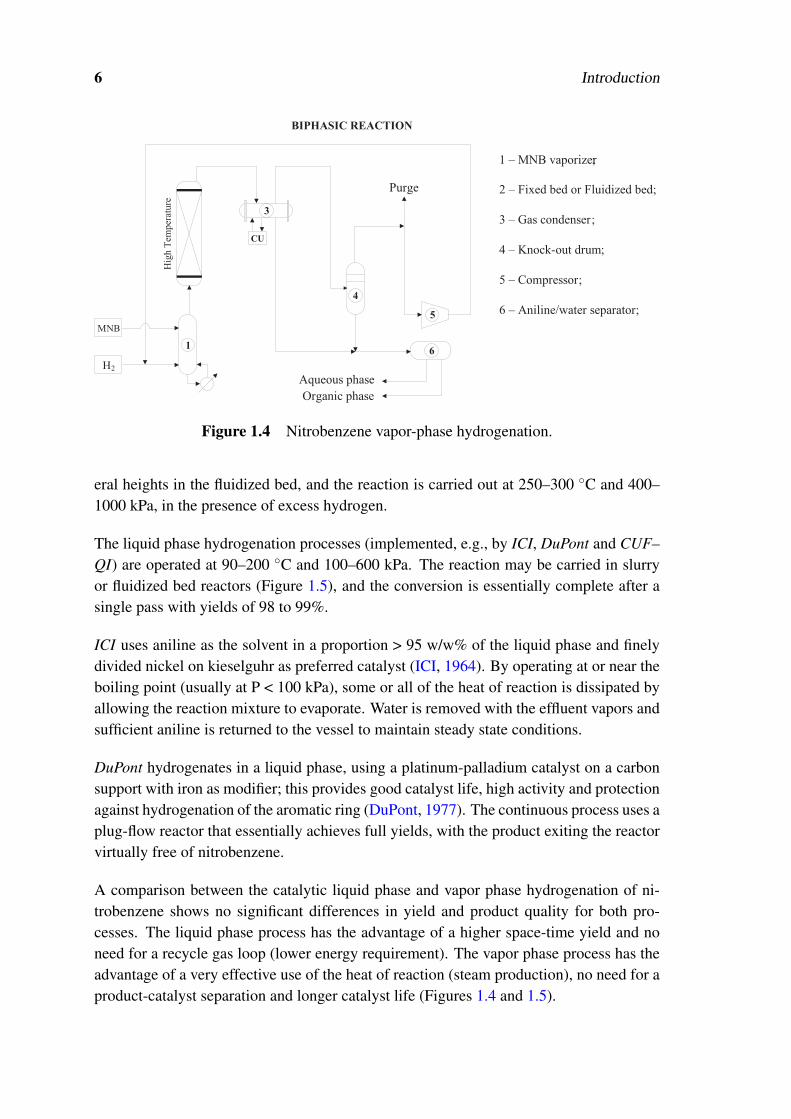
6 Introduction
4
1
3
5
2
CU
6
BIPHASIC REACTION
Organic phase
Aqueous phase
Purge
1 – MNB vaporizer;
2 – Fixed bed or Fluidized bed;
3 – Gas condenser;
4 – Knock-out drum;
5 – Compressor;
6 – Aniline/water separator;
H2
MNB
Hig
h T
emper
ature
Figure 1.4 Nitrobenzene vapor-phase hydrogenation.
eral heights in the fluidized bed, and the reaction is carried out at 250–300 C and 400–1000 kPa, in the presence of excess hydrogen.
The liquid phase hydrogenation processes (implemented, e.g., by ICI, DuPont and CUF–QI) are operated at 90–200 C and 100–600 kPa. The reaction may be carried in slurryor fluidized bed reactors (Figure 1.5), and the conversion is essentially complete after asingle pass with yields of 98 to 99%.
ICI uses aniline as the solvent in a proportion > 95 w/w% of the liquid phase and finelydivided nickel on kieselguhr as preferred catalyst (ICI, 1964). By operating at or near theboiling point (usually at P < 100 kPa), some or all of the heat of reaction is dissipated byallowing the reaction mixture to evaporate. Water is removed with the effluent vapors andsufficient aniline is returned to the vessel to maintain steady state conditions.
DuPont hydrogenates in a liquid phase, using a platinum-palladium catalyst on a carbonsupport with iron as modifier; this provides good catalyst life, high activity and protectionagainst hydrogenation of the aromatic ring (DuPont, 1977). The continuous process uses aplug-flow reactor that essentially achieves full yields, with the product exiting the reactorvirtually free of nitrobenzene.
A comparison between the catalytic liquid phase and vapor phase hydrogenation of ni-trobenzene shows no significant differences in yield and product quality for both pro-cesses. The liquid phase process has the advantage of a higher space-time yield and noneed for a recycle gas loop (lower energy requirement). The vapor phase process has theadvantage of a very effective use of the heat of reaction (steam production), no need for aproduct-catalyst separation and longer catalyst life (Figures 1.4 and 1.5).

1.4 The CUF aniline plant 7
H2
MNB
21
3OR
5
TRIPHASIC REACTION
Organic phase
Aqueous phase
OR
1 – CSTR slurry reactor
2 – Fluidized bed reactor
3 – Decanter
4 – Filter
5 – Phase separator
4
Relativelly low
Temperature
Figure 1.5 Nitrobenzene liquid-phase hydrogenation.
1.4 The CUF aniline plant
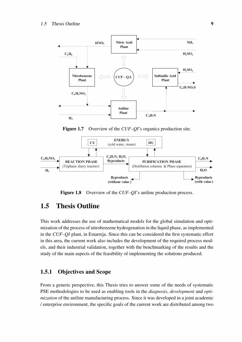
The aniline plant under study, owned by CUF–QI, is part of a chemical cluster located inEstarreja, Portugal (Figures 1.6 and 1.7). The site integration contributes for the overallsuccess of the company, since transportation costs are minimized, and some commoninfrastructures can be shared (e.g., utilities, effluent treatment).
In addition to manufacturing aniline, CUF–QI owns three other plants (nitrobenzene,nitric acid and sulfanilic acid), that together constitute the organics production site. Asshown in Figures 1.7 and 1.8, the raw materials acquired are sulfuric acid (not producedin Portugal), hydrogen (supplied by Air Liquide), benzene (mostly provided by Galp)and ammonia (from Adubos de Portugal, also a CUF–QI company). In the organics site,aniline is the main commercialized product, mostly absorbed by Dow for the synthesis ofMDI.
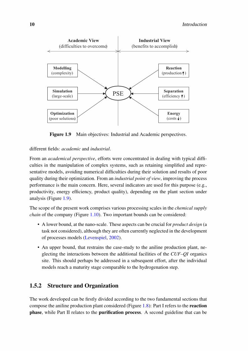
Currently, the aniline plant assures a production of approximately 120 kton/year, via theliquid phase hydrogenation of nitrobenzene. The process can be decomposed in two majorsections: reaction (a large consumer of cold utilities) and purification (a large consumerof hot utilities) — Figure 1.8. The first section, composed by several triphasic reactors(slurry type), includes several mass transfer steps (gas-liquid and liquid-solid), associatedto a reaction step using finely suspended catalyst particles. The second section compre-hends a complex arrangement of 7 distillation columns and 5 phase separators, where10 components (most of them byproducts, in vestigial compositions) exhibit complexequilibria.

8 Introduction
Meth
an
ol
Ben
zene
NH
3
H2
PV
C
CO
MD
I
Salt
An
iline
Ste
am
Ch
lorin
e
NaO
H
HC
l
VC
M
HC
l
NaO
H
Ind
ustr
ial
dete
rgen
ts
Nafta
H2
Form
alin
BR
ES
FO
R
Ele
ctr
ic P
ow
er
An
iline
Nitr
ob
en
zen
e
H2
Nitr
ic A
cid
Su
lfan
ilic A
cid
Hyp
och
lorite
HC
lC
hlo
rin
eN
aO
H
H2 S
O4
Alu
min
ium
salts
O2
N2
CO
2A
rgon
(form
er U
nite
ca)
(form
er Q
uim
igal)
Min
eira
de
Sais
Alc
alin
os
S.A
.
Es
pe
cia
lidad
es
Qu
ímic
as, L
da
Em
pre
sa
Co
ge
raç
ão
Es
tarre
ja, L
da
.
Figure1.6
Overview
ofthechem
icalclusterinE
starreja.
1.5 Thesis Outline 9
Aniline
Plant
Nitrobenzene
Plant
Sulfanilic Acid
Plant
Nitric Acid
PlantHNO3
C6H6
C6H7N
C6H5NO2
H2
H2SO4
C6H7NO3S
H2SO4
NH3
CUF - Q.I.
Figure 1.7 Overview of the CUF–QI’s organics production site.
REACTION PHASE
(Triphasic slurry reactors)
PURIFICATION PHASE
(Distillation columns & Phase separators)
ENERGY
(cold water, steam) HUCU
C6H5NO2
H2
C6H7N, H2O,
Byproducts
Byproducts
(without value )
H2O
C6H7N
Byproducts
(with value )
Figure 1.8 Overview of the CUF–QI’s aniline production process.
1.5 Thesis Outline
This work addresses the use of mathematical models for the global simulation and opti-mization of the process of nitrobenzene hydrogenation in the liquid phase, as implementedin the CUF–QI plant, in Estarreja. Since this can be considered the first systematic effortin this area, the current work also includes the development of the required process mod-els, and their industrial validation, together with the benchmarking of the results and thestudy of the main aspects of the feasibility of implementing the solutions produced.
1.5.1 Objectives and Scope
From a generic perspective, this Thesis tries to answer some of the needs of systematicPSE methodologies to be used as enabling tools in the diagnosis, development and opti-mization of the aniline manufacturing process. Since it was developed in a joint academic/ enterprise environment, the specific goals of the current work are distributed among two
10 Introduction
Reaction
(production )
Modelling
(complexity)
Simulation
(large-scale)
Optimization
(poor solutions)
PSE
Industrial View
(benefits to accomplish)
Separation
(efficiency )
Energy
(costs )
Academic View
(difficulties to overcome)
Figure 1.9 Main objectives: Industrial and Academic perspectives.
different fields: academic and industrial.
From an academical perspective, efforts were concentrated in dealing with typical diffi-culties in the manipulation of complex systems, such as retaining simplified and repre-sentative models, avoiding numerical difficulties during their solution and results of poorquality during their optimization. From an industrial point of view, improving the processperformance is the main concern. Here, several indicators are used for this purpose (e.g.,productivity, energy efficiency, product quality), depending on the plant section underanalysis (Figure 1.9).
The scope of the present work comprises various processing scales in the chemical supplychain of the company (Figure 1.10). Two important bounds can be considered:
• A lower bound, at the nano-scale. These aspects can be crucial for product design (atask not considered), although they are often currently neglected in the developmentof processes models (Levenspiel, 2002).
• An upper bound, that restrains the case-study to the aniline production plant, ne-glecting the interactions between the additional facilities of the CUF–QI organicssite. This should perhaps be addressed in a subsequent effort, after the individualmodels reach a maturity stage comparable to the hydrogenation step.
1.5.2 Structure and Organization
The work developed can be firstly divided according to the two fundamental sections thatcompose the aniline production plant considered (Figure 1.8): Part I refers to the reactionphase, while Part II relates to the purification process. A second guideline that can be

1.5 Thesis Outline 11
1 pm 1 nm 1 μm 1 mm 1 m 1 km
ps
ns
ms
s
min
h
day
week
month
Chemical Scale
Small
Intermediate
Large
Thesis
scope
Molecules
Moleculeclusters
Particles, thin films
Single and multi-phase systems
Process units
Plants
Site
Enterprise
Figure 1.10 Thesis scope: physical scales involved in the developed work (Grossmannand Westerberg, 2000).
followed to understand the sequence in which the work is presented, is the scale of theinvolved problems. Figure 1.10 expresses a possible interpretation. For a better under-standing of the Thesis structure, presented in Figure 1.11, the following correspondences(adapted to the developed activities) should be assumed:
• Micro-scale: related to the modelling of intrinsic fundamental phenomena. Thisincludes the description of mechanistic mass-transfer and reaction steps, as well asthe prediction of LL and VL equilibria, at a functional group level.
• Meso-scale: relative to the individual solution of unit models. Here, the stand-alone performance of a given reactor, column or phase-separator is predicted and /or optimized, as a sum of microscopic steps.
• Macro-scale: involving the simulation and optimization of unit arrangements. Inthis case, new plant configurations are pursued as a sum of interactions betweenmeso-scale units.
The adopted structure also closely expresses the process of knowledge build-up that be-comes necessary when moving from local choices (e.g., the number of equilibrium stagesin a column) to plant-wide decisions (e.g., the number of columns). This relates not onlyto a better and deeper understanding of the plant behavior, but also to the recognition ofkey aspects that need to be considered during the development of the PSE formulations.This point deserves special attention, since it relates to the data flow between differentChapters (Figure 1.12). It also presents several advantages:
• Problems are kept as simple as possible. For example, the validation of a simpli-fied reactor model in Chapter 2 allows a faster and easier solution of the network

12 Introduction
L1
L2
V
L
L VLVS LS
Feed
Organic Aqueous
Feed Product
Byproducts
Byproducts
Reaction
+
Mass
transfer
Vapour-Liquid
equilibria
Liquid-Liquid
equilibria
Network
Optimization
MIC
RO
-SC
AL
EM
ES
O-S
CA
LE
MA
CR
O-S
CA
LE
PART I - REACTION PART II - SEPARATION
Network
Optimization
Simulation,
Sensitivity studies
Simulation
Units Optimization
Modelling ModellingChapter 2 Chapter 4
Chapter 4Chapter 5
Chapter 2
Chapter 3 Chapter 6
Reactant
(H2)
Catalyst
Product &Byproducts
Reactant
(MNB )
S
Figure 1.11 Thesis structure: division of subjects per Part.

1.5 Thesis Outline 13
PART I -REACTION PART II -SEPARATION
CH
AP
TE
R 2
Go
als
: S
imu
late
th
e re
acti
on
un
its
P
erfo
rm s
ensi
tiv
ity
stu
die
s
Ta
sk
s:
Dev
elo
p t
he
un
its
mo
del
s
Dev
elo
p t
he
solu
tio
n s
chem
e
CH
AP
TE
R 4
Go
als
: S
imu
late
th
e se
par
atio
n u
nit
s
Sim
ula
te t
he
sep
arat
ion
blo
ck
Ta
sk
s:
Dev
elo
p t
he
un
it’s
mo
del
s
Dev
elo
p t
he
solu
tio
n s
chem
es
CH
AP
TE
R 3
Go
als
: O
pti
miz
e th
e re
acti
on
net
wo
rk
(n
on-f
ixed
lay
ou
t)
Ta
sk
s:
Dev
elo
p t
he
op
tim
izat
ion
p
roce
du
re
Sh
ared
In
form
ati
on:
-C
riti
cal
op
tim
izat
ion
var
iab
les
(s
yst
em d
epen
den
t)
-V
alid
ated
mat
hem
atic
al m
od
el
(
sim
pli
fied
ap
pro
ach
)
CH
AP
TE
R 5
Go
als
: O
pti
miz
e se
par
atio
n u
nit
s
(f
ixed
lay
ou
t/n
o i
nte
gra
tio
n)
Ta
sk
s:
Dev
elo
p t
he
op
tim
izat
ion
p
roce
du
re
Sh
ared
In
form
ati
on:
-C
riti
cal
un
it s
ub
sets
-V
alid
ated
mat
hem
atic
al m
od
els
CH
AP
TE
R 6
Go
als
: O
pti
miz
e th
e se
par
atio
n n
etw
ork
(no
n-f
ixed
hea
t in
teg
rate
d l
ayo
ut)
Ta
sk
s:
Dev
elo
p t
he
op
tim
izat
ion
p
roce
du
re
Sh
ared
In
form
ati
on:
-P
re-p
roce
ssin
g p
roce
du
re
(f
or
sets
of
com
ple
x u
nit
s)
-M
ath
emat
ical
fo
rmu
lati
on
(
for
com
ple
x u
nit
s)
Figu
re1.
12T
hesi
sor
gani
zatio
n:da
taflo
wal
ong
the
chap
ters
.

14 Introduction
synthesis problem addressed in Chapter 3.
• Problems are kept as small as possible. For instance, the identification of a criticalsubset of distillation columns in Chapter 4 allows a reduction of the scale of theoptimization problems considered in Chapters 5 and 6.
Finally, it should also be pointed out that all of the remaining Chapters exhibit a similarstructure: the first Section(s) introduce the required theoretical background, reviewingthe currently available PSE methodologies. The following Section(s) describe the math-ematical approaches developed, emphasizing their advantages and drawbacks relative topredecessor strategies. The last Section(s) are dedicated to the application of the newmethodologies to the industrial case-study, ending with the presentation of the resultsobtained and the quantification of the specific gains.
Bibliography 15
Bibliography
BASF (1964). Production of aniline, US Patent 3 136 818.
Bayer (1990). Catalyst for the preparation of aniline, US Patent 5 304 525.
DuPont (1972). Amination of aromatic compounds in liquid hydrogen fluoride, USPatent 3 832 364.
DuPont (1977). Hydrogenation of mixed aromatic nitrobodies, US Patent 4 185 036.
FCC (1986). Co-production of an aromatic monoamine and an aromatic diamine directlyfrom benzene or a benzene derivative through controlled nitration, US Patent 4 740 621.
Gibson, J. (2004). Aniline outlook shows growth. European Chemical News, October:10.
Grossmann, I. E. and Westerberg, A. W. (2000). Research challenges in process systemengineering. AIChE Journal, 46:1700.
Guenkel, A. and Maloney, T. (1996). Nitration, recent laboratories and industrial devel-opments. ACS Symposium Series, 623:223.
Halcon (1975). Process for the production of organic amines, US Patent 3 860 650.
Harries, K. (2004). Aniline the builder. European Chemical News, March:16.
ICI (1964). Catalytic hydrogenation of nitro aromatic compounds to produce the corre-sponding amino compounds, US Patent 3 270 057.
Kirk-Othmer (2001). Encyclopedia of chemical technology. John Wiley & Sons, NewYork.
Levenspiel, O. (2002). Modeling in chemical engineering. Chemical Engineering Sci-ence, 57:4691.
Lonza (1969). Method for the catalytic hydrogenation of organic nitro derivatives in thegaseous state to corresponding amines, US Patent 3 636 152.
Nexant (2003). Aniline — business report.
Quimigal, S. (2007). Private communication.
Ullmann (2006). Encyclopedia of Industrial Chemistry. John Wiley & Sons, New York,7th (electronic release) edition.

16 Bibliography
Celestial navigation is based on the premise that the Earth is the center of the universe.The premise is wrong, but the navigation works. An incorrect model can be a useful tool.
Kelvin Throop III (fictitious character)

Part I
Reaction Step
17


Table of Contents
2 Modelling and Simulation of Heterogeneous Catalytic Reaction Systems 212.1 Catalytic reaction processes . . . . . . . . . . . . . . . . . . . . . . . . . 212.2 Multiphasic units . . . . . . . . . . . . . . . . . . . . . . . . . . . . . . 252.3 Industrial case-study . . . . . . . . . . . . . . . . . . . . . . . . . . . . 30
3 Optimization of Reaction Units and Networks 613.1 Optimization of reaction units . . . . . . . . . . . . . . . . . . . . . . . 613.2 Optimization of reaction networks . . . . . . . . . . . . . . . . . . . . . 643.3 Analogy with other “hard” problems . . . . . . . . . . . . . . . . . . . . 683.4 Developed strategy . . . . . . . . . . . . . . . . . . . . . . . . . . . . . 723.5 Industrial case-study . . . . . . . . . . . . . . . . . . . . . . . . . . . . 93
Final notes 107Conclusions and Future Work . . . . . . . . . . . . . . . . . . . . . . . . . . . 107Nomenclature . . . . . . . . . . . . . . . . . . . . . . . . . . . . . . . . . . . 110Bibliography . . . . . . . . . . . . . . . . . . . . . . . . . . . . . . . . . . . 113
A Physical property estimation 119

20 Table of Contents

Chapter 2
Modelling and Simulation ofHeterogeneous Catalytic ReactionSystems
Summary
This Chapter considers the derivation and validation of a mathematical model for the CUF–QIhydrogenation units. These are triphasic slurry reactors, where several mass and energy transfersteps, combined with an heterogeneous reaction, result in overall complex behavior. An explicitobjective in the development of this model is its future use as a tool for process diagnosis, namely:(i) to identify the limiting steps, (ii) to evaluate the influence of the distinct operational variables,(iii) to explain industrial data obtained. Considering its mechanistic nature, the model also sup-ports the scale-up of these units, and the synthesis of optimal reactor configurations, consideredin the next Chapter.
The Chapter starts with a review of the fundamental aspects and distinctive approaches in themodelling of heterogeneous reactors. Later, two modelling approaches are implemented: a macro-scopic one, where an homogeneous description of the solid phase is adopted, and a microscopicperspective, where the internal diffusional and conductive phenomena are explicitly considered,within the catalyst particles. The results obtained show good agreement between rigorous and sim-plified approaches, and provide important indications on the level of complexity more adequatefor further studies.
2.1 Catalytic reaction processes
Catalytic reaction processes are the basis of almost all chemical production processes.For example, among the top 10 most produced components in the USA, 4 of them arecatalyzed. If, instead, the top 50 ranking is considered, the previous number rises to 31,
21

22 Modelling and Simulation of Heterogeneous Catalytic Reaction Systems
representing approximately 60% in number and 40% in quantity (Araújo, 2005). Amongthese processes, heterogeneous catalysis (where the catalyst and the reaction mixtures arein different phases) is usually predominant.
This Chapter considers the modelling of heterogeneous catalytic reactions, which corre-sponds to the type of process used by CUF–QI for hydrogenation of nitrobenzene. Thesemodels are later used to identify the major limiting factors in the industrial performanceof the currently available units. Moreover, in the next Chapter, these models are also usedto support the scale-up and the intensification of the aniline production, as currently im-plemented. Therefore, particular attention is given in the initial part of this Chapter to theavailable alternative modelling approaches, and how they can best be used to describe thedifferent physical configurations used to carry these catalytic reactions.
Heterogeneous catalytic processes are inherently characterized by the existence of differ-ent physical phases. The reactants / products can be fed / drawn as gas and / or liquidstreams, while the catalyst is usually available as a solid phase, commonly in the form ofparticles. From a modelling perspective, it is usually convenient to separate the modellingof the reaction step from the specific equipment (unit) where it occurs. Here, different ap-proaches can be used to model a given unit, and a similar description of the physicalphenomena might be useful as building blocks for the models of different units. Dis-tinct alternative approaches can be used for model building, depending on the intendedfinal use and the accuracy desired for the model. Several of the steps involved can bedescribed with different levels of detail, or grouped together for modelling purposes. Forexample, Langmuir-Hinshelwood kinetics can be used to simultaneously describe kineticand adsorption / desorption mechanisms. Moreover, the diffusional processes (intra andextra-particles), an aspect that can cause a major impact on the complexity of the resultingmodel, can also be described differently.
Independently of the modelling approach, in heterogeneous catalysis it it usually impos-sible to completely dissociate the mass transfer step(s) from the reaction process, sinceboth are intrinsically connected. In fact, the conversion of reactants into products is onlypossible after an external diffusional process, as illustrated in Figure 2.1. In the most com-plex case, different internal and external phenomena of mass transfer may compete withchemical reaction, leading to a complex equilibrium that need to be expressed using theindividual rates of each phenomena (Froment and Bischoff, 1990). This leads to a fullymicroscopic approach, expressed by a distributed parameter (or PDE) model. To avoidthe solution of these mathematical systems, that can offer significant challenges and / orrequire large CPU times, the use of simplified approaches is often employed, as discussedin the following Section.

2.1 Catalytic reaction processes 23
MICROSCOPIC MODELLING
(Rigorous Approach)
Cm
G
Cm
P (rP) TGTP(rP )
Mass Balances (Particle) Energy Balance (Particle)
( )2
P Peff P P2
P P P
2,
m m
m m mC CD C T
r r r
∂ ∂+ = − ∂ ∂
( ) ( )2
P Peff R P P2
P P P
2,m
T TH C T
r r rλ
∂ ∂+ = −∆ ∂ ∂
γ Γ Γ
Figure 2.1 Microscopic modelling of the solid phase in heterogeneous systems.
2.1.1 Simplified modelling approaches
Two main forms of avoiding distributed parameter models during the mathematical de-scription of heterogeneous reactions can be considered. The first one still considers theintra-particle phenomena, although simplifying their evaluation through the use of effi-ciency factors; the second approach totally neglects them, in what can be considered amacroscopic approach, an approximation that can be justified in certain circumstances.
To avoid differential mass and energy balance equations, the conditions inside the cata-lyst particles should not be distinguished. In other words, temperature and concentrationscannot be considered as functions of the particle internal radius, and a representative valueneeds to be assumed for the solid phase (Figure 2.2). Under these circumstances, massdiffusion as well as heat conduction and reaction are not rigorously evaluated, since theydepend pointwise on TP and Cm
P . However, in some cases, this dependence can be esti-mated and the global influence of these phenomena still considered (although implicitly),through the use of efficiency factors.
Use of efficiency factors
The efficiency factor can be seen as a corrective coefficient, often used to express com-plex phenomena through a simple (approximate) expression. It seeks to contemplate theinfluence of the intra-particle processes, by evaluating the ratio between limiting reaction

24 Modelling and Simulation of Heterogeneous Catalytic Reaction Systems
MACROSCOPIC MODELLING
(Simplified Approach)
Cm
G
Cm
S TG
TS
Mass Balances (Solid Phase) Energy Balance (Solid Phase)
( ) ( )GS S G S S S ,
m m m m mK a C C C T η− = − ( ) ( ) ( )GS S S G R S S
,m
h a T T H C Tη− = −∆γ Γ Γ
Figure 2.2 Simplified modelling of the solid phase in heterogeneous systems (use ofefficiency factors).
rates (at the surface conditions) and the overall observed rate:
η =
∫∫∫VP
Γ(CmP ,TP) dVP
Γ(CmS ,TS)
(2.1)
In practice, the use of η is advantageous when expressed through an algebraic correlationthat avoids the solution of the integral term; however for complex reaction systems, andextended ranges of operating conditions, this might require a demanding data regressionexercise. The use of η allows a greatly simplified model of the solid phase (Figure 2.2),with the mass and energy balances relative to the catalyst particles now purely algebraic.
Macroscopic models
As mentioned, the use of detailed microscopic descriptions can be relieved in specialsituations, through the use of macroscopic approximations. Two limiting scenarios areknown where, as a result of an equilibrium between competing phenomena (reaction andinternal diffusion), a macroscopic approximation is usually applicable:
• Pure diffusional regime: when the internal diffusion rate is very low compared tothe chemical reaction rate, this last occurs, almost completely, at the solid phasesurface. In this case, there is no need to distinguish conditions inside the catalyst,because reaction does not take place significantly in the intra-particle volume.
• Pure chemical regime: when the internal diffusion rate is very high, compared to

2.2 Multiphasic units 25
Table 2.1 Classification of heterogeneous reactors.
Reaction Phases Reactor types
Two Phases (G/S or L/S) 2-Phase CSTR, Fluidized bed, Fixed bed.
Three Phases (G/L/S) Trickle-bed, Bubble fixed bed, CSTR slurry,Bubble slurry, 3-Phase fluidized.
the chemical reaction rate, the internal concentration profiles become essentiallyflat. In this case, the internal conditions are essentially identical to the conditions inthe particle surface.
In both situations, a macroscopic approach allows accurate results, since the catalyst parti-cles can be treated, in practice, as a pseudo-homogeneous solid phase. Therefore, a globalreaction rate can be defined, for example, per unit of catalyst surface area or per unit ofcatalyst volume, since its efficiency (η) is expected to remain approximately unchanged.The modelling and solution procedures can be greatly simplified in both cases.
2.2 Multiphasic units
In addition to heat and mass transfer to the catalyst particles, there is also the possibilityof additional transference phenomena in multiphasic units, according to their mechanicaldesign. This is important when considering alternative equipment for heterogeneous cat-alytic reactions, or for diagnosing the behavior of existing units. In fact, the number ofcoexisting phases, and the form of promoting mass transfer essentially define the type ofmultiphasic reactor (Table 2.1):
• Trickle bed: Concurrent down-flow of gas and liquid over a fixed bed of catalyst;liquid trickles down, while gas phase is continuous.
• Bubble fixed bed: Concurrent up-flow of gas and liquid; the catalyst bed is com-pletely immersed in a continuous liquid flow while gas rises as bubbles.
• CSTR slurry: Mechanically agitated gas-liquid-catalyst reactor; the fine catalystparticles are suspended in the liquid phase by means of agitation.
• Bubble slurry column: Liquid is agitated by means of the dispersed gas bubbles;these also provide the momentum to suspend the catalyst particles.
• 3-phase fluidized bed: Catalyst particles are fluidized by an upward liquid flowregime while gas phase rises in a dispersed bubble regime.
Although triphasic reactions can (theoretically) occur in these five different configura-tions, more practically only three main mechanical designs are usually considered: CSTR,

26 Modelling and Simulation of Heterogeneous Catalytic Reaction Systems
LIQUID
GAS
GAS
LIQUID
TRICKLE BED SLURRY CSTR3-PHASE FLUIDIZED
Fixed catalyst bed Dispersed gas bubbles Fine catalyst particles
& BUBBLE SLURRY
LIQUID
GAS
LIQUID
GAS
BUBBLE FIXED BED
LIQUID GAS
LIQUID
S
SOLID
LIQUID
GAS
LIQUID
GAS
Figure 2.3 Main types of multiphasic (3-phase) reaction units.
fluidized bed and fixed-bed (Figure 2.3). Here, it is possible to observe that the tricklebed and bubble fixed bed reactors differ only in the relative movement of the phases. Ata mechanical design level, the differences between the 3-phase fluidized bed and the bub-ble slurry column are even smaller. However, each configuration involves characteristicoperational regimes, defined by typical mass / heat transfer coefficients and by specificintra-particle conditions, which might need to be considered individually.
Choosing the most suitable configuration for a particular reaction is not an easy task, sincethere are many aspects that need to be considered. In fact, each reactor type presents awell defined set of advantages an drawbacks, as stated in Tables 2.2 and 2.3, where acomparison of reactors within the same type of bed is made (fixed or suspended). Acomparison between these two classes of reactors is also possible, revealing significantdifferences in key aspects (Perry and Green, 1997; Ullmann, 2006; Kirk-Othmer, 2001):
• Fixed bed: The fluid flow regimes often approach plug flow, which can be advan-tageous for some reactions. The catalyst load per reactor volume is comparativelyhigher and the pressure drop is low. Heat and mass transfer rates are usually low andthe catalyst replacement is relatively hard, requiring shutdown most of the times.
• Suspended bed: The vigorous particle motion reduces external resistances, en-abling high mass and heat transfer rates and, consequently, near isothermal condi-tions and a better temperature control. All intensive properties of the bed tend to behomogenized and, therefore, axial or radial profiles are difficult to promote, whichmight be undesirable; particle attrition may reduce the catalyst life.

2.2 Multiphasic units 27
Table 2.2 Comparison of three phase fixed bed reactors (Hopper et al., 2001).
Variable Trickle bed Bubble fixed bed
Pressure drop Channelling at low flowrates Good flow distributionHeat control Relatively difficult EasierRadial mixing Poor radial mixing Good mixingL/S ratio Low HighCatalyst wetting Partial wetting is possible Complete wettingConversion High Lower due to back mixing
Table 2.3 Comparison of three phase suspended bed reactors (Hopper et al., 2001).
Variable CSTR slurry Bubble slurry 3-Phase fluidized
Catalyst attrition Significant Insignificant InsignificantMass/Heat transfer Highest High HighMechanical design Difficult Simple SimpleCatalyst separation Easy Easy EasiestPower consumption Highest Intermediate LowestCatalyst distribution Uniform Uniform∗ Uniform∗
(∗) Non-uniform conditions may sometimes occur.
Depending on the geometry of the kinetic curves, the required reaction volume might begreatly reduced using sequential reaction steps, or promoting a plug-flow regime (here,fixed bed reactors would be more competitive). If minimizing the yield of byproducts isthe most crucial aspect, the plug-flow regime will be unfavorable in the presence of serialsecondary reactions, although advantageous in a situation where these occur in parallel.On the other hand, the previous analysis becomes meaningless if the reactants cannotreach the surface of the catalyst particles, due to mass transfer problems (here, suspendedbeds may play an important role).
2.2.1 Modelling aspects
When building a mechanistic model of an heterogeneous system, several numerical as-pects usually need to be explicitly addressed:
• The complexity of the resulting model, the effort required for its solution, and theease of integration of the model with existing optimization strategies.
• The accuracy of the model predictions.
• The derivation of the model parameters required.
For heterogeneous catalytic systems, the above considerations have various practical im-plications. Depending on the reactor configuration, the solid phase may not be the only

28 Modelling and Simulation of Heterogeneous Catalytic Reaction Systems
one to exhibit concentration / temperature profiles. In some multiphasic units, mass trans-portation due to radial and axial dispersion may be an important phenomena, requiringmore complex models to accurately describe the overall behavior. Therefore, even whena macroscopic approach can be adopted for the catalyst, a distributed parameter modelmight be unavoidable for the remaining phases, depending on the operational regime thatis promoted.
Among all triphasic units, the slurry reactor is the simplest one to model. Due to thevigorous stirring that is promoted, all phases are usually considered to be homogeneouslydistributed, resulting in a mixture whose intrinsic properties do not depend on the spacialcoordinates. Under these circumstances, simple algebraic models define the balances inthe reacting mixture, as illustrated in the the following equation, for components that donot enter the gas phase:(
Q/V iR)(
Ci,mL −Ci−1,m
L
)−Ki,m
LS aS
(Ci,m
L −Ci,mS
)= 0 (2.2)
All of the remaining unit types involve a dispersion regime, and therefore require a dis-tributed parameter model to describe the heat / mass balances in the non-catalytic phases.This is illustrated in equation (2.3), for the non-volatile components, where radial profilesare neglected and only axial dispersion in the liquid phase is considered:
DmL
d2CmL (l)
dl2 −uLdCm
L (l)dl
−KmLS(l)aS (Cm
L (l)−CmS (l)) = 0 (2.3)
This equation is applicable not only to fixed bed units, but also to some reactors of thesuspended bed type (e.g., bubble slurry column and 3-phase fluidized). These last ones,although far from the plug-flow regime, are still segregated-flow reactors, where a certainprofile is established along the axial coordinate. Therefore, the same base model can beshared by all of these configurations, with the higher / lower back-mixing phenomena andthe distinct mass / heat transfer properties considered through specific coefficients (e.g.,Dm
L and KmLS).
Another important aspect, that becomes clear through comparison of equations (2.2) and(2.3), is that the plug-flow regime can be approximated by a sequence of CSTR units,with negligible error in the limit. In fact, by ignoring the axial dispersion term in (2.2)and by establish an analogy between uL and Q/VR and between ∆i and ∆l, the implicitmathematical equivalence is revealed. For this reason, some authors (e.g., Kokossis andFloudas (1990)) have suggested the use of this approximation to model and optimize tubu-lar reactors. Using this approach, the solution of differential equations could be avoided,allowing an easier implementable solution procedure. However, and as illustrated in Fig-ure 2.4, this analogy only represents a direct equivalence for the homogeneous case, sincesignificantly different configurations are possible in heterogeneous systems. These in-volve not only solid phases with distinct characteristics, but also specific ways of promot-

2.2 Multiphasic units 29
GAS
LIQ.
GAS
LIQ.
GAS
LIQ.
LIQ.
TUBULAR REACTOR
(Fluidized or Fixed-Bed)
BATERY OF SLURRY REACTORS
Requires adaptation
for multi-phase systems
Direct approximation for
homogeneous systems
Figure 2.4 Approximation of a dispersion regime to a battery of CSTR regimes.
ing mass transfer. As a consequence, the internal and external diffusional / conductivesteps that are involved in a slurry reactor differ significantly from those in a trickle-bed orfluidized-bed reactor. Therefore, the approximation of a triphasic tubular reactor througha battery of slurry units requires the use of significantly modified model building blocksand parameters, capable of effectively expressing the specific operational regime of eachconfiguration. This will further discussed in the optimization studies of Chapter 3.
It is important to notice that this type of methodology (limit or approximate modelling)often provides only a “good-enough” solution which, depending on the objectives, mightbe insufficient. For this reason, most authors still prefer to solve the original system ofequations, a task that involves different degrees of difficulty, depending on the reactorunder study. In this sense, the most complex situation occurs when, simultaneously, a de-tailed microscopic approach is adopted for the solid phase and a dispersion regime (withaxial and / or radial profiles) is considered for the remaining ones. Here, the resulting PDEsystem might be difficult to handle, due to the different space scales involved, requiringelaborated solution techniques. Therefore, to avoid these difficulties, all reasonable sim-plifications should be considered during the modelling phase.
In the two other potential scenarios — a CSTR regime where a microscopic descrip-tion of the catalyst particles is employed, and a dispersion regime where a macroscopicapproach is adopted for the solid phase — the involved differential equations will be ordi-nary differential equations (ODEs), provided that only one independent (spatial) variableis considered for the reactor (rR or lR). In both situations, initial-value or boundary valueproblem (BVPs) will be generated. These can be solved by either shooting, relaxation andweighted residual methods (Cameron and Hangos, 2001). The last two classes of methods

30 Modelling and Simulation of Heterogeneous Catalytic Reaction Systems
ANL+MNB
Cooling Water
Water Steam
Catalyst
Recicle (recovery of catalyst)
Reaction products
Non-converted reactants
Non-recovered catalyst
H2
Figure 2.5 Schematic representation of the pilot reaction system (Prodeq, 2001).
are known to be less susceptible to numerical instability, and are also more easily inte-grable with equation-oriented optimization strategies, and therefore are more commonlyused for the solution of these models.
2.3 Industrial case-study
After the general considerations relative to model building in heterogeneous systems,the current Section describes the derivation of a mathematical model for the industrial ni-trobenzene hydrogenation reactor considered (as implemented by CUF–QI). Section 2.3.1starts with a brief description of the system under study, Section 2.3.2 reviews some ofspecific goals considered, Sections 2.3.3 and 2.3.4 deal with the modelling and solutionaspects, and finally Sections 2.3.5 and 2.3.6 report the most important results obtained.
2.3.1 System description
The mathematical model was directly developed and validated in a pilot plant unit, whichis a faithful scale-down replica of the existing industrial units. The hydrogenation unitis composed by a slurry reactor and a decanter (Figure 2.5). As can be observed, threephases are involved: the reactor is fed with nitrobenzene (MNB, in the liquid phase) andhydrogen (gas phase), and the reaction is carried on heterogeneously, using catalyst par-ticles (solid phase). In addition to the reactants, the feed stream also contains aniline, tosolubilize the water produced in the reaction, avoiding the occurrence of a biphasic mix-ture in the vessels. A small purge of hydrogen is performed discontinuously, to maintainthe pressure at its desired value.
The reactor outlet stream contains fine catalyst particles that are suspended in the liquidmixture, and is mainly composed by water and aniline, although it includes also several

2.3 Industrial case-study 31
Structural formula Name Label
CyclohexylamineNH2 CHA
OH
Cyclohexanone CHONAO
Cyclohexanol CHOL
NH
NH2 Aniline ANL
“Light”
Byproducts
“Heavy”
Byproducts
Dicyclohexylamine DICHA
N
NH
Cyclohexylidene-aniline CHENO
Cyclohexyl-aniline CHANIL
TBP (ºC)
134
161
155
184
256
303
336
Figure 2.6 Products of nitrobenzene hydrogenation in CUF–QI.
Table 2.4 Main geometrical dimensions of the pilot reactor and decanter.
Reactor Decanter
Height: 0.747 m Height: 1.4 mDiameter : 0.492 m Capacity: 0.3 m3
Liquid quota: 0.509 m
byproducts. These result from a number of secondary reactions (Silva, 1997) and, asshown in Figure 2.6, cover a wide range of boiling points, which enables a classificationbased on their relative volatilities to aniline. The suspended particles are recovered in thedecanter and recycled back to the reactor. Despite the high efficiency of this separationstep, some minor losses occur in practice. Therefore a make-up stream of solid phase isused, to accommodate also the catalyst aging and deactivation processes. The catalystdispersion and its mixture with the two remaining phases is assured by the reactor tur-bine. This promotes an ascending flux that enables a good emulsion of the hydrogen, andallows the mixture to circulate between the reactor and the decanter. Due to the highlyexothermic reaction internal coils are employed, where cooling water flows to remove thelarge amount of generated heat. The main dimensions of the pilot unit are presented inTable 2.4.
2.3.2 Modelling objectives
In the beginning of this work, the development of a mechanistic model for the hydro-genation reactors was motivated by relatively specific groups of objectives, described in
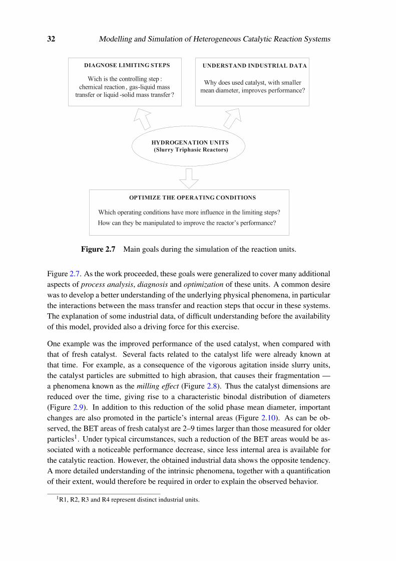
32 Modelling and Simulation of Heterogeneous Catalytic Reaction Systems
DIAGNOSE LIMITING STEPS UNDERSTAND INDUSTRIAL DATA
OPTIMIZE THE OPERATING CONDITIONS
HYDROGENATION UNITS
(Slurry Triphasic Reactors)
Wich is the controlling step :
chemical reaction , gas-liquid mass
transfer or liquid -solid mass transfer ?
Why does used catalyst, with smaller
mean diameter, improves performance?
Which operating conditions have more influence in the limiting steps?
How can they be manipulated to improve the reactor’s performance?
Figure 2.7 Main goals during the simulation of the reaction units.
Figure 2.7. As the work proceeded, these goals were generalized to cover many additionalaspects of process analysis, diagnosis and optimization of these units. A common desirewas to develop a better understanding of the underlying physical phenomena, in particularthe interactions between the mass transfer and reaction steps that occur in these systems.The explanation of some industrial data, of difficult understanding before the availabilityof this model, provided also a driving force for this exercise.
One example was the improved performance of the used catalyst, when compared withthat of fresh catalyst. Several facts related to the catalyst life were already known atthat time. For example, as a consequence of the vigorous agitation inside slurry units,the catalyst particles are submitted to high abrasion, that causes their fragmentation —a phenomena known as the milling effect (Figure 2.8). Thus the catalyst dimensions arereduced over the time, giving rise to a characteristic binodal distribution of diameters(Figure 2.9). In addition to this reduction of the solid phase mean diameter, importantchanges are also promoted in the particle’s internal areas (Figure 2.10). As can be ob-served, the BET areas of fresh catalyst are 2–9 times larger than those measured for olderparticles1. Under typical circumstances, such a reduction of the BET areas would be as-sociated with a noticeable performance decrease, since less internal area is available forthe catalytic reaction. However, the obtained industrial data shows the opposite tendency.A more detailed understanding of the intrinsic phenomena, together with a quantificationof their extent, would therefore be required in order to explain the observed behavior.
1R1, R2, R3 and R4 represent distinct industrial units.

2.3 Industrial case-study 33
0
50
100
450
500
0 50 100
Catalyst charge 1
Catalyst charge 2
Catalyst charge 3
Catalyst: Ni / SiO2
dP (t=0): 0.4-0.6 mm
dP
(µm
)
t (hours)
Figure 2.8 Milling effect in slurry hydrogenation units (Turek et al., 1986).
0.0
0.5
1.0
1.5
2.0
2.5
3.0
3.5
4.0
4.5
0 1 10 100 1000
d (µm)
R1
R2
R3
R4
Fresh
P
% (volume)
Figure 2.9 Binodal distribution of the catalyst diameters, as a consequence of themilling effect in CUF–QI units (Lucas et al., 2001).
0
20
40
60
80
100
120
140
160
R1 R2 R3 R4 Fresh
BE
T a
rea
(m
g )
2-1
Catalyst
Figure 2.10 Reduction of the catalyst BET areas, as a consequence of the milling effectin CUF–QI units (Lucas et al., 2001).

34 Modelling and Simulation of Heterogeneous Catalytic Reaction Systems
Inte
rfac
e G
L
Inte
rfac
e L
S
CG
CL
Gas phase
Liquid phase
Solid phase
CATALYST
PARTICLE
m
m
CP
m
Figure 2.11 Schematic representation of the main phenomena under study.
2.3.3 Prediction of fundamental phenomena
As mentioned previously, the global behavior of the system depends on a set of distinctfundamental steps, including mass transfer (gas-liquid and liquid-solid), heat transfer andreaction (Machado, 1994; Ramachandran and Chaudhari, 1980b). Figure 2.11 illustratesthese different steps, considered individually in this Section.
Mass transfer (GL and LS)
The quantity of hydrogen transferred across the gas-liquid interface can expressed as
ϑmGL = Km
GLaB(C∗,m
G −CmL)
(2.4)
where C∗,mG represents the concentration of a chemical species in a liquid mixture that is
in equilibrium with the gas phase. Here, the parameters KmGL and aB must be estimated.
Promoting mass transfer between a gas and liquid is a very common operation where theinterfacial surface area plays an important role in the overall process; this explains thelarge number of correlations that have been developed for its estimation. Several litera-ture reviews describe a large diversity of experiments, using liquids with different chem-ical properties, vessels with distinct geometries and analytical techniques based on veryspecific assumptions (Hicks and Gates, 1976; Reith, 1970). Here, the work of Chaudhariand Ramachandran (1980) was used, since their experiments involved stirred vessels withsuspended catalyst, similar to the ones under study. More specifically, the Yagi-Yoshida

2.3 Industrial case-study 35
0 10 20 30 40
ω (rps)
0
10
20
30
40
K a
(
s )
GL
B-1
Figure 2.12 Dependence of KGLaB on the stirring speed: correlation of Yagi-Yoshida (Chaudhari and Ramachandran, 1980).
correlation was selected, with yy1 = 1.50, yy2 = 0.19, yy3 = 0.50, yy4 = 0.60, yy5 = 0.32:
KmGLaBd2
I0.06Dm
L=(
d2I ωρL
µL
)yy1(dIω2
g
)yy2(µL
ρLDmL
)yy3(
µLuG
σL
)yy4(
ωdI
uG
)yy5
(2.5)
This correlation predicts that KmGLaB increases with the stirring speed, in a convex form,
as represented in Figure 2.12. However, this behavior is not in agreement with the ex-perimental results obtained by Turek et al. (1987), in their hydrogen absorption studiesperformed at laboratory scale (Figure 2.13). Contrarily to equation (2.5), these authorsconclude that the previous mass transfer coefficient remains practically unaltered for stir-ring speeds greater than 800 rpm, assuming in this operating range a value close to unity.A further comparison, in closer detail, between these two sources of information washowever not possible, since:
• No data could be retrieved, relative to the dimensions of the impeller that was usedduring the experimental studies of Turek et al. (1987).
• The range of considered stirring speeds is significantly different in both situations.In Turek et al. (1987), the maximum limit set for ω was 800 rpm, while in theCUF–QI pilot reactor this variable can reach values around 2000 rpm.
Using the set of reference operational conditions presented in Section 2.3.5, the Yagi-Yoshida correlation returns Km
GLaB = 26.7, a value that is therefore potentially one orderof magnitude larger than those reported in Figure 2.13. However, and as discussed inSection 2.3.6, the use of a lower value of Km
GLaB will not influence any of the conclusionsdrawn from the mathematical models considered.
More rigorously, it also should be emphasized that the Yagi-Yoshida correlation only al-lows the estimation of Km
L aB, i.e., the mass transfer coefficient in the liquid film. Assum-ing that the Henry law is applicable, the global mass transfer coefficient can be estimated

36 Modelling and Simulation of Heterogeneous Catalytic Reaction Systems
1
0.5
0400 800
10-3
10-2
10-1
100
10
T=90ºC
Γ/Γmax
KGL aB(s-1)
ω (rpm)
Figure 2.13 Dependence of KGLaB on the stirring speed: experimental results in Tureket al. (1987).
by1
KGLaB=
1KLaB
+1
He KGaB(2.6)
where He represents the Henry constant, and where the existence of both films is consid-ered. However, for low solubility gases (like hydrogen), the resistance is mostly concen-trated in the liquid film, which enables the assumption
KGLaB ' KLaB ⇒ ϑmGL = Km
GLaB[CmG/He−Cm
L ] (2.7)
to more conveniently express ϑ mGL; here, Cm
G represents the concentration in the gas phase,an easily estimated quantity.
Similarly, the mass transfer between the liquid phase and the surface of the catalyst parti-cles can be evaluated by:
ϑmLS = KLSaS (Cm
L −CmS ) (2.8)
In this case both KmLS and aS need to be estimated. Considering again the work of Chaud-
hari and Ramachandran (1980), the Boon-Long correlation was selected
KmLSdP
0.46DmL
=(
dPρLdRπ2ω
0.5µL
)bl1(ρ2
Ld3Pg
µ2L
)bl2(mCVL
d3PρL
)bl3(dR
dP
)bl4( µL
ρLDmL
)bl5(2.9)
with bl1 = 0.283, bl2 = 0.173, bl3 =−0.011, bl4 = 0.019 and bl5 = 0.461.
The evaluation of the liquid-solid mass transfer coefficient (KmLS) is dissociated in this case
from the calculation of the external surface area parameter (aS), that now relates to thesolid phase. This can be easily obtained through the following equation, since only a few

2.3 Industrial case-study 37
0 20 40 60 80 100
ω (rps)
0
0.0005
0.0010
0.0015
0.0020
0.0025
K
(m/s
)L
S
H2
Figure 2.14 Dependence of KH2LS on the stirring speed: Boon-Long correlation.
properties of the catalyst need to be known:
aS =6mC
ρCdP(2.10)
As illustrated in Figure 2.14, equation (2.9) predicts a concave behavior for the depen-dence of Km
LS on the stirring speed. Therefore, for high values of ω , the value of thismass transfer coefficient should remain approximately constant — an indication oppositeto that obtained for KGLaB.
Heat transfer
Contrarily to the mass transfer phenomena, no correlations for heat transfer were foundin the literature, reporting specifically to slurry reactors. From the bibliographic review itwas also possible to conclude that most of the modelling approaches developed for thesesystems considered isothermal conditions, approximating the fluid phase temperature tothat of the catalyst particles.
However, due to the strong exothermicity of the reaction under study, this simplificationwas not considered at the beginning; instead, efforts were concentrated in the estimationof hLS. For this purpose, it was assumed that the catalyst particles, due to their reduced di-mensions, moved according to the streamlines generated in the fluid phase, with reducedrelative movement between the liquid and solid phases (Fogler, 1992). This behaviorallows an analogy with the diffusional phenomena that occur around a particle, when lo-cated in the middle of a stagnated fluid. Under these circumstances the following equationbecomes applicable
Sh = KmLS dP/Dm
L ' 2 (2.11)
where Sh denotes the dimensionless Sherwood coefficient. This calculation method can
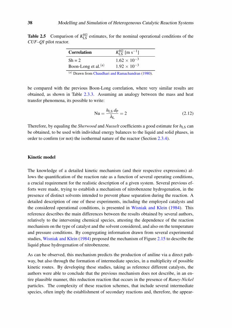
38 Modelling and Simulation of Heterogeneous Catalytic Reaction Systems
Table 2.5 Comparison of KH2LS estimates, for the nominal operational conditions of the
CUF–QI pilot reactor.
Correlation KH2LS [m s−1]
Sh = 2 1.62 × 10⁻³
Boon-Long et al.(a) 1.92 × 10⁻³
(a) Drawn from Chaudhari and Ramachandran (1980).
be compared with the previous Boon-Long correlation, where very similar results areobtained, as shown in Table 2.3.3. Assuming an analogy between the mass and heattransfer phenomena, its possible to write:
Nu =hLS dP
λL= 2 (2.12)
Therefore, by equaling the Sherwood and Nusselt coefficients a good estimate for hLS canbe obtained, to be used with individual energy balances to the liquid and solid phases, inorder to confirm (or not) the isothermal nature of the reactor (Section 2.3.4).
Kinetic model
The knowledge of a detailed kinetic mechanism (and their respective expressions) al-lows the quantification of the reaction rate as a function of several operating conditions,a crucial requirement for the realistic description of a given system. Several previous ef-forts were made, trying to establish a mechanism of nitrobenzene hydrogenation, in thepresence of distinct solvents intended to prevent phase separation during the reaction. Adetailed description of one of these experiments, including the employed catalysts andthe considered operational conditions, is presented in Wisniak and Klein (1984). Thisreference describes the main differences between the results obtained by several authors,relatively to the intervening chemical species, attesting the dependence of the reactionmechanism on the type of catalyst and the solvent considered, and also on the temperatureand pressure conditions. By congregating information drawn from several experimentalstudies, Wisniak and Klein (1984) proposed the mechanism of Figure 2.15 to describe theliquid phase hydrogenation of nitrobenzene.
As can be observed, this mechanism predicts the production of aniline via a direct path-way, but also through the formation of intermediate species, in a multiplicity of possiblekinetic routes. By developing these studies, taking as reference different catalysts, theauthors were able to conclude that the previous mechanism does not describe, in an en-tire plausible manner, this reduction reaction that occurs in the presence of Raney-Nickelparticles. The complexity of these reaction schemes, that include several intermediatespecies, often imply the establishment of secondary reactions and, therefore, the appear-

2.3 Industrial case-study 39
NO2 NH2
N
N
NH
NH
N→ O
N
NO NHOH
(AZXB) (AZB) (HB)
(NSB )
(MNB) (ANL)
(PHA)
Figure 2.15 Hydrogenation mechanism of nitrobenzene (Wisniak and Klein, 1984).
ance of byproducts. These will largely depend on the adopted operational conditions, ascan be concluded by comparison of Figures 2.6 and 2.15.
In the domain of experimental studies of slurry hydrogenation units, a literature reviewreveals a remarkable set of works in several ex-RDA universities, by Turek, Geike andLang, possibly in cooperation with the chemical company Leuna (Geike et al., 1986;Turek et al., 1986, 1987; Geike et al., 1989). This group studied the hydrogenation ofnitrobenzene to aniline at a laboratory scale, in a discontinuous stirred tank reactor, usingsuspended nickel catalyst and considering the effect of several variables (temperature,pressure and reactants concentration). Table 2.6 summarize the employed operationalconditions, while Figures 2.16 and 2.17 report the main results obtained.
Due to the complex mechanisms involved, these authors preferred to develop a pragmaticapproach, considering the main physicochemical phenomena that are present in the sys-tem. Therefore, assuming that the hydrogen adsorption occur in distinct catalytic centers,different from those used by the remaining components, and assuming that the catalystsurface is permanently covered by organic species, these authors proposed the followingequation to predict the reaction rate:
Γ = κkMNBCMNB
(1+κMNBCMNB +κANLCANL +κEtHCEtH +κWaterCWater)κH2CH2
(1+κH2CH2)(2.13)

40 Modelling and Simulation of Heterogeneous Catalytic Reaction Systems
Table 2.6 Main operational conditions used by Turek et al. (1986).
Variable Value
Liquid volume 1 lTemperature 50–130CPressure of H2 0.2–2.1 MPaInitial nitrobenzene concentration 4–45 × 10−3 mol l−1
Catalyst type Ni/Al2O3Catalyst concentration 0.5–1 g l−1
pH 9.0–9.5Solvent Mixture of water / ethanolLiquid phase composition (mass) wANL = 0.5; wWater = 0.3; wEtH = 0.2Stirring speed 150–800 min−1
Catalyst diameter 27 µm
0.5
05
130ºC
Con
ver
sion
of
nit
roben
zen
e
t (min)
1.0
0 10 15 20 25
100ºC
90ºC 80ºC
70ºC
60ºC
50ºCP=1.57 MPa
mC =0.82 g
C0=0.02 mol/l
Figure 2.16 Dependence of MNB conversion on temperature (Turek et al., 1986).
0.5
01
Con
ver
sion
of
nit
roben
zen
e
t (min)
1.0
0 2 3 4 5
T=128º C
mC =0.82 g
0.59 MPa
0.73 MPa
0.98 MPa
1.76 MPa
Figure 2.17 Dependence of MNB conversion on H2 pressure (Turek et al., 1986).

2.3 Industrial case-study 41
Since variations in the concentrations of water, aniline and ethanol were not considered inthese experimental studies, the previous expression can be simplified to its correspondingLangmuir-Hinshelwood form:
Γ = κκMNBCMNB
1+κMNBCMNBκH2SH2PH2
1+κH2SH2PH2 [mol m−3 s−1] (2.14)
The parameters κ , κH2 and κMNB in the above equation were determined by adjustingthe kinetic model to the obtained experimental results. In a first phase, the parameters κ
and κH2 were correlated, by considering the linear sections of the curves in Figures 2.16and 2.17. The influence of the normalized nitrobenzene concentration was latter evalu-ated, this time over the entire curves, to express κMNB. This procedure was based on thetwo following assumptions:
• The linear sections of the concentration-time profiles express zero order kineticstowards nitrobenzene. Therefore, κ and κH2 can be rigorously considered here.
• The final curvature of the concentration-time profiles can only be caused by aninhibition of the nitrobenzene adsorption, allowing the contribution of κMNB to beisolated.
The fitted equations are:
κ = 4.128×10⁶ exp(−53.25×10³
RT
)[mol kg−1 s−1] (2.15a)
κH2 = 1.097×10⁻² exp
(28.29×10³
RT
)[l mol−1] (2.15b)
KMNB = 3.503×10¹⁴ exp(−71.70×10³
RT
)[l mol−1] (2.15c)
The authors also studied the diffusional limitations (internal and external) for a widerange of operational conditions. They concluded that these mass transfer inhibitionsdid not cause significant errors during the determination of the kinetic parameters, pro-vided that high temperatures (T > 130 C) and low nitrobenzene concentrations (CMNB <
10−4mol l−1) were avoided. When the previous conditions were not fulfilled, strong in-hibitions were observed, relative to the mass transfer at the liquid-solid interface andthe diffusional intra-particle process. Under these circumstances, the final curvature ofthe profiles illustrated in Figures 2.16 and 2.17 could not be described by consideringuniquely equation (2.14).
As can be observed, the developed kinetic model enables a good fitting of the obtainedexperimental data. To transpose the results obtained at a laboratory scale for other situa-tions like, for example, an industrial reactor, Turek et al. (1986) suggest the introduction

42 Modelling and Simulation of Heterogeneous Catalytic Reaction Systems
of a corrective factor (Φ):Γreal = ΦΓlab (2.16)
Relatively to the effect of other variables, like pH, the information about their effect isscarce, leading to the premise that their effect might be included in the definition of theprevious Φ factor, as long as significant variations are avoided, with possible impact onthe reaction mechanism or in a significant change of the catalyst activity.
Finally, it should also be remarked that the previous kinetic model does not consider theformation of byproducts. This is due to the lack of confirmed mechanisms that origi-nate these “light” and “heavy” components reported in Figure 2.6, at the present stateof knowledge. To correlate the presence of these with some operational variables Tureket al. (1986) also adopted a pragmatic approach, based on the regression of simple ex-pressions, where the reaction mechanisms were not further investigated. This informationwill not be used here, due to its much higher dependence on the specific properties of theexperimental system used.
2.3.4 Modelling and solution
Based on the extensive information gathered from the literature, especially focused onunits with a configuration similar to that represented in Figure 2.5, the following assump-tions were made:
• The liquid phase is perfectly agitated (no radial or axial gradients are present).
• The catalyst particles and the hydrogen bubbles are uniformly distributed throughthe reacting mixture.
• The existing heat exchanging equipment assures the efficient removal of all thereaction heat, allowing to maintain the liquid phase temperature at a constant (pre-determined) value.
• The gas feed stream is composed by pure hydrogen.
• The mixture density depends only on the aniline and water mass fractions, since theconcentrations of the remaining species are several orders of magnitude lower.
• The catalyst particles are mono-disperse and can be completely characterized bytheir radius (rP) or diameter (dP).
• The active centers are uniformly distributed and equally available along the internalvolume of the catalyst particles.
Considering the underlying physicochemical phenomena, to find an optimal trade-off be-tween model accuracy and solution difficulty, two approaches were developed (Neveset al., 2002):

2.3 Industrial case-study 43
Table 2.7 Variables and parameters for the hydrogenation models developed.
Fundamental variables Dependent variables Parameters
CmL m = 1, . . . ,nc CH2
G TL
CmS m = 1, . . . ,nc(∗) SH2 PH2
QL He FMNBL , FANL
LFH2
G κ, κH2, κMNB ω
TS KmLS m = 1, . . . ,nc mC
KGLaB dPhLS aSDm
L m = 1, . . . ,nc VR, dR, dI(∗) In the microscopic model Cm
S →CmP (rP) and TS → TP(rP).
• A macroscopic one, where a simplified description of the catalyst particles is em-ployed, assuming that the physical variables (e.g., temperature and concentration)can be described by global values. These will characterize the entire solid phase,thus enabling the complete description of the system through an algebraic model.
• A microscopic one, where the diffusional and conductive phenomena are explicitlyconsidered inside the catalyst particles, resulting in a distributed-parameter model.In this case, only the radial dependence of the variables is considered, leading to aset of differential-algebraic equations.
The comparison of the results of these two previous models allows a direct assessment ofthe capability of the macroscopic approach to rigorously describe the global behavior ofthe system. This test is important, in order to derive a model as simple as possible for theoptimization studies considered in Chapter 3.
In both models, an effective exit flowrate (QL) was defined for the system reactor / de-canter. This corresponds to the difference between the reactor outlet and the recirculationstream that comes from the decanter (Figure 2.5). This procedure also assumes that noreaction takes place in the decanter where, therefore, only a physical separation step ispromoted. This premise is based on the low availability of hydrogen inside this unit, thathinders the hydrogenation of non-converted MNB that abandons the reactor.
To facilitate the analysis of both models, as well as for a better understanding of the op-erational details of the system under study, Table 2.7 lists all quantities involved, groupedinto fundamental variables (directly calculated from the solution of the model), dependentvariables (calculated from the fundamental variables) and model parameters. As can beobserved, the only difference between the microscopic and macroscopic approaches isrelative to the treatment of Cm
S and TS.
Another important aspect is relative to the solid phase temperature, assumed as a funda-mental variable in Table 2.7. In fact, two versions were developed for each modelling ap-proach: one considering heat balances to the solid phase, and another assuming isothermal
44 Modelling and Simulation of Heterogeneous Catalytic Reaction Systems
conditions, where TL = TS = TP(rP). The underlying motivation is, once again, to keepthe modelling procedure as simple as possible in the subsequent optimization studies.
Macroscopic model
The macroscopic model will be composed by the following equations:
• A global mass balance, where FmL are the partial feeds of each component and where
QL represents the system total outlet stream:
FANLL MANL +FMNB
L MMNB +FH2G MH2 = QLρL (2.17)
• A mass balance to the gas phase. This expresses that all the hydrogen that entersthe system is transferred through the GL interface:
FH2G = KGLaB
(CH2
GHe
−CH2L
)VR (2.18)
• A mass balance to hydrogen, in the liquid mixture. This equals the mass transferredthrough the GL interface to the amount of hydrogen that reach the solid phase:
KGLaB
(CH2
GHe
−CH2L
)VR = KH2
LS aS(CH2
L −CH2S)VR +CH2
L QL (2.19)
• Partial mass balances around the remaining chemical species, in the liquid phase:
FmL = Km
LSaS(Cm
L −CmS)VR +Cm
L QL, m = MNB,Water,ANL (2.20)
• Partial mass balances in the solid phase, that expresses an equality between themass transferred through the LS interface and that consumed (or produced) in thereaction, in a pseudo-homogeneous approach:
KmLSaS
(Cm
L −CmS)
= (−γm)ΓmC, m = MNB,H2,Water,ANL (2.21)
• A global energy balance:
hLSaS(TS−TL
)= (−∆HR)ΓmC (2.22)
In (2.21) and (2.22), the implicit reaction rate (Γ) is a macroscopic one, equivalent to thatof (2.14).

2.3 Industrial case-study 45
Microscopic model
In this second approach, the diffusional and conductive phenomena are explicitly consid-ered. The mass balances around the global system and the gas phase remain unchanged(equations (2.17) and (2.18), respectively). Only slight modifications are required in themass balances around the liquid phase (equations 2.19 and 2.20), as a consequence of adifferent approach relative to the solid phase:
FmL = Km
LSaS(Cm
L −CmP |rP=RP
)VR +Cm
L QL, m = MNB,Water,ANL (2.23)
The conditions at the catalyst surface are now distinguished from those in the intra-particlespace. Therefore, it becomes necessary to substitute the concentrations (and temperature)that were written for an homogeneous solid phase, by new ones that refer explicitly to theexternal particle radius. The mass and energy balances to the solid phase are now:
Dmeff
(∂ 2Cm
P∂ r2
P+
2rP
∂CmP
∂ rP
)= (−γ
m)Γ (2.24a)
∂CmP
∂ rP
∣∣∣∣rP=0
= 0 (symmetry condition) (2.24b)
Dmeff
∂CmP
∂ rP
∣∣∣∣rP=RP
= KmLS(Cm
L −CmP |rP=RP
), m = MNB,Water,ANL (2.24c)
λeff
(∂ 2TP
∂ r2P
+2rP
∂TP
∂ rP
)= (−∆HR)Γ (2.24d)
∂TP
∂ rP
∣∣∣∣rP=0
= 0 (symmetry condition) (2.24e)
λeff∂TP
∂ rP
∣∣∣∣rP=RP
= hLS(TL− TP|rP=RP
)(2.24f)
In the above equations, the reaction rate term is given by:
Γ = κκMNBCMNB
P
(1+κMNBCMNBP )
κH2CH2P
(1+κH2CH2P )
mP
VP(2.25)
Since in equations (2.24a) and (2.24d) the reaction rate is microscopic, a constant termmP/VP is introduced in (2.25), assuming an homogeneous active center distribution insidethe particles. This approximation, although (eventually) unrealistic, is necessary due to

46 Modelling and Simulation of Heterogeneous Catalytic Reaction Systems
the unavailability of data relative to this type of catalysts.
Solution aspects
For the solution of the macroscopic model, the resulting system of nonlinear algebraicequations was solved using a constrained implementation of Newton’s method, imple-mented in the Mathematica programming system (Wolfram, 1999). A previous normal-ization of variables and equations was necessary, to improve the numerical condition ofthe Jacobian matrices obtained. This was done using the LAPACK routine for matrixbalancing (Anderson et al., 1999).
For the second model, expressed as a differential-algebraic system of equations, a dis-cretization procedure was adopted in the domain 0≤ rP ≤RP, using centered second orderfinite differences. To treat the boundary conditions, two fictitious auxiliary points wereused outside the previous domain. These allow the use of a centered discretization schemefor rP = 0 and rP = RP, although requiring the introduction of auxiliary equations. Theprevious procedure represents a good compromise between accuracy and solution effort.The microscopic approach revealed also to be extremely dependent on proper scaling ofthe variables and equations; in the absence of good numerical conditioning and approxi-mate initial estimates, no solution could be obtained. This is due to the accentuated profileinside the catalyst particles, with concentration changes of several orders of magnitudesbetween adjacent discretization points (Section 2.3.5).
Interpolating functions were built with the temperature and concentration profiles, start-ing with a small number of discretization points, in order to estimate the initial solution ofthe model, in the final case. For example, using 14 discretization points in the current mi-croscopic model, 86 nonlinear algebraic equations are obtained. This already constitutesan interesting numerical problem, whose dimension is capable of amplifying the previ-ous problems. However, if only 2 points are employed, the problem dimension drops to26 equations, thus becoming much easier to solve.
2.3.5 Main results
The two modelling approaches previously discussed require the estimation of severalphysical properties, for each of the three involved phases (e.g., SH2,Dm
L ,ξP). Most ofthe adopted correlations derive from the work of Yaws (1976a,b,c), although a large num-ber of other references has also been consulted; these are presented in Appendix A, whilethe predicted values for the nominal operational conditions are listed in Table 2.8.
The values obtained for the fundamental variables, through the solution of both developedmodels, are exhibited in Table 2.9. As can be observed, the results obtained for the macro-scopic and microscopic approaches are practically identical. The small differences relate

2.3 Industrial case-study 47
Table 2.8 Nominal values for parameters and properties.
Operating conditions
Reaction temperature [K] TL = 413.15
Hydrogen pressure [Pa] PH2 = 13×105
Stirring speed [rpm] ω = 2000
Nitrobenzene feed flowrate [mol s−1] FMNB = 4.85×10⁻²
Aniline feed flowrate [mol s−1] FANL = 5.01×10⁻²
Catalyst charge [kg m−3] mC = 15
Solid Phase
Particles diameter [m] dP = 17×10−6
Porosity εP = 0.6
BET area [m2 g−1] ABET = 100
Density [kg m−3] ρP = 1500
Tortuosity factor ξP = 1.67
Gas Phase
Hydrogen Solubility [mol m−3 Pa−1] SH2 = 2.27×10⁻⁵
Henry constant He = 12.84
Hydrogen concentration [mol m−3] CH2G = 378.5
Liquid Phase
Density [kg m−3] ρL = 918.4
Thermal conductivity [W m−1 K−1] λL = 0.196
Superficial tension [N m−1] σL = 3.9×10⁻²
Viscosity [Pa s−1] µL = 3.81×10⁻⁴
Nitrobenzene diffusivity [m2 s−1] DMNBL = 3,83×10⁻⁹
Hydrogen diffusivity [m2 s−1] DH2L = 1.38×10⁻⁸
Aniline diffusivity [m2 s−1] DANLL = 1.00×10⁻⁹
Water diffusivity [m2 s−1] DWaterL = 1.00×10⁻⁹
Mass & Heat Transfer
Hydrogen mass transfer in the GL interface [s−1] KGLaB = 26.7
Nitrobenzene mass transfer in the LS interface [m s−1] KMNBLS = 9.61×10⁻⁴
Hydrogen mass transfer in the LS interface [m s−1] KH2LS = 1.92×10⁻³
Aniline mass transfer in the LS interface [m s−1] KANLLS = 4.66×10⁻⁴
Water mass transfer in the LS interface [m s−1] KWaterLS = 4.66×10⁻⁴
Heat transfer in the LS interface [W m−2 K−1] hLS = 23.1×10³

48 Modelling and Simulation of Heterogeneous Catalytic Reaction Systems
Table 2.9 Results obtained by solution of the two developed models.
Macroscopic MicroscopicVariable Units model model
QL [m3 h−1] 4.82×10⁻² 4.82×10⁻²
FH2G [mol s−1] 0.146 0.146
CMNBL [mol m−3] 0.148 0.150
CH2L [mol m−3] 29.4 29.4
CANLL [mol m−3] 8.28×10³ 8.28×10³
CWaterL [mol m−3] 8.15×10³ 8.15×10³
CMNBS [mol m−3] 9.04×10⁻⁵ 1.74×10⁻³
CH2S [mol m−3] 29.2 29.2
CANLS [mol m−3] 8.28×10³ 8.28×10³
CWaterS [mol m−3] 8.15×10³ 8.15×10³
TS [K] 413.15 413.15Note: for the microscopic model consider Cm
S = CmP |rP=RP
and TS = TP|rP=RP.
Table 2.10 Comparison between model predictions and industrial data.
Variable Macroscopic Microscopic Pilot reactor
wANL 0.840 0.840 ' 0.84wWater 0.160 0.160 ' 0.16CMNB
L 20 ppm 20 ppm 5–300 ppm
mostly to the solid phase values, and are easily understandable due to the different treat-ment in both cases. A comparison between computational predictions and experimentalresults is shown in Table 2.10, although limited to the industrial data presented.
For a better comprehension of the role that the mass and energy transfer steps play inthe system performance, the associated internal and external resistances were evaluated(Table 2.11 and Figures 2.18 and 2.19). It is possible to observe the following:
• From Table 2.11, the external diffusion of nitrobenzene is a major limiting step,since the concentration of this reactant decreases significantly at the liquid-solidinterface (' 99%).
• From Figures 2.18 and 2.19 it is possible to observe that nitrobenzene is the limitingreactant, and that it is considerably depleted in a zone close to the particle’s externalradius. This clearly denotes a surface reaction, also confirmed by the calculatedefficiency factor value (η ' 0.02), obtained through numerical integration of (2.1),considering the above intra-particle profiles.
Both indications are in agreement with the results of Turek et al. (1987), and also with

2.3 Industrial case-study 49
Table 2.11 Mass and heat transfer resistances, predicted by the macroscopic model.
H2 absorption External reactants External heatin the liquid diffusion dispersion
C?,H2G −CH2
L
C?,H2G
CH2L −CH2
SCH2
L
CMNBL −CMNB
SCMNB
L
TL−TSTL
2.2×10⁻³ 7.5×10⁻³ 0.988 ' 0
0.0 0.2 0.4 0.6 0.8 1.0
r (normalized)
0.0
0.2
0.4
0.6
0.8
1.0
C
(n
orm
aliz
ed)
MN
B
P
P
0.0 0.2 0.4 0.6 0.8 1.00.99990
0.99992
0.99994
0.99996
0.99998
1.00000
r (normalized)P
C
(no
rmal
ized
)H
2
P
(a) (b)
Figure 2.18 Concentration profiles of the reactants, predicted by the microscopicmodel, inside the catalyst particle: (a) nitrobenzene, (b) hydrogen.
other references that specifically relate to this type of systems (Furusawa and Smith, 1973;Ramachandran and Chaudhari, 1980a).
It is also important to notice that the high resistance to internal diffusion has a relativelysmall impact on the reactor performance. This is due to the high mass-transfer resistanceat the liquid-solid interface, which accounts for a significant drop in the concentrationof this reactant, as it reaches the catalyst surface. This indicates that the best mode ofenhancing the reaction efficiency would be to reduce this external resistance.
Another interesting aspect relates to heat transfer. As represented in Figure 2.19 (b) and
0.0 0.2 0.4 0.6 0.8 1.0
0.999992
0.999994
0.999996
0.999998
1.000000
0.999990
C
,
C
(no
rmal
ized
)A
NL
r (normalized)P
Wat
er
PP
0.0 0.2 0.4 0.6 0.8 1.0
0.999992
0.999994
0.999996
0.999998
1.000000
0.999990
r (normalized)P
T (
norm
aliz
ed)
P
(a) (b)
Figure 2.19 Profiles inside the catalyst particle, predicted by the microscopic model,for: (a) Products concentration, (b) temperature.
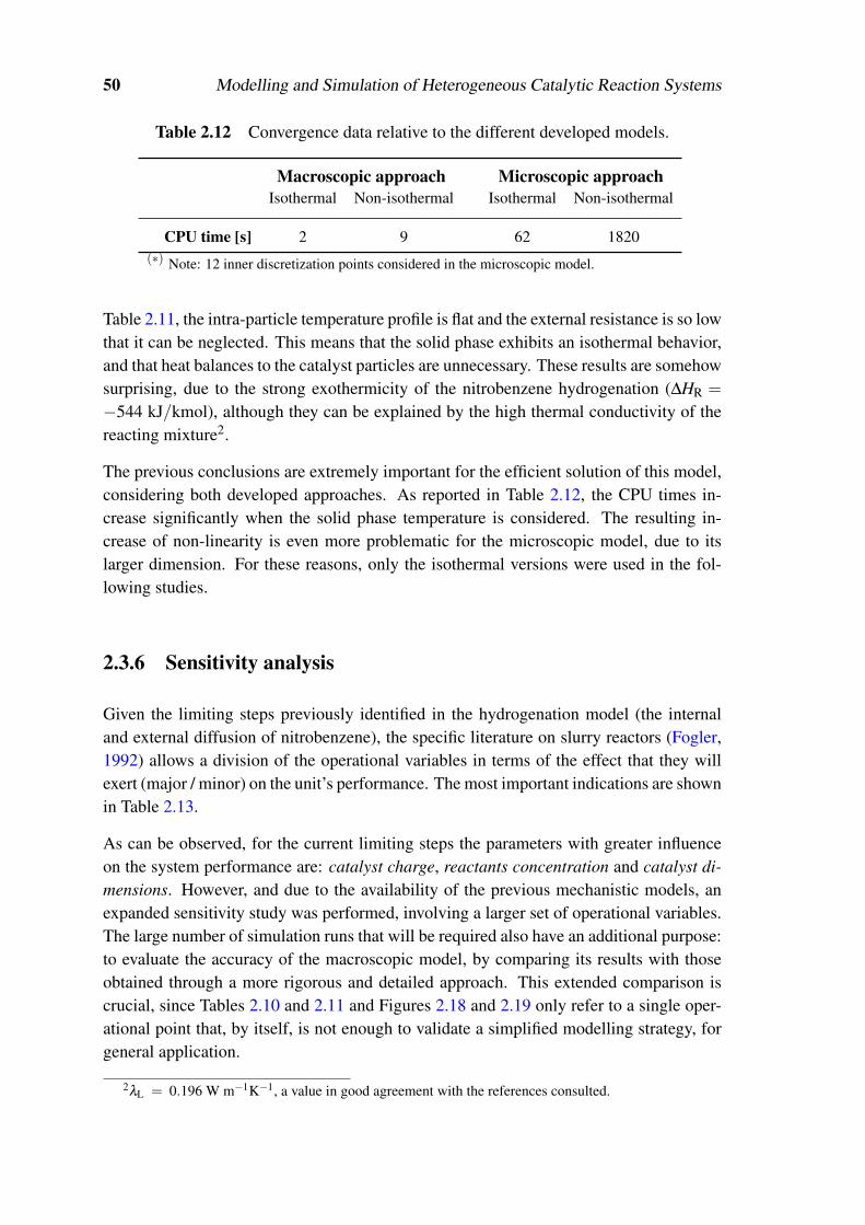
50 Modelling and Simulation of Heterogeneous Catalytic Reaction Systems
Table 2.12 Convergence data relative to the different developed models.
Macroscopic approach Microscopic approachIsothermal Non-isothermal Isothermal Non-isothermal
CPU time [s] 2 9 62 1820(∗) Note: 12 inner discretization points considered in the microscopic model.
Table 2.11, the intra-particle temperature profile is flat and the external resistance is so lowthat it can be neglected. This means that the solid phase exhibits an isothermal behavior,and that heat balances to the catalyst particles are unnecessary. These results are somehowsurprising, due to the strong exothermicity of the nitrobenzene hydrogenation (∆HR =−544 kJ/kmol), although they can be explained by the high thermal conductivity of thereacting mixture2.
The previous conclusions are extremely important for the efficient solution of this model,considering both developed approaches. As reported in Table 2.12, the CPU times in-crease significantly when the solid phase temperature is considered. The resulting in-crease of non-linearity is even more problematic for the microscopic model, due to itslarger dimension. For these reasons, only the isothermal versions were used in the fol-lowing studies.
2.3.6 Sensitivity analysis
Given the limiting steps previously identified in the hydrogenation model (the internaland external diffusion of nitrobenzene), the specific literature on slurry reactors (Fogler,1992) allows a division of the operational variables in terms of the effect that they willexert (major / minor) on the unit’s performance. The most important indications are shownin Table 2.13.
As can be observed, for the current limiting steps the parameters with greater influenceon the system performance are: catalyst charge, reactants concentration and catalyst di-mensions. However, and due to the availability of the previous mechanistic models, anexpanded sensitivity study was performed, involving a larger set of operational variables.The large number of simulation runs that will be required also have an additional purpose:to evaluate the accuracy of the macroscopic model, by comparing its results with thoseobtained through a more rigorous and detailed approach. This extended comparison iscrucial, since Tables 2.10 and 2.11 and Figures 2.18 and 2.19 only refer to a single oper-ational point that, by itself, is not enough to validate a simplified modelling strategy, forgeneral application.
2λL = 0.196 W m−1K−1, a value in good agreement with the references consulted.
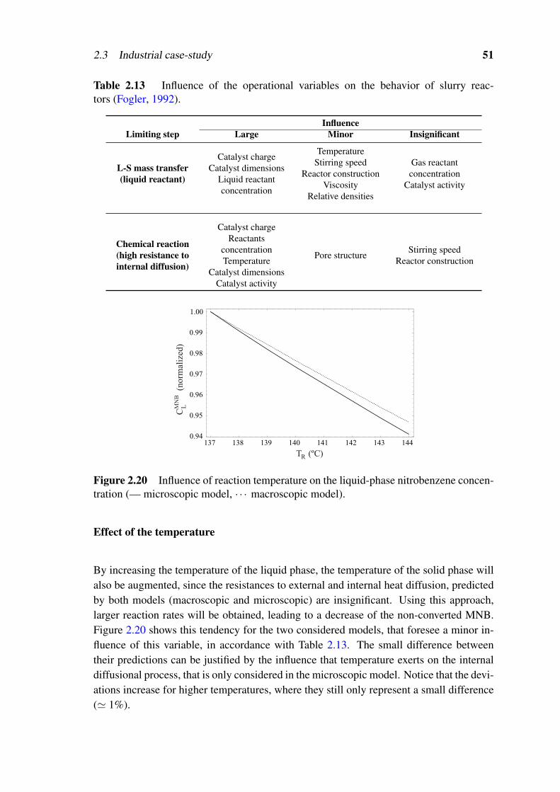
2.3 Industrial case-study 51
Table 2.13 Influence of the operational variables on the behavior of slurry reac-tors (Fogler, 1992).
InfluenceLimiting step Large Minor Insignificant
L-S mass transfer(liquid reactant)
Catalyst chargeCatalyst dimensions
Liquid reactantconcentration
TemperatureStirring speed
Reactor constructionViscosity
Relative densities
Gas reactantconcentration
Catalyst activity
Chemical reaction(high resistance tointernal diffusion)
Catalyst chargeReactants
concentrationTemperature
Catalyst dimensionsCatalyst activity
Pore structure Stirring speedReactor construction
137 138 139 140 141 142 143 1440.94
0.95
0.96
0.97
0.98
0.99
1.00
T (ºC) R
C (n
orm
aliz
ed)
MN
B
L
Figure 2.20 Influence of reaction temperature on the liquid-phase nitrobenzene concen-tration (— microscopic model, · · · macroscopic model).
Effect of the temperature
By increasing the temperature of the liquid phase, the temperature of the solid phase willalso be augmented, since the resistances to external and internal heat diffusion, predictedby both models (macroscopic and microscopic) are insignificant. Using this approach,larger reaction rates will be obtained, leading to a decrease of the non-converted MNB.Figure 2.20 shows this tendency for the two considered models, that foresee a minor in-fluence of this variable, in accordance with Table 2.13. The small difference betweentheir predictions can be justified by the influence that temperature exerts on the internaldiffusional process, that is only considered in the microscopic model. Notice that the devi-ations increase for higher temperatures, where they still only represent a small difference(' 1%).
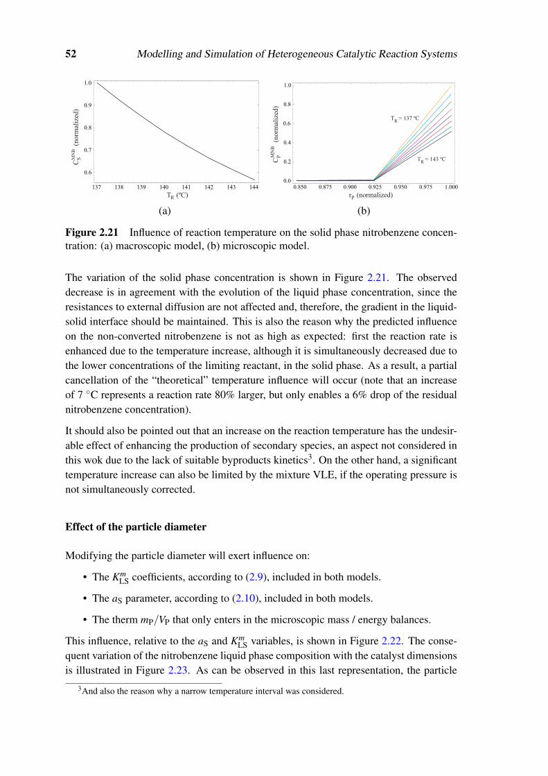
52 Modelling and Simulation of Heterogeneous Catalytic Reaction Systems
137 138 139 140 141 142 143 144
0.6
0.7
0.8
0.9
1.0
C
(n
orm
aliz
ed)
S
T (ºC) R
MN
B
0.850 0.875 0.900 0.925 0.950 0.975 1.0000.0
0.2
0.4
0.6
0.8
1.0
C
(
norm
aliz
ed)
P
T = 137 ºC R
T = 143 ºC R
r (normalized)P
MN
B
(a) (b)
Figure 2.21 Influence of reaction temperature on the solid phase nitrobenzene concen-tration: (a) macroscopic model, (b) microscopic model.
The variation of the solid phase concentration is shown in Figure 2.21. The observeddecrease is in agreement with the evolution of the liquid phase concentration, since theresistances to external diffusion are not affected and, therefore, the gradient in the liquid-solid interface should be maintained. This is also the reason why the predicted influenceon the non-converted nitrobenzene is not as high as expected: first the reaction rate isenhanced due to the temperature increase, although it is simultaneously decreased due tothe lower concentrations of the limiting reactant, in the solid phase. As a result, a partialcancellation of the “theoretical” temperature influence will occur (note that an increaseof 7 C represents a reaction rate 80% larger, but only enables a 6% drop of the residualnitrobenzene concentration).
It should also be pointed out that an increase on the reaction temperature has the undesir-able effect of enhancing the production of secondary species, an aspect not considered inthis wok due to the lack of suitable byproducts kinetics3. On the other hand, a significanttemperature increase can also be limited by the mixture VLE, if the operating pressure isnot simultaneously corrected.
Effect of the particle diameter
Modifying the particle diameter will exert influence on:
• The KmLS coefficients, according to (2.9), included in both models.
• The aS parameter, according to (2.10), included in both models.
• The therm mP/VP that only enters in the microscopic mass / energy balances.
This influence, relative to the aS and KmLS variables, is shown in Figure 2.22. The conse-
quent variation of the nitrobenzene liquid phase composition with the catalyst dimensionsis illustrated in Figure 2.23. As can be observed in this last representation, the particle
3And also the reason why a narrow temperature interval was considered.

2.3 Industrial case-study 53
5 10 15 20 25
d (µ m )
4
6
8
10
12
(x10
-3
m-1
)
2
a S
P
5 10 15 20 25
0.90
0.95
1.00
1.05
1.10
1.15
1.20
d (µ m )P
(x
10
-3
m s
-1)
KL
S
MN
B
(a) (b)
Figure 2.22 Influence of the particle diameter on the: (a) solid phase surface area, (b)nitrobenzene LS mass transfer coefficient.
5 10 15 20 25
d (µ m )P
0.2
0.4
0.6
0.8
1.0
C
(n
orm
aliz
ed)
L
0.0
MN
B
Figure 2.23 Influence of the particle diameter on the nitrobenzene liquid phase concen-tration (— microscopic model, · · · macroscopic model).
dimensions exert a considerable effect on the conversion. For example, changing theirdiameter to 5 µm allows a 80% decrease on the residual MNB concentration. This is ac-complished due to a significant reduction of the external diffusional limitations (relativeto nitrobenzene); it results from two effects:
• For the same catalyst charge, a lower particle diameter correspond to a larger exter-nal area, that is highly advantageous in the presence of surface reactions.
• The nitrobenzene mass transfer coefficient in the liquid-solid interface increases forcatalysts with smaller dimensions.
Therefore, both effects contribute to enhance the mass transfer rates in the layer aroundthe particles, although in different extents. In fact, the external resistances are not sig-nificantly reduced (since Km
LS only increases 30% and, therefore, the nitrobenzene con-centration still drops considerably); the global behavior is almost totally justified by theincrease of the available transfer area (aS(5µm)' 6aS(25µm)).

54 Modelling and Simulation of Heterogeneous Catalytic Reaction Systems
0.9994
0.9995
0.9996
0.9997
0.9998
0.9999
1.0000
5 10 15 20 25
d (µ m )P
C (n
orm
aliz
ed)
SMN
B
0.850 0.875 0.900 0.925 0.950 0.975 1.0000.0
0.2
0.4
0.6
0.8
1.0
d (normalized)P
d = P 26 µm
d = P 5 µm
C
(n
orm
aliz
ed)
PMN
B
(a) (b)
Figure 2.24 Influence of particle diameter on the nitrobenzene solid phase concentra-tion (a) macroscopic model, (b) microscopic model.
The dependence of the nitrobenzene solid phase concentration on the particle dimensionis show in Figure 2.24. Here, both approaches differ to a larger extent, since the micro-scopic model predicts a more accentuated decrease. This is expected, due to the influenceof the catalyst dimension on the intra-particle mass / heat balances, especially relativelyto the effect of internal diffusion. However, due to the weak impact of this phenomenaon the system performance, the predictions for the liquid-phase are identical. This is pos-sible because the macroscopic model, which does not consider intra-particle phenomena,estimates a higher resistance to external diffusion; the resulting global agreement derivesfrom a re-distribution of the different types of resistances.
It should be noticed that using particles with reduced dimensions rises some operationaldifficulties. These are related with the sedimentation / filtration stages for catalyst separa-tion, and may cause a significant overall impact, by increasing the catalyst consumption(due to its less effective recovery). However, once these difficulties are overcome, theprevious analysis points towards the use of smaller catalyst particles, as an effective formof enhancing the performance of the reactors. This indication is in accordance with theguidelines provided in Table 2.13 and, additionally, also explains the better behavior ofthe used catalyst, when compared with the fresh one (Section 2.3.2). The milling effectthat, in the absence of the previous indications, could be seen as a negative occurrence, isnow identified as advantageous, since it reduces the mean particle diameter.
Effect of the catalyst charge
Like the particle dimensions, the variation of the catalyst charge also affects the param-eters aS and Km
LS. This time, the influence is directly proportional in aS and indirectly inKm
LS, where a slightly negative effect is observed (Figure 2.25). As a consequence of thelarger external area available for reaction, the nitrobenzene residual concentration dropsboth in the liquid and solid phases (Figures 2.26 and 2.27). Their decrease leads to anaugmented external diffusion resistance, although in a small extent (since the value of
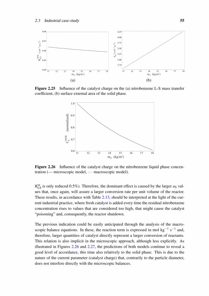
2.3 Industrial case-study 55
11 12 13 14 15 16 17 18
m (kg/m )
0.94
0.95
0.96
0.97
0.98
(x
10
-3
m s
-1)
KL
S
C3
MN
B
3.00
3.25
3.50
3.75
4.25
(x
10
-3
m-1
)
2.75
a S
11 12 13 14 15 16 17 18
m (kg/m )C3
4.00
(a) (b)
Figure 2.25 Influence of the catalyst charge on the (a) nitrobenzene L-S mass transfercoefficient, (b) surface external area of the solid phase.
11 12 13 14 15 16 17 18
0.7
0.8
0.9
1.0
m (kg/m )C3
C
(n
orm
aliz
ed)
L
0.6
MN
B
Figure 2.26 Influence of the catalyst charge on the nitrobenzene liquid phase concen-tration (— microscopic model, · · · macroscopic model).
KmLS is only reduced 0.5%). Therefore, the dominant effect is caused by the larger aS val-
ues that, once again, will assure a larger conversion rate per unit volume of the reactor.These results, in accordance with Table 2.13, should be interpreted at the light of the cur-rent industrial practice, where fresh catalyst is added every time the residual nitrobenzeneconcentration rises to values that are considered too high, that might cause the catalyst“poisoning” and, consequently, the reactor shutdown.
The previous indication could be easily anticipated through the analysis of the macro-scopic balance equations. In these, the reaction term is expressed in mol kg−1 s−1 and,therefore, larger quantities of catalyst directly represent a larger conversion of reactants.This relation is also implicit in the microscopic approach, although less explicitly. Asillustrated in Figures 2.26 and 2.27, the predictions of both models continue to reveal agood level of accordance, this time also relatively to the solid phase. This is due to thenature of the current parameter (catalyst charge) that, contrarily to the particle diameter,does not interfere directly with the microscopic balances.

56 Modelling and Simulation of Heterogeneous Catalytic Reaction Systems
11 12 13 14 15 16 17 180.6
0.7
0.8
0.9
1.0
C
(n
orm
aliz
ed)
S
m (kg/m )C3
MN
B
0.850 0.875 0.900 0.925 0.950 0.975 1.0000.0
0.2
0.4
0.6
0.8
1.0
m = 11 kg/m C3
m = 18 kg/m C3
C (n
orm
aliz
ed)
P
r (normalized)P
MN
B
(a) (b)
Figure 2.27 Influence of the catalyst charge on the nitrobenzene solid phase concentra-tion (a) macroscopic model, (b) microscopic model.
2000 2200 2400 2600 2800 3000
0.8
0.9
1.0
1.1
1.2
1.3
ω (rpm)
(x10
-3
m s
-1)
KL
S
MN
B
2000 2200 2400 2600 2800 3000
30
40
50
60
70
80
ω (rpm)
( s
-1)
KG
La
B
(a) (b)
Figure 2.28 Influence of stirring speed on the (a) nitrobenzene LS mass transfer, (b)hydrogen GL mass transfer.
Effect of the stirring speed
The stirring speed has a direct effect on the gas-liquid and liquid-solid mass transfer coef-ficients, as shown in Figure 2.28, within the considered range of variation. For the systemunder study, and due to the current limiting steps, this effect is important only in Km
LS,where a minor influence is observed. Therefore, the resistance to the external diffusion ofMNB cannot be significantly reduced by manipulation of the stirring speed; this becomesclear by analysis of Figure 2.29. This conclusion was also obtained by Turek et al. (1987),using a fairly different correlation for the prediction of KGLaB and, therefore, consideringa distinct influence of the ω parameter (Section 2.3.3). This correlation, reported in Fig-ure 2.13, predicts that in the limit the gas-liquid mass transfer coefficient reaches valuesclose to unity and, therefore, one order of magnitude below those implicit in Figure 2.29results.
However, it was possible to confirm that when low values of KGLaB are used (similarto those obtained in the experimental studies of Turek et al. (1987)), together with thedeveloped models, the results obtained are essentially identical. The explanation is related

2.3 Industrial case-study 57
2000 2200 2400 2600 28000.7
0.8
0.9
1.0
1.1
ω (rpm)
C (n
orm
aliz
ed)
LMN
B
Figure 2.29 Influence of the stirring speed on the nitrobenzene liquid phase concentra-tion (— microscopic model, · · · macroscopic model).
to the gas-liquid mass transfer, a step characterized by negligible resistances, that does notlimit the reactor performance, even when its efficiency is reduced.
Effect of the operating pressure
The adopted Langmuir-Hinshelwood kinetic expression, expressed by equations (2.14)or (2.23) (depending on the employed model), predicts an increase of the reaction rate forhigher partial pressures of hydrogen (or, from a microscopic perspective, for higher CH2
P ).Therefore, it is important to quantify how this effect will impact the reactor conversion.
As illustrated in Figure 2.30, both models predict the operating pressure as a variable ofreduced influence in the system performance. This behavior is easily justified, consideringthat the reaction rate cannot profit from the higher hydrogen concentrations in the liquidphase (and, consequently, in the catalyst particles), since nitrobenzene is the limiting reac-tant. The external diffusion step is unaffected (since KMNB
LS and aS remain unaltered) and,therefore, so is the system conversion. These results are in agreement with the indicationsof Table 2.13 and also with the experimental work of Turek et al. (1987). Therefore, theoperating pressure should be set for a given temperature mostly to maintain the reactionmixture in a liquid state, avoiding its partial vaporization4.
Effect of the feed flowrate
From most of the previous analysis, it became clear that the nitrobenzene solid phaseconcentration is very low (' 10−3 mol m−3), due to the limiting nature of this component.This fact has a direct impact in the system performance, since it expresses a reaction ratethat is very low. Therefore, an increase of the reaction rate can be accomplished simply by
4This also explains why it was excluded as an independent optimization variable.

58 Modelling and Simulation of Heterogeneous Catalytic Reaction Systems
10 11 12 13 14 15 16 17
0.96
0.98
1.00
1.02
1.04
C (
norm
aliz
ed)
L
P (bar)H2
MN
B
Figure 2.30 Influence of the operating pressure on the liquid phase nitrobenzene con-centration (— microscopic model, · · · macroscopic model).
0.00 0.02 0.04 0.06 0.08 0.10
5
10
15
20
C (mol m )S
3
Γ (
mol
kg s
)
-1
-1
0
Region of interest
MNB
Figure 2.31 Dependence of the reaction rate on the nitrobenzene solid phase concentra-tion, as predicted by (2.14).
promoting higher nitrobenzene concentrations in the catalyst particles. Figure 2.31 showsthis dependence for the adopted kinetic curve. The analysis of Figure 2.31 also enablesanother important indication: within the current operating range (' 10−3mol m−3), anysmall variation on CMNB
S will have a significant impact on the overall reaction rate, sincethe kinetic curve exhibits an accentuated slope in the low concentration zone. In thissense, studying the effect of larger nitrobenzene feed flowrates, as a way of enhancing thereactor productivity, becomes an important point.
By increasing the feed flowrate, maintaining the same volume of reaction mixture, thereactants residence times will drop, causing an increase of the residual concentration ofnitrobenzene in the liquid phase (Figure 2.32). However, these larger values of CMNB
L willalso imply an increase of nitrobenzene concentration in the solid phase, according to theexternal diffusional resistances that prevail in the system (Figure 2.33). Therefore, a largefraction of the expected increase in CMNB
L is cancelled, and better levels of productivitycan be achieved, due to an enhanced reaction rate.

2.3 Industrial case-study 59
5.0 5.5 6.0 6.5 7.0 7.5 8.01.0
1.1
1.2
1.3
1.4
1.5
1.6
1.7
C
(m
ol
m
)L
-3
F (x10 mol s )-1 -1 MNB
MN
B
Figure 2.32 Influence of the nitrobenzene feed flowrate on the respective liquid phaseconcentration (— microscopic model, · · · macroscopic model).
5.0 5.5 6.0 6.5 7.0 7.5 8.01.0
1.1
1.2
1.3
1.4
1.5
1.6
1.7
F (x10 mol s )-1 -1 MNB
C (n
orm
aili
zed)
S
MN
B
0.850 0.875 0.900 0.925 0.950 0.975 1.0000.0
0.5
1.0
1.5
2.0
2.5
C (m
ol
m )
P
-3
F = 0.0825 mol s -1 MNB
F = 0.0485 mol s -1 MNB
r (normalized)P
MN
B
(a) (b)
Figure 2.33 Influence of the nitrobenzene feed flowrate on the respective solid phaseconcentration (a) macroscopic model, (b) microscopic model.
The previous explanation can be confirmed through the analysis of Figure 2.34. Here, itis possible to observe the weak influence that the nitrobenzene feed flowrate exerts on theobtained reaction conversion, and confirm the indications of Table 2.13. This negligibledependence has, nevertheless, a limit. In fact, it will not remain applicable for CMNB
Shigher than approximately 3× 10⁻² mol m−3. In this last operating region, the kineticcurve exhibits an horizontal asymptotic behavior, and any small increase on FMNB
L willcause a significant decrease of the reactor conversion.
From an overall analysis it becomes clear that the shape of the kinetic curve plays acrucial role in the performance of these systems. Considering that equation (2.14) wasnot experimentally validated for the CUF–QI units, the accentuated slope reported inFigure 2.31 can be somehow inaccurate. For this reason, additional studies should beconsidered in the future, to provide a more rigorous location of the optimal operation pointwhere, in kinetic terms, the switch to an horizontal asymptotic behavior (independent ofCMNB
S ) occurs.

60 Modelling and Simulation of Heterogeneous Catalytic Reaction Systems
5.0 5.5 6.0 6.5 7.0 7.5 8.00.9992
0.9994
0.9996
0.9998
1.0000
Co
nv
ersi
on
(n
orm
.)
F (x10 mol s )-2 -1 MNB
Figure 2.34 Influence of the nitrobenzene feed flowrate on the reaction conversion (—microscopic model, · · · macroscopic model).
It is also important to emphasize that a large increase of the reactants feed flowrate doesnot assure, by itself, the enhancement of the overall productivity. Two important addi-tional aspects should be considered:
• The nitrobenzene conversion cannot significantly increase from its reference value.If the concentration of residual nitrobenzene rises above 50 ppm, the purity specifi-cations of the final product will not be fulfilled, since it is very difficult to promotethe separation of this reactant from aniline (through distillation, in the separationphase).
• During the nitrobenzene hydrogenation, water is stoichiometrically produced in alarger extension than aniline. Therefore, the aqueous fraction of the reaction mix-ture will increase, causing solubility problems; these must be avoided to prevent theappearance of a biphasic behavior and consequent operational failures.
While the second aspect is easy to be considered by simply recirculating more dehydratedaniline back to the reactors, the first one requires a more elaborated strategy. In fact, theonly way of overcoming it implies the reconfiguration of the reaction network — this willbe discussed in Chapter 3.

Chapter 3
Optimization of Reaction Units andNetworks
Summary
This Chapter presents a strategy for the optimization of complex reaction networks, that addressessome of major difficulties of this problem; these include very large problem sizes, extreme nonlin-earity and the presence of many (local) optimal solutions. The key idea followed in this approachis the use of a continuous formulation, not only for the optimization of the individual units butalso for the synthesis of an optimal structure of interconnections. For this purpose, quadratic con-straints with adjustable parameters are enforced to translate the aggregation level of each stream,and consequently control the complexity of the resulting network. This is particularly useful inmulti-objective scenarios, more adequate for this class of problems than single oriented func-tions (e.g., economical or conversion based). Another important point of this strategy is the useof interior-point methods that, as will be shown, exhibit superior performance when in the pres-ence of a large number of inequalities and bilinear terms, characteristic of network optimizationproblems. The efficiency of the overall methodology is illustrated by considering the industrialcase-study of aniline production, as implemented in CUF–QI.
3.1 Optimization of reaction units
In the optimization of reactor networks, two types of units emerge as fundamental buildingblocks that should be considered: plug-flow (PFR) and continuous stirred-tank (CSTR)reactors. These essentially correspond to the mathematical idealizations of two extremeflow regimes (completely segregated and perfectly mixed, respectively). Although highlyidealized, these types of units can be understood as fundamental building blocks, since:
• Any abstract reactor network configuration can be decomposed (or replaced) by aset of these units, with arbitrary connections and recycle streams, using if necessary
61

62 Optimization of Reaction Units and Networks
DSR
f(l)
q(l)
CInl COut
F0
m m
Q0
PFRCInl COut
F0
m m
Q0
Differential side-stream reactor
Plug-flow reactor reactor
Figure 3.1 Optimization of feed and side-streams locations in tubular reactors.
units of differential size.
• In the limit, when the size (volume) parameter tends to zero, a PFR unit becomesequivalent to a CSTR, and vice-versa.
Therefore, the synthesis of optimal reactor networks has been naturally addressed by sev-eral authors, considering a superstructure of alternatives in an arrangement of either (orboth) of these types of units (Floudas, 1995; Biegler et al., 1997).
Before a comparison of the relative merits of these approaches is established, it is alsouseful to consider the concept of attainable regions (Horn, 1964), as a geometric gener-alization of the principles of reactor design of Levenspiel (1998). This concept expressesthe convex hull, in the concentration space, of the region of concentrations that can beachieved, starting from the feed point, and using reaction and mixing operations. Thisanalysis is usually performed considering isothermal operation, in order to simplify theinterpretation of the results obtained. A particular important result in the theory of at-tainable regions is the characterization of its boundaries, since any interior point can beachieved by mixing two points located on the boundary. The available results state thefollowing:
• In two-dimensional reactor network synthesis the attainable region can be mappedusing only CSTRs and PFRs (Hildebrandt et al., 1990).
• In addition to CSTRs and PFRs, in three or higher-dimensional systems differentialside-stream reactors (DSRs) can be effectively used to navigate along the attainableregion’s boundary (Glasser et al., 1992; Feinberg and Hildebrandt, 1997; Feinberg,2000).
Hence the use of DSR units, as a generalization of PFRs (Figure 3.1), can be highly ad-vantageous in reactor network synthesis, in order to limit the number of units obtained inthe optimal solution, and their final physical realization. If considered individually, theoptimization of a single DSR unit can be straightforward addressed by an optimal control

3.1 Optimization of reaction units 63
Qz,1
Qz,2
Qz,3
CEndz-1,m
G z-1,nw
CEndz,m
Gz,nw
Δlz
Reacting segment zz+1
CBeg
z,m
Gz,1
CBegz+1,m
Gz+1,1
To the reactor exit
Fz,1
Fz+1,1
F0
m
Δlz,c
z-1
CInl
C ;z,c,m
Gz,c
Figure 3.2 Representation of a tubular reactor for continuous optimization.
formulation, since q(l) and f (l) represent continuous profiles. The following expres-sions, equivalent to those found in Biegler et al. (1997), illustrate a possible mathematicalformulation for this problem (Figure 3.2):
maxq(l), f (l),τ
J (Cm(l),τ) (3.1a)
s.t.dCm(l)
dl= γ
mΓ(Cm(l))+
f (l)F0
G(l)(Cm
Inl−Cm(l)) (3.1b)
Cm(0) = CmInl, Cm
Out =∫
∞
0q(l)Cm(l)dl (3.1c)
f (l) = F(l)/F0, q(l) = Q(l)/F0 (3.1d)∫∞
0f (l)dl = 1,
∫∞
0q(l)dl = 1 (3.1e)
G(l)/F0 =∫ L
0
[f (l′)−q(l′)
]dl′,
∫∞
0
∫ L
0
[f (l′)−q(l′)
]dl′dl = τ (3.1f)
As expressed in (3.1a), the goal is the determination of the feed / segregation controlprofiles q(l), f (l) and the optimal residence time τ , according to a pre-specified objectivefunction that might minimize the dimension of the reactor or maximize the yield on agiven chemical species. The parametrization of the control profiles allows the solution ofthe above problem by NLP.
An alternative formulation, also applied to the optimization of a single real unit, usesCSTRs with fixed volumes as building blocks (Kokossis and Floudas, 1990). This isillustrated in Figure 3.3 and the following equations:
maxY v
J(Cv,m,τ) (3.2a)
s.t. Cv,mBegGv = ISRv,m, Cv,m
EndGv = OSRv,m, Cv,mBegBv = BSRv,m (3.2b)
F0CmInl = IT Rm, FvCm
Inl = FSRv,m, FRm =nsr
∑v
FSRv,m (3.2c)

64 Optimization of Reaction Units and Networks
F0
CInl
m
CSTR v-1
CSTR v
CSTR v+1
Fv-1
Fv
Fv+1
CEnd
z-1,mCBeg
v-1,mCBeg
z,m
CEnd
v,m
ΔVv
CBeg
v+1,mCEnd
v+1,m
Gv-1
Bv-1
Gv-1
Bv
Bv+1
Gv
Gv
Gv+1
Gv+1
Figure 3.3 Representation of a tubular reactor for discrete formulations.
Gv =nc
∑m
ISRv,m, Bv =nc
∑m
BSRv,m, τR =nsr
∑v
(V v/
nc
∑m
ISRv,m)
(3.2d)
FSRv,m +OSRv−1,m +BSRv−1,m = ISRv,m +BSRv,m (3.2e)
OSRnsr,m +BSRnsr,m = OT Rm (3.2f)
OSRv,m = ISRv,m + γm
Γ(Cv,m)V v (3.2g)
Cv,m = OSRv,m/
( nc
∑m
OSRv,m/ρm)
(3.2h)
V v ≤UY v, Gv ≤UY v, Bv ≤U(1−Y v), Y v ∈ 0,1 (3.2i)
As can be observed, this formulation avoids the solution of a system of a DAE systemby approximating the behavior of the unit using a battery of identical CSTR units. Theresulting problem can therefore be made equivalent to the discretization of the previousplug-flow unit. To achieve this, discrete decision variables Y v are introduced, to switchthe activation / deactivation of bypass streams, to enable the control of the global resi-dence time and the identification of the optimal feed policy. Therefore the complexity ofthe optimization of a continuous DAE problem is traded with the requirement of havingto solve a discrete nonlinear optimization problem. In addition to the possible complexityof the reaction network, a major source of difficulty is introduced in both cases by thepresence of the mixing and separation terms, which introduce a large number of bilin-ear terms in the formulations. This aspect will be considered further, in the followingSections. Similar alternative formulations are also available in the literature.
3.2 Optimization of reaction networks
More generally, the synthesis problem requires the determination of the optimal type andnumber of reaction units, as well as the most advantageous exchange policies betweenthem. Here, two different systematic methodologies proposed in the past can be high-lighted: those based on general superstructures and those based on sequential modules.
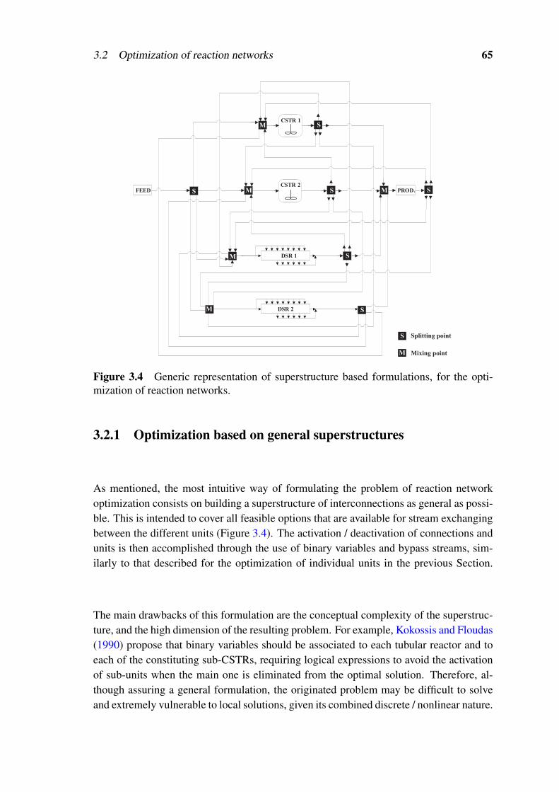
3.2 Optimization of reaction networks 65
CSTR 1
FEEDCSTR 2
PROD.
M
M
M
S
S
S
S M
DSR 1
DSR 2 SM
S
S
M
Splitting point
Mixing point
Figure 3.4 Generic representation of superstructure based formulations, for the opti-mization of reaction networks.
3.2.1 Optimization based on general superstructures
As mentioned, the most intuitive way of formulating the problem of reaction networkoptimization consists on building a superstructure of interconnections as general as possi-ble. This is intended to cover all feasible options that are available for stream exchangingbetween the different units (Figure 3.4). The activation / deactivation of connections andunits is then accomplished through the use of binary variables and bypass streams, sim-ilarly to that described for the optimization of individual units in the previous Section.
The main drawbacks of this formulation are the conceptual complexity of the superstruc-ture, and the high dimension of the resulting problem. For example, Kokossis and Floudas(1990) propose that binary variables should be associated to each tubular reactor and toeach of the constituting sub-CSTRs, requiring logical expressions to avoid the activationof sub-units when the main one is eliminated from the optimal solution. Therefore, al-though assuring a general formulation, the originated problem may be difficult to solveand extremely vulnerable to local solutions, given its combined discrete / nonlinear nature.

66 Optimization of Reaction Units and Networks
CSTR 1
DSR 1
FEED
DSR 2
CSTR 2
M S MS
DSR 3
CSTR 3
S S
S MS
MPROD. M S
Figure 3.5 Generic representation of sequential modules based formulations, for theoptimization of reaction networks.
3.2.2 Optimization based on the use of sequential modules
To reduce the complexity of the previous formulations, Balakrishna and Biegler (1992a);Biegler and Lakshmanan (1996) proposed a simplification of the original synthesis prob-lem, using the geometric attainable region concepts, to develop a systematic optimizationstrategy of general application. One of the key-ideas consisted in breaking down the di-mension of the original problem, based on the premise that a global recycle around anetwork of reactors is not part of the attainable-region boundary. Therefore, and assum-ing that a candidate region for a recycle network could always be extended by CSTRsand DSRs, and / or mixing lines, the synthesis problems could be solved modularly, asrepresented in Figure 3.5.
The major advantage of this methodology consists in keeping the problem dimensiononly as large as strictly required, since the number of modules is only increased whenthe obtained objective function values justify that decision. Additionally, and due to thesequential nature of the solution procedure, initialization aspects become also easier toimplement, in this case.
3.2.3 Cases of higher complexity
The two methodologies briefly described in the previous Sections can, in some situa-tions, require the inclusion of additional details and, therefore, become more complexand difficult to be solved. The following three situations deserve special attention fortheir commonness:
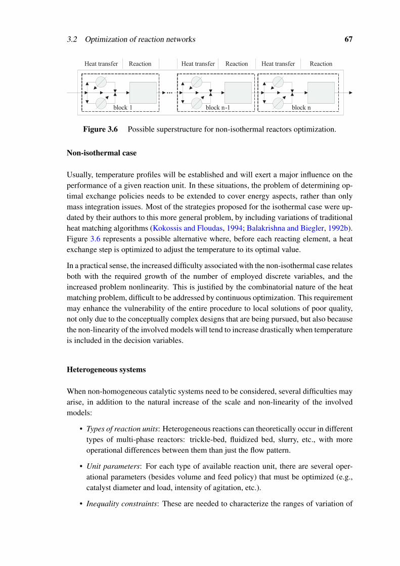
3.2 Optimization of reaction networks 67
ReactionHeat transfer ReactionHeat transfer ReactionHeat transfer
block 1 block n-1 block n
Figure 3.6 Possible superstructure for non-isothermal reactors optimization.
Non-isothermal case
Usually, temperature profiles will be established and will exert a major influence on theperformance of a given reaction unit. In these situations, the problem of determining op-timal exchange policies needs to be extended to cover energy aspects, rather than onlymass integration issues. Most of the strategies proposed for the isothermal case were up-dated by their authors to this more general problem, by including variations of traditionalheat matching algorithms (Kokossis and Floudas, 1994; Balakrishna and Biegler, 1992b).Figure 3.6 represents a possible alternative where, before each reacting element, a heatexchange step is optimized to adjust the temperature to its optimal value.
In a practical sense, the increased difficulty associated with the non-isothermal case relatesboth with the required growth of the number of employed discrete variables, and theincreased problem nonlinearity. This is justified by the combinatorial nature of the heatmatching problem, difficult to be addressed by continuous optimization. This requirementmay enhance the vulnerability of the entire procedure to local solutions of poor quality,not only due to the conceptually complex designs that are being pursued, but also becausethe non-linearity of the involved models will tend to increase drastically when temperatureis included in the decision variables.
Heterogeneous systems
When non-homogeneous catalytic systems need to be considered, several difficulties mayarise, in addition to the natural increase of the scale and non-linearity of the involvedmodels:
• Types of reaction units: Heterogeneous reactions can theoretically occur in differenttypes of multi-phase reactors: trickle-bed, fluidized bed, slurry, etc., with moreoperational differences between them than just the flow pattern.
• Unit parameters: For each type of available reaction unit, there are several oper-ational parameters (besides volume and feed policy) that must be optimized (e.g.,catalyst diameter and load, intensity of agitation, etc.).
• Inequality constraints: These are needed to characterize the ranges of variation of

68 Optimization of Reaction Units and Networks
the operational parameters and also to define the validity zones for the correlationsused. When coupled with non-convex process models, these bounds can introducedisconnected feasible operating regions.
Presence of separation units
In some practical situations, streams exchanged between reactors should go through con-tactors / separators (also with possible complex behavior), to enhance the performanceof the overall process. This is a very challenging situation, capable of largely enhancingthe combinatorial nature of the problem. Previous works have addressed this more gen-eral situation (Kokossis and Floudas, 1991; Lakshmanan and Biegler, 1996), although notspecifically in the heterogeneous reaction case. The reported results show a good perfor-mance of the proposed strategies, with only moderately nonlinear examples. Here, evenin these cases, the problems become unavoidably more complex. For example, the elimi-nation of recycle streams can no longer be fully accomplished, since their existence maynot be related with the extension of the attainable region but, instead, with the feasibilityof the entire problem.
3.3 Analogy with other “hard” problems
Several of the key aspects that need to be addressed during the synthesis of optimal reac-tion networks can also be found in many other synthesis problems that, although reportingto different operations (e.g., separation, mixing), share an identical structure. In fact, op-timizing networks of connections is a very general problem in PSE, that has receivedsignificant attention in the past and is still, currently, an active field of research. Select-ing which streams to activate / eliminate is far from a trivial task, and can contribute asmuch to the overall difficulty of a given network synthesis problem as the nature of theintervening units itself.
3.3.1 The pooling problem
From a conceptual point of view, the pooling problem is one of the simplest networksynthesis problems, since the intervening units are simple reservoirs where the attributesof different streams are blended. In this case, the nonlinear expressions that are handledcorrespond to bilinear terms, expressing ideal mixture rules. Although appearing simple,this problem is generally recognized as extremely hard, since poor quality solutions areoften obtained and the global optimum of the problem rarely identified (Audet et al.,2004).

3.3 Analogy with other “hard” problems 69
1
1
22
3
1
2
3
Feeds
(Initial products)Pools
(Mixers)Blends
(Final products)
FB3,2
FP2,1
PB2,1
Figure 3.7 Schematic representation of the generalized pooling problem.
To better understand where the difficulties are originated, Figure 3.7 shows a representa-tion of an hypothetical pooling problem. Generally, there are g feed streams with unde-sired properties that can be mixed in j pools to originate k blends with the final desiredattributes. The question to be answered consists on identifying the solution that maxi-mizes the difference between the revenue generated by selling the final blends and thecost of purchasing the feeds. This goal needs to be pursued considering a large numberof constraints, expressed as:
maxFB,PB,FP
nf
∑g
(np
∑k
(pk
1− pg2
)FBg,k
)+
nt
∑j
(np
∑k
pk1PB j,k
)−
nf
∑g
(nt
∑j
pg2FPg, j
)
s.t. ABk,a
(nf
∑g
FBg,k +nt
∑j
PB j,k
)=
nf
∑i
(AFg,aFBg,k
)+
nt
∑j
(AP j,aPB j,k
)ABk,a
lo
(nf
∑g
FBg,k +nt
∑j
PB j,k
)≤
nf
∑i
(AFg,aFBg,k
)+
nt
∑j
(AP j,aPB j,k
)ABk,a
up
(nf
∑g
FBg,k +nt
∑j
PB j,k
)≥
nf
∑i
(AFg,aFBg,k
)+
nt
∑j
(AP j,aPB j,k
)AP j,a
np
∑k
PB j,k =nf
∑g
(AFg,aFPg, j), nf
∑g
FPg, j =np
∑k
PB j,k
nt
∑j
FPg, j+np
∑k
FBg,k ≤ FCgup,
nf
∑g
FBg,k +nt
∑j
PB j,k ≥ BCklo,
np
∑k
PB j,k ≤ PC jlo,
FBg,klo ≤ FBg,k ≤ FBg,k
up , FPg, jlo ≤ FPg, j ≤ FPg, j
up , PB j,klo ≤ PB j,k ≤ PB j,k
up
As can be observed, in addition to the desired attributes in the final blends, many othersconstraints can be present. These may refer to a number of possible scenarios, e.g., the
70 Optimization of Reaction Units and Networks
availability of feeds, the mixing capacity of the pools, the transport capacity of the arcs(the lines that connect feeds, pools and blends), the demand on blends, etc. The solutionof the pooling problem is extremely difficult because:
• There are many degrees of freedom. This characteristic is intrinsic to any networksynthesis problem since, generally, the number of active streams required to gen-erate a feasible solution is small, when compared to the high number of possibleinterconnections. According to Poku et al. (2004), this may constitute a difficulty,since many of the widely used solution strategies are designed for the efficient so-lution of problems with few degrees of freedom only.
• On the other hand, there are many bilinear terms, a characteristic of network op-timization problems, due to the necessary existence of mixing / derivation points.Bilinear programs (BLP) are a particular case of a nonconvex quadratic programswith nonconvex constrains (QP), and are strongly NP-hard problems since theycomprehend the strongly NP-hard linear maxmin problem. Moreover, simply find-ing a feasible solution is NP-hard, as the constraint set generalizes the NP-hardlinear complementary problem (Audet et al., 2004). The objective function is nei-ther convex nor concave, and the feasible region may even be disconnected.
Clearly, the two main aspects that difficult the solution of the pooling problem are alsointrinsic to the optimal synthesis of reaction networks. Due to the importance of adoptingan adequate solution strategy for this last problem, the next Section discusses some of themain employed techniques for the solution of pooling problems.
3.3.2 Solution strategies for the pooling problem
Many authors have concentrated their efforts in developing solution strategies for the gen-eral pooling problem; a good review can be found in Audet et al. (2004). Some of the pro-posed strategies are based in fairly different assumptions: Aggarwal and Floudas (1990)proposed a method using Bender’s decomposition. Floudas and Visweswaran (1993) de-veloped a decomposition-based global optimization algorithm (GOP), subsequently im-proved in Visweswaran and Floudas (1993). The branch-and-bound algorithm, initiallydeveloped by Al-Khayyal and Falk (1983) for the BLP, is also applied by Foulds et al.(1992) to the pooling problem. Adhya and Tawarmalani (1999) employ a Lagrangianapproach, with a reformulation that generates a mixed-integer program, solved with theglobal optimization software BARON (Sahinidis, 1996). Despite their nature and relativeefficiency, all these strategies seem to present, however, a limited applicability to largeproblems (especially when incorporating global optimization procedures), intrinsicallyrelated to the problem dimension.
The difficulty of the BLP problem can be roughly estimated by the number of bilinearvariables, terms and constraints present. Two different formulations for the pooling prob-
3.3 Analogy with other “hard” problems 71
lem are available: the flow model and the proportional model. Although mathematicallyequivalent, the number of bilinear terms used in these two approaches are not always thesame, and depends on specific characteristics of the problem1. Thus, one of these possibleformulations might be preferred, to keep the problem difficulty as lower as possible. Evenso, in many practical cases, most of the previously referred strategies require extremelylarge CPU times, as the complexity of the problem increases, specially when trying toassure theoretical guarantees of finding the global optimum.
To answer to the issue of the limited applicability exhibited by the more elaborated strate-gies, some authors have proposed the use of heuristic methods (Audet et al., 2004). Oneof these examples is the Alternate Heuristic method (ALT) that, given two subsets of vari-ables, alternately solves the problem with the variables of one of the subsets fixed; thesetwo problems, by the choice of the variable subsets, need to be linear. After one prob-lem is solved, its solution becomes a set of fixed parameters in the remaining problem,alternating in this manner until convergence is achieved2. Although of simple implemen-tation, and less vulnerable to the dimension of the problem, these methods often returnpoor solutions, requiring the use of multi-start procedures to be usable, in practice.
More recently, a radically different approach to the solution of these problems was intro-duced (Poku et al., 2004). The authors do not consider global optimization methods oradopt any reformulation of the original problems. Instead, they propose the idea of simplyusing adequate local solvers, capable of generating solutions much faster and leading tosignificant improvements of the objective function. Their conclusions demonstrate thatthe use of an interior-point codes (like IPOPT and KNITRO), designed to handle manydegrees of freedom and many potentially active constraint sets, can be extremely com-petitive in the solution of large-scale pooling problems (and others with similar structure,like data-reconciliation problems).
An important characteristic of Interior-Point (IP) methods relates to the problem reformu-lation that is implemented for the treatment of constraints. This is usually done using abarrier function in the objective, which is defined to be convex within the feasible region,and infinite on the outside:
minx
J1(x) minx
J1(x)−ν ∑p
ln(xp)
s.t. J2(x) = 0 V s.t. J2(x) = 0
x≥ 0
Here the index p defines a set of positive variables. Since the barrier is incorporateddirectly in the objective, an equivalent unconstrained optimization problem is obtained,
1For instance, the flow model tends to be advantageous when the number of attributes is lower.2Hence this class of methods has similarities with the generalized Bender’s decomposition (Floudas,
1995).

72 Optimization of Reaction Units and Networks
Active Set
IP
Figure 3.8 Convergence characteristics of interior point methods.
which can be solved much simpler using variants of the Newton’s method. In fact, theIP algorithms solve a sequence of barrier problems, enabling the search for the optimumwhile avoiding extreme points in the original domain (Figure 3.8). The value of ν is suc-cessively decreased (ν → 0) in order to retrieve the exact solution of the original problem3.Two major advantages can be attributed to this class of methods:
• For problems with a large number of degrees of freedom and many constraintsfeasibility can be accomplished faster and more easier, leading to final solutions ofimproved quality.
• Avoiding the extreme points in the original domain also corresponds to smallersensitivity to the presence of local optima, often located at the boundary of thedomain; this also contributes significantly to the quality of the final solutions.
Another significant aspect of the work of Poku et al. (2004) is that pooling problems (andothers of similar nature) are now addressed through NLP, avoiding the use of conven-tional discrete formulations. Therefore, when the non-linearity of the models increases(e.g., in a different network synthesis problem), this will not be as problematic as in thepreviously proposed strategies. In fact, Kawajiri and Biegler (2006) have successful ad-dressed the optimal location of streams, in Simulating Moving-Bed (SMB) systems, alsothrough the use of interior-point codes. After a reformulation, this problem shares someof the problematic characteristics of the pooling problems, with the additional difficultyof adsorption models (of increased non-linearity) instead of mixing rules.
3.4 Developed strategy
After clarifying some of the main issues related to the synthesis of optimal reaction net-works, the current Section introduces a new strategy focused on some of these importantaspects. Section 3.4.1 presents the underlying motivations, Section 3.4.2 focus on the
3For additional background on the convergence properties of IP methods see Forsgren et al. (2002).
3.4 Developed strategy 73
major key-ideas and Sections 3.4.3–3.4.5 discuss important details withe a crucial contri-bution to the success of the overall methodology.
3.4.1 Scope and motivations
Despite the significant number of contributions found in literature, there are actually fewreferences that address complex multi-phase reaction systems. The work of Mehta andKokossis (2000) deals with two-phase systems, and considers the non-isothermal synthe-sis problem. However, the examples presented, although considering different kinds ofunits (CSTR and plug flow) with feed policies and reaction volumes as decision variables,are relatively simple and do not include large-scale nonlinear models.
A more recent work (Diaconescu et al., 2002) elucidates that, for highly complex reactionsystems, there are several additional decisions that must be considered. Accordingly tothe authors, the mathematical complexity of the mechanistic models, required to expressall the functional relations between state and decision variables, is typically very high.Therefore, the resulting models, when considered within an optimal network synthesisproblem, tend to prevent the use of systematic approaches. The strategy adopted by theseauthors was to make some a priori decisions, e.g., the types of units and partial networktopology, decreasing the complexity of the synthesis problem to a level that could be suc-cessfully handled. The obvious disadvantage of this approach is that the a priori decisionsmay hinder, from the start, possible better solutions.
Therefore, the main motivation beyond the development of a new strategy relates to theneed of optimizing complex reaction networks, through systematic formulations, whenthe involved units lead to large-scale nonlinear models. In this work, only the isother-mal case is considered. The ultimate goal will be the successful application of the newmethodology to an elaborated industrial case-study (the triphasic reaction step of CUF–QI, where phase separation units play an important role), with the expectation of identi-fying new configurations of improved global efficiency, not only during the optimizationof the current process but also considering the root design of a new one.
3.4.2 Key-ideas of the methodology
One of the main aspects of the developed strategy is to use a continuous formulation forthe entire synthesis problem, not only for the optimization of intervening units (e.g., resi-dence time, feed policy), but also in what relates to the derivation of an optimal networkof interconnections. This is a crucial aspect, due to the high non-linearity of the modelsthat are treated.

74 Optimization of Reaction Units and Networks
Optimization of intervening units via NLP
A simple application example allows a comparison of the relative efficiency of continu-ous / discrete formulations, when complex reaction models are handled. In this case, bothformulations discussed in Section 3.1 were tested in the optimization of an heterogeneousDSR. This unit does not constitute an industrial case-study or corresponds to a practi-cal application; instead, it was idealized for the comparison of different mathematicalstrategies. The considered DSR unit comprehends the triphasic hydrogenation reactiondiscussed in Section 2.3. Since this reaction is now considered to occur in an hypothet-ical trickle-bed reactor, corrections had to be made to the mass transfer coefficients andthe efficiency factor. The larger particle sizes involved tend to increase the resistance tothe internal and external diffusion of reactants / products, when compared with the slurryregime. The new estimates comprehend a decrease of 4 times on Ki
LS and over 10 timeson the value of η , considering the values reported in Section 2.3.5 as references. As inletconditions, 30.5, 11.0 and 40.4 Kmol/h of nitrobenzene, water and aniline, respectively,were considered; the maximum residence time (τ) was set to 50 hours.
The discrete formulation of Section 3.2.1 was implemented considering a sequence of40 CSTR units, with modified mass transfer and kinetic parameters, to approximate thebehavior of the DSR unit (Figure 2.4). The adopted modelling approach is an isothermalmacroscopic one and, therefore, the equations that describe each sub-unit are equivalentto those presented in Section 2.3.4. The formulation of Section 3.2.2 was implementedusing a weighted residuals method to handle the original differential-algebraic system.The obtained NLP formulation can be generally expressed by (3.3–3.8). Notice that,since a heterogeneous system is considered, the variable concentration (Cz,c,m) is nowsubstituted by Cz,c,m
L and Cz,c,mS , to distinguish the liquid phase and the catalytic phases.
Additionally, mass and heat balances need to be written within the elements to link bothphases, as described in Section 2.3.4. In the NLP implementation, 13 elements with2 interior collocation points were used. The resulting model was made equivalent to thatof the discrete formulation, assuring the same number of independent decision variables.Both strategies involved approximately 2000 equations / variables, with this number onlyslightly larger in the continuous formulation.
Generic NLP formulation for the optimization of a DSR
minqz,c, f z,c
J (τ, CmOut)
s.t. (3.4−3.8)(3.3)
• Constraints related to orthogonal collocation:
lz,tFP =
((z−1)
nz+
ζ t
nz
)τmax ∆lz,c = lz,c+1
FP − lz,cFP (3.4a)

3.4 Developed strategy 75
ϒz,w,c = ∏
tt 6=w
(lz,cFP − lz,t
FP)(
lz,wFP − lz,t
FP) ϒ
z,w,c1D =
∑u
u6=w
∏t
t 6=w,u
(lz,cFP − lz,t
FP)
∏t
t 6=w
(lz,wFP − lz,t
FP) (3.4b)
Cz,c = ∑w
ψz,w
ϒz,w,c Cz,c
1D = ∑w
ψz,w
ϒz,w,c1D (3.4c)
• Auxiliary expressions:
f z,c = Fz,c/F0 Cz,mBeg = Cz,1,m
nz
∑z
nw
∑c
f z,c = 1 (3.5a)
qz,c = Qz,c/F0 Cz,mEnd = Cz,nw,m
nz
∑z
nw
∑c
qz,c = 1 (3.5b)
τ =nz
∑z
nw
∑c
∆lz,c(
Gz,c
F0
)Cm
Out =nz
∑z
nw
∑c
qz,cCm,z,cβ
z =f z,1F0
Gz,1 (3.5c)
• Initial conditions (z = 1, c = 1):
C1,1,m = CmInl, G1,1 =
(f 1,1−q1,1)F0 (3.6)
• Continuity conditions (z = 2, . . . ,nz, c = 1):
Cz,1,m = βzC1,1,m +(1−β
z)Cz−1,nw,m (3.7a)
Gz,1 = Gz−1,nw +(
f z,1−qz,1)F0 (3.7b)
• Balances within the elements (z = 1, . . . ,nz; c = 2, . . . ,nw):
Cz,c,m1D = γ
mΓ(Cz,c,m) , Gz,c = Gz,c−1 +( f z,c−qz,c)F0 (3.8)
Therefore, in this example, the most important difference between both strategies relatesonly to the mechanism of activation / deactivation of a given reaction volume: eitherusing a continuous control profile or through the association to a binary variable. Thiscan be observed by solving the DSR with all decision variables fixed (degrees of freedomset to 0). As shown in Figure 3.9, the results obtained are very close, clearly stating theequivalence of the formulations. The small differences in the concentration profiles aredue to the consideration of constant density in the NLP formulation.
The results shown in Figure 3.9 are obtained by fixing the residence time at is max-imum value (i.e., using the entire available reaction volume), and by setting the feedpolicy as in a conventional plug-flow (no side-streams are allowed). To evaluate the rel-ative efficiency of the strategies under study (and the quality of the returned solutions), a

76 Optimization of Reaction Units and Networks
0
1000
2000
3000
4000
5000
6000
7000
8000
9000
10000
0 5 10 15 20 25 30 35 40
τ (hours)
Co
nce
ntr
atio
n (
mo
l m
-3)
MNB (Sub-CSTR)
ANL (Sub-CSTR)
Water (Sub-CSTR)
MNB (DSR)
ANL (DSR)
Water (DSR)
Figure 3.9 Solution of a heterogeneous reactor through different representations.
second study was performed, this time considering the optimization of all decision vari-ables. The goal was to minimize the residence time, subject to an operational constraint(CMNB
L < 500 mol/m3). While the NLP strategy returned τopt = 22.1 hours, the discreteformulation exhibited several numerical difficulties, returning results of poor quality. Sev-eral similar studies were performed, leading to identical results. All cases were solved inGAMS (Brooke et al., 1998), using CONOPT and DICOPT for the NLP and MINLPstrategies, respectively.
Hence, the similar efficiency that both strategies seem to exhibit (according to the previousworks) for the simpler homogeneous case, is not maintained in the above examples. Theresults obtained in this work strengthen the idea that discrete strategies will see theirefficiency reduced in highly nonlinear examples, advising the use of a NLP formulationwhen more complex heterogeneous reaction units are optimized.
Synthesis of optimal networks via NLP
As mentioned, previous works have proposed to address the optimization of the decisionvariables of each unit through NLP formulations. However, when considering the opti-mization of the reaction network structure (i.e., which connections to activate / eliminate),all authors seem to suggest the use of discrete schemes, due to the combinatorial natureof the problem, and also due to an easier formulation. Notice that even the strategy dis-cussed in Section 3.2.2, that considers a continuous formulation to optimize feed policiesand reaction volumes, makes use of integer variables, as illustrated in Figure 3.10.
The problem of stream selection is of major importance, since it is intrinsically relatedwith the activation / deactivation of the reaction units. If the binary variable associated to

3.4 Developed strategy 77
CSTR
DSR
MS MF F
Fi Y
i
Fj Y
j
Yi+Yj=1
0 Fi U Yi , 0 Fj U Yj
Yi 0,1 , Yj 0,1
F= Fi+Fj
≤ ≤ ≤ ≤
∈ ∈
Figure 3.10 Network synthesis through the use of discrete stream selection.
the inlet flow of the CSTR takes the value 0, this unit will not receive any feed and, there-fore, becomes inactive in the final solution. Naturally, special attention should be givento how the model equations are written, since they need also to hold for null flowrates.Other strategies, like the one discussed in Section 3.2.1, also propose the association ofan additional binary variable to the existence of the unit (instead of deactivated, it may beeliminated). The only advantage is that equipment cost functions can be more rigorouslyevaluated (since these include a fixed component that does not depend on the flowratevalue). The major drawback is that more complexity is introduced, making the problemmore difficult to be solved.
Since the new developed strategy is intended to deal with large-scale and highly nonlin-ear models, an alternative to this kind of approaches was searched, to prevent potentialnumerical problems or poor quality solutions. Here, the key idea is to keep in mind theanalogy between the pooling problem and the synthesis of reaction networks, taking ad-vantage of the superior performance that interior-point methods seem to exhibit in thepresence of large-number of degrees of freedom, even when the non-linearity of the prob-lem is increased. When large-scale problems with a high number of superbasic variablesand inequality constraints must be addressed, special care needs be taken during solverselection. In order to be appropriate, solvers must be capable of exploiting the problemstructure (usually sparse), using second-order information from the optimization model,and deal with computational difficulties such as redundant constraints and lack of positivedefiniteness in the reduced Hessian matrix (Kawajiri and Biegler, 2006).
Most of the current state-of-the-art NLP solvers are based in Sequential Quadratic Pro-gramming (SQP) or in Generalized Reduced Gradient methods (GRG), whose efficiencycan be seriously compromised during the solution of the previous type of problems. InSQP methods, the presence of many inequality constraints can be troublesome during thesolution of the QPs, due to the identification of the proper active set — a task with acombinatorial nature, growing in complexity exponentially with the problem size. GRGsmethods approximate second-order information, using dense quasi-Newton approxima-tions updated in the reduced space, a procedure that also significantly increases the re-quired CPU effort, as the dimension of the considered problems becomes larger.
According to Kawajiri and Biegler (2006), and as explained in Section 3.3.2, interior-point

78 Optimization of Reaction Units and Networks
Table 3.1 Main characteristics of the considered pooling problems.
Problem Feeds Pools Blends Attributes Equations
RT2 3 2 3 4 76AST3 8 3 4 6 153
Table 3.2 Obtained objective function values through the different tested solvers.
Problem Optimal IPOPT KNITRO CONOPT SNOPT MINOS
RT2 4391.83 4391.83 4391.62 3273.95 3273.95 3273.95AST3 561.05 559.61 559.39 50.74 0.00 Infeasible
approaches can help overcoming some of these difficulties, in particular those associatedto the handling of the active set of constraints (Figure 3.8). In order to confirm the in-dications of these authors, a small benchmark study was additionally done, consideringtwo pooling problems (RT2 and AST3) drawn from Adhya and Tawarmalani (1999), andseveral local solvers that, together, cover a wide range of distinct solution methods:
• IPOPT / KNITRO: these two codes implement state-of-the-art interior point meth-ods, where the nonlinear programming problem is substituted by a series of barriersubproblems. Depending on the solver, the algorithm can use trust regions or linesearches to achieve convergence.
• MINOS: uses a Reduced Gradient Technique (GRG) to solve linearly constrainedmodels; when nonlinear constraints are present, subproblems with linearized con-straints and an augmented Lagrangian objective function are iteratively used.
• SNOPT: uses Sequential Quadratic Programming (SQP) where search directionsare obtained from a sequence of QP subproblems. Each QP minimizes a quadraticmodel of a certain Lagrangian function, subject to linearization of constraints.
• CONOPT III: is a multi-method solver that includes sub-methods like Sequen-tial Linear Programming (SLP), Steepest Descend, Quasi-Newton and SQP. UnlikeMINOS, this solver is based on a feasible path method.
A brief description of the problems considered is provided in Table 3.1, while the resultsobtained are shown in Table 3.2. As can be seen, the quality of the solutions returnedby IPOPT and KNITRO are largely superior to those of the remaining codes, especiallywith the AST3 problem that, due to is higher complexity, amplifies the differences ofperformance.
These results, together with the indications of Poku et al. (2004) and Kawajiri and Biegler(2006), strengthen the idea that nonlinear programming can be used for the optimal syn-thesis of reaction networks, thus avoiding the introduction of discrete variables duringstream activation and elimination. However, the use of interior-point methods is only part

3.4 Developed strategy 79
of the solution; as will be shown in the next Section, additional details need to be ad-dressed to retain a continuous formulation. One of them consists in controlling the totalnumber of streams active in the final solution, a task that is trivial when binary variablescan be used, but requires special efforts within the context of continuous optimization.
3.4.3 Formulation aspects
As introduced in the previous Section, stream selection plays an extremely importantrole during the activation / deactivation of units. In this context, and as illustrated inFigure 3.10, binary choices might be required, e.g., “if a given unit is selected, thananother one is not”, leading to discrete nonlinear problems.
Reformulations of discrete-continuous problems
As mentioned, the classical method of solving nonlinear discrete-continuous problems isthrough MINLP algorithms. These are either based on branch & bound with nonlinearprogramming subproblems or on decomposition methods that alternate between NLP andMILP subproblems; the SBB and DICOPT solvers are examples of these two distinctways of solving MINLP problems, further discussed in Section 5.4.1. One of the majordrawbacks of MINLP algorithms is that all model constraints must be satisfied, includingthose referring to units that are eliminated from the problem. This can be troublesomewhen linearization steps take part of the solution procedure, since singularities are oftengenerated, causing poor quality solutions and / or the premature end of the optimizationphase.
To improve the efficiency of discrete solution schemes, an alternative strategy has beenproposed. The idea is to formulate a generalized disjunctive program (GDP), whereboolean variables are used to activate or deactivate subsets of the constraints. This tech-nique enables the relieve of some of the difficulties associated to MINLP algorithms and,for that reason, its use has been proposed for a wide class of problems, e.g., generalnetwork synthesis problems (Yeomans and Grossmann, 1999), optimal design of distilla-tion columns (Yeomans and Grossmann, 2000b), synthesis of heat integrated separationsequences (Yeomans and Grossmann, 2000a), as further discussed in Chapters 5 and 6.However, for practical purposes, GDP formulations are, generally, subsequently solvedusing either MINLP methods or special purpose modifications of them (Grossmann andHooker, 2000). Therefore, some of the drawbacks of current MINLP codes are not en-tirely avoided, namely their reduced performance when in the presence of highly nonlin-ear models. Therefore, and since the key-idea of the new developed strategy is to maintaina NLP formulation and still be able to handle discrete choices, the use of binary variablesneeds to be replaced through an equivalent continuous approximation, using a conceptsimilar to that represented in Figure 3.11.

80 Optimization of Reaction Units and Networks
binary variable (Y)
continuous approximation
0
1
deviation zones
Figure 3.11 Approximation of an integer variable through a differentiable function.
This approach is not entirely new; many authors have used different methods that fall intothis general category, proposing alternative mathematical approaches for this purpose.Stein et al. (2004) present a recent review on this subject.
One possible manner of reformulating the problem of deciding, between two continu-ous variables x and y, which one should be zero is the formulation of a complementarycondition:
• Complementarity condition:
JCC(x,y)≡ x · y = 0. (3.9)
Thus if x,y ≥ 0 and x + y = 1 are additionally imposed, only one set of discrete solutionswill be feasible: (x,y) ∈W0 ≡ (0,1),(1,0). Replacing y by (1− x) in (3.9), then eitherx = 0 or x = 1 and therefore complementarity problems can be used as a complete alter-native to MINLP formulations4. This approach has, however, two major drawbacks, thathave limited its practical application:
• First, the extreme nonlinearity and non-convexity of (3.9) difficults the convergenceto the optimal solution, independently of the NLP algorithm used.
• Moreover, the Mangasarian-Fromovitz constraint qualification (MFCQ) does nothold in this case (Bazaraa and Shetty, 1993). According to Jongen and Weber(1991); Scheel and Scholtes (2000); Günzel and Jongen (2006), this fact can beassociated with the strong stability of the problem5 and, therefore, not being able toverify it constitutes also a serious disadvantage.
For practical purposes, the contributions of both these drawbacks should be, however,separated. While the first one assumes the nature of an inherently hard limitation (onlyremovable by a problem reformulation), the second limitation has the character of more
4By straightforward inference of the suggestions of Raghunathan and Biegler (2003).5Related to local existence and uniqueness of a solution of a system under small perturbations.

3.4 Developed strategy 81
an operational difficulty, that perhaps can be circumvented. Also, it should be mentionedthat this last disadvantage is shared by many existing methodologies of dealing with logicconstraints, both in classical MILP and MINLP models. For instance, the establishedmethod of dealing with fixed charge models is through the use of a MILP formulationsimilar to (Biegler et al., 1997):
minx,y
CTOT = CFIX · y+CVAR · x (3.10a)
s.t. x≤U · y (3.10b)
x≥ 0 (3.10c)
y ∈ 0,1 (3.10d)
implying the fact that x should be zero, if the logical variable y is also null. Here, if thishappens at the solution, it is easy to see that both (3.10b) and (3.10c) become active, andtherefore they do not satisfy the MFCQ since their gradients are collinear and point inopposite directions, even if they just correspond to simple bounds6. Moreover, Floudas(1995) suggests as a standard method for deactivation of continuous variables (or equalityconstraints) adding a set of inequalities of the type
xlo · y≤ x≤ y · xup
to the formulation, where xlo and xup are lower and upper bounds on the continuous vari-able x. Here, a problem similar to the previous example occurs, when x = 0. Despite thenumerical problems that can be incurred in each situation, the fact that both of these tech-niques are so widespread, both in MILP and MINLP applications, is a reliable indicationthat these numerical problems can be successfully overcome (if not simply ignored), inmany practical situations.
On a more rigorous track, Luo et al. (1996) present several strategies that can be usedto improve the numerical treatment of complementarity conditions. In fact, the study ofthese particular expressions constitute an active field of research, due to the common-ness and importance of general Mathematical Programs with Equilibrium Constraints(MPECs), which can be defined as optimization problems that comprehend complemen-tary conditions in the constraints (Outrata et al., 1998). In this field, a well know approachconsists in the use of regularization techniques, where the relaxation of the original equa-tion is considered:
• Relaxed complementarity condition: JCC,rlx (x,y)≡ x · y≤ α .
The idea is to trace the solution of a sequence of auxiliary problems, where α is se-quentially decreased towards 0, until the original condition is satisfied. In this type ofapproach, the discrete set W0 is replaced by a one-dimensional relaxed set Wα , that be-comes disconnected for α ≤ 0.25. The use of this type of relaxations is very common
6Contrarily, if y = 1, then both constraints become inactive, and this problem disappears.
82 Optimization of Reaction Units and Networks
and can be found, for example, in some commercial codes like NLPEC (Brooke et al.,1998) that deal with the reformulation of MPECs. As an alternative, also in this context,Raghunathan and Biegler (2003) propose the use of interior-point methods. The authorsshow that after minor modifications, these methods can be successfully applied to situa-tions where the Mangasarian-Fromovitz constraint qualification does not hold. However,this approach is tied to the specific IP approach used, with software implementations notgenerally available, at the moment.
Despite their usefulness, the introduction of complementary conditions is far from beingthe only approach for the continuous reformulation of discrete decisions. For example,Stein et al. (2004) propose the use of functions with a smooth zero set and the correctintersection points:
• Circle condition (Stein et al., 2004): (x−0.5)2 +(y−0.5)2 = 0.5
According to the authors, the use of the above expression has the advantage of satisfyingthe Mangasarian-Fromovitz constraint qualification, although not over the entire domain.In fact, when the proposed relaxation of the original expression is adopted
(x−0.5)2 +(y−0.5)2 ≤ 0.5, (x−0.5)2 +(y−0.5)2 ≥(
1/√
2−α
)2, x+ y = 1
it is possible to observe that if α = 0, the domain is described by two inequalities with gra-dients pointing in opposite directions, a situation that violates the Mangasarian-Fromovitzconstraint qualification. As reported by Stein et al. (2004), the properties of this limitingcase did not cause any kind of difficulties during the solution of the simple examples con-sidered, leading to well-performing numerical methods. However, and according to theseauthors, the previous situation might affect the numerical solution of larger and morecomplex methods. For this reason, two additional continuous reformulations, with bettertheoretical features, are also identified as potential alternatives:
• Natural residual function:
JNR(x,y)≡ 0.5(
x+ y−√
(x− y)2)
= 0
• Fischer-Burmeister function (Fischer, 1992):
JFB(x,y)≡ x+ y−√
x2 + y2 = 0
The potential advantage of the above functions is that, when employed, the linear in-dependence constraint qualification holds everywhere in the feasible set, assuring betterstability properties. Nevertheless, and as far as we know, the previously major limitationof complementarity conditions (non-convexity and extreme non-linearity) still apply, al-though in different degrees, to all of the previous alternatives. Thus, some of them might

3.4 Developed strategy 83
present different practical performance, even if they possess similar theoretical proper-ties. From our perspective, this fact has not been explicitly identified and addressed inthe previous works, despite its practical importance for the success of the solution of thecorresponding NLP.
One additional previous work on the domain of large-scale optimization has shown thatrelaxed continuous approximations appear to have the potential to address several prob-lems that, classically, are solved through discrete formulations (Neves et al., 2005). In thiscase, circle conditions have been successfully employed to deal with the optimal locationof streams, during the design of highly non-ideal distillation columns (see also Chapter 5):
• Circle condition (Neves et al., 2005):
x2 + y2 ≥ α (3.11a)
x+ y = 1, x,y ∈ [0,1] (3.11b)
In this case a succession of problems is solved with α ≥ 0 → 1; when α = 1, one of thesolutions in W0 is identified. The advantages of this approach over the circle conditionin Stein et al. (2004) are the following:
• Its numerical simplicity and reduced nonlinearity.
• The active constraints are now linearly independent in the final solution, satisfyingtherefore the Mangasarian-Fromovitz constraint qualification.
An illustration of the mechanism of the previous reformulations is presented in Fig-ure 3.12, for the simple case of two continuous variables x and y. In this Figure, thecurves obtained by the relaxation of the various conditions are observed; this allows aninformal quantification of the relative measures of non-linearity introduced by each one.An additional important advantage of the circle condition of Neves et al. (2005) for highlynonlinear problems can be realized from Figure 3.12(f). Here, we see that if the linearconstraint (3.11b) is relaxed as |x+y−1| ≤ δ , then the continuous region delimited by thetwo dashed lines of the Figure is obtained. Since this region is two-dimensional, its usewould simplify the initial solution phase of a highly nonlinear problem, where the deter-mination of a feasible (approximate) first estimate of the solution is sought, comparativelyto the use of the original one-dimensional constraint (3.11b).
In this case, using the approach of Figure 3.12(f), and for sufficiently small values ofα , one can observe that it is now relatively simple to maintain the feasible region con-nected during the convergence procedure when α → 1, using only small values of δ inthe relaxation, especially in the first phase when (3.11a) starts to be active, and when thedecision of the direction to take is more relevant. This is a consequence of the fact that,from all of the alternatives illustrated in this Figure, the circle condition of Neves et al.(2005) requires the smallest value of δ , for an identical “exclusion length” on the segmentx+ y = 1. Moreover, as can be observed, this required value of δ to avoid a disconnected

84 Optimization of Reaction Units and Networks
1.0
0.8
0.6
0.4
0.2
0.0
y
0.0 0.2 0.4 0.6 0.8 1.0x
1.0
0.8
0.6
0.4
0.2
0.0
y
1.0
0.8
0.6
0.4
0.2
0.0
y
1.0
0.8
0.6
0.4
0.2
0.0
y
1.0
0.8
0.6
0.4
0.2
0.0
y
1.0
0.8
0.6
0.4
0.2
0.0
y
0.0 0.2 0.4 0.6 0.8 1.0x
0.0 0.2 0.4 0.6 0.8 1.0x
0.0 0.2 0.4 0.6 0.8 1.0x
0.0 0.2 0.4 0.6 0.8 1.0x
0.0 0.2 0.4 0.6 0.8 1.0x
(a) (b) (c)
(d) (e) (f)
-δ+δ
Figure 3.12 Relaxations of the original continuous expressions: (a) Natural residualfunction; (b) Fischer-Burmeister function; (c) Complementarity condition; (d) Circle con-dition (Stein et al., 2004); (e) Circle condition (Neves et al., 2005); (f) Circle conditionwith variable tolerance (Neves et al., 2005).
feasible region can be made arbitrarily smaller in this case, simply by displacing the centerof the circle in (3.11a) to infinity, e.g. along the coordinates (−ι ,−ι), with ι → ∞. Thus,simply by keeping the possibility of using δ ≥ 0 along the convergence to the solution(with α → 1), this strategy has the potential to reduce the occurrence of two importantpractical problems:
• Stopping at infeasible non-integer solutions, since backtracking to different extremais now possible, within the feasible region.
• Convergence to local solutions of significantly poor quality, due to the disconnectednature of the feasible region.
These characteristics are in accordance with the computational experience reported inChapter 5, where the trade-offs between different convergence schemes (i.e. variable δ
versus fixed δ ) are analyzed in detail. However, it should be noted that these correspondonly to desirable properties, from a practical point of view; no formal guarantee relativeto the convergence to the global optimum should be assumed from the above description.
The following Sections will explore this approach in the context of reactor network syn-thesis. The application to the optimization of separation blocks is considered in Sec-tion 5.3.1.

3.4 Developed strategy 85
R1
S
R1
S
R1
S
( )ncr
2R1,
RR RR
1
j
j
b α
=
≥∑
R1
S
ncrR1 R1,
1R1
j
jj
RR RR=≠
= ∑ R1, R1, R1
RR
j jRR b RR= ×
RRα
RRα
RRαRR
α =1
Figure 3.13 Control of stream splitting through concave expressions.
Proposed methodology
As shown in Figure 3.13, the number of active streams can be continuously reduced byenforcing constraints of the type (3.12), where s represents a type of connection (Reactor-Reactor — RR, for the particularly illustrated example):
nu
∑j=1
(bi, j
s)2 ≥ αs (3.12)
These simple concave constraints, equivalent to a multi-dimensional version of the relaxedcircle function shown in Figure 3.12(e), have the following properties:
1. When αs = 0, constraint (3.12) is trivially satisfied for any set of values of bi, js that
also satisfy the following conservation condition:
nu
∑j=1
bi, js = 1 with 0≤ bi, j
s ≤ 1 (3.13)
2. In the limit case, when αs = 1, constraint (3.12) can only be satisfied when one ofthe bi, j
s coefficients is unitary. Given the conservation relation (3.13), this propertyimplies that the remaining bi, j
s coefficients must vanish. Therefore the correspond-ing stream has been located and converged to a single unit. To see this, note that inthis case we have simultaneously from (3.12) and (3.13):
1 =nu
∑j
(bi, j
s)2 ≤
nu
∑j
bi, js = 1, and 0≤ bi, j
s ≤ 1

86 Optimization of Reaction Units and Networks
which can only be satisfied when one of the coefficients is unitary and all the re-maining ones null.
3. When 0 ≤ αs ≤ 1, the fractional nature of the partition coefficients bi, js define a
threshold value αs,rlx. This limit can be computed by applying equation (3.12) tothe relaxed solution:
αs,rlx =nu
∑j=1
(bi, j
s,rlx
)2= ∑
j∈Es,rlx
(bi, j
s,rlx
)2
In this expression Es,rlx represents the set of units for which the correspondent coef-ficients bi, j
s are strictly positive, that is, the set of units where a given stream shouldbe directed, accordingly to the relaxed solution. For values of αs < αs,rlx, the re-spective equation (3.12) becomes redundant (i.e., inactive) in the formulation.
4. A minimum amount of stream aggregation can be introduced by equation (3.12), forvalues of αs,rlx ≤ αs ≤ 1. Here, Es,α denotes the set of units where a connection sis present, after solution of the optimal design problem subject to constraints (3.12)and (3.13), using a fixed value of αs. The correspondent state of aggregation of thissolution, relative to connection s, can be measured by the maximum split fraction(supreme) observed in the set Es,α :
bs∗(αs) = supw∈Es,α
(bw)
5. The state of aggregation of a solution relative to a connection s varies monotonicallyfrom a minimum at αs = αs,min, to a maximum for αs = 1, where bs∗(1) = 1, andthe stream is directed entirely to only one unit. When constraint (3.12) is active, asimple lower bound for bs∗(αs) can be derived by writing:
αs = b2s∗+ ∑
j∈Es,α\∗
(bi, j
s)2 ≤ b2
s∗+ ∑j∈Es,α\∗
bi, js
From (3.13), bs∗ = 1−∑ j∈Es,α\∗ bi, js , and the previous equation becomes αs ≤ b2
s∗+1−bs∗, or equivalently:
bs∗(αs)≥1+
√4αs−32
for αs ≥ 0.75
This bound is monotone with αs, and becomes progressively tighter to the value ofbs∗, as αs → 1.
The proposed method starts with the solution of the relaxed NLP design problem, whereall streams to be optimally located are distributed to each candidate unit, subject to in-dividual constraints of type (3.13). The first solution produces values of αs,rlx for eachstream, which are then progressively increased towards unity in the optimization prob-

3.4 Developed strategy 87
lems solved subsequently.
As previously mentioned, this procedure does not guarantee that the global optimum ofthe problem will be found. However, the expectation is that when the sequence of relaxedNLP problems is solved with a suitable method (i.e., interior-point based), the chances onavoiding poor local optima will be high. Although it may not seem an ambitious goal, itis important to remember the experience with the global optimization algorithms in theexample considered previously in this Section. A further confirmation was obtained byconsidering a test problem, where the connections between 3 CSTR slurry units (modelledby the macroscopic equations of Section 2.3.4) should be optimized to maximize theproductivity of the arrangement (all reactors are fixed as active units). When attempting tosolve this problem through the commercial code BARON (Sahinidis, 1996), no solutionwas retrieved after one week of calculations (using GAMS and a 1.7 GHz Pentium IVCPU).
Two further advantages of the methodology corresponding to the application of the circlecondition (3.11) will become clear in the next Section:
• Apart from an easier numerical solution, when α is successively increased to unity,the intermediate solutions not only have physical meaning, but also have feasible(non-optimal) physical implementations, and correspond to specific trade-offs thatresult from further constrained solutions. Therefore, their availability might be im-portant, for a more complete evaluation of the final solution7. Hence, more thanjust converging to one final optimal topology, the observation of the intermediatesolutions might produce value-added information relative to the problem being con-sidered. This also is related to the importance of using multiple-objectives in thesynthesis problem, as considered in the next Section.
• One particularly important aspect of reactor network synthesis is the effective con-trol of the complexity of the obtained solutions. This aspect can also be easilytackled in the context of multiple-objective optimization; the previous solution forthe control of stream aggregation allows a straightforward integration of this aspectin the optimization context.
3.4.4 Objective function
The large majority of the strategies for reaction networks synthesis found in literatureaddress the problem in a single context, e.g., economical or conversion related. How-ever, as pointed out by Neves et al. (2006), these approaches can be insufficient in morepractically oriented applications.
7In fact, this is illustrated with some of the examples presented later.

88 Optimization of Reaction Units and Networks
AQUEOUSAQUEOUS ORGANIC ORGANICORGANIC ORGANIC
Figure 3.14 Reducing the network topological complexity.
Importance of multi-objectives in reaction network synthesis
When the synthesis of reaction networks is applied to complex scenarios, several conflict-ing objectives may be present:
• Conversion / reaction volume: When operating near complete conversion, e.g., inmass-transfer limited processes, a small increase in the reaction yield might requirean exponential increase of the reaction volume.
• Existing / new technologies and configurations: This can be understood as a crite-rion related to risk analysis (“fear factors”). Often, industry is only willing to tradecurrent technologies (e.g., reactor’s types) by new ones for which no operationalexperience is available, if the predicted gains are substantially large.
• Flexibility / operability: For the same global reaction volume, a larger number ofsmaller units offers better chances of limiting the production losses due to plantfailures, in each of them. On the other hand, more complex control rooms, togetherwith higher investment and labor costs are involved.
• Complexity / performance: Very often, the solutions obtained involve a large num-ber of exchange streams that only contribute moderately to the network perfor-mance. Reducing the number of connections between units can lead to simplernetworks, at the cost of only minor performance losses.
Among the previous conflicting objectives, the potential trade-offs between complexityand performance will receive special attention during the current Section since, as illus-trated in Figures 3.14 and 3.15, they refer to important and common situations. Addi-tionally, their evaluation will also require special considerations, to maintain the problemformulation within a NLP context.
To illustrate how the obtained solutions can be unnecessarily complex, especially whenmulti-objective scenarios are not considered, Figures 3.14 and 3.15 show several hypo-

3.4 Developed strategy 89
AQUEOUS
ORGANIC
AQUEOUS
ORGANIC
1A
2A
3A 4A
1B
2B
3B 4B
wat wat wat
1A 1B max,w w w≤1B 1A 2B 2A 4B 4A
3B 3A wat wat wat wat wat wat
1B 1A 2B 2A 4B 4A
1.51.8 , and
0.7
F F F F F FF F
w w w w w w⇒
≃ ≃ ≃
≃
≃ ≃ ≃
with
water water water water water water
water water water
Figure 3.15 Controlling the flowrate of free recycle streams.
thetical configurations, based on the industrial problem under study (the reaction phaseof CUF–QI). More rigorously, this constitutes a reaction-separation problem since, asintroduced in Section 2.3.1, there is a need to feed dehydrated aniline to the reactors toavoid a biphasic mixture. This is accomplished in liquid-liquid separators, that sepa-rate the outlet of the reaction units in two phases — an organic one (partially recycled)and an aqueous one; a more detailed description of the problem can be found in Sec-tion 3.5. On the left side of the figures are shown scenarios that would correspond toa good practice; on the right side, alternative configurations that, although feasible andcomplying with the same operational restrictions (productivity and conversion), exhibitssome obvious disadvantages8. For example, the solution represented on the right side ofFigure 3.14 comprehends four unnecessary extra connections, increasing the topologicalcomplexity of the network. Additionally, Figure 3.15 shows how a recycle stream with alarger flowrate could be feasible, although with no advantages for the process (and somedrawbacks, like higher power consumption in the required pumps).
If not penalized in the objective function, these unnecessary connections and large recycleflowrates might appear in the final solutions. In some particular problems they may beimportant for the feasibility of the problem, although often their influence on the objectivefunction should be “weighted” to evaluate if they are really necessary.
Implementation aspects
To improve the quality of the obtained solutions, a multi-objective formulation can betherefore highly beneficial, to address the synthesis of practical reaction networks. Twoapproaches are usually considered for this purpose: the first one, more numerically ori-
8Some of these schematics are only intend to serve for general illustrative purposes and, therefore, donot correspond to the industrial practice.

90 Optimization of Reaction Units and Networks
Revam
pin
g f
acto
r (REV
)Goal 1
Network Productiviy (NP)
Goal 2
Network Simplicity (NS)Aggregation factor (α)
Pareto curve
Zone I Zone II Zone III
Zone I: Goal 2 can be improved without
affecting Goal 1;
Zone II: Optimal zone, where the trade-offs
are “balanced”;
Zone III: Goal 1 is drastically compromised.
Figure 3.16 Proposed strategy for the evaluation of multiple objectives.
ented, builds a composite performance index that includes all objectives together withtheir respective weighting factors in a single objective; the second one, more analytical,tries to elucidate the trade-offs between different conflicting objectives (mainly by graph-ical studies, e.g., constructing the Pareto curves), leaving the final choice of the preferredsolution to the decision maker.
The proposed methodology includes aspects of both approaches, since it comprehends theconstruction of a Pareto curve, where one of the objectives is evaluated by consideringa weighted objective function (Figure 3.16): here, Goal 1 (NP) represents the classicalobjective functions that are normally considered in literature (productivity is given has anexample, although conversion and investment are also possibilities). Goal 2 expresses theconcept of network simplicity (NS) that, due to its nature, needs to be evaluated throughthe sum of several contributions. We propose the following measure:
NS = ν1 ∑s
αs +ν2 ∑s
Fs (3.14)
In this equation, the variable Fs represents the total flow on a type of connection (covering,in this manner, all candidate streams). The values that are given to the different weightsexpress, in the user perspective, the characteristics that are more appreciated in the fi-nal network, as a measure of its simplicity: a minor number of active streams or lowerexchanged flowrates. In addition to these two attributes, several others can also be ac-counted analogously, depending on the specific needs of each problem. An illustration ofthis situation will be given in Section 3.5, during the solution of an industrial case-study.
By solving a sequence of optimization problems, where the value of α is successivelyincreased in small steps, an analysis equivalent to that of Figure 3.16 can be made that,

3.4 Developed strategy 91
Extract sensibilities
or
Construct “local” models
Update lower /upper bounds
on the decision variables Optimize the network
(using simplified models )
TOL.
?
Solution
Y
N
Define network
superstructure
Postulate an initial point
(solve original models )
Refine the obtained results
(using the original models )
Figure 3.17 Possible iterative scheme for network optimization (use of local models).
ultimately, will enable the user to select an improved network design.
3.4.5 Model simplification
The aspects discussed along Sections 3.4.2–3.4.4 define a continuous formulation for theoptimal synthesis of reaction networks, capable of handling multi-objective scenarios andcomplex large-scale models. However, and although less vulnerable to highly nonlinearproblems when compared with classical discrete strategies, a limit of applicability willalways exist for the proposed strategy. This implies that for some problems to be treatable,the models involved need to be previously simplified.
In these situations, one of the classical procedures consists in decomposing the originalproblem and iterate between two different kinds of reduced subproblems, to avoid the nu-merical difficulties associated with the detailed formulation of the original synthesis prob-lem. This is a common concept in simulation / optimization, since avoiding pure equationoriented strategies (Ganesh and Biegler, 1987) or using reduced models (Briesen andMarquardt, 2004) is sometimes useful, or even strictly necessary, to overcome numericaldifficulties of current solvers in process synthesis problems. The procedure of Figure 3.17was developed for this purpose; it can be described through the following main steps:
1. Decide the type and number of units to be considered and enclose all possible con-nections (candidate streams) within an appropriate superstructure.
2. Obtain an initialization point, by considering a scenario where all units and streams
92 Optimization of Reaction Units and Networks
are active and the remaining decision variables are fixed at their nominal values.According to the gathered numerical experience, this procedures improves the qual-ity of the obtained final solutions and, therefore, should always be adopted.
3. For the current values of the input variables, obtain simplified relations between theoutput and the decision variables, using the original rigorous models.
4. Considering the quality of the simplified relations obtained in the previous step, fixthe maximum ranges of variations for the input and decision variables.
5. Obtain optimum values for all input and decision variables, solving the networksynthesis problem with the simplified (local) models.
6. Compare the obtained values with the ones of the previous iteration and, based onthe imposed tolerance, decide about the need to iterate again.
7. If the tolerance was satisfied, refine the obtained results through the use of theoriginal models (check if all of the previous optimal values are maintained).
This procedure can therefore be understood as similar to a trust-region approach to opti-mization (Conn et al., 2000). Its application can be mainly justified when the difficultyin the optimization of the original models is hindered by their inherent complexity. How-ever, it suffers from the vulnerability to local optima, similarly to the use of the originalmodels, due to the difficulty in eliminating this aspect in the simplified models. On theother hand, obtaining local models can also be a difficult task, depending on the natureof the problem. Sometimes, complex multi-variable regression procedures might be in-volved that, if performed at each iteration, can convert the optimization procedure into adifficult and time-consuming exercise.
As an alternative, when extremely complex models are handled, a model reduction exer-cise can also be considered as the first step. Model reduction can be difficult to performbut, if successfully accomplished, allows the global behavior of the system to be capturedthrough the description of its more representative phenomena (Figure 3.18). Under thesecircumstances, the resulting models constitute good approximations over the entire do-main of the search space; this allows a more direct control of the presence of multipleoptima in the optimization of the superstructure considered subsequently. Nevertheless,even when using “global” approximations, the obtained solutions should be confirmed (ifpossible), by executing a final run with the original models.
For all of the previous reasons, and as stated in the next Section, the procedure schemat-ically represented in Figure 3.18 was adopted during the solution of the industrial case-study considered.

3.5 Industrial case-study 93
o yOriginal
Model
Simplified
Model
I(o) J(x)
x y
All detailed
mecanisms
(I)
Only limiting
mecanisms
(J)
All manipulated
variables
(o)
Only critical
variables
(x)
Figure 3.18 Model reduction in complex systems.
3.5 Industrial case-study
To illustrate the efficiency of the developed continuous strategy, several optimization stud-ies will be considered around a complex industrial case-study. The problem is defined inSection 3.5.1, particular formulation aspects are discussed in Section 3.5.2, while themain obtained results are presented in Section 3.5.3.
3.5.1 Problem description
The optimization of the reaction network implemented in CUF–QI will be done con-sidering only reaction units of the type currently employed (slurry CSTRs). Althoughpotentially interesting, the evaluation of other alternatives (e.g., fluidized and trickle-bedreactors) is, in practice, not feasible. This is due to the lack of kinetic data related to thenitrobenzene hydrogenation in these systems (no references could be found in the litera-ture). While the mass transfer coefficients could be roughly estimated by several availablecorrelations, the behavior of this heterogeneous reaction in different catalyst particles (notonly in dimension but also probably in type) is extremely difficult to predict.
In Section 3.4.2 there was a concern in emphasizing that the results shown in Figure 3.9could only be used to compare the performance of different mathematical approaches.In fact, the kinetic curve of Section 2.3.3 was considered for catalyst particles that, in atrickle-bed, are several times larger. This simplification can be far from reality and, there-fore, the obtained residence times (about 50 times higher than that of a slurry unit) maycarry an implicit large error. Naturally, the indication that a fixed bed reactor might beinappropriate for this hydrogenation will, probably, be correct. The low diffusivity of theliquid mixture within the solid catalyst strongly limits the use of its internal volume and,therefore, the larger particle diameters in fixed-bed reactors will be a considerable disad-vantage. However, when more competitive configurations are considered (e.g., fluidizedbed reactors), selecting the best type of reactor will be impossible, since the difference

94 Optimization of Reaction Units and Networks
NO2
G
C
NH2 NH2
OH O
NHNHN
3H2 2H2O 2H2 H2
ANLH2O
NH3
H2
ANL
H2O
H2
NH33H2
Figure 3.19 Hydrogenation mechanism of nitrobenzene, including kinetic paths forbyproducts formation (Relvas, 2007).
on performance that might separate them can be inferior to the error introduced by theassumed approximations (that become necessary in the absence of specific kinetic data).
Besides considering slurry CSTRs as the only type of candidate units, the following net-work synthesis problem also incorporates another simplification: only the kinetics of themain reaction will be considered. Once again, the reason relates to a lack of availableinformation, this time regarding the mechanisms of byproducts formation, as already re-ported in Section 2.3.3. Although studies are being developed in this field (Relvas, 2007),and several potential pathways have already been proposed (Figure 3.19), the final ver-sion of the mathematical model was not available at the time of the writing of this Thesis.In this scenario, no studies relative to the improvement of the network selectivity can beperformed. Although not currently feasible, these should be considered in the future,since the conclusions may lead to a drastic increase of the overall process efficiency. No-tice that operational problems (in fulfilling the final product specifications) and energyconsumption in the purification phase are intrinsically related to the performance of thereaction phase, namely to the specific yields on harder-to-separate species (e.g., CHOLand DICHA).
As a result, the network productivity will be, in practice, the most important attribute. Itsoptimization is going to be considered in a multi-objective perspective, by also evaluatingthe topology of the obtained solutions. Notice that, despite the “forced” simplifications,the resulting problem (Figure 3.20) is still extremely complex, due to the presence oftriphasic reactors and biphasic separation units; as explained in Section 3.4.4, these last

3.5 Industrial case-study 95
Feed
(Fresh) S
Reactor
1
Reactor
ncr
Separator
1
Separator
nps
FR1,m
FRncr,m
FFm
Product 1(Organic)
M
SPnps,2, m
SP1, 2, m
RPncr,1, m
RP1, 1, m
RPTOT
1, m
S
PR1,m
M
Product 2(Aqueous)
M
S
SP1, 1,m
SP
SP1, m
SP2,m
PS2,m
THREE PHASE
REACTION
TWO PHASE
SEPARATION
nps,1, m
TOT
TOT
TOT
TOT
Figure 3.20 Schematic representation of the network optimization problem, for the con-sidered industrial case-study.
cannot be detached from the synthesis problem.
As introduced previously, two products must be isolated: an organic one, mainly com-posed by aniline, that will then enter a primary purification phase to fulfill commercialspecifications; an aqueous one, that can be seen as a waste-stream, subsequently treatedin a secondary purification phase where the dissolved aniline will be recovered. With thisin mind, recycling Product II to the separators (or to the reactors) does not make sense.Allowing the reactors to send their outlet streams directly to Product II is also an optionthat can be excluded at start. These trivial simplifications are implicit in Figure 3.20, andwill enter the mathematical formulation as:
PR2,i,m = 0, PS2,k,m = 0, RPi,2,m = 0
3.5.2 Application aspects
The previous description introduced globally the industrial case-study. Specific aspectswill now be addressed, that seek to simplify, without loss of performance, the formulationof synthesis problem.
Model simplification
In Section 3.4.5, the importance of reducing the scale and non-linearity of complex mod-els was emphasized. As pointed out, efforts should be concentrated in obtained simplified

96 Optimization of Reaction Units and Networks
7 manipulated variables(all potentially optimizable)
2 optimization variables(remaining are fixed)
dP
mC
P H2
TR
ω
INR
V
OUT
Cm
L, Inl
Cm
L, Out INR
Cm
L, Inl OUT
Cm
L, Out
Figure 3.21 Model reduction: decreasing the number of decision variables.
models capable of retaining a global approximation of the original ones (especially dur-ing the solution of network synthesis problems). For this particular case-study, this taskwas already accomplished (see Chapter 2). As explained in Section 2.3.5, an isothermalmacroscopic model is sufficiently accurate to describe the behavior of the slurry units, andcan replace a detailed non-isothermal microscopic approach. On the other hand, accord-ing to the sensibility studies of Section 2.3.6, the initial number of candidate optimizationvariables can be decreased (Figure 3.21) since the influence of some of them (PH2, ω ,TR) on the performance of the individual units is practically negligible. Additionally, theoptimization of mC, VR and dP, although potentially important, is difficult to consider inpractice:
mC: increasing the catalyst load implies higher operational costs (more fresh catalyst isspent) and, on the other hand, a higher production rate per unit of reaction volume.Although this trade-off should be optimized, a lack of industrial data relative to theefficiency of the separation system (that recycles the catalyst into the reactors) indifferent operational conditions, hinders (for now) the optimization of mC.
VR: selecting the best volume for new reaction units is a task that, somehow, is con-nected to the optimization of mC (e.g., smaller volumes could be compensated byhigher catalyst loads, and vice-versa). For this reason, it will be assumed that, whenacquiring new units, the current dimensions will be maintained. In practice, this as-sumption is not far from reality due to the risks involved during the scale-up of agiven technology, and because scale-downs are rarely performed in industry.
dP: working with smaller catalyst particles would favor the surface reaction that prevailsin the considered hydrogenation units. However, as referred in Section 2.3.6, thiscan interfere with the performance of the decanters, meaning higher fresh catalystconsumption and higher operational costs. Therefore, without a model capable ofdescribing the units where the catalyst is recovered, it is safer to consider dP asfixed. Additionally, different catalyst particles will probably mean different yieldsof byproducts that cannot be predicted without performing experimental studies.

3.5 Industrial case-study 97
MOUT
R1,mReactor R1
SINR
R1,m
ORGS1,m
SMINS
S1,mSeparator S1
AQUS1,m
RRR1,j,m
j=1j ≠ R1
ncr
RSR1,k,m
nps
k=1
Product 1
Product 1
Product 2
SSS1,k,m
k=1
nps
SRk,R1,m
nps
k=1
Feed
Product 1
RRi ,R1,m
ncr
i=1i ≠ R1
Product 2
RSi,S1,m
ncr
i=1
S
S
M
M
S
M
MSSl,S1,m
nps
l=1l ≠ S1
SRS1,i,m
i=1
ncr
S
Can be eliminated Can be eliminated
k ≠ S1
Can be eliminated
Can be eliminated
Figure 3.22 Eliminated connections in the simplified network formulation.
Network simplification
Another procedure that can be employed to simplify the network formulation, consists inanalyzing the specific nature of the problem and, if possible, eliminate some of the con-nections that are enclosed in the initial superstructure. This technique is also commonlyused during the solution of pooling problems (Audet et al., 2004) and, when adopted,should be performed without eliminating potential optimal solutions.
The main idea is to reformulate the original problem to obtain a simpler and equivalentrepresentation. This is shown in Figure 3.22, for the particular industrial case-study. No-tice that eliminating these connections will not limit the quality of the final solutions, asexplained next:
• Separator - Separator (SS) connections: although the organic phase of a given sep-arator could be sent to the inlet of another one, this scenario does not make sensefor the considered problem. In fact, this would only be advantageous if the inletconditions of a separator were required to be maintained between certain bounds,to assure LL equilibrium and / or avoid the excess of a given component in one ofthe outlet streams. In the adopted case-study, these bounds are naturally imposedthrough other problem restrictions and, therefore, no additional efforts are neces-

98 Optimization of Reaction Units and Networks
sary. Notice that the inlet water percentage cannot increase too much, because thisis constrained in the reactors9. On the other hand, the aniline content within the re-actors does not have an upper bound and can theoretically increase at the inlet of theseparators, depending on the selected recycle flowrate (Figure 3.15). However, thissituation is not problematic; the only concern would be a potential increase of thewater content in the outlet organic phase, although in practice this will never occur,since LL equilibrium compositions only depend significantly on temperature.
• Product I - Separator (PS) connections: these will also be forbidden, due to thesame reasons previously presented for the SS connections (no advantages can bederived from the recycling of organic product to the separators inlet).
• Product I - Reactor (RP) connections: as explained, dehydrated aniline needs to becontinuously feed into the reactors (to solubilize the water produced). This can beassured by recycling Product I or by the organic phase of the LL separators. Sincethe formation of byproducts is not considered both alternatives are equivalent, andone of them (RP) can be eliminated (to avoid redundancy).
• Reactor - Product I (RP) connections: The water content in the outlet streams ofthe reactors will be, in general, higher than the specification imposed in the finalorganic product. If it is lower, an indirect pathway through a phase separator willnot be disadvantageous, making the use of RP connections redundant.
After introducing the previous simplifications, the candidate connections (that may re-main active in the final solutions) are: Feed(fresh) - Reactor (FR), Separator - Reactor(SR), Reactor - Separator (RS), Reactor - Reactor (RR), and Separator - Product1 (SP).
Network Synthesis Formulation (CUF-QI case-study) The following mathematicalformulation will be used:
minFRi,m, SRk,i,m, RRk,i,m
RSi,k,m, SPk,i,m
J (NP, NS)
s.t. (3.16–3.22)
(3.15)
• Feed and Products:
FFm Rev =ncr
∑i
FRi,m, PP2,m =nps
∑k
SPk,2,m (3.16a)
PP1,m =nps
∑k
SPk,1,m +ncr
∑i
RPi,1,m−ncr
∑i
PR1,i,m−nps
∑k
PS1,k,m (3.16b)
9They must be operated with wWater < 0.17, as explained.

3.5 Industrial case-study 99
• Hydrogenation reactors:
INRi,m = FRi,m +PR1,i,m +nps
∑k
SRk,i,m +ncr
∑j
j 6=i
RR j,i,m (3.17a)
INRi,m +Θi,mMain = OUT i,m (3.17b)
Θi,mmain = γ
mΓ
iη
i(
Ci,mS ,T i
)V i
R (3.17c)
Ci,mL,Out = OUT i,m/
( nc
∑m
OUT i,m/ρm)
(3.17d)
Ki,mLS ai
S
(Ci,m
S −Ci,mL,Out
)= γ
1,mη
i,1Γ
i,1(
Ci,mS ,T i
)(3.17e)
OUT i,m =ncr
∑j
j 6=i
RRi, j,m +nps
∑k
RSi,k,m+RPi,1,m (3.17f)
• LL phase separators:
INSk,m = ORGk,m +AQUk,m (3.18a)
INSk,m =NS
∑l
l 6=k
SSl,k,m +PS1,k,m +ncr
∑i
RSi,k,m (3.18b)
Ck,mO = ORGk,m/
( nc
∑m
ORGk,m/ρm)
(3.18c)
Ck,mA = AQUk,m/
( nc
∑m
AQUk,m/ρm)
(3.18d)
φk,mO Ck,m
O = φk,mA Ck,m
A (3.18e)
ORGk,m =ncr
∑i
SRk,i,m +SPk,1,m +nps
∑k
k 6=l
SSl,k,m (3.18f)
AQUk,m = SPk,2,m (3.18g)
• Network simplifications:
SSk,l,m = 0, PS1,k,m = 0, PR1,i,m = 0, RPi,1,m = 0 (3.19)
• Stream splitting:
FRi,m = FRm biFR, SRk,i,m = SRk,m bk,i
SR (3.20a)
RR j,i,m = RR j,m b j,iRR, RSi,k,m = RSi,m bi,k
RS (3.20b)

100 Optimization of Reaction Units and Networks
• Stream aggregation:
ncr
∑i=1
(bi
FR)2 ≥ αFR,
ncr
∑i=1
(bk,i
SR
)2≥ αSR,
nps
∑k=1
(bi,k
RS
)2≥ αRS,
ncr
∑i=1
(b j,i
RR
)2≥ αRR (3.21)
• Control equations:
ncr
∑i=1
biFR = 1,
ncr
∑i=1
bk,iSR = 1,
nps
∑k=1
bi,kRS = 1,
ncr
∑i=1
b j,iRR = 1 (3.22)
3.5.3 Case-studies considered
Three problems, of increasing scale (and complexity), were addressed through the pre-vious continuous formulation; their main characteristics are summarized in Table 3.3.The primary goal consists in studying the dependence of the network productivity on thenumber of employed reactors, by evaluating the synthesized optimal configurations ina multi-objective scenario. For all of the problems considered, several constraints wereimposed to more faithfully describe the industrial reality:
• Reaction extent: a constraint is imposed in the maximum MNB flowrate that canbe converted in the hydrogenation units. This bound (set on 300% of the nominalflowrate) will limit the extrapolation of the developed model to very different opera-tional conditions, where the homogenization of the mixture may not be maintained,and the assumed reaction efficiency significantly decreased.
• Hydraulic residence times: besides constraining the amount of converted MNB ineach reactor, a maximum bound is also imposed on the total inlet flowrate (freshfeed + outlet of other units). The chosen value (600% of the nominal value) intendsto avoid solutions that may not be sustained by the mechanical design of the units.
• Attributes of the final product: two important specifications are imposed for theorganic product (Product I). The first one relates to the maximum water content(set to 6%), while the second one (in practice, the most important) is relative tothe maximum amount of non-converted MNB (set to 10 ppm). In fact, MNB canbe difficult to separate from aniline (in the purification phase) and, therefore, it isimportant to assure a global network conversion close to 100%.
• Reacting conditions: As already introduced, the adopted case-study will be treatedthrough an isothermal approach, where temperature (within the reactors) is fixedat its nominal value. Therefore a maximum amount of water content (17%) mustbe imposed, to avoid a biphasic reaction media. A second constraint relates to the

3.5 Industrial case-study 101
Table 3.3 Main characteristics of the different industrial case-studies.
Heterogeneous LL phase Equations Constraints ConnectionsProblem reactors separators (total) (bounds) (candidate)
1 4 2 250 22 382 6 2 400 32 683 8 2 580 42 106
concentration of MNB, for which an upper bound is also defined (1000 ppm), sincethere are evidences that, above a certain limit, a significant catalyst deactivationmight occur in practice.
• Heat removal capacity: the hydrogenation under study is highly exothermic and,to maintain the reaction temperature at is nominal value, several heat exchangingequipments assure the removal of the heat of reaction (Section 6.4.3). Notice thatbounding this capacity is not a redundant task, since the constraints on the residencetimes are the same for each unit, and the heat exchanging mechanisms may differfrom one reactor to another.
As a consequence, a large number of bounds can become active during the solution ofthe network synthesis problems. This fact, that strengthens an analogy with the poolingproblem, increases the number of potential local optima (Section 3.4.2 and Table 3.2).Another important aspect that should also be emphasized is the pre-processing phaseimplemented. As previously referred, initializing the problem with all candidate streamsactive (no zero flows present) seems to favor the quality of the final obtained solutions.For this reason, all problems in Table 3.3 were previously solved imposing an aggregationlevel for each type of connection, that assured an equally distribution of flows amongthe resulting streams. Thus the optimization phase only starts after the solution of thisminimum aggregation scenario.
All of the results reported were obtained in GAMS (Brooke et al., 1998), using the IPOPTsolver and a Pentium IV CPU at 1.7 GHz.
3.5.4 Results
Problem 1
The results obtained for Problem 1, relative to the trade-offs between the network produc-tivity and its conceptual simplicity, are shown in Table 3.4. This can replace a graphicalrepresentation like that of Figure 3.16 since, basically, the same level of information isprovided. The productivity index is reported through a normalized revamping factor,while the simplicity index can be evaluated through the number of active streams (dis-criminated by type of connection) and by the total exchanged flowrates.
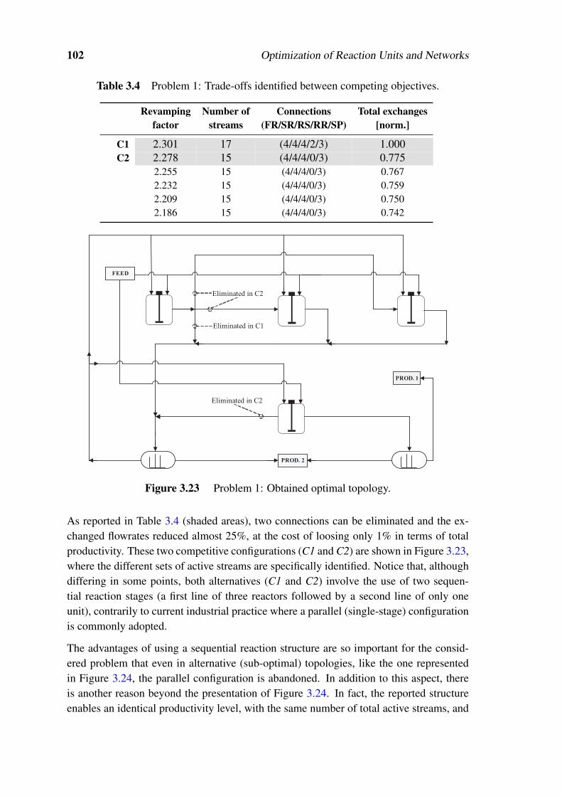
102 Optimization of Reaction Units and Networks
Table 3.4 Problem 1: Trade-offs identified between competing objectives.
Revamping Number of Connections Total exchangesfactor streams (FR/SR/RS/RR/SP) [norm.]
C1 2.301 17 (4/4/4/2/3) 1.000C2 2.278 15 (4/4/4/0/3) 0.775
2.255 15 (4/4/4/0/3) 0.7672.232 15 (4/4/4/0/3) 0.7592.209 15 (4/4/4/0/3) 0.7502.186 15 (4/4/4/0/3) 0.742
PROD. 1
PROD. 2
FEED
Eliminated in C2
Eliminated in C1
Eliminated in C2
Figure 3.23 Problem 1: Obtained optimal topology.
As reported in Table 3.4 (shaded areas), two connections can be eliminated and the ex-changed flowrates reduced almost 25%, at the cost of loosing only 1% in terms of totalproductivity. These two competitive configurations (C1 and C2) are shown in Figure 3.23,where the different sets of active streams are specifically identified. Notice that, althoughdiffering in some points, both alternatives (C1 and C2) involve the use of two sequen-tial reaction stages (a first line of three reactors followed by a second line of only oneunit), contrarily to current industrial practice where a parallel (single-stage) configurationis commonly adopted.
The advantages of using a sequential reaction structure are so important for the consid-ered problem that even in alternative (sub-optimal) topologies, like the one representedin Figure 3.24, the parallel configuration is abandoned. In addition to this aspect, thereis another reason beyond the presentation of Figure 3.24. In fact, the reported structureenables an identical productivity level, with the same number of total active streams, and

3.5 Industrial case-study 103
PROD. 1
PROD. 2
FEED
Figure 3.24 Problem 1: Alternative optimal topology.
is only considered sub-optimal because slightly larger exchanged flowrates are required(approximately 10% in a total basis). In other words, multiple configurations with similarperformance exist in this problem. Considering that the major differences may only corre-spond to differences in the active streams, it can be helpful to discriminate in the objectivefunction the type of preferential connections. For example, some of the RS connectionsin C1 and C2 are replaced by RR ones in the structure of Figure 3.24. Thus the secondreaction stage might be receiving directly from the first line of units or, alternatively, viathe phase separators10. However, if the objective function is modified as
Goal 2 = ν1
(∑s
αs
)+ν2
(∑s
Fs
)+ν3
(∑
i∑
jRRi, j
)(3.23)
the connections of type RR will be penalized, relative to the remaining ones (the relationbetween the values of ν2 and ν3 translate the level of discrimination). For the particularproblem under study, the objective function in (3.23) is more adequate than (3.14), sinceit is much easier to connect the reactors via the phase separators, than directly (in this lastscenario, new physical connections would have to be made). For this reason, structureslike that of Figure 3.24 should be explicitly considered as less competitive in the simplicityindex. Therefore, in order for them to be selected as optimal solutions, they will have todemonstrate an improved productivity index.
Problem 2
The results obtained for Problem 2, where six hydrogenation units were considered, areshown in Table 3.5. Here, and contrarily to the previous example, the network topol-
10Notice that these alternatives are only equivalent because the formation of byproducts is not considered.

104 Optimization of Reaction Units and Networks
Table 3.5 Problem 2: Identified trade-offs between competing objectives.
Revamping Number of Connections Total exchangesfactor streams (FR/SR/RS/RR/SP) [norm.]
C3 3.625 21 (5/6/7/0/3) 1.0003.589 21 (5/6/7/0/3) 0.8303.552 21 (5/6/7/0/3) 0.7103.516 21 (5/6/7/0/3) 0.6613.480 21 (5/6/7/0/3) 0.6533.444 21 (5/6/7/0/3) 0.645
PROD. 1
PROD. 2
FEED
Figure 3.25 Problem 2: Obtained optimal topology.
ogy cannot be simplified without significantly decreasing its productivity. Even when therevamping factor is sacrificed by 5%, the number of required active streams remains un-changed (this means that, for the imposed weights, Goal 2 can only be improved througha reduction on the total exchanged flowrates).
Under these circumstances, configuration C3, that maximizes the network productivity,may be selected as the optimal solution for Problem 211. Its structure, also shared by theremaining solutions of Table 3.5, is illustrated in Figure 3.25. Notice that, once again,two sequential reaction steps need to be assured: this time, a first line of 4 reactors and asecond stage composed by the remaining two, due to the shape of the kinetic curve (Fig-ure 2.31). As described in Section 2.3.6, it is possible to increase the MNB feed flowratewithout decreasing the reaction conversion, to a large extent. In a parallel configuration,
11Although, ultimately, this decision will depend on how the user evaluates the trade-offs.

3.5 Industrial case-study 105
Table 3.6 Problem 3: Identified trade-offs between competing objectives.
Revamping Number of Connections Total exchangesfactor streams (FR/SR/RS/RR/SP) [norm.]
4.675 28 (7/8/8/2/3) 1.000C4 4.628 26 (7/8/7/1/3) 0.687C5 4.581 26 (7/8/8/0/3) 0.697
4.535 26 (7/8/8/0/3) 0.6884.488 26 (7/8/8/0/3) 0.6804.441 26 (7/8/8/0/3) 0.672
the consequent increase of the MNB residual concentration, although small in absoluteterms, is prohibitive (due to potential difficulties in the purification step, as explained).However, if this single-stage reaction structure is abandoned, it becomes possible to op-erate a first line of reactors at higher production rates and deplete the the non-convertedMNB in a second reaction step (fulfilling the imposed restrictions).
Problem 3
The trade-offs identified, relative to example 3, are shown in Table 3.6. As mentioned,when eight hydrogenators are employed, the network simplicity can be improved (twoconnections less, and more than 30% reduction of the total flows) at the cost of decreasingthe overall productivity approximately 1% (configuration C4).
A particularly interesting aspect of this example is that, contrarily to the previous prob-lems, the relation between the total exchanged flows and the revamping factor is notmonotonous (in C5, the tendency is singularly inverted). This derives from the use ofan objective function (3.23) where a certain type of connections is penalized. Thus inaccordance with the imposed weights, from C4 to C5 a RR connection is replaced by a(preferable) RS one, at the cost of a small increase of the total exchanged flows.
As in the two first problems, a structure with two reaction steps is once again present (sixreactors in a first line and the remaining two in a second one). Considering that in theinitialization procedure all connections are active and that in the final solutions similaroptimal patterns are observed (with a much lesser number of streams), good indicationsare left relative to the performance of the developed strategy. Naturally, no guarantees canbe made about the quality of the obtained solutions (i.e., the reported configurations mayconstitute local optima). However, the new methodology enabled important conclusionsabout the best form of increasing the productivity of the current network, solving severalcomplex problems, within acceptable CPU times (all examples required less than 2 min-utes of calculations). Notice that, due to their scale, none of the previous problems couldbe addressed by global optimization strategies and that, due to their non-linearity, discretenumerical schemes would reveal a large number of difficulties.

106 Optimization of Reaction Units and Networks
PROD. 1
PROD. 2
FEED
Eliminated in C4
Eliminated in C5
Figure 3.26 Problem 3: Obtained optimal topology.
Final notes
Conclusions and Future Work
Academic perspective
Solution of multiphasic systems When dealing with complex systems, described by asequence of mass transfer and reaction steps, the development of several modelling ap-proaches, characterized by different degrees of detail, is of crucial importance. Here, twoparticular aspects deserve special attention: the description of intra-particle phenomena,with direct impact on the scale of the problem, and the assumption of isothermal condi-tions, with huge influence on the model non-linearity. The suitability of these decisionswill depend on the considered system, although for some particular cases they may leadto identical conclusions, with distinct solution effort. This was observed for the currentcase-study, where all modelling approaches returned similar results (corroborated overa large number of sensitivity studies), and where radically distinct CPU times and nu-merical difficulties were involved: the isothermal macroscopic model developed couldbe solved in 5 seconds, without special concerns, while the non-isothermal microscopicmodel, besides involving CPU times around 1000 seconds, required special initializationand scaling procedures to return a solution, due to the sharp profiles inside the catalystparticles that cause convergence problems in the absence of a robust numerical condition-ing. Therefore, the development of simplified models should always be tried since, whensufficiently accurate, the easier solution procedure may play a decisive role, especiallywhen the simultaneous simulation / optimization of several units needs to be considered,as required for the synthesis of reaction networks.
Synthesis of reaction networks When simple models (single-phase units) are involvedand heat integrations aspects need to be considered, the weak non-linearity and the highcombinatorial nature of the involved problem justifies the common use of discrete non-linear strategies (MINLP, GDP). However, even in these cases the vulnerability to localsolutions cannot be avoided at the start. For this reason, special solution schemes werealso developed. Although increasing the chances of obtaining the global optimum, they
107

108 Optimization of Reaction Units and Networks
limit the dimension of the treatable problems, due to the large required CPU times. In anopposite situation, i.e., when the scale and non-linearity of the considered models is high(multiphasic units, even when simplified approaches are considered) and when energymatches are not important, the use of nonlinear programming can be appealing, providedan adequate solution scheme is employed. The strategy developed in this work is basedon the previous premise and takes advantage of interior point method solvers for whichsuperior performance has been reported during the solution of problems with a identicalstructure (i.e., where the goal is to determine the best network of inter-connections, as inthe pooling problem and in the optimization of simulated moving beds). Using this ap-proach, several network synthesis problems were solved, considering a different numberof reactors and studying its influence on the objective function value. For each problem,the best exchange policies are determined, and the trade-offs between network complex-ity and performance evaluated, through the use of quadratic inequalities, that control thelevel of aggregation of each stream. This way, a continuous formulation can be retained,assuring a robust convergence procedure.
Industrial perspective
Simulation of the slurry units The results obtained indicate that the reaction takesplace in a thin layer, close to the surface of the catalyst particles, in the presence ofstrong resistances to the internal and external diffusion of the limiting reactant (nitroben-zene). This fact enables an important set of conclusions, namely the good performanceof the used catalyst (that, due to the milling effect, present a higher global surface area),when compared with the fresh one (where no advantage can be taken from the largeintra-particle space). The sensitivity studies predict a minor influence for many operatingvariables (temperature, pressure, stirring speed), with the exception of the catalyst chargeand the particles dimensions, due to their direct influence on the solid phase externalarea. Among all the conclusions drawn, the most important one is, probability, the weakdependence of the reactor conversion on the nitrobenzene feed flowrate (that was con-firmed, in practice, for the industrial units). This behavior can be related with the shapeof the kinetic curve, and is valid for a certain range of operational conditions, where anysmall (positive) variation of the nitrobenzene concentration causes a large increase of thereaction rate, enabling an augmented productivity.
Optimization of reaction step Outside the previous operating range, the reaction con-version can start to drop in an accentuated manner, for any increase on the fresh feedflowrate. This will cause the non-converted concentration of nitrobenzene to grow con-siderably, a situation that can be allowed in practice, due to its difficult separation fromthe main product (aniline). In other words, there is a point a maximum productivity that,to be further extended, requires the current (parallel) configuration to be abandoned. The

3.5 Industrial case-study 109
studies show that, independently of the desired revamping and of the number of em-ployed units, the optimal solution will always include exchange policies that translate twosequential reaction steps: a first line where all units are working at the maximum produc-tivity level, with high concentrations of nitrobenzene in the outlet stream (limited by avalue related with the catalyst inhibition), and a second set of units where the operationalregime will be lower, to treat a quantity of fresh nitrobenzene and the streams comingfrom the first line, assuring a final mixture that fulfills all specifications and, therefore,can proceed to the separation step.
Future work
Future work will deal with the inclusion of more realistic kinetic curves, specifically de-termined for the current reaction mixture and for the catalyst particles used. The regionwhere the reaction rate depends drastically on the nitrobenzene concentration will thus bebetter described, and the maximum productivity of each industrial unit more accuratelyevaluated. In this field, the formation of byproducts should also be accounted in the future,by considering kinetic mechanisms capable of rigorously describing all the side reactionsthat occur in practice. Relatively to the mathematical formulations, these should be im-proved to incorporate additional concepts like network flexibility, preferentially, withoutthe use of discrete nonlinear approaches. If successful accomplished, the previous taskswill enable new and more interesting studies, where the the current configuration can beoptimized to minimize / maximize the yield on a given chemical species (due to its dif-ficult separation or because a economical valorization is desired) or to enhance its ownadaptability to potential failures and / or different production regimes (that may fluctuatedepending on the market).

110 Optimization of Reaction Units and Networks
Nomenclature
Roman Letters
a External surface areaA Area (generic)AB Attribute of a blendAF Attribute of a feedAP Attribute of a poolAQU Aqueous outlet streamb Associated to steam splittingB Total bypassed flowrateBC Capacity of a blend (flowrate)BSR Partial bypassed flowrateC Concentrationd DiameterD DiffusivityE Set of unitsf Feed control profileF Generic feed flowrateFB Feed to blend flowrateFC Feed availability (flowrate)FF Fresh feed flowrateFP Feed to pool flowrateFR Feed to reactor flowrateFSR Feed to sub-CSTR flowrateg Gravity’s acceleration constantG Internal flowrate in a reactorh Heat transfer coefficientH EnthalpyHe Henry’s constantI Generic function/modelINR Inlet flowrate to a CSTRINS Inlet flowrate to a phase separatorISR Inlet flowrate to a sub-CSTRIT R Inlet flowrate to a tubular reactorJ Generic function/modelK Mass transfer coefficientl Axial coordinateL Lengthm/m mass/mass charge per volume unitM Molecular weight
nc Number of componentsncr Number of CSTRsne Number of discretization pointsn f Number of feedsnp Number of final productsNP Network productivity (objective)nps Number of phase separatorsNS Network simplicity (objective)nsr Number of sub-CSTRsns Number of connectionsnt Number of tanks (pools)nu Number of generic unitsNu Nusselt numbernw Number of collocation pointsnz Number of discrete segmentso Generic variableORG Organic outlet streamOSR Outlet flowrate from a sub-CSTROT R Outlet flowrate from a tubular reactorOUT Outlet flowrate from a CSTRp PriceP PressurePB Pool to blend flowratePC Pool capacity (flowrate)PP Flowrate of a final productPR Product to reactor flowratePS Product to separator flowrateq Exit control profileQ Generic exit flowrater Radial coordinateR RadiusREV Revamping factorRP Reactor to product flowrateRR Reactor to reactor flowrateRS Reactor to separator flowrateℜ Universal gas constantS SolubilitySh Sherwood numberSP Separator to product flowrate

3.5 Industrial case-study 111
SR Separator to reactor flowrateSS Separator to separator flowratet TimeT Temperatureu Tangential / superficial velocityU Parameter for equations consistenceV Volumew Mass fractionW Set of discrete valuesx Generic variabley Generic variableY Binary variable
Greek Letters
α Adjustable parameter (aggregation)β Auxiliary simplification variableγ Stoichiometric coefficientΓ Reaction velocityδ Tolerance∆ Gradient / differenceε Porosityζ Weighted residuals methodsθ Shooting methodsΘ Reaction thermι Circle coordinatesη Efficiency factorκ Kinetic parameterλ Thermal conductivityµ Viscosityξ Tortuosity factorρ Densityσ Superficial tensionτ Residence timeϑ Mass transfer velocityϒ Weighted residuals methodsφ Parameter for LLE predictionΦ Corrective factorψ Weighted residuals methodsν Weighting / penalty parameterω Stirring speed
Lower Scripts
A Aqueous phaseB BubbleBeg Beginning conditionsBP Boiling pointBeg Beginning conditionsC CatalystCC Complementary conditioncri Critical value / propertyeff Effective value / propertyEnd Ending conditionsFB Fischer-BurmeisterFIX Fixed component / contributionFP Fixed pointG Gas phaseGL Gas-liquid interfaceGS Gas-solid interfaceI ImpellerInl Inlet conditionsL Liquid phaselo lower limitLS Liquid-solid interfacemax Maximum valuenom Nominal quantity / valueNR Natural residualO Organic phaseOPE Operational component / contributionopt Optimal valueOut Outlet conditionsP ParticleR ReactorRev Revamped quantityrlx Relaxed solutions Connection typeS Solid phaseTOT Total quantityVAR Variable component / contributionup Upper limitw Connection type0 Fixed / initial quantity1D First order derivative

112 Optimization of Reaction Units and Networks
Upper Scripts
a Attribute aANL Anilinebl Boon-Long correlation coefficientc Collocation point cEtH Ethanolg Feed stream gH2 Hydrogeni Reactor ij Reactor (or pool) jk Separator (or blend) k
l Separator lm Chemical species mMNB Mononitrobenzenep Positive variable ps Solvent st Collocation point tu Collocation point uv Sub-CSTR vw Collocation point wyy Yagi-Yoshida correlation coefficientz Discrete segment z

Bibliography 113
Bibliography
Adhya, N. and Tawarmalani, M. (1999). A lagrangian approach to the pooling problem.Industrial & Engineering Chemistry Research, 38:1956.
Aggarwal, A. and Floudas, C. A. (1990). A decomposition approach for global optimumsearch in qp, nlp and minlp problems. Annals of Operations Research, 25(1):119–145.
Al-Khayyal, F. and Falk, J. (1983). Jointly constrained biconvex programming. Mathe-matics of Operations Research, 8:273–286.
Anderson, E., Bai, Z., Bischof, C., Blackford, S., Demmel, J., Dongarra, J., Croz, J. D.,Greenbaum, A., Hammarling, S., McKenney, A., and Sorensen, D. (1999). LAPACKUsers’ Guide. SIAM, Philadelphia, PA, 2nd edition.
Araújo, P. A. P. (2005). A catálise na indústria química. In Proc. 9th InternationalChemical Engineering Conference — ChemPor 2005, Coimbra.
AspenTech (2006). ASPEN Plus — simulation engine, version 11.1. Technical report,AspenTech, Boston, MA.
Audet, C., Brimberg, J., Hansen, P., Digabel, S., and Mladenovic, N. (2004). Poolingproblem: alternate formulations and solution methods. Management science, 50:761.
Balakrishna, S. and Biegler, L. T. (1992a). A constructive targeting approach for the syn-thesis of isothermal reactor networks. Industrial & Engineering Chemistry Research,27:1811.
Balakrishna, S. and Biegler, L. T. (1992b). Targeting strategies for synthesis and energyintegration of non-isothermal reactor networks. Industrial & Engineering ChemistryResearch, 27:1811.
Bazaraa, M. and Shetty, C. (1993). Nonlinear programming. John Wiley & Sons, NewYork, 2nd edition.
Biegler, L., Grossmann, I., and Westerberg, A. (1997). Systematic Methods of ChemicalProcess Design. Prentice Hall, Englewood Cliffs, NJ.
Biegler, L. T. and Lakshmanan, A. (1996). Synthesis of optimal chemical reactor net-works. Industrial & Engineering Chemistry Research, 35:1344.
Briesen, H. and Marquardt, W. (2004). New approach to refinery process simulation withadaptive composition representation. AIChE Journal, 50:633.
Brooke, A., Kendrick, D., Meeraus, A., and Raman, R. (1998). GAMS, a user’s guide.GAMS Development Corporation, Washington.
Cameron, I. and Hangos, K. (2001). Process Modelling and Model Analysis. AcademicPress, New York.
Chaudhari, R. V. and Ramachandran, P. A. (1980). Three phase slurry reactors. AIChEJournal, 26:177.
Conn, A. R., Gould, N., and Toint, P. L. (2000). Trust-region Methods. SIAM, Philadel-

114 Bibliography
phia, PA, 2nd edition.
Daubert, T. E. and Danner, R. P. (1994). Physical and thermodinamic properties of purechemicals — Data compilation. Taylor & Francis, Philadelphia, PA.
Diaconescu, R., Tudose, R. Z., and Curteanu, S. (2002). A case study for optimal re-actor networks synthesis: styrene polymerization. Polymer-Plastics Technology andEngineering, 41:297.
Feinberg, M. (2000). Optimal reactor design from a geometric viewpoint — ii. criticalsidestream reactors. Chemical Engineering Science, 55:2455.
Feinberg, M. and Hildebrandt, D. (1997). Optimal reactor design from a geometric view-point — i. universal properties of the attainable region. Chemical Engineering Science,52:1637.
Figueiredo, F. and L. Lobo, E. (1988). Catálise Heterogénea na Produção de Anilina— Casos Observados na Instalação de Produção de Anilina da Quimigal. Quimigal,S.A., Estarreja.
Fischer, A. (1992). A special newton-type optimization method. Optimization, 24(3):269–284.
Floudas, C. A. (1995). Nonlinear and Mixed-Integer Optimization: Fundamentals andApplications. Oxford University Press, Oxford, UK.
Floudas, C. A. and Visweswaran, V. (1993). A primal-relaxed dual global optimizationapproach. Journal of Optimization Theory and Applications, 78(2):187–225.
Fogler, H. S. (1992). Elements of Chemical Reaction Engineering. Prentice-Hall, NewJersey, 2nd edition.
Forsgren, A., Gill, P., and Wright, M. (2002). Interior methods for nonlinear optimization.SIAM Review, 44:525.
Foulds, L. R., Haugland, D., and Jornsten, K. (1992). A bilinear approach to the poolingproblem. Optimization, 24:165.
Froment, G. F. and Bischoff, K. B. (1990). Chemical Reactor Analysis and Design. JohnWiley & Sons, New York, 2nd edition.
Furusawa, T. and Smith, J. M. (1973). Fluid-particle and intraparticle mass transport ratesin slurries. Industrial & Engineering Chemistry Fundamentals, 12:197.
Ganesh, N. and Biegler, L. T. (1987). A robust technique for process flowsheet opti-mization using simplified model approximations. Computers & Chemical Engineering,11:553.
Geike, R., Alscher, G., Kinza, H., and Turek, F. (1989). Untersuchungder katalytis-chen hydrierung von nitrobenzen durch messung des elektrochemischen redoxpoten-tials. Chemical Technology, 41:301.
Geike, R., Pröter, J., and Turek, F. (1986). Zum stofftransport gas-fluessigkeit inruehrreaktoren mit suspendiertem katalysator. Chemical Technology, 38:147.
Bibliography 115
Glasser, B., Hildebrandt, D., and Glasser, D. (1992). Optimal mixing for exothermicreversible reactions. Industrial & Engineering Chemistry Research, 31:1540.
Grossmann, I. and Hooker, J. (2000). Logic based approaches for mixed integer program-ming models and their application in process synthesis. AIChE Symposium Series,323:70.
Günzel, H. and Jongen, H. T. (2006). Strong stability implies Mangasarian-FromovitzConstraint Qualification. Optimization, 55(5):605–610.
Hicks, R. W. and Gates, L. E. (1976). How to select turbine agitators for dispersing gasinto liquids. Chemical Engineering, July:141.
Hildebrandt, D., Glasser, D., and Crowe, C. (1990). The geometry of the attainable regiongenerated by reaction and mixing with and without constraints. Industrial & Engineer-ing Chemistry Research, 29:49.
Hopper, J. R., Saleh, J. M., and Pike, R. (2001). Design of multi-phase and catalytic chem-ical reactors: a simulation tool for pollution prevention. Clean Production Processes,3:92.
Horn, F. (1964). Attainable regions in chemical reaction technique. In Third EuporeanSymposium on Chemical Reaction Engineering, London.
Jongen, H. and Weber, G. (1991). Nonlinear optimization: Characterization of structuralstability. Journal of Global Optimization, 1:47.
Kawajiri, Y. and Biegler, L. (2006). Large-scale optimization strategies for zone configu-rations of simulated moving beds. In Proc. European Symposium on Computer AidedProcess Engineering, ESCAPE-16, Garmisch-Partenkirchen.
Kirk-Othmer (2001). Encyclopedia of chemical technology. John Wiley & Sons, NewYork.
Kokossis, A. C. and Floudas, C. A. (1990). Optimization of complex reactor networks —i. isothermal operation. Chemical Engineering Science, 45:595.
Kokossis, A. C. and Floudas, C. A. (1991). Synthesis of isothermal reactor-sperator-recycle systems. Chemical Engineering Science, 46:1361.
Kokossis, A. C. and Floudas, C. A. (1994). Optimization of complex reactor networks —ii. nonisothermal operation. Chemical Engineering Science, 49:1037.
Lakshmanan, A. and Biegler, L. T. (1996). Synthesis of optimal chemical reactor net-works with simultaneous mass integration. Industrial & Engineering Chemistry Re-search, 35:4523.
Levenspiel, O. (1998). Chemical Reaction Engineering. John Wiley & Sons, New York,3rd edition.
Lucas, I., Andrade, R., and Araújo, P. A. P. (2001). Envelhecimento do catalisadorem reactores slurry. In Proc. 8th International Chemical Engineering Conference,ChemPor 2001, Aveiro.

116 Bibliography
Luo, Z., Pang, J., and Ralph, D. (1996). Mathematical Programs with Equilibrium Con-straints. Cambridge University Press, Cambridge.
Machado, R. M. (1994). Fundamentals of mass transfer and kinetics for the hydrogena-tion of nitrobenzene to aniline. <http://us.mt.com/mt/ed/appEdStyle/wr_RXEForum_US94_09_Editorial-Generic_1119887410259.jsp>.
Mehta, V. L. and Kokossis, A. C. (2000). Nonisothermal synthesis of homogeneous andmultiphase reactor networks. AIChE Journal, 46:2256.
Ness, H. C. V. and Abbott, M. M. (1982). Classical Thermodynamics of NonelectrolyteSolutions. McGraw-Hill, New York.
Neves, F. J. M., Oliveira, N. M. C., Baptista, C. M. G., and Araújo, P. A. P. (2002). Mech-anistic models of a slurry hydrogenation reactor as a tool for process diagnosis andoptimization. In Proc. International Symposium on Chemical Reaction Engineering,ISCRE 17, Hong-Kong.
Neves, F. J. M., Silva, D. C. M., and Oliveira, N. M. C. (2005). A continuous strat-egy for optimizing large-scale models of distillation columns. Computers & ChemicalEngineering, 29:1547.
Neves, F. J. M., Silva, D. C. M., Oliveira, N. M. C., and Mendes, F. P. (2006). Multi-objective reactor network synthesis for industrial mass transfer limited processes. InProc. European Symposium on Computer Aided Process Engineering, ESCAPE-16,Garmisch-Partenkirchen.
Outrata, J., Kocvara, M., and Zowe, J. (1998). Nonsmooth Approach to OptimizationProblems with Equilibrium Constraints: Theory, Applications and Numerical Results.Kluwer Academic Publishers, Dordrecht.
Perry, R. H. and Green, D. W. (1997). Perry’s Chemical Engineer’s Handbook. McGraw-Hill, New York, 7th edition.
Poku, M. Y., Biegler, L. T., and Kelly, J. D. (2004). Nonlinear optimization with manydegrees of freedom in process engineering. Industrial & Engineering Chemistry Re-search, 43:6803.
Prodeq (2001). AP2000 project — hidrogenation reactor model. Technical report, Quimi-gal, S.A., Estarreja.
Raghunathan, A. U. and Biegler, L. T. (2003). Mathematical programs with equilibriumconstraints (MPECs) in process engineering. Computers & Chemical Engineering,27:1381.
Ramachandran, P. A. and Chaudhari, R. V. (1980a). Overall effectiveness factor of aslurry reactor for non-linear kinetics. The Canadian Journal of Chemical Engineering,58:412.
Ramachandran, P. A. and Chaudhari, R. V. (1980b). Predicting the performance of three-phase catalystic reactors. Chemical Engineering, December:74.

Bibliography 117
Reid, R. C., Prausnitz, J. M., and Polling, B. E. (1988). The Properties of Gases andLiquids. McGraw-Hill, New York, 4th edition.
Reith, T. (1970). Interfacial area and scaling-up of gas-liquid contactors. Brit. Chem.Eng., 15:1559.
Relvas, J. (2007). (in preparation). PhD thesis, IST — Universidade Técnica de Lisboa.
Sahinidis, N. V. (1996). Baron: A general purpose global optimization software package.Journal of Global Optimization, 8(2):201–205.
Scheel, H. and Scholtes, S. (2000). Mathematical programs with complementarity con-straints: stationarity, optimality and sensitivity. Mathematics of Operations Research,25:1.
Silva, D. C. M. (1997). Hidrogenação do Mononitrobenzeno a Anilina — Caracterizaçãode catalisadores. Quimigal S.A., Estarreja.
Stein, O., Oldenburg, J., and Marquardt, W. (2004). Continuous reformulations ofdiscrete-continuous optimization problems. Computers & Chemical Engineering,28:1951.
Turek, F., Geike, R., and Lange, R. (1986). Liquid-phase hydrogenation of nitrobenzenein a slurry reactor. Chemical Engineering Processing, 20:213.
Turek, F., Geike, R., and Lange, R. (1987). Problems encountered in the scale-up of agas-liquid reaction in a stirred reactor with suspended catalyst. Chemical EngineeringJournal, 36:51.
Ullmann (2006). Encyclopedia of Industrial Chemistry. John Wiley & Sons, New York,7th (electronic release) edition.
Visweswaran, V. and Floudas, C. A. (1993). New properties and computational improve-ment of the gop algorithm for problems with quadratic objective function and con-straints. Journal of Global Optimization, 3(3):439–462.
Wisniak, J. and Klein, M. (1984). Reduction of nitrobenzene to aniline. Industrial &Engineering Chemistry Product Research and Development, 23:44.
Wolfram, S. (1999). The Mathematica Book. Cambridge University Press, Cambridge,4th edition.
Yaws, C. L. (1976a). Correlation constants for chemical compounds — procedures tospeed calculation for: Gas thermal conductivity, gas viscosity, liquid viscosity and va-por pressure. Chemical Engineering, 25:153–162.
Yaws, C. L. (1976b). Correlation constants for chemical compounds — procedures tospeed calculations for: Heat capacities, heats of formation, free energies of formationand heats of vaporization. Chemical Engineering, 25:73–81.
Yaws, C. L. (1976c). Correlation constants for liquids — procedures to speed calcula-tions for: surface tensions, heat capacities, liquid densities and thermal conductivities.Chemical Engineering, 25:127–135.

118 Bibliography
Yeomans, H. and Grossmann, I. E. (1999). A systematic modeling framework of su-perstructure optimization in process synthesis. Computers & Chemical Engineering,23:709.
Yeomans, H. and Grossmann, I. E. (2000a). Disjunctive programming models for the opti-mal design of distillation columns and separation sequences. Industrial & EngineeringChemistry Research, 35:1637.
Yeomans, H. and Grossmann, I. E. (2000b). Optimal design of complex distillationcolumns using rigorous tray-by-tray disjunctive programming models. Industrial &Engineering Chemistry Research, 39:4326.

Appendix A
Physical property estimation
Besides reaction kinetics and heat / mass transfer correlations, additional expressions wereconsidered to estimate physical and thermodynamic properties, for each of the interven-ing phases (gas, liquid and solid). In this appendix, the following remarks should beconsidered:
• In all T -dependent equations, temperature must be considered in [K].
• In all x-dependent equations, x denotes a molar composition.
• The parameter χ denotes a general correlation coefficient.
Gas phase related
• Hydrogen solubility (Turek et al., 1987):
SH2 = 0.0997×10⁻³ exp(−612/T ) [mol m−3 Pa−1]
• Henry’s constant (Fogler, 1992):
He = 1/(SH2ℜT ) [dimensionless]
• Hydrogen concentration (Ness and Abbott, 1982):
CH2G = PH2/(ℜT ) [mol m−3]
since, when evaluating the compressibility factor on the considered range of (P, T )values, the assumption of ideal gas is suitable.
119

120 Physical property estimation
Liquid phase related
• Density of a pure component (Yaws, 1976c):
ρmL =
χm1
(χm2 )(1−T/T m
cri)2/7 [Kg m−3]
• Density of the mixture (Reid et al., 1988):
ρL = wANLL ρ
ANLL +wWater
L ρWaterL
• Viscosity of water (Reid et al., 1988):
µWaterL = exp
(−24.71+
4.209×10³
T+4.527×10⁻²T −3.377×10⁻⁵T 2
)[cP]
• Viscosity of aniline (Figueiredo and L. Lobo, 1988):
log10(µANLL )=−2.454+
0.8866×10³
T−2.522×10⁻⁴T +5.411×10⁻⁷T 2 [cP]
• Viscosity of the mixture (Reid et al., 1988):
ln(µL) = xANLL ln(µ
ANLL )+ xWater
L ln(µWaterL )+ xANL
L xWaterL χ
ANL,Water
according to the method of Grunberg & Nissan, where χANL,Water ' 0.766 repre-sents an interaction coefficient that is also a function of temperature.
• Thermal conductivity of aniline (Reid et al., 1988):
λANLL = 0.2251−12.74×10⁻³T −63.29×10⁻⁹T 2 [W m−1K−1]
• Thermal conductivity of water (Reid et al., 1988):
λWaterL =−0.3838−5.254×10⁻³T −6.369×10⁻⁶T 2 [W m−1K−1]
• Thermal conductivity of the mixture (Reid et al., 1988):
λL = wANLL λ
ANLL +wWater
L λWaterL − (λ Water
L −λANLL )
(1−√
wWaterL
)wWater
L
• Diffusion coefficient of a component m in a solvent s, at infinite dilution condi-
121
tions (Reid et al., 1988):
Dm,sL =
5.9×10⁻¹⁷√χsMsTµs
L(V mmol)
0.6 [m2 s−1]
according to the correlation of Perkins-Geankoplis, with V mmol in [m3 mol −1], Ms in
[Kg mol−1] and where χs represents a dimensionless association coefficient.
• Diffusion coefficient of a component m in a mixture (Reid et al., 1988):
DmL (µL)0.8 =
nc
∑m=1m 6=s
xsL Dm,s
L (µsL)0.8
• Superficial tension of aniline (Figueiredo and L. Lobo, 1988):
σANLL = 57.19×10⁻⁶ (699.15−T )1.1022 [N m−1]
• Superficial tension of water (Figueiredo and L. Lobo, 1988):
σWaterL = 83.19×10⁻⁶ (647.35−T )1.169 [N m−1]
• Superficial tension of the mixture:
σL = xANLL σ
ANLL + xWater
L σWaterL
Solid phase related
• Effective diffusion coefficient:
Dmeff = Dm
L εP/ξP
• Tortuosity factor:ξP = 1/εP

122 Physical property estimation
General data
Table A.1 Additional data for the involved components (Daubert and Danner, 1994).
M Tcri Pcri Vcri Vmol(b) Acentric Compress.
[g/mol] [K] [bar] [m3/Kmol] [m3/Kmol] factor factor
Benzene 78.11 562 49.0 0.259 0.0894 0.211 0.271Water 18.02 647 220 0.055 0.0181 0.345 0.229CHA 99.18 615 42.0 0.360 0.1150 0.360 0.296
CHONA 98.15 629 38.5 0.311 0.1041 0.450 0.229CHOL 100.2 625 37.5 0.322 0.1043 0.514 0.232Aniline 93.13 699 53.1 0.270 0.0916 0.404 0.247MNB 123.1 719 44.0 0.349 0.1027 0.448 0.257
DICHA 181.3 737 25.2 0.619 0.1994 0.513 0.255CHENO(a) 173.3 773 28.8 0.603 0.1646 0.509 0.252CHANIL(a) 175.3 810 27.9 0.568 0.2009 0.505 0.254(a) The properties of these components were estimated through ASPEN Plus (AspenTech, 2006).(b) At the normal boiling point temperature.
Any intelligent fool can make things bigger, more complex, and more violent. It takes atouch of genius — and a lot of courage — to move in the opposite direction.
Albert Einstein (1879–1955)

Part II
Separation Step
123


Table of Contents
4 Modelling and Simulation of Separation Blocks 1274.1 Separation phases in chemical processes . . . . . . . . . . . . . . . . . . 1274.2 Gathering and treatment of experimental data . . . . . . . . . . . . . . . 1294.3 Model Validation and Solution . . . . . . . . . . . . . . . . . . . . . . . 1384.4 Convergence of large-scale flowsheets . . . . . . . . . . . . . . . . . . . 155
5 Optimization of Distillation Units 1795.1 Design of separation units . . . . . . . . . . . . . . . . . . . . . . . . . 1795.2 Overview of available strategies . . . . . . . . . . . . . . . . . . . . . . 1815.3 Developed methodology . . . . . . . . . . . . . . . . . . . . . . . . . . 1945.4 Benchmark study . . . . . . . . . . . . . . . . . . . . . . . . . . . . . . 2065.5 Industrial case-studies . . . . . . . . . . . . . . . . . . . . . . . . . . . . 231
6 Optimization of Distillation Networks 2436.1 Optimization of blocks of separation units . . . . . . . . . . . . . . . . . 2436.2 Synthesis of integrated sequences . . . . . . . . . . . . . . . . . . . . . 2596.3 Complex large-scale processes . . . . . . . . . . . . . . . . . . . . . . . 2666.4 Industrial case-studies . . . . . . . . . . . . . . . . . . . . . . . . . . . . 275
Final notes 303Conclusions and Future Work . . . . . . . . . . . . . . . . . . . . . . . . . . . 303Nomenclature . . . . . . . . . . . . . . . . . . . . . . . . . . . . . . . . . . . 307Bibliography . . . . . . . . . . . . . . . . . . . . . . . . . . . . . . . . . . . 309
B Complements 317B.1 Prediction of physical properties . . . . . . . . . . . . . . . . . . . . . . 317

126 Table of Contents
Chapter 4
Modelling and Simulation of SeparationBlocks
Summary
The work presented in this Chapter refers to model development, validation and solution, of partsof flowsheets based on separation units. In order to simulate purification processes, it is neces-sary to complete a sequence of important steps, each one of them involving significant challenges.Such steps, that are discussed along the following Sections, include the implementation of a datareconciliation strategy, the selection of accurate prediction methods, the development of suitablesolution schemes for the units models and, finally, the convergence of the complex flowsheetswhere these last ones are integrated. For each of these tasks, robust methodologies were devel-oped / implemented and their efficiency illustrated, by considering the aniline purification processunder study — an arrangement of several different units, linked by an elaborated network of in-terconnections and characterized by highly non-ideal LV and LL equilibria. The results obtainedclearly demonstrate not only the robustness of the overall developed methodology, in dealing withcomplex large-scale real problems, but also the benefits that can arise when the capability of sim-ulating an entire process is accomplished.
4.1 Separation phases in chemical processes
Almost all chemical production processes present one or more separation steps. Theexistence of these purification phases is difficult to avoid because, even for the com-modities market, the set of purity specifications, imposed for commercial purposes, isvery demanding and usually impossible to fulfill at the exit streams of the reaction units.Although quite different, depending on the manufacturing process where they are inte-grated, these purification phases can often be more complex (from a topological point ofview) than the reaction steps, due to the common necessity of gathering a high number
127
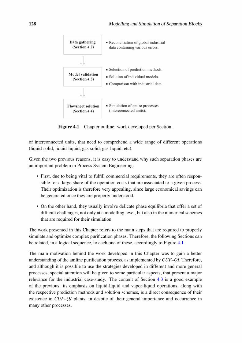
128 Modelling and Simulation of Separation Blocks
Data gathering
(Section 4.2)
Reconciliation of global industrial
data containing various errors.
Model validation
(Section 4.3)
Flowsheet solution
(Section 4.4)
Selection of prediction methods.
Solution of individual models.
Comparison with industrial data.
Simulation of entire processes
(interconnected units).
Figure 4.1 Chapter outline: work developed per Section.
of interconnected units, that need to comprehend a wide range of different operations(liquid-solid, liquid-liquid, gas-solid, gas-liquid, etc).
Given the two previous reasons, it is easy to understand why such separation phases arean important problem in Process System Engineering:
• First, due to being vital to fulfill commercial requirements, they are often respon-sible for a large share of the operation costs that are associated to a given process.Their optimization is therefore very appealing, since large economical savings canbe generated once they are properly understood.
• On the other hand, they usually involve delicate phase equilibria that offer a set ofdifficult challenges, not only at a modelling level, but also in the numerical schemesthat are required for their simulation.
The work presented in this Chapter refers to the main steps that are required to properlysimulate and optimize complex purification phases. Therefore, the following Sections canbe related, in a logical sequence, to each one of these, accordingly to Figure 4.1.
The main motivation behind the work developed in this Chapter was to gain a betterunderstanding of the aniline purification process, as implemented by CUF–QI. Therefore,and although it is possible to use the strategies developed in different and more generalprocesses, special attention will be given to some particular aspects, that present a majorrelevance for the industrial case-study. The content of Section 4.3 is a good exampleof the previous; its emphasis on liquid-liquid and vapor-liquid operations, along withthe respective prediction methods and solution schemes, is a direct consequence of theirexistence in CUF–QI plants, in despite of their general importance and occurrence inmany other processes.

4.2 Gathering and treatment of experimental data 129
4.2 Gathering and treatment of experimental data
When trying to perform simulation and / or optimization studies around a given processunit, it is necessary to assure that the underlying model equations are capable to capturethe fundamental phenomena present. In other words, one of the major difficulties indeveloping mathematical models is to guarantee that these describe, accurately, the realitythat they pretend to emulate. It may appear simple to infer about the rigor of a particularmodel, when experimental data is available, but this task can offer significant challenges,especially if the difficulties start when trying to establish “what is the reality” or, in otherwords, which experimental data is reliable and which is not.
The previous problem should therefore be solved, before trying to to validate (by com-parison) the results obtained through mathematical prediction models. This is especiallyimportant when the “real” data, that is used as reference, is derived from industrial plantequipment that, due to a number of reasons (e.g., wearing out, lack of frequent calibration,malfunctions), often generates measurement errors. In these situations, it becomes crucialto eliminate such errors, through data reconciliation strategies, in order to correctly char-acterize the industrial reality and obtain a faithful description of the units performance.
In fact, many of the recorded values for flow streams and compositions carry impliciterrors (random and, less frequently, gross errors) that, when used to determine the plantmass balance diagram, give rise to violations in the mass conservation laws. The prob-lem can be therefore understood as how to reconcile the data (measurements) in orderto satisfy the process constraints, while minimizing the error in a least squares sense; bydoing it is possible to obtain an estimate of the true state of the plant, free of both randomand non-random errors. To achieve this purpose, Kuehn and Davidson (1961) proposedthe first solution to the steady-state reconciliation problem and, since them, many otherauthors have been suggesting improvements and developing new approaches to the prob-lem.
Since the beginning, it was recognized that gross errors should be previously eliminatedfrom the set of used data values (Knepper and Gorman, 1980; Mah and Tamhane, 1982).These would compromise the entire reconciliation scheme, by erroneously enlarging thedegree of corrections required — the reason for this is easy to understand: when usinga least squares objective function, in the data reconciliation problem, it is assumed thatall measurements are normally distributed. If gross errors are indeed present, the resultof data reconciliation will be biased because all of the measurements, including the grosserrors, are given the same weight in the estimation.
The first solutions proposed to deal with gross error presence were based on the use of sta-tistical tests — some of the more recently improved versions can be found in Narasimhanand Mah (1989); Rosenberg et al. (1987). Although capable of detecting great part of thegross errors present, the use of statistical tests have two disadvantages (Biegler and Tjoa,1991):

130 Modelling and Simulation of Separation Blocks
• The reconciliation needs to be performed again, after removing the gross errors,thus leading to an iterative process.
• The majority of these tests are based on linear or linearized models (e.g., Croweet al. (1983); Crowe (1986)) and thus the validity of their statistical properties isquestionable, when applied to nonlinear models.
To improve the robustness of data-reconciliation strategies, Biegler and Tjoa (1991) pro-posed the substitution of statistical tests by the use of an objective function that was con-structed using maximum likelihood principles on a combined distribution function. Theproposed function (the contaminated Gaussian distribution) considers contributions fromrandom and gross errors. The advantage of minimizing this bivariate objective function,is that the presence of gross errors can be considered and simultaneously treated througha proper constructed detection test, thus eliminating the iterative nature of the originalproblem.
By establishing an analogy between minimum likelihood rectification and robust regres-sion, Johnston and Kramer (1995) used robust estimators as the objective function in thedata reconciliation problem; these authors reported improved performance, especially inthe presence of gross errors. Subsequently, other authors (e.g., Arora and Biegler (2001))have been suggesting the use of different robust estimators. A comparative study relativeto the performance of the main strategies used for data reconciliation can be found inÖzyurt and Pike (2004).
4.2.1 Developed procedure: a pragmatic approach
Despite their significant theoretical contributions, most of the works found in literaturedo not include application examples referring to the data reconciliation of large-scalechemical plants. In fact, when real processes of high complexity are considered, a setof additional difficulties may emerge, hindering the use of of traditional reconciliationtechniques:
• Equations expressing functional relations between the process variables are in mostcases inexistent. The objective of this task is often the generation of completelycoherent mass balance diagrams, to be subsequently used as basic information inthe validation of mathematical models of the process. This limits the level of redun-dancy that can be used to make this procedure more robust to measurement errors.
• A large number of variables, streams, and process units is usually involved, wherecomplex behaviors, difficult to be described by simple empirical models, can bepresent. Even when rigorous mathematical models are available, the resulting prob-lem becomes large-scale and highly nonlinear, and thus difficult to solve.
• Complete process measurements are not available, in most cases, with impact again

4.2 Gathering and treatment of experimental data 131
on the level of redundancy that can be established. This also limits the possibilityof calculating the variance, a fundamental parameter in this task.
When a reconciliation exercise is applied to a plant presenting all these difficulties, adifferent strategy needs to be defined since, for reconciliation purposes, redundancy isalways required. In the absence of a model and with few available measurements, tradi-tional techniques will fail due to the lack of mathematical relations that can be posed torelate all problem variables. To overcome the difficulties earlier described, an alternativemethodology was developed (Neves et al., 2005a) to establish the overall mass balancediagram in large-scale processes (Figure 4.2).
The key aspect of this strategy consists in working with redundancy directly on the massbalances equations. Global and partial mass balances are written for all units, and effortsconcentrated at the beginning of the work, in a data collection phase, trying to obtain atleast one simultaneous measurement of the composition and flowrate of each stream. Thiscan be achieved by collecting, in a minimal time window:
• Samples of all streams; these can be latter characterized through detailed laboratoryanalysis, using a suitable technique / equipment.
• Values for the respective volumetric flows; a portable ultrasonic measurer may bean option when a local flow transmitter is not available.
Although developed for purification blocks, where normally only separation processestake place, the strategy presented in Figure 4.2 can also be used when, undesirably, somespecies are involved in secondary reactions. In fact, the occurrence of reaction in separa-tion units is not a rare phenomena and may be impossible to completely avoid when theselast ones are operated at high temperatures (a common situation in distillation based op-erations). In these cases, partial mass conservation cannot be obviously verified, neithershould be attempted in a reconciliation step that does not consider it. Doing so wouldcompromise the entire reconciliation scheme, by introducing bias in the corrections re-quired, similarly to gross measurement errors. In order to overcome this problem, andsince the reactions are many times unconfirmed, the reconciliation exercise was dividedin two phases.
1st reconciliation phase: Similarly to a gross error detection phase, only total flowsare reconciled, using fixed concentrations corresponding to the measured values. This isdone by minimizing the weighted deviations of the errors observed in the total and partial

132 Modelling and Simulation of Separation Blocks
DA
TA
CO
LL
EC
TIO
N
2N
D R
EC
ON
CIL
IA
TIO
N P
HA
SE
1
ST
RE
CO
NC
IL
IA
TIO
N P
HA
SE
Selectio
n o
f poin
ts for
stream sam
plin
g.
Selectio
n o
f poin
ts for
ultra
-sonic flo
w
Measu
remen
t.
Selectio
n o
f poin
ts with
on
-line lo
cal flow
indicatio
n.
Data g
atherin
g fo
r
streams w
ith o
nlin
e
flow
record
ing.
Sam
ple ch
aracterisation
by a su
itable an
alytical
techniq
ue
.
Com
po
sition estim
ates for
all streams, w
ith d
ifferent
deg
ress of co
nfid
ence
.
Data g
atherin
g d
urin
g a
perio
d o
f time, n
ecessary
to estab
lish m
easurem
ent
con
fiden
ce.
Flo
w estim
ates for all
streams w
ith d
ifferent
deg
rees of co
nfid
ence
.
Input fo
r the first
recon
ciliation
phase
For sp
ecies takin
g p
art in ch
emical reactio
ns
, inter-
conversio
n
relation
s are
dev
eloped
(su
ppo
rted
by
experim
ental
stud
ies) an
d
inco
rpo
rated
in
the
form
ulatio
n o
f a secon
d reco
nciliatio
n step
.
In each
unit, th
e remain
ing erro
r associated
to th
e
mass
con
servatio
n
law
of
each
com
po
nen
t is
carefully
analy
sed in
ord
er to id
entify
species th
at
are poten
tially in
volv
ed in
chem
ical reaction step
s.
A
quad
ratic fo
rmulatio
n
(QP
) is
used
, w
here
streams co
mpositio
ns are fix
ed an
d flo
w v
alues are
optim
ization
variab
les.
The o
bjectiv
e functio
n co
nsists in
min
imizin
g th
e
error asso
ciated to
total/p
artial mass co
nserv
ation
of
all interv
enin
g co
mponen
ts in all p
rocess u
nits
.
Inpu
t for th
e secon
d
reconciliatio
n p
hase
A
non-lin
ear fo
rmulatio
n
(NL
P)
is used
where
both
co
mpositio
ns
and
flow
s are
treated as o
ptim
ization v
ariables
, in
ord
er to
close all m
ass balan
ces.
The
objectiv
e fu
nctio
n
consists
in
min
imizin
g th
e total co
rrections m
ade to
the
valu
es obtain
ed in
the d
ata collectio
n p
hase
,
accountin
g
for
differen
t d
egrees
of
confid
ence in
the g
athered
info
rmatio
n.
A M
ass Flo
w D
iagram
is ob
tained
where
:
-glo
bal
and
partial
balan
ces are
closed
either
for
main
an
d vestig
ial co
mp
onen
ts,
enterin
g o
r not in
chem
ical reaction step
s.
-v
alues o
btain
ed fo
r flow
s/co
mpo
sitions are
as close as p
ossib
le to th
ose m
easured
in th
e
ind
ustrial p
lant.
Figure4.2
Main
stepsofthe
developedreconciliation
procedure.

4.2 Gathering and treatment of experimental data 133
mass balances for each unit, resulting in a Quadratic Problem (QP):
minγu
M,C1∑
iwi
BP(ε
iBP)2
+(εBT)2
s.t. ∑p
(xi,p
OM MpC1
)=∑
o
(xi,o
OM MoC1
)− ε
iBP
∑p
MpC1 =∑
oMo
C1− εBT
MuC1 = Mu
OM + γuM,C1
βuC1,lo Mu
OM < MuC1 < β
uC1,up Mu
OM
u≡ o∪ p, p = 1, . . . ,ni o = 1, . . . ,no, i = 1, . . . ,nc
This first phase allows to obtain a set of more coherent flowrates estimates and, more im-portantly, the identification of units and species where significant residuals are observed,when trying to close the mass balances. After careful analysis, this behavior needs to berelated to reactions between the species involved, and expressions added to the set of massbalance equations, to model their inter-conversion.
2nd reconciliation phase: In a second phase, partial and global mass balances aroundthe units are closed, this time considering both flowrates and compositions as decisionvariables, and using the inter-conversion expressions — f
(xi
C2)
— obtained after the firstphase. The corresponding formulation, although resulting in a non-linear problem (NLP),presents a relatively easy solution, given the solution obtained in the previous phase asinitial estimate:
minγu
M,C2, γi,ux,C2
∑u
wuM(γ
uM,C2
)2 +∑i
∑u
wi,ux γ
i,ux,C2
s.t. ∑p
(xi,p
C2 MpC2
)= ∑
o
(xi,o
C2 MoC2
)+ f
(xi
C2)
∑p
MpC2 = ∑
oMo
C2
MuC2 = Mu
C1 + γuM,C2
xi,uC2 = xi,u
OM + γi,ux,C2
βuC2,lo Mu
C1 < MuC2 < β
uC2,up Mu
C1
θuC2,lo xi,u
OM < xi,uC2 < θ
uC2,up xi,u
OM
u≡ p∪o, p = 1, . . . ,ni o = 1, . . . ,no, i = 1, . . . ,nc
Different ranges of allowed corrections are imposed in the mathematical formulationssince, for some processes including biphasic mixtures, the separation between organic

134 Modelling and Simulation of Separation Blocks
and aqueous phases can lead to a less precise measurement of water percentage. Theseparameters (that play a role analogous to the traditional variance usage) may also be usedto consider the existence of less and more precise flow indications, and the fact of somechemical species presenting inexact concentration measurements (even when the best an-alytical techniques are used).
Another aspect that was also considered in the approach developed was the possibility ofsome processes presenting chemical species in extremely different ranges of concentra-tion. Such situations can be troublesome since the error in mass conservation of speciesin vestigial concentrations might be neglected when trying to close the balances aroundmain components (in much greater concentrations). To overcome this problem, differentweighting factors are specified in the mathematical formulation, assuring that all speciesreceive similar importance during the reconciliation procedure.
The above described strategy intends to be a pragmatic approach: it can be generallyemployed in many existing industrial processes and, by retaining the essentials of a rec-onciliation procedure through the use of simple mathematical formulations, it increasesthe chances of success in extremely complex problems. In particular, the similarity ofthis approach to the ALT procedure described in Section 3.3.2 for the solution of poolingproblems, and with Bender’s decomposition (Floudas, 1995) should be noted.
4.2.2 Industrial case-study
The efficiency of the approach discussed in Section 4.2.1 will be illustrated by consideringthe aniline purification plant, owned by CUF–QI.
As shown in Figure 4.3, this purification process involves 8 distillation columns (2 ofthem with attached flash units) and 5 phase separators, where 10 components (8 of them investigial concentrations) exhibit, respectively, a strong non-ideal LV and LL equilibrium,for which no models were available at the time. None of the process streams had theircompositions measured on-line. Only a few of them were analyzed daily in the laboratory;even in these cases, the concentrations were not determined for all components. Theflow measurements followed a similar pattern. The level of knowledge relative to theprocess represented in Figure 4.3, was relatively low in the beginning. No mass (andheat) balances diagrams were available and some of the process P&IDs needed to beupdated before starting the data collection phase. Some attempts in tracking the vestigialspecies (reaction byproducts) were made in the past, although without success due tothe incapacity of closing all mass balances simultaneously. For all the earlier referredcharacteristics and conditions, the current purification process offered a great challengefor the new developed reconciliation strategy.

4.2 Gathering and treatment of experimental data 135
1 2 3 4
8 7 6 5
9 10 11 12
13
Aniline CHA Residue Water
REACTION PHASE
AnilineProducts
Figure 4.3 Topology of the industrial separation phase under study.
Implementation aspects
Since several flowrates were not recorded in the control room, and also not locally mea-sured in the plant, a portable ultrasonic meter was employed. The values obtained throughthis equipment were gathered during a time period sufficiently long to capture the vari-ability of the readings. For sample characterization, gas chromatography (GC) was usedto determine the composition of the organic phases, while the Karl-Fisher technique wasemployed to quantify the water percentage (Neves, 2002). As expected, some problemsoccurred due to the high immiscibility in some (few) samples. At the high distillation tem-peratures, only one phase prevails and the miscibility is complete, but when the sampleswere taken to room temperature, phase separation begun to establish almost immediately.Some problems were also felt, when trying to measure the concentration of the “heav-ier” byproducts (in the organic phase), due to the lack of the best adsorption internalsand calibration routines, in the available analytical equipments. All this situations werecarefully recorded and used to model the relative uncertainties associated with the variousmeasurements used.
As explained in Section 4.2.1, careful tuning of the weights used in the objective functionwas also required, due to the presence of several species in vestigial compositions. In fact,in the majority of the streams, aniline and water present a joint mass fraction of more than99.5%, and some byproducts (e.g., DICHA) exhibit a concentration 50 000 times inferiorto that of a main component.
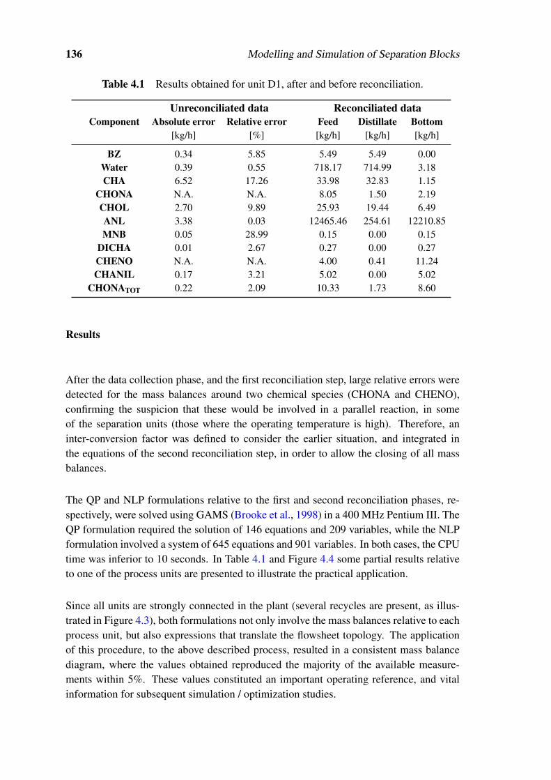
136 Modelling and Simulation of Separation Blocks
Table 4.1 Results obtained for unit D1, after and before reconciliation.
Unreconciliated data Reconciliated dataComponent Absolute error Relative error Feed Distillate Bottom
[kg/h] [%] [kg/h] [kg/h] [kg/h]
BZ 0.34 5.85 5.49 5.49 0.00Water 0.39 0.55 718.17 714.99 3.18CHA 6.52 17.26 33.98 32.83 1.15
CHONA N.A. N.A. 8.05 1.50 2.19CHOL 2.70 9.89 25.93 19.44 6.49ANL 3.38 0.03 12465.46 254.61 12210.85MNB 0.05 28.99 0.15 0.00 0.15
DICHA 0.01 2.67 0.27 0.00 0.27CHENO N.A. N.A. 4.00 0.41 11.24CHANIL 0.17 3.21 5.02 0.00 5.02
CHONATOT 0.22 2.09 10.33 1.73 8.60
Results
After the data collection phase, and the first reconciliation step, large relative errors weredetected for the mass balances around two chemical species (CHONA and CHENO),confirming the suspicion that these would be involved in a parallel reaction, in someof the separation units (those where the operating temperature is high). Therefore, aninter-conversion factor was defined to consider the earlier situation, and integrated inthe equations of the second reconciliation step, in order to allow the closing of all massbalances.
The QP and NLP formulations relative to the first and second reconciliation phases, re-spectively, were solved using GAMS (Brooke et al., 1998) in a 400 MHz Pentium III. TheQP formulation required the solution of 146 equations and 209 variables, while the NLPformulation involved a system of 645 equations and 901 variables. In both cases, the CPUtime was inferior to 10 seconds. In Table 4.1 and Figure 4.4 some partial results relativeto one of the process units are presented to illustrate the practical application.
Since all units are strongly connected in the plant (several recycles are present, as illus-trated in Figure 4.3), both formulations not only involve the mass balances relative to eachprocess unit, but also expressions that translate the flowsheet topology. The applicationof this procedure, to the above described process, resulted in a consistent mass balancediagram, where the values obtained reproduced the majority of the available measure-ments within 5%. These values constituted an important operating reference, and vitalinformation for subsequent simulation / optimization studies.
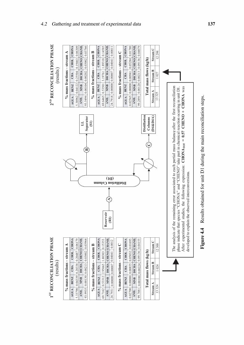
4.2 Gathering and treatment of experimental data 137
AG
UA
BE
NZ
CH
AC
HO
LC
HO
NA
AN
ILM
NB
DIC
HA
CH
EN
OC
HA
NIL
5.3
37
90
% m
ass
fracti
on
s – s
tream
A
1S
T R
EC
ON
CIL
IAT
ION
PH
AS
E
Str
eam
AS
trea
m B
Str
eam
C
13
32
41 0
24
12 3
00
Tota
l m
ass
flo
ws
(kg
/h)
Rese
rv
oir
(R1)
C
B
A
(res
ult
s)
% m
ass
fracti
on
s – s
tream
B
0.0
43
39
0.2
83
38
0.2
048
70
.061
79
AG
UA
BE
NZ
CH
AC
HO
LC
HO
NA
AN
ILM
NB
DIC
HA
CH
EN
OC
HA
NIL
93
.99
35
0.0
01
30
0.0
02
13
0.0
300
20
.039
64
% m
ass
fracti
on
s – s
tream
C
2N
D R
EC
ON
CIL
IAT
ION
PH
AS
E
(res
ult
s)
AG
UA
BE
NZ
CH
AC
HO
LC
HO
NA
AN
ILM
NB
DIC
HA
CH
EN
OC
HA
NIL
69
.71
62
0.5
33
12
2.9
56
65
1.8
03
03
0.1
53
53
24
.79
31
0.0
00
00
0.0
00
07
0.0
40
41
0.0
012
0.0
27
00
0.0
00
00
0.0
08
55
0.0
503
20
.016
95
99
.78
81
0.0
01
00
0.0
02
24
0.0
913
60
.041
55
Distillation Column
(D1)
Dis
till
ati
on
Co
lum
ns
(D4
&D
4A
)
LL
Sep
ara
tor
(S1
)
Str
eam
AS
trea
m B
Str
eam
C
Tota
l m
ass
flo
ws
(kg/h
)
BE
NZ
CH
AC
HO
LC
HO
NA
AN
ILM
NB
DIC
HA
CH
EN
OC
HA
NIL
5.3
89
62
% m
ass
fracti
on
s – s
tream
A
0.0
41
22
0.2
55
04
0.1
94
63
0.0
63
09
93
.54
94
0.0
01
04
0.0
02
02
0.0
30
02
0.0
37
66
AG
UA
BE
NZ
CH
AC
HO
LC
HO
NA
AN
ILM
NB
DIC
HA
CH
EN
OC
HA
NIL
69
.64
65
% m
ass
fracti
on
s –
str
eam
B
0.5
35
01
3.1
97
61
1.8
93
18
0.1
45
85
24
.79
18
0.0
00
00
0.0
00
07
0.0
40
41
0.0
00
11
AG
UA
BE
NZ
CH
AC
HO
LC
HO
NA
AN
ILM
NB
DIC
HA
CH
EN
OC
HA
NIL
0.0
25
65
% m
ass
fracti
on
s – s
tream
C
0.0
00
00
0.0
09
41
0.0
52
84
0.0
17
80
99
.28
91
0.0
01
20
0.0
02
13
0.0
91
36
0.0
40
79
AG
UA
13 3
25
1 0
27
12
29
8
The a
naly
sis
of
the r
em
ain
ing e
rror
ass
ocia
ted t
o e
ach p
art
ial
mass
bala
nce,
aft
er
the f
irst
reconcil
iati
on
phase
indic
ate
that
specie
s “C
HO
NA
” a
nd “
CH
EN
O” t
ake p
art
in c
hem
ical
reacti
on o
curr
ing i
n u
nit
D1
.
Aft
er
experi
menta
l st
udie
s, t
he fo
llow
ing expre
ssio
n:
CH
ON
AT
OT
=
0.5
7
CH
EN
O +
C
HO
NA
w
as
develo
ped t
o e
xpla
in t
he o
bse
rved i
nte
rconvers
ions.
Figu
re4.
4R
esul
tsob
tain
edfo
runi
tD1
duri
ngth
em
ain
reco
ncili
atio
nst
eps.

138 Modelling and Simulation of Separation Blocks
4.3 Model Validation and Solution
Due to the same reasons discussed in Chapter 2 for reaction systems, describing the phe-nomena inherent to separation processes also constitutes a crucial step where, once again,balancing the rigor and complexity of the adopted mathematical models can be decisive.The next Sections are centered in liquid-liquid and vapor-liquid operations (referring tothe particular case of phase separators and distillation columns), due to their greater rele-vance for the current industrial case-study.
4.3.1 Liquid-Liquid separation
Generally, liquid-liquid operations are characterized by low cost, for being simple froman operational point of view and for presenting a limited separation efficiency. There-fore, such operations are normally associated to other separation techniques, with greaterefficiency (like distillation), in order to reduce their higher operating costs.
If, from a design perspective, a phase separator is a simple equipment, at an operatinglevel the scenario is not much different. Although it is possible to consider the additionof an extra chemical species, to change the overall equilibrium favorably, and / or touse a sequence of these units (in co-current or counter-current operation), to extend theseparation degree, there are actually few operating parameters that can be considered asoptimizing variables1.
Despite this conceptual and operational simplicity, developing mathematical models fora phase separator can be a difficult task. The modelling equations at a macroscopic levelcomprehend only the mass and control balances, as stated by equations (4.1–4.3), thatconsider a battery of these units, in counter-current mode:
• Mass balances:
xi, jF F j + xi, j−1
L1L j−1
1 + xi, j+1L2
L j−11 = xi, j
L1L j
1 + xi, jL2
L j2 (4.1)
• Control equations:nc
∑i=1
xi, jL1
= 1,nc
∑i=1
xi, jL2
= 1 (4.2)
• Equilibrium equations:κ
i, jL1
xi, jL1
= κi, jL2
xi, jL2
(4.3)
Calculating the values of κ iL1
and κ iL2
, in equation (4.3), will require a set of auxiliary ex-pressions, corresponding to an adopted prediction method. Selecting a suitable method is
1Temperature can be one of them, although it is normally fixed at ambient temperature.

4.3 Model Validation and Solution 139
a critical step, especially because trade-offs between rigor and complexity should alwaysbe present. There are two main forms of predicting LLE:
• The first one relies on the use of state equations (e.g., Wilson, Van Laar), capableof good predictions for moderately complex equilibria (where the deviations fromideality are not large).
• The second corresponds to the use of group contribution methods (e.g., UNIFAC,UNIQUAC, NRTL) that, in general, present a large number of adjustable parame-ters and, therefore, allow more accurate results for the extremely non-ideal cases.The following equations translate the NRTL (Non Random Two Liquids) method,a typical choice for LLE prediction (Sandler, 1994):
lnκiL =
∑q φq,iNkφ
q,iNgxq
∑l φl,iNgxl
+∑q
φq,iNgxq
∑l φl,iNgxl
(φ
i,qNk−
∑n φn,qNk φ
n,qNg xn
∑l φl,qNgxl
)(4.4a)
φq,iNg = exp(−φ
q,iNl φ
q,iNk) (4.4b)
φq,iNk =
(φ q,iNh−φ
i,iNk)
RT= φ
q,iNa +
φq,iNbT
+φq,iNe lnT +φ
q,iNf T (4.4c)
φq,iNl = φ
q,iNc +φ
q,iNd(T −273.15) (4.4d)
φi,iNg = 1, φ
i,iNk = 0, φ
q,iNh = φ
i,qNk, φ
q,iNl = φ
i,qNl (4.4e)
In this method φq,iNg 6= φ
i,qNg, i.e., the matrix of coefficient is asymmetric. As can
be observed, in addition to requiring approximately 30 variables per species, thenon-linearity of the involved equations is considerably high.
4.3.2 Vapour-Liquid separation
Generally, vapor-liquid operations are more complex (optimizing some key variables isof crucial importance), more expensive (relatively to investment and operation) but alsomore efficient (higher separation degrees can be obtained) than liquid-liquid operations.Among them, and for large-scale continuous processes, absorption and distillation are themost common and representative.
From a modelling perspective, it is possible to treat distillation and absorption as equilib-rium based operations, and therefore use identical sets of balance equations. However, theresulting final models will rarely have similar properties since the adopted VLE predictionmethods need to be based in different phenomena:
• In absorption, the separation is based on fact that different gas components presentdistinct solubilities towards a given liquid phase and, therefore, will be absorbed indifferent extents.

140 Modelling and Simulation of Separation Blocks
• In distillation, the separation is based on the relative volatilities of the interveningcomponents, that will cause their different distribution among the formed liquid andvapor phases, when the mixture is reboiled.
The adoption of distinct prediction models will implicate different mathematical treat-ment (solution procedures) for the two types of vapor-liquid operations previously re-ferred. Due to the major importance of distillation, for the current industrial case-study,the following discussion will be centered exclusively on it.
Despite some references that propose a mass transfer based modelling for distillation sys-tems (Kooijman and Taylor, 1995; Wesselingh, 1997), common approaches treat these asequilibrium controlled, as stated in equation 4.7. Therefore, an important set of auxiliaryexpressions that need to be introduced corresponds to the calculation of the vapor-liquidequilibria coefficients (κ i, j
L ,κi, jV ) in each stage.
When adopting an “equilibrium-based” approach, the ruling equations are generally re-ferred as the MESH balances (Mass-Equilibrium-Summation-Heat) translated, in theirgeneral form, by equations (4.5–4.8). Some balances may require slight changes, depend-ing on the column type (e.g., when side reboilers / condensers are employed), althoughthe impact on the mathematical properties of the overall model is marginal.
• Mass balances:
L j−1xi, j−1 +V j+1yi, j+1 +F jxi, jF =
(L j +LS j)xi, j +
(V j +V S j)yi, j (4.5)
• Heat balances:
L j−1H j−1L +V j+1H j+1
V +F jH jF−Q j =
(L j +LS j)H j
L +(V j +V S j)H j
V (4.6)
• Equilibrium relations:κ
i, jV yi, j = κ
i, jL xi, j (4.7)
• Control expressions:nc
∑i=1
yi, j = 1,nc
∑i=1
xi, j = 1 (4.8)
As equations (4.6) reflect, the energy flow along the column is of major importance. Itsprediction requires the use of another set of auxiliary expressions for (liquid and vaporphase) enthalpy estimation, as given bellow:
H jL = f (T j,xi, j), H j
V = f (T j,yi, j) (4.9)
By the same reasons discussed for LLE, the choice of a prediction model for VLE isalso of major importance. The equations of these models will have, once again, a huge
4.3 Model Validation and Solution 141
impact on the dimension and non-linearity of the resulting overall model, contributing ina greater extent than the MESH equations. Once again, the use of state equations andgroup contribution methods is also possible. Some of these equations and methods can,inclusively, found application in both cases (VLE and LLE), since the goal is essentiallythe same: estimate, for a given phase, the deviations from the ideal equilibrium situation(independently of the system nature); the similarity between equations (4.3) and (4.7),clearly illustrates the above.
However, for the VLE case, with the exception of systems that are operated well abovethe atmospheric pressure (P > 5 atm), the vapor phase is normally considered to behaveideally and, therefore, the corresponding correcting parameters (that are used to calculateκ
i, jV ) take the unitary value. This assumption does not affect (typically) the quality of
the results obtained, independently of the considered mixture, and greatly reduces thecomplexity of the resulting model.
On the other hand, for the liquid phase, the previous simplification cannot be generalized.However, two distinct situations can still occur in practice:
• Certain mixtures may present an approximately ideal behavior, where the correctiveparameters assume values close to unity. This situation is typical in petrochemicalprocesses, where the common hydrocarbon mixtures exhibit equilibria that are easyto describe.
• Other mixtures, involving components that establish strong chemical bonds be-tween themselves (e.g., water and ethanol, due to the presence of hydrogen bonds),will interact in complex equilibria (typically involving azeotropes), difficult to de-scribe and requiring correcting parameters well deviated from the unitary value, toobtain good predictions.
In this last situation, and as previously discussed for the LLE case, the use of more elabo-rated methods (as those based on group contribution theory) will be, in practice, unavoid-able. Equation (4.10) can be generally used to obtain κ
i, jL , assuming an ideal behavior for
the vapor phase, and using ψ i, j as corrective parameters for the liquid phase.
κi, jL = f (T j,xi, j,yi, j) = ψ
i, jPSi, j/P (4.10)
The ψ i, j can be estimated through (4.11), that translate the UNIFAC method, a typi-cal choice for the liquid phase, when dealing with complex mixtures in distillation pro-cesses (Sandler, 1994).
ψiUr = ψ
i,vUmψ
vUp (4.11a)
ψiUq = ψ
i,vUmψ
vUt (4.11b)
ψi, jUo = ψ
iUr/(ψ
iUrx
i, j) (4.11c)

142 Modelling and Simulation of Separation Blocks
ψi, jUl = ψ
iUq/(
ψiUqxi, j
)(4.11d)
ψv,iUg = ψ
i,vUmψ
vUt (4.11e)
ψv, jUh = ψ
v,iUgxi, j (4.11f)
ψv,v, jUk = exp
(−ψ
v,vUa/T j) (4.11g)
ψv,i, jUe = ψ
v,iUgψ
v,v, jUk (4.11h)
ψv, jUn = ψ
v,i, jUe xi, j (4.11i)
ψi, jUc = 1−ψ
i, jUl + ln
(ψ
i, jUo−5ψ
iUq
(1−ψ
i, jUo/ψ
i, jUl + ln
(ψ
i, jUo/ψ
i, jUl
)))(4.11j)
ψi, jUd = ψ
iUq
(1− ln
(ψ
i, jUl
))−∑
vψ
v,v, jUk ψ
v,i, jUe /ψ
v, jUn−ψ
v,iUg ln
(ψ
v,i, jUe /ψ
v, jUn
)(4.11k)
ψi, j = exp
(ψ
i, jUc +ψ
i, jUd
)(4.11l)
The analysis of equations (4.11) shows that the resulting system is extremely nonlinearand characterized by a large dimension (around 60 equations per species, per equilibriumstage are required).
4.3.3 Solution of equilibrium-staged operations
Solving models of equilibrium staged units can be difficult, especially when the equilib-rium prediction methods are complex and the number of used stages is high (Han andRangaiah, 1997). Therefore, simulating the behavior of liquid-liquid operations will gen-erally be a less challenging exercise than the solution of distillation based models since:
• In practice, the number of liquid-liquid separators in a given battery is typicallyinferior to 5, while the number of equilibrium stages in distillation columns canoften be higher than 30.
• In liquid-liquid operations, temperature is normally fixed (and not considered as anoptimization variable), while in distillation columns it exerts a major influence inthe VLE of each stage varying, some times in an accentuated manner, from the topto the bottom.
This last point has a direct impact on complexity of the required solution methods. Infact, when temperature is considered to be variable, the non-linearity of the equilibriumprediction models increases drastically (equations (4.4) and (4.11)). On the other hand,the temperature profile in distillation columns cannot be established independently, sinceit is determined by the joint solution of mass, equilibrium and energy balances aroundall stages. This means that thermodynamic calculations are intrinsically connected to theremaining ones, making the overall solution procedure a very difficult problem, due to thestrong dependence between all model equations.
4.3 Model Validation and Solution 143
For the previous reasons, the solution of distillation based models has received large at-tention in the past, replacing the simultaneous solution of all equations by iterative proce-dures. Several methods have been proposed to explore the particular properties of thesesystems of equations since, excluding the balances around the top (condenser) and bottom(reboiler) stages, all the remaining stages are only connected to that immediately aboveor bellow; in other words, the incidence matrix of this problem will be characterized by awell defined diagonal structure.
Different ways of making use of the previous structure, during an iterative procedure,define distinct categories of methods. These are characterized by particular convergencephilosophies:
• Stage-by-stage methods: These methods take advantage of the diagonal structureto suggest that all calculations can be made sequentially, solving one stage afteranother. They derive from the pioneer work of Lewis and Matheson (1932) and canbe based on different numerical schemes, including modified versions of the suc-cessive substitution procedure and Newton-Raphson based algorithms. However,stage-by-stage methods are usually known for not being reliable; during the itera-tive procedure, calculations are often interrupted due to instability problems. Latterrevisions proposed modifications to minimize the previous situations but, althoughimproving the general convergence properties, they require larger CPU times andare not capable of fully eliminating the bad reputation that these methods gained inthe past.
• Matricial methods: The lack of robustness that characterize stage-by-stage meth-ods can be overcome if, instead of doing the calculations sequentially (accumulatingerrors from one equilibrium stage to the next one), a more simultaneous strategy isadopted, considering all stages in each iteration. Matricial methods do not takefull advantage from the diagonal structure of the incidence matrix since they solveequations by type (e.g., detaching mass and heat balances) and not by stage. Thesemethods, based on the work of Thiele and Geddes (1933), present a large num-ber of variants due to the several possible forms of rearranging the equations and/ or selecting the independent variables. The major drawback relates to the directtranslation of a distillation system into a set of equations that is merely seen in amathematical perspective and, therefore, difficult to interpret in a physical point-of-view.
• Relaxation methods: This third class of methods calculates the profiles of a mul-ticomponent distillation system by integrating their dynamic model, from the ini-tial time moment (the column start up) until a sufficiently high value (where theequilibrium is established and the asymptotic values obtained). This technique isrecognized as the most reliable and robust, from all the available solution alterna-tives, although it presents a major drawback: integrating the dynamic model untilthe stationary point is reached requires a CPU time 10 to 100 times higher than the

144 Modelling and Simulation of Separation Blocks
MESH
equations
MESH
equations
MESH
equations
Complex
thermodynamic
models
Complex
thermodynamic
models
Approximate
thermodynamic
models
Complex
thermodynamic
models
i,jx
i,j yi,j
Lj
VjH
jV H
jL
Tj
,
, ,
,
Tj,V
j
(loop)
i,j
HjV H
jL,
Lj
Vj,
Tj
Lj
Vj,
Tj
(loop)
i,j, H
j
parameters
i,j
HjV H
jL,
(inner loop)
xi,j yi,j
Lj
Vj
Tj,
,
,
(outer loop)
Bubble-Point methods Sum-Rates methods Inside-Out methods
κ κ κ
κ
Figure 4.5 Types of matricial methods for the solution of distillation models.
direct algebraic solution of this last one. For this reason, relaxation methods arerarely used when only stationary simulation studies are required.
Because of the previous reasons, matricial methods are normally preferred in most ofthe situations. They constitute a balanced choice where trade-offs between robustnessand computational effort are optimal, when compared to those of the remaining classes.However, and as already introduced, a large number of variants are available, that can begrouped in three main categories (Seader and Henley, 1998) — Figure 4.5.
Methods belonging to the Bubble-point and Sum-of-Rates categories present an easierimplementation, but cannot be generally used in all problems (Perry and Green, 1997).Bubble-point methods, which include the well known Wang-Henke algorithm, are onlysuitable when the difference between the bubble-point and dew-point temperatures (atfeed conditions) is small — a typical situation in distillation. For larger ∆TDB, thesemethods start to become unstable and the robustness of the iteration procedure is seriouslycompromised. This is illustrated in Figure 4.6 where ξmax ≥ 1 defines a zone whereconvergence is not guaranteed. In a complete opposite range of application the Sum-of-Rates methods can be found, only suitable for wide-boiling mixtures, where the value of∆TDB is large — a typical situation in absorption problems.
The Inside-Out methods, based on the work of Boston and Sullivan (1974), are consid-ered to be state-of-the-art solution procedures, with guaranteed convergence properties,in almost all situations. However, and despite of their higher robustness, the use of thesemethods can be sometimes set back, due to the very demanding computational imple-mentations that are required. In fact, the algorithms of Inside-Out methods usually com-prehend more than 20 steps, in complex iteration procedures, making Bubble-Point andSum-of-Rates methods very appealing, when facing single nature problems, i.e., the sep-aration of narrow or wide boiling mixtures, respectively.
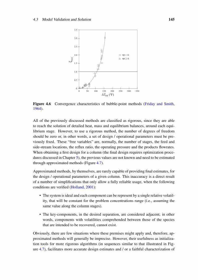
4.3 Model Validation and Solution 145
0 15050 100 300200 250 3500
0.5
1.0
1.5
2.0
2.5
3.0
3.5
< 6
np ≥ 6
ΔTDB (ºF)
max
ξ
np
Figure 4.6 Convergence characteristics of bubble-point methods (Friday and Smith,1964).
All of the previously discussed methods are classified as rigorous, since they are ableto reach the solution of detailed heat, mass and equilibrium balances, around each equi-librium stage. However, to use a rigorous method, the number of degrees of freedomshould be zero or, in other words, a set of design / operational parameters must be pre-viously fixed. These “free variables” are, normally, the number of stages, the feed andside-stream locations, the reflux ratio, the operating pressure and the products flowrates.When obtaining a first design for a column (the final design requires optimization proce-dures discussed in Chapter 5), the previous values are not known and need to be estimatedthrough approximated methods (Figure 4.7).
Approximated methods, by themselves, are rarely capable of providing final estimates, forthe design / operational parameters of a given column. This inaccuracy is a direct resultof a number of simplifications that only allow a fully reliable usage, when the followingconditions are verified (Holland, 2001):
• The system is ideal and each component can be represent by a single relative volatil-ity, that will be constant for the problem concentrations range (i.e., assuming thesame value along the column stages).
• The key-components, in the desired separation, are considered adjacent; in otherwords, components with volatilities comprehended between those of the speciesthat are intended to be recovered, cannot exist.
Obviously, there are few situations where these premises might apply and, therefore, ap-proximated methods will generally be imprecise. However, their usefulness as initializa-tion tools for more rigorous algorithms (in sequences similar to that illustrated in Fig-ure 4.7), facilitates more accurate design estimates and / or a faithful characterization of
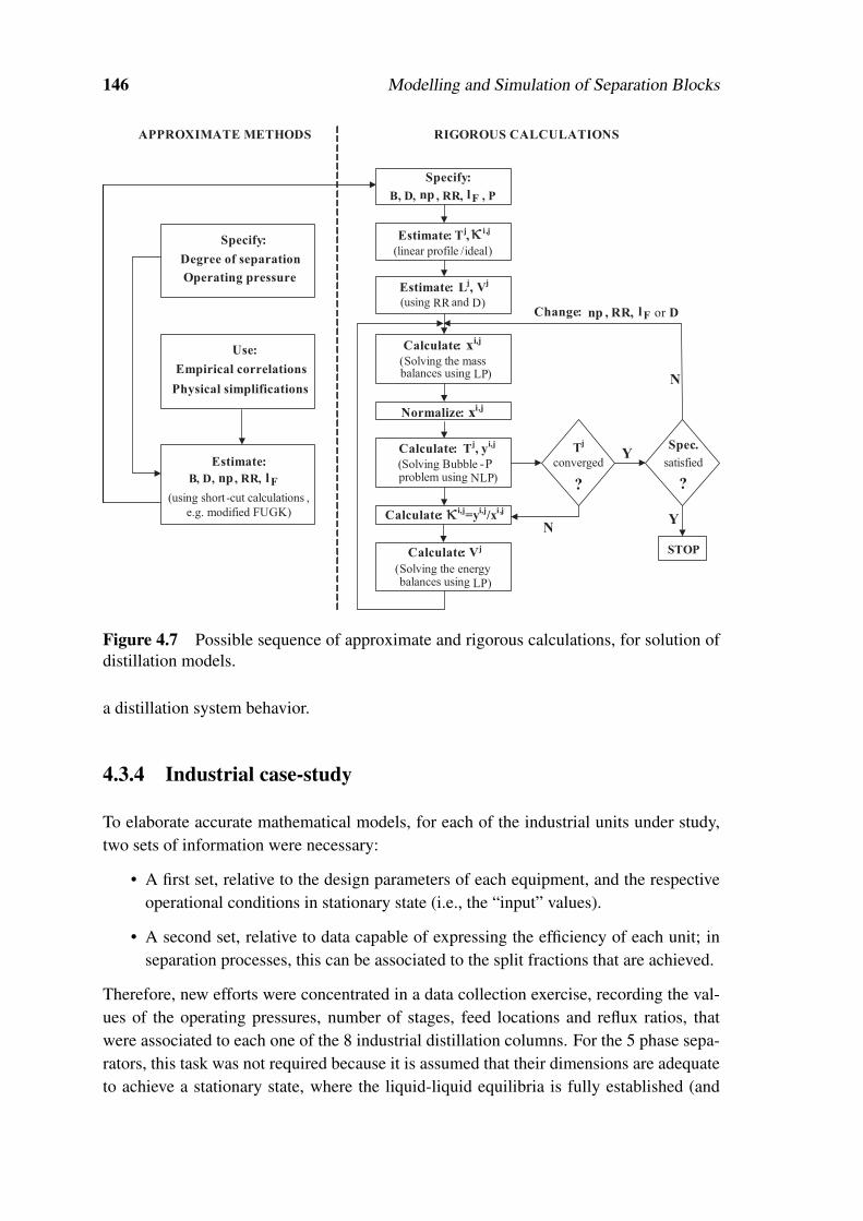
146 Modelling and Simulation of Separation Blocks
Estimate: Tj,
i ,j
(linear profile /ideal)
Specify:
B, D, , RR, , P
Estimate: Lj, V
j
(using RR and D)
Calculate: xi,j
(Solving the mass balances using LP)
Normalize: xi,j
Calculate: Tj, y
i,j
(Solving Bubble -P problem using NLP)
Calculate:i,j
=yi,j
/xi ,j
Calculate: Vj
(Solving the energy balances using LP)
Tj
converged
?
Spec.
satisfied
?
STOP
YN
Change: , RR, or D
Estimate:
Specify:
Use:
Empirical correlations
Physical simplifications
Degree of separation
Y
N
(using short-cut calculations ,
e.g. modified FUGK)
Operating pressure
B, D, , RR,
APPROXIMATE METHODS RIGOROUS CALCULATIONS
np lF
np lF
np lF
κ
κ
Figure 4.7 Possible sequence of approximate and rigorous calculations, for solution ofdistillation models.
a distillation system behavior.
4.3.4 Industrial case-study
To elaborate accurate mathematical models, for each of the industrial units under study,two sets of information were necessary:
• A first set, relative to the design parameters of each equipment, and the respectiveoperational conditions in stationary state (i.e., the “input” values).
• A second set, relative to data capable of expressing the efficiency of each unit; inseparation processes, this can be associated to the split fractions that are achieved.
Therefore, new efforts were concentrated in a data collection exercise, recording the val-ues of the operating pressures, number of stages, feed locations and reflux ratios, thatwere associated to each one of the 8 industrial distillation columns. For the 5 phase sepa-rators, this task was not required because it is assumed that their dimensions are adequateto achieve a stationary state, where the liquid-liquid equilibria is fully established (and

4.3 Model Validation and Solution 147
95
115
135
155
175
195
0.0 0.1 0.2 0.3 0.4 0.5 0.6 0.7 0.8 0.9 1.0
T (
ºC)
Water (mole fraction)
Vapor phase
Liquid phase
98
100
102
104
0.95 0.96 0.97 0.98 0.99 1.00
Figure 4.8 Experimental results for the VLE between water and aniline (CUF-QI,2007).
no more “input” variables exist in practice). For the second set of required data, the splitfractions that are promoted in each equipment (distillation column or phase separator)were easily obtained from the results of the previous data reconciliation exercise.
Creating accurate models, for the industrial units under study, is a goal that cannot bereduced to the selection of good LLE and VLE prediction methods. As already intro-duced, thermodynamic calculations are extremely important when simulating distillationcolumns and, therefore, the selection of suitable correlations for (liquid and gas) en-thalpies and heat capacities estimation, need also to be considered. To systematize allinformation relative to the choices made during model development, the next Sectionpresents all correlations and methods adopted.
Adopted correlations and models
The selection of suitable phase equilibrium models needs to be done by confronting theirresults (via numerical solution) with experimental LLE and VLE curves. On the otherhand, since the units under study comprehend mixtures of 10 components, the above pro-cedure may become impracticable. There are few references in literature to experimentalcurves involving the components under study and, when these can be found, they alwaysreport to binary solutions. However, in practice, a method capable of predicting highlynon-ideal binary equilibria (for different pairs of chemical species) will be, in most situ-ations, capable of generating good results for the mixture behavior (although no generalguarantees can be made). Therefore, and taking in consideration the previous premise, thetwo experimental curves, presented in Figures 4.8 and 4.9, were selected as references.
Figure 4.8 exhibits the well known VLE between water and aniline, a system that presentsa heterogeneous azeotrope at 98.7 C and 0.044 of aniline mole fraction, where three

148 Modelling and Simulation of Separation Blocks
Solubility of water in aniline
Solubility of aniline in water
10
30
50
70
90
110
130
150
170
T (
ºC)
0.0 0.1 0.2 0.3 0.4 0.5 0.6 0.7 0.8 0.9 1.0
Water (mole fraction)
Figure 4.9 Experimental results for the LLE between water and aniline (CUF-QI,2007).
phases are in equilibrium: a vapor phase and two liquid phases (an organic one with30.3% water, and an aqueous one with 98.6% water, in a molar basis). This is a pointof major importance that, if not correctly considered, will have significant impact on thesimulation of some distillation units that operate in different sides of this azeotrope.
The LLE curve, shown in Figure 4.9, exhibits the solubility of water in aniline, at differenttemperatures, as experimentally determined in laboratory. These results are crucial for thesimulation of some phase separators and, like the ones represented in Figure 4.8, are alsorecognized by being of difficult theoretical prediction.
As discussed in Sections 4.3.1 and 4.3.2, when the LLE and VLE are approximately ideal,the prediction methods can and should be translated by a few simple equations, resultingin overall models of small dimensions and weak nonlinear properties. However, andas already suspected, mixtures like the ones involved in CUF–QI plants, exhibit phaseequilibria where the parameters κ i
V and κ iL are difficult to estimate, requiring complex
procedures. The only method capable of accurately describing the VLE of Figure 4.8 wasthe UNIFAC method, together with equation (4.12) for vapor pressure estimation; for theLLE in Figure 4.9, the only suitable choice was the NRTL method.
• Vapor pressures (pure components):
PSi, j = exp
(Gi
vpc1 +Gi
vpc2
T j +Givpc3 ln
(T j)+Gi
vpc4(T j)Gi
vpc5
)(4.12)
Choosing adequate correlations, for the estimation of heat capacities and enthalpies, wasalso a difficult task, for the same reasons discussed during LLE and VLE prediction.Some of the chemical species (e.g., CHANIL and CHENO) are rare and, therefore, typicalliterature does not include thermodynamic data related to them. Daubert and Danner
4.3 Model Validation and Solution 149
(1994) was the best reference found, reporting regression coefficients for 8 of the 10components under study, accordingly with the following expressions:
• Heat capacities (gas components):
λi, jV = Gi
gcc1 +Gigcc2T j +Gi
gcc3(T j)2
+Gigcc4(T j)3
(4.13)
• Enthalpy (gas phase mixture):
H jV =∑
iyi, j
Gigcc1(T j−TBP
)+Gi
gcc2Gigcc3
coth(
Gigcc3
)T j −
coth(
Gigcc3
)TBP
+
Gigcc4Gi
gcc5
tanh(
Gigcc5
)TBP
−tanh
(Gi
gcc5
)T j
+∆H iVAP (4.14)
• Heat capacities (liquid components):
λi, jL = Gi
lcc1+Gilcc2T j +Gi
lcc3(T j)2
+Gilcc4(T j)3
+Gilcc5(T j)4
(4.15)
• Enthalpy (liquid phase mixture):
H jL = ∑
ixi
(∫ T j
TBP
λi, jL (xi,T ) dT
)(4.16)
For the two remaining components (CHANIL and CHENO), the Aspen Plus softwarewas employed. Here, the structural form of the species was introduced, and the aboveproperties estimated through adequate methods. The results obtained were latter regressedto polynomial expressions, as shown in Table B.5.
For the more common components (e.g., water and aniline), many other references reportdifferent correlations and / or regression parameters (e.g., Reid et al. (1988)); some com-parison studies were performed and, generally, a good agreement between the differentavailable sources was found.
Simulation aspects
The simulation of the industrial units under study proceed in the following manner:
• For the phase separators, a classical Newton method was adopted to solve a systemof equations composed by mass, equilibrium and control balances (equations (4.1–4.3), with j = 1) and the NRTL model (equations (4.4)).

150 Modelling and Simulation of Separation Blocks
Table 4.2 Solution difficulties for each type of industrial units.
Iteration CPUModel Dimension Non-linearity procedures time (s)
Distillation units (4−9)×103 Very high yes 6–70Phase separators ' 200 Moderate no 1–3
Table 4.3 Difference between bubble-point and dew-point temperatures, at feed condi-tions, for all distillation units.
Column D1 D2 D4 D4A D5 D6 D7 D12
∆TDB[K] 70 77 1a/1b/0c 1a/1b 32 59 12 0a/29b
a First feed; b Second feed; c Third feed.
• For the distillation columns, a Bubble-point method was implemented, more specif-ically the Wang-Henke algorithm, as schematized in the right side of Figure 4.7.For each unit, the system of equations is composed by mass, energy, equilibriumand control balances (equations (4.5–4.10), with j = 1, . . . ,np), and the UNIFACmodel (4.11).
• For the flash units, a classical Newton method was also employed. Despite theinvolved UNIFAC method, no special solution procedures (e.g., Boston and Britt(1978)) were required, when in the presence of suitable initialization and bounding.
All the previous simulations were implemented in the Mathematica 4.0 language (Wol-fram, 1999), and carried on a 1.7 GHz Pentium IV processor. In the simulation of thephase separators, no numerical difficulties were felt. The solution of each model waseasily achieved in CPU times of only a few seconds, since the overall dimension wasreduced and, therefore, the simultaneous solution of all equations could be readily at-tempted (Table 4.2). On the other hand, the simulation of the distillation units requiredhigher CPU times (' 0.2–1 min). The dimension of the involved models was 20–30 timeslarger, the non-linearity more accentuated (due to variable T j) and, as a consequence,time-consuming iteration procedures had to be implemented, as previously explained.
Another circumstance, that caused some numerical problems, during the solution of distil-lation based models, relates to the nature of the desired separations. In fact, and as statedin Table 4.3, the difference between bubble-point and dew-point temperatures, at feedconditions, is very large for some industrial units. As already described, methods like theWang-Henke algorithm exhibit poor convergence properties for wide boiling point mix-tures (Figure 4.6) and, as expected, some problems were experienced, especially duringthe solution of certain units (D1 and D2). In fact, while some units (involving ∆TDB ' 0)required less than 10 iterations and only involved a few seconds of CPU time, other ones(more troublesome) could not be converged with the original implementation of the Wang-Henke algorithm (the method proved to be unstable, as theoretically expected).

4.3 Model Validation and Solution 151
0.0
0.2
0.4
0.6
0.8
1.0
1.2
42 47 52 57 62 67 72 77
with damping
without damping
Iteration
Err
or
(no
rmal
ized
)
Figure 4.10 Influence of damping in the convergence of column D1.
To overcome the previous difficulties, the Wang-Henke method was modified by intro-ducing a bound on the maximum accepted corrections, as suggested by Friday and Smith(1964). When implementing damping procedures, two measures can be adopted:
• The maximum correction in the outer loop variables, from one iteration to the fol-lowing, is bounded (a maximum % of variation is imposed).
• Minimum and maximum values that the output variables can take in all iterations,are imposed (avoiding intermediate results, very different from the expected ones).
In practice, these measures can extend the range of ∆TDB, where the Bubble-point meth-ods exhibit convergence; for this reason they were adopted during the simulation of unitsD1 and D2 (for which the original formulation failed).
The success of the implemented damping procedures is clearly illustrated in Figures 4.10and 4.11, where the instability of the original algorithm is avoided, resulting in a robustconvergence towards the solution.
After modifying the original Wang-Henke algorithm, no more difficulties were felt duringthe simulation of distillation units, with the exception of column D1. Now, the problemswere not related with the convergence procedure (since a solution was always obtained)but, instead, with the quality of the final results. Unit D1 is particularly difficult to solve,not only because it presents a wide-boiling feed, but also due to an extremely complexVLE. To fully understand this last sentence, Table 4.4 is presented, where data of therelative volatilities inside this column is shown.
The variance of the volatilities (σϕ) along the column stages is extremely high for water(and also for benzene), a direct consequence of the complex equilibrium that is establishedbetween this component and aniline (although several other azeotropes are also present).

152 Modelling and Simulation of Separation Blocks
0.0
0.2
0.4
0.6
0.8
1.0
1.2
1.4
1.6
40 45 50 55 60
with damping
without damping
Iteration
Err
or
(norm
aliz
ed)
Figure 4.11 Influence of damping during the convergence of column D2.
Table 4.4 Typical feed stream specifications and mean volatilities for distillation col-umn D1.
Variable BZ Water CHA CHONA CHOL ANL MNB DICHA CHENO CHANIL
% (a) 0.68 89.72 4.30 3.11 0.94 N.A. <0.01 0.03 0.49 0.71
ϕ 38.83 46.85 4.58 3.33 3.10 1.00 0.74 0.97 0.09 0.31
σϕ 54.16 20.48 1.60 1.18 1.29 0.38 0.95 0.60 0.10 0.44
(a) Molar basis, not considering aniline.
In practice, column D1 only presents a stationary point although, when simulated, twooperational points emerge: one corresponding to the known situation (solution A), and asecond point referring to more unfavorable circumstances (solution B), never experiencedin the plant (see Figures 4.12–4.16, where both solutions are shown).
The two different solutions (A and B) were identified, because several initialization pointswere tested during the simulation of all columns. If ψ i, j = 10 (in the UNIFAC method)is employed as first estimate for all components in all equilibrium stages, solution A isobtained; when ψ i, j = 1 is considered in the first iteration (again, for all species in allstages), the Wang-Henke algorithm converges to solution B.
Since the occurrence of multiple stationary points is a rare phenomena in distillation pro-cesses (although not impossible), the residues of all equations were evaluated at the ob-tained solution points. In both situations, all model equations were verified (with nullresidues), thus indicating that solution B also comprehends a VLE operation point, withphysical meaning (when using the UNIFAC method equations).
Since solution B was never observed in the plant, it may correspond to an unstable pointof operation. This could only be verified through the dynamic simulation of unit D1, atask that was not conducted. However, these results are a proof of the complex equilibriaunder study, and require special attention during the simulation procedures; not obtaining

4.3 Model Validation and Solution 153
0.0
0.2
0.4
0.6
0.8
1.0
1 3 5 7 9 11 13
ANL-A
Water-A
ANL-B
Water-B
Stage
Fra
ctio
n (
norm
aliz
ed)
Figure 4.12 Concentration profiles (main products), obtained for unit D1.
0.0
0.2
0.4
0.6
0.8
1.0
1 3 5 7 9 11 13
CHA-A
CHONA-A
CHOL-A
CHA-B
CHONA-B
CHOL-B
Stage
Fra
ctio
n (
no
rmal
ized
)
Figure 4.13 Concentration profiles (light byproducts), obtained for unit D1.
0.0
0.2
0.4
0.6
0.8
1.0
1 3 5 7 9 11 13
DICHA-A
CHENO-A
CHANIL-A
DICHA-B
CHENO-B
CHANIL-B
Stage
Fra
ctio
n (
no
rmal
ized
)
Figure 4.14 Concentration profiles (heavy byproducts), obtained for unit D1.

154 Modelling and Simulation of Separation Blocks
0.78
0.83
0.88
0.93
0.98
1 3 5 7 9 11 13
T -A
T -B
Stage
Tem
per
ature
(norm
aliz
ed)
j
j
Figure 4.15 Temperature profiles, obtained for unit D1.
0.0
0.2
0.4
0.6
0.8
1.0
1 3 5 7 9 11 13
L -A
V -A
L -B
V -B
Stage
Flo
wra
te (
norm
aliz
ed)
j
j
j
j
Figure 4.16 Internal flowrates profiles, obtained for unit D1.
solution A, will lead to wrong conclusions, in any sensitivity studies that may be con-ducted.
When observing Figure 4.12, the differences between the main component profiles, in thetwo obtained solutions, seem to be negligible. On the other hand, Figures 4.13 and 4.14exhibit composition profiles, for the light and heavy byproducts, that are significantly dif-ferent. If carefully analyzed, the previous results reveal a less efficient column, when solu-tion B is taken as reference — the separation of CHA, CHONA and CHOL is performedto a minor extent, when compared with the results of solution A. It would be difficultto reach the previous conclusion, by analysis of the temperature profiles shown in Fig-ures 4.16, since the different amounts of byproducts in the distillate and bottom products(present only in vestigial compositions) are not capable of changing the condenser and re-boiler temperatures. However, the temperature values obtained in intermediate stages arequite different, revealing two separations that do not share the same equilibria betweenwater and aniline. This last observation can also be drawn by analysis of Figure 4.15,

4.4 Convergence of large-scale flowsheets 155
where the vapor and liquid profiles obtained in solution A and B start to diverge bellow thefeed stage (located at position 6). To avoid, in further studies, obtaining solution point B,special considerations were adopted in the initialization procedure, and additional boundswere defined for the aniline and water compositions, along the stages of column D1.
At this point, it could be asked why column D1 was the only one to exhibit this behav-ior, and to require special attention, among all distillation units. The reason is simple:although other units (e.g., D12, where all organic components are vestigial), present largeamounts of water, at feed conditions, D1 is the only column where aniline and water ex-hibit similar mole fractions in some stages and, therefore, also the only one where thecomplex binary interactions are sufficiently strong to be noticed in such an extreme way.
Regardless of the damping procedures that were implemented, and despite special effortsduring the initialization procedure of column D1, the Wang-Henke method revealed tobe a good choice — all 8 industrial columns were successful solved through an algorithmthat, without any doubts, balances trade-offs between robustness and computational effort.
Results
After solving the unit models, the simulation results were confronted with the valuesobtained in the data reconciliation exercise. This comparison intended to validate all madechoices — the selected LLE and VLE prediction methods and the adopted thermodynamiccorrelations. Table 4.5 presents the obtained results, for two units of difficult modelling:
• Unit D1 that, in addition to all the complex phenomena involved, is operated topromote the partial recovery of some components (e.g., CHOL), thus becomingmore difficult to correctly predict the split fractions involved.
• Unit S4, a separator where temperature exerts a large influence on the LLE betweenaqueous and organic phases and, therefore, represents a challenge in the predictionof the split fractions for all components involved.
Despite the complex behavior of units D1 and S4, the agreement between simulation andreconciliation results is extremely high. This scenario was observed for all industrialunits (Tourais, 2003; PRODEQ, 2004), that clearly validate the developed models, and allthe choices that they involve.
4.4 Convergence of large-scale flowsheets
The solution of flowsheets, or flowsheeting, is an important and well studied field inProcess System Engineering. First, acquiring the capacity of simulating entire processesis extremely useful, since the impact of some measures can be anticipated, without havingto run tests (some times expensive and / or dangerous) in loco. On the other hand, this may

156 Modelling and Simulation of Separation Blocks
Table 4.5 Comparison of split fraction values obtained by data-reconciliation and sim-ulation, for units D1 and S4.
Column D1 Separator S4Species Reconciliation Simulation Reconciliation Simulation
BZ 1.000/0.000 1.000/0.000 1.000/0.000 0.999/0.001Water 0.996/0.004 1.000/0.000 0.319/0.681 0.314/0.686CHA 0.967/0.033 0.968/0.032 0.978/0.022 0.997/0.003
CHONA 0.186/0.272 0.195/0.264 0.993/0.007 0.988/0.012CHOL 0.750/0.250 0.749/0.251 0.982/0.018 0.999/0.001ANL 0.020/0.980 0.019/0.981 0.995/0.005 0.996/0.004MNB 0.000/1.000 0.001/0.999 1.000/0.000 1.000/0.000
DICHA 0.002/0.998 0.011/0.989 1.000/0.000 1.000/0.000CHENO 0.102/2.810 0.091/2.972 1.000/0.000 1.000/0.000CHANIL 0.000/1.000 0.000/1.000 1.000/0.000 1.000/0.000
represent a major computational challenge, since if the model of a single unit is sometimesdifficult to be solved, the simulation of several ones, interconnected accordingly withcomplex flowsheets, will present an increased level of difficulty.
4.4.1 Types of classical approaches
When no recycle streams are present, the solution of a given flowsheet is largely simpli-fied, since the problem can be treated sequentially, and the solution of each unit conductedindividually. However, this situation is not a general one and often the feed streams ofsome units depend on the outlet conditions of other, located at upstream positions in theprocess. Under these circumstances, each unit can no longer be treated isolated, and thesolution procedure will require a more elaborate scheme.
There are three main types of strategies that can be used, during the solution of complexflowsheets:
• Sequential-modular approaches: the model of each unit is solved individually,guessing inlet conditions when in the presence of recycle streams, and implement-ing an iterative procedure to converge the overall problem.
• Equation-oriented approaches: all units are considered simultaneously and theresulting overall model, that also encloses the process topology, solved as an ordi-nary system of equations, through proper mathematical treatment.
• Simultaneous modular approaches: these lie somewhere between the equationoriented and the sequential modular extremes.
Each type of strategies exhibits advantages and drawbacks, and presents a large num-ber of variations, although maintaining the previously referred convergence philosophies.

4.4 Convergence of large-scale flowsheets 157
Therefore, it is difficult to generally elect the most suitable procedure, especially becausethis decision may depend on the problem nature: the dimension and non-linearity of theunits models and the complexity of the process topology (e.g., the number of recyclestreams).
Sequential-modular (SM) strategies, available in state-of-the-art commercial simulatorslike ASPEN Plus and HYSYS, can be understood as decomposition approaches where atwo-level nested iteration is implemented:
• An inner level, where specific methods are employed to solve the units models;these may be general Newton-type methods, converging the equations of each unitsimultaneously, or other procedures, including another level of iterative calcula-tions.
• An outer (iteration) level, where tear variables are chosen to break the originalproblem into a set of subproblems of lesser dimension (the units models), allowingthe problem to be solved sequentially.
Their main advantage is that each unit is not merely seen as a block of equations, insidea more general model — they still continue to be easily identified and treated as a givenoperation (reaction, distillation, absorption, etc.).
Equation oriented (EO) strategies are easier to describe than to implement in practice (Bar-ton, 2000): in a first step, the equations and variables of all units in the flowsheet aredefined individually; in a second step, they are assembled together, in a large system ofequations; a third step, comprehends the imposition of additional specifications, to obtaina well posed mathematical problem; a last step, where a general purpose root finding codeis employed to obtain a solution.
The main advantage of equation oriented strategies, is that time consuming, and sometimes unstable, two step iteration procedures can be avoided, with straight benefits forcomplex flowsheets, where the number of recycles streams is large. However, there areseveral drawbacks associated to the simultaneous solution of the entire problem:
• The units are merely seen as sets of equations that, when agglomerated, easily loosetheir physical meaning. Under these circumstances, initializing and bounding theproblem variables (a crucial step) becomes extremely difficult.
• Large systems of equations, sometimes highly nonlinear, need to be solved simul-taneously and, therefore, the success of these strategies will largely depend on theefficiency of the numerical solver employed.
This last point deserves special attention, since a lot of work has been dedicated inacademy to the development and improvement of these numerical solvers. Some ofthe best known examples of these efforts are the ASCEND, ABACUSS and gPROMSsystems that, by incorporating tearing procedures at an equation level (rather than at astream level), exhibit enhanced convergence capabilities, especially for extremely large

158 Modelling and Simulation of Separation Blocks
and highly non-ideal systems of equations. In practice, this is equivalent to an equationreordering, that seeks to break the original system of equations in subproblems of lesserdimension, that can now be solved easily and sequentially (Barton, 1995). These reorder-ing algorithms can, inclusively, be used to identify over and under-determined systemsof equations, thus facilitating the construction of well posed mathematical models, byidentifying formulation errors.
The last type of strategies (the simultaneous modular approaches) are considered to behybrid solution procedures since their main philosophy, broadly speaking, is to movemore and more variables from the inner iteration loops, to the outer iteration, and then usesophisticated techniques based on derivative evaluation. These strategies try to congre-gate the advantages of sequential-modular and equation-oriented approaches, althoughalso sharing some of their particular drawbacks. Most of the modern SM flowsheetingpackages have at least options that support a more simultaneous approach.
4.4.2 Developed flowsheeting strategies
As it will be presented in this Section, instead of using already available simulation envi-ronments (e.g., ASPEN Plus, gPROMS), two flowsheeting strategies were developed. Theprevious decision may seem strange, since commercial codes are known for their robust-ness, incorporating several years of research and development. Therefore, the followingdiscussion will try to clarify the main underlying motivations.
Available simulation environments can be divided in two groups:
• Black-box type: where, for example, ASPEN Plus and HYSYS can be considered.They are powerful and extremely easy to use tools, where state-of-the-art librariesare already implemented. These include not only robust solution procedures (e.g.,Inside-Out algorithms, for distillation columns), but also accurate properties esti-mation methods (e.g., the UNIFAC and NRTL models). Some of these environ-ments (e.g., ASPEN Plus), allow equation-oriented simulation although generallysequential-modular convergence is their strong point, where detailed unit models,for a wide rang of operations, are already offered in specialized packages. Themain drawback of these process simulators, its the reduced access to internal data.In addition to results relative to the values of the output variables, little additionalinformation can actually be obtained — access to detailed convergence data or fullknowledge of the equations that compose each unit model is, normally, not available(thus justifying the black-box designation).
• Open-source type: where, for example, ASCEND and ABACUSS can be placed.These codes, instead of the “process simulator” label, are better described as math-ematical environments, oriented for the solution of equations. They do not includeany kind of sequential-modular algorithms and, in general, pre-built packages of

4.4 Convergence of large-scale flowsheets 159
detailed unit models and physical property estimation libraries are also not avail-able. Instead, these environments offer state-off-the-art technology for equationssolution, by incorporating sophisticated algorithms (e.g., enabling equation reorder-ing, as previously discussed), and / or by allowing specialized numerical solvers tobe used (that can take advantage from the problems structure, e.g., sparsity). Fullaccess to internal data is available, since all equations are inserted by the user.This means that model development and pre-processing (initialization, boundingand scaling procedures), are tasks that will not be automatically assured.
Despite their relative drawbacks, sequential-modular approaches are still the most com-monly employed for the stationary simulation of a given process. The possibility of usingefficient methods, dedicated to the solution of each unit, and an easy and efficient ini-tialization of the entire problem, are strong points that, in most situations, surpass thedisadvantage of some lack of robustness that may be associated to the iterative conver-gence procedure.
On the other hand, for optimization the use of EO strategies is practically unavoidable. Infact, when the design parameters are not fixed, the efficiency of SM procedures is largelyreduced — the search for the optimal values will require a large number of passes throughthe flowsheet, and cannot be performed robustly. Artificial distinction between simulationand optimization is completely removed in EO strategies and, in general, provided a wellposed problem is considered, there is little different in computational load, when thenumber of freedom degrees is not zero.
Therefore, when the steady simulation of industrial processes is the only goal, the use of aSM approach, in a Black-box type environment, can be a natural and fully justified choice.The implementation will be easy and fast, since all models and libraries are already pre-built and available.
However, when optimization studies are also an important goal, the previous analysis be-comes somehow reductive. As will be latter demonstrated, the interactions (informationflows) between simulation and optimization steps can be crucial and, under these circum-stances, using black-box environments, during simulation, may be disadvantageous.
For all the previous reasons, two strategies were developed:
• A first one (Neves et al., 2003), based on sequential-modular convergence, but builton units modules that are treated in a transparent way (all data relative to the mod-elling equations and the solution procedures, is fully available). The main goalof this SM strategy is to enable the simulation of large and complex flowsheets,efficiently and robustly.
• A second one (Neves et al., 2005b), based on equation-oriented convergence, that isintended to incorporate information (e.g., initialization) drawn from the SM strat-egy. The purpose of this second strategy is to generate feasible starting points for
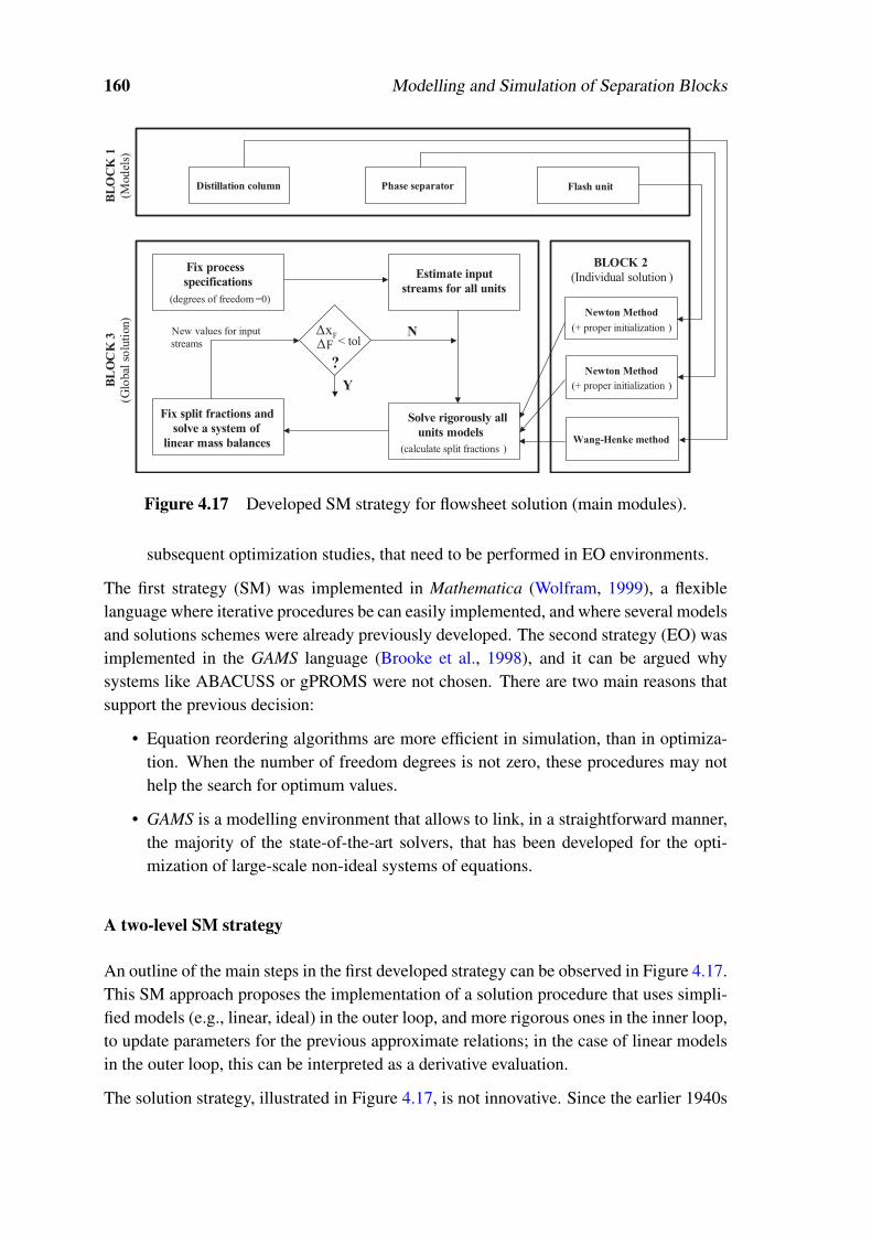
160 Modelling and Simulation of Separation Blocks
Fix process
specifications
(degrees of freedom =0)
Estimate input
streams for all units
Fix split fractions and
solve a system of
linear mass balances
Solve rigorously all
units models
(calculate split fractions )Wang-Henke method
Flash unit
STOP
New values for input
streams
ΔxF
Δ < tol
?
N
YNewton Method
BL
OC
K 1
(Mod
els)
BLOCK 2
BL
OC
K 3
(Glo
bal
soluti
on)
Phase separatorDistillation column
(+ proper initialization )
Newton Method
(+ proper initialization )
(Individual solution )
F
Figure 4.17 Developed SM strategy for flowsheet solution (main modules).
subsequent optimization studies, that need to be performed in EO environments.
The first strategy (SM) was implemented in Mathematica (Wolfram, 1999), a flexiblelanguage where iterative procedures be can easily implemented, and where several modelsand solutions schemes were already previously developed. The second strategy (EO) wasimplemented in the GAMS language (Brooke et al., 1998), and it can be argued whysystems like ABACUSS or gPROMS were not chosen. There are two main reasons thatsupport the previous decision:
• Equation reordering algorithms are more efficient in simulation, than in optimiza-tion. When the number of freedom degrees is not zero, these procedures may nothelp the search for optimum values.
• GAMS is a modelling environment that allows to link, in a straightforward manner,the majority of the state-of-the-art solvers, that has been developed for the opti-mization of large-scale non-ideal systems of equations.
A two-level SM strategy
An outline of the main steps in the first developed strategy can be observed in Figure 4.17.This SM approach proposes the implementation of a solution procedure that uses simpli-fied models (e.g., linear, ideal) in the outer loop, and more rigorous ones in the inner loop,to update parameters for the previous approximate relations; in the case of linear modelsin the outer loop, this can be interpreted as a derivative evaluation.
The solution strategy, illustrated in Figure 4.17, is not innovative. Since the earlier 1940s

4.4 Convergence of large-scale flowsheets 161
that similar versions have been employed to converge flowsheets and, still nowadays,these type of procedures are advised to perform preliminary calculations (Biegler et al.,1997). The major difference between these early versions, and the one represented in inFigure 4.17, refers to the rigor of the models considered in the inner loop. While, typically,during the calculation of preliminary mass and heat balances, performance relations areused in the inner loop, the strategy of Figure 4.17 considers the solution of the detailed unitmodels. Their respective split fractions (linear relations that express the efficiency of eachunit) can be therefore more accurately calculated and used, through the solution of a linearsystem of equations (that translates the process topology), to update all the estimated inletconditions. In this way, when the iterative procedure reaches convergence (the differencebetween the inlet values of two successive iterations satisfies the tolerance), the resultsobtained do not depend on any approximations and, therefore, held the rigorous solutionof the problem.
Alternating between approximate and rigorous models, in two steps iteration procedures,is a philosophy not exclusively found in flowsheeting problems. In fact, other solutionschemes, proposed for different classes of problems, are based on similar decompositions:
• Inside-out methods (Seader and Henley, 1998): used for individual unit simula-tion, where two levels of detail are considered (only the inner loop models includerigorous thermodynamic calculations), to relieve some of the numerical difficulties.
• ALT methods (Audet et al., 2004), used during the optimization of pooling prob-lems, where two sub-systems of equations are generated comprehending, each oneof them, different sets of fixed variables, in an attempt to avoid local optima phe-nomena.
The use of these procedures was even suggested, in the past, for rigorous flowsheet op-timization (Ganesh and Biegler, 1987), to reduce the required CPU time. These authorsreport improved convergence when a decomposition of the original problem, and the useof different levels of rigor, are employed during the search for an optimal solution.
As already referred and illustrated in Figure 4.17, the proposed strategy estimate newvalues for the inlet conditions of each unit, based on the split fractions values that werecalculated in the previous iteration. This scheme, similar to a successive substitutionmethod, is one of the simplest updating procedures that can be used and, in general, can-not guarantee global convergence properties. However, even if some instability problemsmay arise, this fact does not necessary imply an unavoidable failure of the overall pro-cedure. As it will be shown in Section 4.4.3, simple modifications can, sometimes, bemade to the original implementation, to overcome the previous difficulties and assure arobust convergence towards the solution. Thus, updating procedures based on the use ofsecond order derivative information can be avoided: although improving the convergenceproperties, these procedures cannot be generally advised since, in most situations, and es-pecially for large-scale non-ideal problems, they involve complex implementations (also

162 Modelling and Simulation of Separation Blocks
Apply Wang - Henke
algorithm (or other) (perform a few iterations)
Restrain all variables
Determine Jacobian
and balance its matrix
(calculate scaling factors)
INITIALIZATION
(Individual )
BOUNDING
(Individual )
SCALING
(Individual)
Introduce slack variables
lo = -
up = +
Impose a final set of
restrictions
(Process topology)
SIMULATION
(Individual)
SIMULATION
(Global)
PHASE 1
PHASE 2
PHASE 3
εε
δ
δ
(impose ranges of variation)
Figure 4.18 EO strategy developed for flowsheet solution (main steps).
vulnerable to numerical failures) and significant computational effort.
An hybrid methodology
The second developed strategy does not consider, as primary goal, the simulation of an en-tire large-scale process (the previous SM approach is more suitable for this task). Instead,it needs to assure that partial results can be efficiently transferred to subsequent solutionphases, where they will play an important role as feasible starting points. In other words,it is intended as a pre-processing phase during optimization studies, a reason why it needsto be developed within an equation-oriented context, as already discussed. The main mo-tivation beyond its development relates to the special numerical considerations that arerequired in the synthesis problems of Chapter 4 and 5. These, although involving modelsof smaller dimension, since they do not report to all units in the plant, require howevermore elaborated and complex formulations, difficult to treat even in equation-orientedenvironments.
This second strategy, represented in Figure 4.18, incorporates three main phases. In thefirst phase, three steps can be distinguished:
1. An initialization procedure is performed by specialized routines. These incorporatethe same methods that are used to solve the unit models in the strategy of Fig-ure 4.17, but only perform a few iterations, not trying to achieve full convergence.
2. The values obtained in the previous phase for all dependent and independent vari-

4.4 Convergence of large-scale flowsheets 163
ables are used to automatically impose maximum ranges of variation (defininglower and upper bounds as percentages of the current levels).
3. Suitable scaling factors are incorporated both for equations and variables, to balancethe Jacobian matrix. These factors are calculated outside the EO environment, usingspecial tools developed in Mathematica code, and the information derived from thetwo earlier steps.
These steps enable to overcome the two main drawbacks that are typically associated toEO strategies:
• The loss of physical meaning, when models are assembled and treated in a puremathematical point of view. Now, the problem is initialized through iterative meth-ods that consider blocks of equations, accordingly to their nature (Step 1).
• The difficulty in obtaining initial estimates for all variables, and in minimizing typ-ical numerical difficulties that emerge during the solution of large-scale non-idealmodels.
This last point deserves special attention since, when non-ideal expressions are used, thatare only defined over a given domain, the imposition of proper bounds is crucial to avoidunderflow / overflow problems in EO environments. On the other hand, when in the pres-ence of large-scale systems, assuring that the residues of all equations are within similar(and proper) orders of magnitude is also of particular importance, to avoid “neglecting”some of them.
After initializing, bounding and scaling the equations of each unit, these are rigorouslysolved in a second phase. This is an individual solution procedure that relies, exclusively,on the provided initialization point neglecting, therefore, the overall process interactions.
Finally, and with crucial importance to the success of the developed EO strategy, slackvariables are introduced in a third phase. In fact, although capable of initializing all vari-ables, phase 1 does not rigorously considers the interactions between intervening units.It considers feed compositions that need to be estimated, due to the existence of recyclestreams, and may be extremely inaccurate. Therefore, when assembling the equationsof all intervening units (after phase 2), together with additional expressions that translatethe flowsheet structure, a final mathematical system is obtained that, in an overall sense,can still present a deficient initialization. Slack variables are used to minimize any poten-tial problems that may derive form the earlier situations. These are introduced in someselected equations (e.g., the MESH balances of distillation columns), to avoid a largenumber of infeasibilities, in the earlier solution stages. The problem is therefore initially

164 Modelling and Simulation of Separation Blocks
solved, within a given tolerance:
minu,ε
δ
s.t. f (u)− ε = 0
‖ε‖ ≤ δ
(4.17)
After a first solution is obtained, the tolerance value can be decreased, until the rigoroussolution of the problem is obtained. Although involving a sequence of solution steps, theoverall procedure is more robust and less vulnerable to numerical problems.
4.4.3 Industrial case-study
As already introduced, the goals for the two developed strategies were substantially dif-ferent. The SM approach, suitable for problems of larger dimension, was used during thesimulation of the entire purification phase represented in Figure 4.3, in order to:
• Acquire the capacity of predicting the plant global behavior, anticipating the effectof newly proposed measures and of any other changes in the operating parameters.
• Identify plant sections (sets of units) that should be targets of further optimizationstudies, due to their particular importance, in an economical and / or product qualityperspective.
This second objective deserves special attention since, for optimization purposes, anydecrease on the original problem dimension is an extremely important advantage. Inother words, efforts should be, in general, concentrated in trying to avoid EO studies overentire plant models, due to required simultaneous solution of all equations.
Therefore, for the second developed strategy, the main goal was the efficient solution,in an EO approach, of sub-systems of equations that could translate the behavior of allunit sets, previously identified as crucial. Using this approach, a proper numerical pre-processing can be achieved, and a feasible starting point generated, for the optimizationstrategies reported in Chapters 5 and 6.
Implementation aspects
When implementing the SM strategy, to solve the flowsheet of Figure 4.3, the overallconvergence procedure exhibited some instability. After carefully analyzing the obtaineddata, the source of the experienced difficulties was related to a strong interdependencebetween two particular units: distillation columns D4 and D5.
As represented in Figure 4.19, the two previous units are strongly connected. Althoughseveral recycle streams can be found in the process, the mass and energy flows that aban-
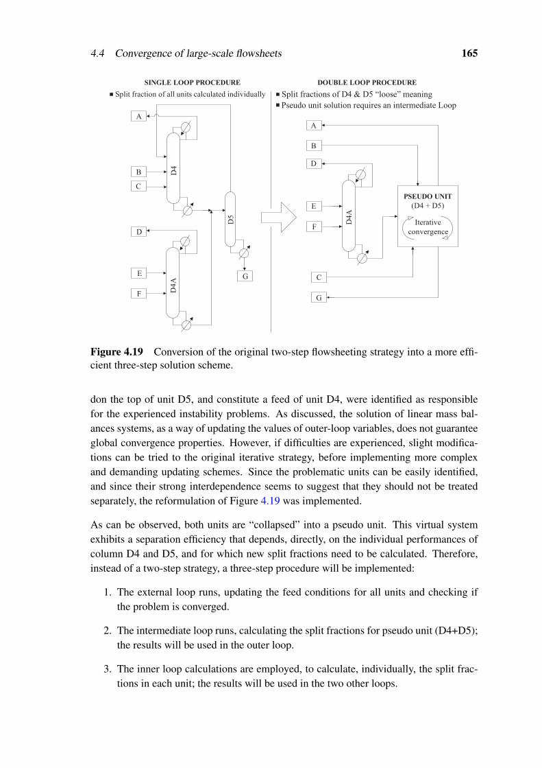
4.4 Convergence of large-scale flowsheets 165
D4
D4
A
D5
D4A
(D4 + D5)
PSEUDO UNIT
A
B
C
D
E
F
G
D
E
F
A
B
C
G
SINGLE LOOP PROCEDURE DOUBLE LOOP PROCEDURE
Pseudo unit solution requires an intermediate Loop
Split fractions of D4 & D5 “loose” meaningSplit fraction of all units calculated individually
Iterative
convergence
Figure 4.19 Conversion of the original two-step flowsheeting strategy into a more effi-cient three-step solution scheme.
don the top of unit D5, and constitute a feed of unit D4, were identified as responsiblefor the experienced instability problems. As discussed, the solution of linear mass bal-ances systems, as a way of updating the values of outer-loop variables, does not guaranteeglobal convergence properties. However, if difficulties are experienced, slight modifica-tions can be tried to the original iterative strategy, before implementing more complexand demanding updating schemes. Since the problematic units can be easily identified,and since their strong interdependence seems to suggest that they should not be treatedseparately, the reformulation of Figure 4.19 was implemented.
As can be observed, both units are “collapsed” into a pseudo unit. This virtual systemexhibits a separation efficiency that depends, directly, on the individual performances ofcolumn D4 and D5, and for which new split fractions need to be calculated. Therefore,instead of a two-step strategy, a three-step procedure will be implemented:
1. The external loop runs, updating the feed conditions for all units and checking ifthe problem is converged.
2. The intermediate loop runs, calculating the split fractions for pseudo unit (D4+D5);the results will be used in the outer loop.
3. The inner loop calculations are employed, to calculate, individually, the split frac-tions in each unit; the results will be used in the two other loops.

166 Modelling and Simulation of Separation Blocks
The advantages of the above procedure focus on the existence of an intermediate loop,exclusively dedicated to the joint solution of units D4 and D5. Thus the complex con-vergence of these units is detached from the main problem, and approached separatelythrough a suitable method.
Since the solution of the pseudo unit (D4+D5) will also be done using a SM approach, theonly remaining issue is the selection of a robust updating procedure for the intermediateloop. This time, and since only two units are involved, the first choice relied in a simplesuccessive substitution method. Again, global convergence properties are not guaranteedfor all cases, although they can be easily analyzed in particular cases.
The dominant eigenvalue method can be used to evaluate the robustness of the successivesubstitution method, in a given problem. Therefore, a sensitivity matrix was obtained forpseudo-unit (D4+D5), by perturbing the partial mass flows of each component at feedconditions, and the respective eigenvalues calculated, as presented in Table 4.6. When alleigenvalues are inferior to 1, as obtained for pseudo-unit (D4+D5), the convergence of thesuccessive substitution method is guaranteed, since the previous condition is both neces-sary and sufficient. After implementing the three-step procedure, using the above methodfor the convergence of the intermediate loop, all instability problems were eliminated. Aswill be latter discussed, several runs were performed and, in all of them, the developedSM strategy exhibited a good performance.
For the EO approach, represented in Figure 4.18, some difficulties were also felt duringits implementation. Although using good initial estimates, proper bounds and suitablescaling factors, the high non-linearity of the involved expressions was still problematic,often causing a premature end of the convergence process.
To overcome the previous difficulties, other numerical solvers were tested, in additionto the one initially selected (CONOPT III). All solvers are based on a well defined setof assumptions and convergence schemes (e.g., GRG, SQP, etc.) that may present ad-vantages and drawbacks, depending on the characteristics of a given problem (this issuewas introduced in Section 3.4.2 and is extended in Section 5.4.1). Therefore, by cover-ing a wide-range of different solution algorithms, a more suitable one could in principlebe found, capable of exhibiting a good performance for the systems of equations understudy. However, despite the large number of tests using the NEOS server (NEOS, 2007),all employed solvers failed to assure a robust convergence.
Under the previous circumstances, the only remaining choice consists in reformulatingthe original system of equations, decomposing each one of problematic expressions, insystems of more well-behaved equations. Instead on focusing on the numerical solutionscheme, this well known technique emphasizes the importance of how to write equations,with two direct implications: a decrease of the problem non-linearity and a increase on itsdimension. In other words, the goal its to obtain a larger (although more linear) system ofequations, that should be globally easier to solve.

4.4 Convergence of large-scale flowsheets 167
Tabl
e4.
6Se
nsiti
vity
mat
rix
(S)a
ndre
spec
tive
eige
nval
ues(
V),
obta
ined
duri
ngth
eso
lutio
nof
unit
(D4+
D5)
bysu
cces
sive
subs
titut
ions
.
S=
4.80×
10−
51.
05×
10−
127.
64×
10−
51.
10×
10−
31.
42×
10−
30
9.46×
10−
43.
55×
10−
41.
26×
10−
91.
44×
10−
8
1.64×
10−
116.
93×
10−
64.
71×
10−
42.
17×
10−
31.
45×
10−
20
1.42×
10−
21.
04×
10−
33.
07×
10−
9−
2.89×
10−
8
8.03×
10−
151.
09×
10−
151.
19×
10−
31.
44×
10−
66.
29×
10−
6−
1.91×
10−
37.
30×
10−
72.
14×
10−
89.
40×
10−
14−
6.62×
10−
10
8.65×
10−
151.
22×
10−
152.
47×
10−
72.
70×
10−
36.
72×
10−
6−
2.81×
10−
32.
76×
10−
6−
8.66×
10−
8−
2.99×
10−
13−
6.71×
10−
10
7.82×
10−
151.
13×
10−
152.
33×
10−
71.
45×
10−
62.
97×
10−
3−
2.98×
10−
32.
68×
10−
6−
9.08×
10−
8−
3.08×
10−
13−
6.82×
10−
10
8.61×
10−
151.
23×
10−
152.
33×
10−
71.
40×
10−
66.
17×
10−
6−
8.41×
10−
66.
96×
10−
7−
8.37×
10−
8−
2.76×
10−
13−
6.88×
10−
10
1.13×
10−
141.
24×
10−
153.
67×
10−
72.
11×
10−
69.
30×
10−
6−
5.13×
10−
25.
14×
10−
2−
3.88×
10−
7−
1.02×
10−
12−
7.05×
10−
10
1.84×
10−
122.
11×
10−
135.
17×
10−
51.
03×
10−
32.
29×
10−
30
2.52×
10−
3−
3.97×
10−
4−
1.20×
10−
9−
4.96×
10−
7
1.91×
10−
121.
47×
10−
131.
72×
10−
55.
13×
10−
41.
26×
10−
30
−3.
47×
10−
3−
2.39×
10−
4−
5.26×
10−
10−
3.75×
10−
7
7.34×
10−
131.
01×
10−
131.
72×
10−
53.
15×
10−
41.
18×
10−
30
1.58×
10−
3−
1.10×
10−
3−
3.67×
10−
91.
28×
10−
1
V=
[ 1.28×
10−
15.
14×
10−
22.
96×
10−
32.
70×
10−
31.
19×
10−
3−
3.95×
10−
44.
80×
10−
56.
93×
10−
6−
9.67×
10−
73.
23×
10−
10]

168 Modelling and Simulation of Separation Blocks
380 400 420 440 460 480 500360
2.5
2.0
1.5
1.0
0.5
0.0
T (K)
PS
(
bar
)
AN
L
Figure 4.20 Calculation of vapor pressures for pure components (— Rigorous correla-tion, · · · approximate fit).
This procedure was adopted to reformulate the UNIFAC and NRTL models — the sourceof solution difficulties, since the mass and energy balances are weakly nonlinear (bilin-ear). In (4.18) and (4.19), one of the employed transformations is presented, for illustra-tive purposes. Although increasing three times the overall problem dimension, the severaldecompositions used generated new systems of equations capable of being solved nowthrough the CONOPT solver.
ψi, jUc = 1−ψ
i, jUl + ln
(ψ
i, jUo−5ψ
iUq
(1−ψ
i, jUo/ψ
i, jUl + ln
(ψ
i, jUo/ψ
i, jUl
)))(4.18)
m
ψi, jUc = 1−ψ
i, jUl +ψ
i, jaux1 (4.19a)
exp(ψ i, jaux1) = ψ
i, jUo−5ψ
iUq
(1−ψ
i, jaux2 +ψ
i, jaux3
)(4.19b)
ψi, jUl ψ
i, jaux2 = ψ
i, jUo (4.19c)
ψi, jUl exp(ψ i, j
aux3) = ψi, jUo (4.19d)
However, state-of-the-art solvers like MINOS, SNOPT, IPOPT and KNITRO were stillunable of returning a solution, despite the ability of some of them to handle large-scalesystems of equations. This fact was interpreted as a sign that, if possible, further sim-plifications should continue to be made in the system of equations. Since UNIFAC andNRTL methods had already been rearranged, and since mass and energy balances offeredno problems, efforts were concentrated in trying to simplify the adopted correlations forvapor pressure and thermodynamic properties. This time, a regression procedure wasemployed, to replace the original equations by simple polynomial fits (Table B.5).
As illustrated in Figures 4.20 and 4.21, fits of good quality can be obtained, thus enablingthe substitution of equations (4.12–4.14) by polynomial expressions similar to those rep-resented in (4.20). Notice that, although exhibiting an ideal behavior, vapor enthalpies

4.4 Convergence of large-scale flowsheets 169
50000
45000
40000
35000
30000
360 380 400 420 440 460 480 500
T (K)
H
(J
km
ol
)
-1V
10000
5000
-5000
-10000
-20000
360 380 400 420 440 460 480 500
T (K)
H (J
km
ol
)
-1L
-15000
0
Figure 4.21 Calculation of liquid and vapor enthalpies (— Rigorous correlation, · · ·approximate fit).
were estimated by an extremely complex correlation. For vapor pressure and liquid en-thalpies prediction, the new obtained expressions also allow a large reduction of the orig-inal non-linearity.
PSANL, j =−45.029+0.371T j−1.024×10⁻³ (T j)2+9.447×10⁻⁷ (T j)3
(4.20a)
H jL =−82951.000+143.160T j +8.340×10⁻² (T j)2
(4.20b)
H jV = 697.462+28.212T j +0.146
(T j)2
(4.20c)
The previous simplifications presented a drastic impact on the characteristics of the overallproblem, since they are written for all stages of each distillation column. After theirintroduction, the efficiency of several solvers changed significantly2.
Results obtained
Two main studies were considered, using the developed SM strategy, for the current indus-trial process. The underlying motivations and the main results obtained will be presentedin the following brief discussion.
The first study intended to identify crucial sets of units, through the solution of the entireflowsheet (Neves et al., 2003). In fact, the energy balances, not considered during thereconciliation procedure of Section 4.2, can now be established and used to evaluate howthe utilities consumption is distributed in the plant.
As illustrated in Figure 4.22, a small set of distillation columns (D1+D4+D4A+D5) isresponsible for 92% of all hot utilities consumption. The strongly exothermic reactionstep assumes the role of the major consumer of cold utilities. Under these circumstances,and considering that heating is much more expensive (around 10 times) than cooling, the
2E.g., MINOS and IPOPT were now capable of solving some of the considered problems and SNOPT,although not converging the more complex ones, exhibited a much better performance.

170 Modelling and Simulation of Separation Blocks
8%
92%
7%
17%
76%
Hot Utility
(Medium Pressure Vapor)
Cold Utility
(Cooling Water)
D1+D4+D4A+D5 D2+D6+D7+D12 Other
Figure 4.22 Hot and cold utility consumptions for different sets of units.
Table 4.7 Operating conditions for the separation core — nominal values.
PCOL TC TR QC QR D RR CCU CHU
Column [bar] [K] [K] [GJ/h] [GJ/h] [kg/h] [kAC/yr] [kAC/yr]
D1 1.0 85 183 2.33 4.44 1027 0.30 14.5 295.6
D4A 0.38 150 151 4.01 3.51 213 36.8 24.9 233.7
D4B 0.38 149 151 4.26 3.80 224 36.8 26.5 253.0
DR 0.38 150 176 N.A. 0.1 254 N.A. 0 6.7
Total 65.9 789.0
set of units represented in Figure 4.23 will be responsible for a large share of the totaloperational costs.
Besides the previous economical motives, other aspects should be considered to justify theemphasis given to distillation columns of Figure 4.23. In fact, these are also the units thatexhibit a larger impact on the final product specifications. As confirmed through severalsensitivity studies, any changes on the operational specifications of units D1, D4, D4A andD5, will have a direct significant impact on the obtained aniline purity. Therefore, thesefour units behave like a separation core, currently operated accordingly to the referenceconditions of Table 4.7.
The second study intended to evaluate the consequences of using a new catalyst, in allprocess outlets (products and waste streams). Since this goal required, once again, theentire flowsheet solution, the developed SM strategy was employed. The yields of thenew considered catalyst are presented in Table 4.8; these are normalized relatively to thecurrent reaction conditions. Two scenarios (A and B) are shown, since the catalytic testsat a laboratory scale generated results with some variance.
A brief analysis of Table 4.8 shows that, independently of the considered scenario, the

4.4 Convergence of large-scale flowsheets 171
T9
S1
T8
T1
D1
T5
F4
F4A
D4A
D4
A
D5
T5
Figure 4.23 Separation core: large impact on the product specifications and large shareof the total operational costs.
Table 4.8 Relative yields of a new catalyst, in two different scenarios, when comparedwith the current catalyst.
Scenario BZ Water CHA CHONA CHOL ANL MNB DICHA CHENO CHANIL
A 0.928 0.939 1.166 3.449 1.462 1.000 N.A. 0.537 1.053 1.194
B 0.398 0.957 0.388 1.420 0.453 1.006 N.A. 0.170 0.212 0.397
new catalyst produces more CHONA, less DICHA and approximately the same amountof aniline. The new relative amounts of each byproduct, at the exit streams of the reac-tion units, do not necessarily imply a proportional effect on the compositions of the finalproducts. Each component behaves differently, in a LLE and VLE perspective, a reasonwhy simulation studies are required around the purification step.
Table 4.9 shows the purity specifications for aniline, where each secondary species presentsa maximum allowed concentration. The main product is not the only one to require a spe-cial attention, since two more outlet streams have their concentration controlled: the CHAco-production, where a purity higher than 99.5% must be obtained, and the process aque-ous waste, where the total amount of organic components should be less than 5 ppm.
The simulation results obtained showed that even when the more conservative conditions(scenario A) are considered, the new catalyst does not cause any violation of the pre-

172 Modelling and Simulation of Separation Blocks
Table 4.9 Absolute mass fractions, required in the main product streams, for commer-cial purposes (purity restrictions).
BZ Water CHA CHONA CHOL ANL MNB DICHA CHENO CHANIL
<50 <300 <50 <250 <300 >99.97 <50 <50 <250 <50
ppm ppm ppm ppm ppm % ppm ppm ppm ppm
0.0
0.2
0.4
0.6
0.8
1.0
CHA CHONA CHOL ANL DICHA CHENO CHANIL
current catalyst
new catalyst - A
new catalyst - B
Fra
ctio
n (
norm
aliz
ed)
Components
Figure 4.24 Results obtained for the new catalyst considered.
vious specifications (relative to aniline, CHA and aqueous streams). Figure 4.24 refersexclusively to the main product stream, and exhibit the predicted concentrations for eachcomponent, after normalization by the corresponding limit value of Table 4.9. Three im-portant indications can be drawn, assuming scenario A and considering that all operatingconditions are maintained in the plant:
• The CHOL mass fraction will increase significantly (' 200 %).
• The DICHA contamination will decrease appreciably (' 50 %).
• CHANIL will maintain, approximately, the same concentration levels.
In all of these studies, the developed SM approach exhibited good convergence properties:the three-loop iterative procedure never denoted any kind of instability problems. Sim-ulating the entire flowsheet of Figure 4.3, although involving a model of approximately95 000 equations / variables, only required about 5–7 outer loop iterations.
Table 4.10 reports some of the convergence data typically obtained. As can be observed,both for the intermediate and outer loops, the error decreases significantly, from one itera-tion to the next one. The only reason beyond the large CPU times involved (' 15 minutesare required to solve the flowsheet), relates to the use of the Mathematica environment.
The efficiency of the developed EO strategy was also tested during two important studies.

4.4 Convergence of large-scale flowsheets 173
Table 4.10 Convergence data obtained for the developed three-step flowsheeting strat-egy, when solving the industrial separation phase.
Inner loop Outer loop
Iteration Error Iteration Error
1 50.000001 570.62 0.000960
3 0.000027
1 0.076082
2 305.72 0.0038313 0.0002014 0.000011
1 0.0062033 2.39
2 0.000020
1 0.0011554 0.40
2 0.000003
1 0.0007405 0.24
2 0.000004
These are exclusively related to the separation core represented in Figure 4.23 involv-ing, therefore, problems with a smaller dimension than those where the SM strategy wasemployed. However, the joint simulation of all units represented in Figure 4.23 is stilla large-scale problem, where ' 20 000 equations need to be simultaneously solved andwhere the high non-linearity of the UNIFAC method (used for VLE prediction) is implicit.
The first study relates to the interactions between nitration and hydrogenation steps. Itintends to predict the effect of using a new raw benzene stream, on the final aniline spec-ifications. In the current conditions, the hydrogenation units treat a fresh feed constitutedby nitrobenzene (coming from the nitration plant), and traces of some byproducts that, dueto their incomplete purification, are recycled back in small extents. Under these circum-stances, and when the separation core is operated according to Table 4.7, all specificationspresented in Table 4.9 are fulfilled. However, for economical reasons, it would be advan-tageous to nitrate a different fresh feed where, in addition to benzene, three secondaryspecies are present — toluene, xylene and ethylbenzene. Under these circumstances, andconsidering the reaction sequences illustrated in Figure 4.25, small amounts of amino-toluene, amino-xylene and amino-ethylbenzene would reach the purification core of Fig-ure 4.23. Therefore, the main goal of this first study is to evaluate if, in the previousconditions, it is still possible to obtain aniline with a purity higher than 99.97%.
To clarify the previous question, a new feed stream was considered for distillation columnD1, and the separation efficiency of each unit, towards all the new secondary species,evaluated. The main results obtained are shown in Table 4.11.
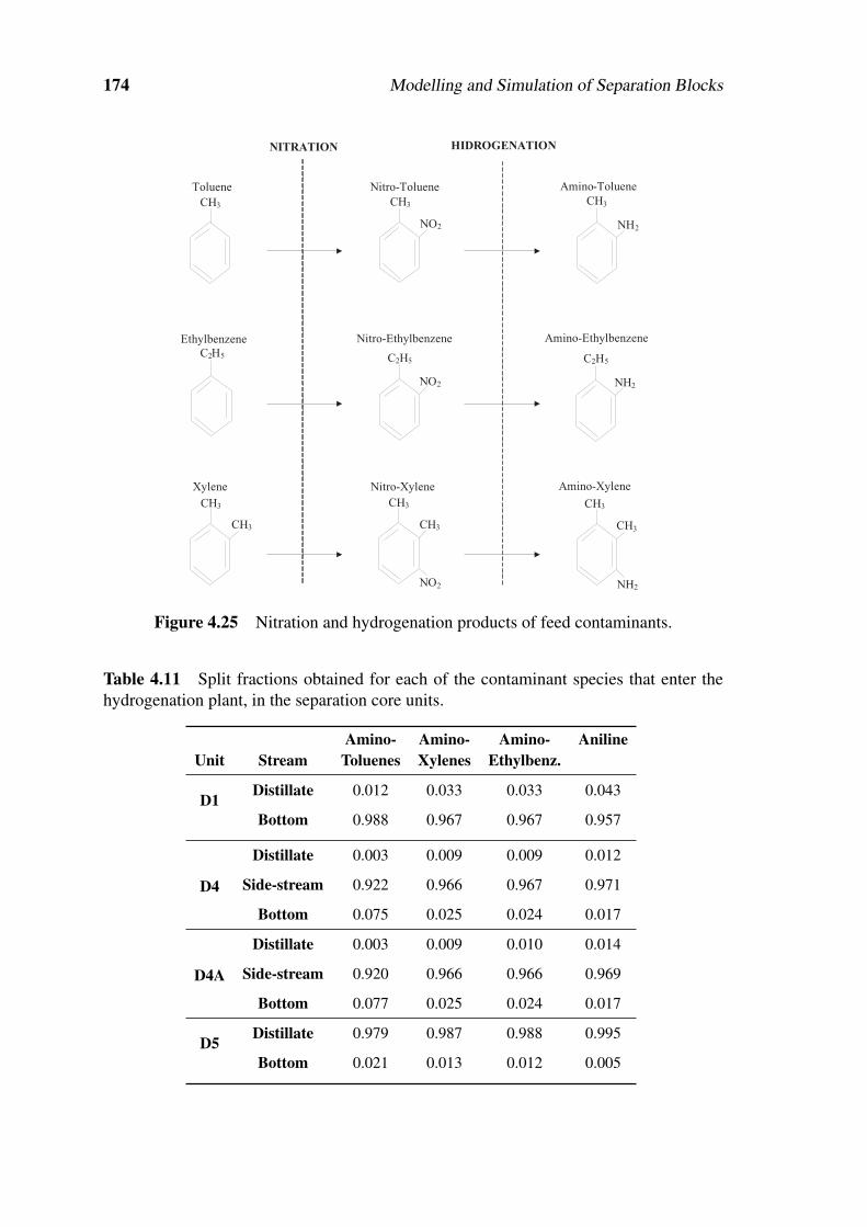
174 Modelling and Simulation of Separation Blocks
Ethylbenzene
NH2
C2H5
NO2
C2H5C2H5
Nitro-Ethylbenzene Amino-Ethylbenzene
CH3
NH2
CH3
NO2
CH3
Toluene Nitro-Toluene Amino-Toluene
CH3
CH3 CH3
NO2
CH3
NH2
CH3
CH3
Xylene Nitro-Xylene Amino-Xylene
NITRATION HIDROGENATION
Figure 4.25 Nitration and hydrogenation products of feed contaminants.
Table 4.11 Split fractions obtained for each of the contaminant species that enter thehydrogenation plant, in the separation core units.
Amino- Amino- Amino- AnilineUnit Stream Toluenes Xylenes Ethylbenz.
D1 Distillate 0.012 0.033 0.033 0.043
Bottom 0.988 0.967 0.967 0.957
D4
Distillate 0.003 0.009 0.009 0.012
Side-stream 0.922 0.966 0.967 0.971
Bottom 0.075 0.025 0.024 0.017
D4A
Distillate 0.003 0.009 0.010 0.014
Side-stream 0.920 0.966 0.966 0.969
Bottom 0.077 0.025 0.024 0.017
D5 Distillate 0.979 0.987 0.988 0.995
Bottom 0.021 0.013 0.012 0.005
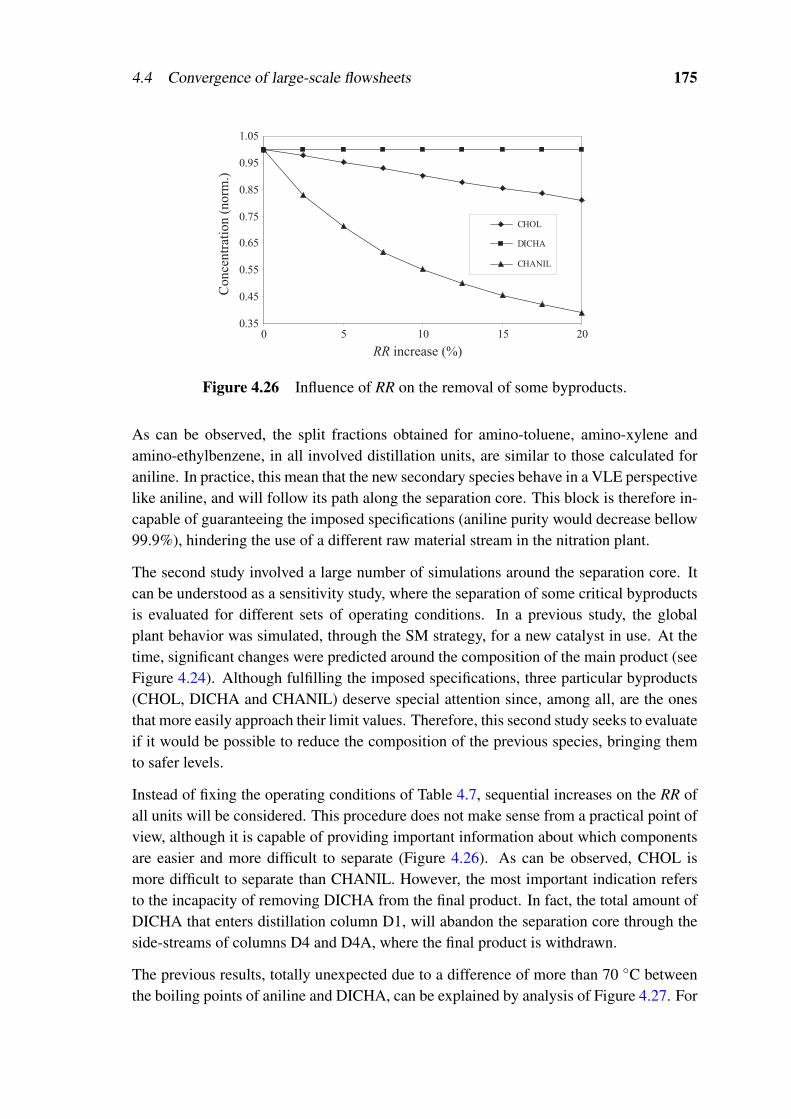
4.4 Convergence of large-scale flowsheets 175
Conce
ntr
atio
n (
norm
.)
RR increase (%)
0.35
0.45
0.55
0.65
0.75
0.85
0.95
1.05
0 5 10 15 20
CHOL
DICHA
CHANIL
Figure 4.26 Influence of RR on the removal of some byproducts.
As can be observed, the split fractions obtained for amino-toluene, amino-xylene andamino-ethylbenzene, in all involved distillation units, are similar to those calculated foraniline. In practice, this mean that the new secondary species behave in a VLE perspectivelike aniline, and will follow its path along the separation core. This block is therefore in-capable of guaranteeing the imposed specifications (aniline purity would decrease bellow99.9%), hindering the use of a different raw material stream in the nitration plant.
The second study involved a large number of simulations around the separation core. Itcan be understood as a sensitivity study, where the separation of some critical byproductsis evaluated for different sets of operating conditions. In a previous study, the globalplant behavior was simulated, through the SM strategy, for a new catalyst in use. At thetime, significant changes were predicted around the composition of the main product (seeFigure 4.24). Although fulfilling the imposed specifications, three particular byproducts(CHOL, DICHA and CHANIL) deserve special attention since, among all, are the onesthat more easily approach their limit values. Therefore, this second study seeks to evaluateif it would be possible to reduce the composition of the previous species, bringing themto safer levels.
Instead of fixing the operating conditions of Table 4.7, sequential increases on the RR ofall units will be considered. This procedure does not make sense from a practical point ofview, although it is capable of providing important information about which componentsare easier and more difficult to separate (Figure 4.26). As can be observed, CHOL ismore difficult to separate than CHANIL. However, the most important indication refersto the incapacity of removing DICHA from the final product. In fact, the total amount ofDICHA that enters distillation column D1, will abandon the separation core through theside-streams of columns D4 and D4A, where the final product is withdrawn.
The previous results, totally unexpected due to a difference of more than 70 C betweenthe boiling points of aniline and DICHA, can be explained by analysis of Figure 4.27. For
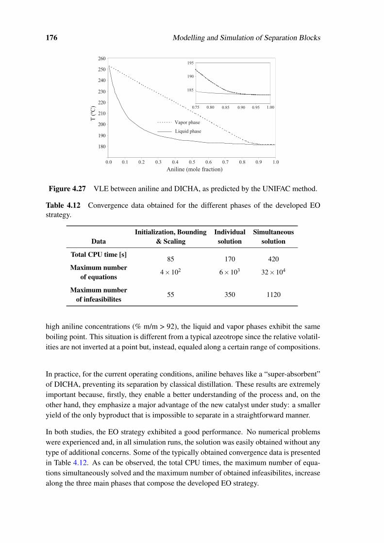
176 Modelling and Simulation of Separation Blocks
0.0 0.1 0.2 0.3 0.4 0.5 0.6 0.7 0.8 0.9 1.0
T (
ºC)
Aniline (mole fraction)
Vapor phase
Liquid phase
180
190
200
210
220
230
240
250
260
185
190
195
0.75 0.80 0.85 0.90 0.95 1.00
Figure 4.27 VLE between aniline and DICHA, as predicted by the UNIFAC method.
Table 4.12 Convergence data obtained for the different phases of the developed EOstrategy.
Initialization, Bounding Individual SimultaneousData & Scaling solution solution
Total CPU time [s]85 170 420
Maximum number4×102 6×10³ 32×104
of equations
Maximum number55 350 1120
of infeasibilites
high aniline concentrations (% m/m > 92), the liquid and vapor phases exhibit the sameboiling point. This situation is different from a typical azeotrope since the relative volatil-ities are not inverted at a point but, instead, equaled along a certain range of compositions.
In practice, for the current operating conditions, aniline behaves like a “super-absorbent”of DICHA, preventing its separation by classical distillation. These results are extremelyimportant because, firstly, they enable a better understanding of the process and, on theother hand, they emphasize a major advantage of the new catalyst under study: a smalleryield of the only byproduct that is impossible to separate in a straightforward manner.
In both studies, the EO strategy exhibited a good performance. No numerical problemswere experienced and, in all simulation runs, the solution was easily obtained without anytype of additional concerns. Some of the typically obtained convergence data is presentedin Table 4.12. As can be observed, the total CPU times, the maximum number of equa-tions simultaneously solved and the maximum number of obtained infeasibilites, increasealong the three main phases that compose the developed EO strategy.
4.4 Convergence of large-scale flowsheets 177
This convergence data illustrates the important philosophy that is implicit: start with thesolution of smaller and easier problems, and use the results obtained as warm starts forthe following more complex ones. This can be understood as a decomposition procedure,that seeks to avoid the initial solution of the original system of equations. In practice, themaximum number of obtained infeasibilites is kept low, which corresponds to a more ro-bust convergence, since the probabilities of experiencing solver failures will be reduced.Although not explicitly detailed, the convergence data reported in Table 4.12, for the si-multaneous solution of all units, considered three sequential problems. Before attemptingto solve all problem equations, and as already introduced, slack variables are imposedand the associated tolerance initially relaxed. This one is latter smoothly reduced (e.g,δ = 1×10⁻⁵ → 5×10⁻⁶ → 1×10⁻⁶), to obtain the rigorous solution. Once again, thegoal is to allow a more robust convergence, decreasing the maximum number of obtainedinfeasibilites. This will be better explained in the optimization studies of Chapter 5 and 6,where the usefulness of the EO strategy, as a pre-processing phase, is also discussed andillustrated.

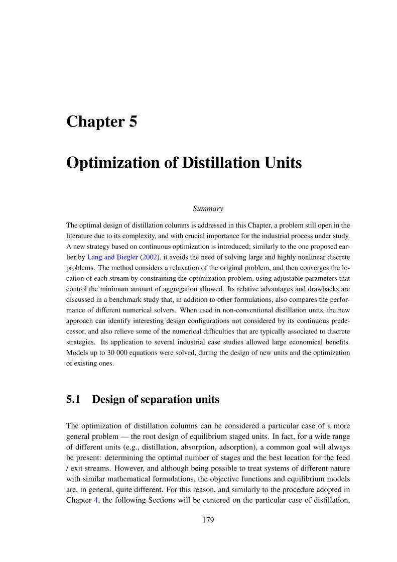
Chapter 5
Optimization of Distillation Units
Summary
The optimal design of distillation columns is addressed in this Chapter, a problem still open in theliterature due to its complexity, and with crucial importance for the industrial process under study.A new strategy based on continuous optimization is introduced; similarly to the one proposed ear-lier by Lang and Biegler (2002), it avoids the need of solving large and highly nonlinear discreteproblems. The method considers a relaxation of the original problem, and then converges the lo-cation of each stream by constraining the optimization problem, using adjustable parameters thatcontrol the minimum amount of aggregation allowed. Its relative advantages and drawbacks arediscussed in a benchmark study that, in addition to other formulations, also compares the perfor-mance of different numerical solvers. When used in non-conventional distillation units, the newapproach can identify interesting design configurations not considered by its continuous prede-cessor, and also relieve some of the numerical difficulties that are typically associated to discretestrategies. Its application to several industrial case studies allowed large economical benefits.Models up to 30 000 equations were solved, during the design of new units and the optimizationof existing ones.
5.1 Design of separation units
The optimization of distillation columns can be considered a particular case of a moregeneral problem — the root design of equilibrium staged units. In fact, for a wide rangeof different units (e.g., distillation, absorption, adsorption), a common goal will alwaysbe present: determining the optimal number of stages and the best location for the feed/ exit streams. However, and although being possible to treat systems of different naturewith similar mathematical formulations, the objective functions and equilibrium modelsare, in general, quite different. For this reason, and similarly to the procedure adopted inChapter 4, the following Sections will be centered on the particular case of distillation,
179

180 Optimization of Distillation Units
due to its major relevance for the industrial process under study.
5.1.1 Typical challenges involved
The topic of optimization of distillation columns has received significant attention in thepast decades due, at the same time, to its economical importance and the numerical dif-ficulties associated with the solution of this type of problems. Among the difficultiesusually encountered, it is possible to emphasize:
• The complexity of the models required to adequately describe the equilibrium phe-nomenon that takes place. The use of detailed non-ideal equilibrium models, suchas the UNIFAC group contribution method is often necessary (Reid et al., 1988).When the non-ideality of the vapor and liquid phases is simultaneously considered,the corresponding models can require up to 50 scalar variables per component perequilibrium stage, leading easily to overall unit models with tens of thousands ofnonlinear algebraic equations, and highly nonlinear behavior (Chapter 4).
• The need to incorporate discrete decisions in the solution process, related to theoptimal location of feed and product streams, and the total number of equilibriumstages. These problems are usually addressed as mixed-integer nonlinear programs— MINLP (Viswanathan and Grossmann, 1993; Bauer and Stilchmair, 1998; Bart-tfeld and Aguirre, 2002; Barttfeld et al., 2003) or general disjunctive programs —GDP (Yeomans and Grossmann, 2000a,b; Barttfeld et al., 2003).
Perhaps the most important limitation on the use of these discrete formulations, from apractical point of view, is the still limited choice of numerical solvers available for thesetypes of problems, associated with moderate numerical robustness and computational re-quirements that can be extremely dependent on proper initialization and bounding of theproblem. For this reason, a recently proposed formulation (Lang and Biegler, 2002) ad-dresses the problem through continuous optimization. Although allowing the use of morerobust solvers, some important drawbacks can still be pointed, leaving room for furtherimprovements, as will be latter discussed.
5.1.2 Classical objective functions
Before discussing possible mathematical strategies for distillation columns synthesis, itis important to clarify the main underlying motivations. In most cases, the goal is toobtain design specifications capable of minimizing an economical objective function (e.g.,total annualized costs), subject to some physical restrictions (e.g., purity degrees). Whenconsidering the root design of given unit, two different costs must be considered:
• Operating costs (COPE), related with the cold / hot utilities consumptions that are

5.2 Overview of available strategies 181
required in the unit. These depend directly on the condenser / reboiler duties thatare strongly influenced by the feed flowrate and imposed reflux ratio:
CCU = f (QC,TCU), CHU = f (QR,THU) (5.1)
• Fixed costs (CFIX), related with the required investment, during the acquisition ofall involved equipments. These depend on the column height (related to number ofstages), on the column diameter, and on the condenser / reboiler areas (functions ofthe thermal profile and exchanged heats):
CCOL = CSHE +CINT CEC = CC +CR (5.2a)
CSHE = f (hSHE,dSHE) CINT = f (hINT,dINT) (5.2b)
CC = f (AC) CR = f (AR) (5.2c)
dSHE ' dINT ' dCOL hSHE ' (hINT +∆h)' hCOL (5.2d)
dCOL = f (V j,T j) hCOL = f (np, HETP) (5.2e)
AC = f (QC,TCU,T j) AR = f (QR,THU,T j) (5.2f)
Therefore, the problem objective function will be, in general, non-convex, due to thenonlinear correlations that are adopted to evaluate the operational and fixed costs. Equa-tions (5.1) and (5.2), although greatly simplified, also give an idea about the strong in-teractions between the problem variables. Under these circumstances, optimizing thetrade-offs between np, lF and RR becomes difficult, and can only be rigorously performedthrough systematic approaches, like those discussed in the following Section.
5.2 Overview of available strategies
As referred in Section 5.1, due to the significant challenges involved, and in the attemptof improving the quality of the obtained solutions, several strategies has been proposedin the past. These include not only different mathematical formulations, but also dis-tinct numerical solution schemes. The next Sections will try to summarize these maincontributions, providing an adequate theoretical background.
5.2.1 Tray elimination schemes
The first available formulations for the root synthesis of distillation units were all based ondiscrete formulations, and part of their evolution regarded the scheme adopted to selectthe optimal number of equilibrium stages. During the optimization procedure, addingequilibrium trays is fairly difficult, from a mathematical point of view, since it requires

182 Optimization of Distillation Units
Total
condenser
Partial
reboiler
2
np-13
4
5
np-2
np-3
bRef2 =0
bRef3 =0
bRef4 =1
bReb
np -1 =0
bReb
np -2
=0
bReb
np -3=1
L2 =0
L3 =0
Vnp -1 =0
Vnp -2
= 0
Top product
Bottom product
Loss of vapor phase Loss of liquid phase Phase equilibria
Figure 5.1 Variable reflux and variable reboil schemes.
the introduction of extra variables in the formulation. Therefore, it is natural that, sincethe earlier formulations, the basic idea is to start with a sufficiently large number of traysthat will be later reduced. Nevertheless, this tray reduction / elimination, by it self, isnot a trivial scheme. Viswanathan and Grossmann (1990) started by suggesting the useof a binary variable associated to each tray to denote is existence. Although allowing thereduction of an initial number of stages, the mathematical impact of tray disappearancein the model equations raised numerical difficulties, causing a reduced computationalefficiency. Therefore, only the optimization of simple ideal columns was possible and,even for this case, obtaining a solution could be a difficult task.
Variable reboil / reflux
Due to the reduced robustness of their pioneer scheme, Viswanathan and Grossmann(1993) improved their approach by transforming the problem of tray reduction in a prob-lem involving the optimal location of the reflux and reboil streams (Figure 5.1). This lastscheme presented two main advantages: it was computationally more robust, allowingthe optimization of non-ideal distillation columns, and it was conceptually simple, sincenothing was necessarily known about the temperature, flowrate or composition of the twoprevious streams.
Tray elimination is accomplished due to loss of one phase, during the optimization pro-cedure. If an equilibrium stage looses one of their phases, it is clear that no liquid-vaporequilibrium will take place in it, and therefore, it can be considered as non-existing in theobjective function. The previous implications are valid for stages where no feed streamsare allowed. In a different situation, special considerations might be needed, dependingon the adopted tray reduction scheme (i.e., variable reflux, variable reboil or variable re-flux and reboil), and on the feed thermal condition (i.e., vapor or liquid), as will be latterdiscussed.

5.2 Overview of available strategies 183
2
np-1
3
4
5
np-2
np-3
bC2 =0
bC3 = 0
bC4 =1
L2 =0
L3 =0
Top product
Bottom product
Loss of vapor phase Loss of liquid phase
Vnp -1 =0
bR
np -1 =0
bR
np =0np
Vnp =0
bR
np -2 =1
Phase equilibria
Figure 5.2 Variable condenser and variable reboiler schemes.
Variable reboiler / condenser
More recently, Barttfeld et al. (2003) proposed a new scheme based on the variable lo-cation of the heat exchanging equipments (condenser and reboiler). In this scheme, allstages located above the condenser will lose the liquid phase and all those located bellowthe reboiler will lose the vapour phase (Figure 5.2). Although appearing very similar to itspredecessor, this new scheme is conceptually different since the condenser and reboilerare no longer fixed in the extremities of the column. This fact may allow the synthesisof more efficient configurations, because energy can now be exchanged at intermediatetrays temperatures, allowing the use of less expensive hot and cold utilities; a detaileddiscussion of this matter can be found in Chapter 6.
As in the variable reboil / reflux scheme, eliminated trays are still considered in a math-ematical sense (and the respective MESH equations solved) although, from a practicalpoint of view, they no longer contribute to the final objective function value (since phaseequilibrium does not occur). Therefore, the numerical difficulties associated to the pio-neer scheme are still avoided and a good robustness assured.
5.2.2 Mathematical formulations
In the previous Section, two different strategies were discussed for tray reduction. Theseminimize potential numerical problems, by transforming the original problem into a newone, where optimal locations are selected for a given stream or heat exchanging equip-ment. However, selecting locations is still a complex problem, from a mathematical pointof view. The next formulations use different methods to approach this, and are classifiedaccordingly to the required numerical treatment.

184 Optimization of Distillation Units
Stage location based on MINLP
For the optimization of distillation columns, discrete models based on MINLP are moregeneral, and perhaps more intuitive and easier to develop than any other type of formu-lations. When using MINLP, the models are usually constituted by two different sets ofconstraints. The first one involves only continuous variables and include the main bal-ance equations around each stage of the column (the MESH equations), expressions forproperties estimation (e.g., liquid and vapor enthalpies, equilibrium correction factors),economical correlations and also some equations relative to operational restrictions (e.g.,required recoveries and purities). The second set of constrains involves binary variablesthat express logical choices relative to the number of equilibrium stages and the locationsof feed and product streams and, therefore, is the responsible for the discrete nature of theoverall formulation.
Before solving the MINLP problem, it is usual to obtain first its relaxed solution. ThisRMINLP identifies a lower bound of the objective function, generally provides useful in-formation about the preferable regions of the column where the feed and product streamstend to be located and also gives a good indication of the optimal number of equilibriumstages. In the presence of this information, the initial sets of candidate trays for eachbinary variable can be reduced (Barttfeld et al., 2003). This domain reduction is veryimportant because, for the numerical schemes that are in the basis of MINLP formula-tions (these will be latter discussed in Section 5.4.1), it means a significant decrease ofthe problem difficulty, and of the respective required CPU time.
Stage location based on GDP
A common difficulty associated with the use of MINLP formulations is the need to sat-isfy each model constraint, even in cases where a particular equilibrium stage is elimi-nated from the correspondent superstructure. This can lead to models of large size, wheresingularities can be encountered during the integer solution phase, especially associatedwith linearizations at zero flows. These characteristics affect adversely the robustness ofMINLP approaches and constitute the main motivation for the development of alternativeGDP formulations. Contrarily to MINLP, GDP models use logic constraints to select agiven subset of model equations to be satisfied (Yeomans and Grossmann, 2000a; Bart-tfeld et al., 2003), thus requiring the solution of smaller NLP subproblems, which can beconverged more reliably.
The use of logical disjunctions avoids zero flows (L j = 0 or V j = 0) in the eliminatedtrays, because the VLE is enabled / disabled in a completely different manner. Two setsof expressions are written for each conditional stage, including distinct mass, heat andequilibrium balances (one corresponds to phase equilibria, and the other to stream by-passing, as shown in Figure 5.3).

5.2 Overview of available strategies 185
Total
condenser
Partial
reboiler
2
np-13
4
5
np-2
np-3
Top product
Bottom product
Phases not in equilibrium Liquid-Vapour equilibrium
K2 =False
K3=False
K4 =True
Knp -3 =True
Knp -2 =False
Knp -1 =False
yi, j+1=y
i, jxi, j-1=x
i, j
Lj-1=L
jVj+1=V
j
HV
j+1=HV
jHL
j-1=HL
j
If K j= False
Else (K j= True )
Standard
MESH balances
Figure 5.3 Use of logical disjunctions for tray selection.
Lj ≠0
Eliminated plate Selected plate
Plate j-1
Plate j
Plate j+1
Plate j-1
Plate j+1
Conventional Approach
Vj ≠0
L = 0
V ≠0
GDP based approach
Plate j-1
Plate j
Plate j+1
Plate j
L ≠0
V =0
Tj
L ≠0
Tj
V ≠0
Tj ≠0 T
j ≠0Plate j
j
j j
j
Figure 5.4 Differences between GDP and other classical formulations.
It is important to note that in a conditional tray both phases will always be present and,therefore, the previously discussed tray reduction schemes do not apply. Additionally, atemperature for the liquid and for the vapor is defined, instead of a tray temperature asoccurs in conventional distillation columns representations (Figure 5.4). In case the trayis selected, the emerging liquid and vapor temperatures are the same and equal to thetemperature of the tray. Otherwise, each bypassed stream keeps its own temperature.
Perhaps, the major drawback of GDP formulations is relative to a less efficient pre-processing of the problem. An important property of MINLP formulations for distillationis that they often possess continuous relaxations that constitute good approximations ofthe true integer solution (Barttfeld et al., 2003). This property is not exploited by theGDP approach, since in this case only random NLP subproblems, with a fixed number ofequilibrium stages, are solved.

186 Optimization of Distillation Units
Total
condenser
Partial
reboiler
RR D bRefj
F0 bF
j
2
3
456
8
910
1112
131415
1617
1819
20
2223
242526
2728
29
Total
condenser
Partial
reboiler
2
29
21
7
Total
condenser
Partial
reboiler
2
Best candidate tray to receive the feed
Best candidate tray to receive the reflux
σRefσF >
σF , σRef
∑
−−
−−
=2
Ref
2
Ref
fRe
Exp
Exp
np
w
j
w
j
b
σ
σ
∑
−−
−−
=2
F
2
F
F
Exp
Exp
np
w
j
w
j
b
σ
σ
3
4
6
8
910
1112
131415
1617
18
20
2223
242526
2728
21
7
2
5
19
3
4
6
89
10
1112
1314
1516
17
20
2223
2425
262728
21
7
5
19
29
18
29
µF
µRef
µF
µRef
Figure 5.5 Use of differentiable distribution functions for tray selection.
Stage location based on NLP
Recently, Lang and Biegler (2002) introduced a strategy for column optimization thatavoids the use of discrete formulations. This strategy has the advantage of requiring onlythe solution of continuous optimization problems (NLP), allowing therefore the use ofmore robust numerical solvers available for this kind of problems (Figure 5.5).
In this method, each stream to be optimally located is associated with a differentiable dis-tribution function (DDF), characterized by a central value (µ) and a dispersion factor (σ ).The parameter σ can be seen as expressing the uncertainty associated with the locationof a particular stream, at a given iteration step. Thus, for a set of fixed parameters σ (oneper stream) a continuous optimization problem is solved, producing the optimal estimatesof the central values relative to each stream. The method requires the solution of a se-quence of optimization problems, with increasingly narrower distributions, to convergethe stream locations to single equilibrium stages.
It should be noted that in this procedure it is also possible to fix each σ at a value thatwill guarantee that only one tray will be selected, and therefore formulate only one opti-mization problem for the optimal column design. However, the available computational

5.2 Overview of available strategies 187
experience shows that, in general, this leads to an extremely nonlinear problem, very sus-ceptible to the presence of local optima, requiring the use of global NLP algorithms. Forthis reason, sufficiently large values of the parameters σ are instead considered during theearly solution phases, producing a wide distribution that covers significantly well all ofthe candidate trays of interest. As the solution proceeds, smaller values of σ are progres-sively introduced, leading to narrower distributions, and therefore to the iterative optimallocation of the stream.
The previous procedure can be performed much more easily using gradient-based NLPsolvers, as the examples presented by Lang and Biegler (2002) show. An interestingproperty of this approach is the relation of its intermediate solutions with the continuousrelaxations of the corresponding MINLP formulations, described previously. As men-tioned, the NLP relaxations of the MINLP problems constitute often good approxima-tions of the true integer solutions. For simple columns, where the continuous relaxationstend to distribute the streams by a few adjacent trays, the initial solutions produced bythe DDF approach tend also to be close to the optimum, and therefore require only fewiterations, provided that the “shape” of the distribution function and the dispersion factorσ are carefully tuned.
However, for more complex columns, that might benefit from stream splitting and their in-troduction in different points of the columns, the solutions produced by the DDF approachcan be quite different from the correspondent MINLP relaxations, as will be further dis-cussed. In this case, the efficient use of the DDF approach requires a priori knowledgeof whether and where this type of more complex arrangements might be advantageous, toproduce comparable solutions to the MINLP approach.
A further aspect of the DDF approach is that, due to their nature, the equations introducedby this method can present high sensitivities to changes in the continuous variables rep-resenting the location of the feed or product streams (DDF), for the range of distributionparameters σ necessary to discriminate individual optimal locations. This might poten-tially lead to ill-conditioning, or high numerical sensitivity in the resulting optimizationmodels, and therefore to numerical difficulties in more demanding cases.
5.2.3 Implementation details
Reducing the initial number of trays by optimizing the locations of reflux / reboil streamsor condensers / reboilers minimizes some problems, although it does not eliminate themcompletely. The following discussion relates to particular situations that deserve specialattention.

188 Optimization of Distillation Units
IF Vj = 0 L
j ≠ 0
True
Pressure LossEquilibrium Loss
FalseIF Vj ≠ 0 ^ L
j= 0
True False
IF Vj ≠ 0 L
j ≠ 0 False True
Eliminated plate Selected plate
^
^
Figure 5.6 Complementary conditions during tray elimination.
Phase and pressure loss
During the optimization of a distillation unit, the MESH equations written around elim-inated and permanent stages remain the same, and must accommodate two distinct sce-narios: phase equilibria and phase loss. This last situation can be problematic when thepressure profile along the column is non negligible (a typical situation for P 1 bar orP 1 bar), since pressure loss can only occur in existing stages and, therefore, shouldnot be considered in the eliminated ones (Figure 5.6).
As already discussed, GDP strategies use logical constraints to model, individually, bothcases and, therefore, different sets of MESH equations can be used to avoid any potentialproblems. However, for the remaining approaches, VLE and pressure drop relations arealso considered around non-existing stages, a situation that deserves special attention.
Lang and Biegler (2002) address the situations illustrated in Figure 5.6 by adding com-plementary constraints to the original problem, taking advantage of a previously approachdeveloped to model the loss of phases during the optimization of a flash unit (Gopal andBiegler, 1999). Their main idea is to rewrite the equilibrium balance equations, introduc-ing slack variables that assume different values accordingly to each particular situation:
• Phase loss modelling:
yi, j−S j ·κ i, j · xi, j, S jVLE−1 = S j
−−S j+ (5.3a)
V j ·S j− = 0, L j ·S j
+ = 0 (5.3b)
L j,V j,S j−,S j
+ ≥ 0 (5.3c)
If
V j = 0 then S j
− > 0 and S jVLE > 1
L j = 0 then S j+ > 0 and S j
VLE < 1(5.3d)
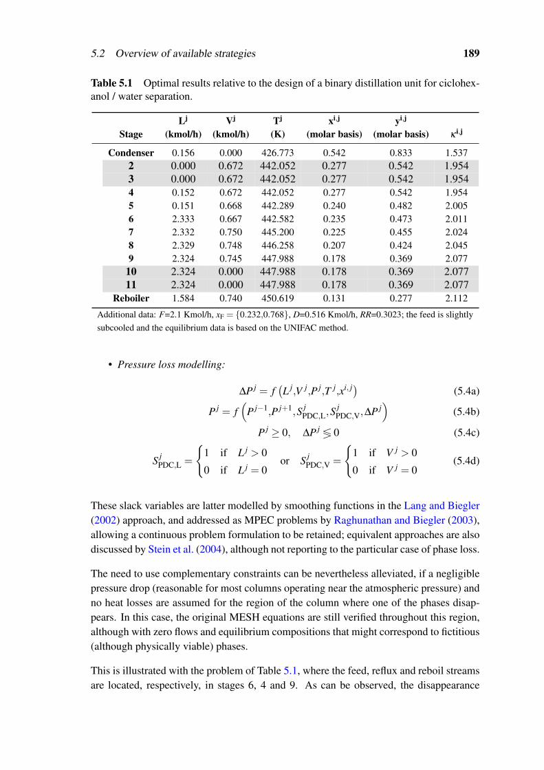
5.2 Overview of available strategies 189
Table 5.1 Optimal results relative to the design of a binary distillation unit for ciclohex-anol / water separation.
Lj Vj Tj xi,j yi,j
Stage (kmol/h) (kmol/h) (K) (molar basis) (molar basis) κ i,j
Condenser 0.156 0.000 426.773 0.542 0.833 1.5372 0.000 0.672 442.052 0.277 0.542 1.9543 0.000 0.672 442.052 0.277 0.542 1.9544 0.152 0.672 442.052 0.277 0.542 1.9545 0.151 0.668 442.289 0.240 0.482 2.0056 2.333 0.667 442.582 0.235 0.473 2.0117 2.332 0.750 445.200 0.225 0.455 2.0248 2.329 0.748 446.258 0.207 0.424 2.0459 2.324 0.745 447.988 0.178 0.369 2.077
10 2.324 0.000 447.988 0.178 0.369 2.07711 2.324 0.000 447.988 0.178 0.369 2.077
Reboiler 1.584 0.740 450.619 0.131 0.277 2.112
Additional data: F=2.1 Kmol/h, xF = 0.232,0.768, D=0.516 Kmol/h, RR=0.3023; the feed is slightlysubcooled and the equilibrium data is based on the UNIFAC method.
• Pressure loss modelling:
∆P j = f(L j,V j,P j,T j,xi, j) (5.4a)
P j = f(
P j−1,P j+1,S jPDC,L,S j
PDC,V,∆P j)
(5.4b)
P j ≥ 0, ∆P j ≶ 0 (5.4c)
S jPDC,L =
1 if L j > 0
0 if L j = 0or S j
PDC,V =
1 if V j > 0
0 if V j = 0(5.4d)
These slack variables are latter modelled by smoothing functions in the Lang and Biegler(2002) approach, and addressed as MPEC problems by Raghunathan and Biegler (2003),allowing a continuous problem formulation to be retained; equivalent approaches are alsodiscussed by Stein et al. (2004), although not reporting to the particular case of phase loss.
The need to use complementary constraints can be nevertheless alleviated, if a negligiblepressure drop (reasonable for most columns operating near the atmospheric pressure) andno heat losses are assumed for the region of the column where one of the phases disap-pears. In this case, the original MESH equations are still verified throughout this region,although with zero flows and equilibrium compositions that might correspond to fictitious(although physically viable) phases.
This is illustrated with the problem of Table 5.1, where the feed, reflux and reboil streamsare located, respectively, in stages 6, 4 and 9. As can be observed, the disappearance
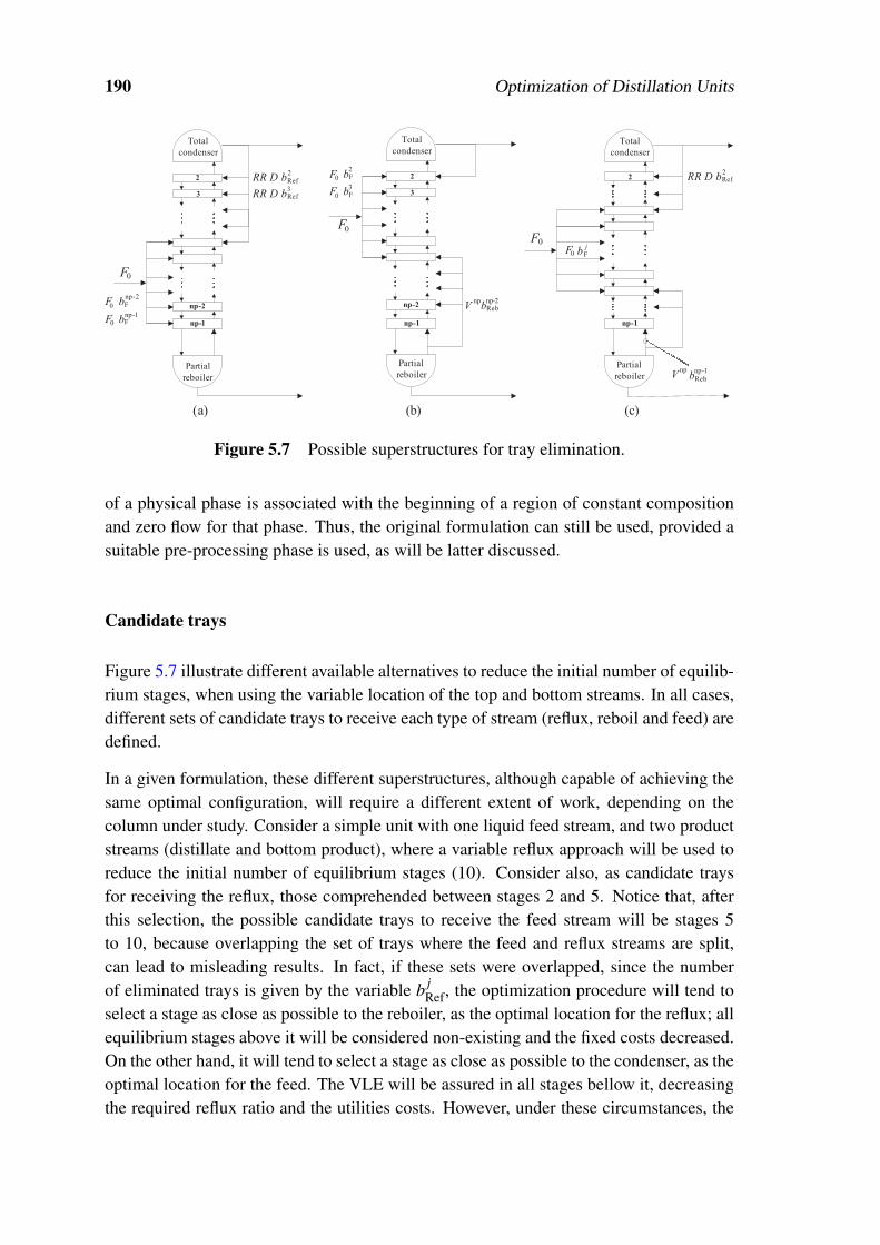
190 Optimization of Distillation Units
Total
condenser
Partial
reboiler
Total
condenser
Partial
reboiler
Total
condenser
Partial
reboiler
2
3
np-1
np-2
2
np-1
2
3
np-1
np-2
RR D bRef2
RR D bRef3
F0
F0
F0
F0 bFnp -1
F0 bF
np -2
RR D bRef2
F0 bFj
Vnp
bRebnp -2
F0 bF2
Vnp
bReb
np -1
F0 bF3
(a) (b) (c)
Figure 5.7 Possible superstructures for tray elimination.
of a physical phase is associated with the beginning of a region of constant compositionand zero flow for that phase. Thus, the original formulation can still be used, provided asuitable pre-processing phase is used, as will be latter discussed.
Candidate trays
Figure 5.7 illustrate different available alternatives to reduce the initial number of equilib-rium stages, when using the variable location of the top and bottom streams. In all cases,different sets of candidate trays to receive each type of stream (reflux, reboil and feed) aredefined.
In a given formulation, these different superstructures, although capable of achieving thesame optimal configuration, will require a different extent of work, depending on thecolumn under study. Consider a simple unit with one liquid feed stream, and two productstreams (distillate and bottom product), where a variable reflux approach will be used toreduce the initial number of equilibrium stages (10). Consider also, as candidate traysfor receiving the reflux, those comprehended between stages 2 and 5. Notice that, afterthis selection, the possible candidate trays to receive the feed stream will be stages 5to 10, because overlapping the set of trays where the feed and reflux streams are split,can lead to misleading results. In fact, if these sets were overlapped, since the numberof eliminated trays is given by the variable b j
Ref, the optimization procedure will tend toselect a stage as close as possible to the reboiler, as the optimal location for the reflux; allequilibrium stages above it will be considered non-existing and the fixed costs decreased.On the other hand, it will tend to select a stage as close as possible to the condenser, as theoptimal location for the feed. The VLE will be assured in all stages bellow it, decreasingthe required reflux ratio and the utilities costs. However, under these circumstances, the
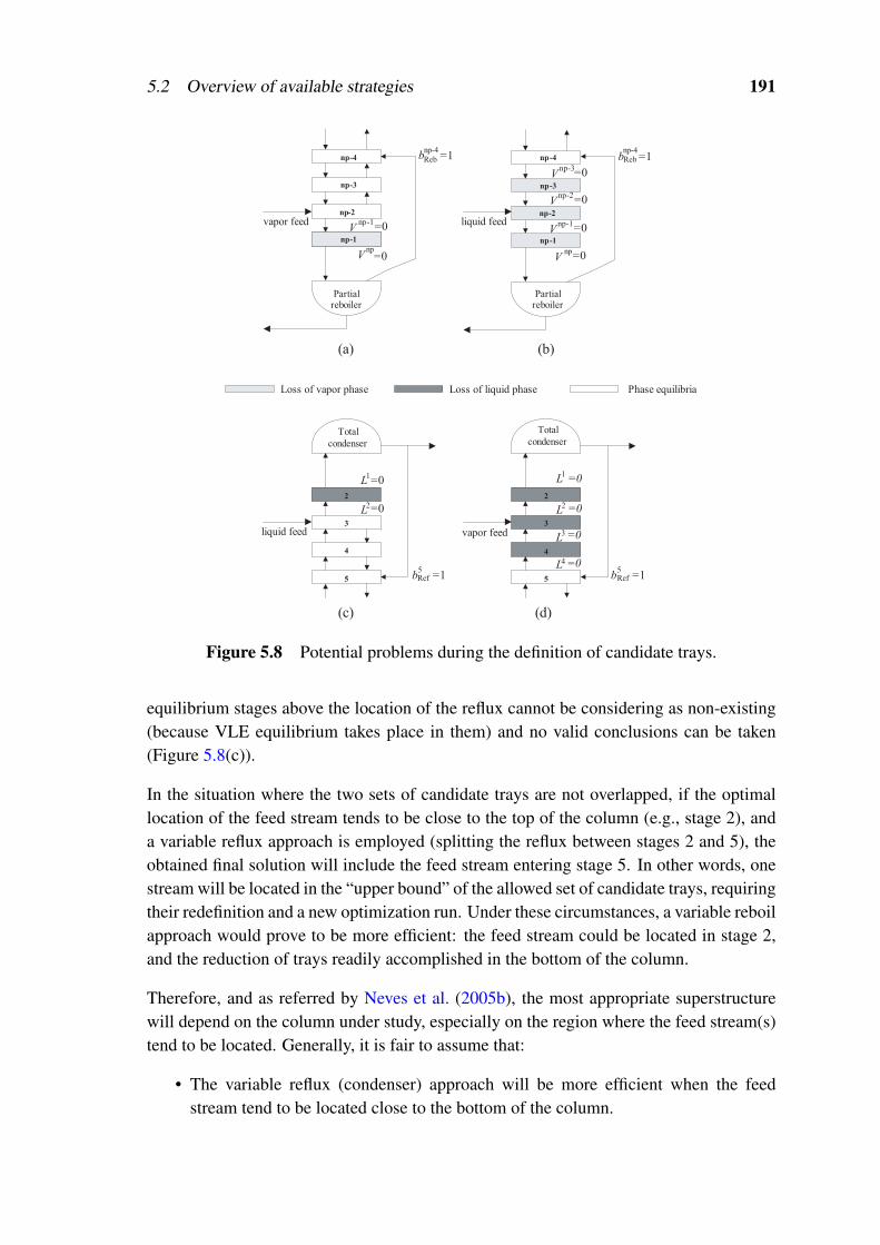
5.2 Overview of available strategies 191
vapor feed liquid feed
vapor feedliquid feed
Loss of vapor phase Loss of liquid phase
(a) (b)
(c) (d)
L2 =0
L1 =0
L3=0
L4=0
L1 =0
L2 =0
2
3
4
5 bRef5 =1bRef
5 =1
Total
condenserTotal
condenser
2
3
5
4
np-1
np-2
np-3
np-4
np-1
np-2
np-3
np-4
Partialreboiler
Partialreboiler
Vnp-3 =0
Vnp =0V
np =0
Vnp -1 =0
bReb
np -4 =1 bReb
np -4 =1
Phase equilibria
Vnp-2 =0
Vnp-1 =0
Figure 5.8 Potential problems during the definition of candidate trays.
equilibrium stages above the location of the reflux cannot be considering as non-existing(because VLE equilibrium takes place in them) and no valid conclusions can be taken(Figure 5.8(c)).
In the situation where the two sets of candidate trays are not overlapped, if the optimallocation of the feed stream tends to be close to the top of the column (e.g., stage 2), anda variable reflux approach is employed (splitting the reflux between stages 2 and 5), theobtained final solution will include the feed stream entering stage 5. In other words, onestream will be located in the “upper bound” of the allowed set of candidate trays, requiringtheir redefinition and a new optimization run. Under these circumstances, a variable reboilapproach would prove to be more efficient: the feed stream could be located in stage 2,and the reduction of trays readily accomplished in the bottom of the column.
Therefore, and as referred by Neves et al. (2005b), the most appropriate superstructurewill depend on the column under study, especially on the region where the feed stream(s)tend to be located. Generally, it is fair to assume that:
• The variable reflux (condenser) approach will be more efficient when the feedstream tend to be located close to the bottom of the column.
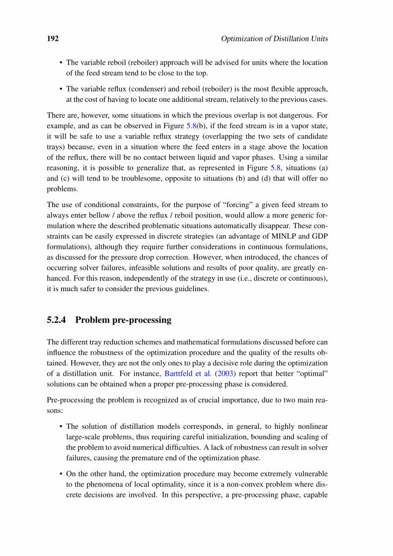
192 Optimization of Distillation Units
• The variable reboil (reboiler) approach will be advised for units where the locationof the feed stream tend to be close to the top.
• The variable reflux (condenser) and reboil (reboiler) is the most flexible approach,at the cost of having to locate one additional stream, relatively to the previous cases.
There are, however, some situations in which the previous overlap is not dangerous. Forexample, and as can be observed in Figure 5.8(b), if the feed stream is in a vapor state,it will be safe to use a variable reflux strategy (overlapping the two sets of candidatetrays) because, even in a situation where the feed enters in a stage above the locationof the reflux, there will be no contact between liquid and vapor phases. Using a similarreasoning, it is possible to generalize that, as represented in Figure 5.8, situations (a)and (c) will tend to be troublesome, opposite to situations (b) and (d) that will offer noproblems.
The use of conditional constraints, for the purpose of “forcing” a given feed stream toalways enter bellow / above the reflux / reboil position, would allow a more generic for-mulation where the described problematic situations automatically disappear. These con-straints can be easily expressed in discrete strategies (an advantage of MINLP and GDPformulations), although they require further considerations in continuous formulations,as discussed for the pressure drop correction. However, when introduced, the chances ofoccurring solver failures, infeasible solutions and results of poor quality, are greatly en-hanced. For this reason, independently of the strategy in use (i.e., discrete or continuous),it is much safer to consider the previous guidelines.
5.2.4 Problem pre-processing
The different tray reduction schemes and mathematical formulations discussed before caninfluence the robustness of the optimization procedure and the quality of the results ob-tained. However, they are not the only ones to play a decisive role during the optimizationof a distillation unit. For instance, Barttfeld et al. (2003) report that better “optimal”solutions can be obtained when a proper pre-processing phase is considered.
Pre-processing the problem is recognized as of crucial importance, due to two main rea-sons:
• The solution of distillation models corresponds, in general, to highly nonlinearlarge-scale problems, thus requiring careful initialization, bounding and scaling ofthe problem to avoid numerical difficulties. A lack of robustness can result in solverfailures, causing the premature end of the optimization phase.
• On the other hand, the optimization procedure may become extremely vulnerableto the phenomena of local optimality, since it is a non-convex problem where dis-crete decisions are involved. In this perspective, a pre-processing phase, capable

5.2 Overview of available strategies 193
Feed Flash
Calculations
Theoretical Reversible
Products Calculations
Saddle Pinch
Points Calculations
Direct/Indirect
Energy Demand
Calculation
Rigorous
Reversible
Column
Rigorous
Direct/Indirect
Approximation
Figure 5.9 Pre-processing phase based on reversible distillation conditions.
of restricting the search space, and conveniently bound some important decisionvariables, may exert a decisive influence on the quality of the results obtained.
Pre-processing phases, used to initialize the model variables before the start of the opti-mization phase, have been studied in great detail by several authors. Fletcher and Morton(2000) presented a systematic procedure to overcome the difficulties mentioned, based ona limiting case of the column model, using infinite reflux or zero feed. Bausa et al. (1998,1999) proposed a shortcut method based on the Rectification Body Method (RBM), pro-viding an estimate of the minimum energy demand together with a check for feasibleproduct specifications. Barttfeld and Aguirre (2002) developed the Reversible Distilla-tion Sequence Model (RDSM), a method that relies on thermodynamic aspects, leadingthe process synthesis to energetically efficient designs. This is based on a pre-processingphase where auxiliary optimization models are solved sequentially (Figure 5.9). Morerecently, Barttfeld et al. (2003) extended the RDSM method to azeotropic distillation andBek-Pedersen and Gani (2004) proposed a new procedure, based on a driving force ap-proach, to generate preliminary designs of distillation based systems.
All of these approaches share several common key aspects: easy application (based onsmall systems of simple equations), useful initialization of model variables, and deriva-tion of critical bounds for important operational specifications, such as energy demand.The RDSM method, illustrated in Figure 5.9 is a good example of a procedure that fulfillall these requirements. Therefore, the main goal of a pre-processing phase is, usually, togenerate a feasible design of the distillation column, to select proper bounds in variablessuch as the total number of equilibrium stages and the column heat consumption. After-wards, the optimization phase will be simpler and more reliable (including the location ofthe feed streams), according to a specified objective function.
194 Optimization of Distillation Units
5.3 Developed methodology
An alternative continuous strategy developed for the optimal design of distillation unitswill be discussed in this Section (Neves et al., 2005b). Instead of relying on distributionfunctions, this introduces simple constraints to control the amount of stream splitting,and to converge the relaxation of the initial design problem to its optimal solution. Here,the most important advantages of both previous discrete and continuous approaches arecombined. This is done by solving only NLP subproblems, and by retaining a greatersimilarity between the intermediate solutions and the continuous relaxations of the corre-sponding discrete formulations. These two key points are intended to generate a strategycapable of dealing with highly non-ideal models (e.g., UNIFAC based) and adequate forthe optimization of complex units (e.g., multiple feeds and side-streams), assuring a ro-bust convergence and the synthesis of the most interesting configurations.
5.3.1 Key aspects
In this Section, the key-aspects of the new developed strategy (further named as CCAP1)will be discussed in detail, namely: (i) the pre-processing phase, especially adapted tohighly non-ideal models and (ii) the optimization phase, where concave expressions areused to control the streams aggregation levels, and slack variables introduced to enabledifferent forms of converging the problem.
Pre-processing phase
The first key-aspect of the new continuous strategy is relative to a robust pre-processingphase. The importance of this step was already discussed in Section 5.2.4 and, despite ofthe already available methodologies (e.g., RBM, RSDM, etc.), a new approach was alsodeveloped. Two main reasons are in the basis of this decision:
• First, most of the available methods present a difficult implementation in non-conventional cases, like the industrial process under study. The existence of a largenumber of vestigial byproducts hinders the possibility of defining key-componentsin a traditional fashion, a usual requirement of short-cut approaches, to establishsimplified design relations.
• On the other hand, almost all of the available methods were developed assuming thefurther use of discrete optimization strategies where, due to the numerical schemesinvolved (e.g., linearizations), the bounding of some decision variables is crucial,to constrain the search space around the problem optimal solution.
1Concave Conditions with Adjustable Parameters.

5.3 Developed methodology 195
Obtain estimates for:
i) maximum allowed number of plates ( )
ii) minimum required reflux ratio (RRmin)
iii) location of the feed streams
Apply Wang-Henke (or other) algorithm(approximate solution)
Automatically restrict each variable
Automatically scale variables & equations(use suitable factors)
Solve all equations simultaneously(with the problem degrees of freedom = 0)
STEPS OBJECTIVES
(i, ii) Obtain a feasible column design close
to minimum energy demand operation.
(iii) Choose the sets of candidate trays to
receive each feed.
Obtain a good initialization for all problem
variables (dependent and independent).
Obtain a good bounding of the problem;
avoid undefined expressions..
Avoid “unbalanced” Jacobian matrix and
large numerical derivatives..
Generate a feasible starting point for the
optimization phase..
Add slack variables to the MESH equations(impose lower and upper bounds in their values)
Avoid problems caused by infeasibilities in
the early stages of the optimization phase. .
maxnp
Figure 5.10 Developed pre-processing phase, for a single unit.
The new pre-processing phase presents a completely different philosophy, since it pre-cedes a continuous optimization strategy where the previous concerns relative to initial-ization (and bounding) close to the final solution are not crucial. The new main goals are aflexible implementation, also suitable for non-conventional units, and a robust numericalconditioning of the problem, adequate for large-scale and highly non-ideal models. Thislast point deserves special attention, due to the complex VLE that will be involved in theindustrial case studies of Section 5.5.
For the previous purposes, the equation oriented strategy discussed in Section 4.4.2, con-stitutes a good choice, although requiring some modifications. In fact, it was initiallydeveloped for the simulation of existing units where, contrarily to the root design of newones, the parameters np, lF and RR were already know. Therefore, the only remainingissue that must be now considered is the inclusion of a new (first) step, where the earlierdesign specifications must be roughly estimated (Figure 5.10).
The objective of the first step is to generate a feasible design for each distillation column,that involves a minimum energy demand, and therefore allows the derivation of a lowerbound for the reflux ratio (RRmin) and an upper bound on the total number of equilibriumstages required (npmax). Efforts are also concentrated in defining the most favorable re-

196 Optimization of Distillation Units
gions of the column, where each feed stream (or side-stream) must enter / leave. This isperformed using existing shortcut methods for simple (Doherty and Malone, 2001; Hol-land, 2001; Seader and Henley, 1998) and complex (Barnés et al., 1972; Nikolaides andMalone, 1987; Jelinek, 1988) columns, considering the splitting of streams throughouttheir candidate regions. For non-conventional problems, where the traditional definitionof key components is hindered, and the efficiency of approximate methods is low, theseestimates can be further corrected offline, using suitable rigorous simulation methods. Forexample, an upper bound on the maximum number of equilibrium stages of the columncan be corrected in a fast trial-and-error approach, by noticing when further increases onthe number of stages of the column do not allow significant decreases in the reflux rationecessary to meet the imposed operational specifications. A similar study can be done toanalyze the influence of lF. Notice that, in the above procedure, the RRmin and npmax val-ues do not correspond to an initialization close to the optimum. From a thermodynamicalpoint of view, they express a column design that is, in general, much less efficient thenthat pursued by the RDSM or RBM methods. Now, the goal is to pre-process the prob-lem, with a sufficiently high initial number of stages, and with suitable candidate regionsfor each feed / exit stream. This last point deserves special emphasis, since the chancesof selecting the most appropriate approach for tray reduction are significantly enlarged,allowing the optimization phase to be done more efficiently (Section 5.2.3).
The second step requires the application of one (or few) iterations of a rigorous simulationmethod, to initialize properly all model variables. The number of iterations required canbe controlled by observing the residuals of the model equations. Due to its straightforwardimplementation and fair rate of convergence, the method of Wang-Henke (Friday andSmith, 1964) was used, since it can be implemented based on simple rearrangements ofthe MESH equations already present in the model. For columns with feed streams thatpresent very wide boiling mixtures, more specific methods like the Sum of Rates (SR)or more robust methods like the Inside-Out can be selected instead (Seader and Henley,1998). Once in the presence of reasonable initial values for all variables, bounds forthem are automatically added to the formulation, using scale factors appropriate to theirexpected range of variation. The model equations and variables produce then a Jacobianmatrix which is approximately equilibrated. It is also assumed that proper care has beenplaced in the simplification and rearrangement of the original model equations, not onlyto avoid mathematical singularities, but also to produce models with simple and morelinear partial derivatives.
The third step consists in obtaining an exact solution of all model equations, relative tothe configuration considered during the previous steps. In this case, the main decisionvariables of the problem (total number of stages, stream distribution, and reflux ratio)are fixed, resulting in a problem with zero degrees of freedom. As already introduced inSection 4.4.2, and similarly to the approach that will be followed during the optimiza-tion phase, the design problem is then more conveniently formulated as expressed byequation (4.17). The pre-processing phase is therefore terminated with a feasible column

5.3 Developed methodology 197
SIMULATION
(Mathematica)
OPTIMIZATION
(GAMS)
In all columns: select npmax , estimate RRmin and split feed and product streams
among the candidate trays
Fix the feed streams composition and
flowrate of the entire set of units.
Sequential-Modular Approach Equation-Oriented Approach
Set the Degrees of Freedom = 0
(for each column: fix np= npmax, RR=RRmin
and the destilate flowrate)
Obtain a feasible solution for the entire
set with all streams splitted
Good starting point for the entire set
Scale/bound and add slack variables(as described for the pre -processing phase of an
individual unit )
Impose operational specifications(purities in streams /recoveries in columns )
Construct economical objective function(regarding the entire set of columns )
Obtain optimal reflux ratios, number of
plates an feed locations
Figure 5.11 Developed pre-processing phase, for a set of units.
design, which can be subsequently used as an initial iterate in the optimization procedure.
The previous discussion considered the pre-processing of a single unit. However, some ofthe industrial application examples that will be addressed in the current Chapter includethe optimization of sets of distillation units, with fixed topology. In these cases, the mainsteps illustrated in Figure 5.10 are still considered for each of the involved columns, butadditional effort will be accounted, due to the necessary coherency of the initialization.In fact, due to the existence of recycles, estimating the feed streams of all units maybecome a non-trivial task. If poor estimates are used, the iterative methods of Step 2will be incapable of assuring a proper initialization (and also bounding), from an overallpoint of view. Therefore, when trying to simultaneously solve all units, a large number ofinfeasibilites may be generated, causing significant numerical problems.
To overcome potential difficulties, the sequential modular approach discussed in Sec-tion 4.4.2 is used to generate coherent estimates for all feed streams, as represented inFigure 5.11. These are then passed to the EO pre-processing phase, that will obtain afeasible starting point for the entire set of units, before entering the optimization calcu-lations. In practice, the previous procedure was crucial to prevent extremely large CPUtimes and, in more complex cases, to avoid solver failures. Its adoption was not necessaryin Chapter 4, because the case-studies solved by the EO strategy (Section 4.4.2) couldbenefit from excellent initial estimates, given by a previous data reconciliation exercise.However, this is impossible to assure during the root synthesis of new units.

198 Optimization of Distillation Units
Total
condenser
Partial
reboiler
2
3
4
5
6
7
8
9
10
11
12
13
14
15
Total
condenser
Partial
reboiler
2
3
4
5
6
7
8
9
10
11
12
13
14
15
Total
condenser
Partial
reboiler
2
3
4
5
6
7
8
9
10
11
12
13
14
15
Total
condenser
Partial
reboiler
2
3
4
5
6
7
8
9
10
11
12
13
14
15
αs
αs
αs=1
∑=
≥1
s
np
j
α
RefLS,F,s =
RR D bRef
j
F0 bF
jLS0 bLS
j
( )2
jsb
Figure 5.12 Use of concave expressions and adjustable parameters for tray selection.
Optimization phase
In the optimization phase, and similarly to the DDF case, the feed and product streams areinitially distributed to each tray of the column, using continuous variables (b j
F and b jRef, in
the case of Figure 5.12).
These variables represent the split fraction of a given stream s (feed or product) amongthe different equilibrium stages of the column, and therefore are subject to conservationconstraints of the form:
np
∑j=1
b js = 1, ∀s = 1, . . . ,ns with 0≤ b j
s ≤ 1 (5.5)
Initially, the optimal design problem is solved considering that each stream is distributedto each stage in a candidate region (not necessarily composed only by adjacent equi-librium stages), subject to the respective constraints of type (5.5). This corresponds tocontinuous relaxation solution of an equivalent MINLP design problem. To converge thelocation of each stream to a single equilibrium stage, constraints of the form:
np
∑j=1
(b js)
2 ≥ αs, ∀s = 1, . . . ,ns (5.6)

5.3 Developed methodology 199
are added to the previous solution, using an adjustable parameter αs ∈ [0,1] relative to eachstream. This strategy is similar to the one used during the optimal synthesis of reactionnetworks, discussed in Chapter 3. The mathematical properties of the previous concaveconstraints can be found in Section 3.4.3, where a detailed description of the convergenceprocedure is presented. The number of intermediate steps required to achieve full con-vergence depends on the nonlinearity of the LV equilibrium and on the complexity of theseparation problem (e.g. number of streams and operational constraints). The computa-tional experience acquired indicates that, similarly to the DDF approach, the prematureuse of large values of α makes the problem more sensitive to local solutions. There-fore the effect of this parameter should be considered by cautious variation, especially oncomplex problems, instead of just considering directly a final solution with α = 1.
During the previous convergence procedure, each NLP subproblem to be solved is ini-tialized from the solution of the previous NLP, except in the case of the relaxed problem,which uses the values obtained during the pre-processing phase. The warm start cor-responds to an infeasible point, since increasing the value of α makes constraints (5.6)violated. Thus, especially for very large / complex columns models, a large number ofinfeasibilities are subsequently generated during the first iterations of the solution of eachNLP subproblem, as the design variables are adapted to accommodate for constraints(5.6) with larger values of α . This provides an additional argument for careful variationof the parameters αs during the optimization procedure. Using the examples consideredalong this Chapter, and a variety of commercial NLP solvers, this step was found to betoo sensitive to failures when locating a feasible solution, introducing therefore impor-tant limitations in the rates of change of α that could be successfully used. To avoid thistype of numerical difficulties, the original NLP subproblems are instead reformulated andsolved as:
minu,ε
J(u)
s.t. f (u)− ε = 0
g(u,α)≤ 0
‖ε‖ ≤ δ
(5.7)
by introducing slack variables ε in the model equations, and a scalar bound δ on themaximum allowed tolerance for the model equations. No slack variables were introducedin the remaining inequality constraints of the model, since in some cases they relate tofeasibility and operational constraints that need to be enforced to avoid failures during theevaluation of the model f (u).
Similarly to the role of α , the δ constant represents a tuning parameter in the algorithm,which can be adapted using different strategies. At the end, αs = 1 and δ = 0 must beobtained. However, the intermediate NLP subproblems can be solved using a variety ofcombinations of the values of α and δ . Depending on the type of problem, differentstrategies can be used, to maximize the rate and robustness of the convergence to the finalsolution. These can be summarized as follows:

200 Optimization of Distillation Units
• Fixed α / variable δ : This corresponds to the most aggressive, and usually thefastest approach, since only one NLP subproblem needs to be solved for each valueof δ to converge all streams to their final locations. It also tends to be more sensitiveto the presence of local optima, and therefore require a closer initialization than theremaining alternatives.
• Fixed δ / variable α : In this strategy δ is maintained fixed (e.g., δ = 10−6, that mustbe a sufficiently small value), and a sequence of NLP problems are solved until theconvergence of α → 1 has occurred. Thus, the evolution of the objective functionwith the minimum amount of stream aggregation can be more easily studied. Thiscan be useful to study alternative configurations of complex columns, with severalfeeds and side streams.
• Variable α / variable δ : This is the most general approach, capable of potentiallymaximizing the numerical robustness of the method, at the cost perhaps of an in-creased number of NLP subproblems to be solved, relatively to each of the previousapproaches.
The numerical performance and other merits of these alternatives are discussed along theexamples reported in this Chapter.
5.3.2 Main advantages
Two illustrative examples are presented in this Section, to clarify the advantages of thenew developed strategy over previous continuous formulations. They intend to demon-strate the gains that can be achieved during the optimization of complex columns, byallowing feed splitting between non-consecutive trays, in the final configuration. The firstexample considers an existing industrial unit (with fixed np), drawn from the aniline pu-rification process, as implemented by CUF–QI. The second refers to the root synthesis (npvariable) of an extractive distillation column, from the winner solution of the EURECHAstudent contest competition in 2004 (Eurecha, 2004). In both cases, the UNIFAC groupcontribution method was used to describe the vapor-liquid equilibria. The resulting mod-els were solved using CONOPT III, in a 2.6 GHz Pentium IV computer, accordingly tothe mathematical formulations presented in Section 5.4.1.
Example 1
The first example considers a distillation unit with 10 components, represented in Fig-ure 5.13. This is equivalent to unit D4, involved in the separation core of Figure 4.23.Here, aniline is the required product and several “light” and “heavy” byproducts arepresent, accordingly to the relative volatilities shown in Table 5.2. This column has3 feeds, with compositions also shown in Table 5.2: stream S4, rich in 4 components

5.3 Developed methodology 201
Total
condenser
Partial
reboiler
2
3
np-2
np-1
S4
S5
S10
S6
S7
S8
Large amount of
“light” byproducts
Large amount of “heavy” byproducts
Reduced amount of byproducts (almost pure aniline)
Side-stream where anilinemust be withdrawn
Figure 5.13 Distillation column with multiple feeds and one side-stream for anilinepurification, as implemented by CUF–QI.
Table 5.2 Feed streams data, for the distillation unit of Figure 5.13.
Variable BZ Water CHA CHONA CHOL ANL MNB DICHA CHENO CHANIL
%(m
olar
) S4 <0.01 37.19 8.21 12.0 37.58 N.A. <0.01 0.31 4.44 0.27
S5 <0.01 4.05 3.72 9.03 26.74 N.A. <0.01 0.82 40.30 15.32
S10 <0.01 2.07 0.64 2.12 1.45 N.A. <0.01 2.03 52.19 38.74
ϕ 57.79 20.99 4.86 3.40 3.27 1.00 0.48 0.99 0.04 0.10
σϕ 0.16 0.70 0.06 0.04 0.04 0.01 0.04 0.03 ' 0 ' 0
lighter than the desired product, stream S5 rich in two heavy components, and stream S10rich in aniline (although with small extents of some byproducts).
The purity of the middle boiling point component in the liquid side-stream (S7) should behigher than 99.97% and should also comply with the remaining specifications presentedin Table 5.3, relative to individual contamination restrictions for some byproducts. Noticethat the information contained in Table 5.3 does not correspond to the current industrialpractice (this one is expressed by Table 4.7); it translates a fictitious scenario, more suit-able for illustrative purposes.
Estimates for the minimum required reflux ratio for this separation were made using thepre-processing method illustrated in Figure 5.10, considering the current np fixed. Afterthis, the feed streams were split among the respective candidate trays: stream S4 equallysplit between stages 2 and 5, streams S5 and S10 between stages (np− 1) and (np− 6),and stream S7 between stage 5 and stage (np− 6). This selection of sets of candidate

202 Optimization of Distillation Units
Table 5.3 Final product specifications for the unit of Figure 5.13.
BZ Water CHA CHONA CHOL ANL MNB DICHA CHENO CHANIL
<50 <300 <50 <250 <300 >99.97 N.A. N.A. N.A. N.A.
ppm ppm ppm ppm ppm %
Table 5.4 Convergence data relative to the optimization of the distillation column inFigure 5.13.
Optimization phaseStrategy Infeasibilities CPU time (s)
Variable α , fixed δ238 41
(α = 0.8, 0.9, 1.0)
Fixed α , variable δ115 29
(δ = 1×10⁻⁵, 5×10⁻⁶, 1×10⁻⁶)
trays was based on the information obtained in the pre-processing phase, relative to theestimates for the most favorable regions of the column to receive each of the three feedsand to draw the outlet liquid side-stream.
Table 5.4 summarizes the obtained convergence data, during the optimization phase. Thisstudy involved a mathematical model with approximately 6000 equations / variables, anda CPU time of 12 seconds for the pre-processing phase, excluding the first step, whichwas done separately.
It can be noticed that with a fixed α / variable δ strategy the maximum number of infea-sibilities observed during the sequential steps of the optimization procedure decreased,together with the CPU time necessary to obtain the problem solution.
However, an important advantage of the strategy with variable α is that interesting eco-nomic configurations can be investigated, as shown in Figure 5.14. In this particular studythe locations of the streams S4, S10 and S7 remained fixed, but αF,S5 was relaxed to 0. Inthis way, the importance of allowing non-adjacent splitting for stream S5 can be isolatedand better evaluated.
As shown, smaller reflux ratios (and, therefore, small operational costs) can be accom-plished when S2 is allowed to be split between stage 5 and stage (np−1). Constrainingthis split has a significant impact on the performance of the column, and should be avoided(when αF,S5 = 1 is imposed, the required reflux ration increases almost 50%). The optimalconfigurations found, regarding the fractioned and aggregate solution for this problem, areshown in Table 5.5.

5.3 Developed methodology 203
0.00
0.20
0.40
0.60
0.80
1.00
1.20
0.00 0.70 0.80 0.90 0.92 0.94 0.96 0.98 1.00
αF,S5
1.00
1.05
1.10
1.15
1.20
1.25
1.30
1.35
1.40
1.45
1.50stage 5
RR
stage np-1
Fra
ctio
nin
g
RR
(norm
aliz
ed)
Figure 5.14 Dependence of the objective function value, on the aggregation degree, forthe unit of Figure 5.13.
Table 5.5 Obtained optimal configurations for the unit of Figure 5.13.
Variable Aggregated solution Fractioned solution
Location of S7 Stage (np−2) Stage (np−2)
Location of S4 Stage 4 Stage 4
Location of S10 Stage (np−1) Stage (np−1)
Location of S5 Stage (np−1) 63% on stage (np−1)37% on stage 5
Reflux ratio 1.47 RRopt RRopt
COPE(AC/h) 22.4 14.3
Example 2
The next example involves the optimization of an extractive column represented in Fig-ure 5.15. This unit has two feeds: stream S1, where a mixture of three organic componentsand water is present, and from which ethyl acetate must be recovered; stream S2, mainlycomposed by an extractive agent (1,4-butanediol), used to break the existing azeotropesthat prevent a direct separation. The compositions of all feeds, and the ethyl acetate spec-ifications in the distillate stream, are also included in Figure 5.15. A highly non-idealVLE is exhibited by the considered mixture, where 4 binary and a ternary azeotrope arepresent. The objective of this example is to design a new unit, with minimum annualizedtotal cost.
According to the information obtained from preliminary calculations, the following deci-sions were made:
• The initial number of equilibrium stages was set to 45, generating a problem with

204 Optimization of Distillation Units
Total
condenser
Partial
reboiler
S1
S2
Operational Specifications
(regarding ethyl acetate)
> 0.80
EXTRACTIVE DISTILLATION COLUMN
Feed from which ethyl acetatemust be recovered;
Feed containing the extractive agent
NOTE : All compositions have a molar basis
F (mol/h)
Acetone
S1 S2
9460 6500
0.018 0.000
0.149 0.000
0.395 0.000
0.438 0.079
0.000 0.921
Ethyl acetate
Ethanol
Water
Butanediol
Fra
ctio
ns
Purity (destilate)
> 0.95Recovery (destilate)
•
•
Figure 5.15 Extractive distillation unit with multiple feeds, for ethyl acetate recovery.
approximately 9000 equations / variables.
• A fixed reflux / variable reboil scheme was selected to reduce the maximum numberof trays.
• The candidate region to receive S1 included the stages between 10 and 30, forstream S2 those between stages 2 and 44, and those between stages 20 and 44 forthe reboil.
The economical data for this example was taken from the design literature (Tourton et al.,1998). The type of correlations employed and a detailed description of the objectivefunction considered are described in Section 5.5.2.
Under these conditions, 105 seconds were spent in the pre-processing phase and 103 sec-onds were necessary to obtain the relaxed solution of the problem. This last one presentedthe feed and reboil streams split in the following manner: S1 - 100% in stage 18, S2 - 75%in stage 2 and 25% in stage 26, reboil - 35% in stage 25 and 65% in stage 26. The con-vergence data for this example is presented in Table 5.6, relatively to the solution whereall streams are located in single equilibrium stages. Again, using a variable δ approach,the total CPU time and the maximum number of infeasibilities obtained is lower than in asituation where δ remains fixed during the entire procedure.
Once more, the variable α / fixed δ approach was used to study alternative final configu-rations for this unit. Figure 5.16 presents normalized values of CTA and RR, as a functionof the parameter αF. As can be observed, it is advantageous to allow one of the feeds (S2)to be split among non-contiguous stages, because the operational costs become lower.

5.3 Developed methodology 205
Table 5.6 Convergence data relative to the optimization of the extractive distillationcolumn in Figure 5.15.
Optimization phaseStrategy Infeasibilities CPU time (s)
Variable α , fixed δ1542 104
(α = 0.8, 0.9, 1.0)
Fixed α , variable δ383 39
(δ = 1×10⁻⁵, 5×10⁻⁶, 1×10⁻⁶)
0.0
0.2
0.4
0.6
0.8
1.0
1.2
0.00 0.60 0.70 0.80 0.90 1.000.98
1.00
1.02
1.04
1.06
1.08
1.10
1.12
1.14
stage 2
stage 40
RR
CTA
Fra
ctio
nin
g
Norm
aliz
ed v
alues
αF,S2
Figure 5.16 Dependence of the objective function value, on the aggregation degree, forthe unit of Figure 5.15.
Table 5.7 Optimal configurations obtained for the unit of Figure 5.15.
Variable Aggregated solution Fractioned solution
Number of stages 27 27
Location of S1 Stage 18 Stage 18
Location of S2 Stage 2 75% on stage 225% on stage 26
Reflux ratio 5.31 4.95
CTA(kAC/yr) 34.9 33.1

206 Optimization of Distillation Units
Table 5.7 compares the optimal designs obtained in both cases. The low CPU times,previously reported, can be once again justified by the proximity between the relaxedsolutions and the final configurations.
5.4 Benchmark study
To evaluate the performance of different optimization strategies, a benchmark study ispresented in this Section, considering four examples of increasing complexity (Neves andOliveira, 2004). This time, and to simplify the analysis of the results obtained, the pre-vious problems will be solved considering that all streams must be converged to singlelocations. A similar study has been reported in the literature (Barttfeld et al., 2003), al-though only discrete formulations were tested, with relatively ideal problems. Therefore,a comparison of the relative merits of both continuous and discrete approaches, in large-scale highly non-ideal problems, was still lacking.
5.4.1 Tested formulations and numerical schemes
In this study, two classical discrete strategies — MINLP (Viswanathan and Grossmann,1993) and GDP (Barttfeld et al., 2003), and two continuous approaches — DDF (Lang andBiegler, 2002) and CCAP (Neves et al., 2005b) are employed. Different tray reductionschemes (variable reflux / reboil and variable condenser / reboiler) were also used, toevaluate any potential impacts on the quality of the results and / or in the robustness ofthe convergence procedure (except for the GDP strategy, where they are not applicable).In all cases, the same pre-processing phase is implemented, according to the contents ofSection 5.3.1, guaranteeing an equivalent initialization (and numerical conditioning).
Among the tested mathematical formulations, three of them (MINLP, DDF and CCAPbased) share the same philosophy during tray reduction, where phase loss must necessar-ily occur (Figure 5.4). Therefore, the core of the ruling equations will be similar, both forthe variable reboil / reflux and condenser / reboiler schemes (equations (5.12), (5.13) and(5.14)) and, under these circumstances, the differences between the previous strategiesare only related to the method of mathematically expressing the involved discrete choices(equations (5.18), (5.19) and (5.20)).
In expressions (5.8–5.20), the following considerations are implicit:
• Columns with a total condenser and a partial reboiler.
• Ideal vapor phase behavior; non-ideal liquid phase (UNIFAC method).
• Feed and liquid / vapor side-streams allowed to enter in all equilibrium stages, withthe exception of the condenser and the reboiler.
5.4 Benchmark study 207
Mathematical Formulation
The objective of the problem is to minimize the total annualized costs (CTA):
minb j
F ,b jLS,b
jV S,RR,
b jReb,b
jRef,b
jC,b j
R
CTA
s.t. (5.1), (5.2), (5.9–5.17), (5.18) or (5.19) or (5.20)
(5.8)
• Property correlations:
H jL = f
(xi, j,T j) , H j
V = f(yi, j,T j) , κ
i, j = f(xi, j,T j) ,
i = 1, . . . ,nc; j = 1, . . . ,np (5.9)
• Control equations:
nc
∑i
xi, j = 1 andnc
∑i
yi, j = 1, j = 1, . . . ,np (5.10)
• Phase equilibrium:
yi, j = κi, jxi, j− ε
i, jEQ, i = 1, . . . ,nc; j = 1, . . . ,np (5.11)
• Mass and energy balances:
– Condenser (i = 1, . . . ,nc; j = 1):
V j+1yi, j+1 = L j (1+1/
RR)
xi, j− εi, jBMP (5.12a)
QC +V j+1H j+1V = L j (1+1
/RR)
H jL− ε
jBE (5.12b)
– Column (i = 1, . . . ,nc; j = 2, . . . ,np−1):
L j−1xi, j−1 +V j+1yi, j+1 +F0 ·b jF · x
iF +RR ·D ·b j
Ref · xi,1 +V np ·b j
Reb · yi,np =(
L j +LS0 ·b jLS
)xi, j +
(V j +V S0 ·b j
VS
)yi, j− ε
i, jBMP
(5.13a)
QC ·b jC +L j−1H j−1
L +V j+1H j+1V +F0 ·b j
F ·HF +RR ·D ·b jRef ·H
1L+
+V np ·b jReb ·H
,npV = QR ·b j
R +(
L j +LS0 ·b jLS
)H j
L +(
V j +V S0 ·b jVS
)H j
V− εj
BE
(5.13b)

208 Optimization of Distillation Units
– Reboiler (i = 1, . . . ,nc; j = np):
L j−1xi, j−1 = L jxi, j +V jyi, j− εi, jBMP (5.14a)
QR +L j−1H j−1L = L jH j
L +V jH jV− ε
jBE (5.14b)
• Auxiliary expressions:
– Slack variable constraints:∥∥∥εj
BMT
∥∥∥≤ δ ,∥∥∥ε
i, jBMP
∥∥∥≤ δ ,∥∥∥ε
i, jEQ
∥∥∥≤ δ ,∥∥∥ε
jBE
∥∥∥≤ δ ,
i = 1, . . . ,nc; j = 1, . . . ,np (5.15)
– Split fraction summations:
np
∑j=1
b jF = 1,
np
∑j=1
b jC = 1,
np
∑j=1
b jR = 1,
np
∑j=1
b jRef = 1,
np
∑j=1
b jReb = 1
np
∑j=1
b jLS = 1,
np
∑j=1
b jVS = 1 (5.16)
– Operational specifications for the side-streams:
OSiLS =
np
∑j
(b j
LSxi, jLS0
)/
(np
∑j
(nc
∑i
b jLSxi, jLS0
)), i = 1, . . . ,nc (5.17a)
OSiVS =
np
∑j
(b j
VSyi, jV S0
)/
(np
∑j
(nc
∑i
b jVSyi, jV S0
)), i = 1, . . . ,nc (5.17b)
• Feed and product streams convergence:
– Applicable only in the MINLP based strategy:
b jF,b
jLS,b
jVS,b
jC,b j
R,b jRef,b
jReb ∈ 0,1 (5.18)
– Applicable only in the DDF based strategy:
b jF = exp
(−(( j−µF)/σF)
2)
/∑w
exp(−((w−µF)/σF)
2)
(5.19a)
b jLS = exp
(−(( j−µLS)/σLS)
2)
/∑w
exp(−((w−µLS)/σLS)
2)
(5.19b)
b jVS = exp
(−(( j−µVS)/σVS)
2)
/∑w
exp(−((w−µVS)/σVS)
2)
(5.19c)

5.4 Benchmark study 209
b jC = exp
(−(( j−µC)/σC)2
)/∑
wexp(−((w−µC)/σC)2
)(5.19d)
b jR = exp
(−(( j−µR)/σR)2
)/∑
wexp(−((w−µR)/σR)2
)(5.19e)
b jRef = exp
(−(( j−µRef)/σRef)
2)
/∑w
exp(−((w−µRef)/σRef)
2)
(5.19f)
b jReb = exp
(−(( j−µReb)/σReb)
2)
/∑w
exp(−((w−µReb)/σReb)
2)(5.19g)
– Applicable only in the CCAP strategy:
np
∑j=1
(b jF)
2 ≥ αF,np
∑j=1
(b jLS)
2 ≥ αLS,np
∑j=1
(b jVS)
2 ≥ αVS (5.20a)
np
∑j=1
(b jC)2 ≥ αC,
np
∑j=1
(b jR)2 ≥ αR (5.20b)
np
∑j=1
(b jRef)
2 ≥ αRef,np
∑j=1
(b jReb)
2 ≥ αReb (5.20c)
The objective function includes costs of utilities (CCU +CHU) and of fixed equipment(CEC +CCOL) that are given by (5.1) and (5.2). The economical data was gathered fromTourton et al. (1998), and the objective function built as detailed in Section 5.5.2. Itis also important to emphasize that expressions (5.8–5.20), by conciliating different for-mulations and numerical schemes, are presented differently when compared to previousworks. Nevertheless, they are mathematically equivalent and, therefore, adequate forbenchmark purposes.
In the GDP formulation, the core of the previous mathematical model, given by expres-sions (5.12–5.14), is not suitable. As illustrated in Figures 5.3 and 5.4, the use of logi-cal disjunctions during tray reduction implicates a completely different optimization ap-proach. However, the required mathematical formulation can be found elsewhere (Bart-tfeld et al., 2003) and will not be presented here. One further aspect that deserves specialattention during the use of GDP approaches is the involved numerical solution scheme. Infact, and as stated in Barttfeld et al. (2003), the obtained disjunctive models must be solvedthrough a decomposition algorithm proposed by Yeomans and Grossmann (2000b), whichis a modified version of the logic-based OA algorithm (Turkay and Grossmann, 1996).Therefore, the original GDP model must be rewritten as a set of reduced MINLP andNLP formulations, that are then iterated during the solution procedure. This approach canconstitute a difficult and time-consuming step that, in practice, make GDP implementa-tions less appealing. Due to this reason, the LogMIP code has recently emerged (Vec-chietti, 2005). More then a solver, it intends to be a “translating” tool that enables a

210 Optimization of Distillation Units
straightforward solution of disjunctive models, by automatically decomposing the origi-nal formulation, as previously explained. The solution and iteration of the resulting NLPand MINLP models is also managed by LogMIP, by interfacing with suitable solvers thatare available in GAMS (Brooke et al., 1998).
All the examples reported in the next Section were approached through GDP formula-tions, subsequently passed to LogMIP. Despite the numerical experience reported by Vec-chietti and Grossmann (2004) (although relative to different classes of problems), noneof the considered examples could be solved. Severe difficulties were felt in the MINLPphases that, by generating bad estimates, caused infeasible NLP subproblems, and a pre-mature end of the optimization procedure. Considering the conclusions reported in Bart-tfeld et al. (2003), where GDP formulations revealed a better efficiency than MINLP ones(as theoretically expected), the obtained results can only be explained by limited capabil-ities of the LogMIP solver. The current release (dated from 30/06/2005) still correspondsto an “under development” implementation, and does not offer the same level of robust-ness as the works developed by Yeomans and Grossmann (2000b,a); Barttfeld et al. (2003)that certainly include extra precautions, with crucial importance for the specific problemunder study. For this reason, the next Section will only report the results obtained bythe MINLP, DDF and CCAP approaches, the only ones able to successfully solve theexamples considered.
The previous results confirm, nevertheless, that the success of a given formulation oftendepends on the chosen numerical scheme (e.g., as discussed in Chapter 3 during the solu-tion of pooling problems). For this reason, in addition to three continuous solvers alreadyintroduced in Section 3.4.2 (CONOPT III, MINOS, SNOPT), two discrete numerical im-plementations were also tested (Brooke et al., 1998):
• DICOPT: this is an implementation of the OA / ER algorithm, where the baseassumption is that MIP models can be solved efficiently, while NLP models aredifficult to solve. Linearizations are used to successively approximate and boundNLP models.
• SBB: in this solver most of the effort is concentrated in solving NLP models. Thecritical assumption is that the successive NLP models differ only in a few bounds,and for that reason can be solved quickly using a restart procedure.
5.4.2 Examples and Results
All the following examples correspond to fictitious situations, although incorporatingcomponents and units similar to those involved in CUF–QI plants. A detailed discus-sion relative to the construction of the objective functions can be found in Section 5.5.2.The objective is to test the performance of different formulations (and numerical solvers)and, therefore, enable conclusions about their relative advantages and drawbacks. The

5.4 Benchmark study 211
resulting indications will be then followed, during the optimization of real industrial casestudies, reported in Section 5.5.1.
Example 1: conventional column (1 feed, 2 products), 5 components
In the first example, the objective was to synthesize a column that could recover, at thebottom, aniline and nitrobenzene. The feed was contaminated with CHA, for which amaximum allowed molar fraction in the bottom was set (0.05%). Only 0.1% of the ni-trobenzene present in the feed stream was allowed to be lost in the distillate. The firststep of the adopted pre-processing phase indicated npmax = 50, RRmin = 0.45 and the re-gion close to the bottom of the column as the most favorable to receive the feed stream.According to this information, a variable reflux (candidate trays: 2, . . ., 21) with fixedreboiler approach was selected. The candidate trays to receive the feed stream were thosecomprehended between stages 40 and 49 and, in these conditions, a model with approxi-mately 1700 equations and variables was generated for optimization.
For the CCAP strategy, the optimization problem was initialized with the reflux and feedstreams equally divided among the respective candidate trays. The MINLP strategy con-sidered an initial design according to the column configuration obtained in the first step ofthe pre-processing phase, with all streams (reflux and feed) entering in single locations.Finally, for the DDF strategy the problem was pre-processed according to the initial cen-tral values and dispersion factors chosen for the reflux and feed streams. The first cor-respond to the integer locations used to initialize the MINLP strategy, while the secondwere set to cover all of the candidate trays.
The main results are presented in Table 5.8 and Table 5.9, considering P=1 bar in allequilibrium stages. For the MINLP strategy, the reported results were obtained with theSBB solver, since DICOPT showed severe difficulties when trying to obtain the integersolution of the problem. For the continuous strategies, CONOPT III presented the bestperformance within all the NLP solvers tested. During the optimization phase, MINOSwas not able to find the first feasible point and SNOPT reached a final optimal solutionwith poor quality. When using the split fraction strategy, the final results translate acolumn configuration slightly different from that obtained in the remaining strategies.This can be justified by the similar values of CTA involved in the two obtained solutions,and by the numerical tolerance imposed.

212 Optimization of Distillation Units
Table 5.8 Results obtained for Example 1 with a variable reflux scheme: (a) using theCCAP based strategy and the CONOPT III solver; (b) using the MINLP based strategyand the SBB solver.
Optimization phaseVariable Pre-processing Relaxed solution Single locations
bjRef
b2Ref · · · b21
Ref = 0.05 (a) b18Ref = 0.475 b19
Ref = 1b2
Ref = 1(b) b19Ref = 0.525 b18
Ref = 1
bjF
b40F · · · b49
F = 0.1b46
F = 1 b46F = 1
b44F = 1
bReb,j FIXED FIXED FIXED
RR 2.370 2.9613.008 (a)
2.925 (b)
CTA (AC/yr) N.A. 382 589382 966 (a)
382 962 (b)
CPU time (s) 205 4
11 5
The results obtained were confirmed in Figure 5.17, using detailed calculations. This re-quire identifying, for each np, the best location for the feed stream (lF), and then optimizethe reflux ratio, for the considered objective function (a time-consuming study due to thenumber of required runs).
Tray reduction scheme — Example 1 A tray reduction scheme, based on a variablecondenser approach, was also tested. The initialization procedure is performed analo-gously to the variable reflux scheme, although since the heat exchanging equipments areno longer fixed at the edges of the column, there are a few conceptual differences. For
0.75
0.88
1.00
1.13
1.25
1.38
26 30 34 38 42 46 500.99
1.00
1.01
1.02
1.03
1.04
1.05
1.06
1.07
1.08
26 30 34 38 42 46 50
np np
C (n
orm
aliz
ed)
TA
RR
(norm
aliz
ed)
Figure 5.17 Optimal CTA and RR, for a fixed np and lF (Example 1).

5.4 Benchmark study 213
Table 5.9 Results obtained for Example 1 with a variable reflux scheme, using the DDFbased strategy and the CONOPT III solver.
Optimization phaseVariable Pre-processing σF = σRef = 0.9 σF = σRef = 0.35 Single locations
RR 2.370 2.967 2.896 2.925
bjRef
(µRef = 18.479)According to: b17
Ref = 0.042 (µRef = 17.549) (µRef = 17.960)(µRef = 10) b18
Ref = 0.473 b17Ref = 0.311 b18
Ref = 1(σRef = 0.9) b19
Ref = 0.448 b18Ref = 0.689
b20Ref = 0.036
bjF
(µF = 46.123)According to: b45
F = 0.132 (µF = 46.018) (µF = 46.010)(µF = 44) b46
F = 0.615 b46F = 0.999 b46
F = 1(σF = 0.9) b47
F = 0.242b48
F = 0.008
bjReb FIXED FIXED FIXED FIXED
CTA (AC/yr) N.A. 383 053 382 758 382 962
CPU time (s) 20 28 15 16
the CCAP strategy, the condenser heat obtained in the pre-processing phase (for npmax
and RRmin conditions) is equally split and supplied between all candidate trays (the refluxstream is now fixed at stage 2. For the DDF strategy, each candidate tray receives a heatamount, in the initialization procedure, according with the initial values choose for thecentral values and dispersion factors. The obtained results are not presented as detailed asfor the variable reflux scheme, because they are equivalent. All strategies converged forone of the previously obtained column configurations: condenser heat exchanged in the17th stage, the feed stream entering in stage 46 and a required reflux ratio ' 2.93. Al-though obtaining similar final configurations, for the two different tray reduction schemesused, it is important to notice that the relaxed solutions are fairly different. When usingthe variable condenser scheme, the relaxed solutions of all strategies presents a value ofCTA significantly lower. The reason is due to the possibility of exchanging heat in almostall candidate trays (and not only in the top stage). This allows to approximate reversibledistillation conditions, a more energy efficient design, that favors the objective function(see Chapter 6). As a consequence, the total CPU times spent by all strategies, whenusing the variable condenser scheme, are slightly larger (' 20%), since the relaxed so-lutions present the heat split among the candidate trays in a greater extension than thesplitting of the reboil stream, in the other tray reduction scheme. The MINLP and thecontinuous formulations were again successfully solved with the SBB and CONOPT IIIsolvers, respectively. DICOPT, MINOS and SNOPT failed, once again, by the same rea-sons described previously.

214 Optimization of Distillation Units
Pressure loss modelling — Example 1 After testing two tray reduction schemes, theinfluence of using different approaches for pressure loss modelling was also studied. Asreferred in Section 5.2.3, when the operating pressure deviates from the atmosphericvalue, its value must be corrected in non-eliminated trays. Therefore, Example 1 wassolved again, considering vacuum conditions inside the column, as stated in equation (5.21).The constant ∆P j considered, although not capable of rigorously describing a real situa-tion is, nevertheless, suitable for the current illustrative purposes:
PC = 0.4 bar
P j = P j−1 +∆P j ·S jPDC,L j = 2, . . . ,np
with ∆P j = 0.01 bar (constant)
(5.21)
As referred in Section 5.2.3, there are two main forms of modelling the involved condi-tional expressions, while maintaining a continuous formulation: the implementation ofMPEC reformulations or the use of smoothing functions.
L j ·(
1−S jPDC,L
)= 0 (using a MPEC reformulation) (5.22a)
or
S jPDC,L =
L j√((L j)2 +10−8
) (using a smoothing function) (5.22b)
Therefore, equation (5.22a) was reformulated in GAMS, using the NLPEC solver, andequation (5.22b) directly used as proposed in Lang and Biegler (2002), to address theproblem of phase loss modelling through different approaches. Both of them enable toappropriately consider pressure drop, without introducing discrete variables.
As can be observed in Table 5.10, which reports the results obtained with the CCAPstrategy, pressure drop activation / deactivation can be successfully achieved through boththe previously described approaches. No additional numerical difficulties were felt andthe required CPU times are similar to those involved in the situation where pressure ismaintained fixed along the column. Notice that, when using MPEC reformulations, thelocation of the reflux is set on stage 14 (with RRopt=3.08) while, through the use of asmoothing function, the obtained final solution include the reflux entering stage 13 (withRRopt=3.00). However, the final objective function values are very similar (CTA ' 383.51)within the imposed numerical tolerances. On the other hand, the CTA values obtainedwhen the operating pressure is fixed are significantly different from those obtained for asituation where this last one is corrected along the column. This is a natural consequenceof different temperature profiles and changes on the components relative volatilities, thatwill influence the optimal trade-offs between operational and investment costs.
Naturally, the use of concave expressions could also be employed to deal with the prob-
5.4 Benchmark study 215
Table 5.10 Results obtained for pressure loss activation / deactivation, through two dif-ferent approaches (Example 1).
MPEC reformulations Smoothing functions
Pj SjL Lj Vj Pj Sj
L Lj Vj
Stage [bar] [Kmol/h] [Kmol/h] [bar] [Kmol/h] [Kmol/h]
Cond. 0.400 0 0.326 0.000 0.400 0 0.319 0.0002 0.400 0 0.000 0.433 0.400 0 0.000 0.4263 0.400 0 0.000 0.433 0.400 0 0.000 0.426...
......
......
......
......
12 0.400 0 0.000 0.433 0.400 0 0.000 0.42613 0.400 0 0.000 0.433 0.410 1 0.366 0.42414 0.410 1 0.375 0.431 0.420 1 0.370 0.47215 0.420 1 0.381 0.482 0.430 1 0.371 0.478
lem of pressure drop modelling (in a similar fashion to the problem of stream location),while maintaining a continuous formulation. However, the idea was to test, in first place,existing strategies in literature. Since these have shown a good performance, no newapproaches were this time attempted.
Example 2: conventional column (1 feed, 2 products), 10 components
In the second example, the objective was to synthesize a column similar to unit D1 fromFigure 4.23, that could separate aniline plus four “heavy” components (CHENO, DICHA,CHANIL and nitrobenzene) from a contaminated feed with 5 “light” byproducts (ben-zene, water, CHA, CHONA and CHOL). The feed conditions considered are given byTable 4.4 and the new operational specification are the maximum molar fraction of CHOLallowed at the bottom (0.1%); the recovery of aniline in the distillate product was set to99.5%. Two different tray reduction schemes were again tested. Since the pre-processingphase indicated the region close to the top of the column as the most favorable to receivethe feed stream, the variable reboil/fixed reflux and variable reboiler/fixed condenser al-ternatives were chosen. For both tray reduction alternatives, the candidate trays to receivethe reboil (reboiler) were those comprehended between stage 10 and 29. The feed streamwas allowed to be located between stage 2 and 6. This problem involved the solution ofmodels with approximately 16000 equations and variables.
The results presented in Tables 5.12, 5.11 and 5.13 were obtained using a variable reboil/ fixed reflux alternative (with P=1 bar, in all stages). As can be observed, all strategiesconverge for the same optimal configuration, that was also the best found when usingdetailed simulations (Figure 5.18).
The reason why all strategies were able, apparently, to avoid local optima in this two first

216 Optimization of Distillation Units
Table 5.11 Results obtained for Example 2, with a variable reboil scheme, using theDDF based strategy and the CONOPT III solver.
Optimization phase
Variable Pre-processing σF = σRef = 0.9 σF = σRef = 0.35 Single locations
bjRef FIXED FIXED FIXED FIXED
bjF
(µF = 4.796)According to: b3
F = 0.012 (µF = 4.110) (µF = 4.020)(µF = 4) b4
F = 0.287 b4F = 0.998 b4
F = 1(σF = 0.9) b5
F = 0.595b6
F = 0.105
bjRef
(µReb = 18.493)According to: b17
Reb = 0.040 (µReb = 17.570) (µReb = 18.035)(µReb = 20) b18
Reb = 0.465 b17Reb = 0.241 b18
Reb = 1(σReb = 0.9) b19
Reb = 0.457 b18Reb = 0.759
b20Reb = 0.038
RR 0.0453 0.0639 0.0571 0.0580
CTA (AC/yr) N.A. 187 880 187 242 187 244
CPU time (s) 245 161 170+347 87
Table 5.12 Results obtained for Example 2, with a variable reboil scheme, using theCCAP based strategy and the CONOPT III solver.
Relaxed Single locationsVariable solution δ = 1×10⁻⁵ δ = 5×10⁻⁶ δ = 1×10⁻⁶
bjRef FIXED FIXED FIXED FIXED
bjF b4
F = 1 b4F = 1 b4
F = 1 b4F = 1
bjReb
b18Reb = 0.722
b18Reb = 1 b18
Reb = 1 b18Reb = 1
b19Reb = 0.278
RR 0.0453 0.0552 0.0567 0.0580
CTA (AC/yr) 187 137 186 976 187 125 187 244
CPU time (s) 238 106 46 51

5.4 Benchmark study 217
Table 5.13 Results obtained for Example 2, with a variable reboil scheme, using theMINLP based strategy and the SBB solver.
Optimization phaseVariable Pre-processing Relaxed solution Single locations
bjRef FIXED FIXED FIXED
bjF b2
F · · · b6F = 0.2 b4
F = 1 b4F = 1
bjReb b10
Reb · · · b29Reb = 0.05
b18Reb = 0.722
b18Reb = 1
b19Reb = 0.278
RR 0.0453 0.0569 0.0580
CTA (AC/yr) N.A. 187 137 187 244
CPU time (s) 227 238 329
0.75
1.00
1.25
1.50
1.75
2.00
2.25
2.50
12 16 20 24 28
0.998
1.000
1.003
1.005
1.008
1.010
1.013
1.015
1.018
1.020
1.023
1.025
12 16 20 24 28np np
C (n
orm
aliz
ed)
TA
RR
(norm
aliz
ed)
Figure 5.18 Optimal CTA and RR, for a fixed np and lF (Example 2).
examples may be related to the second step of the adopted pre-processing phase, wheregood initialization and bounding of variables is obtained. This step is critical to avoidsolver failures and, as experienced by other authors (Barttfeld et al., 2003), can exert amajor influence in the quality of the obtained final solutions. In the pre-processing phaseof this second example, the streams were equally split among the candidate trays, evenwhen using the MINLP strategy, since this proved to be computationally more efficientfor the solution of the RMINLP problem.
In Example 1, the CPU times required to obtain the relaxed solutions in the MINLP andCCAP strategies were similar although for Example 2, a problem with a much largerdimension, it was possible to notice that, when the MINLP strategy is initialized (pre-processed) with all streams entering in single locations, the relaxed solution requires aCPU time that is approximately 30% higher. In the reported CPU times for the DDFstrategy (from Table 5.11), we can observe two parcels for σ = 0.35. This is due to thehigh complexity of the problem, that required a new pre-processing phase (initialization

218 Optimization of Distillation Units
Table 5.14 Results obtained for Example 2 with the CCAP strategy and different con-vergence schemes.
Optimization phaseStrategy Variables α = 0.8 α = 0.9 α = 1.0
Variable α , fixed δ Infeasibilities 1209 1205 1509(δ = 1×10⁻⁶) CPU time (s) 153 141 156
Variable α , Variable δ Infeasibilities 896 875 827(δ = 1×10⁻⁵, 5×10⁻⁶, 1×10⁻⁶) CPU time (s) 217 235 201
step only), when the value of the dispersion factor was decreased. Not doing this resultedin solver failures, due to the numerical difficulties that are introduced by the differentiabledistribution functions. For the CCAP strategy, and also due to the large problem dimen-sion, several convergence schemes were tested, some of them including the use of threevalues of δ , to allow a faster (variable δ / fixed α) or more robust (variable α / variableδ ) solution process. As already introduced, the sequential decrease of the tolerance value(within all model equations must be verified) reduces the number of infeasibilities that areobtained when the streams are forced to enter in single locations, allowing increased ro-bustness (Table 5.14). Although requiring the solution of a larger number of optimizationproblems, each run is fairly faster than in a situation where the tolerance value is alwaysfixed and, globally, the required CPU time does not increase drastically (Table 5.14). Asalready expected, and clearly stated in Table 5.12, the fastest way of solving the prob-lem consists on converging α → 1 in a single step, a procedure that involves a largervulnerability to the presence of local optima, according to the gathered experience. How-ever, in this particular example, the obtained final solution was the same, for all testedconvergence schemes.
Notice that the final tolerance value (10−6) is sufficiently small to not interfere in thequality of the solution. In other words, when decreasing this value no changes are causedin the results obtained (a situation where the allowed error in the model equations isalready negligible). This was set according to the scaling of the equations conducted inthe pre-processing phase.
Tray reduction scheme — Example 2 A tray reduction scheme, based on a variablereboiler approach, was also tested. The initialization procedure was done analogouslyto Example 1. Once again, all strategies converged for the same column configuration:reboiler located in the 20th stage, the feed stream entering in stage 4 and a required refluxratio of 0.058. This solution is equivalent to that obtained through a variable reboil / fixedreflux approach and, once again, the impact of using different tray reduction schemes inthe quality of the final results was found to be negligible.
As expected, when using the variable reboiler scheme, the obtained relaxed solutions,

5.4 Benchmark study 219
QR
QC
RR= 0.052
CTA =186 281 €/yearbR
11= 0.333
bR
19=0.121
bR20 =0.198
bR21 =0.236
bR22 =0.112
FbF
4= 1.000
4
11
19
20
21
22
Figure 5.19 Relaxed solution obtained for Example 2, with a variable reboiler scheme,using the CCAP strategy (CONOPT III solver).
through all tested strategies, exhibit a significantly lower value of CTA. As discussed forExample 1, the underlying reason relates to multiple heat exchanges along the column(and not only in the bottom stage), that approximate reversible distillation conditions,and contribute for a reduction of the operational costs. This can be better understood byanalyzing the relaxed solution of the CCAP strategy, illustrated in Figure 5.19.
Once again, as already discussed for Example 1, all strategies exhibited a larger difficultyin obtaining a final solution, since more effort was required to force the split heat to enterin a unique location. Therefore, the total CPU times, spent when using a variable reboilerscheme, were slightly larger (' 20%). For both tray reduction schemes, the SBB andCONOPT III solvers were the only ones to successfully solve the involved problems;DICOPT, MINOS and SNOPT continued to exhibit a poor performance.
Pressure loss modelling — Example 2 The activation / deactivation of pressure dropswas also considered during the solution of Example 2. This time, instead of assuming P= 1 bar along the column, the pressure was set to 2.0 bar in the reboiler, and corrected inall the above non-eliminated trays through:
PR = 2.0 bar
P j = P j+1 +∆P j ·S jPDC,V j = 1, . . . , np−1
with ∆P j =−0.02 bar (constant)
(5.23)
This time, and since tray reduction must be accomplished at the bottom of the column,through a variable reboil (reboiler) scheme, the conditional expressions are written for the
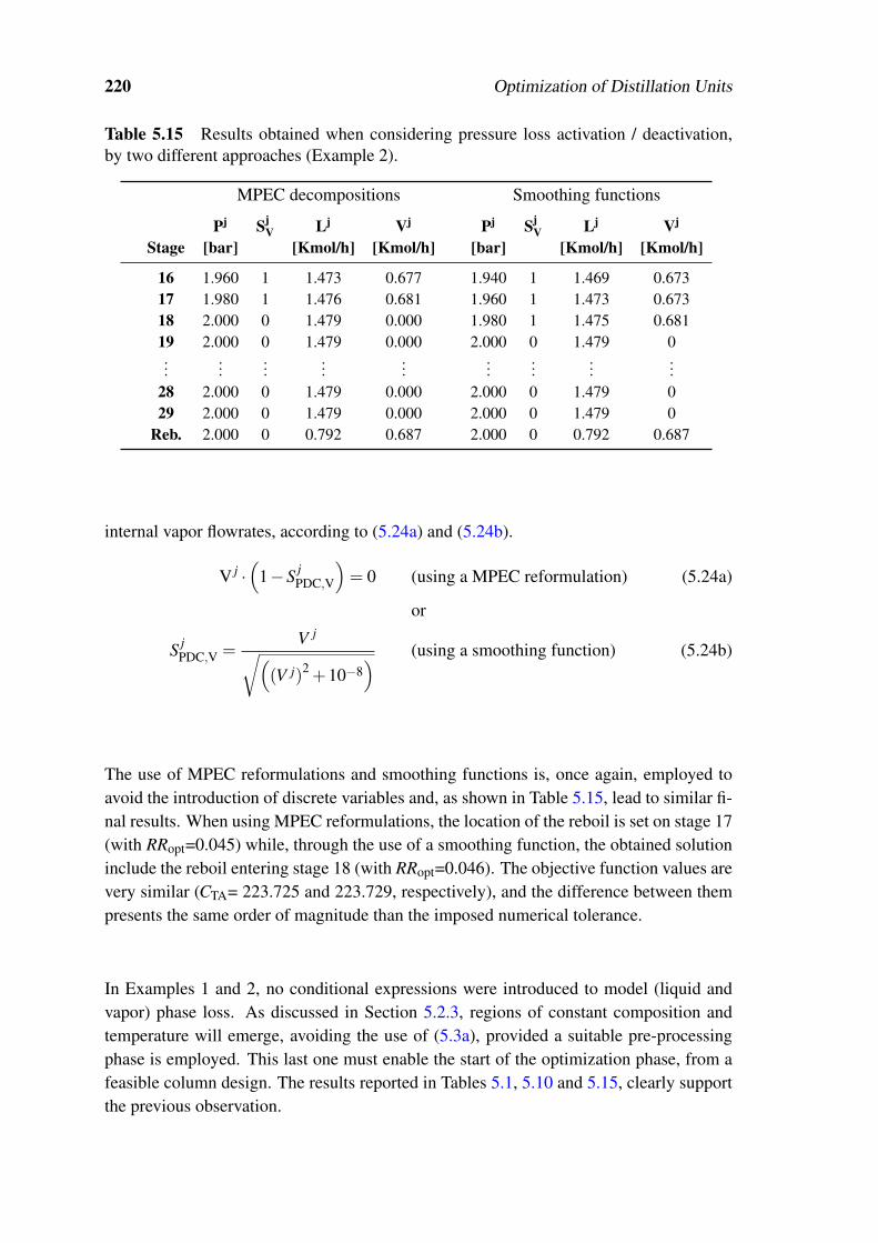
220 Optimization of Distillation Units
Table 5.15 Results obtained when considering pressure loss activation / deactivation,by two different approaches (Example 2).
MPEC decompositions Smoothing functions
Pj SjV Lj Vj Pj Sj
V Lj Vj
Stage [bar] [Kmol/h] [Kmol/h] [bar] [Kmol/h] [Kmol/h]
16 1.960 1 1.473 0.677 1.940 1 1.469 0.67317 1.980 1 1.476 0.681 1.960 1 1.473 0.67318 2.000 0 1.479 0.000 1.980 1 1.475 0.68119 2.000 0 1.479 0.000 2.000 0 1.479 0...
......
......
......
......
28 2.000 0 1.479 0.000 2.000 0 1.479 029 2.000 0 1.479 0.000 2.000 0 1.479 0
Reb. 2.000 0 0.792 0.687 2.000 0 0.792 0.687
internal vapor flowrates, according to (5.24a) and (5.24b).
V j ·(
1−S jPDC,V
)= 0 (using a MPEC reformulation) (5.24a)
or
S jPDC,V =
V j√((V j)2 +10−8
) (using a smoothing function) (5.24b)
The use of MPEC reformulations and smoothing functions is, once again, employed toavoid the introduction of discrete variables and, as shown in Table 5.15, lead to similar fi-nal results. When using MPEC reformulations, the location of the reboil is set on stage 17(with RRopt=0.045) while, through the use of a smoothing function, the obtained solutioninclude the reboil entering stage 18 (with RRopt=0.046). The objective function values arevery similar (CTA= 223.725 and 223.729, respectively), and the difference between thempresents the same order of magnitude than the imposed numerical tolerance.
In Examples 1 and 2, no conditional expressions were introduced to model (liquid andvapor) phase loss. As discussed in Section 5.2.3, regions of constant composition andtemperature will emerge, avoiding the use of (5.3a), provided a suitable pre-processingphase is employed. This last one must enable the start of the optimization phase, from afeasible column design. The results reported in Tables 5.1, 5.10 and 5.15, clearly supportthe previous observation.

5.4 Benchmark study 221
Example 3: non-conventional column (3 feeds, 3 products), 10 components
The third example is relative to the synthesis of a non-conventional column, similar to theunit represented in Figure 5.13, where the same components of Example 2 are present,according to the feed conditions of Table 5.2. This column will still have to recover thelight secondaries in the distillate and the heavy components in the bottom, although nowfulfilling the aniline purity specifications that are reported in Table 4.92.
In the first step of the adopted pre-processing phase, the implemented short-cut meth-ods (Barnés et al., 1972; Nikolaides and Malone, 1987) allowed to estimate RRmin andnpmax, and gave a first indication about the most favorable regions to locate the feeds andthe side-stream. Nevertheless, and due to the difficulty in defining key components in atraditional fashion, these estimates were further refined using a rigorous method (Wang-Henke) and a quick trial-and-error procedure, as already explained. At the end, the fol-lowing reliable information could be identified:
• RRmin=19 and npmax=20.
• S4 tend to be located next to top, S5 and S10 next to the bottom and S7 approxi-mately in the middle of the column.
The above information also indicates that independently of choosing a variable reboil(reboiler) or a variable reflux (condenser) scheme, their respective set of candidate trayswill always have to be partially overlapped with the set of candidate trays selected toreceive the feed streams, since these last ones present favorable locations that cover allregions of the column (top, middle and bottom). As already discussed in Section 5.2.3,there are situations where this overlapping can be dangerous. For this particular example,since the feed stream that tend to be located close to the top of the column is in a vapourphase, and since the two remaining feeds that tend to be located next to the bottom are ina liquid phase, the previously referred overlap is safe.
A variable reboil / fixed reflux and a variable reboiler / fixed condenser approaches wereadopted during the solution of the current example. For stream S4, the allowed candi-dates trays are those comprehended between stages 2 and 11, for streams S5 and S10those between stages 10 and 19 and, for stream S7, those between stages 5 and 14. Theallowed locations for the reboil stream will be stages 10 to 19. For the variable reboilerscheme, the candidate trays to receive this heat exchanging equipment will be stages 11 to20. Independently of the tray reduction scheme used, optimization problems with around11 000 variables / equations were generated, for all tested strategies.
The results obtained will not be presented as detailed as in the previous examples. In-formation relative to the convergence procedure will be omitted, and only final resultswill be shown. The underlying reason is the following: the first two examples, besidescomparison purposes, had also the objective of illustrating how all strategies worked in
2Contrarily to those found in Table 5.3, these results express the industrial practice.

222 Optimization of Distillation Units
Table 5.16 Results obtained for Example 3, with a variable reboil scheme, when usingall strategies under study.
Strategy
Variable DDF MINLP CCAP
Fina
lloc
atio
ns S4 Stage 4 Stage 4 Stage 4S5 Stage 15 Stage 15 Stage 14
S10 Stage 13 Stage 14 Stage 12S7 Stage 10 Stage 11 Stage 10
Reboil Stage 15 Stage 16 Stage 14
RR 25.333 25.319 25.380CTA (AC/yr) 216 085 216 279 216 224
practice. In this final example, the main goal is to study the capability of each strategyto avoid local optima, when a more conceptually elaborated problem is considered. Thenumber of possible column configurations is now much larger, due to the large numberof feasible combinations between the locations of the involved streams. This will alsoprevent the use of the procedure based on detailed simulations (that could be adopted forthe first two examples) to infer about the quality of the obtained solutions.
The initialization procedure, for all strategies, is similar to that described for the conven-tional columns of Example 1 and Example 2. What was applicable to one feed streamis now valid for the three existing ones. For the side-stream, an analogous procedure isdefined considering that this stream can be treated as a “negative” feed. Therefore, forthe MINLP and CCAP strategies, the problem is pre-processed with equal fractions ofthe total side-stream amount, leaving the column in all respective candidate trays. For theDDF strategy, these partial flows are defined through a proper central value and disper-sion factor. The final results obtained for the three strategies, when using a variable reboilscheme, are presented in Table 5.16.
It is possible to notice that, contrarily to the previous examples, all strategies seem toconverge to slightly different optimal solutions. This phenomenon of local optimality canalso be observed by analyzing the final results obtained, for a given strategy, when theoptimization problem is initialized with different values of RR. As shown in Table 5.17,for the CCAP strategy, different column configurations are synthesized and the best designachieved when the problem is pre-processed with RR=28, a value higher then RRmin; theMINLP and DDF strategies also exhibit a similar behaviour. Therefore, for columns withlarger conceptual complexity, it is fair to assume that all strategies present a significantprobability of stopping in local optima. This is still applicable when proper effort is givento the initialization, bounding and scaling of the problem.
Although not shown, the final results obtained for the variable reboiler scheme also pre-sented different column configurations, depending on the strategy used, revealing that

5.4 Benchmark study 223
Table 5.17 Results obtained for Example 3, with a variable reboil scheme, using theCCAP based strategy, for different pre-processing conditions.
Pre-processing conditionsVariable RR = 28 RR = 36
Fina
lloc
atio
ns S1 Stage 4 Stage 4S2 Stage 14 Stage 14S3 Stage 12 Stage 11S4 Stage 9 Stage 8
Reboil Stage 14 Stage 14
RR 25.366 25.449CTA (AC/yr) 216 090 216 852
the problem of local optimality continues to subsist. The DDF strategy, that presentedthe best solution in the previous scheme, exhibited a final solution worst than the CCAPstrategy, showing that no conclusions can be taken about the relative efficiency of eachstrategy. This significant vulnerability to local optima should be related to the higher con-ceptual complexity of the problem, where 10 operational constraints are imposed in thefinal product, and where the optimal location of 3 feeds and 1 liquid side-stream must behandled.
As illustrated in Example 1 and 2, the objective function value obtained in the relaxedsolutions is better when the variable location of heat exchanging equipments is employedto reduce the initial number of trays. This is valid for all strategies (for the DDF strategy,the relaxed solution can be understood as the solution obtained for a value of the disper-sion factor that allows a given stream to enter in more than one stage). However, in thecurrent example, this is not only due to the possibility of exchanging heat at intermediatetemperatures, but also because a given feed stream can now be partially located bellow aregion where heat is supplied, due to the overlapping of different sets of candidate trays(Table 5.18).
In practice, this feed stream fraction is not distilled and can be considered as bypassed;this will only happen to an extent determined by the product specifications in stream S7.These relaxed solutions express a new optimal trade-off, where the heat consumption issignificantly lowered at the cost of some product recovery loss, and that in some situa-tions can give interesting indications about alternative configurations, where streams andheat are not necessarily entering in single locations. Notice that, although not shown, therelaxed solutions obtained for the variable reboil scheme always presented (for all testedstrategies) values of CTA larger than 216 000 AC/year. The total CPU times required byall formulations, in this example, were within the same order of magnitude. The vari-able reboiler scheme continued to require a larger computational effort. Among all thetested solvers, CONOPT III and SBB were, again, the only ones to successfully solve theprevious optimization problems.

224 Optimization of Distillation Units
Table 5.18 Relaxed solutions obtained for Example 3, with a variable reboiler scheme,using all strategies under study.
StrategyVariable CCAP & MINLP DDF (σF = σR = 0.9)
S1 b4S1 = 1
b3S1 = 0.183; b4
S1 = 0.697b5
S1 = 0.116
S2 b14S2 = 0.087; b15
S2 = 0.082 b15S2 = 0.021; b16
S2 = 0.472b18
S2 = 0.309; b19S2 = 0.522 b17
S2 = 0.485; b18S2 = 0.022
S3 b10S3 = 1.000
b11S3 = 0.129; b12
S3 = 0.701b13
S3 = 0.166
S4 b7S4 = 1.000
b7S4 = 0.033; b9
S4 = 0.554b8
S4 = 0.399; b10S4 = 0.013
Reboilb12
R = 0.618; b13R = 0.269 b14
R = 0.355; b15R = 0.592
b14R = 0.075; b15
R = 0.023 b16R = 0.043
b18R = 0.015
CTA (AC/yr) 214.194 214.108
Example 4: set of columns (3 conventional and 1 non-conventional), 4 components
The final example refers to an international student contest problem (Eurecha, 2004),and consists on designing a process to recover all organic products from a waste stream(500 kg/h, 20 C, 1 bar). This stream has the following composition (weight percentages):25% acetone, 35% ethanol, 25% ethyl acetate and 15% water. Each recovered productmust present a purity higher than 90%, and the resulting aqueous stream must contain lessthan 0.1% of organic materials. The utilities available are steam (saturated, 10 bar) andcooling water at 20 C.
The selection of the process configuration is a critical step, since the adopted flowsheettopology will determine the maximum operational efficiency and economical return thatcan be achieved in further optimization studies. The considered example is a separationproblem, which makes distillation a natural choice. However, the use of conventionalunits alone might be insufficient, due to the several existing azeotropes (Table 5.19).More elaborated distillation-based techniques can also be considered as natural candi-dates, namely extractive distillation or pressure-swing distillation, among others.
Figure 5.20 illustrates the elected alternative. The main idea is to start by the easierseparation: acetone can be recovered at the top of the first distillation unit (D-01), sincenone of the identified azeotropes is problematic for this particular separation. The bottomstream of this unit (mainly composed by ethyl acetate / ethanol / water) will then enteran extractive distillation unit (D-02) where ethyl acetate is recovered in the distillate. Thebottom stream, containing mostly water, ethanol and the extractive agent (solvent), is
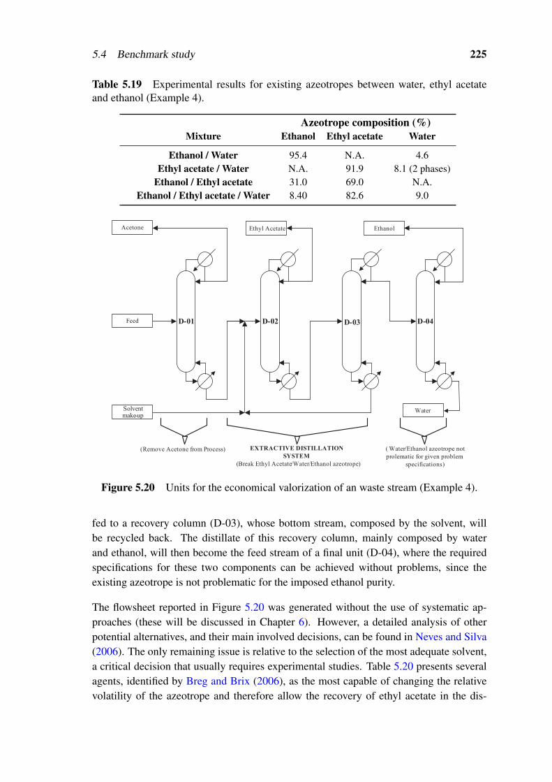
5.4 Benchmark study 225
Table 5.19 Experimental results for existing azeotropes between water, ethyl acetateand ethanol (Example 4).
Azeotrope composition (%)Mixture Ethanol Ethyl acetate Water
Ethanol / Water 95.4 N.A. 4.6Ethyl acetate / Water N.A. 91.9 8.1 (2 phases)
Ethanol / Ethyl acetate 31.0 69.0 N.A.Ethanol / Ethyl acetate / Water 8.40 82.6 9.0
D-03D-01 D-02 D-04Feed
Acetone Ethyl Acetate Ethanol
WaterSolventmake-up
EXTRACTIVE DISTILLATION
SYSTEM
(Remove Acetone from Process)
(Break Ethyl Acetate/Water/Ethanol azeotrope)
( Water/Ethanol azeotrope not
prolematic for given problem
specifications)
Figure 5.20 Units for the economical valorization of an waste stream (Example 4).
fed to a recovery column (D-03), whose bottom stream, composed by the solvent, willbe recycled back. The distillate of this recovery column, mainly composed by waterand ethanol, will then become the feed stream of a final unit (D-04), where the requiredspecifications for these two components can be achieved without problems, since theexisting azeotrope is not problematic for the imposed ethanol purity.
The flowsheet reported in Figure 5.20 was generated without the use of systematic ap-proaches (these will be discussed in Chapter 6). However, a detailed analysis of otherpotential alternatives, and their main involved decisions, can be found in Neves and Silva(2006). The only remaining issue is relative to the selection of the most adequate solvent,a critical decision that usually requires experimental studies. Table 5.20 presents severalagents, identified by Breg and Brix (2006), as the most capable of changing the relativevolatility of the azeotrope and therefore allow the recovery of ethyl acetate in the dis-

226 Optimization of Distillation Units
Table 5.20 Possible agents for ethyl acetate recovery using extractive distillation (Ex-ample 4).
Agent(s) Agent Relativemolar ratios volatility
Glycerin / Ethylene Glycol / 1,4-Butanediol 1:1:1 3.7Glycerin / Diethylene Glycol 1:1 3.4
1,4-Butanediol N.A. 3.2
tillate product of column D-02. Although slightly less efficient that the remaining ones,1,4-butanediol has a important characteristic that makes it the best choice for the currentproblem: its boiling point of 228 C.
Glycerin, ethylene glycol and diethylene glycol have boiling points of 290 C, 197 C and245 C respectively, and when combined in the molar ratios of Table 5.20, originate mix-tures with a much higher boiling point then that of 1,4-butanediol. This is disadvantageousfor the current problem, since the available hot utility is steam at 10 bar (THU = 180 C).In other words, since the solvent (mixture) is recovered at the bottom of column D-03,higher boiling points of the extractive agents implies letting go to the bottom stream alarger quantity of the lower boiling components, to decrease the reboiler temperature toa value inferior to that of the hot utility. The recycle of these components reduces theenergy efficiency of the overall process, since larger heat duties will be required in unitD-02.
All the previous examples were introduced with very specific purposes: Example 1 and 2allowed to illustrate the practical implementation of all strategies, and to test the efficiencyof different tray reduction schemes and different approaches for pressure drop modelling.Example 3 evaluated the vulnerability of all strategies to local optima, considering annon-conventional column, with increased conceptual complexity. The current problem,illustrated in Figure 5.20, intends to test the numerical robustness of all formulations,when in the presence of an extremely large-scale and highly non-ideal problem.
Due to the several columns involved, and since a recycle stream is present, the pre-processing phase not only involved the steps illustrated in Figure 5.10, as also benefitfrom the previous use of a SM approach (see Figure 5.11). The information obtained,relative to initial estimates of RRmin and npmax, and the most favorable feed regions isreported in Table 5.21.
Based on the previous information, decisions about suitable tray reduction schemes andsets of candidate trays were taken (Table 5.22). The resulting problem involves the simul-taneous solution of approximately 30 000 equations / variables.
All strategies (MINLP, DDF and CCAP based) were once again employed but, this time,only the CCAP strategy was able to successfully solve the problem reported in Figure 5.20and Tables 5.21 and 5.22:

5.4 Benchmark study 227
Table 5.21 Information drawn from the pre-processing phase (Example 4).
Distillation unitsStream D-01 D-02 D-03 D-04
npmax 45 35 25 45RRmin 3 5 0.01 1
Feed region Bottom Top(a)/Bottom(b) Top Bottom(a) First feed; (b) Second feed.
Table 5.22 Tray reduction scheme and candidate positions for each stream (Example 4).
Distillation unitsVariable D-01 D-02 D-03 D-04
Tray Reduction Variable Reflux Variable Reboil Variable Reboil Variable RefluxFeed(s) (25, . . . ,44) (2, . . . ,11)(a) (2, . . . ,11) (25, . . . ,44)
(15, . . . ,34)(b)
Reflux (2, . . . ,21) FIXED FIXED (2, . . . ,11)Reboil FIXED (25, . . . ,34) (15, . . . ,24) FIXED
(a) First feed; (b) Second feed.
• The MINLP strategy (even when using the SBB solver) generated solutions of poorquality, due to a low efficiency of the MIP phases that hindered the possibility ofperforming the NLP steps reliably.
• In the DDF strategy, the numerical difficulties introduced by the use of the differen-tial distribution functions caused solver failures (even when using CONOPT), andthe premature end of the optimization phase.
In other words, the properties of the considered problem (related to its large scale andhigh non-linearity) enhanced the particular vulnerabilities of each strategy. Notice that theCCAP strategy was only successfully employed, when a variable α / variable δ approachwas considered — see the convergence data reported in Table 5.23.
As mentioned, four sequential δ values, for each of the four α steps, were required toassure a proper numerical robustness; even so, the maximum number of obtained infea-sibilities reached a value of approximately 6000. Therefore, although involving a large
Table 5.23 Convergence data of Example 4, when using the CCAP strategy and theCONOPT III solver.
Pre-processing Optimization phase (a)
Variable δ = 10−4 α = 0.7 α = 0.8 α = 0.9 α = 1.0
CPU time [s] 1260 1920 960 1440 2160(a) Variable α / variable δ approach with δ = 10−4 → 10−5 → 5×10⁻⁵ → 10−6.

228 Optimization of Distillation Units
Table 5.24 Final design specifications for all units (Example 4).
Distillation unitsVariable D-01 D-02 D-03 D-04
Theoretical trays 36 30 10 37Feed tray(s) 14 2(a)/20(b) 3 34Reflux ratio 5.6 5.2 0.02 1.54
Distillate [Kmol/h] 2.09 1.73 7.71 4.69Diameter [m] 0.35 0.32 0.23 0.32
Height [m] 12.1 10.3 5.4 12.7Condenser [GJ/h] 0.41 0.37 0.32 0.47Reboiler [GJ/h] 0.46 0.30 0.39 0.48
(a) First feed; (b) Second feed.
number of optimization problems and, consequently, a large total CPU time, the previousprocedure was critical to avoid solver failures and, consequently, to obtain a final feasiblesolution (Table 5.24).
There are no guarantees that the reported design specifications constitute the best so-lution for the considered objective function. However, and as referred by Neves andSilva (2006), they translate a configuration much more advantageous than that synthe-sized through the use of commercial simulators (e.g., ASPEN Plus). In these last ones,where discrete choices cannot be properly handled, a rigorous optimization procedure ishindered and empirical decomposition approaches must be adopted. Therefore, the ca-pability of solving problems like the one reported in Figure 5.20, through simultaneousapproaches, is always extremely profitable.
5.4.3 Main indications
The current Section summarizes the main indications from the benchmark study, relativeto the efficiency of the mathematical formulations and numerical solvers tested.
Mathematical formulations
For conventional columns (Examples 1 and 2), all formulations were capable of obtainingthe best solution that was possible to be found, within CPU times of the same orderof magnitude, and independently of the adopted tray reduction scheme. This can be aresult of the typical similarity between relaxed solutions and final configurations. In fact,these are often only separated by a few constraints that need to be satisfied during theoptimization phase.
Although synthesizing the same final configurations, the two tested tray reduction schemes
5.4 Benchmark study 229
involved different relaxed solutions, within each formulation. When using the variable lo-cation of the condenser and / or reboiler, the relaxed solutions of all strategies presenteda lower value of CTA, due to the possibility of exchanging heat in almost candidate trays(and not only in the top and bottom stages). This enables the approximation of reversibledistillation conditions, a situation of higher energy efficiency that reduces the operationalcosts.
The previous results deserve special attention, since an earlier work reports fairly differentfinal configurations, when the tray reduction scheme is changed (Barttfeld et al., 2003).Therefore, this apparent capacity to avoid local optima might be related to the second stepof the adopted pre-processing phase, where good initialization, scaling and bounding ofthe problem is obtained. This step is critical to avoid solver failures and can exert a majorinfluence in the quality of the relaxed solutions.
In Examples 1 and 2, two pressure loss modelling approaches were also tested. Theseare based on fairly different grounds (smoothing functions and MPEC reformulations)and avoid the introduction of additional discrete variables, allowing to retain a continuousformulation in the DDF and CCAP based strategies. The results obtained show a similarperformance, both in the numerical robustness and the quality of the final solutions. Infact, the respective CPU times and objective function values were practically identical.
For a column with larger conceptual complexity (Example 3), all strategies exhibited theirvulnerability to the phenomena of local optimality. This was still applicable when thedimension of the problem was smaller, and when proper pre-processing effort was taken.Nevertheless, the final configurations obtained were similar, revealing that, in principle,solutions of poor quality were avoided. Several runs were additionally considered, solvingthe problem for different pre-processing conditions. These supported the observation thatno conclusions could be drawn about which strategy was best capable of avoiding localoptima. For this reason, solving the optimization problem with formulations of differentnature can be extremely advantageous, especially when model equations are written in amanner that easily allows changing from one strategy to another — equation (5.8).
The final problem (Example 4) that considered the optimization of a set of distillationunits, intended to involve a dimension and non-linearity capable of enhancing the numer-ical problems associated to each strategy and, therefore, test their robustness in extremelycomplex cases. The previous goal was achieved since, from all case-studies, Example 4was the only one not successfully solved by the MINLP and DDF strategies. Here, aconvergence procedure based on a sequential solution of several optimization problems(a CCAP strategy, with a variable α / variable δ approach) was crucial to avoid solverfailures and to return a final feasible solution.

230 Optimization of Distillation Units
Numerical solvers
The performance exhibited by the tested solvers maintained the same tendency along allof the examples considered. SBB and CONOPT III were the only ones to successfullyconverge the respective strategies, independently of the tray reduction scheme and / or ofthe pressure loss modelling approach (with the exception of Example 4, where the SBBsolver also failed).
Most of the failures showed by DICOPT were related to the solution of the NLP sub-problems (returning an infeasible message), although in the three last examples (of largerdimension), also some difficulties related to the solution of the MIP problems were ob-served. In some runs, DICOPT was simply not able to solve these MIP problems. Inother situations, when their solution was accomplished, the lower bound produced for theobjective function value was inferior to that obtained in the relaxed solution or, in otherwords, difficulties related with the convergence to local optima were observed (these areunavoidable, since DICOPT was developed to address convex problems).
According to previous works, the robustness of MINLP formulations depends consider-ably on the solution scheme (Barttfeld et al., 2003). These authors state that, when usingDICOPT, the total solution time will always be long because the convergence of the NLPproblems is very difficult to achieve and, on the other hand, the MIP sub problems includeconstraints that were generated by linearizing the original expressions at zero flows. Thiswould not produce, in general, valid lower bounds of the problem forcing to adopt a stop-ping criterion based on the lack of improvement of the NLP’s objective function. Theselinearizations around zero flows, used for the MIP model, can also create ill-conditioning.Under these circumstances, the MIP models may become very difficult to solve and fail-ures can occur.
The observations of Barttfeld et al. (2003), together with results obtained in the presentwork, seem to be in accordance with the general idea that DICOPT should perform bet-ter on models that have a significant and difficult combinatorial part, while SBB mayperform better on models that have fewer discrete variables but more difficult nonlineari-ties (Brooke et al., 1998). Since the optimization of distillation problems fits better in thislast description, it is understandable the better performance exhibited by the SBB solverin this work.
Relatively to the NLP solvers, it is generally accepted that CONOPT is well suited formodels with very nonlinear constraints, and that it has a very effective method for findinga first feasible solution, especially for models with few degrees of freedom. On the otherhand, MINOS is commonly accepted as the best choice when the model presents a numberof variables much larger than the number of constraints, and in situations where fewnonlinearities can be found outside the objective function (Brooke et al., 1998). In otherwords, MINOS is especially suitable for a class of problems where distillation modelscannot be fitted. Therefore, the difficulties showed by this solver, when trying to obtain the

5.5 Industrial case-studies 231
first feasible point during the optimization procedure, are acceptable. On the other hand,the SNOPT solver is more suitable for large-scale linear and quadratic programming, andfor linearly constrained optimization. SNOPT can be use in general nonlinear programs,although it will be more efficient in a situation where only some of the variables enternonlinearly (Brooke et al., 1998) — a rare characteristic of distillation problems, that canjustify the poor efficiency of this solver. For all that has been said, the better performanceshowed by CONOPT III seems natural, since this solver is well suited for square modelswith very nonlinear constraints — a good description of the examples considered in thisbenchmark study.
5.5 Industrial case-studies
In this Section, several industrial case-studies will be briefly presented, to illustrate thebenefits that can derive from the implementation of rigorous optimization approaches. Inthe next subsections, the CCAP based strategy and CONOPT III were selected to solve allthe involved problems. This choice relies on the large-scale models that will be consid-ered (some of them involving the simultaneous optimization of several columns), and onthe conclusions from the previous benchmark study. Once again, the GAMS modellingenvironment was used, in a 2.6 GHz Pentium IV computer.
5.5.1 Optimization of existing units
The first industrial study considers the set of columns illustrated in Figure 4.23. This hasalready been identified as a separation core, due to its importance to the final product spec-ifications and due to the large utility consumptions involved (Section 4.4.3). Therefore itconstitutes an appropriate target for the following optimization studies.
Since the current study involves the optimization of existing units, the number of stagesis considered fixed in each column. Therefore, the objective function will not include ainvestment component (the structure of the columns will remain unchanged and no newheat exchanging equipments will be acquired), and can be restricted to the minimizationof the overall operational costs. These can be correctly evaluated through the followingequations, together with the information shown in Table 5.19.
CkCU = Fk
CUCCU,unit with FkCU =
QkC
λCU(TCU,out−TCU,inl
) (5.25a)
CkHU = Fk
HUCHU,unit with FkHU = Qk
R/ΘHU (5.25b)

232 Optimization of Distillation Units
Table 5.25 Available utilities in CUF–QI plants, and respective costs.
Stream P [bar] T [ C] Unitary cost [AC/ton] Other properties
Cold Water N.A. 27(a)/35(b) 0.026 λ= 4.18 kJ/(kg C)Steam (LP) 2 120 3.5 Θ= 2258 kJ/kgSteam (MP) 25 224 15.4 Θ= 1850 kJ/kg(a) Inlet temperature; (b) Outlet temperature.
Total
condenser
Partial
reboiler
Total
condenser
Partial
reboiler
Flash
2
3
4
5
6
np-2
np-1
S1
S2
S3
S4
S5
S6
S8
S7
Column A Column B Column C
4
np-4
np-3
np-2
np-1
2
3
5
Total
condenser
Partial
reboiler
2
3
4
5
6
np-2
np-1
S9
S10
S11
Figure 5.21 Equivalent representation of the current separation core.
On the other hand, since the root design of new units in not contemplated, the originalproblem can be simplified, replacing the representation of Figure 4.23 by that illustratedin Figure 5.21. In fact, columns D4 and D4A are twin units, operated at the same pres-sure and according with identical separation purposes. The only difference remains inthe respective flowrates that, nevertheless, are only important during the design of newshells/internals.
Therefore, for the minimization of the global utilities consumption, these two units can becompacted in a single virtual one, enabling a reduction of the problem scale and facilitat-ing its solution. Notice that Figure 5.21 already provides information about the candidateregions that are defined for each feed / exit stream.
Several optimization studies were performed around the previous set of units, whit thefollowing main goals in the horizon:
1. To check if the actual locations (for the feed and exit streams) are, indeed, the mostsuitable ones. All units (D1, D4 and D5) were installed many years ago, for a feedcomposition that was significantly different from the current one; therefore, someof their design specifications may be out of date.
2. To identify new reflux ratios and distillate flowrates, capable of maximizing the per-formance of the arrangement, when all discrete choices are fixed. In fact, changingthe location of feed / exit streams is extremely difficult in practice and, therefore,

5.5 Industrial case-studies 233
Table 5.26 Optimal stage displacement, relative to the current industrial configuration,considering also the manipulation of distillate flowrates and reflux ratios.
OptimizationVariable Column A Column B Simultaneous
Dis
plac
emen
t S1 -1 N.A. -1S4 N.A. -2 0S5 N.A. -1 -1S7 N.A. -1 -1S9 N.A. N.A. +1S10 N.A. -3 -3
Savings (kAC/yr) 53.7 105.8 129.1
the benefits derived from more easily implementable measures should be rigorouslyevaluated.
3. To evaluate the impact of considering a new distillation unit D1 (with increasednumber of stages), and the use of a new catalyst (with different yield of byproducts).This study intends to quantify the economical return that may derive from newlyproposed measures and, therefore, contribute for a more supported decision makingprocess.
For the above studies, all results will be presented taking as reference the information ofTable 4.7, and considering the following set of assumptions (and restrictions):
• Fresh feed characterized according to Table 4.4.
• Total aniline production (within specifications): > 11700 kg/h.
• Final product specification accordingly to Table 4.9.
• Maximum aniline losses (in the bottom stream of unit D5): 3.0 kg/h.
Table 5.26 shows the main results obtained for the first study. As can be observed, theoptimal locations for the feed / exit streams do not correspond to the current ones. Addi-tionally, it is also possible to observe the importance of simultaneous optimization, sincethe results generated are different from those obtained during the separate optimizationof each unit. The individual optimization of column D5 was not considered, because theflowrates involved in this unit are too small and, therefore, an isolated analysis would notbe profitable.
However, it is important to isolate the impact of stage displacement on the arrangementperformance, evaluating if then new optimal locations represent, by themselves, signif-icant economical benefits. This second study will therefore decompose the informationof Table 5.26, separating the contributions of different operational variables. As shownin Table 5.27, the optimization of the reflux ratio (in each column) is much more im-

234 Optimization of Distillation Units
Table 5.27 Savings obtained, relative to the current industrial configuration, during theoptimization of different variables.
OptimizationSavings RR RR & lF RR & D
∑QC (%) 16.5 16.5 16.7∑QR (%) 14.7 14.7 14.9
Utilities (kAC/yr) 127.1 127.4 128.9
650
660
670
680
690
700
710
720
730
740
750
Current
catalyst
New catalyst
(scenario A)
New catalyst
(scenario B)
CO
PE
(k€
/ano
)
D1 - current
D1 - extended
Figure 5.22 Influence of extending the number of equilibrium stages in unit D1, con-sidering a new catalyst under study.
portant than any other change on the remaining operational variables. In fact, just bymanipulating the RRs, 98.6% of the maximum attainable savings can be accomplished.The displacement of the streams locations (or the optimization of the distillate flowrates)contributes marginally for the considered objective function and, contrarily to what wouldbe expected by the single analysis of Table 5.26, should therefore be neglected. This isan important conclusion, that clearly attest the suitableness of the current units for thedesired separation purposes.
In a final study, the influence of using a new catalyst is evaluated on the utility consump-tions of the separation block. Two scenarios are considered (A and B), relative to differentbyproduct yields (Table 4.8). Additionally, two different D1 columns were considered:one corresponding to the current unit (D1-current), and another with the number of equi-librium stages extended (D1-extended). This last scenario does not correspond to theacquisition of a new unit, but instead to the possibility of placing the current D1 in se-ries with an already existing column, that has become available in the past due to processmodifications and where 30 extra stages can be inserted.
The results obtained are reported in Figure 5.22, where the optimization of reflux ratios

5.5 Industrial case-studies 235
Table 5.28 Convergence data relative to the optimization of the set of distillationcolumns represented in Figure 5.21.
Optimization phaseStrategy Infeasibilities CPU time (s)
Variable α , fixed δ2911 785
(α = 0.8, 0.9, 1.0)
Fixed α , variable δ1537 567
(δ = 1×10⁻⁵, 5×10⁻⁶, 1×10⁻⁶)
and distillate flowrates is implicit. The manipulation of these last ones is now critical,due to different byproducts yields. As can be observed, the new catalyst only enablessignificant savings, when scenario B and the current D1 are considered. If the number ofstages is extended, both scenarios (A and B) exhibit an energy efficiency similar to that ofthe reference configuration.
The underlying reason is easy to understand: the separation of light byproducts, thattakes place (extensively) in unit D1, is more difficult than the removal of the heavy ones.Therefore, when the number of equilibrium stages is greatly increased, the operationalcosts associated to this column reach their minimum. Under these circumstances, even inscenario A, where large amounts of CHONA are produced, the value of the objective func-tion will remain practically unchanged (since the required RR increase will be marginal).On the other hand, when the number of stages is maintained in unit D1, the increases onRR that are necessary to accommodate an additional yield of light byproducts will alwaysbe significant. Therefore, the smaller energy efficiency of scenario B, and the much higheroperational costs that are in general obtained, are understandable.
Some of the typical convergence data, obtained during the previous optimization studies,is shown in Table 5.28. Once again, it is possible to observe that when considering avariable δ approach, the numerical robustness of the convergence procedure is enhanced.
5.5.2 Root design of new units
The previous Section reports several studies around existing units, where the evaluationof investment costs is not necessary. However, when the root synthesis of new distillationsystems is considered, in addition to CHU and CCU, it also becomes necessary to includeCCOL, and CEC (Section 5.1.2):
CkTA = Ck
CU +CkHU +Ck
C+CkR +Ck
SHE+CkINT (5.26)
Under these circumstances, the objective function is given by equation (5.26), and CC,CR, CSHE and CINT need to be estimated through appropriated correlations. For this pur-

236 Optimization of Distillation Units
pose, economical data from Tourton et al. (1998) was used, according to the followingexpressions:
CkC = G0
EC10(G1EC+G2
EC log10(AkC)) (5.27a)
CkR = G3
EC10(
G4EC+G5
EC log10(AkR)+G6
EC(log10(AkREB))
2)
(5.27b)
CkSHE = G0
COL10(
G1,kCOL+G2,k
COL log10(hkSHE)+G3,k
COL(log10(hkSHE))
2)
(5.27c)
G1,kCOL = G4
COL +G5COLdk
SHE, G2,kCOL = G6
COL +G7COLdk
SHE,
G3,kCOL = G8
COL +G9COLdk
SHE (5.27d)
CkINT = G10
COL10(
G11,kCOL+G12,k
COL log10(hkINT)
)(5.27e)
G11,kCOL = G13
COL +G14COLdk
INT, G12,kCOL = G15
COL +G16COLdk
INT (5.27f)
Through the analysis of equations (5.27), it is possible to observe that the investment costsare related to the size parameters, characteristic of each equipment: areas (AC, AR) for theheat exchangers; diameters and heights (dINT, dSHE, hINT and hSHE) for the column shelland internals. As implicit in equations (5.28) and (5.29), these size parameters are thenlinked to the remaining problem variables, expressing the different trade-offs that must beoptimized:
AkCUC∆T k
C = QkC (5.28a)
∆T kC ln
(χ
k)
=(TCU,out−TCU,inl
), with χ
k(
T kC −TCU,out
)= T k
C −TCU,inl (5.28b)
AkRUR
(T k
R −THU
)= Qk
R (5.28c)
As always, special attention should be given to the specific form of the equations. Thisis illustrated in (5.28b), where the logarithmic average is evaluated through the use of anauxiliary variable (χk). Decomposition procedures, like previously referred, were crucialto avoid, once again, solver failures and the premature end of the optimization phase.
hkSHE '
(hk
INT +∆h)' hk
COL, with hkINT = HETPk×npk (5.29a)
dkSHE ' dk
INT ' dkCOL, with dk
INT =
√4V np,k
0.9πρVϑVand ϑV = 0.6ϑFL (5.29b)
Relatively to the calculation of size parameters for the column structure, the involvedmethodology is conceptually complex. The estimation of heights and diameters requiresa previous knowledge of the type of internals to use (plates or packings) and of theircharacteristics (e.g., HETP and ϑFL, for packings).
In fact, the dimensioning process is based on models of pressure drop, specific for a given

5.5 Industrial case-studies 237
Separation Efficiency
HE
TP
(m
)
ϒ (Pa0.5
)
0.20
0.25
0.30
0.35
0.40
0 1 2 3 4 5
Pressure Drop
ΔP/Δh
(mbar
m-1
)
ϒ (Pa0.5
)
0.1
1
10
0 1 2 3 4 5
MellapakPlus 452.Y
960 mbar
400 mbar
100 mbar
MellapakPlus 452.Y
960 mbar
400 mbar
100 mbar
(a) (b)
Figure 5.23 (a) HETP and (b) pressure drop calculation for the internals of a column.
type of internals. For packing columns (that are, presently, the most typical choice) thenormalized pressure drop value (∆P/∆h) at flooding conditions, allows to determine thegas velocity (ϑV ) at the same limit situation. According to Ulrich (1984), and as statedin (5.29b), the column should be design for 60% of this last value.
To facilitate the calculation process, each packing supplier represents is own data, as il-lustrated in Figure 5.23. This was reprinted from a commercial catalog (Sulzer, 2004),and corresponds to the Mellapack Plus 452, a widely used internal for distillation pur-poses. The calculation sequence involves, in the first place, the estimation of (∆P/∆h)|FLthrough the following equation, with G1
FL, G2FL and ζ drawn from specific literature:
(∆P/∆h)|FL = G1FLG2
FL (ζ )0.7 and ϑFL = ϒ/√
ρV (5.30)
Next, with the help of Figure 5.23(b), the value of ϒ can be obtained. Finally, usingthe right side of (5.30) and Figure 5.23 (a), the value of ϑFL and HETP are calculated,respectively. Although involving many steps, the overall procedure guarantees that thepacking characteristics are considered during column optimization. After obtaining ϑFL
and HETP, equations (5.27a–5.29b) are able to provide a reasonable evaluation of theinvestment costs, in the objective function.
The only drawback of the previous methodology relates to the high non-linearity of theinvolved economical correlations, especially those reported in equations (5.27a), (5.27b),(5.27c) and (5.27e). To minimize potential numerical problems, a procedure similar tothat described in Section 4.4.3 (at the time, for the simplification of thermodynamic cal-culations), was now adopted for the objective function (Figures 5.24 and 5.25).
Using this approach, the original economical correlations were fitted to continuous func-

238 Optimization of Distillation Units
50
75
100
125
0..20
0.25
0.30
0.35
0.40
5.0
7.5
10.0
12.5
15.0
5.0 7.5 10.0 12.5 15.0
0..200.25
0.300.35
0.4050
75
100
125
d (m)COL
h (m)COL
C (k€)COL
d (m)COL
h (m)COL
C (k€)COL
Rigorous correlation
Approximate correlation
Figure 5.24 Rigorous and approximate correlations for the calculation of investmentcosts of distillation units.
tions, between certain limits. These translate lower and upper bounds on the equipmentdimensions, that are imposed during the optimization phase. Hitting one of these limits,in the final obtained solution, implicates a new fitting exercise and an extra optimizationrun. However, in practice, this seems a small price to pay due to the increased robustnessand reliability of the entire process.
As shown in Figures 5.24 and 5.25, and in equations (5.31a) and (5.31b), the investmentcosts can be evaluated through much simpler correlations (since the fit is restricted toa certain domain), without a significant decrease on the overall accuracy. It should beemphasized that, although involving a fit with a slightly lower quality, the (approximated)
12 14 16 18 20
C (k
€)
C
A (m )2 C
28
30
32
24
26
12 14 16 18 20
2.5
3.0
3.5
4.0
4.5
C
(k
€)
R
A (m )2 R
Figure 5.25 Investment costs of heat exchangers (— rigorous correlations, · · · approxi-mated fit).

5.5 Industrial case-studies 239
expressions for column cost estimation (CCOL) exhibit a maximum error of 5%:
CkCOL = 12.810+16.353dk
INT +24.404(
dkINT
)2+3.719hk
INT+
+5.081dkINThk
INT +3.836(
dkINT
)2hk
INT +0.174(
hkINT
)2−
−0.108dkINT
(hk
INT
)2−0.200
(dk
INT
)2(hk
INT
)2(5.31a)
CkEC = 14.003+0.223Ak
C +1.178AkR−0.010
(Ak
R
)2(5.31b)
The previous economical data, illustrated in Figures 5.24 and 5.25, already reports to theconsidered industrial case-study. Here, and contrarily to that discussed in Section 5.5.1,the goal will be a root design for a batch distillation system.
As referred in Chapter 1, two main light byproducts are obtained in the reaction phase ofthe aniline production process: CHA and CHOL. The first one, as illustrated in Figure 4.3,is already valued. On the other hand, the recovery of CHOL, according to a recent mar-ket study, can also be advantageous. Therefore, designing a suitable purification process,and evaluating the involved costs (investment and operational), is the first natural step.Notice that the destination of all non-recovered byproducts is a final stage where the or-ganic effluent is treated through incineration. Therefore, when this path is avoided severalbenefits can be obtained, not only in economical sense, but also from an environmentalperspective (reduction of the pollutant emissions).
However, and as already introduced, due to the reduced flowrates of these byproducts, acontinuous (two columns) distillation process in not suitable. Instead, a two-step (batch)operation should be implemented in a single unit. The use of multiple separation tasksrelates to the considered feed, from which CHOL must be recovered. This stream includestwo additional components: CHA, with a volatility higher then CHOL, and aniline thatexhibits inverse boiling point properties.
All the mathematical formulations tested in Section 5.4 were developed for the optimiza-tion of continuous units / systems. Their application to the current case-study requiresa previous problem reformulation, to eliminate the batch nature of this last one. Theproposed transformation is illustrated in Figure 5.26 and, as shown, includes special con-straints. These assure, in the optimal solution, that a same number of stages is obtainedfor both virtual units (D9’ and D9”). Since the fictitious columns (that translate the twodifferent separation tasks) correspond the same real unit (D9), its easy to understand theprevious constraints. By a similar reasoning, the same feed location could also be en-forced in the final results, although a deeper analysis becomes necessary for this discretechoice. In fact, a new unit can be designed to accommodate different feed points, thatcan be switched on / off through a simple valve. Naturally, this involves a slightly largerinvestment, but it can be largely compensated by a reduction on the operational costs;all will depend on the involved VLE, and on the required separation degree (that affect
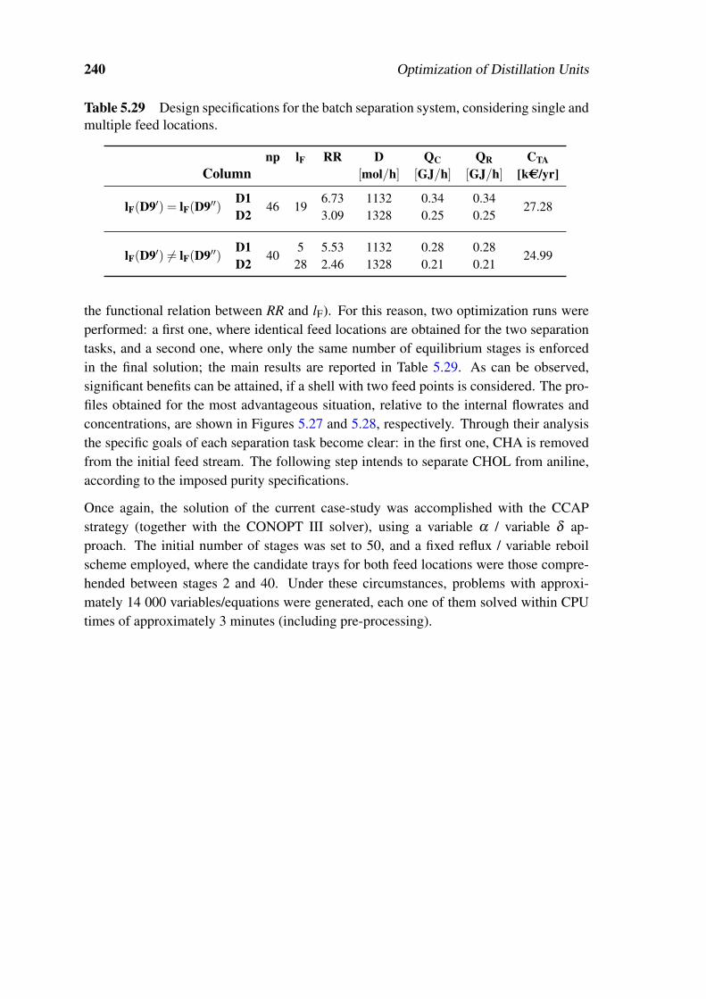
240 Optimization of Distillation Units
Table 5.29 Design specifications for the batch separation system, considering single andmultiple feed locations.
np lF RR D QC QR CTAColumn [mol/h] [GJ/h] [GJ/h] [kAC/yr]
lF(D9′) = lF(D9′′) D146 19
6.73 1132 0.34 0.3427.28
D2 3.09 1328 0.25 0.25
lF(D9′) 6= lF(D9′′) D140
5 5.53 1132 0.28 0.2824.99
D2 28 2.46 1328 0.21 0.21
the functional relation between RR and lF). For this reason, two optimization runs wereperformed: a first one, where identical feed locations are obtained for the two separationtasks, and a second one, where only the same number of equilibrium stages is enforcedin the final solution; the main results are reported in Table 5.29. As can be observed,significant benefits can be attained, if a shell with two feed points is considered. The pro-files obtained for the most advantageous situation, relative to the internal flowrates andconcentrations, are shown in Figures 5.27 and 5.28, respectively. Through their analysisthe specific goals of each separation task become clear: in the first one, CHA is removedfrom the initial feed stream. The following step intends to separate CHOL from aniline,according to the imposed purity specifications.
Once again, the solution of the current case-study was accomplished with the CCAPstrategy (together with the CONOPT III solver), using a variable α / variable δ ap-proach. The initial number of stages was set to 50, and a fixed reflux / variable reboilscheme employed, where the candidate trays for both feed locations were those compre-hended between stages 2 and 40. Under these circumstances, problems with approxi-mately 14 000 variables/equations were generated, each one of them solved within CPUtimes of approximately 3 minutes (including pre-processing).

5.5 Industrial case-studies 241
Total
Partial
Fresh
feed
Reserv.
CHA
CHOL
CHOL+ANL
ANL
Discontinuous Operation
First cycle
Second cycle
2500
F (mol/h) xFCHA
Fresh feed
0.010
Operational Specifications (regarding CHOL)
> 0.995
> 0.90(Second cycle )
0.5880.402
Total
Partial
Total
Partial
Continuous Operation
(approximation )
Column D9
Column D9' Column D9"
Fresh
feed
CHA
CHOL+ANL
CHOL
ANL
l (D9') =
Same feed
conditions
Same purity &
recovery restrictionsF l (D9F ")
np (D9') = (D9")np
Purity (destilate)
Recovery (destilate)
xFCHOL xF
ANL
•
•
Figure 5.26 Continuous approximation of the batch separation system in study.

242 Optimization of Distillation Units
0.85
0.95
1.05
1.15
1.25
1.35
1.45
1.55
1.65
1.75
1.85
1.95
2.05
2.15
1 6 11 16 21 26 31 36 41 46
Liquid (2nd cycle) Vapor (2nd cycle)
Liquid (1st cycle) Vapor (1st cycle)
Flo
wra
te (
norm
aliz
ed)
Stage
Figure 5.27 Optimal internal flowrates for the batch separation system.
0.0
0.1
0.2
0.3
0.4
0.5
0.6
0.7
0.8
0.9
1.0
1 6 11 16 21 26 31 36 41 46
Cha (2nd cycle) Chol (2nd cycle) Anil (2nd cycle)
Cha (1st cycle) Chol (1st cycle) Anil (1st cycle)
Conce
ntr
atio
n (
norm
aliz
ed)
Stage
Figure 5.28 Concentrations profiles for the batch separation system.

Chapter 6
Optimization of Distillation Networks
Summary
The goals of the present Chapter are centered in the development of an optimization strategy ori-ented for the synthesis of distillation networks, especially adapted for problems similar to theindustrial case-study considered, where the non-conventional nature of the involved units diffi-cults the use of the more classical strategies. The new methodology introduces a mathematicalapproach based on the decomposition of the original problem, replacing the use of MINLP / GDPformulations by the solution of a sequence of subproblems (NLP-MILP), that handles the unitoptimal designs and the network structure determination (and associated heat exchange policies)in separated programming phases. The application of this new strategy to an arrangement of ex-isting industrial units allowed the identification of heat integration schemes, already industriallyimplemented, generating savings of approximately 300 kAC/year. The root design of a new core forthe industrial process under study was also considered. The results obtained point to a new dis-tillation network capable of increasing the final product purity and consuming, for that purpose,a smaller amount of energy when compared with the current units, even when these last ones areenergetically integrated.
6.1 Optimization of blocks of separation units
For the same reasons presented in Chapter 5, due to the significant importance of dis-tillation columns in the industrial case-study considered, the following analysis will becentered on aspects that specifically regard this type of units.
6.1.1 Reaction versus separation
The optimization of arrangements of distillation columns shares many of the goals andchallenges involved in the synthesis of reaction networks (Smith and Pantelides, 1995),
243
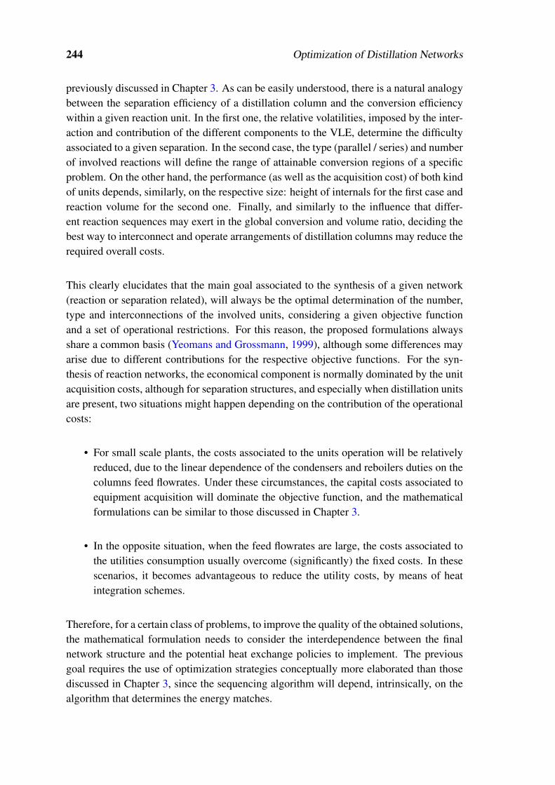
244 Optimization of Distillation Networks
previously discussed in Chapter 3. As can be easily understood, there is a natural analogybetween the separation efficiency of a distillation column and the conversion efficiencywithin a given reaction unit. In the first one, the relative volatilities, imposed by the inter-action and contribution of the different components to the VLE, determine the difficultyassociated to a given separation. In the second case, the type (parallel / series) and numberof involved reactions will define the range of attainable conversion regions of a specificproblem. On the other hand, the performance (as well as the acquisition cost) of both kindof units depends, similarly, on the respective size: height of internals for the first case andreaction volume for the second one. Finally, and similarly to the influence that differ-ent reaction sequences may exert in the global conversion and volume ratio, deciding thebest way to interconnect and operate arrangements of distillation columns may reduce therequired overall costs.
This clearly elucidates that the main goal associated to the synthesis of a given network(reaction or separation related), will always be the optimal determination of the number,type and interconnections of the involved units, considering a given objective functionand a set of operational restrictions. For this reason, the proposed formulations alwaysshare a common basis (Yeomans and Grossmann, 1999), although some differences mayarise due to different contributions for the respective objective functions. For the syn-thesis of reaction networks, the economical component is normally dominated by the unitacquisition costs, although for separation structures, and especially when distillation unitsare present, two situations might happen depending on the contribution of the operationalcosts:
• For small scale plants, the costs associated to the units operation will be relativelyreduced, due to the linear dependence of the condensers and reboilers duties on thecolumns feed flowrates. Under these circumstances, the capital costs associated toequipment acquisition will dominate the objective function, and the mathematicalformulations can be similar to those discussed in Chapter 3.
• In the opposite situation, when the feed flowrates are large, the costs associated tothe utilities consumption usually overcome (significantly) the fixed costs. In thesescenarios, it becomes advantageous to reduce the utility costs, by means of heatintegration schemes.
Therefore, for a certain class of problems, to improve the quality of the obtained solutions,the mathematical formulation needs to consider the interdependence between the finalnetwork structure and the potential heat exchange policies to implement. The previousgoal requires the use of optimization strategies conceptually more elaborated than thosediscussed in Chapter 3, since the sequencing algorithm will depend, intrinsically, on thealgorithm that determines the energy matches.

6.1 Optimization of blocks of separation units 245
6.1.2 Sequencing aspects
Identifying the best separation sequence for a given multi-component mixture has re-ceived significant attention since the earlier 1970s. A good review of the pioneer strate-gies (some of them based on heuristics) can be found in Nishida et al. (1981). Since then,and especially over the last two decades, several contributions allowed a significant im-provement of the proposed mathematical formulations, as well of the numerical schemesrequired for their solution.
Pure streams versus multi-component streams
The first systematic formulations suggested for the optimal sequencing of distillationcolumns considered a particular case of the more general problem (Westerberg, 1985).The main constraint consisted in the assumption that pure streams should be obtained forall components present in the feed stream. In other words, for a problem involving ncomponents, it would be obligatory to obtain n pure products.
With this purpose, the first strategies considered the use of distillation columns wherethe recovery of key components was necessarily total. Under these circumstances, theproblem formulation can be simplified, especially due to two main reasons:
• First, each column is supposed to generate a pure product. Therefore, only theremaining(s) stream(s) need to be subjected to a new separation task where, onceagain, a new component will be isolated. This procedure is propagated until nomulti-component streams remain, resulting in a branch expansion approach (Fig-ure 6.1).
• On the other hand, since within the considered units all light-key components (andthose lighter than them) are totally recovered in the distillate, and all heavy-keycomponents (and those heavier that them) are recovered in the bottom, obtainingsimplified models becomes easier.
As it will be later discussed, this last point deserves special attention, since the majorityof the proposed strategies try to avoid the original unit models. The reason for this pro-cedure is simple: these models, even in units with ideal VLE, are significantly nonlinearand may aggravate the vulnerability of the sequencing algorithm to local optima. To over-come this, the solution often relies on the use of simpler models capable of constitutinga good approximation of the original system of equations. Depending on the degree ofsimplification, it is possible to deal with problems characterized by variable linearity andprecision properties that will require, inclusively, different numerical solution schemes(Section 6.2).
The use of these simplified models (of minor scale and reduced non-linearity) allowedthe first approaches, based on the use of superstructures, to emerge (Andrecovich and

246 Optimization of Distillation Networks
A
B
C
D
B C D
B C D
A
C D
B C
DA
B C
D
B
C
1
1
5
2
2
A B
C D
A
B
C
D
10
8
A B C
D C
A BA
B
7 10
A B C
D
A
B C
B
C
3 8
4 9
6 9
“Branch” expansion:
Great number of columns
Sequential solution
Figure 6.1 Branch expansion of sequencing alternatives
Westerberg, 1985). As can be shown in Figure 6.2, the branch concept is eliminatedby introducing mixing and derivation points. These allow all units to be interconnected,thus sustaining a more compact problem formulation. The representation of Figure 6.2is also known as a State Task Network (STN) superstructure, since it is based on theconcept of separation tasks, and in the association of these last to different “dedicated”units (Grossmann et al., 2004).
It should be noticed that branch expansion approaches require a large number of units,due to the unavoidable repetition of some of them. However, each branch of Figure 6.1can be solved individually (considering a maximum of 3 units), while in Figure 6.2 thesimultaneous solution of the 10 units models is required. For this reason, if simplifiedmodels cannot be obtained, the use of superstructure based approaches can present seriousdifficulties.
To reduce the overall problem dimension (that might be considerable, even when simpli-fied models are used), a new strategy was developed, motivated by the work of Smith andPantelides (1995), known as the State Equipment Network (SEN) superstructure. In thisrepresentation (Figure 6.3) the “task” concept is replaced by the equipment concept. Asa result, and opposite to the STN approach, each column might correspond to differenttypes of separations, thus allowing a more compact formulation, since a minor numberof units is considered. Another consequence is that the process in which a given separa-

6.1 Optimization of blocks of separation units 247
1
2
3
4
5
6
7
8
9
10
A
B
C
D
B C D
A
D
B
C D
C
D
D
B C
B
C
A
B
A B C
A
C
A B
Superstructure:
Minor number of columns
Simultaneous solution
No recycle streams
Figure 6.2 STN superstructure for optimal sequencing.
tion task is attributed to a specific distillation unit must be described by the mathematicalmodel, thus requiring a more elaborated mathematical approach.
From a practical point of view, this procedure corresponds to the use of logical disjunc-tions that will allow the activation / inactivation of a given separation task, within a givenunit. Notice that all 10 units of Figure 6.2 can now be represented in a superstructurethat considers only 3 distillation columns. Although allowing smaller scale problems,this representation cannot avoid the vulnerability of the overall process to local optima,as will be latter discussed.
However, and apart of the adopted formulation, the previous optimal sequencing prob-lem can exhibit several disadvantages in the presence of byproducts (without commercialvalue) or when it is desired to obtain mixtures with pre-specified compositions (common,e.g., in the petrochemical industry). In these situations, it becomes necessary to con-sider the more general separation problem where, from a feed containing n components,m multi-component product streams are obtained (Figure 6.4). Due to the nature of thisnew problem, the use of the previously discussed approaches might become inappropri-ate. The main reason is related, essentially, to the separation efficiencies assumed withinthe units, as will be explained next.

248 Optimization of Distillation Networks
1 2 3
ABCD A B C D
A | B
A | BC
A | BCD
B | C
AB | C
AB | CD
B | CD
C | D
BC | D
ABC | D1
6
10
9
7
5
3
8
4
2
Figure 6.3 SEN superstructure for optimal sequencing.
P1
P2
A
B
C
D
OPTIMAL
n componentsm multicomponent
products
SEQUENCE
Figure 6.4 General separation sequencing problem.
Sharp versus non-sharp separations
When multi-component products must be obtained, the type of units previously consid-ered, that promote sharp separations, are poorly efficient. This is illustrated in Figure 6.5.As shown, to obtain the multi-component products of Figure 6.5, when the total recoveryof key components is imposed, two distillation units are required. On the other hand, if thedistribution of these components is allowed among the different exit streams, it becomespossible to fulfill all problem restrictions using only one column. Thus, considering non-sharp separations might be crucial, when determining the optimal number of units forthe general sequencing problem. Therefore, and considering that the multi-componentproducts of Figure 6.5 can be obtained by mixture of several streams, a new strategy wasintroduced (Aggarwal and Floudas, 1990). In this case, any separation sequence can besynthesized by means of a connecting superstructure, where the existence of non-sharpseparations plays a vital role (Figure 6.6).
A closer look at this Figure shows that all possibilities of stream fractioning, mixture

6.1 Optimization of blocks of separation units 249
10
10
10
2
9
6
8
1
4
A
B
C
A
BC
B
C
10 9
6
10 4
1
8
2
10
10
10
A
B
C
2
9
6
8
1
4
Sharp separations Non-sharp separation
Figure 6.5 Disadvantage of sharp separations (Aggarwal and Floudas, 1990).
1
2
3
A(B)
P1
P2
(A)BCD
AB(C)
(B)CD
ABC(D)
(C)D
Separation
1
2
3
Light-key Heavy-key
A
B
C
B
C
D
Figure 6.6 STN superstructure of non-sharp separations.

250 Optimization of Distillation Networks
and bypassing are present, similarly to that encountered in some of the representationsdiscussed in Chapter 3, for the optimal synthesis of reaction networks. Notice that Fig-ures 6.2, 6.3 and 6.6, although dealing with the same number of components, presenta fairly different number of initial units. The use of non-sharp separations can, there-fore, reduce the overall problem dimension, without requiring the introduction of logicaldisjunctions.
However, the use of mathematical approaches based on superstructures like the one rep-resented in Figure 6.6, cannot be generally elected as the best choice. Due to the fact ofconsidering non-sharp separations, these strategies require a large effort when construct-ing approximated models and sometimes, these tasks can be, inclusively, non-practical.In fact, when sharp separations are considered, the recovery of all involved componentsare unitary or null (depending of the exit stream that is taken as reference). In this situa-tion, correlating the operational costs (proportional to the reboiler and condenser duties)and the capital costs (proportional to the required number of stages), with different feedcompositions is relatively easy. On the other hand, when the possibility of componentdistribution is enabled, the respective recovery fractions may vary within a certain range,which can largely increase the required number of simulations and regression exercises,necessary to obtain representative simplified versions of the original models.
To summarize the main aspects of the optimal separation sequencing, the following guide-lines can be noted:
• When multi-component products are desired (the more general case), the use of for-mulations that consider non-sharp separations is vital, especially due to the impacton the quality of the obtained solutions.
• In a more specific case, where all product streams are pure in a given component,the use of non-sharp separation models can allow a more compact problem formu-lation, although it will always require a complex and demanding phase of modelsimplification.
• In the latter circumstances, the use of SEN based superstructures can be advanta-geous since it allows a reduction of the problem dimension and only requires sharpseparation models, more easily constructed.
• The strategies based on the branch expansion of all separation alternatives will onlybe competitive when two conditions are fulfilled. First, obtaining multi-componentproducts cannot be an objective and, second, the use of simplified models shouldbe difficult / impracticable. Only in these circumstances, where highly nonlinearlarge-scale models must be used, it is advantageous to consider the individual opti-mization of each branch; not only the problem is maintained in a minimal dimension(n− 1 columns in each branch) as the optimization of complex superstructures isavoided. This aspect can be decisive, due to the low efficiency of superstructureoptimization in the presence of highly non-convex large-scale problems.

6.1 Optimization of blocks of separation units 251
In fact, this last point deserves special attention. As will become clear along the followingSections, the developed optimization approach for the optimal synthesis of separationnetworks is substantially different from that implemented in Chapter 3. The optimizationof distillation sequences and of reaction networks, although sharing similar aspects, candiffer significantly on the type of involved mathematical models. For example, while themost complex case-study (an 8 reactors network) presented in Section 3.5.4 consideredaround 600 variables/equations, the model of a single distillation unit can comprehendup to 15 000 equations / variables (Section 5.5.2). Additionally, during the optimizationof distillation sequences, the number of involved choices is also higher (specially whenheat integration is pursued), increasing the combinatorial and non-convex nature of theproblem. This larger overall complexity of the resulting problems require, in practice,the adoption of decompositions / simplification methodologies, crucial to avoid solverfailures and/or poor quality solutions.
6.1.3 Integration aspects
The importance of energy integration studies was recognized long ago (Broeck, 1944),due to its major impact on the reduction of operational costs. In fact, the resulting eco-nomical savings can be so significant that often the viability of a given industrial processdepends directly on them. The main idea consists in reducing the external utilities con-sumption (that have significant acquisition / production costs) by means of heat exchangesbetween the process streams. Therefore, and since these energy matches can influence thestructure of the optimal separation network, the present Section will discuss some of themain concepts associated to this theme.
Preliminary process diagnosis
Nowadays, and after more than three decades since their introduction by Linnhoff, it isstill common to use graphical representations for the preliminary evaluation of a processenergy efficiency. Despite their usefulness, the previous graphical analysis has severallimitations, e.g., the minimum utility consumptions can only be evaluated if a minimumtemperature gradient (necessary to exchange heat between hot and colds streams) is previ-ously imposed. In other words, the consumptions determined are not necessarily optimal,since the overall procedure completely neglects the required capital investment necessaryto implement the energy matches (Linnhoff, 1981).
In a general manner, obtaining a feasible design for a heat exchangers network is rela-tively simple, but guaranteeing its global optimality is extremely difficult. In fact, twonetworks can fulfill the same ∆Tmin, exhibit the same utilities consumption and use thesame number of exchangers but, if the areas of each exchanger are not the same in bothsituations, their total annualized costs will differ. Therefore, and due to the non-convexity
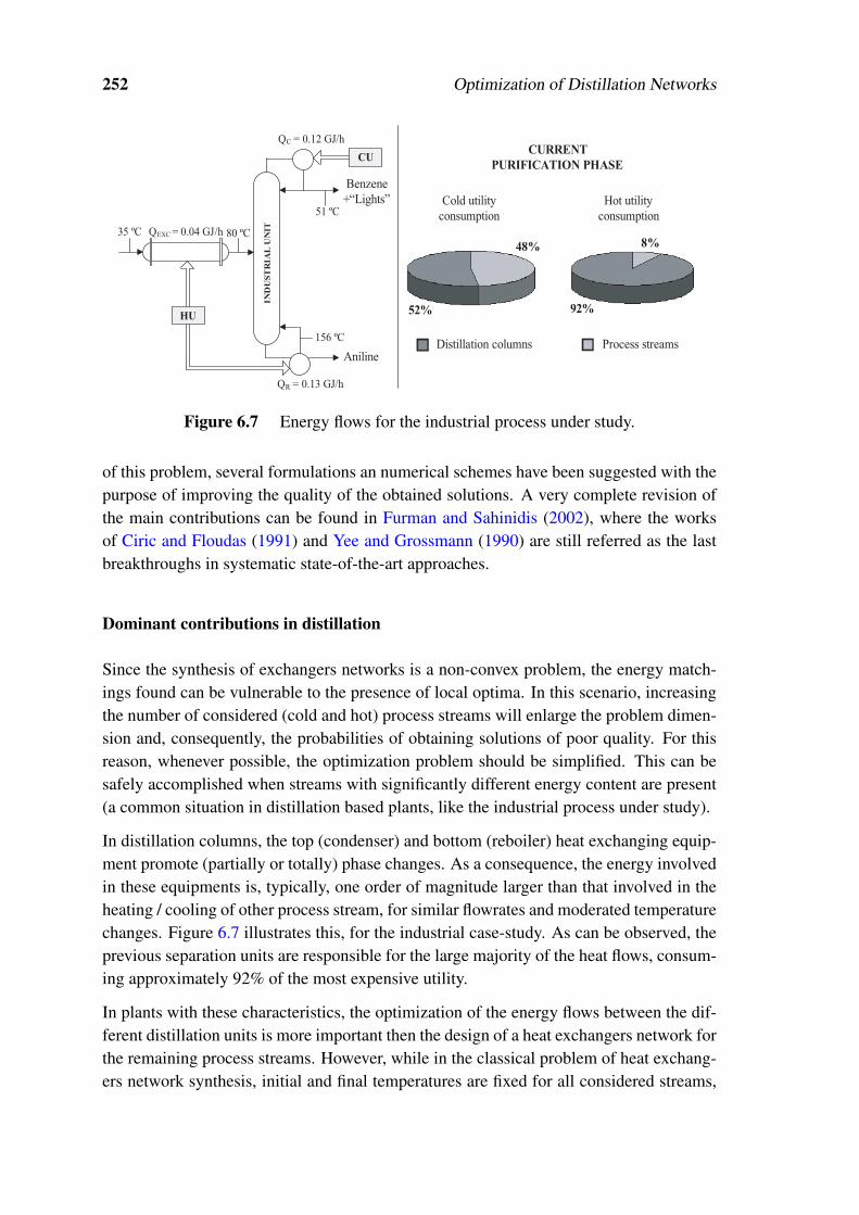
252 Optimization of Distillation Networks
HU
CU
IN
DU
ST
RIA
L U
NIT
35 ºC 80 ºC
51 ºC
156 ºC
QC = 0.12 GJ/h
QR = 0.13 GJ/h
QEXC = 0.04 GJ/h
Cold utility
consumption
Hot utility
consumption
Distillation columns Process streams
CURRENT
PURIFICATION PHASE
52%
48% 8%
92%
Benzene
+“Lights”
Aniline
Figure 6.7 Energy flows for the industrial process under study.
of this problem, several formulations an numerical schemes have been suggested with thepurpose of improving the quality of the obtained solutions. A very complete revision ofthe main contributions can be found in Furman and Sahinidis (2002), where the worksof Ciric and Floudas (1991) and Yee and Grossmann (1990) are still referred as the lastbreakthroughs in systematic state-of-the-art approaches.
Dominant contributions in distillation
Since the synthesis of exchangers networks is a non-convex problem, the energy match-ings found can be vulnerable to the presence of local optima. In this scenario, increasingthe number of considered (cold and hot) process streams will enlarge the problem dimen-sion and, consequently, the probabilities of obtaining solutions of poor quality. For thisreason, whenever possible, the optimization problem should be simplified. This can besafely accomplished when streams with significantly different energy content are present(a common situation in distillation based plants, like the industrial process under study).
In distillation columns, the top (condenser) and bottom (reboiler) heat exchanging equip-ment promote (partially or totally) phase changes. As a consequence, the energy involvedin these equipments is, typically, one order of magnitude larger than that involved in theheating / cooling of other process stream, for similar flowrates and moderated temperaturechanges. Figure 6.7 illustrates this, for the industrial case-study. As can be observed, theprevious separation units are responsible for the large majority of the heat flows, consum-ing approximately 92% of the most expensive utility.
In plants with these characteristics, the optimization of the energy flows between the dif-ferent distillation units is more important then the design of a heat exchangers network forthe remaining process streams. However, while in the classical problem of heat exchang-ers network synthesis, initial and final temperatures are fixed for all considered streams,
6.1 Optimization of blocks of separation units 253
A
B
C A
B
A
B
A
B
1A
2
multi-effectintegration
C
C
P2
P1
multi-taskintegration
1B
Figure 6.8 Multi-effect and multi-task integrations.
in the optimization of energy flows between distillation columns this rule should not beapplied. Instead, the top and bottom temperature of these units should be also optimized,to extend the maximum attainable energy efficiency of a given process.
Due to the complexity of this problem, and considering the larger heat flows around dis-tillation units, the synthesis of an exchanger network for the remaining process streamsis often considered separately. From a theoretical point of view, all streams (of fixedand variable temperature) can be simultaneously considered within the same optimizationproblem. However, due to the non-convexity of this last one, the probabilities of obtaininglocal optima would grow significantly, with clear disadvantages for the efficiency of theoverall procedure.
Before introducing the mathematical formulations proposed for the synthesis of heat in-tegrated separation sequences, it is important to analyze the different forms that can beused to maximize the energy efficiency of distillation based processes.
Heat integrated distillation schemes
Two of the most commonly implemented configurations, known as multi-effect and multi-task integrations, can be observed in Figure 6.8. The first one implies unfolding a specificseparation task (normally accomplished in one single column) in more than one unit, topromote heat exchange between a condenser and a reboiler (Biegler et al., 1997).
Because all “twin” columns that might be considered perform the same type of separation(AB/C), it becomes necessary to uneven their pressure to enable the heat exchange in themulti-effect integration. In essence, deciding which number of “twin” columns to use isanalogous to the problem of optimally designing an evaporator line: as the number of

254 Optimization of Distillation Networks
HU2
HU
QR,1
QR,2
THU
THU
CHU = €/ton
CHU = p €/ton
Side-reboiler Side-condenser
THU < THU ; p < p
CUQC,1
QC,2
TC,1
TC,2
QEXC
TEXC
2
1 2
2
1
1
1
2
1 2
p1
Figure 6.9 Advantages of side-condensers and side-reboilers.
effects grows, the energy savings achieved with the introduction of a new evaporator willbe successively reduced, contrary to the equipment acquisition costs (Perry and Green,1997).
In a multi-task integration, heat is exchanged between a condenser and a reboiler ofcolumns that undergo different separation tasks (condenser of A/B with reboiler of AB/C,in Figure 6.8). Sometimes, this energy matching can be feasible without changes in thecurrent operating pressures.
When the separation considers components with very distinct boiling points, the thermalgradient between the top and the bottom of a given distillation column will be very large.This situation is normally disadvantageous for heat integration purposes, since it reducesthe range of possible operating pressures. Introducing side-reboilers (Figure 6.9), a frac-tion of the heat is supplied at lower temperatures, allowing the consumption of hot utili-ties with reduced thermal levels that are, typically, less expensive (Aggarwal and Herron,1998; Aggarwal and Fidkowski, 1996). Similarly, a side-condenser allows to withdrawsome heat at higher temperatures, what can be very advantageous for heat integration pur-poses (since, in this situation, the side-condenser can act as an hot stream with increasedthermal level).
In addition to heat exchanging schemes among two different columns, it is possible toconsider more elaborated solutions, that allow the energy flow between the condenserand the reboiler of a same unit (HPC, 2006; Seider et al., 1999). In these systems, themain idea consists in withdrawing the heat at a low thermal level source (condenser) andsupplying it at a higher thermal level “sink” (reboiler). Obviously, this operation cannot bedone without a given extent of external work (as imposed by thermodynamic laws), thatwill tend to increase drastically for higher temperature differences between the energy

6.1 Optimization of blocks of separation units 255
Q2
P2
Q1
P2
P1 P1
bottom
expansion
valve
compressor
distillate
distillate
P1
P1
P2
bottom
Q2
Heat pump Vapour recompression
(work)
Figure 6.10 Heat pumps (closed and open-cycle).
“sink” and the energy source.
For this purpose, two main types of configurations are available: the Mechanical VaporRecompression systems (MVR) and closed-cycle heat pumps (Figure 6.10). In the firstones, also known as open-cycle heat pumps, the vapor stream that abandons the columntop is directly compressed, to supply its heat to the reboiler. After that, it suffers an ex-pansion and partially returns to the column, assuring the required liquid reflux. When thedirect compression is not possible, it is necessary to employ a closed-cycle where an ap-propriated fluid will suffer successive expansions (absorbing heat at a lower temperature)and compressions (releasing heat at higher temperatures), a configuration usually knownas a heat pump.
The use of MVR systems or closed-cycle heat pumps as a form of promoting heat ex-change between the top and the bottom of a same column is a mature technology, com-monly used in large-scale plants (HPC, 2006). In a different situation, and therefore muchmore experimental and under heavy development, is the configuration represented in Fig-ure 6.11. Although not yet encountered in industry, the underling concept of this kindof solutions is very ambitious and promising, which justifies the significant attention thatis currently dedicated to them (PSE, 2006). The main idea derives directly from the re-versible distillation principle (already discussed in Chapter 5) that, although reporting toan ideal and unattainable situation, can provide interesting guidelines on how to improvethe energy efficiency, namely relative to the benefits of exchanging heat along the column.
In fact, the configuration represented in Figure 6.11, also known as Heat Integrated Dis-tillation Column (HIDiC), intends to eliminate a significant handicap of MVR systemsand closed-cycle heat pumps that, due to the large costs (capital and operational) asso-ciated to the compression process, are only attractive when the temperature difference
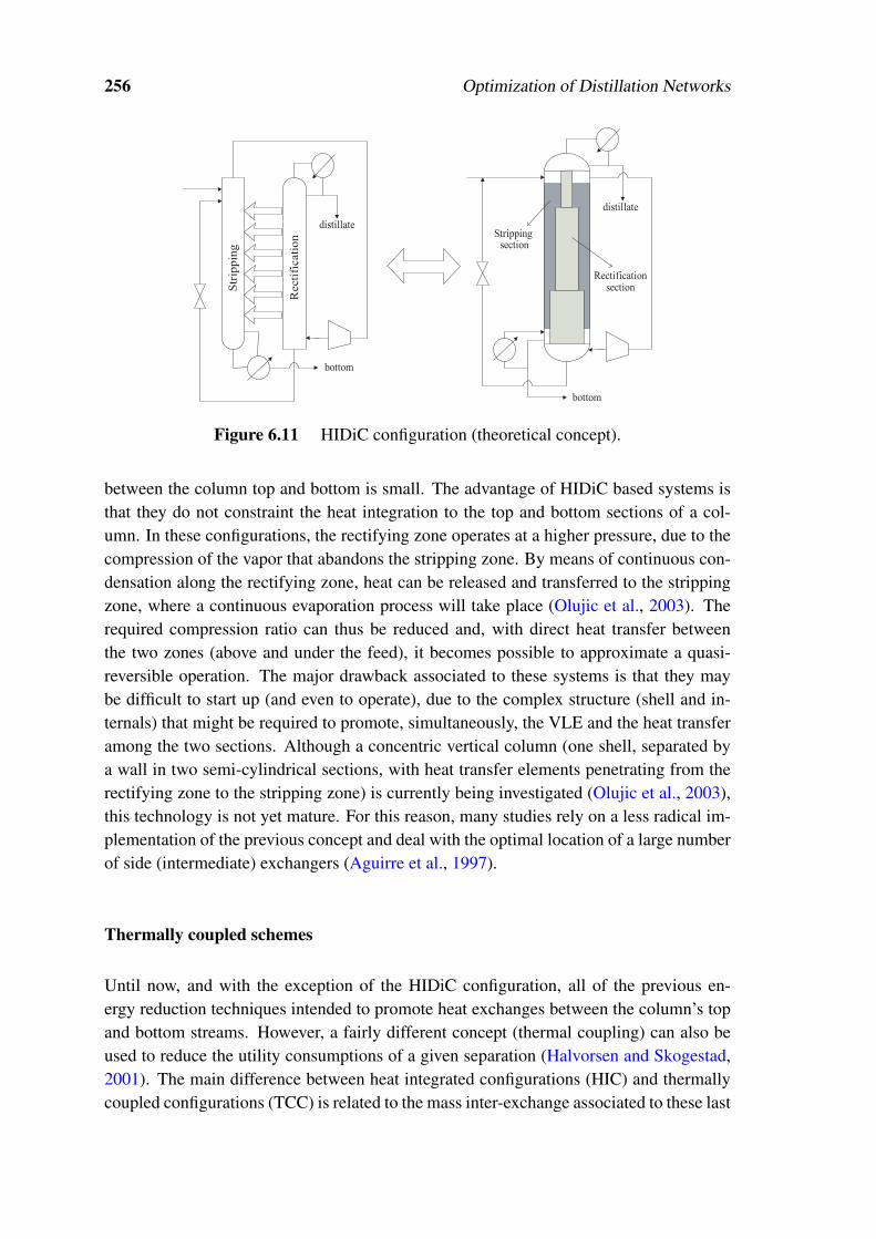
256 Optimization of Distillation Networks
Stripping
Rectification
distillate
bottom
distillate
bottom
Strippingsection
Rectificationsection
Figure 6.11 HIDiC configuration (theoretical concept).
between the column top and bottom is small. The advantage of HIDiC based systems isthat they do not constraint the heat integration to the top and bottom sections of a col-umn. In these configurations, the rectifying zone operates at a higher pressure, due to thecompression of the vapor that abandons the stripping zone. By means of continuous con-densation along the rectifying zone, heat can be released and transferred to the strippingzone, where a continuous evaporation process will take place (Olujic et al., 2003). Therequired compression ratio can thus be reduced and, with direct heat transfer betweenthe two zones (above and under the feed), it becomes possible to approximate a quasi-reversible operation. The major drawback associated to these systems is that they maybe difficult to start up (and even to operate), due to the complex structure (shell and in-ternals) that might be required to promote, simultaneously, the VLE and the heat transferamong the two sections. Although a concentric vertical column (one shell, separated bya wall in two semi-cylindrical sections, with heat transfer elements penetrating from therectifying zone to the stripping zone) is currently being investigated (Olujic et al., 2003),this technology is not yet mature. For this reason, many studies rely on a less radical im-plementation of the previous concept and deal with the optimal location of a large numberof side (intermediate) exchangers (Aguirre et al., 1997).
Thermally coupled schemes
Until now, and with the exception of the HIDiC configuration, all of the previous en-ergy reduction techniques intended to promote heat exchanges between the column’s topand bottom streams. However, a fairly different concept (thermal coupling) can also beused to reduce the utility consumptions of a given separation (Halvorsen and Skogestad,2001). The main difference between heat integrated configurations (HIC) and thermallycoupled configurations (TCC) is related to the mass inter-exchange associated to these last

6.1 Optimization of blocks of separation units 257
A
B
C
A
B
C
A
B
C
A
B
C
A
B
C
A
B
C
Side Rectifier Side Stripper Petlyuk column
Figure 6.12 Alternative configurations for thermal coupling.
ones. This key aspect is so important that allows the suppression of (at least) one heat ex-changing equipment (condenser or reboiler), as shown in Figure 6.12 for the ternary case.Therefore, and contrarily to the HIC, where investment costs (exchangers acquisition)must be increased to reduce energy consumption, the TCC solutions allow a simultane-ous reduction of both operational and capital costs. Their major drawback is related tothe maximum attainable energy efficiency that, for a ternary separation, will typically beinferior when compared to that of HIC (Annakou and Mizsey, 1996).
Another disadvantage commonly pointed to TCC is their supervision, that might presentincreased difficulties. Configurations like those represented in Figure 6.12 exhibit a stronginterdependence that exceeds the need to satisfy individual energy demands. In otherwords, although presenting two units, each configuration represented in Figure 6.12 be-haves like a single column, due to a high interdependency that prohibit individual analysis/ operation. This is particularly true for the Petlyuk arrangement (where two distinct sep-aration tasks can be accomplished with a single condenser / reboiler) that, some times, isimplemented as a Dividing Wall Column (DWC) — see Figure 6.13. In essence, a DWCconsists in a Petlyuk arrangement where two structures (internals or plates) are placedwithin a single shell (to reduce capital costs). This type of units was introduced morethen two decades ago and are, presently, a mature technology (Montz, 2006). Despitebeing thermodynamically more efficient, when compared to sequences of conventionalcolumns (Aggarwal and Fidkowski, 1998), thermally coupled configurations are not com-mon in industry, with the exception of the petrochemical branch, where the use of side-reboilers and side-strippers is quite often. This scenario may seem even more surprisingdue to the singular characteristics of a Petlyuk arrangement — the adiabatic configurationwith minor heat consumption, for a given ternary separation (Halvorsen and Skogestad,2001).
Although supervision details may contribute for the reduced industrial interest in this kindof systems, this reason, by itself, cannot justify the current reality. In fact, the major handi-
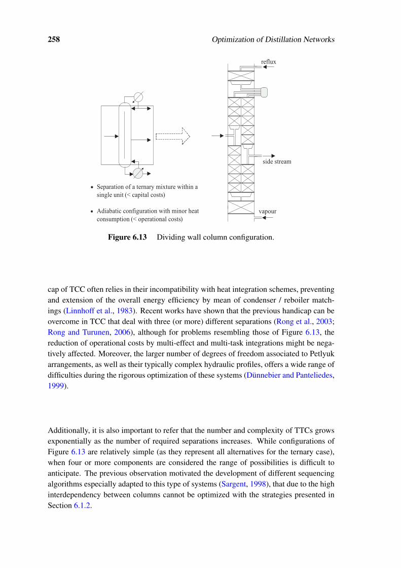
258 Optimization of Distillation Networks
reflux
vapour
side stream
Separation of a ternary mixture within a
single unit (< capital costs)
Adiabatic configuration with minor heat
consumption (< operational costs)
Figure 6.13 Dividing wall column configuration.
cap of TCC often relies in their incompatibility with heat integration schemes, preventingand extension of the overall energy efficiency by mean of condenser / reboiler match-ings (Linnhoff et al., 1983). Recent works have shown that the previous handicap can beovercome in TCC that deal with three (or more) different separations (Rong et al., 2003;Rong and Turunen, 2006), although for problems resembling those of Figure 6.13, thereduction of operational costs by multi-effect and multi-task integrations might be nega-tively affected. Moreover, the larger number of degrees of freedom associated to Petlyukarrangements, as well as their typically complex hydraulic profiles, offers a wide range ofdifficulties during the rigorous optimization of these systems (Dünnebier and Panteliedes,1999).
Additionally, it is also important to refer that the number and complexity of TTCs growsexponentially as the number of required separations increases. While configurations ofFigure 6.13 are relatively simple (as they represent all alternatives for the ternary case),when four or more components are considered the range of possibilities is difficult toanticipate. The previous observation motivated the development of different sequencingalgorithms especially adapted to this type of systems (Sargent, 1998), that due to the highinterdependency between columns cannot be optimized with the strategies presented inSection 6.1.2.
6.2 Synthesis of integrated sequences 259
6.2 Synthesis of integrated sequences
The following Sections will present the main available strategies for the simultaneoussolution of integrated distillation network structures, already including all heat exchangepolicies capable of minimizing the total annualized costs. Since thermally coupled con-figurations often require the use of different sequencing algorithms, they will not be con-sidered now. Their discussion will be latter resumed in Section 6.4.3.
Several strategies can be considered for the synthesis of heat integrated sequences, includ-ing different ranges of applicability and distinct numerical schemes. As will be shown inSection 6.3 all of the available formulations present advantages and drawbacks, and it isdifficult to generally elect the best mathematical approach. This will depend, intrinsically,on the nature and characteristics of the problem under study.
6.2.1 Methodologies based on MILP
The simplest strategy that can be used for the synthesis of integrated distillation networksconsiders, when determining the optimal structure, that identifying energy matches ismuch more important than individually designing each unit. Under these circumstances,the adopted model for each unit can be reduced to a set of linear equations that expressapproximated relations between the separation efficiency and the required duties (con-denser and reboiler). These approaches try to reduce the mathematical complexity of thesolution process, and therefore the influence of np and RR on the separation degree andenergy demand of each unit is not optimized during the network synthesis.
For the previous reason, these formulations are almost exclusively used in the less generalseparation problem, where all obtained streams need to be pure in a given component.Because each unit must promote a sharp separation, its efficiency is approximately fixed,and adequate np and RR can be fairly estimated in an independent step. Rigorously, thevalues calculated for the design parameters might not be optimal, since these should beobtained during the network synthesis. Nevertheless, because the separation efficiencies(and, consequently, also the feed conditions) associated to the columns are more or lessfixed, the previous estimates will always exhibit a good quality.
In this case, the problem can be decomposed in three distinct steps (Figure 6.14):
• Step 1: Optimally design each unit (np, RR, lF), considering its individual sepa-ration task (total recovery of key components). Extract linear relations capable ofeconomically evaluate the column’s existence / operation.
• Step 2: Considering the separation thermal gradients (calculated in the previousstep), determine all possible “effects” (twin columns) within a temperature rangevarying from TCU +∆Tmin until THU−∆Tmin.

260 Optimization of Distillation Networks
A
B
C
A | BC
AB | C
A | B
B | C
RR=?
l =?
np =?QC =?
QR =?
D =?
ΔT = ?
A | BC AB | C A | B B | C
STEP 1 STEP 2
THU
TCU
A
B
C
AB
C
AB
C
A
BC
B
C
A
B
A
B
A
B
STEP 3
A
A
A
A
B
B
B
B
C
C
C
inactive stream
active stream
heat exchange
utilities consumption
RCF
Figure 6.14 Main steps in MILP based strategies.
• Step 3: The linear relations (relative to mass balances and cost correlations) areincluded in a mathematical algorithm that will determine the type of separations,the number of effects to use, and all optimal mass and energy flows between theactive units:
min CTA = ∑k
[Ψ
k +G3,kCOLFk +CHU Qk
CU +CHU QkHU
]+∑
k∑m
m 6=k
CEC Qk,mEXC (6.1a)
s.t. Ψk ≥ G1,k
COL
[1+G2,k
COL
(T k
C −TCU−∆Tmin
TCU +∆Tmin
)]−Φ
k(
1−Y k)
(6.1b)
QkC−Gk
CFk = 0, QkR−Gk
RFk = 0, Fk−ΦkY k ≤ 0 (6.1c)
∑m
∑k
k 6=m
Qk,mEXC +Qk
CU = QkC, ∑
m∑k
k 6=m
Qk,mEXC +Qk
HU = QkR (6.1d)
T kR = T k
C +∆TRC, T kR ≤ THU−∆Tmin, T k
C ≥ TCU +∆Tmin (6.1e)

6.2 Synthesis of integrated sequences 261
Qk,mEXC−Ω
kZk,mEXC ≤ 0, T k
C ≥ T mR +∆Tmin−Λ
k,m(
1−Zk,mEXC
)(6.1f)
Fk,QkC,Qk
R,Ψk ≥ 0, Y k ∈ 0,1 k ∈ COL
Qk,mEXC ≥ 0, Zk,m
EXC ∈ 0,1 m,k ∈ COL,m 6= k
In Step 3, where all energy matching decisions are taken, it becomes necessary to in-clude a mathematical algorithm capable of dealing with the synthesis of heat exchangernetworks, as discussed in Section 6.1.3; for this purpose, equations (6.1a–6.1f) can beused. Equation (6.1a) represents the problem objective function, including both capitaland operational costs. To maintain a linear formulation, the first ones are approximatedby simple expressions1. Equation (6.1b) is used to ensure that the investment costs arecorrectly considered: notice that with Φk representing an upper limit on the column costs,if a given unit is active (Y k=1), Ψk will take the value of the equation right hand therm.On the other and, if the unit is not selected (Y k=0), the inequality becomes redundant and,considering that Ψk must be a positive number, this last one will be null. Expression (6.1c)translates, for a given separation, the relation between condensers / reboilers duties andthe units feed stream. Additionally, they also enforce that this latter should be null whenthe associated column is not active. Equations (6.1d) express the energy balances aroundeach column, while in (6.1e) all thermal gradients are declared and upper and lower limitsare imposed to the bottom and top temperatures of each column, considering the avail-able cold and hot utilities. Finally, equations (6.1f) are introduced to force, when a givenenergy match is selected (Zk,m
EXC=1), the condenser temperature of column k to be higherthat the reboiler temperature of column m. If a given match is not active, the first inequal-ity will imply a null exchanged heat (Qk,m
EXC=0) and the second inequality, relative to thetemperatures, will become redundant.
All of the above equations, together with simplified mass balance equations (based onsplit fractions, calculated in step 1), allow a linear formulation. However, it is clear thatthese procedures involve a certain precision sacrifice, namely relative to the evaluation ofinvestment costs. For example, the acquisition costs of heat exchangers do not considerthe thermal gradient between the intervening hot and cold streams; the exchange areacannot be calculated and, therefore, the equipment prices are only roughly estimated.
6.2.2 Methodologies based on MINLP
As discussed previously, in certain situations (sharp separations) it is reasonable to disso-ciate the unit design from the network structure synthesis (and respective energy matches).Nevertheless, in certain cases, it can be advantageous to promote non-sharp separations
1These are Ψk +G3,kCOLFk for the distillation units and CEC Qk,m
EXC for the exchangers.

262 Optimization of Distillation Networks
(Section 6.1.2). In these cases, predicting the best unit designs (and operation) in a pre-vious step is almost impossible, due to its dependence on the network structure. As aconsequence, both problems must be considered simultaneously or, in other words, in theseparation sequence the unit design parameters and all potential energy matches shouldbe determined in a single step.
On the other hand, and as also discussed in Section 6.1.2, the optimal design of distillationunits involves by itself significant challenges, and should be avoided during superstruc-tures optimization, especially when the VLE models are highly nonlinear. Therefore, andconsidering that the current problem is even more complex than those of Section 6.1.2(since it must determine optimal heat exchange policies), it becomes necessary once againto rely on simplifications of the original models 2.
The major difference is that simplified models of non-sharp separations need to expressthe influence of the design parameters (np, lF, RR) on the units performance (partial re-coveries of key components and energy demands) — a necessary step to improve thequality of the solutions. As a consequence, demanding data regression exercises needto be endeavored to obtain approximate relations capable of expressing the interdepen-dence between critical sets of variables. Equations (6.2a)–(6.4) clear illustrate this, whereG0,
COL, . . . ,G9,kCOL, G0
EC, . . . ,G6EC, G0,k
TC, . . . ,G5,kTC, . . . ,G0,k
QR, . . . ,G5,kQR are regression parame-
ters, obtained through a number of previous simulations (Aggarwal and Floudas, 1992):
min CTA = [CCOL +CEC +COPE] (6.2a)
CCOL = ∑k
(G0,k
COL +G1,kCOL rk
lk +G2,kCOL rk
hk +∑n
G3,n,kCOL xn,k +G4,k
COL Pk)
Y k+
+∑k
(G5,k
COL +G6,kCOL rk
lk +G7,kCOL rk
hk +∑n
G8,n,kCOL xn,k +G9,k
COL Pk)
Fk (6.2b)
CEC = ∑k
∑m
m6=k
G0ECZk,m
EXC +G1EC
Qk,m
EXC
UEXC(T k
C −T mR)+
+∑k
G3EC Zk
CU +G4EC
Qk
CU
UC(T k
C −TCU)+
+∑k
G5EC Zk
HU +G6EC
Qk
HU
UR(THU−T k
R) (6.2c)
COPE = ∑k
(CCU Qk
UF +CHU QkHU
)(6.2d)
2Notice the analogy between this procedure and that of Figure 6.14, since both comprehend a decom-position of the original problem to break its complexity.

6.2 Synthesis of integrated sequences 263
T kC = G0,k
TC +G1, jTC rk
lk +G2, jTC rk
hk +∑n
G3,n,kTC xn,k +G4,k
TC Pk+G5,kTC
(Pk)2
(6.3)
QkR =
(G0,k
QR +G1,kQR rk
lk +G2,kQR rk
hk +∑n
G3,n,kQR xn,k+G4,k
QR Pk +G5,kQR
(Pk)2)
Fk (6.4)
In this type of approaches it becomes necessary to consider the units top and bottomtemperatures as functions of the “light” and “heavy” key components recoveries. Thesame observation is also true for the condensers and reboiler duties and for the investmentrelated to the acquisition of distillation units. The capital costs associated to heat exchang-ing equipments can also be more accurately evaluated as a function of Qk,m
EXC/(T kC −T m
R ),Qk
CU/(T kC −TCU) or Qk
HU/(THU−T kREB), since the use of nonlinear expressions is not pro-
hibitive. Notice that equations (6.2a)–(6.4) do not represent all of the necessary dataregression exercises. Their purpose is illustrative and only intends to give an idea aboutthe major differences, from a mathematical point of view, between MILP and MINLPbased formulations, when these last ones consider non-sharp separations.
Another consequence derived from the use of MINLP formulations for the synthesis ofheat integrated separation networks, regards the necessary numerical schemes. From aconceptual point a view the mathematical formulation, used for energy matching, can besimilar to that discussed for the MIP based strategies, if a STN representation is con-sidered. However, the nonlinear terms that allow a more flexible and rigorous approachalso imply, on the other hand, a more complex solution process. To better illustrate this,Figure 6.15 is presented. It intends to elucidate the differences, at a superstructure level,between the problem reported in Figure 6.6 and the current one, where the optimizationof heat exchange policies is also an objective. Therefore, column II of Figure 6.15 is anal-ogous to column II of Figure 6.6 and partially represents an STN approach, where eachcolumn undergoes a single separation task and where each exchanger assumes only onetype of heat matching.
As can be observed, when three non-sharp separations are considered an equal numberof condensers (reboilers) is initially associated to each column. The first condenser (re-boiler) exchanges heat exclusively with a cold (hot) utility source, while the second andthird exchangers promote energy flows between the column to which they belong andthe two remaining units, respectively. With this type of representation, the exchangersnetwork synthesis can be translated by equations structurally similar to those in (6.1b–6.1f), although special solution algorithms will be required, since a linear formulationcannot be maintained. These should be particularly adapted to the problem’s nature tominimize difficulties that typically arise during the use of discrete solution schemes onnonlinear and non-convex problems. One of the characteristics of these algorithms is,often, the use of a problem decomposition procedure, as represented in Figure 6.15. Themethodology shown, proposed by Aggarwal and Floudas (1992), is a good example of theprevious remark, since it deals with the network structure synthesis and with the energymatch optimization, in separated steps. Thus it is possible to reduce the non-linearity of

264 Optimization of Distillation Networks
Q 1,2
Product 1
Product 2
Colu
mn 2
Column 3
Product 1
Column 1
Product 2
Column 3
Column 1
Feed (fresh)
Outside Loop
Inside Loop
Network structure optimization
Fixed heat exchange policies
Energetic matching
optimization
HU QEXC
3,2Q
EXC
QCU
2,1Q
EXC
2,3Q
EXC
Figure 6.15 Possible MINLP formulation (and solution scheme).
both subproblems (since some variables will be fixed on each one), thus improving thechances of obtaining solutions of better quality.
6.2.3 Methodologies based on GDP
In situations were the use of non-sharp models cannot be avoided, the main differencesbetween GDP and MINLP formulations are not due to the effort that is required to buildapproximated models, since the procedure (data regression) is similar in both cases. In-stead, the main difference relates to the type of adopted representation. This last one isthe basis of the decision process and present a major impact on the required numericalschemes, independently of the type of separation models considered.
To illustrate this difference, Figure 6.16 shows a SEN representation for the synthesis ofintegrated sharp separation sequences, where each column may undergo a different sepa-ration task and where each exchanger may assume distinct energy matches. For example,column I may promote the separation A|BC or separation AB|C; analogously, exchanger Imay assure heat exchange between the condenser of column I and the reboiler of col-umn II or between the reboiler of column I and the condenser of column II. These SENrepresentations allow a reduction on the number of separation and heat exchanging unitsthat must be initially considered in the superstructure, although requiring the introduc-tion of logical disjunctions. These are necessary to enable / disable a given task in a givenequipment and share the basic structure of equations (6.5a–6.5c) that, although simplified,

6.2 Synthesis of integrated sequences 265
A
B
C
A
CC
olu
mn
1C
olu
mn
2
A | BC
- ou -
AB | C
B | C
- ou -
A | B
A ou B
B ou C
HU
CU
Exchanger 1
Exchanger 3
Exchanger 4
Exchanger 2
MassEnergy
Figure 6.16 GDP based formulation (SEN representation).
are still adequate for illustrative purposes:
T tC = T t
R +∆T tRC (6.5a)
Y t,k
Ψk = G1,tCOL
[1+G2,t
COL
(T k
C−TCU−∆TminTCU+∆Tmin
)]Qk
C = GtCFk∧Qk
R = GtRFk
T kC = T t
C∧T kR = T t
R
∨¬Y t,k
Ψk = 0Qk
C = 0∧QkR = 0
T kC = 0∧T k
R = 0
(6.5b)
W e Ze,k,m
EXCQe = Qk,m
EXCT k
C ≥ T mR +∆Tmin
∨ Ze,k
CUQe = Qk
CUT k
C ≥ TUF +∆Tmin
∨ Ze,k
HUQe = Qk
HUTHU ≥ T k
R +∆Tmin
∨[¬W e
Qe = 0
] (6.5c)
W e, Y t,k, Ze,k,mEXC , Ze,k
CU, Ze,kHU ∈ True, False (6.5d)
Equation (6.5a) impose the thermal gradients, characteristic of each different separationtask, while (6.5b) allows the attribution (or not) of this last one to a given unit k, by meansof a boolean variable Y t,k. If a separation t is activated in a column k (Y t,k=True), equa-tions (6.5b) will also enforce the respective energy balances to be verified and the relatedcosts (necessary equipment) to be considered. If not (Y t,k=False), the match separa-

266 Optimization of Distillation Networks
tion t / column k will be disabled and the disjunction right-hand term will consider allcapital (column total cost) and operational (condenser and reboiler duties) costs to be null.
On the other hand, (6.5c) comprehends a set of disjunctions to describe all possibilitiesof satisfy the superstructure energy demands, considering a set of exchangers that cananalogously undergo different heat trading policies.
6.3 Complex large-scale processes
After describing the main available strategies for the synthesis of heat integrated sepa-ration networks, we consider now their main advantages and drawbacks, as well as thedifficulties that they might exhibit in the presence of non-conventional problems, similarto the industrial case-study.
6.3.1 Limitations of the classical formulations
When the optimization of energy matches is also an objective, the synthesis of separationnetworks requires more elaborated formulations. However, the guidelines presented atthe end of Section 6.1.2 can still be considered to analyze the weaknesses and strengthsof all strategies in general.
At first sight, it is possible to point versatility as the major difference between MILP (thatdo not consider non-sharp separations) and GDP / MINLP approaches, since the last canbe used without restrictions. However, a closer look shows that this assumption might bedangerous, since GDP / MINLP strategies are also limited in their range of applicability,as will be discussed latter.
Because of their restrictions in the types of separations considered, MILP strategies are of-ten adopted as pre-processing phases of MINLP / GDP formulations. The results obtainedby means of very simple (sharp) models can therefore be used as initialization points formore general (non-sharp) problems, to improve the quality of the final solutions.
MINLP and GDP based strategies also present some disadvantages and, as already in-troduced, their vulnerability to local optima requires special attention. Since the pro-gramming phase that determines the network structure (and related energy matches) nowinvolves nonlinear expressions, it is possible to obtain final solutions of poor quality. Al-though the use of GDP strategies may reduce some of the difficulties associated to thesolution of discrete nonlinear problems, their efficiency will always depend on lineariza-tion procedures (Section 5.4) that can be very problematic in some situations. This facthas motivated many works, especially dedicated to the improvement of initialization pro-cedures and solution algorithms for this class of problems. A good example is the work

6.3 Complex large-scale processes 267
of Yeomans and Grossmann (2000a) that recognizes the extreme difficulties that typi-cally arise when dealing with the original distillation models, even when these are weaklynonlinear. Instead of building approximate models, these authors suggest the use of theoriginal system of equations inside an iterative procedure that, once more, is based on adecomposition of the problem.
With this approach, the synthesis of a network structure is separated from the optimaldesign of the units: in a first subproblem, a set of disjunctions will allow the selection ofactive columns (or sections of these), while in a second subproblem the use of anotherGDP formulation will optimize the number of equilibrium stages (and remaining operat-ing variables) of the non-eliminated units. The goal consists in reducing the complexityof the original problem, breaking it in two subproblems that will be solved in differentprogramming steps. This concept is the key to reduce a large number of problems andcan also be found in other works, in different application fields (Section 4.4 is an exam-ple). Nevertheless, according to Yeomans and Grossmann (2000a), even with this typeof procedure developed for the sequencing of thermally coupled columns (when energymatching is not considered), the numerical difficulties can be significant for units exhibit-ing strongly non-ideal VLE. In other words, the goal of avoiding approximate models(data regression procedure) could only be accomplished, until the present date, for prob-lems where the original mathematical models are not too complex.
After discussing the relative advantages and drawbacks of classical formulations, it isimportant to analyze the difficulties that might arise when trying to use these latter innon-conventional problems, characterized by the existence of a large number of vestigialbyproducts with crucial importance for a set of purity restrictions.
Although theoretically applicable to any kind of problem (when using regression models)MILP / GDP strategies can exhibit several implementation problems for certain specialapplications. The underlying reason relates precisely to the method of deriving these ap-proximated models. The data regression exercises try to establish an equilibrium betweenthe required computational effort (the number of simulations needed to correlate the re-sults) and their intrinsic precision (that will define a region where the approximation isvalid). However, from a practical point of view, the flexibility of these models is alsolimited due to the amount of effort required by the regression exercise. In fact, whencorrelating key variables, it is obligatory to assume that the distribution of non-key com-ponents does not occur (Aggarwal and Floudas, 1992). Once the light-key and heavy-keycomponents are decided, a certain number of simulations is performed to correlate RR andnp with the separation degree (among other variables, as previously explained), althoughthis procedure will stop when the first component lighter then the light-key, or the firstcomponent heavier then the heavy-key, starts to distribute among the unit exit streams.
The reason why this restriction is introduced is simple: correlating the distribution de-gree of all non-key components, among themselves and with the design parameters of theunits, would require an extremely large number of simulations and a very complex regres-

268 Optimization of Distillation Networks
sion exercise. This procedure could generate, inclusively, a very complex approximatedmodel, almost as nonlinear as the original one and offering the same kind of problemsthat were intended to be avoided.
However, the previous limitation is non-restrictive for a large number of problems andregression models can be adopted without harming the optimization procedure:
• When distillation columns promote separations where the recovery of key-componentsis practically complete.
• When, although the distribution of non-key components occurs, the extent of thisone is reduced and does not have a direct impact on the constraints of the problem.
Although common, both of these situations may not occur in certain processes (like theone under study) and additional implementation problems can arise. By analyzing theresults obtained for column D1 (Figure 4.4 and Table 4.1), it is possible to observe that:
• It is difficult to define key-components in certain units. The rules for selecting theseindicate that they should be present in a significant amount (>10%), in the columnfeed stream (Seider et al., 1999). Through analysis of column D4 (its feed is givenby the bottom product of column D1), it is easy to verify that only aniline fulfill thisrequirement.
• Most of the light byproducts in unit D1 (with higher boiling point than aniline) aredistributed among the column top and bottom streams; this causes a certain fractionof these byproducts to pass to the next unit. Additionally, this situation should notbe avoided, since the complete removal of these components in the top stream ofunit D1 would imply increased operational costs that are not compensated by alarger product purity (that is not economically valued) in unit D4.
• The distribution of these light byproducts, in the bottom stream of unit D1, al-though occurring in a small extent, cannot be neglected. The tight contaminationrestrictions (Table 4.9) require the careful consideration of all vestigial traces ofany byproduct. In other words, monitoring these components along the process iscrucial, and their degree of distribution among the different exit streams is of majorimportance.
For these reasons, obtaining approximate models can be difficult in some situations. Thismotivated the development of a new strategy, especially adapted to industrial processessimilar to that under study.
6.3.2 Developed strategy
Considering all the theoretical aspects previously introduced, a new strategy was devel-oped congregating three main characteristics:

6.3 Complex large-scale processes 269
• Heat integration aspects, when determining the optimal separation structure. Theimportance of this aspect can be easily understood by noticing the high flowratesof the process under study, that will cause investment costs to be dominated byoperational ones.
• A decomposition of the original problem, as most of the previously proposed strate-gies. This should enable separated programming phases, dealing with subprob-lems of reduced complexity, and avoid a set of numerical difficulties that typicallyemerge for large-scale non-ideal models.
• Avoiding the use of approximated models that could require complex data regres-sion exercises or even, for some units, be impossible to obtain due to the non-conventional nature of the considered industrial problem.
Therefore, this strategy implements a somewhat pragmatic approach, especially built toovercome the difficulties offered by the non-conventional process under study. Neverthe-less, it can also be advantageous for other problems exhibiting similar characteristics.
Definition of pseudo-components
Often, a given problem includes a large number of components that can be significantlyreduced by analysis of their relative importance, considering the goals of the optimizationprocedure. Thus, it is possible to distinguish two different sets of components:
• A main set, presenting an important contribution for the problem objective function.
• A secondary set that, although relevant for some problem constraints, is not part ofany specific objective (or has a relevance that is comparatively reduced).
This secondary set of components can be easily illustrated by the common occurrence ofthe following two situations:
• Situation A: when certain byproducts are considered secondary species that do notpresent any economical value. In this case, obtaining product streams rich on thesecomponents does not make sense, and this should be considered in order to simplifythe sequencing algorithm.
• Situation B: when certain components economically valued are present in reducedquantities (vestigial compositions, when compared to the set of main species). Here,giving the same importance to both sets of components may be disadvantageouswhen designing a separation network. It would be wiser to approach both problemsseparately, to avoid a more complex formulation that, due to the phenomena oflocal optima, might favor a good solution for the secondary set, neglecting the muchgreater importance of the main one.

270 Optimization of Distillation Networks
A, B, C, D, E,
F, G, H, I
A, B, C
D, E
F,G, H, I
Pseudo-Light (PL)
Pseudo-Heavy (PP)
Pseudo-Intermediate (PI)
A, B, C,
PI
D, E, F,
PL,
High
Importance
Moderated
Importance
Negligible
lmportance
A
B
C
PI
D
E
PL
Secondary Problem
(to be solved after the main one)
PP
PP
Figure 6.17 Reduction of problem complexity by definition of pseudo-components.
If possible, in any of these previous situations, it would be advantageous to group setsof secondary components with adjacent volatilities, treating them as pseudo-components.Depending on the problem nature, this procedure may reduce significantly the complexityof the required mathematical formulation, due to a smaller number of species considered(Figure 6.17).
Components A, B and C of Figure 6.17 are present in vestigial concentrations, althoughtheir economical value cannot be neglected (situation A). Components D and E presentthemselves in significant quantities and are both considered as products of high commer-cial value. Components F , G, H and I have also representative concentrations but, froma commercial point of view, they are not interesting. Therefore, only rich streams ofcomponents A, B, C, D and E must be obtained, and considering that all of them havesimilar economical value and that components D and E are present in far larger amount,the sequencing problem can be reformulated as shown.
As illustrated, the primary goal of obtaining rich streams on the two main components(D and E) can be approached by converting a large problem, initially involving 9 species,into a “pseudo-quaternary” one, of simpler solution: components D and E will be seenas species of intermediate boiling points, contaminated by two pseudo-components (one“lighter” and another “heavier”). Under these circumstances, the problem may be solvedconsidering a tree expansion, since the number of involved branches is small and theuse of superstructure based formulations does not present significant advantages (Sec-tion 6.1.2).

6.3 Complex large-scale processes 271
The last aspect that needs to be considered relates to the fact that tree expansion strate-gies are only adequate when distillation units promote sharp-separations; this is relativelyuncommon in the industrial practice, though. However, as will be discussed, for certainproblems this “limitation” can be overcome by adopting a special solution procedure.
Decomposition NLP-MILP
As previously described, distillation columns often involve non-sharp separations, sinceit is very difficult to avoid the distribution of light and heavy components in the bottomand top streams. Here, two situations should be distinguished:
• Processes that, although involving non-sharp separations, are intended to producemulti-component streams almost totally constituted by a single species (the compo-nent distribution only occur in a very reduced extent).
• Processes that are intended to obtain specific multi-component products where sev-eral species will assume representative compositions.
The first situation is much more common in the chemical industry, where most commer-cialized products (commodities and specialities) are characterized by a high purity. Con-sidering that the system represented in Figure 6.17 fits this situation, the “new” resultingproblem (after defining pseudo-components) continues to involve only sharp separations.Notice that all species (including pseudo ones) still need to be isolated in the form of purestreams:
• Streams of D and E, of high purity, for commercial purposes.
• A stream of light pseudo-component, containing minor quantities of D and E, sincethe presence of large quantities of these would imply a subsequent recovery stepinvolving recycle streams and additional costs. Moreover, the commercial specifi-cations for each of the secondary products will have to obey, most certainly, highpurity constraints not compatible with contamination in D and E (that will behaveas unwanted species, when designing a byproduct purification network).
• A stream of heavy pseudo-component, also as pure as possible, since these species(without economical value) will follow, in general, to an effluent treating stage.Therefore, if any significant quantities of D and E are present, they must be recov-ered, with all the disadvantages previously referred.
Although similar to a sharp separation problem, after the pseudo-component reformula-tion, the total recovery of all components will certainly be impractical, from an economi-cal point of view. The degree of component distribution within the units can therefore beimportant, especially if strict purity restrictions are considered. Since these are defined forreal species (and not pseudo-components), the suggested mathematical approach includesboth situations, with real and pseudo components:

272 Optimization of Distillation Networks
Step 1: Generate all sequencing possibilities (by tree expansion), considering a pseudo-component analysis. Treat all intervening units of a given branch using a real-component approach, selecting a set of adequate methods for the estimation ofnpmax and RRmin. Optimize individually each branch (considering all purity con-straints) using the continuous formulation developed in Section 5.3, for the simulta-neous root design of all intervening units. At the end of this step it will be possibleto obtain, for each branch, all rigorous design parameters that minimize the totalannualized costs, in a situation where no heat integration schemes are used.
Step 2: Use the results obtained in the previous step to generate, for all units of eachbranch, a set of linear expressions that correlate the critical variables (capital / oper-ation costs, condenser / reboiler temperatures and duties) with the units feed condi-tions (flowrates and compositions). Use these simplified relations, together with amathematical formulation similar to that of Section 6.2.1, to identify in each branchand in a pseudo-component approach, the best heat exchange policies (e.g., energymatches between condensers and reboilers). The main goal of this step is thereforeto approximately evaluate where it would be advantageous to invest in equipment(exchangers and / or twin columns) to reduce the utility consumptions and extendthe minimization of the total annualized costs. Notice that these linear relations ex-press a certain separation efficiency for each column, that will be fixed in this step.This efficiency cannot be considered variable because it would be impossible toavoid nonlinear relations and, on the other hand, when using pseudo-components,the impact of the separation degree on the product specifications (that relate to realcomponents) cannot be predicted.
Step 3: Consider the heat exchange polices (and additional twin columns, if selected)identified in the previous step. Include a new set of constraints, in the Step 1 for-mulation (for each branch), that will rigorously account certain aspects related withthe industrial implementation of energy matching (necessity of QC > QR and TC >TR, capital / operation costs of twin columns, heat exchanging and pressure manip-ulation costs). Solve the modified NLP problem of Step 1, considering, again, thesimultaneous optimal design of all intervening units in each branch. The outcomeof this last step will include all the decisions and design parameters that allow, ineach branch, the minimization of the problem objective function, in a situation ofincreased energy efficiency (when compared to Step 1).
Notice that, although not yet referred, the inclusion of MVR and heat pumps, in Step 2 ofthe proposed procedure, is relatively simple. This kind of systems can be approached asa conventional unit where the condenser and reboiler duties are practically null (sincethe energy of the top vapor stream is released in the bottom of the unit), due to theacquisition of specific equipment (compressor) and by performing a certain amount ofwork (to generate the required temperature gradient). Therefore, it is only necessary toinclude simplified expressions to predict (approximately) the additional investment and
6.3 Complex large-scale processes 273
operational costs, associated to the units where these special heat integration schemes areimplemented.
At last, it is also important to refer that, from a theoretical point of view, only the branch(and respective heat exchange policy) identified in Step 2 as the most favorable should berigorously optimized in Step 3. However, in practice, this decision may carry some risks,and it is advisable to rigorously optimize all alternatives that, in Step 2, present objectivefunction values similar to the best obtained. This cautious procedure intends to “compen-sate” some of the lack of precision in Step 2, caused by two introduced simplifications:
• Firstly, the linear relations used in Step 2 for determining the best heat exchangepolicies are obtained by solving a problem where all energy excesses / deficits arecompensated by external utilities consumption (cold and hot). Therefore, and con-sidering that some units may not operate, rigorously, a sharp separation, all theprevious simplified relations only express a possible manner of fulfilling the con-straints of the problem. In other words, it is possible to consider design parameters(different from those obtained in Step 1) that express other separation efficiencies.These will correspond to alternative equilibria between capital and operation costsand may originate slightly different objective function values in Step 2.
• On the other hand, because it is desired to maintain a linear formulation in Step 2,it is impossible to rigorously consider the capital costs involved in the implemen-tation of energy matching schemes (e.g., a precise calculation of exchange areasis impossible), or the variation of the condenser / reboiler duties with the columnpressure. This is only accomplished in Step 3, where the use of rigorous nonlinearrelations is used to yield a final accurate solution.
Using this approach, the objective function values obtained in Step 2 will always be im-precise. In can be argued that, in relative terms, the difference between the values obtainedin Step 2 and Step 3 is typically reduced since:
• Considering heat integration schemes will never radically affect the optimal de-sign of the units. Although the reduction of operational costs, consequence of anhigher energy efficiency, might affect the optimal separation degree and the columnphysical structure, this influence cannot be significant. In other words, the optimaldesign, in the absence of energy matching, will not be greatly disadvantageous forheat integration.
• It is possible to obtain good estimates of the operational (pressure manipulation)and capital (units, exchangers and compressors acquisition) costs, if proper consid-erations are taken.
However, it is impossible to guarantee that a given alternative, identified as the most ad-vantageous in Step 2, will definitively be the optimal solution. Therefore, all alternativesexhibiting a similar objective function value should be rigorously optimized in Step 3.

274 Optimization of Distillation Networks
This procedure does not intend to generally replace the classical strategies presented inliterature. The adopted solution scheme always needs to be adapted to the nature andcharacteristics of the problem under study. Therefore, in situations where the units VLEis ideal and the resulting mathematical models are small and weakly nonlinear, it maybecome possible to apply directly GDP strategies, without having to consider approximatemodels. On the other hand, if the VLE is non-ideal and large-scale conventional modelsare considered, MINLP / GDP strategies together with data regression exercises may be avalid alternative.
For the optimization of processes similar to that under study, characterized by a highcomplexity and a non-conventional nature, the new methodology presents the advantageof decomposing the original problem in a sequence of subproblems (NLP-MIP-NLP),without having to deal with demanding data regression phases, that can be problematic oreven impractical.
The generally accepted idea is that the use of regression models constitutes a good trade-off, since they are more flexible and precise than MILP strategies and, on the other hand,avoid the use of the original large-scale non-ideal models (and their respective numericaldifficulties). Therefore, it is implicitly assumed that the precision sacrifice, related to theuse of approximate models, will not affect the unit optimal design and the quality of theobtained solutions
On the other hand, the proposed strategy relies on a very distinct assumption, that obtain-ing regression models can imply serious disadvantages and be very limiting. Under thesecircumstances, the best procedure is to consider two separated decision phases, avoidingnonlinear discrete formulations:
• A phase related to the optimal (and simultaneous) design of all intervening units.This can be considered separately, for each branch, using especially adapted con-tinuous formulations, capable of dealing with large-scale highly nonlinear originalmodels.
• A phase where the separation network is synthesized and all favorable heat ex-change policies are identified. This can take advantage of a set of linear expres-sions, derived from the previous step, that will allow all discrete decisions to bederived through the solution of a simple MILP problem. Any loss of precision thatthis step may involve can be compensated by repeating the previous design phase,considering again a more accurate formulation.
However, this strategy also presents its own disadvantages, due to its basis on the rigorousoptimization of the original distillation models. Therefore, in certain cases where:
• The number of considered components is very high.
• The introduction of pseudo-components does not simplify considerably the originalproblem.
6.4 Industrial case-studies 275
• The VLE is extremely non-ideal.
the large number of columns in each branch, together with the mathematical propertiesof their models, may originate problems difficult to solve, even when state-of-art solversand especially adapted formulations (and respective pre-processing phases) are used.
This is an important aspect, since each branch represents a problem far more complexthen any of the two industrial cases considered in Section 5.5. The first case study consid-ered, although a large-scale problem, does not deal with the optimization of the numberof stages, avoiding the related numerical difficulties. The second case-study, althoughconsidering all possible discrete decisions, presents a more reduced scale (due to a minornumber of components and columns).
6.4 Industrial case-studies
The two case-studies that will be considered in the current Section have different goals.The first one, discussed in Section 6.4.2, intends to identify heat integration schemes (andrelated optimal operating conditions) capable of maximizing the energy efficiency of thecurrent purification core. The second case study, presented in Section 6.4.3, will considerthe design of a new separation core, evaluating different separations sequences (and theirrespective optimal heat exchange schemes). For this last purpose, the simultaneous rootdesign of all involved units needs to be considered.
6.4.1 Objective function
The objective function of both problems will include the total annualized costs. Thediscussion of the main aspects related to the evaluation of these can be found in Sec-tion 5.5.2. Therefore, most of the required correlations and parameters were alreadypresented, namely those relative to the estimation of capital and operational costs fordistillation units. For this reason, the current Section will only discuss the evaluation ofcosts that relate to the industrial implementation of the heat integration schemes.
Fixed Costs
For capital costs, it is important to distinguish those related to heat exchanging unitsand those regarding pressure manipulation equipments. In an energy match (between acondenser and reboiler) the heat flows occur between the vapor that abandons the firststage (hot source) and the liquid that abandons the last stage (cold source). This exchangetakes place inside a unit that can often present large dimensions due to the typical ∆Tmin
(10 C) selected and due to the high amounts of energy involved. In fact, the dimensions

276 Optimization of Distillation Networks
of these exchangers can be so large that their installation cost might represent a significantfraction of the global investment, especially due to the civil (supporting infra-structures)and mechanical engineering (assembling) components. For this reason, and to rigorouslycalculate the investment costs on these units, two contributions will be considered:
• A variable one, depending on the required exchanging area, to estimate the acqui-sition cost.
• A fixed one, based on a typical civil and mechanical engineering budget (Mendes,2006), to estimate the installation cost, difficult to predict by available correlations.
On the other hand, the conventional top condensers and bottom reboilers must continueto exist (and be designed) for a situation where no heat exchanges occur; these will benecessary during start-up, when all energy requirements are satisfied by external utilities.Additionally, these can also be necessary to “tune” a given energy match, since the heatof the cold and hot streams involved may not be exactly the same.
For pressure manipulation, it is necessary to distinguish two types of equipments: vac-uum rings (to operate at P < 1 atm) and compressors. Typically vacuum rings involvelow acquisition costs that, nevertheless, vary accordingly with the required operatingrange (Perry and Green, 1997). As a general rule, lower pressure values involve higherequipment costs, although this tendency is not accentuated, and it is possible to oper-ate near absolute vacuum (P < 0.1 atm) without having to invest in extremely expensiveequipment (Walas, 1990). The acquisition costs of these pressure manipulators can beestimated using the correlations found in Tourton et al. (1998). Often, comparatively toother equipments, this value is reduced and can be neglected, to avoid an increase in thenon-linearity of the objective function.
In a very different situation are the equipment capable of increasing the pressure of agiven stream that will, generally, involve extremely high capital costs. Notice that it isassumed that the previous stream is in a vapor phase, since the pressure manipulation of aliquid stream can be accomplished through the use of a simple pump, requiring far morereduced costs. Therefore, the costs that are interesting to evaluate are those related tothe acquisition of an heat pump compressor (Section 6.1.3). Contrarily to that observedfor vacuum promotion, distinct operating ranges may require equipments with fairly dif-ferent investment costs, some of them involving extremely large sums (Perry and Green,1997; Walas, 1990). Selecting an appropriate compressor is a very delicate and complexsubject since, for a given purpose, several solutions might be available, each one of themwith significantly differentiated costs. For this reason, instead of relying on literaturecorrelations, the acquisition cost of these units was exclusively evaluated by consultingspecialized manufacturers (Mendes, 2006), considering the desired operating ranges (∆P,∆T , F).
Notice that operating a distillation unit above the atmospheric pressure does not alwaysrequire the acquisition of a compressor, since it is possible to rely on a simpler and less

6.4 Industrial case-studies 277
expensive solution. In fact, when pressures higher than 1 bar are desired, the most com-mon procedure consists in connecting the unit shell to a pressurized stream, containingan inert component (typically N2). In this type of solution, the only involved costs willcorrespond to the consumption of the inert gas, that will always occur due to the impos-sibility of avoiding its leakage to atmosphere. In this case, the feed streams also need tobe pressurized to enable their introduction inside the column; since these are typically ina liquid phase, a pump is sufficient to adjust their pressure.
Finally, it is also important to refer the influence of the operating pressure in the capitalcosts of the columns. For columns operating above or bellow the atmospheric value, itbecomes necessary to acquire special and more expensive shells (to avoid high leakageflowrates). These additional costs can be estimated using correcting parameters in theadopted correlations.
Operating costs
As will be discussed in Section 6.4.3, the possibility of using low pressure vapor (pro-duced in the reaction phase) in the optimal separation network was also studied. Thistype of hot utility will involve a certain investment, especially in what regards the acqui-sition of external exchangers for the reaction phase. Therefore, and considering that nooperational costs are associated to this kind of utility, it will be assumed that CHU,LP=0and the costs of the required heat exchanging units evaluated as usual.
For the operating costs related to pressure manipulation equipment several observationsare important. When promoting vacuum inside a distillation column, if the desired pres-sure is > 0.1 bar, the acquisition of a two-staged oil-sealed ring is adequate, and a lowoperating cost will be involved (Walas, 1990). This last one, related to the electricalconsumption of the intervening pumps, depends directly on the air leakage flowrate, thatwill be a function of the desired ∆P. On the other hand, for P < 0.1 bar, most availableequipment typically require high pressure stream (instead of electrical energy) to pro-mote vacuum (Walas, 1990), thus involving increased operational costs that cannot beneglected.
Similarly to that discussed for vacuum promotion, the costs related to the pressurization ofa given distillation unit also depend on the leakage flowrates. These correspond directly tothe inert “consumption” which is typically reduced, and therefore can be neglected duringan economical analysis.
In opposition, the costs related to the operation of a compressor will always be high, whencompared to those related to vacuum promotion or column pressurization. Good estimatescan be obtained using correlations found in Tourton et al. (1998), or by consulting aspecialized supplying company.

278 Optimization of Distillation Networks
6.4.2 Optimization of the current configuration
In Section 5.5.1, the current purification core was optimized (reduction of the consump-tion of external utilities), by determining new operating conditions (RR, D) that couldbe readily implemented, without acquiring new equipment or changing critical param-eters (e.g., column pressures). The purpose of the present Section is to perform a newoptimization of this core, eliminating the previous constraints relative to fixed variables,thus evaluating the potential benefits that may result from the adoption of heat integrationschemes.
Problem description
The optimization studies around the current purification core will not consider the in-vestment on new distillation columns. The acquisition of new units will be limited toheat exchanging equipment, necessary to promote energy matching within the same orbetween different existing columns.
Relatively to the set of decision variables, the current number of stages and feed streamlocations of each existing column will be maintained fixed (since their change is verydifficult). Therefore, the goal will be to determine new optimal reflux ratios, distillateflowrates and operating pressures, capable of enabling heat integration policies. For thepresent case-study, it is not necessary to consider the influence of the operating pressureon the shells costs, since lower and upper limits are going to be imposed on this variable.On the other hand, considering that the current vacuum rings (connected to units D4Aand D4B) are are also capable of promoting vacuum in unit D1, if required in the finalsolution, no extra capital costs are necessary to be considered, in what relates to thismatter.
The optimization procedure will follow all the steps discussed in Section 6.3.2. Firstly,the current core is optimized in the absence of heat integration schemes, to generate aset of simplified relations between critical variables (this was already considered in Sec-tion 5.5.1). All potential energy matches will be identified in a second step, using amathematical formulation that considers the existence of multiple effects (twin columnsof uneven pressure) for each involved separation. Finally, the selected heat exchange poli-cies are fixed in a last problem, and considered together with the simultaneous optimaldesign of all active units, to extend the object function minimization (total annualizedcosts).
In the previous steps, the following constraints are considered:
• Minimum condenser temperatures: 70 C.
• Maximum reboiler temperatures: 210 C.
• Minimum operating pressure: 0.5 bar for D1; 0.2 bar for D4A and D4B.
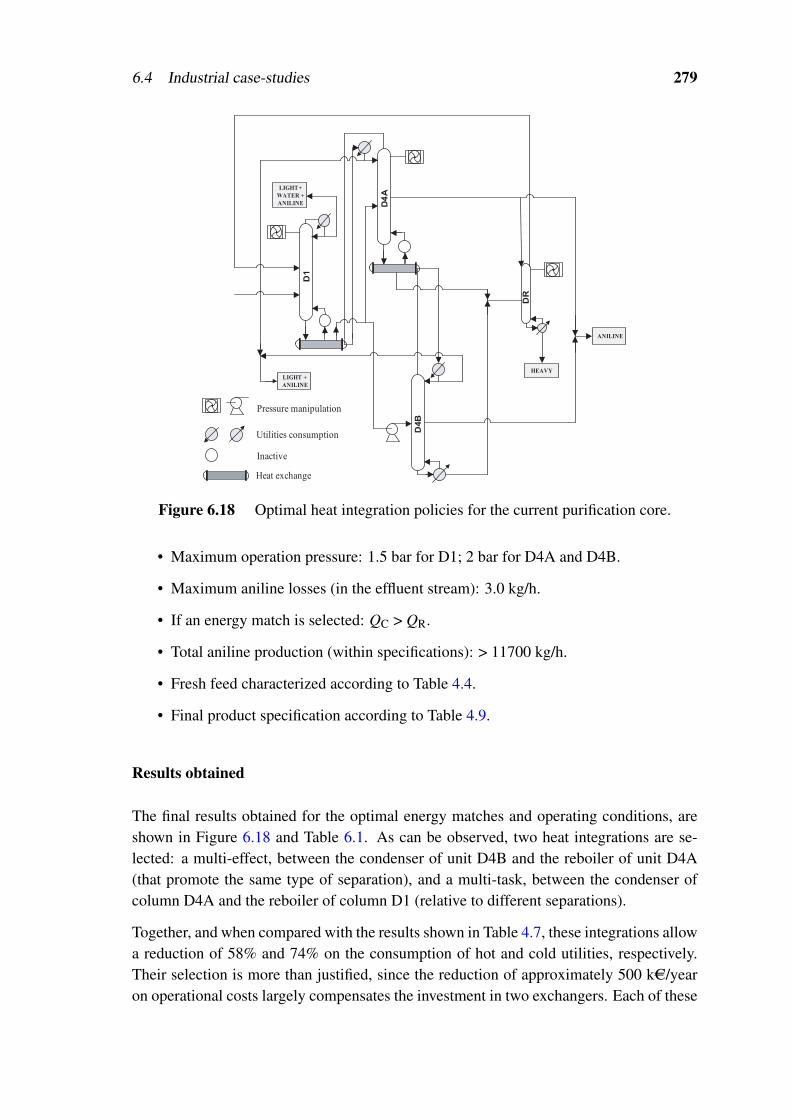
6.4 Industrial case-studies 279
D1
D4A
D4B
DR
HEAVY
ANILINE
LIGHT+
WATER +
ANILINE
LIGHT +
ANILINE
Utilities consumption
Inactive
Heat exchange
Pressure manipulation
Figure 6.18 Optimal heat integration policies for the current purification core.
• Maximum operation pressure: 1.5 bar for D1; 2 bar for D4A and D4B.
• Maximum aniline losses (in the effluent stream): 3.0 kg/h.
• If an energy match is selected: QC > QR.
• Total aniline production (within specifications): > 11700 kg/h.
• Fresh feed characterized according to Table 4.4.
• Final product specification according to Table 4.9.
Results obtained
The final results obtained for the optimal energy matches and operating conditions, areshown in Figure 6.18 and Table 6.1. As can be observed, two heat integrations are se-lected: a multi-effect, between the condenser of unit D4B and the reboiler of unit D4A(that promote the same type of separation), and a multi-task, between the condenser ofcolumn D4A and the reboiler of column D1 (relative to different separations).
Together, and when compared with the results shown in Table 4.7, these integrations allowa reduction of 58% and 74% on the consumption of hot and cold utilities, respectively.Their selection is more than justified, since the reduction of approximately 500 kAC/yearon operational costs largely compensates the investment in two exchangers. Each of these

280 Optimization of Distillation Networks
Table 6.1 Optimal operating conditions for the current purification core.
PCOL TC TR QC QR D RR CCU CHU
Column [bar] [K] [K] [GJ/h] [GJ/h] [kg/h] [kAC/yr] [kAC/yr]
D1 0.5 72 161 2.8 QEXC,1a 1108 0.5 174 0
D4A 0.7 171 172 QEXC,1 QEXC,2a 209 41 0 0
D4B 1.0 182 184 QEXC,2 4.9 153 60 0 325.9
DR 0.7 170 191 N.A. 0.1 268 N.A. 0 6.7
Total 17.4 332.6
−73.6% b −57.8% b
a QEXC,1 = 4.3; QEXC,2 = 4.5.b Comparatively to results of Table 4.7.
units, although presenting large dimensions (an exchange area of approximately 250 m2)and a high cost (300 kAC), allow the recovery of the investment on their acquisition in lessthan two years.
The industrial implementation of these heat exchange policies was already started, withthe first energy match (between units D4A and D4B) already completed (Figure 6.19).Presently, the new operating conditions of unit D1 were already reached and the thermalgradient necessary for the second integration has been also achieved; the industrial imple-mentation of the second integration is scheduled for the near future. The impact of thesepolicies in the process composite curves is shown in Figures 6.20 and 6.21.
As can be observed in Figure 6.20, the energy efficiency of the current purification corewas extremely low. This is clearly evidenced by the inexistent overlap region between thehot and cold composite curves. After introducing the multi-effect and multi-task integra-tions (Figure 6.21), two overlapping zones emerge, corresponding to the heat exchangesbetween columns D1 and D4A and between columns D4A and D4B.
Another interesting aspect relates to the non selection of heat integration schemes basedon the use of heat pumps (or MVR systems), in the problem final solution. In fact, al-though requiring a reduced pressure variation, to allow heat exchange between the con-denser and reboiler of a unit such as D4A or D4B, this type of configurations were elimi-nated during the optimization procedure. Notice that the previous distillation units presentthermal gradients that would be extremely favorable to implement this type of solutions.Since the temperature difference between the top and bottom of these units is practicallynull, the ∆T that would need to be induced in the fluid that suffers consecutive expansionsand compressions (or in the vapor that abandons the first stage) is identical to the ∆Tmin
imposed during the exchangers design; in other words, the required compression ratiocould difficulty be lower. However, even under these circumstances, this type of solutionsseems to not be competitive for the set of constraints that rule the current case-study.

6.4 Industrial case-studies 281
Exchanger
Figure 6.19 Industrial exchanger acquired for multi-effect integration.
In fact, by being able to exchange energy differently (since it is clear that the VLE andthe problem specifications promote favorable thermal gradients), it becomes unnecessaryto invest in heat pumps (or MVR systems) because the level of heat integration can beincreased by simply acquiring exchangers and adjusting some operating variables. On theother hand, when “forcing” the heat exchange between the condensers and reboilers ofunits D4A and D4B (Figure 6.22), it becomes impossible to select heat matches capableof including unit D1. Therefore, this unit must fulfil all of its energy requirements byexternal utilities consumption — a disadvantageous configuration that involves a globalenergy efficiency inferior to that represented in Figure 6.19. To invert this scenario theutility consumption in unit D1 needs to be somewhat reduced. Because this last onecannot be “duplicated”, to promote a multi-effect integration (since the constraints do notallow the acquisition of new distillation columns), the only possibility corresponds to theuse of a heat pump based solution (Figure 6.22).
Although it corresponds to a potential alternative, the previous solution is also not com-petitive, due to some unfavorable characteristics of column D1:
• The accentuated thermal gradient, between the top and bottom sections. This willrequire a high compression ratio that will imply large operational costs.
• The aniline / water azeotrope that will forbid the use of an intermediate condenser,as a way of reducing the required compression ratio.
As already discussed in Section 6.1.3, the use of a side-condenser allows the consump-tion of cold utility at higher temperature. On the other hand, when considering an energymatch, the vapor stream that needs to be condensed in this intermediate exchanger be-
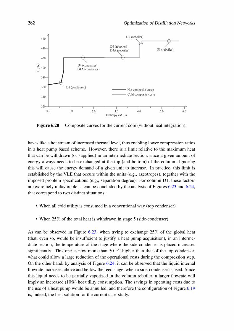
282 Optimization of Distillation Networks
0.0 1.0 2.0 3.0 4.0 5.0 6.0
320
340
360
380
400
420
440
460
Hot composite curve
Cold composite curve
D1 (condenser)
D4 (condenser)D4A (condenser)
D4 (reboiler)D4A (reboiler)
DR (reboiler)
D1 (reboiler)
T (
ºK)
Enthalpy (MJ/s)
Figure 6.20 Composite curves for the current core (without heat integration).
haves like a hot stream of increased thermal level, thus enabling lower compression ratiosin a heat pump based scheme. However, there is a limit relative to the maximum heatthat can be withdrawn (or supplied) in an intermediate section, since a given amount ofenergy always needs to be exchanged at the top (and bottom) of the column. Ignoringthis will cause the energy demand of a given unit to increase. In practice, this limit isestablished by the VLE that occurs within the units (e.g., azeotropes), together with theimposed problem specifications (e.g., separation degree). For column D1, these factorsare extremely unfavorable as can be concluded by the analysis of Figures 6.23 and 6.24,that correspond to two distinct situations:
• When all cold utility is consumed in a conventional way (top condenser).
• When 25% of the total heat is withdrawn in stage 5 (side-condenser).
As can be observed in Figure 6.23, when trying to exchange 25% of the global heat(that, even so, would be insufficient to justify a heat pump acquisition), in an interme-diate section, the temperature of the stage where the side-condenser is placed increasessignificantly. This one is now more than 50 C higher than that of the top condenser,what could allow a large reduction of the operational costs during the compression step.On the other hand, by analysis of Figure 6.24, it can be observed that the liquid internalflowrate increases, above and bellow the feed stage, when a side-condenser is used. Sincethis liquid needs to be partially vaporized in the column reboiler, a larger flowrate willimply an increased (10%) hot utility consumption. The savings in operating costs due tothe use of a heat pump would be annulled, and therefore the configuration of Figure 6.19is, indeed, the best solution for the current case-study.

6.4 Industrial case-studies 283
320
340
360
380
400
420
440
460
0.0 1.0 2.0 3.0 4.0 5.0
D1 (condenser)
D1 (reboiler)
D4 (condenser)
D4A (condenser)
D4 (reboiler)
D4A (reboiler)
DR (reboiler)
Hot composite curve
Cold composite curve
6.0
T (
ºK)
Enthalpy (MJ/s)
Figure 6.21 Composite curves for the current core (after energy matching).
6.4.3 Synthesis of a new configuration
Once the best manner of increasing the energy efficiency of the current arrangement isdetermined, the optimal design of a new purification core is the natural following goal.The purpose is to evaluate if the current separation sequence was indeed the most adequateamong a wide range of possibilities.
Sequencing alternatives
Considering the theory presented in Section 6.3.2, it is possible to observe that the in-dustrial process under study fits a class of problems where the new developed strategy isadvantageous. Therefore, and establishing an analogy between the generic componentspresented in Figure 6.17 and those involved in the aniline purification phase:
• The byproducts with boiling points inferior to that of aniline (BZ, CHA, CHOL andCHONA) can be grouped in a light pseudo-component, for the reasons explainedin situation B (Section 6.3.2).
• The byproducts with boiling points higher than that of aniline (DICHA, CHANIL,CHENO) can be treated as a heavy pseudo-component, according to situation A,also described in Section 6.3.2.
The multi-component problem, initially involving 10 components, can therefore be treatedusing a pseudo-ternary approach, allowing a far simpler analysis: aniline will continue tobe an intermediate boiling point component, although now only contaminated with two(pseudo) components.
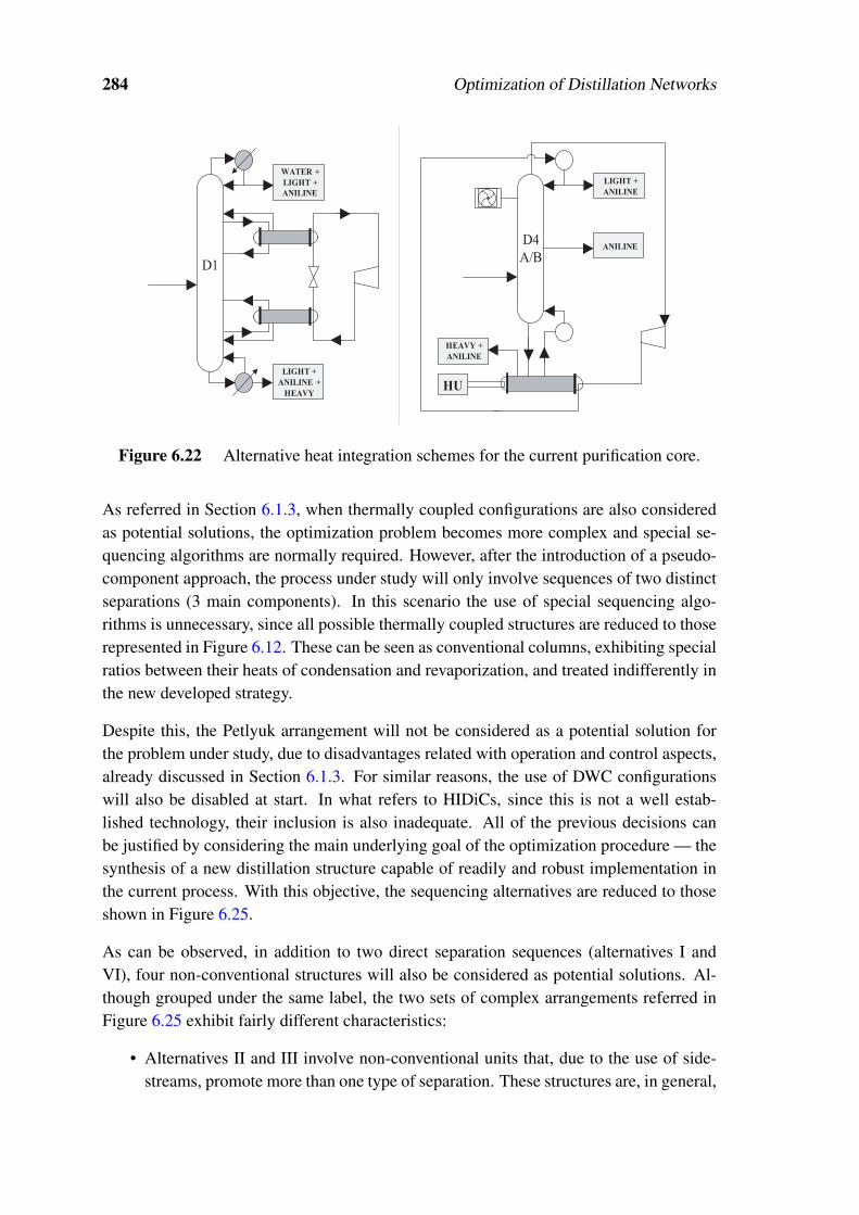
284 Optimization of Distillation Networks
D4
A/BANILINE
LIGHT +
ANILINE
HEAVY +
ANILINE
HU
D1
WATER +
LIGHT +
ANILINE
LIGHT +
ANILINE +
HEAVY
Figure 6.22 Alternative heat integration schemes for the current purification core.
As referred in Section 6.1.3, when thermally coupled configurations are also consideredas potential solutions, the optimization problem becomes more complex and special se-quencing algorithms are normally required. However, after the introduction of a pseudo-component approach, the process under study will only involve sequences of two distinctseparations (3 main components). In this scenario the use of special sequencing algo-rithms is unnecessary, since all possible thermally coupled structures are reduced to thoserepresented in Figure 6.12. These can be seen as conventional columns, exhibiting specialratios between their heats of condensation and revaporization, and treated indifferently inthe new developed strategy.
Despite this, the Petlyuk arrangement will not be considered as a potential solution forthe problem under study, due to disadvantages related with operation and control aspects,already discussed in Section 6.1.3. For similar reasons, the use of DWC configurationswill also be disabled at start. In what refers to HIDiCs, since this is not a well estab-lished technology, their inclusion is also inadequate. All of the previous decisions canbe justified by considering the main underlying goal of the optimization procedure — thesynthesis of a new distillation structure capable of readily and robust implementation inthe current process. With this objective, the sequencing alternatives are reduced to thoseshown in Figure 6.25.
As can be observed, in addition to two direct separation sequences (alternatives I andVI), four non-conventional structures will also be considered as potential solutions. Al-though grouped under the same label, the two sets of complex arrangements referred inFigure 6.25 exhibit fairly different characteristics:
• Alternatives II and III involve non-conventional units that, due to the use of side-streams, promote more than one type of separation. These structures are, in general,
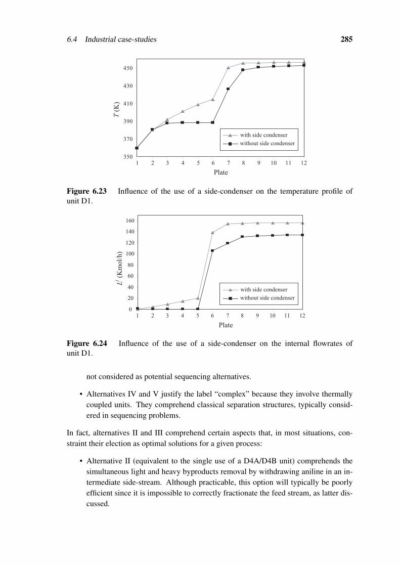
6.4 Industrial case-studies 285
350
370
390
410
430
450
1 2 3 4 5 6 7 8 9 10 11 12
Plate
with side condenser
without side condenser
T (
K)
Figure 6.23 Influence of the use of a side-condenser on the temperature profile ofunit D1.
0
20
40
60
80
100
120
140
160
1 2 3 4 5 6 7 8 9 10 11 12
with side condenser
without side condenser
L (K
mol/
h)
Plate
j
Figure 6.24 Influence of the use of a side-condenser on the internal flowrates ofunit D1.
not considered as potential sequencing alternatives.
• Alternatives IV and V justify the label “complex” because they involve thermallycoupled units. They comprehend classical separation structures, typically consid-ered in sequencing problems.
In fact, alternatives II and III comprehend certain aspects that, in most situations, con-straint their election as optimal solutions for a given process:
• Alternative II (equivalent to the single use of a D4A/D4B unit) comprehends thesimultaneous light and heavy byproducts removal by withdrawing aniline in an in-termediate side-stream. Although practicable, this option will typically be poorlyefficient since it is impossible to correctly fractionate the feed stream, as latter dis-cussed.

286 Optimization of Distillation Networks
PL
PP
Aniline
PL
AnilinePP
Aniline
PP
PL
Aniline
PP
PP
AnilinePL
Aniline
PL
CONVENTIONAL
SEQUENCE
CONVENTIONAL
SEQUENCE
COMPLEX
CONFIGURATIONS
Side-stripper
Side-rectifier
Side-streams
Side-streams (current process)
Use of
I
II
III
IV
V
VI
ALTERNATIVES
(single column)
Figure 6.25 Sequencing alternatives for a new aniline purification core.
• Alternative III (identical to the current purification core) comprehends the repetitionof a separation task, since the removal of the light byproducts is performed in twodistinct columns (D1 and D4A/D4B); this is an unusual sequence, that is normallynot accounted in classical algorithms.
Although looking less attractive, the two previous alternatives will not be excluded sincethey represent important references for benchmark purposes. Alternative II will define thesituation that involves larger operational costs (as latter explained), while alternative III,identical to the current purification core, will establish the CTA value that should be im-proved by adoption (or not) of a different separation sequence.
Even when systematic mathematical formulations are employed, the optimization of agiven process can profit from the introduction of heuristics, especially when these resultfrom knowledge gathered through industrial practice. Therefore, when empirical rulesare taken in consideration, it becomes often possible to improve the quality of the finalsolutions; the use of the DR unit, shown in Figure 6.18, is one of these examples. Thisrecovery column plays a vital role in the current process, despite its small dimensionsand almost negligible operational costs. The reason for this is simple: the aniline that is“lost” in the light byproduct streams (distillates of units D1 and D4A/D4B) can be easilyrecovered, contrarily to the aniline that follows in the heavy byproduct streams (bottomof units D4A/D4B) that will be treated as an waste effluent, if a DR units is not used. Thisscenario is a direct consequence of the economical value of light byproducts (that enter anew purification stage where aniline can be separated) and the reduced interest in heavy

6.4 Industrial case-studies 287
byproducts that are treated as a waste stream. Therefore, due to the presence of unit DR,a larger amount of aniline is allowed in the bottom streams of units D4A/D4B, since theoverall productivity is kept unaffected. As a consequence, the thermal gradient betweenthe top and bottom of these units is reduced, which is very advantageous:
• In a scenario of heat integration, since it facilitates the implementation of energymatches by smoothing required changes in the current operational conditions.
• In a scenario of utilities consumption, since the reboiler temperatures of columnsD4A/D4B will be decreased and, therefore, lower pressure steam (less expensive)can be consumed.
For the previous reasons, it becomes important to include a DR unit in all sequencingalternatives of Figure 6.25. This unit should be treated as a complement of separations (PI/ PP) and (PL PI / PP) and should not be dissociated from them during the optimizationprocedure. From a mathematical point of view, the above scenario can be included inthe new developed strategy, by considering modified thermal gradients and additionalcapital/operation costs for the previously referred separations.
Integrating the heat of reaction
The industrial process under study comprehends the hydrogenation of nitrobenzene in aliquid phase, a reaction pathway that is not unique. Other companies (e.g., Lonza, BASFand Bayer) consider a different step where aniline is produced in a gas phase (Chapter 1).In practice, it is very difficult to identify the best choice, since different reaction steps in-volve different amounts and types of byproducts. These will require distinct purificationblocks that may present advantages and drawbacks that are difficult to compare. Theycan depend, inclusively, on the value that the surrounding market attributes to the sec-ondary components. However, in a very superficial analysis, it is generally assumed that(Section 1.3):
• The liquid hydrogenation of nitrobenzene involves reaction temperatures signifi-cantly lower. Therefore, the steam that can be produced through the released heatof reaction will be less appealing, since its lower thermal level constrains the rangeof possible applications.
• Producing aniline in a gas phase usually requires the recompression of the non-converted hydrogen, thus involving high capacity compressors (and significant cap-ital and operational costs).
The main aspect to retain is that liquid phase processes difficult the energy integrationbetween reaction and purification steps. This major drawback is a direct consequence ofthe low pressure steam produced in slurry or fluidized units, that is often inadequate forthe higher operating temperatures of distillation units. This scenario can also be observed

288 Optimization of Distillation Networks
Cooling
Vaporization
coil
tubes
Externalexchanger
15%
17%
62%
Reaction phase
Purification phase
(core)
Others
HEAT REMOVAL
( REACTION)COLD UTILITY CONSUMPTION
(CURRENT PROCESS)
Figure 6.26 Removal of the reaction heat (possible alternatives).
in the industrial process under study — the bottom temperatures of columns D1, D4A andD4B are higher than the current reaction temperature.
Under these circumstances, and due to the large amount of heat that is released, the reac-tion units will behave as major consumers of external cold utility, a very disadvantageousscenario (Figure 6.26). Truly, part of this heat is not completely wasted in the currentprocess: 50% is used to produce a low pressure steam (1 barg) that is employed in otherplants. However, the remaining 50% are removed in cooling coils that, although assuringthe temperature control, do not need, for this purpose, to dissipate so much heat.
Therefore, and considering that
• producing 11700 kg/h of aniline will release 65 GJ/h (∆HR =-544 kJ/mol);
• 50% of this heat should be dissipated in vaporization tubes, to satisfy the need forlow pressure steam (1 barg);
• from the remaining 50% approximately 15% should be subtracted, to enable thecontrol of the reaction temperature, using cooling coils;
it is possible to estimate that approximately 22 GJ/h could be used to supply the hot utilityneeds of the purification phase. Notice that this block of units, in the current configurationand in the absence of heat integration policies, only requires approximately 11 GJ/h — avalue well beyond the available amount of energy. For the previous reason, overcomingthis major handicap of the current process was taken as an important goal and, therefore,the synthesis of a new distillation structure, capable of using the heat released in thereaction step, was also pursued. Notice that the existence of this separation network couldimply a radical impact on the process profitability, since CHU,LP=0.

6.4 Industrial case-studies 289
Instead of modifying the purification phase, it can be argued that increasing the reac-tion temperature could also be a simpler and attractive solution for the previous problem.However, in practice, this procedure present serious drawbacks and cannot be currentlyimplemented, since increasing the operation temperature has the following two conse-quences:
• A reduction of the process selectivity; less aniline is obtained which represents asignificant economical loss.
• Greater quantities of DICHA are obtained that, due to the existing azeotrope be-tween this byproduct and aniline (Figure 4.27), will contaminate the final productto an extent higher than allowed.
The decrease of the reaction selectivity could be economically compensated by the ad-vantages of producing steam with a higher thermal level but, in practice, this trade-off ishindered by the purity specifications that are imposed for commercial purposes. There-fore, the maximum temperature for the steam produced in the reaction step is fixed in135 C (P=2 barg). This value comprehends a ∆Tmin=10 C, that is imposed in the ex-ternal exchangers (Figure 6.26). In fact, and due to the large exchanging areas that arerequired to obtain steam at 2 barg, this cannot be produced inside the reaction units (IST,2006); the current internal areas are only adequate to produce steam of lower pressure,benefiting from the larger temperature differences.
Problem descriptions
The current Section includes two problems, both of them relative to the design of a newpurification core for the process under study. The only difference between them relatesto the hot utilities that are considered to be available: in the first problem, it will not bepossible to use low pressure steam produced in the reaction step. Therefore, since thesecond problem presents an extra degree of freedom (two hot utility sources, instead ofone), the results obtained for this one will always be better (or, in the worst scenario,equal). This can raise an obvious question: why solve the first problem? The reason isquite simple: the use of steam produced in the reaction step can be associated with somerisks that are easy to anticipate, namely the completely different operational conditionsthat will be required, if the current industrial practice is taken as reference. In fact, thelower thermal level of this steam will “force” the operating pressure of the new core to bedecreased significantly, a situation for which no knowledge / practice is available. There-fore, it is important to compare the optimal solutions (namely their CTA) identified foreach problem. In the case of obtaining similar objective function values, it may be wiserto choose the solution of the first problem as the most adequate one, since its operationalconditions will be closer to the current ones, thus involving less risks.
The two previous problems will be far more elaborated that that of Section 6.4.2, since

290 Optimization of Distillation Networks
the number and type of units to use, as well as their respective number of stages andfeed stream locations, are not fixed. Therefore, Step 1 and Step 3, of the new developedstrategy, will have to deal with extremely complex problems.
The adopted methodology follows, once again, the procedure described in Section 6.3.2,where a set of short-cut methods are employed in the first place. These are crucial togenerate preliminary designs for the units involved in the new separation sequences, thatwill be subsequently optimized rigorously in Step 1.
The operating range of the column’s pressure and also other process variables is nowwider, since the acquisition of new and more flexible equipment is considered. In otherwords, bottlenecks imposed by existing units are now eliminated and, as a consequence,some problem restrictions are relaxed:
• Minimum temperature in the condensers: 40 C.
• Maximum temperature in the reboilers: 250 C.
• Minimum operating pressure: 0.1 bar.
• Maximum operating pressure: 3 bar.
Additionally, the following set of restrictions (also adopted for the case-study of Sec-tion 6.4.2) will continue to prevail:
• Maximum aniline losses (in the effluent stream): 3.0 kg/h.
• If an energy match is selected: QC > QR.
• Total aniline production (within specifications): > 11700 kg/h.
• Fresh feed characterized according to Table 4.4.
• Final product specification according to Table 4.9.
Although maintaining the same type of cold utility, the minimum temperature in the con-densers is now 40 C, well inferior to that assumed in Section 6.4.2, where the existingexchanging areas were limiting. On the other hand, the maximum temperature in the re-boilers is now increased. In this case, the underlying reason relates to a different hot utilitythat is now considered to be available. In fact, instead of consuming steam at 24 barg (asin Section 6.4.2) it is assumed that for the construction of a new purification core a higherpressure hot utility (P=40 barg) can be acquired.
Results obtained
The main results obtained for the first problem (not considering the use of low pressuresteam, produced in the reaction step) are shown in Figures 6.27–6.31 and in Table 6.2,
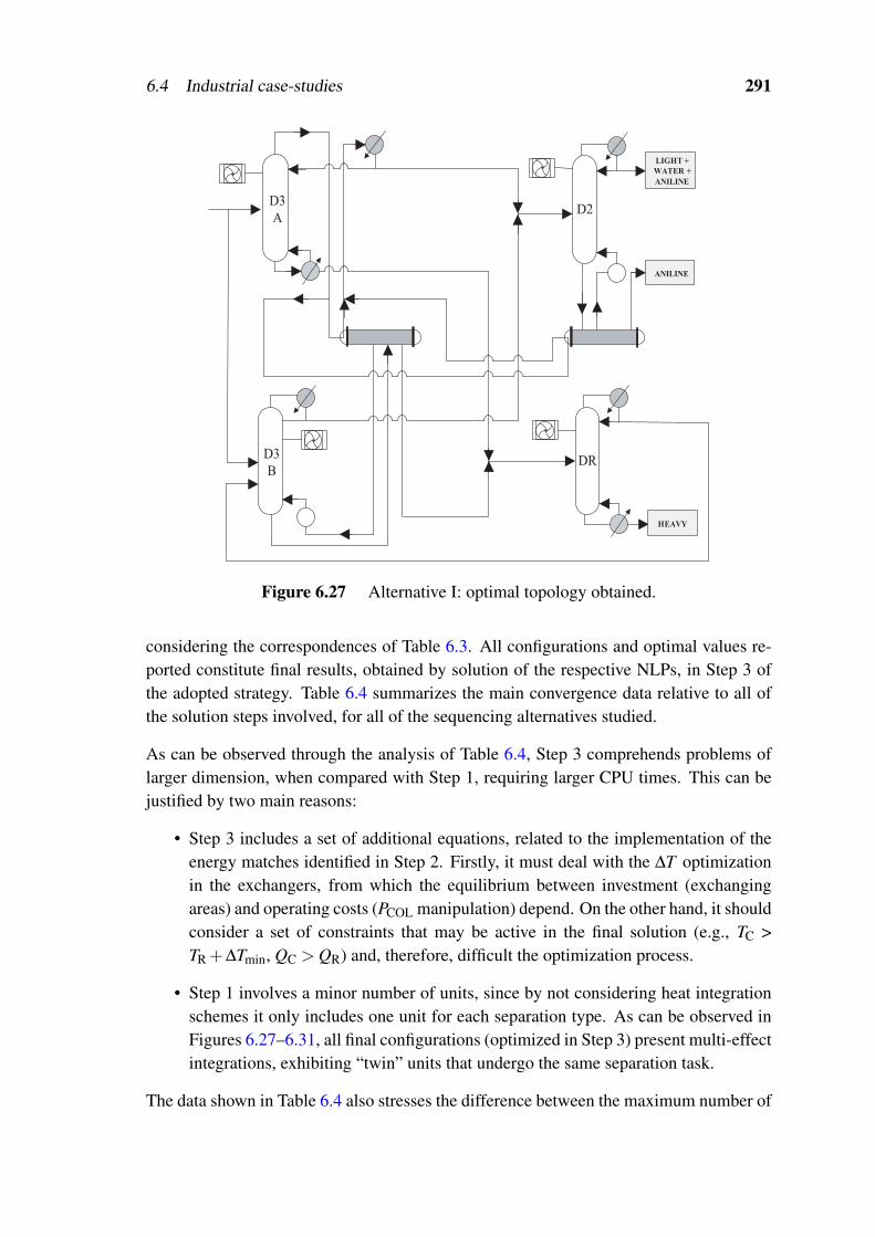
6.4 Industrial case-studies 291
D3
AD2
LIGHT +
WATER +
ANILINE
ANILINE
D3
BDR
HEAVY
Figure 6.27 Alternative I: optimal topology obtained.
considering the correspondences of Table 6.3. All configurations and optimal values re-ported constitute final results, obtained by solution of the respective NLPs, in Step 3 ofthe adopted strategy. Table 6.4 summarizes the main convergence data relative to all ofthe solution steps involved, for all of the sequencing alternatives studied.
As can be observed through the analysis of Table 6.4, Step 3 comprehends problems oflarger dimension, when compared with Step 1, requiring larger CPU times. This can bejustified by two main reasons:
• Step 3 includes a set of additional equations, related to the implementation of theenergy matches identified in Step 2. Firstly, it must deal with the ∆T optimizationin the exchangers, from which the equilibrium between investment (exchangingareas) and operating costs (PCOL manipulation) depend. On the other hand, it shouldconsider a set of constraints that may be active in the final solution (e.g., TC >TR +∆Tmin, QC > QR) and, therefore, difficult the optimization process.
• Step 1 involves a minor number of units, since by not considering heat integrationschemes it only includes one unit for each separation type. As can be observed inFigures 6.27–6.31, all final configurations (optimized in Step 3) present multi-effectintegrations, exhibiting “twin” units that undergo the same separation task.
The data shown in Table 6.4 also stresses the difference between the maximum number of

292 Optimization of Distillation Networks
Table 6.2 Optimal specifications obtained (Alternatives I–VI).
PCOL TC TR QC QR QEXC CFIX COPEColumn [bar] [ C] [ C] [GJ/h] [GJ/h] [GJ/h] [kAC/yr] [kAC/yr]
Alte
rnat
ive
I D3A 1.9 123 210 QEXC 7.6 7.0 91.7 506.1D3B 0.1 51 113 3.3 QEXC 2.9 86.4 20.5D2 0.1 40 113 3.8 QEXC 4.1 98.2 23.6DR 0.1 113 128 0.1 0.1 N.A. 38.2 7.5
Total 314.5 557.7
Alte
rnat
ive
II D4A 0.1 40 112 17.6 QEXC 18.2 251.8 109.4D4B 2.7 123 212 QEXC 20.5 18.2 153.9 1398.4DR 0.1 113 127 0.2 0.2 N.A. 37.9 11.2
Total 443.6 1519.0
Alte
rnat
ive
III D1 0.5 75 159 2.6 QEXC,1 4.1 98.2 16.2
D4A 0.7 169 171 QEXC,1 QEXC,2 8.4 99.9 0D4B 1.0 182 185 QEXC,2 4.7 4.3 61.6 312.9DR 0.7 170 194 0.1 0.1 N.A. 38.3 8
Total 298.0 337.1
Alte
rnat
ive
IV D1 0.75 85 173 3.0 N.A. N.A. 47.3 18.7D5A 0.75 173 174 2.1 QEXC 3.7 94.2 13.1D5B 1.00 183 184 QEXC 7.1 3.7 69.1 472.8DR 0.75 173 192 0.1 0.1 N.A. 38.4 7.3
Total 249.0 511.9
Alte
rnat
ive
V D3 2.8 215 228 N.A. 10.1 N.A. 92.9 672.6D2A 2.8 124 227 QEXC 1.1 2.8 44.7 73.2D2B 0.1 40 114 10.8 QEXC 2.8 101.3 67.2DR 0.1 114 127 0.3 0.1 N.A. 38.0 11.5
Total 276.9 824.5
Alte
rnat
ive
VI D1 0.5 76 159 2.7 QEXC,1 4.2 96.9 16.8
D5A 0.7 170 171 QEXC,1 QEXC,2 8.6 93.9 0D5B 1.0 183 185 QEXC,2 4.8 4.4 55.4 319.6DR 0.7 170 193 0.1 0.1 N.A. 38.3 8
Total 284.5 344.4
Table 6.3 Column labels and separation types (correspondences).
D1 D2 D3 D4 D5 DR
(PL / PI PH) (PL / PI) (PL PI / PH) (PL / PI / PH) (PI / PH) Recovery

6.4 Industrial case-studies 293
D4
A
D4
B
WATER +
LIGHT +
ANILINE
ANILINE DR
HEAVY
WATER +
LIGHT +
ANILINE
ANILINE
Depending on THU
x 3
Figure 6.28 Alternative II: optimal topology obtained.
Table 6.4 Convergence data relative to the solution process.
NLP (Step 1) MILP (Step 2) NLP (Step 3)Variable FPP FOC FPP FOC
Equations [×103] (a) 8–12 18–40 0.1 8–12 37–56
Independent variables 0 6–18 8–22 0 12–24
CPU time [×102 s] 1.8–3.0 3.2–7.1 0.02–0.1 1.8–4.5 4.5–9.6
(a) Simultaneously solved (maximum number).
equations that need to be solved, simultaneously, in the pre-processing and optimizationphases of Steps 1 and 3. In the first numerical phase (FPP), the unit models can besolved individually, with all variables assuming fixed values (previously determined byuse of a sequential-modular approach) that guarantee a coherent initialization of an entirearrangement (Section 5.3.1). The models to be solved vary between a minimum of 8000and a maximum of 12 000 equations never requiring, for the initialization of all unitsinvolved in a given branch, more than 300 CPU seconds.
The optimization phase naturally involves larger CPU times, due to the degrees of freedomand the larger number of equations that need to be simultaneously solved. However, it isimportant to stress that the first phase (FPP) is responsible for a significant fraction of thetotal CPU time spent in Steps 1 and 3. This clearly shows the need and importance ofrobust numerical pre-processing, before entering the optimization process.
Another important aspect, also stated in Table 6.4, relates to the reduced number of in-dependent variables in Step 3. In fact, and although in the presence of large-scale squareproblems, the degrees of freedom are restricted to a small set of design parameters in eachcolumn (P, np, lF, RR, D) and to the fractioning level of some streams (that will definethe feed streams of “twin” columns and impose the heat involved in their exchangers).For optimization problems involving these characteristics, the solver selection assumes

294 Optimization of Distillation Networks
D5
A
D5
B
DR
HEAVY
D1
WATER +
LIGHT +
ANILINE
ANILINE
ANILINE
Figure 6.29 Alternative IV: optimal topology obtained.
D2
A
D2
B
DR
HEAVY
D3
LIGHT +
WATER +
ANILINE
ANILINE
ANILINE
Depending
on THU
LIGHT +
WATER +
ANILINE
Figure 6.30 Alternative V: optimal topology obtained.

6.4 Industrial case-studies 295
D1D5
A
WATER +
LIGHT +
ANILINE
ANILINE
DR
HEAVY
D5
B
ANILINE
Figure 6.31 Alternative VI: obtained optimal topology.
a special importance. Therefore, and considering the numerical data obtained in Sec-tion 5.4, the CONOPT solver (in the GAMS modelling environment) was used to solvethe problems involved in Steps 1 and 3.
For Step 2, as stated in Table 6.4, the number of equations considered and the CPU timesrequired are quite reduced, due to the simplified relations that are assumed. The solutionprocess of the involved MILPs can be easily accomplished, using the OSL2 solver in theGAMS modelling environment.
After the presentation of Figures 6.27–6.31 and Table 6.2, conclusions relative to theoptimal configurations that were synthesized for the different separation alternatives canbe derived.
Alternative I For this alternative, the results obtained in Step 1 indicate that the con-denser and reboiler duties of column D3 are similar to each other and a lot larger (ap-proximately 2 times) than those of unit D2. In this case, the algorithm of Step 2 predictsthe unfolding of the first column in two “twin” units (D3A and D3B) that, when operatedat optimal pressures, allow the incorporation of multi-effect and multi-task integrationschemes, accordingly with the matches represented in Figure 6.27. Notice that if a DRunit was not considered, the compositions of the bottom streams in columns D3A andD3B would have to present a significant concentration in heavy components, since theaniline losses are limited to a maximum of 3 Kg/h. This would implicate higher tem-peratures in the reboilers of these units, that would hinder the possibility of combining

296 Optimization of Distillation Networks
multi-effect and multi-task schemes. Increasing the condenser temperature in unit D3A,by pressure manipulation, could not solve the problem, since the reboiler temperaturewould become higher than that of the available hot utility (250 C). Therefore, and tomaximize the heat exchanges, it is crucial to lower the reboiling temperatures of columnsD3A and D3B, letting the composition in aniline to build up in their bottoms. This isonly possible by recovering and recycling this component, through a DR unit. This sce-nario is not exclusive from alternative I, occurring for many of the remaining alternativesequences — an observation that illustrates the advantages of including heuristics in sys-tematic mathematical approaches.
Comparing the objective function values obtained for alternative I and VI, it is possibleto conclude that removing the heavy components in a first column (unit D3) is disad-vantageous, since this separation task requires a large amount of energy. Although it ispossible to involve this last one in multi-effect and multi-task integrations, the global op-erating costs will always be larger than those relative to a configuration where the removalof light byproducts is considered firstly.
Another disadvantage of the current alternative is relative to the thermal gradients thatoccur on these units. In fact, and by comparison to alternative VI, these tend to difficult theenergy matches, by requiring more drastic operation conditions (pressures significantlymore distant from the atmospheric value).
Alternative II This configuration presents the highest operating costs, among all con-sidered separation alternatives. This scenario was already expected since the removal of3 components, in a single conventional column, is usually disadvantageous:
• If the feed enters below the side-stream, problems will arise in contamination bylight byproducts. Since these are introduced in the stripping zone and need to beconcentrated in the distillate, they will necessarily build up in the ascending vaporstream, undesirably reaching the stage where the product is withdrawn.
• If the feed stream is placed above the side-stream, contamination problems will alsoarise, this time with the heavy byproducts. These are introduced in the rectifyingzone and need to be withdrawn in the column’s bottom. Therefore, their build up inthe descending liquid stream is impossible to be avoided, reaching the stage wherethe product is obtained.
The only possibility of solving the previous problems relies on the use of a Petlyuk ar-rangement. Although often analyzed as a single unit (since it only possesses one con-denser and one reboiler), this special configuration includes a previous column that willcorrectly fractionate the feed stream. The existence of this structure (pre-fractionator)is responsible for the high efficiency of Petlyuk based configurations, since it allows theintroduction of the light and heavy components above and bellow the product withdrawstage, respectively. The previous aspect allows a decrease of the required reflux ratios

6.4 Industrial case-studies 297
Table 6.5 Optimal split fractions in unit D1 (Alternative III).
BZ Water CHA CHONA CHOL ANL DICHA MNB CHENO CHANIL
'1 '1 0.998 0.946 0.928 0.038 0.023 0.003 '0 '0
and, for a similar reason, the optimal configuration shown in Figure 6.28 also presentsthe feed streams divided among non-adjacent stages — this splitting is a result of anoptimal compromise between the side-stream contamination that is caused by the lightbyproducts entering above and heavy byproducts entering bellow. Unfortunately, a sim-ple stream splitter does not work as a pre-fractionator since, by assuring VLE, this allowsthe outlet streams to be enriched in different components — thus it is possible to favor theseparation and obtain radically different energy efficiencies.
Relatively to alternative II, it also important to stress that the use of 3 multi-effect inte-grations would benefit the problem objective function. In fact, the obtained reduction onthe operating costs would justify the investment in two additional units (D4C and D4D).However, in practice, due the larger amount of water that is present in the distillates,the thermal gradients calculated in Step 1 do not allow the selection of the previous heatcascade in Step 2 — the range of operating pressures that would be required is not imple-mentable, due to the constraints around the cold and hot utility temperatures.
Alternative III The optimal configuration synthesized for alternative III, including theselected matches, is identical to that of the current purification core, already shown in Fig-ure 6.19. On the other hand, the operating costs in Table 6.2 relative to alternative III, arealso very similar to those shown in Table 6.1. The small difference relative to the obtainedvalues for QC, QR and QEXC, can be justified by the fact of Table 6.2 reporting values thatconsider the acquisition of new units, where np and lF can be optimized to favor the objec-tive function (that, for obvious reasons, is different in these two tables). Since the designparameters that are implicit in Table 6.2 are optimal, it can be concluded that the physicalstructure of the current units is adequate for the new operational conditions (required toimplement the selected heat exchange policies). In the opposite situation, a large differ-ence between the maximum energy efficiency that could be obtained in a new and in thecurrent purification core would exist.
Another interesting aspect is the similarity between the objective function values obtainedfor alternatives III and VI (Table 6.2). This fact means that both alternatives exhibit anidentical equilibrium between operational and capital costs, a surprising result consideringthat different separation tasks are involved. Although seeming difficult to explain, theunderlying reason can be easily understood by analysis of the results shown in Table 6.5.
In fact, the split fractions (taking the distillate as reference) obtained for unit D1 in al-ternative III, are practically unitary for all light byproducts. In other words, the removal

298 Optimization of Distillation Networks
of these components, instead of also accomplished in units D4A/D4B, is achieved exclu-sively in unit D1. Therefore, and although presenting side-streams where the final productis withdrawn, units D4A/D4B are only promoting the removal of heavy byproducts, notassuming a separation (PL / PI / PH), as it would be expected.
Under these circumstances, the separation sequence in alternatives III and V is the same,as well as the energy requirements. Since similar relations between the condenser andreboiler duties in Step 1 are obtained, it is natural that the selected energy matches inStep 2 will also be the same, leading to very similar CTA values in Step 3. The smalldifference in the objective function values is due to the different liquid and vapor inter-nal flowrates (affected by the use of side-streams), that will interfere in the design andcosts of the involved units. Although surprising, these results clearly demonstrate thatthe optimization procedure is robust and efficient. Notice that in alternative III all unitswere initialized (FPP) considering that the removal of light byproducts should occur inunits D1 and D4. However, after the optimization phase (FOC) in Step 1, all determinedoperational parameters predicted the removal of the light species (almost) exclusively inunit D1.
Alternatives IV and V As referred in Section 6.1.3, when thermally coupled columnsare used, the reduction of operational costs through heat exchanges between condensersand reboilers can be hindered. The current case-study verifies the previous sentence, sincealternatives IV and V comprehend the same separation sequence of alternatives VI andI, respectively, but present objective function values less attractive. By analysis of Ta-ble 6.2, it is possible to observe that the different ratios between the condensation andrevaporization heats are less favorable for heat integration, a consequence of thermal cou-pling. Therefore, and although multi-task and multi-effect matches are possible, the lastare not as effective as in alternatives I and VI. Notice that if no heat exchanges betweencondensers and reboilers were allowed, alternatives VI and V would present themselvesas the most attractive, since thermal coupling always reduce the global energy associatedto a given separation sequence (Table 6.2). The results obtained for alternatives VI andV also stress again the advantages of the removal of light byproducts in the first place (asalready concluded by comparison of alternatives I and VI).
Alternative VI The configuration reported in Figure 6.31 presents the best objectivefunction value that was found. Therefore, it corresponds to the best separation structurethat can be adopted, considering the set of constraints of the current case-study.
Another aspect that should be emphasized is the non-selection of any configuration basedon the use of heat pumping schemes. When analyzing the best heat integration schemesfor the current purification core, the reasons pointed for this scenario were related withdifficulties in involving all units in energy exchanges. In fact, when selecting a heatpump for unit D4, column D1 would not be able to participate in multi-task integrations
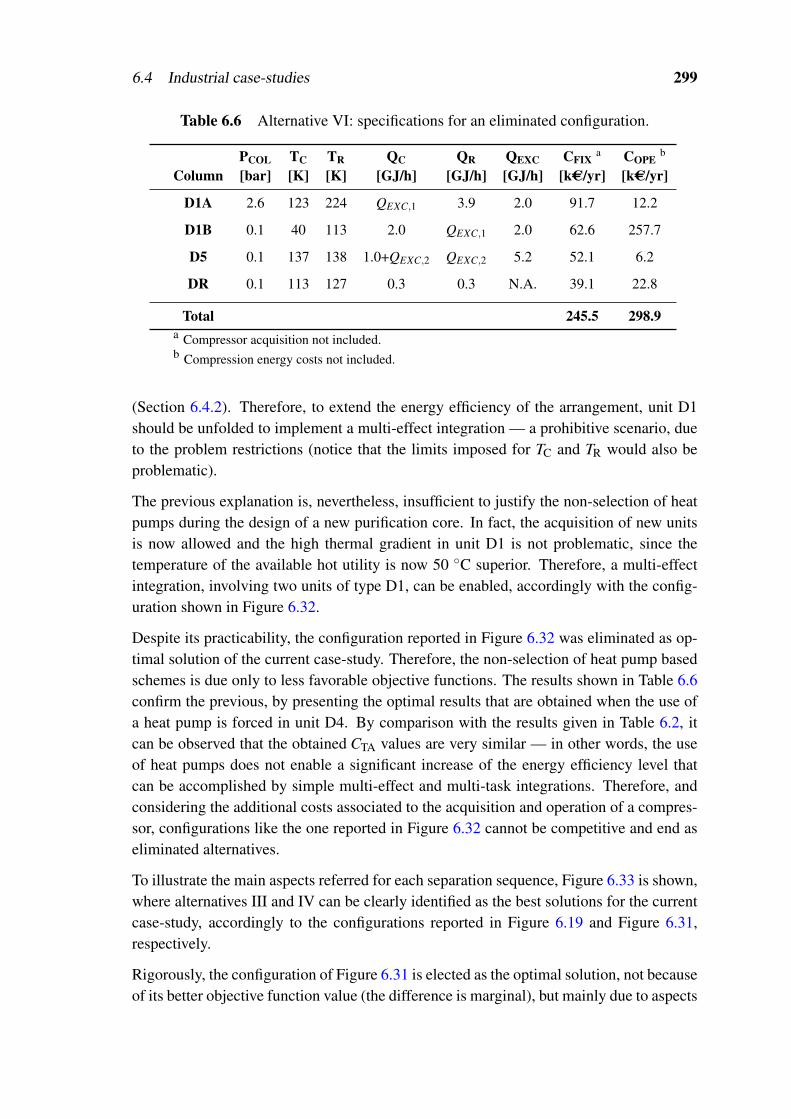
6.4 Industrial case-studies 299
Table 6.6 Alternative VI: specifications for an eliminated configuration.
PCOL TC TR QC QR QEXC CFIXa COPE
b
Column [bar] [K] [K] [GJ/h] [GJ/h] [GJ/h] [kAC/yr] [kAC/yr]
D1A 2.6 123 224 QEXC,1 3.9 2.0 91.7 12.2
D1B 0.1 40 113 2.0 QEXC,1 2.0 62.6 257.7
D5 0.1 137 138 1.0+QEXC,2 QEXC,2 5.2 52.1 6.2
DR 0.1 113 127 0.3 0.3 N.A. 39.1 22.8
Total 245.5 298.9a Compressor acquisition not included.b Compression energy costs not included.
(Section 6.4.2). Therefore, to extend the energy efficiency of the arrangement, unit D1should be unfolded to implement a multi-effect integration — a prohibitive scenario, dueto the problem restrictions (notice that the limits imposed for TC and TR would also beproblematic).
The previous explanation is, nevertheless, insufficient to justify the non-selection of heatpumps during the design of a new purification core. In fact, the acquisition of new unitsis now allowed and the high thermal gradient in unit D1 is not problematic, since thetemperature of the available hot utility is now 50 C superior. Therefore, a multi-effectintegration, involving two units of type D1, can be enabled, accordingly with the config-uration shown in Figure 6.32.
Despite its practicability, the configuration reported in Figure 6.32 was eliminated as op-timal solution of the current case-study. Therefore, the non-selection of heat pump basedschemes is due only to less favorable objective functions. The results shown in Table 6.6confirm the previous, by presenting the optimal results that are obtained when the use ofa heat pump is forced in unit D4. By comparison with the results given in Table 6.2, itcan be observed that the obtained CTA values are very similar — in other words, the useof heat pumps does not enable a significant increase of the energy efficiency level thatcan be accomplished by simple multi-effect and multi-task integrations. Therefore, andconsidering the additional costs associated to the acquisition and operation of a compres-sor, configurations like the one reported in Figure 6.32 cannot be competitive and end aseliminated alternatives.
To illustrate the main aspects referred for each separation sequence, Figure 6.33 is shown,where alternatives III and IV can be clearly identified as the best solutions for the currentcase-study, accordingly to the configurations reported in Figure 6.19 and Figure 6.31,respectively.
Rigorously, the configuration of Figure 6.31 is elected as the optimal solution, not becauseof its better objective function value (the difference is marginal), but mainly due to aspects

300 Optimization of Distillation Networks
D1
AD5
ANILINE
D1
B DR
HEAVY
LIGHT +
WATER +
ANILINE
LIGHT +
WATER +
ANILINE
HUDepending
on THU
Figure 6.32 Alternative VI: topology of an eliminated configuration.
0
200
400
600
800
1000
1200
1400
1600
1800
2000
I II III IV V VI
Alternative
Cost
(k
€/y
r)
Operating
Fixed
Figure 6.33 Comparative results for all alternatives under study.

6.4 Industrial case-studies 301
Table 6.7 Alternative IV: Design parameters for the involved units.
np lF,1 lF,2 RR dINT hINT D AR AC AEXCColumn [m] [m] [kg/h] [m2] [m2] [m2]
D1 16 5 N.A. 0.31 1.4 8.5 1448 21 36 227
D5A 9 6 3 0.45 1.6 6.0 5927 14 45 238
D5B 9 6 N.A. 0.62 1.7 6.0 5773 13 65 N.A.
DR 8 4 N.A. 0.08 0.4 5.5 352 1 1 N.A.
related with its industrial implementation. In fact, when promoting the complete removalof the light byproducts in a first column, it becomes unnecessary to use side-streams inthe following unit — these cannot decrease the energy requirements and, on the otherhand, will require the acquisition of additional equipment (e.g., pumps). For this reason,Table 6.7 gives the optimal design specifications for all units involved in the configurationof Figure 6.31.
As already described, the influence of using lower pressure vapor (produced in the reac-tion phase) in the optimal configuration of a new core, was also studied. The optimizationprocedure is identical to that adopted in the previous case-study, following the three stepsreported in Table 6.4 — the only difference relies on the availability of two hot utilitysources that present fairly different thermal levels and acquisition costs.
The obtained optimal configuration is again alternative VI (Figure 6.34 and Table 6.8).Although not shown, it is important to stress that the possibility of using steam producedin the reaction step influenced the best configurations obtained for all separation alterna-tives under study. In fact, due to this new type of hot utility, the configurations reported inFigures 6.27–6.31 are replaced by structures involving a minor number of units and thatdo not contemplate multi-effect or multi-task integrations. The reason for this scenario issimple: due to the availability of a (practically) inexhaustible hot utility source, with an(approximately) null acquisition cost, the inter-unit heat matches are replaced by energytrades between the purification and the reaction steps. In fact, the advantages of usingmulti-effect and multi-task integrations are now null, since the investment costs that theyrequire cannot be compensated by the (reduced) operational savings that they enable. Inother words, although continuing to allow a drastic reduction on the energy demand of agiven configuration, from a economical point of view this contribution is very reduced,due to the null cost of the hot utility saved.
The previous scenario, that can be illustrated by comparison of Figures 6.31 and 6.34,occurred for all separation alternatives under study. The main underlying principle issimple: to invest in heat exchanging area in order to save in operational costs — a conse-quence of the low thermal level that an inexpensive hot utility source presents. However,and despite corresponding to a simple idea, the production of this hot utility is indeed of

302 Optimization of Distillation Networks
D1 D5
WATER +
LIGHT +
ANILINE
ANILINE
DR
HEAVY
REACTION PHASE
(LOW PRESSURE VAPOR )
Figure 6.34 Alternative VI: Optimal topology obtained (HU=HULP).
Table 6.8 Alternative VI: optimal specifications obtained (HU=HULP).
PCOL TC TR QC QR QEXC CFIX COPEColumn [bar] [K] [K] [GJ/h] [GJ/h] [GJ/h] [kAC/yr] [kAC/yr]
D1 0.1 40 113 4.2 QEXC,1 4.1 100.2 25.9
D5 0.1 113 113 6.3 QEXC,2 6.3 97.1 39.0
DR 0.1 113 128 0.4 0.4 N.A. 30.0 25.5
Total 227.3 90.4
crucial importance: notice the difference between the total annualized costs presented inTable 6.2 and 6.8, for alternative VI; after a period of 7 years, choosing not to integratethe heat of reaction would hinder the possibility of saving approximately 2 MAC what,by itself, is enough to reveal the superiority of the configuration reported in Figure 6.34.Additionally, by analysis of the results presented in Table 6.9, it can also be stated thatthis new configuration involves distillation units that present separation tasks and dimen-sions similar to those currently used. Therefore, it does not represent a radically differentsolution that could be feared due to the absence of industrial operational experience.
Table 6.9 Alternative VI: design parameters for the involved units (HU=LPV).
np lF,1 lF,2 RR dINT hINT D AR AC AEXCColumn [m] [m] [kg/h] [m2] [m2] [m2]
D1 15 5 N.A. 0.93 1.5 8.0 1448 20 80 175
D5 9 6 3 0.02 1.8 6.0 11700 31 35 285
DR 8 4 N.A. 0.06 0.3 5.5 298 1 1 N.A.

Final notes
Conclusions and Future Work
Academic perspective
• Solution of large-scale flowsheets: Before simulating a given flowsheet, the recon-ciliation of industrial data assumes special importance, due to its role in the valida-tion of mathematical prediction methods. The strategy used in this work presents apragmatic methodology of approaching this problem, while simultaneously requir-ing large amounts of data or the solution of complex models. For flowsheet sim-ulation, two approaches were considered: a sequential-modular and an equation-oriented one. The computational experience indicates that for the solution of com-plex large-scale flowsheets SM strategies are more adequate, since they enable adecomposition of the original problem into a set of smaller subproblems, wherespecific (iterative) methods can be employed to facilitate their local convergence.However, when simulation is only a first goal, and the results obtained must beshared with subsequent optimization studies, the use of EO approaches is advanta-geous, since these can be straightforward adapted to robust pre-processing phases.With the SM approach implemented, it was possible to observe that even in the pres-ence of complex problems the use of simple convergence procedures, where outerloop variables are updated with basis on linear information, can substitute moreelaborated (and time consuming) methods; the number of required iterations waslower, and the few instability problems that emerged were easily overcome. Rela-tively to the EO strategy, the incorporation of initialization routines, similar to thoseof the SM approach, enabled an hybrid convergence procedure, where the controlof the numerical conditioning assured the solution of all considered problems.
• Optimization of distillation columns: In this field, most of the currently availablestrategies are based on the use of discrete nonlinear programming (MINLP andGDP). As shown, these can be substituted by continuous formulations, not only tomodel the discrete choices involved (number of stages and locations of streams),but also to handle complementary conditions that are often required (e.g., to de-activate pressure loss in eliminated trays). The benchmark study indicated that
303

304 Optimization of Distillation Networks
in addition to the type of formulation adopted, the choice of a suitable solutionscheme and the implementation of a robust pre-processing phase are also aspectsof major importance. Therefore, if a good numerical conditioning is provided andan efficient solver selected, all approaches are able to return similar results, inde-pendently of the employed tray reduction scheme (i.e., variable reboil / reflux orvariable reboiler / condenser) or of the type of column under study (i.e., ideal orcharacterized by complex VLE). This can be generally justified by the proximitybetween the optimal and relaxed solutions, which can robustly be obtained whenthe use of linearization schemes is minimized. During the simultaneous optimiza-tion of several units (arrangements of fixed topology), the convergence can be moredifficult, especially when large-scale and highly nonlinear models are generated.In these situations, using the new developed strategy can be extremely advanta-geous; by taking advantage of the solution of a number of sequential problems, theconvergence towards an “integer” solution can be achieved smoothly, minimizingpotential numerical problems and avoiding solver failures.
• Synthesis of separation networks: The previous problem can become even morecomplex when the topology of the arrangement is not fixed and, besides determin-ing the best separation sequence, heat integration aspects should also be considered.For this class of problems, the use of strategies based on MINLP and GDP is, onceagain, the most common type of approach. In the optimization of distillation se-quences, the efficiency of these approaches depends on the scale and linearity ofthe problems, which often makes the adoption of additional procedures to simplifyand reduce the involved models a crucial step. However, and as shown in cur-rent work, for some non-conventional problems (where almost all components arepresent in vestigial concentrations, although they participate in important problemconstraints) these reduced models can be difficult to obtain and, consequently, theuse of the previous strategies might be impracticable. In these situations, the newdeveloped methodology, that uses the original models during the optimization ofeach separation sequence, will be advantageous. Although large-scale problemsare generated, the previous continuous formulations (and pre-processing phases)can assure a robust solution procedure, by relying on efficient NLP solvers. Thesynthesis formulation is therefore decomposed into a sequence of NLP-MIP-NLPphases, where the design of the distillation units is dissociated from the step wherethe heat exchange policies are optimized. This last one, where mixed integer pro-gramming is unavoidable due to its high combinatorial nature, can rely only onsimplified linear relations, provided the equipment design specifications (columnsand heat exchangers) and the amounts of exchanged heats are corrected latter.
Industrial perspective
• Global process simulation: As an output of the data reconciliation step, the NRTL

6.4 Industrial case-studies 305
and UNIFAC methods were validated for the prediction of liquid-liquid and vapor-liquid equilibria, respectively. After acquiring the capacity of globally simulatingthe purification step, several studies were performed. Among these, two can bestressed out for their particular importance: predicting the effects of using a newcatalyst (with different yields on byproducts) and the impact of feeding a differ-ent nitrobenzene stream (contaminated with some secondary components). In bothcases, the main goal was to estimate the new final product specifications. Addition-ally to the results obtained (the benefic effect of the new catalyst and the intolerableusage of the new raw stream), it was also possible to observe the particular impor-tance of a small set of units (separation core), whose operational conditions presenta direct impact on the aniline purity and, additionally, were also responsible by alarge share of the total hot utilities consumption.
• Optimization of new / existing units: Due to its importance, several studies wereconsidered around the previous separation core, to maximize its energy efficiency.The results obtained point towards a possible reduction of the current reflux ratios,indicating negligible impacts for the remaining operational parameters (distillateflowrates and feed locations). In addition to the optimization of existing units, theroot synthesis of a new distillation column was also considered (for the economi-cal valorization of a byproduct). In this case, and due the involved discontinuousoperation (two separations performed in a single unit), a reformulation of the orig-inal problem was considered, to implement the mathematical strategies developed.The obtained design parameters emphasize the importance of using different feedlocations (depending on the specific separation), with large benefits not only in theutility consumptions, but also in the investment costs.
• Design of a new separation core: The separation core was also optimized, consid-ering the possibility of implementing heat integration schemes and / or new sepa-ration sequences. In this field, two main studies were considered: one where thetraditional medium pressure steam was the only available hot utility, and anotherwhere a steam of lower thermal level, generated in the reaction step, was also takenas a potential alternative. Both studies confirmed the current separation sequenceas the most adequate. In the first case, two energy matches were identified thatallow savings of approximately 300 kAC/year. These were already industrially im-plemented, since the design obtained for the new units is similar to the current ones(and, therefore, can accommodate the different operational conditions). The secondstudy contemplates a simpler design for the separation core (one less column), al-though involving more radical conditions (lower pressures) and a higher investmentin heat exchanging equipment. This new configuration comprehends an ambitiousgoal: the energy integration between the reaction and separation steps (instead ofinter-column matches), taking advantage of an abundant and inexpensive source ofheat. The predictions point to savings of approximately 500 kAC/year in utilities,and obtaining a final product with better purity specifications.

306 Optimization of Distillation Networks
As future work, it would be important to adapt the developed optimization strategy to themore complex case of reactive distillation. This could enable, for example, a more rigor-ous simulation / optimization of columns where the CHENO / CHONA inter-conversionoccurs. Another important point would be the transition of the current models, developedfor steady state, to their dynamic version. Once accomplished, the potential instabilitiesof the process could be evaluated (clarifying the multiple profiles obtained for columnD1), and an optimal control structure designed, for the already implemented (and future)heat integration matches.
From a more academic perspective, future work should also consider further developmentand systematization of the continuous optimization methodology presented in Chapter 3.Clearly, several methods of generalizing the quadratic constraints considered can be envi-sioned. Relating these constraints to several methods for the solution of MINLP problemspreviously investigated should also be considered. A more systematic treatment will al-low its direct application in larger scale problems, and more complex, like the synthesisof reaction and separation blocks, using rigorous process models.
6.4 Industrial case-studies 307
Nomenclature
Roman Letters
A Areab Associated to stream fractioningB Bottom flowrateC Costd DiameterD Distillate flowratef Generic function / modelF Flowrate (feed or not)g Generic function / modelG General correlation coefficienth HeightH EnthalpyJ Generic objective functionK Existence of a platel Stream locationL Liquid flowrateLS Liquid side-stream flowrateM Generic flowratenc Number of componentsng Number of functional groupsni Number of inlet steamsno Number of outlet streamsnp Number of stagesns Number of connectionsOS Operational specificationp PriceP Operating pressurePS Partial vapor pressureQ Heatr Component recoveryR Universal gas constantRR Reflux ratioS Slack variableT Temperatureu Generic variableU Global heat transfer coefficientV Vapor flowrateV S Vapor side-stream flowrate
w Weighting factorW Existence of heat transferx Composition (liquid phase)y Composition (vapor phase)Y Existence of a columnZ Existence of a given heat match
Greek Letters
α Adjustable parameter (aggregation)β Range of correction in flowratesγ Correction to an unreconciled valueδ Tolerance∆ Difference (gradient)ε Slack variable (error)ζ Internals filling factorθ Range of correction in compositionsΘ Heat of vaporizationκ Liquid-vapor equilibrium constantλ Heat capacityΛ Bound on a temperature gradientµ Central value of a DDFν Superficial velocityξ Related to convergence propertiesρ Density of a liquid mixtureσ Central value of a DDFϑ Velocity inside a columnϒ Internals efficiency factorφ Parameter of the NRTL methodΦ Bound on columns capital costχ Auxiliary (decomposition) variableψ Parameter of the UNIFAC methodΨ Associated to fixed cost activationν Weight parameterΩ Bound on the exchanged heatϕ Component volatility

308 Optimization of Distillation Networks
Upper Scripts
e Heat exchange ei Chemical species ij Stage jk Distillation column kl Chemical species lm Distillation column mn Chemical species no Outlet stream op Inlet stream pq Chemical species qt Separation task tu Generic stream uv Functional group vw Stage w
Lower Scripts
aux Auxiliary variableBE Energy balanceBMP Partial mass balanceBMT Total mass balanceBP Boiling pointC CondenserCOL ColumnCU Cold utilityC1(C2) Correction in a 1st / 2nd stepDB Dew and Bubble pointEC Heat exchangerEQ Equilibrium equationsEXC Energy matchF Feed streamFIX Fixed componentFL Flooding conditionsgcc Gas heat capacity coefficienthk Heavy-key componentHP High pressure vaporHU Hot utility
hvc Heat of vaporization coefficientinl Inlet conditionsINT Internals of a columnINV Investment componentL Liquid phaselcc Liquid heat capacity coefficientlk Light-key componentlo Lower boundLP Low pressure vaporLS Liquid side-streamM Flowratesmax Maximum valuemin Minimum valueMP Medium pressure vaporN∗ Related to the NRTL methodOM Originally measured quantityOPE Operational componentopt Optimal valueout Outlet conditionsPDC Pressure drop correctionQR Heat of a reboilerR ReboilerRC Condenser and reboilerReb Reboiled vapor streamRef Reflux liquid streams Connection type sSHE Shell of a columnTA Total annualized quantityTC Condenser’s temperatureU∗ Related to the UNIFAC methodunit Unitary quantityup Upper boundV Vapor phaseVAP VaporizationVLE Vapor-liquid equilibriumvpc Vapor pressure coefficientVS Vapor side-streamx Compositions0 Nominal / fixed / constant quantity

Bibliography 309
Bibliography
Aggarwal, R. and Fidkowski, Z. T. (1996). On the use of intermediate reboilers in therectifying section and condensers in the stripping section of a distillation column. In-dustrial & Engineering Chemistry Research, 35:2801.
Aggarwal, R. and Fidkowski, Z. T. (1998). Are thermally coupled distillation columnsalways thermodynamically more efficient for thernary distillation columns? Industrial& Engineering Chemistry Research, 37:3444.
Aggarwal, R. and Floudas, C. A. (1990). Synthesis of general distillation sequences —nonsharp separations. Computers & Chemical Engineering, 14:631.
Aggarwal, R. and Floudas, C. A. (1992). Synthesis of heat integrated nonsharp distillationsequences. Computers & Chemical Engineering, 16:89.
Aggarwal, R. and Herron, D. M. (1998). Efficient use of an intermediate reboiler orcondenser in a binary distillation. AIChE Journal, 44:1303.
Aguirre, P., J., E., Tarifa, E., and Scenna, N. (1997). Optimal thermodynamic approxi-mation to reversible distillation by means of interheaters and intercoolers. Industrial &Engineering Chemistry Research, 36:4882.
Andrecovich, M. J. and Westerberg, A. W. (1985). A MILP formulation for heat-integrated distillation sequence synthesis. AIChE Journal, 31:1461.
Annakou, O. and Mizsey, P. (1996). Rigorous comparative-study of energy-integrateddistillation schemes. Industrial & Engineering Chemistry Research, 35:1877.
Arora, N. and Biegler, L. T. (2001). Redescending estimators for data reconciliation andparameter estimation. Computers & Chemical Engineering, 25:1585.
AspenTech (2006). ASPEN Plus — simulation engine, version 11.1. Technical report,AspenTech, Boston, MA.
Audet, C., Brimberg, J., Hansen, P., Digabel, S., and Mladenovic, N. (2004). Poolingproblem: alternate formulations and solution methods. Management science, 50:761.
Barnés, F. J., Hanson, D. N., and King, C. J. (1972). Calculation of minimum reflux fordistillation columns with multiple feeds. Industrial & Engineering Chemistry ProcessDesign and Development, 11:136.
Barton, P. I. (1995). Structural analysis of systems of equations. Technical report, Mas-sachusetts Institute of Technology, Boston, MA.
Barton, P. I. (2000). The equation oriented strategy for process flowsheeting. Technicalreport, Massachusetts Institute of Technology, Boston, MA.
Barttfeld, M. and Aguirre, P. A. (2002). Optimal synthesis of multicomponent zeotropicdistillation processes 1. preprocessing phase and rigorous optimization for a single unit.Industrial & Engineering Chemistry Research, 41:5298.
Barttfeld, M., Aguirre, P. A., and Grossmann, I. E. (2003). Alternative representations and
310 Bibliography
formulations for the economic optimization of multicomponent distillation columns.Computers & Chemical Engineering, 27:363.
Bauer, M. H. and Stilchmair, J. (1998). Design and economic optimization of azeotropicdistillation processes using mixed integer nonlinear programming. Computers & Chem-ical Engineering, 22:1271.
Bausa, J., Watzdorf, R. V., and Marquardt, W. (1998). Shortcut methods for nonidealmulticomponent distillation: 1. simple columns. AIChE Journal, 44:2181.
Bausa, J., Watzdorf, R. V., and Marquardt, W. (1999). Shortcut methods for nonidealmulticomponent distillation: 2. complex columns. AIChE Journal, 45:1615.
Bek-Pedersen, E. and Gani, R. (2004). Design and synthesis of distillation systems usinga drivinf-force-based approach. Chemical Engineering & Processing, 43:251.
Biegler, L., Grossmann, I., and Westerberg, A. (1997). Systematic Methods of ChemicalProcess Design. Prentice Hall, Englewood Cliffs, NJ.
Biegler, L. T. and Tjoa, I. B. (1991). Simultaneous strategies for data reconciliationand gross error detection of nonlinear systems. Computers & Chemical Engineering,15:679.
Boston, J. F. and Britt, H. I. (1978). A radically different formulation and solution of thesingle-stage flash problem. Computers & Chemical Engineering, 2:109.
Boston, J. F. and Sullivan, S. L. (1974). A new class of solution methods for multicompo-nent, multistage separation processes. The Canadian Journal of Chemical Engineering,52:52.
Breg, L. and Brix, A. (2006). Studies in extractive and azeotropic distillation series.<http://brix-berg.com/study4.htm>.
Broeck, H. T. (1944). Economic selection of exchanger sizes. Industrial & EngineeringChemistry Research, 36:64.
Brooke, A., Kendrick, D., Meeraus, A., and Raman, R. (1998). GAMS, a user’s guide.GAMS Development Corporation, Washington.
Ciric, A. R. and Floudas, C. A. (1991). Heat exchanger network synthesis without de-composition. Computers & Chemical Engineering, 15:385.
Crowe, C. M. (1986). Reconciliation of process flow rates by matrix projection — part ii:The nonlinear case. AIChE Journal, 32:616.
Crowe, C. M., Campos, Y. A. G., and Hrymak, A. (1983). Reconciliation of processflowrates by matrix projection — part i: Linear case. AIChE Journal, 29:881.
CUF-QI (2007). Aniline production plant — operation manual. Technical report, CUF— Químicos Industriais, S.A., Estarreja.
Daubert, T. E. and Danner, R. P. (1994). Physical and thermodinamic properties of purechemicals — Data compilation. Taylor & Francis, Philadelphia, PA.

Bibliography 311
Doherty, M. F. and Malone, M. F. (2001). Conceptual design of distillation systems.McGraw-Hill, New York.
Dünnebier, G. and Panteliedes, C. (1999). Optimal design of thermally coupled distilla-tion columns. Industrial & Engineering Chemistry Research, 38:162.
Eurecha (2004). Student contest problem competition 2004. The European Committeefor Computers in Chemical Engineering Education.
Fletcher, R. and Morton, W. (2000). Initializing distillation column models. Computers& Chemical Engineering, 23:1811.
Floudas, C. A. (1995). Nonlinear and Mixed-Integer Optimization: Fundamentals andApplications. Oxford University Press, Oxford, UK.
Friday, J. R. and Smith, B. D. (1964). An analysis of the equilibrium stage separationsproblem — formulation and convergence. AIChE Journal, 10:698.
Furman, K. C. and Sahinidis, N. V. (2002). A critical review and annotated bibliographyfor heat exchanger network synthesis in the 20th century. Industrial & EngineeringChemistry Research, 41:2235.
Ganesh, N. and Biegler, L. T. (1987). A robust technique for process flowsheet opti-mization using simplified model approximations. Computers & Chemical Engineering,11:553.
Gopal, V. and Biegler, L. T. (1999). Smoothing methods for complementary problems inprocess engineering. AIChE Journal, 45:1535.
Grossmann, I. E., Aguirre, P. A., and Barttfeld, M. (2004). Optimal synthesis of com-plex distillation columns using rigorous models. In Proc. European Symposium onComputer Aided Process Engineering, ESCAPE-14, Lisbon.
Halvorsen, I. J. and Skogestad, S. (2001). Integrated column designs for minimum energyand entropy requirements in multicomponent distillation. In AIChE Annual Meeting,Nevada.
Han, G. and Rangaiah, G. P. (1997). A method for calculation of vapor-liquid and liquid-liquid equilibria. Computers & Chemical Engineering, 21:905.
Holland, C. (2001). Multicomponent distillation. Prentice Hall, New Jersey, 2nd edition.
HPC (2006). Heat pumps technology. <http://www.heatpumpcentre.org>.
IST (2006). AROMA project. Technical report, Instituto Superior Técnico, Lisbon.
Jelinek, J. (1988). The calculation of multistage equilibrium separation problems withvarious specifications. Computers & Chemical Engineering, 12:195.
Johnston, L. P. M. and Kramer, M. A. (1995). Maximum likelihood data rectification:steady-state systems. AIChE Journal, 41:2415.
Knepper, J. C. and Gorman, J. W. (1980). Statistical analysis of constrained data sets.AIChE Journal, 26:260.
312 Bibliography
Kooijman, H. A. and Taylor, R. (1995). Modelling mass transfer in multicomponentdistillation. Chemical Engineering Journal, 57:177.
Kuehn, D. R. and Davidson, H. (1961). Computer control ii: Mathematics of control.Chemical Engineering Progress, 57:44.
Lang, Y.-D. and Biegler, L. T. (2002). A distributed stream method for tray optimization.AIChE Journal, 48:582.
Lewis, W. K. and Matheson, G. L. (1932). Studies in distillation design of rectifyingcolumns for natural and refinery gasoline. Industrial & Engineering Chemistry Re-search, 24:494.
Linnhoff, B. (1981). A user guide on process integration for the efficient use of energy.The Institution of Chemical Engineers, Warks, UK.
Linnhoff, B., Dunford, H., and Smith, R. (1983). Heat integration of distillation columnsinto overall processes. Chemical Engineering Science, 38:1175.
Mah, R. S. H. and Tamhane, A. C. (1982). Detection of gross errors in process data.AIChE Journal, 28:828.
Mendes, F. (2006). Personnal comunication.
Montz (2006). Dividing wall columns. <http://www.montz.de/sites/products/dividing.html>.
Narasimhan, S. and Mah, R. S. H. (1989). Treatment of genereal steady state processmodels in gross error identification. Computers & Chemical Engineering, 13:851.
NEOS (2007). Neos server for optimization. <http://www-neos.mcs.anl.gov/>.
Neves, F. J. M. (2002). Internship report (PRODEQ III). Technical report, Quimigal,S.A., Estarreja.
Neves, F. J. M. and Oliveira, N. M. C. (2004). A comparison of strategies for optimizationof complex distillation columns. In Proc. Foundations of Computer Aided ProcessDesign, FOCAPD, Princeton, NJ.
Neves, F. J. M., Oliveira, N. M. C., Andrade, R., and Araújo, P. (2005a). A data recon-ciliation strategy for model validation and diagnosis of a chemical plant. In Proc. 9thInternational Chemical Engineering Conference — ChemPor 2005, Coimbra.
Neves, F. J. M. and Silva, D. C. M. (2006). Design of a solvent recovery plant. EngenhariaQuímica, 2:14.
Neves, F. J. M., Silva, D. C. M., and Oliveira, N. M. C. (2005b). A continuous strat-egy for optimizing large-scale models of distillation columns. Computers & ChemicalEngineering, 29:1547.
Neves, F. J. M., Silva, D. C. M., Tourais, J. I., and Oliveira, N. M. C. (2003). Globalsimulation of a large chemical plant. In Workshop on Modeling and Simulation inChemical Engineering, Coimbra.

Bibliography 313
Nikolaides, I. P. and Malone, M. F. (1987). Approximate design of multiple-feed/side-stream distillation systems. Industrial & Engineering Chemistry Research, 26:1839.
Nishida, N., Stephanopoulos, G., and Westerberg, A. W. (1981). A review of processsynthesis. AIChE Journal, 17:321.
Olujic, Z., Fakhri, F., Rijke, A., Graauw, J., and Jansens, P. J. (2003). Internal heatintegration — the key to an energy-conserving distillation column. Journal of ChemicalTechnology and Biotechnology, 78:241.
Perry, R. H. and Green, D. W. (1997). Perry’s Chemical Engineer’s Handbook. McGraw-Hill, New York, 7th edition.
PRODEQ (2004). INOVA project — simulation of the aniline production plant (currentconfiguration). Technical report, Quimigal, S.A., Estarreja.
PSE (2006). Model based innovation. <http://www.psenterprise.com/gproms/concepts/mbi_applications.html>.
Raghunathan, A. U. and Biegler, L. T. (2003). Mathematical programs with equilibriumconstraints (MPECs) in process engineering. Computers & Chemical Engineering,27:1381.
Reid, R. C., Prausnitz, J. M., and Polling, B. E. (1988). The Properties of Gases andLiquids. McGraw-Hill, New York, 4th edition.
Rong, B., Kraslawski, A., and Turunen, I. (2003). Synthesis of heat integrated thermallycoupled distillation systems for multicomponent separations. Industrial & EngineeringChemistry Research, 42:4239.
Rong, B. and Turunen, I. (2006). Synthesis of new distillation systems by simultaneousthermal coupling and heat integration. Industrial & Engineering Chemistry Research,45:3830.
Rosenberg, J., Mah, R. S. H., and Corneliu, I. (1987). Evaluation of schemes for detect-ing and identifying gross errors in process data. Industrial & Engineering ChemistryResearch, 26:555.
Sandler, S. I. (1994). Models for thermodynamic and phase equilibria calculations. Mar-cel Dekker, Inc, New York.
Sargent, R. W. H. A. (1998). Functional approach to process synthesis and its applicationto distillation systems. Computers & Chemical Engineering, 22:31.
Seader, J. D. and Henley, E. S. (1998). Separation process principles. John Wiley &Sons, New York.
Seider, W. D., Seader, J. D., and Lewin, D. R. (1999). Process design principles —Synthesis, analysis and evaluation. John Wiley & Sons, New York.
Smith, E. B. and Pantelides, C. C. (1995). Design of reaction/separation networks usingdetailed models. Computers & Chemical Engineering, 19(supplement):S83.
Stein, O., Oldenburg, J., and Marquardt, W. (2004). Continuous reformulations of

314 Bibliography
discrete-continuous optimization problems. Computers & Chemical Engineering,28:1951.
Sulzer (2004). Sulzer Chemtech — structured packings for distillation, absorption andreactive distillation.
Thiele, E. W. and Geddes, R. L. (1933). Computation of distillation apparatus for hydro-carbon mixtures. Industrial & Engineering Chemistry, 25(3):289–295.
Tourais, J. I. (2003). Analysis of the industrial operation of liquid-liquid separators inQuimigal, S.A. Technical report, Quimigal, S.A., Estarreja.
Tourton, R., Bailie, R. C., Whiting, W. B., and Shaeiwitz, J. A. (1998). Analysis, Synthesisand Design of Chemical Processes. Prentice Hall, New Jersey.
Turkay, M. and Grossmann, I. E. (1996). Logic-based MINLP algorithms for the optimalsynthesis of process networks. Computers & Chemical Engineering, 20:959.
Ullmann (2006). Encyclopedia of Industrial Chemistry. John Wiley & Sons, New York,7th (electronic release) edition.
Ulrich, G. (1984). A Guide to Chemical Engineering Process Desing and Economics.John Wiley & Sons, New York.
Vecchietti, A. (2005). LogMIP users manual. <http://www.logmip.ceride.gov.ar/eng/documentation/logmip_manual.pdf>.
Vecchietti, A. and Grossmann, I. E. (2004). Computation experience with LogMIP solv-ing linear and nonlinear disjunctive programming models. In Proc. Foundation onComputer Aided Process Design, FOCAPD, Princeton, NJ.
Viswanathan, J. and Grossmann, I. E. (1990). A combined penalty function and outer-approximation method for MINLP optimization. Computers & Chemical Engineering,14:769.
Viswanathan, J. and Grossmann, I. E. (1993). An alternate MINLP model for finding thenumber of trays required for a specified separation objective. Computers & ChemicalEngineering, 17:949.
Walas, S. M. (1990). Chemical Process Equipment — Selection and Design. Butterworth-Heinemann, Newton, MA.
Wesselingh, J. A. (1997). Non-equilibrium modelling of distillation. Chemical Engineer-ing Research & Design, 75:529.
Westerberg, A. W. (1985). The synthesis of distillation-based separation systems. Com-puters & Chemical Engineering, 9:421.
Wolfram, S. (1999). The Mathematica Book. Cambridge University Press, Cambridge,4th edition.
Yee, T. F. and Grossmann, I. E. (1990). Simultaneous optimization models for heat inte-gration — ii. heat exchanger network synthesis. Computers & Chemical Engineering,14:1165.

Bibliography 315
Yeomans, H. and Grossmann, I. E. (1999). A systematic modeling framework of su-perstructure optimization in process synthesis. Computers & Chemical Engineering,23:709.
Yeomans, H. and Grossmann, I. E. (2000a). Disjunctive programming models for the opti-mal design of distillation columns and separation sequences. Industrial & EngineeringChemistry Research, 35:1637.
Yeomans, H. and Grossmann, I. E. (2000b). Optimal design of complex distillationcolumns using rigorous tray-by-tray disjunctive programming models. Industrial &Engineering Chemistry Research, 39:4326.
Özyurt, D. B. and Pike, R. W. (2004). Theory and practice of simultaneous data rec-onciliation and gross error detection for chemical processes. Computers & ChemicalEngineering, 28:381.


Appendix B
Complements
B.1 Prediction of physical properties
To simulate / optimize the involved distillation columns and phase separators, severalphysical and thermodynamic properties had to be evaluated:
• Tables B.1 and B.2 report data for the calculation of ψi, jUc and ψ
i, jUd (equation (4.11)),
considering that the temperature is inserted in [K].
• Tables B.3 and B.4, report data for the calculation of φi,iNk and φ
i,iNg (equation (4.4)),
considering that the temperature is inserted [K].
• In Table B.5, the reported data relates to a general third order polynomial expressionof the type: Gi,0 + Gi,1T + Gi,2(T )2 + Gi,3(T )3, where the temperature must beconsidered in [ C] to obtain ∆H i
VAP in [J kmol−1], PSi in [Pa], λ iV in [J kmol−1
K−1] and λ iL in [J kmol−1 K−1].
317

318 Complements
Table B.1 Incidence matrix (ψ i,vUm) of functional groups for the UNIFAC method (Reid
et al., 1988).
i\v 1 2 3 4 5 6 7 8 9 10 11 12
Benzene 0 0 6 0 0 0 0 0 0 0 0 0Water 0 0 0 0 0 1 0 0 0 0 0 0CHA 5 0 0 0 0 0 0 1 0 0 0 0
CHONA 4 0 0 0 0 0 1 0 0 0 0 0CHOL 5 1 0 0 1 0 0 0 0 0 0 0Aniline 0 0 5 0 0 0 0 0 0 1 0 0MNB 0 0 5 0 0 0 0 0 0 0 0 1
DICHA 10 1 0 0 0 0 0 0 1 0 0 0CHENO 5 0 5 1 0 0 0 0 1 0 0 0CHANIL 4 0 5 1 0 0 0 0 0 0 1 0
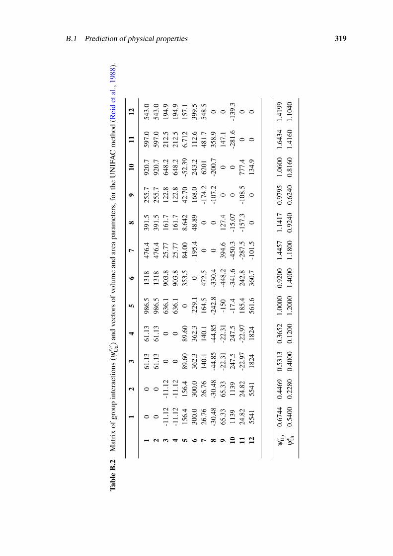
B.1 Prediction of physical properties 319
Tabl
eB
.2M
atri
xof
grou
pin
tera
ctio
ns(ψ
v,v
Ua)
and
vect
ors
ofvo
lum
ean
dar
eapa
ram
eter
s,fo
rthe
UN
IFA
Cm
etho
d( R
eid
etal
.,19
88).
12
34
56
78
910
1112
10
061
.13
61.1
398
6.5
1318
476.
439
1.5
255.
792
0.7
597.
054
3.0
20
061
.13
61.1
398
6.5
1318
476.
439
1.5
255.
792
0.7
597.
054
3.0
3-1
1.12
-11.
120
063
6.1
903.
825
.77
161.
712
2.8
648.
221
2.5
194.
94
-11.
12-1
1.12
00
636.
190
3.8
25.7
716
1.7
122.
864
8.2
212.
519
4.9
515
6.4
156.
489
.60
89.6
00
353.
584
.00
8.64
242
.70
-52.
396.
712
157.
16
300.
030
0.0
362.
336
2.3
-229
.10
-195
.448
.89
168.
024
3.2
112.
639
9.5
726
.76
26.7
614
0.1
140.
116
4.5
472.
50
0-1
74.2
6201
481.
754
8.5
8-3
0.48
-30.
48-4
4.85
-44.
85-2
42.8
-330
.40
0-1
07.2
-200
.735
8.9
09
65.3
365
.33
-22.
31-2
2.31
-150
-448
.239
4.6
127.
40
014
7.1
010
1139
1139
247.
524
7.5
-17.
4-3
41.6
-450
.3-1
5.07
00
-281
.6-1
39.3
1124
.82
24.8
2-2
2.97
-22.
9718
5.4
242.
8-2
87.5
-157
.3-1
08.5
777.
40
012
5541
5541
1824
1824
561.
636
0.7
-101
.50
013
4.9
00
ψv U
p0.
6744
0.44
690.
5313
0.36
521.
0000
0.92
001.
4457
1.14
170.
9795
1.06
001.
6434
1.41
99ψ
v Ut
0.54
000.
2280
0.40
000.
1200
1.20
001.
4000
1.18
000.
9240
0.62
400.
8160
1.41
601.
1040

320 Complements
TableB
.3M
atrices(φ
i,iN
a ,φ
i,iN
b )ofbinaryinteractions
fortheN
RT
Lm
ethod( A
spenTech,2006).
Benzene
Water
CH
AC
HO
NA
CH
OL
Aniline
MN
BD
ICH
AC
HE
NO
CH
AN
IL
Benzene
045.19
-0.55160
02.479
-1.2890
00
Water
140.10
065.83
90.70141.0
5.8550
00
CH
A-0.03670
00
0-4.582
-2.4020
00
0C
HO
NA
097.45
00
00
00
00
CH
OL
0106.2
5.4190
016.13
00
00
Aniline
-1.75227.08
3.5460
-9.7890
00
00
MN
B-0.8730
-5.1550
00
00
00
0D
ICH
A0
00
00
00
00
0C
HE
NO
00
00
00
00
00
CH
AN
IL0
00
00
00
00
0
Benzene
0591.4
507.91.487
614.3-403.2
98.8327.49
-459.5-416.3
Water
-59540
1587-4071
-4573-6518
229.53452
3252.12944
CH
A-227.5
1.7700
57.891754
691.2-7.281
119.2189.9
179.9C
HO
NA
-17.24-3858
-31.350
-262.8-437.4
228.7167.1
377.6364.0
CH
OL
-116.3-4764
-2219368.3
0-6778
210.64231.1
243.2206.7
Aniline
460.4-549.5
-1033706.0
41620
-216.3923.9
388.2320.0
MN
B630.2
2270125.4
-50.64499.0
285.00
491.3311.6
240.7D
ICH
A-65.72
456.1-89.41
20.69-11.67
-279.232.05
0-6.992
-49.35C
HE
NO
658.7451.0
-161.8-279.3
-33.29-95.00
-76.5062.73
0-114.6
CH
AN
IL574.4
413.2-141.6
-270.1-16.02
-80.17-53.60
126.0128.9
0
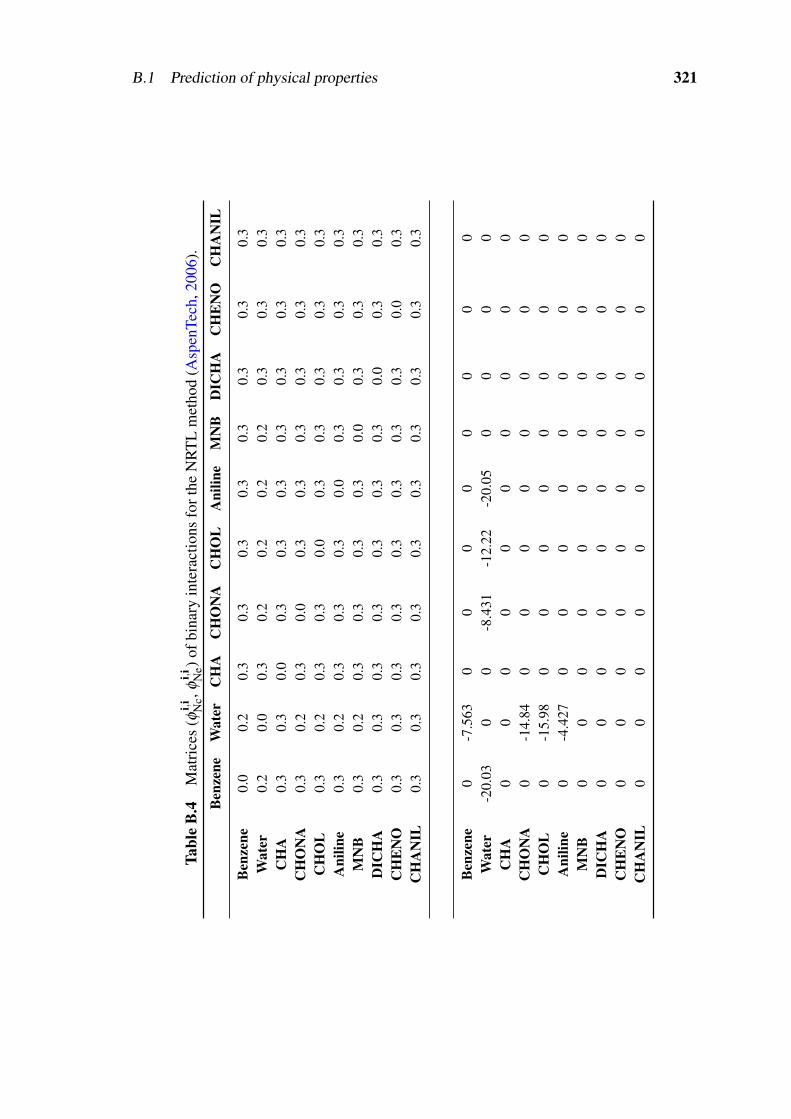
B.1 Prediction of physical properties 321
Tabl
eB
.4M
atri
ces
(φi,i N
c,φ
i,i Ne)
ofbi
nary
inte
ract
ions
fort
heN
RT
Lm
etho
d(A
spen
Tech
,200
6).
Ben
zene
Wat
erC
HA
CH
ON
AC
HO
LA
nilin
eM
NB
DIC
HA
CH
EN
OC
HA
NIL
Ben
zene
0.0
0.2
0.3
0.3
0.3
0.3
0.3
0.3
0.3
0.3
Wat
er0.
20.
00.
30.
20.
20.
20.
20.
30.
30.
3C
HA
0.3
0.3
0.0
0.3
0.3
0.3
0.3
0.3
0.3
0.3
CH
ON
A0.
30.
20.
30.
00.
30.
30.
30.
30.
30.
3C
HO
L0.
30.
20.
30.
30.
00.
30.
30.
30.
30.
3A
nilin
e0.
30.
20.
30.
30.
30.
00.
30.
30.
30.
3M
NB
0.3
0.2
0.3
0.3
0.3
0.3
0.0
0.3
0.3
0.3
DIC
HA
0.3
0.3
0.3
0.3
0.3
0.3
0.3
0.0
0.3
0.3
CH
EN
O0.
30.
30.
30.
30.
30.
30.
30.
30.
00.
3C
HA
NIL
0.3
0.3
0.3
0.3
0.3
0.3
0.3
0.3
0.3
0.3
Ben
zene
0-7
.563
00
00
00
00
Wat
er-2
0.03
00
-8.4
31-1
2.22
-20.
050
00
0C
HA
00
00
00
00
00
CH
ON
A0
-14.
840
00
00
00
0C
HO
L0
-15.
980
00
00
00
0A
nilin
e0
-4.4
270
00
00
00
0M
NB
00
00
00
00
00
DIC
HA
00
00
00
00
00
CH
EN
O0
00
00
00
00
0C
HA
NIL
00
00
00
00
00
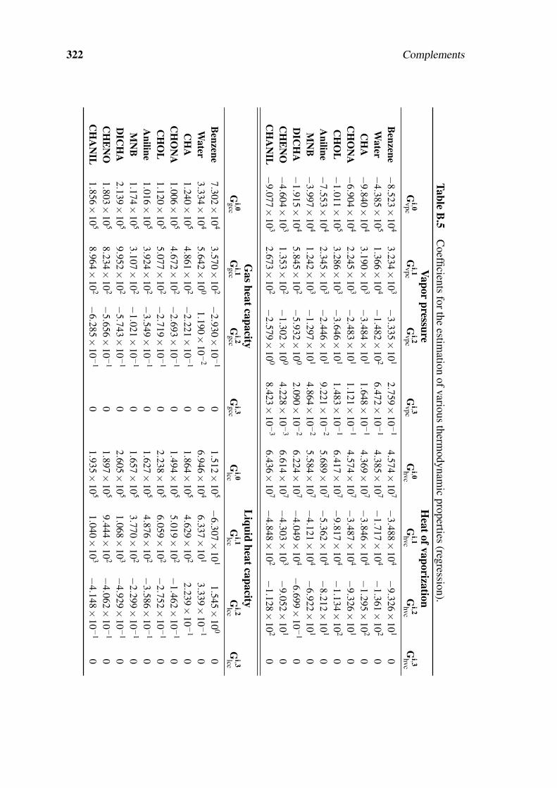
322 Complements
TableB
.5C
oefficientsforthe
estimation
ofvarioustherm
odynamic
properties(regression).
Vaporpressure
Heatofvaporization
Gi,0vpc
Gi,1vpc
Gi,2vpc
Gi,3vpc
Gi,0hvc
Gi,1hvc
Gi,2hvc
Gi,3hvc
Benzene
−8.523×
104
3.234×10
3−
3.335×
101
2.759×
10−
14.574×
107
−3.488×
104
−9.326×
101
0W
ater−
4.385×10
51.366×
104
−1.482×
102
6.472×
10−
14.385×
107
−1.717×
104
−1.361×
102
0C
HA
−9.840×
104
3.190×10
3−
3.484×
101
1.648×
10−
14.369×
107
−3.846×
104
−1.295×
102
0C
HO
NA
−6.904×
104
2.245×10
3−
2.483×
101
1.121×
10−
14.574×
107
−3.487×
104
−9.326×
101
0C
HO
L−
1.011×10
53.286×
103
−3.646×
101
1.483×
10−
16.417×
107
−9.817×
104
−1.134×
102
0A
niline−
7.553×10
42.345×
103
−2.446×
101
9.221×
10−
25.689×
107
−5.362×
104
−8.212×
101
0M
NB
−3.997×
104
1.242×10
3−
1.297×
101
4.864×
10−
25.584×
107
−4.121×
104
−6.922×
101
0D
ICH
A−
1.915×10
45.845×
102
−5.932×
100
2.090×
10−
26.224×
107
−4.049×
104
−6.699×
10−
10
CH
EN
O−
4.604×10
31.353×
102
−1.302×
100
4.228×
10−
36.614×
107
−4.303×
103
−9.052×
101
0C
HA
NIL
−9.077×
103
2.673×10
2−
2.579×10
08.423×
10−
36.436×
107
−4.848×
102
−1.128×
102
0
Gasheatcapacity
Liquid
heatcapacityG
i,0gccG
i,1gccG
i,2gccG
i,3gccG
i,0lccG
i,1lccG
i,2lccG
i,3lcc
Benzene
7.302×
104
3.570×10
2−
2.930×10
−1
01.512×
105
−6.307×
101
1.545×
100
0W
ater3.334×
104
5.642×10
01.190×
10−
20
6.946×
104
6.337×10
13.339×
10−
10
CH
A1.240×
105
4.861×10
2−
2.221×10
−1
01.864×
105
4.629×10
22.239×
10−
10
CH
ON
A1.006×
105
4.672×10
2−
2.693×10
−1
01.494×
105
5.019×10
2−
1.462×
10−
10
CH
OL
1.120×
105
5.077×10
2−
2.719×10
−1
02.238×
105
6.059×10
2−
2.752×
10−
10
Aniline
1.016×
105
3.924×10
2−
3.549×10
−1
01.627×
105
4.876×10
2−
3.586×
10−
10
MN
B1.174×
105
3.107×10
2−
1.021×10
−1
01.657×
105
3.770×10
2−
2.299×
10−
10
DIC
HA
2.139×
105
9.952×10
2−
5.743×10
−1
02.605×
105
1.068×10
3−
4.929×
10−
10
CH
EN
O1.803×
105
8.234×10
2−
5.656×10
−1
01.897×
105
9.444×10
2−
4.062×
10−
10
CH
AN
IL1.856×
105
8.964×10
2−
6.285×10
−1
01.935×
105
1.040×10
3−
4.148×
10−
10