Modelos de nicho, mudanças climáticas e a vulnerabilidade ...
202
UNIVERSIDADE FEDERAL DO ESPÍRITO SANTO CENTRO DE CIÊNCIAS HUMANAS E NATURAIS PROGRAMA DE PÓS-GRADUAÇÃO EM CIÊNCIAS BIOLÓGICAS Modelos de nicho, mudanças climáticas e a vulnerabilidade do clado Perissodactyla ao longo do tempo Andressa Gatti Vitória, ES Junho, 2013
Transcript of Modelos de nicho, mudanças climáticas e a vulnerabilidade ...
UNIVERSIDADE FEDERAL DO ESPÍRITO SANTO
CENTRO DE CIÊNCIAS HUMANAS E NATURAIS
PROGRAMA DE PÓS-GRADUAÇÃO EM CIÊNCIAS BIOLÓGICAS
Modelos de nicho, mudanças climáticas e a vulnerabilidade
do clado Perissodactyla ao longo do tempo
Andressa Gatti
Vitória, ES
Junho, 2013
UNIVERSIDADE FEDERAL DO ESPÍRITO SANTO
CENTRO DE CIÊNCIAS HUMANAS E NATURAIS
PROGRAMA DE PÓS-GRADUAÇÃO EM CIÊNCIAS BIOLÓGICAS
Modelos de nicho, mudanças climáticas e a vulnerabilidade
do clado Perissodactyla ao longo do tempo
Andressa Gatti
Orientador: Paulo De Marco Júnior
Tese submetida ao Programa de Pós-Graduação em Ciências
Biológicas (Biologia Animal) da Universidade Federal do
Espírito Santo como requisito parcial para a obtenção do grau
de Doutor em Biologia Animal.
Vitória, ES
Junho, 2013


“Não há parte da história natural mais
interessante ou instrutiva do que o estudo da
distribuição geográfica dos animais.” Alfred
Russell Wallace (1823-1913)
AGRADECIMENTOS
Aprendi logo cedo na minha vida profissional que um trabalho não se faz sozinho, uma ideia não
se sustenta somente com o seu "criador" em longo prazo, que ninguém é autossuficiente e que as
parcerias que criamos precisam ser mantidas com respeito e cuidado. E antes de tudo, antes do
trabalho, está o respeito pelas pessoas, pelos amigos. Logo, estes agradecimentos são feitos de
coração para os meus amigos.
Primeiramente quero agradecer ao meu amigo e orientador, Paulo De Marco Júnior. Eu lembro
quando entrei há um pouco mais de quatro anos em sua sala e perguntei se ele aceitaria me
orientar. Pois é, ele aceitou me orientar mesmo eu morando aqui em Vitória, coordenando o
Projeto Pró-Tapir e com as minhas limitações. Paulo, muito, muito obrigada por ser um Mestre,
no sentido literal da palavra, você me fez manter a calma e acreditar em mim, que eu poderia
fazer uma tese que eu realmente tivesse orgulho. Não sei se atendi às suas expectativas, mas eu
sei que é muito bom ter alguém que confia no seu trabalho e em você, especialmente. E, sim, eu
tenho muito orgulho de ter sido sua aluna!
Muito obrigada também a Caroline Nóbrega, minha amiga e co-orientadora. Toda vez que me
lembro da Carolzinha, a primeira sensação é de quietude. Tão simples e tão poderosa ao mesmo
tempo. Com uma mente brilhante, mas com um coração mais brilhante ainda. Muito obrigada,
minha amiga, por toda a ajuda, abraços apertados, colaboração, discussões e por compartilhar tão
livremente tudo que você tem aprendido. Estes quatro anos me trouxeram muito mais do que
scripts, ideias e hipóteses, me trouxeram uma grande amiga.
Ao Matheus Lima-Ribeiro, um pesquisador competente que aceitou o meu convite em participar
de um dos capítulos dessa tese. Matheus leu tudo atentamente, discutiu e colaborou com outras
partes da tese também. Muito obrigada, Matheus, você foi muito bacana!
Sabe aquele amigo que chega de mansinho, vai tomando espaço e quando você percebe, ele se
tornou um dos seus melhores amigos?! Pois é, Paulo Rogério Mangini ou simplesmente
Paulinho, meu revisor oficial, é assim! Sempre que eu precisei, lá estava o Paulinho, com suas
brincadeiras, conversas sérias, discussões pra lá de interessantes sobre os Perissodactyla, sempre
disposto a ler o que eu escrevi. Muito obrigada, meu amigo!
Muito, muito, muito obrigada a todos os amigos que me acolheram tão bem em suas casas, em
Goiânia, e por muitas vezes dividiram seu quarto, ao longo desses quatro anos: Karina, Thiago,
Daniel, Miriam; Joana, Leandro e Fabio; Poli e Camis; Renas e Carla; Livia e a pequena Nalu;
Monik e Daniel; Carol e Edu; Paulinho e sua querida família; Shayana, Yasmim e Adriano.
Aos amigos do laboratório The MetalLand, antigo “Limno”, que me receberam super bem desde
o início e dispenderam de seu tempo para me ajudar a pensar, analisar e discutir o meu trabalho.
Sim, eu tive uma comitiva, com vários assessores (risos), como minha querida amiga Renata, que
me assessorou nos assuntos amazônicos e nos mapas. Apesar de não ter vivenciado o dia a dia do
laboratório por muito tempo, eu pude construir laços de amizade e de trabalho, que eu tenho
certeza que seguirão por toda a minha vida. E um agradecimento especial pelas risadas, piadas,
abraços, sorrisos, músicas matinais, gemadas com chá e tantos outros carinhos.
Super obrigada aos membros da banca: Patricia Medici, Natália Mundim Tôrres, Sérgio Lucena
Mendes, Albert David Ditchfield, Daniel Brito e Francisco Barreto por terem aceitado
prontamente o convite e especialmente, porque cada um deles contribuiu muito positivamente
para a minha formação acadêmica e profissional ao longo desses anos.
Um super agradecimento a minha equipe do Pró-Tapir/Instituto Marcos Daniel, que durante a
minha ausência ficou firme no projeto, resolvendo tudo que estava ao alcance deles. Obrigada
por terem abraçado o meu projeto de vida, que eu sei que hoje também é o de muitos de vocês!!
Aos meus amigos da UFES, que sempre me motivaram, me fizeram rir e me apoiaram. Amo ter a
amizade de todos vocês. Em especial, as minhas grandes amigas de turma e de vida, Carla e
Dani, que também participaram da elaboração dessa tese, em diferentes momentos.
Agradeço imensamente a minha família. A minha mãe Marilene, que me deu tanto amor e
sempre me mostrou que o respeito e educação estão acima de tudo. Ela é guerreira, tomou
decisões em sua vida que outra pessoa não teria coragem, e sempre foi muito cuidadosa comigo e
com minhas irmãs. Ela é a minha grande inspiração, por ela eu faria tudo de novo. E minhas
irmãs tão queridas, Vanessa e Ana Paula, que me apoiaram incondicionalmente quando eu decidi
fazer o doutorado. Seguraram as pontas aqui em casa e sempre estiveram por perto quando eu
mais precisei. Eu dedico essa tese especialmente a vocês, mãe, Vanessa e Paulinha.
SUMÁRIO
RESUMO ....................................................................................................................................... v
ABSTRACT ................................................................................................................................. vii
1. INTRODUÇÃO GERAL E FUNDAMENTAÇÃO TEÓRICA ........................................ 1
1.1. História evolutiva dos Perissodactyla ............................................................................... 1
1.1.1. A história dos Tapiridae: uma abordagem mais detalhada sobre Tapirus
terrestris................................................................................................................................... 6
1.2. Mudanças climáticas: passado e futuro ........................................................................... 8
1.3. Vulnerabilidade às mudanças climáticas globais .......................................................... 12
1.4. Teoria do Nicho Ecológico ............................................................................................... 15
1.5. Modelagem de Nicho Ecológico ...................................................................................... 18
2. APRESENTAÇÃO DOS CAPÍTULOS ................................................................................ 21
3. REFERÊNCIAS ...................................................................................................................... 27
CAPÍTULO 1 .............................................................................................................................. 43
Climatic niche and vulnerability to global climate change: an analysis of clade
Perissodactyla .......................................................................................................................... 43
CAPÍTULO 2 .............................................................................................................................. 98
Ecological niche models predict range expansion for Tapirus terrestris after last ice age 98
CAPÍTULO 3 ............................................................................................................................ 138
Present and future challenges for conservation of Tapirus terrestris as revealed by
ecological niche models ......................................................................................................... 138
CONSIDERAÇÕES FINAIS....................................................................................................190
v
RESUMO
A Terra sofreu várias mudanças climáticas no passado e as mais recentes ocorreram
durante os ciclos glacial-interglacial no Quaternário resultando na perda de habitat, em
expansões e reduções do nível dos oceanos, produzindo mudanças nos ecossistemas e alterações
significativas no habitat disponível para os herbívoros terrestres, principalmente. Muitas
extinções dessa época são associadas às mudanças climáticas “naturais”, no entanto, as predições
indicam que as alterações climáticas, ocasionadas pelas atividades antrópicas, serão uma das
principais ameaças à biodiversidade no futuro. Em resposta às flutuações climáticas, a
distribuição de algumas espécies poderá sofrer mudanças ou, ainda, as espécies poderão se
deslocar para novas áreas adequadas. Contudo, isso dependerá de sua capacidade em dispersar e
de características ambientais. Assim, é fundamental identificar quais são as características que
tornariam as espécies mais vulneráveis a essas mudanças. Nesse contexto, os Perissodactyla
mostraram-se um modelo adequado para testarmos nossas hipóteses, pois compreendem um
grupo de grandes mamíferos herbívoros, extremamente ameaçados, que passaram por inúmeras
mudanças ambientais desde a sua origem. Nosso principal objetivo foi avaliar a influência das
alterações climáticas sobre os mamíferos do clado Perissodactyla, em uma escala temporal
ampla, abrangendo desde o Quaternário (a partir do Último Interglacial) até o futuro (ano 2080).
Utilizamos duas abordagens: i) a relação entre as características do nicho e a vulnerabilidade do
clado no futuro; e ii) a influência do clima na distribuição de áreas ambientalmente adequadas,
de Tapirus terrestris, no passado e no futuro. Para testar nossas predições nos baseamos na
Modelagem de Nicho Ecológico, que tem sido uma das abordagens mais empregadas e
relevantes para predizer as mudanças na distribuição das espécies. Nós usamos diferentes
vi
conjuntos de modelos climáticos (paleoclimáticos, atuais e futuro) e procedimentos de
modelagem. Os resultados indicam que os Perissodactyla apresentaram características de nicho
distintas, e que espécies consideradas generalistas também podem sofrer negativamente com os
efeitos das mudanças climáticas. Além disso, grande parte das respostas das espécies foi
idiossincrática. Outro ponto importante são as barreiras que podem limitar a dispersão dessas
espécies para novas áreas ambientalmente adequadas, pois concluímos que várias espécies do
clado ocorrem em áreas altamente ameaçadas pelas mudanças climáticas. Dentre os
Perissodactyla, T. terrestris, se mostrou a espécie mais climaticamente generalista. Contudo, a
avaliação da resposta da espécie em relação às diferentes mudanças climáticas, sugere que as
condições mais críticas, que prevaleceram durante o Último Máximo Glacial, reduziram a
extensão geográfica das áreas climaticamente adequadas para a anta, com uma subsequente
expansão. Se o clima não foi um problema muito sério na história evolutiva da espécie, os
desafios para a sua conservação na atualidade e no futuro podem ser bem maiores. Mesmo que a
extensão da distribuição geográfica da anta em si não se altere como resposta às alterações
climáticas, predizer as mudanças da adequabilidade ambiental ao longo dessa distribuição nos
auxiliará na priorização de áreas para a conservação da espécie. Dessa forma, o desaparecimento
das condições climáticas e a emergência de novas áreas ambientalmente adequadas devem ser
considerados em planos de manejo futuros, especialmente na criação de novas unidades de
conservação tanto para T. terrestris quanto para os demais Perissodactyla.
Palavras-chave: Mudanças climáticas, Mamíferos, Perissodactyla, Paleoclima, Modelagem de
distribuição de espécies, Unidades de conservação.
vii
ABSTRACT
The Earth has undergone several climate changes in the past, and the latest occurred during the
glacial-interglacial cycles in the Quaternary, resulting in habitat loss, during ocean expansions
and reductions, and several ecosystem changes. Numerous extinctions of that time are associated
with "natural” climate change. However, the predictions indicated that climate change caused by
human activities is now the major threat to biodiversity. In response to climatic fluctuations, the
distribution of some species may change, or species can move to new suitable areas. But this will
depend on their ability to disperse and environmental characteristics in an anthropic ecosystem.
Thus, it is essential to identify the most important characteristics that make species more
vulnerable to those changes. In this context, the clade Perissodactyla was a good model to test
our hypotheses, because they are a group of large herbivorous mammals extremely threatened,
that went through numerous environmental changes since its origin. I evaluated the influence of
climate change on the Perissodactyla clade, on a wide time scale, ranging from the Quaternary
(from the Last Interglacial) to the future (2080). I used two approaches: i) the relationship
between the characteristics of the niche and the vulnerability of the clade in the future, and ii) the
influence of climate on the distribution of environmentally suitable areas of Tapirus terrestris, in
the past and future. To test the predictions, I used an Ecological Niche Modeling, which has been
one of the most relevant approaches to predict changes in the species distributions. I used
different sets of climate models (i.e. paleoclimate, present and future climates) and modeling
procedures. The results indicated that the Perissodactyla showed distinct niche characteristics.
Generalist species may also suffer negative effects of climate change. Furthermore, most of the
species had idiosyncratic responses. Another important point is that barriers may have limited the
dispersion of these species to new areas environmentally appropriate because several of these
Perisodactyla occurred in areas highly threatened by climate change. The evaluation of the
response of T. terrestris (the species most climatically generalist), to different climate scenarios,
suggests that the most critical condition that prevailed during the UMG reduced the geographical
extent of areas climatically suitable, with subsequent expansion. If the weather was not a very
serious problem in the evolutionary history of the lowland tapir, the challenge to conserve this
viii
taxon today and in the future may be much higher. Even if the total size range itself does not
change as a response to climate variations, predicting the suitability of the environmental
changes, along the distribution of tapirs, can help us to prioritize areas for their conservation.
Thus, the disappearance of the climatic conditions and the emergence of new environmentally
suitable areas should be considered in future management plans, especially concerning to
creation of new protected areas for both T. terrestris as for other Perissodactyla species.
Keywords: Climate change, Mammals, Perissodactyla, Paleoclimate, species distribution
modeling, Conservation Units
1
1. INTRODUÇÃO GERAL E FUNDAMENTAÇÃO TEÓRICA
1.1. História evolutiva dos Perissodactyla
A Era Cenozóica, há 66 milhões de anos, é comumente conhecida como a "Era dos
Mamíferos", mesmo abrangendo apenas o terço final da fase de maior diversificação na evolução
dos mamíferos (Archibald & Deutschman, 2001). O máximo de diversidade dos mamíferos
placentários na Terra foi no início do Eoceno, durante o ótimo climático (55–52 Ma; Zachos et
al., 2001). Esse foi considerado um período de grande produtividade primária, com altas
temperaturas, favorecendo o surgimento de uma grande área habitável. A vegetação nas altas
latitudes foi similar às florestas tropicais modernas no que diz respeito à diversidade de plantas
(Collinson et al., 1981; Wolfe, 1985), o que provavelmente favoreceu o desenvolvimento de
mamíferos florestais e sua diversificação.
Foi neste cenário que o clado Perissodactyla -- constituído por mamíferos ungulados que
mantêm o apoio corporal sobre número ímpar de dedos -- tornou-se um grupo importante de
herbívoros, especialmente folívoros, de médio e grande porte, sendo considerado o grupo mais
abundante no início do Terciário. Existem opiniões divergentes sobre as relações entre os
Perissodactyla, resultantes dos paralelismos que ocorreram no início de sua radiação. Uma
hipótese é que a origem do clado tenha sido a partir dos Condylarthra (Phenacodontidae) baseada
nas similaridades da estrutura bilofodonte dos dentes, no final do Paleoceno (Radinsky, 1969). Já
McKenna et al. (1989) propõem que Radinskya, um Condylarthra – Phenacolophidae, tenha sido
o ancestral do clado. Existe também discordância sobre qual grupo dentre os Perissodactyla é o
mais primitivo (tapiróides, brontotérios ou equóideos) (Radinsky, 1963).
2
Neste momento inicial, três ou talvez quatro das cinco superfamílias de Perissodactyla
teriam surgido. No registro fóssil, existem evidências de espécimes representativos de cinco
superfamílias (Tapiroidea, Rhinocerotoidea, Chalicotheroidea, Equoidea and Brontotheroidea),
incluindo 14 diferentes famílias (Holbrook, 1999).
Os primeiros Perissodactyla originaram-se na América do Norte e Europa (Prothero &
Schoch, 1989). Em adição a estes, uma radiação adaptativa inicial ocorreu após o surgimento da
ordem com novas formas de ungulados representadas, por exemplo, pelos brontotérios
(Titanotheriomorpha), mamíferos semelhantes a rinocerontes (Kemp, 2005). Os Equoidea
também diversificaram neste período, particularmente na Europa (Radinsky, 1969), onde
Palaeotherium, um ungulado similar a uma anta, foi bastante comum (Kemp, 2005). A terceira
linhagem dos Perissodactyla diversificou-se na fase mais quente (15 milhões de anos antes do
presente), coincidindo com o segundo pico de diversidade dos mamíferos no Cenozóico.
Novamente, a alta produtividade vegetal criou oportunidades para uma diversificação de
mamíferos herbívoros e seus predadores (Janis, 1993). Os Chalicoteriidae (Chalicotherium)
foram os maiores e mais especializados do Oligoceno até o Pleistoceno, embora estivessem
presentes no Eoceno, a principal radiação ocorreu no Mioceno.
A linhagem dos Tapiroidea e Rhinocerotoidae divergiu do ancestral comum há 50
milhões de anos (Colbert & Schoch, 1998). Os Tapiroidea foram amplamente diversos durante o
Eoceno, quando houve uma abundância de gêneros na América do Norte, Europa e Ásia, e
algumas dessas formas originais (e.g., Heptodon da família Helaletidae), mostraram muitas
semelhanças com as antas atuais (gênero Tapirus). Os Rhinocerotoidae, aparentemente derivados
de radiações secundárias dos Tapiroidea (Radinsky, 1969), foram muito mais diversos desde o
Eoceno até o Mioceno do que são atualmente, incluindo desde formas pequenas semelhantes a
3
uma anta até o gigante Indricotherium. Foi apenas durante o Oligoceno e Mioceno que ocorreu o
surgimento dos rinocerontes verdadeiros (família Rhinocerotidae), os quais se tornaram
abundantes em todos os continentes do Norte e na África (Kemp, 2005). Os Rhinocerotidae
foram um dos grupos de mamíferos de maior sucesso na América do Norte. Após a extinção dos
titanotérios no Eoceno Superior, os rinocerontes foram os maiores mamíferos até o aparecimento
dos mastodontes no Mioceno Médio. Entretanto, no final do Mioceno os rinocerontes foram
extintos da América do Norte, muito provavelmente devido à perda de habitats florestais
subtropicais durante o resfriamento e aridificação.
Diferentes hipóteses foram propostas para justificar o sucesso dos Perissodactyla durante
milhões de anos. Uma das mais difundidas está relacionada à sua fisiologia. O sistema de
fermentação alimentar realizado no ceco (hindgut) possibilita o consumo de itens alimentares
altamente fibrosos, incluindo diferentes espécies de plantas encontradas durante o Eoceno (Janis,
1989). Mais da metade dos ungulados, no início do terciário, foram fermentadores de ceco, uma
condição plesiomórfica para estes mamíferos (Janis, 1989). No entanto, os padrões de
diversidade dos Perissodactyla mostraram uma mudança no final do Mioceno em paralelo a uma
mudança similar na diversidade dos Artiodactyla. Na América do Norte, por exemplo, a
diversidade de ungulados foi alta e incluiu além dos Perissodactyla, os mamíferos da ordem
Artiodactyla.
Desde o final do Eoceno, a diversidade genérica dos Perissodactyla declinou enquanto
que a dos Artiodactyla aumentou (Janis, 1989, 1993; Cifelli, 1981). Chalicotérios e tapirídeos
continuaram a aparecer como elementos raros da fauna durante o Ótimo Climático do Mioceno
(Blois & Hadly, 2009), no entanto, há o registro do surgimento do gênero Tapirus durante este
período (25–5 maa). Existem alguns debates e hipóteses propostas sobre o declínio dos
4
Perissodactyla em relação à diversificação dos Artiodactyla (Cifelli, 1981; Mitchell & Lust,
2008; Janis, 1989, 2009). Janis (1989) argumenta que a interação competitiva não foi um fator
impactante, mas sim, as mudanças climáticas, pois o clado Artiodactyla continuou a crescer a
partir do Oligoceno e desde o Mioceno Médio o número dos perissodáctilos foi constante.
A transição Eoceno/Oligoceno marca o início de profundas diferenças sazonais na
disponibilidade e abundância de vegetação. Janis (1976) sugeriu que em resposta a essas
diferenças, os artiodáctilos desenvolveram um trato digestivo ruminante e diferentes estratégias
de seleção de habitat, além da melhora na locomoção, facilitando a adaptação a áreas abertas.
Mitchell & Lust (2008) chamam a atenção para a habilidade termorregulatória dessas espécies e
consequente vantagem competitiva sobre os Perissodactyla, durante o clima altamente sazonal
pós-Eoceno. No entanto, Cifelli (1981) não evidencia competição nem substituição entre as
ordens, ao contrário, argumenta que as ordens evoluíram independentemente. De qualquer
forma, analisar o evento da radiação dos Artiodactyla é extremamente importante para
entendermos quais fatores (biótico, abiótico ou a combinação entre eles) podem ter contribuído
para moldar a história evolutiva dos Perissodactyla.
Alguns eventos geológicos e climáticos também contribuíram na formação da história
evolutiva dos Perissodactyla e, em diferentes períodos, houve migrações entre os continentes.
Imigrações em combinação com mudanças climáticas podem ter um grande efeito sobre estrutura
e composição de comunidades. Há 20-16.5 Ma (final do Mioceno Inferior), um decréscimo no
nível do mar (Keller & Barron, 1983) permitiu o intercâmbio extensivo entre África e Eurásia, e
também entre Eurásia e América do Norte. Conexões intermitentes entre América do Norte e
Ásia, através do Estreito de Bering, favoreceram o aparecimento das antas na Eurásia (Medici,
2011).
5
A história da fauna na América do Sul, a partir do Plioceno, está intimamente ligada à
emergência do Istmo do Panamá, que ocorreu entre 7.0-2.5 milhões de anos, possibilitando o
fluxo de fauna entre América do Norte e América do Sul, evento este donominado Grande
Intercâmbio da Biota Americana (Marshall, 1988). Este evento proporcionou a imigração das
antas para a América do Sul, originando no continente pelo menos cinco espécies já extintas e as
espécies viventes: Tapirus pinchaque e T. terrestris (Marshall, 1988; Holanda et al., 2011;
Medici, 2011). Antes deste intercâmbio, a fauna da América do Sul era diferente de qualquer
outra e foi representada por ungulados nativos, tais como os Meridiungulata (por exemplo,
Litopterna, Toxodonte), que durante o intercâmbio permaneceram. No entanto, estes
sobreviventes foram extintos no final do Pleistoceno.
Assim, os Perissodactyla atuais são remanescentes de uma ampla radiação no Terciário,
seguida de uma redução na sua diversidade, permanecendo apenas quatro famílias até o
Quaternário. Atualmente apenas três famílias são representadas em 16 espécies distribuídas em
seis gêneros. Tradicionalmente, os Perissodactyla têm sido divididos em duas subordens: i)
Hippomorpha, que é representada pela família Equidae, e ii) Ceratomorpha, compreendendo as
famílias modernas Tapiridae e Rhinocerotidae (Radinsky, 1966; Prothero & Schoch, 1989).
Diferentes trabalhos examinaram as relações filogenéticas do clado Perissodactyla (Norman &
Ashley, 2000; Price & Bininda, 2009; Willerslev et al., 2009; Steiner & Ryder, 2011) e, de
maneira geral, os resultados suportam a monofilia das subordens Ceratomorpha e Hippomorpha,
e as famílias Rhinocerotidae, Tapiridae e Equidae. Recentemente, dois trabalhos sobre a
filogeografia das espécies viventes de Tapirus foram publicados (Thoisy et al., 2010; Ruíz-
Garcia, 2012). Thoisy et al. (2010) sugerem que os eventos climáticos no final do Pleistoceno
6
podem ter moldado a história de T. terrestris, além de indicar a Amazônia Ocidental como o
ponto de dispersão da espécie para as demais regiões da América do Sul.
1.1.1. A história dos Tapiridae: uma abordagem mais detalhada sobre Tapirus terrestris
Os registros mais antigos da família Tapiridae são datados do Oligoceno da Europa (33-
37 Maa) e seus fósseis têm sido frequentemente encontrados na Europa, América do Norte e
Ásia (Hulbert, 1995). A evolução da família envolveu, principalmente, um refinamento da
probóscide, a molarização dos pré-molares e o aumento geral no tamanho corporal. A família
incluiu os gêneros Protapirus (1º tapirídeo verdadeiro), Tapirus, Miotapirus e Tapiravus
(América do Norte), Megatapirus e Plesiotapirus (Ásia), e Tapiriscus, Eotapirus e Palaeotapirus
(Europa) (Colbert, 2007). Cerca de 20 diferentes espécies de Tapirus são reconhecidas paras
regiões da América do Norte, Europa e Ásia. O registro mais antigo do gênero Tapirus na
América do Sul data do Pleistoceno Inferior-Médio na Argentina (Tonni, 1992; Cione & Tonni,
2005; Nabel et al., 2000). Os três gêneros com origem na América do Norte compartilham a
condição derivada de Tapiridae que envolve a redução relativa no comprimento dos ossos
frontais, a migração posterior dos ossos nasais e o aumento na altura vertical pós-craniana
(Medici, 2011).
As antas são consideradas “fósseis vivos” (Janis, 1984; Medici, 2011), pois dentre os
Perissodactyla, foram as espécies que mais retiveram características similares dos ungulados
primitivos (por exemplo, Hyracotherium), especialmente do esqueleto pós-cranial, como os
membros anteriores tetradáctilos e os posteriores tridáctilos. A dentição de Tapirus também é
considerada plesiomórfica (padrão bilofodonte estabelecido no início da história do grupo). Além
disso, as antas também retiveram vários aspectos comportamentais, como o hábito solitário e a
7
geração de um único filhote por gestação (são raros os casos de gêmeos), o que é uma condição
derivada nos ungulados (Janis, 1984).
A família Tapiridae (Gray 1821) é composta, atualmente, por um único gênero, Tapirus
(Brünnich 1772), com cinco espécies viventes: T. bairdii, T. indicus, T. pinchaque, T. kabomani
e T. terrestris. Tapirus kabomani foi descrita recentemente por Cozzuol et al. (2013). As relações
monofiléticas entre as antas da América do Sul, T. pinchaque e T. terrestris (Thoisy et al., 2010;
Ruíz-Garcia, 2012) são consistentes com a hipótese de que elas se originaram de um único
evento de dispersão de seu ancestral pelo Istmo do Panamá. Tapirus terrestris, a Anta Brasileira
ou Sul-Americana, é o tapirídeo vivente com a mais ampla distribuição georgráfica ocorrendo
nas zonas tropicais da América do Sul, em 11 países: Argentina, Bolívia, Brasil, Colômbia,
Equador, Guiana, Guiana Francesa, Paraguai, Peru, Suriname e Venezuela (Medici et al., 2007;
IUCN, 2012), onde a espécie habita uma multitude de diferentes ambientes. Quatro subespécies
de T. terrestris são reconhecidas: terrestris, colombianus, aenigmaticus e spegazzinii (para mais
detalhes sobre a distribuição das subespécies veja Medici, 2011).
Tapirus terrestris é um dos últimos remanescentes de dispersores a longa-distância de
espécies vegetais com grandes sementes, que já foram uma vez dispersadas por mamíferos no
Pleistoceno, especialmente nos Neotrópicos (Janzen & Martin, 1982; Hansen & Galetti, 2009). É
provável que as antas tenham vivido em áreas mesotermais úmidas, onde a diversidade e a
quantidade de folhagem eram grandes. O desenvolvimento da probóscide e de estratégias de
forrageamento seletivas podem ter permitido que os tapirídeos do Oligoceno e Mioceno
maximizassem a utilização de recursos em refúgios mesotermais restritos – áreas ripárias em
ambientes mais secos (Rose, 2006).
8
Desde a sua origem, a distribuição das antas vem mudando ao longo do tempo eessas
mudanças foram provavelmente causadas por migrações, mudanças continentais e climáticas, e
consequentemente a distribuição das florestas (García et al., 2012). De fato, os habitats ocupados
pelas antas na atualidade incluem, sobretudo, florestas tropicais associadas a corpos de água e
ambientes ripários (Medici, 2010). No entanto, é possível que T. terrestris e as demais espécies
do clado Perissodactyla não consigam lidar com as futuras mudanças climáticas uma vez que
grande parte das espécies encontra-se extremamente ameaçada de extinção devido às pressões
antrópicas.
1.2. Mudanças climáticas: passado e futuro
A Terra tem passado por diferentes cenários climáticos. No passado, as principais
alterações de clima foram associadas com a formação periódica de supercontinentes, episódios
glaciais e vulcanismo. Durante os últimos 100 milhões de anos houve inicialmente uma ligeira
tendência de resfriamento, que foi gradualmente revertida há cerca de 80 milhões de anos. Em
seguida, houve um breve e intenso período de aquecimento, há aproximadamente 55 milhões de
anos atrás. Este período corresponde à transição do Paleoceno-Eoceno, ou seja, coincide com o
início da Era Cenozóica, no período Terciário, o qual foi marcado por vários eventos climáticos
críticos (Zachos et al., 2001). A paleogeografia do início do Terciário difere consideravelmente
dos dias atuais (Janis, 1993) e o aquecimento no início do Paleoceno (66–57 Maa) foi seguido
por clima mais tropical (Paleoceno Médio) (Janis, 1993). Nesta fase, as florestas eram
aparentemente mais densas do que no Cretáceo, possivelmente porque a precipitação era maior e
menos sazonal (Krause & Maas, 1990).
9
O rápido aquecimento no final do Paleoceno foi seguido por um ótimo climático no início
do Eoceno (55–52 Ma; veja Zachos et al., 2001). Segundo Janis (1993), os eventos tectônicos
podem ter influenciado essa tendência, resultando em atividades vulcânicas e consequente
aumento na atividade hidrotermal dos oceanos, o que pode ter aumentado os níveis de CO2 (Rea
et al., 1990; Gingerich, 2006). Esse aquecimento possivelmente favoreceu a expansão das
florestas tropicais em maiores latitudes (Wolfe, 1985; Wing & Tiffney, 1987). Em seguida a essa
fase, houve um episódio de frio extremo nas maiores latitudes, com o surgimento de uma
vegetação decidual há 45 Ma (Janis, 2008), preparando um cenário de clima mais temperado no
Oligoceno, com ambientes mais áridos em médias latitudes. As temperaturas começaram a
aumentar no Oligoceno, em torno de 25 Ma, e depois de uma breve queda alcançaram um novo
pico, chegando ao ótimo climático há aproximadamente 15 Ma, durante o Mioceno Médio
(Zachos et al., 2001), com períodos mais quentes e mais secos. Diferentes trabalhos indicaram
uma tendência de decréscimo de CO2 durante a transição Oligoceno/Mioceno (Pagani et al.,
2005; Plancq et al., 2012; Grein et al., 2013), quando ocorreu um período de glaciação (Miller et
al., 1991).
No final do Mioceno (~ 6 Ma) as savanas da América do Norte foram substituídas por
pradarias (Retallack, 2001). A expansão da vegetação C4 (adaptadas a maior luminosidade e
climas mais quentes) foi registrada durante o Mioceno, entre 10 e 6 Ma (Cerling et al., 1997;
Uno et al., 2011), determinada principalmente pela mudança na dieta de equídeos e rinocerontes
fósseis (identificada a partir de análise de dentição). Porém, segundo Feakins et al. (2013), antes
dessa expansão das plantas C4 existiam extensos e produtivos campos durante o Mioceno Médio
dominados por vegetação C3, no norte da África. Esse período exibiu um declínio mais estável
das temperaturas e uma continuação das estiagens (Wolfe, 1978).
10
No entanto, o início do Plioceno foi um período de aquecimento global e transgressões
marinhas (Ravelo et al., 2004) com uma transição para o final (cerca de 2.5 Maa), representada
por glaciação no Ártico e um resfriamento global significante. Tipos modernos de desertos e
semi-desertos foram comuns nessa época, assim como pradarias, estepes e pampas (Wolfe,
1985). Ao mesmo tempo, surge o Istmo do Panamá, conectando as Américas do Norte e do Sul e
interrompendo a circulação circum-equatorial (Janis, 2008). Comparativamente ao período atual,
o período quente do Plioceno foi caracterizado por temperaturas mais altas em pelo menos
3ºC(Raymo et al., 1996; Ravelo & Andreasen, 2000). Um evento importante que ocorreu durante
o Mioceno foi a elevação dos Andes, sendo crucial para a formação da biota antes do
Quaternário (Hoorn et al., 2010). Além disso, as oscilações do nível do mar nos últimos 4 Ma
foram associadas com os ciclos de Milankovitch, desencadeando significativas mudanças na
paisagem da América do Sul (Dynesius & Jansson, 2000; Hoorn & Wesselingh, 2010).
Mais precisamente, a dinâmica do clima foi particularmente dramática durante o
Quaternário, que abrangeu os últimos 2.0-1.8 Ma. Composto pelas épocas do Pleistoceno e
Holoceno-Atual, este período foi caracterizado por pelo menos 20 avanços e retrações glaciais.
Condições glaciais dominaram esse período, com intervalos quentes de efeito estufa (~100 mil
anos) e com apenas alguns milhares de anos cada (Ruddiman, 2001). Esse período foi
caracterizado por muita variabilidade climática, incluindo súbitos desvios às condições mais
quentes ou mais frias, que ocorreram em menos de 1000 anos, por exemplo, o evento Younger
Dryas (12.9–11.6 mil anos atrás) que marcou a transição glacial-interglacial mais recente
(Rodbell, 2000). Após estas oscilações, o clima tornou-se muito estável e tem persistido como tal
durante os últimos 11.000 anos. Além disso, durante o Quaternário os períodos relativamente
secos (glaciais) foram mais frios também nos trópicos.
11
De forma geral, o clima tornou-se progressivamente mais frio e mais seco desde o último
período interglacial (~125 mil anos atrás) até o Último Máximo Glacial (UGM; ~21 mil anos
atrás) e, então, tornou-se mais quente e úmido no Holoceno Médio (~ 6 mil anos atrás) (Nogués-
Bravo et al., 2008). No Pleistoceno, durante o UGM (~21.000 anos atrás), o clima alcançou o
máximo do resfriamento em diferentes locais do mundo, com condições mais secas (Ledru et al.,
1998). Segundo Mayle et al. (2004), as florestas tropicais expandiram mais do que uma vez no
final do Holoceno devido ao aumento da precipitação. Além disso, estudos mostram que espécies
de florestas tropicais persistiram durante o UGM, por exemplo, nas terras baixas da região
Amazônica (Colinvaux et al., 1996).
Todas essas evidências suportam fortemente que as mudanças climáticas que ocorreram
no passado foram eventos chave para entender a mudança da vegetação tanto em escala espacial
quanto temporal. Mas será que o aumento na velocidade das mudanças climáticas preditas para o
futuro permitirá o entendimento de tais processos? Atualmente, uma das principais causas das
rápidas mudanças climáticas pode ser a liberação de gases de efeito estufa, tais como CO2 e
metano. No passado, tais liberações podem ter ocorrido naturalmente a partir das erupções
vulcânicas, por exemplo. Entretanto, as emissões atuais têm efeitos massivos sobre o ciclo global
do carbono e direcionam as principais mudanças no clima.
A estimativa é de que a concentração de CO2 na atmosfera tenha aumentado mais do que
30% no século passado, devido principalmente à queima de combustíveis fósseis. As últimas
previsões do Painel Intergovernamental sobre Mudanças Climáticas (em inglês,
Intergovernmental Panel on Climate Change – IPCC) indicam ainda que a média da temperatura
do ar na superfície global vai continuar a aumentar ao longo do século 21 (IPCC, 2007). As
projeções feitas para o fim do século (2090–2099) apontam para um aumento da temperatura
12
média global da ordem de 1.8 a 4ºC (IPCC, 2007). Na região Neotropical, as previsões apontam
para aquecimento de 0.4°C a 1.8°C até 2020, e de 1°C a 7.5°C até 2080. Os valores de
aquecimento mais elevados são projetados para a região tropical da América do Sul, como a
região Amazônica (Magrin et al., 2007). Ao mesmo tempo, temperaturas extremas e chuvas
também se tornarão mais comum, enquanto que a cobertura de neve e gelo do mar vai diminuir
contribuindo para a elevação do nível do mar (IPCC, 2007).
Diante desse cenário, um dos maiores desafios da atualidade é entender quais novos riscos as
mudanças climáticas trarão para a conservação de espécies a nível global. É provável que muitas
dessas mudanças não façam parte das experiências prévias vividas por cada organismo no
passado, afetando assim a habilidade das espécies em responder a essas mudanças. Dessa forma,
é crucial identificar como as espécies, e a dinâmica e composição dos ecossistemas locais podem
ser afetados pelas mudanças climáticas e como eles poderão potencialmente responder a essas
perturbações.
1.3. Vulnerabilidade às mudanças climáticas globais
O aumento nas emissões de gases de efeito estufa, como o CO2, implicará em uma
mudança climática significativa nas próximas décadas. Desta forma, o potencial para a perda de
biodiversidade e rompimento de serviços ecológicos deverá ser seriamente avaliado no processo
de tomada de decisões relativas à conservação. No passado geológico, muitas extinções de
espécies podem ter sido associadas a mudanças climáticas “naturais” resultando em perda de
habitat e mudanças nos ecossistemas (McKinney, 1997). No entanto, as mudanças climáticas
observadas na atualidade são reconhecidas como uma das principais ameaças à biodiversidade
13
global e vem causando extinções locais em diferentes partes do mundo. Espera-se que essas
alterações tenham um profundo efeito tanto sobre indivíduos quanto em populações animais
(Thomas et al., 2004; Schloss et al., 2012) e vegetais (Thuiller et al., 2006; Franklin et al., 2013).
A multiplicidade de resultados observados nas projeções realizadas para diferentes taxa e tipos
de história de vida enfatizam as respostas do passado, que provavelmente refletem no presente e
no futuro (Dawson, 2011), indicando que nem todas as espécies responderão da mesma forma,
mesmo em níveis similares de alterações climáticas (Arribas et al., 2012).
Lorenzen et al. (2011) demonstraram que o clima tem sido o principal direcionador de
mudanças populacionais nos últimos 50 mil anos. No entanto, cada espécie responde
diferentemente aos efeitos das alterações climáticas. Por exemplo, o clima por si só explicou a
extinção do rinoceronte lanudo, Coelodonta antiquitatis, comum na Europa e norte da Ásia. Em
geral, a proporção de espécies extintas foi maior nos continentes que estiveram mais expostos a
mudanças climáticas mais drásticas, reservando ao clima o papel principal na perda dessas
espécies. Além disso, espécies expostas a intensas alterações climáticas em combinação com
suscetibilidade intrínseca a essas alterações enfrentarão um maior risco de extinção (Foden et al.,
2008).
Em resposta às flutuações climáticas, a distribuição de algumas espécies poderá sofrer
contrações, expansões ou as espécies poderão se deslocar para habitats climaticamente mais
favoráveis (Parmesan & Yohe 2003). De acordo com Schloss et al. (2012), as mudanças
climáticas provavelmente ultrapassarão a capacidade de resposta de muitos mamíferos e a sua
vulnerabilidade a essas alterações poderá ser muito maior do que previsto anteriormente. Espera-
se que 90% das espécies de mamíferos experimentem reduções em sua distribuição e que essas
14
reduções serão, provavelmente, devidas às limitadas habilidades de dispersão, que
potencialmente proporcionaria a ocupação de novas áreas ambientalmente adequadas. Espécies
com maior habilidade de dispersão podem expandir rapidamente sua distribuição após mudanças
no ambiente, por exemplo, após as glaciações que ocorreram durante o Pleistoceno (Dynesius &
Jansson, 2000).
A compreensão da capacidade das espécies em expandir sua distribuição para novos
habitats adequados quando expostas a mudanças climáticas é importante, uma vez que indica as
probabilidades de extinção espécie-específica (ou espécies-específicas) (Thomas et al., 2004;
Loarie et al., 2008) e a estrutura da comunidade no futuro (Lawler et al., 2009; Gilman et al.,
2010). Thuiller et al. (2005) e Broennimann et al. (2006) colocam que a sensibilidade de uma
dada espécie às mudanças climáticas dependerá de sua distribuição geográfica e suas
propriedades do nicho ecológico, tais como amplitude e marginalidade.
Além da avaliação das consequências das mudanças climáticas sobre as espécies e sobre
os ecossistemas, é necessário considerar a sinergia entre tais mudanças e o acelerado aumento
das ameaças à biodiversidade, tais como perda de habitat e fragmentação, caça, disseminação de
doenças, invasão de espécies, entre outras. Tais ameaças podem intensificar o efeito das
mudanças climáticas sobre os organismos, aumentando a sua vulnerabilidade (para mais detalhes
veja a revisão feita por Brook et al., 2008). Estudos sugerem que o advento das mudanças
climáticas poderá superar a destruição de habitat no ranking de ameaças mundiais à
biodiversidade (Leadley et al., 2010). É tarefa fundamental da comunidade conservacionista, em
todo o mundo, identificar as características das espécies que as tornem resistentes ou suscetíveis
a mudanças climáticas. Desta forma, poderemos subsidiar melhores avaliações de risco de
extinção e desenvolver estratégias de conservação efetivas. Neste aspecto, como é possível
15
avaliar a vulnerabilidade das espécies e de seus habitats, e a distribuição do seu nicho climático
sob o efeito das mudanças climáticas, especialmente de um grupo extremamente ameaçado,
como é o caso dos grandes mamíferos herbívoros pertencentes à ordem Perissodactyla?
1.4. Teoria do Nicho Ecológico
Um dos principais impactos causados pelas mudanças climáticas é a alteração na
adequabilidade ambiental nas áreas ocupadas pelas espécies ou em potenciais locais que virão a
ocupar no futuro. Em teoria, os indivíduos estabelecem-se em habitats onde as condições
ambientais locais são propícias à sua sobrevivência e reprodução. No entanto, os fatores
climáticos e físicos podem afetar a distribuição das espécies, expressa pela ecologia e história
evolutiva de cada uma delas, em diferentes intensidades e escalas (Pearson & Dawson 2003), por
um longo período de tempo (Soberón & Peterson, 2005). Algumas das teorias mais fundamentais
sobre as condições ambientais que influenciam a distribuição de espécies foram apresentadas por
Joseph Grinnell há mais de 90 anos, quando foi registrado o primeiro uso da palavra “nicho”
(Grinnell, 1917, 1924).
Grinnell referiu-se ao "nicho ecológico ou ambiental" como a unidade de distribuição
final de uma espécie, sem levar em consideração a presença de interações com outras espécies,
considerando somente os locais que possuem as condições ambientais necessárias para uma
espécie sobreviver. Dessa forma, o nicho Grinnelliano pode ser definido por variáveis
fundamentalmente não interativas (cenopoéticas) (James et al., 1984; Austin, 2002) e pelas
condições ambientais em ampla escala, relevantes ao entendimento de propriedades ecológicas e
geográficas em grande escala (Jackson & Overpeck, 2000; Peterson, 2003). Outro conceito de
16
nicho foi proposto por Elton, em 1927, com enfoque nas interações bióticas e na dinâmica de
recursos-consumidor, que Hutchinson (1978) definiu como variáveis bionômicas, e que pode ser
medido, principalmente, em uma escala local. Ambas as classes de nichos são relevantes para a
compreensão da distribuição dos indivíduos de uma espécie (Soberón, 2007).
O conceito de nicho evoluiu ao longo do tempo. Hutchinson (1957) definiu nicho
ecológico como: “Hipervolume n-dimensional limitado pelas interações com outros organismos,
que envolve todas as respostas fisiológicas às condições do meio e depende da disponibilidade de
recursos, sob as quais as populações apresentam taxa de crescimento positivo”. Adicionalmente,
Hutchinson dividiu o conceito de nicho em fundamental (fisiológico ou potencial) e realizado
(ecológico, atual). Nicho fundamental é definido como o conjunto de todas as condições
ambientais que permitem o crescimento e a reprodução da espécie, distinguindo-se de nicho
realizado no qual os efeitos da competição reduzem o nicho fundamental de uma espécie, ou
ainda a área que ela pode ocupar Soberón (2007). Para Vandermeer (1972), talvez essa distinção
tenha sido o mais importante princípio derivado do conceito original de Hutchinson. De forma
geral, Hutchinson definiu nicho como uma propriedade da espécie e não do ambiente, como
discutido por Pulliam (2000).
Sobéron & Peterson (2005) e Guisan & Thuiller (2005) apresentam três fatores que
podem determinar a área em que uma espécie pode ser encontrada e que, consequentemente,
corresponde ao nicho da espécie: 1. Fatores abióticos, que impõem os limites fisiológicos sobre a
capacidade de sobrevivência de uma espécie; 2. Fatores bióticos, o conjunto de interações com
outras espécies que afetam a habilidade da espécie em manter suas populações; 3. As regiões que
são acessíveis à dispersão pela espécie. Deve-se considerar ainda que uma espécie somente
estará presente em um dado local, onde os três primeiros fatores estiverem reunidos, apesar de
17
outros fatores também contribuírem, como por exemplo, a capacidade evolutiva da espécie
(Sobéron & Peterson, 2005).
Dessa forma, Soberón & Peterson (2005) e Soberón (2007) apresentaram um diagrama,
que descreve alguns resultados da interação dos fatores que determinam a distribuição de
espécies: diagrama Biótico-Abiótico-Mobilidade, mais conhecido como diagrama BAM. Os
autores usam o diagrama como uma representação abstrata do espaço geográfico. A região
geográfica que apresenta somente as condições cenopoéticas favoráveis é chamada de “A”, que
Peterson & Soberón (2012) chamam de "nicho fundamental existente", onde a taxa de
crescimento intrínseco da espécie pode ser positiva (Soberón, 2010). A região identificada como
“B” é a área onde as condições bióticas estão disponíveis para a espécie e a terceira região, a
“M”, inclui áreas que têm sido acessíveis à espécie ao longo de períodos de tempo relevantes
(Soberón & Peterson, 2005; Peterson & Soberón, 2012) e foi previamente discutida por
(Barve et al., 2011).
Embora o nicho realizado possa ser mapeado, essa não é uma tarefa fácil do ponto de
vista conceitual e nem facilmente exequível do ponto de vista prático, pois as interações bióticas
são muito difíceis de mensurar. Dessa forma, reduzindo a definição de nicho ao conceito
Grinnelliano (ou nicho fundamental de Hutchinson), a dualidade entre os espaços ambiental e
geográfico se torna uma questão apenas operacional (Colwell & Rangel, 2009), porém de
extrema importância para modelagem em Ecologia, especialmente sob a perspectiva
paleoecológica e das mudanças climáticas futuras.
18
1.5. Modelagem de Nicho Ecológico
A teoria de nicho ecológico suporta fortemente uma das principais ferramentas utilizadas
atualmente, a Modelagem de Nicho Ecológico (mais à frente discutiremos as diferentes
denominações para esta ferramenta) (Guisan & Zimmermann, 2000; Soberón, 2007), a qual é
baseada principalmente no nicho Grinnelliano. Consequentemente, a teoria do nicho será a base
central do presente trabalho. Conforme apresentado anteriormente, as primeiras aplicações desta
teoria foram as de Joseph Grinnell, que utilizou a distribuição espacial de ocorrência de espécies
para inferir os fatores limitantes de suas distribuições, estabelecendo uma base sólida para os
trabalhos subsequentes neste campo. A diversidade de tais aplicações, no entanto, já cresceu
consideravelmente, mas de uma forma geral, estes estudos têm como principal objetivo
reconstruir os requerimentos ecológicos das espécies e/ou predizer suas distribuições potenciais
(Peterson, 2006). Resumidamente, os modelos são simplificações da realidade (Franklin, 2009),
formulados a partir de parâmetros observados na natureza.
Antes de considerarmos as demais questões envolvendo o uso dessa ferramenta, é preciso
entender as diferentes terminologias utilizadas. Os modelos de nicho ecológico (MNEs)
(Peterson et al., 1999) são também chamados de modelos de envelope bioclimático (Araújo &
Peterson, 2012) ou modelos de distribuição de espécies (MDEs) (Elith & Leathwick, 2009).
Segundo Peterson & Soberón (2012), o debate entre MNE e MDE está longe de ser meramente
semântico. É preciso entender que a distribuição geográfica normalmente obtida por tais modelos
não reflete os efeitos de dispersão e interações bióticas (Soberón, 2010). Desta forma, na maioria
das vezes não estamos lidando com a distribuição real da espécie, mas sim com sua distribuição
potencial. De acordo com a análise feita por Peterson & Soberón (2012), a terminologia MNE
19
deve ser usada somente quando o foco seja estimar o nicho fundamental ou o conjunto de áreas
que atendam às condições do nicho fundamental de uma espécie. Ou ainda, qualquer distribuição
potencial frente às mudanças nas condições ambientais e as circunstâncias utilizadas pelo
modelo. Considerando-se o foco central deste estudo, especialmente no que diz respeito
àdistribuição potencial de áreas ambientalmente adequadas para as espécies avaliadas, e
limitações técnicas, será adotado em todo o trabalho o termo “Modelos de Nicho Ecológico -
MNEs”.
Independentemente de terminologias, o princípio geral da MNE é obter um mapa de
adequabilidade ambiental, a partir de um modelo que descreva o nicho das espécies (Pearce &
Ferrier, 2000; Guisan et al., 2002; Thuiller, 2003). Este é um dos campos de pesquisa mais ativos
em Ecologia (Zimmermann et al., 2010), sendo aplicado a estudos com diferentes metas
(Peterson et al., 2011; Svenning et al., 2011), desde a descoberta da biodiversidade, passando
pela discussão de padrões biogeográficos, predição da invasão das espécies até a predição para o
futuro dos efeitos das mudanças climáticas sobre as espécies, buscando estabelecer estratégias
efetivas de conservação para as espécies e seus ambientes (Pearson et al., 2007; Keith et al.,
2008; Rood et al., 2010; Nóbrega & De Marco, 2011; Araújo et al., 2011; Hof et al., 2011,
Ochoa-Ochoa et al., 2012). Além disso, os MNEs também têm sido utilizados para reconstruir
nichos de espécies no passado buscando entender, por exemplo, a dinâmica de distribuição das
espécies e dos ecossistemas sob cenários de mudanças climáticas passadas, e a extinção da
megafauna no final do Pleistoceno (Nogués-Bravo et al., 2008, Varela et al., 2010, Lorenzen et
al., 2011, Lima-Ribeiro et al., 2012; Werneck et al., 2012).
Tecnicamente o MNE é sustentado por três pilares fundamentais: 1) a informação sobre
as espécies (tolerância fisiológica a partir de dados de ocorrência), 2) as variáveis ambientais
20
(variáveis preditoras), e 3) os métodos analíticos (funções ou modelos que relacionam as
informações sobre as espécies aos preditores ambientais). As projeções para o futuro ou
reconstruções para o passado são um resultado da distribuição conhecida da espécie e das
variáveis climáticas da região onde a espécie se encontra, identificando, assim, outras regiões as
quais a espécie possa potencialmente habitar ou as mudanças na distribuição das áreas
ambientalmente adequadas tanto no futuro quanto no passado (Heikkinen et al., 2006). O mapa
de adequabilidade define quais locais são mais ou menos adequados à sobrevivência da espécie
focal, dados seus requerimentos ecológicos (isto é, o modelo), o que é chamado de distribuição
geográfica modelada ou mapa preditivo (Elith & Leathwick, 2009, Franklin, 2009).
Existem várias classes de métodos analíticos utilizados para determinar o nicho ecológico
de uma espécie. Estes podem ser divididos em dois grupos de acordo com seus princípios
metodológicos: modelos mecanísticos e modelos correlativos. Em um modelo mecanístico, o
nicho é predito por um conjunto de funções baseadas em seu conhecimento fisiológico (Kearney
& Porter, 2009). Modelos correlativos são mais gerais e utilizam a informação ambiental contida
em um conjunto de pontos de ocorrência de uma espécie para determinar suas condições
ambientais favoráveis (Franklin, 2009). Os modelos correlativos assumem que a distribuição
geográfica da espécie focal é resultado de seus requerimentos ambientais (Soberón, 2007;
Soberón & Nakamura, 2009; Peterson et al., 2011). Dessa forma, é possível ajustar os modelos
utilizando tanto simulações paleoclimáticas, quanto as condições climáticas projetadas para o
futuro, a partir dos modelos climáticos globais de acordo com diferentes cenários de emissão de
gás carbônico (Hannah, 2011). Por essa razão, apenas modelos correlativos serão apresentados e
discutidos neste trabalho.
21
Com base em todas as informações, os MNEs têm se mostrado úteis especialmente no
planejamento de ações de conservação, chamando a atenção para espécies ou ecossistemas
ameaçados. É importante ressaltar, entretanto, que os modelos projetados precisam ser analisados
com cautela, considerando, principalmente, as características biológicas e ecológicas de cada
espécie avaliada, assim como outras variáveis como a fragmentação ambiental e outros impactos
antrópicos.
2. APRESENTAÇÃO DOS CAPÍTULOS
O clima foi um importante direcionador na história evolutiva dos Perissodactyla, mas
entender o que ocorreu no passado e prever o que acontecerá com seus representantes e,
principalmente, com os ambientes onde habitam no futuro, é desafiador. A base teórica
consultada nos incentivou a realizar uma abordagem integrada e propor hipóteses sobre a
influência do clima nesses grandes mamíferos herbívoros, em diferentes períodos temporais (125
mil anos antes do presente até 2080). O grau de vulnerabilidade das espécies do clado
Perissodactyla, em particular Tapirus terrestris, a diferentes cenários climáticos, foi avaliado no
intuito de acrescentar mais uma abordagem às análises de priorização de estratégias de
conservação. A base metodológica para testar nossas predições foi centrada na Modelagem de
Nicho Ecológico, a qual é sustentada especialmente pela Teoria do Nicho. Resultados e
discussões são apresentados na forma de três artigos, aqui denominados como capítulos.
O Capítulo 1 apresenta os aspectos de nicho climático que podem determinar a
vulnerabilidade do clado Perissodactyla às mudanças climáticas. Projeções resultantes de
modelos de nicho ecológico, baseadas em um cenário pessimista de emissão de gás carbônico,
foram utilizadas para examinar tais relações e testar se as espécies mais marginais e com baixa
22
tolerância climática teriam distribuição potencial mais restrita e se espécies com menor
tolerância e mais marginais teriam maior perda de áreas ambientalmente adequadas no futuro.
Resultados das análises demonstraram que a anta brasileira (Tapirus terrestris) é considerada a
mais generalista climaticamente enquanto que o cavalo de Przewalski é o mais especialista.
Os Perissodactyla apresentaram características de nicho distintas e, de acordo com as
análises, nem sempre a espécie mais especialista foi predita a sofrer mais seriamente os efeitos
das mudanças climáticas. Além disso, grande parte das respostas das espécies foi idiossincrática,
mesmo apresentando valores similares de marginalidade, como as espécies que habitam áreas de
montanhas. Isso sugere que é preciso avaliar cada espécie isoladamente, considerando suas
características biológicas e as características de sua área de ocorrência. Adicionalmente, é crucial
considerar as barreiras e características biológicas que poderiam potencialmente limitar a
dispersão dessas espécies a novas áreas ambientalmente adequadas. Deve-se considerar também
que muitas dessas espécies estão em áreas afetadas e ameaçadas por mudanças climáticas e por
alterações da paisagem produzidas pelo homem, além de outras pressões como a caça, que vem
dizimando centenas de indivíduos de todas as espécies avaliadas neste trabalho. Dessa forma,
consideramos que não somente as pressões antrópicas, mas também as mudanças nas condições
climáticas e a potencial emergência de novas áreas ambientalmente adequadas são fatores que
devem ser considerados em planos de ação futuros.
Uma questão que chamou a atenção neste capítulo está ligada à hipótese de que espécies
generalistas, com ampla distribuição, seriam menos ameaçadas pelas mudanças climáticas. A
Anta Brasileira foi a espécie mais generalista deste trabalho e, mesmo assim, quando foram
projetados os cenários mais pessimistas (maior emissão de gás carbônico e seleção apenas de
áreas consideradas altamente adequadas) demonstrou alto grau de vulnerabilidade. Tal resultado,
23
indicando que uma espécie generalista podeser altamente vulnerável a mudanças climáticas, leva
a uma nova pergunta: O que poderia contradizer a hipótese proposta por diferentes autores? Os
dois próximos capítulos foram estruturados com base nisso, focando somente na Anta Brasileira,
a qual se mostrou uma espécie intrigante, pois sobreviveu a fortes oscilações climáticas no
passado e, diferentemente do restante da megafauna que habitava a América do Sul naquele
momento, não desapareceu do continente.
Logo, o Capítulo 2 está bastante focado em como as áreas ambientalmente adequadas
para a anta estavam distribuídas no passado, considerando os impactos das oscilações climáticas
durante o Quaternário, e em como o clima pode ter contribuído para moldar a distribuição atual
da espécie. A hipótese utilizada foi a da mudança climática, que propõe que as reduções de áreas
climaticamente favoráveis podem ter levado à redução da distribuição da espécie, aumentando
sua suscetibilidade à extinção. Foram também trabalhadas hipóteses filogeográficas e
paleontológicas, as quais sugerem que a distribuição de T. terrestris sofreu retração durante o
Último Máximo Glacial (UGM), com uma rápida expansão após este período. Dessa forma, duas
predições foram testadas: 1. As áreas ambientalmente adequadas para a espécie foram restritas
durante o UGM; e 2. Houve expansão de áreas ambientalmente adequadas após esse período.
A fim de testar essas predições, dados atuais (pontos de ocorrência) de Tapirus terrestris
foram projetados para condições paleoclimáticas no Quaternário (Último Interglacial ~125 mil
anos atrás; Último Máximo Glacial ~21 mil anos atrás; Holoceno Médio ~6 mil anos atrás), a
partir de modelos de nicho ecológico, utilizando quatro diferentes algoritmos. As condições
paleoclimáticas têm sido razoavelmente bem estimadas para estes períodos geológicos, que são
considerados os períodos importantes do Pleistoceno e Holoceno, utilizando os modelos de
circulação geral. Para avaliarmos as mudanças na distribuição de um período a outro, tais como
24
expansão e contração, nós usamos duas métricas, mudança relativa e perda proporcional, as quais
têm sido frequentemente utilizadas em estudos com enfoque em mudanças climáticas.
Os resultados sugerem que as condições mais críticas que prevaleceram durante o UMG
reduziu a extensão geográfica das áreas climaticamente adequadas para a anta, expandindo
durante o período interglacial atual, com temperaturas mais quentes. Dessa forma, a modelagem
da paleodistribuição suportou fortemente hipóteses propostas previamente por estudos
filogeográficos e paleontológicos. O amplo nicho ambiental da anta, conforme observado no
Capítulo 1, pode ter favorecido que a anta expandisse rapidamente sua distribuição geográfica,
como proposto por outros estudos. Além disso, foi identificada uma grande área estável que foi
mantida ao longo do tempo, indicando que o efeito do clima para a anta pode ter sido bem menor
do que para as espécies de mamíferos extintas da megafauna.
Embora o clima não pareça ter sido um problema muito sério na história evolutiva da
espécie, o desafio para a sua conservação atualmente e no futuro pode ser bem maior. O efeito
combinado das mudanças climáticas com a perda e fragmentação de habitat, caça e outras
ameaças podem afetar severamente as populações da espécie e seu habitat. Esta questão gerou a
temática para o Capítulo 3 desta tese, o qual está focado no impacto futuro das mudanças
climáticas sobre as populações da anta brasileira. Adicionalmente, as predições foram utilizadas
para avaliar se as unidades de conservação atuais serão efetivas para a proteção da espécie no
futuro. Para a modelagem da distribuição das áreas adequadas nas condições climáticas atuais e
futuras foram utilizados dois procedimentos de modelagem diferentes (algoritmos). As condições
atuais foram projetadas para três modelos climáticos e dois níveis de emissão de gás carbônico,
um mais otimista (com menores taxas de emissão) e outro mais pessimista (com maiores taxas).
Para avaliar a efetividade das áreas protegidas, foram compilados dados do ICMBio (Instituto
25
Chico Mendes de Conservação da Biodiversidade) e selecionadas apenas as unidades com
tamanho ≥ 500 km2. Este valor foi considerado, por estudos anteriores, como o mínimo ideal
para manter populações viáveis de antas na Mata Atlântica, dessa forma, decidimos seguir este
cenário mais conservativo.
Os modelos gerados predizem uma acentuada perda na adequabilidade ambiental,
especialmente nas áreas de florestas tropicais úmidas, por exemplo, as florestas úmidas das
Guianas. Já em outras áreas, como na Floresta de Araucária, é predito um aumento no número de
áreas adequadas. Embora não tenham sido observadas grandes mudanças no tamanho total da
distribuição da anta brasileira, os modelos predizem acentuadas mudanças na distribuição
espacial da adequabilidade climática, inclusive onde as Unidades de Conservação estão
presentes. Estes resultados demonstram a importância na análise das mudanças na
adequabilidade ambiental, especialmente para espécies generalistas, como a anta. Mesmo que o
tamanho da distribuição em si não altere ou sofra pequenas expansões como uma resposta às
alterações climáticas, identificar as mudanças na adequabilidade ambiental em toda a
distribuição da anta brasileira contribuirá para a priorização de áreas para a conservação da
espécie. Embora a anta brasileira tenha resistido às alterações de clima ao longo de milhares de
anos, seu sucesso futuro não é uma certeza. Deve-se considerar que a sinergia entre a perda na
adequabilidade ambiental, fragmentação do habitat, caça e muitas outras ameaças podem
intensificar os efeitos das mudanças climáticas, aumentando a vulnerabilidade da espécie. Além
disso, os modelos gerados demonstram que muitas das Unidades de Conservação que ainda
mantêm populações de antas certamente enfrentarão ambientes extremos, muito provavelmente
não suportando populações viáveis de grandes mamíferos, como a anta, em longo prazo.
26
Os resultados apresentados nos três capítulos desta tese reforçam fortemente a
importância dos modelos de nicho ecológico como ferramenta de predição e suas perspectivas de
aplicabilidade para modelagem do passado, presente e futuro, particularmente para um grupo de
espécies tão ameaçado e com características climáticas razoavelmente distintas entre si. Além
disso, mesmo espécies, como os representantes da Ordem Perissodactyla com uma longa história
evolutiva, que experimentaram diferentes alterações no clima e mudanças no ambiente, poderão
não se manter no futuro, uma vez que tanto seus ambientes quanto suas populações já estão em
níveis críticos de ameaça.
27
3. REFERÊNCIAS
Araújo, M., Alagador, D., Cabeza, M., Nogués-Bravo, D. & Thuiller, W. (2011) Climate change
threatens European conservation areas. Ecology Letters, 14, 484–492.
Archibald, J.D. & Deutschman, D.H. (2001) Quantitative analysis of the timing of the origin and
diversification of extant placental orders. Journal of Mammalian Evolution, 8, 107-124.
Arribas, P., Abellán, P., Velasco, J., Bilton, D.T., Millán, A. & Sánchez-Fernández, D. (2012)
Evaluating drivers of vulnerability to climate change: a guide for insect conservation
strategies. Global Change Biology, 18, 2135-2146.
Austin, M. (2002) Spatial prediction of species distribution: an interface between ecological
theory and statistical modelling. Ecological Modelling, 157, 101–118.
Barve, N., Barve, V., Jiménez-Valverde, A., Lira-Noriega, A., Maher, S.P., Peterson, A.T.,
Soberón, J. & Villalobos, F. (2011) The crucial role of the accessible area in ecological niche
modeling and species distribution modeling. Ecological Modelling, 222, 1810–1819.
Blois, J.L. & Hadly, E.A. (2009) Mammalian Response to Cenozoic Climatic Change. Annual
Review of Earth and Planetary Sciences, 37, 8.1-8.28.
Broennimann, O., Thuiller, W., Hughes, G., Midgley, G.F., Alkemade, J.M.R. & Guisan, A.
(2006) Do geographic distribution, niche property and life form explain plants’ vulnerability to
global change? Global Change Biology, 12, 1079–1093.
Brook, B., Sodhi, N. & Bradshaw, C. (2008) Synergies among extinction drivers under global
change. Trends in ecology and evolution, 23, 453–460.
28
Brooks, D.M., Bodmer, R.E. & Matola, S. (1997) Tapirs: Status Survey and Conservation Action
Plan. IUCN, Gland, Switzerland.
Cerling, T.E., Harris, J.M., MacFadden, B.J., Leakey, M.G., Quade, J., Eisenmann, V. &
Ehleringer, J.R. (1997) Global vegetation change through the Miocene/Pliocene boundary.
Nature, 389, 153–158.
Cifelli, R.L. (1981) Patterns of evolution among Artiodactyla and Perissodactyla (Mammalia).
Evolution, 35, 433–440.
Cione, A.L. & Tonni, E.P. (2005). Bioestratigrafía basada em mamíferos del Cenozóico Superior
de la Província de Buenos Aires, Argentina. Geología y recursos minerales de Província de
Buenos Aires (ed. by E. Barrio, R.O. Etcheverry, M.F. Caballé and E. Llambias), pp. 183–200.
Quick Press, La Plata, Argentina.
Colbert, M.W. & Schoch, R.M. (1998) Tapiroidea and other moropomorphs. Evolution of
Tertiary Mammals of North America (eds. by C.M. Janis, K.M. Scott and L.L. Jacobs), pp. 569-
582. Cambridge University Press, Cambridge, United Kingdom.
Colbert, M. (2007) New fossil discoveries and the history of Tapirus. Tapir Conservation, 16,
12-14.
Collinson, M.E., Fowler, K. & Boulter, M.C. (1981) Floristic changes indicate a cooling climate
in the Eocene of southern England. Nature, 291, 315-317.
Colinvaux, P., De, P. & Bush, M. (2000) Amazonian and neotropical plant communities on
glacial time-scales: the failure of the aridity and refuge hypotheses. Quaternary Science Reviews,
19, 141-169.
29
Colwell, R. & Rangel, T. (2009) Hutchinson’s duality: the once and future niche. Proceedings of
the National Academy of Sciences of the United States of America, 106 Suppl 2, 19651–19658.
Cozzuol, M.A., Clozato, C. L., Holanda, E.C., Rodrigues, F.H.G., Nienow, S., Thoisy, B. de,
Redondo, R. A. F & Santos, F. R. (2013) A new species of tapir from the Amazon. Journal of
Mammalogy, 94 (6): 1331-1345.
Dawson, T., Jackson, S., House, J., Prentice, I. & Mace, G. (2011) Beyond predictions:
biodiversity conservation in a changing climate. Science (New York, N.Y.), 332, 53–58.
Dynesius, M. & Jansson, R. (2000) Evolutionary consequences of changes in species’
geographical distributions driven by Milankovitch climate oscillations. Proceedings of the
National Academy of Sciences of the United States of America, 97, 9115–9120.
Elith, J. & Leathwick, J.R. (2009) Species Distribution Models: Ecological Explanation and
Prediction Across Space and Time. Annual Review of Ecology, Evolution, and Systematics, 40,
677–697.
Elton, C. (1927) Animal Ecology. Sedgwick and Jackson, London.
Feakins, S.J., Levin, N.E., Liddy, H.M., Sieracki, A., Eglinton, T.I. & Bonnefille, R. (2013)
Northeast African vegetation change over 12 m.y. Geology, 41, 295-298.
Foden, W., Mace, G., Vié, J.-C., Angulo, A., Butchart, S., DeVantier, L., Dublin, H., Gutsche,
A., Stuart, S. & Turak, E. (2008) Species susceptibility to climate change impacts. Wildlife in a
changing world: an analysis of the 2008 IUCN Red List of threatened species (ed. by J.-C. Vié,
C. Hilton-Taylor and S. N. Stuart), pp.77–87, Gland, Switzerland: IUCN.
30
Franklin, J. (2009) Mapping species distributions: spatial inference and prediction. Cambridge
University Press, Cam-bridge, UK.
Franklin, J., Davis, F., Ikegami, M., Syphard, A., Flint, L., Flint, A. & Hannah, L. (2013)
Modeling plant species distributions under future climates: how fine scale do climate projections
need to be? Global Change Biology, 19, 473–483.
García, M., Medici, E., Naranjo, E., Novarino, W. & Leonardo, R. (2012) Distribution, habitat
and adaptability of the genus Tapirus. Integrative Zoology, 7, 346–355.
Gilman, S.E., Urban, M.C., Tewksbury, J., Gilchrist, G.W. & Holt, R.D. (2010) A framework for
community interactions under climate change. Trends in Ecology and Evolution, 25, 325–331.
Gingerich, P. (2006) Environment and evolution through the Paleocene-Eocene thermal
maximum. Trends in ecology & evolution, 21, 246–53.
Grein, M., Oehm, C., Konrad, W., Utescher, T., Kunzmann, L. & Roth-Nebelsick, A. (2013)
Atmospheric CO2 from the late Oligocene to early Miocene based on photosynthesis data and
fossil leaf characteristics. Palaeogeography, Palaeoclimatology, Palaeoecology, 374, 41-51.
Grinnell, J. (1917) The niche-relationships of the California Thrasher. The Auk, 34(4), 427-433.
Grinnell, J. (1924) Geography and evolution. Ecology, 5(3), 225-229.
Guisan, A. & Zimmermann, N.E. (2000) Predictive habitat distribution models in
ecology. Ecological Modelling, 135, 147–186.
Guisan, A., Edwards, T.C. & Hastie, T. (2002) Generalized linear and generalized additive
models in studies of species distributions: setting the scene. Ecological Modelling, 157, 89-100.
31
Guisan, A. & Thuiller, W. (2005) Predicting species distribution: offering more than simple
habitat models. Ecology Letters, 8, 993–1009.
Hannah, L.J. (2011) Climate Change Biology. Academic Press, Burlington, MA.
Hansen, D.M. & Galetti, M. (2009) The Forgotten Megafauna. Science, 324, 42-43.
Heikkinen, R.K., Luoto, M., Araujo, M.B., Virkkala, R., Thuiller, W. & Sykes, M.T. (2006)
Methods and uncertainties in bioclimatic envelope modelling under climate change. Progress in
Physical Geography, 30, 1-27.
Hof, C., Levinsky, I., Araújo, M.B. & Rahbek, C. (2011) Rethinking species’ ability to cope with
rapid climate change. Global Change Biology, 17, 2987-2990.
Holanda, E.C., Ferigolo, J. & Ribeiro, A.M. (2011) New Tapirus species (Mammalia:
Perissodactyla: Tapiridae) from the upper Pleistocene of Amazonia, Brazil. Journal of
Mammalogy, 92, 111-120.
Holbrook, L.T. (1999) The phylogeny and classification of tapiromorph perissodactyls
(Mammalia). Cladistics, 15, 331-250.
Hoorn, C. & Wesselingh, F.P. (2010) Amazonia—landscape and species evolution: a look into
the past. Blackwell Publishing Ltd.
Hulbert, R.C. (1995) The giant tapir, Tapirus haysii, from Leisey Shell Pit 1A and other Florida
Irvingtonian localities. Bulletin of the Florida Museum of Natural History, 37, 515–551.
Hutchinson, G.E. (1957) Concluding remarks. Cold Spring Harb.Symp. Quantitative Biology,
22, 415–427.
32
Hutchinson, G.E. (1978) An Introduction to Population Ecology. Yale University Press, New
Haven.
IPCC, Climate Change. (2007). Impacts, Adaptation and Vulnerability. Contribution of Working
Group II to the Fourth Assessment Report of the Intergovernmental Panel on Climate Change.
Cambridge University Press, Cambridge.
IUCN (2012). IUCN Red List of Threatened Species. Version 2012.2. <www.iucnredlist.org>.
Downloaded on 20 June 2013.
Jackson, S.T. & Overpeck, J.T. (2000) Responses of plant populations and communities to
environmental changes of the late Quaternary. Paleobiology, 26, 194–220.
James, F.C., Johnston, R.F., Warner, N.O., Niemi, G. & Boecklen, W. (1984) The Grinnellian
niche of the Wood Thrush. American Naturalist, 124, 17–47.
Janis, C.M. (1984). The significance of fossil ungulate communities as indicators of vegatation
structure and climate. In Fossils and Climate (ed. by P.J. Brenchley), pp. 85-104. New York:
Wiley.
Janis, C. (1976) The evolutionary strategy of the Equidae, and the origin of rumen and cecal
digestion. Evolution, 30, 757–774.
Janis, C.M. (1989) A climatic explanation for patterns of evolutionary diversity in ungulate
mammals. Palaeontology, 32, 463–481.
Janis, C. (1993) Tertiary mammal evolution in the context of changing climates, vegetation, and
tectonic events. Annual Review of Ecology, Evolution, and Systematics, 24, 467–500.
33
Janis, C. (2008) The Ecology of Browsing and Grazing. An Evolutionary History of Browsing
and Grazing Ungulates (ed. by I.J. Gordon and H.H.T. Prins), pp. 21-45. Ecological Studies.
Janis, C. (2009) Artiodactyl “success” over perissodactyls in the late Palaeogene unlikely to be
related to the carotid rete: a commentary on Mitchell & Lust (2008). Biology letters, 5, 97–98.
Janzen, D. & Paul S.M. (1982) Neotropical anachronisms: The fruits the gomphotheres ate.
Science, 215, 19-27.
Kearney, M. & Porter, W. (2009) Mechanistic niche modelling: combining physiological and
spatial data to predict species’ ranges. Ecology Letters, 12, 334–350.
Keith, D., Akçakaya, H., Thuiller, W., Midgley, G., Pearson, R., Phillips, S., Regan, H., Araújo,
M. & Rebelo, T. (2008) Predicting extinction risks under climate change: coupling stochastic
population models with dynamic bioclimatic habitat models. Biology Letters, 4, 560-563.
Keller, G. & Barron, J.A. (1983) Paleoceanographic implications of Miocene deep-sea
hiatuses. Geological Society of America Bulletin, 94, 590-613.
Kemp, T.S. (2005). The Origin and Evolution of Mammals. New York: Oxford University Press.
Krause, D.W. & Maas, M.C. (1990) The biogeographic origins of late Paleocene-early Eocene
mammalian immigrants to the Western Interior of North America. Dawn of the Age of Mammals
in the northern part of the Rocky Mountain Interior, North America (ed. by T. M. Bown and K.
D. Rose). Geological Society of America, Special Paper, 243, 71-105.
Lawler, J.J., Shafer, S.L., White, D., Kareiva, P., Maurer, E.P., Blaustein, A.R. & Bartlein, P.J.
(2009) Projected climate-induced faunal change in the Western Hemisphere. Ecology, 90, 588–
597.
34
Leadley, P., Pereira, H.M., Alkemade, R., Fernandez-Manjarres, J.F., Proenca & V.,
Scharlemann, J.P.W. (2010) Biodiversity scenarios: projections of 21st century change in
biodiversity and associated ecosystem services. Secretariat of the Convention on Biological
Diversity (ed. by Diversity SotCoB), pp. 1-132. Published by the Secretariat of the Convention
on Biological Diversity, Montreal. Technical Series no. 50.
Ledru, M.P., Labouriau, M. L.S. & Lorscheitter, M. L. (1998) Vegetation dynamics in southern
and central Brazil during the last 10,000 year B. P. Review of Palaeobotany and Palynology, 99,
131 – 142.
Lima-Ribeiro, M.S., Varela, S., Nogués-Bravo, D. & Diniz-Filho, J.A.F. (2012) Potential
suitable areas of giant ground sloths dropped before its extinction in South America: the
evidences from bioclimatic envelope modeling. Natureza & Conservação, 10, 145-151.
Loarie, S., Duffy, P., Hamilton, H., Asner, G., Field, C. & Ackerly, D. (2009) The velocity of
climate change. Nature, 462, 1052–1055.
Lorenzen, E., Nogués-Bravo, D., Orlando, L., Weinstock, J., Binladen, J., et al. (2011) Species-
specific responses of Late Quaternary megafauna to climate and humans. Nature, 479, 359–364.
McKenna, M.C., Chow, M., Ting, S. & Luo, Z. (1989) "Radinskya yupingae, a perissodactyl-like
mammal from the late Paleocene of China". The evolution of perissodactyls (ed. by D.R.
Prothero and R.M. Schoch), pp. 24-36. Oxford monographs on geology and geophysics 15. New
York: Oxford University Press.
Magrin, G., García, C.G., Choque, D.C., Giménez, A.R.M.J.C., Nagy, G.J., Nobre, C. &
Villamizar, A. (2007) Latin America. Climate Change 2007: Impacts, Adaptation and
35
Vulnerability. Contribution of Working Group II to the Fourth Assessment Report of the
Intergovernmental Panel on Climate Change (ed. by M. L. Parry, O. F. Canziani, J. P. Palutikof,
P. J. van der Linden and C. E. Hanson), pp. 581-615. Cambridge University Press, Cambridge,
UK.
Marshall, L.G. (1988) Land Mammals and the Great American Interchange. American
Scientist, 76: 380-388.
Mayle, F.E., Beerling, D.J., Gosling, W.D. & Bush, M.B. (2004) Responses of Amazonian
ecosystems to climatic and atmospheric CO2 changes since the Last Glacial Maximum.
Philosophical Transactions of the Royal Society, London B, 359(1443), 499–514.
Medici, E.P. (2011). Family Tapiridae (Tapirs). Handbook of the Mammals of the World,
Volume 2: Hoofed Mammals (ed. by D.E. Wilson, R.A. Mittermeier), pp. 182–204. Lynx Edi-
cions, Spain.
McKinney, M.L. (1997) Extinction vulnerability and selectivity: combining ecological and
paleontological views.Annual Review of Ecology and Systematics, 495–516.
Miller, K.G., Wright, J.D. & R.G. (1991) Fairbanks, Unlocking the Ice House: Oligocene-
Miocene oxygen isotopes, eustasy, and margin erosion. Journal of Geophysical Research, 96,
6829-6848.
Mitchell, G. & Lust, A. (2008) The carotid rete and artiodactyl success. Biology Letters, 4, 415–
418.
36
Nabel, P.E., Cione, A. & Tonni, E. P. (2000) Environmental changes in the Pampean area of
Argentina at the Matuyama– Brunhes (C1r–C1n) Chrons boundary. Palaeogeography, Palaeo-
climatology, Palaeoecology, 162, 403–412.
Nóbrega, C.C. & Marco, P.D. (2011) Unprotecting the rare species: a niche-based gap analysis
for odonates in a core Cerrado area. Diversity and Distributions, 17, 1-15.
Nogués-Bravo, D., Rodríguez, J., Hortal, J., Batra, P. & Araújo, M. (2008) Climate change,
humans, and the extinction of the woolly mammoth. PLoS biology, 6, e79.
Norman, J. & Ashley, M. (2000) Phylogenetics of Perissodactyla and test of the molecular clock.
Journal of Molecular Evolution, 50, 11–21.
Ochoa-Ochoa, L.M., Rodríguez, P., Mora, F., Flores-Villela, O. & Whittaker, R.J. (2012)
Climate change and amphibian diversity patterns in Mexico. Biological Conservation, 150, 94-
102.
Pagani, M., Zachos, J., Freeman, K., Tipple, B. & Bohaty, S. (2005) Marked decline in
atmospheric carbon dioxide concentrations during the Paleogene. Science (New York, N.Y.), 309,
600–603.
Parmesan, C. & Yohe, G. (2003) A globally coherent fingerprint of climate change impacts
across natural systems. Nature, 421, 37–42.
Pearce, J., & Ferrier, S. (2001) The practical value of modelling relative abundance of species for
regional conservation planning: a case study. Biological Conservation, 98, 33–43.
37
Pearson, R.G. & Dawson, T.P. (2003) Predicting the impacts of climate change on the
distribution of species: are bioclimate envelope models useful? Global Ecology and
Biogeography, 12, 361–371.
Pearson, R.G., Raxworthy, C.J., Nakamura, M. & Peterson, A.T. (2007) Predicting species
distributions from small numbers of occurrence records: a test case using cryptic geckos in
Madagascar. Journal of Biogeography, 34, 102-117.
Peterson, A.T., Soberón, J. & Sánchez-Cordero, V. (1999) Conservatism of ecological niches in
evolutionary time. Science, 285, 1265–1267.
Peterson, A. (2003) Predicting the geography of species’ invasions via ecological niche
modeling. The Quarterly Review of Biology, 78, 419–433.
Peterson, A.T. (2006) Uses and requirements of ecological niche models and related
distributional models. Biodiversity Informatics, 3, 59–72.
Peterson, A.T., Soberón, J., Pearson, R.G., Anderson, R.P., Nakamura, M., Martinez-Meyer, E.,
& Araújo, M. B. (2011) Ecological niches and geographical distributions. Princeton University
Press, Princeton, New Jersey, USA.
Peterson, A.T. & Soberón, J. (2012) Species Distribution Modeling and Ecological Niche
Modeling: Getting the Concepts Right. Natureza & Conservação, 10, 102-107.
Plancq, J., Grossi, V., Henderiks, J., Simon, L. & Mattioli, E. (2012). Alkenone producers during
the late Oligocene–early Miocene revisited. Paleoceanography, 27.
38
Price, S.A. & Bininda-Emonds, O.R.P. (2009) A comprehensive phylogeny of extant horses,
rhinos and tapirs (Perissodactyla) through data combination. Zoosystematics and Evolution, 85,
277-292.
Prothero, D.R. & Schoch, R.M. (1989) The Evolution of Perissodactyls. Oxford: Oxford Univ.
Press.
Pulliam, H. (2000) On the relationship between niche and distribution. Ecology letters, 3, 349-
361.
Radinsky, L.B. (1963) Origin and early evolution of North American Tapiroidea. Bulletin of
the Peabody Museum of Natural History, 17, 100-106.
Radinsky, L.B. (1966) The Families of the Rhinocerotoidea (Mammalia, Perissodactyla).
Journal of Mammalogy, 47, 631-639.
Radinsky, L.B. (1969) The Early Evolution of the Perissodactyla. Evolution, 23, 308-328.
Ravelo, A.C. & Andreasen, D.H. (2000) Enhanced circulation during a warm period.
Geophysical Research Letters, 27, 1001–1004.
Raymo, M.E., Grant, B., Horowitz, M. & Rau, G.H. (1996) Mid-Pliocene warmth: Stronger
greenhouse and stronger conveyer. Marine Micropaleontology, 27, 313–326.
Ravelo, A., Andreasen, D., Lyle, M., Olivarez Lyle, A. & Wara, M. (2004) Regional climate
shifts caused by gradual global cooling in the Pliocene epoch. Nature, 429, 263–267.
Rea, D.K., Zachos, J.C., Owen, R.M. & Gingerich, P.D. (1991) Global change at the Paleocene-
Eocene boundary: climatic and evolutionary consequences of tectonic events. Palaeogeography,
Palaeoclimatology, Palaeoecology, 79, 117-128.
39
Retallack, G.J. (2001) Cenozoic expansion of grasslands and climatic cooling. The Journal of
Geology, 109, 407–426.
Rodbell, D.T. (2000) The Younger Dryas: Cold, Cold Everywhere? Science, 290, 285-286.
Rood, E., Ganie, A.A. & Nijman, V. (2010) Using presence-only modelling to predict Asian
elephant habitat use in a tropical forest landscape: implications for conservation. Diversity and
Distributions, 16, 975–984.
Rose, K.D. (2006) The Beginning of the Age of Mammals. Baltimore: Johns Hopkins University
Press.
Ruddiman, W.F. (2001) Earth's Climate: past and future. W.H. Freeman & Sons, New York.
Schloss, C., Nuñez, T. & Lawler, J. (2012) Dispersal will limit ability of mammals to track
climate change in the Western Hemisphere. Proceedings of the National Academy of Sciences of
the United States of America, 109, 8606–8611.
Ruiz-García, M., Vásquez, C., Pinedo, M., Sandoval, S., Kaston, J., Thoisy, B., & Shostell, J.
(2012) Phylogeography of the mountain tapir (Tapirus pinchaque) and the Central American
tapir (Tapirus bairdii) and the molecular origins of the three South American tapirs. Current
Topics in Phylogenetics and Phylogeography of Terrestrial and Aquatic Systems (ed. by K.
Anamthawat-Jónsson). Rijeka, Croatia: In Tech.
Soberón, J. & Peterson, A.T. (2005) Interpretation of models of fundamental ecological niches
and species’ distributional areas. Biodiversity Informatics, 2, 1-10.
Soberón, J. (2007) Grinnellian and Eltonian niches and geographic distributions of
species. Ecology Letters, 10, 1115–1123.
40
Soberón, J. & Nakamura, M. (2009) Niches and distributional areas: concepts, methods, and
assumptions. Proceedings of the National Academy of Sciences of the United States of
America, 106 Suppl 2, 19644–19650.
Soberón, J. (2010) Niche and area of distribution modeling: a population ecology perspective.
Ecography, 33, 159-167.
Steiner, C.C. & Ryder, O.A. (2011) Molecular phylogeny and evolution of the
Perissodactyla. Zoological Journal of the Linnean Society, 163, 1289–1303.
Svenning, J.-C., Fløjgaard, C., Marske, K.A., Nógues-Bravo, D. & Normand, S. (2011)
Applications of species distribution modeling to paleobiology. Quaternary Science
Reviews, 30, 2930–2947.
Thoisy, B. de, da Silva, A., Ruiz-García, M., Tapia, A., Ramirez, O., Arana, M., Quse, V., Paz-y-
Miño, C., Tobler, M., Pedraza, C. & Lavergne, A. (2009) Population history, phylogeography,
and conservation genetics of the last Neotropical mega-herbivore, the lowland tapir (Tapirus
terrestris). BMC Evolutionary Biology, 10, 278.
Thomas, C., Cameron, A., Green, R., Bakkenes, M., Beaumont, L., Collingham, Y., Erasmus, B.,
De Siqueira, M., Grainger, A., Hannah, L., Hughes, L., Huntley, B., Van Jaarsveld, A., Midgley,
G., Miles, L., Ortega-Huerta, M., Peterson, A., Phillips, O. & Williams, S. (2004) Extinction risk
from climate change. Nature, 427, 145–148.
Thuiller, W. (2003) BIOMOD - optimizing predictions of species distributions and projecting
potential future shifts under global change. Global Change Biology, 9, 1353–1362.
41
Thuiller, W., Lavorel, S. & Araújo, M.B. (2005) Niche properties and geographical extent as
predictors of species sensitivity to climate change. Global Ecology and Biogeography, 14, 347–
357.
Thuiller, W., Lavorel, S., Sykes, M.T. & Araújo, M.B. (2006) Using niche-based modelling to
assess the impact of climate change on tree functional diversity in Europe. Diversity and
Distributions, 12, 137–152.
Tonni, E.P. (1992) Tapirus Brisson, 1762 (Mammalia, Perissodactyla) en el Lujanense
(Pleistoceno superior–Holoceno inferior) de la Provincia de Entre Rios, Republica Argentina.
Ameghiniana, 29, 3–8.
Uno, K.T., Cerling, T.E., Harris, J.M., Kunimatsu, Y., Leakey, M.G., Nakatsu-kasa, M., and
Nakaya, H., 2011, Late Miocene to Pliocene carbon isotope record of differential diet change
among East African herbivores. Proceedings of the National Academy of Sciences of the United
States of America, 108, 6509–6514.
Vandermeer, J. (1972) Niche theory. Annual Review of Ecology, Evolution, and Systematics, 3,
107-132.
Varela, S., Lobo, J.M., Rodríguez, J. & Batra, P. (2010) Were the Late Pleistocene climatic
changes responsible for the disappearance of the European spotted hyena populations?
Hindcasting a species geographic distribution across time. Quaternary Science Reviews, 29,
2027-2035.
Werneck, F.P., Nogueira, C., Colli, G.R., Sites, J.W. & Costa, G.C. (2012) Climatic stability in
the Brazilian Cerrado: implications for biogeographical connections of South American
42
savannas, species richness and conservation in a biodiversity hotspot. Journal of
Biogeography, 39, 1695–1706.
Wing, S.L. & Tiffney, B. H. (1987) Interactions of angiosperms and herbivorous tetrapods
through time. The origins of angiosperms and their biological consequences. (ed. by E. M. Friis,
W. G. Chaloner and P. R. Crane), pp. 203–224. Cambridge University Press, Cambridge.
Willerslev, E., Gilbert, M., Binladen, J., Ho, S., Campos, P., Ratan, A., Tomsho, L., da Fonseca,
R., Sher, A., Kuznetsova, T., Nowak-Kemp, M., Roth, T., Miller, W. & Schuster, S. (2008)
Analysis of complete mitochondrial genomes from extinct and extant rhinoceroses reveals lack
of phylogenetic resolution. BMC Evolutionary Biology, 9, 95.
Wolfe, J.A. (1978) A Paleobotanical Interpretation of Tertiary Climates in the Northern
Hemisphere: Data from fossil plants make it possible to reconstruct Tertiary climatic changes,
which may be correlated with changes in the inclination of the earth's rotational axis. American
Scientist, 66, 694-703.
Wolfe, J.A. (1985) Distribution of major vegetational types during the Tertiary. The Carbon
Cycle and Atmospheric CO2 Natural Variations Archean to Present (ed. by E.T. Sundquist &
W.S. Broecker), pp. 357-375. American Geophysical Union, Washington D.C.
Zachos, J.C., Pagani, M., Sloan, L., Thomas, E. & Billups, K. (2001) Trends, rhythms, and ab-
errations in global climate 65 Ma to present. Science, 292, 686–693.
Zimmermann, N.E., Edwards, T.C., Graham, C.H., Pearman, P.B. & Svenning, J.-C. (2010) New
trends in species distribution modelling. Ecography, 33, 985-989.
43
CAPÍTULO 1
A ser submetido para: Global Ecology and Biogeography
Climatic niche and vulnerability to global climate change: an analysis of clade
Perissodactyla
Andressa Gatti1*, Caroline C. Nóbrega
2, Paulo De Marco Júnior
2
1Programa de Pós-Graduação em Biologia Animal, Universidade Federal do Espírito Santo, Av.
Marechal Campos, 1468, Maruípe, Vitória, Espírito Santo, Brazil, CEP: 29040-070
2Laboratório de Ecologia Teórica e Síntese, Departamento de Biologia Geral, Instituto de
Ciências Biológicas 1, Universidade Federal de Goiás, Campus Samambaia, Caixa Postal 131,
Goiânia, Goiás, Brazil, CEP: 74001-970
Keywords: Climate change, Ecological Niche Modeling, forecasting, future potential habitats,
mammals, niche breadth, range size
Short Running Title: Vulnerability of Perissodactyla to Climate Change.
*Correspondence: Andressa Gatti, Universidade Federal do Espírito, Brazil
E-mail: [email protected]
44
ABSTRACT
Aim We explored the relationship between climate niche and the species distributional properties
to evaluate if the vulnerability of Perissodactyla clade is related to the distribution of their
climatic niches.
Location Afrotropical, Indomalayan, Neotropical, Paleartic bioregions
Methods The niche properties were estimated using a multivariate analysis. The future potential
distribution for 15 species from the Perissodactyla clade was predicted by ecological niche
models. We calculated the range changes for each species from the difference between the
climatically suitable habitats. Then, we related the ranges changes to the species niche properties,
using generalized linear models. To quantify the accessible area for each species, we used two
dispersal scenarios.
Results Thirteen Perissodactyla species were considered more specialized in terms of climate
conditions, and the marginality was negatively related with tolerance between species. The
lowland tapir was close to the origin of the axes, i.e., most general habitat conditions (low
marginality) and with greater tolerance. In contrast, the Przewalski's horse was the more
specialized. We did not find any correlation between tolerance/marginality and habitat loss, but
projections from climate models indicated that five of the species will lose more than 50% of
their environmentally suitable areas.
Main conclusions We understand that each species may have unique answer to this threat, once
marginal species, of Perissodactyla clade, are not always the most vulnerable to climate change.
Although our models did not consider the limitations of dispersal which is important to consider
in ecological niche models, especially to species that inhabit endangered regions, such some of
45
those large herbivores. Furthermore, we must consider that climatic tolerance of a species may
be underestimated because some climatically distinct, but tolerable, areas cannot be accessible to
the individuals. Thus, changes in the current climatic conditions and the emergence of new
climatic scenarios should be considered in future management and conservation strategies.
46
INTRODUCTION
INTRODUCTION
Climate change is a long-term phenomenon that can affect the biodiversity negatively
(Miles et al., 2004; Parmesan, 2006; D’Amen et al., 2011; Torres et al., 2013), with
consequences often irreversible (Parmesan & Yohe, 2003; Lapola et al., 2009; Leadley et al.,
2010). It can create cascading effects on ecosystem functioning by changing the interactions
between species (Memmott et al., 2007; Altermatt, 2010), increasing the vulnerability of
thousands of species, eventually driving them to extinction (Thomas et al., 2004; Hof et al.,
2010; Dawson et al., 2011; Bellard et al., 2012). Even if overall habitat suitability does not
change in the future, species range can become fragmented and individual populations may not
be able to migrate to new environmentally suitable areas (Massot et al., 2008; Vos et al., 2008).
This poses a challenge for current ecological theory, which in response will need to produce
empirical support to understand these changes as well as generate models to predict the
vulnerability of species and ecological systems to future impacts.
The vulnerability of a given species to climate change will depend on both its ability to
maintain current populations as well as its ability to shift its geographical range to future suitable
environments. In general, vulnerability is an integrated measure that quantifies the degree of
threats that a species or an ecosystem is susceptible to as well as its inability to cope with adverse
impacts of climate change (Smit et al., 2000; Füssel & Klein, 2006; IPCC, 2007). Vulnerability
includes three aspects: exposure (external dimension or environmental conditions), sensitivity
(internal dimension or intrinsic characteristics of species) and inherent ability of species to adapt
to changes (adaptive capacity) (Füssel & Klein, 2006; Williams et al., 2008; Dawson et al.,
47
2011). Specifically, species characteristics such as dispersal ability and temperature tolerance
can influence the species distribution and, consequently, species vulnerability to climate change
(Calosi et al., 2008). Recently, a study carried out by Schloss et al. (2012) showed that the speed
of climate change will most likely exceed the ability of various mammals to respond and, thus,
their vulnerability will be higher than it was expected, especially for species with narrower
climatic niches.
Furthermore, Thuiller et al. (2005) and Broennimann et al. (2006) demonstrated that the
sensitivity of a species to climate change depends on its geographic range and niche properties,
such as niche breadth and marginality. Emphasis has been given to the assumption that marginal
species (climate specialists), i.e., species with requirements which do not correspond to the mean
climate conditions in an area, should be more susceptible to climate change than generalist
species (Swihart et al., 2003; Williams et al., 2007). Marginal species may be less tolerant in
terms of climate and likely to have problems to colonize new areas that may become climatically
suitable in the future (Jansson, 2009). Or because they have restricted geographic distributions
with little or no opportunity for range expansion (Learmonth et al., 2006).
Assessments of vulnerability considering the three components is complex. However, one
promising approach involves tools as the ecological niche models (ENMs). They are perhaps the
most widely used of all climate change biological models (Hannah, 2011) to evaluate climate
change impacts on biodiversity with different conservation purposes (Thomas et al., 2004;
Thuiller et al., 2005; Bradley et al., 2010; Araújo et al., 2011; Fordham et al., 2012; Zimbres et
al., 2012; Bagchi et al., 2013). ENMs have been used more frequently to identify exposure to
climate change, one of the three components of vulnerability. Most ENMs are correlative models
(Kearney & Porter, 2009) and do not integrate physiological characteristics, such as climatic
48
tolerance, as mechanistic models do (Beerling et al., 1995; Thuiller et al., 2008). Nevertheless,
this evaluation is important given that the intensity of the climate change varies widely among
species and the exposure to these alterations is inevitable, especially if we consider the life
history and the evolutionary history of the species. For instance, groups such as the
Perissodactyla have diversified at least 60 million years ago and have coped with a variety of
climatic fluctuations during this time.
However, each species can be unique in its response to climate. Exploring the
relationship between climate niche and distributional properties of species, such as niche
position, tolerance and range size, and their sensitivity to climate change can provide information
about the potential distribution of climatic niche of the Perissodactyla may be related to their
vulnerability. We used projections from ENMs to examine these relationships. We expected that:
1) Marginal species (outlying niches) and with lower climatic tolerance have more restricted
potential distribution, making them more vulnerable; 2) Species with lesser tolerance and more
marginal are predicted to have greater habitat loss, in the future.
METHODS
Studied species
The Perissodactyla order or odd-toed ungulates is a very old group of mammals, the first
appearing in the beginning of the Eocene, approximately 55 Mya, and comprising a group of
strict herbivores adapted for running and dietary specialization (Janis, 2008; Steiner & Ryder,
2011). In the fossil record, there are representative specimens from five main superfamilies
49
(Holbrook, 1999) and currently, only three superfamilies and three families are present (Equidae,
Rhinocerotidae and Tapiridae) (Rose, 2006). The family Equidae includes only one genus and
seven species survive to the present day: four in Africa (African wild ass E. africanus, Grevy’s
zebra E. grevyi, plains zebra E. quagga and mountain zebra E. zebra); and three Asian horses
(Przewalski’s horse E. ferus, Asiatic wild ass E. hemionus, Kiang E. kiang) (Moehlman, 2002).
The family Tapiridae includes five living species of tapirs that belong to a single genus: three in
South America (lowland tapir Tapirus terrestris, T. kabomani (new species) and mountain tapir
T. pinchaque), one in Central America and northwestern South America (central american tapir
T. bairdii), and one in Southeast Asia (Malayan tapir T. indicus) (Cozzuol et al., 2013; Medici,
2011). The family Rhinocerotidae includes five surviving species of rhinoceroses in four genera:
two species of African rhinoceros -- the black rhino (Diceros bicornis) and the white rhino
(Ceratotherium simum); and three species of Asian rhinos: the Indian rhinoceros (Rhinoceros
unicornis), the Javan rhinoceros (R. sondaicus), and the Sumatran rhinoceros (Dicerorhinus
sumatrensis) (Foose & van Strien, 1997; Emslie & Brooks, 1999). The estimation of divergence
times used in the analysis was based in the complete phylogeny of living Perissodactyla
(Equidae, Rhinocerotidae and Tapiridae), published by Steiner & Ryder (2011).
Species records
We compiled 829 occurrence records for 15 species of Perissodactyla (Table 1). The
Javan rhinoceros was not included in the analysis, since the number of records is very small and
the species in present in only two areas and very small populations (IUCN, 2012). The set of
geographic records of Tapiridae was mostly gathered from data provided by experts from the
IUCN/SSC Tapir Specialist Group (TSG). Information on the species of the family
50
Rhinocerotidae and Equidae were mostly compiled from previously published action plans and
other documents prepared and provided by IUCN/SSC Specialist Groups (Foose & van Strien,
1997; Emslie & Brooks, 1999; Moehlman, 2002). The IUCN/SSC rhino specialist groups do not
release accurate locations of rhinos in the wild. Hunting has strongly impacted populations over
time, therefore much of the data refer to the location of the region where the species occur.
Environmental Variables and Climate Change Models
Environmental data were obtained from the WorldClim Database (www.worldclim.org)
and included six variables (from 19 variables available): annual mean temperature, temperature
seasonality (coefficient of variation), mean temperature of the driest quarter, annual
precipitation, precipitation seasonality (coefficient of variation) and precipitation during the
warmest quarter. These data were used at a 5’ spatial resolution (~ 9 km of cell-side size).
We used future climate datasets derived from three general circulation models (GCMs),
for the year 2080 (www.ccafs-climate.org/data): 1) Canadian Centre for Climate Modelling and
Analysis (CCCma) Coupled Global Climate Model (CGCM2), Second Version (Flato & Bôer,
2001); 2) CSIRO Atmospheric Research Mark 2b Climate Model (Hirst et al., 1996, 2000), and
3) HadCM3, which is the coupled ocean–atmosphere general circulation model developed by the
Hadley Centre for Climate Prediction and Research (Gordon et al., 2000). These GCMs
projected the mean climate under a rather extreme scenario, the A2 - considered more severe,
assuming 1 % yr-1
CO2 increase and do not take into account effects of sulfate aerosols -
describes a heterogeneous world, in continuously increasing global population. All climate layers
were used at a 5’ spatial resolution.
Modeling approach
51
We use MaxEnt Software (Version 3.3.3e) (Phillips et al., 2006) to predict the size of the
current distribution and potential future habitats and thus relate to characteristics of climatic
niches of species and their distributions. MaxEnt is a general-purpose machine-learning approach
that uses a simple mathematical formulation for modeling geographic distribution of species with
presence-only data (Phillips et al., 2006). Absence data are generated by randomly selecting
‘‘pseudo-absence’’ points or the background of the area. MaxEnt models were built using 1000
iterations, the logistic output format, as well as removing all duplicates. Recent studies have
shown that MaxEnt models suffer from over-parameterization leading to transferability problems
(Peterson et al., 2007) that may effect its predictions, especially for future climate (Elith et al.,
2010). In order to control for over-parameterization, we developed the MaxEnt models using the
“simple” setting, including only the two features: (i) linear, which constrains the output
distribution for each species as having the same expectation for each of the continuous
environmental variables and the sample locations for that species; and (ii) the quadratic feature,
which models the tolerance of the species to variation from its optimal conditions (Phillips et al.,
2006; Phillips & Dudík, 2008). This choice generated models with a substantial decrease in the
total number of parameters, which helps control known problems of MaxEnt related to model
transferability (Peterson et al., 2007; Elith et al., 2010).
Models were evaluated through True Skill Statistics (TSS), which seems to be more
appropriate when compared to other similar measures (Liu et al., 2011), mostly because it is less
sensitive to differences in prevalence among models (Allouche et al., 2006). TSS takes into
account both omission and commission errors and ranges from −1 to +1, where +1 indicates
perfect agreement and values of zero or less indicate a performance no better than random. And
selected a threshold-independent measure, the AUC that values range from 0 to 1, where a score
52
of 1 indicates perfect discrimination and a score of 0.5 implies discrimination that is no better
than random (Elith et al., 2006).
The thresholds are used to convert continuous species distribution model outputs in
binary maps predicting presence/absence of each species. Values smaller than the threshold were
considered zero whereas values higher than threshold were considered one. For this, we adopted
the “ROC plot-based approach” threshold, which minimizes the commission error. The potential
future distributions were obtained by intersection the binary maps from three AOGCMs resulting
from modeling procedure, and considering one scenario more conservative, in which only the
areas predicted by the three common climatic models were considered. The binary maps are
included as Supporting Information (Appendix S1).
Species range shift
The evaluation of the shift in environmentally suitable areas, both in the past as well as in
the future, has been carried out by different research studies (Thuiller et al., 2005; Broennimann
et al., 2006; Waltari & Guralnick, 2009; Nenzén & Araújo, 2011; Loyola et al., 2012). Changes
in distribution range for each species were calculated from the difference between the current
climatically suitable habitat, defined as the grid cells suitable, relative to the number of grid cells
lost or gained under the scenario of climate change. Thus, based on these preliminary studies, we
used the following metrics of changes in climatically suitable areas: 1) Of the currently suitable
areas, the remaining grid cells, predicted to become unsuitable, resulted in the percentage of
habitat loss (proportional loss); 2) The relative change of the distribution (values >1 and <1
represent expanding and shrinking climates, respectively) calculated by dividing the area
53
occupied under the future projections by the area occupied under current climates; 3) We also
quantified the number of overlapping suitable cells in the present and the future.
Quantification of accessible area
Recently, Barve et al. (2011) discussed the importance of considering “M”, one of the
three classes of factors of the BAM diagram, proposed by Soberón & Peterson (2005). “M”
refers to areas of the world that have been accessible to a given species over certain periods of
time. Barve et al. (2011) identified three approaches to estimate “M” that should be considered
before starting the analysis and we selected the first approach, that uses the selection of biotic
regions and is considered more operational. Using this approach, we adjusted the models to
consider the biogeographic regions - Neotropical, Afrotropical, Paleartic and Indo-Malayan -
where each species of the Perissodactyla clade occurs.
The modelling process can produce areas outside M (where the species cannot occur) will
generally be predicted at lower suitability levels or not connected to areas where there are
occurrence records of the species. According to Barve et al. (2011), it is crucial to understand the
areas which the species can potentially visit. Thus, in order to be able to to quantify the
accessible areas for each species in this study two dispersal scenarios were used, unlimited or no
dispersal. The first scenario assumes that species can track their shifting climate envelopes. The
second assumes that suitable habitat and climate for the establishment, survival, and reproduction
if a given species will only exist in areas where the predicted current and future climate
envelopes overlap and that individuals will disperse directly toward the closest suitable grid cell.
This means that we only considered as accessible the suitable areas that have current records of
the species and those connected to them.

54
Quantification of climatic niche
For characterization of climatic niches of species we used an ordination approach termed
‘‘Outlying Mean Index’’ (OMI), published by Dolédec et al. (2000). OMI is a multivariate
method based on the evaluation of marginality of species, i.e., gives the species average position
(‘‘niche position’’) within environmental space, which in turn represents the distance between
the climatic conditions used by the species and the mean environmental conditions of the
sampling area (origin G) (Dolédec et al., 2000). These conditions were measured as a function of
19 climatic variables, which are detailed in Hijmans et al. (2005), for the entire distribution area
of Perissodactyla clade. A high OMI index for a given species is interpreted as higher habitat
specialization (Galassi et al., 2009). We used 1000 Monte Carlo randomizations in order to
access the statistic significance of the marginality of each taxon and to determine the mean
marginality of the species (Dolédec et al., 2000).
The variability of species niches was also represented by two others components: tolerance
index or niche breadth, and residual tolerance. The first quantifies the variability in the species
response to environmental variables, which is presented by the standard deviation along their
OMI axes (Thuiller et al., 2004, 2005). The second represents the proportion of variability in
habitat that is not explained by measured environmental variables. Furthermore, OMI analysis
also compute the total inertia, which expresses the influence of environmental variables on the
separation of species niche and contributes to the characterization of the overall overlap of the
species global niche (Dolédec et al., 2000). OMI analysis was performed using the ade-4
package in R (Chessel et al., 2004, R Development Core Team 2008).
55
RESULTS
Of the 15 species analyzed, 13 can be considered more specialized in terms of climate,
i.e., high values of OMI (Table 2). Two tapir species (T. terrestris and T. bairdii) are among the
most generalists, with OMI values ≤50%; and two horses (E. ferus and E. kiang) are the most
specialists (OMI values ≥90%). Thirteen of the 15 species showed a significant deviation of their
niche from the origin suggesting a more marginal position in the environmental space.
The response of climatic tolerance and evolutionary time may present stationary (equal
rate of divergence through time) and non-stationary (varying rates of divergence) behavior. We
found a strong non-stationarity in observed variables, with contrasting directions between recent
and early species. Recent species as T. pinchaque and the equids increase tolerance with
divergence time, but early species which includes the rhinos and the other three tapir species
decrease tolerance as the divergence time among species increase (Fig. 2). The threshold for this
difference appears to be near 3 Mya.
The marginality is negatively related to tolerance among species (R2 = 0.785; p<0.05;
Fig. 1). The lowland tapir was close to the origin of the axes, i.e., most general habitat conditions
(low marginality) and with greater tolerance. In contrast, the Przewalski's horse was the species
with most specialized climatic niche, showing high OMI value and less tolerance. Three species,
mountain zebra, Sumatran rhinoceros and mountain tapir showed similar OMI value (Table 2),
but the mountain zebra is the less tolerant of the three.
We did not find any correlation between tolerance/marginality and habitat loss, which
contradicts our original hypothesis that Perissodactyla species with high marginality and low
tolerance would be more sensitive to climate change. However, projections from three climate
56
models indicated five species -- four horses E. ferus, E. grevyi, E. quagga and E. zebra; and one
tapir T. terrestris -- could lose more than 50% of suitable environmentally area. In addition, five
other species are predicted to lose area in the future: Diceros bicornis and C. simum, based on
CCCma and HadCM3 climate models; T. pinchaque and Dicerorhinus sumatrensis, based on
CSIRO and HadCM3, respectively, and E. kiang based on CCCma and CSIRO (Table 4).
Three of the ten species that were predicted to lose suitable area are considered more
generalist in terms of climate according with OMI values. Furthermore, the models predict that
the African ass, Baird’s tapir and Indian rhinoceros will have a gain of environmentally suitable
areas. The AUC and TSS values for all resulting models of each species show an excellent fit
and the ROC threshold choice was reinforced by TSS values, which were higher than TSS values
from LPT in the three climate models (Table 3).
We did not find correlation between potential current distribution predicted by models
and tolerance/marginality values, as well as the suitable habitat in the future not increased with
niche position (marginality) and breadth (tolerance). Restricting the potential distribution area of
the species, there is a decrease on average of 1.50 times compared to the current distribution
estimated by MaxEnt (Fig. 3). The species with higher reduction of areas were T. bairdii and E.
hemionus. When evaluating by bioregion the reduction of distribution area is predicted to occur
most intensely (>50%) in species located in the Afrotropical region, regardless of the climate
model. Five of the six species can be considered vulnerable in this context, except African ass
inhabiting regions in eastern Africa.
DISCUSSION
57
Our original prediction that more marginal Perissodactyla species of would be less
tolerant was corroborated by the results, as it was suggested by previous studies (Swihart et al.,
2003; Thuiller et al., 2005). Furthermore, contradicting our expectations, the oldest species were
not found to be more tolerant than the more recent species. In addition, we did not identify a
relationship between niche properties and the vulnerability of each species, expressed here by the
size of environmentally suitable areas and loss of these areas in the future. Moreover, we
observed that marginal species are not always the most vulnerable to climate change, but we
understand that each species may present a unique response to this threat, as previously
discussed by Broennimann et al. (2006) and I-Ching Chen et al. (2011). Thus, we suggest that
species sensitivity to climate change may depend on their ecological characteristics related to
regional patterns of exposure to climate change.
These large herbivore mammals have survived and persisted through major climatic
events since the Eocene. Today, they are distributed in four bioregions (Afrotropical,
Neotropical, Paleartic and Indomalayan), which are predicted to be impacted by climate change
in different ways and degrees of intensity (IPCC, 2007). Our data suggest that there was an
increase in the climatic tolerance from approximately 26 kyr BP to 3.0 kyr BP and these values
decreased until the period of more recent species origin. One possible explanation is that the
diversification of species with low tolerance occurred in critical climatic periods and, the
persistence of these species may have been favored, probably by resistance, i.e., the ability of a
species to withstand an environmental perturbation. For instance, the Asian species, the first to
diversify (Oligocene) (Steiner & Ryder, 2011) experimented an episode of extreme cold, with
temperatures starting to rise again in the late Oligocene (Zachos et al., 2001). In addition, the
58
more recent species, as the genus Equus and T. pinchaque were exposed to relatively rapid
climate shifts during the Quaternary.
Although we have not investigated if there is niche conservatism here, there are two
scenarios related to this phenomenon: i) species may have evolved their temperature niches
(tolerance) and are, hence, able to readily cope with environmental changes (Wiens et al., 2010;
Cooper et al., 2011); ii) species may have retained their climatic niche over time and their niche
has always been restricted. The degree of niche conservatism in mammals varies among tropical
and temperate, large-ranged and small-ranged, and generalist and specialist species (Cooper et
al., 2011).
There is an assumption that generalist species can tolerate a wide range of environmental
conditions and, thus, will have a larger range size than specialist species with a more restricted
environmental niche (Brown, 1984). In this context, we identified the species with extreme traits,
in terms of tolerance and marginality, and both are predicted to lose climatically suitable areas.
The lowland tapir is the more generalist species and the Przewalski's horse is the more
specialized. The lowland tapir has the widest geographic distribution among the Perissodactyla.
However, the species faces several threats throughout its distribution including habitat loss and
fragmentation, unsustainable hunting, road-kill and infectious diseases (Medici et al., 2012).
Furthermore, our models predict a marked loss in the highly suitable areas, indicating suitable
areas in the future, principally, in portions of the Brazilian Atlantic Forest, where the species is
already endangered (Gatti et al., 2011; Medici et al., 2012).
The geographic ranges of all species of the Equidae family have declined significantly
during the past 200 years (Moehlman, 2002). The Przewalski's horse is regionally extinct in eight
countries, which occurred until the late 18th
century (Sokolov & Orlov, 1986). The species

59
formerly inhabited steppe and semi-desert habitats, but most of this range became degraded or
was occupied by domestic livestock (Van Dierendonck et al., 1996). Today, the species occurs
only in Mongolia, a reintroduced population (IUCN, 2012). The models predict a loss of 80% of
the environmentally suitable areas in relation to the current climate conditions, especially in the
Gobi desert. The models indicated a gain of new suitable areas in the East Siberian Taiga,
located in Russia, in which the species occurred historically. However, whether the species
would persist in this ecoregion, through a possible reintroduction, is not possible to say. Or
maybe these new potential areas predicted as environmentally suitable may be inaccessible to the
species, especially by habitat loss and fragmentation (Thomas et al., 2004). Thus, the synergy
between low climatic tolerance, preference for specific habitats (Kaczensky et al., 2008; Van
Dierendonck & de Vries, 1996), competition with livestock, increasing land use pressure and
climate change can intensify the susceptibility to extinction.
The mountain zebra, mountain tapir and Sumatran rhinoceros are equally marginal, i.e.
are positioned at close distance from the average conditions of the environmental space sampled.
These species inhabit mountainous regions, but with different altitudes and specific
characteristics: 1) Mountain tapirs occur in Andean mountains in the South America, in five
habitat types between 2200–4800 m (Downer, 1997; Medici, 2011); 2) Mountain zebras occur in
Namibia and South Africa (Eastern Cape Province, Northern Cape Province), particularly in
broken mountainous and escarpment areas up to around 2000 m (Novellie, 2008); and 3)
Sumatran rhinoceros occur in montane forests in Sumatra (> 1000 m) (IUCN, 2012). However,
different species can present different sensitivities to climate change (Williams et al., 2008) and
these mammals respond idiosyncratically to climate change. Amont the three of them, mountain
zebras arepredicted to lose more suitable areas according with our results.
60
These habitats are generally occupied by species with narrow habitat tolerance and low
dispersal capacity, which may increase the risk from the environmental effects of climate change
(Broennimann et al., 2006; Ruiz et al., 2008). Furthermore, these habitats have been drastically
impacted by extensive agriculture and livestock grazing, threatening the water supply, for
example, in high mountain Andean forests and páramos (high Andean savanna/grassland habitat)
(Anderson et al., 2011). A good example is D. sumatrensis, a species that although being
confined to protected lowland forests or high-altitude forests that are largely inaccessible to
conversion, is currently threatened by small population size (Uryu et al., 2010; Zafir et al.,
2011). Thus, these large herbivores, with distribution restricted by climate, declining populations
and close association with perennial water sources, may be unable to adapt to new climate
conditions and, hence, have a higher risk of extinction (Isaac, 2009; Wasserman et al., 2013).
In theory, a species located in regions most exposed to climate change is expected to be
more sensitive than a species in a region less exposed (Thuiller et al., 2005). The
Intergovernmental Panel on Climate Change (IPCC) projects that the average annual temperature
in South Asia and Tibet, region of the occurrence of E. kiang and E.hemionus, will increase by 3-
4ºC by 2080-2099, while annual precipitation is expected to increase throughout this region as
well (Christensen et al., 2007). These species are now under different threats levels -- the Kiang
is considered as Least Concern and the Asiatic Wild ass is listed as Endangered (IUCN, 2012).
However, although Kiang has a wide distribution and large populations, it is more climatically
specialist than Asiatic Wild ass and according to the models. Kiang is predicted to lose nearly
55% of its suitable habitats, being considered more vulnerable to climate change when compared
to the Asiatic wild ass. In this approach, is interesting to discuss the climate change impact in
each bioregion de occurrence of the species, because the response of these mammals can be
61
linked to the characteristics of the region and especially as the changes can affect the vegetation.
Obviously, the consequences of this impact to large herbivores can be drastic, principally if we
associate the alterations in the landscape by anthropogenic activities and the intrinsic traits of the
species. For example, studies in South Africa identified that species with distributions in Fynbos
and the Namib Desert biomes, and the Cape Floristic Region, will suffer consequences of future
global changes (Broennimann et al., 2006; Yates, 2009; Abbott & Le Maitre, 2010), and
consequently the larger part of wildlife, such as the equids and rhinoceros, that today already at
critical levels of threat will be affected.
Some species that are currently listed as Endangered or Critically Endangered are
predicted to gain environmentally suitable areas based in our models, such as the African Wild
ass and the Baird's tapir. Nevertheless, we have to consider if the areas are geographically
available/or environmentally accessible. Our models do not consider dispersal trajectories:
topography, rivers, roads, cities and other barriers to dispersal. It is important to consider
dispersal limitations (the "M" set of Soberón & Peterson, 2005) in the models and discussions,
since the loss of suitable areas in the future may restrict access to new suitable areas (Barve et
al., 2011). Furthermore, we must consider the idea that climatic tolerance of a species may be
underestimated because some climatically distinct areas, but tolerable, cannot be accessible to
the individuals due to non-climatic constraints on dispersal (e.g. urban areas, roads, industrial
and agricultural belts, intense used rivers). Peterson et al. (2011) defined this as the "existing
fundamental niche".
One extremely important variable for modeling future distribution and which is never
included in projections is that dispersal barriers, mostly related to economic development, are
expected to increase, particularly in developing countries. These barriers may decrease available
62
suitable habitat for the majority of species and became a dominant effect on their future
distribution. It is quite possible that most of these mammals will depend on protected areas for
their conservation in the future, notwithstanding the environment within them may change,
especially with climate change (Wiens et al., 2011; see Chapter 3). Changes in the current
climate conditions and emergence of new conditions should be taken into consideration in future
management actions. The creation and establishment of protected areas should consider potential
range shifts for both both threatened and non-threatened species.
ACKNOWLEDGEMENTS
The authors would like to thank P. R. Mangini, R. Frederico and C. F. Kurzam for their
insightful discussions and helpful comments on previous versions of this manuscript.
Additionally, we would like to thank the IUCN/SSC Tapir Specialist Group (TSG) for providing
distribution data for tapirs. AG is supported by FAPES - Fundação de Amparo à Pesquisa do
Estado do Espírito Santo. CN is supported by CAPES - Coordenação de Aperfeiçoamento de
Pessoal de Nível Superior. PM is continually supported by grants from CNPq – Conselho
Nacional de Desenvolvimento Científico e Tecnológico. Lastly, we would like to thank all the
researchers who provided information for this paper.
REFERENCES
Abbott, I. & Maitre, D.L. (2009) Monitoring the impact of climate change on biodiversity: The
challenge of megadiverse Mediterranean climate ecosystems. Austral Ecology, 35, 406–422.
63
Allouche, O., Tsoar, A. & Kadmon, R. (2006) Assessing the accuracy of species distribution
models: prevalence, kappa and the true skill statistic (TSS). Journal of Applied Ecology, 43,
1223–1232.
Altermatt, F. (2010) Tell me what you eat and I’ll tell you when you fly: diet can predict
phenological changes in response to climate change. Ecology letters, 13, 1475–1484.
Anderson, E.P., Marengo, J., Villalba, R., Halloy, S., Young, B., Cordero, D., Gast, F., Jaimes,
E. & Ruiz, D. (2011) Consequences of climate change for ecosystems and ecosystem services in
the tropical Andes. Climate Change and Biodiversity in the Tropical Andes (ed. by S.K. Herzog,
R. Martínez, P.M. Jørgensen and H. Tiessen), pp. 1-5. MacArthur Foundation, Inter-American
Institute for Global Change Research (IAI), Scientific Committee on Problems of the
Environment (SCOPE).
Araújo, M., Alagador, D., Cabeza, M., Nogués-Bravo, D. & Thuiller, W. (2011) Climate change
threatens European conservation areas. Ecology letters, 14, 484–492.
Bagchi, R., Crosby, M., Huntley, B., Hole, D.G., Butchart, S.H.M., Collingham, Y., Kalra, M.,
Rajkumar, J., Rahmani, A., Pandey, M., Gurung, H., Trai, L.T., Quang, N.V. & Willis, S.G.
(2013) Evaluating the effectiveness of conservation site networks under climate change:
accounting for uncertainty.Global Change Biology, 19, 1236-1248.
Barve, N., Barve, V., Jiménez-Valverde, A., Lira-Noriega, A., Maher, S.P., Peterson, A.T.,
Soberón, J. & Villalobos, F. (2011) The crucial role of the accessible area in ecological niche
modeling and species distribution modeling. Ecological Modelling, 222, 1810–1819.
Beerling, D.J., Huntley, B. & Bailey, J.P. (1995) Climate and the distribution of Fallopia
japonica: use of an introduced species to test the predictive capacity of response surfaces.
Journal of Vegetation Science, 6, 269–282.
64
Bellard, C., Bertelsmeier, C., Leadley, P., Thuiller, W. & Courchamp, F. (2012) Impacts of
climate change on the future of biodiversity. Ecology letters, 15, 365–377.
Boyd, L. & King, S.R.B. (2011) Equus ferus. IUCN 2012. IUCN Red List of Threatened
Species. Version 2012.2.
Bradley, B.A., Wilcove, D.S. & Oppenheimer, M. (2009) Climate change increases risk of plant
invasion in the Eastern United States. Biological Invasions, 12, 1855–1872.
Broennimann, O., Thuiller, W., Hughes, G., Midgley, G.F., Alkemade, J.M.R. & Guisan, A.
(2006) Do geographic distribution, niche property and life form explain plants’ vulnerability to
global change? Global Change Biology, 12, 1079–1093.
Brown, J.H. (1984) On the relationship between abundance and distribution of species. American
Naturalist, 124, 255-279.
Calosi, P., Bilton, D. & Spicer, J. (2008) Thermal tolerance, acclimatory capacity and
vulnerability to global climate change. Biology letters, 4, 99–102.
Chen, I.-C., Hill, J.K., Ohlemuller, R., Roy, D.B. & Thomas, C.D. (2011) Rapid Range Shifts of
Species Associated with High Levels of Climate Warming. Science, 333, 1024-1026.
Chessel, D., Dufour, A.-B. & Thioulouse, J. (2004) The ade4 package-I- One-table methods. R
News, 4, 5–10.
Cifelli, R.L. (1981) Patterns of evolution among Artiodactyla and Perissodactyla (Mammalia).
Evolution, 35, 433–440.
Cooper, N., Freckleton, R. & Jetz, W. (2011) Phylogenetic conservatism of environmental niches
in mammals. Proceedings. Biological sciences / The Royal Society, 278, 2384–2391.
Christensen, J.H., Hewitson, B., Busuioc, A., Chen, A., Gao, X., Held, I., Jones, R., Kolli, R.K.,
Kwon, W.-T., Laprise, R., Magaña Rueda, V., Mearns, L., Menéndez, C.G., Räisänen, J., Rinke,
65
A., Sarr, A. & Whetton, P. (2007) Regional Climate Projections. Climate Change 2007: The
Physical Science Basis. Contribution of Working Group I to the Fourth Assessment Report of the
Intergovernmental Panel on Climate Change (ed. By S. Solomon, D. Qin, M. Manning, Z. Chen,
M. Marquis, K.B. Averyt, M. Tignorand H.L. Miller). Cambridge University Press. Cambridge,
United.
D’Amen, M., Bombi, P., Pearman, P.B., Schmatz, D.R., Zimmermann, N.E. & Bologna, M.A.
(2011) Will climate change reduce the efficacy of protected areas for amphibian conservation in
Italy? Biological Conservation, 144, 989–997.
Dawson, T., Jackson, S., House, J., Prentice, I. & Mace, G. (2011) Beyond predictions:
biodiversity conservation in a changing climate. Science (New York, N.Y.), 332, 53–58.
Dolédec, S., Chessel, D. & Gimaret-Carpentier, C. (2000) Niche separation in community
analysis: a new method. Ecology, 81, 2914–2927.
Downer, C.C. (1997). Status and Action Plan of the Mountain Tapir (Tapirus pinchaque). Tapirs
- Status Survey and Conservation Action Plan (ed. by D.M. Brooks, R.E. Bodmer and S.
Matola), pp. 10-22. IUCN, Gland, Switzerland and Cambridge, UK.
Elith, J., Kearney, M. & Phillips, S. (2010) The art of modelling range-shifting species. Methods
in Ecology & Evolution, 1, 330–342.
Emslie, R.H. & Brooks, M. (1999) African Rhinos: Status Survey and Conservation Action Plan.
IUCNISSC African Rhino Specialist Group, Gland and Cambridge.
Fisher-Reid, M., Kozak, K. & Wiens, J. (2012) How is the rate of climatic-niche evolution
related to climatic-niche breadth? Evolution; international journal of organic evolution, 66,
3836–3851.
66
Flato, G.M. & Boer, G.J. (2001). Warming asymmetry in climate change simulations.
Geophysical Research Letters, 28, 195-198.
Fordham, D.A., Akçakaya, H.R., Araújo, M.B., Elith, J., Keith, D.A., Pearson, R., Auld, T.D.,
Mellin, C., Morgan, J.W., Regan, T.J., Tozer, M., Watts, M.J., White, M., Wintle, B.A., Yates,
C. & Brook, B.W. (2012) Plant extinction risk under climate change: are forecast range shifts
alone a good indicator of species vulnerability to global warming? Global Change Biology, 18,
1357–1371.
Foose, T.J. & van Strien, N. (1997) Asian Rhinos – Status Survey and Conservation Action Plan.
IUCN, Gland, Switzerland.
Füssel, H.-M. & Klein, R.J.T. (2006) Climate Change Vulnerability Assessments: An Evolution
of Conceptual Thinking. Climatic Change, 75, 301–329.
Galassi, D.M.P., Stoch, F., Fiasca, B., Lorenzo, T.D. & Gattone, E. (2009) Groundwater
biodiversity patterns in the Lessinian Massif of northern Italy. Freshwater Biology, 54, 830–847.
Gatti, A., Brito, D. & Mendes, S.L. (2011) How many lowland tapirs (Tapirus terrestris) are
needed in Atlantic Forest fragments to ensure long-term persistence? Studies on Neotropical
Fauna and Environment, 46(2), 77-84.
Gordon, C., Cooper, C., Senior, C.A., Banks, H., Gregory, J.M., Johns, T.C., Mitchell, J.F.B. &
Wood, R.A. (2000) The simulation of SST, sea ice extents and ocean heat transports in a version
of the Hadley Centre coupled model without flux adjustments. Climate Dynamics, 16, 147-168.
Hannah, L.J. (2011) Climate Change Biology. Academic Press, Burlington, MA.
Hirst, A.C., Gordon, H.B. & OFarrell, S.P. (1996) Global warming in a coupled climate model
including oceanic eddy-induced advection. Geophysical Research Letters, 23, 3361-3364.
67
Hirst, A.C., OFarrell, S.P. & Gordon, H.B. (2000). Comparison of a Coupled Ocean-Atmosphere
Model with and without Oceanic Eddy-Induced Advection. Part I: Ocean Spinup and Control
Integrations. Journal of Climate, 13, 139-163.
Hof, C., Rahbek, C. & Araújo, M.B. (2010) Phylogenetic signals in the climatic niches of the
world’s amphibians. Ecography, 33, 242-250.
Holbrook, L.T. (1999) The phylogeny and classification of tapiromorph perissodactyls
(Mammalia). Cladistics, 15, 331-350.
IPCC, Climate Change. (2007) Impacts, Adaptation and Vulnerability. Contribution of Working
Group II to the Fourth Assessment Report of the Intergovernmental Panel on Climate Change.
Cambridge Univ. Press, Cambridge.
Isaac, J. (2009) Effects of climate change on life history: implications for extinction risk in
mammals. Endangered Species Research, 7, 115–123.
IUCN (2012). IUCN Red List of Threatened Species. Version 2012.2. <www.iucnredlist.org>.
Downloaded on 01 June 2013.
Janis, C.M. (2008) An evolutionary history of browsing and grazing ungulates. The Ecology of
Browsing and Grazing (ed. by I.J. Gordon, H.H.T. Prins), pp. 21–45. Berlin: Springer.
Jansson, R. (2008) Extinction risks from climate change: macroecological and historical
insights. F1000 biology reports, 1, 1-5.
Kaczensky, P., Ganbaatar, O., Wehrden, H. von & Walzer, C. (2008) Resource selection by
sympatric wild equids in the Mongolian Gobi. Journal of Applied Ecology, 45, 1762–1769.
Kearney, M. & Porter, W. (2009) Mechanistic niche modelling: combining physiological and
spatial data to predict species’ ranges. Ecology Letters, 12, 334–350.
68
Lapola, D.M., Oyama, M.D. & Nobre, C.A. (2009) Exploring the range of climate biome
projections for tropical South America: The role of CO 2 fertilization and seasonality. Global
Biogeochemical Cycles, 23, 1-16.
Leadley, P., Pereira, H.M., Alkemade, R., Fernandez-Manjarres, J.F., Proenca & V.,
Scharlemann, J.P.W. (2010) Biodiversity scenarios: projections of 21st century change in
biodiversity and associated ecosystem services. Secretariat of the Convention on Biological
Diversity (ed. by Diversity SotCoB), pp. 1-132. Published by the Secretariat of the Convention
on Biological Diversity, Montreal. Technical Series no. 50.
Learmonth, J., MacLeod, C., Santos, M., Pierce, G., Crick, H. & Robinson, R. (2006) Potential
effects of climate change on marine mammals. Oceanography and Marine Biology, 44, 431.
Liu, C., White, M. & Newell, G. (2011) Measuring and comparing the accuracy of species
distribution models with presence-absence data. Ecography, 34, 232-243.
Loyola, R.D., Lemes, P., Nabout, J.C., Trindade-Filho, J., Sagnori, M.D., Dobrovolski, R. &
Diniz-Filho, J.A.F. (2012) A straightforward conceptual approach for evaluating spatial
conservation priorities under climate change. Biodiversity and Conservation, 22, 483-495.
Massot, M., Clobert, J. & Ferrière, R. (2008) Climate warming, dispersal inhibition and
extinction risk.Global Change Biology, 14, 461–469.
Medici, E.P. (2011). Family Tapiridae (Tapirs). Handbook of the Mammals of the World,
Volume 2: Hoofed Mammals (ed. by D.E. Wilson, R.A. Mittermeier), pp. 182–204. Lynx Edi-
cions, Spain.
Medici, E.P., Flesher, K., Beisiegel, B.M., Keuroghlian, A., Desbiez, A.L.J., Gatti, A., Pontes,
A.R.M., Campos, C.B., Tófoli, C.F., Moraes, E.A., Azevedo, F.C., Pinho, G.M., Cordeiro,
J.L.P., Santos, T.S.Jr., Morais, A.A., Mangini, P.R., Rodrigues, L.F. & Almeida, L.B. (2012).
69
Avaliação do Risco de Extinção da Anta brasileira Tapirus terrestris Linnaeus, 1758, no Brasil.
Biodiversidade Brasileira Ano II, 3, 103-116.
Memmott, J., Craze, P., Waser, N. & Price, M. (2007) Global warming and the disruption of
plant-pollinator interactions.Ecology letters, 10, 710–717.
Miles, L., Grainger, A. & Phillips, O. (2004) The impact of global climate change on tropical
forest biodiversity in Amazonia. Global Ecology and Biogeography, 13, 553–565.
Moehlman, P.D. (2002) Equids: Zebras, Asses and Horses. Status Survey and Conservation
Action Plan, pp. 2-10. IUCN, Gland, Switzerland.
Nenzén, H.K. & Araújo, M.B. (2011) Choice of threshold alters projections of species range
shifts under climate change. Ecological Modelling, 222, 3346-3354.
Parmesan, C. & Yohe, G. (2003) A globally coherent fingerprint of climate change impacts
across natural systems. Nature, 421, 37–42.
Parmesan, C. (2006) Ecological and Evolutionary Responses to Recent Climate Change. Annual
Review of Ecology, Evolution, and Systematics, 37, 637–669.
Peterson, A.T., Papeş, M. & Eaton, M. (2007) Transferability and model evaluation in ecological
niche modeling: a comparison of GARP and Maxent. Ecography, 30, 550-560.
Peterson, A.T., Soberón, J., Pearson, R.G., Anderson, R.P., Nakamura, M., Martinez-Meyer, E.
& Araújo, M. B. (2011) Ecological niches and geographical distributions. Princeton University
Press, Princeton, New Jersey, USA.
Phillips, S.J., Anderson, R.P. & Schapire, R.E. (2006) Maximum entropy modeling of species
geographic distributions. Ecological Modelling, 190, 231–259.
Phillips, S.J. & Dudík, M. (2008) Modeling of species distributions with Maxent: new extensions
and a comprehensive evaluation. Ecography, 31, 161-175.
70
Rose, K.D. (2006) The Beginning of the Age of Mammals. Baltimore: Johns Hopkins Univ.
Press.
Ruiz, D., Moreno, H.A., Gutierrez, M.E. & Zapata, P.A. (2008) Changing climate and
endangered high mountain ecosystems in Colombia. Science of the Total Environment, 398, 122-
132.
Schloss, C., Nuñez, T. & Lawler, J. (2012) Dispersal will limit ability of mammals to track
climate change in the Western Hemisphere. Proceedings of the National Academy of Sciences of
the United States of America, 109, 8606–8611.
Smit, B., Burton, I., Klein, R. & Wandel, J. (2000) An anatomy of adaptation to climate change
and variability. Climatic Change, 45, 223–251.
Soberón, J. & Peterson, A.T. (2005) Interpretation of models of fundamental ecological niches
and species’ distributional areas. Biodiversity Informatics, 2, 1-10.
Sokolov, V.E. & Orlov, V.N. (1986) Introduction of Przewalski horses into the wild. The
Przewalski Horse and Restoration to its Natural Habitat in Mongolia. FAO Animal Production
and Health, 61, 77–88.
Steiner, C.C. & Ryder, O.A. (2011) Molecular phylogeny and evolution of the
Perissodactyla. Zoological Journal of the Linnean Society, 163, 1289–1303.
Swihart, R.K., Gehring, T.M., Kolozsvary, M.B. & Nupp, T.E. (2003) Responses of ‘resistant’
vertebrates to habitat loss and fragmentation: the importance of niche breadth and range
boundaries. Diversity and Distributions, 9, 1–18.
Thomas, C., Cameron, A., Green, R., Bakkenes, M., Beaumont, L., Collingham, Y., Erasmus, B.,
De Siqueira, M., Grainger, A., Hannah, L., Hughes, L., Huntley, B., Van Jaarsveld, A., Midgley,
71
G., Miles, L., Ortega-Huerta, M., Peterson, A., Phillips, O. & Williams, S. (2004) Extinction risk
from climate change. Nature, 427, 145–148.
Thuiller, W., Lavorel, S., Midgley, G.F., Lavergne, S. & Rebelo, T. (2004) Relating plant traits
and species distributions along bioclimatic gradients for 88 Leucadendron species in the Cape
Floristic Region. Ecology, 85, 1688 –1699.
Thuiller, W., Lavorel, S. & Araújo, M.B. (2005) Niche properties and geographical extent as
predictors of species sensitivity to climate change. Global Ecology and Biogeography, 14, 347–
357.
Thuiller, W., Albert, C., Araújo, M.B., Berry, P.M., Cabeza, M., Guisan, A., Hickler, T.,
Midgley, G.F., Paterson, J., Schurr, F.M., Sykes, M.T. & Zimmermann, N.E. (2008) Predicting
global change impacts on plant species’ distributions: Future challenges. Perspectives in Plant
Ecology, Evolution and Systematics, 9, 137-152.
Torres, R., Jayat, J.P. & Pacheco, S. (2013) Modelling potential impacts of climate change on the
bioclimatic envelope and conservation of the Maned Wolf (Chrysocyon
brachyurus). Mammalian Biology - Zeitschrift für Säugetierkunde, 78, 41-49.
Uryu, Y., Purastuti, E.P., Laumonier, Y., Setiabudi, A. & STUWE, M. (2010) Sumatra
Snapshots: 1985–2008–2023. The Past, Present, and Future of Sumatra’s Forests and Wildlife
and What It Means for Our Climate. WWF–Indonesia Technical Report. Jakarta, Indonesia.
Van Dierendonck, M. & Wallis de Vries, M.F. (1996) Ungulate reintroductions: experiences
with takhi or Przewalski horse (Equus ferus przewalskii) in Mongolia. Conservation Biology, 10,
728-740.
72
Van Dierendonck, M., Bandi, N., Batdorj, D., Dugerlham, S. & Munkhtsog, B. (1996)
Behavioural observations of reintroduced takhi or Przewalski horses (Equus ferus przewalskii) in
Mongolia. Applied Animal Behaviour Science, 50, 95-114.
Vos, C.C., Berry, P., Opdam, P., Baveco, H., Nijhof, B., O’Hanley, J., Bell, C. & Kuipers, H.
(2008) Adapting landscapes to climate change: examples of climate-proof ecosystem networks
and priority adaptation zones. Journal of Applied Ecology, 45, 1722–1731.
Waltari, E. & Guralnick, R.P. (2009) Ecological niche modelling of montane mammals in the
Great Basin, North America: examining past and present connectivity of species across basins
and ranges. Journal of Biogeography, 36, 148-161.
Wasserman, T.N., Cushman, S.A., Littell, J.S., Shirk, A.J. & Landguth, E.L. (2012) Population
connectivity and genetic diversity of American marten (Martes americana) in the United States
northern Rocky Mountains in a climate change context. Conservation Genetics, 14, 529–541.
Wiens, J., Ackerly, D., Allen, A., Anacker, B., Buckley, L., Cornell, H., Damschen, E., Jonathan
Davies, T., Grytnes, J.-A., Harrison, S., Hawkins, B., Holt, R., McCain, C. & Stephens, P. (2010)
Niche conservatism as an emerging principle in ecology and conservation biology. Ecology
letters, 13, 1310–1324.
Wiens, J.A., Seavy, N.E. & Jongsomjit, D. (2011) Protected areas in climate space: What will the
future bring? Biological Conservation, 144, 2119–2125.
Williams, J., Jackson, S. & Kutzbach, J. (2007) Projected distributions of novel and disappearing
climates by 2100 AD.Proceedings of the National Academy of Sciences of the United States of
America, 104, 5738–5742.
73
Williams, S., Shoo, L., Isaac, J., Hoffmann, A. & Langham, G. (2008) Towards an integrated
framework for assessing the vulnerability of species to climate change. PLoS biology, 6, 2621–
2626.
Yates, C.J., Elith, J., Latimer, A.M., Maitre, D.L., Midgley, G.F., Schurr, F.M. & West, A.G.
(2009) Projecting climate change impacts on species distributions in megadiverse South African
Cape and Southwest Australian Floristic Regions: Opportunities and challenges. Austral
Ecology, 35, 374–391.
Zachos, J.C., Pagani, M., Sloan, L., Thomas, E. & Billups, K. (2001) Trends, rhythms, and ab-
errations in global climate 65 Ma to present. Science, 292, 686–693.
Zafir, A.W.A., Payne, J., Mohamed, A., Lau, C.F., Sharma, D.S.K., Alfred, R., Williams, A.C.,
Nathan, S., Ramono, W.S. & Clements, G.R. (2011) Now or never: what will it take to save the
Sumatran rhinoceros Dicerorhinus sumatrensis from extinction? Oryx, 45, 225–233.
Zimbres, B.Q.C., Aquino, P.D.P.U. de, Machado, R.B., Silveira, L., Jácomo, A.T.A., Sollmann,
R., Tôrres, N.M., Furtado, M.M. & Marinho-Filho, J. (2012) Range shifts under climate change
and the role of protected areas for armadillos and anteaters. Biological Conservation, 152, 53–
61.
BIOSKETCH
Andressa Gatti is currently concluding her PhD in in Animal Biology (Universidade Federal do
Espírito Santo, Brazil). She is the coordinator of the Pró-Tapir project: monitoring and protection
of tapirs in the Atlantic Forest, southeastern Brazil, which is linked to the NGO Marcos Daniel
Institute. She is interested in ecology and conservation biology of mammals, especially large

74
Herbivores. She also has been studied species distribution modelling and its application in
conservation strategies.
Author contributions: A.G., C.C.N. and P.M.J. conceived the ideas; A.G. collected the data;
N.M.T., C.C.N and P.M.J. analyzed the data; and A.G. led the writing.
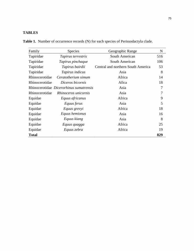
75
TABLES
Table 1. Number of occurrence records (N) for each species of Perissodactyla clade.
Family Species Geographic Range N
Tapiridae Tapirus terrestris South American 516
Tapiridae Tapirus pinchaque South American 106
Tapiridae Tapirus bairdii Central and northern South America 53
Tapiridae Tapirus indicus Asia 8
Rhinocerotidae Ceratotherium simum Africa 14
Rhinocerotidae Diceros bicornis Afica 18
Rhinocerotidae Dicerorhinus sumatrensis Asia 7
Rhinocerotidae Rhinoceros unicornis Asia 7
Equidae Equus africanus Africa 9
Equidae Equus ferus Asia 5
Equidae Equus grevyi Africa 18
Equidae Equus hemionus Asia 16
Equidae Equus kiang Asia 8
Equidae Equus quagga Africa 25
Equidae Equus zebra Africa 19
Total 829
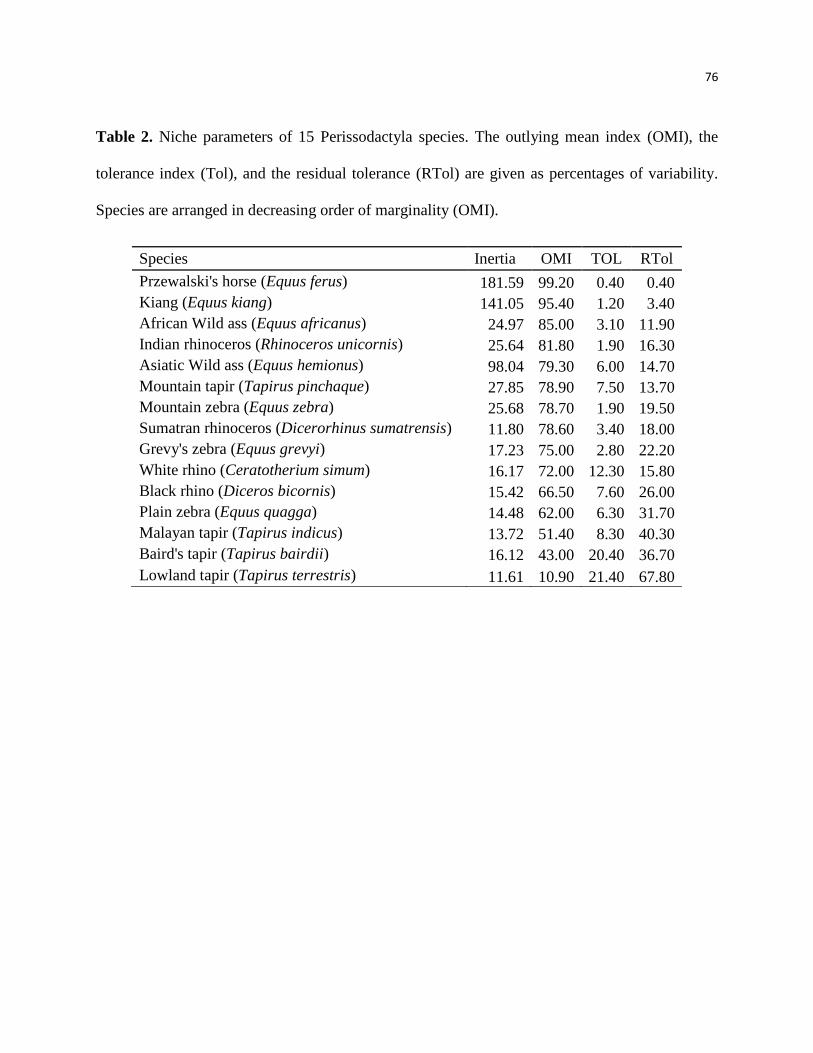
76
Table 2. Niche parameters of 15 Perissodactyla species. The outlying mean index (OMI), the
tolerance index (Tol), and the residual tolerance (RTol) are given as percentages of variability.
Species are arranged in decreasing order of marginality (OMI).
Species Inertia OMI TOL RTol
Przewalski's horse (Equus ferus) 181.59 99.20 0.40 0.40
Kiang (Equus kiang) 141.05 95.40 1.20 3.40
African Wild ass (Equus africanus) 24.97 85.00 3.10 11.90
Indian rhinoceros (Rhinoceros unicornis) 25.64 81.80 1.90 16.30
Asiatic Wild ass (Equus hemionus) 98.04 79.30 6.00 14.70
Mountain tapir (Tapirus pinchaque) 27.85 78.90 7.50 13.70
Mountain zebra (Equus zebra) 25.68 78.70 1.90 19.50
Sumatran rhinoceros (Dicerorhinus sumatrensis) 11.80 78.60 3.40 18.00
Grevy's zebra (Equus grevyi) 17.23 75.00 2.80 22.20
White rhino (Ceratotherium simum) 16.17 72.00 12.30 15.80
Black rhino (Diceros bicornis) 15.42 66.50 7.60 26.00
Plain zebra (Equus quagga) 14.48 62.00 6.30 31.70
Malayan tapir (Tapirus indicus) 13.72 51.40 8.30 40.30
Baird's tapir (Tapirus bairdii) 16.12 43.00 20.40 36.70
Lowland tapir (Tapirus terrestris) 11.61 10.90 21.40 67.80
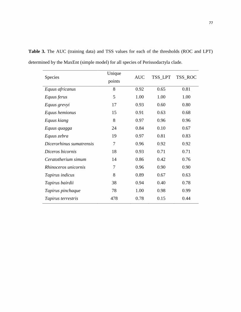
77
Table 3. The AUC (training data) and TSS values for each of the thresholds (ROC and LPT)
determined by the MaxEnt (simple model) for all species of Perissodactyla clade.
Species Unique
points AUC TSS_LPT TSS_ROC
Equus africanus 8 0.92 0.65 0.81
Equus ferus 5 1.00 1.00 1.00
Equus grevyi 17 0.93 0.60 0.80
Equus hemionus 15 0.91 0.63 0.68
Equus kiang 8 0.97 0.96 0.96
Equus quagga 24 0.84 0.10 0.67
Equus zebra 19 0.97 0.81 0.83
Dicerorhinus sumatrensis 7 0.96 0.92 0.92
Diceros bicornis 18 0.93 0.71 0.71
Ceratotherium simum 14 0.86 0.42 0.76
Rhinoceros unicornis 7 0.96 0.90 0.90
Tapirus indicus 8 0.89 0.67 0.63
Tapirus bairdii 38 0.94 0.40 0.78
Tapirus pinchaque 78 1.00 0.98 0.99
Tapirus terrestris 478 0.78 0.15 0.44
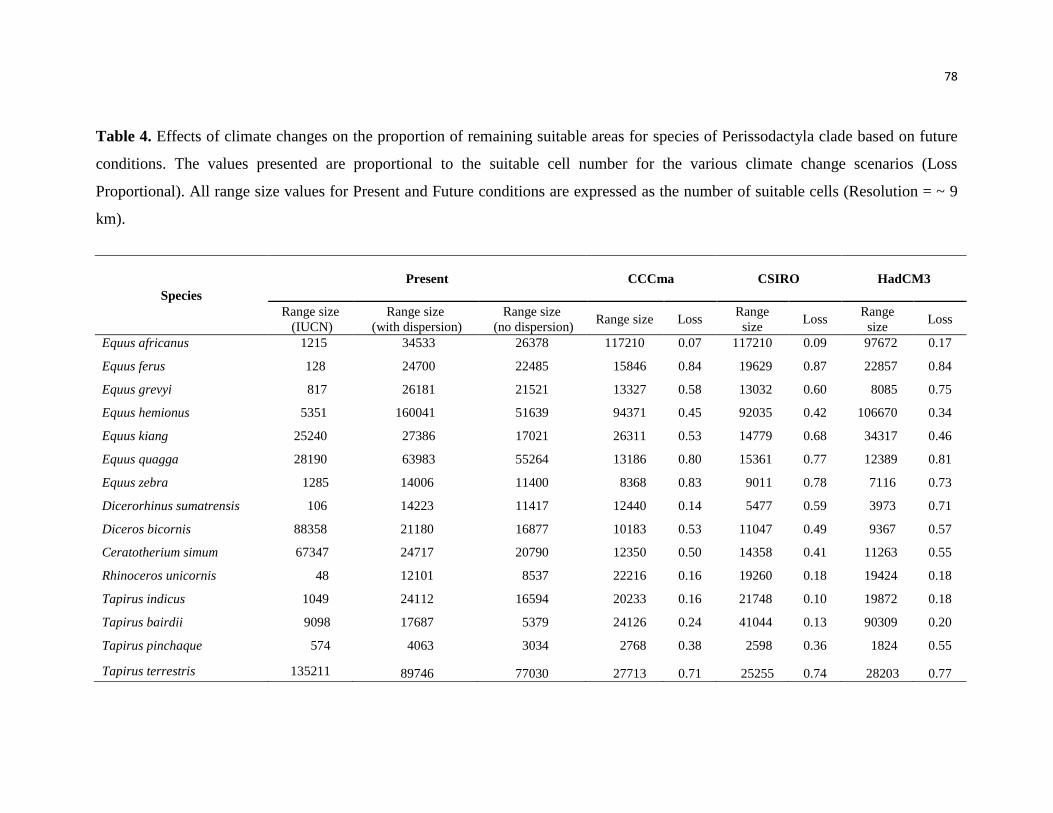
78
Table 4. Effects of climate changes on the proportion of remaining suitable areas for species of Perissodactyla clade based on future
conditions. The values presented are proportional to the suitable cell number for the various climate change scenarios (Loss
Proportional). All range size values for Present and Future conditions are expressed as the number of suitable cells (Resolution = ~ 9
km).
Species
Present CCCma CSIRO HadCM3
Range size
(IUCN)
Range size
(with dispersion)
Range size
(no dispersion) Range size Loss
Range
size Loss
Range
size Loss
Equus africanus 1215 34533 26378 117210 0.07 117210 0.09 97672 0.17
Equus ferus 128 24700 22485 15846 0.84 19629 0.87 22857 0.84
Equus grevyi 817 26181 21521 13327 0.58 13032 0.60 8085 0.75
Equus hemionus 5351 160041 51639 94371 0.45 92035 0.42 106670 0.34
Equus kiang 25240 27386 17021 26311 0.53 14779 0.68 34317 0.46
Equus quagga 28190 63983 55264 13186 0.80 15361 0.77 12389 0.81
Equus zebra 1285 14006 11400 8368 0.83 9011 0.78 7116 0.73
Dicerorhinus sumatrensis 106 14223 11417 12440 0.14 5477 0.59 3973 0.71
Diceros bicornis 88358 21180 16877 10183 0.53 11047 0.49 9367 0.57
Ceratotherium simum 67347 24717 20790 12350 0.50 14358 0.41 11263 0.55
Rhinoceros unicornis 48 12101 8537 22216 0.16 19260 0.18 19424 0.18
Tapirus indicus 1049 24112 16594 20233 0.16 21748 0.10 19872 0.18
Tapirus bairdii 9098 17687 5379 24126 0.24 41044 0.13 90309 0.20
Tapirus pinchaque 574 4063 3034 2768 0.38 2598 0.36 1824 0.55
Tapirus terrestris 135211 89746 77030 27713 0.71 25255 0.74 28203 0.77
79
FIGURE LEGENDS
Figure 1. Relationship between niche properties (Tolerance and OMI) of fifteen species
of the Perissodactyla clade. OMI = Outlying mean index. The straight line shows a
negative relationship between Tolerance and OMI. The points correspond to species.
Figure 2. Relationships between Tolerance Index and the divergence time of the fifteen
species of Perissodactyla clade. The straight lines filled correspond to relationships.
Figure 3. Maps depicting the distribution of the environmental suitable areas for fifteen
species of the Perissodactyla clade. The maps show the potential distribution for only
one climate model (CCCma) and for the current climate using scenario with and no
dispersion.
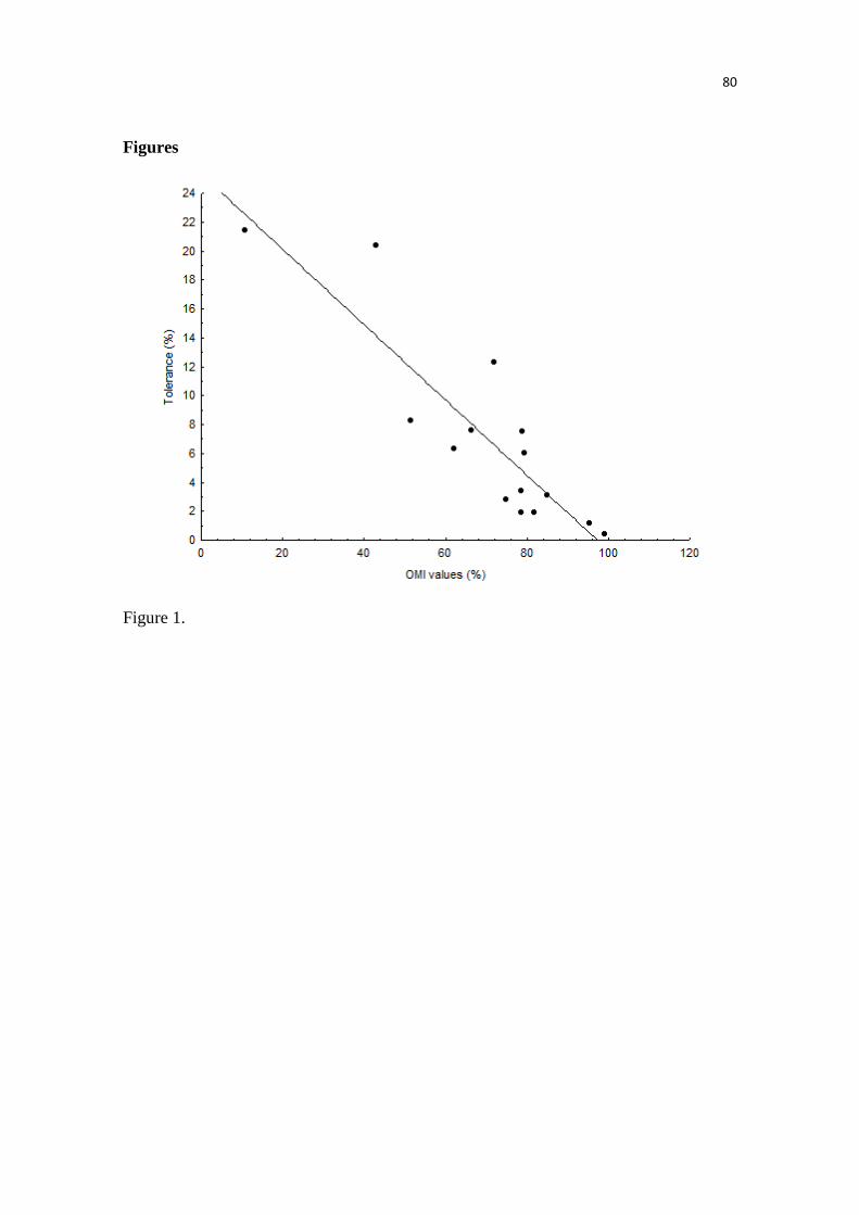
80
Figures
Figure 1.
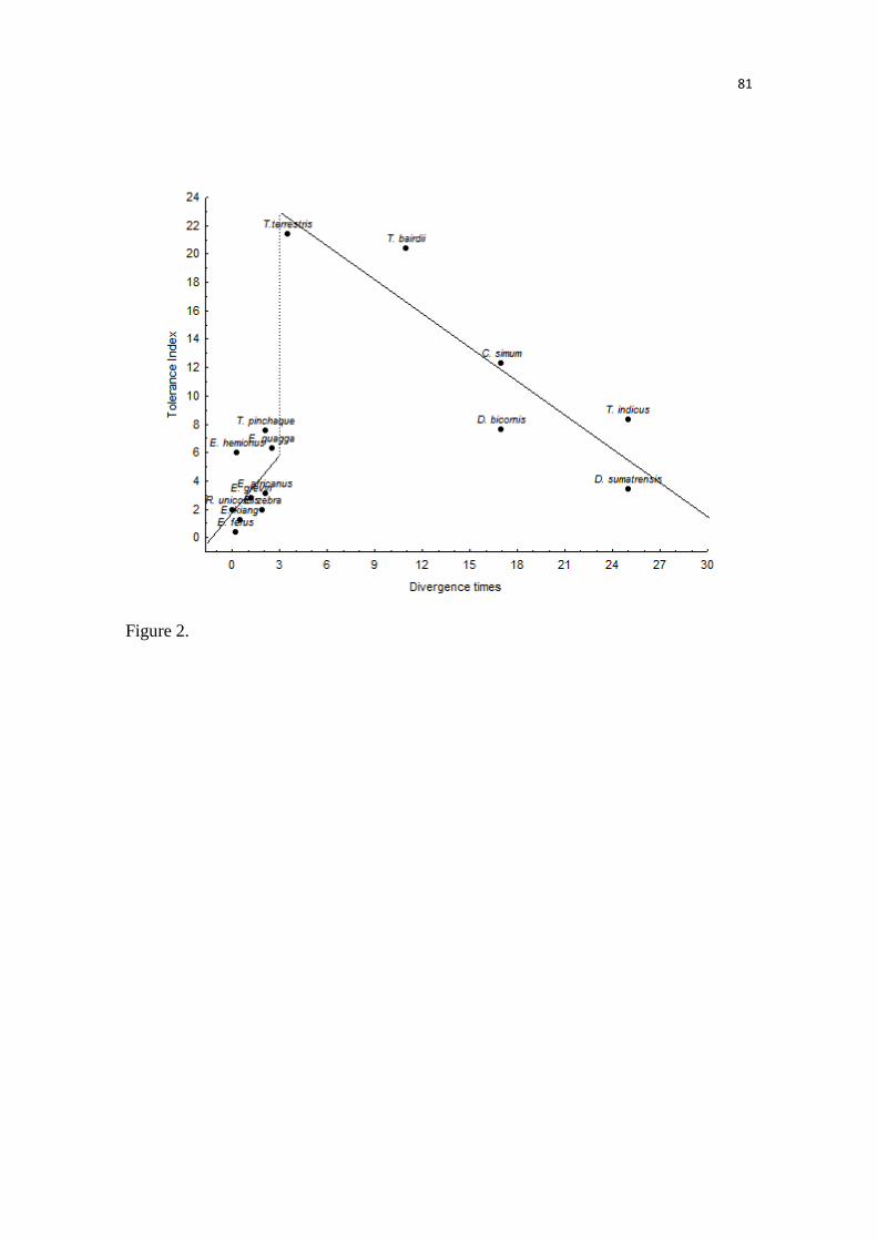
81
Figure 2.
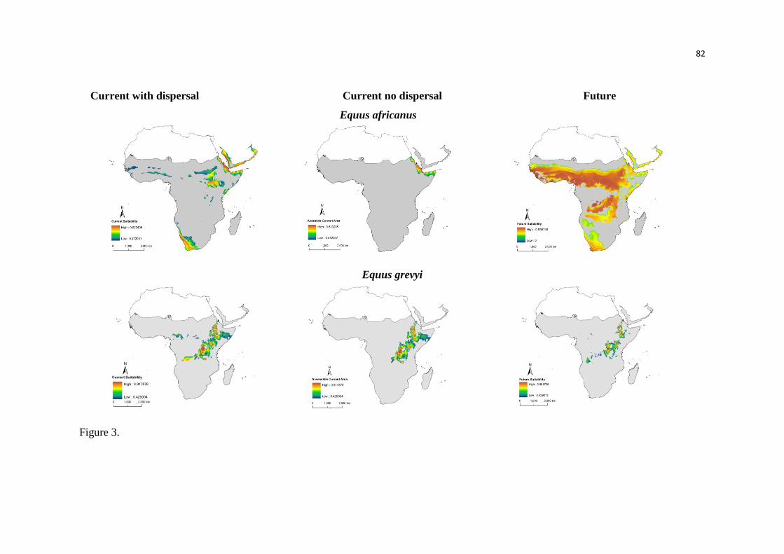
82
Current with dispersal Current no dispersal Future
Equus africanus
Equus grevyi
Figure 3.
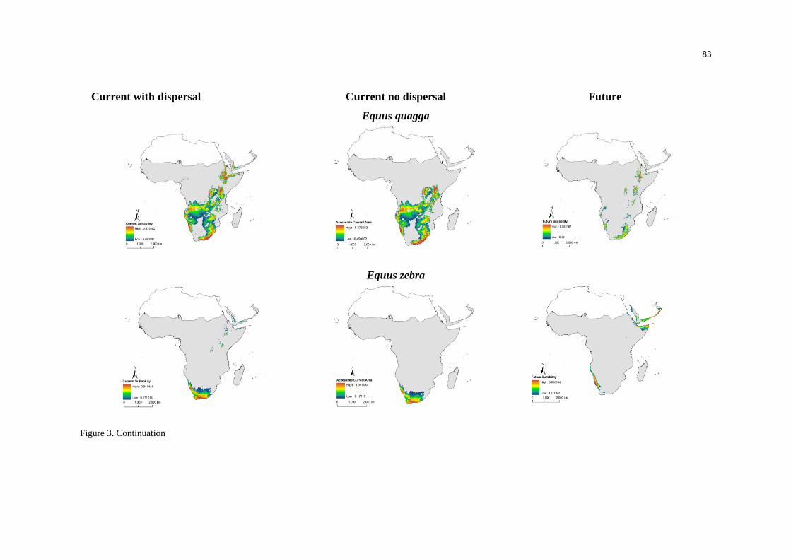
83
Current with dispersal Current no dispersal Future
Equus quagga
Equus zebra
Figure 3. Continuation
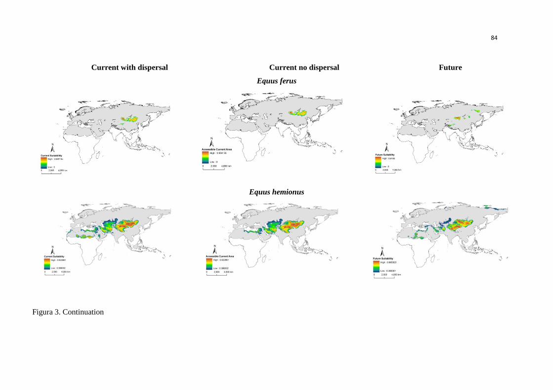
84
Current with dispersal Current no dispersal Future
Equus ferus
Equus hemionus
Figura 3. Continuation
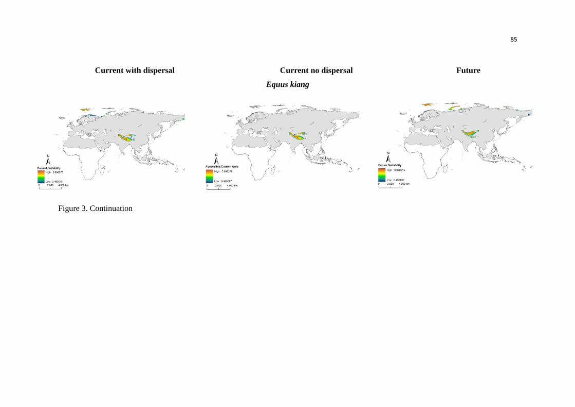
85
Current with dispersal Current no dispersal Future
Equus kiang
Figure 3. Continuation
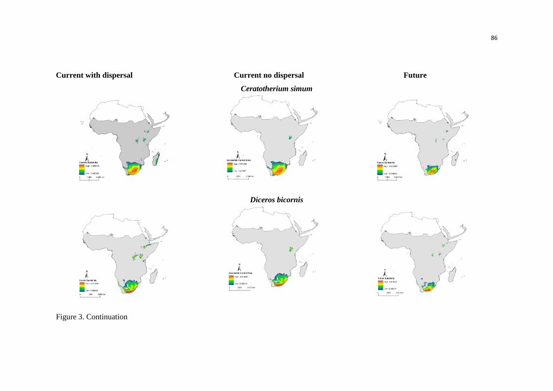
86
Current with dispersal Current no dispersal Future
Ceratotherium simum
Diceros bicornis
Figure 3. Continuation
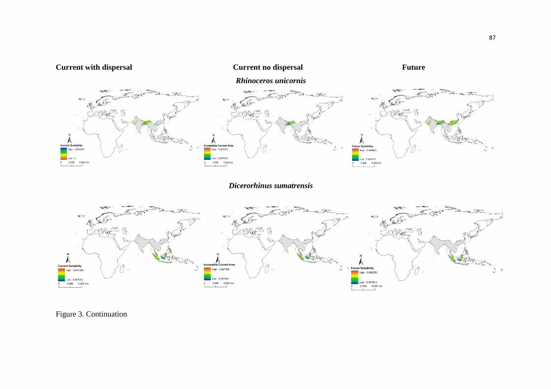
87
Current with dispersal Current no dispersal Future
Rhinoceros unicornis
Dicerorhinus sumatrensis
Figure 3. Continuation
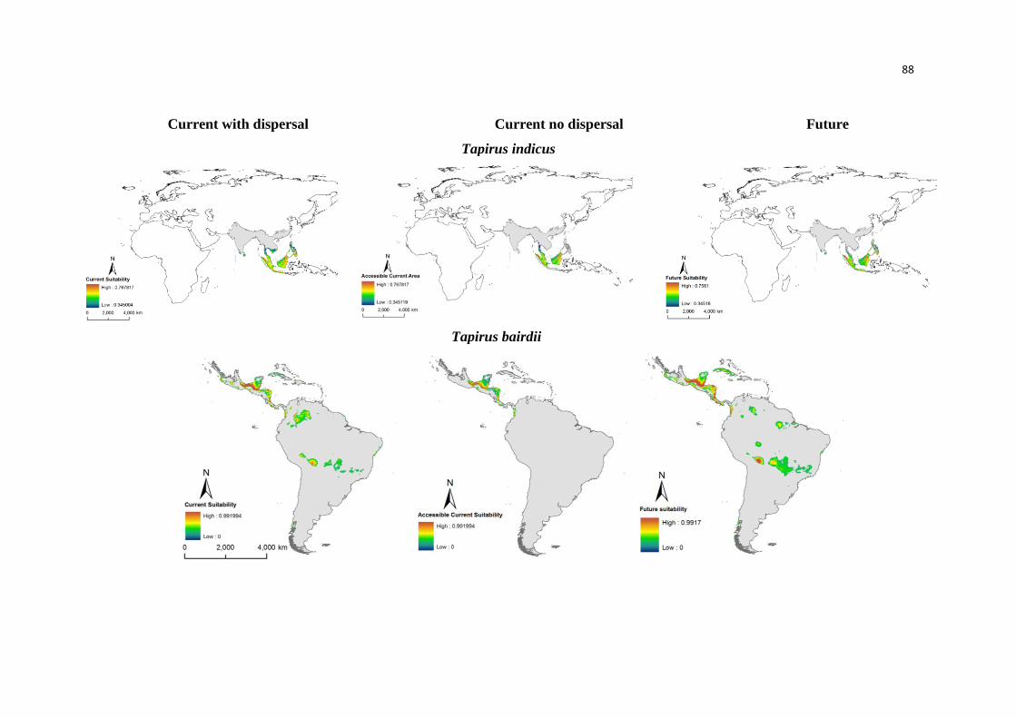
88
Current with dispersal Current no dispersal Future
Tapirus indicus
Tapirus bairdii
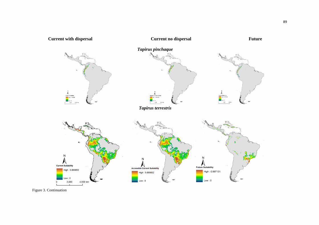
89
Current with dispersal Current no dispersal Future
Tapirus pinchaque
Tapirus terrestris
Figure 3. Continuation
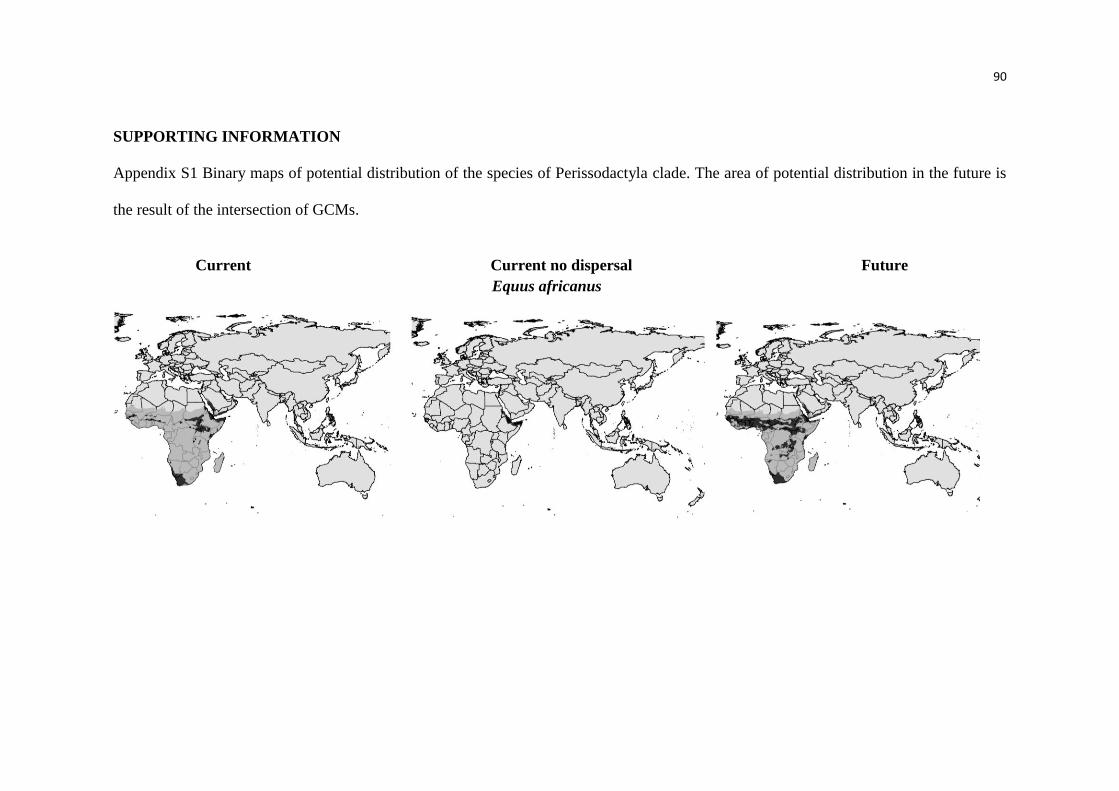
90
SUPPORTING INFORMATION
Appendix S1 Binary maps of potential distribution of the species of Perissodactyla clade. The area of potential distribution in the future is
the result of the intersection of GCMs.
Current Current no dispersal Future
Equus africanus
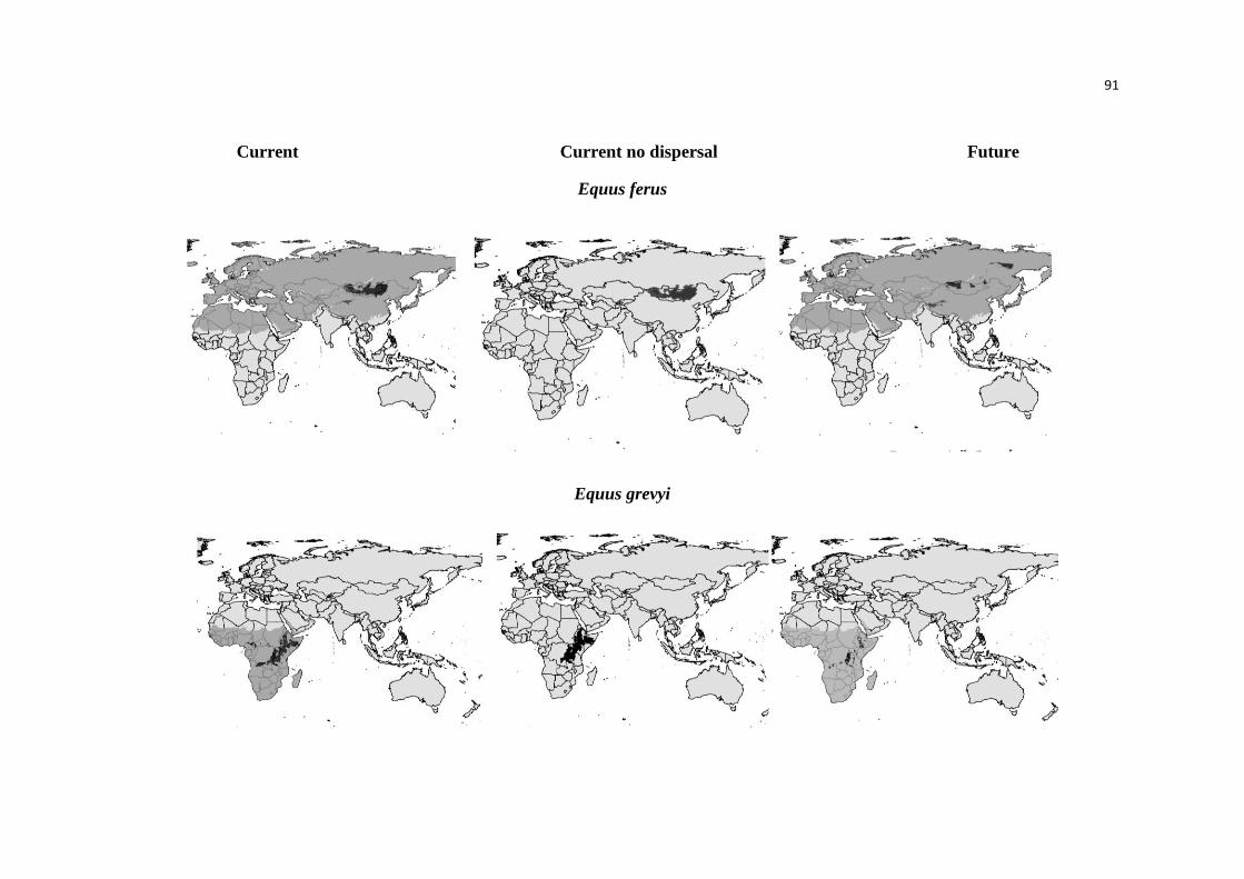
91
Current Current no dispersal Future
Equus ferus
Equus grevyi
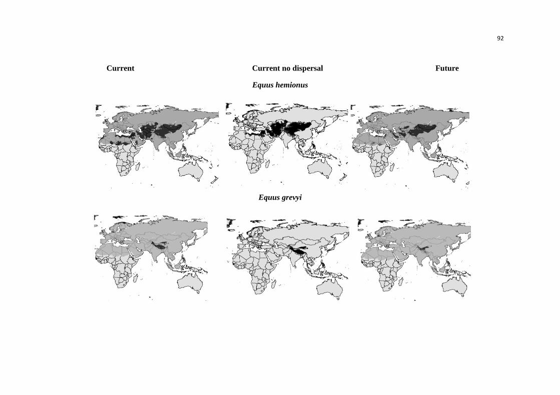
92
Current Current no dispersal Future
Equus hemionus
Equus grevyi
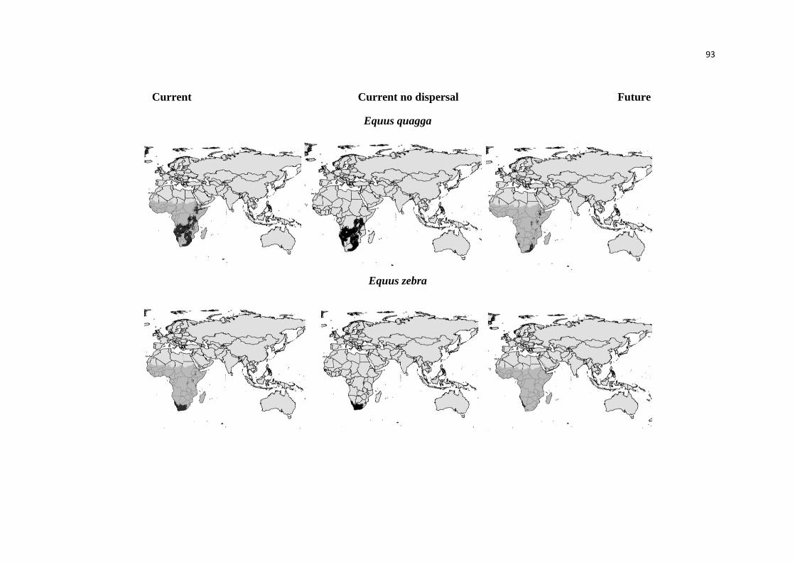
93
Current Current no dispersal Future
Equus quagga
Equus zebra
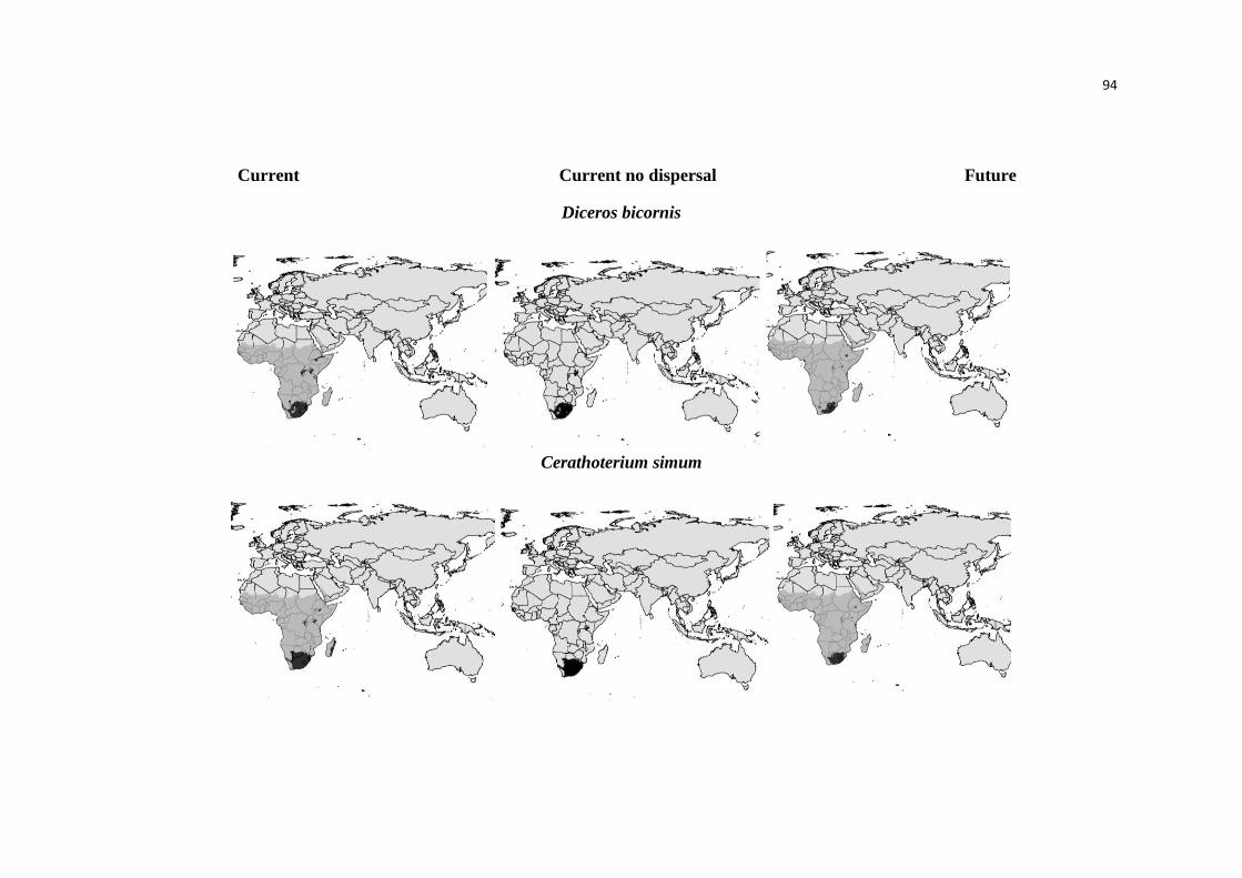
94
Current Current no dispersal Future
Diceros bicornis
Cerathoterium simum
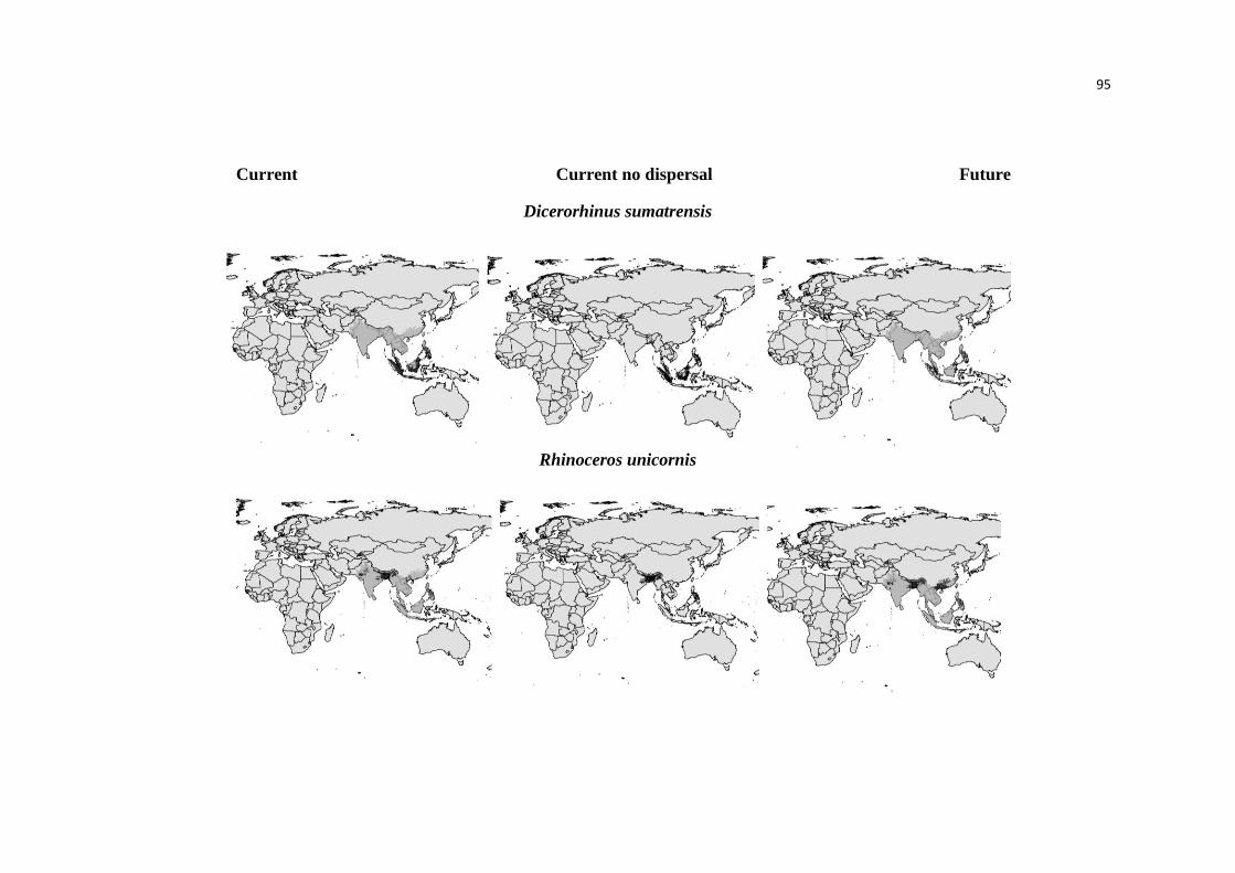
95
Current Current no dispersal Future
Dicerorhinus sumatrensis
Rhinoceros unicornis
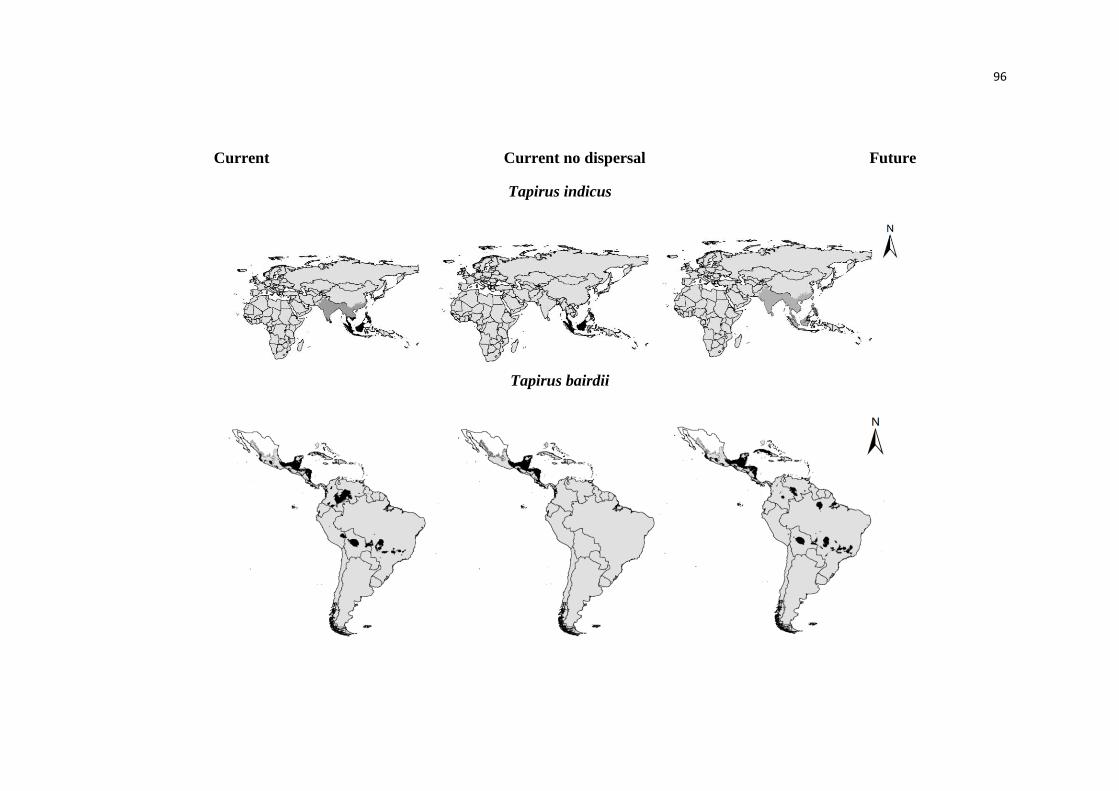
96
Current Current no dispersal Future
Tapirus indicus
Tapirus bairdii
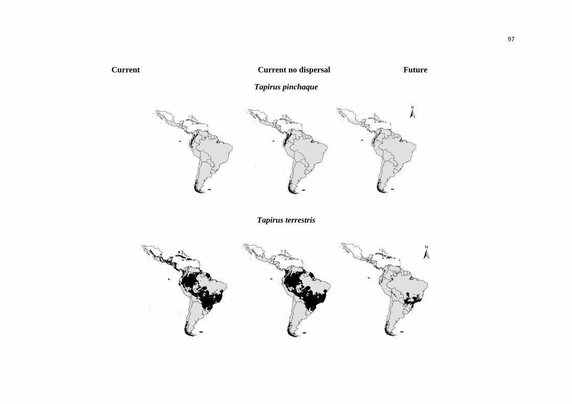
97
Current Current no dispersal Future
Tapirus pinchaque
Tapirus terrestris
98
CAPÍTULO 2
A ser submetido para: Jounal of Biogeography
Ecological niche models predict range expansion for Tapirus terrestris after last ice
age
Andressa Gatti1*, Matheus S. Lima-Ribeiro
2, Caroline C. Nóbrega
3, Paulo De
Marco Júnior3
1 Programa de Pós-Graduação em Biologia Animal, Universidade Federal do Espírito
Santo, Av. Marechal Campos, 1468, Maruípe, Vitória, Espírito Santo, Brazil, CEP:
29040-070
2 Laboratório de Macroecologia, Universidade Federal de Goiás, Campus Jataí, Caixa
Postal 3, Jataí, Goiás, Brazil, CEP: 75804-020
3 Laboratório de Ecologia Teórica e Síntese, Departamento de Biologia Geral, Instituto
de Ciências Biológicas 1, Universidade Federal de Goiás, Campus Samambaia, Caixa
Postal 131, Goiânia, Goiás, Brazil, CEP: 74001-970
*Correspondence: Andressa Gatti, Programa de Pós-graduação em Biologia Animal,
Universidade Federal do Espírito Santo, Av. Marechal Campos, 1468 – Maruípe,
Vitória -ES, Brazil, 29040-070
E-mail: [email protected]
Short Running Head Tapirus terrestris's range expansion during the ice age
99
ABSTRACT
Aim We tested the hypothesis that environmental changes during the late Quaternary
shaped the distribution of climatically suitable areas for lowland tapirs in the
Neotropical region.
Location Neotropics
Methods We used Ecological Niche Modeling to simulate the paleoclimatic conditions
from Last Interglacial, Last Glacial Maximum and Mid-Holocene, further pre-industrial
climate condition. Climatic conditions for LGM, mid-Holocene and pre-industrial were
compiled from five coupled Atmosphere-Ocean General Circulation Models
(AOGCMs). The paleodistributions for lowland tapir were obtained using four
algorithms.
Results Our results suggest that the most critical conditions that prevailed during the
LGM reduced the geographical extent of areas climatically suitable for the tapir,
expanding during the current interglacial period, with warmer temperatures.
Furthermore, we identified a large area that was stable over time.
Main conclusions The paleodistribution modeling for the lowland tapir strongly
supported the hypotheses proposed previously for phylogeographic and paleontological
studies. Their wide environmental niche may have allowed lowland tapirs to rapidly
expand its geographic distribution. The existence of a large stable area indicates that
climate change effects may have been less significant for lowland tapirs when compared
with other megafauna species. Although climate change does not appear to have been a
serious problem for the species during its evolutionary history, the future should be
different. Effects of climate change combined with other threats such as habitat loss can
severely affect lowland tapir populations and their habitats.

100
Keywords: Climate change, hindcasting, lowland tapir, Neotropical, paleoclimate,
Quaternary, range shift.
101
INTRODUCTION
The Quaternary was characterized by dramatic climatic oscillations between
colder glacial and warmer interglacial climates (Jackson & Overpeck, 2000) and is
considered to be one of the most dramatic periods of climatic change in Earth history.
The transitions between glacial and interglacial climate promoted many evolutionary
divergences and drastic alterations in ecosystems (Williams et al., 2004), causing
several megafaunal extinctions worldwide (Nogués-Bravo et al., 2010). The late
Quaternary was marked by a wave of extinctions in all continents and some islands
(Koch & Barnosky, 2006), which affected many of the larger species of mammals (as
well as birds and reptiles) (Nogués-Bravo et al., 2008; Lima-Ribeiro et al., 2012).
Additionally, the megafauna extinction coincided with the appearance and expansion of
humans in most continents (Barnosky et al., 2004). The debate about which stressor
caused the extinction, or the synergy between them, is long-standing and has generated
different discussions (Koch & Barnosky, 2006; Barnosky & Lindsey, 2010).
This paper focuses on the climate change hypothesis, which proposes that
reductions in climatically suitable areas for species would have caused a reduction in
their geographic ranges, thus increasing their vulnerability to extinction (Nogués-Bravo
et al., 2010). Graham et al. (1996) showed that the geographic ranges of various species
in the continental United States shifted at different times and directions in response to
late Quaternary climatic changes. This species’ range dynamics can be driven by the
evolutionary and climatic history of the region in which the species occurs, as well as
by their biological and ecological traits (Johnson, 2002; Thuiller et al., 2005; Heikkinen
et al., 2006). For Davies et al. (2009), great climatic oscillations during the Quaternary
may have favored species with wide distribution through the selection of generalist
102
species. In addition, wide-ranging species may have survived climate change effects
because they are inherently more climatically tolerant and, thus, can occupy a wider
variety of environmental conditions (Owens & Bennett, 2000; Fisher & Owens, 2004;
Thuiller et al., 2005).
Good models to test these assumptions are generalist species that survived these
major environmental changes, especially throughout the Pleistocene period. A good
example is the lowland tapir (Tapirus terrestris), one of the larger-bodied Neotropical
herbivorous mammals of the order Perissodactyla, a generalist species (Tobler et al.,
2010; Medici, 2011) and the last representative of the megafauna of Late Quaternary in
South America. Although South America has lost most of its megafauna genera during
late Quaternary extinctions (Koch & Barnosky, 2006, Barnosky et al., 2010), lowland
tapirs survived and present today a wide geographic distribution throughout most of the
South American continent (Medici, 2011; García et al., 2012).
The ancestral of T. terrestris dispersed from the Neartic to the Neotropical
region together with other mammalian migrants from 3.1 to 2.7 million years ago,
during the Great American Biotic Interchange (Marshall, 1988; Webb, 2006;
Woodburne et al., 2006). Since then, the species has coped with various environmental
alterations, especially in terms of vegetation. The earliest fossil records of lowland
tapirs are reported in the southern range of the genus’ current distribution (Ferrero &
Noriega, 2003; 2007). These fossil records indicate that the lowland tapir geographic
range expansion occurred immediately after their diversification (Thoisy et al., 2010).
Furthermore, the hypothesis proposed by Thoisy et al. (2010), based on
phylogeographical analysis (nucleotide diversity), is that populations of lowland tapirs
were drastically reduced during the Last Glacial Maximum (LGM – 21 kyr), with
103
significant expansion during interglacial, occupying new environments. But how to do a
retrospective analysis of what happened with the distribution of environmentally
suitable areas for tapirs under the impacts of Quaternary climate oscillations?
The Ecological Niche Modeling (ENM) approach, coupled with paleoclimatic
simulations, has been increasingly applied to predict species paleodistribution at
regional and global scales (Nogués-Bravo, 2009; Varela et al., 2011; Svenning et al.,
2011). In addition, it has been used to test biogeographical hypotheses, such as
geographic range dynamics of extinct and extant species through the last glacial cycle
(Martínez-Meyer & Peterson, 2006; Nogués-Bravo et al., 2008; Waltari & Guralnick,
2009; Varela et al., 2010; Colevatti et al., 2013). The main source of paleoclimatic data
for ENM studies are past climatic reconstructions based on general circulation models
(GCMs; or AOGCMs when the climatic simulations integrate an atmospheric-ocean
coupled model). The mid- Holocene (6 kyr) and the LGM (21 kyr) are recognized as
benchmark periods throughout the last glacial cycle (Otto-Bliesner, 2009), and have
been the main focus for paleoclimatic simulations (see Paleoclimate Modelling
Intercomparison Project – PMIP: http://pmip3.lsce.ipsl.fr).
In this paper, we address the hypothesis that environmental alterations during
late Quaternary shaped the distribution of climatically suitable areas for lowland tapirs
in the Neotropical region. Specifically, we used ENMs to test predictions made by
previous phylogeographical and paleontological studies (Thoisy et al., 2010; Ruíz-
Garcia, 2012): 1. The climatically suitable areas for T. terrestris were restricted during
LGM, and 2. There was an expansion after the LGM. We used paleoclimate data from
Last Interglacial (~125 kyr BP), LGM, Mid-Holocene, and Present (pre-industrial)
conditions.
104
MATERIAL AND METHODS
The history of Tapirus terrestris
The family Tapiridae as a taxonomic entity is first recognizable in the Eocene of
North America, nearly 50 Mya. Tapirs (Perissodactyla, Tapiridae, Tapirus) were
distributed in nine genera and inhabited Europe, North America, and Southeast Asia
(Colbert, 2007). Tapirs were part of a community of large Neotropical browsers that
largely disappeared at the end of the Pleistocene and among the surviving
Perissodactyla, tapirs are the most conservative (Kemp, 2005).
The current Tapiridae family (Gray 1821) is composed of a single genus, Tapirus
(Brünnich 1772), which first appeared in the Miocene (25–5 Mya). Tapirs entered South
America with the formation of the Isthmus of Panama between North and South
America, during the Pliocene (7–2 Mya-- Ensenadan South American Land Mammal
Age (SALMA)), late Pliocene to early Pleistocene (Cione & Tonni, 1996; Tonni et al.,
1999; Nabel et al., 2000). Tapir species persist today in Southeast Asia, Central
America, and South America. The lowland tapir (Tapirus terrestris) is one of four living
species, presenting the widest geographic distribution throughout most of South
America and found in a variety of habitats, from Venezuela to northern Argentina, and
from the Brazilian Atlantic forest to the Ecuadorian sub-Andean foothills (Medici,
2011)
Occurrence data
Most of the records of current presence of lowland tapirs were obtained from
data provided by experts from the IUCN/SSC Tapir Specialist Group (TSG). This
database was complemented with data from literature, museum specimens deposited in
online databases ((Global Biodiversity Information Facility, GBIF, www.gbif.org) and
105
from records obtained from other research colleagues in Brazil. We used 312 spatially
distinct occurrence points (from 525 compiled) to generate the distribution of lowland
tapirs for both current and past climate conditions across the entire Neotropics.
Environmental Variables and Paleoclimatic simulations
To evaluate how the last glacial cycle affected the distribution of climatically
suitable areas for T. terrestris we used paleoclimatic simulations from pre-industrial
(representing current climate conditions), Last Glacial Maximum (LGM; ~21,000 years
ago - 21 kyr BP) and Mid-Holocene (~6,000 years ago - 6 kyr BP). Because of
relatively coarse resolution from native AOGCMs outputs, we used the standard
change-factor approach (Wilby et al., 2004) to downscale the climatic layers to a 0.5o
spatial resolution (~55 km at the height of Ecuador), according to Collevatti et al.
(2013). From the interpolated data of monthly precipitation and mean, maximum and
minimum temperatures, we calculated 19 bioclimatic variables (see
www.worldclim.org/bioclim). We used six variables (from a total of 19 available
variables): annual mean temperature, temperature seasonality (coefficient of variation),
mean temperature of the driest quarter, annual precipitation, precipitation seasonality
(coefficient of variation) and precipitation during the warmest quarter.
Climatic conditions for LGM, mid-Holocene and pre-industrial were compiled
from five coupled Atmosphere-Ocean General Circulation Models (AOGCMs) --
CCSM, CNRM, MIROC, MPI and MRI (Table 1) -- available in the databases CMIP5
(Coupled Model Intercomparison Project, Phase 5; http://cmip-pcmdi.llnl.gov) and
PMIP3 (Paleoclimate Modelling Intercomparison Project, Phase 3;
http://pmip3.lsce.ipsl.fr). LGM and mid-Holocene represent, respectively, the coldest
106
and warmest phases through the last glacial cycle. In the second phase, we used the Last
Interglacial (LIG; ~125,000 years ago - 125 kyr BP) climate data available only for
CCSM (Otto-Bliesner et al., in press).
Paleodistributions modeling approach
The paleodistributions for lowland tapirs were obtained using four algorithms,
including methods for presence-only data, which was selected based on its complexity
in the following order: Envelope Score (ES), Mahalanobis Distance (MD), MaxEnt and
Support Vector Machines (SVM). This complexity reflects directly on some properties
of these models, such as over-fitting and transferability (Varela et al., 2011). Selected
modeling procedures are based on two classes of methods: 1) The first class of models
is only based on distances and therefore does not require adjustment to previously
defined models, as Envelope Score and Mahalanobis Distance; 2) The second class uses
presence/pseudo-absence data and requires some type of fit of the data to a model that
represents the response to environmental conditions, as MaxEnt and SVM.
The Envelope Score is equivalent to the inclusive 'OR' implementation of Bioclim
described in Piñeiro et al. (2007) and for each given environmental variable the
algorithm finds the minimum and maximum at all occurrence sites. During the
modeling process, the probability is determined by dividing between the layers within
min-max threshold by number of layers. Mahalanobis Distance is a simpler model
allowing for easier interpretation based on a geometric view of the Hutchinsonian niche
-- this approach has been used as a multivariate index of environmental quality in
studies examining species distribution (Farber & Kadmon, 2003). MD scores should be
interpreted as a similarity index to climate conditions from sites where the species has
been recorded.
107
The MaxEnt Software (version 3.3.3e) (Computer Sciences Department,
Princeton University, 2004) is a general-purpose machine learning approach that uses a
simple mathematical formulation for modeling geographic distribution of species with
presence-only data (Phillips et al., 2006). Absence data are generated by randomly
selecting ‘‘pseudo-absence’’ points from regions where the species was not recorded
(i.e., the background of the area). The SVMs consist of a new group of learning
algorithms used for classification and regression (Schlkopf & Smola, 2001) and are a
class of non-probabilistic statistical pattern recognition algorithms for estimating,
among other quantities, the boundary of the set from which a collection of observations
is drawn (Drake et al., 2006; Drake & Bossenbroek, 2009). These algorithms are
typically designed for a two-class problem where the SVM seeks to define a hyperplane
in predictor space that separates two classes, such as species presence/absence (Guo et
al., 2005).
All models were fitted using current climate data (pre-industrial) and then back-
projected (“hindcasting”) onto those relevant time periods in Pleistocene and Holocene
(LIG, LGM and Mid-Holocene).
Model evaluation
Most modeling studies use AUC measure to evaluate generated models. The
AUC is a threshold-independent measure that, for prediction from algorithms using
presence-only or presence-absence data, can be interpreted as the ability of the
algorithm to discriminate between a suitable climate condition and a random analysis
pixel (Phillips et al., 2006). AUC values range from 0 to 1, in which a score of 1
indicates perfect discrimination and a score of 0.5 or less implies discrimination that is
no better than random (Elith et al., 2006). Nevertheless, there is a series of concerns
108
about its measure. Pearson et al. (2007) argue that the false-positive should not be
considered for evaluating potential distribution models built only to reveal areas that
can be occupied, and Lobo et al. (2008) list five reasons not to use AUC as a measure of
evaluation (e.g., AUC weights omission and commission errors equally). Thus, we used
Liu et al. (2011) who suggested the use of AUC as a threshold independent general
measure of fit, but added a threshold depended measure to evaluate the cases for which
a binary prediction is needed.
We chose to use True Skill statistics (TSS) to evaluate model predictions because
it performs well when compared to similar measures (Liu et al., 2011). This measure is
also highly correlated with AUC, but it is not biased by prevalence (Allouche et al.,
2006). TSS takes into account both omission and commission errors and ranges from −1
to +1, where +1 indicates perfect agreement, and values of zero or less indicate a
performance that is no better than random predictions. TSS is a measure dependent on
the threshold used to convert continuous species distributions model outputs in binary
maps predicting potential presence/absence of each species. We adopted the lowest
presence threshold (LPT) because it equals the minimum model prediction value for any
of the training occurrence data. This approach can be interpreted ecologically as
identifying pixels predicted as being at least as suitable as those where the species’
presence has been recorded.
The potential paleodistributions were obtained by addint up the binary maps from
five AOGCMs resulting from each algorithm, and considering two scenarios: 1. a more
conservative scenario, in which only the areas predicted by the five common climatic
models were considered; 2. a less conservative scenario, considering the area in which
at least one climate model was predicted as climatically suitable for T. terrestris. Thus,
109
the maps presented for each algorithm, in a time period was used as the single
representative potential geographical prediction for the species.
Species range shift
To evaluate the range shifts of lowland tapirs throughout the last
interglacial/glacial cycle (from Last Interglacial to current period), such as the
expansions and contractions, we used the relative change (values >1 and <1 represent
expanding and shrinking climate conditions, respectively) and proportional loss in
potential distribution. These metrics have been used in other studies (Beaumont et al.,
2005; Thuiller et al., 2005; Garcia et al., 2012).
The relative change values were obtained by dividing the area occupied in a
given period of time (e.g., Last Interglacial) by the area occupied under climates on next
time period (i.e., Last Glacial Maximum). The proportional loss was calculated by
dividing the number of lost cells in a time slice by the potential distribution of basal
time period (i.e., compared with the analyzed distribution). Thus, we evaluated the
shifts in size of the climatically suitable areas in the following sequence: LIG to LGM;
LGM to Mid-Holocene; Mid-Holocene to present-day. Furthermore, we defined areas of
stability (regions in which the species were predicted to occupy irrespective of the time
period) (Carnaval et al., 2009), as a result of the intersection of the predicted suitable
areas under current conditions and climatic extremes of the Late Quaternary (LGM and
Mid-Holocene).
110
RESULTS
The AUC and TSS values for all models showed a relatively good fit (Table 2)
and the ROC threshold choice was reinforced by TSS values, which were higher than
TSS values from LPT in 16 of 20 models.
The combinations from AOGCMs and algorithms reveal that the climatically
suitable areas available to lowland tapir increased from LGM (21 kyr BP) to mid-
Holocene (6 kyr BP) (points above the reference line with 1:1 relationship; Fig. 1a).
Only the models generated by SVM showed a decrease in potential distribution for this
period (Table 3). From mid-Holocene to present-day (pre-industrial), the potential
distribution of lowland tapir seems to have been stable, although slight variations were
predicted (Fig. 1b; Table 4). The regression analyses showed that when a model predicts
a high value for the size of the area in a given period, it also predicts for the other time
period evaluated (Fig. 1a, b). The less complex algorithms, Envelope Score and
Mahalanobis Distance, were those that least overpredicted the potential distribution in
the three periods analyzed (Fig. 2).
When we analyzed the models through a more conservative approach, it was
observed that the five AOGCMs indicated the same limits of distribution of climatically
suitable areas and the central area of distribution for the species. Although the potential
distribution of lowland tapirs increases through time, the models predicted loss of
climatically suitable areas from the LGM to Mid-Holocene in some Neotropical
regions, mainly in the Guiana Shield, portions of Eastern, Central and Western
Amazonia, and in the northernmost region of the Brazilian Caatinga. Contrarily,
portions of southern Brazil, northern Argentina and regions bordering the Andes in
Bolivia and Peru became climatically suitable to the lowland tapir after LGM.
111
Therefore, our results strongly suggest that constraints on the distribution of climatically
suitable areas for lowland tapirs throughout the last ice age occurred mainly during the
LGM and expanded subsequently with small geographic alterations in the availability of
climatically suitable areas after mid-Holocene.
However, we observed that there was also an increase in the potential
distribution from the LIG (125 kyr BP) to LGM (Table 5). During the LIG, the three
algorithms (ES, MD and MaxEnt) predicted unsuitable areas for lowland tapirs in a
region that extends from eastern to western Brazil, including principally the Amazon
River basin and central Amazonian lowlands. Furthermore, portions of Guiana and
Brazilian Shields and a wide region of Argentina and Uruguay were also predicted as
unsuitable. During the LGM, all these areas were predicted to become environmentally
suitable.
The models predicted a wide refugium for lowland tapirs from LGM to present-
day (areas climatically suitable in all time periods), which occurs particularly in the
peripheral areas of the Amazon River basin, and in the central region of the South
America. In addition, according with our models, most of central Amazonian lowlands
along the Amazon River were unstable for T. terrestris through the last glacial cycle
(Fig. 5).
DISCUSSION
Our results suggest that the coldest conditions prevailing during the LGM would
have reduced the geographic extent of climatically suitable areas for the lowland tapir,
expanding again during warmer current interglacial. Our findings from paleodistribution
modeling strongly support predictions made by previous phylogeographic and
112
paleontological studies (Ferrero & Noriega, 2003; 2007; Thoisy et al., 2010; Ruiz-
García et al., 2012). As discussed by Colevatti et al. (2013), the demographic history of
a species is more reliably described through time when both paleodistribution modeling,
phylogeographic analysis, and fossil records provide convergent evidences (see also
Svenning et al., 2011). This paper supports previous evidence that lowland tapirs
experienced a clear historical population expansion after LGM (Thoisy et al., 2010;
Ruiz-García et al., 2012), most probably becoming the most successful large herbivore
in South America, surviving the late Quaternary extinctions. The fact that lowland tapirs
occupy a broader environmental niche (García et al., 2012; see Chapter 1) most
probably favored the species and allowed for a relatively rapid expansion of their
geographic range after dramatic changes in their environment (e.g., after the LGM).
According to Dynesius & Jansson (2000), species with low specialization - such as the
lowland tapir - are also more likely to survive while moving through heterogeneous
environments.
It has often been stated that animal species survive environmental changes in
two main ways: by evolving adaptations to new conditions or by shifting their
geographic range, seeking a favored habitat (Lister, 2010). Thus, species may have
responded to the Quaternary glaciations with large range shifts (Graham et al., 1996). In
contrast, species with broader niches and flexible adaptations often stayed where they
were (frequently over a wide area) or showed relatively minor expansions and
contractions of their geographic range (see examples in Lyons et al., 2003, 2010).
Although we are fully aware of the uncertainties inherent to the AOGCMs and ENM
algorithms (Pearson et al., 2006), we identified a large stable area for lowland tapirs.
The maintenance of this area indicates that the effect of climate change on lowland
113
tapirs may have been much smaller than on the extinct megafaunal species.
Eremotherium, for instance, an extinct giant ground sloth in South America, was
predicted to have been narrowly distributed during early Holocene across scattered
refugia, which most probably made it more prone to extinction under probable hunting
by humans (Lima-Ribeiro & Diniz-Filho, 2013). Approximately 80% of climatically
suitable areas for Eremotherium were lost from LGM to mid-Holocene (Lima-Ribeiro et
al., 2012).
Negative effects of climate change were observed for different organisms
worldwide. Contractions of climatically suitable areas during the last glacial cycle were
recorded for frogs (Carnaval et al., 2009), birds (Bonaccorso et al., 2006; Ribas et al.,
2011), mammals (Nogués-Bravo et al., 2008, Varela et al., 2010, Lima-Ribeiro &
Diniz-Filho, 2012) and woody plants (Bonaccorso et al., 2006). However, each species
responds differently to climate changes, as demonstrated by Lorenzen et al. (2011).
Likewise, the evident contraction of climatically suitable areas for various extinct
megafauna species at the end of the Pleistocene/earliest Holocene in South America
(Lima-Ribeiro & Diniz-Filho, 2013) does not seem to have affected lowland tapirs. It is
likely that lowland tapirs occupied new environments after the extinction of the
Neotropical megafauna herbivores (Thoisy et al., 2010), which supports the idea that
this widespread species presents high climate tolerance, principally in relation to
average temperature, but not extreme cold as occurred during LGM (also in high
altitudes, for example, Andean region).
Davies et al. (2009) suggest that large climate oscillations in the Quaternary may
have shaped the distribution of geographic range size via the selective extinction of
narrow-ranged species during glacial expansion or recolonization by species able to
114
disperse after glacial retreats (Williams et al., 2004). The lowland tapir has the ability to
disperse and occurred in a wide refuge in South America, allowing it to survive the last
glacial cycle, as opposed to other megafauna species narrowly distributed in scattered
refugia at the end of the Pleistocene.
However, our approach presents some issues. ENM-based predictions can be
highly variable, given that both AOGCMs and modeling procedures can bring
uncertainties to the predictions (Pearson et al., 2006; Thuiller et al., 2008). Although
different models predicted different distributions of climatically suitable areas for
lowland tapirs, the combined use of various AOGCMs and ENM algorithms (the
ensemble approach; see Araújo & New, 2007) indicated a relationship between them.
The size of potential distribution was similar for all predictions between time periods,
regardless of AOGCM or ENM algorithm used (Fig. 1).
Moreover, various assumptions can also affect the application of the ENM
approach to test biogeographical hypotheses. A critical assumption of the ENMs for
modeling past distributions is the climatic niche stability over the study period (Nogués-
Bravo, 2009; Varela et al., 2011; Svenning et al., 2011). However, as stated by Peterson
(2011), over relatively short periods, such as from LGM to present-day, evolutionary
changes on species ecological niches are less likely than for longer time spans.
Lastly, it is well known that barriers to species dispersal and interspecific
interactions may restrict the species distribution to narrower ranges than those predicted
by ENMs (Soberón & Nakamura, 2009, Soberón, 2010). Rivers, mountains and
vegetation can be considered as barriers, which was recently proposed by Barve et al.
(2011) (see also De Marco et al., 2008). However, the inclusion of barriers in
paleodistribution modeling is a challenging issue. Given that the lowland tapir is a
115
generalist herbivore which has the ability to move across heterogeneous environments,
we did not incorporate barrier restrictions in our models. Our goal was not determine
the true geographic distribution of lowland tapirs in the past, nor its exact geographic
range size over time. Our aim was to determine how the species geographic distribution
has changed since the last glacial cycle, which can be reliably tested from potential
distributions.
Concluding Remarks
Although the ENM approach presents some methodological uncertainties, the
evaluation of model predictions and assumptions, as well as the ecological traits of the
studied species, indicate that our results are reliable to test the biogeographical
hypotheses for the lowland tapir. Our results, coupled with previous phylogeographical
and paleontological analyses, support a reduction of the lowland tapir geographic range
during LGM, with subsequent expansion through current glacial. At the contrary of
most megafauna species in South America, which did not recover from climate crisis
during last glacial cycle, the lowland tapir was widely distributed on climatically
suitable areas (refugial) throughout this time slice, surviving the late Quaternary
extinctions.
A critical assumption for the distribution models based in hindcasting is the
climatic niche stability over the study period. Peterson (2011) assumes that over
relatively short periods, such as the LGM to recent period (21000 years), evolutionary
niche changes are less likely than for longer time spans. Obviously, this is a
Furthermore, we do not incorporated the restriction in species dispersion, considering
that lowland tapir is able to move in heterogeneous environments, although the recent
studies discuss the importance inserting dispersal scenarios into predictive models
116
(Barve et al., 2011). Nevertheless, it is possible to start thinking about the restriction of
the dispersion over time considering rivers, mountains and vegetation as barriers which
was recently proposed by Barve et al. (2011), but how to operationalize this approaches
still an issue to be assessed. We consider that to overcome both problems – climatic
uncertain and dispersal modeling -- it is needed the use of alternative
paleoenvironmental reconstructions and several ENM algorithms, considering
principally the species characteristics.
The resulting predictions can provide valuable information about the
evolutionary history of the lowland tapir. Although climate change does not seem to
have been a serious problem for the species during its evolutionary history, the
challenges ahead can be serious. Climate change will most probably result in changes in
environmental suitability throughout the lowland tapir distribution and affect
particularly the vegetation, interfering with important ecological processes, such as seed
dispersal. Furthermore, the combined effect of climate change with habitat loss and
fragmentation, unsustainable hunting, road-kill and disease transmission could be
drastic.
117
ACKNOWLEDGEMENTS
The authors would like to thank the IUCN/SSC Tapir Specialist Group (TSG) for
providing distribution data for tapirs. AG is supported by FAPES - Fundação de
Amparo à Pesquisa do Estado do Espírito Santo. CN is supported by CAPES -
Coordenação de Aperfeiçoamento de Pessoal de Nível Superior. PM is continually
supported by grants from CNPq – Conselho Nacional de Desenvolvimento Científico e
Tecnológico. Lastly, we would like to thank all the researchers who provided
information for this paper.
REFERENCES
Allouche, O., Tsoar, A. & Kadmon, R. (2006) Assessing the accuracy of species
distribution models: prevalence, kappa and the true skill statistic (TSS). Journal of
Applied Ecology, 43, 1223–1232.
Barnosky, A., Koch, P., Feranec, R., Wing, S. & Shabel, A. (2004) Assessing the causes
of late Pleistocene extinctions on the continents. Science (New York, N.Y.), 306, 70–75.
Barnosky, A.D. & Lindsey, E.L. (2010) Timing of Quaternary megafaunal extinction in
South America in relation to human arrival and climate change. Quaternary
International, 217, 10-29.
Beaumont, L., Hughes, L. & Pitman, A. (2008) Why is the choice of future climate
scenarios for species distribution modelling important? Ecology letters, 11, 1135–1146.
Bonaccorso, E., Koch, I. & Peterson, A.T. (2006) Pleistocene fragmentation of Amazon
species’ ranges. Diversity and Distributions, 12, 157–164.
118
Carnaval, A., Hickerson, M., Haddad, C., Rodrigues, M. & Moritz, C. (2009) Stability
predicts genetic diversity in the Brazilian Atlantic forest hotspot. Science (New York,
N.Y.), 323, 785–789.
Cione, A.L. & Tonni, E.P. (2005). Bioestratigrafía basada em mamíferos del Cenozóico
Superior de la Província de Buenos Aires, Argentina. Geología y recursos minerales de
Província de Buenos Aires (ed. by E. Barrio, R.O. Etcheverry, M.F. Caballé and E.
Llambias), pp. 183–200. Quick Press, La Plata, Argentina.
Cione, A.L. & Tonni, E.P. (2006) Central American provincialism and the Great
American Biotic Interchange. Advances in Late Tertiary Vertebrate Paleontology in
Mexico and the Great American Biotic Interchange (ed. by O. Carranza-Castañeda &
E.H. Lindsay), pp. 10. Univ Nac Aut Mex. Inst Geol Centro Geoscien Publ Espec 4:73–
100.
Colbert, M. (2007) New fossil discoveries and the history of Tapirus. Tapir
Conservation, 16, 12-14.
Collevatti, R. G., Terribile, L.C., Oliveira, G. de, Lima-Ribeiro, M., Nabout, J.C.,
Rangel, T.F. & Diniz-Filho, J.A.F. (2013) Drawbacks to palaeodistributions modelling:
the case of South American seasonally dry forests. Journal of Biogeography, 40, 345–
358.
Davies, T., Purvis, A. & Gittleman, J. (2009) Quaternary climate change and the
geographic ranges of mammals. The American naturalist, 174, 297–307.
De Marco, P., Diniz-Filho, J.A.F. & Bini, L.M. (2008) Spatial analysis improves
species distribution modelling during range expansion. Biology Letters, 4, 577-580.
119
Drake, J.A., Randin, C. & Guisan, A. (2006) Modelling ecological niches with support
vector machines. Journal of Applied Ecology, 43, 424–432.
Drake, J.M. & Bossenbroek, J.M. (2009) Profiling ecosystem vulnerability to invasion
by zebra mussels with support vector machines. Theoretical Ecology, 2, 189-198.
Dynesius, M. & Jansson, R. (2000) Evolutionary consequences of changes in species’
geographical distributions driven by Milankovitch climate oscillations. Proceedings of
the National Academy of Sciences of the United States of America, 97, 9115–9120.
Elith, J., Graham, C.H., Anderson, R.P., et al. (2006) Novel methods improve
prediction of species’ distributions from occurrence data. Ecography, 29, 129-151.
Farber, O. & Kadmon, R. (2003) Assessment of alternative approaches for bioclimatic
modeling with special emphasis on the Mahalanobis distance. Ecological Modelling,
160, 115-130.
Ferrero, B.S. & Noriega, J.J. (2003) El registro fósil de los tapires (Perissodactyla:
Tapiridae) en el Pleistoceno de Entre Ríos. Ameghiniana, 40, 84R.
Ferrero, B.S. & Noriega, J.I. (2007) A new upper Pleistocene tapir from Argentina:
remarks on the phylogenetics and diversification of neotropical Tapiridae. Journal of
Vertebrate Paleontology, 27, 504–511.
Fisher, D. & Owens, I. (2004) The comparative method in conservation biology. Trends
in Ecology & Evolution, 19, 391–398.
Garcia, R.A., Burgess, N.D., Cabeza, M., Rahbek, C. & Araújo, M.B. (2012) Exploring
consensus in 21st century projections of climatically suitable areas for African
vertebrates. Global Change Biology, 18, 1253–1269.
120
García, M., Medici, E., Naranjo, E., Novarino, W. & Leonardo, R. (2012) Distribution,
habitat and adaptability of the genus Tapirus. Integrative Zoology, 7, 346–355.
Graham, R.W., Lundelius, E.L. Jr and Graham, M.A et al. (1996) Spatial response of
mammals to late-Quaternary environmental fluctuations. Science, 272, 1601–1606.
Guo, Q., Kelly, M. & Graham, C.H. (2005) Support vector machines for predicting
distribution of Sudden Oak Death in California. Ecological Modelling, 182, 75-90.
Heikkinen, R.K., Luoto, M., Araujo, M.B., Virkkala, R., Thuiller, W. & Sykes, M.T.
(2006) Methods and uncertainties in bioclimatic envelope modelling under climate
change. Progress in Physical Geography, 30, 1-27.
Jackson, S.T. & Overpeck, J.T. (2000) Responses of plant populations and communities
to environmental changes of the late Quaternary. Paleobiology, 26, 194–220.
Johnson, C.N. (2002) Determinants of loss of mammal species during the Late
Quaternary 'megafauna' extinctions: life history and ecology, but not body size.
Proceedings of the Royal Society B, 269, 2221-2227.
Kemp, T.S. (2005). The Origin and Evolution of Mammals. New York: Oxford
University Press.
Koch, P.L. & Barnosky, A.D. (2006) Late Quaternary Extinctions: State of the Debate.
Annual Review of Ecology, Evolution, and Systematics, 37, 215-250.
Lima-Ribeiro, M.S., Varela, S., Nogués-Bravo, D. & Diniz-Filho, J.A.F. (2012)
Potential suitable areas of giant ground sloths dropped before its extinction in South
America: the evidences from bioclimatic envelope modeling. Natureza &
Conservação, 10, 145-151.
121
Lima-Ribeiro, M,S. & Diniz-Filho, J.A.F. (2012) Modelando a distribuição geográfica
das espécies no passado: uma abordagem promissora em paleoecologia. Revista
Brasileira de Paleontologia, 15, 371-385.
Lima-Ribeiro, M.S. & Diniz-Filho, J.A.F. (2013). Modelos Ecológicos e a Extinção da
Megafauna: Clima e Homem na América do Sul. Editora Cubo, São Paulo.
Liu, C., White, M. & Newell, G. (2011) Measuring and comparing the accuracy of
species distribution models with presence-absence data. Ecography, 34, 232-243.
Lobo, J.M., Jiménez-Valverde, A. & Real, R. (2008) AUC: a misleading measure of the
performance of predictive distribution models. Global Ecology and Biogeography, 17,
145-151.
Lorenzen, E., Nogués-Bravo, D., Orlando, L., Weinstock, J., Binladen, J., et al. (2011)
Species-specific responses of Late Quaternary megafauna to climate and
humans. Nature, 479, 359–364.
Lyons, S.K. (2003) A quantitative assessment of the range shifts of Pleistocene
mammals. Journal of Mammalogy, 84, 385-402.
Lyons, S.K., Wagner, P.J. & Dzikiewicz, K. (2010) Ecological correlates of range shifts
of Late Pleistocene mammals. Philosophical Transactions of the Royal Society B, 365,
3681-3693.
Marshall, L.G. (1988) Land Mammals and the Great American Interchange. American
Scientist, 76: 380-388.
122
Martínez-Meyer, E. & Peterson, A.T. (2006) Conservatism of ecological niche
characteristics in North American plant species over the Pleistocene-to-Recent
transition. Journal of Biogeography, 33, 1779–1789.
Medici, E.P. (2011). Family Tapiridae (Tapirs). Handbook of the Mammals of the
World, Volume 2: Hoofed Mammals (ed. by D.E. Wilson, R.A. Mittermeier), pp. 182–
204. Lynx Edicions, Spain.
Nabel, P.E., Cione, A. & Tonni, E. P. (2000) Environmental changes in the Pampean
area of Argentina at the Matuyama– Brunhes (C1r–C1n) Chrons boundary.
Palaeogeography, Palaeo-climatology, Palaeoecology, 162, 403–412.
Nogués-Bravo, D., Rodríguez, J., Hortal, J., Batra, P. & Araújo, M. (2008) Climate
change, humans, and the extinction of the woolly mammoth. PLoS Biology, 6, e79.
Nogués-Bravo, D. (2009) Predicting the past distribution of species climatic niches.
Global Ecology and Biogeography, 18, 521-531.
Nogués-Bravo, D., Ohlemüller, R., Batra, P. & Araújo, M. (2010) Climate predictors of
late quaternary extinctions. Evolution; International Journal of organic evolution, 64,
2442–2449.
Owens, I. & Bennett, P. (2000) Ecological basis of extinction risk in birds: habitat loss
versus human persecution and introduced predators. Proceedings of the National
Academy of Sciences of the United States of America, 97, 12144–12148.
Pearson, R.G., Thuiller, W., Araújo, M.B., Martinez-Meyer, E., Brotons, L., McClean,
C., Miles, L., Segurado, P., Dawson, T.P. & Lees, D.C. (2006) Model-based uncertainty
in species range prediction. Journal of Biogeography, 33, 1704–1711.
123
Pearson, R.G., Raxworthy, C.J., Nakamura, M. & Peterson, A.T. (2007) Predicting
species distributions from small numbers of occurrence records: a test case using cryptic
geckos in Madagascar. Journal of Biogeography, 34, 102-117.
Peterson, A.T. (2011) Ecological niche conservatism: a time-structured review of
evidence. Journal of Biogeography, 38, 817–827.
Piñeiro, R., Aguilar, J. F., Munt, D. D. & Feliner, G. N. (2007) Ecology matters:
Atlantic-Mediterranean disjunction in the sand-dune shrub Armeria pungens
(Plumbaginaceae). Molecular Ecology, 16, 2155-2171.
Phillips, S.J., Anderson, R.P. & Schapire, R.E. (2006) Maximum entropy modeling of
species geographic distributions. Ecological Modelling, 190, 231–259.
Ribas, C., Aleixo, A., Nogueira, A., Miyaki, C. & Cracraft, J. (2011) A
palaeobiogeographic model for biotic diversification within Amazonia over the past
three million years. Proceedings. Biological sciences / The Royal Society, 279, 681–
689.
Ruiz-García, M., Vásquez, C., Pinedo, M., Sandoval, S., Kaston, J., Thoisy, B., &
Shostell, J. (2012) Phylogeography of the mountain tapir (Tapirus pinchaque) and the
Central American tapir (Tapirus bairdii) and the molecular origins of the three South
American tapirs. Current Topics in Phylogenetics and Phylogeography of Terrestrial
and Aquatic Systems (ed. by K. Anamthawat-Jónsson). Rijeka, Croatia: In Tech.
Schölkopf, B. & Smola, A. (2001) Learning with kernels: support vector machines,
regularization, optimization and beyond. MIT Press, Cambridge.
124
Soberón, J. & Nakamura, M. (2009) Niches and distributional areas: Concepts,
methods, and assumptions. Proceedings of the Notional Academy of Sciences USA, 106,
19644–19650.
Soberón, J. (2010) Niche and area of distribution modeling: a population ecology
perspective. Ecography, 33, 159-167.
Svenning, J.-C., Fløjgaard, C., Marske, K.A., Nógues-Bravo, D. & Normand, S. (2011)
Applications of species distribution modeling to paleobiology. Quaternary Science
Reviews, 30, 2930–2947.
Thoisy, B. de, da Silva, A., Ruiz-García, M., Tapia, A., Ramirez, O., Arana, M., Quse,
V., Paz-y-Miño, C., Tobler, M., Pedraza, C. & Lavergne, A. (2009) Population history,
phylogeography, and conservation genetics of the last Neotropical mega-herbivore, the
lowland tapir (Tapirus terrestris). BMC Evolutionary Biology, 10, 278.
Thuiller, W., Lavorel, S. & Araújo, M.B. (2005) Niche properties and geographical
extent as predictors of species sensitivity to climate change. Global Ecology and
Biogeography, 14, 347–357.
Thuiller, W., Albert, C., Araújo, M.B., Berry, P.M., Cabeza, M., Guisan, A., Hickler,
T., Midgley, G.F., Paterson, J., Schurr, F.M., Sykes, M.T. & Zimmermann, N.E. (2008)
Predicting global change impacts on plant species’ distributions: Future
challenges. Perspectives in Plant Ecology, Evolution and Systematics, 9, 137-152.
Tobler, M.W., Janovec, J.P. & Cornejo, F. (2010) Frugivory and Seed Dispersal by the
Lowland Tapir Tapirus terrestris in the Peruvian Amazon. Biotropica, 42, 215–222.
125
Tonni, E.P., Cione, A.L. & Figini, A.J. (1999) Predominance of arid climates indicated
by mammals in the pampas of Argentina during the Late Pleistocene and Holocene.
Palaeogeography Palaeoclimatology, Palaeocology, 147, 257-268.
Varela, S., Lobo, J.M., Rodríguez, J. & Batra, P. (2010) Were the Late Pleistocene
climatic changes responsible for the disappearance of the European spotted hyena
populations? Hindcasting a species geographic distribution across time. Quaternary
Science Reviews, 29, 2027-2035.
Varela, S., Lobo, J.M. & Hortal, J. (2011) Using species distribution models in
paleobiogeography: a matter of data, predictors and concepts. Palaeogeography,
Palaeoclimatology, Palaeoecology, 310, 451-463.
Waltari, E. & Guralnick, R.P. (2009) Ecological niche modelling of montane mammals
in the Great Basin, North America: examining past and present connectivity of species
across basins and ranges. Journal of Biogeography, 36, 148–161.
Webb, S.D. (2006) The Great American Biotic Interchange: patterns and processes.
Annals of the Missouri Botanical Garden, 93, 245–257.
Wilby, R.L., Charles, S.P., Zorita, E., Timbal, B., Whetton, P. & Mearns, L.O. (2004)
Guidelines for use of climate scenarios developed from statistical downscaling
methods: supporting material of the Intergovernmental Panel on Climate Change. Task
Group on Data and Scenario Support for Impacts and Climate Analysis, Rotherham.
Williams, J.W., Shuman, B.N., Webb, T., Bartlein, P.J. & Leduc, P. L. (2004) Late-
quaternary vegetation dynamics in North America: scaling from taxa to biomes.
Ecological Monographs, 74, 309–334.
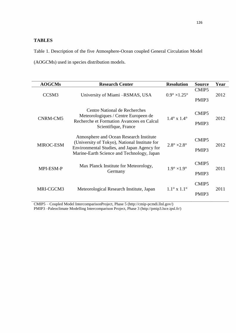
126
TABLES
Table 1. Description of the five Atmosphere-Ocean coupled General Circulation Model
(AOGCMs) used in species distribution models.
AOGCMs Research Center Resolution Source Year
CCSM3 University of Miami –RSMAS, USA 0.9° ×1.25° CMIP5
PMIP3 2012
CNRM-CM5
Centre National de Recherches
Meteorologiques / Centre Europeen de
Recherche et Formation Avancees en Calcul
Scientifique, France
1.4° x 1.4° CMIP5
PMIP3 2012
MIROC-ESM
Atmosphere and Ocean Research Institute
(University of Tokyo), National Institute for
Environmental Studies, and Japan Agency for
Marine-Earth Science and Technology, Japan
2.8° ×2.8° CMIP5
PMIP3 2012
MPI-ESM-P Max Planck Institute for Meteorology,
Germany 1.9° ×1.9°
CMIP5
PMIP3 2011
MRI-CGCM3 Meteorological Research Institute, Japan 1.1° x 1.1° CMIP5
PMIP3 2011
CMIP5 – Coupled Model IntercomparisonProject, Phase 5 (http://cmip-pcmdi.llnl.gov/)
PMIP3 –Paleoclimate Modelling Intercomparison Project, Phase 3 (http://pmip3.lsce.ipsl.fr/)
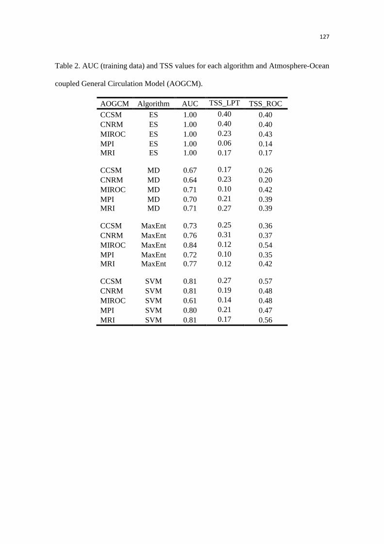
127
Table 2. AUC (training data) and TSS values for each algorithm and Atmosphere-Ocean
coupled General Circulation Model (AOGCM).
AOGCM Algorithm AUC TSS_LPT TSS_ROC
CCSM ES 1.00 0.40 0.40
CNRM ES 1.00 0.40 0.40
MIROC ES 1.00 0.23 0.43
MPI ES 1.00 0.06 0.14
MRI ES 1.00 0.17 0.17
CCSM MD 0.67 0.17 0.26
CNRM MD 0.64 0.23 0.20
MIROC MD 0.71 0.10 0.42
MPI MD 0.70 0.21 0.39
MRI MD 0.71 0.27 0.39
CCSM MaxEnt 0.73 0.25 0.36
CNRM MaxEnt 0.76 0.31 0.37
MIROC MaxEnt 0.84 0.12 0.54
MPI MaxEnt 0.72 0.10 0.35
MRI MaxEnt 0.77 0.12 0.42
CCSM SVM 0.81 0.27 0.57
CNRM SVM 0.81 0.19 0.48
MIROC SVM 0.61 0.14 0.48
MPI SVM 0.80 0.21 0.47
MRI SVM 0.81 0.17 0.56
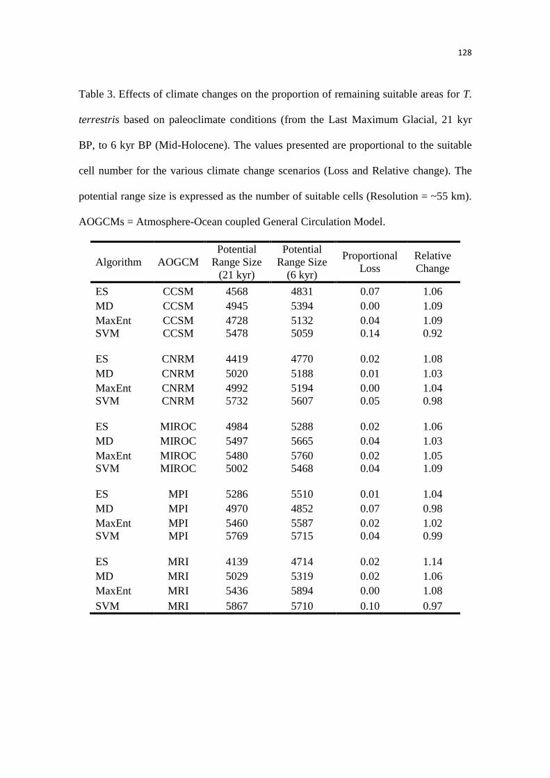
128
Table 3. Effects of climate changes on the proportion of remaining suitable areas for T.
terrestris based on paleoclimate conditions (from the Last Maximum Glacial, 21 kyr
BP, to 6 kyr BP (Mid-Holocene). The values presented are proportional to the suitable
cell number for the various climate change scenarios (Loss and Relative change). The
potential range size is expressed as the number of suitable cells (Resolution = ~55 km).
AOGCMs = Atmosphere-Ocean coupled General Circulation Model.
Algorithm AOGCM
Potential
Range Size
(21 kyr)
Potential
Range Size
(6 kyr)
Proportional
Loss
Relative
Change
ES CCSM 4568 4831 0.07 1.06
MD CCSM 4945 5394 0.00 1.09
MaxEnt CCSM 4728 5132 0.04 1.09
SVM CCSM 5478 5059 0.14 0.92
ES CNRM 4419 4770 0.02 1.08
MD CNRM 5020 5188 0.01 1.03
MaxEnt CNRM 4992 5194 0.00 1.04
SVM CNRM 5732 5607 0.05 0.98
ES MIROC 4984 5288 0.02 1.06
MD MIROC 5497 5665 0.04 1.03
MaxEnt MIROC 5480 5760 0.02 1.05
SVM MIROC 5002 5468 0.04 1.09
ES MPI 5286 5510 0.01 1.04
MD MPI 4970 4852 0.07 0.98
MaxEnt MPI 5460 5587 0.02 1.02
SVM MPI 5769 5715 0.04 0.99
ES MRI 4139 4714 0.02 1.14
MD MRI 5029 5319 0.02 1.06
MaxEnt MRI 5436 5894 0.00 1.08
SVM MRI 5867 5710 0.10 0.97
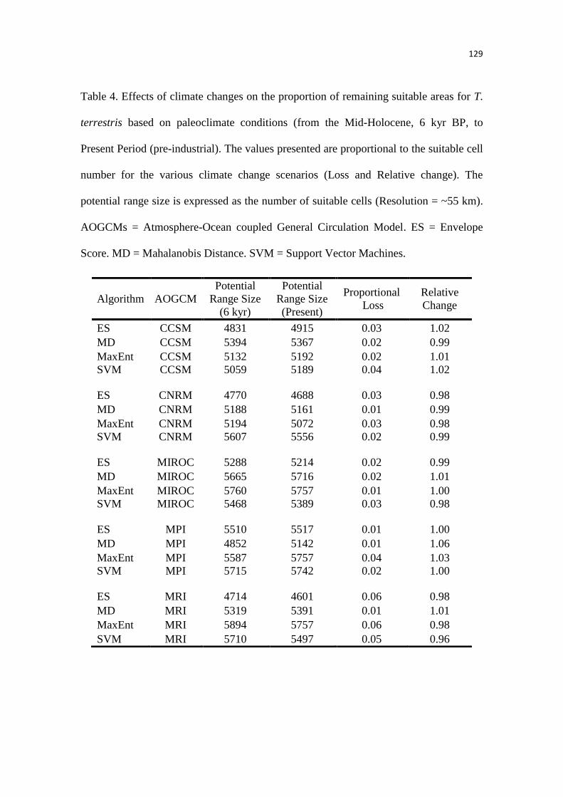
129
Table 4. Effects of climate changes on the proportion of remaining suitable areas for T.
terrestris based on paleoclimate conditions (from the Mid-Holocene, 6 kyr BP, to
Present Period (pre-industrial). The values presented are proportional to the suitable cell
number for the various climate change scenarios (Loss and Relative change). The
potential range size is expressed as the number of suitable cells (Resolution = ~55 km).
AOGCMs = Atmosphere-Ocean coupled General Circulation Model. ES = Envelope
Score. MD = Mahalanobis Distance. SVM = Support Vector Machines.
Algorithm AOGCM
Potential
Range Size
(6 kyr)
Potential
Range Size
(Present)
Proportional
Loss
Relative
Change
ES CCSM 4831 4915 0.03 1.02
MD CCSM 5394 5367 0.02 0.99
MaxEnt CCSM 5132 5192 0.02 1.01
SVM CCSM 5059 5189 0.04 1.02
ES CNRM 4770 4688 0.03 0.98
MD CNRM 5188 5161 0.01 0.99
MaxEnt CNRM 5194 5072 0.03 0.98
SVM CNRM 5607 5556 0.02 0.99
ES MIROC 5288 5214 0.02 0.99
MD MIROC 5665 5716 0.02 1.01
MaxEnt MIROC 5760 5757 0.01 1.00
SVM MIROC 5468 5389 0.03 0.98
ES MPI 5510 5517 0.01 1.00
MD MPI 4852 5142 0.01 1.06
MaxEnt MPI 5587 5757 0.04 1.03
SVM MPI 5715 5742 0.02 1.00
ES MRI 4714 4601 0.06 0.98
MD MRI 5319 5391 0.01 1.01
MaxEnt MRI 5894 5757 0.06 0.98
SVM MRI 5710 5497 0.05 0.96
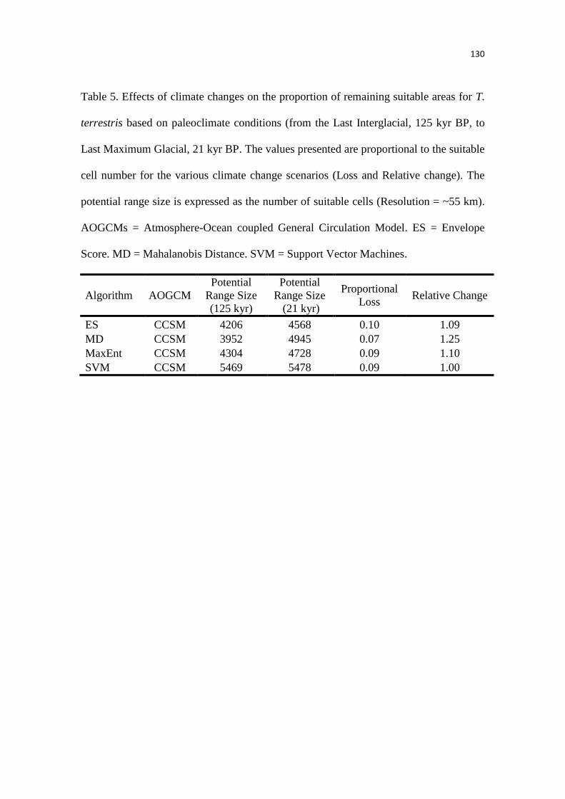
130
Table 5. Effects of climate changes on the proportion of remaining suitable areas for T.
terrestris based on paleoclimate conditions (from the Last Interglacial, 125 kyr BP, to
Last Maximum Glacial, 21 kyr BP. The values presented are proportional to the suitable
cell number for the various climate change scenarios (Loss and Relative change). The
potential range size is expressed as the number of suitable cells (Resolution = ~55 km).
AOGCMs = Atmosphere-Ocean coupled General Circulation Model. ES = Envelope
Score. MD = Mahalanobis Distance. SVM = Support Vector Machines.
Algorithm AOGCM
Potential
Range Size
(125 kyr)
Potential
Range Size
(21 kyr)
Proportional
Loss Relative Change
ES CCSM 4206 4568 0.10 1.09
MD CCSM 3952 4945 0.07 1.25
MaxEnt CCSM 4304 4728 0.09 1.10
SVM CCSM 5469 5478 0.09 1.00
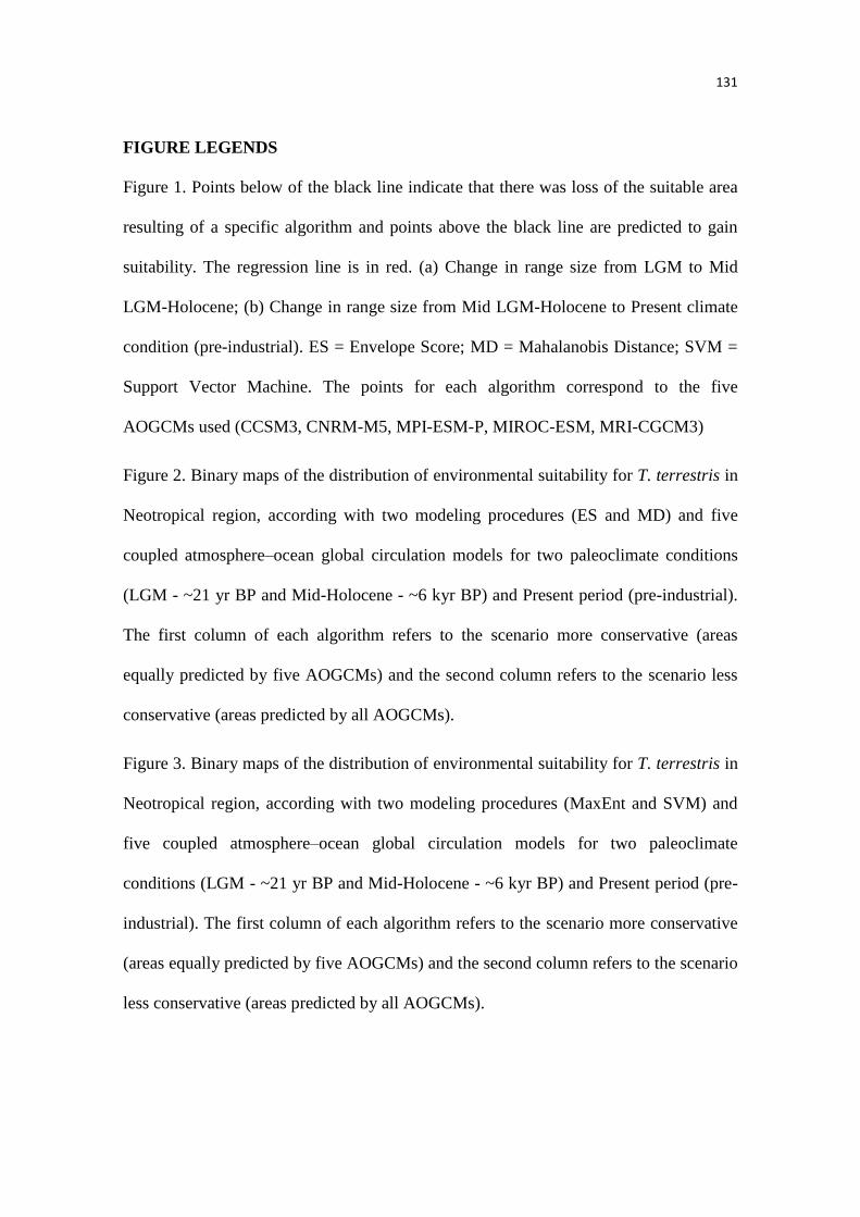
131
FIGURE LEGENDS
Figure 1. Points below of the black line indicate that there was loss of the suitable area
resulting of a specific algorithm and points above the black line are predicted to gain
suitability. The regression line is in red. (a) Change in range size from LGM to Mid
LGM-Holocene; (b) Change in range size from Mid LGM-Holocene to Present climate
condition (pre-industrial). ES = Envelope Score; MD = Mahalanobis Distance; SVM =
Support Vector Machine. The points for each algorithm correspond to the five
AOGCMs used (CCSM3, CNRM-M5, MPI-ESM-P, MIROC-ESM, MRI-CGCM3)
Figure 2. Binary maps of the distribution of environmental suitability for T. terrestris in
Neotropical region, according with two modeling procedures (ES and MD) and five
coupled atmosphere–ocean global circulation models for two paleoclimate conditions
(LGM - ~21 yr BP and Mid-Holocene - ~6 kyr BP) and Present period (pre-industrial).
The first column of each algorithm refers to the scenario more conservative (areas
equally predicted by five AOGCMs) and the second column refers to the scenario less
conservative (areas predicted by all AOGCMs).
Figure 3. Binary maps of the distribution of environmental suitability for T. terrestris in
Neotropical region, according with two modeling procedures (MaxEnt and SVM) and
five coupled atmosphere–ocean global circulation models for two paleoclimate
conditions (LGM - ~21 yr BP and Mid-Holocene - ~6 kyr BP) and Present period (pre-
industrial). The first column of each algorithm refers to the scenario more conservative
(areas equally predicted by five AOGCMs) and the second column refers to the scenario
less conservative (areas predicted by all AOGCMs).
132
Figure 4. Binary maps of the distribution of environmental suitability for T. terrestris in
Neotropical region, according with four modeling procedures (ES, MD, MaxEnt and
SVM) and one AOGCM (CCSM) for three paleoclimate conditions (LIG - ~125 kyr BP,
LGM - ~21 yr BP and Mid-Holocene - ~6 kyr BP) and Present period (pre-industrial).
Figure 5. The map shows the areas environmentally predicted by four algorithms for
lowland tapir (Tapirus terrestris). This map is the result of the intersection areas
between all time periods (LGM, mid-Holocene and pre-industrial).
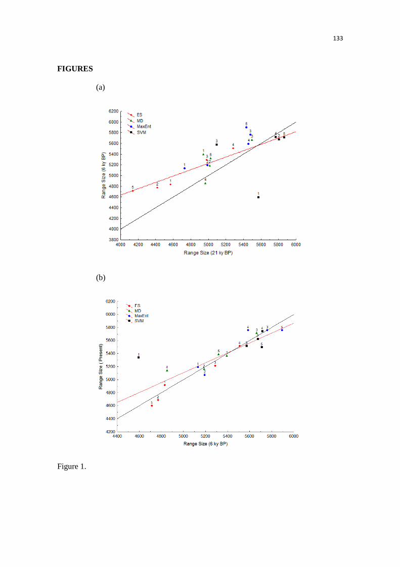
133
FIGURES
(a)
(b)
Figure 1.
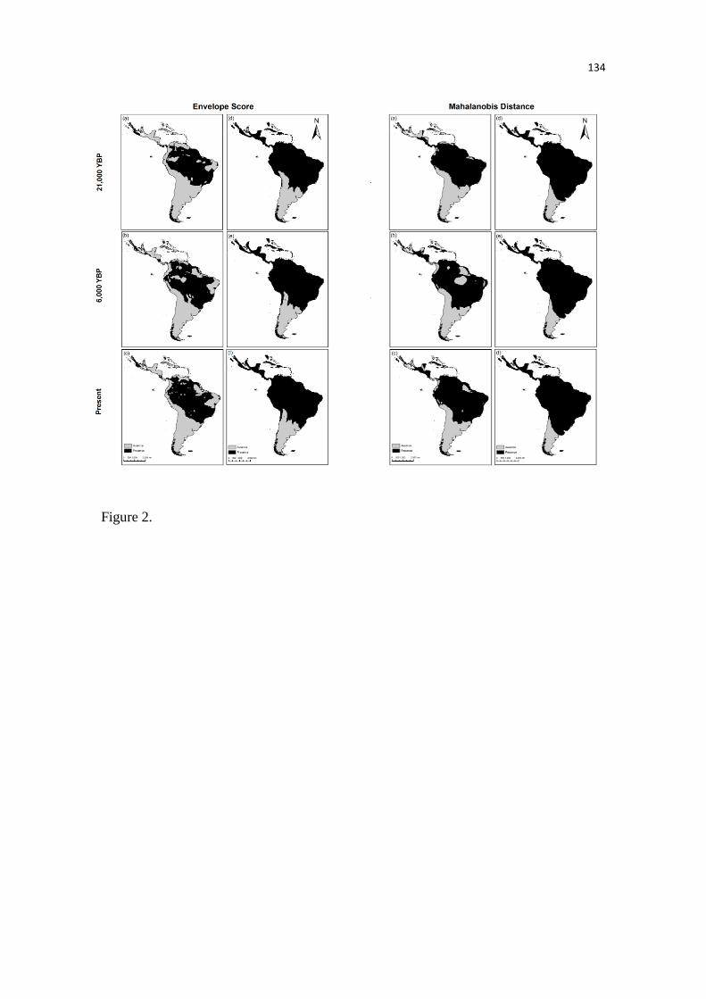
134
Figure 2.
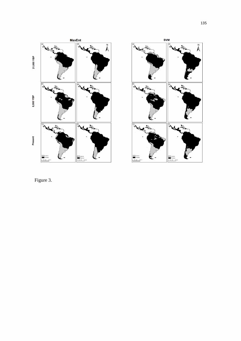
135
Figure 3.
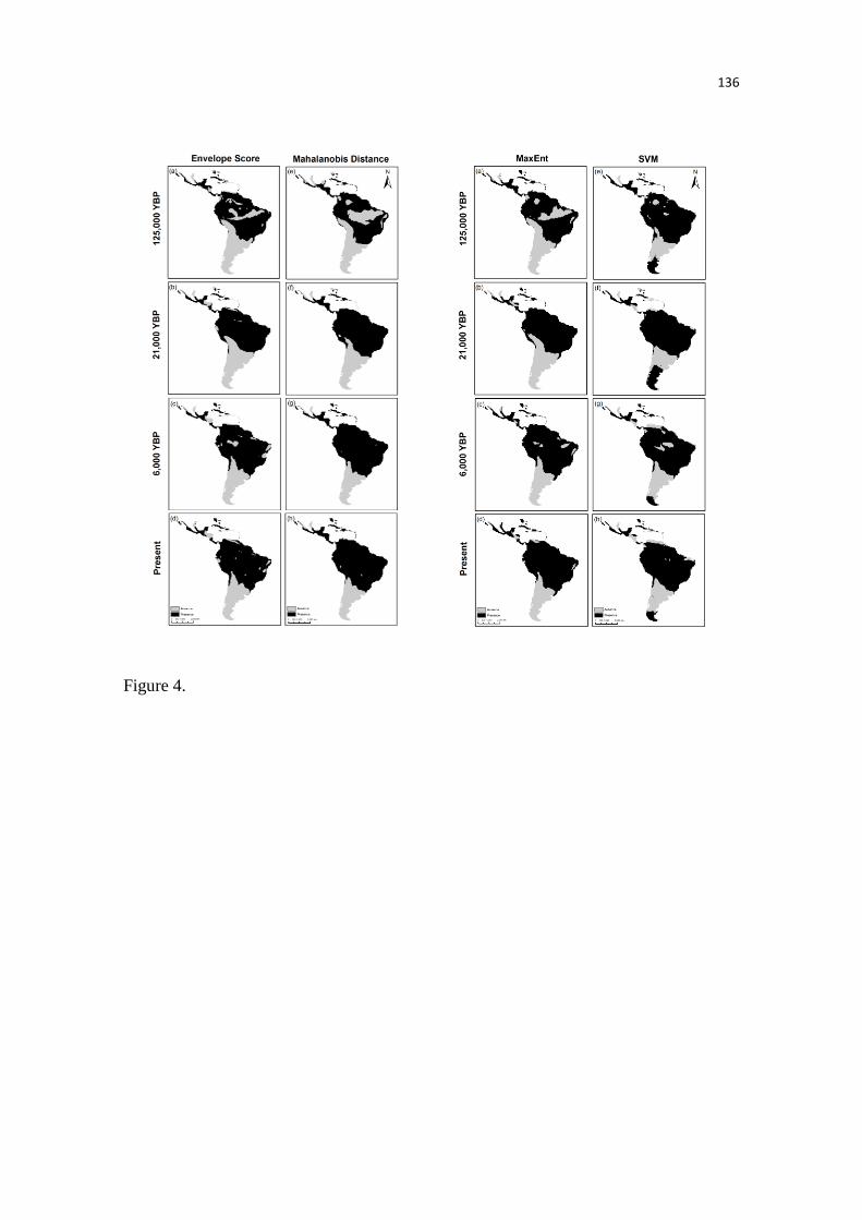
136
Figure 4.
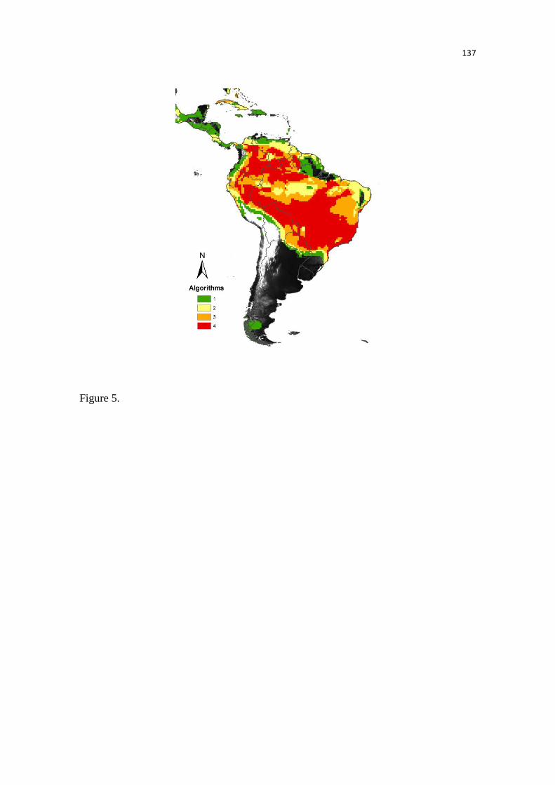
137
Figure 5.
138
CAPÍTULO 3
A ser submetido para: Biological Conservation
Present and future challenges for the conservation of Tapirus terrestris as revealed
by ecological niche models
Andressa Gattia*, Caroline C. Nóbrega
b, Paulo De Marco Júnior
b
a Programa de Pós-Graduação em Biologia Animal, Universidade Federal do Espírito
Santo, Av. Marechal Campos, 1468, Maruípe, Vitória, Espírito Santo, Brazil, CEP:
29040-070
b Laboratório de Ecologia Teórica e Síntese, Departamento de Biologia Geral, Instituto
de Ciências Biológicas 1, Universidade Federal de Goiás, Campus Samambaia, Caixa
Postal 131, Goiânia, Goiás, Brazil, CEP: 74001-970
*Correspondence: Andressa Gatti, Universidade Federal do Espírito Santo, E-mail
address: [email protected]
Short Running Title Tapirus terrestris conservation revealed by ecological niche
models
139
ABSTRACT
Climate change can potentially increase the susceptibility of species to
extinction, particularly when a combination of modifications in climate suitability, life
history and extrinsic threats occurs. Therefore, future losses of large mammals, such as
the lowland tapir (Tapirus terrestris), could take place faster than expected. Through the
use of species distribution models, we modeled the distribution of lowland tapirs in
current and future climates, evaluating potential changes in suitable habitats of the
species. In addition, we assessed existing Brazilian Protected Areas ( ≥ 500 km2) and
their effectiveness with regards to the distribution of suitable areas for T. terrestris. The
models predicted a marked loss in environmental suitability, particularly in tropical
moist broadleaf forests. Nevertheless, the total suitable area for lowland tapirs in
protected areas should not change. We expect that areas with greater environmental
suitability could sustain larger lowland tapir populations and could therefore be more
resilient to various threats. This observation may suggest that simple comparisons in
range limits may represent the potential negative effects of climate change on the
species distribution very poorly. Thus examining changes in climatic suitability will
provide important information regarding generalist species such as tapirs.
Keywords
Climate change, lowland tapir, protected areas, species distribution modeling,
suitability, vulnerability.
140
1. Introduction
Climate change poses a major threat to biodiversity especially when complex
interactions between life history and extrinsic threats (e.g., habitat loss and
fragmentation) increase the susceptibility of a species to extinction under future climate
scenarios (Ackerly et al., 2010; Brook et al., 2009; Keith et al., 2008). As result of this
combination, future losses of large mammals could be far more rapid than expected
(Cardillo et al., 2005). The removal of large herbivores, such as the lowland tapir, from
their natural habitats will most certainly impact the structure and composition of
regenerating forests due to the tapirs’role as a long-distance seed disperser (Fragoso et
al., 2003; Galetti et al., 2001; Tobler et al., 2010).
Climate change may modify the suitable areas for a specific species, driving
these species to shift their geographic ranges, thus increasing their vulnerability to
extinction (Nogués-Bravo et al., 2010; Root et al., 2003; Thomas et al., 2004). This
process can affect the probability of species persistence in areas designated for
conservation, forcing them into inadequate habitats or causing local extinctions (Araújo
et al., 2004; Coetzee, 2008; Hannah et al., 2007; Parmesan and Yohe, 2003). Diverse
climate change scenarios present an enormous challenge for the development of
strategies for the protection and conservation of several species. Climate change
presents a complex spatial problem for species conservation. Conservation requires
finding future suitable places that are often restricted by current habitat fragmentation
but are within the known range of the species. Moreover, evaluating the effectiveness of
protected areas is problematic in conservation planning because these are immovable
geographic areas which is hardly adequate under the dynamic scenarios of climate
change (Dudley et al., 2008; Parmesan and Yohe, 2003; Root et al., 2003).
141
In recent years, the evaluation of species and reserve responses to global
climate change has been possible through the application of different tools of
conservation planning. One such tool, the Ecological Niche Model (ENM), has
facilitated studies in basic and applied ecology, biogeography, conservation biology and
wildlife management (Araújo et al., 2006; Coetzee et al., 2009; Guisan and
Zimmermann, 2000; Rodríguez et al., 2007). The ENMs have become popular in
predicting the suitability of the current habitat and future range shifts and particularly
for estimating extinction risks induced by climatic changes (Araújo and Rahbek, 2006;
Beever et al., 2011; Keith et al., 2008; Thomas et al., 2004). These models have also
been used to evaluate the effectiveness of natural reserves in species protection (Hannah
et al., 2005; Nóbrega and De Marco, 2011; Rodríguez-Soto et al., 2011; Urbina-
Cardona and Loyola, 2008).
The availability of a set of global climate layers (climate grids) (Hijmans et al.,
2005), along with the development of a large number of climate models, such as general
circulation models (GCMs), by various meteorological research centers, has increased
the predictive power of ENMs and has improved the evaluation of individual species
responses to global climate change (Araújo et al., 2006; Beaumont et al., 2008; Peterson
et al., 2002; Thuiller, 2003; Thuiller et al., 2005; ). According to Beaumont et al.
(2008), climate models are currently the best tools available for simulating future
climate scenarios. However, ENMs present a certain level of uncertainty due to
differences in alternated models, species characteristics and future scenarios (Thuiller et
al., 2008). The crucial question is whether the models that predict current species
distribution can also provide robust predictions for future distribution following climate
change (Araújo and Rahbek, 2006; Elith and Leathwick, 2009). Additionally, whether
142
the ENMs can predict the species’ distribution in new or unsampled regions following
predicted climate changes must be determined. Should these ENMs prove to be
transferable (Heikkinen et al., 2012; Peterson et al., 2007; Randin et al., 2006), they
could be used to manage anticipated climate conditions (Mbogga et al., 2010). Recent
studies have addressed the errors, uncertainties and transferability of these models
(Beaumont et al., 2008; Buisson et al., 2010; Heikkinen et al., 2012; Marmion et al.,
2009). The identification and quantification of these uncertainties are crucial for
improving the reliability of projected species range shifts in the future (Pearson et al.,
2006; Thuiller, 2004). These projections are particularly important for completing risk-
assessment exercises (Ormsby, 2005), making conservation management decisions
(reintroduction programs (Hartley et al., 2006) and creating new or expanding protected
areas.
The lowland tapir, Tapirus terrestris, is a suitable model for examining the
impacts of climate change on the persistence of large mammal populations present at
low densities. The last IUCN Red List assessment for tapirs has estimated that the
number of lowland tapirs in the wild will continue to decline over the next three
generations (33 years) (IUCN, 2012). Synergistic interactions between intrinsic
biological traits, such as a slow reproductive cycle, delayed sexual maturity and long
gestation period producing a single offspring (Barongi, 1993; Eisenberg, 1997), and
extrinsic threats, including deforestation, hunting and road-kill, are driving the decline
of lowland tapir populations (Medici et al., 2007). Consequently, tapir populations have
become small and increasingly isolated throughout their geographic distribution,
particularly in the Cerrado (Brazil), Atlantic Forest (Brazil) and Llanos
(Venezuela/Colombia) biomes (Medici et al., 2007; Medici et al., 2012). Lowland tapir
143
populations have become extinct in some regions of the Brazilian Atlantic Forest
(Flesher and Gatti, 2010), in addition to the grasslands in Southern Brazil and the
Caatinga (Brazil) (Medici et al., 2012).
Considering the current distribution of lowland tapir populations, this paper
presents a distribution model outlining suitable habitats under the present climate and
under predicted climate scenarios for the future. Moreover, these predictions were used
to evaluate current protected areas in Brazil with regards to their inclusion of suitable
areas and predicted effectiveness under future climates.
2. Material and methods
2.1. Study species and Occurrence data
The first appearance of Tapirus in North America occurred in the late middle
Miocene as a result of their immigration from Asia. In South America, the first records
indicate that they appeared during the Plio-Pleistocene period (Cione and Tonni, 1996;
Nabel et al., 2000) following migration from North America after the formation of the
Isthmus of Panamá, during the Great American Biotic Interchange (Marshall et al.,
1988; Webb, 2006). The lowland tapir, Tapirus terrestris, is a Neotropical mega-
herbivore mammal (Hansen and Galetti, 2009). The species has expanded its
distribution since it first appeared in the Pleistocene period (Thoisy et al., 2010), and
has therefore become the most successful large herbivore in South America.
Tapirus terrestris occurs in Argentina, Bolivia, Brazil, Colombia, Ecuador,
Guyana, French Guyana, Paraguay, Peru, Suriname and Venezuela (Taber et al., 2008).
Occurrence points were gathered and distributed over nearly the entire current
geographic distribution of the lowland tapir. These data were provided by experts from
144
the IUCN/SSC Tapir Specialist Group (TSG) in Bolivia, Brazil, Colombia, Ecuador and
Paraguay and corresponded to approximately 70% of all records, including unpublished
field data. To complement the data, we compiled information from the literature and
from museum specimens deposited in online databases available within the Data Portal
of the Global Biodiversity Information Facility (GBIF; www.gbif.org). We used 475
spatially distinct occurrence points (from 516 compiled) to generate the distribution of
lowland tapirs for both current and future climate conditions throughout the Neotropics.
2.2. Climate layers
Environmental data were obtained from the WorldClim Database
(www.worldclim.org) and included six variables (from 19 available): annual mean
temperature, temperature seasonality (coefficient of variation), mean temperature of the
driest quarter, annual precipitation, precipitation seasonality (coefficient of variation)
and precipitation during the warmest quarter. These data were used at a 5’ spatial
resolution (~9 km of cell-side size).
We used future climate datasets derived from three general circulation models
(GCMs), for the year 2080 (www.ccafs-climate.org/data). These models included: 1)
Canadian Centre for Climate Modelling and Analysis (CCCma) Coupled Global
Climate Model (CGCM2), Second Version (Flato and Bôer, 2001); 2) CSIRO
Atmospheric Research Mark 2b Climate Model (Hirst et al., 1996, 2000) and 3)
HadCM3, which is the coupled ocean–atmosphere general circulation model developed
by the Hadley Centre for Climate Prediction and Research (Gordon et al., 2000).
For each GCM described above, two emission scenarios for the year 2080 were
selected. The first scenario, A2 was considered to be more severe and assumed 1% yr-1
145
CO2 increase and did not take into account the effects of sulfate aerosols. The A2 model
describes a heterogeneous world with a continuously increasing global population. The
second scenario, B2, was more conservative and assumed 0.5%yr-1
CO2 increase and
incorporated the effects of sulfate aerosols. The B2 scenario highlighted a world in
which the emphasis is placed on local solutions to economic, social and environmental
sustainability at a time when the global population is continuously expanding at a rate
lower than that described in scenario A2 (Nakicenovic and Swart, 2000).
2.3. Modelling approach
To model the habitat suitability for T. terrestris, we used two different algorithms:
Maximum Entropy (MaxEnt) and Mahalanobis Distance. A comparative analysis of
these algorithms with other methods indicated that they have greater predictive accuracy
(Elith et al., 2006; Elith and Graham, 2009; Farber and Kadmon, 2003; Johnson and
Gillingham, 2005). Furthermore, we chose these two algorithms because they reflect
distinct approaches. MaxEnt is a complex parameter-rich model that may produce less
transferability estimates (Peterson et al., 2007; Phillips, 2008), especially for studies
using large datasets. Mahalanobis Distance is a simpler model allowing for easier
interpretation based on a geometric view of the Hutchinsonian niche (Farber and
Kadmon, 2003). These distinct models helped us evaluate the uncertainties in our study.
MaxEnt Software (version 3.3.3e) (Computer Sciences Department, Princeton
University, 2004) is a general-purpose machine learning approach that uses a simple
mathematical formulation for modeling geographic distribution of species with
presence-only data (Phillips et al., 2006). Absence data are generated by randomly
selecting ‘‘pseudo-absence’’ points or the background of the area. MaxEnt models were
built using 1000 iterations, logistic output format, and removal of all duplicates.
146
Recent studies have shown that MaxEnt models suffer from over-
parameterization leading to transferability problems (Peterson et al., 2007) that may
affect its predictions, particularly future climate (Elith et al., 2010). MaxEnt provides a
number of features (linear, quadratic, hinges, logistic and product) representing the
types of functions and combination of functions used during the process. The number of
parameters in the model is directly (and sometimes exponentially) related to the number
of features used in the model.
To control for over-parameterization, we developed the MaxEnt models using
two distinct settings. The first used the “default” setting ("auto-features"), which allows
for inclusion of six features (Phillips et al., 2006). The first set was called “complete”
model. The second set was called “simple” setting and includes only two features: (i)
linear, which constrains the output distribution for each species as having the same
expectation for each of the continuous environmental variables and the sample locations
for that species; and (ii) the quadratic feature, which models the tolerance of the species
to variation from its optimal conditions (Phillips et al., 2006; Phillips and Dudík, 2008).
Elith et al. (2010) argue that linear and quadratic features produce smoother models.
Simple models with fewer parameters are expected to generate models with higher
transferability.
The other approach used in this study was based on Mahalanobis Distance, a
generalized squared distance statistic. This approach has been used as a multivariate
index of environmental quality in studies examining species distribution. This generic
algorithm was based on environmental dissimilarity metrics, which is an extension of
the standardized Euclidian Distance and takes into account the covariance structure
among the predictor variables. Mahalanobis Distance is more complex because the
147
model considers the covariance matrix among environmental variables in the occurrence
points (Farber and Kadmon, 2003).
2.4. Model evaluation
Recent advances in the evaluation procedures for species distribution models
suggest that the use of both threshold-independent and threshold-dependent evaluation
measures should be used to ensure that the methods are efficient both generally as well
as with regards to the chosen threshold (Liu et al., 2011). In this paper we chose to use
the True Skill Statistics (TSS), which performed well when compared to similar
measures (Liu et al., 2011). This statistic is highly correlated with AUC (Area Under
Curve) and is not biased by prevalence (Allouche et al., 2006). TSS takes into account
both omission and commission errors and ranges from −1 to +1, where +1 indicates
perfect agreement, and values of zero and less indicate a performance that is no better
than random.
The AUC is a threshold-independent measure that can be interpreted as the
ability of the algorithm to discriminate between a suitable environmental condition and
a random analysis pixel (Phillips et al., 2006). AUC values range from 0 to 1, where 1
indicates perfect discrimination and a score of 0.5 implies discrimination that is no
better than random (Elith et al., 2006). AUC was only used to determine the relative
performance of the various models.
Thresholds are used to convert continuous species distributions model outputs in
binary maps to predict the presence or absence of the species. Values smaller than the
threshold were considered to be zero, while values higher than the threshold were
considered to be 1. The low presence threshold (LPT) was used because it equals the
minimum model prediction value for any of the training occurrence point data. Thus,
148
the LPT minimizes omission errors in the models, which can be considered as an
effective strategy for species conservation. This choice is especially appropriate for T.
terrestris as the occurrence points are precise and contain no mis-identification or other
common problems. Moreover, a comparison of the results using LPT with the threshold
derived from the ROC curve showed extensive omission of known occurrences in the
latter model (Supplementary material S1). Threshold was derived from the ROC curve
representing the value with the lowest Euclidean distance from the zero point, the false
positive and true positive (Elith et al., 2006).
The model transferability was quantified using the method proposed by Wenger
and Olden (2012), which is based on a non-random division of the dataset and involves
cross-validation. Thus, we initially separated the dataset into two spatially distinct
subsets based on longitude, fitting the model with the first subset (denoted as the
training dataset) and evaluating with the second subset (test dataset). Then, the reverse
process was completed with the second subset. For each evaluation, we calculated the
AUC and TSS values.
2.5. Species range shift and conservation under climate change
To evaluate the future range shifts of T. terrestris, such as expansions and
contractions, we used relative changes in distribution (values >1 and <1 to represent
expanding and shrinking climates, respectively) and the proportional distribution loss.
The first metric was calculated by dividing the area occupied under future projections
by the area occupied under current climate. The second metric was calculated by
dividing the number of lost cells in future distribution by the number of cells in the
current distribution. We also quantified the number of overlapping suitable cells in the
present and the future, furthermore novel climates (absent now and present in the
149
future); this was defined as a presently unsuitable habitat that was predicted to become
suitable in the future (Thuiller et al., 2005; Williams et al., 2007). The differences in
size of current and future distributions were tested using a t test for dependent samples.
To evaluate the effectiveness of existing protected areas (PAs) with respect to
the distribution of suitable areas predicted under climate change scenarios, we
assembled the geographical limits of Brazilian protected areas from ICMBio (Instituto
Chico Mendes de Conservação da Biodiversidade), the official Brazilian environmental
agency. This dataset contains federal and state reserves implemented until 2012
including both strictly protected areas (equivalent to IUCN categories I and II) as well
as sustainable use reserves (equivalent to IUCN category V).
Previous studies have estimated the size of the area required to maintain
genetically viable populations (~200 individuals) of lowland tapirs in Atlantic Forest
sites (Medici, 2010; Gatti et al., 2011; Medici and Desbiez, 2012). In this paper we used
a conservative scenario and selected protected areas ≥ 500 km² regardless of the biome.
We selected a total of 178 areas. In addition to these areas, we used the second scenario
for all protected areas and placed no size restrictions on the analysis. In this group we
included Private Natural Heritage Reserves (called Reserva Particular do Patrimônio
Natural in Portuguese and denoted hereafter as “RPPN”), which are an official protected
area category that allows private landowners to voluntarily turn their private forest into
protected areas maintaining them in perpetuity. Furthermore, we categorized the CUs
for five Brazilian biomes (Amazon, Atlantic Forest, Caatinga, Cerrado and Pantanal),
calculated the mean climatic suitability for each conservation unit within the first group
and evaluated whether there was a gain or loss in suitability in the future.
150
Conservation units were converted to a final resolution of 0.2º X 0.2º
(approximately 22 X 22 km) independently of their size (Nóbrega and De Marco, 2011).
For this analysis, we limited the resulting models of lowland tapir distribution to the
Brazilian territory. The maps depicting predicted current and future suitable
environments were compared to existing maps of protected areas in Brazil.
3. Results
3.1. Model evaluation
MaxEnt models produced higher AUC and TSS values compared to
Mahalanobis Distance (Table 1). However, both yielded high transferability (Table 1,
Figure 1), which is a desirable property for such models. Furthermore, the distribution
areas predicted by Mahalanobis Distance indicated a potentially high rate of over-
prediction, suggesting that the potential lowland tapir distribution could include areas
where no records of tapir occurrence exist (e.g., central region of Argentina) (Figure 1).
The complete MaxEnt models showed higher training AUC and TSS values
(Table 1). However, the simple models demonstrated higher average transferability
(0.46). Moreover, the distribution resulting from the complete models contained some
gaps, particularly the model produced from the second data subset (Figure 1;
Supplementary Material S2). These gaps occur in areas where tapirs are present and
contribute to an increased model omission rate.
Considering the evaluation measure results (AUC and TSS) and the
transferability of the models, we determined that the MaxEnt simple model was the
most appropriate to describe potential tapir distributional areas. Specifically, we focused
151
on the limited over-prediction by the MaxEnt models and the slightly higher
transferability characteristic of the simple models.
3.2. Climate change and potential distribution shifts
The MaxEnt model predicts an average potential distribution of 15,322,662.00
km2 for T. terrestris under current climate conditions; additionally, nearly 97% of the
suitability cells were maintained in the future for all climate models and emission
scenarios (Table 3). The values obtained for the relative change (>1) indicate that the
suitable areas will expand in the future, increasing the potential distribution by
384,844.50 km2 and 843,642.00 km
2 for
new potentially suitable habitats (Table 2).
No significant difference was observed between the range size of the species in
the present and in the future (t = -1.346, df = 5, p = 0.236). However, the models predict
pronounced changes in the spatial distribution of suitable climates, with lost and gained
habitats in various regions where lowland tapirs are currently distributed (Figure 2).
Results from different climate models follow the same pattern, but the Hadcm3
models (scenarios A2 and B2) yielded areas with greater losses than suggested by the
other climate models. These models predict that a marked loss in environmental
suitability will occur for the lowland tapir, especially in Tropical Moist Broadleaf
Forests (Figure 2). The western Amazon (Brazil, Colombia and Peru) is predicted to
suffer from the largest suitability losses when compared to other regions. Guianan moist
forests are also predicted to be negatively affected by climate change.
The Cerrado and Pantanal biomes are predicted to undergo a considerable loss in
suitability as well. Furthermore, other ecoregions such as Beni Savana (Bolivia),
rainforests of Napo (Ecuador and a portion of Peru) and dry Chaco (portions of
152
Argentina, Bolivia and Paraguay) are expected to experience suitability shifts under
climate change (Figure 2). The cells located in the Caatinga and the Atlantic Forest
located above the Serra do Mar coastal forests will be affected by climate alterations as
well, but these changes are likely to be less intense than those mentioned before.
Increases in the suitability are predicted to occur in areas where the species is
not thought to be present, such as some regions in the Andes. Moreover, an increase in
suitable grid cells may occur in the Brazilian Atlantic Forest, specifically in Araucaria
moist forests, Alto Paraná Atlantic Forests and the Serra do Mar Coastal Forest (Figure
2).
3.3. Effectiveness of the Brazilian network of protected areas
As with the total distribution, there will be no change in the size of lowland tapir
geographic distribution area under protection. Nevertheless, only 12% of the lowland
tapir distribution will be within protected areas capable of supporting viable populations
(≥ 500 km2) (Table 3). When considering all Brazilian protected areas, approximately
15% of the potential lowland tapir distribution will be under some form of legal
protection in the future.
Although there were no changes in the total distribution of tapirs, the models
predicted pronounced changes in the spatial distribution of climatic suitability. All of
the future climate models, using both emission scenarios, show similar qualitative
patterns in changing environmental suitability, quantified in protected areas (PAs).
However, the mean values for suitability are slightly different among the models (Table
2; Figure 3). The HadCM3 (A2 and B2) models are more pessimistic than the others,
153
producing greater suitability losses (Table 2; Figure 3c, f). When evaluated by biome,
the trend indicates a clear decrease in the environmental suitability of most of the PAs,
especially in the Amazon, Cerrado, Caatinga and Pantanal biomes.
The protected areas in the Atlantic Forest include regions where the models
predict a minimal increase in climatic suitability, with the exception of the Csiro (B2)
model, which predicted an increase in these areas (B2) (Figure 3e). Furthermore, the
suitability is stable over time based on the analysis of a small group (Figure 3). We note
that the increase in suitability usually occurred in the same areas, principally in the
Atlantic Forest regardless of the climate model; this observation minimizes the
uncertainty among the models (Figure 3; Supplementary Material S3).
4. Discussion
4.1. Present and future challenges for lowland tapir conservation
The comparison between the current and the future distribution of lowland tapirs
resulted in small changes in the overall species distribution. Nonetheless, model
outcomes clearly show a strong shift in the average environmental suitability throughout
the species distribution. This observation highlights the fact that simple comparisons of
range limits do not fully describe the possible negative effects of climate change on
species distribution. This reasoning is in line with recent advances in species
distribution modeling, which is currently moving from strict estimation of species range
to a more thoughtful evaluation of suitability distributions (Araújo et al., 2011; Diniz-
Filho et al., 2010; Tôrres et al., 2012).
154
Predicted environmental suitability can be used to better understand the effects
of environmental changes as these models represent how the physiological and
ecological requirements of the species are met at a specific location (VanDerWal et al.,
2009). For example, lowland tapirs have diverse behavioral strategies and physiological
characteristics that can favor the occupation and use of the wide range of resources in
extensive areas (García et al., 2012; Medici, 2010), and these characteristics may
explain the large lowland tapir distribution size that the models predicted. Thus, a key
element of this reasoning is that environmental suitability is at least monotonically
related to actual population densities; therefore, environmental suitability has become
an important surrogate for population survival and persistence.
Recent studies have tested whether environmental suitability, derived from
species distribution modeling, could serve as a surrogate for species’ performance and
density. Tôrres et al. (2012) demonstrated that high jaguar densities were restricted to
areas where the environmental suitability was the greatest. Low jaguar densities were
observed in areas with low suitability. Recent studies (Montoya et al., 2009; Tôrres et
al., 2012; VandDerWal et al., 2009) suggest that species distribution models provide
valuable information on species abundance and on the effectiveness of conservation
efforts for threatened species, such as the lowland tapir. These models are extremely
valuable because it is usually difficult to obtain real species performance measures
along environmental gradients (Thuiller et al., 2010).
The sensitivity of each species to climate change can vary with the life-history
characteristics of the organism (Willians et al., 2008) and with their individual lifestyle.
Low reproductive rates and low population density are usually associated with higher
sensitivity to climate change. Therefore, the lowland tapir is a good model for ENM
155
analyses given its very low reproductive rates and generally low population density
(Medici et al., 2007; Medici, 2010; Novaro et al., 2000). These characteristics,
combined with a decline in climatically suitable areas predicted by our models, could
potentially influence the vulnerability of this species to extinction, similar to what has
been predicted for other organisms (Araújo et al., 2006; Beever et al., 2011; Capinha et
al., 2012; Cardillo et al., 2005; Diniz-Filho et al., 2010; Ochoa-Ochoa et al., 2012).
Specifically, climate change can introduce changes in vegetation, affecting the
integrity of several biomes in South America (Leadley et al., 2010; Salazar et al., 2007)
and consequently the survival of large herbivores such as tapirs (García et al., 2012).
Climate change can prevent the species from maintaining a minimum viable population
size (Willians et al., 2008), while small populations are extremely vulnerable to
demographic stochasticity (Melbourne and Hastings, 2008). Additionally, if the patterns
of rainfall and temperature change increasing the climate variability as predicted (IPCC,
2007; Schneider et al., 2007), tapirs may become even more dependent on water to
regulate their body temperature (García et al., 2012).
Most of the areas predicted by the models to suffer moderate to high losses in
future suitability are located in regions where tapir populations are currently declining at
alarming rates, and local extinctions have also been reported(Flesher and Gatti, 2010;
IUCN, 2012; Medici et al., 2012). Contrarily, some of the models have predicted that
climate change will negatively impact areas where tapir populations are not considered
to be threatened, such as the Brazilian Amazon, or in areas where the tapir is listed as
Near Threatened, such as Pantanal (Medici et al., 2012).
These predictions are very serious, particularly if habitat loss and tapir hunting
continue to take place (Medici et al., 2012). These threats could potentially have an
156
overriding effect after drastic losses in climate suitability. Tapir populations in eastern
and southern Amazonia -- the so-called “arc of deforestation” -- are rapidly declining
due to extensive hunting and deforestation (Bodmer and Lozano, 2001; IUCN, 2012;
Medici et al., 2007). In the Pantanal, the intensification of traditional cattle ranching
practices threatens the medium-large frugivorous mammal community (Alho, 2011;
Junk and Cunha, 2005). In fact, the Pantanal floodplains may be an appropriate model
to study the potential impacts of climate change on Neotropical communities as extreme
climate events such as droughts can significantly change local wildlife communities
(Desbiez et al., 2010). Thus, the areas located in the Amazon and Pantanal biomes
should be considered vulnerable to species survival in the future if no conservation
strategy is implemented to minimize the predicted changes in climatic suitability and at
the landscape level.
Recent studies have suggested that combinations of threats, including hunting,
habitat loss, fire, invasive species and climate change, or feedback between threats can
affect species survival and persistence and foster unpredictable interactions among
plants, animals and microorganisms (Brook et al., 2008; Laurance and Useche, 2009;
Thuiller, 2007). García et al. (2012) emphasized that the combination of environmental
changes and threats including poaching, road-kill and infectious diseases strongly
affects the likelihood of extinction of remaining tapir populations. Again, we expect that
areas with higher environmental suitability could maintain larger populations and likely
be more resilient to such threats.
Medici et al. (2012) assessed the conservation status of the T. terrestris in five
Brazilian biomes (Amazon, Atlantic Forest, Caatinga, Cerrado and Pantanal). Tapir
populations in the Atlantic Forest and Cerrado biomes were found to be seriously
157
threatened. Our results indicated that the Cerrado biome as well as a portion of the
Atlantic Forest above the Serra do Mar coastal forests, will be extremely threatened by
the decline in environmental suitability. The Atlantic Forest is one of the most
threatened tropical forests in the world and is highly fragmented as a consequence of a
long history of degradation (Metzger, 2009; Myers et al., 2000; Ribeiro et al., 2009). It
shelters many species that are threatened with extinction by anthropogenic pressures
(Galetti et al., 2009).
Lowland tapirs were negatively impacted by habitat fragmentation in the
Atlantic Forest and populations have been heavily hunted (Cullen et al., 2000; Flesher
and Gatti, 2010). The Tabuleiro sand plain lowlands, located in southeastern Brazil,
were drastically reduced and completely lost in some areas. Nevertheless, these areas
still shelter the last lowland tapir populations in this forest type (Flesher and Gatti,
2010). Currently, 70% of tapir populations in the Atlantic Forest are considered to be at
critical levels (Medici et al., 2012), meaning that they are below the minimum viable
population size of 200 individuals (Gatti et al., 2011; Medici, 2010). The deleterious
genetic effects of isolation are a long-term threat to small tapir populations (Gatti et al.,
2011). A reduction in the genetic variability in tapir population is expected to affect the
ability of the population to adapt to environmental fluctuations (Medici and Desbiez,
2012), such as those predicted to occur under climate change.
In the Cerrado biome, only 20% of tapir populations have long-term chance of
survival, and populations will be restricted to protected areas (Medici et al., 2012). This
is the second largest biome in the Neotropical region, but it has been transformed into
one of the most important regions for cattle ranching and commodity crops in Brazil
(Ferreira et al., 2012). Remaining natural patches within the Cerrado have been
158
restricted to sloped areas (Carvalho et al., 2009). Recent studies have predicted severe
landscape changes on the biome scale, and these changes are concentrated in the
northern and northeastern regions of Brazil (Diniz-Filho et al., 2009; Ferreira et al.,
2012). Habitat modifications and loss of environmental suitability in the Cerrado can
affect small populations that are more susceptible to genetic, environmental and
demographic constraints (Brito, 2009; Gatti et al., 2011; Lacy, 2000).
Tapir conservation efforts are also needed in areas that are predicted to
experience decreases in environmental suitability in the future. These include regions in
Argentina, Bolivia, Paraguay, Colombia, Ecuador and Peru. Many tapir populations in
these regions are small and isolated due to an increase in agricultural and cattle ranching
activities as well as overhunting (IUCN, 2012; Medici et al., 2007). In the Bolivian
Chaco, lowland tapirs are an important food source for indigenous people (Brooks and
Eisenberg, 1999) and are usually overexploited (Noss and Cuéllar, 2008).
In addition, our models predicted an increase in climatic suitability in areas
located in the Atlantic Forest, such as the Serra do Mar Coastal Forests, which currently
holds the largest lowland tapir population in the biome. Today, approximately 40% of
the lowland tapir populations are found along the coast of São Paulo and Paraná States
(Medici et al., 2012). The Serra do Mar is characterized by large forest fragments that
extend into the Interior and Araucaria regions (Ribeiro et al., 2009). Medici and Desbiez
(2012) presented the results of a population viability analysis (PVA) of a lowland tapir
population in aprotected area (Morro do Diabo State Park) and surrounding forest
fragments located in the Atlantic Forest of the Interior. Results of this PVA
demonstrated that the effectiveness of tapir conservation efforts depends on promoting
the functional connectivity of the landscape.
159
In southern Brazil, the species is locally extinct in several sites and is mostly
found in protected areas (Fontana et al., 2003; Mikich and Bérnils, 2004; Rocha-
Mendes et al., 2005). The Llanos in Venezuela has dwindling tapir populations due to
subsistence hunting by indigenous people, peasants and settlers (Medici et al., 2007;
Rodríguez and Rojas-Suárez, 2008). As discussed by Tôrres et al. (2012), extrinsic
factors can limit species populations in regions with increased climate suitability values,
contradicting what would be expected in regions where environmental conditions are
favorable to persistence (Thuiller et al., 2010).
Although the models have predicted new suitable areas for lowland tapirs, it is
very important to note that the dispersal to those areas could be limited (Hodgson et al.,
2009). Brooker et al. (2007) observed that when the rates of climate change increase,
decreased levels of long-distance dispersal drives mutualists to extinction. Ochoa-
Ochoa et al. (2012) evaluated the dispersal of an amphibian species in Mexico and
found that its low dispersal ability generates increased levels of extinction. Furthermore,
species may not have sufficient time to adapt to new conditions (Loiselle et al., 2010).
Despite a possible higher dispersal ability of tapirs in some regions, the increase of
human-dominated landscapes, including pastures, agroecosystems and urban areas, may
seriously limit the dispersal of existing populations in the future. Some studies provide a
glimpse of hope and suggest that tapirs can use complex landscapes that include humans
and populations could therefore persist in this new environments (Centoducatte et al.,
2011; Medici, 2010; Noss et al., 2003). Furthermore, these new environments also have
their own challenges, including hunting, road-kill, and the potential introduction of new
infectious pathogenic agents into tapir habitat (Furtado et al., 2010; Mangini et al.,
2012; Medici et al., 2007).
160
Many bionomic processes also affect local species distribution but may not have
a measurable contribution at larger scales (global and regional, for example), in which
the scenopoetics and biogeographical factors have a determinant effect (Hortal et al.,
2010; Thuiller et al., 2004). Nevertheless, it is not possible to account for all of these
factors in species distribution models (Kamino et al., 2011). An alternative approach is
to compare the resulting habitat suitability models to characteristics of the habitats,
including the presence, size and conservation state of forest remnants, connectivity
between these remnants, presence of roads, existence of conservations units among
others.
Currently, most lowland tapir populations are found in protected areas (Flesher
and Gatti, 2010; IUCN, 2012; Medici et al., 2012). Unfortunately, only a small portion
of the tapir’s distribution in Brazil will remain protected in the future. Existing
protected areas within the lowland tapir range are unevenly distributed between biomes.
The PAs in the Amazon account for approximately 80% of the Brazilian PAs ≥500km2,
but these areas are expected to become less suitable for tapirs in the future. The
effectiveness of protected areas in maintaining species and the predicted habitats
following climate change have been discussed in previous studies (D’Amen et al., 2011;
Marini et al., 2009). Although protected areas are geographically immovable (Wiens et
al., 2011), and changes in environmental conditions can occur over time, as predicted by
our models. Climate change will modify the conditions within protected areas
worldwide, unleashing a cascade of changes within specific habitats (Wiens et al.,
2011).
4.2.Methodological Issues
161
Species distribution modeling is still a growing science and any study focusing
on the use of these methods should make contributions to the discussion of
methodological issues. We observed that MaxEnt performed better than Mahalanobis
Distance based on AUC and TSS values, a result that was also observed in other studies
(Elith et al., 2006; Nabout et al., 2010; Rodríguez-Soto et al., 2011; Roura-Pascual et
al., 2008). Farber and Kadmon (2003) found that Mahalanobis Distance model
produced more accurate ENMs than other methods. However, we must emphasize that
the values for predictive accuracy for both algorithms were relatively low; this finding
indicates that tolerance negatively affects the predictive accuracy of our models, as
discussed in previous studies (Brotons et al., 2004; Stockwell and Peterson, 2002; Tsoar
et al., 2007). These authors discussed one possible explanation; they suggested that
widespread and more general species, such as the lowland tapir, do not discriminate
between slight differences in the environment and that the differences in ecological
characteristics may be local or regional. Stockwell and Peterson (2002) also presented
methodological justification to address the issue of presence data and background,
which reduces the accuracy of these models.
Our data demonstrate the importance of model transferability in addition to
model accuracy for model evaluation. In fact, the model developed in a specific region
could be successfully used to predict changes in a different region. Peterson et al. (2007)
also observed that the MaxEnt model was transferable only at very low thresholds,
which reinforced our decision to use the low threshold presence (LTP) instead of the
ROC threshold for our analyses.
5. Conclusion
162
Tapirs were part of a large community of Neotropical herbivores, whose habitat
has undergone environmental fluctuations causing the extinction of the vast majority of
these animals during the transition at the end of the Pleistocene-Holocene period (Lessa
and Fariña, 1996). Tapirs have been successful for the last 3.5 million years of their
diversification (Ruiz-García et al., 2012) and should be assumed to be able to find a way
to cope with the spatial variation in climate conditions and future climate change.
However, these large mammals may not be as successful in the future. The combination
of lost climate suitability, habitat loss and fragmentation, hunting, road-kill, diseases
and decreases in the overall population density can exacerbate the effects of climate
change, consequently increasing the threats for its survival. We must define and
prioritize critical habitats for the conservation of tapirs, planning future actions that
consider the impacts of climate change.
6. Acknowledgements
The authors would like to thank the IUCN/SSC Tapir Specialist Group (TSG) for
providing distribution data for tapirs. AG is supported by FAPES - Fundação de
Amparo à Pesquisa do Estado do Espírito Santo. CN is supported by CAPES -
Coordenação de Aperfeiçoamento de Pessoal de Nível Superior. PM is continually
supported by grants from CNPq – Conselho Nacional de Desenvolvimento Científico e
Tecnológico. Lastly, we would like to thank all the researchers who provided
information for this paper.
7. References
Ackerly, D.D., Loarie, S.R., Cornwell, W.K., Weiss, S.B., Hamilton, H., Branciforte,
R., Kraft, N.J.B., 2010. The geography of climate change: implications for conservation
biogeography. Diversity and Distributions 16, 476-487.
163
Alho, C., 2011. Concluding remarks: overall impacts on biodiversity and future
perspectives for conservation in the Pantanal biome. Brazilian Journal of Biology 71,
337–341.
Allouche, O., Tsoar, A., Kadmon, R., 2006. Assessing the accuracy of species
distribution models: prevalence, kappa and the true skill statistic (TSS). Journal of
Applied Ecology 43, 1223–1232.
Araújo, M.B., Cabeza, M., Thuiller, W., Hannah, L., Williams, P.H., 2004. Would
climate change drive species out of reserves? An assessment of existing reserve-
selection methods. Global Change Biology 10: 1618–1626.
Araújo, M.B., Thuiller, W, Pearson, R.G., 2006. Climate warming and the decline of
amphibians and reptiles in Europe. Journal of Biogeography 33, 1712–1728.
Araújo, M.B., Rahbek, C., 2006. How does climate change affect biodiversity? Science:
313, 1396–1397.
Araújo, M., Alagador, D., Cabeza, M., Nogués-Bravo, D., Thuiller, W., 2011. Climate
change threatens European conservation areas. Ecology letters 14, 484–492.
Barongi, R.A., 1993. Husbandry and conservation of tapirs. International Zoo Yearbook
32, 7-15.
Beaumont, L.J., Hughes, L., Pitman, A.J., 2008. Why is the choice of future climate
scenarios for species distribution modelling important? Ecology Letters 11, 1135–1146.
Beever, E.A., Ray, C., Wilkening, J.L., Brussard, P.F., Mote, P.W., 2011.
Contemporary climate change alters the pace and drivers of extinction. Global Change
Biology 17, 2054–2070.
164
Bodmer, R.E., Lozano, E.P., 2001. Rural development and sustainable wildlife use in
Peru. Conservation Biology 15, 1163-1170.
Brito, D., 2009. Análise da viabilidade de populações: uma ferramenta para a
conservação da biodiversidade no Brasil. Oecologia Brasiliensis 13(3), 452-469.
Brook, B., Sodhi, N., Bradshaw, C., 2008. Synergies among extinction drivers under
global change. Trends in Ecology & Evolution 23, 453–460.
Brook, B., Akçakaya, H., Keith, D., Mace, G., Pearson, R., Araújo, M., 2009.
Integrating bioclimate with population models to improve forecasts of species
extinctions under climate change. Biology Letters 5, 723-725.
Brooker, R., Travis, J., Clark, E., Dytham, C., 2007. Modelling species’ range shifts in a
changing climate: the impacts of biotic interactions, dispersal distance and the rate of
climate change. Journal of Theoretical Biology 245, 59–65.
Brooks, D., Eisenberg, J.F., 1999. Estado y biología de los tapires neotropicales:
perspectiva general, in: Fang, T.G., Montenegro, O.L., Bodmer, R.E. (Eds.). Manejo y
conservación de la fauna silvestre en América Latina, Editorial-Instituto de Ecología. La
Paz, Bolivia, pp. 409-414.
Brotons, L., Thuiller, W., Araújo, M.B., Hirzel, A.H., 2004. Presence-absence versus
presence-only modelling methods for predicting bird habitat suitability. Ecography 27,
437-448.
Buisson, L., Thuiller, W., Casajus, N., Sovan L., Grenouillet, G., 2010. Uncertainty in
ensemble forecasting of species distribution. Global Change Biology 16, 1145–1157.
165
Capinha, C., Anastácio, P., Tenedório, J.A., 2012. Predicting the impact of climate
change on the invasive decapods of the Iberian inland waters: an assessment of
reliability. Biological Invasions 14, 1737-1751.
Cardillo, M., Mace, G., Jones, K., Bielby, J., Bininda-Emonds, O., Sechrest, W., Orme,
C., Purvis, A., 2005. Multiple causes of high extinction risk in large mammal species.
Science (New York, N.Y.) 309, 1239–1241.
Carvalho, F.M.V., DeMarco, Jr. P., Ferreira, L.G., 2009. The cerrado into-pieces:
habitat fragmentation as a function of landscape use in the savannas of central Brazil.
Biological Conservation 142, 1392-1403.
Centoducatte, L., Moreira, D.O., Seibert, J.B., Gondim, M.F.N., Acosta, I.C.L., Gatti,
A., 2011. Tapirus terrestris occurrence in a landscape mosaic of Atlantic Forest and
Eucalyptus monoculture in southeast Brazil. Tapir Conservation 20, 16-19.
Cione A.L., Tonni E.P., 1996. Reassessment of the Pliocene-Pleistocene continental
time scales of Southern South America. Correlations of the type Chapadmalalan with
Bolivian sections. Journal of South American Earth Sciences 9, 221-236.
Coetzee, B.W.T., 2008. Conservation with caveats. Science 321, 340–341.
Coetzee, B.W.T., Robertson, M.P., Erasmus, B.F.N., Rensburg, B.J.van, Thuiller, W.
2009. Ensemble models predict Important Bird Areas in southern Africa will become
less effective for conserving endemic birds under climate change. Global Ecology and
Biogeography 18, 701–710.
Cullen, L., Bodmer, R.E., Pádua, C.V., 2000. Effects of hunting in habitat fragments of
the Atlantic forests, Brazil. Biological Conservation 95, 49-56.
166
D’Amen, M., Bombi, P., Pearman, P.B., Schmatz, D.R., Zimmermann, N.E., Bologna,
M.A., 2011. Will climate change reduce the efficacy of protected areas for amphibian
conservation in Italy? Biological Conservation 144, 989–997.
Desbiez, A.L.J., Bodmer, R.E., Tomas, W.M., 2010. Mammalian Densities in a
Neotropical Wetland Subject to Extreme Climatic Events. Biotropica 42, 372-378.
Diniz-Filho, J.A.F., Oliveira, G. de, Lobo, F., Ferreira, L.G., Bini, L.M., Rangel,
T.F.L.V.B., 2009. Agriculture, habitat loss and spatial patterns of human occupation in
a biodiversity hotspot. Scientia Agricola 66, 764–771.
Diniz-Filho, J.A.F., Nabout, J.C., Bini, L.M., Loyola, R.D., Rangel, T.F., Nogues-
Bravo, D., Araújo, M.B., 2010. Ensemble forecasting shifts in climatically suitable
areas for Tropidacris cristata (Orthoptera: Acridoidea: Romaleidae). Insect
Conservation and Diversity 3, 213–221.
Dudley, N., 2008. Guidelines for Applying Protected Area Management Categories.
Gland, Switzerland: IUCN.
Eisenberg, J.F., 1997. Introduction, in: Brooks, D.M., Bodmer, R.E., Matola, S. (Eds.),
Tapirs: Status Survey and Conservation Action Plan, IUCN/SSC Tapir Specialist Group
(TSG), Gland, Switzerland, pp. 5-7.
Elith, J., Graham, C.H., Anderson, R.P., Dudík, M., Ferrier, S., Guisan, A., Hijmans,
R.J., Huettmann, F., Leathwick, J.R, Lehmann, A., Li, J., Lohmann, L.G., Loiselle,
B.A., Manion, G., Moritz, C., Nakamura, M., Nakazawa, Y., Overton, J.M.M.,
Peterson, A.T., Phillips, S.J., Richardson, K., Scachetti-Pereira, R., Schapire, R.E.,
Soberón, J., Williams, S., Wisz, M.S., Zimmermann, N.E., 2006. Novel methods
167
improve prediction of species’ distributions from occurrence data. Ecography 29, 119-
156.
Elith, J., Graham, C.H., 2009. Do they? How do they? WHY do they differ? On finding
reasons for differing performances of species distribution models. Ecography 32, 66-77.
Elith, J., Leathwick, J.R., 2009. Species Distribution Models: Ecological Explanation
and Prediction Across Space and Time. Annu. Rev. Ecol. Evol. Syst. 40, 677–697.
Farber, O., Kadmon, R., 2003. Assessment of alternative approaches for bioclimatic
modeling with special emphasis on the Mahalanobis distance. Ecological Modelling
160, 115-130.
Elith, J., Kearney, M., Phillips, S., 2010. The art of modelling range-shifting species.
Methods in Ecology & Evolution 1, 330–342.
Ferreira, M.E., Ferreira, L.G., Miziara, F., Soares-Filho, B.S., 2012. Modeling
landscape dynamics in the central Brazilian savanna biome: future scenarios and
perspectives for conservation. Journal of Land Use Science, 1-19.
Flato, G.M., Boer, G.J., 2001. Warming asymmetry in climate change simulations.
Geophysical Research Letters 28, 195-198.
Flesher, K.M., Gatti, A., 2010. Tapirus terrestris in Espírito Santo, Brazil. Tapir
Conservation 19/1(26), 16-23.
Fontana, C.S., Bencke, G.A., Reis, R.E., 2003. Livro vermelho da fauna ameaçada de
extinção no Rio Grande do Sul. EDIPUCRS.
Fragoso, J.M.V., Silvius, K.M., Correa, J.A., 2003. Long-Distance seed dispersal by
tapirs increases seed survival and aggregates tropical trees. Ecology 84(8), 1998–2006.
168
Furtado, M., Jácomo, A., Kashivakura, C., Tôrres, N., Marvulo, M., Ragozo, A., de
Souza, S., Neto, J., Vasconcellos, S., Morais, Z., Cortez, A., Richtzenhain, L., Silva, J.,
Silveira, L., 2010. Serologic survey for selected infectious diseases in free-ranging
Brazilian tapirs (Tapirus terrestris) in the cerrado of central Brazil. Journal of zoo and
wildlife medicine : official publication of the American Association of Zoo
Veterinarians 41, 133–6.Galetti, M., Keuroghlian, A., Hanada, L., Morato, M.I.,
2001.Frugivory and Seed Dispersal by the Lowland Tapir (Tapirus terrestris) in
Southeast Brazil. Biotropica 33(4), 723–726.
Galetti, M., Giacomini, H.C., Bueno, R.S., Bernardo, C.S.S., Marques, R.M.,
Bovendorp, R.S., Steffler, C.E., Rubim, P., Gobbo, S.K., Donatti, C.I., Begotti, R.A.,
Meirelles, F., Nobre, R.deA., Chiarello, A.G., Peres, C.A., 2009. Priority areas for the
conservation of Atlantic forest large mammals. Biological Conservation 142, 1229-
1241.
García, M., Medici, E., Naranjo, E., Novarino, W., Leonardo, R., 2012. Distribution,
habitat and adaptability of the genus Tapirus. Integrative Zoology 7, 346–355.
Gatti, A., Brito, D., Mendes, S.L., 2011. How many lowland tapirs (Tapirus terrestris)
are needed in Atlantic Forest fragments to ensure long-term persistence? Studies on
Neotropical Fauna and Environment 46(2), 77-84.
Gordon, C., Cooper, C., Senior, C.A., Banks, H., Gregory, J.M., Johns, T.C., Mitchell,
J.F.B., Wood, R.A., 2000. The simulation of SST, sea ice extents and ocean heat
transports in a version of the Hadley Centre coupled model without flux adjustments.
Climate Dynamics 16, 147-168.
169
Guisan, A., Zimmermann, N.E., 2000. Predictive habitat distribution models in ecology.
Ecological Modelling 135: 147–186.
Hannah, L., Midgley, G., Hughes, G., Bomhard, B. 2005. The View from the Cape:
Extinction Risk, Protected Areas, and Climate Change (55) 3, 231-242.
Hannah, L., Midgley, G., Andelman, S., Araújo, M., Hughes, G., Martinez-Meyer, E.,
Pearson, R., Williams, P., 2007. Protected area needs in a changing climate. Front Ecol
Environ 5(3), 131–138.
Hansen, D., Galetti, M., 2009. Ecology. The forgotten megafauna. Science (New York,
N.Y.) 324, 42–43.
Hartley, S., Harris, R., Lester, P.J., 2006. Quantifying uncertainty in the potential
distribution of an invasive species: climate and the Argentine ant. Ecology Letters 9,
1068–1079.
Heikkinen, R.K., Marmion, M., Luoto, M., 2012. Does the interpolation accuracy of
species distribution models come at the expense of transferability? Ecography 35, 276-
288.
Hijmans, R.J., Cameron, S.E., Parra, J.L., Jones, P.G., Jarvis, A., 2005. Very high
resolution interpolated climate surfaces for global land areas. International Journal of
Climatology 25, 1965-1978.
Hirst, A.C., Gordon, H.B., OFarrell, S.P., 1996. Global warming in a coupled climate
model including oceanic eddy-induced advection. Geophysical Research Letters 23,
3361-3364.
170
Hirst, A.C., OFarrell, S.P., Gordon, H.B., 2000. Comparison of a Coupled Ocean-
Atmosphere Model with and without Oceanic Eddy-Induced Advection. Part I: Ocean
Spinup and Control Integrations. Journal of Climate 13, 139-163.
Hodgson, J.A., Thomas, C.D., Wintle, B.A., Moilanen, A., 2009. Climate change,
connectivity and conservation decision making: back to basics. Journal of Applied
Ecology 46, 964-969.
Hortal, J., Roura-Pascual, N., Sanders, N.J., Rahbek, C., 2010. Understanding (insect)
species distributions across spatial scales. Ecography 33, 51-53.
Johnson, C.J., Gillingham, M.P., 2005. An evaluation of mapped species distribution
models used for conservation planning. Environmental Conservation 32, 117-128.
Junk, W.J., Cunha, C.N., 2005. Pantanal: A large South American wetland at a
crossroads. Ecological Engineering 24, 391-401.
Kamino, L., Stehmann, J., Amaral, S., De Marco, P., Rangel, T., de Siqueira, M., De
Giovanni, R., Hortal, J., 2012. Challenges and perspectives for species distribution
modelling in the neotropics. Biology Letters 8, 324–326.
Keith, D., Akçakaya, H., Thuiller, W., Midgley, G., Pearson, R., Phillips, S., Regan, H.,
Araújo, M., Rebelo, T., 2008. Predicting extinction risks under climate change:
coupling stochastic population models with dynamic bioclimatic habitat models.
Biology letters 4, 560-563.
Lacy, R.C., 2000. Considering threats to the viability of small populations using
individual-based models. Ecological Bulletin 48, 39-51.
171
Laurance, W., Useche, D., 2009. Environmental synergisms and extinctions of tropical
species. Conservation biology: the journal of the Society for Conservation Biology 23,
1427–1437.
Leadley, P., Pereira, H.M., Alkemade, R., Fernandez-Manjarres, J.F., Proenca, V.,
Scharlemann, J.P.W., 2010. Biodiversity scenarios: projections of 21st century change in
biodiversity and associated ecosystem services. In: Secretariat of the Convention on
Biological Diversity (ed. Diversity SotCoB). Published by the Secretariat of the
Convention on Biological Diversity, Montreal, pp. 1–132. Technical Series no. 50.
Lessa, E.P., Farina, R.A., 1996. Reassessment of extinction patterns among the late
Pleistocene mammals of South America. Palaeontology 39, 651-662.
Liu, C., White, M., Newell, G., 2011. Measuring and comparing the accuracy of species
distribution models with presence-absence data. Ecography 34, 232-243.
Lobo, J.M., Jiménez-Valverde, A., Real, R., 2008. AUC: a misleading measure of the
performance of predictive distribution models. Global Ecology and Biogeography
17,145-151.
Loiselle, B.A., Graham, C.H., Goerck, J.M., Ribeiro, M.C., 2010. Assessing the impact
of deforestation and climate change on the range size and environmental niche of bird
species in the Atlantic forests, Brazil. Journal of Biogeography 37, 1288–1301.
Mangini, P., Medici, E.P., Fernandes-Santos, R., 2012. Tapir health and conservation
medicine. Integrative Zoology 7, 331–345.
172
Marini, M.Â., Barbet-Massin, M., Lopes, L.E., Jiguet, F., 2009. Major current and
future gaps of Brazilian reserves to protect Neotropical savanna birds. Biological
Conservation 142, 3039–3050.
Marmion, M., Parviainen, M., Luoto, M., Heikkinen, R.K., Thuiller. W., 2009.
Evaluation of consensus methods in predictive species distribution modelling. Diversity
and Distributions 15, 59–69.
Marshall, L.G., 1988. Land mammals and the great American interchange. American
Scientist 76, 380-388.
Mbogga, M.S., Wang, X., Hamann, A., 2010. Bioclimate envelope model predictions
for natural resource management: dealing with uncertainty. Journal of Applied Ecology
47, 731–740.
Medici, E.P., Desbiez, A.L.J., Gonçalves da Silva, A., Jerusalinsky, L., Chassot, O.,
Montenegro, O.L., Rodríguez, J.O., Mendoza, A., Quse, V.B., Pedraza, C., Gatti, A.,
Oliveira-Santos, L.G.R., Tortato, M.A., Ramos, Jr. V., Reis, M.L., Landau-Remy, G.,
Tapia, A., Morais, A.A., 2007. Lowland Tapir (Tapirus terrestris) Conservation Action
Plan. IUCN/SSC Tapir Specialist Group (TSG) & IUCN/SSC Conservation Breeding
Specialist Group (CBSG), Brasil.
Medici, E.P., Flesher, K., Beisiegel, B.M., Keuroghlian, A., Desbiez, A.L.J., Gatti, A.,
Pontes, A.R.M., Campos, C.B., Tófoli, C.F., Moraes, E.A., Azevedo, F.C., Pinho,
G.M., Cordeiro, J.L.P., Santos, T.S.Jr., Morais, A.A., Mangini, P.R., Rodrigues, L.F.,
Almeida, L.B., 2012. Avaliação do Risco de Extinção da Anta brasileira Tapirus
terrestris Linnaeus, 1758, no Brasil. Biodiversidade Brasileira Ano II, 3, 103-116.
173
Medici, E., Desbiez, A., 2012. Population viability analysis: using a modeling tool to
assess the viability of tapir populations in fragmented landscapes. Integrative Zoology
7, 356–372.
Melbourne, B., Hastings, A., 2008. Extinction risk depends strongly on factors
contributing to stochasticity. Nature 454, 100–103.
Metzger, J.P., 2009. Conservation issues in the Brazilian Atlantic forest. Biological
Conservation 142, 1138-1140.
Mikich, S.B., Bérnils, R.S., 2004. Livro vermelho da fauna ameaçada no Estado do
Paraná. Instituto Ambiental do Paraná.
Montoya, D., Purves, D.W., Urbieta, I.R., Zavala, M.A., 2009. Do species distribution
models explain spatial structure within tree species ranges? Global Ecology and
Biogeography 18, 662-673.
Myers, N., Mittermeier, R.A., Mittermeier, C.G., Fonseca, G.A.B. da, Kent, J., 2000.
Biodiversity hotspots for conservation priorities. Nature 403, 853-858.
Nabel, P.E., Cione, A., Tonni, E.P., 2000. Environmental changes in the Pampean area
of Argentina at the Matuyama-Brumbes (C1r-C1n) Chrons boundary. Palaeogeography,
Palaeoclimatology, Palaeoecology 162, 403-412.
Nabout, J., Soares, T., Diniz-Filho, J., De Marco Júnior, P., Telles, M., Naves, R.,
Chaves, L., 2010. Combining multiple models to predict the geographical distribution of
the Baru tree (Dipteryx alata Vogel) in the Brazilian Cerrado. Revista Brasileira de
Biologia 70, 911–919.
174
Nakicenovic, N., Swart, R., 2000. Emissions scenarios. 2000 Special Report of the
Intergovernmental Panel on Climate Change. Cambridge CB2 2RU ENGLAND,
Cambridge University Press, The Edinburgh Building Shaftesbury Road.
Nóbrega, C.C., Marco, P.D., 2011. Unprotecting the rare species: a niche-based gap
analysis for odonates in a core Cerrado area. Diversity and Distributions 17, 1-15.
Nogués-Bravo, D., Ohlemüller, R., Batra, P., Araújo, M., 2010. Climate predictors of
late quaternary extinctions. Evolution; international journal of organic evolution 64,
2442–2449.
Noss, A.J., Cuéllar, R.L., Barrientos, J., Maffei, L., Cuéllar, E., Arispe, R., Rúmiz D.,
Rivero K., 2003. A camera trapping and radio telemetry study of lowland tapir (Tapirus
terrestris) in Bolivian dry forests. Tapir Conservation 12, 24–32.
Noss, A.J, Cuéllar, R.L., 2008. La sostenibilidad de la cacería de Tapirus terrestris y de
Tayassu pecari en la tierra comunitaria de origen isoso: el modelo de cosecha
unificado. Mastozoología Neotropical 15(2), 241-252.
Ochoa-Ochoa, L.M., Rodríguez, P., Mora, F., Flores-Villela, O., Whittaker, R.J., 2012.
Climate change and amphibian diversity patterns in Mexico. Biological Conservation
150, 94-102.
Parmesan, C., Yohe, G., 2003 A globally coherent fingerprint of climate change impacts
across natural systems. Nature 421(2), 37-42.
Pearson R.G., Thuiller W., Araujo M.B., Martinez-Meyer, E., Brotons, L., McClean, C.,
Miles, L., Segurado, P., Dawson, T.P., Lees, D.C., 2006. Model-based uncertainty in
species range prediction.Journal of Biogeography 33, 1704–1711.
175
Phillips, S.J., Anderson, R.P., Schapire, R.E., 2006. Maximum entropy modeling of
species geographic distributions. Ecological Modelling 190, 231–259.
Phillips, S.J., 2008. Transferability, sample selection bias and background data in
presence-only modelling: a response to Peterson et al. (2007). Ecography 31, 272-278.
Phillips, S.J., Dudík, M., 2008. Modeling of species distributions with Maxent: new
extensions and a comprehensive evaluation. Ecography 31, 161-175.
Ormsby, M.,2005. Risk analysis for biosecurity in New Zealand. Biosecurity 64: 24–25.
Peterson, A.T., Ball, L.G., Cohoon, K.C., 2002. Predicting distributions of Mexican
birds using ecological niche modelling methods. Ibis 144, 27–32.
Peterson, A.T., Papeş, M., Eaton, M., 2007. Transferability and model evaluation in
ecological niche modeling: a comparison of GARP and Maxent. Ecography 30, 550-
560.
Randin, C.F., Dirnböck, T., Dullinger, S., Zimmermann, N.E., Zappa, M., Guisan, A.,
2006. Are niche-based species distribution models transferable in space? Journal of
Biogeography 33, 1689–1703.
Ribeiro, M.C., Metzger, J.P., Martensen, A.C., Ponzoni, F.J., Hirota, M.M., 2009. The
Brazilian Atlantic Forest: How much is left, and how is the remaining forest
distributed? Implications for conservation. Biological Conservation 142, 1141-1153.
Rocha-Mendes, F., Mikich, S.B., Bianconi, G.V., Pedro, W.A., 2005. Mamíferos do
município de Fênix, Paraná, Brasil: Etnozoologia e Conservação. Revista Brasileira de
Zoologia 22(4), 991-1002.
176
Rodríguez, J.P., Brotons, L., Bustamante, J., Seoane, J., 2007. The application of
predictive modelling of species distribution to biodiversity conservation. Diversity and
Distributions 13, 243-251.
Rodríguez, J., Rojas-Suárez, F., 2008. Libro rojo de la fauna venezolana. Provita and
Shell of Venezuela, Caracas, Venezuela.
Rodríguez-Soto, C., Monroy-Vilchis, O., Maiorano, L., Boitani, L., Faller, J.C.,
Briones, M.Á., Núñez, R., Rosas-Rosas, O., Ceballos, G., Falcucci, A., 2011. Predicting
potential distribution of the jaguar (Panthera onca) in Mexico: identification of priority
areas for conservation. Diversity and Distributions 17, 350–361.
Root, T., Price, J., Hall, K., Schneider, S., Rosenzweig, C., Pounds, J., 2003.
Fingerprints of global warming on wild animals and plants. Nature 421, 57–60.
Roura-Pascual, N., Brotons, L., Peterson, A.T., Thuiller, W., 2008. Consensual
predictions of potential distributional areas for invasive species: a case study of
Argentine ants in the Iberian Peninsula. Biological Invasions 11, 1017–1023.
Ruiz-García, M. Vásquez, C., Pinedo-Castro, M., Sandoval, S., Castellanos, A., Kaston,
F., Thoisy, B. de, Shostell, J. 2012. Phylogeography of the Mountain Tapir (Tapirus
pinchaque) and the Central American Tapir (Tapirus bairdii) and the Origins of the
Three Latin-American Tapirs by Means of mtCyt-B Sequences, in: Current Topics in
Phylogenetics and Phylogeography of Terrestrial and Aquatic Systems, pp. 83-116.
Salazar, L.F., Nobre, C.A., Oyama, M.D., 2007. Climate change consequences on the
biome distribution in tropical South America. Geophysical Research Letters 34, 1-6.
177
Schneider, S.H., Semenov, S., Patwardhan, A., Burton, I., Magadza, C.H.D.,
Oppenheimer, M., Pittock, A.B., Rahman, A., Smith, J.B., Suarez, A., Yamin, F., 2007.
Assessing key vulnerabilities and the risk from climate change, in: Parry, M.L.,
Canziani, O.F., Palutikof, J.P., van der Linden, P.J., Hanson, C.E. (Eds.), Climate
Change 2007: Impacts, Adaptation and Vulnerability. Contribution of Working Group
II to the Fourth Assessment Report of the Intergovernmental Panel on Climate Change, ,
Cambridge University Press, Cambridge, UK, pp. 779-810.
Schloss, C., Nuñez, T., Lawler, J., 2012. Dispersal will limit ability of mammals to
track climate change in the Western Hemisphere. Proceedings of the National Academy
of Sciences of the United States of America 109, 8606–8611.
Stockwell, D., Peterson, A., 2002. Effects of sample size on accuracy of species
distribution models. Ecological Modelling 148, 1–13.
Taber, A., Chalukian, S.C., Altrichter, M., Minkowski, K., Lizárraga, L., Sanderson, E.,
Rumiz, D., Edsel, A.M., de Angelo, C., Antúnez, M., Ayala, G., Beck, H., Bodmer, R.,
Salvador, B.B., Cartes, J.L., de Bustos, S., Eaton, D., Emmons, L., Estrada, N.,
Flamarion, L., Fragoso, J., Garcia, R., Gomez, C., Gómez, H., Keuroghlian, A.,
Ledesma, K., Lizcano, D., Lozano, C., Montenegro, O., Neris, N., Noss, A., Palacio, V.
J.A., Paviolo, A., Perovic, P., Portillo, H., Radachowsky, J., Reyna-Hurtado, R.,
Rodriguez, O.J., Salas, L., Sarmiento, D. A., Sarria, P.J.A., Schiaffino, K., Thoisy, B.,
Tobler, M., Utreras, V., Varela, D., Wallace, R., Zapata, R.G., 2008. El Destino de los
Arquitectos de los Bosques Neotropicales: Evaluación de la Distribución y el Estado de
Conservación de los Pecaríes Labiados y los Tapires de Tierras Bajas.Pigs, Peccaries
178
and Hippos Specialist Group (IUCN/SSC); Tapir Specalist Group (IUCN/SSC);
Wildlife Conservation Society and Wildlife Trust.
Thoisy, B. da Silva, A., Ruiz-García, M., Tapia, A., Ramirez, O., Arana, M., Quse, V.,
Paz-y-Miño, C., Tobler, M., Pedraza, C., Lavergne, A., 2009. Population history,
phylogeography, and conservation genetics of the last Neotropical mega-herbivore, the
lowland tapir (Tapirus terrestris). BMC Evolutionary Biology 10, 278-295.
Thomas, C., Cameron, A., Green, R., Bakkenes, M., Beaumont, L., Collingham, Y.,
Erasmus, B., De Siqueira, M., Grainger, A., Hannah, L., Hughes, L., Huntley, B., Van
Jaarsveld, A., Midgley, G., Miles, L., Ortega-Huerta, M., Peterson, A., Phillips, O.,
Williams, S., 2004. Extinction risk from climate change. Nature 427, 145–148.
Thuiller, W., 2003. BIOMOD – optimizing predictions of species distributions and
projecting potential future shifts under global change. Global Change Biology 9, 1353–
1362.
Thuiller, W., 2004. Patterns and uncertainties of species’ range shifts under climate
change. Global Change Biology 10, 2020–2027.
Thuiller, W., Araújo, M.B., Lavorel, S., 2004. Do we need land-cover data to model
species distributions in Europe? Journal of Biogeography 31, 353–361.
Thuiller, W., Lavorel, S., Araújo, M.B., Sykes, M.T., Prentice, I.C., 2005. Climate
change threats to plant diversity in Europe. Proceedings of the National Academy of
Sciences USA 102, 8245–8250.
Thuiller, W., 2007. Climate change and the ecologist. Nature 448(2), 550-552.
179
Thuiller, W., Albert, C., Araújo, M.B., Berry, P.M., Cabeza, M., Guisan, A., Hickler,
T., Midgley, G.F., Paterson, J., Schurr, F.M., Sykes, M.T., Zimmermann, N.E., 2008.
Predicting global change impacts on plant species’ distributions: Future challenges.
Perspectives in Plant Ecology, Evolution and Systematics 9, 137–152.
Thuiller, W., Albert, C., Dubuis, A., Randin, C., Guisan, A., 2010. Variation in habitat
suitability does not always relate to variation in species’ plant functional traits. Biology
letters 6, 120–123.
Tobler, M.W., Janovec, J.P., Cornejo, F., 2010. Frugivory and seed dispersal by the
Lowland Tapir Tapirus terrestris in the Peruvian Amazon. Biotropica 42(2), 215–222.
Tôrres, N.M., Marco, P.D., Santos, T., Silveira, L., Jácomo, A.T. de A, Diniz-Filho,
J.A.F., 2012. Can species distribution modelling provide estimates of population
densities? A case study with jaguars in the Neotropics. Diversity and Distributions 18,
615–627.
Tsoar, A., Allouche, O., Steinitz, O., Rotem, D., Kadmon, R., 2007. A comparative
evaluation of presence-only methods for modelling species distribution. Diversity and
Distributions 13, 397–405.
Urbina-Cardona, J.N., Loyola, R.D., 2008. Applying niche-based models to predict
endangered-hylid potential distributions: are neotropical protected areas effective
enough? Tropical Conservation Science 1(4), 417-445.
VanDerWal, J., Shoo, L., Johnson, C., Williams, S., 2009. Abundance and the
environmental niche: environmental suitability estimated from niche models predicts
the upper limit of local abundance. The American Naturalist 174, 282–291.
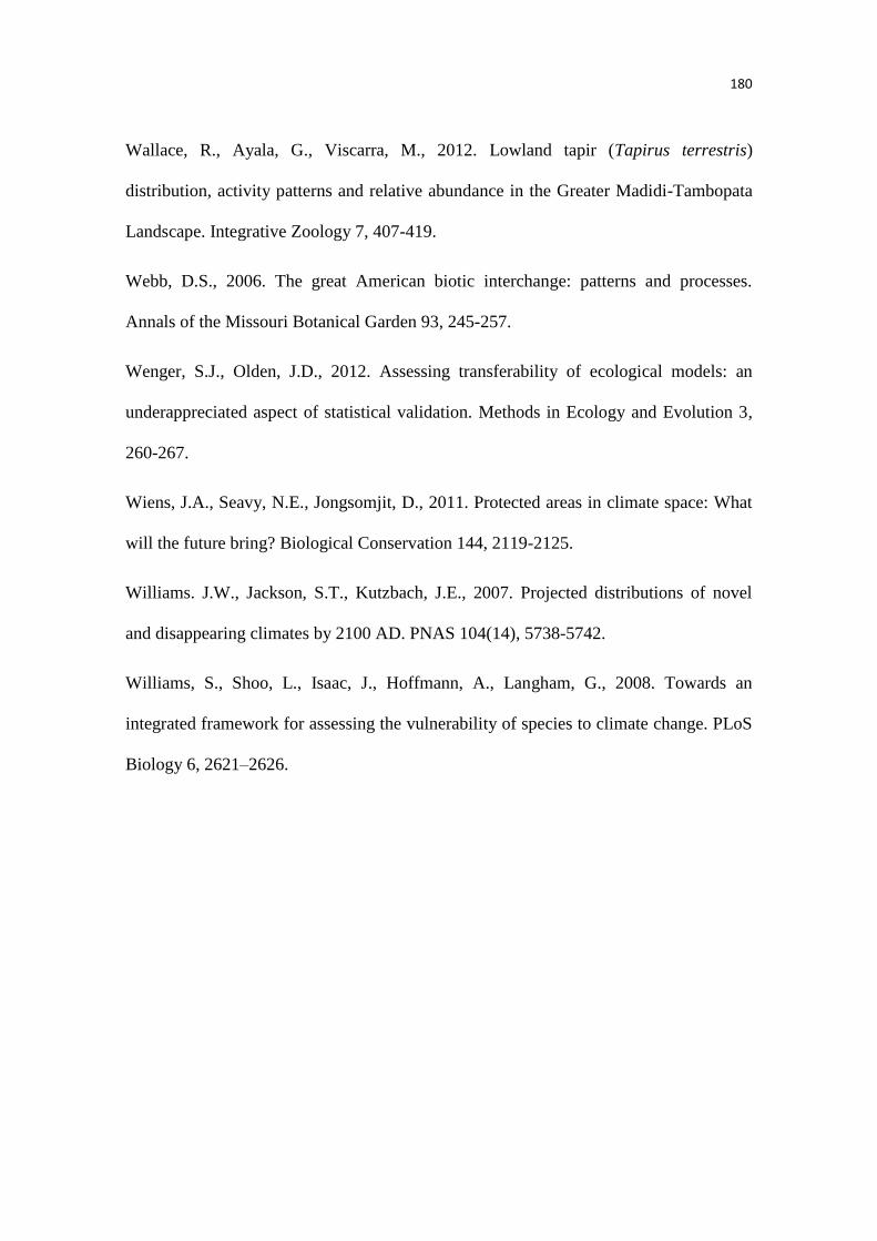
180
Wallace, R., Ayala, G., Viscarra, M., 2012. Lowland tapir (Tapirus terrestris)
distribution, activity patterns and relative abundance in the Greater Madidi-Tambopata
Landscape. Integrative Zoology 7, 407-419.
Webb, D.S., 2006. The great American biotic interchange: patterns and processes.
Annals of the Missouri Botanical Garden 93, 245-257.
Wenger, S.J., Olden, J.D., 2012. Assessing transferability of ecological models: an
underappreciated aspect of statistical validation. Methods in Ecology and Evolution 3,
260-267.
Wiens, J.A., Seavy, N.E., Jongsomjit, D., 2011. Protected areas in climate space: What
will the future bring? Biological Conservation 144, 2119-2125.
Williams. J.W., Jackson, S.T., Kutzbach, J.E., 2007. Projected distributions of novel
and disappearing climates by 2100 AD. PNAS 104(14), 5738-5742.
Williams, S., Shoo, L., Isaac, J., Hoffmann, A., Langham, G., 2008. Towards an
integrated framework for assessing the vulnerability of species to climate change. PLoS
Biology 6, 2621–2626.
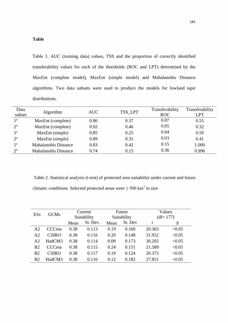
181
Table
Table 1. AUC (training data) values, TSS and the proportion of correctly identified
transferability values for each of the thresholds (ROC and LPT) determined by the
MaxEnt (complete model), MaxEnt (simple model) and Mahalanobis Distance
algorithms. Two data subsets were used to produce the models for lowland tapir
distributions.
Data
subset Algorithm AUC TSS_LPT
Transferability
ROC
Transferability
LPT
1º MaxEnt (complete) 0.86 0.37 0.07 0.55
2º MaxEnt (complete) 0.92 0.46 0.05 0.32
1º MaxEnt (simple) 0.85 0.25 0.04 0.50
2º MaxEnt (simple) 0.89 0.35 0.03 0.41
1º Mahalanobis Distance 0.83 0.42 0.15 1.000
2º Mahalanobis Distance 0.74 0.15 0.36 0.996
Table 2. Statistical analysis (t-test) of protected area suitability under current and future
climatic conditions. Selected protected areas were ≥ 500 km2 in size
ESs GCMs Current
Suitability
Future
Suitability
Values
(df= 177)
Mean St. Dev. Mean St. Dev t p
A2 CCCma 0.38 0.113 0.19 0.160 20.363 <0.05
A2 CSIRO 0.38 0.116 0.20 0.148 31.952 <0.05
A2 HadCM3 0.38 0.114 0.09 0.173 30.202 <0.05
B2 CCCma 0.38 0.115 0.24 0.151 21.589 <0.05
B2 CSIRO 0.38 0.117 0.19 0.124 20.373 <0.05
B2 HadCM3 0.38 0.116 0.12 0.182 27.851 <0.05
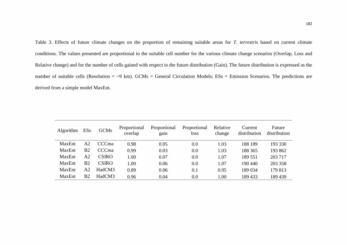
182
Table 3. Effects of future climate changes on the proportion of remaining suitable areas for T. terrestris based on current climate
conditions. The values presented are proportional to the suitable cell number for the various climate change scenarios (Overlap, Loss and
Relative change) and for the number of cells gained with respect to the future distribution (Gain). The future distribution is expressed as the
number of suitable cells (Resolution = ~9 km). GCMs = General Circulation Models; ESs = Emission Scenarios. The predictions are
derived from a simple model MaxEnt.
Algorithm ESs GCMs Proportional
overlap
Proportional
gain
Proportional
loss
Relative
change
Current
distribution
Future
distribution
MaxEnt A2 CCCma 0.98 0.05 0.0 1.03 188 189 193 330
MaxEnt B2 CCCma 0.99 0.03 0.0 1.03 188 365 193 862
MaxEnt A2 CSIRO 1.00 0.07 0.0 1.07 189 551 203 717
MaxEnt B2 CSIRO 1.00 0.06 0.0 1.07 190 440 203 358
MaxEnt A2 HadCM3 0.89 0.06 0.1 0.95 189 034 179 813
MaxEnt B2 HadCM3 0.96 0.04 0.0 1.00 189 433 189 439
183
Figure Legends
Figure 1 Transferability predicted by the MaxEnt simple model (a, b), the MaxEnt
complete model (c, d) and by Mahalanobis Distance (e, f). The lowland tapir
distributions were divided into two spatially independent regions: eastern and western.
The blue points were used to train the models, and the models were then tested using the
red points for both data subsets.
Figure 2 Maps depicting differences in the environmental suitability for lowland tapir
distributions. Maps are shown for the three climate models (CCCma, HadCM3 and
Csiro) and for the current climate using both emission scenarios.
Figure 3 Mean climatic suitability for each Brazilian protected area (≥ 500 km2) located
in five biomes and the lowland tapir distribution (localized in Brazil only). Points below
the line indicate the CUs that are predicted to lose climatic suitability, and points above
the line are predicted to gain suitability.
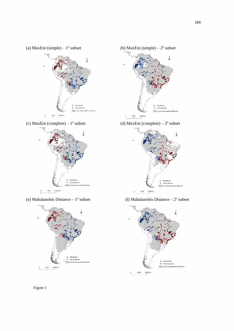
184
(a) MaxEnt (simple) – 1º subset (b) MaxEnt (simple) – 2º subset
(c) MaxEnt (complete) – 1º subset (d) MaxEnt (complete) – 2º subset
(e) Mahalanobis Distance – 1º subset (f) Mahalanobis Distance – 2º subset
Figure 1
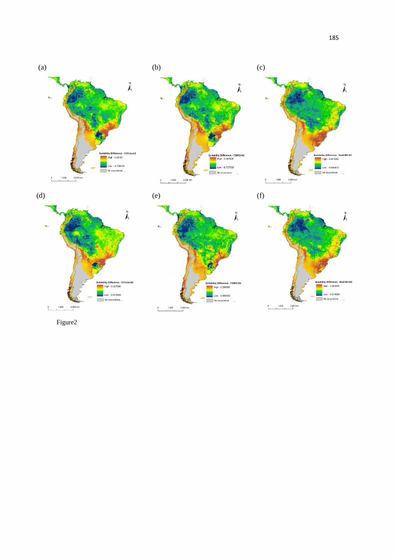
185
(a) (b) (c)
(d) (e) (f)
Figure2
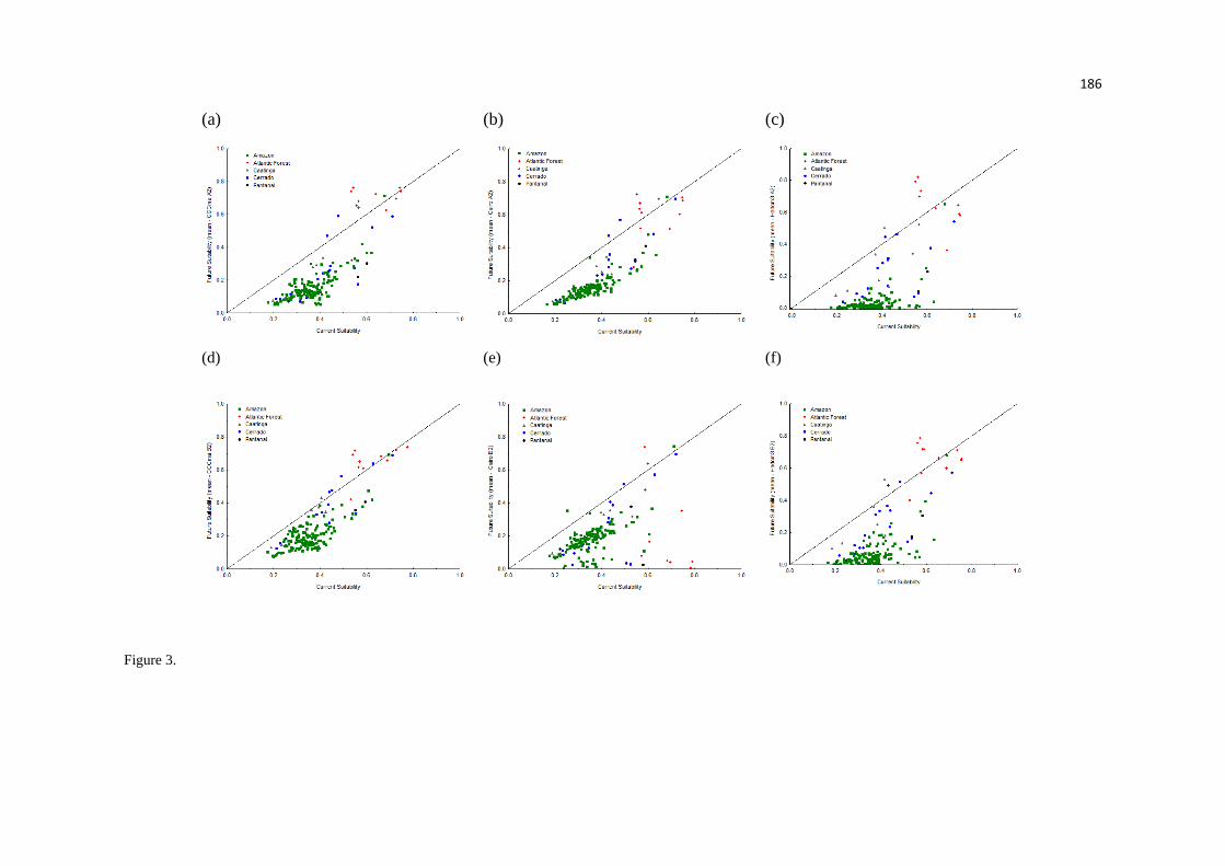
186
Figure 3.
(a) (b) (c)
(d) (e)
(f)
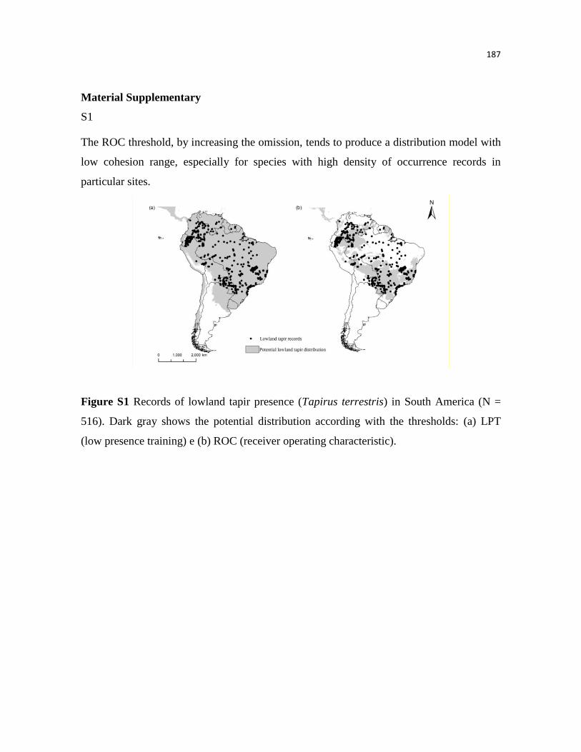
187
Material Supplementary
S1
The ROC threshold, by increasing the omission, tends to produce a distribution model with
low cohesion range, especially for species with high density of occurrence records in
particular sites.
Figure S1 Records of lowland tapir presence (Tapirus terrestris) in South America (N =
516). Dark gray shows the potential distribution according with the thresholds: (a) LPT
(low presence training) e (b) ROC (receiver operating characteristic).
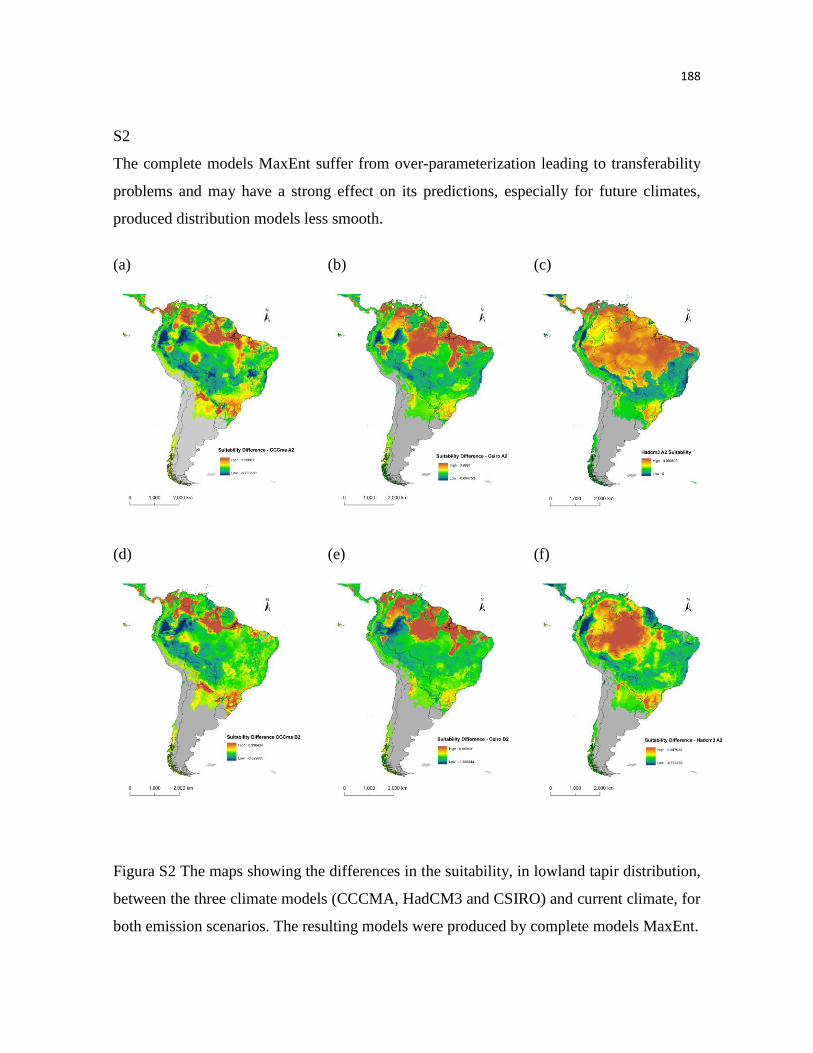
188
S2
The complete models MaxEnt suffer from over-parameterization leading to transferability
problems and may have a strong effect on its predictions, especially for future climates,
produced distribution models less smooth.
(a) (b) (c)
(d)
(e)
(f)
Figura S2 The maps showing the differences in the suitability, in lowland tapir distribution,
between the three climate models (CCCMA, HadCM3 and CSIRO) and current climate, for
both emission scenarios. The resulting models were produced by complete models MaxEnt.
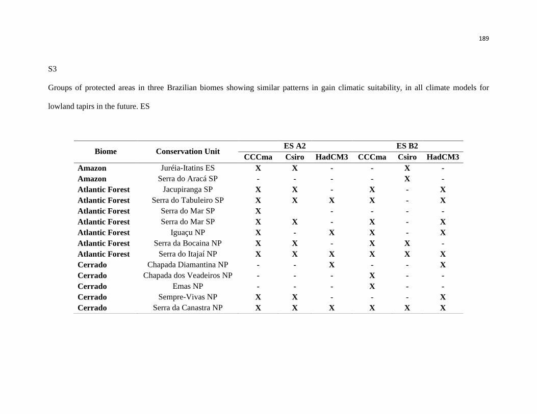
189
S3
Groups of protected areas in three Brazilian biomes showing similar patterns in gain climatic suitability, in all climate models for
lowland tapirs in the future. ES
Biome Conservation Unit ES A2 ES B2
CCCma Csiro HadCM3 CCCma Csiro HadCM3
Amazon Juréia-Itatins ES X X - - X -
Amazon Serra do Aracá SP - - - - X -
Atlantic Forest Jacupiranga SP X X - X - X
Atlantic Forest Serra do Tabuleiro SP X X X X - X
Atlantic Forest Serra do Mar SP X - - - -
Atlantic Forest Serra do Mar SP X X - X - X
Atlantic Forest Iguaçu NP X - X X - X
Atlantic Forest Serra da Bocaina NP X X - X X -
Atlantic Forest Serra do Itajaí NP X X X X X X
Cerrado Chapada Diamantina NP - - X - - X
Cerrado Chapada dos Veadeiros NP - - - X - -
Cerrado Emas NP - - - X - -
Cerrado Sempre-Vivas NP X X - - - X
Cerrado Serra da Canastra NP X X X X X X
190
CONSIDERAÇÕES FINAIS
Em um cenário que inclui todos os Perissodactyla, é evidente que cada espécie
apresenta características de nicho distintas, e que não só as espécies especialistas podem
sofrer negativamente com os efeitos das mudanças climáticas. Outro ponto que deve ser
considerado é que as barreiras podem limitar a dispersão dessas espécies para novas áreas
ambientalmente adequadas. Dentre os Perissodactyla, a anta sul-americana T. terrestris, se
mostrou a espécie mais climaticamente generalista. Contudo, a avaliação da resposta da
espécie em relação às diferentes mudanças climáticas sugere que as condições mais críticas,
que prevaleceram durante o Último Máximo Glacial, reduziram a extensão geográfica das
áreas climaticamente adequadas, com uma subsequente expansão.
Apesar do clima não ter sido um problema muito sério na história evolutiva da
espécie, os desafios para a sua conservação na atualidade e no futuro podem ser bem
maiores. Além disso, a combinação da perda da adequabilidade ambiental, perda de habitat
e fragmentação, caça, atropelamentos, doenças e decréscimo na população total pode
intensificar os efeitos das mudanças climáticas e, consequentemente, diminuir a
sobrevivência da espécie. Dessa forma, a emergência de novas áreas ambientalmente
adequadas deve ser considerada em planos de manejo futuros, especialmente na criação de
novas unidades de conservação tanto para T. terrestris quanto para as demais espécies do
clado Perissodactyla, sejam elas ameaçadas ou não.