Non-proportional hardening models for predicting mean and peak stress evolution

in multiaxial fatigue using Tanaka’s incremental plasticity concepts

Marco Antonio Meggiolaro*,1

, Jaime Tupiassú Pinho de Castro1, Hao Wu

2

1Department of Mechanical Engineering, Pontifical Catholic University of Rio de Janeiro

Rua Marquês de São Vicente 225 – Gávea, Rio de Janeiro, RJ, 22451-900, Brazil

2School of Aerospace Engineering and Applied Mechanics, Tongji University

1239 Siping Road, Shanghai, P.R. China

meggi@puc-rio.br, jtcastro@puc-rio.br, wuhao@tongji.edu.cn

Abstract

Non-proportional (NP) hardening can have a significant influence on fatigue life due to its in-

crease in mean and peak stresses. Its effect is both material and history path dependent, quantified re-

spectively by the additional hardening coefficient NP and the NP factor FNP. Several estimates for the

steady-state value of FNP have been proposed, based on enclosing ellipses or on integrals calculated

along the stress, strain, or plastic strain path. Tanaka’s incremental plasticity model, on the other hand,

is able to predict the NP hardening evolution as a function of the accumulated plastic strain p, based

on the concept of a polarization tensor [PT] that represents an internal dislocation structure. In this

work, it is shown that the eigenvectors of [PT] represent principal directions along which dislocation

structures may form, whose intensity is quantified by the respective eigenvalues. Two new integral es-

timates for the steady-state FNP of periodic load histories are proposed, one that exactly reproduces the

incremental plasticity predictions from Tanaka’s model, and a simpler version calculated solely as a

function of the eigenvalues of [PT]. Both can be readily used in fatigue design to correctly account for

the mean stress effect in NP periodic histories. For non-periodic histories, it is also shown that

Tanaka’s model can be expressed as an evolution equation for FNP(p). Tension-torsion experiments

with 316L steel tubular specimens under especially selected discriminating square NP strain paths are

conducted to validate the proposed models.

Keywords: Multiaxial fatigue; Non-proportional loadings; Non-proportionality factor; Additional

hardening; Equivalent ranges.

1. Introduction

A few materials can strain-harden much more than it would be expected from the uniaxial cyclic

curve when subjected non-proportional (NP) multiaxial cyclic loads. This phenomenon, called NP

hardening, cross-hardening, or additional strain hardening, depends on the load history, through the

NP factor FNP, where 0 FNP 1, and on the material, through the additional hardening coefficient

NP (typically 0 NP 1). NP hardening is usually modeled using the exponent hc from the uniaxial

* Corresponding author. Tel.: +55-21-3527-1424; fax: +55-21-3527-1165. E-mail: meggi@puc-rio.br

cyclic Ramberg-Osgoodequation, see Fig. 1(left), assuming hc does not vary while the hardening co-

efficient is gradually increased from Hc to the NP hardening coefficient

HNP Hc(1 + NPFNP) (1)

Fig. 1: Effect of cyclic NP loadings on the NP hardening (left) and proportional and NP loops caused

by the same range in AISI 304 steel (right) [1].

Defining SYNP as the stabilized NP yield strength associated with a 0.2% plastic strain amplitude,

the same value adopted in the monotonic SY and cyclic SYc yield strength definitions, it follows that

SYNP SYc(1 + NPFNP) (2)

since the cyclic and NP hardening exponenents are assumed to be equal.

Note that the NP hardening effect can multiply the uniaxial cyclic coefficient Hc, and therefore

the cyclic yield strength SYc, by a factor as high as (1 + 11) 2, as shown in Fig. 1(right) for a 304

austenitic stainless steel [1]. This figure compares elastoplastic hysteresis loops produced by a NP out-

of-phase tension-torsion history and a proportional history, both with the same normal strain ampli-

tude /2 0.4%. In the NP history, the yield surface radius gradually increases from an isotropic

hardening value in-between SY and SYc to its NP-hardened yield strength SYNP.

When NP hardening is significant, NP histories can produce fatigue lives that are much shorter

than the ones from proportional histories with same strain range , since NP hardening increases the

corresponding range. Therefore, calculations based on strain-controlled NP histories, as found in

N specimen tests or around sharp notch tips, must account for NP hardening effects to avoid non-

conservative predictions. Conversely, fatigue lives of stress-controlled histories, as found in SN spec-

imen tests, around mild notch tips or in un-notched components that work under imposed loads, not

displacements, can be much higher under NP loads than under proportional loads with same range ,

due to the lower range necessary to achieve such because of the NP hardening effect.

The fatigue life associated with the strain-controlled NP loading from Fig. 1(right) can be orders

of magnitude shorter than under proportional loading, even though both have the same normal strain

amplitude /2 0.4%. This large difference is caused by the maximum normal stress in the NP histo-

ry, which is about twice the value from the proportional history, further opening the initiating mi-

crocracks and thus lowering the fatigue crack initiation life.

However, Coffin-Manson’s strain-life equation or its Morrow’s variations including mean stress-

es m would not be able to predict such difference, even if extended from an uniaxial to a multiaxial

critical-plane approach formulation, because in both hysteresis loops from Fig. 1(right) the mean stress

m = 0. On the other hand, the multiaxial critical-plane version of Smith-Watson-Topper’s (SWT)

model, also called SWT-Bannantine [2], would account for such NP hardening effect on the fatigue

life, because its damage parameter depends on both and the maximum max, not on m. Therefore,

the SWT model would predict, as expected, a shorter initiation life in the presence of higher peak

stresses max induced by NP hardening. This implies that the use of traditional N equations, which

were developed to model uniaxial fatigue problems, can be non-conservative when strain-controlled

loading histories are NP. Obviously, such non-conservative errors are inadmissible both for mechani-

cal design and for structural integrity evaluations.

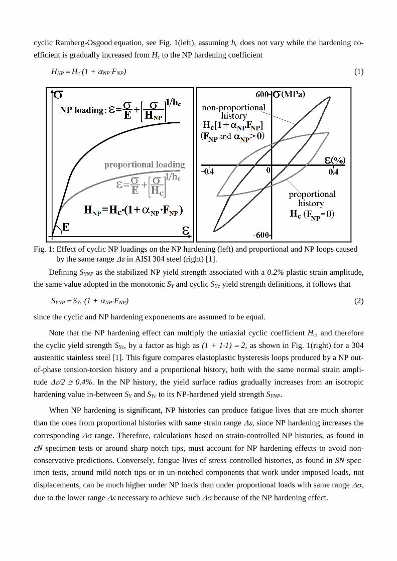
Microstructurally, NP hardening is related with stacking faults, which are local regions of incor-

rect stacking of crystal planes. Figure 2 shows stacking fault examples for HCP (Hexagonal Close-

Packed) and for FCC (Face Centered Cubic) lattices. HCP lattices superimpose the various atomic

planes following a sequence type ab-ab-ab-ab-ab. The stacking fault in the HCP lattice from Fig.

2(top) is caused by the plane arranged in the c configuration, causing an interruption of the stacking

sequence of the crystal structure, which becomes ab-ab-abc-ab-ab. FCC lattices, on the other hand,

which usually follow a sequence abc-abc-abc-abc, may present stacking faults from the local absence

of such c configuration, as shown in the sequence abc-abc-ab-abc in Fig. 2(bottom). Such faults cause

the HCP lattice to become locally FCC in the abc plane sequence, while the FCC lattice locally be-

comes HCP in the ab region. These planar defects cause lattice incompatibilities that prevent or impair

dislocations from switching gliding planes.

ab

ab

ab

ab

ab

ab

c ab

c ab

c

c

ab

HCP

FCC

Fig. 2: HCP and FCC lattices with stacking faults.

On the other hand, stacking faults are rarely seen in materials with high SFE, such as in most

aluminum alloys, which may require more than 200mJ per m2 to generate them. Without the obstruc-

tion caused by stacking faults, the screw dislocations may cross-slip even under proportional loadings,

giving the material an extra ductility since the many slip systems are able to well distribute the defor-

mation in all possible directions in 3D. Slips of dislocations are wavy, changing their glide planes

easily, even for uniaxial histories. So, since cross-slip bands already happen naturally even under pro-

portional loadings, NP histories do not cause any significant hardening increase, thus their NP 0.

In summary, the additional hardening coefficient NP is a parameter that reflects the material sen-

sitivity to the non-proportionality of the loads. Table 1 shows typical values of NP, which is usually

high in austenitic stainless steels at room temperature (NP 1 for 316 stainless steel), medium in car-

bon steels (NP 0.3 for 1045 steel), and very low in aluminum alloys (NP 0 for Al 7075). Note that

the NP hardening effect is not only significant in austenitic stainless steels, but also in several other

structural metals, since even NP values as low as e.g. 0.1 could cause a stress range and peak increase

of up to 10%, resulting in significant changes in fatigue life due to the highly non-linear relation be-

tween fatigue damage and stress/strain ranges or stress peaks.

Table 1: Additional hardening coefficient NP for several materials [1].

material NP

316 stainless 0.8-1.0

304 stainless 0.5-1.0

OFHC copper 0.3-0.4

304 stainless (650oC) 0.3-0.4

316 stainless (550oC) 0.37

1045 steel, SGV410, S25C 0.3

Inconel 718, S55C 0.2

Sn8Zn3Bi solder 0.2

Al 6061-T6 0.2

42 CrMo steel 0.15

1% Cr Mo-V, En15R steel 0.14

Al 7075 0.0

Al 1100 0.0

Finally, as mentioned above, NP hardening is not only material-dependent, through NP, but also

load-path dependent, through the NP factor FNP. Proportional histories do not lead to NP hardening,

resulting in FNP 0. On the other hand, the largest NP hardening effect occurs when FNP 1, e.g. un-

der a properly scaled 90o out-of-phase tension-torsion loading that generates a circle in the von Mises

stress 3 or strain /3 diagrams.

For a tension-torsion history, FNP is usually estimated from the aspect ratio of an ellipse that en-

closes the stress or strain path in the von Mises diagrams. Other FNP estimates have been proposed,

such as Itoh’s [3] and Bishop’s [4]. These models were compared in [5], where another FNP estimation

model was presented, based on the Moment Of Inertia (MOI) of the plastic strain path represented in a

5D deviatoric space E5p:

Tx y zpl 1pl 2 pl 3 pl 4 pl 5 pl 1pl pl pl pl

y z xy xz yz2 pl pl pl 3pl pl 4 pl pl 5 pl pl

e [ e e e e e ] , e ( ) 2 ,

3 3 3 3e ( ) , e , e , e

2 2 2 2

(3)

where xpl, ypl,zpl,xypl,xzpl andyzpl are the plastic components of the normal and shear strains. This

5D deviatoric space is appropriate to define an integral equation to estimate FNP because, contrary to

the stress space used in Bishop’s method [4], it is independent of the hydrostatic components.

Note that such ple vector is equal to the 5D representation of plastic strains proposed by Tanaka

[6] multiplied by 3/2:

23

2 3 3 3 3

pl pl pl pl pl

pl

Tx y xy xz yz

pl x

Tanaka's 5D deviatoric space

e ee e

(4)

since the identity expl eypl ezpl 0 implies that eypl – ezpl expl 2eypl. There are six motivations to

prefer the 5D projection ple of the plastic strain space to calculate FNP, instead of a stress space, total

strain space, or even the 6D plastic strain space:

(i) this projection is a non-redundant representation of the plastic strains, since the linear dependency

expl eypl ezpl 0 has been removed when projecting the 6D strains onto this 5D deviatoric sub-

space E5p;

(ii) for either free-surface conditions, un-notched tension-torsion, or uniaxial histories, respectively

3D, 2D, or 1D sub-spaces of this 5D representation could be used, significantly decreasing com-

putational cost. Voigt-Mandel’s 6D deviatoric representation, on the other hand, would need e.g.

to use a 3D formulation even under uniaxial conditions in x, since the non-zero ypl andzpl (due

to plastic Poisson effects) and xpl would be present in all three normal deviatoric components. On

the other hand, a 1D representation from x y z1pl pl pl ple ( ) 2 would be enough in the

uniaxial case, because y z2 pl pl ple ( ) 3 / 2 0 (since y z ypl pl pl , where is the

effective Poisson ratio, a weighted mean of the elastic and plastic 0.5 Poisson ratios) and all

shear xy3pl ple 3 /2 , xz4pl ple 3 /2 and yz5pl ple 3 /2 would be zero as well;

(iii) similarly to the e projection, ple is also independent of the hydrostatic strain h, since it is a 5D

projection of a deviatoric space as well, compatible with the expected independence between FNP

and h;

(iv) the scaled down version pl( 2 3 ) e of this projection is identical to Tanaka’s 5D plastic strain

vector defined in [6], which has been shown to be appropriate to evaluate the NP hardening evo-

lution in incremental plasticity calculations;

(v) the Euclidean norm pl( 2 3 ) e is equal to the von Mises plastic equivalent strain, which pro-

vides a convenient metric for the deviatoric plastic strain space associated with this representa-

tion; and

(vi) the direction of such 5D strain vectors is related with the principal direction of the loading. This

last statement can be observed, for instance, in the calculation of the principal direction angle p

with respect to the y axis in the y-z plane

pl plp yz y z 5 2 5 2tan2 ( ) e e e e (5)

where the approximation e5/e2 e5pl/e2pl is valid for large plastic strains, resulting in ple e .

Several incremental plasticity equations make use of the Euclidean norm of the increments of the

plastic strain vector, which define infinitesimal variations of ple . One way to account for this norm is

through the equivalent plastic strain increment dp, a positive scalar quantity that can be defined as an

infinitesimal absolute variation of the plastic von Mises strain pl , Mises ple (1 0.5 ) , assuming that

plastic strains conserve volume, thus the plastic Poisson ratio is 0.5. The value of dp can be defined in

the 5D plastic strain space E5p from

pl , Mises pl pl2 2

e dp de3 3

(6)

The integral of these positive infinitesimal increments dp is defined as the accumulated plastic

strain p, which in integral form is expressed as

pl2

d de3

p p (7)

Note that pl , Mises and p are different quantities, since the von Mises plastic strain pl , Mises can

oscillate during a load cycle, while the accumulated plastic strain p increases monotonically in any de-

formation process.

In the following sections, Tanaka’s NP hardening model is applied to the E5p space to predict the

transient evolution of NP hardening, which can be very important in fatigue life calculations if such

transient period is associated with some ratcheting or mean stress relaxation. From Tanaka’s model, an

evolution equation for FNP is developed, from which new steady-state FNP estimate equations are de-

rived. Such estimates are then experimentally verified from tension-torsion experiments in tubular

316L specimens under NP histories describing square paths in a normal-shear stress diagram.

2. Tanaka’s NP Hardening Model

Estimates for the steady-state value of FNP have been proposed in [3-5, 7]. Such estimates are es-

pecially useful for periodic histories that consist of a few cycles per period, where FNP reaches an ap-

proximately constant stabilized value. However, general multiaxial load histories have a NP factor

FNP(p) that depends on the accumulated plastic strain p and on the previous plastic history, which con-

tinually evolves and changes the hardening behavior of materials that have an additional hardening

coefficient NP > 0.

In these materials, a sequence of NP loading cycles causes an additional hardening effect that in-

creases as a function of p and of the non-proportionality of the load, until reaching a steady-state level

also known as the target value of FNP(p). Conversely, a long series of proportional loads may cause a

“proportional softening” effect that reverts a previous NP hardening process. Incremental plasticity

models must account for this transient NP hardening and proportional softening to correctly predict fa-

tigue lives, because such transients can have a significant effect on the resulting strain or stress ampli-

tudes respectively under stress or strain-controlled conditions in low-cycle fatigue, and a very large ef-

fect on ratcheting and on mean stress relaxation problems.

The transient NP hardening model proposed by Tanaka [6] is the most widely adopted in incre-

mental plasticity calculations. Tanaka defined a polarization tensor [PT] that can store information on

the directionality of the accumulated plastic strains induced by the loading history, which can be pro-

portional or NP. This macroscopic structural tensor is an internal state variable that is able to describe

the loading-path-shape dependence of the NP hardening process through the mathematical representa-

tion of an internal dislocation structure. The directions stored in such tensor are the ones described by

5D normal unit vectors n , which are defined as the direction of the current infinitesimal plastic strain

increment plde in the 5D E5p plastic strain space. According to the normality rule [8], these unit vec-

tors are perpendicular to the E5p representation of the yield surface during plastic straining.

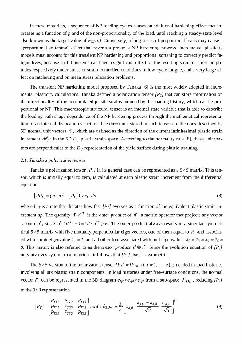
2.1. Tanaka’s polarization tensor

Tanaka’s polarization tensor [PT] in its general case can be represented as a 5 × 5 matrix. This ten-

sor, which is initially equal to zero, is calculated at each plastic strain increment from the differential

equation

TT T TdP ( n n P ) hr dp (8)

where hrT is a rate that dictates how fast [PT] evolves as a function of the equivalent plastic strain in-

crement dp. The quantity Tn n is the outer product of n , a matrix operator that projects any vector

v onto n , since T Tn ( n v ) ( n n ) v . The outer product always results in a singular symmet-

rical 5 × 5 matrix with five mutually perpendicular eigenvectors, one of them equal to n and associat-

ed with a unit eigenvalue 1 1, and all other four associated with null eigenvalues 2 3 4 5

0. This matrix is also referred to as the tensor product n n . Since the evolution equation of [PT]

only involves symmetrical matrices, it follows that [PT] itself is symmetric.

The 5 × 5 version of the polarization tensor [PT] [PTij] (i, j 1, …, 5) is needed in load histories

involving all six plastic strain components. In load histories under free-surface conditions, the normal

vector n can be represented in the 3D diagram e1pl e2pl e3pl from a sub-space pl3De , reducing [PT]

to the 3 3 representation

T11 T12 T13

T T21 T22 T23

T31 T32 T33

P P P

P P P P

P P P

, with pl pl pl

pl pl

Ty z xy

3D x3

e2 3 3

(9)

Moreover, [PT] can be further simplified to a 2 2 representation for tension-torsion histories,

where n is represented in the 2D diagram e1pl e3pl from the sub-space pl2De , resulting in

T11 T13T

T31 T33

P PP

P P

, and pl

pl pl pl pl

TxyT

2D 1 3 x3

e e e2 3

(10)

This dimensional reduction down to 2 2 is only possible because of the properties of the adopted

5D plastic strain space E5p, which was one of the six motivations listed in the last section to adopt it.

The polarization tensor can be used to model the cross-hardening effect, see Fig. 3, which shows

the transient behavior H(p)/Hc of the Ramberg-Osgood hardening coefficient H(p) for materials with

NP > 0, where Hc is the cyclically-stabilized uniaxial hardening coefficient. In this example, a virgin

specimen is initially cycled in tension-compression, until the accumulated plastic strain reaches some

value p pa. During this process, isotropic hardening causes the hardening coefficient to gradually

change from its monotonic value Hmt to the cyclically-stabilized one Hc. For simplicity, in this exam-

ple it is assumed that both monotonic and cyclic exponents are not too different, represented by the

cyclic value hc. A uniaxial dislocation structure is then gradually generated in the direction of such

tension-compression cycles, represented in [PT] by

T11 T13 TT

T31 T33

P P 1 exp( hr p ) 0P

P P 0 0

, for 0 ≤ p ≤ pa (11)

where exp(x) is the exponential function ex, with e 2.71828. This uniaxial dislocation structure is ful-

ly formed when the first element of [PT] converges to its target value PT11 1, see Fig. 3, resulting in a

unit eigenvalue associated with an eigenvector in the normal direction e1pl.

PT11

p

H(p)/Hc

PT33

cyclic tension cyclic tensioncyclic torsion

Hmt/Hc

HNP/Hc

1.0

PT11

PT11 PT33

PT33

pa pb

T1 0

[ P ]0 0

T

0 0[ P ]

0 1

0

Fig. 3: Variation of the hardening coefficient H(p) due to cross-hardening effects in materials with ad-

ditional hardening coefficient NP > 0, adapted from [6].

Then, if the tension-compression cycles are replaced by cyclic torsion, this change causes a sud-

den increase in the transient hardening coefficient from the uniaxial Hc to the NP value HNP. This sud-

den strain-hardening is explained by the cross-hardening effect caused by the uniaxial dislocation

structure formed in the preceding tension-compression cycles, represented by PT11 1, which resists

much more to the mismatched torsional loads than to previous tensile loads. But the torsional cycles

gradually destroy this uniaxial tension-compression dislocation structure, making PT11 tend towards

zero, as seen in Fig. 3 for the interval pa ≤ p ≤ pb, which allows the material to soften again from HNP

to Hc. Meanwhile, a new dislocation structure is gradually generated in the torsional direction through

PT33, leading to the [PT] solution

T aT

T a

exp[ hr ( p p )] 0P

0 1 exp[ hr ( p p )]

, for pa ≤ p ≤ pb (12)

The torsional dislocation structure is fully formed when PT33 converges to its target value PT33 1

near p pb, see Fig. 3, resulting in a unit eigenvalue for [PT] associated with an eigenvector in the tor-

sional direction e3pl.

If the torsional cycles are replaced with cyclic tension-compression for p ≥ pb, another sudden in-

crease in the hardening coefficient from Hc to HNP is observed, as seen in Fig. 3. Now, the tension-

compression cycles are resisted by the mismatched torsional dislocation structure formed in the pre-

ceding torsional cycles, represented by PT33 1, causing a sudden strain-hardening effect. But this tor-

sional dislocation structure is gradually destroyed as PT33 tends towards zero, allowing the material to

soften again from HNP to Hc. Meanwhile, PT11 starts increasing again towards PT11 1, while the unit

eigenvalue of [PT] becomes associated with the tensile direction e1pl, and the process continues.

It can be concluded from this example that the eigenvectors of [PT] represent principal directions

along which dislocation structures may form, whose intensity is quantified by the respective eigenval-

ues, ranging from 0 (no dislocation structures in the considered direction) to 1 (all dislocation struc-

tures in such direction).

For general multiaxial histories, after several plastic strain increments, Tanaka’s polarization ten-

sor [PT] results in a 5 × 5 matrix whose eigenvalues T1 T2 … T5 > 0 are proportional to the ac-

cumulated plastic strains in the direction of each unit eigenvector T1 T 2 T5v , v , ..., v . So, proportional

load histories always result in a polarization tensor [PT] with only one non-zero eigenvalue, corre-

sponding to the eigenvector parallel to the constant plastic straining direction associated with propor-

tional loading conditions. The other four eigenvalues would either be equal to zero or very close to ze-

ro for quasi-proportional histories.

On the other hand, highly NP load histories have at least two dominant (high) eigenvalues T1 and

T2. These eigenvalues should be equal (T1 T2) in the 90o out-of-phase tension-torsion case with

equal normal and effective shear amplitudes, i.e. x/2 (xy/2)3. In this case, the plastic straining

direction is constantly changed as the load path describes a circle in the e1pl e3pl diagram, keeping the

cross-hardening effect alive while the transient Ramberg-Osgood coefficient is evolving to reach a

target NP value HNP without posterior hardening or softening.

In summary, the eigenvectors and eigenvalues of the target values of the evolution of [PT] math-

ematically represent the stabilized internal dislocation structure formed by the loading process. These

eigenvalues are also useful to detect reduced dimensionality of such structures, ranging from 1D for

proportional histories (with only one non-zero eigenvalue) to 5D if all eigenvalues are significantly

higher than zero.

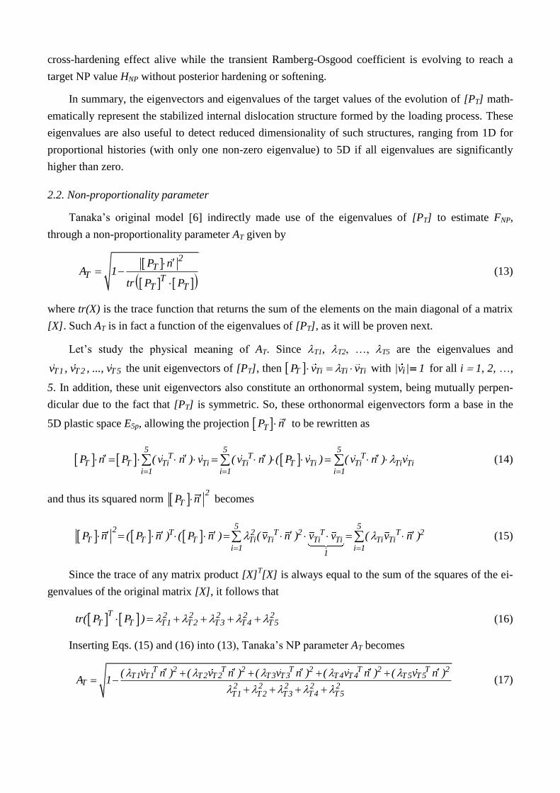
2.2. Non-proportionality parameter

Tanaka’s original model [6] indirectly made use of the eigenvalues of [PT] to estimate FNP,

through a non-proportionality parameter AT given by

2T

T TT T

P nA 1

tr P P

(13)

where tr(X) is the trace function that returns the sum of the elements on the main diagonal of a matrix

[X]. Such AT is in fact a function of the eigenvalues of [PT], as it will be proven next.

Let’s study the physical meaning of AT. Since T1, T2, …, T5 are the eigenvalues and

T1 T 2 T5v , v , ..., v the unit eigenvectors of [PT], then T Ti Ti TiP v v with i|v | 1 for all i 1, 2, …,

5. In addition, these unit eigenvectors also constitute an orthonormal system, being mutually perpen-

dicular due to the fact that [PT] is symmetric. So, these orthonormal eigenvectors form a base in the

5D plastic space E5p, allowing the projection TP n to be rewritten as

5 5 5

T T TT T Ti Ti Ti T Ti Ti Ti Ti

i 1 i 1 i 1

P n P ( v n ) v ( v n ) ( P v ) ( v n ) v

(14)

and thus its squared norm 2

TP n becomes

5 52 T 2 T 2 T T 2

T T T Ti Ti Ti Ti Ti Tii 1 i 1

1

P n ( P n ) ( P n ) ( v n ) v v ( v n )

(15)

Since the trace of any matrix product [X]T[X] is always equal to the sum of the squares of the ei-

genvalues of the original matrix [X], it follows that

T 2 2 2 2 2

T T T1 T 2 T 3 T 4 T 5tr( P P ) (16)

Inserting Eqs. (15) and (16) into (13), Tanaka’s NP parameter AT becomes

T 2 T 2 T 2 T 2 T 2T1 T1 T 2 T 2 T 3 T 3 T 4 T 4 T 5 T 5

T 2 2 2 2 2T 4 T 5T1 T 2 T 3

( v n ) ( v n ) ( v n ) ( v n ) ( v n )A 1

(17)

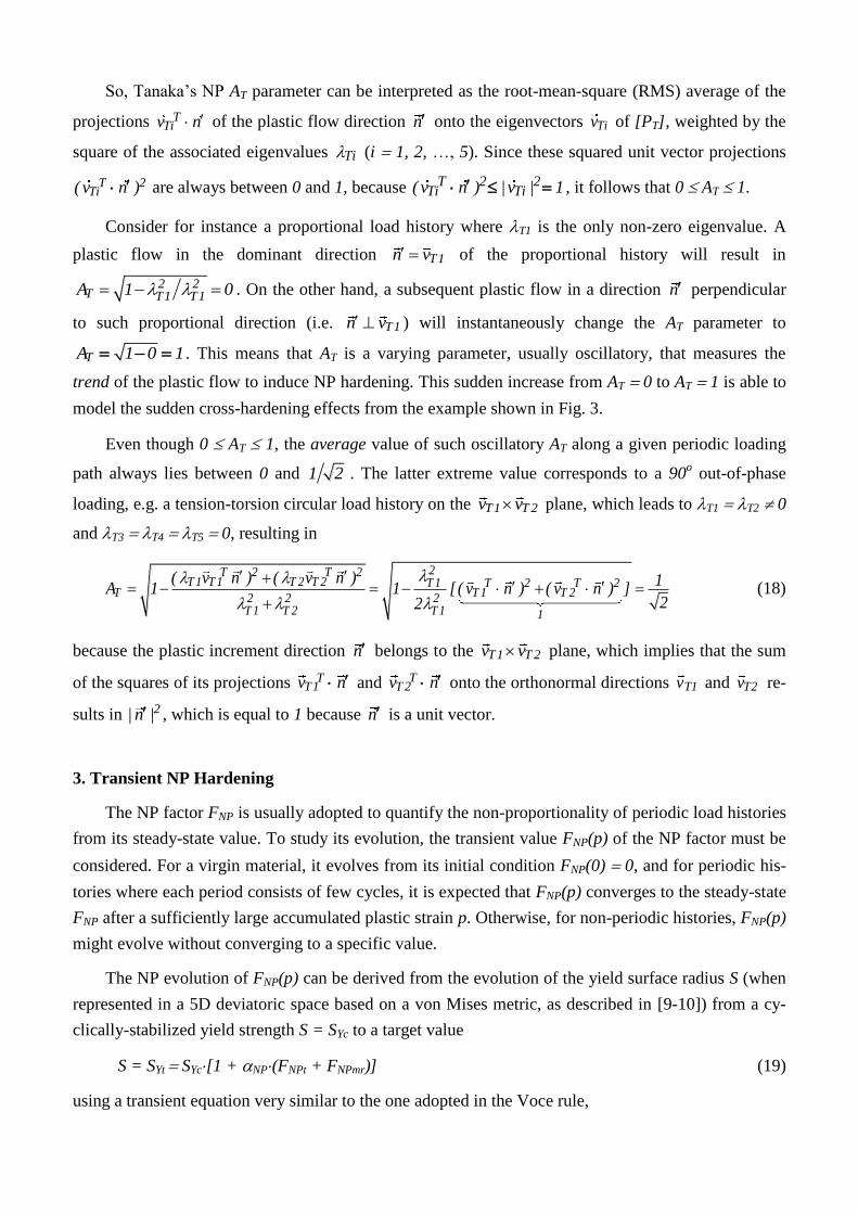
So, Tanaka’s NP AT parameter can be interpreted as the root-mean-square (RMS) average of the

projections TTiv n of the plastic flow direction n onto the eigenvectors Tiv of [PT], weighted by the

square of the associated eigenvalues Ti (i 1, 2, …, 5). Since these squared unit vector projections

T 2Ti( v n ) are always between 0 and 1, because T 2 2

Ti Ti( v n ) |v | 1 , it follows that 0 AT 1.

Consider for instance a proportional load history where T1 is the only non-zero eigenvalue. A

plastic flow in the dominant direction T1n v of the proportional history will result in

2 2T T1 T1A 1 0 . On the other hand, a subsequent plastic flow in a direction n perpendicular

to such proportional direction (i.e. T1n v ) will instantaneously change the AT parameter to

TA 1 0 1 . This means that AT is a varying parameter, usually oscillatory, that measures the

trend of the plastic flow to induce NP hardening. This sudden increase from AT 0 to AT 1 is able to

model the sudden cross-hardening effects from the example shown in Fig. 3.

Even though 0 AT 1, the average value of such oscillatory AT along a given periodic loading

path always lies between 0 and 1 2 . The latter extreme value corresponds to a 90o out-of-phase

loading, e.g. a tension-torsion circular load history on the T1 T 2v v plane, which leads to T1 T2 0

and T3 T4 T5 0, resulting in

2T 2 T 2T 1 T 1 T 2 T 2 T 1 T 2 T 2

T T 1 T 22 2 2T 1 T 2 T 1 1

( v n ) ( v n ) 1A 1 1 [( v n ) ( v n ) ]

22

(18)

because the plastic increment direction n belongs to the T1 T 2v v plane, which implies that the sum

of the squares of its projections TT1v n and T

T 2v n onto the orthonormal directions T1v and T2v re-

sults in 2| n | , which is equal to 1 because n is a unit vector.

3. Transient NP Hardening

The NP factor FNP is usually adopted to quantify the non-proportionality of periodic load histories

from its steady-state value. To study its evolution, the transient value FNP(p) of the NP factor must be

considered. For a virgin material, it evolves from its initial condition FNP(0) 0, and for periodic his-

tories where each period consists of few cycles, it is expected that FNP(p) converges to the steady-state

FNP after a sufficiently large accumulated plastic strain p. Otherwise, for non-periodic histories, FNP(p)

might evolve without converging to a specific value.

The NP evolution of FNP(p) can be derived from the evolution of the yield surface radius S (when

represented in a 5D deviatoric space based on a von Mises metric, as described in [9-10]) from a cy-

clically-stabilized yield strength S = SYc to a target value

S = SYt SYc[1 + NP(FNPt + FNPmr)] (19)

using a transient equation very similar to the one adopted in the Voce rule,

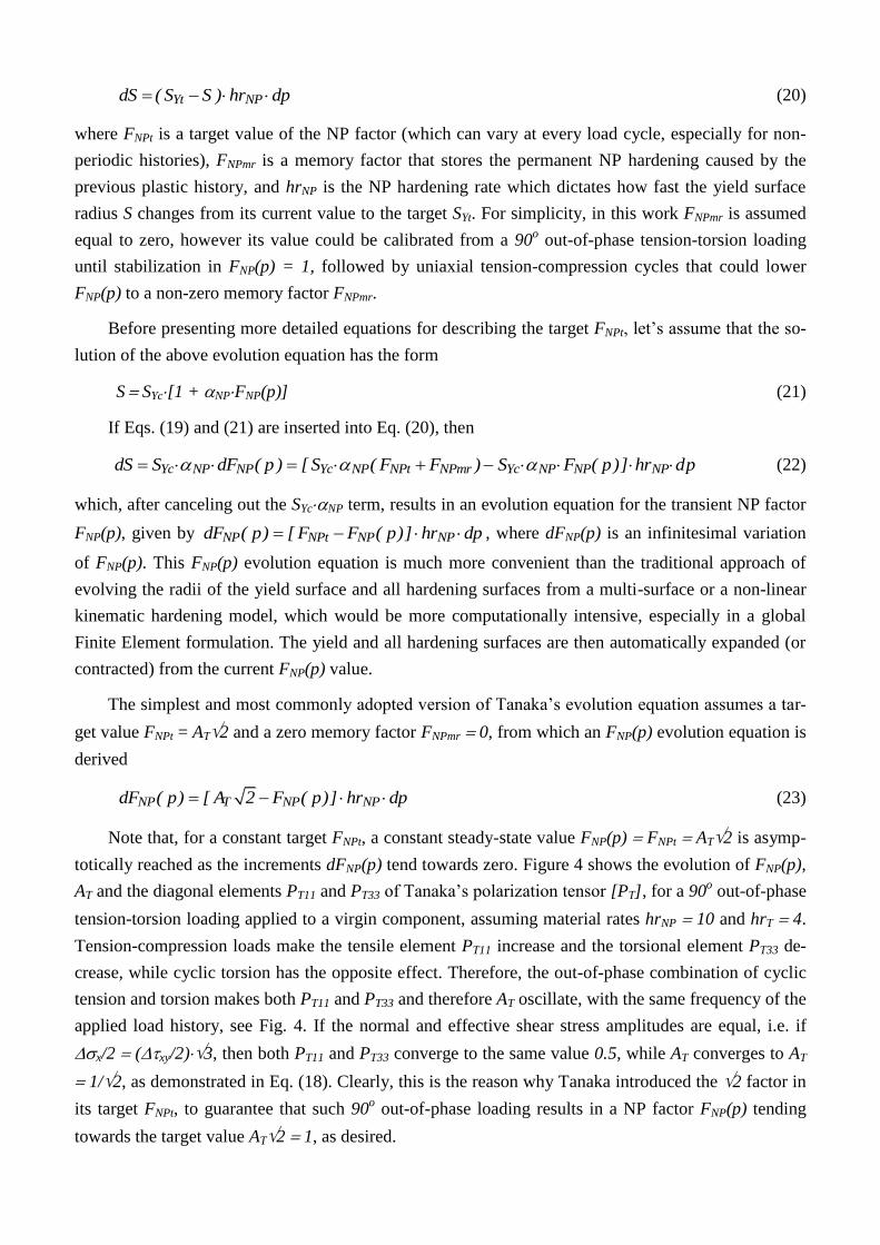
Yt NPdS ( S S ) hr dp (20)

where FNPt is a target value of the NP factor (which can vary at every load cycle, especially for non-

periodic histories), FNPmr is a memory factor that stores the permanent NP hardening caused by the

previous plastic history, and hrNP is the NP hardening rate which dictates how fast the yield surface

radius S changes from its current value to the target SYt. For simplicity, in this work FNPmr is assumed

equal to zero, however its value could be calibrated from a 90o out-of-phase tension-torsion loading

until stabilization in FNP(p) = 1, followed by uniaxial tension-compression cycles that could lower

FNP(p) to a non-zero memory factor FNPmr.

Before presenting more detailed equations for describing the target FNPt, let’s assume that the so-

lution of the above evolution equation has the form

S SYc[1 + NPFNP(p)] (21)

If Eqs. (19) and (21) are inserted into Eq. (20), then

Yc NP NP Yc NP NPt NPmr Yc NP NP NPdS S dF ( p) [ S ( F F ) S F ( p)] hr dp (22)

which, after canceling out the SYcNP term, results in an evolution equation for the transient NP factor

FNP(p), given by NP NPt NP NPdF ( p) [ F F ( p)] hr dp , where dFNP(p) is an infinitesimal variation

of FNP(p). This FNP(p) evolution equation is much more convenient than the traditional approach of

evolving the radii of the yield surface and all hardening surfaces from a multi-surface or a non-linear

kinematic hardening model, which would be more computationally intensive, especially in a global

Finite Element formulation. The yield and all hardening surfaces are then automatically expanded (or

contracted) from the current FNP(p) value.

The simplest and most commonly adopted version of Tanaka’s evolution equation assumes a tar-

get value FNPt = AT2 and a zero memory factor FNPmr 0, from which an FNP(p) evolution equation is

derived

NP T NP NPdF ( p) [ A 2 F ( p)] hr dp (23)

Note that, for a constant target FNPt, a constant steady-state value FNP(p) FNPt AT2 is asymp-

totically reached as the increments dFNP(p) tend towards zero. Figure 4 shows the evolution of FNP(p),

AT and the diagonal elements PT11 and PT33 of Tanaka’s polarization tensor [PT], for a 90o out-of-phase

tension-torsion loading applied to a virgin component, assuming material rates hrNP 10 and hrT 4.

Tension-compression loads make the tensile element PT11 increase and the torsional element PT33 de-

crease, while cyclic torsion has the opposite effect. Therefore, the out-of-phase combination of cyclic

tension and torsion makes both PT11 and PT33 and therefore AT oscillate, with the same frequency of the

applied load history, see Fig. 4. If the normal and effective shear stress amplitudes are equal, i.e. if

x/2 (xy/2)3, then both PT11 and PT33 converge to the same value 0.5, while AT converges to AT

1/2, as demonstrated in Eq. (18). Clearly, this is the reason why Tanaka introduced the 2 factor in

its target FNPt, to guarantee that such 90o out-of-phase loading results in a NP factor FNP(p) tending

towards the target value AT2 1, as desired.

p

PT11T

0.5 0[ P ]

0 0.5

0 0.2 0.4 0.6 0.8 1 1.2 1.4 1.60

0.1

0.2

0.3

0.4

0.5

0.6

0.7

0.8

0.9

1

PT33

FNP(p) 1

AT

FNP(p)

AT 1/2

Fig. 4: Evolution of [PT], AT and FNP(p) for a 90o out-of-phase tension-torsion loading.

The accumulated plastic strain p needed to settle the values of both [PT] and AT in periodic histo-

ries is related to the material hardening rate hrT. Since their evolution is exponential, it can be estimat-

ed that their values should have converged within [1 exp(4)] 98.2% when hrT p 4. For the hrT

4 used in this example, the settling of PT11, PT33 and AT occurs near p 4/hrT 1 100%, as verified

in Fig. 4, even though both PT11 and PT33 remain oscillatory along each cycle under such NP loading.

Note that the NP parameter AT reached an average value near its target 1/2 much before its settling at

p 1 100%, which allowed FNP(p) to evolve faster than expected, independently of hrT. Since the

adopted NP hardening rate in that example was hrNP 10, FNP(p) settled near p 4/hrNP 0.4 40%,

see Fig. 4.

However, in general, the settling of the non-proportional factor FNP(p) is influenced by both

Tanaka’s hrT and non-proportional hrNP hardening rates. Figure 5 shows the evolution of FNP(p), AT,

PT11 and PT33 under cyclic torsion, applied for p pa just after uniaxial tension-compression cycles ap-

plied in the interval 0 p pa. As in Fig. 3, the normal and effective shear stress amplitudes are equal,

i.e. x/2 (xy/2)3. The adopted hardening rate hrT 4 results in a 98.2% settling of PT11, PT33 and

AT near p 4/hrT 1 100%, as expected. As seen in Fig. 5, the relatively slow evolution of AT to

reach its zero target value delays the settling of FNP(p) to an accumulated plastic strain much larger

than the p 0.4 40% from Fig. 4, even using the same hrNP 2.5hrT 10 from the 90o out-of-phase

tension-torsion example shown in Fig. 4. In practice, FNP(p) settles (within 98.2%) in periodic histo-

ries at accumulated plastic strain values p between (4/hrNP) and (4/hrNP 4/hrT).

Note in Fig. 5 that the peak value reached by FNP(p) also depends on the rates hrT and hrNP. Low

ratios such as hrNP/hrT << 1 may underestimate NP hardening effects, resulting in FNP(p) peaks much

smaller than the target value AT2. Moreover, such rates hrNP/hrT << 1 would imply that the NP hard-

ening effect (whose rate is mainly controlled by hrNP) would only be significant much after the stabili-

zation of the dislocation structures (at a rate controlled by hrT), not a physically sound hypothesis,

since any dislocation structure has an immediate effect on NP hardening. On the other hand, ratios

hrNP/hrT > 2.5 could result in peak values of FNP(p) larger than one, violating its definition 0 FNP(p)

1. Hence, it is recommended to calibrate hrT and hrNP with the restriction hrT hrNP 2.5hrT.

ppa

PT11

PT33

AT

FNP(p) (hrNP = 2.5hrT)

0 0.2 0.4 0.6 0.8 1 1.2 1.4 1.6 1.8 20

0.1

0.2

0.3

0.4

0.5

0.6

0.7

0.8

0.9

1

FNP(p) (hrNP = hrT)

FNP(p) (hrNP = 0.5hrT)

T0 0

[ P ]0 1

Fig. 5: Evolution of [PT], AT and FNP(p) for a cyclic torsion history applied just after uniaxial tension-

compression cycles.

Note as well that, except for a few very simple plastic strain paths, Eq. (23) does not have an ana-

lytical solution, since the target value AT2 usually changes at every strain increment following highly

non-linear equations that depend on the load path shape. Therefore, except for very simple periodic

histories, the evolution of FNP(p) can only be calculated through an incremental plasticity algorithm.

Finally, isotropic and NP hardening can be combined using Voce rule and Eq. (21) into the same

model, if their effects are assumed mutually independent, giving the yield surface radius evolution

equation

chrYc NP NP Y Yc

isotropic evolutionNP evolution

S S [1 F ( )] ( S S ) e

pp (24)

where hrc is a uniaxial strain hardening rate that calibrates the monotonic-to-cyclic hardening transient

under uniaxial tension-compression. If the monotonic stress-strain curve is calibrated from Ramberg-

Osgood’s equation forcing its exponent to be equal to the cyclic exponent hc, generating a modified

monotonic hardening coefficient Hmt, then it is possible to cancel out the ch0.002 term from the equa-

tions chYS H 0.002 and ch

Yc cS H 0.002 , resulting in the evolution of the transient Ramberg-

Osgood NP hardening coefficient

chrc NP NP mt c

isotropic evolutionNP evolution

H( ) H [1 F ( )] ( H H ) e

pp p (25)

4. Estimates of FNP for Periodic Histories

In periodic histories where each period consists of very few cycles, preventing Tanaka’s tensor

[PT] from varying significantly in-between periods, it is expected that [PT] and FNP(p) converge to ap-

proximately constant steady-state values. In this case, integral-based estimates [3-4] or the MOI meth-

od [5] could be used to calculate such constant steady-state FNP. In the following sections, two new es-

timates for the steady-state FNP are proposed, based on Tanaka’s transient model.

4.1. Tanaka’s NP parameter steady-state estimate

The introduced FNP(p) transient NP hardening equations, based on Tanaka’s model, can also be

used to calculate the steady-state FNP of such periodic histories. Integrating Eq. (8) along one of the

loading periods and assuming a constant [PT] with a negligible variation [PT] after stabilization, it

follows that

TTT

T T T T TT

hr n n dp( n n [ P ]) hr dp d [ P ] [ P ] 0 [ P ]

hr dp

(26)

Tanaka’s tensor [PT] can be assumed approximately constant as long as hrT∙p << 1, where p is

the accumulated plastic strain integrated along one loading period, resulting in

TT[ P ] (1 p ) n n dp , where p dp (27)

which is independent of the hardening rate hrT. Tanaka’s tensor [PT] can then be interpreted as an in-

tegral of the directionality matrices Tn n of the plastic strain directions n weighted by the associat-

ed equivalent plastic strain increments dp.

Following the same reasoning, Eq. (23) can be integrated along a full load period assuming a con-

stant FNP(p) FNP with a negligible variation FNP after stabilization, as long as hrNP∙p << 1, resulting

in a steady-state estimate for FNP independent of hrNP:

T NP NP NP NP NP T( A 2 F ) hr dp dF F 0 F (1 p ) A 2 dp (28)

In a discrete formulation, where the history path is simulated or measured at small finite incre-

ments p instead of the infinitesimal dp, generating a polygonal plastic strain path, the steady-state

value FNP can be calculated from the NP Parameter Steady-State (SS) estimate

NP T1

F A 2 pp

, where p= p and TT

1[ P ] n n p

p (29)

and AT is given by Eq. (13).

4.2. Rectangular plastic strain path example

Let’s apply the above estimate to obtain the steady-state FNP of a plastic strain history that de-

scribes a rectangle centered at the origin of the e1pl × e3pl plastic strain diagram, with sides 2a and 2b

(with a b), caused by a x ×xy tension-torsion history.

The e1pl × e3pl diagram is equivalent to the von Mises plastic strain diagram xpl × xypl/3 scaled up

by a factor (3/2), since e1pl (3/2)xpl and e3pl xypl3/2 (3/2)(xypl/3). But such xpl × xypl/3 dia-

gram would not be convenient to represent the plastic strain history in this case, because the descrip-

tion of the actual path would require the 4D diagram xpl × ypl × zpl × xypl/3, since the stress condition

y z 0 results in non-zero plastic strain components pl pl ply z x0.5 0 . The e1pl × e3pl 2D

diagram, on the other hand, completely describes this plastic strain path because in this tension-torsion

case e2p (ypl zpl)3/2 0, while the remaining components of the 5D plastic strain space E5p be-

come e4pl e5pl 0 due to xzpl yzpl 0.

Hence, the equivalent plastic strain increments pldp ( 2 3 ) de can be fully calculated in such

reduced-order e1pl × e3pl diagram using Tpl 1pl 3 plde [e e ] , resulting in an accumulated plastic strain

per period equal to p (2/3)∙(4a 4b), where 4a 4b is the rectangle perimeter. Assuming a 2D for-

mulation of the plastic strains, each of the two horizontal segments of the path has a constant outer

product Tn n obtained from Tn [ 1 0] integrated along the equivalent plastic strain variation

ph (2/3)∙(2a) 4a/3, while each of the two vertical segments has Tn n with Tn [0 1] inte-

grated along pv (2/3)∙(2b) 4b/3, resulting in

TT

1 0 0 0 a ( a b ) 01 2 4a 2 4b[ P ] n n dp

0 0 0 1 0 b ( a b )p p p3 3

(30)

The NP parameter AT cannot be assumed constant since it can abruptly change during a load peri-

od. It must be calculated from Eq. (13) for each path segment. Since [PT] is diagonal, its eigenvalues

are the diagonal elementsT1 a/(a b) and T2 b/(a b). The trace of [PT]T∙[PT] is then equal to

2 2 2 2 2T1 T 2 ( a b ) ( a b ) . For the two horizontal segments with Tn [ 1 0] ,

2 2 2 2 2 2 2 2T T[ P ] n a ( a b ) A 1 a ( a b ) b a b (31)

while for the two vertical segments with Tn [0 1] ,

2 2 2 2 2 2 2 2T T[ P ] n b ( a b ) A 1 b ( a b ) a a b (32)

resulting in the estimate

NP T2 2 2 2

2

1 2 b 2 4a a 2 4bF A 2 dp

p p 3 3a b a b

b 2 2

a ( 1 b / a ) 1 ( b / a )

(33)

Note that this estimate results in the limit cases FNP 0 for b/a 0, as expected from a propor-

tional history, and FNP 1 for b/a 1. The FNP estimate for the same rectangular plastic strain path ob-

tained in the MOI method [5] is different from the above, however it also results in the same limit cas-

es.

4.3. Eigenvalue steady-state estimate

The previous example suggests that, for 2D histories involving only two stress or strain compo-

nents, the degree of non-proportionality can be estimated from the ratio T2/T1 between the second

largest eigenvalue T2 of [PT] and the largest T1, since FNP was indeed calculated as a function of

T2/T1 b/a. From this observation, it becomes evident that there are several similarities between

Tanaka’s polarization tensor [PT] and the Rectangular Moment Of Inertia (RMOI) tensor OrI from the

MOI method [5]: (i) both are 5 × 5 tensors defined in the same E5p space, with the possibility to repre-

sent them under free-surface conditions as 3 × 3 or 2 × 2 tensors in reduced-order spaces; (ii) their ei-

genvectors represent principal directions of plastic straining for the considered ple path; (iii) their ei-

genvalues are a measure of the accumulated plastic strain in the direction of the associated eigenvec-

tors; and (iv) in 2D histories, the NP factor FNP can be estimated from the ratio between their two ei-

genvalues. However, despite their similarities, [PT] and OrI have different formulations, thus have dif-

ferent eigenvalues and eigenvectors.

If extrapolated to general 6D histories represented in the 5D E5p plastic space, the above analogy

with the MOI method suggests that the steady-state NP factor could be estimated from the ratio T2/T1

(T2 T1) between the two largest eigenvalues of [PT], through

NP T 2 T1F (Tanaka’s Eigenvalue SS estimate) (34)

which is called here Tanaka’s Eigenvalue Steady-State (SS) estimate for FNP. Since this equation ne-

glects any transient effects on the value of FNP, it should only be applied to load histories where [PT]

stabilizes to an almost constant tensor, as in most 2D periodic histories consisting of few cycles per

period.

However, for complex load histories involving significant plastic straining in all six strain com-

ponents, perhaps FNP might also be influenced by the three lower remaining eigenvalues T3, T4 and

T5, provided that they are significantly higher than zero. On the other hand, if plastic straining along

the eigenvectors T1v and T 2v associated with T1 and T2 is enough to activate cross-slip in all possi-

ble directions of the material microstructure, then the effects of the three remaining eigenvalues on

FNP might be negligible.

In summary, the two FNP estimates presented in Sections 4.1 and 4.3 for periodic histories esti-

mate the steady-state value of [PT] from Eq. (27). The first estimate, shown in Eq. (28), requires the

calculation of an additional integral involving the AT parameter, or a summation in the discrete version

from Eq. (29), while the second estimate from Eq. (34) is simply based on an eigenvalue ratio. The

main advantages of these estimates are their integral formulation, which does not require the transient

solution of Tanaka’s evolution equation in an incremental plasticity formulation, and their independ-

ence of the hrT and hrNP hardening rates, which would not need to be calibrated if only the steady-state

FNP and the associated Ramberg-Osgood NP hardening coefficient HNP Hc(1 NPFNP) are desired.

In fact, for balanced periodic histories where FNP(p) stabilizes to a constant value FNP without

causing any ratcheting or mean stress relaxation effects, an incremental plasticity algorithm could cal-

culate the stress or strain paths assuming that H(p) HNP since the beginning of the load history (as-

suming p 0), without having to deal with transient isotropic and NP hardening and thus a yield sur-

face with changing radius. The resulting stress-strain paths would be very similar to the stabilized ones

that would be calculated considering all the transient effects, but at a much lower computational cost.

This simplified approach is similar to the one adopted in the N method, where the uniaxial cyclic

curve is assumed stabilized with H(p) Hc since the beginning of the load history, neglecting the uni-

axial monotonic-to-cyclic transient.

Note however that the transient response should be fully calculated for unbalanced loadings,

where ratcheting or mean stress relaxation can occur. In this case, neglecting hardening or softening

transients would compromise the accuracy of the stress or strain path predictions.

5. Experimental Validation

The presented NP hardening formulation has been implemented in the ViDa 3D software to

predict multiaxial elastoplastic stress-strain relations [11], where kinematic hardening was considered

using the non-linear kinematic (NLK) models from Chaboche [12], Jiang-Sehitoglu [13-14], Ohno-

Wang II [15] and Delobelle [16]. The computer code accuracy is verified using the same model in

both stress and strain control, as recommended in [1]. That is, the stress history is calculated in the

code from a given strain history, and then the computed stresses are used as input to the same code to

predict the original strain history, with residual numerical errors as small as possible. The code accu-

racy was verified for all adopted NLK models. Simulation comparisons with experimental data from

Itoh [17] showed a slightly better agreement for Jiang-Sehitoglu’s model.

To improve the calculation accuracy, the backstress was divided into 10 additive components, fol-

lowing Chaboche’s idea [12], with stress increments at each integration step limited to only 2MPa.

Jiang-Sehitoglu’s material parameters were calibrated from the uniaxial data using the procedure de-

scribed in [14], neglecting transient ratcheting effects.

Tension-torsion experiments are then performed on tubular annealed 316L stainless steel speci-

mens in an MTS tension-torsion testing machine, see Fig. 6. The cyclic propertied of this steel were

obtained from uniaxial tests, resulting in uniaxial cyclic hardening coefficient Hc 1242MPa and ex-

ponent hc 0.18. Engineering stresses and strains were measured using a load/torque cell and a MTS

axial/torsional extensometer. An additional hardening coefficient NP 0.9 was assumed in the simu-

lations for this material.

A thin wall of 1.5mm is usually adopted in the tubular specimen, to avoid having to deal with

stress gradient effects across the thickness. But, since some experiments involved large compression

strains, the minimum wall thickness was increased from 1.5 to 2.0mm to avoid buckling. On the criti-

cal section, the tubular specimen has then an external diameter dext = 20mm and internal dint = 16mm,

see Fig. 7.

Fig. 6: Tubular tension-torsion specimen mounted in an MTS tension-torsion machine, showing the

axial/torsional extensometer.

Fig. 7: Drawing of the tubular specimen used in the multiaxial tension-torsion experiments.

Note that linear elastic (LE) stress analyses tend to overestimate the elastoplastic stresses espe-

cially for specimens with thicker walls, therefore ASTM E2207-08 recommends replacing the term

(dext4 dint

4) = (dext

2 dint

2)(dext

2 + dint

2) from the denominator of the LE expression for the engineer-

ing shear stress engxy (due to torsion) with the higher (dext

2 dint

2)(dext

2 + dext dint) to decrease

engxy .

The conversion from engineering (eng) to true strains is obtained from

and

eng1engxy xyx x

eng eng1y xzy xz

eng1engyz yzz z

tan ( )ln(1 )

ln(1 ) tan ( )

tan ( )ln(1 )

(35)

But the conversion from engineering to true stresses requires a general multiaxial formulation that

incorporates Poisson effects in all directions, based on the equations

eng eng engx zx y

eng eng engy zy x

eng eng engz z x y

eng eng eng eng eng engxy z yx zxy y yx x

eng eng engxz z zxxz y z

(1 ) (1 )

(1 ) (1 )

(1 ) (1 )

(1 ) (1 ) (1 ) (1 )

(1 ) (1 )

eng eng engx x y

eng eng eng eng eng engyz z zyyz x zy x y

(1 ) (1 )

(1 ) (1 ) (1 ) (1 )

(36)

Note that the force Fyx that causes the engineering shear stress engyx is in general different from

the Fxy that causes engxy , because the equilibrium of moments in a deformed element of lengths x and y

requires that the moment Fxy(x/2) caused by Fxy with respect to the element centroid has the same

magnitude as the moment Fyx(y/2) caused by Fyx. But, even though in general eng engxy yx for engi-

neering shear stresses, the tensor symmetry condition xy yx must be satisfied for true shear stresses

to guarantee static equilibrium.

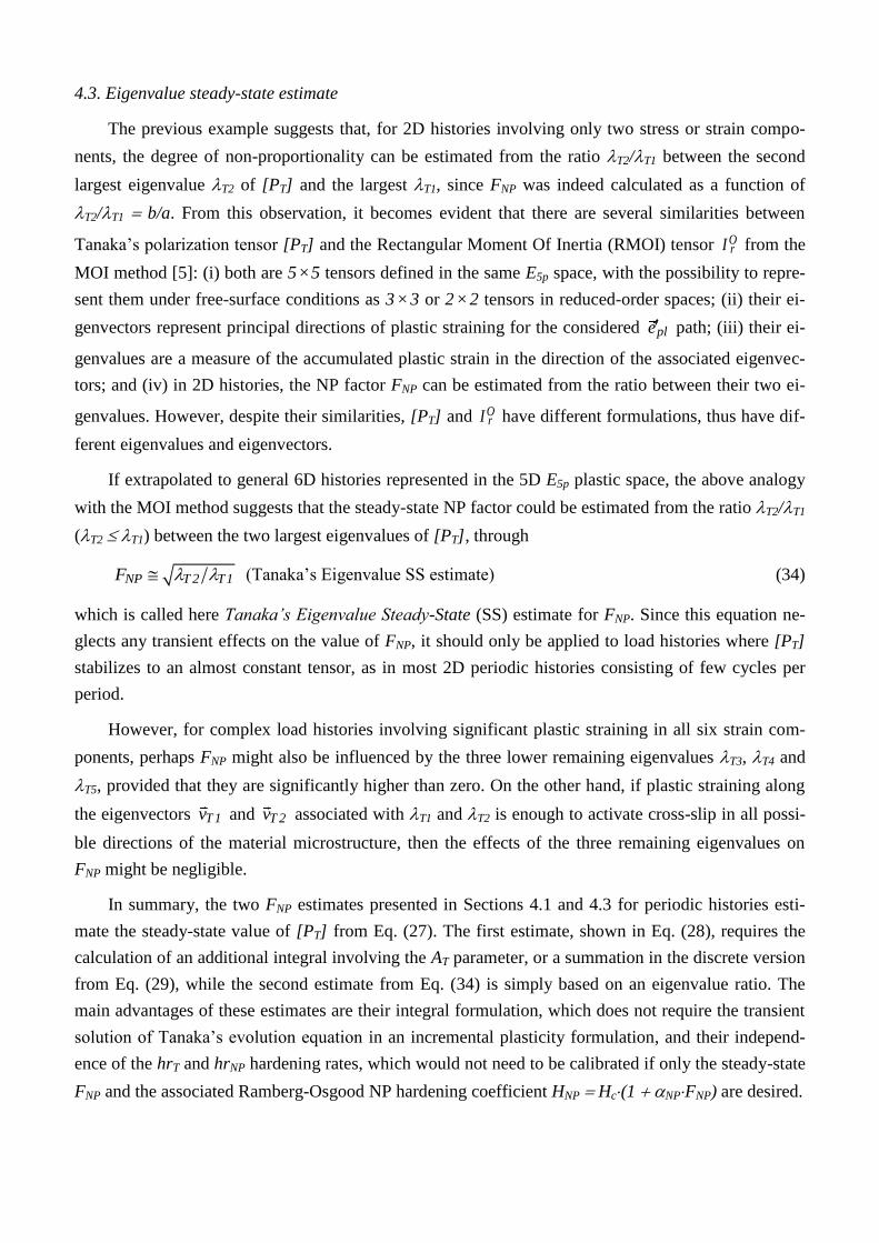
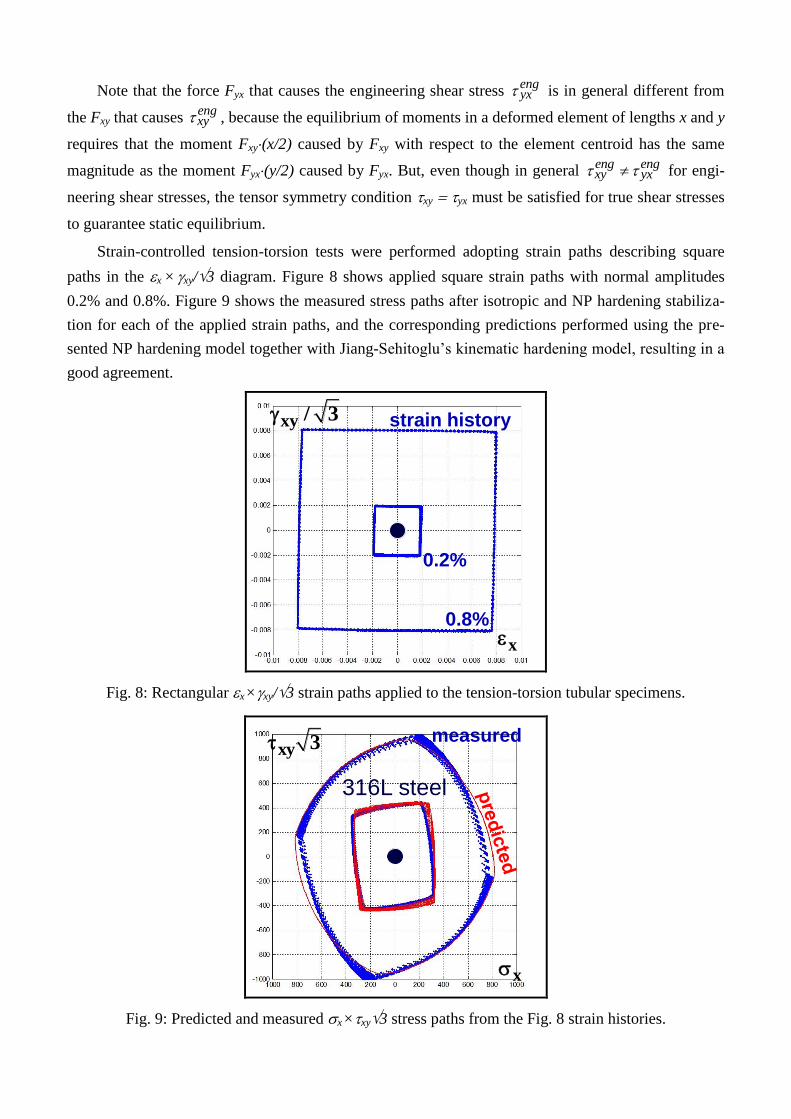
Strain-controlled tension-torsion tests were performed adopting strain paths describing square

paths in the x × xy/3 diagram. Figure 8 shows applied square strain paths with normal amplitudes

0.2% and 0.8%. Figure 9 shows the measured stress paths after isotropic and NP hardening stabiliza-

tion for each of the applied strain paths, and the corresponding predictions performed using the pre-

sented NP hardening model together with Jiang-Sehitoglu’s kinematic hardening model, resulting in a

good agreement.

xy / 3

x

strain history

0.2%

0.8%

Fig. 8: Rectangular x × xy/3 strain paths applied to the tension-torsion tubular specimens.

xy 3

x

measured

316L steel

Fig. 9: Predicted and measured x × xy3 stress paths from the Fig. 8 strain histories.

Figure 10 shows the measured and predicted normal and shear hysteresis loops. Note that the

stress paths would be overestimated if the very high NP hardening effect of the 316L steel had been

neglected in the simulations.

x

x

316L steel - normal

xy

xy

predicted

316L steel - shear

Fig. 10: Predicted and measured normal and shear hysteresis loops from the Fig. 8 strain histories.

6. Conclusions

In this work, Tanaka’s incremental plasticity model was presented in a special 5D plastic strain

space, from which an evolution equation for the non-proportionality factor FNP was obtained, as a

function of the accumulated plastic strain p. It was shown that the eigenvectors of Tanaka’s polariza-

tion tensor represent principal directions along which dislocation structures may form, while the ei-

genvalues quantified them. Two new integral estimates for the steady-state FNP of periodic load histo-

ries were proposed. The presented equations were validated from non-proportional tension-torsion ex-

periments with 316L steel tubular specimens.

References

[1] Socie, D.F., Marquis, G.B., Multiaxial Fatigue, SAE 1999.

[2] Bannantine J.A., Socie, D.F. A variable amplitude multiaxial fatigue life prediction method. Fa-

tigue Under Biaxial and Multiaxial Loading, ESIS Publication 1991;10:35-51.

[3] Itoh T., Sakane M., Ohnami M., Socie D.F. Nonproportional low cycle fatigue criterion for type

304 stainless steel. ASME J Eng Materials Techn 1995;117:285–292.

[4] Bishop J.E. Characterizing the non-proportional and out-of-phase extent of tensor paths. Fatigue

Fract Eng Mater Struct 2000;23:1019-1032.

[5] Meggiolaro, M.A., Castro, J.T.P. Prediction of non-proportionality factors of multiaxial histories

using the Moment Of Inertia method. International Journal of Fatigue 2014;61:151-159.

[6] Tanaka, E. A nonproportionality parameter and a cyclic viscoplastic constitutive model taking in-

to account amplitude dependences and memory effects of isotropic hardening. European Journal

of Mechanics - A/Solids 1994;13:155-173.

[7] Kanazawa, K., Miller, K. and Brown, M. Cyclic deformation of 1% Cr-Mo-V steel under out-of-

phase loads. Fatigue Fract Eng Mater Struct 1979;2:217-228.

[8] Safaei, M., Zang, S.-L., Lee, M.G., Waele, W.D. Evaluation of anisotropic constitutive models:

mixed anisotropic hardening and non-associated flow rule approach. International Journal of Me-

chanical Sciences 2013;73:53-68.

[9] Meggiolaro, M.A., Castro, J.T.P. An Improved Multiaxial Rainflow Algorithm for Non-

Proportional Stress or Strain Histories - Part I: Enclosing Surface Methods. International Journal

of Fatigue 2012;42:217-226.

[10] Meggiolaro, M.A., Castro, J.T.P. An Improved Multiaxial Rainflow Algorithm for Non-

Proportional Stress or Strain Histories - Part II: The Modified Wang Brown Method. International

Journal of Fatigue 2012;42:194-206.

[11] Meggiolaro, M.A., Castro, J.T.P. Automation of the Fatigue Design under Variable Amplitude

Loading Using the ViDa Software. International Journal of Structural Integrity 2010;1:1-6.

[12] Chaboche, J.L., Dang Van, K., Cordier, G. Modelization of the Strain Memory Effect on the Cy-

clic Hardening of 316 Stainless Steel. Transactions of the Fifth International Conference on

Structural Mechanics in Reactor Technology, Div. L, Berlin, 1979.

[13] Jiang, Y., Sehitoglu, H. Modeling of Cyclic Ratchetting Plasticity, Part I: Development of Consti-

tutive Relations. ASME Journal of Applied Mechanics 1996;63(3):720-725.

[14] Jiang, Y., Sehitoglu, H. Modeling of Cyclic Ratchetting Plasticity, Part II: Comparison of Model

Simulations with Experiments. ASME Journal of Applied Mechanics 1996;63(3):726-733.

[15] Ohno, N., Wang, J.D. Kinematic hardening rules with critical state of dynamic recovery, part I:

formulations and basic features for ratchetting behavior. International Journal of Plasticity

1993;9:375-390.

[16] Delobelle, P., Robinet, P., Bocher, L. Experimental Study and Phenomenological Modelization of

Ratchet under Uniaxial and Biaxial Loading on an Austenitic Stainless Steel. International Jour-

nal of Plasticity 1995;11:295-330.

[17] Itoh, T., Sakane, M., Ohnami, M., Socie, D.F. Nonproportional low cycle fatigue criterion for

type 304 stainless steel. ASME Journal of Engineering Materials and Technology 1995;117:285-

292.