
Output Feedback Controllers For Continuous-Time Switched...
80
Universidade Estadual de Campinas Faculdade de Engenharia Mecânica Guilherme Kairalla Kolotelo Output Feedback Controllers For Continuous-Time Switched Affine Systems Controladores via Realimentação de Saída para Sistemas Afins com Comutação a Tempo Contínuo Campinas 2018
-
Upload
nguyenkhue -
Category
Documents
-
view
218 -
download
0
Transcript of Output Feedback Controllers For Continuous-Time Switched...

Universidade Estadual de Campinas
Faculdade de Engenharia Mecânica
Guilherme Kairalla Kolotelo
Output Feedback Controllers ForContinuous-Time Switched Affine Systems
Controladores via Realimentação de Saída paraSistemas Afins com Comutação a Tempo Contínuo
Campinas2018

Universidade Estadual de Campinas
Faculdade de Engenharia Mecânica
Guilherme Kairalla Kolotelo
Output Feedback Controllers For Continuous-Time Switched AffineSystems
Controladores via Realimentação de Saída para Sistemas Afins comComutação a Tempo Contínuo
Supervisor: Prof. Dr. Grace S. Deaecto
Este exemplar corresponde à versão final da monografia
apresentada pelo aluno Guilherme Kairalla Kolotelo, e
orientada pela Profa. Dra. Grace S. Deaecto.
Monograph presented to the School of MechanicalEngineering of the University of Campinas in par-tial fulfillment of the requirements for the degreeof Bachelor of Control and Automation Engineer-ing, in the field of Control Theory.
Monografia apresentada à Faculdade de Engen-haria Mecânica da Universidade Estadual deCampinas como parte dos requisitos exigidos paraa obtenção do título de Bacharel em Engenhariade Controle e Automação, na área de Teoria deControle.
Campinas2018

Acknowledgements
Agradeço à FAPESP pelo apoio financeiro sem o qual esta pesquisa não seria possível.

Abstract
Currently, there is an increasing interest within the scientific community with regard to switched dynamical
systems. These systems are comprised of a finite number of subsystems and a switching function used for
selecting one subsystem at each instant of time. In our context, this function is a control variable to be designed,
so as to guarantee stability and a suitable performance of the overall system. In the literature, there are
important contributions on this topic, however, due to the theoretical characteristics and the practical interest
of this wide class of systems, there still exist several problems of great importance to be studied. In this context,
our focus is to treat the problem of dynamical output feedback control design for continuous-time switched
affine systems. These systems are more general when compared to switched linear systems, since they possess
several equilibrium points, thus making the control design problem more challenging. As it will become clear
throughout this work, our main contribution is to propose a technique for the simultaneous design of two
control structures, while the existing literature considers exclusively the synthesis of the switching function.
More specifically, a full-order dynamical controller and a switching function, dependent only on the measured
output signal, are considered so as to guarantee stability as well asH2 andH∞ performance indices. The design
conditions are expressed in terms of linear matrix inequalities, and do not require any stability property of each
isolated subsystem. Furthermore, the proposed methodology allows for a wider range of equilibrium points to
be attained, when compared to available techniques. Several examples illustrate the theory and make clear the
importance of the joint action of both control structures.

Resumo
Atualmente, é crescente o interesse da comunidade científica no estudo de sistemas dinâmicos com comutação.
Estes sistemas são compostos por um número finito de subsistemas e uma função de comutação que seleciona a
cada instante de tempo um deles. No nosso contexto, esta função de comutação é uma variável de controle a ser
projetada, de forma a garantir estabilidade e um desempenho adequado do sistema global. Na literatura existem
contribuições importantes sobre este tema, entretanto, devido às suas características teóricas e o interesse prático
desta abrangente classe de sistemas, ainda existem vários problemas de grande importância a serem estudados.
Neste contexto, nosso interesse é tratar o projeto de controle via realimentação dinâmica de saída de sistemas
afins com comutação a tempo contínuo. Estes sistemas são mais gerais quando comparados aos lineares, pois
possuem vários pontos de equilíbrio formando uma região no espaço de estado, tornando assim o problema de
projeto de controle mais desafiador. Como ficará claro ao longo do texto, nossa principal contribuição é propor
uma técnica para o projeto simultâneo de duas estruturas de controle, enquanto que a literatura disponível
considera exclusivamente a síntese da regra de comutação. Mais especificamente, um controlador dinâmico
de ordem completa, e uma função de comutação, dependentes somente da saída medida, são considerados de
forma a assegurar estabilidade e desempenhoH2 eH∞ do sistema global. As condições de projeto são expressas
em termos de desigualdades matriciais lineares e não exigem nenhuma propriedade de estabilidade de cada
subsistema isolado. Além disso a metodologia proposta permite considerar um conjunto maior de pontos
de equilíbrio quando comparada às técnicas disponíveis. Vários exemplos ilustram a teoria e deixam claro a
importância da ação conjunta de ambas as estruturas de controle.

List of Figures
3.1 Lyapunov function for a destabilizing switching signal. . . . . . . . . . . . . . . . . . . . . . . . 26
3.2 Phase portrait for each unforced linear subsystem. . . . . . . . . . . . . . . . . . . . . . . . . . . 30
3.3 Trajectories in time of each state for the switched linear system. . . . . . . . . . . . . . . . . . . . 31
3.4 Phase portrait for the switched linear system using the min-type quadratic rule. . . . . . . . . . 32
3.5 Phase portrait for each unforced affine subsystem. . . . . . . . . . . . . . . . . . . . . . . . . . . 36
3.6 Phase portrait for the switched affine system under the min-type quadratic rule. . . . . . . . . . 37
3.7 Trajectories of each state for the switched affine system under the min-type quadratic rule. . . . 37
3.8 Trajectories of each state for the switched affine system under Theorem 3.4. . . . . . . . . . . . . 43
3.9 Trajectories of each state for the switched affine system under Theorem 3.5. . . . . . . . . . . . . 50
3.10 Trajectories of each state for the switched affine system under Theorem 3.6. . . . . . . . . . . . . 50
4.1 Closed-loop system. . . . . . . . . . . . . . . . . . . . . . . . . . . . . . . . . . . . . . . . . . . . . 53
4.2 Trajectories of each state for the switched affine system under Theorem 4.1. . . . . . . . . . . . . 60
4.3 Output and control signal for the switched affine system under Theorem 4.1. . . . . . . . . . . . 60
4.4 Phase portrait for the switched affine system under Theorem 4.1. . . . . . . . . . . . . . . . . . . 61
4.5 Detailed phase portrait for the switched affine system under Theorem 4.1. . . . . . . . . . . . . 61
4.6 Trajectories of each state for the switched affine system under Theorem 4.1 for ψ1. . . . . . . . . 62
4.7 Output and control signal for the switched affine system under Theorem 4.1 for ψ1. . . . . . . . 63
4.8 Switching rule for the switched affine system under Theorem 4.1 for ψ1. . . . . . . . . . . . . . . 63
4.9 Trajectories of each state for the switched affine system under Theorem 4.2. . . . . . . . . . . . . 71
4.10 Output and control signal for the switched affine system under Theorem 4.2. . . . . . . . . . . . 72
4.11 Switching rule for the switched affine system under Theorem 4.2. . . . . . . . . . . . . . . . . . 72
4.12 Trajectories of each state for the switched affine system under Theorem 4.3. . . . . . . . . . . . . 73
4.13 Output and control signal for the switched affine system under Theorem 4.3. . . . . . . . . . . . 73
4.14 Switching rule for the switched affine system under Theorem 4.3. . . . . . . . . . . . . . . . . . 74

Nomenclature
Abbreviations
DC Direct Current
LMI Linear Matrix Inequality
LT I Linear Time-Invariant
Latin Letters
R Set of real numbers.
Fσ Dynamical Filter under switching rule σ .
C Set of complex Numbers
Rn×m Set of real matrices of dimension n×m.
K Set composed of the first N positive natural numbers KB 1, ·,N .
H Set of Hurwitz matrices.
L2 Set of square-integrable trajectories.
I Identity matrix.
v(·) Lyapunov function.
Cσ Dynamical controller under switching rule σ .
Greek Letters
ω Angular frequency.
σ Switching function
ΛN Unit simplex of order N , ΛN Bλ ∈RN : λi ≥ 0,
∑Ni=1λi = 1
.
λ Arbitrary vector belonging to ΛN .
Supercripts
X∗ Conjugate transpose of matrix X.
XT Transpose of matrix X.
Subscripts
xi i−th element of vector x.
zei i−th element of vector ze.
Xi i−th matrix of the set X1, . . . ,N .
πij Element at row i, column j of matrix Π.
Hwz(s) Transfer matrix from input w to output z.
λ0 A given constant vector belonging to ΛN .
Xλ0Convex combination of matrices X1, . . . ,XN in λ0, Xλ0
=∑Ni=1λ0iXi
Symbols
• Symmetric block of a symmetric matrix.
He X Hermitian operator He XB X + XT .
tr (X) Trace of matrix X.
diag(X,Y) Block diagonal matrix, whose elements are X and Y.
‖ · ‖2 Euclidean norm.
| · | Absolute value of a scalar.
X 0 (X ≺ 0) Matrix X is symmetric and positive (negative) definite, such that ∀v , 0, vTXv > (<)0.
X 0 (X 0) Matrix X is symmetric and positive (negative) semi-definite, such that ∀v , 0, vTXv ≥ (≤)0.
min (·) Minimum optimization problem subject to LMI restrictions.
sup (·) Supremum of a set.
arg mini∈K (·) i−th element in K whose value (·) is minimum.

Table of Contents
1 Introduction 11
1.1 Motivation . . . . . . . . . . . . . . . . . . . . . . . . . . . . . . . . . . . . . . . . . . . . . . . . . 11
1.2 Publications . . . . . . . . . . . . . . . . . . . . . . . . . . . . . . . . . . . . . . . . . . . . . . . . 13
1.3 Outline of Chapters . . . . . . . . . . . . . . . . . . . . . . . . . . . . . . . . . . . . . . . . . . . . 13
2 Preliminaries 15
2.1 Stability of LTI Systems . . . . . . . . . . . . . . . . . . . . . . . . . . . . . . . . . . . . . . . . . . 15
2.1.1 Equilibrium Points . . . . . . . . . . . . . . . . . . . . . . . . . . . . . . . . . . . . . . . . 16
2.1.2 Stability of Dynamical Systems . . . . . . . . . . . . . . . . . . . . . . . . . . . . . . . . . 16
2.2 Lyapunov Stability Theory . . . . . . . . . . . . . . . . . . . . . . . . . . . . . . . . . . . . . . . . 16
2.2.1 Lyapunov’s Direct Method . . . . . . . . . . . . . . . . . . . . . . . . . . . . . . . . . . . . 17
2.3 Performance Indices for LTI Systems . . . . . . . . . . . . . . . . . . . . . . . . . . . . . . . . . . 20
2.3.1 Parseval’s Theorem . . . . . . . . . . . . . . . . . . . . . . . . . . . . . . . . . . . . . . . . 20
2.3.2 L2 Space . . . . . . . . . . . . . . . . . . . . . . . . . . . . . . . . . . . . . . . . . . . . . . 20
2.3.3 System Definition . . . . . . . . . . . . . . . . . . . . . . . . . . . . . . . . . . . . . . . . . 21
2.3.4 H2 norm for LTI systems . . . . . . . . . . . . . . . . . . . . . . . . . . . . . . . . . . . . . 21
2.3.5 H∞ norm for LTI systems . . . . . . . . . . . . . . . . . . . . . . . . . . . . . . . . . . . . 23
3 Switched Systems 25
3.1 Introduction . . . . . . . . . . . . . . . . . . . . . . . . . . . . . . . . . . . . . . . . . . . . . . . . 25
3.2 Stability of Switched Linear Systems . . . . . . . . . . . . . . . . . . . . . . . . . . . . . . . . . . 27
3.2.1 Switching Rules for Switched Linear Systems . . . . . . . . . . . . . . . . . . . . . . . . . 28
3.3 Stability of Switched Affine Systems . . . . . . . . . . . . . . . . . . . . . . . . . . . . . . . . . . 33
3.3.1 Switching Rules for Switched Affine Systems . . . . . . . . . . . . . . . . . . . . . . . . . 34
3.4 Performance Indices . . . . . . . . . . . . . . . . . . . . . . . . . . . . . . . . . . . . . . . . . . . . 40
3.4.1 H2 Performance Index for Switched Systems . . . . . . . . . . . . . . . . . . . . . . . . . 40
3.4.2 H∞ Performance Index for Switched Systems . . . . . . . . . . . . . . . . . . . . . . . . . 43
4 Joint Action Output Feedback Control 51
4.1 Introduction . . . . . . . . . . . . . . . . . . . . . . . . . . . . . . . . . . . . . . . . . . . . . . . . 51
4.2 Problem Statement . . . . . . . . . . . . . . . . . . . . . . . . . . . . . . . . . . . . . . . . . . . . 52
4.3 H2 Control Design . . . . . . . . . . . . . . . . . . . . . . . . . . . . . . . . . . . . . . . . . . . . . 55
4.3.1 Numerical example: H2 Control Design . . . . . . . . . . . . . . . . . . . . . . . . . . . . 58

4.4 H∞ Control Design . . . . . . . . . . . . . . . . . . . . . . . . . . . . . . . . . . . . . . . . . . . . 63
4.4.1 H∞ Control Design: Output Dependent Rule . . . . . . . . . . . . . . . . . . . . . . . . . 64
4.4.2 H∞ Control Design: Disturbance Measurement . . . . . . . . . . . . . . . . . . . . . . . . 67
4.4.3 Numerical example: Output Dependent Rule . . . . . . . . . . . . . . . . . . . . . . . . . 70
4.4.4 Numerical example: Disturbance Measurement . . . . . . . . . . . . . . . . . . . . . . . . 72
5 Conclusion 75
References 80
11
Chapter 1
Introduction
1.1 Motivation
From the simplest cellphone charger to the most complex bipedal robot, the use of digital control
systems incorporating decision-making algorithms which act upon continuous-time processes
is pervasive. This interaction between systems of continuous nature at a lower level, and discrete
events at a higher level is subsumed under the term hybrid systems. For example, the switching
of a transistor in a power converter, an automotive transmission changing gears, a thermostat turning the heat
on or off, or an aircraft flight control system alternating between different flight modes are some of the many
real-life processes that exhibit an intrinsically hybrid behavior. Motivated by the remarkable advancement of
embedded systems over these past decades, and its application in control systems, the study of hybrid systems
has never had more relevance than it does now. Although in widespread use today, the history of hybrid
systems is fairly recent, stemming from the introduction and rapid adoption of the electromagnetic relay in
industrial automation by the mid 1900’s. Since then, progressively more complicated hybrid systems displaying
unique behaviors have emerged, and with them, the necessity to develop tools and techniques for the modeling,
analysis and control of these types of systems, taking into account the intertwined nature of the continuous and
discrete dynamics. Further details on this topic can be found in [1, 2].
A particularly important subclass of hybrid systems, known as switched systems, has gathered much
attention lately due to its usefulness in modeling a wide range of applications. For instance, active and semi-
active automotive suspensions control [3, 4], the control of wind turbines [5], power electronics [6, 7], aircraft
roll angle control [8], and autonomous robotics [9, 10]. In essence, these systems are comprised of a finite set of
subsystems, defining the available modes of operation, and a switching signal that selects which mode will
be active at each instant of time. As such, these systems exhibit a complex and nonlinear dynamical behavior,
distinct to that of their modes of operation. Furthermore, a suitable switching signal may stabilize the switched
system, in the case where all modes of operation are unstable, or conversely, destabilize a switched system
even when all subsystems are stable. This underscores the importance of the switching signal, which can be an
arbitrary time-dependent signal, such as an external input or disturbance, or a control variable to be designed.
In both cases, the control problem is centered on developing conditions for stability, and additionally, assuring
certain performance criteria for the switched system. The books [11, 12] and the survey [13] explore this topic
in greater detail.
These subsystems may individually present different kinds of dynamical behavior. In this work, the
focus is given to switched systems comprised of affine subsystems, referred to as switched affine systems. This
case is more general when compared to a switched system composed of linear subsystems, and introduces
CHAPTER 1. INTRODUCTION 12
greater difficulty by giving rise to a set of attainable nontrivial equilibrium points. This particular characteristic
brings light to the relevance of this category of switched systems, especially given the multitude of applications
that can be modeled in this framework. One such application is the previously mentioned switched mode
DC-DC power converter, and switched affine systems are especially suited to model these electronic circuits,
given their switched nature, and affine dynamical behavior. These circuits are ubiquitous, and power nearly
all electronic devices that operate from a DC source. As such, several publications in the literature treat of
the buck, buck-boost and flyback topologies [14, 15, 16, 17, 18], and are concerned with devising an appropriate
switching function tasked with maintaining a certain operating condition.
Many results regarding the design of an appropriate switching function, also referred to as a switching
rule, in order to guarantee asymptotic stability of switched linear system are already solidly established
[19, 20, 21, 22, 23, 15, 24, 25] some of which also deal with performance criteria, such as the H2 or H∞ indices,
and will be presented in greater detail in Chapter 3. With regard to switched affine systems, some references
consider exclusively the action of a switching function dependent on state information, capable of stabilizing
the system [26, 27, 28], while others deal with the joint action of a switching function, alongside a control
law [29]. More specifically, the latter is based on a set of state feedback matrix gains and a state dependent
switching rule assuring asymptotic stability of the closed-loop system, while guaranteeing optimal H2 or H∞costs.
In practical applications, however, it is not uncommon for some state variables to be unavailable, whether
due to the difficulty or expense in effecting these measurements; because of physical constraints in sensor
placement or size; or simply due to the unavailability of sensors to measure a certain state variable. As such,
control design methodologies that rely on output information in place of state information constitute a very
relevant and applicable topic of study. Existing results in the literature consider the case where the only
control variable is an output-dependent switching rule [30, 16] implemented via a switched dynamical filter
responsible for providing the information needed. On the other hand, as of yet, results in the literature treating
the control design problem considering the joint action of an output dependent stabilizing switching function
and a dynamical controller, do so only for switched linear systems [24]. To fill this void in the context of
switched affine systems, in this work we propose three control design techniques based on a full-order switched
dynamical controller, also available in [31]. The first generalizes the results of [24], taking into account an
output-dependent switching rule and control law that together guarantee global asymptotic stability of a
desired equilibrium point for the closed-loop system, as well as an upper bound for the H∞ performance index.
The second reduces the conservativeness of these conditions by considering a switching rule dependent on
both output and input information. The third technique introduces an output-dependent switching rule and
control law assuring an H2 guaranteed cost and global asymptotic stability of the equilibrium point of interest.
The proposed approaches do not require any stability property of the individual subsystems, guaranteeing
stability when the subsystems are not controllable, or when a stable convex combination of dynamical matrices
cannot be verified. Furthermore, the proposed techniques allow for a wider range of equilibrium points to be
attained when compared to existing methods. This reinforces the importance of the joint action of both control

CHAPTER 1. INTRODUCTION 13
structures, and will be discussed at length in Chapter 4.
This work in its present form, encompasses part of my Master’s dissertation, which besides the contents
here presented, will also study the classical filtering problem for switched systems. To the best of our knowledge,
this problem has yet to be treated in the context of switched affine systems. The following publications represent
the results obtained during my Master’s program.
1.2 Publications
This monograph is based in part on the following papers:
• G. K. Kolotelo and G. S. Deaecto, “Controle H2 e H∞ via Realimentação de Saída de Sistemas Afins com
Comutação por Ação Conjunta de Função de Comutação e Entrada de Controle”, Congresso Brasileiro de
Automática - CBA, Submitted.
• G. K. Kolotelo, L. N. Egidio, and G. S. Deaecto, “H2 and H∞ Filtering for Continuous–Time Switched
Affine Systems”, IFAC Symposium on Robust Control Design ROCOND, 2018, To appear.
• G. K. Kolotelo, L. N. Egidio, and G. S. Deaecto, “Projeto de Filtros com ComutaçãoH2 eH∞ para Sistemas
Afins a Tempo Contínuo”, Congresso Brasileiro de Automática - CBA, Submitted.
1.3 Outline of Chapters
This work is divided in 5 chapters, explained in brief:
• Chapter 1: Introduction
Presents the motivation and sets the context for the topics that are treated in this work.
• Chapter 2: Preliminaries
Reviews the fundamental concepts of dynamical systems, important for the next chapters. In particular,
the stability properties of dynamical systems are studied via Lyapunov’s stability theory. Lastly,
performance criteria for these systems are defined.
• Chapter 3: Switched Systems
Broaches the subject of switched systems, and discusses in greater detail their unique features. Next,
well known results in the literature are introduced, which present conditions for the stability of
switched linear and affine systems. Finally, the H2 and H∞ performance indices for switched affine
systems are defined, important for the subsequent chapters.
• Chapter 4: Joint Action Output Feedback Control
Presents the main results of this monograph in regard to the joint design of an output-dependent

CHAPTER 1. INTRODUCTION 14
switching rule alongside a control law. More specifically, the methodology for the design of a full-order
switched dynamical controller and a switching function that together assure global asymptotic stability
of a desired equilibrium point, as well as a guaranteedH2 orH∞ performance indices is introduced. A
set of numerical examples are provided to illustrate the theory.
• Chapter 7: Conclusion
Summarizes the topics explored by this dissertation, and examines some prospects for future develop-
ments on these topics.

15
Chapter 2
Preliminaries
The analysis of stability properties in the context of switched systems is largely based on the theory
of stability introduced by Lyapunov, due to the nonlinear behavior that is intrinsic to these types
of systems. As such, prior to delving into this subject, we review some key ideas and definitions
that permeate this work, and constitute the theoretical basis under which its results depend.
The purpose of this chapter is to introduce the underlying concepts concerning the stability analysis and
performance indices for Linear Time-Invariant systems, henceforth referred to as a LTI system. Firstly, following
a brief discussion on the concepts of equilibrium and stability, Lyapunov’s stability theory is introduced. More
specifically, the second method of Lyapunov, also known as the direct method, extensively used in the analysis
and control of nonlinear systems, will be used to verify the conditions for which stability properties of a
dynamical system are verified for a certain equilibrium point. Lastly, the definition of the H2 andH∞ norms
for LTI systems will be presented. These ideas are extremely important in classical control theory, and will be
extended to deal with the stability analysis and the control design problem for switched systems, considered in
the next chapters. References [32, 33, 34] will be used to support the discussions throughout.
2.1 Stability of LTI Systems
Before investigating the stability properties of dynamical systems in the following sections, let us first introduce
some basic concepts regarding linear dynamical systems. The state space representation of a continuous-time
LTI system is given by
x(t) = Ax(t) + Bu(t) + Hw(t), x(0) = x0
y(t) = Cx(t) + Dw(t)
z(t) = Ex(t) + Fu(t) + Gw(t)
(2.1)
where x(t) ∈Rnx is the state vector, with the number of states nx being referred to as the order of the system,
u(t) ∈Rnu is the control input, w(t) ∈Rnw is the disturbance, y(t) ∈Rny is the measured output, and z(t) ∈Rnz
is the performance output. Also A, B, H, C, D, E, F, and G are constant matrices of appropriate dimensions.
In the case of G = 0, the system is named a strictly proper system. For simplicity, we initiate our discussions
considering the following unforced LTI system
x(t) = Ax(t), x(0) = x0 (2.2)
which disregards the inputs and outputs of system (2.1), allowing us to analyze its stability properties.

CHAPTER 2. PRELIMINARIES 16
2.1.1 Equilibrium Points
A state vector xe is termed an equilibrium point of the system, if once x(t) = xe, for some t = t0, the system
remains at the equilibrium point from that moment onwards, or equivalently, x(t) = 0 for t ≥ t0. For the case of
linear systems, the origin xe = 0 will always be an equilibrium point. Moreover, it will be the single equilibrium
point of the system, unless A is singular, in which case, there exist multiple equilibrium points beyond xe = 0,
given by the null space of the matrix A, such that Ax = 0. See [32, 33] for more details.
For convenience, any equilibrium point can be shifted to the origin by means of the change of variables
ξ = x− xe with no loss of generality, see [33, 34], facilitating some of our subsequent analyses.
2.1.2 Stability of Dynamical Systems
The concept of stability for dynamical systems is defined in terms of an equilibrium point. More specifically,
[32] defines the equilibrium point xe ∈Rnx as stable if whenever the state vector is moved slightly away from
that point, it tends to return to it, or at least does not keep moving further away. In other words, the state
vector remains within a bounded region in the state space around the equilibrium point. Furthermore, if
whenever t→∞, the state vector x(t)→ xe, then the equilibrium point is referred to as asymptotically stable. It
is designated unstable, if for a given initial conditionx(0), the state vector x(t) tends to infinity. Whenever this
concept of stability only holds for initial conditions within a certain region of the state space, the equilibrium
point is said to be locally stable. If however, it is valid for for any given initial condition, it is said to be globally
stable. Moreover, the equilibrium point is globally asymptotically stable if x(t)→ xe as t→∞, for any initial
condition.
For the specific case of LTI systems, necessary and sufficient conditions for the stability of continuous-
time systems can be derived by studying the eigenvalues of the matrix A. For these systems, an equilibrium
point is globally asymptotically stable if and only if all eigenvalues of A are located at the open left half complex
plane, that is, the eigenvalues have strictly negative real part. In this case, the matrix A is said to be Hurwitz, or
A ∈ H, where H is defined as the set of Hurwitz matrices.
2.2 Lyapunov Stability Theory
For many decades, one of the most useful techniques for the evaluation of stability properties for linear and
nonlinear systems has been the theory introduced by Lyapunov in the late 1800’s. When compared to linear
systems, nonlinear systems may exhibit entirely new and complex behaviors. This, coupled with the fact that
explicit analytical solutions most often cannot be attained for these systems, sheds light upon the importance
of Lyapunov’s findings. The theory is comprised of two widely used methods, commonly referred to as the
linearization or indirect method, and the direct method. The latter will be used extensively throughout this
work, and will be introduced below for LTI systems, followed by a brief discussion of its application on affine
CHAPTER 2. PRELIMINARIES 17
nonlinear systems.
2.2.1 Lyapunov’s Direct Method
Lyapunov’s direct method, as defined in [32, 33, 34], can be used to evaluate the stability of linear and nonlinear
systems in an indirect manner, enabling the characterization of the stability properties of all equilibrium points
for a given system, without the need to derive explicit numerical or analytical solutions. The stability analysis
is based on a scalar energy-like or summarizing function, dependent on the state vector. The purpose of this
function, known as a Lyapunov function, is to describe the behavior of the entire dynamical system as a function
of time, and allow conclusions to be inferred on the stability of the set of its governing differential equations.
The search for a suitable Lyapunov function may be a difficult task for more sophisticated systems, since it must
respect the set of requirements introduced below.
2.2.1.1 Lyapunov Function
A scalar function v : D→R, with D ⊂Rnx a region of the state space containing x = 0, is a Lyapunov function if
it satisfies the following set of conditions [32, 34]:
1. v is continuously differentiable
2. v(0) = 0
3. v(x(t)) > 0, ∀x ∈D, x , 0
4. v(x(t)) ≤ 0, ∀x ∈D
If these requirements are verified for the system in question, then the equilibrium point xe = 0 is stable.
Moreover, whenever
5. v(x(t)) < 0, ∀x ∈D, x , 0
is satisfied, then xe = 0 is asymptotically stable. Additionally, if
6. ‖x‖ →∞ ⇒ v(x)→∞, D = Rnx radially unbounded
can also be verified, then the equilibrium point at the origin is globally asymptotically stable.
2.2.1.2 Lyapunov Stability Analysis of LTI Systems
For LTI systems, an adequate choice for the Lyapunov function v is the quadratic form of a symmetric positive
definite matrix P ∈Rnx×nx such that
v(x(t)) = x(t)TPx(t) (2.3)
It can be verified that this function meets all the conditions of a Lyapunov function. Indeed, conditions (1)− (3)
are evidently verified. In addition, (6) is satisfied, and the validity of condition (5) can be demonstrated as

CHAPTER 2. PRELIMINARIES 18
follows
v(x(t)) = x(t)TPx(t) + x(t)TPx(t)
= x(t)T(ATP + PA
)x(t)
= −x(t)TQx(t)
(2.4)
where Q ∈Rnx×nx is any given symmetric positive definite matrix. In this case, if there exists P 0 satisfying
the so-called Lyapunov equation
ATP + PA + Q = 0 (2.5)
for a given Q 0, then v(x(t)) = −x(t)TQx(t) < 0 ∀x(t) , 0 is valid, assuring the equilibrium point xe = 0 of the
system to be globally asymptotically stable.
It should be mentioned that the existence of a positive definite solution P 0 for the Lyapunov equation
is not only a sufficient condition for global asymptotic stability, but also a necessary condition. Indeed, assume
that matrix A is Hurwitz, and consider a symmetric positive definite matrix Q, as well as a matrix P defined by
P =∫ ∞
0eAT tQeAt dt (2.6)
Whenever the eigenvalues of A have strictly negative real part, the integral exists. Furthermore P is symmetric
positive definite since, for any vector u , 0
uTPu =∫ ∞
0uT eAT tQeAtu dt
=∫ ∞
0xTQx dt
(2.7)
where x = eAtu is the analytical solution of the system x = Ax, assigning u = x(0). As Q 0, then P must be
positive definite. Finally, by substituting (2.6) in (2.5) we have
ATP + PA =∫ ∞
0AT eAT tQeAt dt +
∫ ∞0
eAT tQeAtA dt
=∫ ∞
0
ddt
eAT tQeAt dt
= limt→∞
eAT tQeAt −Q
= −Q
(2.8)
which indicates that whenever matrix A is Hurwitz, and thus all eigenvalues its have strictly negative real part,
then limt→∞ eAT tQeAt = 0, and the Lyapunov equation is verified.
This gives rise to the following theorem, prescribing asymptotic stability of the origin for LTI systems, in
terms of the solution of the Lyapunov equation, stated in [34] as follows
Theorem 2.1. A matrix A is Hurwitz, that is, the eigenvalues of A have strictly negative real part if and only if, for
CHAPTER 2. PRELIMINARIES 19
any given symmetric positive definite matrix Q, there exists a symmetric positive definite matrix P that satisfies the
Lyapunov equation (2.5).
It is worth noting that although LTI system stability can be easily determined by evaluating the eigenval-
ues of the matrix A, this analysis is rendered moot when studying other types of systems, including switched
systems, which will be presented in more detail in the ensuing chapters. This reinforces the influence of
Lyapunov’s theory for the stability analysis of complex and nonlinear systems.
Finally, a related point to consider is that the Lyapunov equation was originally expressed in terms of
linear matrix inequalities, in the form known as the Lyapunov inequality
ATP + PA ≺ 0 (2.9)
This inequality was originally solved for P analytically, via a set of linear equations, by choosing any Q 0
that satisfied (2.5), as discussed in [35]. Only in the 1980’s it would become clear that the Lyapunov inequality
could be solved numerically by means of convex optimization algorithms, with great efficiency. Throughout this
work, we will focus on expressing stability conditions and control design problems in terms of Linear Matrix
Inequalities, from this point onwards referred to as LMIs, which can be solved without difficulty by several
standard and readily available tools.
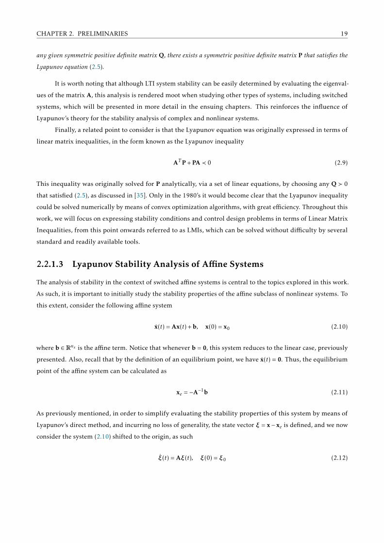
2.2.1.3 Lyapunov Stability Analysis of Affine Systems
The analysis of stability in the context of switched affine systems is central to the topics explored in this work.
As such, it is important to initially study the stability properties of the affine subclass of nonlinear systems. To
this extent, consider the following affine system
x(t) = Ax(t) + b, x(0) = x0 (2.10)
where b ∈Rnx is the affine term. Notice that whenever b = 0, this system reduces to the linear case, previously
presented. Also, recall that by the definition of an equilibrium point, we have x(t) = 0. Thus, the equilibrium
point of the affine system can be calculated as
xe = −A−1b (2.11)
As previously mentioned, in order to simplify evaluating the stability properties of this system by means of
Lyapunov’s direct method, and incurring no loss of generality, the state vector ξ = x− xe is defined, and we now
consider the system (2.10) shifted to the origin, as such
ξ(t) = Aξ(t), ξ(0) = ξ0 (2.12)

CHAPTER 2. PRELIMINARIES 20
Observe that the problem can now be treated as an LTI system, such that the methodology and conditions for
stability introduced in Section 2.2.1.2 remain valid for the analysis of affine time invariant systems. In this case,
for a certain affine system under consideration, whenever there exists P 0 such that the Lyapunov inequality
(2.9) is satisfied for this system, then xe is as globally asymptotically stable equilibrium point, since as ξ→ 0,
we have x→ xe.
2.3 Performance Indices for LTI Systems
In this section the H2 and H∞ norms for LTI systems are introduced. These norms are used extensively in
control design, see [34, 35, 36, 37], to characterize the effects of a given input signal on the output of the system.
They will be expressed both with respect to the transfer function of the system, as well as in terms of its impulse
response, the latter being essential to allow their generalization in order to deal with switched systems, thus
providing an effective measure of performance for this class of systems. But first, some fundamental concepts
that are important to the development of the next topics will be presented, namely, Parseval’s Theorem for
continuous-time LTI systems, and the L2 space, will be introduced.
2.3.1 Parseval’s Theorem
Consider the function f(t) : [0,∞)→Rn and its Laplace transform F(s), as well as the conjugate transpose F(s)∗,
whose domain dom(F), contains the imaginary axis. Parseval’s theorem is then defined by [38] as∫ ∞0
f(t)T f(t) dt =1
2π
∫ ∞−∞
F(jω)∗F(jω)dω
=1π
∫ ∞0
F(jω)∗F(jω)dω(2.13)
This relation will later be employed for the calculation of the H2 and H∞ norms in the coming sections.
2.3.2 L2 Space
The norm ‖ · ‖ : Rn→R, as defined in [34, 39], is a real-valued function satisfying the following four axioms, for
all vectors u,v ∈Cn and all α ∈R:
• ‖v‖ ≥ 0 Nonnegativity
• ‖v‖ = 0 if and only if v = 0 Positivity
• ‖αv‖ = |α|‖v‖ Homogeneity
• ‖u + v‖ ≤ ‖u‖+ ‖v‖ Triangle Inequality
CHAPTER 2. PRELIMINARIES 21
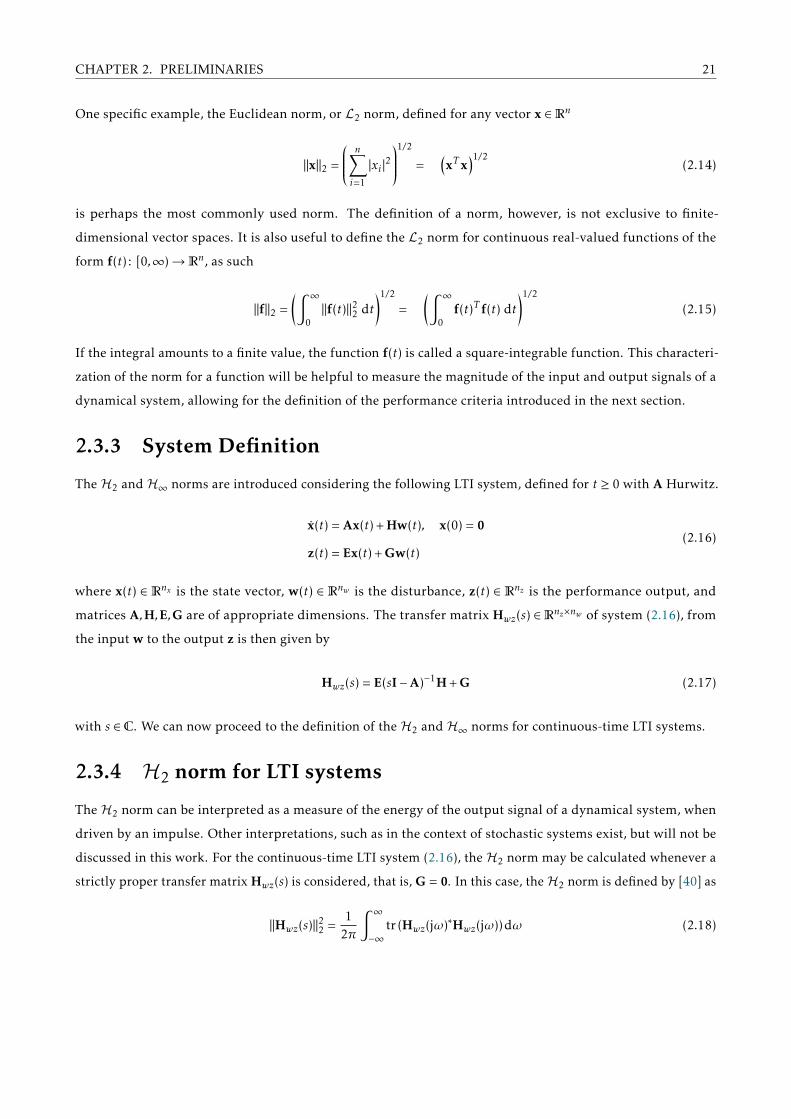
One specific example, the Euclidean norm, or L2 norm, defined for any vector x ∈Rn
‖x‖2 =
n∑i=1
|xi |21/2
=(xT x
)1/2(2.14)
is perhaps the most commonly used norm. The definition of a norm, however, is not exclusive to finite-
dimensional vector spaces. It is also useful to define the L2 norm for continuous real-valued functions of the
form f(t) : [0,∞)→Rn, as such
‖f‖2 =(∫ ∞
0‖f(t)‖22 dt
)1/2
=(∫ ∞
0f(t)T f(t) dt
)1/2
(2.15)
If the integral amounts to a finite value, the function f(t) is called a square-integrable function. This characteri-
zation of the norm for a function will be helpful to measure the magnitude of the input and output signals of a
dynamical system, allowing for the definition of the performance criteria introduced in the next section.
2.3.3 System Definition
The H2 and H∞ norms are introduced considering the following LTI system, defined for t ≥ 0 with A Hurwitz.
x(t) = Ax(t) + Hw(t), x(0) = 0
z(t) = Ex(t) + Gw(t)(2.16)
where x(t) ∈ Rnx is the state vector, w(t) ∈ Rnw is the disturbance, z(t) ∈ Rnz is the performance output, and
matrices A,H,E,G are of appropriate dimensions. The transfer matrix Hwz(s) ∈Rnz×nw of system (2.16), from
the input w to the output z is then given by
Hwz(s) = E(sI−A)−1H + G (2.17)
with s ∈C. We can now proceed to the definition of the H2 and H∞ norms for continuous-time LTI systems.
2.3.4 H2 norm for LTI systems
The H2 norm can be interpreted as a measure of the energy of the output signal of a dynamical system, when
driven by an impulse. Other interpretations, such as in the context of stochastic systems exist, but will not be
discussed in this work. For the continuous-time LTI system (2.16), the H2 norm may be calculated whenever a
strictly proper transfer matrix Hwz(s) is considered, that is, G = 0. In this case, theH2 norm is defined by [40] as
‖Hwz(s)‖22 =1
2π
∫ ∞−∞
tr (Hwz(jω)∗Hwz(jω))dω (2.18)

CHAPTER 2. PRELIMINARIES 22
By applying Parseval’s Theorem, introduced in (2.13), the H2 norm can be expressed in the time domain, as
such
‖Hwz(s)‖22 =∫ ∞
0tr
(hwz(t)
T hwz(t))
dt (2.19)
By realizing that the impulse response hwz(t) of the system, when initial conditions are set to zero, is
hwz(t) =
EeAtH, t ≥ 0
0, otherwise(2.20)
and that for multiple-input, multiple-output systems, hwz(t) is of the form
hwz(t) =
h11(t) . . . hnw (t)...
. . ....
hnz (t) . . . hnznw (t)
(2.21)
then, from (2.19) and (2.21), the H2 norm can be written as
‖Hwz(s)‖22 =nw∑k=1
nz∑i=1
∫ ∞0h2ik(t) dt (2.22)
It is worth noting that for single-input, single-output systems, the H2 norm becomes simply the L2 norm of the
impulse response for the system in question. This emphasizes the need of considering a strictly proper system
in order to obtain a finiteH2 norm. Furthermore, observe that equation (2.22) may alternatively be expressed as
‖Hwz(s)‖22 =∫ ∞
0tr
(HT eAT tET EeAtH
)dt =
∫ ∞0
tr(EeAtHHT eAT tET
)dt (2.23)
This allows the H2 norm to be stated either as
‖Hwz(s)‖2 =√
tr (HT LoH) , or ‖Hwz(s)‖2 =√
tr (ELcET ) (2.24)
where the matrices Lo and Lc are respectively referred to as the controllability Gramian and the observability
Gramian, given by
Lo =∫ ∞
0eAT tET EeAtdt, and Lc =
∫ ∞0
eAtHHT eAT tdt (2.25)
These are, in turn, the solutions to their associated Lyapunov equations, briefly discussed in Section 2.2.1.2, as
follows
AT Lo + LoA + ET E = 0, and ALc + LcAT + HHT = 0 (2.26)
Observe that the H2 norm, expressed in this manner, can be easily solved via numerical methods by the
following convex optimization problem, subject to LMI restrictions, as shown in [35]

CHAPTER 2. PRELIMINARIES 23
min tr(HTPH
)subject to: P 0
ATP + PA + EET ≺ 0
(2.27)
min tr(EPET
)subject to: P 0
AP + PAT + HHT ≺ 0
(2.28)
It is important to note that the ‘min’ and ‘inf’ terms for optimization problems can be used interchangeably
whenever we consider that the non-compact set of restrictions is closed by the numerical solver to a known
tolerance ε > 0. As such, the solution P obtained is arbitrarily close to the respective solutions of Lc or
Lo in (2.25). In this case, the H2 norm is given by ‖Hwz(s)‖22 = tr(HT LoH
)< tr
(HTPH
), or alternatively
‖Hwz(s)‖22 = tr(ELcET
)< tr
(EPET
).
2.3.5 H∞ norm for LTI systems
The H∞ norm characterizes a measure of greatest possible L2 gain of the system, which is the ratio between the
L2 norm of the output signal and the L2 norm of a square integrable input signal, across any input channel,
that maximizes this ratio. It is defined for system (2.16), considering external inputs w ∈ L2, and is defined by
[34] as
‖Hwz(s)‖∞ = supω∈R‖Hwz(jω)‖2 (2.29)
For single-input, single-output systems, theH∞ norm becomes simply the peak gain observed for the frequency
response of Hwz(jω), ω ∈R.
The H∞ norm can also be defined in the time domain, as demonstrated in [34, 41], by the following
‖Hwz(s)‖∞ = sup0,w∈L2
‖z‖2‖w‖2
≤ γ (2.30)
where the scalar γ > 0 is the upper bound of the H∞ norm of system (2.16). Alternatively, (2.30) can be
rewritten, when considering (2.15), as∫ ∞0
z(t)T z(t) dt ≤ γ2∫ ∞
0w(t)Tw(t) dt, w(t) , 0, w(t) ∈ L2, t ≥ 0 (2.31)
This definition allows the H∞ norm to be expressed completely in terms of the input and output signals in the
time domain. When considering performance indices for switched systems, this becomes especially important,
since these systems cannot be expressed in terms of transfer functions, as will become clear in the forthcoming
chapter.
As for the H2 norm, the upper bound for H∞ norm can also be calculated by means of a convex
optimization problem subject to LMI constraints. By considering the quadratic Lyapunov function v(x) = xTPx,
CHAPTER 2. PRELIMINARIES 24
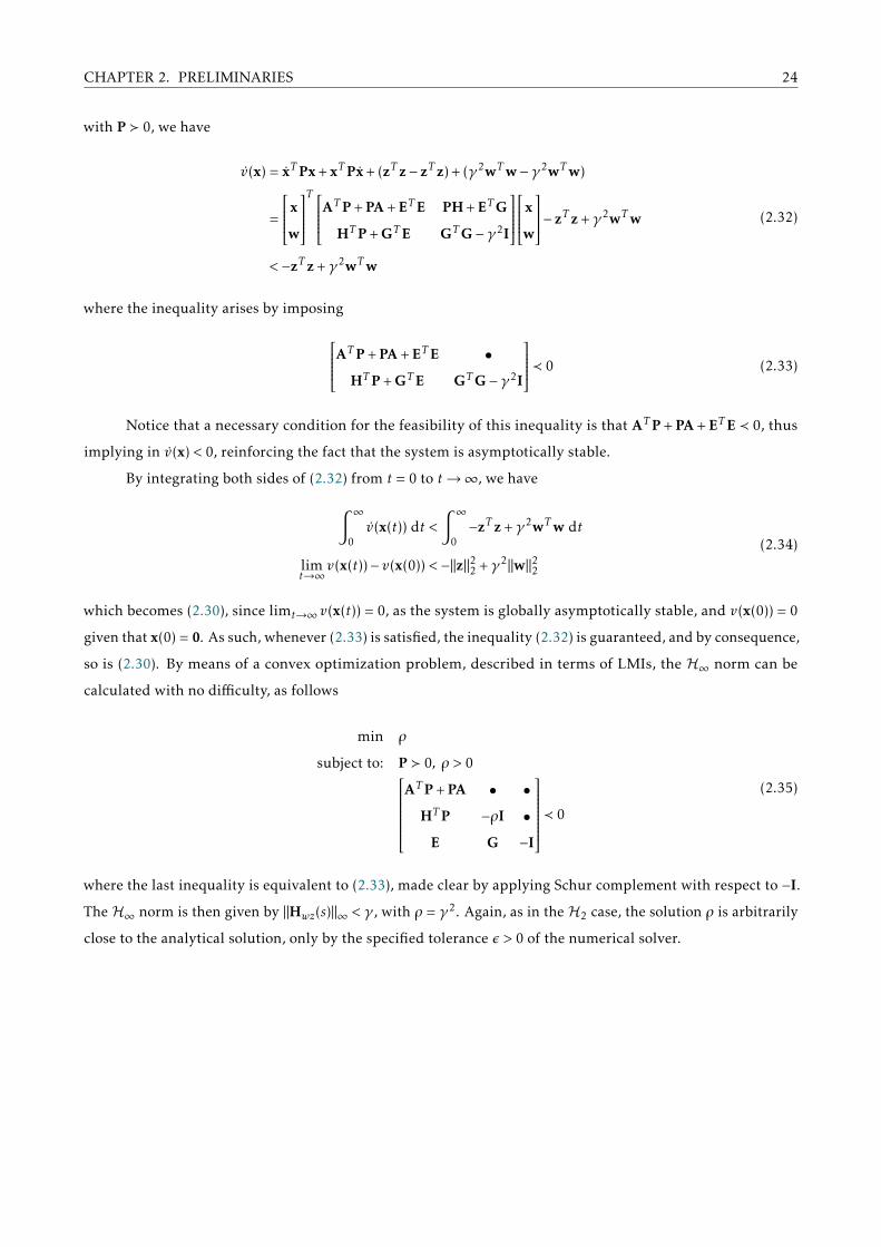
with P 0, we have
v(x) = xTPx + xTPx + (zT z− zT z) + (γ2wTw−γ2wTw)
=
x
w
T ATP + PA + ET E PH + ETG
HTP + GT E GTG−γ2I
x
w
− zT z +γ2wTw
< −zT z +γ2wTw
(2.32)
where the inequality arises by imposing
ATP + PA + ET E •
HTP + GT E GTG−γ2I
≺ 0 (2.33)
Notice that a necessary condition for the feasibility of this inequality is that ATP + PA + ET E ≺ 0, thus
implying in v(x) < 0, reinforcing the fact that the system is asymptotically stable.
By integrating both sides of (2.32) from t = 0 to t→∞, we have∫ ∞0v(x(t)) dt <
∫ ∞0−zT z +γ2wTw dt
limt→∞
v(x(t))− v(x(0)) < −‖z‖22 +γ2‖w‖22(2.34)
which becomes (2.30), since limt→∞ v(x(t)) = 0, as the system is globally asymptotically stable, and v(x(0)) = 0
given that x(0) = 0. As such, whenever (2.33) is satisfied, the inequality (2.32) is guaranteed, and by consequence,
so is (2.30). By means of a convex optimization problem, described in terms of LMIs, the H∞ norm can be
calculated with no difficulty, as follows
min ρ
subject to: P 0, ρ > 0ATP + PA • •
HTP −ρI •
E G −I
≺ 0
(2.35)
where the last inequality is equivalent to (2.33), made clear by applying Schur complement with respect to −I.
The H∞ norm is then given by ‖Hwz(s)‖∞ < γ , with ρ = γ2. Again, as in the H2 case, the solution ρ is arbitrarily
close to the analytical solution, only by the specified tolerance ε > 0 of the numerical solver.

25
Chapter 3
Switched Systems
In this chapter, we introduce the concept of switched systems, followed by the study of the stability
properties of switched linear and affine systems, as well as revelant performance criteria, which
generalize the concepts previously established. The topics presented in this chapter review
several foundational results already existent in the literature, for instance [13, 19] for switched
linear systems, and [15, 29] for switched affine system, as well as the books [12] and [11], important to support
the ideas presented later in this work.
3.1 Introduction
Switched systems constitute a subclass of hybrid systems, in the sense that these systems are governed by
a set of modes of operation, each of which may be represented by a dynamical system, and is coupled with
discrete switching events across these modes, thus affecting the trajectory of the overall system. The switching
between modes is orchestrated by a switching function, also known as a switching rule, denoted by σ (·). It
encompasses a decision-making process that selects values within the set KB 1, . . . ,N , at every instant of
time, such that each i ∈K corresponds to an individual mode of operation, refereed to as a subsystem of the
switched system. This chapter will deal with the so-called continuous-time switched linear systems, which
concerns the case where all subsystems are governed by linear dynamical systems, and subsequently, we discuss
the continuous-time switched affine systems, pertaining to the situation where at least one of the subsystems
presents a nonzero affine term, contemplating the main focus of this work.
The effect of switching in switched systems is not trivial, since not only does it establish the nonlinear
and time-varying nature of these systems, but also, the stability properties of the switched system are inherently
dependent on the switching signal. Indeed, it may give rise to complex and unprecedented behaviors, even
when simple subsystems are considered. An example of this is the occurrence of sliding modes, in which the
switched system switches infinitely fast. This specific situation, although sometimes undesirable, allows for a
behavior significantly different than that of each isolated subsystem, and in the case of switched affine systems,
it introduces new attainable equilibrium points that are distinct from those of each subsystem, a topic that will
be discussed in greater detail shortly. It is important to note that although the switching function modifies the
trajectory of the switched system, the continuous state evolves without discontinuities, that is, the state does
not jump impulsively on switching events.
To illustrate how the stability properties of a switched system are intertwined with the switching signal,
consider two unforced stable linear subsystems given by x = Aix, for i = 1,2. Individually, these subsystems
would display a monotonically decreasing Lyapunov function v(x) = xTPix, however, when subject to a specific

CHAPTER 3. SWITCHED SYSTEMS 26
switching signal, the switched system may prove to be unstable, as exemplified in Figure 3.1. In this figure it
can be observed that although v(x(t)) decreases while the subsystem is active, an upward trend for v(x(t)) can
be seen, indicating that the switching signal under consideration destabilizes the switched system. Fortunately,
0 0.1 0.2 0.3 0.4 0.5 0.6 0.7 0.8 0.9 10
0.1
0.2
0.3
0.4
0.5
0.6
0 0.1 0.2 0.3 0.4 0.5 0.6 0.7 0.8 0.9 1
1
1.5
2
Figure 3.1: Lyapunov function for a destabilizing switching signal.
a suitable switching rule can also be used to stabilize the switched system.
Given its crucial role in the behavior of switched systems, it is important to characterize the switching
function σ (·), which may be either an arbitrary time-dependent function, or a control variable to be designed.
In the first case, the central problem is determining conditions to assure stability for some unknown switching
signal σ (t) : R+→K, such as a disturbance, an assigned external input, or which may model the effects of a
component failure. On the other hand, the second case concerns the design of a switching function σ (·) ∈K,
which can be state, output or input dependent, or a combination thereof, in order to guarantee stability of the
switched system. The survey [13] reviews stability conditions for a variety of switched systems that have been
introduced in the literature throughout the past decades.
The design of a switching function σ (·) as a control variable attracts much interest, as the choice of an
appropriate switching rule may assure stability even in the case where all subsystems are unstable, furthermore,
whenever all subsystems are stable, it may improve the performance of the overall system when compared to
that of each isolated subsystem, in this case the switching function is said to be strictly consistent [25]. This
scenario also has a wide scope of applications, for instance, the automatic transmission of an automobile, the
problem of temperature regulation by a thermostat, and several applications on power electronic systems. Given
that such systems are intrinsically switched, it makes sense to model these in a switched system framework. The
following results in the literature, for example, deal with the design of a stabilizing switching rule for switched
mode DC-DC power converters, more specifically the buck-boost, see [14, 17], and the flyback converters, see
[18].
It is also relevant to consider measures of performance when designing switching functions for switched
systems. In this work, the H2 and H∞ performance indices, will be presented, as introduced in [23, 24, 25] for

CHAPTER 3. SWITCHED SYSTEMS 27
the linear case, and in [15, 29] for the affine case. These indices generalize the H2 and H∞ norms introduced
previously, as they cannot be employed, since their definition is given in terms of the transfer function of an
LTI system. It should be noted that even though each isolated subsystem may possess a frequency domain
representation, the switched system does not, given its nonlinear and time-varying characteristics that stem
from the influence of the switching function. It will become evident, however, that whenever the switching
function remains fixed at a certain subsystem σ (t) = i, these indices are equivalent to the square of the H2 or
H∞ norms for the i-th subsystem. These performance criteria will be essential when we treat the problems of
control and filter design in the next chapters, as we seek to develop techniques that minimize these indices.
3.2 Stability of Switched Linear Systems
Consider the following state space representation of an unforced continuous-time switched linear system
x(t) = Aσx(t), x(0) = x0 (3.1)
where x(t) ∈Rnx is the state vector, and σ (·) ∈K, for KB 1, . . . ,N , is the switching rule, a piecewise continuous
function, which selects one of the N available subsystems as active, at every instant of time. Notice that the
origin is the single equilibrium point of the system.
In this case, the problem consists in determining an adequate switching rule σ (·), capable of stabilizing
the system, and making the origin x = 0 a globally asymptotically stable equilibrium point. The work of [19]
introduces some circumstances which must be satisfied, so that a stabilizing switching rule is guaranteed to
exist. These conditions are derived under Lyapunov’s direct method, introduced in Section 2.2, by adopting the
quadratic Lyapunov function v(x) = xTPx, with P 0, and x(t) expressed as x for simplicity.
In the context of linear systems, several well established results for stabilizing switching rules exist, some
of which are based on different Lyapunov functions. Before introducing the min-type quadratic rule in the next
section, with which many of the results in this work are based upon, we investigate the motivation behind its
conception by means of an example, based on [19].
Example 3.1.
Consider the switched linear system (3.1), comprised of two unstable subsystems, with matrices A1 and A2.
Also, consider symmetric indefinite matrices Q1 and Q2, a symmetric positive definite matrix P 0, and
suppose that a given λ0 = [µ 1−µ]T , with µ ∈ (0,1) exists, such that Aλ0= µA1 + (1−µ)A2 is Hurwitz. Let
Q1 = AT1 P + PA1 and Q2 = AT
2 P + PA2
Notice that, since Aλ0∈ H, and approaching the stability analysis by Lyapunov’s direct method under the

CHAPTER 3. SWITCHED SYSTEMS 28
quadratic Lyapunov function, the following LMI
ATλ0
P + PAλ0≺ 0
is verified. This implies that, for all x ∈Rnx , x , 0,
xT(ATλ0
P + PAλ0
)x = xTQλ0
x < 0
indicating that Qλ0≺ 0. Expanding the convex combination in λ0, we have
µ(xTQ1x
)+ (1−µ)
(xTQ2x
)< 0
This suggests that either
xTQ1x < 0 or xTQ2x < 0
However, by our initial hypothesis that both subsystems are not Hurwitz, there does not exist a matrix P1 0
such that AT1 P1 + P1A1 ≺ 0, nor does exist P2 0 satisfying AT
2 P2 + P2A2 ≺ 0. This, coupled with the fact that
Qλ0≺ 0, implies that indeed Qi , i ∈ 1,2 are indefinite, and thus, the sign of xTQix are dependent of the value
of x. As such, it can be inferred that while neither subsystem is stable for all x(t) ∈Rnx , as the state trajectory
progresses in time, xTQ1x and xTQ2x take turns in becoming strictly negative, as a consequence of Qi being
indefinite, thus always guaranteeing ATλ0
P + PAλ0≺ 0 at any given moment in time.
Notice that xT(ATi P + PAi
)x = xTQix is precisely the time derivative of the quadratic Lyapunov function
for the i-th subsystem. This invites the question of what switching function would select the appropriate
subsystem so as to guarantee the time derivative of the Lyapunov function be strictly negative for all instant of
time.
A recurrent condition in the literature, applicable to the results in this chapter, and employed by this
example, is that the convex combination of matrices Aλ0, for λ0 ∈ΛN , be Hurwitz, or Aλ0
∈ H. This requirement
is sufficient to assure that a stabilizing switching rule exists, as discussed in [19, 20].
3.2.1 Switching Rules for Switched Linear Systems
Several switching rules, along with their respective conditions for stability, have been proposed for linear
switched systems over the past decades, with varying degrees of conservativeness. Switching rules of the form
σ (x(t)), σ (y(t)), and σ (x(t),w(t)) have been introduced, depending whether these measurements are accessible
in order to implement the rule. At the moment, we will focus on switching rules dependent on the state, σ (x(t)),
and based on quadratic stability [15, 19, 20, 21, 22]. Some other results available in the literature will be shown
in brief, towards the conclusion of this section.
CHAPTER 3. SWITCHED SYSTEMS 29
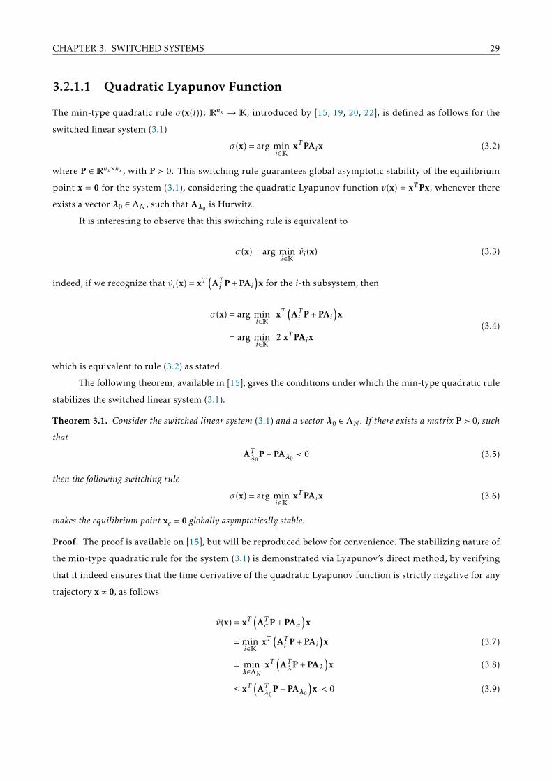
3.2.1.1 Quadratic Lyapunov Function
The min-type quadratic rule σ (x(t)) : Rnx → K, introduced by [15, 19, 20, 22], is defined as follows for the
switched linear system (3.1)
σ (x) = arg mini∈K
xTPAix (3.2)
where P ∈ Rnx×nx , with P 0. This switching rule guarantees global asymptotic stability of the equilibrium
point x = 0 for the system (3.1), considering the quadratic Lyapunov function v(x) = xTPx, whenever there
exists a vector λ0 ∈ΛN , such that Aλ0is Hurwitz.
It is interesting to observe that this switching rule is equivalent to
σ (x) = arg mini∈K
vi(x) (3.3)
indeed, if we recognize that vi(x) = xT(ATi P + PAi
)x for the i-th subsystem, then
σ (x) = arg mini∈K
xT(ATi P + PAi
)x
= arg mini∈K
2 xTPAix(3.4)
which is equivalent to rule (3.2) as stated.
The following theorem, available in [15], gives the conditions under which the min-type quadratic rule
stabilizes the switched linear system (3.1).
Theorem 3.1. Consider the switched linear system (3.1) and a vector λ0 ∈ΛN . If there exists a matrix P 0, such
that
ATλ0
P + PAλ0≺ 0 (3.5)
then the following switching rule
σ (x) = arg mini∈K
xTPAix (3.6)
makes the equilibrium point xe = 0 globally asymptotically stable.
Proof. The proof is available on [15], but will be reproduced below for convenience. The stabilizing nature of
the min-type quadratic rule for the system (3.1) is demonstrated via Lyapunov’s direct method, by verifying
that it indeed ensures that the time derivative of the quadratic Lyapunov function is strictly negative for any
trajectory x , 0, as follows
v(x) = xT(ATσP + PAσ
)x
= mini∈K
xT(ATi P + PAi
)x (3.7)
= minλ∈ΛN
xT(ATλP + PAλ
)x (3.8)
≤ xT(ATλ0
P + PAλ0
)x < 0 (3.9)

CHAPTER 3. SWITCHED SYSTEMS 30
where the equality (3.7) comes from applying the switching rule; equality (3.8) comes from the fact that the
minimum of a objective function linear in λ always occurs at one of the vertices of the convex polytope defined
by ΛN , thus selecting the i-th subsystem is equivalent to setting the i-th element of λ to 1, and the rest to 0;
inequality (3.9) stems from the fact that since there exists a vector λ0, such that a convex combination of the
subsystems is Hurwitz, then at any given time, the minimum of the objective function in λ will be always less
than or equal to it, and finally, v(x) < 0 follows from the fact that Aλ0is Hurwitz, and thus, AT
λ0P + PAλ0
≺ 0.
As discussed in Example 3.1, this result implies that at any given moment, for all trajectories x(t) , 0, t ≥ 0,
at least one of the subsystems is assured to make v(x) < 0, that is, ∃i ∈K, such that
xT(ATi P + PAi
)x < 0 (3.10)
for some x ∈Rnx . It is also important to note that no stability property is imposed on the individual subsystems,
the only requirement is that Aλ0be Hurwitz for some λ0 ∈ΛN .
This result will be illustrated in the following numerical example, where we consider switching across
two unstable subsystems.
Example 3.2.
Consider the switched linear system (3.1) consisting of the following two unstable subsystems
A1 =
−10 3
8 −1
, A2 =
−1 2
4 −6
Notice that the equilibrium points of both subsystems are unstable saddles, as illustrated in the phase
portrait in Figure 3.2. and that at λ0 = [0.5 0.5]T , a Hurwitz convex combination Aλ0is verified.
-1.5 -1 -0.5 0 0.5 1 1.5
-1.5
-1
-0.5
0
0.5
1
1.5
-1.5 -1 -0.5 0 0.5 1 1.5
-1.5
-1
-0.5
0
0.5
1
1.5
Figure 3.2: Phase portrait for each unforced linear subsystem.

CHAPTER 3. SWITCHED SYSTEMS 31
Figure 3.2 displays the trajectories of each isolated subsystem from initial conditions x0 around a unit
circle ‘ ’ centered at the origin ‘+’, that is, x0 = [cos(θ) sin(θ)]T , θ ∈ [0,2π]. In order to implement the
switching rule (3.6) of Theorem 3.1, first, a matrix P 0 is calculated satisfying restriction (3.5) of Theorem 3.1.
For the value of λ0 given, we have considered
P =
30.2067 62.5002
62.5002 135.1940
It can be verified that the switching rule is able to stabilize the switched system, by inspecting the phase portrait
and the state trajectories in Figures 3.3 and 3.41 which asymptotically converge to the origin, as desired.
0 2 4 6 8
-1
-0.8
-0.6
-0.4
-0.2
0
0.2
0.4
0.6
0.8
1
0 2 4 6 8
-1
-0.8
-0.6
-0.4
-0.2
0
0.2
0.4
0.6
0.8
1
Figure 3.3: Trajectories in time of each state for the switched linear system.
Also, in Figure 3.4 the boundaries in which switching events occur, referred to as a switching surface,
are indicated by the line ‘ ’. This situation arises whenever xTPA1x = xTPA2x which, in this case, produces
two straight lines intersecting at the origin. Notice that when at the switching surface, the switching rule may
select another subsystem as active, transitioning from one dynamical behavior to another, or the occurrence of
sliding modes may ensue. In this example, this phenomenon is distinctly visible in Figure 3.4, where the two
subsystems switch at an arbitrarily high frequency, resulting in a behavior distinct from that of each isolated
subsystem, and causing the state trajectory to evolve along the switching surface towards the equilibrium point,
as indicated by the arrows ‘I’.
1Numerical simulations of switched systems were carried out using the SWSYSToolbox for MATLAB, developed by the author. Thetoolbox is available at https://github.com/gkolotelo/SWSYSToolbox, along with the detailed documentation.

CHAPTER 3. SWITCHED SYSTEMS 32
-1 -0.5 0 0.5 1
-1
-0.5
0
0.5
1
Figure 3.4: Phase portrait for the switched linear system using the min-type quadratic rule.
3.2.1.2 Min-Type Lyapunov Function
As alluded to earlier, less conservative results when compared to those based on quadratic Lyapunov functions
have been obtained, such as those derived from multiple Lyapunov functions, introduced by [42, 2], and from
the min-type piecewise quadratic Lyapunov function, as shown in [43, 44]. The latter two adopt the following
Lyapunov function
v(x) = mini∈K
xTPix (3.11)
with matrices Pi 0, i ∈K, the solutions of the well-known Lyapunov-Metzler inequalities
ATi Pi + PiAi +
N∑j=1
πjiPj + ETi Ei ≺ 0, i ∈K (3.12)
where Π =πji
is a subclass of Metzler matrices satisfying the following additional property
N∑j=1
πji = 0, i ∈ 1, . . . ,N (3.13)
Under these conditions, the following switching rule
σ (x) = arg mini∈K
xTPix (3.14)
guarantees global asymptotic stability of the origin. An important remark, as discussed in [45], is that the
inequalities (3.12) are less conservative than assuring the existence of a Hurwitz convex combination of
subsystem matrices as required in Theorem 3.1. Note that the conditions (3.12) are non-convex due to the

CHAPTER 3. SWITCHED SYSTEMS 33
product of matrix variables, however, for a small number of subsystems, they can be solved by means of
one-dimensional searches with respect to the elements of matrix Π coupled with a set of LMIs. For an arbitrary
number of subsystems, alternative conditions, easier to solve but more conservative, are available in [43].
3.3 Stability of Switched Affine Systems
In this section, we introduce the fundamental concepts of switched affine systems that will be extensively used
throughout the remainder of this work. Furthermore, we engage in discussions about the unique characteristics
of these types of systems, and how these features are useful for modeling many practical applications.
Consider the following state space representation of an unforced continuous-time switched affine system
x(t) = Aσx(t) + bσ , x(0) = x0
z(t) = Eσx(t)(3.15)
where x(t) ∈ Rnx is the state vector, bσ is the affine term, σ (·) ∈ K is the switching rule, and z(t) ∈ Rnz is the
performance output, which will allow for the definition of performance indices for these systems.
Notice that whenever the affine terms bi = 0 for all i ∈K, the system (3.15) reduces to a continuous-time
switched linear system, whose equilibrium point is the origin. However, for the more general case of bi , 0,
system (3.15) exhibits several distinct equilibrium points, constituting a subset of the state space. This imposes
greater difficulty in the study of the stability properties of switched affine systems, as will soon become evident.
Definition 1. The set of all equilibrium points of the system (3.15) is given by
Xe =xe ∈Rnx : xe = −A−1
λ bλ, λ ∈ΛN
(3.16)
With no loss of generality, system (3.15) can be shifted so as to move the equilibrium point xe ∈ Xe to the
origin by defining the new state vector ξ(t) = x(t)− xe, resulting in the equivalent system
ξ(t) = Aσξ(t) + `σ , ξ(0) = ξ0
ze(t) = Eσξ(t)(3.17)
where `i = Aixe + bi , for all i ∈K, are the new affine terms, and ze(t) = z(t)−Eσxe is the shifted output. Notice
that for global asymptotic stability, ξ(t) → 0 as t → ∞, and in this condition, x(t) → xe for system (3.15).
Furthermore, observe that whenever xe ∈ Xe, with its associated λ0 ∈ΛN , we have `λ0= 0. This choice of state
variables will simplify our further developments.
CHAPTER 3. SWITCHED SYSTEMS 34
3.3.1 Switching Rules for Switched Affine Systems
On the realm of switched affine systems, fewer switching rules along with suitable Lyapunov functions have
been introduced, compared to switched linear systems. The authors [26, 27, 28] present state dependent
switching rules, whereas [16, 30] introduce an output dependent switching function. First we present the
min-type switching rule, originally devised in [26], along with the conditions which guarantee global asymptotic
stability of an equilibrium point xe ∈ Xe. We then introduce the concept of guaranteed cost for switched systems,
along with an appropriate switching rule, presented in [14, 15], and capable of assuring this metric, important
for the definition of the H2 and H∞ performance indices towards the end of this chapter.
3.3.1.1 Min-Type Quadratic Rule
The following theorem introduces the results of [15, 26], presenting conditions that assure global asymptotic
stability of a desired equilibrium point xe ∈ Xe.
Theorem 3.2. Consider the switched affine system (3.17), and a chosen xe ∈ Xe of interest with its associated λ0 ∈ΛN .
If there exist a matrix P 0, such that
ATλ0
P + PAλ0≺ 0 (3.18)
then the following switching rule
σ (ξ) = arg mini∈K
ξTPAiξ +ξTP`i (3.19)
makes the equilibrium point xe globally asymptotically stable.
Proof. The proof, available in [26], is presented below for convenience, and explained throughout its unraveling.
When adopting the switching strategy (3.19), and realizing that it is equivalent to
σ (ξ) = arg mini∈K
ξT(ATi P + PAi
)ξ + 2ξTP`i (3.20)
then the time derivative of the quadratic Lyapunov function v(ξ(t)), for any state trajectory ξ , 0, is given by
v(ξ) = ξTPξ +ξTPξ
= ξT(ATσP + PAσ
)ξ + 2ξTP`σ
= mini∈K
ξT(ATi P + PAi
)ξ + 2ξTP`i
= minλ∈ΛN
ξT(ATλP + PAλ
)ξ + 2ξTP`λ
≤ ξT(ATλ0
P + PAλ0
)ξ + 2ξTP`λ0
< 0 (3.21)
which unfolds in a similar manner to the proof of the min-type quadratic rule for switched linear systems,
presented in Section 3.2.1.1, when recalling the fact that `λ0= 0, and that Aλ0
is Hurwitz, as ensured by

CHAPTER 3. SWITCHED SYSTEMS 35
condition (3.18), thus making inequality (3.21) valid.
Notice that this theorem encompasses Theorem 3.1, since in the event that bi = 0, ∀i ∈K, they become
equivalent. It is also important to observe that not all equilibrium points xe ∈ Xe are attainable, but in fact only
those for which the vectors λ ∈ΛN satisfy Aλ ∈ H. In the case where there exists no stable convex combination
of dynamical matrices, however, the system is not stabilizable under Theorem 3.2.
Overall, this result is very attractive for a range of real life applications, since it allows the switched
system to operate at a chosen equilibrium point of interest. The works of [14, 15, 17, 18] apply this particular
characteristic of switched affine systems to different topologies of DC-DC power converters with much success.
A numerical example is presented below to demonstrate the validity of Theorem 3.2 with respect to the min-type
quadratic rule for switched affine systems.
3.3.1.2 Numerical Example
The following numerical example illustrates the peculiarities of switched affine systems and how the switching
function plays an important role in this class of switched systems.
Example 3.3.
Consider the switched affine system (3.15) comprised of a stable and an unstable subsystem, as follows
A1 =
8 0
1 2
, A2 =
−2 −9
5 −4
, b1 =
57 , b2 =
7
−3
whose respective equilibrium points are
xe1 =
−0.625
−3.1875
, xe2 =
1.0377
0.5472
For the equilibrium point of interest xe = [0.9158 0.8160]T ∈ Xe, with its vector λ0 = [0.15 0.85]T associated,
a Hurwitz convex combination Aλ0∈ H is verified. In Figure 3.5, we can observe the dynamical behavior of
each isolated subsystem in the ξ phase plane, where ‘×’ denotes the origin of the shifted system. For subsystem
1, we have considered ξ0 = x0 − xe1 − xe describing points over the line ‘ ’ from x0 = [2 − 2]T to x0 = [−2 2]T .
For subsystem 2 we have considered initial conditions ξ0 = x0 − xe with x0 = 3× [cos(θ) sin(θ)]T , θ ∈ [0,2π],
corresponding to points distributed around the circle ‘ ’. Notice that the equilibrium point xe1 , marked by
‘’, is an unstable node, whereas xe2 , indicated by ‘’, is a stable focus, also, notice how xe differs from the
equilibrium points of the isolated subsystems. These different behaviors across subsystems bring about complex
dynamical behaviors for the switched system.
Before proceeding, the vectors `i = Aixe + bi , for i ∈ 1,2 are calculated. We have also considered matrix

CHAPTER 3. SWITCHED SYSTEMS 36
-6 -4 -2 0 2
-8
-7
-6
-5
-4
-3
-2
-1
0
1
-4 -3 -2 -1 0 1 2
-4
-3
-2
-1
0
1
2
Figure 3.5: Phase portrait for each unforced affine subsystem.
P 0 as follows
P =
0.2491 −0.0650
−0.0650 0.4107
which satisfies the LMI restriction (3.18) of Theorem 3.2. Implementing the switching rule (3.19), and allowing
initial conditions distributed around the circle ‘ ’ with ξ0 = [2cos(θ) 2sin(θ)]T + ξ•, θ ∈ [0,2π], where
ξ• = [−0.6079 − 1.0480]T , the switched system is successfully stabilized, as observed in the phase portrait
shown in Figure 3.6. Notice that ξ• is the center of the switching surface, indicated by the line ‘ ’, taking place
when ξTPA1ξ +ξTP`1 = ξTPA2ξ +ξTP`2, forming, in this case, an ellipse.
Notice that when the trajectory is outside this ellipse, it assumes the behavior of subsystem 2, conversely,
when inside the ellipse, the trajectory follows the dynamical behavior of subsystem 1. It is interesting to
observe that when at the switching surface, the trajectory may exhibit a particular behavior, characteristic of
switched system, known as sliding mode. The occurrence of sliding modes is clearly visible in Figure 3.6. This
phenomenon, resulting from an arbitrarily fast switching between subsystems, or chattering, is sometimes an
undesirable condition in real systems, given the increased equipment wear that may ensue. However, it may
also be a sought after situation, as it allows for the stability of the overall system. In the case of switched affine
systems, sliding modes are crucial, allowing an equilibrium point different than that of each isolated subsystem
to be attained, as evidenced by this example.
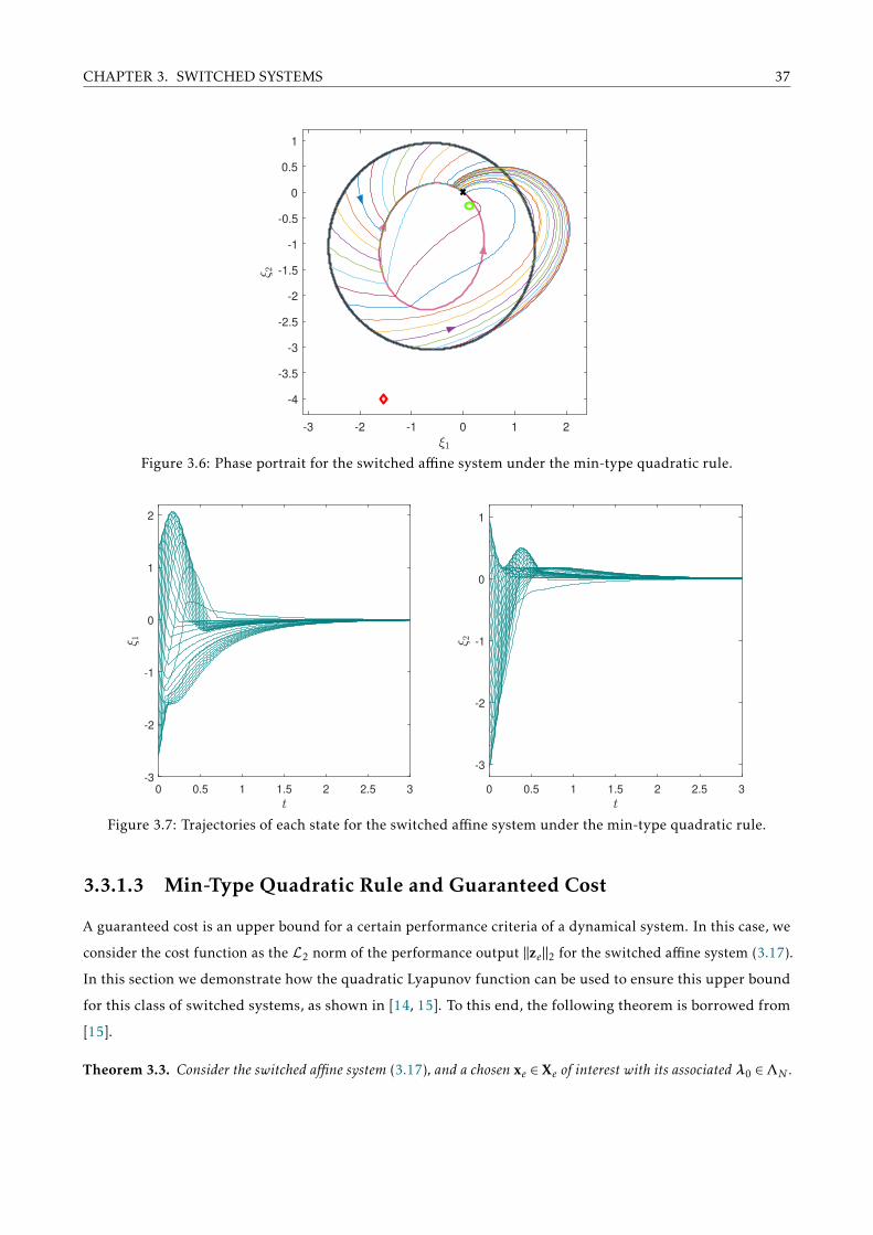
Figure 3.7 reveals the states of the switched affine system asymptotically reaching the equilibrium point
ξ = 0, or equivalently, x = xe for the initial conditions considered.
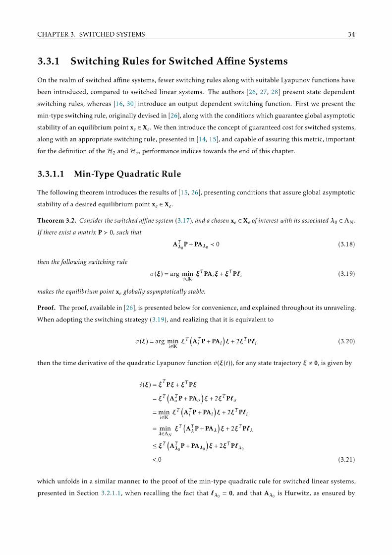
CHAPTER 3. SWITCHED SYSTEMS 37
-3 -2 -1 0 1 2
-4
-3.5
-3
-2.5
-2
-1.5
-1
-0.5
0
0.5
1
Figure 3.6: Phase portrait for the switched affine system under the min-type quadratic rule.
0 0.5 1 1.5 2 2.5 3
-3
-2
-1
0
1
2
0 0.5 1 1.5 2 2.5 3
-3
-2
-1
0
1
Figure 3.7: Trajectories of each state for the switched affine system under the min-type quadratic rule.
3.3.1.3 Min-Type Quadratic Rule and Guaranteed Cost
A guaranteed cost is an upper bound for a certain performance criteria of a dynamical system. In this case, we
consider the cost function as the L2 norm of the performance output ‖ze‖2 for the switched affine system (3.17).
In this section we demonstrate how the quadratic Lyapunov function can be used to ensure this upper bound
for this class of switched systems, as shown in [14, 15]. To this end, the following theorem is borrowed from
[15].
Theorem 3.3. Consider the switched affine system (3.17), and a chosen xe ∈ Xe of interest with its associated λ0 ∈ΛN .
CHAPTER 3. SWITCHED SYSTEMS 38
If there exist a matrix P 0, and symmetric indefinite matrices Qi , such that
ATi P + PAi + ETi Ei + Qi ≺ 0, ∀i ∈K (3.22)
Qλ0 0 (3.23)
then the following switching rule
σ (ξ) = arg mini∈K−ξTQiξ + 2ξTP`i (3.24)
makes the equilibrium point ξ = 0 globally asymptotically stable, and the guaranteed cost
‖ze‖22 < ξT0 Pξ0 (3.25)
holds.
Proof. The proof follows from the definition of the guaranteed cost available in [15]. By implementing the
switching strategy (3.24) of Theorem 3.3, the time derivative of the quadratic Lyapunov function v(ξ), for any
state trajectory ξ , 0, is given by
v(ξ) = ξTPξ +ξTPξ
= ξT(ATσP + PAσ
)ξ + 2ξTP`σ +
(zTe ze − zTe ze
)= ξT
(ATσP + PAσ + ETσ Eσ
)ξ + 2ξTP`σ − zTe ze
< −ξTQσξ + 2ξTP`σ − zTe ze (3.26)
= mini∈K−ξTQiξ + 2ξTP`i − zTe ze
= minλ∈Λ−ξTQλξ + 2ξTP`λ − zTe ze
≤ −ξTQλ0ξ + 2ξTP `λ0
− zTe ze
≤ −zTe ze (3.27)
where inequality (3.26) comes from the conditions (3.22) of Theorem 3.3, and inequality (3.27) stems from the
fact that Qλ0 0. Thus, global asymptotic stability is assured for the equilibrium point xe, as zTe ze > 0. Finally,
by integrating both sides of (3.27) we have∫ ∞0v(ξ) dt < −
∫ ∞0
ze(t)T ze(t) dt
limt→∞
v(ξ(t))− v(ξ0) < −∫ ∞
0ze(t)
T ze(t) dt∫ ∞0
ze(t)T ze(t) dt < v(ξ0)
‖ze‖22 < ξT0 Pξ0
(3.28)
where limt→∞ v(ξ(t)) = 0, since the system is asymptotically stable. This assures the guaranteed cost for the

CHAPTER 3. SWITCHED SYSTEMS 39
system ‖ze‖22 < ξT0 Pξ0 whenever ze(t) is square-integrable.
It is worth noticing that, as Qλ0 0, the following can be verified
ATλ0
P + PAλ0+
N∑i=0
λiETi Ei ≺ 0 (3.29)
which shows that the matrices Ei directly influence P, and consequently, the guaranteed cost for the system, as
should be expected. Furthermore, the above condition requires that Aλ0be Hurwitz. This, however, is not an
onerous imposition, since matrices Qi , ∀i ∈K, are indefinite, thus no stability property is required from the
subsystem matrices Ai themselves, for all i ∈K.
To implement Theorem 3.3, matrices P and Qi , for i ∈K, important for the switching rule (3.24), can be
calculated numerically by solving the following convex optimization problem, subject to the LMI restrictions
(3.22) and (3.23) of Theorem 3.3, that is
min ξT0 Pξ0
subject to: P 0
ATi P + PAi + ETi Ei + Qi ≺ 0, ∀i ∈K
Qλ0 0
(3.30)
This result is important for the definition of an upper bound for the H2 performance index, which will be
introduced shortly.
The following corollary proposes a min-type linear switching rule, possible in the event that all subsys-
tems are individually stable.
Corollary 3.1. Consider the switched affine system (3.17), and a chosen xe ∈ Xe of interest with its associated λ0 ∈ΛN .
If there exist a matrix P 0, such that
ATi P + PAi + ETi Ei ≺ 0, ∀i ∈K (3.31)
then the following switching rule
σ (ξ) = arg mini∈K
ξTPAixe (3.32)
makes the equilibrium point ξ = 0 globally asymptotically stable, and the guaranteed cost
‖ze‖22 < ξT0 Pξ0 (3.33)
holds.
Proof. The proof is a direct consequence of Theorem 3.3. By imposing Qi 0, for all i ∈K.
The condition in the corollary requires that all the subsystems be quadratically stable, that is, the
subsystems must be Hurwitz stable and, furthermore, they must admit the same matrix P 0. Although this

CHAPTER 3. SWITCHED SYSTEMS 40
result is more conservative when compared to Theorem 3.3, it is useful when considering practical applications,
as it guarantees global asymptotic stability for any xe ∈ Xe, such that Aλ0∈ H, by only calculating the matrix P
once, as opposed to Theorem 3.3, in which P depends on λ0. This allows for the equilibrium point to change at
execution time by simply altering xe on the switching rule (3.32).
3.4 Performance Indices
This section aims to introduce the concept of performance indices for switched systems, as well as proposes
suboptimal switching rules that assure an upper bound for these indices. For theH2 case, the results of Theorem
3.3 will be generalized, and a state dependent switching function is proposed. For the H∞ case, two switching
rules are introduced, one dependent on the state, and another that additionally depends on the disturbance.
These concepts have already been applied in the context of switched linear systems as in [23, 24, 25], as well as
in the context of switched affine systems [16, 29].
For this section, the following switched affine system is considered, in its shifted representation, such
that the origin is the unique equilibrium point
ξ(t) = Aσξ(t) + Hσw(t) + `σ , ξ(0) = 0
ze(t) = Eσξ(t) + Gσw(t)(3.34)
where ξ(t) ∈ Rnx is the state vector, `σ is the affine term, σ (·) ∈ K is the switching rule, ze(t) ∈ R
nz is the
performance output, and w(t) ∈Rnw is the external disturbance input. The following performance indices will
establish a relationship between this disturbance and the output ze(t).
3.4.1 H2 Performance Index for Switched Systems
As in the case for the H2 norm of LTI systems, Gi = 0 for all i ∈K must be considered to ensure that the output
ze(t), associated to external impulsive disturbances, be square-integrable.
The H2 performance index is defined as
J2(σ ) =nw∑k=1
‖zek ‖22 (3.35)
where zek (t) refers to the output of system (3.34) when subject to an impulsive disturbance applied to the k-th
input, in other words, w(t) = δ(t)ψk , such that ψk , for k ∈ 1, . . . ,nw form a standard basis. Considering this,
observe that (3.35) can be expressed as
J2(σ ) =nw∑k=1
∫ ∞0
zTek (t)zek (t) dt =nw∑k=1
nz∑i=1
∫ ∞0zeik (t)
2 dt (3.36)
CHAPTER 3. SWITCHED SYSTEMS 41
It is interesting to observe that minimizing J2(σ ) generally leads to a faster convergence to the equilibrium
point.
For an LTI system, the H2 norm, shown in (2.22), can be defined in terms of the frequency response of
the system, this procedure, however, cannot be employed for switched systems, as they do not admit a transfer
matrix due to the effect of switching rule. Nevertheless, notice that for a fixed switching rule, that is σ (t) = i,
for all t ≥ 0, the H2 index is indeed equivalent to the square of the H2 norm since in this case zeik (t), for an
impulsive disturbance, equates to hik(t) of (2.22).
To deal with switched systems, the upper bound for theH2 index is defined by considering the guaranteed
cost introduced in Theorem 3.3, which was obtained with w(t) = 0, and an arbitrary initial condition. Notice
that the system (3.34) subjected to an impulsive disturbance w(t) = δ(t)ψk can be cast as system (3.17) when
ξ(0) = Hσ (0)ψk is assigned. This can be verified by integrating (3.34)
∫ t
0ξ(t) dt =
∫ t
0Aσξ(t) + `σ dt +
∫ t
0Hσw(t) dt
ξ(t)−ξ(0) =∫ t
0Aσξ(t) + `σ dt + Hσ (0)ψk
ξ(t)−Hσ (0)ψk =∫ t
0Aσξ(t) + `σ dt
(3.37)
Hence, the upper bound for theH2 index can be calculated by using the familiar result (3.25) from Theorem 3.3
J2(σ ) =nw∑k=1
∫ ∞0
zTek (t)zek (t) dt
<nw∑k=1
ξT (0)Pξ(0)
=nw∑k=1
ψTk HTj PHjψk
= tr(HTj PHj
)(3.38)
where P satisfies theorem 3.3, and σ (0) = j is the initial value of the switching rule, chosen appropriately. Two
choices for this value may be of interest, firstly, the choice of j ∈K such that the upper bound J2 is minimized,
providing the smallest guaranteed H2 performance index; and secondly, a choice of j that maximizes the upper
bound J2, thus making the H2 index robust with respect to the initial subsystem σ (0) ∈K. More information of
this topic can be found in the reference [23].
Finally, it is also worth mentioning that, although this definition has been established for the shifted
system (3.17) considering the performance output ze(t), this result equally guarantees an upper bound for the
system (3.15) with the performance output z(t), since these definitions are related by ze(t) = z(t)−Eσxe.
With this, the following theorem can be stated
Theorem 3.4. Consider the switched affine system (3.34), with Gi = 0 for all i ∈K, and a chosen xe ∈ Xe of interest
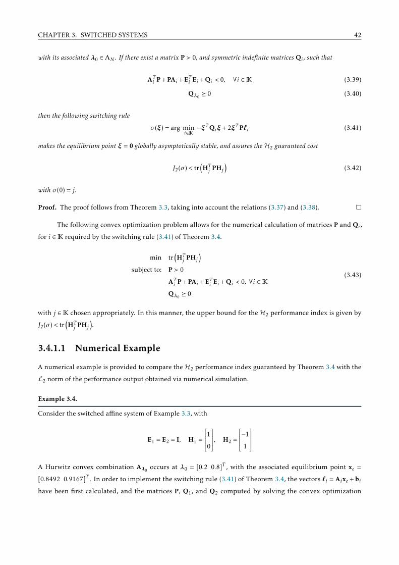
CHAPTER 3. SWITCHED SYSTEMS 42
with its associated λ0 ∈ΛN . If there exist a matrix P 0, and symmetric indefinite matrices Qi , such that
ATi P + PAi + ETi Ei + Qi ≺ 0, ∀i ∈K (3.39)
Qλ0 0 (3.40)
then the following switching rule
σ (ξ) = arg mini∈K−ξTQiξ + 2ξTP`i (3.41)
makes the equilibrium point ξ = 0 globally asymptotically stable, and assures the H2 guaranteed cost
J2(σ ) < tr(HTj PHj
)(3.42)
with σ (0) = j.
Proof. The proof follows from Theorem 3.3, taking into account the relations (3.37) and (3.38).
The following convex optimization problem allows for the numerical calculation of matrices P and Qi ,
for i ∈K required by the switching rule (3.41) of Theorem 3.4.
min tr(HTj PHj
)subject to: P 0
ATi P + PAi + ETi Ei + Qi ≺ 0, ∀i ∈K
Qλ0 0
(3.43)
with j ∈K chosen appropriately. In this manner, the upper bound for the H2 performance index is given by
J2(σ ) < tr(HTj PHj
).
3.4.1.1 Numerical Example
A numerical example is provided to compare the H2 performance index guaranteed by Theorem 3.4 with the
L2 norm of the performance output obtained via numerical simulation.
Example 3.4.
Consider the switched affine system of Example 3.3, with
E1 = E2 = I, H1 =
10 , H2 =
−1
1
A Hurwitz convex combination Aλ0
occurs at λ0 = [0.2 0.8]T , with the associated equilibrium point xe =
[0.8492 0.9167]T . In order to implement the switching rule (3.41) of Theorem 3.4, the vectors `i = Aixe + bi
have been first calculated, and the matrices P, Q1, and Q2 computed by solving the convex optimization

CHAPTER 3. SWITCHED SYSTEMS 43
problem (3.43), resulting in the following matrices
P =
0.3290 −0.1190
−0.1190 0.4847
, Q1 =
−6.0266 0.7058
0.7058 −2.9389
, Q2 =
1.5066 −0.1765
−0.1765 0.7347
associated to the guaranteed cost J2(σ ) < 0.3290 for σ (0) = 1. For comparison, by choosing σ (0) = 2, the
guaranteed cost for the switched system would be J2(σ ) < 1.0518, and would be robust against the choice of
σ (0). The trajectories in time for each state can be seen in Figure 3.8 with the initial condition ξ(0) = H1ψ1 = H1,
since only a single input channel exists as discussed in Section 3.4.1. The figure indicates the system state
trajectories asymptotically converging to ξ = 0.
0 1 2 3 4
0
0.2
0.4
0.6
0.8
1
0 1 2 3 4
-0.2
-0.1
0
0.1
0.2
Figure 3.8: Trajectories of each state for the switched affine system under Theorem 3.4.
Finally, by numerical integration of the output signal ze(t)T ze(t) from t = 0 to t → ∞, the actual H2
cost obtained from the suboptimal switching function implementation (3.41) was calculated as being J2(σ ) =
0.0705 < 0.3290, within the cost guaranteed by Theorem 3.4, as expected.
3.4.2 H∞ Performance Index for Switched Systems
In a manner analogous to the definition of theH∞ norm (2.30) established for LTI systems, theH∞ performance
index for switched systems is defined as
J∞(σ ) := sup0,w∈L2
‖ze(t)‖22‖w(t)‖22
< ρ, ρ > 0 (3.44)
with the scalar ρ being an upper bound for this index.
In a similar manner to the procedure used in the proof of Theorem 3.3, the upper bound for the H∞index can be inferred from the time derivative of the quadratic Lyapunov function v(ξ), for state trajectories
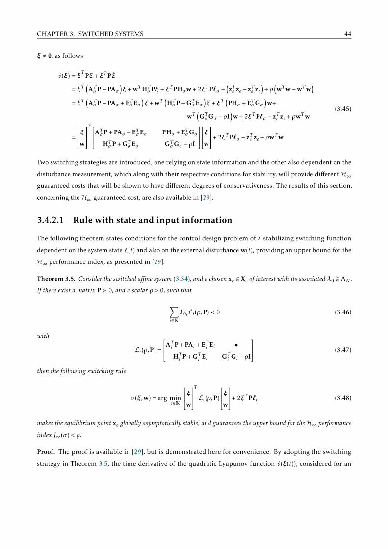
CHAPTER 3. SWITCHED SYSTEMS 44
ξ , 0, as follows
v(ξ) = ξTPξ +ξTPξ
= ξT(ATσP + PAσ
)ξ + wTHT
σPξ +ξTPHσw + 2ξTP`σ +(zTe ze − zTe ze
)+ ρ
(wTw−wTw
)= ξT
(ATσP + PAσ + ETσ Eσ
)ξ + wT
(HTσP + GT
σ Eσ)ξ +ξT
(PHσ + ETσGσ
)w+
wT(GTσGσ − ρI
)w + 2ξTP`σ − zTe ze + ρwTw
=
ξwT AT
σP + PAσ + ETσ Eσ PHσ + ETσGσ
HTσP + GT
σ Eσ GTσGσ − ρI
ξw
+ 2ξTP`σ − zTe ze + ρwTw
(3.45)
Two switching strategies are introduced, one relying on state information and the other also dependent on the
disturbance measurement, which along with their respective conditions for stability, will provide differentH∞guaranteed costs that will be shown to have different degrees of conservativeness. The results of this section,
concerning the H∞ guaranteed cost, are also available in [29].
3.4.2.1 Rule with state and input information
The following theorem states conditions for the control design problem of a stabilizing switching function
dependent on the system state ξ(t) and also on the external disturbance w(t), providing an upper bound for the
H∞ performance index, as presented in [29].
Theorem 3.5. Consider the switched affine system (3.34), and a chosen xe ∈ Xe of interest with its associated λ0 ∈ΛN .
If there exist a matrix P 0, and a scalar ρ > 0, such that
∑i∈K
λ0iLi(ρ,P) ≺ 0 (3.46)
with
Li(ρ,P) =
ATi P + PAi + ETi Ei •
HTi P + GT
i Ei GTi Gi − ρI
(3.47)
then the following switching rule
σ (ξ,w) = arg mini∈K
ξwT
Li(ρ,P)
ξw+ 2ξTP`i (3.48)
makes the equilibrium point xe globally asymptotically stable, and guarantees the upper bound for theH∞ performance
index J∞(σ ) < ρ.
Proof. The proof is available in [29], but is demonstrated here for convenience. By adopting the switching
strategy in Theorem 3.5, the time derivative of the quadratic Lyapunov function v(ξ(t)), considered for an

CHAPTER 3. SWITCHED SYSTEMS 45
arbitrary state trajectory ξ , 0, is calculated from (3.45) as follows
v(ξ) =
ξwT
Lσ (ρ,P)
ξw+ 2ξTP`σ − zTe ze + ρwTw
= mini∈K
ξwT
Li(ρ,P)
ξw+ 2ξTP`i − zTe ze + ρwTw
= minλ∈Λ
∑i∈K
λi
ξwT
Li(ρ,P)
ξw+ 2ξTP`λ − zTe ze + ρwTw
≤∑i∈K
λ0i
ξwT
Li(ρ,P)
ξw+ 2ξTP`λ0
− zTe ze + ρwTw
< −zTe ze + ρwTw (3.49)
where inequality (3.49) comes from condition (3.46), and by recalling that `λ0= 0. Notice that, for w(t) = 0, we
have v(ξ) < 0, and as such, the equilibrium point ξ = 0 is globally asymptotically stable. This allows for the
calculation of the upper bound ρ given by
v(ξ) < −zTe ze + ρwTw∫ ∞0v(ξ) dt < −
∫ ∞0
zTe ze dt + ρ∫ ∞
0wTw dt
limt→∞
v(ξ(t))− v(ξ(0)) < −‖ze‖22 + ρ‖w‖22
‖ze‖22 < ρ‖w‖22
(3.50)
where limt→∞ v(ξ(t)) = 0, for an asymptotically stable system, and v(ξ(0)) = 0, since ξ(0) = 0. For any
disturbance w(t) ∈ L2, w(t) , 0, ρ gives the upper bound for the H∞ performance index
J∞(σ ) = sup0,w∈L2
‖ze‖22‖w‖22
< ρ (3.51)
as desired.
Theorem 3.5 may be implemented by solving the following convex optimization problem, providing
matrix P, necessary to the switching rule (3.48)
min ρ
subject to: P 0, ρ > 0∑i∈K
λ0iLi(ρ,P) ≺ 0
(3.52)

CHAPTER 3. SWITCHED SYSTEMS 46
3.4.2.2 Rule with state information
A second switching strategy dependent only on state information σ (ξ) is of great relevance, given that the
disturbance w(t) is most often unavailable for measurement. To accomplish this, a disturbance w(t)? is
considered, such that it maximizes the product
supw∈L2
ξwT
Li(ρ,P)
ξw (3.53)
By defining the matrix product f (ξ,w) as
f (ξ,w) =
ξwT
Li(ρ,P)
ξw = ξT
(ATi P + PAi + ETi Ei
)ξ + 2ξT
(PHi + ETi Gi
)w + wT
(GTi Gi − ρI
)w (3.54)
taking the partial derivative of f (ξ,w) with respect to w(t), and setting it to zero
∂∂w
f (ξ,w) = 2(HTi P + GT
i Ei)ξ + 2
(GTi Gi − ρI
)w = 0 (3.55)
the disturbance input w(t)? can be calculated
w(t)? = −(GTi Gi − ρI
)−1 (HTi P + GT
i Ei)ξ(t) (3.56)
Notice that w(t)? indeed maximizes f (ξ,w), evidenced by evaluating the second derivative of f (ξ,w) with
respect to w(t)∂2
∂w2 f (ξ,w) = 2(GTi Gi − ρI
)(3.57)
whenever (GTi Gi − ρI) is negative definite.
Substituting w(t)? = −(GTi Gi − ρI
)−1 (HTi P + GT
i Ei)ξ(t) for the disturbance w(t) in f (ξ,w), thus eliminat-
ing its dependency on the disturbance, we obtain
f (ξ) = ξT(ATi P + PAi + ETi Ei −
(PHi + ETi Gi
)(GTi Gi − ρI
)−1 (HTi P + GT
i Ei))ξ (3.58)
By defining the new matrix termNi(ρ,P) as
Ni(ρ,P) = ATi P + PAi + ETi Ei −
(PHi + ETi Gi
)(GTi Gi − ρI
)−1 (HTi P + GT
i Ei)
(3.59)
and introducing symmetric indefinite matrices Qi , for i ∈K, then the following inequalities are satisfied
Ni(ρ,P) + Qi ≺ 0 (3.60)(GTi Gi − ρI
)≺ 0 (3.61)
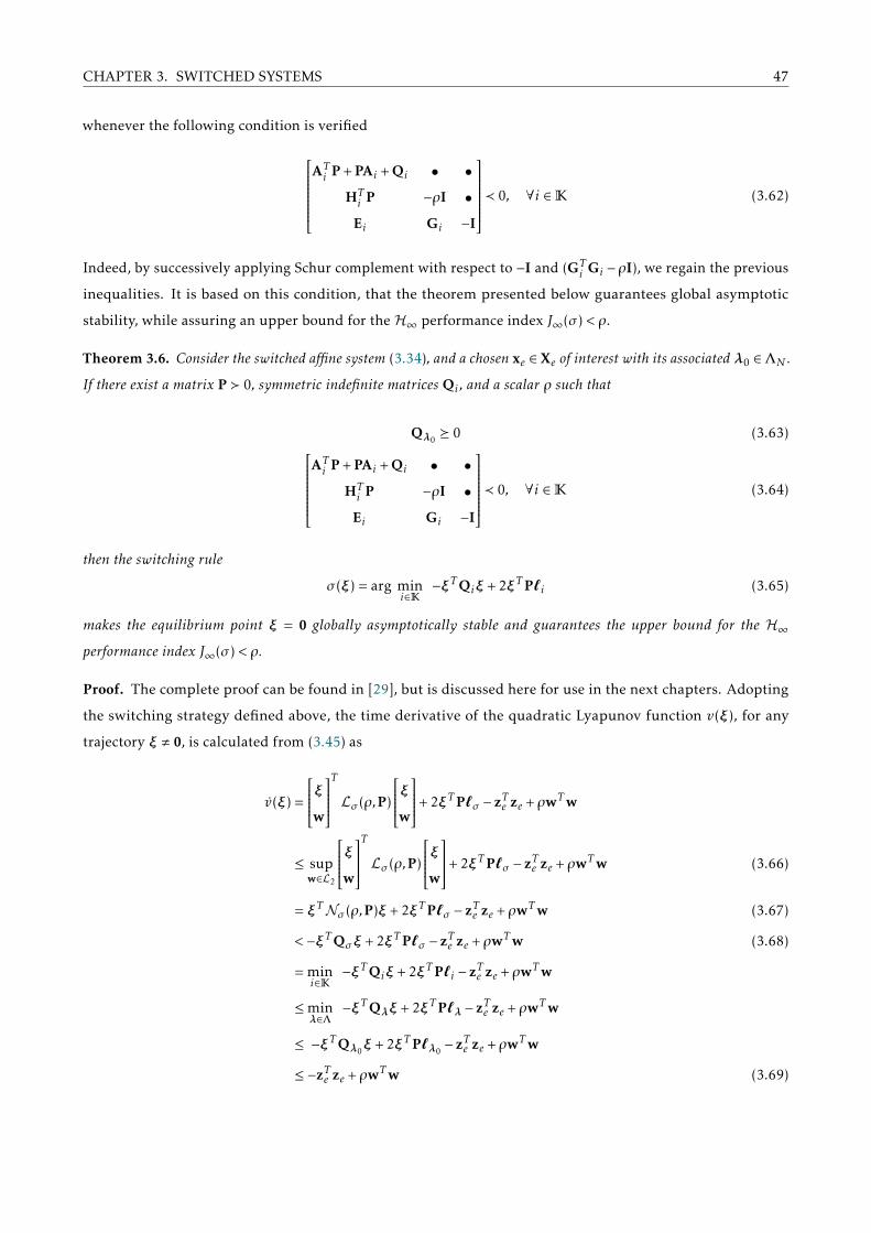
CHAPTER 3. SWITCHED SYSTEMS 47
whenever the following condition is verified
ATi P + PAi + Qi • •
HTi P −ρI •
Ei Gi −I
≺ 0, ∀i ∈K (3.62)
Indeed, by successively applying Schur complement with respect to −I and (GTi Gi − ρI), we regain the previous
inequalities. It is based on this condition, that the theorem presented below guarantees global asymptotic
stability, while assuring an upper bound for the H∞ performance index J∞(σ ) < ρ.
Theorem 3.6. Consider the switched affine system (3.34), and a chosen xe ∈ Xe of interest with its associated λ0 ∈ΛN .
If there exist a matrix P 0, symmetric indefinite matrices Qi , and a scalar ρ such that
Qλ0 0 (3.63)
ATi P + PAi + Qi • •
HTi P −ρI •
Ei Gi −I
≺ 0, ∀i ∈K (3.64)
then the switching rule
σ (ξ) = arg mini∈K
−ξTQiξ + 2ξTP`i (3.65)
makes the equilibrium point ξ = 0 globally asymptotically stable and guarantees the upper bound for the H∞performance index J∞(σ ) < ρ.
Proof. The complete proof can be found in [29], but is discussed here for use in the next chapters. Adopting
the switching strategy defined above, the time derivative of the quadratic Lyapunov function v(ξ), for any
trajectory ξ , 0, is calculated from (3.45) as
v(ξ) =
ξwT
Lσ (ρ,P)
ξw+ 2ξTP`σ − zTe ze + ρwTw
≤ supw∈L2
ξwT
Lσ (ρ,P)
ξw+ 2ξTP`σ − zTe ze + ρwTw (3.66)
= ξTNσ (ρ,P)ξ + 2ξTP`σ − zTe ze + ρwTw (3.67)
< −ξTQσξ + 2ξTP`σ − zTe ze + ρwTw (3.68)
= mini∈K
−ξTQiξ + 2ξTP`i − zTe ze + ρwTw
≤minλ∈Λ
−ξTQλξ + 2ξTP`λ − zTe ze + ρwTw
≤ −ξTQλ0ξ + 2ξTP`λ0
− zTe ze + ρwTw
≤ −zTe ze + ρwTw (3.69)

CHAPTER 3. SWITCHED SYSTEMS 48
where equality (3.67) comes from the fact that from definition (3.54) the supremum indicated in (3.66) provides
(3.58) with Ni(ρ,P) defined in (3.59); inequality (3.68) stems from (3.64) which is equivalent to (3.60); and
inequality (3.69) arises from condition (3.63), and by realizing that `λ0= 0. Once again, we have that, for
w(t) = 0, v(ξ) < 0, and as a consequence, the equilibrium point ξ = 0 is globally asymptotically stable, and the
upper bound for the H∞ performance index J∞(σ ) < ρ is guaranteed, as previously demonstrated in the proof
of Theorem 3.5.
It should be noted that Theorems 3.5 and 3.6 do not impose that Ai be Hurwitz, for all i ∈K, because of
the presence of matrices Qi , i ∈K as discussed in the previous sections. However, conditions (3.46) and (3.64)
do require that Aλ ∈ H, as has been recurrent thus far. Furthermore, an important aspect of Theorem 3.6 is
that the conditions are based on the fact that Qλ 0, and as such,∑i∈KλiNi(ρ,P) ≺ 0, but due to the product
between indexed matrices, specifically ETi Ei , GTi Ei and GT
i Gi , we have that
Nλ(ρ,P) ∑i∈K
λiNi(ρ,P) ≺ 0, λ ∈ΛN
which indicates that a less conservative, and thus more desirable condition would beNλ(ρ,P) ≺ 0. Unfortunately,
a stability condition assured by this inequality does not exist for switched systems in general. For the special
case where the matrices Hi , Ei and Gi are constant throughout the subsystems, that is, Hi = H, Ei = E and
Gi = E, ∀i ∈K, we haveNλ(ρ,P) =∑i∈KλiNi(ρ,P) and a stability condition based on the convex combination
of subsystem matrices holds true. Notice that, for the conditions of Theorem 3.5, the same conclusion can be
drawn without requiring that matrices Hi be constant across subsystems.
To implement switching rule (3.65) of Theorem 3.6, the following convex optimization problem
min ρ
subject to: P 0, ρ > 0
Qλ0 0
ATi P + PAi + Qi • •
HTi P −ρI •
Ei Gi −I
≺ 0, ∀i ∈K
(3.70)
provides the matrices Qi , for i ∈K, as well as matrix P required.

CHAPTER 3. SWITCHED SYSTEMS 49
3.4.2.3 Numerical Example
The following numerical example is supplied to compare the H∞ performance index guaranteed by Theorems
3.5 and 3.6, as well as those obtained via numerical simulation.
Example 3.5.
Consider the switched affine system of Example 3.3, with
E1 = E2 =[1 1
], H1 =
30 , H2 =
−3
3
Before implementing the switching rule (3.48) of Theorem 3.5, matrix P has been calculated by solving the
optimization problem (3.52), which in this case yielded
P =
0.7339 −0.2187
−0.2187 1.2374
along with the guaranteed cost of J∞(·) < 4.0697. Similarly, for Theorem 3.6, the matrices P, Q1, and Q2 were
calculated by solving (3.70), resulting in
P =
0.7669 −0.2638
−0.2638 1.2982
, Q1 =
−13.4815 0.5943
0.5943 −6.2805
, Q2 =
3.3704 −0.1486
−0.1486 1.5701
associated to the guaranteed cost J∞(·) < 7.1601, slightly larger than that guaranteed by Theorem 3.5, given the
greater conservativeness imposed.
By applying the following disturbance to the system
w(t) =
sin(πt), 2 ≤ t ≤ 5
0, otherwise
the trajectories in time for each state can be seen in Figure 3.9, for Theorem 3.5, and Figure 3.10, for Theorem
3.6. Notice that, after the disturbance ceases, the respective switching functions are able to successfully stabilize
the systems to the equilibrium point ξ = 0. For the H∞ case it is not possible to obtain the actual cost J∞(σ ) by

CHAPTER 3. SWITCHED SYSTEMS 50
0 2 4 6 8 10
-1.5
-1
-0.5
0
0.5
1
0 2 4 6 8 10
-1.5
-1
-0.5
0
0.5
1
Figure 3.9: Trajectories of each state for the switched affine system under Theorem 3.5.
0 2 4 6 8 10
-1.5
-1
-0.5
0
0.5
1
0 2 4 6 8 10
-1.5
-1
-0.5
0
0.5
1
Figure 3.10: Trajectories of each state for the switched affine system under Theorem 3.6.
numerical integration, in contrast with the analysis employed for the H2 case, since the worst case external
input w(t) for switched system is in general extremely difficult to calculate.

51
Chapter 4
Joint Action Output Feedback Control
The previous chapters introduced underlying concepts that are essential to the main contributions
of this work, which consist in the H2 and H∞ dynamic output feedback control design of
continuous-time switched affine systems by considering the simultaneous design of a set of full
order controllers and a switching function. To the best of the author’s knowledge, this is the first
time that the joint design of two control variables are taken into account in the context of output feedback
control of switched affine systems, and have resulted in the following submitted publication [31] in which the
contents of this chapter are based upon.
4.1 Introduction
Most results available in the literature treat the control design problem for switched affine systems considering
the switching function as the sole control variable to be determined. Some results have been previously
mentioned, such as the references [26, 27, 28] which deal with the design of state dependent switching rules,
and references [16, 30], which consider an output dependent switching rule. In [30], the switching rule is
implemented by means of a full-order switched affine observer, while [16] considers the design of a full-
order switched dynamical filter to provide the information needed by the switching function. However fewer
references treat the control design problem considering the joint action of a switching rule in tandem with a
control law u(t). The following authors [29] approach this problem by adopting a state dependent switching
rule paired with a control law of the form u(t) = Kσx(t), σ ∈ K. This however limits the scope of practical
applications in which this technique may be considered for, given that in many situations the state vector is not
available for measurement.
Given the above, the control design problem considering two output-dependent control structures is
clearly a relevant topic of research, having only been tackled for the case of switched linear systems in [24] and
[46]. As such, the results in this chapter generalize the ideas introduced by [16, 24, 29] to deal with the joint
design of two stabilizing control variables in the context of switched affine systems, more specifically three
techniques based on a full-order switched dynamical controller acting in cooperation with a switching rule,
both dependent entirely on the measured output, and guaranteeing global asymptotic stability of the desired
equilibrium point are introduced. The first assures an H2 guaranteed cost while the other two methodologies
assure upper bounds for the H∞ performance indices with varying degrees of conservativeness.
Some important characteristics of this new methodology are that not only no stability property is expected
of individual subsystem matrices Ai , for all i ∈K, but it is no longer required that Aλ ∈ H, thus not restricting
the choice of the vector λ ∈ΛN , a requirement which has permeated the results of the previous chapters. This

CHAPTER 4. JOINT ACTION OUTPUT FEEDBACK CONTROL 52
characteristic is very compelling since it allows a larger set of equilibrium points Xe of the switched system to
be attainable, instead of only the subset where Aλ is Hurwitz. This is made possible by joint action of both
control structures, and will become clear throughout the course of the chapter.
4.2 Problem Statement
Consider the switched affine system with the following state space representation, already given in its shifted
configuration
ξ(t) = Aσξ(t) + Bσu(t) + Hσw(t) + `σ , ξ(0) = 0
ye(t) = Cσξ(t) + Dσw(t)
ze(t) = Eσξ(t) + Fσu(t) + Gσw(t)
(4.1)
where ξ(t) ∈ Rnx is the state vector, considered to be unavailable for measurement, u(t) ∈ Rnu is the control
input to be designed, w(t) ∈Rnw is the external disturbance, ye(t) ∈Rny is the measured output, ze(t) ∈Rnz is
the performance output, and `i = Aixe + bi for all i ∈K are the affine terms. Notice that ye(t) = y(t)−Cσxe, with
y(t) = Cσx(t) + Dσw(t), when expressed in terms of x(t).
Recall from Definition 1 that whenever bi , 0 for some i ∈ K, the switched system possesses several
equilibrium points, characterizing the subset of the state space given by
Xe =xe ∈Rnx : xe = −A−1
λ bλ, λ ∈ΛN
(4.2)
A given choice of xe ∈ Xe, with its associated vector λ0 ∈ΛN completes the definition of system (4.1).
Our main objective is to design a control law u(t), implemented via a full-order switched dynamical
controller and dependent of the measured output y(t), along with a switching function σ (ye(t)) : Rny → K
that together are capable of guaranteeing global asymptotic stability of a chosen equilibrium point xe ∈ Xe,
or equivalently, ξ = 0. These two control structures must also assure upper bounds for the H2 and H∞performance indices. To this end, the following full-order switched affine controller is proposed, with state
space representation given by
Cσ :
˙ξ(t) = Aσ ξ(t) + Bσye(t) + ˆ
σ , ξ(0) = 0
u(t) = Cσ ξ(t)(4.3)
where ξ ∈Rnx is the state vector of the controller, u(t) ∈Rnu is the control signal, and matrices Ai , Bi , Ci to be
determined, have appropriate dimensions. The controller state ξ will not only be used to provide the control
signal u(t), but it will also make possible implementing the switching function σ (ye(t)).
By connecting the controller (4.3) to the switched system (4.1), as illustrated in Figure 4.1, and defining

CHAPTER 4. JOINT ACTION OUTPUT FEEDBACK CONTROL 53
System Dynamics
Controllerσ
w(t)
ye(t)ξ(t)
ze(t)
u(t)
Figure 4.1: Closed-loop system.
the state vector ξ(t) =[ξ(t)T ξ(t)T
]T∈R2nx , the following augmented system emerges
˙ξ(t) = Aσ ξ(t) + Hσw(t) + ˜σ , ξ(0) = 0
ze(t) = Eσ ξ(t) + Gσw(t)(4.4)
with matrices given by
Ai =
Ai BiCi
BiCi Ai
, ˜i =
`iˆi
, Hi =
Hi
BiDi
Ei =
[Ei FiCi
], Gi = Gi
(4.5)
The control design problem consists in determining appropriate conditions that will satisfy Theorems
3.4, 3.5, and 3.6, introduced in Chapter 3, for the augmented system (4.4), thus guaranteeing global asymptotic
stability of the closed-loop system, and assuring an upper bound for the H2 and H∞ performance indices, as
defined in (3.35) and (3.44), respectively.
Before proceeding, we first address the problem of obtaining a switching rule that forgoes any dependency
on the unknown system state, a result that will be used for the two first theorems, and will be further extended
to deal with a switching rule also relying on the disturbance measurement. To accomplish this, we first define
block symmetric matrices P and P−1 as
P−1 =
X U
UT X
, P =
Y V
VT Y
(4.6)
such that the relation P−1P = I holds. This implies in the following
XY + UVT = I, XV + UY = 0, UTY + XVT = 0, UTV + XY = I (4.7)
and let Qi be the block symmetric indefinite matrix
Qi =
0 0
0 Qi
, i ∈K (4.8)
Now, recall the following switching rule, employed in Theorems 3.4 and 3.6, and applied to the augmented

CHAPTER 4. JOINT ACTION OUTPUT FEEDBACK CONTROL 54
system (4.4)
σ (ξ) = arg mini∈K−ξT Qi ξ + 2ξ
T P˜i (4.9)
Let us first consider the matrix product ξT Qi ξ. Observe that the structure of Qi has been defined in order to
eliminate any dependency on the unknown system state. Notice that the choice of a constant matrix M for
block (1,2), and a constant symmetric matrix for block (1,1), would also be possible, since although the product
ξT Qi ξ would depend on ξ(t), as such
ξT Qi ξ = ξTNξ + 2ξ
TMT ξ + ξ
TQi ξ, i ∈K (4.10)
the dependent terms ξTNξ and ξT
MT ξ are not indexed, and thus, would be constant across i ∈K. This would
allow for the definition of an equivalent switching function considering only the product ξT
Qi ξ. This approach,
however, has not shown any advantage with regard to the optimality of the guaranteed cost over the structure
of Qi originally defined in (4.8). As such, we base this technique on this simpler choice of Qi .
Now we consider the product ξT P˜
i , as follows
ξT P˜
i =
ξξT Y V
VT Y
`iˆi
(4.11)
Notice that by assuring Y`i + V ˆi = 0, the first nx rows of term P˜
i are null, as such, the dependency on the
system state is eliminated by making the appropriate choice of ˆi as
ˆi = −V−1Y`i , ∀i ∈K (4.12)
where V is such that ∃V−1. Observe that this choice also guarantees the nullity of ˜λ0
= 0, since `λ0= 0, as such
˜λ0
=
`λ0
ˆλ0
=
`λ0
−V−1Y`λ0
= 0 (4.13)
The term ξT P˜
i , given in (4.11), with (4.12) and the relations Y = −U−1XV and VT = U−1 (I−XY) from (4.7),
can be rewritten as
ξT P˜
i =
ξξT 0
VT `i + Y ˆi
= ξT
(VT `i + Y ˆi) = ξ
TU−1`i (4.14)
Thus, as desired, the switching rule can be expressed with a dependency solely on the state of the controller ξ,
that is
σ (ξ) = σ (ξ) = arg mini∈K−ξT Qi ξ + 2ξ
TU−1`i (4.15)
The problem consists in finding conditions that can be expressed in terms of LMIs, allowing us to obtain
the matrices Ai , Bi , and Ci , i ∈K, as well as the vectors ˆi , needed for implementing the dynamical controller,
and matrices Qi and U−1 important for the switching rule σ (·), by solving a convex optimization problem by
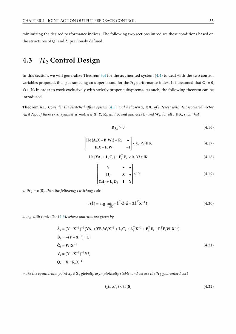
CHAPTER 4. JOINT ACTION OUTPUT FEEDBACK CONTROL 55
minimizing the desired performance indices. The following two sections introduce these conditions based on
the structures of Qi and ˜i previously defined.
4.3 H2 Control Design
In this section, we will generalize Theorem 3.4 for the augmented system (4.4) to deal with the two control
variables proposed, thus guaranteeing an upper bound for theH2 performance index. It is assumed that Gi = 0,
∀i ∈K, in order to work exclusively with strictly proper subsystems. As such, the following theorem can be
introduced
Theorem 4.1. Consider the switched affine system (4.1), and a chosen xe ∈ Xe of interest with its associated vector
λ0 ∈ΛN . If there exist symmetric matrices X, Y, Ri , and S, and matrices Li and Wi , for all i ∈K, such that
Rλ0 0 (4.16)
He AiX + BiWi+ Ri •
EiX + FiWi −I
≺ 0, ∀i ∈K (4.17)
He YAi + LiCi+ ETi Ei ≺ 0, ∀i ∈K (4.18)S • •
Hj X •
YHj + LjDj I Y
0 (4.19)
with j = σ (0), then the following switching rule
σ (ξ) = arg mini∈K−ξT Qi ξ + 2ξ
TX−1`i (4.20)
along with controller (4.3), whose matrices are given by
Ai = (Y−X−1)−1(YAi + YBiWiX−1 + LiCi + AT
i X−1 + ETi Ei + ETi FiWiX−1)
Bi = −(Y−X−1)−1Li
Ci = WiX−1
ˆi = (Y−X−1)−1Y`i
Qi = X−1RiX−1
(4.21)
make the equilibrium point xe ∈ Xe globally asymptotically stable, and assure the H2 guaranteed cost
J2(σ,Cσ ) < tr (S) (4.22)
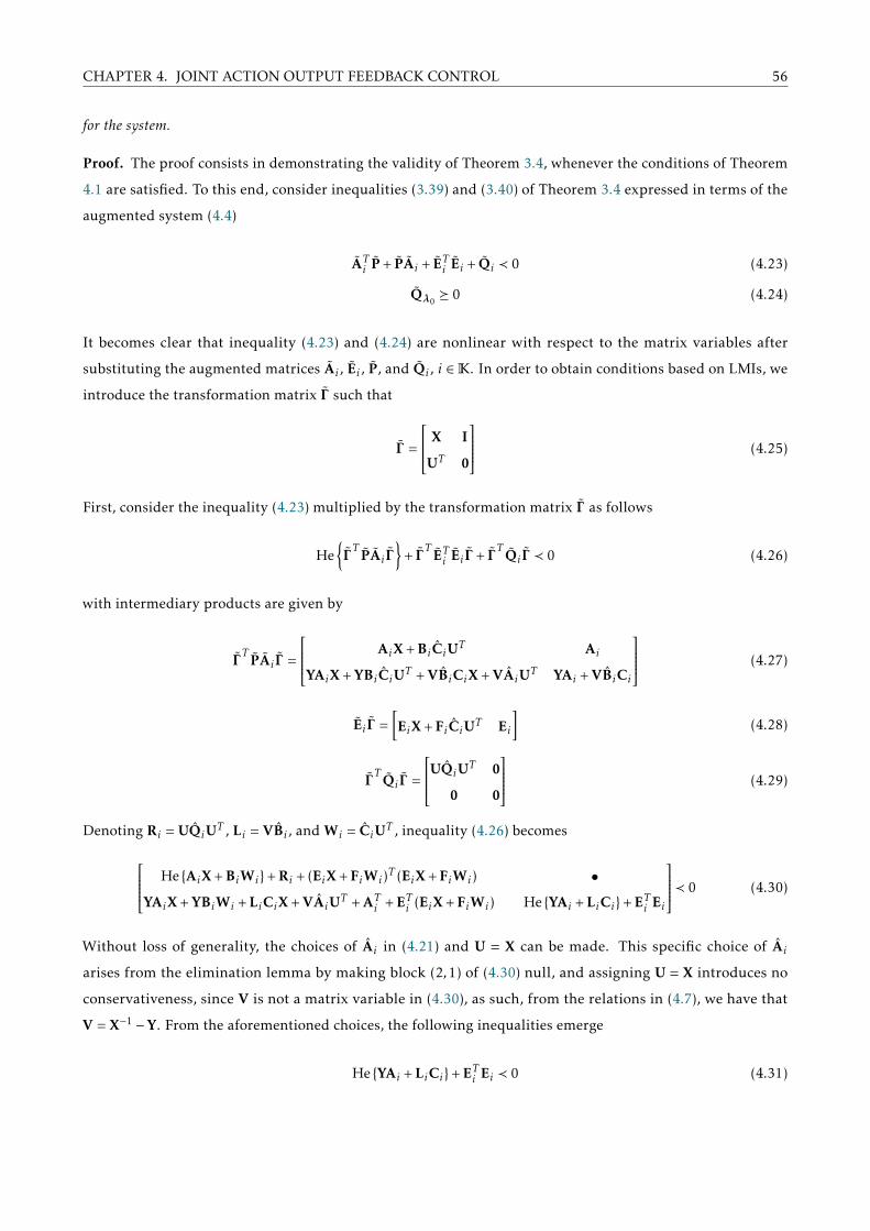
CHAPTER 4. JOINT ACTION OUTPUT FEEDBACK CONTROL 56
for the system.
Proof. The proof consists in demonstrating the validity of Theorem 3.4, whenever the conditions of Theorem
4.1 are satisfied. To this end, consider inequalities (3.39) and (3.40) of Theorem 3.4 expressed in terms of the
augmented system (4.4)
ATi P + PAi + ETi Ei + Qi ≺ 0 (4.23)
Qλ0 0 (4.24)
It becomes clear that inequality (4.23) and (4.24) are nonlinear with respect to the matrix variables after
substituting the augmented matrices Ai , Ei , P, and Qi , i ∈K. In order to obtain conditions based on LMIs, we
introduce the transformation matrix Γ such that
Γ =
X I
UT 0
(4.25)
First, consider the inequality (4.23) multiplied by the transformation matrix Γ as follows
HeΓT PAi Γ
+ Γ
T ETi Ei Γ + ΓT Qi Γ ≺ 0 (4.26)
with intermediary products are given by
ΓT PAi Γ =
AiX + BiCiUT Ai
YAiX + YBiCiUT + VBiCiX + VAiUT YAi + VBiCi
(4.27)
Ei Γ =[EiX + FiCiUT Ei
](4.28)
ΓT Qi Γ =
UQiUT 0
0 0
(4.29)
Denoting Ri = UQiUT , Li = VBi , and Wi = CiUT , inequality (4.26) becomes
He AiX + BiWi+ Ri + (EiX + FiWi)T (EiX + FiWi) •
YAiX + YBiWi + LiCiX + VAiUT + ATi + ETi (EiX + FiWi) He YAi + LiCi+ ETi Ei
≺ 0 (4.30)
Without loss of generality, the choices of Ai in (4.21) and U = X can be made. This specific choice of Ai
arises from the elimination lemma by making block (2,1) of (4.30) null, and assigning U = X introduces no
conservativeness, since V is not a matrix variable in (4.30), as such, from the relations in (4.7), we have that
V = X−1 −Y. From the aforementioned choices, the following inequalities emerge
He YAi + LiCi+ ETi Ei ≺ 0 (4.31)

CHAPTER 4. JOINT ACTION OUTPUT FEEDBACK CONTROL 57
He AiX + BiWi+ Ri •
EiX + FiWi −I
≺ 0 (4.32)
Indeed, (4.31) comes directly from block (2,2) of (4.30), and inequality (4.32) is obtained by applying Schur
complement on block (1,1) of (4.30) with respect to (EiX + FiWi)T (EiX + FiWi). It can be seen that whenever
these inequalities are satisfied, and by adopting Ai and U as above, inequality (4.23) from Theorem 3.4 is
verified. Also, observe that (4.16) assures that Qλ0 0, thus satisfying condition (4.24) of Theorem 3.4 for the
augmented system (4.4).
Furthermore, notice that the switching rule
σ (ξ) = arg mini∈K−ξT Qi ξ + 2ξ
TX−1`i (4.33)
comes directly from (4.15) when considering U = X, as well as the identities (4.21).
Finally, we have that the following inequality
S • •
Hj X •
YHj + LjDj I Y
0 (4.34)
is equivalent to S •
ΓT PHj Γ
T PΓ
0 (4.35)
with intermediary terms are given by
ΓT PΓ =
X I
I Y
(4.36)
HTj PΓ =
[HTj HT
j Y + DTj LTj
](4.37)
By multiplying inequality (4.35) to the left by diag(I, (Γ T )−1), to the right by its transpose, and subsequently
applying Schur complement with respect to P, we obtain
HTj PHj ≺ S (4.38)
and thus,
J2(σ,Cσ ) < tr(HTj PHj
)< tr (S) (4.39)
with j = σ (0), is guaranteed by Theorem 3.4. This concludes the proof.
This theorem presents a few compelling characteristics. First, notice that the inequalities in (4.17) do not
require that the closed-loop matrices Acl,i = Ai + BiKc,i , with Kc,i = WiX−1, be Hurwitz, since matrices Ri are
indefinite. Thus, Theorem 4.1 can assure stability of the switched system even if each individual subsystem is

CHAPTER 4. JOINT ACTION OUTPUT FEEDBACK CONTROL 58
not stabilizable. Also, notice that not only there is no imposition on matrices Ai ∈ H, but no convex combination
of subsystem matrices Aλ ∈ H needs to exit, as was recurrent in the previous chapter. Instead, inequalities
(4.16) and (4.17) impose that ∑i∈K
λ0i
(He
Acl,iX
+ XETcl,iEcl,iX
)≺ 0 (4.40)
with Ec,i = Ei + FiKcl,i , i ∈K. In other words, it is now only necessary that a stable convex combination of the
closed loop matrices exists. These considerations bring to light the fact that Theorem 4.1 is able to guarantee
global asymptotic stability of the equilibrium point of interest even in the case where a control law u(t) and a
switching rule σ (t) are unable to do so when operating independently, allowing for a wider range of problems
to be considered. This interesting situation is considered in a numerical example presented towards the
end of this chapter. It should be noted that, although the inequalities in (4.18) make necessary that closed
loop matrices Ai + Ko,iCi , with Ko,i = Y−1Li be quadratically stable with respect to Y, this, however, is not a
difficult requirement, since these inequalities are uncoupled from (4.17), through different matrices Y and X.
Furthermore, the matrix gains Ko,i depend in the index i, and thus are independent for each restriction. Finally,
notice that, as in the case for Theorem 3.4, an appropriate choice of σ (0) can be made so as to optimize the H2
performance index, or alternatively, by considering σ (0) of worst case the H2 control design problem is made
robust with respect to σ (0), as previously discussed.
When compared to existing results in the literature, such as [30] and [16], Theorem 4.1 presents more
lenient conditions. The first reference requires that all matrices Ai be Hurwitz, thus being a more conservative
result, while the latter requires Aλ ∈ H, since a control law u(t) is not taken into account. The following
optimization problem, subject to the LMI conditions in Theorem 4.1, provides the matrices necessary to
implement the dynamical controller and switching rule, through the relations in (4.21).
min tr(S)
subject to: Rλ0 0
He YAi + LiCi+ ETi Ei ≺ 0, ∀i ∈KHe AiX + BiWi+ Ri •
EiX + FiWi −I
≺ 0, ∀i ∈KS • •
Hj X •
YHj + LjDj I Y
0
(4.41)
The next examples aim to illustrate the relevance and usefulness of the proposed methodology. The first
reminisces the switched affine system of Example 3.3, and the second is based on the example of [31].
4.3.1 Numerical example: H2 Control Design
In this example, the switched affine system of Example 3.3 is adopted, with additional inputs u(t) and w(t), and
outputs ye(t) and ze(t) as in (4.1).

CHAPTER 4. JOINT ACTION OUTPUT FEEDBACK CONTROL 59
Example 4.1.
Consider the switched affine system (4.1) with dynamical matrices given in Example 3.3, and with
B1 = B2 =
10
10
, H1 =
10 , H2 =
−1
1
C1 = C2 =
[1 1
], D1 = D2 = 1, E1 = E2 = I, G1 = G2 = 0, F1 = F2 =
41
By choosing the equilibrium point xe = [0.2982 1.2586]T of interest, associated to λ0 = [0.4 0.6]T , it can be
noted that the convex combination Aλ0is not Hurwitz, as such, Theorem 3.4 cannot guarantee the global
asymptotic stability of the desired equilibrium point, and another approach must be used. A state feedback
control design technique may be employed if the state is available for measurement, however in many situations
this is not the case. The methodology introduced in this work addresses this scenario, and will be used in this
example.
First, the convex optimization problem (4.41) is solved, in order to implement the switching rule (4.20).
The following matrices, needed to implement the dynamical controller are obtained via the identities in (4.21).
A1 =
−4.8637 −4.8656
1.1615 1.1621
× 104, A2 =
−17.7251 −16.3277
4.1664 −7.3999
, B1 =
4.8646
−1.1617
× 104, B2 =
11.0817
−0.5102
C1 = C2 =
[−0.2287 −0.1773
], ˆ
1 =
1.6111
12.4843
, ˆ2 =
−1.0741
−8.3229
as well as the matrices important for the switching rule
Q1 =
−0.2608 0.7002
0.7002 −1.3657
, Q2 =
0.1739 −0.4668
−0.4668 0.9105
, X =
101.7381 10.6627
10.6627 5.5607
along with the guaranteed cost J2(σ,Cσ ) < 34.1051 for σ (0) = 2, which minimizes the H2 index. For the initial
condition ξ0 = H2, the trajectories in time for each state can be seen in Figure 4.2. The output ze(t) and control
signal u(t) are shown in Figure 4.3. Notice that the joint action of both control inputs, σ (ye(t)) and u(t), were
able to asymptotically stabilize the system.
Furthermore, by numerical integration of the product ze(t)′ze(t), the H2 cost of the system is calculated
as J2 = 5.2066 < 34.1051, within the cost assured by Theorem 4.1, as expected.
Now, only for the sake of illustration, we considered multiple initial conditions distributed around a
circle ‘ ’ of radius 10 centered at the origin ‘×’, that is, ξ0 = ξ0 = 10× [cos(θ) sin(θ)]T , θ ∈ [0,2π] and we have
implemented the switching rule and the switched controllers previously determined for the system
˙ξ = Aσ ξ + ˜σ , ξ(0) = ξ0 (4.42)
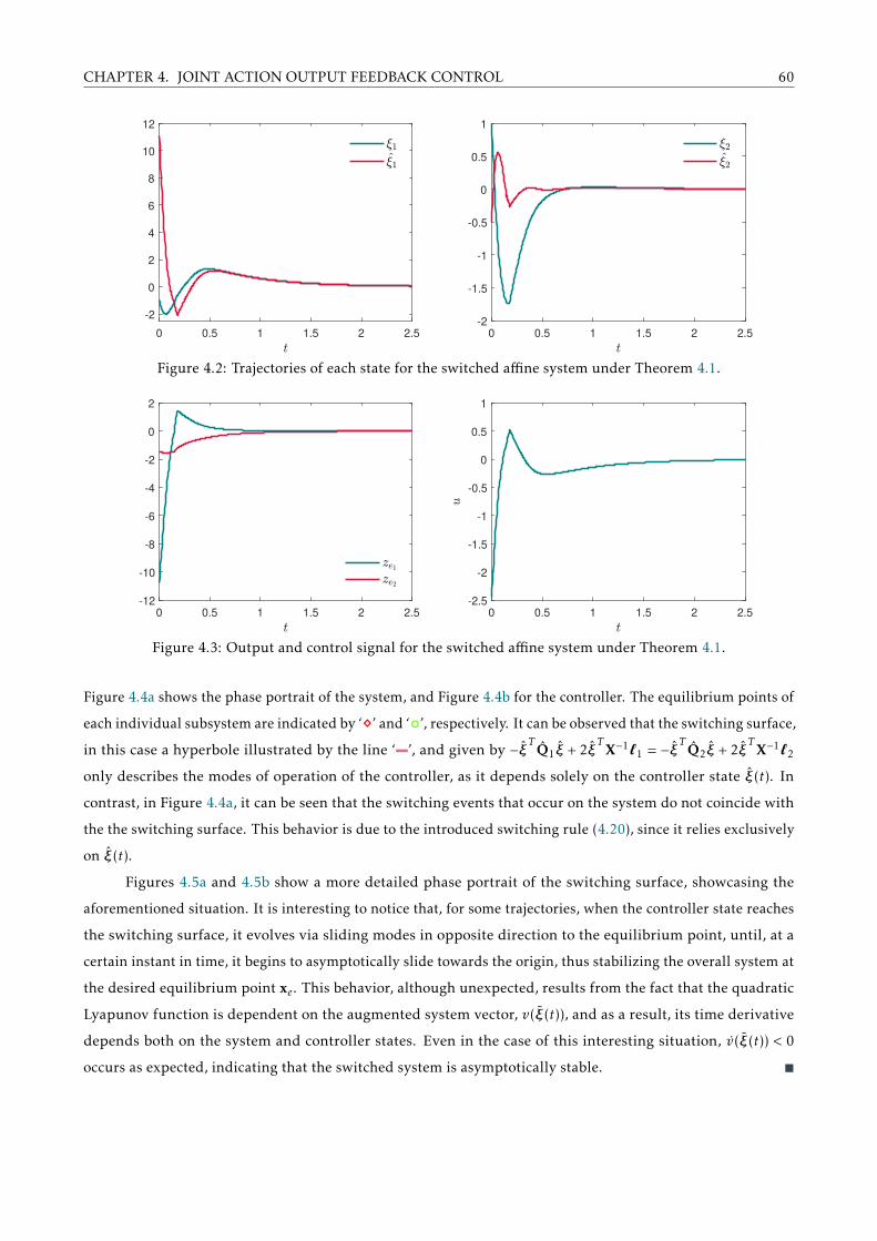
CHAPTER 4. JOINT ACTION OUTPUT FEEDBACK CONTROL 60
0 0.5 1 1.5 2 2.5
-2
0
2
4
6
8
10
12
0 0.5 1 1.5 2 2.5
-2
-1.5
-1
-0.5
0
0.5
1
Figure 4.2: Trajectories of each state for the switched affine system under Theorem 4.1.
0 0.5 1 1.5 2 2.5
-12
-10
-8
-6
-4
-2
0
2
0 0.5 1 1.5 2 2.5
-2.5
-2
-1.5
-1
-0.5
0
0.5
1
Figure 4.3: Output and control signal for the switched affine system under Theorem 4.1.
Figure 4.4a shows the phase portrait of the system, and Figure 4.4b for the controller. The equilibrium points of
each individual subsystem are indicated by ‘’ and ‘’, respectively. It can be observed that the switching surface,
in this case a hyperbole illustrated by the line ‘ ’, and given by −ξT Q1ξ + 2ξT
X−1`1 = −ξT Q2ξ + 2ξT
X−1`2
only describes the modes of operation of the controller, as it depends solely on the controller state ξ(t). In
contrast, in Figure 4.4a, it can be seen that the switching events that occur on the system do not coincide with
the the switching surface. This behavior is due to the introduced switching rule (4.20), since it relies exclusively
on ξ(t).
Figures 4.5a and 4.5b show a more detailed phase portrait of the switching surface, showcasing the
aforementioned situation. It is interesting to notice that, for some trajectories, when the controller state reaches
the switching surface, it evolves via sliding modes in opposite direction to the equilibrium point, until, at a
certain instant in time, it begins to asymptotically slide towards the origin, thus stabilizing the overall system at
the desired equilibrium point xe. This behavior, although unexpected, results from the fact that the quadratic
Lyapunov function is dependent on the augmented system vector, v(ξ(t)), and as a result, its time derivative
depends both on the system and controller states. Even in the case of this interesting situation, v(ξ(t)) < 0
occurs as expected, indicating that the switched system is asymptotically stable.
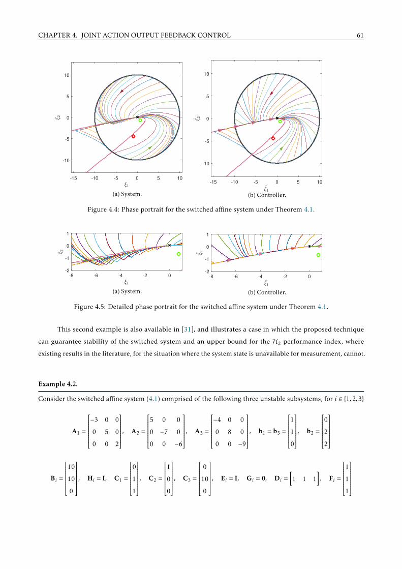
CHAPTER 4. JOINT ACTION OUTPUT FEEDBACK CONTROL 61
-15 -10 -5 0 5 10
-10
-5
0
5
10
(a) System.
-15 -10 -5 0 5 10
-10
-5
0
5
10
(b) Controller.
Figure 4.4: Phase portrait for the switched affine system under Theorem 4.1.
-8 -6 -4 -2 0
-2
-1
0
1
(a) System.
-8 -6 -4 -2 0
-2
-1
0
1
(b) Controller.
Figure 4.5: Detailed phase portrait for the switched affine system under Theorem 4.1.
This second example is also available in [31], and illustrates a case in which the proposed technique
can guarantee stability of the switched system and an upper bound for the H2 performance index, where
existing results in the literature, for the situation where the system state is unavailable for measurement, cannot.
Example 4.2.
Consider the switched affine system (4.1) comprised of the following three unstable subsystems, for i ∈ 1,2,3
A1 =
−3 0 0
0 5 0
0 0 2
, A2 =
5 0 0
0 −7 0
0 0 −6
, A3 =
−4 0 0
0 8 0
0 0 −9
, b1 = b3 =
1
1
0
, b2 =
0
2
2
Bi =
10
10
0
, Hi = I, C1 =
0
1
1
, C2 =
1
0
0
, C3 =
0
10
0
, Ei = I, Gi = 0, Di =[1 1 1
], Fi =
1
1
1

CHAPTER 4. JOINT ACTION OUTPUT FEEDBACK CONTROL 62
also available in [31]. It is important to observe that the matrix pairs (Ai ,Bi) are not controllable for i ∈ 1,2,3,
and that there exists no λ ∈Λ3 such that a convex combination Aλ is Hurwitz. As such, only the joint action of
a switching function operating alongside a control signal, as proposed in this work, are able to stabilize the
system.
Choosing the equilibrium point xe = [0.636 − 0.517 0.237]T ∈ Xe of interest, associated to λ0 =
[0.2 0.3 0.5]T , we can proceed with solving the optimization problem (4.41). For the present example, the
following matrices were obtained
Y =
116.8807 68.5008 110.6348
68.5008 50.1472 79.2307
110.6348 79.2307 129.5470
, X =
183.9763 126.7359 115.2653
126.7359 88.5686 80.6768
115.2653 80.6768 85.1066
W1 =
−145.2052
−101.9092
−93.5959
T
, W2 =
−145.2252
−101.9232
−93.6103
T
, W3 =
−145.1352
−101.8601
−93.5454
T
L1 =
0.0956
−1.5061
−1.4760
× 103, L2 =
−3.6887
−0.0868
−0.1354
× 104, L3 =
−104.7484
−73.1233
−115.8267
used for implementing the dynamic controller and the switching rule considering the relations in (4.21). An
associated guaranteed cost of J2(σ,Cσ ) < 18.6502 for σ (0) = 3 was also obtained. For the initial condition
ξ0 = H3ψ1 = [1 0 0]T , the trajectories in time for each state can be seen in Figure 4.2. The output ze(t) and
control signal u(t), are shown in Figure 4.3. The joint action of both control structures were successfully able to
0 0.5 1 1.5
0
0.2
0.4
0.6
0.8
1
0 0.5 1 1.5
-0.5
0
0.5
1
1.5
2
2.5
3
3.5
0 0.5 1 1.5
-1.5
-1
-0.5
0
0.5
1
Figure 4.6: Trajectories of each state for the switched affine system under Theorem 4.1 for ψ1.
stabilize the switched system at the desired equilibrium point xe, and numerical integration of the product
ze(t)′ze(t) for all three initial conditions H3ψi , i ∈ 1,2,3, gives theH2 cost of the system J2 = 2.3490 < 18.6502,
lower than the cost assured by Theorem 4.1.
Figure 4.8 shows the switching rule σ (ye(t)) for this example. Notice how at t ≈ 0.13, the system evolves
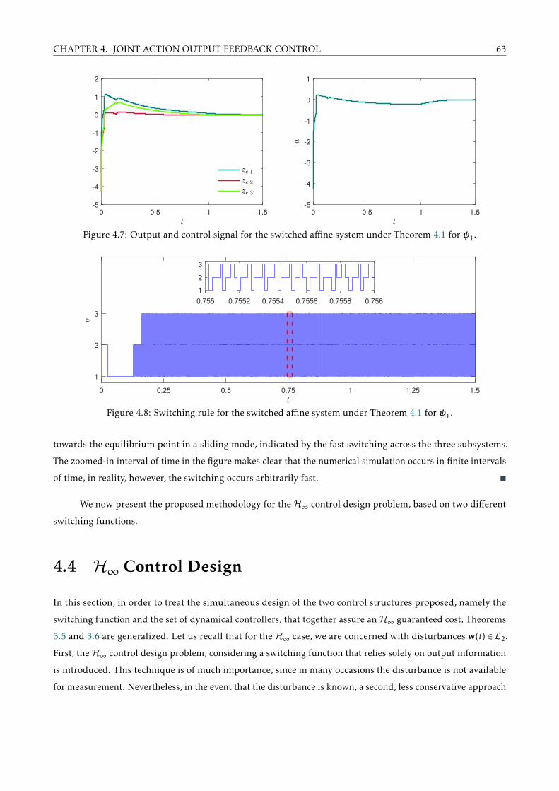
CHAPTER 4. JOINT ACTION OUTPUT FEEDBACK CONTROL 63
0 0.5 1 1.5
-5
-4
-3
-2
-1
0
1
2
0 0.5 1 1.5
-5
-4
-3
-2
-1
0
1
Figure 4.7: Output and control signal for the switched affine system under Theorem 4.1 for ψ1.
0 0.25 0.5 0.75 1 1.25 1.5
1
2
3
0.755 0.7552 0.7554 0.7556 0.7558 0.756
1
2
3
Figure 4.8: Switching rule for the switched affine system under Theorem 4.1 for ψ1.
towards the equilibrium point in a sliding mode, indicated by the fast switching across the three subsystems.
The zoomed-in interval of time in the figure makes clear that the numerical simulation occurs in finite intervals
of time, in reality, however, the switching occurs arbitrarily fast.
We now present the proposed methodology for the H∞ control design problem, based on two different
switching functions.
4.4 H∞ Control Design
In this section, in order to treat the simultaneous design of the two control structures proposed, namely the
switching function and the set of dynamical controllers, that together assure anH∞ guaranteed cost, Theorems
3.5 and 3.6 are generalized. Let us recall that for the H∞ case, we are concerned with disturbances w(t) ∈ L2.
First, the H∞ control design problem, considering a switching function that relies solely on output information
is introduced. This technique is of much importance, since in many occasions the disturbance is not available
for measurement. Nevertheless, in the event that the disturbance is known, a second, less conservative approach

CHAPTER 4. JOINT ACTION OUTPUT FEEDBACK CONTROL 64
is introduced afterwards, which may provide a better H∞ performance.
4.4.1 H∞ Control Design: Output Dependent Rule
The next theorem generalizes the conditions of Theorem 3.6, and presents the proposed H∞ control design
technique for the case where the switching rule depends only on the measured output.
Theorem 4.2. Consider the switched affine system (4.1), and a chosen xe ∈ Xe of interest with its associated λ0 ∈ΛN .
If there exist symmetric matrices X, Y, Ri , matrices Li and Wi , for all i ∈K, and a scalar ρ, such that
Rλ0 0 (4.43)
X •
I Y
0 (4.44)
He AiX + BiWi+ Ri • •
HTi −ρI •
EiX + FiWi Gi −I
≺ 0, ∀i ∈K (4.45)
He YAi + LiCi • •
HTi Y + DT
i LTi −ρI •
Ei Gi −I
≺ 0, ∀i ∈K (4.46)
then the following switching rule
σ (ξ) = arg mini∈K−ξT Qi ξ + 2ξ
TX−1`i (4.47)
along with controller (4.3), whose matrices are given by
Ai = (Y−X−1)−1(YAi + YBiWiX−1 + LiCi + AT
i X−1 + ETi Ei + ETi FiWiX−1 +Mi(ρI−GT
i Gi)−1N i
Bi = −(Y−X−1)−1Li
Ci = WiX−1
ˆi = (Y−X−1)−1Y`i
Qi = X−1RiX−1
(4.48)
withMi = YHi + LiDi + ETi Gi andN i = HTi X−1 + GT
i Ei + GTi FiWiX−1, make the equilibrium point xe ∈ Xe globally
asymptotically stable, and assure the H∞ guaranteed cost
J∞(σ,Cσ ) < ρ (4.49)
for the system.
Proof. Similarly to Theorem 4.1, this proof consists in demonstrating the validity of Theorem 3.6, whenever

CHAPTER 4. JOINT ACTION OUTPUT FEEDBACK CONTROL 65
the conditions of Theorem 4.2 are verified. For this, consider inequalities (3.63) and (3.64) of Theorem 3.6,
applied to the augmented system (4.4)
Qλ0 0 (4.50)
ATi P + PAi + Qi • •
HTi P −ρI •
Ei Gi −I
≺ 0, ∀i ∈K (4.51)
In order to linearize inequality (4.51), we again consider the transformation matrix Γ in (4.25), and multiply to
the left of (4.51) by diag(ΓT,I,I), and to the right by its transpose, as follows
Γ 0 0
0 I 0
0 0 I
T
ATi P + PAi + Qi PHT
i ETiHTi P −ρI GT
i
Ei Gi −I
Γ 0 0
0 I 0
0 0 I
≺ 0, ∀i ∈K (4.52)
whose intermediary products were determined in the proof of Theorem 4.1, and are given in (4.27), (4.28),
(4.29), and (4.37). By adopting Ri = UQiUT , Li = VBi , and Wi = CiUT , inequality (4.52) can be expressed as
He AiX + BiWi+ Ri • • •
YAiX + YBiWi + LiCiX + VAiUT + ATi He YAi + LiCi • •
HTi HT
i Y + DTi LTi −ρI •
EiX + FiWi Ei Gi −I
≺ 0 (4.53)
Applying Schur complement successively with respect to −I, followed by (ρI−GTi Gi), the following inequality
is obtained Ξi •
Ωi Υ i
≺ 0 (4.54)
where
Ξi = He AiX + BiWi+ Ri + (EiX + FiWi)T (EiX + FiWi)+
+(HTi + GT
i (EiX + FiWi))T (
ρI−GTi Gi
)−1 (HTi + GT
i (EiX + FiWi))
(4.55)
Ωi = YAiX + YBiWi + LiCiX + VAiUT + AT
i + ETi (EiX + FiWi)+
+(HTi Y + DT
i LTi + GTi Ei
)T (ρI−GT
i Gi
)−1 (HTi + GT
i (EiX + FiWi))
(4.56)
Υ i = He YAi + LiCi+ ETi Ei +(HTi Y + DT
i LTi + GTi Ei
)T (ρI−GT
i Gi
)−1 (HTi Y + DT
i LTi + GTi Ei
)(4.57)
By assigning U = X without loss of generality, as previously discussed, and choosing Ai as in (4.48), we have that
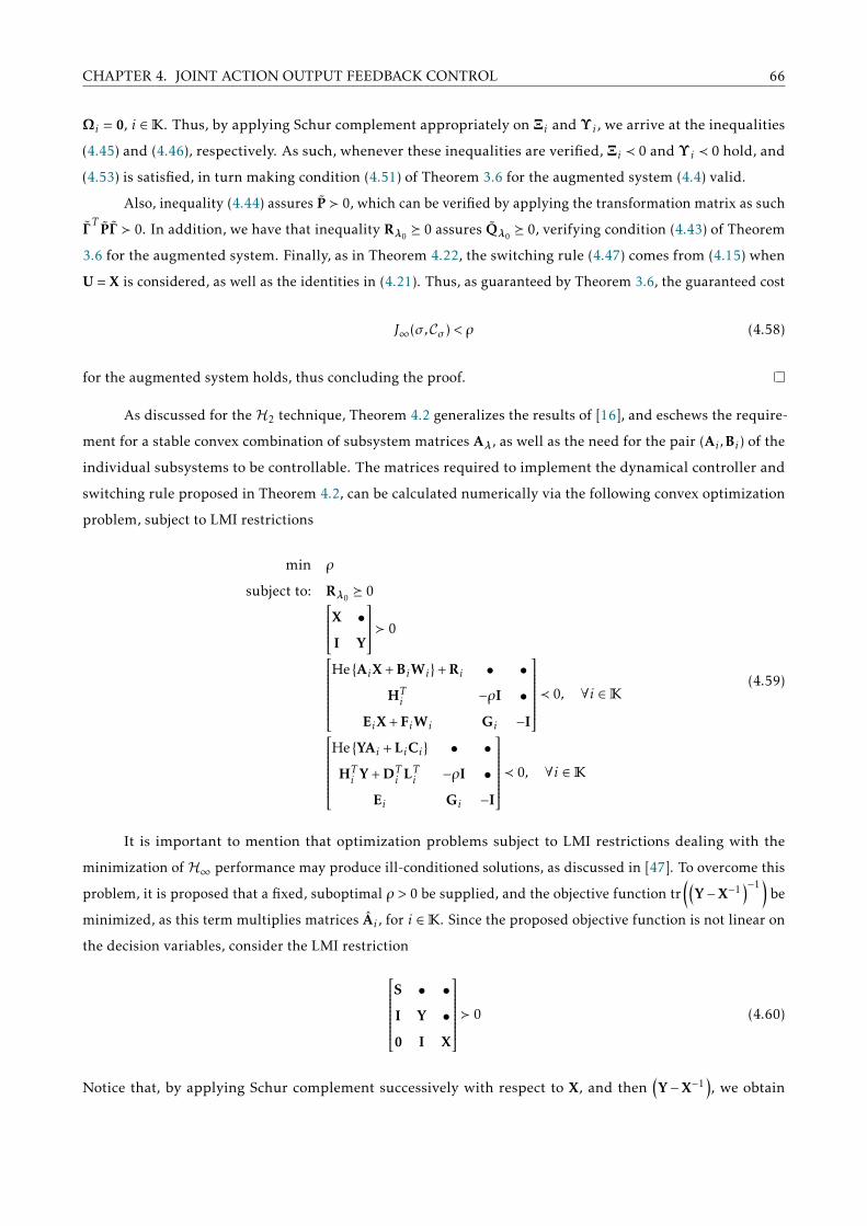
CHAPTER 4. JOINT ACTION OUTPUT FEEDBACK CONTROL 66
Ωi = 0, i ∈K. Thus, by applying Schur complement appropriately on Ξi and Υ i , we arrive at the inequalities
(4.45) and (4.46), respectively. As such, whenever these inequalities are verified, Ξi ≺ 0 and Υ i ≺ 0 hold, and
(4.53) is satisfied, in turn making condition (4.51) of Theorem 3.6 for the augmented system (4.4) valid.
Also, inequality (4.44) assures P 0, which can be verified by applying the transformation matrix as such
ΓT PΓ 0. In addition, we have that inequality Rλ0
0 assures Qλ0 0, verifying condition (4.43) of Theorem
3.6 for the augmented system. Finally, as in Theorem 4.22, the switching rule (4.47) comes from (4.15) when
U = X is considered, as well as the identities in (4.21). Thus, as guaranteed by Theorem 3.6, the guaranteed cost
J∞(σ,Cσ ) < ρ (4.58)
for the augmented system holds, thus concluding the proof.
As discussed for the H2 technique, Theorem 4.2 generalizes the results of [16], and eschews the require-
ment for a stable convex combination of subsystem matrices Aλ, as well as the need for the pair (Ai ,Bi) of the
individual subsystems to be controllable. The matrices required to implement the dynamical controller and
switching rule proposed in Theorem 4.2, can be calculated numerically via the following convex optimization
problem, subject to LMI restrictions
min ρ
subject to: Rλ0 0X •
I Y
0He AiX + BiWi+ Ri • •
HTi −ρI •
EiX + FiWi Gi −I
≺ 0, ∀i ∈K
He YAi + LiCi • •
HTi Y + DT
i LTi −ρI •
Ei Gi −I
≺ 0, ∀i ∈K
(4.59)
It is important to mention that optimization problems subject to LMI restrictions dealing with the
minimization of H∞ performance may produce ill-conditioned solutions, as discussed in [47]. To overcome this
problem, it is proposed that a fixed, suboptimal ρ > 0 be supplied, and the objective function tr((
Y−X−1)−1
)be
minimized, as this term multiplies matrices Ai , for i ∈K. Since the proposed objective function is not linear on
the decision variables, consider the LMI restriction
S • •
I Y •
0 I X
0 (4.60)
Notice that, by applying Schur complement successively with respect to X, and then(Y−X−1
), we obtain

CHAPTER 4. JOINT ACTION OUTPUT FEEDBACK CONTROL 67
(Y−X−1
)−1≺ S. Thus, for a given ρ > 0 the following optimization problem
min tr(S)
subject to: Rλ0 0
S • •
I Y •
0 I X
0
He AiX + BiWi+ Ri • •
HTi −ρI •
EiX + FiWi Gi −I
≺ 0, ∀i ∈K
He YAi + LiCi • •
HTi Y + DT
i LTi −ρI •
Ei Gi −I
≺ 0, ∀i ∈K
(4.61)
yields controller matrices with greater numerical stability overall. The next section deals with the H∞ control
design problem based on less conservative conditions, albeit considering that the disturbance w(t) is measurable,
or known beforehand.
4.4.2 H∞ Control Design: Disturbance Measurement
The next theorem generalizes the conditions of Theorem 3.5, and states the proposed H∞ control design
methodology for the case where the switching rule depends not only on the measured output, but also on the
external disturbance.
Theorem 4.3. Consider the switched affine system (4.1), and a chosen xe ∈ Xe of interest with its associated λ0 ∈ΛN .
If there exist symmetric matrices X, Y, Ri , and Zi , matrices Ji , Li and Wi , for all i ∈K, and a scalar ρ > 0, such that
Rλ0•
JTλ0Zλ0
0 (4.62)
X •
I Y
0 (4.63)
He AiX + BiWi+ Ri • •
HTi + JTi −ρI + Zi •
EiX + FiWi Gi −I
≺ 0, ∀i ∈K (4.64)
He YAi + LiCi • •
HTi Y + DT
i LTi −ρI + Zi •
Ei Gi −I
≺ 0, ∀i ∈K (4.65)
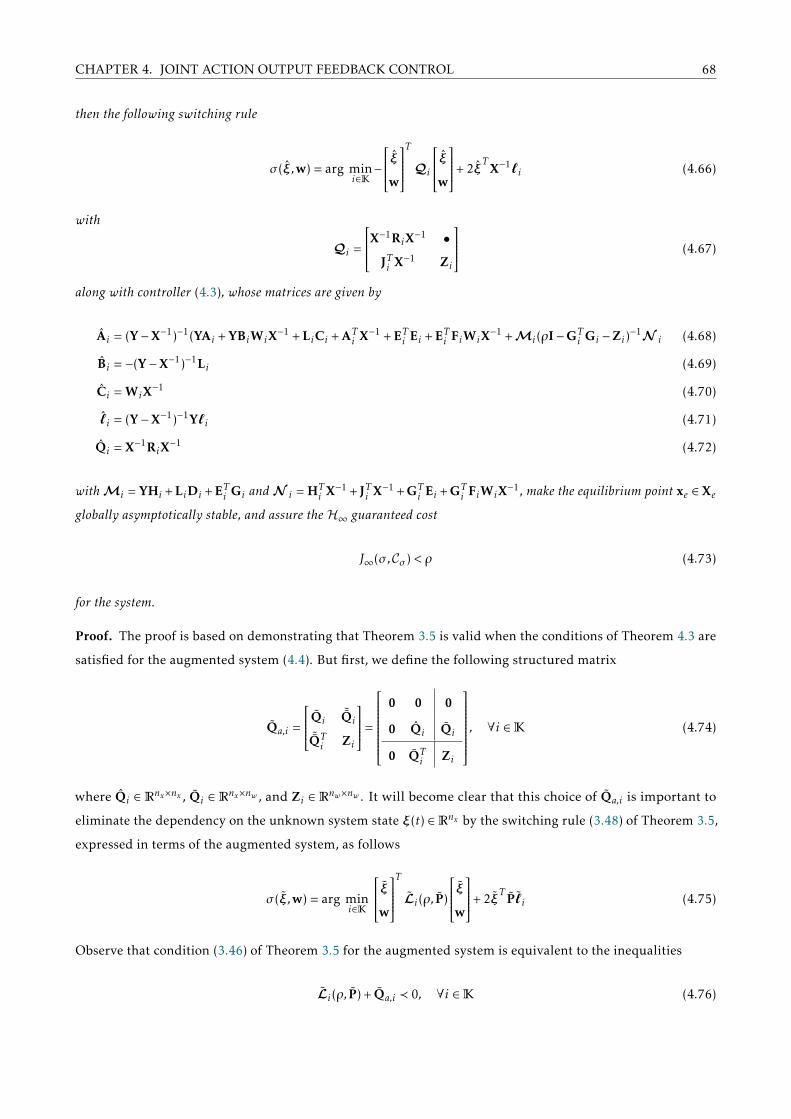
CHAPTER 4. JOINT ACTION OUTPUT FEEDBACK CONTROL 68
then the following switching rule
σ (ξ,w) = arg mini∈K−
ξwT
Qi
ξw+ 2ξ
TX−1`i (4.66)
with
Qi =
X−1RiX−1 •
JTi X−1 Zi
(4.67)
along with controller (4.3), whose matrices are given by
Ai = (Y−X−1)−1(YAi + YBiWiX−1 + LiCi + AT
i X−1 + ETi Ei + ETi FiWiX−1 +Mi(ρI−GT
i Gi −Zi)−1N i (4.68)
Bi = −(Y−X−1)−1Li (4.69)
Ci = WiX−1 (4.70)
ˆi = (Y−X−1)−1Y`i (4.71)
Qi = X−1RiX−1 (4.72)
withMi = YHi + LiDi + ETi Gi andN i = HTi X−1 + JTi X−1 + GT
i Ei + GTi FiWiX−1, make the equilibrium point xe ∈ Xe
globally asymptotically stable, and assure the H∞ guaranteed cost
J∞(σ,Cσ ) < ρ (4.73)
for the system.
Proof. The proof is based on demonstrating that Theorem 3.5 is valid when the conditions of Theorem 4.3 are
satisfied for the augmented system (4.4). But first, we define the following structured matrix
Qa,i =
Qi˜Qi
˜QTi Zi
=
0 0 0
0 Qi Qi
0 QTi Zi
, ∀i ∈K (4.74)
where Qi ∈ Rnx×nx , Qi ∈ Rnx×nw , and Zi ∈ Rnw×nw . It will become clear that this choice of Qa,i is important to
eliminate the dependency on the unknown system state ξ(t) ∈Rnx by the switching rule (3.48) of Theorem 3.5,
expressed in terms of the augmented system, as follows
σ (ξ,w) = arg mini∈K
ξwT
Li(ρ, P)
ξw+ 2ξ
T P˜i (4.75)
Observe that condition (3.46) of Theorem 3.5 for the augmented system is equivalent to the inequalities
Li(ρ, P) + Qa,i ≺ 0, ∀i ∈K (4.76)

CHAPTER 4. JOINT ACTION OUTPUT FEEDBACK CONTROL 69
together with Qa,λ0 0, where
Li(ρ, P) =
ATi P + PAi + ETi Ei •
HTi P + GT
i Ei GTi Gi − ρI
, i ∈K (4.77)
By applying Schur complement in (4.76) with respect to(GTi Gi − ρI
), the equivalent inequality
ATi P + PAi + Qi • •
HTi P + ˜QT
i −ρI + Zi •
Ei Gi −I
≺ 0 (4.78)
is obtained. Multiplying to the left of this inequality by diag(ΓT,I,I), and to the right by its transpose, in a
similar manner to (4.52), with intermediary products given by (4.27), (4.28), (4.29), and (4.37), and further
denoting Ri = UQiUT , ˜QTi Γ =
[JTi 0
], JTi = QT
i UT , Li = VBi , and Wi = CiUT the following inequality emerges
He AiX + BiWi+ Ri • • •
YAiX + YBiWi + LiCiX + VAiUT + ATi He YAi + LiCi • •
HTi + JTi HT
i Y + DTi LTi −ρI + Zi •
EiX + FiWi Ei Gi −I
≺ 0 (4.79)
In a similar fashion to Theorem 4.2, we apply Schur complement with respect to −I followed by(GTi Gi − ρI + Zi
),
obtaining Ξi •
Ωi Υ i
≺ 0 (4.80)
where
Ξi = He AiX + BiWi+ Ri + (EiX + FiWi)T (EiX + FiWi)+
+(HTi + JTi + GT
i (EiX + FiWi))T (
ρI−GTi Gi + Zi
)−1 (HTi + JTi + GT
i (EiX + FiWi))
(4.81)
Ωi = YAiX + YBiWi + LiCiX + VAiUT + AT
i + ETi (EiX + FiWi)+
+(HTi Y + DT
i LTi + GTi Ei
)T (ρI−GT
i Gi + Zi)−1 (
HTi + JTi + GT
i (EiX + FiWi))
(4.82)
Υ i = He YAi + LiCi+ ETi Ei +(HTi Y + DT
i LTi + GTi Ei
)T (ρI−GT
i Gi + Zi)−1 (
HTi Y + DT
i LTi + GTi Ei
)(4.83)
Choosing U = X, and Ai as in (4.68), we have Ωi = 0, i ∈ K, and, by applying Schur complement as
appropriate on Ξi and Υ i , the inequalities (4.64) and (4.65) are obtained, respectively. In this manner, whenever
these inequalities are satisfied, Ξi ≺ 0 and Υ i ≺ 0 hold, and (4.79) is verified, thus making condition (4.76) valid.
This, along with (4.62) guaranteeing that Qa,λ0 0 satisfies (3.46) of Theorem 3.5 for the augmented system.

CHAPTER 4. JOINT ACTION OUTPUT FEEDBACK CONTROL 70
Once again, inequality (4.44) assures P 0. Finally, the switching rule (4.66) with (4.67) comes from (4.75)
since
σ (ξ,w) = argmini∈K
ξwT
Li(ρ, P)
ξw+ 2ξ
T P˜i
≡ argmini∈K−
ξwT
Qa,i
ξw+ 2ξ
T P˜i
= argmini∈K−
ξwT
Qi
ξw+ 2ξ
TX−1`i (4.84)
when considering Ri = UQiUT , JTi = QTi UT , and U = X. Also, recalling that the choice ˆ
i allows for (4.14) which
removes any dependency on the system state. In this manner, the guaranteed cost of Theorem 3.5
J∞(σ,Cσ ) < ρ (4.85)
is assured for the augmented system. This concludes the proof.
Theorem 4.3 can be implemented by means of the following convex optimization problem, subject to
LMI restrictions.min ρ
s. to: (4.62), (4.63), (4.64), and (4.65)(4.86)
The solution to this problem provides the necessary matrices for the dynamical controller and switching rule,
by considering the identities (4.68). Additionally, as previously discussed, to avoid ill-conditioned matrix
solutions, by providing a fixed, suboptimal ρ > 0, the following optimization problem
min tr(S)
s. to:
S • •
I Y •
0 I X
0
(4.62), (4.64), and (4.65)
(4.87)
results in matrices with greater numerical stability for the dynamical controller.
In the next section, we present two examples on H∞ Control Design, also based on that of [31], imple-
menting the techniques just introduced.
4.4.3 Numerical example: Output Dependent Rule
This example now illustrates the proposed methodology for the H∞ control design problem, also based on the
example of [31], considering that the switching rule are dependent only on the measured output.
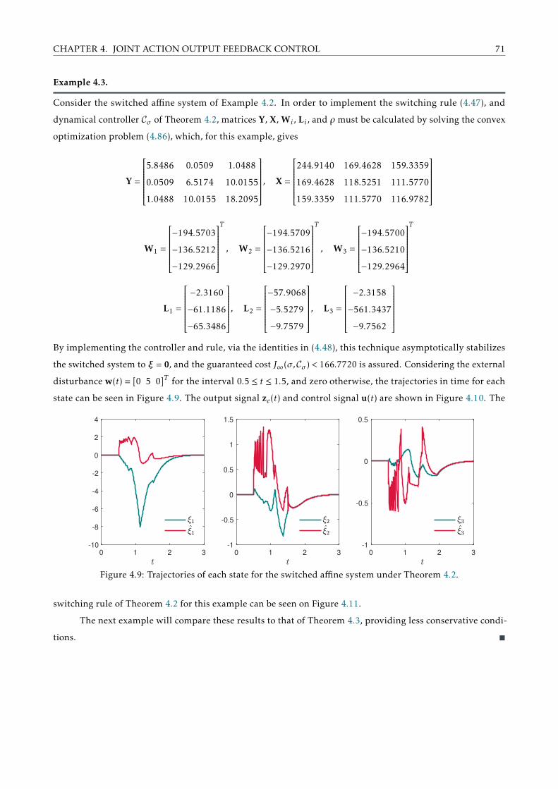
CHAPTER 4. JOINT ACTION OUTPUT FEEDBACK CONTROL 71
Example 4.3.
Consider the switched affine system of Example 4.2. In order to implement the switching rule (4.47), and
dynamical controller Cσ of Theorem 4.2, matrices Y, X, Wi , Li , and ρ must be calculated by solving the convex
optimization problem (4.86), which, for this example, gives
Y =
5.8486 0.0509 1.0488
0.0509 6.5174 10.0155
1.0488 10.0155 18.2095
, X =
244.9140 169.4628 159.3359
169.4628 118.5251 111.5770
159.3359 111.5770 116.9782
W1 =
−194.5703
−136.5212
−129.2966
T
, W2 =
−194.5709
−136.5216
−129.2970
T
, W3 =
−194.5700
−136.5210
−129.2964
T
L1 =
−2.3160
−61.1186
−65.3486
, L2 =
−57.9068
−5.5279
−9.7579
, L3 =
−2.3158
−561.3437
−9.7562
By implementing the controller and rule, via the identities in (4.48), this technique asymptotically stabilizes
the switched system to ξ = 0, and the guaranteed cost J∞(σ,Cσ ) < 166.7720 is assured. Considering the external
disturbance w(t) = [0 5 0]T for the interval 0.5 ≤ t ≤ 1.5, and zero otherwise, the trajectories in time for each
state can be seen in Figure 4.9. The output signal ze(t) and control signal u(t) are shown in Figure 4.10. The
0 1 2 3
-10
-8
-6
-4
-2
0
2
4
0 1 2 3
-1
-0.5
0
0.5
1
1.5
0 1 2 3
-1
-0.5
0
0.5
Figure 4.9: Trajectories of each state for the switched affine system under Theorem 4.2.
switching rule of Theorem 4.2 for this example can be seen on Figure 4.11.
The next example will compare these results to that of Theorem 4.3, providing less conservative condi-
tions.

CHAPTER 4. JOINT ACTION OUTPUT FEEDBACK CONTROL 72
0 0.5 1 1.5 2 2.5 3
-10
-8
-6
-4
-2
0
2
0 0.5 1 1.5 2 2.5 3
-1.5
-1
-0.5
0
0.5
Figure 4.10: Output and control signal for the switched affine system under Theorem 4.2.
0 0.5 1 1.5 2 2.5 3
1
2
3
0.754 0.7542 0.7544 0.7546 0.7548 0.755
1
2
3
Figure 4.11: Switching rule for the switched affine system under Theorem 4.2.
4.4.4 Numerical example: Disturbance Measurement
This final example considers Example 4.3, now assuming that the disturbance w(t) is known, and serves as a
comparison between the two techniques introduced for the H∞ control design problem.
Example 4.4.
Constructing upon Example 4.3, and applying Theorem 4.3, the following matrices are calculated so as to
implement the switching rule (4.66) as well as the dynamic controller Cσ
Y =
0.4120 −0.2157 0.6139
−0.2157 6.5200 10.0130
0.6139 10.0130 18.2039
, X =
246.2547 170.3845 160.2929
170.3845 119.1525 112.2339
160.2929 112.2339 117.6591
W1 =
−195.6495
−137.2608
−130.0659
T
, W2 =
−195.6426
−137.2560
−130.0610
T
, W3 =
−195.6394
−137.2537
−130.0587
T

CHAPTER 4. JOINT ACTION OUTPUT FEEDBACK CONTROL 73
L1 =
−0.2434
−61.3656
−65.5285
, L2 =
−5.0956
−1.6023
−2.9202
, L3 =
−0.4222
−11.1887
−17.6459
obtained by solving (4.86) and considering the identities in (4.68). Under Theorem 4.3, the guaranteed cost
J∞(σ,Cσ ) < 38.6818 is assured. Observe that this guaranteed cost is 76.8% smaller than that assured by Theorem
4.2, due to the reduced conservativeness of its conditions. In this example, we assume that the disturbance is
known, thus allowing the switching rule (4.66) to be implemented. Adopting the same external disturbance of
Example 4.3, the trajectories in time for each state can be seen in Figure 4.12. The switching rule of Theorem
0 1 2 3
-0.4
-0.2
0
0.2
0.4
0 1 2 3
-0.4
-0.2
0
0.2
0.4
0.6
0.8
1
0 1 2 3
-0.6
-0.5
-0.4
-0.3
-0.2
-0.1
0
0.1
Figure 4.12: Trajectories of each state for the switched affine system under Theorem 4.3.
0 0.5 1 1.5 2 2.5 3
-1.5
-1
-0.5
0
0.5
0 0.5 1 1.5 2 2.5 3
-1.5
-1
-0.5
0
0.5
Figure 4.13: Output and control signal for the switched affine system under Theorem 4.3.
4.3 for this example can be seen on Figure 4.14.
Both examples show the effectiveness of the proposed techniques.

CHAPTER 4. JOINT ACTION OUTPUT FEEDBACK CONTROL 74
0 0.5 1 1.5 2 2.5 3
1
2
3
1.4995 1.5 1.5005
1
2
3
Figure 4.14: Switching rule for the switched affine system under Theorem 4.3.
75
Chapter 5
Conclusion
In this work, we have treated the problems of analysis and control design for continuous-time switched affine
systems. First, we presented some important concepts with regard to dynamical systems, focusing on their
stability properties, as well as on the definition of the H2 and H∞ norms for linear time invariant systems.
With these concepts on hand, we have introduced the subclass of hybrid systems known as switched systems,
and presenting some results already available in the literature on switched linear and affine systems. These
results allowed us to understand the particularities and intrinsic characteristics of this important subclass
of systems, for instance, the peculiar occurrence of sliding modes, a phenomenon characteristic of switched
systems that although sometimes undesirable, due to its very high switching frequency which may lead to
equipment damage, it is otherwise crucial when the goal is to attain asymptotic stability of an equilibrium point
of interest. In particular, this phenomenon is essential to obtain the asymptotic stability of switched affine
systems, since the desired equilibrium point is in general different than those of the individual subsystems, and
therefore, an arbitrarily high switching frequency is made necessary to lead and maintain the state trajectories
at that point.
For this subclass of hybrid systems in special, the switching function plays a central role, because it can
combine the behavior of several different subsystems with the intention of assuring stability and obtaining
enhanced performance. On the other hand, the overall dynamical behavior of the system becomes more difficult
to analyze mathematically, since it makes the system nonlinear and time-variant. As such, most of the classical
tools and methodologies developed for the analysis and control of dynamical systems, some of which were
introduced in Chapter 2, cannot be employed anymore. For instance, the H2 and H∞ norms can no longer be
used, as the switched system cannot be represented by a transfer function. Given this, novel performances
indices have been introduced in the literature, and presented with detail towards the end of Chapter 3.
Despite the many mathematical challenges involved in studying these types of systems, the use of
switched systems for practical applications is compelling, since they can model a wide range of real life
processes, thus warranting the great interest in this field of research. It is within this scenario that the main
contributions of this work are proposed. More specifically, in order to deal with the more realistic case where
the state measurements are unavailable, in Chapter 4 we introduce techniques based on the simultaneous
design of two control structures, namely a switching function and a set of dynamical controllers, that together
guarantee global asymptotic stability as well as theH2 andH∞ performance criteria for switched affine systems.
The proposed methodology, to the extent of our knowledge, is first being treated in this work. The same control
structure has already been adopted in the literature but only for the simpler case of switched linear systems.
Compared to the existing approaches on switched affine systems in the literature, the proposed methods
allow for a greater number of equilibrium points to be attained by the effect of the switching rule, since the
recurrent condition in the literature, requiring that the convex combination of dynamical subsystem matrices
Aλ be Hurwitz, is no longer imposed. Instead only the convex combination of closed-loop dynamical matrices

CHAPTER 5. CONCLUSION 76
must be stable. Furthermore, the proposed techniques are able to guarantee global asymptotic stability of the
equilibrium point of interest even in the case where all subsystems are not individually controllable. This
reveals the relevance of the joint action of both these control structures for the stability of switched affine
systems.
Numerical examples introduced along Chapter 3 illustrate the peculiarities and interesting features
of switched systems. Furthermore, examples are provided in Chapter 4 to validate the proposed techniques,
and showcase the unique features of our methodologies, and how they contrast with existing results. More
specifically, examples considering non-controllable subsystems where no stable convex combination of dynami-
cal matrices exists, are considered. These examples demonstrate that the methods proposed are successful in
asymptotically guiding the trajectories of the switched system to the desired equilibrium point, while assuring
H2 and H∞ guaranteed costs.
It should be mentioned that the results presented in this work has originated the recent publication
[31]. Two further publications, more specifically [48] and [49] introduce techniques for the classical filtering
problem for switched affine systems, and will become an integral part of my Master’s dissertation. This
prominent problem so far has only been treated for the linear case, to the best of our knowledge. The following
publications consider either time-dependent switching functions [50, 51, 52], or the joint design of a stabilizing
switching function along with a switched filter [53]. However for the more general case of switched affine
systems, references [54, 55] only consider the state estimation problem under a switched observer structure.
The absence of publications in this topic compelled us to develop a methodology for the classical filter design
problem in the context of switched affine systems. The conditions introduced in [48, 49] are based on a full-
order switched dynamical filter, which is designed in tandem with an output-dependent stabilizing switching
function, collectively assuring an H2 or H∞ guaranteed cost for the estimation error. Furthermore it is proved
that the optimal guaranteed cost filters present an observer-based format, and can be designed independently
of the switching function.
Many topics of research in the context of switched affine systems remain to be explored, some of which
stand to have much impact for practical applications. Specifically, the development of conditions for a robust
control design problem have much relevance for applications in power electronics, as many electrical component
values cannot be precisely identified, or depend on operating conditions. Another interesting topic is the
development of conditions that guarantee stability considering only a partial information of the equilibrium
point of interest assuring global asymptotic stability of the overall system.

77
References[1] M. S. Branicky, Studies in Hybrid Systems: Modeling, Analysis, and Control. PhD thesis, MIT, May 1995.
[2] R. A. DeCarlo, M. S. Branicky, S. Pettersson, and B. Lennartson, “Perspectives and results on the stability
and stabilizability of hybrid systems,” Proceedings of the IEEE, vol. 88, no. 7, pp. 1069–1082, 2000.
[3] S. M. Savaresi, E. Silani, and S. Bittanti, “Acceleration-Driven-Damper (ADD): An Optimal Control
Algorithm For Comfort-Oriented Semiactive Suspensions,” Journal of Dynamic Systems, Measurement, and
Control, vol. 127, no. 2, p. 218, 2005.
[4] L. Soltanian, A. K. Sedigh, and O. Namaki-Shoushtari, “Multi-objective control of an active vibration
system via switching,” in Control and Automation, 2009. ICCA 2009. IEEE International Conference on,
pp. 2194–2199, IEEE, 2009.
[5] D. J. Leith, R. N. Shorten, W. E. Leithead, O. Mason, and P. Curran, “Issues in the design of switched linear
control systems: a benchmark study,” International Journal of Adaptive Control and Signal Processing, vol. 17,
no. 2, pp. 103–118, 2003.
[6] R. Cardim, M. Teixeira, E. Assuncao, and M. Covacic, “Variable-structure control design of switched
systems with an application to a DC-DC power converter,” IEEE Trans. on Industrial Electronics, vol. 56,
pp. 3505–3513, Sept. 2009.
[7] F. S. Garcia, J. A. Pomilio, G. S. Deaecto, and J. C. Geromel, “Analysis and control of DC-DC converters
based on Lyapunov Stability Theory,” in Energy Conversion Congress and Exposition, 2009. ECCE 2009.
IEEE, pp. 2920–2927, IEEE, 2009.
[8] J. Daafouz, J. C. Geromel, and G. S. Deaecto, “A simple approach for switched control design with control
bumps limitation,” Systems & Control Letters, vol. 61, pp. 1215–1220, Dec. 2012.
[9] J. M. Toibero, R. Carelli, and B. Kuchen, “Switching control of mobile robots for autonomous navigation in
unknown environments,” in Robotics and Automation, 2007 IEEE International Conference on, pp. 1974–
1979, IEEE, 2007.
[10] O. Namaki-Shoushtari, A. Pedro Aguiar, and A. Khaki-Sedigh, “Target tracking of autonomous robotic
vehicles using range-only measurements: a switched logic-based control strategy: a switched based control
strategy for target tracking using rom,” International Journal of Robust and Nonlinear Control, vol. 22,
pp. 1983–1998, Nov. 2012.
[11] D. Liberzon, Switching in Systems and Control. Springer-Verlag New York, 2013. OCLC: 968905642.
[12] Z. Sun and S. S. Ge, Stability theory of switched dynamical systems. Communications and control engineer-
ing, London ; New York: Springer, 2011. OCLC: ocn690089770.
REFERENCES 78
[13] R. Shorten, F. Wirth, O. Mason, K. Wulff, and C. King, “Stability Criteria for Switched and Hybrid
Systems,” SIAM Review, vol. 49, pp. 545–592, Jan. 2007.
[14] D. Corona, J. Buisson, B. De Schutter, and A. Giua, “Stabilization of switched affine systems: An
application to the buck-boost converter,” pp. 6037–6042, 2007.
[15] G. S. Deaecto, J. Geromel, F. Garcia, and J. Pomilio, “Switched affine systems control design with
application to DC–DC converters,” IET Con. The. & App., vol. 4, pp. 1201–1210, July 2010.
[16] G. S. Deaecto, “Dynamic output feedback H∞ control of continuous-time switched affine systems,”
Automatica, vol. 71, pp. 44–49, Sept. 2016.
[17] L. N. Egidio, H. R. Daiha, G. S. Deaecto, and J. C. Geromel, “DC motor speed control via buck-boost
converter through a state dependent limited frequency switching rule,” in Proceedings of the IEEE Conference
on Decision and Control, pp. 2072–2077, 2017.
[18] G. Beneux, P. Riedinger, J. Daafouz, and L. Grimaud, “Stabilisation of power converters with uncertain
equilibrium: An adaptive switched approach with guarantee of stability in continuous and discontinuous
conduction modes,” IFAC-PapersOnLine, vol. 50, no. 1, pp. 10401–10406, 2017.
[19] M. A. Wicks, P. Peleties, and R. A. DeCarlo, “Construction of piecewise Lyapunov functions for stabilizing
switched systems,” in Decision and Control, 1994., Proceedings of the 33rd IEEE Conference on, vol. 4,
pp. 3492–3497, IEEE, 1994.
[20] E. Feron, “Quadratic Stabilizability of Switched Systems via State and Output Feedback,” tech. rep.,
Center for Intelligent Control Systems, Laboratory for Information and Decision Systems, MIT, 1996.
[21] Z. Guisheng and L. Hai, “Quadratic Stabilizability of Switched Linear Systems with Polytopic Uncertain-
ties,” 2003.
[22] Z. Ji, L. Wang *, and G. Xie, “Quadratic stabilization of switched systems,” International Journal of Systems
Science, vol. 36, pp. 395–404, June 2005.
[23] J. C. Geromel, P. Colaneri, and P. Bolzern, “Dynamic output feedback control of switched linear systems,”
IEEE Transactions on Automatic Control, vol. 53, pp. 720–733, Apr. 2008.
[24] G. S. Deaecto, J. C. Geromel, and J. Daafouz, “Dynamic output feedback H∞ control of switched linear
systems,” Automatica, vol. 47, pp. 1713–1720, Aug. 2011.
[25] J. C. Geromel, G. S. Deaecto, and J. Daafouz, “Suboptimal Switching Control Consistency Analysis for
Switched Linear Systems,” IEEE Transactions on Automatic Control, vol. 58, pp. 1857–1861, July 2013.
[26] P. Bolzern and W. Spinelli, “Quadratic stabilization of a switched affine system about a nonequilibrium
point,” in American Control Conference, 2004. Proceedings of the 2004, vol. 5, pp. 3890–3895, IEEE, 2004.

REFERENCES 79
[27] A. Trofino, C. C. Scharlau, T. J. Dezuo, and M. C. de Oliveira, “Switching rule design for affine switched
systems withH∞ performance,” in Proceedings of the IEEE Conference on Decision and Control, pp. 1923–
1928, 2012.
[28] C. C. Scharlau, M. C. de Oliveira, A. Trofino, and T. J. Dezuo, “Switching rule design for affine switched
systems using a max-type composition rule,” Sys. & Cont. Lett., vol. 68, pp. 1–8, June 2014.
[29] G. S. Deaecto and G. C. Santos, “State Feedback H∞ Control Design of Continuous-time Switched Affine
Systems,” IET Control Theory & Applications, vol. 9, pp. 1511–1516, 2015.
[30] V. L. Yoshimura, E. Assunção, E. R. P. da Silva, M. C. M. Teixeira, and E. I. Mainardi Júnior, “Observer-
Based Control Design for Switched Affine Systems and Applications to DC–DC Converters,” Journal of
Control, Automation and Electrical Systems, vol. 24, pp. 535–543, Aug. 2013.
[31] G. K. Kolotelo and G. S. Deaecto, “Controle H2 e H∞ via Realimentação de Saída de Sistemas Afins com
Comutação por Ação Conjunta de Função de Comutação e Entrada de Controle,” Congresso Brasileiro de
Automática - CBA, Submitted.
[32] D. G. Luenberger, Introduction to dynamic systems: theory, models, and applications. New York: Wiley, 1979.
[33] J.-J. E. Slotine and W. Li, Applied nonlinear control. Englewood Cliffs, N.J: Prentice Hall, 1991.
[34] K. Hassan, Nonlinear Systems. Prentice-Hall, Inc., New Jersey, 1996.
[35] S. P. Boyd, E. Feron, L. E. Ghaoui, and V. Balakrishnan, Linear Matrix Inequalities in System and Control
Theory. No. vol. 15 in SIAM studies in applied mathematics, Philadelphia, PA: Society for Industrial and
Applied Mathematics, SIAM, 1994.
[36] P. Colaneri, J. C. Geromel, and A. Locatelli, Control theory and design: an RH2 and RHoo viewpoint. San
Diego, Calif: Academic Press, 1997.
[37] K. Zhou and J. C. Doyle, Essentials of robust control, vol. 104. Prentice hall Upper Saddle River, NJ, 1998.
[38] A. V. Oppenheim, A. S. Willsky, and S. H. Nawab, Signals & Systems. Prentice-Hall signal processing
series, Upper Saddle River, N.J: Prentice Hall, 2nd ed ed., 1997.
[39] R. A. Horn and C. R. Johnson, Matrix analysis. Cambridge ; New York: Cambridge University Press, 2nd
ed ed., 2012.
[40] W. S. Levine, The Control Handbook. CRC Press, Feb. 1996. Google-Books-ID: 2WQP5JGaJOgC.
[41] T. Başar and P. Bernhard, H∞-Optimal Control and Related Minimax Design Problems. Boston, MA:
Birkhäuser Boston, 2008. DOI: 10.1007/978-0-8176-4757-5.
[42] M. S. Branicky, “Multiple Lyapunov functions and other analysis tools for switched and hybrid systems,”
IEEE Transactions on automatic control, vol. 43, no. 4, pp. 475–482, 1998.

REFERENCES 80
[43] J. C. Geromel and P. Colaneri, “Stability and Stabilization of Continuous Time Switched Linear Systems,”
SIAM Journal on Control and Optimization, vol. 45, pp. 1915–1930, Jan. 2006.
[44] J. C. Geromel and G. S. Deaecto, “Switched state feedback control for continuous-time uncertain systems,”
Automatica, vol. 45, pp. 593–597, Feb. 2009.
[45] J. C. Geromel and G. S. Deaecto, “Stability analysis of Lur’e-type switched systems,” IEEE Transactions on
Automatic Control, vol. 59, pp. 3046–3050, Nov. 2014.
[46] P. Riedinger and J.-C. Vivalda, “Dynamic output feedback for switched linear systems based on a LQG
design,” Automatica, vol. 54, pp. 235–245, Apr. 2015.
[47] P. Gahinet and P. Apkarian, “A linear matrix inequality approach to H∞ control,” International Journal of
Robust and Nonlinear Control, vol. 4, no. 4, pp. 421–448, 1994.
[48] G. K. Kolotelo, L. N. Egidio, and G. S. Deaecto, “H2 and H∞ Filtering for Continuous–Time Switched
Affine Systems,” IFAC Symposium on Robust Control Design ROCOND, To appear.
[49] G. K. Kolotelo, L. N. Egidio, and G. S. Deaecto, “Projeto de Filtros com ComutaçãoH2 eH∞ para Sistemas
Afins a Tempo Contínuo,” Congresso Brasileiro de Automática - CBA, Submitted.
[50] X. Xiao, L. Zhou, and G. Lu, “Event-triggered H∞ filtering of continuous-time switched linear systems,”
Signal Processing, vol. 141, pp. 343–349, Dec. 2017.
[51] B. Wang, H. Zhang, G. Wang, and C. Dang, “Asynchronous H∞ filtering for linear switched systems with
average dwell time,” International Journal of Systems Science, vol. 47, pp. 2783–2791, Sept. 2016.
[52] L. Zhang and P. Shi, “H∞ filtering for a class of switched linear parameter varying systems,” International
Journal of Systems Science, vol. 42, pp. 781–788, May 2011.
[53] C. Duan and F. Wu, “Robust switched filtering for time-varying polytopic uncertain systems,” Journal of
Dynamic Systems, Measurement, and Control, vol. 135, Aug. 2013.
[54] L. P. G. Pinto and A. Trofino, “Switched observers for state and parameter estimation with guaranteed
cost,” Proceedings of the IFAC World Congress, vol. 47, pp. 563–568, 2014.
[55] L. Menini, C. Possieri, and A. Tornambè, “On observer design for a class of continuous-time affine
switched or switching systems,” Proceedings of the IEEE Conference on Decision and Control, pp. 6234–6239,
2014.