STRUCTURAL RESPONSE OF K AND T TUBULAR JOINTS UNDER STATIC LOADING

Luciano R. O. de Lima, Pedro C. G. da S. Vellasco, Sebastião A. L. de Andrade Structural Engineering Department, UERJ, Rio de Janeiro, Brazil lucianolima@uerj.br; vellasco@uerj.br; seb.andrade@uol.com.br

José G. S. da Silva

Mechanical Engineering Department, UERJ, Rio de Janeiro, Brazil jgss@uerj.br

Luís F. da C. Neves

Civil Engineering Department, Coimbra, Portugal luis@dec.uc.pt

Mateus C. Bittencourt

Civil Engineering Post-Graduate Program, UERJ, Rio de Janeiro, Brazil matebittencourt@yahoo.com.br

Abstract: The intensive worldwide use of tubular structural elements, mainly due to its associated aesthetical and structural advantages, led designers to be focused on the technologic and design issues. Consequently, their design methods accuracy plays a fundamental role when economical and safety points of view are considered. Additionally, recent tubular joint studies indicate further research needs, especially for some joint geometries. In this work, a nonlinear numerical analysis based on a parametric study is presented, for K and T tubular joints where both chords and braces are made of hollow tubular sections. Starting from test results available in the literature, a model has been derived, taking into account the weld geometry, material and geometric nonlinearities. The proposed model was validated by comparison to the experiments, analytical results suggested on the Eurocode 3 (2003) and to the classic deformation limits proposed in literature.

INTRODUCTION

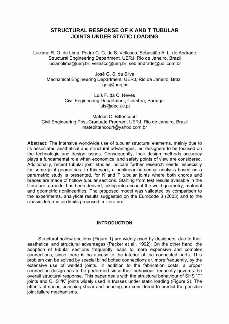
Structural hollow sections (Figure 1) are widely used by designers, due to their aesthetical and structural advantages (Packer et al., 1992). On the other hand, the adoption of tubular sections frequently leads to more expensive and complex connections, since there is no access to the interior of the connected parts. This problem can be solved by special blind bolted connections or, more frequently, by the extensive use of welded joints. In addition to the fabrication costs, a proper connection design has to be performed since their behaviour frequently governs the overall structural response. This paper deals with the structural behaviour of SHS “T” joints and CHS “K” joints widely used in trusses under static loading (Figure 2). The effects of shear, punching shear and bending are considered to predict the possible joint failure mechanisms.

The circular hollow section (CHS) K-joint configuration is commonly adopted in steel offshore platforms (e.g. jackets and jack-ups) which are designed for extreme environmental conditions during their operational life. The ultimate and service strengths of such structures significantly depend on the component (member and joint) responses. Consequently, in the past few years various research programmes on tubular joints funded by oil and gas companies and national governments were initiated.

c) T tubular joint detail

a) footbridge in Coimbra, Portugal b) footbridge in Vila Nova de Gaia, Portugal d) K tubular joint detail

Figure 1. Examples of tubular structures with T and K tubular joints

Traditionally, design rules for hollow sections joints are based on either plastic analysis or on a deformation limit criteria. The use of plastic analysis to define the joint ultimate limit state is based on a plastic mechanism corresponding to the assumed yield line pattern. Typical examples of these approaches can be found on Packer et al (1992), Cao et al (1998), Packer (1993), Choo et al. (2006) and Kosteski et al (2003). Each plastic mechanism is associated to a unique ultimate load that is directly related to this particular failure mechanism. The typically adopted yield lines were: straight, circular, or a combination of those patterns.

0

1

bb

=β 0

0

t2b

=γ tb

=μ 0

21

d2dd +

=β 50td

100,i

0,i ≤≤ 0

0

t2d

=γ

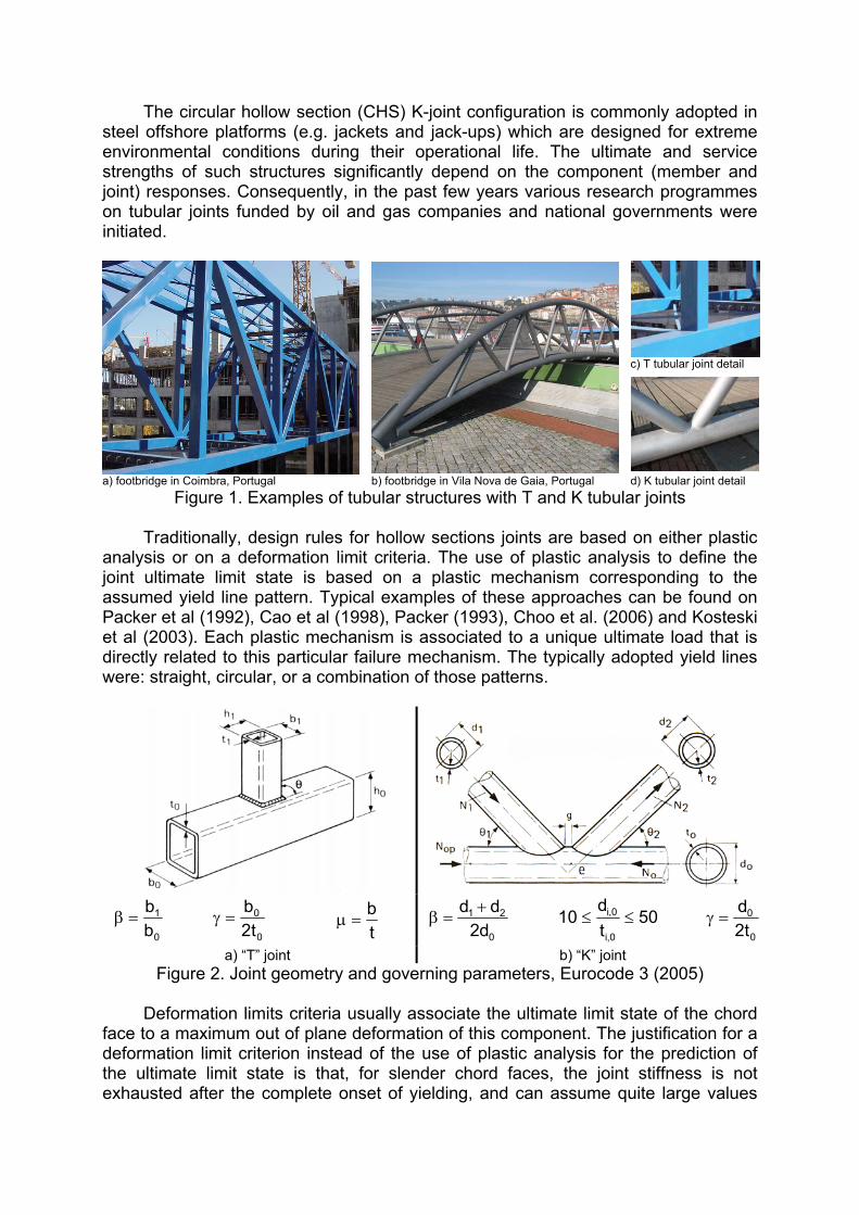
a) “T” joint b) “K” joint Figure 2. Joint geometry and governing parameters, Eurocode 3 (2005)

Deformation limits criteria usually associate the ultimate limit state of the chord

face to a maximum out of plane deformation of this component. The justification for a deformation limit criterion instead of the use of plastic analysis for the prediction of the ultimate limit state is that, for slender chord faces, the joint stiffness is not exhausted after the complete onset of yielding, and can assume quite large values

due to membrane effects. This phenomenon is clearly shown in the curves obtained from the material and geometrical nonlinear finite element analysis performed in the present study. It is evident that, if the maximum load is obtained from experimental curves, the absence of a “knee” in the curve could complicate the identification of this ultimate limit state point. Additionally, there is still the need of further comparisons to experimental and plastic analysis results based on a deformation criteria.

For T tubular joints, Korol and Mirza (1982) proposed that the ultimate limit state should be associated to a chord face displacement of 1.2 times its thickness. This value is approximately equal to 25 times the chord face elastic deformation. Lu et al (1994) proposed that the joint ultimate limit state should be associated to an out of plane deformation equal to 3% of the face width, corresponding to the maximum load reached in their experimental study. This 3% limit was proposed as well by Zhao (1991), and is actually adopted by the International Institute of Welding to define this particular ultimate limit state.

Similarly, for K tubular joints, the deformation limit proposed by Lu et al. (1994) and reported by Choo et al. (2003) may be used to evaluate the axial and/or rotational capacity of a joint subjected to the corresponding brace axial or moment loads. The joint strength is based on a comparison of the deformation at the brace-chord intersection for two strength levels: the ultimate strength, Nu which corresponds to a chord indentation, Δu = 0.03d0, and the serviceability strength, Ns that is related to Δs = 0.01d0. Lu et al. (1994) stated that the first peak in the load-deformation diagram should be used if it corresponds to a deformation smaller than the limit Δu = 0.03d0. According to Lu et al. (1994), if the ratio of Nu/Ns is greater than 1.5, the joint strength should be based on the ultimate limit state, and if Nu /Ns < 1.5, the serviceability limit state controls the design. In the case of CHS joints, Nu /Ns > 1.5 and the appropriate deformation limit to be used to determine the ultimate joint strength should be equal to 0.03d0.

EUROCODE 3 PROVISIONS (Eurocode 3, 2005)

For connections between CHS joints, such as the ones represented in Fig. 1 and Fig. 2, the methodology proposed by the Eurocode 3 (2003) part 1-8 is based on the assumption that these joints are pinned. Therefore the relevant design characteristic (in addition to the deformation capacity) is the chord and braces strength, primarily subjected to axial forces according to Eurocode 3 (2003) provisions. Equation (1) and (2) define, according to Eurocode 3 (2003), the chord face plastic load for the investigated T and “K” joint, respectively, with the geometric parameters defined in Figure 2. N1,Rd is the brace axial load related to the development of the chord face yielding or punching limit states.

( ) ⎟⎟⎠

⎞⎜⎜⎝

⎛β−+

θβ

θβ−= 14

sen2

sen1tfk

N11

200yn

Rd,1 (1)

where kn is 1,0 for tensioned members, fy0 is the chord yield stress, t0 the chord thickness, β is a geometrical parameter defined in Figure 2 and θ1 the angle between the chord and the brace.

5M0

1

1

200ypg

Rd,1 /dd2.108.1

sentfkk

N γ⎟⎟⎠

⎞⎜⎜⎝

⎛+

θ= and Rd,1

2

1Rd,2 N

sinsinN

θθ

= (2)

where fy0 is the chord yield stress, t0 the chord thickness, θ1 and θ2 are the angle between the chord and the braces, kp and kg can be obtained from eq. (3).

⎟⎟⎠

⎞⎜⎜⎝

⎛−+

γ+γ=

)33.1t/g5.0exp(1024.01k

0

2.12.0

g ; 0.1)n1(n 3.01k ppp ≤+−= ;0y0

Sd,0

0y0

Sd,pp fW

MfA

Nn += (3)

NUMERICAL MODEL – CALIBRATION AND RESULTS

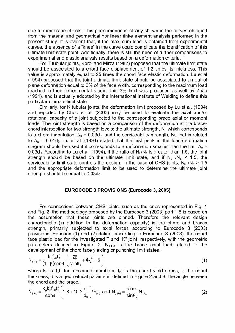
Tubular joints are most commonly modelled by shell elements that represent the mid-surfaces of the joint member walls. The welds are usually represented by shell (see Figure 3) or three-dimensional solid elements, may be included or not in the model. It is common practice to analyse this type of joints without an explicit consideration of the welds. This is made simply modelling the mid-surfaces of the member walls using shell elements, Lee (1999) and Lie et al. (2006). Despite this fact, some authors stated that this effect may be significant especially for K-joints with a gap, since the weld does not have a negligible size when compared to the gap size, Lie et al. (2006). In the present investigation the weld for T joint was firstly modelled by using a ring of shell elements (SHELL 181 - four nodes with six degree of freedom per node), Figure 3, similarly to the configuration proposed by Lee (1999) and Van der Vegte et al. (2007). Afterwards, solid elements (SOLID45 - eight nodes with three d.o.f. at each node) were used to considerate the joint welds to properly assess its influence.

a) shell elements (after Lee, 1999) b) shell elements c) solid elements

Figure 3. Modelling of the welds

For an ultimate strength analysis, this approach is generally acknowledged as sufficiently accurate to simulate the overall joint structural response. The decisions on the choice of element and the better strategy to represent the welds (if included), should be made in advance since it determines the model layout and the required mesh density.

The finite element models in the present study were generated using automatic mesh generation procedures. A finite element model adopted four-node thick shell elements, therefore considering bending, shear and membrane deformations. For the “T” joint model calibration, the numerical results found in Lie et al. (2006) (T1 & T2 models) were used. Their mechanical and geometrical properties are depicted in Table 1. For the T1 joint, the parameters of Figure 2 assumes values of β = 0.57, μ0 = 23.3, μ1 = 12.5 and γ0 = 11.67. It should be noted that a value of β = 0.57 is not critical.

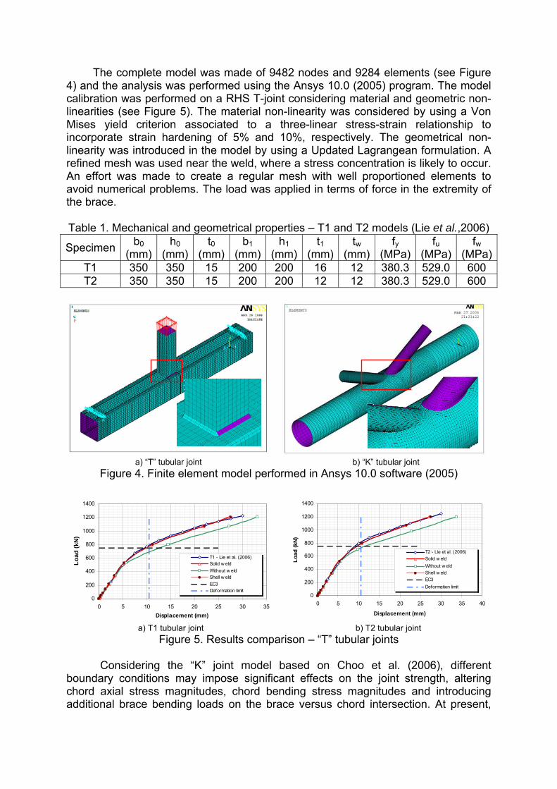
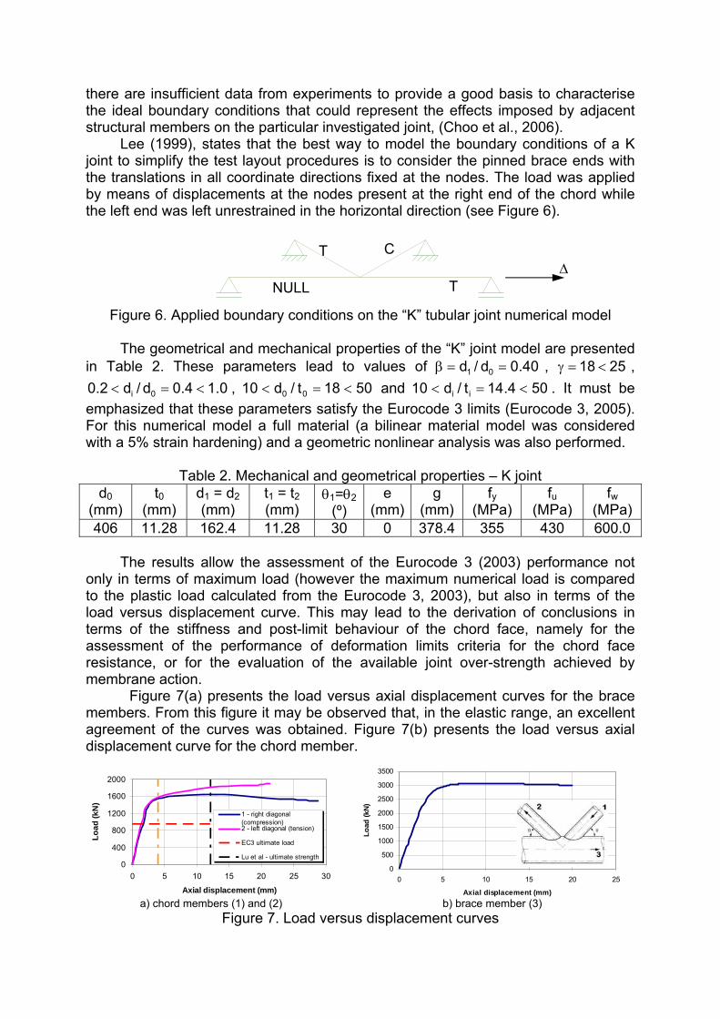
The complete model was made of 9482 nodes and 9284 elements (see Figure 4) and the analysis was performed using the Ansys 10.0 (2005) program. The model calibration was performed on a RHS T-joint considering material and geometric non-linearities (see Figure 5). The material non-linearity was considered by using a Von Mises yield criterion associated to a three-linear stress-strain relationship to incorporate strain hardening of 5% and 10%, respectively. The geometrical non-linearity was introduced in the model by using a Updated Lagrangean formulation. A refined mesh was used near the weld, where a stress concentration is likely to occur. An effort was made to create a regular mesh with well proportioned elements to avoid numerical problems. The load was applied in terms of force in the extremity of the brace. Table 1. Mechanical and geometrical properties – T1 and T2 models (Lie et al.,2006)

Specimen b0 (mm)

h0 (mm)

t0 (mm)

b1 (mm)

h1 (mm)

t1 (mm)

tw (mm)

fy (MPa)

fu (MPa)

fw (MPa)

T1 350 350 15 200 200 16 12 380.3 529.0 600 T2 350 350 15 200 200 12 12 380.3 529.0 600

a) “T” tubular joint b) “K” tubular joint Figure 4. Finite element model performed in Ansys 10.0 software (2005)

0

200

400

600

800

1000

1200

1400

0 5 10 15 20 25 30 35Displacement (mm)

Load

(kN

)

T1 - Lie et al. (2006)Solid w eldWithout w eldShell w eldEC3Deformation limit

0

200

400

600

800

1000

1200

1400

0 5 10 15 20 25 30 35 40

Displacement (mm)

Load

(kN)

T2 - Lie et al. (2006)Solid w eldWithout w eldShell w eldEC3Deformation limit

a) T1 tubular joint b) T2 tubular joint

Figure 5. Results comparison – “T” tubular joints Considering the “K” joint model based on Choo et al. (2006), different boundary conditions may impose significant effects on the joint strength, altering chord axial stress magnitudes, chord bending stress magnitudes and introducing additional brace bending loads on the brace versus chord intersection. At present,

there are insufficient data from experiments to provide a good basis to characterise the ideal boundary conditions that could represent the effects imposed by adjacent structural members on the particular investigated joint, (Choo et al., 2006).

Lee (1999), states that the best way to model the boundary conditions of a K joint to simplify the test layout procedures is to consider the pinned brace ends with the translations in all coordinate directions fixed at the nodes. The load was applied by means of displacements at the nodes present at the right end of the chord while the left end was left unrestrained in the horizontal direction (see Figure 6).

Figure 6. Applied boundary conditions on the “K” tubular joint numerical model

The geometrical and mechanical properties of the “K” joint model are presented

in Table 2. These parameters lead to values of 40.0d/d 01 ==β , 25 18 <=γ , 0.14.0d/d2.0 0i <=< , 5018t/d10 00 <=< and 504.14t/d10 ii <=< . It must be

emphasized that these parameters satisfy the Eurocode 3 limits (Eurocode 3, 2005). For this numerical model a full material (a bilinear material model was considered with a 5% strain hardening) and a geometric nonlinear analysis was also performed.

Table 2. Mechanical and geometrical properties – K joint d0

(mm) t0

(mm) d1 = d2 (mm)

t1 = t2 (mm)

θ1=θ2 (º)

e (mm)

g (mm)

fy (MPa)

fu (MPa)

fw (MPa)

406 11.28 162.4 11.28 30 0 378.4 355 430 600.0

The results allow the assessment of the Eurocode 3 (2003) performance not only in terms of maximum load (however the maximum numerical load is compared to the plastic load calculated from the Eurocode 3, 2003), but also in terms of the load versus displacement curve. This may lead to the derivation of conclusions in terms of the stiffness and post-limit behaviour of the chord face, namely for the assessment of the performance of deformation limits criteria for the chord face resistance, or for the evaluation of the available joint over-strength achieved by membrane action.

Figure 7(a) presents the load versus axial displacement curves for the brace members. From this figure it may be observed that, in the elastic range, an excellent agreement of the curves was obtained. Figure 7(b) presents the load versus axial displacement curve for the chord member.

0

400

800

1200

1600

2000

0 5 10 15 20 25 30

Axial displacement (mm)

Load

(kN

)

1 - right diagonal(compression)2 - left diagonal (tension)

EC3 ultimate load

Lu et al - ultimate strength

0

500

1000

1500

2000

2500

3000

3500

0 5 10 15 20 25

Axial displacement (mm)

Load

(kN)

a) chord members (1) and (2) b) brace member (3)

Figure 7. Load versus displacement curves

Δ T C

T NULL

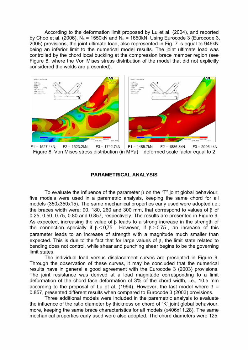
According to the deformation limit proposed by Lu et al. (2004), and reported by Choo et al. (2006), Ns = 1550kN and Nu = 1650kN. Using Eurocode 3 (Eurocode 3, 2005) provisions, the joint ultimate load, also represented in Fig. 7 is equal to 946kN being an inferior limit to the numerical model results. The joint ultimate load was controlled by the chord local buckling at the compression brace member region (see Figure 8, where the Von Mises stress distribution of the model that did not explicitly considered the welds are presented).

F1 = 1527.4kN; F2 = 1523.2kN; F3 = 1742.7kN F1 = 1485.7kN F2 = 1886.8kN F3 = 2996.4kN Figure 8. Von Mises stress distribution (in MPa) – deformed scale factor equal to 2

PARAMETRICAL ANALYSIS To evaluate the influence of the parameter β on the “T” joint global behaviour, five models were used in a parametric analysis, keeping the same chord for all models (350x350x15). The same mechanical properties early used were adopted i.e.: the braces width were: 90, 180, 260 and 300 mm, that correspond to values of β of 0.25, 0.50, 0.75, 0.80 and 0.857, respectively. The results are presented in Figure 9. As expected, increasing the value of β leads to a strong increase in the strength of the connection specially if 75,0≤β . However, if 75,0≥β , an increase of this parameter leads to an increase of strength with a magnitude much smaller than expected. This is due to the fact that for large values of β, the limit state related to bending does not control, while shear and punching shear begins to be the governing limit states. The individual load versus displacement curves are presented in Figure 9. Through the observation of these curves, it may be concluded that the numerical results have in general a good agreement with the Eurocode 3 (2003) provisions. The joint resistance was derived at a load magnitude corresponding to a limit deformation of the chord face deformation of 3% of the chord width, i.e., 10.5 mm according to the proposal of Lu et al. (1994). However, the last model where β = 0.857, presented different results when compared to Eurocode 3 (2003) provisions. Three additional models were included in the parametric analysis to evaluate the influence of the ratio diameter by thickness on chord of “K” joint global behaviour, more, keeping the same brace characteristics for all models (φ406x11.28). The same mechanical properties early used were also adopted. The chord diameters were 125,

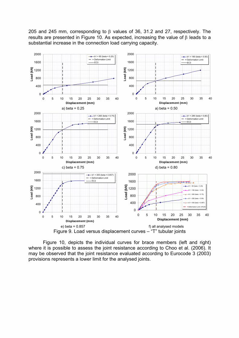
205 and 245 mm, corresponding to β values of 36, 31.2 and 27, respectively. The results are presented in Figure 10. As expected, increasing the value of β leads to a substantial increase in the connection load carrying capacity.

0

400

800

1200

1600

2000

0 5 10 15 20 25 30 35 40Displacement (mm)

Load

(kN

)

b1 = 90 (beta = 0.25)Deformation LimitEC3

0

400

800

1200

1600

2000

0 5 10 15 20 25 30 35 40Displacement (mm)

Load

(kN

)

b1 = 180 (beta = 0.50)Deformation LimitEC3

a) beta = 0.25 a) beta = 0.50

0

400

800

1200

1600

2000

0 5 10 15 20 25 30 35 40Displacement (mm)

Load

(kN

)

b1 = 260 (beta = 0.75)Deformation LimitEC3

0

400

800

1200

1600

2000

0 5 10 15 20 25 30 35 40Displacement (mm)

Load

(kN

)

b1 = 280 (beta = 0.80)Deformation LimitEC3

c) beta = 0.75 d) beta = 0.80

0

400

800

1200

1600

2000

0 5 10 15 20 25 30 35 40Displacement (mm)

Load

(kN

)

b1 = 300 (beta = 0.857)Deformation LimitEC3

0

400

800

1200

1600

2000

0 5 10 15 20 25 30 35 40Displacement (mm)

Load

(kN

)

b1 = 90 (beta = 0.25)

b1 = 180 (beta = 0.50)

b1 = 260 (beta = 0.75)

b1 = 280 (beta = 0.80)

b1 = 300 (beta = 0.857)

Deformation Limit (3%b0)

e) beta = 0.857 f) all analysed models

Figure 9. Load versus displacement curves – “T” tubular joints Figure 10, depicts the individual curves for brace members (left and right) where it is possible to assess the joint resistance according to Choo et al. (2006). It may be observed that the joint resistance evaluated according to Eurocode 3 (2003) provisions represents a lower limit for the analysed joints.

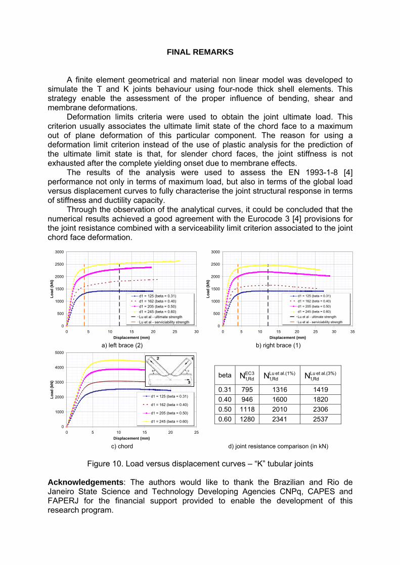
FINAL REMARKS

A finite element geometrical and material non linear model was developed to simulate the T and K joints behaviour using four-node thick shell elements. This strategy enable the assessment of the proper influence of bending, shear and membrane deformations.

Deformation limits criteria were used to obtain the joint ultimate load. This criterion usually associates the ultimate limit state of the chord face to a maximum out of plane deformation of this particular component. The reason for using a deformation limit criterion instead of the use of plastic analysis for the prediction of the ultimate limit state is that, for slender chord faces, the joint stiffness is not exhausted after the complete yielding onset due to membrane effects.

The results of the analysis were used to assess the EN 1993-1-8 [4] performance not only in terms of maximum load, but also in terms of the global load versus displacement curves to fully characterise the joint structural response in terms of stiffness and ductility capacity.

Through the observation of the analytical curves, it could be concluded that the numerical results achieved a good agreement with the Eurocode 3 [4] provisions for the joint resistance combined with a serviceability limit criterion associated to the joint chord face deformation.

0

500

1000

1500

2000

2500

3000

0 5 10 15 20 25 30Displacement (mm)

Load

(kN

)

d1 = 125 (beta = 0.31)d1 = 162 (beta = 0.40)d1 = 205 (beta = 0.50)d1 = 245 (beta = 0.60)Lu et al - ultimate strengthLu et al - serviciability strength

0

500

1000

1500

2000

2500

3000

0 5 10 15 20 25 30 35Displacement (mm)

Load

(kN

)

d1 = 125 (beta = 0.31)d1 = 162 (beta = 0.40)d1 = 205 (beta = 0.50)d1 = 245 (beta = 0.60)Lu et al - ultimate strengthLu et al - serviciability strength

a) left brace (2) b) right brace (1)

0

1000

2000

3000

4000

5000

0 5 10 15 20 25Displacement (mm)

Load

(kN

)

d1 = 125 (beta = 0.31)

d1 = 162 (beta = 0.40)

d1 = 205 (beta = 0.50)

d1 = 245 (beta = 0.60)

beta 3ECRd,1N

al.(1%) et LuRd,1N al.(3%) et Lu

Rd,1N

0.31 795 1316 1419 0.40 946 1600 1820 0.50 1118 2010 2306 0.60 1280 2341 2537

c) chord d) joint resistance comparison (in kN)

Figure 10. Load versus displacement curves – “K” tubular joints Acknowledgements: The authors would like to thank the Brazilian and Rio de Janeiro State Science and Technology Developing Agencies CNPq, CAPES and FAPERJ for the financial support provided to enable the development of this research program.

REFERENCES

ANSYS 10.0 ® (2005), ANSYS - Inc. Theory Reference. Cao, J.J., Packer, J.A., Young, G.J. (1998), “Yield line analysis of RHS connections with axial loads”, Journal of Constructional Steel Research, Vol. 48, (pp 1-25). Choo, Y. S., Qian, X. D., Liew, J. Y. R, Wardenier, J. (2003), “Static strength of thick-walled CHS X-joints - Part I. New approach in strength definition”, Journal of Constructional Steel Research, Vol.59 (pp. 1201-1228). Choo, Y. S., Qian, X. D., Wardenier, J. (2006), “Effects of boundary conditions and chord stresses on static strength of thick-walled CHS K-joints”, Journal of Constructional Steel Research, Vol.62 (pp. 316-328). Eurocode 3, prEN 1993-1.8 (2003), Design of steel structures – Part 1.8: Design of joints, CEN, European Committee for Standardisation, Brussels. Korol, R., Mirza, F. (1982), “Finite Element Analysis of RHS T-Joints”, Journal of the Structural Division, ASCE, Vol.108, (pp. 2081-2098). Kosteski, N., Packer, J.A., Puthli, R.S. (2003), “A finite element method based yield load determination procedure for hollow structural section connections”, Journal of Constructional Steel Research, Vol. 59, (pp. 427-559). Lee M. M. K. (1999), “Strength, stress and fracture analyses of offshore tubular joints using finite elements”, Journal of Constructional Steel Research Vol. 51 (pp. 265-286). Lie S. T., Lee C. K., Chiew S. P. and Yang, Z. M. (2006), “Static Strength of Cracked Square Hollow Section T Joints under Axial Loads. I: Experimental”, ASCE Journal of Structural Engineering, Vol. 132, (pp. 368-377). Lie S. T., Lee C. K., Chiew S. P. and Yang, Z. M. (2006), “Static Strength of Cracked Square Hollow Section T Joints under Axial Loads. II: Numerical”, ASCE - Journal of Structural Engineering Vol. 132, (pp. 378-386). Lu, L. H., de Winkel, G.D., Yu, Y., Wardenier, J. (1994), “Deformation limit for the ultimate strength of hollow section joints”. Proceedings of Sixth International Symposium on Tubular Structures, Melbourne. Packer, J. A., (1993), “Moment Connections between Rectangular Hollow Sections”, Journal of Constructional Steel Research, Vol. 25 (pp. 63-81). Packer, J. A., Wardenier, J., Kurobane, Y., Dutta, D. and Yoemans, N. (1992), Design Guide for Rectangular Hollow Section (RHS) Joints Under Predominantly Static Loading, CIDECT - Construction with Hollow Steel Sections, Verlag TÜV Rheinland. Van Der Vegte G. J., Koning C. H. M., Puthli R. S. and Wardenier J. (2007), “Numerical Simulation of Experiments on Multiplanar Steel X-Joints”, International Journal of Offshore and Polar Engineering, Vol. 1, (pp. 200). Zhao, X., Hancock, G., (1991), “T-Joints in Rectangular Hollow Sections Subject to Combined Actions”, ASCE - Journal of the Structural Division, Vol.117, (pp. 2258-2277).