UNIVERSIDADE ESTADUAL DE CAMPINAS

INSTITUTO DE FıSICA GLEB WATAGHIN

Tese de Doutorado

Modelos de discos e outras estruturas

auto-gravitantes em Relatividade Geral

Aluno: Daniel Vogt – IFGW/UNICAMPOrientador: Dr. Patricio Anibal Letelier Sotomayor – IMECC/UNICAMP

Co-orientador: Dr. Marcus A. M. de Aguiar – IFGW/UNICAMP

20 de Marco de 2006

Banca Examinadora:Dr. Patricio Anibal Letelier Sotomayor – IMECC/UNICAMPDr. George Emanuel Avraam Matsas – IFT/UNESPDr. Alberto Vazquez Saa – IMECC/UNICAMPDra. Kyoko Furuya – IFGW/UNICAMPDra. Carola Dobrigkeit Chinellato – IFGW/UNICAMP

Livros Grátis

http://www.livrosgratis.com.br

Milhares de livros grátis para download.

Toda a nossa ciencia, comparada com a realidade, e primi-tiva e infantil—e, no entanto, e a coisa mais preciosa quetemos.

Albert Einstein

As teorias sao redes, lancadas para capturar aquilo que de-nominamos “o mundo”: para racionaliza-lo, explica-lo, do-mina-lo. Nossos esforcos sao no sentido de tornar as malhasda rede cada vez mais estreitas.

Karl Popper, A Logica da Pesquisa Cientıfica

ii

Agradecimentos

Ao meu orientador Dr. Patricio Letelier, que me mostrou o caminho. Paramim foi um privilegio ter sido seu aluno de mestrado e doutorado.

A CAPES, pelo suporte financeiro.

Ao Dr. Rogerio L. de Almeida, pessoa com vasta cultura geral, pelas nossasestimulantes conversas ao longo dos anos sobre os mais variados assuntos(alguns deles impublicaveis).

A Donald E. Knuth, criador do TEX, e a todos que desenvolveram o LATEXe seus inumeros pacotes.

Zuletzt, aber nicht unwichtiger, mochte ich meinen Eltern danken. OhneIhre Unterstutzung ware ich nie so weit gekommen.

iii

Resumo

Solucoes exatas das equacoes do campo de Einstein que representam es-pacos-tempo com distribuicoes de materia em forma de discos sao cons-truıdas pelo metodo inverso (metodo das imagens). Estas solucoes incluemdiscos estaticos finos de fluido perfeito com e sem halos, discos estaticos fi-nos de fluido perfeito com carga eletrica e modelos de discos finos formadospor poeira carregada. Sao estudadas ainda novas solucoes em varios siste-mas de coordenadas que representam discos estaticos grossos com espessuraconstante. Uma forma particular para a metrica isotropica em coordenadascilındricas e usada para obter-se versoes relativısticas de pares potencial-densidade Newtonianos comumente usados na Astronomia Galactica. Ummodelo relativıstico simplificado, porem exato, de um nucleo ativo de galaxiatambem e apresentado. Finalmente, e feito um estudo de alguns pares-potencial densidade Newtonianos obtidos a partir da expansao multipolardo potencial Newtoniano que generalizam pares conhecidos.

iv

Abstract

Exact solutions of Einstein field equations that represent space-times withdisklike matter distributions are constructed using the inverse method (im-age method). These solutions include static thin perfect fluid disks withand without halos, static thin charged perfect fluid disks and models of thincharged dust disks. New solutions in various coordinate systems that repre-sent static thick disks with constant thickness are also studied. A particularform of the isotropic metric in cylindrical coordinates is employed to obtainrelativistic versions of Newtonian potential-density pairs commonly used inGalactic Astronomy. A simplified, although exact, relativistic model of anactive galactic nuclei is also presented. Finally, some Newtonian potential-density pairs obtained from the Newtonian multipolar expansion that gene-ralize known pairs are studied.

v

vi

Conteudo

1 Introducao 1

2 Elementos de Relatividade Geral 5

2.1 Equacoes geodesicas . . . . . . . . . . . . . . . . . . . . . . . 52.2 Formalismo de Tetradas . . . . . . . . . . . . . . . . . . . . . 6

2.3 Tensor energia-momento de fluidos . . . . . . . . . . . . . . . 72.4 Equacoes de Einstein e Einstein-Maxwell . . . . . . . . . . . . 8

3 Algumas Solucoes Exatas em Relatividade Geral 11

3.1 Coordenadas esfericas canonicas . . . . . . . . . . . . . . . . . 11

3.2 Coordenadas de Weyl . . . . . . . . . . . . . . . . . . . . . . 123.2.1 Solucao de Chazy-Curzon . . . . . . . . . . . . . . . . 12

3.2.2 Solucao para uma barra finita . . . . . . . . . . . . . . 133.2.3 Solucao de Schwarzschild . . . . . . . . . . . . . . . . 13

3.3 Coordenadas Isotropicas . . . . . . . . . . . . . . . . . . . . . 143.3.1 Esferas de fluido perfeito em coordenadas isotropicas . 15

3.4 Metricas conformastaticas . . . . . . . . . . . . . . . . . . . . 17

4 Construcao de Discos pelo Metodo Inverso 19

4.1 O metodo “deslocar, cortar e refletir” . . . . . . . . . . . . . 194.2 Distribuicoes em espacos-tempo curvos . . . . . . . . . . . . . 21

4.3 Outros parametros fısicos dos discos . . . . . . . . . . . . . . 254.4 O metodo “deslocar, cortar, encher e refletir” . . . . . . . . . 26

4.5 Pares potencial-densidade como modelos de galaxias . . . . . 284.5.1 Modelo de Plummer . . . . . . . . . . . . . . . . . . . 28

4.5.2 Modelos de Miyamoto-Nagai . . . . . . . . . . . . . . 28

5 Resumo dos Artigos e Conclusao 31

5.1 Resumo dos artigos . . . . . . . . . . . . . . . . . . . . . . . . 315.2 Conclusao . . . . . . . . . . . . . . . . . . . . . . . . . . . . . 34

vii

Bibliografia . . . . . . . . . . . . . . . . . . . . . . . . . . . . . . . 37

A Exact general relativistic perfect fluid disks with halos 41

A.1 Introduction . . . . . . . . . . . . . . . . . . . . . . . . . . . . 42

A.2 Einstein equations and disks . . . . . . . . . . . . . . . . . . . 43

A.3 The simplest disk . . . . . . . . . . . . . . . . . . . . . . . . 46

A.4 Disks with halos . . . . . . . . . . . . . . . . . . . . . . . . . 51

A.4.1 Buchdahl’s Solution . . . . . . . . . . . . . . . . . . . 51

A.4.2 Narlikar-Patwardhan-Vaidya Solutions 1a and 1b . . . 54

A.4.3 Narlikar-Patwardhan-Vaidya Solutions 2a and 2b . . . 57

A.5 Disks with composite halos from spherical solutions . . . . . . 68

A.5.1 Internal Schwarzschild solution and Buchdahl solution 68

A.5.2 NPV Solution 2b with n =√

2 and NPV solution 1bwith k = −2 +

√2 . . . . . . . . . . . . . . . . . . . . 73

A.6 Discussion . . . . . . . . . . . . . . . . . . . . . . . . . . . . . 75

Bibliography . . . . . . . . . . . . . . . . . . . . . . . . . . . . . . 80

B Exact general relativistic static perfect fluid disks 83

B.1 Introduction . . . . . . . . . . . . . . . . . . . . . . . . . . . . 83

B.2 Einstein equations and disks . . . . . . . . . . . . . . . . . . . 85

B.3 Perfect Fluid Disk in Isotropic Coordinates . . . . . . . . . . 86

B.4 Stability of Perfect Fluid Disks . . . . . . . . . . . . . . . . . 89

B.5 Conclusion . . . . . . . . . . . . . . . . . . . . . . . . . . . . 91

Bibliography . . . . . . . . . . . . . . . . . . . . . . . . . . . . . . 94

C Exact relativistic static charged dust discs and non-axisymme-

tric structures 97

C.1 Introduction . . . . . . . . . . . . . . . . . . . . . . . . . . . . 97

C.2 Einstein-Maxwell equations, discs and conformastatic space-times . . . . . . . . . . . . . . . . . . . . . . . . . . . . . . . . 99

C.3 Aligned extreme Reissner-Nordstrom black holes on the z-axis 101

C.4 Aligned extreme Reissner-Nordstrom black holes on the y-axis 104

C.5 Discussion . . . . . . . . . . . . . . . . . . . . . . . . . . . . . 107

Bibliography . . . . . . . . . . . . . . . . . . . . . . . . . . . . . . 110

D Exact relativistic static charged perfect fluid disks 113

D.1 Introduction . . . . . . . . . . . . . . . . . . . . . . . . . . . . 113

D.2 Einstein-Maxwell Equations and Disks . . . . . . . . . . . . . 115

D.3 Stability Conditions for Perfect Fluid Disks . . . . . . . . . . 116

D.4 Charged Perfect Fluid Disks . . . . . . . . . . . . . . . . . . . 118

viii

D.5 Discussion . . . . . . . . . . . . . . . . . . . . . . . . . . . . . 120

Bibliography . . . . . . . . . . . . . . . . . . . . . . . . . . . . . . 124

E General relativistic model for the gravitational field of active

galactic nuclei surrounded by a disk 127

E.1 Introduction . . . . . . . . . . . . . . . . . . . . . . . . . . . . 127

E.2 Thin disk solutions in Weyl coordinates . . . . . . . . . . . . 129

E.3 Superposition of thin disks and other Weyl solutions . . . . . 130

E.4 Black holes and rods in Weyl coordinates . . . . . . . . . . . 131

E.5 Superposition of disk, black hole and rods . . . . . . . . . . . 133

E.6 Horizontal and vertical oscillations of the disk . . . . . . . . . 137

E.7 Geodesic orbits . . . . . . . . . . . . . . . . . . . . . . . . . . 143

E.8 Discussion . . . . . . . . . . . . . . . . . . . . . . . . . . . . . 144

Bibliography . . . . . . . . . . . . . . . . . . . . . . . . . . . . . . 148

F New models of general relativistic static thick disks 151

F.1 Introduction . . . . . . . . . . . . . . . . . . . . . . . . . . . . 152

F.2 Newtonian Thick Disks . . . . . . . . . . . . . . . . . . . . . 153

F.3 Thick Disks from the Schwarzschild Metric in Isotropic Co-ordinates . . . . . . . . . . . . . . . . . . . . . . . . . . . . . 157

F.4 Thick Disks from the Schwarzschild Metric in Weyl Coordinates163

F.5 Thick Disks from the Schwarzschild Metric in SchwarzschildCoordinates . . . . . . . . . . . . . . . . . . . . . . . . . . . . 166

F.6 Discussion . . . . . . . . . . . . . . . . . . . . . . . . . . . . . 170

Bibliography . . . . . . . . . . . . . . . . . . . . . . . . . . . . . . 170

G Relativistic Models of Galaxies 173

G.1 Introduction . . . . . . . . . . . . . . . . . . . . . . . . . . . . 173

G.2 Einstein Equations in Isotropic Coordinates . . . . . . . . . . 175

G.3 General Relativistic Miyamoto-Nagai Models . . . . . . . . . 177

G.3.1 First Model . . . . . . . . . . . . . . . . . . . . . . . . 177

G.3.2 Second Model . . . . . . . . . . . . . . . . . . . . . . . 182

G.4 A General Relativistic Satoh Model . . . . . . . . . . . . . . . 188

G.5 Geodesic Orbits . . . . . . . . . . . . . . . . . . . . . . . . . . 191

G.6 First-order Effects of Galactic Rotation on the Rotation Profiles193

G.7 Discussion . . . . . . . . . . . . . . . . . . . . . . . . . . . . . 199

References . . . . . . . . . . . . . . . . . . . . . . . . . . . . . . . . 202

ix

H On Multipolar Analytical Potentials for Galaxies 205

H.1 Introduction . . . . . . . . . . . . . . . . . . . . . . . . . . . . 205H.2 Multipolar Models for Flattened Galaxies . . . . . . . . . . . 206

H.2.1 Generalized Miyamoto and Nagai Model 2 . . . . . . . 207H.2.2 Generalized Miyamoto and Nagai Model 3 . . . . . . . 211H.2.3 Thin Disk Limit . . . . . . . . . . . . . . . . . . . . . 214

H.3 Discussion . . . . . . . . . . . . . . . . . . . . . . . . . . . . . 216References . . . . . . . . . . . . . . . . . . . . . . . . . . . . . . . . 218

x

Capıtulo 1

Introducao

Grande parte dos objetos astronomicos apresenta distribuicoes de materiacom simetria axial, com destaque para as formas discoidais encontradas porexemplo, em certos tipos de galaxias e discos de acrescimo.

Quanto a morfologia, as galaxias podem ser classificadas como [1]: ga-laxias elıpticas (sistemas que contem pouca poeira ou gases e cujo formatoe elipsoidal), galaxias lenticulares (possuem um proeminente disco que naocontem gas, poeira ou bracos espirais, formam uma classe de transicao entreelıpticas e espirais), galaxias espirais e galaxias irregulares (as que nao seencaixam nas classificacoes anteriores). As galaxias espirais, cujos exem-plos tıpicos sao a Via-lactea e Andromeda, formam a classe mais numerosa.Nossa galaxia e formada por um proeminente disco com gas, poeira e bracosespirais com cerca de 30 kpc de diametro (1pc=3,26 anos-luz) e cerca de 1,5kpc de espessura. Apresenta ainda um nucleo e um halo galactico quase-esferico formado por concentracoes de estrelas denominados aglomeradosglobulares. Estas estrelas possuem propriedades bastante distintas das quese encontram no disco.

Ha ainda numerosas evidencias observacionais de que a maioria dasgalaxias hospedam em seus nucleos buracos negros gigantes com massasque variam de milhoes a alguns bilhoes de massas solares e que acrescemmateria ao redor dos mesmos. Alguns nucleos ativos de galaxias apresen-tam ainda extensos jatos relativısticos de materia que se estendem ao longodo eixo de simetria. Um possıvel mecanismo para a producao destes jatosenvolve a interacao, por meio de campos magneticos, entre o buraco negrocentral e o disco de acrescimo [2]. O acrescimo de materia em forma de dis-co por buracos negros massivos provavelmente tambem e o responsavel pelagigantesca quantidade de energia liberada pelos quasares, cuja luminosidade

1

tıpica equivale a de centenas de galaxias. Em geral, a teoria Newtonianafornece uma boa descricao da dinamica destes sistemas para distancias mai-ores do que cerca de 100 raios de Schwarzschild no caso estatico. Entretanto,nas proximidades de um buraco negro a nao-linearidade e os efeitos rota-cionais relativısticos nao podem ser desprezados (ao contrario da gravitacaoNewtoniana, que nao distingue campos estaticos de estacionarios, na lin-guagem “gravito-eletromagnetica” da Relatividade Geral a gravidade naoapenas possui um componente eletrico, gerado pela massa, mas tambem umcomponente magnetico originario de correntes carregadas de massa).

Estes breves comentarios mostram que solucoes exatas das equacoes deEinstein na forma de configuracoes discoidais de materia (com ou sem bura-cos negros centrais) nao possuem apenas interesse puramente teorico, maspodem ser bastante uteis para a astrofısica moderna. Ao longo dos anosum grande numero destas solucoes exatas tem sido estudadas. Solucoesde discos estaticos finos finitos foram inicialmente estudadas por Bonnor eSackfield [3], e Morgan e Morgan [4, 5]. No primeiro caso as solucoes repre-sentavam discos feitos de poeira (sem pressao), enquanto Morgan e Morganobtiveram uma classe de discos com pressao azimutal mas sem pressao ra-dial, e mais tarde discos com materia anisotropica com pressao radial nao-nula. Outras classes de solucoes exatas de discos finos estaticos com ou sempressao radial foram obtidas por diversos autores [6–10]. Tambem foramestudados discos finos com tensoes radiais [11], campos magneticos [12] ecampos eletricos e magneticos [13]. No caso estacionario, foram construıdosmodelos de discos finos como fontes da metrica de Kerr [14], com camposeletromagneticos [15] e com e sem fluxo de calor na direcao tangencial [16].

A estabilidade de discos sem pressao radial usualmente e justificada comduas interpretacoes: a existencia de tensoes de suporte ou que as partıculasno disco movem-se sob a influencia de seu proprio campo gravitacional detal modo que haja igual numero delas movendo-se tanto no sentido horarioquanto no sentido anti-horario. Esta interpretacao e conhecida como “mo-delo de contrarotacao”. Uma discussao detalhada deste modelo, incluindooutras condicoes sobre o movimento das partıculas, e solucoes de discosobtidas, e apresentada em [17–20].

A sobreposicao de discos estaticos com um buraco negro de Schwarzschildfoi primeiramente considerada por Lemos e Letelier [21–23]. Uma solucaoparticularmente interessante estudada pelos autores consiste na sobreposicaode um buraco negro com um disco anular obtido pela inversao do primeiromembro da famılia de discos de Morgan-Morgan. Para este sistema foramestudadas as linhas de campo gravitacional [24], movimento de partıculas-teste [25], frequencias de oscilacoes epicıclicas e verticais [26] e generalizacoes

2

[27, 28]. Um passo adiante seria a inclusao de rotacao, ou seja, a sobreposicaode um buraco negro de Kerr com um disco estacionario. Infelizmente esteproblema nao e simples e ate o presente nao foram encontradas solucoesexatas explıcitas para sistemas deste tipo (ver [29] para uma tentativa nestadirecao).

Todos os modelos de discos mencionados acima foram obtidos pelo meto-do inverso, isto e, a fonte de materia e calculada a partir de uma dadametrica por meio das equacoes de Einstein. O metodo direto, no qual afonte e dada e as equacoes de Einstein sao resolvidas, tem sido usado porum grupo germanico para gerar classes de discos [30–36]. O procedimentoconsiste basicamente na solucao de um problema de Riemann-Hilbert. Em-bora matematicamente nao-triviais, estas solucoes de discos possuem umainterpretacao fısica direta. Uma revisao sobre este assunto e feita em [37].

A hipotese de discos infinitesimalmente finos e satisfatoria numa primeiraaproximacao. Por exemplo, um disco galactico tıpico possui um raio de cercade uma ordem de grandeza maior que sua espessura. Em modelos maisrealistas a espessura deve ser considerada e pode alterar significativamentecertas propriedades do sistema, como sua estabilidade. Gonzalez e Letelier[38] generalizaram o procedimento inverso ate entao usado para construirdiscos finos e apresentaram varias solucoes de discos estaticos grossos.

Nesta tese usamos o metodo inverso para construir novos modelos de dis-cos relativısticos estaticos, que incluem: discos finos de fluido perfeito com esem halos em coordenadas isotropicas, discos finos de fluido perfeito com car-ga eletrica em coordenadas isotropicas, discos e estruturas sem simetria axialfeitos de poeira carregada, uma generalizacao dos modelos de discos grossosapresentados em [38] e versoes relativısticas dos pares potencial-densidadede Miyamoto-Nagai [39] e Satoh [40] usados como modelos Newtonianos degalaxias. Estudamos ainda a sobreposicao de disco, buraco negro central eduas barras em coordenadas de Weyl como modelo relativıstico simplificadode nucleos ativos de galaxias. O trabalho esta dividido da seguinte for-ma: no Capıtulo 2 fazemos um resumo dos conceitos de Relatividade Geralusados na tese, e no Capıtulo 3 apresentamos algumas solucoes exatas dasequacoes de Einstein para varias metricas. Estas solucoes formam a basepara a construcao dos discos citados. No Capıtulo 4 discutimos em detalheos metodos para gerar discos finos e grossos a partir de uma dada metrica.No Capıtulo 5 comentamos brevemente o assunto e resultados de cada umdos artigos publicados ao longo do doutoramento e comentarios finais. Essesartigos sao reproduzidos nos Apendices A a H.

3

4

Capıtulo 2

Elementos de Relatividade Geral

Neste capıtulo revisamos alguns conceitos de Relatividade Geral que seraousados adiante. Usamos unidades nas quais c = G = 1 e metricas comassinatura (+,−,−,−). Neste capıtulo e nos seguintes, os ındices gregosassumem os valores 0, 1, 2, 3; nas equacoes vırgula indica derivada comum eponto e vırgula indica derivada covariante.

2.1 Equacoes geodesicas

Dada uma metrica com elemento de linha geral na forma:

ds2 = gµν(xλ)dxµdxν, (2.1)

o movimento de uma partıcula-teste num campo gravitacional descrito pelametrica Eq. (2.1) segue uma trajetoria geodesica cujas equacoes de movi-mento sao dadas por:

xµ + Γµαβ x

αxβ = 0, (2.2)

onde os pontos indicam derivada em relacao ao tempo proprio τ e os sımbolosde Christoffel definem-se por:

Γµαβ =

1

2gµλ (gλβ,α + gαλ,β − gαβ,λ) . (2.3)

As equacoes geodesicas podem tambem ser obtidas a partir da Lagrangeana:

L =1

2gµν

dxµ

dτ

dxν

dτ, (2.4)

5

e das equacoes de Euler-Lagrange:

d

dτ

(

∂L∂xµ

)

− ∂L∂xµ

= 0. (2.5)

Quando os coeficientes do tensor metrico independem de uma certa coorde-nada xα, a correspondente equacao de Lagrange fornece o momento genera-lizado conservado

∂L∂xα

= cte. (2.6)

Obtem-se o limite Newtoniano das Eq. (2.2) considerando que as partıcu-las movem-se lentamente e que os campos gravitacionais sejam fracos. Aprimeira condicao implica xi t, onde xi sao os componentes espaciais daquadrivelocidade. A condicao de campos fracos e descrita por:

gµν = ηµν + hµν , (2.7)

onde ηµν e a metrica de Minkowski e |hµν | 1. Com estas restricoes, asEq. (2.2) reduzem-se a:

d2xi

dt2= −1

2

∂htt

∂xi, (2.8)

que quando comparada a equacao Newtoniana de movimento num potencialgravitacional Φ fornece a relacao htt = 2Φ.

2.2 Formalismo de Tetradas

Em alguns problemas torna-se vantajoso a escolha de uma base de tetradas(vierbeine) constituıda por quatro quadrivetores linearmente independentese projetar as grandezas fısicas convenientes nesta base. Um desenvolvimentodetalhado deste formalismo pode ser encontrado em [41].

Em cada ponto do espaco-tempo definimos uma base de quatro vetorescontravariantes e(a)

µ, onde os ındices entre parenteses denotam os ındicesda tetrada e os ındices sem parenteses referem-se aos ındices do tensor.Associados aos vetores contravariantes temos os vetores covariantes: e(a)µ =

gµνe(a)ν . Definimos ainda a inversa e(b)µ da matriz [e(a)

µ] de modo que:

e(a)µe(b)µ = δ(b)(a) e e(a)

µe(a)ν = δµ

ν . (2.9)

6

Assumimos ainda que e(a)µe(b)µ = η(a)(b), onde η(a)(b) e a matriz diagonal

com elementos diagonais (1,−1,−1,−1). Com isto temos:

η(a)(b)e(a)

µ = e(b)µ, η(a)(b)e(a)µ = e(b)µ, (2.10)

alem da importante propriedade e(a)µe(a)

ν = gµν .Dado um vetor ou tensor, projetamo-lo na base de tetradas para obter-

mos seus componentes de tetradas da seguinte maneira:

A(a) = e(a)µAµ = e(a)

µAµ,

T(a)(b) = e(a)µe(b)νTµν = e(a)

µe(b)νTµν . (2.11)

2.3 Tensor energia-momento de fluidos

O tensor energia-momento de materia na ausencia de forcas externas etensoes internas e dado por:

Mµν = ρuµuν , (2.12)

onde ρ e definido como a densidade de energia da materia. Havendo tensoesinternas adiciona-se a Eq. (2.12) um tensor de tensoes simetrico Sµν , quedeve ser ortogonal a quadrivelocidade: Sµνuν = 0. No caso particular deum fluido perfeito com pressao isotropica P , a forma mais simples para Sµν

consiste em tomar a combinacao linear entre gµν e uµuν :

Sµν = P (αuµuν + βgµν). (2.13)

A condicao de ortogonalidade fornece β = −α. Escolhendo-se α = 1, obtem-se o tensor energia-momento T µν para um fluido perfeito:

T µν = (P + ρ)uµuν − Pgµν . (2.14)

Note-se que T tt = ρ e T i

i = −P , onde o ındice i refere-se aos componentesespaciais.

Se o tensor energia-momento tiver componentes nao-diagonais nao-nulos,pode-se escreve-lo na forma canonica em termos de seus autovalores e auto-vetores, resolvendo-se T µ

ν eν = λeµ. Em alguns modelos de discos estudadosnesta tese, o tensor energia-momento assume a forma:

T µν =

T tt 0 0 00 T r

r T rz 0

0 T zr T z

z 00 0 0 Tϕ

ϕ

. (2.15)

7

Apos a diagonalizacao, tem-se:

T µν = ρe(t)µe(t)

ν + P+e(+)µe(+)

ν + P−e(−)µe(−)

ν + Pϕe(ϕ)µe(ϕ)

ν , (2.16)

onde e(t)µ, e(+)µ, e(−)

µ, e(ϕ)µ sao os autovetores (base de tetradas), e

ρ = T tt , e(t)

µ = Nt(1, 0, 0, 0),

λ± =(T r

r + T zz )

2± 1

2

√

(T rr − T z

z )2 + 4T rz T

zr ,

P± = −λ±, e(±)µ = N±

(

0, 1,λ± − T r

r

T rz

, 0

)

,

Pϕ = −Tϕϕ , e(ϕ)

µ = Nϕ(0, 0, 0, 1), (2.17)

onde Nt, N±, Nϕ sao fatores de normalizacao.

2.4 Equacoes de Einstein e Einstein-Maxwell

As equacoes de Einstein do campo gravitacional escrevem-se:

Gµν ≡ Rµν − 1

2Rgµν = 8πTµν , (2.18)

ondeGµν e definido como o tensor de Einstein, Rµν e R sao, respectivamente,o tensor e o escalar de Ricci e Tµν e o tensor energia-momento da materia.O tensor de Ricci e obtido a partir do tensor de curvatura de Riemann:

Rρµσν = Γρ

µν,σ − Γρµσ,ν + Γλ

µνΓρλσ − Γλ

µσΓρλν , (2.19)

de acordo com Rµν = Rρµρν , e o escalar de Ricci calcula-se a partir de

R = Rµµ. Uma forma alternativa das Eq. (2.18) e:

Rµν = 8π

(

Tµν − 1

2Tgµν

)

, onde T = T µµ. (2.20)

No caso de espacos-tempo riemannianos, o tensor de curvatura satisfazas seguintes identidades:

Rρµσν +Rρ

σνµ +Rρνµσ = 0 (identidade cıclica), (2.21)

Rρµσν;λ +Rρ

µνλ;σ +Rρµλσ;ν = 0 (identidade de Bianchi.) (2.22)

Em consequencia da identidade de Bianchi tem-se Gµν;µ = 0, o que im-

plica nas equacoes T µν;µ = 0, que determinam a dinamica da materia e

8

dos campos materiais. Ve-se assim como as equacoes para o movimentoda materia (fonte do campo gravitacional) estao automaticamente incluıdasnas equacoes do campo gravitacional (ao contrario do que ocorre no eletro-magnetismo).

A equacao de Poisson pode ser obtida a partir do componente tt dasEq. (2.20), impondo as condicoes de baixas velocidades e campos fracos. Otensor energia-momento para um fluido perfeito Eq. (2.14) fornece Ttt ≈ρutut ≈ ρ e T = ρ− 3P . Temos entao:

Rtt ≈ 4π(ρ+ 3P ). (2.23)

Usando a Eq. (2.7) e a definicao do tensor de Ricci, o componente Rtt reduz-se a:

Rtt ≈1

2∇2htt. (2.24)

Comparando-se a Eq. (2.23) com a Eq. (2.24) e usando a relacao htt = 2Φ,obtemos a equacao ∇2Φ = 4π(ρ + 3P ). O termo entre parenteses podeser denominado “densidade efetiva” Newtoniana ρN . Na materia comum,a pressao (P/c2 em unidades nao geometricas) e muito menor do que adensidade de energia, assim temos ρN ≈ ρ. Quando o fluido e anisotropico,a “densidade efetiva” Newtoniana sera dada por:

ρN = ρ+∑

i

Pi, (2.25)

onde os Pi sao as pressoes ao longo das direcoes espaciais principais.Na presenca de campos eletromagneticos, as equacoes para o campo

gravitacional devem ser acrescentadas as equacoes de Maxwell escritas naforma manifestamente covariante:

F µν;µ = 4πJν , (2.26a)

Fαβ;γ + Fγα;β + Fβγ;α = 0, (2.26b)

Fµν = Aν,µ −Aµ,ν , (2.26c)

onde Fµν e o tensor campo eletromagnetico, Aµ e o quadrivetor potencial eJµ o quadrivetor densidade de corrente. No caso eletrostatico, existe um sis-tema de coordenadas no qual o quadrivetor potencial pode ser expresso comoAµ = (φ, 0, 0, 0), sendo φ o potencial eletrico. O tensor energia-momento docampo eletromagnetico na ausencia de cargas assume a forma:

T (e.m.)µν =

1

4π

(

FµσFσν +

1

4gµνFρσF

ρσ

)

. (2.27)

9

Na presenca de cargas eletricas, o tensor energia-momento Eq. (2.27) naosatisfaz a relacao T µν(e.m.)

;µ = 0; logo para satisfaze-la o termo a direi-ta das equacoes de Einstein (2.18) deve conter a soma do tensor energia-momento do campo eletromagnetico Eq. (2.27) e do tensor energia-momentodas partıculas portadoras de carga. No caso de materia constituıda por po-eira carregada, o tensor energia-momento das partıculas assume a formaT µν(mat.) = ρuµuν .

10

Capıtulo 3

Algumas Solucoes Exatas em

Relatividade Geral

Neste capıtulo discutimos algumas solucoes exatas das equacoes de Einsteinem coordenadas de Weyl e coordenadas isotropicas. Apresentamos algumassolucoes para esferas de fluido em coordenadas isotropicas e ainda discutire-mos uma classe especial de metricas conformastaticas. Todas estas solucoesserao usadas posteriormente para a construcao de modelos de discos pelometodo inverso. O livro de Stephani et al [42] e a referencia secundariapadrao para solucoes exatas em Relatividade Geral.

3.1 Coordenadas esfericas canonicas

O elemento de linha em coordenadas esfericas canonicas (t, r, θ, ϕ) e dadopor:

ds2 = A(r)dt2 −B(r)dr2 − r

2(dθ2 + sin2 θdϕ2). (3.1)

Como referencia, a solucao de Schwarzschild e dada por:

A(r) = 1 − 2m

r, B(r) =

1

1 − 2mr

. (3.2)

A solucao de Reissner-Nordstrom, que representa um buraco negro estaticocom massa m e carga eletrica Q escreve-se como:

A(r) = 1 − 2m

r+Q2

r2, B(r) =

1

1 − 2mr

+ Q2

r2

. (3.3)

O potencial eletrico φ expressa-se por φ = Q/r.

11

3.2 Coordenadas de Weyl

A metrica que descreve um espaco-tempo estatico com simetria axial podeser expressa de maneira geral como [43, 44]:

ds2 = eΦdt2 − e−Φ[

eΛ(dr2 + dz2) + r2dϕ2]

, (3.4)

onde (t, r, z, ϕ) sao coordenadas quase-cilındricas e Φ e Λ sao funcoes de r, z.As equacoes de Einstein (2.18) no vacuo para a metrica Eq. (3.4) reduzem-sea:

∇2Φ = Φ,rr +Φ,r

r+ Φ,zz = 0, (3.5a)

Λ =1

2

∫

r[

(Φ2,r − Φ2

,z)dr + 2Φ,rΦ,zdz]

. (3.5b)

A funcao Φ esta relacionada com o potencial Newtoniano U por Φ = 2U .Uma propriedade importante da metrica de Weyl e o fato de a Eq. (3.5a) sera equacao de Laplace em coordenadas cilındricas, que por ser linear permitea sobreposicao de solucoes. A outra funcao metrica Λ e nao-linear, poremusando-se a Eq. (3.5b) pode-se mostrar facilmente que:

Λ[Φ1 + Φ2] = Λ[Φ1] + Λ[Φ2] + 2Λ[Φ1,Φ2], (3.6)

com

Λ[Φ1,Φ2] =1

2

∫

r [(Φ1,rΦ2,r − Φ1,zΦ2,z)dr + (Φ1,rΦ2,z + Φ1,zΦ2,r)dz] ,

(3.7)

onde Φ1 e Φ2 sao solucoes da Eq. (3.5a).Algumas das solucoes assintoticamente planas das Eq. (3.5a)–(3.5b) sao

listadas a seguir.

3.2.1 Solucao de Chazy-Curzon

A solucao para uma partıcula com massa m na posicao z = z0 e dadapor [45, 46]:

Φ = −2m

R, Λ = −m

2r2

R4, (3.8)

onde R =√

r2 + (z − z0)2. Em alguns casos e conveniente expressar afuncao Φ na forma:

Φ = limα→0

m

αln

(

z0 − α− z +√

r2 + (z0 − α− z)2

z0 + α− z +√

r2 + (z0 + α− z)2

)

. (3.9)

12

3.2.2 Solucao para uma barra finita

Tomando-se o potencial Newtoniano para uma barra homogenea com den-sidade linear de massa λ e cujas extremidades possuem coordenadas z = z1,z = z2, z1 < z2, as funcoes metricas Φ e Λ escrevem-se:

Φ = −2λ ln

(

µ2

µ1

)

, (3.10)

Λ = 4λ2 ln

[

(r2 + µ1µ2)2

(r2 + µ21)(r

2 + µ22)

]

, (3.11)

onde definimos µ1 = z1−z+√

r2 + (z1 − z)2 e µ2 = z2−z+√

r2 + (z2 − z)2.A funcao Eq. (3.11) obtem-se com o uso da relacao Eq. (3.6):

Λ[lnµ2 − lnµ1] = Λ[lnµ2] + Λ[lnµ1] − 2Λ[lnµ1, lnµ2], (3.12)

e dos resultados [7]:

Λ[lnµi] = ln

(

µ2i

r2 + µ2i

)

, Λ[lnµ1, lnµ2] = ln(µ1 − µ2). (3.13)

3.2.3 Solucao de Schwarzschild

A solucao de Schwarzschild em coordenadas de Weyl pode ser expressa naforma [43]:

Φ = ln

(

R1 +R2 − 2m

R1 +R2 + 2m

)

, Λ = ln

[

(R1 +R2)2 − 4m2

4R1R2

]

, (3.14)

onde R1 =√

r2 + (m− z)2 e R2 =√

r2 + (m+ z)2. Esta solucao podeainda ser escrita em termos de µ3 = m− z +

√

r2 + (m− z)2 e µ4 = −m−z +

√

r2 + (m+ z)2, usando-se as seguintes identidades [22]:

R1 =µ2

3 + r2

2µ3, m− z =

µ23 − r2

2µ3,

R2 =µ2

4 + r2

2µ4, −m− z =

µ24 − r2

2µ4. (3.15)

Assim,

Φ = ln

(

µ4

µ3

)

, Λ = ln

[

(r2 + µ3µ4)2

(r2 + µ23)(r

2 + µ24)

]

. (3.16)

Comparando-se as Eq. (3.16) com Eq. (3.10)–(3.11), observa-se que a solucaode Schwarzschild em coordenadas de Weyl pode ser interpretada como umabarra centrada na origem com comprimento 2m e densidade linear λ = 1/2.

13

3.3 Coordenadas Isotropicas

O elemento de linha em coordenadas isotropicas com simetria esferica (t, r, θ, ϕ)pode ser expresso como:

ds2 = eνdt2 − eλ[

dr2 + r2(dθ2 + sin2 θdϕ2)]

, (3.17)

onde ν e λ sao funcoes de r. Aplicando-se a lei de transformacao do tensormetrico de coordenadas esfericas canonicas para coordenadas esfericas iso-tropicas, obtem-se a seguinte equacao diferencial entre a coordenada radialisotropica r e a coordenada radial canonica r:

dr

dr=

r√

B(r)r. (3.18)

No caso da solucao de Schwarzschild, a Eq. (3.18) fornece a relacao:

r = r(

1 +m

2r

)2, (3.19)

o que permite obter a solucao de Schwarzschild em coordenadas isotropicas:

eν =

(

1 − m2r

)2

(

1 + m2r

)2 , eλ =(

1 +m

2r

)4. (3.20)

Para a solucao de Reissner-Nordstrom Eq. (3.3), a relacao entre as co-ordenadas radiais e da forma:

r = r(

1 +m

2r

)2− Q2

4r, (3.21)

o que permite expressar a solucao de Reissner-Nordstrom em coordenadasisotropicas:

eν =

[

1 − (m2−Q2)4r2

]2

(

1 + m+Q2r

)2 (

1 + m−Q2r

)2 , eλ =

(

1 +m+Q

2r

)2(

1 +m−Q

2r

)2

,

(3.22)

com o potencial eletrico dado por:

φ =Q

r(

1 + m2r

)2 − Q2

4r

. (3.23)

14

3.3.1 Esferas de fluido perfeito em coordenadas isotropicas

Seja um fluido perfeito com tensor energia-momento dado pela Eq. (2.14).As equacoes de Einstein (2.18) para a metrica Eq. (3.17) reduzem-se a:

8πρ = − 1

eλ

(

λ′′ +λ′2

4+

2λ′

r

)

, (3.24a)

8πP =1

2eλ

(

λ′′ + ν ′′ +ν ′2

2+λ′ + ν ′

r

)

, (3.24b)

8πP =1

eλ

(

λ′2

4+λ′ν ′

2+λ′ + ν ′

r

)

. (3.24c)

Igualando-se Eq. (3.24b) e Eq. (3.24c) e definindo w = eν/2, obtem-se aseguinte equacao diferencial [47]:

w′′ −(

λ′ +1

r

)

w′ +

(

λ′′

2− λ′2

4− λ′

2r

)

w = 0. (3.25)

Dada uma forma funcional para a funcao metrica λ, a Eq. (3.25) torna-seuma EDO linear de segunda ordem para w.

Tendo sido encontrada uma solucao da Eq. (3.25), certas condicoes fısicasdevem ser impostas: a densidade e pressao devem ser funcoes nao-negativase monotonicamente decrescentes no interior da esfera de fluido, a velocidadede propagacao do som v2

s = dP/dρ deve satisfazer 0 < v2s ≤ 1. Alem disso,

na superfıcie da esfera de fluido, caracterizada pelo raio no qual a pressaoP se anula, a solucao interior deve ser ajustada a solucao de SchwarzschildEq. (3.20), impondo continuidade das funcoes metricas eλ e eν e de suasderivadas primeiras em relacao ao raio [47, 48].

Numerosas solucoes para esferas de fluido em coordenadas isotropicas fo-ram apresentadas por Kuchowicz [48], inclusive as encontradas por Narlikaret al [47], originalmente publicadas num periodico pouco acessıvel. Discuti-remos duas solucoes simples que foram usadas para construir discos de fluidoperfeito com halos (Apendice A).

Solucao de Buchdahl

Buchdahl [49] assumiu uma forma para as funcoes metricas semelhante asolucao de Schwarzschild:

eν =[1 − f(r)]2

[1 + f(r)]2, eλ = [1 + f(r)]4. (3.26)

15

Com isto, a Eq. (3.25) reduz-se a:

ff ′′ − 3f ′2 − ff ′

r= 0, (3.27)

cuja solucao e:

f =A√

1 + kr2, (3.28)

onde A e k sao constantes. A densidade, pressao e equacao de estado saodadas por:

ρ =3Ak

2π(

A+√

1 + kr2)5 , (3.29a)

P =kA2

2π(

−A+√

1 + kr2)(

A+√

1 + kr2)5 , (3.29b)

P =(2π)1/5A

3

ρ6/5

(3Ak)1/5 − 2A(2πρ)1/5. (3.29c)

Nota-se uma certa semelhanca entre a Eq. (3.29c) e a equacao politropicaNewtoniana P = κρ6/5. Como a Eq. (3.29b) nao possui raızes, a esfera defluido de Buchdahl estende-se por todo o espaco.

Solucao interior de Schwarzschild

A solucao interior de Schwarzschild em coordenadas isotropicas e obtidatomando-se:

λ′′

2− λ′2

4− λ′

2r= 0. (3.30)

As solucoes das Eq. (3.30) e Eq. (3.25) sao, respectivamente,

eλ =1

(A2 +A1r2)2 , eν =

(

B2 +B1r2)2

(A2 +A1r2)2 , (3.31)

onde Ai e Bi sao constantes. A densidade e pressao sao dadas por:

ρ =3A1A2

2π, (3.32a)

P =A2

2B1 +A21B2r

2 − 2A1A2(B2 +B1r2)

2π(B2 +B1r2). (3.32b)

16

As condicoes de continuidade das funcoes metricas Eq. (3.20) e Eq. (3.31) ede suas derivadas primeiras em relacao ao raio no raio rb tal que P (rb) = 0fornecem as expressoes para as constantes:

A1 =4m

(m+ 2rb)3, A2 =

8r3b(m+ 2rb)3

,

B1 =4m(4rb −m)

(m+ 2rb)4, B2 =

16r3b (rb −m)

(m+ 2rb)4. (3.33)

3.4 Metricas conformastaticas

Esta classe de metricas constitui uma interessante solucao das equacoes deEinstein-Maxwell. Consideremos a seguinte forma para a metrica:

ds2 = V −2(x, y, z)dt2 − V 2(x, y, z)(

dx2 + dy2 + dz2)

. (3.34)

Substituindo a Eq. (3.34) nas equacoes de Einstein-Maxwell Eq. (2.18) e(2.26a)–(2.26c), com:

Tµν = Tmat.µν + T e.m.

µν , (3.35)

onde Tmat.µν = ρuµuν , T

e.m.µν dado pela Eq. (2.27) e J ν = σδν

t V , estas saosatisfeitas contanto que (a) V seja solucao da equacao de Poisson nao-linear:

∇2V = −4πρV 3, (3.36)

(b) a relacao entre a funcao V (x, y, z) e o potencial eletrico φ(x, y, z) sejada forma:

φ = ± 1

V+ const., (3.37)

e (c) a relacao entre a densidade de massa ρ e a densidade de carga σ sejaρ = ±σ. Assim, esta solucao descreve um espaco-tempo no qual materia emforma de poeira possui densidade de massa igual a densidade de carga (nasunidades adotadas). Esta poeira encontra-se em equilıbrio pois a atracaogravitacional e contrabalancada pela repulsao eletrostatica. Em princıpio,distribuicoes de materia com forma arbitraria podem ser construıdas (ver,por exemplo, [50–54] para algumas destas distribuicoes). Na ausencia demateria, a Eq. (3.36) reduz-se a equacao de Laplace para V. A linearidadeda equacao de Laplace pode entao ser usada para construir solucoes querepresentam buracos negros extremos de Reissner-Nordstrom em posicoesarbitrarias em equilıbrio [55, 56].

17

18

Capıtulo 4

Construcao de Discos pelo Metodo

Inverso

O objetivo deste capıtulo e apresentar o metodo inverso usado para construirmodelos de discos finos e grossos tanto na teoria Newtoniana quanto emRelatividade Geral. No caso de discos finos este procedimento e conhecidocomo metodo “deslocar, cortar e refletir” (Sec. 4.1) e e semelhante ao metododas imagens usado comumente em eletrostatica. A fim de obter discos comespessura arbitraria, e necessario modificar o procedimento adicionando umpasso intermediario, o assim denominado metodo “deslocar, cortar, encher erefletir”. Discutimos inicialmente o caso de discos infinitesimalmente finos.O formalismo para o tratamento de campos tensoriais como distribuicoese brevemente apresentado na Sec. 4.2. Este formalismo permite o calculodas propriedades da materia que constitui o disco a partir do tensor metrico.Outras propriedades fısicas de interesse para a analise dos discos sao expostasna Sec. 4.3. Na Sec. 4.4 mostramos como adicionar espessura arbitraria aosdiscos. Alguns pares potencial-densidade Newtonianos usados na AstrononiaGalactica sao apresentados na Sec. 4.5.

4.1 O metodo “deslocar, cortar e refletir”

Um procedimento simples para obter o potencial gravitacional de um discofoi introduzido por Kuzmin [57]. Consideremos o potencial:

Φ = − Gm√

r2 + (a+ |z|)2. (4.1)

19

z=0

z=a

z=−a

m

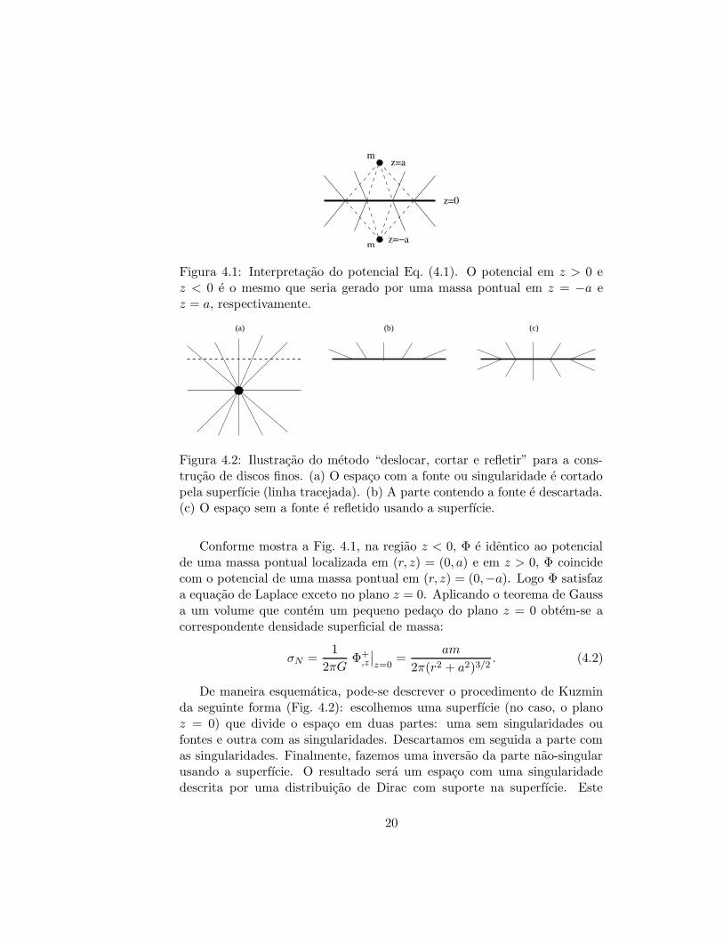
m

Figura 4.1: Interpretacao do potencial Eq. (4.1). O potencial em z > 0 ez < 0 e o mesmo que seria gerado por uma massa pontual em z = −a ez = a, respectivamente.

(a) (b) (c)

Figura 4.2: Ilustracao do metodo “deslocar, cortar e refletir” para a cons-trucao de discos finos. (a) O espaco com a fonte ou singularidade e cortadopela superfıcie (linha tracejada). (b) A parte contendo a fonte e descartada.(c) O espaco sem a fonte e refletido usando a superfıcie.

Conforme mostra a Fig. 4.1, na regiao z < 0, Φ e identico ao potencialde uma massa pontual localizada em (r, z) = (0, a) e em z > 0, Φ coincidecom o potencial de uma massa pontual em (r, z) = (0,−a). Logo Φ satisfaza equacao de Laplace exceto no plano z = 0. Aplicando o teorema de Gaussa um volume que contem um pequeno pedaco do plano z = 0 obtem-se acorrespondente densidade superficial de massa:

σN =1

2πGΦ+

,z

∣

∣

z=0=

am

2π(r2 + a2)3/2. (4.2)

De maneira esquematica, pode-se descrever o procedimento de Kuzminda seguinte forma (Fig. 4.2): escolhemos uma superfıcie (no caso, o planoz = 0) que divide o espaco em duas partes: uma sem singularidades oufontes e outra com as singularidades. Descartamos em seguida a parte comas singularidades. Finalmente, fazemos uma inversao da parte nao-singularusando a superfıcie. O resultado sera um espaco com uma singularidadedescrita por uma distribuicao de Dirac com suporte na superfıcie. Este

20

(a) (c)(b)

Figura 4.3: Ilustracao do metodo “deslocar, cortar e refletir” para a cons-trucao de discos finos com halos. (a) A esfera de fluido e cortada pela su-perfıcie (linha tracejada). (b) A parte inferior que contem o centro da esferae descartada. (c) O espaco com a calota e refletido usando a superfıcie.

procedimento e conhecido como metodo “deslocar, cortar e refletir”. Ma-tematicamente, consiste em aplicar a transformacao z → |z| + a, onde a euma constante positiva, a um potencial gravitacional.

O mesmo procedimento tambem pode ser usado para gerar discos comhalos (Fig. 4.3). Neste caso, uma esfera de fluido e cortada por um planoa uma distancia do centro menor que o raio da esfera. A parte do espacocontendo o centro da esfera e descartada, e a outra parte e refletida usandoa superfıcie. O resultado sera um disco com um halo central. A parte dodisco dentro do halo tera propriedades diferentes da parte externa ao halo.Se o metodo for aplicado a uma esfera de fluido perfeito em coordenadasisotropicas (Sec. 3.3.1), o resultado sera um disco de fluido perfeito com umhalo central.

4.2 Distribuicoes em espacos-tempo curvos

A transformacao matematica descrita na secao anterior aplicada a um ele-mento de linha em Relatividade Geral leva a necessidade de tratar campostensoriais em termos da teoria de distribuicoes. A teoria geral de distri-buicoes em espacos-tempo curvos com suporte em hipersuperfıcies tridimen-sionais foi desenvolvida por Hamoui e Papapetrou [58], Lichnerowicz [59] eTaub [60]. Seguimos a exposicao de Taub e particularizamos a teoria parao caso de discos.

O disco localizado no plano z = 0 divide a regiao Ω do espaco-tempoem duas metades Ω+ e Ω− onde z > 0 e z < 0, respectivamente. O tensor

21

metrico gµν e suposto ser contınuo atraves de z = 0, ou seja,

[gµν ] = gµν |z=0+ − gµν |z=0− = 0. (4.3)

Na vizinhanca de z = 0 podemos expandir gµν em:

g±µν = g0µν + zg±µν,z +

1

2z2g±µν,zz + . . . , (4.4)

onde os sinais ± referem-se a expansao acima e abaixo do disco, respectiva-mente. Desta maneira, pode-se caracterizar as descontinuidades na derivadaprimeira do tensor metrico pelo tensor bµν , definido como:

bµν ≡ [gµν,z ] = g+µν,z

∣

∣

z=0− g−µν,z

∣

∣

z=0. (4.5)

O tensor metrico e construıdo de forma a possuir simetria de reflexao emrelacao ao plano z = 0, o que significa g−µν(r, z) = g+

µν(r,−z). Esta relacaoimplica que, quando z 6= 0, g−µν,z(r, z) = −g+

µν,z(r,−z). Assim, no limiteapropriado quando z → 0, a Eq. (4.5) pode ser escrita como:

bµν = 2gµν,z |z=0 , (4.6)

onde definimos gµν,z|z=0 = g+µν,z|z=0.

No sentido de distribuicoes podemos expressar os sımbolos de ChristoffelEq. (2.3) como:

Γαβγ = (Γα

βγ)D = Γα+βγθ + Γα−

βγ(1 − θ), (4.7)

onde θ e a funcao de Heaviside:

θ =

1, z > 0

1/2, z = 0

0, z < 0

. (4.8)

Derivando-se a Eq. (4.7), pode-se escrever:

Γαβγ,λ = (Γα

βγ,λ)D + [Γαβγ ] δz

λδ(z), (4.9)

onde δ(z) e a distribuicao de Dirac com suporte em z = 0 e a descontinuidadedos sımbolos de Christoffel em z = 0 e dada por:

[Γαβγ ] ≡ Γα+

βγ − Γα−βγ =

1

2

(

δzβb

αγ + δz

γbαβ − gzαbβγ

)

. (4.10)

22

Usando-se a definicao do tensor de curvatura de Riemann Eq. (2.19), obtem-se para o tensor de Riemann distribucional:

Rρµσν = (Rρ

µσν)D +Hρµσνδ(z), (4.11)

onde:

Hρµσν = [Γρ

µν ] δzσ − [Γρ

µσ] δzν

=1

2

(

δzµδ

zσb

ρν − δz

µδzνb

ρσ − gzρδz

σbµν + gzρδzνbµσ

)

. (4.12)

Supondo que o tensor energia-momento possa ser expresso na forma:

Tµν = (Tµν)D +Qµνδ(z), (4.13)

as equacoes de Einstein sao equivalentes ao sistema:

R±µν − 1

2gµνR

± = 8πT±µν , (4.14a)

Hµν − 1

2gµνH = 8πQµν , (4.14b)

onde Hµν = Hρµρν e H = Hσ

σ. Assim, conhecendo-se a solucao das Eq.(4.14a) nas regioes Ω± fora do disco, pode-se calcular os componentes do ten-sor energia-momento da materia do disco por meio das Eq. (4.14b). Usandoa Eq. (4.12), obtemos:

Qµν =

1

16π

bzµδzν − bzzδµ

ν + gzµbzν − gzzbµν + bρρ (gzzδµν − gzµδz

ν)

. (4.15)

Para uma metrica estatica geral na forma:

ds2 = gtt(r, z)dt2 + grr(r, z)dr

2 + gzz(r, z)dz2 + gϕϕ(r, z)dϕ2, (4.16)

o tensor energia-momento Qµν sera diagonal. Definindo a base ortonormal

de tetradas:

e(t)µ =

(

1√gtt, 0, 0, 0

)

, e(r)µ =

(

0,1√−grr

, 0, 0

)

,

e(z)µ =

(

0, 0,1√−gzz

, 0

)

, e(ϕ)µ =

(

0, 0, 0,1√−gϕϕ

,

)

, (4.17)

o tensor energia momento pode ser expresso como:

Qµν = σe(t)µe(t)

ν + Pre(r)µe(r)

ν + Pze(z)µe(z)

ν + Pϕe(ϕ)µe(ϕ)

ν , (4.18)

23

onde a densidade superficial de energia, pressoes (ou tensoes) nas direcoesradial, direcao do eixo z e azimutal sao dados, respectivamente, por σ = Qt

t,Pr = −Qr

r, Pz = −Qzz e Pϕ = −Qϕ

ϕ. Devido ao termo√−gzz que divide a

distribuicao de Dirac, para obter as “verdadeiras” grandezas fısicas acimaelas devem ser multiplicadas por

√−gzz.

No caso da metrica de Weyl Eq. (3.4), usando as Eq. (4.6) e Eq. (4.15)obtemos as seguintes expressoes para σ, Pϕ, Pr e Pz (ja multiplicadas por√−gzz):

σ =1

8πe(Φ−Λ)/2Φ,z(2 − rΦ,r), (4.19a)

Pϕ =1

8πe(Φ−Λ)/2rΦ,rΦ,z, (4.19b)

Pr = Pz = 0. (4.19c)

Por nao haver pressao na direcao radial, a estabilidade dos discos geradospela metrica de Weyl pode ser justificada pela hipotese de contrarotacao,citada na Introducao. Neste caso define-se uma velocidade de contrarotacaoV das partıculas no disco dada por [8]:

V 2 =Pϕ

σ=

rΦ,r

2 − rΦ,r. (4.20)

Para a metrica em coordenadas isotropicas cilındricas:

ds2 = eνdt2 − eλ(

dr2 + dz2 + r2dϕ2)

, (4.21)

os componentes nao-nulos do tensor energia-momento do disco sao:

σ = − 1

4πe−λ/2λ,z (4.22a)

Pr = Pϕ =1

8πe−λ/2(λ,z + ν,z) (4.22b)

Ve-se que nestas coordenadas a isotropia entre os componentes radial eazimutal permite a construcao de discos de fluido perfeito.

Os componentes do tensor energia-momento devem satisfazer certas desi-gualdades fisicamente razoaveis [61]. A condicao fraca de energia e satisfeitase σ ≥ 0, a condicao dominante de energia impoe que σ ≥ |Pi|, i = r, z, ϕ. Fi-nalmente a condicao forte de energia e satisfeita se ρN = σ+Pr+Pz+Pϕ ≥ 0,onde ρN e a “densidade efetiva” Newtoniana.

24

4.3 Outros parametros fısicos dos discos

O estudo de orbitas geodesicas circulares no plano z = 0 permite obterinformacoes importantes sobre as propriedades dos discos, sejam eles finosou grossos. No caso da metrica geral Eq. (4.16), as equacoes geodesicas (2.2)fornecem a seguinte expressao para orbitas circulares:

ϕ2

t2= − gtt,r

gϕϕ,r, (4.23)

onde o ponto indica derivada em relacao ao tempo proprio. Tomando abase ortonormal de tetradas Eq. (4.17) e o quadrivetor vµ = (t, 0, 0, ϕ), aprojecao de vµ sobre a base de tetradas fornece:

v(t) = η(t)(t)e(t)µv

µ =√gtt t, (4.24a)

v(ϕ) = η(ϕ)(ϕ)e(ϕ)µv

µ =√

−gϕϕϕ. (4.24b)

O quadrado da velocidade circular vc medida por um observador no infinitosera dada por:

v2c =

(

v(ϕ)

v(t)

)2

=gϕϕgtt,r

gttgϕϕ,r, (4.25)

onde usou-se a Eq. (4.23). Particularizando-se para as metricas de WeylEq. (3.4) e isotropicas Eq. (4.21) obtem-se, respectivamente, as seguintesexpressoes para a velocidade circular:

v2c =

rΦ,r

2 − rΦ,r, v2

c =r2eλ(eν),reν(r2eλ),r

, (4.26)

lembrando que todas as quantidades sao calculadas em z = 0. Outra grande-za fısica de interesse e o momento angular por unidade de massa h = −gϕϕϕdas partıculas-teste em orbitas circulares. Substituindo a Eq. (4.23) na re-lacao:

1 = gtt t2 + gϕϕϕ

2, (4.27)

derivada a partir da Eq. (4.16), temos que o momento angular e expressopor:

h = −gϕϕ

√

gtt,r

gtt,rgϕϕ − gttgϕϕ,r. (4.28)

25

Aplicando as metricas de Weyl Eq. (3.4) e isotropicas Eq. (4.21) temos,respectivamente:

h = r3/2e−Φ/2

√

Φ,r

2(1 − rΦ,r), (4.29)

h = r2eλ

√

(eν),reν(r2eλ),r − r2eλ(eν),r

, (4.30)

onde novamente todas as quantidades sao calculadas em z = 0.O momento angular permite estabelecer uma extensao relativıstica do

criterio de estabilidade de Rayleigh para um fluido em repouso num campogravitacional [62]. Consideremos uma partıcula que se move numa trajetoriacircular com raio r0 = cte. e com momento angular por unidade de massah0 = r20ϕ. No referencial da partıcula a forca de atracao gravitacional eequilibrada pela forca centrıfuga de modulo Fc = h2

0/r30. Suponhamos que a

partıcula seja deslocada ligeiramente para um raio r > r0, com o momentoangular permanecendo constante. O modulo da forca centrıfuga na novaposicao passa a ser F ′

c = h20/r

3. Para que a partıcula tenda a retornara posicao original, o valor de F ′

c deve ser menor que o valor h2/r3 queequilibraria a forca gravitacional. Assim devemos ter:

h2(r) − h20(r0) > 0. (4.31)

Expandindo h2(r) em torno de r − r0, obtemos:

h2(r) − h20(r0) ≈ (r − r0)

dh2

dr> 0 ⇒ dh2

dr> 0, ou h

dh

dr> 0. (4.32)

Lembremos que se trata de um criterio de estabilidade de partıculasindividuais movendo-se no plano do disco. Uma analise de estabilidade maiscompleta deve levar em consideracao o movimento coletivo das partıculas dodisco, o que envolve a perturbacao de equacoes hidrodinamicas e a solucaode um problema nao-trivial de autovalores (ver Apendice B).

4.4 O metodo “deslocar, cortar, encher e refletir”

Na Sec. 4.1 discutimos o metodo inverso para construir discos com espessurainfinitesimal. Uma generalizacao deste metodo foi proposta por Gonzalez eLetelier [38] para gerar discos grossos e consiste no seguinte: apos descartara metade do espaco contendo as fontes ou singularidades, adiciona-se uma

26

(a) (b) (c)

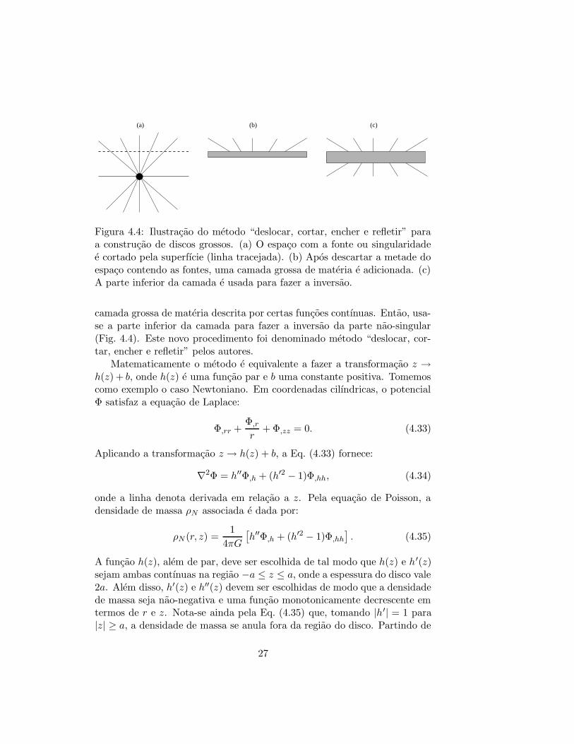
Figura 4.4: Ilustracao do metodo “deslocar, cortar, encher e refletir” paraa construcao de discos grossos. (a) O espaco com a fonte ou singularidadee cortado pela superfıcie (linha tracejada). (b) Apos descartar a metade doespaco contendo as fontes, uma camada grossa de materia e adicionada. (c)A parte inferior da camada e usada para fazer a inversao.

camada grossa de materia descrita por certas funcoes contınuas. Entao, usa-se a parte inferior da camada para fazer a inversao da parte nao-singular(Fig. 4.4). Este novo procedimento foi denominado metodo “deslocar, cor-tar, encher e refletir” pelos autores.

Matematicamente o metodo e equivalente a fazer a transformacao z →h(z) + b, onde h(z) e uma funcao par e b uma constante positiva. Tomemoscomo exemplo o caso Newtoniano. Em coordenadas cilındricas, o potencialΦ satisfaz a equacao de Laplace:

Φ,rr +Φ,r

r+ Φ,zz = 0. (4.33)

Aplicando a transformacao z → h(z) + b, a Eq. (4.33) fornece:

∇2Φ = h′′Φ,h + (h′2 − 1)Φ,hh, (4.34)

onde a linha denota derivada em relacao a z. Pela equacao de Poisson, adensidade de massa ρN associada e dada por:

ρN (r, z) =1

4πG

[

h′′Φ,h + (h′2 − 1)Φ,hh

]

. (4.35)

A funcao h(z), alem de par, deve ser escolhida de tal modo que h(z) e h′(z)sejam ambas contınuas na regiao −a ≤ z ≤ a, onde a espessura do disco vale2a. Alem disso, h′(z) e h′′(z) devem ser escolhidas de modo que a densidadede massa seja nao-negativa e uma funcao monotonicamente decrescente emtermos de r e z. Nota-se ainda pela Eq. (4.35) que, tomando |h′| = 1 para|z| ≥ a, a densidade de massa se anula fora da regiao do disco. Partindo de

27

um polinomio de grau par para h′′(z), obtem-se a seguinte classe de funcoesh(z) que satisfaz as restricoes impostas:

h(z) =

−z + C, z ≤ a,

Az2 +Bz2n+2, −a ≤ z ≤ a,

z + C, z ≥ a,

(4.36)

onde:

A =2n+ 1 − ac

4na, B =

ac− 1

4n(n+ 1)a2n+1, C = −a(2n+ 1 + ac)

4(n+ 1), (4.37)

n = 1, 2, . . . e c e o salto da derivada segunda em |z| = a. O caso particularac = 1 foi o inicialmente adotado em [38].

4.5 Pares potencial-densidade como modelos de

galaxias

O procedimento inverso tem sido amplamente usado para fornecer expressoesanalıticas simples para o campo gravitacional e distribuicoes de massa que semostraram uteis na modelagem de diversas classes de galaxias e aglomeradosglobulares. Uma descricao ampla de tais modelos pode ser encontrada em [1]Alguns destes pares potencial-densidade sao dados a seguir.

4.5.1 Modelo de Plummer

Um par potencial-densidade usado por Plummer [63] para descrever a distri-buicao de luminosidade em aglomerados globulares pode ser obtido fazendo-se a transformacao r →

√r2 + b2 com b > 0 na expressao para o potencial

Newtoniano de uma massa pontual em coordenadas esfericas. Disto resul-tam as seguintes expressoes para o potencial gravitacional e a distribuicaode massa:

Φ(r) = − Gm√r2 + b2

, ρN (r) =3b2m

4π(r2 + b2)5/2. (4.38)

4.5.2 Modelos de Miyamoto-Nagai

Miyamoto e Nagai [39] propuseram uma famılia de pares potencial-densidadeadequados para descrever a distribuicao de massa em galaxias espirais. Opar mais simples e obtido aplicando a transformacao z → a+

√z2 + b2 com

28

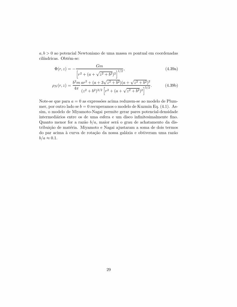
a, b > 0 ao potencial Newtoniano de uma massa m pontual em coordenadascilındricas. Obtem-se:

Φ(r, z) = − Gm[

r2 + (a+√z2 + b2)2

]1/2, (4.39a)

ρN (r, z) =b2m

4π

ar2 + (a+ 3√z2 + b2)(a+

√z2 + b2)2

(z2 + b2)3/2[

r2 + (a+√z2 + b2)2

]5/2. (4.39b)

Note-se que para a = 0 as expressoes acima reduzem-se ao modelo de Plum-mer, por outro lado se b = 0 recuperamos o modelo de Kuzmin Eq. (4.1). As-sim, o modelo de Miyamoto-Nagai permite gerar pares potencial-densidadeintermediarios entre os de uma esfera e um disco infinitesimalmente fino.Quanto menor for a razao b/a, maior sera o grau de achatamento da dis-tribuicao de materia. Miyamoto e Nagai ajustaram a soma de dois termosdo par acima a curva de rotacao da nossa galaxia e obtiveram uma razaob/a ≈ 0.1.

29

30

Capıtulo 5

Resumo dos Artigos e Conclusao

Neste capıtulo descrevemos resumidamente os assuntos e resultados dos ar-tigos publicados em periodicos durante o curso de doutorado (Sec. 5.1). Osartigos sao reproduzidos nos Apendices A a H. A conclusao do trabalho ecomentarios finais sao apresentados na Sec. 5.2.

5.1 Resumo dos artigos

Apendice A. Exact general relativistic perfect fluid disks with

halos

O metodo “deslocar, cortar e refletir” (Sec. 4.1) e primeiramente aplica-do a solucao de Schwarzschild em coordenadas isotropicas Eq. (3.20) paraconstruir discos estaticos de fluido perfeito (isotropia entre pressoes nas di-recoes radial e azimutal). Impondo-se restricoes sobre os parametros livresdo disco, a condicao forte de energia e velocidade de propagacao do somsublumial sao satisfeitos. A densidade superficial de energia e as pressoesdecaem rapidamente e monotonicamente com o raio de maneira a poder, emprincıpio, definir um raio de corte e considerar os discos finitos. O criteriode estabilidade de Rayleigh mostra que as orbitas circulares de partıculas-teste no plano do disco tendem a ser mais instaveis para discos altamenterelativısticos. A velocidade circular das partıculas apresenta um maximo edepois decai com r−1/2.

Outras solucoes que representam discos de fluido perfeito com halos saoobtidas aplicando-se o metodo “deslocar, cortar e refletir” a solucoes dasequacoes de Einstein para esferas de fluido perfeito em coordenadas iso-tropicas. Sao derivadas expressoes para as densidades de energia, pressoes,

31

velocidades de propagacao do som, velocidade circular e momento angularde discos com halos obtidos a partir das solucoes de Buchdahl Eq. (3.26)e solucoes para esferas de fluido encontradas por Narlikar et al [48, 47].As propriedades dos discos assim obtidos sao semelhantes as dos discos novacuo.

Apendice B. Exact general relativistic static perfect fluid disks

A primeira parte do artigo contem os resultados do artigo anterior sobrediscos de fluido perfeito obtidos a partir da solucao de Schwarzschild. Nasegunda parte, a estabilidade destes discos e estudada fazendo-se pertur-bacoes de primeira ordem nos componentes do tensor energia-momento dofluido no disco e analisando-se as equacoes perturbativas decorrentes dasequacoes de conservacao. O problema de autovalores resultante e resolvidonumericamente. Obtem-se que as quantidades perturbadas do fluido apre-sentam solucoes oscilatorias que favorecem a formacao de aneis. A presencade pressao radial contribui para a estabilidade do disco.

Apendice C. Exact relativistic static charged dust discs and

non-axisymmetric structures

O procedimento “deslocar, cortar e refletir” e aplicado a classe de metricasconformastaticas (Sec. 3.4) para gerar distribuicoes de materia feitas depoeira carregada. A sobreposicao de dois buracos extremos de Reissner-Nordstrom alinhados ao longo do eixo z permite a construcao de discos;quando os buracos negros sao alinhados ao longo do eixo y obtem-se dis-tribuicoes de poeira carregada no plano z = 0 sem simetria axial, massimetricas em relacao a um ou dois eixos coordenados, respectivamente, paramassas diferentes ou iguais dos buracos-negros. Para estas distribuicoes demateria estuda-se ainda o potencial efetivo de partıculas-teste neutras emmovimento geodesico.

Apendice D. Exact relativistic static charged perfect fluid

disks

Discos estaticos carregados de fluido perfeito sao gerados aplicando-se ometodo “deslocar, cortar e refletir” a solucao de Reissner-Nordstrom Eq.(3.22) em coordenadas isotropias. De maneira semelhante ao caso nao car-regado, a densidade superficial de energia e pressoes radial e azimutal decaemrapida- e monotonicamente com o raio, assim como a densidade superficial

32

de carga. A partir da equacao de equilıbrio hidrostatico de um fluido car-regado sob a influencia de um campo gravitacional, deriva-se uma condicaode estabilidade semelhante a do criterio de Rayleigh (Sec. 4.3). Encontra-seque a presenca de carga tende a desestabilizar o disco.

Apendice E. General relativistic model for the gravitational

field of active galactic nuclei surrounded by a disk

Este artigo trata de um modelo extremamente simples, porem exato, de umnucleo ativo de galaxia: a sobreposicao de um disco de Chazy-Curzon comum buraco negro de Schwarzschild central e duas barras, representando jatosde materia ao longo do eixo de simetria em coordenadas de Weyl (Sec. 3.2).O principal objetivo e verificar qual a influencia das barras sobre a materiaque compoe o disco e sua estabilidade. Em geral, a presenca das barrasaumenta as regioes de instabilidade do disco. O mesmo comportamentoe observado pelo calculo das frequencias epicıclica e vertical originarias daperturbacao de orbitas geodesicas circulares no plano do disco. Por ultimo,algumas orbitas fora do plano do disco sao calculadas por meio da solucaonumerica das equacoes geodesicas.

Apendice F. New models of general relativistic static thick

disks

O metodo “deslocar, cortar, encher e refletir” (Sec. 4.4) e usado para cons-truir novas solucoes de discos grossos. Uma classe de funcoes usada no“enchimento” dos discos e deduzida impondo-se restricoes as derivadas pri-meira e segunda das funcoes a fim de obter discos com propriedades fisica-mente aceitaveis. Esta classe de funcoes e usada juntamente com a solucaode Schwarzschild em coordenadas isotropicas, coordenadas de Weyl e coor-denadas canonicas para gerar discos grossos. Nestas ultimas coordenadasuma funcao adicional deve ser utilizada para gerar solucoes exatas de dis-cos. Os modelos obtidos em coordenadas isotropicas e de Weyl satisfazemas condicoes de energia. Os discos gerados em coordenadas canonicas possu-em algumas propriedades semelhantes aos discos em coordenadas de Weyl,porem nao satisfazem a condicao dominante de energia.

Apendice G. Relativistic models of galaxies

Usando uma forma particular para a metrica em coordenadas cilındricas,obteve-se modelos que podem ser interpretados como versoes relativısticas

33

de pares potencial-densidade Newtonianos (Sec. 4.5) usualmente usados co-mo modelos de galaxias. Em particular, os componentes do tensor energia-momento sao calculados para os dois primeiros potenciais de Miyamoto-Nagai e um potencial obtido por Satoh. Todos os potenciais geram distri-buicoes de materia com pressoes e que satisfazem as condicoes de energiapara certos intervalos dos parametros livres. Algumas orbitas geodesicasnao-planares sao calculadas numericamente para estes potenciais. Os efei-tos de primeira ordem da rotacao no perfil de velocidades sao calculados pormeio de uma forma aproximada da metrica de Kerr expressa em coordenadasisotropicas.

Apendice H. On multipolar analytical potentials for galaxies

Este artigo trata da teoria do potencial Newtoniano. Aplicando uma trans-formacao do tipo Miyamoto-Nagai a expansao multipolar ate o termo qua-drupolar, obtemos pares potencial-densidade que generalizam os pares deMiyamoto-Nagai. Infelizmente para certos intervalos dos parametros livresas distribuicoes de densidade de materia nao sao fisicamente aceitaveis. Paraos pares apresentados calculam-se ainda o perfil de rotacao e as frequenciasepicıclica e vertical de oscilacoes em torno de orbitas circulares em equilıbriono plano galactico. Obtem-se que para valores menores dos parametros re-lacionados aos momentos multipolares, o ponto de maximo das curvas derotacao e deslocado para raios maiores, e ambas as frequencias epicıclica evertical tem o valor reduzido para um raio fixo.

5.2 Conclusao

Nesta tese usamos o metodo inverso para construir diversas solucoes exatasdas equacoes de Einstein que representam espacos-tempo com distribuicoesdiscoidais de materia. Um primeiro conjunto de solucoes consiste em discosestaticos finos de fluido perfeito (pressoes radial e azimutal iguais) com esem halos em coordenadas isotropicas. Neste mesmo sistema de coordena-das, obteve-se solucoes de discos finos de fluido perfeito com carga eletrica.Utilizando-se das metricas conformastaticas, construiu-se modelos de discosconstituıdos por poeira carregada, alem de estruturas sem simetria axial.Todos estes modelos foram construıdos utilizando-se do procedimento “des-locar, cortar e refletir”. Elaborou-se ainda um modelo relativıstico muitosimples de um nucleo ativo de galaxia composto pela sobreposicao de umdisco de Chazy-Curzon com um buraco negro de Schwarzschild central eduas barras representando jatos de materia ao longo do eixo de simetria.

34

No que se refere a solucoes estaticas de discos grossos, utilizou-se ometodo “deslocar, cortar, encher e refletir” juntamente com um novo con-junto de funcoes usadas no “enchimento” para estudar novos modelos dediscos grossos em coordenadas isotropicas, coordenadas de Weyl e coorde-nadas canonicas. Estes discos possuem espessura constante e finita. Poroutro lado, ao utilizar-se uma forma particular para a metrica isotropica emcoordenadas cilındricas, obteve-se modelos tridimensionais de distribuicoesde materia que podem ser vistos como versoes relativısticas de alguns parespotencial-densidade Newtonianos usados na modelagem de galaxias. Estasdistribuicoes de materia ocupam todo o espaco fısico. Por fim, estudou-semodelos puramente Newtonianos de pares potencial-densidade obtidos pelaaplicacao de uma transformacao a expansao multipolar. Estes pares gene-ralizam os conhecidos pares de Miyamoto-Nagai usados como modelos paragalaxias espirais.

Uma possıvel extensao dos trabalhos desenvolvidos consistiria na intro-ducao de elementos fısicos adicionais aos discos, como campos magneticose rotacao. Em particular, seria interessante estudar como estes elementosalteram as propriedades dos discos grossos. O estudo da estabilidade destessistemas por meio de perturbacoes do tensor energia-momento tambem eimportante, embora se trate de um problema nao-trivial. Outra area pra-ticamente inexplorada e a elaboracao de modelos de discos relativısticoscom constante cosmologica. A sobreposicao de discos e/ou outras estrutu-ras (aneis, halos, jatos etc) com buracos negros consiste em outro tema comcrescente interesse teorico e importancia na astrofısica.

Neste ponto convem mencionar brevemente um dos problemas em abertomais importantes da astronomia moderna: a origem, composicao e influenciada materia escura no universo. As curvas de rotacao para grandes raios ob-tidas para muitas galaxias mostram um comportamento muito diferente deuma curva com decaimento Kepleriano (∝ r−1/2), permanecendo pratica-mente constantes ou decaindo muito pouco com o raio. A interpretacaomais simples para isto e que essas galaxias encontram-se envolvidas por ha-los com raio indefinido feitos por um tipo de materia nao-visıvel mas cujosefeitos gravitacionais sao mensuraveis. A exata natureza da materia escurae incerta, possivelmente constituıda por partıculas elementares exoticas cujaexistencia ainda nao foi detectada.

Em vista desta dificuldade, ha propostas alternativas que procuram ex-plicar a anomalia das curvas de rotacao das galaxias sem a necessidade demateria escura. Algumas delas incluem modificacoes na dinamica Newtoni-ana para grandes distancias [64] e modelos relativısticos de halos esfericoscom pressoes anisotropicas comparaveis a densidade de energia ao redor de

35

galaxias [65]. Recentemente mostrou-se que o chamado cenario do mun-do das branas permite a modelagem de halos galacticos por meio de umaequacao de Einstein modificada [66]. Neste cenario, nosso espaco-tempoquadridimensional e interpretado como uma hipersuperfıcie (brana) imersanum espaco-tempo curvo com dimensao ≥ 5. A equacao de Einstein efetivacontem um termo tensorial adicional originario desta imersao e que depen-de das propriedades geometricas do espaco-tempo com dimensao superior.Devemos lembrar que se trata apenas de uma possibilidade, uma vez que ateoria das branas encontra-se ainda num estagio bastante especulativo.

Por fim, durante os cerca de 90 anos desde sua elaboracao, houve pro-gressos extraordinarios na compreensao e aplicacoes da Relatividade Geral.No entanto, a teoria e tao rica que ainda ha muito por fazer e descobrir.Os detectores de ondas gravitacionais atualmente em construcao e/ou fasede testes, certamente trarao um novo impulso a area, alem de inevitaveissurpresas (boas ou ruins).

36

Bibliografia

[1] S. Binney and S. Tremaine, Galactic Dynamics, Princeton UniversityPress, Princeton, N. J., 1987.

[2] J. H. Krolik, Active Galactic Nuclei: from the Central Black Hole to

the Galactic Environment, Princeton University Press, Princeton, NewJersey, 1999.

[3] W. A. Bonnor and A. Sackfield, Comm. Math. Phys. 8, 338 (1968).

[4] T. Morgan and L. Morgan, Phys. Rev. 183, 1097 (1969).

[5] L. Morgan and T. Morgan, Phys. Rev. D 2, 2756 (1970).

[6] D. Lynden-Bell and S. Pineault, Mon. Not. R. Astron. Soc. 185, 679(1978).

[7] P. S. Letelier and S. R. Oliveira, J. Math. Phys. 28, 165 (1987).

[8] J. P. S. Lemos, Class. Quantum Grav. 6, 1219 (1989).

[9] J. Bicak, D. Lynden-Bell and J. Katz, Phys. Rev. D 47, 4334 (1993).

[10] J. Bicak, D. Lynden-Bell and C. Pichon, Mon. Not. R. Astron. Soc.

265, 126 (1993).

[11] G. A. Gonzalez and P. S. Letelier, Class. Quantum Grav. 16, 479 (1999).

[12] P. S. Letelier, Phys. Rev. D 60, 104042 (1999).

[13] J. Katz, J. Bicak and D. Lynden-Bell, Class. Quantum Grav. 16, 4023(1999).

[14] J. Bicak and T. Ledvinka, Phys. Rev. Lett. 71, 1669 (1993).

[15] T. Ledvinka, M. Zofka and J. Bicak, em Proceedings of the 8th Marcel

Grossman Meeting in General Relativity, editado por T. Piran, WorldScientific, Singapore, 1999.

[16] G. A. Gonzalez and P. S. Letelier, Phys. Rev. D 62, 064025 (2000).

[17] G. A. Gonzalez and O. A. Espitia, Phys. Rev. D 68, 104028 (2003).

[18] G. Garcıa R. and G. A. Gonzalez, Phys. Rev. D 69, 124002 (2004).

37

[19] G. Garcıa R. and G. A. Gonzalez, Class. Quantum Grav. 21, 4845(2004).

[20] G. Garcıa R. and G. A. Gonzalez, Phys. Rev. D 70, 104005 (2004).

[21] J. P. S. Lemos and P. S. Letelier, Class. Quantum Grav. 10, L75 (1993).

[22] J. P. S. Lemos and P. S. Letelier, Phys. Rev. D 49, 5135 (1994).

[23] J. P. S. Lemos and P. S. Letelier, Int. J. Mod. Phys. D 5, 53 (1996).

[24] O. Semerak, T. Zellerin and M. Zacek, Mon. Not. R. Astron. Soc. 308,691 (1999).

[25] O. Semerak, M. Zacek and T. Zellerin, Mon. Not. R. Astron. Soc. 308,705 (1999).

[26] O. Semerak and M. Zacek, Publ. Astron. Soc. Japan 52, 1067 (2000).

[27] O. Semerak, Class. Quantum Grav. 19, 3829 (2002).

[28] O. Semerak, Class. Quantum Grav. 20, 1613 (2003).

[29] T. Zellerin and O. Semerak, Class. Quantum Grav. 17, 5103 (2000).

[30] G. Neugebauer and R. Meinel, Phys. Rev. Lett. 75, 3046 (1995).

[31] C. Klein, Class. Quantum Grav. 14, 2267 (1997).

[32] C. Klein and O. Richter, Phys. Rev. Lett. 83, 2884 (1999).

[33] C. Klein, Phys. Rev. D 63, 064033 (2001).

[34] J. Frauendiener and C. Klein, Phys. Rev. D 63, 084025 (2001).

[35] C. Klein, Phys. Rev. D 65, 084029 (2002).

[36] C. Klein, Phys. Rev. D 68, 027501 (2003).

[37] C. Klein, Ann. Phys. 12(10), 599 (2003).

[38] G. A. Gonzalez and P. S. Letelier, Phys. Rev. D 69, 044013 (2004).

[39] M. Miyamoto and R. Nagai, Publ. Astron. Soc. Japan 27, 533 (1975).

[40] C. Satoh, Publ. Astron. Soc. Japan 32, 41 (1980).

38

[41] S. Chandrasekhar, The Mathematical Theory of Black Holes, OxfordUniversity Press, 1998.

[42] H. Stephani, D. Kramer, M. MacCallum, C. Hoenselaers and E. Herlt,Exact Solutions to Einstein’s Field Equations, 2nd Ed., Cambridge Uni-versity Press, Cambridge, 2003.

[43] H. Weyl, Ann. Phys. Lpz. 54, 117 (1917).

[44] H. Weyl, Ann. Phys. Lpz. 59, 185 (1919).

[45] M. Chazy, Bull. Soc. Math. France 52, 17 (1924).

[46] H. Curzon, Proc. London Math. Soc. 23, 477 (1924).

[47] V. V. Narlikar, G. K. Patwardhan and P. C. Vaidya, Proc. Natl. Inst.

Sci. India 9, 229 (1943).

[48] B. Kuchowicz, Acta Phys. Polon. B3, 209 (1972).

[49] H. A. Buchdahl, Astrophys. J. 140, 1512 (1964).

[50] W. B. Bonnor and S. B. P. Wickramasuriya, Mon. Not. R. Astron. Soc.

170, 643 (1975).

[51] W. B. Bonnor, Gen. Rel. Grav. 12, 453 (1980).

[52] W. B. Bonnor, Class. Quantum. Grav. 15, 351 (1998).

[53] M. Gurses, Phys. Rev. D 58, 044001 (1998).

[54] V. Varela, Gen. Rel. Grav. 35, 1815 (2003).

[55] S. D. Majumdar, Phys. Rev. 72, 930 (1947).

[56] A. Papapetrou, Proc. R. Ir. Acad. A 51, 191 (1947).

[57] G. G. Kuzmin, Astron. Zh. 33, 27 (1956).

[58] A. Papapetrou and A. Hamoui, Ann. Inst. Henri Poincare 9, 179(1968).

[59] A. Lichnerowicz, C. R. Acad. Sci. 273, 528 (1971).

[60] A. H. Taub, J. Math. Phys. 21, 1423 (1980).

39

[61] S. W. Hawking and G. F. R. Ellis, The Large Scale Structure of Space-

Time, Cambridge University Press, Cambridge, 1973.

[62] Lord Rayleigh, Proc. R. Soc. London A 93, 148 (1917); ver tambemL. D. Landau e E. M. Lifshitz, Fluid Mechanics, 2nd Ed., PergamonPress, Oxford, 1987, §27.

[63] H. C. Plummer, Mon. Not. R. Astron. Soc. 71, 460 (1911).

[64] M. Milgrom, Astrophys. J. 270, 365 (1983).

[65] S. Bharadwaj and S. Kar, Phys. Rev. D 68, 023516 (2003).

[66] S. Pal, S. Bharadwaj and S. Kar, Phys. Lett. B 609, 194 (2005).

40

Apendice A

Exact general relativistic perfect

fluid disks with halos

Daniel Vogt and Patricio S. Letelier, Physical Review D 68, 084010 (2003).

Received 26 June 2003; published 24 October 2003.

Abstract

Using the well-known “displace, cut and reflect” method used to generatedisks from given solutions of Einstein field equations, we construct staticdisks made of perfect fluid based on vacuum Schwarzschild’s solution inisotropic coordinates. The same method is applied to different exact so-lutions to the Einstein’s equations that represent static spheres of perfectfluids. We construct several models of disks with axially symmetric perfectfluid halos. All disks have some common features: surface energy densityand pressures decrease monotonically and rapidly with radius. As the “cut”parameter a decreases, the disks become more relativistic, with surface en-ergy density and pressure more concentrated near the center. Also, regionsof unstable circular orbits are more likely to appear for high relativisticdisks. Parameters can be chosen so that the sound velocity in the fluidand the tangential velocity of test particles in circular motion are less thanthe velocity of light. This tangential velocity first increases with radius andreaches a maximum.

PACS numbers: 04.20.Jb, 04.40.–b, 97.10.Gz

41

A.1 Introduction

Axially symmetric solutions of Einstein’s field equations corresponding todisklike configurations of matter are of great astrophysical interest, sincethey can be used as models of galaxies or accretion disks. These solutionscan be static or stationary and with or without radial pressure. Solutionsfor static disks without radial pressure were first studied by Bonnor andSackfield [1], and Morgan and Morgan [2], and with radial pressure by Mor-gan and Morgan [3]. Disks with radial tension have been considered in [4],and models of disks with electric fields [5], magnetic fields [6], and bothmagnetic and electric fields have been introduced recently [7]. Solutions forself-similar static disks were analyzed by Lynden-Bell and Pineault [8], andLemos [9]. The superposition of static disks with black holes were consideredby Lemos and Letelier [10–12], and Klein [13]. Also Bicak, Lynden-Bell andKatz [14] studied static disks as sources of known vacuum spacetimes andBicak, Lynden-Bell and Pichon [15] found an infinite number of new staticsolutions. For a recent survey on relativistic gravitating disks, see [16].

The principal method to generate the above mentioned solution is the“displace, cut and reflect” method. One of the main problem of the solutionsgenerated by using this simple method is that usually the matter content ofthe disk is anisotropic i. e., the radial pressure is different from the azimuthalpressure. In most of the solutions the radial pressure is null. This made thesesolutions rather unphysical. Even though, one can argue that when no radialpressure is present stability can be achieved if we have two circular streamsof particles moving in opposite directions (counterrotating hypothesis, seefor instance [14]).

In this article we apply the “displace, cut and reflect” method to spher-ically symmetric solutions of Einstein’s field equations in isotropic coordi-nates to generate static disks made of a perfect fluid, i. e., with radial pressureequal to tangential pressure and also disks of perfect fluid surrounded by anhalo made of perfect fluid matter.

The article is organized as follows. Section A.2 gives an overview of the“displace, cut and reflect” method. Also we present the basic equationsused to calculate the main physical variables of the disks. In Sec. A.3 weapply the formalism to obtain the simplest model of disk, which is basedon Schwarzschild’s vacuum solution in isotropic coordinates. The generatedclass of disks is made of a perfect fluid with well behaved density and pres-sure. Section A.4 presents some models of disks with halos obtained fromdifferent known exact solutions of Einstein’s field equations for static spheresof perfect fluid in isotropic coordinates. In Sec. A.5 we give some examples

42

(a)

(b)

Figure A.1: An illustration of the “displace, cut and reflect” method for thegeneration of disks. In (a) the spacetime with a singularity is displaced andcut by a plane (dotted line), in (b) the part with singularities is disregardedand the upper part is reflected on the plane.

of disks with halo generated from spheres composed of fluid layers. SectionA.6 is devoted to discussion of the results.

A.2 Einstein equations and disks

For a static, spherically symmetric spacetime the general line element inisotropic spherical coordinates can be cast as

ds2 = eν(r)dt2 − eλ(r)[

dr2 + r2(dθ2 + sin2 θdϕ2)]

. (A.1)

In cylindrical coordinates (t,R,z,ϕ) the line element (A.1) takes the form

ds2 = eν(R,z)dt2 − eλ(R,z)(

dR2 + dz2 +R2dϕ2)

. (A.2)

The metric of the disk will be constructed using the well known “displace,cut and reflect” method that was used by Kuzmin [17] in Newtonian gravityand later in general relativity by many authors [4–16]. The material contentof the disk will be described by functions that are distributions with supporton the disk. The method can be divided in the following steps that areillustrated in Fig. A.1. First, in a space wherein we have a compact sourceof gravitational field, we choose a surface (in our case, the plane z = 0) thatdivides the space in two pieces: one with no singularities or sources andthe other with the sources. Then we disregard the part of the space withsingularities and use the surface to make an inversion of the nonsingularpart of the space. This results in a space with a singularity that is a deltafunction with support on z = 0. This procedure is mathematically equivalent

43

to make the transformation z → |z|+ a, with a as constant. In the Einsteintensor we have first and second derivatives of z. Since ∂z|z| = 2ϑ(z) − 1and ∂zz|z| = 2δ(z), where ϑ(z) and δ(z) are, respectively, the Heavisidefunction and the Dirac distribution. Therefore the Einstein field equationswill separate in two different pieces [18]: one valid for z 6= 0 (the usualEinstein’s equations), and other involving distributions with an associatedenergy-momentum tensor, Tab = Qabδ(z), with support on z = 0. For themetric (A.2), the non-zero components of Qab are

Qtt =

1

16π

[

−bzz + gzz(bRR + bzz + bϕϕ)]

, (A.3)

QRR = Qϕ

ϕ =1

16π

[

−bzz + gzz(btt + bRR + bzz)]

, (A.4)

where bab denotes the jump of the first derivatives of the metric tensor onthe plane z = 0,

bab = gab,z |z=0+ − gab,z|z=0− , (A.5)

and the other quantities are evaluated at z = 0+. The “true” surface energy-momentum tensor of the disk can be written as Sab =

√−gzzQab, thus thesurface energy density σ and the radial and azimuthal pressures or tensions(P ) read:

σ =√−gzzQ

tt, P = −√−gzzQ

RR = −√−gzzQ

ϕϕ. (A.6)

Note that when the same procedure is applied to an axially symmetric space-time in Weyl coordinates we have QR

R = 0, i. e., we have no radial pressureor tension.

This procedure in principle can be applied to any spacetime solution ofthe Einstein equations with or without source (stress tensor). The applica-tion to a static sphere of perfect fluid is schematized in Fig. A.2. The sphereis displaced and cut by a distance a less then its radius rb. The part of thespace that contains the center of the sphere is disregarded. After the inver-sion of the remaining space, we end up with a disk surrounded by a cap ofperfect fluid. The properties of the inner part of the disk will depend on theinternal fluid solution, but if the internal spherical fluid solution is joined tothe standard external Schwarzschild solution, the physical properties of theouter part of the disk will be those originated from Schwarzschild’s vacuumsolution.

In isotropic coordinates the matching at the boundary of the fluid sphereleads to four continuity conditions: the two metric functions eλ and eν

44

(b)(a)

Figure A.2: An illustration of the “displace, cut and reflect” method for thegeneration of disks with halos. In (a) the sphere of perfect fluid is displacedand cut by a plane (dotted line); in (b) the lower part is disregarded andthe upper part is reflected on the plane.

together with their first derivatives with respect to the radial coordinateshould be continuous across the boundary. In addition, to have a compactbody the pressure at the surface of the material sphere has to drop to zero.Also to have a meaningful solution the velocity of sound, V2 = dp/dρ, shouldbe restricted to the interval 0 ≤ V < 1.

The Einstein equations for a static, spherically symmetric space time inisotropic coordinates for a perfect fluid source give us that density ρ andpressure p are related to the metric functions by

ρ = −e−λ

8π

[

λ′′

+1

4(λ′)2 +

2λ′

r

]

, (A.7)

p =e−λ

8π

[

1

4(λ′)2 +

1

2λ′ν ′ +

1

r(λ′ + ν ′)

]

, (A.8)

where primes indicate differentiation with respect to r.

Also static spheres composed of various layers of fluid can be used togenerate disks with halos of fluid layers (see Fig. A.3). The disk will then becomposed of different axial symmetric “pieces” glued together. The match-ing conditions at the boundary of adjacent spherical fluid layers in isotropiccoordinates involves four continuity conditions: the two metric functions eλ

and eν , the first derivative of λ with respect to the radial coordinate, and thepressure should be continuous across the boundary. At the most externalboundary, the metric functions eλ and eν , and their first derivatives withrespect to the radial coordinate should be continuous across the boundary;also the pressure there should go to zero.

45

(b)(a)

Figure A.3: An illustration of the “displace, cut and reflect” method forthe generation of disks with various layers of halos. In (a) the sphere withdifferent layers of fluid is displaced and cut with a plane (dotted line); in(b) the field is reflected on the plane.

A.3 The simplest disk

We first apply the “displace, cut and reflect” method to generate disks dis-cussed in the previous section and depicted in Fig. A.1 to the Schwarzschildmetric in isotropic coordinates (t, r, θ, ϕ),

ds2 =

(

1 − m2r

)2

(

1 + m2r

)2 dt2 −(

1 +m

2r

)4[

dr2 + r2(dθ2 + sin2 θdϕ2)]

. (A.9)

Expressing solution (A.9) in cylindrical coordinates, and using Eqs. (A.3)–(A.6), we obtain a disk with surface energy density σ and radial and az-imuthal pressures (or tensions) P given by

σ =4ma

π(m+ 2√R2 + a2)3

, (A.10)

P = − 2m2a

π(m+ 2√R2 + a2)3(m− 2

√R2 + a2)

. (A.11)

The total mass of the disk can be calculated with the help of Eq. (A.10):

M =

∫ ∞

0

∫ 2π

0σ√gRRgϕϕ dRdϕ =

m

4a(m+ 4a). (A.12)

Eq. (A.10) shows that the disk’s surface energy density is always posi-tive (weak energy condition). Positive values (pressure) for the stresses inazimuthal and radial directions are obtained if m < 2

√R2 + a2. The strong

46

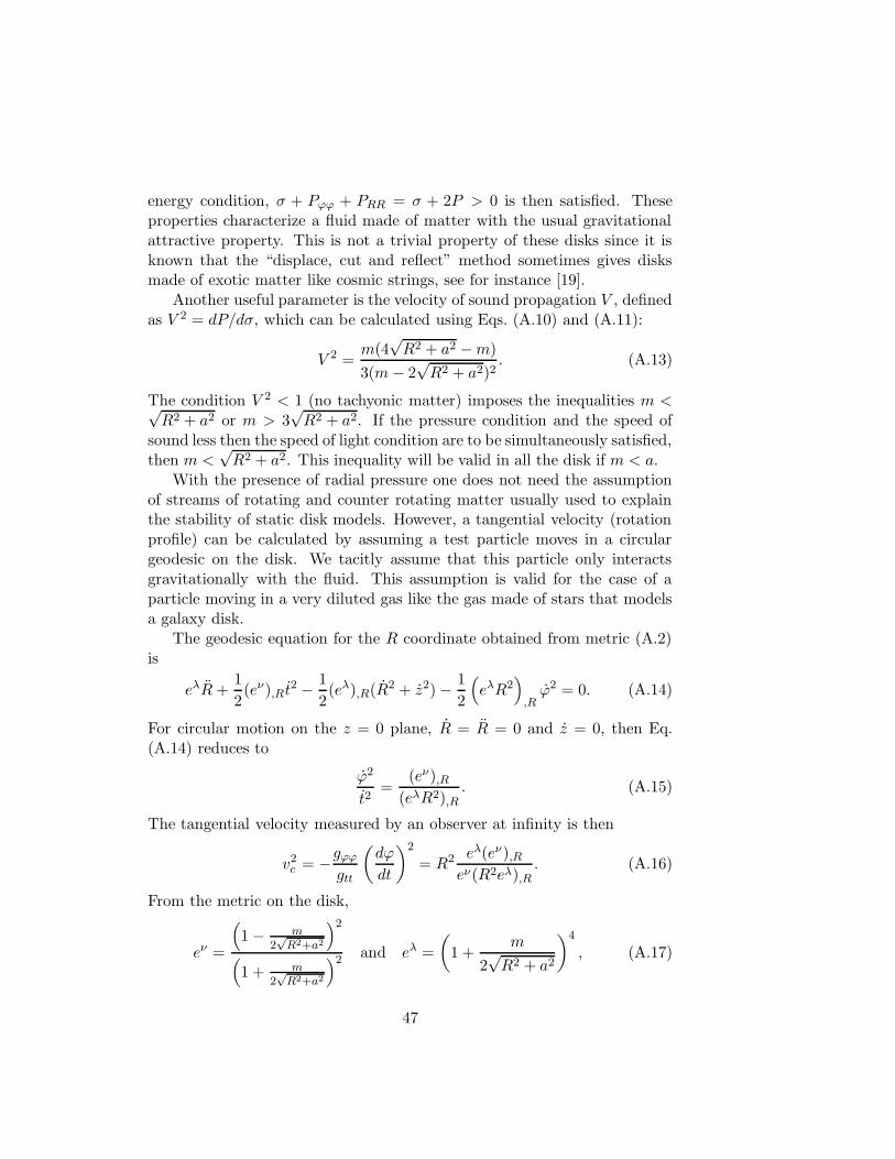
energy condition, σ + Pϕϕ + PRR = σ + 2P > 0 is then satisfied. Theseproperties characterize a fluid made of matter with the usual gravitationalattractive property. This is not a trivial property of these disks since it isknown that the “displace, cut and reflect” method sometimes gives disksmade of exotic matter like cosmic strings, see for instance [19].

Another useful parameter is the velocity of sound propagation V , definedas V 2 = dP/dσ, which can be calculated using Eqs. (A.10) and (A.11):

V 2 =m(4

√R2 + a2 −m)

3(m− 2√R2 + a2)2

. (A.13)

The condition V 2 < 1 (no tachyonic matter) imposes the inequalities m <√R2 + a2 or m > 3

√R2 + a2. If the pressure condition and the speed of

sound less then the speed of light condition are to be simultaneously satisfied,then m <

√R2 + a2. This inequality will be valid in all the disk if m < a.

With the presence of radial pressure one does not need the assumptionof streams of rotating and counter rotating matter usually used to explainthe stability of static disk models. However, a tangential velocity (rotationprofile) can be calculated by assuming a test particle moves in a circulargeodesic on the disk. We tacitly assume that this particle only interactsgravitationally with the fluid. This assumption is valid for the case of aparticle moving in a very diluted gas like the gas made of stars that modelsa galaxy disk.

The geodesic equation for the R coordinate obtained from metric (A.2)is

eλR+1

2(eν),R t

2 − 1

2(eλ),R(R2 + z2) − 1

2

(

eλR2)

,Rϕ2 = 0. (A.14)

For circular motion on the z = 0 plane, R = R = 0 and z = 0, then Eq.(A.14) reduces to

ϕ2

t2=

(eν),R(eλR2),R

. (A.15)

The tangential velocity measured by an observer at infinity is then

v2c = −gϕϕ

gtt

(

dϕ

dt

)2

= R2 eλ(eν),Reν(R2eλ),R

. (A.16)

From the metric on the disk,

eν =

(

1 − m2√

R2+a2

)2

(

1 + m2√

R2+a2

)2 and eλ =

(

1 +m

2√R2 + a2

)4

, (A.17)

47

0

0.01

0.02

0.03

0.04

0.05

0.06

0.07

0.08

0 1 2 3 4 5

R = R / m~

(a)

σ

a = 0.6a = 0.8a = 1.0a = 1.2

0

0.005

0.010

0.015

0.020

0.025

0.030

0 1 2 3 4 5

R = R / m~

(b)

P

a = 0.6a = 0.8a = 1.0a = 1.2

0.2

0.3

0.4

0.5

0.6

0.7

0.8

0.9

0 1 2 3 4 5

R = R / m~

(c)

V

a = 0.6a = 0.8a = 1.0a = 1.2

Figure A.4: (a) The surface energy density σ, (b) pressures P , (c) soundvelocity V with m = 0.5 and a = 0.6, 0.8,1.0, and 1.2 as function of R =R/m. We use geometric units G = c = 1.

48

0

0.1

0.2

0.3

0.4

0.5

0.6

0.7

0 1 2 3 4 5

R = R / m~

(d)

vc

a = 0.6a = 0.8a = 1.0a = 1.2

Figure A.4(d): The tangential velocity vc (rotation curve or rotation profile)with m = 0.5 and a = 0.6, 0.8,1.0, and 1.2 as function of R = R/m. We usegeometric units G = c = 1.

we find that Eq. (A.16) can be cast as,

v2c =

mR2

(

1 − m2√

R2+a2

)

[

(R2 + a2)3/2 + m2 (a2 −R2)

]

. (A.18)

For R >> a, Eq. (A.18) goes as vc = (m/R)1/2, the Newtonian circularvelocity.

To determine the stability of circular orbits on the disk’s plane, we usean extension of Rayleigh [20, 21] criteria of stability of a fluid at rest in agravitational field

hdh

dR> 0, (A.19)

where h is the specific angular momentum of a particle on the disk’s plane:

h = −gϕϕdϕ

ds= −gϕϕ

dϕ

dt

dt

ds. (A.20)

Using Eq. (A.15) and the relation

1 = eν(

dt

ds

)2

−R2eλ(

dϕ

ds

)2

, (A.21)

49

0

0.005

0.010

0.015

0.020

0.025

0.030

0.035

0.040

0.045

0.050

0 1 2 3 4 5

R = R / a~

(a)

σ

m = 0.2m = 0.4m = 0.6m = 0.8

0

0.002

0.004

0.006

0.008

0.010

0.012

0.014

0.016

0 1 2 3 4 5

R = R / a~

(b)

P

m = 0.2m = 0.4m = 0.6m = 0.8

0.1

0.2

0.3

0.4

0.5

0.6

0.7

0.8

0 1 2 3 4 5

R = R / a~

(c)

V

m = 0.2m = 0.4m = 0.6m = 0.8

Figure A.5: (a) The surface energy density σ, (b) pressures P and (c) soundvelocity V with a = 1.0 and m = 0.2, 0.4, 0.6, and 0.8 as function ofR = R/a.

50

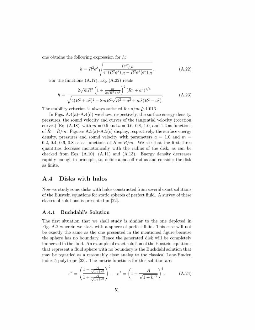
one obtains the following expression for h:

h = R2eλ

√

(eν),Reν(R2eλ),R −R2eλ(eν),R

. (A.22)

For the functions (A.17), Eq. (A.22) reads

h =2√mR2

(

1 + m2√

R2+a2

)2(R2 + a2)1/4

√

4(R2 + a2)2 − 8mR2√R2 + a2 +m2(R2 − a2)

. (A.23)

The stability criterion is always satisfied for a/m

1.016.In Figs. A.4(a)–A.4(d) we show, respectively, the surface energy density,

pressures, the sound velocity and curves of the tangential velocity (rotationcurves) [Eq. (A.18)] with m = 0.5 and a = 0.6, 0.8, 1.0, and 1.2 as functionsof R = R/m. Figures A.5(a)–A.5(c) display, respectively, the surface energydensity, pressures and sound velocity with parameters a = 1.0 and m =0.2, 0.4, 0.6, 0.8 as as functions of R = R/m. We see that the first threequantities decrease monotonically with the radius of the disk, as can bechecked from Eqs. (A.10), (A.11) and (A.13). Energy density decreasesrapidly enough in principle, to, define a cut off radius and consider the diskas finite.

A.4 Disks with halos

Now we study some disks with halos constructed from several exact solutionsof the Einstein equations for static spheres of perfect fluid. A survey of theseclasses of solutions is presented in [22].

A.4.1 Buchdahl’s Solution

The first situation that we shall study is similar to the one depicted inFig. A.2 wherein we start with a sphere of perfect fluid. This case will notbe exactly the same as the one presented in the mentioned figure becausethe sphere has no boundary. Hence the generated disk will be completelyimmersed in the fluid. An example of exact solution of the Einstein equationsthat represent a fluid sphere with no boundary is the Buchdahl solution thatmay be regarded as a reasonably close analog to the classical Lane-Emdenindex 5 polytrope [23]. The metric functions for this solution are:

eν =

(

1 − A√1+kr2

1 + A√1+kr2

)2

, eλ =

(

1 +A√

1 + kr2

)4

, (A.24)

51

where A and k are constants. Far from the origin the solution goes over intothe external Schwarzschild metric, when m = 2A/

√k. The density, pressure

and sound velocity are given by:

ρ =3Ak

2π(A+√

1 + kr2)5, p =

kA2

2π(−A+√

1 + kr2)(A+√

1 + kr2)5,

(A.25)

V2 =2A(−2A+ 3

√1 + kr2)

15(A −√

1 + kr2)2. (A.26)

The condition V < 1 is satisfied for A < [(18 −√

39)/19]√

1 + kr2.

Using Eq. (A.24) and Eqs. (A.3)–(A.6), we get the following expressionsfor the energy density, pressure and sound velocity of the disk:

σ =akA

π[

A+√

1 + k(R2 + a2)]3 , (A.27)

P =akA2

2π[

−A+√

1 + k(R2 + a2)] [

A+√

1 + k(R2 + a2)]3 , (A.28)

V 2 =A[

−A+ 2√

1 + k(R2 + a2)]

3[

A−√

1 + k(R2 + a2)]2 . (A.29)

The conditions V < 1 and P > 0 are both satisfied if A < 12

√1 + ka2.

Figures A.6(a)–A.6(d) show, respectively, σ, P , V and rotation curves, Eq.(A.30), as functions of R = R/m for the disk calculated from Buchdahl’ssolution.

In Figs. A.7(a) and A.7(b) we show, respectively, the density ρ togetherwith pressure p, and sound velocity V of the halo along the axis z for A =0.6; k = 1 and a = 1. Note that in this solution there is no boundary of thefluid sphere: the disk is completely immersed in the fluid.

The tangential velocity vc calculated from metric coefficients (A.24) is

v2c =

2AkR2

(

1 −A/√

1 + k(R2 + a2))

[1 + k(R2 + a2)]3/2 +A[1 + k(a2 −R2)]

.

(A.30)

For R >> a, Eq. (A.30) goes as vc = (2A)1/2/(R1/2k1/4). The specific

52

0

0.005

0.010

0.015

0.020

0.025

0 2 4 6 8 10

R = R / m~

(a)

σ

a=1a=2a=3

0

0.002

0.004

0.006

0.008

0.010

0.012

0.014

0.016

0 2 4 6 8 10

R = R / m~

(b)

P

a=1a=2a=3

0.1

0.2

0.3

0.4

0.5

0.6

0.7

0.8

0.9

0 2 4 6 8 10

R = R / m~

(c)

V

a=1a=2a=3

Figure A.6: (a) The surface energy density σ, Eq. (A.27), (b) the pressureP Eq. (A.28), (c) the velocity of sound V Eq. (A.29) for the disk withA = 0.6; k = 1; for a = 1, 2 and 3 as function of R = R/m.

53

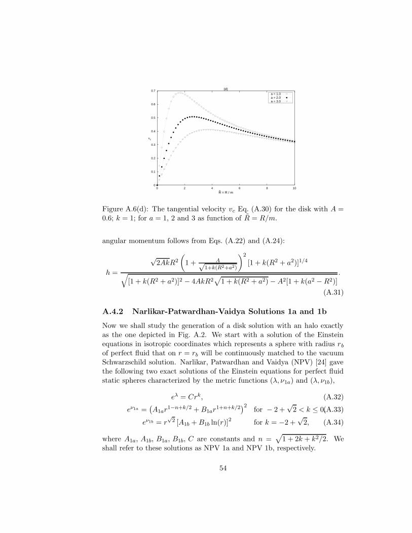
0

0.1

0.2

0.3

0.4

0.5

0.6

0.7

0 2 4 6 8 10

R = R / m~

(d)

vc

a = 1.0a = 2.0a = 3.0

Figure A.6(d): The tangential velocity vc Eq. (A.30) for the disk with A =0.6; k = 1; for a = 1, 2 and 3 as function of R = R/m.

angular momentum follows from Eqs. (A.22) and (A.24):

h =

√2AkR2

(

1 + A√1+k(R2+a2)

)2

[1 + k(R2 + a2)]1/4

√

[1 + k(R2 + a2)]2 − 4AkR2√

1 + k(R2 + a2) −A2[1 + k(a2 −R2)].

(A.31)

A.4.2 Narlikar-Patwardhan-Vaidya Solutions 1a and 1b

Now we shall study the generation of a disk solution with an halo exactlyas the one depicted in Fig. A.2. We start with a solution of the Einsteinequations in isotropic coordinates which represents a sphere with radius rb

of perfect fluid that on r = rb will be continuously matched to the vacuumSchwarzschild solution. Narlikar, Patwardhan and Vaidya (NPV) [24] gavethe following two exact solutions of the Einstein equations for perfect fluidstatic spheres characterized by the metric functions (λ, ν1a) and (λ, ν1b),

eλ = Crk, (A.32)

eν1a =(

A1ar1−n+k/2 +B1ar

1+n+k/2)2

for − 2 +√

2 < k ≤ 0,(A.33)

eν1b = r√

2 [A1b +B1b ln(r)]2 for k = −2 +√

2, (A.34)

where A1a, A1b, B1a, B1b, C are constants and n =√

1 + 2k + k2/2. Weshall refer to these solutions as NPV 1a and NPV 1b, respectively.

54

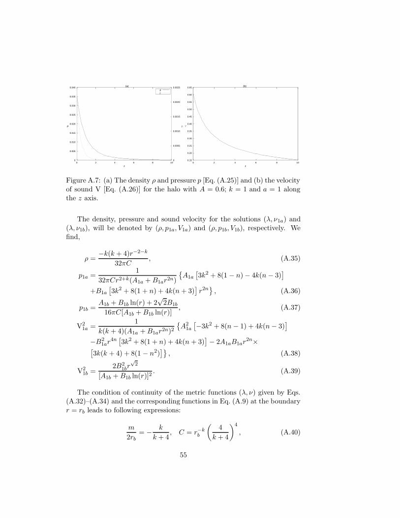
0

0.005

0.010

0.015

0.020

0.025

0.030

0.035

0.040

0 2 4 6 8 100

0.0005

0.0010

0.0015

0.0020

0.0025

z

ρ

(a)

p

ρp

0.15

0.20

0.25

0.30

0.35

0.40

0.45

0.50

0.55

0.60

0.65

0 2 4 6 8 10

z

(b)

V

Figure A.7: (a) The density ρ and pressure p [Eq. (A.25)] and (b) the velocityof sound V [Eq. (A.26)] for the halo with A = 0.6; k = 1 and a = 1 alongthe z axis.

The density, pressure and sound velocity for the solutions (λ, ν1a) and(λ, ν1b), will be denoted by (ρ, p1a, V1a) and (ρ, p1b, V1b), respectively. Wefind,

ρ =−k(k + 4)r−2−k

32πC, (A.35)

p1a =1

32πCr2+k(A1a +B1ar2n)

A1a

[

3k2 + 8(1 − n) − 4k(n− 3)]

+B1a

[

3k2 + 8(1 + n) + 4k(n+ 3)]

r2n

, (A.36)

p1b =A1b +B1b ln(r) + 2

√2B1b

16πC[A1b +B1b ln(r)], (A.37)

V21a =

1

k(k + 4)(A1a +B1ar2n)2

A21a

[

−3k2 + 8(n− 1) + 4k(n− 3)]

−B21ar

4n[

3k2 + 8(1 + n) + 4k(n+ 3)]

− 2A1aB1ar2n×

[

3k(k + 4) + 8(1 − n2)]

, (A.38)

V21b =

2B21br

√2

[A1b +B1b ln(r)]2. (A.39)

The condition of continuity of the metric functions (λ, ν) given by Eqs.(A.32)–(A.34) and the corresponding functions in Eq. (A.9) at the boundaryr = rb leads to following expressions:

m

2rb= − k

k + 4, C = r−k

b

(

4

k + 4

)4

, (A.40)

55

A1a = −3k2 + 8(1 + n) + 4k(n+ 3)

16nr1−n+k/2b

, B1a =3k2 + 8(1 − n) − 4k(n− 3)

16nr1+n+k/2b

,

(A.41)

A1b = −2√

2 + ln(rb)

4r1/

√2

b

, B1b =1

4r1/

√2

b

. (A.42)

V1a has its maximum at r = 0, and V1b at r = rb. Condition V1b(rb) < 1 is

satisfied if rb < 41/√

2.

Using Eqs. (A.32)–(A.34) in Eqs. (A.3)–(A.6), we get the following ex-pressions for the energy density, pressure and sound velocity of the disk:

σ = − ka

4π√CR1+k/4

, (A.43)

P1a =a

4π√CR1+k/4

[A1a(k − n+ 1) +B1a(k + n+ 1)Rn]

[A1a +B1aRn], (A.44)

P1b =a

4π√CR1/2+

√2/4[2A1b +B1b ln(R)]

[

2A1b(√

2 − 1) + 2B1b

+B1b(√

2 − 1) ln(R)]

, (A.45)

V 21a =

1

k(k + 4)[

A1aR−n/2 +B1aRn/2]2

[

−B21aRn(k2 + 5k + nk + 4n+ 4)

+A21aR−n(−k2 − 5k + nk + 4n− 4) + 2A1aB1a(−k2 − 5k + 4n2 − 4)

]

,

(A.46)

V 21b =

1

2(2A1b +B1b ln(R))2

[

B21b

√2 ln2(R) + 2B1b(2B1b +B1b

√2 + 2A1b

√2)

× ln(R) + 4A1bB1b(2 +√

2) + 4√

2A21b + 8B2

1b

]

, (A.47)

where R = R2 + a2. V1a and V1b have their maximum values at R = 0.Because the expressions are rather involved, the restrictions on the con-stants, to ensure that the velocities are positive and less then one, are bestmade graphically. The curves of σ, P and V as function of R = R/mwith parameters k = −1/2; rb = 2 and a = 0.5, 1.0,1.5 are displayed inFigs. A.8(a)–A.8(c), respectively. Figures A.9(a)–A.9(b) show the den-sity ρ, pressure p and velocity of sound V for the halo with parametersk = −1/2; rb = 2, for a = 0.5 along the axis z. The same physical quantitiesare shown in Figs. A.10(a)–A.10(c) and A.11(a)–A.11(b) with k = −2+

√2.

We note that σ and P are continuous at the boundary between the internal

56

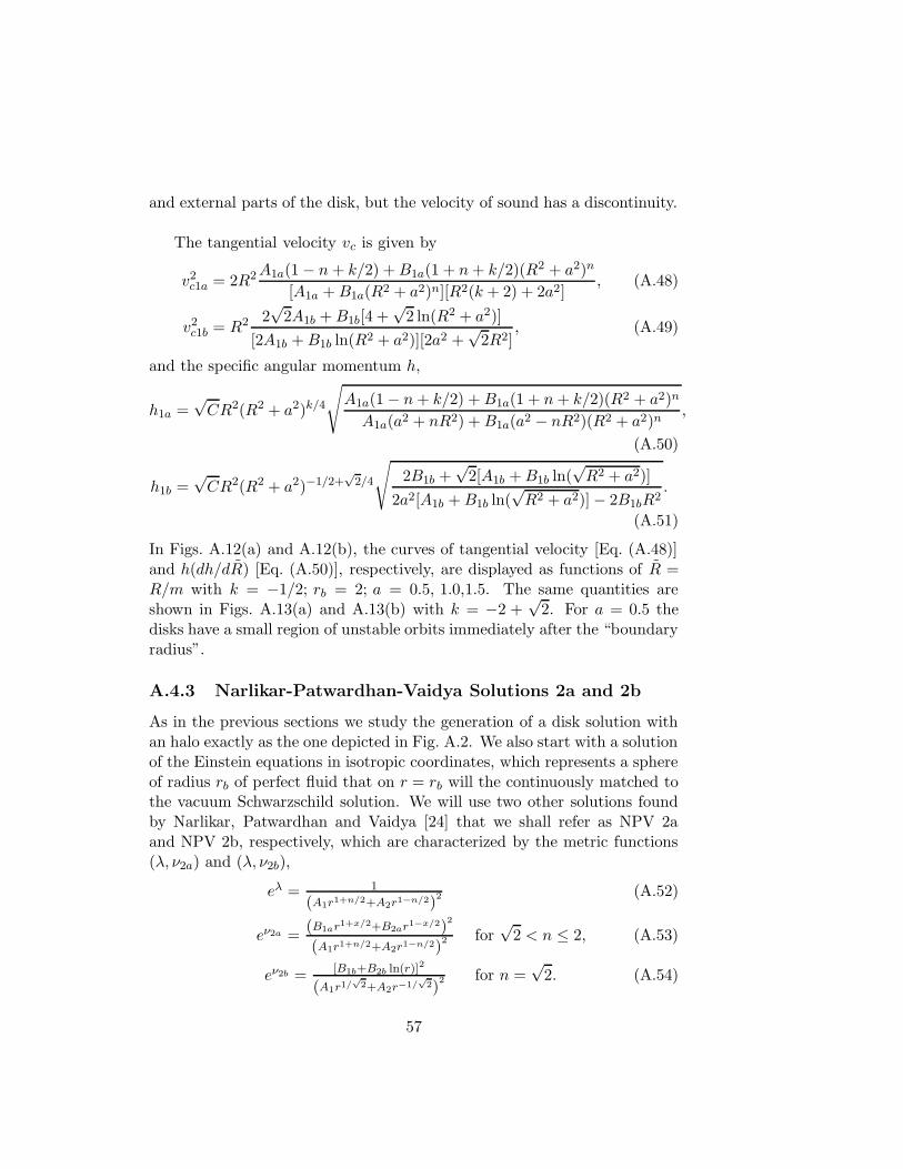
and external parts of the disk, but the velocity of sound has a discontinuity.

The tangential velocity vc is given by

v2c1a = 2R2A1a(1 − n+ k/2) +B1a(1 + n+ k/2)(R2 + a2)n

[A1a +B1a(R2 + a2)n][R2(k + 2) + 2a2], (A.48)

v2c1b = R2 2

√2A1b +B1b[4 +

√2 ln(R2 + a2)]

[2A1b +B1b ln(R2 + a2)][2a2 +√

2R2], (A.49)

and the specific angular momentum h,

h1a =√CR2(R2 + a2)k/4

√

A1a(1 − n+ k/2) +B1a(1 + n+ k/2)(R2 + a2)n

A1a(a2 + nR2) +B1a(a2 − nR2)(R2 + a2)n,

(A.50)

h1b =√CR2(R2 + a2)−1/2+

√2/4

√

2B1b +√

2[A1b +B1b ln(√R2 + a2)]

2a2[A1b +B1b ln(√R2 + a2)] − 2B1bR2

.

(A.51)

In Figs. A.12(a) and A.12(b), the curves of tangential velocity [Eq. (A.48)]and h(dh/dR) [Eq. (A.50)], respectively, are displayed as functions of R =R/m with k = −1/2; rb = 2; a = 0.5, 1.0,1.5. The same quantities areshown in Figs. A.13(a) and A.13(b) with k = −2 +

√2. For a = 0.5 the

disks have a small region of unstable orbits immediately after the “boundaryradius”.

A.4.3 Narlikar-Patwardhan-Vaidya Solutions 2a and 2b

As in the previous sections we study the generation of a disk solution withan halo exactly as the one depicted in Fig. A.2. We also start with a solutionof the Einstein equations in isotropic coordinates, which represents a sphereof radius rb of perfect fluid that on r = rb will the continuously matched tothe vacuum Schwarzschild solution. We will use two other solutions foundby Narlikar, Patwardhan and Vaidya [24] that we shall refer as NPV 2aand NPV 2b, respectively, which are characterized by the metric functions(λ, ν2a) and (λ, ν2b),

eλ = 1

(A1r1+n/2+A2r1−n/2)2 (A.52)

eν2a =(B1ar1+x/2+B2ar1−x/2)

2

(A1r1+n/2+A2r1−n/2)2 for

√2 < n ≤ 2, (A.53)

eν2b = [B1b+B2b ln(r)]2

(A1r1/√

2+A2r−1/√

2)2 for n =

√2. (A.54)

57

0

0.005

0.010

0.015

0.020

0.025

0.030

0.035

0.040

0.045

0 2 4 6 8 10

R = R / m~

(a)

σ

a=0.5a=1.0a=1.5

0

0.001

0.002

0.003

0.004

0.005

0.006

0.007

0.008

0.009

0.010

0 2 4 6 8 10

R = R / m~

(b)

P

a=0.5a=1.0a=1.5

0.15

0.20

0.25

0.30

0.35

0.40

0.45

0.50

0.55

0 2 4 6 8 10

R = R / m~

(c)

V

a=0.5a=1.0a=1.5

Figure A.8: (a) The surface energy density σ [Eq. (A.43)], (b) the pressureP [Eq. (A.44) and (c) the velocity of sound V [Eq. (A.46)] for the disk withk = −1/2; rb = 2; for a = 0.5, 1.0 and 1.5 as function of R = R/m.

58

0

0.005

0.010

0.015

0.020

0.025

0 0.5 1 1.5 20

0.001

0.002

0.003

0.004

0.005

z

ρ

(a)

p

ρp

0

0.1

0.2

0.3

0.4

0.5

0.6

0 0.5 1 1.5 2

z

(b)

V

Figure A.9: (a) The density ρ [Eq. (A.35)] and pressure p [Eq. (A.36)], and(b) the velocity of sound V [Eq. (A.38)] for the halo with k = −1/2; rb =2; for a = 0.5 along the z axis.

where the A’s and B’s are constants and x =√

2n2 − 4. The solution (λ, ν2a)with n = 2 corresponds to Schwarzschild’s internal solution in isotropiccoordinates (see for instance Ref. [22]). This solution has constant densityand is conformally flat when B1a = 0.

The density, pressure and sound velocity for the solutions (λ, ν2a) and(λ, ν2b), will be denoted by (ρ, p2a, V2a) and (ρ, p2b, V2b), respectively. Wefind,

ρ =1

32π

[

(4 − n2)(

A1rn/2 +A2r

−n/2)2

+ 12n2A1A2

]

, (A.55)

p2a =1

32π

[

−12n2A1A2 + (3n2 − 4)(

A1rn/2 +A2r

−n/2)2

+2nx(B2a −B1ar

x)

B2a +B1arx

(

A21r

n −A22r

−n)

]

, (A.56)

p2b =1

16π(B1b +B2b ln(r))

[

(B1b +B2b ln(r))(

A21r

√2 +A2

2r−√

2 − 10A1A2

)

+2√

2B2b

(

A22r

−√

2 −A21r

√2)]

, (A.57)

V22a =

1

(4 − n2)(

A21r

n −A22r

−n)

(B2a +B1arx)2

B22a

[

A21r

n(3n2 + 2nx− 4)

+A22r

−n(−3n2 + 2nx+ 4)]

+B21ar

2x[

A21r

n(3n2 − 2nx− 4)

+A22r

−n(−3n2 − 2nx+ 4)]

+ 2B1aB2arx[

A21r

n(3n2 − 2x2 − 4)

+A22r

−n(−3n2 + 2x2 + 4)]

, (A.58)

59

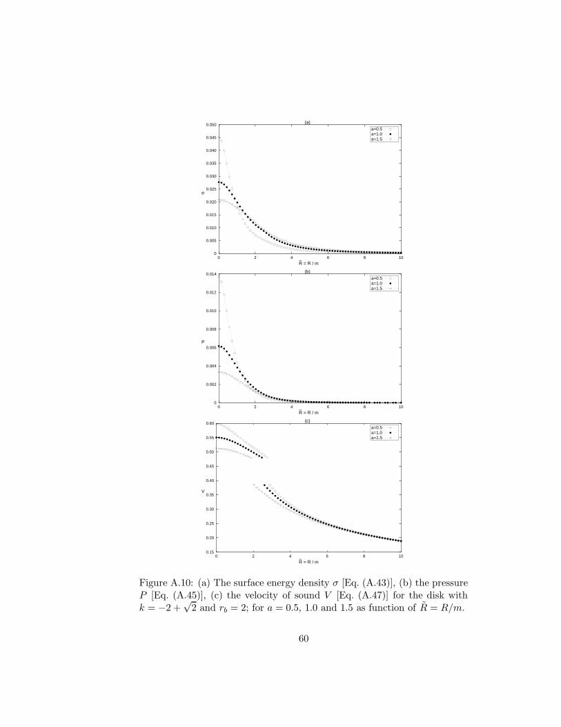
0

0.005

0.010

0.015

0.020

0.025

0.030

0.035

0.040

0.045

0.050

0 2 4 6 8 10

R = R / m~

(a)

σ

a=0.5a=1.0a=1.5

0

0.002

0.004

0.006

0.008

0.010

0.012

0.014

0 2 4 6 8 10

R = R / m~

(b)

P

a=0.5a=1.0a=1.5

0.15

0.20

0.25

0.30

0.35

0.40

0.45

0.50

0.55

0.60

0 2 4 6 8 10

R = R / m~

(c)

V

a=0.5a=1.0a=1.5

Figure A.10: (a) The surface energy density σ [Eq. (A.43)], (b) the pressureP [Eq. (A.45)], (c) the velocity of sound V [Eq. (A.47)] for the disk withk = −2 +

√2 and rb = 2; for a = 0.5, 1.0 and 1.5 as function of R = R/m.

60

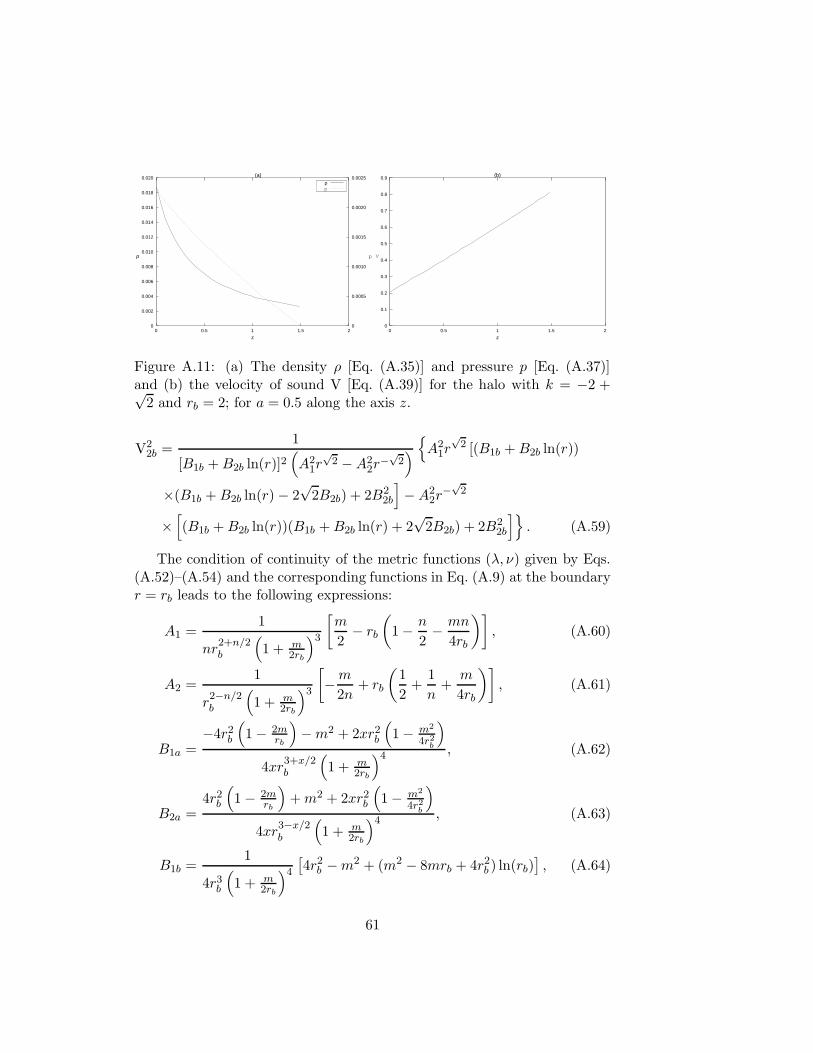
0

0.002

0.004

0.006

0.008

0.010

0.012

0.014

0.016

0.018

0.020

0 0.5 1 1.5 20

0.0005

0.0010

0.0015

0.0020

0.0025

z

ρ

(a)

p

ρp

0

0.1

0.2

0.3

0.4

0.5

0.6

0.7

0.8

0.9

0 0.5 1 1.5 2

z

(b)

V

Figure A.11: (a) The density ρ [Eq. (A.35)] and pressure p [Eq. (A.37)]and (b) the velocity of sound V [Eq. (A.39)] for the halo with k = −2 +√

2 and rb = 2; for a = 0.5 along the axis z.

V22b =

1

[B1b +B2b ln(r)]2(

A21r

√2 −A2

2r−√

2)

A21r

√2 [(B1b +B2b ln(r))

×(B1b +B2b ln(r) − 2√

2B2b) + 2B22b

]

−A22r

−√

2

×[

(B1b +B2b ln(r))(B1b +B2b ln(r) + 2√

2B2b) + 2B22b

]

. (A.59)

The condition of continuity of the metric functions (λ, ν) given by Eqs.(A.52)–(A.54) and the corresponding functions in Eq. (A.9) at the boundaryr = rb leads to the following expressions:

A1 =1

nr2+n/2b

(

1 + m2rb

)3

[

m

2− rb

(

1 − n

2− mn

4rb

)]

, (A.60)

A2 =1

r2−n/2b

(

1 + m2rb

)3

[

−m

2n+ rb

(

1

2+

1

n+

m

4rb

)]

, (A.61)

B1a =−4r2

b

(

1 − 2mrb

)

−m2 + 2xr2b

(

1 − m2

4r2b

)

4xr3+x/2b

(

1 + m2rb

)4 , (A.62)

B2a =4r2b

(

1 − 2mrb

)

+m2 + 2xr2b

(

1 − m2

4r2b

)

4xr3−x/2b

(

1 + m2rb

)4 , (A.63)

B1b =1

4r3b

(

1 + m2rb

)4

[

4r2b −m2 + (m2 − 8mrb + 4r2b ) ln(rb)

]

, (A.64)

61

0

0.1

0.2

0.3

0.4

0.5

0.6

0.7

0 2 4 6 8 10

R = R / m~

(a)

vc

a = 0.5a = 1.0a = 1.5

-0.1

0

0.1

0.2

0.3

0.4

0.5

0.6

0.7

0.8

0 2 4 6 8 10

R = R / m~

h dh/dR

(b)

~

a = 0.5a = 1.0a = 1.5

Figure A.12: (a) The tangential velocity vc1a [Eq. (A.48)] and (b) thecurves of h(dh/dR) [Eq. (A.50)] with k = −1/2 and rb = 2; for a =0.5, 1.0, and 1.5 as function of R = R/m. A region of instability appears onthe disk generated with parameter a = 0.5.

62

0

0.1

0.2

0.3

0.4

0.5

0.6

0.7

0 2 4 6 8 10

R = R / m~

(a)

vc

a = 0.5a = 1.0a = 1.5

-0.5

0

0.5

1

1.5

0 2 4 6 8 10

R = R / m~

h dh/dR

(b)

~

a = 0.5a = 1.0a = 1.5

Figure A.13: (a) The tangential velocity vc1b [Eq. (A.49)] and (b) thecurves of h(dh/dR) [Eq. (A.51)] with k = −2 +

√2 and rb = 2; for a =

0.5, 1.0, and 1.5 as function of R = R/m. As in the previous case, the sameregion of instability occurs.

63

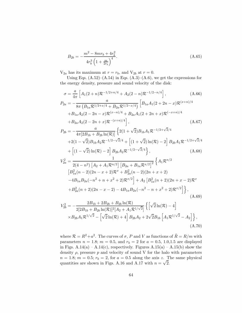
B2b = −m2 − 8mrb + 4r2

b

4r3b

(

1 + m2rb

)4 . (A.65)

V2a has its maximum at r = rb, and V2b at r = 0.Using Eqs. (A.52)–(A.54) in Eqs. (A.3)–(A.6), we get the expressions for

the energy density, pressure and sound velocity of the disk:

σ =a

4π

[

A1(2 + n)R−1/2+n/4 +A2(2 − n)R−1/2−n/4]

, (A.66)

P2a = − a

8π(

B1aR1/2+x/4 +B2aR1/2−x/4)

[

B1aA1(2 + 2n− x)R(x+n)/4

+B1aA2(2 − 2n− x)R(x−n)/4 +B2aA1(2 + 2n+ x)R(−x+n)/4

+B2aA2(2 − 2n+ x)R−(x+n)/4]

, (A.67)

P2b = − a

4π[2B1b +B2b ln(R)]

2(1 +√

2)B1bA1R−1/2+√

2/4

+2(1 −√

2)B1bA2R−1/2−√

2/4 +[

(1 +√

2) ln(R) − 2]

B2bA1R−1/2+√

2/4

+[

(1 −√

2) ln(R) − 2]

B2bA2R−1/2−√

2/4

, (A.68)

V 22a =

1

2(4 − n2)[

A2 +A1Rn/2] [

B2a +B1aRx/2]2

A1Rn/2

[

B21a(n− 2)(2n − x+ 2)Rx +B2

2a(n− 2)(2n + x+ 2)

−4B1aB2a(−n2 + n+ x2 + 2)Rx/2]

+A2

[

B21a(n+ 2)(2n+ x− 2)Rx

+B22a(n+ 2)(2n − x− 2) − 4B1aB2a(−n2 − n+ x2 + 2)Rx/2

]

,

(A.69)

V 22b = − 2B1b + 2B2b +B2b ln(R)

2[2B1b +B2b ln(R)]2[A2 +A1R1/√

2]

[√2 ln(R) − 4

]

×B2bA1R1/√

2 −[√

2 ln(R) + 4]

B2bA2 + 2√

2B1b

[

A1R1/√

2 −A2

]

,

(A.70)

where R = R2+a2. The curves of σ, P and V as functions of R = R/m withparameters n = 1.8; m = 0.5, and rb = 2 for a = 0.5, 1.0,1.5 are displayedin Figs. A.14(a) – A.14(c), respectively. Figures A.15(a) – A.15(b) show thedensity ρ, pressure p and velocity of sound V for the halo with parametersn = 1.8; m = 0.5; rb = 2, for a = 0.5 along the axis z. The same physicalquantities are shown in Figs. A.16 and A.17 with n =

√2.

64

0

0.005

0.010

0.015

0.020

0.025

0 2 4 6 8 10

R = R / m~

(a)

σ

a=0.5a=1.0a=1.5

0

0.0005

0.0010

0.0015

0.0020

0.0025

0.0030

0 2 4 6 8 10

R = R / m~

(b)

P

a=0.5a=1.0a=1.5

0.15

0.20

0.25

0.30

0.35

0.40

0.45

0.50

0.55

0.60

0 2 4 6 8 10

R = R / m~

(c)

V

a=0.5a=1.0a=1.5

Figure A.14: (a) The surface energy density σ [Eq. (A.66)], (b) the pressureP [Eq. (A.67)], (c) the velocity of sound V [Eq. (A.69)] for the disk withn = 1.8; m = 0.5; rb = 2; for a = 0.5, 1.0 and 1.5 as function of R = R/m.

65

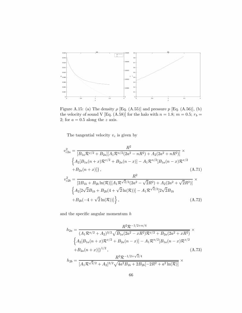
0

0.002

0.004

0.006

0.008

0.010

0.012

0.014

0.016

0.018

0 0.5 1 1.5 20

0.0005

0.0010

0.0015

0.0020

0.0025

z

ρ

(a)

p

ρp

0

0.1

0.2

0.3

0.4

0.5

0.6

0.7

0.8

0.9

0 0.5 1 1.5 2

z

(b)

V

Figure A.15: (a) The density ρ [Eq. (A.55)] and pressure p [Eq. (A.56)], (b)the velocity of sound V [Eq. (A.58)] for the halo with n = 1.8; m = 0.5; rb =2; for a = 0.5 along the z axis.

The tangential velocity vc is given by

v2c2a =

R2

[B1aRx/2 +B2a][A1Rn/2(2a2 − nR2) +A2(2a2 + nR2)]×

A2[B1a(n+ x)Rx/2 +B2a(n− x)] −A1Rn/2[B1a(n− x)Rx/2

+B2a(n+ x)] , (A.71)

v2c2b =

R2

[2B1b +B2b ln(R)][A1R√

2/2(2a2 −√

2R2) +A2(2a2 +√

2R2)]×

A2[2√

2B1b +B2b(4 +√

2 ln(R))] −A1R√

2/2[2√

2B1b

+B2b(−4 +√

2 ln(R))]

, (A.72)

and the specific angular momentum h

h2a =R2R−1/2+n/4

(A1Rn/2 +A2)3/2√

B1a(2a2 − xR2)Rx/2 +B2a(2a2 + xR2)×

A2[B1a(n+ x)Rx/2 +B2a(n− x)] −A1Rn/2[B1a(n− x)Rx/2

+B2a(n+ x)]1/2 , (A.73)

h2b =R2R−1/2+

√2/4

[A1R√

2/2 +A2]3/2√

4a2B1b + 2B2b[−2R2 + a2 ln(R)]×

66

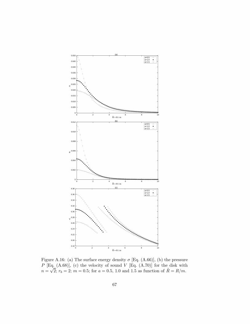
0

0.005

0.010

0.015

0.020

0.025

0.030

0.035

0.040

0.045

0.050

0 2 4 6 8 10

R = R / m~

(a)

σ

a=0.5a=1.0a=1.5

0

0.002

0.004

0.006

0.008

0.010

0.012

0 2 4 6 8 10

R = R / m~

(b)

P

a=0.5a=1.0a=1.5

0.18

0.20

0.22

0.24

0.26

0.28

0.30

0.32

0.34

0.36

0.38

0 2 4 6 8 10

R = R / m~

(c)

V

a=0.5a=1.0a=1.5

Figure A.16: (a) The surface energy density σ [Eq. (A.66)], (b) the pressureP [Eq. (A.68)], (c) the velocity of sound V [Eq. (A.70)] for the disk withn =

√2; rb = 2; m = 0.5; for a = 0.5, 1.0 and 1.5 as function of R = R/m.

67

0

0.005

0.010

0.015

0.020

0.025

0 0.5 1 1.5 20

0.001

0.002

0.003

0.004

0.005

0.006

z

ρ

(a)

p

ρp

0

0.1

0.2

0.3

0.4

0.5

0.6

0 0.5 1 1.5 2

z

(b)

V

Figure A.17: (a) The density ρ [Eq. (A.55)] and pressure p [Eq. (A.57)],(b) the velocity of sound V [Eq. (A.59)] for the halo with n =

√2; rb =

2; for a = 0.5 along the z axis.

A2[2√

2B1b +B2b(4 +√

2 ln(R))] −A1R√

2/2[2√

2B1b

+B2b(−4 +√

2 ln(R))]1/2

. (A.74)

In Figs. A.18(a) and A.18(b), the curves of tangential velocities Eq. (A.71)and h(dh/dR) Eq. (A.73), respectively, are displayed as functions of R =R/m with n = 1.8; m = 0.5; rb = 2; a = 0.5, 1.0,1.5. Figure A.19 shows thesame quantities with n =

√2. Unlike solution 2, no unstable circular orbits

are present for the disks constructed with these parameters.

A.5 Disks with composite halos from spherical so-

lutions

We study two examples of disks with halos constructed from spheres of fluidswith two layers as the ones depicted in Fig. A.3.

A.5.1 Internal Schwarzschild solution and Buchdahl solution

Let us consider that a fluid sphere is formed by two layers: The internal layer,0 ≤ r < r1, will be taken as the internal Schwarzschild solution (solution 2awith n = 2),

eν =

(

B1r2 +B2

)2

(A1r2 +A2)2 , eλ =

1

(A1r2 +A2)2 . (A.75)

68

0

0.1

0.2

0.3

0.4

0.5

0.6

0 2 4 6 8 10

R = R / m~

(a)

vc

a = 0.5a = 1.0a = 1.5

0

0.5

1

1.5

2

2.5

3

3.5

4

0 1 2 3 4 5 6 7 8 9 10

R = R / m~

h dh/dR

(b)

~

a = 0.5a = 1.0a = 1.5

Figure A.18: (a) The tangential velocity vc2a [Eq. (A.71)], and (b) thecurves of h(dh/dR) [Eq. (A.73)] with n = 1.8; m = 0.5; rb = 2; for a =0.5, 1.0, and 1.5 as function of R = R/m. The disks have no unstable orbitsfor these parameters.

69

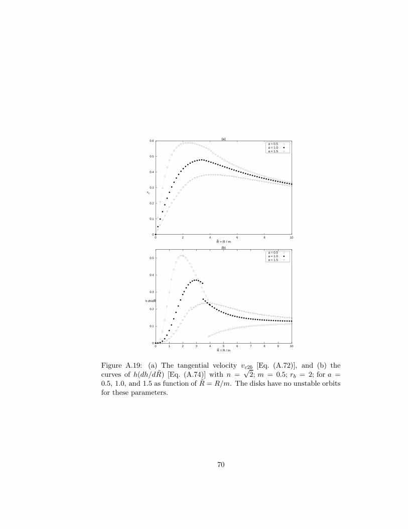
0

0.1

0.2

0.3

0.4

0.5

0.6

0 2 4 6 8 10

R = R / m~

(a)

vc

a = 0.5a = 1.0a = 1.5

0

0.1

0.2

0.3

0.4

0.5

0 1 2 3 4 5 6 7 8 9 10

R = R / m~

h dh/dR

(b)

~

a = 0.5a = 1.0a = 1.5

Figure A.19: (a) The tangential velocity vc2b [Eq. (A.72)], and (b) thecurves of h(dh/dR) [Eq. (A.74)] with n =

√2; m = 0.5; rb = 2; for a =

0.5, 1.0, and 1.5 as function of R = R/m. The disks have no unstable orbitsfor these parameters.

70

The external layer, r > r1 is taken as the Buchdahl solution,

eν =

(

1 − C√1+kr2

1 + C√1+kr2

)2

, eλ =

(

1 +C√

1 + kr2

)4

. (A.76)

Note that the external layer has no boundary, i. e., this layer has infiniteradius.

According to the continuity conditions at r = r1, the constants are re-lated through

A1 =Ck

(

C +√

1 + kr21

)3 , A2 =1 + C

(1+kr21)3/2

(

1 + C√1+kr2

1

)3 , (A.77)

B1 =Ck

(1 + kr21)

(

1 + C√1+kr2

1

)3D, (A.78)

D =

[

C(1 − 3kr21) − C2√

1+kr21

(1 − kr21) + 2(1 + kr2

1)3/2

]

[

(1 + kr21)

2 + 2C√

1 + kr21 + C2(1 − kr2

1)] , (A.79)

B2 =1 − C√

1+kr21

(

1 + C√1+kr2

1

)3 −B1r21. (A.80)

With these relations, one verifies that, using Eqs. (A.27) and (A.66), Eqs.(A.28) and (A.67), both the energy density and the pressure are continuousat the radius R =

√

r21 − a2 of the disk.

Figures A.20(a)–A.20(c) show, respectively, σ, P and V for the diskobtained from fluid layers Eq. (A.75) and (A.76) with parameters m =1; k = 1; r1 = 2; for a = 0.5, 1.0 and 1.5 as function of R = R/m. Thedensity ρ, pressure p, and velocity of sound V, for the halo along the z axiswith the same parameters for a = 0.5 is shown in Fig. A.21.

In Figs. A.22(a) and A.22(b), the curves of tangential velocities and ofh(dh/dR), respectively, are displayed as functions of R = R/m.

71

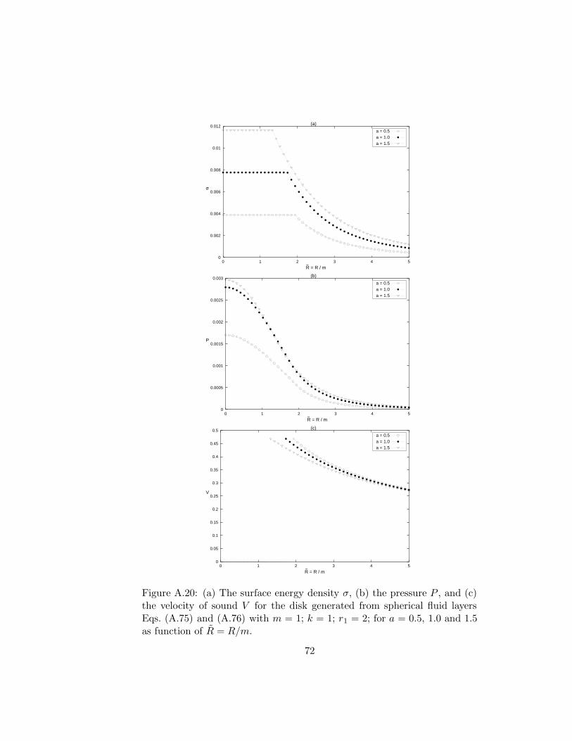
0

0.002

0.004

0.006

0.008

0.01

0.012

0 1 2 3 4 5

R = R / m~

(a)

σ

a = 0.5a = 1.0a = 1.5

0

0.0005

0.001

0.0015

0.002

0.0025

0.003

0 1 2 3 4 5

R = R / m~

(b)

P

a = 0.5a = 1.0a = 1.5

0

0.05

0.1

0.15

0.2

0.25

0.3

0.35

0.4

0.45

0.5

0 1 2 3 4 5

R = R / m~

(c)

V

a = 0.5a = 1.0a = 1.5

Figure A.20: (a) The surface energy density σ, (b) the pressure P , and (c)the velocity of sound V for the disk generated from spherical fluid layersEqs. (A.75) and (A.76) with m = 1; k = 1; r1 = 2; for a = 0.5, 1.0 and 1.5as function of R = R/m.

72

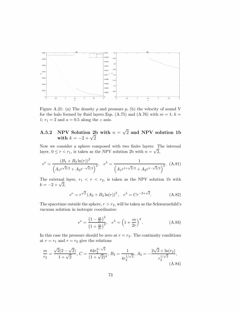
0

0.001

0.002

0.003

0.004

0.005

0.006

0.007

0 0.5 1 1.5 2 2.5 30

0.0002

0.0004

0.0006

0.0008

0.001

0.0012

0.0014

0.0016

0.0018

0.002

z

ρ

(a)

p

ρp

0

0.05

0.1

0.15

0.2

0.25

0.3

0.35

0.4

0 0.5 1 1.5 2 2.5 3

z

(b)

V

Figure A.21: (a) The density ρ and pressure p, (b) the velocity of sound Vfor the halo formed by fluid layers Eqs. (A.75) and (A.76) with m = 1; k =1; r1 = 2 and a = 0.5 along the z axis.

A.5.2 NPV Solution 2b with n =√

2 and NPV solution 1b

with k = −2 +√

2

Now we consider a sphere composed with two finite layers: The internallayer, 0 ≤ r < r1, is taken as the NPV solution 2b with n =

√2,

eν =(B1 +B2 ln(r))2

(

A1r√

2/2 +A2r−√

2/2)2 , eλ =

1(

A1r1+√

2/2 +A2r1−√

2/2)2 . (A.81)

The external layer, r1 < r < r2, is taken as the NPV solution 1b withk = −2 +

√2,

eν = r√

2 (A3 +B3 ln(r))2 , eλ = Cr−2+√

2. (A.82)

The spacetime outside the sphere, r > r2, will be taken as the Schwarzschild’svacuum solution in isotropic coordinates:

eν =

(

1 − m2r

)2

(

1 + m2r

)2 , eλ =(

1 +m

2r

)4. (A.83)

In this case the pressure should be zero at r = r2. The continuity conditionsat r = r1 and r = r2 give the relations

m

r2=

√2(2 −

√2)

1 +√

2, C =

64r2−√

22

(1 +√

2)4, B3 =

1

4r1/

√2

2

, A3 = −2√

2 + ln(r2)

r1/

√2

2

,

(A.84)

73

0

0.1

0.2

0.3

0.4

0.5

0.6

0.7

0 1 2 3 4 5

R = R / m~

(a)

vc

a = 0.5a = 1.0a = 1.5

0

2

4

6

8

10

12

14

16

18

20

0 1 2 3 4 5

R = R / m~

h dh/dR

(b)

~

a = 0.5a = 1.0a = 1.5

Figure A.22: (a) The tangential velocity vc, (b) the curves of h(dh/dR)for the disk generated from fluid layers Eqs. (A.75) and (A.76) with m =1; k = 1; r1 = 2; for a = 0.5, 1.0 and 1.5 as function of R = R/m. Thedisks obtained with these parameters have no unstable orbits.

74

A1 = 0, A2 =1√C

, B2 =r√

21

2√

2C

[

(A3 +B3 ln(r1)) (1 − r−√

21 ) + 2

√2B3

]

,

(A.85)

B1 =r√

21

2√

2C

[

(A3 +B3 ln(r1))(

2√

2r−√

21 − ln(r1) + ln(r1)r

−√

21

)

−2√

2B3 ln(r1)]

. (A.86)

Using Eqs. (A.43) and (A.66), the energy density of the disk at R =√

r21 − a2

is continuous, but not the pressure. The difference between Eqs. (A.68) and(A.45) is

∆P =a(r

√2/2

1 − r−√

2/21 )

16π√Cr1(A3 +B3 ln(r1))

[√2(A3 +B3 ln(r1)) + 4B3

]

. (A.87)

The pressure is continuous if r√

2/21 − r

−√

2/21 = 0 → r1 = 1.

Figures A.23(a)–A.23(c) show, respectively, σ, P and V for the diskobtained from fluid layers (A.81) and (A.82) with parameters r1 = 1; r2 =2; for a = 0.3, 0.6 and 0.9 as function of R = R/m. The density ρ, pressurep, and velocity of sound V, for the halo along the z axis with the sameparameters for a = 0.3 is shown in Figs. A.24. In Figs. A.25(a) andA.25(b), the curves of tangential velocities and of h(dh/dR), respectively,are displayed as functions of R = R/m. In this case, regions of unstableorbits exist for parameters a = 0.3 and a = 0.6.

A.6 Discussion

The “displace, cut and reflect” method applied to solutions of Einstein fieldequations in isotropic coordinates can generate disks with positive energydensity and equal radial and azimuthal pressures (perfect fluid). With so-lutions of static spheres of perfect fluid it is possible to construct disks ofperfect fluid surrounded also by a perfect fluid matter. As far we know theseare the first disk models of this kind in the literature.

All disks constructed as examples have some common features: surfaceenergy density and pressures decrease monotonically and rapidly with ra-dius. As the “cut” parameter a decreases, the disks become more relativistic,with surface energy density and pressure more concentrated near the center.Also regions of unstable circular orbits are more likely to appear for highlyrelativistic disks. Parameters can be chosen so that the sound velocity in the

75

0

0.01

0.02

0.03

0.04

0.05

0.06

0.07

0 1 2 3 4 5

R = R / m~

(a)

σ

a=0.3a=0.6a=0.9

0

0.005

0.010

0.015

0.020

0.025

0 1 2 3 4 5

R = R / m~

(b)

P

a=0.3a=0.6a=0.9

0.25

0.30

0.35

0.40

0.45

0.50

0.55

0.60

0 1 2 3 4 5

R = R / m~

(c)

V

a=0.3a=0.6a=0.9

Figure A.23: (a) The surface energy density σ, (b) the pressure P , (c) thevelocity of sound V for the disk generated from spherical fluid layers Eqs.(A.81) and (A.82) with r1 = 1; r2 = 2; for a = 0.3, 0.6 and 0.9 as functionof R = R/m.

76

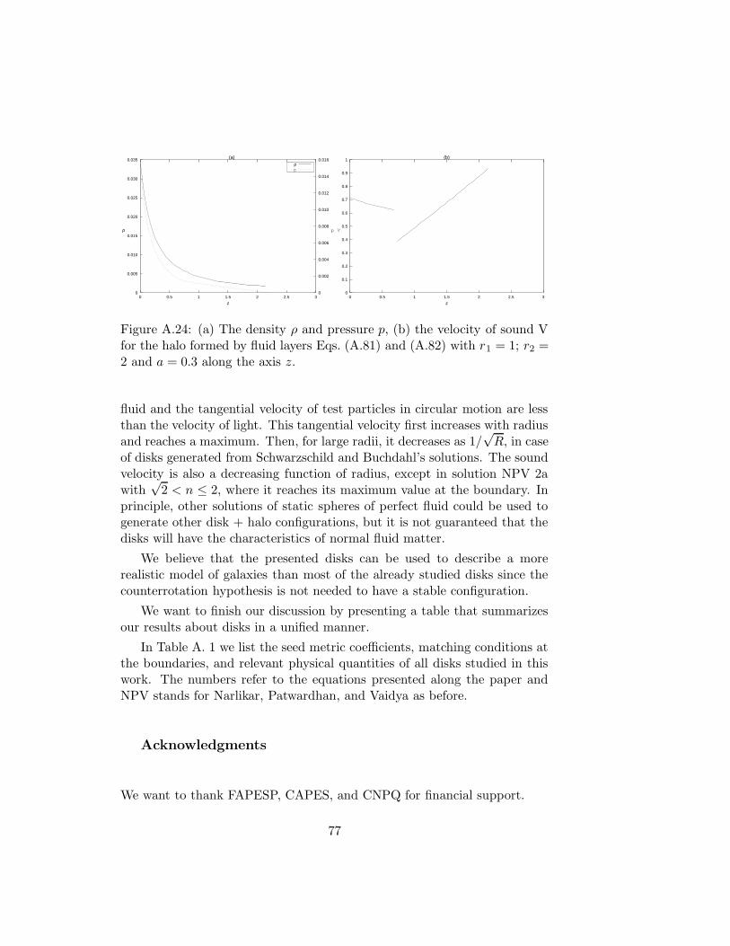
0

0.005

0.010

0.015

0.020

0.025

0.030

0.035

0 0.5 1 1.5 2 2.5 30

0.002

0.004

0.006

0.008

0.010

0.012

0.014

0.016

z

ρ

(a)

p

ρp

0

0.1

0.2

0.3

0.4

0.5

0.6

0.7

0.8

0.9

1

0 0.5 1 1.5 2 2.5 3

z

(b)

V

Figure A.24: (a) The density ρ and pressure p, (b) the velocity of sound Vfor the halo formed by fluid layers Eqs. (A.81) and (A.82) with r1 = 1; r2 =2 and a = 0.3 along the axis z.

fluid and the tangential velocity of test particles in circular motion are lessthan the velocity of light. This tangential velocity first increases with radiusand reaches a maximum. Then, for large radii, it decreases as 1/

√R, in case

of disks generated from Schwarzschild and Buchdahl’s solutions. The soundvelocity is also a decreasing function of radius, except in solution NPV 2awith

√2 < n ≤ 2, where it reaches its maximum value at the boundary. In

principle, other solutions of static spheres of perfect fluid could be used togenerate other disk + halo configurations, but it is not guaranteed that thedisks will have the characteristics of normal fluid matter.

We believe that the presented disks can be used to describe a morerealistic model of galaxies than most of the already studied disks since thecounterrotation hypothesis is not needed to have a stable configuration.

We want to finish our discussion by presenting a table that summarizesour results about disks in a unified manner.

In Table A. 1 we list the seed metric coefficients, matching conditions atthe boundaries, and relevant physical quantities of all disks studied in thiswork. The numbers refer to the equations presented along the paper andNPV stands for Narlikar, Patwardhan, and Vaidya as before.

Acknowledgments

We want to thank FAPESP, CAPES, and CNPQ for financial support.

77

0

0.1

0.2

0.3

0.4

0.5

0.6

0.7

0.8

0 1 2 3 4 5

R = R / m~

(a)

vc

a = 0.3a = 0.6a = 0.9

-1.5

-1

-0.5

0

0.5

1

1.5

2

0 1 2 3 4 5

R = R / m~

h dh/dR

(b)

~

a = 0.3a = 0.6a = 0.9

Figure A.25: (a) The tangential velocity vc, and (b) the curves of h(dh/dR)for the disk generated from spherical fluid layers Eqs. (A.81) and (A.82) withr1 = 1; r2 = 2; for a = 0.3, 0.6 and 0.9 as function of R = R/m. Regionsof unstable circular orbits appear for the disks obtained with parametersa = 0.3 and 0.6.

78

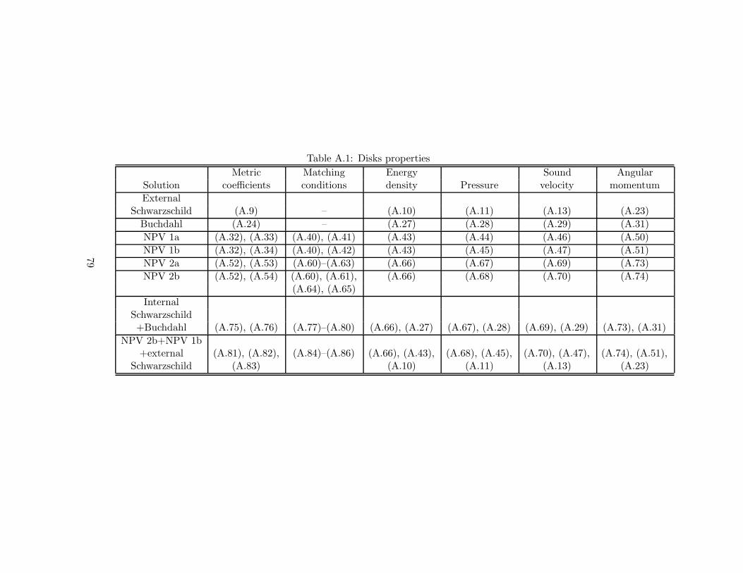
Table A.1: Disks properties

Metric Matching Energy Sound AngularSolution coefficients conditions density Pressure velocity momentum

ExternalSchwarzschild (A.9) – (A.10) (A.11) (A.13) (A.23)

Buchdahl (A.24) – (A.27) (A.28) (A.29) (A.31)

NPV 1a (A.32), (A.33) (A.40), (A.41) (A.43) (A.44) (A.46) (A.50)

NPV 1b (A.32), (A.34) (A.40), (A.42) (A.43) (A.45) (A.47) (A.51)

NPV 2a (A.52), (A.53) (A.60)–(A.63) (A.66) (A.67) (A.69) (A.73)

NPV 2b (A.52), (A.54) (A.60), (A.61), (A.66) (A.68) (A.70) (A.74)(A.64), (A.65)

InternalSchwarzschild+Buchdahl (A.75), (A.76) (A.77)–(A.80) (A.66), (A.27) (A.67), (A.28) (A.69), (A.29) (A.73), (A.31)

NPV 2b+NPV 1b+external (A.81), (A.82), (A.84)–(A.86) (A.66), (A.43), (A.68), (A.45), (A.70), (A.47), (A.74), (A.51),

Schwarzschild (A.83) (A.10) (A.11) (A.13) (A.23)

79

Bibliography

[1] W. A. Bonnor and A. Sackfield, Commun. Math. Phys. 8, 338 (1968).

[2] T. Morgan and L. Morgan, Phys. Rev. 183, 1097 (1969).

[3] L. Morgan and T. Morgan, Phys. Rev. D 2, 2756 (1970).

[4] G. Gonzalez and P. S. Letelier, Class. Quantum Grav. 16, 479 (1999).

[5] T. Ledvinka, M. Zofka, and J. Bicak, in Proceedings of the 8th Marcel

Grossman Meeting in General Relativity, edited by T. Piran (WorldScientific, Singapore, 1999), pp. 339-341.

[6] P. S. Letelier, Phys. Rev. D 60, 104042 (1999).

[7] J. Katz, J. Bicak, and D. Lynden-Bell, Class. Quantum Grav. 16, 4023(1999).

[8] D. Lynden-Bell and S. Pineault, Mon. Not. R. Astron. Soc. 185, 679(1978).

[9] J. P. S. Lemos, Class. Quantum Grav. 6, 1219 (1989).

[10] J. P. S. Lemos and P. S. Letelier, Class. Quantum Grav. 10, L75 (1993).

[11] J. P. S. Lemos and P. S. Letelier, Phys. Rev D 49, 5135 (1994).

[12] J. P. S. Lemos and P. S. Letelier, Int. J. Mod. Phys. D 5, 53 (1996).

[13] C. Klein, Class. Quantum Grav. 14, 2267 (1997).

[14] J. Bicak, D. Lynden-Bell and J. Katz, Phys. Rev. D 47, 4334 (1993).

[15] J. Bicak, D. Lynden-Bell and C. Pichon, Mon. Not. R. Astron. Soc.265, 126 (1993).

[16] O. Semerak, in Gravitation: Following the Prague Inspiration, to Cele-brate the 60th Birthday of Jiri Bicak, edited by O. Semerak, J. Podolskyand M. Zofka (World Scientific, Singapore, 2002), p. 111, available athttp://xxx.lanl.gov/abs/gr-qc/0204025.

[17] G. G. Kuzmin, Astron. Zh. 33, 27 (1956).

[18] A. H. Taub, J. Math. Phys. 21, 1423 (1980).

80

[19] J.P.S. Lemos and P.S. Letelier, Phys Lett. A 153, 288 (1991).

[20] Lord Rayleigh, Proc. R. Soc. Lond. A 93, 148 (1916).

[21] L. D. Landau and E. M. Lifshitz, Fluid Mechanics, 2nd ed. (Pergamon,Oxford, 1987), Sec. 27.

[22] B. Kuchowicz, Acta Phys. Pol. B 3, 209 (1972).

[23] H. A. Buchdahl, Astrophys. J., 140, 1512 (1964).

[24] V. V. Narlikar, G. K. Patwardhan, P. C. Vaidya, Proc. Natl. Inst. Sci.India, 9, 229 (1943).

81

82

Apendice B

Exact general relativistic static

perfect fluid disks

M. Ujevic, P. S. Letelier and D. Vogt, Theory and Observation in Cosmology

and Gravitation, J. C. Fabris et al Eds. (in press).

Abstract

Using the well-known “displace, cut and reflect” method used to gen-erate disks from given solutions of Einstein field equations, we constructstatic disks made of perfect fluid based on vacuum Schwarzschild’s solutionin isotropic coordinates. The surface energy density and pressures of thedisks decrease monotonically and rapidly with radius. As the “cut” pa-rameter a decreases, the disks become more relativistic, with surface energydensity and pressure more concentrated near the center. The stability of theperfect fluid disks is investigated under a general first order perturbation ofthe energy momentum tensor. In particular we consider temporal, radialand azimuthal “test matter”perturbations of the quantities involved on theplane z = 0. We find that the presence of radial pressure which supportsgravitational attraction stabilizes the disk and the perturbation favors theformation of rings.

B.1 Introduction

Axially symmetric solutions of Einstein’s field equations corresponding todisklike configurations of matter are of great astrophysical interest, since

83

they can be used as models of galaxies or accretion disks. These solutionscan be static or stationary and with or without radial pressure. Solutionsfor static disks without radial pressure were first studied by Bonnor andSackfield [1], and Morgan and Morgan [2], and with radial pressure by Mor-gan and Morgan [3]. Disks with radial tension have been considered in [4],and models of disks with electric fields [5], magnetic fields [6], and bothmagnetic and electric fields have been studied [7]. Solutions for self-similarstatic disks were analyzed by Lynden-Bell and Pineault [8], and Lemos [9].The superposition of static disks with black holes were first considered byLemos and Letelier [10–12]. Also Bicak, Lynden-Bell and Katz [13] studiedstatic disks as sources of known vacuum spacetimes and Bicak, Lynden-Belland Pichon [14] found an infinity number of new static solutions. Thickstatic relativistic disks in various coordinate systems were presented in [15].For a recent survey on relativistic gravitating disks, see for instance [16].

In the works cited above an inverse style method was used to solve theEinstein equations, i. e., the energy-momentum tensor is computed fromthe metric representing the disk. Another approach to generate disks is bysolving the Einstein equations given a source (energy-momentum tensor).This has been used by the Jena group to generate several exact solutions ofdisks [17–24].

The study of stability is vital to the acceptance and applicability ofthe different disks models mentioned. When applied to stellar structures,different types of perturbations usually give an insight on the formation ofbars, rings or other stellar patterns. In General Relativity, the stabilityanalysis is usually done by studying the particle motion along geodesics andnot perturbing the energy-momentum tensor of the fluid and its conservationequations. The stability of particle motion along geodesics has been studiedby transforming the Rayleigh criteria of stability [25, 26] into a GeneralRelativistic formulation, see [27] and references therein.

In this article we apply the “displace, cut and reflect” method to spher-ically symmetric solutions of Einstein’s field equations in isotropic coor-dinates to generate static disks made of a perfect fluid, i. e., with radialpressure equal to tangential pressure [28]. We first study the disk stabilitythrough the Rayleigh criteria of stability. Then we study numerically thestability of the disks by performing a general first order perturbation onthe temporal, radial and azimuthal components of the quantities involved inthe energy momentum tensor of the fluid and analyzing the correspondingperturbed conservation equations of motion [29]. The perturbations consid-ered do not modified the background metric obtained from the solution ofEinstein equations, i. e. are treated as “test matter”.

84

(a)

(b)

Figure B.1: An illustration of the “displace, cut and reflect” method for thegeneration of disks. In (a) the spacetime with a singularity is displaced andcut by a plane (dotted line), in (b) the part with singularities is disregardedand the upper part is reflected on the plane.

B.2 Einstein equations and disks

For a static spherically symmetric spacetime the general line element inisotropic cylindrical coordinates (t,R,z,ϕ) can be cast as,

ds2 = eν(R,z)dt2 − eλ(R,z)(

dR2 + dz2 +R2dϕ2)

. (B.1)

The metric of the disk will be constructed using the well known “displace,cut and reflect” method that was used by Kuzmin [30] in Newtonian gravityand later in general relativity by many authors [4–14]. The material contentof the disk will be described by functions that are distributions with supporton the disk. The method can be divided in the following steps that areillustrated in Fig. B.1: First, in a space wherein we have a compact sourceof gravitational field, we choose a surface (in our case, the plane z = 0) thatdivides the space in two pieces: one with no singularities or sources andthe other with the sources. Then we disregard the part of the space withsingularities and use the surface to make an inversion of the nonsingularpart of the space. This results in a space with a singularity that is a deltafunction with support on z = 0. This procedure is mathematically equivalentto make the transformation z → |z| + a, with a constant. In the Einsteintensor we have first and second derivatives of z. Since ∂z |z| = 2ϑ(z) − 1and ∂zz|z| = 2δ(z), where ϑ(z) and δ(z) are, respectively, the Heavisidefunction and the Dirac distribution. Therefore the Einstein field equationswill separate in two different pieces [31]: one valid for z 6= 0 (the usualEinstein’s equations), and other involving distributions with an associatedenergy-momentum tensor, Tab = Qabδ(z), with support on z = 0. For the

85

metric (B.1), the non-zero components of Qab are

Qtt =

1

16π

[

−bzz + gzz(bRR + bzz + bϕϕ)]

, (B.2)

QRR = Qϕ

ϕ =1

16π

[

−bzz + gzz(btt + bRR + bzz)]

, (B.3)

where bab denote the jump of the first derivatives of the metric tensor onthe plane z = 0,

bab = gab,z |z=0+ − gab,z|z=0− , (B.4)

and the other quantities are evaluated at z = 0+. The “true” surface energy-momentum tensor of the disk can be written as Sab =

√−gzzQab, thus thesurface energy density σ and the radial and azimuthal pressures or tensions(P ) read:

σ =√−gzzQ

tt, P = −√−gzzQ

RR = −√−gzzQ

ϕϕ. (B.5)

Note that when the same procedure is applied to an axially symmetric space-time in Weyl coordinates we have QR

R = 0, i.e., we have no radial pressureor tension.

B.3 Perfect Fluid Disk in Isotropic Coordinates

Now we apply the “displace, cut and reflect” method to generate disks dis-cussed in the previous section and depicted in Fig. B.1 to the Schwarzschildmetric in isotropic coordinates (t, r, θ, ϕ),

ds2 =

(

1 − m2r

)2

(

1 + m2r

)2 dt2 −(

1 +m

2r

)4[

dr2 + r2(dθ2 + sin2 θdϕ2)]

. (B.6)

Expressing solution (B.6) in cylindrical coordinates, and using Eq. (B.2)–(B.5), we obtain a disk with surface energy density σ and radial and az-imuthal pressures (or tensions) P given by

σ =4ma

π(m+ 2√R2 + a2)3

, (B.7)

P = − 2m2a

π(m+ 2√R2 + a2)3(m− 2

√R2 + a2)

. (B.8)

86

The total mass of the disk can be calculated with the help of Eq. (B.7):

M =

∫ ∞

0

∫ 2π

0σ√gRRgϕϕ dR dϕ =

m

4a(m+ 4a). (B.9)

Thus, for a > 0, the disk always has a finite mass.

Eq. (B.7) shows that the disk’s surface energy density is always positive(weak energy condition). Positive values (pressure) for the stresses in az-imuthal and radial directions are obtained if m < 2

√R2 + a2. The strong

energy condition, σ + Pϕϕ + PRR = σ + 2P > 0 is then satisfied. Theseproperties characterize a fluid made of matter with the usual gravitationalattractive property. This is not a trivial property of these disks since it isknown that the “displace, cut and reflect” method sometimes gives disksmade of exotic matter like cosmic strings, see for instance [32].

Another useful parameter is the velocity of sound propagation V , definedas V 2 = dP

dσ , which can be calculated using Eq. (B.7) and Eq. (B.8):

V 2 =m(4

√R2 + a2 −m)

3(m− 2√R2 + a2)2

. (B.10)

The condition V 2 < 1 (no tachyonic matter) imposes the inequalities m <√R2 + a2 or m > 3

√R2 + a2. If the pressure condition and the speed of

sound less then the speed of light condition are to be simultaneously satisfied,then m <

√R2 + a2. This inequality will be valid in all the disk if m < a.

To determine the stability of circular orbits on the disk’s plane, we usethe General Relativistic extension of Rayleigh [25, 26] criteria of stability ofa fluid at rest in a gravitational field

hdh

dR> 0, (B.11)

where h is the specific angular momentum of a particle on the disk’s plane:

h = −gϕϕdϕ

ds= −gϕϕ

dϕ

dt

dt

ds. (B.12)

Using the geodesic equation for circular motion on the z = 0 plane oneobtains the following expression for h:

h = R2eλ

√

(eν),Reν(R2eλ),R −R2eλ(eν),R

. (B.13)

87

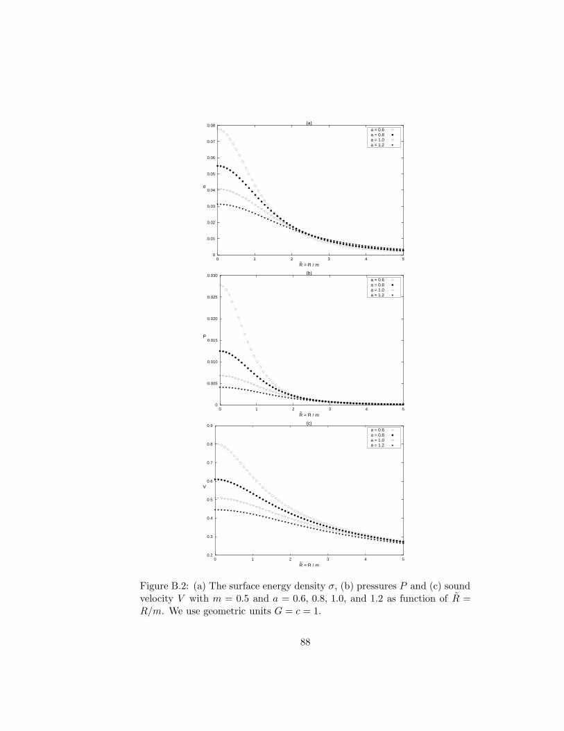
0

0.01

0.02

0.03

0.04

0.05

0.06

0.07

0.08

0 1 2 3 4 5

R = R / m~

(a)

σ

a = 0.6a = 0.8a = 1.0a = 1.2

0

0.005

0.010

0.015

0.020

0.025

0.030

0 1 2 3 4 5

R = R / m~

(b)

P

a = 0.6a = 0.8a = 1.0a = 1.2

0.2

0.3

0.4

0.5

0.6

0.7

0.8

0.9

0 1 2 3 4 5

R = R / m~

(c)

V

a = 0.6a = 0.8a = 1.0a = 1.2

Figure B.2: (a) The surface energy density σ, (b) pressures P and (c) soundvelocity V with m = 0.5 and a = 0.6, 0.8, 1.0, and 1.2 as function of R =R/m. We use geometric units G = c = 1.

88

For the metric (B.6), Eq. (B.13) reads

h =2√mR2

(

1 + m2√

R2+a2

)2(R2 + a2)1/4

√

4(R2 + a2)2 − 8mR2√R2 + a2 +m2(R2 − a2)

. (B.14)

The stability criterion is always satisfied for am 1.016.

In Figures B.2(a)–(c) we show, respectively, the surface energy den-sity, pressures and the sound velocity with parameters m = 0.5 and a =0.6, 0.8, 1.0, and 1.2 as functions of R = R/m. We see that these quantitiesdecrease monotonically with the radius of the disk, as can be checked fromEq. (B.7), (B.8) and (B.10). Energy density decreases rapidly enough to, inprinciple, define a cut off radius and consider the disk as finite.

B.4 Stability of Perfect Fluid Disks

Now we study the stability of the perfect fluid disks by performing a generalfirst order perturbation of the energy-momentum tensor. We express theunperturbed energy-momentum tensor as

T µν = (σUµUν + prXµXν + pϕY

µY ν)δ(z), (B.15)

where σ is the surface energy density, pr and pϕ are, respectively, the ra-dial and azimuthal pressures, and (U µ, Xµ, Y µ) are the components of theorthonormal tetrad

Uµ = e−ν/2(1, 0, 0, 0),

Xµ = e−λ/2(0, 1, 0, 0),

Y µ =e−λ/2

R(0, 0, 0, 1) (B.16)

Due to the form of the energy-momentum tensor Eq. (B.15), all quantitiesare only functions of the radial coordinate. Thus we construct the pertur-bation Aµ

P of a quantity Aµ in the form

AµP (t, r, ϕ) = Aµ(r) + δAµ(t, r, ϕ), (B.17)

where Aµ(r) is the unperturbed quantity and δAµ(t, r, ϕ) is the perturba-tion. Applying Eq. (B.17) in Eq. (B.15) and assuming that the perturbedenergy-momentum tensor does not modify the background metric, i. e., the

89

perturbation δT µν acts as a test fluid, the perturbed conservation equationsfor thin disks can be written as

(δT µν);ν |z=0 = 0, (B.18)

where ; ν denotes covariant derivative with respect to the coordinate ν. As-suming a perturbation of the form

δAµ(t, r, ϕ) = δAµ(r)ei(kϕϕ−wt), (B.19)

the perturbed conservation equations Eq. (B.18) can be written as

µ = t δU r,r(σU

t + ξ1prXr) + δU r[F(t, r, σU t) + ξ1,rprX

r

+ ξ1F(t, r, prXr)] + δUϕ[ikϕ(σU t + ξ2pϕY

ϕ)] + δσ(−iwU tU t) = 0,

(B.20)

µ = r δpr,r(XrXr) + δU r[−iw(σU t + ξ1prX

r)] + δσ(U tU tΓrtt)

+ δprG(r, r,XrXr) + δpϕ(Y ϕY ϕΓrϕϕ) = 0, (B.21)

µ = ϕ δUϕ[−w(σU t + ξ2pϕYϕ)] + δpϕ(kϕY

ϕY ϕ) = 0, (B.22)

where δU r and δUϕ are perturbed components of the tetrad, ξ1 = −Xr/Ut,ξ2 = −Yϕ/Ut and

F(I, J,K) = K,J +K(2ΓIIJ + Γα

αJ), (B.23)

G(I, J,K) = K,J +K(ΓIIJ + Γα

αJ), (B.24)

where Γαβγ are the Christoffel symbols.

We want our perturbations to be in accordance with the equation ofstate of the fluid, i.e. p = p(r) and σ = σ(r). Thus, δpr and δσ satisfy

δp = δpr = δpϕ = p,rdr, (B.25)

δσ = σ,rdr, (B.26)

from which we find the useful relation

δp =

(

p,r

σ,r

)

δσ. (B.27)

Substituting δU r and δUϕ in Eq. (B.20) from Eq. (B.21) and Eq. (B.22),and using relation Eq. (B.27), we find a second order differential equationfor the energy density perturbation δσ of the form

ASδσ,rr +BSδσ,r + CSδσ = 0, (B.28)

90

where (AS , BS , CS) are functions of (r, a,m,w, kϕ). To study stability of thedisks we need a criterion to make a cut-off in the radial coordinate to createa finite disk. The cut-off radius Rcut of the disk is set by the followingcriterion: the matter within the thin disk formed by the cut-off radius ismore than 90% of the total energy density of the infinite disk. The secondorder equation Eq. (B.28) is solved with two boundary conditions, one inr ≈ 0 and the other in the cut-off radius set by the criterion establishedabove. At r ≈ 0 we set the perturbation to be ≈ 10% of the unperturbedenergy density value and at the edge of the disk δσ|r=Rcut

= 0. The lastcondition is imposed because we want the perturbation to vanish when rtends to the outer radius.

Now, we consider the isotropic Schwarzschild thin disk with parameters(a = 0.5,m = 0.4). With these parameters, the outer radius of the disk is setto r = 4 (approximately 90% of the energy density is inside the disk). In Fig.B.3 we show the amplitude profiles of the true energy density perturbationδσ for different modes of the perturbation Eq. (B.19). We see from Fig.B.3 that the energy density perturbation profiles are stable and have anoscillatory character. When we increase the parameter w the number ofoscillations within the disk increases and when we increase the wave numberk the amplitude of the oscillations decreases. Note that the amplitudes ofthe modes decay quickly when we increase the value of the wave number.From Fig. B.3 we see that there is a factor of approximately 10−3 betweenthe modes (w = 1, k = 0) and (w = 1, k = 2). In Fig. B.4, we present theamplitude profiles of the true pressure perturbation and the physical radialvelocity perturbation ( ˜δU r = δU r√grr) for the first three w modes with k =0, and the amplitude profile of the physical azimuthal velocity perturbation( ˜δUϕ = δUϕ√gϕϕ) for the first three w modes with k = 1. The modes of theazimuthal velocity perturbation with k = 0 are equal to zero. We see fromFig. B.4 that the pressure perturbation has the same qualitative aspects ofthe density perturbation. The azimuthal velocity perturbation amplitudeshows an oscillatory behavior but the difference between it and the radialvelocity perturbation is that after the first oscillations the maximum valueof the amplitude remains almost constant for the rest of the disk.

B.5 Conclusion

The “displace, cut and reflect” method applied to the Schwarzschild solutionin isotropic coordinates can generate disks with positive energy density andequal radial and azimuthal pressures (perfect fluid). Surface energy density

91

0 1 2 3 4r

-6×10-3

0

6×10-3

δσ(r

)

w=1, k=0w=2, k=0w=3, k=0

~

0 1 2 3 4r

-4×10-4

0

4×10-4

δσ(r

)

w=1, k=1w=2, k=1w=3, k=1

~

0 1 2 3 4r

-6×10-7

0

6×10-7

δσ(r

)

w=1, k=2w=2, k=2w=3, k=2

~

Figure B.3: Profiles of the energy density perturbation amplitudes of theisotropic Schwarzschild thin disk with parameters (a=0.5,m=0.4). The firstthree different w modes for the first three wave number k are plotted, wesee that increasing the w mode the number of oscillations within the diskincreases while increasing the wave number k the amplitude decreases.

92

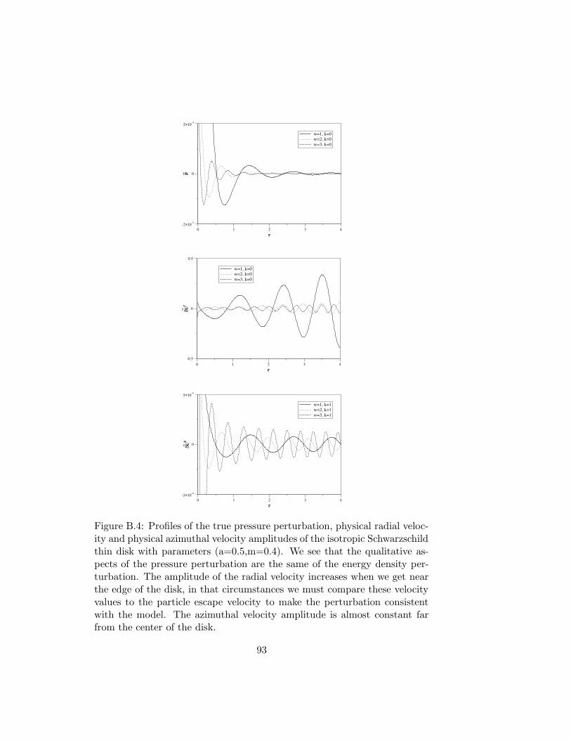
0 1 2 3 4r

-2×10-3

0

2×10-3

p

w=1, k=0w=2, k=0w=3, k=0

~

0 1 2 3 4r

-0.5

0

0.5

δUr

w=1, k=0w=2, k=0w=3, k=0

~

0 1 2 3 4r

-5×10-4

0

5×10-4

δUϕ

w=1, k=1w=2, k=1w=3, k=1

~

Figure B.4: Profiles of the true pressure perturbation, physical radial veloc-ity and physical azimuthal velocity amplitudes of the isotropic Schwarzschildthin disk with parameters (a=0.5,m=0.4). We see that the qualitative as-pects of the pressure perturbation are the same of the energy density per-turbation. The amplitude of the radial velocity increases when we get nearthe edge of the disk, in that circumstances we must compare these velocityvalues to the particle escape velocity to make the perturbation consistentwith the model. The azimuthal velocity amplitude is almost constant farfrom the center of the disk.

93

and pressures decrease monotonically and rapidly with radius. As the “cut”parameter a decreases, the disks become more relativistic, with surface en-ergy density and pressure more concentrated near the center. Also regions ofunstable circular orbits are more likely to appear for high relativistic disks.The stability analysis using a general first order perturbation of the disk’senergy-momentum tensor shows that the fluid variables, in the isotropicSchwarzschild thin disk, present an oscillatory character with the ampli-tudes vanishing when r approaches the outmost radius. In the case of theazimuthal perturbation, the amplitude is almost constant within the disk.In general, when we increase the parameter w the number of oscillationsincreases inside the disk and the amplitudes decrease. When we increasethe wave number k the values of the amplitudes decrease abruptly. We notethat the perturbation Eq. (B.19) made in the isotropic Schwarzschild thindisk favors the formation of rings. As expected, the presence of a radialpressure is fundamental to the stability of thin disks.

Bibliography

[1] W. A. Bonnor and A. Sackfield, Commun. Math. Phys. 8, 338 (1968).

[2] T. Morgan and L. Morgan, Phys. Rev. 183, 1097 (1969).

[3] L. Morgan and T. Morgan, Phys. Rev. D 2, 2756 (1970).

[4] G. Gonzalez and P. S. Letelier, Class. Quantum Grav. 16, 479 (1999).

[5] T. Ledvinka, M. Zofka, and J. Bicak, in Proceedings of the 8th Marcel

Grossman Meeting in General Relativity, edited by T. Piran (WorldScientific, Singapore, 1999), pp. 339-341.

[6] P. S. Letelier, Phys. Rev. D 60, 104042 (1999).

[7] J. Katz, J. Bicak, and D. Lynden-Bell, Class. Quantum Grav. 16, 4023(1999).

[8] D. Lynden-Bell and S. Pineault, Mon. Not. R. Astron. Soc. 185, 679(1978)

[9] J. P. S. Lemos, Class. Quan. Grav. 6, 1219 (1989)

[10] J. P. S. Lemos and P. S. Letelier, Class. Quan. Grav. 10, L75 (1993)

[11] J. P. S. Lemos and P. S. Letelier, Phys. Rev D 49, 5135 (1994)

94

[12] J. P. S. Lemos and P. S. Letelier, Int. J. Mod. Phys. D 5, 53 (1996).

[13] J. Bicak, D. Lynden-Bell and J. Katz, Phys. Rev.D 47, 4334 (1993).

[14] J. Bicak, D. Lynden-Bell and C. Pichon, Mon. Not. R. Astron. Soc.

265, 126 (1993).

[15] G. Gonzalez and P. S. Letelier, Phys. Rev. D69, 044013 (2004).

[16] V. Karas, J. M. Hure and O. Semerak, Class. Quantum Grav. 21, R1(2004).

[17] C. Klein, Class. Quantum Grav. 14, 2267 (1997).

[18] G. Neugebauer and R. Meinel, Phys. Rev. Lett. 75, 3046 (1995).

[19] C. Klein and O. Richter, Phys. Rev. Lett. 83, 2884 (1999).

[20] C. Klein, Phys. Rev. D63, 064033 (2001).

[21] J. Frauendiener and C. Klein, Phys. Rev. D63, 084025 (2001).

[22] C. Klein, Phys. Rev. D65, 084029 (2002).

[23] C. Klein, Phys. Rev. D68, 027501 (2003).

[24] C. Klein, Ann. Phys. 12 (10), 599 (2003).

[25] Lord Rayleigh, Proc. R. Soc. Lond. Ser. A 93, 148 (1916).

[26] L. D. Landau, E. M. Lifshitz, Fluid Mechanics, 2nd Ed. (PergamonPress, Oxford, 1987), §27.

[27] P.S. Letelier, Phys. Rev. D 68, 104002 (2003).

[28] D. Vogt and P. S. Letelier, Phys. Rev. D 68, 084010 (2003).

[29] M. Ujevic and P. S. Letelier, On the Stability of General Relativistic

Geometric Thin Disks, Phys. Rev. D (in press).

[30] G. G. Kuzmin, Astron. Zh., 33, 27 (1956).

[31] A. H. Taub, J. Math. Phys. 21, 1423 (1980).

[32] J.P.S. Lemos and P.S. Letelier, Phys Lett. A 153, 288 (1991).

95

96

Apendice C

Exact relativistic static charged

dust discs and non-axisymmetric

structures

D. Vogt and P. S. Letelier, Class. Quantum Grav. 21, 3369–3378 (2004).

Received 16 April 2004; published 18 June 2004.

Abstract

The well-known ‘displace, cut and reflect’ method used to generate discsfrom given solutions of Einstein field equations is applied to the superposi-tion of two extreme Reissner-Nordstrom black holes to construct discs madeof charged dust and also non-axisymmetric planar distributions of chargeddust on the z = 0 plane. They are symmetric with respect to two or one co-ordinate axes, depending on whether the black holes have equal or unequalmasses, respectively. For these non-axisymmetric distributions of matter wealso study the effective potential for geodesic motion of neutral test particles.

PACS numbers: 04.20.Jb, 04.40.–b, 04.40.Nr

C.1 Introduction

Solutions of Einstein’s field equations representing disc-like configurations ofmatter are of great astrophysical interest, since they can be used as modelsof galaxies or accretion discs. Disc solutions can be static or stationary

97

and with or without radial pressure. Solutions for static thin discs withoutradial pressure were first studied by Bonnor and Sackfield [1] and Morganand Morgan [2], and with radial pressure by Morgan and Morgan [3]. Otherclasses of static thin disc solutions have been obtained [4–7], while stationarythin discs were studied in [8–10]. An exact solution to the problem of arigidly rotating disc of dust in terms of ultraelliptic functions was reportedin [11]. Also thin discs with radial tension [12], magnetic fields [13] andboth electric and magnetic fields [14] have been studied. The nonlinearsuperposition of a disc and a black hole was first considered by Lemos andLetelier [15]. Models of thin discs and thin discs with halos made of perfectfluids were considered in [16]. The generalization of the ‘displace, cut andreflect’ method (section C.2) of constructing thick static discs was consideredby Gonzalez and Letelier [17].

An interesting class of solutions of the Einstein-Maxwell field equationsis the conformastatic spacetimes with charged dust, in which the chargedensity is equal to the mass density. Therefore, the matter is in equilibriumbecause the mutual gravitational attractions are balanced by the electricalrepulsions. This kind of matter has been called by some authors ‘electri-cally counterpoised dust’ (ECD). Distributions of ECD in equilibrium inboth classical and relativistic theories were studied by Bonnor [18]. Modelsof oblate and prolate spheroids made of ECD were considered, respectively,in [19, 20]. Gurses [21] and Varela [22] studied static spheres of ECD. Discsources for conformastationary metrics (the stationary version of confor-mastatic metrics) were considered in [14]. Although one may intuitivelyexpect that astrophysical objects do not have a net charge, there existsthe possibility that electrons escape from a compact star, leaving behind apositively charged one (see, for example, [23, 24]).

In this paper we apply the well known ‘displace, cut and reflect’ methodto the superposition of two extreme Reissner-Nordstrom black holes alignedon the z-axis to generate static discs of ECD on the z = 0 plane. Nextwe repeat the same procedure for Reissner-Nordstrom black holes alignedon the y-axis and generate non-axisymmetric distributions of ECD on theplane z = 0. We briefly study the effective potential of geodesic motion ofneutral test particles on these structures.

The paper is divided as follows. Section C.2 discusses the Einstein-Maxwell equations, the ‘displace, cut and reflect’ method and the particularclass of conformastat metrics. In section C.3 discs of charged dust are con-structed using the superposition of two aligned Reissner-Nordstrom blackholes and in section C.4 we obtain non-axisymetric distributions of chargeddust. We also present some analysis of the geodesic motion on these matter

98

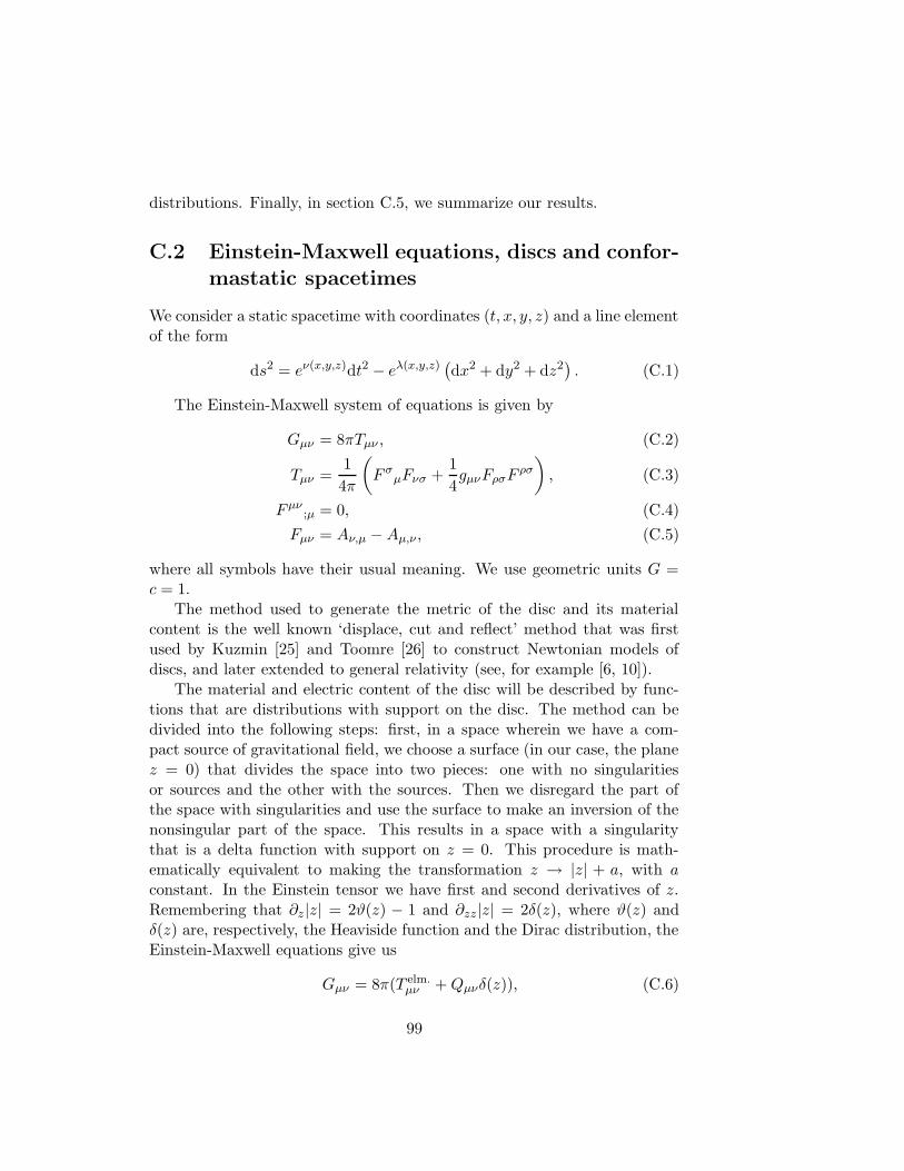
distributions. Finally, in section C.5, we summarize our results.

C.2 Einstein-Maxwell equations, discs and confor-

mastatic spacetimes

We consider a static spacetime with coordinates (t, x, y, z) and a line elementof the form

ds2 = eν(x,y,z)dt2 − eλ(x,y,z)(

dx2 + dy2 + dz2)

. (C.1)

The Einstein-Maxwell system of equations is given by

Gµν = 8πTµν , (C.2)

Tµν =1

4π

(

F σµFνσ +

1

4gµνFρσF

ρσ

)

, (C.3)

F µν;µ = 0, (C.4)

Fµν = Aν,µ −Aµ,ν , (C.5)

where all symbols have their usual meaning. We use geometric units G =c = 1.

The method used to generate the metric of the disc and its materialcontent is the well known ‘displace, cut and reflect’ method that was firstused by Kuzmin [25] and Toomre [26] to construct Newtonian models ofdiscs, and later extended to general relativity (see, for example [6, 10]).

The material and electric content of the disc will be described by func-tions that are distributions with support on the disc. The method can bedivided into the following steps: first, in a space wherein we have a com-pact source of gravitational field, we choose a surface (in our case, the planez = 0) that divides the space into two pieces: one with no singularitiesor sources and the other with the sources. Then we disregard the part ofthe space with singularities and use the surface to make an inversion of thenonsingular part of the space. This results in a space with a singularitythat is a delta function with support on z = 0. This procedure is math-ematically equivalent to making the transformation z → |z| + a, with aconstant. In the Einstein tensor we have first and second derivatives of z.Remembering that ∂z|z| = 2ϑ(z) − 1 and ∂zz|z| = 2δ(z), where ϑ(z) andδ(z) are, respectively, the Heaviside function and the Dirac distribution, theEinstein-Maxwell equations give us

Gµν = 8π(T elm.µν +Qµνδ(z)), (C.6)

99

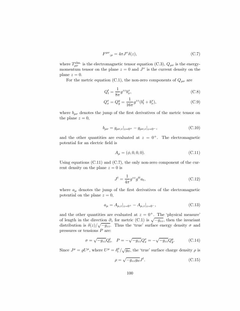
F µν;µ = 4πJνδ(z), (C.7)

where T elm.µν is the electromagnetic tensor equation (C.3), Qµν is the energy-

momentum tensor on the plane z = 0 and J ν is the current density on theplane z = 0.

For the metric equation (C.1), the non-zero components of Qµν are

Qtt =

1

8πgzzbxx, (C.8)

Qxx = Qy

y =1

16πgzz(btt + bxx), (C.9)

where bµν denotes the jump of the first derivatives of the metric tensor onthe plane z = 0,

bµν = gµν,z |z=0+ − gµν,z|z=0− , (C.10)

and the other quantities are evaluated at z = 0+. The electromagneticpotential for an electric field is

Aµ = (φ, 0, 0, 0). (C.11)

Using equations (C.11) and (C.7), the only non-zero component of the cur-rent density on the plane z = 0 is

J t =1

4πgzzgttat, (C.12)

where aµ denotes the jump of the first derivatives of the electromagneticpotential on the plane z = 0,

aµ = Aµ,z|z=0+ −Aµ,z|z=0− , (C.13)

and the other quantities are evaluated at z = 0+. The ‘physical measure’of length in the direction ∂z for metric (C.1) is

√−gzz, then the invariantdistribution is δ(z)/

√−gzz. Thus the ‘true’ surface energy density σ andpressures or tensions P are:

σ =√−gzzQ

tt, P = −√−gzzQ

xx = −√−gzzQ

yy. (C.14)

Since Jµ = %Uµ, where Uµ = δµt /

√gtt, the ‘true’ surface charge density ρ is

ρ =√−gzzgttJ

t. (C.15)

100

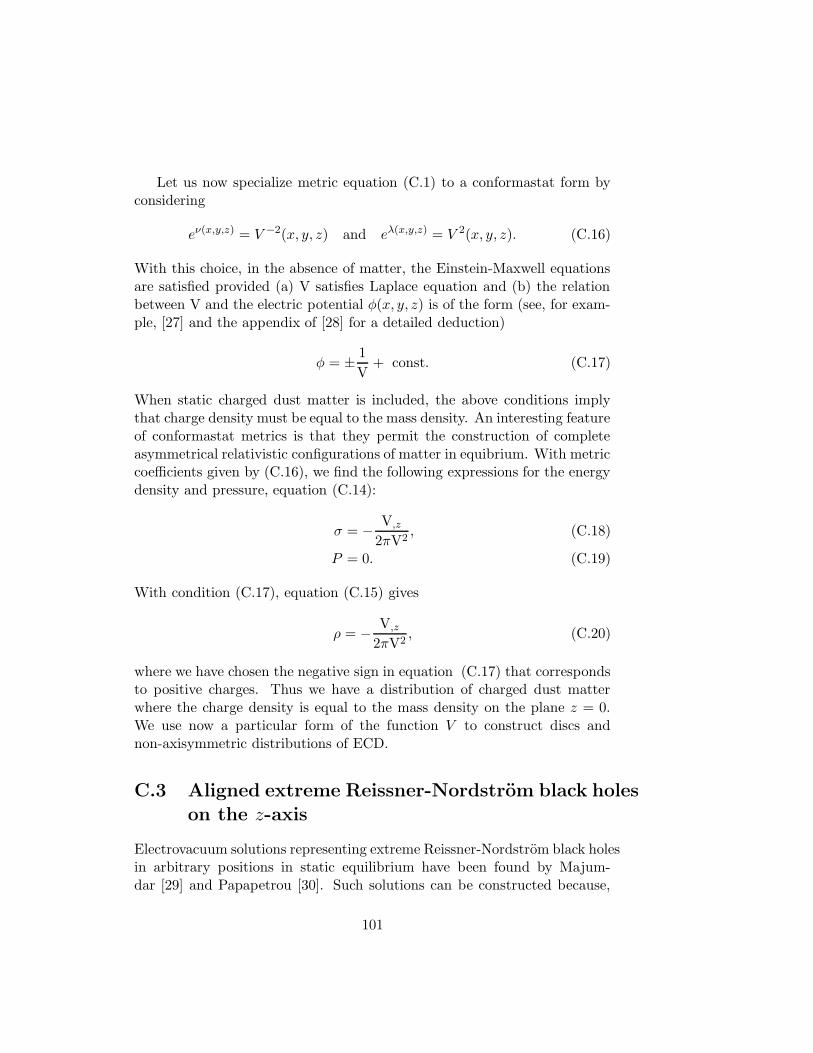
Let us now specialize metric equation (C.1) to a conformastat form byconsidering

eν(x,y,z) = V −2(x, y, z) and eλ(x,y,z) = V 2(x, y, z). (C.16)

With this choice, in the absence of matter, the Einstein-Maxwell equationsare satisfied provided (a) V satisfies Laplace equation and (b) the relationbetween V and the electric potential φ(x, y, z) is of the form (see, for exam-ple, [27] and the appendix of [28] for a detailed deduction)

φ = ± 1

V+ const. (C.17)

When static charged dust matter is included, the above conditions implythat charge density must be equal to the mass density. An interesting featureof conformastat metrics is that they permit the construction of completeasymmetrical relativistic configurations of matter in equibrium. With metriccoefficients given by (C.16), we find the following expressions for the energydensity and pressure, equation (C.14):

σ = − V,z

2πV2, (C.18)

P = 0. (C.19)

With condition (C.17), equation (C.15) gives

ρ = − V,z

2πV2, (C.20)

where we have chosen the negative sign in equation (C.17) that correspondsto positive charges. Thus we have a distribution of charged dust matterwhere the charge density is equal to the mass density on the plane z = 0.We use now a particular form of the function V to construct discs andnon-axisymmetric distributions of ECD.

C.3 Aligned extreme Reissner-Nordstrom black holes

on the z-axis

Electrovacuum solutions representing extreme Reissner-Nordstrom black holesin arbitrary positions in static equilibrium have been found by Majum-dar [29] and Papapetrou [30]. Such solutions can be constructed because,

101

m

m2

1

a

z2

z=0

z

Figure C.1: Schematic drawing of the configuration used to constructcharged dust discs.

as previously stated, the functions V (x, y, z) must satisfy the Laplace equa-tion and thus can be superposed. Suppose we have two extreme Reissner-Nordstrom black holes on the z-axis, the first with mass m1 at z = 0 and thesecond with mass m2 at z = −z2 (figure C.1). For convenience we use cylin-drical coordinates (t, R, z, ϕ). The function V representing the superpositionis given by

V = 1 +m1√R2 + z2

+m2

√

R2 + (z + z2)2. (C.21)

If we apply the ‘displace, cut and reflect’ method to the system representedby equation (C.21), we have for the energy density equation (C.18):

σ =m1aR3/2

2 +m2(a+ z2)R3/21

2π√R1R2

(√R1R2 +m1

√R2 +m2

√R1

)2 , (C.22)

where R1 = R2 + a2 and R2 = R2 + (z2 + a)2. Note that σ is always non-negative. In figure C.2 we graph the energy density of the disc equation(C.22) as a function of R in two situations: in (a) we fix m1 = 2, a = 1,z2 = 1 and change m2, in (b) we fix m1 = 1, m2 = 1, a = 1 and changez2. In situation (a) we note that as m2 is increased, the energy density ismore uniformly distributed along the radius. In (b) z2 = 0 corresponds toone black hole with mass m1 = 2 (curve m2 = 0 in (a)). The energy densityon R = 0 assumes a minimum value when z2 = 1, and then increases asz2 is increased. The curve with z2 = 1 × 106 (mass m2 is very far away)corresponds to a disc generated solely by m1.

102

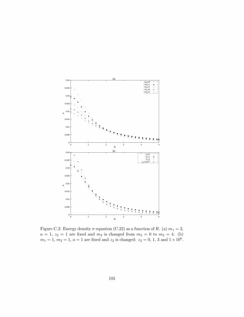
0

0.005

0.01

0.015

0.02

0.025

0.03

0.035

0.04

0 1 2 3 4 5R

σ

(a)m2=0m2=1m2=2m2=3m2=4

0

0.005

0.01

0.015

0.02

0.025

0.03

0.035

0.04

0 1 2 3 4 5R

σ

(b)z2=0z2=1z2=3

z2=1x106

Figure C.2: Energy density σ equation (C.22) as a function of R. (a)m1 = 2,a = 1, z2 = 1 are fixed and m2 is changed from m2 = 0 to m2 = 4. (b)m1 = 1, m2 = 1, a = 1 are fixed and z2 is changed: z2 = 0, 1, 3 and 1× 106.

103

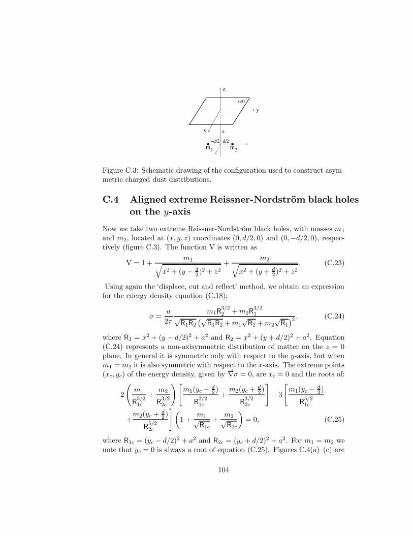
z=0

z

x

y

m2m1

−d/2 d/2

a

Figure C.3: Schematic drawing of the configuration used to construct asym-metric charged dust distributions.

C.4 Aligned extreme Reissner-Nordstrom black holes

on the y-axis

Now we take two extreme Reissner-Nordstrom black holes, with masses m1

and m2, located at (x, y, z) coordinates (0, d/2, 0) and (0,−d/2, 0), respec-tively (figure C.3). The function V is written as

V = 1 +m1

√

x2 + (y − d2 )2 + z2

+m2

√

x2 + (y + d2)2 + z2

. (C.23)

Using again the ‘displace, cut and reflect’ method, we obtain an expressionfor the energy density equation (C.18):

σ =a

2π

m1R3/22 +m2R

3/21√

R1R2

(√R1R2 +m1

√R2 +m2

√R1

)2 , (C.24)

where R1 = x2 + (y − d/2)2 + a2 and R2 = x2 + (y + d/2)2 + a2. Equation(C.24) represents a non-axisymmetric distribution of matter on the z = 0plane. In general it is symmetric only with respect to the y-axis, but whenm1 = m2 it is also symmetric with respect to the x-axis. The extreme points(xc, yc) of the energy density, given by ~∇σ = 0, are xc = 0 and the roots of:

2

(

m1

R3/21c

+m2

R3/22c

)[

m1(yc − d2 )

R3/21c

+m2(yc + d

2)

R3/22c

]

− 3

[

m1(yc − d2)

R5/21c

+m2(yc + d

2 )

R5/22c

]

(

1 +m1√R1c

+m2√R2c

)

= 0, (C.25)

where R1c = (yc − d/2)2 + a2 and R2c = (yc + d/2)2 + a2. For m1 = m2 wenote that yc = 0 is always a root of equation (C.25). Figures C.4(a)–(c) are

104

−2 −1 0 1 2−2

−1

0

1

2

x

y

0.01

0.016

0.024

0.032

(a)

−2 −1 0 1 2−2

−1

0

1

2

x

y 0.01

0.015

0.02

0.025 0.029

(b)

−2 −1 0 1 2−2

−1

0

1

2

x

y

0.01

0.015 0.024

0.029

(c)

−1 −0.5 0 0.5 10.02

0.025

0.03

0.035

y

(d)

σ

(a)

(b)

(c)

Figure C.4: Level curves of the energy density equation (C.24), withm1 = 1,m2 = 1, a = 1 and (a) d = 0.5, (b) d = 0.85, (c) d = 1. (d) The energydensity is plotted along x = 0, showing the extreme points yc for cases(a)–(c).

a contour plot of equation (C.24) for m1 = 1, m2 = 1, a = 1 and (a) d = 0.5,(b) d = 0.85, (c) d = 1. We note that as d is increased, yc = 0 changes froma maximum to a local minimum point, and two other symmetrical extremepoints appear. This is seen in figure C.4(d), where σ is plotted along x = 0for cases (a), (b) and (c). The transition of the extreme point yc = 0 froma local maximum to a local minimum is determined by σ,yy = 0 evaluatedat (xc, yc) = (0, 0). In the particular case when m1 = m2 = a = k, thisbecomes

12k4 − 9d2k2 − 3d4 + 4k(k2 − 2d2)√

4k2 + d2 = 0. (C.26)

Equation (C.26) has a real root

d = k

√

2 + 2√

145

6≈ 0.8511k. (C.27)

Figures C.5(a)–(c) are other contour plots of the energy density withm1 = 1, m2 = 0.5, a = 1 and (a) d = 1, (b) d = 1.3 and (c) d = 1.6. For

105

−2 −1 0 1 2

−2

−1

0

1

2

x

y

0.01

0.02

0.025 0.032

(a)

−2 −1 0 1 2

−2

−1

0

1

2

x

y

0.015

0.024 0.027 0.032

(b)

−2 −1 0 1 2

−2

−1

0

1

2

x

y 0.015

0.024

0.024

0.028 0.032

(c)

−1 0 10.01

0.02

0.03

0.04

y

(d)

σ

(a)

(b) (c)

Figure C.5: Level curves of the energy density equation (C.24), with m1 = 1,m2 = 0.5, a = 1 and (a) d = 1, (b) d = 1.3, (c) d = 1.6. (d) The energydensity is plotted along x = 0, showing the extreme points yc for cases(a)–(c).

d 1.3 there is one maximum extreme point yc. When d 1.3, there appeartwo maximum and one minimum extreme points yc, all in asymmetricalpositions. This is pictured in figure C.5(d).

It is also interesting to study the effective potential of geodesic motion ofneutral test particles for this kind of matter distribution. The Lagrangeanassociated with the metric (C.1) is

2L = V−2 t2 − V2(x2 + y2 + z2), (C.28)

where the dots indicate derivatives with respect to the parameter s. One ofLagrange’s equations gives

d

ds

(

∂L∂t

)

− ∂L∂t

= 0 ⇒ V −2t = E = const. (C.29)

For time-like geodesic motion on the xy plane, we may write

1 = V−2 t2 − V2(x2 + y2) → x2 + y2 +1

V 2= E2. (C.30)

106

Thus we can define an effective potential Veff. as

Veff. =1

V2. (C.31)

For our matter distribution, equation (C.31) reads

Veff. =1

[

1 + m1x2+(y− d

2)2+a2

+ m2x2+(y+ d

2)2+a2

]2 . (C.32)

Calculating ~∇Veff. = 0, one obtains the extreme points xc = 0 and the rootsof

m1(yc − d2 )

[

(

yc − d2

)2+ a2

]3/2+

m2(yc + d2 )

[

(

yc + d2

)2+ a2

]3/2= 0. (C.33)

For m1 = m2, yc = 0 is always a root of equation (C.33). Figures C.6(a)–(c)are a contour plot of equation (C.32) for m1 = 1, m2 = 1, a = 1 and (a)d = 1, (b) d = 1.4, (c) d = 2. As d is increased, yc = 0 changes from amaximum to a local minimum point, and two other symmetrical extremepoints appear. This is seen in figure C.6(d), where Veff. is plotted alongx = 0 for cases (a), (b) and (c). The transition of the extreme point yc = 0from a local maximum to a local minimum is determined by (Veff.),yy = 0evaluated at (xc, yc) = (0, 0). Setting m1 = m2 = m, we obtain

(2a2 − d2)(4m+√

d2 + 4a2) = 0, (C.34)

which has a real root d = a√

2.Figures C.7(a)–(c) are another contour plot of Veff. with m1 = 1, m2 =

0.5, a = 1 and (a) d = 2, (b) d = 2.5 and (c) d = 3. For d 2.5 there isone minimum extreme point yc. When d 2.5, there appear two minimumand one maximum extreme points yc, all in asymmetrical positions. This ispictured in figure C.7(d).

C.5 Discussion

We applied the ‘displace, cut and reflect’ method to a conformastat formof the metric to generate discs made of electrically counterpoised dust inequilibrium. The seed metric used was two extreme Reissner-Nordstrom

107

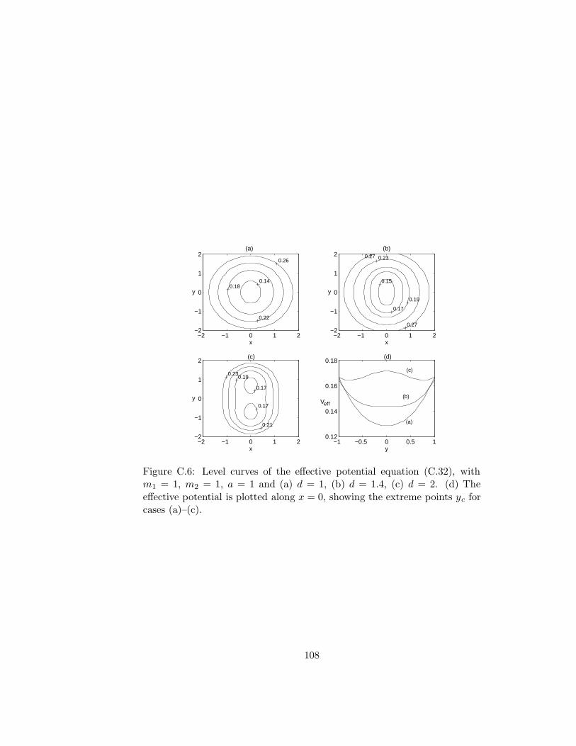
−2 −1 0 1 2−2

−1

0

1

2

x

y

0.14 0.18

0.22

0.26

−2 −1 0 1 2−2

−1

0

1

2

x

y

0.15

0.17

0.19

0.23

0.27

0.27

−2 −1 0 1 2−2

−1

0

1

2

x

y

0.17

0.17

0.19

0.21

0.23

−1 −0.5 0 0.5 10.12

0.14

0.16

0.18

y

(a) (b)

(c) (d)

Veff

(a)

(b)

(c)

Figure C.6: Level curves of the effective potential equation (C.32), withm1 = 1, m2 = 1, a = 1 and (a) d = 1, (b) d = 1.4, (c) d = 2. (d) Theeffective potential is plotted along x = 0, showing the extreme points yc forcases (a)–(c).

108

−2 0 2

−2

0

2

x

y

0.21 0.23

0.27

0.35

0.45

(a)

−2 0 2

−2

0

2

x

y

0.22 0.26

0.3 0.34 0.38

(b)

−2 0 2

−2

0

2

x

y

0.24

0.28 0.32

0.36

0.4

(c)

−2 −1 0 1 20.2

0.25

0.3

0.35

0.4

y

(d)

Veff

(a)

(b)

(c)

Figure C.7: Level curves of the effective potential equation (C.32), withm1 = 1, m2 = 0.5, a = 1 and (a) d = 2, (b) d = 2.5, (c) d = 3. (d) Theeffective potential is plotted along x = 0, showing the extreme points yc forcases (a)–(c).

109

black holes placed along the symmetry axis. The non-axisymmetric matterdistribution of ECD on the z = 0 plane was obtained from the metric oftwo extreme Reissner-Nordstrom black holes located along the y-axis. Toour knowledge no such configurations of matter satisfying Einstein’s fieldequations exist in the literature. We studied the variation of the energydensity distribution by varying the coordinate distance between the blackholes as well as their masses. For equal black hole masses the energy densitydistribution is symmetric with respect to both the x- and y-axes, while forunequal masses it possesses symmetry only with respect to the y-axis. Theeffective potential for geodesic motion of neutral test particles on the planeof such a matter distribution was also analysed.

Of course one could extend the procedure used in this paper to generatecomplete asymmetric planar configurations of ECD by putting N > 2 ex-treme Reissner-Nordstrom black holes in arbitrary positions on the xy planeand then applying the ‘displace, cut and reflect’ method.

Acknowledgments

DV thanks CAPES for financial support. PSL thanks FAPESP and CNPqfor financial support.

Bibliography

[1] Bonnor W A and Sackfield A 1968 Commun. Math. Phys. 8 338

[2] Morgan T and Morgan L 1969 Phys. Rev. 183 1097

[3] Morgan L and Morgan T 1970 Phys. Rev. D 2 2756

[4] Lynden-Bell D and Pineault S 1978 Mon. Not. R. Astron. Soc. 185 679

[5] Lemos J P S 1989 Class. Quantum Grav. 6 1219

[6] Bicak J, Lynden-Bell D and Katz J 1993 Phys. Rev. D 47 4334

[7] Bicak J, Lynden-Bell D and Pichon C 1993 Mon. Not. R. Astron. Soc.

265 126

[8] Bicak J and Ledvinka T 1993 Phys. Rev. Lett. 71 1669

[9] Ledvinka T, Zofka M and Bicak J 1999 Proceedings of the 8th Marcel

Grossman Meeting in General Relativity ed T Piran (Singapore: WorldScientific) p 339-41

110

[10] Gonzalez G and Letelier P S 2000 Phys. Rev. D 62 064025

[11] Neugebauer G and Meinel R 1995 Phys. Rev. Lett. 75 3046

[12] Gonzalez G and Letelier P S 1999 Class. Quantum Grav. 16 479

[13] Letelier P S 1999 Phys. Rev. D 60 104042

[14] Katz J, Bicak J and Lynden-Bell D 1999 Class. Quantum Grav. 16

4023

[15] Lemos J P S and Letelier P S 1993 Class. Quantum Grav. 10 L75

[16] Vogt D and Letelier P S 2003 Phys. Rev. D 68 084010

[17] Gonzalez G and Letelier P S 2004 Phys. Rev. D 69 044013

[18] Bonnor W B 1980 Gen. Rel. Grav. 12 453

[19] Bonnor W B and Wickramasuriya S B P 1975 Mon. Not. R. Astron.

Soc. 170 643

[20] Bonnor W B 1998 Class. Quantum Grav. 15 351

[21] Gurses M 1998 Phys. Rev. D 58 044001

[22] Varela V 2003 Gen. Rel. Grav. 35 1815

[23] Rosseland S 1924 Mon. Not. R. Astron. Soc. 84 720

[24] Bally J and Harrison E R 1978 Astrophys. J. 220 743

[25] Kuzmin G G 1956 Astron. Zh. 33 27

[26] Toomre A 1962 Astrophys. J. 138 385

[27] Synge J L 1971 Relativity the General Theory (Amsterdam: North-Holland) chapter X, section 4, p. 367

[28] Lynden-Bell D, Bicak J and Katz J 1999 Ann. Phys. 271 1

[29] Majumdar S D 1947 Phys. Rev. 72 930

[30] Papapetrou A 1947 Proc. R. Irish Acad. A 51 191

111

112

Apendice D

Exact relativistic static charged

perfect fluid disks

D. Vogt and P. S. Letelier, Phys. Rev. D 70, 064003 (2004).

Received 30 March 2004; published 2 September 2004.

Abstract

Using the well-known “displace, cut and reflect” method used to generatedisks from given solutions of Einstein field equations, we construct staticcharged disks made of perfect fluid based on the Reissner-Nordstrom solutionin isotropic coordinates. We also derive a simple stability condition forcharged and non charged perfect fluid disks. As expected, we find that thepresence of charge increases the regions of instability of the disks.

PACS numbers: 04.40.–b, 04.20.Jb, 04.40.Nr, 98.62.Mw

D.1 Introduction

Axisymmetric solutions of Einstein field equations corresponding to disklikeconfigurations of matter have been extensively studied. These solutions canbe static or stationary and with or without radial pressure. Solutions forstatic thin disks without radial pressure were first studied by Bonnor andSackfield [1], and Morgan and Morgan [2], and with radial pressure by Mor-gan and Morgan [3]. Other classes of static thin disk solutions have beenobtained [4–7], while stationary thin disks were studied in [8–10]. Also thin

113

disks with radial tension [11], magnetic fields [12] and both electric and mag-netic fields [13] have been studied. An exact solution to the problem of arigidly rotating disk of dust in terms of ultra-elliptic functions was reportedin [14], while models of static relativistic counterrotating dust disks wererecently presented in [15]. Structures of nonaxisymmetric matter distribu-tions of static charged dust were also recently studied [16]. The non-linearsuperposition of a disk and a black hole was first considered by Lemos andLetelier [17]. Models of thin disks and thin disks with halos made of perfectfluids were considered in [18]. The generalization of the “displace, cut andreflect” method (Sec. D.2) to construct thick static disks was considered byGonzalez and Letelier [19]. For a recent review on relativistic accretion diskssee [20].

Gravitationally bound stellar objects are likely to be positively chargeddue to the fact that the electrons are lighter than the protons so the formerscan more easily scape from the stellar object. One should expect to havean equilibrium situation when the electrostatic energy of the electron (eV )is of the order of its thermal energy (kT ) [21], then the scape would stop.Similar considerations can be found in Ref. [22].

The aim of this paper is to present a charged version of perfect fluiddisks that were studied in [18]. They are constructed with the well known“displace, cut and reflect” method applied to the Reissner-Nordstrom metricin isotropic coordinates. The stability of this new model of charged diskswill also be considered. We present an extension of the Rayleigh criteria ofstability [23] for the case of relativistic disks made of a charged perfect fluid.We find a simple condition to have gravitationally bounded disks.

The paper is divided as follows. Sec. D.2 discusses the formalism whichcan be used to construct disks given a solution of Einstein-Maxwell equa-tions, and the main physical variables of the disk. In Sec. D.3, Rayleighinspired criteria of stability criteria for the stability of charged and non-charged perfect fluid disks is established. The properties and stability ofthe charged disks are discussed in Sec. D.4. Finally, in Sec. D.5, we discussour results and make some considerations about the construction of chargedperfect fluid disks with halos. The “displace, cut and reflect” method isreviewed in the Appendix.

114

D.2 Einstein-Maxwell Equations and Disks

The isotropic metric representing a static spherically symmetric space-timecan be expressed as

ds2 = eν(r)dt2 − eλ(r)(dr2 + r2dΩ2), (D.1)

where dΩ2 = dθ2 + sin2 θdϕ2. The same metric in cylindrical coordinates(t, R, z, ϕ) reads:

ds2 = eν(R,z)dt2 − eλ(R,z)(

dR2 + dz2 +R2dϕ2)

. (D.2)

The Einstein-Maxwell system of equations is given by

Gµν = 8πTµν , (D.3)

Tµν =1

4π

(

FµσFνσ +

1

4gµνFρσF

ρσ

)

, (D.4)

F µν;µ = 0, (D.5)

Fµν = Aν,µ −Aµ,ν , (D.6)

where all symbols have their usual meaning. We use geometric units withG = c = 1.

The method used to generate the metric of the disk and its materialcontent is the well known “displace, cut and reflect” method (see the Ap-pendix) that was first used by Kuzmin [24] and Toomre [25] to constructNewtonian models of disks, and later extended to general relativity (see,for example [6, 10]). Given a solution of the Einstein-Maxwell equation,this procedure is mathematically equivalent to apply the transformationz → |z| + a, with a constant, on that solution. In the Einstein tensor wehave first and second derivatives of z. Remembering that ∂z|z| = 2ϑ(z) − 1and ∂zz|z| = 2δ(z), where ϑ(z) and δ(z) are, respectively, the Heavisidefunction and the Dirac distribution, Einstein-Maxwell equations give us

Gµν = 8π(T elm.µν +Qµνδ(z)), (D.7)

F µν;µ = 4πJνδ(z), (D.8)

where T elm.µν is the electromagnetic tensor Eq. (D.4), Qµν is the energy-

momentum tensor on the plane z = 0 and J ν is the current density on theplane z = 0. For the metric (D.2), the nonzero components of Qµν are

Qtt =

1

16π

[

−bzz + gzz(bRR + bzz + bϕϕ)]

, (D.9)

115

QRR = Qϕ

ϕ =1

16π

[

−bzz + gzz(btt + bRR + bzz)]

, (D.10)

where bµν denotes the jump of the first derivatives of the metric tensor onthe plane z = 0,

bµν = gµν,z |z=0+ − gµν,z|z=0− , (D.11)

and the other quantities are evaluated at z = 0+. The electromagneticpotential for an electric field is

Aµ = (φ, 0, 0, 0). (D.12)

Using Eq. (D.12) and Eq. (D.8), the only nonzero component of the currentdensity on the plane z = 0 is

J t =1

4πgzzgttat, (D.13)

where aµ denotes the jump of the first derivatives of the electromagneticpotential on the plane z = 0,

aµ = Aµ,z|z=0+ −Aµ,z|z=0− , (D.14)

and the other quantities are evaluated at z = 0+. The “physical measure”of length in the direction ∂z for metric (D.2) is

√−gzz, then the invariantdistribution is δ(z)/

√−gzz. Thus the “true” surface energy density σ andthe azimuthal and radial pressures or tensions (P ) are

σ =√−gzzQ

tt, P = −√−gzzQ

RR = −√−gzzQ

ϕϕ. (D.15)

Since Jµ = ρUµ, where Uµ = δµt /

√gtt, the “true” surface charge density ρ

is

ρ =√−gzzgttJ

t. (D.16)

D.3 Stability Conditions for Perfect Fluid Disks

One way to explain stability of static disks without radial pressure is to as-sume that the particles on the disk plane move under the action of their owngravitational field in such a way that as many particles move clockwise ascounterclockwise (counterrotating model). With this assumption, stabilityof the matter on the disk can be associated with stability of circular orbits

116

along geodesics (see [26] for a detailed explanation). The usual stabilitycriteria for circular orbits is adapted from the Rayleigh criteria of stabil-ity for a rotating fluid [23]. One finds that stability against small radialperturbations is achieved when

hdh

dr> 0, (D.17)

where h is the specific angular momentum of the circular orbit.

In the case of perfect fluid disks the situation is somewhat different,since radial pressure can equilibrate the inward gravitational force and nocounterrotating hypothesis is needed. Using T µν

;ν = 0 where T µν is thesum of the energy-momentum tensor for a perfect fluid and Eq. (D.4), theequilibrium condition in the radial direction on the plane z = 0 is given by

1

2(P + σ)(eν),R = −ρeν/2φ,R − eνP,R. (D.18)

The left side of Eq. (D.18) can be interpreted as the gravitational forcewhich equilibrates the pressure and electric forces that appear on the rightside. Now suppose an element of fluid at radius R is displaced to R + ∆Rkeeeping P , σ and ρ constant. The right side of Eq. (D.18) becomes

−eν(R+∆R)/2φ,R(R+ ∆R)ρ(R) − eν(R+∆R)P,R(R). (D.19)

These “forces” should be compared with the right side of Eq. (D.18) atradius R+ ∆R:

−eν(R+∆R)/2φ,R(R + ∆R)ρ(R+ ∆R) − eν(R+∆R)P,R(R + ∆R). (D.20)

To have stability expression (D.19) must be less then expression (D.20).Expanding ρ(R+ ∆R) and P,R(R+ ∆R) around R, we get

eν/2φ,Rρ,R + eνP,RR < 0. (D.21)

For an uncharged fluid, condition (D.21) reduces to P,RR < 0.

Note that this criterium of stability refers only to radial perturbations ofthe pressure and charge. It really gives us a condition to have gravitationallybounded systems. In other words the disks do not explode, but they cancollapse. In the general case, the study of the stability of gravitating systemsreduces to the much harder problem of the study of the eigenvalue problemfor a nontrivial elliptic operator [27].

117

D.4 Charged Perfect Fluid Disks

We apply now the results of the previous sections to construct charged disks.The Reissner-Nordstrom solution in Schwarzschild coordinates is given by

ds2 =

(

1 − 2m

r+Q2

r2

)

dt2 − dr2(

1 − 2mr + Q2

r2

) − r2dΩ2, (D.22)

where m and Q are, respectively, the mass and charge of the black hole, andm > Q. The electromagnetic potential associated to solution (D.22) is

Aµ =

(

Q

r, 0, 0, 0

)

. (D.23)

With the radial coordinate transformation

r = r′(

1 +m+Q

2r′

)(

1 +m−Q

2r′

)

, (D.24)

metric (D.22) and Eq. (D.23) can be expressed in isotropic coordinates(t, r′, θ, ϕ) as

ds2 =

[

1 − (m2−Q2)4r′2

]2

[

1 + (m+Q)2r′

]2 [

1 + (m−Q)2r′

]2 dt2 −[

1 +(m+Q)

2r′

]2

×[

1 +(m−Q)

2r′

]2

(dr′2 + r′2dθ2 + r′2 sin2 θdϕ2), (D.25)

Aµ =

Q

r′(

1 + m+Q2r′

)(

1 + m−Q2r′

) , 0, 0, 0

. (D.26)

Transforming Eq. (D.25) and (D.26) to cylindrical coordinates, and usingEq. (D.15) and (D.16), we obtain a disk with surface energy density σ =σ/m, equal radial and azimuthal pressures (or tensions) P = P /m andsurface charge density ρ = ρ/m where

σ =4a

π

2√

R2 + a2 + 1 − Q2

[(1 + 2√

R2 + a2)2 − Q2]2, (D.27)

P = −2a

π

1 − Q2

[(1 + 2√

R2 + a2)2 − Q2][1 − Q2 − 4(R2 + a2)], (D.28)

118

ρ =8Qa

√

R2 + a2

π[

4√

R2 + a2(1 +√

R2 + a2) + 1 − Q2]2 , (D.29)

with R = R/m, a = a/m and Q = Q/m.

Eq. (D.27) shows that the disk’s surface density is always positive (weakenergy condition) for Q < 1. Positive values (pression) for the stresses in

azimuthal and radial directions are obtained if a >

√

1 − Q2/2. The velocity

of sound propagation V , defined as V 2 = dPdσ , is calculated using Eq. (D.27)

and Eq. (D.28):

V 2 =

(1 − Q2)[(1 + 2√

R2 + a2)2 − Q2][(1 + 2√

R2 + a2)2(1 − 4√

R2 + a2) − Q2]

[1 − Q2 − 4(R2 + a2)]2[−3(1 + 2√

R2 + a2)2 + Q2(3 + 8√

R2 + a2)].

(D.30)

Figure D.1 shows the curves of V 2 = 1 (solid curve) and of a =

√

1 − Q2/2

(dotted curve) where P changes sign as functions of the parameters a = a/mand Q = Q/m. Above the dotted curve, stresses are positive (pressure) forall R and above the solid curve, condition V 2 < 1 is also satisfied for allR. Thus, choosing values for a and Q that lie above the solid curve ensuresthat the entire disk will have pressures and sublumial sound velocities. Wealso note that when we increase the charge, the range of the cut parametera (that generates disks for which the conditions stated above are satisfied)is enlarged. Figure D.2(a)–D.2(d) shows, respectively, the surface energydensity σ, pressures P , sound velocity V and charge density ρ with a = 1,Q = 0, 0.3, 0.6 and 0.9 as functions of R. As charge increases, the disksbecome less relativistic for the same cut parameter; energy density and pres-sures are lowered and charge density becomes more concentrated near thedisk center.

Figure D.3(a) is a graph of curves where Eq. (D.21) changes sign. Thecurves have been plotted only for ranges of parameter a where V 2 < 1 (Fig.D.1). At the left of each curve, the stability condition (D.21) is satisfied.Thus, the disks are stable only in a small region near their centers. We alsonote that the charge decreases the radii of stability. The left side of Eq.D.21 is plotted in Fig. D.3(b) for the same parameters as in Fig. D.2.

119

0

0.1

0.2

0.3

0.4

0.5

0.6

0.7

0.8

0.9

1

1.1

0 0.1 0.2 0.3 0.4 0.5 0.6 0.7 0.8 0.9 1

Q / m

a/m

Figure D.1: Curve V 2 = 1 (solid curve) as a function of the parametersa = a/m and Q = Q/m for the charged disk of perfect fluid. Also a =√

1 − Q2/2 (dotted curve).

D.5 Discussion

We applied the “displace, cut and reflect” method on the Reissner-Nordstromsolution in isotropic coordinates and generated static charged disks made ofperfect fluid. We also derived a simple criteria for the stability for chargedand uncharged perfect fluid disks that is an extension of the Rayleigh cri-teria of stability for rotating fluids. The addition of charge decreases theenergy density and pressures near the disk’s centers, while charge densityin enhanced there. Furthermore, presence of charge decreases the stableregions of the disks that are reduced to small regions near the center evenin the absence of charge. This is a rather different result from that of ourprevious stability analysis of the uncharged perfect fluid disk [18] based onthe stability study of circular orbits of test particles, where we found thatthe disks were completely stable for a

1.016. It is worthwhile to note that

the criteria used to study stability of disks made of counterrotating matteris based on a particle consideration, whereas the stability criteria derived forperfect fluid disks is based on collective phenomena. Therefore, the stabilitycriteria derived in this paper seems to us to be more appropriate for thestudy of perfect fluid disks.

In principle it is possible to add charged halos to the disks presentedin this work by applying the “displace, cut and reflect” method to a staticcharged sphere of perfect fluid in isotropic coordinates (see the Appendix).

120

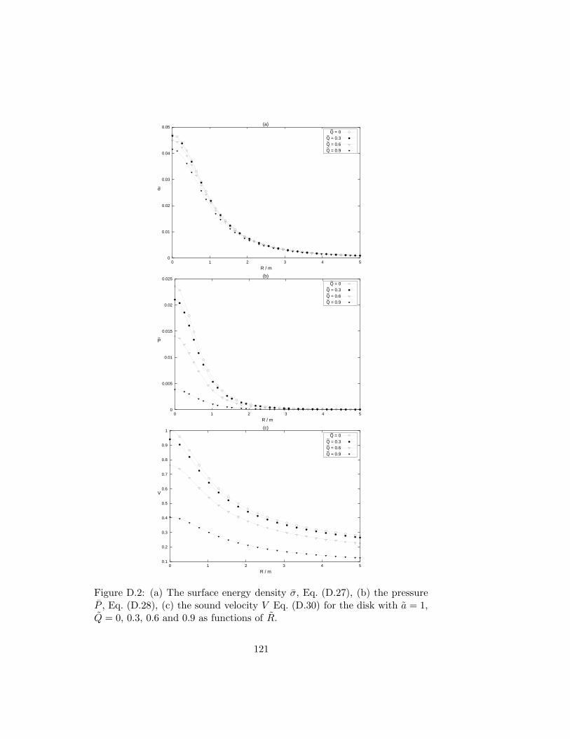
0

0.01

0.02

0.03

0.04

0.05

0 1 2 3 4 5

R / m

σ

(a)

Q = 0~

Q = 0.3~

Q = 0.6~

Q = 0.9~

0

0.005

0.01

0.015

0.02

0.025

0 1 2 3 4 5

R / m

P

(b)

Q = 0~

Q = 0.3~

Q = 0.6~

Q = 0.9~

0.1

0.2

0.3

0.4

0.5

0.6

0.7

0.8

0.9

1

0 1 2 3 4 5

R / m

V

(c)

Q = 0~

Q = 0.3~

Q = 0.6~

Q = 0.9~

Figure D.2: (a) The surface energy density σ, Eq. (D.27), (b) the pressureP , Eq. (D.28), (c) the sound velocity V Eq. (D.30) for the disk with a = 1,Q = 0, 0.3, 0.6 and 0.9 as functions of R.

121

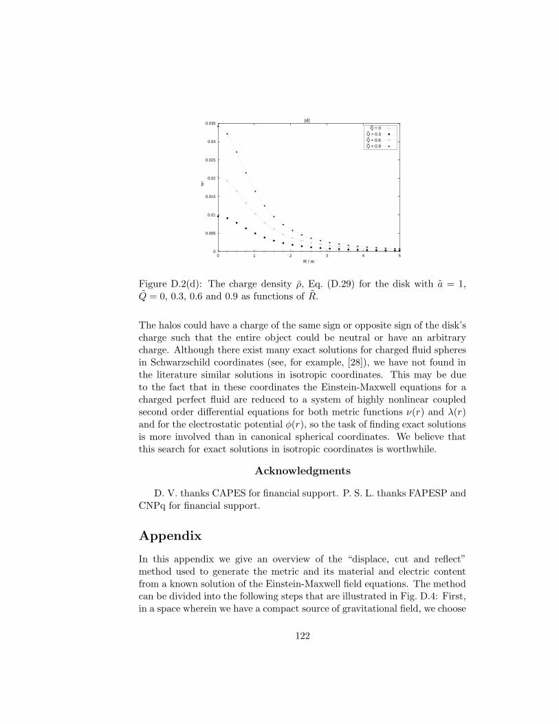
0

0.005

0.01

0.015

0.02

0.025

0.03

0.035

0 1 2 3 4 5

R / m

ρ

(d)

Q = 0~

Q = 0.3~

Q = 0.6~

Q = 0.9~

Figure D.2(d): The charge density ρ, Eq. (D.29) for the disk with a = 1,Q = 0, 0.3, 0.6 and 0.9 as functions of R.

The halos could have a charge of the same sign or opposite sign of the disk’scharge such that the entire object could be neutral or have an arbitrarycharge. Although there exist many exact solutions for charged fluid spheresin Schwarzschild coordinates (see, for example, [28]), we have not found inthe literature similar solutions in isotropic coordinates. This may be dueto the fact that in these coordinates the Einstein-Maxwell equations for acharged perfect fluid are reduced to a system of highly nonlinear coupledsecond order differential equations for both metric functions ν(r) and λ(r)and for the electrostatic potential φ(r), so the task of finding exact solutionsis more involved than in canonical spherical coordinates. We believe thatthis search for exact solutions in isotropic coordinates is worthwhile.

Acknowledgments

D. V. thanks CAPES for financial support. P. S. L. thanks FAPESP andCNPq for financial support.

Appendix

In this appendix we give an overview of the “displace, cut and reflect”method used to generate the metric and its material and electric contentfrom a known solution of the Einstein-Maxwell field equations. The methodcan be divided into the following steps that are illustrated in Fig. D.4: First,in a space wherein we have a compact source of gravitational field, we choose

122

0.6

0.8

1

1.2

1.4

1.6

1.8

2

0.2 0.3 0.4 0.5 0.6 0.7 0.8 0.9

R / m

a/m

(a)

Q=0~

Q=0.3~

Q=0.6~

Q=0.9~

-0.01

-0.008

-0.006

-0.004

-0.002

0

0.002

0.004

0 1 2 3 4 5

R / m

(b)

Q=0~

Q=0.3~

Q=0.6~

Q=0.9~

Figure D.3: (a) Curves where Eq. (D.21) defining stability changes sign asfunctions of radius R, cut parameter a and charge Q. Disks are stable atthe left of each curve. (b) Curves of the left side of Eq. (D.21) for the sameparameters as in Fig. D.2.

123

(a)

(b)

Figure D.4: An illustration of the “displace, cut and reflect” method for thegeneration of disks. In (a) the spacetime with a singularity is displaced andcut by a plane (dotted line), in (b) the part with singularities is disregardedand the upper part is reflected on the plane.

a surface (in our case, the plane z = 0) that divides the space in two pieces:one with no singularities or sources and the other with the sources. Thenwe disregard the part of the space with singularities and use the surface tomake an inversion of the nonsingular part of the space. This results in aspace with a singularity that is a delta function with support on z = 0. Thesame procedure can be used with a static sphere of charged perfect fluidto generate charged disks with halos, as depicted in Fig. D.5: the sphere isdisplaced and cut by a distance a less then its radius. The part of the spacethat contains the center of the sphere is disregarded. After the inversionof the remaining space, one ends up with a charged disk surrounded by acap of charged perfect fluid. If the internal fluid solution is matched to theReissner-Nordstrom metric Eq. (D.25), the outer part of the disk will havethe physical properties deduced in Sec. D.4, while the properties of the innerpart will depend on the particular fluid solution.

Bibliography

[1] W. A. Bonnor and A. Sackfield, Commun. Math. Phys. 8, 338 (1968).

[2] T. Morgan and L. Morgan, Phys. Rev. 183, 1097 (1969).

[3] L. Morgan and T. Morgan, Phys. Rev. D 2, 2756 (1970).

[4] D. Lynden-Bell and S. Pineault, Mon. Not. R. Astron. Soc. 185, 679(1978).

[5] J. P. S. Lemos, Classical Quantum Gravity 6, 1219 (1989).

124

(b)(a)

Figure D.5: An illustration of the “displace, cut and reflect” method for thegeneration of charged disks with halos. In (a) the sphere of perfect fluid isdisplaced and cut by a plane (dotted line), in (b) the part that contains thecenter of the sphere is disregarded and the upper part is reflected on theplane.

[6] J. Bicak, D. Lynden-Bell and J. Katz, Phys. Rev. D 47, 4334 (1993).

[7] J. Bicak, D. Lynden-Bell and C. Pichon, Mon. Not. R. Astron. Soc.265, 126 (1993).

[8] J. Bicak and T. Ledvinka, Phys. Rev. Lett. 71, 1669 (1993).

[9] T. Ledvinka, M. Zofka and J. Bicak, in Proceedings of the 8th Marcel

Grossman Meeting in General Relativity, edited by T. Piran (WorldScientific, Singapore, 1999), p. 339-341.

[10] G. Gonzalez and P. S. Letelier, Phys. Rev. D 62, 064025 (2000).

[11] G. Gonzalez and P. S. Letelier, Classical Quantum Gravity 16, 479(1999).

[12] P. S. Letelier, Phys. Rev. D 60, 104042 (1999).

[13] J. Katz, J. Bicak and D. Lynden-Bell, Classical Quantum Gravity 16,4023 (1999).

[14] G. Neugebauer and R. Meinel, Phys. Rev. Lett. 75, 3046 (1995).

[15] G. Garcıa R. and G. Gonzalez, Phys. Rev. D 69, 124002 (2004).

[16] D. Vogt and P. S. Letelier, Classical Quantum Gravity (to be pub-lished).

125

[17] J. P. S. Lemos and P. S. Letelier, Classical Quantum Gravity 10, L75(1993).

[18] D. Vogt and P. S. Letelier, Phys. Rev. D 68, 084010 (2003).

[19] G. Gonzalez and P. S. Letelier, Phys. Rev. D 69, 044013 (2004).

[20] V. Karas, J.-M. Hure and O. Semerak, Classical Quantum Gravity 21,R1 (2004).

[21] J. Bally and E.R. Harrison, Astrophys. J. 220, 743 (1978).

[22] V.F. Shvartsman, Zh. Eksp. Teor. Fiz. 60, 881 (1971) [Sov. Phys. JETP33, 475 (1971)].

[23] Lord Rayleigh, Proc. R. Soc. London A 93, 148 (1917); see also L.D. Landau and E. M. Lifshitz, in Fluid Mechanics (Pergamon Press,Oxford, 1987), 2nd Ed. Sec. 27.

[24] G. G. Kuzmin, Astron. Zh. 33, 27 (1956).

[25] A. Toomre, Astrophys. J. 138, 385 (1962).

[26] P. S. Letelier, Phys. Rev. D 68, 104002 (2003).

[27] See for instance, A.N. Friedman and V.L.K. Polyachenko, Physics of

Gravitating Systems (Springer-Verlag, New York, 1983).

[28] B. V. Ivanov, Phys. Rev. D 65, 104001 (2002).

126

Apendice E

General relativistic model for the

gravitational field of active galactic

nuclei surrounded by a disk

D. Vogt and P. S. Letelier, Physical Review D 71, 044009 (2005).

Received 26 August 2004; published 9 February 2005.

Abstract

An exact but simple general relativistic model for the gravitational field ofactive galactic nuclei is constructed, based on the superposition in Weylcoordinates of a black hole, a Chazy-Curzon disk and two rods, which rep-resent matter jets. The influence of the rods on the matter properties ofthe disk and on its stability is examined. We find that in general they con-tribute to destabilize the disk. Also the oscillation frequencies for perturbedcircular geodesics on the disk are computed, and some geodesic orbits forthe superposed metric are numerically calculated.

PACS numbers: 04.40.–b, 04.20.Jb, 98.58 Fd, 98.62 Mw

E.1 Introduction

There is strong observational evidence that active galactic nuclei (AGN),X-ray transients and gamma-ray bursts (GRBs) are associated with accre-tion onto black holes, and that these sources are able to form collimated,

127

ultrarelativistic flows (relativistic jets).The exact mechanisms to explain the production of jets are still uncer-

tain, but they probably involve the interaction between a spinning blackhole, the accretion disk, and electromagnetic fields in strong gravitationalfields (see, for example, [1–3] and references therein).

Thus, a reasonably accurate general relativistic model of an AGN wouldrequire an exact solution of Einstein-Maxwell field equations that describes asuperposition of a Kerr black hole with a stationary disk and electromagneticfields. Not even an exact solution of a stationary black hole-disk system hasbeen found yet. Solutions for static thin disks without radial pressure werefirst studied by Bonnor and Sackfield [4], and Morgan and Morgan [5], andwith radial pressure by Morgan and Morgan [6]. Several classes of exactsolutions of the Einstein field equations corresponding to static thin diskswith or without radial pressure have been obtained by different authors[7–16]. Thin rotating disks were considered in [17, 18]. Perfect fluid diskswith halos [19] and charged perfect fluid disks [20] were also studied, whereasthick relativistic disks were reported in [21]. Several solutions of the Einsteinequations coupled to matter that represent disks have also been studied bythe Jena group [22–29].

The static superposition of a disk and a black hole was first consideredby Lemos and Letelier [10]. Zellerin and Semerak [30] found a stationarymetric that reduces to the superposition of a disk and a black hole in thestatic limit and thus may represent a stationary disk-black hole system. Theanalysis of their solution is complicated by the fact that the metric functionscannot be analytically computed. For a survey on self gravitating relativisticthin disks, see for instance [31].

The aim of this paper is to consider the gravitational field of an AGNthrough a simple model: the static superposition of a black hole with aChazy-Curzon disk and two rods placed on the symmetry axis, which willrepresent jets. Our principal interest here is to see how the presence of therods affect the matter properties and stability of the disk.

The article is divided as follows. In Sec. E.2 we review the “displace,cut and reflect” method used to construct thin disks from a known solutionof Einstein field equations in Weyl coordinates. Section E.3 summarizesthe formalism to superpose thin disks and other Weyl solutions. SectionE.4 discusses Schwarzschild solution and the metric of a finite rod in Weylcoordinates. In Sec. E.5 the results of Secs. E.3 and E.4 are then applied toconstruct the superposition of disk, black hole and rods and the resultingenergy-momentum tensor. In Sec. E.6 the disk stability is studied throughsmall horizontal and vertical oscillations about equatorial circular geodesics.

128

In Sec. E.7 some geodesic orbits for the superposed metric are numericallycalculated. Finally, Sec. E.8 is devoted to discussion of the results. We takeunits such that c = G = 1.

E.2 Thin disk solutions in Weyl coordinates

In absence of matter, the general metric for a static axially symmetric space-time in Weyl’s canonical coordinates (t, r, z, ϕ) is given by

ds2 = −eφdt2 + eν−φ(dr2 + dz2) + r2e−φdϕ2, (E.1)

where φ and ν are functions of r and z only. Einstein vacuum field equationsfor the metric Eq. (E.1) yield [32, 33]

φ,rr +φ,r

r+ φ,zz = 0, (E.2a)

ν[φ] =1

2

∫

r[

(φ2,r − φ2

,z)dr + 2φ,rφ,zdz]

. (E.2b)

Given a solution of Eqs. (E.2a) and (E.2b), one can construct a thin disk byusing the well known “displace, cut and reflect” method, due to Kuzmin [34].First, a surface (z = 0) is chosen so that it divides the usual space in twoparts: one with no singularities or sources, and the other with them. Thenthe part of the space with singularities or sources is disregarded. At last,the surface is used to make an inversion of the nonsingular part of the space.The result will be a space with a singularity that is a delta function withsupport on z = 0. The method is mathematically equivalent to making atransformation z → |z| + a, where a is a constant.

The application of the formalism of distributions in curved spacetimes tothe Weyl metric Eq. (E.1) is exposed in [13]. One finds that the componentsof the distributional energy-momentum tensor [T a

b] on the disk are

−T tt = eφ−ν(2 − rφ,r)φ,zδ(z), (E.3)

Tϕϕ = eφ−νrφ,rφ,zδ(z), (E.4)

T rr = T z

z = 0, (E.5)

where δ(z) is the Dirac distribution with support on the disk and is un-derstood that φ,z = limz→0+ φ,z. The “true” energy density and azimuthalpressure are, respectively,

σ = e(ν−φ)/2(−T tt), (E.6)

129

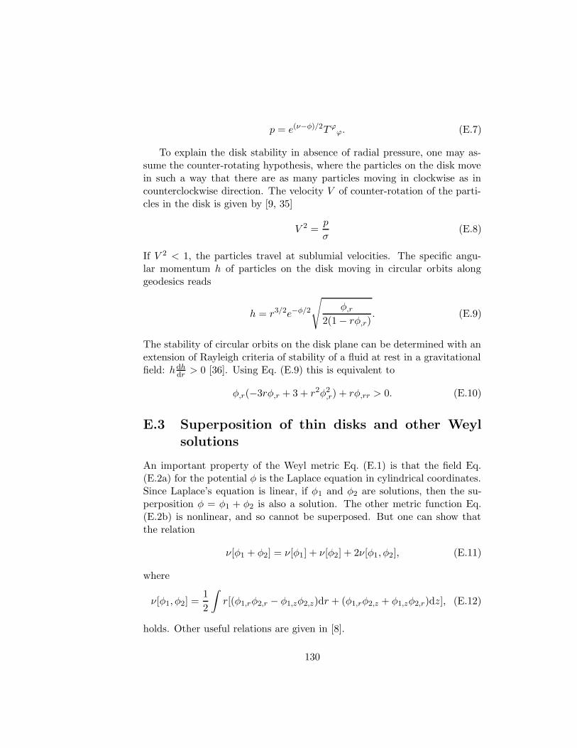
p = e(ν−φ)/2Tϕϕ. (E.7)

To explain the disk stability in absence of radial pressure, one may as-sume the counter-rotating hypothesis, where the particles on the disk movein such a way that there are as many particles moving in clockwise as incounterclockwise direction. The velocity V of counter-rotation of the parti-cles in the disk is given by [9, 35]

V 2 =p

σ(E.8)

If V 2 < 1, the particles travel at sublumial velocities. The specific angu-lar momentum h of particles on the disk moving in circular orbits alonggeodesics reads

h = r3/2e−φ/2

√

φ,r

2(1 − rφ,r). (E.9)

The stability of circular orbits on the disk plane can be determined with anextension of Rayleigh criteria of stability of a fluid at rest in a gravitationalfield: hdh

dr > 0 [36]. Using Eq. (E.9) this is equivalent to

φ,r(−3rφ,r + 3 + r2φ2,r) + rφ,rr > 0. (E.10)

E.3 Superposition of thin disks and other Weyl

solutions

An important property of the Weyl metric Eq. (E.1) is that the field Eq.(E.2a) for the potential φ is the Laplace equation in cylindrical coordinates.Since Laplace’s equation is linear, if φ1 and φ2 are solutions, then the su-perposition φ = φ1 + φ2 is also a solution. The other metric function Eq.(E.2b) is nonlinear, and so cannot be superposed. But one can show thatthe relation

ν[φ1 + φ2] = ν[φ1] + ν[φ2] + 2ν[φ1, φ2], (E.11)

where

ν[φ1, φ2] =1

2

∫

r[(φ1,rφ2,r − φ1,zφ2,z)dr + (φ1,rφ2,z + φ1,zφ2,r)dz], (E.12)

holds. Other useful relations are given in [8].

130

The energy-momentum tensor of the combined system disk and blackhole has been computed by Lemos and Letelier [13]. Let φD and φBH bethe metric potentials of the disk and of the black hole, respectively. Thenthe components [T a

b] of the superposition are

−T tt = eφD+φBH−ν [2 − r(φD + φBH),r]φD,zδ(z), (E.13)

Tϕϕ = eφD+φBH−νr(φD + φBH),rφD,zδ(z), (E.14)

T rr = T z

z = 0, (E.15)

where ν = ν[φD +φBH ], and again φD,z = limz→0+ φD,z. The “true” energydensity and azimuthal pressure read

σ = e(ν−φD−φBH )/2(−T tt), (E.16)

p = e(ν−φD−φBH )/2Tϕϕ. (E.17)

Equation (E.13) and (E.14) show that the potential of the black hole in-teracts with the disk and changes its matter properties. Although Eqs.(E.13)–(E.17) have been derived for superposition of disk and black hole,they are also valid when the potential function φBH is a sum of other Weylsolutions, like the superposition of a black hole and rods.

E.4 Black holes and rods in Weyl coordinates

The Schwarzschild black hole metric function φBH in Weyl coordinates isgiven by

φBH = ln

(

r1 + r2 − 2M

r1 + r2 + 2M

)

, (E.18)

where r21 = (M − z)2 + r2 and r2

2 = (M + z)2 + r2. The function φ(r, z) canbe related to the Newtonian potential U by

φ = 2U . (E.19)

Thus, the metric potential φR of a finite rod of linear mass density λ lyingon the z axis and located along [c1, c2] is

φR = −2λ ln

[

c2 − z +√

r2 + (c2 − z)2

c1 − z +√

r2 + (c1 − z)2

]

. (E.20)

131

The calculation of the other metric function ν for Eqs. (E.18) and (E.20) andlater for the superposed metric, is considerably simplified when one definesthe following µ function

µk = αk − z +√

r2 + (αk − z)2, (E.21)

where αk is an arbitrary constant. This function is a natural consequenceof the formalism of the inverse scattering method [37, 38]. Equations (E.18)and (E.20) can be rewritten as

φBH = ln

(

µ1

µ2

)

, (E.22)

φR = −2λ ln

(

µ3

µ4

)

, (E.23)

where we defined

µ1 = −M − z +√

r2 + (M + z)2, µ2 = M − z +√

r2 + (M − z)2,

µ3 = c2 − z +√

r2 + (c2 − z)2, µ4 = c1 − z +√

r2 + (c1 − z)2.

On using Eq. (E.11)

ν[lnµi − lnµj] = ν[lnµi] + ν[lnµj ] − 2ν[lnµi, lnµj]; (E.24)

the result

ν[lnµi, lnµj] = ln(µi − µj), (E.25)

which also follows from the inverse scattering method; and the identity

(r2 + µiµj)(µi − µj) = 2(αi − αj)µiµj, (E.26)

one obtains following expressions for the metric function ν

νBH = ln

[

(r2 + µ1µ2)2

(r2 + µ21)(r

2 + µ22)

]

, (E.27)

νR = 4λ2 ln

[

(r2 + µ3µ4)2

(r2 + µ23)(r

2 + µ24)

]

. (E.28)

132

−c2

−c1

c1

c2

z=−a

z=0

−M

M

Figure E.1: Superposition of a black hole with mass M , two rods and aChazy-Curzon disk on the plane z = 0.

E.5 Superposition of disk, black hole and rods

We now consider the superposition illustrated in Fig. E.1: a black hole withmass M whose center is on z = 0, two rods with equal mass density λ, eachone with mass M located along [−c2,−c1] and [c1, c2] on the z axis, anda disk on the plane z = 0 constructed with the “displace, cut and reflectmethod” from the Chazy-Curzon solution with mass m, whose singularitylies on z = −a:

φD = − 2m√

r2 + (|z| + a)2. (E.29)

It should be remembered that in Weyl coordinates a black hole with mass Mis represented by a rod with length 2M , thus in Fig. E.1 we put a dotted cir-cle around the rod in the middle. Such a configuration is not gravitationallystable: a consequence of the nonlinearity of Eq. (E.2b) is the appearence ofgravitationally inert singular structures like struts between the rods and theblack hole that keep them appart. Also in the superposition of the disk withthe black hole, superlumial regions (V 2 > 1) exist because there is matterup to the event horizon.

The metric function φ of the superposition can be expressed as

φ = −2λ ln

(

µ3

µ4

)

+ ln

(

µ1

µ2

)

− 2λ ln

(

µ5

µ6

)

+ φD, (E.30)

with µ5 = −c1 − z +√

r2 + (c1 + z)2 and µ6 = −c2 − z +√

r2 + (c2 + z)2.Now we consider the case when both rods just touch the horizon of the

black hole, that is, when c1 = M . Then µ4 = µ2 and µ5 = µ1. From Eqs.

133

(E.13), (E.14) and (E.8), we get following conditions:

σ > 0 →√

r2 + c22

[

(r2 + a2)3/2(√

1 + r2 − 1) − αr2√

1 + r2]

+ 2λ(r2 + a2)3/2

(

√

r2 + c22 − c2√

1 + r2

)

> 0, (E.31)

p > 0 →√

r2 + c22

[

αr2√

1 + r2 + (r2 + a2)3/2]

− 2λ(r2 + a2)3/2

(

√

r2 + c22 − c2√

1 + r2

)

> 0, (E.32)

V 2 < 1 →√

r2 + c22

[

2αr2√

1 + r2 + (r2 + a2)3/2(2 −√

1 + r2)]

− 4λ(r2 + a2)3/2

(

√

r2 + c22 − c2√

1 + r2

)

< 0, (E.33)

where r = r/M , a = a/M , c2 = c2/M , α = m/M , β = M/M and λ =M/(c2 −M) = β/(c2 − 1). The conditions imposed are that of weak energy(σ > 0), azimuthal pressure (p > 0) and sublumial velocity (V 2 < 1) ofcounter-rotation of particles on the disk. For r → ∞, all three conditionsare satisfied. In the regions where V 2 < 1, the weak energy condition isalways satisfied, as can be seen by inequalities (E.31) and (E.33).

Figure E.2(a)–E.2(c) shows curves of V 2 = 1 (dotted curves) and ofhdh/dr = 0 (solid curves) as function of λ and r for three different valuesof α. The mass of each rod is kept constant β = 0.5 and the cut parametertakes values a = 1 and a = 3 in E.2(a) and E.2(b), respectively. At the rightof each dotted curve we have V 2 < 1 and the unstable regions of the diskappear between the curves of hdh/dr = 0. We note that in general withincreasing mass of the disk and smaller length of the rods, the disk becomesmore unstable and the regions of superlumial velocity also increase. Thereis, however, an interval of values for the rod’s mass density where the zone ofstability is increased, as can be seen in the lower part of the curve hdh/dr = 0for α = 0.001 in Fig. E.2(a). This is probably due to the prolate quadrupolemoment of the rods, which scale as Ml2, where l is their length. Thus, forlarger rods, the effect of prolate deformations may overwhelm the effect ofthe oblate quadrupole moment of the disk, and increase stability (see [39]for a detailed discussion of the effect of quadrupolar fields on the stabilityof circular orbits).

Figure E.3(a) and E.3(b) shows again curves of V 2 = 1 (dotted curves)and of hdh/dr = 0 (solid curves) as function of λ and r for three differentvalues of α, but now the length of each rod is kept constant (c2 = 11) and

134

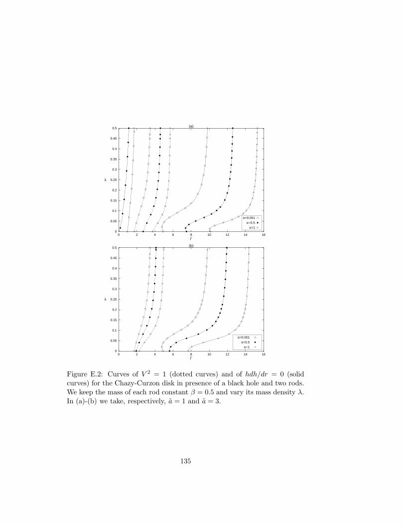
0

0.05

0.1

0.15

0.2

0.25

0.3

0.35

0.4

0.45

0.5

0 2 4 6 8 10 12 14 16r~

λ

(a)

α=0.001

α=0.5

α=1

0

0.05

0.1

0.15

0.2

0.25

0.3

0.35

0.4

0.45

0.5

0 2 4 6 8 10 12 14 16

λ

r~

(b)

α=0.001

α=0.5

α=1

Figure E.2: Curves of V 2 = 1 (dotted curves) and of hdh/dr = 0 (solidcurves) for the Chazy-Curzon disk in presence of a black hole and two rods.We keep the mass of each rod constant β = 0.5 and vary its mass density λ.In (a)-(b) we take, respectively, a = 1 and a = 3.

135

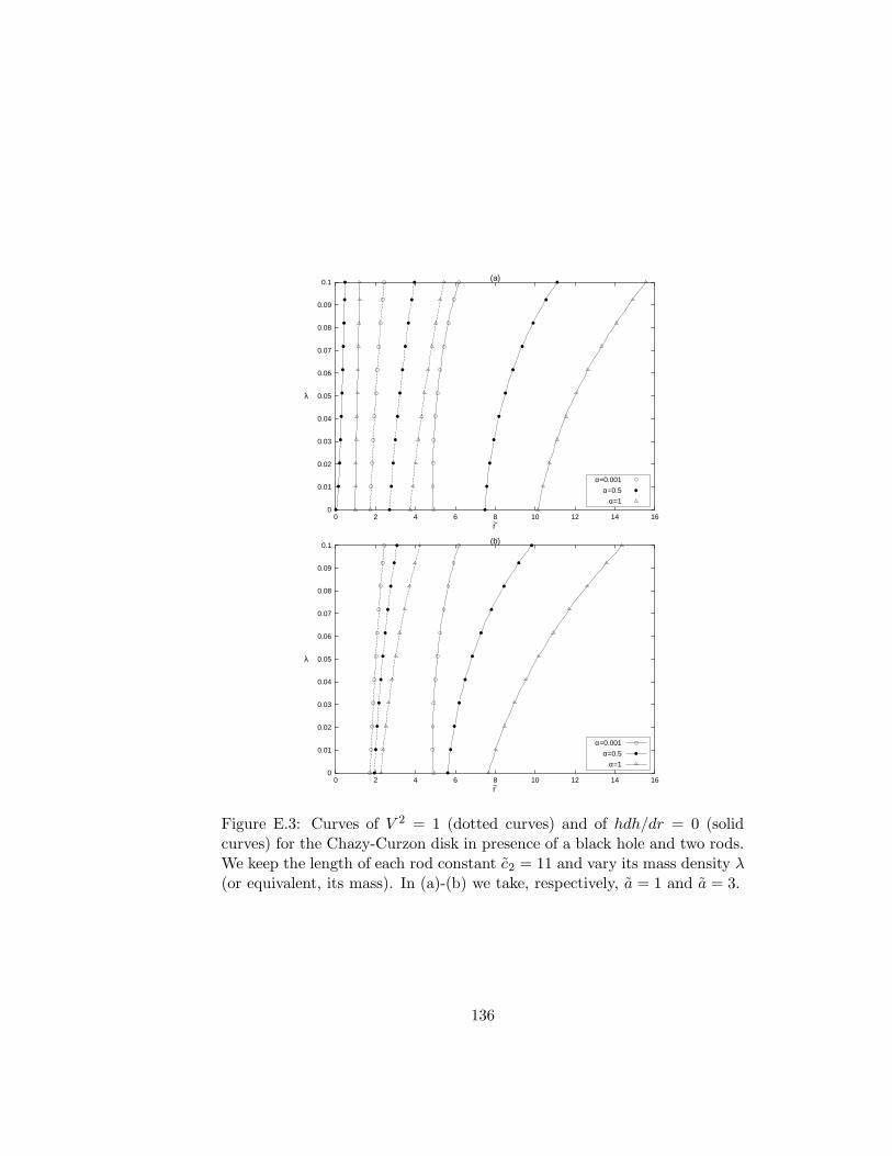
0

0.01

0.02

0.03

0.04

0.05

0.06

0.07

0.08

0.09

0.1

0 2 4 6 8 10 12 14 16

λ

r~

(a)

α=0.001

α=0.5

α=1

0

0.01

0.02

0.03

0.04

0.05

0.06

0.07

0.08

0.09

0.1

0 2 4 6 8 10 12 14 16

λ

r~

(b)

α=0.001

α=0.5

α=1

Figure E.3: Curves of V 2 = 1 (dotted curves) and of hdh/dr = 0 (solidcurves) for the Chazy-Curzon disk in presence of a black hole and two rods.We keep the length of each rod constant c2 = 11 and vary its mass density λ(or equivalent, its mass). In (a)-(b) we take, respectively, a = 1 and a = 3.

136

the cut parameter takes values a = 1 and a = 3 in E.3(a) and E.3(b), re-spectively. With increasing masses of the disk and of the rods, the zones ofinstability and superlumial velocity of the disk are enhanced. In Fig. E.4(a)–E.4(d) we plot the energy density σ = Mσ, azimuthal pressure p = Mp,square of the counterrotating velocity V and specific angular momentumh = Mh as functions of r for a = 3, α = 1, c2 = 11 (constant length) anddifferent values of the rod’s linear mass density λ. The curves were com-puted using Eqs. (E.13)–(E.17), (E.8), (E.9) and (E.30). The expressionfor the corresponding metric function ν is given in the Appendix. Energydensity is lowered for a fixed radius as the rods become more massive, whilepressure is slightly increased. Velocity of counter-rotation and specific an-gular momentum are enhanced by increasing mass of the rods, as can alsobe deduced from Fig. E.3(b).

E.6 Horizontal and vertical oscillations of the disk

It is interesting to study the disk stability through the computation of hor-izontal (epicyclic) and vertical oscillation frequencies from perturbations ofequatorial circular geodesics. Semerak and Zacek [40] have done such calcu-lations for the superposition of a Schwarzschild black hole with the Lemos-Letelier disk. They found that heavier disks are more stable with respectto horizontal perturbations near their inner rims, whereas they are less sta-ble with respect to vertical perturbations. For astrophysical relevance, it isimportant to determine not only the stability of circular motion on the diskplane, but also stability in the vertical direction.

Using the perturbed equations for equatorial circular geodesics, the epi-cyclic frequency with respect to infinity ωh and the vertical oscillation fre-quency with respect to infinity ωv for the metric (E.1) are given by (see [40]for a detailed deduction)

ω2h =

e2φ−ν

2 − rφ,r

(

φ,rr + rφ3,r − 3φ2

,r +3

rφ,r

)

, (E.34)

ω2v =

e2φ−ν

2 − rφ,r

[

φ,zz − 2φ2z(1 − rφ,r)

]

. (E.35)

In Eq. (E.35) the function φz is obtained from the limit limz→0± φz andφ,zz follows from Eq. (E.2a). Stable horizontal and vertical orbits are onlypossible where ω2

h > 0 and ω2v > 0, respectively. Note that condition ω2

h >0 is equivalent to condition (E.10) which follows from Rayleigh stabilitycriteria.

137

0

0.005

0.01

0.015

0.02

0.025

0.03

0.035

0.04

4 6 8 10 12 14 16 18 20r~

(a)

σ

λ=0

λ=0.05

λ=0.1

0

0.005

0.01

0.015

0.02

0.025

0.03

4 6 8 10 12 14 16 18 20r~

(b)

p

λ=0

λ=0.05

λ=0.1

0.1

0.2

0.3

0.4

0.5

0.6

0.7

0.8

0.9

1

4 6 8 10 12 14 16 18 20

V2

(c)

r~

λ=0λ=0.05

λ=0.1

Figure E.4: (a) Energy density σ, (b) azimuthal pressure p, (c) counter-rotating velocity V 2 as functions of r for α = 1, a = 3, c2 = 11 and threedifferent values for the rod’s mass density λ.

138

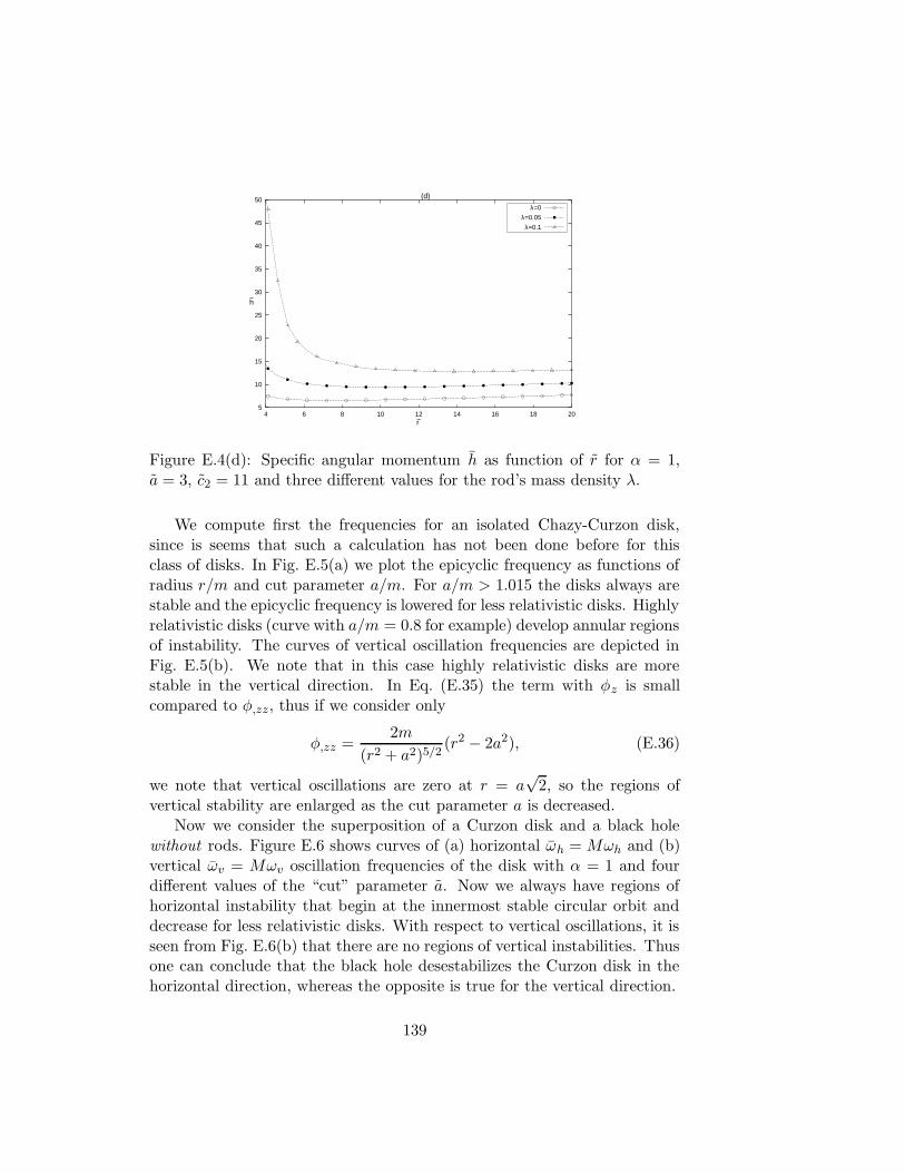
5

10

15

20

25

30

35

40

45

50

4 6 8 10 12 14 16 18 20r~

(d)

h

λ=0

λ=0.05

λ=0.1

Figure E.4(d): Specific angular momentum h as function of r for α = 1,a = 3, c2 = 11 and three different values for the rod’s mass density λ.

We compute first the frequencies for an isolated Chazy-Curzon disk,since is seems that such a calculation has not been done before for thisclass of disks. In Fig. E.5(a) we plot the epicyclic frequency as functions ofradius r/m and cut parameter a/m. For a/m > 1.015 the disks always arestable and the epicyclic frequency is lowered for less relativistic disks. Highlyrelativistic disks (curve with a/m = 0.8 for example) develop annular regionsof instability. The curves of vertical oscillation frequencies are depicted inFig. E.5(b). We note that in this case highly relativistic disks are morestable in the vertical direction. In Eq. (E.35) the term with φz is smallcompared to φ,zz, thus if we consider only

φ,zz =2m

(r2 + a2)5/2(r2 − 2a2), (E.36)

we note that vertical oscillations are zero at r = a√

2, so the regions ofvertical stability are enlarged as the cut parameter a is decreased.

Now we consider the superposition of a Curzon disk and a black holewithout rods. Figure E.6 shows curves of (a) horizontal ωh = Mωh and (b)vertical ωv = Mωv oscillation frequencies of the disk with α = 1 and fourdifferent values of the “cut” parameter a. Now we always have regions ofhorizontal instability that begin at the innermost stable circular orbit anddecrease for less relativistic disks. With respect to vertical oscillations, it isseen from Fig. E.6(b) that there are no regions of vertical instabilities. Thusone can conclude that the black hole desestabilizes the Curzon disk in thehorizontal direction, whereas the opposite is true for the vertical direction.

139

0

0.05

0.1

0.15

0.2

0.25

0.3

0 2 4 6 8 10 12 14 16 18 20

ωh

(a)

m

r/m

a/m=0.8

a/m=1

a/m=2

a/m=3

a/m=4

0

0.02

0.04

0.06

0.08

0.1

0.12

0.14

0 2 4 6 8 10 12 14 16 18 20

ωvm

r/m

(b)

a/m=0.8

a/m=1

a/m=2

a/m=3

a/m=4

Figure E.5: Radial profiles of (a) the epicyclic frequency mωh and (b) thevertical oscillation frequency mωv for an isolated Chazy-Curzon disk.

140

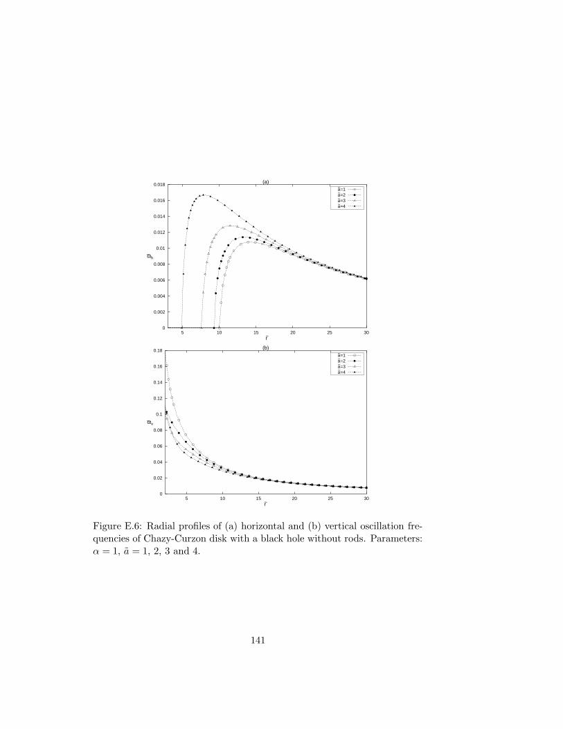
0

0.002

0.004

0.006

0.008

0.01

0.012

0.014

0.016

0.018

5 10 15 20 25 30

ω_

h

r~

(a)a~=1a~=2a~=3a~=4

0

0.02

0.04

0.06

0.08

0.1

0.12

0.14

0.16

0.18

5 10 15 20 25 30

ω_

v

r~

(b)a~=1a~=2a~=3a~=4

Figure E.6: Radial profiles of (a) horizontal and (b) vertical oscillation fre-quencies of Chazy-Curzon disk with a black hole without rods. Parameters:α = 1, a = 1, 2, 3 and 4.

141

0

0.002

0.004

0.006

0.008

0.01

0.012

0.014

5 10 15 20 25 30

ω_

h

r~

(a)

λ=0

λ=0.05

λ=0.1

0.005

0.01

0.015

0.02

0.025

0.03

0.035

0.04

0.045

0.05

0.055

0.06

5 10 15 20 25 30

ω_

v

r~

(b)

λ=0

λ=0.05

λ=0.1

Figure E.7: Radial profiles of (a) horizontal and (b) vertical oscillation fre-quencies of Chazy-Curzon disk with black hole and rods. Parameters arec2 = 11, α = 1, a = 3, λ = 0, 0.05 and 0.1.

142

In Fig. E.7(a) and E.7(b) we graph again ωh = Mωh and ωv = Mωv,respectively, for the Chazy-Curzon disk with black hole and rods, with theirlength fixed and vary the linear mass density λ. As expected from the curvesof Fig. E.3(b), the more massive the rods, the larger are the disk’s unstableregions in the horizontal direction. The rods also tend to lower the verticaloscillation frequencies near the disk’s center, but unstable regions do notappear.

E.7 Geodesic orbits

In the previous section perturbations of equatorial circular geodesics wereused to discuss disk stability for the system disk + black hole + rods. Nowwe solve numerically the geodesic equations of motion

xµ + Γµαβx

αxβ = 0, (E.37)

for metric Eq. (E.1), where Γµαβ are the Christoffel symbols and the dot

denote differentiation with respect to the proper time. Defining the or-thonormal tetrad V a,W a, Y a, Za where

V a = e−φ/2(1, 0, 0, 0), (E.38a)

W a = e(φ−ν)/2(0, 1, 0, 0), (E.38b)

Y a = e(φ−ν)/2(0, 0, 1, 0), (E.38c)

Za =eφ/2

r(0, 0, 0, 1), (E.38d)

the tetrad components of the four-velocity va read

va = γ(1, v sinψ cosχ, v sinψ sinχ, v cosψ), (E.39)

with γ = 1/√

1 − v2. The specific energy and angular momentum of the testparticle are

E = eφt = eφ/2γ, (E.40)

h = r2e−φϕ = re−φ/2γv cosψ. (E.41)

As initial conditions we take a position at radius r0 on the disk’s plane andcomponents of the four-velocity va

0 = γ(1, 0, v0 sinψ, v0 cosψ), where v0 isequal to the tangential velocity of circular orbits at radius r0. We chooseinitial radii such that the energy is slightly higher than the escape energy.

143

Figure E.8(a) and E.8(b) shows the orbits of particles in the presence of theblack hole and Curzon disk without rods. The parameters are α = 1, a = 3,r0 = 3.9, E ≈ 1.01 and different initial angles ψ. Figure E.8(a) is a projectionof the orbits on the x − z plane. The coordinates have been transformedfrom Weyl to Schwarzschild coordinates (t, r, θ, ϕ) via the relations

r =√

r(r − 2M) sin θ, z = (r −M) cos θ, (E.42)

and then to x = r sin θ cosϕ, y = r sin θ sinϕ and z = r cos θ.

In Fig. E.9(a)–E.9(d) we have computed some orbits now with the rods.The parameters are α = 1, a = 3, r0 = 7.43, λ = 0.1, c2 = 11, E ≈ 1.01and different initial angles ψ. The orbit with ψ = 89o has been placed in aseparate graph for better visualization. For low initial angles, the rods havelittle effect on the trajectories, but this is not true as the particles approachthe z axis. The orbit in Fig. E.9(c) and E.9(d) even suggests that we canexpect chaotic behaviour for orbits that pass very near the rods. In fact,it has been shown [41] that prolate quadrupole deformations can introducechaotic motion of geodesic test particles. In the oblate case, only regularmotion was found.

E.8 Discussion

We presented a very simplified, although exact, general relativistic modelof an active galactic nuclei based on a superposition of a Schwarzschildblack hole, a Chazy-Curzon disk and two rods placed on the symmetry axis,representing jets. We found that the presence of the rods enhances the diskregions with superlumial velocities. Using an extension of Rayleigh criteriaof stability, it was found that in general the rods also increase the regions ofinstability, but when the rods are large and the disk’s mass is low they cancontribute to stabilize the disk. Also disk stability in the vertical directionwas studied through perturbation of circular geodesics. The rods contributeto lower the vertical oscillation frequencies near the disk’s center. Somegeodesic orbits calculated numerically for the system black hole + disk +rods show the possibility of chaotic trajectories near the rods.

The model here presented should be viewed as a first approach. As wasstated in the introduction, more realistic models of active galactic nucleishould incorporate rotation and electromagnetic fields. However, the analy-sis of such a model would not be trivial, because of the large number of freeparameters involved.

144

-30

-25

-20

-15

-10

-5

0

5

10

-10 -5 0 5 10 15 20 25 30x~

z~

(a)

z~

(b)

ψ=30o

ψ=45o

ψ=60o

ψ=89o

-10-5

05

1015

2025

30

x~

-30-25

-20-15

-10-5

05

10

y~

-30-25-20-15-10

-505

10

Figure E.8: Geodesic orbits for the superposition Curzon disk + black holewithout rods. Parameters: α = 1, a = 3, E ≈ 1.01, r0 = 3.9. (a) Projectionon the x− z plane of the curves in (b).

145

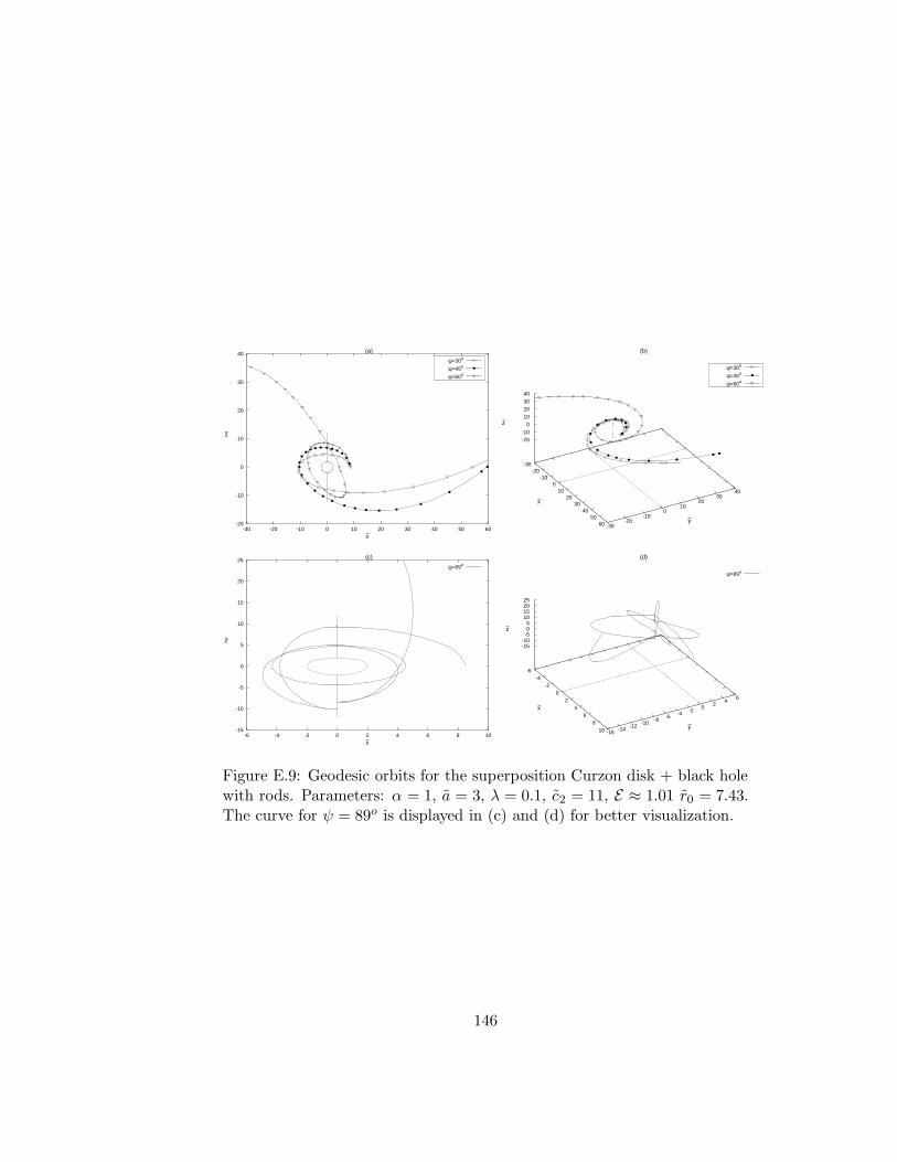
-20

-10

0

10

20

30

40

-30 -20 -10 0 10 20 30 40 50 60x~

z~

(a)

ψ=30o

ψ=45o

ψ=60o

z~

(b)

ψ=30o

ψ=45o

ψ=60o

-30-20

-100

1020

3040

5060

x~

-30-20

-100

1020

3040

y~

-20-10

010203040

-15

-10

-5

0

5

10

15

20

25

-6 -4 -2 0 2 4 6 8 10x~

z~

(c)

ψ=89o

z~

(d)

ψ=89o

-6-4

-20

24

68

10

x~

-16-14

-12-10

-8-6

-4-2

02

46

y~

-15-10

-505

10152025

Figure E.9: Geodesic orbits for the superposition Curzon disk + black holewith rods. Parameters: α = 1, a = 3, λ = 0.1, c2 = 11, E ≈ 1.01 r0 = 7.43.The curve for ψ = 89o is displayed in (c) and (d) for better visualization.

146

Appendix

The metric function Eq. (E.2b) for the superposition of a black hole, tworods and a disk generated from Chazy-Curzon solution can be calculated asfollows. We rewrite potential Eq. (E.30) as

φ = φR1 + φBH + φR2 + φ+D, (E.43)

where

φR1 = −2λ ln

(

µ3

µ4

)

, φBH = −2λ ln

(

µ1

µ2

)

φR2 = −2λ ln

(

µ5

µ6

)

, φ+D =

m

εln

(

µ7

µ8

)

, (E.44)

with µ7 = −a − ε − z +√

r2 + (−a− ε− z)2 and µ8 = −a + ε − z +√

r2 + (−a+ ε− z)2. In the limit ε → 0 expression for φ+D reduces to the

Chazy-Curzon disk Eq. (E.29) on z > 0. Thus all terms can be expressedas µ potentials. Using repeatedly properties (E.24)–(E.26) we get

ν[φR1 + φBH + φR2 + φ+D] = ν[φR1] + ν[φBH ] + ν[φR2] + ν[φ+

D]

+ 2ν[φR1, φBH ] + 2ν[φR1, φR2] + 2ν[φR1, φ+D] + 2ν[φBH , φR2]

+ 2ν[φBH , φ+D] + 2ν[φR2, φ

+D], (E.45)

with

ν[φR1] = 4λ2 ln

[

(r2 + µ3µ4)2

(r2 + µ23)(r

2 + µ24)

]

, ν[φBH ] = ln

[

(r2 + µ1µ2)2

(r2 + µ21)(r

2 + µ22)

]

,

ν[φR2] = 4λ2 ln

[

(r2 + µ5µ6)2

(r2 + µ25)(r

2 + µ26)

]

, ν[φ+D] = − m2r2

[r2 + (z + a)2]2,

ν[φR1, φBH ] = 2λ ln

[

(r2 + µ1µ3)(r2 + µ2µ4)

(r2 + µ1µ4)(r2 + µ2µ3)

]

,

ν[φR1, φR2] = 4λ2 ln

[

(r2 + µ3µ6)(r2 + µ4µ5)

(r2 + µ3µ5)(r2 + µ4µ6)

]

,

ν[φR1, φ+D] =

2λm

(a+ c1)(a+ c2)√

r2 + (a+ z)2

[

(a+ c2)√

r2 + (c1 − z)2

−(a+ c1)√

r2 + (c2 − z)2 + (c1 − c2)√

r2 + (a+ z)2]

,

ν[φBH , φR2] = 2λ ln

[

(r2 + µ1µ5)(r2 + µ2µ6)

(r2 + µ1µ6)(r2 + µ2µ5)

]

,

147

ν[φBH , φ+D] =

m

(a2 −M2)√

r2 + (a+ z)2

[

(a+M)√

r2 + (M + z)2

−(a−M)√

r2 + (M − z)2 − 2M√

r2 + (a+ z)2]

,

ν[φR2, φ+D] =

2λm

(a− c1)(a− c2)√

r2 + (a+ z)2

[

(c2 − a)√

r2 + (c1 + z)2

−(c1 − a)√

r2 + (c2 + z)2 + (c1 − c2)√

r2 + (a+ z)2]

.

In the particular case c1 = M (µ4 = µ2 and µ5 = µ1), and on z = 0, Eq.(E.45) simplifies to

ν[φR1 + φBH + φR2 + φ+D] =

ln

[

r16λ2−8λ+2(r2 + µ1µ6)8λ2−4λ(r2 + µ2µ3)

8λ2−4λ

(r2 + c22)4λ2(r2 +M2)4λ2−4λ+1(r2 + µ1µ3)8λ2−4λ(r2 + µ2µ6)8λ2−4λ

]

− m2r2

(r2 + a2)2+

8λm

(a2 − c22)(a2 −M2)

√r2 + a2

[

c2(a2 −M2)

√

r2 + c22

−M(a2 − c22)√

r2 +M2 + (M − c2)(a2 +Mc2)

√

r2 + a2]

+ 4mM(√r2 +M2 −

√r2 + a2)

(a2 −M2)√r2 + a2

. (E.46)

Acknowledgments

D. V. thanks CAPES for financial support. P. S. L. thanks CNPq andFAPESP for financial support.

Bibliography

[1] Jets from Stars and Galactic Nuclei, edited by W. Kundt (Springer,New York, 1996).

[2] J. H. Krolik, Active Galactic Nuclei: from the Central Black Hole to

the Galactic Environment (Princeton University Press, Princeton, NewJersey, 1999).

[3] R. D. Blandford, Prog. Theor. Phys. Suppl. 143, 182 (2001).

[4] W. A. Bonnor and A. Sackfield, Comm. Math. Phys. 8, 338 (1968).

148

[5] T. Morgan and L. Morgan, Phys. Rev. 183, 1097 (1969).

[6] L. Morgan and T. Morgan, Phys. Rev. D 2, 2756 (1970).

[7] D. Lynden-Bell and S. Pineault, Mon. Not. R. Astron. Soc. 185, 679(1978).

[8] P. S. Letelier and S. R. Oliveira, J. Math. Phys. 28, 165 (1987).

[9] J. P. S. Lemos, Classical Quantum Gravity 6, 1219 (1989).

[10] J. P. S. Lemos and P. S. Letelier, Classical Quantum Gravity 10, L75(1993).

[11] J. Bicak, D. Lynden-Bell and J. Katz, Phys. Rev. D 47, 4334 (1993).

[12] J. Bicak, D. Lynden-Bell and C. Pichon, Mon. Not. R. Astron. Soc.265, 126 (1993).

[13] J. P. S. Lemos and P. S. Letelier, Phys. Rev. D 49, 5135 (1994).

[14] J. P. S. Lemos and P. S. Letelier, Int. J. Mod. Phys. D 5, 53 (1996).

[15] G. Gonzalez and O. A. Espitia, Phys. Rev. D 68, 104028 (2003).

[16] G. Garcıa and G. Gonzalez, Phys. Rev. D 69, 124002 (2004).

[17] J. Bicak and T. Ledvinka, Phys. Rev. Lett. 71, 1669 (1993).

[18] G. Gonzalez and P. S. Letelier, Phys. Rev. D 62, 064025 (2000).

[19] D. Vogt and P. S. Letelier, Phys. Rev. D 68, 084010 (2003).

[20] D. Vogt and P. S. Letelier, “Exact Relativistic Static Charged PerfectFluid Disks” (to be published).

[21] G. Gonzalez and P. S. Letelier, Phys. Rev. D 69, 044013 (2004).

[22] C. Klein, Classical Quantum Gravity 14, 2267 (1997).

[23] G. Neugebauer and R. Meinel, Phys. Rev. Lett. 75, 3046 (1995).

[24] C. Klein and O. Richter, Phys. Rev. Lett. 83, 2884 (1999).

[25] C. Klein, Phys. Rev. D 63, 064033 (2001).

[26] J. Frauendiener and C. Klein, Phys. Rev. D 63, 084025 (2001).

149

[27] C. Klein, Phys. Rev. D 65, 084029 (2002).

[28] C. Klein, Phys. Rev. D 68, 027501 (2003).

[29] C. Klein, Ann. Phys. 12, 599 (2003).

[30] T. Zellerin and O. Semerak, Classical Quantum Gravity 17, 5103(2000).

[31] V. Karas, J. M. Hure and O. Semerak, Classical Quantum Gravity 21,R1 (2004).

[32] H. Weyl, Ann. Phys. 54, 117 (1917).

[33] H. Weyl, Ann. Phys. 59, 185 (1919).

[34] G. G. Kuzmin, Astron. Zh. 33, 27 (1956).

[35] J. P. S. Lemos, Mon. Not. R. Astron. Soc. 230, 451 (1988).

[36] Lord Rayleigh, Proc. R. Soc. London A 93, 148 (1917); see also L. D.Landau and E. M. Lifshitz, Fluid Mechanics (Pergamon Press, Oxford,1987), 2nd ed., §27.

[37] V. A. Belinsky and V. E. Zakharov, Zh. Eksp. Teor. Fiz. 75, 1955 (1978)[Sov. Phys. JETP 48, 985 (1978)].

[38] V. A. Belinsky and V. E. Zakharov, Zh. Eksp. Teor. Fiz. 77, 3 (1979)[Sov. Phys. JETP 50, 1 (1979)].

[39] P. S. Letelier, Phys. Rev. D 68, 104002 (2003).

[40] O. Semerak and M. Zacek, Publ. Astron. Soc. Jpn. 52, 1067 (2000).

[41] E. Gueron and P. S. Letelier, Phys. Rev. E 63, 035201(R) (2001); 66,046611 (2002).

150

Apendice F

New models of general relativistic

static thick disks

D. Vogt and P. S. Letelier, Physical Review D 71, 084030 (2005).

Received 28 September 2004; published 28 April 2005.

Abstract

New families of exact general relativistic thick disks are constructedusing the “displace, cut, fill and reflect” method. A class of functionsused to fill the disks is derived imposing conditions on the first and sec-ond derivatives to generate physically acceptable disks. The analysis of thefunction’s curvature further restrict the ranges of the free parameters thatallow physically acceptable disks. Then this class of functions together withthe Schwarzschild metric is employed to construct thick disks in isotropic,Weyl and Schwarzschild canonical coordinates. In these last coordinates anadditional function must be added to one of the metric coefficients to gen-erate exact disks. Disks in isotropic and Weyl coordinates satisfy all energyconditions, but those in Schwarzschild canonical coordinates do not satisfythe dominant energy condition.

PACS numbers: 04.20.Jb, 04.40.–b

151

F.1 Introduction

Exact solutions of Einstein’s field equations with axial symmetry play animportant role in the astrophysical applications of general relativity, sincethe natural shape of an isolated self-gravitating fluid is axially symmetric.In particular, disklike configurations of matter are of great interest, sincethey can be used as models of galaxies and accretion disks.

Solutions for static thin disks without radial pressure were first studiedby Bonnor and Sackfield [1], and Morgan and Morgan [2], and with radialpressure by Morgan and Morgan [3]. Several classes of exact solutions of theEinstein field equations corresponding to static thin disks with or withoutradial pressure have been obtained by different authors [4–13]. Thin rotatingdisks that can be considered as a source of the Kerr metric were presentedin [14], while rotating disks with heat flow were studied in [15]. Also thindisks with radial tension [16], magnetic fields [17] and magnetic and electricfields [18] were considered. The nonlinear superposition of a disk and ablack hole was first obtained by Lemos and Letelier [7]. Perfect fluid diskswith halos [19] and charged perfect fluid disks [20] were also studied. For asurvey on self-gravitating relativistic thin disks, see for instance [21].

In the works cited above, an inverse style method was used to solve theEinstein equations, i. e., the energy-momentum tensor is computed fromthe metric representing the disk. Another approach to generate disks is bysolving the Einstein equations given a source (energy-momentum tensor).This has been used to generate several exact solutions of thin disks [22,24–29].

Even though in a first approximation thin disks can be used as usefulmodels of galaxies, in a more realistic model the thickness of the disk shouldbe considered. The addition of a new dimension may change the dynamicalproperties of the disk source, e. g., its stability. Thick static relativistic disksin various coordinate systems were presented in [30]. The method used toconstruct the thick disks is a generalization of the well known “displace, cutand reflect” method used to generate thin disks from vacuum solutions ofEinstein equations. This generalization adds a new step and thus can benamed “displace, cut, fill and reflect” method. In [30] a particular functionwith properties that will be discussed later was used to “fill” the disks.

In this article we present a class of the functions mentioned above anduse them together with the Schwarzschild metric to construct more modelsof exact relativistic thick disks. In Sec. F.2 we discuss briefly the mainidea of the displace, cut, fill and reflect method and use the NewtonianKuzmin-Toomre disk to put constraints on the parameter in the class of

152

fill functions so that the disks are physically acceptable. Then in Sec. F.3we take the Schwarzschild solution in isotropic cylindrical coordinates togenerate thick disks. These disks have equal radial and azimuthal pressuresbut are different from vertical pressures. In Sec. F.4 the same procedureis repeated in Weyl coordinates. The resulting disks have radial tensionsthat have the same modulus as the vertical pressures, azimuthal tensionsnear the center and azimuthal pressures for larger disk radii. In Sec. F.5thick disks are constructed in canonical Schwarzschild coordinates, whichwere not previously studied. Here an additional function must be addedin order to generate exact disks. The disks show similar characteristics ofthose constructed in Weyl coordinates, but radial tensions are different fromvertical pressures. Finally, in Sec. F.6 we summarize the main results.

F.2 Newtonian Thick Disks

The method used to construct a thick disk is described in detail in [30] andconsists in a modification of the displace, cut and reflect method, due toKuzmin [31]. The “thickening” is obtained by the introduction of a thickshell after the cut and before the inversion of the space, thus the modifiedmethod can be named displace, cut, fill and reflect.

Mathematically the procedure is equivalent to making the transforma-tion z → h(z) + b, where b is a constant and h(z) an even function of z.In order to generate thick disks with well-defined properties, the functionh(z) and its first derivative should be continuous in the region −a ≤ z ≤ a,where 2a is the disk thickness. Furthermore, the first and second derivativesof h(z) with respect to z should be chosen such that the mass density of thedisk (i) be non-negative everywhere and (ii) be a monotonously decreasingfunction of r and z. These conditions strongly restrict the possible func-tional forms for h(z). In the case of Newtonian gravity, the potential Φ(r, z)satisfies the Laplace equation

Φ,rr +Φr

r+ Φ,zz = 0. (F.1)

After we make the transformation z → h(z) + b, Eq. (F.1) leads to

∇2Φ = h′′Φ,h + (h′2 − 1)Φ,hh, (F.2)

where primes indicate differentiation with respect to z. From Eq. (F.2) wehave that, if |h′| = 1 and thus h′′ = 0 when |z| ≥ a, the mass density

153

vanishes outside the disk. For |z| ≤ a, we get from the Poisson equation

ρ =1

4πG

[

h′′Φ,h + (h′2 − 1)Φ,hh

]

. (F.3)

If we start from an even and positive polynomial for h′′(z), we arrive ata class of functions h(z) that satisfy all the requirements stated above givenby

h(z) =

−z + C, z ≤ −a,Az2 +Bz2n+2, −a ≤ z ≤ a,

z + C, z ≥ a,

(F.4)

with

A =2n+ 1 − ac

4na, B =

ac− 1

4n(n+ 1)a2n+1, C = −a(2n+ 1 + ac)

4(n+ 1).

Here n = 1, 2, . . . , and c is the jump of the second derivative on z = ±a. Thespecial case when ac = 1 was considered in [30]. As an example we considerthe gravitational potential of a mass point in cylindrical coordinates

Φ = − Gm√r2 + z2

. (F.5)

By doing the transformation z → h(z) + b in the previous potential andusing Eq. (F.3), we obtain the mass density

ρ =m

4π

[

h′′(h+ b) + h′2 − 1

R3+

3(1 − h′2)(h + b)2

R5

]

, (F.6)

with R2 = r2 + (h + b)2 and the variables and parameters were rescaled interms of the disk half-thickness: r = r/a, h = h/a, b = b/a, m = m/a,ρ = a2ρ and with c = c/a and z = z/a in Eq. (F.4). The mass density willbe positive if

h′′(h+ b) + h′2 − 1 ≥ 0. (F.7)

When z = 0, condition (F.7) reduces to

b2n+ 1 − c

2n− 1 ≥ 0 → b ≥ 2n

2n+ 1 − c, (F.8)

154

and c < 2n+ 1 to make b positive. When z = ±1, (F.7) gives c(h+ b) ≥ 0,or c ≥ 0. Thus the parameter c is restricted to 0 ≤ c < 2n+ 1.

The total mass M of the disk is easily calculated

M =

∫ 2π

0

∫ 1

z=−1

∫ ∞

r=0ρ r dr dz dϕ = m, (F.9)

thus the disks have finite mass.In Fig. F.1 we plot the curves of h(z) and its first and second derivatives

with n = 1 for c = 0, 0.5, 1 and 2. We also plot the curvature κ of h,calculated from the expression

κ =|h′′|

(1 + h′2)3/2. (F.10)

Figures F.2 and F.3 show the mass density for a Newtonian thick disk cal-culated with the function h(z) depicted in Fig. F.1(a) and with parametersm = 1 and b = 2. In Fig. F.4 we plot again h(z) with n = 2 and the samevalues for c as in Fig. F.1; and the mass density for a Newtonian disk usingthis function with parameters m = 1 and b = 2 is shown in Figs. F.5 andF.6. We note that the mass distribution along r = 0 has a similar shapeto the curves for the curvature κ. Above some value of the jump c, themaximum of the mass density at (r, z) = (0, 0) becomes a local minimumpoint and two other maximum points appear. This may be interpreted as asplit from one into two disklike distributions of matter, a configuration thatdoes not seem to be physically reasonable. Thus, we restrict the interval ofvalues for c such that the mass density has only a central maximum. Thecritical points of the curvature function are given by

h′′′(1 + h′2) − 3h′h′′2 = 0. (F.11)

For n = 1, this condition leads to z = 0 and the roots of

7(c− 1)3z6 + 11(3 − c)(c − 1)2z4 + 5(3 − c)2(c− 1)z2

− 8(c − 1) + (3 − c)3 = 0. (F.12)

To have z = 0 as only critical point, Eq. (F.12) should not have real roots.A graphical analysis shows that this happens if c 1.46. For n = 2, thepolynomial equation in question is

55(c − 1)3z12 + 65(5 − c)(c− 1)2z8 + 13(5 − c)2(c− 1)z4

− 320(c − 1)z2 + 3(5 − c)3 = 0, (F.13)

155

0

0.2

0.4

0.6

0.8

1

1.2

-1.5 -1 -0.5 0 0.5 1 1.5

h~(z~)

z~

(a)

c~=0c~=0.5

c~=1c~=2

-1

-0.5

0

0.5

1

-1.5 -1 -0.5 0 0.5 1 1.5

h~’(z~)

z~

(b)

c~=0c~=0.5

c~=1c~=2

0

0.2

0.4

0.6

0.8

1

1.2

1.4

1.6

1.8

2

-1.5 -1 -0.5 0 0.5 1 1.5

h~’’(z~)

z~

(c)

c~=0c~=0.5

c~=1c~=2

Figure F.1: (a) The function h(z) and (b) its first and (c) second derivativeswith n = 1 for c = 0, 0.5, 1 and 2.

156

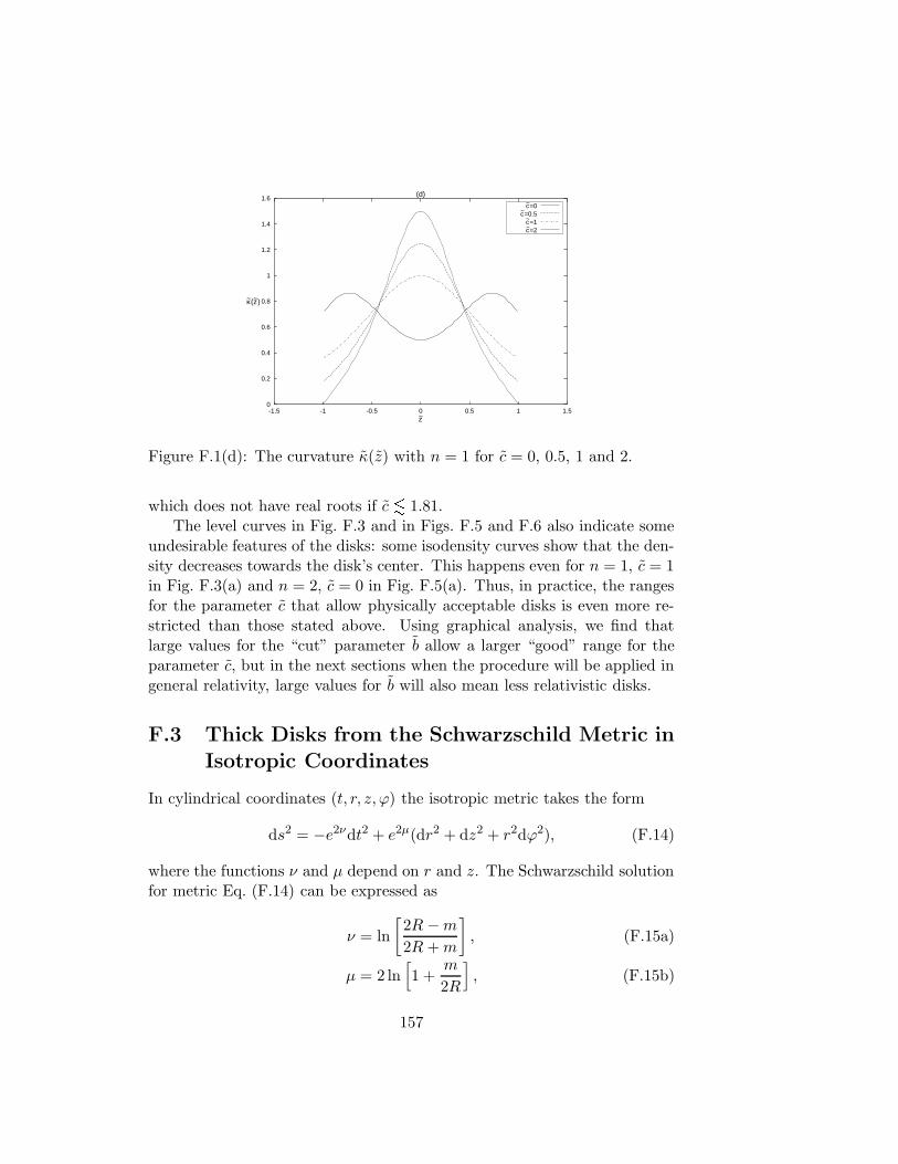
0

0.2

0.4

0.6

0.8

1

1.2

1.4

1.6

-1.5 -1 -0.5 0 0.5 1 1.5

κ~(z~)

z~

(d)

c~=0c~=0.5

c~=1c~=2

Figure F.1(d): The curvature κ(z) with n = 1 for c = 0, 0.5, 1 and 2.

which does not have real roots if c 1.81.The level curves in Fig. F.3 and in Figs. F.5 and F.6 also indicate some

undesirable features of the disks: some isodensity curves show that the den-sity decreases towards the disk’s center. This happens even for n = 1, c = 1in Fig. F.3(a) and n = 2, c = 0 in Fig. F.5(a). Thus, in practice, the rangesfor the parameter c that allow physically acceptable disks is even more re-stricted than those stated above. Using graphical analysis, we find thatlarge values for the “cut” parameter b allow a larger “good” range for theparameter c, but in the next sections when the procedure will be applied ingeneral relativity, large values for b will also mean less relativistic disks.

F.3 Thick Disks from the Schwarzschild Metric in

Isotropic Coordinates

In cylindrical coordinates (t, r, z, ϕ) the isotropic metric takes the form

ds2 = −e2νdt2 + e2µ(dr2 + dz2 + r2dϕ2), (F.14)

where the functions ν and µ depend on r and z. The Schwarzschild solutionfor metric Eq. (F.14) can be expressed as

ν = ln

[

2R −m

2R +m

]

, (F.15a)

µ = 2 ln[

1 +m

2R

]

, (F.15b)

157

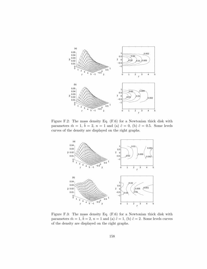
0 1 2 3 4 5 −1−0.5

00.5

10

0.010.020.030.040.05

r~ z~

~

(a)

ρ

0 1 2 3 4 5

−1

−0.5

0

0.5

1

r~

z~

0.002

0.005 0.01

0.02

0.03

0 1 2 3 4 5 −1−0.5

00.5

10

0.010.020.030.040.05

r~ z~

~

(b)

ρ

0 1 2 3 4 5

−1

−0.5

0

0.5

1

r~

z~ 0.002

0.005

0.01

0.02

0.03

Figure F.2: The mass density Eq. (F.6) for a Newtonian thick disk withparameters m = 1, b = 2, n = 1 and (a) c = 0, (b) c = 0.5. Some levelscurves of the density are displayed on the right graphs.

0 1 2 3 4 5 −1−0.5

00.5

10

0.01

0.02

0.03

0.04

r~ z~

~

(a)

ρ

0 1 2 3 4 5

−1

−0.5

0

0.5

1

r~

z~

0.02

0.01

0.005 0.002

0.001

0 1 2 3 4 5 −1−0.5

00.5

10

0.01

0.02

0.03

0.04

r~ z~

~

(b)

ρ

0 1 2 3 4 5

−1

−0.5

0

0.5

1

r~

z~ 0.001 0.005

0.01

0.02

0.03

Figure F.3: The mass density Eq. (F.6) for a Newtonian thick disk withparameters m = 1, b = 2, n = 1 and (a) c = 1, (b) c = 2. Some levels curvesof the density are displayed on the right graphs.

158

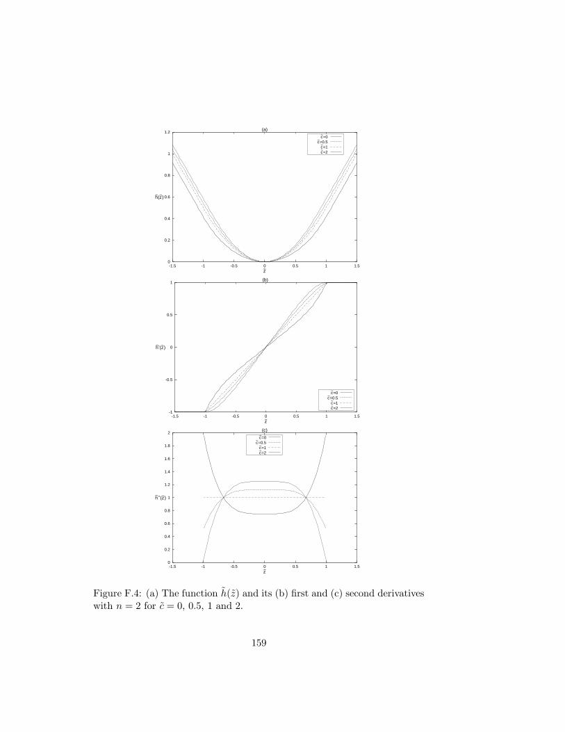
0

0.2

0.4

0.6

0.8

1

1.2

-1.5 -1 -0.5 0 0.5 1 1.5

h~(z~)

z~

(a)

c~=0c~=0.5

c~=1c~=2

-1

-0.5

0

0.5

1

-1.5 -1 -0.5 0 0.5 1 1.5

h~’(z~)

z~

(b)

c~=0c~=0.5

c~=1c~=2

0

0.2

0.4

0.6

0.8

1

1.2

1.4

1.6

1.8

2

-1.5 -1 -0.5 0 0.5 1 1.5

h~’’(z~)

z~

(c)

c~=0c~=0.5

c~=1c~=2

Figure F.4: (a) The function h(z) and its (b) first and (c) second derivativeswith n = 2 for c = 0, 0.5, 1 and 2.

159

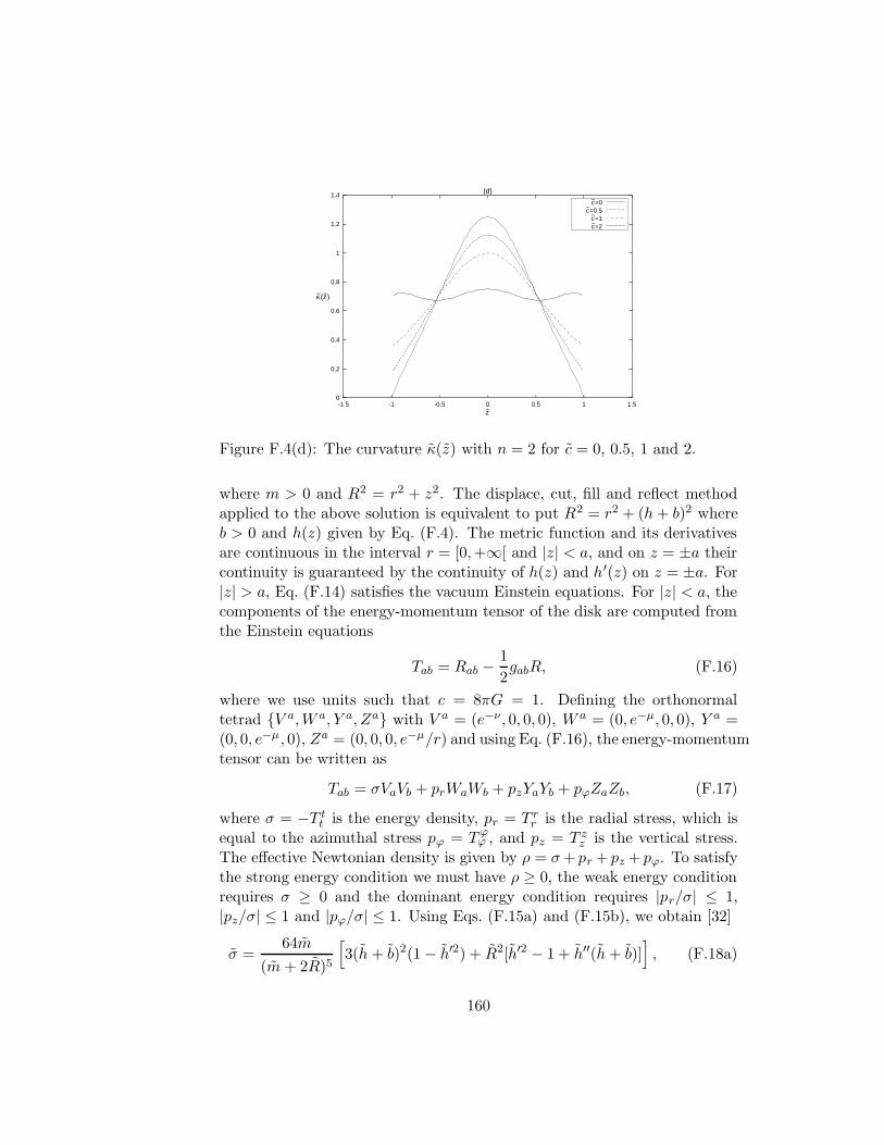
0

0.2

0.4

0.6

0.8

1

1.2

1.4

-1.5 -1 -0.5 0 0.5 1 1.5

κ~(z~)

z~

(d)

c~=0c~=0.5

c~=1c~=2

Figure F.4(d): The curvature κ(z) with n = 2 for c = 0, 0.5, 1 and 2.

where m > 0 and R2 = r2 + z2. The displace, cut, fill and reflect methodapplied to the above solution is equivalent to put R2 = r2 + (h+ b)2 whereb > 0 and h(z) given by Eq. (F.4). The metric function and its derivativesare continuous in the interval r = [0,+∞[ and |z| < a, and on z = ±a theircontinuity is guaranteed by the continuity of h(z) and h′(z) on z = ±a. For|z| > a, Eq. (F.14) satisfies the vacuum Einstein equations. For |z| < a, thecomponents of the energy-momentum tensor of the disk are computed fromthe Einstein equations

Tab = Rab −1

2gabR, (F.16)

where we use units such that c = 8πG = 1. Defining the orthonormaltetrad V a,W a, Y a, Za with V a = (e−ν , 0, 0, 0), W a = (0, e−µ, 0, 0), Y a =(0, 0, e−µ, 0), Za = (0, 0, 0, e−µ/r) and using Eq. (F.16), the energy-momentumtensor can be written as

Tab = σVaVb + prWaWb + pzYaYb + pϕZaZb, (F.17)

where σ = −T tt is the energy density, pr = T r

r is the radial stress, which isequal to the azimuthal stress pϕ = Tϕ

ϕ , and pz = T zz is the vertical stress.

The effective Newtonian density is given by ρ = σ+ pr + pz + pϕ. To satisfythe strong energy condition we must have ρ ≥ 0, the weak energy conditionrequires σ ≥ 0 and the dominant energy condition requires |pr/σ| ≤ 1,|pz/σ| ≤ 1 and |pϕ/σ| ≤ 1. Using Eqs. (F.15a) and (F.15b), we obtain [32]

σ =64m

(m+ 2R)5

[

3(h+ b)2(1 − h′2) + R2[h′2 − 1 + h′′(h+ b)]]

, (F.18a)

160

02

46

8 −1−0.5

00.5

10

0.010.020.030.040.05

r~ z~

~

(a)

ρ

0 1 2 3 4

−1

−0.5

0

0.5

1

r~

z~

0.002

0.005

0.01

0.02

0.03

02

46

8 −1−0.5

00.5

10

0.010.020.030.040.05

r~ z~

~

(b)

ρ

0 1 2 3 4

−1

−0.5

0

0.5

1

r~

z~

0.002

0.005

0.01

0.02

0.03

Figure F.5: The mass density Eq. (F.6) for a Newtonian thick disk withparameters m = 1, b = 2, n = 2 and (a) c = 0, (b) c = 0.5. Some levelscurves of the density are displayed on the right graphs.

02

46

8 −1−0.5

00.5

10

0.01

0.02

0.03

0.04

r~ z~

~

(a)

ρ

0 1 2 3 4 5

−1

−0.5

0

0.5

1

r~

z~ 0.001

0.002

0.005

0.01

0.02

02

46

8 −1−0.5

00.5

10

0.01

0.02

0.03

0.04

r~ z~

~

(b)

ρ

0 1 2 3 4 5

−1

−0.5

0

0.5

1

r~

z~ 0.002

0.005

0.01

0.02

0.03

Figure F.6: The mass density Eq. (F.6) for a Newtonian thick disk withparameters m = 1, b = 2, n = 2 and (a) c = 1, (b) c = 2. Some levels curvesof the density are displayed on the right graphs.

161

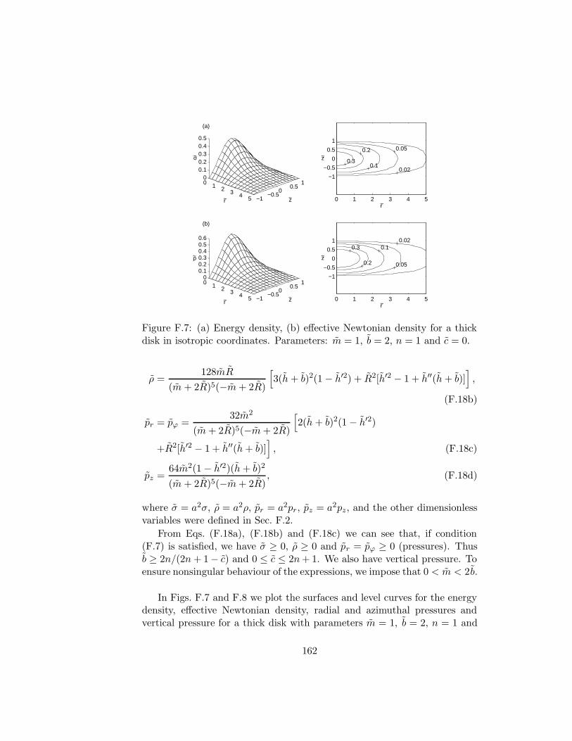
0 1 2 3 4 5 −1−0.5

00.5

10

0.10.20.30.40.5

r z~ ~

~

(a)

σ

0 1 2 3 4 5

−1

−0.5

0

0.5

1

r~

z~

0.02

0.05

0.1

0.2

0.3

0 1 2 3 4 5 −1−0.5

00.5

10

0.10.20.30.40.50.6

r~ z~

~

(b)

ρ

0 1 2 3 4 5

−1

−0.5

0

0.5

1

r~

z~

0.02

0.05

0.1

0.2

0.3

Figure F.7: (a) Energy density, (b) effective Newtonian density for a thickdisk in isotropic coordinates. Parameters: m = 1, b = 2, n = 1 and c = 0.

ρ =128mR

(m+ 2R)5(−m+ 2R)

[

3(h + b)2(1 − h′2) + R2[h′2 − 1 + h′′(h+ b)]]

,

(F.18b)

pr = pϕ =32m2

(m+ 2R)5(−m+ 2R)

[

2(h + b)2(1 − h′2)

+R2[h′2 − 1 + h′′(h+ b)]]

, (F.18c)

pz =64m2(1 − h′2)(h+ b)2

(m+ 2R)5(−m+ 2R), (F.18d)

where σ = a2σ, ρ = a2ρ, pr = a2pr, pz = a2pz, and the other dimensionlessvariables were defined in Sec. F.2.

From Eqs. (F.18a), (F.18b) and (F.18c) we can see that, if condition(F.7) is satisfied, we have σ ≥ 0, ρ ≥ 0 and pr = pϕ ≥ 0 (pressures). Thusb ≥ 2n/(2n+ 1 − c) and 0 ≤ c ≤ 2n+ 1. We also have vertical pressure. Toensure nonsingular behaviour of the expressions, we impose that 0 < m < 2b.

In Figs. F.7 and F.8 we plot the surfaces and level curves for the energydensity, effective Newtonian density, radial and azimuthal pressures andvertical pressure for a thick disk with parameters m = 1, b = 2, n = 1 and

162

0 1 2 3 4 5 −1−0.5

00.5

10

0.010.020.030.040.050.06

r z~ ~

(a)

p~r

0 1 2 3 4 5

−1

−0.5

0

0.5

1

r~

z~

0.001

0.005

0.01

0.03

0.05

0 1 2 3 4 5 −1−0.5

00.5

10

0.0050.01

0.0150.02

0.0250.03

r~ z~

(b)

p~z

0 1 2 3 4 5

−1

−0.5

0

0.5

1

r~

z~

0.0001

0.0005

0.005

0.01

0.02

Figure F.8: (a) Radial and azimuthal pressures, (b) vertical pressure for athick disk in isotropic coordinates. Parameters: m = 1, b = 2, n = 1 andc = 0.

c = 0. The ratio between any pressure and energy density is less than 0.15.Thus all energy conditions are satisfied. The shape of the level curves alsoshow that for these parameters the disk is physically acceptable.

F.4 Thick Disks from the Schwarzschild Metric in

Weyl Coordinates

The general metric for a static axially symmetric spacetime in Weyl’s canon-ical coordinates (t, r, z, ϕ) is given by

ds2 = −e2Φdt2 + e−2Φ[

e2Λ(dr2 + dz2) + r2dϕ2]

, (F.19)

where Φ and Λ are functions of r and z. The Einstein vacuum equations forthis metric reduce to the Weyl equations [33, 34]

Φ,rr +Φr

r+ Φ,zz = 0, (F.20a)

Λr = r(Φ2r − Φ2

z), (F.20b)

Λz = 2rΦrΦz. (F.20c)

163

In these coordinates, Schwarzschild solution assumes the form [33]

Φ =1

2ln

[

R1 +R2 − 2m

R1 +R2 + 2m

]

, (F.21a)

Λ =1

2ln

[

(R1 +R2)2 − 4m2

4R1R2

]

, (F.21b)

where R21 = r2 +(m+z)2, R2

2 = r2 +(−m+z)2 and m > 0. By applying thetransformation z → h(z)+b on Eqs. (F.21a) and (F.21b), using Eqs. (F.20a)–(F.20c) and Einstein equations (F.16), the energy-momentum tensor can bewritten as

Tab = εVaVb + prWaWb + pzYaYb + pϕZaZb, (F.22)

with the orthonormal tetrad V a,W a, Y a, Za where V a = (e−Φ, 0, 0, 0),W a = (0, eΦ−Λ, 0, 0), Y a = (0, 0, eΦ−Λ, 0) and Za = (0, 0, 0, eΦ/r). In Eq.(F.22) ε = −T t

t is the energy density and pr = T rr , pz = T z

z = −T rr , pϕ = Tϕ

ϕ

are respectively, the radial, vertical and azimuthal stresses. The effectiveNewtonian density is given by ρ = ε+ pϕ. The explicit expressions are

ρ =e2(Φ−Λ)

R31R

32

h′′(R1 − R2)R21R

22 + (1 − h′2)

[

(h+ b)(R31 − R3

2)

−m(R31 + R3

2)]

, (F.23a)

ε = ρ

[

1 − 2mr2(R1 + R2)

R1R2[(R1 + R2)2 − 4m2]

]

+e2(Φ−Λ)(1 − h′2)(R1 − R2)

4R41R

42

×[

(R1 − R2)R21R

22 − 2r2(R3

1 − R32)]

, (F.23b)

pϕ =2mρr2(R1 + R2)

R1R2[(R1 + R2)2 − 4m2]+e2(Φ−Λ)(h′2 − 1)(R1 − R2)

4R41R

42

×[

(R1 − R2)R21R

22 − 2r2(R3

1 − R32)]

, (F.23c)

pr =4m2e2(Φ−Λ)(h′2 − 1)(h + b)2

R21R

22(R1 + R2)2

, (F.23d)

pz =4m2e2(Φ−Λ)(1 − h′2)(h + b)2

R21R

22(R1 + R2)2

, (F.23e)

From Eqs. (F.23d) and (F.23e) we have vertical pressures and radial tensions.From Eq. (F.23b) the condition ε ≥ 0 on |z| = 1 gives

2mr2(R1 + R2)

R1R2[(R1 + R2)2 − 4m2]≤ 1. (F.24)

164

0 1 2 3 4 5 −1−0.5

00.5

10

0.2

0.4

0.6

0.8

r z~ ~

~

(a)

ρ

0 1 2 3 4 5

−1

−0.5

0

0.5

1

r~

z~

0.02

0.05

0.1

0.3

0.5

0 1 2 3 4 5 −1−0.5

00.5

10

0.2

0.4

0.6

0.8

r z~ ~

~

(b)

ε

0 1 2 3 4 5

−1

−0.5

0

0.5

1

r~

z~

0.02

0.05

0.1

0.3

0.5

Figure F.9: (a) Effective Newtonian density, (b) energy density for a thickdisk in Weyl coordinates. Parameters: m = 1, b = 2, n = 1 and c = 0.

Since R1 > r, R2 > r, and R1 + R2 ≥ 2b, we have

mb

b2 − m2≤ 1, (F.25)

which is equivalent to m ≤ (√

5 − 1)b/2 [35]. It is not easy to obtainother constraints over the parameters m and b in order to satisfy all energyconditions. The analysis is better done graphically.

In Figs. F.9 and F.10 we plot the surfaces and level curves for the effec-tive Newtonian density, energy density, vertical pressure and the azimuthalstresses for a thick disk with parameters m = 1, b = 2, n = 1, and c = 0. Forthese values we have ρ ≥ 0 and ε ≥ 0 everywhere. The ratio between anypressure or tension and energy density is less than 0.35, thus the dominantenergy condition is also satisfied.

165

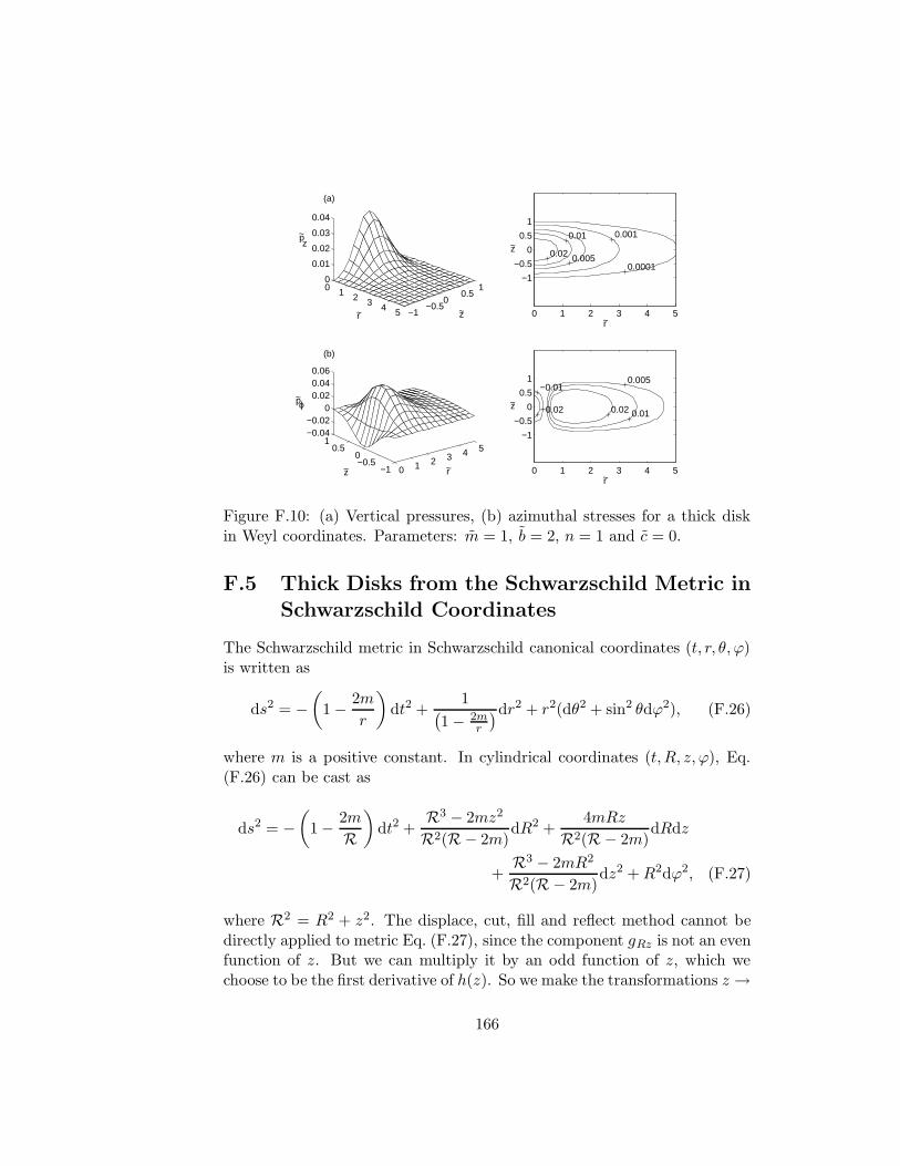
0 1 2 3 4 5 −1−0.5

00.5

10

0.01

0.02

0.03

0.04

r z~ ~

(a)

pz

~

0 1 2 3 4 5

−1

−0.5

0

0.5

1

r~

z~

0.0001

0.001

0.005

0.01

0.02

0 1 2 3 4 5

−1−0.50

0.51

−0.04−0.02

00.020.040.06

z r~ ~

(b)

p~ϕ

0 1 2 3 4 5

−1

−0.5

0

0.5

1

r~

z~

0.005

0.01 0.02

−0.01

−0.02

Figure F.10: (a) Vertical pressures, (b) azimuthal stresses for a thick diskin Weyl coordinates. Parameters: m = 1, b = 2, n = 1 and c = 0.

F.5 Thick Disks from the Schwarzschild Metric in

Schwarzschild Coordinates

The Schwarzschild metric in Schwarzschild canonical coordinates (t, r, θ, ϕ)is written as

ds2 = −(

1 − 2m

r

)

dt2 +1

(

1 − 2mr

)dr2 + r2(dθ2 + sin2 θdϕ2), (F.26)

where m is a positive constant. In cylindrical coordinates (t, R, z, ϕ), Eq.(F.26) can be cast as

ds2 = −(

1 − 2m

R

)

dt2 +R3 − 2mz2

R2(R− 2m)dR2 +

4mRz

R2(R− 2m)dRdz

+R3 − 2mR2

R2(R− 2m)dz2 +R2dϕ2, (F.27)

where R2 = R2 + z2. The displace, cut, fill and reflect method cannot bedirectly applied to metric Eq. (F.27), since the component gRz is not an evenfunction of z. But we can multiply it by an odd function of z, which wechoose to be the first derivative of h(z). So we make the transformations z →

166

h(z)+b and gRz → gRzh′(z) in Eq. (F.27), and use the Einstein equations Eq.

(F.16) to compute the components of the disk’s energy-momentum tensor.With h(z) defined by Eq. (F.4), the metric equation (F.27) satisfies thevacuum Einstein equations for |z| > a and the metric functions togetherwith their derivatives with respect to z are continuous on z = ±a. Note thatthe function multiplying gRz may be other kind of function not necessarilyrelated to h(z), but its possible form is also limited by the requirements thatthe generated disks are physically acceptable, as was discussed in Sec. F.2.The physical variables of the disk are obtained by solving the eigenvalueproblem for T a

b : T ab ξ

b = λξa. We find that T ab can be put in the form

T ab = εUaU b + p+VaV b + p−X

aXb + pϕWaW b, (F.28)

where

ε = −T tt , Ua =

1√−gtt(1, 0, 0, 0),

p± =T r

r + T zz

2± 1

2

√

(T rr − T z

z )2 + 4T rz T

zr ,

V a = (0, V r, V z, 0), Xa = (0, Xr , Xz, 0),

pϕ = Tϕϕ , W a =

1

R(0, 0, 0, 1), (F.29)

and

V r =1

√

gRR − 2gRz∆ + gzz∆2, V z = −∆V r, ∆ =

T rr − p+

T rz

,

Xr =1

√

gRR − 2gRzΓ + gzzΓ2, Xz = −ΓXr, Γ =

T rr − p−T r

z

. (F.30)

The effective Newtonian density reads ρ = ε+p++p−+pϕ = ε+T rr +T z

z +pϕ.

Although the expressions are exact, we do not state them explicitly, sincethey have dozens of terms. The analysis must also be done graphically. Wefind that p+ is a pressure along a direction mostly vertical and p− is a tensionalong a direction mostly radial. In Figs. F.11–F.13 we graph the surfacesand level curves of the energy density, the effective Newtonian density, thepressure mostly vertical, the tension mostly radial and the azimuthal stresseswith parameters m = 1, b = 5, n = 1 and c = 0. The variables andparameters were rescaled as in the previous sections. While densities andthe radial tension decrease monotonously with r and z → ±1, the upwardpressure first increases with radius and then decreases monotonously. The

167

0 2 4 6 8 10 −1−0.5

00.5

10

0.1

0.2

0.3

0.4

r~ z~

~

(a)

ε

0 2 4 6 8 10

−1−0.5

00.5

1

r~

z~ 0.01

0.05

0.1

0.2

0 2 4 6 8 10 −1−0.5

00.5

10

0.05

0.1

0.15

0.2

r~ z~

~

(b)

ρ

0 2 4 6 8 10

−1−0.5

00.5

1

r~

z~ 0.01

0.05 0.1

0.15

Figure F.11: (a) Energy density, (b) effective Newtonian density for a thickdisk in Schwarzschild coordinates. Parameters: m = 1, b = 5, n = 1 andc = 0.

0 2 4 6 8 10 −1−0.5

00.5

10

0.20.40.60.8

1x 10

−3

r~ z~

(a)

~p+

0 2 4 6 8 10

−1−0.5

00.5

1

r~

z~5E−5

1E−43E−4

5E−4

0 2 4 6 8 10

−1−0.50

0.51

−0.08

−0.06

−0.04

−0.02

0

r~z~

(b)

~p−

0 2 4 6 8 10

−1−0.5

00.5

1

r~

z~ −0.005

−0.01 −0.03

−0.05

Figure F.12: (a) The pressure mostly vertical, (b) tension mostly radial fora thick disk in Schwarzschild coordinates. Parameters: m = 1, b = 5, n = 1and c = 0.

168

0 2 4 6 8 10

−1−0.50

0.51

−0.08−0.06−0.04−0.02

00.02

r~z~

(a)

~pϕ

0 2 4 6 8 10

−1−0.5

00.5

1

r~

z~ 0.01

0.015

−0.01

−0.05

0 2 4 6 8 10

−1−0.5

00.5

1

r~

z~

(b)

0 5 10−1

−0.5

0

0.5

1

r~

z~

(c)

Figure F.13: (a) The azimuthal stresses, (b) the level curve of |pϕ/ε| = 1 and(c) the lines of flow calculated from Eqs. (F.31a) and (F.31b). Parameters:m = 1, b = 5, n = 1 and c = 0.

azimuthal stresses are negative near the disk’s center, then increase to apositive maximum at the z = 0 plane and then decrease monotonously. Insome sense this new class of disks has similar characteristics of those obtainedin Weyl coordinates, but here the almost radial tensions are different fromthe almost vertical pressures. Unfortunately the dominant energy conditiondoes not hold with respect to the azimuthal stresses. Figure F.13(b) showsthe level curve of |pϕ/ε| = 1. For r

8 the dominant energy condition is not

satisfied. This also seems to happen for larger values of b. In Fig. F.13(c)we plot the lines of flow calculated by numerically solving the differentialequations

dV z

dV r=V z

V r, (F.31a)

dXz

dXr=Xz

Xr. (F.31b)

The vertical and horizontal lines in Fig. F.13(c) are, respectively, the linesof flow associated with Eqs. (F.31a) and (F.31b). We note that the lines arevery parallel to the coordinate axes. This happens because the componentT z

r is about two orders of magnitude smaller than the other componentsof the energy-momentum tensor, thus the eigenvalues p± are almost equal

169

to the corresponding diagonal elements. We call then the eigenvalue p+

with eigenvector V a the pressure mostly vertical and the eigenvalue p− witheigenvector Xa the tension mostly radial.

F.6 Discussion

The displace, cut, fill and reflect method and a class of functions used to fillwas used to construct new classes of thick general relativistic disks that gen-eralize the models studied in a previous work [30]. The Newtonian Kuzmin-Toomre disks were used to put constraints on the parameter in the classof fill functions so that the disks were physically acceptable. Then theSchwarzschild solution was used to construct disks in isotropic cylindricalcoordinates, Weyl coordinates and canonical Schwarzschild coordinates. Inisotropic coordinates the disks have equal radial and azimuthal pressures(isotropic fluid) but different vertical pressures. Disks in Weyl coordinatespresent radial tensions that are equal in modulus as vertical pressures, az-imuthal tensions near the disk’s center and azimuthal pressures for largerradii. All disks are in agreement with the strong, weak and dominant energyconditions.

In canonical Schwarzschild coordinates the displace, cut, fill and reflectmethod cannot be applied directly and an additional odd function must beadded to generate exact disks. We find that the disks have tensions along adirection mostly radial that are different from the pressures along a directionmostly vertical, and the azimuthal stresses have similar behavior as in disksin Weyl coordinates. These disks are in agreement with the strong and weakenergy conditions, but the azimuthal stresses do not satisfy the dominantenergy condition.

Acknowledgments

D. V. thanks CAPES for financial support. P. S. L. thanks CNPq andFAPESP for financial support.

Bibliography

[1] W. A. Bonnor and A. Sackfield, Comm. Math. Phys. 8, 338 (1968).

[2] T. Morgan and L. Morgan, Phys. Rev. 183, 1097 (1969).

[3] L. Morgan and T. Morgan, Phys. Rev. D 2, 2756 (1970).

170

[4] D. Lynden-Bell and S. Pineault, Mon. Not. R. Astron. Soc. 185, 679(1978).

[5] P. S. Letelier and S. R. Oliveira, J. Math. Phys. (N.Y.) 28, 165 (1987).

[6] J. P. S. Lemos, Classical Quantum Gravity 6, 1219 (1989).

[7] J. P. S. Lemos and P. S. Letelier, Classical Quantum Gravity 10, L75(1993).

[8] J. Bicak, D. Lynden-Bell and J. Katz, Phys. Rev. D 47, 4334 (1993).

[9] J. Bicak, D. Lynden-Bell and C. Pichon, Mon. Not. R. Astron. Soc.265, 126 (1993).

[10] J. P. S. Lemos and P. S. Letelier, Phys. Rev. D 49, 5135 (1994).

[11] J. P. S. Lemos and P. S. Letelier, Int. J. Mod. Phys. D 5, 53 (1996).

[12] G. Gonzalez and O. A. Espitia, Phys. Rev. D 68, 104028 (2003).

[13] G. Garcıa and G. Gonzalez, Phys. Rev. D 69, 124002 (2004).

[14] J. Bicak and T. Ledvinka, Phys. Rev. Lett. 71, 1669 (1993).

[15] G. Gonzalez and P. S. Letelier, Phys. Rev. D 62, 064025 (2000).

[16] G. Gonzalez and P. S. Letelier, Classical Quantum Gravity 16, 479(1999).

[17] P. S. Letelier, Phys. Rev. D 60, 104042 (1999).

[18] J. Katz, J. Bicak and D. Lynden-Bell, Classical Quantum Gravity 16,4023 (1999).

[19] D. Vogt and P. S. Letelier, Phys. Rev. D 68, 08410 (2003).

[20] D. Vogt and P. S. Letelier, Phys. Rev. D 70, 064003 (2004).

[21] V. Karas, J. M. Hure and O. Semerak, Classical Quantum Gravity 21,R1 (2004).

[22] C. Klein, Classical Quantum Gravity 14, 2267 (1997).

[23] G. Neugebauer and R. Meinel, Phys. Rev. Lett. 75, 3046 (1995).

[24] C. Klein and O. Richter, Phys. Rev. Lett. 83, 2884 (1999).

171

[25] C. Klein, Phys. Rev. D 63, 064033 (2001).

[26] J. Frauendiener and C. Klein, Phys. Rev. D 63, 084025 (2001).

[27] C. Klein, Phys. Rev. D 65, 084029 (2002).

[28] C. Klein, Phys. Rev. D 68, 027501 (2003).

[29] C. Klein, Ann. Phys. (N.Y.) 12 (10), 599 (2003).

[30] G. Gonzalez and P. S. Letelier, Phys. Rev. D 69, 044013 (2004).

[31] G. G. Kuzmin, Astron. Zh. 33, 27 (1956).

[32] These expressions are the generalizations of Eqs. (30a)–(30e) of Ref.[30]. There is a misprint in Eqs. (30a) and (30b), where the numericalfactor multiplying the equations should be 32.

[33] H. Weyl, Ann. Phys. (Leipzig) 54, 117 (1917).

[34] H. Weyl, Ann. Phys. (Leipzig) 59, 185 (1919).

[35] Note that this inequality is different from condition (24) deduced inRef. [30], because Eq. (22b) in that paper has an error in the termthat multiplies ρ: the product R1R2 in the denominator should notbe squared [see Eq. (F.23b)]. The corrected inequality is 0 < m <(b2 − k2)/b.

172

Apendice G

Relativistic Models of Galaxies

D. Vogt and P. S. Letelier, Mon. Not. R. Astron. Soc. 363, 268–284 (2005).

Abstract

A special form of the isotropic metric in cylindrical coordinates is used toconstruct what may be interpreted as the general relativistic versions ofsome well-known potential-density pairs used in Newtonian gravity to modelthree-dimensional distributions of matter in galaxies. The components of theenergy-momentum tensor are calculated for the first two Miyamoto-Nagaipotentials and a particular potential due to Satoh. The three potentials yielddistributions of matter in which all tensions are pressures and all energyconditions are satisfied for certain ranges of the free parameters. A few non-planar geodesic orbits are computed for one of the potentials and comparedwith the Newtonian case. Rotation is also incorporated to the models andthe effects of the source rotation on the rotation profile are calculated asfirst-order corrections by using an approximate form of the Kerr metric inisotropic coordinates.

Key words: relativity – stellar dynamics – celestial mechanics – galax-ies: kinematics and dynamics.

G.1 Introduction

Analytical axially symmetric solutions of gravitating matter provide veryaccurate models for the mass distribution of galaxies. In Newtonian the-

173

ory, models for globular clusters and spherical galaxies were presented byPlummer (1911) and King (1966). On the other hand, to describe the massdistribution within highly flattened axisymmetric galaxies, Toomre (1963)found a family of density potential pairs, the first of which was first derivedby Kuzmin (1956). Later, Miyamoto & Nagai (1975) and Nagai & Miyamoto(1976) ‘thickened-up’ Toomre’s series of disc models to yield pairs of three-dimensional potential and density functions. In a similar way, Satoh (1980)obtained a family of three-dimensional axisymmetric mass distributions fromthe higher order Plummer models. For a detailed account and the descrip-tion of other potential-density pairs used in galactic models, see for exampleBinney & Tremaine (1987).

In general relativity, several exact disc-like solutions have been found,among them the static discs without radial pressure studied by Bonnor &Sackfield (1968) and Morgan & Morgan (1969), and discs with radial pres-sure by Morgan & Morgan (1970). Several classes of exact solutions ofthe Einstein field equations corresponding to static thin discs with or with-out radial pressure have been obtained by different authors (Lynden-Bell& Pineault 1978; Letelier & Oliveira 1987; Lemos 1989; Bicak, Lynden-Bell & Katz 1993a; Bicak, Lynden-Bell & Pichon 1993b; Lemos & Letelier1993, 1994, 1996; Gonzalez & Espitia 2003; Garcıa & Gonzalez 2004). Thinrotating discs that can be considered as a source of the Kerr metric were pre-sented by Bicak & Ledvinka (1993), while rotating discs with heat flow werestudied by Gonzalez & Letelier (2000). Also thin discs with radial tension(Gonzalez & Letelier 1999), magnetic fields (Letelier 1999) and magneticand electric fields (Katz, Bicak & Lynden-Bell 1999) were considered. Thenon-linear superposition of a disc and a black hole was first obtained byLemos & Letelier (1993). Perfect fluid discs with haloes were studied byVogt & Letelier (2003) and charged perfect fluid discs by Vogt & Letelier(2004). The stability of some general relativistic thin disc models using afirst-order perturbation of the energy-momentum tensor was investigated byUjevic & Letelier (2004). For a survey on self-gravitating relativistic discs,see for instance Karas, Hure & Semerak (2004).

In the works cited above, an inverse style method was used to solve theEinstein equations, i. e., the energy-momentum tensor is computed fromthe metric representing the disc. Another approach to generate discs is bysolving the Einstein equations given a source (energy-momentum tensor).Essentially, they are obtained by solving a Riemann-Hilbert problem andare highly non-trivial. This has been used by the Jena group to generateseveral exact solutions of discs (Neugebauer & Meinel 1995; Klein 1997,2001, 2002, 2003a,b; Klein & Richter 1999; Frauendiener & Klein 2001).

174

Recently, Gonzalez & Letelier (2004) constructed models of static rela-tivistic thick discs in various coordinate systems. Although the discs haveconstant thickness, the matter density decreases rapidly with radius and thez coordinate, and in principle they may also be used to represent both thedisc part and the central bulges of galaxies.

The aim of this work is to consider more realistic three-dimensional mod-els for the gravitational field of galaxies in a general relativistic context. Thedistribution of matter fills all the space, but the total mass is finite. Essen-tially we formulate general relativistic versions in isotropic coordinates ofthe potential-density pairs deduced by Miyamoyo and Nagai (1975), Nagai& Miyamoto (1976) and Satoh (1980). Also, the influence of galactic rota-tion on the rotation profile of test particles on the galactic plane is estimatedusing an approximate form of the Kerr metric in isotropic coordinates.

The paper is organized as follows. In Section G.2 we present a specialform of the isotropic metric and the components of the energy-momentumtensor as functions of the metric coefficients, from which the physical prop-erties of the galactic matter distributions can be calculated. We also deriveexpressions for the tangential circular velocity and specific angular momen-tum of test particles in circular motion on the galactic plane. These resultsare then applied in Sections G.3 and G.4 to construct general relativisticanalogues of two Miyamoto-Nagai models and one galactic model proposedby Satoh. As an example of application of these models, in Section G.5 wecalculate a few geodesic orbits and compare them with the Newtonian case.In Section G.6 we deduce the first-order effects of galactic rotation on thetangential circular velocity of geodesic motion of particles on the galacticplane using an approximate form of the Kerr metric in isotropic coordinates,and apply the result to the above-mentioned models. Finally, we summarizeour results in Section G.7.

G.2 Einstein Equations in Isotropic Coordinates

Let us consider the particular case of axial symmetric space-times whosemetric can be written in an isotropic form in cylindrical coordinates (t, R, z, ϕ),

ds2 = eν(R,z)c2dt2 − eλ(R,z)(

dR2 + dz2 +R2dϕ2)

. (G.1)

In order to construct a general relativistic formulation of the known New-tonian models for the mass distribution of galaxies, it is convenient to use aparticular form of metric equation (G.1), suggested by generalizing the form

175

of the Schwarzschild metric in isotropic coordinates

ds2 =

(

1 − f

1 + f

)2

c2dt2 − (1 + f)4(

dR2 + dz2 +R2dϕ2)

, (G.2)

where f = f(R, z). Metric equation (G.2) gives the Schwarzschild solutionwhen f is taken as

f =GM

2c2√R2 + z2

. (G.3)

For metric equation (G.2), the Einstein equations Gµν = −(8πG/c4)Tµν

yield the following expressions for the components of the energy-momentumtensor1

T tt = − c4

2πG(1 + f)5

(

f,RR + f,zz +f,R

R

)

, (G.4a)

TRR =

c4

4πG(1 + f)5(1 − f)

(

ff,zz +ff,R

R+ 2f2

,R − f2,z

)

, (G.4b)

T zz =

c4

4πG(1 + f)5(1 − f)

(

ff,RR +ff,R

R+ 2f2

,z − f2,R

)

, (G.4c)

TRz = T z

R = − c4

4πG(1 + f)5(1 − f)(ff,Rz − 3f,Rf,z) , (G.4d)

Tϕϕ =

c4

4πG(1 + f)5(1 − f)

[

f (f,RR + f,zz) − f2,R − f2

,z

]

. (G.4e)

The energy density is given by σ = T tt /c

2, and the stresses (pressures ortensions) along a particular direction read Pi = −T i

i when the energy-momentum tensor is diagonal. It is a surprising fact that the component T t

t

is proportional to the usual Laplacian of the function f in flat cylindricalcoordinates. Note that in the Newtonian limit when f 1, equation (G.4a)reduces to the Poisson equation

∇2Φ = 4πGρN , (G.5)

if the function f is related to the gravitational potential Φ by

f = − Φ

2c2. (G.6)

1The Einstein tensor was computed using MAPLE and the result was checked using

REDUCE.

176

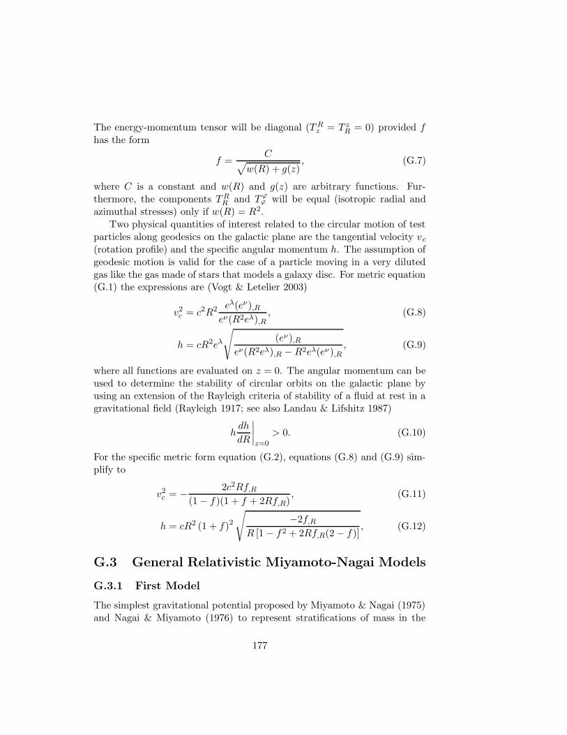
The energy-momentum tensor will be diagonal (T Rz = T z

R = 0) provided fhas the form

f =C

√

w(R) + g(z), (G.7)

where C is a constant and w(R) and g(z) are arbitrary functions. Fur-thermore, the components TR

R and Tϕϕ will be equal (isotropic radial and

azimuthal stresses) only if w(R) = R2.Two physical quantities of interest related to the circular motion of test

particles along geodesics on the galactic plane are the tangential velocity vc

(rotation profile) and the specific angular momentum h. The assumption ofgeodesic motion is valid for the case of a particle moving in a very dilutedgas like the gas made of stars that models a galaxy disc. For metric equation(G.1) the expressions are (Vogt & Letelier 2003)

v2c = c2R2 eλ(eν),R

eν(R2eλ),R, (G.8)

h = cR2eλ

√

(eν),Reν(R2eλ),R −R2eλ(eν),R

, (G.9)

where all functions are evaluated on z = 0. The angular momentum can beused to determine the stability of circular orbits on the galactic plane byusing an extension of the Rayleigh criteria of stability of a fluid at rest in agravitational field (Rayleigh 1917; see also Landau & Lifshitz 1987)

hdh

dR

∣

∣

∣

∣

z=0

> 0. (G.10)

For the specific metric form equation (G.2), equations (G.8) and (G.9) sim-plify to

v2c = − 2c2Rf,R

(1 − f)(1 + f + 2Rf,R), (G.11)

h = cR2 (1 + f)2

√

−2f,R

R [1 − f2 + 2Rf,R(2 − f)], (G.12)

G.3 General Relativistic Miyamoto-Nagai Models

G.3.1 First Model

The simplest gravitational potential proposed by Miyamoto & Nagai (1975)and Nagai & Miyamoto (1976) to represent stratifications of mass in the

177

central bulges and in the disc parts of galaxies is given by

Φ(R, z) = − GM√

R2 + (a+√z2 + b2)2

, (G.13)

where a and b are positive constants. The corresponding three-dimensionaldensity distribution ρN (R, z) is easily derived from Poisson equation (G.5)

ρN (R, z) =b2M

4π

aR2 + (a+ 3√z2 + b2)(a+

√z2 + b2)2

[

R2 + (a+√z2 + b2)2

]5/2(z2 + b2)3/2

. (G.14)

Now we consider the function f(R, z) defined in the previous section as

f(R, z) =GM

2c2√

R2 + (a+√z2 + b2)2

. (G.15)

Substituting equation (G.15) in equations (G.4a)–(G.4e) we find the fol-lowing expressions for the non-zero components of the energy-momentumtensor

σ =b2[

aR2 + (a+ ξ)2(a+ 3ξ)]

4πξ3

[

1 +√

R2 + (a+ ξ)2]5 , (G.16a)

pR = pϕ =b2

8πξ3

[

aR2 + (a+ ξ)2(a+ 2ξ)]

[

1 +√

R2 + (a+ ξ)2]5 [

−1 +√

R2 + (a+ ξ)2], (G.16b)

pz =b2(a+ ξ)2

4πξ2

[

1 +√

R2 + (a+ ξ)2]5 [

−1 +√

R2 + (a+ ξ)2], (G.16c)

where the variables and parameters were rescaled in terms of the Schwarzschildradius in isotropic spherical coordinates rs = GM/(2c2):2 R = R/rs,

z = z/rs, a = a/rs, b = b/rs, σ = Mr3sσ, pi = Mc2

r3spi and ξ =

√

z2 + b2.

The ‘effective Newtonian density’ ρ = σ + pR/c2 + pϕ/c

2 + pz/c2 reads

ρ =b2√

R2 + (a+ ξ)2[

aR2 + (a+ ξ)2(a+ 3ξ)]

4πξ3

[

1 +√

R2 + (a+ ξ)2]5 [

−1 +√

R2 + (a+ ξ)2], (G.17)

2Note that the Schwarzschild radius rs in isotropic spherical coordinates is related to

Schwarzschild radius r′s in canonical spherical coordinates by rs = r′s/4.

178

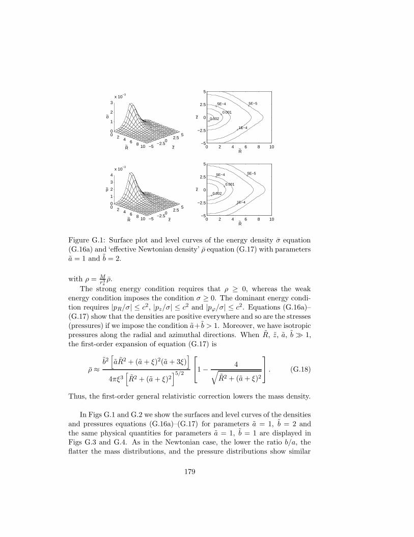
0 2 4 6 8 10 −5−2.5

02.5

50

1

2

3x 10

−3

R z~ ~

−σ

0 2 4 6 8 10−5

−2.5

0

2.5

5

R~

z~

5E−5

1E−4

5E−4

0.001

0.002

0 2 4 6 8 10 −5−2.5

02.5

50

1

2

3

4x 10

−3

R z~ ~

−ρ

0 2 4 6 8 10−5

−2.5

0

2.5

5

R~

z~

5E−5

1E−4

5E−4

0.001

0.002

Figure G.1: Surface plot and level curves of the energy density σ equation(G.16a) and ‘effective Newtonian density’ ρ equation (G.17) with parametersa = 1 and b = 2.

with ρ = Mr3sρ.

The strong energy condition requires that ρ ≥ 0, whereas the weakenergy condition imposes the condition σ ≥ 0. The dominant energy condi-tion requires |pR/σ| ≤ c2, |pz/σ| ≤ c2 and |pϕ/σ| ≤ c2. Equations (G.16a)–(G.17) show that the densities are positive everywhere and so are the stresses(pressures) if we impose the condition a+ b > 1. Moreover, we have isotropicpressures along the radial and azimuthal directions. When R, z, a, b 1,the first-order expansion of equation (G.17) is

ρ ≈b2[

aR2 + (a+ ξ)2(a+ 3ξ)]

4πξ3[

R2 + (a+ ξ)2]5/2

1 − 4√

R2 + (a+ ξ)2

. (G.18)

Thus, the first-order general relativistic correction lowers the mass density.

In Figs G.1 and G.2 we show the surfaces and level curves of the densitiesand pressures equations (G.16a)–(G.17) for parameters a = 1, b = 2 andthe same physical quantities for parameters a = 1, b = 1 are displayed inFigs G.3 and G.4. As in the Newtonian case, the lower the ratio b/a, theflatter the mass distributions, and the pressure distributions show similar

179

0 2 4 6 8 10 −5−2.5

02.5

5012345

x 10−4

R z~ ~

−pR

0 2 4 6 8 10−5

−2.5

0

2.5

5

R~

z~

5E−6

1E−5

5E−5

1E−4

2E−4

0 2 4 6 8 10 −5−2.5

02.5

50

1

2

3

4x 10

−4

R z~ ~

−pz

0 2 4 6 8 10−5

−2.5

0

2.5

5

R~

z~

5E−6

1E−5

5E−5

1E−4

2E−4

Figure G.2: Surface plot and level curves of the radial pressure pR equation(G.16b) and vertical pressure pz equation (G.16c) with parameters a = 1and b = 2.

0 2 4 6 8 10 −5−2.5

02.5

5012345

x 10−3

R z~ ~

−σ

0 2 4 6 8 10−5

−2.5

0

2.5

5

R~

z~

5E−5

1E−4

5E−4

0.001

0.003

0 2 4 6 8 10 −5−2.5

02.5

50

0.0020.0040.0060.0080.01

R z~ ~

−ρ

0 2 4 6 8 10−5

−2.5

0

2.5

5

R~

z~

5E−5

1E−4

5E−4

0.001

0.003

Figure G.3: Surface plot and level curves of the energy density σ equation(G.16a) and ‘effective Newtonian density’ ρ equation (G.17) with parametersa = 1 and b = 1.

180

0 2 4 6 8 10 −5−2.5

02.5

50

0.5

1

1.5

2x 10

−3

R z~ ~

−pr

0 2 4 6 8 10−5

−2.5

0

2.5

5

R~

z~

2E−6

1E−5

1E−4

5E−4

0.001

0 2 4 6 8 10 −5−2.5

02.5

50

0.5

1

1.5x 10

−3

R z~ ~

−pz

0 2 4 6 8 10−5

−2.5

0

2.5

5

R~

z~

1E−6

1E−5

1E−4

0.001

Figure G.4: Surface plot and level curves of the radial pressure pR equation(G.16b) and vertical pressure pz equation (G.16c) with parameters a = 1and b = 1.

behaviour. For a = 1, b = 2 we have pR/σ < 0.2 and pz/σ < 0.15 and fora = 1, b = 1 the ratios are pR/σ < 0.4 and pz/σ < 0.3. Thus, for theseparameters all energy conditions are satisfied.

The tangential circular velocity equation (G.11) and specific angularmomentum equation (G.12) for f given by equation (G.15) evaluated onz = 0 read

(vc

c

)2=

2R2√

R2 + η2

(

−1 +

√

R2 + η2

)

[

−R2 + η2 + (R2 + η2)3/2]

, (G.19)

h =

√2R2

(

1 +

√

R2 + η2

)2

(R2 + η2)3/4

√

(R2 + η2)2 + R2 − η2 − 4R2

√

R2 + η2

, (G.20)

where we defined h = crsh and η = a + b. The first-order expansion of

181

equation (G.19) reads

vc

c=

R√

2[

R2 + (a+ b)2]3/4

1 +R2

[

R2 + (a+ b)2]3/2

. (G.21)

Figs G.5(a) and (b) show, respectively, the rotation profile equation(G.19) and the curves of specific angular momentum equation (G.20) forparameters a = 1 and b = 2, b = 1 and b = 0.5. In Fig. G.5(a) the dashedcurves represent the Newtonian tangential velocities. Relativistic tangen-tial velocities are always higher than the Newtonian ones, as suggested bythe first-order correction in equation (G.21). The curves of specific angularmomentum show that the circular orbits on the plane z = 0 turn out to beunstable for higher flattened matter distributions (the curve for b = 0.5).The orbits for the parameters a = 1, b = 2 are all stable, whereas in thecase of b = 1 a small region of instability appears between R ≈ 5 and R ≈ 6.The Newtonian limit of equation (G.20) gives

h =

√2R2

[R2 + (a+ b)2]3/4, (G.22)

from which it is easily checked that (dh/dR) ≥ 0 for all a, b and R. Thus, theinstability is a pure relativistic effect (the same is verified for circular orbitsaround the superposition of black holes and axially symmetric structures inWeyl coordinates; see Letelier (2003)).

G.3.2 Second Model

Another pair of potential and density functions presented by Miyamoto andNagai as a generalization of the Toomre model 2 is described by

Φ(R, z) = − GM√

R2 + (a+ ζ)2

[

1 +a(a+ ζ)

R2 + (a+ ζ)2

]

, (G.23a)

ρN (R, z) =3b2M

4πζ3 [R2 + (a+ ζ)2]7/2

[

R2(a3 + ζ3) + (ζ + a)3(ζ2 + 4aζ + a2)]

,

(G.23b)

where ζ =√z2 + b2. Using f defined by equation (G.6) in equations (G.4a)–

(G.4e), we find that the components TRz = T z

R are non-zero. The physical

182

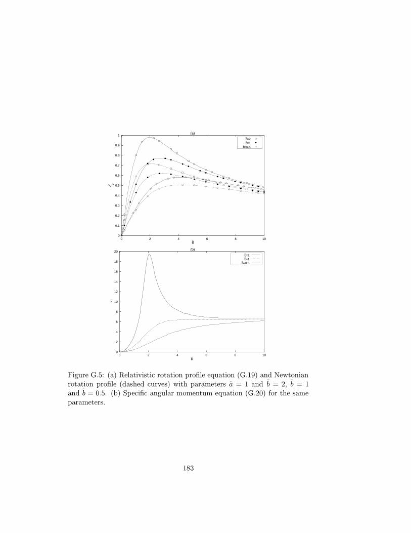
0

0.1

0.2

0.3

0.4

0.5

0.6

0.7

0.8

0.9

1

0 2 4 6 8 10

vc/c

R~

(a)

b~=2b~=1

b~=0.5

0

2

4

6

8

10

12

14

16

18

20

0 2 4 6 8 10

h

R~

(b)

b~=2b~=1

b~=0.5

Figure G.5: (a) Relativistic rotation profile equation (G.19) and Newtonianrotation profile (dashed curves) with parameters a = 1 and b = 2, b = 1and b = 0.5. (b) Specific angular momentum equation (G.20) for the sameparameters.

183

variables of the matter distribution are obtained by solving the eigenvalueproblem for T a

b

T ab Ξb = λΞa. (G.24)

We find that T ab can be put in the form

T ab = σea(0)eb(0) + p+e

a(1)e

b(1) + p−e

a(2)e

b(2) + pϕe

a(3)e

b(3), (G.25)

where

σ =T t

t

c2, ea(0) =

(

1 + f

1 − f, 0, 0, 0

)

,

p± = −TRR + T z

z

2∓ 1

2

√

(TRR − T z

z )2 + 4(TRz )2, (G.26)

ea(1) = (0, eR(1), ez(1), 0), ea(2) = (0, eR(2), e

z(2), 0),

pϕ = −Tϕϕ , ea(3) =

(

0, 0, 0,1

R(1 + f)2

)

, (G.27)

and

eR(1) = − TRz

(1 + f)2√

(TRz )2 + (TR

R + p+)2, ez(1) =

TRR + p+

(1 + f)2√

(TRz )2 + (TR

R + p+)2,

eR(2) = − TRz

(1 + f)2√

(TRz )2 + (TR

R + p−)2, ez(2) =

TRR + p−

(1 + f)2√

(TRz )2 + (TR

R + p−)2.

(G.28)

The effective Newtonian density reads ρ = σ + p+/c2 + p−/c

2 + pϕ/c2 =

σ − TRR /c

2 − T zz /c

2 + pϕ/c2. The explicit expressions for σ, ρ and pϕ are

σ =3b2χ4

[

R2(a3 + ξ3) + (a+ ξ)3(a2 + ξ2 + 4aξ)]

4πξ3[

χ3/2 + R2 + (a+ ξ)(2a+ ξ)]5 , (G.29)

ρ =3b2χ11/2

[

R2(a3 + ξ3) + (a+ ξ)3(a2 + ξ2 + 4aξ)]

4πξ3[

χ3/2 + R2 + (a+ ξ)(2a+ ξ)]5 [

χ3/2 − R2 − (a+ ξ)(2a+ ξ)],

(G.30)

pϕ =χ4

8πξ3[

χ3/2 + R2 + (a+ ξ)(2a+ ξ)]5 [

χ3/2 − R2 − (a+ ξ)(2a+ ξ)]×

184

R4[

ξ3(a2 + 2b2) + 3a3b2]

+ R2(a+ ξ)2[

9a3b2 + 12ab2ξ2 + 4b2ξ3

+2a2(7b2 + z2)ξ]

+ (a+ ξ)4[

6a3b2 + 12ab2ξ2 + 2b2ξ3 + a2(19b2 + z2)ξ]

,

(G.31)

where ξ =√

z2 + b2, χ = R2 +(a+ ξ)2 and the dimensionless variables werepreviously defined. The components TR

R , TRz and T z

z read

TRR = −Mc2

r3s

χ4

8πξ3[

χ3/2 + r2 + (a+ ξ)(2a + ξ)]5 [

χ3/2 − r2 − (a+ ξ)(2a+ ξ)]×

r4[

ξ3(a2 + 2b2) + 3a3b2]

+ r2(a+ ξ)2[

9a3b2 + 12ab2ξ2 + 4b2ξ3

+2a2(b2 − 5z2)ξ]

+ (a+ ξ)4[

6a3b2 + 12ab2ξ2 + 2b2ξ3 + a2(19b2 + z2)ξ]

,

(G.32)

TRz = T z

R = −Mc2

r3s×

3a2rz(a+ ξ)χ4[

r2 − (a+ ξ)2]

4πξ[

χ3/2 + r2 + (a+ ξ)(2a + ξ)]5 [

χ3/2 − r2 − (a+ ξ)(2a+ ξ)],

(G.33)

T zz =

Mc2

r3s

χ4

4πξ2[

χ3/2 + r2 + (a+ ξ)(2a+ ξ)]5 [

χ3/2 − r2 − (a+ ξ)(2a + ξ)]×

r4ξ2(a2 − b2) − 2r2ξ(a+ ξ)2[

3ab2 + ξ(2a2 + b2)]

+(a+ ξ)4[

a2(z2 − 8b2) − b2ξ(6a+ ξ)]

, (G.34)

and p± is further adimensionalized as p± = Mc2

r3sp±.

The condition (a + b)2 > (2a + b) ensures positive densities and non-singular behaviour for the densities and pressures. The first-order expansionof equation (G.30) reads

ρ ≈3b2[

R2(a3 + ξ3) + (a+ ξ)3(a2 + ξ2 + 4aξ)]

4πξ3[R2 + (a+ ξ)2]7/2×

1 − 4[R2 + (a+ ξ)(2a+ ξ)]

[R2 + (a+ ξ)2]3/2

. (G.35)

The surfaces and level curves of the densities equations (G.29) and (G.30)and pressures equation (G.26) are shown in Figs G.6 and G.7, respectively,

185

0 2 4 6 8 10 −5−2.5

02.5

50

1

2

3x 10

−3

R z~ ~

−σ

0 2 4 6 8 10−5

−2.5

0

2.5

5

R~

z~

5E−5

1E−4

5E−4

0.001

0.002

0 2 4 6 8 10 −5−2.5

02.5

50

2

4

6x 10

−3

R z~ ~

−ρ

0 2 4 6 8 10−5

−2.5

0

2.5

5

R~

z~

5E−5

1E−4

5E−4

0.001

0.002

Figure G.6: Surface plot and level curves of the energy density σ equation(G.29) and ‘effective Newtonian density’ ρ equation (G.30) with parametersa = 1 and b = 2.

0 2 4 6 8 10 −5−2.5

02.5

50

0.20.40.60.8

1x 10

−3

R z~ ~

−p+

0 2 4 6 8 10−5

−2.5

0

2.5

5

R~

z~

5E−6

1E−5

5E−5

1E−4

5E−4

0 2 4 6 8 10 −5−2.5

02.5

50

0.20.40.60.8

1x 10

−3

R z~ ~

−p−

0 2 4 6 8 10−5

−2.5

0

2.5

5

R~

z~

5E−6

1E−5

5E−5

1E−4

5E−4

Figure G.7: Surface plot and level curves of the pressures p± equation (G.26)with parameters a = 1 and b = 2.

186

0 2 4 6 8 10 −5−2.5

02.5

50

0.20.40.60.8

1x 10

−3

R~ z~

−pϕ

(a)

0 2 4 6 8 10−5

−2.5

0

2.5

5

R~

z~

5E−6

1E−5

5E−5

1E−4

5E−4

Figure G.8: Surface plot and level curves of the azimuthal pressure pϕ equa-tion (G.31) with parameters a = 1 and b = 2.

0

0.1

0.2

0.3

0.4

0.5

0.6

0.7

0.8

0 2 4 6 8 10

vc/c

R~

(a)

b~=3b~=2

0

1

2

3

4

5

6

7

0 2 4 6 8 10

h

R~

(b)

b~=3

b~=2

Figure G.9: (a) Relativistic rotation profile equation (G.36) and Newtonianrotation profile (dashed curves) with parameters a = 1 and b = 3, b = 2.(b) Specific angular momentum equation (G.37) for the same parameters.

187

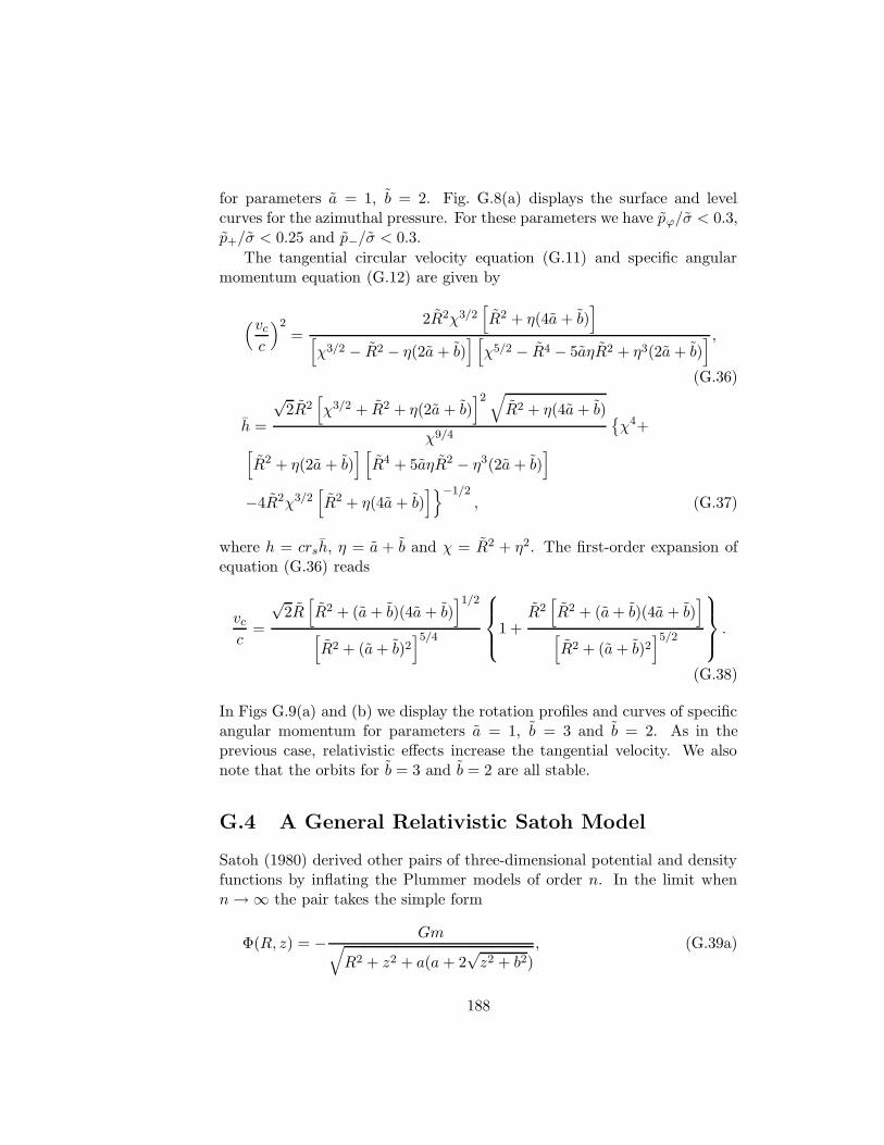
for parameters a = 1, b = 2. Fig. G.8(a) displays the surface and levelcurves for the azimuthal pressure. For these parameters we have pϕ/σ < 0.3,p+/σ < 0.25 and p−/σ < 0.3.

The tangential circular velocity equation (G.11) and specific angularmomentum equation (G.12) are given by

(vc

c

)2=

2R2χ3/2[

R2 + η(4a+ b)]

[

χ3/2 − R2 − η(2a + b)] [

χ5/2 − R4 − 5aηR2 + η3(2a + b)] ,

(G.36)

h =

√2R2

[

χ3/2 + R2 + η(2a + b)]2√

R2 + η(4a+ b)

χ9/4

χ4+

[

R2 + η(2a + b)] [

R4 + 5aηR2 − η3(2a+ b)]

−4R2χ3/2[

R2 + η(4a+ b)]−1/2

, (G.37)

where h = crsh, η = a + b and χ = R2 + η2. The first-order expansion ofequation (G.36) reads

vc

c=

√2R[

R2 + (a+ b)(4a+ b)]1/2

[

R2 + (a+ b)2]5/4

1 +R2[

R2 + (a+ b)(4a + b)]

[

R2 + (a+ b)2]5/2

.

(G.38)

In Figs G.9(a) and (b) we display the rotation profiles and curves of specificangular momentum for parameters a = 1, b = 3 and b = 2. As in theprevious case, relativistic effects increase the tangential velocity. We alsonote that the orbits for b = 3 and b = 2 are all stable.

G.4 A General Relativistic Satoh Model

Satoh (1980) derived other pairs of three-dimensional potential and densityfunctions by inflating the Plummer models of order n. In the limit whenn→ ∞ the pair takes the simple form

Φ(R, z) = − Gm√

R2 + z2 + a(a+ 2√z2 + b2)

, (G.39a)

188

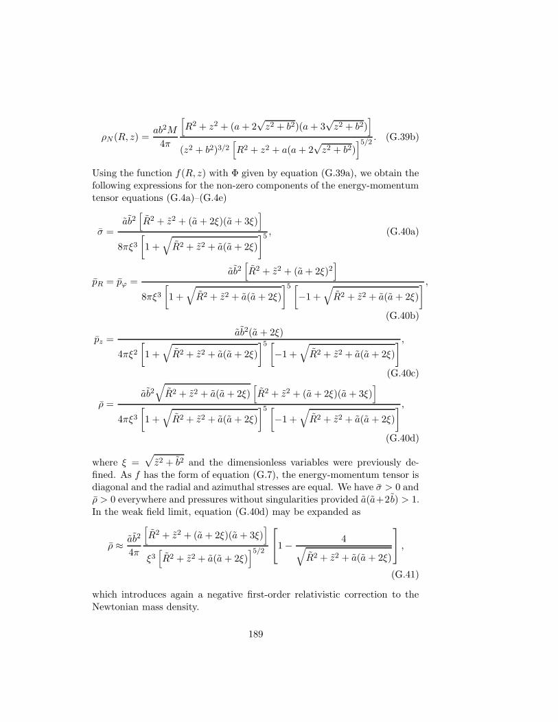
ρN (R, z) =ab2M

4π

[

R2 + z2 + (a+ 2√z2 + b2)(a+ 3

√z2 + b2)

]

(z2 + b2)3/2[

R2 + z2 + a(a+ 2√z2 + b2)

]5/2. (G.39b)

Using the function f(R, z) with Φ given by equation (G.39a), we obtain thefollowing expressions for the non-zero components of the energy-momentumtensor equations (G.4a)–(G.4e)

σ =ab2[

R2 + z2 + (a+ 2ξ)(a + 3ξ)]

8πξ3

[

1 +√

R2 + z2 + a(a+ 2ξ)

]5 , (G.40a)

pR = pϕ =ab2[

R2 + z2 + (a+ 2ξ)2]

8πξ3

[

1 +√

R2 + z2 + a(a+ 2ξ)

]5 [

−1 +√

R2 + z2 + a(a+ 2ξ)

],

(G.40b)

pz =ab2(a+ 2ξ)

4πξ2

[

1 +√

R2 + z2 + a(a+ 2ξ)

]5 [

−1 +√

R2 + z2 + a(a+ 2ξ)

],

(G.40c)

ρ =ab2√

R2 + z2 + a(a+ 2ξ)[

R2 + z2 + (a+ 2ξ)(a+ 3ξ)]

4πξ3

[

1 +√

R2 + z2 + a(a+ 2ξ)

]5 [

−1 +√

R2 + z2 + a(a+ 2ξ)

],

(G.40d)

where ξ =√

z2 + b2 and the dimensionless variables were previously de-fined. As f has the form of equation (G.7), the energy-momentum tensor isdiagonal and the radial and azimuthal stresses are equal. We have σ > 0 andρ > 0 everywhere and pressures without singularities provided a(a+2b) > 1.In the weak field limit, equation (G.40d) may be expanded as

ρ ≈ ab2

4π

[

R2 + z2 + (a+ 2ξ)(a+ 3ξ)]

ξ3[

R2 + z2 + a(a+ 2ξ)]5/2

1 − 4√

R2 + z2 + a(a+ 2ξ)

,

(G.41)

which introduces again a negative first-order relativistic correction to theNewtonian mass density.

189

0 2 4 6 8 10 −5−2.5

02.5

50

0.5

1

1.5

2x 10

−3

R z~ ~

−σ

0 2 4 6 8 10−5

−2.5

0

2.5

5

R~

z~

2E−5

5E−5

1E−4 5E−4

0.001

0 2 4 6 8 10 −5−2.5

02.5

50

2

4

6

8x 10

−3

R z~ ~

−ρ

0 2 4 6 8 10−5

−2.5

0

2.5

5

R~

z~

2E−5

5E−5

1E−4 5E−4

0.001

Figure G.10: Surface plot and level curves of the energy density σ equation(G.40a) and ‘effective Newtonian density’ ρ equation (G.40d) with parame-ters a = 1 and b = 2.

0 2 4 6 8 10 −5−2.5

02.5

50

0.20.40.60.8

1x 10

−3

R z~ ~

−pr

0 2 4 6 8 10−5

−2.5

0

2.5

5

R~

z~

5E−6

1E−5

5E−5

1E−4

5E−4

0 2 4 6 8 10 −5−2.5

02.5

50

0.20.40.60.8

1x 10

−3

R z~ ~

−pz

0 2 4 6 8 10−5

−2.5

0

2.5

5

R~

z~

5E−6

1E−5

5E−5

1E−4

5E−4

Figure G.11: Surface plot and level curves of the radial pressure pR equation(G.40b) and vertical pressure pz equation (G.40c) with parameters a = 1and b = 2.

190

Expressions for the tangential velocity and angular momentum followdirectly from equations (G.11) and (G.12)

(vc

c

)2=

2R2√

R2 + η[

−R2 + η + (R2 + η)3/2]

(

−1 +

√

R2 + η

) , (G.42)

h =

√2R2

(

1 +

√

R2 + η

)2

(R2 + η)3/4

√

(R2 + η)2 + R2 − η − 4R2

√

R2 + η

, (G.43)

where h = crsh and η = a(a + 2b). The first-order expansion of equation(G.42) is given by

vc

c=

R√

2[

R2 + a(a+ 2b)]3/4

1 +R2

[

R2 + a(a+ 2b)]3/2

. (G.44)

The surfaces and level curves of the densities and pressures equations(G.40a)–(G.40d) for parameters a = 1, b = 2 are plotted in Figs G.10 andG.11. We have pR/σ < 0.6 and pz/σ < 0.5, so all energy conditions aresatisfied. Rotation profiles and curves of specific angular momentum aredisplayed in Fig. G.12 for parameters a = 1, b = 2 and b = 1. We note thatcircular orbits are stable for b = 2.

G.5 Geodesic Orbits

An interesting application of the general relativistic galactic models is thestudy of geodesic orbits outside the galactic plane. As an example we cal-culate numerically two orbits for the first Miyamoto-Nagai model (SectionG.3.1) and compare them with the Newtonian case.

We solve numerically the geodesic equations of motion

xµ + Γµαβx

αxβ = 0, (G.45)

for metric equation (G.2), where Γµαβ are the Christoffel symbols and the dot

denote differentiation with respect to the proper time. With the orthonormaltetrad defined as

ei(t) =1 + f

1 − f(1, 0, 0, 0), ei

(R) =1

(1 + f)2(0, 1, 0, 0),

191

0

0.1

0.2

0.3

0.4

0.5

0.6

0.7

0.8

0.9

0 2 4 6 8 10

vc/c

R~

(a)

b~=2b~=1

0

1

2

3

4

5

6

7

8

0 2 4 6 8 10

h

R~

(b)

b~=2b~=1

Figure G.12: (a) Relativistic rotation profile equation (G.42) and Newtonianrotation profile (dashed curves) with parameters a = 1 and b = 2, b = 1.(b) Specific angular momentum equation (G.43) for the same parameters.

192

ei(z) =1

(1 + f)2(0, 0, 1, 0), ei

(ϕ) =1

R(1 + f)2(0, 0, 0, 1), (G.46)

the tetrad components of the four-velocity vi read

vi = γ(1, v sinψ cos θ, v sinψ sin θ, v cosψ), (G.47)

with γ = 1/√

1 − v2 (we have set c = 1). The specific energy and angularmomentum of the test particle are

E = γ1 − f

1 + f, (G.48)

h = r(1 + f)2γv cosψ. (G.49)

As initial conditions, we take a position at radius R0 on the disc’s planeand components of the four-velocity vi

0 = γ(1, 0, v0 sinψ, v0 cosψ), where v0

is equal to the tangential velocity of circular orbits at radius R0. Similarinitial conditions for the Newtonian case are chosen with the same angularmomentum and energy E − 1. Both the geodesic and Newtonian equationsare solved with the fourth-fifth Runge-Kutta method with adaptive size step.

In Figs G.13–G.16 we compare both orbits for the first Miyamoto-Nagaimodel with parameters a = 1 and b = 1. For the orbits shown in FigsG.13 and G.14 large radii have been chosen as initial conditions. As ex-pected, general relativistic effects are small. A noticeable difference is seenin a periodic variation of the amplitude of the R coordinate as function ofthe azimuthal angle in the relativistic case. On the other hand, the orbitsshown in Figs G.15 and G.16 have been computed near the center where thegravitational fields are strong, and the deviation between relativistic andNewtonian orbits are much more pronounced.

G.6 First-order Effects of Galactic Rotation on

the Rotation Profiles

The galactic models presented in the last sections are all static. Astrophys-ical objects are expected to have angular momentum; thus, more realisticmodels should incorporate rotation. An exact stationary general relativisticgalactic model could be constructed, for example, if one managed to find aclosed form of the Kerr metric in terms of elementary functions in station-ary isotropic coordinates, and then repeated the procedure outlined in the

193

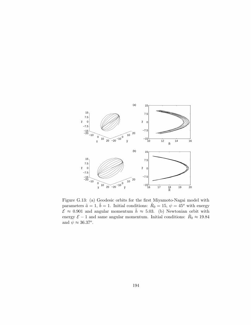
−20−10

010

20 −20−10

010

20−15

−7.5

0

7.5

15

x y~ ~

z~

(a)

10 12 14 16−15

−7.5

0

7.5

15

R

z

~

~

−20−10

010

20 −20−10

010

20−15

−7.5

0

7.5

15

x~ y~

z~

(b)

16 17 18 19 20−15

−7.5

0

7.5

15

R

z

~

~

Figure G.13: (a) Geodesic orbits for the first Miyamoto-Nagai model withparameters a = 1, b = 1. Initial conditions: R0 = 15, ψ = 45o with energyE ≈ 0.901 and angular momentum h ≈ 5.03. (b) Newtonian orbit withenergy E − 1 and same angular momentum. Initial conditions: R0 ≈ 19.84and ψ ≈ 36.37o.

194

0 1 2 3 4 510

12

14

16

ϕ/2π

R~

(a)

0 1 2 3 4 5−12

−6

0

6

12

ϕ/2π

z~

0 1 2 3 4 516

17

18

19

20

ϕ/2π

R~

(b)

0 1 2 3 4 5−12

−6

0

6

12

ϕ/2π

z~

Figure G.14: The coordinates R and z as functions of the number of rev-olutions ϕ/2π for the orbits shown in Fig. G.13. (a) Geodesic and (b)Newtonian orbit.

previous sections to calculate the matter properties. Although this cannotbe done for the exact Kerr solution, the same is not true for the first-orderexpansion of the Kerr metric with respect to the rotation parameter. Itreads

ds2 =

(

1 − 2GM

rc2

)

c2dt2 − dr2

1 − 2GMrc2

− r2(dθ2 + sin2 θdϕ2)

+4GMα

rcsin2 θdtdϕ, (G.50)

where α is the rotation parameter. If we transform metric equation (G.50)to cylindrical isotropic coordinates (t, R, z, ϕ) and express it in terms of thefunction f given by equation (G.3) we obtain

ds2 =

(

1 − f

1 + f

)2

c2dt2 − (1 + f)4(

dR2 + dz2 +R2dϕ2)

+32αR2f3c5

G2M2(1 + f)2dtdϕ. (G.51)

Now the function f may be replaced by any of the forms presented in theprevious sections to generate space-times with matter. However, a direct

195

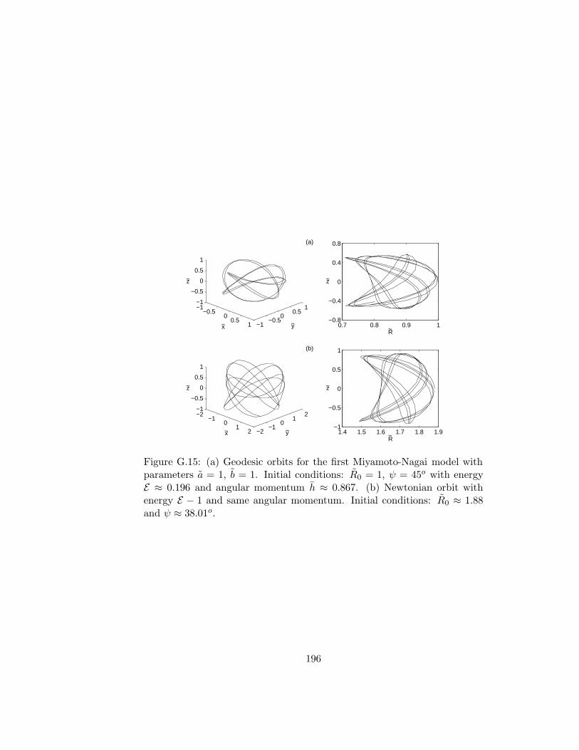
0.7 0.8 0.9 1−0.8

−0.4

0

0.4

0.8

R

z

~

~

−1−0.5

00.5

1 −1−0.5

00.5

1−1

−0.5

0

0.5

1

x y~ ~

z~

(a)

−2−1

01

2 −2−1

01

2−1

−0.5

0

0.5

1

x~ y~

z~

(b)

1.4 1.5 1.6 1.7 1.8 1.9−1

−0.5

0

0.5

1

R

z

~

~

Figure G.15: (a) Geodesic orbits for the first Miyamoto-Nagai model withparameters a = 1, b = 1. Initial conditions: R0 = 1, ψ = 45o with energyE ≈ 0.196 and angular momentum h ≈ 0.867. (b) Newtonian orbit withenergy E − 1 and same angular momentum. Initial conditions: R0 ≈ 1.88and ψ ≈ 38.01o.

196

0 1 2 3 4 50.7

0.8

0.9

1

ϕ/2π

R~

(a)

0 1 2 3 4 5−0.6

−0.3

0

0.3

0.6

ϕ/2π

z~

0 1 2 3 4 51.4

1.6

1.8

ϕ/2π

R~

(b)

0 1 2 3 4 5−1

−0.5

0

0.5

1

ϕ/2π

z~

Figure G.16: The coordinates R and z as functions of the number of rev-olutions ϕ/2π for the orbits shown in Fig. G.15. (a) Geodesic and (b)Newtonian orbit.

calculation using the Einstein field equations and metric equation (G.51)shows that the influence of rotation on the physical variables of the matteris of at least O(α2). Thus, to have a consistent correction one should alsostart with metric form equation (G.51) corrected at least to O(α2); however,it does not seem possible to express this particular form of the metric withsecond-order corrections of the rotation parameter. Despite this, a consistentfirst-order correction of the rotation profiles can be calculated.

We rewrite equation (G.51) as

dτ2 = gttdt2 − gRR

(

dR2 + dz2 +R2dϕ2)

+ 2gtϕdtdϕ, (G.52)

where for convenience we have set c = 1. Let va = (t, 0, 0, ϕ) be the ve-locity four-vector, where dots denote differentiation with respect to τ . Thegeodesic equation for circular orbits is

gtt,R t2 + 2gtϕ,R tϕ− (R2gRR),Rϕ

2 = 0 ⇒ϕ

t=gtϕ,R ±

√

(gtϕ,R)2 + gtt,R(R2gRR),R(R2gRR),R

. (G.53)

Thus, the prograde and retrograde angular velocities are, in general, differ-

197

ent. We define an orthonormal tetrad e(b)i as

e(t)i =

√

g2tϕ +R2gttgRR

R√gRR

, 0, 0, 0

,

e(R)i = (0,−√gRR, 0, 0), e(z)i = (0, 0,−√

gRR, 0),

e(ϕ)i =

(

gtϕ

R√gRR

, 0, 0,−R√gRR

)

, (G.54)

and project the components of va on the tetrad: v(a) = e

(a)i vi= η(a)(b)e(b)iv

i

v(t) =

√

g2tϕ +R2gttgRR

R√gRR

t, (G.55a)

v(ϕ) = − gtϕ

R√gRR

t+R√gRRϕ. (G.55b)

Using equation (G.53) in equations (G.55a) and (G.55b) we obtain

v(ϕ)

v(t)=

1√

g2tϕ +R2gttgRR

[

−gtϕ +R2gRR

(R2gRR),R×

(

gtϕ,R ±√

(gtϕ,R)2 + gtt,R(R2gRR),R

)]

. (G.56)

The terms g2tϕ and (gtϕ,R)2 in equation (G.56) are of O(α2) and thus can be

neglected. Using metric equation (G.51), equation (G.56) can be rearrangedas

vc = c

√

−2Rf,R

(1 − f)(1 + f + 2Rf,R)

[

±1 +24αf2Rc4

G2M2(1 + f)3

√

−Rf,R(1 − f)

2(1 + f + 2Rf,R)

]

,

(G.57)

where c has been reintroduced. The term outside brackets is the tangentialvelocity equation (G.11). The term with α is always positive, thus thefirst-order effect of rotation increases (decreases) the prograde (retrograde)tangential velocity.

Equation (G.57) calculated with the functions f used in Sections G.3

198

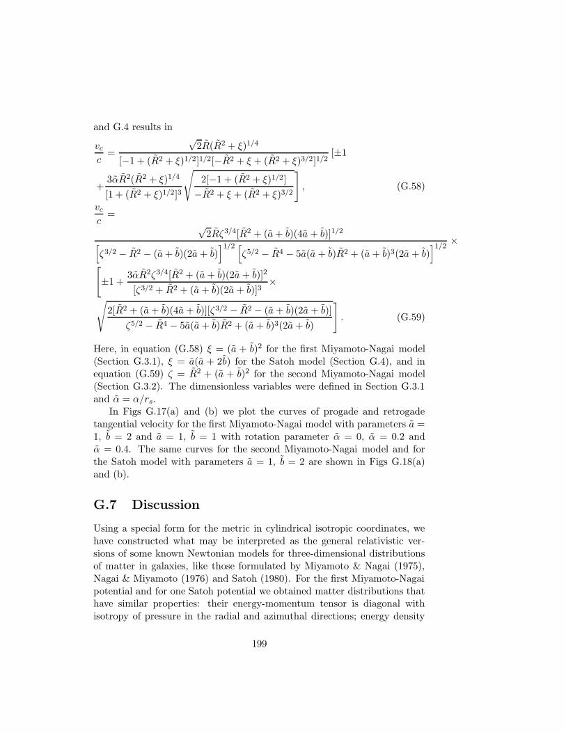
and G.4 results in

vc

c=

√2R(R2 + ξ)1/4

[−1 + (R2 + ξ)1/2]1/2[−R2 + ξ + (R2 + ξ)3/2]1/2[±1

+3αR2(R2 + ξ)1/4

[1 + (R2 + ξ)1/2]3

√

2[−1 + (R2 + ξ)1/2]

−R2 + ξ + (R2 + ξ)3/2

]

, (G.58)

vc

c=

√2Rζ3/4[R2 + (a+ b)(4a + b)]1/2

[

ζ3/2 − R2 − (a+ b)(2a+ b)]1/2 [

ζ5/2 − R4 − 5a(a+ b)R2 + (a+ b)3(2a+ b)]1/2

×

[

±1 +3αR2ζ3/4[R2 + (a+ b)(2a+ b)]2

[ζ3/2 + R2 + (a+ b)(2a+ b)]3×

√

2[R2 + (a+ b)(4a + b)][ζ3/2 − R2 − (a+ b)(2a+ b)]

ζ5/2 − R4 − 5a(a+ b)R2 + (a+ b)3(2a+ b)

]

. (G.59)

Here, in equation (G.58) ξ = (a + b)2 for the first Miyamoto-Nagai model(Section G.3.1), ξ = a(a + 2b) for the Satoh model (Section G.4), and inequation (G.59) ζ = R2 + (a + b)2 for the second Miyamoto-Nagai model(Section G.3.2). The dimensionless variables were defined in Section G.3.1and α = α/rs.

In Figs G.17(a) and (b) we plot the curves of progade and retrogadetangential velocity for the first Miyamoto-Nagai model with parameters a =1, b = 2 and a = 1, b = 1 with rotation parameter α = 0, α = 0.2 andα = 0.4. The same curves for the second Miyamoto-Nagai model and forthe Satoh model with parameters a = 1, b = 2 are shown in Figs G.18(a)and (b).

G.7 Discussion

Using a special form for the metric in cylindrical isotropic coordinates, wehave constructed what may be interpreted as the general relativistic ver-sions of some known Newtonian models for three-dimensional distributionsof matter in galaxies, like those formulated by Miyamoto & Nagai (1975),Nagai & Miyamoto (1976) and Satoh (1980). For the first Miyamoto-Nagaipotential and for one Satoh potential we obtained matter distributions thathave similar properties: their energy-momentum tensor is diagonal withisotropy of pressure in the radial and azimuthal directions; energy density

199

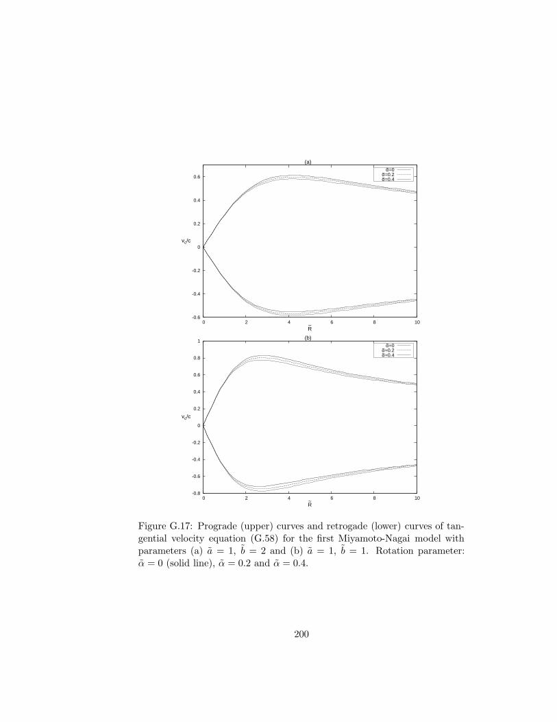
-0.6

-0.4

-0.2

0

0.2

0.4

0.6

0 2 4 6 8 10

vc/c

R~

(a)α~=0

α~=0.2α~=0.4

-0.8

-0.6

-0.4

-0.2

0

0.2

0.4

0.6

0.8

1

0 2 4 6 8 10

vc/c

R~

(b)α~=0

α~=0.2α~=0.4

Figure G.17: Prograde (upper) curves and retrogade (lower) curves of tan-gential velocity equation (G.58) for the first Miyamoto-Nagai model withparameters (a) a = 1, b = 2 and (b) a = 1, b = 1. Rotation parameter:α = 0 (solid line), α = 0.2 and α = 0.4.

200

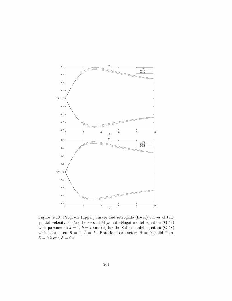
-0.8

-0.6

-0.4

-0.2

0

0.2

0.4

0.6

0.8

0 2 4 6 8 10

vc/c

R~

(a)α~=0

α~=0.2α~=0.4

-0.8

-0.6

-0.4

-0.2

0

0.2

0.4

0.6

0.8

0 2 4 6 8 10

vc/c

R~

(b)α~=0

α~=0.2α~=0.4

Figure G.18: Prograde (upper) curves and retrogade (lower) curves of tan-gential velocity for (a) the second Miyamoto-Nagai model equation (G.59)with parameters a = 1, b = 2 and (b) for the Satoh model equation (G.58)with parameters a = 1, b = 2. Rotation parameter: α = 0 (solid line),α = 0.2 and α = 0.4.

201

and the ‘effective Newtonian density’ are positive everywhere as well as thestresses (pressures) in the vertical direction. For particular values of the freeparameters, we found that the dominant energy condition is also satisfied.Stability analysis of the circular geodesic orbits on the galactic plane us-ing an extension of the Rayleigh criteria of stability shows stable orbits forsome combination of free parameters. The second Miyamoto-Nagai poten-tial function, after diagonalization of the energy-momentum tensor, yieldsmatter distributions with positive energy density and three different pres-sures. Also in this case, free parameters can be chosen so that all energyconditions are satisfied and circular orbits are stable on the galactic plane.

As an example of application of the models, we have numerically calcu-lated some geodesic orbits for one of the potentials and compared them withthe Newtonian orbits with the same energy and angular momentum. Nearthe central regions where the gravitational fields are strong, the motion ofparticles is considerably altered by general relativistic effects.

We also calculated the first-order effects of galactic rotation on the tan-gential velocity of circular orbits on the galactic plane using an approximateform of the Kerr metric expressed in cylindrical isotropic coordinates. Ingeneral, rotation increases the progade tangential velocity and has an oppo-site effect on the retrogade tangential velocity.

It should be mentioned that the stability study of the models presentedbased on the extension of Rayleigh criteria of stability is very limited. Amore realistic stability analysis should rely on the first-order perturbed gen-eral relativistic fluid equations taking into account two spatial coordinates,which may be not a trivial task (see, for instance, Ujevic & Letelier 2004 forthe one-dimensional case). This will be the subject of further investigation.

Acknowledgments

DV thanks CAPES for financial support. PSL thanks CNPq and FAPESPfor financial support. This research has made use of NASA’s AstrophysicsData System.

References

Bicak J., Ledvinka T.,1993, Phys. Rev. Lett., 71, 1669Bicak J., Lynden-Bell D., Katz J., 1993a, Phys. Rev. D, 47, 4334Bicak J., Lynden-Bell D., Pichon C., 1993b, MNRAS, 265, 126Binney S., Tremaine S., 1987, Galactic Dynamics. Princeton Univ. Press,Princeton, NJ

202

Bonnor W. A., Sackfield A., 1968, Commun. Math. Phys., 8, 338Frauendiener J., Klein C., 2001, Phys. Rev. D, 63, 084025Garcıa G., Gonzalez G., 2004, Phys. Rev. D, 69, 124002Gonzalez G., Espitia O. A., 2003, Phys. Rev. D, 68, 104028Gonzalez G., Letelier P. S., 1999, Class. Quantum Grav., 16, 479Gonzalez G., Letelier P. S., 2000, Phys. Rev. D, 62, 064025Gonzalez G., Letelier P. S., 2004, Phys. Rev. D, 69, 044013Karas V., Hure J. M., Semerak O., 2004, Class. Quantum Grav., 21, R1Katz J., Bicak J., Lynden-Bell D., 1999, Class. Quantum Grav., 16, 4023King I. R., 1966, AJ, 71, 64Klein C., 1997, Class. Quantum Grav., 14, 2267Klein C., 2001, Phys. Rev. D, 63, 064033Klein C., 2002, Phys. Rev. D, 65, 084029Klein C., 2003a, Phys. Rev. D, 68, 027501Klein C., 2003b, Ann. Phys., 12 (10), 599Klein C., Richter O., 1999, Phys. Rev. Lett., 83, 2884Kuzmin G. G., 1956, AZh, 33, 27Landau L. D., Lifshitz E. M., 1987, Fluid Mechanics, 2nd edn. PergamonPress, OxfordLemos J. P. S., 1989, Class. Quantum Grav., 6, 1219Lemos J. P. S., Letelier P. S., 1993, Class. Quantum Grav., 10, L75Lemos J. P. S., Letelier P. S., 1994, Phys. Rev. D, 49, 5135Lemos J. P. S., Letelier P. S., 1996, Int. J. Mod. Phys. D, 5, 53Letelier P. S., 1999, Phys. Rev. D, 60, 104042Letelier P. S., 2003, Phys. Rev. D, 68, 104002 Letelier P. S., Oliveira S. R.,1987, J. Math. Phys., 28, 165Lynden-Bell D., Pineault S., 1978, MNRAS, 185, 679Miyamoto M., Nagai R., 1975, PASJ, 27, 533Morgan T., Morgan L., 1969, Phys. Rev., 183, 1097Morgan L., Morgan T., 1970, Phys. Rev. D, 2, 2756Nagai R., Miyamoto M., 1976, PASJ, 28, 1Neugebauer G., Meinel R., 1995, Phys. Rev. Lett., 75, 3046Plummer H.C., 1911, MNRAS, 71, 460Rayleigh J. W. S., 1917, Proc. R. Soc. London A, 93, 148Satoh G., 1980, PASJ, 32, 41Toomre A., 1963, ApJ, 138, 385Ujevic M., Letelier P. S., 2004, Phys. Rev. D, 70, 084015Vogt D., Letelier P. S., 2003, Phys. Rev. D, 68, 084010Vogt D., Letelier P. S., 2004, Phys. Rev. D, 70, 064003

203

204

Apendice H

On Multipolar Analytical

Potentials for Galaxies

Daniel Vogt and Patricio S. Letelier, Publ. Astron. Soc. Japan 57, 871-875(2005).

Abstract

We present analytical potential–density pairs in three dimensions for thegravitational field of galaxies, obtained by thickening the multipolar expan-sion up to the quadrupole term. These may be interpreted as generaliza-tions of the Miyamoto and Nagai potential–density pairs. With a suitablerestriction on the possible values of the multipole moments, the density dis-tributions are positive and monotone decreasing functions of the radial andaxial coordinates.

Key Words: galaxies: kinematics and dynamics – galaxies: structure

H.1 Introduction

There are several three-dimensional analytical models in the literature forthe gravitational field of different types of galaxies and galactic compo-nents. Jaffe (1983) and Hernquist (1990) discuss models for spherical galax-ies and bulges. Three-dimensional models for flat galaxies were obtainedby Miyamoto and Nagai (1975) and Satoh (1980). de Zeeuw and Pfen-niger (1989) considered a set of ellipsoidal models appropriate to galacticbars. Long and Murali (1992) derived simple potential–density pairs for a

205

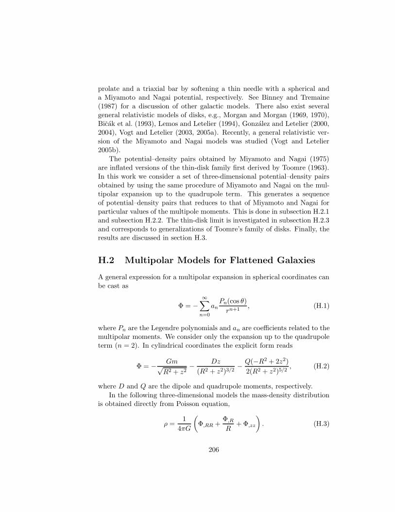
prolate and a triaxial bar by softening a thin needle with a spherical anda Miyamoto and Nagai potential, respectively. See Binney and Tremaine(1987) for a discussion of other galactic models. There also exist severalgeneral relativistic models of disks, e.g., Morgan and Morgan (1969, 1970),Bicak et al. (1993), Lemos and Letelier (1994), Gonzalez and Letelier (2000,2004), Vogt and Letelier (2003, 2005a). Recently, a general relativistic ver-sion of the Miyamoto and Nagai models was studied (Vogt and Letelier2005b).

The potential–density pairs obtained by Miyamoto and Nagai (1975)are inflated versions of the thin-disk family first derived by Toomre (1963).In this work we consider a set of three-dimensional potential–density pairsobtained by using the same procedure of Miyamoto and Nagai on the mul-tipolar expansion up to the quadrupole term. This generates a sequenceof potential–density pairs that reduces to that of Miyamoto and Nagai forparticular values of the multipole moments. This is done in subsection H.2.1and subsection H.2.2. The thin-disk limit is investigated in subsection H.2.3and corresponds to generalizations of Toomre’s family of disks. Finally, theresults are discussed in section H.3.

H.2 Multipolar Models for Flattened Galaxies

A general expression for a multipolar expansion in spherical coordinates canbe cast as

Φ = −∞∑

n=0

anPn(cos θ)

rn+1, (H.1)

where Pn are the Legendre polynomials and an are coefficients related to themultipolar moments. We consider only the expansion up to the quadrupoleterm (n = 2). In cylindrical coordinates the explicit form reads

Φ = − Gm√R2 + z2

− Dz

(R2 + z2)3/2− Q(−R2 + 2z2)

2(R2 + z2)5/2, (H.2)

where D and Q are the dipole and quadrupole moments, respectively.

In the following three-dimensional models the mass-density distributionis obtained directly from Poisson equation,

ρ =1

4πG

(

Φ,RR +Φ,R

R+ Φ,zz

)

. (H.3)

206

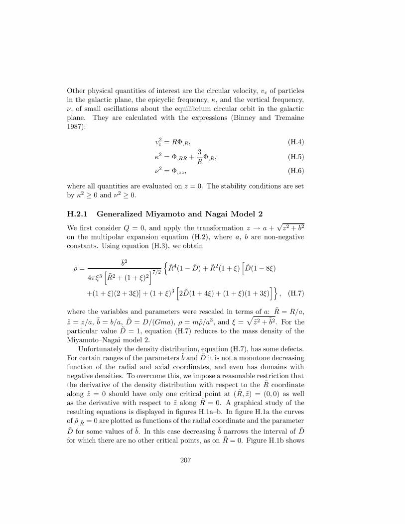
Other physical quantities of interest are the circular velocity, vc of particlesin the galactic plane, the epicyclic frequency, κ, and the vertical frequency,ν, of small oscillations about the equilibrium circular orbit in the galacticplane. They are calculated with the expressions (Binney and Tremaine1987):

v2c = RΦ,R, (H.4)

κ2 = Φ,RR +3

RΦ,R, (H.5)

ν2 = Φ,zz, (H.6)

where all quantities are evaluated on z = 0. The stability conditions are setby κ2 ≥ 0 and ν2 ≥ 0.

H.2.1 Generalized Miyamoto and Nagai Model 2

We first consider Q = 0, and apply the transformation z → a +√z2 + b2

on the multipolar expansion equation (H.2), where a, b are non-negativeconstants. Using equation (H.3), we obtain

ρ =b2

4πξ3[

R2 + (1 + ξ)2]7/2

R4(1 − D) + R2(1 + ξ)[

D(1 − 8ξ)

+(1 + ξ)(2 + 3ξ)] + (1 + ξ)3[

2D(1 + 4ξ) + (1 + ξ)(1 + 3ξ)]

, (H.7)

where the variables and parameters were rescaled in terms of a: R = R/a,

z = z/a, b = b/a, D = D/(Gma), ρ = mρ/a3, and ξ =√

z2 + b2. For theparticular value D = 1, equation (H.7) reduces to the mass density of theMiyamoto–Nagai model 2.

Unfortunately the density distribution, equation (H.7), has some defects.For certain ranges of the parameters b and D it is not a monotone decreasingfunction of the radial and axial coordinates, and even has domains withnegative densities. To overcome this, we impose a reasonable restriction thatthe derivative of the density distribution with respect to the R coordinatealong z = 0 should have only one critical point at (R, z) = (0, 0) as wellas the derivative with respect to z along R = 0. A graphical study of theresulting equations is displayed in figures H.1a–b. In figure H.1a the curvesof ρ,R = 0 are plotted as functions of the radial coordinate and the parameter

D for some values of b. In this case decreasing b narrows the interval of Dfor which there are no other critical points, as on R = 0. Figure H.1b shows

207

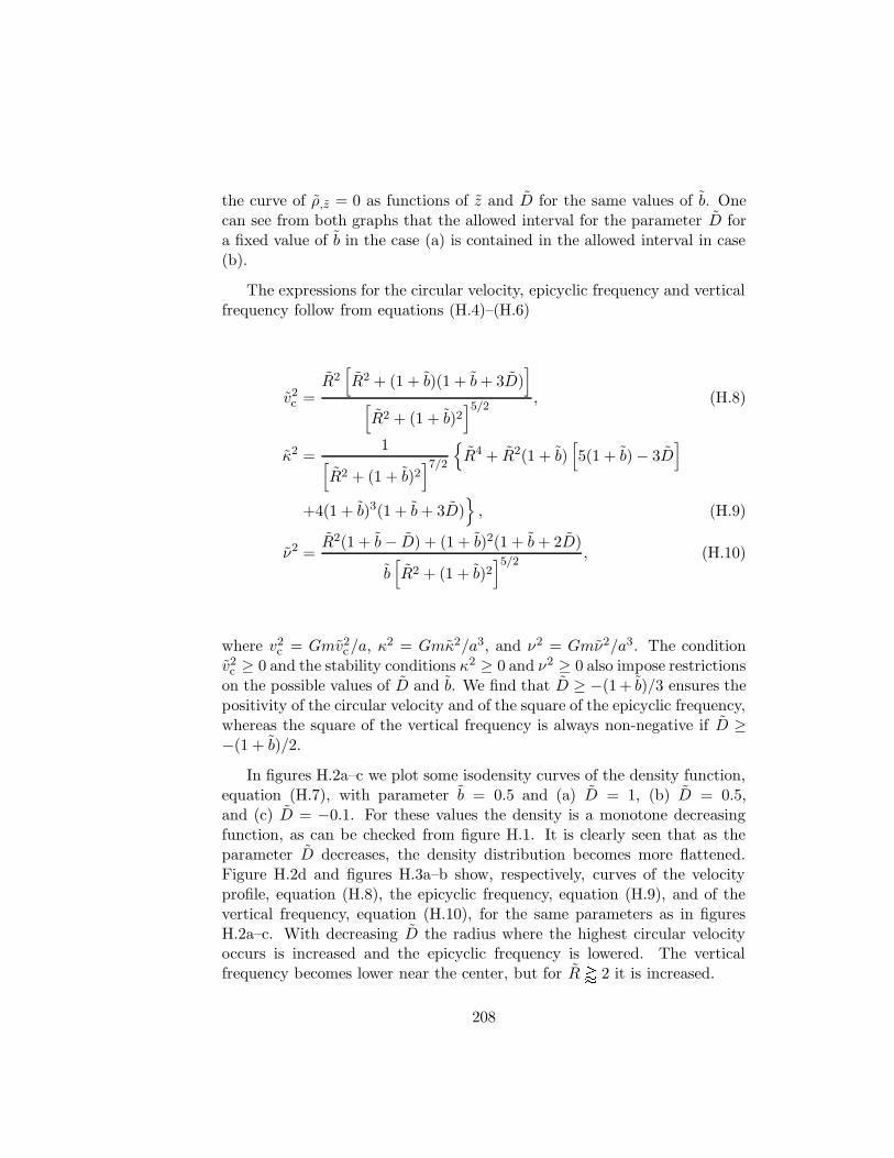
the curve of ρ,z = 0 as functions of z and D for the same values of b. Onecan see from both graphs that the allowed interval for the parameter D fora fixed value of b in the case (a) is contained in the allowed interval in case(b).

The expressions for the circular velocity, epicyclic frequency and verticalfrequency follow from equations (H.4)–(H.6)

v2c =

R2[

R2 + (1 + b)(1 + b+ 3D)]

[

R2 + (1 + b)2]5/2

, (H.8)

κ2 =1

[

R2 + (1 + b)2]7/2

R4 + R2(1 + b)[

5(1 + b) − 3D]

+4(1 + b)3(1 + b+ 3D)

, (H.9)

ν2 =R2(1 + b− D) + (1 + b)2(1 + b+ 2D)

b[

R2 + (1 + b)2]5/2

, (H.10)

where v2c = Gmv2

c/a, κ2 = Gmκ2/a3, and ν2 = Gmν2/a3. The condition

v2c ≥ 0 and the stability conditions κ2 ≥ 0 and ν2 ≥ 0 also impose restrictions

on the possible values of D and b. We find that D ≥ −(1 + b)/3 ensures thepositivity of the circular velocity and of the square of the epicyclic frequency,whereas the square of the vertical frequency is always non-negative if D ≥−(1 + b)/2.

In figures H.2a–c we plot some isodensity curves of the density function,equation (H.7), with parameter b = 0.5 and (a) D = 1, (b) D = 0.5,and (c) D = −0.1. For these values the density is a monotone decreasingfunction, as can be checked from figure H.1. It is clearly seen that as theparameter D decreases, the density distribution becomes more flattened.Figure H.2d and figures H.3a–b show, respectively, curves of the velocityprofile, equation (H.8), the epicyclic frequency, equation (H.9), and of thevertical frequency, equation (H.10), for the same parameters as in figuresH.2a–c. With decreasing D the radius where the highest circular velocityoccurs is increased and the epicyclic frequency is lowered. The verticalfrequency becomes lower near the center, but for R 2 it is increased.

208

-2

-1.5

-1

-0.5

0

0.5

1

1.5

2

0 2 4 6 8 10

D~

R~

(a)

b~

=2.0

b~

=1.0

b~

=0.5

b~

=0.1

-1.8

-1.6

-1.4

-1.2

-1

-0.8

-0.6

-0.4

-4 -3 -2 -1 0 1 2 3 4

D~

z~

(b)

b~

=2.0

b~

=1.0

b~

=0.5

b~

=0.1

Figure H.1: (a) Curves of ρ,R = 0 as functions of R and D for b = 2, 1, 0.5,

and 0.1. (b) ρ,z = 0 as functions of z and D for b = 2, 1, 0.5, and 0.1.

209

0 2 4 6 8−4

−2

0

2

4

R~

z~

(a)

2E−4

1E−3

0.01

0.05

0 2 4 6 8−4

−2

0

2

4

R~

z~

(b)

2E−4

1E−3

0.01

0.05

0 2 4 6 8−4

−2

0

2

4

R~

z~

(c)

2E−4

1E−3

0.01

0.05

D=1 ~

D=0.5 ~

D=−0.1~

0 1 2 3 4 50

0.2

0.4

0.6

R~

v~

(d)

c

Figure H.2: Constant-density curves of equation (H.7) with parameters b =0.5 and (a) D = 1, (b) D = 0.5, and (c) D = −0.1. (d) The circular velocityvc (equation (H.8)), in the galactic plane for cases (a)–(c).

D=1 ~

D=0.5 ~

D=−0.1~

0 1 2 3 4 50

0.5

1

1.5

2

R~

κ∼

(a)

D=1 ~

D=0.5 ~

D=−0.1~

0 1 2 3 4 50

0.5

1

1.5

R~

ν∼

(b)

Figure H.3: Curves of (a) the epicyclic frequency, κ (equation (H.9)), and(b) the vertical frequency, ν (equation (H.10)), for the same parameters asin figure H.2.

210

H.2.2 Generalized Miyamoto and Nagai Model 3

We now consider the full expression equation (H.2) and apply the transfor-mation z → a+

√z2 + b2. The resulting mass density distribution reads

ρ =b2

8πξ3[

R2 + (1 + ξ)2]9/2

2R6(1 − D) + 3R4[

2(1 + ξ)3 − 6Dξ(1 + ξ)

−3Q]

+ 3R2(1 + ξ)2[

2(1 + ξ)2(1 + 2ξ) + 2D(1 + ξ) − Q(1 + 25ξ)]

+2(1 + ξ)4[

(1 + ξ)2(1 + 3ξ) + 2D(1 + ξ)(1 + 4ξ) + 3Q(1 + 5ξ)]

, (H.11)

where the variables and parameters have been rescaled, as in subsectionH.2.1 and Q = Q/(Gma2). For particular values D = 1, Q = 2/3 werecover the Miyamoto and Nagai model 3.

Also here the range of the parameters must be restricted to producephysically acceptable density distributions. In figures H.4a–b we show, re-spectively, some curves of ρ,R = 0 along z = 0 and ρ,z = 0 along R = 0

as functions of Q for some sets of values of D and b. The expressions forthe circular velocity, epicyclic frequency and vertical frequency follow fromequations (H.4)–(H.6)

v2c =

R2

2[

R2 + (1 + b)2]7/2

2R4 + R2[

4(1 + b)2 + 6D(1 + b) − 3Q]

+2(1 + b)2[

(1 + b)2 + 3D(1 + b) + 6Q]

, (H.12)

κ2 =1

2[

R2 + (1 + b)2]9/2

2R6 + 3R4[

4(1 + b)2 − 2D(1 + b) + Q]

+18R2(1 + b)2[

(1 + b)2 + D(1 + b) − 3Q]

+8(1 + b)4[

(1 + b)2 + 3D(1 + b) + 6Q]

, (H.13)

ν2 =1

2b[

R2 + (1 + b)2]7/2

2R4(1 + b− D) + R2(1 + b)[

4(1 + b)2

+2D(1 + b) − 9Q]

+ 2(1 + b)3[

(1 + b)2 + 2D(1 + b) + 3Q]

, (H.14)

A graphical analysis of the constraints on the parameters imposed by v2c ≥ 0,

κ2 ≥ 0 and ν2 ≥ 0 shows that they are contained in the restrictions imposedby the gradient of the mass density.

211

-2

-1.5

-1

-0.5

0

0.5

1

1.5

2

0 1 2 3 4 5 6 7

Q~

R~

(a)

b~

=0.5, D~

=1.0

b~

=0.5, D~

=0.5

b~

=0.5, D~

=0

b~

=0.5, D~

= - 0.5

b~

=0.5, D~

= - 1.0

b~

=0.1, D~

=1.0

b~

=0.1, D~

=0.5

b~

=0.1, D~

=0

b~

=0.1, D~

= - 0.5

b~

=0.1, D~

= - 1.0

-2

-1.5

-1

-0.5

0

0.5

-4 -3 -2 -1 0 1 2 3 4

Q~

z~

(b)

b~

=0.5, D~

=1.0

b~

=0.5, D~

=0.5

b~

=0.5, D~

=0.0

b~

=0.5, D~

= -0.5

b~

=0.5, D~

= -1.0

b~

=0.1, D~

=1.0

b~

=0.1, D~

=0.5

b~

=0.1, D~

=0.0

b~

=0.1, D~

= -0.5

b~

=0.1, D~

= -1.0

Figure H.4: (a) Curves of ρ,R = 0 as functions of R and Q for some values

of the parameters b and D. (b) Curves of ρ,z = 0 as functions of z and Qfor some values of the parameters b and D.

212

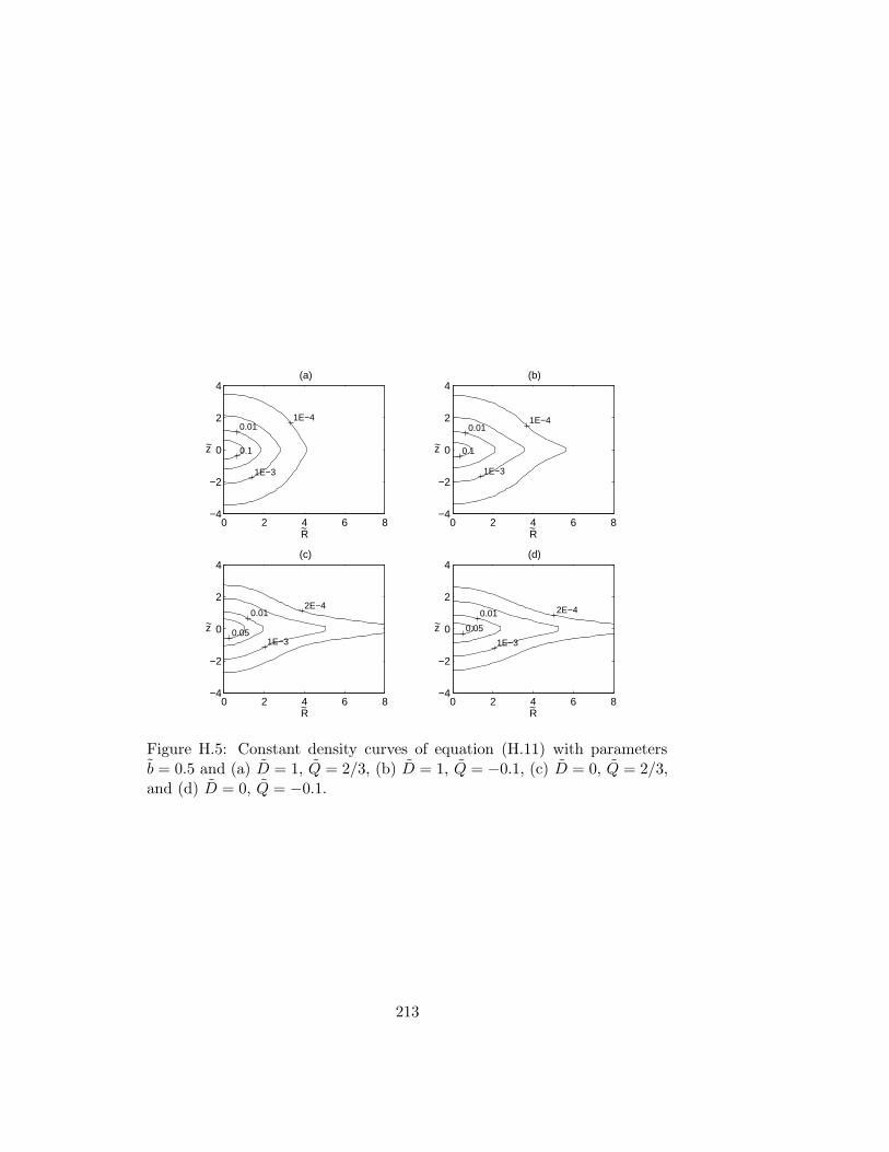
0 2 4 6 8−4

−2

0

2

4

R~

z~

(a)

1E−4

1E−3

0.01

0.1

0 2 4 6 8−4

−2

0

2

4

R~

z~

(b)

1E−4

1E−3

0.01

0.1

0 2 4 6 8−4

−2

0

2

4

R~

z~

(c)

2E−4

1E−3

0.01

0.05

0 2 4 6 8−4

−2

0

2

4

R~

z~

(d)

2E−4

1E−3

0.01

0.05

Figure H.5: Constant density curves of equation (H.11) with parametersb = 0.5 and (a) D = 1, Q = 2/3, (b) D = 1, Q = −0.1, (c) D = 0, Q = 2/3,and (d) D = 0, Q = −0.1.

213

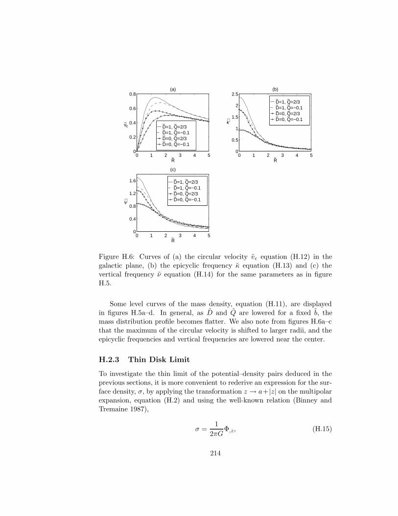
D=1, Q=2/3 ~ ~

D=1, Q=−0.1~ ~

D=0, Q=2/3 ~ ~

D=0, Q=−0.1~ ~

0 1 2 3 4 50

0.2

0.4

0.6

0.8

R~

v~

(a)

c

D=1, Q=2/3 ~ ~

D=1, Q=−0.1~ ~

D=0, Q=2/3 ~ ~

D=0, Q=−0.1~ ~

0 1 2 3 4 50

0.5

1

1.5

2

2.5

R~

κ∼

(b)

D=1, Q=2/3 ~ ~

D=1, Q=−0.1~ ~

D=0, Q=2/3 ~ ~

D=0, Q=−0.1~ ~

0 1 2 3 4 50

0.4

0.8

1.2

1.6

R~

ν∼

(c)

Figure H.6: Curves of (a) the circular velocity vc equation (H.12) in thegalactic plane, (b) the epicyclic frequency κ equation (H.13) and (c) thevertical frequency ν equation (H.14) for the same parameters as in figureH.5.

Some level curves of the mass density, equation (H.11), are displayedin figures H.5a–d. In general, as D and Q are lowered for a fixed b, themass distribution profile becomes flatter. We also note from figures H.6a–cthat the maximum of the circular velocity is shifted to larger radii, and theepicyclic frequencies and vertical frequencies are lowered near the center.

H.2.3 Thin Disk Limit

To investigate the thin limit of the potential–density pairs deduced in theprevious sections, it is more convenient to rederive an expression for the sur-face density, σ, by applying the transformation z → a+ |z| on the multipolarexpansion, equation (H.2) and using the well-known relation (Binney andTremaine 1987),

σ =1

2πGΦ,z, (H.15)

214

where the right-hand side is evaluated at z → 0+. We obtain

σ =1

4π(R2 + 1)7/2

[

2(R2 + 1)2(1 − D) + 6D(R2 + 1) − 3Q(3R2 − 2)]

.

(H.16)

The variables and parameters were rescaled as in subsection H.2.2, andσ = mσ/a2. In particular cases with D = 1, Q = 0 and D = 1, Q = 2/3 weobtain Toomre’s models 2 and 3, respectively (Toomre 1963). Expressionsfor the circular velocity and epicyclic frequency are given by equation (H.12)and equation (H.13) with b = 0, and the vertical frequency is calculated fromequation (H.6) evaluated at z → 0+:

ν2 =1

2(R2 + 1)9/2

[

2R6 + 9R4(2D − Q)

+6R2(−1 + D + 12Q) − 4(1 + 3D + 6Q)]

. (H.17)

Figure H.7 shows curves of σ,R = 0 (lines without circles) and ν = 0 (lines

with circles) as functions of Q and R for some values of the parameter D.In the thin limit, the disks always have regions of vertical instability. TheKuzmin disk (D = Q = 0) is stable for R ≥

√2; Toomre’s model 2 (D = 1,

Q = 0) is stable for R ≥√

2√

−2 +√

6; if Q = 0 the disk is stable for

R ≥√

2

2

[

1 − 9D +

√

3(27D2 + 2D + 3)

]1/2

(H.18)

if D ≥ −1/3; and

0 ≤ R ≤√

2

2

[

1 − 9D −√

3(27D2 + 2D + 3)

]1/2

, (H.19)

and R ≥√

2

2

[

1 − 9D +

√

3(27D2 + 2D + 3)

]1/2

(H.20)

if D < −1/3.In figure H.8 we plot some curves of the surface density equation (H.16),

the circular frequency equation (H.12) with b = 0, the epicyclic frequencyequation (H.13) also with b = 0 and the vertical frequency equation (H.17)for some values of D and Q. The behaviour of the three first physical quan-tities, displayed as the multipole parameters are decreased, is very similarto those of the thick-disk model of the previous section.

215

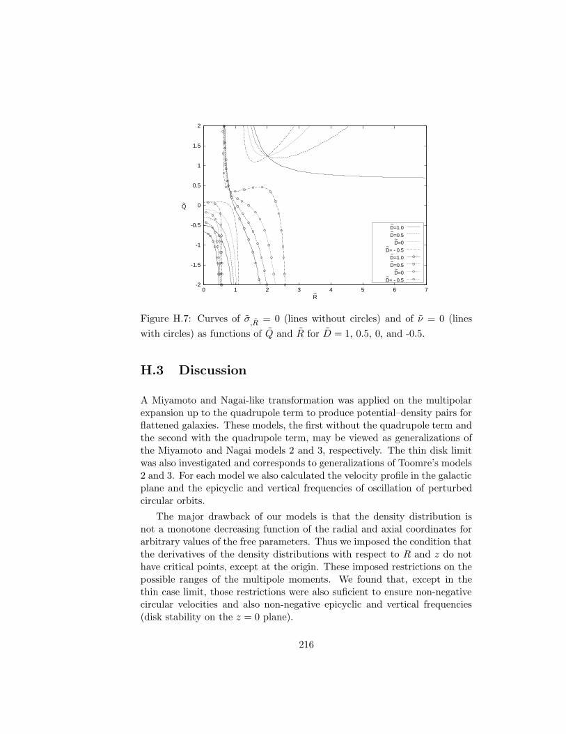
-2

-1.5

-1

-0.5

0

0.5

1

1.5

2

0 1 2 3 4 5 6 7

Q~

R~

D~

=1.0

D~

=0.5

D~

=0

D~

= - 0.5

D~

=1.0

D~

=0.5

D~

=0

D~

= - 0.5

Figure H.7: Curves of σ,R = 0 (lines without circles) and of ν = 0 (lines

with circles) as functions of Q and R for D = 1, 0.5, 0, and -0.5.

H.3 Discussion

A Miyamoto and Nagai-like transformation was applied on the multipolarexpansion up to the quadrupole term to produce potential–density pairs forflattened galaxies. These models, the first without the quadrupole term andthe second with the quadrupole term, may be viewed as generalizations ofthe Miyamoto and Nagai models 2 and 3, respectively. The thin disk limitwas also investigated and corresponds to generalizations of Toomre’s models2 and 3. For each model we also calculated the velocity profile in the galacticplane and the epicyclic and vertical frequencies of oscillation of perturbedcircular orbits.

The major drawback of our models is that the density distribution isnot a monotone decreasing function of the radial and axial coordinates forarbitrary values of the free parameters. Thus we imposed the condition thatthe derivatives of the density distributions with respect to R and z do nothave critical points, except at the origin. These imposed restrictions on thepossible ranges of the multipole moments. We found that, except in thethin case limit, those restrictions were also suficient to ensure non-negativecircular velocities and also non-negative epicyclic and vertical frequencies(disk stability on the z = 0 plane).

216

D=1, Q=0 ~ ~

D=1, Q=−0.25 ~ ~

D=0.5, Q=0 ~ ~

D=0.5, Q=−0.25~ ~

0 1 2 3 4 50

0.1

0.2

0.3

0.4

0.5

R~

σ∼

(a)

D=1, Q=0 ~ ~

D=1, Q=−0.25 ~ ~

D=0.5, Q=0 ~ ~

D=0.5, Q=−0.25~ ~

0 1 2 3 4 50

0.2

0.4

0.6

0.8

1

R~

v~

(b)

c

D=1, Q=0 ~ ~

D=1, Q=−0.25 ~ ~

D=0.5, Q=0 ~ ~

D=0.5, Q=−0.25~ ~

0 1 2 3 4 50

1

2

3

4

R~

κ∼

(c)

D=1, Q=0 ~ ~

D=1, Q=−0.25 ~ ~

D=0.5, Q=0 ~ ~

D=0.5, Q=−0.25~ ~

0 1 2 3 4 50

0.1

0.2

0.3

0.4

0.5

0.6

R~

ν∼

(d)

Figure H.8: (a) Curves of the surface density equation (H.16), (b) the circu-lar velocity equation (H.12) with b = 0, (c) the epicyclic frequency equation(H.13) with b = 0 and the vertical frequency equation (H.17). Parameters:D = 1, Q = 0 (solid lines); D = 1, Q = −0.25 (dashed lines); D = 0.5,Q = 0 (lines with points); D = 0.5, Q = −0.25 (lines with +).

217

D. Vogt thanks CAPES for financial support. P. S. Letelier thanks CNPqand FAPESP for financial support. This research has made use of NASA’sAstrophysics Data System.

References

Bicak, J., Lynden-Bell, D., & Katz, J. 1993, Phys. Rev. D, 47, 4334Binney, S., & Tremaine, S. 1987, Galactic Dynamics (Princeton, PrincetonUniversity Press), p. 121de Zeeuw, T., & Pfenniger, D. 1988, MNRAS, 235, 949Gonzalez, G. A., & Letelier, P. S. 2000, Phys. Rev. D, 62, 064025Gonzalez, G. A., & Letelier, P. S. 2004, Phys. Rev. D, 69, 044013Hernquist, L. 1990, ApJ, 356, 359Jaffe, W. 1983, MNRAS, 202, 995Lemos, J. P. S., & Letelier, P. S. 1994, Phys. Rev. D, 49, 5135Long, K., & Murali, C. 1992, ApJ, 397, 44Miyamoto, M., & Nagai, R. 1975, PASJ 27, 533Morgan, L., & Morgan, T. 1970, Phys. Rev. D, 2, 2756Morgan, T., & Morgan, L. 1969, Phys. Rev., 183, 1097Satoh, C. 1980, PASJ, 32, 41Toomre, A. 1963, ApJ, 138, 385Vogt, D., & Letelier, P. S. 2003, Phys. Rev. D, 68, 084010Vogt, D., & Letelier, P. S. 2005a, Phys. Rev. D, 71, 084030Vogt, D., & Letelier, P. S. 2005b, MNRAS, 363, 268

218

Livros Grátis( http://www.livrosgratis.com.br )

Milhares de Livros para Download: Baixar livros de AdministraçãoBaixar livros de AgronomiaBaixar livros de ArquiteturaBaixar livros de ArtesBaixar livros de AstronomiaBaixar livros de Biologia GeralBaixar livros de Ciência da ComputaçãoBaixar livros de Ciência da InformaçãoBaixar livros de Ciência PolíticaBaixar livros de Ciências da SaúdeBaixar livros de ComunicaçãoBaixar livros do Conselho Nacional de Educação - CNEBaixar livros de Defesa civilBaixar livros de DireitoBaixar livros de Direitos humanosBaixar livros de EconomiaBaixar livros de Economia DomésticaBaixar livros de EducaçãoBaixar livros de Educação - TrânsitoBaixar livros de Educação FísicaBaixar livros de Engenharia AeroespacialBaixar livros de FarmáciaBaixar livros de FilosofiaBaixar livros de FísicaBaixar livros de GeociênciasBaixar livros de GeografiaBaixar livros de HistóriaBaixar livros de Línguas

Baixar livros de LiteraturaBaixar livros de Literatura de CordelBaixar livros de Literatura InfantilBaixar livros de MatemáticaBaixar livros de MedicinaBaixar livros de Medicina VeterináriaBaixar livros de Meio AmbienteBaixar livros de MeteorologiaBaixar Monografias e TCCBaixar livros MultidisciplinarBaixar livros de MúsicaBaixar livros de PsicologiaBaixar livros de QuímicaBaixar livros de Saúde ColetivaBaixar livros de Serviço SocialBaixar livros de SociologiaBaixar livros de TeologiaBaixar livros de TrabalhoBaixar livros de Turismo