Thiago Pinheiro da Silva Enhanced fluid rheology ...€¦ · March 2016 . PUC-Rio - Certificação...

Thiago Pinheiro da Silva

Enhanced fluid rheology characterization for Managed Pressure Drilling

Dissertação de Mestrado

Dissertation presente to the Programa de Pós-graduação em Engenharia Mecânica of the Departamento de Engenharia Mecânica, PUC-Rio as partial fulfillment of the requirements for the degree of Mestre em Engenharia Mecânica.

Advisor: Profa. Mônica Feijó Naccache

Rio de Janeiro March 2016

DBD

PUC-Rio - Certificação Digital Nº 1412759/CA


Enhanced fluid rheology characterization for Managed

Pressure Drilling

Dissertation presented to the Programa de Pós-Graduação em Engenharia Mecânica of the Departamento de Engenharia Mecânica do Centro Técnico Cientifico da PUC-Rio, as partial fulfillment of the requirements for the degree of Mestre.

Profa. Mônica Feijó Naccache Advisor

Departamento de Engenharia Mecânica – PUC-Rio

Dr. Sidney Stuckenbruck Olympus Software Científico e Engenharia Ltda. - OLYMPUS

Dr. Antonio Carlos Vieira Martins Lage Petróleo Brasileiro

Márcio da Silveira Carvalho Coordinador of the Centro Técnico Científico da PUC-Rio

Rio de Janeiro, March 17th, 2016

DBD


All rights reserved


He graduated in Mechanical Engineering from the Federal

University of Itajubá in 2003. He has over 13 years of

professional experience in the oil industry with emphasis on

Underbalanced Drilling (UBD), Coiled Tubing Drilling (CTD)

and Managed Pressure Drilling (MPD) working in more than

20 countries. He is currently a consultant for new technologies

and a project manager for Blade Energy Partners Ltd. He’s a

Member of the Society of Petroleum Engineers (SPE) and a

guest instructor at the Federal University of Itajubá within the

Human Resources program of the National Petroleum Agency

(ANP).

Bibliografic data

CDD: 621

Silva, Thiago Pinheiro da Enhanced fluid rheology characterization for managed pressure drilling / Thiago Pinheiro da Silva ; advisor: Mônica Feijó Naccache. – 2016. (em Inglês) 114 f. ; 30 cm Dissertação (mestrado)–Pontifícia Universidade Católica do Rio de Janeiro, Departamento de Engenharia Mecânica, 2016.

Inclui bibliografia 1. Engenharia Mecânica – Teses. 2. MPD. 3. Perfuração com gerenciamento de pressão. 4. Reologia. 5. Caracterização de Fluido. I. Naccache, Mônica Feijó. II. Pontifícia Universidade Católica do Rio de Janeiro. Departamento de Engenharia Mecânica. III. Título. (em português)

DBD


To my family, Ana Gabriela, Maria Cecilia and Helena, thank

you for believing in me and supporting me at all times and in all

circumstances, making my dream a reality. I am grateful for the

support, care and love. I love you.

DBD


Acknowledgments

Above all, I’d like to thank God. Because of my faith, it allows me to believe that

everything is possible.

I’d also like to thank Blade Energy Partners for providing the opportunity, technical

support and financial support for me to participate in this program.

The Rheological Characterization Laboratory at PUC-Rio and friends there have

given me some (several) hours of conversations, ideas and experiences regarding

the characterization of fluids. In particular, I’d like to thank the student of chemical

engineering, Carolina Dias Grossi, for technical support, which was of fundamental

importance, showing patience and remaining calm even when everything seemed

to go wrong.

To Victor Meléndez Rock-Fluid Interaction Laboratory (LIRF PUC-Rio) for the

availability and aid in the characterization of fluids.

To CENPES and Petrobras also for providing the necessary equipment in this work.

To my friends, Antonio Lage and Emmanuel Franco Nogueira for their

recommendation.

To my teacher and supervisor, Monica Feijo Naccache for believing in the proposal

and the project and her masterful guidance so that the objectives were achieved.

To PUC-Rio, for the knowledge acquired during these two years.

To Rio de Janeiro, for welcoming me and my family.

To my parents and sister, who cheered me on every step of the way and always gave

me positive encouragement.

Finally, I would like to especially thank my wife and friend Ana Gabriela, for

making my dream our dream, to be next to me in the best and worst moments of my

life, and endure with love and patience all the time and effort devoted to obtaining

this title.

After completing this study it is clear to me that I would not have gone so far without

the help of you and many others. As the popular African saying goes, "If you want

to go quickly, go alone. If you want to go far, go together."

My sincere thanks to all of you.

DBD


Abstract

Silva, Thiago Pinheiro da; Naccache, Mônica Feijó (Advisor). Enhanced

fluid rheology characterization for Managed Pressure Drilling. Rio de

Janeiro, 2016. 114p. MSc. Dissertation – Departamento de Engenharia

Mecânica, Pontifícia Universidade Católica do Rio de Janeiro.

Enhanced fluid rheology characterization for Manage Pressure Drilling.

Hydraulics play an important role in many oil field operations including drilling,

completion, fracturing, acidizing, workover and production. In Managed Pressure

Drilling (MPD) applications, where pressure losses become critical to accurately

estimate and control the well within the operational window, it is necessary to use

the correct rheology for a precise mathematical modelling of fluid behavior. The

standard API methods for drilling fluid hydraulics employ Herschel-Bulkley (H-

B), Power Law (PL) or Bingham plastic as rheological models. This work

summarizes the results of an extensive study on issues and relevant aspects related

to the equipment and methods used to characterize the drilling fluids for MPD

applications, as well as the operational implications that diverge from conventional

practices. A comparison of fluid rheology characterization is made using high

precision rheometers versus conventional FANN35 methods. Subsequently, a

comparison of rheology model selection proposed by API 13B and by Non Linear

Regression (NLR) is presented. Further investigation of shear rate ranges is

presented in a MPD “typical” annular geometry. Results obtained via

Computational Fluid Dynamics (CFD), and with the formulas suggested in API RP

13D are compared. To conclude, the effects of measurements, data treatment

(Curve Fit), and environment (laboratory observations versus field experiences) in

the accuracy of fluid rheology characterization and annulus pressure loss estimation

are presented and discussed.

Keywords

MPD; Managed Pressure Drilling; Rheology; Fluid Characterization.

DBD


Resumo

Silva, Thiago Pinheiro da; Naccache, Mônica Feijó. Caracterização

Reológica de Fluidos para Perfuração com Gerenciamento de Pressão.

Rio de Janeiro, 2016. 114p. Dissertação de Mestrado – Departamento de

Engenharia Mecânica, Pontifícia Universidade Católica do Rio de Janeiro.

Caracterização Reológica de Fluidos para Perfuração com Gerenciamento de

Pressão. Forças Hidráulicas desempenham uma função importante em muitas

operações de campo de petróleo, incluindo perfuração, completação, fraturamento,

acidificação, workover e produção. Em aplicações de Perfuração com

Gerenciamento de Pressão (Managed Pressure Drilling - MPD), onde as

estimativas de perdas de pressão são críticas para controlar o poço dentro da janela

de operacional, é necessário utilizar a reologia correta para a modelagem

matemática precisa do comportamento do fluido. Os métodos API (American

Petroleum Institute) empregam para os cálculos de hidráulica os modelos

reológicos de Herschel-Bulkley (H-B), Power Law (PL) ou plástico de Bingham.

Este trabalho resume os resultados de um estudo aprofundado sobre as questões e

os aspectos relevantes relacionados com o equipamento e os métodos utilizados

para caracterizar os fluidos de perfuração para aplicações MPD, bem como as

implicações operacionais que divergem das práticas convencionais. Uma

comparação da caracterização reológica de fluídos é feita usando reômetros de alta

precisão contra métodos convencionais tais como o viscosímetro FANN35.

Subsequentemente, é apresentada uma comparação da seleção do modelo reológico

proposto por API 13B em contrapartida com o método de Regressão Não Linear

(NLR). Investigações detalhadas das faixas de taxas de cisalhamento são

apresentadas para geometrias de um poço anular MPD "típico", calculadas através

de Dinamica de Fluidos Computacional (CFD) e comparadas com as fórmulas

sugeridas na API RP 13D. Para concluir, é apresentada uma discussão sobre os

efeitos das medições, do tratamento de dados (Curve Fit) e do meio ambiente

(observações de laboratório em comparação com experiências de campo) na

precisão da obtenção da reologia do fluido e as consequências na estimativa das

perdas de carga no anular.

Palavras-chave

MPD; Perfuração com Gerenciamento de Pressão; Reologia; Caracterização

de Fluido.

DBD


Contents

1 Introduction 19

1.1. Managed Pressure Drilling Concept 20

1.1.1. Pressure Gradients 21

1.2. Controlling BHP 24

1.3. Literature Review 24

2 Aspects and Issues of Managed Pressure Drilling Connections 27

2.1. Hydraulic Simulations determines Applied Surface Back Pressure 28

2.1.1. MPD Industry Software 29

2.2. Rheology Measurements: Equipment 31

2.2.1. FANN - Model 35 Viscometer [19] 31

2.2.2. Rheometer Geometry Considerations 32

2.2.3. Shear Rate Operating Range – FANN 35 speeds 34

3 The Thought 35

3.1. The Motivation 35

3.2. Thesis Objectives 35

3.3. Scope of Work & Methodology 36

4 Industry Practices, Equipment and Standards 39

4.1. Drilling Fluid Characterization according Recommended Practice

for Field Testing Water-based Drilling Fluids - ANSI/API RP 13B-1 39

4.2. API Recommended Practice 13D — Rheology and hydraulics of

oilwell drilling fluids 40

4.2.1. API RP 13 D - Clause 4 -Fundamentals and fluid models 40

4.2.2. API RP 13 D - Clause 5 - Determination of Drilling Fluid

Rheological Parameters 42

4.2.2.1. Herschel-Bulkley Rheological Model 42

4.2.2.1.1. Solution Methods for H-B Fluid Parameters 43

4.2.2.2. Other rheological models used in API 13 D 44

4.2.3. API RP 13 D - Clause 7 - Pressure-loss modeling 44

4.2.3.1. Shear Rate at the Wall 45

4.2.3.2. Flow regime: Reynolds number (generalized) 47

4.2.3.3. Critical Reynolds number (laminar to transitional regimes) 47

4.2.3.4. Friction factor 48

4.2.3.5. Laminar-flow pressure loss 48

4.2.3.5.1. Laminar-flow pressure loss (special case) 48

4.3. Standard Oilfield Viscometer Correction Factors 49

5 Fluid Characterization 50

5.1. Fluids Selection and Preparation 50

5.1.1. Fluid Selection Criteria 50

DBD


5.1.1.1. Viscosity Range and Concentration Criteria 50

5.1.2. Xanthan Gum preparation 51

5.2. Measurements of Rheological Properties 54

5.2.1. Equipment and Laboratories 54

5.2.2. Tests and Methodology 55

5.2.3. Rheology Measurements Results 56

5.2.3.1. Steady Flow Time Tests 56

5.2.3.2. Flow Curve Tests 57

5.2.3.3. Evaluation of FANN 35 Performance 60

5.2.3.4. Representativeness of Chosen Fluid Samples 62

5.3. Drilling Fluid Model Characterization 63

5.3.1. Curve Fitting Influence 63

5.3.2. Solving the Rheological Parameters with Nonlinear Regression 63

5.3.2.1. Xanthan Gum 0.8% 65

5.3.2.1.1. “Test #1 - PP50/P2(Cross Hatch) - Anton Paar - Physica

MCR 301” 65

5.3.2.1.2. “Test #2 - PP50/P2(Cross Hatch) - Anton Paar - Physica

MCR 301” 66

5.3.2.1.3. “Fann 35 - PUC - F1 B1 R1” 67

5.3.2.2. Low Lime WBM 68

5.3.2.2.1. Test #1 - PP50/P2(Cross Hatch) - Anton Paar - Physica

MCR 301 68

5.3.2.2.2. Test #2 - PP50/P2 (Cross Hatch) - Anton Paar - Physica

MCR 301 69

5.3.2.2.3. Test #1 - “Fann 35 - PUC - F1 B1 R1” 70

5.3.2.2.4. Test #2 - “Fann 35 - PUC - F1 B1 R1” 71

5.3.3. Solving the Rheological Parameters: API RP 13 D - Clause 5 71

5.3.4. Curve Fitting & Model Selection 73

5.3.4.1. Accuracy of the process 77

6 Mapping Shear Rate 80

6.1. Fluid Properties Selection 80

6.2. Geometry Selection 80

6.3. Flow Rate Selection 81

6.4. Shear Rate and Shear Stress Calculations as per API 13 D 82

7 Validating the Shear Rate Map: CFD Numerical Verification 86

7.1. About ANSYS Fluent 86

7.2. Computational Fluid Dynamics Setup 87

7.2.1. Solver and Solution Methods 87

7.2.1.1. Pressure Based Solver 87

7.2.1.2. General Scalar Transport Equation Setup – Solution Methods 88

7.2.1.2.1. Discretization (Interpolation Method) 90

7.2.1.2.2. Interpolation Method - Gradients 90

DBD


7.2.1.2.3. Interpolation Methods for Face Pressure 91

7.3. Critical Shear Rate Selection for Non-Newtonian Fluids 91

7.4. Geometry and Meshing Considerations 94

7.5. Physics and Boundaries 95

7.6. Convergence Criteria & Monitoring 96

7.7. CFD ANSYS Fluent: Shear Rates Mapping Cases 99

7.7.1. Influence of Hydraulics and Environment: Results 101

8 Pressure Losses Estimations 103

8.1. Case (a): “8.5 Section” 103

8.2. Case (b): “12.25 Section” 104

9 Recommendations and Conclusions 107

10 Bibliographic References 109

APPENDIX A API 13 D Method - Results 112

APPENDIX B CFD by ANSYS Fluent - Results 113

DBD


List of Figures Figure 1 - The blowout at Spindletop 19

Figure 2 - Conventional drilling fluid gradients & casing setting points. 22

Figure 3 - MPD fluid gradients and drilling window. 23

Figure 4 - Pump Step-Down Schedule 27

Figure 5 – Automatic Connection - Ramp Schedule for 12-¼” Section 28

Figure 6 - Automatic Connection - Ramp Schedule for 8-½” Section 28

Figure 7 – Drillbench: Rheology Input User Interface Screen 30

Figure 8 - SafeVision: Rheology Input User Interface Screen 30

Figure 9 – MC2: Rheology Input User Interface Screen 31

Figure 10 – FANN Model 35 Viscometer 32

Figure 11 - Schematic diagram of basic tool geometries for the

rotational rheometer: concentric cylinder 33

Figure 12 - Schematic diagram showing alternative cylindrical

tool design in cut-away view: Double Gap 33

Figure 13 - Brazil MPD Operations Rheogram:

IADC Historical Field Data 51

Figure 14 – Preparation of Xanthan Gum in the Mechanical

Shaker at 300 rpm 53

Figure 15 – Xanthan Gum being stirred 53

Figure 16 – Xanthan Gum bottle samples 54

Figure 17 - Anton Paar - Physica MCR 301 55

Figure 18 - Steady State Flow Behavior Test: Equilibrium time

and Flow Curve Optimization 56

Figure 19 - Flow Curve: Xanthan Gum 0.1% - Shear Stress

vs. Shear Rate 58

Figure 20 - Flow Curve: Xanthan Gum 0.1% - Viscosity vs Shear Rate 58

Figure 21 - Flow Curve: Xanthan Gum 0.8% - Viscosity vs. Shear Rate 59

Figure 22 - Flow Curve: Xanthan Gum 0.8% - Shear Stress

vs Shear Rate 59

Figure 23 - Flow Curve: Low Lime WBM - Viscosity vs. Shear Rate 60

Figure 24 - Flow Curve: Low Lime WBM - Shear Stress vs Shear Rate 60

Figure 25 - Cross Hatch Geometry 61

Figure 26 - Kaleidah Graph NLR – Xanthan Gum 0.8%

- “Test #1 - PP50/P2(Cross Hatch) - Anton Paar - Physica MCR 301” 65

Figure 27 - Kaleidah Graph NLR – Xanthan Gum 0.8%


Figure 28 - Kaleidah Graph NLR – Xanthan Gum 0.8% - “Fann 35

- PUC - F1 B1 R1” 67

Figure 29 - Kaleidah Graph NLR – Low Lime WBM


Figure 30 - Kaleidah Graph NLR – Low Lime WBM


DBD


Figure 31 - Kaleidah Graph NLR – Low Lime WBM - “Fann 35

- PUC - F1 B1 R1” – Test#1 70

Figure 32 - Kaleidah Graph NLR – Low Lime WBM - “Fann 35 -

PUC - F1 B1 R1” – Test#2 71

Figure 33 - Curve Fitting for Low Lime Water Based Mud 73

Figure 34 - Curve Fitting for Xanthan Gum 0.8% 74

Figure 35 – Shear Rate Interval of Interest and Model Selection 75

Figure 36 - Xhantam Gum 0.8% - Power Law Curve Fit Comparison 76

Figure 37 – Curve Fit vs Actual Fluid Properties 78

Figure 38 – Fluid Properties versus Curve Fit Accuracy 79

Figure 39 - Case (a): “8.5 Section” 81

Figure 40 - Case (b): “12.25 Section” 81

Figure 41 – Map of Shear Rate at Wall, according API 13 D – 8.5

and 12.25 Section 84

Figure 42 – FANN 35 Rheogram and “Shear Rate vs Shear Stress

API 13 D Results” 85

Figure 43 - Typical Casing Program and Annulus 85

Figure 44 - Control Volume Example 87

Figure 45 - Transport Equations 88

Figure 46 - Fluent Solution Methods 89

Figure 47 - Fluent Solution Controls 89

Figure 48 - Discretization - Interpolation Methods 90

Figure 49 - Gradients - Interpolation Methods 90

Figure 50 - ANSYS Fluent - Fluid Properties Input Screen (H-B Model) 93

Figure 51 - Critical Shear Rate Selection and Behavior 93

Figure 52 – 2D Mesh Transversal View 94

Figure 53 - Velocity Profile of Newtonian Fluid at 1000 gpm in

the 12.25 Section 95

Figure 54 - Velocity Profile of Non-Newtonian Fluid at 1000 gpm in

the 12.25 Section 95

Figure 55 – Representation of the Annulus Flow: 3D Mesh –

Perspective View 96

Figure 56 - Annulus Flow Development - Case (a) - 400 gpm 97

Figure 57 - Annulus Flow Development - Case (b) - 1000 gpm 97

Figure 58 - Velocity Distribution at Observation Point

(12.25 Section - GX0.8% - Physica NLR) 98

Figure 59 -Strain Rate distribution at Observation Point 98

Figure 60 – Wall Shear Stress at Observation Point 99

Figure 61 - Influence of Hydraulic Modeling: Analytical vs Numerical 99

Figure 62 – Influence of Environment: Field versus Laboratory 100

Figure 63 - Numerical Solution for Shear Rate vs. Flow Rate in

8.5” Section and API13D Comparison 101

Figure 64 - Numerical Solution for Shear Rate vs. Flow Rate in

12.25” Section and API13D Comparison. 102

DBD


Figure 65 - Pressure Loss Estimation: 8.5" Section (case (a)) 104

Figure 66 - Pressure Loss Estimation: 12.25" Section (case (b)) 105

DBD


List of Tables Table 1 - Xamthan Gum 0.1% Recipe 52

Table 2 - Xamthan Gum 0.8% Recipe 52

Table 3 - Xanthan Gum 0.1% - Fann 35 - CENPES - F1 B1 R1

(3 readings average) 62

Table 4 - Xanthan Gum 0.1% - Fann 35 - PUC - F1 B1 R1

(2 readings average) 62

Table 5 - Rheological Parameters: PL Model - NLR Method -

Xanthan Gum 0.8% Test#1 65

Table 6 - Rheological Parameters: H-B Model - NLR Method -







Xanthan Gum 0.8% - Fann 35 PUC 67


Xanthan Gum 0.8% - Fann 35 PUC 67

Table 11 - Rheological Parameters: PL Model - NLR Method –

Low Lime WBM - Test#1 68

Table 12 - - Rheological Parameters: H-B Model - NLR Method –




Table 14 - Rheological Parameters: H-B Model - NLR Method –



Low Lime WBM - “Fann 35 - PUC - F1 B1 R1” – Test#1 70



Table 17 - - Rheological Parameters: PL Model - NLR Method –




Table 19 - Rheological Parameters: PL Model - API RP 13 D

Method- Xanthan Gum 0.8% - Fann 35 PUC 72

Table 20 - Rheological Parameters: H-B Model - API RP 13 D

Method- Xanthan Gum 0.8% - Fann 35 PUC 72

Table 21 – API 13 D Curve Fit Method - Comparison 72

Table 22 – Curve Fitting and Coefficient of Determination Results 77

Table 23 - Annulus Fluid Velocity for 8.5 Section – Case (a) 82

DBD


Table 24 – Annulus Fluid Velocity for 12.25 Section – Case (b) 82

Table 25 – Shear Stress and Shear Rate as per API 13 D

Method - Herschel-Bulkley Model - 8.5 Section. 83

Table 26 - Shear Stress and Shear Rate as per API 13 D Method -

Herschel-Bulkley Model – 12.25 Section 83

Table 27 - API 13 D Method - Herschel-Bulkley Model - 8.5

Section - GX0.8_FANN35 112

Table 28 - API 13 D Method - Herschel-Bulkley Model - 12.25

Section - GX0.8_FANN35 112

Table 29 - Fluent Ansys - Herschel-Bulkley Model - 8.5

Section - GX0.8_FANN35_ɣ.critical 5e-05_1e-10 113


Section - GX0.8_DG#2-NLR_ɣ.critical 5e-05_1e-10 113


Section - GX0.8_FANN35_ɣ.critical 5e-05_1e-10 114


Section - GX0.8_DG#2-NLR_ɣ.critical 5e-05_1e-10 114

DBD


Terms, Definitions, symbols and abbreviations

Symbol Definition Standard Units

Conversion Multiplier SI Units

A Surface area in2 6.4516E+02 mm2

Ba Well geometry correction factor dimensionless - dimensionless

Bx Viscometer geometry correction factor

dimensionless - dimensionless

d Diameter in. 2.54E+01 mm

dh Hole diameter or casing inside diameter

in. 2.54E+01 mm

dhyd Hydraulic diameter in. 2.54E+01 mm

di Pipe internal diameter in. 2.54E+01 mm

dp Pipe outside diameter in. 2.54E+01 mm

ECD Equivalent Circulating Density lbm/gal 1.198264E+02 kg/m3

EMW Equivalent Mud Weight lbm/gal 1.198264E+02 kg/m3

f Fanning friction factor dimensionless - dimensionless

F Force lbf 4.448222E+00 N

flam Friction factor (laminar) dimensionless - dimensionless

ftrans Friction factor (transitional) dimensionless - dimensionless

fturb Friction factor (turbulent) dimensionless - dimensionless

g Acceleration of gravity 32.152 ft/s2 3.048E-01 m/s2

G Geometry shear-rate correction (Herschel-Bulkley fluids


Gp Geometry shear-rate correction (power-law fluids)


K , 𝑘 Consistency factor (Herschel-Bulkley fluids)

lbf•sn/100 ft2 4.78803E-01 Pa•sn

kp Consistency factor (power-law fluids)

lbf•sn/100 ft2 4.78803E-01 Pa•sn

L Length of drillstring or annular segment

ft 3.048E-01 M

N, n Flow behavior index (Herschel-Bulkley fluids)


N Viscometer rotary speed r/min - r/min

np Flow behavior index (power-law fluids)


NRe Reynolds number dimensionless - dimensionless

NReG Generalized Reynolds number dimensionless - dimensionless

NRep Particle Reynolds number dimensionless - dimensionless

P Pressure lbf/in2 6.894757E+00 kPa

Pa Annular pressure loss lbf/in2 6.894757E+00 kPa

PV Plastic Viscosity cP 1.0E-03 Pa•s

Q Flow rate gal/min 6.309.20E-02 dm3/s

Qc Critical flow rate gal/min 6.309.20E-02 dm3/s

R Ratio yield stress / yield point (τy / YP)


Θ100, R100

Viscometer reading at 100 r/min ° deflection - ° deflection

Θ200,

R200 Viscometer reading at 200 r/min ° deflection - ° deflection

Θ3, R3 Viscometer reading at 3 r/min ° deflection - ° deflection

DBD


Θ300

,R300 Viscometer reading at 300 r/min ° deflection - ° deflection

Θ6, R6 Viscometer reading at 6 r/min ° deflection - ° deflection

Θ600,

R600 Viscometer reading at 600 r/min ° deflection - ° deflection

RF Rheology Factor - - -

T Temperature °F (°F-32)/1.8 °C

V Velocity ft/min 5.08E-03 m/s

Va Fluid velocity in annulus ft/min 5.08E-03 m/s

Vc Critical velocity ft/min 5.08E-03 m/s

Vcb Critical velocity (Bingham plastic fluids)

ft/min 5.08E-03 m/s

Vcp Critical velocity (power-law fluids) ft/min 5.08E-03 m/s

Vp Fluid velocity inside pipe ft/min 5.08E-03 m/s

x Viscometer ratio (sleeve radius / bob radius)


YP Yield point lbf/100 ft2 4.788026E-01 Pa

Α Geometry factor dimensionless - dimensionless

γ , ɣ Shear rate s-1 - s-1

γw Shear rate at the wall s-1 - s-1

μ Viscosity cP 1.0E-03 Pa•s

ρ Fluid density lbm/gal 1.198264E+02 kg/m3

τ , 𝝉 Shear stress lbf/100 ft2 4.788026E-01 Pa

τb Shear stress at viscometer bob ° deflection - ° deflection

τi Iterative shear stress in curve-fit method

lbf/100 ft2 4.788026E-01 Pa

τw Shear stress at the wall lbf/100 ft2 4.788026E-01 Pa

τy , 𝝉y Yield stress lbf/100 ft2 4.788026E-01 Pa

DBD


"Ipsa scientia potestas est"

DBD


1 Introduction

Controlling the pressure in a wellbore while drilling for oil or gas is an

operation that draws its roots from Colonel Drake’s Spindletop well drilled in the

late 1800’s. Arguably thought of as the moment which gave rise to the modern

Blow Out Preventer (BOP) and drilling fluid industries, the geyser of oil at

Spindletop graphically demonstrated that geological pressure must be respected

in order to access what lies beneath.

Figure 1 - The blowout at Spindletop

Historically, the most apparent way to control subterranean pressure was to

take advantage of hydrostatics. Altering the density of the drilling fluid, or mud,

allowed the driller to keep those hydrocarbons at bay while drilling and reach the

desired target ‘safely’. Drilling in this manner continued for decades, until three

key characteristics began to emerge:

Reservoir pressures do not remain at ‘virgin’ conditions and eventually

decline below the hydrostatic pressure of even the lightest drilling fluids,

Exerting excessive hydrostatic pressure on a formation could (in some

cases) cause terminal loss of drilling mud, and

Although hydrostatically over-pressuring the reservoir kept hydrocarbons

in place, the exerted pressure on the porous rock had (in some cases)

limited the reservoir’s productive potential through damaging the near

wellbore.

DBD


20

These characteristics, amongst a host of others, prompted the drilling

industry to explore new avenues of annular pressure control. Technological

advances in surface equipment resulted in a host of new terms and acronyms

thrust upon drillers and engineers to describe these new techniques:

Mud Cap Drilling

Dual-gradient Drilling

Air Drilling

Managed Pressure Drilling (MPD)

Underbalanced Drilling (UBD)

The common theme linking these different drilling techniques is the attempt

to actively or proactively control the annular wellbore pressure profile. In contrast,

conventional drilling practices react to changing wellbore conditions by altering the

mud weight according to observations of differences in mud volumes (kicks or

losses). All of the terms mentioned in the bulleted list above have come to signify

specific annular pressure control techniques, and thus none can be used as an

umbrella term to adequately describe them all.

1.1. Managed Pressure Drilling Concept

In conventional drilling operations, the mud weight is selected such that its

static gradient is higher than the exposed formation pressure. The system is open,

returning the fluid to atmospheric tanks. When circulating, the pressure imposed

on the formation increases due to frictional pressure of fluid moving in the wellbore.

The Bottom Hole Pressure (BHP) is controlled by the following equation:

Equation 1 – Conventional Drilling BHP variables

FrictionGravity PPBHP

Where:

PGravity = hydrostatic pressure due to mud weight

PFriction = friction pressure due to circulation

While conventional drilling uses only fluid density to manage pressure, MPD

uses a combination of surface pressure, fluid density, friction, and energy terms to

balance the exposed formation pressure [1]. The addition of specialized MPD

equipment like the Rotating Control Device (RCD) and MPD choke enable the

DBD


21

application of surface pressure to achieve the desired annular pressure profile.

Other variables are now introduced into the pressure equation:

Equation 2 – MPD Drilling BHP variables

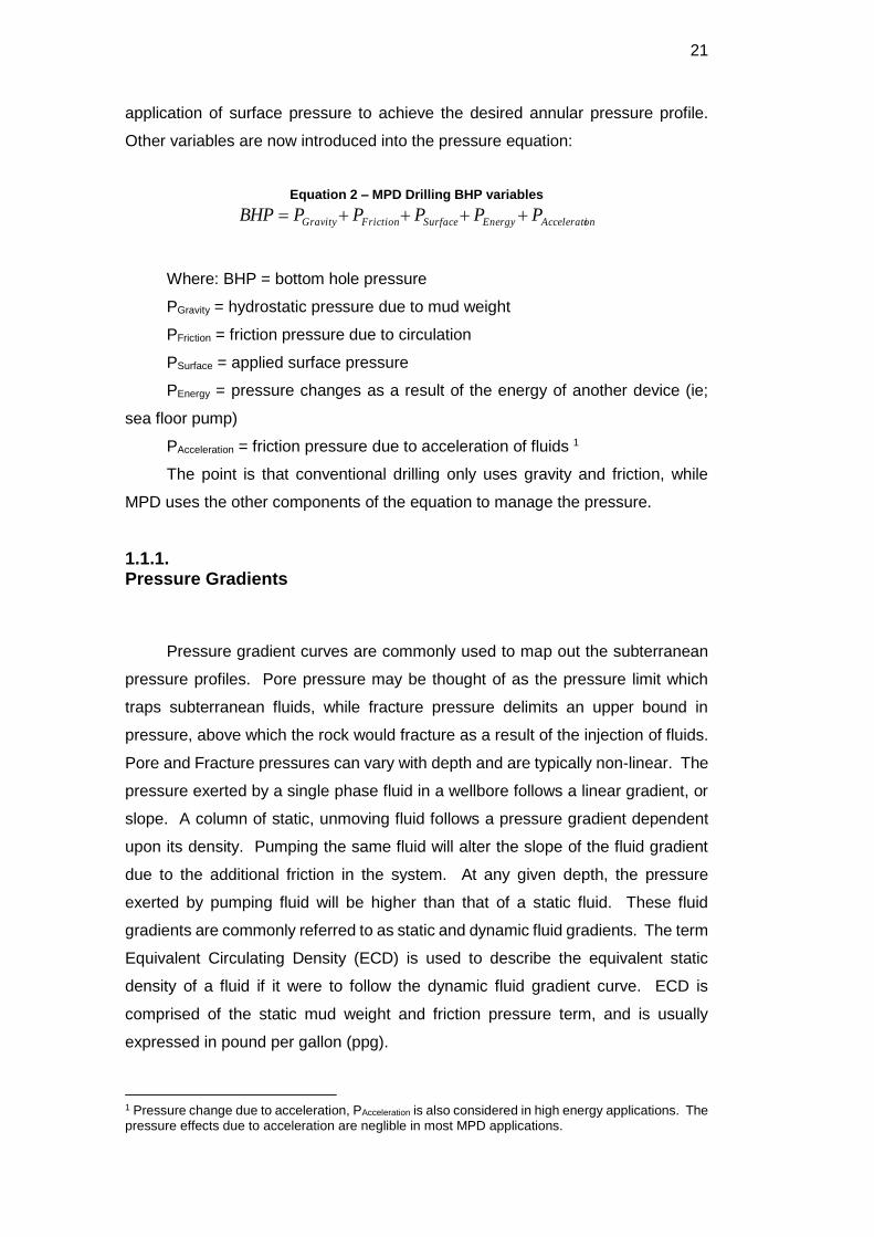
onAcceleratiEnergySurfaceFrictionGravity PPPPPBHP

Where: BHP = bottom hole pressure

PGravity = hydrostatic pressure due to mud weight

PFriction = friction pressure due to circulation

PSurface = applied surface pressure

PEnergy = pressure changes as a result of the energy of another device (ie;

sea floor pump)

PAcceleration = friction pressure due to acceleration of fluids 1

The point is that conventional drilling only uses gravity and friction, while

MPD uses the other components of the equation to manage the pressure.

1.1.1. Pressure Gradients

Pressure gradient curves are commonly used to map out the subterranean

pressure profiles. Pore pressure may be thought of as the pressure limit which

traps subterranean fluids, while fracture pressure delimits an upper bound in

pressure, above which the rock would fracture as a result of the injection of fluids.

Pore and Fracture pressures can vary with depth and are typically non-linear. The

pressure exerted by a single phase fluid in a wellbore follows a linear gradient, or

slope. A column of static, unmoving fluid follows a pressure gradient dependent

upon its density. Pumping the same fluid will alter the slope of the fluid gradient

due to the additional friction in the system. At any given depth, the pressure

exerted by pumping fluid will be higher than that of a static fluid. These fluid

gradients are commonly referred to as static and dynamic fluid gradients. The term

Equivalent Circulating Density (ECD) is used to describe the equivalent static

density of a fluid if it were to follow the dynamic fluid gradient curve. ECD is

comprised of the static mud weight and friction pressure term, and is usually

expressed in pound per gallon (ppg).

1 Pressure change due to acceleration, PAcceleration is also considered in high energy applications. The pressure effects due to acceleration are neglible in most MPD applications.

DBD


22

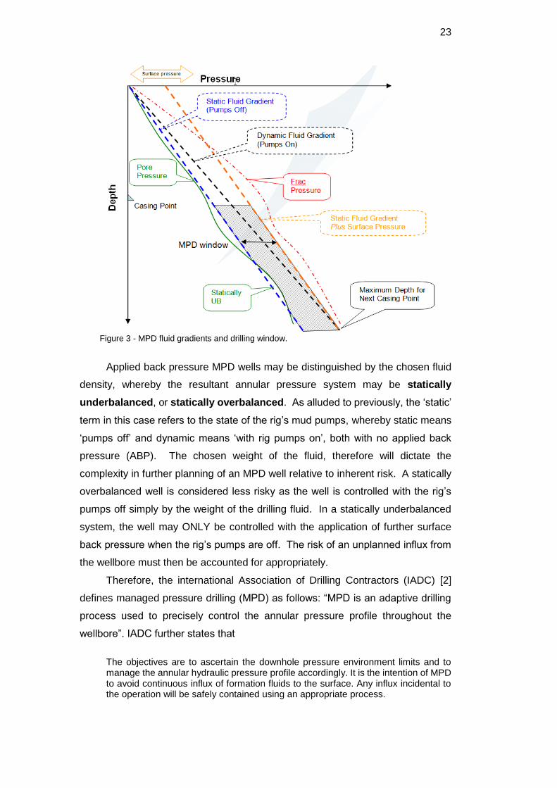
Figure 2 and Figure 3 illustrate the differences between conventional and managed

pressure drilling pictorially. Figure 2 depicts a traditional pore-fracture gradient

window for a hypothetical well. Static and dynamic fluid gradient curves are

superimposed. Simplistically, the next casing point is highlighted at the bottom of

the figure where the dynamic circulating density line approaches the fracture

gradient.

Figure 2 - Conventional drilling fluid gradients & casing setting points.

The margin between the static and dynamic gradients defines the drilling

window, shown shaded. Figure 3 shows the same hypothetical well, demonstrating

an MPD option with a static mud weight gradient (blue) less than pore pressure.

Note that although the dynamic gradient (black) results in an overbalanced state

while, the system is statically underbalanced at some points in the wellbore.

Application of surface back pressure however, results in a shift of the static gradient

(orange) above pore pressure. In this example, an anchor point pressure at the bit

is chosen, whereby the pressure is matched with pumps on and pumps off at this

point. Higher in the wellbore, this curve crosses frac pressure, however the result

is inconsequential as this point is behind casing.

The one dramatic result demonstrated in this figure is the ability to drill deeper

with the same mud system, thus extending the casing depth or reaching the

planned target.

DBD


23

Figure 3 - MPD fluid gradients and drilling window.

Applied back pressure MPD wells may be distinguished by the chosen fluid

density, whereby the resultant annular pressure system may be statically

underbalanced, or statically overbalanced. As alluded to previously, the ‘static’

term in this case refers to the state of the rig’s mud pumps, whereby static means

‘pumps off’ and dynamic means ‘with rig pumps on’, both with no applied back

pressure (ABP). The chosen weight of the fluid, therefore will dictate the

complexity in further planning of an MPD well relative to inherent risk. A statically

overbalanced well is considered less risky as the well is controlled with the rig’s

pumps off simply by the weight of the drilling fluid. In a statically underbalanced

system, the well may ONLY be controlled with the application of further surface

back pressure when the rig’s pumps are off. The risk of an unplanned influx from

the wellbore must then be accounted for appropriately.

Therefore, the international Association of Drilling Contractors (IADC) [2]

defines managed pressure drilling (MPD) as follows: “MPD is an adaptive drilling

process used to precisely control the annular pressure profile throughout the

wellbore”. IADC further states that

The objectives are to ascertain the downhole pressure environment limits and to manage the annular hydraulic pressure profile accordingly. It is the intention of MPD to avoid continuous influx of formation fluids to the surface. Any influx incidental to the operation will be safely contained using an appropriate process.

DBD


24

1.2. Controlling BHP

The purpose of managed pressure drilling is to create a pressure profile in

the annulus within the operating window guided by pore and fracture pressures.

Most often, pressure control in the annulus is achieved by employing the following

techniques: adjusting fluid density, frictional pressure losses and the surface

backpressure by using a combination inclusive of a rotating control device (RCD),

choke, pump, and the design of well bore and drill string configuration.

An important goal of all drilling is to manage the bottom hole pressure.

In conventional overbalanced drilling, the ABP is by definition zero (or

atmospheric), and only density and friction loss are available as control

parameters. Changing density means changing the mud weight, which takes time.

Moreover, for the full impact of density change to be felt in terms of BHP, the new

density fluid has to circulate all the way to surface. This means that in practice,

BHP control through change in density is slow. Frictional pressure loss can be

changed more easily, by changing the flow rate. The main limitation of this

approach is the minor impact of frictional pressure loss on BHP in large-clearance

annuli. In tighter clearances (or if the clearance is deliberately reduced by using,

for example, large OD drill collars), frictional pressure loss can have a significant

impact on BHP control. It should be remembered that there is a lower limit of rate

governed by hole cleaning requirements, and an upper limit dictated by the

downhole motors and equipment used.

In classical MPD, where a rotating control device is used to allow applied

back pressure, greater control is now available. Density and friction are still

available as control parameters, just as in conventional drilling. Moreover, since

ABP is now a control parameter, far greater flexibility is available in the design of

the operation. This is a common MPD variation.

1.3. Literature Review

The importance of hydraulic calculations and rheology models used to

characterize the flow behavior of drilling fluids are widely known as first illustrated

by Bourgoyne et al [3] and later investigated by Pilehvari [4].

DBD


25

The simplicity of fluid rheology calculations provided by the Bingham Plastic

[5] and Power Law [6] models contributed to the widespread use of those models

in the oil and gas industry, although Herschel Bulkley [7] has become the model of

choice to predict pressure losses when drilling fluids are circulated in a well [8].

Several studies have been carried out considering the Herschel-Bulkley flow

in wellbores. Fairly complex model covering laminar, transitional and turbulent

flows and eccentricity effects in hydraulics were presented by Reed and Pilehvari

(1993) [9].

The approach has also been followed also by Merlo et al. (1995) [10], Bailey

and Peden (2000) [11], and Maglione et al. (2000) [12] to cover all flow regimes for

flow of Herschel–Bulkley fluids and of generalized non-Newtonian fluids in

concentric annuli for different types of applications. The main contributions of these

studies have been of high relevance for the evolution of the calculations performed.

Merlo et al. (1995) [10] proposed a prediction of the exact pressure

distribution along the well and the circulating temperature distribution in the fluid

based on viscometer readings for the Newton, Bingham, Power law and Herschel-

Bulkley models.

Peden (2000) [11] proposed a new rheological parameter which couples

laminar flow and turbulent flow functions whereas pressure loss functions for flow

of non-Newtonian fluids in pipes and concentric annuli are independent of the

rheological model of choice. His work highlights the importance of a rigorous

method for providing confidence bounds on any fitted nonlinear functions. It is

considered beneficial for any calculation requiring fitted nonlinear functions.

On other side, it has been demonstrated by Maglione et al. (2000) [12] that

rheological triad from the viscometer data obtained in the laboratory using a Fann

VG 35 viscometer does not always coincide with the rheological triad from the in-

situ drilling test.

Moreover, Okafor & Evens, (1992) [13] illustrated that no single rheological

model is able to accurately represent the flow behavior of most pseudoplastic and

yield-pseudoplastic fluids over the full spectrum of shear rates and proved that the

chosen rheology model can be found to approximate the behavior of an actual fluid

(within certain ranges) with an accuracy commensurate with the reproducibility of

measured field data.

The understanding and efficient control of drilling-fluid behavior requires a

fundamentally sound method of flow-properties analysis which is practical to use

in the field, especially on Managed Pressure Drilling (MPD) applications. It appears

that the practical application of sound rheological concepts had been the lack of

DBD


26

suitable viscometric methods for the routinely measurement of fundamental flow

properties outsides the laboratory and the concern raised by Savins & Ropers

(1954) [14] remains unresolved whenever considering the newer models that

drilling industry has adopted.

Nguyen and Boger (1987) [15] confirmed that the methods normally

employed for shear rate calculations from concentric cylinder viscometer data

generally are not applicable for fluids with a yield stress and proposed a correct

calculation of the shear rate for time-independent yield stress fluids. In particular

when cylindrical systems with large radius ratios the yield stress induces two

possible flow regimes in the annulus.

Another perspective of the issue can be attributed to the fact that several

controversial measurement and curve-fitting techniques remains a great challenge

to determine the rheological parameters for a given fluid. Klotz and Brigham (1998)

[16] presents an accurate method for determining the three coefficients of the

Herschel-Bulkley equation from six-speed Fann viscometer data in attempt to fulfill

the determination of these coefficients from the data points.

Zamora and Power (2002) [8] discussed techniques to determine key

rheological parameters using the measurement method as well as complexities

involved in rheological modeling. It is important to mention that iterative techniques

available to solve daunting Herschel-Bulkley assume true Herschel-Bulkley

behavior before processing or relies on the raw data and technically assumes no

particular rheological model. The same drawback was observed on the API method

[17] is the wide shear-rate span between data points (especially in the range of 5

to 170 s-1, or 3 to 100 rpm).

Aided by computational fluid dynamics (CFD), recent study performed by

Erge et al. (2015) [18] evaluated the behavior of the flow of Newtonian and non-

Newtonian fluids in annuli demonstrating that CFD as the accurate pressure loss

estimations. However, the determination of fluid properties and selection of

rheology also remains vital for the convergence of the numerical results when

compared to the experimental results.

After all, it is trusted that the requirements to measure the rheology properties

are not well understood or explored. It is proposed that while MPD is a concern,

equipment and techniques should be reassessed. Followed by the characterization

and adoption of a rheology model to best describe the physics and the fluid

dynamics.

DBD


2 Aspects and Issues of Managed Pressure Drilling Connections

Traditionally, Managed Pressure Drilling Connections, the back pressure

values must follow a pump rate versus pressure schedule to maintain the annular

pressure constant down the hole. As the example presented in Figure 4 it can be

observed that the bottom hole pressure is kept constant (represented by the ECD

– red curve) while the pumps are lowered in a preparation for a connection.

Figure 4 - Pump Step-Down Schedule

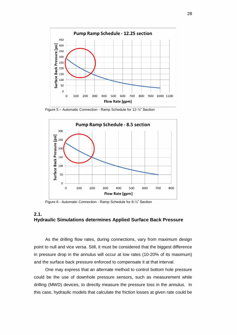
The most recent MPD system adjusts the applied surface back pressure

automatically based on the desired calculated bottom hole pressure by predicting

the friction annular losses through a hydraulics model. As the model uses the real

time data of pump flow rate, at any time the pump rate is changed, an automatic

adjustment in the surface back pressure will be produced to maintain a constant

bottom hole pressure by compensating the friction losses by surface back

pressure. Opposed to manual MPD connections, in automatic MPD systems the

pump rate versus pressure schedule plots are presented in a smoother way, as

the steps changes are automatically compensate and calculated by the hydraulic

simulators installed on the MPD’s Control Units (Figure 5 and Figure 6).

DBD


28

Figure 5 – Automatic Connection - Ramp Schedule for 12-¼” Section

Figure 6 - Automatic Connection - Ramp Schedule for 8-½” Section

2.1. Hydraulic Simulations determines Applied Surface Back Pressure

As the drilling flow rates, during connections, vary from maximum design

point to null and vice versa. Still, it must be considered that the biggest difference

in pressure drop in the annulus will occur at low rates (10-20% of its maximum)

and the surface back pressure enforced to compensate it at that interval.

One may express that an alternate method to control bottom hole pressure

could be the use of downhole pressure sensors, such as measurement while

drilling (MWD) devices, to directly measure the pressure loss in the annulus. In

this case, hydraulic models that calculate the friction losses at given rate could be

DBD


29

replaced. Although, at lower rates falls outside the operating range of the existing

technology for MWD tools which turning them inoperable and not an option.

The issue gets importance as the only method to accurately predict the

requirements for surface back pressure as the connection progresses relies on

hydraulic model. All the information needed to correctly calculate the friction

losses, such as amount of data points to characterize a drilling fluid rheology, the

range of shear rate observed in the flow, the rheology model selection, curve fit

and rheology parameters and ultimately the equipment and calculation method

itself among others becomes critical for an accurate and safe connection

procedure.

2.1.1. MPD Industry Software

The common software used in “Managed Pressure Drilling (MPD) Design

and Operations” are the Drillbench Dynamic Drilling Simulation Software by

Schlumberger, Microflux Control System MC2 by Weatherford and SafeVision by

Safe Kick.

It is well-known that the existing systems mentioned above poses limitations

to MPD design such as:

1. only a single rheology model can be selected from an existing

database, usually available Bingham, Power Law (PL), Herschel-

Bulkley (H-B) and Newtonian;

2. the number of rheology readings, shear rate vs. shear stress,

commonly known in the industry as FANN readings [degrees] by rotor

speed are limited from 6 to 8 [rpm] reading maximum.

3. the readings for rotor speed [rpm] (or shear rate [1/s]) are defined as

fixed values where the lowest available input is defined as 3 [rpm] (or

5.11 [1/s]) and the maximum as 600 [rpm] (or 1021.38 [1/s]) in

accordance to the API standards and common practices .

The user interface input screen for Drillbench, SafeVision and MC2 can be

found below on Figure 7, Figure 8 and Figure 9 respectively.

DBD


30

Figure 7 – Drillbench: Rheology Input User Interface Screen

Figure 8 - SafeVision: Rheology Input User Interface Screen

DBD


31

Figure 9 – MC2: Rheology Input User Interface Screen

2.2. Rheology Measurements: Equipment

2.2.1. FANN - Model 35 Viscometer [19]

The Model 35 Viscometer is the best known and most commonly used as the

Standard of the Industry for drilling fluid viscosity.

As true Couette coaxial cylinder rotational viscometer, the test fluid is

contained in the annular space or shear gap between the cylinders. Rotation of the

outer cylinder at known velocities accomplished through precision gearing. The

viscous drag exerted by the fluid creates a torque on the inner cylinder or bob. This

torque is transmitted to a precision spring where its deflection is measured and

then related to the test conditions and instrument constants.

DBD


32

Figure 10 – FANN Model 35 Viscometer

Direct Indicating Viscometers combine accuracy with simplicity of design and

are recommended for evaluating materials that are Bingham plastics. In particular,

the Model 35 Viscometer is equipped with factory installed R1 Rotor Sleeve, B1

Bob, F1 Torsion Spring, and a stainless steel sample cup for testing according to

American Petroleum Institute Specification RP 13B-1 [20]

Shear stress is read directly from a calibrated scale. Plastic viscosity and

yield point of a fluid can be determined easily by making two simple subtractions

from the observed data when the instrument is used with the R1-B1 combination

and the standard F1 torsion spring.

2.2.2. Rheometer Geometry Considerations

Obviously material functions (the viscosity η, the yield stress 𝜏0, storage

modules and loss G’, G’’, among others) do not depend on the geometry chosen

to measure them. Therefore, rheological tests with two different geometries are

expected to deliver the same result. However, this may not be observed in practice,

since often one or more of available geometries may not be appropriate for

characteristics of the sample question [21]. In this case, assessment of each case

and selection of geometry and test type that will provide the most reliable data is

required.

In the concentric cylinder (also called Couette or Coaxial geometry), either

the inner, outer, or both cylinders may rotate, depending on instrument design. The

test fluid is maintained in the annulus between the cylinder surfaces. The double-

gap configuration is useful for low viscosity fluids, as it increases the total area,

DBD


33

and therefore the viscous drag, on the rotating inner cylinder, and generally

increases the accuracy of the measurement.

Figure 11 - Schematic diagram of basic tool geometries for the rotational rheometer: concentric cylinder

Figure 12 - Schematic diagram showing alternative cylindrical tool design in cut-away view: Double Gap

The rheometer FANN 35 consists of a single geometry the Couette. Hence,

it is objective of this study to evaluate if encompass its applicability for the broad

range of drilling fluid samples encountered on Managed Pressure Drilling

operations. Further issues are presented to be investigated.

DBD


34

2.2.3. Shear Rate Operating Range – FANN 35 speeds

In the past and the present, conventional drilling applications are concerned

to equivalent circulating densities (ECD) at full drilling rates. The ECD generated

at the transition from pumps off to pumps on at full drilling rates had not

represented a problem, thus never investigated. One reason for that is the

conventional drilling maintains a fluid density (mud weight) higher than the pore

pressure all times, removing the risk of a kick due to the lack of hydrostatic. As

briefly commented on Chapter “1.1. Managed Pressure Drilling Concept”, the MPD

allows the utilization of statically underbalance fluid density meaning the

hydrostatically only exerted by the drilling fluid will not suffice to balance the pore

pressure and an additional pressure at the surface – Applied Surface Back

Pressure – plus the friction losses will constitute the terms to balance the well

statically.

Under this perspective, Managed Pressure Drilling mandates the full

spectrum of ECD’s to be investigated for the drilling fluid and well geometry, from

a static condition (pumps off) to full drilling rates (ECD drilling), possibly covering

and extrapolating the limits offered by a FANN 35 operating range (3rpm as

minimum and 600 rpm as maximum).

Pointed out all, becomes clear that the rheological properties obtained from

the FANN 35 based on 6 points readings only - six speeds of 600, 300, 200, 100,

6, and 3 rpm – does not suffice completely the MPD requirements by its nature.

As a final point, FANN 35 for several years was the default equipment for

oilfield applications as variation in drilling rates had not impacted the operations

but implementation of new technologies should evaluate if the measurements

reproduced by existing practices and equipment suffice the technique, especially

when low flow rates and flow rates variations are critical part of the system.

DBD


3 The Thought

“Would you be able to design a wing and not know the air properties?”

3.1. The Motivation

Successfully drilling challenging wells requires an in-depth understanding of

the hydraulics during all phases of the operation. The drilling process is highly

dynamic and complicated to model; thus, much of the dynamics have traditionally

been neglected. However, with diminishing operational margins, the impact of

dynamic effects is growing. Coupled with increasing well construction costs,

modeling the dynamics becomes essential and strategically important [22].

3.2. Thesis Objectives

With the adoption of Managed Pressure Drilling (MPD), the drilling industry

is exploring new avenues of annular pressure control. Current drilling practices has

reacted to changing wellbore conditions by altering the mud weight according to

observed differences in mud volumes (influxes or losses), and via the application

of MPD to actively or proactively control the annular pressure profile. To be able to

accomplish this goal, this technique may include control of back pressure, fluid

density, fluid rheology, annular fluid level, circulating friction and hole geometry, or

a combination thereof.

This study ensures that the current methods, standards and equipment are

able to satisfy the design of MPD operations in terms of Fluid Rheology

Characterization and Pressure Loss estimations.

The following ideas will constitute the goals of the present work:

Identify the shear rates usually seen on 12-1/4” Section and 8-1/2" Section

drilling geometries executed by the MPD system at the entire flow rate range;

DBD


36

Assessment of shear rate points measurements as per API RP 13B in the

range relevant for its applications (3rpm - 600 rpm);

Evaluation of FANN35 capabilities to characterize the rheology properties of

a drilling fluid designed for MPD Applications;

Evaluate Curve Fit Methods proposed by API RP 13D versus Non Linear

Regression (NLR), the influence of 6 points vs. "wide range full flow curve"

quantifying the variance and its impact on pressure loss estimation;

Leverage the utilization of Computational Fluid Dynamics (CFD) analysis in

comparison of API RP 13D Formulas to predict Annular Pressure Losses (APL).

3.3. Scope of Work & Methodology

The issues and aspects of the equipment and methods used to characterize

the drilling fluids for MPD Applications as well as the operational aspects that

diverge from conventional practices aimed to be investigated.

Three fluid samples will be selected that would suggest a representation of

the drilling fluid properties of MPD applications based on field data available from

several operations performed by the industry. For each sample, the methodology

to be used is to be unfolded as follows.

The sampling will be prepared and the data required to describe a Steady

Flow Time (Shear Rate Constant) and Flow Curve (Shear Rate x Shear Stress)

will be performed. The Flow Time will be used to identify the time requisite to the

sample reach the steady state flow and a reliable measurement acquired. The Flow

Curve will map the viscosity across a range of shear rates from which a viscosity

value at a shear rate relevant to the process usage conditions can be read.

The measurements of Shear Rate [1/s], Shear Stress [Pa], Viscosity [Pa·s]

and Torque [µNm] at controlled temperature of 25 [Celsius] will be taken at High

Precision Rheometers (HPR) - Anton‐Paar Physica MCR301, Anton‐Paar Physica

MCR 501 and Thermo Scientific Haake Mars II – depending upon availability.

The Flow Curve obtained from HPR will consist of 50 shear rate points

ranging between 0.1 to 1000 [1/s]. Then and there, the same sample will be

measured at FANN35 following the API Recommended Practice 13B (API RP

13B). A graphical comparison of the readings between the HPR and FANN35 will

be used to evaluate the performance of FANN 35 having the HPR as base line for

DBD


37

all the 3 samples in question. All tests will be performed twice to guarantee the

reliability and repeatability of the results.

After, the data points will be curve fitted to select the Rheology Model that

best represent the fluid sample – in this work, limited to Herschel-Bulkley (HB) and

Power Law (PL). As the API Recommended Practice 13D (API RP 13D) suggests

a “field” approximation for curve fitting, it also becomes part of the scope of the

work to evaluate and compare both cases, the one proposed by API RP 13D

against a mathematical NLR, and the discrepancy among them. A brief argument

about the implications of curve fitting and single rheology model selection for MPD

applications is discussed.

The graphical comparison will be provided followed by the estimation

Coefficient of Determination (R2) to determine the Fluid Rheology Characterization

in a laboratory environment using HPR versus conventional FANN35 methods as

well as Curve Fitting Techniques – API 13D and NLR. Fluid Rheological

Parameters - such as flow index (n) and consistency index (k) - that describes each

Rheology Model - PL and HB - will be estimated.

Subsequently, the study will continue to develop by further investigating the

Shear Rates presented in two typical annular geometries generally seen MPD

application. They will be calculated with the aid of Computational Fluid Dynamics

(CFD) by the utilization of the ANSYS Fluent software and compared against the

direct formulas suggested in API RP 13D. This step will be done only for the most

representative fluid sample; however it will consider the Rheological Parameters

obtained from Curve Fitting from NLR and from API RP 13D. As a result of mapping

the shear rate range, it will allow to infer the measurement range obtained when

API RP 13B is followed (limited 6 points) satisfy or not the MPD requirements of

viscosity values and how a wider flow curve would be beneficial.

The geometries for the sake of calculations and model simplicity are defined

as 12-1/4” Open Hole Diameter by a drill pipe of 5.5” referred as “12-1/4” Section”

and 8-1/2" Open Hole Section by a drill pipe of 5.5” referred as “8-1/2" Section”.

The selection of flow rates will be an approximation of the field conditions

usually seen that assures proper hole cleaning and other requirements during

drilling operations. The flow rates in the 8-1/2" Section case will vary from 10 [gpm]

(which represents a flow velocity and 0.029645 [m/s]) to 400 [gpm] (equivalent to

1.185817 [m/s]). The flow rates in the 12-1/4” Section case will vary from 10 [gpm]

(or 0.01039 [m/s]) to 1000 gpm (or 1.03921 [m/s]).

Finally, conclusions will present the Pressure Loss comparison for the 3

conditions on both geometries (12-1/4” and 8-1/2") below:

DBD


38

1. Rheological Properties measured by FANN35 following the API RP 13B

guidelines, curve fitted and HB rheological parameter described by API

RP 13D Method and Pressure Loss calculated by API RP 13D direct

formula Method.



RP 13D Method and Pressure Loss calculated by Fluent ANSYS CFD.

3. Rheological Properties measured by HPR, curve fitted and HB

rheological parameter described by NLR Method and Pressure Loss

calculated by Fluent ANSYS CFD.

While the comparison between condition 1 and 2 will allow determining the

accuracy of API RP 13D Direct Formula Calculation, the comparison between

condition 2 and 3 will permit to conclude if Curve Fitting and Equipment should be

revisited for MPD Applications.

DBD


4 Industry Practices, Equipment and Standards

4.1. Drilling Fluid Characterization according Recommended Practice for Field Testing Water-based Drilling Fluids - ANSI/API RP 13B-1

The scope of API RP 13B is to provide standard procedures for determining

the characteristics of water based drilling fluids, among them the viscosity. The

latest version - 5th Edition - was issued in March 2009. The errata released in

August 2014, although without changes to the Section 6 - Viscosity and Gel

Strength. Relevant to note that the API standard is also refereed as ISO 10414-

1:2008, Petroleum and natural gas industries—Field testing of drilling fluids— Part

1: Water-based fluids.

Revisiting the API RP 13B, it is found the measurements of viscosity must

be done through a direct-indicating viscometer and it shall meet fixed specifications

in terms of geometry. It delimits fixed shear rate values to characterize the drilling

fluid [1], being the most common 3 – 6 – 100 – 200 – 300 – 600 rpm (5.11 – 10.21

170.23 – 340.46 – 510.69 – 1021.38s-1 respectively)

These 2 aspects restrict the available equipment in the market that can be

used for fluid rheology characterization.

The recommended practice also suggests waiting for viscometer dial reading

to reach a steady value as the time required is dependent on the drilling-fluid

characteristic. Although, it does not recommend the minimum time requirements

nor suggests acquiring the information from laboratory.

Overall, the recommended practice does not allow flexibility or adaptability

for rheology and applications that may be needed for different device geometries

and other shear rate values not available on direct viscometer devices. Moreover,

the indication of time to reach the steady reading are often neglected for

conventional drilling, but become critical aspect for MPD.

DBD


40

4.2. API Recommended Practice 13D — Rheology and hydraulics of oilwell drilling fluids

The objective of API Recommended Practice 13D (API RP 13D) is to provide

a basic understanding of and guidance about drilling fluid rheology and hydraulics,

and their application to drilling operations. The latest revision was issued in May

2010 as its sixth edition. The purpose for updating the existing RP, last published

in May 2003, is to make the work more applicable to the complex wells. These

included: High-Temperature/High-Pressure (HTHP), Extended-Reach Drilling

(ERD), and High-Angle Wells (HAW) [17]. Although the revision included complex

wells on the 2010 version, MPD Applications was left aside and not addressed.

The API RP 13 D likewise highlight that drilling fluid rheology is important in

the following determinations: calculating frictional pressure losses in pipes and

annuli, determining equivalent circulating density of the drilling fluid under

downhole conditions and determining flow regimes in the annulus, among others.

The discussion of rheology on that document is limited to single-phase liquid

flow and some commonly used concepts pertinent to rheology and flow are

presented. Mathematical models relating shear stress to shear rate and formulas

for estimating pressure losses, equivalent circulating densities and hole cleaning

are included.

The following 3 Clauses of API 13 D are relevant to this study: 4 -

Fundamentals and fluid models, 5 - Determination of drilling fluid rheological

parameters and 7 - Pressure-loss modeling.

4.2.1. API RP 13 D - Clause 4 -Fundamentals and fluid models

Flow Regime Principles are presented along with the turbulent and laminar

flow explanation. Importance of viscous forces and inertial forces in the flow are

explained and the concept of Reynolds Number in a pipe is introduced and defined.

The Reynolds Number in a Pipe is defined in equation (1):

(1)

DBD


41

where:

d is the diameter of the flow channel

V is the average flow velocity

ρ is the fluid density

μ is the fluid viscosity

The concept of Hydraulic Diameter is presented. Later, viscosity (μ) , shear

stress (τ) and shear rate (ɣ) are presented for Newtonian fluids along with

mathematical relationship of shear stress and shear rate, viscosity.

Still on this Clause, the classification of fluid rheological behavior is

publicized: fluids whose viscosity remains constant with changing shear rate are

known as Newtonian fluids and Non-Newtonian fluids are those fluids whose

viscosity varies with changing shear rate.

In terms of Rheological Models, the API RP 13 D states Rheological models

are intended to provide assistance in characterizing fluid flow. No single,

commonly-used model completely describes rheological characteristics of drilling

fluids over their entire shear rate range. Knowledge of rheological models

combined with practical experience is necessary to fully understand fluid behavior.

A plot of shear stress versus shear rate (rheogram) is often used to graphically

depict a rheological model.

Extracted from the API 13 D, the most common Rheological models are

presented. The mathematical treatment of Herschel-Bulkley, Bingham plastic and

Power Law fluids is described in Clause 5.

Bingham Plastic Model—This model describes fluids in which the shear

stress/shear rate ratio is linear once a specific shear stress has been exceeded.

Two parameters, plastic viscosity and yield point, are used to describe this model.

Because these parameters are determined from shear rates of 511 s-1 (300 rpm)

and 1022 s-1 (600 rpm) this model characterizes fluids in the higher shear-rate

range. A rheogram of the Bingham plastic model on rectilinear coordinates is a

straight line that intersects the zero shear-rate axis at a shear stress greater than

zero (yield point).

Power Law—The Power Law is used to describe the flow of shear thinning

or pseudoplastic drilling fluids. This model describes fluids in which the rheogram

is a straight line when plotted on a log-log graph. Such a line has no intercept, so

a true Power Law fluid does not exhibit a yield stress. The two required Power Law

constants, n and K, from this model are typically determined from data taken at

shear rates of 511 s-1 (300 rpm) and 1022 s-1 (600 rpm). However, the generalized

DBD


42

Power Law applies if several shear-rate pairs are defined along the shear-rate

range of interest. This approach has been used in the recent versions of API 13D.

Herschel-Bulkley Model—Also called the “modified” Power Law and yield-

pseudoplastic model, the Herschel-Bulkley model is used to describe the flow of

pseudoplastic drilling fluids which require a yield stress to initiate flow. A rheogram

of shear stress minus yield stress versus shear rate is a straight line on log-log

coordinates. This model is widely used because it (a) describes the flow behavior

of most drilling fluids, (b) includes a yield stress value important for several

hydraulics issues, and (c) includes the Bingham plastic model and Power Law as

special cases.

4.2.2. API RP 13 D - Clause 5 - Determination of Drilling Fluid Rheological Parameters

Measurements of rheological parameters are distinct by the standard to be

either by Orifice viscometer (Marsh funnel) and/or concentric-cylinder viscometer

divided in Low-temperature, non-pressurized instruments and High-temperature,

pressurized instruments.

It is suggested in this section, the rheological model recommended for field

and office use as the Herschel-Bulkley (H-B) rheological model. Originally

developed in 1926, the model consistently provides good simulation of measured

rheological data for both water-based and non-aqueous drilling fluids. According to

the API RP 13 D, it has become the drilling industry’s de facto rheological model

for advanced engineering calculations.

4.2.2.1. Herschel-Bulkley Rheological Model

The H-B model requires three parameters as per Herschel-Bulkley

rheological model equation defined in equation (2):

𝝉 = 𝝉𝒚 + 𝒌ɣ𝒏 𝝉𝒚 < 𝝉

ɣ = 𝟎 𝝉𝒚 > 𝝉 (2)

DBD


43

Where:

𝝉 – Shear stress, (force/area)

𝝉y – Yield point, (force/area)

𝑘 – Consistency index, (force/area times time)

ɣ– Shear rate, s-1

𝑛 – Flow behavior index (dimensionless)

It should be noted that the H-B governing equation reduces to more

commonly-known rheological models under certain conditions. When the yield

stress 𝝉y equals the yield point (YP) and the flow index (n) is defined as 1, the H B

equation reduces to the Bingham plastic model. When 𝝉y = 0 (e.g. a drilling fluid

with no yield stress), the H-B model reduces to the Power Law. Consequently, the

H-B model can be considered the unifying model that fits Bingham plastic fluids,

Power Law fluids, and everything else in between.

4.2.2.1.1. Solution Methods for H-B Fluid Parameters

Solving for drilling fluid H-B parameters using the measurement method [17]

, [8] involves the following steps:

The true yield stress τy can be approximated using measurements from field

viscometers. API 13 D suggests approximates the fluid yield stress, commonly

known as the low-shear-rate yield point, by the following equation. The τy value

should be between zero and the yield stress (also known as “Bingham yield point”):

The low-shear-rate yield point is defined in equation (3):

(3)

The fluid flow index n is defined in equation (4):

(4)

The fluid consistency index K is defined in equation (5):

(5)

DBD


44

4.2.2.2. Other rheological models used in API 13 D

API 13 D also suggests parameters from the Bingham plastic and Power Law

rheological models. As the interest of scope of this study, only the Power Law is

cited below.

The model uses two sets of viscometer dial readings to calculate flow index

n and consistency index K for pipe flow and annular flow. As concerned, the Power

Law Annular Flow is presented. The values obtained using the calculation methods

given below will produce values of n and K that are usually significantly different

from those calculated using the Herschel-Bulkley rheological model.

The fluid flow index n (Power Law - Annular) as per API 13 D is defined in

equation (6):

(6)

The fluid consistency index K (Power Law Annular) as per API 13 D is defined

in equation (7):

(7)

4.2.3. API RP 13 D - Clause 7 - Pressure-loss modeling

The Clause 7 explores the methods and equations to calculate frictional

pressure losses and hydrostatic pressures through the different elements of the

circulating system of a drilling well. It is believed the information is suitable for

hydraulics analyses, planning, and optimization.

Although it does mentioned that useful for modeling special well-construction

operations such as well control, cementing, tripping, and casing runs, it will be later

verified in this study it’s applicability on MPD Operations.

The subsequent formulas and concepts are replicate to illustrate the method

implemented on this study:

DBD


45

Fluid velocity: Average (bulk) velocities (Va) in the annulus are

inversely proportional to the cross-sectional area of the respective

fluid conduit. The Fluid Velocity in the Annulus is defined in equation

(8):

(8)

where:

V - Fluid velocity in annulus [ft/min]

Q -Flow rate [gal/min]

dh -Hole diameter or casing inside diameter [in.]

dp - Pipe outside diameter [in.]

Hydraulic diameter: based on the ratio of the cross-sectional area to

the wetted perimeter of the annular section, the annular hydraulic

diameter to relate fluid behavior in an annulus is presented in

equation (9):

(9)

4.2.3.1. Shear Rate at the Wall

According to the API 13 D, the Newtonian (or “nominal”) shear rate (ɣ) first

must be converted to shear rate at the wall (ɣw) in order to calculate pressure loss.

By using correction factors that adjust for the geometry of the flow conduit and

oilfield viscometers used to measure rheological properties – such as FANN35 - ,

the appropriate corrections are combined into a single factor, labeled as “G”. This

technique was proposed by Zamora et all in 1974 [23]:

Well geometry shear-rate correction: Shear-rate correction for well

geometry Ba is also dependent on the rheological parameter n. It is

convenient to use a geometry factor α so that flow in pipes and annuli

can be considered in a single expression. For simplicity without

significant loss of accuracy, the annulus can be treated as an equivalent

slot (α =1). The Well geometry shear-rate correction is defined in

equation (10):

DBD


46

(10)

where

α = 0 is the geometry factor in the pipe

α = 1 is the geometry factor in the annulus

Field viscometer shear-rate correction: Unfortunately, closed

analytical solutions do not exist for Herschel-Bulkley fluids, and

complex numerical methods are inaccurate at very low shear rates.

Practically speaking, it can be assumed that the viscometer

correction Bx ≈ 1. Otherwise, if Power Law Fluids, the following

formula can be used if desired to preserve the exact solution. The

Field viscometer shear-rate correction is defined in equation (11):

(11)

where

x = 1.0678 in the standard bob/sleeve combination R1B1 [dimensionless]

Bx Viscometer geometry correction factor [dimensionless]

Combined geometry shear-rate correction factor: Shear rate at

the wall (ɣw) required to determine the shear stress at the wall is

calculated by multiplying nominal shear rate by the geometry factor

G. The Combined geometry shear-rate correction factor is defined in

equation (12).

(12)

where

G Geometry shear-rate correction (Herschel-Bulkley fluids)

[dimensionless]

V Velocity [ft/min]

dhyd Hydraulic diameter [in.]

Shear stress at the wall (flow equation): Frictional pressure loss is

directly proportional to the shear stress at the wall τw defined by the

fluid-model dependent flow equation. Flow equations for Bingham-

plastic and Herschel-Bulkley fluids are complex and require iterative

DBD


47

solutions; however, they can be approximated by an expression of

the same recognizable form as the respective constitutive equations.

The Shear stress at the wall in viscometer units is defined in equation

(13) and the shear stress at the wall in engineering units is defined in

equation (14):

(13)

(14)

4.2.3.2. Flow regime: Reynolds number (generalized)

Generalized Reynolds number NReG applies to both pipes and annuli [17],

[24]. The most convenient form of the equation involves the shear stress at the

wall.

The Generalized Reynolds Number is defined in equation (15).

(15)

where

ρ Fluid density lbm/gal

V Velocity ft/min

τw Shear stress at the wall lbf/100 ft2

4.2.3.3. Critical Reynolds number (laminar to transitional regimes)

The critical Reynolds number NCRe is defined by API 13 D as the value of

NReG where the regime changes from laminar to transitional flow.

The Critical Reynolds number is defined in equation (16):

(16)

DBD


48

4.2.3.4. Friction factor

Pressure loss in pipes and annuli is proportional to the fanning friction factor

f , which is a function of generalized Reynolds number, flow regime, and fluid

rheological properties. Laminar-flow friction factors flam for pipes and concentric

annuli are combined into a single relationship when using the generalized

Reynolds number NReG.

The Laminar-flow friction factor is defined in equation (17):

(17)

4.2.3.5. Laminar-flow pressure loss

Frictional pressure losses in the drillstring and annulus are equal to the sum

of the losses in the individual segments. The fanning equation is used to calculate

incremental pressure losses; however, the various parameters should be defined

for each segment in the drillstring and annulus.

The Laminar-flow pressure loss is defined in equation (18):

(18)

4.2.3.5.1. Laminar-flow pressure loss (special case)

Substitution of the laminar-flow friction factor flam into the general equations

yields simplified relationships for laminar-flow pressure loss that also can be

derived by force-balance analysis [17], [3]. The individual parameters should be

defined for each well segment.

The special case for Laminar-flow pressure loss is defined in equation (19):

(19)

DBD


49

4.3. Standard Oilfield Viscometer Correction Factors

In the mathematics of fluid rheology as measured using a standard oilfield

viscometer, there are instrument conversion factors that need to be applied in the

calculations. [19]

a) Shear stress (lbf/100 ft2) is determined by multiplying the dial reading (°

deflection) by 1.066. This correction is sometimes ignored in doing simple

calculations.

Relevant to highlight that is found in this study that the correction factor must

only be applied when the combination of spring-bob-rotor F1 - B1 - R1 is used on

FANN 35 devices. According to the FANN 35 Operations Manual [19], Indexes F1

- B1 – R1 will composed the following constants:

k1 - Torsion Spring Constant [Dynes/cm/degree deflection]: 386

k2 - Shear Stress constant for the effective bob surface [cm3]: 0.01323

k3 - Shear Rate Constant [1/s /rpm]: 1.7023

Therefore, the 1.066 factor to obtain the shear stress from the deflection is

resultant from the k1 - Torsion Spring Constant times the k2 - Shear stress constant

for the effective bob surface times the conversion value from Pascals to (lbf/100

ft2) (noted 2.08854342). Field personnel must pay attention if other combination of

spring-bob-rotor is used, as the deflection to shear-stress factor must be revised.

On this study, as accuracy is aimed, the value (with 6 decimals) of 1.066573

is used.

b) Shear rate (s-1) is determined by multiplying the rotor speed (r/min)

by 1.7023.

DBD


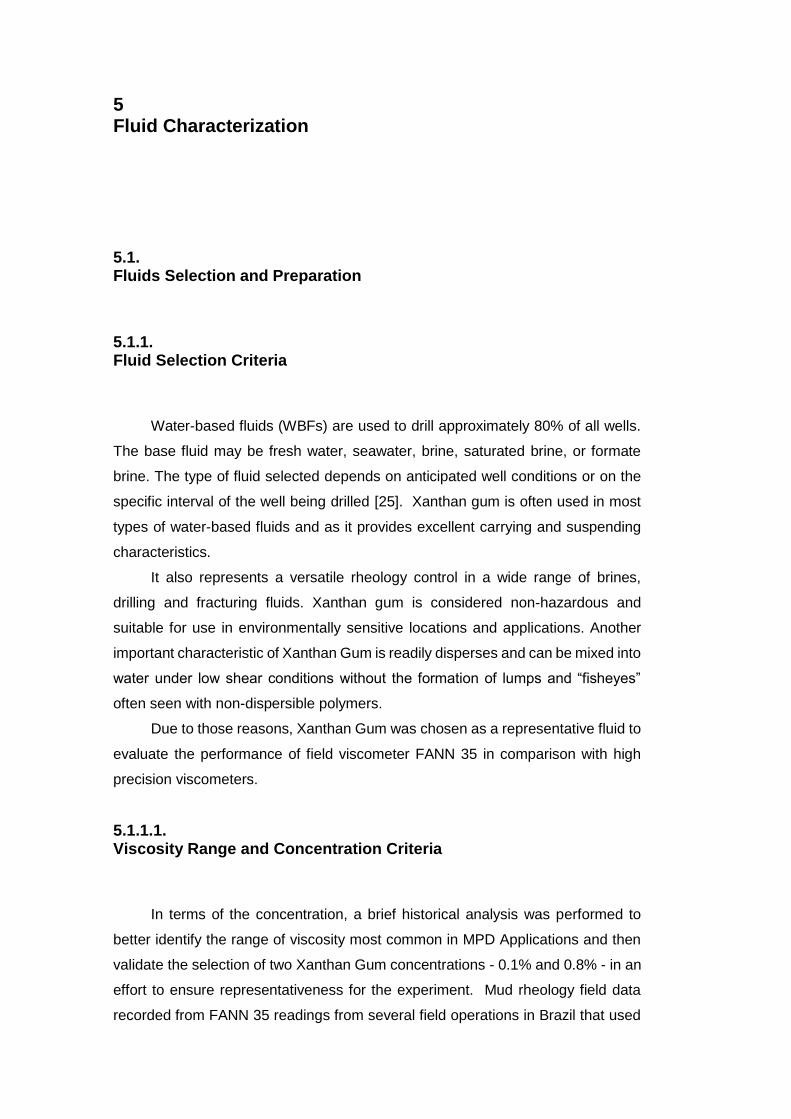
5 Fluid Characterization

5.1. Fluids Selection and Preparation

5.1.1. Fluid Selection Criteria

Water-based fluids (WBFs) are used to drill approximately 80% of all wells.

The base fluid may be fresh water, seawater, brine, saturated brine, or formate

brine. The type of fluid selected depends on anticipated well conditions or on the

specific interval of the well being drilled [25]. Xanthan gum is often used in most

types of water-based fluids and as it provides excellent carrying and suspending

characteristics.

It also represents a versatile rheology control in a wide range of brines,

drilling and fracturing fluids. Xanthan gum is considered non-hazardous and

suitable for use in environmentally sensitive locations and applications. Another

important characteristic of Xanthan Gum is readily disperses and can be mixed into

water under low shear conditions without the formation of lumps and “fisheyes”

often seen with non-dispersible polymers.

Due to those reasons, Xanthan Gum was chosen as a representative fluid to

evaluate the performance of field viscometer FANN 35 in comparison with high

precision viscometers.

5.1.1.1. Viscosity Range and Concentration Criteria

In terms of the concentration, a brief historical analysis was performed to

better identify the range of viscosity most common in MPD Applications and then

validate the selection of two Xanthan Gum concentrations - 0.1% and 0.8% - in an

effort to ensure representativeness for the experiment. Mud rheology field data

recorded from FANN 35 readings from several field operations in Brazil that used

DBD


51

water based drilling fluids was retrieved from the available IADC Daily Drilling

Reports.

The rheograms are shown in Figure 13 and plotted against the planned

Xanthan Gum Concentration of 0.1% and 0.8%. In addition, an actual sample of

Low Lime Water Based Fluid (labeled as LLMEG) recently used in a MPD

Operation carried out in Brazil during the 2013/2014 was used as baseline to

ensure that the historical data matched with the range of viscosities observed in

the field.

Figure 13 - Brazil MPD Operations Rheogram: IADC Historical Field Data

5.1.2. Xanthan Gum preparation

The following recipe and list of materials were used to prepare the Xanthan

Gum at concentrations of 0.1% and 0.8% according to Table 1 and Table 2

DBD


52

Materials

Bucket

3 beaker glass

Spatula

Analytical Balance

Mechanical mixer

Impeller type anchor

Reagents

Xanthan Gum

Water Deionized

Sodium Benzoate

Potassium sorbate

Table 1 - Xamthan Gum 0.1% Recipe

Table 2 - Xamthan Gum 0.8% Recipe

Procedure 1. Weigh reagents according to concentration (see table) to be used;

2. Place the bucket of water on the mechanical shaker (Fisaton, model

723) with the anchor blade, using the rotation of 300 rpm;

3. Carefully add the heavy xanthan gum, lest disperse too (hint: play

between the blade and the wall of the bucket);

% mass (g)

Xanthan Gum 0.10% 3

Water Deionized 2997

Solution - 3000

Potassium sorbate 0.50% 15.00

Sodium Benzoate 0.50% 15.00

% mass (g)

Xanthan Gum 0.80% 24

Water Deionized 2976

Solution - 3000

Potassium sorbate 0.50% 15.00

Sodium Benzoate 0.50% 15.00

DBD


53

4. Stir this rotation for 15 minutes;

5. Add the heavy bactericidal and stir for 1 hour;

6. Let stand 24 hours before testing.

Figure 14 – Preparation of Xanthan Gum in the Mechanical Shaker at 300 rpm

Figure 15 – Xanthan Gum being stirred

After the samples were prepared, they were divided in bottles and labeled

(Figure 16) in preparation to be shipped and used in the different laboratories and

devices.

Important to note that it was observed an expiration date of 7 days in the

Xanthan Gum, even with the addition of stabilizers and preservatives..

DBD


54

Figure 16 – Xanthan Gum bottle samples

5.2. Measurements of Rheological Properties

5.2.1. Equipment and Laboratories

The Equipment and Laboratories utilized to measure the rheological

properties of the 3 selected fluids were done in three different locations:

at Petrobras Research Center “CENPES”

o “Fann 35 - CENPES - F1 B1 R1”: Viscometer FANN 35 using the

combination of bob-rotor-spring “F1 B1 R1” strictly according to the

guidelines of API RP 13B and API RP 13D.

at Pontifical Catholic University of Rio de Janeiro - Fluid-Rock Interaction

Laboratory (LIRF) Technology Group and Petroleum Engineering

Department of Civil Engineering (GTEP)

o “Fann 35 - PUC - F1 B1 R1”: Viscometer FANN 35 using the

combination of bob-rotor-spring “F1 B1 R1” strictly according to the

guidelines of API RP 13 B and API 13 API D.

at Rheological Characterization Laboratory - Rheology Group (GReo) at

Pontifical Catholic University of Rio de Janeiro.

o Anton Paar - Physica MCR 501 as geometry selected the Double

Gap DG#26.7

o Anton Paar - Physica MCR 301 as geometry selected the Cross

Hatch PP50/P2

DBD


55

Figure 17 - Anton Paar - Physica MCR 301

5.2.2. Tests and Methodology

Flow Curve (Shear Rate x Shear Stress): In order to determine the general

flow behavior of a sample the viscosity is measured as a function of the shear rate

in a rotational rheometer. For the presentation of the data either the viscosity or

the shear stress is plotted against the shear rate for steady state regime. The thus

obtained graph is called flow curve. It shows the flow behavior for low shear rates

(slow motions) as well as high shear rates (fast motion).

The flow curves obtained from FANN35 Viscometers were performed

following the API 13 B and API 13 D Recommended Practices. The sample’s

temperature was kept at 25 Celsius through the entire experiment.

The flow curves range performed at Physica’s Rheometers (MC 301 and

501) were set from 0.1 to 1000 s-1 and data 50 points. Although the API RP lowest

shear rate is 5.11 s-1, it is relevant to MPD flow rate transitions and connections

the observation of flows at low shear rates, hence the decision to evaluate as the

minimum value of 0.1 s-1, observed equipment limitations. Temperature was also

controlled at 25 Celsius.

Torque and equipment’s range of operations and limitations were verified on

all cases.

Steady Flow Time (Shear Rate Constant): The viscosity has to be obtained

at different shear rates, and it’s critical to define the time to reach equilibrium at

any given shear rate. It is known that the time to reach the steady state increases

as the shear rate decreases. Therefore, a ‘Single Point Test’ was run at lowest

shear rate to determine ‘delay before measure’ for steady rate sweep and the time

DBD


56

to reach the equilibrium is used as ‘delay before measurement’. As higher shear

rates will require less time to reach equilibrium that will ensure all data acquired

was collected under steady state conditions in addition to shorten experiment time.

5.2.3. Rheology Measurements Results

5.2.3.1. Steady Flow Time Tests

Steady Flow Time Tests were conducted for all samples using Physica’s

Rheometers (MC 501 and 301) since it allows for programmable test parameters

and for the duration to reach more than 2000 seconds in few cases.

Four different shear rate tests were performed using Xanthan Gum 0.1%.

The rates were 0.1, 2.5, 5 and 10 s-1; and each sample stabilized in approximately

10 seconds. Two tests, both at 1.0 s-1, were performed using Xanthan Gum 0.8%,

and again stabilized at 10 seconds. Finally, two 1.0 s-1 , shear rate tests were

performed on Low Lime samples and it required almost 100 seconds before the

stabilization was reached.

Figure 18 - Steady State Flow Behavior Test: Equilibrium time and Flow Curve Optimization

DBD


57

Prior to determining the viscosity at different shear rates, it was important to

define the time to reach equilibrium for a given shear rate. The steady flow time

determines the delay that must be applied prior a reading is taking during the

rheogram. Optimizing the delay will lead to a faster flow curve experiment and will

ensure that the measurement points are obtained at a steady state condition.

The stabilization time found on this test was then used on the subsequent

flow curves for each respective fluid sample.

As a remark, API RP 13B advises to “wait for the viscometer dial reading to

reach a steady value (the time required is dependent on the drilling fluid

characteristics)”. However, based on the results gained from the Steady State Flow

Behavior Test, equilibrium time must be closely observed. There is a risk of

jeopardizing the entire fluid characterization test when completed under field

conditions.

5.2.3.2. Flow Curve Tests

Figure 19 to Figure 24 represent combined results from flow curves obtained

from FANN35 and Physica’s Rheometers (MC 501 and 301). The flow curves

range performed at Physica’s Rheometers were set from 0.1 to 1000 s-1 and 50

data points. Even though API recommended lowest shear rate is 5.11 s-1, for MPD

applications lower shear rates might be observed, hence the decision to evaluate

as the minimum value of 0.1 s-1, observed equipment limitations.

Rheogram results for all three samples (Xanthan Gum 0.1%, Xanthan Gum

0.8% and Low Lime Water Based Mud (LL WBM) were compared with the

graphical results being presented in Figure 19 through Figure 24.

Xanthan Gum 0.1%

3 readings Fann 35 - CENPES - F1 B1 R1.

2 readings Fann 35 - PUC - F1 B1 R1.

3 readings Anton Paar - Physica MCR 501 - DG26.7 (Double Gap).

DBD


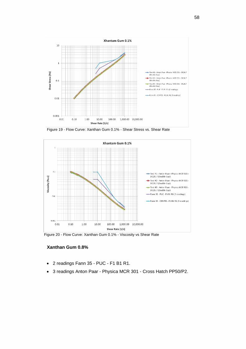
58

Figure 19 - Flow Curve: Xanthan Gum 0.1% - Shear Stress vs. Shear Rate

Figure 20 - Flow Curve: Xanthan Gum 0.1% - Viscosity vs Shear Rate

Xanthan Gum 0.8%


3 readings Anton Paar - Physica MCR 301 - Cross Hatch PP50/P2.

DBD


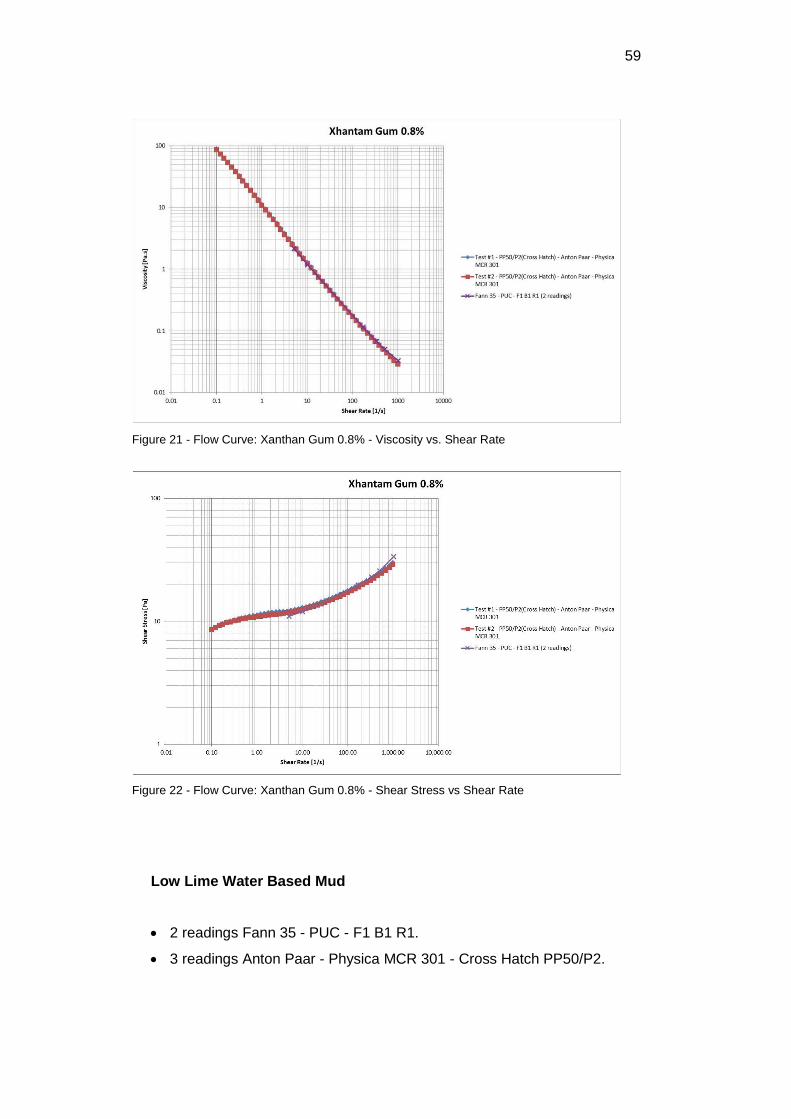
59

Figure 21 - Flow Curve: Xanthan Gum 0.8% - Viscosity vs. Shear Rate

Figure 22 - Flow Curve: Xanthan Gum 0.8% - Shear Stress vs Shear Rate

Low Lime Water Based Mud


3 readings Anton Paar - Physica MCR 301 - Cross Hatch PP50/P2.

DBD


60

Figure 23 - Flow Curve: Low Lime WBM - Viscosity vs. Shear Rate

Figure 24 - Flow Curve: Low Lime WBM - Shear Stress vs Shear Rate

5.2.3.3. Evaluation of FANN 35 Performance

In the respect of the statement from API RP 13 B, “wait for the viscometer

dial reading to reach a steady value (the time required is dependent on the drilling

fluid characteristics)” it becomes clear that based on the results of Steady State

Flow Behavior Test, the equilibrium time must be always observed, with the risk of

jeopardize the entire fluid characterization when this is done under field conditions.

0.01

0.1

1

10

0.01 0.1 1 10 100 1000 10000

Vis

cosi

ty [P

a.s]

Shear Rate [1/s]

LowLime 20%MEG

Test #1 - PP50/P2(Cross Hatch) - Anton Paar -Physica MCR 301


Fann 35 - PUC - F1 B1 R1 (#1)

Fann 35 - PUC - F1 B1 R1 (#2)

0.1

1

10

100

0.01 0.10 1.00 10.00 100.00 1,000.00 10,000.00

Shea

r St

ress

[Pa]

Shear Rate [1/s]

LowLime 20%MEG



Fann 35 - PUC - F1 B1 R1 (#1)

Fann 35 - PUC - F1 B1 R1 (#2)

DBD


61

While the rheograms results for all 3 samples were compared, it is fair to say

results obtained using the FANN 35 and the Physica for Xanthan Gum 0.8% and

Low Lime WBM are similar. The results achieved by FANN 35 were satisfactory

when within its range capabilities.

For the very low rheology fluids, in this testing, Xanthan Gum 0.1%, results

from the FANN 35 do not correspond with Physica’s results as the second presents

superior performance for dealing with low viscosity fluids.

A possible cause for the reading discrepancies between FANN 35 and the

Physica rheometer when evaluating the 0.1% concentration could be attributed to

the physical geometry of the rotational rheometer. As the selection of the geometry

- Couette, plate-cone and plate-plate - are dependent on three factors: the type of

fluid, the viscosity range and strain rate [26].

Whereas the cross hatched geometry (Figure 25) comprises of grooves

etched into the inner surfaces of the plates thus preventing the sliding of material

observed when a smooth surface is used.

While, the plate-plate cross hatch PP50/2 type was selected for Physica’s

test, the Couette was the standard configuration for the FANN35.

Figure 25 - Cross Hatch Geometry

Another possible reason for the disparity in results when testing the Xanthan

Gum 0.1% could be the low shear rate itself. 3 rpm (5.11 s-1) and 6 rpm (10.21 s-1)

are very much at the low-end capability of the FANN 35 specified operating range

as indicated on Table 3 and Table 4.

DBD


62

Table 3 - Xanthan Gum 0.1% - Fann 35 - CENPES - F1 B1 R1 (3 readings average)

Table 4 - Xanthan Gum 0.1% - Fann 35 - PUC - F1 B1 R1 (2 readings average)

5.2.3.4. Representativeness of Chosen Fluid Samples

For this study purposes, it was important to verify that the three chosen fluid

samples – 0.1% Xanthan Gum , 0.8% Xanthan Gum and Low Lime WBM - were a

representative sample of ‘real’ WBM drilling fluid used in MPD operations.

To achieve this, data recorded using the FANN 35 rheometer form actual

wells in Brazil was plot against the three muds tests as characterized in Figure 13

- Brazil MPD Operations Rheogram: IADC Historical Field Data compares the test

muds with the actual field muds used.

Due to the lack of representativeness of 0.1% Xanthan Gum as a possible

MPD drilling fluid, the 0.1% Xanthan gum was then removed from all further testing.

The FANN 35 rheometer applicability must be further investigated for testing

very low rheology fluids. Also, the identification of lower limits of very low rheology

fluids used for drilling MPD by obtaining additional historical data from similar

operations.

Rotation [rpm] Deflection [degrees]

600 7.67

300 5.33

200 4.00

100 3.00

6 2.00

3 1.00

Fann 35 - CENPES - F1 B1 R1

Xanthan Gum 0.1 %

Rotation [rpm] Deflection [degrees]

600 7.00

300 5.00

200 4.00

100 3.00

6 1.00

3 0.50

Xanthan Gum 0.1 %

Fann 35 - PUC - F1 B1 R1

DBD


63

Moreover, it is suggested for future works the study of applicability of FANN

35 performances in higher viscosities ranges than the ones found in Xanthan Gum

0.1%, such as 0.3% or 0.5%, in attempt to identify where it can be used with

confidence and results accurately enough to real rheological properties.

5.3. Drilling Fluid Model Characterization

5.3.1. Curve Fitting Influence

The definitions of curve fitting2, interpolation and extrapolation becomes

serious as a point of matter as one of the objectives is to evaluate the boundary

limits - 3 rpm and 600 rpm - in terms of shear rates when characterizing drilling

fluids in the field. The implications of those limits are later discussed in this chapter.

5.3.2. Solving the Rheological Parameters with Nonlinear Regression

Although the API RP 13 D Clause 5 also point out solving the parameters

using numerical techniques, a Nonlinear Regression (NLR) software package –

Kaleida Graph – was utilized to calculate them for PL and H-B models.

In statistics, NLR is a form of regression analysis in which observational data

are modeled by a function, which is a nonlinear combination of the model

parameters and depends on one or more independent variables. The data are fitted

by a method of successive approximations.

The curve fitting software Kaleida Graph supports both linear and nonlinear curve

fitting. Nonlinear curve fitting was accomplished through general curve fit. The

equations for PL Model (n and K) and H-B Model (n, K and To) were set and the

2 Curve fitting [30] is known as the process of constructing a curve, or mathematical function that has the best fit to a series of data points, possibly subject to constraints. Curve fitting can involve either interpolation, where an exact fit to the data is required, or smoothing, in which a "smooth" function is constructed that approximately fits the data. A related topic is regression analysis, which focuses more on questions of statistical inference such as how much uncertainty is present in a curve that is fit to data observed with random errors. Fitted curves can be used as an aid for data visualization, to infer values of a function where no data are available, and to summarize the relationships among two or more variables. Extrapolation refers to the use of a fitted curve beyond the range of the observed data, and is subject to a degree of uncertainty since it may reflect the method used to construct the curve as much as it reflects the observed data.

DBD


64

variables retrieved for all readings listed on 5.2.3.2. Flow Curve Tests of Xanthan

Gum 0.8% and the Low Lime WBM:

Xanthan Gum 0.8%

o “Test #1 - PP50/P2(Cross Hatch) - Anton Paar - Physica MCR

301”

o “Test #2 - PP50/P2(Cross Hatch) - Anton Paar - Physica MCR

301”

o “Fann 35 - PUC - F1 B1 R1” (3 equal readings)

Low Lime WBM

o Test #1 - PP50/P2(Cross Hatch) - Anton Paar - Physica MCR

301

o Test #2 - PP50/P2 (Cross Hatch) - Anton Paar - Physica MCR

301

o Test #1 - “Fann 35 - PUC - F1 B1 R1”

o Test #2 - “Fann 35 - PUC - F1 B1 R1”

In addition, the coefficient of determination, denoted R2, was calculated for

all cases. The coefficient of determination was used to indicate how well the data

fitted the model. To note, an R2 of 1 indicates that the regression line perfectly fits

the data, while an R2 of 0 indicates that the line does not fit the data at all. It

provides a measure of how well observed outcomes are replicated by the model,

as the proportion of total variation of outcomes explained by the model.

DBD


65

5.3.2.1. Xanthan Gum 0.8%

5.3.2.1.1. “Test #1 - PP50/P2(Cross Hatch) - Anton Paar - Physica MCR 301”

Figure 26 - Kaleidah Graph NLR – Xanthan Gum 0.8% - “Test #1 - PP50/P2(Cross Hatch) - Anton Paar - Physica MCR 301”

Table 5 - Rheological Parameters: PL Model - NLR Method - Xanthan Gum 0.8% Test#1

Table 6 - Rheological Parameters: H-B Model - NLR Method - Xanthan Gum 0.8% Test#1

K 10.319000

n 0.135540

R2 0.935950

Curve Fit: Power-Law (Test #1)

τ0 9.310700

K 1.537800

n 0.374350

R2 0.994980

Curve Fit: Herschel-Bulkley (Test #1)

DBD


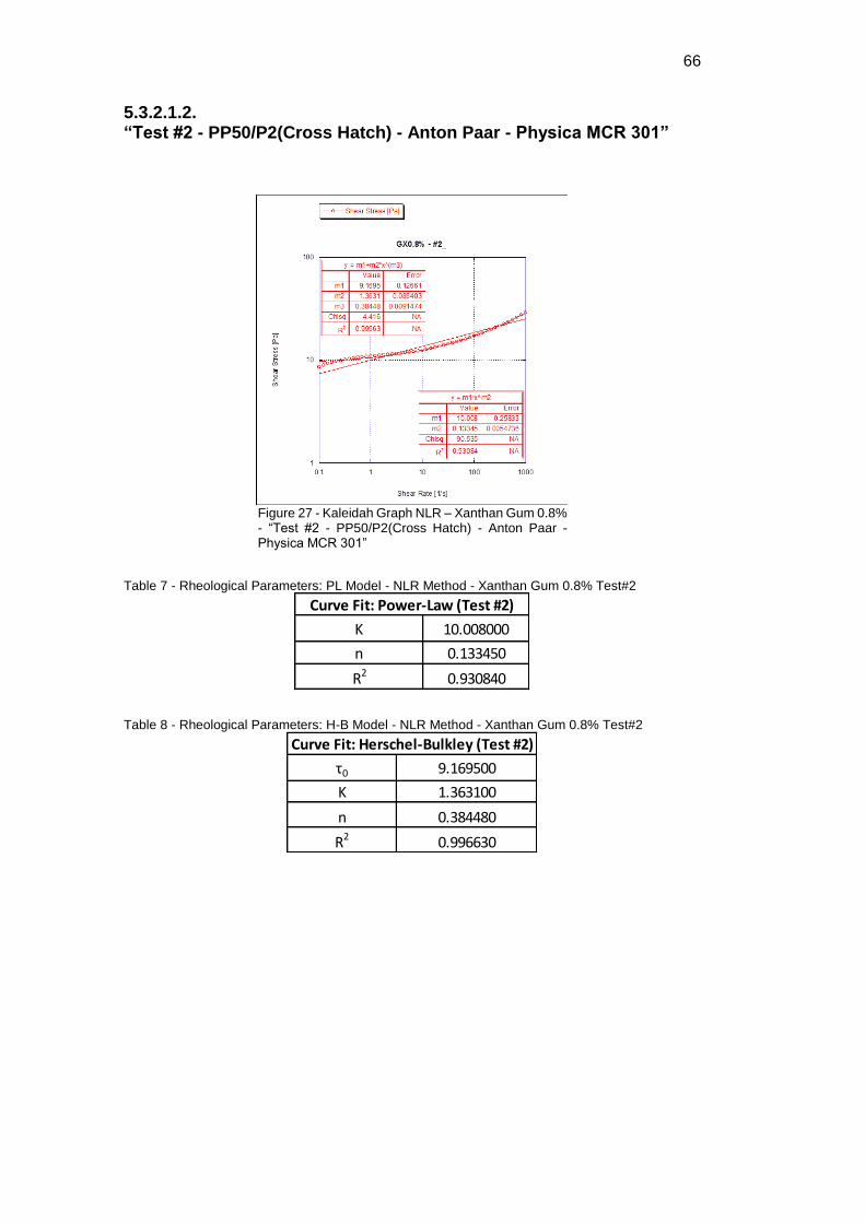
66

5.3.2.1.2. “Test #2 - PP50/P2(Cross Hatch) - Anton Paar - Physica MCR 301”

Figure 27 - Kaleidah Graph NLR – Xanthan Gum 0.8% - “Test #2 - PP50/P2(Cross Hatch) - Anton Paar - Physica MCR 301”

Table 7 - Rheological Parameters: PL Model - NLR Method - Xanthan Gum 0.8% Test#2

Table 8 - Rheological Parameters: H-B Model - NLR Method - Xanthan Gum 0.8% Test#2

K 10.008000

n 0.133450

R2 0.930840

Curve Fit: Power-Law (Test #2)

τ0 9.169500

K 1.363100

n 0.384480

R2 0.996630


DBD


67

5.3.2.1.3.

“Fann 35 - PUC - F1 B1 R1”

Figure 28 - Kaleidah Graph NLR – Xanthan Gum 0.8% - “Fann 35 - PUC - F1 B1 R1”

Table 9 - Rheological Parameters: PL Model - NLR Method - Xanthan Gum 0.8% - Fann 35 PUC

Table 10 - Rheological Parameters: H-B Model - NLR Method - Xanthan Gum 0.8% - Fann 35 PUC

K 6.651200

n 0.223880

R2 0.963900

Curve Fit: Power-Law (Fann 35 - PUC)

τ0 9.648000

K 0.672570

n 0.514700

R2 0.998012

Curve Fit: Herschel-Bulkley (Fann 35 - PUC)

DBD


68

5.3.2.2. Low Lime WBM

5.3.2.2.1. Test #1 - PP50/P2(Cross Hatch) - Anton Paar - Physica MCR 301

Figure 29 - Kaleidah Graph NLR – Low Lime WBM - “Test #1 - PP50/P2(Cross Hatch) - Anton Paar - Physica MCR 301”

Table 11 - Rheological Parameters: PL Model - NLR Method – Low Lime WBM - Test#1

Table 12 - - Rheological Parameters: H-B Model - NLR Method - – Low Lime WBM - Test#1

K 0.876640

n 0.446690

R2 0.9904

Curve Fit: Power-Law ( Test #1)

τ0 1.340600

K 0.268450

n 0.616920

R2 0.9935


DBD


69

5.3.2.2.2. Test #2 - PP50/P2 (Cross Hatch) - Anton Paar - Physica MCR 301

Figure 30 - Kaleidah Graph NLR – Low Lime WBM - “Test #2 - PP50/P2(Cross Hatch) - Anton Paar - Physica MCR 301”

Table 13 - Rheological Parameters: PL Model - NLR Method – Low Lime WBM - Test#2

Table 14 - Rheological Parameters: H-B Model - NLR Method – Low Lime WBM - Test#2

K 0.866900

n 0.447710

R2 0.99047

Curve Fit: Power-Law ( Test #1)

τ0 1.324100

K 0.267600

n 0.626810

R2 0.99354


DBD


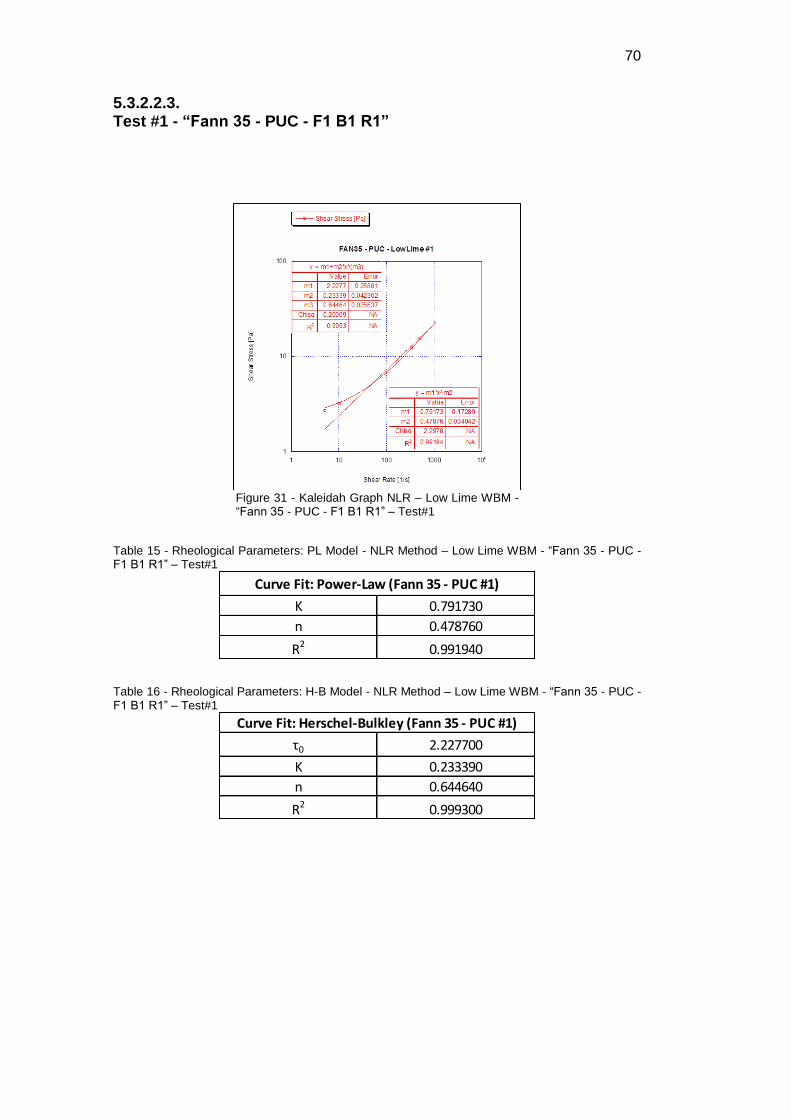
70

5.3.2.2.3. Test #1 - “Fann 35 - PUC - F1 B1 R1”

Figure 31 - Kaleidah Graph NLR – Low Lime WBM - “Fann 35 - PUC - F1 B1 R1” – Test#1

Table 15 - Rheological Parameters: PL Model - NLR Method – Low Lime WBM - “Fann 35 - PUC - F1 B1 R1” – Test#1

Table 16 - Rheological Parameters: H-B Model - NLR Method – Low Lime WBM - “Fann 35 - PUC - F1 B1 R1” – Test#1

K 0.791730

n 0.478760

R2 0.991940

Curve Fit: Power-Law (Fann 35 - PUC #1)

τ0 2.227700

K 0.233390

n 0.644640

R2 0.999300

Curve Fit: Herschel-Bulkley (Fann 35 - PUC #1)

DBD


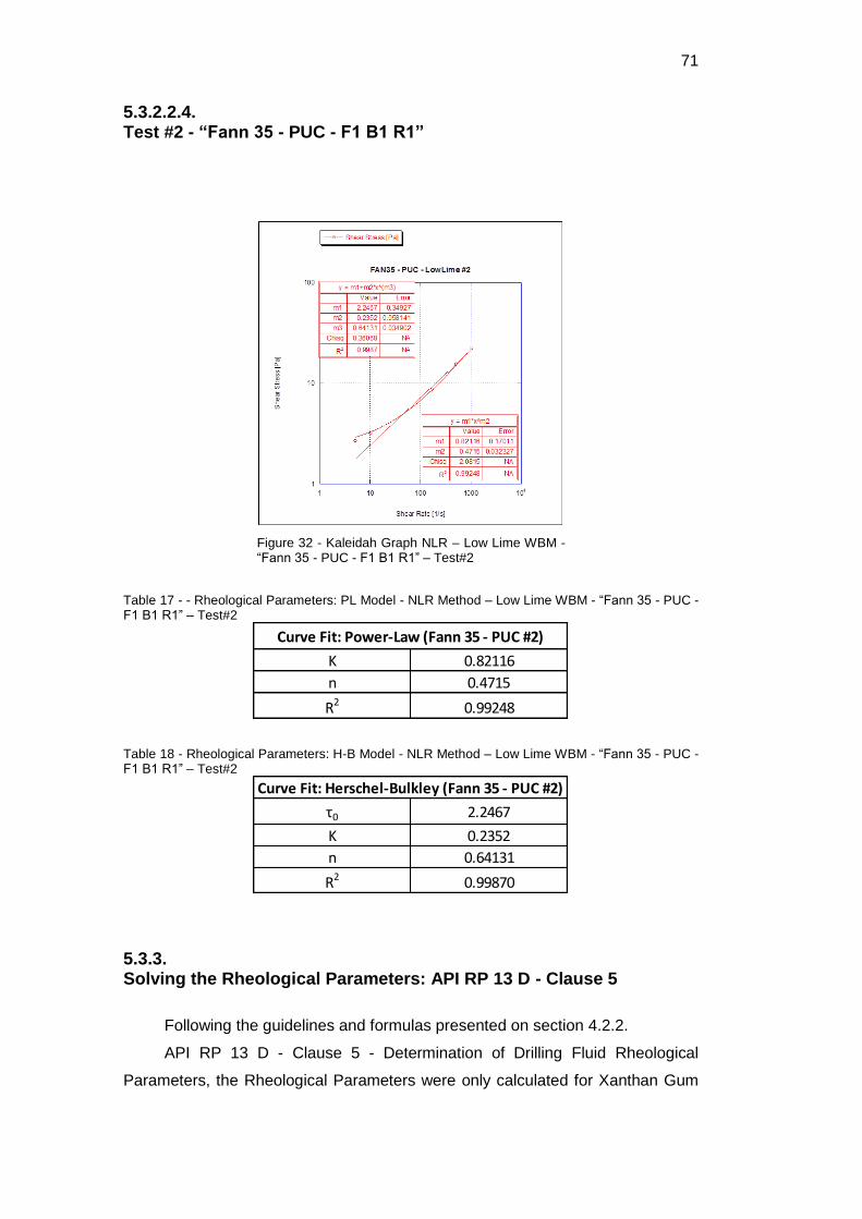
71

5.3.2.2.4. Test #2 - “Fann 35 - PUC - F1 B1 R1”

Figure 32 - Kaleidah Graph NLR – Low Lime WBM - “Fann 35 - PUC - F1 B1 R1” – Test#2

Table 17 - - Rheological Parameters: PL Model - NLR Method – Low Lime WBM - “Fann 35 - PUC - F1 B1 R1” – Test#2

Table 18 - Rheological Parameters: H-B Model - NLR Method – Low Lime WBM - “Fann 35 - PUC - F1 B1 R1” – Test#2

5.3.3. Solving the Rheological Parameters: API RP 13 D - Clause 5

Following the guidelines and formulas presented on section 4.2.2.

API RP 13 D - Clause 5 - Determination of Drilling Fluid Rheological

Parameters, the Rheological Parameters were only calculated for Xanthan Gum

K 0.82116

n 0.4715

R2 0.99248

Curve Fit: Power-Law (Fann 35 - PUC #2)

τ0 2.2467

K 0.2352

n 0.64131

R2 0.99870

Curve Fit: Herschel-Bulkley (Fann 35 - PUC #2)

DBD


72

0.8% according the PL (Annular Flow) and H-B models, based on the readings

performed at the FANN 35 PUC. The coefficient of determination also determined

as per this methodology and results presented on Table 19 and Table 20.

Table 19 - Rheological Parameters: PL Model - API RP 13 D Method- Xanthan Gum 0.8% - Fann 35 PUC

Table 20 - Rheological Parameters: H-B Model - API RP 13 D Method- Xanthan Gum 0.8% - Fann 35 PUC

The Curve Fitting values, could then be compared against the real values

obtained from the rheogram and a direct comparison made, as illustrate on Table

21 along with the coefficient of determination for each set of values.

Table 21 – API 13 D Curve Fit Method - Comparison

Due to time and resource limitations, the Low Lime WBM rheogram results

obtained from FANN35 were not used and the parameters not determined as per

API RP 13D guidelines. For this reason only the 0.8% Xanthan Gum samples were

used to demonstrate the importance of equipment, curve fitting technique, model

selection and calculation method of friction loss pressure.

K 8.369519069

n 0.166235631

R2 0.951181

Curve Fit: Power-Law (Fann 35 - PUC) - API 13D Method (Annular Flow)

τy 9.958221

K 0.413146183

n 0.58462298

R2 0.996197

Curve Fit: Herschel-Bulkley (Fann 35 - PUC) - API 13D Method

[rpm] [1/s] [Pa] [Pa] % [Pa] %

600 1021.38 33.705 26.481 21.43% 33.691 0.04%

300 510.69 25.789 23.599 8.49% 25.784 0.02%

200 340.46 22.981 22.061 4.00% 22.444 2.34%

100 170.23 19.661 19.660 0.01% 18.284 7.00%

6 10.21 12.001 12.316 -2.62% 11.566 3.63%

3 5.11 10.980 10.975 0.04% 11.030 -0.46%

R² 0.951180634 R² 0.996197333

Rotation Power Law Shear Stress

(Curve Fit)

Herschel-Bulkley Shear Stress

(Curve Fit)

FANN 35

Actual ValuesShear Rate

DBD


73

5.3.4. Curve Fitting & Model Selection

In drilling, because of thin clearances used, the estimation of dynamic

pressure in the annulus is very sensitive to the choice of the mud model (smaller

the annulus clearance - more difficult prediction). Application of model has

important implications for calculating mud hydraulics in drilling process to neither

select a model that overestimates nor underestimates pressure loss in annulus

[27].

Assuming a high degree of fit between the measured and predicted dial

readings, the calculated values of the rheological models - H-B or PL - parameters

can be applied with confidence in hydraulics and hole-cleaning equations to

calculate pressure losses and Equivalent Circulating Density (ECD).

To graphically demonstrate the issue, the curve fitting curves were plotted

for the shear rate interval of 0.1 to 1000 s-1 (Figure 33 and Figure 34). The data

obtained by the utilization of curve fitting technique may lead to errors not

affordable on the MPD process. In the particular case, it worsens for shear rates

lower than 10 s-1. Still, it is expected that the range of shear rates observed in an

annulus during a MPD connection is below the 10 s-1, which can further complicate

the problem.

Figure 33 - Curve Fitting for Low Lime Water Based Mud

DBD


74

Figure 34 - Curve Fitting for Xanthan Gum 0.8%

Although it may appear a straight forward process, further complications

might be added due to the amount of data points available (shear stress vs. shear

rate), which may mislead to false interpretation of the true rheological model to be

adopted to better describe the fluid in question. The consequences are the wrong

prediction of pressure losses, as explained earlier, which are of the extreme

importance for MPD applications, reason why it is important to raise awareness to

the amount of readings required when characterizing a drilling fluid and

identification of the range of shear rates that the flow in the annulus will experience

during the drilling operations.

It can be observed based on Table 21 – API 13 D Curve Fit Method -

Comparison that, although the coefficient of determination is one tool to assist in

Model Rheology selection, it still may induce to errors if the interval of interest is

not observed. For instance, on the example below illustrated by Figure 35, one

may select the Power Law Model curve fitted by the API 13 D Method as

satisfactory for the interval of shear rate between 10 and 100 s-1, but it’s known

that the fluid in question is a H-B as the Curve Fitting performed by NLR indicates.

In this case, an erroneous selection of Power Law Model for application below

shear rate of 5 s-1 can lead to severe consequences in terms of pressure loss

predictions.

Utilization of PL rheology model may not capture the entire interval of interest

for the shear rates present in annular flow during MPD applications. In addition,

DBD


75

API RP 13D Curve Fitting for Power Law Model does not capture the flow behavior

and may lead to wrong interpretation.

Figure 35 – Shear Rate Interval of Interest and Model Selection

Ideally, the range of shear rates where the flow will be evaluated should be

known in advance in order to ensure that the model selected will be appropriate for

the operational conditions. However, in most cases, it tends to happen the other

way around, whereby the fluid rheology is required in order to estimate the shear

rates in a given geometry and to subsequently determine the interval of shear rate.

A typical approach is to select the best estimate for the fluid rheology model,

perform the calculations for shear rates, and verify if the selected model

corresponds to the best description of the fluid properties within the desired

interval. In cases where it is known that flow will be studied from “no flow” condition

to its maximum flow rate (such in MPD connections) the range of shear rates

becomes from zero to its maximum calculated. In addition, it is relevant that the

fluid model must be representative for the entire range of values for shear rates

versus shear stresses.

Nevertheless, as for the Curve Fit results from the API 13 D method, a brief

investigation leads to conclude that the curve fit matches with 3 and 100 rpm

readings (5.11 and 170.23 s-1) as the rheological parameters are calculated based

on those 2 readings. Conversely, applications between 6 and 100 rpm (10.21 and

170.23 s-1) are susceptible to minor failures. Beyond that interval, the

consequences can be poorest as illustrated on Figure 36. If shear rates are

observed within the above range, it may be pertinent to the industry to evaluate the

DBD


76

necessity of additional viscosity readings in between the 3 and 100 rpm readings.

Later on this study, this affirmation is verified.

Figure 36 - Xhantam Gum 0.8% - Power Law Curve Fit Comparison

The remaining question would be how to best select a rheology model. The

answer could be both graphically by looking at the interval of shear rates that the

process is implemented and, as suggested, via the coefficient of determination.

All the results from the Xantham Gum 0.8 are presented on the Table 22.

Direct comparison of coefficient of determination allows selecting between the two

models evaluated - PL (red tab) and H-B (green tab) - by comparing the coefficient

of determination regardless the instrument used (FANN 35 or Physica) to perform

the rheogram or the curve fitting method implemented (NLR or API 13 D). On all

cases, the H-B model has been identified as a most appropriate rheology model

for the samples.

The second conclusion is, once the model is chosen, the rheograms done by

the Physica rheometers (50 points readings) lead to coefficient of determination

lower than the FANN35 (6 points readings) through NLR Curve Fitting, and it

should be carefully evaluated. As coefficient of determination being a statistical

measure of how well the regression line approximates the real data points, it is

expected that larger amount of data points returns a higher variation over the total

variation. In this manner, to be able to further decide the best curve fitting may not

be possible in comparing values obtained from 6 points versus 50 points and for

different range intervals, as the Physica’s data points extended the readings to

down low 0.1 s-1. In this specific case, it should be done by graphical observation.

DBD


77

The graphical observation indicates that 50 points still have a better performance

in representing the fluid model on its range as earlier exemplified.

Table 22 – Curve Fitting and Coefficient of Determination Results

The third affirmation is direct comparison of curve fitting by NLR versus API

13D, given the exception of the direct comparison of the number of points. In the

case of 6 data points following the API 13 B guidelines, certainly the NLR method

offers a superior result than API 13 D for the FANN 35 reading. Then the NLR

method must be the preferable method for determining curve fitting parameters.

5.3.4.1. Accuracy of the process

The importance of the entire process to obtain a mathematical representation

of rheology properties of a fluid relies on taking into account several factors, and

the accurate selection of: equipment, geometry, range of specification, means of

measurements, amount of data available, curve fitting method and statistical tools

to better infer on the final result selection.

In reality, it must be bear in mind that curve fit is only an approximation for

the real fluid properties. As earlier discussed, it is highly dependent of the process

implemented:

DBD


78

the equipment used for the rheogram,

the amount of data points collected and the range and

method to fit the points and retrieve a mathematical model that represents

the set of data.

Exemplified on Figure 37, further illustrate the relationship of all the three

aspects listed above. The information is then absent when less precise equipment

is used to measure the same data and the amount of readings lower with narrow

interval. In this case, it is observed that the FANN35 readings for shear rates lower

than 10 s-1 missed the accuracy.

Figure 37 – Curve Fit vs Actual Fluid Properties

Subsequently, the discrepancy in results between the field3 and the

laboratory environment4 was analyzed. Such comparison allowed understand in a

better way how the measurement process and curve fitting technique can influence

the results for pressure loss estimation in a given annulus. It is important to remark

that, the equipment used may not be able to capture the fluid rheology properly. In

addition, the mathematical manipulation of data might not be representative of real

properties on its entire domain.

The Figure 38 concludes and exemplifies the Xanthan Gum 0.8% fluid

sample with the six data points acquired by FANN35 Oilfield Viscometer and curve

fitted for an H-B Model following the API 13D Method. It also embraces the 50

points acquired through the Physica Rheometer in the laboratory and curve fitted

using NLR method.

3 Defined as the fluid properties measured at FANN35 and Curve Fitted by API RP 13D Method. 4 Defined as the fluid properties measured at Physica and Curve Fitted by Non Linear Regression.

DBD


79

Figure 38 – Fluid Properties versus Curve Fit Accuracy

To enhance the prediction of rheology model selection it is suggested to

include additional measurements between the 3 and 100 rpm FANN 35 readings

when this equipment is used, thus increasing the amount of points and delivering

a more accurate mathematical model.

Ultimately, MPD design would benefit from a model rheology that could

represent the fluid rheology property to a near zero shear rate and be continuous

numeric solved on entire domain as the H-B curve fitting calculated for the case

above does not properly fit for the very low end of the curve.

DBD


6 Mapping Shear Rate

6.1. Fluid Properties Selection

For the subsequent analysis of the shear mapping following the API13 D

guidelines, the results obtained for the Xanthan Gum 0.8% were used. The

following two sets of fluid properties results were selected as most representative

results between different environment conditions:

1. Rheogram performed on the Anton Paar - Physica MCR 301 with

PP50/P2 Cross Hatch geometry. Rheological Parameters and curve fit

calculated as H-B Model using NLR Method (Table 8).

2. Rheogram performed on the Fann 35 – PUC as per API RP 13 B.

Rheological Parameters calculated as H-B Model using the API RP 13 D

Method (Table 20).

While set (1) intended to represent the controlled laboratory condition, the

set (2) is the standard oilfield practice suggested by API under field conditions.

6.2. Geometry Selection

Two typical hole sections and a drill pipe were stipulated based on the most

commonly drilled hole sizes using MPD with the objective of illustrate a annular

geometry and allows to verify the range of shear rates.

Hence, two different geometries have been assumed to illustrate the goals

of this study:

Case (a): “8.5 Section” set as Open Hole Diameter of 8.5 inches (215.9

mm) and Drill Pipe of 5.5 inches (139.7 mm).

Case (b): “12.25 Section” set as Open Hole Diameter of 12.25 inches

(215.9 mm) and Drill Pipe of 5.5 inches (139.7 mm).

DBD


81

Figure 39 - Case (a): “8.5 Section”

Figure 40 - Case (b): “12.25 Section”

While in case (a) it is believed that the major impact of inaccuracies from

equipment and estimations leads to higher differences in pressure loss calculations

due to the smaller clearance when compared with case (b), case (b) is expected

to encompass the lower end range of shear rate values due to the lower flow

velocities (larger annulus) when compared with (a).

6.3. Flow Rate Selection

As for the flow rate range selection, typical maximum drilling flow rates on

the cases (a) and (b) above are in the range of 400 gpm (0.0252 m3/s) and 1,000

gpm (0.063 m3/s). Care was taken to ensure that the flow observed under these

conditions were still on the laminar region.

Although the stipulated maximum flow rates above may slightly differ from

operation to operation, the objective was to map the shear rate during a transition

process, in other words, from its maximum estimation to zero.

The average (bulk) velocities (Va), for both geometries – (a) and (b) - given

the flow rate range are found Table 23 and Table 24 calculated by the application

of the equation (8).

DBD


82

Table 23 - Annulus Fluid Velocity for 8.5 Section – Case (a)

Table 24 – Annulus Fluid Velocity for 12.25 Section – Case (b)

6.4. Shear Rate and Shear Stress Calculations as per API 13 D

As discussed on section 0, API RP 13 D suggests a set of formulae and

procedures to estimate the shear stress at wall. The utilization of the formulae

presented on API 13D and reproduced in this study by equations (10), (11) and

(12), allowed to calculate the Shear Rate in the Annulus (measured at the wall).

Q - Flow Rate

[gpm]

Va - Annulus Fluid Velocity

[m/s]

10 0.029645

20 0.059291

30 0.088936

40 0.118582

50 0.148227

60 0.177873

70 0.207518

80 0.237163

90 0.266809

100 0.296454

200 0.592909

300 0.889363

400 1.185817

Q - Flow Rate

[gpm]


[m/s]

10 0.010392

20 0.020784

30 0.031176

40 0.041569

50 0.051961

60 0.062353

70 0.072745

80 0.083137

90 0.093529

100 0.103921

200 0.207843

300 0.311764

400 0.415686

500 0.519607

700 0.727450

1000 1.039214

DBD


83

The corresponding value of shear stress for both geometries (case “a” and

case “b” previously mentioned) using the fluid properties as per field conditions5,

andusing the equations (13) and (14) were also estimated.

Values obtained are presented in the results Table 25 and Table 26.

Table 25 – Shear Stress and Shear Rate as per API 13 D Method - Herschel-Bulkley Model - 8.5 Section.

Table 26 - Shear Stress and Shear Rate as per API 13 D Method - Herschel-Bulkley Model – 12.25 Section

In possession of the results, it was possible to make the verification regarding

the range of values suggested by API 13 B (6 points). Maximum shear rates

observed for maximum flows, 400 gpm on case (a) and 1000 gpm on case (b) are

lower than 100 s-1. In these cases, only 2 actual readings from FANN 35 are then

used to infer about the rheology model calculations: 3 rpm (5.11 s-1) and 6 rpm

5 Defined as the fluid properties measured at FANN35 and Curve Fitted by API RP 13D Method.

Q - Flow Rate

[gpm]

ɣ.wall - (API 13 D - 7.4.7)

Shear Rate at the Wall [1/s]

τf - Shear Stress

at the Wall [lbf / 100 ft²]

τf - Shear Stress

at the Wall [Pa]

10 2.4528 27.8047 13.3130

20 4.9057 28.5328 13.6616

30 7.3585 29.1173 13.9415

40 9.8114 29.6247 14.1844

50 12.2642 30.0813 14.4030

60 14.7171 30.5013 14.6041

70 17.1699 30.8930 14.7917

80 19.6228 31.2621 14.9684

90 22.0756 31.6124 15.1361

100 24.5285 31.9469 15.2963

200 49.0569 34.7447 16.6359

300 73.5854 36.9909 17.7114

400 98.1139 38.9403 18.6447

Q - Flow Rate

[gpm]

ɣ.wall - (API 13 D - 7.4.7)


τf - Shear Stress

at the Wall [lbf / 100 ft²]

τf - Shear Stress

at the Wall [Pa]

10 0.3822 26.8389 12.8505

20 0.7643 27.0845 12.9681

30 1.1465 27.2816 13.0625

40 1.5286 27.4527 13.1444

50 1.9108 27.6067 13.2182

60 2.2929 27.7484 13.2860

70 2.6751 27.8805 13.3492

80 3.0572 28.0049 13.4088

90 3.4394 28.1231 13.4654

100 3.8215 28.2359 13.5194

200 7.6430 29.1794 13.9712

300 11.4645 29.9370 14.3339

400 15.2860 30.5944 14.6487

500 19.1076 31.1862 14.9321

600 22.9291 31.7305 15.1926

700 26.7506 32.2381 15.4357

800 30.5721 32.7164 15.6647

900 34.3936 33.1704 15.8821

1000 38.2151 33.6039 16.0896

DBD


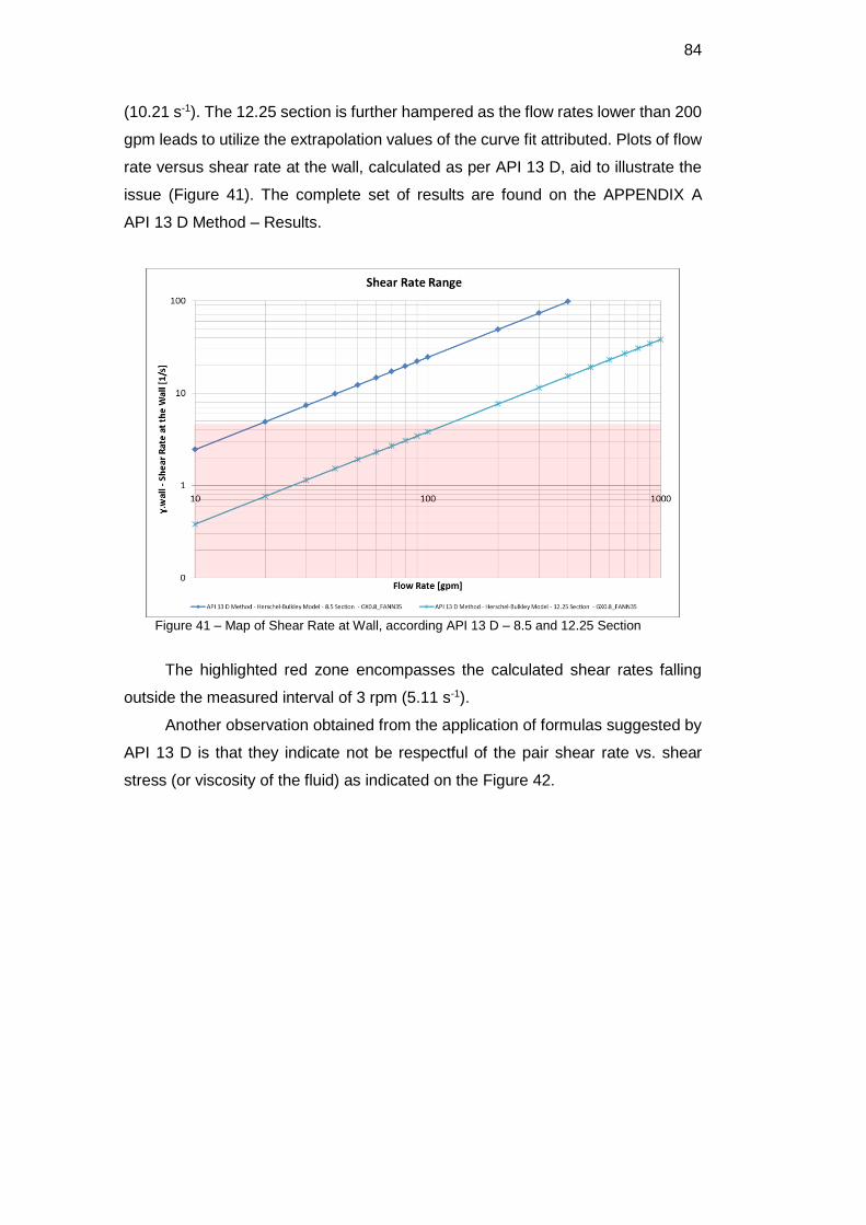
84

(10.21 s-1). The 12.25 section is further hampered as the flow rates lower than 200

gpm leads to utilize the extrapolation values of the curve fit attributed. Plots of flow

rate versus shear rate at the wall, calculated as per API 13 D, aid to illustrate the

issue (Figure 41). The complete set of results are found on the APPENDIX A

API 13 D Method – Results.

Figure 41 – Map of Shear Rate at Wall, according API 13 D – 8.5 and 12.25 Section

The highlighted red zone encompasses the calculated shear rates falling

outside the measured interval of 3 rpm (5.11 s-1).

Another observation obtained from the application of formulas suggested by

API 13 D is that they indicate not be respectful of the pair shear rate vs. shear

stress (or viscosity of the fluid) as indicated on the Figure 42.

DBD


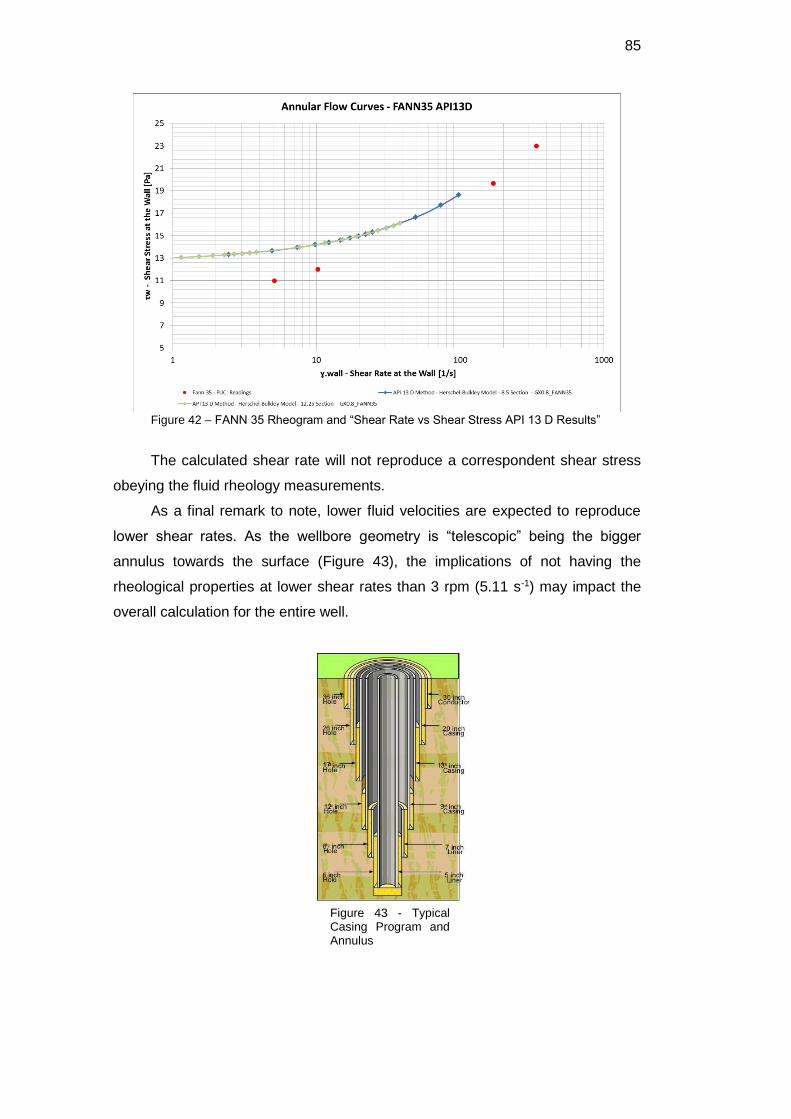
85

Figure 42 – FANN 35 Rheogram and “Shear Rate vs Shear Stress API 13 D Results”

The calculated shear rate will not reproduce a correspondent shear stress

obeying the fluid rheology measurements.

As a final remark to note, lower fluid velocities are expected to reproduce

lower shear rates. As the wellbore geometry is “telescopic” being the bigger

annulus towards the surface (Figure 43), the implications of not having the

rheological properties at lower shear rates than 3 rpm (5.11 s-1) may impact the

overall calculation for the entire well.

Figure 43 - Typical Casing Program and Annulus

DBD


7 Validating the Shear Rate Map: CFD Numerical Verification

The awkward results of shear rates obtained by the direct formulas of API

RP 13 D required the implementation of a verification method rather than analytical.

Due to the nature of a non-Newtonian flow problem, the course of the study

decided to rely on numerical methods as secondary form of verification.

The numerical solution of the non-Newtonian flow obtained with the aid of

the Computational Fluid Dynamics (CFD) using the Fluent Software by ANSYS -

version 15.07 (released 2014) and version 16.0 (released 2015) - allowed to proof

the application of standards early tested.

Equally, the cases formulated and solve by the API 13 D methods were

solved using the CFD Technique in an assessment of the analytical solution

method against a numerical method. The utilization of the CFD also permitted the

direct evaluation of curve fitting and equipment implemented to obtain the fluid

data.

In this chapter, a briefly discussion of the method is presented along with the

relevant modeling of the problem and the setup performed to ensure the physics,

boundaries. At the end, the results comparison of shear rates are presented and

preliminary conclusions stated in regards to the API 13 B and API 13 D standards.

7.1. About ANSYS Fluent

ANSYS Fluent provides comprehensive modeling capabilities for a wide

range of applications; among them is the analysis of incompressible laminar non-

Newtonian fluid flow, which is the main interest for the current study

ANSYS Fluent uses a control-volume-based technique to convert a general

scalar transport equation to an algebraic equation that can be solved numerically.

This control volume technique consists of integrating the transport equation about

each control volume, yielding a discrete equation that expresses the conservation

law on a control-volume basis.

DBD


87

Figure 44 - Control Volume Example

In summary, the control-volume-based technique consists of three (3) steps:

1. Division of the domain into discrete control volumes using a

computational grid.

2. Integration of the governing equations on the individual control volumes

to construct algebraic equations for the discrete dependent variables

(“unknowns”) such as velocities, pressure, temperature, and conserved

scalars.

3. Linearization of the discretized equations and solution of the resultant

linear equation system to yield updated values of the dependent

variables.

7.2. Computational Fluid Dynamics Setup

7.2.1. Solver and Solution Methods

7.2.1.1. Pressure Based Solver

In this type of solver, the velocity field is obtained from the momentum

equations. The pressure field is extracted by solving a pressure or pressure

correction equation that is obtained by manipulating continuity and momentum

equations. ANSYS Fluent will solve the governing integral equations for the

conservation of mass and momentum.

DBD


88

Figure 45 - Transport Equations

The pressure-based solver employs the algorithm that belongs to a general

class of methods called the projection method. The constraint of mass

conservation (continuity) of the velocity field is achieved by solving a pressure (or

pressure correction) equation.

The pressure equation is derived from the continuity and the momentum

equations in such way that the velocity field, corrected by the pressure, satisfies

the continuity. Since the governing equations are nonlinear and coupled to one

another, the solution process involves iterations wherein the entire set of governing

equations is solved repeatedly until the solution converges.

Yet, the pressure-based solver approach is applicable for low-speed

incompressible flows.

7.2.1.2. General Scalar Transport Equation Setup – Solution Methods

Under the pressure-based solver, the solution method selected was the

Pressure-Velocity Coupling in the Coupled scheme.

The Coupled scheme provides a robust and efficient single phase

implementation for steady-state flows, with superior performance compared to the

segregated solution schemes [28].

DBD


89

Figure 46 - Fluent Solution Methods

Spatial Discretization (Solution Methods) were set as “Green Gauss Node

Based” for gradient, PRESTO! for pressure and “Second Order Upwind” for

Momentum (Figure 46). Regarding the Solution Controls, the explicit relaxation

factors were 0.5 for pressure and 0.5 for momentum while the under–relaxation

factors were set to 1 for density and body forces (Figure 47).

Figure 47 - Fluent Solution Controls

Justifications of the selected methods are further explained on the following

sections.

DBD


90

7.2.1.2.1. Discretization (Interpolation Method)

As the ANSYS Fluent uses a control-volume-based technique to convert a

general scalar transport equation to an algebraic equation that can be solved

numerically, it requires the field variables (stored at cell centers) must be

interpolated to the faces of the control volumes.

Figure 48 - Discretization - Interpolation Methods

Among the interpolation schemes available for the convection term

(Momentum), the Second-Order Upwind has been chosen. The Second Order

Upwind quantities at cell faces are computed using a multidimensional linear

reconstruction approach and uses larger stencils for 2nd order accuracy. It is

remarkably to note that convergence may be slower when this scheme is selected.

7.2.1.2.2. Interpolation Method - Gradients

Gradients of solution variables are required in order to evaluate diffusive

fluxes, velocity derivatives, and for higher-order discretization schemes.

Figure 49 - Gradients - Interpolation Methods

The gradients of solution variables at cell centers can be determined using

three approaches:

Green-Gauss Cell-Based – The default method; solution may have false

diffusion (smearing of the solution fields).

Green-Gauss Node-Based – More accurate; minimizes false diffusion;

recommended for tri/tet meshes.

DBD


91

Least-Squares Cell-Based – Recommended for polyhedral meshes; has

the same accuracy and properties as Node-based Gradients.

The interpolation method for gradient on all simulated cases was chosen as

Green Gauss Node Based. To note, the method computes the gradient of the

scalar at the cell center by the arithmetic average of the nodal values on the face

of the element.

7.2.1.2.3. Interpolation Methods for Face Pressure

Interpolation scheme for calculating cell-face pressures were selected as

PRESTO! (PREssure STaggering Option). The scheme uses the discrete

continuity balance for a “staggered” control volume about the face to compute the

“staggered” (that is, face) pressure. This procedure is similar to the staggered-grid

schemes used with structured meshes. The PRESTO! scheme applies when large

surface-normal pressure gradients near boundaries with steep pressure changes

are present in the flow.

7.3. Critical Shear Rate Selection for Non-Newtonian Fluids

ANSYS Fluent defines a normalized version of Herschel-Bulkley (H-B)

model to be able to numerically solves the equation.

While the Herschel-Bulkley (HB) model is usually defined as previously

defined on equation (2), the normalization is achieved by replacing equation (20),

(20)

into equation (21)

(21)

DBD


92

Resulting in equation (22).

(22)

Where

is the critical shear rate[1/s].

The normalized viscosity equation for H-B model calculated by Fluent can

then be expressed as equation (23) below:

(23)

Granting a value of critical shear rate must be input on ANSYS Fluent as one of

the requirements for the H-B property as indicated on Figure 50.

DBD


93

Figure 50 - ANSYS Fluent - Fluid Properties Input Screen (H-B Model)

The impact of chosen Critical Shear Rate value versus the shear rate of the

flow are exemplified on the sensitivity analysis by application of the equation (23)

for various shear rates. As observed, high critical shear rates leads to the numerical

solution to be solved as the fluid as Newtonian or near solid (constant viscosity).

Figure 51 - Critical Shear Rate Selection and Behavior

M. Soares et al [29] suggested that critical shear rate value should be in the

order of thousands of the shear rate observed in the flow. After several tests

0

0

1

10

100

1000

10000

100000

0.0001 0.001 0.01 0.1 1 10 100 1000

Vis

cosi

ty [

Pa.

s]

Shear Rate [1/s]

Critical Shear Rate Selection

1 0.1 0.01 0.001 1 0.1 0.01 0.001 Lab Test

DBD


94

performed, a critical shear rate value was established as 5e10-5 [1/s] for all cases

ran on Fluent. The selection allowed satisfactory results and convergence.

7.4. Geometry and Meshing Considerations

The numerical solution was modeled for half of the annular space, in a bi-

dimensional (2D) axisymmetric plane for both annulus geometries (Case (a) and

Case (b)).

Figure 52 illustrates the 2D numerical mesh, with 8,500 axial and 60 radial

divisions, which lead to 510000 cells (maximum allowed by ANSYS Fluent Version

15.07– Student License capped in 512000 cells). Mesh Control through Inflation of

the cells at the inner and outer wall in a proportion of 1.1 has been applied.

Figure 52 – 2D Mesh Transversal View

To achieve satisfactory mesh quality in terms of skewness and orthogonality

controls, the total length of the annulus was defined as 500 inches (12.7 m) and

1000 inches (25.4 m) respectively for the Case (a) and Case (b).

The quality have been checked and considered satisfactory for orthogonality

and skewness. The experimental simulation of a Newtonian fluid (pure water -

Figure 53) of developed fluid velocity profile (compared against the non-Newtonian

fluid (Xanthan Gum 0.8% - Figure 54) had also tested the mesh quality.

DBD


95

Figure 53 - Velocity Profile of Newtonian Fluid at 1000 gpm in the 12.25 Section

Figure 54 - Velocity Profile of Non-Newtonian Fluid at 1000 gpm in the 12.25 Section

7.5. Physics and Boundaries

The flow was modeled as laminar steady-state with double digit precision.

The flow is isothermal, so the energy equation was not solved.

The boundary conditions were defined as below, being u the vector velocity

component in x-axis and v in the y-axis:

DBD


96

1. uniform velocity prescribed at the inlet (Figure 55) according to the Table

23 - Annulus Fluid Velocity for 8.5 Section – Case (a) and Table 24 –

Annulus Fluid Velocity for 12.25 Section – Case (b);

u=C, v=0

2. fully-developed condition at the outlet;

d/dx=0

3. impermeability and no slip wall condition at cylinder walls;

u=v=0

4. symmetry conditions at the symmetry plane.

Figure 55 – Representation of the Annulus Flow: 3D Mesh – Perspective View

7.6. Convergence Criteria & Monitoring

At convergence, all discrete conservation equations (momentum, energy,

etc.) are obeyed in all cells to a specified tolerance, or the solution no longer

changes with subsequent iterations. The convergence criteria ensured that overall

mass, momentum, and scalar balances were achieved.

The Residual History has been utilized as control parameter for all cases.

Generally, a decrease in residuals by three orders of magnitude indicates at least

qualitative convergence. At this point, the major flow features should be

established. In this evaluation, the convergence criteria for the residuals were set

as 10e-10 for Continuity, X-Velocity and Y-Velocity and demonstrated to be

satisfactory for all cases.

A secondary quantitative convergence used was the standard deviation of

the velocity at the centerline of the annular flow. This monitoring technique ensured

DBD


97

the appropriate selection of the values observed in the fully developed region of

the flow (no variation of velocity along the X-axis), as illustrate on Figure 56 and

Figure 57 for cases (a) and (b). In the case, Observation Points (OP) for the shear

rate and shear stress were then set at half of the length for each case (i.e.: 250

and 500 inches respectively on X-axis position) to ensure an undisturbed flow

distant from the inlet and outlet.

Figure 56 - Annulus Flow Development - Case (a) - 400 gpm

Figure 57 - Annulus Flow Development - Case (b) - 1000 gpm

This technique allows obtaining the velocity profile (Figure 58), shear rate (or

strain rate) distribution along the annulus - YZ plane at 500 inches located on X

axis - (Figure 59), and shear stress at the wall measurements (Figure 60) for all

simulated cases.

DBD


98

Figure 58 - Velocity Distribution at Observation Point (12.25 Section - GX0.8% - Physica NLR)

Figure 59 -Strain Rate distribution at Observation Point (12.25 Section - GX0.8% - Physica NLR - 1000 gpm)

0

0.2

0.4

0.6

0.8

1

1.2

1.4

0 0.05 0.1 0.15 0.2

Ve

loci

ty M

agn

itu

de

[m

/s]

Annulus Position (y-axis) [inches]

Velocity Distribution at Observation PointAnnulus Fluid Velocity for 12.25 Section - Case (b)

10 gpm

50gpm

300 gpm

700gpm

1000 gpm

DBD


99

Figure 60 – Wall Shear Stress at Observation Point (12.25 ection - GX0.8% - Physica NLR – 1000 gpm)

7.7. CFD ANSYS Fluent: Shear Rates Mapping Cases

The usage of CFD Method had the objectives achieved. It allowed the

comparison of two different scenarios relevant for MPD Applications:

The first comparison attempted to compare the influence of calculation

method. In specific the API RP 13D Direct Formula Calculation versus the

numerical results obtained by software Fluent ANSYS CFD.

In this scenario (Figure 61), the same H-B fluid properties model parameters

(n and K) was used as input for the application of formulas while in API and

description of the fluid on the software. The model index properties used are found

on Table 20 - Rheological Parameters: H-B Model - API RP 13 D Method- Xanthan

Gum 0.8% - Fann 35 PUC.

Figure 61 - Influence of Hydraulic Modeling: Analytical vs Numerical

API 13D CFD / VOF

Curve Fit by API 13D Method

Fann 35

Fluid Sample

Press Loss Field Press Loss Lab

Pressure Loss Model: API13D Pressure Loss Model: CFD / VOF

DBD


100

The second analysis attempted to evaluate the curve fitting methodology and

equipment accuracy. Subsequently, the discrepancy in results between the field6

and the laboratory environment7 has been examined in terms of fluid

characterization. Figure 62 illustrates the comparison thought process herein

proposed. Such comparison allowed to understand in a better way how the

measurement process and curve fitting technique can influence the results for

pressure loss estimation in a given annulus.

Figure 62 – Influence of Environment: Field versus Laboratory

The numerical solutions of shear rates according to the Table 23 - Annulus

Fluid Velocity for 8.5 Section – Case (a) and Table 24 – Annulus Fluid Velocity for

12.25 Section – Case (b) have been successfully obtained from the simulations

considering the fluid properties obtained from “Table 20 - Rheological Parameters:

H-B Model - API RP 13 D Method- Xanthan Gum 0.8% - Fann 35 PUC” and “Table

8 - Rheological Parameters: H-B Model - NLR Method - Xanthan Gum 0.8%

Test#2”.

In total, 26 CFD simulations were performed for case (a) and 32 CFD

simulations for case (b). After all, on each proposed case - (a) and (b) – 3 sets of

data were available for comparison purposes as previously outlined:



6 Defined as the fluid properties measured at FANN35 and Curve Fitted by API RP 13D Method 7 Defined as the fluid properties measured at Physica and Curve Fitted by Non Linear Regression

DBD


101

RP 13D Method and Pressure Loss calculated by API RP 13D direct

formula Method.



RP 13D Method and Pressure Loss calculated by Fluent Ansys CFD.

3. Rheological Properties measured by HPR, curve fitted and HB rheological

parameter described by NLR Method and Pressure Loss calculated by

Fluent Ansys CFD.

7.7.1. Influence of Hydraulics and Environment: Results

The direct comparison results indicate that there were minor variations of

shear rates when considered the four sets of results (APPENDIX B

CFD by ANSYS Fluent – Results) from the numeric solution obtained by ANSYS

Fluent hydraulic simulator. The proposed comparison of the Field and Laboratory

scheme indicates that that curve fitting method and equipment has minimal impact

when regarding shear rates values.

Controversially of the shear rate obtained from API RP 13D analytical

calculations, as shows on Figure 63 and Figure 64, the numerical results suggest

that the shear rate ranges for 8.5” section are confirmed within the 3-100 rpm (5.11

s-1 - 170.23 s-1) of FANN35 readings. The same conclusions of the numerical

results for the 12.25” section are observed.

Figure 63 - Numerical Solution for Shear Rate vs. Flow Rate in 8.5” Section and API13D Comparison

DBD


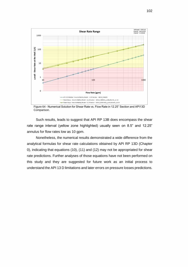
102

Figure 64 - Numerical Solution for Shear Rate vs. Flow Rate in 12.25” Section and API13D Comparison.

Such results, leads to suggest that API RP 13B does encompass the shear

rate range interval (yellow zone highlighted) usually seen on 8.5” and 12.25”

annulus for flow rates low as 10 gpm.

Nonetheless, the numerical results demonstrated a wide difference from the

analytical formulas for shear rate calculations obtained by API RP 13D (Chapter

0), indicating that equations (10), (11) and (12) may not be appropriated for shear

rate predictions. Further analyses of those equations have not been performed on

this study and they are suggested for future work as an initial process to

understand the API 13 D limitations and later errors on pressure losses predictions.

DBD


8 Pressure Losses Estimations

The upmost objective of a pump step-down schedule used in MPD is the

accurately predict the pressure loss estimation at various flow rates.

The aid of numerical results allowed the representation of the field conditions

versus laboratory conditions in a first instance and the validation of analytical

methods suggested by API.

Although previously observed that shear rates estimation are not major

impacted by the measurement device and curve fitting technique, the same

conclusions could not be observed for shear stress and consequently pressure

loss estimations.

The pressure loss estimation was mapped for the flow rate interval

suggested by the two annulus geometries and a qualitative analysis conducted.

Applications of formulas found on API RP 13 D and from numerical simulations

allowed estimating the pressure loss per unit of length.

8.1. Case (a): “8.5 Section”

The numerical outcomes for case (a) – 8.5” section – in respect of field and

laboratory circumstances for fluid characterization points out that laboratory pattern

(green line) delivers the approximately same “slope” of the pressure loss by flow

rate curves obtained by field patterns (light blue line).

The results from a fluid sample characterized in a laboratory environment

present a higher value by average of 7% in comparison with the same fluid

characterized in a field environment. The minimum and maximum differences

observed at low and high end of the flow rates are 9% and 2% respectively (Figure

65). The difference is attributed to the process in obtaining the fluid properties as

extensively discussed earlier and suggests that an enhanced method should be

evaluated for MPD Applications.

Still, if considered the pressure loss per 1,000 ft (304.8m) of 8.5” by 5.5”

annulus – case (a) - only 3 psi (0.0206843 MPa) in difference is perceived. The

DBD


104

difference may not be representative enough to justify different methods for MPD

fluid characterization; however, an enhanced method would be justified by the

assurance of correct rheology model selection or when a more challenging and

complex well with minimal operation window is ought to be drilled.

While comparing the API 13 D analytical method for pressure loss estimation

(dark blue line), indicates that the slope of the curves is not analogous. Differences

between the analytical method and the numerical results using the same FANN 35

properties values (green line) produces a variation of -7% at low flow rates (e.g.:

10 gpm) up to 22% at 450 gpm (Figure 65).

Figure 65 - Pressure Loss Estimation: 8.5" Section (case (a))

In this case, the analytical formulas suggested by API 13D should be avoided

whenever possible. Pressure loss prediction for critical operations such MPD,

which has significant impact and consequences due to wrong estimations, must

rely on more complex and precise forms of hydraulic calculations.

8.2. Case (b): “12.25 Section”

The case (b) – 12.25” section - which encompass the lower end range of

shear rate values due to the lower flow velocities (larger annulus) indicates a

slighter higher difference in relative values of 9% between the two numerical

DBD


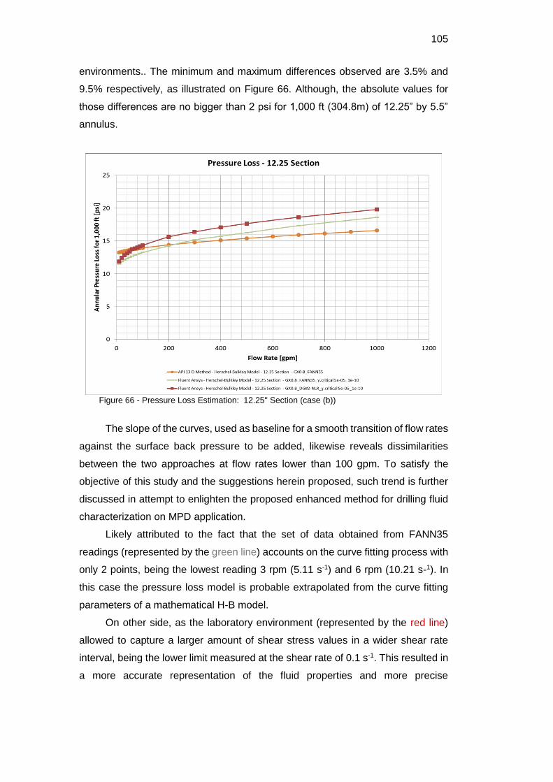
105

environments.. The minimum and maximum differences observed are 3.5% and

9.5% respectively, as illustrated on Figure 66. Although, the absolute values for

those differences are no bigger than 2 psi for 1,000 ft (304.8m) of 12.25” by 5.5”

annulus.

Figure 66 - Pressure Loss Estimation: 12.25" Section (case (b))

The slope of the curves, used as baseline for a smooth transition of flow rates

against the surface back pressure to be added, likewise reveals dissimilarities

between the two approaches at flow rates lower than 100 gpm. To satisfy the

objective of this study and the suggestions herein proposed, such trend is further

discussed in attempt to enlighten the proposed enhanced method for drilling fluid

characterization on MPD application.

Likely attributed to the fact that the set of data obtained from FANN35

readings (represented by the green line) accounts on the curve fitting process with

only 2 points, being the lowest reading 3 rpm (5.11 s-1) and 6 rpm (10.21 s-1). In

this case the pressure loss model is probable extrapolated from the curve fitting

parameters of a mathematical H-B model.

On other side, as the laboratory environment (represented by the red line)

allowed to capture a larger amount of shear stress values in a wider shear rate

interval, being the lower limit measured at the shear rate of 0.1 s-1. This resulted in

a more accurate representation of the fluid properties and more precise

DBD


106

mathematical representation obtained from the curve fitting parameters for the

shear rates interval observed on the flow rates of 12.25” section.

As it can be inferred from the study, attribution to the variance is due to the

equipment used to obtain the viscosity properties of the fluid (FANN 35 vs. Physica)

and the technique used to manipulate the properties, since all calculations,

software engine and set up process was the same for all the samples.

Reasonably assuming that the numerical results are accurate, the pressure

loss results obtained by numerical simulation indicates that although shear rate

ranges are very similar, they do not reproduce the same results on shear stress

(and consequently on pressure loss estimation). From these results, it is valid to

state that MPD application, in terms of drilling fluid characterization, would benefit

from the use of an enhanced method, which could improve the accuracy of API

13B (six points and FANN35).

As a last observation, in regards to the comparison with API 13 D hydraulic

equations (orange line), the numerical simulation provided a difference up to 13%

on 12.25” Section over the API RP 13D and the same conclusions ought to be

found as stated for 8.5” Section.

DBD


9 Recommendations and Conclusions

Hydraulics play an important role in many oil field operations including

drilling, completion, fracturing, acidizing, workover and production. The standard

API methods for drilling fluid hydraulics assume either Power Law, Bingham plastic

or Herschel-Bulkley rheological model. These models and corresponding hydraulic

calculations do provide a simple way for fair estimates of hydraulics for

conventional vertical wells using simple drilling fluids.

In Managed pressure drilling (MPD) technique, pressure losses become

critical to accurate estimate and control the well within the operational window.

Therefore, it is necessary to use appropriate rheological model for mathematical

modelling of fluid behavior. The fluid characterization is still the upmost importance

on the process of proper model selection, and it can only be achieved through a

reasonable amount of rheology readings that allows infer about the fluid property,

later generating a mathematical model and curve fit.

MPD technique is quite often used to drill the more challenging wells, and as

a result, greater understanding of fluid hydraulics for the different phases of this

technique is required. The impact on the well through use of inadequate dynamic

modelling is increasing as wells with narrower operational windows are drilled. This

study highlighted several areas where improvements in fluid characterization can

improve the overall understanding of fluid behavior as it transitions from static to

fully dynamic, and thus further enable MPD as a solution to drilling challenging

wells.

Shear rates in the 12.25” and 8.5” hole sections were found to be within the

3-100 rpm range when numerical simulation methods are used. The interval of

shear rate for the given flow rates (0-400 gpm and 0-1000 gpm) contains only three

measurement points when following API RP 13B, which is insufficient for correct

fluid characterization.

The method proposed by API RP 13D infers a shear rate range below 3rpm

when modeling a 12 .25” hole section with a flow rate of below 100gpm. The result

of pressure loss estimation is only based on the extrapolation of selected

rheological model. These aspects may lead to potential risks such as a loss of well

control.

DBD


108

In terms of fluid characterization equipment, the Couette geometry

associated with the FANN35 Viscometer appears inadequate for low viscous fluids.

Instead, the available geometry in high precision rheometers such as "double gap"

or "cross-hatch" plate proved more efficient, although not available on FANN35

devices. A further drawback of FANN35 is its limited shear rate range (minimum

and maximum) and limited speed settings. Both pose problems when using it for

MPD operations.

Rheology measurements must be more vigilant regarding the time taken for

dial deflection readings or shear stress values to stabilize. Whenever possible, Non

Linear Regression methods and larger amounts of data points should be obtained

to better characterize a drilling fluid. This will produce a more accurate

understanding of the rheology property and aid in improved model selection, which

in turn, improves pressure loss estimation accuracy.

It appears to be appropriate when selecting a rheological model, that it

should be valid for the range of shear rates that will constitute the process. If the

selected rheological model does not satisfy the entire range, the problem can be

solved by sub-dividing the shear rate range and selecting a rheological model for

each sub-range. Alternatively, investigation into a rheological model - other than

H-B or PL - that is continuous across the entire shear rate range should be made.

Finally, the results demonstrate that utilizing an appropriate geometry while

conducting a rheogram test, 50 point readings, and NLR method for curve fitting,

will result in about a 9% difference when compared to traditional methods.

Ultimately, to improve the accuracy when modeling fluid dynamics during a

typical MPD connection procedure, several areas of improvement exist. These

include:

Increasing the number of data points sampled.

Focusing on the shear rate range applicable to that anticipated while

transitioning from drilling rate to a connection,

Selection of the more appropriate rheological model

Curve fitting method that will deliver the most representative index

parameters for the selected rheological model.

Increased used of more tailored and accurate measuring equipment.

The MPD industry would be prudent to focus on developing enhanced

modeling methods beyond the existing ones in order to improve accuracy and

operational safety.

DBD


10

Bibliographic References

[1] Blade Energy Partners. Managed Pressure Drilling - Well Design and

Operations, Frisco, Dallas, 2013.

[2] IADC, "INTERNATIONAL ASSOCIATION OF DRILLING CONTRACTORS"

[Online]. Available: http://www.iadc.org/.

[3] A. T. Bourgoyne. Applied drilling engineering, Richardson, Texas: SPE, 1991.

[4] A. Pilehvari, R. Serth and V. Lagad. Generalized Hydraulic Calculation Method

Using Rational Polynomial Model, New Orleans, Louisiana, 2001.

[5] E. C. Bingham. An investigation of the laws of plastic flow, vol. 13, Bulletin of

the Bureau of Standards, 1917, pp. 308-352.

[6] W. Ostwald. "The velocity function of viscosity of disperse systems", Kolloid

Zeitschrift, vol. 47, no. 2, pp. 176-187, 1929.

[7] W. H. Herschel and R. Bulkley. "Konsistenzmessungen von Gummi-

Benzollösungen", Kolloid-Zeitschrift, vol. 39, no. 4, pp. 291-300, 1926.

[8] M. Zamora and D. Power. "Making a case for AADE hydraulics and the unified

rheological model - AADE-02-DFWH-HO-13", AADE 2002 Technology Conf,

Houston, TX, 2002.

[9] A. Pilehvari and T. Reed. A New Model for Laminar, Transitional, and Turbulent

Flow of Drilling Muds. Oklahoma City, Oklahoma: SPE Production Operations

Symposium, 1993.

[10] A. Merlo, R. Maglione and C. Piatti. An Innovative Model For Drilling Fluid

Hydraulics. Kuala Lumpur: SPE Asia Pacific Oil and Gas Conference, 1995.

[11] W. Bailey and J. Peden. "A Generalized and Consistent Pressure Drop and

Flow Regime Transition Model for Drilling Hydraulics," SPE Drilling &

Completion, vol. 15, no. 01, pp. 44 - 56, March 2000.

[12] R. Maglione, G. Robotti and R. Romagnoli. "In-Situ Rheological

Characterization of Drilling Mud", SPE Journal, vol. 5, no. 04, pp. 377 - 386,

December 2000.

[13] M. Okafor and J. Evers. Experimental Comparison of Rheology for Drilling

Fluids. Bakersfield, California: SPE Western Regional Meeting, 1992.

DBD


110

[14] J. Savins and W. Roper. A Direct-indicating Viscometer for Drilling Fluids. D. a.

P. Practice, Ed., New York, New York : American Petroleum Institute, 1954.

[15] Q. D. Nguyen and D. V. Boger. Characterization of Yield Stress Fluids with

Concentric Cylinder Viscometers. vol. 26, Rheologica Acta, 1987, pp. 508-515.

[16] J. A. Klotz and W. E. Brigham. "To Determine Herschel-Bulkley Coefficients",

Journal of Petroleum Technology, vol. 50, no. 11, pp. 80-81, November 1998.

[17] American Petroleum Institute API. API Recommended Practice 13D. 6th ed.,

2010.

[18] O. Erge, E. M. Ozbayoglu, S. Z. Miska, Y. Mengjiao, N. Takach, A. Saasen and

R. May. CFD Analysis and Model Comparison of Annular Frictional Pressure

Losses While Circulating Yield Power Law Fluids. Bergen: Society of Petroleum

Engineers, 2015.

[19] Company, Fann Instrument. Fann 35 - Instruction Manual. Houston, Texas,

USA, 2013.

[20] American Petroleum Institute API. API Recommended Practice 13B-1. 4th ed.,

2009.

[21] P. R. Souza Mendes. "Diretrizes para o programa de comparação

interlaboratorial de caracterização reológica de um fluido de perfuração", PUC-

Rio, Rio de Janeiro, 2013.

[22] Schlumberger. "Drillbench Dynamic Drilling Simulation Software",

Schlumberger Software, [Online]. Available:

http://www.software.slb.com/products/foundation/Pages/drillbench.aspx.

[23] M. Zamora and D. Lord. "SPE 4976 - Practical analysis of drilling mud flow in

pipes and annuli", in SPE 1974 Annual Technical Conference, Houston, Texas.

[24] A. Metzner and J. Reed. "Flow of non-Newtonian fluids – correlation of laminar,

transition and turbulent flow regions", American Institute of Chemical

Engineers, vol. 1, no. 4, pp. pp. 434-440, December 1955.

[25] Spears & Assoc. Inc. "Oilfield Market Report", Tulsa, Oklahoma, 2014.

[26] M. F. Naccache. "Introdução aos reômetros e reometria rotacional", Rio de

Janeiro-RJ, 2012.

[27] K. Simon. The Role of Different Rheological Models in Accuracy of Pressure of

Pressure Loss Prediction. vol. 16, Zagreb, Zagreb: Faculty of Mining, Geology

and Petroleum Engineering, University of Zagreb, Croatia, 2004, pp. 85-89.

DBD


111

[28] ANSYS, Inc. ANSYS Fluent Theory Guide. Release 15.0 ed., ANSYS, Inc.,

2013.

[29] M. Soares, M. F. Naccache and P. R. Souza Mendes. "Heat transfer to

viscoplastic materials fowing laminarly in the entrance region of tubes",

International Journal of Heat and Fluid Flow, pp. 60-67, 1999.

[30] Wikipedia. "Wikipedia", 17 December 2015. [Online]. Available:

https://en.wikipedia.org/wiki/Curve_fitting. [Accessed 04 January 2016].

DBD


112

APPENDIX A API 13 D Method – Results

Table 27 - API 13 D Method - Herschel-Bulkley Model - 8.5 Section - GX0.8_FANN35

Table 28 - API 13 D Method - Herschel-Bulkley Model - 12.25 Section - GX0.8_FANN35

Q - Flow Rate

[gpm]


[ft/min]

ɣ.wall - (see 7.4.7)


τf -

Shear Stress at the Wall [lbf / 100 ft²]

τf -

Shear Stress at the Wall [Pa]

Annulus Pressure Loss (Laminar Flow

- see 7.4.12.2) [psi]

Reynolds Number (generalized) (see

7.4.9.1)

Laminar Flow Friction Factor f-lam

(see 7.4.11.1)

Frictional Pressure Loss/Annulus

(see 7.4.12) [psi]

10 5.836 2.4528 27.8047 13.3130 31 0.528 30.32418572 30.891

20 11.671 4.9057 28.5328 13.6616 32 2.057 7.779563881 31.700

30 17.507 7.3585 29.1173 13.9415 32 4.535 3.528421099 32.350

40 23.343 9.8114 29.6247 14.1844 33 7.923 2.019317497 32.913

50 29.179 12.2642 30.0813 14.4030 33 12.192 1.312285041 33.421

60 35.014 14.7171 30.5013 14.6041 34 17.315 0.924032124 33.887

70 40.850 17.1699 30.8930 14.7917 34 23.269 0.68759965 34.322

80 46.686 19.6228 31.2621 14.9684 35 30.034 0.532732754 34.732

90 52.521 22.0756 31.6124 15.1361 35 37.590 0.425641738 35.122

100 58.357 24.5285 31.9469 15.2963 35 45.922 0.348417896 35.493

200 116.714 49.0569 34.7447 16.6359 39 168.896 0.094732667 38.602

300 175.071 73.5854 36.9909 17.7114 41 356.941 0.044825382 41.097

400 233.429 98.1139 38.9403 18.6447 43 602.794 0.026543066 43.263

Q - Flow Rate

[gpm]


[ft/min]

ɣ.wall - (see 7.4.7)


τf -

Shear Stress at the Wall [lbf / 100 ft²]

τf -

Shear Stress at the Wall [Pa]

Annulus Pressure Loss (Laminar Flow

- see 7.4.12.2) [psi]

Reynolds Number (generalized) (see

7.4.9.1)

Laminar Flow Friction Factor f-lam

(see 7.4.11.1)

Frictional Pressure Loss/Annulus

(see 7.4.12) [psi]

10 2.046 0.3822 26.8389 12.8505 13 0.067 238.2000487 13.253

20 4.091 0.7643 27.0845 12.9681 13 0.266 60.09483977 13.374

30 6.137 1.1465 27.2816 13.0625 13 0.595 26.90322898 13.471

40 8.183 1.5286 27.4527 13.1444 14 1.051 15.22797222 13.556

50 10.228 1.9108 27.6067 13.2182 14 1.633 9.800577362 13.632

60 12.274 2.2929 27.7484 13.2860 14 2.339 6.840874735 13.702

70 14.320 2.6751 27.8805 13.3492 14 3.168 5.049877667 13.767

80 16.366 3.0572 28.0049 13.4088 14 4.120 3.883573383 13.828

90 18.411 3.4394 28.1231 13.4654 14 5.192 3.081448403 13.887

100 20.457 3.8215 28.2359 13.5194 14 6.385 2.505985319 13.942

200 40.914 7.6430 29.1794 13.9712 14 24.713 0.647431769 14.408

300 61.371 11.4645 29.9370 14.3339 15 54.197 0.295217864 14.782

400 81.828 15.2860 30.5944 14.6487 15 94.280 0.169706885 15.107

500 102.285 19.1076 31.1862 14.9321 15 144.517 0.110713343 15.399

600 122.742 22.9291 31.7305 15.1926 16 204.536 0.078226027 15.668

700 143.199 26.7506 32.2381 15.4357 16 274.012 0.05839167 15.919

800 163.656 30.5721 32.7164 15.6647 16 352.661 0.045369382 16.155

900 184.113 34.3936 33.1704 15.8821 16 440.227 0.036344873 16.379

1000 204.570 38.2151 33.6039 16.0896 17 536.479 0.02982407 16.593

DBD


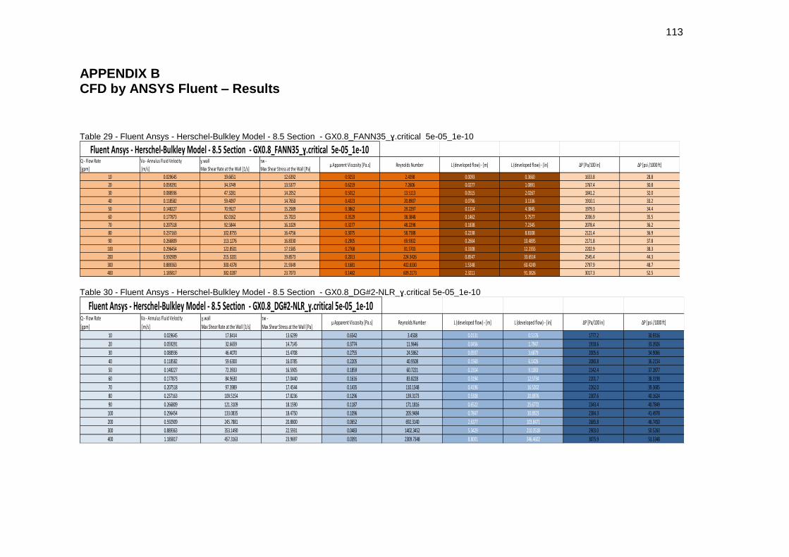
113

APPENDIX B CFD by ANSYS Fluent – Results

Table 29 - Fluent Ansys - Herschel-Bulkley Model - 8.5 Section - GX0.8_FANN35_ɣ.critical 5e-05_1e-10

Table 30 - Fluent Ansys - Herschel-Bulkley Model - 8.5 Section - GX0.8_DG#2-NLR_ɣ.critical 5e-05_1e-10

Q - Flow Rate

[gpm]


[m/s]

ɣ.wall

Max Shear Rate at the Wall [1/s]

τw -

Max Shear Stress at the Wall [Pa] μ Apparent Viscosity [Pa.s] Reynolds Number L (developed flow) - [m] L (developed flow) - [in] ΔP [Pa/100 in] ΔP [psi /1000 ft]

10 0.029645 19.6651 12.6392 0.9253 2.4398 0.0093 0.3660 1653.8 28.8

20 0.059291 34.3749 13.5377 0.6219 7.2606 0.0277 1.0891 1767.4 30.8

30 0.088936 47.3281 14.2052 0.5012 13.5113 0.0515 2.0267 1841.2 32.0

40 0.118582 59.4097 14.7650 0.4323 20.8907 0.0796 3.1336 1910.1 33.2

50 0.148227 70.9527 15.2589 0.3862 29.2297 0.1114 4.3845 1979.3 34.4

60 0.177873 82.0162 15.7023 0.3529 38.3848 0.1462 5.7577 2036.9 35.5

70 0.207518 92.5844 16.1029 0.3277 48.2298 0.1838 7.2345 2078.4 36.2

80 0.237163 102.8755 16.4756 0.3075 58.7388 0.2238 8.8108 2121.4 36.9

90 0.266809 113.1276 16.8330 0.2905 69.9302 0.2664 10.4895 2171.8 37.8

100 0.296454 122.8501 17.1585 0.2768 81.5703 0.3108 12.2355 2202.9 38.3

200 0.592909 215.3201 19.8573 0.2013 224.3426 0.8547 33.6514 2545.4 44.3

300 0.889363 300.4378 21.9349 0.1681 402.8330 1.5348 60.4249 2797.9 48.7

400 1.185817 382.0287 23.7073 0.1482 609.2173 2.3211 91.3826 3017.3 52.5

Fluent Ansys - Herschel-Bulkley Model - 8.5 Section - GX0.8_FANN35_ɣ.critical 5e-05_1e-10

Q - Flow Rate

[gpm]


[m/s]

ɣ.wall


τw -


10 0.029645 17.8414 13.6299 0.6542 3.4508 0.0131 0.5176 1777.2 30.9316

20 0.059291 32.6659 14.7145 0.3774 11.9646 0.0456 1.7947 1918.6 33.3926

30 0.088936 46.4070 15.4708 0.2755 24.5862 0.0937 3.6879 2005.6 34.9066

40 0.118582 59.6300 16.0785 0.2205 40.9508 0.1560 6.1426 2080.8 36.2154

50 0.148227 72.3933 16.5905 0.1859 60.7221 0.2314 9.1083 2142.4 37.2877

60 0.177873 84.9630 17.0440 0.1616 83.8228 0.3194 12.5734 2201.7 38.3198

70 0.207518 97.3989 17.4544 0.1435 110.1348 0.4196 16.5202 2262.0 39.3685

80 0.237163 109.5154 17.8236 0.1296 139.3173 0.5308 20.8976 2307.6 40.1624

90 0.266809 121.3109 18.1590 0.1187 171.1816 0.6522 25.6772 2343.4 40.7849

100 0.296454 133.0835 18.4750 0.1096 205.9484 0.7847 30.8923 2384.3 41.4978

200 0.592909 245.7881 20.8800 0.0652 692.3140 2.6377 103.8471 2685.8 46.7450

300 0.889363 353.1490 22.5931 0.0483 1402.3452 5.3429 210.3518 2903.0 50.5260

400 1.185817 457.3163 23.9697 0.0391 2309.7348 8.8001 346.4602 3075.9 53.5348

Fluent Ansys - Herschel-Bulkley Model - 8.5 Section - GX0.8_DG#2-NLR_ɣ.critical 5e-05_1e-10

DBD


114

Table 31 - Fluent Ansys - Herschel-Bulkley Model - 12.25 Section - GX0.8_FANN35_ɣ.critical 5e-05_1e-10

Table 32 - Fluent Ansys - Herschel-Bulkley Model - 12.25 Section - GX0.8_DG#2-NLR_ɣ.critical 5e-05_1e-10

Q - Flow Rate

[gpm]


[m/s]

ɣ.wall


τw -


10 0.010392 4.42363 11.39683 3.0296 0.5877 0.0050 0.1984 659.3076 11.4749

20 0.020784 8.21124 11.80487 1.8148 1.9623 0.0168 0.6623 679.5617 11.8275

30 0.031176 11.66858 12.11472 1.3737 3.8885 0.0333 1.3124 694.7546 12.0919

40 0.041569 14.90195 12.37308 1.1383 6.2571 0.0536 2.1118 707.3401 12.3109

50 0.051961 17.96953 12.59861 0.9890 9.0015 0.0772 3.0380 718.5564 12.5061

60 0.062353 20.90450 12.80063 0.8847 12.0751 0.1035 4.0754 728.3662 12.6769

70 0.072745 23.73370 12.98516 0.8070 15.4451 0.1324 5.2127 737.5119 12.8361

80 0.083137 26.46803 13.15532 0.7465 19.0822 0.1636 6.4402 745.2026 12.9699

90 0.093529 29.13529 13.31506 0.6976 22.9729 0.1969 7.7534 753.6860 13.1176

100 0.103921 31.73192 13.46503 0.6572 27.0932 0.2323 9.1439 761.0823 13.2463

200 0.207843 55.28186 14.65422 0.4528 78.6467 0.6742 26.5433 819.6636 14.2659

300 0.311764 76.45019 15.55790 0.3686 144.9302 1.2424 48.9139 871.2535 15.1638

400 0.415686 95.89343 16.29951 0.3208 222.0489 1.9035 74.9415 903.4477 15.7241

500 0.519607 114.46925 16.95356 0.2885 308.5698 2.6452 104.1423 934.3999 16.2628

700 0.727450 149.96634 18.09486 0.2465 505.5561 4.3339 170.6252 995.1919 17.3209

1000 1.039214 199.89505 19.52607 0.2097 849.1643 7.2795 286.5930 1068.4214 18.5954

Fluent Ansys - Herschel-Bulkley Model - 12.25 Section - GX0.8_FANN35_ɣ.critical 5e-05_1e-10

Q - Flow Rate

[gpm]


[m/s]

ɣ.wall


τw -


10 0.010392 3.885308 11.886744 3.3846 0.5261 0.0045 0.1776 682.0867 11.8714

20 0.020784 7.253065 12.504663 2.0069 1.7745 0.0152 0.5989 714.8172 12.4411

30 0.031176 10.408469 12.937932 1.5023 3.5556 0.0305 1.2000 737.3899 12.8339

40 0.041569 13.422803 13.281775 1.2328 5.7774 0.0495 1.9499 754.1941 13.1264

50 0.051961 16.346148 13.573206 1.0615 8.3869 0.0719 2.8306 769.6565 13.3955

60 0.062353 19.245377 13.834332 0.9401 11.3643 0.0974 3.8355 789.4768 13.7405

70 0.072745 21.989248 14.056895 0.8528 14.6161 0.1253 4.9329 796.0520 13.8549

80 0.083137 24.701265 14.261642 0.7842 18.1650 0.1557 6.1307 804.5142 14.0022

90 0.093529 27.392117 14.452369 0.7286 21.9958 0.1886 7.4236 814.7265 14.1799

100 0.103921 30.039276 14.629037 0.6828 26.0777 0.2236 8.8012 823.7763 14.3374

200 0.207843 55.175179 15.968564 0.4534 78.5483 0.6734 26.5101 897.0004 15.6119

300 0.311764 78.576889 16.904856 0.3623 147.4205 1.2638 49.7544 941.3067 16.3830

400 0.415686 101.142320 17.657604 0.3106 229.2962 1.9656 77.3875 980.6494 17.0677

500 0.519607 123.069900 18.295843 0.2765 322.0231 2.7605 108.6828 1013.9707 17.6477

700 0.727450 165.591810 19.358303 0.2330 534.9154 4.5856 180.5339 1069.5942 18.6158

1000 1.039214 227.163710 20.632990 0.1954 911.0818 7.8102 307.4901 1137.2876 19.7940

Fluent Ansys - Herschel-Bulkley Model - 12.25 Section - GX0.8_DG#2-NLR_ɣ.critical 5e-05_1e-10

DBD


Thiago Pinheiro da Silva Enhanced fluid rheology ...€¦ · March 2016 . PUC-Rio - Certificação...

Documents

Transcript of Thiago Pinheiro da Silva Enhanced fluid rheology ...€¦ · March 2016 . PUC-Rio - Certificação...