Understand Thermodynamics (Bom)

20 www.aiche.org/cep December 2011 CEP

Computational Methods

When using a chemical process simulator, the most important decision affecting the quality of results is selection of a thermodynamic model. New and

experienced engineers alike often find this task challenging. Many do not realize how important this decision is, how to make it, or how to validate the decision. This article provides a basic overview of how to select and validate a vapor-liquid equilibrium model for process simulation. Process simulation software calculates heat and mate-rial balances. This requires determining the separation of a chemical mixture between the liquid and vapor phases. While many different thermodynamic models are available, using the wrong model, or estimating a physical property incorrectly, can lead to inaccurate results for the overall simulation. Early process simulators were mainframe programs that were beyond the reach of most engineers, and were used almost exclusively for sophisticated process design. Advances in both software and hardware have since made process simulators available in virtually any engineering environment and accessible to more users, including under-graduate students, process and project engineers, and even others who are not chemical engineers. Expert skill is not required to use a process simulator; however, a basic understanding of applied thermodynamics can be crucial. Making the wrong assumptions or select-ing the wrong thermodynamic model can lead to results that range from non-optimal to catastrophic. Unfortunately, many simulator users are not trained in the fundamentals of applied thermodynamics and have difficulty selecting an appropriate thermodynamic model.

The right K model is the key A thermodynamic model, sometimes called a vapor-liquid equilibrium (VLE) model, is a method to calculate phase separation for a mixture at a given temperature, pres-sure, and composition. These models are also referred to as K models because relative volatility, Ki, can be determined by VLE calculations, Ki = yi/xi, where yi is the vapor-phase mole fraction of component i and xi the liquid-phase mole fraction of i. Tables of experimental K values can be used to back-calculate yi and xi, in lieu of a rigorous K model. Most K models are for vapor-liquid separation; some can perform equilibrium calculations for two liquid phases. No single K model can be used to calculate the behavior of all possible chemical mixtures. Different mixtures have different dominating behaviors, and different models have been developed to fit these behaviors. For example, the VLE for a mixture of water and ethanol is dominated by the liquid-phase behavior of these two nonideal liquids, which requires a different model than a mixture of hexane and pro-pane, where the liquid is fairly ideal but the vapor is affected by the molecules’ size and shape differences. Some K models were derived from physical laws, some from thermodynamic constraints, and some simply fit to observed data. Some mixtures are well behaved and predict-able, some are well documented (the VLE of water and ethanol has been studied for centuries), and others are very poorly understood. Choosing the appropriate K model for a particular mix-ture requires engineering judgment to review the chemicals, type of mixture, and range of conditions (temperature, pres-sure, and concentration). Start by identifying the solution

Selecting a thermodynamic model is an important step in process simulation — one that many engineers

overlook. This overview of applied thermodynamics can help you choose the right model for your process.

David HillFred C. Justice, P.E.Chemstations, Inc.

Understand Thermodynamics to Improve

Process Simulations

Copyright © 2011 American Institute of Chemical Engineers (AIChE)

CEP December 2011 www.aiche.org/cep 21

behavior for the mixture and select the K model category. Then choose a specific model from within the category and validate the results. With experience, your judgment will improve and initial model selection will become easier. However, whether you are a novice or an experienced user, it is important to validate the model selection. Depending on the application, selecting an incorrect model can have minor or drastic effects. For example, in a benzene-phenol mixture, the wrong K model might not affect the calculation of number of stages to separate the mixture, but it will result in an incorrect vapor-phase predic-tion at low concentrations of benzene (Figure 1).

Know the mixture Understanding the behavior of molecules in the vapor and liquid phases can help you determine which K model category might be appropriate for your mixture. Begin by listing the chemicals you expect to find in the mixture. Do not include any chemicals found in a separate utility stream if they are not in the mixture being modeled. Consider the behavior of important binary pairs of chemicals in the mixture, and try to identify their solution behavior in the vapor and liquid phases. Evaluate the binary combinations even if the actual mixture contains multiple components. Also consider the temperature and pressure range of your process. Ideal (perfect) gas. Boyle observed that pressure (P), volume (V), and temperature (T) are related. Clapeyron later recognized the importance of the number of moles (n) and the universal gas constant (R) and expressed the ideal gas law as PV = nRT. The ideal gas law applies when inter-molecular forces and the absolute sizes of the gas molecules are not significant. At ambient conditions, many light gases approximate ideal gas behavior. At elevated pressure or lower temperature, the ideal gas model is less accurate. Sys-tems that approximate ideal gas behavior include air at room temperature and pressure, and the vapor over a mixture of water and methanol at moderate tempera-ture and pressure of 1 to 3 bar. Real gas. Gases that deviate from ideal gas law predictions can be modeled by adjusting the ideal gas law for molecule size, molecule shape, and vapor compress-ibility, and considering the enthalpy of departure due to pressure effects. The real gas model becomes valid at high pres-sures, near critical points, and for mixtures of molecules with moderate differences in molecule size. Combustion gases at high temperature and pressure, and alkane mixtures at high temperature and pressure of several bar are examples of real gases.

Atmospheric gases, especially at medium to high pressure, can generally be considered real gases. Ideal liquid. In an ideal liquid solution (Figure 2, left), the molecules are randomly distributed and the interactions are, on average, very similar, so Raoult’s law is applicable. Partial molar volumes are nearly the same in an ideal liquid solution. While few liquid mixtures are ideal, the ideal liquid assump-tion is somewhat valid for liquid mixtures at high pressure. Regular liquid. In a regular liquid solution (Figure 2, center), different chemicals can — and often do — have molecules that differ moderately in size. Molecular interac-tions are influenced primarily by these size differences. A regular liquid solution will have weak — or no — inter-molecular forces between molecules A and B. When A and B mix in a liquid, there can be a slight nonideal interaction. The solution will not be a regular liquid if there is a large size difference between molecules, or if there is hydrogen bonding or another strong intermolecular force. Polar liquid. In polar liquid solutions (Figure 2, right),

1

x = Liquid Mole Fraction of Benzene

y =

Vap

or M

ole

Frac

tion

of B

enze

ne 0.9

0.8

0.7

0.6

0.5

0.4

0.3

0.2

0.1

00 0.20.1 0.3 0.5 0.7 0.9

SRKIdealNRTL

0.4 0.6 0.8 1

p Figure 1. Understanding solution behavior can help you select an appropriate model for the mixture. For the benzene-phenol mixture represented here, two different thermodynamic models, SRK and NRTL, predict different vapor-phase fractions at low benzene concentrations.

p Figure 2. Unlike an ideal liquid solution with randomly distributed and uniformly interacting molecules (left), regular liquid solutions are characterized by differences in molecular size and weak intermolecular forces (center). In polar liquid solutions, intermolecular forces dominate and molecules are not randomly distributed (right).

Regular Liquid Solution of A and B

Ideal Liquid Solution Behavior

Polar Liquid Solution, with Clumping




the particles are not distributed randomly; intermolecular forces of attraction and repulsion dominate. Hydrogen bonding can be significant. The nonrandom distribution can lead to clumping, which in turn may lead to the formation of azeotropes or a second liquid phase. The presence of liquid water is a good indicator of a polar liquid solution.

K model categories K models fall into several general categories: equation of state (EOS), activity coefficient, combined and special-purpose, and aqueous electrolyte system models. Equations of state. Well suited to modeling ideal and real gases, EOS models are derived from PVT relation-ships; many are modifications of PV = nRT. EOS models are less reliable when the sizes of the mixture components are significantly different, or when the mixture is at the critical point of any of its components. These models also generally do a poor job of predicting the behavior of nonideal liquids, especially polar mixtures. EOS models are able to calculate enthalpy of departure for a mixture, pressure effect on enthalpy, and compress-ibility factor. These strengths often make an EOS the best choice when modeling compressed gases and compressors. EOS calculations are based on pure component parameters, such as the normal boiling point (Tb), critical temperature (Tc), critical pressure (Pc), and acentric factor (ω). It is important to have accurate values for these prop-erties if you intend to use an EOS. Hydrocarbon mixtures, light-gas mixtures, and atmo-spheric gases are well modeled by an EOS. Some EOS are well suited to high-pressure systems, and can be used to model supercritical CO2 compression. An EOS is also often used to model gases and hydrocarbons at high pressure. Systems that are poorly modeled by an EOS include liquid water, alcohols, and other nonideal liquids. Activity coefficient models. These are based on thermo-dynamic constraints on the liquid. They are derived math-

ematical models that use activity to fit Gibbs excess energy deviation of mixtures. The activity coefficient is calculated as a function of temperature and composition of the mix-ture. Activity models focus on the behavior of the liquid and assume ideal gas behavior; advanced users sometimes use an EOS to fine-tune the vapor fugacity. Activity models are used for nonideal liquid solutions. The molecules may have drastically different sizes. Binary interaction parameter (BIP) models calculate activity from binary interaction parameters, which are fit to data. For the most accurate results, you need BIPs that have been regressed from empirical data. Predictive activity models are based on general molecu-lar structure. For example, a subgroup model considers the interaction between cyclohexane and water as the sum of interactions between six CH subgroups and one water sub-group. Predictive models cannot be used for all chemicals because the behavior of all subgroups is not yet understood. Organophosphate components, for example, are among the many components that have not yet been modeled by a predictive subgroup activity model. Some activity models can be used to calculate (or predict) liquid-liquid equilibrium. Special modifications can be used for electrolytes, polymer systems, and solid-liquid equilibria. The accuracy of activity models depends on the quality of the regressed data. A BIP model needs binary interaction parameters that were regressed for the chemicals in the sys-tem being modeled. A predictive model requires that group interaction parameters be available for the various subgroups of a chemical’s structure. If you want to use an activity coef-ficient model but do not have BIPs, consider regressing them from data or using a predictive subgroup model. Systems that are well modeled by activity models include mixtures of water and ethanol, two-liquid-phase mixtures such as water and toluene, and the ethanol/ethyl-acetate/water system, which exibits a homogeneous binary azeotrope, a heterogeneous binary azeotrope, and one

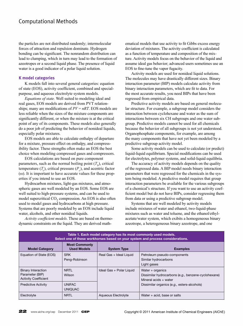
Table 1. Each model category has its most commonly used models. Select one of these workhorses based on your system and process considerations.

Model CategoryMost Commonly

Used Models System Type Examples

Equation of State (EOS) SRKPeng-Robinson

Real Gas + Ideal Liquid Petroleum pseudo-componentsSimilar hydrocarbonsLight gases

Binary Interaction Parameter (BIP) Activity Coefficient

NRTLWilson

Ideal Gas + Polar Liquid Water + organicsDissimilar hydrocarbons (e.g., benzene-cyclohexane) Mineral acids + waterDissimilar organics (e.g., esters-alcohols)Predictive Activity UNIFAC

UNIQUAC

Electrolyte NRTL Aqueous Electrolyte Water + acid, base or salts



ternary azeotrope. Systems that are not well modeled by activity methods include light-gas mixtures, high-pressure systems, hot combustion gases, and alkane mixtures. Combined and special-purpose models. Advanced models combine the concept of activity with an equation of state. The most popular of these is the Predictive Soave-Redlich-Kwong (PSRK) model, which often works well for systems in which the vapor is a real gas and the liquid is nonideal or polar. Special-purpose models may use an EOS or activity model that is modified to fit one particular system. The Maurer model, for example, modifies the UNIFAC (Univer-sal Functional Activity Coefficient) model to fit the water/formaldehyde/methanol system. Aqueous electrolyte system models. Rigorous electrolyte models can model dissociation, heats of solution, and boiling point elevation, and because these models account for ion interactions, they can also represent pH. Electrolyte models are meant to be used for aqueous systems that are at or near atmospheric pressure.

Workhorse thermodynamic models Once you understand the nature of the mixture you are modeling and select a model category, you will find there are many model choices. You may, for example, want to use an equation of state — but which of the 10 or more EOS models offered in your simulator should you use? First, ask your colleagues which thermodynamic models they have used to model your process successfully. If you are the first to model the process, the following discussion can help you screen the alternatives. As a starting point, consider the most commonly used models in the category (Table 1). These workhorse models might not be the best choices for your process, but as an initial iteration, they should indicate whether a particular category is suitable. You will need real plant data to deter-mine whether there might be a better model choice within the category for your process. As you learn more about applied thermodynamics, you will learn when to select certain models. For instance, when modeling distillation of a medium crude oil, you might select Soave-Redlich-Kwong (SRK) or Peng-Robinson as your K model; even though a more specialized petroleum VLE model would give better results, SRK or Peng-Robin-son will typically be acceptable. SRK and Peng-Robinson are also the most commonly used EOS models for real gases. Of the BIP activity coefficient models, the nonrandom two-liquid (NRTL) and Wilson models are the most fre-quently used. These are appropriate for regular solutions, nonideal liquids, polar liquids, and generally ideal vapor. UNIFAC and UNIQUAC (Universal Quasichemical) are the most commonly used predictive activity coefficient models.

If you have an electrolyte system, select a customized electrolyte model. If your simulator does not have an elec-trolytes package, it might have a simplified module that can model some of the industrially important reactions, such as gas sweetening with caustic.

Validating the thermodynamic model Once you have selected a K model, it is crucial to vali-date that it will accurately model your system. Sometimes a model that should give good results does not fit a particular mixture — it might be missing parameters for a chemical, system conditions might be outside its applicability range, or the model type might not be appropriate for the system. Validating a thermodynamic model involves several steps. First, verify that the inputs are correct, and then inspect the model results. Compare the results to results from similar models and to experimental data for your sys-tem. Also compare the behavior of similar mixtures. Verify physical property data. If you are using an EOS, Tc, Pc, Tb, and ω must be accurate. For a BIP activity model, accurate Tb, vapor pressure (as a function of temperature), and binary interaction parameters between important chemicals are necessary. The BIP pairs must be known or regressed from available experimental equilibrium data. Predictive activity subgroup models consider a molecule as the sum of smaller parts whose interactions are known. For this model type, verify that all of the chemicals in the system are described by functional subgroups, because in the absence of BIPs or subgroups, the behavior of the chemicals will simplify to that of an ideal liquid. Inspect the modeling results. Do not assume the simula-tor is giving the results you want — it will give results based on the models you selected. Always inspect model results. An easy way to do this is to construct Txy and Pxy plots for important pairs of components. Plot and inspect several Txy and Pxy diagrams to validate that the model is matching your expectations. Learn how to recognize azeotropes and second liquid phases on the diagram. If you know that two chemicals in the mixture being modeled form an azeotrope, plot the x-y diagram to determine whether the simulator is calculating the azeotrope. Another option is to perform simple flash separations on the flowsheet to verify that the vapor and liquid separa-tion conforms to your expectations. If you have selected an inappropriate model, the phase separation may be obviously wrong. If you are modeling existing equipment, try to match experimental observed data. For highly nonideal systems, consider generating ternary binodal plots or residue curve maps. These steps can validate that you are on the right path or send up warning flags that the model will not give realistic results. Work through these steps for every simulation, even




in the absence of data for comparison, and you will develop a feel for how the process may respond to different tempera-tures, pressures, and compositions. Compare to a similar model. Different models in the same category will typically give similar results. If you are using the SRK model, for example, you can compare the results to those of other EOS models; if you are using an activity coefficient model, compare to UNIFAC, modified UNIFAC, and PSRK results. If similar models do not give similar results, investigate the differences. Figure 3 shows that NRTL and modified UNIFAC provide comparable results for an azeotropic mixture of acetone and water, whereas the results from SRK (an inappropriate model for azeotropes or polar liquids) are obviously incorrect. Compare to external data. To be certain the selected model fits your system, it is necessary to compare the mod-eling results to data. Even a few datapoints can be valuable, either to validate the model or adjust it to better approximate reality. If you do not have VLE data, search the literature. This is often much more affordable than generating new experimental data. If multiple sources of data are available, there will be disagreement among the data sets. The best source of data is typically operations data from your plant. Pilot plant opera-tions data are the next best, followed by laboratory data, and then literature data. Literature data are better than estimated (or guesstimated) data. Trust your judgment on the skills of the chemist or accuracy of the equipment when comparing data. A very skilled chemist is often more reliable than an expensive online analyzer. Try to simulate the same conditions in the model as the conditions at which your datapoints were obtained, and inspect how closely the model can match them. If you have binary x-y data, plot it against the x-y diagram created by the simulator. If you have multicomponent data, try to model it

with flash separations. For instance, if you have plant data for the liquid composition from a reboiler, assume that this is a liquid at its bubble point. Enter the composition into a stream in the simulator, and specify pressure and a small vapor fraction for a flash calculation. If the calculated tem-perature and liquid composition are not close to your plant data, the model might not be appropriate. Find relevant data. The Internet is useful for finding relevant physical property data. Material safety data sheets (MSDSs) provided by chemical manufacturers and the NIST Chemistry WebBook (http://webbook.nist.gov) are good sources. In some cases, a brief search for articles will lead to VLE data for your system. AIChE members have free access to a wide variety of references and data through the AIChE eLibrary (www.aiche.org/membercenter/elibrary.aspx), in partnership with Knovel and McGraw-Hill. Paid databases can also be very good sources. AIChE’s Design Institute for Physical Properties Research (DIPPR; www.aiche.org/dippr) database provides evaluated physi-cal property data for pure components; project sponsors get three-year exclusive access to new data. The DETHERM database, also available through AIChE, provides unevalu-ated data for physical properties and VLE, based on data gathered from literature sources and laboratories. The UNIFAC Consortium expands the number of chemicals that can be predicted with VLE models such as UNIFAC and PSRK; sponsors receive the data as well as files to use with their process simulators. Compare to similar systems. Obtaining VLE data for your mixture may not be possible or practical. For instance, some chemicals are too expensive or dangerous to test, and some models are preliminary studies made before attempting a pilot plant or benchtop experiment. Try to find similar data; it is often reasonable to assume that similar chemicals will have similar behavior. For example, if you are attempting to model a mixture of cyclohexane and toluene and cannot find VLE data for this system, it is reasonable to expect it to behave somewhat similarly to a mixture of n-hexane and toluene or n-hexane and benzene. Estimate data. When predicting pure-component proper-ties, take care with model selection, and be sure to review Properties of Gases and Liquids (1). If data for similar components or systems are available, use homologue analysis to guesstimate values that you are missing. Plot data for the related chemicals you do have, and determine an approximate value for the missing data that is consistent with the family.

Learning more This introduction to applied thermodynamics does not cover all situations. From this starting point, you may want to learn about modeling at ppm levels (infinite dilution), how to regress BIPs from data, or other more advanced problem

p Figure 3. Modified UNIFAC and NRTL, both activity coefficient models, provide similar results for an azeotrope system. SRK, an EOS model, produces inaccurate results.

1

0.9

0.8

0.7

0.6

0.5

0.4

0.3

0.2

0.1

00 0.20.1 0.3 0.5 0.7 0.9

Modified UNIFACNRTLSKREquilibrium Line

0.4 0.6 0.8 1x = Liquid Mole Fraction of Benzene

y =

Vap

or M

ole

Frac

tion

of B

enze

ne



areas. More information is available in articles and books, as well as from colleagues. Advanced users of simulators can give you advice, as can the technical support group for your company’s simulator. Online communities can also offer learning opportunities. As you work with different thermodynamic models, always remember to inspect the results of your model selec-tions. The more rules you learn for thermodynamics, the more exceptions to the rules you will learn.

Literature Cited1. Poling, B. E., et al., “Properties of Gases and Liquids,” McGraw-

Hill, New York, NY (2000).

Further ReadingCarlson, E. C., “Don’t Gamble with Physical Properties for Simula-

tions,” Chem. Eng. Progress, 92 (10), pp. 35–46 (Oct. 1996).Edwards, J. E., “Chemical Engineering in Practice,” www.pidesign.

co.uk/publication.htm, P&I Design Ltd., Billingham Press, Bill-ingham, U.K. (2011).

Walas, S. M., “Phase Equilibria in Chemical Engineering Thermody-namics,” Butterworth-Heinemann, Boston, MA (1985).

DAVID HILL is Manager of Technical Support at Chemstations, Inc. (11490 Westheimer Rd., Suite 900, Houston, TX 77077; Phone: (713) 978-7700; Fax: (713) 978-7727; Email: [email protected]), where he manages the group that supports the CHEMCAD simulation software suite. He mentors the company’s technical support engi-neers, provides technical expertise to distributors, provides training to international customers, and represents Chemstations at technical forums, trade shows, and consortium meetings. He holds a BS in chemical engineering from the Univ. of Houston. A member of AIChE, he has been involved in leadership of the South Texas Local Section (STS-AIChE), and is currently vice chair of the DIPPR administrative committee. He has given numerous presentations at AIChE meetings and other venues.

FRED C. JUSTICE, P.E., is the Midwest Office Business Development Manager for Chemstations, Inc. (11490 Westheimer Rd., Suite 900, Houston, TX 77077; Phone: (989) 799-2716; Fax: (713) 978-7727; Email: [email protected]). He has had a wide-ranging career supplying technology to the international chemical process indus-tries, including licensed processes, capital equipment, and process simulation software. He received his BChE from the Univ. of Detroit, Mercy, and an MS from the State Univ. of New York at Buffalo. He also has an MBA and studied international marketing at Cambridge Univ. He is a registered professional engineer in Michigan. A fellow of AIChE, he serves as the deputy chair of the Fellows Council and is a director of the Education Division. He is an active member of the Mid-Michigan Local Section and received the Section’s Service to Society Award.

CEP


http://www.aiche.org/redirect/index.aspx?source=CEPDisplayAd&date=1211&url=http://dippr.byu.edu/download.asp

Understand Thermodynamics (Bom)

Documents

Transcript of Understand Thermodynamics (Bom)