Universidade de Aveiro Departamento de Ambiente e ... · necessários à obtenção do grau de...
172
Universidade de Aveiro 2014 Departamento de Ambiente e Ordenamento Isabel Lavrador Ribeiro The impact of biofuels for road traffic on air quality: a modelling approach Modelação do impacto do uso de biocombustíveis nos transportes rodoviários na qualidade do ar
Transcript of Universidade de Aveiro Departamento de Ambiente e ... · necessários à obtenção do grau de...

Universidade de Aveiro
2014
Departamento de Ambiente e Ordenamento
Isabel Lavrador Ribeiro
The impact of biofuels for road traffic on air quality: a modelling approach
Modelação do impacto do uso de biocombustíveis nos transportes rodoviários na qualidade do ar


Universidade de Aveiro
2014
Departamento de Ambiente e Ordenamento
Isabel Lavrador Ribeiro
The impact of biofuels for road traffic on air quality: a modelling approach
Modelação do impacto do uso de biocombustíveis nos transportes rodoviários na qualidade do ar
Tese apresentada à Universidade de Aveiro para cumprimento dos requisitos necessários à obtenção do grau de Doutor em Ciências e Engenharia do Ambiente, realizada sob a orientação científica da Doutora Myriam Lopes, Professora Assistente do Departamento de Ambiente e Ordenamento da Universidade de Aveiro e sob co-orientação científica da Doutora Alexandra Monteiro, docente convidada do Departamento de Engenharia e Gestão Industrial e Pós-doc no Departamento de Ambiente e Ordenamento da mesma Universidade, e do Doutor Markus Amann, co-lider do “Greenhouse Gas Initiative” do International Institute for Applied Systems Analysis (IIASA).
Apoio Financeiro do FEDER através do Programa Operacional Fatores de Competitividade (COMPETE) e por Fundos Nacionais através da FCT do PTDC no âmbito dos Projetos BIOGAIR (PTDC/AAC-AMB/103866/2008) e CLICURB (EXCL/AAG-MAA/0383/2012).
Apoio financeiro da Fundação para a Ciência e Tecnologia (FCT) através do POPH-QREN, comparticipado pelo Fundo Social Europeu (FSE) e por fundos nacionais do MCTES pela Bolsa de Doutoramento com a referência SFRH / BD / 60370 / 2009.


o júri
presidente Prof. Doutor Nelson Fernando Pacheco da Rocha Professor Catedrático da Universidade de Aveiro
Prof. Doutor Ole John Nielsen Professor Catedrático no Instituto de Química da Universidade de Copenhaga
Doutor Nelson Augusto Cruz de Azevedo Barros Professor associado da Faculdade de Ciências e Tecnologia da Universidade Fernando Pessoa, Porto
Doutor Luís António da Cruz Tarelho Professor auxiliar do Departamento de Ambiente e Ordenamento da Universidade de Aveiro
Doutora Myriam Alexandra dos Santos Batalha Dias Professora auxiliar do Departamento de Ambiente e Ordenamento da Universidade de Aveiro
Doutor Luís Manuel Ventura Serrano Professor adjunto da Escola Superior de Tecnologia e Gestão do Instituto Politécnico de Leiria


agradecimentos
Às minhas Amigas e orientadoras Myriam Lopes e Alexandra Monteiro, por todo o apoio e orientação para o meu desenvolvimento científico. Ao Professor Carlos Borrego e Professora Ana Isabel Miranda pela disponibilidade, dedicação, espírito crítico e ensinamentos científicos. Ao GEMAC, que há 6 anos me acolheu e me faz sentir numa casa cheia de irmãos. Por me aturarem e me ensinarem tanto! A todos eles, mas em especial à Helena Martins, Anabela Carvalho, Joana Ferreira, Jorge H. Amorim, Joana Valente, Elisa Sá, minha companheira nesta “estrada” e Sandra Rafael companheira no BIOGAIR. Um agradecimento especial aos ex-gemaquianos Pedro Cascão e Cláudia Pimentel, pela amizade e desabafos, e à Ana Cristina Carvalho, não só pela amizade e desabafos mas também pelo seu incrível sentido crítico, sabedoria e encorajamento em seguir em frente. To Hendrik Elbern, Achim Strunk, Elmar Friese and Lars Nieradzik for having teaching me to work with the EURAD-IM modelling system. A special thank you to the whole team of the experimental studies, in particular to those that made this work successful: Prof. Luís Serrano, Luís Tarelho, Ole Nielsen, Nuno Pires and Pedro Cascão (again), and also to Prio Energy for providing biodiesel gallons. À FCT, pelo seu patrocínio financeiro através da Bolsa de Doutoramento (SFRH / BD / 60370 / 2009) e dos Projectos BIOGAIR (PTDC/AAC-AMB/103866/2008), o alicerce deste trabalho, e CLICURB (EXCL/AAG-MAA/0383/2012). À Agência Portuguesa do Ambiente (APA), pelo financiamento de protocolos que tanto me ajudaram a ganhar experiência em modelação da qualidade do ar. Aos meus pais, irmãos, sobrinhos, cunhados e tios, que mesmo longe, pelo apoio incondicional, paciência e incentivo na superação dos obstáculos.


palavras-chave
Biocombustíveis, transportes rodoviários, emissões de poluentes atmosféricos, qualidade do ar, modelação numérica, estratégia energética
resumo A escolha de fontes energéticas para o sector dos transportes é uma das preocupações da sociedade moderna devido a questões relacionadas com o paradigma energético, e ao facto de este ser uma das principais fontes de polução do ar nas cidades, afectando significativamente a saúde humana e a sua qualidade de vida. Devido às limitações técnicas com que as formas de mobilidade avançadas ainda se deparam, os biocombustíveis são considerados uma alternativa viável para as próximas décadas, contribuindo para a redução de gases com efeito de estufa e estimulando o desenvolvimento rural. Portugal, motivado pelas políticas Europeias, tem aposto nos biocombustíveis, em especial no biodiesel, a fim de atingir a meta da Directiva 2009/28/CE. No entanto, não são conhecidos os impactos na qualidade do ar decorrentes da utilização de biodiesel. Assim, este trabalho pretende clarificar esta situação respondendo à seguinte questão: a utilização de biodiesel promove uma melhoria na qualidade do ar em Portugal, particularmente nas áreas urbanas? A primeira tarefa deste trabalho consistiu na caracterização da cadeia de biocombustíveis em Portugal, verificando-se que a cadeia tem problemas de sustentabilidade, uma vez que toda a matéria-prima usada é importada, não estando a promover a redução da dependência energética externa. Posteriormente foram avaliados os impactos associados à utilização de biodiesel nas emissões de poluentes atmosféricos e na qualidade do ar em Portugal e em particular na área urbana do Porto, através da utilização do sistema de modelação numérica à mesoscala WRF-EURAD e tendo por base 2 cenários de emissões: o cenário de referência que considera que não é usado biodiesel e o cenário B20 que reflecte a utilização de um combustível constituído por 80% de gasóleo fóssil e 20% de biodiesel. Com este trabalho, verificou-se que o uso de B20 pode ajudar a controlar os níveis de poluição atmosférica tanto em Portugal como na área urbana do Porto, promovendo a redução das emissões de PM10, PM2.5, CO e COVNM e respectivas concentrações no ambiente atmosférico. Por outro lado, são esperados aumentos nas emissões de formaldeído, acetaldeído e acroleína com o uso de B20 e aumentos nas concentrações de NO2 na área urbana do Porto. Apesar destes compostos serem considerados tóxicos e cancerígenos, os COVNM dominantes no gasóleo de origem fóssil, presentes em quantidades reduzidas no biodiesel, têm coeficientes de perigo crónico mais elevados. Assim, a utilização de B20 nos transportes rodoviários apresenta maiores benefícios para a saúde humana e para a qualidade do ar quando comparado com a utilização de gasóleo convencional.


keywords
Biofuels, road traffic, atmospheric pollutant emissions, air quality, numeric modelling, energy strategy
abstract The selection of the energy source to power the transport sector is one of the main current concerns, not only relative with the energy paradigm but also due to the strong influence of road traffic in urban areas, which highly affects human exposure to air pollutants and human health and quality of life. Due to current important technical limitations of advanced energy sources for transportation purposes, biofuels are seen as an alternative way to power the world’s motor vehicles in a near-future, helping to reduce GHG emissions while at the same time stimulating rural development. Motivated by European strategies, Portugal, has been betting on biofuels to meet the Directive 2009/28/CE goals for road transports using biofuels, especially biodiesel, even though, there is unawareness regarding its impacts on air quality. In this sense, this work intends to clarify this issue by trying to answer the following question: can biodiesel use contribute to a better air quality over Portugal, particularly over urban areas? The first step of this work consisted on the characterization of the national biodiesel supply chain, which allows verifying that the biodiesel chain has problems of sustainability as it depends on raw materials importation, therefore not contributing to reduce the external energy dependence. Next, atmospheric pollutant emissions and air quality impacts associated to the biodiesel use on road transports were assessed, over Portugal and in particular over the Porto urban area, making use of the WRF-EURAD mesoscale numerical modelling system. For that, two emission scenarios were defined: a reference situation without biodiesel use and a scenario reflecting the use of a B20 fuel. Through the comparison of both scenarios, it was verified that the use of B20 fuels helps in controlling air pollution, promoting reductions on PM10, PM2.5, CO and total NMVOC concentrations. It was also verified that NO2 concentrations decrease over the mainland Portugal, but increase in the Porto urban area, as well as formaldehyde, acetaldehyde and acrolein emissions in the both case studies. However, the use of pure diesel is more injurious for human health due to its dominant VOC which have higher chronic hazard quotients and hazard indices when compared to B20.

i
Table of contents
LIST OF FIGURES ............................................................................................................. III
LIST OF TABLES .............................................................................................................. VII
LIST OF ABBREVIATIONS AND SYMBOLS ............................................................................. IX
CHAPTER 1. SCOPE AND STRUCTURE OF THE WORK .......................................... 1
CHAPTER 2. BIOFUELS IN THE WORLD’S AND PORTUGUESE CONTEXTS ........... 5
2.1 BIOFUELS IN THE WORLD ...................................................................................... 5
2.2 BIOFUELS IN THE EUROPE ..................................................................................... 7
2.3 THE ENERGY AND TRANSPORT SECTORS IN PORTUGAL ..........................................10
2.4 CHARACTERIZATION OF THE PORTUGUESE BIOFUELS SUPPLY CHAIN.......................13
2.4.1 Raw material production and transportation .............................................................. 14
2.4.2 Biodiesel production ................................................................................................... 16
2.4.3 Biodiesel/diesel blending ............................................................................................ 17
2.4.4 Transport and distribution associated to the national biodiesel supply chain ............ 18
2.5 DISCUSSION AND FINAL REMARKS .........................................................................19
CHAPTER 3. ATMOSPHERIC POLLUTANT EMISSION RELATED TO BIOFUELS USE
IN ROAD TRANSPORTS ............................................................................................ 23
3.1 EFFECTS OF BIODIESEL ON EMISSIONS ..................................................................23
3.1.1 NOx ............................................................................................................................ 28
3.1.2 Particulate matter (PM) .............................................................................................. 29
3.1.3 CO and HC ................................................................................................................. 30
3.1.4 CO2 ............................................................................................................................. 32
3.1.5 Non-regulated pollutants ............................................................................................ 33
3.1.6 Synthesis .................................................................................................................... 38
3.2 EMISSIONS CHARACTERIZATION FROM EURO 5 DIESEL/BIODIESEL PASSENGER
VEHICLE .........................................................................................................................39
3.2.1 Exhaust gas sampling and analysis ........................................................................... 41
3.2.1 Determination of the mass and volumetric exhaust flow ............................................ 46
3.2.2 Determination of the emission factors ........................................................................ 48
3.2.3 Synthesis .................................................................................................................... 55
CHAPTER 4. EMISSION SCENARIOS ..................................................................... 57
4.1 TRANSPORT EMISSION MODEL FOR LINE SOURCES (TREM) ..................................57
4.2 THE REF SCENARIO ............................................................................................61
4.3 THE B20 SCENARIO .............................................................................................66
4.4 EMISSION SCENARIOS COMPARISON .....................................................................67
4.5 SYNTHESIS .........................................................................................................71

ii
CHAPTER 5. THE AIR QUALITY MODELLING SYSTEM .......................................... 73
5.1 SELECTION OF THE MODELLING SYSTEM ............................................................... 73
5.2 WRF-EURAD MODELLING SYSTEM ...................................................................... 75
5.2.1 Geometry of the modelling system ............................................................................. 76
5.2.2 Weather Research Forecasting model (WRF) ........................................................... 79
5.2.3 EURAD Emissions Model (EEM) ............................................................................... 83
5.2.4 EURopean Air Pollution Dispersion – Chemical Transport Model (EURAD-CTM) .... 86
CHAPTER 6. EVALUATION OF THE AIR QUALITY MODELLING SYSTEM ............. 93
6.1 THE AIR QUALITY MONITORING NETWORK .............................................................. 94
6.2 BIAS-CORRECTION APPROACH ............................................................................. 97
6.3 OPERATIONAL EVALUATION OF THE WRF-EURAD MODELLING SYSTEM ................. 99
6.3.1 PT05 ......................................................................................................................... 101
6.3.2 OP01 ........................................................................................................................ 105
CHAPTER 7. IMPACTS OF BIODIESEL USE ON AIR QUALITY ............................. 109
7.1 IMPACTS ON AIR QUALITY OVER MAINLAND PORTUGAL ......................................... 109
7.2 IMPACTS ON AIR QUALITY IN PORTO URBAN AREA ................................................ 116
CHAPTER 8. CONCLUSIONS ................................................................................ 125
REFERENCES ......................................................................................................... 131

iii
List of figures
Figure 1.1 – Scheme of the defined methodology. ............................................................ 3
Figure 2.1 - Bioethanol/biodiesel production/consumption in the world from 2000 to 2011
(URL 5). ............................................................................................................................ 7
Figure 2.2 - Biodiesel production in Europe, Germany, France, Spain and Portugal, from
2002 to 2011 (URL 4) .....................................................................................................10
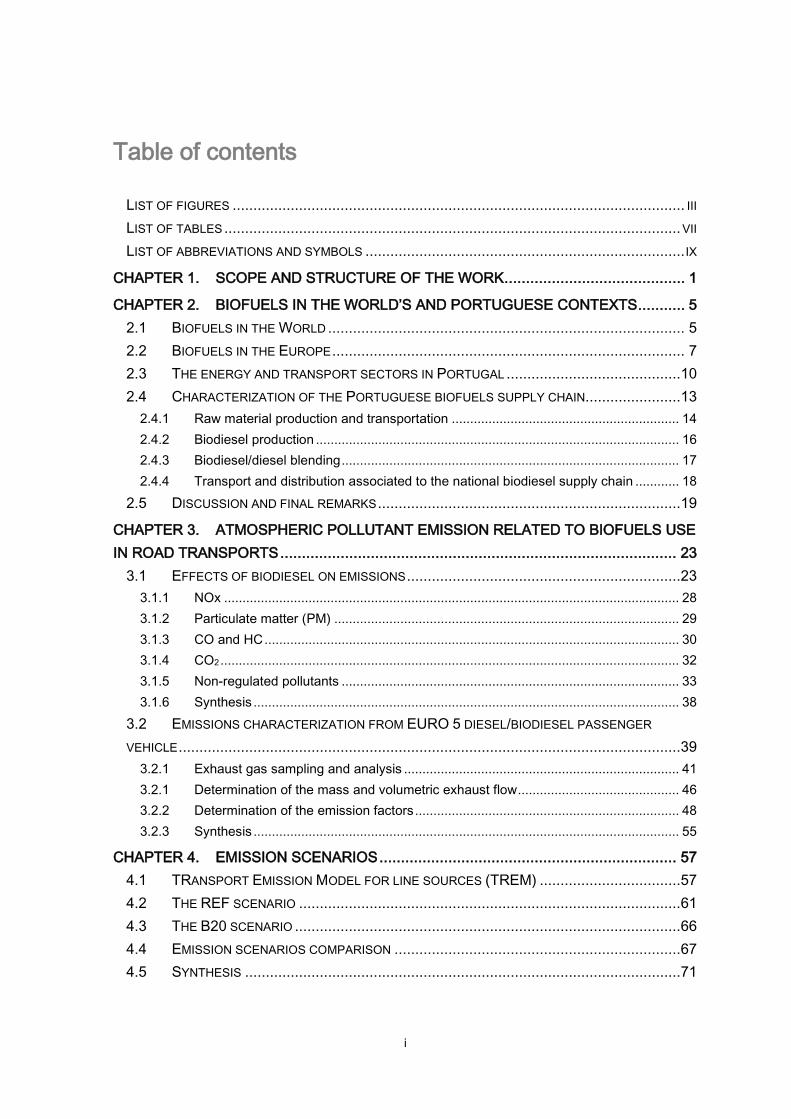
Figure 2.3 - Diesel and gasoline consumption (ktoe) by road transportation in Portugal,
from 1990 to 2012 (URL 3). .............................................................................................12
Figure 2.4 – Typical biodiesel supply chain. .....................................................................13
Figure 2.5 – Number of producers with aid to produce energy crops and respective
cultivated area, from 2007 to 2009, in Portugal (URL 7). ..................................................14
Figure 2.6 – Vegetable oil used to biodiesel production in Portugal in 2007 (a) and 2010
(b) (URL 9). ......................................................................................................................15
Figure 2.7 – Origin of vegetable oils used in Portugal, for 2010 (URL 9). .........................15
Figure 2.8 – Biodiesel consumption and blends really used from 2006 to 2011.
Recommended biofuel and biodiesel blends until 2020 and biodiesel blend projected by
2020. The data are related to Portugal (MEID, 2010; URL 3 and URL 6). ........................17
Figure 2.9 – Biodiesel production plans, petroleum refineries, main communication lines
and harbours. ..................................................................................................................18
Figure 3.1 – Research work conclusions regarding the effects of biodiesel on engine
performance and emissions with respect to pure diesel, beyond 2000 (adapted from Xue
et al., 2011). .....................................................................................................................24
Figure 3.2 – Molecular structure of a biodiesel a) and a conventional diesel b). Carbon,
hydrogen and oxygen atoms are represented as grey, white and red bools, respectively.
........................................................................................................................................25
Figure 3.3 – Speed profile of the a) NEDC and b) CADC (Fontaras et al., 2014). ............27
Figure 3.4 – Average of carbonyl compound emission factors (mg.km-1) for diesel, B10,
B20 and B30, over the a) NEDC, b) CAU, c) CAR and d) CAM driving cycles (from:
Karavalakis et al., 2011b). ...............................................................................................35

iv
Figure 3.5 – Maximum incremental reactivity (MIR) of carbonyl compounds (CC) (Carter,
2009). .............................................................................................................................. 36
Figure 3.6 – Scheme of the experimental infrastructure. .................................................. 41
Figure 3.7 - B20 profiles of speed and exhausts gases temperature (a) and measured
concentrations of O2 and CO2 (b), NOx (c) and SO2 (d). .................................................. 45
Figure 3.8 – CO2 emission factors by fuel type and driving cycle. .................................... 49
Figure 3.9 – NO, NO2 and NOx (NO+NO2) emission factors by fuel type and driving cycle,
and the emission limit value indicated by the EC Regulation 715/2007. .......................... 50
Figure 3.10 – Variation on SO2 emission factor by fuel type and driving cycle, relative to
pure diesel. ...................................................................................................................... 52
Figure 3.11 – Coarse and fine fraction (EC and OC) of total carbon (TC) emission factor in
PM10, for B0, B7 and B20, considering all the NEDC. .................................................... 53
Figure 3.12 – Total VOC emission factor (a), and concentration of some species of VOC,
for B0, B7 and B20 (b). .................................................................................................... 54
Figure 4.1 - TREM input data and main calculation modules for exhaust emission
quantification (adapted from Tchepel, 2003). .................................................................. 58
Figure 4.2 – Vehicle fleet distribution by type and fuel. .................................................... 59
Figure 4.3 – The TREM-HAP simulation domain covering the Northern region of Portugal:
the Porto urban area, the road network and the daily mean traffic volume (vehicle.day-1)
for each road, main cities and population distribution. ..................................................... 60
Figure 4.4 – Diesel and gasoline (95+98) sold by municipality in 2012 (URL 10). ............ 61
Figure 4.5 – The Porto urban area domain: population distribution, main cities and road
network including the daily mean traffic volume (vehicle.day-1). ....................................... 62
Figure 4.6 - Road-transport NOx (a,c) and formaldehyde (b,d) emissions for Portugal and
for the Porto urban area (in a grid of 11km2), regarding the REF scenario. .................... 65
Figure 4.7 – Emission variations (%) between B20 and REF scenarios [(B20-REF)/REF].
........................................................................................................................................ 68
Figure 4.8 – Difference between REF and B20 annual emissions (ton.y-1) of: a)
formaldehyde, b) acetaldehyde, c) acrolein/acetone and d) benzene; e) increment on
Equivalent Ozone Production (EOP) by the use of B20 and f) population distribution, over
Portugal. .......................................................................................................................... 69
Figure 4.9 – Difference between REF and B20 annual emissions (ton.y-1) of: a)
formaldehyde, b) acetaldehyde, c) acrolein/acetone and d) benzene; e) increment on

v
Equivalent Ozone Production (EOP) by the use of B20 and f) population distribution, over
the urban area of Porto. ...................................................................................................70
Figure 5.1 – Scheme of the WRF-EURAD air quality modelling system. ..........................75
Figure 5.2 – WRF-EURAD modelling system geometry: a) horizontal and vertical views of
the Arawaka C-grid configuration; b) example of the vertical structure of a grid for 15
vertical layers (solid lines denote sigma levels and dashed lines denote half-sigma levels)
(Skamarock et al., 2008). .................................................................................................76
Figure 5.3 – Simulation domains used in the WRF-EURAD modelling system application.
........................................................................................................................................79
Figure 5.4 – WRF model flow chart (adapted from Wang et al., 2014). ............................80
Figure 5.5 – EEM time-profiles defined by EMEP for SNAPs and pollutants: a-c) annual
profiles; d) weekly profiles and e-f) daily profiles. .............................................................84
Figure 5.6 – Scheme of the EURAD-CTM model. ............................................................86
Figure 5.7 – EURAD-CTM configuration options piece from the model run-script. ...........88
Figure 6.1 – Location and main characteristics of the selected monitoring stations for
Portugal (PT05) and Porto urban area domains (OP01): stations environment and the
terrain elevation (in m) (a); stations influence (b). ............................................................95
Figure 6.2 – Daily profiles, averaged over all monitoring stations, of observed values
(OBS), EURAD simulations (RAW) and EURAD simulations with RAT04 correction
(RAT04) for O3 and PM10 (adapted from Monteiro et al., 2013a) .....................................98
Figure 6.3– Statistical parameters for the corrected (RAT04) results from the WRF-
EURAD modelling system, regarding the REF scenario (2012 year), for each pollutant and
station environment: a) bias (µgm-3); b) RMSE (µgm-3); c) R, IA and FAC2; d) MG and
VG; e) NSD, ANB and NMSE. Median for all the monitoring sites, over the PT05 domain.
...................................................................................................................................... 103
Figure 6.4 – Daily profiles of measured (blue line) and predicted (purple line)
concentrations of CO, NO2, O3, PM10 and PM2.5, as well as the concentration ranges
between percentiles 25th/75th, over the PT05 domain, regarding rural, suburban and urban
environments. ................................................................................................................ 104
Figure 6.5 - Statistical parameters for the corrected (RAT04) results from the WRF-
EURAD modelling system, regarding the REF scenario (2012 year), for each pollutant and
station environment: a) bias (µgm-3); b) RMSE (µgm-3); c) R, IA and FAC2; d) MG and
VG; e) NSD, ANB and NMSE. Median for all the monitoring sites, over the OP01 domain.
...................................................................................................................................... 106

vi
Figure 6.6 – Daily profiles of measured (blue line) and predicted (purple line)
concentrations of CO, NO2, O3, PM10 and PM2.5, as well as the concentration ranges
between percentiles 25th/75th, over the OP01 domain, regarding background, industrial
and traffic influence. ...................................................................................................... 108
Figure 7.1 – Annual, summer and winter mean concentrations of NO2 (gm-3), NMVOC
(ppbv) and O3 (gm-3) for REF scenario (a-c) and differential concentrations between B20
and REF (d-f), over the PT05 domain. ........................................................................... 110
Figure 7.2 – Histograms of 1-99% of NO2 (top), NMVOC (middle) and O3 (bottom) hourly
concentrations, regarding annual, summer and winter periods for REF (blue or green) and
B20 (yellow) scenarios, for the PT05 domain. The difference between the probabilities of
occurrence of B20 against REF is presented in grey. .................................................... 112
Figure 7.3 - Annual, summer and winter mean concentrations of CO, PM10 and PM2.5 for
REF scenario (a-c) and differential concentrations between B20 and REF (d-e), over the
PT05 domain. ................................................................................................................ 114
Figure 7.4 – Histograms of 1-99% of CO (top), PM10 (middle) and PM2.5 (bottom) hourly
concentrations, regarding annual, summer and winter periods for REF (blue or green) and
B20 (yellow) scenarios, for the PT05 domain. The difference between the probabilities of
occurrence of B20 against REF is presented in grey. .................................................... 115
Figure 7.5 – Annual, summer and winter mean concentrations of NO2 (gm-3), NMVOC
(ppbv) and O3 (gm-3) for REF scenario (a-c) and differential concentrations between B20
and REF (d-f), over the OP01 domain. .......................................................................... 117
Figure 7.6 - Histograms of 1-99% of NO2 (top), NMVOC (middle) and O3 (bottom) hourly
concentrations, regarding annual, summer and winter periods for REF (blue or green) and
B20 (yellow) scenarios, for the OP01 domain. The difference between the probabilities of
occurrence of B20 against REF is presented in grey. .................................................... 119
Figure 7.7 – Annual, summer and winter mean concentrations of CO, PM10 and PM2.5 for
REF scenario (a-c) and differential concentrations between B20 and REF (d-f), over the
OP01 domain. ............................................................................................................... 120
Figure 7.8 - Histograms of 1-99% of CO (top), PM10 (middle) and PM2.5 (bottom) hourly
concentrations, regarding annual, summer and winter periods for REF (blue or green) and
B20 (yellow) scenarios, for the OP01 domain. The difference between the probabilities of
occurrence of B20 against REF is presented in grey. .................................................... 122

vii
List of tables
Table 3.1 – Physical and chemical specifications regarding biodiesel and diesel fuels
(from: Bakeas et al., 2011; Ayhan Demirbas, 2009; Gupta and Demirbas, 2010; Lapuerta
et al., 2008; Lin and Fan, 2011). ......................................................................................24
Table 3.2 – Effects of biodiesel blends on diesel vehicle NOx emissions for EURO 3
(EMEP/EEA, 2013) and EURO 4 (Bakeas et al., 2011) vehicles. .....................................29
Table 3.3 – Effects of biodiesel blends on diesel vehicle PM emissions for EURO 3
(EMEP/EEA, 2013) and EURO 4 (Bakeas et al., 2011) vehicles. .....................................30
Table 3.4 – Effects of biodiesel blends on diesel vehicle CO and HC emissions for EURO
3 (EMEP/EEA, 2013) and EURO 4 (Bakeas et al., 2011) vehicles. ..................................32
Table 3.5 – Effects of biodiesel blends on diesel vehicle PM emissions for EURO 3
(EMEP/EEA, 2013) and EURO 4 (Bakeas et al., 2011) vehicles. .....................................33
Table 3.6 – Benzene, toluene and xylene emissions at various engine loads (Di et al.,
2009). ..............................................................................................................................37
Table 3.7 - Technical specifications of the test vehicle. ....................................................39
Table 3.8 - Fuel properties used in the experiment. .........................................................40
Table 3.9 – Equipment used in the experimental work. ....................................................43
Table 3.10 – Stoichiometric elemental composition (% m/m) of fuel, on dry basis. ...........47
Table 3.11 – Fuel consumption, mass air flow, and exhaust gas flow rates in mass and
volume basis, by fuel and for each driving cycle. .............................................................48
Table 4.1 – Portuguese vehicle fleet by age and type in 2009 (ACAP, 2010). ..................59
Table 4.2 – Average emission factors (gpollutant.gfuel-1) calculated by TREM and TREM-HAP
for the Northern region of Portugal. ..................................................................................61
Table 4.3 – Road-transport sector annual pollutant emissions estimated by TREM-HAP
(T), regarding the REF scenario, and included in INERPA (I), over mainland Portugal and
the Porto urban area. Ratio of emission estimated and INERPA emissions (T/I) and the
representativity of the Porto urban area in mainland Portugal’s emissions (Porto/Portugal).
........................................................................................................................................63

viii
Table 4.4 - Average emission variations (%) of regulated pollutants for an EURO 4 LPV
over the NEDC and CADC (Bakeas et al., 2011) and for an EURO 5 LPV over the NEDC
(Lopes et al., 2014). ........................................................................................................ 66
Table 4.5 – Average carbonyl compound emission variations (%) for an EURO 4 LPV
over the NEDC and CADC (Karavalakis et al., 2011b) and average benzene* emissions at
different engine loads for an EURO 4 LPV (Di et al., 2009). ............................................ 66
Table 4.6 – Annual pollutant emissions (ton) estimated for road-transports in Portugal and
Porto urban area, regarding the B20 scenario. ................................................................ 67
Table 4.7 - Representativeness of the estimated variations (B20-REF) in total emissions
regarding the studied pollutant, for Portugal and the Porto urban area (APA, 2011). ...... 68
Table 5.1 – The vertical structure of the WRF-EURAD grid, defined by terrain-following
sigma coordinates. .......................................................................................................... 77
Table 5.2 – Dimensions of the simulation domains used in WRF-EURAD modelling
system. ............................................................................................................................ 78
Table 5.3 – Summary of WRF physic options used. ........................................................ 83
Table 5.4 – Vertical distribution of anthropogenic emissions: percentage of each SNAP (S)
sector allocated to the vertical layers of the EURAD-CTM (EMEP, 2013). ....................... 85
Table 5.5 – Physic and chemical options used in EURAD-CTM. ..................................... 91
Table 6.1 – Monitoring stations selected and their classification (environment and
influence and pollutants measured, for Portugal and Porto urban area domains (PT05 and
OP01). ............................................................................................................................. 96
Table 6.2 – Statistical quality indicators for air quality model performance evaluation
(Hanna et al., 1993; Borrego et al., 2008). ..................................................................... 100

ix
List of abbreviations and symbols
Abbreviations
ACAP Associação Automóvel de Portugal
AEBIOM European Biomass Association
ANB Average normalized absolute bias
APA Agência Portuguesa do Ambiente
APC Analytical Predictor of Condensation
APPB Associação Portuguesa de Produtores de Biocombustiveis
B20 B20 Scenario / blend fuel with 20% (v/v) of biodiesel
Bias Mean Systematic error
BIOFRAC BIOfuel Research Advisory Council
BTX Benzene, Toluene and Xylene
Bx Blend fuel with x% (v/v) of biodiesel
CAM Common ARTEMIS Motorway
CAU Common ARTEMIS Urban
CAR Common ARTEMIS Rural
C125 Simulation domain over the Europe and Northern Africa (125 125 km2)
CADC Common Artemis Driving Cycle
CAP Common Agricultural Policy
CC Carbonyl compounds
CCE Carbonyl Compound Emission
CMQA Community Multiscale Air Quality
DGEG Direcção Geral de Energia e Geologia
DL Decree-Law
EBB European Biodiesel Board
EC Elemental Carbon
EC European Commission
ECU Engine control unit
EEA European Environment Agency
EEM EURAD Emission Model
EF Emission Factors
EGR Exhaust Gas Recirculation
EIA U.S. Energy Information Administration
EMEP European Monitoring and Evaluation Programme
ENE2020 National Strategy to Energy 2020

x
Abbreviations
EOP Equivalent Ozone Production
EU European Union
EUDC Extra-Urban Driving Cycle
EURAD-CTM EURopean Air pollution Dispersion - Chemistry Transport Model
FAC2 Fact of two Observations
FAIRMODE Forum for AIR quality MODelling in Europe
FAME Fatty acid methyl ester
FB Fractional bias
GFS Global Forecast System
GHG Greenhouse Gas
HDMR High Dimensional Model Representation technique
HDV Heavy duty vehicles
HPV Heavy passenger vehicles
IA Index of agreement
IEA International Energy Agency
ILUC Indirect land use change
INERPA National Emission Inventory
IP25 Simulation domain over the Iberian Peninsula (25 25 km2)
IPCC Intergovernmental Panel on Climate Change
IPMA Instituto Português do Mar e da Atmosfera
KF Kalman filter
LCA Life Cycle Assessment
LDV Light duty vehicles
LNEG Portuguese Laboratory for Energy and Geology
LPG Liquid petroleum gas
LPV Light passenger vehicles
MADE Modal Aerosol Dynamics model for Europe
MEID Ministério da Economia, Inovação e Desenvolvimento
MG Geometric mean bias
MIM Mainz Isoprene Mechanism
MIR Maximum Incremental Reactivity
MMM Mesoscale and Microscale Mateorology Division
MOBI.E National Electric Mobility Network
NCAR National Center for Atmospheric Research's
NCEP National Centers for Environmental Prediction
NEDC New European Driving Cycle
NMSE Normalized mean squared error
NMVOC Non-methane Volatile Organic Compounds
NOOA National Oceanic and Armospheric Administration's

xi
Abbreviations
NRL Naval Research Laboratory
NSD Normalized standard deviation
OBS Observed values
OC Organic Carbon
OP01 Simulation domain over the Porto urban area (1 1 km2)
PAH Aromatic Polyaromatic Hydrocarbons
PM Particulate matter
PM10 Particulate matter with an aerodynamic diameter smaller than 10 µm
PM2.5 Particulate matter with an aerodynamic diameter smaller than 2.5 µm
PNAEE National Action Plane for Energy Efficiency
PNAER National Action Plane for Renewable Energies
ppbv Parts per billion in volume basis
PPC Pre-processor
PT05 Simulation domain over mainland Portugal (5 5 km2)
R Correlation coefficient
RACM-MIM Regional Atmospheric Chemical Mechanism-Mainz Isoprene Mechanism
RAT Multiplicative ratio correction
RAT04 Multiplicative ratio correction with 4 days training period
REDirective Renewable Energy Directive
REF Reference Scenario
RES Renewable Energy Sources
RME Root mean squared error
SD Standard deviation
SNAP Standardized Nomenclature for Air Pollutants
SOA Secondary Organic Aerosols
SOF Soluble Organic Fraction
SORGAM Secondary ORGanic Aerosol Module
SUBST Subtractive/additive correction of the mean bias
TREM-HAP Transport Emission Model for line sources - Hazardous Air Pollutant
UDC Urban Driving Cycle
UK United Kingdom
USA United States of America
VG Geometric variance
VOC Volatile Organic Compounds
WHO World Health Organization
WPS WRF Pre-processing System
WRF Weather Research & Forecasting model
3D Tridimensional

xii
Symbols of elements and chemical compounds
C16H34 Hexadecane
C19H36O2 elaidic acid methyl ester
CO Carbon Monoxide
CO2 Carbon Dioxide
H2O Water
H2O2 Hydrogen peroxide
HC Hydrocarbon
HCL Hydrogen chloride
HF Hydrogen fluoride
HNO3 Nitric Acid
N2 Nitrogen
N2O5 Dinitrogen pentoxide
NH3 Ammonia
NH4+ amonium ion
NO Nitric Oxide
NO2 Nitrogen dioxide
NO3- Nitrate
NOx Nitrogen Oxides
O2 Oxygen
O3 Ozone
SO2 Sulphur dioxide
SO32- Sulfite anion
SO42- sulphate ion
SOx Sulphur Oxides
VOC Volatile Organic Compounds

The impact of biofuels for road traffic on air quality: a modelling approach
Scope and structure of the work
1
Chapter 1. Scope and structure of the work
The energy sector is a key factor in the socio-economic and environmental domains. The
increasing industrialization and motorization of the world has led to a steep rise for the
demand of fossil fuels. To fulfil the energy demand the sources of these fossil fuels are
becoming exhausted. Today fossil fuels take up 80% of the primary energy consumed in
the world, of which 20% is used in the transport sector (IEA, 2013). Furthermore, they are
major contributors to greenhouse gas (GHG) emissions, which leads to adverse effects on
climate change, receding of glaciers, rising sea level, increasing of extremes weather
events and loss of biodiversity (IPCC, 2007). Progressive depletion of conventional fossil
fuels with increasing energy consumption and GHG emissions have led to a move
towards alternative, renewable, sustainable, efficient and cost-effective energy sources
with less emissions (Zhao et al., 2009; He et al., 2010; Singh et al., 2010a, 2010b).
Biomass1 as an alternative energy source has taken an important rode in the worldwide
energy strategy due to its multiple energy applications such as electricity, heat production
and the use on transportation (biofuels). In fact, biofuels are seen as an alternative way to
power the world’s motor vehicles in a near-future, due to current important technical
limitations of advanced energy sources for transports (e.g. electric and hydrogen fuel cell
vehicles) (Felipe et al., 2014; URL 1 and URL 2). Additionally, they can help reducing
GHG emissions and diversifying the energy sources from the transport sector, as well as
stimulating rural development and creating jobs.
Biofuels have attracted great attention all over the world due to their renewability and
availability, promising to contribute to regional and rural development as well as to
improve environmental quality. However, there has been widespread debate in popular
media and scientific journals about the sustainability of biofuels production and use,
1 According to the Directive 2009/28/EC on the promotion of the use of energy from renewable sources,
biomass is the biodegradable fraction of products, waste and residues from biological origin from agriculture
(including vegetal and animal substances), forestry and related industries including fisheries and aquaculture,
as well as the biodegradable fraction of industrial and municipal waste. Thus, biomass is biological material
containing energy from recent carbon fixed.

The impact of biofuels for road traffic on air quality: a modelling approach
Scope and structure of the work
2
related to social, economic, environmental and technical issues. The "food vs fuel"
debate, the impacts of land use changes linked to deforestation and soil erosion, loss of
biodiversity and impact on water resources, as well as the possible modifications on
engine to be fuelled by biofuels, are examples of issues that led to several scientific
studies and stimulated the definition of sustainability criteria. Actually, depending on
feedstock and production technique, there are several biofuels and not all of them have
similar performance in terms of their impact on climate, energy security and ecosystems.
Thus, these impacts should be assessed, specifically for each biofuel and scenario,
throughout the entire life cycle (Bringezu et al., 2009), helping different countries to adopt
specific measures on biofuels introduction, including sustainability criteria (Nigam and
Singh, 2011; Savaliya et al., 2013). Some sustainability criteria on biofuels are already
included in the current European Directive 2009/28/EC on the promotion of the use of
energy from renewable sources (Renewable Energy Directive, REDirective). Motivated by
European strategies, Portugal has been betting on biofuels, particularly biodiesel,
because diesel was, and still is, the main fuel consumed, representing about 75% (e/e) of
the energy consumed by the national transport sector (URL 3). Thus, Portugal intends to
meet the REDirective goals for road transports (replacement of 10% fossil fuels by
renewable energy in the transportation sector by 2020) using biofuels, especially
biodiesel. In fact, how to fuel the transport sector is one of the main concerns of modern
society due to energy issues but also due to the strong influence of road traffic in urban
areas, which highly affects human exposure to air pollutants and consequently human
health and quality of life. According to the World Health Organization news release (WHO,
2014), 7 million premature deaths annually are linked to air pollution. Nevertheless there
is a lack of knowledge with respect to the impacts of biodiesel blends use on regional and
urban air quality.
In this sense, this work aims to assess the impact on air quality derived from the biodiesel
blends usage on road transports by trying to answer this question: can biodiesel use
contribute to a better air quality over Portugal, particularly over urban areas? Several
experimental studies have demonstrated the benefits of diesel/biodiesel blends use on
vehicles exhaust gases emissions, helping in controlling air pollution (Lapuerta et al.,
2008; Xue et al., 2011). Moreover, road traffic is one of the main air pollution sources in
European cities (EEA, 2013), largely contributing to high levels of nitrogen oxides (NOx),
particulate matter with an aerodynamic diameter smaller than 10 µm (PM10) and 2.5 µm
(PM2.5) measured at traffic monitoring stations (EEA, 2013).
To reach the goal of this work, the impacts on air quality over mainland Portugal and the
Porto urban area were assessed making use of numerical modelling tools. This type of
tools has become as fundamental to support decision makers on air quality management
due to its ability to estimate atmospheric pollutants concentrations over the entire region

The impact of biofuels for road traffic on air quality: a modelling approach
Scope and structure of the work
3
of interest, taking into account complex and non-linear physic and chemical mechanisms
that characterize the atmosphere, as well as to evaluate the efficiency of emission
scenarios (Ribeiro et al., 2014). In this scope, the air quality numerical simulations were
forced by CO, NOx, NH3, sulfur oxides (SOx), PM10, PM2.5 and non-methane volatile
organic compounds (NMVOC) emissions of all activity sectors. For the road transport
sector, emission scenarios were designed considering that vehicles are powered by fossil
fuels or by biodiesel blends.
Figure 1.1 presents the methodology defined to achieve the purposes of this work.
Figure 1.1 – Scheme of the defined methodology.
Firstly, an overview regarding the biofuels situation in the world and over Portugal was
conducted and it is presented in Chapter 2. This chapter also includes the analysis of the
Portuguese energy sector and the operation mode characterization of the national
biodiesel supply chain. This characterization was carried out through a vast collection of
information and statistical data from literature and contacts with stakeholders.
In parallel, a literature review regarding the effects on atmospheric pollutant emissions
when diesel/biodiesel blends are used in diesel vehicles was accomplished (Chapter 3)
aiming to define emission scenarios. Here, two main groups of atmospheric pollutants
were analysed: the first group comprehends the regulated pollutants, such as CO, CO2,
NOx and NMVOC; and the second group includes the non-regulated pollutants, namely
formaldehyde (CH2O), acetaldehyde (C2H4O), benzene (C6H6) and acrolein (C3H4O). The
interest on these non-regulated pollutants is related to their potential for tropospheric

The impact of biofuels for road traffic on air quality: a modelling approach
Scope and structure of the work
4
ozone formation, as well as their carcinogenic and toxic characteristics, which is
especially important on urban areas due to human exposure to these pollutants.
Based on the emission factors from the use of diesel/biodiesel blends, two emission
scenarios were defined for mainland Portugal and for the Porto urban area in Chapter 4.
Regulated and non-regulated emissions were estimated regarding each scenario and
case study, through the Transport Emission Model for line sources with Hazardous Air
Pollutant (TREM-HAP, Tchepel et al., 2012). The analysis and comparison of both
emission scenarios are also addressed in this chapter.
Chapter 5 is dedicated to the selection and description of the air quality numerical
modelling system used to simulate both emission scenarios and to investigate the impacts
of biodiesel blends use on road transports. In this sense, the air quality numerical
modelling comprising the Weather Research & Forecasting (WRF, Skamarock et al.,
2008) and the EURopean Air pollution Dispersion – Chemistry Transport Model (EURAD-
CTM, Hass, 1991; Ebel et al., 1997; Elbern et al., 2007) was selected through a multi-
model comparison exercise. A detailed description of the modelling system is given in this
chapter, including the model setup defined for this study (simulation domains, physic and
chemical parameterization options).
The performance of the WRF-EURAD modelling system is evaluated for both case studies
(mainland Portugal and the Porto urban area), in Chapter 6, using observational and
modelling data.
The emission scenarios developed in Chapter 4 were used as input data to the EURAD
model to investigate the impacts of biodiesel blends use on air quality over both case
studies, regarding CO, NO2, NMVOC, O3, PM10 and PM2.5 levels (Chapter 7).
Finally, in Chapter 8, a brief summary of the main results is carried out and the final
conclusions are explored. Additionally, possible future developments are discussed.

The impact of biofuels for road traffic on air quality: a modelling approach
Biofuels in the World’s and Portuguese contexts
5
Chapter 2. Biofuels in the World’s and
Portuguese contexts
This chapter gives a general overview of the biofuels world’s history and production over
the last decades. The European strategies on biofuels are also described and analyzed,
as well as biofuels production in Europe. Aiming for a better understanding of the
Portuguese situation on biofuels, the national energy sector is analyzed from the point of
view of the road transport sector. Finally, the Portuguese biodiesel supply chain is
characterized. It includes an overview of its operation as well as the biodiesel production
from 2006 to 2012.
2.1 Biofuels in the World
By 1880s, Rudolph Diesel, who invented diesel engine, envisioned that vegetable oils
could power diesel engines for agriculture in remote areas of the world, where petroleum
was not available at that time. However, due to the low cost of the fossil fuels at that time,
vegetable oils as an energy source were side-lined for decades. During petroleum crisis,
in the 1970s, the world realized the pressing need to find alternative energy sources. Then
renewable energy technologies were developed (Regnier, 2007; de Alegría Mancisidor et
al., 2009). The first biofuel produced in an industrial scale was bioethanol in Brazil (1975)
(Rosillo-Calle and Cortez, 1998), followed by biodiesel in Germany in 1991, according to
the European Biodiesel Board website (URL 4).
Biofuels are renewable energy sources derived from biomass, which might replace
petroleum fuels. Currently, the biofuels largely produced and consumed worldwide are
bioethanol and biodiesel that can substitute gasoline and diesel, respectively. They can be
produced through chemical conversion (acid hydrolysis, transesterification/esterification,
supercritic fluid extraction, aqueous phase reforming), biological conversion (fermentation,
anaerobic digestion, enzymatic hydrolysis, photochemical conversion) or by

The impact of biofuels for road traffic on air quality: a modelling approach
Biofuels in the World’s and Portuguese contexts
6
thermochemical conversion (combustion, gasification, pyrolysis, liquefaction) (Demirbas,
2009; Gupta and Demirbas, 2010). Biofuels can also be classified as traditional (or first
generation biofuels) which are derived from food crops, while advanced biofuels (including
second and third generations) are produced by non-food biomass, such as microalgaes
(third generation biodiesels), cereal straw, forest residues, as well as industrial and
domestic waste. Traditional biofuels are already in the market, but second and third
generation biofuels are produced by advanced technologies, still under development,
aiming at massive production (Demirbas, 2009; Gupta and Demirbas, 2010; Nigam and
Singh, 2011).
Bioethanol fuels, widely used in the United States of America and in Brazil, are alcohols
produced from sugar and starch crops, such as corn, sugarcane and sweet sorghum, but
also from cellulosic biomass derived from non-food sources, namely forest biomass
residues. This type of fuel can be used in its pure form, but it is usually used as a gasoline
additive or substitute, replacing gasoline up to 85% (v/v), and contributing to improve
vehicle performance and exhaust gases emissions (Jacobson, 2007; Demirbas, 2009;
Gupta and Demirbas, 2010; Randazzo and Sodré, 2011). On the other hand, biodiesels
are derived from vegetable oils (e.g. soybean, sunflower, palm oil, rapeseed, jathropha
and microalgaes) or animal fats. They are commonly produced by converting vegetable
oils into compounds called fatty acid methyl esters (FAME), throughout a
transesterification reaction with methanol (Demirbas, 2007). This is the most common
biofuel produced and used in European countries as an additive of petroleum-based
diesel (URL 4), helping on reduction of particulate matter (PM), carbon monoxide (CO),
and hydrocarbons (HC) emissions from diesel-powered vehicles (Lapuerta et al., 2008;
Demirbas, 2009; Gupta and Demirbas, 2010; Xue et al., 2011).
Over the last decades, the European Union (EU) has adopted strategies (e.g. the Kyoto
Protocol in 1997, and the European Climate Change Programme in 2001) to raise the
diversification of energy sources, facing the external energy dependence, and the use of
endogenous energy resources, contributing at the same time to reduce the GHG
emissions and to encourage a more sustainable development. Thenceforth, the world’s
biofuel production has been growing. According to the U.S. Energy Information
Administration (EIA, URL 5), from 2000 to 2011 the bioethanol output increased 5 times
and the biodiesel output increased 26 times (Figure 2.1). This rapid growth in biofuels
output is mostly supported by government policies which are driven by external energy
dependence and energy security issues, coupled with the objective of revitalizing the
agricultural sector and reducing GHG emissions from the transport sector.

The impact of biofuels for road traffic on air quality: a modelling approach
Biofuels in the World’s and Portuguese contexts
7
Biodiesel Bioethanol
Pro
ductio
n
(thousands b
arr
iersy
ear-
1)
Consum
ptio
n
(thousands b
arr
iersy
ear-
1)
Figure 2.1 - Bioethanol/biodiesel production/consumption in the world from 2000 to 2011 (URL 5).
Bioethanol and biodiesel represent 84% and 16% of the biofuels production worldwide,
respectively. Bioethanol is produced and consumed essentially in the USA and Brazil,
from corn and sugar cane, while 60% of the biodiesel is produced by European countries,
mostly Germany and France, from food feedstocks namely soybean, rapeseed and palm
oil. The Europe is responsible for the consumption of 70% of biodiesel, which means that
10% of the European needs are imported from non-European countries (Figure 2.1). this
difference between American and European countries are related to the importance of
gasoline and diesel to fuel transport sector, respectively.
2.2 Biofuels in the Europe
Aiming to reduce GHG emissions and develop medium- to long-term alternatives for fossil
fuels, reducing the external energy dependence, the EU launched the first Directive
(2003/30/EC) on the promotion of the use of biofuels or other renewable fuels for
transport. Three years later the “EU Strategy for Biofuels" (COM(2006) 34 final) was
published, as a complement to the Biomass Action Plan from 2005. In its strategy, the
European Commission defines the role that biofuels may play in the future as a renewable

The impact of biofuels for road traffic on air quality: a modelling approach
Biofuels in the World’s and Portuguese contexts
8
energy source (RES) and proposes measures to promote the production and use of
biofuels in the EU countries. Seven strategic policy axes were set to:
1. Stimulate demand for biofuels, including the implementation and revision of the
Directive 2003/30/EC;
2. Capture environmental benefits by highlighting the advantages of biofuels in terms of
reducing emissions of GHG and guaranteeing that feedstock for biofuels is produced
in a sustainable manner;
3. Develop the production and distribution of biofuels, highlighting the opportunities
offered by biofuels in terms of economic activity and job creation within the context of
the cohesion policy and rural development policy;
4. Expand feedstock supplies as a way to ensure sustainable production of biofuels;
5. Enhance trade opportunities of biofuels, including the insurance that European
production and imports of biofuels are sustainable;
6. Support developing countries with potential in terms of biofuels, establishing a
framework for effective cooperation including the development of national biofuel
platforms and regional biofuel action plans;
7. Support research and innovation particularly in order to improve production processes
and to lower costs, as well as by establishing a shared European vision and strategy
for the production and use of biofuels.
Also in 2006, in an effort to implement future research and development of biofuels in
Europe, a foresight report – “A vision for biofuels up to 2030 and beyond” was developed
by a group of experts (BIOFRAC, 2006) invited by the European Commission. In this
report the biofuels feedstocks, production and conversion techniques in Europe were
evaluated and conclusions point out that by 2030 up to one quarter of the European’s
transport fuel needs could be met by clean and efficient biofuels. The BIOfuel Research
Advisory Council (BIOFRAC) made fourteen recommendations, such as the needs on
investigation and investments concerning advanced biofuels production and development
of quality and environmental standards for biofuels.
In December 2008, the Climate and Energy Package (aka 20-20-20 targets) was adopted
in order to reduce GHG emissions by 20% compared to 1990, to reduce the energy
consumption by 20% through increased efficiency, and to achieve a 20% share of RES in
gross final energy consumption until 2020. Under the 20-20-20 targets, the REDirective
(2009/28/EC) establishes a common framework for the use of RES in order to limit GHG
emissions and to promote cleaner transport, proposing sustainability criteria schemes for

The impact of biofuels for road traffic on air quality: a modelling approach
Biofuels in the World’s and Portuguese contexts
9
biofuels. These criteria include GHG emissions reductions, land use and environmental
issues, as well as economic and social criteria, and adherence to the International Labour
Organization conventions. These criteria are not only applicable to the biofuel supply
chain within the EU, but also to the biofuel produced from raw materials sourced from
non-European countries. In addition, each Member State shall ensure that the share of
RES in the transport sector in 2020 will be at least 10% of the final consumption of energy
in transport sector. To this end, each Member State must adopt national action plans to
reach the share of RES consumed in transport, as well as in the production of electricity
and heating, by 2020. The REDirective sets that biofuels should contribute to a reduction
of at least 35% of GHG emissions in order to be taken into account to the 2020 goals.
According to the European Parliament press release, dated 11 September 2013,
Members of the European Parliament have voted to adopt proposals which aim at
reducing the environmental impact of biofuel production, particularly those resulting from
indirect land use change (ILUC), by 2020. Among the proposals adopted are:
The amount of food-based biofuels (first generation biofuels) should not exceed 6% of
the final energy consumption in transport, as opposed to the current 10% target in
existing legislation;
Advanced biofuels, sourced from seaweed or certain types of waste, should represent
at least 2.5% of energy consumption in transport;
A 7.5% limit on ethanol in gasoline blends.
As a result of this recent discussion, the EU biofuel sector is currently under close
scrutiny.
As already discussed in section 2.1, Europe is the most important producer and consumer
of biodiesel fuels (Figure 2.1). In 2012, the share of biodiesel in the biofuels consumed by
transport sector was 79%, while 20% corresponded to bioethanol and the remaining 1% to
biogas (EurObserv’ER, 2013). Following the biofuel global trend, the biodiesel production
over the EU was 12 times higher in 2011 than in 2000 (Figure 2.1).
The main European biodiesel producers in 2011 were Germany (33%), France (18%) and
Spain (7%) (Figure 2.2). France is also the main bioethanol producer, contributing with
20% of the European bioethanol produced in 2011 and 24% in 2012 (Observ’ER, 2013).
Despite the biggest slice of European biofuels is produced in Germany, France and Spain,
is in the Slovak Republic where the incorporations of RES in road transports are higher
(8.2%), followed by Austria (6.3%) and Sweden (6.1%). Spain, France and Germany are

The impact of biofuels for road traffic on air quality: a modelling approach
Biofuels in the World’s and Portuguese contexts
10
the following countries, and in the 9th position is Portugal with 5.3%. The EU-27 average
incorporation of RES in transports was 4.7% (AEBIOM, 2013).
Figure 2.2 - Biodiesel production in Europe, Germany, France, Spain and Portugal, from 2002 to 2011
(URL 4)
Regarding the sustainability of biofuel used, the EurObserverv’ER survey (Observ’ER,
2013) points out that 61% of the total biofuel consumed across the EU-27 met the
sustainability criteria in 2011 (100% in 13 countries) and it should be 82% in 2012 (100%
in 15 countries). In Portugal, only 3% of the total biofuel used in 2011 is certified as
sustainable, and it is estimated that this percentage increased to 4% in 2012 (Observ’ER,
2013).
2.3 The energy and transport sectors in Portugal
According to the EUROSTAT data referred to 2011 (EUROSTAT, 2013), Portugal was the
seventh Member State of the EU-27 with higher energy import dependence (77.4%). Most
of the imported energy is oil (46.1%), followed by gas (20.0%) and coal (9.9%). For the
same year, the primary energy consumption was 30.1% higher than 1990. However, the
consumption decreased 10.9% in the last decade (DGEG, 2013). This fact can be
explained, in part, by the use of more efficient technologies and the investments on
endogenous and renewable energy sources (like wind power), motivated by the Directive
2001/77/CE, from which Portugal has undertaken to produce a minimum amount of 39%
of its gross electric power consumption from renewable sources by 2010.

The impact of biofuels for road traffic on air quality: a modelling approach
Biofuels in the World’s and Portuguese contexts
11
In 2010, Portugal launched the National Strategy to Energy 2020 (ENE2020, MEID,
2010), driven by REDirective, aiming to reduce the energy external dependence to 74%
by 2020, producing 31% of energy final consumption through endogenous sources (10%
in transport sector), as well as increase the energy efficiency in 20% (39% in transport
sector), among other objectives with relation to electric power. As a strategic document,
the ENE2020 contemplates five axes:
1. Competitiveness, growth, energy and financial independence;
2. To bet on renewable energy sources (consubstantiated by National Action Plane for
Renewable Energies – PNAER, 2010);
3. The promotion of energy efficiency through the National Action Plane for Energy
Efficiency – PNAEE, 2008); 4) assurance safety supply;
4. Sustainability of energy strategy.
During the last two decades, Portugal has been making an effort to reduce external and
fossil fuel energy dependence. In the 1990’s the options were focused on coal, natural
gas, hydroelectricity and biomass. With the ENE2020 (MEID - Ministério da economia
inovação e desenvolvimento, 2010), Portugal has been focused on renewable energies
such as solar, wind energy and biomass, including liquid biofuels to transport sector,
reaching a share of RES of 24.6% of gross final energy consumption, in 2012
(EUROSTAT, 2014). Additionally, measures to reduce the energy consumption such as
the use of more energy efficiency technologies have been seen as one of the most
important strategies to achieve the EU’s proposed goals.
In Portugal, the biggest slice of primary energy consumption is the oil: 60.0% (e/e) in 2000
and 49.3% (e/e) in 2011. The most important oil consumer is the transportation sector,
accounting for 72% (e/e) of oil consumption and 35.5% (e/e) of total final energy
consumption, in 2011 (DGEG, 2013). There are two main types of fossil fuels used by
road transports: diesel and gasoline (liquid petroleum gas – LPG – is also used, however
with a contribution lower than 0.5%, in energy basis). The share of diesel consumption on
road transport has been increasing (Figure 2.3) from about 50% (e/e) between 1990 and
1995 to 70-76% (e/e) during 2006-2012.
The impact of biofuels for road traffic on air quality: a modelling approach
Biofuels in the World’s and Portuguese contexts
12
Figure 2.3 - Diesel and gasoline consumption (ktoe) by road transportation in Portugal, from 1990 to 2012
(URL 3).
Regarding GHG emissions, the transportation accounting for 24.8% (e/e) of total GHG
emissions, which 96.8% (e/e) is referred to road transportation (IEA, 2013; APA, 2014).
From 1990 to 2010, GHG emissions of the transport sector increased 84% (e/e) (APA,
2014), due to the steady growth of the vehicle fleet and road travel, in association with the
increase in family income and the strong investment in road infrastructure in the 90s. The
increase in road traffic activity also augmented the emissions from fossil fuel storage,
handling and distribution. However, this situation has changed in the last years, and the
transport emissions has started to decline in most recent years, caused by economic
factors and the use of more efficient technologies (EEA, 2012; APA, 2014).
In 2006 (Decreto-Lei nº 62/2006, 21 March 2006), Portugal committed itself to replace
10% of conventional fuel for transport by biofuels in 2010, instead of 5.75% (in energy
basis) as EU suggested, taking into account:
The importance of the transport sector on the Portuguese energy budget;
The fact that national transport sector consumes, presently, 76% (e/e) of diesel and
24% (e/e) of gasoline (Figure 2);
The European environmental and energy concerns, namely regarding energy security
and supply and climate change;
The Directive 2003/30/EC.
However, Portugal was far to achieve the proposed goal: in 2008 the incorporation of
biofuels on energy to transportation was 3.12% (e/e) (market statistics from Portuguese
Association of Biofuels Producers (URL 6). With the launch of the REDirective in 2009,
Portugal and all the Member State, have a goal of 10% of renewable energy in the

The impact of biofuels for road traffic on air quality: a modelling approach
Biofuels in the World’s and Portuguese contexts
13
transportation sector by 2020. Portugal intends to meet this goal with a contribution from
biofuels, especially biodiesel (7.5% v/v), but also with a contribution of 2.5% (v/v) from
bioethanol and a residual contribution from electric vehicles (Decreto-Lei nº 117/2010, 25
October 2010; MOBI.E, 2013).
Aligned with the European Roadmap 2050 (COM(2011) 112 final), which intends to
reduce GHG emissions in 79-82% by 2050 (54-67% in transport sector), Portugal
presented the national Roadmap for moving to a low-carbon economy in 2050 (APA –
Agência Portuguesa do Ambiente, 2012). According to the modelling approach used to
perform this roadmap, by 2030 the hybrid plug-in vehicles will begin to gain worth on light
passenger transportation envisaging that the light passenger vehicle fleet will consist in
99% by hybrid plug-in vehicles and 1% by diesel vehicles (using a biodiesel blend) by
2050. On the other hand, the use of fuel with high biodiesel blends on heavy duty and
passenger vehicles could represent an important slice on this sector (85%), followed by
natural gas and fuel cells (APA, 2012).
2.4 Characterization of the Portuguese biofuels supply chain
Typically, the biofuels supply chain (Figure 2.4) comprises: the feedstocks production
(energy crops); the feedstocks storage, handling and transportation to the biofuels
production plants (or biorefinaries); the production processes, followed by the blending,
the fuel distribution and finally the end use on road transport.
Figure 2.4 – Typical biodiesel supply chain.

The impact of biofuels for road traffic on air quality: a modelling approach
Biofuels in the World’s and Portuguese contexts
14
A detailed description of each step is given following.
2.4.1 Raw material production and transportation
In the same year EU has published the biofuels Directive (2003/30/EC), it also established
specific support schemes for producing energy crops in order to assist to the development
of the sector (Council Regulation No 1782/2003), under the EU farm policy (aka Common
Agricultural Policy – CAP). These support schemes includes an aid of
45 €.ha-1.y-1 for areas sown under energy crops. In Portugal the aids started in 2007 for an
area of 196 km2 of plantation, but the number of farmers interested on aids to energy
crops decreased 78% on the next year and 92% in 2009 (to 21.96 km2 of plantation)
(Figure 2.5).
Figure 2.5 – Number of producers with aid to produce energy crops and respective cultivated area, from 2007
to 2009, in Portugal (URL 7).
According to statistical data from the Portuguese Laboratory for Energy and Geology
(LNEG, URL 8), in 2007, Portugal used 183 kton of oil to biodiesel, being 3% from
endogenous seeds (sunflower seeds), 82% from imported seed with national oil extraction
(soybean and rapeseed), and the reminder 15% of the oil was directly imported (palm and
rapeseed oil).
During this 3-years period of subsidized energy crops production, Portuguese farmers
showed less and less attraction by bio-feedstocks cultivation, although there were five
biodiesel production plants operating in national territory. Nowadays, sunflower crops in

The impact of biofuels for road traffic on air quality: a modelling approach
Biofuels in the World’s and Portuguese contexts
15
Portugal are intended only for the food industry. From 2009 onwards there is no more
endogenous cultivation of raw material for biofuels production.
Indeed, Portugal has some interesting land potential to produce energy crops to
bioethanol (barley, wheat, maize and sugar beet), but it has not an interesting potential to
produce oil crops to biodiesel (rapeseed, soybean, palm and jatropha) (Fischer et al.,
2010). Moreover, an increase of the potential to produce advanced biofuels is not
expected for Portugal (Fischer et al., 2010; Krasuska et al., 2010; Rettenmaier et al.,
2010). Thereby, to import raw material (especially in grain basis) from the most important
producers has shown to be more economic efficient. As Figure 2.6 shows, Portugal had
been import soybean and rapeseed in oil and grain basis, as well as palm oil (Figure
2.6a,b), from Europe, America and Asia (Figure 2.7).
Figure 2.6 – Vegetable oil used to biodiesel production in Portugal in 2007 (a) and 2010 (b) (URL 9).
Figure 2.7 – Origin of vegetable oils used in Portugal, for 2010 (URL 9).

The impact of biofuels for road traffic on air quality: a modelling approach
Biofuels in the World’s and Portuguese contexts
16
The statistical data suggests an increasing trend to the use of rapeseed oil from Europe
and a trend to decrease the shares of palm oil and soybean from Asia and America,
respectively, as well as the use of endogenous sunflower and rapeseed from Canada. In
fact, there is an intention to shift towards the use of rapeseed from Europe over other
feedstocks from non-European countries due to the cost associated to the raw materials
transportation and to increase the sustainability of the biodiesel. According to the
REDirective and life cycle assessment studies, soyabean has a worst environmental
performance than rapeseed, namely in what concerns climate change (Sanz Requena et
al., 2011).
Note that Figure 2.7 just presents the origin of vegetable oils used to biodiesel in 2010
because the 2010 picture is similar to 2007, except in what respect to rapeseed: in 2007,
almost 100% of the rapeseed used was from Canada instead of Europe.
2.4.2 Biodiesel production
Portugal, motivated by the Directive 2003/30/CE, and taking advantage of national by-
products from cattle feed industry, started to produce biodiesel derived from food sources
(first generation biodiesel), in 2006. Beyond the commitment required by the Directive
2003/30/CE, biodiesel production was seen as a way to taking advantage of the vegetable
oil, from the production process of food bran, namely soybean bran.
In 2006, two production plants (PP1 and PP2) initialized the biodiesel production with a
total production capacity of 225 kton·y-1. In the followed year, three more plants were
implemented (PP3, PP4 and PP5), totalizing the actual production capacity of
550 kton·y-1 (the PP are geographically represented in Figure 2.7). There are other
biodiesel producers in Portugal (APPB, URL 6), with a small dimension, but only these
five are producing biodiesel in accordance with the EN 14214. They are also the founders
of the Portuguese Association of Biofuel Producers that was created to tackle the
challenges of the growing sector of biofuels and the lack of knowledge by the general
public about the biodiesel market in Portugal.
Two of the production plants (PP1 and PP5) extract oil from seed (soybean, rapeseed and
sunflower) to yield bran (no oil part), vegetable oil to food purpose, and biodiesel. All of
the PP use a transesterification reaction between vegetable oil (soybean, rapeseed,
sunflower and palm oils) and methanol, in the presence of a base catalyst (sodium or

The impact of biofuels for road traffic on air quality: a modelling approach
Biofuels in the World’s and Portuguese contexts
17
potassium hydroxides) to produce biodiesel. Glycerine is an important product of the
transesterification reaction, with value for both pharmaceutical and cosmetic industries
and all the glycerine is forwarded to these industries. However, information regarding the
countries of destination and quantities exported are not known.
According to the General Direction for Energy and Geology (DGEG, URL 3), which is in
charge to make the annual energy budget for Portugal, the biodiesel produced in Portugal
is only used internally. Additionally, there are not records of biodiesel importation in this
period.
The biodiesel production and incorporation have increased from 91 000 m3 in 2006 to
384 000 m3 in 2011, being the maximum production registered to 2010 (441 000 m3) (URL
3 and URL 6).
2.4.3 Biodiesel/diesel blending
From 2006 to present, the national biodiesel production has been increasing as well as its
incorporation in diesel, in order to fulfil the EU targets (Figure 2.8).
Figure 2.8 – Biodiesel consumption and blends really used from 2006 to 2011. Recommended biofuel and
biodiesel blends until 2020 and biodiesel blend projected by 2020. The data are related to Portugal (MEID,
2010; URL 3 and URL 6).
According to Figure 2.8 it is noticed that the targets for 2011 (5% v/v), proposed by
Directive 2009/28/EC and imposed by national law (DL 117/2010) were accomplished

The impact of biofuels for road traffic on air quality: a modelling approach
Biofuels in the World’s and Portuguese contexts
18
(6.99% v/v). The actual level of biodiesel incorporation must be kept at 7% (v/v) until 2019
and then it should be increased to 7.5% (v/v), at least (but maximum incorporation of
biodiesel allowed by EN 590:2009 is 7% v/v). Moreover, the substitution of 2.5% v/v of
gasoline by bioethanol is expected from 2015 onwards. With both biofuels contribution,
the transport sector would account for 10% (e/e) of energy from non-fossil sources.
2.4.4 Transport and distribution associated to the national biodiesel supply
chain
The main infrastructures related to the biodiesel supply chain, namely the harbours of
Lisbon and Aveiro, the petroleum refineries at Sines and Matosinhos and the biodiesel
production plants (PP1-5), are represented in Figure 2.9. Additionally, the main railway
and highways are also presented in Figure 2.9.
Figure 2.9 – Biodiesel production plans, petroleum refineries, main communication lines and harbours.
The raw materials enter into Portugal through the harbours of Lisbon and Aveiro. Then,
they are distributed to the PP1 and PP4 by roadway and by railway to PP2. The
distribution of raw materials to PP3 and PP5 are directly made from the harbours.
The vegetable oil is converted to biodiesel in each PP and it is distributed to the petroleum
refineries at Sines and Matosinhos in order to perform the fuel blends. This transportation
is carried out by shipping and train. The quantities of biodiesel forward to each petroleum
refinery are not known. However, it is known that the Refinery of Sines produces 65-70%

The impact of biofuels for road traffic on air quality: a modelling approach
Biofuels in the World’s and Portuguese contexts
19
(v/v) of diesel at national level and the remaining comes from Matosinhos (Galp, 2012a,
2012b).
Hereupon, the biodiesel production implies a significant increase of shipping traffic due to
the raw material importation. As a consequence, there are atmospheric pollutants and
GHG emissions associated to this logistics. According to Jonson et al. (2009) emissions
from international shipping in sea areas surrounding Europe contribute about 30% of the
EU27 emissions of SOx and NO and affect ozone levels all over Europe.
The blend distribution to the final consumer follows the same path as others petroleum
derivate. For this purpose there is a pipeline connecting Sines and the fuel storage facility
located nearby PP1 and PP4. The total storage capacity is approximately 350 000 m3 of
which 315 000 m3 for diesel/biodiesel, gasoline and jet, and 30 800 m3 for LPG. The
facility is equipped with a loading station for liquid fuels with capacity for 10 tanker trucks.
The distribution of diesel/biodiesel blends for all the fuel station scattered across national
territory is carried out by the tanker trucks.
2.5 Discussion and final remarks
In Europe, biofuels have been pursued as a potential way to reduce the use of petroleum-
based fuels and the emission of GHG as well, which have been a source of concern for
the EU. With the REDirective (2009/28/EC), which replaced the 2003/30/EC directive,
specifics targets on the promotion of renewable energy sources use in transport sector by
2020 and sustainability criteria for biofuels were established. According to more recent
intentions from Members of the European Parliament, a new directive will be published to
promote advanced biofuels, limiting the production and use of first generation biofuels to
minimize biofuel impacts on environment and socio-economy (ILUC impacts).
In Portugal, the production and use of biodiesel started in 2006 and the current biodiesel
supply chain is characterized by:
The importation of grain and vegetable oil (rapeseed, soybean and palm) from
Europe, Asia and America;
The national extraction of a part of the vegetable oil from imported seeds,
The production of the total amount of biodiesel (production capacity of 550 kton·y-1);

The impact of biofuels for road traffic on air quality: a modelling approach
Biofuels in the World’s and Portuguese contexts
20
A vast transport operations of raw materials from the origin countries to national
harbours and then to biodiesel production plants, and finally the transport of biodiesel
to petroleum refineries.
Besides biofuels are seen as one of the ways to reduce energy external dependence of
the developed countries as well as to decrease GHG emissions, the Portuguese
strategies and policies related to biofuel issues are only focused on the biofuels
production and end-use. Moreover, the biodiesel supply chain has problems of
sustainability due to its dependence on the raw materials importation from Europe, Asia
and America.
To address the importance of biofuels on national economy and the perspectives of this
sector, meetings were organized involving experts and national stakeholders. Some
conclusion and guidelines for decision makers came out from these meetings, namely:
Portugal has some interesting land potential to produce energy crops for bioethanol
(barley, wheat, maize and sugar beet), but the same is not true for oil crops production
for biodiesel (rapeseed, soybean, palm and jatropha), except sunflower. Additionally,
there is just a few amount of area available for energy crops. Thereby, the importation of
raw material from the most important producers has shown to be more economically
efficient;
The importation and internal transportation of raw materials and biodiesel leads to
atmospheric pollutant and GHG emissions increase. In this sense, the Portuguese
energy policies and strategies related to biofuels are neither contributing to the reduction
of external energy dependence nor to balance the GHG emitted from the biodiesel
supply chain. Moreover, only 4% of the total biofuel consumed in Portugal was certified
as sustainable according to the criteria defined by the REDirective. Therefore some
additional measures/actions should be considered to define a more sustainable biofuels
strategy for Portugal integrated with European strategies;
The risk of food-energy competition should be discarded by favouring the use of
residues from other industries, such as the food industry, on biofuels production;
European and national law established that by 2015 a 2.5% share of bioethanol should
be incorporated in gasoline. Portugal has an interesting land potential to produce energy
crops for bioethanol, these crops should be actively promoted as an opportunity for rural
development by incorporating agriculture in the energy market, generating jobs and
incomes;
The impact of biofuels for road traffic on air quality: a modelling approach
Biofuels in the World’s and Portuguese contexts
21
Recognizing some sustainability problems of the national biodiesel supply chain in terms
of biodiesel feedstocks origins, the APPB launched, in July 2013, a campaign to promote
national energy crops production based on food feedstocks to biodiesel
(http://www.biodiesel.pt/), claiming that it is a challenge to increase investment in biodiesel
production reducing, at the same time, the cost associated to the soyabean-based animal
feed chain. More than one year after the release of this campaign no progress reports are
known.
In order to successfully incorporate biofuels, additional information is required regarding
their environmental impact, especially nowadays that the introduction of advanced
biofuels is being debated. Additionally to the use of biofuels for transportation, these
advanced biofuels should be promoted in other sectors. At the national industry level,
several studies have been performed in order to convert by-products and/or industrial
residues to biofuels for use in the industrial process itself (Carvalho et al., 2010b; Dias et
al., 2012; Fernandes and Gaspar, 2012).


The impact of biofuels for road traffic on air quality: a modelling approach
Atmospheric pollutant emission related to biofuels use in road transports
23
Chapter 3. Atmospheric pollutant emission
related to biofuels use in road
transports
An extended literature review regarding engine performance and the effects on
atmospheric pollutant emissions when diesel/biodiesel blends are used as fuels on EURO
3-4 light passenger vehicles constitutes the first part of this chapter. Two main groups of
atmospheric pollutants were analysed: regulated pollutants (CO, CO2, PM10, PM2.5, NOx
and NMVOC) and non-regulated pollutants (formaldehyde, acetaldehyde, benzene and
acrolein). Moreover, to against to the lack of information an experimental work was
conducted aiming the study of exhaust gases emissions from a EURO 5 light passenger
vehicle.
3.1 Effects of biodiesel on emissions
Over the last years, several studies have been published regarding engine performance
and the effects on atmospheric pollutant emissions when biodiesel is used as pure or
blend fuel. Based on the these studies, the review developed by Xue et al. (2011) points
out that the blend fuels with small content of biodiesel in place of petroleum diesel can
help in controlling air pollution and easing the pressure on scarce resources without
significantly sacrificing engine power and economy. The effect of biodiesel on
performance and exhaust emissions (Figure 3.1) depends on the type of engine, engine
speed, load conditions, ambient conditions as well as biodiesel quality and feedstocks.
These are parameters on which the engine performance and emissions assessment and
analysis should be based.

The impact of biofuels for road traffic on air quality: a modelling approach
Atmospheric pollutant emission related to biofuels use in road transports
24
Figure 3.1 – Research work conclusions regarding the effects of biodiesel on engine performance and
emissions with respect to pure diesel, beyond 2000 (adapted from Xue et al., 2011).
The biodiesel quality is highly depend on physical and chemical properties of the fuel
(Table 3.1), which are also dependent on the feedstock characteristics (Kumar and
Chauhan, 2013).
Table 3.1 – Physical and chemical specifications regarding biodiesel and diesel fuels (from: Bakeas et al.,
2011; Ayhan Demirbas, 2009; Gupta and Demirbas, 2010; Lapuerta et al., 2008; Lin and Fan, 2011).
Parameter Biodiesel Diesel
Density (kgm-3), at 15 ºC 860-895 810-860
Viscosity (mm2s-1), at 40 ºC 3.3-5.5 2-3.5
Cetane number 45-65 40-55
Flash point 120-180 55-63
Heating value (MJkg-1) 39-41 46
Water content (mgkg-1) 0-500 <50
Acid number (mg KOHg-1) <0.60 -
Ester content (% mm-1) >96 -
Glycerine content (% mm-1) <0.25 -
Sulphur content (mgkg-1) 0 15-500 (<10 in the EU)
More than 70% of the literatures consulted by Xue et al. (2011) (Figure 3.1), suggest that
engine power drop with the increasing of biodiesel content due to the loss of heating value
of biodiesel. According to Lin et al. (2009) and Öner and Altun (2009), higher viscosity of
biodiesel, enhancing fuel spray penetration, improves air-fuel mixing and thus recovers
the torque and power losses and improves the combustion efficiency as well, due to the
lubrication improvement of the injection metallic components of the engine (Lopes et al.,
2014). The use of biodiesel also leads to reductions on PM, CO, HC and aromatic
compounds emissions, while the NOx and carbonyl compounds emissions usually

The impact of biofuels for road traffic on air quality: a modelling approach
Atmospheric pollutant emission related to biofuels use in road transports
25
increase (Figure 3.1). These variations on emissions are mainly related to the biodiesel
content, the cetane number, the aromatic and oxygen contents, and the physic
characteristics of biodiesel, namely viscosity and density (e.g. Bakeas et al., 2011;
Karavalakis et al., 2011; Lapuerta et al., 2008; Lopes et al., 2014; Randazzo and Sodré,
2011; Tan et al., 2012; Xue et al., 2011).
The molecular structure of biodiesel (e.g. C19H36O2, elaidic acid methyl ester, Figure 3.2a)
differs from that of conventional diesel (e.g. C16H34, hexadecane, Figure 3.2b). Typically,
biodiesel is a fatty acid methyl ester (FAME) containing oxygen atoms, and they could
have simple (saturated) or double bounds (monounsaturated or polyunsaturated) within
fatty acid chain with between 12 and 22 carbon atoms long. Conventional diesel is a linear
alkane with a shorter carbon chain (8-21 carbon atoms) than biodiesel. The molecular
structure of the fatty acids strongly influences the biodiesel properties such as ignition
quality, cold flow, oxidative stability, viscosity and lubricity (Kumar and Chauhan, 2013).
a) Elaidic acid methyl ester (C19H36O2)
b) Hexadecane (C16H34)
Figure 3.2 – Molecular structure of a biodiesel a) and a conventional diesel b). Carbon, hydrogen and oxygen
atoms are represented as grey, white and red bools, respectively.
One of the most important differences between biodiesel and conventional diesel is the
oxygen content. Biodiesel has 10-12 %(m/m) oxygen while diesel does not have it. In this
sense, lower CO, PM and VOC emissions, but higher NOx emissions are expected from
biodiesel when compared to diesel (Demirbas, 2009; Gaffney and Marley, 2009; Gupta
and Demirbas, 2010; Krahl et al., 2001; McCormick et al., 2006; Serrano et al., 2011;
Taylor, 2008; Xue et al., 2011).
It is commonly accepted that the use of biodiesel instead of diesel decreases the engine
power (Figure 3.1). This fact is attributed to the lower heating value of biodiesel, which
means that biodiesel fuels release less energy for producing work. In some literatures
(Monyem et al., 2001; Lin et al., 2009; Öner and Altun, 2009) are reported that the
recovery in torque and engine power for biodiesel is possible due to its higher viscosity,
which can play an important role in improving the lubrication of the injection metallic

The impact of biofuels for road traffic on air quality: a modelling approach
Atmospheric pollutant emission related to biofuels use in road transports
26
components of the engine, enhancing fuel spray penetration, improving air-fuel mixing,
and then increases combustion efficiency (Ramadhas et al., 2005; Lopes et al., 2014).
However, if fuel viscosity reaches a very value of viscosity it could decrease combustion
efficiency due to bad fuel injection atomization (Utlu and Koçak, 2008; Wu et al., 2009;
Aydin and Bayindir, 2010a).
Other fuel characteristic that usually is pointed out as an advantage for biodiesel is its high
cetane number. Cetane number, only used for the relatively light distillate diesel oils, is a
measure of the time period between the start of ignition and the first identifiable pressure
increase during combustion of the fuel (fuel’s ignition delay). Thus, it is an indicator of the
combustion quality of diesel fuels during the compression ignition. Higher cetane number
fuels, like biodiesel, have shorter ignition delay periods than lower cetane number fuels,
like diesel. Minimize this delay, and so increasing cetane number, results in less unburned
fuel in the cylinder and more efficient combustion process. Thus, the use of biodiesel
instead of diesel, generally leads to a quick burning and to lower premixed combustion,
which provides softer changes in pressure and temperature. Accordingly, the use of a
high cetane fuel results in less PM (e.g. Kidoguchi, 2000; Korres et al., 2008;
Kwanchareon et al., 2007), CO (e.g. Kumar et al., 2009; Wu et al., 2009), HC emissions
(e.g. Wu et al., 2009) and NOx (namely NO, Wu et al. (2009) and EPA, (2002)).
As mentioned above, emissions are strongly influenced by the driving cycle. The
kinematic profile of the driving cycles is a major factor in the measured emission
representatively (Fontaras et al., 2009). Therefore, driving cycles were established to
assess the performance of vehicles namely in terms of fuel consumption and pollutant
emissions. The most important driving cycles defined to Europe driving conditions are
New European Driving Cycle (NEDC, Figure 3.3a) and the Common Artemis Driving
Cycle (CADC, Figure 3.3b).

The impact of biofuels for road traffic on air quality: a modelling approach
Atmospheric pollutant emission related to biofuels use in road transports
27
a)
b)
Figure 3.3 – Speed profile of the a) NEDC and b) CADC (Fontaras et al., 2014).
The NEDC, described in detail by the Directive 70/220/EEC and further amendments,
represents the typical usage of a car in Europe and it is designed to assess the emission
levels of car engines and fuel economy in passenger cars. It is constituted by two different
cycles (Figure 3.3a): the first one is known as Urban Driving Cycle (UDC), and the second
one is defined as Extra-Urban Driving Cycle (EUDC). In the UDC the vehicle is driven
through 1 013 m at an average speed of 18.7 km·h-1 during 195 s. This routine is repeated
four times in a sequence, totalizing 4 052 m in 780 s. The urban driving conditions are
characterized by low speed, low engine load, and low exhaust gas temperature. In
contrast, the EUDC, in the second part of the NEDC, accounts for extra-urban and high
speed driving modes up to a maximum speed of 120 km·h-1. The vehicle has an average
speed of 62.6 km·h-1 and it takes 400 s to move through 6955 m. The entire NEDC covers
a distance of 11 007 m in a time period of 1 180 s and at an average speed of 33.6 km·h-1.
However, the NEDC has been criticised for not being representative of real-world vehicle
operation (Dings, 2013). Therefore, the CADC (Figure 3.3b) was developed to simulate a
real-world driving cycle, representing average driving conditions in Europe (André, 2004).
It was specifically designed for emission modelling purposes. This driving cycle is

The impact of biofuels for road traffic on air quality: a modelling approach
Atmospheric pollutant emission related to biofuels use in road transports
28
distinguished into an urban (CAU), a rural (CAR), and a motorway (CAM) part, each
representative of the corresponding driving condition.
Based on literature review, including experimental procedures under NEDC and CADC,
the effects of biodiesel on road transports emissions including regulated and non-
regulated pollutants are surveyed and analysed throughout this section.
3.1.1 NOx
Nitrogen oxides (NOx) is a generic term for nitric oxide (NO) and nitrogen dioxide (NO2).
They are mainly produced from the combustion reaction, especially at high temperatures,
when nitrogen (N2) from the air combines with oxygen (O2) also from the air or from the
oxygenated fuel. The burning of fossil fuels, namely on road transport sector, is the main
anthropogenic source of NOx. Besides NOx emissions from the road transport sector has
decreased almost 40% over the last two decades in Europe (EEA, 2013), this sector is still
the main source of this pollutant emissions, representing 46% of NOx total emissions in
Portugal (APA - Agência Portuguesa do Ambiente, 2011) and 41% in Europe (EEA,
2013).
As represented in Figure 3.1, more than a half of the research studies suggest that the
use of biodiesel causes increases on NOx emissions (Xue et al., 2011). This increase is
mainly due to higher oxygen content of biodiesel. However, the effects of oxygenated fuel
blends on NOx emissions is complex and there is no unanimity among the experimental
studies performed over the last years (Lapuerta et al., 2008; Bakeas et al., 2011;
Karavalakis et al., 2011a; Xue et al., 2011; Kumar and Chauhan, 2013). According to
Kalligeros et al. (2003), reducing the ignition delay by increasing the cetane number drives
to a lower NOx formation rate since the combustion pressure rises slowly, giving more
time for cooling through heat transfer. Then, higher cetane number leads to lower
localized gas temperature, minimizing the NO formation by thermal reactions. Additionally,
saturated ester are pointed out to have higher cetane number than unsaturated esters
(Canakci and Gerpen, 2001; Knothe, 2014), and then the saturation level of the fatty acids
also leads to decrease of the NOx emissions (Wyatt et al., 2005; Knothe et al., 2006; Lin
et al., 2009).
Engine load also plays an important role on the NOx formation mechanism. NOx
increases as load is increased, as a result of higher combustion temperature during the
high engine load (Bakeas et al., 2011; Xue et al., 2011). The low speed and load imposed
by an urban driving cycle are the main reasons for the decreasing trend of NOx emission

The impact of biofuels for road traffic on air quality: a modelling approach
Atmospheric pollutant emission related to biofuels use in road transports
29
with the increase of biodiesel content (Gumus and Kasifoglu, 2010; Zhu et al., 2010; Xue
et al., 2011; Lopes et al., 2014).
Modern internal combustion engine vehicles have been recently using the exhaust gas
recirculation (EGR) technique to reduce NOx emission by recirculating a portion of an
engine's exhaust gas back to the engine cylinders. The use of this technique is the main
reason for the decrease of NOx emission found for modern vehicles, and when biodiesel
is used the reduction is more effective (Tsolakis et al., 2007). However, EGR rates are
optimized to match the operating conditions of diesel. Therefore, EGR rates may need
adjustments due to the change of the combustion characteristics of each biodiesel blends
(Xue et al., 2011).
The NOx emission variations from the biodiesel use on diesel vehicles are presented in
Table 3.2, for EURO 3 (EMEP/EEA, 2013) and EURO 4.
Table 3.2 – Effects of biodiesel blends on diesel vehicle NOx emissions for EURO 3 (EMEP/EEA, 2013) and
EURO 4 (Bakeas et al., 2011) vehicles.
European emission
standards Vehicle type B10 B20 B30
EURO 3
(under NEDC)
Passenger vehicles 0.4% 1.0% -
Light commercial vehicles 1.7% 2.0% -
Heavy-duty vehicles 3.0% 3.5% -
EURO 4
(under NEDC and CADC) Passenger vehicles 2.1% 5.9% 9.3%
3.1.2 Particulate matter (PM)
Particulate matter is mainly composed by dry soot, sulphate and soluble organic fraction
(SOF) (Chen et al., 2007). Due to the higher oxygen content, the low (or inexistent) levels
of sulphur content and higher cetane number of biodiesel, it is an overwhelming argument
that the PM emissions decrease with the use of biodiesel instead of diesel (Lapuerta et
al., 2008; Xue et al., 2011; Kumar and Chauhan, 2013). However, the reductions in PM
emissions have been shown as being more effective with lower diesel concentrations in
the blends, mainly due to the high viscosity that characterize biodiesel, which may cause
a worse fuel atomization and volatilization processes, and further deteriorate the
combustion quality (Senthil Kumar et al., 2003; Turrio-Baldassarri et al., 2004;
Banapurmath and Tewari, 2008; Song and Zhang, 2008a; Wu et al., 2009; Aydin and

The impact of biofuels for road traffic on air quality: a modelling approach
Atmospheric pollutant emission related to biofuels use in road transports
30
Bayindir, 2010b; Qi et al., 2010). Moreover, according to Armas et al. (2010), the
increasing of PM emissions can also occur due to the unburned or partly unburned HC
compounds that condensate and be absorbed on the PM surface, increasing the SOF (the
main component of PM in exhaust gases).
PM are formed in the locally rich regions of the heterogeneous mixture of fuel and air
during combustion in the combustion chamber. Further air-fuel mixing results in burning of
PM at the boundary of diffusive flame due to the high temperature and available oxygen at
the region. The increase of oxygen content in the fuel contributes to a complete fuel
oxidation even in locally rich zones and it is also leads to a significant decrease in PM
emissions and smoke (Lapuerta et al., 2008). The high cetane number of biodiesel is
another reason to justify the reduction of PM emissions, due to its contribution on
combustion efficiency improvement (Kwanchareon et al., 2007; Song and Zhang, 2008b;
Nabi et al., 2009).
The PM emission variations from the biodiesel use on diesel vehicles are presented in
Table 3.3, for EURO 3 (EMEP/EEA, 2013) and EURO 4.
Table 3.3 – Effects of biodiesel blends on diesel vehicle PM emissions for EURO 3 (EMEP/EEA, 2013) and
EURO 4 (Bakeas et al., 2011) vehicles.
European emission
standards Vehicle type B10 B20 B30
EURO 3
(under NEDC)
Passenger vehicles -13.0% -20.0% -
Light commercial vehicles -15.0% -20.0% -
Heavy-duty vehicles -10.0% -15.0% -
EURO 4
(under NEDC and CADC) Passenger vehicles -0.7% -3.4% -5.8%
3.1.3 CO and HC
According to up to 84% of the consulted literatures, CO emissions are reduced when
diesel is replaced by biodiesel (Figure 3.1). Similar to CO, almost 90% of the literature
points out that the use of biodiesel instead of diesel reduces HC emissions (Figure 3.1).
This is mainly due to the oxygen content of biodiesel, that promotes a more complete
combustion, and its higher cetane number that contributes to lower possibility of formation
of rich fuel zone, and then less CO emissions (Xue et al., 2011; Kumar and Chauhan,
2013). Additionally, according to Abd-Alla et al. (2001), higher cetane number of biodiesel

The impact of biofuels for road traffic on air quality: a modelling approach
Atmospheric pollutant emission related to biofuels use in road transports
31
could reduce the burning delay, which results in the total HC emissions reduction.
Nevertheless, experimental studies have shown that the lower biodiesel concentration is
more effective than the higher one in terms of HC emissions, because higher reduction in
HC emissions appeared with the low content of biodiesel (up to 50%) (Song and Zhang,
2008b; Ghobadian et al., 2009).
Experimental results (Ramadhas et al., 2005; Gumus and Kasifoglu, 2010) justify that the
differences in CO emissions for biodiesel and diesel fuels at high load is caused by the
oxygen content, but at low load they point out to the high cetane number. Actually, engine
load has been proven to have a significant impact on CO emissions. There is an
unanimous conclusion about the effect of engine speed on CO emissions: they decrease
with an increase in engine speed (Xue et al., 2011). Regarding the engine load and HC
emissions, the compiled existing studies lead to inconsistent conclusions (Xue et al.,
2011).
Knothe et al. (2006) reported that CO and HC emissions reduced with the increasing of
the chain length after tested on an engine with lauric (C12:0), palmitic (C16:0) and oleic
(C18:1) methyl ester. Indeed, feedstocks of biodiesel affect CO and HC emissions, as well
as the combustion process, since cetane number increase with decreasing unsaturation
and increasing chain length, which are influenced by biodiesel feedstock, oil processing
technology and climate condition of the area where oil is collected (Ramadhas et al.,
2006; Kumar and Chauhan, 2013).
Nevertheless, some authors have reported a significant increase in CO emissions for pure
biodiesel and also for blend fuels (Banapurmath and Tewari, 2008; Fontaras et al., 2009;
Sahoo et al., 2009). The main reasons given by the authors are related to the higher
viscosity and poor spray characteristic for biodiesel, which lead to poor mixing and poor
combustion conditions.
The CO and HC emission variations from the biodiesel use on diesel vehicles are
presented in Table 3.3, for EURO 3 (EMEP/EEA, 2013) and EURO 4.

The impact of biofuels for road traffic on air quality: a modelling approach
Atmospheric pollutant emission related to biofuels use in road transports
32
Table 3.4 – Effects of biodiesel blends on diesel vehicle CO and HC emissions for EURO 3 (EMEP/EEA,
2013) and EURO 4 (Bakeas et al., 2011) vehicles.
Pollutant European emission
standards Vehicle type B10 B20 B30
CO
EURO 3
(under NEDC)
Passenger vehicles 0.0% -5.0% -
Light commercial
vehicles 0.0% -6.0% -
Heavy-duty vehicles -10.0% -9.0% -
EURO 4 (under
NEDC and CADC) Passenger vehicles -7.5% -17.0% -22.6%
HC
Passenger vehicles 0.0% -10.0% -
EURO 3
(under NEDC)
Light commercial
vehicles -10.0% -15.0% -
Heavy-duty vehicles -10.0% -15.0% -
EURO 4 (under
NEDC and CADC) Passenger vehicles -3.4% -8.1% -12.3%
3.1.4 CO2
Carbon dioxide is an important GHG especially due to the huge amount emitted by
anthropogenic sources (electricity generation, industrial and domestic combustion and
transportation) worldwide. One of the main motivations for the use of biofuels, namely
biodiesel, in the transport sector is the reduction of these GHG emissions.
All the published works that study the effects of biodiesel on engine performance and
exhaust gases emissions include CO2. However, their conclusions vary considerably
(Figure 3.1). On one hand, some authors suggest that the use of biodiesel generates
more CO2 emissions than pure diesel. This increase is mainly due to the presence of
oxygen into the biodiesel molecules, promoting a more complete combustion (Lin and Lin,
2007; Utlu and Koçak, 2008; Chauhan et al., 2012). On the other hand, some researches
have reported that the high viscosity of biodiesel reduces cone angle which leads to the
reduction of the amount of air available for the combustion process, resulting in hindrance
to complete the combustion reaction (Gumus, 2008; Mani et al., 2009). Thus, contrarily to
other pollutants, CO2 emission increase as more efficient is the combustion reaction.
Nevertheless, the increase of CO2 emissions is not a concern due to nature’s recovery by
raising biodiesel crops and by decreasing of production of petroleum-based diesel. Thus,
the effect of biodiesel on CO2 emissions should be performed through life cycle
assessment (LCA) methodologies (Nanaki and Koroneos, 2012). There are several

The impact of biofuels for road traffic on air quality: a modelling approach
Atmospheric pollutant emission related to biofuels use in road transports
33
published studies that evaluate the effect of biodiesels on global greenhouses gases
emissions through the LCA, which have pointed out that biodiesel can cause a 50-80%
reduction in CO2 emissions compared to petroleum-based diesel, regarding each fuel life
cycle, considering biodiesel feedstocks as endogenous (Malça and Freire, 2011; Kumar et
al., 2012; Nanaki and Koroneos, 2012).
The CO2 emission variations from the biodiesel use on diesel vehicles are presented in
Table 3.3, for EURO 3 (EMEP/EEA, 2013) and EURO 4.
Table 3.5 – Effects of biodiesel blends on diesel vehicle PM emissions for EURO 3 (EMEP/EEA, 2013) and
EURO 4 (Bakeas et al., 2011) vehicles.
European emission
standards Vehicle type B10 B20 B30
EURO 3
(under NEDC)
Passenger vehicles -1.5% -2.0% -
Light commercial vehicles -0.7% -1.5% -
Heavy-duty vehicles 0.2% 0.0% -
EURO 4
(under NEDC and CADC) Passenger vehicles 0.4% 1.1% 1.6%
3.1.5 Non-regulated pollutants
Beyond basic regulated pollutants, several measurements on non-regulated pollutants
emitted by road transports have been recently performed (Xue et al., 2011), most
concentred on the composition and quantification of HC and PM (Peng et al., 2012).
These include quantification of volatile organic compounds (VOC) and carbonyl
compounds (aldehydes) from gaseous exhaust and measurements of aromatic and
polyaromatic hydrocarbons (PAH) from both gaseous and particulate emissions. The
interest on these pollutants are mainly because they are hazardous for human health and
environmentally dangerous (Peng et al., 2008).
The existing studies point out that exhaust emissions are lower in total VOC, total
carbonyl compounds and total PAH when biodiesel blends are used (Corrêa and Arbilla,
2008; Peng et al., 2008; Macor et al., 2011). However, the same studies reveal that the
ratio of total VOC to HC increase with the biodiesel concentration and the soluble organic
fraction of the emitted PM is greater in biodiesel exhaust emissions that it is in diesel’s,
even though the reduction are shown in total HC and total mass of PM for biodiesel.

The impact of biofuels for road traffic on air quality: a modelling approach
Atmospheric pollutant emission related to biofuels use in road transports
34
3.1.5.1 Carbonyl compounds
Carbonyl compounds (CC) belongs to a class of substances produced by the partial
oxidation of the hydrocarbons, which appear in intermediate phases of the combustion
process (Lapuerta et al., 2008). Aldehydes and ketones are the CC more frequently
studied in diesel exhaust.
Due to its adverse health effects, such as eyes respiratory system and irritation, and
carcinogenicity, carbonyl compounds are drew the public's and research’s attention.
Moreover, they are also precursors of photochemical smog (Bakeas et al., 2003; Macor et
al., 2011). In urban areas, most of the aldehyde emissions are from automotive exhaust
(Bakeas et al., 2003; Jacobson, 2007). Therefore, the effects of biodiesel fuel on these
emissions are important for urban air quality and human health.
Besides the discordant results for biodiesel regarding carbonyl compounds emissions, it is
widely accepted and proved by 80% of the experimental works consulted by Xue et al.
(2011) (Figure 3.1), that biodiesel increases these emissions as a consequence of the
oxygen content in the molecule. Corrêa and Arbilla (2008) found that all carbonyl
emissions exhibit a strong correlation (correlation coefficients of 0.96) with the biodiesel
content (B2, B5, B10, B20), which indicates that the biodiesel ester molecules are
probably the source of these carbonyls. Liu et al. (2009) detected that exist a weaker
correlation between the biodiesel content (B10, B30, B50, B75, B100) and the carbonyl
compounds, partially due to the fact that the engine used was designed to run on diesel.
Carbonyl compound emissions are also influenced by the driving cycle.
The effects of the use of biodiesel blends on CC emissions were analysed by Karavalakis
et al. (2011b), regarding an EURO 4 light passenger vehicle. The carbonyl compound
emission factors found for each fuel over the NEDC and the three phases of the CADC
(urban-CAU, road-CAR and motorway-CAM) are shown in Figure 3.4.

The impact of biofuels for road traffic on air quality: a modelling approach
Atmospheric pollutant emission related to biofuels use in road transports
35
a) b)
c) d)
Figure 3.4 – Average of carbonyl compound emission factors (mg.km-1) for diesel, B10, B20 and B30, over the
a) NEDC, b) CAU, c) CAR and d) CAM driving cycles (from: Karavalakis et al., 2011b).
Formaldehyde, acetaldehyde and Acrolein/acetone are the aldehydes present in greater
quantity in the exhaust gas when the diesel is used. Karavalakis et al. (2011b) verified that
carbonyl compounds emissions are higher over the extra-urban cycle than over the urban
cycle.
Additionally, subjects as aldehyde emissions other than formaldehyde, acetaldehyde, and
acrolein, the effects of vehicle/engine age on carbonyl emissions, and ozone potential of
carbonyl emissions, have been concerned in relation to exhaust emissions from biodiesel
fuels. The importance of these concerns increases when more vehicles use biodiesel as a
fuel and run over a long period of time (Peng et al., 2008). The aldehydes in exaust gases
contribute to ozone formation in conjunction with NOx and sunlight (Macor et al., 2011).
The Equivalent Ozone Production (EOP) is calculated based on the product of measured
hydrocarbon emission factors and maximum incremental reactivity (MIR) (Carter, 1994;
Chang et al., 2001; Peng et al., 2008). The MIR values for the carbonyl compounds
presented in diesel and biodiesel blends are shown in Figure 3.5.
0
0,1
0,2
0,3
0,4
0,5
0,6
0,7
0,8
0,9
1
Fo
rma
lde
hyde
Ace
tald
eh
yde
Acro
lein
/ace
tone
Pro
pio
na
lde
hyde
Cro
ton
ald
eh
yde
Me
tha
cro
lein
2-B
uta
no
ne
Bu
tyra
lde
hyde
Ben
za
lde
hyde
Va
lera
lde
hyde
p-T
olu
ald
eh
yde
He
xan
ald
eh
yde
Em
issio
n f
ac
tor
(mg
.km
-1) NEDC Diesel B10
B20 B30
0
0,1
0,2
0,3
0,4
0,5
0,6
0,7
0,8
0,9
1
Fo
rmald
eh
yd
e
Aceta
ldeh
yd
e
Acro
lein
/ace
ton
e
Pro
pio
nald
ehyd
e
Cro
ton
ald
ehyd
e
Meth
acro
lein
2-B
uta
no
ne
Buty
rald
eh
yd
e
Be
nzald
ehyd
e
Vale
rald
ehyd
e
p-T
olu
ald
ehyd
e
He
xa
nald
ehyd
e
Em
iss
ion
fa
cto
r (m
g.k
m-1
) CAU
0
0,1
0,2
0,3
0,4
0,5
0,6
0,7
0,8
0,9
1
Form
ald
eh
yd
e
Ace
tald
eh
yd
e
Acro
lein
/ace
ton
e
Pro
pio
na
lde
hyd
e
Cro
ton
ald
eh
yd
e
Me
tha
cro
lein
2-B
uta
no
ne
Bu
tyra
lde
hyd
e
Ben
za
lde
hyd
e
Va
lera
lde
hyd
e
p-T
olu
ald
eh
yd
e
He
xan
ald
eh
yd
e
Em
iss
ion
fa
cto
r (m
g.k
m-1
) CAR
0
0,1
0,2
0,3
0,4
0,5
0,6
0,7
0,8
0,9
1
Form
ald
eh
yd
e
Ace
tald
eh
yd
e
Acro
lein
/ace
ton
e
Pro
pio
na
ldeh
yd
e
Cro
tona
ldeh
yd
e
Me
tha
cro
lein
2-B
uta
no
ne
Bu
tyra
lde
hyd
e
Be
nza
ldeh
yd
e
Va
lera
ldeh
yd
e
p-T
olu
ald
eh
yd
e
He
xa
na
ldeh
yd
e
Em
iss
ion
fa
cto
r (m
g.k
m-1
)
CAM

The impact of biofuels for road traffic on air quality: a modelling approach
Atmospheric pollutant emission related to biofuels use in road transports
36
Figure 3.5 – Maximum incremental reactivity (MIR) of carbonyl compounds (CC) (Carter, 2009).
The main contributors to the Equivalent Ozone Production (EOP, Equation 3.1) are
formaldehyde, crotonaldehyde, acetaldehyde, acrolein/cetone and propinaldehyde due to
their high MIR and high concentrations in exhaust gases.
𝐸𝑂𝑃 = ∑(𝐶𝐶𝐸𝑖 × 𝑀𝐼𝑅𝑖)
𝑖
Equation 3.1
(Ballesteros et al., 2012)
Where:
EOP – Equivalent Ozone Production (mg O3)
CCE – Carbonyl Compound Emission (mg CC)
MIR – Maximum Incremental Reactivity (mg O3.mg CC-1)
3.1.5.2 Aromatic and PAH compounds
Aromatic and polyaromatic hydrocarbons (PAH) compounds, especially benzene, toluene
and xylene (BTX) and derivate are toxic, mutagenic, carcinogenic and teratogenic and
they contribute to the formation of tropospheric ozone (Krahl et al., 2002). As well as
carbonyl compounds, the main sources of aromatic and PAH compounds are unburned
molecules from fuel and structural modifications during combustion (Krahl et al., 2003;
Turrio-Baldassarri et al., 2004; He et al., 2010). 85% of the published results (Figure 3.1)
indicate that aromatic and PAH compounds emissions for biodiesel are reduced with
regard to diesel. The reduction in PAH is usually due to enhanced adsorption of these
components to PM (Turrio-Baldassarri et al., 2004). According to Cheung et al. (2009), Di
et al. (2009), Krahl et al. (2003) and Takada et al. (2003), aromatic and PAH emissions
are strongly dependent on the engine operating conditions (load, driving cycle, etc.).

The impact of biofuels for road traffic on air quality: a modelling approach
Atmospheric pollutant emission related to biofuels use in road transports
37
The BTX compounds are most notably emitted by motor vehicles and they have been
found in the urban areas air (Schauer et al., 2002). Nevertheless, no experimental results
were found for BTX covering the usage of biodiesel blends over the NEDC or the CADC.
However, Di et al. (2009) measured BTX emissions from a 4-cylinder direct-injection
diesel engine. The experiments were performed at three engine loads corresponding to
break mean effective pressure of 0.20, 0.38 and 0.55 MPa. The results obtained for diesel
and B20 are compiled in Table 3.6.
Table 3.6 – Benzene, toluene and xylene emissions at various engine loads (Di et al., 2009).
mg.kW-1.h Diesel B20 B40 B60 B80 B100
0.20 MPa Benzene 79.2 109.1 127.6 143.0 133.3 119.3
Toluene 17.1 5.8 6.2 5.4 3.6 3.3
Xylene 69.7 20.4 25.4 24.5 13.4 12.8
BTX 166.0 135.3 159.2 172.9 150.3 135.4
0.38 MPa Benzene 57.0 59.4 75.1 83.7 76.4 76.2
Toluene 8.3 4.5 3.8 3.8 2.6 2.5
Xylene 33.2 13 16.1 12.7 10.1 8.3
BTX 98.5 75.9 95 100.2 89.1 87
0.55 MPa Benzene 28.1 28.5 33.1 38.3 39.2 35.4
Toluene 3.3 1.9 2.0 1.9 1.6 1.4
Xylene 18.7 7.5 8.4 7.7 6.2 5.6
BTX 50.1 37.9 43.5 47.9 47 42.4
BTX emissions decrease with the increase of engine load due to BTX compounds are
easily oxidized at high exhaust gas temperature, which typically occur at high engine
loads (Takada et al., 2003; Di et al., 2009). On the other hand, the addition of biodiesel to
diesel leads to the reduction of exhaust gas temperature, contributing to increase in the
benzene emissions, especially at low engine load. It is also interesting to note that for
biodiesel concentrations higher than 20%, the benzene emissions are higher that those
for B20. This could be explained by the biggest temperature reduction from Diesel (510 K)
and B20 (508 K) to B40 (502 K), B60 (501 K), B80 (501 K) and B100 (499 K) (Di et al.,
2009). These temperatures are regarding the low engine load (0.20 MPa). However, the
same trends were verified for the remaining engine loads.
Regarding toluene and xylene emissions, the results found by Di et al. (2009) reveal that
those emissions are reduced with the addition of biodiesel mainly due to the oxygen
enrichment that promotes the oxidation of these compounds.

The impact of biofuels for road traffic on air quality: a modelling approach
Atmospheric pollutant emission related to biofuels use in road transports
38
3.1.6 Synthesis
The presence of oxygen on biodiesel fuels and their higher cetane number, in comparison
to diesel, are important reasons pointed out to explain the reductions on PM, CO and HC
emissions. Additionally, the low aromatic compound, the low carbon to hydrogen ratio and
the advances in injection and combustion of biodiesel are factors arguing in favour of
decreases on PM, CO and HC emissions, respectively. On the other hand, the majority of
the experimental studies revealed that the oxygen content and the high cetane number of
biodiesel contribute to the increase of the combustion temperature and therefore NOx
emission will increase as well.
Regarding the CO2 emissions, there are not consistent conclusions: some experimental
results revealed that CO2 emission are reduced when biodiesel is used instead of diesel
as a result of low carbon to hydrocarbons ratio, while others studies indicate that CO2
emissions increase or keep constant due to a more effective combustion.
85% of the published works showed that aromatic and PAH compound emissions for
biodiesel reduce with regards to diesel, especially toluene and xylene, due to the oxygen
content that improve the combustion efficiency, contributing to the degradation of these
compounds. However, the decrease of exhaust gas temperature with the increase of
biodiesel in the fuel blend is lead to the significant increasing of benzene emissions. The
oxygen content is also pointed out as the cause of aldehyde emissions increasing, such
as formaldehyde, acetaldehyde and acrolein. The increase of carbonyl compounds
emissions when biodiesel is used is an issue of concern due to their ozone formation
potential and their carcinogenic characteristics.
According to the majority of the studies consulted, it can be concluded that low biodiesel
blends (< 30 %v/v) could be used to help in controlling air pollution and to reduce the
pressure on scarce resources without compromising engine power and economy.
Additionally, most of them also indicate B20 as the blend fuel with higher combustion
efficiency and lower emissions than diesel and other blends.

The impact of biofuels for road traffic on air quality: a modelling approach
Atmospheric pollutant emission related to biofuels use in road transports
39
3.2 Emissions characterization from EURO 5 diesel/biodiesel
passenger vehicle2
Based on a set of diesel/biodiesel blends as fuel, some recent studies (Karavalakis et al.,
2009, 2010, 2011b; Fontaras et al., 2010; Bakeas et al., 2011; Bermúdez et al., 2011;
Randazzo and Sodré, 2011; Kousoulidou et al., 2012) have been published contributing to
the understanding of the engine behaviour in terms of emission and performance profiles
under specific driving cycles, such as NEDC and CADC (Figure 3.3). However, these
studies focused on the EURO 2, EURO 3 and EURO 4 vehicle technology classes, thus
referring to emission profiles of vehicles sold from 1996 to 2009.
Due to the identified lack of information on EURO 5 emission characterization, an
experimental work was conducted to evaluate the effects of diesel/biodiesel blends on the
fuel consumption and the gaseous emissions from a new diesel EURO 5 passenger
vehicle. The vehicle used in this experiment was a Renault Megane 1.5 dCi (2011)
equipped with a common-rail direct injection diesel engine and meeting EURO 5 emission
standards. The technical specifications of the vehicle are listed in Table 3.7. This vehicle
was selected because it is the most sold vehicle in Portugal with 7324 units sold between
January and October 2011 (ACAP, 2010).
Table 3.7 - Technical specifications of the test vehicle.
Engine type Renault Mégane 1.5 dCi
Fuel injection system Direct injection, common-rail
Cylinders/valves 4/8
Displacement (cm3) 1461
Maximum power (kW/hP) 81/110
Maximum torque (Nm) 240/1750 rpm
Weight (kg) 1215
Aerodynamic (S(M²)/Cd) 2.21/0.326
Equipped with a DPF system self-regenerating
Equipped with a EGR system -
2 Based on Lopes, M., Serrano, L., Ribeiro, I., Cascão, P., Pires, N., Rafael, S., Tarelho, L., Monteiro, A.,
Nunes, T., Evtyugina, M., Nielsen, O.J., Gameiro da Silva, M., Miranda, A.I., Borrego, C., 2014. Emissions
characterization from EURO 5 diesel/biodiesel passenger car operating under the new European driving cycle.
Atmos. Environ. 84, 339–348 (DOI: 10.1016/j.atmosenv.2013.11.071).

The impact of biofuels for road traffic on air quality: a modelling approach
Atmospheric pollutant emission related to biofuels use in road transports
40
This vehicle, as all modern diesel cars, is equipped with diesel particulate filter systems in
order to fulfil the requirements of EURO 5 standard. This vehicle is also fitted with an
exhaust gas recirculation system.
Fuel blends containing 7%v/v (B7, the blend that is currently used in Portugal) and 20%v/v
(B20) of soyabean/palm biodiesel (84%/16%), in volume basis, in petroleum-based diesel
were tested and compared with a 100% diesel fuel (B0). The fuel properties are presented
in Table 3.8.
Table 3.8 - Fuel properties used in the experiment.
Parameter/unit B0 B7 B20 Test method
Density at 15 ºC (kg·m-3) 837.0 840.1 846.0 EN ISO 3675
Viscosity at 40 ºC (mm2·s-1) 2.430 2.845 2.980 EN ISO 3104
Flash point (ºC) >55 74.5 76.5 EN ISO 2719
Water content (mg·kg-1) <50 105 171 EN ISO 12937
Calculated cetane index 51.8 51.9 52.1 EN ISO 4264
FAME content [% (v/v)] <0.1 6.9 20.0 EN 14078
Heating value (MJ·kg-1) 45.598 45.146 44.418 ASTM D-240
Distillation
Recovered at 250ºC [% (v/v)] 36 34 27 EN ISO 3405
Recovered at 350ºC [% (v/v)] 93 93 93 EN ISO 3405
95% recovered (ºC) 361.6 359.5 357.1 EN ISO 3405
It is relevant to note the main differences when comparing biodiesel with fossil diesel:
biodiesel is more viscous, fuel diesel has a higher heating value, biodiesel is denser and it
has about 10-11% of oxygen content while petroleum-based diesel does not have oxygen.
As discusses previously (section 3.1), these factors will influence the combustion process
and, namely the fuel consumption and emission factors for gaseous and particulate
pollutants.
The experiments were carried out with the vehicle placed over a chassis dynamometer
(Figure 3.6), according to the NEDC (Figure 3.3), simulating the typical usage of a car in
Europe in order to quantify vehicle emissions (CO2, CO, NO2, NO, SO2, VOC and PM)
under distinct driving conditions.

The impact of biofuels for road traffic on air quality: a modelling approach
Atmospheric pollutant emission related to biofuels use in road transports
41
Figure 3.6 – Scheme of the experimental infrastructure.
To assure the comparability of the emission measurements, the NEDC was repeated four
times for each fuel blend and each first replica was not considered in data analysis in
order to minimize the impacts of the fuel change on the engine performance. Moreover,
the exhaust gases and the engine coolant temperatures were approximately 100 ºC and
80 ºC, respectively, at the start of the test procedure, to guarantee that each trial was
performed at the same conditions. Thus, the concentration measurements were
performed under hot conditions.
3.2.1 Exhaust gas sampling and analysis
The sampling and analysis of regulated pollutant emissions from motor vehicles are
performed in accordance to the European regulation (Directive 70/220/EEC and further
amendments), following the constant volume sampling technique. This technique
maintains a constant total flow rate of vehicle exhaust plus dilution air. With a constant
volume sampling system, as exhaust flow increases, such as during heavy acceleration,
the dilution air is automatically decreased and the sampling source is representative of
exhaust variations.
The constant volume sampling method has been used to support vehicle emissions
testing for over 25 years and the ‘bag’ measurement of emissions is the key method that
is used for legislative purposes (Randazzo and Sodré, 2011). Bag measurements provide
a single figure for CO, CO2 and NOx emissions species for the complete drive cycle, but
have their own limitations, providing no information on the emission profile throughout the

The impact of biofuels for road traffic on air quality: a modelling approach
Atmospheric pollutant emission related to biofuels use in road transports
42
test. Thus, a different sampling methodology based on continuous on-line exhaust gas
composition measurements was adopted in the work presented here. This methodology
provides a time profile for O2, CO, CO2, NOx, SO2 and VOC along the experimental test of
the vehicle.
For sampling the exhaust gas, an experimental apparatus was implemented, which
allowed connecting the vehicle tail pipe to a larger duct simulating a flue gas stack
chimney (Figure 3.6). The sampling probes and particulate matter filters were introduced
in the vertical duct in a sampling hole. The location of the sampling section is in
accordance with the Portuguese Standard 2167:2007. The entire system was heated
above 100 ºC to prevent water vapour and organics condensation, avoiding any
interference with the measurements. Moreover, a heated filter was installed in the
sampling probe to remove particulate compounds, protecting the flame ionization detector
that measures VOC.
The set of measured parameters and the respective equipment used in this experimental
work is compiled in Table 3.9.
The monitoring of O2, CO, CO2, NO2, NO, SO2 and total VOC concentrations was carried
out on-line and continuously (registering period: a second for O2, CO, CO2, NO2, NO, SO2
and a minute for total VOC). The gas sample was extracted and conducted to an infrared
sensor to measure CO2 concentration and to electrochemical cells through a heated line,
for the remaining gaseous compounds. Regarding PM measurement, a parallel sampler
extracted the exhaust gas and forces it to pass through an impactor, which separates
particles according to their diameter. The particles have been divided into three fractions,
corresponding to diameters above 10 µm (1st filter), between 2.5 µm and 10 µm (2nd filter)
and less than 2.5 µm (3rd filter). The impactor which contained quartz filters was kept at
the temperature of the system (above 100 ºC) to avoid condensation in the sampler pipe.
The mass collected in the various filters was determined gravimetrically, after a drying
process. After gravimetric determination, filter punches were analyzed by a thermo-optical
transmission system in order to quantify the carbonaceous content into organic carbon
and elemental carbon. Details of the analytical technique are provided in Alves et al.
(2011). Finally, samples of exhausted gas were collected using Tedlar bags in order to
perform VOC speciation analysis by gas chromatography according to the methodology
described by Evtyugina et al. (2013).

The impact of biofuels for road traffic on air quality: a modelling approach
Atmospheric pollutant emission related to biofuels use in road transports
43
Table 3.9 – Equipment used in the experimental work.
Equipment Parameters Detection
limit
Response
time (s) Resolution Accuracy Test method
Andersen control
unit Dry gas meter - -
0.0001
< ± 2 %
m.v. -
Hot Box
Support and
heating the
filter sampling
- - - - ISO
23210:2009
Impactor and
quartz filters
PM10 and
PM2.5 - - - -
ISO
23210:2009
Cold box
Bubblers
cooling in an
ice bath
- - - - EN
14790:2005
Thermocouple Exhaust gas
temperature - - 1 < ± 3 -
TESTO
350 XL
(gas analyser)
O2 0.1% < 20 0.01 % < 0.2 %
m.v.
EN
15259:2007
CO 1 ppm < 40 1 ppm < 5 % m.v.
CO2 0.02 % < 10 0.01 % < 1.5 %
m.v.
NO 1.8 ppm < 30 1 ppm < 10 %
m.v.
NO2 0.5 ppm < 40 0.1 ppm < 2 % m.v.
SO2 1 ppm < 30 1 ppm < 5 % m.v.
Bernath Atomic
Model 3006
Analyser (flame
ionization
detector)
VOC 0.4 ppm 3 0.2 ppm < 5 %
Span
EN
15259:2007
EPA 25A
Balance Mettler
(mod. AG285) Mass - - 0.1 mg ± 0.017 mg -
Balance
Sartorius (PT
1200)
Mass - - 0.1 g ±0.058 g
Gas
chromatograph VOC 0.4 ng -
< ± 7 %
m.v. -
Thermo-optical
transmission
system
Elemental
carbon /
organic
carbon
0.6 ppm(1) 1
± 2
.filter-1
(2)
-
m.v. - measured value
1 NDIR CO2 analyzer
2 Accuracy based on TC variability on blank quartz filter

The impact of biofuels for road traffic on air quality: a modelling approach
Atmospheric pollutant emission related to biofuels use in road transports
44
The measurement of concentration allows the understanding of the complete profile for
O2, CO, CO2, NOx and SO2. However, the equipments used have a time response (Table
3.9) which must be taken into account during the data post-processing. In spite of the
equipments were capable to make the measurement cycle showing obvious variations of
the various pollutants as a function of the speed in perfectly conditions, they took a little bit
to take the first value when tests began. To address the time response problem, both
speed and concentration curves were crossed in order to reject the first seconds of the
concentration data series to coincide with the both curves. Since the concentration profiles
from the tests were quite consistent, Figure 3.7 only represents the observed
concentration profiles and the vehicle speed regarding the B20.

The impact of biofuels for road traffic on air quality: a modelling approach
Atmospheric pollutant emission related to biofuels use in road transports
45
a)
b)
c)
d)
Figure 3.7 - B20 profiles of speed and exhausts gases temperature (a) and measured concentrations of O2
and CO2 (b), NOx (c) and SO2 (d).

The impact of biofuels for road traffic on air quality: a modelling approach
Atmospheric pollutant emission related to biofuels use in road transports
46
All trials followed the velocity profile that characterizes the NEDC cycle (Figure 3.7a),
presenting a Pearson’s correlation coefficient of 0.998. This value reveals a strong
association between the standard and the experimental profiles, which allows the
validation of the tests performed.
The O2 and CO2 contents vary oppositely throughout the test (Figure 3.7b). Moreover the
observed CO concentrations are low, below the detection limit of the equipment (Table
3.9), which means that the combustion process is close to complete. Additionally, the
analysis of the oxygen content shows the consistency of results, all tests varied in the
range of 5.28 and 16.71 % of O2, during the EUDC and UDC, respectively.
NOx (Figure 3.7c) and SO2 (Figure 3.7d) concentrations were keeping at low levels during
the UDC, increasing with both speed and exhaust gases temperature in the EUDC since
both pollutants are produced especially at high temperatures (Lupiáñez et al., 2013; Shao
et al., 2013). The concentration levels increase is especially observed during the speeding
up periods and declines in cruise speed periods.
3.2.1 Determination of the mass and volumetric exhaust flow
The principle of mass conservation was applied to calculate of the mass and volumetric
flow rate. The calculations were based on the assumption of complete oxidation of the
chemical elements that compose the fuel and that the combustion air was dry.
Furthermore, as the gaseous products resulting from combustion include a diversified set
of substances, only their major components (CO2, H2O, O2 and N2) were considered for
effects of global mass balance. In fact pollutants such as HC, H2, CO, NO, NO2, SO2, HCl,
HF, and some organic micropollutants (PAH, dioxins, furans, among others) have small
effect on the total of exhaust emissions (Heywood, 1988).
Combustion flow was calculated by applying the principle of mass conservation, through
the analysis of the chemical reactions translating the combustion processes of diesel
(Equation 3.2) and biodiesel (Equation 3.3) fuels. The elemental composition of the fuels
used in the experiments (%, m/m), on dry basis, was determined based on the analysis of
the stoichiometry (Equation 3.2 and Equation 3.3). The data obtained are presented in
Table 3.10.
C12H26 + 18.5 O2 + 18.5 × 3.76 N2 → 12 CO2 + 13 H2O + 69.56 N2 Equation 3.2
C19H34O2 + 26.5 O2 + 26.5 × 3.76 N2 → 19 CO2 + 17 H2O + 99.64 N2 Equation 3.3

The impact of biofuels for road traffic on air quality: a modelling approach
Atmospheric pollutant emission related to biofuels use in road transports
47
Table 3.10 – Stoichiometric elemental composition (% m/m) of fuel, on dry basis.
Element Elemental composition (%)
Diesel Biodiesel
Carbon 5.314 5.799
Oxygen 21.848 22.381
Hydrogen 0.959 0.865
Nitrogen 71.879 70.956
∑ 100 100
Since the combustion process and its products are directly dependent of the existing air, it
becomes indispensable to determine the current oxygen requirements, dependent of the
stoichiometric requirement of oxygen that enables the complete oxidation of fuel. Thus,
since the oxygen content of the combustion gases for each fuel type was measured,
values of excess of air were arbitrated until the value of the current oxygen requirements
is obtained (about 70%). Having compiled the information described, the mass flow of
each combustion product (ṁgas i), expressed in ggas i·h-1, was obtained by applying
Equation 3.4.
�� 𝑔𝑎𝑠 𝑖 = 𝑛𝑖 × 𝑀𝑖 × 𝐺𝐹 Equation 3.4
Where, ni is the elemental mass balance, in mol of element i by kg of dry fuel; Mi is the
molar mass of product i, in g·mol-1; and GF is the fuel consumption, in g·h-1.
Table 3.11 shows the fuel consumption and the mass air flow measured as indicator of
the engine behaviour during the trials carried out, as well as the mass flow rates of
exhaust gases determined according to the Equation 3.4. It should be noticed that the
consumptions presented correspond to the mean value of the tests performed for each
fuel, with the distinction between the respective driving cycles, whereby the flows obtained
are presented as mean flows. By this way, the error associated with the experimental
work was reduced. With the same purpose, the first test of each fuel type was excluded,
to eliminate errors associated to the adjustment of the engine to the fuel.

The impact of biofuels for road traffic on air quality: a modelling approach
Atmospheric pollutant emission related to biofuels use in road transports
48
Table 3.11 – Fuel consumption, mass air flow, and exhaust gas flow rates in mass and volume basis, by fuel
and for each driving cycle.
Fuel
type
Driving
cycles
Fuel Consumption
(l.100km-1) Mass air flow
(kg·h-1)
Exhaust
mass flow
(kg.h-1)
Exhaust
volumetric flow
(Nm3.h-1) Range Average
B0
UDC 6.32 – 6.47 6.33 30.96 31.65 24.61
EUDC 5.56 – 5.64 5.59 65.55 93.23 72.48
NEDC 5.84 – 5.94 5.86 48.26 52.52 40.83
B7
UDC 6.35 – 6.48 6.44 32.22 32.35 25.14
EUDC 5.56 – 5.67 5.61 64.78 94.36 73.34
NEDC 5.89 – 5.97 5.92 48.50 53.37 41.48
B20
UDC 6.27 – 6.37 6.31 30.78 31.65 24.60
EUDC 5.53 – 5.50 5.53 65.28 92.71 72.05
NEDC 5.79 – 5.84 5.82 48.03 52.35 40.69
The fuel consumption and the mass air flow are similar among the different used fuel
blends. Therefore there was no noticeable effect of the use of biodiesel in the diesel
engine operation.
Once the mass flow of combustion products is obtained (Table 3.11), the determination of
the volumetric flow rate was based on the estimation of the densities of each product (ρi,
in kg·m-3) and assuming ideal conditions. The volumetric flow rates of exhaust (Gexh), in
Nm3·h-1, are also presented in Table 3.11.
3.2.2 Determination of the emission factors
The emission factors (EF) were calculated taking into account the volumetric flow rate for
each fuel type analysed and each driving cycle (UDC and EUDC), the velocity (v) and the
pollutant concentration emitted (C0i), on a dry basis (as expressed by Equation 3.5).
Emission factors were then obtained for each pollutant, for each driving cycle and for each
fuel type examined, expressed in g·km-1.
𝐸𝐹 = 𝐺𝑒𝑥ℎ × 𝐶0𝑖
1000 ∙ 𝑉 Equation 3.5
In order to establish the comparison between the different fuels analysed, mass
concentrations were corrected for standard conditions. This condition of specific reference
includes the temperature (T0), the absolute pressure (P0), and a value to molar fraction of

The impact of biofuels for road traffic on air quality: a modelling approach
Atmospheric pollutant emission related to biofuels use in road transports
49
oxygen (y00), which depends on the applications (Portuguese Decree No. 178/2003).
Since the Portuguese Decree No. 677/2009, of June 23, establishes the emission limit
values applicable to combustion plants, especially on internal combustion engines, to an
oxygen content of 15%, this was the value used in the correction of oxygen. The
acronyms T, P and y0 correspond, respectively, to the values of temperature, pressure and
molar fraction of oxygen measured during the tests. In these circumstances the
concentration in standard conditions, C0i, expressed in mg.Nm-3, was estimated through
Equation 3.6.
𝐶0𝑖 = 𝐶𝑚𝑖 × 0.21 − 𝑦0
0
0.21 − 𝑦0 ×
𝑇
𝑇0 ×
𝑃0
𝑃 Equation 3.6
3.2.2.1 CO2
One of the main motivations for the use of biodiesel in the transportation sector is the
reduction of CO2 emissions. Despite some authors (e.g. Xue et al., 2011) reporting a
reduction of CO2 emission when biodiesel is added to petroleum-based diesel, the current
experimental results show that CO2 emissions can slightly increase with the use of
biodiesel blends (Figure 3.8). The same results were obtained by Bakeas et al. (2011),
Fontaras et al. (2010) and Karavalakis et al. (2011).
Figure 3.8 – CO2 emission factors by fuel type and driving cycle.
Comparing the emission factors estimated for all tested fuel blends, B7 is the fuel with
higher CO2 emissions and higher fuel consumption (Table 3.11). On the other hand, B20
presents the lower fuel consumption, but the emission factors under the NEDC (115.36

The impact of biofuels for road traffic on air quality: a modelling approach
Atmospheric pollutant emission related to biofuels use in road transports
50
g·km-1) are between pure diesel (113.71 g·km-1) and B7 blend (117.48 g·km-1). These two
factors could probably mean that the B20 blend leads to a more efficient and complete
combustion than B0 and B7.
3.2.2.2 CO
As indicated in Table 3.9, the detection limit of the equipment used (TESTO 350XL) is 1
ppm and the accuracy error of the analyser is 5% of the value measured. The high values
measured were founded for B7, nevertheless the CO concentrations in the exhaust gas
were within or below the detection level of the monitoring equipment used. Taking this into
account, it was not possible to conclude about CO emission behaviour using B0, B7 and
B20 fuels.
3.2.2.3 NOx
Various nitrogen-based components are formed during the combustion process on a
diesel engine, in particular NO and NO2. The formation of NOx depends mainly on the
oxygen available, the local combustion temperatures and the load conditions (Sun et al.,
2010). The nitrogen oxides emission factors obtained by fuel type and driving cycle are
presented in Figure 3.9.
Figure 3.9 – NO, NO2 and NOx (NO+NO2) emission factors by fuel type and driving cycle, and the emission
limit value indicated by the EC Regulation 715/2007.

The impact of biofuels for road traffic on air quality: a modelling approach
Atmospheric pollutant emission related to biofuels use in road transports
51
Looking at the complete driving cycle, the NOx emissions are below the EURO 5 limit
value for all blends (0.18 g·km-1, EC Regulation 715/2007). Typically, the NOx produced
by a combustion reaction on a diesel engine is about 98% NO (Sun et al., 2010).
However, the experimental results point out a distribution of about 50% of NO and 50% of
NO2, which means that the combustion processes occurred in the presence of excessive
O2, allowing the oxidation of NO to NO2 from the motor to the tailpipe.
B20 was the fuel with lower NOx emission factors (0.15 g·km-1 over NEDC) with a
reduction of 10.8% and 11.4%, when compared to B0 and B7, respectively. Furthermore,
the trend of NO emissions for each fuel is similar to NOx. This can be explained by the
reduced need of air and fuel (see Table 3.11) of B20, since NO is mainly formed during
the combustion process, in other words, B20 promotes a more efficient combustion (as
already mentioned in section 3.2.2.1).
The exhaust gas temperatures of B20 and B0 are similar (109.1 ºC and 109.0 ºC for B0
and B20, respectively) and higher than B7 (100.4 ºC), which could explain the lower NO2
emissions associated to B7 over UDC and NEDC, due to NO2 being mainly formed by the
Zeldovich mechanism (Lavoie et al., 1970).
Besides the results not displaying a clear trend, they point out to a decrease of NOx
emissions, mainly due to the increase of combustion efficiency with higher mixture rates of
biodiesel. The improvement of combustion efficiency is probably due to the increase of the
blend’s viscosity (biodiesel is more viscous than diesel – see Table 3.8), which can play
an important role in improving the lubrication of the injection metallic components of the
engine.
3.2.2.4 SO2
The SO2 present in exhaust gas is entirely due to the sulphur content of the fuel. As Table
3.8 shows, the fuels used in these set of tests had higher sulphur content than the
maximum allowed in Europe (10 ppm) by EN 590:2009. In this sense, the SO2 emission
factor obtained should be just analysed as variations between B7 and B20 regarding pure
diesel (Figure 3.10).
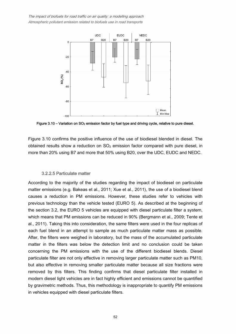
The impact of biofuels for road traffic on air quality: a modelling approach
Atmospheric pollutant emission related to biofuels use in road transports
52
Figure 3.10 – Variation on SO2 emission factor by fuel type and driving cycle, relative to pure diesel.
Figure 3.10 confirms the positive influence of the use of biodiesel blended in diesel. The
obtained results show a reduction on SO2 emission factor compared with pure diesel, in
more than 20% using B7 and more that 50% using B20, over the UDC, EUDC and NEDC.
3.2.2.5 Particulate matter
According to the majority of the studies regarding the impact of biodiesel on particulate
matter emissions (e.g. Bakeas et al., 2011; Xue et al., 2011), the use of a biodiesel blend
causes a reduction in PM emissions. However, these studies refer to vehicles with
previous technology than the vehicle tested (EURO 5). As described at the beginning of
the section 3.2, the EURO 5 vehicles are equipped with diesel particulate filter a system,
which means that PM emissions can be reduced in 90% (Bergmann et al., 2009; Tente et
al., 2011). Taking this into consideration, the same filters were used in the four replicas of
each fuel blend in an attempt to sample as much particulate matter mass as possible.
After, the filters were weighed in laboratory, but the mass of the accumulated particulate
matter in the filters was below the detection limit and no conclusion could be taken
concerning the PM emissions with the use of the different biodiesel blends. Diesel
particulate filter are not only effective in removing larger particulate matter such as PM10,
but also effective in removing smaller particulate matter because all size fractions were
removed by this filters. This finding confirms that diesel particulate filter installed in
modern diesel light vehicles are in fact highly efficient and emissions cannot be quantified
by gravimetric methods. Thus, this methodology is inappropriate to quantify PM emissions
in vehicles equipped with diesel particulate filters.

The impact of biofuels for road traffic on air quality: a modelling approach
Atmospheric pollutant emission related to biofuels use in road transports
53
Despite the low content of particles found in the filters, it was possible to quantify the
levels of total particulate carbon (Figure 3.11) using a thermo-optical transmission system,
including its speciation in organic carbon (OC) and elemental carbon (EC) for fine
particulate fractions (PM<2.5).
Figure 3.11 – Coarse and fine fraction (EC and OC) of total carbon (TC) emission factor in PM10, for B0, B7
and B20, considering all the NEDC.
The main carbonaceous content was concentrated in the fine fraction of all experiments,
and is dominated by organic compounds, The OC/EC ratio ranged between 3 and 6 in the
fine fraction. A decrease in emission factor for total carbon is observed with an increase of
biofuel in the blend mixture. The emission factor of total particulate carbon could be used
as a lower limit of PM emission factor for these experiments.
3.2.2.6 VOC
As described in section 3.2.1, two different tupes of measurements of VOC concentrations
took place during the experiments: (1) through the flame ionization detector total VOC
concentrations were measured per minute; and (2) a sample of exhausted gases was
collected into a bag during the third UDC and EUDC of each NEDC in order to perform a
VOC speciation analysis by gas chromatography. Figure 3.12a represents the total VOC
emissions from the three fuels used, and Figure 3.12b shows the concentration of a set of
VOC species found in the exhaust gas.

The impact of biofuels for road traffic on air quality: a modelling approach
Atmospheric pollutant emission related to biofuels use in road transports
54
a)
b)
Figure 3.12 – Total VOC emission factor (a), and concentration of some species of VOC, for B0, B7 and B20
(b).
Compared with pure diesel, the B7 fuel displays higher values of total VOC emissions
(Figure 3.12a), especially over the UDC, while the B20 fuel presents similar values to B0.
However, the comparison between B7 and B20 fuels indicates that total VOC emissions
decrease with higher biodiesel rates. Lower emissions may result from higher cetane
number and oxygen content for B20 fuels. Fuels with high cetane number can reduce
ignition delay and help promote more complete combustion, which could lead to the
reduction of hydrocarbon emissions. In addition, higher oxygen content in B20 fuel helps
to combust completely and reduces emissions (Peng et al., 2008; Rounce et al., 2012).
Gas chromatography results (Figure 3.12b) show that the set of VOC species and their
concentrations change according to the fuel blend used. Sixteen different VOC species
were found in B7 and B20, instead of the twelve presented on exhaust gases from

The impact of biofuels for road traffic on air quality: a modelling approach
Atmospheric pollutant emission related to biofuels use in road transports
55
experiments with pure diesel. The set of dominant VOC (species with concentration above
50 ng·m-3) regarding pure diesel is characterized by the presence of benzene (25.9%),
toluene (21.1%) and octane (18.1%). On the other hand the set of dominant VOC for B7
includes nonane (16.0%), benzene (13.7%), butanal (11.1%), m,p-xylene (10.6%) and 2-
ethoxyethanol (8.9%). Finally, for B20 the main VOC are butanal (18.3%) and m,p-xylene
(14.1%). The obtained results point out that the concentration of the three main VOC
species in exhaust gases from B0 (benzene, toluene and octane) decrease between 60
and 80% if a B20 blend is used.
It is also interesting to verify that specific VOC species may appear in exhaust gases if a
biodiesel blend is used as fuel instead of pure diesel, namely 2-propanol, 1-butanol, 2-
ethoxyethanol, α-pinene.
In accordance to Peng et al. (2012) the dominant VOC of pure diesel engine exhausts
have higher chronic hazard quotients and hazard indices than VOC from B20. Thus, the
use of pure diesel is more injurious for human health than biodiesel blends, in terms of
VOC emissions.
3.2.3 Synthesis
The influence of diesel/biodiesel blends on the fuel consumption and the exhaust gas
emissions patterns of a EURO 5 passenger vehicle (technology from 2009 to 2014) was
assessed. Experiments were performed using a Renault Megane 1.5 dCi (2011), operated
over the New European Driving Cycle (NEDC) on a laboratory chassis dynamometer. Fuel
blends containing, in volume basis, 7% (B7) and 20% (B20) of biodiesel
(84% soybean / 16% palm) in petroleum-based diesel were tested and compared with a
100% diesel fuel (B0).
Despite the reduction of CO2 emissions as one main reason for the use of biodiesel in
road transportation, the results of this experimental work show that CO2 emissions may
slightly increase with both biodiesel blends (B7 and B20), may be due to a more efficient
combustion revealed.
The analysis of NOx within the set of fuels tested allows the confirmation that B20 was the
better blend in terms of emissions and also combustion efficiency. The opposite was
found with B7. In the combustion chamber, the NO emissions decrease in the presence of
B20, when compared to B0. On the other hand, after the combustion, NO2 emissions
increase with B20 and decrease with B7. This occurred mainly because B20 allows higher
combustion temperature (due to a better efficiency) than B7 and B0.

The impact of biofuels for road traffic on air quality: a modelling approach
Atmospheric pollutant emission related to biofuels use in road transports
56
The results show a positive influence of the use of biodiesel blended in diesel in the SO2
emissions. Regarding the complete NECD is possible to reduce SO2 emission factor from
pure diesel in more than 20% using B7 and 50% using B20. On the other hand, the results
were inconclusive concerning the influence of biodiesel on PM emissions, since the mass
collected in the filters (by gravimetric method) was below the detection limit. However,
through a thermo-optical transmission system, it was possible to quantify the levels of
both organic and elemental carbon for PM2.5, which allowed verifying that, for all the
experiments, the main carbonaceous content was concentrated in the fine fraction and is
dominated by organic compounds. Additionally, the total carbon emissions decrease with
the increasing of biodiesel content in the blend.
Total VOC emissions may increase with biodiesel blend ratios. However the set of VOC
species present on exhausted gases is highly dependent on the fuel blend used.
B7 had a non-expectable behaviour regarding all the parameters that were taken into
account. For all the studied pollutants and for all the replicas executed, large error bar for
B7 were obtained. Probably, the variation on the temperature of exhausted gases founded
to B7 (100ºC by average) in relation to B0 and B20 (109ºC by average) may indicates that
the combustion temperature was lower for B7 than for other blends and then justify the
odd behaviour of B7. Moreover, the higher fuel consumption and the mass air flow, as well
as high CO2 and VOC emissions and lower NOx emissions for B7, point out to the same
direction. To sum up, lower combustion temperature that may occur at B7 probably
destabilized the combustion and catalyst processes and thus increasing the fuel
consumption and CO2, CO, NOx and VOC emissions.

The impact of biofuels for road traffic on air quality: a modelling approach
Emission scenarios
57
Chapter 4. Emission scenarios
To assess the impact of biodiesel use on road transport sector emissions, two study
domains were considered: Portugal and the Porto urban area. For both domains two
emission scenarios were built:
1. The reference scenario (REF) considering that biodiesel is not used as fuel by
road transport sector;
2. The B20 scenario (B20) assuming that all diesel engines are fuelled with diesel
blended with 20% of biodiesel.
Atmospheric pollutant emissions for the REF scenarios were estimated using the
TRansport Emission Model for line sources (TREM, Borrego et al., 2003). The emission
factors identified and discussed on Chapter 3 regarding the use of B20 fuel were used to
correct the emissions of REF to obtain the B20 scenario.
4.1 TRansport Emission Model for line sources (TREM)
The TRansport Emission Model for line sources (TREM), was firstly developed on the
basis of MEET/COST methodology and focused on regulated pollutants (CO, NOx, VOC,
CO2, SO2 and PM10) (Borrego et al., 2000, 2003, 2004; Tchepel, 2003). Recently, the
TREM Hazardous Air Pollutant (TREM-HAP) extension was developed to calculate
emissions of benzene, 1,3-butadiene, formaldehyde, acetaldehyde, acrolein, naphthalene
and PM2.5 (Tchepel et al., 2012).
The main objective of the TREM is the estimation of road traffic emissions with high
spatial resolution, which can be used as supporting tool for air quality modelling studies
and air quality management proposes. TREM considers roads as line sources and
emissions induced by vehicles are estimated individually for each road segment

The impact of biofuels for road traffic on air quality: a modelling approach
Emission scenarios
58
considering detailed information on traffic fluxes, vehicle fleet distribution and road
segment length (Figure 4.1).
Figure 4.1 - TREM input data and main calculation modules for exhaust emission quantification
(adapted from Tchepel, 2003).
TREM uses the state of the art emission factors from the EMEP/EEA air pollutant
emission inventory guidebook (EMEP/EEA, 2013) for regulated pollutants, and updated
emission factors from Artemis methodology (André and Joumard, 2005; Boulter and
McCrae, 2007) for hazardous air pollutant relevant for mobile source. The emission
factors are function of the average speed and vehicle class (based on engine age, type,
and capacity, vehicle weight, fuel type, and emission reduction technology). To process
these data, TREM is linked to Geographical Information System (ArcGIS) (Tchepel, 2003;
Tchepel et al., 2012).
In sum, three types of input data are needed for TREM application:
The vehicle fleet distribution;
The road network of the study area, including the type and the length of each road;
Traffic information of each road (traffic fluxes and average speed of circulation).
Based on the national statistics on automobile sector for 2009 (ACAP, 2010), it was
possible to characterize the national vehicle fleet by age and type (Table 4.1). The vehicle

The impact of biofuels for road traffic on air quality: a modelling approach
Emission scenarios
59
types considered are: light passenger vehicles (LPV), light duty vehicles (LDV), heavy
passenger vehicles (HPV) and heavy duty vehicles (HDV).
Table 4.1 – Portuguese vehicle fleet by age and type in 2009 (ACAP, 2010).
Due to the lack of detailed information regarding the number of existing vehicles by type of
fuel, the characterization of the vehicle fleet distribution is based on the number vehicles
sold in 2009 by fuel type (ACAP, 2010). The vehicle fleet distribution estimated per vehicle
type and fuel is presented in Figure 4.2.
Figure 4.2 – Vehicle fleet distribution by type and fuel.
According to the Figure 4.2, almost 72% of the vehicle fleet is diesel fuelled and the
quantity of HPV, LDV and HDV fuelled by other fuel than diesel is negligible. Regarding
LPV, 32.52%, 66.50%, 0.71% and 0.26% are fuelled by gasoline, diesel, hybrid and
gasoline/liquefied petroleum gas (LPG), respectively.
Age
(year)
LPV LDV HPV HDV
(%)
< 1 5.52 3.93 4.03 4.64
1 – 2 4.08 3.32 3.96 4.34
2 – 3 5.74 4.70 5.40 5.96
3 – 4 5.58 5.60 4.83 5.87
4 – 5 5.35 5.38 4.02 5.35
5 – 10 26.79 30.59 22.21 20.48
10 – 15 27.67 29.39 21.38 19.17
15 – 20 15.32 13.06 11.97 12.10
>20 3.95 4.03 22.20 22.09

The impact of biofuels for road traffic on air quality: a modelling approach
Emission scenarios
60
The available information to characterize the national road network in terms of traffic
volume only regards to motorways, which is not enough to calculate the total emissions
from the road transport sector over Portugal. This problem was overcome applying the
TREM-HAP model over the Northern Region of Portugal, for which the available
information is significantly more detailed. It includes the mean daily traffic for several
roads of the Northern Region of Portugal, namely: motorways, other major roads,
secondary roads and urban roads over the municipality of Porto (Figure 4.3) (Borrego et
al., 2009).
Figure 4.3 – The TREM-HAP simulation domain covering the Northern region of Portugal: the Porto urban
area, the road network and the daily mean traffic volume (vehicle.day-1) for each road, main cities and
population distribution.
TREM-HAP was applied over the Northern region of Portugal (Figure 4.3): a first run to
calculate the emissions from gasoline vehicles and another one considering diesel
vehicles. TREM-HAP calculate the mass of CO, CO2, PM10, NOx, NMVOC,
acetaldehyde, acrolein, formaldehyde and PM2.5 emitted (gpollutant.km-1), as well as the
mass of fuel consumed (gfuel.km-1) for each road. The average emission factors
(gpollutant.gfuel-1) were calculated for each road of the Northern region of Portugal (Table
4.2).

The impact of biofuels for road traffic on air quality: a modelling approach
Emission scenarios
61
Table 4.2 – Average emission factors (gpollutant.gfuel-1) calculated by TREM and TREM-HAP for the Northern
region of Portugal.
Pollutant
gpollutant.gfuel-1
Diesel Gasoline
NOx 2.05E-02 8.93E-04
PM10 6.56E-04 1.90E-05
PM2.5 1.27E-03 7.75E-05
CO 4.99E-03 5.61E-03
NMVOC 1.63E-03 4.07E-03
Formaldehyde 1.23E-04 6.09E-05
Acethaldehyde 6.69E-05 2.69E-05
Acrolein 3.08E-05 6.79E-06
Benzene 9.51E-06 2.01E-04
CO2 3.14E+00 2.85E+00
4.2 The REF scenario
The reference scenario (REF) considers that the diesel used by the road transport sector
is a petroleum-based diesel, meaning that no biodiesel is used.
From the information provided by TREM-HAP and to determine the road traffic emissions
for Portugal, the average emission factors for each pollutant and fuel (Table 4.2) were
multiplied by the quantity of fuel sold (diesel and sum of gasoline 95 and 98) in Portugal
during 2012, at municipality scale (URL 10) (Figure 4.4).
Figure 4.4 – Diesel and gasoline (95+98) sold by municipality in 2012 (URL 10).

The impact of biofuels for road traffic on air quality: a modelling approach
Emission scenarios
62
Since the TREM-HAP simulation (Figure 4.3) covered the entire Porto urban area (Figure
4.5), the fuel consumption data was not taken into account, but the road network and the
daily mean traffic volume for this area. Keeping the road transport emissions over the
roads instead of distributed by municipality areas is especially important for the Porto
urban area to improve the emission information to further air quality simulation (Chapter
6).
Figure 4.5 – The Porto urban area domain: population distribution, main cities and road network including the
daily mean traffic volume (vehicle.day-1).
Road-transport emissions estimated by TREM-HAP for mainland Portugal and the Porto
urban area are compiled in Table 4.3. Because this is the reference scenario, atmospheric
pollutant emission from TREM-HAP were compared against the road transport emission
on national emission inventory (APA, 2011). Additionally, they are compared to INERPA
emissions, which do not consider the use of biodiesel blends for road transports to
emission estimation, in order to validate the methodology here used and to build REF
scenarios with more realistic emission values. The representativity of the Porto urban area
in terms of road-transport emissions within Portugal is also shown in Table 4.3.

The impact of biofuels for road traffic on air quality: a modelling approach
Emission scenarios
63
Table 4.3 – Road-transport sector annual pollutant emissions estimated by TREM-HAP (T), regarding the REF
scenario, and included in INERPA (I), over mainland Portugal and the Porto urban area. Ratio of emission
estimated and INERPA emissions (T/I) and the representativity of the Porto urban area in mainland Portugal’s
emissions (Porto/Portugal).
Pollutant
Mainland Portugal Porto urban area Porto/Portugal
(%) TREM-HAP
(T)
INERPA
(I)
T/I
(%)
TREM-HAP
(T)
INERPA
(I)
T/I
(%)
Acroleine 129.8 - - 23.1 - - 17.8
Benzene 252.2 - - 36.7 - - 14.5
Acetaldehyde 295.2 - - 45.4 - - 15.4
Formaldehyde 556.9 - - 85.5 - - 15.3
PM2.5 2478.1 5136.9 48.2 357.3 356.064 100.3% 14.4
PM10 2636.3 5326.7 49.5 397 370.9 107.0% 15.1
NMVOC 10854.8 20889.9 52.0 2082 2648.1 78.6% 19.2
CO 25878.3 130253 19.9 7483.5 13605.7 55.0% 28.9
NOx 82616.2 99917.8 82.7 5641 5684.2 99.2% 6.8
CO2 15570067.6 17441509.0 89.3 1223253.4 1205696.3 101.5% 7.7
The comparison between the emissions determined through TREM-HAP and emission in
the INERPA (Table 4.3) revealed that the methodology presented here based on fuel
consumption was able to estimate more than 80% of the total NOx and CO2 emissions for
mainland Portugal, but only about 20% of CO and 50% of NMVOC, PM10 and PM2.5
emissions. Different results were found for the Porto urban area, mainly because the
methodologies used for each case study were somewhat different. The comparison
between TREM-HAP and INERPA emissions suggest that TREM-HAP was able to
estimate emissions with more accuracy based on road-network and vehicle fleet
information that using national statistics on fuel consumption, as expected. The pollutant
with worst result was CO, for which the TREM-HAP was able to estimate only half of its
emissions, while slightly overstates PM10, PM2.5 and CO2 emissions. NMVOC and NOx
emissions estimated by TREM-HAP corresponding to about 80% and 99% of their
INERPA emissions. These variations on emission estimations are mainly derived from the
models used with in this work and INERPA: the COPERT IV (Ntziachristos et al., 2009)
emission model is used within INERPA, while road-transport emissions were estimated by
TREM in this work. The extrapolation made from the Northern Region of Portugal as well
as the non-consideration of cold-emission, due to the lack of information on origin/destiny
matrix per municipality, are also factors that contributed to the verified differences,
especially on total NMVOC, PM10 and CO emissions. INERPA does not include
emissions of acroleine, benzene, acetaldehyde and formaldehyde; and no other emission
inventory that included these pollutants was found for Portugal.

The impact of biofuels for road traffic on air quality: a modelling approach
Emission scenarios
64
The differentials between emissions from TREM-HAP and from the national inventory
were determined and applied to correct REF scenario. As it will be discussed in next
section, the same differentials were also applied to correct the B20 emission scenario.
As an example of the emission distribution for both case studies, Figure 4.6 presents the
REF emissions of NOx (Figure 4.6a,c) and formaldehyde (Figure 4.6b,d), since they are
the most important pollutants emitted by the road transport sector from each pollutant
group (regulated and non-regulated pollutants), according to Ho et al. (2007) and APA
(2014). In Figure 4.6, NOx and formaldehyde emissions are in tons per year for each
municipality of Portugal, while for the Porto urban area there was a need to convert line
emission (from TREM-HAP) to emissions in area in order to perform the emission
correction (see the previous two paragraphs). Both emission correction and the
representation were made based on a 11km2 grid to be compatible with the horizontal
resolution of the air quality simulation domain (topic addressed further in Chapter 5).

The impact of biofuels for road traffic on air quality: a modelling approach
Emission scenarios
65
a) b)
c) d)
Figure 4.6 - Road-transport NOx (a,c) and formaldehyde (b,d) emissions for Portugal and for the Porto urban
area (in a grid of 11km2), regarding the REF scenario.

The impact of biofuels for road traffic on air quality: a modelling approach
Emission scenarios
66
4.3 The B20 scenario
The B20 scenario considers that the fuel used in diesel vehicles is a blend with 20% (v/v)
of biodiesel. This emission scenario was calculated based on REF values and on the
emission variation factors summarized in Table 4.4 and Table 4.5, and discussed in detail
within the sections 3.1 and 3.2. Wherever possible it has been taken into account the type
of road to use the appropriated emission factor: emission factors related to complete
driving cycles (NEDC and CADC, Figure 3.3) were used for Portugal, while urban (UDC
and CAU) and extra-urban (EUDC, CAR and CAM) factors from specific slices of the
driving cycles were considered on the Porto urban area case study.
Table 4.4 - Average emission variations (%) of regulated pollutants for an EURO 4 LPV over the NEDC and
CADC (Bakeas et al., 2011) and for an EURO 5 LPV over the NEDC (Lopes et al., 2014).
Pollutant EURO 4 EURO 5
Avg (NEDC;CADC) UDC EUDC NEDC
NOx 5.92 -20.36 -4.09 -10.83
NO - -69.92 -13.82 -29.44
NO2 - 1.28 8.12 4.52
PM10 / PM2.5 -3.42 - - -61.57
HC -8.13 1.21 4.13 2.38
CO -16.98 - - -
CO2 1.11 -0.23 3.55 1.46
Table 4.5 – Average carbonyl compound emission variations (%) for an EURO 4 LPV over the NEDC and
CADC (Karavalakis et al., 2011b) and average benzene* emissions at different engine loads for an EURO 4
LPV (Di et al., 2009).
Pollutant NEDC CAU
(0.20 MPa)
CAR
(0.38 MPa)
CAM
(0.55 MPa)
Formaldehyde 18.03 25.80 19.96 23.97
Acetaldehyde 23.57 22.67 16.58 22.80
Acrolein/acetone 45.97 28.02 34.52 46.07
Benzene* - 37.75 4.21 1.42
The total pollutant emissions estimated for the B20 scenario and for both case studies are
presented in Table 4.6.

The impact of biofuels for road traffic on air quality: a modelling approach
Emission scenarios
67
Table 4.6 – Annual pollutant emissions (ton) estimated for road-transports in Portugal and Porto urban area,
regarding the B20 scenario.
Pollutant Emission (ton)
Portugal Porto urban area
Acrolein 177 68
Benzene 257 91
Acetaldehyde 352 129
Formaldehyde 664 247
PM2.5 4523 2445
PM10 5009 931
NMVOC 20464 3608
CO 20807 11145
NOx 102586 29184
CO2 17589714 7272492
Since the spatial distribution of B20 emissions is similar to the REF ones the spatial
distribution of B20 emissions is not presented here. However, the comparison between
both emission scenarios is shown in section 4.4.
4.4 Emission scenarios comparison
The variations of the total emissions estimated for REF and B20 scenarios are presented
in Figure 4.7. The emission variations found between both study areas are mainly due to
different methodologies and input data used for each of them, including the emission
factor, which are function of the driving cycles that characterize each study area (complete
driving cycles for Portugal and specific emission factors taking into account the road
network information for the Porto urban area).

The impact of biofuels for road traffic on air quality: a modelling approach
Emission scenarios
68
Figure 4.7 – Emission variations (%) between B20 and REF scenarios [(B20-REF)/REF].
According to the Figure 4.7, three pollutant groups can be identified. The first group is
composed by carbonyl compounds (acrolein, formaldehyde and acetaldehyde), for which
an increase of more than 20% in emissions was estimated when using B20 fuel. The
second group comprehends NOx, C6H6, CO2 and NMVOC which emissions vary in a
small range [-3.98 ; 3.65]% for both domains. The third group includes CO, PM2.5 and
PM10 which emissions are reduced when B20 is used instead of pure diesel, varying
between [-19.60 ; -5.96]%. The higher reduction regards to CO, being the B20 emissions
almost 20% lower than REF emissions for Portugal and 16% lower for the Porto urban
area). PM10 and PM2.5 emission differentials for B20 are about 10% lower than for REF
over both domains. The results obtained for regulated pollutants are in accordance to
previous works over the Northern region of Portugal (Ribeiro et al., 2011, 2012).
The representativeness of the estimated variations in total emissions (APA, 2011) for
each pollutant and case studies are compiled in Table 4.7.
Table 4.7 - Representativeness of the estimated variations (B20-REF) in total emissions regarding the
studied pollutant, for Portugal and the Porto urban area (APA, 2011).
Pollutant Portugal (%) Porto urban area (%)
NOx 0.94 1.89
CO2 0.26 0.41
Total NMVOC -0.07 -0.54
PM10 -0.30 -0.81
PM2.5 -0.66 -1.04
CO -4.98 -5.31

The impact of biofuels for road traffic on air quality: a modelling approach
Emission scenarios
69
According to Table 4.7, the use of B20 on road transports represent a variation in total
emission inferior that 1% for both case studies, with exception for CO (~5%) and NOx and
PM2.5 over the Porto urban area (~2%).
As already discussed in section 3.1.5, the use of biodiesel/diesel blends in road transports
increase aromatic hydrocarbon and aldehyde emissions that are especially important due
to their reactivity, potentiating tropospheric ozone formation and rising of the probability of
cancer, among other health disease. Figure 4.8 and Figure 4.9 show the spatial
distribution of these pollutant emissions (a-d) over Portugal and the Porto urban area
respectively, as well as the equivalent ozone production (EOP, see section 3.1.5) (e)
regarding the difference between B20 and REF scenarios (B20-REF). The population
which is potentially exposed to these pollutants is presented in Figure 4.8f) for Portugal
and in Figure 4.9f) for the Porto urban area.
Figure 4.8 – Difference between REF and B20 annual emissions (ton.y-1) of: a) formaldehyde, b)
acetaldehyde, c) acrolein/acetone and d) benzene; e) increment on Equivalent Ozone Production (EOP) by
the use of B20 and f) population distribution, over Portugal.

The impact of biofuels for road traffic on air quality: a modelling approach
Emission scenarios
70
As expected, the replacement of pure diesel by B20 increases the non-regulated pollutant
emissions especially over the urban areas and coastline of Portugal were the population is
greater (Figure 4.8) and the fuel consumption is higher (Figure 4.4). The EOP from
benzene and carbonyl compounds is especially important in urban areas, increasing the
ground level ozone and potentiating the occurrence of photochemical smog.
Figure 4.9 – Difference between REF and B20 annual emissions (ton.y-1) of: a) formaldehyde, b)
acetaldehyde, c) acrolein/acetone and d) benzene; e) increment on Equivalent Ozone Production (EOP) by
the use of B20 and f) population distribution, over the urban area of Porto.
Regarding the urban area of Porto (Figure 4.9), results point out that if B20 fuel is used
instead of conventional diesel, the pollutant emissions increase significantly (Figure 4.7).
Due to their maximum incremental reactivity value (MIR, see Figure 3.5) and emission
amounts, formaldehyde is the most critic pollutants among the non-regulated pollutant
studied, which emissions increment from the use of B20 contributes to 58% of the EOP
over the entire domain, while the contribution of benzene is insignificant (0.25%) and the
remaining pollutants effect the total EOP in about 20%. Figure 4.9 also reveals that the
hot spots are located at West and at North of the city, where the road traffic is higher.

The impact of biofuels for road traffic on air quality: a modelling approach
Emission scenarios
71
4.5 Synthesis
In order to assess the impact of a 20% of biodiesel blended with petroleum-based diesel
over Portugal and the Porto urban area, two emission scenarios were built (REF and
B20). The TRansport Emission Model for line sources (TREM) was applied to estimate the
emissions for both mentioned scenarios. The input data required by TREM includes
information about the traffic fluxes, the vehicle fleet distribution and the road network.
The difference between REF and B20 scenarios includes the fuel characteristics used by
diesel engines: REF scenario considers that the conventional diesel is used by the road-
transport sector, while B20 assumes that the diesel is blended with 20% (v/v) of biodiesel.
Thereby, the B20 scenario was built based on REF and the application of updated
emission factors according to the approached presented in sections 3.1 and 3.2.
The results obtained suggest that the introduction of 20% of biodiesel in petroleum-based
diesel in road transportation promotes a reduction in PM10, PM2.5 and CO emissions
over Portugal and urban area of Porto. However, the changes on emissions represent
less than 1% regarding the total emissions, with exception for CO, with emission
variations can reach to 5% in both case studies.
On the other hand, an increase on NOx and non-regulated pollutants emissions, such as
acrolein, formaldehyde and acetaldehyde, was observed, potentiating tropospheric ozone
formation and eventually causing adverse effects on human health.
In order to predict the effects of biodiesel use and its emissions on air quality over both
study domains, air quality modelling studies were performed, especially to investigate the
impacts on PM10, PM2.5 and O3 atmospheric concentration levels, which are currently
the most current critical pollutants in terms of exceedences of legislated values. This work
will be addressed in Chapter 7.


The impact of biofuels for road traffic on air quality: a modelling approach
The air quality modelling system
73
Chapter 5. The air quality modelling system
This fifth chapter focused on the selection and description of the numerical and mesoscale
air quality modelling system that will be used to investigate the impacts of biodiesel use
for road transports on air quality over Portugal and the Porto urban area. The selection of
the WRF-EURAD air quality modelling system was based on a multi-model comparison
exercise that is addressed in section 5.1. A detailed description of the selected modelling
system is addressed in section 5.2.
5.1 Selection of the modelling system
The selection of the air quality modelling system to be applied in this study was supported
by the national project “ENSEMBLAIR – Improving air quality assessment with ensemble
modelling” (Monteiro et al., 2013a, 2013b). This project aimed to reduce the uncertainty
on numerical chemical transport models results through the applications of ensemble
techniques. To achieve this objective five chemical transport models were selected and
their results were compared within a multi-model comparison exercise (Monteiro et al.,
2013a). The models were select based on a state of the art revision of regional chemical
transport models. The selection criteria were focused on models applicability and tests
over Portugal; the availability of spatially resolved modules for anthropogenic and biogenic
emissions as well as a complete chemical mechanism. The selected models include
CHIMERE (Schmidt et al., 2001; Bessagnet et al., 2004), EURAD (Elbern et al., 2007),
LOTOS-EUROS (Schaap et al., 2008), CAMx (Tesche et al., 2006) and TAPM (Hurley et
al., 2003). All of them are mesoscale models designed for short and long-term simulations
of oxidants and aerosol formation, through different degrees of complexity, as discussed
by Monteiro et al. (2013a).
The five models were applied in their optimized set up regarding input data,
parameterization and boundary conditions, and considering an horizontal resolution of 5
5 km2. The Portuguese anthropogenic emissions inventory (INERPA, APA, 2011) was

The impact of biofuels for road traffic on air quality: a modelling approach
The air quality modelling system
74
used as a common basis for all models, and models were meteorologically driven by the
“Weather Research and Forecasting Model” (WRF, Skamarock et al., 2008), excepting
TAPM that has an own meteorological data base coupled. All models were applied to over
July 2006, with a spin-up time period of 1-2 days.
The multi-model evaluation and comparison exercise was focused on O3 and PM10
concentrations, due to the common exceedences of limit values of these two pollutants
over mainland Portugal. This exercise was supported by observed data from 22
background stations (including urban, suburban and rural environments) from the national
air quality monitoring network3. Three statistical parameters, described in detail in section
6.2 and Table 6.2, were chosen to evaluate the five models performance: the correlation
factor (R) indicates the correspondence of timing and evolution between observed and
simulated concentration values; the root mean square error (RMSE) gives information
about the skill in predicting the magnitude of a pollutant concentration; and the systematic
error (bias) which translate the average difference between simulated and observed
values (negative for overestimations and positive for underestimations).
According to the multi-model performance assessment (Monteiro et al., 2013a) the model
with more robust prediction skills was the EURAD model (Elbern et al., 2007), having
presented higher correlation factors and lower RMSE values for O3 (R = 0.64, RMSE =
28.92 gm-3) and PM10 (R = 0.51, RMSE = 19.76 gm-3) surface concentrations. Based
on this result, EURAD was selected to perform the air quality simulations to assess the
impact of biofuels on air quality over Portugal and Porto urban area.
Additionally, all of the applied models were found to have significant biases for both
pollutants, indicating an overestimation of ozone (bias values range from -45.0 gm-3 to
6.7 gm-3 for TAPM and EURAD, respectively). A different picture was obtained for
PM10, with positive bias values for all selected models ranging from 7.0 gm-3, for TAPM,
to 22.0 gm-3 for LOTOS-EUROS, pointing out to an underestimation of PM10
concentrations.
3 For more information about the selected monitoring sites, see Monteiro et al. (2013a), and section
5.3.2 for detailed information regarding the national air quality monitoring network.

The impact of biofuels for road traffic on air quality: a modelling approach
The air quality modelling system
75
5.2 WRF-EURAD modelling system
The WRF-EURAD is an Eulerian modelling system with the structure presented in Figure
5.1, consists on the following three major models:
The Weather Research & Forecasting (WRF) model (Skamarock et al., 2008), version
3.5.0, acts as meteorological driver for the CTM, delivering the meteorological fields
needed (e.g. wind, relative humidity and temperature);
The EURAD Emission Model (EEM) (Memmesheimer et al., 1991) delivers emission
fields for the specific grid used considering seasonal, weekly and diurnal cycles, as well
as international holidays;
The EURopean Air pollution Dispersion – Chemistry Transport Model (EURAD-CTM)
(Hass, 1991; Ebel et al., 1997; Elbern et al., 2007) – version 5.6 – computes transport,
chemical reactions and deposition of gas-phase and aerosol-phase species.
Figure 5.1 – Scheme of the WRF-EURAD air quality modelling system.
The input information needed to simulate air quality includes the orography and land use
types for its specific geographical domain as well as the climatological boundary
conditions to provide the meteorological condition fields produced by WRF model and to
calculate biogenic emissions by EEM. Additionally, meteorological fields are processed by
the pre-processor (PPC) in order to calculate additional meteorological information

The impact of biofuels for road traffic on air quality: a modelling approach
The air quality modelling system
76
needed to the EURAD-CTM, that, together with biogenic and anthropogenic emissions,
constitute the main input data for EURAD-CTM. The EURAD-CTM outputs include 3-D
gases and aerosols deposition and concentrations fields.
In this section, the WRF-EURAD modelling system is described in detail in terms of the
models that this system includes and its geometry as well as the modelling system setup
and details of its application with in this study.
5.2.1 Geometry of the modelling system
Both WRF and EURAD-CTM use a Lambert conformal conic projection grid with an
equidistant rectangular horizontal spacing. The state variables are represent according to
the Arakawa C-Grid staggering (Arakawa and Lamb, 1977) (Figure 5.2a), what means
that the u components are located at the centre of the left and right grid faces, and the v
and w components at the centre of the upper and lower grid faces. Mass points, such as
potential temperature, pressure, density, moisture variables, pollutant concentrations,
among other variables, are defined in the centre of the grid cell. Vertically, the atmosphere
is divided by terrain-following sigma coordinate layers defined by Equation 5.1. (Figure
5.2b)
a) b)
Figure 5.2 – WRF-EURAD modelling system geometry: a) horizontal and vertical views of the Arawaka C-grid
configuration; b) example of the vertical structure of a grid for 15 vertical layers (solid lines denote sigma
levels and dashed lines denote half-sigma levels) (Skamarock et al., 2008).

The impact of biofuels for road traffic on air quality: a modelling approach
The air quality modelling system
77
𝜎𝑘 =𝑝𝑘 − 𝑝𝑡𝑜𝑝
𝑝𝑏𝑜𝑡 − 𝑝𝑡𝑜𝑝 Equation 5.1
Where:
𝑘: layer number;
𝑝𝑏𝑜𝑡,𝑘,𝑡𝑜𝑝: Pressure at the surface, layer 𝑘 and top of the model, respectively.
The geometry of the simulation domains used in this study is described in next section
(5.2.1.1) regarding their vertical and horizontal structures and dimensions.
5.2.1.1 Geometry of the simulation domains
Based on previous applications of this modelling system (Nieradzik, 2011; Elbern and
Friese, 2013), it was assumed that the atmosphere is divided into 23 terrain-following
sigma coordinate layers. The top boundary of the WRF-EURAD is set at 100 hPa and the
diffuse vertical fluxes at the top are set to zero. About 15 layers are defined above 2 km
height and the Earth’s surface defines the bottom boundary. The vertical structure of the
atmosphere used within this modelling application is presented in Table 5.1.
Table 5.1 – The vertical structure of the WRF-EURAD grid, defined by terrain-following sigma coordinates.
Layer index values Pressure (hPa) Height (m)
Surface 1.000 1013.25 0
1 0.995 1008.68 38
2 0.990 1004.12 76
3 0.985 999.55 115
4 0.980 994.99 153
5 0.970 985.85 231
6 0.960 976.72 309
7 0.945 963.02 427
8 0.930 949.32 546
9 0.910 931.06 708
10 0.890 912.79 872
11 0.865 889.96 1081
12 0.840 867.13 1294
13 0.810 839.73 1556
14 0.780 812.34 1825
15 0.740 775.81 2196
16 0.700 739.28 2581
17 0.600 647.95 3615
18 0.500 556.63 4775
19 0.400 465.3 6101
20 0.300 373.98 7658
21 0.200 282.65 9560
22 0.100 191.33 12064
23 0.000 100.00 16179

The impact of biofuels for road traffic on air quality: a modelling approach
The air quality modelling system
78
Since the pollutant concentrations variables are defined in the centre of the cells and the
thickness of the lowest layer is about 38 m, the concentration pollutants extracted to the
first level correspond to a height of approximately 19 m.
On air quality simulations is desired, in general, a high resolved look at physics and
chemical states of the atmosphere in a certain region. To simulate only the region of
interest would be a great loss of information since many tropospheric constituents are
long-living and can be transported over large distances and information inflow from
outside the area could not be considered this way. On the other hand, to simulate an area
large enough to comprise all necessary sources with desired high resolution is not
feasible due to computational limitations. To overcome these impasses, different domains
with increasingly finer resolution are considered using nesting capacities.
In this study, the WRF-EURAD simulations were started on a grid with large extent, in a
continental scale, covering Southern Europe and Sahara Desert, but with a low horizontal
resolution of 125 125 km2 (C125, the coarse domain). Inside C125, is defined a region
around the area of the next domain to provide boundary conditions that need to be
interpolated to the next smaller domain grid. The second simulation domain covers Iberian
Peninsula with 25 25 km2 of horizontal resolution (IP25). The same nesting process is
applied to the third domain over Mainland Portugal, with 5 5 km2 (PT05) and then to the
last domain covering the Porto urban area with a fine horizontal resolution of 1 1 km2
(OP01). The OP01 horizontal resolution is on the limit recommended by EURAD-CTM
(Ebel et al., 1997; Monteiro et al., 2012).
Table 5.2 compiles all the information regarding domain dimensions and Figure 5.3 shows
the simulation domains chain.
Table 5.2 – Dimensions of the simulation domains used in WRF-EURAD modelling system.
ID Domain Parent
ID
Horizontal resolution
(km)
Number
of cells (WRF)
Number
of cells (EURAD)
x y x y x y
1* C125 - 125 125 49 39 49 39
2 IP25 1 25 25 55 50 51 46
3 PT05 2 5 5 85 140 81 136
4 OP01 3 1 1 30 30 26 26
* Coarse domain

The impact of biofuels for road traffic on air quality: a modelling approach
The air quality modelling system
79
Figure 5.3 – Simulation domains used in the WRF-EURAD modelling system application.
With exception to the coarse domain, that has the same dimensions for WRF and EURAD
simulations, the remaining simulation domains are not exactly the same for both models,
but very similar (Table 5.2). In fact, WRF domains have two more cells in each side of the
domain in order to better integrate the meteorological input on the CTM model.
5.2.2 Weather Research Forecasting model (WRF)
The WRF model (Skamarock et al., 2008) is a numerical weather prediction and
atmospheric simulation system designed for both research and operational applications.
Its dynamics solver integrates compressible and non-hydrostatic Euler equations.

The impact of biofuels for road traffic on air quality: a modelling approach
The air quality modelling system
80
A multi-agency4 effort is on the basis of the WRF development to build a next-generation
model and data assimilation system. Currently, WRF is a state-of-the-art model reflecting
flexibility portable code, being efficient in computing environments ranging from
massively-parallel supercomputers to laptop. It is suitable for a board span of applications
from large-eddy (grid cell size >1 km) to global simulations (grid cell size >100 km). Such
applications include real-time numerical weather predictions, data assimilation
development and studies, parameterized-physics research, regional climate simulations,
air quality modelling, atmosphere-ocean coupling and idealized simulations. WRF have
been supported as a common tool for the universities/research and operational
communities, and to facilitate the wide internationally use (Skamarock et al., 2008).
Here, a simplified description of the WRF model is given in the flow chart presented in
Figure 5.4. Skamarock et al. (2008) and Wang et al. (2014) provide more detailed
information regarding this model.
Figure 5.4 – WRF model flow chart (adapted from Wang et al., 2014).
To weather prediction, WRF needs topography and land-use for each domain, and
meteorological global data to initialize the coarse domain simulation (Figure 5.4). Firstly,
external data is prepared by the WRF Preprocessing System (WPS) throughout three
programs (Geogrid, Ungrib and Metgrid) (Figure 5.4). The first program of the WPS chain
is Geogrid, which defines model domain and interpolates static geographical data to the
model domain grids. GRIB-formatted global data files contain several encoded variables
4 The agencies that have been collaborating into the WRF development are: the National Center for
Atmospheric Research’s (NCAR) Mesoscale and Microscale Meteorology (MMM) Division, the National
Oceanic and Atmospheric Administration’s (NOAA) National Centers for Environmental Prediction (NCEP) and
Earth System Research Laboratory (ESRL), the Department of Defense’s Air Force Weather Agency (AFWA)
and Naval Research Laboratory (NRL), the Center for Analysis and Prediction of Storms (CAPS) at the
University of Oklahoma, the Federal Aviation Administration (FAA) and university scientists.
The impact of biofuels for road traffic on air quality: a modelling approach
The air quality modelling system
81
(more than are needed to initialize WRF). Ungrib uses “variable tables” (Vtables),
provided with the software for common GRIB model output files, to identify the fields
though codes. Then, Ungrib extracts needed meteorological fields from GRIB files and
writes the data in a simple and WPS specific format (intermediate format). Metgrid
horizontally interpolates the intermediate-format meteorological files extracted by Ungrib
onto the simulation domains defined by Geogrid. The interpolated Metgrid output can then
be ingested by the Real WRF program.
Like WPS, the WRF model also contains three programs, namely: Real, Ndown and WRF
(Figure 5.4). Real reads the meteorological and static input information from the WPS and
generate initial condition files. It vertically interpolates the required levels (Table 5.1) for
the specified land surface scheme, in order to prepare soil fields for use into the model,
and check if soil categories, land use, land mask, soil temperature and sea surface
temperature are all consistent with each other. Additionally, Real generates initial
condition files and processes multiple input time periods to generate the 3D lateral
boundary conditions, namely u-, v- and w- wind components, potential temperature,
vapour mixing ratio and geopotential height, which are couple with total column pressure.
This program can run as either a serial or a distributed memory (parallel) job. For this
work the second option was used. The Ndown program applies the nesting technique.
WRF supports two nested options: 1-way nesting and 2-way nesting. 1-way nesting uses
the output of a coarser grid simulation as input for the finer grid simulation, while 2-way
nesting involves feedback from the fine domain to the coarse domain and vice versa
(Misenis and Zhang, 2010). Ndown run in-between the coarser and finest domains in
order to provide the initial and boundary conditions from the coarse together with input
from higher resolution terrestrial fields provided by Real with regards to nest domain. In
this work it was used the 1-way nesting technique because EURAD-CTM is not prepared
to use other. Moreover, according to Misenis and Zhang (2010), that performed a
comparison between these two nesting techniques, both reveal similar results and 2-way
nesting requires more computational time. Finally, the WRF program provides 3D
meteorological fields required by EURAD-CTM for each simulation domain, through
numerical integration methods, based on data from previous programs.
The WRF setup used in this study is described in following section (5.2.2.1).

The impact of biofuels for road traffic on air quality: a modelling approach
The air quality modelling system
82
5.2.2.1 WRF model application
The global meteorological fields from the National (USA) Center for Environmental
Prediction (NCEP/NOAA, 2000), which provides final (FNL) operational global data on 1º
by 1º grids with a temporal resolution of six hours, were used to supply initial and
boundary conditions for the coarse domain (C125). The FNLs are produced from the
same model which NCEP uses in the Global Forecast System (GFS), however the FNLs
are prepared about an hour after the GFS is initialized in order to observational data can
be used. The FNL are available on the surface and at 63 sigma layers from 1000 millibars
to 10 millibars. Parameters include surface pressure, sea level pressure, geopotential
height, temperature, sea surface temperature, soil values, ice cover, relative humidity, u-
and v- winds, vertical motion, vorticity and ozone (NCEP/NOAA, 2000). They are linearly
interpolated to the WRF grid and linear time interpolation is also applied to obtain hourly
values. For the other domains (not C125), the initial and boundary conditions come from
the respective parent domain (Table 5.2 and Figure 5.3) and from the previous simulated
day.
The WRF model has a large variety of physic parameterizations (described in detail in
Wang et al. (2014)), namely regarding:
Microphysics (mp_physics);
Long- and shortwave radiation (ra_lw_physics and ra_sw_physics);
Land and surface schemes (soil temperature and moisture) (sf_sfclay_physics
and sf_surface_physics);
Planetary boundary layer schemes (bl_pbl_physics);
Cumulus parameterization (cu_physics).
Table 5.3 summarizes the selected physics options used in this study. Their selection was
based on recommendations included in Wang et al. (2014), as well as on validation and
sensitivity studies previously performed over Portugal (Aquilina et al., 2005; Carvalho et
al., 2006) and over the Iberian Peninsula (Fernández et al., 2007).

The impact of biofuels for road traffic on air quality: a modelling approach
The air quality modelling system
83
Table 5.3 – Summary of WRF physic options used.
Physic parameter Option Domain ID
mp_physics WSM 6-class graupel scheme (Hong and Lim, 2006) 1-4
ra_lw_physics Rapid Radiative Transfer Model scheme 1-4
ra_sw_physics Rapid Radiative Transfer Model scheme 1-4
sf_sfclay_physics Pleim-Xiu surface layer (ARW only)
Monin-Obukhov (Janjic) scheme
1-3
4
sf_surface_physics Pleim-Xiu LSM (ARW) 1-4
bl_pbl_physics ACM2 (Pleim) PBL (ARW) (Pleim, 2007)
Mellor-Yamada-Janjic TKE scheme (Janjić, 1994)
1-3
4
cu_physics Kain-Fritsch (new Eta) scheme (Kain, 2004)
no cumulus
1-3
4
The WRF model generates several meteorological fields required by the EURAD-CTM,
such as wind, temperature, water vapour mixing ratio, cloud liquid water content, 2 m
temperature, surface heat, moisture fluxes and precipitation.
5.2.3 EURAD Emissions Model (EEM)
The EURAD Emission Model (EEM) aims to estimate proper emission data for the CTM
simulations. The EEM converts annual anthropogenic emission (tonyear-1) of CO, NH3,
NMVOC, SOx, NOx, PM2.5 and PMcoarse for each anthropogenic source-sectors, the so-
called SNAP5 codes, into gs-1 grid box, following seasonal, weekly and diurnal variations.
The time-profiles used are shown in Figure 5.5.
5 SNAP1 – Combustion in energy and transformation industries; SNAP2 – Non-industrial combustion plants;
SNAP3 – Combustion in manufacturing industry; SNAP4 – Production processes; SNAP5 – Extraction and
distribution of fossil fuels and geothermal energy; SNAP6 – Solvent use and other product use; SNAP7 –
Road transport; SNAP8 – Other mobile sources and machinery; SNAP9 – Waste treatment and disposal;
SNAP10 – Agriculture.

The impact of biofuels for road traffic on air quality: a modelling approach
The air quality modelling system
84
Figure 5.5 – EEM time-profiles defined by EMEP for SNAPs and pollutants: a-c) annual profiles; d) weekly
profiles and e-f) daily profiles.
The time-profiles defined by EMEP and used in EEM, suggest a larger share of emissions
during the winter months in the annual profiles (Figure 5.5a-c), especially for activity
sectors involving combustion (SNAP 2, 3 and 7), as well as during working days in relation
to the weekend (Figure 5.5d). Regarding the daily profiles (Figure 5.5e-f), a difference
between day and night periods is well marked, especially for the transport sector (SNAP
7, Figure 5.5f), which daily profile identifies two rush hour (7-9h and 17-19h) on working
days. During the weekend there is only a peak at lunch time on Saturday and another one
on Sunday evening.
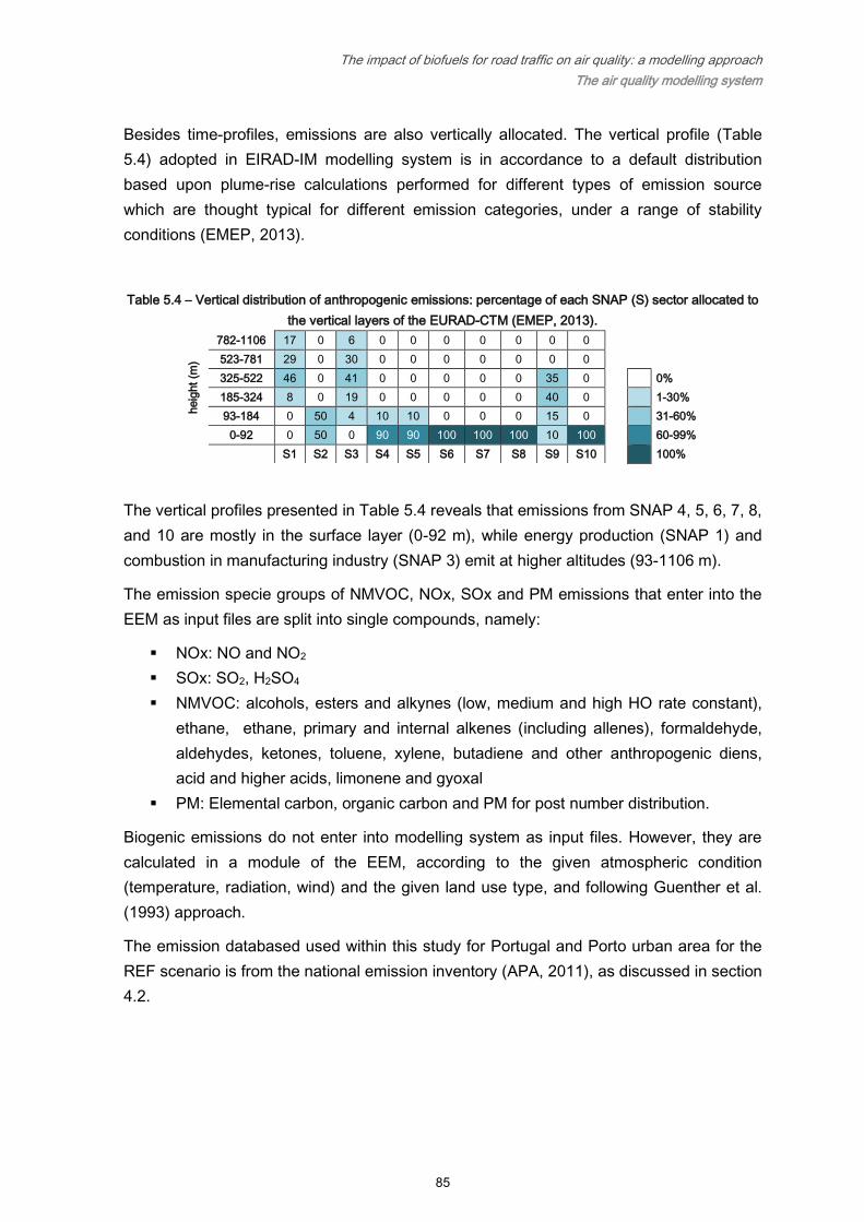
The impact of biofuels for road traffic on air quality: a modelling approach
The air quality modelling system
85
Besides time-profiles, emissions are also vertically allocated. The vertical profile (Table
5.4) adopted in EIRAD-IM modelling system is in accordance to a default distribution
based upon plume-rise calculations performed for different types of emission source
which are thought typical for different emission categories, under a range of stability
conditions (EMEP, 2013).
Table 5.4 – Vertical distribution of anthropogenic emissions: percentage of each SNAP (S) sector allocated to
the vertical layers of the EURAD-CTM (EMEP, 2013).
heig
ht
(m)
782-1106 17 0 6 0 0 0 0 0 0 0
523-781 29 0 30 0 0 0 0 0 0 0
325-522 46 0 41 0 0 0 0 0 35 0 0%
185-324 8 0 19 0 0 0 0 0 40 0 1-30%
93-184 0 50 4 10 10 0 0 0 15 0 31-60%
0-92 0 50 0 90 90 100 100 100 10 100 60-99%
S1 S2 S3 S4 S5 S6 S7 S8 S9 S10 100%
The vertical profiles presented in Table 5.4 reveals that emissions from SNAP 4, 5, 6, 7, 8,
and 10 are mostly in the surface layer (0-92 m), while energy production (SNAP 1) and
combustion in manufacturing industry (SNAP 3) emit at higher altitudes (93-1106 m).
The emission specie groups of NMVOC, NOx, SOx and PM emissions that enter into the
EEM as input files are split into single compounds, namely:
NOx: NO and NO2
SOx: SO2, H2SO4
NMVOC: alcohols, esters and alkynes (low, medium and high HO rate constant),
ethane, ethane, primary and internal alkenes (including allenes), formaldehyde,
aldehydes, ketones, toluene, xylene, butadiene and other anthropogenic diens,
acid and higher acids, limonene and gyoxal
PM: Elemental carbon, organic carbon and PM for post number distribution.
Biogenic emissions do not enter into modelling system as input files. However, they are
calculated in a module of the EEM, according to the given atmospheric condition
(temperature, radiation, wind) and the given land use type, and following Guenther et al.
(1993) approach.
The emission databased used within this study for Portugal and Porto urban area for the
REF scenario is from the national emission inventory (APA, 2011), as discussed in section
4.2.

The impact of biofuels for road traffic on air quality: a modelling approach
The air quality modelling system
86
5.2.4 EURopean Air Pollution Dispersion – Chemical Transport Model
(EURAD-CTM)
The EURAD-CTM (Hass, 1991; Ebel et al., 1997; Elbern et al., 2007) is a comprehensive
Eulerian chemical transport mesoscale model in a non-hydrostatic configuration. The
model’s nesting facility enables to telescope from 1000 km to 1 km of horizontal
resolution, allowing the combination of both high grid resolutions and the representation of
large-scale transport processes. As already mentioned, anthropogenic and biogenic
emissions temporally disaggregated from EEM, static geographical data of the simulation
domains (geogrid file, from WPS), as well as meteorological fields from WRF and
processed by the PPC, are the key information for the EURAD-CTM simulates transport,
chemical transformation and deposition of tropospheric constituents (Figure 5.6).
Figure 5.6 – Scheme of the EURAD-CTM model.
The chemistry is calculated on a fixed three-dimensional (3D) grid and transport is
simulated as fluxes through the boundaries of each grid cell. As a CTM, the model
simulates advection and diffusion, chemical conversion and deposition of trace gases and
aerosols in the atmosphere (Nieradzik, 2011) thought solving mass conservation equation
(Equation 5.2,(Hass, 1991).

The impact of biofuels for road traffic on air quality: a modelling approach
The air quality modelling system
87
𝜕𝑐𝑖
𝜕𝑡= −∇(𝑢𝑐𝑖) + ∇(𝐾∇𝑐𝑖) +
𝜕𝑐𝑖
𝜕𝑡|𝑐ℎ𝑒𝑚 + 𝐸𝑖 + 𝐹𝑖 +
𝜕𝑐𝑖
𝜕𝑡|𝑐𝑙𝑜𝑢𝑑 +
𝜕𝑐𝑖
𝜕𝑡|𝑎𝑒𝑟𝑜𝑠𝑜𝑙 Equation 5.2
Where:
𝐶𝑖: is the mean concentration of the specie i
−∇(𝑢𝑐𝑖): Advection, that is transport by wind, where u is the vector of wind velocity
∇(𝐾∇𝑐𝑖): Turbulent diffusion, with the tensor of turbulent diffusion K 𝜕𝑐𝑖
𝜕𝑡|𝑐ℎ𝑒𝑚: Chemical conversion in the gas phase
𝐸𝑖: Emission rates
𝐹𝑖: Sum of the following fluxes:
- 𝐹𝑖,𝑒𝑚𝑖𝑠: Flux by emissions from the surface
- 𝐹𝑖,𝑑𝑒𝑝: Flux by dry deposition to the surface 𝜕𝑐𝑖
𝜕𝑡|𝑐𝑙𝑜𝑢𝑑: Aqueous chemistry, transport in clouds and wet deposition
𝜕𝑐𝑖
𝜕𝑡|𝑎𝑒𝑟𝑜𝑠𝑜𝑙: Aerosol chemistry processed in Modal Aerosol Dynamics Model for Europe (MADE)
To initialize the simulation, latitude-dependent vertical profiles of the transported species
are equally distributed over the whole coarse domain. However, for short-lived species
initial values are set to zero. In this sense, and according to Schell (1996), a spin up run of
four or five days should be computed providing realistic 3D fields of initial values for the
desired period-time. Nevertheless, a simulation can also be set up on existing restart files
from previous simulations, on interpolated fields from a mother domain or from initial
values from data assimilation (Nieradzik, 2011). With initial values and boundary
conditions defined, the chemical and physical calculations take place according to
parameterization options that are described in following (section 5.2.4.1).
5.2.4.1 Chemical and physics options
The EURAD-CTM has several chemical and physical options available to simulate
deposition, chemical transformations and transport of the pollutants on the atmosphere,
namely regarding:
Photolysis frequencies;
Cloud processing;
Dry deposition;
Diffusion;
Aerosol dynamics;
Gas phase chemical mechanism;
Data assimilation (not used in this study);
Pollen module (not used in this study);
EURAD-Fire-Model (not used in this study).

The impact of biofuels for road traffic on air quality: a modelling approach
The air quality modelling system
88
The chemical and physical options available to EURAD-CTM simulations are compiled in
the model’s run-script file, which an excerpt is shown in Figure 5.7. The options selection
has also place in this run-script file.
# ================================== CTM configuration ====================================
#
# DATASS: variational data assimilation
# = 0: no
# = 1: 1D-VAR (not yet available...)
# = 2: 2D-VAR (not yet available...)
# = 3: 3D-VAR
# = 4: 4D-VAR
# PHOTO: Method for calculation of photolysis frequencies
# = 1: S. Madronich (offline)
# = 2: A. Ruggaber (online)
# = 3: S. Madronich (online)
# = 4: FTUV (online)
# CLOUD: Cloud module
# = 0: no clouds
# = 1: R2.6 version
# = 2: R2.6 version with MM5 clouds (B.Roeben)
# MADE: Aerosol dynnamics
# = 0: Disable modal aerosol dynamics
# Bit 1 = 1: Include modal aerosol dynamics
# Bit 2 = 1: modal aerosol dynamics with secondary organic aerosol
# (SORGAM, Schell et al. 2001)
# Bit 3 = 1: permit APC and HDMR of APC
# Bit 4 = 1: permit natural particle sources
# POLLEN: Pollen module
# = 0: disable pollen module
# = 1: enable pollen module
# CHEMISTRY: Choose kinetic chemistry mechanism
# = radm2: RADM2
# = adradm2: Adjoint version of the RADM2 mechanism
# = euro_radm: EURO_RADM + RADM-C
# = racm: RACM
# = racm_soa: RACM with extensions for secondary organic aerosol
# = racm_mim: RACM_MIM mechanism
# (RACM with updated isoprene degradation)
# = racm_mim2: RACM_MIM2 mechanism
# = chest: CHEST
# (RACM_MIM with extensions for stratospheric chemistry)
# = tracer: TRACER
# = racm_radon: RACM_MIM with radon decay chain
# SOLVER: Chemistry solver
# = 1: QSSA
# = 2: ros2 (Rosenbrock integrator with 2 stages)
# = 3: radau5 (implicit Runge-Kutta method of order 5)
# EFM: EURAD-Fire-Modell
# = 0: off
# = 1: on, emission model according to J. Hoelzemann
# = 2: on, GFAS wildfire emission data
# DRYDEP: Dry deposition module
# Bit 1 = 1: enable Wesely (1989)
# Bit 2 = 1: enable Zhang et al. (2003)
#==========================================================================================
Figure 5.7 – EURAD-CTM configuration options piece from the model run-script.
The set of parameterization options used herein was recommended for applications over
Europe and Portugal (Borrego et al., 2011; Nieradzik, 2011; Monteiro et al., 2013a). A
description of each selected parameterization is given following.

The impact of biofuels for road traffic on air quality: a modelling approach
The air quality modelling system
89
5.2.4.1.1 Photolysis frequencies
Tropospheric ultraviolet (UV) radiation is the driving force for all tropospheric
photochemical processes, having the potential to break down molecules into free radicals
(photolysis) and thus initiate reaction chains by which primary pollutants (hydrocarbons
and NOx) react to form secondary pollutants such as peroxyacyl nitrates and tropospheric
ozone. The radiative transfer model used by EURAD-CTM is based on the Tropospheric
Ultraviolet-Visible Model (Madronich, 1987), for calculating the spectral irradiance, the
spectral actinic flux and photodissociation coefficients (J-values).
5.2.4.1.2 Cloud processing
According to (Elbern and Friese, 2013), the sub-grid cloud scheme in the EURAD-CTM
was derived from the cloud model in the EPA Models-3 Community Multiscale Air Quality
(CMAQ) modelling system (Roselle and Binkowski, 1999). Cloud effects on both gas
phase species and aerosols are simulated by the cloud module. The effects of sub-grid
clouds on grid-averaged concentrations are parameterized by modelling the mixing,
scavenging, aqueous chemistry, and wet deposition of a representative cloud within the
grid cell. For all sub-grid clouds, a 1-hour live time has been assumed. Depending upon
weather the pollutant participates in the cloud water chemistry and on the liquid water
content, pollutant scavenging is calculated by two methods:
1. For those pollutants that are absorbed into the cloud water and participate in the cloud
chemistry, the amount of scavenging depends on Henry’s law constants, dissociation
constants, and cloud water pH;
2. For pollutants, which do not participate in aqueous chemistry, the model uses the
Henry’s law equilibrium to calculate ending concentration and deposition amount.
The accumulation mode and coarse mode aerosols are assumed to be completely
absorbed by cloud water and rain water. Some rapidly established equilibria between the
gas and aqueous phase (HNO3 ,N2O5, NH3, O3, H2O2, SO2, formic acid, methyl hydrogen
peroxide and peracetic acid) are superimposed on five irreversible reaction involving the
oxidation of SO2 to SO32- (Walcek and Taylor, 1986).

The impact of biofuels for road traffic on air quality: a modelling approach
The air quality modelling system
90
5.2.4.1.3 Dry deposition
The deposition scheme devised by Zhang et al. (2003) has been employed to calculate
dry deposition velocities of twenty gas phase species6 using a model which considers the
aerodynamic resistance, the quasi-laminar layer resistance and, the ground or canopy
resistances, depending on land use characteristics.
5.2.4.1.4 Diffusion
An upstream algorithm (Bott, 1989) was chosen to calculate the horizontal and vertical
advection. The calculation of vertical Eddy diffusion is based on the specific turbulent
structure in the individual regimes of the planetary boundary layer (PBL) according to the
PBL height and the Monin-Obukhov length (Holtslag and Nieuwstadt, 1986). The vertical
diffusion is semi–implicitly discretised following Crank–Nicholson scheme, with the
Thomas algorithm used as solver.
5.2.4.1.5 Gas phase chemical mechanism
The chemical mechanism selected within this work was developed by Geiger et al. (2003).
It is based on the Regional Atmospheric Chemical Mechanism (RACM) combined with the
Mainz Isoprene Mechanism (MIM, Poeschl et al., 2000). The RACM-MIM reflects an
advanced description of the air chemistry of biogenic ozone precursors like isoprene and
others. It treats 84 chemical species (as real species and condensed species classes) and
contains 23 photolysis reactions and 221 chemical reactions of higher order, solved by a
stage-2 Rosenbrock algorithm (Verwer et al., 1999).
5.2.4.1.6 Aerosols dynamics
To simulate the aerosols dynamics, the EURAD-CTM incorporates the Modal Aerosol
Dynamics model for Europe (MADE, Ackermann et al., 1998), developed specifically to
EURAD-CTM, that describes the physical and chemical processes concerning particles
species.
The dynamical processes concerning size distribution are transport, nucleation,
condensation, coagulation and evaporation, which are calculated taking into account the
interaction with clouds, wet and dry deposition, emissions into the air and the gas phase
6 Sulphur dioxide; Formaldehyde; Sulphuric acid; Acetaldehyde; Nitrogen dioxide; Methyl-Vinyl-Ketone;
Ozone; Methacrolein; Hydrogene peroxide; Methylglyoxal; Nitric acid; Cresol; Nitrous acid; Formic acid;
Pernitric acid; Acetic acid; Ammonia; Organic peroxides; Peroxyacetylnitrate and Organic nitrates.
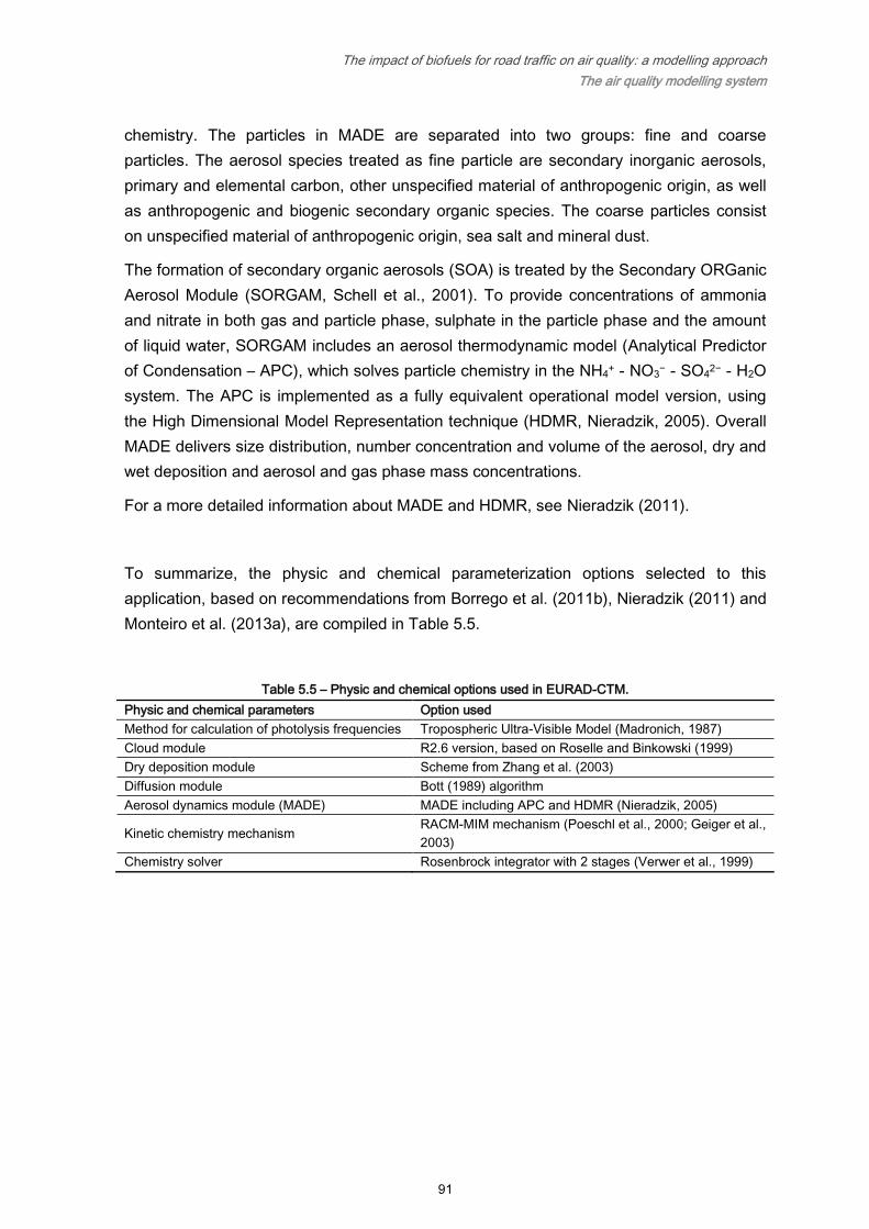
The impact of biofuels for road traffic on air quality: a modelling approach
The air quality modelling system
91
chemistry. The particles in MADE are separated into two groups: fine and coarse
particles. The aerosol species treated as fine particle are secondary inorganic aerosols,
primary and elemental carbon, other unspecified material of anthropogenic origin, as well
as anthropogenic and biogenic secondary organic species. The coarse particles consist
on unspecified material of anthropogenic origin, sea salt and mineral dust.
The formation of secondary organic aerosols (SOA) is treated by the Secondary ORGanic
Aerosol Module (SORGAM, Schell et al., 2001). To provide concentrations of ammonia
and nitrate in both gas and particle phase, sulphate in the particle phase and the amount
of liquid water, SORGAM includes an aerosol thermodynamic model (Analytical Predictor
of Condensation – APC), which solves particle chemistry in the NH4+ - NO3
− - SO42− - H2O
system. The APC is implemented as a fully equivalent operational model version, using
the High Dimensional Model Representation technique (HDMR, Nieradzik, 2005). Overall
MADE delivers size distribution, number concentration and volume of the aerosol, dry and
wet deposition and aerosol and gas phase mass concentrations.
For a more detailed information about MADE and HDMR, see Nieradzik (2011).
To summarize, the physic and chemical parameterization options selected to this
application, based on recommendations from Borrego et al. (2011b), Nieradzik (2011) and
Monteiro et al. (2013a), are compiled in Table 5.5.
Table 5.5 – Physic and chemical options used in EURAD-CTM.
Physic and chemical parameters Option used
Method for calculation of photolysis frequencies Tropospheric Ultra-Visible Model (Madronich, 1987)
Cloud module R2.6 version, based on Roselle and Binkowski (1999)
Dry deposition module Scheme from Zhang et al. (2003)
Diffusion module Bott (1989) algorithm
Aerosol dynamics module (MADE) MADE including APC and HDMR (Nieradzik, 2005)
Kinetic chemistry mechanism RACM-MIM mechanism (Poeschl et al., 2000; Geiger et al.,
2003)
Chemistry solver Rosenbrock integrator with 2 stages (Verwer et al., 1999)


The impact of biofuels for road traffic on air quality: a modelling approach
Evaluation of the air quality modelling system
93
Chapter 6. Evaluation of the air quality
modelling system
Air quality modelling systems describe mathematically innumerable physical and chemical
processes that characterize the atmosphere. In addition, they must be able to adequately
quantify species concentrations in the atmosphere (Dennis et al., 2010). However, the
atmosphere is characterized by random processes that cannot be precisely described by
numerical approached. Turbulence, which controls atmospheric dispersion, is one of
these processes, promoting spatial and temporal variability on the observed concentration
fields. Additionally, uncertainties in the input data and model formulation itself are also
important factors that increase the uncertainty in the model outputs. Uncertainties
associated to model formulation may be due to erroneous or incomplete representation of
the dynamic and chemistry of the atmosphere, incommensurability, numerical solution
techniques, and choice of modelling domain and grid structure. On the other side,
uncertainties in the input data may include variability on emission sources and imprecise
geophysical representation of the simulation domains. Therefore, model results should be
properly evaluated and their uncertainties correctly estimated (Hanna et al., 1993; Borrego
et al., 2008) before using model results.
Since a model is only useful if it reflects the behaviour of the real world atmospheric
processes being its simulations within a pre-defined level of accuracy that is acceptable
for the intended purpose of use, the quality of a model should be determined by
validation, verification, and evaluation (Schlünzen and Sokhi, 2008).
Validation is defined by Schlünzen and Sokhi (2008), as the testing of the extent to which
a model describes the phenomena it was developed for. Typically, model validations carry
out on model development laboratories (e.g. wind tunnels) to produce validation datasets,
or using monitoring datasets, to check the performance of the model for a specific
application. For each particular case, the required data completeness (suitable size,
temporal and spatial coverage, minimum number of data gaps and consideration of any
compilation procedures that may have caused data to be eliminated), quality and

The impact of biofuels for road traffic on air quality: a modelling approach
Evaluation of the air quality modelling system
94
accuracy of the model have to be specified. These requirements vary according to the
intended model application, as well as the model properties, such as model scale and
parameterizations.
Also in according to Schlünzen and Sokhi (2008), verification is the act of confirming that
the model exhibits a specified behaviour for a given case (e.g. an air pollution episode),
while the main goal of evaluation exercises is to demonstrate that the model is
“performing adequately” when compared with observations (Dennis et al., 2010).
According to previous studies, including the multi-model comparison presented in section
5.1 (Djalalova et al., 2010; Borrego et al., 2011; Miranda et al., 2012; Monteiro et al.,
2013a), air quality modelling systems results have important uncertainties associated, part
of them related to systematic errors which could be removed or minimized through bias-
correction approaches. A set of these techniques was tested and the main results are
shown in section 6.2.
The WRF-EURAD modelling system evaluation (Dennis et al., 2010) is addressed in this
chapter, generating statistics of the deviations between REF scenario unbiased modelling
results and observations, comparing their magnitudes accordingly to a set of statistical
parameters (section 6.2), for PT05 and OP01 simulation domains.
6.1 The air quality monitoring network
Observed data is essential information to validate an air quality modelling system. Thus,
data from the air quality monitoring network of mainland Portugal
(http://qualar.apambiente.pt/), with respect to the REF scenario year (2012), were used to
evaluate the WRF-EURAD modelling system performance. The air quality monitoring
network includes 68 stations classified as urban, suburban and rural regarding the type of
environment and as background, traffic and industrial in terms of influence, following the
classification in Garber et al. (2002). The air quality monitoring stations used for the model
evaluation present a minimum data collection efficiency of 85% for each pollutant (CO, O3,
NO2, PM10 and PM2.5), according to what is required by Air Quality Directive
(2008/50/EC). A total of 28 stations with background influence (8 rural, 12 urban, and 8
suburban) were selected for the PT05 domain. The selection of only background influence
stations is justified by the PT05 horizontal resolution (5 5 km2) which is not sufficient
detailed to correctly represent areas influenced by emissions from industrial or traffic
activities (Monteiro et al., 2013a). On the other hand, 8 stations (5 urban, and 3 suburban)
classified as industrial, background and traffic influence were selected for the OP01
domain, because the horizontal resolution of this domain is finer (1 1 km2). Figure 6.1

The impact of biofuels for road traffic on air quality: a modelling approach
Evaluation of the air quality modelling system
95
shows the location and classification of the selected stations in the study domain. Note
that the monitoring equipment follows a quality control/quality assurance procedure which
guarantees validation and confidence in the use of these data.
a) b)
Figure 6.1 – Location and main characteristics of the selected monitoring stations for Portugal (PT05) and
Porto urban area domains (OP01): stations environment and the terrain elevation (in m) (a); stations influence
(b).
The pollutants measured in each monitoring station are listed in Table 6.1.

The impact of biofuels for road traffic on air quality: a modelling approach
Evaluation of the air quality modelling system
96
Table 6.1 – Monitoring stations selected and their classification (environment and influence and pollutants
measured, for Portugal and Porto urban area domains (PT05 and OP01).
Abbreviation Name Type of
environment
Type of
influence
Pollutants
OP01
CO
NO
2
O3
PM
10
PM
25
ALV Alverca Urban Background X X X X
ANT Antas Urban Traffic X X
X
X
ARC Arcos Urban Background X X X X
CHA Chamusca Rural Background
X X X X
COI Coimbra - Inst. Geog. Urban Background
X X
CUS Custóias Suburban Industrial
X X X
X
ERM Ermesinde Urban Background
X
X
X
ERV Ervedeira Rural Background
X
X X
FPO Fernando Pó Suburban Background
X X X X
FRN Fornelo do Monte Rural Background
X X
FUN Fundão Rural Background
X X X X
HOR S. Hora Urban Traffic X X
X
X
HRT Horto Suburban Background
X X X
ILH Ílhavo Suburban Background
X X X
LAR Laranjeiro Urban Background X X X X X
LEC Leça do Balio Suburban Background
X
X
LNH Lourinhã Suburban Background
X
LOU Loures Urban Background
X X
MEC Meco Suburban Industrial
X X
X
MEM Mem Martins Urban Background
X X X X
MOV Montemor-o-Velho Suburban Background
X X
MVE Monte Velho Rural Background X
OLI Olivais Urban Background X X X X X
OLO Lamas de Olo Rural Background
X X X X
PFR Paços de Ferreira Urban Background
X X X X
PP Paio Pires Urban Background
X
SMN S. Minho Rural Background
X X X
SOB Sobreiras Urban Background
X X X
X
STR Sto. Tirso Urban Background
X X X
TER Terena Rural Background
X X X
VCO Vila do Conde Suburban Background
X X X
VER Vermoim Urban Traffic
X X X X X
VNT Vila Nova da Telha Suburban Background
X
X
Total 7 25 26 28 11 8

The impact of biofuels for road traffic on air quality: a modelling approach
Evaluation of the air quality modelling system
97
6.2 Bias-correction approach
To increase the model skills and minimize model uncertainty, there are several techniques
based on ensemble dispersion modelling (Galmarini et al., 2004; Wilczak et al., 2006; van
Loon et al., 2007; Vautard et al., 2009; Monteiro et al., 2013b) and on methods for
combining results from models and monitoring data (Borrego et al., 2011b; Denby and
Spangl, 2010; McKeen et al., 2005; Monteiro et al., 2013). It is possible to combine these
two types of data through methodologies that take into account physical laws (data
assimilation) or that are based on a statistic or geometric way to combine data sources to
create a new data set (data fusion) (Denby and Spangl, 2010). Examples of data fusion
approaches are the bias-correction techniques which the objective is not to try to gain
additional insight into model deficiencies or performance nor to correct artificially for them,
but to remove potential systematic model errors intrinsic to each model formulation or
input data. Bias-correction can be applied through different techniques, such as mean
subtraction (McKeen et al., 2005; Wilczak et al., 2006), multiplicative ration adjustment
(McKeen et al., 2005), hybrid forecast (Kang et al., 2005) and Kalman filter (Kang et al.,
2005; Delle Monache et al., 2006; Djalalova et al., 2010), among others. Based on
previous studies (Borrego et al., 2011; Monteiro et al., 2013a), three bias-correction
techniques were applied to EURAD simulation results over Portugal: a Kalman filter (KF)
technique, a subtractive/additive correction of the mean bias (SUBST, Equation 6.1) and a
multiplicative ratio correction (RAT, Equation 6.2).
SUBST ),)(1
, modmod day(hCCCndays
day)(hC el
ndays
obs
h
el
h
corrected Equation 6.1
RAT ),(),(
),(
),( mod
moddayhC
dayhC
dayhC
dayhC el
ndays
el
ndays
obs
corrected
Equation 6.2
The KF is a recursive, linear, and adaptive method that has been used recently to improve
air quality forecasts of ground-based O3 (Kang et al., 2005; Delle Monache et al., 2006,
2008; Djalalova et al., 2010; Sicardi et al., 2011). KF performance is sensitive to the error
ratio between variances of white noise and random error, which indicates the way in which
the KF responds to the variations in biases at prior steps. An optimal error ratio exists for
generating the best prediction given the numerical modelling system and the dynamics of
the study area. One way to estimate the optimal error is described by Kang et al. (2008)
which consists in minimizing the RMSE and maximizing the correlation coefficient for all

The impact of biofuels for road traffic on air quality: a modelling approach
Evaluation of the air quality modelling system
98
the stations and modelling system. SUBST (Equation 6.1) and RAT (Equation 6.2)
corrections force the mean bias at each monitoring site to be zero, using the bias detected
from the previous days for each particular hour (h) of the day. These three bias-correction
procedures are model specific, site specific and time of day specific.
For the case of SUBST and RAT corrections, to estimate the previous days bias, different
training periods were tested (Monteiro et al., 2013a): a 7 day training period was chosen
as a compromise between having a sufficiently long period to gather adequate statistics,
but not too long to mask seasonal variations in ozone, as discussed in Wilczak et al.
(2006); and a 4 day period was also tested in order to distinguish different synoptic
conditions, which are characterized by a 3-4 day period (Stull, 1988; Carvalho et al.,
2010a; Tchepel and Borrego, 2010). This test revealed that the RAT technique with a 4-
day training period is the most appropriate bias-correction approach to apply over
Portugal, demonstrating significant improvements for both analysed pollutants (PM10 and
O3), as demonstrated by daily profiles for O3 and PM10 in Figure 6.2.
Figure 6.2 – Daily profiles, averaged over all monitoring stations, of observed values (OBS), EURAD
simulations (RAW) and EURAD simulations with RAT04 correction (RAT04) for O3 and PM10 (adapted from
Monteiro et al., 2013a)
The improvement of the corrected data skill was measured by a bias reduction of 76 % for
O3, and 91 % for PM10, a decrease of RMSE in 14 % for O3 and 32 % for PM10, and an
improvement on the correlation factor of 14% for O3 and 54% for PM10. In this sense, the
RAT04 bias-correction technique will be applied to WRF-EURAD modelling system
(described in detail in section 5.2) outputs in order to obtain more accurate simulation
results to investigate the impact of biofuels for road traffic on air quality over mainland
Portugal and the Porto urban area.

The impact of biofuels for road traffic on air quality: a modelling approach
Evaluation of the air quality modelling system
99
6.3 Operational evaluation of the WRF-EURAD modelling system
Within the framework for evaluating regional-scale numerical modelling systems
developed by Dennis et al. (2010), operational evaluation refers to statistical and graphical
analysis to determine whether modelling system estimates are in agreement with the
observations in an overall sense, measuring the deviations and their magnitudes between
simulated results and observations through statistic parameters. The set of statistic
parameters recommended by Hanna et al. (1993) and Borrego et al. (2008), and listed in
Table 6.2, are used to evaluate the WRF-EURAD modelling system performance
regarding the REF scenario results for PT05 and OP01 domains, bias-corrected through
the application of the RAT04 technique (section 6.2).
Measured concentrations from a set of stations of the Portuguese air quality monitoring
network (see Figure 6.1 and Table 6.1) were used in the operational evaluation process
here presented, regarding CO, NO2, O3, PM10 and PM2.5 concentrations. This evaluation
process cannot be applied to NMVOC because there are no measurements of total
NMVOC on the national monitoring network.
The correlation factor (R) reflects the linear relationship between two variables. However it
is insensitive to either an additive or a multiplicative factor. To allows for sensitivity on the
difference in observed and predicted values as well as proportionality changes, Elbir
(2003) included the Index of Agreement (IA) to the statistical analysis. This indicator
determines the degree to which magnitudes and signs of the observed value about mean
observed value are related to the predicted deviation about mean predicted value
(Borrego et al., 2008). Root Mean Square Error (RMSE) and bias are frequently used
measures of the differences between values predicted and the values actually observed
(bias) or absolute values (RMSE). Bias reflects the trends of the model results error: a
negative bias indicates that the model is overestimating and a positive bias reveals an
underestimated trend. However bias should not be analysed alone, because so over-
prediction and under-prediction may cancel each other, leading to bias=0, the result for an
ideal prediction. On the other hand, RMSE allows assessing the magnitude of these errors
(Ribeiro, 2008). Thus, bias and RMSE can provide add value to each other when taken
together. Normalised mean square error (NMSE) and RMSE give information about the
errors obtained within the observed-predicted pairs of results. However, RMSE ignores
the range of the variable, which in some cases could lead to misleading interpretations of
this parameter result. Thus, a normalized form of the parameter, NMSE, could be more
adequate. The fraction of predictions within a factor of 2 of observations (FAC2) is a tool
to remove outliers and can be a way of improving statistical analysis results. Thus, FAC2
is considered as the most robust measure (Borrego et al., 2008; COST Action 732, 2009).

The impact of biofuels for road traffic on air quality: a modelling approach
Evaluation of the air quality modelling system
100
Table 6.2 – Statistical quality indicators for air quality model performance evaluation (Hanna et al., 1993;
Borrego et al., 2008).
Indicator Formula Range of
acceptable values
Ideal
value
Correlation coefficient
(R)
𝑅 =∑ (𝐶𝑂𝑖 − 𝐶𝑂
)(𝐶𝑀𝑖 − 𝐶𝑀 )𝑁
𝑖=1
√∑ (𝐶𝑂𝑖 − 𝐶𝑂 )2(𝐶𝑀𝑖 − 𝐶𝑀
)2𝑁𝑖=1
[0.0 ; 1.0] 1.0
Index of agreement
(IA) 𝐼𝐴 = 1 −
∑ (𝐶𝑀𝑖 − 𝐶𝑂𝑖)2𝑁𝑖=1
∑ (|𝐶𝑀𝑖 − 𝐶𝑂 | + |𝐶𝑂𝑖 − 𝐶𝑂
|)2𝑁𝑖=1
[0.0 ; 1.0] 1.0
Root mean squared
error (RMSE) 𝑅𝑀𝑆𝐸 = √
1
𝑁∑(𝐶𝑂𝑖 − 𝐶𝑀𝑖)2
𝑁
𝑖=1
n.a. 0.0
Normalized mean
squared error (NMSE) 𝑁𝑀𝑆𝐸 =
(𝐶𝑂 − 𝐶𝑀)2
𝐶𝑂𝐶𝑀
n.a. 0.0
Mean systematic error
(bias) 𝑏𝑖𝑎𝑠 =
1
𝑁 ∑(𝐶𝑂𝑖 − 𝐶𝑀𝑖)
𝑁
𝑖=1
n.a. 0.0
Fractional bias
(FB) 𝐹𝐵 =
𝐶𝑂 − 𝐶𝑀
0,5(𝐶𝑂 + 𝐶𝑀
) [-2.0 ; 2.0] 0.0
Average normalized
absolute bias (ANB) 𝐴𝑁𝐵 = (
|𝐶𝑂 − 𝐶𝑀|
𝐶𝑂) n.a. 0.0
Normalized standard
deviation (NSD)
𝑁𝑆𝐷 =𝜎𝑀
𝜎𝑂 [0.0 ; 1.0] 1.0
Geometric mean bias
(MG) 𝑀𝐺 = 𝑒𝑥𝑝(ln 𝐶𝑂
− ln 𝐶𝑀 ) > 0.0 1.0
Geometric variance
(VG) 𝑉𝐺 = 𝑒𝑥𝑝 [(ln 𝐶𝑂
− ln 𝐶𝑀 )
2] > 0.0 1.0
Factor of two of
Observations (FAC2)
𝐹𝐴𝐶2 =∑ 𝐴𝑖
𝑁𝑖=1
𝑁
𝑤𝑖𝑡ℎ 𝐴𝑖 = {1 𝑓𝑜𝑟 0.5 ≤
𝐶𝑀𝑖
𝐶𝑂𝑖≤ 2.0
0, 𝑒𝑙𝑠𝑒
n.a. 1.0
n.a. – not applicable.
𝐶𝑂𝑖 and 𝐶𝑀𝑖 are the observed and predicted concentration in monitoring station i in n monitoring station.
CO and CM
are the averaged concentration observed and predicted.
σO and σM are the standard deviation of observations and predictions.
Due to the distributions of the majority of pollutant concentrations are close to log-normal,
the linear measures fractional bias (FB) and normalized mean square error (NMSE) may
be exceedingly influenced by infrequently occurring high observed and/or predicted
concentrations, whereas the logarithmic measures geometric mean bias (MG) and
geometric variance (VG) may provide a more balanced treatment of extreme high and low
values. Nevertheless, MG and VG may be excessively influenced by extremely low
values, near the instrument thresholds and are undefined for zero values. FB and MG are

The impact of biofuels for road traffic on air quality: a modelling approach
Evaluation of the air quality modelling system
101
measures of mean relative bias and indicate only systematic errors. NMSE and VG are
measures of mean relative scatter reflecting both systematic and unsystematic (random)
errors, but they are not a direct measure of these errors (Borrego et al., 2008).
The statistical quality indicators shown in Table 6.2 were adopted as a common European
model evaluation framework (Olesen, 2001), which have been integrated and updated into
the DELTA tool (Thunis et al., 2012). The DELTA tool is a software developed in the
scope of the FAIRMODE (URL 11) activity by the Joint Research Centre of the European
Commission for the evaluation and benchmarking of air quality modelling applications and
for rapid diagnostics of model performances of air quality models, focusing on O3, PM10
and NO2 so far, addressing from local to regional scales. In the coming years, the DELTA
tool will be extended to other pollutants mentioned in the air quality Directive
(2008/50/EC), as well as for scenarios assessment. In spite of this software is a powerful
and updated tool for air quality modelling evaluations, its application in this work was
limited since the modelling system evaluation in terms of CO and PM2.5 is required. Thus,
the operational evaluation of the WRF-EURAD modelling system was not based on
DELTA tool, but on the statistical parameters listed in Table 6.2. The main results from the
operational evaluation exercise are presented in section 6.3.1 for mainland Portugal
domain (PT05) and in section 0 for the Porto urban area (OP01).
In spite of the results are bias-corrected, analysing their bias values, as well as bias
related parameter values, is important to verify how far the systematic error is minimized.
This is especially important because RAT04 results may be sharply influenced by high
pollutant concentrations due to air pollution episodes or errors on observed and modelled
data, and then these errors are propagated through the 4-days period (Borrego et al.,
2011).
6.3.1 PT05
Regarding the PT05 simulation domain, the median of the statistic parameters estimated
for each type of station environment are presented in Figure 6.3, in order to investigate
the main differences on modelling system performance over rural, suburban and urban
environments.
As expected, WRF-EURAD modelling system results unbiased (hereinafter referred to as
predicted concentrations) exhibit statistical parameters values close to the ideal ones, in
particular for background rural stations (Figure 6.3). This was already expected since
background influence in rural environments is not largely influenced by anthropogenic
emissions, which decrease the uncertainty associated to the simulation processes.

The impact of biofuels for road traffic on air quality: a modelling approach
Evaluation of the air quality modelling system
102
Bias values (Figure 6.3a) are typically negative suggesting that the results from the
RAT04 technique application are slightly under predicted for all studied pollutants.
However, they are insignificants being smaller than 0.5 µgm-3 (absolute value) for NO2,
O3, PM10 and PM2.5, and smaller than 1.3 µgm-3 (absolute value) for CO.
High RMSE values (Figure 6.3b) were found for CO in urban (154.3 µgm-3) and rural
(41.8 µgm-3) environments, but other parameters such as NMSE, FAC2, ANB and NSD
(Figure 6.3c,d) suggest that CO is well predicted, which is also translated by the daily
profiles in Figure 6.4. This is mainly because the magnitude of the CO concentrations is
higher comparing to the other pollutants, fact that NMSE has into account, contrarily to
RMSE.

The impact of biofuels for road traffic on air quality: a modelling approach
Evaluation of the air quality modelling system
103
Figure 6.3– Statistical parameters for the corrected (RAT04) results from the WRF-EURAD modelling system,
regarding the REF scenario (2012 year), for each pollutant and station environment: a) bias (µgm-3); b) RMSE
(µgm-3); c) R, IA and FAC2; d) MG and VG; e) NSD, ANB and NMSE. Median for all the monitoring sites, over
the PT05 domain.
In Figure 6.4 are compiled a daily profile per studied pollutant and type of environment
(rural, suburban and urban), comparing measured and predicted concentrations, including
their concentration percentiles 25th/75th. According to the statistical parameters (Figure
6.3) and daily profiles (Figure 6.4), the hourly mean predicted concentrations are quite
similar to measured concentrations for all the studied pollutants and for all environments.

The impact of biofuels for road traffic on air quality: a modelling approach
Evaluation of the air quality modelling system
104
Rural Suburban Urban
CO
No monitoring site available
NO
2
O3
PM
10
PM
2.5
Figure 6.4 – Daily profiles of measured (blue line) and predicted (purple line) concentrations of CO, NO2, O3,
PM10 and PM2.5, as well as the concentration ranges between percentiles 25th/75th, over the PT05 domain,
regarding rural, suburban and urban environments.

The impact of biofuels for road traffic on air quality: a modelling approach
Evaluation of the air quality modelling system
105
For O3, a secondary pollutant, daily profiles present higher concentrations during the
periods of sunlight and higher temperature, while the daily profiles of the remaining
pollutants present higher concentrations during the night-time than during the daylight
period, in rural environments. This concentrations behaviour is also found for PM10 and
PM2.5 in suburban and urban environments. On the other hand, on suburban/urban
profiles for CO and NO2, two pecks can be identified at the typical rush hours (6h - 9h and
17h - 22h). This is mainly due to the importance of the CO and NO2 emissions from the
transport sector in urban/suburban areas.
Despites the good quality of the predicted results, presenting identical daily profiles
between measured and predicted concentrations, the daily profiles of the percentiles
25th/75th, regarding the measured concentrations, typically cover a wider range of
concentrations than for predicted data (Figure 6.4). This is especially visible for PM10 and
PM2.5, which the daily profiles of the 75th percentile of the predictions are lower than
those measured, while the daily profiles of the 25th percentile of measured and predicted
concentrations are similar. This suggests that emissions of these pollutants used as input
data to WRF-EURAD simulations may be underpredicted.
6.3.2 OP01
The OP01 domain, covering the Porto urban area, comprises 8 monitoring stations under
urban and suburban environments (Table 6.1). Moreover, because this is an area strongly
influenced by industrial and traffic activities, the evaluation process will take into account
monitoring stations with industrial and traffic influence, in addition to the background. In
this sense, the median values of the statistical parameters estimated per type of station
influence are presented in Figure 6.5. Note that there are no rural monitoring stations in
this domain (Table 6.1).

The impact of biofuels for road traffic on air quality: a modelling approach
Evaluation of the air quality modelling system
106
Figure 6.5 - Statistical parameters for the corrected (RAT04) results from the WRF-EURAD modelling system,
regarding the REF scenario (2012 year), for each pollutant and station environment: a) bias (µgm-3); b) RMSE
(µgm-3); c) R, IA and FAC2; d) MG and VG; e) NSD, ANB and NMSE. Median for all the monitoring sites, over
the OP01 domain.
Similarly to what was found for the previous domain (PT05, section 6.3.1), the statistical
parameters estimated are close to the ideal values (Figure 6.5) presenting similar
magnitudes than for PT05. The main reason to explain this is related to the bias-correction
technique applied to the raw prediction results from WRF-EURAD modelling system for
both domains.
As well as verified to PT05, the RMSE regarding CO concentrations is about ten times
larger than for other pollutants, due to its high magnitude of concentrations values. On the

The impact of biofuels for road traffic on air quality: a modelling approach
Evaluation of the air quality modelling system
107
other hand, for the OP01 domain there is no clear evidence that the predicted results have
more quality for sites with background influence than for others, since the majority of the
statistical parameters have similar values regardless the pollutant and the monitoring site
influence.
The daily profiles, comparing measured and predicted concentrations as well as their
25th/75th concentration percentiles, for each pollutant and type of influence (background,
industrial and traffic) are presented in Figure 6.6. The analysis of these daily profiles
corroborates the good overall performance of the air quality modelling, predicting the
hourly mean concentration of the several pollutants over the OP01 domain. The PBL
height variation during the day and the emission time-profiles (Figure 5.5) are also
reflected by daily profiles.
Observed and predicted 25th/75th percentile profiles (Figure 6.6) are close to each other,
while in PT05 (Figure 6.4) only the predicted 25th percentile match to observations,
suggesting that the improvement on road traffic emissions in terms of spatial resolution
performed and described in Chapter 4 should be taking into account in further simulations
for 1 × 1km2 but also for 5 × 5 km2 horizontal resolutions.
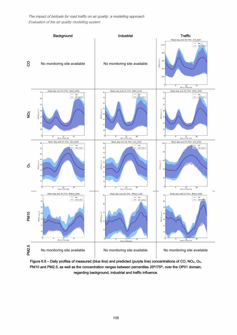
The impact of biofuels for road traffic on air quality: a modelling approach
Evaluation of the air quality modelling system
108
Background Industrial Traffic
CO
No monitoring site available No monitoring site available
NO
2
O3
PM
10
PM
2.5
No monitoring site available No monitoring site available No monitoring site available
Figure 6.6 – Daily profiles of measured (blue line) and predicted (purple line) concentrations of CO, NO2, O3,
PM10 and PM2.5, as well as the concentration ranges between percentiles 25th/75th, over the OP01 domain,
regarding background, industrial and traffic influence.

The impact of biofuels for road traffic on air quality: a modelling approach
Impacts of biodiesel use on air quality
109
Chapter 7. Impacts of biodiesel use on air
quality
The impacts of biodiesel use on air quality over mainland Portugal and the Porto urban
area are addressed and discussed in this chapter. The emission scenarios REF and B20,
developed in section Chapter 4, were used as input data to the WRF-EURAD modelling
system (Chapter 5), which performance evaluation is addressed in Chapter 6, in order
evaluate eventual impacts due to the use of B20 fuel instead of pure petroleum-based
diesel in road transports. The analysis presented here is focused on mean concentration
differentials (B20-REF) of CO, NO2, NMVOC, O3, PM10 and PM2.5, for three different
periods defined in accordance to the European Directive 2008/50/EC on ambient air
quality and cleaner air for Europe, in the scope of air quality assessment:
Annual: The entire year of 2012;
Summer season: from April to September 2012;
Winter season: from January to March and from October to December 2012.
7.1 Impacts on air quality over mainland Portugal
The REF and B20 emission scenarios defined in Chapter 4 were used to simulate the air
quality over mainland Portugal (PT05), through the application of the WRF-EURAD
mesoscale numerical modelling system (Chapter 5). The main results are shown in Figure
7.1 regarding the spatial distribution for annual-, summer- and winter-mean concentrations
of NO2, NMVOC and O3 for the REF scenario. The differentials found between both
scenarios (B20-REF) are also presenting in Figure 7.1. NO2 and O3 concentration values
are presented in gm-3. However, due to the multiple compounds in the NMVOC its
concentrations are in parts per billion in volume basis (ppbv).

110
Annual Summer Winter Annual Summer Winter N
O2
RE
F S
cenario
a
Diffe
rencia
ls (
B20
-RE
F)
d
NM
VO
C
b e
O3
c f
Figure 7.1 – Annual, summer and winter mean concentrations of NO2 (gm-3), NMVOC (ppbv) and O3 (gm-3) for REF scenario (a-c) and differential concentrations
between B20 and REF (d-f), over the PT05 domain.

The impact of biofuels for road traffic on air quality: a modelling approach
Impacts of biodiesel use on air quality
111
In general, the simulation results (Figure 7.1) show that the use of B20 fuels may implies a
reduction on air quality levels in terms of NO2 and NMVOC, especially in urban areas. In
spite of NOx total emissions increase in about 3% with B20 use (Figure 4.7), NO2
concentrations decrease over the West coast of Portugal, representing a reduction in
order of ~2 µgm-3 in Lisbon and ~1 µgm-3 in Porto urban areas (Figure 7.1a). In fact,
relations between NOx emissions and NO2 concentrations are driven by complex
nonlinear chemistry mechanisms, which also include NMVOC and ozone. This illustrates
the importance of the use of a chemical transport model, like EURAD-CTM, to investigate
the impacts on air quality in the scope of emission scenarios.
The simulation results for REF scenario (Figure 7.1a) also suggest that NO2
concentrations are superior during the winter period then in the summer, presenting
higher reductions of this pollutant concentrations when B20 is compared to REF
scenarios. This leads to a slight increment of the O3 average concentration (Figure 7.1c)
in about 1-2 µgm-3 over the West coast, especially in urban regions.
In the summer season, O3 concentrations decrease about 1.5 gm-3 over the inland of the
territory, representing less than 2% of the total O3 concentrations. Negligible changes are
found in the most polluted areas in terms of NO2 and NMVOC (Lisbon, Porto, Aveiro,
Sines and Figueira da Foz regions).
NMVOC is a group of pollutants mainly emitted by biogenic activity (especially during the
summer, as shown in Figure 7.1b) and solvent industries, such as petroleum refineries
located in Sines and Matosinhos (close to Porto). According to INERPA (APA, 2011), the
transport sector is responsible by 3.5% of the NMVOC total emissions and the use of B20
instead of pure diesel in road traffic can reduce NMVOC emissions in about 2%, as
already discussed in section 4.4 (Figure 4.7). This emission reduction induces a decrease
on NMVOC concentrations in about 8 ppbv over Porto and Sines regions. The simulation
results also suggest that the use of B20 fuel will contribute to reduce NMVOC in a
maximum of 5 ppbv over the remaining territory. Still for NMVOC, no significant changes
on B20-REF differentials were also verified when summer is compared to winter period
results over the West coast, which is the national area mostly influenced by traffic
activities.
To investigate the variations on the concentration bins, an analysis through histograms
was carried out. Figure 7.2 presents the histograms for B20 and REF regarding NO2,
NMVOC and O3, for annual, summer and winter periods. This figure also depicts the
difference between the probability of occurrence of B20 against REF, for each
concentration bin (∆𝑃𝐵20−𝑅𝐸𝐹 = 𝑃𝐵20𝑏𝑖𝑛 𝑖−𝑃𝑅𝐸𝐹𝑏𝑖𝑛 𝑖
).

The impact of biofuels for road traffic on air quality: a modelling approach
Impacts of biodiesel use on air quality
112
PT05 Annual Summer Winter
NO
2
P(R
EF
) and P
(B20) (%
)
P(B
20 -
RE
F) (%
)
NM
VO
C P(R
EF
) and P
(B20) (%
)
P(B
20 -
RE
F) (%
)
O3
P(R
EF
) and P
(B20) (%
)
P(B
20 -
RE
F) (%
)
Figure 7.2 – Histograms of 1-99% of NO2 (top), NMVOC (middle) and O3 (bottom) hourly concentrations,
regarding annual, summer and winter periods for REF (blue or green) and B20 (yellow) scenarios, for the
PT05 domain. The difference between the probabilities of occurrence of B20 against REF is presented in
grey.
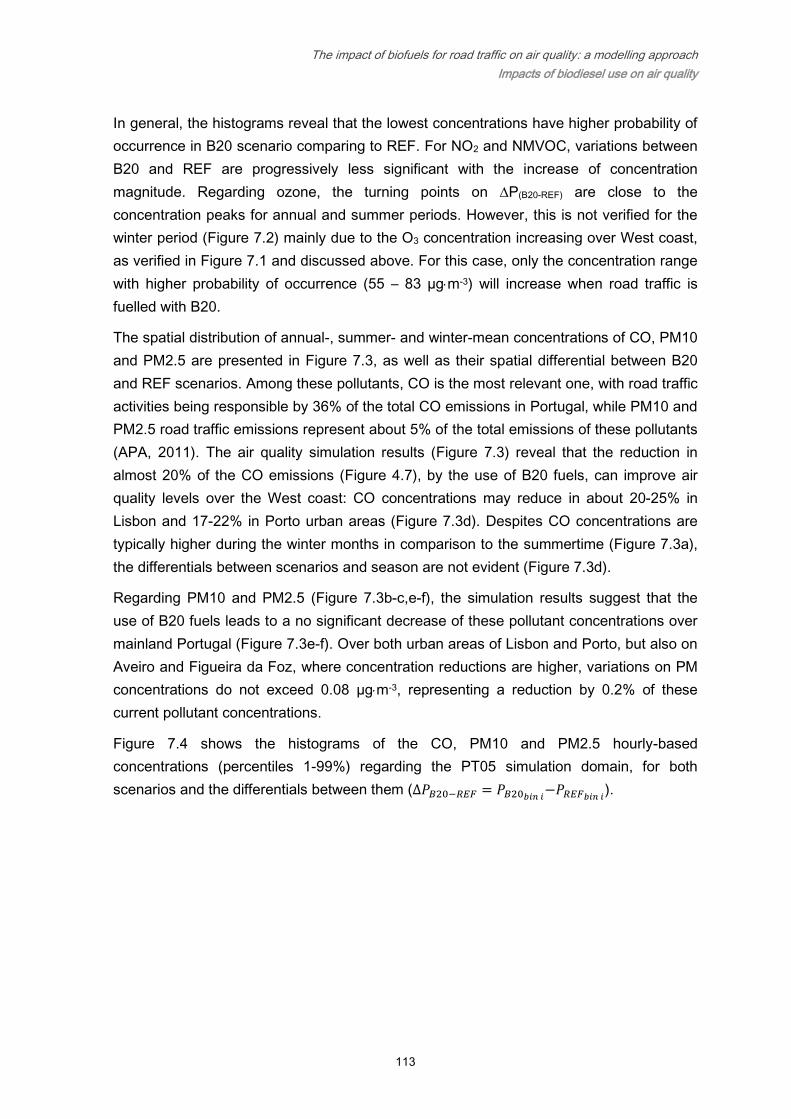
The impact of biofuels for road traffic on air quality: a modelling approach
Impacts of biodiesel use on air quality
113
In general, the histograms reveal that the lowest concentrations have higher probability of
occurrence in B20 scenario comparing to REF. For NO2 and NMVOC, variations between
B20 and REF are progressively less significant with the increase of concentration
magnitude. Regarding ozone, the turning points on P(B20-REF) are close to the
concentration peaks for annual and summer periods. However, this is not verified for the
winter period (Figure 7.2) mainly due to the O3 concentration increasing over West coast,
as verified in Figure 7.1 and discussed above. For this case, only the concentration range
with higher probability of occurrence (55 – 83 µgm-3) will increase when road traffic is
fuelled with B20.
The spatial distribution of annual-, summer- and winter-mean concentrations of CO, PM10
and PM2.5 are presented in Figure 7.3, as well as their spatial differential between B20
and REF scenarios. Among these pollutants, CO is the most relevant one, with road traffic
activities being responsible by 36% of the total CO emissions in Portugal, while PM10 and
PM2.5 road traffic emissions represent about 5% of the total emissions of these pollutants
(APA, 2011). The air quality simulation results (Figure 7.3) reveal that the reduction in
almost 20% of the CO emissions (Figure 4.7), by the use of B20 fuels, can improve air
quality levels over the West coast: CO concentrations may reduce in about 20-25% in
Lisbon and 17-22% in Porto urban areas (Figure 7.3d). Despites CO concentrations are
typically higher during the winter months in comparison to the summertime (Figure 7.3a),
the differentials between scenarios and season are not evident (Figure 7.3d).
Regarding PM10 and PM2.5 (Figure 7.3b-c,e-f), the simulation results suggest that the
use of B20 fuels leads to a no significant decrease of these pollutant concentrations over
mainland Portugal (Figure 7.3e-f). Over both urban areas of Lisbon and Porto, but also on
Aveiro and Figueira da Foz, where concentration reductions are higher, variations on PM
concentrations do not exceed 0.08 µgm-3, representing a reduction by 0.2% of these
current pollutant concentrations.
Figure 7.4 shows the histograms of the CO, PM10 and PM2.5 hourly-based
concentrations (percentiles 1-99%) regarding the PT05 simulation domain, for both
scenarios and the differentials between them (∆𝑃𝐵20−𝑅𝐸𝐹 = 𝑃𝐵20𝑏𝑖𝑛 𝑖−𝑃𝑅𝐸𝐹𝑏𝑖𝑛 𝑖
).

114
Annual Summer Winter Annual Summer Winter C
O
RE
F S
ce
na
rio
a
Diffe
ren
tia
ls (
B2
0-R
EF
)
d
PM
10
b e
PM
2.5
c f
Figure 7.3 - Annual, summer and winter mean concentrations of CO, PM10 and PM2.5 for REF scenario (a-c) and differential concentrations between B20 and REF (d-
e), over the PT05 domain.

The impact of biofuels for road traffic on air quality: a modelling approach
Impacts of biodiesel use on air quality
115
PT05 Annual Summer Winter C
O
P(R
EF
) and P
(B20) (%
)
P(B
20 -
RE
F) (%
)
PM
10 P
(RE
F) and P
(B20) (%
)
P(B
20 -
RE
F) (%
)
PM
2.5
P(R
EF
) and P
(B20) (%
)
P(B
20 -
RE
F) (%
)
Figure 7.4 – Histograms of 1-99% of CO (top), PM10 (middle) and PM2.5 (bottom) hourly concentrations,
regarding annual, summer and winter periods for REF (blue or green) and B20 (yellow) scenarios, for the
PT05 domain. The difference between the probabilities of occurrence of B20 against REF is presented in
grey.

The impact of biofuels for road traffic on air quality: a modelling approach
Impacts of biodiesel use on air quality
116
The graphs in Figure 7.4 suggest that the use of B20 fuels increase the probability of
occurrence of the lowest CO concentrations (from ~80 to ~135 gm-3) and a reduction on
the probability for concentrations after the peak of the distribution curve. Additionally, a
second probability peak is notable for concentrations around 175 – 190 gm-3, suggesting
that these peaks, that represent the CO concentrations in urban areas, will be reduced in
B20 scenario.
Regarding PM histograms, they suggest that the B20 scenario increases the probability of
occurrence of the concentrations up to 8 and 5 gm-3 for PM10 and PM2.5, respectively.
For higher concentrations the results suggest that B20 induce a reduction on their
probability of occurrence.
In sum, the use of a B20 to fuel road transports can contribute to an improvement of NO2
and CO concentration levels in urban airshed in order of 10 and 30%, respectively. A no
significant increase (~2%) was found to O3 winter-mean concentrations over the entire
West coast of mainland Portugal. For the remaining studied pollutants, namely PM10 and
PM2.5, their mean concentrations will be reduced all over the territory, however in a no
significant amount (<1%).
7.2 Impacts on air quality in Porto urban area
To investigate more deeply the influence of B20 fuels used by road transports in urban
areas, a downscaling modelling technique was performed over the Porto urban area
(OP01 domain) using the WRF-EURAD mesoscale modelling system to simulate REF and
B20 scenarios (see section Chapter 4) with higher resolution. The OP01 simulation
domain has a horizontal resolution of 1×1km2 and covers an area of 26 × 26 km2 (Table
5.2).
The spatial distribution of annual-, summer- and winter-mean concentrations of NO2,
NMVOC and O3 obtained for the REF scenario, as well as spatial distribution of differential
of those pollutant concentrations between both scenarios is presented in Figure 7.5.

117
Annual Summer Winter Annual Summer Winter
NO
2
RE
F S
ce
na
rio
a
Diffe
rencia
ls (
B2
0-R
EF
)
d
NM
VO
C
b e
O3
c f
Figure 7.5 – Annual, summer and winter mean concentrations of NO2 (gm-3), NMVOC (ppbv) and O3 (gm-3) for REF scenario (a-c) and differential concentrations
between B20 and REF (d-f), over the OP01 domain.

The impact of biofuels for road traffic on air quality: a modelling approach
Impacts of biodiesel use on air quality
118
The simulation results presented in Figure 7.5 suggest that NMVOC and O3
concentrations decrease over the OP01 when B20 fuel is used instead of pure diesel. On
the other hand, an increase of NO2 concentrations was predicted, regardless the period of
the year. Nevertheless, these variations on NO2, NMVOC and O3 concentrations are very
small reaching the maximum of 0.07 µgm-3 for NO2 and -0.9 ppbv for NMVOC in the
winter, and -0.03 µgm-3 for O3 during the summer period. Variations found for O3 were in
order of 0.05%, which may be considered as negligible. This was expected because
ozone is mainly formed during the transport of its precursors emitted in urban areas
(namely, NO2, NMVOC and CO), causing ozone formation in remote regions. Also, the
small dimension of the OP01 domain (26 26 km2) may have contributed to the no
significant differences found since the transport of ozone precursors may be not
completely reproduced.
The areas with largest NO2 and NMVOC concentration values are Northern and West of
Porto city town, matching with major road traffic activity hotspots (Figure 4.3) and higher
atmospheric pollutant emission associated (Figure 4.6 and Figure 4.9). As expected, the
highest concentration variations, notwithstanding small (less than 1%), are also located in
those hotspots.
The histograms of hourly-based concentrations for these three pollutants, which are
compiled in Figure 7.6, suggest that the differences between the probabilities of the
concentration bins (Figure 7.6, graph in grey) of each scenario are negligible. However,
due to the verified increase on NO2 concentrations for B20 when compared to REF
scenario, the histograms reveal that the probability of occurrence NO2 concentrations
between [0 ; 4] µgm-3 decrease in B20 scenario in order of 0.004%, regardless the season
of the year. The opposite is verified to NMVOC, for which the probability of occurrence low
concentrations (from 2 to ~40 ppb) increase by 0.02% when B20 is compared to REF
scenario. In contrast to PT05, the turning point location of O3 concentrations is not
obvious, especially for the summer period. Nevertheless, for annual and winter periods,
there is a trend to increase the probability in the first half of each graph that present P
(grey graph in Figure 7.6), which turns to a decreasing trend in the second half of them.

The impact of biofuels for road traffic on air quality: a modelling approach
Impacts of biodiesel use on air quality
119
OP01 Annual Summer Winter N
O2 P
(RE
F) and P
(B20) (%
)
P(B
20 -
RE
F)
(%)
NM
VO
C
P(R
EF
) and P
(B20) (%
)
P(B
20 -
RE
F) (%
)
O3
P(R
EF
) and P
(B20) (%
)
P(B
20 -
RE
F) (%
)
Figure 7.6 - Histograms of 1-99% of NO2 (top), NMVOC (middle) and O3 (bottom) hourly concentrations,
regarding annual, summer and winter periods for REF (blue or green) and B20 (yellow) scenarios, for the
OP01 domain. The difference between the probabilities of occurrence of B20 against REF is presented in
grey.
The spatial distribution of annual-, summer- and winter-mean concentration of CO, PM10
and PM2.5 are shown in Figure 7.7, as well as their concentration differentials (B20-REF).

The impact of biofuels for road traffic on air quality: a modelling approach
Impacts of biodiesel use on air quality
120
Annual Summer Winter Annual Summer Winter
CO
RE
F S
ce
na
rio
a
Diffe
rencia
ls (
B2
0-R
EF
)
d
PM
10
b e
PM
2.5
c f
Figure 7.7 – Annual, summer and winter mean concentrations of CO, PM10 and PM2.5 for REF scenario (a-c) and differential concentrations between B20 and REF (d-
f), over the OP01 domain.

The impact of biofuels for road traffic on air quality: a modelling approach
Impacts of biodiesel use on air quality
121
According to the obtained results (Figure 7.7a), the use of B20 fuel improve CO levels by
5%, reaching a reduction of more than 30 gm-3 on the Northeast hotspots (Figure 7.7).
Regarding PM (PM10 and PM2.5), B20 scenario presents lower particulate matter
concentrations than REF. Additionally, higher reductions on PM mean-concentrations
were found for OP01 (~2%) than for PT05 over the Porto region (~0.2%), suggesting that
considering line sources emission, instead of traffic emissions in area, increase the
influence of road traffic activities in urban areas.
As verified to NO2, NMVOC and O3, also for CO, PM10 and PM2.5. no significant
differences were found between B20 and REF scenarios, taking into account the time
periods, regarding CO, PM10 and PM2.5. This is verified not only in terms of spatial
distribution but also on probability distribution, as shown in the histograms in Figure 7.8.
Since the concentrations of these pollutants decrease with the use of B20 instead of pure
diesel, the probability of occurrence lower concentrations increase in B20 scenario and
decrease for higher concentrations. The turning points for CO, PM10 and PM2.5
correspond to ~270 µgm-3, ~12 µgm-3 and ~10 µgm-3, respectively, which are higher
when compared to the turning points verified to the PT05 domain (Figure 7.4): ~145 µgm-
3 for CO, ~5 µgm-3 for both PM10 and PM2.5. This also supports the idea that the
simulated influence of road traffic activity on the Porto region is higher when using the
OP01 instead of the PT05 simulation domain.
The impact of biofuels for road traffic on air quality: a modelling approach
Impacts of biodiesel use on air quality
122
OP01 Annual Summer Winter
CO
P(R
EF
) and P
(B20) (%
)
P(B
20 -
RE
F) (%
)
PM
10 P
(RE
F) and P
(B20) (%
)
P(B
20 -
RE
F) (%
)
PM
2.5
P(R
EF
) and P
(B20) (%
)
P(B
20 -
RE
F) (%
)
Figure 7.8 - Histograms of 1-99% of CO (top), PM10 (middle) and PM2.5 (bottom) hourly concentrations,
regarding annual, summer and winter periods for REF (blue or green) and B20 (yellow) scenarios, for the
OP01 domain. The difference between the probabilities of occurrence of B20 against REF is presented in
grey.

The impact of biofuels for road traffic on air quality: a modelling approach
Impacts of biodiesel use on air quality
123
The graphs representing P for all the studied pollutants regarding the OP01 domain
(Figure 7.6 and Figure 7.8), suggest a variability on close concentration bins that is not
verified on the PT05 domain (Figure 7.2 and Figure 7.4). This may be caused by unsteady
on the modelling system response within the emission scenarios, as a consequence of the
high horizontal resolution of the OP01 domain that could be too high for a mesoscale
modelling system. The small dimension of the domain can also contributes to the verified
unsteady due to a strong influence of the boundary conditions over the entire domain.
Even so, this study also allows concluding that the use of high resolution emissions is
crucial to obtain more realistic simulations of the urban airshed, which is also foreseen by
the modelling system performance evaluation (Chapter 6).
In sum, this analysis confirms that the use of B20 has a small effect on the air quality of
the Porto urban area when compared to the REF scenario. Nevertheless, B20 can
promote a slight improvement on air quality levels over the OP01 domain especially taking
into account CO, but also total NMVOC, PM10 and PM2.5 concentrations. On the other
hand, it was predicted that NO2 concentrations may increase over the entire domain.


The impact of biofuels for road traffic on air quality: a modelling approach
Conclusions
125
Chapter 8. Conclusions
The main aim of this study was to assess the impacts of the use of biodiesel for road
traffic on air quality over mainland Portugal and the Porto urban area, through a
mesoscale numerical modelling tool. The work is organized in eight chapters, starting with
the overall introduction to the scope of this work – climate and energy policies,
atmospheric pollutant emissions from the use of biodiesel on road transports and air
quality numerical modelling tools.
An overview on the World’s biofuels situation is reported with a special focus on the
Portuguese biodiesel supply chain. In fact, biofuels have attracted great attention all over
the world since 1970’s due to their renewability and availability, promising to contribute to
regional and rural development as well as to face issues such as climate change, energy
external dependence and increasing demand of fossil-fuels. The biofuel mostly produced
and consumed worldwide (mainly in America continent) is bioethanol, replacing gasoline.
On the other hand, Europe is the greatest producer and consumer of biodiesel as
substitute of conventional diesel, which is the main fuel used in the transport sector in
European countries, including Portugal.
Based on EU strategies on energy and environmental issues, Portugal started to produce
biodiesel derived from energy crops (sunflower, rapeseed, soybean and palm oil) in 2006.
Currently, the diesel fuel supplied to the national distribution network has a biodiesel
content of 7% (v/v) (B7), being totally produced within the five production plants in
mainland Portugal representing 550 kton·y-1 of production capacity. In spite of biodiesel
production being a driver for economic growth of Portugal, the national biodiesel supply
chain has problems of sustainability (only 4% of the total biodiesel consumed in Portugal
is certified as sustainable), mainly due to its external dependence on raw materials
(rapeseed, soybean and palm oil) that are all imported from Brazil, Malaysia, Indonesia
and Romania. Additionally, these energy crops still compete to food feedstocks
production.
The sale of blend fuels with more than 7% (v/v) of biodiesel is not allowed in Europe due
to a claimed incompatibility of diesel passenger cars for biodiesel blends higher than B7,

The impact of biofuels for road traffic on air quality: a modelling approach
Impacts of biodiesel use on air quality
126
mainly related to variations on fuel injection characteristics. However, in order to
accomplish the goal concerning the replacement of 10% fossil fuels by biofuels in the
transport sector in Portugal, the blend fuel would contain about 13% (v/v) of biodiesel,
which will probably increase to 20% in a near future, taking into account the importance
and the increasing trend of diesel use in Portugal, and assuming a contribution of 2.5% of
bioethanol. This demonstrates that there is an inconsistency on transport biofuels policy in
Portugal.
An extended literature review on the effects on atmospheric pollutant emissions from the
use of diesel/biodiesel blends on road transport was addressed, aiming to identify
emission factor to further emission scenarios definition. The majority of the experimental
studies suggest that a blend fuel with 20% (v/v) of biodiesel promotes higher combustion
efficiency, lower PM, CO and total NMVOC but higher NOx emissions than diesel and
other blends. The oxygen content on biodiesel molecule and its higher cetane number
have been the most important factors pointed out to explain these improvements as well
as to justify increases of aldehyde emissions, such as formaldehyde, acetaldehyde and
acrolein. These results are in contradiction with the European guideline that limits to
7% (v/v) the biodiesel content. The increase of carbonyl compounds emissions when
biodiesel is used is an issue of concern due to their potential for ozone formation and their
carcinogenic characteristics. On the other hand, experimental studies have pointed out
that the use of blend fuels reduce aromatic and PAH compound emissions with regards to
diesel, especially toluene and xylene.
Besides the influence of the physics and chemical characteristics of the fuel on exhaust
gases emissions, it is well known that emissions vary with the vehicle technology and
driving characteristics, namely the speed and engine load. Thus, only those studies
carried out under European driving cycles were taken in consideration to emission
scenarios design. Both the New European Driving Cycle (NEDC) and the Common
Artemis Driving Cycle (CADC) comprise different driving cycles covering low to high
speeds and engine loads. However, the existing experimental studies are focused on up
to EURO 4 light passenger vehicles, not comprising the EURO 5 vehicles built from 2009
to 2014. To overcome this lack of information, an experimental work was conducted
aiming the study of exhaust gases emissions from EURO 5 engine operating over the
NEDC and fuelled by: pure conventional diesel (B0), B7 and B20. The results of this work
suggested that B20 blends revealed an improvement on combustion efficiency when
compared to other fuels tested, increasing CO2 and total VOC emissions and reducing
NOx, PM, VOC and CO emissions. This experimental study was also first one in literature
presenting results from B7 blend. However, B7 had an unpredictable behaviour presenting
large deviation results for all the studied pollutants, pointing out to instability on
combustion and catalyst processes, increasing the fuel consumption and emission of all

The impact of biofuels for road traffic on air quality: a modelling approach
Conclusions
127
studied atmospheric pollutant. The main reason pointed out to explain such instability is
the biodiesel content, since other studies have revealed that a blend with less than
10% (v/v) of biodiesel can promote instability on combustion processes. Additionally, a set
of VOC species was analysed, allowing to verify a discrepancy regarding the dominant
species among B0, B7 and B20 fuels and revealing that benzene, toluene and octane
emissions (dominant VOC on B0 exhaust gases) may decrease between 60 to 80% when
B20 is used.
Based on emission factors collected from published experimental studies, two emission
scenarios were designed aiming to assess biodiesel blends use influence on vehicle
exhaust gases emissions and further in air quality over mainland Portugal and the Porto
urban area. The reference scenario (REF) considered that biodiesel is not used as fuel by
road transport sector and the B20 scenario (B20) assumed that all diesel engines are
fuelled with diesel blended with 20% of biodiesel. The emissions for both scenarios were
estimated through the emission model TREM-HAP, regarding CO, CO2, NOx, PM10,
PM2.5, total NMVOC, formaldehyde, acetaldehyde, acrolein, and benzene.
In general, the comparison between emission scenarios showed that the introduction of
20% (v/v) of biodiesel in petroleum-based diesel promotes a reduction by 15-20% in CO
and by 10% in PM10 and PM2.5 emissions in both case studies. Nevertheless, NOx and
carbonyl compounds emissions (acrolein, formaldehyde and acetaldehyde) increased by
5% and more than 20%, respectively. Increments of these carbonyl pollutants, which
occur mainly in urban areas, are especially critical due to their reactivity and carcinogenic
characteristics, enhancing tropospheric ozone formation and the probability of cancer
diseases. On the other hand, experimental studies suggest that dominant VOC of pure
diesel engine exhausts (e.g. toluene), with higher chronic hazard quotients and hazard
indices than VOC from B20, can sharply decrease when blend fuels are used, which
points out to a less injurious characteristics of biodiesel blends against pure fossil diesel to
atmospheric pollution and human health. Nevertheless, due to the rise on NOx and
carbonyl compounds emissions, a significant increase of the equivalent ozone potential
over the most populated regions (the West coast of mainland Portugal, including Lisbon
and Porto metropolitan areas) is projected, potentiating the occurrence of photochemical
smog.
As expected, the methodology based on road network, applied over the Porto urban area,
revealed an improvement in terms of spatial resolution of emissions when compared to
mainland Portugal case study. In fact, the emission estimation based on fuel consumption
at municipal scale implies a loss of information regarding emission spatial distribution, due
to the accounting of line emissions as area sources. The use of road network information
to estimate road transport pollutant emission allowed the identification of hotspots located

The impact of biofuels for road traffic on air quality: a modelling approach
Impacts of biodiesel use on air quality
128
at northeast of the Porto city, which are the major contributors to total pollutant emissions
over the Porto urban area.
The REF and B20 emission scenarios were used as input to investigate the effects of
biodiesel use on air quality in both case studies. Mainland Portugal was simulated through
a domain with 5 5 km2 of horizontal resolution (PT05) while in the Porto urban area the
considered simulation domain had five times finer resolution (OP01). The selection of the
WRF-EURAD mesoscale modelling system was carried out based on a multi-model
comparison exercise, where EURAD exhibited the best performance at simulating air
quality over PT05. However, as indicated by previous works on air quality modelling
evaluation, they have important systematic errors (bias) that can be removed by bias-
correction techniques. Thus, the WRF-EURAD simulation results were corrected through
the application of the RAT04 bias-correction technique, to improve the modelling system
performance. In general, the evaluation exercise indicated that the WRF-EURAD-RAT04
system provides suitable air quality simulations within the quality parameters defined for
both regional and urban simulation domains. This was the first assessment of
WRF-EURAD mesoscale modelling system performance applied at urban scale over
Portugal.
Towards achieving clear outcomes on the impact of the B20 fuel use on air quality, both
scenario simulations were driven by meteorology regarding the year of 2012 and the
same emission data for all the activity sectors with exception of the road transport sector,
for which emissions differ according to REF and B20 scenarios. In general, simulation
results revealed that B20 scenario promotes reductions up to 25% and 10% for CO and
NO2 concentrations, respectively, on air quality over mainland Portugal, despite the slight
increase on NOx emissions for B20 when compared to REF scenario.
Regarding O3, slight increases on winter-mean concentrations were estimated over the
West coast of the territory including urban areas. Nevertheless, pollutants such as PM10,
PM2.5 and NMVOC, which have the main emission source not related with road traffic
activity, do not assume significant variations over urban areas either in PT05 and OP01.
Differences between scenarios concerning annual-, summer- and winter-mean
concentrations of the studied pollutants are negligible over the Porto urban area, with
exception to CO, which annual-mean concentrations were reduced in about 5%. Contrary
to PT05 domain, NO2 concentrations slightly increase over OP01. The different
approaches used on emissions calculations may be the most obvious reason to explain
these contradictory results. On the other hand, OP01 domain may be too small (26 × 26
km2) to include all the dynamic and chemical processes of the atmosphere that have an
influence over the area of interest. This study also revealed a higher reduction on PM

The impact of biofuels for road traffic on air quality: a modelling approach
Conclusions
129
concentrations over the OP01 compared to PT05, which is also justified with the
methodology used for emission estimation.
This study suggests that there is a co-benefit from the introduction of biodiesel as a
renewable energy and to improve air quality. However, the Portuguese biodiesel supply
chain (from the feedstock production to the biodiesel end-use) should be analysed
holistically and compared to the reduction on fossil fuels production and consumption in
terms of GHG emissions to verify if this chain is truly contributing to the climate change
policy and its targets.
The use of a chemical transport model has proved to be crucial to investigate the impacts
of atmospheric pollutant emissions on air quality levels, since they react and are
converted to other compounds in the atmosphere through complex and non-linear physics
and chemical mechanisms. However, future developments should consider non-regulated
pollutants emissions (aromatic, PAH and carbonyl compounds), to improve the knowledge
on biodiesel blends for road transports impacts on air quality at regional and urban areas,
especially in what concerns to tropospheric ozone formation. This type of pollutants
should also be considered as individual emission inputs in chemical transport models that
should be enhanced to include a more detailed chemical reaction mechanism. Human
exposure to aromatic, PAH and carbonyl compounds should also be included in future
scientific studies.
Finally, this work represents an important attempt to assess the of EU’s and Portuguese
efforts related to climate change and energy issues on air quality at regional and urban
scales. It allowed to conclude that the use of B20 – the blend fuel that provides higher
combustion efficiency and lower exhaust gases emissions – on road transport sector can
improve air quality over mainland Portugal, especially in the West coast, and over the
Porto urban area.


The impact of biofuels for road traffic on air quality: a modelling approach
References
131
References
Abd-Alla, G.H., Soliman, H.A., Badr, O.A., Abd-Rabbo, M.F., 2001. Effects of diluent admissions
and intake air temperature in exhaust gas recirculation on the emissions of an indirect
injection dual fuel engine. Energy Convers. Manag. 42, 1033–1045. doi:10.1016/S0196-
8904(00)00072-8
ACAP, 2010. Estatísticas do Sector Automóvel. Lisboa, Portugal.
Ackermann, I.J., Hass, H., Memmesheimer, M., Ebel, A., Binkowski, F.S., Shankar, U., 1998.
Modal aerosol dynamics model for Europe. Atmos. Environ. 32, 2981–2999.
doi:10.1016/S1352-2310(98)00006-5
AEBIOM - European Biomass Association, 2013. European Bioenergy Outlook 2013. Brussels.
Alves, C., Vicente, A., Nunes, T., Gonçalves, C., Fernandes, A.P., Mirante, F., Tarelho, L.,
Sánchez de la Campa, A.M., Querol, X., Caseiro, A., Monteiro, C., Evtyugina, M., Pio, C.,
2011. Summer 2009 wildfires in Portugal: Emission of trace gases and aerosol composition.
Atmos. Environ. 45, 641–649. doi:10.1016/j.atmosenv.2010.10.031
André, J.M., Joumard, R., 2005. Modelling of cold start excess emission for passenger cars.
André, M., 2004. The ARTEMIS European driving cycles for measuring car pollutant emissions.
Sci. Total Environ. doi:10.1016/j.scitotenv.2004.04.070
APA, 2014. Portuguese National Inventory Report on greenhouse gases, 1990-2012. Amadora,
Portugal.
APA - Agência Portuguesa do Ambiente, 2011. Emissões de Poluentes Atmosféricos por Concelho
2009: Gases acidificantes e eutrofizantes, precursores de ozono, partículas, metais pesados
e gases com efeito de estufa. Amadora, Portugal.
APA – Agência Portuguesa do Ambiente, 2012. Roteiro Nacional do Baixo Carbono 2050.
Amadora, Portugal.
Aquilina, N., Dudek, A.V., Carvalho, A., Borrego, C., Nordeng, T.E., 2005. MM5 high resolution
simulations over Lisbon, in: Geophysical Research Abstracts, Vol. 7, 08685. p. 2. doi:1607-
7962/gra/EGU05-A-08685
Arakawa, A., Lamb, V.R., 1977. Computational design for the basic dynamical processes of UCLA
general circulation model. Meth. Comp. Phys., 17, 174–264.

The impact of biofuels for road traffic on air quality: a modelling approach
References
132
Armas, O., Yehliu, K., Boehman, A.L., 2010. Effect of alternative fuels on exhaust emissions during
diesel engine operation with matched combustion phasing. Fuel.
doi:10.1016/j.fuel.2009.09.022
Aydin, H., Bayindir, H., 2010a. Performance and emission analysis of cottonseed oil methyl ester in
a diesel engine. Renew. Energy. doi:10.1016/j.renene.2009.08.009
Aydin, H., Bayindir, H., 2010b. Performance and emission analysis of cottonseed oil methyl ester in
a diesel engine. Renew. Energy. doi:10.1016/j.renene.2009.08.009
Bakeas, E., Karavalakis, G., Stournas, S., 2011. Biodiesel emissions profile in modern diesel
vehicles. Part 1: Effect of biodiesel origin on the criteria emissions. Sci. Total Environ. 409,
1670–1676. doi:http://dx.doi.org/10.1016/j.scitotenv.2011.01.024
Bakeas, E.B., Argyris, D.I., Siskos, P.A., 2003. Carbonyl compounds in the urban environment of
Athens, Greece. Chemosphere 52, 805–813.
Ballesteros, R., Hernández, J.J., Guillén-Flores, J., 2012. Carbonyls speciation in a typical
European automotive diesel engine using bioethanol/butanol–diesel blends. Fuel 95, 136–
145. doi:10.1016/j.fuel.2011.09.012
Banapurmath, N.R., Tewari, P.G., 2008. Performance of a low heat rejection engine fuelled with
low volatile Honge oil and its methyl ester (HOME). Proc. Inst. Mech. Eng. Part A J. Power
Energy. doi:10.1243/09576509JPE514
Bergmann, M., Kirchner, U., Vogt, R., Benter, T., 2009. On-road and laboratory investigation of
low-level PM emissions of a modern diesel particulate filter equipped diesel passenger car.
Atmos. Environ. 43, 1908–1916. doi:http://dx.doi.org/10.1016/j.atmosenv.2008.12.039
Bermúdez, V., Lujan, J.M., Pla, B., Linares, W.G., 2011. Comparative study of regulated and
unregulated gaseous emissions during NEDC in a light-duty diesel engine fuelled with Fischer
Tropsch and biodiesel fuels. Biomass and Bioenergy 35, 789–798.
doi:http://dx.doi.org/10.1016/j.biombioe.2010.10.034
Bessagnet, B., Hodzic, A., Vautard, R., Beekmann, M., Cheinet, S., Honoré, C., Liousse, C., Rouil,
L., 2004. Aerosol modeling with CHIMERE—preliminary evaluation at the continental scale.
Atmos. Environ. 38, 2803–2817. doi:10.1016/j.atmosenv.2004.02.034
BIOFRAC - BIOFuel Research Advisory Council, 2006. Biofuels in the European Union - a vision
for 2030 and beyond. Brussels, Belgium.
Borrego, C., Tchepel, O., Barros, N., Miranda, A.., 2000. Impact of road traffic emissions on air
quality of the Lisbon region. Atmos. Environ. doi:10.1016/S1352-2310(00)00301-0
Borrego, C., Tchepel, O., Costa, A.M., Amorim, J.H., Miranda, A.I., 2003. Emission and dispersion
modelling of Lisbon air quality at local scale, in: Atmospheric Environment. pp. 5197–5205.
doi:10.1016/j.atmosenv.2003.09.004
Borrego, C., Tchepel, O., Salmim, L., Amorim, J.H., Costa, A.M., Janko, J., 2004. Integrated
Modeling of Road Traffic Emissions: Application to Lisbon Air Quality Management. Cybern.
Syst. 35, 14p. doi:10.1080/0196972049051904

The impact of biofuels for road traffic on air quality: a modelling approach
References
133
Borrego, C., Monteiro, A., Ferreira, J., Miranda, A.I., Costa, A.M., Carvalho, A.C., Lopes, M., 2008.
Procedures for estimation of modelling uncertainty in air quality assessment. Environ. Int. 34,
613–20. doi:10.1016/j.envint.2007.12.005
Borrego, C., Miranda, A.I., Ferreira, J., Tchepel, O., Monteiro, A., Dias, D., Ribeiro, I., Tavares, R.,
Barbedo, P., 2009. Melhoria do actual inventário de emisões de poluentes atmosféricos da
Região Norte (AMB – QA – 09/2009). Aveiro, Portugal.
Borrego, C., Monteiro, A., Pay, M.., Ribeiro, I., Miranda, A.., Basart, S., Baldasano, J.., 2011. How
bias-correction can improve air quality forecasts over Portugal. Atmos. Environ.
doi:10.1016/j.atmosenv.2011.09.006
Bott, A., 1989. A Positive Definite Advection Scheme Obtained by Nonlinear Renormalization of the
Advective Fluxes. Mon. Weather Rev. 117, 1006–1016. doi:http://dx.doi.org/10.1175/1520-
0493(1989)117<1006:APDASO>2.0.CO;2
Boulter, P.G., McCrae, I.S., 2007. ARTEMIS : Assessment and Reliability of Transport Emission
Models and Inventory Systems – final report, 2007.
Bringezu, S., Schütz, H., O’Brien, M., Kauppi, L., Howarth, R.W., McNeely, J., 2009. Towards
sustainable production and use of resources: Assessing Biofuels. United Nations
Environmental Programme, Paris, France.
Canakci, M., Gerpen, J.H. Van, 2001. Comparison of Engine Performance and Emissions for
Petroleum Diesel Fuel , Yellow Grease Biodiesel , and Soybean Oil Biodiesel. Trans. Am.
Soc. Agric. Eng. 46, 937–944.
Carter, W.P.L., 1994. Development of ozone reactivity scales for volatile organic compounds. J. Air
Waste Manag. Assoc. 44, 881–899.
Carter, W.P.L., 2009. Updated maximum incremental reactivity scale and hydrocarbon bin
reactivities for regulatory applications. Prep. Californian air Resour. board Contract 07-339;
2010.
Carvalho, A., Monteiro, A., Ribeiro, I., Tchepel, O., Miranda, A.I., Borrego, C., Saavedra, S., Souto,
J.A., Casares, J.J., 2010a. High ozone levels in the northeast of Portugal: Analysis and
characterization. Atmos. Environ. doi:10.1016/j.atmosenv.2009.12.020
Carvalho, A.C., Carvalho, A., Gelpi, I., Barreiro, M., Borrego, C., Miranda, A.I., Pérez-Muñuzuri, V.,
2006. Influence of topography and land use on pollutants dispersion in the Atlantic coast of
Iberian Peninsula. Atmos. Environ. 40, 3969–3982. doi:10.1016/j.atmosenv.2006.02.014
Carvalho, T.B., Brito, P.S.D., Oliveira, A.., 2010b. Gaseificação térmica de resíduos sólidos da
indústria do azeite, in: 1st International Congress on Bioenergy. Portalegre, Portugal, p. 6.
Chang, C.-C., Lo, J.-G., Wang, J.-L., 2001. Assessment of reducing ozone forming potential for
vehicles using liquefied petroleum gas as an alternative fuel. Atmos. Environ. 35, 6201–6211.
doi:10.1016/S1352-2310(01)00386-7

The impact of biofuels for road traffic on air quality: a modelling approach
References
134
Chauhan, B.S., Kumar, N., Cho, H.M., 2012. A study on the performance and emission of a diesel
engine fueled with Jatropha biodiesel oil and its blends. Energy 37, 616–622.
doi:10.1016/j.energy.2011.10.043
Chen, H., Shi-Jin, S., Jian-Xin, W., 2007. Study on combustion characteristics and PM emission of
diesel engines using ester–ethanol–diesel blended fuels. Proc. Combust. Inst.
doi:10.1016/j.proci.2006.07.130
Cheung, C.S., Zhu, L., Huang, Z., 2009. Regulated and unregulated emissions from a diesel
engine fueled with biodiesel and biodiesel blended with methanol. Atmos. Environ. 43, 4865–
4872. doi:10.1016/j.atmosenv.2009.07.021
Corrêa, S., Arbilla, G., 2008. Carbonyl emissions in diesel and biodiesel exhaust. Atmos. Environ.
42, 769–775. doi:10.1016/j.atmosenv.2007.09.073
COST Action 732, 2009. Model evaluation case studies: aproach and results - Quality assurance
and improvement of microscale meteorological models. Brussels, Belgium.
De Alegría Mancisidor, I.M., Díaz de Basurto Uraga, P., Martínez de Alegría Mancisidor, I., Ruiz de
Arbulo López, P., 2009. European Union’s renewable energy sources and energy efficiency
policy review: The Spanish perspective. Renew. Sustain. Energy Rev. 13, 100–114.
doi:10.1016/j.rser.2007.07.003
Delle Monache, L., Nipen, T., Deng, X., Zhou, Y., Stull, R., 2006. Ozone ensemble forecasts: 2. A
Kalman filter predictor bias correction. J. Geophys. Res. doi:10.1029/2005JD006311
Delle Monache, L., Wilczark, J., McKeen, S., Grell, G., Pagowski, M., Peckham, S., Stull, R.,
McHenry, J., McQueen, J., 2008. A Kalman-filter bias correction method applied to
deterministic, ensemble averaged and probabilistic forecasts of surface ozone. Tellus B 60,
238–249. doi:10.1111/j.1600-0889.2007.00332.x
Demirbas, A., 2007. Importance of biodiesel as transportation fuel. Energy Policy 35, 4661–4670.
doi:10.1016/j.enpol.2007.04.003
Demirbas, A., 2009. Biofuels – Securing the Planet’s Future Energy Needs. Springer, Heidelberg,
Germany. doi:10.1007/978-1-84882-011-1
Demirbas, A., 2009. Progress and recent trends in biodiesel fuels. Energy Convers. Manag. 50,
14–34. doi:10.1016/j.enconman.2008.09.001
Denby, B., Horálek, J., Walker, S.E., Eben, K., 2005. Interpolation and assimilation methods for
European scale air quality assessment and mapping - Part I: Review and recommendations
ETC/ACC Technical Paper 2005/7.
Denby, B., Spangl, W., 2010. The combined use of models and monitoring for applications related
to the european air quality directive : a working sub-group of FAIRMODE, in: 13th
Conference on Harmonisation within Atmospheric Dispersion Modelling for Regulatory
Purposes. p. 6.
Dennis, R., Fox, T., Fuentes, M., Gilliland, A., Hanna, S., Hogrefe, C., Irwin, J., Rao, S.T., Scheffe,
R., Schere, K., Steyn, D., Venkatram, A., 2010. A framework for evaluating regional-scale

The impact of biofuels for road traffic on air quality: a modelling approach
References
135
numerical photochemical modeling systems. Environ. Fluid Mech. 10, 471–489.
doi:10.1007/s10652-009-9163-2
DGEG - Direcção Geral de Energia e Geologia, 2013. Portugal - Key energy statistics. Lisboa,
Portugal.
Di, Y., Cheung, C.S., Huang, Z., 2009. Experimental investigation on regulated and unregulated
emissions of a diesel engine fueled with ultra-low sulfur diesel fuel blended with biodiesel
from waste cooking oil. Sci. Total Environ. 407, 835–846. doi:10.1016/j.scitotenv.2008.09.023
Dias, J.M., Costa, J.F., Alvim-Ferraz, M.C.M., Almeida, M, F., 2012. Biodiesel production from olive
oil bagasse, in: 1st International Congress on Bioenergy. Portalegre, Portugal, p. 6.
Dings, J., 2013. Mind the gap! Why official car fuel economy figures don’t match up to reality.
Djalalova, I., Wilczak, J., McKeen, S., Grell, G., Peckham, S., Pagowski, M., DelleMonache, L.,
McQueen, J., Tang, Y., Lee, P., 2010. Ensemble and bias-correction techniques for air quality
model forecasts of surface O3 and PM2.5 during the TEXAQS-II experiment of 2006. Atmos.
Environ. doi:10.1016/j.atmosenv.2009.11.007
Ebel, A., Elbern, H., Feldmann, H., Jakobs, H.J., Kessler, C., Memmesheimer, M., Oberreuter, A.,
Piekorz, G., 1997. Air pollution studies with the EURAD model system (3).
EEA, 2012. Greenhouse gas emission trends and projections in Europe 2012, Europe.
Copenhagen, Denmark. doi:10.2800/56770
EEA, 2013. A closer look at urban transport. TERM 2013: transport indicators tracking progress
towards environmental targets in Europe. Copenhagen, Denmark.
Elbern, H., Strunk, A., Schmidt, H., Talagrand, O., 2007. Emission rate and chemical state
estimation by 4-dimensional variational inversion. Atmos. Chem. Phys. 7, 3749–3769.
doi:10.5194/acp-7-3749-2007
Elbern, H., Friese, E., 2013. MACC II deliverables: EURAD-IM regional forecasting system and
performances.
Elbir, T., 2003. Comparison of model predictions with the data of an urban air quality monitoring
network in Izmir, Turkey. Atmos. Environ. 37, 2149–2157. doi:10.1016/S1352-2310(03)00087-
6
EMEP, 2013. Transboundary Acidification, Eutrophication and Ground Level Ozone in Europe.
PART I. Unified EMEP Model Description. EMEP Report 1/2003.
EMEP/EEA, 2013. EMEP/EEA air pollutant emission inventory guidebook 2013.
EPA, 2002. A comprehensive analysis of biodiesel impacts on exhaust emissions. United States.
EurObserv’ER, 2013. Biofuels Baramoter. Paris, France.
EUROSTAT, 2013. Energy consumption EU27 energy dependence rate at 54% in 2011 Energy
consumption down by 6% between 2008 and 2011. (ref. STAT/13/23).
EUROSTAT, 2014. Renewable energy in the EU28 - 37/2014, EUROSTAT news release.

The impact of biofuels for road traffic on air quality: a modelling approach
References
136
Evtyugina, M., Calvo, A.I., Nunes, T., Alves, C., Fernandes, A.P., Tarelho, L., Vicente, A., Pio, C.,
2013. VOC emissions of smouldering combustion from Mediterranean wildfires in central
Portugal. Atmos. Environ. doi:10.1016/j.atmosenv.2012.10.001
Felipe, Á., Ortuño, M.T., Righini, G., Tirado, G., 2014. A heuristic approach for the green vehicle
routing problem with multiple technologies and partial recharges. Transp. Res. Part E Logist.
Transp. Rev. 71, 111–128. doi:10.1016/j.tre.2014.09.003
Fernandes, S., Gaspar, A., 2012. Valorização da biomassa florestal: pre-extrações e hidrólise de
polissacarídeos a açúcares simples para a bioindústria (ex. bioethanol), in: 1st International
Congress on Bioenergy. Portalegre, Portugal, p. 6.
Fernández, J., Montávez, J.P., Sáenz, J., González-Rouco, J.F., Zorita, E., 2007. Sensitivity of the
MM5 mesoscale model to physical parameterizations for regional climate studies: Annual
cycle. J. Geophys. Res. Atmos. 112. doi:10.1029/2005JD006649
Fischer, G., Prr, S., van Velthuizen, H., Lensink, S.M., Londo, M., de Wit, M., 2010. Biofuel
production potentials in Europe: Sustainable use of cultivated land and pastures. Part I: Land
productivity potentials. Biomass and Bioenergy 34, 159–172.
doi:http://dx.doi.org/10.1016/j.biombioe.2009.07.008
Fontaras, G., Karavalakis, G., Kousoulidou, M., Tzamkiozis, T., Ntziachristos, L., Bakeas, E.,
Stournas, S., Samaras, Z., 2009. Effects of biodiesel on passenger car fuel consumption,
regulated and non-regulated pollutant emissions over legislated and real-world driving cycles.
Fuel 88, 1608–1617. doi:10.1016/j.fuel.2009.02.011
Fontaras, G., Kousoulidou, M., Karavalakis, G., Tzamkiozis, T., Pistikopoulos, P., Ntziachristos, L.,
Bakeas, E., Stournas, S., Samaras, Z., 2010. Effects of low concentration biodiesel blend
application on modern passenger cars. Part 1: Feedstock impact on regulated pollutants, fuel
consumption and particle emissions. Environ. Pollut. 158, 1451–1460.
doi:http://dx.doi.org/10.1016/j.envpol.2009.12.033
Fontaras, G., Franco, V., Dilara, P., Martini, G., Manfredi, U., 2014. Development and review of
Euro 5 passenger car emission factors based on experimental results over various driving
cycles. Sci. Total Environ. 468-469, 1034–42. doi:10.1016/j.scitotenv.2013.09.043
Gaffney, J.S., Marley, N.A., 2009. The impacts of combustion emissions on air quality and climate
– From coal to biofuels and beyond. Atmos. Environ. 43, 23–36.
doi:http://dx.doi.org/10.1016/j.atmosenv.2008.09.016
Galmarini, S., Bianconi, R., Klug, W., Mikkelsen, T., Addis, R., Andronopoulos, S., Astrup, P.,
Baklanov, A., Bartniki, J., Bartzis, J.C., Bellasio, R., Bompay, F., Buckley, R., Bouzom, M.,
Champion, H., D’Amours, R., Davakis, E., Eleveld, H., Geertsema, G.T., Glaab, H., Kollax,
M., Ilvonen, M., Manning, A., Pechinger, U., Persson, C., Polreich, E., Potemski, S.,
Prodanova, M., Saltbones, J., Slaper, H., Sofiev, M.A., Syrakov, D., Sørensen, J.H., Auwera,
L.V. der, Valkama, I., Zelazny, R., 2004. Ensemble dispersion forecasting—Part I: concept,
approach and indicators. Atmos. Environ. doi:10.1016/j.atmosenv.2004.05.030

The impact of biofuels for road traffic on air quality: a modelling approach
References
137
Galp, 2012a. Refinaria de Matosinhos – Data book de segurança. Saúde e Ambiente 2011.
Galp, 2012b. Refinaria de Sines – Data book de segurança. Saúde e Ambiente 2011.
Garber, W., Colosio, J., Grittner, S., Larssen, S., Rasse, D., Schneider, J., Houssiau, M., 2002.
Guidance on the Annexes to Decision 97/101/EC on Exchange of Information as Revised by
Decision 2001/752/EC.
Geiger, H., Barnes, I., Bejan, I., Benter, T., Spittler, M., 2003. The tropospheric degradation of
isoprene: an updated module for the regional atmospheric chemistry mechanism. Atmos.
Environ. 37, 1503–1519. doi:10.1016/S1352-2310(02)01047-6
Ghobadian, B., Rahimi, H., Nikbakht, A.M., Najafi, G., Yusaf, T.F., 2009. Diesel engine
performance and exhaust emission analysis using waste cooking biodiesel fuel with an
artificial neural network. Renew. Energy 34, 976–982. doi:10.1016/j.renene.2008.08.008
Guenther, A.B., Zimmerman, P.R., Harley, P.C., Monson, R.K., Fall, R., 1993. Isoprene and
monoterpene emission rate variability: Model evaluations and sensitivity analyses. J.
Geophys. Res. doi:10.1029/93JD00527
Gumus, M., 2008. Evaluation of hazelnut kernel oil of Turkish origin as alternative fuel in diesel
engines. Renew. Energy 33, 2448–2457. doi:10.1016/j.renene.2008.02.005
Gumus, M., Kasifoglu, S., 2010. Performance and emission evaluation of a compression ignition
engine using a biodiesel (apricot seed kernel oil methyl ester) and its blends with diesel fuel.
Biomass and Bioenergy 34, 134–139. doi:10.1016/j.biombioe.2009.10.010
Gupta, R.B., Demirbas, A., 2010. Gasoline, diesel and etanol biofuels from grasses and plants, 1st
ed. Cambridge University Press, New York.
Hanna, S.R., Chang, J.C., Strimaitis, D.G., 1993. Hazardous gas model evaluation with field
observations. Atmos. Environ. Part A. Gen. Top. 27, 2265–2285. doi:10.1016/0960-
1686(93)90397-H
Hass, H., 1991. Description of the EURAD Chemistry-Transport-Model version2 (CTM2). Cologne.
He, C., Ge, Y., Tan, J., You, K., Han, X., Wang, J., 2010. Characteristics of polycyclic aromatic
hydrocarbons emissions of diesel engine fueled with biodiesel and diesel. Fuel 89, 2040–
2046. doi:10.1016/j.fuel.2010.03.014
He, Y., Wang, S., Lai, K.K., 2010. Global economic activity and crude oil prices: A cointegration
analysis. Energy Econ. 32, 868–876. doi:http://dx.doi.org/10.1016/j.eneco.2009.12.005
Heywood, J.B., 1988. Internal Combustion Engine Fundamentals, McGrawHill series in mechanical
engineering.
Ho, K.F., Sai Hang Ho, S., Cheng, Y., Lee, S.C., Zhen Yu, J., 2007. Real-world emission factors of
fifteen carbonyl compounds measured in a Hong Kong tunnel. Atmos. Environ. 41, 1747–
1758. doi:10.1016/j.atmosenv.2006.10.027
Holtslag, A.A.M., Nieuwstadt, F.T.M., 1986. Scaling the atmospheric boundary layer. Boundary-
Layer Meteorol. 36, 201–209. doi:10.1007/BF00117468

The impact of biofuels for road traffic on air quality: a modelling approach
References
138
Hong, S.-Y., Lim, H.-O.J., 2006. The WRF single-moment 6-class microphysics scheme (WSM6).
J. Korean Meteorol. Soc. 42, 129–151.
Hurley, P., Manins, P., Lee, S., Boyle, R., Ng, Y.L., Dewundege, P., 2003. Year-long, high-
resolution, urban airshed modelling: verification of TAPM predictions of smog and particles in
Melbourne, Australia. Atmos. Environ. doi:10.1016/S1352-2310(03)00047-5
IEA, 2013. Key world energy statistics 2013. International Energy Agency, OECD/IEA, Paris.
IPCC, 2007. Climate Change 2007 : An Assessment of the Intergovernmental Panel on Climate
Change, Change. Cambridge University Press. doi:10.1256/004316502320517344
Jacobson, M.Z., 2007. Effects of ethanol (E85) versus gasoline vehicles on cancer and mortality in
the United States. Environ. Sci. Technol. 41, 4150–4157. doi:10.1021/es062085v
Janjić, Z.I., 1994. The Step-Mountain Eta Coordinate Model: Further Developments of the
Convection, Viscous Sublayer, and Turbulence Closure Schemes. Mon. Weather Rev.
doi:10.1175/1520-0493(1994)122<0927:TSMECM>2.0.CO;2
Jonson, J.E., Tarrasón, L., Klein, H., Vestreng, V., Cofala, J., Whall, C., 2009. Effects of ship
emissions on European ground-level ozone in 2020. Int. J. Remote Sens. 30, 4099–4110.
doi:10.1080/01431160902821858
Kain, J.S., 2004. The Kain–Fritsch Convective Parameterization: An Update. J. Appl. Meteorol.
doi:10.1175/1520-0450(2004)043<0170:TKCPAU>2.0.CO;2
Kalligeros, S., Zannikos, F., Stournas, S., Lois, E., Anastopoulos, G., Teas, C., Sakellaropoulos, F.,
2003. An investigation of using biodiesel/marine diesel blends on the performance of a
stationary diesel engine. Biomass and Bioenergy 24, 141–149. doi:10.1016/S0961-
9534(02)00092-2
Kang, D., Eder, B.K., Stein, A.F., Grell, G.A., Peckham, S.E., McHenry, J., 2005. The New England
Air Quality Forecasting Pilot Program: development of an evaluation protocol and
performance benchmark. J. Air Waste Manag. Assoc. 55, 1782–1796.
doi:10.1080/10473289.2005.10464775
Kang, D., Mathur, R., Rao, S.T., Yu, S., 2008. Bias adjustment techniques for improving ozone air
quality forecasts. J. Geophys. Res. Atmos. 113, n/a–n/a. doi:10.1029/2008JD010151
Karavalakis, G., Stournas, S., Bakeas, E., 2009. Effects of diesel/biodiesel blends on regulated and
unregulated pollutants from a passenger vehicle operated over the European and the Athens
driving cycles. Atmos. Environ. 43, 1745–1752.
doi:http://dx.doi.org/10.1016/j.atmosenv.2008.12.033
Karavalakis, G., Deves, G., Fontaras, G., Stournas, S., Samaras, Z., Bakeas, E., 2010. The impact
of soy-based biodiesel on PAH, nitro-PAH and oxy-PAH emissions from a passenger car
operated over regulated and nonregulated driving cycles. Fuel 89, 3876–3883.
doi:10.1016/j.fuel.2010.07.002

The impact of biofuels for road traffic on air quality: a modelling approach
References
139
Karavalakis, G., Bakeas, E., Fontaras, G., Stournas, S., 2011a. Effect of biodiesel origin on
regulated and particle-bound PAH (polycyclic aromatic hydrocarbon) emissions from a Euro 4
passenger car. Energy 36, 5328–5337. doi:http://dx.doi.org/10.1016/j.energy.2011.06.041
Karavalakis, G., Boutsika, V., Stournas, S., Bakeas, E., 2011b. Biodiesel emissions profile in
modern diesel vehicles. Part 2: Effect of biodiesel origin on carbonyl, PAH, nitro-PAH and
oxy-PAH emissions. Sci. Total Environ. 409, 738–47. doi:10.1016/j.scitotenv.2010.11.010
Kidoguchi, Y., 2000. Effects of fuel cetane number and aromatics on combustion process and
emissions of a direct-injection diesel engine. JSAE Rev. doi:10.1016/S0389-4304(00)00075-8
Knothe, G., Sharp, C.A., Ryan, T.W., 2006. Exhaust Emissions of Biodiesel, Petrodiesel, Neat
Methyl Esters, and Alkanes in a New Technology Engine. Energy & Fuels 20, 403–408.
doi:10.1021/ef0502711
Knothe, G., 2014. A comprehensive evaluation of the cetane numbers of fatty acid methyl esters.
Fuel 119, 6–13.
Korres, D.M., Karonis, D., Lois, E., Linck, M.B., Gupta, A.K., 2008. Aviation fuel JP-5 and biodiesel
on a diesel engine. Fuel. doi:10.1016/j.fuel.2007.04.004
Kousoulidou, M., Ntziachristos, L., Fontaras, G., Martini, G., Dilara, P., Samaras, Z., 2012. Impact
of biodiesel application at various blending ratios on passenger cars of different fueling
technologies. Fuel 98, 88–94. doi:http://dx.doi.org/10.1016/j.fuel.2012.03.038
Krahl, J., Baum, K., Hackbarth, U., Jeberien, H. –E., Munack, A., Schütt, C., Schröder, O., Walter,
N., Bünger, J., Müller, M.M., Weigel, A., 2001. Gaseous compounds, ozone precursors,
particle number and particle size distributions, and mutagenic effects due to biodiesel. Am.
Soc. Agric. Biol. Eng. 44, 179–191. doi:doi: 10.13031/2013.4675
Krahl, J., Munack, A., Schroder, O., Dutz, M., Bunger, J., 2002. Exhaust Gas Emissions and Health
Effects from Biodiesel, Fossil Diesel Fuel, and Swedish Low Sulfur Diesel Fuel MKI. ASEA
02-6082. doi:10.13031/2013.9771
Krahl, J., Munack, A., Schröder, O., Stein, H., Al., E., 2003. Influence of Biodiesel and Different
Designed Diesel Fuels on the Exhaust Gas Emissions and Health Effects. SAE.
doi:doi:10.4271/2003-01-3199
Krasuska, E., Cadorniga, C., Tenorio, J.L., Testa, G., Scordia, D., 2010. Potential land availability
for energy crops production in Europe. Biofuels Bioprod. Biorefining-Biofpr 4, 658–673.
doi:10.1002/bbb.259
Kumar, M.S., Ramesh, A., Nagalingam, B., 2009. A Comparison of the Different Methods of Using
Jatropha Oil as Fuel in a Compression Ignition Engine. J. Eng. Gas Turbines Power 132,
32801.
Kumar, N., Chauhan, S.R., 2013. Performance and emission characteristics of biodiesel from
different origins: A review. Renew. Sustain. Energy Rev. 21, 633–658.
doi:10.1016/j.rser.2013.01.006

The impact of biofuels for road traffic on air quality: a modelling approach
References
140
Kumar, S., Singh, J., Nanoti, S.M., Garg, M.O., 2012. A comprehensive life cycle assessment
(LCA) of Jatropha biodiesel production in India. Bioresour. Technol. 110, 723–729.
doi:10.1016/j.biortech.2012.01.142
Kwanchareon, P., Luengnaruemitchai, A., Jai-In, S., 2007. Solubility of a diesel–biodiesel–ethanol
blend, its fuel properties, and its emission characteristics from diesel engine. Fuel.
doi:10.1016/j.fuel.2006.09.034
Lapuerta, M., Armas, O., Rodríguez-Fernández, J., 2008. Effect of biodiesel fuels on diesel engine
emissions. Prog. Energy Combust. Sci. 34, 198–223.
doi:http://dx.doi.org/10.1016/j.pecs.2007.07.001
Lavoie, G., Heywood, J., Keck, J., 1970. Experimental and Theoretical Study of Nitric Oxide
Formation in Internal Combustion Engines. Combust. Sci. Technol. 1, 313–326.
doi:10.1080/00102206908952211
Lin, B.-F., Huang, J.-H., Huang, D.-Y., 2009. Experimental study of the effects of vegetable oil
methyl ester on DI diesel engine performance characteristics and pollutant emissions. Fuel.
doi:10.1016/j.fuel.2009.04.006
Lin, C.Y., Lin, H.A., 2007. Engine performance and emission characteristics of a three-phase
emulsion of biodiesel produced by peroxidation. Fuel Process. Technol. 88, 35–41.
doi:10.1016/j.fuproc.2006.07.008
Lin, C.-Y., Fan, C.-L., 2011. Fuel properties of biodiesel produced from Camellia oleifera Abel oil
through supercritical-methanol transesterification. Fuel 90, 2240–2244.
doi:10.1016/j.fuel.2011.02.020
Liu, Y.-Y., Lin, T.-C., Wang, Y.-J., Ho, W.-L., 2009. Carbonyl Compounds and Toxicity
Assessments of Emissions from a Diesel Engine Running on Biodiesels. J. Air Waste
Manage. Assoc. 59, 163–171. doi:10.3155/1047-3289.59.2.163
Lopes, M., Serrano, L., Ribeiro, I., Cascão, P., Pires, N., Rafael, S., Tarelho, L., Monteiro, A.,
Nunes, T., Evtyugina, M., Nielsen, O.J., Gameiro da Silva, M., Miranda, A.I., Borrego, C.,
2014. Emissions characterization from EURO 5 diesel/biodiesel passenger car operating
under the new European driving cycle. Atmos. Environ. 84, 339–348.
doi:http://dx.doi.org/10.1016/j.atmosenv.2013.11.071
Lupiáñez, C., Guedea, I., Bolea, I., Díez, L.I., Romeo, L.M., 2013. Experimental study of SO2 and
NOx emissions in fluidized bed oxy-fuel combustion. Fuel Process. Technol. 106, 587–594.
doi:http://dx.doi.org/10.1016/j.fuproc.2012.09.030
Macor, A., Avella, F., Faedo, D., 2011. Effects of 30 % v / v biodiesel / diesel fuel blend on
regulated and unregulated pollutant emissions from diesel engines. Appl. Energy 88, 4989–
5001. doi:10.1016/j.apenergy.2011.06.045
Madronich, S., 1987. Photodissociation in the atmosphere: 1. Actinic flux and the effects of ground
reflections and clouds. J. Geophys. Res. doi:10.1029/JD092iD08p09740

The impact of biofuels for road traffic on air quality: a modelling approach
References
141
Malça, J., Freire, F., 2011. Life-cycle studies of biodiesel in Europe: A review addressing the
variability of results and modeling issues. Renew. Sustain. Energy Rev.
doi:10.1016/j.rser.2010.09.013
Mani, M., Subash, C., Nagarajan, G., 2009. Performance, emission and combustion characteristics
of a DI diesel engine using waste plastic oil. Appl. Therm. Eng. 29, 2738–2744.
doi:10.1016/j.applthermaleng.2009.01.007
McCormick, R.L., Williams, A., Ireland, J., Brimhall, M., Hayes, R.R., 2006. Effects of Biodiesel
Blends on Vehicle Emissions (Milestone Report NREL/MP-540-40554 October 2006).
Colorado, USA.
McKeen, S., Wilczak, J., Grell, G., Djalalova, I., Peckham, S., Hsie, E.-Y., Gong, W., Bouchet, V.,
Menard, S., Moffet, R., McHenry, J., McQueen, J., Tang, Y., Carmichael, G.R., Pagowski, M.,
Chan, A., Dye, T., Frost, G., Lee, P., Mathur, R., 2005. Assessment of an ensemble of seven
real-time ozone forecasts over eastern North America during the summer of 2004. J.
Geophys. Res. doi:10.1029/2005JD005858
MEID - Ministério da economia inovação e desenvolvimento, 2010. National Energy Strategy 2020
- Decreto-Lei n.o 117/2010. Diário da República, 1.a série - N.o 207 - 25 de Outubro de 2010,
Lisbon, Portugal.
Memmesheimer, M., Tippke, A., Ebel, H., Hass, H.J., Jakobs, M., Laube, 1991. On the use of
EMEP emission inventories for European scale air pollution modeling with the EURAD model,
in: EMEP Workshop on Photooxidant Modelling for Long-Range Transport in Relation to
Abatement Strategies, Berlin, 16.-19. April 1991,. pp. 307–324.
Miranda, A.I., Borrego, C., Monteiro, A., Tchepel, O., Ribeiro, I., Monteiro, A.C., Fernandes, A.P.,
2012. Avaliação da qualidade do ar para efeitos de reporting à Comissão Europeia – 2010 e
2011. Protocolo APA/UA 2011-2013, Avaliação e previsão da qualidade do ar em Portugal –
R2. Aveiro.
Misenis, C., Zhang, Y., 2010. An examination of sensitivity of WRF/Chem predictions to physical
parameterizations, horizontal grid spacing, and nesting options. Atmos. Res. 97, 315–334.
doi:10.1016/j.atmosres.2010.04.005
MOBI.E - Mobilidade elétrica, 2013. MOBI.E - Mobilidade elétrica [WWW Document]. URL
http://www.mobie.pt/
Monteiro, A., Strunk, A., Carvalho, A., Tchepel, O., Miranda, A.I., Borrego, C., Saavedra, S.,
Rodríguez, A., Souto, J., Casares, J., Friese, E., Elbern, H., 2012. Investigating a high ozone
episode in a rural mountain site. Environ. Pollut. doi:10.1016/j.envpol.2011.11.008
Monteiro, A., Ribeiro, I., Tchepel, O., Sá, E., Ferreira, J., Carvalho, A., Martins, V., Strunk, A.,
Galmarini, S., Elbern, H., Schaap, M., Builtjes, P., Miranda, A.I., Borrego, C., 2013a. Bias
Correction Techniques to Improve Air Quality Ensemble Predictions: Focus on O3 and PM
Over Portugal. Environ. Model. Assess. 18, 533–546. doi:10.1007/s10666-013-9358-2
The impact of biofuels for road traffic on air quality: a modelling approach
References
142
Monteiro, A., Ribeiro, I., Tchepel, O., Carvalho, A., Martins, H., Sá, E., Ferreira, J., Martins, V.,
Galmarini, S., Miranda, A.I., Borrego, C., 2013b. Ensemble Techniques to Improve Air Quality
Assessment: Focus on O3 and PM. Environ. Model. Assess. 18, 249–257.
doi:10.1007/s10666-012-9344-0
Monyem, A., Gerpen, J.H. Van, Canakci, M., 2001. The effect of timing and oxidation on emissions
from biodiesel-fueled engines. Trans. Am. Soc. Agric. Eng. 44, 35–42.
Nabi, M.N., Rahman, M.M., Akhter, M.S., 2009. Biodiesel from cotton seed oil and its effect on
engine performance and exhaust emissions. Appl. Therm. Eng. 29, 2265–2270.
doi:10.1016/j.applthermaleng.2008.11.009
Nanaki, E.A., Koroneos, C.J., 2012. Comparative LCA of the use of biodiesel, diesel and gasoline
for transportation. J. Clean. Prod. 20, 14–19. doi:10.1016/j.jclepro.2011.07.026
NCEP/NOAA, 2000. NCEP FNL Operational Model Global Tropospheric Analyses, continuing from
July 1999. doi:10.5065/D6M043C6
Nieradzik, L., 2011. Four-Dimensional Variational Assimilation of Aerosol Data from In-situ and
Remote Sensing Platforms. University of Cologne.
Nieradzik, L.P., 2005. Application of a High Dimensional Model Representation on the Atmospheric
Aerosol Module MADE of the EURAD-CTM. University of Cologne.
Nigam, P.S., Singh, A., 2011. Production of liquid biofuels from renewable resources. Prog. Energy
Combust. Sci. doi:10.1016/j.pecs.2010.01.003
Ntziachristos, L., Gkatzoflias, D., Kouridis, C., Samaras, Z., 2009. COPERT: A European Road
Transport Emission Inventory Model, in: Athanasiadis, I., Rizzoli, A., Mitkas, P., Gómez, J.
(Eds.), Information Technologies in Environmental Engineering SE - 37, Environmental
Science and Engineering. Springer Berlin Heidelberg, pp. 491–504. doi:10.1007/978-3-540-
88351-7_37
Observ’ER, 2013. The state of renewable energies in Europe.
Olesen, H.R., 2001. Ten years of harmonization activities: past, present and future., in: 7th Int.
Conf. on Harmonization within Atmospheric Dispersion Modelling for Regulatory Purposes.
Belgirate, Italy, p. 10.
Öner, C., Altun, Ş., 2009. Biodiesel production from inedible animal tallow and an experimental
investigation of its use as alternative fuel in a direct injection diesel engine. Appl. Energy.
doi:10.1016/j.apenergy.2009.01.005
Peng, C.-Y., Yang, H.-H., Lan, C.-H., Chien, S.-M., 2008. Effects of the biodiesel blend fuel on
aldehyde emissions from diesel engine exhaust. Atmos. Environ. 42, 906–915.
doi:http://dx.doi.org/10.1016/j.atmosenv.2007.10.016
Peng, C.-Y., Lan, C.-H., Yang, C.-Y., 2012. Effects of biodiesel blend fuel on volatile organic
compound (VOC) emissions from diesel engine exhaust. Biomass and Bioenergy.
doi:10.1016/j.biombioe.2011.10.016

The impact of biofuels for road traffic on air quality: a modelling approach
References
143
Pleim, J.E., 2007. A Combined Local and Nonlocal Closure Model for the Atmospheric Boundary
Layer. Part II: Application and Evaluation in a Mesoscale Meteorological Model. J. Appl.
Meteorol. Climatol. doi:10.1175/JAM2534.1
Poeschl, U., Von Kuhlmann, R., Poisson, N., Crutzen, P.J., 2000. Development and
intercomparison of condensed isoprene oxidation mechanisms for global atmospheric
modeling. J. Atmos. Chem. 37, 29–52. doi:10.1023/A:1006391009798
Qi, D.H., Chen, H., Geng, L.M., Bian, Y.Z., 2010. Experimental studies on the combustion
characteristics and performance of a direct injection engine fueled with biodiesel/diesel
blends. Energy Convers. Manag. 51, 2985–2992.
Ramadhas, A.S., Muraleedharan, C., Jayaraj, S., 2005. Performance and emission evaluation of a
diesel engine fueled with methyl esters of rubber seed oil. Renew. Energy.
doi:10.1016/j.renene.2005.01.009
Ramadhas, A.S., Jayaraj, S., Muraleedharan, C., Padmakumari, K., 2006. Artificial neural networks
used for the prediction of the cetane number of biodiesel. Renew. Energy 31, 2524–2533.
doi:10.1016/j.renene.2006.01.009
Randazzo, M.L., Sodré, J.R., 2011. Exhaust emissions from a diesel powered vehicle fuelled by
soybean biodiesel blends (B3–B20) with ethanol as an additive (B20E2–B20E5). Fuel 90, 98–
103. doi:10.1016/j.fuel.2010.09.010
Regnier, E., 2007. Oil and energy price volatility. Energy Econ. 29, 405–427.
doi:10.1016/j.eneco.2005.11.003
Rettenmaier, N., Köppen, S., Gärtner, S.O., Reinhardt, G.A., 2010. Life cycle assessment of
selected future energy crops for Europe. Biofuels, Bioprod. Biorefining 4, 620–636.
doi:10.1002/bbb.245
Ribeiro, I., 2008. Análise da previsão da qualidade do ar em Portugal Continental durante 2007-
2008 (MS.c thesis). University of Aveiro.
Ribeiro, I., Tavares, A.M., Sá, E., Lopes, M., 2011. Impacts of Biofuels on Air Quality: Northern
Portugal Case Study, in: International Conference on Climate Change and Global Warming
2011. 28-30 November 2011, Venice, Italy. Vol. 59. World Academy of Science, Engineering
and Technology, pp. 12889 – 12894.
Ribeiro, I., Cascão, P., Monteiro, A., Lopes, M., Tavares, R., Figueira de Sousa, J., Miranda, A.I.,
Borrego, C., 2012. The impact of biodiesel on air pollutant emissions: Northern Portugal case
study, in: 32nd Annual Meeting of the International Association for Impact Assessment -
Energy Future The Role of Impact Assessment. 27 May- 1 June 2012, Porto, Portugal. p. 6.
Ribeiro, I., Valente, J., Amorim, J., Miranda, A., Lopes, M., Borrego, C., Monteiro, A., 2014. Air
Quality Modelling and Its Applications, in: Cao, G., Orrù, R. (Eds.), Current Environmental
Issues and Challenges SE - 3. Springer Netherlands, pp. 45–56. doi:10.1007/978-94-017-
8777-2_3

The impact of biofuels for road traffic on air quality: a modelling approach
References
144
Roselle, S., Binkowski, F., 1999. Capter 11: Cloud dynamics and chemistry. Science Algorithms of
the EPA Models-3 Community Multiscale Air Quality (CMAQ) Modeling System. EPA Report
EPA/600/R-99/030., Science Algorithms of the EPA Models-3 Community Multiscale Air
Quality (CMAQ) Modeling System. U.S.A.
Rosillo-Calle, F., Cortez, L.A.B., 1998. Towards ProAlcool II—a review of the Brazilian bioethanol
programme. Biomass and Bioenergy 14, 115–124. doi:10.1016/S0961-9534(97)10020-4
Rounce, P., Tsolakis, A., York, A.P.E., 2012. Speciation of particulate matter and hydrocarbon
emissions from biodiesel combustion and its reduction by aftertreatment. Fuel 96, 90–99.
doi:http://dx.doi.org/10.1016/j.fuel.2011.12.071
Sahoo, P.K., Das, L.M., Babu, M.K.G., Arora, P., Singh, V.P., Kumar, N.R., Varyani, T.S., 2009.
Comparative evaluation of performance and emission characteristics of jatropha, karanja and
polanga based biodiesel as fuel in a tractor engine. Fuel 88, 1698–1707.
doi:10.1016/j.fuel.2009.02.015
Sanz Requena, J.F., Guimaraes, A.C., Quirós Alpera, S., Relea Gangas, E., Hernandez-Navarro,
S., Navas Gracia, L.M., Martin-Gil, J., Fresneda Cuesta, H., 2011. Life Cycle Assessment
(LCA) of the biofuel production process from sunflower oil, rapeseed oil and soybean oil. Fuel
Process. Technol. 92, 190–199. doi:10.1016/j.fuproc.2010.03.004
Savaliya, M., Dhorajiya, B., Dholakiya, B., 2013. Recent advancement in production of liquid
biofuels from renewable resources: a review. Res. Chem. Intermed. 1–35.
doi:10.1007/s11164-013-1231-z
Schaap, M., Timmermans, R.M.A., Roemer, M., Boersen, G.A.C., Builtjes, P., Sauter, F., Velders,
G., Beck, J., 2008. The LOTOS-EUROS model: description, validation and latest
developments. Int. J. Environ. Pollut. 32, 270–290. doi:10.1504/IJEP.2008.017106
Schauer, J.J., Kleeman, M.J., Cass, G.R., Simoneit, B.R.T., 2002. Measurement of Emissions from
Air Pollution Sources. 5. C 1 −C 32 Organic Compounds from Gasoline-Powered Motor
Vehicles. Environ. Sci. Technol. 36, 1169–1180. doi:10.1021/es0108077
Schell, B., 1996. Zu den Rand- und Anfangswertbedingungen des EURAD Chemie- Transport-
Modells Version2 (CTM2): Erstellung eines Szenarios auf der Basis von Messdaten.
University of Cologne.
Schell, B., Ackermann, I.J., Hass, H., Binkowski, F.S., Ebel, A., 2001. Modeling the formation of
secondary organic aerosol within a comprehensive air quality model system. J. Geophys.
Res. 106, 28275–28293.
Schlünzen, H., Sokhi, R.S., 2008. Overview of Tools and Methods for Meteorological and Air
Pollution Mesoscale Model Evaluation and User Training. Joint Report of COST Action 728
(Enhancing Mesoscale Meteorological Modelling Capabilities for Air Pollution and Dispersion
Applications) and GURME (GAW Urban Research Meteorology and Environment Project).

The impact of biofuels for road traffic on air quality: a modelling approach
References
145
Schmidt, H., Derognat, C., Vautard, R., Beekmann, M., 2001. A comparison of simulated and
observed ozone mixing ratios for the summer of 1998 in Western Europe. Atmos. Environ. 35,
6277–6297. doi:10.1016/S1352-2310(01)00451-4
Senthil Kumar, M., Ramesh, A., Nagalingam, B., 2003. An experimental comparison of methods to
use methanol and Jatropha oil in a compression ignition engine. Biomass and Bioenergy.
doi:10.1016/S0961-9534(03)00018-7
Serrano, L., Carreira, L., Câmara, R., Gameiro da Silva, M., 2011. On-road performance
comparison between two cars consuming petrodiesel and biodiesel, in: 4th International
Congress on Energy and Environment Engineering and Management. Merida, Spain, p. 6.
Shao, L.-M., Fan, S.-S., Zhang, H., Yao, Q.-S., He, P.-J., 2013. SO2 and NOx emissions from
sludge combustion in a CO2/O2 atmosphere. Fuel 109, 178–183.
doi:10.1016/j.fuel.2013.01.027
Sicardi, V., Ortiz, J., Rincón, A., Jorba, O., Pay, M.T., Gassó, S., Baldasano, J.M., 2011. Ground-
level ozone concentration over Spain: an application of Kalman Filter post-processing to
reduce model uncertainties. Geosci. Model Dev. Discuss. 4, 343–384. doi:10.5194/gmdd-4-
343-2011
Singh, A., Smyth, B.M., Murphy, J.D., 2010a. A biofuel strategy for Ireland with an emphasis on
production of biomethane and minimization of land-take. Renew. Sustain. Energy Rev. 14,
277–288. doi:http://dx.doi.org/10.1016/j.rser.2009.07.004
Singh, A., Pant, D., Korres, N.E., Nizami, A.-S., Prasad, S., Murphy, J.D., 2010b. Key issues in life
cycle assessment of ethanol production from lignocellulosic biomass: Challenges and
perspectives. Bioresour. Technol. 101, 5003–5012.
doi:http://dx.doi.org/10.1016/j.biortech.2009.11.062
Skamarock, W.C., Klemp, J.B., Dudhia, J., Gill, D.O., Barker, D.M., Huang, X.Y., Wang, W.,
Powers, J.G., 2008. A Description of the Advanced Research WRF Version 3.
Song, J.-T., Zhang, C.-H., 2008a. An experimental study on the performance and exhaust
emissions of a diesel engine fuelled with soybean oil methyl ester. Proc. Inst. Mech. Eng. Part
D J. Automob. Eng. 222 , 2487–2496. doi:10.1243/09544070JAUTO932
Song, J.-T., Zhang, C.-H., 2008b. An experimental study on the performance and exhaust
emissions of a diesel engine fuelled with soybean oil methyl ester. Proc. Inst. Mech. Eng. Part
D J. Automob. Eng. 222 , 2487–2496. doi:10.1243/09544070JAUTO932
Stull, R.B., 1988. An Introduction to Boundary Layer Meteorology, Book. doi:10.1007/978-94-009-
3027-8
Sun, J., Caton, J.A., Jacobs, T.J., 2010. Oxides of nitrogen emissions from biodiesel-fuelled diesel
engines. Prog. Energy Combust. Sci. doi:10.1016/j.pecs.2010.02.004
Takada, K., Yoshimura, F., Ohga, Y., Kusaka, J., Al., E., 2003. Experimental Study on Unregulated
Emission Characteristics of Turbocharged DI Diesel Engine with Common Rail Fuel Injection
System. SAE Tech. Pap. 2003-01-31.

The impact of biofuels for road traffic on air quality: a modelling approach
References
146
Tan, P., Hu, Z., Lou, D., Li, Z., 2012. Exhaust emissions from a light-duty diesel engine with
Jatropha biodiesel fuel. Energy. doi:10.1016/j.energy.2012.01.002
Taylor, G., 2008. Biofuels and the biorefinery concept. Energy Policy 36, 4406–4409.
doi:http://dx.doi.org/10.1016/j.enpol.2008.09.069
Tchepel, O., 2003. Emission Modelling as a Decision Support Tool for Air Quality Management
(Ph.D Thesis). University of Aveiro.
Tchepel, O., Borrego, C., 2010. Frequency analysis of air quality time series for traffic related
pollutants. J. Environ. Monit. 12, 544–550. doi:10.1039/B913797A
Tchepel, O., Dias, D., Ferreira, J., Tavares, R., Isabel Miranda, A., Borrego, C., 2012. Emission
modelling of hazardous air pollutants from road transport at urban scale. Transport 27, 299–
306. doi:10.3846/16484142.2012.720277
Tente, H., Gomes, P., Ferreira, F., Amorim, J.H., Cascão, P., Miranda, A.I., Nogueira, L., Sousa,
S., 2011. Evaluating the efficiency of Diesel Particulate Filters in high-duty vehicles: Field
operational testing in Portugal. Atmos. Environ. 45, 2623–2629.
doi:10.1016/j.atmosenv.2011.02.069
Tesche, T.W., Morris, R., Tonnesen, G., McNally, D., Boylan, J., Brewer, P., 2006. CMAQ/CAMx
annual 2002 performance evaluation over the eastern US. Atmos. Environ. 40, 4906–4919.
doi:http://dx.doi.org/10.1016/j.atmosenv.2005.08.046
Thunis, P., Georgieva, E., Pederzoli, A., 2012. A tool to evaluate air quality model performances in
regulatory applications. Environ. Model. Softw. 38, 220–230.
doi:10.1016/j.envsoft.2012.06.005
Tsolakis, A., Megaritis, A., Wyszynski, M.L., Theinnoi, K., 2007. Engine performance and
emissions of a diesel engine operating on diesel-RME (rapeseed methyl ester) blends with
EGR (exhaust gas recirculation). Energy 32, 2072–2080. doi:10.1016/j.energy.2007.05.016
Turrio-Baldassarri, L., Battistelli, C.L., Conti, L., Crebelli, R., De Berardis, B., Iamiceli, A.L.,
Gambino, M., Iannaccone, S., 2004. Emission comparison of urban bus engine fueled with
diesel oil and “biodiesel” blend. Sci. Total Environ. 327, 147–162.
doi:10.1016/j.scitotenv.2003.10.033
Utlu, Z., Koçak, M.S., 2008. The effect of biodiesel fuel obtained from waste frying oil on direct
injection diesel engine performance and exhaust emissions. Renew. Energy.
doi:10.1016/j.renene.2007.10.006
Van Loon, M., Vautard, R., Schaap, M., Bergström, R., Bessagnet, B., Brandt, J., Builtjes, P.J.H.,
Christensen, J.H., Cuvelier, C., Graff, A., Jonson, J.E., Krol, M., Langner, J., Roberts, P.,
Rouil, L., Stern, R., Tarrasón, L., Thunis, P., Vignati, E., White, L., Wind, P., 2007. Evaluation
of long-term ozone simulations from seven regional air quality models and their ensemble.
Atmos. Environ. doi:10.1016/j.atmosenv.2006.10.073
Vautard, R., Schaap, M., Bergström, R., Bessagnet, B., Brandt, J., Builtjes, P.J.H., Christensen,
J.H., Cuvelier, C., Foltescu, V., Graff, A., Kerschbaumer, A., Krol, M., Roberts, P., Rouïl, L.,

The impact of biofuels for road traffic on air quality: a modelling approach
References
147
Stern, R., Tarrason, L., Thunis, P., Vignati, E., Wind, P., 2009. Skill and uncertainty of a
regional air quality model ensemble. Atmos. Environ. doi:10.1016/j.atmosenv.2008.09.083
Verwer, J.G., Spee, E.J., Blom, J.G., Hundsdorfer, W., 1999. A second-order Rosenbrock method
applied to photochemical dispersion problems. SIAM J. Sci. Comput. 20, 1456–1480.
doi:10.1137/S1064827597326651
Walcek, C.J., Taylor, G.R., 1986. A Theoretical Method for Computing Vertical Distributions of
Acidity and Sulfate Production within Cumulus Clouds. J. Atmos. Sci. 43, 339–355.
doi:http://dx.doi.org/10.1175/1520-0469(1986)043<0339:ATMFCV>2.0.CO;2
Wang, W., Bruyère, C., Duda, D., Dudhia, J., Gill, D., Kavulich, M., Keene, K., Chuan, H.-C.,
Michalakes, J., Rizvi, S., Zhang, X., 2014. WRF-ARW Version 3 Modeling system user’d
guide.
WHO - World Health Organization, 2014. 7 million premature deaths annually linked to air pollution.
News release, 25th March.
Wilczak, J., McKeen, S., Djalalova, I., Grell, G., Peckham, S., Gong, W., Bouchet, V., Moffet, R.,
McHenry, J., McQueen, J., Lee, P., Tang, Y., Carmichael, G.R., 2006. Bias-corrected
ensemble and probabilistic forecasts of surface ozone over eastern North America during the
summer of 2004. J. Geophys. Res. doi:10.1029/2006JD007598
Wu, F., Wang, J., Chen, W., Shuai, S., 2009. A study on emission performance of a diesel engine
fueled with five typical methyl ester biodiesels. Atmos. Environ. 43, 1481–1485.
doi:10.1016/j.atmosenv.2008.12.007
Wyatt, V.T., Hess, M.A., Dunn, R.O., Foglia, T.A., Haas, M.J., Marmer, W.N., 2005. Fuel properties
and nitrogen oxide emission levels of biodiesel produced from animal fats. J. Am. Oil Chem.
Soc. doi:10.1007/s11746-005-1113-2
Xue, J., Grift, T.E., Hansen, A.C., 2011. Effect of biodiesel on engine performances and emissions.
Renew. Sustain. Energy Rev. 15, 1098–1116. doi:http://dx.doi.org/10.1016/j.rser.2010.11.016
Zhang, L., Brook, J.R., Vet, R., 2003. A revised parameterization for gaseous dry deposition in air-
quality models. Atmos. Chem. Phys. 3, 2067–2082. doi:10.5194/acp-3-2067-2003
Zhao, R., Bean, S.R., Wang, D., Park, S.H., Schober, T.J., Wilson, J.D., 2009. Small-scale
mashing procedure for predicting ethanol yield of sorghum grain. J. Cereal Sci. 49, 230–238.
doi:http://dx.doi.org/10.1016/j.jcs.2008.10.006
Zhu, L., Zhang, W., Liu, W., Huang, Z., 2010. Experimental study on particulate and NOx
emissions of a diesel engine fueled with ultra low sulfur diesel, RME-diesel blends and PME-
diesel blends. Sci. Total Environ. 408, 1050–8. doi:10.1016/j.scitotenv.2009.10.056

The impact of biofuels for road traffic on air quality: a modelling approach
References
148
List of web pages consulted
URL 1 – General Motors (http://www.gm.com/vision/greener_vehicles.html)
URL 2 – Shell Global (http://www.shell.com/global/environment-society/environment/climate-
change/biofuels-alternat)
URL 3 – DGEG – Direcção Geral de Energia e Geologia (http://www.dgeg.pt/)
URL 4 – EBB – European Biodiesel Board (http://www.ebb-eu.org/)
URL 5 – EIA – US Energy Information Administration
(http://www.eia.gov/cfapps/ipdbproject/IEDIndex3.cfm)
URL 6 – APPB – Associação Portuguesa de Produtores de Biocombustiveis (http://appb.pt/)
URL 7 – IFAP – Instituto de Financiamento da Agricultura e das Pescas (http://www.ifap.min-
agricultura.pt/)
URL 8 – LNEG – Laboratório Nacional de Energia e Geologia (http://www.lneg.pt/)
URL 9 – INE – Instituto Nacional de Estatística (http://www.ine.pt/)
URL 10 – PORDATA – Base de dados de Portugal contemporâneo
(http://www.pordata.pt/Municipios/Venda+de+combustiveis+para+consumo-34)
URL 11 – FAIRMODE – Forum for AIR quality MODelling in Europe
(http://fairmode.jrc.ec.europa.eu/)