1

Universidade Federal do Estado do Rio de Janeiro

Centro de Ciências Exatas e Tecnologia

Escola de Informática Aplicada

Dermatologic Diagnosis through Computer Vision and Pattern Recognition

Juliana Louback

Mentor Sean Wolfgand Matsui Siqueira Ph.D.

Rio de Janeiro, RJ ­ Brazil June 2014

2

Dermatologic Diagnosis through Computer Vision and Pattern Recognition

Juliana Louback

Undergraduate thesis and graduation project presented at the Escola de Informática Aplicada da Universidade Federal do Estado do Rio de Janeiro (UNIRIO) in order to obtain the title of Bachelor in Information Systems.

______________________________________ Sean Wolfgand Matsui Siqueira Ph. D. (UNIRIO) ______________________________________ Fernanda Araujo Baião Amorim Ph.D. (UNIRIO)

______________________________________ Asterio Kiyoshi Tanaka Ph.D. (UNIRIO)

Rio de Janeiro, RJ ­ Brazil June 2014

3

I would like to dedicate this monograph to prof. Rob Fergus who first introduced

me to the field of Computer Vision; and Dr. Jefferson Braga Louback, my father, whose

devotion to enabling access to medical care has long inspired my admiration.

4

Acknowledgements

I would like to express my gratitude first and foremost to my mentor, prof. Sean

Wolfgand Matsui Siqueira without whose guidance this monograph would never have

been completed; prof. Rob Fergus, prof. Richard Staunton and prof. Li Ma who provided

invaluable advice regarding the development of the algorithms used; Tom Gibara for his

most effective implementation of the Canny Edge Detector and Yuri Pourre for

permitting the use of his implementation of the Quick Hull algorithm; my 6 siblings Piero,

Daniela, Paula, Natali, Davi and Larissa, some of whom I am certain did all within their

power to keep the noise level down to a minimum to avoid hindering my work; my

mother Sylvia for her unwavering support and confidence in my ability; Dr. Jefferson B.

Louback and Dr. Ricardo Barbosa Lima who contributed with curated images of skin

lesions and acted as consultants for the medical aspects of the monograph, which are

beyond my domain of knowledge.

5

Abstract

This project endeavors to quantify the effectivity of a selection of computer vision

and pattern recognition techniques in the analysis of digital images of skin lesions to

diagnose melanoma. In dermatology, the ABCD criteria is a widely known method for

the detection of a malignant melanoma. This guide is a set of four identifying traits:

Asymmetry; Border irregularity; Color variegation; Diameter greater than 6 mm. Over the

past decade, various algorithms that examine digital images of skin lesions to detect the

presence of malignant melanomas have been developed and tested. Certain algorithms

using the analysis of border irregularity alone to provide a diagnosis have presented

noteworthy results. The most recent of these was developed by Dr. Richard Staunton of

the University of Warwick and Li Ma of the Hangzhou Dianzi University and presents

the best results with regards to accuracy and performance. This algorithm uses 13

features based on a set of statistical and geometric irregularity descriptors. The

experiment proposed is to first evaluate the images using only a geometric descriptor for

border irregularity and compare its effectiveness to Ma and Staunton’s multi­descriptor

analysis. Next, a metric is developed to represent the remaining 3 categories of the

ABCD melanoma diagnosis criteria to be used in conjunction with the Border

Irregularity metric. and increase levels of accuracy. A second round of evaluations is

performed to ascertain the influence of the additional metrics. The algorithms are run on

a labeled dataset of 70 images and the sensitivity, the true­positive rate indicating

number of accurately diagnosed images of melanoma, is calculated. Specificity

measures the true­negative rate and as such is of lesser importance as incorrectly

classifying a non­malignant lesion as malignant presents less critical consequences as

overlooking a malignant lesion. However, in both cases, specificity is also taken into

consideration in the final evaluation. In conclusion, a practical application of these

techniques is explored with the intent of providing solutions to the prevalent issue of

limited access to medical care. The process, maturation and findings of the undertaking

are detailed in this monograph.

Keywords: Computer Vision, ABCD Criteria, Pattern Recognition.

6

Index

1. INTRODUCTION

1.1 The Scope of Analysis…………………. ...……………………………………………..91.2 Monograph Structure..………………...….………………………………………….11

2. FUNDAMENTALS

2.1 ABCD Criteria……………………….……..…………………………………………122.2 Related Work…………………………..…...…………………..…………………….15

3. APPROACH…………………………….…….………………………………………….18 4. REIMPLEMENTATION…………………..…...…………………………………………20

5. IMPLEMENTATION 5.1 Canny Edge Detector……………………….……………………………………….275.2 AB*CD Metrics

5.2.1 Asymmetry Metric….……………………….………………………………….…315.2.2 Border Irregularity Metric………....….…………………………………………..345.2.3 Color Variegation Metric.……………....………………………………………...365.3.4 Diameter size……………………...…...…………………………………………37

6. ANALYSIS 6.1 Dataset………………………………….…..…………………………………………386.2 Pre­processing……………………….. …...…………………………………………386.3 Data Analysis…………….…………….…..…………………………………………396.4 Analysis Conclusions……………………..…………………………………………42

7. CONCLUSION……..……………………...…..…………………………………………43

7

List of Tables

Table 1 ­ Comparison of classification performances………………………….…......17

Table 2 ­ Summary of Key ABCD(E) Sensitivity and Specificity Studies…….....….18

Table 3 ­ Final feature selection………………………………………………………...26

Table 4 ­ BP Neural Net and Naïve Bayes performance……………………………..40

Table 5 ­ Abbreviation Glossary……………..………………………………………….41

Table 6 ­ Comparison: StauntonMa + A + C with BP Neural Net…………………...41

Table 7 ­ Comparison: StauntonMa + A + C with Naïve Bayes……………………..41

8

List of Figures

Figure 1 ­ Mean dermatologist density among US counties…………………….……..10

Figure 2 ­ Asymmetry: Malignant and benign example…………………………….…...12

Figure 3 ­ Border Irregularity: Malignant and benign example…………………….…...13

Figure 4 ­ Color Variegation: Malignant and benign example.…………………….…...13

Figure 5 ­ Diameter Size: Malignant example……………………………………….…...14

Figure 6 ­ Wavelet decomposition tree……………………………………………….…...21

Figure 7 ­ Contours after wavelet reconstruction…………………………………….…..24

Figure 8 ­ Comparison of optimal and Gaussian operator………………………….…..28

Figure 9 ­ Threshold performance comparison…………...…………………..………….30

Figure 10 ­ Threshold performance on image of melanoma……..…………….……….30

Figure 11 ­ Polygon containing the skin lesion: Melanoma and Neoplasm..….…..….33

Figure 12 ­ Summary of Symmetry Detector results: Melanoma and Neoplasm....….34

Figure 13 ­ Comparison of simple border irregularity metric………..………...….….….35

Figure 14 ­ Comparison of Melanoma and Neoplasm Average Delta­E……………...36

Figure 15 ­ Comparison of B* metric precision……………………………………….......40

9

1. INTRODUCTION

The first chapter of this monograph provides a high­level understanding of the

motivation behind this research. The scope of analysis is defined in order to

demonstrate the importance and potential value which may be added followed by a

brief description of the structure of the monograph to facilitate comprehension.

1.1 The Scope of Analysis

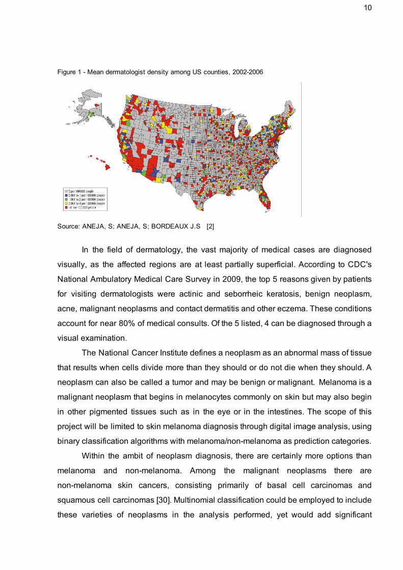
There is a noted undersupply of dermatologic services worldwide, common to

both developing and developed countries. The effects of such a deficit in the workforce

is clearly shown in the excessive mean wait times for appointment availability; it was

recently discovered that a patient must schedule a dermatologic consult an average of

33 days in advance in the United States [13] and 26 days in advance in Brazil [23].

Estimates of the current number of practicing dermatologists range from 8,000 to

8,500 in the United States and approximately 6,000 in Brazil. This is a pitifully

inadequate number of professionals to cater to the 300 million americans and 200

million brazilians. Researchers from the Case Western Reserve University and Yale

University performed a study that showed the direct correlation between dermatologist

density and melanoma mortality rates [2]. This finding is already significant in countries

like the United States and Brazil where there is an estimated ratio of 35,000 people per

dermatologist and even more severe in countries like South Africa with 3 to 4 million

people per dermatologist [21].

Dermatology specialists are mainly based in capitals and major cities, limiting

greatly the access to a dermatologist (See Figure 1). Technology has previously been

applied to other fields to overcome geographical barriers; this project evaluates the

efficiency and effectiveness of a series of computerized methods that may be applied to

the dermatologic diagnosis process, in an effort to assuage this disequilibrium in supply

and demand.

10

Figure 1 ­ Mean dermatologist density among US counties, 2002­2006

Source: ANEJA, S; ANEJA, S; BORDEAUX J.S [2]

In the field of dermatology, the vast majority of medical cases are diagnosed

visually, as the affected regions are at least partially superficial. According to CDC's

National Ambulatory Medical Care Survey in 2009, the top 5 reasons given by patients

for visiting dermatologists were actinic and seborrheic keratosis, benign neoplasm,

acne, malignant neoplasms and contact dermatitis and other eczema. These conditions

account for near 80% of medical consults. Of the 5 listed, 4 can be diagnosed through a

visual examination.

The National Cancer Institute defines a neoplasm as an abnormal mass of tissue

that results when cells divide more than they should or do not die when they should. A

neoplasm can also be called a tumor and may be benign or malignant. Melanoma is a

malignant neoplasm that begins in melanocytes commonly on skin but may also begin

in other pigmented tissues such as in the eye or in the intestines. The scope of this

project will be limited to skin melanoma diagnosis through digital image analysis, using

binary classification algorithms with melanoma/non­melanoma as prediction categories.

Within the ambit of neoplasm diagnosis, there are certainly more options than

melanoma and non­melanoma. Among the malignant neoplasms there are

non­melanoma skin cancers, consisting primarily of basal cell carcinomas and

squamous cell carcinomas [30]. Multinomial classification could be employed to include

these varieties of neoplasms in the analysis performed, yet would add significant

11

complexity. On that account, it was decided that a more conservative approach would

be most adequate for the initial stages of this study, limiting the classifier algorithm to

two categories. As melanomas are more commonly fatal than non­melanoma malignant

neoplasms [30], melanoma diagnosis was defined as the the focus of the research.

Skin melanoma may be diagnosed through a visual examination performed by a

dermatologist. The definitive diagnosis is usually rendered on pathologic evaluation of

a lesional skin biopsy specimen [29]. The potential malignancy is recognized during the

initial (visual) examination, following which a biopsy is performed to confirm the

prognosis. As such, although image analysis systems are not to be relied upon for a

complete diagnosis, they may be a viable solution to perform a triage and prioritize

examinations.

1.2 Monograph Structure

The monograph is organized into 7 chapters, these being Introduction,

Fundamentals, Approach, Reimplementation, Implementation, Analysis and

Conclusion. The first chapter describes the domain of the issue, that of automated

melanoma detection, as well as a high level description of the solution proposed. The

introductory chapter also provides a basic explanation of the medical terms employed.

Fundamentals discusses previous studies in related fields and how prior findings will

be included in this monograph. Approach details the solution developed, describing the

components and logic pertaining to the image analysis system. Reimplementation

describes Staunton and Ma’s Border irregularity analysis algorithm and the process of

reconstructing it’s code. The Implementation chapter documents the development of

three additional algorithms to be used in conjunction with Staunton and Ma’s. Analysis

outlines the execution of the image analysis system, resulting in a dataset to be used in

the classifier system as well as the intermediate results obtained during testing.

Conclusion will summarize the performance of the classifier system, its findings and

ongoing work.

12

2. FUNDAMENTALS

The following chapter details the identifying traits used to detect melanoma in a

visual examination and a description of previous studies related to the employment of

computer vision methods and algorithms for dermatologic diagnosis.

2.1 ABCD Criteria

The ABCD acronym was first coined in the article Early Detection of Malignant

Melanoma:The Role of Physician Examination and Self­Examination of the Skin [7]

written by Dr. Robert Friedman, Dr. Darrell Rigel and Dr. Alfred Kopf of the New York

University School of Medicine in 1985. The article was prepared in conjunction with the

Task Force on Preventive Dermatology of the American Academy of Dermatology and

the American Cancer Society; the ABCD Criteria was meant to be used by both the lay

public and health professionals to assist in the early detection of melanoma and

consequently increase survival rates [7]. ABCD stands for Asymmetry, Border

irregularity, Color variegation, and Diameter generally greater than six mm [7].

Asymmetry

Figure 2 ­ Asymmetry: Malignant and benign example

Source: prof. Ricardo Barbosa Lima of UNIRIO [16]

“Unlike benign pigmented lesions, which are generally round and symmetrical, early

malignant melanomas are usually asymmetrical” [7] (Figure 2)

13

Border irregularity

Figure 3 ­ Border irregularity: Malignant and benign example

Source: prof. Ricardo Barbosa Lima of UNIRIO [16]

“Unlike benign pigmented lesions, which generally have regular margins, the borders of

early malignant melanomas are usually irregular. “ [7] (Figure 3)

Color Variegation

Figure 4 ­ Color Variegation: Malignant and benign example

Source: prof. Ricardo Barbosa Lima of UNIRIO [16]

“Unlike benign pigmented lesions, which are generally uniform in color, macular

malignant melanomas are variegated, ranging from various hues of tan and brown to

black, and sometimes intermingled with red and white.” [7] (Figure 4)

14

Diameter Size

Figure 5 ­ Diameter size: Malignant example

Source: prof. Ricardo Barbosa Lima of UNIRIO [16]

“Unlike most benign pigmented lesions, which generally have diameters less than six

mm, the diameters of macular malignant melanomas when first identified are often more

than six mm.” [7] (Figure 5)

It is possible that the fourth trait, ‘Diameter greater than 6 mm’, may not be as

symptomatic as the previous 3 traits. A study performed in 2004 by Dr. Friedman, Dr.

Rigel, and Dr. Kopf and other colleagues of the New York University School of

Medicine and the Sydney Melanoma Unit suggested a reexamination of the ABCD

criteria in view of data attesting to the existence of melanoma with a diameter smaller

than 6 mm [1]. Although the conclusion reached was that the available data did not

support a lowering of the 6mm threshold, the study emphasizes the need to use the

ABCD traits in conjunction as there are cases of small­diameter melanomas.

During the same study by Kopf and his colleagues, detailed in the article Early

Diagnosis of Cutaneous Melanoma: Revisiting the ABCD Criteria [1] it was concluded

that an additional criterion ‘E’ should be added to the acronym, representing the

evolution of pigmented lesions. It is said that “Physicians and patients (...) should be

attentive to changes (evolving) of size, shape, symptoms (itching, tenderness), surface

(especially bleeding), and shades of color.” [1] However, this additional criterion cannot

be well represented by a digital image and as such is not included in this experiment.

15

2.2 Related Work

In dermatology, the ABCD guide is a widely known method for the identification

of a malignant melanoma [25]. This guide is a set of 4 traits common to malignant

melanomas: Asymmetry; Border irregularity; Color variegation; Diameter greater than 6

mm. Symmetry in medical imaging has played an important role in contributing to

diagnosis in other fields of medicine. An example of this is measuring asymmetry on

mandibles from children with cleft lip and palate and children with plagiocephaly

syndrome [10], measuring the asymmetry of the hippocampi to classify schizophrenic

patients [10] and using the asymmetry principle in the detection of breast tumors [14].

Extensive research has been performed regarding the digital analysis of border

irregularity in relation to melanoma diagnosis. Some of these studies indicate that the

diagnosis of malignant melanomas can be based on the analysis of the shape of the

lesion alone [15]. Many of said studies which present most noteworthy results make use

of Wavelet Transform Analysis.

The term ‘wavelet’ (originally in French, ‘ondelettes’) was first coined in 1982 by

the French geophysicist Jean Morlet [24], one of the pioneers in Wavelet Analysis.

Morlet sought an alternative to the short time Fourier Transform [6] which is a

modification of the Fourier transform to permit the analysis of non­stationary signals.

Assuming a time­domain signal as the raw signal, a Fourier transform could be used to

obtain the Frequency Spectrum. The Fourier Transform contains no information with

regard to time, ergo the need for the short time Fourier Transform for a non­stationary

signal. The short time Fourier Transform performs sequential Fourier Transforms on

segments of the signal which are (near) stationary.

The disadvantage of the short time Fourier transform lies in the necessary

sacrifice of either good time resolution or good frequency resolution according to the

window used in the kernel function. To gain good time resolution in the high­frequency

components as well as good frequency resolution in low­frequency components in a

single transform, Morlet proposed an alternate method for generating the transform

functions. In sum, instead of using a window of changeable width to perform a Fourier

Transform on a time interval of the signal, Morlet took a windowed cosine wave whose

width was shifted to adjust to low or high frequencies and shifted these functions in time

16

as well [6]. As a result, the transform functions relied on two parameters: the time

location and scale, which represents the frequency. Since then, the basis Wavelet

theory has been built upon by a series of scientist who have explored its applications in

a variety of fields.

There are two main trends in the use of Wavelet Transforms [12], the Continuous

Wavelet Transforms and the Discrete Wavelet Transforms. The Continuous Wavelet

Transforms (CWT) consists of an analysis window (function) of varying scale being

shifted not only in scale but in time, obtaining the signal product and integrating over all

times. In the Discrete Wavelet Transform (DWT) low and high pass filters are used to

analyze low and high pass frequencies, respectively, removing redundancy present in

the CWT. The CWT’s redundancy does have a purpose, emphasizing traits and adding

readability. The DWT reduced computational time due to reduced redundancy may be

the cause of its greater popularity among engineers [12].

A study performed by K.M. Clawson of the University of Ulster uses the Harmonic

Wavelet Transform to analyze lesion border irregularity, claiming maximum

classification accuracy of 93.3% with 80% sensitivity [5] when tested on 30 cutaneous

lesions. The Harmonic Wavelet Transform was developed by David Newman in 1993

[26]. This name may be derived from its frequency resolution, “confined exactly to an

octave band so that it is compact in the frequency domain” [26]. However, this fixed

resolution throughout the frequency band inhibits the separation of signal components

[19] which in turn hinders the distinction of structural and textural irregularities. It is the

structural irregularity that has clinical importance for melanoma diagnosis [19]. In 2012,

Li Ma of the Hangzhou Dianzi University and Richard C. Staunton of the University of

Warwick circumvented this difficulty by using a Discrete Wavelet Transform to single out

the structural components [19]. Their study involved 134 images of skin lesions; of these

72 were of melanomas and 62 of moles. The most significant distinction between

melanomas and moles is that moles are benign neoplasms whereas melanomas are

malignant neoplasms. The algorithm could be summarized as a two­step procedure:

multi­scale wavelet decomposition of the extracted contour followed by the selection of

significant sub­bands.

17

Wavelet decomposition was used to extract the structure from the contour which

were then modeled as signatures with scale normalization to give position and

frequency resolution invariance. Energy distributions among different wavelet

sub­bands were then analyzed to extract those with significant levels and differences to

enable maximum discrimination. A set of statistical and geometric irregularity

descriptors were applied at each of the significant sub­bands, followed by an

effectiveness evaluation to select which descriptors contribute to an accurate diagnosis.

The effectiveness of the descriptors was measured using the Hausdorff distance

between sets of data from melanoma and mole contours. The best descriptor outputs

were input to a back projection neural network to construct a combined classifier

system. This algorithm will be described in greater detail in the implementation chapter

of the monograph.

Li and Staunton’s optimum combination resulted in 90% specificity and 83%

sensitivity, similar to Clawson’s findings. These results were obtained from a small data

set consisting of 18 images, 9 of which were of melanomas and 9 of moles. With a

larger training set of 67 images (31 moles and 36 melanomas), these numbers fell to

83% sensitivity and 74% specificity, which signifies that a greater number of

non­malignant moles would be classified as melanomas.

Table 1 ­ Comparison of classification performances

Source: MA, L.; STAUNTON, R.C. [19] These findings are incredibly significant given the high levels of accuracy and

reduced computational cost. It is of interest to analyse this algorithm in conjunction with

remaining three features of the ABCD criteria: asymmetry, color variegation and

diameter size.

18

3. APPROACH This study implemented and evaluated a multi feature image analysis system in

an effort to gauge the effectivity of its employment in melanoma diagnosis. It became

necessary to first identify the significance of each feature in the classification of skin

lesions to determine what combination of features provide the most accurate results.

Li Ma and Richard C. Staunton generously agreed to the inclusion of their

algorithm in this experiment. However, the original software for the algorithm detailed in

the article Analysis of the contour structural irregularity of skin lesions using wavelet

decomposition [19] could not be recovered. To circumvent this contretemps, the

algorithm was reimplemented in consultation with Ma and Staunton as part of the study.

Our approach is divided into two parts; the first is Ma and Staunton’s algorithm,

which uses border irregularity to determine malignancy. Border irregularity is one of four

identifying traits used in the diagnosis of melanoma. Studies have shown that accuracy

levels vary according to the traits included in performing diagnosis, both singly and in

combination. Table 2 summarizes the findings of research led by L. Thomas in 1998

[30], displaying distinct fluctuations in performance when combining multiple criteria

Therefore the second part of the system consists of three algorithms to formulate

additional metrics, these being Asymmetry, Color variegation and a simple geometric

border irregularity descriptor.

Table 2 ­ Summary of Key ABCD(E) Sensitivity and Specificity Studies

Source: Thomas, L. et al. [30]

19

Staunton and Ma’s algorithm uses 13 features based on a set of statistical and

geometric border irregularity descriptors. In addition, this algorithm extracts the

structural component of the lesion from the raw image data, eliminating the misleading

textural component. The simple geometric descriptor is compared with Ma and

Staunton’s algorithm to measure the added accuracy of the 13 features used as well as

the impact of refining the raw data. Subsequently the two descriptors for Asymmetry and

Color variegation are included in a combined algorithm. As stated by Kopf and his

colleagues [1], “It should be emphasized that not all melanomas have all 4 ABCD

features. It is the combination of features (eg, ABC, A+C, and the like) that render

cutaneous lesions most suspicious for early melanoma.” If this is true of in­person

examinations performed by a specialist, it may also be implied of computer vision

analysis.

Combining the 13 features in Staunton and Ma’s algorithm and the 3 additional

metrics, a total of 16 features are attributed to each image of a skin lesion, recorded in

the data set which is run through a Back Propagation Neural Network to classify each

instance as melanoma or non­melanoma. The back propagation (BP) neural network

algorithm is a multi­layer feedforward network trained according to error back

propagation algorithm and is one of the most widely applied neural network models

[11]. This model was used in the development of Ma and Staunton’s algorithm and will

continue to be used to maintain consistency. The algorithm is measured for sensitivity

and specificity levels in addition to overall accuracy.

Sensitivity, also known as the true­positive rate, is given a higher priority than

specificity, the true­negative rate, as the correct identification of a malignant or

potentially malignant tumor is of greater consequence than a false positive diagnosis,

within reasonable levels. Of course, the inconvenience of an false positive diagnosis is

by no means irrelevant, so despite specificity being a secondary priority, this category

of performance is still carefully observed. As achieving 100% accuracy is an unrealistic

expectation and the biopsy a requirement for a definitive diagnosis [29], specialist

confirmation remains necessary. This project seeks to contribute to the discussion of

whether it is advantageous to incorporate computer vision algorithms to current

traditional diagnosis methods.

20

4. REIMPLEMENTATION

Li Ma and Richard C. Staunton of the Hangzhou Dianzi University and Warwick

University [19] developed an algorithm to analyze skin lesion border irregularity using

multi­scale wavelet decomposition. As the code for the algorithm was not recovered, it

was necessary to re­implement it so as to enable its inclusion in this study. The code

was originally written in Matlab [34], a high­level technical computing language and

interactive environment for algorithm development. However, due to budget limitations

the algorithm was re­implemented in Octave [35], an open source alternative

comparable to and generally compatible with Matlab. The algorithm is roughly divided

into two phases: Wavelet decomposition of a lesion contour and Sub­band descriptions

of contour structural components. Following is a summarized and commented

description of the algorithm extracted from the article Analysis of the contour structural

irregularity of skin lesions using wavelet decomposition [19].

1. Wavelet decomposition

1.1. Represent the contour in 1D signal

The contour of a skin lesion in an image is described by the points

. [These points were obtained using a Canny edgex , , , , ..x , C = 1 y1 x2 y2 . N yN

detector function.] To represent this 2D data as 1D, the contour is modeled as a

signature where the radial distance from the geometric center r , r , ..r Cr = 1 2 . N

and is the coordinate of the , i , , ..n ri =√(x ) y ) i − x′2 + ( i − y′

2 = 1 2 . x , y )( ′ ′

geometric center of the closed contour.

1.2 Scale normalization

It was noted that many moles have a shorter contour for a given nominal area than do

melanomas. Together with size variability between the samples in the database, this

can lead to variations in estimated frequency and resolution in the frequency domain.

Scale normalization is required to enable a comparison between moles and

melanomas in this domain. The proposed normalization was modified to give radius:

21

Where i is an integer used to resample the contour points with a spacing distance of

(n/N) and the ceiling function ⎡⎤is used to produce an integer index to r. The

values μ1 and μ2 are the averaged radial distances of all the melanomas and benign

moles respectively in the data base. T is a threshold.

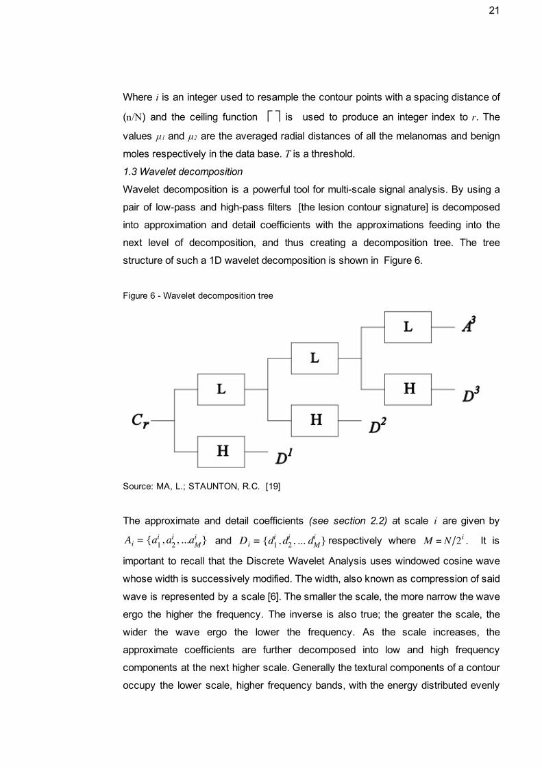
1.3 Wavelet decomposition

Wavelet decomposition is a powerful tool for multi­scale signal analysis. By using a

pair of low­pass and high­pass filters [the lesion contour signature] is decomposed

into approximation and detail coefficients with the approximations feeding into the

next level of decomposition, and thus creating a decomposition tree. The tree

structure of such a 1D wavelet decomposition is shown in Figure 6.

Figure 6 ­ Wavelet decomposition tree

Source: MA, L.; STAUNTON, R.C. [19]

The approximate and detail coefficients (see section 2.2) at scale are given by i

and respectively where . It isa , , ..a Ai = i1 a

i2 . i

M d , , .. d Di = i1 d

i2 . i

M 2 M = N/ i

important to recall that the Discrete Wavelet Analysis uses windowed cosine wave

whose width is successively modified. The width, also known as compression of said

wave is represented by a scale [6]. The smaller the scale, the more narrow the wave

ergo the higher the frequency. The inverse is also true; the greater the scale, the

wider the wave ergo the lower the frequency. As the scale increases, the

approximate coefficients are further decomposed into low and high frequency

components at the next higher scale. Generally the textural components of a contour

occupy the lower scale, higher frequency bands, with the energy distributed evenly

22

between bands to give a relatively small total energy within each. However the

structural components generally have a larger energy and occupy the lower

frequency bands. By using wavelet decomposition to level s, an original contour

signature Cr is transformed to a series of sub­band signals As, Ds, Ds­1, ...D1 covering

the whole signal frequency space at [0, 1/2s fmax], [1/2i fmax, 1/2i­1fmax], i=s, s­1,

…, 2, 1 and fmax is half the sampling frequency. This represents a concatenation of

the frequency bands from the lowest to the highest. The task is to identify at which

decomposition levels the structural components of a lesion contour can be extracted

and which sub­bands in the frequency domain provide significant discriminative

information

2. Sub­band descriptions of contour structural components

The Discrete Wavelet Transform was selected for use over the Fast Fourier

Transform because it presents the capability of confining signal components to

dyadically increasing width frequency bands with different resolutions. This enables

the distinction between structural and textural components, an essential factor in

Staunton and Ma’s algorithm.

2.1 Significant sub­band selection

To obtain just the contour’s structural components ignoring the less relevant textural

components, several lower frequency sub­bands need to be identified from which to

reconstruct that portion of the original contour using both multi­scale approximate and

detail coefficients. The evaluation of the significant sub­band range was

accomplished by performing a Hausdorff distribution analysis between each of the

sample sets at each level of wavelet decomposition. When analyzing the

decomposition of a contour signal, the total energy at any decomposition level

indicates the significance of that sub­band frequency to the original signal. The

energy of a wavelet sub­band Dj is given by:

(D ) j , 2, .. nE j = ∑

i

ij

2 = 1 .

2.2 Procedure for investigating significant sub­band selection

An algorithm was developed to identify those sub­bands which enabled the largest

discrimination between moles and melanomas. This was done with a set of p benign

mole contours and a set of q melanoma contours

Step 1: For a preset maximum level of wavelet decomposition n, calculate the

wavelet energy for every contour from the set of moles and melanomas. Then

23

calculate the energy of each sub­band [obtained from the wavelet decomposition to

level n].

Step 2: Form energy sets from the individual energies calculated for each

transformed benign mole and melanoma contour at each sub­band.

Step3. Compute the Hausdorff Distance value between energy sets of moles Eb and

melanomas Em for each band. This measures the discrimination between the two

classes for each sub­band.

Step 4. Plot the distribution of the Hausdorff Distance with respect to each

sub­band. The sub­bands with the highest HD are considered as the most significant

and used in the final classification.

2.3 Extraction of the structural component of a lesion contour

Based on the theory of wavelet reconstruction, the structural component of a lesion

contour is given by combining the significant coefficient groups from As , Ds, Ds­1,

...D1 where the original decomposition was stopped at level s. The decomposed detail

sub­bands need to be divided into high­scale (low­frequency) and low­scale

(high­frequency) groups using a threshold st so that:

Cs = As + D s + Ds­1 +… + Dst

Ct = Dst­1+ Dst­2 +... + D1

Where Cs contains lower­frequency information and represents the structural

component of the contour, and Ct contains higher­frequency information and

represents the textural component. Choosing both s and st are difficult tasks, as a

large s generates many narrow sub­bands close to zero frequency. Although these

will contain structural information that will be relatively free of textural irregularity,

there is an extra cost in increased computational complexity. A small s can lead to

structural contours contaminated with textural irregularity. The value of st chosen is

crucial to obtain useful structural and textural contour information. The significant

sub­band selection process described in Section 2.2 was run on the test data which

lead to the straightforward selection of a single, general value for st . The frequency

bands that contained significant discrimination information were sub­bands D6 to D9,

and as such were selected as the significant levels.

It is simple to reconstruct the structural components of the contour after the

significant levels in the wavelet decomposition stack have been determined. Figure 7

shows the extracted contours of a mole (a,b,c) and a melanoma (d,e,f), where Figure

24

7 a) and d) are the original contours, Figure 7 b) and e) are the corresponding

contours reconstructed from A9 and D1 to D5. The approximation coefficient, A9 has

been included to give the basic structure of the contour onto which the more complex

textural part has been superimposed. Figure 7 c) and f) are reconstructed from A9

and D6 to D9 (s = 9, st= 6), that is the boundaries representing the structural portion of

the original lesion. With the textural information removed, these have the property of

the highest discrimination between different lesion classes. In the remainder of the

monograph these significant sub­bands will be referred to as the structural

sub­bands.

Figure 7 ­ Contours after wavelet reconstruction

Source: MA, L.; STAUNTON, R.C. [19]

Observing Figure 7, one can easily note the striking difference in discrimination

based on textural and structural components. The contours in b) and e) reconstructed

from the textural components of the mole and melanoma respectively present an almost

imperceptible difference and would add very little to a classification system. In contrast,

the contours c) and f) which were reconstructed from the structural components are

clearly distinctive. As the significant sub­band selection was performed during Ma and

Staunton’s study, leading to the selection of a single value for st, with the approval of Li

Ma, this phase of the algorithm was bypassed; the re­implementation uses the selected

st value directly.

25

Once the significant sub­bands were identified, it was possible to calculate the

series of border irregularity measures the algorithm is comprised of. Ma and Staunton

used 7 different measures, these being either statistical or geometric based [19]. The

measures and their respective formulas are listed below as described in Ma and

Staunton’s article:

3.1 Statistical measures The following features related to contour irregularity were defined: (1) The mean of the energy of Dj at each significant level, given by:

where di is the the ith component of Dj. N μ = (∑N

i=1di) /

(2) Entropy of wavelet energy, log(p )wj = − ∑N

i=1pji

ji

where is the energy probability of the ith component of Dj, Ej is the total E pji = E ji / j

energy of the coefficients in band j as calculated by ,[E (D ) j , 2, .. n] j = ∑

i

ij

2 = 1 .

and . The energy entropy measures the magnitude of signal fluctuations.E ji = D | | ji | | 2

(3) Ultimate width. For any signal , the ultimate width is defined as x , , ..x X = 1 x2 . N idth w = μ

2σ where and are the mean and variance of signal X. A large width indicates sharp variations.

3.2 Geometric based irregularity measures At each significant level j, a supposed structural component of a , s C j ≥ j ≥ st contour is reconstructed from the wavelet coefficients, . In D ..C j = As + s + . +Dj addition to a simple variance measure (4), the other irregularity measures of the reconstructed contours are evaluated as:

(5) Radial Deviation, DR = 1N ∑

N

i=1(r ) | | i − r

| |

where is the mean radius of the contour signature.r

(6) Contour Roughness, Ro = 1N ∑

N

i=1r | | i − ri+1

| |

(7) Irregularity Measure, MI = Area(S )s

Area(C ⊕ S )j s where Ss is reconstructed from the approximate data, As, at the significant level s, and ⊕ is the exclusive­or operator.

With the seven irregularity measures described above and the four significant

sub­bands (D6, D7, D8, and D9), there would be a total of 25 features: measures (1) to (6)

26

for each of the four significant sub­bands (24 features thus far), and IM (irregularity

measure 7) at the threshold scale st. However, these features were filtered to remove

redundancy. This was done by a correlation analysis followed by performance based

feature selection. Correlation analysis computes the correlation coefficient for a pair of

features ti, tj, from a feature vector F=t1, t2, …, tn and a sample set S=x1, x2, …, xm . A

large correlation coefficient indicates redundancy [19]. The performance based feature

selection requires calculating the probability distribution of each feature’s contribution to

a correct classification, tested on both benign and malignant sample sets. The

accumulated probability is found, then each feature is verified with an established

classification error threshold [19].

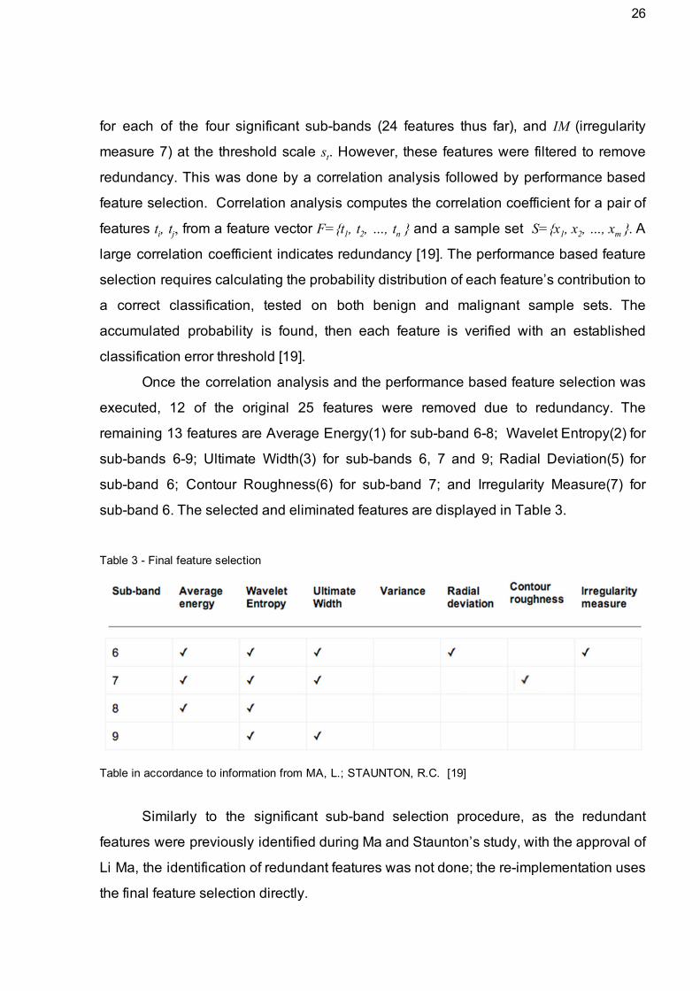
Once the correlation analysis and the performance based feature selection was

executed, 12 of the original 25 features were removed due to redundancy. The

remaining 13 features are Average Energy(1) for sub­band 6­8; Wavelet Entropy(2) for

sub­bands 6­9; Ultimate Width(3) for sub­bands 6, 7 and 9; Radial Deviation(5) for

sub­band 6; Contour Roughness(6) for sub­band 7; and Irregularity Measure(7) for

sub­band 6. The selected and eliminated features are displayed in Table 3.

Table 3 ­ Final feature selection

Table in accordance to information from MA, L.; STAUNTON, R.C. [19]

Similarly to the significant sub­band selection procedure, as the redundant

features were previously identified during Ma and Staunton’s study, with the approval of

Li Ma, the identification of redundant features was not done; the re­implementation uses

the final feature selection directly.

27

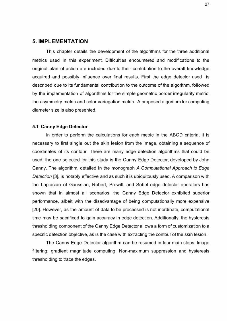
5. IMPLEMENTATION

This chapter details the development of the algorithms for the three additional

metrics used in this experiment. Difficulties encountered and modifications to the

original plan of action are included due to their contribution to the overall knowledge

acquired and possibly influence over final results. First the edge detector used is

described due to its fundamental contribution to the outcome of the algorithm, followed

by the implementation of algorithms for the simple geometric border irregularity metric,

the asymmetry metric and color variegation metric. A proposed algorithm for computing

diameter size is also presented.

5.1 Canny Edge Detector

In order to perform the calculations for each metric in the ABCD criteria, it is

necessary to first single out the skin lesion from the image, obtaining a sequence of

coordinates of its contour. There are many edge detection algorithms that could be

used, the one selected for this study is the Canny Edge Detector, developed by John

Canny. The algorithm, detailed in the monograph A Computational Approach to Edge

Detection [3], is notably effective and as such it is ubiquitously used. A comparison with

the Laplacian of Gaussian, Robert, Prewitt, and Sobel edge detector operators has

shown that in almost all scenarios, the Canny Edge Detector exhibited superior

performance, albeit with the disadvantage of being computationally more expensive

[20]. However, as the amount of data to be processed is not inordinate, computational

time may be sacrificed to gain accuracy in edge detection. Additionally, the hysteresis

thresholding component of the Canny Edge Detector allows a form of customization to a

specific detection objective, as is the case with extracting the contour of the skin lesion.

The Canny Edge Detector algorithm can be resumed in four main steps: Image

filtering; gradient magnitude computing; Non­maximum suppression and hysteresis

thresholding to trace the edges.

28

1 ­ Image filtering

The Canny Edge detector is highly susceptible to noise; the first step in the

algorithm is filtering the image to reduce the misleading effect of noise pixels through a

step edge detector. Canny calculated the optimal filter for this task, named ‘Filter

number 6’ in his article [3]. However, he observed that although the first derivative of

Gaussian operator performed approximately 20% worse than the optimal operator in the

performance evaluations, this difference is hardly noticeable when visualizing their

effects on real images. Figure 8 contains a graph showing the similarities between the

optimal step edge operator and the first derivative of a Gaussian. As the optimal

operator requires much more computational effort than the first derivative of the

Gaussian, the image is convolved with a Gaussian filter to obtain the desired noise

reduction.

Figure 8 ­ Comparison of optimal and Gaussian operator.

Source: CANNY, John. [3]

2 ­ Gradient magnitude computing

The gradient of an image indicates the direction of a rapid change in intensity

and as such provides information regarding the orientation of the edge, whether it is

horizontal, vertical or diagonal. In a two dimensional coordinate system as is this case,

the gradient is given by

= ∂f∂x + ∂f

∂y

the vector composed of the partial derivatives of . A horizontal gradient is given by

0= + ∂f∂y

29

as the change is in the direction; a vertical gradient is given by

= ∂f∂x + 0

as the change is in the direction. The magnitude of the gradient is given by

|| || =√( ∂f∂x)

2+ ( ∂f

∂y )2

and is calculated for every pixel in the image.

3 ­ Non­maximum suppression

Once the gradient magnitude calculation is performed on each pixel, its value is

then verified to determine whether it assumes a local maximum in the gradient direction.

The gradient direction is given by

θ = tan−1 ( ∂f∂x / ∂f

∂y )

The implementation of the algorithm does not compute the gradient direction so

as to avoid performing a division calculation. Instead, the two derivatives are checked

for the same sign and then the largest of the two derivatives is singled out. The pixel

magnitude is then compared to its two neighbor’s values in the four possible directions,

these being north ­ south, east ­ west, northeast ­ southwest and northwest­southeast.

Linear interpolation is used between the two neighbor pixels for greater accuracy. Only

local maximums are considered edge candidates, therefore if the central pixel’s

magnitude is not greater than that of its two neighbors it is suppressed’ by setting its

edge strength value to zero.

4 ­ Hysteresis thresholding

The pixels that correspond to a local maximum and in effect possess a high edge

strength value are set aside as the edges detected in the image. Yet the selected edge

pixels can be further refined through specifying a threshold as the final comparison to

determine an existing edge. Hysteresis thresholding is done using a low and a high

threshold. The low threshold detects weak edges and the high threshold the strong

edges. It was necessary to experiment to determine the optimal combination of

thresholds for the situation in question, that of singling out the skin lesion in the image.

The effects of different threshold levels can be seen in Figure 9.

30

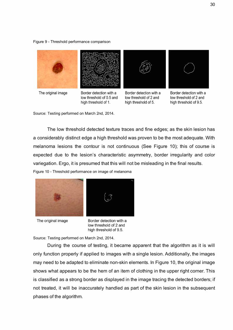
Figure 9 ­ Threshold performance comparison

Source: Testing performed on March 2nd, 2014.

The low threshold detected texture traces and fine edges; as the skin lesion has

a considerably distinct edge a high threshold was proven to be the most adequate. With

melanoma lesions the contour is not continuous (See Figure 10); this of course is

expected due to the lesion’s characteristic asymmetry, border irregularity and color

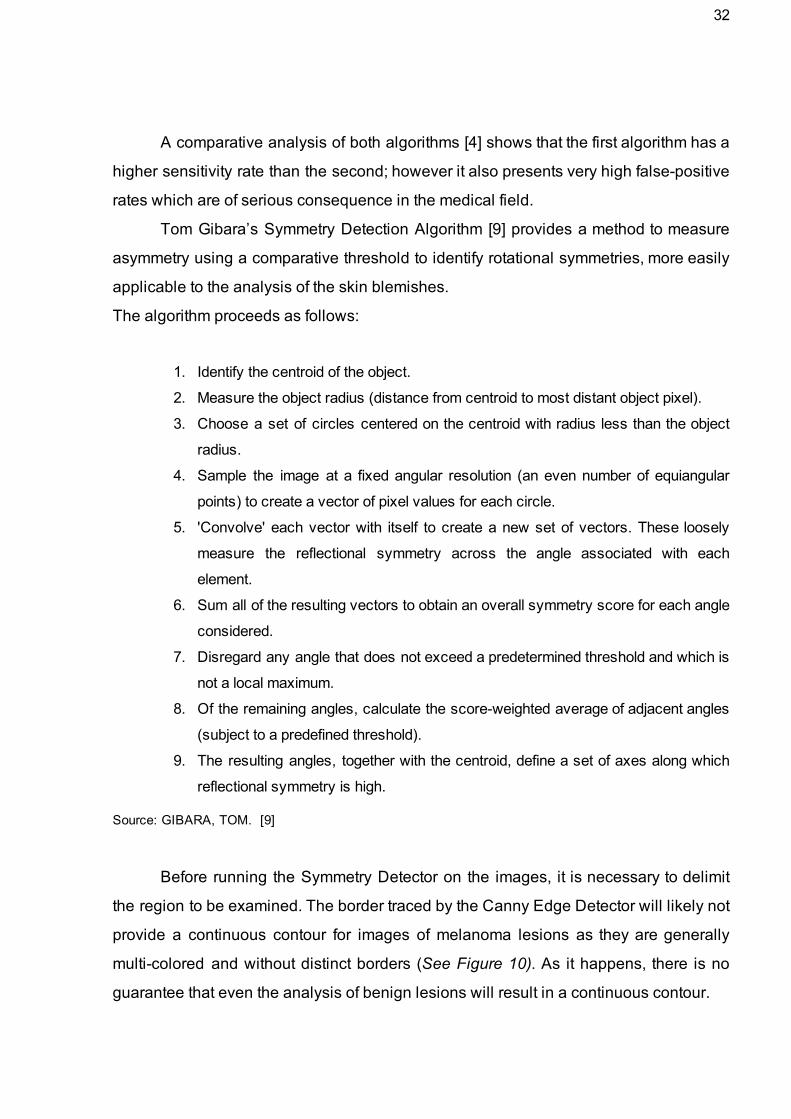
variegation. Ergo, it is presumed that this will not be misleading in the final results.

Figure 10 ­ Threshold performance on image of melanoma

Source: Testing performed on March 2nd, 2014. During the course of testing, it became apparent that the algorithm as it is will

only function properly if applied to images with a single lesion. Additionally, the images

may need to be adapted to eliminate non­skin elements. In Figure 10, the original image

shows what appears to be the hem of an item of clothing in the upper right corner. This

is classified as a strong border as displayed in the image tracing the detected borders; if

not treated, it will be inaccurately handled as part of the skin lesion in the subsequent

phases of the algorithm.

31

The re­implementation of Ma and Staunton’s algorithm was written in Octave,

which has a built­in Canny Edge Detector function. The geometric Border irregularity

metric, the Asymmetry metric and the Color variegation metric algorithms were written in

Java [36]. For this phase of the process, Tom Gibara’s Java implementation of the

Canny Edge Detector [8] algorithm is used. The implementation of the Canny Border

Detector developed by Tom Gibara was slightly modified so as to return a list of

coordinates of the detected edge pixels as opposed to an image of the traced edges.

5.2 AB*CD Metrics

5.2.1 A ­ Asymmetry Metric

Asymmetrical skin growths, in which one part is different from the other, may

indicate melanoma. [32]

Symmetry is defined mathematically as invariability regardless of

transformations, an absolute characteristic that cannot be measured in degrees [10].

Due to this most rigid definition, rarely if ever is it possible to label a naturally formed

figure as symmetrical [10]. As the images to be analyzed are of the human body, it is

safe to assume that all the figures will be asymmetric. As symmetry cannot be

measured, the symmetry metric used in this algorithm is the number of rotational

symmetries identified with a 10% tolerance for imperfection. As such, the symmetries

detected and numbered will not be perfectly symmetrical.

In examining skin blemishes, rotation and reflection symmetry is of greater

relevance. Two of the more recent rotation/reflection symmetry detection algorithms are

Loy and Eklundh’s Detecting symmetry and symmetric constellations of features [18]

and Prasad and Davis’ Detection rotational symmetries [28]. Loy and Eklundh’s

algorithm is feature based; it uses pairwise matching and voting for symmetry foci in a

Hough transform to identify asymmetry. Prasad and Davis created an algorithm that

filters in an input color image into a gradient vector flow field, extracting and matching

the features into the gradient vector flow field, using a voting scheme for symmetry

detection.

32

A comparative analysis of both algorithms [4] shows that the first algorithm has a

higher sensitivity rate than the second; however it also presents very high false­positive

rates which are of serious consequence in the medical field.

Tom Gibara’s Symmetry Detection Algorithm [9] provides a method to measure

asymmetry using a comparative threshold to identify rotational symmetries, more easily

applicable to the analysis of the skin blemishes.

The algorithm proceeds as follows:

1. Identify the centroid of the object.

2. Measure the object radius (distance from centroid to most distant object pixel).

3. Choose a set of circles centered on the centroid with radius less than the object

radius.

4. Sample the image at a fixed angular resolution (an even number of equiangular

points) to create a vector of pixel values for each circle.

5. 'Convolve' each vector with itself to create a new set of vectors. These loosely

measure the reflectional symmetry across the angle associated with each

element.

6. Sum all of the resulting vectors to obtain an overall symmetry score for each angle

considered.

7. Disregard any angle that does not exceed a predetermined threshold and which is

not a local maximum.

8. Of the remaining angles, calculate the score­weighted average of adjacent angles

(subject to a predefined threshold).

9. The resulting angles, together with the centroid, define a set of axes along which

reflectional symmetry is high.

Source: GIBARA, TOM. [9]

Before running the Symmetry Detector on the images, it is necessary to delimit

the region to be examined. The border traced by the Canny Edge Detector will likely not

provide a continuous contour for images of melanoma lesions as they are generally

multi­colored and without distinct borders (See Figure 10). As it happens, there is no

guarantee that even the analysis of benign lesions will result in a continuous contour.

33

The solution to this issue is found in Yuri Pourre’s implementation of the Quick

Hull algorithm [27], which draws the smallest polygon possible given a set of

coordinates. Once the Canny Edge Detector is run on the image, the resulting list of

coordinates of the detected edge pixels is fed into the Quick Hull program.

Figure 11 ­ Polygon containing the skin lesion: Melanoma and Neoplasm

Source: Testing performed on March 9th, 2014.

An image with the polygon outline is then filled in and converted to grayscale for

compatibility with Gibara’s Symmetry Detector algorithm. The important algorithm

parameters [9] are Angular Resolution, Angular Aliasing, Radius Count (‘Radii’ in the

sample output in Figure 12), and Threshold. The Angular Resolution is the number of

sample arcs in the circle. Angular Aliasing is the smallest angle permitted between

identified axes of symmetry. Angles closer together than this value are combined into a

single angle. Radii indicates the number of different radii at which samples are taken.

Threshold is the proportion of the maximum possible score that an angle must obtain to

be considered. Once the detector is run, a summary of the execution is displayed. The

above parameters and their respective values are listed. Blue pixels indicate pixels

identified with the object, in this case the polygon surrounding the skin lesion. The

green 'plus' indicates the position of the centroid, currently not visible due to the many

traced lines of reflectional symmetry. The green 'cross' indicates a pixel at maximum

distance from the centroid. Green circles indicate the circles from which samples of

image data were taken. Green lines indicate the lines of reflectional symmetry identified

by the algorithm. The array of numbers in between the square brackets indicate the

location of the symmetries identified, indicating the amount of symmetries identified.

34

Figure 12 ­ Summary of Symmetry Detector results: Melanoma and Neoplasm

Source: Testing performed on March 9th, 2014.

5.2.2 B ­ Border Irregularity Metric

Melanomas may have borders that are vaguely defined. Growths with irregular,

notched or scalloped borders need to be examined by a doctor [32].

Staunton and Ma’s analysis of border irregularity used both statistical and

geometrical measures of the structural component of the skin lesion. To observe the

added value of removing the textural component from the calculation and the utilization

of statistical measures in addition to geometrical, a simple geometric border irregularity

metric was developed. Succinctly, it is the coefficient of variance of the lesion’s radii.

This was done in Staunton and Ma’s algorithm, however the calculation was performed

on the extracted structural component; in this metric all edges detected from the lesion

are used, both structural and textural. The algorithm to obtain the simple border

irregularity metric is detailed below:

1. A list of coordinates of the lesion’s border is obtained from the Canny Edge

Detector;

2. The centroid of the lesion would be calculated by finding the mean and

values; however, as the contour of melanoma lesions is not continuous, it was

necessary to correct this formula. The coordinates of the centroid are the minimum

value and plus an offset of the difference between the maximum and minimum

35

value of and divided by 2.

x ) 2 Cx = xm + ( M − xm / y ) 2 Cy = ym + ( M − ym /

3. The mean radius is obtained by calculating the average of the euclidean

distance between the centroid and each point in the list of border coordinates;

4. The standard deviation is given by

σ =√ n1 ∑

n

i=1(r ) i − r

2

with as the number of coordinate pairs (points) in the list, as the radius at point ri

and as the mean radius. Bias correction is unnecessary given the sample is r

equal to the population.

5. Obtain the coefficient of variance given by

cv = μσ

being that is the mean radius calculated in step 3.

An example of the calculated metric is displayed in Figure 13, for both a benign

neoplasm and melanoma.

Figure 13 ­ Comparison of simple border irregularity metric

Source: Testing performed on March 5th, 2014.

36

5.2.3 C ­ Color Variegation Metric

Multiple colors or uneven distribution of color may indicate cancer. [32]

Depending on the resolution and lighting of the image taken of the skin lesion,

color variance may be noticeable even in benign lesions. This makes it necessary once

again to measure the difference between colors in the lesion and compare this

difference to a defined threshold. The difference between colors is represented by

Delta­E, a metric established by the International Commission on Illumination (CIE) to

quantify color differences [33]. The first Delta­E formula was developed in 1976; since

then more sophisticated formulae have been developed and approved by CIE [33]. As

the subsequent Delta­E versions are of a more complex nature and consequentially

more computationally expensive, the 1976 CIELAB is used in this study. A suggestion

of ongoing work is to experiment using the other Delta­E formulae to determine whether

there is significant increase in efficiency in analyzing the color variegation of skin

lesions. Using the CIELAB, the algorithm is quite straightforward:

1. Identify lesion borders within the image using the Canny edge detector; 2. Delimit a region to analyze color variegation including all detected edges; 3. Calculate the average color of the lesion; 4. Convert the average color of the lesion from RGB to L*a*b*; 5. Iterate through each pixel in the delimited region;

5.1 Convert the color of the pixel from RGB to L*a*b*; 5.2 Calculate the CIELAB Delta­E of the pixel color and average color;

6. Return the average Delta­E of the region. Yuri Pourre’s implementation of the Quick Hull algorithm was used. In addition to

this, Pourre contributed with a function to determine the average color of a given region.

In sum, the color variegation metric is the average Delta­E of each pixel in the lesion

compared to the average color of the lesion.

Figure 14 ­ Comparison of Melanoma and Neoplasm Average Delta­E

Source: Testing performed on May 2nd, 2014.

37

5.2.4 D ­ Diameter greater than 6mm

A skin growth's large size may be an indication of cancer. [32]

The schedule limitations of this project difficulted the development of an

algorithm to measure the lesion diameter. As there is potential in exploring the use of

lesion diameter in image analysis, a suggested method is described to obtain this

metric.

This final criteria presents a challenge for the application of computerized image

analysis; the images will be taken at different ranges with no comparative figure,

impairing an accurate calculation of real size. A proposed solution is to identify the

pores in the image and measure the average distance between them in pixels; this

would provide a scale of the lesion’s diameter. An adaptation of Q. Zhang and T.

Whangbo’s Skin Pores Detection Algorithm [31] could be implemented to find the

pores in the image and note their coordinates so as to determine the distance between

them. The algorithm is based on image segmentation. A preprocessing algorithm to

balance the illumination of the image must be run before the pore detection algorithm.

The Global Luminance Proportion algorithm is noted below.

Using the original image of MxN size:

1. a. Calculate the average luminance of the image; b. Split the image S into V sub­blocks, calculating the average luminance; c. Obtain luminance difference matrix D; 2. Interpolation algorithm for matrix D until element number in matrix equals MxN; 3. Merge matrix D and original image S into new image sized MxN.

When the image has balanced luminance, the segmentation is performed using

the Fuzzy C­Means Algorithm. After this segmentation, pixels in the image are labeled

to 8 connectivity and skin pores can be classified from the 8­connectivity labeled image

by calculating the quadratic moment and the ratio between row and column moments.

38

6. ANALYSIS

6.1 Dataset

The images used in training and testing the classifier were obtained from the

Dermatlas Interactive Dermatology Atlas and the records of Dr. Jefferson B. Louback

[17] and Dr. Ricardo Barbosa Lima [16], a total of 70 images. A total of 32 of the images

are of malignant melanomas and 38 are of various types of benign neoplasms. The

images from Dermatlas are from various sources, among them both organizations and

medical professionals. To provide a reference to the image’s source, each image ID (file

name) contains a specific prefix: RB for Ricardo Barbosa Lima M.D.; JL for Jefferson

Louback M.D; AC for Armand Cognetta, M.D.; RU for Richard Usatine, M.D.; SCF for

Skin Cancer Foundation; SS for Skin Surgery: A Practical Guide.

The images from Dermatlas had a numerical ID; this number is maintained in the

dataset. Dr. Lima and Dr. Louback’s records also were numbered and these numbers

were also maintained. Images of malignant lesions is marked with an ‘M’ and images of

benign lesions with an ‘N’. An example of the ID of an image of a malignant lesion from

Dr. Lima’s records is “M142_RB”: M for malignant, 142 is the numbering provided by Dr.

Lima’s records, RB is his initials. All of the images used were submitted for diagnosis

confirmation to Dr. Louback.

There is a total of 17 features in the algorithms used, these being Staunton and

Ma’s 14 features and the 3 additional ones for Asymmetry, Border irregularity and Color

variegation. Unfortunately one of Staunton and Ma’s features, the Irregularity Measure

based on the approximate data signal, was not validated within the project’s time frame

and consequently was not included in the final analysis so as to avoid the use of a

component that could possibly not be true to the original algorithm.

6.2 Pre­Processing

To reduce the amount of data to be processed and expedite the algorithms’

execution, the images were cropped to the minimum size while still containing the

lesion in its entirety. This was performed manually.

39

During the delimitation of the lesion within the image using the Canny Edge

Detector, it was observed that a single set of low and high thresholds was not enough to

cater to all the images in the database. When an image was slightly blurred or when the

lesion, regardless of being malignant or benign, presented similar color to the

surrounding skin, the Canny Edge Detector failed to identify edges in the image.

Lowering the threshold was not an option as that added noise and detected skin texture

in other images. To solve this problem, two sets of thresholds were used: a standard set

of [6, 13] for the low and high threshold respectively, and a second set of [2, 8] for

images that failed to return more than 70 edge coordinates. Of the 70 images analyzed,

12 utilized the second set of thresholds. These thresholds were established after

successive tests and manual examinations of the results; there is no evidence that they

are the optimal selection. Thresholds that result in more accurate discrimination are

likely to increase the overall effectiveness of the analysis algorithms as they contribute

to the correct delimitation of the lesion that is then analyzed to reach a diagnosis,

eliminating unnecessary and possibly misleading parts of the image not pertaining to

the lesion. Identifying optimal thresholds for singling out the skin lesion from an image

may be a valid alternative to bettering the performance of the algorithms.

6.3 Data Analysis

To perform the classification, the Waikato Environment for Knowledge Analysis 1

(Weka) software was used. Developed at the university of Waikato, it contains a

collection of machine learning algorithms written in Java and is licensed under the GNU

General Public License.

To separate the test and training data, a percentage split of 28% was done to

emulate the optimum size of the training set determined by Staunton and Ma, which is

18 instances (half malignant, half benign) [19]. In Staunton and Ma’s study, a Back

Propagation neural network was used as the training algorithm. However, as

occasionally some features returned undefined values, a Naïve Bayes classifier was

also used due to its ability in dealing with missing data [22].

1 http://www.cs.waikato.ac.nz/ml/weka

40

The Multilayer Perceptron (Weka’s neural net with Back Propagation) presented

better performance than the Naïve Bayes classifier, as seen in Table 4.

Table 4 ­ BP Neural Net and Naïve Bayes performance

=== BP Neural Net === Correctly Classified Instances 73.6842 % Incorrectly Classified Instances 26.3158 % === Detailed Accuracy By Class === TP Rate FP Rate Precision ROC Area Class 0.778 0.3 0.7 0.747 true 0.7 .222 0778 0.747 false

=== Naïve Bayes === Correctly Classified Instances 70.5882 % Incorrectly Classified Instances 29.4118 % === Detailed Accuracy By Class === TP Rate FP Rate Precision ROC Area Class 0.556 0.125 0.833 0.639 true 0.875 0.444 0.636 0.639 false

Source: Weka classifier output

When including the simple Border irregularity metric (See section 4.3.2) in the

analysis, the accuracy was not altered, both in the BP Neural Net model and the Naïve

Bayes. Figure 15 compares the added precision of the simple Border irregularity metric

(which for the remainder of the monograph is referred to as B*) and the 7 attributes with

the least precision of Staunton and Ma’s 13 features using a Naïve Bayes model (The

remaining 6 presented extremely high levels of precision and could not be compared in

the same graph). Table 5 shows the relation between the features and the abbreviations

used in the graphs and dataset.

Figure 15 ­ Comparison of B* metric precision

Source: Based on data from the Weka classifier

41

Table 5 ­ Abbreviation glossary

A Asymmetry metric

B* Simple Border irregularity metric

C Color variegation metric

CR­7 Contour Roughness of sub­band 7

EE­6 Energy Entropy of sub­band 6

EE­7 Energy Entropy of sub­band 7

EE­8 Energy Entropy of sub­band 8

EE­9 Energy Entropy of sub­band 9

ME­6 Mean Energy of sub­band 6

ME­7 Mean Energy of sub­band 7

ME­8 Mean Energy of sub­band 8

RD­6 Radial Deviation of sub­band 6

UW­6 Ultimate Width of sub­band 6

UW­7 Ultimate Width of sub­band 7

UW­9 Ultimate Width of sub­band 9

A second round of analysis was performed, this time including the Asymmetry

and Color variegation metric. This addition increased the performance of both the BP

neural net and Naïve Bayes model. The specifics of each classification are listed in

Table 6 and Table 7.

Table 6 ­ Comparison: StauntonMa + A + C with BP Neural Net

StauntonMa === BP Neural Net === Correctly Classified Instances 73.6842 % Incorrectly Classified Instances 26.3158 % === Detailed Accuracy By Class === TP Rate FP Rate Precision ROC Area Class 0.778 0.3 0.7 0.747 true 0.7 0.222 0.778 0.747 false

StauntonMa + A + C === BP Neural Net === Correctly Classified Instances 76.3158 % Incorrectly Classified Instances 23.684 % === Detailed Accuracy By Class === TP Rate FP Rate Precision ROC Area Class 0.833 0.3 0.714 0.803 true 0.7 0.167 0.824 0.803 false

Source: Excerpts of Weka classifier output Table 7 ­ Comparison: StauntonMa + A + C with Naïve Bayes

StauntonMA === Naïve Bayes === Correctly Classified Instances 70.5882 % Incorrectly Classified Instances 29.4118 % === Detailed Accuracy By Class === TP Rate FP Rate Precision ROC Area Class 0.556 0.125 0.833 0.639 true 0.875 0.444 0.636 0.639 false

StauntonMa +A +C === Naïve Bayes === Correctly Classified Instances 76.4706 % Incorrectly Classified Instances 23.5294 % === Detailed Accuracy By Class === TP Rate FP Rate Precision ROC Area Class 0.667 0.125 0.857 0.806 true 0.875 0.333 0.7 0.806 false

Source: Excerpts of Weka classifier output

42

6.4 Analysis Conclusions

A significant disclaimer to the findings of this experiment is that none of the

images of skin lesion in the dataset were of darkly pigmented skin. It has not been

determined whether this would affect the outcome of the algorithm. Additionally, there

are abnormalities in both benign neoplasms and malignant melanomas that are likely to

be misleading. According to Dr. Jefferson B. Louback [17], the Amelanotic Melanoma

variety can be the same color as the surrounding skin, and as such would possibly not

be detected by the algorithm. The Congenital Melanocytic Nevus, in layman’s terms, a

birthmark, often doesn’t adhere to the typical benign neoplasm traits. Samples of these

specific variations were also not in the dataset, although a series of atypical nevi

(benign neoplasms) were included. In sum, digital image analysis can be an effective

identifier of a wide range of melanomas and may contribute to an early diagnosis.

However, it remains necessary to obtain a medical confirmation.

Based on the analysis performed, it is safe to conclude that in measuring lesion

border irregularity to diagnose melanoma it is essential to extract the structural

components, as proposed by Staunton and Ma [19]. As seen in Table 4, a geometric

border irregularity measure based on raw data containing both structural and textural

components did not add accuracy due to insignificant precision. It is curious to observe

in Figure 15 how the B* metric fared in comparison to RD­6 and CR­7; B* being the

geometric irregularity measure of raw data with precision of 0.008 and RD­6 and CR­7

being geometric irregularity measures of only structural data with precision of 1.46 and

0.035.

Although the performance of Staunton and Ma’s algorithm is certainly

noteworthy, it was observed that the inclusion of metrics for asymmetry and color

variegation added substantial precision. In Tables 6 and 7 we see the accuracy leap

from from 73.68% to 76.31% when using a BP neural net, and from 70.58% to 76.47%

using Naïve Bayes. There was also an increase in the area under the ROC curve of

7.5% and 25% respectively. It is therefore suggested that algorithms to diagnose

melanoma by studying digital images of skin lesions only stand to gain by using metrics

for Asymmetry, Border irregularity, and Color variegation in conjunction.

43

7. CONCLUSION

This study comprises two leading objectives: to assess the effectiveness of

certain image analysis techniques in the detection of melanoma and to examine the

influence of combining these techniques in an effort to improve overall performance.

The proposed approach was to use distinct algorithms that focused on one of the four

symptomatic traits in melanoma which are asymmetry, border irregularity, color

variegation and diameter size.

The central component of the study began with the re­implementation of Li Ma

and Richard Staunton’s algorithm for skin lesion border irregularity analysis. The

original software written in Matlab for their algorithm had previously been lost; one of the

deliverables yielded by this project was the restoration of the algorithm’s

implementation in Octave, a Matlab compatible language. Furthermore, Ma and

Staunton’s algorithm was run on an entirely new image database, confirming the

reported accuracy indices.

Three additional algorithms were developed and implemented in Java to create

three metrics: a simple border irregularity metric, an asymmetry metric and a color

variegation metric. The simple border irregularity metric is a geometric descriptor such

as some of the descriptors in Ma and Staunton’s algorithm. The core difference is the

algorithm is run on data with both textural and structural components. When used in

conjunction with Ma and Staunton’s algorithm, this metric caused no significant

increase in precision, demonstrating the positive impact of segregating the structural

components from the image of the skin lesion during analysis.

The remaining two metrics, asymmetry and color variegation, produced a

positive and notable contribution to Ma and Staunton’s algorithm. The additional metrics

improved both the sensitivity and specificity levels, decreasing the error rate. This

reinforces the concept of simulating the approach used in presential consults that

observe all identifying traits to determine the potential presence of melanoma.

Future work includes the development of an algorithm for measuring the

diameter of skin lesions. Another line of research that could prove a worthy pursuit is the

enhancement of the methods used to delimitate the skin lesion in the digital image. This

44

is likely to have a major impact on the effectiveness of algorithms that examine all four

traits, as well as on some counts increase efficiency. The efficiency would increase

when the optimal or near­optimal delimitation of the skin lesion results in a reduced

region of analysis. The border detection method used is not discriminative enough to

avoid the wrongful inclusion of some portions of skin or wrongful exclusion of portions of

the lesion. As such, the effectiveness is prone to increase in the analysis of all four

traits; in asymmetry, border irregularity and diameter size, if the shape of the region

analyzed corresponds neatly to the lesion, there are higher chances of an accurate

classification. With regard to color variegation, the improved delimitation is capable of

decreasing the false positive rate. This is because the inclusion of skin in the analysis

as opposed to only the lesion would indicate a high level of color variegation due to the

likely contrast between the color of the skin and color of the lesion. A high level of color

variegation is one of the indicators of malignancy.

Clearly, there is much potential in using image analysis algorithms to detect the

possibility of malignancy in digital images of skin lesions. Current algorithms present

noteworthy accuracy levels and can be further enhanced. It is suggested that image

analysis algorithms would in fact be a feasible solution to promote early detection of

melanoma, being of great use in situations where access to specialized medical care is

limited.

45

References

[1] ABASSI, Naheed R. et al. Early Diagnosis of Cutaneous Melanoma: Revisiting the ABCD Criteria. Journal of the American Medical Association, December 8, 2004, Vol 292, No. 22

[2] ANEJA, S; ANEJA, S; BORDEAUX J.S. Association of Increased Dermatologic Density With Lower Melanoma Mortality. Case Western Reserve University, Yale University School of Medicine, 2012. [3] CANNY, John. A Computational Approach to Edge Detection. IEE Transactions on Pattern Analysis and Machine Intelligence, Vol. PAMI­8, NO. 6, November 1986. [4] CHEN, Po­chen et. al. A Quantitative Evaluation of Symmetry Detection Algorithms. 17 pages. Penn State University & Carnegie Mellon University, 2007. [5] CLAWSON, K.M. et al. Analysis of Pigmented Skin Lesion Border Irregularity Using the Harmonic Wavelet Transform. Machine Vision and Image Processing Conference, 2009. IMVIP '09. [6] DAUBECHIES, Ingrid. Where do wavelets come from? ­ A personal point of view. Department of Mathematics and Program in Applied and Computational Mathematics, Princeton University. [7] FRIEDMAN, R. J.; RIGEL, D. S.; KOPF, A. W. Early Detection of Malignant Melanoma:The Role of Physician Examination and Self­Examination of the Skin. CA Cancer Journal for Clinicians. 1985 May­Jun;35(3):130­51 [8] GIBARA, Tom. Canny Edge Detector Implementation. Available at: <http://www.tomgibara.com/>. Accessed on January 23rd, 2014.

[9] GIBARA, Tom. Symmetry Detection algorithm. Available at: <http://www.tomgibara.com/>. Accessed on January 23rd, 2014.

[10] GLERUP, Nanna. Asymmetry measures in medical image analysis. 174 pages. Department of Innovation, IT University of Copenhagen, 2005. [11] JING, Li et al., Brief Introduction of Back Propagation (BP) Neural Network Algorithm and Its Improvement. Advances in Intelligent and Soft Computing Volume 169, 2012, pp 553­558

46

[12] JORGENSEN, P.E.T.; SONG, M.­S. Comparison of Discrete and Continuous Wavelet Transforms. Springer Encyclopedia of Complexity and Systems Science, Springer, 2008.

[13] KIMBALL, A.B.; RESNECK, J.S. The US dermatology workforce: a specialty remains in shortage. Journal of the American Academy of Dermatology, 2008 Nov; 59(5):741­5. [14] KURUGANTI, P.T.; HAIRONG, Qi. Asymmetry analysis in breast cancer detection using thermal infrared images. Engineering in Medicine and Biology, 2002. 24th Annual Conference and the Annual Fall Meeting of the Biomedical Engineering Society EMBS/BMES Conference, 2002. Proceedings of the Second Joint. [15] LEE, Tim K. et al. Irregularity index: A new border irregularity measure for cutaneous melanocytic lesions. Vancouver: Elsevier, 2003. [16] LIMA, Ricardo B. Personal communication, 2014. [17] LOUBACK, Jefferson B. Personal communication, 2014. [18] LOY, G.; EKLUNDH, J. Detecting symmetry and symmetric constellations of features. European Conference on Computer Vision (ECCV’04), Part II, LNCS 3952, pages 508,521, 2006. [19] MA, L.; STAUNTON, R.C. Analysis of the contour structural irregularity of skin lesions using wavelet decomposition. Hangzhou Dianzi University & University of Warwick, 2012. [20] MAINI, R.; AGGARWAL, H. Study and Comparison of Various Image Edge Detection Techniques. International Journal of Image Processing (IJIP), Volume (3) : Issue (1) [21] McKOY, Karen. The Importance of Dermatology in Global Health. Harvard Medical School Department of Dermatology. [22] MERETAKIS, Dimitris; WÜTHRICH, Beat. Extending naïve Bayes classifiers using long itemsets. Proceedings of the fifth ACM SIGKDD international conference on Knowledge discovery and data mining, Pages 165­174. 1999 [23] MONTEIRO, Fábio. Saúde privada não consegue administrar o aumento da procura. Correio Braziliense, May 2011. [24] MORLET, J. et al. Wave propagation and sampling theory. Geophysics, VOL. 47, NO. 2, Pages 203­221, February 1982. [25] NACHBAR, Franz et al. The ABCD rule of dermatoscopy. Journal of the

47

American Academy of Dermatology, Volume 30, Issue 4 , Pages 551­559, April 1994. [26] NEWLAND, David E. Harmonic Wavelet Analysis. Department of Engineering, University of Cambridge, 1993. [27] POURRE, Yuri. Quick Hull Algorithm. Available at: <https://github.com/yuripourre/>. Accessed on March 5th, 2014.

[28] PRASAD, V.;DAVIS, L. Detection rotational symmetries. IEEE International Conference on Computer Vision (ICCV), pages 346–352, 2005. [29] RICOTTI, Charles et al., Malignant Skin Neoplamsms. Medical Clinics of North America, Vol. 93, Issue 6, Pages 1241­1264 [30] THOMAS, L. et al., Semiological Value of ABCDE Criteria in the Diagnosis of Cutaneous Pigmented Tumors. Unité de Dermatologie et Département d’Informatique Médicale des Hospices Civils de Lyon, Hôpital de l’Hôtel­Dieu, Lyon, France Dermatology, 1998. [31] ZHANG, Qian; WHANGBO, Taeg Keun. Skin Pores Detection for Image­Based Skin Analysis. 5 pages. Department of Computer Science, Kyungwon University, 2008.

[32] Melanoma pictures to help identify skin cancer. Available at: <http://www.mayoclinic.com/health/melanoma/DS00575>. Accessed on October 19th 2013.

[33] Joint ISO/CIE standard.CIE Colorimetry ­ Part 4: 1976 L*a*b* Colour Space.ISO 11664­4:2008(E)/CIE S 014­4/E:2007

[34] Matlab computing language and IDE. http://www.mathworks.com/products/matlab [35] GNU Octave language. http://www.gnu.org/software/octave/about.html [36] Java programming language. https://www.java.com

48